Portland State University Portland State University

PDXScholar PDXScholar

Business Faculty Publications and Presentations The School of Business

8-1-2016

Production Planning Using Evolving Demand Production Planning Using Evolving Demand

Forecasts in the Automotive Industry Forecasts in the Automotive Industry

Hakan Yildiz Michigan State University

Scott DuHadway Portland State University, duhadway@pdx.edu

Ram Narasimhan Michigan State University

Sriram Narayanan Michigan State University

Follow this and additional works at: https://pdxscholar.library.pdx.edu/busadmin_fac

Part of the Operations and Supply Chain Management Commons

Let us know how access to this document benefits you.

Citation Details Citation Details Yildiz, H., DuHadway, S., Narasimhan, R., & Narayanan, S. Production Planning Using Evolving Demand Forecasts in the Automotive Industry.

This Post-Print is brought to you for free and open access. It has been accepted for inclusion in Business Faculty Publications and Presentations by an authorized administrator of PDXScholar. Please contact us if we can make this document more accessible: pdxscholar@pdx.edu.

1

Production Planning Using Evolving Demand Forecasts in the Automotive Industry

Hakan Yildiz, Scott DuHadway, Ram Narasimhan and Sriram Narayanan

Department of Supply Chain Management

Michigan State University, East Lansing, MI 48864

Abstract – This paper considers an auto parts supplier who receives order release updates from

its customers and revises its production plan for future periods on a weekly basis. The inaccuracy

of the order releases causes significant costs in the form of premium expedited transportation,

production overtime and excess inventory. This setting provides a rich context for studying order

release variance because the supply chain has adopted a JIT approach where ideal inventory

levels are kept at zero. This leads to a high reliance on order release accuracy in order to manage

production quantities. This paper presents an optimization model that extends previous

approaches focused on optimizing production plans to the JIT setting. Further, based on real

order release information provided to the supplier, two simple adjustment heuristic methods are

developed. The performances of these approaches are compared to relying solely on order

releases received from the customers. The simple median based adjustment heuristic performs

the best of all the approaches. Implications of the analysis are also discussed.

Index Terms—Forecasting, forecast evolution, heuristics, linear optimization,

production/inventory management, supply chain integration

I. INTRODUCTION

One core aspect of effective communication within a supply chain involves the flow of timely

and accurate information upwards in a supply chain from the end consumer to the various

2

suppliers. In order for the information to be of value, the information needs to be provided early

enough so that suppliers can account for adjusting production quantities and order quantities in

anticipation of demand changes. The information also needs to accurately represent future

quantities so that supply chain partners can appropriately react. When this information is not

accurate or timely, negative effects occur within a supply chain including bullwhip [1], higher

levels of inventory, expedited shipping costs [2], and over/under production [3].

This study is motivated by a real forecasting/production planning problem faced by a major

first tier auto parts supplier (referred to as Parts Inc.) who supplies to automobile manufacturers

in the US, Europe, and Asia. One of these automobile manufacturers (referred to as Car Co.)

releases weekly preliminary orders (i.e. forecasts) to Parts Inc. These order releases are estimates

for actual orders starting from several weeks before the due date. Car Co. can update their order

releases anywhere from the current week to forty weeks out. Suppliers of Parts Inc. have long

lead times and do not have inventory to adjust to changes in these releases quickly, which results

in premium freight costs. Therefore, production planning decisions have to be made carefully by

both the Parts Inc. and its suppliers in order to achieve high service levels and lower premium

freight costs.

There were two key drivers of Parts Inc.’s inventory and replenishment strategy: having a true

JIT system with no safety stock, and meeting fluctuating demand requests from Car Co. The

primary problem faced by Parts Inc. was that the order release quantities forecasted by the

customer for the same future time period had high levels of fluctuation between different weeks.

High variation in order releases led to part shortages and expedited freight shipping costs. Parts

Inc. has difficulty in analyzing and relying on the Car Co. order releases over time as an input to

production planning efforts. Thus Parts Inc. was in need of a simple approach to analyzing the

3

order release update behavior of Car Co., which can be used to alert Parts Inc. and its suppliers

of potential changes of future orders and consequently lead to reduced supply chain costs. In

addition, such an approach must be fast since there are hundreds of parts to look at each week.

Currently this is handled by material managers manually and it is very time consuming. This will

provide visibility to manage order release volatility more proactively.

The automotive industry provides a unique and rich context for studying the problem of

evolution of order releases and their accuracy because of the specific expectations that the

automobile OEMs have of their suppliers. Specifically, many OEMs operate in a JIT

environment and do not carry safety stock. Because of that, they expect their suppliers to provide

the parts in a timely manner even if that meant that the supplier expedites shipment or rushes

production, both of which are expensive.

Although there is effort on the part of the OEMs to work closely with their suppliers, in many

ways the industry is still driven by the OEM, which pushes its influence throughout the supply

chain. So the suppliers are reliant on information provided by the OEM for forecasting

information.

A number of researchers have developed and used optimization techniques to suggest

appropriate models for managing order release variance. Graves et al., [5] focuses on adjusting

forecast information using changes in order release quantities to have optimal safety stock levels.

Huggins and Olsen [6] address a very similar problem by balancing inventory levels with

expediting costs in response to managing order release variance. Altintas and Trick [7] suggest a

tool to compare different customers based on order release accuracy and bias in order to create a

performance analysis of customers. These studies highlight the challenge of utilizing order

release information in order to have higher performance in the existence of order release

4

variance. In addition, they demonstrate different approaches that have been used to manage order

release variance, including inventory, expediting, and customer classification.

Following the previous research, we focus on identifying and evaluating strategies for

managing order release variance. Our research diverges in a number of critical ways. First, our

research focuses on a manufacturing setting of strict JIT where safety stock is set to zero and the

supplier did not carry a buffer. Thus Parts Co. cannot rely on inventory as a buffer for managing

order release variance. This requires careful management and optimization of order release

variance rather than relying on inventory. Poor production plans and inability to manage order

release variance lead to significant costs from both excess inventory, due to overproduction,

which disrupts the strategic orientation of the company, and expedited shipping costs when

shortages occur. Second, we use actual order release data provided to Parts Inc. by Car Co. and

the methods we used do not rely on assumptions of normality, unbiasedness or stationary data,

which is not the case in past studies. Third, our research presents both an optimization modeling

approach and two heuristics that are then compared against one another. This provides a test of a

simple solution that manufacturers can implement compared to the more complex modeling

approaches. Both the modeling approach and the heuristic are useful for providing unique and

interesting insights about the data.

The optimization method, which we will discuss more fully later on in the paper, acts as an

expansion of and a test for the findings in the Graves et al., [5] paper about the value of order

release update information for production planning purposes. Using the order release data

received by Parts Inc., we model the optimal usage of order release quantity change information

in revising the production plan for future periods. The findings in the model suggest that

adjustments to order releases provide valuable information for changes in future weeks (i.e. the

5

change in order release quantities for period T+2 is relevant for adjusting the production plans

for T+2 as well as T+1 and T+3).

The heuristic approach is based on the observation that the Car Co. consistently changes its

order release quantities for the actual orders in the last minute. The heuristic adjusts the

production plan based on a historic adjustment factor and the order release information received.

When compared with the optimization method, the heuristic approach provides a more accurate

tool for predicting actual quantities of production without relying on the complicated modeling

approach. Thus, both approaches are useful in analysis.

II. LITERATURE REVIEW

Demand uncertainty is a major supply chain risk faced by managers and can have major impact

on production planning, and consequently profitable operations [20]. Because of that, the

accuracy of the order releases and the evolution of order releases over time have received

significant attention in the literature. There has been emphasis in the literature on dynamic

modeling of requirements planning from customer forecasts [9, 10]. One key approach is the

Martingale model of forecast evolution (MMFE) such as that by Heath and Jackson [11]. The

other is the dynamic models such as presented by Graves et al. [5], which assumes that updates

closer to the production period make the forecasts more accurate. Based on this assumption, they

calculate optimal weights for forecast updates within the planning horizon to smoothen

production plans. In contrast, Cattani and Hausman [4] investigate why forecast updates are

often disappointing. A key result of their study is that there is randomness in forecast data, and

updates can frequently result in poor forecast accuracy. They conclude that “many manufacturers

and business managers may have unrealistic expectations concerning forecast accuracy

improvements as forecasts are updated in the final periods before the demand event.” [4; p. 125].

6

Thus, it is unclear how should forecast updates influence the production planning process and

whether this depends on the industry characteristics of the firms experiencing this type of a

problem.

Others such as Hausman [8] provide a dynamic programming analysis of forecast evolution,

which provided a building block for future research on forecast evolutions. Dynamic

programming is an effective theoretical framework for analyzing optimal theoretical properties

of forecast evolution, but difficult to apply in practice [10]. Simplicity and ease of use is a key

aspect of a methodology embraced by practitioners since managers shy away from complex

forecasting methods and get stuck with their preferred methods of choice [19]. Many firms may

not have capabilities to use complex methods. Moreover, many of the complex methods require

the data to satisfy some assumptions before they can be applied, which may make these methods

not very useful in practice. Furthermore, firms such as Parts Inc. may not necessarily place equal

weight on shortage and overage costs that are natural outcomes of forecasts that are never

perfect. However traditional forecasting methods treat both inaccuracies as equivalent. For these

reasons, we consider an adaptation and test of the Graves et al. [5] optimization model and

compare it with a heuristic technique, which can be easily adopted into practical use.

Forecasting through collaboration has been shown to have impact on supply chain

performance. Aviv [13, 14] finds that collaboration can lead to superior inventory management

performance. Terwiesch et al. [15] finds that forecast sharing can lead to significantly better

performance but is hampered by self-interested forecast inflation and variance. Altintas and

Trick [7] provide a framework to compare forecast performance of different automobile

manufacturers, which divides customers into separate groups based on forecast biases and found

that customers were consistent in biased forecast behavior. However, the paper did not offer

7

strategies for managing forecast biases. In buyer-seller relationships where suppliers are

absolutely required to satisfy the orders fully, due to contractual requirements, keeping safety

stock is one of the important means to achieve this. Huggins and Olsen [6] consider the scenario

where order quantities are required to be met through expediting when they are unable to be met

through inventory. Their research focused on optimal inventory levels when considering the

balance between inventory levels and expediting costs. In the context of our study, keeping

safety stock is not an option due to the JIT manufacturing environment that both Car Co. and

Parts Inc. are in. Thus, revising the production plan in order to manage order release variance

according to firm objectives is the main focus of our study. Poor production plans lead to

significant costs from both excess inventory, due to overproduction, and expedited shipping costs

when shortages occur.

Previous research has also called for additional research on the structure of the demand [6].

This paper is based on analysis of actual order release data in the relationship between Parts Inc.

and Car Co. and does not rely on assumptions of normality, unbiasedness or stationary data in its

analysis, which is not the case in past studies. Using actual order information allows a test of

previous models presented in the literature such as Graves et al. [5].

III. METHODOLOGY

We first compiled the historical order releases received by Parts Inc. from Car Co. Next, the

release data were examined for data irregularities prior to automation. Furthermore, everything

needed to be done in a spreadsheet environment so that the managers can make sense of the

analysis with their existing capabilities. Once the data was structured and regularized, it was

realized that there are several data trends that can be of value. Table I provides sample order

release data and the aforementioned data trends.

8

In Table I, rows represent the order release received at a certain week. For instance, for week

T, which was received on 6/23/2014, the actual order quantity for week T was 82. The

anticipated order quantities for the following weeks are 80, 113, etc. The first data trend is the

evolution of the order quantity over time, which is found in the columns in Table I. Although the

demand for week T was 82, the previous week, Car Co. anticipated that a demand of 66.

Similarly, the order quantity was 77, 76, and 57 in the order releases sent two, three and four

weeks ago, respectively. Depending on the lead time of the part in consideration, Parts Inc. needs

to make a production plan and transmit that information to its suppliers so that demand and

production can be matched upstream. For instance, for this part number, the lead time is one

week. Thus for week T’s production, the last order quantity received was 66. If Parts Inc. relies

on this quantity, it would end up with a shortage of 82-66 = 16 units, which needs to be

expedited by overtime production and premium freight.

The second data trend is the actual order quantities, which is the highlighted diagonal on the

lower left side of Table I. The order quantities vary from week to week, starting at 168 in the

week of 5/26/2014 and continuing in the following weeks with 68, 97, 111, and 82. This is the

demand information for each week. In addition to the actual demand, each of the other diagonal

data represents the week-out order release quantities. For instance, the next diagonal is the 1-

TABLE I

SAMPLE ORDER RELEASE DATA

5/26/2014 6/2/2014 6/9/2014 6/16/2014 6/23/2014 6/30/2014 7/7/2014

Week - T - 4 168 64 61 68 57 42 54

Week - T - 3

68 76 76 76 57 69

Week - T - 2

97 73 77 73 100

Week - T - 1

111 66 79 111

Week - T

82 80 113

9

week out order release quantities.

The third data trend is dependent on the lead time of the part. If the lead time is one week, for

instance, then the difference between the actual order and the 1-week out order release quantity

for the same week is the relative change in order quantity. In Table I, this data is 68-64 =4 at

week T-3, 97-76 = 21 for week T-2, etc. By dividing these by the 1-week out order release

quantity, we find the percentage change. For example for week T-3, the change is 21/76 =

27.6%. A sample data set with 40 weeks order releases for a specific part is given in Appendix 1,

where the data is transformed for confidentiality reasons. Figure 1 partially illustrates all of three

data trends for a specific part. The solid line at the top is the actual demands for each week. The

remaining three dashed lines are the corresponding previous order release quantities.

Fig. 1. Sample observed data received in order releases by Parts Inc. for a single part number.

These data trends may be useful for creating better production plans for future periods so that

total cost can be minimized. We investigated two approaches to achieve this. The first is an

optimization method, which is somewhat similar to the model of Graves et al. [5], in logic. This

0

20

40

60

80

100

120

140

160

180

5/12 5/19 5/26 6/2 6/9 6/16 6/23

3 Week Out Order Release 2 Week Out Order Release 1 Week Out Order Release Actuals

10

method uses not only the actual demand data, but also the order release evolution for each actual

demand for a number of weeks. This means, it implicitly uses the order release percentage

change information as well. Thus, all three data trends are utilized in this approach.

The second approach is based on an observation of the bias in order release changes and

adjusting for that. Next we discuss these methods.

IV. OPTIMIZATION MODEL

The basic idea of the optimization model is similar to the Graves et al. [5] single stage model.

That is, the primary goal is to find a way to convert the incoming new order release information

into a revision in the production plan. Both models use order release information for the next H

periods. In our model, we use actual order release information and make no assumptions

regarding the data, whereas Graves et al. [5] use a stochastic model for this order release process

and assume that customer forecasts are unbiased, they improve as they are revised and the

customer forecast error over the horizon matches the variability in the demand process. Since our

model makes no assumptions, there is no need to perform a check and convert the data to

confirm those assumptions before applying the model. This significantly improves the

practicality of our model.

In both models, a key constraint is related to the total change in order releases. Graves et al. [5]

equates this change to the total change in the production plan. That is, they require that the

cumulative revision to the production plan must equal the cumulative order release revision in

each period. In our model, we relax this constraint and use the cumulative order release revision

as an upper bound on the cumulative revision to the production plan in each period. This

provides more flexibility to the model.

Another key component of the models is how the production plan for a week is calculated. In

11

both models, this is done through a linear system, where a weighted sum of order release

revisions is used to decide on the change that will be made to the production plan.

The objective of our model is to minimize the cost of shortage and overage, whereas Graves et

al. [5] focus on minimizing the variance in production plans. With these key components, our

optimization model is as follows:

Data

�: ���� ℎ���� � ���������� ������ ���ℎ��. �: ��� ������ ℎ����. �� ���ℎ ��� ���� 1 ≤ � ≤ � �� ��� ������ � �ℎ� ��������� � �ℎ� ���� � �����. !� + # = ��� ������ � ��� � + �� ��� �, = 1,2, … �

!�# = ������ ��� ������( �� ��� �

) !� + # = !� + # − +,!� + # !��� ������ -��� � ��� � + �� ��� �, =1,2, … �)

� = ��� �ℎ����� ����

ℎ = ��� �-���� ����

Decision Variables

. !� + # = /������� ���� � ��� � + �� ��� �, = 1,2, … �

. !�# = ������ �������� ��������� �� ��� �

). !� + # = . !� + # − . +,!� + # !/������� ���� �-��� � ��� � + �� ��� �, = 1,2, … �)

�01 = /������ � �ℎ� ��� ������ �ℎ���� � ���� � + 2 ����� �� �ℎ�

�������� ���� � ���� � + Model

12

����� � ∑ !4 5, !�# − . !�##6 + ℎ ∑ !4 5, . !�# − !�##6 (1)

). !� + # = 7 �018

159) !� + 2# = 0,1, … � !2#

7 ). !� + #8

059≤ 7 ) !� + 2# � = 1,2, … � !3#

8

159

7 �01 ≤ 18

059 2 = 0,1, … � !4#

0 ≤ �01 ≤ 1 , 2 = 0,1, … � !5#

In this model, (1) is the objective function that minimizes the cost of shortage and overage. (2)

calculates the change that will be made to the production plan for a time period t+i as a weighted

sum of forecast revisions. (3) sets the cumulative order release revision as an upper bound on the

cumulative revision to the production plan in each time period. (4) limits the sum of weights,

which are the proportion of the order release revisions for t+j that is added to the production plan

for t+i.

V. HEURISTIC APPROACHES

As mentioned earlier, in our study we use real data from the automotive industry and make no

assumptions about the incoming order releases to Parts Inc. One of the findings of Altintas and

Trick [7], who analyzed the order release behavior of automotive manufacturers, is that OEMs

tend to be biased, i.e. most of them tend to increase or decrease their forecast consistently. In this

study we find that Car Co.’s order releases are also biased for most of the parts. Fig. 2 illustrates

the percentage changes in 1 week-out order releases for a period of more than a year. Since there

are outliers, looking at the median percentage change is more robust than the mean percentage

change. For this part the median percentage change is 7.11%. We looked at many other parts and

13

found similar results. This clearly shows us that the 1 week-out order releases are biased and Car

Co. consistently changes its actual order quantity at the last minute. Using this observation, we

tested adjusting the 1-week out order releases using two methods: In the first approach, we find

the optimal adjustment factor solving a simple optimization model as follows.

Data

�: ���� ℎ���� � ���������� �ℎ� ������ ��2������� ����. +,!�# = ��� ������ � ��� � �� ��� � − 1 !�# = ������ ��� ������( �� ��� �

� = ��� �ℎ����� ����

ℎ = ��� �-���� ����

Decision Variables

��> = ��2������� ����

. !�# = /������� ���� � ��� � + 1 �� ��� �

Model

����� � ∑ !4 5, !�# − . !�##6 + ℎ ∑ !4 5, . !�# − !�##6 (6)

. !�# = ��> ∗ +,!�# � = 1, … � !7#

In this model, (6) is the objective function that minimizes the cost of shortage and overage,

which is exactly the same as (1). (7) calculates the production plan for time period t using the

order release quantity and the adjustment factor.

In the second approach, we use the historical median percentage change and use it as the

production plan.

14

Fig. 2. Sample observed data of percentage changes from 1 week out order release to actual

orders for a single part number.

Similar to our optimization model presented in Section IV, this heuristic, regardless of the way

the adjustment factor is calculated, also makes no assumptions regarding the data. So there is no

need to perform a check and convert the data to confirm those assumptions before applying the

heuristic. Furthermore, the adjustment factors can be automatically updated as new data is

received over time.

In addition, one of the biggest advantages of the median adjustment heuristic approach is its

robustness and ease of use. As it is the case of any real data set, the data Parts Inc. receives from

Car Co. has various irregularities. Since we only need to calculate the median adjustment factor,

there is no need for data cleaning and preparation, thus the process can be automated easily.

Furthermore, everything can be done in a spreadsheet environment with the use of advanced

formulas that do not need any manual intervention once setup.

-20.00%

-10.00%

0.00%

10.00%

20.00%

30.00%

40.00%

50.00%

60.00%

15

VI. RESULTS

In this section, we provide results for five parts that resulted in excessive premium freight costs

for the Parts Inc. Both methods are implemented in Microsoft Excel. The optimization models

utilize OpenSolver [17]. In our tests, for the optimization method, we used actual demand for

each week along with the customer forecasts for the next five weeks. Thus H=6 in our

optimization model. For both methods, we use several weeks of data to calculate the optimal

weights and the adjustment factors, respectively. Then, we use the values to test the performance

of the methods and validate these methods on another set of data for the same part. In Table II,

OPT refers to the results for the optimization model. OR refers to the results of the order release

being used with no modifications. HEURISTIC-OPT refers to the results for the optimization

based adjustment heuristic. HEURISTIC-MEDIAN refers to the results for the median

adjustment heuristic. The metrics of interest are total cost, shortage percentage, average shortage

quantity and average overage quantity. Cost consists of both shortage and overage costs.

Consistent with the focus on premium freight shipments, the per unit shortage cost is assumed to

be twice as much as the per unit overage cost. Shortage percentage provides the frequency of

shortage occurrence. The average shortage and overage quantities provide the magnitude of

shortages and overages, respectively.

16

Overall, the simple median adjustment heuristic performs best. The optimization based

heuristic adjustment performs second. The optimization model performs third best. Relying

solely on the order releases usually results in the worst outcomes. More specifically, in terms of

cost, both adjustment heuristics resulted in significantly lower costs. The optimization model, on

the other hand performs fairly well compared to relying on order releases. For three out of five

parts, the optimization model is able to obtain lower costs than relying solely on order releases.

TABLE II

PERFORMANCE COMPARISON OF METHODOLOGIES BY PART

Parts Part 1 Part 2 Part 3 Part 4 Part 5

Cost (OR) 395.0 327.0 1018.0 304.0 347.0

Cost (OPT) 534.7 214.0 794.0 523.5 204.2

Cost (HEURISTIC-OPT) 341.0 194.0 503.9 237.0 184.5

Cost (HEURISTIC-MEDIAN) 228.4 181.3 278.1 184.5 177.9

Shortage % (OR) 90.0% 83.3% 95.7% 80.0% 82.6%

Shortage % (OPT) 40.0% 52.4% 55.0% 50.0% 57.1%

Shortage % (HEURISTIC-OPT) 10.0% 21.4% 0.0% 33.3% 32.0%

Shortage %(HEURISTIC-MEDIAN) 35.0% 29.2% 43.5% 35.0% 26.1%

Avg. Shortage Qty (OR) 9.6 7.3 25.3 7.2 7.8

Avg. Shortage Qty (OPT) 8.6 3.6 14.0 10.0 3.4

Avg. Shortage Qty (HEURISTIC-

OPT) 2.2 1.1 0.0 0.5 1.3

Avg. Shortage Qty (HEURISTIC-

MEDIAN) 3.3 1.3 3.0 1.4 1.5

Avg. Overage Qty (OR) 0.7 1.0 0.4 2.4 1.0

Avg. Overage Qty (OPT) 9.6 2.9 11.6 9.0 3.0

Avg. Overage Qty (HEURISTIC-

OPT) 12.7 7.1 25.2 12.1 6.2

Avg. Overage Qty (HEURISTIC-

MEDIAN) 4.8 6.0 7.9 7.5 5.4

17

Since the shortages result in overtime production and expedited premium freight shipments, the

frequency and magnitude of shortages is very important. Again, both of the adjustment heuristics

perform best for all five parts. Optimization model also performs very well compared to relying

on the order releases. One downside is the increase in the overages for both methods. These

overages are excess production and inventory that is used in the next week’s production.

The five parts that are presented in Table II are all produced in the same plant of Parts Inc. To

see if the results hold in other parts’ data, we applied both methods on another set of five parts

from a different plant of Parts Inc. The results are presented in Table III, which are similar to

those of Table II, in general. One difference this time is the fact that, for parts 9 and 10 the bias

was actually small and positive (i.e. the actual orders are less than the 1-week out customer

forecasts). Even though the focus and motivation of this study is the set of parts that results in

high expedited shipping costs due to shortage, we have included these parts for illustrative

purposes. For parts 9 and 10, the median based adjustment heuristic happens to perform better

than the order release in terms of cost, but the difference is not very significant. In general, the

heuristic adjustment may not perform better than solely relying on order releases for such parts

with positive bias. Because the bias correction potentially can cause higher shortage costs since it

has a higher weight in our cost objective function. We also see the impact of decreasing the

order quantity as an increase in the frequency of shortages and the average shortage quantity for

these two parts. For the parts with negative bias (Parts 6-8), the median based adjustment

heuristic performs best in terms of cost and shortages, which is similar to the results for Parts 1-

5. The optimization based adjustment heuristic performs second best for three of the five parts.

The optimization method, on the other hand, performs third best for two of the five parts, but for

the remaining three parts, relying on order release information performs better than the

18

optimization method. Interestingly, optimization method results in the least cost among the four

methods for part 9, which has a positive bias.

When we compare the two adjustment heuristics, we find a somewhat surprising result.

Overall, the simple median adjustment approach performs better than the optimization based

adjustment in terms of total cost. It seems that the optimization based adjustment suffers from

overfitting as it generally results in a much higher adjustment factor that performs very well for

TABLE III

PERFORMANCE COMPARISON OF METHODOLOGIES BY PART

Parts Part 6 Part 7 Part 8 Part 9 Part 10

Cost (OR) 340.0 2781.0 58.0 1357.0 329.0

Cost (OPT) 594.0 1936.5 161.9 1257.4 359.2

Cost (HEURISTIC-OPT) 300.9 1373.4 64.4 1346.4 339.4

Cost (HEURISTIC-MEDIAN) 310.2 1372.7 54.1 1346.5 305.2

Shortage % (OR) 44.4% 93.8% 50.0% 25.0% 12.5%

Shortage % (OPT) 66.7% 50.0% 56.3% 43.8% 18.8%

Shortage % (HEURISTIC-OPT) 27.8% 43.8% 12.5% 25.0% 12.5%

Shortage %(HEURISTIC-

MEDIAN) 38.9% 43.8% 18.8% 37.5% 18.8%

Avg. Shortage Qty (OR) 6.7 83.8 1.2 16.3 3.8

Avg. Shortage Qty (OPT) 14.8 42.2 4.0 19.2 4.3

Avg. Shortage Qty (HEURISTIC-

OPT) 3.8 26.8 0.3 16.7 3.7

Avg. Shortage Qty (HEURISTIC-

MEDIAN) 5.0 26.9 0.5 20.8 4.2

Avg. Overage Qty (OR) 5.4 6.2 1.3 52.3 12.9

Avg. Overage Qty (OPT) 3.4 36.7 2.2 40.3 13.9

Avg. Overage Qty (HEURISTIC-

OPT) 9.1 32.2 3.4 50.7 13.8

Avg. Overage Qty (HEURISTIC-

MEDIAN) 7.3 32.0 2.4 42.5 10.8

19

the training data but does not perform as well in the test data. For five of the eight parts with

negative bias, the adjustment factor calculated by the optimization model is at least 50% more

than what the median based adjustment suggests. Because of this, the optimization based

adjustment results is lower shortage percentage and quantity, and unnecessarily high average

overage quantity. On the other hand, for the remaining two parts with positive bias, the

optimization based adjustment factor significantly underestimates the positive bias. Because of

that, the same higher overage quantity and lower shortage percentage and quantity are observed

for these parts as well. This overall difference between the two adjustment approaches also gives

us an indication of the less than expected performance of the optimization method as that method

suffers from overfitting to the training data.

One other interesting result emanates from the analysis of the weights obtained from the

optimization model as illustrated in Table IV for two parts produced by Parts Inc.

In these tables, the first column is the proportion of the order release change for the current

week added to the next 4 weeks’ production plans. This is somewhat similar to the bias

adjustment done in the median adjustment heuristic. Interestingly, the summation of these

weights is very high even though the information is past. Also, these weights do not seem to

have a pattern.

The diagonal cells shaded in grey are production plan revision weights for target production

week, based on order release adjustment for that week. Similar to what Graves et al (1998)

found, in a column, weights always peak at these diagonal cells and the weights usually drop

exponentially around the diagonal. This can be interpreted as the change of order release

information is most relevant for the matching week that's planned for. The cells in the upper right

side of the diagonal are adjustment weights based on predicted future changes that occur

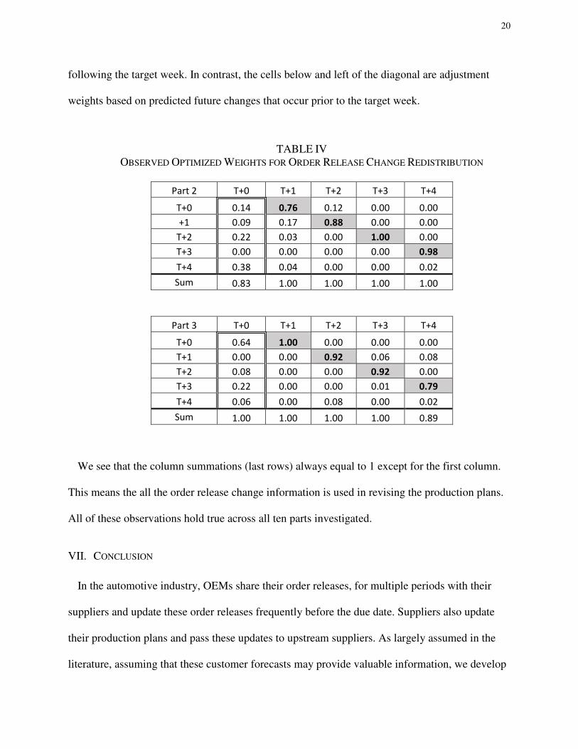
20

following the target week. In contrast, the cells below and left of the diagonal are adjustment

weights based on predicted future changes that occur prior to the target week.

We see that the column summations (last rows) always equal to 1 except for the first column.

This means the all the order release change information is used in revising the production plans.

All of these observations hold true across all ten parts investigated.

VII. CONCLUSION

In the automotive industry, OEMs share their order releases, for multiple periods with their

suppliers and update these order releases frequently before the due date. Suppliers also update

their production plans and pass these updates to upstream suppliers. As largely assumed in the

literature, assuming that these customer forecasts may provide valuable information, we develop

TABLE IV

OBSERVED OPTIMIZED WEIGHTS FOR ORDER RELEASE CHANGE REDISTRIBUTION

Part 2 T+0 T+1 T+2 T+3 T+4

T+0 0.14 0.76 0.12 0.00 0.00

+1 0.09 0.17 0.88 0.00 0.00

T+2 0.22 0.03 0.00 1.00 0.00

T+3 0.00 0.00 0.00 0.00 0.98

T+4 0.38 0.04 0.00 0.00 0.02

Sum 0.83 1.00 1.00 1.00 1.00

Part 3 T+0 T+1 T+2 T+3 T+4

T+0 0.64 1.00 0.00 0.00 0.00

T+1 0.00 0.00 0.92 0.06 0.08

T+2 0.08 0.00 0.00 0.92 0.00

T+3 0.22 0.00 0.00 0.01 0.79

T+4 0.06 0.00 0.08 0.00 0.02

Sum 1.00 1.00 1.00 1.00 0.89

21

a model that takes the customer forecast updates as input and converts this into a production

plan. This model is similar to the single stage model developed by Graves et al. [5]. The model

provides mixed results. For some parts, it is able to generate a production plan better than the

order releases received. In some other parts, it performs worse than just relying on the order

release received. Although the performance of the model is not great as a forecasting tool, the

weights generated provide some useful insights similar to what Graves et al. [5] have found,

without making any of the assumptions regarding the structure of the data. Thus, our findings

confirm and extend their findings.

Because of the way managers make forecasts, such as a myopic behavior, customer forecast

adjustments and updates are not necessarily information-adding in all scenarios. Moreover, in the

JIT setting we consider, there is a strong emphasis on avoiding inventories in ordering amounts

placed by Car Co., which may be one of the reasons for the systematic, mostly negative, bias in

the order quantities that are being placed by Car Co. The JIT emphasis may be causing the order

release quantities to be lower than the actual demand that occurs in order to avoid having excess

inventory within the supply chain.

We find that when there is bias in the order release updates, it is likely that the information can

contain so little use (because of their randomness) and cause significant disruptions (potentially

wrong or poor planning) in the supply chain if exchanged and acted upon. To remedy this, we

develop two versions of a simple adjustment heuristic to adjust the order release information to

create production plans. Although the optimization based adjustment heuristic was expected to

perform best, surprisingly, the simpler median based adjustment heuristic performs best. This

may be attributed to overfitting of the adjustment factor in the former approach. The median

adjustment heuristics performs very well especially when the bias is negative and significant.

22

When the bias is positive, the heuristic does not perform well since the emphasis is on shortage

costs compared to overage cost. When there is no bias, the heuristic makes no adjustment to the

order release information, thus it has no impact. Part of the reason we explored using a heuristic

was based on the reaction we had from Parts Inc. when discussing different forecasting

approaches and optimization methodologies. The primary concerns expressed by the

management during interviews were not understanding the methodologies and the challenge of

maintaining a complex methodology without adequate support and with possible turnover of

employees, who are familiar with such a complex methodology.

A major benefit of being able to adjust order release information to better production plans is

providing increased visibility to the upstream supply chain. Incorporating the adjusted releases in

the information communicated to the suppliers provides (some) forward visibility. It is known

that information visibility can reduce bullwhip effect. The median based adjustment that we are

suggesting is easy to implement in practice and outperforms both the optimization based

adjustment heuristic and the optimization method in general.

One limitation of this paper is its reliance on a single firm’s data. It would be very useful to

test the proposed methods on data from other firms to investigate if similar results can be

obtained.

REFERENCES

[1] Lee, H. L., Padmanabhan, V., & Whang, S. “Information distortion in a supply chain: the

bullwhip effect.” Management Science, vol. 43, no. 4, pp. 546-558, Apr. 2004.

[2] Lee, H. L., So, K. C., & Tang, C. S. “The value of information sharing in a two-level supply

chain.” Management science, vol. 46, no. 5, pp. 626-643, May 2000.

23

[3] Chen, H., Chen, J., & Chen, Y. F. “A coordination mechanism for a supply chain with

demand information updating.” International Journal of Production Economics, vol. 103, no.

1, pp. 347-361, Sep. 2006.

[4] Cattani, K., & Hausman, W. “Why are forecast updates often disappointing?” Manufacturing

& Service Operations Management, vol 2, no. 2, pp. 119-127. Spring 2000.

[5] Graves, S. C., Kletter, D. B., & Hetzel, W. B. “A dynamic model for requirements planning

with application to supply chain optimization.” Operations Research, vol. 46 no. 3, S35-S49.

May-Jun 1998

[6] Huggins, E. L., & Olsen, T. L. “Supply chain management with guaranteed

delivery”. Management Science, vol. 49, no. 9, pp. 1154-1167. Sep. 2003.

[7] Altintas, N., & Trick, M. “A data mining approach to forecast behavior.” Annals of

Operations Research, vol. 49, no. 1, pp. 3-22. Nov. 2012.

[8] Hausman, W. H. “Sequential decision problems: A model to exploit existing

forecasters.” Management Science, vol.6, no. 2, pp. B93-B111, Oct. 1969.

[9] Baker, K. “Requirements Planning,” in Handbooks in Operations Research and Management

Science, Logistics of Production and Inventory. Vol 4. Amsterdam, Netherlands. North-

Holland, 1993.

[10] Sarimveis, H., Patrinos, P., Tarantilis, C. D., & Kiranoudis, C. T. “Dynamic modeling and

control of supply chain systems: A review.” Computers & Operations Research, vol. 35, no.

11, pp. 3530-3561. Nov. 2008.

[11] Heath, D. C., & Jackson, P. L. “Modeling the evolution of demand forecasts ITH application

to safety stock analysis in production/distribution systems.” IIE transactions, vol. 26, no. 3,

pp. 17-30. May 1994.

24

[12] Graves, S. C., & Willems, S. P. “Optimizing strategic safety stock placement in supply

chains.” Manufacturing & Service Operations Management, vol. 2, no. 1, pp. 68-83. Jan.

2000.

[13] Aviv, Y. “The effect of collaborative forecasting on supply chain performance.”

Management science, vol. 47, no. 10, pp. 1326-1343. Oct. 2001.

[14] Aviv, Y. “On the benefits of collaborative forecasting partnerships between retailers and

manufacturers.” Management Science, vol 53, no. 5, pp. 777-794. May 2007.

[15] Terwiesch, C., Ren, Z. J., Ho, T. H., & Cohen, M. A. “An empirical analysis of forecast

sharing in the semiconductor equipment supply chain.” Management Science, vol. 51, no. 2,

pp. 208-220. Feb. 2005.

[17] Mason, A.J., “OpenSolver – An Open Source Add-in to Solve Linear and Integer

Progammes in Excel”, Operations Research Proceedings 2011, eds. Klatte, Diethard, Lüthi,

Hans-Jakob, Schmedders, Karl, Springer Berlin Heidelberg pp 401-406, 2012,

http://dx.doi.org/10.1007/978-3-642-29210-1_64, http://opensolver.org

[19] Armstrong, J. S., Lusk, E. J., Gardner Jr, E. S. , Geurts, M. D., Lopes, L. L. , Markland, R.

E., McLaughlin, R. L., Newbold, P., Pack, D. J., Andersen, A., Carbone, R., Fildes, R.,

Parzen, E., Newton, H. J. , Winkler, R. L., & Makridakis, S.S.S. "Commentary on the

Makridakis Time Series Competition (M-Competition)," Journal of Forecasting, vol. 2, no.

3, pp. 259-311, 1983.

[20] Ho, W., Zheng, T., Yildiz, H., & Talluri, S. Supply chain risk management: a literature

review. International Journal of Production Research, 53(16), 5031-5069, 2015.

25

APPENDICES Appendix 1: Sample full raw data with 40-week out order releases for a specific part.

Expanded DataOrder Release for Production Week…

Production ForecastTT+1

T+2T+3

T+4T+5

T+6T+7

T+8T+9

T+10T+11

T+12T+13

T+14T+15

T+16T+17

T+18T+19

T+20T+21

T+22T+23

T+24T+25

T+26T+27

T+28T+29

T+30T+31

T+32T+33

T+34T+35

T+36T+37

T+38T+39

T+40T+41

T+42T+43

T+44

Order Release Date

T-40*

T-39*

*

T-38*

**

T-37*

**

*

T-3633

3230

31

T-3533

3326

3640

T-3432

2437

3021

*

T-3333

3233

4444

**

T-3221

3130

3243

3731

15

T-3128

4334

3437

3224

17*

T-3014

3022

2933

3425

13*

*

T-2926

2321

4321

2714

9*

**

T-2826

2321

4321

2714

9*

**

*

T-2723

1914

2531

2818

1728

3634

2615

T-2622

2625

2925

2823

1627

1835

2620

18

T-259

3224

2536

2618

2122

2038

2617

26*

T-2418

2638

2721

3521

1237

2729

2617

28*

*

T-2320

2619

3323

2527

2226

3426

2926

2526

3321

T-2218

2722

2636

3223

2027

2827

3229

2436

3426

23

T-2116

2034

3031

3214

1830

3336

2218

2035

2729

22*

T-2018

2432

2823

3117

2425

3735

2423

2430

1723

21*

*

T-1914

2733

3126

3123

2429

2829

2522

2730

2936

3122

3328

T-1814

2726

2826

3214

2124

2730

2123

2432

2921

1830

3937

24

T-1732

3042

3550

3529

3021

3934

4137

3144

3032

4340

4046

45*

T-1666

8185

9987

9561

6859

11394

8172

7792

9579

8794

7597

76*

*

T-1558

6759

8670

9050

5885

8281

7657

6192

6367

4162

7767

5962

**

T-1454

6652

6558

7350

3958

7168

5157

5865

5150

5867

5657

6657

012

35

T-1346

5766

8859

6146

3656

7473

7150

5260

5553

5067

6760

5756

021

50*

T-1251

6368

8368

6435

3158

7166

6147

5363

4560

6360

5158

6455

023

39*

*

T-1156

6951

6259

5143

5158

7466

6254

5562

5255

4147

5959

6758

020

40*

**

T-1063

7967

6065

7246

4449

7470

7353

4168

6158

6172

6260

6258

016

4347

5844

41

T-955

7677

7351

7753

4464

7588

7352

5742

5462

6573

5964

5549

023

3841

4850

5434

T-842

6171

6265

7464

4653

8272

6451

5453

4846

4868

5549

4751

016

6345

4152

5152

*

T-745

10496

11980

13277

7291

12598

10061

7084

102105

123109

104112

6993

035

7473

7469

6364

**

T-672

7153

4239

4837

3952

6056

7032

3753

6771

8778

9057

5966

026

8284

7858

6467

3426

55

T-597

119115

4742

5445

5161

5664

5046

4339

8570

6593

7871

6848

028

6560

6163

6060

3526

38*

T-428

95165

9777

7062

4551

5547

4939

4137

7163

7786

8374

6549

027

6562

6951

7363

3826

39*

*

T-343

74169

10582

8158

3452

5968

6747

5254

7658

5978

8563

5267

020

6760

7865

5959

2926

39*

*

T-250

79176

10693

9455

4468

5483

6545

4454

6476

6675

6872

6451

029

5058

6670

6070

2629

3845

3841

T-150

79175

10794

10069

5055

6749

7736

4457

6567

8279

6867

5963

021

5557

5973

7064

2732

4342

3231

*

T57

81174

104106

15094

5448

6665

7745

5279

6670

7273

6964

6169

014

5949

7257

6955

3622

4240

2933

**

T+178

176106

104152

8648

6570

5476

5146

5667

7850

8493

7276

670

1365

6654

5657

5535

2444

3842

34*

**

T+2194

96103

16978

4758

6171

7143

4555

8986

8860

7568

6454

020

7675

7680

6775

2925

5647

4443

3449

4345

T+3105

110178

8262

8439

4191

4569

6685

9692

7585

6877

620

3688

93102

8696

8330

2147

3743

3435

4442

4235

T+4131

17291

68119

61144

11262

5264

8795

9772

8171

8681

040

7878

9072

96103

3441

5037

4234

3446

4143

35*

T+5185

9098

9657

154111

4672

7089

8889

7284

7576

720

3882

9199

78100

9594

8130

5228

3546

5158

4139

**

T+697

98129

78202

9850

4573

9982

8666

7843

5033

023

7267

7077

7667

8176

3853

4338

4755

5847

34*

**

* indicates data within the time horizon that was not provided (order releases for the most future time periods were added on a monthly basis)