Short-term electricity demand and gas price forecastsusing wavelet transforms and adaptive models

Hang T. Nguyena,�, Ian T. Nabneya

aNon-linearity and Complexity Research Group, School of Engineering and Applied Science,Aston University, Aston Triangle, Birmingham, B4 7ET, UK

Abstract

This paper presents some forecasting techniques for energy demand and price

prediction, one day ahead. These techniques combine wavelet transform (WT)

with �xed and adaptive machine learning/time series models (multi-layer per-

ceptron (MLP), radial basis functions, linear regression, or GARCH). To create

an adaptive model, we use an extended Kalman �lter or particle �lter to up-

date the parameters continuously on the test set. The adaptive GARCH model

is a new contribution, broadening the applicability of GARCH methods. We

empirically compared two approaches of combining the WT with prediction

models: multicomponent forecasts and direct forecasts. These techniques are

applied to large sets of real data (both stationary and non-stationary) from the

UK energy markets, so as to provide comparative results that are statistically

stronger than those previously reported. The results showed that the forecast-

ing accuracy is signi�cantly improved by using the WT and adaptive models.

The best models on the electricity demand/gas price forecast are the adaptive

MLP/GARCH with the multicomponent forecast; their MSEs are 0.02314 and

0.15384 respectively.

Key words: multi-layer perceptron, radial basis function, GARCH, linear

regression, adaptive models, and wavelet transform.

�Corresponding authour, Tel: +44 121 257 7718, Fax: +44 121 204 3685, email address:thihangn@aston.ac.uk

Preprint submitted to Elsevier July 15, 2010

1. Introduction

1.1. Context

An important characteristic of electricity is that it cannot be stored. There-

fore, an electricity demand forecast is valuable for power generators who can use

such forecasts to schedule operations of their power stations to match generation

capacity with demand. Electricity demand forecasting is also considered one of

the fundamental pieces of information for trading in the energy market because

the power price depends on demand.

Accurate electricity/gas price forecasting is very important for traders in

the energy market, especially those associated with energy generators. If an

energy generator makes an accurate forecast of the market price, it can develop

a strategy to maximise its own pro�ts and minimise risk due to price spikes

by appropriate trading in forward contracts. It can also plan its actions to

maximise bene�ts or utilities by reducing/increasing its generation. Energy

suppliers can use short-term price forecasts to adjust their bidding strategies to

achieve the maximum bene�t. In addition, understanding the process of forward

price development can help the generators make pro�ts through trading on the

forward market.

A number of statistical methodologies have been proposed for energy price

0Abbreviations:ACF autocorrelation function MAPE mean absolute percent error

ANN arti�cial neural network MLP multi-layer perceptron

AR autoregressive MSE mean squared error

ARMA autoregressive moving average NMSE normalised mean squared error

ARIMA autoregressive integrated moving average NN neural networks

ARD automatic relevance determination NSE normalised squared errors

AVCM absolute values of correlation matrix PACF partial autocorrelation function

BM benchmark model PF particle �lter

CM correlation matrix RBF radial basis function

EKF extended Kalman �lter RHWT redundant Haar wavelet transform

GARCHgeneralised autoregressive RW random walk model

conditional heteroschedastic SP sum of P-values

IR improvement ratio SSM state space model

LR linear regression WT wavelet transform

MAE mean absolute error

2

and demand forecasting. Many approaches based on time series models have

been used for price forecasting, such as AR models [1], autoregressive integrated

moving average (ARIMA) models [2] [3] [4], and generalised autoregressive

conditional heteroschedastic models (GARCH) [5]. Moreover, neural networks

(NNs) are used widely for electricity price/demand forecasting in the literature

[6], [7]. Due to the complexity of the environment, the functional relationships

we are looking for might be non-linear. Several researchers have proposed ad-

ditional procedures to improve accuracy, such as pre-processing procedures [8]

and regularisation methods [6]. Another approach for improving forecasting

performance is multiple NNs. The use of a committee of NNs for forecasting is

suggested in [9]. Similarly, cascaded neural networks are proposed in [10]. Pao

[11] proposed new hybrid non-linear models that combine a linear model with

an arti�cial neural network (ANN). A novel con�guration combining an AR(1)

with a high pass �lter was presented in [12].

This paper uses several standard forecasting models such as the multi-layer

perceptron (MLP), radial basis function (RBF), linear regression (LR), and

generalized autoregressive conditional heteroschedastic (GARCH) model. We

propose two techniques to improve performance of these prediction models. The

�rst technique is to use a wavelet transform (WT) as a pre-processing procedure.

The WT can produce a good local representation of the signal in both the time

and frequency domains. This technique has previously been used [2], [8], [13],

and [14]. However, this paper makes some contributions as explained in Section

1.2.

The second technique is a hybrid framework to create an adaptive forecast-

ing model, which is a combination of a �lter (such as Kalman �lter (KF), or

Extended Kalman Filter (EKF) or particle �lter (PF)) and a standard predic-

tion model (such as RBF, MLP, LR or GARCH). The forecast model is used

to forecast the next value of a time series, and the �lter is used to update pa-

rameters for the forecast model online whenever a new value of the time series

is observed. There is a large range of previous papers applying this hybrid

framework to di¤erent applications, such as recursively re-estimating parame-

ters of the Black-Scholes model from observations (the Black-Scholes model is a

well-known �nancial model for options pricing) [15], online learning parameters

3

of RBF and linear regression models [16] [17], predicting exchange rates [18],

estimating wind turbine power generation [19], and predicting New England

electricity prices [20]. The results on these previous papers show that this hy-

brid framework is good in the speed of learning and the accuracy of predictions.

1.2. Paper contributions

This paper provides an empirical comparison of a set of machine learn-

ing/time series forecasting models in order to explore the following issues:

� The choice of the type of prediction model from MLP, RBF, LR, and

GARCH.

� The value of a transformation of the target variable prior to modelling,

using the redundant Haar wavelet transform (RHWT). We compare the

prediction performance of prediction models without RHWT and two com-

bination methods:

�Multicomponent forecast: a RHWT decomposes the target value y

into wavelet components, and then each component is forecast with

a separate model.

�Direct forecast: using the components of RHWT as input variables

to a single forecast model to directly predict the target.

� Model parameters are either estimated just once or continuously updated

in the testing period. We evaluated the performance of the standard

forecast methods (i.e. MLP/RBF/LR/GARCH) with two variations:

�Fixed forecast models, i.e. models whose parameters are �xed after

training on a training set.

�Adaptive forecast models, i.e. hybrid of �lters (EKF/PF) and ma-

chine learning/time series forecast models, where parameters are es-

timated on a training set and then adapted continuously on the test

set using the �lter.

We tested these models for forecasting one-day ahead electricity demand and

one-day ahead gas forward price in the UK market.

4

This paper is an extension of our previous conference paper [21]. In this new

paper, we combine the WT with a wider range of models, including not only

�xed models as in [21] but also adaptive models. In [21], we tested the forecast

models on a single small dataset (6 sub-datasets of gas forward prices). In

this new paper we carry out experiments on two large datasets: (1) electricity

daily demand with 821 observations, and (2) 72 sub-datasets of gas forward

prices; each sub-dataset includes approximately 200 observations. Therefore,

the results in this paper compare more models and are more statistically robust

than the previous one.

Compared with earlier work, our paper has the following contributions.

First, we propose new forecasting methods which are the combination of WT, a

range of machine learning/time series models, and �lters. Second, although com-

bining WT with a time series or neural network models has already appeared,

previous papers only used either multicomponent forecast or direct forecast. In

this paper, we use both types of forecast and compare their prediction accuracy,

which provides an answer to the question of which is better for energy datasets.

The experimental results on the UK data showed that multicomponent fore-

casts outperform models without WT and direct forecasts. Third, we combine

�lters (EKF/PF) with machine learning/time series models to create adaptive

models, whose parameters are updated online during forecasts. Among these

adaptive models, the adaptive GARCH model is proposed for the �rst time in

this paper. Moreover, we use not only the EKF for adaptive models as ear-

lier authors but also the PF. The bene�ts of using the PF are that it makes

no a priori assumption of Gaussian noise and also that it is not necessary to

linearise the prediction model. Fourth, besides historical data of target vari-

able (e.g. electricity demand or gas forward price) and its WT components, a

number of exogenous variables (e.g. temperature, wind speed, day pattern, elec-

tricity supply and electricity price etc.), are also considered as input variables.

Some pre-processing procedures (presented in Section 5.2) are used to choose

the relevant input variables for each forecasting model. Finally, beside the stan-

dard error measures, we also provided two additional measures for comparing

and ranking models performance, i.e. improvement ratio (presented in Section

5.3.2) and hypothesis testing for multiple models (presented in Section 5.3.3).

5

1.3. Paper structure

This paper is organised as follows. In Section 2, the RHWT for decomposing

data into components is presented. Section 3 de�nes the detailed forecasting

framework. The �xed forecasting models and the method for creating their

corresponding adaptive models are described in Section 4. Numerical results

and evaluation on data from the UK energy markets are given in Section 5.

Section 6 provides some conclusions.

2. Redundant Haar wavelet transform

2.1. Why RHWT?

Most research in the literature uses symmetric WTs, such as Daubechies,

Morlet, or Symlet, for forecasting applications [2], [8], [13], and [14]. However,

using this type of WT for prediction is not appropriate because in the symmetric

wavelet, the wavelet coe¢ cients take into account not only previous information

but also future information (see Figure 1), but in a forecasting problem, we can

only use data obtained earlier in time. Some earlier papers have mentioned

this problem and use an à trous wavelet transform or a redundant Haar wavelet

transform in �nancial time series forecasting [22] and electricity load forecasting

[23], [24], [25].

In addition, a discrete WT normally has two stages: (1) computing detail and

approximation coe¢ cients with high- and low-pass �lters, and (2) decimation,

i.e. retaining one data point out of every two. The main advantage of decimation

is reducing the storage requirement. However, decimation leads to the loss of

phase information. To overcome this, we can use a redundant or non-decimated

wavelet transform [23]. In a redundant WT, only stage (1) is completed. All

components of a redundant WT have the same length as the original time series.

Therefore, there is a one-to-one correspondence between the original data and

decomposition coe¢ cients at a given time step.

2.2. Computing RHWT

Assuming that there is a time series yt, t = 1; 2; : : : ; T , Figure 2 shows how to

compute its RHWT coe¢ cients to the n-th decomposition level. At level i, the

detail coe¢ cients Di are retained, while the approximation coe¢ cients Ai are

6

decomposed into a further level of detail Di+1 and approximation coe¢ cients

Ai+1. It can be shown that the original time series can now be reconstructed as

yt = An;t +Dn;t + � � �+D1;t.

Note that to calculate a coe¢ cient at level i+1 at time t (Ai+1;t or Di+1;t),

we need to use the value of time series Ai at time step t � 2i. Therefore, at

level i+1, it is impossible to exactly de�ne the value of these coe¢ cients before

time step 2i+1 � 1. After applying the RHWT, this paper will consider only

those coe¢ cients after time step 2n � 1. Each component represents the data

in a frequency range that is less volatile and easier to forecast than the original

time series y.

3. Forecasting frameworks with WT

3.1. Multicomponent forecast

The multicomponent forecasting framework is shown in Figure 3. This is a

combination of forecasting models and the RHWT. A dataset is divided into

two sub-datasets: (1) a training set to estimate the model parameters and (2)

a test set to evaluate performance of these models by calculating appropriate

error functions. The forecasting framework for a time series yt consists of four

steps:

Step 1: Use the RHWT to decompose yt of the training set and the test set

separately: A;Dn; Dn�1; : : : ; D1.

Step 2: Determine the input vectors (including any exogenous variables) for

each model for predicting each component. Details of how we determined the

input variables will be presented in Section 5.2.

Step 3: In the training phase, the training sets are used to develop forecasting

models (i.e. estimate parameters), one forecasting model for each component.

Step 4: In the test phase, the developed models are used to predict the

future value of the components from the current observable data. The out-

puts of these models at time t are the values of A;Dn; Dn�1; : : : ; D1 at time

step t + 1. In this work, the models used for forecasting are �xed or adaptive

MLP/RBF/GARCH/LR. The inverse WT is used to compute the forecast value

of yt from the predictions of the components.

7

3.2. Direct forecast

Like the multicomponent forecast method, the target time series yt in this

method (shown in Figure 4) is also decomposed into WT components. These

components and exogenous variables are also used as candidates for input vari-

ables. However, the main di¤erence between the two methods is that the direct

forecast method directly predicts the time series yt while the multicomponent

forecast method separately forecasts wavelet transform components and the fore-

cast value of yt is derived from these forecast components by using the inverse

wavelet transform. Therefore, the direct forecast method has only one forecast

model while the multicomponent forecast method has several forecast models,

one model for each WT component.

4. Fixed and adaptive forecasting models

This section summarises several forecasting models previously used in en-

ergy markets: MLP, RBF, GARCH, and LR. We also describe how to produce

the corresponding adaptive models using �lters. The parameters of a �xed pre-

diction model are estimated using the training set only, and the test set is not

used to adjust parameters. These �xed forecasting models work well on station-

ary datasets. However, their performance degrades in predicting non-stationary

datasets. The characteristics of a non-stationary time series change over time;

thus the trend and volatility of training set might be di¤erent from these quan-

tities of the corresponding test set. Therefore, the parameters of the prediction

model, which are inferred from the training set, become �out of date�after some

time. This means that these parameters might no longer capture the correct

characteristics of the test set and this might lead to poor prediction perfor-

mance. One approach to reduce the e¤ect of the above issue is to use adaptive

models.

4.1. Fixed models

This paper uses four standard prediction models: MLP, RBF, LR, and

GARCH.

Neural networks

8

An MLP consists of a number of perceptrons organised in layers. Each

perceptron has several inputs and one output, which is a non-linear function of

the inputs. It has been shown that networks with one hidden layer are capable

of approximating any continuous functional mapping if the number of hidden

units is large enough [26]. Therefore, only two-layer networks will be considered

in this paper.

The RBF network is the main alternative to MLP for non-linear modeling

by neural network. The hidden unit in the RBF model computes a non-linear

function of the distance between the input vector and a weight vector.

Linear regression

Linear regression (LR) is a simple model where the output is a linear com-

bination of inputs. Unlike AR, ARMA, or ARIMA models, the input vector

of a LR can include both historical values of target variables and exogenous

variables (e.g. temperature, other components of RHWT, etc.).

Our LR is equivalent to AR with exogenous variables. We computed the

autocorrelation function (ACF) of the residuals of LR models and found that

the autocorrelation was very small for all non-zero lags, thus there is no need

for moving average terms. We also built forecasting models for log returns (i.e.

time series rt = log(pt=pt�1), where pt is gas price), but they did not performed

as well. Therefore in our paper using LR is enough, neither ARMA nor ARIMA

is necessary.

GARCH

In MLP, RBF or LR, the errors are assumed to be homoschedastic (i.e. the

variance of the residual is assumed to be independent of time). The GARCH

[27] can be used to model changes in the variance of the errors as a function of

time.

More detailed descriptions of these four prediction models are presented in

Appendix A.

4.2. Adaptive model framework

In an adaptive model, a �lter (extended Kalman �lter (EKF) or particle �lter

(PF)) will be used to update parameters of a model by treating the weights as the

states of a non-linear dynamic system. This can be considered as an estimation

9

problem where the weight values are unknown. The general framework for

adaptive models is shown in Figure 5.

In the training phase, the training sets are used to estimate parameters of

an MLP (or RBF/GARCH/LR) model in the usual way. In the test phase, two

steps are repeated at each time step:

Step 1: When a new observation is available, the �lter updates parameters

of the predictive model.

Step 2: Use the predictive model with the latest estimated parameters to

predict the next value.

In an adaptive model, we can choose to update all the parameters or only a

subset. The experimental results showed that results on updating a subset are

a little better and hence we restrict our attention to this case. The following

sections describe the EKF and PF, and how to use them in adaptive models.

4.3. Filters

This paper uses the EKF and the PF. They are based on a state space model

(SSM); we assume that the observed time series yt is a function of random

variables zt (the hidden state vector) which are not observed. In an adaptive

model, zt are the model parameters. It is also assumed that we do not know the

dynamics of the observation, but do know the dynamics of hidden state space:

zt+1 = ft(zt) + �t �t � N (0; Qt) (1)

yt = ht(zt) + "t "t � N (0; Rt), (2)

where ft and ht are state transition function and output function respectively,

and "t and �t are zero-mean Gaussian noise; z0 is the system initial condition,

modelled as a Gaussian random vector z0 � N (�0; P0). For our task, ft is the

identity.

The EKF and PF algorithms track the posterior probabilities of hidden

variables zt given a sequence of observed variables up to time t: p(ztjfygt1),

where fygt1 = fy1; : : : ; ytg. The EKF is an extension of the Kalman �lter (KF)

[28]. The di¤erence is that the KF is designed for linear SSMs (i.e. ht and ft

are linear functions) only while the EKF can be applied to either linear or non-

linear models. The EKF does not solve the original problem, but approximates

10

it by locally linearising the non-linear functions ht and ft around previous state

estimates. The linearisations are made with a �rst order Taylor expansion.

When the strength of the non-linearity of the functions ht and ft is great,

the linearisations are poor approximations; and the EKF does not work well.

The particle �lter (PF) is an alternative method which avoids the bad e¤ects of

linearisation. The PF is a sampling-based method. In addition, EKF is limited

to Gaussian noise for �t and "t while there is no assumption of noise distributions

on the PF. Details of the EKF and the PF are given in Appendix B.

4.4. Adaptive MLP/RBF/LR models

In the adaptive MLP model, we update the bias of the second layer !(2)k0

only; in the adaptive RBF model, we update the second layer weight !kj only;

and in the adaptive LR model, only the bias b is updated (see de�nition of these

parameters in Appendix A). This implies that the models adapt only to changes

in the mean of the time series. Adapting all the parameters gave worse results.

Denote these updated parameters �, and the remaining parameters of a model

$. From equations (A.1), (A.2), (A.3), (A.4), and (A.5), we can summarise the

input/output relationship of the models as follows

yt = h(xt; �;$) (3)

� On the training set: we used the same training algorithm in �xed model

to estimate parameters , denoted �0, $0.

� On the test set: two steps are recursively repeated.

Step 1 : Update parameters of the model using the EKF/PF. The non-linear

SSM is given by

�t = �t�1 + �t, �t � N (0; Q) (4)

yt = h(xt; �t; $0) + "t "t � N (0; R). (5)

�t is the hidden state vector. Parameters Q, R, and P0 of the non-linear SSM

can be estimated by using maximum log likelihood [29] or just set to reasonable

values. Other parameters of non-linear SSM are given by

�0 = �0, Ft = I (i.e. identity matrix)

Ht = rhj�t�1t ,

11

(see de�nition of these parameters in Appendix B).

Step 2 : Predict one time step ahead:

yt = h(xt; �t�1t ; $0).

4.5. Adaptive GARCH model

In an adaptive GARCH, all the parameters are �xed at the estimates derived

from the training set, with the exception of the bias e� (see de�nition of thisparameter in Appendix A.4) which is adapted on-line on the test set.

� On the training set: we use maximum likelihood to compute GARCH

parameters as in �xed model (see Appendix A.4), and let �0 = f�0;0; : : : ; �m;0;

1;0; : : : ; r;0g, b�0, and e�0 be these parameters.� On the test set: We use a �lter to update the value of e�t. For thispurpose, a SSM is constructed as follows:

e�t = e�t�1 + �t �t � N (0; Q) (6)

yt = ht(e�t) + "t "t � N (0; Rt) (7)

where the bias e� is the hidden state vector, the output function ht(e�t) =e�t + b�0xt, and parameters Q and P0 of the SSM can be estimated by

using maximum log likelihood (using the Kalman smoother) [29], or just

set to reasonable values. The state transition function ft is chosen to be

identity (see Equation 6) because parameter e� does a random walk: no

pre-determined dynamics (i.e. entirely data dependant). Ft = 1, Ht = 1

(see de�nition of these parameters in Appendix B). Other parameters of

the SSM are given by

�0 = e�0,Rt = �0;0 +

mPi=1

�i;0"2t�i +

rPj=1

j;0Rt�j .

On the test set, two steps are recursively repeated through the observations

in time order:

Step 1 : Estimate parameter e�t of the GARCHmodel: e�t�1t = Ehe�tj fygt�11

i.

In order to obtain this parameter, we use the EKF/PF to estimate the mean of

12

the hidden state at time step t � 1 given observations up to time t � 1: e�t�1t�1.

From equation (6), the estimate of e� at time step t given fygt�11 is e�t�1t = e�t�1t�1.

Step 2 : Use the GARCH model with the latest estimated parameters to

predict the time series at time t:

yt = e�t�1t + b�0xt.5. Experimental results

5.1. Data

We evaluated the performance of the algorithms on two problems: fore-

casting the daily electricity demand and forecasting the price of a monthly gas

forward product (i.e. forward contract). Both datasets were taken from the UK

energy market, and were provided by E.ON. The �rst dataset (see Figure 6)

contains 821 observations of the daily total electricity demand (d) of all users in

Great Britain, from 7th October 2004 to 3rd May 2007. The data has two sea-

sonality e¤ects: (1) a weekly pattern with lower consumption at weekends and

(2) an annual pattern where the consumption is higher during the colder part of

the year. There are about 15 public holidays (Christmas, Easter and Bank hol-

iday) per year. The demand values on public holidays are signi�cantly smaller

than on other days. There are two approaches for dealing with this issue. The

�rst is to exclude these observations from the dataset. To forecast demand of

public holidays, we should consider the corresponding day of previous years, and

build a separate model for public holiday data only. The second is to include

public holidays in the dataset, but introduce a dummy variable (equal to 1 for

public holidays and 0 otherwise). Since the main objective of this paper is to

evaluate the e¤ects of WT and EKF/PF on the standard prediction models, we

chose the �rst approach and have removed the observations on public holidays

from the dataset. The �rst 525 observations were used as training set and the

last 296 observations were used as the test set.

The second dataset (see Figure 7) consists of prices of monthly gas forward

products. The monthly gas product is a forward contract for supplying gas in a

single month in the future. This data is price of gas forward products Jun-2006

to May-2008 and is sampled daily from 1st December 2005 to 30th April 2008. In

13

the UK energy market, it is possible to trade gas from one to six months (before

1st May 2007) or �ve months (after 1st May 2007) ahead. Thus, there are �ve

or six months of daily price data (approximately 110-130 data points) for each

monthly gas product. For example, the Jul-2006 product can be traded from

3rd January 2006 to 30th June 2006. We created 72 sub-datasets; we divided

each forward product into three parts: each part was a test set of a sub-dataset.

Each test set was associated to one training set which includes the multiple

forward products. Of course, observations of a training set occurred before the

associated test set. Figure 8 shows how training and test sets were allocated for

these sub-datasets. Data for the May-08 product was divided into three parts:

each part is a test set of a sub-dataset. In sub-dataset 1, the test set is the �rst

1/3 of the observations of May-08 product, the training set includes data from

Apr-08, Mar-08, Feb-08, and Jan-08 products.

5.2. Variable selection and pre-processing

In addition to electricity demand and monthly forward gas prices, there are

a large number of exogenous variables which may be potential candidates for

inputs. However, only some of them are relevant for prediction. Using irrele-

vant variables as input will reduce the performance of the forecasting models.

Therefore, selecting correct inputs for each kind of model is very important.

The potential inputs include historical data of electricity demand (d), elec-

tricity supply for the UK (s), historical data of real average temperature in

Celsius degrees (�), wind speed, sunset time, system marginal prices (SMP) sell

of gas (m), gas demand (g), price of monthly gas forward product (p), forward

price of monthly/seasonal/annual baseload/peak load electricity products, for-

ward price of monthly/seasonal gas product, weekday ahead/weekend ahead gas

price (denote the price of 1-winter ahead gas forward product by pw), system

average price (SAP) of gas/electricity, exchange rate GBP:USD, oil spot price,

and day pattern (i.e. day of the week). Weather forecast data was not available.

The potential inputs also include the WT components of the target variable.

This paper uses 2-level WT. Denote WT components of electricity demand by

A;D2; D1, and denote WT components of price of monthly gas forward product

by A0; D02; D

01.

14

In the training phase, various measures were used to select the relevant in-

put variables, including the correlation matrix (CM), autocorrelation function

(ACF), partial autocorrelation function (PACF) and automatic relevance deter-

mination (ARD). The �rst three methods were used to select input variables for

linear models (i.e. GARCH and LR). We computed the CM of the target and

exogenous variables; and the exogenous variables which were highly correlated

to the targets were chosen. We also computed the ACF and PACF of target

time series. Lags with high correlations were selected as input variables as well.

Note that, because the day of the week is a periodic variable, we represented

it by two dummy variables: swd = sin(2�i=7) and cwd = cos(2�i=7), where

i = 1 to 7 corresponding to Monday to Sunday. There is another approach to

deal with seasonality: using multiple-equation models with di¤erent equations

for the di¤erent days. We have implemented both approaches, however, the

results of �rst approach were better and are presented in the paper.

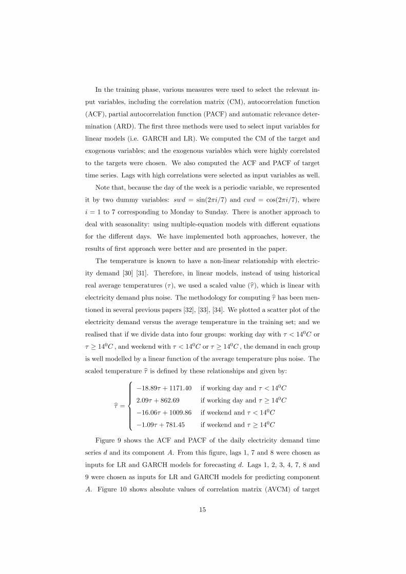
The temperature is known to have a non-linear relationship with electric-

ity demand [30] [31]. Therefore, in linear models, instead of using historical

real average temperatures (�), we used a scaled value (b�), which is linear withelectricity demand plus noise. The methodology for computing b� has been men-tioned in several previous papers [32], [33], [34]. We plotted a scatter plot of the

electricity demand versus the average temperature in the training set; and we

realised that if we divide data into four groups: working day with � < 140C or

� � 140C ; and weekend with � < 140C or � � 140C , the demand in each group

is well modelled by a linear function of the average temperature plus noise. The

scaled temperature b� is de�ned by these relationships and given by:

b� =8>>>>>><>>>>>>:

�18:89� + 1171:40 if working day and � < 140C

2:09� + 862:69 if working day and � � 140C

�16:06� + 1009:86 if weekend and � < 140C

�1:09� + 781:45 if weekend and � � 140C

Figure 9 shows the ACF and PACF of the daily electricity demand time

series d and its component A. From this �gure, lags 1, 7 and 8 were chosen as

inputs for LR and GARCH models for forecasting d. Lags 1, 2, 3, 4, 7, 8 and

9 were chosen as inputs for LR and GARCH models for predicting component

A. Figure 10 shows absolute values of correlation matrix (AVCM) of target

15

variables and potential candidates for inputs. Because we are concerned only

the correlations of �rst four attributes (i.e. targets) with the others, we did

not plot the full AVCM, but only �rst four rows of the AVCM. A summary

of the input variables for LR and GARCH models is shown in Table 1. Note

the signi�cant di¤erences in lags selected for the di¤erent components of the

multicomponent forecast model.

Input variables for non-linear models (i.e. MLP and RBF) were chosen us-

ing ARD [35], which is a Bayesian technique to evaluate the importance of each

input variable. Each potential input variable is assumed to be sampled from

a zero-mean Gaussian distribution: the inverse of the variance is called hyper-

parameter. The evidence procedure is used to optimise these hyperparameters

during model training. If a hyperparameter is small, it is likely that its as-

sociated variable has large weight. This means that the associated variable is

important and should be chosen as an input. Details of ARD and an imple-

mentation can be found in [37], chapter 9. In the electricity demand forecast

using models without WT, hyperparameters range from 7.72 to 198.95. The

variables associated with the smallest hyperparameters were chosen as inputs

for MLP/RBF models: they are shown in Table 2.

The same procedures were implemented for the gas forward price dataset,

see Table 3.

5.3. Model evaluation

There are 36 di¤erent models by combining the standard forecasting models

with the RHWT and the �lters. These models were tested on two large datasets

(i.e. electricity demand and gas price); they are compared systematically on the

same data.

5.3.1. Benchmark models

Because electricity demand is strongly seasonal with a period of one week,

the benchmark model for this dataset is a model in which demand of a day is

assumed to be the same as the demand of the same day in the previous week.

A random walk (RW) model is used as a benchmark to evaluate the per-

formance of forecasting monthly gas forward price. In many heavily traded

markets for �nancial products (e.g. currency, stock market indices), the RW is

16

a very strong benchmark (of the e¢ cient market hypothesis). A RW is given by:

yt+1 = yt + ", where " is zero-mean noise. The model predicts that tomorrow�s

price will be equal to today�s price.

5.3.2. Errors

Three types of prediction errors on the test sets were computed. They are the

mean absolute percent error (MAPE), normalised mean squared error (NMSE),

and mean absolute error (MAE) which are de�ned by

eMAPE =1

T

XT

t=1

����yt � bytyt

����eNMSE =

PTt=1 (yt � byt)2PTt=1 (yt � E[y])

2

eMAE =1

T

XT

t=1jyt � bytj ,

where y is the real demand/price, by is the forecast demand/price, E[y] is themean of y, and T is the number of observations in the test set.

We also computed the improvement ratio (IR) of the errors compared with

the corresponding errors of the benchmark model (BM). For example, the IR of

NMSE of a model M comparing with NMSE of the BM is given by:

IRNMSE(M)=eNMSE(BM)� eNMSE(M)

eNMSE(BM).

Variables were normalised to zero mean and unit variance. Forecast time

series were converted to the original domain, before computing the errors.

5.3.3. Hypothesis testing

Assume that there arem forecasting models. We calculatem series e1; : : : ; em,

each of them associated with one forecast model, where ei represents the error

of the ith model. In order to assess the relative performance of a large number

of models on (potentially) a large number of test sets, the sum of P-values for

each model i (SP i) was evaluated as follows:

SP i =1

m

Pmj=1 Pij ,

where

Pij =

8<: P-value of paired t-test (ei, ej) with hypothesis ei > ej when i 6= j

0:5 when i = j

17

The smaller ei is, the larger SP i. Because ei represents the error of the ith

model, the smaller ei, the better the ith model is. Therefore, we can rank

performance of models based on SP i.

In the electricity demand experiment, because there is only one test set

(containing 296 observations), the series ei associated with the ith model is the

time series of normalised squared errors (NSE) of the observations: NSEi =

[NSEi1; : : : ; NSEi296], where

NSEit=

�yt � byit�2Cov(y)

, t = 1; : : : ; 296,

where byit is the forecast value of y at time t by the ith model.In the gas price forecast, there are 72 sub-datasets. Therefore, instead of

using NSE as in the electricity demand dataset, we used NMSE; the series

ei associate with the ith model is: NMSEi = [NMSEi1; : : : ; NMSEi72], where

NMSEik is the normalised mean squared error of the ith model for sub-dataset

k, k = 1; : : : ; 72, i = 1; : : : ;m.

5.4. Results on daily electricity demand forecast

The program was written in Matlab. The number of hidden units in MLP

models for forecasting d (in raw MLP model), A, D2, D1 (in multiforecast

models), and d (in direct forecast model) were 9, 9, 8, 12, and 11 respectively.

The numbers of hidden units in all RBF models (for d, A, D2, and D1) are

50. Appendices A.1 and A.2 presented how to determine these parameters. We

used MLPs with tanh activation functions.

Table 4 contains the IRNMSE and errors of the prediction methods for daily

electricity demand forecasting. The table shows that the proposed methods are

signi�cantly better than the benchmark. Prediction performance of the non-

linear models (MLP/RBF) is much better than linear models (GARCH/LR):

The IRMSE of �xed MLP and RBF are 81% and 68% while that of �xed LR

and GARCH are 56% and 59% only. Therefore, we will focus on the e¤ects of

the WT and the EKF/PF on MLP and RBF.

Table 4 shows that models with WT outperform the models without wavelet

transform, which proves the usefulness of the WT. For example, the MSE of

the �xed MLP (RBF) model is 0.02827 (0.04714) while that of the �xed MLP

18

(RBF) model combined with multicomponent forecast is 0.02293 (0.02855). The

multicomponent forecast achieves better results than the direct forecast. The

multicomponent forecast combined with �xed/adaptive MLP are the best with

MSE of 0.02293 and 0.02314, their MSE improves more than 84% compared to

the MSE of the benchmark model.

In this dataset, the performance of �xed and adaptive models was almost the

same. The adaptive models did slightly better than �xed models when the WT

was not used, and vice versa on MLP/RBF with multicomponent forecasting.

The adaptive models on this dataset did not work as well as on the gas forward

price (to be presented in the next section). The MLP models provided better

prediction accuracy than the RBF, LR and GARCH models.

5.5. Results on price of monthly gas forward products

Number of hidden units in MLP models for forecasting p (in raw MLP

model), A0, D02, D

01 (in multiforecast models), and p (in direct forecast model)

are 6, 6, 6, 5, and 6 respectively. The numbers of hidden units in all RBF

models (for d, A, D2, and D1) are 40. Appendices A.1 and A.2 presented how

to determine these parameters. We used MLPs with tanh activation functions.

The gas forward price dataset consists of 72 sub-datasets. The IRNMSE ,

NMSE, MAPE, MAE, and SP were computed for each sub-dataset and for

each �xed or adaptive prediction methods. Their averaged values are shown in

Table 5. Because LR and GARCH are much better than MLP and RBF models

(IRMSE of �xed MLP model is only 0.94% and the results of the RBF model

are worse than the benchmark model), in this paper, we will focus on the e¤ects

of WT and adaptive models on GARCH and LR models only.

Similar to results on the daily electricity demand dataset, multicomponent

forecasts outperform the models without wavelet transform. However results

of direct forecasts are worst than that of models without wavelet transform.

The adaptive models are better than the �xed models. For example, the MSE

improvement ratio for the �xed GARCH (LR) model was 2.26% (3.85%) while

that of the adaptive GARCH (LR) model was 5.92% (5.33%). The adaptive

GARCH models with multicomponent forecast achieved the best results with an

MSE of 0.15384, which improves 15.10% compared to the MSE of the benchmark

19

model. The GARCH models generally provided better prediction accuracy than

the LR, MLP, and RBF models.

In general, the adaptive models with PF are expected to provide better

performance than the adaptive models with EKF because the PF does not

require as many assumptions as in EKF. However, the results of these adaptive

models were almost the same in these tests. This could be explained by the

linearity of the SSMs. The state transition functions in equations (4) and (6)

are linear. The outputs of GARCH and LR models were linear in parameters,

thus so were their state space models. MLP and RBF models are non-linear

functions, but we only adjusted on-line the bias of the second layer in MLP

and the second layer weights in RBF which have a linear relationship with

the outputs. Therefore the SSMs for adaptive MLP and RBF models were also

linear. The local linearisation of output functions and space transition functions

on EKF were perfect and the EKF could provide good updates.

6. Conclusions

The paper presents two frameworks for using WT as a pre-processing pro-

cedure for prediction applications. A range of machine learning and time series

models are presented, such as GARCH, MLP, RBF, and LR. The results of elec-

tricity demand forecasting and gas price forecast on several large datasets show

that the use of a WT improves the prediction performance. Multicomponent

forecasting outperforms the methods without wavelet transform and the direct

forecast.

This paper also showed how to combine each type of prediction model with

�lters (EKF/PF). It was shown experimentally that the adaptive models did

improve prediction performance, especially on the gas forward price data (which

is a non-stationary time series). However, this improvement is not as great as

the improvement induced by using the WT. In these prediction models, noise

is assumed to be Gaussian, therefore we can used both extended Kalman �lter

(EKF) and particle �lter (PF) as �lters. The adaptive models with PF and the

adaptive models with EKF achieved similar results.

There are 36 di¤erent models by combining the standard forecasting models

with the WT and the �lters. These models were tested on two large datasets.

20

Beside the popular errors, we proposed a hypothesis testing and improvement

ratio for comparison of di¤erent models.

In electricity demand forecasting, MLP and RBF models are generally better

than GARCH and LR models while GARCH and LR are better than MLP and

RBF in gas price forecast. In the electricity demand forecast, the multicompo-

nent forecast combined with adaptive MLPs are the best with MSE 0.02314; its

MSE improves more than 84% compared to the MSE of the benchmark model.

In the gas price forecast, the adaptive GARCH models with multicomponent

forecast achieves best results with MSE of 0.15384, which improve 15.1% com-

paring to MSE of the random walk model.

7. Acknowledgment

Hang T. Nguyen would like to thank to E.ON for their �nancial support

and their permission to submit the paper for publication. The authors are

grateful to Greg Payne, Matthew Cullen, David Turner, Stuart Gri¢ ths, Nick

Sillito, Daniel Crispin and David Jones from E.ON for providing the datasets,

and their valuable advice. Some part of program have been written using

source code from the NETLAB toolbox by Ian Nabney (available at http://

www.ncrg.aston.ac.uk/netlab/) and Kalman �lter code by Kevin Murphy

(available at http://www.cs.ubc.ca/~murphyk/Software/Kalman/kalman.html).

The authors also thank the anonymous referees for their insightful comments

which have signi�cantly improved the paper.

Appendix A Fixed prediction models

A.1 MLP

For an MLP with two layers, d input variables x = fx(1); : : : ; x(d)g, M hid-

den units, and c output units y = fy(1); : : : ; y(c)g, the output can be calculated

as follows

a(1)j =

dPi=1

!(1)ij x(i) + !

(1)jo , j = 1; : : : ;M (A.1)

y(k) =MPj=1

!(2)kj g(a

(1)j ) + !

(2)k0 , k = 1; : : : ; c, (A.2)

21

where !(1)ji and !(2)kj are the weights of the �rst and second layers respectively,

and the activation function g(:) is usually logistic sigmoidal or tanh.

We optimise the model parameters by maximising likelihood and evidence

procedure. More details on the theory and source code for training an MLP

can be found in [37]. When training an MLP, we often encounter over�tting.

Over�tting is a problem where the model �ts the noise in the training data

rather than the underlying generator and may lead to large errors on unseen

data. There are several approaches to overcome this problem, such as early

stopping [6] or using a committee to combine di¤erent networks. In this paper,

we use weight decay to regularise the model by penalising large weights and

imposing smoothness. The Bayesian evidence procedure is used to compute the

optimal hyperparameters [38]. The number of hidden units is determined from

the number of well-determined parameters found by the evidence procedure; see

[39] section 10.4.

A.2 RBF

The outputs y = fy(1); : : : ; y(c)g of an RBF model for input x are given by:

rj = x� �j j = 0; : : : ;M (A.3)

y(k) =PM

j=0 !kj�j(rj); k = 1; : : : ; c, (A.4)

where x represents the input of the RBF model, �j are the cluster centres or

�rst layer weights, and rj is the distance between the input and the cluster

centre �j . Here �j represents the basis functions (usually Gaussian) and !kj is

the second layer weight corresponding to the kth output unit and the jth basis

function. More information about the theory and source code for training RBF

models can be found in [37].

We used 10-fold cross-validation to select the number of basis functions of

RBF. In a k-fold cross validation, the training set is divided into k nearly equally

sized segments (or folds). We perform k iterations of training and validation.

In each iteration, a single segment is used for validation and the remaining k�1

segments are used for training the model, so for each model there are k error

values (we used NMSE here). The average of the errors is the cross-validation

error of the model. This procedure is performed for the di¤erent RBF models

22

with di¤erent numbers of basis functions. Since the cross-validated error of

a model on the training set maybe taken as an estimate for the error of the

model on unseen data, the network structure corresponding to the smallest

cross-validation error is chosen.

A.3 LR

This model is given by:

y =Pd

i=1 w(i)x(i) + b = wTx+ b, (A.5)

where y represents the output of target data, w = fw(1); : : : ; w(d)g is the weight

vector, b is bias and x = fx(1); : : : ; x(d)g represents the input vector. We

estimate parameters of LR by maximum likelihood. Details about theory and

source code for training LR model can be found in [37].

A.4 GARCH

The GARCH(r;m) model is given by:

yt = e� + b�xt + "t; "t � N (0; nt)

nt = �0 +mPi=1

�i"2t�i +

rPj=1

jnt�j ,

with constraints

�i; j > 0 (A.6)Pmi=1 �i +

Prj=1 j < 1, (A.7)

where xt, yt, and "t represent the input vector, output vector, and error of the

model respectively, nt is variance of error "t, � = fe�; b�g is the parameter vectoroutput function.

We can �t a GARCH model using maximum likelihood. The constraints in

Equation (A.6) can be removed by substituting �i = exp(b�i); j = exp(b j) andwe optimise with respect to b�i, b j instead of �i; j . To satisfy the constraintsin Equation (A.7), we used the penalty function method [37] to optimise the

model.

23

Appendix B Filters

B.1 Extended Kalman �lter

EKF is a recursive algorithm; one iteration of the EKF is composed of the

following consecutive steps [40]:

� Prediction:

zt�1t = ft(zt�1t�1)

P t�1t = FtPt�1t�1F

0t +Qt.

� Update

Kt = P t�1t H 0t[HtP

t�1t H 0

t +Rt]�1

ztt = zt�1t +Kt[yt � ht(zt�1t ))]

P tt = [I �KtHt]Pt�1t ,

where Ft and Ht are the Jacobian matrices of the functions ft(:) and ht(:),

Ft = rftjztt and Ht = rhtjzt�1t , and

z�t = E[ztjfyg�1 ]

P �t = E[(zt � z�t )(zt � z�t )0jfyg�1 ].

B.2 Particle �lter

The PF is a sampling-based method. Firstly, we sampleNp times from initial

distribution z0;i � p(z0) = N (�0; P0), allocating equal weights w0;i = 1=Np to

each sample (or �particle�). Next the state mean at t+1 given yt+1 is estimated

as follows:

� Evolve particles using transition function f : zt+1;i = ft+1(zt;i) + �i,

where �i is sampled from the appropriate noise distribution (here �i �

N (0; Qt+1)), i = 1; : : : Np.

� Re-weight particles when a new observation is available: w0t+1;i / wt;i �

p(yt+1jzt+1;i); where p(yt+1jzt+1;i) = N (yt+1jht+1(zt+1;i); Rt+1), i = 1; : : : ; Np.

� Normalise the weights: wt+1;i = w0t+1;i=PNp

i=1 w0t+1;i.

24

� The mean of state z at time step t+1 is the weighted average of particles:

E[zt+1jyt+1] =PNp

i=1 wt+1;izt+1;i.

In practice, after a large number of time steps, all but a small number of

particles may have negligible weight. The problem with this degeneracy is that

most of the particles contribute insigni�cantly to E[zt+1jyt+1], but they still

consume computational e¤ort. We can reduce the e¤ect of this problem by

resampling [36].

References

[1] Nogales FJ, Contreras J, Conejo AJ, Espinola R. Forecasting next-day elec-

tricity prices by time series models. IEEE Transactions on Power Systems

2002; 17(2): 342-348.

[2] Conejo AJ, Plazas MA, Espinola R, Molina AB. Day-ahead electricity price

forecasting using the wavelet transform and ARIMA models. IEEE Trans-

actions on Power Systems 2005; 20(2): 1035-1042.

[3] Abdel-Aal RE, Al-Garni AZ. Forecasting monthly electric energy consump-

tion in eastern Saudi Arabia using univariate time-series analysis. Energy

1997; 22: 1059-1069.

[4] Chavez SG, Bernat JX, Coalla HL. Forecasting of energy production and

consumption in Asturias (northern Spain). Energy 1999; 24: 183-198.

[5] Zheng H, Xie L, Zhang L. Electricity price forecasting based on GARCH

model in deregulated market. In: Power Engineering Conference. 2005. p.

410-416.

[6] Gao F, Guan ZH, Cao XR, Papalexopoulos A. Forecasting power market

clearing price and quantity using a neural network method. In: Proceedings

of the Power Engineering Summer Meet, vol. 4. Seattle, 2000. p.2183-2188.

[7] Ekonomou L. Greek long-term energy consumption prediction using arti�-

cial neural networks. Energy 2010; 35(2): 512-517.

25

[8] Amjady N, Keynia F. Short-term load forecasting of power systems by

combination of wavelet transform and neuro-evolutionary algorithm. En-

ergy 2009; 34(1): 46-57.

[9] Guo JJ, Luh PB. Improving market clearing price prediction by using a

committee machine of neural networks. IEEE Transactions on Power Sys-

tems 2004; 19(4): 1867-1876.

[10] Zhang L, Luh PB, Kasiviswanathan K. Energy clearing price prediction

and con�dence interval estimation with cascaded neural networks. IEEE

Transactions on Power System 2003; 1: 99-105.

[11] Pao HT. Forecasting energy consumption in Taiwan using hybrid nonlinear

models. Energy 2009; 34:1438-1446.

[12] Saab S, Badr E, Nasr G. Univariate modeling and forecasting of energy

consumption: the case of electricity in Lebanon. Energy 2001; 26: 1-14.

[13] Tai N, Stenzel J, Wu H. Techniques of applying wavelet transform into

combined model for short-term load forecasting. Electric Power Systems

Research 2005; 76: 525-533.

[14] Xu H, Niimura T. Short-term electricity price modeling and forecasting

using wavelets and multivariable time series. In: Power Systems Conference

and Exposition, vol. 1. 2004. p. 208- 212.

[15] Niranjan M. On data driven of options prices using neural networks. In:

Forecasting Financial Markets: Advances for Exchange Rate, Interest Rate

and Asset Management. London, 1999. p. 1-13.

[16] Nabney IT, McLachlan A, Lowe D. Practical method of tracking of non-

stationary time series applied to real world data. In: Aero Sense 96: Ap-

plications and Science of Arti�cial Neural Networks II, SPIE Proceedings,

vol. 2760. 1996. p. 152-163.

[17] Patil SA, Irwin R, Srinivasan S, Prasad S, Lazarou G, Picone J. Sequential

state-space �lters for speech enhancement. In: Proceedings of the IEEE

SoutheastCon 2006. p. 240-243.

26

[18] Andreou AS, Georgopoulos EF, Likothanassis SD. Exchange-rates forecast-

ing: a hybrid algorithm based on genetically optimized adaptive neural

networks. Computational Economics 2002; 20: 191-210.

[19] Li S, Wunsch DC, O�Hair E, Giesselmann MG. Wind turbine power es-

timation by neural network with Kalman �lter training on SIMD parallel

machine. In: International Joint Conference on Neural Networks, vol. 5.

1999. p. 3430-3434.

[20] Zhang L, Luh PB. Power market clearing price prediction and con�dence

interval estimation with fast neural network learning. In: Proceeding of

the IEEE 2002 Power Engineering Society Winter Meeting, vol. 1. 2002. p.

268-273.

[21] Nguyen HT, Nabney IT. Combining the wavelet transform and forecasting

models to predict gas forward prices. In: Proceedings of the 2008 Seventh

International Conference on Machine Learning and Applications. 2008. p.

311-317.

[22] Zhang BL, Coggins R, Jabri A, Dersch D, Flower B. Multiresolution fore-

casting for futures trading using wavelet decompositions. IEEE Transac-

tions on Neural Networks 2001; 12(4): 765-775.

[23] Starck JL, Murtagh F. MR/Finance multiresolution analysis of time series.

2001. See also: http://thames.cs.rhul.ac.uk/~multires/doc/mr�n.pdf

[24] Benaouda D, Murtagh F, Starck JL, Renaud O. Wavelet-based non linear

multiscale decomposition model for electricity load forecasting. Neurocom-

puting 2006; 70: 139-154.

[25] Dong ZY, Zhang BL, Huang Q. Adaptive neural network short-term load

forecasting with wavelet decomposition. In: IEEE Porto Power Tech Con-

ference, vol. 2. 2001.

[26] Hornik K, Stinchcombe M, White H. Multilayer feedforward networks are

universal approximators. Neural Networks 1989; 2(5): 359-366.

[27] Bollerslev T. Generalized autoregressive conditional heteroskedasticity.

Journal of Econometrics 1986; 31:307-327.

27

[28] Kalman RE. A new approach to linear �ltering and prediction problems.

Transactions of the ASME-Journal of Basic Engineering 1960; 82 (Series

D): 35-45.

[29] Ghahramani Z, Hinton GE. Parameter estimation for linear dynamical sys-

tem, report no. CRG-TR-96-2. Canada: University of Toronto, 1996.

[30] Bessec M, Fouquau J. The non-linear link between electricity consumption

and temperature in Europe: A threshold panel approach. Energy Eco-

nomics 2008; 30(5):2705-2721.

[31] Henley A, Peirson, J. Non-linearities in electricity demand and tempera-

ture: parametric versus non-parametric methods. Oxford Bulletin of Eco-

nomics and Statistics 1997; 59(1): 149-62.

[32] Engle RF, Granger CWJ, Rice J, Weiss A. Semiparametric estimates of

the relation between weather and electricity sales. Journal of the American

Statistical Association 1986; 81(394): 310-320.

[33] Cancelo JR, Espasa A, Grafe R. Forecasting the electricity load from one

day to one week ahead for the Spanish system operator. International Jour-

nal of Forecasting 2008; 24:588-602.

[34] Moral-Carcedo J, Vic´ens-Otero J. Modelling the non-linear response of

Spanish electricity demand to temperature variations. Energy Economics

2005; 27: 477-494.

[35] MacKay D. Bayesian method for back prop network. In: Domany E, Hem-

men JL, and Schulten K, editors. Models of Neural Networks III 1994.

Springer. p. 211-254.

[36] Arulampalam SM, Maskell S, Gordon N, Clapp T. A tutorial on particle

�lters for online nonlinear/non-Gaussian Bayesian tracking. IEEE Trans-

actions on Signal Processing 2002; 50(2): 174-188.

[37] Nabney IT. NETLAB: Algorithms for Pattern Recognition. Great Britain:

Springer; 2002.

[38] Mackay D. Bayesian interpolation. Neural Computation 1992; 4: 415-447.

28

[39] Bishop CM. Neural Networks for Pattern Recognition. Oxford University

Press; 1995.

[40] Ribeiro M. Kalman and extended Kalman �lter: Concept, derivation and

properties. Portugal: Institute for Systems and Robotics; 2004.

29

Figure Captions

Figure 1: Values used to compute wavelet coe¢ cients at time t. (a) Sym-

metric WTs. (b) asymmetric WT.

Figure 2: Computation of wavelet coe¢ cients of di¤erent scales in the RHWT.

Figure 3: The multicomponent forecast method. (a) Training phase, (b)

Test phase.

Figure 4: Direct forecast model.

Figure 5: The adaptive MLP/RBF/GARCH/LR. (a) Training phase. (b)

Test phase.

Figure 6: Dataset 1: daily electricity demand. The training set is the earlier

section and the test set is the later section.

Figure 7: Dataset 2: price of monthly forward gas products Jun-2006 to

May-2008. Data is sampled from 1st December 2005 to 30th April 2008.

Figure 8: Training and test set allocation for gas price forecasting.

Figure 9: ACF and PACF of electricity demand d and component A. (a)

PACF of d. (b) ACF of d. (c) PACF of component A. (d) ACF of component

A.

Figure 10: AVCM for determining input variables for daily electricity de-

mand forecast: darker colours represent higher values. The 51 attributes in

the CM are target variables and potential candidates for inputs (i.e. lags 1 or

2 of the targets and exogenous variables). A list of these exogenous variables

are shown in Section 5.2. The �rst four attributes, numbered by 1, 2, 3, 4,

are the targets dt, At, D2;t, and D1;t respectively. The variables which are

highly correlated to the targets are dt�1; At�1; D1;t�1; dt�2; At�2; st�1; st�2;b� t�1; gt�1; swdt; and cwdt (numbered by 5, 6, 8, 9, 10, 13, 14, 16, 22, 23 and24 respectively).

30

Table Captions

Table 1: Input variables of GLM and LR models for daily electricity demand.

Table 2: Input variables of MLP and RBF models for daily electricity de-

mand.

Table 3: Input variables for forecasting price of monthly forward gas prod-

ucts.

Table 4: Errors and NMSE improvement ratio of forecasting methods for the

electricity demand dataset. �MLP+EKF�and �MLP+PF�referred to adaptive

MLP models with EKF and PF respectively. Similar notation was used for RBF

models. Notation �mf�and �df� refers to multicomponent forecast and direct

forecast methodologies respectively.

Table 5: Average errors and NMSE improvement ratio of forecasting meth-

ods for the gas forward price dataset.

31

Methodologies Target Input variables

Without dt dt�1; dt�7; dt�8; st�1;

RHWT b� t�1; cwdt; gt�1At�1; At�2; At�3; At�4;

At At�7; At�8; At�9; dt�1; dt�7;

Multicomponent st�1;b� t�1; cwdt; gt�1forecast D2;t D2;t�1; D2;t�2; D2;t�4; D2;t�5;

D2;t�13; D2;t�14; D2;t�15; D1;t�1; cwdt

D1;t D1;t�5; D1;t�7; swdt

Direct forecast dt dt�1; dt�7; dt�8; At�1; st�1;b� t�1; cwdt; gt�1Table 1: Input variables of GLM and LR models for daily electricity demand.

Figure 1: Values used to compute wavelet coe¢ cients at time t. (a) Symmetric WTs. (b)

asymmetric WT.

32

Methodologies Target Input variables

Without dt dt�1; dt�6; dt�7; dt�8; st�1;

RHWT st�2; � t�1;mt�2; swdt; cwdt

At At�1; At�2; At�3; At�7; At�9;

dt�1; dt�2; st�1; st�2;

� t�1;mt�2; swdt; cwdt

Multicomponent D2;t D2;t�1; D2;t�2; D2;t�4;

forecast D2;t�5; D2;t�7; dt�1; dt�2;

At�1; st�1; swdt; cwdt

D1;t D1;t�2; D1;t�4; D1;t�5;

D1;t�7; dt�1; swdt

Direct forecast dt dt�1; dt�6; dt�7; dt�8; At�1;

At�2; D2;t�1; st�1; st�2;

� t�1;mt�2; swdt; cwdt

Table 2: Input variables of MLP and RBF models for daily electricity demand.

Methodologies Target Input variables

Without RHWT pt pt�1; pt�2; pwt�1; p

wt�2

A0t A0t�1; A0t�2; pt�1;

Multicomponent pt�2; pwt�1; p

wt�2

forecast D02;t D0

2;t�1; D01;t�1; D

01;t�2

D01;t D0

1;t�1; D01;t�2

Direct forecast pt pt�1; pt�2; A0t�1;

A0t�2; pwt�1; p

wt�2

Table 3: Input variables for forecasting price of monthly forward gas products.

33

Models IR(NMSE) NMSE MAPE MAE SP

Benchmark 0.0% 0.14951 0.02998 29444 0.02381

Fixed GARCH 56.8% 0.06464 0.01922 18574 0.08798

Fixed LR 59.5% 0.06059 0.01896 18303 0.13882

Fixed MLP 81.1% 0.02827 0.01379 13042 0.58127

Fixed MLP + mf 84.7% 0.02293 0.01258 12077 0.90427

Fixed MLP +df 82.7% 0.02585 0.01321 12515 0.73692

MLP + EKF 81.7% 0.02732 0.01361 12899 0.65945

MLP + EKF + mf 84.5% 0.02314 0.01260 12084 0.86689

MLP + EKF + df 82.9% 0.02561 0.01317 12475 0.75151

MLP + PF 81.7% 0.02742 0.01360 12886 0.64803

MLP + PF + mf 84.5% 0.02314 0.01259 12077 0.86458

MLP + PF + df 82.9% 0.02564 0.01316 12463 0.74343

Fixed RBF 68.5% 0.04714 0.01570 15006 0.16913

Fixed RBF + mf 80.9% 0.02855 0.01395 13443 0.59129

Fixed RBF +df 75.1% 0.03726 0.01554 14771 0.33580

RBF + EKF 70.6% 0.04393 0.01575 15035 0.24737

RBF + EKF + mf 80.8% 0.02873 0.01409 13546 0.56889

RBF + EKF + df 75.5% 0.03657 0.01543 14676 0.38720

RBF + PF 70.2% 0.04449 0.01573 15014 0.23807

RBF + PF + mf 80.8% 0.02871 0.01408 13538 0.57966

RBF + PF + df 75.5% 0.03664 0.01544 14681 0.37561

Table 4: Errors and NMSE improvement ratio of forecasting methods for the electricity de-

mand dataset. "MLP+EKF" and "MLP+PF" referred to adaptive MLP models with EKF

and PF respectively. Similar notation was used for RBF models. Notation "mf" and "df"

refers to multicomponent forecast and direct forecast methodologies respectively.

34

Models IR(NMSE) NMSE MAPE MAE SP

Benchmark 0.00% 0.17566 0.01823 2.066 0.26457

LR 3.85% 0.17247 0.01855 2.061 0.39394

LR+mf 13.32% 0.15758 0.01739 2.029 0.75999

LR+df 2.14% 0.17949 0.01887 2.088 0.06821

LR+EKF 5.07% 0.16907 0.01818 2.049 0.49429

LR+EKF+mf 13.97% 0.15623 0.01710 2.025 0.79884

LR+EKF+df 3.44% 0.17595 0.01849 2.078 0.17573

LR+PF 5.33% 0.16316 0.01784 2.024 0.54686

LR+PF+mf 14.34% 0.15009 0.01672 2.007 0.86170

LR+PF+df 3.80% 0.16954 0.01814 2.055 0.24447

GARCH 2.26% 0.17490 0.01858 2.013 0.27014

GARCH+mf 12.96% 0.15837 0.01734 2.046 0.70791

GARCH+df 1.51% 0.17883 0.01875 2.124 0.09964

GARCH+EKF 5.92% 0.16782 0.01812 2.049 0.64699

GARCH+EKF+mf 15.10% 0.15384 0.01699 2.019 0.93351

GARCH+EKF+df 4.25% 0.17478 0.01845 2.073 0.31210

GARCH+PF 5.91% 0.16783 0.01812 2.049 0.61759

GARCH+PF+mf 15.10% 0.15384 0.01699 2.017 0.95753

GARCH+PF+df 4.25% 0.17476 0.01845 2.073 0.34599

Table 5: Average errors and NMSE improvement ratio of forecasting methods for the gas

forward price dataset.

35

Figure 2: Computation of wavelet coe¢ cients of di¤erent scales in the RHWT.

36

Figure 3: The multicomponent forecast method. (a) Training phase, (b) Test phase.

Figure 4: Direct forecast model.

37

Figure 5: The adaptive MLP/RBF/GARCH/LR. (a) Training phase. (b) Test phase.

Figure 6: Dataset 1: daily electricity demand. The training set is the earlier section and the

test set is the later section.

38

Products

0

10

20

30

40

50

60

70

80

90

100

1­D

ec­0

5

1­Fe

b­06

1­A

pr­0

6

1­Ju

n­06

1­A

ug­0

6

1­O

ct­0

6

1­D

ec­0

6

1­Fe

b­07

1­A

pr­0

7

1­Ju

n­07

1­A

ug­0

7

1­O

ct­0

7

1­D

ec­0

7

1­Fe

b­08

1­A

pr­0

8

Jun­06 Jul­06

Aug­06 Sep­06

Oct­06 Nov­06

Dec­06 Jan­07

Feb­07 Mar­07

Apr­07 May­07

Jun­07 Jul­07

Aug­07 Sep­07

Oct­07 Nov­07

Dec­07 Jan­08

Feb­08 Mar­08

Apr­08 May­08

Figure 7: Dataset 2: price of monthly forward gas products Jun-2006 to May-2008. Data is

sampled from 1st December 2005 to 30th April 2008.

Figure 8: Training and test set allocation for gas price forecasting.

39

0 10 20­1

0

1(a)

0 10 200

0.5

1(b)

0 10 20­1

0

1(c)

0 10 200

0.5

1(d)

Figure 9: ACF and PACF of electricity demand d and component A. (a) PACF of d. (b)

ACF of d. (c) PACF of component A. (d) ACF of component A.

Figure 10: AVCM for determining input variables for daily electricity demand forecast: darker

colours represent higher values. The 51 attributes in the CM are target variables and potential

candidates for inputs (i.e. lags 1 or 2 of the targets and exogenous variables). A list of these

exogenous variables are shown in Section 5.2. The �rst four attributes, numbered by 1, 2, 3, 4,

are the targets dt, At, D2;t, and D1;t respectively. The variables which are highly correlated

to the targets are dt�1; At�1; D1;t�1; dt�2; At�2; st�1; st�2; b� t�1; gt�1; swdt; and cwdt(numbered by 5, 6, 8, 9, 10, 13, 14, 16, 22, 23 and 24 respectively).

40