Are one man’s rags another man’s riches? Identifying adaptive expectations using panel data

Tania Burchardt

Contents 1. Introduction........................................................................................................................1 2. Existing evidence on the relationship between satisfaction and income ...........................3 3. Methodology......................................................................................................................6 4. Results................................................................................................................................9

4.1 Income and satisfaction..............................................................................................9 4.2 Annual changes in income.......................................................................................15 4.3 Heterogeneity...........................................................................................................20 4.4 Direction and magnitude of changes in income.......................................................22 4.5 Income trajectories over ten years ...........................................................................26

5. Discussion........................................................................................................................29 Appendix: Satisfaction with income and changes in work hours ............................................32 References................................................................................................................................34 CASEpaper 86 Centre for Analysis of Social Exclusion December 2004 London School of Economics Houghton Street London WC2A 2AE CASE enquiries – tel: 020 7955 6679

i

Centre for Analysis of Social Exclusion The ESRC Research Centre for Analysis of Social Exclusion (CASE) was established in October 1997 with funding from the Economic and Social Research Council. It is located within the Suntory and Toyota International Centres for Economics and Related Disciplines (STICERD) at the London School of Economics and Political Science, and benefits from support from STICERD. It is directed by Howard Glennerster, John Hills, Kathleen Kiernan, Julian Le Grand, Anne Power and Carol Propper. Our Discussion Paper series is available free of charge. We also produce summaries of our research in CASEbriefs, and reports from various conferences and activities in CASEreports. To subscribe to the CASEpaper series, or for further information on the work of the Centre and our seminar series, please contact the Centre Administrator, Jane Dickson, on:

Telephone: UK+20 7955 6679 Fax: UK+20 7955 6951 Email: j.dickson@lse.ac.uk Web site: http://sticerd.lse.ac.uk/case

© Tania Burchardt All rights reserved. Short sections of text, not to exceed two paragraphs, may be quoted without explicit permission provided that full credit, including © notice, is given to the source.

ii

Editorial Note

Tania Burchardt is a Research Fellow in the ESRC Centre for Analysis of Social Exclusion at the London School of Economics. Acknowledgements

I am grateful to Peter Krause for stimulating discussions on this topic and to Tom Sefton for generously sharing his work on income trajectories. I received helpful comments from Andrew Clark, Abigail McKnight, Mozzaffar Qizilbash, participants in seminars at the LSE, and at the universities of Oxford and Bath, participants in the 2003 capabilities conference in Pavia and a 2004 Capabilities and Sustainability Centre workshop in Cambridge, and two anonymous referees. This work has been funded by the Economic and Social Research Council through the Centre for Analysis of Social Exclusion at the London School of Economics. Data from the British Household Panel Survey were provided through the Data Archive at the University of Essex. Responsibility for errors and omissions, and for the views expressed, rests with the author alone. Contact details: Tel: UK+(0)20 7955 6700 Fax: UK+(0)20 7955 6951 E-mail: T.Burchardt@lse.ac.uk Abstract

One of the motivations frequently cited by Sen and Nussbaum for moving away from a utility metric towards a capabilities framework is a concern about adaptive preferences or conditioned expectations. If utility is related to the satisfaction of aspirations or expectations, and if these are affected by the individual’s previous experience of deprivation or wealth, then utility cannot provide a basis for assessing well-being, equality or social justice which is independent of the initial distribution. This paper contributes to the identification of adaptive expectations by using ten years of panel data from the British Household Panel Survey to study the process of adaptation based on the individual’s own previous experience. Subjective assessments of financial well-being at time t, for individuals with a given income level, are compared according to the income trajectory of the individual over the previous one to nine years. Descriptive statistics are followed by multivariate analysis, introducing controls for changes in need

iii

(family size and composition, disability), and possible social reference groups (for example, ethnicity and employment status). Fixed effects regressions allow for individual variation in the scaling of satisfaction. The results show that year on year, individuals who have experienced a fall in income since the previous year are less satisfied than those who have a steady income, suggesting that subjective assessments may be made in comparison with previous experience. Surprisingly, individuals who have experienced an increase in income are also less satisfied. This suggests that income is a poor proxy for satisfaction but it does not provide firm evidence for the existence of adaptation over the short term. Over a longer period, those who have experienced falling incomes are less satisfied than those who have had constant income, while those who have experienced rising incomes are no more satisfied than those who have had constant incomes. This suggests that over a longer period, adaptation to changes in income is asymmetric: people adapt to rising incomes but less so falling incomes. The paper concludes that satisfaction with income is influenced by objective circumstances, and to changes in objective circumstances, in complex ways. In particular, the process of adaptation to rises in income masks long-term differences in outcomes for individuals and makes subjective assessments of well-being a flawed basis for judgements of inequality or social justice. An objective normative standard, such as is offered by the capabilities framework, avoids social evaluations being unduly influenced by individuals’ past experiences. Keywords: Adaptation; subjective well-being; satisfaction; income; panel data. JEL classification: D63, I31, B50

iv

1. Introduction

Economists, psychologists and sociologists have all examined the possibility that individuals’ subjective assessments of their situation are not fixed solely by their current objective circumstances, but rather are influenced by their expectations, aspirations, previous experiences, and social reference groups. Using diverse theories, methods and terminology, the three disciplines have tackled the same question of adaptation: is it the case that people become accustomed to the situation they find themselves in, and subsequently set their aspirations, form their expectations, and assess their well-being, relative to that situation? This question is of particular interest to capability theorists, since the existence of adaptive expectations is one of the principal arguments used to demonstrate the advantages of a capabilities framework over welfarism. Sen hypothesises that someone who has never known anything other than material deprivation may not be unhappy or dissatisfied with his or her circumstances:

“The battered slave, the broken unemployed, the hopeless destitute, the tamed housewife, may have the courage to desire little, but the fulfilment of those disciplined desires is not a sign of great success and cannot be treated in the same way as the fulfilment of the confident and demanding desires of the better placed” (Sen, 1987, p.11).

If utility is the only ‘object of value’, the materially deprived individual could be at the same point in the distribution of well-being as someone who achieves the same degree of happiness with four holidays a year and a sports car. Sen questions whether this can be the correct conclusion. Nussbaum describes the experience of a woman who had been the victim of prolonged domestic violence, who believed at the time the abuse was being perpetrated that this was simply a woman’s lot in life. Only after having escaped from the relationship did the woman come to recognise that her rights had been violated (Nussbaum, 2001). Again, Nussbaum questions whether the individual’s contemporary subjective assessment – her utility – is the relevant metric to assess the justice or injustice of the situation. There are at least four possible responses to these observations. One is to insist that utility is indeed the only relevant information – that if an individual does not feel unhappy or dissatisfied, then there is nothing wrong. This is a consistent position although it leads to some unpalatable conclusions: a rational and

1

enlightened policymaker should seek to restrict access to information about the outside world, in order to avoid raising expectations and to limit awareness of alternatives, and thereby be confident of maintaining a happy, ignorant, population. A second response is to retreat to a counterfactual version of utility or preferences – “informed preference” or “preferences that would remain stable in changing context”. However this type of response is difficult to support without the aid of some external authority to define ‘well-informed’ or ‘stable’, an authority for which there is no justification within welfarism or utilitarianism. A third response is to deny that these examples of adaptive expectations are typical. Sen’s examples are hypothetical and Nussbaum’s is anecdotal. This paper contributes to addressing this concern. A fourth and final response is to accept that adaptive expectations are widespread and non-trivial, and to conclude that measuring utility (and therefore welfarism) is not the right approach to assessing well-being, equality or social justice. Instead, we need to move to an objective normative standard (such as fulfilment of basic functionings), or an assessment of the choices that people have open to them (capabilities). In a more specific form, the question of adaptation is also of interest to a committed welfarist. Utility has various interpretations but is always acknowledged to be a subjective mental state, not directly observable. Traditionally, welfarists have used income as a proxy for utility. This is on the basis that utility is equivalent to preference satisfaction, and that in the context of consumer demand theory, higher income gives greater scope for preference satisfaction. More recently, economists such as Easterlin (2001) and Oswald (1997) have explored the possibility of using subjective assessments of satisfaction or well-being as alternative proxies for utility. Intuitively, these are closer to the concept of utility than is income. Unfortunately it turns out that the two proxies for utility, income and satisfaction (or income and subjective well-being), are only weakly correlated. Again, various possible explanations for this discrepancy have been put forward, among them the idea of adaptation (sometimes called the hedonic treadmill or habituation). Failure to find an adequate explanation for the low correlation between income and satisfaction means the welfarist must reject one or the other as a proxy for utility; to reject income would undermine large swathes of welfare economics, to reject satisfaction requires shifting the meaning of utility towards mood (affect). Such a shift makes the insistence on utility as the sole object of value an even less attractive proposition: it denies

2

significance to the distinctively human capacities for critical reflection on, and assessment of, our own experience and activities which contribute to broader notions like life satisfaction, and it fails to distinguish between the subjective outcomes of personal achievement and the drug-induced ecstasy such as that described in Aldous Huxley’s Brave New World. Hence the question of the existence and magnitude of adaptive preferences is a matter of considerable interest both for the welfarist and for the capability theorist. This paper attempts to identify and quantify the process of adaptation in one particular context, namely changes in income and satisfaction with income. As will be described in the following section, it extends previous work in the area by using longitudinal data over a ten year period, and examining income as a whole rather than specific components such as wages.

2. Existing evidence on the relationship between satisfaction and income

A large number of studies have found that cross-sectional correlation between income and satisfaction or subjective well-being is positive but weak (for example, DeNeve and Cooper, 1999; Easterlin, 1995). These studies have been based on comparisons across countries, within countries across time, or across people within a country at a point in time. A number of explanations have been put forward for this finding. Firstly, it has been argued that income has not been measured properly. We need to measure total resources (including savings and benefits in kind), differences in need which those resources are required to meet (for example, due to variations in household size or disability status), and allow for diminishing marginal returns to income (Schyns, 2002). In order to address this concern, a range of income specifications are employed in this paper. Secondly, it has been suggested that many factors not necessarily correlated with income may contribute to overall life satisfaction, such as friendship, love, and being able to fulfil your potential (Michalos, 1991). Of course, unless these factors are negatively correlated with income, one would still expect to find a positive correlation between income and satisfaction. Nevertheless, to give the best possible chance for a strong relationship between income and satisfaction, this paper focuses on income and satisfaction with income, rather than life satisfaction overall. Thirdly, some psychologists have argued that happiness is only marginally affected by current circumstances; rather the disposition to be happy is a

3

personal trait, which may or may not have a heritable component (Abbey and Andrews, 1986; Diener and Lucas, 1999). This possibility is not directly investigated in this paper, although some of the statistical techniques employed allow for individual fixed effects, that is, unobservable differences between individuals which are constant over time. Fourthly, sociologists have theorised that individuals are satisfied if their position is higher than, or equal to, that of a reference group, and dissatisfied otherwise (Michalos, 1991; Tomes, 1986; Davis, 1984). The reference group may be defined in a number of different ways – for example as other family members, an age cohort, occupational group, neighbourhood, or the broader population. Interpretations differ as to whether the reference group merely defines what feels right for each individual, or whether it also shapes his or her expectations or aspirations. Social reference groups are not the main focus of this paper, but the possibility that an individual’s satisfaction with his or her income depends on the income of a reference group is partially incorporated by including control variables for potential reference group identifiers, such as ethnic group and economic activity, in the analysis. It is also important to bear in mind that an individual’s reference group may change over time, either as a result of individual mobility, or as a result of changes within the group.1 If the former, this may be seen as special case of adaptation, discussed below. Finally, it has been suggested that individuals assess their well-being relative to their own previous experience. Therefore while an increase in income results in an increase in satisfaction in the short term, over the medium to long-term, it is hypothesised that the individual becomes accustomed to their new standard of living and is no longer especially satisfied with it. One mechanism by which this could occur is a shift in social reference group, as described below. Conversely, an individual who experiences a drop in income may be initially very dissatisfied, but later become more content. These processes have been variously referred to as adaptation, habituation, conditioned expectations, or the hedonic treadmill. A number of cross-sectional studies are highly suggestive of a process of adaptation, but it cannot be shown conclusively without longitudinal data. Stutzer (2004) finds that individuals with higher income also report higher values for the ‘absolute minimum income required to make ends meet’. Some 1 Frank (1997) describes the ‘frame of reference’ as a social good. Conspicuous

consumption shifts the frame of reference upwards and creates unhappiness for those unable to afford the latest luxury.

4

authors have used retrospective data on perceived changes in income, and found that recent perceived improvements in financial circumstances are positively correlated with satisfaction (Graham and Pettinato, 2002, for Peru and Russia; Ingelhart and Rabier, 1986, for France and Belgium; Davis, 1984, for the US). In some cases, perceived change was more strongly correlated with satisfaction than current level of income. However, there are clear conceptual drawbacks to using subjective data on changes in income. There are a small number of studies using genuine panel data and objective income measures.2 Some focus on job satisfaction and wages: for Britain, Clark (1999) found that job satisfaction was related to changes in wages (controlling for levels of wages), and Grund and Sliwka (2003) produced similar results for Germany. Clark et al (1998) showed that the likelihood of men quitting a job was related to the change in their wages over the last year, but not to the level of their wages. Others focus on household income. For example, Chan et al (2002) use two-wave panel data for Singapore and Taiwan to show that both baseline income and change in income are strongly related to change in perceived income adequacy. By contrast, Diener et al (1993), using two-wave panel data for the US, find that change in income does not affect overall subjective well-being independently of income level. Finally, Ravallion and Lokshin (2001) use two-wave panel data for Russia and conclude that change in household income is a strong independent predictor of change in subjective economic welfare, controlling for baseline income. This study builds on existing research by focusing specifically on the relationship between changes in objective income and subjective financial well-being, rather than relying on retrospective data or using broader measures of satisfaction. It uses ten annual waves of panel data, providing the opportunity to investigate the process of adaptation over time and to control for unobserved individual heterogeneity.

2 There are also a number of longitudinal studies on adaptation in other contexts, for

example unemployment (Winkelman and Winkelman, 1998). According to a summary by Frederick and Lowenstein (1999), there is positive evidence for adaptation to incarceration and changes in health or impairment status. In other areas, the evidence is more mixed, for example with respect to marital status and bereavement. With respect to noise, there is evidence of the opposite of adaptation, that is, sensitisation.

5

3. Methodology

The central question for this paper is whether adaptation to changes in income level takes place, and if so, over what period. The analysis proceeds in three stages. The first stage examines the cross-sectional association between satisfaction and income, in order to show that the variables in these data produce similar results to those used elsewhere. For each individual i, satisfaction S at time t is modelled as a function of current household income Y, factors which affect the rate of conversion R of income into standard of living, such as disability and household composition, and factors which might affect social comparison group C, such as ethnicity and economic activity:

Sit = f(Yit + Rit + Cit). By including C control variables, the model allows for the possibility that individuals evaluate their income relative to, say, the average income for their social reference group. It does not allow for the relationship between income and satisfaction to vary by reference group – that would require interaction terms between C and Y. The second stage of the analysis considers whether the satisfaction derived from a given level of income is affected by the change in income since last year. This is modelled in two ways, firstly as above with the addition of a variable for change in income:

Sit = f(Yit + (Yit – Yit-1) + Rit + Cit), and secondly, in a ‘fixed effects’ framework. The fixed effects framework allows for an unobservable factor, αi, which is constant over time but specific to each individual, such as personality or the meaning attached to each point on the satisfaction scale:

Sit = f(Yit + (Yit – Yit-1) + Rit + Cit+ αi). A significant coefficient on the change in income variable is taken as evidence that individuals’ satisfaction is influenced by their past experience as well as their current circumstances. The third stage estimates current satisfaction as a function of current income and the income trajectory T over the preceding n years (as well as current characteristics):

Sit = f(Yit + Tit + Rit + Cit).

6

(Since T is a fixed characteristic over a given period, this model cannot be estimated in a fixed effects framework). If adaptation has been complete over the period, there will be no difference in satisfaction by income trajectory: for all individuals, satisfaction with current income will be as if that income level had been constant throughout. Incomplete adaptation (i.e. income is still assessed relative to some previous income level) will be revealed by differences in satisfaction by trajectory type. The data are drawn from the first ten waves of the British Household Panel Survey (BHPS). The original BHPS sample in 1991 consisted of adults in around 5000 households, and was designed to be nationally representative of the household population of Great Britain. These original sample members have been re-interviewed in each subsequent year, together with any adults who have moved into a household containing an original sample member, and household members who turn 16. It is a general purpose survey and the questionnaire covers topics such as household composition, income, employment, education, health and impairment, and subjective well-being.3 The question used to define satisfaction with income is administered as part of the self-completion questionnaire in the BHPS. The question occurs in a short section of questions about satisfaction with various aspects of life and reads as follows:

Here are some questions about how you feel about your life. Please tick the number which you feel best describes how dissatisfied or satisfied you are with the following aspects of your current situation. [...] b) The income of your household

1 2 3 4 5 6 7

Not satisfied at all Completely satisfied

3 At the first wave of the BHPS, at least one interview was obtained in 74 per cent of

eligible households. Of the 9912 adults who gave full interviews at Wave 1, 6143 (62 per cent) also gave a full interview at Wave 10. Some longitudinal analysis does not require respondents to be present at all waves (for example, year-on-year transition probabilities), and the strategy followed in this paper is to include as many respondents as possible in any given analysis. Descriptive analyses are weighted using the appropriate weights (cross-sectional or longitudinal) supplied with the data. For a full discussion of weights in the BHPS, see Taylor (2001).

7

A similar question was used by Ravallion and Lokshin (2001), on the grounds that a question directed towards subjective financial well-being was likely to be more closely correlated with income than a general satisfaction question. Most other studies in the literature have used global satisfaction or subjective well-being indicators. For comparison, the distribution of responses to this question and to the overall satisfaction question in Wave 10 of BHPS is shown in Figure 1. Both distributions are skewed towards the upper end of the satisfaction scale, and the life satisfaction distribution is more skewed (modal value 6) than the income satisfaction distribution (modal value 5). Respondents are more likely to report dissatisfaction with income than with life overall; this could be because in the evaluation of life overall respondents allow satisfaction in one domain to compensate subjectively for dissatisfaction in another.

Figure 1: Distribution of satisfaction scores

0

5

10

15

20

25

30

35

Not at all 2 3 4 5 6 Completely

How satisfied are you with...

Per c

ent

Household incomeLife overall

Source: BHPS Wave 10 Questions using these satisfaction scales have generally been found to have a degree of intra- and inter-personal comparability, but some caution is necessary in interpreting responses. In particular, it cannot be assumed that the scale is cardinal. The definition of income used is current net household income, based on the derived variables deposited by Bardasi, Jenkins and Rigg (2003). Current income is income from all sources to the household during the month prior to interview, converted to an equivalent amount in pounds per week. Both ‘before housing costs’ and ‘after housing costs’ measures are used for preliminary

8

investigation (an important distinction in the UK context), but the after housing costs measure is taken forward for the main analysis.4 All incomes are adjusted to year 2000 prices using the RPI (excluding housing costs). Most of the analysis is conducted with control variables for household composition and therefore without using an equivalence scale for income. Where equivalisation is used, the McClements scale is applied.

4. Results

4.1 Income and satisfaction Table 1 gives the cross-sectional correlation between satisfaction and four different measures of income, using data from Wave 10 of BHPS (the year 2000). There is a significant positive correlation between income and satisfaction with income, and although the correlation is not strong, it is nevertheless stronger than the correlation between income and satisfaction with life overall. There is little variation between linear income measures but the after housing costs income measure is slightly more strongly correlated with satisfaction. Taking the log of income increases the correlation substantially; this suggests diminishing marginal returns in satisfaction to income.5 Diminishing marginal returns to income is a consistent finding across various definitions of life satisfaction in the literature (Frey and Stutzer, 2002).

4 The aim is to find a measure of income which corresponds most closely to the concept

of disposable income. Some people choose to spend more on housing and gain satisfaction from it; for these individuals a ‘before housing costs’ measure would be appropriate. However other people have little or no discretion over their housing costs (for example, social housing tenants or those in receipt of Housing Benefit) and in these cases an ‘after housing costs’ measure more closely approximates disposable income. To avoid using different measures for different tenures, an ‘after housing costs’ measure is adopted for all cases. Models 1, 3 and 6 were also run with income measured before housing costs; the sign and significance of the income variables were unchanged.

5 At higher income levels, a larger increase in income is needed to secure the same increase in satisfaction, than is the case at lower incomes.

9

Table 1: Cross-sectional correlation between income and satisfaction Correlation between income and satisfaction with: Income measure (£ per week) income life overall Before housing costs (BHC) 0.23 0.07 After housing costs (AHC) 0.24 0.08 AHC equivalised 0.24 0.07 log AHC equivalised 0.28 0.09 Unweighted N 12,233 12,194

All correlation coefficients statistically significant at 95% level Source: BHPS Wave 10, weighted using cross-sectional weights Table 2 reports results from regressing satisfaction with income on current log income, and including various control variables. Satisfaction is treated as an ordinal variable; hence an ordered logit regression is appropriate. The ordered logit allows for different intercepts (cuts) for each point on the satisfaction scale, but a single coefficient for each independent variable. The magnitudes of the coefficients cannot be interpreted directly as marginal probabilities; to obtain predicted probabilities for each point on the satisfaction score, the coefficients reported need to be compared with the estimated cut points and an error term which is assumed to be logistically distributed.6 Because satisfaction is recorded at an individual level, while income is measured at household level, standard errors are corrected for clustering by household. The first set of controls (model 1) are factors which might affect the resources available to the individual, given their household income: the number and ages of children in the household, the number and disability status of adults,7 and whether the individual has final say over financial decisions.8 This last is included as a proxy for the degree of control the individual has over expenditure relative to other adults in the household, in order to allow for variation in the intra-household distribution of resources (see Pahl, 1989, for a discussion). The coefficient on log income is positive as expected: higher income is associated with higher satisfaction. The household composition variables are 6 The probability of observing outcome i is given by: Pr(outcomej = i) = Pr(ki-1 < β1x1j

+ β2x2j + ... + βkxkj + uj <= ki), where k1, k2, ... , kI-1 are the cut points (I is the number of possible outcomes), β1, β2, ..., βk are the coefficients and uj is a random error term assumed to be logistically distributed.

7 The number of disabled children would ideally also be included but this information is not available in the dataset.

8 In single-adult households, this question is not asked and the response is automatically coded as ‘self’.

10

also in accordance with expectations: individuals in households with greater needs (for example, more children, or a disabled adult) express lower satisfaction with a given level of income than a household with fewer needs. Individuals in households in which financial responsibility is shared are slightly more satisfied than those who make decisions themselves.9 The second set of controls (added in model 2) represent characteristics which might define a social reference group. Of course, some of the demographic characteristics already included in column 1 might also contribute to the definition of a reference group. Results for employment status are shown relative to the omitted category of being unemployed. Employment, including self-employment, is associated with greater satisfaction with income.10 Being long-term sick or disabled is not significantly different from being unemployed (the presence of disabled adults in the household has already been controlled for); either status is significantly less satisfactory than being out of the labour force for other reasons. For unemployment this is a common finding in the literature; see for example Winkelman and Winkelman, 1998. Students express greater satisfaction with a given level of income than those in other statuses, presumably reflecting a combination of an expectation of higher future income, and peer group influences.

9 Detailed exploration of the relationship between control over financial resources,

gender, marital status and satisfaction with income must wait for another paper. Preliminary investigation, not shown in the table, suggests that among couples, men are less satisfied if either their partner has the main responsibility or they share responsibility, and this is independent of the level of household income. For women, having control of financial decisions is associated with greater satisfaction than shared responsibility or partner-control if household income is low, but with lower satisfaction if household income is high.

10 A separate regression only for the employed showed no significant differences in satisfaction according to whether working under 16 hours, part-time, full-time or long hours.

11

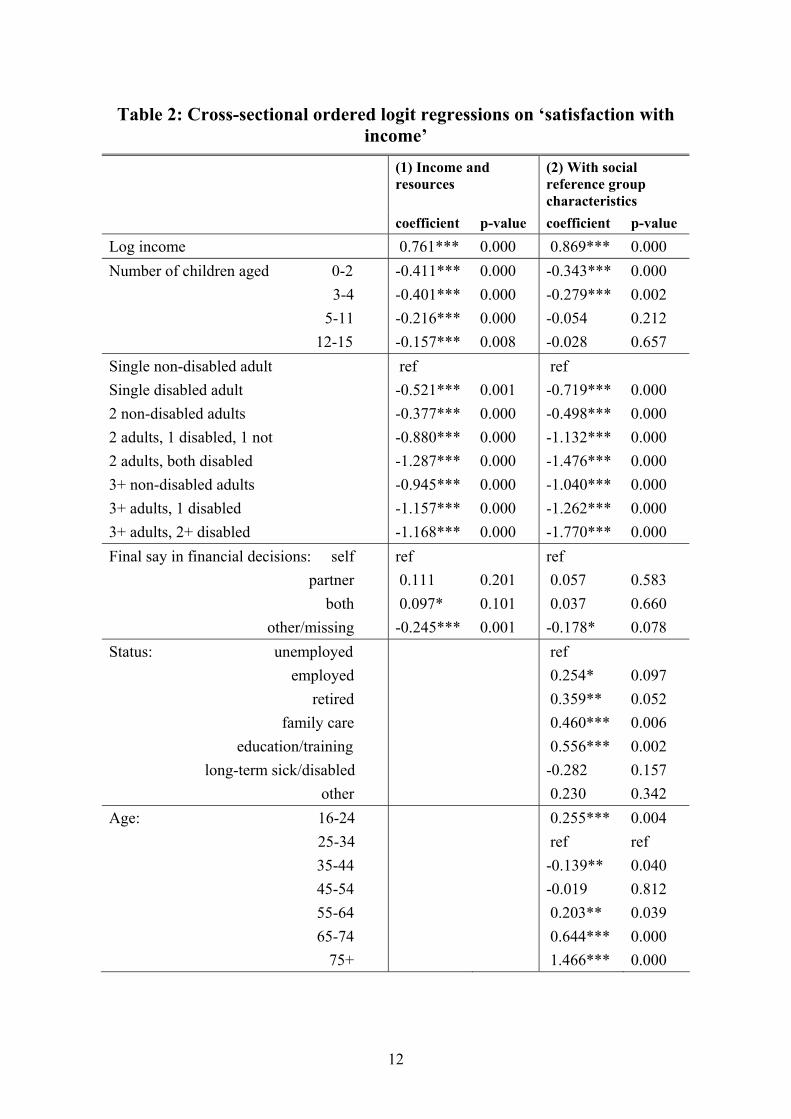
Table 2: Cross-sectional ordered logit regressions on ‘satisfaction with income’

(1) Income and resources

(2) With social reference group characteristics

coefficient p-value coefficient p-value Log income 0.761*** 0.000 0.869*** 0.000 Number of children aged 0-2 3-4 5-11 12-15

-0.411*** -0.401*** -0.216*** -0.157***

0.000 0.000 0.000 0.008

-0.343*** -0.279*** -0.054 -0.028

0.000 0.002 0.212 0.657

Single non-disabled adult Single disabled adult 2 non-disabled adults 2 adults, 1 disabled, 1 not 2 adults, both disabled 3+ non-disabled adults 3+ adults, 1 disabled 3+ adults, 2+ disabled

ref -0.521*** -0.377*** -0.880*** -1.287*** -0.945*** -1.157*** -1.168***

0.001 0.000 0.000 0.000 0.000 0.000 0.000

ref -0.719*** -0.498*** -1.132*** -1.476*** -1.040*** -1.262*** -1.770***

0.000 0.000 0.000 0.000 0.000 0.000 0.000

Final say in financial decisions: self partner both other/missing

ref 0.111 0.097* -0.245***

0.201 0.101 0.001

ref 0.057 0.037 -0.178*

0.583 0.660 0.078

Status: unemployed employed retired family care education/training long-term sick/disabled other

ref 0.254* 0.359** 0.460*** 0.556*** -0.282 0.230

0.097 0.052 0.006 0.002 0.157 0.342

Age: 16-24 25-34 35-44 45-54 55-64 65-74 75+

0.255*** ref -0.139** -0.019 0.203** 0.644*** 1.466***

0.004 ref 0.040 0.812 0.039 0.000 0.000

12

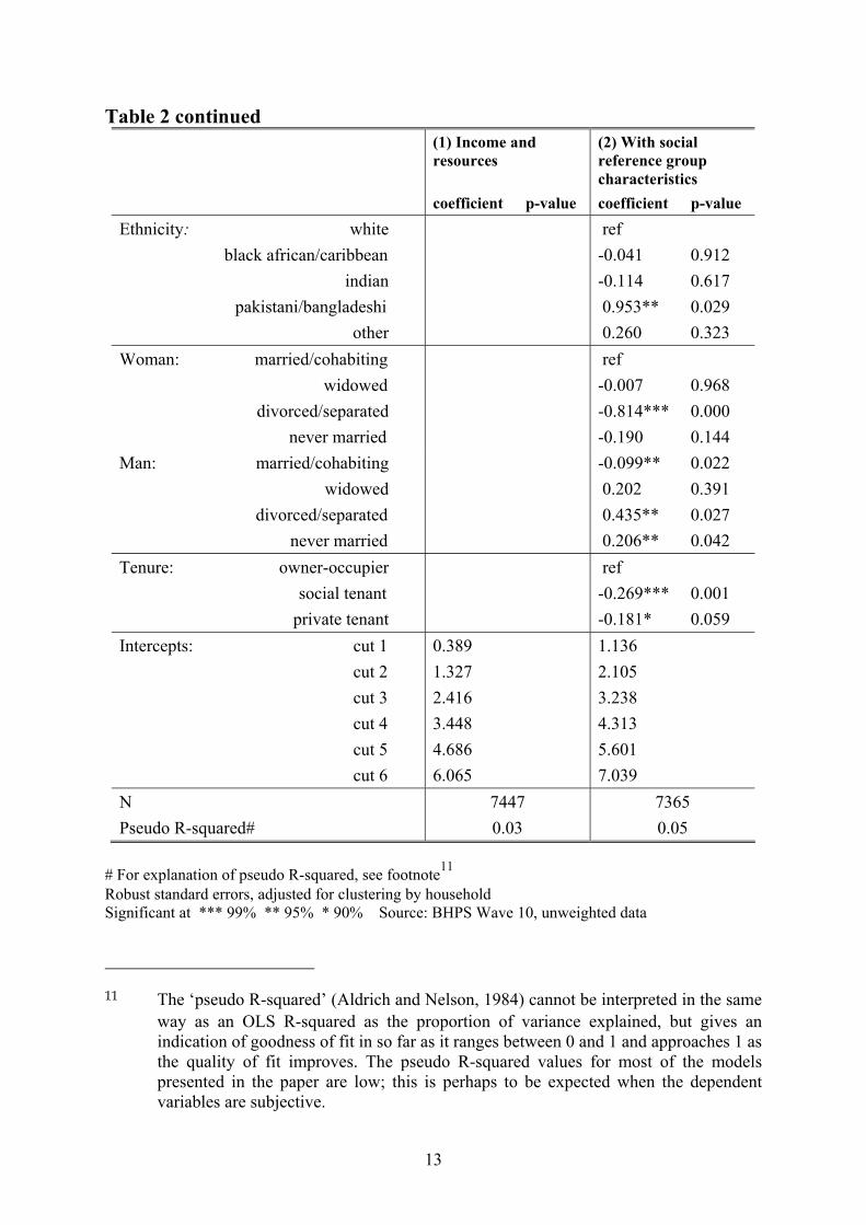
Table 2 continued (1) Income and

resources (2) With social reference group characteristics

coefficient p-value coefficient p-value Ethnicity: white black african/caribbean indian pakistani/bangladeshi other

ref -0.041 -0.114 0.953** 0.260

0.912 0.617 0.029 0.323

Woman: married/cohabiting widowed divorced/separated never married

ref -0.007 -0.814*** -0.190

0.968 0.000 0.144

Man: married/cohabiting widowed divorced/separated never married

-0.099** 0.202 0.435** 0.206**

0.022 0.391 0.027 0.042

Tenure: owner-occupier social tenant private tenant

ref -0.269*** -0.181*

0.001 0.059

Intercepts: cut 1 cut 2 cut 3 cut 4 cut 5 cut 6

0.389 1.327 2.416 3.448 4.686 6.065

1.136 2.105 3.238 4.313 5.601 7.039

N 7447 7365 Pseudo R-squared# 0.03 0.05

# For explanation of pseudo R-squared, see footnote11

Robust standard errors, adjusted for clustering by household Significant at *** 99% ** 95% * 90% Source: BHPS Wave 10, unweighted data 11 The ‘pseudo R-squared’ (Aldrich and Nelson, 1984) cannot be interpreted in the same

way as an OLS R-squared as the proportion of variance explained, but gives an indication of goodness of fit in so far as it ranges between 0 and 1 and approaches 1 as the quality of fit improves. The pseudo R-squared values for most of the models presented in the paper are low; this is perhaps to be expected when the dependent variables are subjective.

13

The results for age are in line with findings in previous studies (for example, Lelkes, 2002): the young and the old are happier than the middle-aged, for a given level of income. Few of the differences by ethnic group are significant (possibly due to small numbers of ethnic minority respondents in the BHPS), but it does appear that people from a Pakistani or Bangladeshi background are more satisfied than their white counterparts, controlling for income. This could indicate a social reference group effect: since Pakistani and Bangladeshi communities are the poorest ethnic groups in Britain (Modood et al, 1997), the expectations of individuals from those backgrounds for financial wealth may be lower. These groups are also more recent immigrant groups than the other large ethnic minorities in the UK, so some of the older members of the community may be comparing their living standards now with those in their country of origin. If so, this would suggest a form of adaptation: immigrants who arrived longer ago (and second and third generation immigrants) have adjusted their expectations to UK living standards while more recent immigrants retain a comparison with their country of origin. A detailed study of date of arrival and living standards in the country of origin would be required to test this hypothesis. With respect to gender and marital status, it appears that divorced or separated women are less satisfied than married or cohabiting women with the same income, but divorced men are more satisfied. On the other hand, married men are significantly less satisfied than their female counterparts. In general, marriage has been found to be associated with higher overall life satisfaction, especially for women, and divorce with lower satisfaction, again especially for women (Clark et al, 2003). The relationship between marital status and satisfaction with income is more complex, however. In addition to ‘spillover’ effects from life satisfaction directly related to marital status, there could be at least two other mechanisms at work: (i) the share of household income which the individual accesses, and (ii) conditioned expectations. Work on intra-household distribution of resources (eg Pahl, 1989) leads us to expect that some married women access less than their ‘fair’ share of household income and consequently that satisfaction with a given level of household income (controlling for household size) would be higher for divorced than for married women. On the other hand, we know that divorce often results in a sharp decrease in income for women and an increase in income for men, so if expectations were conditioned by previous martial status, we would expect divorced women to be less satisfied and divorced men to be more satisfied. The results in Table 2 are more consistent with this second hypothesis, but fuller exploration, including the time elapsed since change in marital status, would be required to confirm it. This must wait for another paper.

14

Finally, tenants, and in particular tenants in social housing, are less satisfied than owner-occupiers in otherwise similar circumstances. Bearing in mind that income is measured here as after housing costs income, this result could be explained by owner-occupiers feeling that some of their income has already been spent on an investment rather than purely on consumption. Various other characteristics, for example educational qualifications, region, and further interaction terms, were included in other versions of the models but they were not found to be significant. 4.2 Annual changes in income Thus far, the associations examined have been cross-sectional. But in order to test for adaptation, it is necessary to investigate change in income over time. In this section, we ask whether respondents who have experienced an increase in income are more satisfied than those with the same current level of income who have experienced no change. Such a result would suggest that individuals are subjectively evaluating their current status relative to their recent experience. In the regressions reported in Table 3, individuals appear for each pair of consecutive waves at which they were a respondent in the survey. For this reason standard errors are adjusted for clustering on individuals (over time), as well as within households (at a point in time).12 The dependant variable is the same as previously – satisfaction with income in the current year, adjusted to year 2000 prices13 – but here the explanatory variables include both the log of current income and change in log income since the previous interview. The average change in income between the current interview and the previous interview (approximately one year previously) is correlated with current income. However, the correlation between log income and change in log income (i.e. percentage change in income) is not so great as to give rise to worries of colinearity.14 Another potential concern is the wide dispersion of changes in income. The range of change in equivalised income is -7024 to +6772 with 1st and 99th percentiles at -529 and +582 respectively. These long tails of the distribution are 12 Strictly speaking, the clusters are defined as all members (in any wave) of the original

household in which respondents entered the survey. 13 In case there is a ‘money illusion’, by which nominal incomes are more salient than

incomes in real terms, the regressions were also performed using nominal incomes and year dummies. The substantive conclusions from the results were the same.

14 The correlation between log income and change in log income is 0.52.

15

strongly suggestive of problems of measurement error. Accordingly, an alternative specification was tried using change in log equivalised income trimmed symmetrically by 1 per cent. The coefficient on change in income was -0.263, similar to that in model 3. In model 3, the coefficient on log (equivalised) income is positive, indicating that as before, a higher current income is associated with greater satisfaction. The coefficient on change in income is negative: for a given current income, those who have experienced an increase in their income since last year are less satisfied. The first impression is that this is counterintuitive. Those who experience a change in income might be in different circumstances to those who remain on constant income; Model 4 therefore adds controls for current characteristics, as in the previous cross-sectional analysis.15 Once again, the coefficient on log income is positive and the coefficient on change in log income is negative. Other correlates show similar relationships with satisfaction as in the cross-sectional analysis. Changes in needs or resources, or a change in social comparison group, might affect satisfaction with income, independently of a change in income. For this reason, Model 5 adds variables reflecting changes in characteristics as well as current status. The results need to be interpreted with caution since some of the changes in characteristics (such as losing an adult from the household or changing employment status) could be the cause of the change in income. In fact, many of the change variables are not statistically significant, and the coefficients on income and change in income, which are of principal interest, are similar to those in model 4.

15 Ethnicity and control over household resources are omitted because they are not

significant once change in income since last year is included.

16

Table 3: Ordered logit regressions on ‘satisfaction with income’, controlling for change in income since last year

(3) Change in income

(4) With current characteristics

(5) With change characteristics

coefficient p-value coefficient p-value coefficient p-value Log equivalised income 0.428*** 0.000 Change in log equivalised income Log income Change in log income

-0.180*** 0.000 0.369*** -0.146***

0.000 0.000

0.374*** -0.155***

0.000 0.000

Number of children aged 0-2 3-4 5-11 12-15 Change in no. children in hh: -2 or more -1 no change +1 +2 or more

-0.271*** -0.104** -0.055** -0.087***

0.000 0.024 0.043 0.010

-0.268*** -0.119*** -0.066** -0.086*** -0.083 -0.032 ref -0.006 0.158

0.000 0.010 0.022 0.012 0.621 0.450 0.894 0.280

Single non-disabled adult Single disabled adult 2 non-disabled adults 2 adults, 1 disabled, 1 not 2 adults, both disabled 3+ non-disabled adults 3+ adults, 1 disabled 3+ adults, 2+ disabled Change in no. and d. status of adults in hh: -2 or more -1 no change +1 +2 or more

ref -0.665*** -0.227*** -0.661*** -1.105*** -0.377*** -0.703*** -1.146***

0.000 0.003 0.000 0.000 0.000 0.000 0.000

ref -0.755*** -0.258*** -0.741*** -1.217*** -0.417*** -0.785*** -1.266*** -0.291*** -0.313*** ref 0.088* 0.032

0.000 0.001 0.000 0.000 0.000 0.000 0.000 0.000 0.000 0.083 0.596

Status unemployed employed retired family care education/training long-term sick/disabled other

ref 0.808*** 0.748*** 0.761*** 0.856*** 0.100 0.687***

0.000 0.000 0.000 0.000 0.375 0.001

17

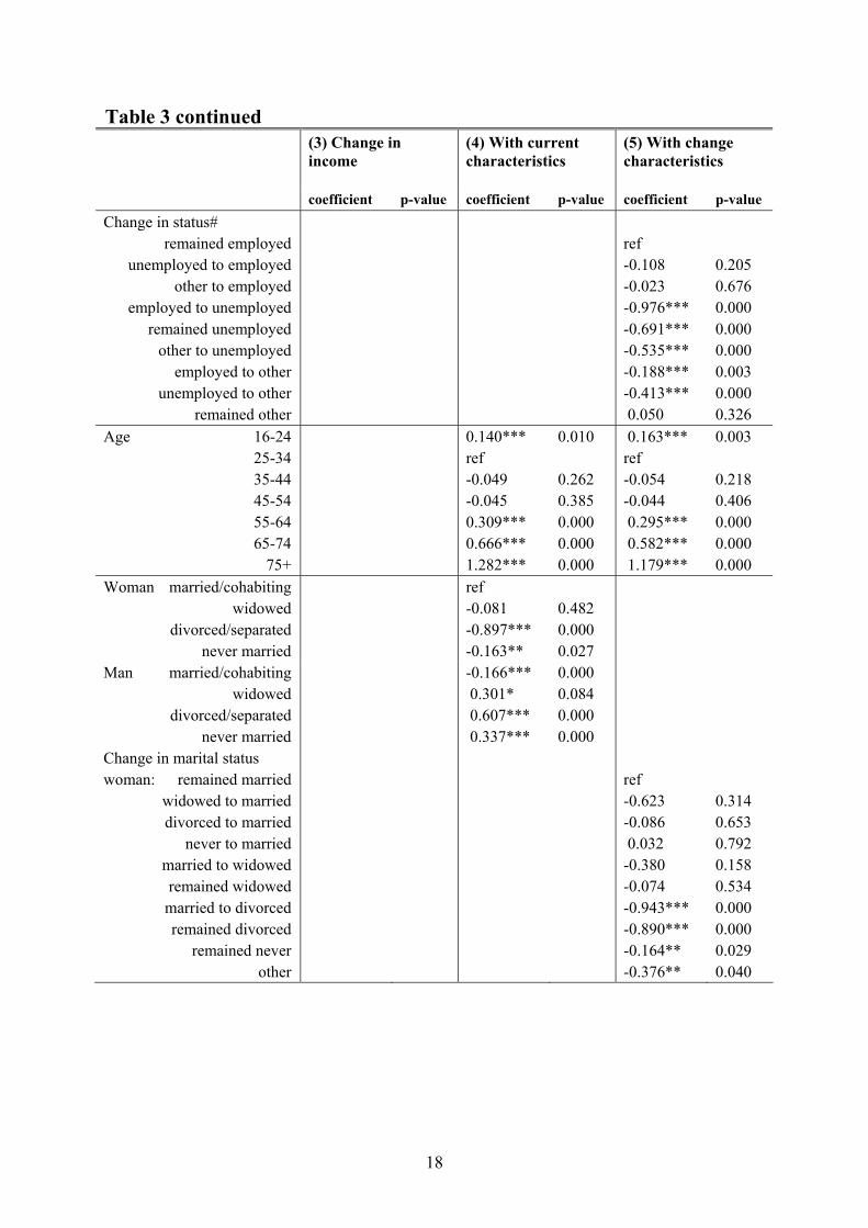
Table 3 continued (3) Change in

income (4) With current characteristics

(5) With change characteristics

coefficient p-value coefficient p-value coefficient p-value Change in status# remained employed unemployed to employed other to employed employed to unemployed remained unemployed other to unemployed employed to other unemployed to other remained other

ref -0.108 -0.023 -0.976*** -0.691*** -0.535*** -0.188*** -0.413*** 0.050

0.205 0.676 0.000 0.000 0.000 0.003 0.000 0.326

Age 16-24 25-34 35-44 45-54 55-64 65-74 75+

0.140*** ref -0.049 -0.045 0.309*** 0.666*** 1.282***

0.010 0.262 0.385 0.000 0.000 0.000

0.163*** ref -0.054 -0.044 0.295*** 0.582*** 1.179***

0.003 0.218 0.406 0.000 0.000 0.000

Woman married/cohabiting widowed divorced/separated never married

ref -0.081 -0.897*** -0.163**

0.482 0.000 0.027

Man married/cohabiting widowed divorced/separated never married Change in marital status woman: remained married widowed to married divorced to married never to married married to widowed remained widowed married to divorced remained divorced remained never other

-0.166*** 0.301* 0.607*** 0.337***

0.000 0.084 0.000 0.000

ref -0.623 -0.086 0.032 -0.380 -0.074 -0.943*** -0.890*** -0.164** -0.376**

0.314 0.653 0.792 0.158 0.534 0.000 0.000 0.029 0.040

18

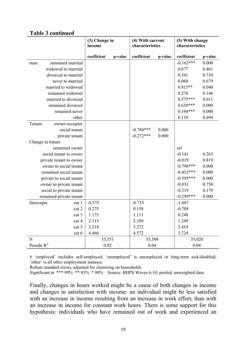
Table 3 continued (3) Change in

income (4) With current characteristics

(5) With change characteristics

coefficient p-value coefficient p-value coefficient p-value man: remained married widowed to married divorced to married never to married married to widowed remained widowed married to divorced remained divorced remained never other

-0.162*** 0.677 0.101 0.068 0.815** 0.274 0.575*** 0.638*** 0.344*** 0.110

0.000 0.461 0.710 0.679 0.040 0.146 0.011 0.000 0.000 0.694

Tenure owner-occupier social tenant private tenant Change in tenure remained owner social tenant to owner private tenant to owner owner to social tenant remained social tenant private to social tenant owner to private tenant social to private tenant remained private tenant

-0.780*** -0.272***

0.000 0.000

ref -0.141 -0.019 -0.796*** -0.452*** -0.595*** -0.033 -0.219 -0.299***

0.263 0.819 0.000 0.000 0.000 0.750 0.179 0.000

Intercepts cut 1 cut 2 cut 3 cut 4 cut 5 cut 6

-0.575 0.275 1.175 2.115 3.218 4.466

-0.733 0.158 1.111 2.109 3.272 4.572

-1.607 -0.708 0.248 1.249 2.419 3.724

N Pseudo R2

35,551 0.02

35,508 0.04

35,020 0.04

# ‘employed’ includes self-employed; ‘unemployed’ is unemployed or long-term sick/disabled; ‘other’ is all other employment statuses. Robust standard errors, adjusted for clustering on households Significant at *** 99% ** 95% * 90% Source: BHPS Waves 6-10, pooled, unweighted data Finally, changes in hours worked might be a cause of both changes in income and changes in satisfaction with income: an individual might be less satisfied with an increase in income resulting from an increase in work effort, than with an increase in income for constant work hours. There is some support for this hypothesis: individuals who have remained out of work and experienced an

19

increase in income are more satisfied than those who have the same increase and level of income but have started part-time work, and the latter are more satisfied than those who have moved into full-time work. Furthermore those who have increased their hours from part-time to full-time work are more satisfied than those who have remained part-time or decreased their hours (controlling for level and change in income). Details of the regressions behind these results are given in the Appendix. However, the relationship between satisfaction and changes in work hours is not sufficient to explain the negative coefficient on change in income; this remains significant even after controlling for changes in hours. In the literature, some models which have apparently found evidence of adaptation to changes in income have included a measure of baseline satisfaction (usually satisfaction in the previous year) as a control variable. This is to allow for the possibility that individuals interpret the seven-point satisfaction scale differently. For the BHPS data used here, including satisfaction last year as an additional control variable does indeed produce the expected result of a positive coefficient on change in income. However, this is equivalent to regressing change in income on change in satisfaction: since we know that higher incomes are associated with higher satisfaction, it is not surprising that individuals who have experienced an increase in income also become more satisfied, but this tells us nothing about adaptation. 4.3 Heterogeneity A better way to account for heterogeneity in the way in which individuals interpret the satisfaction scale is to use the panel structure of the data to compare each individual to him or herself over time, rather than making comparisons across individuals. This also allows for other sources of unobservable heterogeneity, such as the possibility that some individuals (probably the less satisfied) are more motivated to try to increase their income, and for personality traits. Table 4 therefore reports results from fixed effects regressions on satisfaction with income. Each observation is a person-at-a-wave and the variation which is explained is the variation in the satisfaction of that individual from his or her average satisfaction over the period of observation. The fixed effects framework also allows time-varying covariates to be taken into account. The coefficients on explanatory variables relate to the association between satisfaction and a higher-than-average value of that variable for that individual at a particular point in time. Only variables which vary over time have explanatory force; all other characteristics are fixed effects, including, for example, baseline satisfaction for each individual.

20

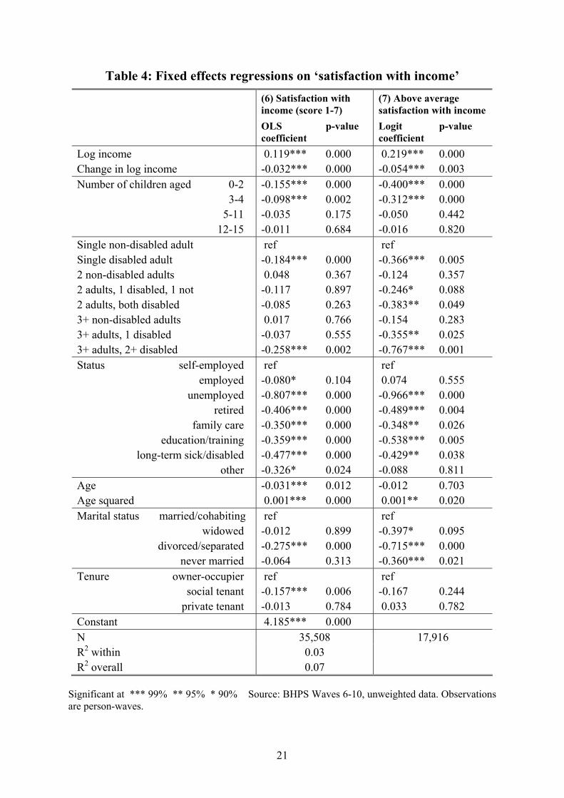
Table 4: Fixed effects regressions on ‘satisfaction with income’ (6) Satisfaction with

income (score 1-7) (7) Above average satisfaction with income

OLS coefficient

p-value Logit coefficient

p-value

Log income 0.119*** 0.000 0.219*** 0.000 Change in log income -0.032*** 0.000 -0.054*** 0.003 Number of children aged 0-2 3-4 5-11 12-15

-0.155*** -0.098*** -0.035 -0.011

0.000 0.002 0.175 0.684

-0.400*** -0.312*** -0.050 -0.016

0.000 0.000 0.442 0.820

Single non-disabled adult Single disabled adult 2 non-disabled adults 2 adults, 1 disabled, 1 not 2 adults, both disabled 3+ non-disabled adults 3+ adults, 1 disabled 3+ adults, 2+ disabled

ref -0.184*** 0.048 -0.117 -0.085 0.017 -0.037 -0.258***

0.000 0.367 0.897 0.263 0.766 0.555 0.002

ref -0.366*** -0.124 -0.246* -0.383** -0.154 -0.355** -0.767***

0.005 0.357 0.088 0.049 0.283 0.025 0.001

Status self-employed employed unemployed retired family care education/training long-term sick/disabled other

ref -0.080* -0.807*** -0.406*** -0.350*** -0.359*** -0.477*** -0.326*

0.104 0.000 0.000 0.000 0.000 0.000 0.024

ref 0.074 -0.966*** -0.489*** -0.348** -0.538*** -0.429** -0.088

0.555 0.000 0.004 0.026 0.005 0.038 0.811

Age Age squared

-0.031*** 0.001***

0.012 0.000

-0.012 0.001**

0.703 0.020

Marital status married/cohabiting widowed divorced/separated never married

ref -0.012 -0.275*** -0.064

0.899 0.000 0.313

ref -0.397* -0.715*** -0.360***

0.095 0.000 0.021

Tenure owner-occupier social tenant private tenant

ref -0.157*** -0.013

0.006 0.784

ref -0.167 0.033

0.244 0.782

Constant 4.185*** 0.000 N 35,508 17,916 R2 within R2 overall

0.03 0.07

Significant at *** 99% ** 95% * 90% Source: BHPS Waves 6-10, unweighted data. Observations are person-waves.

21

Model 6 is an ordinary least squares fixed effects regression, treating the satisfaction score as continuous and cardinal. This is not ideal but is necessary because a fixed effects ordered logit is computationally very demanding. An alternative specification, reducing the satisfaction scale to a binary ‘above or below average’ indicator, and using a fixed effects logit regression, is presented as model 7. The latter loses many data because only those observations at which the value of the dependant variable changes can be used, and in the case of a binary satisfaction indicator, this entails moving across the mean satisfaction threshold. The principal interest of these models is in the coefficients on income and change in income. In both models, the coefficient on log income is positive, indicating that for individual i, in those years when her income is higher than average, she is more satisfied than her own average satisfaction score over the whole period. Once again, the coefficients on change in log income are negative and significant (though small). This implies that for individual i, comparing two periods with identical current income, the period which is preceded by an increase in income is associated with lower satisfaction. This is not consistent with the adaptation hypothesis. Various alternative specifications were tried to test the robustness of this result. Trimming the change in income variable symmetrically by 1 per cent generated a similar size and sign of coefficient on change in income as model 6. Entering change in income without logs (since change in income might have a linear rather than a log-linear effect) produced a very small, but significant, positive coefficient on change in income (0.1 x 10-4). It did not add to the explanatory power of the model. Model 6 remains the preferred specification. 4.4 Direction and magnitude of changes in income Thus far, analysis of annual changes has shown no convincing evidence to support the hypothesis that increases in income result in greater satisfaction in the short term than constant income. If anything, those who experience an increase appear to be less satisfied (compared either to others with similar characteristics, or to themselves in other periods). There are number of possible explanations for these counter-intuitive results. Firstly, the effect of a change in income could depend on an individual’s starting point in the income distribution. This is explored below. Secondly, the size of changes in income could matter. We know from work on income dynamics (for example, Gardiner and Hills, 1999) that some incomes fluctuate from year to year without any overall trend. For these individuals, an increase in income may not bring the expectation of the same or higher income in the following year, and hence may not enhance satisfaction significantly. In fact these small fluctuations could be associated with uncertainty and insecurity. Since large changes in income are

22

comparatively rare, a negative subjective effect of small changes could be outweighing the positive effects of large increases. Thirdly, in a dynamic context, current income may not reflect the true availability of resources: those who have recently been poor may still be paying off debts, while those who have recently been rich may still be living off accumulated assets. If a change in income were sustained over a longer period of time it might make more of a difference. Similarly, expenditure is often thought to be smoother than income, and if it is expenditure rather than income itself that produces satisfaction, then an increase in income might take longer than a year to translate into an increase in satisfaction. Table 5 summarises results from exploring whether the starting point in the income distribution is correlated with the effect of changes in income on satisfaction. Initial position is defined as equivalised income quintile at wave 5, the year before the first data observations used in the analysis. Model 8 is an ordered logit regression on pooled data (comparing across individuals), with an interaction term between change in income since last year and initial position in the income distribution. The results indicate that for the middle three income groups, the relationship between change in income and satisfaction is similar (i.e. the interaction terms are not significant), but for the top income quintile group, an income level which was preceded by an increase in income is associated with greater satisfaction than the same constant income level; while for the bottom income quintile group, the opposite is the case. Thus among the top income group only, there is some support for the adaptation hypothesis: those on constant high incomes have adapted to that level. This is confirmed by the results of the fixed effects regressions (comparing individuals to themselves over time) run separately for those initially in the bottom income quintile group and those in the top group (models 9 and 10 respectively). Model 9 shows a negative coefficient on change in income and model 10 shows a positive coefficient. A possible explanation for the difference between the subjective response of those at top and bottom of the income distribution to changes in income is offered in the conclusions.

23

Table 5: Regressions on ‘satisfaction with income’, taking account of initial position in income distribution

(8) Ordered logit, with interaction term

(9) Fixed effects OLS: bottom initial quintile group only

(10) Fixed effects OLS: top initial quintile group only

coefficient p-value coefficient p-value coefficient p-value Log income Y 0.281*** 0.000 0.115*** 0.000 0.056** 0.018 Change in log Y -0.040*** 0.001 0.045*** 0.007 Initial quintile group: bottom x change in log Y second x change in log Y third x change in log Y fourth x change in log Y top x change in log Y

ref -0.107*** 0.080 -0.014 0.284*** 0.016 0.547*** -0.011 0.846*** 0.063*

0.000 0.248 0.529 0.000 0.477 0.000 0.713 0.000 0.057

Other controls as for model 5

Y

Other controls as for model 6

Y Y

N 30,736 5,655 6,237 Pseudo R2

R2 within R2 overall

0.05 0.06 0.04

0.04 0.00

Robust standard errors, adjusted for clustering on households Significant at *** 99% ** 95% * 90% Source: BHPS Waves 6-10, unweighted data. The size of the change in income could also matter. In Model 11 (Table 6), changes are calculated as percentages of the previous year’s income and the classification divides the sample approximately into fifths.

24

Table 6: Regressions on ‘satisfaction with income’, allowing for differences by magnitude and direction of change in income

(11) Ordered logit (12) Fixed effects OLS: fallers only

(13) Fixed effects OLS: risers only

coefficient p-value coefficient p-value coefficient p-value Log equivalised income Change in income: large fall (<= -20%) fall (-20% < d <= -5%) flat (-5% < d <= 5%) rise (5% < d <= 20%) large rise (>20%)

0.327*** -0.135*** -0.103*** ref -0.012 -0.163***

0.000 0.000 0.005 0.721 0.000

Log income 0.158*** 0.000 0.396*** 0.000 Change in log income -0.130*** 0.001 -0.136 0.198 Other controls as for model 6

Y Y

N 35,551 12,461 16,197 Pseudo R2

R2 within R2 overall

0.01 0.04 0.07

0.04 0.14

Robust standard errors, adjusted for clustering on households Significant at *** 99% ** 95% * 90% Source: BHPS Waves 6-10, unweighted data. Model 11 shows that for a given current level of income, those who have experienced a large fall in income since the last wave are less satisfied than those who have remained on a constant income. Individuals who have experienced a small fall in income are also less satisfied (though not as much as the large fallers). This is consistent with the adaptation hypothesis. However, the results for those who have experienced an increase in income remain puzzling. Small increases are not significantly associated with greater or lesser satisfaction, while large increases are associated with less satisfaction than for those on constant income.16 This could suggest that those who experience a large increase in income are a particular kind of (dissatisfied)

16 Neither excluding outliers from the distribution of changes in income nor interacting

changes in income with level of income produced more consistent results. The interaction did suggest however that falls in income are less strongly associated with dissatisfaction if the individual was initially in a high income quintile group.

25

person – hence the fixed effects regressions in models 12 (fallers) and 13 (risers). The fixed effects regression for fallers confirms the earlier results. For risers, change in income is not significantly associated with a change in satisfaction, once individual heterogeneity and observable time-varying characteristics are taken into account. Drawing together these results, we find some evidence in support of the adaptation hypothesis among those who have experienced a fall in income: fallers appear be comparing their current income unfavourably with their previous income. This holds whether the comparison is made across individuals (between fallers and those with flat incomes), or across time for a particular individual (periods preceded by a fall in income associated with less satisfaction than periods of flat income). For those who experience an increase in income, the story is more complex. Compared to constant income, small rises appear to make little difference to satisfaction. Large rises are associated with dissatisfaction (when comparing individuals), or no change in satisfaction (comparing across time for a particular individual). The contrast in results from the pooled and fixed effects regressions suggests that individuals who experience large rises in income could have certain characteristics which make them more likely to be dissatisfied. There is some support for this hypothesis in the literature: Kasser and Ryan (2001) found that individuals with a materialistic disposition were generally better off but less satisfied with life overall. In addition, the specific dynamics of adaptation to changes in income could contribute to explaining these results: rises in income could take longer than a year to register subjectively with an individual as a genuine increase, or, alternatively, adaptation might have taken place so quickly that the individual has already become accustomed to their new standard of living. With data drawn from annual interviews, we cannot investigate the latter, but we can examine the former, and it is to that longer-run perspective that we now turn. 4.5 Income trajectories over ten years The trajectory types used in this analysis are a simplified version of those developed by Gardiner and Hills (1999) for the BHPS and extended by Rigg and Sefton (2004). Using a balanced 10-wave panel, three trajectory types are defined on the basis of percentiles of the distribution:17

17 A balanced panel means selecting only those individuals who were part or full

respondent households at all 10 waves. N = 3932. Following Rigg and Sefton (2004), percentiles are defined on the wave 1 distribution and then up-rated in line with

26

Flat relatively stable position in the income distribution over all ten waves: all observations within a band of plus or minus 15 percentiles from the mean.

Rising a move of at least 15 percentiles up the income distribution over

the ten waves. Downwards movements may occur but the overall trend is positive and significant.18

Falling a move of at least 15 percentiles down the income distribution over

the ten waves. Upwards movements may occur but the overall trend is negative and significant.

All other trajectories, most of which involve more fluctuation than those described above, are classified as a residual ‘other’ category (see Table 7).

Table 7: Income trajectories over 10 waves, current income and satisfaction

Trajectory types (column %)

Income, wave 10 (mean £ pw)

Satisfaction with income, wave 10

Flat 23 347 4.80 Rising 20 512 4.81 Falling 8 234 4.30 Other 48 323 4.54 All (N = 3,932) 100 360 4.64

Source: BHPS Waves 1-10, balanced panel, weighted using longitudinal weights Not surprisingly, those who have experienced rising incomes have higher current incomes, on average, than those who have had flat trajectories, who in turn have higher average income than those who have experienced falling income. This ranking corresponds to the ranking of average satisfaction scores for the three trajectory types too, although interestingly the difference between

average income growth for each subsequent wave (to create ‘quasi-percentiles’). If the income distribution had not changed over the period, there would therefore be 1 per cent of the sample at each wave in each quasi-percentile group. In practice, there is a slightly higher proportion of the sample in the lower quasi-percentile groups by the end of the panel.

18 Significance is determined by regressing income (adjusted to 2000 prices) against year, using ordinary least squares estimation. If the coefficient on income is positive and significant at the 90 per cent level, this is taken to indicate rising income. A similar procedure is applied to identify falling trajectories.

27

the satisfaction scores for the ‘flat’ and ‘rising’ groups is much less than would be expected on the basis of the difference between their incomes. (The difference between ‘flat’ and ‘rising’ mean satisfaction scores is not statistically significant at the 95% level. The differences between ‘flat’ and ‘falling’, and between ‘flat’ and ‘other’, are significant.) One might expect the impact of previous income trajectory on current satisfaction to vary according to the individual’s position in the income distribution. A breakdown by current income quintile group indicates particularly low satisfaction scores for those in the bottom income quintile at the end of the ten year period who have experienced falling income (3.88) compared to those who have flat low income profiles (4.42). This suggests that those who have fallen into poverty are very much less satisfied than those who have been poor over the longer-term. This is strongly suggestive of a process of adaptation. Turning to multivariate analysis, Table 8 shows an ordered logit regression on satisfaction with income at wave 10, controlling for log of current income and income trajectory over the full 10 wave period as the main explanatory variables. A fixed effects approach cannot be adopted here because income trajectory type is itself a time-invariant characteristic and would be differenced-out in a fixed effects regression.

Table 8: Ordered logit regressions on ‘satisfaction with income’, controlling for ten-wave income trajectory

(14) Ten-wave trajectory coefficient p-value Log income 0.298*** 0.000 Income trajectory flat rising falling other

ref 0.104 -0.262* -0.142*

0.291 0.073 0.104

Other controls as for model 4 Y N 3,889 Pseudo R2 0.04

Significant at *** 99% ** 95% * 90% Source: BHPS Waves 1-10, balanced panel, unweighted data. Observations are unique individuals. Standard errors adjusted for clustering by household. Compared to those who have experienced a flat income trajectory over the ten-year period, those who have had rising incomes are no more satisfied. The troubling negative sign on the coefficient for rising incomes which occurred in

28

the previous models based on annual changes in income has disappeared, but it has not been replaced by a significantly positive coefficient. Over this longer time frame, then, one possible explanation is that individuals with rising incomes have adapted to their improved financial circumstances. By contrast, for a given final income, those who have experienced a falling trajectory over the ten waves are significantly less satisfied than those with long-run flat incomes. This indicates that those whose incomes are falling are not adapting to their changing circumstances over this period, at least not completely. Perhaps they retain some expectations or aspirations relating to their previous level of income. The ‘other’ trajectory type, the bulk of which is made up by fluctuating income patterns, is also associated negatively with satisfaction. This could indicate that for a given level of income, those who faced uncertainty about their income are less satisfied than those who have stable incomes.

5. Discussion

Some economists have suggested that questions about satisfaction are not the right way to measure utility, because they implicitly invite respondents to use cognition and comparison, rather than assessing moment-by-moment affect or mood (Kahneman et al, 2003). Differences between the two types of measure are certainly of interest, but it is far from clear that utility should be interpreted as some aggregation of affect rather than drawing on the distinctively human faculty of critical reflection on, and appraisal of, our own lives. Indeed, the narrower the definition of utility which is adopted, the harder it is to motivate the utilitarian ethic altogether: why should we regard the maximisation of the sum of momentary pleasures to be the be-all and end-all of social arrangements? It seems clear that individuals take many other factors into account in assessing their own lives, and frequently make prolonged sacrifices of positive affect for the sake of uncertain gains. Satisfaction with life, broadly understood, is thus a more plausible interpretation of utility for the welfarist or utilitarian. But as the analysis presented in this paper has shown, investigating the dynamics of satisfaction in one particular domain – income – and its relationship to objective income brings some surprising patterns to light. Satisfaction with a given level of income is not only influenced by who you are and who you have around you (as shown in previous studies and in Table 2 above), it is also affected by who you have been (Table 3). These relationships

29

are intriguing and point to several avenues for further research: for example, analysis of the effect of immigration on expectations of standard of living and how this changes over time and generations; and analysis of the interaction between direct effects of marital status on satisfaction, with share of household resources, and conditioned expectations to explain the differential effect by gender of changes in marital status on satisfaction with income. Falls in income from one year to the next adversely affect satisfaction compared to a constant income at the same final level, while rises in income are met with dissatisfaction or ambivalence (Table 6). These results hold both when comparing across individuals and for a particular individual over time (Table 4). Further work is needed to understand the counter-intuitive results with respect to short-run increases in income. Although some attempt was made to allow for measurement error, more sophisticated techniques could by applied. More substantively, investigating the demographic and labour market events which are associated with short-run changes in income might be revealing, pursuing the leads provided by analysis of changes in hours of work in the Appendix: increases in income associated with increases in work effort are less subjectively rewarding than other increases in income.19

Another promising avenue to explore further would be the differences in the relationship between changes in income and satisfaction for individuals starting at different points in the income distribution (Table 5). The top quintile group shows the strongest evidence of adaptation (those with high income in two consecutive years are less satisfied than those with income which has recently increased), while the bottom quintile group shows the opposite (those with consistent low income are more satisfied than those with recent increases in income). Understanding the underlying causes of changes in income at different points in the income distribution – for example, whether due to increased work effort or change in household composition – could help to explain these differences. Over the longer run, for the same outcome in terms of level of income, those who have experienced rising incomes do not experience greater satisfaction than those who have had constant incomes, while those who have experienced falling incomes are significantly less satisfied (Table 8). Subjective responses to increases and decreases in income therefore appear to be asymmetric; this finding is consistent with Kahneman and Tversky’s prospect theory (1979).

19 Clark et al (2003) have looked at the direct effects of events such as marriage, divorce

and unemployment on life satisfaction, but not in the context of changes in household income.

30

In addition, unstable incomes are subjectively less satisfactory than stable ones. This dislike of uncertainty suggests that individuals’ beliefs about the future play an important role in the subjective evaluation of income. Analysing such data as we have on financial expectations could also be a fruitful area for further research. Taken together, the results confirm that income is a flawed proxy for satisfaction, even within the specific domain of satisfaction with income, and indicate that satisfaction offers an unattractive basis on which to evaluate well-being or equality. Satisfaction is influenced in complex ways not only by current characteristics and situation, but also by individuals’ previous experience. Those who have become poor within a ten-year period are less satisfied than those who have been poor throughout that time, while those who are upwardly mobile are not in general any better satisfied than those who have experienced a higher income over a long period. These past experiences may have been shaped by circumstances of unjust privilege or disadvantage, and the fact that they influence individuals’ current satisfaction, implies that satisfaction – the best proxy we have for the concept of utility – is unsuitable for assessing current well-being, justice or equality. Instead we need an objective normative standard of assessment, such as is offered by the capabilities framework.

31

Appendix: Satisfaction with income and changes in work hours

Table A1 shows results from ordered logit regressions on satisfaction with income, controlling for log equivalised income and change in log income. Model A1 adds controls for changes in work hours, while Model A2 selects those with an increase in income and interacts change in log income with changes in work hours. Model A1 indicates that for a given level of income and change in income since last year, those who remain out of work (0 to 0) are more satisfied than those who remain employed part-time, who are in turn more satisfied than those who remain employed full-time. This is consistent with the idea that longer hours of work reduce satisfaction with given income. However, individuals whose hours of work have changed substantially do not conform to this pattern: for example, those who have moved from full-time to part-time work, or to no work at all, are less satisfied with their income than those who have remained in full-time work. To investigate further, model A2 selects those who have experienced an increase in income and compares those for whom the increase in income is associated with an increase in hours and those for whom it is not. Looking first at those who had no work in the previous year, the interaction terms combined with the main effects indicate that those who have moved into full-time or part-time work are less satisfied than those who have remained out of work. In other words, an increase in income gained at the price of an increase in work effort gives lower returns to satisfaction. The same holds true for those who were initially in part-time work, or for those initially in full-time work.

32

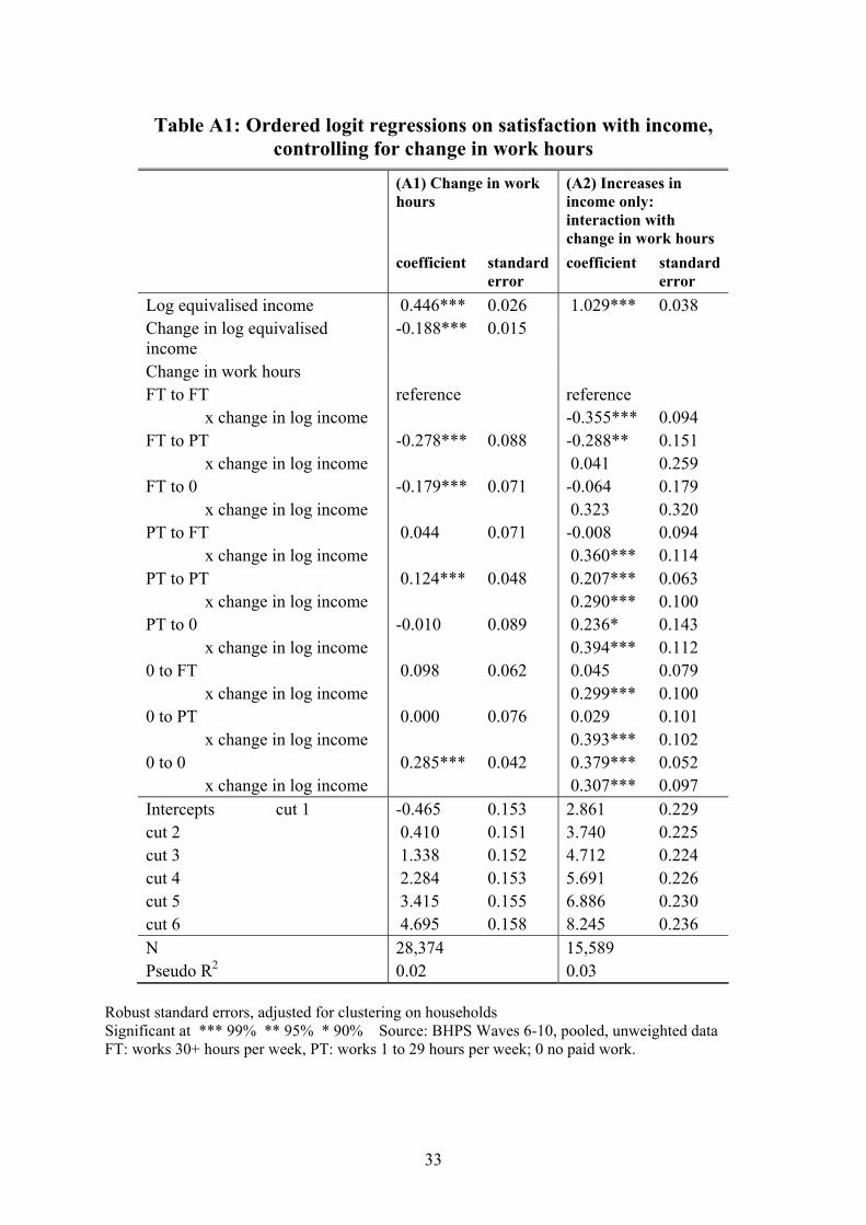
Table A1: Ordered logit regressions on satisfaction with income, controlling for change in work hours

(A1) Change in work hours

(A2) Increases in income only: interaction with change in work hours

coefficient standard error

coefficient standard error

Log equivalised income 0.446*** 0.026 1.029*** 0.038 Change in log equivalised income

-0.188*** 0.015

Change in work hours FT to FT x change in log income FT to PT x change in log income FT to 0 x change in log income PT to FT x change in log income PT to PT x change in log income PT to 0 x change in log income 0 to FT x change in log income 0 to PT x change in log income 0 to 0 x change in log income

reference -0.278*** -0.179*** 0.044 0.124*** -0.010 0.098 0.000 0.285***

0.088 0.071 0.071 0.048 0.089 0.062 0.076 0.042

reference -0.355*** -0.288** 0.041 -0.064 0.323 -0.008 0.360*** 0.207*** 0.290*** 0.236* 0.394*** 0.045 0.299*** 0.029 0.393*** 0.379*** 0.307***

0.094 0.151 0.259 0.179 0.320 0.094 0.114 0.063 0.100 0.143 0.112 0.079 0.100 0.101 0.102 0.052 0.097

Intercepts cut 1 cut 2 cut 3 cut 4 cut 5 cut 6

-0.465 0.410 1.338 2.284 3.415 4.695

0.153 0.151 0.152 0.153 0.155 0.158

2.861 3.740 4.712 5.691 6.886 8.245

0.229 0.225 0.224 0.226 0.230 0.236

N Pseudo R2

28,374 0.02

15,589 0.03

Robust standard errors, adjusted for clustering on households Significant at *** 99% ** 95% * 90% Source: BHPS Waves 6-10, pooled, unweighted data FT: works 30+ hours per week, PT: works 1 to 29 hours per week; 0 no paid work.

33

References

Abbey. A. and Andrews, F. (1986) “Modelling the psychological determinants of life quality”. In F. Andrews (ed.) Research on the Quality of Life. University of Michigan: Institute for Social Research.

Aldrich, J. and Nelson, F. (1984) Linear Probability, Logit and Probit models. Beverly Hills, CA: Sage.

Bardasi, E., Jenkins, S. and Rigg, J. (2003) Documentation for Derived Current and Annual Net Household Income Variables, BHPS waves 1-10. Colchester: Institute for Social and Economic Research, University of Essex.

Chan, A., Ofstedal, M., Hermalin, A. (2002) “Changes in subjective and objective measures of economic well-being and their interrelationship among the elderly in Singapore and Taiwan”. Social Indicators Research, 57: 263-300.

Clark, A. (1999) “Are wages habit-forming? Evidence from micro-data”. Journal of Economic Behavior and Organization, 39: 179-200.

Clark, A., Diener, E., Georgellis, Y. and Lucas, R. (2003) Lags and Leads in Life Satisfaction: a test of the baseline hypothesis. DIW Berlin Discussion Paper 371. Berlin: German Institute for Economic Research.

Clark, A., Georgellis, Y. and Sanfey, P. (1998) “Job satisfaction, wage changes and quits: evidence from Germany”. In S. Polachek (ed.) Research in Labor Economics. Volume 17. London: JAI Press.

Davis, J. (1984) “New money, an old man/lady and ‘two’s company’: subjective welfare in the NORC general social surveys, 1972-1092”. Social Indicators Research, 15: 319-350.

De Neve, K. and Cooper, H. (1999) “The happy personality: a meta analysis of 137 personality traits of subjective well-being”. Psychological Bulletin, 125: 197-229.

Diener, E. and Lucas, R. (1999) “Personality and subjective well-being”. In D. Kahneman, E. Diener and N. Schwarz (eds) Well-Being: the foundations of hedonic psychology. New York: Russell Sage Foundation.

Diener, E., Sandvik, E., Siedlitz, L and Diener, M. (1993) “The relationship between income and subjective well-being: relative or absolute?” Social Indicators Research, 28: 195-223.

Easterlin, R. (1995) “Will raising the incomes of all increase the happiness of all?” Journal of Economic Behavior and Organization, 27: 35-47.

34

Easterlin, R. (2001) “Income and happiness: towards a unified theory”. The Economic Journal, 111 (July): 465-484.

Frank, R. (1997) “The frame of reference as a public good”. The Economic Journal, 107 (November): 1832-1847.

Frederick, S. and Lowenstein, G. (1999) “Hedonic adaptation”. In D. Kahneman, E. Diener and N. Schwarz (eds) Well-Being: the foundations of hedonic psychology. New York: Russell Sage Foundation.

Frey, B. and Stutzer, A. (2002) “What can economists learn from happiness research?” Journal of Economic Literature, XL (June): 402-435.

Gardiner, K. and Hills, J. (1999) “Policy implications of new data on income mobility”. The Economic Journal, 109: F91-F111.

Graham, C. and Pettinato, S. (2002) “Frustrated achievers: winners, losers and subjective well-being in new market economies”. Journal of Development Studies, 38 (4): 100-140.

Grund, C. and Sliwka, D. (2003) The Further we Stretch, the Higher the Sky: on the impact of wage increased on job satisfaction. Bonn Econ Discussion Paper 1/2003. Bonn: University of Bonn.

Inglehart, R. and Rabier, J.-R. (1986) “Aspirations adapt to situations – but why are the Belgians so much happier than the French? A cross-cultural analysis of the subjective quality of life”. In F. Andrews (ed.) Research on the Quality of Life. University of Michigan: Institute for Social Research.

Kahneman, D. and Tversky, A. (1979) “Prospect theory: an analysis of decision under risk”, Econometrica, 47: 263-291.

Kahneman, D., Krueger, A., Schkade, D., Schwarz, N. and Stone, A. (2003) “A survey method for characterizing daily life experience: the Day Reconstruction Method (DRM)”. Paper presented at Centre for Economic Performance seminar, London School of Economics, 14 July.

Kasser, T. and Ryan, R. (2001) “Be careful what you wish for: optimal functioning and the relative attainment of intrinsic and extrinsic goals”. In P. Schmuck and K. Sheldon (eds) Life Goals and Well-Being: towards a positive psychology of human striving. Kirkland, WA: Hogrefe and Huber.

Lelkes, O. (2002) Well-Being and Inequality in Transition: the case of Hungary. PhD thesis, London School of Economics.

Michalos, A. (1991) Global Report on Student Well-Being. Volume 1: life satisfaction and happiness. New York: Springer-Verlag

35

Modood, T., Berthoud, R., Lakey, J., Nazroo, J., Smith, P., Virdee, S., and Beishon, S. (1997) Ethnic Minorities in Britain: diversity and disadvantage. London: Policy Studies Institute.

Nussbaum, M. (2001) “Adaptive preferences and women’s options”. Economics and Philosophy, 17: 67-88.

Oswald, A. (1997) “Happiness and economic performance”. The Economic Journal, 107 (November): 1815-1831.

Pahl, J. (1989) Money and Marriage. Basingstoke: Macmillan. Ravallion, M. and Lokshin, M. (2001) “Identifying welfare effects from

subjective questions”. Economica 68: 335-357. Rigg, J. and Sefton, T. (2004) Income Dynamics and the Lifecycle: evidence

from 10 waves of the British Household Panel Survey. CASEpaper 81. London: Centre for Analysis of Social Exclusion, London School of Economics.

Schyns, P. (2002) “Wealth of nations, individual income and life satisfaction in 42 countries: a multilevel approach”. Social Indicators Research, 60:5-40.

Sen, A. (1987) The Standard of Living. Cambridge: Cambridge University Press.

Stutzer, A. (2004) “The role of income aspirations in individual happiness”. Journal of Economic Behavior and Organization, 54 (1): 89-109.

Taylor, M. (ed) (2001) British Household Panel Survey User Manual. Introduction, Technical Reports and Appendices. Colchester: ESRC Research Centre on Micro-Social Change, University of Essex.

Tomes, N. (1986) “Income distribution, happiness and satisfaction: a direct test of the interdependent preferences model”. Journal of Economic Psychology, 7: 425-446.

Winkelmann, L. and Winkelmann, R. (1998) “Why are the unemployed so unhappy? Evidence from panel data”. Economica, 65:1-15.

36