network planning/scheduling techniques for project

UVA-OM-0294

This case was prepared by Professor Edward W. Davis with the assistance of Gail Ann Zarwell. It was written as a basis for class discussion rather than to illustrate effective or ineffective handling of an administrative situation. Copyright © 1981 by the University of Virginia Darden School Foundation, Charlottesville, VA. All rights reserved. To order copies, send an e-mail to [email protected]. No part of this publication may be reproduced, stored in a retrieval system, used in a spreadsheet, or transmitted in any form or by any means—electronic, mechanical, photocopying, recording, or otherwise—without the permission of the Darden School Foundation. Revised 1996 with the assistance of J.W. Ellis. Rev. 7/96. ¸

NETWORK PLANNING/SCHEDULING TECHNIQUES FOR PROJECT MANAGEMENT Introduction

There is a broad category of Operations Management problems having to do with the management of project-type operations. Such operations are typically illustrated by the example of some large-scale, one-time activity such as the design and production of a new prototype machine, the construction of a new facility, or the design and manufacture of a new weapon system. Project-type activities are in and of themselves nothing new; indeed, they represent one of the oldest known types of production activities. However, it is only comparatively recently that this type of activity has been recognized as an Operations Management problem of great significance. This recognition came about primarily as a result of post-World War II emphasis in the United States on the design and production of very large-scale systems in the aerospace industry, such as the Polaris missile weapon system. Such systems typically involved the development and manufacture of extremely complicated and expensive products in relatively small numbers. Because of the enormous costs involved in these development programs and the national importance assigned to them, entirely new management procedures were needed for their effective control. Such procedures were developed around 1958; since then they have been applied to an amazingly wide variety of activities including building and road construction, equipment and machinery manufacture and maintenance, research and development management, health-care activities (even to the planning of surgical operations), marketing and financial-area program management, and other types of activity too numerous to list.

The special characteristics of this type of problem arise both from (1) the typical complexity of the activity undertaken, wherein custom design and performance of a multiplicity of tasks on a non-repetitive nature may be involved, and (2) the fact that “projects” typically have a specified beginning and end point. In such situations the planning of the sequence of processes required becomes of extreme importance, since operations performed not in the proper sequence can lead to extra costs and delays in the overall project.

-2- UVA-OM-0294

The development of the project plan in the form of a network of activities will indicate the particular sequencing and timing of activities required to complete the project in minimum time (usually called the “critical path schedule”). This plan also shows which operations can be delayed somewhat without delaying the overall project and, perhaps more importantly, it can show the pattern over time of the resource levels needed to achieve the indicated plan. Since the amounts of individual resources available are typically limited in quantity, the question of most effective resource utilization is of extreme importance.

The development of the project network diagram represents one of the greatest advances in project management techniques. Use of a project network facilitates solution of planning and execution problems such as: Which project activities can be performed simultaneously? What kind of labor skills will be required during different phases of the project? How long will the project, or a portion of it, take to complete? These and other questions are answered readily, even for complex projects involving thousands of activities, with the aid of a project network. Network-Based Planning/Scheduling Techniques

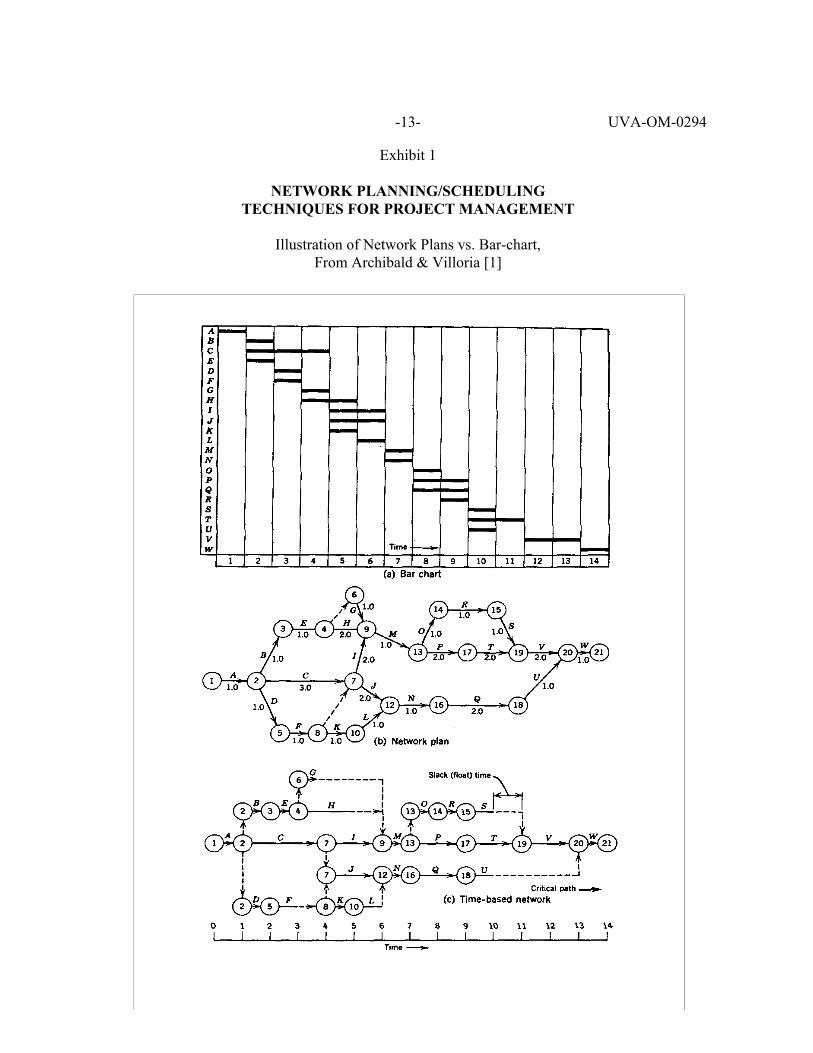
The basis of all network scheduling techniques is the project network diagram. Exhibit 1 depicts an activity-on-arrow network plan of a project, along with the older Gantt or bar chart representation of the same project. In the activity-on-arrow diagram (also referred to as “I-j” diagram), arrows denote activities, or jobs. “Dummy” jobs of zero duration, usually represented by dashed lines such as shown for job 4-6, are often required for correct network logic in some situations. All early network diagrams were of the activity-on-arrow type and this representation is still the most widely used today. Figure 1 also shows a time-scaled network for the same project. This type of representation, while quite useful in manual analysis of small projects (or summary networks of large projects), is obviously limited in application.

Another major type of network representation is the activity-on-node or precedence diagram, in which the role of arrows and nodes is changed. Exhibit 2 shows such a diagram for a house-building project. Here nodes represent activities and arrows indicate precedence. The activity-on-node diagram, relatively unknown during the early years of network technique development, has enjoyed increased popularity in recent years. While still not as popular as the activity-on-arrow format, it is available today as an option on most commercially offered computer programs for network analysis. One advantage of this representation is that “dummy” jobs are not required within the network (but they may be required to provide a single starting and single ending job).

It is important to emphasize that the types of network diagrams described above are often generally referred to as “project networks,” and that the basic concepts and procedures of network analysis apply to each of these types of diagram.

The origins of network analysis date back to 1958 when two separate (but essentially similar) procedures were developed. The first, termed “PERT” (for Program Evaluation and Review

-3- UVA-OM-0294 Techniques) by its developers, involved the use of three separate time estimates for each activity. The second, named “CPM” (for Critical Path Method), involved only one time estimate for each activity. The PERT approach of three time estimates included the use of statistically-based procedures to produce probability estimates of project completion. While this approach at first captured the imagination of many project planners, it was later found to have serious weaknesses and has gradually been discarded in favor of the one-time-estimate-per-job approach. However, the name PERT has continued to be used as a generic term for the procedures of network analysis, and today both PERT and CPM are used interchangeably to refer to the common approach of: (1) representing the project in the form of a network diagram and (2) performing the necessary calculations upon the diagram to determine the critical path and start and finish for each activity. Network Analysis: An Example

Consider the (simplified) problem of preparing a production facility to produce a new product. Assume that this project contains eight separately identifiable steps or activities and that estimates of the time requirements of each activity have been obtained as follows: A: Design production tooling (3 weeks); B: Prepare manufacturing drawings (2 weeks); C: Prepare production facility to receive new tooling and parts (5 weeks); D: Procure tooling (7 weeks); E: Procure production parts (4 weeks); F: Kit parts (1 week); G: Install Tools (2 weeks); H: Test (1 week).

Assume also that the sequence of the eight activities has been determined as follows: Activities A, B, and C can be conducted simultaneously at the start of the project. Activity A must precede activity D and both activities D and C must be complete before activities F and G can take place. Similarly, activity B must precede activity E and activity E must precede activity F. Activities F and G can take place simultaneously if necessary, but both must be complete before activity H can occur (the completion of which signifies end of the project).

With the above information a rough arrow diagram such as shown in Exhibit 3(a) can be drawn. By adding identification nodes at the head and tail end of each arrow, a completed activity-on-arrow diagram (such as shown earlier in Exhibit 1(b)) could be obtained. Alternatively, each activity arrow of Exhibit 3(a) can be replaced with an activity node and arrows drawn between nodes to indicate precedence. This activity-on-node network diagram is shown in Exhibit 3(b).

Note that a start node was added to complete the usual diagram requirement of a single beginning node and single ending node. Note also that the “dummy” activity which was required to satisfy the stated project sequence requirements in the rough activity-on-arrow diagram is not needed in the activity-on-node network representation.

-4- UVA-OM-0294 Critical Path Determination by Network Methods

From examination of Exhibit 3(b), it may be seen that the longest sequence of time durations from start to finish is 13 weeks, which is given by the sequence of activities A, D, G, H. It is this chain of “critical” activities which determines that the completion time of the project is 13 weeks. If any of the activities along this path require longer than their estimated times (with no corresponding reductions in other activities along the chain), the project duration will increase accordingly. This “longest path” chain of activities is called the critical path. It can be found in any network by calculating the sum of activity durations along all possible paths from project start to completion; however, this is a tedious and impractical approach with the size of network diagrams occurring in practice (which often contain thousands of activities). A more systematic approach, and one also suitable for computer programming, is that offered by the standard PERT/CPM calculation procedure.

This produces not only the critical path (or paths, since there often more than one), but also the start and finish times of every activity in the network and the allowable slippage or “slack” associated with each job. This procedure consists of two separate parts: (1) a forward pass through the network from start to finish and (2) a backward pass through the network from finish to start. The purpose of each “pass”, and the steps associated with each, are explained below, using the network diagram shown in Exhibit 4.

The objective of the forward pass calculation is to determine the so-called early start time (EST) and early finish time (EFT) of each activity. The interpretation of these terms is easier if we take zero as an arbitrary starting time for the project. Then, measuring from time zero, the early start time of each activity is the earliest possible time at which the activity can begin assuming that all predecessor activities also start at their EST. The early finish time of each activity is determined by adding the activity duration to its EST. The steps involved in the forward pass calculations are as follows:

1. Place the value of project starting time (zero) to the above left of each beginning activity, as shown for activities A, C and B, in the position shown for early start time in Exhibit 4. The early finish time for these activities is then simply (EST + activity duration), or 3 for activity A and 5 for activity C as shown on Exhibit 4.

2. Choose any new unmarked activity, all of whose immediate predecessor activities have been

marked with their EST and EFT. The EST of the unmarked activity is equal to the largest EFT value of all its immediate predecessor activities. For example, in Exhibit 4 the EST of activity G is shown as 10, which is the largest of the EFT values of its two immediate predecessor activities D and C. Write the newly-determined EST value to the left of the activity as before.

3. The EFT for the newly-marked activity of step 2 above is (EST + activity duration), as

before. Mark this value in the EFT position. For activity G this value is 10 + 2 = 12, as shown.

-5- UVA-OM-0294

4. Continue through the entire network until the final “finish” activity has been marked with its EST and EFT. In Exhibit 4 it can be seen that the EFT for activity H is 13. This is the earliest time at which the project can be completed.

Note that in order to complete these forward pass calculations accurately, care must be taken

at those nodes with several entering arrows. Such activities have their EST determined by the largest EFT of any of their immediate predecessors, as noted above.

The backward pass calculations are performed after the forward pass procedure described above is completed. The objective of this new pass is to determine the so-called late start time (LST) and late finish time (LFT) of each activity. These times are interpreted as the latest possible time at which an activity can start or finish without delaying the project. In calculating these latest possible times, some target completion date for the project must be assigned, and this is usually taken as the EFT of the final activity calculated during the forward pass. This early finish time of the final activity is then also considered to be the latest finish time of that activity—in other words, it is assumed that there is no “slack” or slippage allowed beyond this value and that the project must be completed as early as possible. Once the LFT of the final activity is set, its late start time (LST) is simply (LFT - activity time), and similar values for all other activities can be set by working backwards through the network. The steps in the backward pass procedure are given below:

1. For the final activity of the project, set LFT = EFT, and mark this value in its proper position beside the activity. Then, calculate LST = (LFT - activity time) and mark this value in its proper position. In Exhibit 4, for activity H, LFT = 13 and LST = (13 - 1) = 12, as shown.

2. Choose any new activity without LFT and LST values yet marked, but all of whose

immediate successor (follower) activities have been marked. Mark in the LFT position for the new activity the smallest LST value marked for any of its immediate followers. In Exhibit 4, then, activity G takes its LFT value of 12 from the LST value of H.

3. Calculate the LST of the new activity being marked as (LFT - activity time) and mark this

value in its proper position. For activity G, LST = (12 - 2) = 10.

4. Continue backwards through the network in similar fashion until all activities have been marked with an LFT and LST.

Note that in order to complete the backward pass calculations accurately, careful note must

be taken of those nodes at which several arrows exit. These activities have their LFT values determined by the smallest LST of any of the successor activities (e.g., for activity D, the LFT is 10, not 11).

Once the complete set of early and late start and finish times have been calculated for all activities, the total slack (TS) of each activity can be calculated. Activity total slack is defined as the maximum amount of time that an activity can be delayed without delaying project completion time.

-6- UVA-OM-0294 Since the “critical” activities are those in the sequence of the longest time path through the network, it follows that the activities on this path will have the minimum possible total slack. And since the target completion date (i.e., the EFT) of the final activity is taken as the LFT of the final activity, it can be seen that all critical activities will have total slack equal to zero. Likewise, if the project completion target date were taken as later than the EFT of the final activity, all activities on the critical path would have exactly this amount of slack and all non-critical activities would have their slack increased by an equal amount. For any activity, total slack can be calculated as: TS = (LST - EST) = (LFT - EFT). In the network of Exhibit 4, the calculated slack values are shown for each activity above the box containing start/finish times (e.g., for activity C, total slack = 5).

There is also another type of slack, termed free slack. This is the amount of time that an activity can be delayed without delaying the EST of any follower activity. Free slack for an activity never exceeds the total slack for the activity; it is calculated as the difference between EFT for that activity and the earliest of the EST values of all its immediate followers. For example, in Exhibit 4, activity E with total slack = 5, has free slack = 4, since its EFT = 6 and the EST of activity F = 10. Time/Cost Tradeoff Procedures

It is often true that the performance of some or all project activities can be accelerated by the allocation of more resources at the expense of higher activity direct cost. When this is so there are many different combinations of activity durations which will yield some desired schedule duration. However, each combination may yield a different value of total project cost. Time/cost tradeoff procedures are directed at determining the least-cost schedule for any given project duration.

For example, consider the simple 8-activity project shown in Exhibit 5. Each activity can be performed at different durations ranging from an upper “normal” value, at some associated “normal” cost, down to a lower, “crash” value, with an associated higher cost. Note that if time/cost tradeoff values for each activity are assumed to be linear, the cost of intermediate activity durations between the normal and crash durations is easily determined from the single cost “slope” value for each activity (e.g., the cost of performing activity 0-2 in 7 days instead of 8 equals $400 + $80, or $480).

If all activity durations are set at “normal” values, the project duration is 22 days, as determined by the critical path consisting of activities 0-1, 1-2, 2-4, 4-5. The associated cost of project performance is $3050, as indicated in Exhibit 5. Note that this cost could be increased to $3870 through unintelligent decision making by “crashing” all activities not on the critical path, with no decrease in project duration. Between these upper and lower cost values for a project duration of 22 days there are several other possible values, depending upon the number of noncritical activities crashed.

If all activity durations are set at “crash” values, the project duration can be decreased to 17 days, with a total cost of $4,280, as shown by the extreme upper left point of Exhibit 6. However, a duration of 17 days can also be achieved at lower cost by not “crashing” activities unnecessarily. Thus, activity 0-2 can be set at 7 instead of 6, activity 1-4 at 8 instead of 7, and activity 2-3 at 4

-7- UVA-OM-0294 instead of 1. With all other activities set at crash value, the associated cost of performance for a 17-day project duration is reduced to $3,570. This value is the lowest possible value for a 17-day project duration, as may easily be determined by experimentation.

Between 22 and 17 days there are several possible values of project duration, as shown in Exhibit 6. For each such duration there is a range of possible cost values depending upon the durations of individual activities and whether activities are crashed unnecessarily or not. Exhibit 6 shows the curve of both maximum and minimum costs and the region of possible costs for each duration between these curves.

In this simple example the minimum direct cost curve is easily determined by trial and error. But in more realistic cases consisting of hundreds or even dozens of activities such trial-and-error determination becomes extremely tedious, if not impossible. Thus various systematic computation schemes, including mathematical programming, have been developed to aid in the quick determination of the minimum cost curve for every possible value of project duration. Some of these routines are designed to handle cases in which the activity time/cost tradeoff relationships are nonlinear; many will also produce the lowest total curve (i.e., sum of direct plus indirect costs), as illustrated in Exhibit 7.

There are two important points to note about time/cost procedures: first, resource limitations are usually not considered explicitly. Most procedures mentioned will not automatically produce a minimum-cost schedule that will satisfy stated constraints on the availability of resources such as cost, manpower or equipment.

Secondly, time/cost tradeoff procedures have not been widely implemented in practice. The major reasons for this lie in the amount and complexity of input data required for analysis, coupled with the typical uncertainty of this data. The collection of detailed time/cost information for projects consisting of hundreds of activities, for example, is usually not an easy task, fraught with many uncertainties. Thus, while the information available from time/cost procedures is potentially quite valuable under certain conditions, such procedures today enjoy a relatively unimportant position in the overall hierarchy of network-based resource allocation techniques. Resource Loading

One of the major advantages of the network format of project representation is the ability to easily generate information on the time-phased requirements of such project resources as manpower, equipment, and money. This information is a by-product of the usual critical path method scheduling computations. The only requirement is that the resource demands associated with each project activity represented in the network diagram be identified separately.

Exhibit 8, for example, shows the activity on node, or “precedence diagram,” network for a simple hypothetical project. Beside each network node representing a project activity is shown the duration in months and the cash requirements in hundreds of dollars per month. By application of

-8- UVA-OM-0294 the usual CPM calculations an “Early Start Time” (EST) and “Late Finish Time” (LFT), among other data, can be produced for each activity. From this information a bar-chart diagram, such as shown in Exhibit 9(a), can be drawn, with all activities beginning at their respective EST’s. The bar-chart diagram, in turn, is used to produce the profile of cash flow requirements over time, as shown in Exhibit 9(b). This type of analysis can be performed manually or automatically by the computer program which does the CPM calculations. Exhibit 10, for example, shows a computer-produced diagram of cash flow requirements and the associated diagram of cumulative cash requirements for a sample project as produced by a commercially-available CPM program [5].

The examples in Exhibits 8 & 9 use cash requirements for illustration. Obviously, data on other resources, such as labor, could be used instead.

In such cases the profile of resource usage over time is commonly referred to as a resource loading diagram. In cases of multiple resource types a separate loading diagram for each resource type is obtained. Such loading diagrams are extremely useful in project management; they highlight the resource implications of a particular project schedule and provide the basis for more rational project planning. One major pharmaceutical firm, for example, regularly obtains resource loading information from all CPM schedules for R&D projects to provide resource feasibility checks on the amounts of highly skilled medical and research personnel required at any time. Such procedures are also widely used in the construction industry, with some smaller firms often plotting labor loading diagrams manually from CPM output. In most cases the resource loading data are more important as rough planning guides rather than as precise goals to be obtained, because of schedule uncertainty.

Most good CPM programs today will automatically produce resource loading information (in the form of tables or diagrams) even though they may lack the more sophisticated capability of automatic schedule adjustment to meet desired resource loading requirements. This latter capability falls in the categories of resource leveling or scheduling under fixed resource constraints and is discussed below. Resource Leveling

In many project scheduling situations the total level of resource demands projected for a particular schedule by the resource loading diagram may not be of major concern because simple quantities of the required resources are available. But it may be that the pattern of resource usage has undesirable features, such as frequent changes in the amount of a particular worker skill category required. Resource-leveling techniques are useful in such situations; they provide a means of distributing resource usage over time to minimize the period-by-period variations in labor, equipment or money expended. They can also be used to determine whether peak resource requirements can be reduced with no increase in project duration.

The concepts of resource leveling are easily grasped through a simple example. Consider,

for instance, the same network diagram of Exhibit 8 but assume that the time durations shown beside each node are now days instead of months. And let the resources required, instead of

-9- UVA-OM-0294 hundreds of dollars per month, be number of workers of a particular skill required per day. Then the resource loading diagram of Exhibit 10(a) shows an undesirable pattern of labor requirements over time because of the extreme variation from 24 workers on days 3 and 4 down to 1 worker on days 8, 9 and 10. Resource leveling will produce a more even pattern of labor utilization without increasing project duration beyond 10 days.

As the bar chart of Exhibit 10(a) shows, jobs 1, 2, 4 and 5 have slack and can be delayed within the limits of their slack without delaying other jobs. Job 1, for example, can obviously be delayed until the last 4 days of project performance, as shown in part (b) of Exhibit 10. This reduces peak labor requirements from 24 to 14 and the resulting labor profile is more level than before. However, it still contains considerable fluctuations, with an undesirable “valley” on day 6. By subsequently rescheduling jobs 2 and 5 a more even pattern is obtained, as shown in Exhibit 10(c). This final profile still contains what might be considered undesirable peaks on days 2 and 4 but these cannot be eliminated without either increasing project duration or changing the characteristics of some activities so that the associated worker requirements are changed.

As this simple example shows, the essential idea of resource-leveling centers about the “juggling” or rescheduling of jobs within the limits of available slack (float) to achieve better distribution of resource usage. The slack available in each activity is determined from the standard CPM calculations. Thus the project duration (i.e., the Critical Path) is determined by a “time only” analysis, without consideration of resource requirements, and during the resource-leveling process this duration is not allowed to increase. Constrained Resource Scheduling

Through the process of resource leveling, as illustrated above, the profiles of resource usage of different resources can be “smoothed” to the extent allowed by available job slack. But this process does not always produce satisfactory schedules if the amounts of available resources are tightly constrained. The final worker profile of Exhibit 10(c), for example, is constant at 10 workers per day except for days 2, 4 and 7, where peaks above that level occur. If available labor were strictly limited to 10 workers per day for this project, and if the resource requirements of jobs could not be reduced in some manner, the only way of eliminating these peaks to obtain a resource-feasible schedule would be through further rescheduling, with a resultant increase in project duration. Looking at Exhibit 10(c), for example, it is readily apparent that the labor peaks can be eliminated by delaying the start of job 1 from day 6 until day 7. This permits job 5 to be delayed 1 day, making it concurrent with job 7, and also permits delaying job 2 for 1 day to make it concurrent with job 6. Since the resulting labor requirements in every period total exactly 10 or less, the schedule is resource-feasible. However, the project duration has increased by 1 day, as the resulting schedule of Exhibit 11(a) shows.

The type of rescheduling illustrated by this example falls into another category of procedures

for network analysis. Called constrained-resource scheduling, these are techniques designed to produce schedules that will not require more resources than are available in any period and which at

-10- UVA-OM-0294 the same time have durations that are increased beyond the original critical path duration as little as possible.

Constrained-resource network scheduling procedures were first proposed shortly after the general appearance of PERT/CPM models. During the next two decades interest in constrained-resource procedures continued at a high level and literally dozens of different procedures were developed. Some of these approaches were designed to produce minimum-cost (instead of minimum-duration) schedules; some were much more complicated than others. This great bulk of procedures can be categorized into two major groups on the basis of their distinctly different methods of approach and utility to management. The first - and by far the largest - category includes the heuristic or approximate, procedures which are designed to produce “good” resource-feasible schedules. The second category, in contrast, consists of procedures designed to produce the optimal (“best”) schedule and includes approaches based on linear programming, partial enumeration, and other mathematical techniques. These mathematical optimization procedures, are capable of handling far less complex problems than the heuristic category.

Heuristic procedures have received so much attention over the past two decades that it is not feasible to describe in detail here the many various approaches that have been developed. However, a great many of these approaches are quite similar in nature; a good idea of the general types of capabilities available can be obtained by reference to some of the recent texts on project management, such as [8], [9]. CPM Software Packages

Business organizations and government agencies have been using computer programs since the 1960s to help manage the types of large projects often found in construction, aerospace-defense and new project development activities. Until the late 1980s, the majority of project management programs were designed by organizations for internal use and required access to very expensive mainframe computers. Today, however, with the exponential increases in PC computing power, mainframe software has been largely replaced by PC-based software.

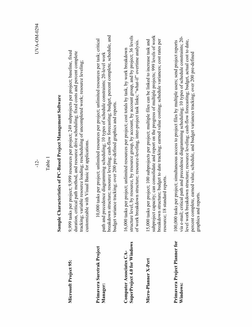
The net result of this change has been an increase in the affordability, availability, and useability of project management software. For example, one of the most popular programs, Microsoft Project 95, costs only a few hundred dollars and can be up and running within a few hours with the help of a Windows-based environment and on-line tutorials. Also, Microsoft Project 95 is only one of the many different programs available (e.g., the Project Management Institute Internet site, www.pmi.org, provides a listing of over 70 different programs and the companies that make them). Table 1 has a sampling of some of the more popular programs available.

Most project management software available for the PC today can do almost everything that has been mentioned in this note, including critical path scheduling, resource loading, and resource leveling. In addition, today’s programs will allow the project manager to e-mail reports to project members, to create specialized calculation functions, to import and export data out of or into Excel

-11- UVA-OM-0294 or Lotus spreadsheets, and to generate various types of cost and schedule reports and charts. For most users this standard set of capabilities is enough to meet their needs. Programs of this type tend to cost between $200-$500.

For the high-end user there are other more expensive programs available, e.g., Cobra, Enterprise, Micro Planner X-Pert, and Primavera Project Planner. These programs run mainly on networked computers and are useful in managing large simultaneous projects, where there are conflicting demands for the same resources. This level of program tends to cost around $2,000-$10,000 or more. These programs also require much more time to master than the less-sophisticated programs referred to above.

But, even with the most expensive software on the market, there are still some very important things a computer program cannot do for the project manager. It cannot define project objectives, prioritize projects, or estimate the length of time individual tasks will take, etc. In the end, while project management software is a valuable tool, it is only a tool. There still needs to be a manager.

UV

A-O

M-0

294

-12-

Ta

ble

1

Sam

ple

Cha

ract

eris

tics o

f PC

-Bas

ed P

roje

ct M

anag

emen

t Sof

twar

e M

icro

soft

Pro

ject

95:

9,99

9 ta

sks p

er p

roje

ct; 9

,999

reso

urce

s per

pro

ject

; 249

subp

roje

cts p

er p

roje

ct; b

asel

ine,

fixe

d du

ratio

n, c

ritic

al p

ath

met

hod,

and

reso

urce

driv

e sc

hedu

ling;

fixe

d co

sts a

nd p

erce

nt c

ompl

ete

track

ing;

var

iabl

e re

sour

ce lo

adin

g; re

sche

dulin

g of

unc

ompl

eted

wor

k; re

sour

ce le

velin

g;

cust

omiz

able

with

Vis

ual B

asic

for a

pplic

atio

ns.

Prim

aver

a Su

retr

ak P

roje

ct

10

,000

task

s per

pro

ject

; unl

imite

d re

sour

ces p

er p

roje

ct; u

nlim

ited

reso

urce

s per

task

; crit

ical

M

anag

er:

pa

th a

nd p

rece

denc

e di

agra

mm

ing

sche

dulin

g; 1

0 ty

pes o

f sch

edul

e co

nstra

ints

; 20-

leve

l wor

k br

eakd

own

stru

ctur

e; re

sour

ce le

velin

g; c

ash-

flow

fore

cast

ing;

bud

get,

perc

ent c

ompl

ete,

sche

dule

, and

bu

dget

var

ianc

e tra

ckin

g; o

ver 2

00 p

re-d

efin

ed g

raph

ics a

nd re

ports

. C

ompu

ter

Ass

ocia

tes C

A-

16

,000

task

s per

pro

ject

; unl

imite

d re

sour

ces p

er p

roje

ct; c

ost t

otal

s by

task

, by

wor

k br

eakd

own

Su

perP

roje

ct 4

.0 fo

r W

indo

ws

stru

ctur

e le

vel,

by re

sour

ce, b

y re

sour

ce g

roup

, by

acco

unt,

by a

ccou

nt g

roup

, and

by

proj

ect;

36 le

vels

of

wor

k br

eakd

own

stru

ctur

e; re

sour

ce-le

velin

g, in

ter-

proj

ect t

ask

links

; “w

hat-i

f” o

verti

me

anal

ysis

. M

icro

-Pla

nner

X-P

ert

15

,000

task

s per

pro

ject

; 100

subp

roje

cts p

er p

roje

ct; m

ultip

le fi

les c

an b

e lin

ked

to in

crea

se ta

sk a

nd

subp

roje

ct c

apac

ity; c

an c

onso

lidat

e an

d re

port

on th

e pr

ogre

ss o

f mul

tiple

pro

ject

s; 9

99 le

vels

of w

ork

brea

kdow

n st

ruct

ure;

bud

get t

o da

te tr

acki

ng; e

arne

d va

lue

cost

ing;

sche

dule

var

ianc

es; c

ost r

ates

per

re

sour

ce; 1

8 st

anda

rd re

ports

. Pr

imav

era

Proj

ect P

lann

er fo

r 10

0,00

0 ta

sks p

er p

roje

ct; s

imul

tane

ous a

cces

s to

proj

ect f

iles b

y m

ultip

le u

sers

; sen

d pr

ojec

t rep

orts

W

indo

ws:

via

e-m

ail;

criti

cal p

ath

and

prec

eden

ce d

iagr

amm

ing

sche

dulin

g; 1

0 ty

pes o

f sch

edul

e co

nstra

ints

; 20-

leve

l wor

k br

eakd

own

stru

ctur

e; re

sour

ce le

velin

g; c

ash-

flow

fore

cast

ing;

bud

get,

actu

al c

ost t

o da

te,

perc

ent c

ompl

ete,

ear

ned

valu

e, sc

hedu

le, a

nd b

udge

t var

ianc

es tr

acki

ng; o

ver 2

00 p

re-d

efin

ed

grap

hics

and

repo

rts.

-13- UVA-OM-0294 Exhibit 1 NETWORK PLANNING/SCHEDULING TECHNIQUES FOR PROJECT MANAGEMENT Illustration of Network Plans vs. Bar-chart, From Archibald & Villoria [1]

-14- UVA-OM-0294 Exhibit 2

NETWORK PLANNING/SCHEDULING

TECHNIQUES FOR PROJECT MANAGEMENT Activity-on-node Network for a House Building Project. From Levy, Thompson & Weist [2]

-15- UVA-OM-0294 Exhibit 3 NETWORK PLANNING/SCHEDULING TECHNIQUES FOR PROJECT MANAGEMENT

(a) Rough Arrow Diagram of Sample Project

(b) Activity-on-Node Diagram of Same Project

0

B2

3

5

E

F

H

GC

Start A D7

4

1

1

2

-16- UVA-OM-0294

Exhibit 4

NETWORK PLANNING/SCHEDULING TECHNIQUES FOR PROJECT MANAGEMENT Network Diagram with Early & Late Times, Critical Path and Activity Slack (TS)

0

B2

3

5

E

F

H

G

C

Start A D

7

4

1

1

2

0,5 2,7

0,0 3,3 3,3 10,10

2,7 6,11

10,11 11,12

12,12 13,13

10,10 12,12

0,5 5,10TS=5

TS=0

TS=0

TS=1

TS=5TS=5

TS=0TS=0

X, X X, X

Start Finish

EarlyLate Early

Late


NETWORK PLANNING/SCHEDULING TECHNIQUES FOR PROJECT MANAGEMENT Illustrative Project With Time/Cost Tradeoff Date [3]

ActivityNormal “Crash”

Cost SlopeTime Cost Time Cost

(0,1)(0,2)(1,2)(1,4)(2,3)(2,4)(3,5)(4,5)

4 days8694537

$210400500540500150150600

$3,050

3 days6471436

$280560600600

1,100240150750

$4,280

$70805030

20090**

150

**This activity cannot be expedited.

0

1

2 3

4

5


NETWORK PLANNING/SCHEDULING TECHNIQUES FOR PROJECT MANAGEMENT Possible Solutions for Illustrative Time/Cost Tradeoff Problem [3]

$4500

4000

3500

3000

42804210

40803970 3920

3870

3570

3410

32603150 3100 3050

17 18 19 20 21 22

“All Crash” PointLine of maximum direct costs

Crash all except CP

“All Normal” PointLine of minimumdirect costs

Cos

t

Days

Region of PossibleDirect Costs


NETWORK PLANNING/SCHEDULING TECHNIQUES FOR PROJECT MANAGEMENT Project Time/Cost Tradeoff Curves [4]

Cost, $

Project Duration

Total CostDirect Costs

Indirect CostsProject duration forminimum total cost


NETWORK PLANNING/SCHEDULING TECHNIQUES FOR PROJECT MANAGEMENT

Hypothetical Project With Cash Requirements

Dummy Start

0

1

2

3

4

5

6 7

8

9

Dummy End4

92

32

62

4

3

82

7

3

2

3

1

Cash required per month (00)

Duration, months


NETWORK PLANNING/SCHEDULING TECHNIQUES FOR PROJECT MANAGEMENT (a) Bar Chart Diagram Generated from Network (all jobs at estimate) (b) Resource Loading Diagram

12345678

1 2 3 4 5 6 7 8 9 10Month

Act

ivity

Cash Required (00)

99

33

66

4488

77

22

11

2500

Month

Cash Requirements Profile(sum of activity requirements bytime period shown above)

2000

1500

1000

500

01 2 3 4 5 6 7 8 9 10

Dollars



TECHNIQUES FOR PROJECT MANAGEMENT Possible Resource Profiles for Illustrative Project [4]

12345678 1 2 3 4 5 6 7 8 9 10

Day

Job

Workers required

99336644

8877

2211

Slack 25

20

15

10

5

01 2 3 4 5 6 7 8 9 10

Day

Workers

12345678 1 2 3 4 5 6 7 8 9 10

Day

Job

10

1 2 3 4 5 6 7 8 9 10

15

5

0

12345678 1 2 3 4 5 6 7 8 9 10

Day

Job

(c) With Jobs 1, 2 and 5 Rescheduled

(b) With Job 1 Rescheduled

(a) Bar Chart and Labor Profile with all jobs at estimate

1 2 3 4 5 6 7 8 9 10

15

10

5

0



TECHNIQUES FOR PROJECT MANAGEMENT Solutions with 10-Worker Resource Limit [4]

(b) 13-Day Schedule Obtained with “Shortest-Job-First” Rule

12345678 1 2 3 4 5 6 7 8 9 10

Day

Job

993366

4488

7722

11

1 2 3 4 5 6 7 8 9 10Day

10

5

0

12345678 1 2 3 4 5 6 7 8 9 10

Day

Job

9933

6644

8877

2211

11 1 2 3 4 5 6 7 8 9 10Day

Workers

10

5

011

(a) 11-Day Schedule Obtained by Further Rescheduling of Resource Levelling Results

11 12 13 11 12 13

-24- UVA-OM-0294 References

1. Archibald, R. D. & Villoria, R. L., “Network-Based Management Systems,” Wiley and Sons, 1967.

2. Levy, F. K., G. Thompson, & J. D. Wiest, “The ABC’s of the Critical Path Method,”

Harvard Business Review, Sept.-Oct., 1963, Reprinted in 7.

3. Davis, E. W., “Networks: Resource Allocation,” Industrial Engineering, April, 1974, Reprinted in 7.

4. Moder, J. J., E. W. Davis and C. R. Phillips, Project Management With CPM, PERT and

Precedence Diagramming, 3rd Edition, Van Nostrand Reinhold Co., 1983.

5. Badiau, A.B., Project Management Tools for Engineering and Management; Institute of Industrial Engineers, 1991.

6. East, E.W. & Kirby, J.G., Guide to Computerized Project Scheduling; Van Nostrand, 1990.

7. Davis, E. W. (editor), Project Management: Techniques, Applications and Managerial

Issues, Second Edition, American Institute of Industrial Engineers, 1983.

8. Spinner, M.P., Elements of Project Management, 2nd Edition; Prentice Hall, 1992.

9. Meredith, J.R. & Mantel, J.J. Jr., Project Management: A Managerial Approach, 2nd Edition; John Wiley, 1989.

network planning/scheduling techniques for project

Documents