michael koch cake filtration modeling – analytical cake ... · would like to thank austrian...
TRANSCRIPT

Michael Koch
Cake filtration modeling – Analytical cake filtration model and filter mediumcharacterization


Michael Koch
Cake filtration modelingAnalytical cake filtration model and filter mediumcharacterization
Thesis for the degree of philosophiae doctor
Trondheim, May 2008
Norwegian University ofScience and Technology
Faculty of Engineering Science and TechnologyDepartment of Energy and Process Engineering


Preface
This thesis is submitted in partial fulfillment of the requirements for the degreephilosophiae doctor (PhD) at the Norwegian University of Science and Technol-ogy, Trondheim.
The work was mainly carried out at the Department of Energy and ProcessEngineering at the Faculty Engineering Science and Technology with ProfessorGernot Krammer as academic advisor.

Acknowledgements
Above all my dear supervisor Professor Gernot Krammer deserves many thanksfor his contributions to this work: He motivated me in the first instance to beginwith doctoral studies, offered me the chance to change the working environmentto from Graz to Trondheim. He offered competent advice at all stages of thework and was available for my questions and concerns at virtually any time.
Harald Hanche-Olsen from the Department of Mathematics at NTNU kindlyhelped me further with the model formulation as Stieltjes integral transform andthe understanding of its properties.
Our industrial partners provided me constantly with challenging questions.The constant questioning for the practical application potential helped to keepan eye on actual industrial needs and challenges. Namely, I would like to thankCarl-Vilhelm Rasmussen from FLSmidth Airtech, Copenhagen, Denmark, forhis stunning optimism during all periods of cooperation, Gunter Gasparin fromEvonic fibres, Lenzing, Austria, for providing experimental data and interestingdiscussions and patience during the finalizing stages of this thesis. In addition, Iwould like to thank Austrian Energy & Environment AG, MGF Gutsche GmbH& Co. KG, and BWF Tec GmbH & Co. KG.
Furthermore, I wish to thank my colleagues at the Graz University of Tech-nology, at the Department of Chemical Apparatus Design, Particle Technologyand Combustion. They provided an atmosphere of open discussion and ques-tioning, which helped to develop my scientific working skills.
I am grateful to my colleagues at the Department of Energy and ProcessEngineering at Norwegian University of Science and Technology (NTNU) forgiving me a warm welcome in an initially foreign environment and making it apleasure to work here in the recent years.
I am sincerely indebted to Tony Hancock for proofreading the thesis.Thanks to all people at NTH flyklubb for providing an enjoyable environment
apart from work and thereby making up for the difference between living andstaying in Norway.
Finally, I wish to thank my family for supporting me during my studies.
Michael Koch

Sammendrag
Kakefiltrering er brukt til a adskille faste partiklene fra et strømmende fluid.Partiklene avsettes pa overflaten av et porøst filtermedium mens fluidet passerergjennom filterporene pga. en trykkdifferanse over filteret. Under filtrasjonendekkes filtermediet med partikler og en filterkake dannes. Etter hvert overtarkaken funksjonen for a tilbakeholde nye partikler fra filtermediet. Dannelsen aven filterkake er forbundet med en reduksjon av filterets permeabilitet, som førertil en mindre fluidvolumstrøm og/eller et økt trykktap.
Den klassiske filtrasjonsteorien forutsier en lineær økning av tykktapet overtid pa homogene filtermedier nar kakeoppbygningen foregar ved konstant vo-lumstrøm. Publiserte simulasjoner av strømningen i inhomogene filtre, indike-rer ikke lineære trykktapsøkninger ved kakeoppbygning. Litteraturen viser atinhomogene filtermedier har hurtigere trykktapsøkning i begynnelsen av filtre-ringen enn homogene filtermedier, og at for de inhomogene filtermedier vil trykk-tapsøkningen flate ut i løpet av filtrasjonen. Sammenligner man filtrasjonen painhomogene filtermedier med den klaskiske teorien viser det seg at inhomogenefiltre har en lavere integrert permeabilitet nar den samme partikkelmassen eravskilt i filterkaken.
Filterkaken ma fjernes periodisk fra industrielle gassfilter, for a kunne opp-rettholde semi-kontinuerlig drift. Hvis regenereringen ikke er fullstendig, menfilterkaken fjernes bare delvis, vil trykktapsprofilen ligne pa profilen til filtra-sjon pa inhomogene filtermedier. Delvis rensning av filterkaken kan skyldes badeutilstrekkelige rensingstiltak og segmentert rensing av filteret. Den ufullstendigeregenereringen fører til en filterkakefordeling, sakalte kakegenerasjoner oppstar,og filterarealer som fortsatt bærer kake etter rensingen har en mindre permeabi-litet enn kakefrie arealer. Dermed dannes det igjen en sakalt permeabilitetsforde-ling (PF). Trykk og hastighets profilene til ufullstendig rensa filter blir modellertmed enkle strømningsmodeller (Darcys lov endimensjonal) i litteraturen.
I denne avhandlingen er det utviklet en filtermodell for inkompressible filter-kaker, som beskriver sammenhenget mellom trykktapet og fluidvolumenstrømmen.Modellen er basert pa Darcys lov i en dimensjon som strømningsmodell og denkan beskrive inhomogene filtermedier gjennom en kontinuerlig PF. PF’en vedbegynnelsen av filtrasjonen kan innfatte bade bidrag fra et inhomogent filterme-dium og en gjenværende kakefordeling. Tidsintegrasjonen av modellen kan løsesanalytisk.
Modellen har matematisk formen av en generalisert Stieltjes integraltrans-formasjon og det kan bevises, at en trykktapsprofil for en konstant fluidvolu-menstrøm tilsvarer akkurat en bestemt PF. En matematisk metode, PF-metode,er utviklet. Metoden inverterer filtermodellen for a identifisere PF’en fra en malttrykktapsprofil i et filter. Inversjonen kan bli utført ved hjelp av en global op-timaliseringsalgoritme. Alternativt kan filtermodellen omskrives til et konvolu-sjonsintegral. Derved blir PF-methoden et dekonvolusjonsproblem, som tillateren vurdering av feilen som pavirker PF’en. Optimaliseringsløsningen er relativtenkelt a omsette og har derfor praktiske fordeler ved a beregne en PF. Dekon-volusjonen brukes for en vurdering av feilen i PF’en.

viii
PF-metode’en er anvendt pa eksperimentelle trykktapsforløp i gassfiltre medtekstile filtermedier. PF’er er bestemt for trykktapsdata av filtermedier i testan-legg, laboratorium-posefilteranlegg, pilotanlegg og industrielle anlegg. Selv forfiltrasjon pa tidligere ubrukte filtermedier finner man det en tydelig PF, dvs. deundersøkte filtermediene er generelt inhomogene. Den kontinuerlige analysen avfiltermediene i kondisjoneringsfasen viser gradsvise endringer av den tilsvarendePF’en. Sammenlignet med vanligvis dokumenterte parameter av en filtertest,som f.eks. permeabiliteten for luft ved 200 Pa, gir en PF mer inngaende infor-masjon om trykktapsøkningen.
Den utviklede modellen inneslutter fullstendig alle kjente kakegenerasjons-modeller, hvis man ser bort fra kakekompresjonseffekter. Kakegenerasjonsmo-dellene ma som regel bestemme en eller flere parameter fra en sammenligningav eksperimentelle og simulerte trykktapskurver. Alle de undersøke filterme-dier i denne avhandlingen har en PF selv. Dette er ikke tatt hensyn til i dekjente filtermodellene fra litteraturen og dermed foregar bestemmelsen av pa-rameterne i disser modeller under brutte modellantagelser. Dessuten vises detat feilen ved a bestemme en PF fra trykktapsprofiler er betydelig, slik at ikkemer en det to yngste kakegenerasjoner kan identifiseres. De numeriske egen-skapene er universelt overførbar fra PF-metoden pa kakegenerasjonsmodeller,fordi den underliggende modellstrukturen er den sammen. Dermed er en para-metertilpasning eller en verifikasjon av mekanisktiske antakelser basert pa entrykktapssammenlikning en tvilsom framgangsmate.
PF-metoden krever en klar trykktapsøkning for a kunne bestemme en PF.Filterdriften i industrien foregar typisk semi-kontinuerlig, dvs. filteret renses pe-riodisk og drives i sykluser. I malte trykktapsforløp kan syklusene neppe skjelnesfra hverandre og følgelig er en klar trykktapsøkning ikke tilgjengelig fra maltdata. En rutine utvikles, som tar utgangspunktet i en antallfordeling av trykk-tapsmalinger og genererer en karateristisk filtrasjonssyklus, som kan analyseresved hjelp av PF-methoden. PF’en bestemmes for et industrielt filter før og etteren bytting av alle filterposer. Siden filteret renses i segmenter er en PF et resul-tat av kombinasjonen av filtermediet med en gjenværende filterkake. Ikke destomindre PF’ene er tydelig forskjellige, ikke bare med tanke pa deres integralverdi, men ogsa deres form.

Summary
Cake filtration is a unit operation to separate solids from fluids. The solidparticles are retained at the surface of a porous filter medium whereas the fluidcan pass though the pores. In the course of filtration, particles are not onlyretained by the filter medium itself, but a filter cake builds up. Since theflow is pressure driven, cake formation is accompanied by a reduction of thepermeability of the combination filter cake and filter medium. This results in areducing volume flow and/or an increasing pressure drop over the filter.
Classical filtration theory predicts a linear pressure drop increase for thebuild up of a cake on a homogeneous filter medium for a constant fluid volumeflow. Flow simulation studies in literature show that an initially inhomogeneousfilter medium permeability with a correspondingly inhomogeneous flow field en-tails a non-linear pressure drop increase. The pressure drop rise at the beginningof filtration is steeper than for a homogeneous medium and the pressure dropslope flattens in the course of filtration. For the same amount of solid depositedin the filter cake, this shape of the pressure drop profile leads to lower integralpermeability values than one expects from the linear increase predicted by theclassical theory.
A similar pressure drop pattern is observed in industrial gas filters, when theyare regenerated partially. Filter regeneration is necessary to be able to operatethe filtration process without interruption and it is achieved by periodicallyremoving the filter cake from the filter medium. Partial regeneration occurs,when the filter cake is not entirely removed from the filter cloth due to aninsufficient cleaning action and/or only partial exposure of the filter medium tothe cleaning action. In literature, models accounting for partial regeneration arepublished, which are typically based upon a rather simple flow model (Darcy’slaw in one dimension). The result of partial regeneration is a distributed residualfilter cake, i.e., several cake generations are present. Filter areas carrying oldercake generations have a lower permeability than cake free areas. This situationrepresents an inhomogeneous distribution of the filter permeability.
A novel filter model describing the pressure drop - volume flow relation hasbeen developed for incompressible filter cakes. The model is based on Darcy’slaw in one dimension to describe the fluid flow and can account for inhomogene-ity of the filter with a continuous permeability distribution (PD). This initialPD can comprise both contributions: the filter medium and a residual filter cakedistribution. The model can be solved analytically in the time domain.
The model has the form of a generalized Stieltjes integral transform and therelation between a pressure drop vs. time is unambiguously linked to the PD. Amathematical method, termed PD-method, is developed, which inverts the filtermodel to determine the PD from pressure drop data of the filter. The inversionis practically accomplished by either global optimization or the reformulationinto a convolution transformation. The latter is also used to assess the error inthe determination of a PD. The optimization approach to determine a PD iscomparatively simple to implement. The most practical approach is therefore anoptimization to determine the PD and the convolution formulation to estimatethe error associated with the determination of the PD.

x
The PD-method is applied to a series of experimental pressure drop data ofgas filters using fabric filter media. Pressure drop data from laboratory scalefilter test-rigs, laboratory scale bag filter plants, pilot scale filter plants and in-dustrial scale filter plants are used to determine corresponding PDs. It is shownthat even virgin filter media examined in various laboratory scale facilities showa significant PD, i.e., the filter media are generally inhomogeneous. Continuousexamination of a filter medium during its conditioning period shows a gradualchange in its PD. It is demonstrated that the PD can provide more exhaus-tive information on the pressure drop performance of the filter medium, thancommonly reported parameters such as the integral air permeability at 200 Papressure differential.
It is shown that cake generation models are fully covered by the model devel-oped in this work, except for cake compression effects. These models determineone or more parameters from a comparison between experimental and simulatedpressure drop curves. Every fabric filter medium investigated exhibits a PD it-self. This is not accounted for by any known cake generation model, which allassume a homogeneous filter medium. Hence such parameter estimations areundertaken with violated model assumptions. In addition, the error in the deter-mination of a PD from pressure drop data is significant (typically not more thanthe two newest cake generations are discernible) and the numerical propertiesare universal to both the literature cake generation models and the presentedmodel. Hence, it is debatable practice to determine model parameters or evenverify mechanistic assumptions from a comparison of simulated and measuredpressure drop data.
The PD-method requires an unobscured pressure drop increase to be ableto determine a PD. Industrially operating filters are typically operating semi-continuously in cycles, i.e., the filters are cleaned intermittently. In the measuredpressure drop patterns the filtration cycles may hardly be discernible and hencea pressure drop increase is not available directly from measured data. A routineis developed based on the estimation of a pressure drop sample number distri-bution from individual measurements, which establishes a characteristic filterpressure drop cycle suitable as input for the PD-method. PDs are determinedfor an industrial filter unit before and after the change of filter bags. Sincethe filter is cleaned only partially the PD results as a combination of the filtercloth with a residual filter cake. Nevertheless, the resulting PDs show a cleardifference, not only of the integral permeability, but also of the shape of the PD.

Zusammenfassung
Kuchenfiltration ist eine Moglichkeit zur Abtrennung einer festen von einer flui-den Phase. Die festen Partikel werden an der Oberflache eines porosen Filterme-diums zuruckgehalten, wahrend das Fluid aufgrund eines aufgepragten Druck-gefalles hindurch tritt. Im Zuge der Filtration wird das Filtermedium zusehendsvon Partikeln bedeckt, sodass die bereits angelagerten Partikel, der sogenannteFilterkuchen, die Funktion der Partikelabscheidung ubernehmen. Der Aufbaudes Filterkuchens geht mit einer Abnahme der Permeabilitat des Filters einher,was einen verringerten Fluidvolumenstrom und/oder einen erhohten Druckver-lust nach sich zieht.
In der klassischen Filtrationstheorie ist wahrend des Kuchenaufbaus fureinen konstanten Fluidvolumenstrom ein linearer Druckverlustanstieg uber dieZeit zu erwarten. Dir Literatur berichtet von Stromungssimulationen auf ei-nem inhomogenen Filtermedium, die einen nichtlinearen Druckverlustverlaufzur Folge haben. Die Steigung des Druckverlustanstiegs zu Beginn er Filtrationist hoher als fur ein homogenes Filtermedium und flacht im Laufe der Filtrationab. Im Vergleich zu dem klassischen Fall der Filtration auf einem homogenenMedium ergibt sich hier eine geringere integrale Permeabilitat des Filters furdie gleiche abgeschiedene Feststoffmasse im Kuchen.
Der Filterkuchen muss von Gasfiltern im industriellen Einsatz periodisch ent-fernt werden, um einen semikontinuierlichen Betrieb zu ermoglichen. Falls dabeidie Regenerierung nicht vollstandig ist, sondern nur ein teilweises Abreinigen desKuchens aufgrund unzulanglicher Abreinigungsmaßnahmen und/oder bewusstsegmentierter Abreinigung erfolgt, so wird ein ahnlicher Druckverlustverlauf wieauf inhomogenen Filtermedien beobachtet. In der einschlagigen Literatur findetman Modelle, die unvollstandige Abreinigung beschreiben und oftmals auf ei-nem einfachen Stromungsmodell basieren (eindimensionales Darcy-Gesetz). Dieunvollstandige Regenerierung fuhrt zu einer Verteilung des Restfilterkuchens, sogenannte Kuchengenerationen entstehen, und jene Bereiche des Filters, die nochKuchen tragen, habe eine geringere Permeabilitat als kuchenfreie Teile, wodurchwiederum eine Permeabilitatsverteilung (PV) entsteht.
In dieser Arbeit wird ein Filtermodell fur inkompressible Filterkuchen ent-wickelt, das den Zusammenhang zwischen Druckverlust und Fluidvolumenstrombeschreibt. Das Model zieht das Darcy-Gesetz zur Beschreibung der Fluid-stromung in einer Dimension heran und kann Inhomogenitat im Filtermediumuber eine kontinuierliche PV beschreiben. Die PV zu Beginn der Filtrationkann sowohl Beitrage eines inhomogenen Filtermediums als auch einer eventu-ellen Restkuchenverteilung beinhalten. Fur die Zeitintegration des Filtermodellswird eine analytische Losung beschrieben.
Das Modell hat mathematisch die Form der generalisierten Stieltjes Inte-graltransformation und es kann gezeigt werden, dass ein Druckverlustprofil fureinen konstanten Fluidvolumenstrom eindeutig einer bestimmten PV entspricht.Durch Invertierung des Filtermodels wird die so genannte PV-Methode erhalten,die die PV aus dem gemessenen Druckverlustverlauf des Filters berechnet. Inder Praxis wird diese Invertierung von einem globalen Optimierungsalgorithmusbewerkstelligt. Alternativ kann das Filtermodell in ein Faltungsintegral umge-

xii
schrieben werden, wodurch die PV-Methode als Entfaltungsproblem betrachtetwerden kann. Dieser Zugang erlaubt eine Fehlerabschatzung bei der Entfaltungund somit bei der Bestimmung der PV. In der Praxis hat sich die Optimierungs-variante aufgrund ihrer einfachen Umsetzung bewahrt und die Entfaltung wirdbei Bedarf zur Fehlerabschatzung herangezogen.
Die PV-Methode wird auf experimentelle Druckverlustdaten von Gasfilternangewandt, die auf Filterteststanden, Laborschlauchfiltern, Pilotfilteranlagenund industriellen Filteranlagen gewonnen werden. Es werden textile Filterme-dien untersucht. Selbst zuvor unbestaubte Medien, die in verschieden Laboran-lagen untersucht wurden, weisen eine deutliche PV auf, d.h. die untersuchtenFiltermedien sind im Allgemeinen inhomogen. Die fortlaufende Untersuchungvon Filtermedien wahrend der Konditionierungsphase zeigt eine schrittweiseAnderung in der zugehorigen PV. Verglichen mit ublicherweise dokumentiertenParametern ist eine PV bezuglich des Druckverlustverlaufs eines Filtermediumsaussagkraftiger.
Wenn man von Kuchenkompressionseffekten absieht, kann gezeigt werden,dass das hier vorgestellte Modell fruher entwickelte Kuchengenerationsmodellevollstandig beinhaltet. Diese Modelle ziehen oftmals einen Vergleich zwischen si-muliertem und experimentellem Druckverlustverlauf heran, um einen oder meh-rere Modellparameter zu bestimmen. In keinem der mir bekannten Generatio-nenmodelle wird ein eventuell inhomogenes Filtertuch berucksichtigt, obwohlalle untersuchten Tucher eine solche Inhomogenitat aufweisen und die Parame-terbestimmung somit unter Verletzung der Modellannahmen erfolgt. Weiterszeigt sich, dass bei der Bestimmung einer PV von Druckverlustdaten kaummehr als die zwei jungsten Kuchengeneration identifizierbar sind, d.h. der Feh-ler wahrend der Entfaltung beachtlich ist; die numerischen Eigenschaften sindaufgrund der gleichen Modellstruktur universell von der PV-Methode auf dieKuchengenerationenmodelle ubertragbar und somit sind die Parameterbestim-mung oder gar die Verifikation von mechanistischen Annahmen uber den Ver-gleich mit Druckverlustdaten eine zweifelhafte Vorgehensweise.
Die PV-Methode benotigt einen klaren Druckverlustanstieg um eine PV be-stimmen zu konnen. Industrieller Filterbetrieb erfolgt typischerweise semikon-tinuierlich in Filterzyklen, d.h. der Filter wird periodisch abgereinigt. DieseFilterzyklen sind in gemessenen Druckverlustprofilen oftmals kaum erkennbarund folglich steht ein klarer Druckverlustanstieg aus gemessen Daten nicht di-rekt zur Verfugung. Es wird eine Routine entwickelt, die ausgehend von derSchatzung einer Anzahlverteilung der Druckverlustmesswerte einen charakte-ristischen Filtrationszyklus, der fur die Auswertung mittels der PV-Methodegeeignet ist, bestimmt. Fur Druckverlustmessdaten eines semikontinuierlich ar-beitenden Filters werden PVen vor und nach dem Austausch der gesamten Fil-terschlauche bestimmt. Da der Filter im Betrieb nur teilweise abgereinigt wird,sind die somit erhaltenen PVen ein Resultat der Kombination des Filtertuchsund des Restfilterkuchens. Dennoch weisen die PVen deutliche Unterschiede insowohl der Lage als auch der Verteilungsform auf.
Contents
Nomenclature . . . . . . . . . . . . . . . . . . . . . . . . . . . . . . . . xv
1 Introduction 1
1.1 Filtration principles . . . . . . . . . . . . . . . . . . . . . . . . . 11.2 Fluid mechanics . . . . . . . . . . . . . . . . . . . . . . . . . . . . 1
1.2.1 One-dimensional flow . . . . . . . . . . . . . . . . . . . . 21.2.2 Higher dimensional flow phenomena . . . . . . . . . . . . 31.2.3 Internally inhomogeneous filter cake . . . . . . . . . . . . 4
1.3 Filter media . . . . . . . . . . . . . . . . . . . . . . . . . . . . . . 41.4 Gas filtration in industry . . . . . . . . . . . . . . . . . . . . . . 61.5 Scope . . . . . . . . . . . . . . . . . . . . . . . . . . . . . . . . . 7
2 Cake filter model 9
2.1 Model structure and assumptions . . . . . . . . . . . . . . . . . . 92.2 Mathematical model development . . . . . . . . . . . . . . . . . . 122.3 Constant pressure filtration . . . . . . . . . . . . . . . . . . . . . 142.4 Constant flow filtration . . . . . . . . . . . . . . . . . . . . . . . 14
3 Constant flow – model properties 17
3.1 Test data . . . . . . . . . . . . . . . . . . . . . . . . . . . . . . . 173.2 Pressure drop characteristic of a PD . . . . . . . . . . . . . . . . 20
3.2.1 Initial pressure drop . . . . . . . . . . . . . . . . . . . . . 203.2.2 Slope of the pressure drop increase . . . . . . . . . . . . . 223.2.3 Asymptote of the pressure drop curve . . . . . . . . . . . 233.2.4 Relation time t - filter state s . . . . . . . . . . . . . . . . 24
4 The PD-method 27
4.1 Optimization approaches . . . . . . . . . . . . . . . . . . . . . . . 284.1.1 Permeability value variable . . . . . . . . . . . . . . . . . 294.1.2 Distribution function variable . . . . . . . . . . . . . . . . 29
4.2 Uncertainties in parameters . . . . . . . . . . . . . . . . . . . . . 31
5 Convolution transform formulation 35
5.1 Motivation . . . . . . . . . . . . . . . . . . . . . . . . . . . . . . 355.2 Mathematical deduction . . . . . . . . . . . . . . . . . . . . . . . 36

xiv CONTENTS
5.3 Implementation and application . . . . . . . . . . . . . . . . . . . 385.3.1 Variable domains and discretization . . . . . . . . . . . . 385.3.2 Convolution situation in the σ-domain . . . . . . . . . . . 395.3.3 Convolution situation in the frequency domain . . . . . . 415.3.4 Convolution implementation . . . . . . . . . . . . . . . . 415.3.5 Deconvolution implementation . . . . . . . . . . . . . . . 435.3.6 Error estimation in deconvolution . . . . . . . . . . . . . 465.3.7 Experimental pressure drop data . . . . . . . . . . . . . . 51
5.4 Discussion and conclusions . . . . . . . . . . . . . . . . . . . . . . 56
6 Application 57
6.1 Inhomogeneous filter media . . . . . . . . . . . . . . . . . . . . . 576.1.1 Filter media test stands . . . . . . . . . . . . . . . . . . . 586.1.2 Laboratory scale filter plants . . . . . . . . . . . . . . . . 626.1.3 Pilot and industrial scale plants . . . . . . . . . . . . . . . 67
6.2 PDs from filter operation . . . . . . . . . . . . . . . . . . . . . . 716.2.1 Patchy cleaning . . . . . . . . . . . . . . . . . . . . . . . . 736.2.2 Segmented filter cleaning . . . . . . . . . . . . . . . . . . 77
6.3 Combined effects: filter medium – filter operation . . . . . . . . . 786.4 Semi-continuous filter operation . . . . . . . . . . . . . . . . . . . 78
6.4.1 Raw pressure drop data - data quality . . . . . . . . . . . 796.4.2 Idealized number distribution of pressure drop samples . . 806.4.3 Varying cycle times and acyclic pressure drop patterns . . 836.4.4 Rescaling to a characteristic cycle . . . . . . . . . . . . . 866.4.5 Application of the PD-method . . . . . . . . . . . . . . . 88
7 Solid distribution 91
7.1 Introduction . . . . . . . . . . . . . . . . . . . . . . . . . . . . . . 917.2 Solid distribution model . . . . . . . . . . . . . . . . . . . . . . . 917.3 Properties of the solid distribution model . . . . . . . . . . . . . 937.4 Results of a two area model . . . . . . . . . . . . . . . . . . . . . 94
8 Conclusions and outlook 99
8.1 Filter media characterization . . . . . . . . . . . . . . . . . . . . 998.2 Industrial filter operation . . . . . . . . . . . . . . . . . . . . . . 1008.3 Solid distribution . . . . . . . . . . . . . . . . . . . . . . . . . . . 1018.4 Further work and potential . . . . . . . . . . . . . . . . . . . . . 102
A Mathematical handling of PDs 109
A.1 Conversion between PDs depending on k and u . . . . . . . . . . 109A.2 Moments of a PD . . . . . . . . . . . . . . . . . . . . . . . . . . . 110A.3 Riemann-Stieljes integral . . . . . . . . . . . . . . . . . . . . . . . 110

Nomenclature
Latin symbols
A location on the filter, m2
A unitary pre-factor for the exponential change of variables, 1 · m−2
Atot total filter area, m2
B Wiener filter functioncsol mean solid concentration in the raw gas, kg · m−3
csol solid concentration in the raw gas, kg · m−3
Ek cumulative amplitude error in Φ′, mEs cumulative amplitude error in Φ, m−2
f cleaning function - patchy cleaningf frequency based on σ, −fk cut-off frequency of the Wiener filter in the k-domain, m−1
fs cut-off frequency of the Wiener filter in the s-domain, m2
fσ cut-off frequency of the Wiener filter in the σ-domainG transformed pressure drop function, m
12
h convolution kernel functioni PD discretization running variablej index denoting filter segmentj measurements running variablek running variable of nodes in the frequency domaink total filter permeability, mk0 initial filter permeability, mkc filter cake permeability, mL filter medium thickness, mm PD number of nodesN number of nodesn number of measurementsn running variable of nodes in the σ-domainP power spectral density, dBp number of filter segmentspc prefactor of the pressure drop transformation, Pa · mq∆p density of the sample pressure drop number distribution, Pa−1
q∆p corrected density q∆p, Pa−1
Q∆p cumulative sample pressure drop number distribution, −
xvi Nomenclature
qt density of sample time number distribution, s−1
s filter state, m−2
scyc filter state change per cycle, m−2
t time, stc prefactor of the time transformation, s · mtcyc (mean) filtration cycle duration, su PD variable, abbreviation for k−2
0 , m−2
V gas volume flow, m3 · s−1
v filtration velocity, m · s−1
X Fourier transform of function x in the frequency domainx arbitrary function in the σ-domainx local coordinate perpendicular to the filter area, mz filter cake mass area load, kg · m−2
z50 parameter of the logarithmic normal distribution cake detachmentfunction, kg · m−2
Greek Symbols
α solid distribution coefficient for a two area model, −αm mass related specific filter cake resistance, m · kg−1
β area distribution coefficient for a two area model, −δ Dirac Delta function∆p filter pressure drop, Pa∆Φ permeability frequency distribution∆phigh highest recorded pressure drop value, Pa∆plow lowest recorded pressure drop value, Pa∆p0 ordinate offset of ∆p asymptote, Paεk amplitude error in the density ϕ′, mεs amplitude error in the density ϕ, m−2
εσ amplitude error in the transformed density ϕ, m12
ηg dynamic gas viscosity, Pa · sγ asymptotic pressure drop correction factor (solid distribution), −κ intrinsic permeability, m2
κs initial pressure drop slope multiplier, −µr rth moment of PD, mr
Φ cumulative PD function depending on u, −ϕ′
cloth PD density ϕ′ of the filter cloth, m−1
Φ′ cumulative PD function depending on k0, −ϕ′ PD density function depending on k0, m−1
ϕ transformed ϕ-function, m12
ϕ PD density function depending on u, m2
Ψ cumulative solid distribution function, −ψ solid distribution density function, −ρc filter cake density, kg · m−3
σ exponentially changed variable s, −

Nomenclature xvii
σLN parameter of the logarithmic normal distribution cake detachmentfunction
Θmax cumulative number distribution of the pressure drop maxima, −Θmin cumulative number distribution of the pressure drop minima, −ξ exponentially changed variable u, −ξ mass flow correction factor for a solid distribution, −ζ solid distribution parameter, −
Indices
cycle referenced to one filter cycle, i.e., from after cleaning to the nextpulse
noise noise model
Acronyms
DFT Discrete Fourier TransformFFT Fast Fourier TransformPD Permeability Distribution


Chapter 1
Introduction
1.1 Filtration principles
Filtration is a mechanical separation process used to separate a disperse phasefrom a continuous fluid phase [1, p. 18-74]. The fluid passes through a porousbarrier, termed filter medium, which retains most of the disperse phase. Thiswork is restricted to the filtration of solid particles.
Filtration can be further classified according to the particle deposition mech-anism [2]: The separation by the capturing of particles inside the porous filtermedium is termed depth filtration and the separation at the filter medium’s sur-face is termed surface filtration. When particles deposit on to already depositedparticles the resulting particle agglomerate is termed filter cake and the corre-sponding filtration mechanism is cake filtration. Cake filtration is preceded bysurface filtration. This work deals with cake filtration only.
As a consequence of the cake build up filtration is locally, i.e., on a certain fil-ter medium part, an intrinsically discontinuous process, since the cake amount ischanging as filtration proceeds. This intrinsic discontinuous element in filtrationmakes it an especially challenging unit operation to describe. However, intrinsicdiscontinuous operation must not be confused with filtration equipment thatcan operate continuously, e.g. rotary drum filters [1, p. 18-96] operate continu-ously, but the filtration itself is still discontinuous with a cake building up on alocalized part of the filter media.
The driving force for filtration is a pressure difference applied to the fluid,that drives the fluid through a possibly present filter cake and the filter medium.
1.2 Fluid mechanics
The flow in a filter can be divided into flow towards to the filter medium andfrom the filter medium within, e.g. a filter housing. This fluid flow upstream ofthe filter medium contains particles. The flow regime here is typically governedby momentum, turbulence, and pressure. The pressure drop in this flow region
2 CHAPTER 1. INTRODUCTION
is for cake filters typically small compared to the flow through the filter cakeand media. The fluid mechanics in the filter are an issue in the design processof a filter plant but are not looked at in this work.
The fluid mechanics of the flow through a filter are characterized by laminarflow in pores. The pores in the filter medium and in the filter cake are oftentreated as a quasi continuous momentum sink. Since the flow velocities throughthe filter are generally low the momentum in the flow is negligible and the flowis exclusively pressure driven.
1.2.1 One-dimensional flow
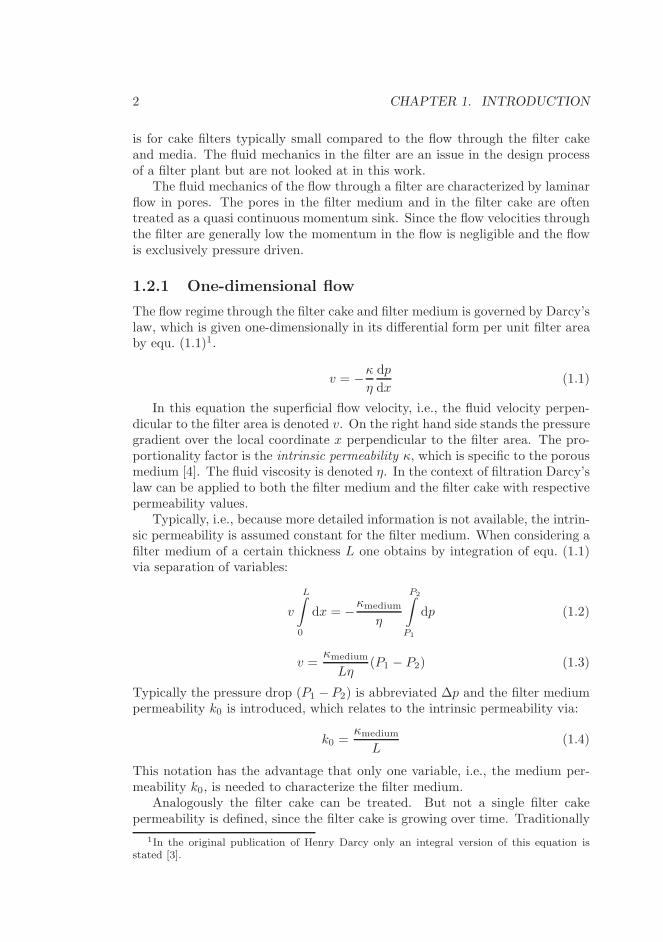
The flow regime through the filter cake and filter medium is governed by Darcy’slaw, which is given one-dimensionally in its differential form per unit filter areaby equ. (1.1)1.
v = −κη
dp
dx(1.1)
In this equation the superficial flow velocity, i.e., the fluid velocity perpen-dicular to the filter area is denoted v. On the right hand side stands the pressuregradient over the local coordinate x perpendicular to the filter area. The pro-portionality factor is the intrinsic permeability κ, which is specific to the porousmedium [4]. The fluid viscosity is denoted η. In the context of filtration Darcy’slaw can be applied to both the filter medium and the filter cake with respectivepermeability values.
Typically, i.e., because more detailed information is not available, the intrin-sic permeability is assumed constant for the filter medium. When considering afilter medium of a certain thickness L one obtains by integration of equ. (1.1)via separation of variables:
v
L∫
0
dx = −κmedium
η
P2∫
P1
dp (1.2)
v =κmedium
Lη(P1 − P2) (1.3)
Typically the pressure drop (P1 − P2) is abbreviated ∆p and the filter mediumpermeability k0 is introduced, which relates to the intrinsic permeability via:
k0 =κmedium
L(1.4)
This notation has the advantage that only one variable, i.e., the medium per-meability k0, is needed to characterize the filter medium.
Analogously the filter cake can be treated. But not a single filter cakepermeability is defined, since the filter cake is growing over time. Traditionally
1In the original publication of Henry Darcy only an integral version of this equation isstated [3].
1.2. FLUID MECHANICS 3
a specific filter cake resistance value αm is used [5], which relates to the intrinsiccake permeabiltiy κc via:
αm =1
κc · ρc(1.5)
This defines the cake resistance based on cake mass with the cake density termedρc. This formulation is used in this work.
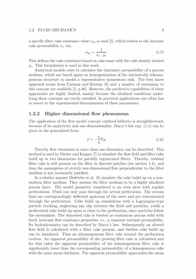
Analytical models exist to calculate the (intrinsic) permeability of a porousmedium, which are based again on homogenization of the intrinsically inhomo-geneous structure to model a representative momentum sink. The best knowapproach stems from Carman and Kozeny [6] and a number of extensions tothis concept are available [5, p.46]. However, the predictive capabilities of theseapproaches are highly limited, mainly because the idealized conditions under-lying these concepts are rarely satisfied. In practical applications one often hasto resort to the experimental determination of these parameters.
1.2.2 Higher dimensional flow phenomena
The application of the flow model concept outlined hitherto is straightforward,because of its analyticity and one-dimensionality. Darcy’s law equ. (1.1) can begiven in the generalized form:
~v = −κη∇p (1.6)
Thereby flow situations in more than one-dimension can be described. Thismethod is used by Dittler and Kasper [7] to simulate the flow field and filter cakebuild up in two dimensions for patchily regenerated filters. Thereby, residualfilter cake is still present on the filter in discrete patches (see section 1.4), andthus the assumption of strictly one-dimensional flow perpendicular to the filtermedium is not necessarily justified.
In a similar manner Dufreche et al. [8] simulate the cake build up on a non-uniform filter medium. They assume the filter medium to be a highly idealizedporous layer. The model geometry considered is an even sieve with regularperforations. Fluid can only pass through the actual perforation. The streamlines are correspondingly deflected upstream of the sieve and are concentratedthrough the perforation. Cake build up simulations with a Lagrangian-typeparticle tracking, neglecting any slip between the fluid and particles, yields apreferential cake build up upon or close to the perforation, since particles followthe streamlines. The deposited cake is treated as continuous porous solid withfixed, isotropic flow resistance properties, i.e., a constant intrinsic permeability.Its hydrodynamics can be described by Darcy’s law. Subsequently an alteredflow field is calculated with a filter cake present, and further cake build upcan be simulated. Thus an inhomogeneous filter cake around the perforationevolves. An apparent permeability of the growing filter cake is calculated andfor thin cakes the apparent permeability of the inhomogeneous filter cake issignificantly lower than the corresponding permeability of a homogeneous cakewith the same mean thickness. The apparent permeability approaches the mean

4 CHAPTER 1. INTRODUCTION
value as cake growth proceeds. This again implies that at a constant flow rateand constant upstream solid concentration, i.e., time-linear mean cake growth,the pressure drop is initially increasing faster, since the pressure drop and thepermeability are inversely proportional. Here the inhomogeneity of the filtercake is not exclusively attributed to the pore structure of the medium, but alsoto the upstream flow. The even model sieve with the combination perforation- impermeable plate is, however, not directly applicable fabric filter media, and[8] rightfully mention their main application in membrane filtration.
1.2.3 Internally inhomogeneous filter cake
The assumption of a constant intrinsic permeability as stated above is certainlynot always justified. Experimental findings show that the apparent intrinsicpermeability of the filter cake may increase when pressure is applied to thefilter cake. This phenomenon is termed cake compression or compaction andit is attributed to a further consolidation of the porous filter cake under theexternal influence of pressure, thereby reducing its permeability.
Experimentally this effect leads to an increasing pressure drop slope as cakebuild up proceeds, since a higher pressure drop entails higher stresses on thecake and therefore consolidation of the cake. The effects of cake compression aremost pronounced in the field of liquid filtration [2]. Schmidt ([9], [10]) studiescake compression for dust filtration.
Another effect, that leads to an apparent similar effect is depth filtration,which precedes cake build up. Particles reaching a clean filter surface may tosome extent penetrate inside the filter media and thereby do not participate inthe formation of a filter cake. Hence the filter cake forms more slowly than onewould expect given the solid mass reaching the filter and decrease in permeabil-ity is not as pronounced [11].
1.3 Filter media
The filter medium and its hydrodynamic properties are partly discussed above.The selection of filter media is a highly complex and empirical process andan overview on this issue for cleanable textile filter media for gas cleaning isgiven by e.g. [5, chapter 2]. Here only an introduction to some filter mediumcharacterization methods is given, which moreover is restricted to the maintype application discussed further in this work: The gas cleaning with cleanabletextile filter media.
The fiber material in state of the art filter media can be a polymer, e.g.polyamides or polytetrafluoroethylene, or of mineral origin, such as glass wool.Occasionally metal fibers are used. The actual choice of the fibers dependson the challenges in filter operation, such as temperature and chemical attack.The filter media is made from separate fibers that are processed into a clothlike form as either woven or needle felt. The latter has frequently a supportingscrim, which is actually woven and used as basis to produce the needle felt. Such

1.3. FILTER MEDIA 5
a needle felt combins the mechanical strength and air permeability of a wovenmaterial, and the good dust separation characteristics of a felt [5]. Generallyfabric filter media are inhomogeneous with respect to both, inner structure andsurface characteristics.
Characterization of filter media is important to determine the suitability ofa medium for a certain application. Moreover the results are used to comparethe performance of different filter media for a certain application in terms ofpressure drop and solid emissions. A series of industry standards are availablewhich standardize filter media testing procedures.
On the one hand there are methods available that aim towards characterizingthe filter media by objective parameters such as air permeability (EN ISO 9237is reporting gas flow at 20 mm water gauge pressure difference) or mechanicalproperties (area weight, thickness, strength in EN 29073) without actually doingfiltration tests.
On the other hand test standards exist that are designed to assess the perfor-mance of the filter media for filtration as the VDI-guideline 3926 [12]. Therebyan actual sample of the filter cloth is exposed to dust and the pressure dropis recorded over time, eventually the filter is regenerated by a jet pulse. Thestandards also give guidelines for evaluating the experiments concerning thefiltration cycle duration between jet pulses and the pressure drop level. In ad-dition, the clean gas concentration after the filter medium can be measured,which is important for meeting the environmental standards.
Some studies indicate that the filtration characteristics are influenced by thestructure of the filter medium. Chen et al. [13] present a detailed experimentalstudy of the pressure drop behavior of three cleanable needle felt filter mediawhen challenged with monodisperse dust. They find a rather fast pressure dropincrease after the filtration start, which reduces in the course of filtration. Thiseffect is observed on all filter media with three different particles sizes of 5,10 and 20µm. The smallest particles, however, show initially a slightly lowerslope of the pressure drop increase, which indicates depth filtration. This isfeasible, since the smallest particles might be able to advance deeper into thefilter media than bigger particles which are retained closer to the surface. Thephenomenon of a fast pressure drop increase at the beginning of filtration isascribed to an initially inhomogeneous particle deposition filling up the poreson the filter media’s surface, before a more homogeneous cake build up evolves.For the case of the monodisperse dusts with 10 and 20µm this phenomenonis discussed using the hypothesis of a two-stage cake build up within and ontop of the pores. They observed that stage one, i.e., pore filtering, is finishedwith the same amount of particles mass irrespective of the particle size. Stagetwo is homogeneous filter cake build up on the entire filter media area. Theexperimental findings in [13] suggest an initially inhomogeneous cake build updue to the pore structure, but no quantitative treatment of these findings isgiven.

6 CHAPTER 1. INTRODUCTION
1.4 Gas filtration in industry
In this section the main application referred to in this work is presented: Dustremoval from industrial gas streams in bag filters. This unit operation is de-scribed in detail by Loffler et al. [5]; here only a brief overview of the mostcommonly applied operation principle is given. Cylindrical filter bags are per-vaded by the process gas, whereby the dust is retained on the filter bag’s surface.The filter bags are pervaded by the gas from the outside and are mounted onwire cages to prevent them from collapsing. Inside the filter bag the clean gasmoves towards the clean gas chamber where it is collected.
The filter bags are typically cleanable. The dust cake removal by e.g. reversejet pulses is described in detail by e.g. [14] and [15]. The movement of thefilter bag and the reverse flow against the filtration flow direction liberate thefilter cake from the bag. The torn-off filter cake settles and is collected in adust hopper at the bottom of the filter. A basic filtration plant is displayed inthe flowchart Figure 1.1. The induced draft fan is used to overcome the flow
PDC
FC
bag filter
jet pulse unit
clean gas
dust laden gas
fan
solid product
Figure 1.1: Basic flowchart of a bag filter plant with crucial control circuits andmeasurements.
resistance of the filter. During filtration this resistance is increasing which eitherleads to a decreased volume flow while the pressure drop over the filter remainsconstant or the flow is kept constant while the pressure drop rises. Eventuallythe filter is cleaned after a certain time interval and/or at a certain pressuredrop level. Loffler et al. [5] provide a basic overview about the possible cleaningmodes.
Filter cleaning is not necessarily complete, i.e., residual dust cake is left onparts of the filter. Incomplete regneration can be intended by cleaning only apart of a filter that is divided into compartment, which can be cleaned separately.Insufficient regneration as described by [16] leaves parts of the filter cake, termed

1.5. SCOPE 7
patches, unchanged on the filter medium, although these patches were exposedto some cleaning action. Thereby a spatially distributed cake arises.
This incomplete regneration mechanism is the basis of several filter model-ing studies that make use of mechanistic assumptions to describe the pressuredrop - flow relation in cleanable filters ([17], [18], [19], [20]). These models useone-dimensional Darcy equations which are solved numerically to describe thepressure drop vs. volume flow through the filter media and filter cake. The fil-ter medium and cake are considered as a uniform flow resistances, respectively.After cleaning cake patches cover some parts of the filter area, while other partsare not carrying any cake. Hence, the permeabilty over the filter in the cake-free areas is higher and filtration will take place preferentially in these areas.Thereby the initially distributed cake will be evened out towards a homogeneouscake coverage. Typically, experimental pressure drop data is used to fit modelparameters, which describe the cake regeneration efficiency. These models focuson the filter cake regeneration, the subsequent distribution on filter cake, andthe implications on the pressure drop - volume flow relation of the filter. They,however, do not consider any inhomogeneity in the filter medium itself.
1.5 Scope
Attempts at filter modelling take their starting point in Darcy’s law as thegoverning equation of fluid mechanics. On the one hand studies employing aone-dimensional approach were conducted for the simulation of industrial filteroperation assuming a discrete distribution of residual filter cake. On the otherhand simulations of the cake build up in two (or more) dimensions were carriedout to study the influence of the flow field on cake build up. In the latter studiesthe inhomogeneity considered is caused by either a distributed residual cake [7]or an inhomogeneous filter medium [8].
An experimental study [13] of fabric filter media’s structure suggests localinhomogeneities, which must be attributed to the pore structure of the media.The effect of any inhomogeneity of the filter at the beginning on the pressuredrop curve is similar, i.e., the initial decrease in the integral permeability isrelatively fast compared to the cake mass increase. This is found by both,experimental and theoretical studies.
In this work a filter model describing the pressure drop - volume flow relationis developed, which can account for inhomogeneity of the permeability in the fil-ter medium. The inhomogeneity is described by a continuous distribution of theinitial permeability of the filter medium, which may also include contributionsof residual filter cake. It is shown that pressure drop - volume flow relations andthe distribution of filter permeability are unambiguously linked. It is demon-strated that a permeability distribution can be quantitatively extracted fromfilter pressure drop data for constant flow filtration.
A convolution transformation formulation of the filter model is developedand used to estimate the error for the determination of a permeability distribu-

8 CHAPTER 1. INTRODUCTION
tion. The developed method is applied to various experimental pressure dropdata from cleanable gas filters with fabric filter media.
The application of the developed filter model to the simulation of industrialfilter operation is discussed. A specialized routine is developed to be able toapply the developed method to semi-continuously operating filter plants.
In a separate chapter a simulation study on the assumption of a solid concen-tration distribution upstream the filter media is presented. Typically a constantsolid distribution is used as model assumption. This section shows the influenceof the violation of this seldom questioned assumption.

Chapter 2
Cake filter model
2.1 Model structure and assumptions
A cake filter model is developed for filter media with a distributed permeability.Starting from an illustration of the cake filtration on an inhomogeneous filtermedia, the required mathematical framework is derived. Hereafter homogeneousrefers to a property that is independent of the location on the filter, whereasinhomogeneous can vary with filter location.
In Fig. 2.1 the plain filter media is displayed schematically. The filter me-dia is illustrated by vertical lines depicting pores penetrating the filter mediavertically. The pore size varies and thereby symbolizes the local permeabilityof the filter media, i.e., small pores (dense lines) have a higher flow resistance,than the wider pores. The filter model assumes Darcy flow [3] through the filtermedia and thus the relation of flow velocity and pressure drop is linear:
v(t = 0, A) = k0(A)∆p(t)
ηg(2.1)
Equ. (2.1) is the proportional relation between the pressure drop and the flowvelocity across the filter media. It is given at time t = 0, which henceforthrefers to the beginning of filtration. The proportionality factor is the ratio ofthe permeability k0 of the filter media and the dynamic gas viscosity ηg. Thevelocity profile in Fig. 2.1 illustrates the effect of the inhomogeneous perme-ability of the filter media: At locations with a lower permeability also the flowvelocity is lower, and according to equ. (2.1) this is a directly proportional rela-tion. The depicted flow velocity is taken directly after or even within the filtercloth. Downstream of the filter viscosity effects will equalize the velocity profilerapidly. The superficial flow, i.e., the flow velocities in or through filter media,encountered in filtration is perpendicular to the filter medium.
It must be noted that, although one-dimensional cake build up is assumed,flow is not restricted to be perfectly perpendicular to the filter medium, ratherthan the cake build up is sufficiently well described one-dimensionally along the

10 CHAPTER 2. CAKE FILTER MODEL
v
∆p
A
Figure 2.1: Scheme of a cross section of a filter medium with inhomogeneouspermeability and the corresponding flow field.
streamlines. Filtration takes place when the fluid upstream contains particles.The particles are retained by the filter media. During cake filtration the particlesdeposit onto the filter media and subsequently onto already deposited particles,thereby forming a filter cake. In Fig. 2.2 the idealized cake formation is depicted.A filter cake is formed on the filter media. Since the flow field for the filtermedia is inhomogeneous due to a distributed permeability, also cake formationis hereby affected. Cake forms faster in areas with an initially high flow velocity,since more particles are deposited on these areas. This is reflected by the filtercake thickness in Fig. 2.2, which is higher at areas with a higher permeability ofthe filter medium and thus a higher initial flow velocity. However, the filter cakeitself represents a flow resistance, too. Under the assumption of an internallyhomogeneous cake, i.e., a cake that has a constant specific flow resistance ata Darcy scale (cf. [8]), the flow resistance is proportional to the filter cakethickness. Mathematically this fact can be captured by equ. (2.2). Here the lefthand side (LHS) is the reciprocal value of the filter cake permeability, i.e., thefilter cake resistance. On the right hand side (RHS) stands the solid area load,which under the assumption of an internally homogeneous cake corresponds to acertain cake thickness. The proportionality factor is the specific cake resistanceαm.
1
kc(t, A)= αm · z(t, A) (2.2)
When a filter cake is present, the fluid flow is determined by the combinedflow resistances of filter medium and filter cake. The flow resistances of filtermedium k−1(A) and filter cake k−1
c (t, A) are in series and thus add linearly:
1
k(t, A)=
1
kc(t, A)+
1
k0(A)(2.3)

2.1. MODEL STRUCTURE AND ASSUMPTIONS 11
v
∆p
filter cake (schematically)
Figure 2.2: Scheme of a cross section of a filter medium carrying filter cake.The correspondingly altered flow field is also displayed.
When cake is present the fluid flow is determined by a linear relation similar toequ. (2.1), but with the combined permeability k instead of just k0:
v(t, A) = k(t, A)∆p(t)
ηg(2.4)
The permeability depends on both, the location on the filter A, and the filtrationtime t. The latter dependency is describing the evolution of the permeabilityas cake build up proceeds. The mechanistic cake build up is described by solidcontinuity. In cake filters almost the entire amount of dust, which is transportedto the filter, is retained on the filter and thereby forming a cake. Here it isassumed that the upstream solid concentration is constant and thereby thefilter cake mass balance reads:
dz(t, A)
dt= csol · v(t, A) (2.5)
From equ. (2.5) the direct proportionality between cake build up flow velocitycan be seen.
The filter cake depicted in Fig. 2.2 causes, as stated, additional flow resis-tance. To overcome that increased resistance and keep the total volume flowconstant (constant flow filtration) the pressure drop augments. In classical fil-tration theory a homogeneous filter medium and a homogeneous filter cake buildup give a linear pressure drop increase [5]. However, if the filter medium is in-homogeneous but an internally homogeneous cake builds up the pressure dropincreases non-linearly and always concave. Of course, if the filter medium ishomogeneous but the cake builds up inhomogeneously the pressure drop mayalso increase non-linearly. Such a case is e.g. described in chapter 7.

12 CHAPTER 2. CAKE FILTER MODEL
2.2 Mathematical model development
In this section a mathematical pressure drop model is developed for a filter thatleads to a characteristic function of the permeability of the filter media. Thispressure drop model is solely based on the equations that comprise of the cakefilter model (chapter 2.1) and the respective assumptions.
The time derivative of equ. (2.2) is
d 1kc(t,A)
dt= αm · dz(t, A)
dt(2.6)
and the time derivative of equ. (2.3) is:
d 1k(t,A)
dt=
d 1kc(t,A)
dt(2.7)
Expressing the solid area load term in equ. (2.6) by equ. (2.5) and subsequentlyby using equ. (2.7) gives:
d 1k(t,A)
dt= αm · csol · v(t, A) (2.8)
Here the filtration velocity v(t, A) can be expressed by equ. (2.4) which reads:
d 1k(t,A)
dt=αm · csol
ηg· k(t, A) · ∆p(t) (2.9)
In this equation the permeability and the pressure drop are time dependent.However, equ. (2.8) can be rearranged by separating variables. Thereby evalu-ating the derivative on the LHS of equ. (2.9) gives:
− dk(t, A)
k3(t, A)=αm · csol
ηg· ∆p(t) · dt (2.10)
Equ. (2.10) is a differential equation with separated variables k(t, A) and t,respectively. Integrating from time zero to t on the RHS and the correspondingpermeabilities on the LHS gives:
1
k2(t, A)− 1
k20(A)
= 2 · αm · csol
ηg·
t∫
0
∆p(t) · dt (2.11)
Hereby, the relation k(t = 0, A) ≡ k0(A) is used, reflecting that at time t = 0the permeability relates only to the filter medium’s permeability (cf. equ. (2.1)).In equ. (2.11) the RHS is only time dependent, i.e., it does not show any de-pendency of the filter area. That implies that the evolution of the permeabilitywith the distributed initial value k0(A) is related by only one scalar value whichshall be abbreviated s(t), hence termed filter state.
s(t) ≡ 2 · αm · csol
ηg·
t∫
0
∆p(t) · dt (2.12)

2.2. MATHEMATICAL MODEL DEVELOPMENT 13
The physical meaning of equ. (2.11) is that the evolution of the permeabilityat any location A on the filter is solely determined by the evolution of thepressure drop over time. This is because the build up of the filter cake is thereason for a changing permeability which in turn is merely determined by thefiltration velocity and thus the pressure difference over the filter.
Equs. (2.11) and (2.12) lead to an additive relation that describes the per-meability by two contributors, the initial permeability k−2
0 (A) only dependingon the filter location and the filter state s(t) only depending on time. Thus aseparation of variables is accomplished in the integrated form, too.
k−2(t, A) − k−20 (A) = s(t) (2.13)
In other words the flow situation of the unloaded filter media (Fig. 2.1)depends only upon the spatial domain. Based on that, the subsequent filtercake build up is only determined by the scalar filter state s(t), which is onlytime dependent.
Hitherto the filter is looked at a scale resolving the inhomogeneities on thefilter location A. However, to describe a filter by a pressure drop model theentire filter must be considered. By integrating over all filter locations A, i.e.the entire filter area Atot, in equ. (2.4) one obtains:
Atot∫
A=0
v(t, A)dA =∆p(t)
ηg
Atot∫
A=0
k(t, A)dA (2.14)
The LHS represents the volume flow through the entire filter V (t). Rear-ranging equ. (2.14) and expressing the permeability by equ. (2.13) yields:
ηg · V (t)
∆p(t)=
Atot∫
A=0
[k−20 (A) + s(t)
]− 12 dA (2.15)
Equ. (2.15) represents a direct relation between the time dependent pres-sure drop ∆p(t) and volume flow V (t) on the LHS and the initial permeabilityfunction k0(A) on the RHS. For simplifying the representation of this relationslightly and with respect to further mathematical treatment it is advisable tointroduce the abbreviation:
u ≡ k−20 (A) (2.16)
The filter location A is barely used to identify an area of the filter to its per-meability value. The permeability is not resolved locally. Thus the relationbetween area A and permeability, i.e., k0 or u, can be inverted, leading to anarea distribution function. This distribution function can be introduced in di-mensionless form by:
Φ(u) ≡ A
Atot(2.17)
Here Atot is the constant total filter area and Φ(u) is the cumulative permeabilityarea distribution function. Since u is unambiguously linked to k0 (equ. (2.16)),

14 CHAPTER 2. CAKE FILTER MODEL
Φ(u) will be referred to as permeability distribution (PD). The limits of inte-gration of equ. (2.15) are changed accordingly to account for the substitutionof the variable of integration by equ. (2.17):
ηg · V (t)
Atot · ∆p(t)=
∞∫
u=0
[u+ s(t)]− 1
2 dΦ(u) (2.18)
The form of equ. (2.18) with a function as variable of integration is calledRiemann-Stieltjes integral. In this equation both, the LHS (namely ∆p andV ) and s appear depending on time t. It is shown below that the filter states is treated as a parameter and therefore the explicit time dependency will beomitted:
ηg · VAtot · ∆p
=
∞∫
u=0
(u+ s)−12 dΦ(u) (2.19)
Equ. (2.19) is the mathematical representation of the cake filter model usedfurther on. The LHS only contains integral, measurable filter parameters, whilethe RHS depends on the PD and the filter state s. The filter state is defined byequ. (2.12).
For the application of the filter model two main cases for filter operation:� constant pressure� constant volume flow
are considered, and the respective formulations are derived in the sections below.
2.3 Constant pressure filtration
Filtration with a time-constant overall pressure difference leads to a simplerelation of filter state s and time t since equ. (2.12) can be integrated analyticallygiving a direct proportionality:
s =2 · αm · csol · ∆p
ηg· t (2.20)
Thus equ. (2.19) made explicit for the volume flow V reads:
V =Atot · ∆p
ηg
∞∫
u=0
(
u+2 · αm · csol · ∆p
ηg· t
)− 12
dΦ(u) (2.21)
2.4 Constant flow filtration
The case of a constant volume flow V requires a slightly more extensive mathe-matical treatment, since the filter state is not so readily obtained from integra-tion of equ. (2.12). Instead a parametric model for the relation of pressure drop∆p and time t is developed with filter state s being the parameter.

2.4. CONSTANT FLOW FILTRATION 15
Two abbreviations of constants are introduced for a simpler model represen-tation:
pc ≡V · ηgAtot
(2.22)
and
tc ≡ Atot
αm · csol · V(2.23)
The pressure drop is obtained by rearranging equ. (2.19) and using the con-stant pc defined:
1
∆p=
1
pc·
∞∫
u=0
(u+ s)− 1
2 dΦ(u) (2.24)
Equ. (2.24) contains s which depends upon the pressure drop ∆p and timet according to the definition by equ. (2.12). Equ. (2.12) shall be manipulatedmathematically to explicitly obtain time t as a function of filter state s and thePD Φ(u).
Rewriting equ. (2.12) by using the abbreviations introduced by equs. (2.22)and (2.23) gives:
s =2
tc · pc
t∫
0
∆pdt (2.25)
Derivation with respect to time yields:
ds
dt=
2
tc · pc∆p (2.26)
Rearranging equ. (2.26) and expressing the pressure drop ∆p by equ. (2.24)yields:
tc2
∞∫
u=0
(u+ s)− 1
2 dΦ(u) =dt
ds(2.27)
Integration of both sides via s from 0 to s yields:
tc2
s∫
s=0
∞∫
u=0
(u+ s)− 1
2 dΦ(u)ds =
s∫
s=0
dt
dsds (2.28)
Changing the order of integration on the LHS and evaluating the RHS gives:
tc2
∞∫
u=0
s∫
s=0
(u+ s)− 1
2 dsdΦ(u) = t (2.29)
Evaluating the definite inner integral on the LHS yields:
tc2
∞∫
u=0
2[
(u+ s)12 − (u+ 0)
12
]
dΦ(u) = t (2.30)

16 CHAPTER 2. CAKE FILTER MODEL
Thus another integral transformation similar to equ. (2.24) is obtained for thetime t:
t = tc
∞∫
u=0
[
(u+ s)12 − u
12
]
dΦ(u) (2.31)
Equs. (2.24) and (2.31) together represent a parametric filter model for theconstant volume flow case with filter state s being the parameter.

Chapter 3
Properties of the constant
flow cake filter model
This chapter discusses selected properties of the filter model for constant flowfiltration presented in section 2.4. An overview over the relation of the filtermodel is given. In addition characteristic values of a PD are reported. For rea-sons of clarity the two integral transformations used in this section are repeated:
1
∆p=
1
pc·
∞∫
u=0
(u+ s)− 1
2 dΦ(u) [2.24]
t = tc
∞∫
u=0
[
(u+ s)12 − u
12
]
dΦ(u) [2.31]
3.1 Test data
In order to illustrate this cake filter model, an analytically generated PD isused. This PD is generated by the cake generation model from Kavouras andKrammer [20]. The connection between this model and the PD is discussed indepth in section 6.2. For the time being it, however, suffices to simply generatea PD by this very model.
The operation chosen to generate the PD uses a cycle time for cleaningone row at a time of tcycle = 300 s and cleaning function parameters used areln(z50) = −0.15 and σLN = 1.11. All other filter parameters are taken unal-tered from [20]. The quite large σLN parameter is chosen to obtain a significantPD also in cakes of generation 2 and older. The resulting PD is displayed in
1The broadness parameter of the cleaning function is originally referred to as barely σ,but in this work the cleaning function broadness is referred to as σLN to account for theLogarithmic Normal distribution and to avoid confusion with the integral transformationparameter introduced in section 5.2.

18 CHAPTER 3. CONSTANT FLOW – MODEL PROPERTIES
Figure 3.1 as the cumulative distribution function Φ′ versus the permeability k.This distribution depending upon the permeability is derived from the math-ematically introduced distribution Φ(u) (see appendix A.1 for the conversionbetween the two). Although Φ(u) is advantageous for mathematical manipula-tion Φ′(k) is usually displayed.
10−10
10−9
0
0.1
0.2
0.3
0.4
0.5
0.6
0.7
0.8
0.9
1
permeability k, m
Φ′ , −
Figure 3.1: PD generated by the cake generation model used for theoreticalstudies.
In Figure 3.2 the pressure drop curve is displayed resulting from this PDfor time t ranging from 0 to 700 s. This time range is used as input datafor deconvolution. Although the transient pressure drop evolution is displayedbeyond the actual cycle time tcycle, the cycle time is used for the PD generation.The displayed ∆p curve over 700 s corresponds to continued filtration withoutcleaning after a stable periodic operation was established.
From the pressure drop curve over time one can directly calculate the valuesof filter state s over time via integration of equ. (2.25), left aside the knowledgeof a PD. In Fig. 3.2 the shaded area under the pressure drop curve is displayedto illustrate the filter state s at a time t = tcycle, which is proportional to thatarea according to equ. (2.25). Alternatively s can be obtained from a knownPD directly using equ. (2.31).

3.1. TEST DATA 19
0 100 200 300 400 500 600 7000
500
1000
1500
2000
2500
3000
time t, s
pres
sure
dro
p ∆p,
Pa
∆p cycle
∆p extrapolation
Figure 3.2: Pressure drop curve generated by the cake generation model. Thesolid line is the pressure drop during semi-continuous operation and the dashedline is the extrapolation to 700 s. The shaded area corresponds to the filter states.

20 CHAPTER 3. CONSTANT FLOW – MODEL PROPERTIES
3.2 Pressure drop characteristic of a PD
In Fig. 3.3 a pressure drop increase over time is displayed, which has the typicalcurvature for a filtration on an inhomogeneous cloth. Together with the boldpressure drop curve the asymptote for t→ ∞ is displayed as a dashed line. Forlong filtration time, any initial PD is leveled out and the slope of the pressuredrop curve is equal to the slope of a homogeneous filter pc
tc. The ordinate offset
is termed ∆p0 and can be seen as a hypothetical initial pressure drop of ahomogeneous filter that is having the asymptote as its pressure drop curve.When the actual inhomogeneous filter is operated until the linear part of thecurve is nearly (i.e. asymptotically) reached, it will give the same performancein terms of cycle time, pressure drop at cleaning as this homogeneous referencefilter.
Moreover the initial tangent at t = 0 to the ∆p-curve is shown. The ordinateoffset here is the initial pressure drop value of the filter ∆p0. For an inhomo-geneous filter medium the slope of the initial tangent is always higher than theasymptotic slope. This increase is captured by a factor κs.
These four characteristic values define the two linear functions and therebyreflect the basic shape of the actual ∆p-curve, too. Below mathematical deriva-tions are given to calculate the mentioned values directly from a the filter model.It can be shown that only three moments of a PD relate to these characteristicvalues.
3.2.1 Initial pressure drop
At the beginning of the filtration both time and filter state are zero. The initialpressure drop is thus straightforwardly calculated from equ. (2.24):
1
∆p0=
1
pc·
∞∫
u=0
u−12 dΦ(u) (3.1)
and thus
∆p0 = pc ·1
∞∫
u=0
u−12 dΦ(u)
(3.2)
In equ. (3.2) the value ∆p0 only depends upon the parameter pc and the PD.By introducing the notation of moments
µr ≡∞∫
0
u−r2 dΦ(u) (3.3)
one obtains:∆p0 = pc · µ−1
1 (3.4)
The scaling of the exponent for the moment in equ. (3.3) is outlined in moredetail in appendix A.2.

3.2. PRESSURE DROP CHARACTERISTIC OF A PD 21
∆p
t0
∆p0
∆p0
1 pc
tc
1
κspc
tc
Figure 3.3: Schematic pressure drop increase together with its initial tangentand asymptote
22 CHAPTER 3. CONSTANT FLOW – MODEL PROPERTIES
The moment µ1 is the arithmetic mean of the permeability distributionΦ′(k). The pressure drop at the beginning of filtration corresponds, of course,to the mean permeability of the filter medium. As such the result is almosttrivial. However, for a stringent deduction of the characteristic values from themodel equations it is mentioned.
3.2.2 Slope of the pressure drop increase
The pressure drop increase can be calculated via a derivative of ∆p over time t.Expressing this derivative via the chain rule one obtains
d∆p
dt=
d∆p
ds· ds
dt(3.5)
Expanding the first factor and rewriting the second one gives:
d∆p
dt= −
d( 1∆p )ds
(1
∆p
)2 · 1dtds
(3.6)
The pressure drop appearing in the first factor is expressed by equ. (2.24) andthe derivative via s is determined. The derivative in the second factor appearedalready in equ. (2.27) and the respective result can be used directly.
d∆p
dt=
−pc
∞∫
0
− 12 (u+ s)
− 32 dΦ(u)
[∞∫
0
(u+ s)−12 dΦ(u)
]2 · 2
tc∞∫
0
(u+ s)− 1
2 dΦ(u)
(3.7)
Simplifying this result gives:
d∆p
dt=
pc
tc·
∞∫
0
(u+ s)−32 dΦ(u)
[∞∫
0
(u+ s)− 1
2 dΦ(u)
]3 (3.8)
To obtain the asymptotic slope of the pressure drop curve, one needs tocalculate the limit of equ. (3.8) for filter state s approaching infinity:
lims→∞
d∆p
dt=
pc
tc
s−32
∞∫
0
dΦ(u)
[
s−12
∞∫
0
dΦ(u)
]3 (3.9)
By using the property of a distribution∞∫
0
dΦ(u) ≡ 1 this limit evaluates to:
lims→∞
d∆p
dt=
pc
tc(3.10)

3.2. PRESSURE DROP CHARACTERISTIC OF A PD 23
It must be emphasized that also this result refers to a trivial situation, becauseit represents the pressure drop increase of a filter with an equalized permeabilityprofile. Thus the slope is identical to the slope of an homogeneous filter.
The slope of the initial tangent is obtained by evaluating equ. (3.8) at s = 0:
d∆p
dt
∣∣∣∣s=0
=pc
tc·
∞∫
0
u−32 dΦ(u)
[∞∫
0
u−12 dΦ(u)
]3 (3.11)
Thus a multiplying factor depending on moments of the PD is the quotientbetween equs. (3.9) and (3.11). This factor is a measure for the augmentedpressure drop increase at the beginning of filtration due to an inhomogeneousPD.
κs =
∞∫
0
u−32 dΦ(u)
[∞∫
0
u−12 dΦ(u)
]3 (3.12)
Using again the notation of moments introduced by equ. (3.3) one can rewriteequ. (3.12) as:
κs =µ3
µ31
(3.13)
3.2.3 Asymptote of the pressure drop curve
The slope of that asymptote is equal to the slope of a completely homogeneousfilter and given by equ. (3.9). A more interesting feature of this asymptote isthe ordinate offset ∆p0, i.e. the pressure drop value at which the asymptoteintersects the ordinate axis.
The asymptote of ∆p(t)-curve is given by equ. (3.14).
∆p =pc
tc· t+ ∆p0 (3.14)
The parameter ∆p0 can be calculated from equ. (3.15):
∆p0 = limt→∞
(
∆p− pc
tc· t
)
(3.15)
Since a closed form expression for ∆p depending on time t is not available, thelimit variable is changed to a limit for s→ ∞. Here the pressure drop ∆p can beexpressed by equ. (2.24) while the time t is given by equ. (2.31). The resultinglimit reads:
∆p0
pc= lim
s→∞
1∞∫
0
(s+ u)−12 dΦ(u)
− 1
tc
∞∫
0
[
(s+ u)12 − u
12
]
dΦ(u)
24 CHAPTER 3. CONSTANT FLOW – MODEL PROPERTIES
For the consideration of the orders of magnitude in this limit calculation theorders of magnitude of s and u should be considered.
∆p0
pc= lim
s→∞
1∞∫
0
(s+ u)−12 dΦ(u)
−∞∫
0
[
(s+ u)12 − u
12
]
dΦ(u)
Filter state s is going towards infinity, whereas u remains limited, since the PD’scontribution to the integral is only significant when the cumulative distributionfunction Φ(u) is actually changing. Hence the comparison of orders of magnitude
s≫ u applies to the inner parentheses. Thus the first integral is reduced to s12
while the second integral can be separated into contributions depending on sand u, respectively:
∆p0
pc= lim
s→∞
1
s−12 · 1
− s12 · 1 +
∞∫
0
u12 dΦ(u)
The result is independent on s and reads:
∆p0
pc=
∞∫
0
u12 dΦ(u) (3.16)
Obviously, also this result can be expressed as a moment equ. (3.3):
∆p0
pc= µ(−1) (3.17)
3.2.4 Relation time t - filter state s
In Fig. 3.4 the relation between filter state s and time t is displayed. The timescale here ranges over an unrealistically wide range, that cannot be measuredpractically. Interestingly the curve has two finite asymptotes in this double-logarithmic plot.
Closer examination of the slopes on the straight sections reveals, that forsmall values the slope is equal to one, whereas right of the transition it is equalto two. The linear relation between t and s for small values, i.e. at the left handside of the bend, and a quadratic relation for big values. From the integral timetransformation equ. (2.31) the mathematical basis of these observations can bederived. For small values of s as compared to u one can develop the integraltransform into a first order Taylor series for s around zero:
t(s ≪ u) ≈ t(s = 0) +dt
ds
∣∣∣∣s=0
(s− 0) = tcs
∞∫
0
1
2√u
dΦ(u) (3.18)

3.2. PRESSURE DROP CHARACTERISTIC OF A PD 25
For big values of filter state s compared to u, i.e., s≫ u applies, one obtainsan analogous relation directly from equ. (2.31). As an additional simplification√s≫ √
u can be applied.
t(s≫ u) ≈ tc
∞∫
0
√sdΦ(u) = tc
√s
∞∫
0
dΦ(u)
︸ ︷︷ ︸
=1
= tc√s (3.19)
In section 3.2.3 the simplification√s ≫ √
u cannot be applied, since therethe limit transition for s→ ∞ is used for an extrapolation back to filter state szero. The goal there was to calculated the asymptotic pressure drop offset. Butallowing
√s≫ √
u would erroneously give an asymptote through the origin.The relationships developed here can be used for extrapolation of filter state
s from measured points to practically not measurable ones at small and bigt values. The results of the analytical expressions equs. (3.18) and (3.19) aredisplayed in Figure 3.4, too.
100
102
104
106
1015
1020
1025
time t, s
filte
r st
ate s
, m−
2
Figure 3.4: Relation between time t and filter state s in a double logarithmicdiagram. The asymptotes of the curve are also displayed.
The asymptotical relations can, of course, be related to filter operation viathe definition of filter state s equ. (2.12). For small values of t the pressuredrop ∆p remains virtually constant, since it does not change measurably withina short time, which leads directly to a linear relation after integration. For
26 CHAPTER 3. CONSTANT FLOW – MODEL PROPERTIES
big t-values the pressure drop will increase linearly, thus yielding a quadraticrelation after integration, which for big t-values is, of course, dominated by thequadratic term (neglecting the linear one).
It must be noted that the resulting equ. (3.18) is practically identical withequ. (2.20) for constant pressure filtration. The difference of these equations isonly notation, since in the latter equation the parameters are not abbreviatedand the pressure drop is explicitly included, whereas in equ. (3.18) the integralmean of the PD embodies the initial pressure drop value.

Chapter 4
The PD-method
In the chapters 2 and 3 a cake filter model is comprehensively developed andsome of its properties are detailed for the case of constant flow filtration. How-ever, this model requires a PD as input.
In this chapter the model is used to determine a PD from operational filterdata. In general a pressure drop - volume flow relation must be available asinput. However, the method is explicated only for the determination of a PDfrom filter pressure drop data and a constant volume flow. Moreover it is shownthat this relation between a pressure drop curve and a PD is unambiguous andthe uncertainty with the determination of the PD is assessed.
The PD-method represents the inversion of the filter model to obtain a PDfrom a filter pressure drop curve. The model assumptions must, of course, befulfilled to properly carry out this inversion.
The completeness of the PD-method is based on 2 model properties:
i The relation between time t and filter state s is bijective for a certainpressure drop profile.
ii The integral pressure drop transformation equ. (2.24) is invertible.
The property (i) is required, since the pressure drop relation is only availableas a function of filter state s, whereas the pressure drop is measured dependingon time t. A bijective assignment between t and s ensures that the pressuredrop curve can be unambiguously transformed into a corresponding functiondepending upon filter state s. From equ. (2.12) one easily finds (i) verified,since the integrand ∆p is always positive and thus the relation between t ands is strictly monotonic. In addition the relation t − s relation is obviouslycontinuous for a continuous ∆p(t) and thus the t− s relation is bijective.
The inversion of equ. (2.24) is subsequently used to determine the actualPD from the LHS via an inversion of the integral transformation. The type ofthis integral transformation is known in mathematics and termed generalizedStieltjes transform (not to be confused with the notation as Riemann-Stieltjesintegral). Hirschman and Widder [21, p. 78 f.] tackle that very transformation

28 CHAPTER 4. THE PD-METHOD
and outline a theory for its inversion based on uniqueness. The inversion formulagiven is highly abstract and makes use of high order derivatives, that cannot beaccurately supplied by experimental data. However, the integral transformationequ. (2.24) is uniquely invertible in theory1 thereby constituting property (ii).
Of course the combination of (i) and (ii) also establishes a bijective t − srelation being derived from equ. (2.31). A certain pressure drop profile givesboth, a unique t−s relation and subsequently an unambiguous PD. In equ. (2.31)a PD is used to calculate t from s, but explicitly no statement on the invertibilityof equ. (2.31) is made.
4.1 Optimization approaches
Practically optimization methods can be used to determine a PD from pressuredrop data. Such pressure drop data is typically availably as discrete measure-ments over time. The measurement couples should be identified as ∆pj,exp andtj with n measurement points. In a first step the time values tj is converted tofilter state sj via numerical integration of equ. (2.12), whereas the experimentalpressure drop is used in the integrand.
The PD is discretized into ui and Φi values. A discretization of the PDon m = 30 nodes proves pratically suitable, when considering the trade off ofcomputational time versus achievable resolution (see section 5.3.6 for attainableresolution). A simulated pressure drop value ∆pj for a certain filter state sj
is computed from equ. (2.24) again via numerical integration by the rectanglerule.
pc
∆pj
=
m∑
i=1
(sj + ui)− 1
2 ∆Φi (4.1)
Note that the equation was also multiplied by pc.
Alternatively to a single optimation run using a fixed discretization of thePD, several optimation runs can be carried out in succession and the discretiza-tion can be refined in between these steps. A simple rule for refining is to insertadditional nodes where the preliminary determined PD has the biggest gradient.Such an adaptive grid method can be used when highly resolved pressure dropdata is available and rather detailed PDs can be determined. The implementa-tion of such a refining step is typically easy to accomplish by modifying the codeusing fixed a discretization. An example for the application of this extension tothe optimisation approach is given in section 6.4.5.
1This fact can also be illustrated by considering the discretized form of the integral transfor-mation. The inversion towards the discretized PD leads to a system of linear equations. Thatsystem is linearly independent and has no trivial solution. Hence the PD is unambiguouslydetermined.

4.1. OPTIMIZATION APPROACHES 29
4.1.1 Permeability value variable
The easiest approach is to fix the discretization of the cumulative distributionfunction Φ linearly between 0 and 1:
Φi =i
mi = 0 . . .m (4.2)
Consequently the differences ∆Φi are constant at 1m+1 for all m nodes. An
initial guess for the PD is made. Commonly a non-distributed permeability istaken as initial guess, i.e., a constant value for all ui’s.
The pressure drop value ∆pj for a certain filter state sj is computed fromequ. (4.1). The goal function for the optimization algorithm is the sum of squareerrors between the measured pressure drop values and the simulated ones foreach measurement point. Generally the measurement points are not weighted.
m∑
j=1
(∆pj − ∆pj,exp)2!= min (4.3)
The changing variables during the optimization are the permeability valuesat each of the m nodes. Note, that none of the nodes is distinguished fromothers because of integration via the rectangle rule and equidistant spacing ofthe Φi vector. Thus it depends largely on the optimization algorithm actuallyused which node assumes a certain value. However, the optimization result iseventually sorted to obtain a distribution function. The result is, of course,not affected. Assuming that a global optimum exists and that the optimizationactually finds that optimum, the result is unambiguous.
The implementation of the problem described was attempted on variousplatforms with different algorithms for nonlinear, unconstrained optimizationproblems. Only absolute values of the optimization variables are used, therebyavoiding unphysical negative permeability during the optimization run. Thisis easily implemented in the calculation of equ. (4.1) itself. Alternatively, onecould add constraints to the optimization problem, which is, however, increasingthe size of the problem and hence the complexity. Additionally the optimizationvariables are scaled. Permeability values are typically in the order of 10−8 −10−10 m and were therefore scaled by a factor of 108, which greatly improvedthe convergence of the optimization algorithms.
The determination of a PD via optimization is chosen because of its straightforward implementation (only two numerical integrations required) and the sim-plicity of the application of optimization methods.
4.1.2 Distribution function variable
An alternative way of discretizing a PD is by fixing the permeability discretiza-tion ui and using the corresponding values of the distribution function Φi asvariables.

30 CHAPTER 4. THE PD-METHOD
Obviously equ. (4.1) makes up a system of n linear equations for the variables∆Φi with the coefficient matrix:
Aj,i = (sj + ui)− 1
2 i = 1 . . .m, j = 1 . . . n (4.4)
To obtain a non-parametric solutions of the system of equations at least as manymeasurement points n as PD nodes m are required. This system is usuallyoverdetermined, since the number of available measurements n is larger thanthe number of nodes of the discretization of the PD m. Hence the system hasin general no solution, however, similar to the optimization approach, the leastsum of square error solution is sought after.
The system is ill conditioned, although the coefficient matrix Aj,i is full inrank2. The numerical properties of this linear system are not discussed in detail.The error stemming from the inversion of the underying integral transform isdiscussed in this thesis in section 5.3.6 with the help of a convolution transformformulation of the problem.
Attempting the solution of the linear square system via the pseudoinverse(ATA)−1AT fails on even generated data, i.e., data having a solution with zeroresidual error. This must be attributed to the ill conditioning of the system.However, QR decomposition, where A is decomposed into an orthogonal matrixQ and a triangular matrix R, succeeds in solving the linear system to its leastsquare solution for all attempted cases using artifiially generated input data [22,p. 112ff].
This way of determining a PD is numerically inexpensive, since it requiresonly one numerical integration to obtain the filter state values sj . The solutionof the linear least square problem is extremely fast.
However, there are several shortcomings of this direct approach when appliedto experimental data, that is always affected by noise. Ideally the solution vector∆Φi must add up to one, since the sum must not exceed one. If this value issmaller than one, it just means that part of the filter has zero permeability,which is physically meaningful. If, however this sum exceeds one the solutionis not physical. An even bigger problem is the possibility of negative solutionswhich must not appear in a frequency distribution.
However, constraints can be added to the linear least square problem to ex-clude unphysical solutions. For m variables ∆Φi m+1 constraints are required:
∆Φi ≥ 0 i = 1, . . . , m (4.5)
m∑
i=1
∆Φi ≤ 1 (4.6)
This turns the pure system of linear equations into an optimization problem.Contrary to the effectively unconstrained non-linear optimization carried out insection 4.1.1, this constrained problem can be tackled by specifically designed
2If the number of linearly independent rows in the coefficient matrix equals the totalnumber of rows the rank of the matrix is termed full.

4.2. UNCERTAINTIES IN PARAMETERS 31
algorithms for linear least squares. The constrains are easily implemented andthe convergence is quite fast because of its linearity.
The only remaining shortcoming known to the author is that the discretiza-tion for the permeability values is fixed. This entails the practical problem ofhow to choose the discretization for this domain. The discretization of the cu-mulative distribution is straightforward between zero and one, thereby covingthe entire possible range at a certain resolution. The fixed discretization of thepermeability values restricts these values to a certain range, although a widerspread of values could be required to determine the optimal PD in a least squaressense. In practice the method of adjusting the permeability values, rather thanthe distribution values proved more flexible and on an equal number of nodesgenerally better fits were obtained using the method proposed in section 4.1.1.However, in terms of computational time the linear approach has an advantage.
4.2 Uncertainties in parameters
In addition to the properties of the cake filter model outlined in chapter 3the influence of uncertainties in the combined model parameters pc and tc isdiscussed here. The main focus when discussing variation in these parametersis the impact on a PD determined by the PD-method for a certain pressuredrop curve. The property (ii), which is the invertibility of the pressure droptransform, introduced at the beginning of this chapter, is a prerequisite for thisdiscussion.
The output of the PD-method obtained by two arbitrarily different sets ofparameters is discussed. The parameters pc and tc are regarded as the true andhence correct parameters for a pressure drop curve corresponding to a certainPD Φ. Meanwhile the parameters pc and tc are the actually used and erroneousparameters with which a PD Φ is obtained from the same pressure drop curve.
From equ. (2.25) it is clear that the filter state s will be altered when usingdifferent parameters and is henceforth termed s. However, since the pressuredrop curve remains the same, one can easily convert the filter states by equatingthe integral for the two sets of parameters:
s · pc · tc = s · pc · tc (4.7)
The pressure drop can be calculated from equ. (2.24) for both sets. Equatingthe pressure drops gives:
1
pc·
∞∫
u=0
(u+ s)− 1
2 dΦ(u) =1
pc·
∞∫
u=0
(u+ s)− 1
2 dΦ(u) (4.8)
32 CHAPTER 4. THE PD-METHOD
The symbol of the integration variable is changed on the RHS to u to avoidconfusion. The filter state s can be expressed via equ. (4.7) as a function of s.The entire equ. (4.8) is multiplied by pc.
∞∫
u=0
(u+ s)− 1
2 dΦ(u) =pc
pc·
∞∫
u=0
(
u+pc · tcpc · tc
· s)− 1
2
dΦ(u) (4.9)
Subsequently u can be substituted by:
u ≡ pc · tcpc · tc
· u
Of course the integral boundaries are changed correspondingly and after sim-plification one obtains:
∞∫
u=0
(u+ s)− 1
2 dΦ(u) =
∞∫
u=0
(u+ s)− 1
2 d
[(pc · tcpc · tc
) 12
· Φ(pc · tcpc · tc
· u)
]
(4.10)
The integral kernels on both sides are obviously identical. Since the Stieltjestransform is unambiguously invertible the functions in the differential must benecessarily identical too. Hence one can write:
Φ(u) =
(pc · tcpc · tc
) 12
· Φ(
pc · tcpc · tc
· u)
(4.11)
Consequently variation in the model parameters pc and tc lead to a scalingand shifting of the resulting PD. Thus all information of the PD Φ is contained inthe determined Φ. Nevertheless, such a variation in the parameters can make thedetermined PD appear physically impossible and thus impede its determination.
The effect of this shifting and scaling is illustrated by Figure 4.1. The originalPD Φ from Figure 3.1 is displayed together with the corresponding PDs for analtered model parameter tc whereby its value was doubled and halved, respec-tively. It must be noted that the resulting Φ functions can be shifted verticallywithout altering the result, since the function only appears in the differential.Therefore the function for tc = 2 tc is shifted, so Φ′ eventually reaches one forlarge permeability values. Since the cumulative distribution function spans lessthan one, as a result from the scaling equ. (4.11), the function value eventuallylevels out at a value higher than zero. That can be interpreted as a part of thetotal filter area not being used for filtration. That area has simply permeabilityzero, and is thus added at the left end of the distribution function. However,the other case with tc = 0.5 tc uses more than the total available filter area,since its cumulative distribution function exceeds one. To illustrate this, thedotted curve is shifted to start at zero permeability with zero cumulative area,and eventually exceeds one. This PD is physically not meaningful, although inthe present case it arose due to an incorrect parameter value.

4.2. UNCERTAINTIES IN PARAMETERS 33
10−10
10−9
0
0.5
1
1.5
permeability k, m
Φ′
Φ′, tc = 2tcΦ′, tc = 0.5tc
Φ′ ,−
Figure 4.1: PDs leading to identical pressure drop profiles for a variation in theparameter tc.

34 CHAPTER 4. THE PD-METHOD
It is shown that altered parameter values only lead to a scaled and shiftedPD, which, however, can be converted to the original one without loss of in-formation. Nevertheless, certain parameter combinations lead to an apparentlyunphysical PD (cumulative area exceeding one), that cannot be identified bythe methods described above. For a fixed discretization between zero and oneon the distribution axis as used in section 4.1 the identification of such a PD issimply impossible and it also contravenes with the constraint equ. (4.6) in sec-tion 4.1.2. The latter could of course be waived in favor of detecting inconsistentvariable values.
Practically one can derive guidelines for determining the model parameterstc and pc. Choosing a fairly large tc and/or rather small pc value ensures thata consistent PD can principally be estimated. The focus is usually put on tcsince this parameters contains the specific cake resistance, which is practicallydifficult to obtain. The remaining filter parameters are quite well known, withthe exemption of perhaps the gas volume flow V . The drawback of intentionallychoosing the parameters as suggested, is a lower resolution of the PD with thesame discretization, since the PD is compressed over a smaller range on thedistribution axis. Additionally its comparability with PDs determined for othersets of parameters is, of course, reduced, since the absolute scaling is missing.Nevertheless the PD preserves its shape during the proposed transformation.

Chapter 5
Convolution transform
formulation
5.1 Motivation
The optimization approaches outlined in section 4.1 are relatively easy to imple-ment. However, the only measure of quality of the obtained fit is the agreementbetween the simulated and experimental pressure drop curve.
The achievable accuracy of a certain PD cannot be assessed independentlyby an analysis of the employed optimization algorithm. Sensitivity analysis of asingle optimization variable on the optimal solution cannot account for a possibleinterdependency of the optimization variables. Such a dependency is, however,very likely to play an important role, since e.g. the integral value of a PDis usually known very accurately in the form of a filter media resistance. Thuschanging only one value of a permeability node at a time is changing this integralvalue. A simultaneous compensation of one or more other node values would berequired to keep ascertained information, i.e., the integral value, correct. Singledata sensitivity analysis cannot deal with such additional information, whichrequires to change multiple variable values at a time to keep that ascertainedinformation unchanged. Thus it is not suitable to assess the possible variationassociated with a PD.
The scatter associated with the input data (pressure drop) affects the achiev-able quality of a PD. The optimization method does not allow for a quantifica-tion of the data quality’s impact on the quality of the output PD either.
The determination of a PD by means of an optimization algorithm is thusintrinsically uncertain with respect to the accuracy of the output PD. Uncer-tainty in solutions caused by imperfections of the data cannot be identified anda measure of quality of the determined PD cannot be given.
The following sections outline the concept of using deconvolution for theimplementation of the PD-method. In contrast to the identification based ona global optimization algorithm, that cannot guarantee more than a local opti-

36 CHAPTER 5. CONVOLUTION TRANSFORM FORMULATION
mum, this method is deterministic and the accuracy of unambiguous identifica-tion of a PD can be ascertained. Also limitations of the PD-method concerningthe identifiability of a PD can be shown.
5.2 Mathematical deduction
In this section the filter model derived in section 2.4 is rewritten to form a con-volution integral. In the following subsections the Riemann integral notationwill be used (cf. appendix A.3). The convolution transform notation is advanta-geous for further treatment since convolution transforms are extensively studiedand error estimations methods are available.
The integral transform formulation of the PD-method consists in the equs. (2.24)and (2.31) which are here repeated in the Riemann notation:
1
∆p(s)=
1
pc
∞∫
0
(u+ s)−12 ϕ(u)du (5.1)
t(s) = tc ·∞∫
0
[
(u+ s)12 − u
12
]
ϕ(u)du (5.2)
The pressure drop transform equ. (5.1) has, as noted previously, the form ofa generalized Stieltjes transform. Following the exponential change of variablessuggested by [21] one obtains the pressure drop transform as a convolutiontransform.
With the exponential change of variables
eσ ≡ s (5.3)
andeξ ≡ u (5.4)
equ. (5.1) can be rewritten as:
pc
∆p(eσ)=
∞∫
−∞
(eξ + eσ
)− 12 ϕ(eξ)eξdξ (5.5)
In addition the equation is multiplied by pc. Note that the integration boundswere transformed accordingly. Using the identity equ. (5.6)
eξ + eσ ≡ eξ+σ2
(
eξ−σ
2 + e−ξ−σ
2
)
(5.6)
one obtains:
pc
∆p(eσ)=
∞∫
0
(
eξ−σ
2 + e−ξ−σ
2
)− 12
e−σ4 e
34
ξϕ(eξ)dξ (5.7)

5.2. MATHEMATICAL DEDUCTION 37
Recalling the definition of the hyperbolic secans sech(x) ≡ 2ex+e−x and using
this function in equ.(5.7) gives:
pc
∆p(eσ)e
σ4 =
∞∫
0
1√2sech
12
(ξ − σ
2
)
e34ξϕ(eξ)dξ (5.8)
By introducing the functions:
h(x) ≡ 1√2sech
12
(x
2
)
(5.9)
G(σ) ≡ pc
∆p(eσ)e
σ4 (5.10)
ϕ(ξ) ≡ ϕ(eξ)e34ξ (5.11)
one can rewrite equ. (5.8) as:
G(σ) =
∞∫
−∞
h(ξ − σ)ϕ(ξ)dξ (5.12)
Equ. (5.12) has the form of a convolution transform, with ϕ(ξ) being thepermeability distribution density, that underwent an exponential change of vari-ables. The term h(ξ − σ) represents the convolution kernel. The function G(σ)is pressure drop related and also underwent an exponential change of variables.
When the Fourier transformation F [·](f), with f denoting the frequency, isapplied to equ. (5.12) and the convolution theorem is used, one obtains:
F [G](f) = F [h](f) · F [ϕ](f) (5.13)
The convolution theorem states, that the convolution of two functions in theoriginal variable domain can be expressed by the simple product of their Fouriertransforms in the frequency domain. The usage of the Fourier transform issuitable for both, convolution and deconvolution, which are accomplished bypointwise multiplication and division of the Fourier-coefficients, respectively.The functions are discretized further on for computational purposes. Whenreferring to the Fourier transform, the discrete Fourier transform (DFT)
F [x(σn)](fk) = X(fk) =
N−1∑
n=0
x(σn) exp (−2πiσnfk) k = 0, 1, 2, . . . , N − 1
(5.14)with its inverse transform
F−1[X(fk)](σn) = x(σn) =1
N
N−1∑
k=0
X(fk) exp (2πiσnfk) n = 0, 1, 2, . . . , N−1
(5.15)is addressed. The notation for the DFT is taken from signal processing, but thetime is replaced with σ for the application at the PD-method.

38 CHAPTER 5. CONVOLUTION TRANSFORM FORMULATION
5.3 Implementation and application
In this section the convolution notation of the filter model is used to demon-strate its ability for convolution, i.e., the calculation of a pressure drop profilefrom a PD, as well as deconvolution, i.e., the PD-method. Deconvolution fromsimulated and experimental data is shown together with error considerations.
5.3.1 Variable domains and discretization
To obtain the formulation of the filter model as a convolution integral the com-monly used variable time t changes twice: The first change of t into filter state sis model inherent by the transformation equs. (2.31) or (2.12), respectively. Thesecond exponential change of variables from s to σ (equ. (5.3)) is required toobtain a convolution transform formulation. The distribution variable u is ac-cording to the filter model (likely the major benefit from this formulation) alsodefined in the same domain as the filter state s, hence termed s-domain. Subse-quently ξ, which stems from u, is defined for the same domain as σ, henceforthcalled σ-domain, too. The Fourier transform applied on the functions of theσ-domain yields an output depending on the frequency f in the frequency do-main. The frequency f is not in the conventional sense a time based frequency,but naturally a σ-based frequency and only indirectly time based1.
Here the Fast-Fourier-Transform FFT is used to compute the DFT. Theuse of the fast Fourier transformation (FFT) for computing a DFT is compu-tationally favorable over the more expensive direct computation of the seriesequs. (5.14) and (5.15), respectively. But certain criteria must be considered,that are imposed by the features of the FFT. Most notably the FFT requiresthe input data to be available on equally spaced nodes on its input-domain.In addition a number of nodes being a power of 2 is speeding up computationsignificantly. Since the FFT inherently treats any input as period the inputdata must be padded with a sufficient number of zeros, so that the end of aninput dataset is not reflected into its beginning. A more concise description ofthe FFT is given by e.g. [23, sec. 13].
Here the input data for the FFT is in the convolution case the transformedPD ϕ which is calculated by equ. (5.11) on an equally spaced σ-domain. Thisimplies a logarithmic spacing of the nodes in the s-domain. Here the σ-domainis divided into N = 215 = 32768 nodes on a range σ ∈ [−103, 103]. Thiscorresponds to a logarithmic spacing of s and u, respectively, in the interval[10−45, 1045]m−2. Notably, the initial point s = 0 is singular in the σ-domain.This range is found to be sufficient in both the required zero padding andaccuracy of computation.
1Concerning the use of units one must note that in the exponential change of variablesequs. (5.3) and (5.4) the unit of s-domain, i.e., m−2 in the SI system, cannot be consistentlypassed on to the exponential σ-domain. A comprehensive exchange of variables should read:s = A · exp σ and u = A · exp ξ with A being a prefactor containing the unit. For the sake ofsimplicity this factor shall be unity and will not be mentioned further on.

5.3. IMPLEMENTATION AND APPLICATION 39
When applying the FFT to a function defined in the σ-domain with an equalspacing ∆σ the sampling frequency is 1
∆σ. The maximum resolvable frequency
from such a sample is according to the sampling theorem the Nyquist frequency:
fc =1
2 ∆σ(5.16)
The FFT will give the discrete frequency values fk whereby k = 0 correspondsto frequency f0 = 0 and positive frequencies 0 < f < fc are correspondingto 1 ≤ k ≤ N
2 − 1. The negative frequencies are appended thereafter with
−fc < f < 0 corresponding to N2 + 1 ≤ k ≤ N − 1. The Nyquist frequency
f = fc and f = −fc corresponds to N2 because of symmetry. An exhaustive
explanation is given by [23, sec. 12.1].
fk =k
N ∆σk = 0, 1, 2, . . . , N − 1 (5.17)
5.3.2 Convolution situation in the σ-domain
The cumulative distribution Φ(u) is analytically generated and can be obtainedwith high accuracy only limited by machine precision (cf. Figure 3.1). Therequired density ϕ(u) is generated by taking the derivative of the stepped func-tion Φ(u) and thus is analytically represented by a sum of appropriately scaledDirac-Delta-functions. This information can also be represented by a series of fi-nite peaks resulting from numerical differentiation on any discretized s-domain.The peaks’ heights, however, depend on the chosen discretization of u in thes-domain and the discrete representation is naturally accompanied by a loss ofinformation, because of discretization. The calculation of the actual values of ϕcan be done pointwise by equ. (5.11) in the σ-domain.
The ∆p-values can be calculated analytically for a given input PD fromequ. (5.1) in the s-domain. Subsequently the value of the G-function is obtainedby equ. (5.10) for the σ-domain.
The situation for the convolution in the σ-domain is displayed in Figure 5.1.The kernel function h is centered on zero, whereas the G-curve is centered on theϕ peaks. The σ-range corresponding to the actual ∆p-curve in Figure 3.2, i.e.,time t ranging from 1 to 700 s, is indicated with a solid G-curve. One can seethat the G-curve can practically be measured in only a limited σ-range. Here acalculated time-range from 1 to 700 s is shown. Although calculation would bepossible for any time range the deconvolution method should be developed forexperimental data, also the computed input is limited to a practically measur-able range.
Following [24] a qualitative analysis of the convolution situation, displayedin Figure 5.1, shows that the kernel function h changes slowly in the σ-domainin comparison with the analytical ϕ. Thus during the convolution of h withϕ fast changes with respect to σ in ϕ are simply smoothed out by the broadkernel. This makes the convolution quite stable against fast changes. However,since the fast nuances in ϕ are smoothed out quickly, information about them

40 CHAPTER 5. CONVOLUTION TRANSFORM FORMULATION
−20 0 20 40 600
0.2
0.4
0.6
0.8
1
σ, −
kernel hG measuredG extrapolatedϕ
105G
-,104ϕ
m0.5
,ker
nelh
-
Figure 5.1: Convolution situation for the test data (Figures 3.1 & 3.2). The or-dinate values are differently scaled for each curve, so the curves can be displayedin one chart.

5.3. IMPLEMENTATION AND APPLICATION 41
is lost in the convoluted curve. In the more practical problem of deconvolution,that is tackled in section 5.3.5, fast changes of ϕ are thus unidentifiable.
5.3.3 Convolution situation in the frequency domain
In a quantitative discussion on the different scales involving functions that arechanging quickly compared to others, it is advantageous to actually look at theFourier transformed functions in question, i.e., their power spectral densities.The power spectral density P at frequency f of a function h can be estimatedby equ. (5.18) [23, sec. 13.4]. Here the asterix denotes the complex conjugate.
Ph(f) = |F [h](f)|2 = F [h](f) · F [h]∗(f) (5.18)
The power spectral density describes how the power in a function is dis-tributed over the frequency range. The definition of a power spectral densityis not necessarily bound to power in the physical sense. By that concept thetotal variation in a function can be decomposed to the contributions at certainfrequencies. The power spectral density values for a certain frequency are thecontributions to the total signal’s variance at that frequency.
In Figure 5.2 the power spectral densities of the functions in equ. (5.13)are displayed for positive frequencies f up to the Nyquist frequency fc. Allfunctions displayed are calculated analytically and thus they do not contain anynoise except one stemming from machine precision limitations. Both the kernelh and G show a significant decrease of their power spectra at higher frequencies,i.e., high frequencies are not essential for describing these functions. This is inaccordance with the observation in section 5.3.2, that the kernel as well as G arechanging slowly over σ. However, the spectra of ϕ is high on the full frequencyrange, which is due to the peaked structure of ϕ. The absolute values of thedifferent spectra arise due to the absolute magnitude of the underlying functionsand are not scaled in this plot.
When looking at the spectra of the kernel and G again, one observes asignificant decrease in power of several decades until the spectra flatten with onlysome fluctuations. At the respective frequencies the power in these functions isalmost negligible (double logarithmic chart), but the scatter and the flatteningare resolved clearly. Since all the displayed curves stem from simulations, thenoise arises from machine precision limitations only. For the G curve morecomputational operations were necessary resulting in a higher noise level thanthe explicit kernel function.
5.3.4 Convolution implementation
The convolution of a PD to a pressure drop curve is the typical filter simula-tion task. The PD is input and as such available. After calculating ϕ and hat appropriate σ-points, as outlined above, the FFT is applied on both, thecorresponding FFT coefficients are multiplied and the inverse FFT is applied tothe result. The obtained G function is transformed into a ∆p-function. Results

42 CHAPTER 5. CONVOLUTION TRANSFORM FORMULATION
10−2
10−1
100
101
−300
−250
−200
−150
−100
−50
0
50
100
frequency f, −
pow
er s
pect
ral d
ensi
ty
P, d
B
Ph
PG
Pϕ
Figure 5.2: Power spectral densities of the functions involved in convolution.
of convolution are omitted here, since they would just lead to the starting pointalready displayed in Fig. 3.2.
Convolution of a PD is mainly used here to check the suitability of thechosen σ-domain for eventual deconvolution. However, the explicit calculationof equ. (5.1) for an equally good resolved ϕ-function as in the convolution versionhas a time complexity O[m2], with m again being the number of nodes in thePD discretization. From the convolution result the time t can be calculatedfrom an integration of equ. (2.26) which is only linearly complex, i.e., O[n] withn again being the number of measurements.
The convolution requires only the number of operations for an (actually 3)FFTs and the explicit evaluation of the integral transform equ. (5.1) is omitted.Thus the governing time complexity is – depending on the actually used FFTalgorithm – around O[N ln(N)], which is, for the same accuracy, lower thanO[n2] as found above. Nevertheless, the number of nodes required to sufficientlyrepresent a PD is much less. In section 4.1 m = 30 nodes are used. Thus theCPU time saving remains small. In practice an acceleration factor of up to 10is observed when using the FFT-convolution on the σ-domain with N = 215
nodes, instead of the conventional numerical integration on m = 30 and n = 215
to obtain the same accuracy. Of course, a reduction of the number of nodes n toa reasonable value, leads to reduced CPU-time for the conventional integration.

5.3. IMPLEMENTATION AND APPLICATION 43
Eventually the use of the FFT-convolution might be unattractive in terms oftime complexity and especially coding effort.
5.3.5 Deconvolution implementation
Deconvolution is reduced to a pointwise division in the frequency domain, whichis the major benefit from using Fourier transformations:
ϕ(f) = F−1
[F [G](f)
F [h](f)
]
(5.19)
Unfortunately deconvolution usually cannot be applied directly because the con-voluted function G is, in practice severely, affected by noise. Even the computedfunctions in Figure 5.2 show at some point a significant noise level.
In the division in equ. (5.19) at a certain frequency f an only slight uncer-tainty in the numerator, i.e., the Fourier transform F [G](f), can be amplifiedenormously by a comparably small value in the denominator, i.e., the Fouriertransform of the kernel F [h](f). The power spectrum of the kernel reaches lowlevels at frequencies that are far lower than the Nyquist frequency (see also Fig-ure 5.2). Even the kernel is affected by numerical noise. Thus a small error ofG will be amplified enormously when reaching higher frequencies. Also in thecase of calculated data used here, deconvolution fails to give any useful resultswhen directly applied to the data displayed in Figure 3.2.
However, this problem can be tackled by appropriately filtering the datain the frequency domain. Following the approach outlined in detail in [23,sec. 13.3] one can design a second order optimal filter, a so called Wiener filter.A filter function B(f) is chosen in a way to minimize the square error differencebetween the (unknown) true function and the deconvoluted one. The filter isincorporated in equ. (5.19), which leads to:
ϕ(f) = F−1
[B(f) · F [G](f)
F [h](f)
]
(5.20)
The determination of the filter function requires a model for the power spectrumof noise affecting G which is denoted as Pnoise. From minimization (cf. [23])one obtains a second order optimal filter:
B(f) =PG(f) − Pnoise(f)
PG(f)(5.21)
The filter is thus the power spectral density of the estimated true input over thepower spectral density of the actual input. When, e.g. the power spectrum ofthe noise has the same magnitude as the actual input signal, the filter functionbecomes zero, i.e., the input and noise cannot be discriminated.
The noise model can often be determined directly from the spectral density ofthe signal in Figure 5.2. Presumably the noise in PG begins when the spectrumlevels out and becomes linear in the double logarithmic chart. Thus a power lawnoise model is chosen. Figure 5.3 shows the new situation with the noise model

44 CHAPTER 5. CONVOLUTION TRANSFORM FORMULATION
and the resulting filter. At the point where the filter is not displayed any longerit is set to zero, i.e., it cannot be displayed on the decibel axis. Once the filterbecomes zero at a certain frequency, because of the noise exceeding the actualsignal, it is kept zero for all higher frequencies, even though the power spectraldensity of the signal may exceed the noise model because of fluctuations.
10−2
10−1
100
101
−300
−250
−200
−150
−100
−50
0
50
100
frequency f, −
pow
er s
pect
ral d
ensi
ty
P d
B, f
ilter
B d
B
Ph
PG
Pnoise
filter B
Figure 5.3: Power spectral densities with noise model for G and the Wienerfilter B.
The ϕ-curve calculated by equ. (5.20) contains some noise on the entire σ-range, even when high frequencies are eliminated. During the transformationto ϕ and further to ϕ′ this noise is amplified for small σ values. Thus a totalcut-off in the σ-domain is used, that sets the ϕ function to zero outside a certainrange from the function centroid. In section 5.3.6 this cut-off is discussed morethoroughly.
The result of the deconvolution with the described filter is displayed in Fig-ure 5.4. Compared to the stepped function of the analytical PD and the oneobtained by optimization the deconvoluted curve is smoother, which is a resultfrom filtering high frequencies. The Wiener filter imposes a fairly sharp cutoffand only frequencies in the signal lower than that cutoff can be resolved.

5.3. IMPLEMENTATION AND APPLICATION 45
10−10
10−9
0
0.1
0.2
0.3
0.4
0.5
0.6
0.7
0.8
0.9
1
permeability k, m
Φ′ , −
Φ′ generated
Φ′ optimizer
Φ′ deconvoluted
Figure 5.4: The result of the deconvolution on the calculated data is displayedtogether with the analytically generated and the optimized PD.

46 CHAPTER 5. CONVOLUTION TRANSFORM FORMULATION
5.3.6 Error estimation in deconvolution
The error in the ϕ and ϕ′ curves can be traced back to the actual deconvolution.The Wiener filter results, as stated, from a least squares minimization of theunknown true function to the approximated result. For the error estimationboth the resolved frequencies and the magnitude of the error are taken intoconsideration.
It is assumed that the error affecting the ϕ-function occurs irrespective ofthe actual σ. The error εσ is affecting the ϕ-function according to equ. (5.22)on the full σ-range.
ϕ(ξ) = ϕtrue(ξ) ± εσ (5.22)
Transforming the ϕ-function to ϕ requires a switch from the σ to the s-domainfollowing equ. (5.11). Consequently, also the error εσ must be transformed,giving εs affecting ϕ:
εs(u) = εσ u− 3
4 (5.23)
Further the error in ϕ′ in the k-domain (cf. appendix A.1) gives an error εk :
εk(k) = εσ 2k−32 (5.24)
Because of these transformations the originally constant error εσ affects theresulting distributions depending on the actual value of s and k, respectively.One can see that the error is amplified for small k-values (see Figure 5.6).Practically this unwanted amplification was countered by just setting ϕ to zeroon a part of the σ-domain, i.e., truncating the function to a certain range aroundthe function centroid.
The actual value of the error in εσ is not known from the deconvolutionand/or noise model directly. In Figure 5.5 the deconvoluted function ϕ is dis-played. The bold curve around the function centroid is the remaining regionafter truncation. In the remaining function range one can see oscillations whichstem from the ground noise level of the deconvoluted function. From the oscila-tions seen in the figure the error magnitude is determined to εσ = 3 · 10−7m
12
The error εσ is quite small around the function centroid compared to thefunction values there. Trivially both εs and εk become infinite for any εσ-valuefor small values of u and k, respectively. A visual comparison of the deconvolutedfunction ϕ′ and the error εk accociated with it, is given in Figure 5.6. In themost relevant part of the PD, i.e. where the density ϕ in Figure 5.5 exceedsthe error level, ranging from around k = 10−10 to 10−9 m in the k-domain theerror is, of course, small. The strongly growing error which eventually exceedsthe actual function for smaller k-values can be clearly seen, too.
However, the resulting PD is mostly represented as a cumulative distribution.Thus the cumulative error should also be looked at. The integral errors overthe entire s- and k-domain are infinite, which is problematic. This can be seen

5.3. IMPLEMENTATION AND APPLICATION 47
−20 0 20 40 60−2
−1
0
1
2
3
4
5
6
x 10−6
σ, −
ϕm
0.5,ε
σ,m
0.5
ϕϕ truncated±εσ
Figure 5.5: Deconvoluted function ϕ. The bold section indicates the remainingregion after truncation. This region is also indicated on the σ-axis by the dottedlines. The level of the error εσ is displayed, too.

48 CHAPTER 5. CONVOLUTION TRANSFORM FORMULATION
10−11
10−10
10−9
−1
−0.8
−0.6
−0.4
−0.2
0
0.2
0.4
0.6
0.8
1x 10
10
permeability k, m
ϕ′ ,
m−
1
ϕ′,m−1
±εk
Figure 5.6: Deconvoluted PD density function ϕ′ together with its error.

5.3. IMPLEMENTATION AND APPLICATION 49
by calculating the cumulative distributions Φ and Φ′ from their densities whichleads to the improper integrals:
∞∫
0
εs(u)du = εσ
∞∫
0
u−34 du = ∞
∞∫
0
εk(k)dk = 2εσ
∞∫
0
k−32 dk = ∞
However, the integrals giving the integral errors Es(u) =u∫
0
εsdu and Ek(u) =
∞∫
k
εkdk converge to finite values:
Es(u) = εσ
u∫
0
u−34 du = 4εσu
14 (5.25)
Ek(k) = 2εσ
∞∫
k
k−32 du = 4εσk
− 12 (5.26)
The resulting cumulative PD is displayed in Figure 5.7 together with the integralerror. Note that this error estimation is particularly pessimistic due to theintegration of original fluctuations in both plus and minus directions withoutallowing for a compensating effect. This compensating effect can be seen in thecomparison between Figures 5.6 and 5.7 when concentrating on small k-values:In Figure 5.6 the fluctuation are occasionally even exceeding the error, whereasin the cumulative function Figure 5.7 the fluctuations are compensated for, butthe error without compensation becomes large.
However, the branches of the cumulative distributions Φ and Φ′ for highu and small k values are unknown, since any small, but non-zero error willbecome infinite on these branches. Nevertheless, the error in the cumulativedistributions for small u and high k-values, respectively, are finite. Note thatthe cumulative error for u approaching equ. (5.25) is finite, although the corre-sponding density error is infinite equ. (5.23).
In other words, the PD for permeabilities towards zero is intrinsically uncer-tain, but in the relevant range of k the error is moderate.
In a next step the frequency resolution is looked at. The cutoff frequencyf = fσ for the σ-domain can be defined at e.g. a filter value B(fσ) = 0.5, whichis used hereafter. This cutoff frequency is constant for the entire σ-domain. Forthe data presented in Figure 5.3 one finds fσ = 0.78. However, converting thefrequency via a first order Taylor approximation into the s-domain gives:
fs(u) = fσ
1
eσ=fσ
u(5.27)

50 CHAPTER 5. CONVOLUTION TRANSFORM FORMULATION
10−11
10−10
10−9
−0.2
0
0.2
0.4
0.6
0.8
1
permeability k, m
Φ′
Φ′
Ek
Figure 5.7: Deconvoluted cumulative PD Φ′ together with its error Ek dis-played as dashed line. The dash dotted lines depict the error band around thedistribution, i.e., Φ′ ± Ek.
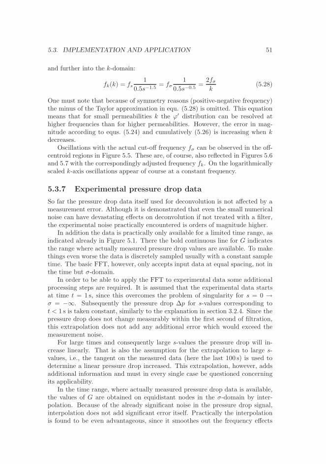
5.3. IMPLEMENTATION AND APPLICATION 51
and further into the k-domain:
fk(k) = fs
1
0.5s−1.5= fσ
1
0.5s−0.5=
2fσ
k(5.28)
One must note that because of symmetry reasons (positive-negative frequency)the minus of the Taylor approximation in equ. (5.28) is omitted. This equationmeans that for small permeabilities k the ϕ′ distribution can be resolved athigher frequencies than for higher permeabilities. However, the error in mag-nitude according to equs. (5.24) and cumulatively (5.26) is increasing when kdecreases.
Oscillations with the actual cut-off frequency fσ can be observed in the off-centroid regions in Figure 5.5. These are, of course, also reflected in Figures 5.6and 5.7 with the correspondingly adjusted frequency fk. On the logarithmicallyscaled k-axis oscillations appear of course at a constant frequency.
5.3.7 Experimental pressure drop data
So far the pressure drop data itself used for deconvolution is not affected by ameasurement error. Although it is demonstrated that even the small numericalnoise can have devastating effects on deconvolution if not treated with a filter,the experimental noise practically encountered is orders of magnitude higher.
In addition the data is practically only available for a limited time range, asindicated already in Figure 5.1. There the bold continuous line for G indicatesthe range where actually measured pressure drop values are available. To makethings even worse the data is discretely sampled usually with a constant sampletime. The basic FFT, however, only accepts input data at equal spacing, not inthe time but σ-domain.
In order to be able to apply the FFT to experimental data some additionalprocessing steps are required. It is assumed that the experimental data startsat time t = 1 s, since this overcomes the problem of singularity for s = 0 →σ = −∞. Subsequently the pressure drop ∆p for s-values corresponding tot < 1 s is taken constant, similarly to the explanation in section 3.2.4. Since thepressure drop does not change measurably within the first second of filtration,this extrapolation does not add any additional error which would exceed themeasurement noise.
For large times and consequently large s-values the pressure drop will in-crease linearly. That is also the assumption for the extrapolation to large s-values, i.e., the tangent on the measured data (here the last 100 s) is used todetermine a linear pressure drop increased. This extrapolation, however, addsadditional information and must in every single case be questioned concerningits applicability.
In the time range, where actually measured pressure drop data is available,the values of G are obtained on equidistant nodes in the σ-domain by inter-polation. Because of the already significant noise in the pressure drop signal,interpolation does not add significant error itself. Practically the interpolationis found to be even advantageous, since it smoothes out the frequency effects

52 CHAPTER 5. CONVOLUTION TRANSFORM FORMULATION
of the exponential sample intervals in the σ-domain, thus simplifying filteringdata in the frequency domain.
The calculation scheme suggested here is applied on data presented by [25].The convolution situation in the σ-domain is depicted together with the de-convolution result in Figure 5.8. The corresponding power spectra are shownin Figure 5.9. The spectrum of the kernel is, of course, not altered from Fig-ure 5.2, but in the spectrum of the G-function the noise level is clearly muchhigher. Thus the noise model is giving generally higher values. Also the Wienerfilter B is shown in Figure 5.9 and here the transition from 1 to 0 is not as sharpas in Figure 5.2, thus a continuous decrease in the value can be seen.
The amplitude error is found from a plot similar to Figure 5.6 to be εσ =2 · 10−6 m
12 .
−20 0 20 40 60−0.1
0
0.1
0.2
0.3
0.4
0.5
0.6
0.7
0.8
σ, −
kernel hG measuredG extrapolatedϕ
104G
-,104ϕ
m0.5
,ker
nelh
-
Figure 5.8: Deconvolution situation for experimental data in the σ-domain.
In Figure 5.10 the result of deconvolution is displayed. The deconvolutedPD shows hardly any jump when compared to the distribution obtained byoptimization. This arises from the relatively low cut-off frequency fσ = 0.26for the given problem, i.e., higher frequencies than that cannot be resolved.However, the PD obtained by deconvolution is equally suitable for describing apressure drop increase ramp which is displayed in Figure 5.11. The deconvolutedPD, however, exhibits significant oscillations and a significant integral errorfor small k-values which reaches even in the negative range being physicallymeaningless.

5.3. IMPLEMENTATION AND APPLICATION 53
10−2
10−1
100
101
−300
−250
−200
−150
−100
−50
0
50
100
frequency f, −
pow
er s
pect
ral d
ensi
ty
P, d
B
Ph
PG
Pnoise
filter B
Figure 5.9: Power spectral densities for the deconvolution situation from exper-imental data.

54 CHAPTER 5. CONVOLUTION TRANSFORM FORMULATION
10−9
10−8
−0.2
0
0.2
0.4
0.6
0.8
1
permeability k, m
Φ′ , −
Φ′ optimizer
Φ′ deconvolutedE
k
Figure 5.10: PD from experimental data obtained by deconvolution. In additionthe corresponding PD determined by optimization and the integrated error Ek
are displayed.
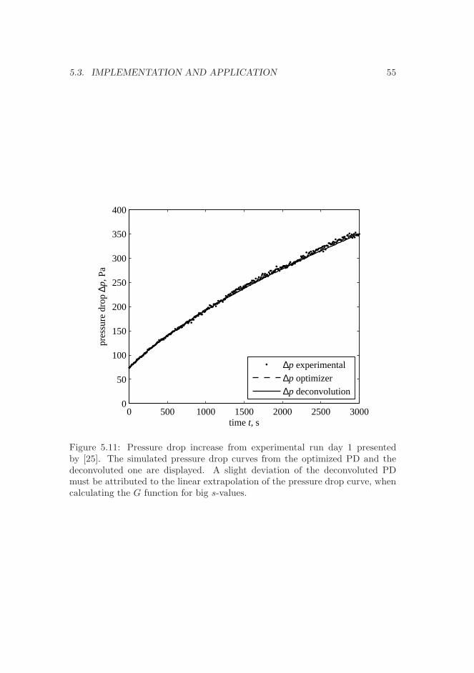
5.3. IMPLEMENTATION AND APPLICATION 55
0 500 1000 1500 2000 2500 30000
50
100
150
200
250
300
350
400
time t, s
pres
sure
dro
p ∆p,
Pa
∆p experimental
∆p optimizer∆p deconvolution
Figure 5.11: Pressure drop increase from experimental run day 1 presentedby [25]. The simulated pressure drop curves from the optimized PD and thedeconvoluted one are displayed. A slight deviation of the deconvoluted PDmust be attributed to the linear extrapolation of the pressure drop curve, whencalculating the G function for big s-values.
56 CHAPTER 5. CONVOLUTION TRANSFORM FORMULATION
5.4 Discussion and conclusions
In the preceding sections the convolution integral version of the PD-method isintroduced and applied. A PD can be obtained from pressure drop data bydeconvolution using FFT. The deconvolution method is orders of magnitudefaster than finding a PD by global optimization and allows for error estimationof the result. The error estimation is given as amplitude oscillations and acut-off frequency.
The probably biggest disadvantage of the PD-method via deconvolution is,that it requires more assumptions on the raw data than the optimization, be-cause of extra- and interpolation. In addition the filter design requires additionalinformation, i.e., a noise model. The implementation effort is bigger and thesubsequent possibility for implementation errors is higher in the deconvolutionversion. A PD from convolution is, in principal, more flexible than one obtainedby optimization, since an optimizer allows only for a very limited number ofnodes for the PD. However, the deconvolution does not give perfectly consistentdistribution results, since oscillations in the results can lead to negative densityfunctions.
The deconvolution is attempted on simulated data from a PD determinedby optimizations (results are not displayed in detail here). In this case the de-convolution version can give a measure on the certainty of the PD determinedby optimization. The pressure drop increase can be copied within very narrowlimits by deconvolution and error bounds on the deconvoluted PD can be ob-tained. The PD from optimization is for the attempted case clearly within theerror bounds. Thus the simplicity of optimization and the error estimation ca-pabilities of deconvolution can be combined. Such an improvement can possiblybe achieved by determining an estimate for a PD from deconvolution which iseventually refined by optimization.
The deconvolution version of the PD-method is applied and its suitability toobtain a PD is shown. More assumptions are necessary to be able to apply thedeconvolution version compared to finding the PD by optimization. The latteris significantly simpler in application, but computationally more expensive. Themost practical form of the PD-method may make use of optimization becauseof its simplicity and robustness, and eventually when an error estimation isrequired a deconvolution might be performed.

Chapter 6
Application
This chapter shows exemplarily applications of the PD-method. It is dividedinto two main sections: The determination of a PD of the filter medium itselfand a PD due to industrial filter operation with incomplete filter cleaning.
6.1 Inhomogeneous filter media
The characterization of filter media by the PD-method requires pressure dropdata of the filtration on the initially clean filter medium, henceforth termed ramptest, as input. Such data can be acquired in e.g. filter test stands, laboratoryfilter plants or even pilot and production scale plants. According to the findingsfrom chapter 4 the obtained pressure drop profile can be transformed into acorresponding PD.
To determine the PD of the filter medium itself it must be ensured that thefilter medium is clean at the beginning of filtration. Any filter cake presentcould add to the PD of the filter medium and will thus corrupt the PD of thefilter medium.
To extract most information from such a PD it is desirable to know mostoperating parameters and, of course, the filter model presumptions must befulfilled.
The extent to which the requirements of cleanliness and ascertained operat-ing parameters are accomplishable depends largely on the filtration facility thatis used to determine the pressure drop curve.
Kavouras and Krammer [20] are using a pilot scale filter and assume thatthe filter is carrying no cake any longer, when the pressure drop at a certaingas flow remains at a constant level despite continuous filter cleaning. However,it cannot be verified externally that the filter medium does not carry any cakeat this stage. Saleem [26] has the possibility to actually verify the existence orlack of cake patches by stereo optical cake thickness measurements.
For practical reasons the clean filter state, used further on, willl be definedin accordance with the definition used by [20]. The clean filter state is thus

58 CHAPTER 6. APPLICATION
reached when further filter cleaning does not have any further influence on thepressure drop level. This is also the most practical definition, since it reflectsthe state of cleanliness achievable by the chosen filter cleaning method.
The way of obtaining the pressure drop increase that is required to deter-mined the PD depends on the actual facility used. In laboratory plants it isgenerally possible to start gas flow and dust feed in sequence. The subsequentpressure drop increase is used as input for the PD-method. The experimentalprocedure may have to differ and is discussed in the respective section.
6.1.1 Filter media test stands
Usually it is easier to assure defined condition in a laboratory scale and alsoinstrumentation is most comprehensive there. Existing filter test rigs do notrequire any modification of the setup or instrumentation and thus even existingdata from past experiments can be used for evaluation with the PD-method.
A typical example of a commonly used test stand is the VDI 3926 [12] standwhich comes in two modifications Type 1 and Type 2. The filter medium sampleto be examined is a square with a total filtration area Atot = 144 cm2. Thusthe isolated effect of cake filtration on that sample is simulated. Any possibleinfluence of the filter medium’s installation as e.g. a bag in a baghouse with apossibly uneven dust distribution and/or dust settling, i.e., some dust is settlingdirectly and not even reaching the filter medium, is eliminated.
In Figure 6.1 the pressure drop data recorded in a VDI 3429 Type 1 teststand is displayed together with its corresponding simulated pressure drop curvefrom the filter model. The pressure drop increase during filter testing of a cleancloth sample is depicted. The filter medium used is a polyimide needle felton a polyester supporting scrim. The test dust used is the alumina monohy-drate powder Pural SB. The agreement between the simulated and experimentalpressure drop curve is excellent. That is not especially surprising, since the un-derlying PD is determined via simple optimization with a fixed distributiondiscretization (cf. section 4.1.1) from the experimental pressure drop data.
The parameter pc is calculated from the design of the filter test rig and themeasured volume flow V = 2.77 m3 · h−1 which is constant within 0.5% duringthe test run. The gas viscosity is taken from air as ηg = 18 · 10−6Pa · s.
The calculation of the tc parameter requires the dust concentration csol =5 g · m−3 in addition, but is not as straightforward because of the unknownspecific cake resistance αm. Since the pressure drop ramp test is not continuedbeyond the time range displayed in Figure 6.1, this value cannot be directlyextracted from the final asymptote of the pressure drop curve. Therefore thePD-method is executed with a roughly overestimated tc value. In Figure 6.2the corresponding PD is displayed as solid line with dot-markers.
A small part of the filter area (< 10 %) is found to have a high permeability.The remaining filter area is exhibiting a significantly lower, but rather homoge-neous permeability. This part can be seen as nearly vertical line in Figure 6.2.The area exhibiting an even lower permeability than the homogeneous area isdiscussed below with respect to the model parameters chosen.
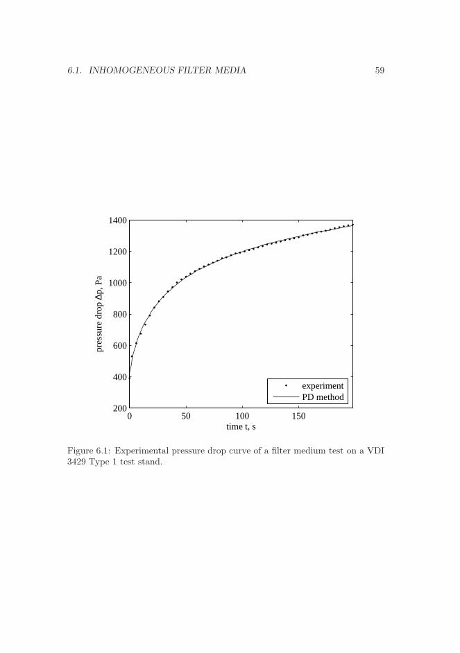
6.1. INHOMOGENEOUS FILTER MEDIA 59
0 50 100 150200
400
600
800
1000
1200
1400
time t, s
pres
sure
dro
p ∆p,
Pa
experimentPD method
Figure 6.1: Experimental pressure drop curve of a filter medium test on a VDI3429 Type 1 test stand.
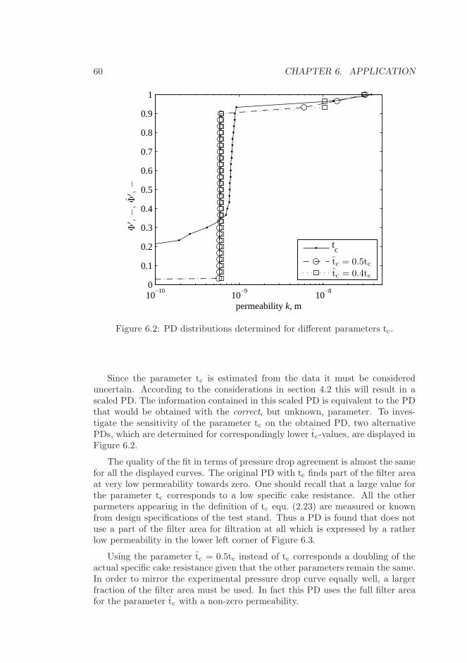
60 CHAPTER 6. APPLICATION
10−10
10−9
10−8
0
0.1
0.2
0.3
0.4
0.5
0.6
0.7
0.8
0.9
1
permeability k, m
tc
tc = 0.5tctc = 0.4tc
Φ′ ,−
,Φ
′ ,−
Figure 6.2: PD distributions determined for different parameters tc.
Since the parameter tc is estimated from the data it must be considereduncertain. According to the considerations in section 4.2 this will result in ascaled PD. The information contained in this scaled PD is equivalent to the PDthat would be obtained with the correct, but unknown, parameter. To inves-tigate the sensitivity of the parameter tc on the obtained PD, two alternativePDs, which are determined for correspondingly lower tc-values, are displayed inFigure 6.2.
The quality of the fit in terms of pressure drop agreement is almost the samefor all the displayed curves. The original PD with tc finds part of the filter areaat very low permeability towards zero. One should recall that a large value forthe parameter tc corresponds to a low specific cake resistance. All the otherparmeters appearing in the definition of tc equ. (2.23) are measured or knownfrom design specifications of the test stand. Thus a PD is found that does notuse a part of the filter area for filtration at all which is expressed by a ratherlow permeability in the lower left corner of Figure 6.3.
Using the parameter tc = 0.5tc instead of tc corresponds a doubling of theactual specific cake resistance given that the other parameters remain the same.In order to mirror the experimental pressure drop curve equally well, a largerfraction of the filter area must be used. In fact this PD uses the full filter areafor the parameter tc with a non-zero permeability.

6.1. INHOMOGENEOUS FILTER MEDIA 61
10−10
10−9
10−8
0
0.1
0.2
0.3
0.4
0.5
0.6
0.7
0.8
0.9
1
permeability k, m
Φ′ , −
tc
tc = 0.5tctc = 0.4tc
Figure 6.3: PD distributions determined for different parameters tc. Curvesdetermined for a paramter tc scaled for comparability to the parameter tc.
62 CHAPTER 6. APPLICATION
The model parameters are different for the curves in Figure 6.2. To ensurecomparability of the PDs determined for tc-values these are transformed to thevalue of the parameter tc according to the transformation outlined in section 4.2.In Figure 6.3 the distribution functions with tc = 0.5 tc is rescaled to the param-eter tc and are thereby comparable to the curve determined with the tc-value.According to equ. (4.11) the scaling factor for the cumulative distribution axis
is√
tctc
=√
0.5 ≈ 0.71. Thus at least 30 % of the filter area must have zero
permeability, which is reflected in the corresponding PD in Figure 6.3, whichintersects the ordinate axis at this value. Nevertheless, the remaining 70 % areused. Good agreement between the original PD and the PD for tc = 0.5tc isobserved for these higher permeability values. At low permeability values thePD is anyway highly uncertain according to the findings in section 5.3.6.
When decreasing the parameter tc even further to tc = 0.4tc the PD makesuse of the entire filter area too (see Figure 6.2), i.e., there are no parts of thefilter area with zero permeablity. In Figure 6.3 this means, of course, a non-zeroPD for
√0.4 ≈ 63% of the filter area. However, one observes a shift of the
large step in the distribution around k = 10−9 m towards bigger permeabilityvalues. This might indicate that the parameter tc chosen is too low, since thepermeability shifts towards higher values to compensate for a higher specificcake resistance. However, the quality of the obtained fit does not worsen, whichmust be mainly attributed to a relatively better resolution of the PD at highpermeability values. Since the PD for relatively lower tc values is scaled to coveronly a part of the distribution axis Φ′, the resolution on this part is higher forthe same number of nodes.
Reversing the train of thoughts leading to the error estimation from sec-tion 5.3.6 one finds that the pressure drop is, of course, most influenced bydeviations of the PD at high permeability values. Thus apparently a small ad-vantage in the resolution of these can compensate for a shortcoming in capturingof small permeability values.
The filter test stands are designed to provide best intercomparability betweenresults determined at different test stands. Thus comparable/reproducible re-sults between different experimental runs and different test stands are expected.However, for the determination of a PD this also entails the greatest shortcom-ing: The test dust is standardized and differs thereby naturally from the dustto be encountered by the filter medium in the application. The PD, however, isdepending on the actual dust and extrapolation from the test dust to the actualdust is not a priori possible.
6.1.2 Laboratory scale filter plants
The next step is to investigate laboratory scale filter plants that resemble indus-trial scale plants in the basic construction and operation. They are, however,smaller and commonly only designed for investigation of various filtration fea-tures. Also here operational parameters are usually well defined and knownand also the instrumentation of such plants is good. One advantage of such

6.1. INHOMOGENEOUS FILTER MEDIA 63
plants is the regeneration mode which closely resembles the regeneration in in-dustrial plants. Also the operation of laboratory filter plants with the samedust as industrial plants is advantageous, since it overcomes the problems ofdust depending PDs.
During this work mainly data gathered by the plants presented by [26] and[25] are used. The former plant is designed for optical cake thickness measure-ments and henceforth identified as plant #1. The latter plant is used to studyreactive gas cleaning and is hereafter termed plant #2. Both filter plants consistof a dust supply unit that disperses a certain mass flow of dust in air which issucked through the filter plant. The gas volume flow after the filter is recordedand controlled to a certain set value via a frequency controlled fan. Experi-ments were conducted with both plants having installed three filter bags whichare pervaded by the dust laden gas from the outside to the inside. In order tosupport filter bags they are mounted on wire cages. Dust particles are retainedat the filter bag’s outer surface. Due to the dust which is accumulating on thefilter bags forming a filter cake the overall permeability of the filter decreases.As the fan keeps the gas volume flow approximately constant the pressure differ-ence over the filter rises. The filter is regenerated either after a certain pressuredifference over the filter is reached or after a certain time interval for filtrationhas elapsed. Filter regeneration is carried out by a reverse air jet pulse. Eachfilter bag can be regenerated separately. The layout of both plants is accordingto the basic scheme (see Figure 1.1). The plants, however, differ in the actualspecification and scale. Table 6.1 gives an overview of these specifications.
Plant Atot mc ηg αm V# m2 kg · s−1 Pa s m · kg−1 m3 · h−1
1 2.04 8.4 10−4 1.8 10−5 6.67 109 2402 0.53 1.5 10−5 2.0 10−5 - 40
Table 6.1: Specifications of laboratory scale filter plants
Only the online measurements of pressure drop over the filter and gas volumeflow are used in this work. The measuring locations are shown in the flowchart(see Figure 1.1) indicated by PDC for pressure difference and FC for flow. Thedust concentration is calculated according to:
csol =mc
V(6.1)
The total dust mass mc conveyed to the filter is set by the dust dosing equip-ment.
Figure 6.4 shows the start up of filter plant #1 as ramp test. The filtermedium is thoroughly cleaned at the beginning of this experimental run andthus does not carry any filter cake. The vertical dashed line indicates the pointin time when the dust dosing equipment is activated. Subsequently one observesan increase in pressure difference.
During the pre-experimental phase of this plant special emphasis was put onthe quality of data recording of transient pressure drop and volume flow data. In
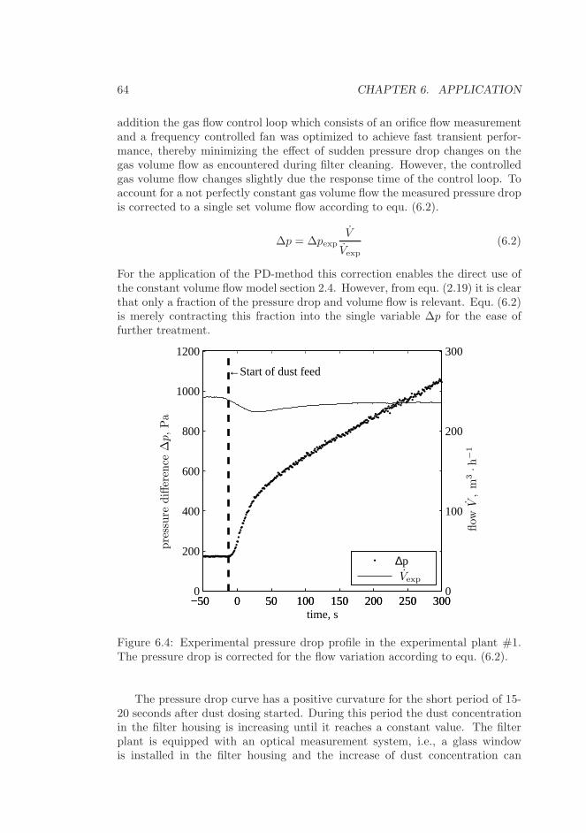
64 CHAPTER 6. APPLICATION
addition the gas flow control loop which consists of an orifice flow measurementand a frequency controlled fan was optimized to achieve fast transient perfor-mance, thereby minimizing the effect of sudden pressure drop changes on thegas volume flow as encountered during filter cleaning. However, the controlledgas volume flow changes slightly due the response time of the control loop. Toaccount for a not perfectly constant gas volume flow the measured pressure dropis corrected to a single set volume flow according to equ. (6.2).
∆p = ∆pexpV
Vexp
(6.2)
For the application of the PD-method this correction enables the direct use ofthe constant volume flow model section 2.4. However, from equ. (2.19) it is clearthat only a fraction of the pressure drop and volume flow is relevant. Equ. (6.2)is merely contracting this fraction into the single variable ∆p for the ease offurther treatment.
−50 0 50 100 150 200 250 3000
200
400
600
800
1000
1200
←Start of dust feed
−50 0 50 100 150 200 250 3000
100
200
300
time, s
∆p
flow
V,
m3·h
−1
Vexp
pre
ssure
diff
eren
ce∆p,Pa
Figure 6.4: Experimental pressure drop profile in the experimental plant #1.The pressure drop is corrected for the flow variation according to equ. (6.2).
The pressure drop curve has a positive curvature for the short period of 15-20 seconds after dust dosing started. During this period the dust concentrationin the filter housing is increasing until it reaches a constant value. The filterplant is equipped with an optical measurement system, i.e., a glass windowis installed in the filter housing and the increase of dust concentration can

6.1. INHOMOGENEOUS FILTER MEDIA 65
be observed qualitatively. Also the average gas residence time in the filterhousing is in the observed range of time. The filter housing contains a raw gasvolume of approximately 0.8 m3 which leads to an average residence time of12 s at the operation point displayed. Assuming infinite backmixing in the filterhousing, which is justified given the turbulence observed in the filter housing,80 % of the final dust concentration is reached after approximately 19 s. Moreinterestingly the curvature of the pressure drop curve changes when a constantdust concentration in the housing is reached. A pronounced concave curvedpressure drop profile can be observed.
Finally the transient pressure drop increases linearly, which can be explainedby a practically equalized permeability profile over the filter. This entails ho-mogenous flow and an isotropic cake builds up homogeneously. The slope ofthe transient pressure drop asymptote can directly be used to obtain the spe-cific cake resistance αm by combining equs. (2.4) and (2.8) for an equalizedpermeability, i.e., no dependency on filter location A has to be considered:
αm =1
ηg csol
(Atot
V
)2
limt→∞
d∆p
dt(6.3)
For practical use one cannot employ the limit but should restrict time t tosufficiently large numbers, i.e., where the pressure increase is linear within theerror of measurement.
The PD corresponding to the pressure drop ramp from Figure 6.4 is displayedin Figure 6.5. The integral mean value can be displayed in addition. Note thatin this figure the abscissa is linearly scaled and thus the area on the left handside of the PD and the mean value curves are equal.
The basic shape of the PD found resembles the PD found in the filter testrig in section 6.1.1 with a significant step in the PD, whereas a small part ofthe area exhibits a high permeability.
In filtration plant #2 filter cloth condition experiments with reactive dust arecarried out. Details to this test series can be found in [25]. The basic featuresare similar to the filtration plant #1 presented already. The different plantspecifications are given in Table 6.1. The specific cake resistance value is notreported there, because several different values are determined corresponding toeach filter start-up.
The aim of the experiments is to study the conditioning of filter media atan elevated temperature of 140 °C over time. The sample dust used is CaO andCa(OH)2 respectively, which is suspended in a simulated flue gas atmospherecontaining H2O and CO2. These compounds are especially reactive towardsCaO forming reaction products such as Ca(OH)2 and CaCO3. Since the reac-tion products have a significantly higher molar volume than CaO a mechanicalexpansion of the reacting particles is expected. In the flue gas atmospheremost residence time is provided whilst the particles are deposited on the filtermedium, i.e., in the filter cake. During the conditioning period some particlesmight even penetrate inside the filter medium and react there. A mechanicalgrowth of the particles there can lead to pore blocking, rendering normal fil-tration impossible. In order to minimize the possible particle penetration with
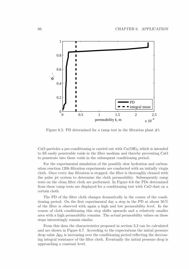
66 CHAPTER 6. APPLICATION
0 0.5 1 1.5 2 2.5
x 10−8
0
0.2
0.4
0.6
0.8
1
permeability k, m
Φ′ , −
PDintegral mean
Figure 6.5: PD determined for a ramp test in the filtration plant #1
CaO particles a pre-conditioning is carried out with Ca(OH)2 which is intendedto fill easily penetrable voids in the filter medium and thereby preventing CaOto penetrate into these voids in the subsequent conditioning period.
For the experimental simulation of the possibly slow hydration and carbon-ation reaction 120h filtration experiments are conducted with an initially virgincloth. Once every day filtration is stopped, the filter is thoroughly cleaned withthe pulse jet system to determine the cloth permeability. Subsequently ramptests on the clean filter cloth are performed. In Figure 6.6 the PDs determinedfrom these ramp tests are displayed for a conditioning test with CaO dust on acertain cloth.
The PD of the filter cloth changes dramatically in the course of the condi-tioning period. On the first experimental day a step in the PD at about 50 %of the filter is observed with again a high and low permeability level. In thecourse of cloth conditioning this step shifts upwards and a relatively smallerarea with a high permeability remains. The actual permeability values on thesesteps interestingly remain similar.
From this data the characteristics proposed in section 3.2 can be calculatedand are shown in Figure 6.7. According to the expectations the initial pressuredrop value ∆p0 is increasing over the conditioning period reflecting the decreas-ing integral resistance of the filter cloth. Eventually the initial pressure drop isapproaching a constant level.

6.1. INHOMOGENEOUS FILTER MEDIA 67
10−9
10−8
0
0.2
0.4
0.6
0.8
1
permeability k, m
cum
ulat
ive
area
Φ, −
day 1day 2day 3day 4day 5day 6
Figure 6.6: PD determined for a ramp test in the filtration plant #2
The asymptotic pressure drop offset on the ordinate ∆p0 is always above∆p0. The broad PD on the first experimental day is reflected in a fairly largedifference between ∆p0 and ∆p0. This span is thereafter reducing slightly.
The initial pressure drop slope augmentation κs is significantly increasingduring the experimental period. This is a result of the increasingly skewed PDsas the condition period proceeds1. Practically that means that the pressuredrop initially increases very fast, with a factor up to 13 from linear. Thus thepressure drop curve is approaching the asymptote quickly. In this situation thefiltration behavior resembles more a homogeneous cloth with the initial pressuredrop ∆p0. The actual initial pressure drop value ∆p0 is not really significantfor the filter performance.
6.1.3 Pilot and industrial scale plants
The pressure drop data from bigger filtration plants is in principle similar to thedata gathered in laboratory scale. However, there the filtration unit is part ofa process which imposes external influence on the filter operation. Operationalparameters such as gas volume flow, dust concentration, dust properties et ceteraare determined by the process operation and can hardly be set directly.
1Note that the skewness of a distribution is described by its third order moment.

68 CHAPTER 6. APPLICATION
1 2 3 4 5 60
50
100
150
200
250
300
350
400
450
1 2 3 4 5 60
5
10
15
experimental day
slope
multip
lierκ
s,-
pre
ssure
dro
p∆p,Pa
∆p0
∆p0
κs
Figure 6.7: The characteristic values of the PDs versus the experimental period:initial pressure drop, asymptotic ordinate intersection and pressure drop slopemultiplier.

6.1. INHOMOGENEOUS FILTER MEDIA 69
Also in laboratory scale tests feed back of periodic filter cleaning on thegas volume flow is observed. This intrinsically semi-continuous filter operationcan feed back into the otherwise continuous plant operation. In turn backcoupling on the filter operation, as described by [27] for a pilot scale plant,can be observed. E.g. a changing dust mass flow violates the assumption ofthe PD-method. Thus special care must be taken when using pressure dropdata from industrial plants. Additionally, industrial plants are often equippedwith limited instrumentation, which makes it even difficult to recognize such aviolation. Nevertheless, when detailed information about the changes in dustmass flow are available a corresponding correction, i.e., an appropriate timescaling, may be applied and the PD-method can eventually be applied.
The study presented by [28] makes use of the PD-method to characterize thefiltration behavior while changing dust properties including the dust mass flow.Measurements are made in an industrial scale bag filter plant which is cleaningthe off-gas of a cement plant. The bag filter is retrofitted after an electrostaticprecipitator (ESP) and enhancing the dust collection efficiency to meet emissionstandards. During ordinary plant operation most dust is removed by the ESPand only a rather small dust concentration is reaching the bag filter.
The experimental parameter is the impact of the ESP on bag filter operation.The plant is operated with the ESP in operation and with the ESP switchedoff. In Figure 6.8 the recorded measurement signals of volume flow and pressuredrop are shown for the experiment with the ESP in operation. Compared to thelaboratory data presented in the earlier section the data quality is clearly worse,with much noise in the pressure drop signal. Initially the normal operation of thefilter is shown. At about 7000 s the filter is extensively cleaned until no furtherreduction of the pressure drop can be observed. Since dust is continuouslyreaching the bags, some cake will always be present on the bags as cleaningthe entire filter once, i.e. pulsing every row once, takes about 90 seconds.However, according to the definition above the filter is considered sufficientlyclean thereafter. Then the pressure drop is allowed to build up without furtherfilter cleaning. This ramp is used to determine a PD.
In this plant the information on the amount of dust reaching the filter bagsis not available and thus the dust concentration is unknown for both ESP inoperation and ESP switched off. This is overcome by determining the entireparameter tc from the linear part of the pressure drop ramps directly, insteadof just determining αm as described in section 6.1.2. Of course two different tcvalues for the operation with and without ESP must be determined. To extractmore interpretable information from these values the definition equ. (2.23) canbe used to calculate the product αm · csol, since the volume flow V and the filterarea Atot are known.
Figure 6.9 shows two PDs determined for the pressure drop ramp discussedabove and a corresponding ramp where the ESP is not in operation. This resultclearly shows the dependency of the PD on the dust properties. The filter setupand plant operation remain unaltered during these tests. Only the amountof dust and probably also its properties, such as the particle size distribution,

70 CHAPTER 6. APPLICATION
0 1 2 3 4 5 6
x 104
0
50
100
150
200
250
300
350
400
experimental time, s
pres
sure
dro
p ∆ p
, Pa
0
1
2
3
4
5
6
7
8
volu
me
flow
, m3 ⋅s−
1
∆ pflow
Figure 6.8: Pressure drop and volume flow measurements in an industrial bagfilter plant with an upstream ESP in operation.

6.2. PDS FROM FILTER OPERATION 71
change when the ESP is switched off. In turn the filtration behavior on thesame cloth is altered.
Generally the PD with the ESP in operation is spread over a wider rangeof permeability values, i.e., a broader distribution is found. After the ESP onlythe fines reach the bag filter, and fine particles pose the greater challenge tothe bag filter, than a coarser fraction [29]. The parameter tc, which differs byalmost a factor 100 between the two runs, accounts for the possible change ofthe specific cake resistance and the absolute difference in dust mass.
10−9
10−8
0
0.1
0.2
0.3
0.4
0.5
0.6
0.7
0.8
0.9
1
permeability k, m
cum
ulat
ive
filte
r ar
ea d
istr
ibut
ion Φ
′ , −
with ESPwithout ESP
Figure 6.9: PDs determined for the filter operation with and without the ESPin operation.
In Figure 6.10 a comparsion is displayed between the calculated pressuredrop cuves generated by the two PDs from Figure 6.9 using the tc-value deter-mined the operation with the ESP on. The initial pressure drop rise caused bythe more pronounced PD with the ESP in operation is clearly visible. Afterthat initial increase the pressure drop curves converge towards a the same slopeof the final asymptote, since tc is the same for both curves.
6.2 PDs from filter operation
In section 6.1 the determination of a PD of the clean filter medium itself isaddressed. However, a filter can exhibit an inhomogeneous PD also because of
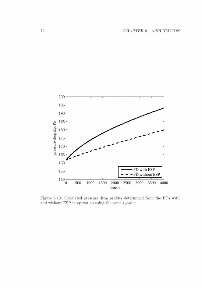
72 CHAPTER 6. APPLICATION
0 500 1000 1500 2000 2500 3000 3500 4000150
155
160
165
170
175
180
185
190
195
200
time, s
pres
sure
dro
p ∆p,
Pa
PD with ESPPD without ESP
Figure 6.10: Calcuated pressure drop profiles determined from the PDs withand without ESP in operation using the same tc-value.

6.2. PDS FROM FILTER OPERATION 73
an uneven residual cake distribution. Residual cake refers to filter cake presenton the filter cloth at the beginning of filtration. Such cake originates fromincomplete filter cleaning.
Kavouras and Krammer [20] give an extensive literature overview on rea-sons and applications for such incomplete cleaning. Two reasons are reportedleading to a residual filter cake. On the one hand the filter cake might not be re-moved entirely from a filter medium that is exposed to regenerative action. E.g.Humphries and Madden [30] and Seville et al. [16] describe this phenomenontermed patchy cleaning. It refers to filter cake that is partially completely re-moved from the filter medium, but patches stay unchanged on the filter mediumdespite a cleaning action. Duo et al. [17], Ju et al. [18], and Dittler et al. [31]focus mainly on patchy cleaning of the filter medium for their pressure dropsimulations. Also Kavouras and Krammer [20] consider patchy cleaning for thesimulation of filter pressure drop.
On the other hand only a part of the filter area is exposed to a cleaning actionat one time in industrial filters. Typically one filter compartment or one filterbag row is cleaned at once, whereas the remaining filter area is unaffected. Thiseasily conceivable mechanism also leads to an uneven distribution of filter cakeover the filter area. Kavouras and Krammer [20] discriminate between patchycleaning and sequenced filter cleaning as reasons for incomplete cleaning for filtersimulation. Duo et al. [17] only mention the possibility for an inhomogeneouscake distribution due to sequenced filter cleaning.
However, the effect on filtration when residual dust cake is present can bedescribed in the same framework as an inhomogeneous filter medium. Filterareas carrying residual cake patches have a lower permeability than clean filterarea or area carrying a thinner residual cake. The filter medium and the residualcake as entity have a distributed permeabilty, which is corresponding to thecake distribution. The filter model and PD-method can therefore be directlyapplied to this type of problem too. The models presented by Duo et al. [17]and Kavouras and Krammer [20] are shown to be embraced by the filter modelpresented in section 2. Under certain provisions concerning cake compressibilityalso the model of Ju et al. [18] is captured. This equivalence of the modelsis based on the same approach with a 1-dimensional flow description and thecorrespondingly identical governing equations. In line with the literature modelsthe PD stems only from a residual cake distribution. The filter cloth is, as inthe literature, homogeneous itself and is thus not contributing to the PD.
6.2.1 Patchy cleaning
In this section patchy cleaning is looked at separately, i.e., without any influencefrom segmented filter cleaning. During semi-continuous filter operation severalcake generations are present on the filter cloth. In Figure 6.11 such patchycleaning is depicted for data from the model by Kavouras and Krammer[20].On the ordinate axis the cumulative area distribution is shown. In the left mostpart the fractional area distribution of the cake area load is displayed. Thesituation immediately after cleaning is depicted. Generation 1 in the uppermost

74 CHAPTER 6. APPLICATION
part of the figure represents the clean filter cloth, i.e., the part of cloth fromwhich cake was successfully removed. The generation 2 area depicted below iscarrying the residual cake which was not removed at cleaning. The cake areaload corresponds to the filtration on the clean filter cloth for one filtration cycle.The area carrying generation 2 is smaller than the cleaned area generation 1,because a part the filter cake from generation 1 is removed at cleaning, andthereby becomes generation 1 again in a new cycle. Generation 3 stems fromthe part of generation 2 where cake is not removed at cleaning. During onefiltration cycle additional cake builds up onto the already present generation2 cake, thereby forming generation 3. Kavouras and Krammer[20] outline thismechanism in detail.
By considering the filter cleaning mechanism one finds that the cake buildingup on the generation 1 spot will reach the cake thickness of generation 2 duringone filtration cycle. Upon filter cleaning, part of this cake will be removed,whereas the rest stays on the cloth unchanged, thereby forming generation 2.In other words the thickness of cake generation 1 before cleaning equals thecake thickness of generation 2 after cleaning. This applies correspondingly toall generations.
According to the notation of the filter model from chapter 2 the cake thick-ness in terms of cake area load is corresponding to a certain permeability kaccording to equs. (2.2) and (2.3). The filter cloth permeability is constant.Hence the cake area load can be converted into the permeability which is dis-played in the center of Figure 6.11. Please note that further on in this chap-ter the nomenclature refers to k as the overall permeability of cake and cloth,whereas k0 denotes the initial permeability. This is necessary to be consistentwith the nomenclature for the filter model presented in chapter 2. In the case ofpatchy cleaning the initial permeability comprises of contributions of both, filtercloth and filter cake. For a consistent nomenclature the initial filter cake mustbe included in the initial permeability k0. However, as in the chapters beforethis index 0 is omitted, since PDs are only displayed for the initial permeability.
Periodic filter operation at period one implies that the pressure drop curvebetween two subsequent cleaning actions is identical for all cycles. This, how-ever, corresponds to a certain change in filter state s defined by equ. (2.12) whichis only depending upon the pressure drop. For periodic filtration a filter statescyc shall be defined as the filter state change during one cycle, i.e., evaluationof equ. (2.12) for one cycle. This filter state change applies of course to all filtergenerations. In the rightmost chart in Figure 6.11 the abbreviation k−2 = uis depicted. The steps between the separate generations have the same height,which results from equ. (2.13) governing the permeability evolution. The heightof the steps is scyc which is shown in the figure for the generations 2-4.
Hence by knowing the area distribution of the cake patches and scyc the dis-tribution of cake on the various generations is analytically known. The perme-ability at the beginning of filtration for each generation can be easily calculatedaccording to
ki =[k−20 + scyc · (i− 1)
]− 12 (6.4)
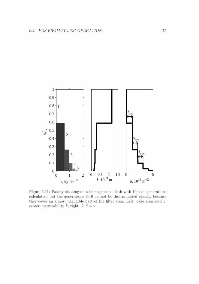
6.2. PDS FROM FILTER OPERATION 75
0 1 20
0.1
0.2
0.3
0.4
0.5
0.6
0.7
0.8
0.9
1
1
2
3
45
z, kg ⋅ m−2
Φ′ ,
−
0 0.5 1 1.5k, 10−9 m
0 5
scyc
scyc
scyc
u, 1019 m−2
Figure 6.11: Patchy cleaning on a homogeneous cloth with 10 cake generationscalculated, but the generations 6-10 cannot be discriminated clearly, becausethey cover an almost negligible part of the filter area. Left: cake area load z,center: permeability k, right: k−2 = u.

76 CHAPTER 6. APPLICATION
The constant cloth permeability is denoted k0 and i is the index for the cakegeneration. Generation 1 is without cake. Thus it trivially has the permeabilityk0.
The filter state change scyc can be determined from the filter operationmode. This only requires a line search of the respective filter state scyc. E.g. forconstant flow filtration with a maxium pressure drop control the correspondingscyc value can be determined from equ. (2.24). Filtration at constant cycle timerequires a line search in equ. (2.31). The corresponding equations for constantpressure filtration are equs. (2.21) and (2.20), respectively.
For the filter model the filter area Atot is divided into areas Ai carrying acake generation i. The density PD function can thus be written as
ϕ′(k) =1
Atot
∑
i
Aiδ (k − ki) (6.5)
whereas δ denotes the Dirac delta function. The cumulative distribution can beobtained by integrating equ. (6.5).
For the determination of the generation area distribution different approacheshave been in used. Kavouras and Krammer [32] use a parametric distributionof filter cake to account for the inhomogeneously deposited filter cake. Themain aim of that work is to simulate the bag filter as a gas-solid reactor, andtherefore the history of the solid dust is of interest. In later work they, however,replace that parametric cake distribution by a mechanistic cleaning implemen-tation outlined below. The direct parametric implementation straightforwardlygives the Ai values.
Duo et al. [17] model patchy cleaning as the complete removal of the filtercake from the a constant area fraction of the filter medium. This fraction isindependent of the cake load.
However, studies such as DeRavin et al. [33] suggest a dependency of theactually cleaned area fraction upon the filter cake area load, arguing that thedislocation forces acting on the cake when the filter is cleaned depend on thecake mass. Ju et al. [18] and Kavouras and Krammer [20] incorporate such arelation for filter simulation. They assume that the fraction of cake removed isa function of the actual cake area load for each generation.
For such a cake area load dependent cleaning function f(k), which is denotingthe fraction of removed cake, one can recursively describe the area evolution as:
Ai+1 = (1 − f(ki+1))Ai i = 1, 2, . . . (6.6)
The first cake generation is present on the accumulated cleaned area originatingfrom all cake generations:
A1 =∑
j
f(ki+1)Ai (6.7)
Note that the cleaning fraction depends on the initial thickness of the generationi+ 1 , which is the thickness before cleaning of the generation i. The cleaning
6.2. PDS FROM FILTER OPERATION 77
function is written here to depend on the overall permeability k, which directlycorresponds to the cake area load. For the model used by Duo et al.[17] therelation is even simpler, since the cleaning function f is constant and does notdepend on the cake thickness.
6.2.2 Segmented filter cleaning
During segmented filter cleaning the filter is divided into several sections, thatare cleaned in sequence. This leads also to different areas of the filter carryingcakes of different thicknesses. For the isolated discussion of segmented filtercleaning the cloth is again assumed to be homogeneous and patchy cleaning isnot considered either.
During periodic operation the pressure drop profile is identical between twosubsequent cleaning actions. This is of course only true when it is always thesame filter area which is cleaned, which implies that usually the segments are ofequal size in terms of filter area and that any cleaning action the same numberof segments is being pulsed.
For a filter divided into p equal segments it takes p cycles before a certainsegment is cleaned again. Using the above definition of the filter state changeper cycle scyc, the total filter state change on a segment between two cleaningactions on that very segment is p · scyc. The permeabilities after cleaning on thevarious filter sections can be calculated as:
kj =[k−20 + scyc · (j − 1)
]− 12 j = 1 . . . p (6.8)
Thus the PD for segmented filter cleaning in periodic operations with thedefinition of the permeability kj according to equ. (6.8):
ϕ′(k) =1
p
∑
j
δ (k − kj) (6.9)
The main advantage of the proposed analytic filter model compared to theliterature models cited, is the analytic time integration. Hence the need tonumerically integrate coupled differential equations [20] or a single differentialequation [17] is replaced by a simple line search procedure. In addition the PDcaused by patchy cleaning and/or segmented cleaning during periodic operationis obtained analytically. This PD corresponds directly to the cake generationsmentioned in literature.
Ju et al. [18] use a constant pressure model and also determine the areadistribution for periodic filtration analytically. They do, however, not give ananalytic expression for the time integration and hence the cake thickness distri-bution.
78 CHAPTER 6. APPLICATION
6.3 Combined effects: filter medium – filter op-
eration
An inhomogeneous cloth, patchy cleaning, and segmented filter cleaning mightoccur all together. E.g. Kavouras and Krammer [20] use a model mirroringboth effects, patchy cleaning and segmented cleaning. The PD correspondingto their model for periodic operation when one segment is pulsed at once isgiven by:
ϕ′(k) =1
Atot
∑
j
∑
i
Aj,i · δ[
k −(k−20 + [(j − 1) + (i− 1) · p] · scyc
)− 12
]
(6.10)
For segmented cleaning the PD of the filter cloth replaces the constant clothpermeability on cleaned area. This PD of the filter medium as tackled in sec-tion 6.1 should be denoted ϕ′
cloth(k). When cake builds up on an inhomogeneouscloth, the cake build up for every segment is uneven. Therefore the entire PDof the filter cloth must be shifted for each segment, instead of just the integralcloth permeability as in equ. (6.8). These combined effects are captured byequ. (6.11).
ϕ′(k) =1
p
∑
i
ϕ′cloth
[(k−2 − (i− 1) · scyc
)− 12
]
(6.11)
The combined consideration of patchy cleaning and a PD on the filter clothleads to a possible interdependency of the separate effects. Patchy cleaning is re-ported to depend on cake thickness. During cake build up on an inhomogeneouscloth, cake builds up unevenly as shown earlier. Hence, the cleaning effective-ness might depend upon the cloth PD. The cleaned fraction per cleaning actioncan thus vary depending on the filter cloth. In addition the cleaned cloth areahas a different PD than the entire filter. This can, of course, be mirrored by thepresent filter model. However, an actual cleaning model is required to describethe evolving PD. Under the assumption that patchy cleaning does not dependon filter cake thickness the closed form PD evolving during periodic operationis analogue to equ. (6.11).
6.4 Pressure drop data from semi-continuously
operating filters
Hitherto, only pressure drop profiles, that clearly show a negative curvature,have been used to apply the PD-method, i.e., either ramp tests or clearly re-solveable filter cycles were required to determine a PD. However, in industrialplants it is frequently impossible to carry out ramp tests, since a plant startuprequires the simultaneous startup of all unit operation and defined conditions forthe filter startup cannot be provided. In addition, the semi-continuous operationdoes not clearly resolve the filtration and cleaning cycles. Frequently cleaning

6.4. SEMI-CONTINUOUS FILTER OPERATION 79
pulses are carried out in quite short succession to keep the pressure drop levelwithin narrow limits. From a process control point of view, small filter pressuredrop variations are certainly favorable, because they generally prevent negativefeedback from excessively fluctuating plants as described in [27].
6.4.1 Raw pressure drop data - data quality
Figure 6.12 the pressure drop pattern of a cement plant filter is displayed overslightly more than an hour. This industrial filter consists of 8 filter sectionsthat are cleaned in sequence. Each section consists of 5 bag rows and thetotal filter area of the plant is Atot ≈ 700 m2. A pressure drop measurement isinstalled across the entire filter and across one specific filter section. The filter isoperated within a narrow pressure drop band between the start to the end of afiltration cycle. In Figure 6.13 only the first 15 minutes of the filter operation are
61.5 61.51 61.52 61.53 61.54 61.5580
82
84
86
88
90
92
94
96
98
100
time, experimental days
pres
sure
dro
p, m
mW
G
Figure 6.12: Pressure drop across a filter section for the semi-continuous opera-tion in a cement plant filter. The minima and maxima of separated filter cyclesare highlighted by circles and squares, respectively.
displayed. Both, the pressure drop signal across the filter segment and acrossthe entire filter including inlet and outlet are displayed. The pressure dropacross the filter is higher, but is closely resembling the pattern of the pressuredrop across the section. In this figure the cleaning cycles can be distinguished

80 CHAPTER 6. APPLICATION
from each other. Typically only one to two segments of the filter are cleaned atthe end of a filtration cycle.
61.5 61.502 61.504 61.506 61.508 61.5180
85
90
95
100
105
110
115
time, experimental days
pres
sure
dro
p, m
mW
G
Figure 6.13: Enlargement of beginning of Figure 6.12. In addition the pressuredrop measurement across the entire filter is displayed.
The resolution of the measurement setup is fairly coarse at 0.5 mmWG. Thelatter is illustrated in the histogram Figure 6.14. The pressure drop axis isdivided into small bins of equal size and the number of actual pressure dropmeasurements in each bin is counted. It is found that in the measured pressuredrop range spanning from 77.86 mmWG to 104.88 mmWG only 61 actually dif-ferent values are recoded, which must be attributed to a coarse digital resolutionof the measurement signal. The recorded values do not show a smooth distri-bution over the non-empty bins either, but approximately every second bin ispopulated with only about one third measurements than neighboring bins. Thereason for this apparent artifact is not known, but it can be speculated that thecoarse digital resolution is not even, i.e., the actual bin widths are possibly notequal.
6.4.2 Idealized number distribution of pressure drop sam-
ples
The resulting pressure drop increases during one cycle as depicted in Figure 6.13cannot be used directly to apply the PD-method, since the fluctuations are
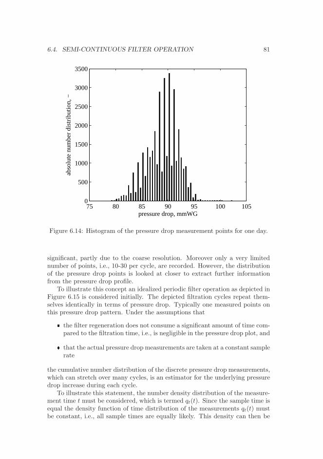
6.4. SEMI-CONTINUOUS FILTER OPERATION 81
75 80 85 90 95 100 1050
500
1000
1500
2000
2500
3000
3500
pressure drop, mmWG
abso
lute
num
ber
dist
ribut
ion,
−
Figure 6.14: Histogram of the pressure drop measurement points for one day.
significant, partly due to the coarse resolution. Moreover only a very limitednumber of points, i.e., 10-30 per cycle, are recorded. However, the distributionof the pressure drop points is looked at closer to extract further informationfrom the pressure drop profile.
To illustrate this concept an idealized periodic filter operation as depicted inFigure 6.15 is considered initially. The depicted filtration cycles repeat them-selves identically in terms of pressure drop. Typically one measured points onthis pressure drop pattern. Under the assumptions that� the filter regeneration does not consume a significant amount of time com-
pared to the filtration time, i.e., is negligible in the pressure drop plot, and� that the actual pressure drop measurements are taken at a constant samplerate
the cumulative number distribution of the discrete pressure drop measurements,which can stretch over many cycles, is an estimator for the underlying pressuredrop increase during each cycle.
To illustrate this statement, the number density distribution of the measure-ment time t must be considered, which is termed qt(t). Since the sample time isequal the density function of time distribution of the measurements qt(t) mustbe constant, i.e., all sample times are equally likely. This density can then be

82 CHAPTER 6. APPLICATION
0 1 2 3 4 5 683
84
85
86
87
88
89
90
91
92
time, cycles
pres
sure
dro
p, m
mW
G
Figure 6.15: Schematic periodic filter operation.
converted into the pressure drop density function q∆p(∆p) by considering themapping of the time axis via the pressure drop curve ∆p(t). Any time interval[t, t + dt] is mapped on the pressure drop axis onto [∆p,∆p + d(∆p)] which isdescribed by:
q∆pd(∆p) = qtdt (6.12)
Integrating via the pressure drop ∆p gives:
∆p∫
∆plow
q∆pd(∆p) = qtt(∆p) (6.13)
The function t(∆p) is the inverse function to the pressure drop relation ∆p(t).The integration limit ∆plow is the lowest measured pressure drop value and ischosen, because the inverse function, of course, does not exist for lower pressuredrop values. The LHS of equ. (6.13) is the cumulative distribution functionQ∆p:
Q∆p(∆p) =
∆p∫
∆plow
q∆pd(∆p) (6.14)
This distribution can be estimated from the pressure drop values of the separatemeasurements using e.g. a kernel density estimator for q∆p. The time compo-

6.4. SEMI-CONTINUOUS FILTER OPERATION 83
nent of the measurements is not used and thus any pressure drop measurementirrespective of the cycle might be used, i.e., the benefit of the method is, ofcourse, that many pressure drop cycles can be used as input to determine Q∆p.However, the time scaling of pressure drop function t(∆p) cannot be determinedfrom this method. I.e., the proportionally constant qt which is scaling the timeaxis cannot be determined inherently from the scheme outlined above. For theexample given in Figure 6.15 the scaling would be qt ≡ 1 to scale the pressuredrop increase on exactly one cycle time. Practically the scaling with an actual(mean) cycle time tcyc is useful.
From Figure 6.15 it is clear that the inverse function t(∆p) does not existunambiguously for the entire time axis, but just for one cycle and the singular-ity at the filter regeneration is not considered. Since the cleaning duration isrequired to be insignificant, it is assumed that he pressure drop measurementsduring cleaning do not significantly affect the estimated distribution.
6.4.3 Varying cycle times and acyclic pressure drop pat-
terns
In section 6.4.2 it is assumed that the pressure drop cycles repeat themselvesidentically in terms of pressure drop. Unfortunately, this is not always a justifiedassumption, as only a glance at e.g. Figure 6.13 reveals. The actual durationof a pressure drop cycle is varying and not constant and also the lower andupper pressure drop values fluctuate. Such behavior might arise from influenceof other unit operation in the plant, variations of filter operating parameters,errors in the pressure drop measurement and consequently inaccuracies in filtercontrol.
To be able to account for such variations a correction is introduced for thepressure drop span of a single filter cycle. It is assumed that all recorded filtercycles have in principal the same underlying pressure drop increase, but onlydifferent parts of that increase are actually recorded. Which part of a certainfilter cycle is recorded, is determined from the minimum and the maximumpressure drop value of a specific cycle.
The situation for varying the minimum pressure drop value is shown schemat-ically in Figure 6.16. The underlying pressure drop curve is shown as dashedcurve from time −1 to 0. The actually available pressure drop consists of 4 num-bered cycles of respective parts of the underlying pressure drop curve, which arestarting from different lower pressure drop values. The cycle durations vary cor-respondingly. Directly applying the density estimation scheme outlined in thesection above fails, because the different starting points of the cycles will influ-ence the distribution of the pressure drop measurements. E.g., in Figure 6.16 allfour cycles are available to be recorded at pressure drop levels above 87 mmWG,but only three cycles are available between 85 mmWG and 87 mmWG. To givepressure drop values in this range the same weight as above 87 mmWG thepressure drop density distribution q∆p in this range must be weighted by 4
3 .From 84 mmWG to 85 mmWG only one of four cycles is available which mustbe weighted with a factor 4. Such weighting is, of course, at the expense of

84 CHAPTER 6. APPLICATION
accuracy, and practically only the pressure drop range that is recorded in manycycles can be used further. An analogue discussion applies to varying maximalpressure drop levels.
−1 0 1 2 3 483
84
85
86
87
88
89
90
91
92
1
2
34
time, cycles
pres
sure
dro
p, m
mW
G
Figure 6.16: Schematic pressure drop cycles with varying minimum values.
In a more general notation the actual parts which are recorded of each filtra-tion cycle can be accounted for by another distribution function: The numberdistribution of the minima and maxima. These distributions can be estimatedfrom the minimum and maximum pressure drop values determined above. Thecumulative number distribution of the minima is termed Θmin. Dividing thedensity q∆p by the cumulative number distribution of the minima yields thecorrection described above for the simple example. For the maxima the situa-tion is analogue, but here the density for pressure drop levels above a certainvalue must be amplified. This correction can be summarized as:
q∆p =1
Θmin· 1
1 − Θmax· q∆p (6.15)
Practically additional information on the minima and maxima of the recordedpressure drop cycles is required. In Figure 6.13 these values are marked by cir-cles and squares, respectively. The actual division of the pressure drop data intocycles is done by a simple pattern recognition routing, which, naturally, is notperfectly able to determine each filtration cycle correctly. This must be consid-

6.4. SEMI-CONTINUOUS FILTER OPERATION 85
ered as error. External information on filter cleaning, e.g. from the cleaningsystem, is not available for the presented dataset, but could also be used.
The situation for the recorded pressure drop data (see Figure 6.12) is de-picted in Figure 6.17. The density estimate obtained from raw pressure dropdata is shown as bold dashed curve and corresponds directly to the histogramFigure 6.14. The uneven distribution between neighboring columns in the his-togram is reflected by oscillations observed in the kernel density estimate q∆p.The cumulative distributions of the minima is depicted as thin dotted curve.Unfortunately, the oscillations in the density estimate q∆p are amplified wherethe correction requires a stronger weighting, i.e., towards the tails of this dis-tribution. This is, of course, to be expected, since relatively fewer pressuredrop cycles were recorded, which actually cover that limited range and thus lessinput information is available. The actual estimate of the underlying pressure
70 75 80 85 90 95 100 105 1100
0.05
0.1
0.15
0.2
0.25
70 75 80 85 90 95 100 105 1100
0.1
0.2
0.3
0.4
0.5
0.6
0.7
0.8
0.9
1
pressure drop, mmWG
Cum
ulat
ive
dist
ribut
ion Θ
, −
q∆p
q∆p
Θmin
1 − Θmax
Den
sity
dis
trib
utionq,
mm
WG
−1
Figure 6.17: Estimated density number distribution (bold, dashed) and cor-rected density (bold, solid). Cumulative pressure drop minima/maxima distri-butions.
drop increase is the cumulative distribution Q∆p. By scaling the correspondingdensity to q∆p the scaling of the density is lost, and the integral over the cor-rected density is bigger than one. This, however, only affects the scaling of thecumulative distribution which is proportional to the time and time informationis anyway not conveyed in this distribution form. It must be reintroduced asdiscussed in section 6.4.4.

86 CHAPTER 6. APPLICATION
6.4.4 Rescaling to a characteristic cycle
The density displayed in Figure 6.17 represents the corrected shape of the un-derlying pressure drop curve. However, the density does not contain any infor-mation on the time scaling. Of course, the non-zero part of the density spansthe entire pressure drop band where measurements are available.
A characteristic reference filter pressure drop cycle is defined. The pressuredrop of this reference cycle is spanning from the mean pressure drop minimum∆pmin to the mean pressure drop maximum ∆pmax. The duration of this refer-ence cycle is the mean cycle time. The mean minima and maxima are calculatedfrom their respective number distributions according to: )
∆pmin =
∞∫
0
∆p d (Θmin(∆p)) (6.16)
∆pmax =
∞∫
0
∆p d (Θmax(∆p)) (6.17)
The parts of the corrected density q∆p lying outside the interval [∆pmin, ∆pmax]are disregarded for the determination of the characteristic filter cycle. Thereby,the large error inherent to the tails of q∆p does not affect the resulting pressuredrop distribution.
Since the PD-method is applicable to any part of a pressure drop curve thistruncation of the characteristic cycle does not impede the application of thePD-method. Although the error will, of course, become bigger.
In Figure 6.18 two characteristic filter cycles determined by the outlinedroutine are shown. The solid curve corresponds to the data underlying theFigures 6.12 to 6.17. The characteristic part of the cycle is depicted as boldline and the truncated tails are thin lines. Towards the end of the cycle aturning point in the pressure drop is observed. Probably this turning pointmust be attributed to an insufficient correction of the pressure drop maxima.The distribution Θmax is quite wide and a perfect correction is apparently notachieved.
In addition to the data discussed in this section another characteristic cycleis displayed as a dashed curve. This characteristic cycle is determined from data,which is recorded on the same filter plant after the filter bags were replaced withnew ones. The same routine is applied as outlined above on recordings of semi-continuous pressure drop data for 24 h. Preceding the evaluated period, thenew filter bags were in operation for about 30 h. The cloth during the evaluatedperiod is hence not directly comparable to virgin filter media.
The maximum pressure drop level of the two characteristic cycles are aboutthe same. Since the filter is cleaned upon reaching a certain pressure drop levelthis must be expected. However, the cycle time with new filter bags is signifi-cantly longer and the operating pressure drop span is also increasing. Therebya more clearly defined cycle structure in the raw data is present and the error

6.4. SEMI-CONTINUOUS FILTER OPERATION 87
−20 0 20 40 60 80 100 120 14065
70
75
80
85
90
95
100
time, s
pres
sure
dro
p, m
mW
G
Old bagsNew bags
Figure 6.18: Characteristic pressure drop profiles.

88 CHAPTER 6. APPLICATION
towards the tails of the pressure drop distribution is decreasing, since relativelyfewer points are close to the beginning or the end of a single cycle (when com-pared with the total available pressure drop measurements). In Figure 6.18this fact is articulated by the truncated tails, which continue the characteristiccurve. In addition, these truncated tails are relatively short because the distri-butions of minima an maxima, Θmin and Θmax, are narrower. The latter mustbe attributed to a more regular pressure drop pattern.
6.4.5 Application of the PD-method
On the pressure drop data displayed in Figure 6.18 the PD-method can beapplied directly. It is, of course, not possible to carry out a dedicated ramptest for these characteristic cycles to determine an accurate specific filter cakeresistance value. Instead the slope of the final asymptote is estimated fromthe available curves in Figure 6.18. In Figure 6.19 the corresponding PDs areshown.
10−11
10−10
10−9
0
0.1
0.2
0.3
0.4
0.5
0.6
0.7
0.8
0.9
1
permeability k0, m
Cum
ulat
ive
area
Φ′ , −
Old bagsNew bags
Figure 6.19: PDs determined from characteristic pressure drop cycles
At first the filter parameters affecting the model parameters pc and tc areignored and a PD Φ is estimated with pc = 1 and the fraction pc
tcequal to the
estimated slope the final asymptote. This facilitates the data processing for theestimation, since varying operating points of the filter can be disregarded. Inaddition, the permeability is scaled by a factor of about 107, which enhances

6.4. SEMI-CONTINUOUS FILTER OPERATION 89
the numerical performance. (Results displayed in Figure 6.19 do not includethis factor and thus Φ′ is plotted versus k0.)
The characteristic pressure drop profiles are typically very well defined witha large number of underlying pressure drop measurements. Because of this aver-aging over a large number of cycles also statistical variations from measurementerrors are largely compensated for. In other words, the characteristic pressuredrop curves present a very nuanced pressure drop profile, that is hardly obtain-able from a single pressure drop increase. During the estimation of PDs viaoptimization it turned out that an even better fit could be obtained when morethan 30 nodes are used for the discretization of the PD. Therefore the PDs inFigure 6.19 are estimated using a simple adaptive mesh routine. Initially, a PDis estimated on a fixed discretization using 30 nodes as in section 4.1.1. Thisoptimization step is terminated, when no significant further improvement of theresulting PD is possible. The gradient of this intermediate result is calculatedand the node at where the gradient is a maximum is replaced by 5 evenly dis-tributed, new nodes, which get the same permeability value assigned as theoriginal node. Thereby the calculated pressure drop curve remains unalteredfrom the original result. Then another run of the same optimization routine isconducted with the refined PD. This run starts at the same target value wherethe first run ended, but because of the finer discretization, further tuning ofthe PD is possible and typically a better fit is obtained. Here, 10 successiveoptimization runs with refining steps in between are carried out.
The thereby obtained PDs are transformed according to the relations out-lined in section 4.2 to actual parameters pc and tc by considering the constantslope of the asymptote:
pc
tc=
pc
tc(6.18)
From equ. (4.11) it can be seen that condition equ. (6.18) leaves the distributionaxis unaltered and only a scaling on the permeability axes occurs.
The PDs in Figure 6.19 characterizes the filter in semi-continuous operation.Thus the combined effects of the filter cloth and the sequenced cleaning areincluded in the PDs. Since the PDs are determined for a characteristic filtercycle, the initial permeability k0 represents the filter condition after cleaning atthe start of the filtration cycle. The clear step at Φ′ ≈ 0.9 for the new filter cloth(dashed line) is caused by the newly cleaned filter fraction. The filter fractioncarrying residual cake is hardly discernible on the rest of the filter area. Theold filter cloth shows a continuously decreasing permeability distribution witha much less dominant step at high permeabilities. The old cloth even exhibits ahigher permeability than the new one for a fairly large area fraction. This canbe explained by the higher cleaning frequency which is in effect for the old cloth.The cycle time for the old cloth is about half the cycle time for the new cloth (seeFigure 6.18). In order to keep the old filter cloth operating below the maximumpressure drop level, where cleaning is initiated, it is cleaned more often. Therebya continuous filter cake distribution evolves, which is reflected by the continuousdecrease in permeability in Figure 6.19. On the new cloth, however, cleaning of

90 CHAPTER 6. APPLICATION
only one segment suffices to reduce the pressure drop further than for the oldcloth. The high permeability on this cleaned segment of new cloth reduces thepressure drop to a significantly lower ∆pmin value for the new cloth, than forthe old one (Figure 6.18). The remaining, i.e., not recently cleaned, filter areacarries a substantial amount of filter cake, since the longer cycle times betweencleaning steps entail a higher cake mass. Thereby the PD for the remainingfilter area is not pronounced.
Due to the setup of the filter with 8 sections which are cleaned separately, oneexpects a distribution of cake generations as outlined in section 6.2.2. However,it is not possible to resolve the expected filter cake distribution from pressuredrop data. If such a filter cake distribution exists, it does not significantlycontribute to the shape of the pressure drop profile and therefore cannot beidentified by the PD-method.
Figure 6.19 shows a clear distinction between the two PDs. Similarly tothe results shown in Figure 6.6 the newer filter media is found to have a morepronounced step in the PD. The older filter bags exhibit a relatively high per-meability only on a very small part of the filter area (< 2 %). However, extremecaution must be applied when quantitatively comparing these curves, since inthe characteristic cycles the influence of the industrial cleaning of separate filtersegments, as described above, is lumped into the PD.

Chapter 7
Solid distribution
7.1 Introduction
Filter operation is affected by inhomogeneities with respect to the filter mediumand/or the filter cake, which is discussed in the preceding chapters. At the be-ginning of filtration inhomogeneities that can be attributed to the filter mediumand/or a residual filter cake, can be tackled with the PD-method. The modelon which the PD-method is based on, however, assumes a clear mechanisticalcake build up with an even solid loading, i.e., the dust concentration in the fluidis a non-distributed constant and irrespective of time. Nevertheless, an unevensolid distribution might arise due to an uneven dust concentration in the filterhousing. In this chapter a modified version of the filter model is presented thatcan account for an uneven distribution of the solid in the fluid.
7.2 Solid distribution model
The filter models basic equs. (2.1) to (2.4) are used unaltered. To account for theuneven solid distribution the mechanistical cake build up equ. (2.5) is modifiedto:
dz(t, A)
dt= csol(t, A) v(t, A) (7.1)
The only formal difference between the original equation is the allowance for avarying solid concentration on both time t and filter location A. A combinationof equs. (2.2) and (7.1) gives:
d(
1kc(t,A)
)
dt= αm csol(t, A) v(t, A) (7.2)
The time dependency is introduced to satisfy solid mass flow continuity. Asa model assumption the solid mass flow and the total volume flow to the filter
92 CHAPTER 7. SOLID DISTRIBUTION
should remain constant. In the case of a constant solid concentration the gasvolume flow continuity automatically satisfies the solid continuity. However,the distribution of the solid concentration over the filter leads to an accordinglychanging filtration velocity, and do thereby not satisfy the solid continuity perse. The solid concentration is therefore be split into a separable term:
csol(t, A) = csol ζ(A) ξ(t) (7.3)
Here the term ζ(A) is the actual solid distribution over the filter location andξ(t) is the correction factor that must be determined to ensue a constant solidflow onto the filter.
The combination of equs. (7.2), (2.4), and (7.3) yields analogous to equ. (2.10):
− dk(t, A)
k3(t,A)=αm csol
ηgζ(A)ξ(t)∆p(t)dt (7.4)
The integration of the separated equ. (7.4) gives:
k−2(t, A) − k−20 (A) =
2αm csol
ηgζ(A)
t∫
0
ξ(t)∆p(t)dt (7.5)
The slightly adjusted abbreviation for filter state s is introduced again as:
s =2αm csol
ηg
t∫
0
ξ(t)∆p(t)dt (7.6)
Integration of equ. (2.4) over the filter area employing equs. (7.5) and (7.6) givescorresponding to equ. (2.15):
ηg · V (t)
∆p(t)=
Atot∫
A=0
(k−20 (A) + s(t)ζ(A))−
12 dA (7.7)
In the following the cloth resistance k0, and according to definition (2.16)the corresponding u, are regarded as constant. A combined dependency of thefilter area of both, the solid concentration and the cloth resistance leads to a2-dimensional distribution.
The dimensionless filter area A can again be replaced by a normalized dis-tribution function:
Ψ(ζ) ≡ A
Atot(7.8)
and the integral transform equ. (7.9) can be rewritten in the same fashion asequ. (2.19):
ηg · VAtot∆p
=
∞∫
0
(u+ s ζ)−12 dΨ(ζ) (7.9)

7.3. PROPERTIES OF THE SOLID DISTRIBUTION MODEL 93
The solid distribution model is only used for constant flow filtration and thusthe governing equations for constant pressure are not outlined here. For constantflow filtration the abbreviations pc and tc, defined in sec. 2.4 by equs. (2.22)and (2.23), respectively, are used. The pressure drop transformation reads to:
pc
∆p=
∞∫
0
(u+ s ζ)−12 dΨ(ζ) (7.10)
The closing condition originates from the analogous calculations explained insection 2.4 and it has the corresponding form:
t = tc
∞∫
0
[
(u + s ζ)12 − u
12
]
dΨ(ζ) (7.11)
Note that the closing condition does not explicitly depend on the time variantcorrection factor ξ introduced in equ. (7.3). However, this correction factor canbe calculated from the definition of s equ. (7.6) in comparison with equ. (7.11)via derivation:
ξ =
∞∫
0
(u+ s ζ)−12 dΨ(ζ)
∞∫
0
(u+ s ζ)−12 ζdΨ(ζ)
(7.12)
7.3 Properties of the solid distribution model
Characteristic values of a solid concentration distribution can be determined,which correspond to the explanations in sec. 3.2. The initial pressure drop valuewithout filter cake ∆p0 is obtained by:
∆p0 =pc
k0= pc
√u (7.13)
The slope of the pressure drop curve for the modified model can be calulatedaccording to equ. (3.6). This differential can be evaluated using the expressionsfor the solid distribution model equs. (7.10) and (7.11):
d∆p
dt=
pc
tc
∞∫
0
(u+ sζ)− 3
2 ζdΨ(ζ)
[∞∫
0
(u+ sζ)− 1
2 dΨ(ζ)
]2 ∞∫
0
(u+ sζ)− 1
2 ζdΨ(ζ)
(7.14)
For s = 0 the evaluation of equ. (7.14) yields pc
tc, i.e., the starting tangent of a
homogeneous filter.The asymptote of the pressure drop curve can be obtained similarly to sec-
tion 3.2.3. However, in the present case neither the slope nor the ordinate offset

94 CHAPTER 7. SOLID DISTRIBUTION
of the asymptote are known. The slope is obtained by evaluating equ. (7.14) fort→ ∞, i.e., s→ ∞:
lims→∞
d∆p
dt=
pc
tc
1∞∫
0
ζ−12 dΨ(ζ)
∞∫
0
ζ12 dΨ(ζ)
(7.15)
The factor describing the deviation from the homogenous filter only depends onmoments of the solid distribution Ψ and is abbreviated as:
γ ≡ 1∞∫
0
ζ−12 dΨ(ζ)
∞∫
0
ζ12 dΨ(ζ)
(7.16)
With this asymptotic slope the ordinate offset is calculated according to:
∆p0 = limt→∞
(
∆p− pc
tcγ · t
)
(7.17)
Surprisingly the evaluation of equ. (7.17), which is analogue to the computationin section 3.2.3, shows that ∆p0 is related to the initial pressure drop value ∆p0
via the same factor γ, applying to the slope:
∆p0 = γ∆p0 (7.18)
and thus the analytical equation of the asymptote reads:
∆p = γ
(pc
tct+
pc
k0
)
(7.19)
The initial tangent of the pressure drop curve for a solid distribution onthe filter coincides with the linear pressure drop increase on a homogeneouslychallenged filter. The final asymptote is derived from that initial tangent by asingle scaling factor γ, which in turn is depending only on moments of the soliddistribution.
7.4 Results of a two area model
To illustrate the effect of a solid distribution a two area model is used. Themodel is easy to be implemented and can be regarded as an extreme case of adistribution. Moreover experimental pressure drop data under a proven soliddistribution is lacking, and thus one can only resort to analytic models for thediscussion.
A two area model can be very simply obtained with the following densityfunction ψ = dΨ/dζ consisting of two Dirac Delta functions:
ψ(ζ) = βδ(ζ − 1) + (1 − β)δ(ζ − α) (7.20)

7.4. RESULTS OF A TWO AREA MODEL 95
Here δ denotes the Dirac Delta function, β the area ratio (β = 0.5 means equallylarge areas), and α is the solid excess in comparison to 1. I.e. on the areafraction (1−β) of the filter the solid concentration is α times the concentrationon the area fraction β. For the parameters the range is for the area distributionnaturally β ∈ [0, 1] and for the solid distribution parameter it may be confinedto α ∈ [0, 1] without loss of generality. This is explained by the definition of thesolid distribution in equ. (7.3), where a correction factor ξ is foreseen to keepthe solid mass flow constant at a time. When one requires an α-value beinglarger than one, then an equivalent model exists with parameters α = α−1 andalso an inverted area distribution β = 1 − β. However, the correction factor ξwill be different to ensure the same mass flow, and thus the s values will differas well. This two area function represents an extreme case of inhomogeneity forall functions ψ(ζ) that are zero for ζ 6∈ [α, 1].
The pressure drop curve can be given parametrically dependent on s. Aclosed form expression ∆p(t) is not obtained as straight forwardly.
∆p(s) =pc
β√u+s
+ 1−β√u+sα
(7.21)
t(s) = tc[β√u+ s+ (1 − β)
√u+ sα−
√u]
(7.22)
The asymptotical factor γ can also be given analytically:
γ =1
(
β + (1 − β) 1√α
)
(β + (1 − β)√α)
(7.23)
For the asymptotical factor it can be shown that for a constant α equ. (7.23)becomes a minimum for β = 1
2 , i.e., the extreme case in terms of inhomogeneityfor a two area filter is the case of equally large areas. The location of theminimum is irrespective from α itself. For this extreme case the γ value dependsonly on α:
γmin =4√α
(1 +√α)2
(7.24)
In Figure 7.1 the pressure drop increases for a two area model distributionwith α = 0.2 and β = 0.5 is shown. The asymptotical pressure drop increase isclearly diverging from the homogeneous filter. The inhomogeneous solid distri-bution leads to a relatively slower simulated pressure drop increase. Interestinglythe pressure drop curve appears to be linear, although the solid distribution ishighly inhomogeneous.
The initial phase of filtration is of special interest and in Figure 7.2 this partis enlarged. One can see that the simulated pressure drop increase has the sameinitial level as the perfectly homogeneous curve. Additionally the initial tan-gent also coincides with the homogeneous filter. However, immediately after thestart of filtration the homogeneous filter continues its linear pressure drop in-crease, whereas the simulated inhomogeneous filter exhibits a lower slope of the

96 CHAPTER 7. SOLID DISTRIBUTION
0 500 1000 1500 2000 2500 3000 3500 40000
1000
2000
3000
4000
5000
6000
7000
8000
time t, s
pres
sure
dro
p ∆ p
, Pa
simulation α=0.2homogeneous filter
Figure 7.1: Simulated pressure drop curve of the two area solid concentrationdistribution model. In addition the pressure drop increase of a perfectly homo-geneous filter is shown.
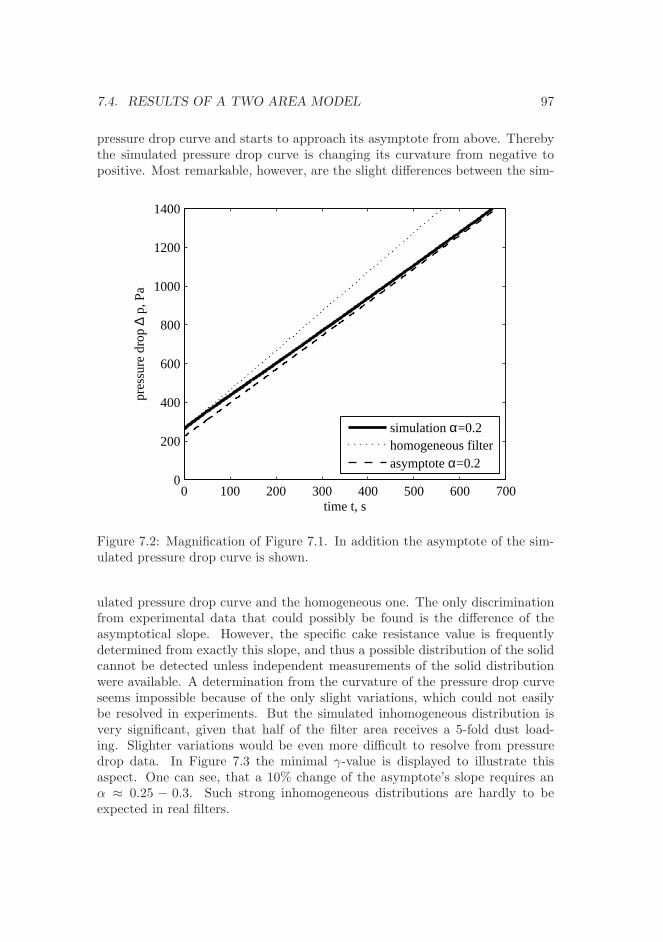
7.4. RESULTS OF A TWO AREA MODEL 97
pressure drop curve and starts to approach its asymptote from above. Therebythe simulated pressure drop curve is changing its curvature from negative topositive. Most remarkable, however, are the slight differences between the sim-
0 100 200 300 400 500 600 7000
200
400
600
800
1000
1200
1400
time t, s
pres
sure
dro
p ∆ p
, Pa
simulation α=0.2homogeneous filterasymptote α=0.2
Figure 7.2: Magnification of Figure 7.1. In addition the asymptote of the sim-ulated pressure drop curve is shown.
ulated pressure drop curve and the homogeneous one. The only discriminationfrom experimental data that could possibly be found is the difference of theasymptotical slope. However, the specific cake resistance value is frequentlydetermined from exactly this slope, and thus a possible distribution of the solidcannot be detected unless independent measurements of the solid distributionwere available. A determination from the curvature of the pressure drop curveseems impossible because of the only slight variations, which could not easilybe resolved in experiments. But the simulated inhomogeneous distribution isvery significant, given that half of the filter area receives a 5-fold dust load-ing. Slighter variations would be even more difficult to resolve from pressuredrop data. In Figure 7.3 the minimal γ-value is displayed to illustrate thisaspect. One can see, that a 10% change of the asymptote’s slope requires anα ≈ 0.25 − 0.3. Such strong inhomogeneous distributions are hardly to beexpected in real filters.
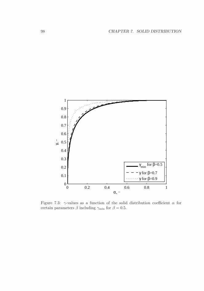
98 CHAPTER 7. SOLID DISTRIBUTION
0 0.2 0.4 0.6 0.8 10
0.1
0.2
0.3
0.4
0.5
0.6
0.7
0.8
0.9
1
α, −
γ, −
γmin
for β=0.5
γ for β=0.7
γ for β=0.9
Figure 7.3: γ-values as a function of the solid distribution coefficient α forcertain parameters β including γmin for β = 0.5.

Chapter 8
Conclusions and outlook
In this work an analytical filter model is developed based upon governing equa-tions commonly used for filter modeling. The focus of this model lies in thesimulation of cake filtration on inhomogeneous filters with respect to the filtermedium and cake distribution for incompressible cakes. It is shown that thisfilter model fully includes previous model concepts targeting towards the de-scription of industrial filter operation. Because of its analyticity it is possibleto make clear statements on invertibility of the model, which is used to developand justify the PD-method. This method can be used to determine the PDof a filter from commonly available pressure drop data. An error estimation isoutlined for the PD-method.
8.1 Filter media characterization
The PD-method is applied to filter media characterization. PD of filter mediaare determined from various filter equipments. It is shown that even apparentlyclean filter media can exhibit a PD, which has not been explicitly reported in theliterature. Depending on the PD the filtration behavior of the filter medium isassessed in the industrial filter application. With the same integral filter mediapermeability and the same dust cake properties a filter medium exhibiting a lesspronounced PD is performing superior over a filter medium with a strong PDin terms of operating pressure drop level and/or cycle time.
The PD-method can be easily applied to filter media testing experiments.The effects affecting the filtration dynamics of a filter media sample are capturedmore completely by a PD, than by today’s reporting standards. The expectedfiltration performance of a certain cloth is closely related to these dynamics.
The analytic filter model is a prerequisite to determine a PD of filter media.Since for optimization routines frequent function calls are required, it wouldnot have been practically possible to determine a PD when the model is carriedout as numerical integration, since the long execution times of the numericalintegration impede the pratical application.

100 CHAPTER 8. CONCLUSIONS AND OUTLOOK
It is shown that for a certain pressure drop curve variations of the modelparameters lead only to a scaling of the PD. All the scaled PDs contain basicallythe same information. Thus parameter variations or error in parameters do notaffect the PD-method’s determination of a PD, making the PD-method ratherrobust against uncertain parameters. In fact this makes the applicability of thePD-method widely independent from the actual availability of parameters, whenabsolute values are not mandatorily required. This feature opens up possibilitiesfor intercomparison of PDs in applications with intrinsically high uncertaintiesin parameters as encountered in most practical applications. However, certainparameter variations can lead to unphysical PDs. In turn errors in parametersmight not be detected by the PD-method.
Characteristics of a pressure drop increase describing the initial tangent andfinal asymptote are identified and analytically derived from moments of a PD.They are readily available from a full PD. These characteristics or moments ofa PD are a compact and easily comparable form of reporting the key dynamicsconveyed by a full PD.
The pressure drop of a filter in operation is increased by a PD. While ahomogeneous filter would give a linear pressure drop increase, which can bepredicted using classical theory, a filter exhibiting a PD is operating along acurved pressure drop profile. For long filtration durations the actual filter pres-sure drop is approximated well by the final asymptote. In addition this is theprediction of filter operation with more caution, since the asymptote always givehigher pressure drop values, than the actual pressure drop. For filter design itis advantageous to use the final asymptote rather than the ideal homogeneousbehavior from classical theory. Thereby one takes into account the increasedpressure drop due to a PD, but at the same time one can resort oneself to thesimplicity of a linear pressure drop increase. This is accomplished by using theasymptotic pressure drop ordinate offset, rather than the initial pressure drop.Otherwise the classical theory can remain unaltered.
The PD of one cloth-dust combination may change over time due to long-term filtration effects, i.e., so called filter ageing. Thus the filtration character-istics of such a combination can change significantly during the life time of thefilter medium. This must also be expected during a life cycle of an industrialfilter bag, although to date no long term filtration monitoring with the PD-method is available. In industrial plants filter bags are frequently not changedall together, but only a few bags at a time. Thus a possible change of filtrationperformance of some bags over time cannot be retraced individually by the PD-method during plant operation. An assembly of bags used parallel for filtrationalways appear as an entity to the PD-method and the PD of some bags cannotbe isolated.
8.2 Industrial filter operation
It is shown that the filter model presented also includes the generation modelsused in literature. Except for the model of Ju et al.[18], where the part with

8.3. SOLID DISTRIBUTION 101
compressible cake is not captured by the proposed filter model, all models foundin literature are fully represented by the proposed model.
The presented model can of course be used to simulate a filter dynamically,which is enhanced by the analytic time integration. Thus the need for numeri-cally solving differential equations is omitted, and the simulations speed up byorders of magnitude. The strength of this model, which distinguishes it fromthe dynamic models, is the fact that for periodic filtration the PD from filter op-eration can be given analytically, without simulating the full transient pressuredrop curves of the filter.
With the PD-method any PD should be identifiable unambiguously. How-ever, error consideration shows that it is not possible to identify a PD for morethan about two cake generations, not even considering segmented cleaning. Thenumerical problem becomes highly ill defined. This argumentation is equallyvalid for the parameter estimations for cake generation models reported in theliterature. Since the basic model structure is the same for all models includ-ing the PD-methods, the inverse problem posed by parameter identification isequally ill defined for the models in literature. However, due to the parametricapproach in literature the number of possible PDs is limited. Under the as-sumption that the chosen mechanistic model is valid, a parameter identificationmight be possible. However, agreement between the model and the actual datamust not be interpreted as verification of the mechanistic approach. Other PDsthat are not captured by the mechanistic models are probably equally or bettersuitable to describe experimental data. The problems of identifying filter op-eration worsen, when a PD of the filter medium itself is superimposed to thePD stemming from filter operation. Admittedly this problem is not tackled inthe literature. The error estimation in this work suggests error bounds, thatlet a separable identification of superimposed PDs appear impossible. Even thedirect problem of only identifying a PD is already difficult to handle.
8.3 Solid distribution
The filter model is adapted to cover the case of inhomogeneous solid distribu-tion in the filter. Characteristic values of the pressure drop curve can be derivedanalogous to the PD-method. The analytically obtained pressure drop asymp-tote is related to the pressure drop for a homogeneous solid distribution by onlyone scaling factor.
Model simulations with this adapted model are carried out for a highly in-homogeneous solid distribution on two model areas. The pressure drop increaseis not significantly distinguished from a linear increase, although its slope issignificantly different from the homogeneous filter. The inhomogeneous soliddistribution is barely reflected in the curvature of the pressure drop curve, evenin this sample case where its quite significant. Consequently, the mere presenceof a solid distribution on a filter can hardly be detected from pressure drop dataeven if solid distribution is pronounced.

102 CHAPTER 8. CONCLUSIONS AND OUTLOOK
However, the determination of filtration parameters is affected if a solid dis-tribution is present. Typically the cake resistance parameter is extracted fromthe slope of the pressure drop asymptote. However, this slope is altered forfiltration with a solid distribution present, although the underlying model pa-rameters remain unaltered. This might also add to the difficulties of reproducingparameters, especially the cake resistance, in laboratory experiments. However,the fluctuation of the cake resistance parameter actually observed may often belarger than the change explainable by a moderate solid distribution.
A combination of a PD of the filter media and a solid concentration distribu-tion is feasible. The corresponding model, however, becomes complex. Since theseparate identification problems of a PD and a solid distribution are difficult,one will hardly be able to identify parameters from pressure drop data for thecombined model. In addition a cross correlation of the PD and the solid dis-tribution is possible, i.e., the two distributions might not be independent fromeach other. However, a combined and dependent PD and solid distributionmay obscure the otherwise clear effects of the PD, which in turn is erroneouslyidentified or rendered unidentifiable.
8.4 Further work and potential
Independent determination of a PD: Speaking of a PD determined frompressure drop data, of course the question arises of independently determining acorresponding distribution directly from an analysis of the filter medium. A pos-sibility for accomplishing such an independent measurement is a highly resolvedvelocity profile measurement as schematically depicted in Figure 2.1. Assumingthat the permeability of a filter medium is a result of viscous flow through poresof the medium an average pore diameter of about 40µm is obtained for a typicalcommercial bag filter medium, assuming a negligible porosity effect acceleratingthe flow through the filter medium.
However, this pathway appears unfeasible, since CFD simulations clearlyshow that the maximum gas velocity of a single pore of this diameter is reducedto about only a third after only 300µm after the pore. Since this is approxi-mately the surface roughness of the textile filter medium, high resolution mea-surement so close to the surface are not possible. Especially the identificationof small local differences in the gas velocities are not feasible.
Experimental methods considered were particle imaging velocimetry andLaser Doppler anemometry. Both methods require tracer-particles in the fluidand therefore only an upstream measurement could be performed. However,since the filter medium will retain the particles the flow will be altered in thecourse of the measurement.
Another possible approach is based on an integral measurement of the flowthrough the filter medium locally resolved. A possible way to accomplish such ameasurement is via the reaction of a reactive layer on the filter medium with agas. The filter medium must be coated with a thin layer of a reactive substanceand then at a certain pressure drop gas containing a reactive compound is

8.4. FURTHER WORK AND POTENTIAL 103
conveyed through the filter medium. The reaction between the layer and thegas should preferentially be fast, so reaction kinetics need not to be accountedfor. Then the conversion of the solid layer with the gas must be evaluatedlocally resolved by e.g. electron microscopy with diffractive scanning for thereaction product. The distribution of the reaction product corresponds to theflow distribution and thereby the PD.
A suitable pair of reactive compounds must be found. The combinationpotassium iodate and sulfur dioxide, as used in gas detection tubes, was con-sidered. It must be possible to coat the filter medium with a thin layer of thesolid reagent. This is typically a challenging task, because the small pore andfiber structure prevent the fibers from wetting.
Evaluation of filter medium tests: The evaluation routines of filter mediumtests in standardized equipment (VDI-3926, [12]) include the monitoring of thefiltration cycle duration, the weight increase of the filter sample, the develop-ment of the pressure drop after cleaning and the clean gas concentration. Inaddition, the guideline states that: It is also possible to derive quality char-acteristics of the filter media from [...] the course of the pressure drop losscurves. Certainly, trained filter test operators are able to deduct informationfrom the shape of the pressure drop curves intuitively. The PD-method canquantitatively derive information from such curves, which is supposedly mostrelevant for industrial application of the filter (when compared to the hithertopracticed data evaluation routine). The generally poor predictability of a filtermedium’s performance in its industrial application must to some extent be at-tributed to the neglecting of any inhomogeneity of the filter media. Especially,the laboratory scale testing of filter media with the very dust used eventuallyin the industrial application is encouraged in combination with an evaluationincorporating the PD-method.
Continuous filter plant monitoring: In section 6.3 a routine is proposedthat can be incorporated into filter process control systems. In addition tothe commonly available information on pressure drop and occasionally cleaningfrequency, a characteristic pressure drop profile can be used for monitoring thecondition of the filter cloth, possibly together with an evaluation by the PDmethod. Gradual and/or discontinuous changes of the filter medium could bedetected and measures, e.g. the replacement of filter bags, can be taken on afactual basis of the operation performance instead of just operational time orthe impression of the plant operator.


Bibliography
[1] R. H. Perry, D. W. Green, and J. O. Maloney, editors. Perry’s chemicalengineers handbook. Mc-Graw-Hill, Singapore, 7 edition, 1997.
[2] C. Tien. Introduction to cake filtration - Analyses, experiments and appli-cations. Elsevier, Amsterdam, 2006.
[3] H. Darcy. Les fontaines publiques de la ville de Dijon. Exposition et affili-ation des principes a suivre et des formules a employer dans les questionsde distribution d’eau. Dalmont, Paris, 1856.
[4] J. Bear. Dynamics of fluids in porous media. Environmental Science Series.American Elsevier Publishing Company, New York, 1972.
[5] F. Loffler, H. Dietrich, and W. Flatt. Dust Collection with Bag Filters andEnvelope Filters. Fried. Vieweg & Sohn, Braunschweig, Germany, 1988.
[6] J. Kozeny. Uber die kapillare Leitung des Wassers im Boden. Sitz. Ber.Akad. Wiss.Wien. Math. Nat. (Abt. IIa), 136a:271–306, 1927.
[7] A. Dittler and G. Kasper. Simulation of operational behaviour of patchilyregenerated, rigid gas cleaning filter media. Chemical Engineering andProcessing, 38:321–327, 1999.
[8] J. Dufreche, M. Prat, P. Schmitz, and J. D. Sherwood. On the apparentpermeability of a porous layer backed by a perforated plate. ChemicalEngineering Science, 57:2933–2944, 2002.
[9] E. Schmidt. Experimental investigations into the compression of dustcakes deposited on filter media. Filtration and Separation, pages 789–793,September 1995.
[10] E. Schmidt. Theoretical investigations into the compression of dust cakesdeposited on filter media. Filtration and Separation, pages 365–368, May1997.
[11] H. Leubner and U. Riebel. Einfluss der Oberflachenbeschaffenheit des Fil-termediums auf den spezifischen Staubkuchenwiderstand. Chemie Inge-nieur Technik, 73:1320–1323, 2001.

106 BIBLIOGRAPHY
[12] VDI-3926: Testing of filter media for cleanable filters. VDI-guideline, BeuthVerlag GmbH, Berlin, December 1994.
[13] C.-C. Chen, W.-Y. Chen, S.-H. Huang, W.-Y. Lin, Y.-M. Kuo, and F.-T. Jeng. Experimental study on the loading characteristics of needlefeltfilters with micrometer-sized monodisperse aerosols. Aerosol Science andTechnology, 34:262–273, 2001.
[14] D. Koch, J. Seville, and R. Clift. Dust cake detachment from gas filters.Powder Technology, 86:21–29, 1996.
[15] W. Peukert and C. Wadenpohl. Industrial separation of fine particles withdifficult dust properties. Powder Technology, 118:136–148, 2001.
[16] J. Seville, W. Cheung, and R. Clift. A patchy cleaning interpretation ofdust cake release from non-woven fabrics. Filtration & Separation, 26:187–190, 1989.
[17] W. Duo, N. Kirkby, J. Seville, and R. Clift. Patchy cleaning of rigid gasfilters – I. A probabilistic model. Chemical Engineering Science, 52(1):141–151, 1997.
[18] J. Ju, M. S. Chiu, and C. Tien. A model for pulse jet fabric filters. J. AirWaste Management Association, 50:600–612, 2000.
[19] A. Kavouras. The filter cake of jet pulsed filters as a fixed bed reactor forSO2 and HCl scrubbing. Ph.D. thesis, Graz University of Technology, 2002.
[20] A. Kavouras and G. Krammer. Deriving cake detachment versus cake areaload in a jet pulsed filter by a mechanistic model. Powder Technology,133:134–146, 2003.
[21] I. I. Hirschman and D. V. Widder. The convolution transform. PrincetonUniversity Press, Princeton, New Jersey, 1955.
[22] R. A. Horn and C. R. Johnson. Matrix analysis. Cambridge UniversityPress, New York, 1985.
[23] W. H. Press. Numerical recipes in C : the art of scientific computing.Cambridge University Press. John Wiley & Sons, Cambridge, 2nd edition,1987.
[24] A. F. Jones and D. L. Misell. The problem of error in deconvolution. J.Phys. A: Gen. Phys., 3:462–472, 1970.
[25] M. Koch, M. Saleem, P. Pucher, and G. Krammer. Conditioning of filterbags with reactive CaO and CaOH2 dust in flue gas. In Proceedings of theInternational Conference & Exhibition for Filtration and Separation Tech-nology, FILTECH, pages II–42–II–49. Wiesbaden, Germany, 27 February -1 March 2007.
BIBLIOGRAPHY 107
[26] M. Saleem. Experimental study of gas cleaning with jet-pulsed bag filter.Ph.D. thesis, Graz University of Technology, 2007.
[27] M. Koch and G. Krammer. Feedback of a semi-continuous bag filter unit ina continuous process operation. In Proceedings of the 7th World Congressof Chemical Engineering. Glasgow, July 11-14, 2005.
[28] C. V. Rasmussen, M. Koch, and G. Krammer. Large scale bag filtrationenhanced by electrostatics. In Proceedings of the 10th Nordic FiltrationSymposium. Trondheim, Norway, 4-5 September 2006.
[29] E. Schmidt. Simulation of three-dimensional dust structures via parti-cle trajectory calculations for cake-forming filtration. Powder Technology,86(1):113–117, 1996.
[30] W. Humphries and J. Madden. Fabric filtration for coal-fired boil-ers: Dust dislodgement in pulse jeg filters. Filtration & Separation,(January/February):40–44, 1983.
[31] A. Dittler, M. F. Ferer, P. Mathur, P. Djuranovix, G. Kasper, and D. H.Smith. Patchy cleaning of rigid gas filters – transient regeneration phenom-ena comparison of modelling to experiment. Powder Technology, 124:55–66,2002.
[32] A. Kavouras and G. Krammer. Distribution of age, thickness and gasvelocity in the cake of jet pulsed filters: application and validation of agenerations filter model. Chemical Engineering Science, 58:223–238, 2002.
[33] M. DeRavin, W. Humphries, and R. Postle. A model for the performanceof a pulse jet filter. Filtration and Separation, pages 201–207, May/June1988.
[34] H. Kestelman. Modern theories of integration. Dover Publications, NewYork, 2 edition, 1960.


Appendix A
Mathematical handling of
PDs
A.1 Conversion between PDs depending on k
and u
For an application of the convolution notation it is helpful to write the dis-tribution as a function of u in the s-domain instead of the plain permeabilityk in the k-domain. However, interpretation might usefully be done using thepermeability k itself. The distributions with k as the variable is denoted by aprime, e.g. ϕ′(k) is the PD density depending on the permeability k.
For the cumulative distribution the conversion is trivial since the type ofthe distributed property (filter area) is not changed. Since the assignmentequ. (2.16) u ≡ k−2 is changing the ordering of the independent variable, i.e.,when k is ordered ascending, u is descending and vice versa, the cumulativedistribution functions are complementary to each other:
Φ′(k) = 1 − Φ(u) = 1 − Φ(k−2) (A.1)
For the distribution density the conversion is obtained from equ. (A.1) bydifferentiation.
dΦ′(k)
dk=
d (1 − Φ(u))
dk
ϕ′(k) = −dΦ(u)
du· du
dk
ϕ′(k) = −ϕ(u) · (−2)k−3
ϕ′(k) = 2k−3ϕ(u)
ϕ′(k) = 2k−3ϕ(k−2) (A.2)

110 APPENDIX A. MATHEMATICAL HANDLING OF PDS
A.2 Moments of a PD
Moments of the PD are defined directly only for the distribution depending onthe permeability Φ′(k).
µr =
∞∫
0
krdΦ′(k) (A.3)
By expressing the cumulative distribution Φ′(k) by Φ(u) according to equ. (A.1)and replacing k by u as defined in equ. (2.16) one obtains equ. (3.3) alreadyintroduced in chapter 3:
µr ≡∞∫
0
u−r2 dΦ(u) [3.3]
because of:
∞∫
k=0
krdΦ′(k) =
∞∫
k=0
(
u−12
)r
d(1 − Φ(k−2)
)=
0∫
u=∞
u−r2 (−1)dΦ(u) =
∞∫
u=0
u−r2 dΦ(u)
A.3 Riemann-Stieljes integral
In chapter 2 the PD is introduced with the cumulative distribution functionΦ(u). This function is used in integtals similar to equ. (2.19) as a so calledRiemann-Stieljes integral of the general form in this work:
∞∫
0
g(u)dΦ(u) (A.4)
This type of integral type is easily converted to a Riemann integral. The deriva-tion of the cumulative PD gives the density function of the PD:
ϕ(u) =dΦ(u)
du(A.5)
With this additional definiton equ. (A.4) can be converted to a Riemann integral:
∞∫
0
g(u)ϕ(u)du (A.6)
The latter integral exists given certain conditions listed by Kestelman [34, chap-ter XI] are fulfilled. Most importantly g(u) must be continuous (which is fulfilledfor all integral kernels used in this work) and ϕ(u) must be integrable in theRiemann sense over the full range (cf. [34, theorem 322]).
Formally the required Riemann integrability of ϕ(u) function is not satisfiedwhen Dirac-Delta functions are used and a rigorous treatment hereto would
A.3. RIEMANN-STIELJES INTEGRAL 111
call for a more advanced mathematical theory. However, practically the useof peaked ϕ(u) functions is unproblematic and this formal inconsistence maybe forgiven as it. Dirac-Delta functions may be approximated by very narrowcontinuous functions and thereby turn into integrable functions.