ISSN

034

4-9

629

GKSS ist Mitglied der Hermann von Helmholtz-Gemeinschaft Deutscher Forschungszentren e.V.

Is the winter European climate of the last500 years conditioned by the variability ofsolar irradiance and volcanism?

Authors:

P. LionelloS. de ZoltJ. LuterbacherE. Zorita

GKSS 2005/10

Is the winter European climate of the last500 years conditioned by the variability ofsolar irradiance and volcanism?

GKSS-Forschungszentrum Geesthacht GmbH • Geesthacht • 2005

Authors:

P. Lionello(University of Lecce, Italy)

S. de Zolt(University of Padua, Italy)

J. Luterbacher(University of Bern, Switzerland)

E. Zorita (Institute for Coastal Research,GKSS Research Centre, Geesthacht, Germany)

GKSS 2005/10

Die Berichte der GKSS werden kostenlos abgegeben.The delivery of the GKSS reports is free of charge.

Anforderungen/Requests:

GKSS-Forschungszentrum Geesthacht GmbHBibliothek/LibraryPostfach 11 60D-21494 GeesthachtGermanyFax.: (49) 04152/871717

Als Manuskript vervielfältigt.Für diesen Bericht behalten wir uns alle Rechte vor.

ISSN 0344-9629

GKSS-Forschungszentrum Geesthacht GmbH · Telefon (04152)87-0Max-Planck-Straße 1 · D-21502 Geesthacht / Postfach 11 60 · D-21494 Geesthacht

GKSS 2005/10

Is the winter European climate of the last 500 years conditioned by the variability of solarirradiance and volcanism?

Piero Lionello, Simona de Zolt, Jürg Luterbacher, Eduardo Zorita

45 pages with 10 figures and 5 tables

Abstract

This study investigates the role of changes in solar irradiance and volcanism on the European winter climate during the past five centuries. The data are based i) on a 500-year long GCM simula-tion forced with reconstructions of solar and volcanic activity and concentrations of greenhousegases and ii) on a chronicle-based reconstruction of the European temperature fields. The simulation shows multidecadal temperature variability that is correlated with the external forcing. The merid-ional temperature contrast (modeled and reconstructed) and precipitation (modeled) are associatedwith the North Atlantic Oscillation (NAO) at all time scales. At the multidecadal time-scale the sim-ulated and empirically reconstructed mean European temperatures show common features during theMaunder Minimum (around 1700) and during the 20th century, in particular in northeastern Europe.However, also distinct discrepancies between the reconstruction and the simulation exist. In thisrespect temperatures over southern Europe are strongly correlated with the external forcing in thesimulation but not in the reconstruction. Furthermore, the reconstruction shows a significant correla-tion between the external forcing and the NAO, which is not evident in the simulation.

Wurde das europäische Winterklima der letzten 500 Jahre durch Variationen der solarenEinstrahlung und des Vulkanismus bestimmt?

Zusammenfassung

In dieser Studie wird der Einfluss von Änderungen der solaren Einstrahlung und des Vulkanismus auf das europäische Winterklima der letzten fünfhundert Jahre untersucht. Die Datengrundlage bildet hierbei: i) eine 500 Jahre lange, mit Rekonstruktionen der solaren und vulkanischen Aktivitätsowie Treibhausgaskonzentrationen angetriebene Simulation mit einem globalen Zirkulationsmo-dell, sowie ii): eine auf historischen Dokumenten basierende Rekonstruktion der europäischenTemperaturen. Die Simulation zeigt dekadische Temperaturvariationen, welche mit dem externenAntrieb korreliert sind. Der meridionale Temperaturgradient (im Modell und in der Rekonstruktion)steht auf allen Zeitskalen in Verbindung mit der Nordatlantischen Oszillation (NAO). Die simulierteund rekonstruierte mittlere Europatemperatur weisen Parallelen im Späten Maunder Minimum (ca. 1700) und im 20. Jahrhundert, insbesondere in Nordosteuropa, auf. Es bestehen allerdings auch deutliche Unterschiede zwischen Simulation und Rekonstruktion. In dieser Hinsicht sind die Tempe-raturen über Südeuropa mit dem externen Antrieb nur innerhalb der Simulation stark korreliert.Darüber hinaus zeigt die Rekonstruktion eine signifikante Korrelation zwischen dem äusserenAntrieb und der NAO, welche in der Simulation nicht vorhanden ist.

Manuscript received / Manuskripteingang in TDB: 10. November 2005

Contents

1 Introduction 7

2 Data used in this study 9

2.1 The reconstruction of European Temperature . . . . . . . . . . . . . . . 9

2.2 NAO and its reconstruction . . . . . . . . . . . . . . . . . . . . . . . . . 11

2.3 The ECHO-G simulations . . . . . . . . . . . . . . . . . . . . . . . . . . 12

3 Relation between NAO index, Radiative Forcing and European climate

in the ECHOG-simulations 15

4 European climate reconstruction: the relation between NAO index,

Radiative Forcing and winter temperature 20

5 Discussion 22

6 Conclusions 25

-7-

1 Introduction

This paper aims at evaluating the importance of the short-wave radiative forcing for

the winter climate over Europe and to compare it to internal climate variability. This

issue is relevant for regional climate studies and has important implications for the

model capability to predict future climate scenarios at the regional scale. Europe is

selected since it presents a well documented record of past climate variability, based

on proxy-based reconstructions and the longest available instrumental time series (e.g.

Luterbacher et al. 2004). The winter season is chosen because in wintertime the regional

European temperature and precipitation fields are strongly connected to the NAO (North

Atlantic Oscillation, e.g. Hurrell (1995), Hurrell and van Loon (1997), Hurrell et al.

(2003), Jones et al. (2003) and, thus, it represents a situation where a large internal

climate variability is present.

During the last 500 years, the Radiative Forcing (RF) of the Earth atmosphere has

varied because of fluctuations of the solar radiation entering it and because of variations

of its internal composition. The variations of solar radiation consist of decadal and

multi-decadal fluctuations of solar irradiance (well-known periods of low solar activity

are the Maunder Minimum, approximately from 1645 to 1715, and the Dalton Minimum,

approximately from 1790 to 1820) and larger, abrupt, short-lived, reductions caused by

volcanic eruptions, which sometimes occurred in sequences overlapping with minima of

solar activity and further decreasing the available solar radiation. The effect of solar

variability and volcanic eruptions can be merged into an effective total solar irradiance

that represents the external short wave RF variability and will be referred to as SVRF

(Solar and Volcanic RF) in this study. Besides this short wave contribution, the RF has

varied also because of the increased long wave radiation associated to increased GHG

(Green House Gases) concentration, largely due to human activities. The amount of

observed European past climate variability that can be attributed to SVRF variability is

still controversial, and, in this respect, the understanding of European regional climate

dynamics in the last 500 years is incomplete.

-8-

Obviously, climate variability is caused, besides by the variations of RF, also by

internal dynamics producing climate oscillations. In general these two effects are si-

multaneously present. The purpose of this study is to investigate the strength of the

conditioning of the SVRF on the regional European climate, that is to distinguish the

variability that is externally forced by changes of the incoming radiation from the in-

ternal variability of the climate system. This requires an analysis of the field behaviour

at different timescales, as the effect of the SVRF is expected to be larger for longer

timescales, and of the spatial distribution of correlation, as internal variability differen-

tiates northern from southern Europe.

The study should also account for the possibility that part of internal variability could

be influenced by the SVRF because of its possible effect on the main ”natural” climatic

oscillation modes affecting the European region. In other words, European temperature

could be directly or indirectly forced by the time dependent RF. In this study a indirect

forcing is discussed analysing the effect of the SVRF on the NAO phase or amplitude,

being NAO the main climatic oscillation in this region.

The manuscript is organized in the following way. Sec.2 describes the data and tools

used in this study. It consists of three subsections devoted to the description of the

temperature reconstruction, NAO time series and model used in this study (sec.2.1, 2.2

and 2.3, respectively) in relation to other existing datasets and model simulations. Sec.3

describes the spatial distribution of correlation between the simulated European winter

climate and both the SVRF and the NAO index, its dependence on the timescale, and

the possible influence of the SVRF on the NAO time behaviour. Sec.4 analyses the

reconstruction and compares it to the RF model simulation. Sec.5 discusses the results

of this study and sec.6 presents its main conclusions.

-9-

2 Data used in this study

2.1 The reconstruction of European Temperature

The reconstructions of the European climate during the last millennium show the pres-

ence of large inter-annual and inter-decadal variability, and two main centennial oscil-

lations, usually referred to as the MWP (Medieval Warm Period), from the 9th to the

13th century, with mild and warm characteristics, and the rather cold LIA (Little Ice

Age), the downturn of temperature between 1350 and 1880, with totally three glacier

advances in the Alps (around 1300-1380; 1570-1640; 1810-1850; Wanner et al. 2000).

In fact, it is now recognized that were much more complex than the terms MWP and

LIA imply, and the timing of the events varied regionally, if they can be discerned at all

(Jones and Mann, 2004. Bradley et al 2003). The dramatic differences between regional

and hemispheric past trends underscore the limited utility in the use of these terms. The

period analysed in this study includes a large part of the LIA.

The present study uses a newly reconstructed gridded dataset (0.5 deg x 0.5 deg

resolution), which includes European land-only temperature since 1500 (further referred

to as ”reconstruction” or Trc4), with seasonal resolution until 1658 and monthly after-

wards (Luterbacher et al 2004). This spatial temperature reconstruction is based on

a multi-proxy approach that includes homogenized early instrumental data series, cali-

brated documentary records1 and natural proxy records2, which provide all-year-round

information about monthly or seasonal mean temperature fields, variability, spatial pat-

terns of trends and of extremes. This in turn allows to assess quantitatively the degree

of certainty and probability of the statements made and the conclusions drawn. The

1Documentary records are based on scientific writings, narratives, annals, monastery records, direc-

tion of cloud movement, wind direction, warm and cold spells, phenomenological information, freezing

of water bodies, droughts and others which are interpreted by climate historians and translated to

temperature values for different areas for Europe (Brazdil et al 1998)2proxy records used in the reconstructions are tree ring data from Scandinavia and Siberia and ice

cores from Greenland, which give indication about summer and winter temperature, respectively

-10-

methodology of Trc4 derived statistical models in order to get information on the rela-

tionships between the available data and the temperature distribution during the 20th

century. These relationships were applied to the data in the period to be reconstructed

in order to obtain the corresponding monthly or seasonal fields.

Fig.1 shows the average winter3 European4 temperature of the Trc4 reconstruction

(black line). Time series have been obtained processing the original data with a digital

low pass filter 5. There is a short and intense cold period during the last decades of

the 17th century, approximately in correspondence with the Late Maunder minimum of

solar activity and large volcanic eruptions, followed by a temperature increase during

the first half of the 18th century. This temporary recovery has been interrupted by a

cooler period punctuated with a sequence of short cold spells, the last and largest of

which took place at the end of the 19th century. On the decadal scale, cold and warm

episodes were characterized by temperature about 0.5K lower and higher than average,

respectively. The following 20th century record presents a warming trend, which shows

appreciable differences with respect to the widely accepted global estimate of about 0.6K

in 100 years (IPCC, 2001). Data show clearly that the period of most rapid warming in

Europe occurred at the turning of the 20th, between 1890 and 1910, and that there are

large inter-decadal oscillations which hinder the identification of the two periods (from

1910 to 1945 and from 1976 onwards) characteristic of the warming trend at hemispheric

scale. The latest warming period is not present in the plot because the filtered time

series ends before its onset.

Reconstructions in general do not resolve intraseasonal variability and spatial distri-

bution. Mann et al. (1998) published annual, boreal cold and warm seasonal spatial

charts back to 1730, covering Europe. Fischer (2002) used a multi-proxy data set to

reconstruct a summer temperature area-average for Europe back to 1761. Bradley and

3Winter consists of December, January, February4The analysis carried out in this study considers the North-Atlantic and European Region (NAE),

from 28.1oW to 39.4oE, and from 28.1oN to 69.4oN5Filters with a 10, 20 and 40-year cut-off period have been used in this study.

-11-

Jones (1993) presented decadal averaged European temperature back to 1400 based on

five regional proxy series. Guiot (1991) used a combination of documentary proxy evi-

dence, European and Moroccan tree-ring data and δ18O data from Greenland to provide

annual temperature estimates from 1068-1979 for the area 35oN-55oN and 10oW-20oE.

Using tree-ring data sets Briffa et al. (2001) reconstructed averaged northern and south-

ern European growing season (April-September) temperature series back to the 17th

century. Additionally, Briffa et al. (2002) published maps of estimated April-September

mean temperature for each year between 1600 and 1887 for parts of the North Hemi-

sphere, including Europe. Some of these reconstruction were analysed by Hegerl et al.

(2003), which reliably detected the response to volcanic forcing on the average north-

ern hemisphere temperature, but found only a weak effect of solar variability, which

is present only in some periods and some records. However, none of these reconstruc-

tions is adequate for the comparison with the monthly temperature regional distribution

computed by the model.

2.2 NAO and its reconstruction

The NAO is a key climatic pattern for understanding the decadal variability of the

European climate, as it is associated with a meridional contrast of temperature and pre-

cipitation (e.g. Hurrell (1995), Hurrell and van Loon (1997), Jones et al. (2003). The

NAO is connected to the dominant signal of European precipitation and temperature, so

that, over Northern Europe, its positive (negative) phases correspond to winters which

are milder (colder) and wetter (drier) than average. Over Southern Europe, generally

a positive (negative) winter NAO is associated with warmer (cooler) and drier (wetter)

conditions over the northern part and cooler (warmer) and wetter (drier) over the south-

ern part (Cullen and de Menocal, 2000; Xoplaki, 2002, Dunkeloh and Jacobeit, 2003;

Xoplaki et al, 2004). The analysis of the connection between the NAO and the SVRF

is an open issue and is basic for understanding the European climate variability and

trends. Fig.1 (third row) shows the winter NAO index reconstruction for the last 500

-12-

years (denoted as Nrc2 in this paper), based on a combination of long instrumental series

and documentary evidence (Luterbacher et al, 1999, Luterbacher et al. 2002). Other

reconstructions of the winter NAO index are available (e.g Cook et al, 2002, shown in

fig.1 ) and differences between them are important. For examples, the two reconstruc-

tion in fig.1 agree on the large negative peak during the Late Maunder minimum but

differ considerably after it, when Cook et al. (2002) reconstruction6 does not show the

large positive peaks that are present in Luterbacher et al. (2002). Moreover, the per-

sistent positive phase in the 19th century is present only in Luterbacher et al. (2992).

However, the correlation between the two reconstruction is statistically significant over

the entire 500 years (tab.1). The differences among the various reconstructed NAO are

extensively discussed elsewhere (Luterbacher et al. 2002; Cook et al. 2002, Schmutz et

al. 2000, Timm et al. 2004). Differences between NAO reconstructions pose a limit on

the confidence of the results that can be reached by this study as the errors that a single

reconstruction contains can actually be larger than the signal.

2.3 The ECHO-G simulations

The model data used in this study have been produced using the ECHO-G model

(Legutke and Voss 1999). The components of the model are atmospheric model ECHAM4

at T30 horizontal resolution (about 3.75× 3.75 degrees) 7 and the ocean model HOPE-G

with a horizontal resolution of 2.8×2.8 degrees. The fields used for the analysis are SLP

(Sea Level Pressure), T2 (Temperature at 2 meter level), P (Precipitation). The model

reproduces satisfactorily the NAO and its link to the winter European temperature and

precipitation patterns (Zorita and Gonzalez-Rouco, 2002). At the same time, the strato-

sphere is only coarsely represented in the ECHAM4 model, which has only the four or

five (depending on latitude) uppermost level inside it, the highest being 10hPa. This

is admittedly a weak point, but a well resolved stratosphere would make the computer

6Note that Nrc2 considers Dec-Jan-Feb until 1658, while the Cook et al. (2002) includes also March.7This resolution is only slightly lower that than often used in scenario simulations, typically T42

-13-

cost of a integration prohibitive. In fact, models with a more realistic stratosphere (as

the model used by Shindell et al 2001b) have a much coarser horizontal resolution. The

choice adopted by ECHO-G is the consequence of a necessary trade-off.

Two model simulations, denoted as RF and CTR (ConTRol) in this manuscript, have

been carried out. In the 500-year long RF simulation a time dependent external RF was

prescribed, that includes both the SVRF and the GHG contribution, that is the effects

of variable solar activity, volcanic eruptions and increasing GHG concentration for the

period from 1470 to 1990 (Fischer-Bruns et al 2002, Zorita et al 2004). The forcing

due to volcanism is independent from the actual location of the eruptions and it is kept

constant for the whole year, independently from the actual date of the events. In the

1000-year long CTR simulation a fixed annual cycle of RF corresponding to the 1990

level was prescribed.

The RF variability adopted in the model considers the 3 3 contributions mentioned

in sec.1: fluctuations of solar irradiance, the effect of volcanic eruptions, and variation of

GHG concentrations. Only the contribution of volcanic eruptions to the short-wave RF

are considered in this study. Volcanic eruptions also contribute to changes in the long-

wave forcing, but due to the difficulty of representing the physics of volcanic aerosols

this forcing is also included in the effective solar constant. Fig.1, bottom panel, shows

the external SVRF forcing represented by the effective total solar irradiance including

the effect solar variability and volcanism. It was derived from the reconstructions of net

radiative forcing provided by Crowley (2000) using his 10Be/Lean splice. These recon-

structions are essentially based on the 10Be and sulphate aerosols records from ice cores,

and on historical sun-spot observations. They involve conversions from concentration

changes in ice cores to RF changes which are affected by uncertainty. The adopted

scaling implies a change in the total solar irradiance (without considering the effect of

volcanic aerosol) between the Late Maunder Minimum and today of about 0.35% , which

is within the range (0.1-0.5%) suggested by IPCC (2001). Beside the Maunder Mini-

mum (1645-1715), the SVRF (Radiative Forcing) was also characterized by the Dalton

-14-

Minimum (1790-1820), and by large volcanic eruptions. The third contribution is due

to the GHG (Green House Gases) concentrations, derived also from concentrations in

air bubbles trapped in ice cores. Anthropogenic aerosols have not been included in this

analysis as they have been relatively important only in the last decades (IPCC, TAR

2001) whereas the focus of this study lies on the climate of the last centuries.

Many studies attempted to reproduce the present climate conditions and future sce-

narios, by considering both equilibrium and transient simulations, but the effort to model

the observed climate variability of recent ”historical” centuries has been limited. Cubasch

et al. (1997) and Cubasch and Voss (2000) performed a transient simulation with vari-

able solar radiative forcing since 1700 and found a clear signature of the RF on long

term temperature variability. Further analysis were carried out by Hegerl et al. (1997).

A detailed analysis including ensemble simulations, though limited to the 20th century

has been carried out by Tett et al. (1999, 2002). Crowley (2000) reproduced the hemi-

spheric response to the single components (solar irradiance, volcanism, GHG) responsible

for the RF changes with an Energy Balance Model. These studies conclude that the re-

cent warming of the northern Hemisphere cannot be explained without resorting to the

anthropogenic GHG increase. The analysis of the climate over Europe is more compli-

cated, because of the larger variability present at several timescales and regional effects.

Model simulations by Shindell et al (2001a) attributed the low European temperature

in the Late Maunder minimum to an association between low solar irradiance and NAO

negative phase. This would induce an amplification of a cold episodes over Europe, am-

plifying the cooling, otherwise modest on the hemispheric scale. Indeed, this mechanism

as proposed by Shindell et al. (2001b, 2003) could also be responsible for the strong

European winter warming and positive NAO trend for the late 17th century/beginning

of 18th century reconstructed by Luterbacher et al. (2004). These results by Shindell et

al. (2001b) rely on the inclusion of stratosphere dynamics in the model used, the NAO

trend being much smaller if this component was not included in the model. At the same

time the model used by Shindell et al. (2001b) uses a lower horizontal resolution (8 by

-15-

10 degrees) than the ECHO-G model used in this study and has no dynamical ocean so

that their conclusions should be confirmed by higher resolution and more comprehensive

coupled models.

3 Relation between NAO index, Radiative Forcing

and European climate in the ECHOG-simulations

The spatial distribution of the correlation between the winter T2 and P fields and the

NAO index in the ECHO-G simulations over the NAE (North Atlantic and European)

region has been computed. The NAO index is given by the mean value of the normalized

SLP difference between Azores and Iceland. Results are shown in fig.2 and 3, left (CTR)

and central (RF) columns. The correlation of the T2 and P fields to the time dependent

SVRF that was used in the RF simulation has been also computed (fig.2 and 3, right

column). Besides considering the time series of average winter values (top row in fig 2

and 3) the correlation has been computed at 3 other different time scales by applying

a digital low-pass (in frequency) filter with a 10year, 20year and 40year cut-off period8

(second to fourth rows, respectively). The first 80 years of the RF simulation were taken

as spin-up period and not included in the analysis.

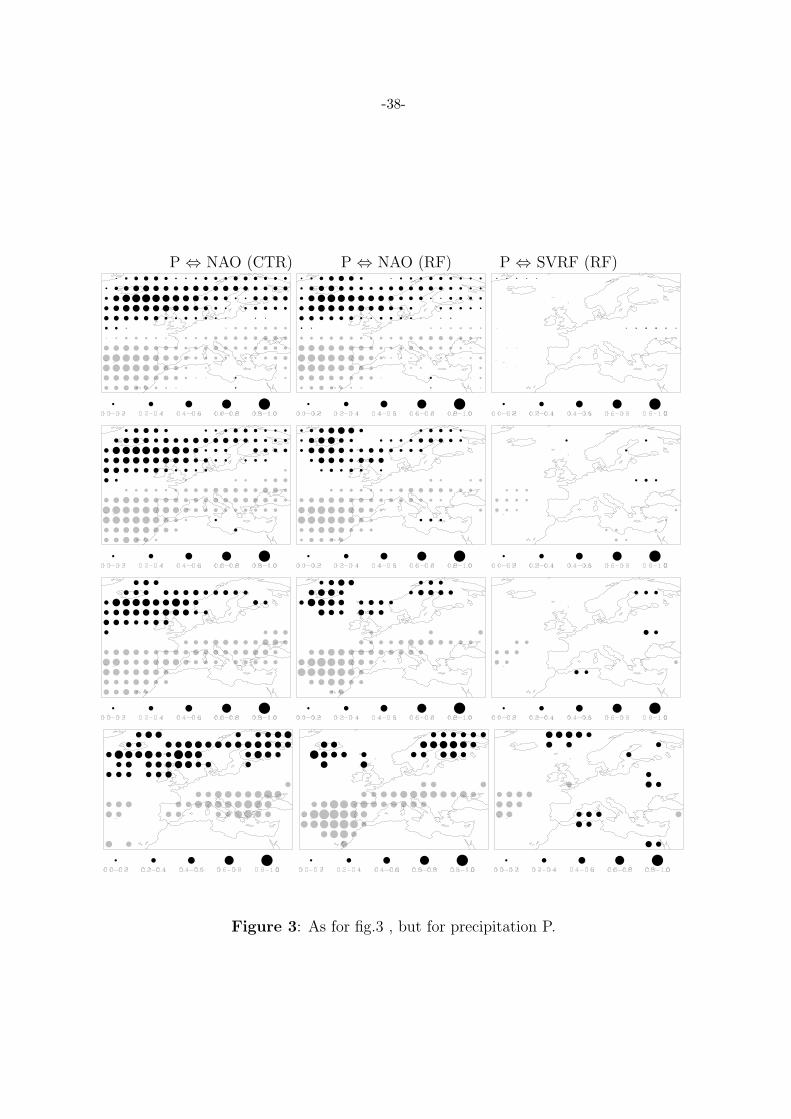
The correlation of T2 and P fields with the NAO index has completely different

characteristics than that with the SVRF. The correlation with the NAO index presents

a weaker dependence on timescale, conserving the same basic structure for the yearly and

the filtered data. It shows the characteristic dipole, corresponding to the advection of

warm humid air towards northern Europe during the positive NAO phase, and towards

Southern Europe during the negative phase, which agrees with the well-known observed

distributions and indicates that the ECHO-G simulation reproduces correctly the link

of the European climate to NAO. On the contrary, the correlation of T2 with the SVRF

8The degrees of freedom of the filtered time series, which are reduced as the cut-off period increases,

have been estimated as Nyear/NF , where NF has been estimated by applying the filter to a white

noise time series and taking the time interval required for the autocorrelation to vanish. It resulted

NF = 6, 16, 25 for the 10, 20, 40-year cut-off, respectively. This has been accounted for in the analysis.

-16-

increases with the length of the timescale, becoming larger than that with NAO at long

timescales. It has a zonal distribution with the largest values at the southern coast of

the Mediterranean Sea. Correlation of P with SVRF is negligible over most continental

Europe, but in the 40-year low-pass filtered time series, where higher SVRF is linked to

an increase of precipitation over the North and the Norwegian Seas, and to a reduction

over the mid latitude Atlantic.

A more detailed analysis of the spatial correlation of the T2 and P with the NAO

shows a small, but interesting, different characteristic in the CTR and RF simulations.

While the patterns based on average winter values are very similar, those based on 40-year

low-pass filtered data are appreciably different. In the CTR simulation, for increasing

timescales, the northern positive lobe in the correlation map of T2 with NAO occupies

an increasingly large area and the negative lobe of the correlation with P moves north-

eastward to Southern Europe. In the RF simulation, the northern positive lobe in the

correlation map of T2 moves eastward and the southern negative one moves northward

inside the Mediterranean Sea. In the correlation map with P, the features above Scan-

dinavia and Southern Central Europe become stronger for increasing timescales. This

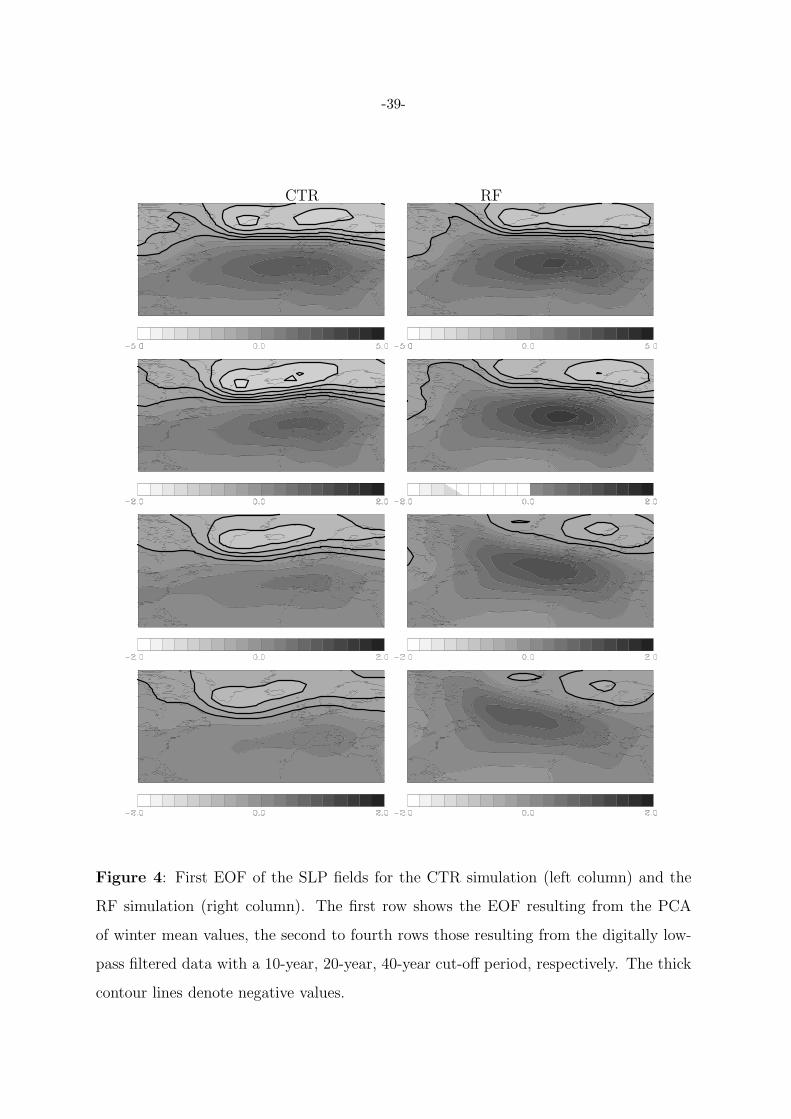
behaviour corresponds to the different timescale dependence of the SLP variability over

the Atlantic, as shown in Fig.4, where the first EOF of the winter SLP fields, that is the

NAO dipole, is plotted at different timescales. At the inter-annual timescale the CTR

and RF simulations are very similar, but, for increasing timescales, the axis of the dipole

has a small anticlockwise rotation in the CTR simulation and a clockwise rotation in

the RF simulation. Consequently, with longer timescales, the European climate is more

strongly associated with the variability of the advection of air masses from sub-tropical

Atlantic in the CTR simulation and of those from North Atlantic in the RF simulation.

This behaviour may indicate an effect, though weak, of the SVRF on the structure of

NAO.

Four indices9 have been computed in order to summarize the characteristics of the

9Indices of both RF and CTR simulations have been computed subtracting the average value and

-17-

behaviour of the T2 and P fields (fig.6). The mean temperature and the total pre-

cipitation indices represent the variability of the average value of T2 and P over the

whole area. The temperature and precipitation contrast indices (denoted with ∆T2 and

∆P ) have been computed as the difference between average values over two selected

areas (fig.5), representative of northern and southern Europe. The selected areas are

different for the precipitation and the temperature contrast index. Positive values of

the contrast index correspond to positive anomalies over Southern Europe and negative

anomalies over northern Europe. These two indices represent the strength of the dipole

affecting the spatial distribution of T2 and P. Time series of the indices are shown in

fig.6. The difference between the two simulations is very clear for the T2 index, which

in the RF simulation presents a much higher variability and two very cold periods in

correspondence to the Late Maunder and Dalton minima of solar activity (two periods

characterized also by strong and frequent volcanic eruptions), and a positive trend since

the last part of the 19th century. The corresponding T2 index of the CTR simulation

presents a smaller variability, and a higher average level, which is consistent with the

constant 1990 RF forcing set for the whole CTR simulation.

Results are summarized in tabs.2 and 3. The NAO correlation with ∆T2 and ∆P

is very large, it is practically constant over the different timescales, and has similar

values in the RF and CTR simulation, varying in the interval from 0.6 to 0.75. The

sign of the correlation of NAO with the average values over the whole area of T2 and

P reflects the dominant role of the positive correlation over northern Europe for T2

and of the negative correlation over southern Europe for P. In the CTR simulation, the

dependence of the spatial distribution of the correlation with the timescale results in an

increasing/decreasing correlation of NAO with the average value of T2/P over the NAE

region. The opposite dependence is present in the RF simulation. The SVRF is clearly,

and somehow obviously, very well correlated with the average European temperature for

normalizing with the variance of the last 500 years of the CTR simulation. This was, obviously not

possible for the SVRF index, which has been computed using the values of the RF simulation itself.

-18-

long timescales, but has no significant link to the other indices.

Therefore, the NAO is correlated with the contrast of the T2 and P fields between

North and South Europe at both inter-annual and decadal timescales. The NAO corre-

lation with the average European T2 and P has a timescale dependence which reveals

an effect of the SVRF at the multi-decadal timescales. The importance of the SVRF for

the European temperature field at multi-decadal timescales is comparable to or larger

than that of the NAO, while at shorter timescale the influence of NAO is much larger.

Though, sometimes, a visual association between minima of SVRF and NAO index

can be identified in fig. 1, no statistically significant correlation has been found between

the NAO index and the SVRF (tab.3). Apparently, no linear relation between SVRF

and NAO is present in the RF simulation, though perhaps a non-linear effect cannot be

completely ruled out.

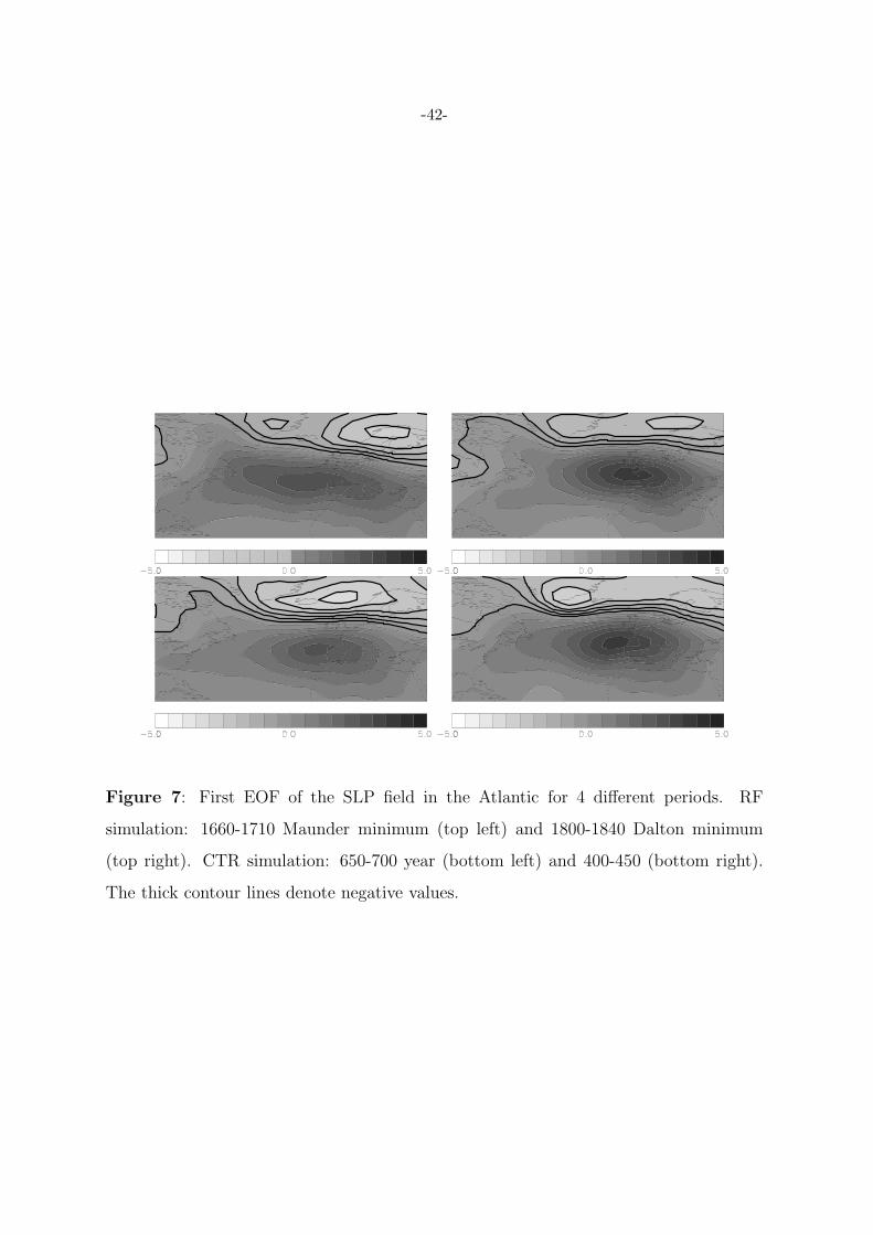
Other effects of the SVRF on the NAO have been considered, but with inconclusive

results. One explored possibility is the presence of recurrent disruptions or perturbations

of the NAO patterns. Fig.7 shows the first EOFs of the (unfiltered) winter mean SLP

fields over the Atlantic in some periods corresponding to very large negative decadal

oscillations of the NAO index. These periods correspond to the Late Maunder and

Dalton periods of solar activity in the RF simulation, and two periods, from 650 to 700

and from 400 to 450, in the CTR simulation. Results show only minor variations. It is

important to observe that large fluctuations of the NAO index and are not present in the

RF simulation only. Actually, the most remarkably persistent negative NAO condition,

with an almost 50-year long duration, is present in the CTR simulation between year

400 and 450 and it has already been noted to present climate anomalies (Zorita et al.,

2003). This period does not seem, however, to result in a deformed NAO dipole.

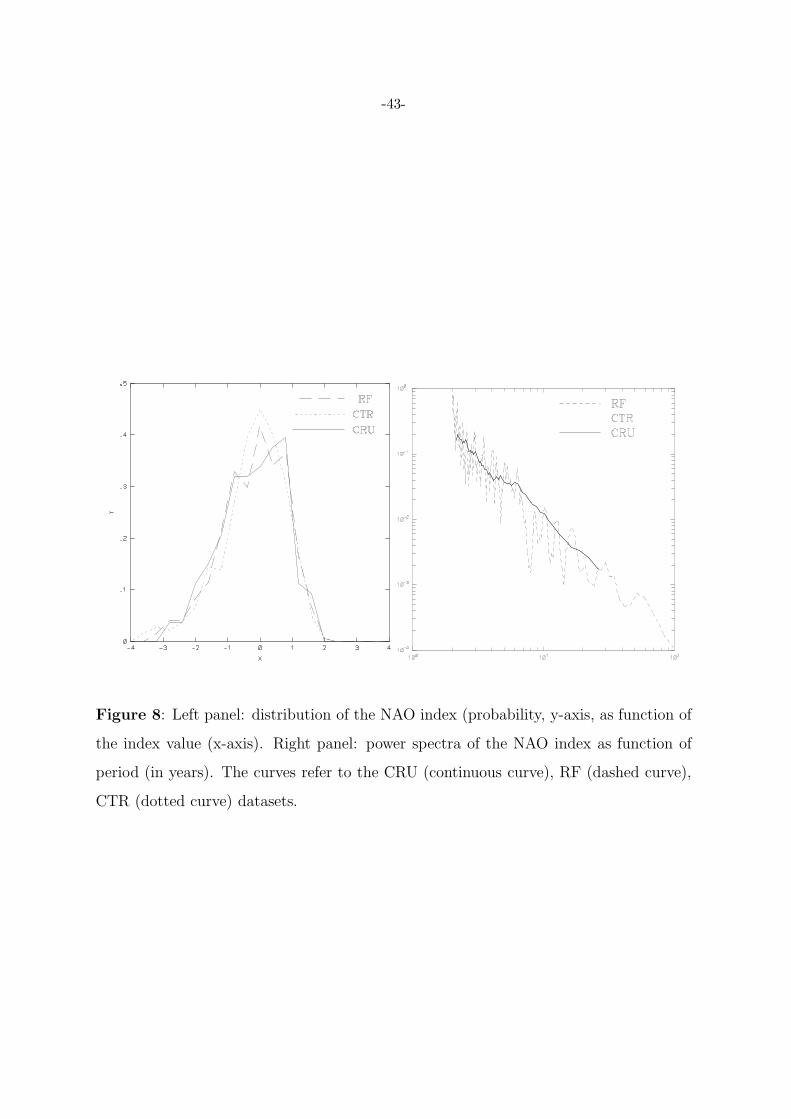
Fig.8 (left panel) shows the statistical distribution of the winter NAO index in the

instrumental data (Jones et al. 1997), and in the RF and CTR simulation. Though the

RF and CTR distributions appear similar, the RF simulation presents an improvement

in reproducing the skewness of the observed distribution. Comparison of spectra (Fig.8,

-19-

right panel) leads to controversial conclusions. On the one hand the differences between

RF and CTR are statistically significant and the RF spectrum reproduces the observed

6 year peak. This would suggest an effect of the SVRF on the NAO spectrum. On the

other hand the NAO simulated in the RF simulation presents a large unrealistic gap in

the 8 year band, which has, instead, approximately the right level in the CTR simulation.

Note that the differences between RF and CTR spectra do not match the peaks in the

RF spectra (not shown), so that the eventual link is weak and nonlinear. Moreover, this

analysis suggests that the model simulations might not be capable of fully reproducing

the correct energy distribution of the observed NAO.

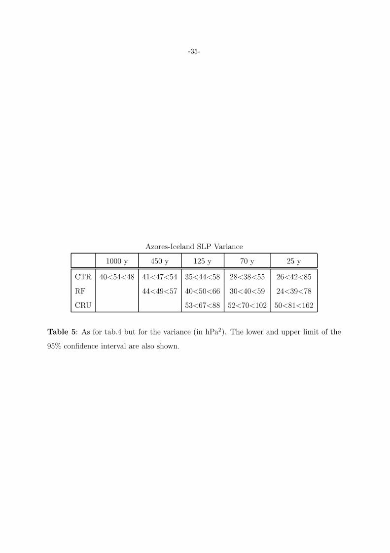
Tabs.4 and 5 compare the mean value and the variance of the Azores-Iceland winter

monthly SLP difference in model simulations and instrumental observations (Jones 1987)

selecting different time intervals. For the instrumental record the two parameters have

been computed until 1990 (final year of the RF simulation) considering the last 25, 70,

125 years (this is the longest possible record). The period has been extended to 450

years for the RF simulation and also to 1000 years for the CTR simulation. No data

set shows a significant trend if statistical uncertainty is taken into account. Considering

the 125-year long period, the difference between RF and CTR simulations is statistically

significant, with the CTR overestimating and the RF underestimating the instrumental

mean value. This difference would be consistent with a positive correlation between

RF and NAO, because the radiative forcing value in the CTR simulation (fixed at the

1990 level) is higher than in the RF simulation. In fact, during the last 25-year long

period, when both simulations have a comparable RF, both simulated mean values are

compatible with the instrumental one, though the RF simulation is much closer to it.

The variance of NAO index is similar in the two simulations, and smaller than the the

instrumental value. However, they cannot be considered statistically different, in view

of the large confidence intervals of the estimates.

-20-

4 European climate reconstruction: the relation be-

tween NAO index, Radiative Forcing and winter

temperature

The correlation between the reconstructed surface air temperature (fig.9) and the NAO

from Nrc2 shows the well known dipole structure (the reconstruction of NAO of Luter-

bacher et al. (2002) has been used). In the reconstruction, the northern positive lobe

is much wider, so that the correlation with the average European temperature is higher

than in the simulations (tab.2). Moreover, the tendency of the correlation to decrease

with longer timescale, though present, is not as large as in the RF simulation.

In Trc4, the correlation of average surface temperature with RF is small at all time

scales (fig.9 and tab.3). This is a consequence of the negative correlation between SVRF

and temperatures in northern Africa, which compensates the small positive correlation

between SVRF and temperatures in the remaining parts of Europe. The average tem-

perature, thus, is uncorrelated with SVRF. This North African negative correlation is

certainly a puzzling feature, which may be artificially due to the lack of data in this

region. In fact, the temperature reconstruction here is mostly based on its statistical

link with temperature in Europe.

The dipolar structure of the correlation between SVRF and temperature might actu-

ally be due to the anti-correlation between reconstructed European and North African

temperatures, this anti-correlation being caused by the influence of the NAO on both

temperatures in the instrumental period. Therefore, if European temperatures are pos-

itively correlated with SVRF ( a reasonable assumption), North African temperatures

would artificially appear anti-correlated with SVRF.

Another aspect is that the reconstruction of the NAO index and of temperatures are

not completely independent, as part of the proxy indicators are used in both reconstruc-

tions. This may explain the high correlation, increasing with the timescale, of the NAO

and SVRF (tab.3). This trend is characteristic of the Nrc2 NAO reconstruction and it is

-21-

present neither in the RF simulation nor in the Cook et al. (2002) reconstruction. Actu-

ally the two NAO reconstructions show some agreement on inter-annual variability, but a

correlation decreasing with time-scale, so that long period fluctuations of the NAO index

in these two time series differ. A similar effect has been detected in analysis of NAO

reconstructions with synthetic data from GCM simulations (Zorita and Gonzalez-Rouco,

2002) (tab.1).

Fig. 1 shows the reconstructed (Trc4) and simulated (RF) average European land

temperature time series filtered with a 10-year (top panel) and 40-year (second row) low

pass filter. The RF simulation presents a much larger variability than the reconstructions.

In spite of this, the correlation between simulated and reconstructed mean European

temperature is significant and it increases with the timescale (tab.3). The two time

series show a remarkable agreement during the cool period of the Maunder minimum

and the subsequent warming. The opposite behaviour is seen in the southern part of

the analysed region, where the correlation of the Trc4 temperature with the SVRF is

negative and that of the RF simulations is large and positive. This hinders a satisfactory

agreement between the respective average temperature time series.

In order to investigate the correlations at grid-point level between the RF and Trc4

fields, the latter have been ”up-scaled” from their 0.5o×0.5o degrees resolution to the

3.75o×3.75o resolution of the gridded ECHO-G data, by taking the average value in each

ECHO-G grid box. Boxes that resulted less than 50% filled with data have been ignored.

Also the sea points of the ECHO-G simulation were not included, so that the analysis is

based only on points that, at the 3.75o×3.75o resolution, can be considered land for both

the reconstruction and the RF simulation. The correlation has been computed including

data from the period 1550 to 1990. Results are shown in fig.10. Correlation is nowhere

significant at the inter-annual timescale, but increases with timescales, becoming signif-

icantly large for multi-decadal timescales on north-eastern Europe, while it remains not

significant on Southern Europe and on the northern African coast of the Mediterranean

Sea. This pattern is consistent with the correlation between temperature and SVRF in

-22-

the simulation and in the reconstruction.

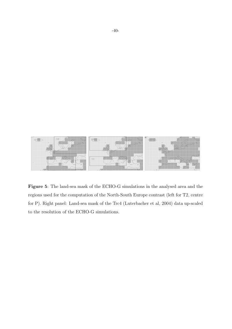
There are two reasons for the different behaviour over northern Africa, where both

datasets are presumably not quite reliable. In the model simulation, the land-sea mask

in the Mediterranean sea region is not accurate (see fig.5) and the Gibraltar Strait is

replaced with a 1000 km wide sea extent. It would not be surprising that the characteris-

tics of Mediterranean air mass are not properly reproduced in the simulation. Moreover,

no temperature sensitive proxy data are available for the reconstruction over northern

Africa before the end of the 19th century, so that the features over this region results

solely from their connection with European temperatures, which has been established

mostly using instrumental data at inter-annual timescales. The NAO is expected to have

a marginal role in the explanation of the correlation between simulated and reconstructed

temperature, as the relative NAO time series are not correlated. At the same time the

absence of correlation between simulated and reconstructed NAO is partially responsi-

ble for the lack of correlation between the simulated and reconstructed temperatures at

inter-annual timescale.

5 Discussion

This study analysed the relative strength of the conditioning exerted by the NAO and by

the RF on the regional European climate in the past few centuries. The analysis of the

results has some importance also for future regional climate change , at least for future

periods when the assumed RF changes do not grossly exceed past variations.

A key aspect is that the effect of the SVRF and the NAO may be entangled by the

influence of SVRF on the NAO itself. This is an important issue, because the absence

of correlation between NAO and SVRF would limit the possibility to reconstruct, or

predict, a major component of the inter-annual and decadal variability of European

Climate. However, the presence of a strong phase lock between SVRF and NAO is

controversial. The Nrc2 reconstruction of the NAO index is the only time series which

shows a significant correlation between the SVRF and the NAO at decadal and multi-

decadal timescales, while the Cook et al. (2002) data and the RF model simulation

-23-

do not present a similar behaviour. Since other modelling studies suggest a stronger

conditioning of the RF on the NAO if the stratospheric dynamics is well represented

(Shindell et al 2001a, 2001b), the lack of correlation between NAO and SVRF might be

explained by the coarse representation of the stratosphere in the ECHO-G model. On the

other hand the link of NAO to SVRF could be nonlinear and present only in particular

situations, like the Late Maunder minimum, at the end of which both reconstructions

show a negative large NAO index, and also the RF simulation has a large negative values,

though about 10 years earlier than the two reconstructions. However, accepting that

validity of the Nrc2 NAO reconstruction, the link of SVRF to NAO would be practically

relevant only at multi-decadal time scales.

In this study a series of possible effects of the SVRF on the NAO, have been consid-

ered with inconclusive results. The shape of the statistical distribution of the Azores-

Iceland pressure seems closer to observations in the RF than in the CTR simulation.

The statistics of this quantity show that the RF and CTR simulations have opposite

errors for its mean value (the RF simulation underestimates it) and both underestimate

its variance. Accounting for statistical errors both the RF and CTR simulations provide

estimates that are consistent with instrumental observations. The consistency margin

is very narrow for the Azores-Iceland pressure difference variance, suggesting that vari-

ability is underestimated in the model simulations. The difference of the mean value

between the RF and CTR simulations is statistically significant suggesting that high

SVRF values would increase the meridional pressure gradient. The analysis of the NAO

spectra does not lead to clear conclusions. Finally, the evidence that the usual NAO

pattern has been partially distorted during the periods corresponding to large negative

decadal oscillations of the NAO index are unconvincing, as large negative oscillations are

present both in the RF and in the CTR simulation.

There is a remarkable aspect of the behaviour of the NAO at multi-decadal timescales.

In the RF simulation the axis of the NAO dipole rotates clockwise for increasing time

scales. This diminishes the advection of humid and warm air over northern Europe

-24-

from mid-Atlantic, so that the positive lobe of the correlation relating the NAO index

to the temperature and precipitation fields over northern Europe shrinks. This causes

a decreasing correlation with timescale of the average European temperature and an

increasing anti-correlation of the overall European precipitation with the NAO index.

The reconstruction does not exclude this trend as correlation of its winter temperature

with NAO decreases with the timescale.

RF simulation and reconstruction do not agree on the effect of SVRF on Euro-

pean Climate during the last five centuries. In the RF simulation, at the multi-decadal

timescale, the SVRF conditioning of European climate becomes comparable to, or even

larger than, that of NAO in the southern part of the analysed region. On the contrary,

the reconstruction does not show a significant correlation, and it presents a negative

correlation to SVRF above northern Africa. This may be caused by the observed anti-

correlation between European and North African temperatures at interannual timescales,

which leaves its imprint on the reconstructed North African temperatures.

In fact, northern Africa is a region where the SVRF conditioning should be strong

and the lacking correspondence between reconstruction and RF simulation over this

area is disappointing. Neither the RF simulation, nor the reconstruction appear in this

situation very reliable. ECHO-G is characterized by very coarse model resolution and an

unrealistic land-sea mask in the Mediterranean Region. The reconstruction is based on

few local proxies and it is derived mostly by its statistical relation with the temperature

over Europe.

It is clear that the results of this study are affected by large uncertainties and different

datasets lead to different interpretations. Both reconstructions and simulations present

shortcomings. Lack of agreement on long term fluctuations of NAO and on temperature

are evident comparing different reconstructions. Differences between model simulations

are justified by simplifications which the models are forced to adopt for integrations

covering multi-centennial periods. It is difficult to establish a priori whether the results

of some model are more reliable than others, that is if the simplified ocean and the lack

-25-

of resolution of the study by Shindell et al. (2001b) are more crucial than the coarse

resolution of the stratosphere in ECHO-G. It is also not clear if the reconstructions tend

to underestimate the temperature variability or the ECHO-G model is over-sensitive to

the variations of the RF. Moreover, other effects not included in the model, as land use

changes, can be also important ( Bauer et al 2003). Finally, five centuries are a short

period for multi-decadal variability and the availability of longer simulations could help

to reduce uncertainties.

6 Conclusions

There are two conflicting interpretations of the results of this study, which appear difficult

to reconcile. According to the RF simulation, NAO has no linear relation to the SVRF,

so that predictability of temperature would be restricted to the part of the temperature

variability directly determined by the RF alone. In future studies, a set of multi-model

simulations could offer important information for confirming this interpretation. On the

other hand, in the reconstruction there is a linear correlation between NAO and SVRF,

which increases with the time scale, so that the predictability may be enhanced by the

additional contribution of the NAO. However, other reconstructions of NAO do not agree

on this multi-decadal behaviour, so that correlation between NAO and SVRF could be

a peculiarity of the Nrc2 reconstruction.

In our view, the most likely interpretation of these results is that, at regional scale, the

SVRF conditioning of temperature becomes dominant only at multi-decadal timescales

as shown by the RF simulation, and shorter timescales are dominated by intrinsic climate

variability, which could be chaotic and unpredictable. It remains possible that the effect

of SVRF on NAO is nonlinear and appears only in particular situations, such as the

Maunder Minimum, while in general NAO is weakly linked to the SVRF. If confirmed,

this would indicate that part of future European temperature changes will be associated

with, internal, eventually unpredictable, climate dynamics. This conclusion should not

be extrapolated to very general validity: other regions or other seasons less under the

influence of internal variability would present a more predictable behaviour. Moreover,

-26-

in climate change scenarios, the variation of the RF forcing is much larger than that

accounted for in this study, and the RF effect could be more dominant.

Acknowledgements P.Lionello thanks the GKSS Forschung Zentrum for the hos-

pitality during his sabbatical year. S.De Zolt has been partially supported by the GKSS

Forschungszentrum J. Luterbacher has been supported by the Swiss National Science

Foundation (NCCR Climate) and by the EU project SO&P. E. Zorita’s contribution was

performed in the frame of the German program DEKLIM.

The CRU data were downloaded from the CRU (Climate Research Unit, Univ. of

East Anglia) web page http://www.cru.uea.ac.uk. Cook et al. (2002) NAO time series

has been extracted from data archived at the World Data Center for Paleoclimatology,

Boulder, Colorado, USA (web page: http://www.ngdc.noaa.gov/paleo).

-27-

References

[1] Bauer, E, Claussen M, Brovkin V, . Huenerbein A (2003) Assessing climate forc-

ings of the Earth system for the past millennium Geophys. Res. Lett. 30: 1276

DOI: 10.1029/2002GL016639.

[2] Bradley RS, Jones PD (1993) ‘Little Ice Age’ summer temperature variations:

their nature and relevance to recent global warming trends. The Holocene 3: 367-

376.

[3] Bradley RS, Hughes MK, Diaz HF (2003) Climate in Medieval Time. Science 302:

404-405.

[4] Brazdil, R., Pfister, C., Wanner, H., von Storch, H., and Luterbacher, J., (2004)

Historical climatology in Europe The State of the Art, Clim. Change 70, 363-430.

[5] Briffa KR, Osborn TJ, Schweingruber FH Harris IC, Jones PD, Shiyatov SG

Vaganov EA (2001) Low-frequency temperature variations from a northern tree-

ring-density network. J. Geophys. Res. 106: 2929-2941.

[6] BriffaKR, Osborn TJ, Schweingruber FH, JonesPD, Shiyatov SG Vaganov EA

(2002) Tree-ring width and density data around the Northern Hemisphere: Part 2,

spatio-temporal variability and associated climate patterns. The Holocene 12:759-

789.

[7] Cook ER, D’Arrigo RD, and Mann ME (2002) A Well-Verified, Multiproxy Re-

construction of the Winter North Atlantic Oscillation Index since A.D. 1400.

Journal of Climate 15: 1754-1764.

[8] Crowley TJ (2000) causes of climate change over the past 1000 years. Science 289:

270-277.

-28-

[9] Cubasch U, Hegerl GC, Voss R, Waskewitz J Crowley TC, (1997) Simulation

with an O-AGCM of the influence of variations of the solar constant on the global

climate. Clim. Dyn. 13: 757-767.

[10] Cubasch U, Voss R (2000) The influence of total solar irradiance on climate. Space

Science Reviews 94: 185-198.

[11] Cullen HM, de Menocal PB (2000) North Atlantic influence on Tigris-Euphrates

streamflow. Int. J. Climatol. 20: 853-863.

[12] Dunkeloh A, Jacobeit J (2003) Circulation dynamics of Mediterranean precipita-

tion variability 1948-1998. Int J Climatol 23: 1843-1866.

[13] Fischer DA (2002) High-resolution multiproxy climatic records from ice cores,

tree-rings, corals and documentary sources using eigenvector techniques and

maps: assessment of recovered signal and errors. The Holocene 12: 401-419.

[14] Fischer-Bruns I, Cubasch U, von Storch H, Zorita E, Gonzalez-Rouco JF, Luter-

bacher J (2002) Modelling the Late Maunder Minimum with a 3-dimensional

OAGCM, CLIVAR exchanges 7: 59-61.

[15] Guiot J. (1991) The combination of historical documents and biological data in

the reconstruction of climate variations in space and time in Frenzel, B., Pfister,

C., and Glaeser, B. (eds.), European Climate Reconstructed from Documentary

Data: Methods and Results, Gustav Fischer Verlag, Stuttgart, Jena, New York,

pp. 93-104.

[16] Hegerl GC, Hasselmann K, Cubasch U, Mitchell JFB, Roeckner E, Voss R,

Waszkewitz J (1997) Multi-fingerprint detection and attribution analysis of green-

house gas, greenhouse gas-plus-aerosol and solar forced climate change. Clim.

Dyn. 13: 613-634.

-29-

[17] Hegerl G C, Crowley TJ, Baum SK, Kim K-Y, Hyde WT (2003) Detec-

tion of volcanic, solar and greenhouse gas signals in paleo-reconstructions of

Northern Hemispheric temperature. Geophys,. Res. Lett 30(5): 12-42. doi:

10/1029/2002GL016635.

[18] Hurrell JW (1995) Decadal trends in the North Atlantic Oscillation and relation-

ships to regional temperature and precipitation. Science 269: 676-679.

[19] Hurrell JM , van Loon H (1997) Decadal variations in climate associated with the

North Atlantic Oscillation. Clim. Change 36: 301-326.

[20] Hurrell JW, Kushnir Y, Otterson G, Visbeck M(Eds.), (2003) North Atlantic

Oscillation, Climatic Significance and Environmental Impact. Geophysical Mono-

graph 134, American Geophysical Union (AGU), Washington.

[21] IPCC (2001) Climate change 2001: the scientific basis. Cambridge University

Press, Cambridge, UK, 881pp.

[22] Jones PD (1987) The early twentieth century Arctic High - fact or fiction? Clim.

Dyn. 1: 63-75.

[23] Jones PD, Jonsson T, Wheeler G (1997) Extension to the North Atlantic Oscil-

lation using early instrumental pressure observations from Gibraltar and South-

West Iceland. Int. J. Climatol. 17: 1433-1450.

[24] Jones PD , Osborn TJ, Briffa KR (2003) in The North Atlantic Oscillation:

Climatic Significance and Environmental Impact [Geophysical Monograph 134],

J. W. Hurrell, Y. Kushnir, G. Ottersen, M. Visbeck, Eds. (American Geophysical

Union, Washington, DC.

[25] Jones PD, Mann ME (2004) Climate Over Past Millennia. Rev. Geophys., 42:

RG2002, doi: 10.1029/2003RG000143.

-30-

[26] Legutke S , Voss R (1999) ECHO-G, The Hamburg Atmosphere-Ocean Coupled

Circulation Model , DKRZ-Report n.18, 43pp.

[27] Luterbacher J, Schmutz C, Gyalistras D, Xoplaki E, Wanner H (1999) Recon-

struction of monthly NAO and EU indices back to AD 1675, Geophys. Res. Lett.

26: 2745-2748.

[28] Luterbacher J, Xoplaki E, Dietrich D, Jones PD, , Davies TD, Portis D, Gonzalez-

Rouco JF, von Storch H, Gyalistras D, Casty C, and Wanner H (2002) Extending

North Atlantic Oscillation Reconstructions Back to 1500. Atmos. Sci. Lett. 2:114-

124 doi:10.1006/asle.2001.0044.

[29] Luterbacher J, Dietrich D, Xoplaki E, Grosjean M, WannerH (2004) European

seasonal and annual temperature variability, trends, and extremes since 1500.

Science 303: 1499-1503 (DOI:10.1126/science.1093877).

[30] Mann ME, Bradley RS, Hughes MK (1998) Global-Scale Temperature Patterns

and Climate Forcing Over the Past Six Centuries Nature 392: 779-787.

[31] Mann, ME, Gille E, Bradley RS, Hughes MK, Overpeck JT, Keimig FT, and

W. Gross, (2000) Global Temperature Patterns in Past Centuries: An interactive

presentation, Earth Interactions, 4-4, 1-29.

[32] Shindell DT, Schmidt GA, Mann ME, Rind D, Waple A (2001a) Solar forcing of

regional climate change during the Maunder Minimum. Science 294: 2149-2152.

[33] Shindell DT, SchmidtGA, Miller RL, Rind D (2001b) Northern Hemisphere winter

climate response to greenhouse gas, ozone, solar, and volcanic forcing. J. Geophys.

Res. 106: 7193-7210.

[34] Schmutz C, Luterbacher J, Gyalistras D, Xoplaki E, Wanner H. (2000) Can we

trust proxy-based NAO index reconstructions? . Geophys. Res. Lett. 27: 1135-

1138.

-31-

[35] Stine S (1998) Medieval Climate Anomaly in the Americas. In: Water, Environ-

ment and Society in Times of Climatic Change (eds. A.S. Issar und N. Brown).

Kluwer, Dordrecht, 43-67.

[36] Tett SFB, Stott PA, Allen MA, Ingram WJ , Mitchell JFB (1999) Causes of

twentieth century temperature change. Nature 399: 569-572.

[37] Tett SFB Jones GS, Stott PA, Hill DC , Mitchell JFB , Allen RM , Ingram

WJ , Johns TC, Johnson CE, Jones A, Roberts DL, Sexton DM , Woodage

MJ (2002) Estimation of natural and anthropogenic contributions to twentieth

century temperature change. J. Geophys. Res. 107: 4307 .

[38] Xoplaki E, Gonzalez-Rouco JF , Luterbacher J , Wanner H, (2004) Wet season

Mediterranean precipitation variability: influence of large-scale dynamics, Clim.

Dyn. 23: 63-78, (DOI 10.1007/s00382-004-0422-0).

[39] Xoplaki E (2002) Climate variability over the Mediterranean. PhD

thesis, University of Bern, Switzerland . ([http://sinus.unibe.ch/

klimet/docs/phd xoplaki.pdf])

[40] Zorita E , Gonzalez-Rouco JF (2002) Are temperature proxies adequate for North

Atlantic Oscillation reconstructions ? Geophys. Res. Lett. 29: 102019, 48-1-48-4.

[41] Zorita E, Gonzalez-Rouco JF, Legutke S (2003): testing the Mann et al (1998)

approach to paleoclimate reconstruction in the context of a 1000-yr control sim-

ulation with the ECHO-G Coupled Climate model, J Climate 16:1378-1390.

[42] Zorita E, von Storch H, Gonzalez-Rouco JF, Cubasch U, Luterbacher J , Fischer-

Bruns I, Legutke S , Schlese U (2004) Climate evolution in the last five cen-

turies simulated by an atmosphere-ocean model: global temperatures, the North

Atlantic Oscillation and the Late Maunder Minimum, Meteorol. Zeitschrift 13:

271-289.

-32-

Correlation: NAO

1-winter 10 y 20 y 40 y

Nrc2 < − > Cook 0.41 0.34 (0.31) (0.17)

Correlation: T2

Trc4 < − > RF (0.01) 0.26 0.40 0.48

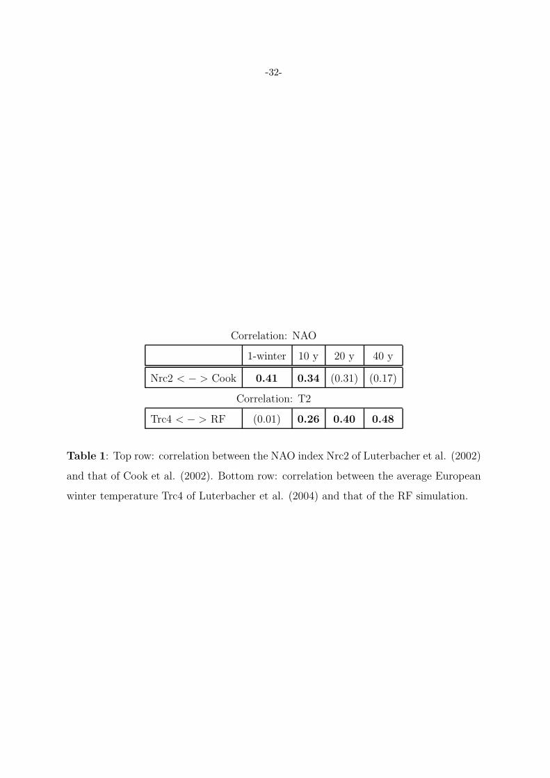
Table 1: Top row: correlation between the NAO index Nrc2 of Luterbacher et al. (2002)

and that of Cook et al. (2002). Bottom row: correlation between the average European

winter temperature Trc4 of Luterbacher et al. (2004) and that of the RF simulation.

-33-

Correlation with NAO index

1-winter 10 y 20 y 40 y

T2 (RF) 0.21 0.27 (0.26) (0.12)

∆T2 (RF) -0.60 -0.64 -0.72 -0.74

P (RF) -0.37 -0.34 -0.38 -0.57

∆P (RF) -0.70 -0.67 -0.71 -0.70

T2 (CTR) 0.27 0.31 0.37 0.44

∆T2 (CTR) -0.64 -0.65 -0.64 -0.64

P (CTR) -0.32 -0.27 (-0.23) (-0.18)

∆P (CTR) -0.76 -0.77 -0.74 -0.67

T2 (Trc4) 0.70 0.62 0.58 0.59

T2 (Cook et al) 0.20 0.24 0.31 (0.34)

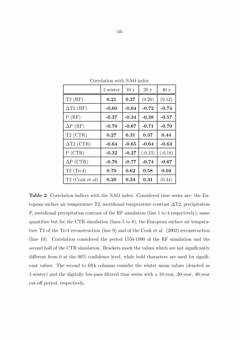
Table 2: Correlation indices with the NAO index. Considered time series are: the Eu-

ropean surface air temperature T2, meridional temperature contrast ∆T2, precipitation

P, meridional precipitation contrast of the RF simulation (line 1 to 4 respectively), same

quantities but for the CTR simulation (lines 5 to 8), the European surface air tempera-

ture T2 of the Trc4 reconstruction (line 9) and of the Cook et al. (2002) reconstruction

(line 10). Correlation considered the period 1550-1990 of the RF simulation and the

second half of the CTR simulation. Brackets mark the values which are not significantly

different from 0 at the 90% confidence level, while bold characters are used for signifi-

cant values. The second to fifth columns consider the winter mean values (denoted as

1-winter) and the digitally low-pass filtered time series with a 10-year, 20-year, 40-year

cut-off period, respectively.

-34-

Correlation with SVRF

1-winter 10 y 20 y 40 y

T2 (RF) 0.14 0.40 0.51 0.62

T2 (Trc4) 0.09 0.24 (0.27) (0.37)

NAO (RF) (0.03) (0.17) (0.20) (0.20)

NAO (Nrc2) 0.12 0.26 0.32 0.43

NAO (Cook) (-0.02) (-0.10) (-0.18) (-0.17)

Table 3: As for tab.2, but referring to the correlation with SVRF. First and second line:

Average European temperature of RF simulation and of Trc4 reconstruction. Third to

fifth line: NAO index of RF simulation, Nrc2 reconstruction and Cook et al. reconstruc-

tion.

Azores-Iceland SLP difference

1000 y 450 y 125 y 70 y 25 y

CTR 20.9±0.4 20.8±0.6 21.6±1.2 21.7±1.4 22.6±2.5

RF 19.1±0.6 19.0±1.2 19.6±1.5 19.7±2.5

CRU 20.5±1.4 19.8±2.0 20.1±3.5

Table 4: Mean value and standard deviation (in hPa) of the winter sea level pressure

difference between Azores and Iceland according to the CTR and RF simulations (first

and second line), to the CRU (Climate Research Unit, East Anglia University dataset,

third line). Values have been computed for the whole 1000 , and for the last 450, 125,

70 , 30 years of the datasets, when available.

-35-

Azores-Iceland SLP Variance

1000 y 450 y 125 y 70 y 25 y

CTR 40<54<48 41<47<54 35<44<58 28<38<55 26<42<85

RF 44<49<57 40<50<66 30<40<59 24<39<78

CRU 53<67<88 52<70<102 50<81<162

Table 5: As for tab.4 but for the variance (in hPa2). The lower and upper limit of the

95% confidence interval are also shown.

-36-

Figure 1: Top: Average European winter temperature over land since year 1500. Values

are anomalies (in K) with respect to the average temperature in the 1850-1950 period.

A low pass digital filter with a 10-year cut-off period has been applied to the data. The

black curve shows the reconstruction Trc4 time series by Luterbacher et al. (2004).

Second row: as the top panel, but filtered using a 40-year cut-off period. Third row: as

the top panel but for the winter NAO index. The black line is the Nrc2 reconstruction

by Luterbacher et al. (2002), the grey line shows the RF simulation, the pale grey curve

shows the values of Cook et al. (2002). Bottom panel: total radiative forcing (in W/m2)

derived from reconstructions of net radiative forcing Crowley (2000) and rescaled to total

solar irradiance. The thin line shows the winter mean values, the thick line shows the

-37-

T2 ⇔ NAO (CTR) T2 ⇔ NAO (RF) T2 ⇔ SVRF (RF)

Figure 2: Spatial distribution of the correlation between the T2 and the NAO index in

the CTR simulation (left column), in the RF simulation (central column), and between

T2 and the SVRF in the RF simulation. The first row considers the winter mean values,

second to fourth rows the digitally low-pass filtered data with a 10-year, 20-year, 40-year

cut-off period, respectively. Black and grey dots denote positive and negative values,

respectively. In the white areas the correlation is not significantly different from 0 at the

90% confidence level.

-38-

P ⇔ NAO (CTR) P ⇔ NAO (RF) P ⇔ SVRF (RF)

Figure 3: As for fig.3 , but for precipitation P.

-39-

CTR RF

Figure 4: First EOF of the SLP fields for the CTR simulation (left column) and the

RF simulation (right column). The first row shows the EOF resulting from the PCA

of winter mean values, the second to fourth rows those resulting from the digitally low-

pass filtered data with a 10-year, 20-year, 40-year cut-off period, respectively. The thick

contour lines denote negative values.

-40-

Figure 5: The land-sea mask of the ECHO-G simulations in the analysed area and the

regions used for the computation of the North-South Europe contrast (left for T2, centre

for P). Right panel: Land-sea mask of the Trc4 (Luterbacher et al, 2004) data up-scaled

to the resolution of the ECHO-G simulations.

-41-

Figure 6: Indices of winter NAO (first row), North-South Europe temperature contrast

(second row) , mean European Temperature (third row), North-South Europe precip-

itation contrast (fourth row), total precipitation over the European area (fifth row),

radiative forcing (sixth row, left). Left panels refer to the RF simulation, right panels to

the CTR simulation (last 450 years). The light lines show the actual winter mean values,

the thick lines the low-pass filtered data with a 10 years cut-off periods. The indices are

computed using the mean and the variance of the last 500 years of the CTR simulation.

-42-

Figure 7: First EOF of the SLP field in the Atlantic for 4 different periods. RF

simulation: 1660-1710 Maunder minimum (top left) and 1800-1840 Dalton minimum

(top right). CTR simulation: 650-700 year (bottom left) and 400-450 (bottom right).

The thick contour lines denote negative values.

-43-

Figure 8: Left panel: distribution of the NAO index (probability, y-axis, as function of

the index value (x-axis). Right panel: power spectra of the NAO index as function of

period (in years). The curves refer to the CRU (continuous curve), RF (dashed curve),

CTR (dotted curve) datasets.

-44-

NAO RF

Figure 9: Reconstruction: correlation of the surface temperature fields with the NAO

index (left column) and with the RF (right column). The first row considers the winter

mean fields, second to fourth rows the digitally low-pass filtered fields with a 10-year,

20-year, 40-year cut-off period, respectively. Black and grey dots denote positive and

negative values, respectively. In the white areas the correlation is not significantly dif-

ferent from 0 at the 90% confidence level.

-45-

Figure 10: Correlation between the surface temperature fields of the reconstruction

and the RF simulation. The first row considers the winter mean values, second to fourth

rows the digitally low-pass filtered data with a 10-year, 20-year, 40-year cut-off period,

respectively. Black and grey dots denote positive and negative values, respectively. In

the white areas the correlation is not significantly different from 0 at the 90% confidence

level.