supplementary information - · pdf filethe details of the ncar csm 1.4 climate model and the...

SUPPLEMENTARY INFORMATIONDOI: 10.1038/NGEO1394

NATURE GEOSCIENCE | www.nature.com/naturegeoscience 1

1

Underestimation of Volcanic Cooling in Tree-Ring Based Reconstructions of

Hemispheric Temperatures

Michael E. Mann1, Jose D. Fuentes1, Scott Rutherford2

1Department of Meteorology and Earth and Environmental Systems Institute,

Pennsylvania State University, University Park, PA, USA

2Department of Environmental Science, Roger Williams University,

Bristol, RI, USA.

SUPPLEMENTARY INFORMATION

© 2012 Macmillan Publishers Limited. All rights reserved.

2

SUPPLEMENTARY METHODS/DISCUSSION


3

I. GCM Simulation The details of the NCAR CSM 1.4 climate model and the simulation analyzed are

provided by ref. 3 of the main article. The solar forcing in ref. 3 was estimated by

cosmogenic (Be10) radioisotopes from ice cores, scaled under the assumption of 0.25%

change in solar constant from Maunder Minimum to present. This relatively large solar

forcing is counterbalanced by the model’s relatively low (ΔT2xCO2=2.1 oC) equilibrium

climate sensitivity. Volcanic radiative forcing was prescribed as latitudinally varying and

linearly proportional to estimated aerosol loading (assuming a constant aerosol size

distribution) as diagnosed from polar ice cores. Anthropogenic forcing included well-

mixed greenhouse gases (CO2 and other trace greenhouse gases) and sulphate aerosols,

were applied as global mean radiative forcings.

II. Energy Balance Model Simulations We employed a simple zero-dimensional Energy Balance Model (“EBM”--see e.g. refs

12-13 of main article) of the form

C dT/dt = S(1-α)/4 + FGHG -A-B T + w(t)

T is the temperature of Earth’s surface (approximated as a 70 m depth mixed layer ocean

covering 70% of Earth’s surface area). C=2.08 x 108 J K-1m-2 is an effective heat

capacity that accounts for the thermal inertia of the mixed layer ocean, but does not allow

for heat exchange with the deep ocean as in more elaborate “upwelling-diffusion

models”1.


4

S ≈1370 Wm-2 is the solar constant, and α≈0.3 is the effective surface albedo. FGHG is the

radiative forcing by greenhouse gases. w(t) represents random weather effects, and was

set to zero to analyze the purely forced response.

The linear “gray body” approximation (see e.g. ref. 24 of main article),

LW=A+B T

has been used to model outgoing longwave radiation in a way that accounts for the

greenhouse effect. The choice A=221.3 WK-1m-2 and B=1.25 Wm-2 yields a realistic pre-

industrial global mean temperature T=14.8 oC and an equilibrium climate sensitivity of

ΔT2xCO2=3.0oC, consistent with mid-range IPCC estimates (ref. 25 of main article).

The EBM was driven with estimated annual mean natural and anthropogenic forcing over

the period AD 850-1999. Estimated past changes in solar irradiance were prescribed as a

change in the solar constant S, while forcing by volcanic aerosols was prescribed as a

change in the surface albedo α. Solar and volcanic forcing were taken from the GCM

simulation of ref 3 described in the section above, with the following modifications: (1)

solar forcing was rescaled under the assumption of a 0.1% change from Maunder

Minimum to present more consistent with recent estimates (e.g. ref. 1 of main article); (2)

volcanic forcing was applied as the mean of the latitudinally-varying volcanic forcing of

ref. 3.

Greenhouse radiative forcing was calculated using the approximation2

FGHG=5.35log(CO2e/280)

where 280 ppm is the preindustrial CO2 level and CO2e is the “equivalent” anthropogenic

CO2, scaled to give the same increase as in ref. 3. Northern Hemisphere anthropogenic

sulphate aerosol forcing was not available for ref. 3 so was taken instead from ref. 13.


5

Sensitivity analyses (see section VII below) were performed with respect to (i) the

equilibrium climate sensitivity assumed (varied from ΔT2xCO2=2-4 oC), (ii) the solar

scaling (0.25% in place of 0.1% Maunder Minimum-present change), (iii) volcanic

aerosol loading estimates used (ref. 4 and 13 estimates in addition to ref. 3) and (iv) the

scaling of volcanic radiative forcing with respect to aerosol loading to account for

possible size distribution effects. For ref. 3 and 4 both a linear scaling and a 2/3 power

law scaling (which has been argued for based on coagulation effects at large aerosol

optical depths) were tested (ref. 13 implicitly assumes a 2/3 power law scaling). The

lowest estimate for the magnitude of the AD 1258/1259 eruption (-8.1 Wm-2)

corresponded to use of the ref. 3 aerosol loading estimates and employing the 2/3 power

law scaling, while the highest estimate (-19.4 Wm-2) corresponded to use of the ref. 4

aerosol loading estimates and employing a linear scaling [for reference, our standard case

employing the ref. 3 aerosol loading estimates and linear scaling gives -11.9 Wm-2 peak

forcing for the AD 1258/1259 eruption].

III. Tree Growth Model

The growth function g(T) is shown in Figure S1a for both functional variants (p=1 and

p=2) of the Shashkin-Vaganov model, and the standard parameter values used in the

article (Topt1=18 oC, Topt2=21 oC, Tmin=10 oC, and Tmax =24 oC).

A single year of the simulated seasonal cycle at treeline for the modern reference interval

of 1961-1990 (based on the values T1 =11.8 oC and T2 =-27 oC discussed in the article) is

shown in Figure S1b, along with the lower threshold for onset of tree growth (10 oC---

note that sensitivity to this choice of threshold is explored in section VIII below). Shown


6

are results both with and without stochastic white noise forcing (amplitude σ=3.0 oC as

discussed in article).

IV. Analysis of Residual Variance

We examined the residual variability defined by subtracting the EBM-simulated

temperature series from the tree-ring reconstruction. If the tree-ring reconstruction were

an unbiased estimate of actual past Northern Hemisphere temperature changes (which we

would expect to contain a component associated purely with radiative forcing, and a

component associated purely with internally-generated climate variability) then we would

expect the residuals to be consistent with internal variability. There should therefore be

no clear structure in the residuals. We find this to be largely true; the residuals (Figure

S2—blue curve) largely fall within their estimated two sigma limits. The standard

deviation of the annual residual series is 0.25 oC. If sampled only over the interval 1500-

1800 (which avoids any of the three major eruptions—the reason which will be clear

below), the standard deviation is reduced to 0.15 oC. The decadal (10 year low-passed)

standard deviation (0.12 oC) is quite close to the estimates cited by ref. 13 for internal

climate variability on decadal timescales. However, we do find clear deterministic

structure in the residuals corresponding to the three major volcanic forcing episodes (AD

1258/1259, AD 1452/1453 and AD 1809+1815) for which the residuals approach or

breach the 3 sigma limit and, in the case of the AD 1258/1259 eruption, the 6 sigma limit.

These findings suggest a systematic loss of amplitude in the cooling response of the few

largest eruptions recorded by the tree-ring reconstruction, but no other obvious systematic

biases. This observation forms part of the basis for our conclusion that the muted

volcanic cooling in the tree-ring reconstructions can be dismissed e.g. as an artifact of the


7

statistical temperature reconstruction methodology. The other reason for rejecting that

hypothesis is described in section V below.

We also estimated the unforced variability by subtracting the EBM-simulated

temperature series from the GCM-simulated temperature series (Figure S2—green; in

principle the forced signal is present in both, while the internal variability component is

only present in the latter, so the difference between the two provides one possible

estimate of the internal variability component alone). The residual variance in this case

too is largely confined within the two sigma limits, but there is a notable exception with

the AD 1258/1259 eruption due to the fact that the timing of peak cooling response in the

EBM and GCM simulations, while similar in magnitude, are staggered by 1 year (which

may relate to assumptions made in the GCM simulation regarding the timing of the

eruption; in the EBM simulation it is assumed uniform over the year). The annual

standard deviation is 0.18 oC, while the decadal standard deviation (0.14 oC) is once

again consistent with independent estimates of the internal variability component (i.e. in

ref 13 of main article).

V. Role of Signal vs. Noise

As noted in section IV, one argument that the statistical properties of the compositing

procedure itself are unlikely to explain the pronounced underestimation of post-volcanic

cooling is that there is no evidence of any serious underestimation bias on any other

timescale, or for “warm” anomalies (as opposed to cold volcanically-induced anomalies)

in the tree-ring reconstruction that we have analyzed; the residual series discussed in

section II display no evidence of any other systematic structure other than the


8

underestimation of large post-volcanic cooling episodes.

Another argument comes from previous work (ref. 15 of main article) that has examined

the properties of simple variance-matched composite-based reconstructions, such as the

D’Arrigo et al (2006) temperature reconstruction (ref. 7 of main article) analyzed in this

study, based on tests using synthetic proxy (“pseudoproxy”) data derived from GCM

simulations constructed with spatial distributions and signal-to-noise attributes roughly

comparable to the tree-ring proxy network of D’Arrigo et al (ref. 7). The analyses

demonstrated that the composite-based “variance-matching” approach (also called

“CPS” for “composite-plus-scale”), applied to such a proxy network, is likely to

faithfully capture the actual short-term cooling due to volcanic eruptions. Ref. 15

specifically comments: “It is noteworthy that the reconstructions faithfully capture the

large, short-term coolings associated with large explosive volcanic forcing events that

take place (see A05) during for example, the late twelfth century, mid thirteenth century,

mid-fifteenth century, and early nineteenth century.” This contrasts with the conclusion

for climate field reconstruction (“CFR”) methods as reported in the same study. CFR

methods are regression based, and do suffer from potential underestimation biases

(though errors-in-variables regression methods such as Regularized Expectation-

Maximization can minimize the associated bias3). The variance-matched composite

approach, however, is not based on linear regression. With this approach a set of

temperature proxies are simply averaged and the result is scaled to match the variance of

the target index. The result asymptotically approaches the true series with zero variance

loss as samples become large (how large being a function of the signal-to-noise ratio of

the proxy data).


9

To test the extent to which that conclusion holds for the specific (ref. 7) tree-ring

reconstruction used in this study, we performed tests using networks of pseudoproxy data

derived from the millennial CSM 1.4 GCM simulation of ref. 3 analyzed in our study,

designed to have similar signal vs. noise attributes and spatial distribution to the actual

ref. 7 network. The pseudoproxy data were derived from annual mean temperatures from

36 gridboxes (at 5°latitude x 5° longitude resolution) yielding broadly the same coverage

as the ref. 7 tree-ring data. The precise locations were perturbed from those of ref. 7

however, as this was necessary (see below) to produce a hemispheric series with

equivalent signal-to-noise characteristics (we attribute this to the fact that the patterns of

temperature variation in the climate model are not identical to those in the real world, and

thus the skillfulness in resolving hemispheric mean signals from any given set of specific

locations differ between the two cases).

The gridbox network was generated randomly, subject to the following constraints to

yield a broadly similar sampling to that of the ref. 7 network: (1) No gridboxes at

latitudes below 37.5°N (location defined by gridbox center); (2) gridboxes are selected

from land regions only; (3) unrealistic locations, such as the Sahara or central Greenland,

are omitted. We generated several random such gridbox distributions consistent with

these constraints and chose one particular distribution (Figure S3) that yields statistical

properties remarkably consistent with those of ref. 7, as described below.

An ensemble of 100 different realizations of a pseudoproxy network were created by

adding white noise to the model gridbox temperature record with variance such that the


10

average signal-to-noise variance ratio is maintained at 0.55 (the range over the ensemble

of 100 realizations was 0.535 to 0.561). This yields an average correlation between each

pseudoproxy and its associated gridbox temperature series of r=0.48 (with range over the

ensemble of 0.47 to 0.49) just slightly lower than the average correlation reported across

the various sampled regions of ref 7 (r=0.51; see Figure 7 therein).

A “CPS” hemispheric mean reconstruction was composed by taking a simple composite

of gridbox pseudoproxy series and scaling the composite to have the same decadal mean

and variance as the target instrumental series over the modern (1850-1980) overlap

interval (see e.g. ref. 15 of main article). The average r2 between the resulting CPS

reconstruction and target series over the modern period of overlap was r2=0.42±0.044

(uncertainties correspond to 1σ range over the ensemble) consistent with the value

r2=0.45 obtained between the actual ref. 7 hemispheric mean series and the HadCRUT3

Northern Hemisphere mean temperature series over the same time interval. [Note: using a

pseudoproxy network with an identical spatial distribution to the actual ref. 7 network, on

the other hand, yielded CPS reconstructions inconsistent with the ref. 7 reconstruction

(we obtained r2=0.36±0.040 in that case, which is not consistent with the higher r2=0.45

value obtained for ref. 7 series, i.e. such a network produces a consistently poorer

reconstruction than the actual ref. 7 reconstruction, and thus, an insufficient case for

comparison)].

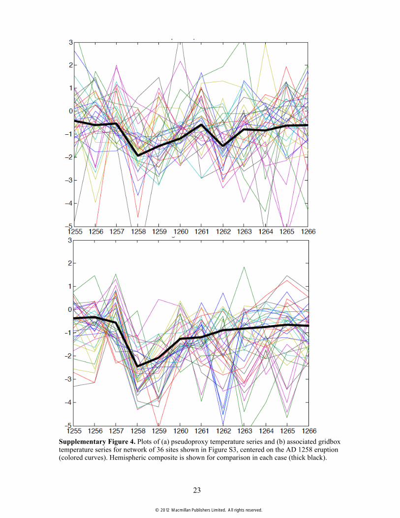
Figure S4 shows the pseudoproxy series for all 36 sites for an interval centered on the AD

1258 eruption for a particular realization from our ensemble of 100 which precisely

matches the r2=0.45 value of ref. 7. The corresponding actual gridbox temperatures are


11

shown for comparison. It is noteworthy that even for this very large eruption, the cooling

episode is not clearly discernible from the background noise for many of the 36

individual pseudoproxy temperature series, while it is easily discerned for the

hemispheric composite (i.e. CPS). In Figure S5, we show the CPS reconstruction for 18

different realizations that have r2 values (ranging between 0.440 and 0.459) closest to the

observed value r2=0.45, again in an interval centered on the AD 1258 eruption. We

observe little loss of signal variance in the CPS reconstruction, and moreover to the

extent that there is some minor loss of variance, it appears related to the restricted spatial

sampling and climate noise, rather than the proxy noise, since a simple composite of the

36 gridbox temperatures with no added proxy noise yields a very similar result to the

CPS reconstruction itself. These results arise from the fact that the signal-to-noise

characteristics of hemispheric composites are substantially greater than for individual

regional proxy records because of the tendency for cancellation of (proxy) noise in the

averaging across many proxies (see Figure S4a) and, secondarily, cancellation of intrinsic

climatic noise itself in a hemispheric mean (see Figure S4b).

These exercises thus establish two important conclusions that have a bearing on this

study:

1. It is necessary to evaluate hemispheric composites of proxy data to clearly detect the

interannual volcanic cooling signals of interest in this study. Individual regional proxy

series are unlikely to be adequate to detect the signals in question.

2. The signal variance lost due to the noise properties of the proxy data and/or statistical

compositing procedure used to form a hemispheric temperature reconstruction is at most

minor, and thus does not provide a viable explanation for the selective, substantial


12

underestimation of post-volcanic cooling seen in the tree-ring reconstruction analyzed in

our study (see Figure 2a of the main article)

VI. Implications for Proxy Reconstructions of Hemispheric Temperature

Nearly all well-validated proxy-based hemispheric temperature reconstructions (e.g. ref.

9 and 10 of the main article) make use of tree-ring data. Indeed, tree-ring data are the

only proxy data source available with hemispheric coverage and with annual resolution

over the past five centuries or more (see ref. 9 and 10 of main article).

While tree-ring growth thickness data form the basis of the analysis and discussion in the

main article, tree-ring density data with hemispheric coverage have also been used to

reconstruct Northern Hemisphere mean temperatures as far back as AD 14004-5. Though

tree-ring density measurements are governed by factors beyond those considered in our

biological growth model, they are subject to the same constraint that temperature-

sensitive records are confined to near-treeline boreal and alpine environments2. Thus,

some of the same biases discussed for tree-ring width measurements (e.g. the possibility

of vanishing or near-vanishing growth rings during cold years) likely apply. However,

hemispheric composites are only available back to AD 1400, and therefore do not reach

back to the critical 13th century for evaluating the response to the AD 1258/1259

eruption.

One of the most comprehensive estimates of Northern Hemisphere mean temperature

reaching back to AD 1200 using the variance-matching/“composite-plus-scale” approach


13

described in section 2 above is provided by ref. 10 of the main article. The reconstruction

was based on the set of essentially all temperature-sensitive proxy data available at

decadal or better resolution in the public domain (77 available in the Northern

Hemisphere back to AD 1200, of which 41 were tree-ring, and 36 are others such corals,

ice cores, sediments, and speleothems). The variance-matching approach was applied to

that network of multiproxy data to reconstruct hemispheric mean temperatures over the

past 1500 years. The resulting reconstruction shows a decadal-scale cooling associated

with the AD 1258 eruption (Figure S6), but it is greatly muted (only a couple tenths of a

degree C) relative to the expected (nearly 1C) decadal timescale cooling given the model-

simulated temperatures. Importantly, the same study found that a statistically verifiable

reconstruction was not possible prior to AD 1500 if tree-ring data were removed from the

network, i.e. tree-ring data were critical to obtaining a validated long-term decadal

timescale hemispheric temperature reconstruction given the available networks of proxy

data, using the variance-matching approach.

Thus, the biases identified in this study with regard to the limited sensitivity of tree-ring

records to the intense 1-2 oC cooling predicted for the largest eruptions of the past eight

centuries likely impact any hemispheric assessments of hemispheric, interannual

temperature changes over the past millennium, whether they are based on tree-ring data

exclusively (e.g. refs. 6-8 of main article), or a combination of tree-ring and other types

of proxy records such as e.g. sediments, corals, ice cores, and speleothems (e.g. refs. 9-10

of main article).

Determining the precise extent to which the potential biases identified in the current


14

study are present in ‘multiproxy’ reconstructions which use a mix of dendroclimatic and

non-dendroclimatic data (e.g. refs 9 and 10 of main article) remains an open question that

will require considerable additional work to address. The answers will depend on the

specific mix of data that was used in any particular study, and the relative weights that

the methods employed place on the different proxy climate records integrated to form a

reconstruction. While it is beyond the scope of this study to evaluate the impact of the

identified potential biases on existing hemispheric multiproxy reconstructions, such

issues represent fertile ground for future studies.

VII. Sensitivity Analyses—Climate Sensitivity and Forcings

Using the Energy Balance Model, we were able to assess the sensitivity of the results to

the assumed climate sensitivity, and various aspects (e.g. assumed scaling) of the

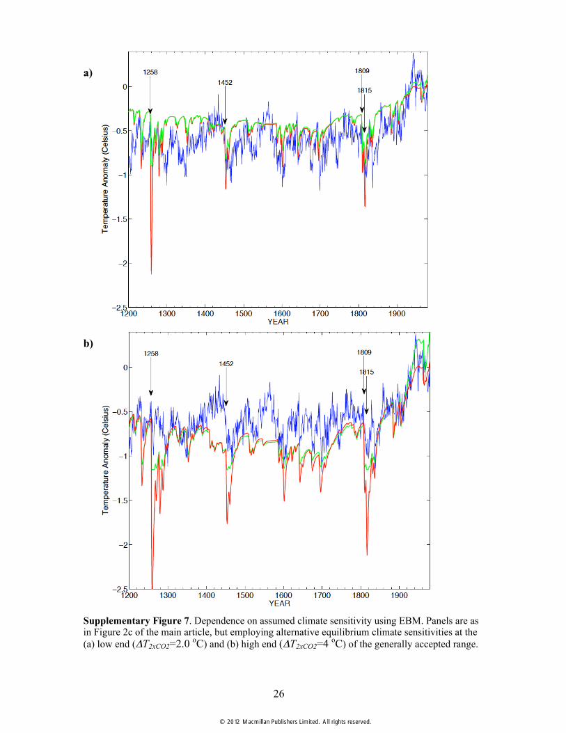
radiative forcing series used. Varying the climate sensitivity widely over the accepted

range (low-end value of ΔT2xCO2=2.0 oC and high end value of ΔT2xCO2=4 oC) leaves the

central conclusion (i.e. that the tree-growth response greatly underestimates the cooling

response to the largest few eruptions) unchanged (Figure S7), though clearly the default

sensitivity assumed in the main article (ΔT2xCO2=3.0 oC) yields a considerably closer

agreement with the tree-ring temperature reconstruction overall than do the higher or

lower sensitivity values.

The same conclusion holds when using a larger scaling (0.25% Maunder Minimum-

present rather than 0.1% as used in main article) of past solar irradiance variations

(Figure S8), using different volcanic aerosol loading estimates (Figure S9) and/or

different scalings (i.e. 2/3 power law dependence on aerosol loading) of volcanic


15

radiative forcing (Figure S10).

One noteworthy discrepancy is that the ref. 4 aerosol forcing chronology indicates two

very large 18th century eruptions (one in 1719 with forcing amplitude -4W/m2 and the

1783 Laki eruption in Iceland, with estimated forcing amplitude -8.3 W/m2). Neither

eruption is prominent in the radiative forcing estimates of either ref. 3 or ref. 13, and

there is no evidence of cooling at all in the tree-ring temperature reconstruction for either

eruption. If the ref. 4 volcanic forcing estimates were correct, this would represent a

conundrum that cannot be explained by our present analyses. Another noteworthy

discrepancy is that the considerably larger aerosol loadings of ref. 3 leads to numerous

extremely large (>-4W/m2) volcanic forcing events, which skews the overall amplitude of

variation in the simulated series. EBM simulations using this particular volcanic forcing

series consequently show the poorest correspondence with the tree-ring temperature

reconstruction (Figures S10c).

VIII. Sensitivity Analyses—Tree Growth Model Assumptions

Using the GCM simulation with stochastic weather forcing, we further investigated the

sensitivity of the results obtained with respect to various assumptions made regarding the

tree-growth model. We find that basic conclusions are once again robust with respect to

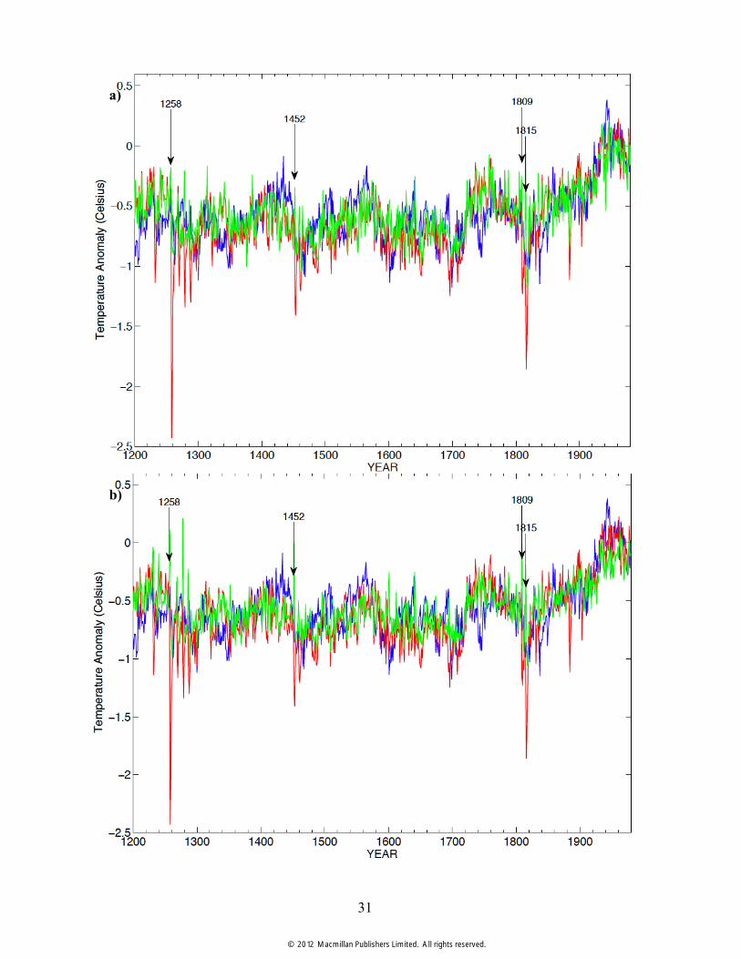
the precise choices made. Specifically, we get similar results (Figure S11) when (a) using

a substantially shorter (14 day) criterion for a ‘missing ring’ rather than the 26 day

criterion used in the main article, (b) Using a lower temperature threshold Tmin=7 oC for

tree growth rather than Tmin=10 oC threshold used in main article, and (c) using the

original Vaganov-Shashkin ‘trapezoidal’ functional form (p=1) for tree growth response


16

curve rather than the alternative (quadratic ramps) form (p=2) used in the main article.

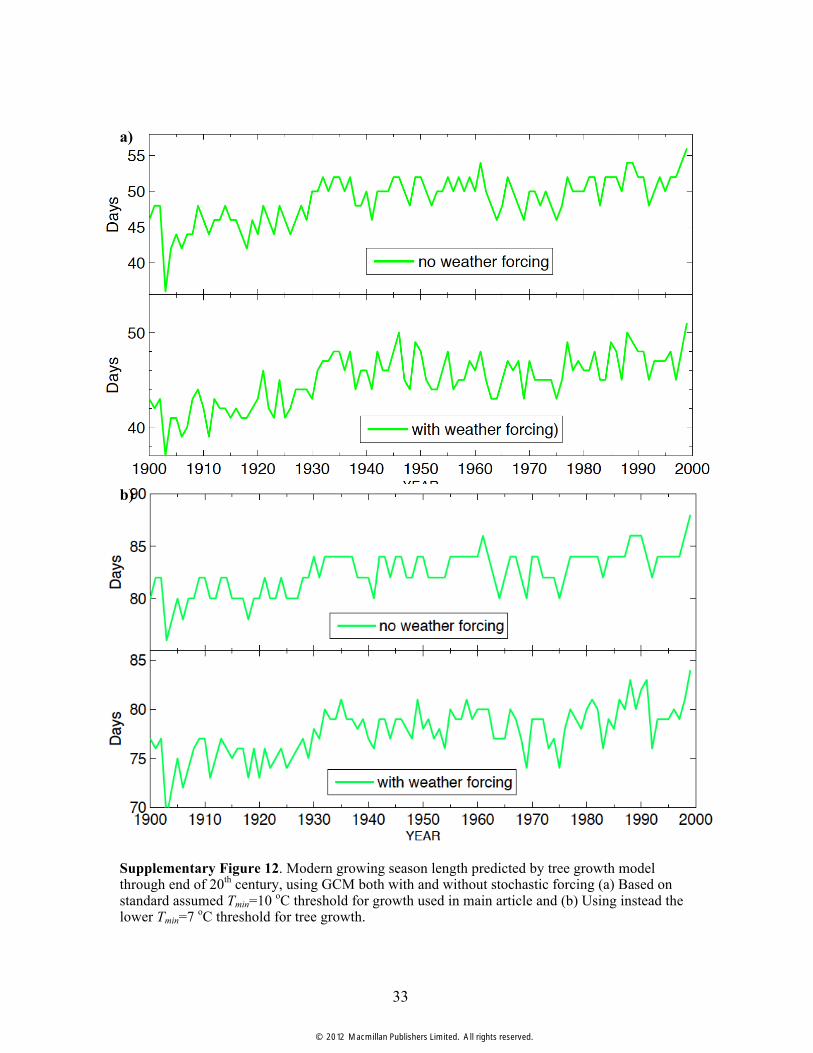
Regarding the choice of Tmin threshold, our default value for Tmin (10 oC) is higher than

the 5oC value used in ref. 17 of main article, though both values are consistent with the

observed range (5-10 oC) reported by ref. 19 of main article. Taking Tmin=10 oC, however,

gives more realistic estimates of mean modern (i.e. end of 20th century) growing season

lengths at treeline of 50-60 days as cited by ref. 20 of main article (see Figure S12a).

Even taking. Tmin=7 oC, for example gives an unrealistic estimate of 80-90 day modern

growing season lengths (see Figure S12b).

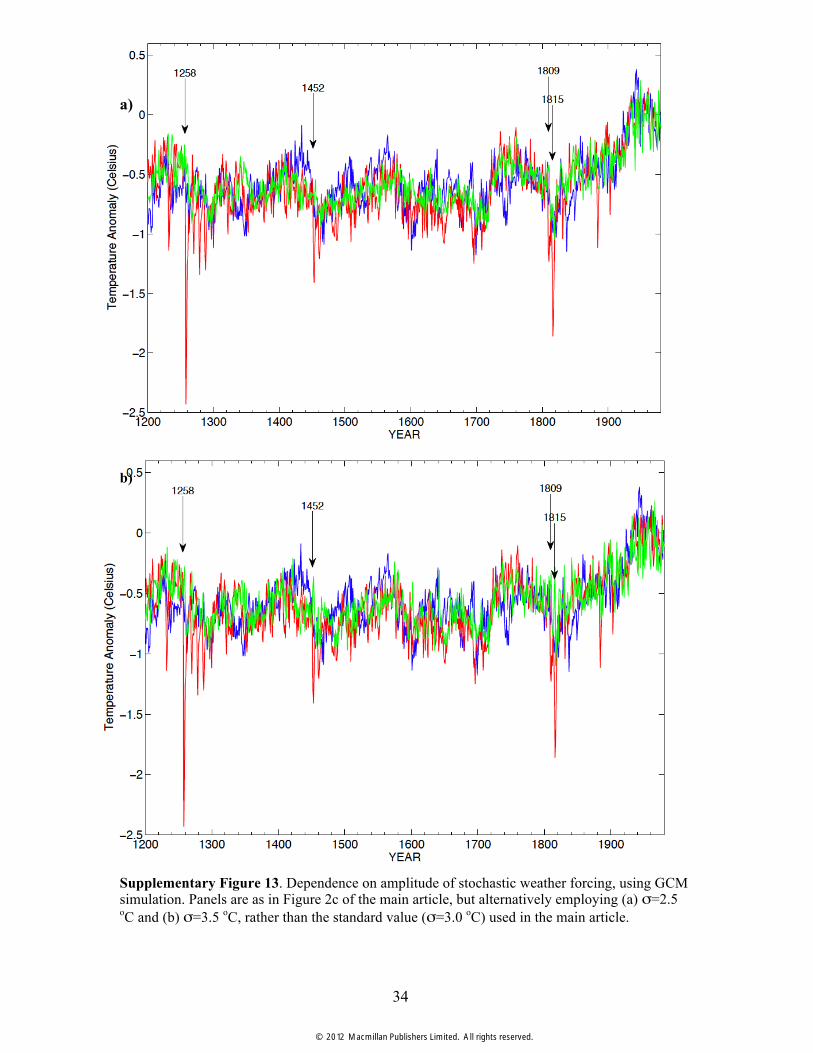
We found our results to be robust with respect to the precise amplitude of the stochastic

weather forcing used, with similar results obtained (Figure S13) regardless of the precise

choices made. Specifically, we observed very similar results employing both a

substantially lower value σ=2.5 oC (Figure S13a) and a substantially higher value σ=3.5

oC (Figure S13b) in place of the standard value (σ=3.0 oC) used in the main article.

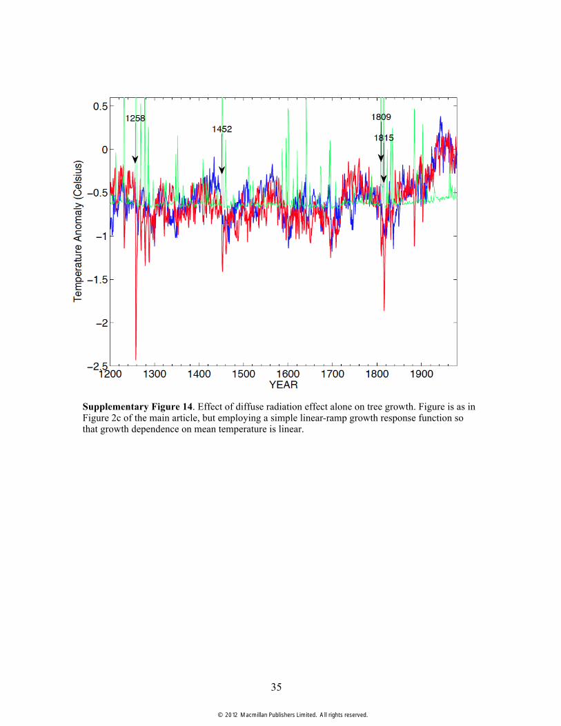
Finally, we demonstrate the insufficiency of the diffuse light effect alone, to explain the

features evidence in the tree-ring temperature composites. To explore the pure response

to the diffuse light effect, we assume a linear ramp temperature-dependent growth

function which is equivalent to the assumption of a purely linear dependence of growth

on temperature [we accomplish this by using linear (p=1) form of the Vaganov-Shashkin

growth function, and adopting a value Tmin=-40 oC that is lower than any temperatures

possible given the standard adopted seasonal temperature parameters, which insures that

the growth dependence on temperature is linear over the entire range of our analysis].


17

The only departure of growth, from a pure linear response to temperature to past

temperature variations, then, results from the diffuse light effect alone.

In the absence of a substantial cooling-induced cessation in growth from the eruption

(which arose before in our biological growth model from temperature threshold effects

which have now been eliminated), the positive impact of the increased diffuse radiation

associated with a substantial volcanic eruption now swamps any temperature-induced

decreases in growth, leading to huge growth response in the wake of the eruption that

dwarfs any volcanic cooling signal. Consequently, one now obtains a very unrealistic

growth series that shows no similarity at all to either the modeled temperatures series or

the actual tree-growth composites (Figure S14).

This behavior results from the fact that the increases in growth due to the diffuse light

effect are proportional in nature (amounting to a 30% increase in productivity/growth, for

each -2 W/m2 of forcing following ref. 2 of the main article). In the absence of any

substantial cooling-induced cessation in growth, then, these fractional increases in

productivity act on a substantially undiminished base growth, producing large absolute

increases in the growth index. The effect is so large that the growth model predicts

unrealistic positive growth responses in the first 1-2 years following an explosive

volcanic eruption that act not only to diminish, but indeed, reverse the signal of volcanic

cooling seen (if in a muted fashion) in the actual tree-ring composite series.

References


18

1. Wigley, T. M. L. & Raper, S. C. B. Natural variability of the climate system and

detection of the greenhouse effect. Nature 344, 324– 327 (1990).

2. Myhre, G., Highwood, E.J., Shine, K.P. & Stordal, F. New estimates of radiative

forcing due to well mixed greenhouse gases, Geophys. Res. Lett. 25, 2715-2718 (1998

3. Mann, M.E., Rutherford, S., Wahl, E., Ammann, C., Robustness of Proxy-Based

Climate Field Reconstruction Methods, J. Geophys. Res., 112, D12109, doi:

10.1029/2006JD008272, 2007.

4. Briffa, K. R., et al., Reduced sensitivity of recent tree-growth to temperature at high

northern latitudes, Nature, 391, 678–682, 1998.

5. Briffa, K. R. et al., Low-frequency temperature variations from a northern tree ring

density network, J. Geophys. Res., 106, 2929–2941, 2001.


19

SUPPLEMENTARY FIGURES


20

a)

b)

Supplementary Figure 1. Details of the biological growth model. (a) Relative tree growth curve as a function of temperature (blue: default value p=2; green; p=1. (b) Seasonal temperature cycle for 1961-1990 reference period (thick=non stochastic forcing; thin is with stochastic forcing) shown with lower temperature threshold (black dashed) for growth (Tmin=10 oC).


21

Supplementary Figure 2. Estimate of residual unforced variability based on (i) tree-ring reconstruction minus EBM-simulated temperature series (blue) and (ii) GCM-simulated temperature series minus EBM-simulated temperature series (green). ±1 and ±2 sigma limits for series (i) are shown by horizontal dashed curves.


22

Supplementary Figure 3. Spatial distribution of pseudoproxy series used in tests of statistical compositing procedure. The network mimics that of D’Arrigo et al. (ref. 7) with some differences noted in text.


23

Supplementary Figure 4. Plots of (a) pseudoproxy temperature series and (b) associated gridbox temperature series for network of 36 sites shown in Figure S3, centered on the AD 1258 eruption (colored curves). Hemispheric composite is shown for comparison in each case (thick black).


24

Supplementary Figure 5. Plots of 18 different pseudoproxy CPS hemispheric temperature reconstructions (thin colored curves; the unique realization that was shown in Fig. 2a of main article is shown here as thick blue curve) as described in supplementary text, compared with actual hemispheric mean temperature (thick red). Shown for comparison is a simple composite of the 36 pseudoproxy gridbox temperature series with no added noise (thick black). The modest underestimation of the post AD 1258 cooling in that series (and by implication, a very similar pattern in the various pseudoproxy CPS series) is due to the spatial sampling of the network of 36 sites, rather than e.g. noise properties of proxy data.


25

Supplementary Figure 6. Reconstruction of Northern Hemisphere mean land temperatures based on a variance-matching/composite-plus-scale (‘CPS’) paleoclimate reconstruction approach applied to a global network of proxy data (tree-rings, corals, ice cores, sediments, and speleothems). Two different versions (based on different target instrumental NH mean temperature series) and the average (‘composite’) are shown, along with estimated 95% confidence interval (yellow shading). The cooling response to the AD 1258 eruption is smeared out in time by the implicit decadal smoothing of the reconstruction, but is clearly evident, albeit much reduced relative to the climate model-predicted cooling.


26

a)

b)

Supplementary Figure 7. Dependence on assumed climate sensitivity using EBM. Panels are as in Figure 2c of the main article, but employing alternative equilibrium climate sensitivities at the (a) low end (ΔT2xCO2=2.0 oC) and (b) high end (ΔT2xCO2=4 oC) of the generally accepted range.


27

Supplementary Figure 8. Dependence on scaling of solar irradiance using EBM. Figure is as in Figure 2c of the main article, but employing a larger (0.25% Maunder Minimum-present) change in solar irradiance than the default value used in the main article (0.1%).


28

Supplementary Figure 9. Dependence on volcanic aerosol loading employed (assuming linear scaling of radiative forcing with dust loading) using EBM. Figure is as in Figure 2c of the main article, but employing the alternative volcanic aerosol loading series of ref. 4 rather than the ref. 3 estimate used in main article.


29

a) b)


30

c) Supplementary Figure 10. Dependence on volcanic aerosol loading estimates used assuming a 2/3 power law scaling of radiative forcing with dust loading, using EBM. Panels are as in Figure 2c of the main article, but employing (a) alternative 2/3 power law scaling with ref. 3 aerosol loading estimate, (b) 2/3 power law scaling with ref. 18 aerosol loading estimate and (c) ref. 13 radiative forcing estimate (which already assumes a 2/3 power law scaling).


31

a) b)


32

c) Supplementary Figure 11. Dependence on various details of the tree growth model, using GCM simulation and standard (σ=3.0 oC) stochastic weather forcing. Panels are as in Figure 2c of the main article, but employing (a) 14 day criterion for a ‘missing ring’ rather than the 26 day criterion used in the main article, (b) Tmin=7 oC lower threshold for tree growth rather than Tmin=10 oC threshold used in main article, (c) Original Vaganov-Shashkin linear functional form (p=1) for tree growth response curve rather than quadratic form (p=2) used in main article.


33

a) b) Supplementary Figure 12. Modern growing season length predicted by tree growth model through end of 20th century, using GCM both with and without stochastic forcing (a) Based on standard assumed Tmin=10 oC threshold for growth used in main article and (b) Using instead the lower Tmin=7 oC threshold for tree growth.


34

a) b) Supplementary Figure 13. Dependence on amplitude of stochastic weather forcing, using GCM simulation. Panels are as in Figure 2c of the main article, but alternatively employing (a) σ=2.5 oC and (b) σ=3.5 oC, rather than the standard value (σ=3.0 oC) used in the main article.


35

Supplementary Figure 14. Effect of diffuse radiation effect alone on tree growth. Figure is as in Figure 2c of the main article, but employing a simple linear-ramp growth response function so that growth dependence on mean temperature is linear.


supplementary information - · pdf filethe details of the ncar csm 1.4 climate model and the...

Documents