climate change and its causes: a discussion about some · pdf fileclimate change and its...

Climate Change and Its Causes:A Discussion about Some Key IssuesNicola Scafetta, Duke University

At the Environmental Protection Agency, Feb/26/2009

Global Surface Temperature (CRU)

Disclaimer (added by EPA)

This presentation by Dr. Nicola Scafetta on February 26, 2009 has neither been reviewed nor approved by the U.S. Environmental Protection Agency. The views expressed by the presenter are entirely his own. The contents do not necessarily reflect the views or policies of the U.S. Environmental Protection Agency, nor does mention of trade names or commercial products constitute endorsement or recommendation for use.

Scafetta, EPA 2009

● Climate Network and Topology ?The IPCC climate “structure” overestimates the human contribution to climate change.

● Total Solar Irradiance ? The TSI likely increased from 1980 to 2002 contrary to the IPCC assumptions.�Evidences that the ACRIM TSI composite is more accurate than the PMOD are presented.�

● Global Temperatures ?The Hockey Stick temperature by Mann has likely misled the GW debate. More recent�paleoclimate temperature reconstructions present a much larger pre-industrial variability�which better agrees with historical records.�

● Climate Models ? IPCC climate models fail to reproduce the climate variability before 1960 and greatly�disagree with the empirical studies evaluating the 11-year solar signature on climate.�Limitations of the multi-linear regression climate models are discussed.�

● Missing Feedbacks and/or Climate Forcings ?A phenomenological climate model studied to overcome the limitations of the current�science is presented. The model well predicts centuries of climate change.�

● Future: Warming or Imminent Cooling ?A forecast of climate change based on the solar system planetary motion is presented. The model appears to reconstruct with great accuracy the observed climate change since 1850 and predicts a cooling until 2030-2040. The physical mechanisms are unknown.

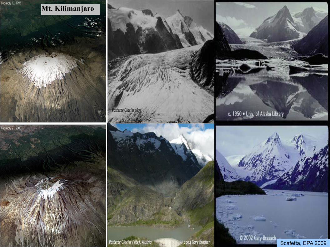
Mt. Kilimanjaro

Scafetta, EPA 2009

IPCC 2007 interpretation of the climate network

?

Scafetta, EPA 2009

Onlyhumans can changeGHGs !

Scafetta, EPA 2009

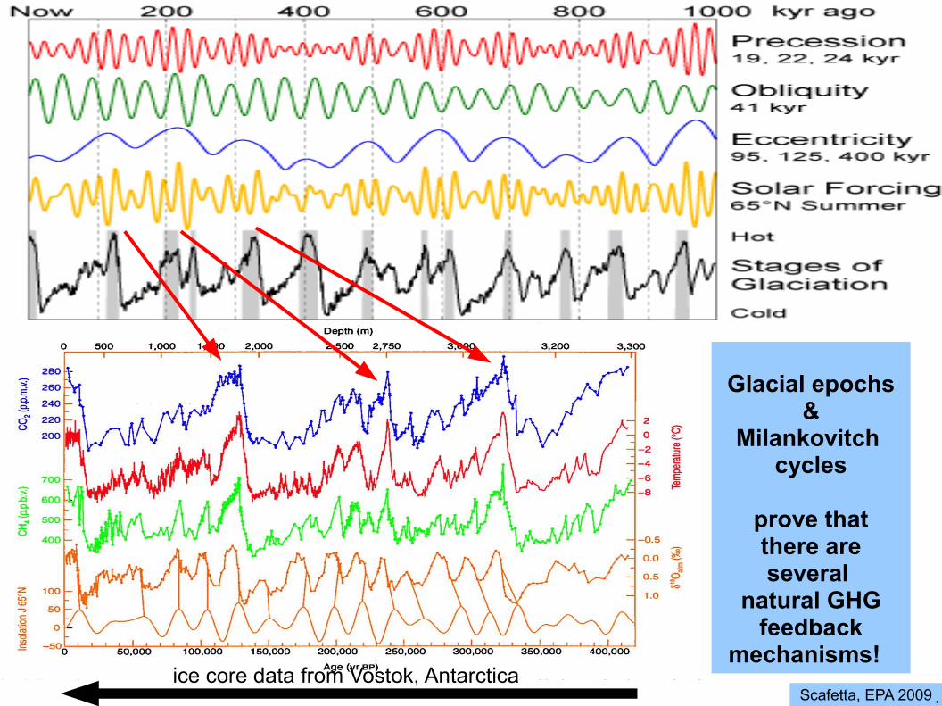
ice core data from Vostok, Antarctica

Glacial epochs&

Milankovitch cycles

prove thatthere are several

natural GHG feedback

mechanisms!�Scafetta, EPA 2009�

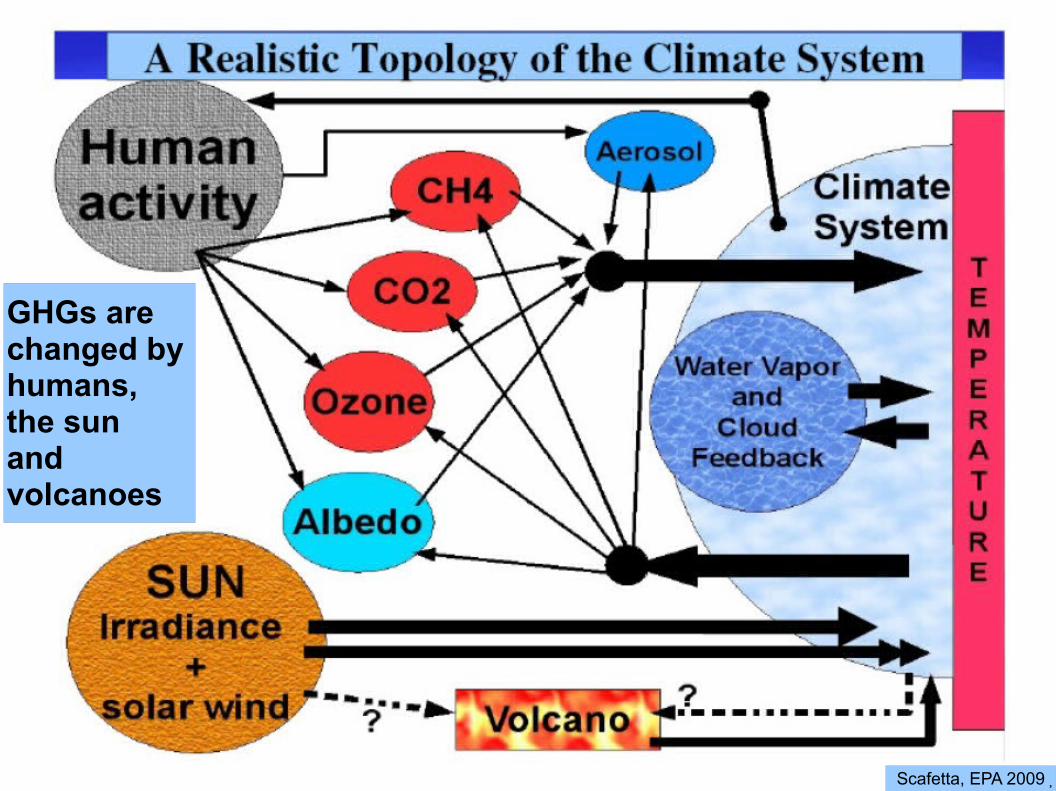
GHGs are changed byhumans, the sun and volcanoes

Scafetta, EPA 2009�

Cosmic ray protons blast nuclei in the upper atmosphere, producing neutrons which in turn bombard nitrogen, the major constituent of the atmosphere . This neutron bombardment produces the radioactive isotope carbon-14. Cosmic ray are modulated by solar wind.

Eddy J.A. (1976), The MaunderMinimum, Science 192, 1189-1202.

Secular correlation between solar and climate records

Scafetta, EPA 2009

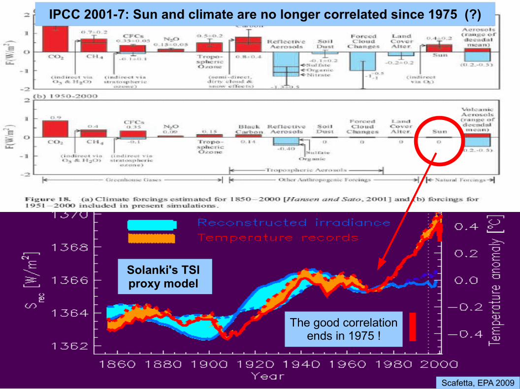
IPCC 2001-7: Sun and climate are no longer correlated since 1975 (?)

Solanki's TSI proxy model

The good correlation ends in 1975 !

Scafetta, EPA 2009

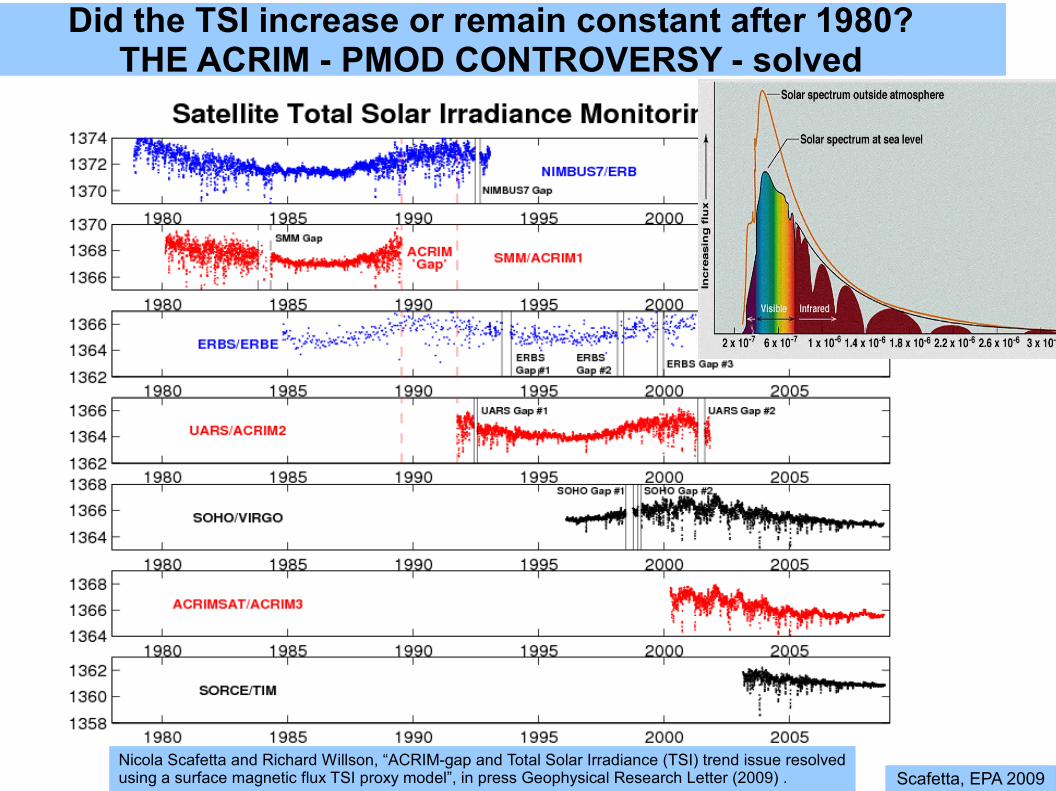
Did the TSI increase or remain constant after 1980?�THE ACRIM - PMOD CONTROVERSY - solved�

Nicola Scafetta and Richard Willson, “ACRIM-gap and Total Solar Irradiance (TSI) trend issue resolved using a surface magnetic flux TSI proxy model”, in press Geophysical Research Letter (2009) . Scafetta, EPA 2009

Scafetta, EPA 2009

Scafetta, EPA 2009

ACRIM team claims that ERBS/ERBE degraded during the ACRIM-gap because during this time ERBS sensors were experiencing the large high frequency solar irradiance for the first time. ERBS also clearly degraded in 1984-1986 when its mission started.

Comparison among TSI Data, Composites and a Proxy reconstruction

1 2

Nimbus7

ACRIM1

ACRIM

PMOD

PMOD team claims that Nimbus7 is corrupted because disagrees with some TSI proxy reconstruction predictions in particular during the periods 1 and 2 (LEAN's 2005, TSI proxy model is the black smooth line).

ACRIM GAP

Scafetta, EPA 2009

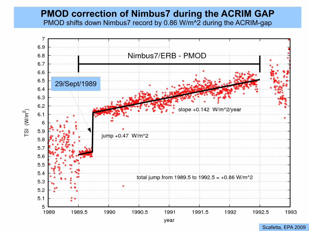
PMOD correction of Nimbus7 during the ACRIM GAPPMOD shifts down Nimbus7 record by 0.86 W/m^2 during the ACRIM-gap

29/Sept/1989

Scafetta, EPA 2009

The above statement is included in Scafetta and Willson, GRL 2009 Supporting Material

Scafetta, EPA 2009

The TSI experimental teams disagree with PMOD

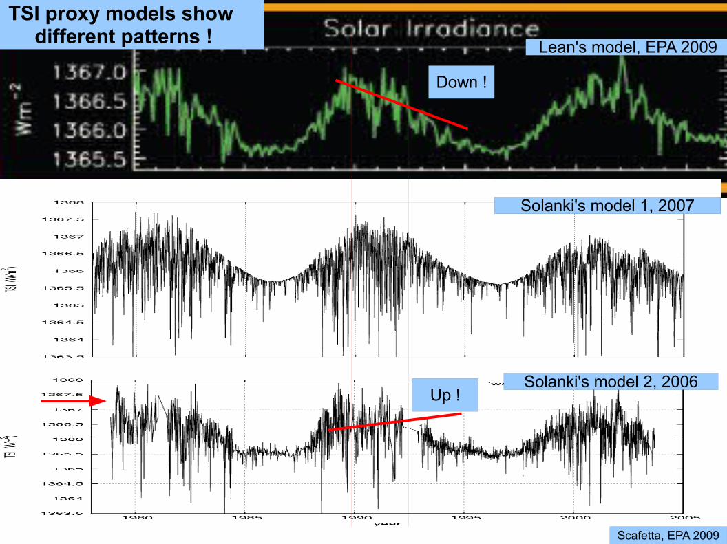
Lean's model, EPA 2009

Solanki's model 1, 2007

Solanki's model 2, 2006

Scafetta, EPA 2009

Down !

Up !

TSI proxy models show different patterns !

Mixed mode TSI composite ACRIM and KBS07 TSI proxy model Scafetta N. and R. C. Willson, 2009, ACRIM-gap and TSI trend issue resolved using a surface magnetic flux TSI proxy model, in press on GRL Krivova N. A., L. Balmaceda, and S. K. Solanki, 2007, Reconstruction of solar total irradiance since 1700 from the surface magnetic flux: Astronomy and Astrophysics, v. 467, p. 335-346.

Scafetta, EPA 2009

Mixed mode TSI composite ACRIM and KBS07 TSI proxy model Scafetta N. and R. C. Willson, 2009, ACRIM-gap and TSI trend issue resolved using a surface magnetic flux TSI proxy model, in press on GRL Krivova N. A., L. Balmaceda, and S. K. Solanki, 2007, Reconstruction of solar total irradiance since 1700 from the surface magnetic flux: Astronomy and Astrophysics, v. 467, p. 335-346.

KBS07 TSI proxy model contradicts PMOD corrections of Nimbus7 and confirms ACRIM claims of a significant degradation of ERBS during theACRIM-gap


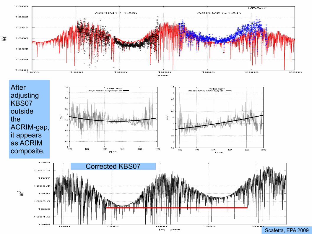
After adjusting KBS07 outside the ACRIM-gap, it appears as ACRIM composite.

Corrected KBS07

Scafetta, EPA 2009

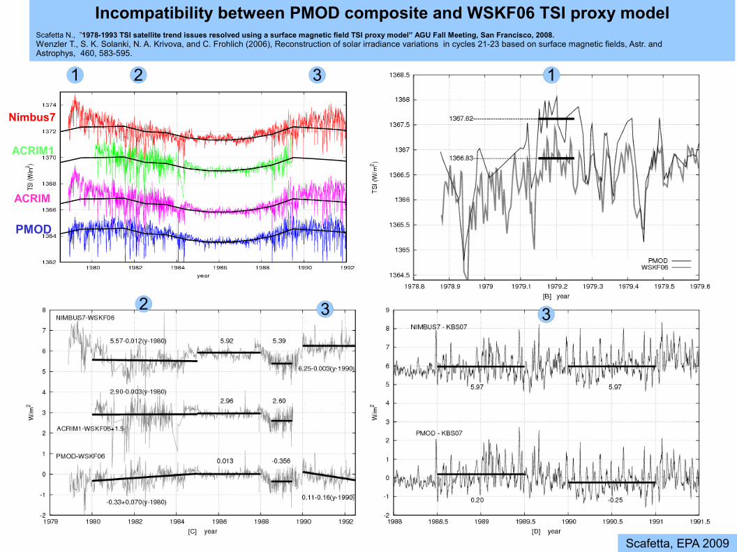
Incompatibility between PMOD composite and WSKF06 TSI proxy model Scafetta N., ”1978-1993 TSI satellite trend issues resolved using a surface magnetic field TSI proxy model” AGU Fall Meeting, San Francisco, 2008. Wenzler T., S. K. Solanki, N. A. Krivova, and C. Frohlich (2006), Reconstruction of solar irradiance variations in cycles 21-23 based on surface magnetic fields, Astr. and Astrophys, 460, 583-595.

Nimbus7

ACRIM1

ACRIM

PMOD

1 2 13

332

Scafetta, EPA 2009

Incompatibility between the 1995-2007 TSI composites and Lean's TSI proxy model Scafetta N., EPA, presentation February 2009. From Judith Lean, presentation at the EPA meeting January 2009

0.4

Lean's model

Scafetta, EPA 2009

KBS07 T SI proxy model is corrected since 1 980 w ith three p ossible T SI composites compatible w ith [A] Nimbus7, [C] ERBS, [B] average. The T SI during the last decades has been the largest in four centuries [Scafetta, 2009 in press, GSA Special Paper on Global Climate Change]

Scafetta, EPA 2009

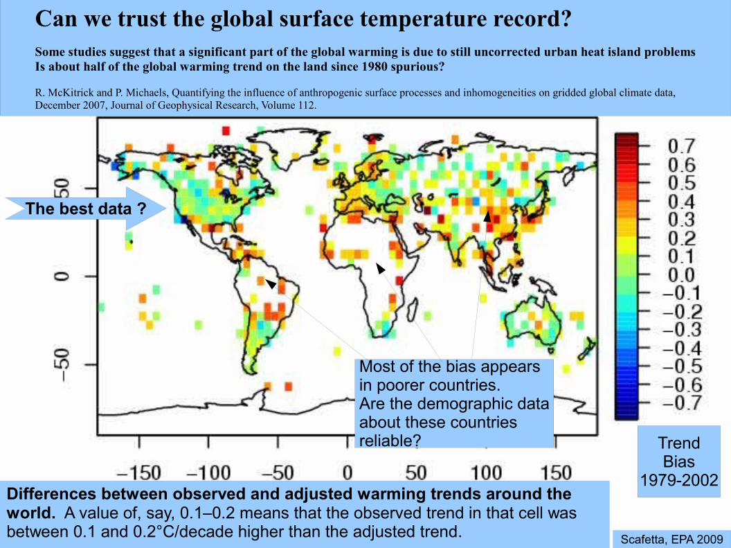
Can we trust the global surface temperature record? Some studies suggest that a significant part of the global warming is due to still uncorrected urban heat island problems Is about half of the global warming trend on the land since 1980 spurious?

R. McKitrick and P. Michaels, Quantifying the influence of anthropogenic surface processes and inhomogeneities on gridded global climate data, December 2007, Journal of Geophysical Research, Volume 112.

The best data ?

Most of the bias appears in poorer countries. Are the demographic data about these countries reliable?

Differences between observed and adjusted warming trends around the world. A value of, say, 0.1–0.2 means that the observed trend in that cell was between 0.1 and 0.2°C/decade higher than the adjusted trend.

Trend Bias

1979-2002

Scafetta, EPA 2009

GISS Surface�Temperature Analysis�

US temp. record suggests thatthe current warming period issimilar to the warming in the 30s!

Did the 20th century havetwo warming periods?

Scafetta, EPA 2009

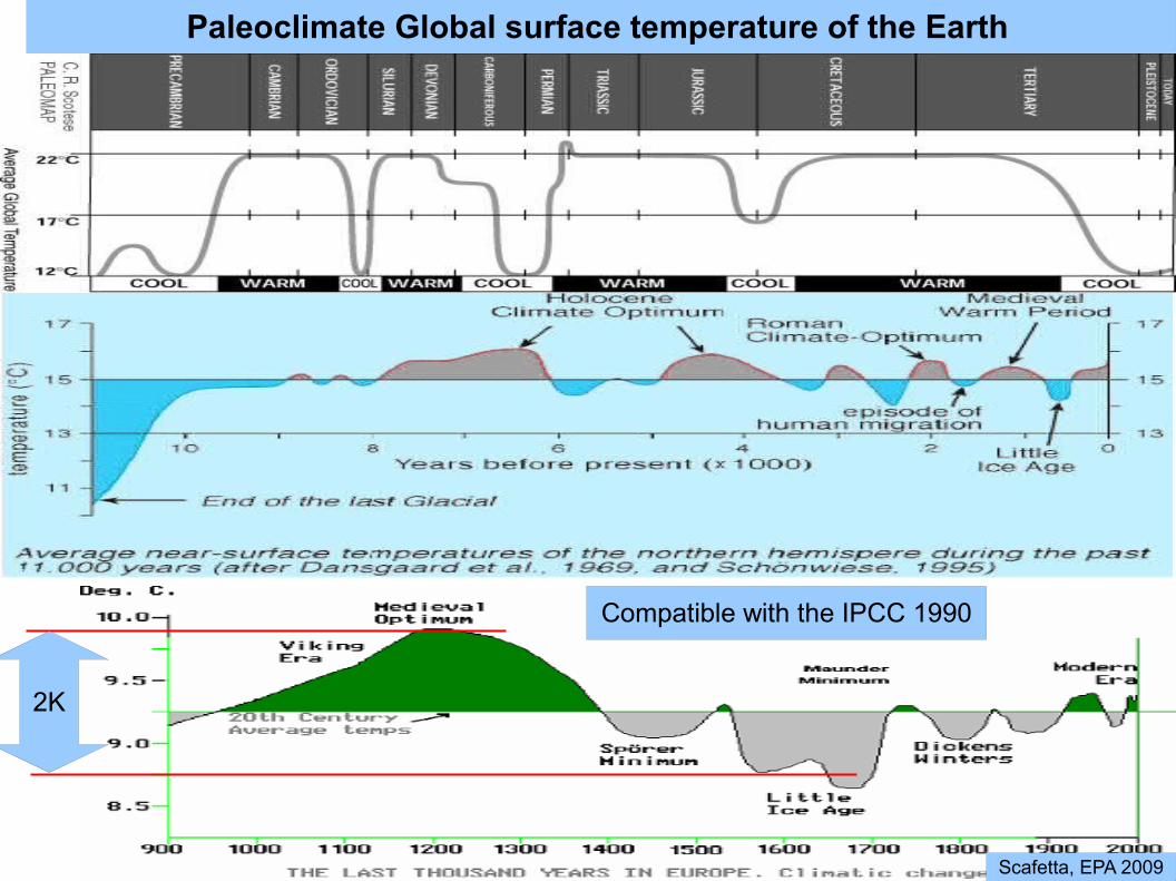
Paleoclimate Global surface temperature of the Earth

Compatible with the IPCC 1990

2K

Scafetta, EPA 2009

1/1/1990 1/1/1999

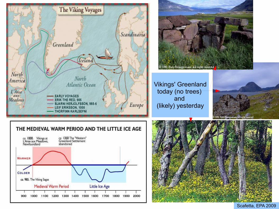
Vikings' Greenland today (no trees)

and (likely) yesterday

Scafetta, EPA 2009

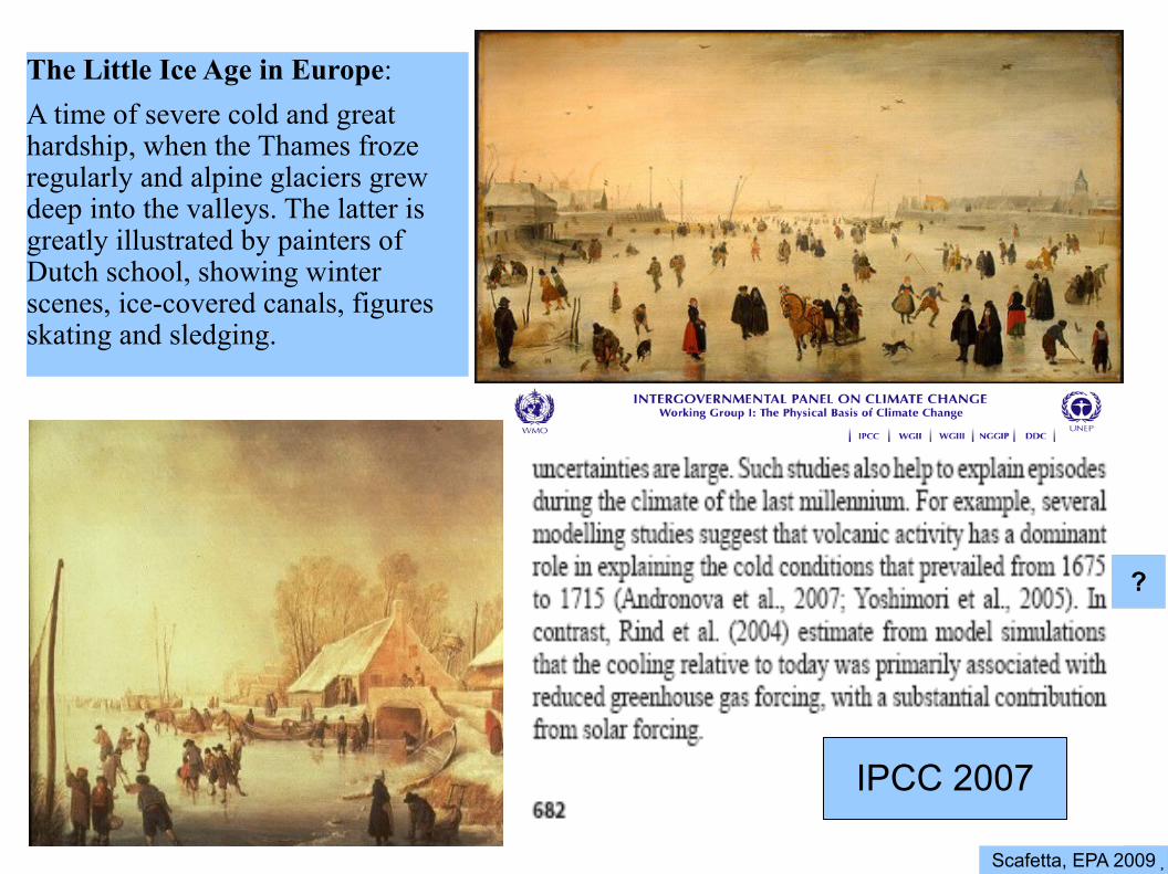
The Little Ice Age in Europe: A time of severe cold and great hardship, when the Thames froze regularly and alpine glaciers grew deep into the valleys. The latter is greatly illustrated by painters of Dutch school, showing winter scenes, ice-covered canals, figures skating and sledging.

IPCC 2007

?


The “Hockey Stick” temperature (Mann, Bradley, Hughes 1998).This record surprised the scientific community because the preindustrial climate (<1900)�varies 5-10 times less than what was previously expected!�

0.2


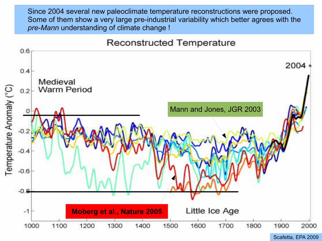
Since 2004 several new paleoclimate temperature reconstructions were proposed. Some of them show a very large pre-industrial variability which better agrees with the pre-Mann understanding of climate change !

Moberg et al., Nature 2005

Mann and Jones, JGR 2003

Scafetta, EPA 2009

Both Loehle (2008) and Moberg (2005) reconstructions show a large preindustrial variability because tree ring records are NOT used for the secular reconstruction!

Tree growth may be characterized by non-linear behavior that reduces their secular variability. (biological adaptation and water dependency)

Loehle and McCulloch, E & E, 2008

1.0 K

Scafetta, EPA 2009

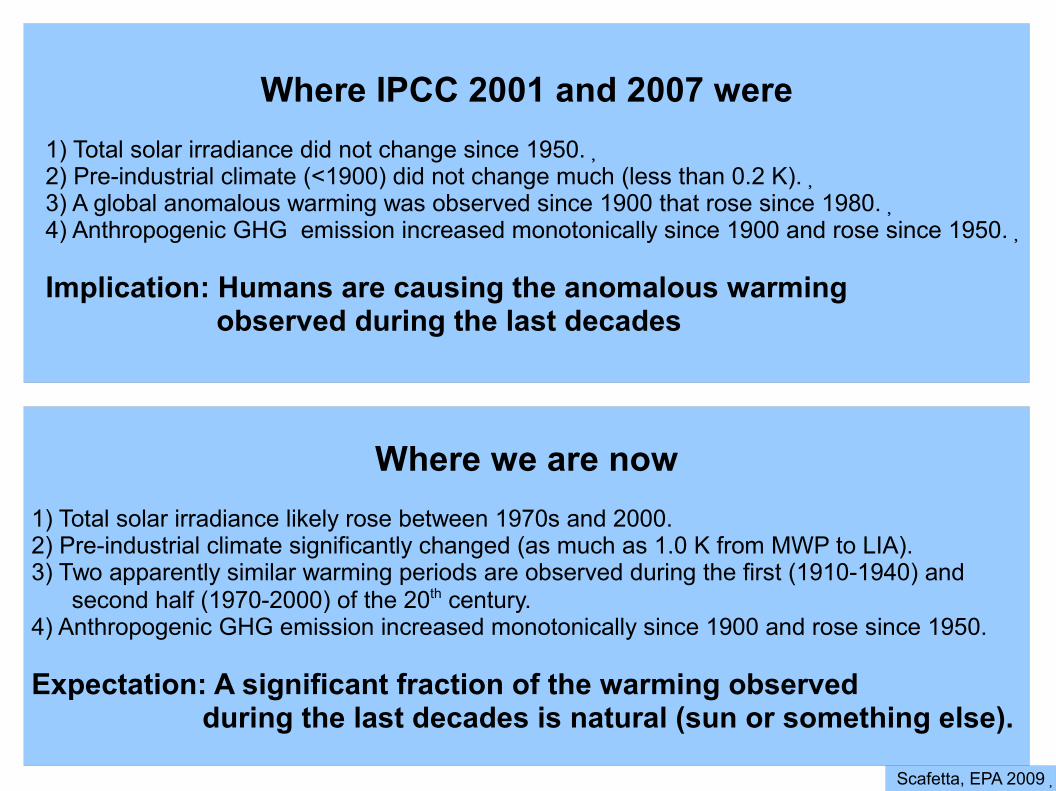
Where IPCC 2001 and 2007 were�

1) Total solar irradiance did not change since 1950.�2) Pre-industrial climate (<1900) did not change much (less than 0.2 K).�3) A global anomalous warming was observed since 1900 that rose since 1980.�4) Anthropogenic GHG emission increased monotonically since 1900 and rose since 1950.�

Implication: Humans are causing the anomalous warming�observed during the last decades�

Where we are now�

1) Total solar irradiance likely rose between 1970s and 2000. 2) Pre-industrial climate significantly changed (as much as 1.0 K from MWP to LIA). 3) Two apparently similar warming periods are observed during the first (1910-1940) and

second half (1970-2000) of the 20th century. 4) Anthropogenic GHG emission increased monotonically since 1900 and rose since 1950.

Expectation: A significant fraction of the warming observed during the last decades is natural (sun or something else).


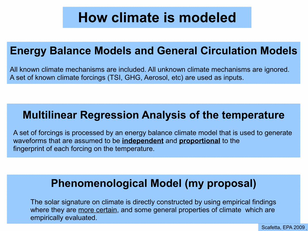
How climate is modeled�

Energy Balance Models and General Circulation Models�

All known climate mechanisms are included. All unknown climate mechanisms are ignored. A set of known climate forcings (TSI, GHG, Aerosol, etc) are used as inputs.

Multilinear Regression Analysis of the temperature�

A set of forcings is processed by an energy balance climate model that is used to generate waveforms that are assumed to be independent and proportional to the fingerprint of each forcing on the temperature.

Phenomenological Model (my proposal)�The solar signature on climate is directly constructed by using empirical findings where they are more certain, and some general properties of climate which are empirically evaluated.


Energy balance model simulation�

Crowley, Science 289, 270-277 (2000)

Mann's temp

Input forcings

Output temp. signatures


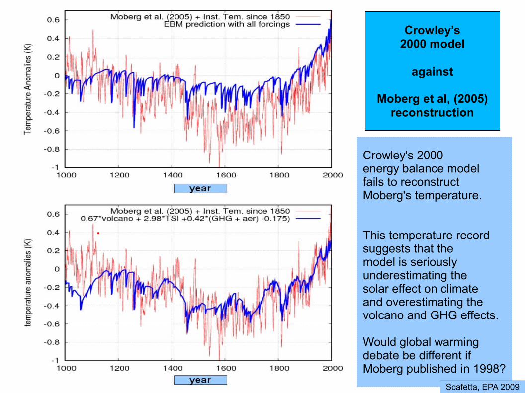
Crowley’s 2000 model

against

Moberg et al, (2005) reconstruction

Crowley's 2000 energy balance model fails to reconstruct Moberg's temperature.

This temperature record suggests that the model is seriously underestimating the solar effect on climate and overestimating the volcano and GHG effects.

Would global warming debate be different if Moberg published in 1998?

Scafetta, EPA 2009

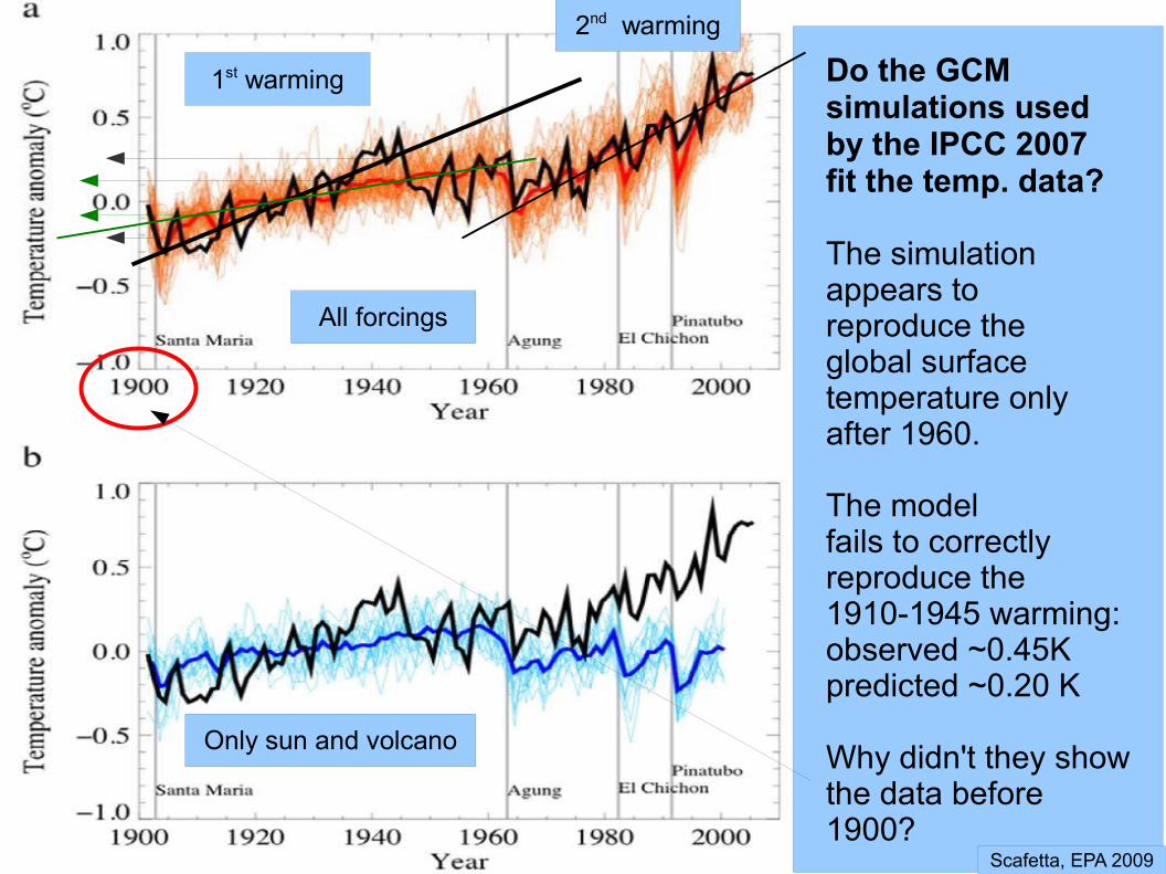
1st warming

2nd warming

Only sun and volcano

All forcings

Do the GCM simulations used by the IPCC 2007 fit the temp. data?

The simulation appears to reproduce the global surface temperature only after 1960.

The model fails to correctly reproduce the 1910-1945 warming: observed ~0.45K predicted ~0.20 K

Why didn't they show the data before 1900?

Scafetta, EPA 2009

cooling ?

Surf. Temp. Data – Model comparison

warming cooling warming cooling warming

GISS modelE (blue) fails to reproduce the climate variability before 1960

Hansen et al. “Climate simulations for 1880–2003 with GISS ModelE,” Clim Dyn (2007) 29:661–696�


Are these IPCC 2007 theoretical projections reliable?

Failure to reproduce the climate variability before 1960

Runaway Global Warming: will the Earth's

become like Venus?

Failure to reproduce the cooling after 2002

Scafetta, EPA 2009

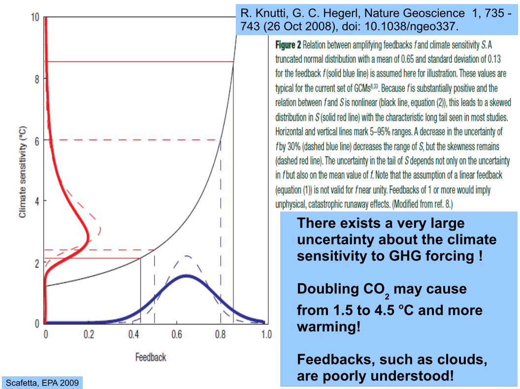
R. Knutti, G. C. Hegerl, Nature Geoscience 1, 735 - 743 (26 Oct 2008), doi: 10.1038/ngeo337.

There exists a very large uncertainty about the climate sensitivity to GHG forcing !

Doubling CO2 may cause

from 1.5 to 4.5 oC and more warming!

Feedbacks, such as clouds, are poorly understood! Scafetta, EPA 2009

Multilinear regression analysis models�The basic idea is that traditional climate models are incomplete. The contribution of the forcings to climate change is statistically evaluated under minimal assumptions such as linearity and mutual independence of the climate forcings.

The temperature is assumed to be the linear superposition of the several waveforms functions “T

f(t)” that are the

temperature fingerprint prototypes generated by a given forcing “f(t)”.

The waveform functions are calculated with an energy balance model (EBM).

The coefficient “af” are the amplification

factors:

If “af=1” then the EBM is fine! (North, Hegerl etc.)

The temperature is assumed to be the linear superposition of the several forcing functions “f(t)” shifted with a time-lag “l” . This functions are assumed to be the temperature fingerprint prototypes of a given forcing “f(t)”.

The coefficient “bf” are the scaling factors.

(Lean, Douglass, Gleisner, etc.)

T t =∑ a f T f t T t =∑ b f f t−l A B

Scafetta, EPA 2009

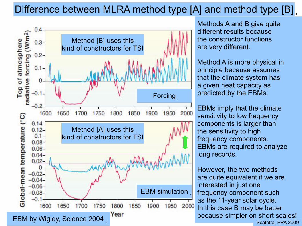
Difference between MLRA method type [A] and method type [B]�

Method [B] uses this�kind of constructors for TSI�

Method [A] uses this�kind of constructors for TSI�

Forcing�

Methods A and B give quite different results because the constructor functions are very different.

Method A is more physical in principle because assumes that the climate system has a given heat capacity as predicted by the EBMs.

EBMs imply that the climate sensitivity to low frequency components is larger than the sensitivity to high frequency components. EBMs are required to analyze long records.

However, the two methods are quite equivalent if we are interested in just one frequency component such as the 11-year solar cycle. In this case B may be better because simpler on short scales!

Scafetta, EPA 2009

EBM simulation�

EBM by Wigley, Science 2004�

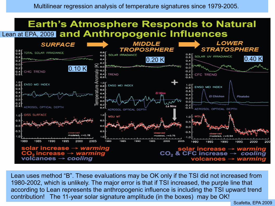
Multilinear regression analysis of temperature signatures since 1979-2005.

Lean uses method “B”. These evaluations may be OK only if the TSI did not increased from 1980-2002, which is unlikely. The major error is that if TSI increased, the purple line that according to Lean represents the anthropogenic influence is including the TSI upward trend contribution! The 11-year solar signature amplitude (in the boxes) may be OK!

0.10 K 0.20 K 0.40 K

Scafetta, EPA 2009

Lean at EPA, 2009

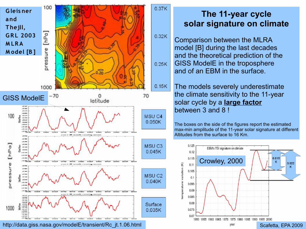
The 11-year cycle solar signature on climate

Comparison between the MLRA model [B] during the last decades and the theoretical prediction of the GISS ModelE in the troposphere and of an EBM in the surface.

The models severely underestimate the climate sensitivity to the 11-year solar cycle by a large factorbetween 3 and 8 !

The boxes on the side of the figures report the estimated max-min amplitude of the 11-year solar signature at different Altitudes from the surface to 16 Km.

GISS ModelE

G leis ner a nd T hejll, G R L 2003 M LR A M odel [B ]

Crowley, 2000

Scafetta, EPA 2009 http://data.giss.nasa.gov/modelE/transient/Rc_jt.1.06.html

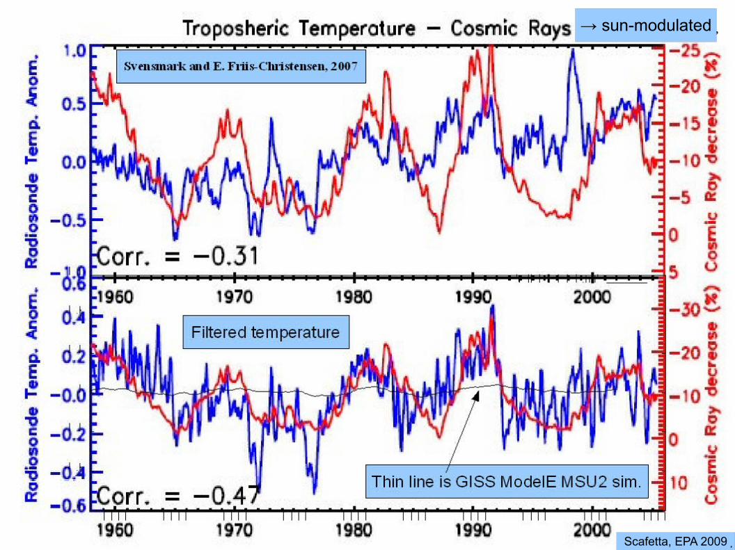
→ sun-modulated�


CLIMATE RESPONSE to the 11-YEAR SOLAR CYCLE

IPCC 2007, page 674

IPCC 2007 contradicts itself by on one side acknowledging the above empirical studies and on the other side using climate models whose predictions are contradicted by these same empirical studies !

Scafetta, EPA 2009

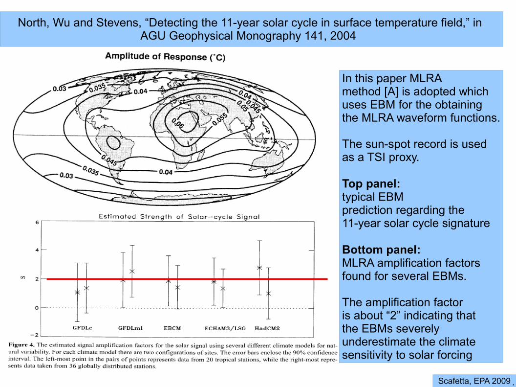
North, Wu and Stevens, “Detecting the 11-year solar cycle in surface temperature field,” in AGU Geophysical Monography 141, 2004

In this paper MLRA method [A] is adopted which uses EBM for the obtaining the MLRA waveform functions.

The sun-spot record is used as a TSI proxy.

Top panel: typical EBM prediction regarding the 11-year solar cycle signature

Bottom panel: MLRA amplification factors found for several EBMs.

The amplification factor is about “2” indicating that the EBMs severely underestimate the climate sensitivity to solar forcing


Hegerl G. C., Crowley T. J., Allen M., et al, (2007), Detection of human influence on a new,�validated 1500-year temperature reconstruction, J. of Climate 20, 650-666.�

This paper uses MLRA method [A] applied to long sequences.

The amplification factors relative to the solar component is severely suspicious because ranges from negative to large positive values.

MLRA is not appropriate because of the uncertainty in the secular data and the lack of independence between the forcings on this large scale.

Scafetta, EPA 2009

Scafetta, EPA 2009

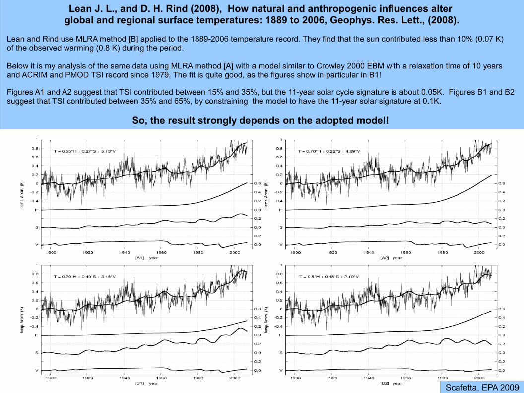
Lean J. L., and D. H. Rind (2008), How natural and anthropogenic influences alter global and regional surface temperatures: 1889 to 2006, Geophys. Res. Lett., (2008).

Lean and Rind use MLRA method [B] applied to the 1889-2006 temperature record. They find that the sun contributed less than 10% (0.07 K) of the observed warming (0.8 K) during the period.

Below it is my analysis of the same data using MLRA method [A] with a model similar to Crowley 2000 EBM with a relaxation time of 10 years and ACRIM and PMOD TSI record since 1979. The fit is quite good, as the figures show in particular in B1!

Figures A1 and A2 suggest that TSI contributed between 15% and 35%, but the 11-year solar cycle signature is about 0.05K. Figures B1 and B2 suggest that TSI contributed between 35% and 65%, by constraining the model to have the 11-year solar signature at 0.1K.

So, the result strongly depends on the adopted model!

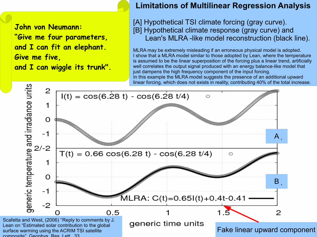
John von Neumann: “Give me four parameters, and I can fit an elephant. Give me five, and I can wiggle its trunk".

Limitations of Multilinear Regression Analysis

[A] Hypothetical TSI climate forcing (gray curve). [B] Hypothetical climate response (gray curve) and

Lean's MLRA -like model reconstruction (black line). MLRA may be extremely misleading if an erroneous physical model is adopted. I show that a MLRA model similar to those adopted by Lean, where the temperature is assumed to be the linear superposition of the forcing plus a linear trend, artificially well correlates the output signal produced with an energy balance-like model that just dampens the high frequency component of the input forcing. In this example the MLRA model suggests the presence of an additional upward linear forcing, which does not exists in reality, contributing 40% of the total increase.

A�

B�

Scafetta and West, (2006) ‘‘Reply to comments by J. Lean on “Estimated solar contribution to the global surface warming using the ACRIM TSI satellite composite”, Geophys. Res. Lett., 33

Fake linear upward component

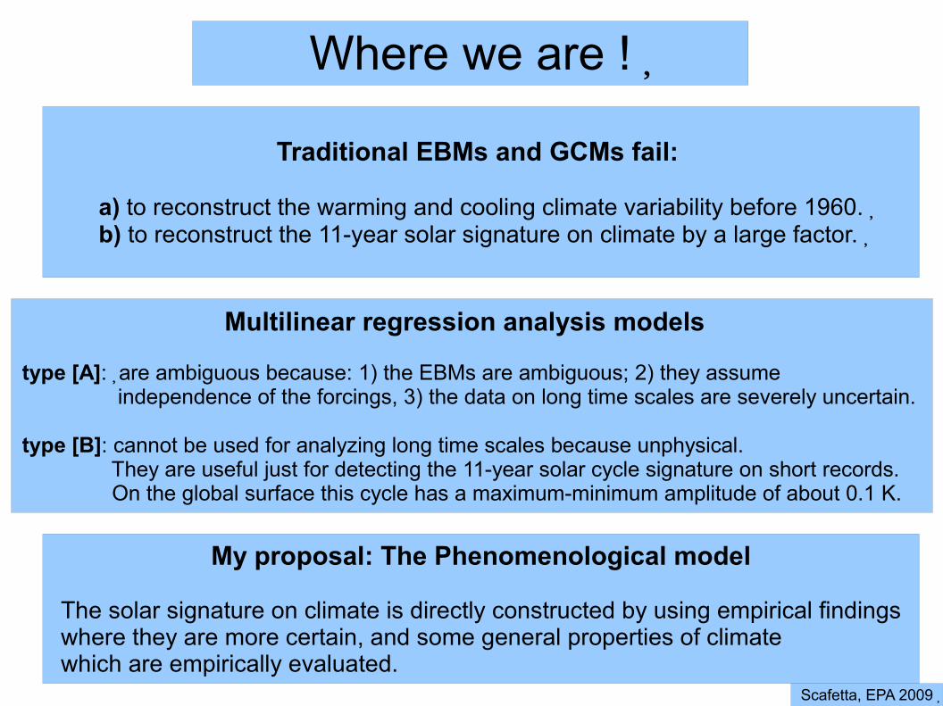
Where we are !�

Traditional EBMs and GCMs fail:�

a) to reconstruct the warming and cooling climate variability before 1960.�b) to reconstruct the 11-year solar signature on climate by a large factor.�

Multilinear regression analysis models�

type [A]:�are ambiguous because: 1) the EBMs are ambiguous; 2) they assume independence of the forcings, 3) the data on long time scales are severely uncertain.

type [B]: cannot be used for analyzing long time scales because unphysical. They are useful just for detecting the 11-year solar cycle signature on short records. On the global surface this cycle has a maximum-minimum amplitude of about 0.1 K.

My proposal: The Phenomenological model�

The solar signature on climate is directly constructed by using empirical findings where they are more certain, and some general properties of climate which are empirically evaluated.


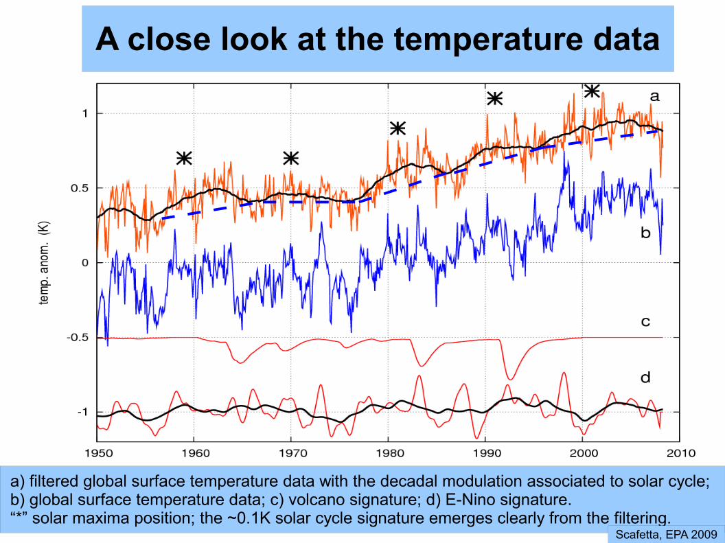
A close look at the temperature data�

a) filtered global surface temperature data with the decadal modulation associated to solar cycle; b) global surface temperature data; c) volcano signature; d) E-Nino signature. “*” solar maxima position; the ~0.1K solar cycle signature emerges clearly from the filtering.

Scafetta, EPA 2009

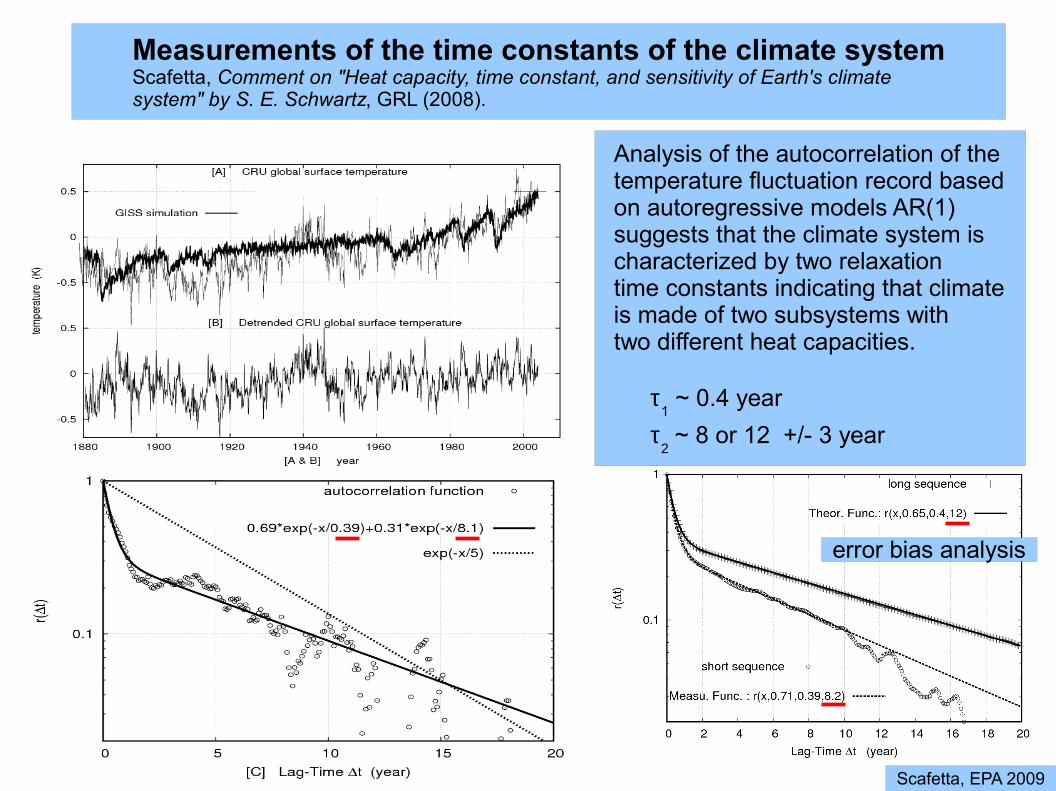
Measurements of the time constants of the climate systemScafetta, Comment on "Heat capacity, time constant, and sensitivity of Earth's climate system" by S. E. Schwartz, GRL (2008).

Analysis of the autocorrelation of the temperature fluctuation record based on autoregressive models AR(1) suggests that the climate system is characterized by two relaxation time constants indicating that climate is made of two subsystems with two different heat capacities.

τ1

~ 0.4 year τ

2 ~ 8 or 12 +/- 3 year

error bias analysis

Scafetta, EPA 2009

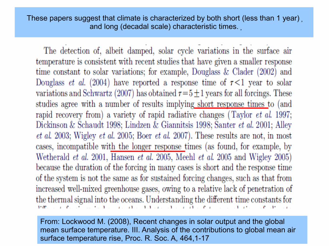
These papers suggest that climate is characterized by both short (less than 1 year)�and long (decadal scale) characteristic times.�

From: Lockwood M. (2008), Recent changes in solar output and the global mean surface temperature. III. Analysis of the contributions to global mean air surface temperature rise, Proc. R. Soc. A, 464,1-17

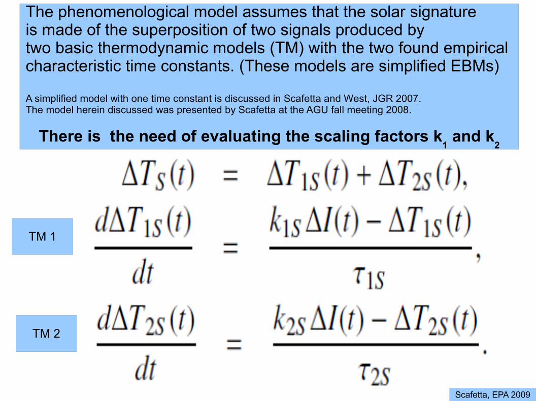
The phenomenological model assumes that the solar signature is made of the superposition of two signals produced by two basic thermodynamic models (TM) with the two found empirical characteristic time constants. (These models are simplified EBMs)

A simplified model with one time constant is discussed in Scafetta and West, JGR 2007. The model herein discussed was presented by Scafetta at the AGU fall meeting 2008.

There is the need of evaluating the scaling factors k1

and k2

TM 1

TM 2

Scafetta, EPA 2009

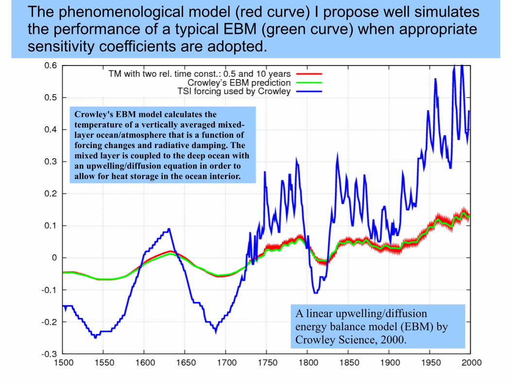
The phenomenological model (red curve) I propose well simulates the performance of a typical EBM (green curve) when appropriate sensitivity coefficients are adopted.

Crowley's EBM model calculates the temperature of a vertically averaged mixed-layer ocean/atmosphere that is a function of forcing changes and radiative damping. The mixed layer is coupled to the deep ocean with an upwelling/diffusion equation in order to allow for heat storage in the ocean interior.

A linear upwelling/diffusion energy balance model (EBM) by Crowley Science, 2000.

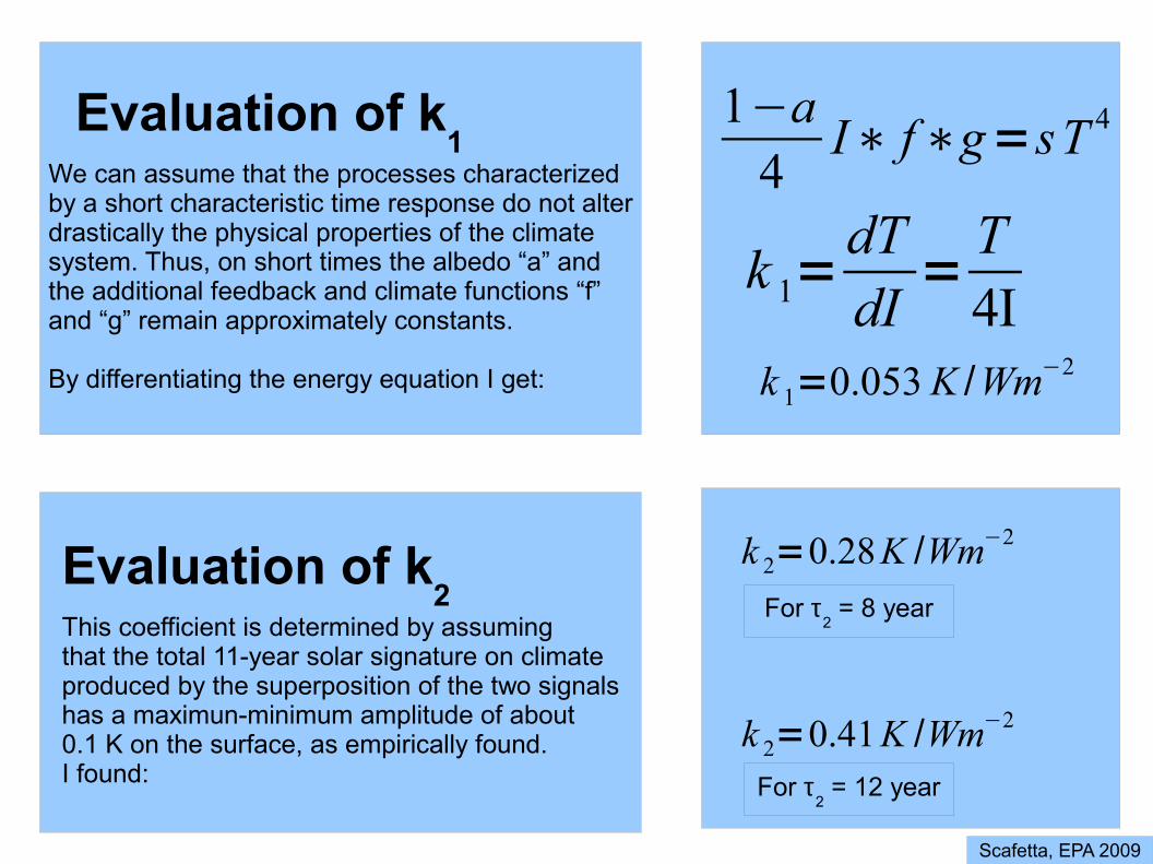
Evaluation of k1

We can assume that the processes characterized by a short characteristic time response do not alter drastically the physical properties of the climate system. Thus, on short times the albedo “a” and the additional feedback and climate functions “f” and “g” remain approximately constants.

By differentiating the energy equation I get:

Evaluation of k2

This coefficient is determined by assuming that the total 11-year solar signature on climate produced by the superposition of the two signals has a maximun-minimum amplitude of about 0.1 K on the surface, as empirically found. I found:

1−a 4

I∗ f ∗g =sT 4

k 1 = dT dI

= T 4I

k 2 =0.28 K /Wm−2

k 2 =0.41 K /Wm−2

For τ2

= 8 year

For τ2

= 12 year

Scafetta, EPA 2009

k 1 =0.053 K /Wm−2

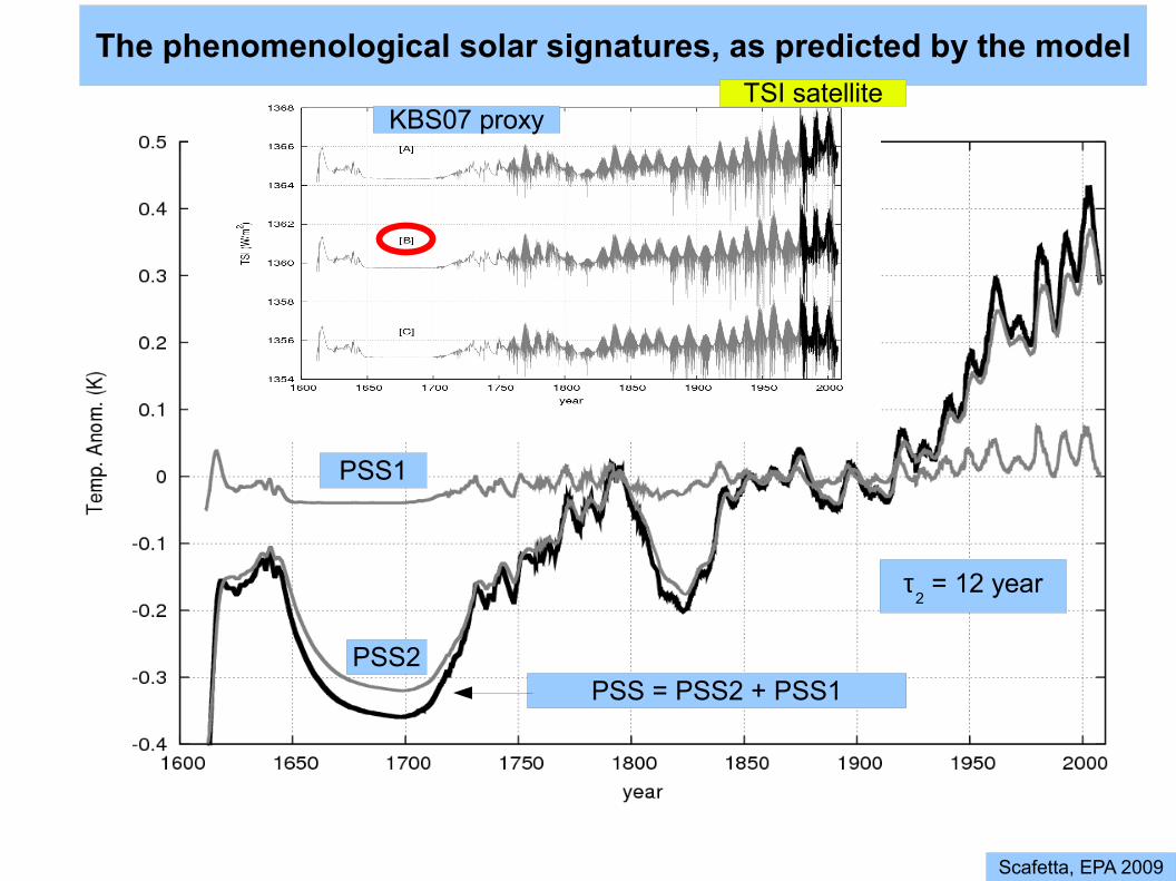
PSS1

PSS2 PSS = PSS2 + PSS1

τ2

= 12 year

The phenomenological solar signatures, as predicted by the model

KBS07 proxy TSI satellite

Scafetta, EPA 2009

The phenomenological solar signature as predicted by the model�

1) τ = 12 year and solar [A]�2

2) τ = 8 year and solar [C]�2

The model well agrees with this secular temperature reconstruction. The model “predicts” centuries of data!


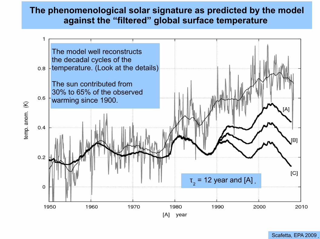
The phenomenological solar signature as predicted by the model�against the “filtered” global surface temperature�

The model well reconstructs the decadal cycles of the temperature. (Look at the details)

The sun contributed from 30% to 65% of the observed warming since 1900.

τ = 12 year and [A]�2


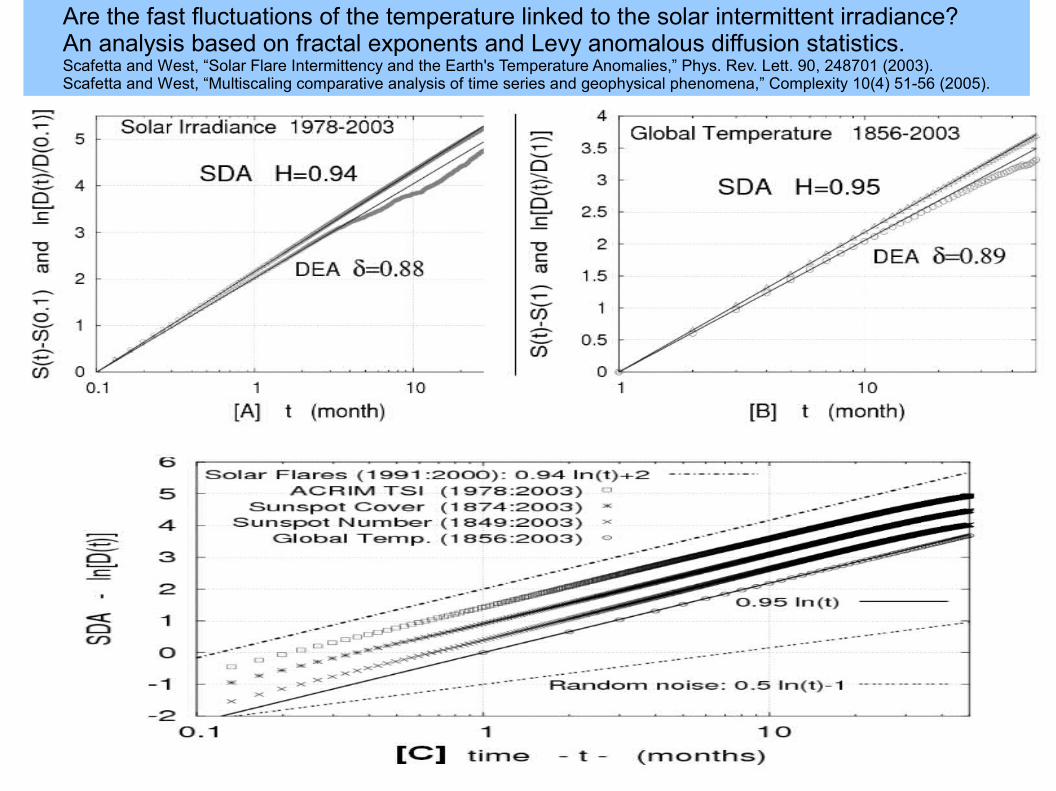
Are the fast fluctuations of the temperature linked to the solar intermittent irradiance? An analysis based on fractal exponents and Levy anomalous diffusion statistics. Scafetta and West, “Solar Flare Intermittency and the Earth's Temperature Anomalies,” Phys. Rev. Lett. 90, 248701 (2003). Scafetta and West, “Multiscaling comparative analysis of time series and geophysical phenomena,” Complexity 10(4) 51-56 (2005).

The phenomenological model predicts quite well centuries of climate change data as well as many decadal details as seen during the last 50 years. The climate is quite sensitive to solar changes.

However, the model does not appear to reproduce well the warming during 1910-1945.

A possible explanation is that the used TSI proxy model record is not accurate enough. This is likely because we have seen that these TSI models may fail to reproduce the observed decadal trends in TSI.

Indeed, the TSI proxy models greatly vary, as the figure shows.Which TSI may be correct? Or is there a missing climate forcing?

Where was the�TSI maximum?�1945 or 1960?�

Scafetta, EPA 2009

Hoyt, 1997

Attempting a forecast of climate change: An astronomical gravitational forcing for the Sun and the Earth?Presented by Scafetta, at AGU fall meeting 2008

Wobbling of the Sun around the center of mass of the solar system.

The Sun wobbles because of the gravitationalattraction of the other planets of the solar system.

In particular becauseof the Jovian planets:Jupiter, Saturn,Uranus and Neptune.

This generates a tidalforce and torque onthe sun and on the Earth.

Is this forcing partiallyshaping solar activityand/or the Earth's climate?

Jose, 1965; Fairbridge and Shirley, 1987; Landscheidt, 1988, 1999; Charvatova and Stvrevstik, 2004; Wilson et al., 2008

Scafetta, EPA 2009

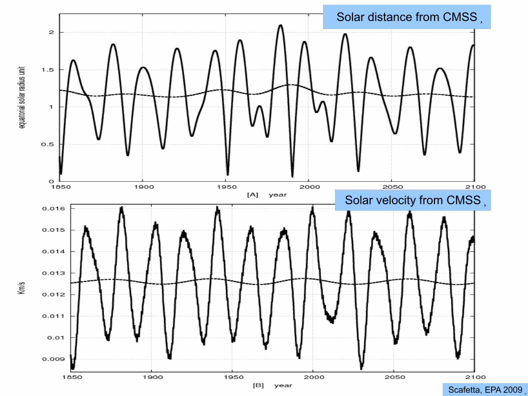
Solar distance from CMSS�

Solar velocity from CMSS�


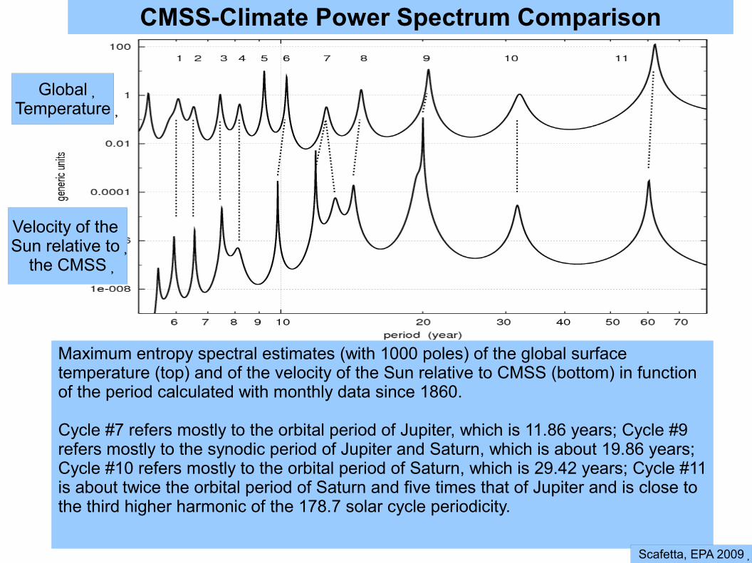
CMSS-Climate Power Spectrum Comparison

Global�Temperature�

Velocity of the Sun relative to�

the CMSS�

Maximum entropy spectral estimates (with 1000 poles) of the global surface temperature (top) and of the velocity of the Sun relative to CMSS (bottom) in function of the period calculated with monthly data since 1860.

Cycle #7 refers mostly to the orbital period of Jupiter, which is 11.86 years; Cycle #9 refers mostly to the synodic period of Jupiter and Saturn, which is about 19.86 years; Cycle #10 refers mostly to the orbital period of Saturn, which is 29.42 years; Cycle #11 is about twice the orbital period of Saturn and five times that of Jupiter and is close to the third higher harmonic of the 178.7 solar cycle periodicity.


[A] Global surface temperature detrended of its quadratic fit plotted against the rescaled 60-year modulation of the velocity of the CMSS: the solar index is lag-shifted by +5 years.

[B] The 20-year oscillation of the climate (grey) plotted against the rescaled velocity (black) of the CMSS detrended of its six decade modulation: no lag-time is applied.

60-year cycle Atlantic Multidecadal Oscillation


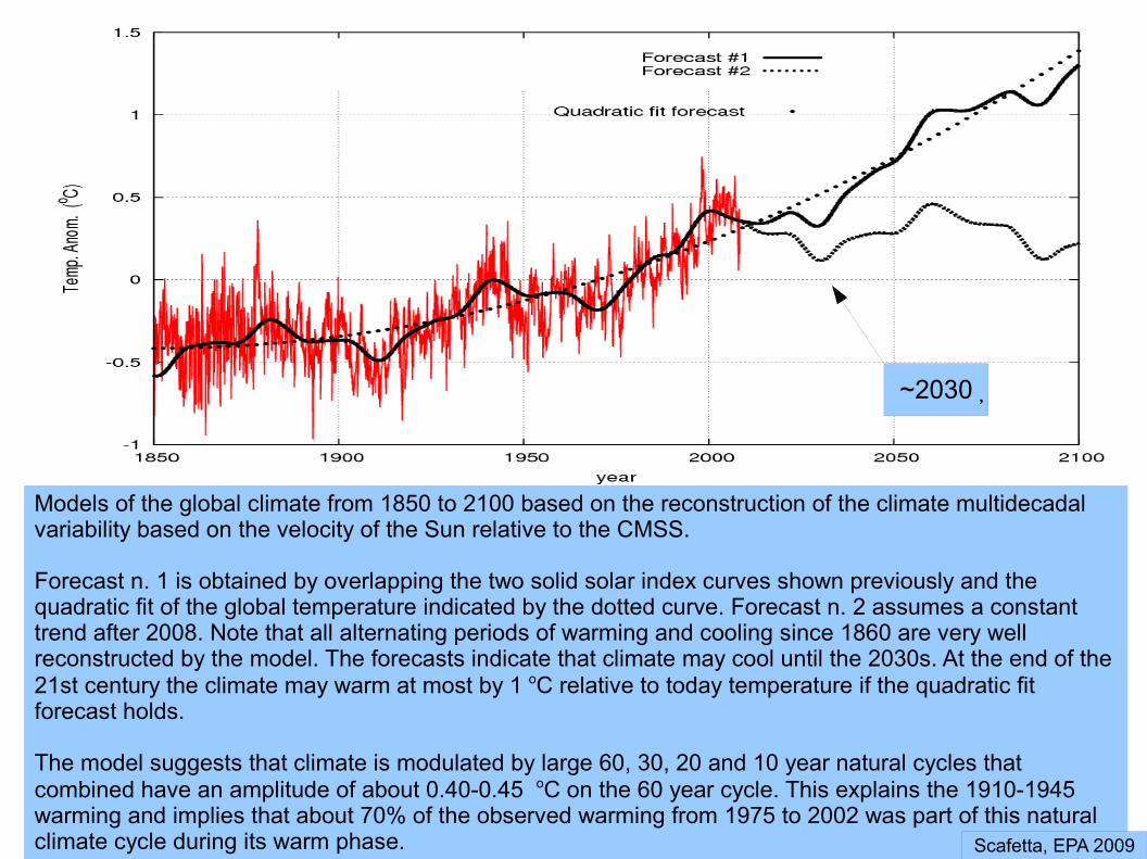
~2030�

Models of the global climate from 1850 to 2100 based on the reconstruction of the climate multidecadal variability based on the velocity of the Sun relative to the CMSS.

Forecast n. 1 is obtained by overlapping the two solid solar index curves shown previously and the quadratic fit of the global temperature indicated by the dotted curve. Forecast n. 2 assumes a constant trend after 2008. Note that all alternating periods of warming and cooling since 1860 are very well reconstructed by the model. The forecasts indicate that climate may cool until the 2030s. At the end of the 21st century the climate may warm at most by 1 oC relative to today temperature if the quadratic fit forecast holds.

The model suggests that climate is modulated by large 60, 30, 20 and 10 year natural cycles that combined have an amplitude of about 0.40-0.45 oC on the 60 year cycle. This explains the 1910-1945 warming and implies that about 70% of the observed warming from 1975 to 2002 was part of this natural climate cycle during its warm phase. Scafetta, EPA 2009

Two still “unproven” hypotheses:

a) The movement of the planets partially modulates solar activity that then modulates climate. This hypothesis requires that current TSI proxy models are imperfect.

b) The movements of the planets drives a change in the Earth's Length Of the Day and the variation of the LOD constitutes a missing climate forcing that significantly contribute to climate change by altering the ocean and atmospheric currents, for example.

The figures below compare the LOD with the 60 year modulation of the solar velocity around the CMSS. Also, the LOD anticipates the change in global temperature by a 4-5 years.

Klyashtorin, L.B. (2001) Climate change and long-term fluctuations of commercial catches: the possibility of forecasting.” FAO Fisheries Technical Paper 410. See also: Mazzarella, The Open Atmospheric Science Journal, 2008, 2, 181-184

Scafetta, EPA 2009

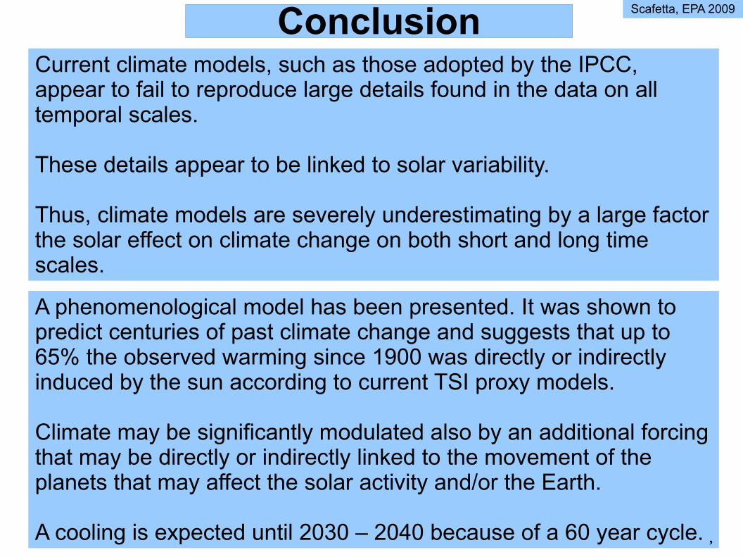
Conclusion�Scafetta, EPA 2009

Current climate models, such as those adopted by the IPCC, appear to fail to reproduce large details found in the data on all temporal scales.

These details appear to be linked to solar variability.

Thus, climate models are severely underestimating by a large factor the solar effect on climate change on both short and long time scales.

A phenomenological model has been presented. It was shown to predict centuries of past climate change and suggests that up to 65% the observed warming since 1900 was directly or indirectly induced by the sun according to current TSI proxy models.

Climate may be significantly modulated also by an additional forcing that may be directly or indirectly linked to the movement of the planets that may affect the solar activity and/or the Earth.

A cooling is expected until 2030 – 2040 because of a 60 year cycle.�

APPENDIX�

General properties of the climate sensitivity function Z(ω) of an EBM�

PERIOD 5-years 10-years 20-years 40-years 80-years 160-years AMPLITUDE

0.15 0.23 0.33 0.46 0.59 0.71 0.08 0.13 0.19 0.28 0.39 0.52 0.04 0.07 0.11 0.17 0.26 0.38 0.02 0.04 0.06 0.1 0.17 0.28

0.5 K/Wm-2

1 K/Wm-2

2 K/Wm-2

4 K/Wm-2

General energy balance models predict that the climate sensitivity to acyclical forcing, with a given period and amplitude, increases with theperiod and decreases with the amplitude. This is mostly due to generalout of equilibrium thermodynamic effects and to the damping effect of the ocean thermal inertia.

Wigley, T. M. L. (1988), The climate of the past 10,000 years andthe role of the Sun, pp. 368 209– 224, Springer, New York.

reduced because of the thermal inertia

A phenomenological and simple sun-climatethermodynamic/relaxation model:A first order EBM

dΔ T (t) cΔ I (t) − Δ T (t)= τdt

c = conversion constant τ = relaxation time

High frequencies are

Scafetta and West, JGR 2007.

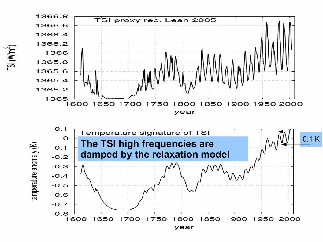
The TSI high frequencies aredamped by the relaxation model

0.1 K

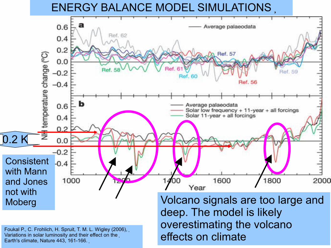
ENERGY BALANCE MODEL SIMULATIONS�

Volcano signals are too large and deep. The model is likely

Foukal P., C. Frohlich, H. Spruit, T. M. L. Wigley (2006),�Variations in solar luminosity and their effect on the�Earth's climate, Nature 443, 161-166.�

0.2 K

overestimating the volcano effects on climate

Consistent with Mann and Jones not with Moberg

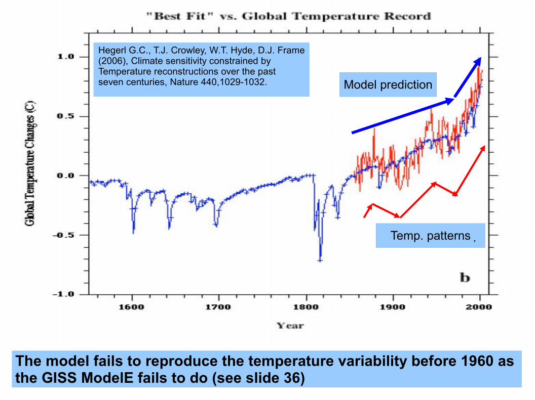
Hegerl G.C., T.J. Crowley, W.T. Hyde, D.J. Frame (2006), Climate sensitivity constrained by Temperature reconstructions over the past seven centuries, Nature 440,1029-1032. Model prediction

Temp. patterns�

The model fails to reproduce the temperature variability before 1960 as the GISS ModelE fails to do (see slide 36)

Some papers on solar inertial motion and the Earth's length of the day oscillation

Charvatova I. (1990), The relation between solar motion and solar variability, Bull. Astron. Inst.�Czechosl. 41, 56-59.�

Charvatova I. and J. Strestik (2004), Periodicities between 6 and 16 years in surface air temperature�in possible relation to solar inertial motion, J. of Atm. and Solar-Terr. Phys. 66, 219-227.�

Fairbridge R. W. and J. H. Shirley (1987), Prolonged minima and the 179-yr cycle of the solar inertial�motion, Solar Physics 110, 191-220.�

Klyashtorin, L.B. (2001) Climate change and long-term fluctuations of commercial catches: the possibility of forecasting. FAO Fisheries Technical Paper No. 410 Rome, FAO.�

Jose P.D. (1965), Suns motion and Sunspots, Astronomical Journal 70, 193-200.�

Landscheidt T. (1988), Solar rotation, impulses of the torque in Sun's motion, and climate change,�Climatic Change 12, 265-295.�

Landscheidt T. (1999), Extrema in Sunspot cycle linked to Sun's motion, Solar Physics 189, 415-426.�

Mackey R., (2007), Rhodes Fairbridge and the idea that the solar system regulates the Earth’s climate, Journal of Coastal Research 50, 955 - 968.�

Mazzarella A. (2008), Solar Forcing of Changes in Atmospheric Circulation, Earth's Rotation and Climate, The Open Atmospheric Science Journal, 2, 181-184.�

Wilson I. R. G., B. D. Carter, and I. A. Waite (2008), Does a spin-orbit coupling between the sun and the jovian planets govern the solar cycle?, Pub. of the Astr. Soc. of Astralia 25, 85-93.�

Some papers about my research on climate change�

Nicola Scafetta and Richard Willson, “ACRIM-gap and Total Solar Irradiance (TSI) trend issue resolved�using a surface magnetic flux TSI proxy model”, in press Geophysical Research Letter (2009) .�

Nicola Scafetta, "Total solar irradiance satellite composites and their phenomenological effect on�climate," In press on a special volume for the Geological Society of America. (2009).�

Nicola Scafetta, Can the solar system planetary motion be used to forecast the multidecadal variability of climate?, invited presentation at�the AGU Fall Meeting, San Francisco (2008).�

Nicola Scafetta, Analysis of the total solar irradiance composites and their contribution to global mean air surface temperature rise, AGU Fall�Meeting, San Francisco (2008).�

Nicola Scafetta, "Comment on ``Heat capacity, time constant, and sensitivity of Earth's climate system'�by Schwartz." J. Geophys. Res. 113, D15104 (2008). doi:10.1029/2007JD009586.�

Erik Kabela and Nicola Scafetta, “Solar Effect and Climate Change,” Bulletin of the American�Meteorological Society, 89, 34-35 (2008).�

Nicola Scafetta and Bruce J. West, “Is climate sensitive to solar variability?” Physics Today, 3 50-51 (2008).�

Nicola Scafetta, and Bruce J. West, “Phenomenological reconstructions of the solar signature in the NH surface temperature records since�1600.” J. Geophys. Res., 112, D24S03, doi:10.1029/2007JD008437 (2007).�

Nicola Scafetta and Bruce J. West , “Phenomenological solar signature in 400 years of reconstructed Northern Hemisphere temperature�record,” Geophys. Res. Lett., 33, doi:10.1029/2006GL027142. (2006).�

Nicola Scafetta and Bruce J. West, ‘‘Reply to comments by J. Lean on “Estimated solar contribution to the global surface warming using the�ACRIM TSI satellite composite”, Geophys. Res. Lett., 33, doi:10.1029/2006GL025668. (2006).�

Nicola Scafetta and Bruce J. West, “Phenomenological solar contribution to the 1900-2000 global surface warming,” Geophys. Res. Lett.,�33, L05708, doi:10.1029/2005GL025539 (2006).�

Nicola Scafetta and Bruce J. West, “Estimated solar contribution to the global surface warming using the ACRIM TSI satellite composite,”�Geophys. Res. Lett., 32(24), doi:10.1029/2005GL023849 (2005).�

Nicola Scafetta and Bruce J. West, “Solar Flare Intermittency and the Earth's Temperature Anomalies,” Phys. Rev. Lett. 90, 248701 (2003).�

Paolo Grigolini, Deborah Leddon, Nicola Scafetta, “The Diffusion entropy and waiting time statistics of hard x-ray solar flares,” Phys. Rev. E�65, 046203 (2002).�

climate change and its causes: a discussion about some · pdf fileclimate change and its...

Documents