1

Inversion of Teleseismic Receiver Functions via

Evolutionary Programming

Chris LynchSeptember 20,1999

Southern California Earthquake Center 1999 Summer Internship

AdvisorDr. Steven Day

Department of Geological SciencesSan Diego State University

2

Table of Contents

Introduction 3

Teleseismic Receiver Functions 4

Inverse Geophysical Modeling 5

Evolutionary Programming 6

Approach and Goals 9

Results 10

Verification 10

Synthetic Data Study 11

Conclusions 19

Acknowledgements 21

References 22

3

IntroductionThe inversion of teleseismic receiver functions is a

seismological method that can be used to help constrainestimates of the velocity structure of the Earth s crust.Evolutionary Programming (EP) is a global optimizationtechnique that uses a simplified model of the evolutionaryprocess to search a solution space for the optimalsolution, often referred to as the global minimum. Thisstudy explores the use of evolutionary programmingtechniques for the inversion of teleseismic receiverfunction data. Application of this technique in SouthernCalifornia may contribute to The Southern CaliforniaEarthquake Center s (SCEC) goal of developing a mastermodel of seismic hazard through the determination ofseismic wave velocities. Better models of seismic wavevelocities can then be used to create theoreticalseismograms, which are useful in the prediction of groundmotion during specific potential earthquakes

A Matlab code was developed in 1998 by Charles Hoelzerat San Diego State University (SDSU) based on work byBernard Minster and Nadya Williams (UCSD). That codecombines evolutionary programming techniques with asimulated annealing-type cost function to produce anevolving family of models of seismic velocity structure.The models are initially distributed randomly over thesolution space. Synthetic receiver functions computed fromthe models are compared with receiver function data and arerated according to some measure of fitness. The bestfitting half of the population is then selected The programthen perturbs the parameters of each parent model togenerates an offspring, producing a subsequent generationof the model population. Stopping conditions can be aspecified fitness tolerance or an arbitrary number ofiterations.

4

Over the course of two semesters (Fall 1998, Spring1999), I combined my interests in geology and computerscience by investigating and developing a more efficientand faster code. This work was done under the guidance ofSteven Day, (Geology, SDSU), later joined by Richard Frost,(Mathematics and Computer Science, SDSU), and produced atranslation into Fortran 90 of the original Matlab code.This Fortran 90 program is named Midcrust. The goal of thisinternship has been to extend this project by improving theefficiency of the code and the scientific techniques itemploys.

Teleseismic Receiver FunctionsTeleseismic waves are seismic waves recorded at

distances greater than 1600km (16 ° of arc) from anearthquake s epicenter. The first arrival is a refracted Pwave (P or PKP). Teleseismic P waves that are incident upona crustal boundary below a receiver station yield P to Swave conversions and multiple reverberations within theshallow layering. By treating the vertical component of ateleseismic seismic signal as a source function, anddeconvolving from the horizontal component, S waveconversions and reverberations can be isolated. This isbecause the horizontal components contain most of theenergy of the S wave conversions. This technique removesthe obscuring effects of source function and instrumentresponse and is called a receiver function. These receiverfunctions can then be inverted, producing a model of theshear velocity structure. This provides a means fordetermining crustal velocity structure. This method can bestable for regions where the layers are nearly horizontal[Ammon et al., 1990, Lay and Wallace, 1995]. Theinformation gained by this method spans a region around thereceiver station, the radius of which is approximatelyequal to the depth of the deepest reflector, usually theMoho [Ammon et al., 1990].

5

Inverse Geophysical ModelingForward modeling takes model parameters as input,

applies them to a mathematical model, and generatespredicted (measurable) data. Inverse modeling takesobserved data as input and estimates model parameters fromit.

Midcrust represents crustal structure with a set ofhorizontal layers with four parameters per layer, P and Swave velocities, layer thickness and density. In thisimplementation only layer thicknesses for P wave velocities(α) are independently estimated. S wave velocities (β) arecalculated from P wave velocities using the equation,

and density is estimated using Birch’s Law, with Poisson’sratio estimated at 0.25 for average crystalline rock [Navaand Brune, 1982]. The number of layers in the models is auser-defined parameter, as are a set of a priori layervelocity and thickness constraints.

For the inversion of teleseismic receiver functions,in Midcrust, forward modeling is required to make receiverfunction time series in order to evaluate model fitness.This is synthetic data, or the data that would be observedfor a crustal structure defined by models parameters. Ammonet al, 1990, designed the code used for this operation. Theresult of inverting a teleseismic receiver function is a Pwave velocity structure for the region under the receiver.Midcrust manufactures a population of these velocitystructure models and evolves them in search of the globalminimum, the optimal solution for the reference receiverfunction.

σσαβ −−= 1/5.0

6

Evolutionary ProgrammingEvolutionary programming attempts to mimic the process

by which species evolve. EP was first developed by Fogel(1962). The algorithm used in Midcrust was firstimplemented by Hoelzer (1998) for inversion of receiverfunctions, and is based upon work by Minster et al. (1995),and Groot-Hedlin and Vernon, (1998). I have made some minormodifications in the course of translating the originalMatlab code into Fortran 90. This algorithm begins with areceiver function and proceeds as follows:(1) Produce a population of velocity/thickness modelsrandomly distributed over a chosen solution space,(2) Calculate the fitness of each model by comparing thereceiver function data with a theoretical receiver functioncalculated for the model.(3) Compete each model against a given number of randomlychosen members of the population and rank them according toa cost function,(4) Select the half of the population with the highestscore to serve as the parental models,(5) Generate an offspring from each parent model byperturbing the parameters of a copy of the parent,(6) Iterate through (2) - (6), new population consisting ofparents and offspring,(7) Quit after the desired number of iterations have beencompleted.

The initial population is created by generating N(e.g., 100) random velocity-thickness models. Each model iscreated by selecting a uniform random number betweenspecified upper and lower bounds for each parameter. Boundsare selected to be reasonable constrains for the velocityand thickness of each model layer based on general seismicknowledge.

Fitness is calculated using an L1 norm, or meanabsolute value of the misfit between the observed(reference) seismogram and the seismogram generated throughthe forward modeling of the predicted (model) parameters.This value can be described as the amount of misfit betweenthe reference and predicted model, where a smaller valuerepresents a closer fit.

7

A weighting function, w(j) is used to place greatersignificance on arrival time within a specified timeperiod. To date no weighting has been used giving theentire time series equal significance and so w(j) = 1. Whensynthetic data with noise, and later when real data is usedfor the reference receiver function the weighting functioncan be used to place emphasis on, for example, the firstarrivals of the P to S wave conversions or on the laterarriving Moho free surface multiples.

Selection is done via competition between models whereeach member of the model population is rated based on acomparison of fitness values between itself and a specifiednumber of different models randomly chosen from the totalpopulation. This is analogous to competition betweenmembers of a population. Competition is implemented byfirst calculating: ∆m = (misfit[a] - misfit[b]) /misfit[a]), where "a" is index of current model and b is arandomly generated index for the competitor. If ∆m ≤ 1 thenmodel[a] has its score increased by one, favoring adownhill move. This means that model a is acceptedunconditionally and favors finding the local minimum.If ∆m > 1 then it will be unconditionally accepted, It willbe conditionally accepted if exp(-∆m/Temp) > R, where R isa random number between 0 and 1 and Temp is a geometricallydecreasing value that governs acceptance of uphill moves.This is an uphill move, which provides a way to break outof a local minimum and continue to explore the solutionspace. Temp controls the probability of accepting an uphillmove and is a specified function of iteration number. Thisfunction is referred to as the cooling schedule .

Adding a perturbation value to each parent parametermakes the offspring of the population. The perturbation iscalculated by multiplying the misfit value of the parent byone fifth of the difference of the upper and lower boundsof the parameter, and a normally distributed random numberwith zero mean and standard deviation of one. Any offspringthat are outside of the a priori bounds are reset to thevalue of the bound that has been crossed.

= =

−=N

i

N

i

iwiobservedjwispredictediobservedmisfit1 1

|)()(|/)(|)()(|

8

The Midcrust algorithm is being tested on syntheticdata computed from a known layered crustal model. We referto this test model as our reference model to distinguish itfrom the models generated randomly during the solutionprocess. The reference model used for most of the testingof Midcrust is a four-layer model that was used as thestandard reference model by Hoelzer (1998) to test theoriginal Matlab implementation. It is a challenging testcase because it has a small velocity contrast betweenlayers 2 and 3, and a low velocity zone (LVZ) just abovethe crust-mantle boundary, or Mohorovicic discontinuity(Moho), which is a difficult solution to find. One of theadvantages of Evolutionary Programming is the ability tofind unexpected model solutions, being free from thenecessity of having a close starting model in order to finda LVZ, as in linear inversion methods [Groot-Hedlin andVernon, 1998].

Figure 1. Reference Model Receiver Function

9

Approach and GoalsThe first step of this project was to complete

development of the uni-processor implementation of theoriginal Matlab driver into Fortran 90. This code is usedin combination with a collection of Fortran 77 seismicsolvers and their helper subroutines that were use in theoriginal Matlab code. These perform the forward modelingand other required computational tasks. Then the ability ofthe Fortran 90 code to drive these solvers correctly wasverified. After verification, a synthetic data study wasinitiated to evaluate the quality of the model solutions.The data study was designed to gain an understanding of theeffects of the main evolutionary parameters and how theyaffect the final population. This in turn would enabletuning the code to produce optimal solutions. Next, aparallel implementation would be undertaken to provide amuch more efficient program, thereby allowing a greaternumber of runs to be conducted within a given period oftime, and allowing larger sized problems to be solved. Anadditional study objective is to test the code s ability togenerate good solutions given known synthetic data withdifferent levels of noise added.

Accomplishing the above would provide the startingpoint for studies with real data, generating possiblesolutions to crustal structure in the Peninsular RangesBatholith (PRB) in Southern California. These solutions canthen be compared with solutions determined from othermethodologies including seismic tomography,magnetotellurics, reflective seismology, and field geology.Success in these goals along with steady improvements tothe scientific techniques used in the code should yield aproduction level code. This code can then be used inprojects like SCEC’s Master Seismic Hazard Model of the LosAngeles Basin by helping to determine seismic wavevelocities.

10

ResultsThe uni-processor code has been completed and verified

to drive the F77 solvers correctly. This verificationconsisted of producing a variant of the Midcrust code tooutput a synthetic receiver function time series from a setof model parameters as input.

A substantial decrease in processing time has beenachieved. A normal run of 100 iterations, 100 models andcompetition with 20 different models takes around an hourcompared with between 2 and 3 hours for the original code.

A preliminary study with synthetic data has beenconducted. The results of this study have been used to dodiscover errors in the implementation and to start tuningthe Midcrust application, and have provided severalopportunities for improvements to the evolutionarytechnique.

VerificationObjective: To verify that Midcrust produces correct

forward models for input data. This would prove that theMidcrust program is driving the Fortran 77 seismic routinescorrectly. This can be shown by generating receiverfunction time series forward models for several uniqueinput models and then comparing them to independentlygenerated receiver functions.

The velocity and thickness parameters that were usedto construct the different reference seismograms would beused as the input model for the forward modeling codes andthe time series generated from these would be compared withthe reference time series. These reference seismograms weremade using a different suite of Fortran 77 codes incombination with some Seismic Analysis Code (SAC) routines,and so were independent of the Midcrust routines.

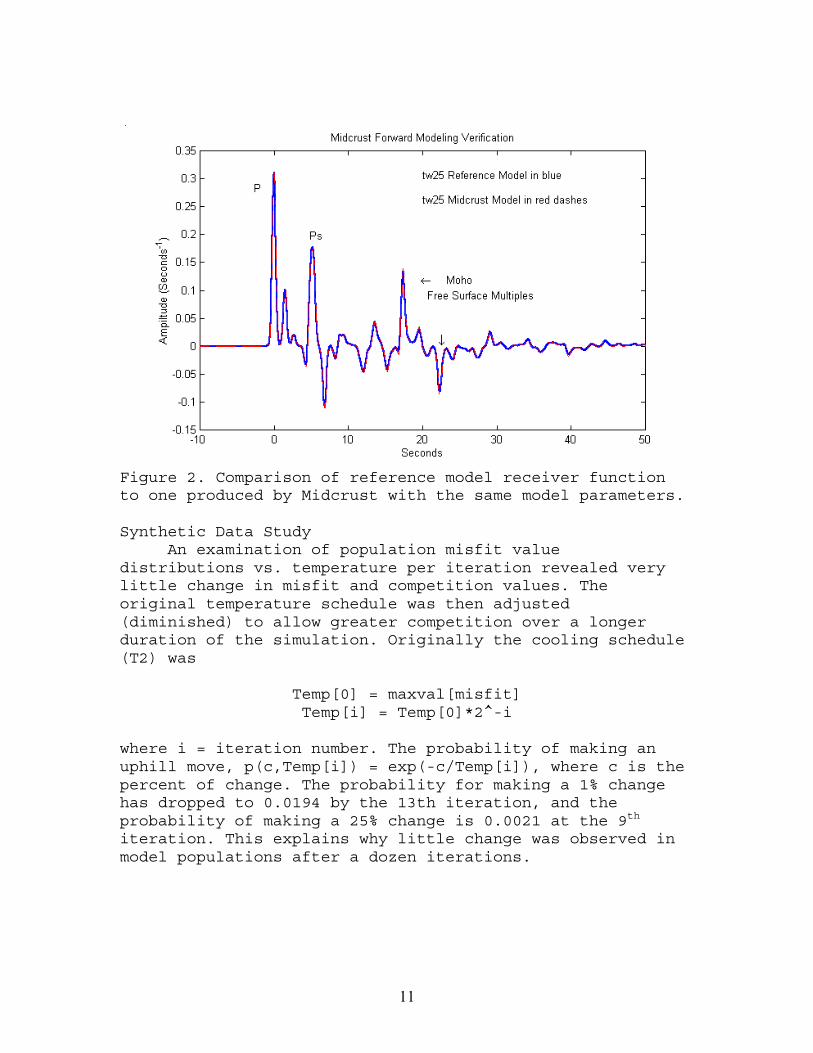
Three distinct models and matching time series wereused. The Midcrust program was able to produce virtuallyidentical time series from these model parameters. InFigure 3, the independently generated reference model isshown plotted along with the one made by Midcrust.

11

Figure 2. Comparison of reference model receiver functionto one produced by Midcrust with the same model parameters.

Synthetic Data StudyAn examination of population misfit value

distributions vs. temperature per iteration revealed verylittle change in misfit and competition values. Theoriginal temperature schedule was then adjusted(diminished) to allow greater competition over a longerduration of the simulation. Originally the cooling schedule(T2) was

Temp[0] = maxval[misfit]Temp[i] = Temp[0]*2^-i

where i = iteration number. The probability of making anuphill move, p(c,Temp[i]) = exp(-c/Temp[i]), where c is thepercent of change. The probability for making a 1% changehas dropped to 0.0194 by the 13th iteration, and theprobability of making a 25% change is 0.0021 at the 9th

iteration. This explains why little change was observed inmodel populations after a dozen iterations.

12

The new cooling schedule (TE) is

Temp[0] = maxval[misfit]Temp[i] = Temp[i-1]/A

where

A = Temp[0]*exp(( ln(-1%/( T[0]*ln(0.01) )) ) / -N)

and N is the total number of iterations selected for aprogram run.

Figure 3. Probability of making an up hill move for the twocooling schedules, T2 is the old and TE the new schedule.

As can be seen from Figure 3 the new cooling scheduleoffers a greater probability of making uphill moves formore iterations.

Uphill Compet it ion Probabilit ie

0.00

0.10

0.20

0.30

0.40

0.50

0.60

0.70

0.80

0.90

1.00

1 21 41 61 81 101

ite rat ion

pro

ba

bil

ity

p(1%,T2)

p(25%,T2)

p(1%,TE)

p(25%,TE)

13

Figure 4. Model Energy with Temperature Schedule T2.

Model energy is an alternative term for fitness, oftenreferred to as misfit, since this value quantifies thedifference between a model prediction and the data. Theterm energy indicates the likelihood of an offspring modelending up a good distance away from its parent if plottedin the multidimensional parameter or solution space. Thisspace is the multi-axis coordinate system defined by themodel parameters. In Figure 4 the long plateau in energyacross magnitudes of temperature indicates that thepopulation has become trapped in local minima. This wouldbe fine if the energy surface were concave, but it is knownthat in this type of problem the energy surface usuallycontains many hills and valleys [Groot-Hedlin and Vernon,1998]. Note: in these plots, temperature decreases fromright to left with iteration.

Energy vs. Temperat ure

0.00

1.00

2.00

3.00

4.00

5.00

6.00

1.0E-30 1.0E-24 1.0E-18 1.0E-12 1.0E-06 1.0E+0 0

t emp erat ure

en

erg

ies

min E

max E

avg E

14

Figure 5. Model scores from competition stage compared totemperature for T2.

For schedule T2 the average model scores remain highthroughout the run. It would be preferred if they woulddrop to a low plateau when the temperature has cooled tothe last order of magnitude.

Figure 6. Energy vs. temperature for cooling schedule TE.

Score vs. Tempera ture

0

5

10

15

20

1.0E-30 1.0E-24 1.0E-18 1.0E-1 2 1.0E-06 1.0E+ 00

temperatur e

sc

ore

smin S

max S

avg S

Energy vs. Tempera ture

0.00

1.00

2.00

3.00

4.00

5.00

6.00

1.E-0 3 1.E-02 1.E-01 1.E+00 1.E+ 01 1.E+02

t empera tur e

en

erg

ies min E

max E

avg E

15

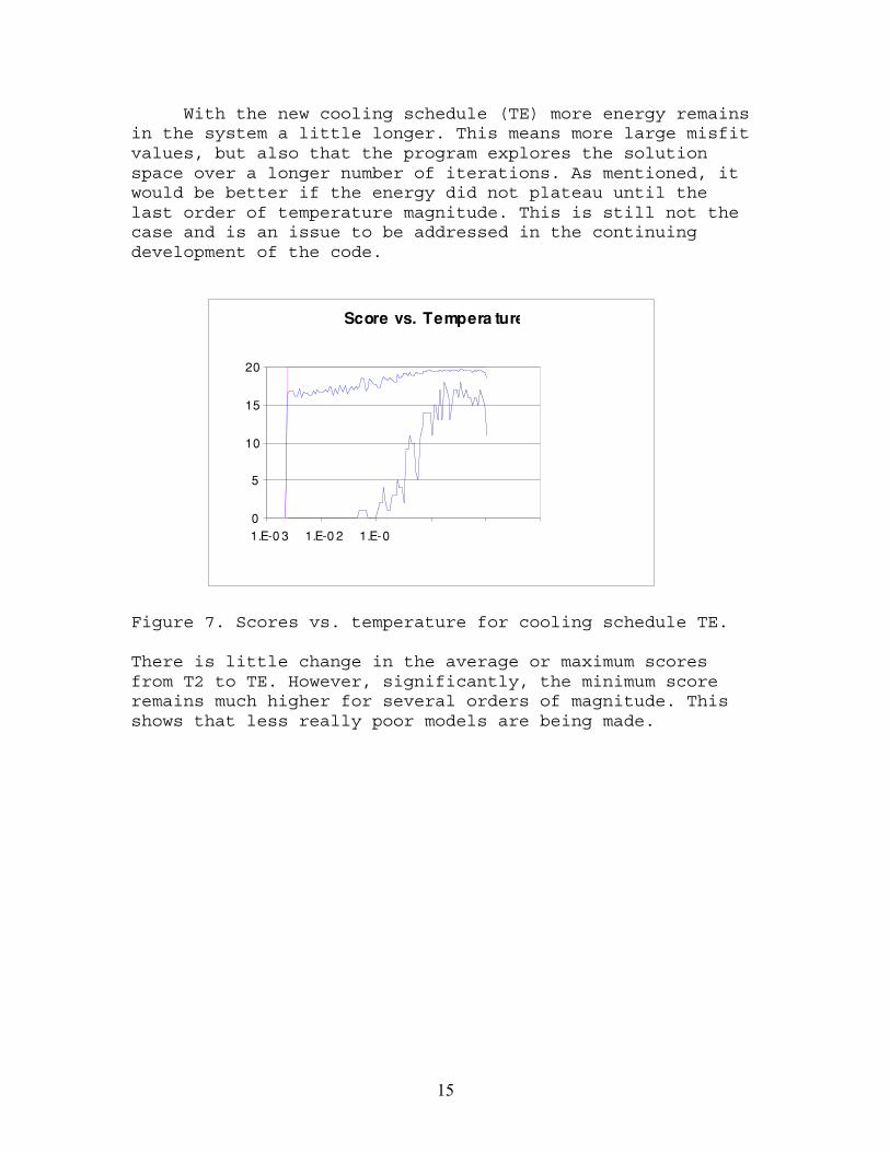
With the new cooling schedule (TE) more energy remainsin the system a little longer. This means more large misfitvalues, but also that the program explores the solutionspace over a longer number of iterations. As mentioned, itwould be better if the energy did not plateau until thelast order of temperature magnitude. This is still not thecase and is an issue to be addressed in the continuingdevelopment of the code.

Figure 7. Scores vs. temperature for cooling schedule TE.

There is little change in the average or maximum scoresfrom T2 to TE. However, significantly, the minimum scoreremains much higher for several orders of magnitude. Thisshows that less really poor models are being made.

Score vs. Tempera ture

0

5

10

15

20

1.E-0 3 1.E-0 2 1.E-0

16

Figure 8. Histogram of misfit values after 100 iterations

Figure 10. Histogram of misfit values at iteration 53.

Distribution a t iterat ion 1

0

1

2

3

4

5

6

7

8

9

0.64 0.68 0.72 0.7 6 0.8 0.84 0.88 0.9 2 0.96 1 1.04 1.0 8

misf it bins

fre

qu

en

cy

Dist ribution at it e ra tion

0

1

2

3

4

5

6

7

8

0.64 0.68 0.72 0.7 6 0.8 0.84 0.88 0.9 2 0.96 1 1.04 1.0 8

misf i t bins

fre

qu

en

cy

17

The best model overall was found to be at iteration 53(model #92), and has a misfit value 6.42053E-01 compared to6.48278E-01, the smallest misfit after iteration 100 (model#13). The histogram of misfit values at iteration 53 (Fig.10)is shown along with the one after iteration 100 (Fig.9). These histograms, showing the distribution of misfitvalues, exhibit a fairly bell shaped curves, and are nottoo badly skewed.

The time series for the best model overall, based onmisfit value, (Fig. 10), shows that this model does a goodjob of fitting the first arrivals but fails to pick up theMoho free surface multiples.

Figure 10. Time Series for Best Model after 100 Iterations

18

Figure 11. Velocity/thickness for population at 53rd

iteration.

The velocity and depth plots for the 53rd and 101st

iterations are showing some clustering of models. Thedistribution of the 53rd is looking a bit better than the100th. Even in the 53rd iteration very few models arepicking up the low velocity zone (6.2km/s at 35km to 40km), and at the 101st there are none. This is clearly animportant issue to address in the further development ofthis code.

velocity depth for population at iteration 53

0.00E+00

5.00E+00

1.00E+01

1.50E+01

2.00E+01

2.50E+01

3.00E+01

3.50E+01

4.00E+01

4.50E+01

0.00E+00

2.00E+00

4.00E+00

6.00E+00

8.00E+00

1.00E+01

velocity (km/s)d

epth

(km

)

19

Figure 12. Velocity/thickness for population after 100th

iteration.

ConclusionsThe new cooling schedule has improved the competition

among population members but has provided littleimprovement in the energy evolution of the system.Determination of temperature schedules, model parameterperturbation functions, and misfit (energy) metrics for anygiven problem which evolve the system energy and resultingcompetitions in a meaningful way requires a significantamount of experimentation. Different cooling schedules canbe tried, the number of competitions can be adjusted, and abetter delta value for perturbing the parent parameters maybe found. I also feel that there may be a better norm forthe signal correlation, although an L1 norm is good atdealing with outliers [Groot-Hedlin and Vernon, 1998]. Theproblem being addressed has a high dimensionality, thereare a lot of different, valid moves to make when perturbinga model.

velocity depth for population after iteration 100

0.00E+005.00E+001.00E+011.50E+012.00E+012.50E+013.00E+013.50E+014.00E+014.50E+015.00E+01

0.00E+00

2.00E+00

4.00E+00

6.00E+00

8.00E+00

1.00E+01

velocity (km/s)d

epth

(km

)

20

Inverse modeling tends to be non-unique [Sheriff andGeldart, 1995] and materials of different density andthickness can produce the same travel times. One of thebest features of EP is the ability to suggest solutionsthat are unexpected. This is one of the biggest challengesfor modeling and simulation. We need to be able to verifythat our modeling and simulations are valid and preservethe ability of the algorithms used to find unexpectedsolutions. This is where combining different methods fordetermining velocity structure, combined with a goodgeological understanding, and the ability to make intuitivedecisions is required to meet the challenges inherent tothis type of problem.

Two important areas are next on the agenda: tests withnoisy data as compared to noiseless synthetics, and aparallel implementations targeting the IBM SP2 at San DiegoSupercomputing Center (SDSC), and the more accessiblemultiprocessor Sun Enterprise Systems at SDSU. The mostcritical of these is the noise study, which will determinejust how effective this modeling technique will be withreal data. Success in this area will enable this program tomake a serious contribution to determining actual velocitystructure. The parallel implementation is also of greatimportance, however, and will contribute directly to thesuccess of the noise study by enabling more program runsthrough faster execution. It will also allow largerproblems to be addressed, that is to search a largersolution space, (i.e. models with more layers), and to addmore parameters, thereby increasing the resolution of themodels. This will be an important step toward tackling morecomplex inverse problems with larger data sets and multi-dimensional models.

There are several other related areas in which furtherwork on this project will yield beneficial results. One isin the area of data management, and the other in datavisualization. The ability to produce large amounts ofoutput is very nice but without the ability to manage andcommunicate this data it is not of much use. Therefore asuite of Unix shell scripts (developed as a part of theongoing data studies) will be included in the Midcrustpackage that will catalogue, store and filter the data.Visualization of the data has produced some challenges aswell. It is not hard to interpret a couple of time seriesplots or velocity/depth profiles, but it is not as easy todo this with many models over many iterations. Therefore,another goal will be to explore this area of scientificvisualization.

21

AcknowledgementsI would like to thank Dr. Steven Day, Professor, SDSU,

Geology, for bringing this project to my attention andbeing my mentor in this internship. His guidance andpatience have been of tremendous help, both in this projectand in helping me find a focus for my continued studies. Iwould also like to thank Richard Frost, SDSU, Mathematicsand Computer Science, for being my computer science advisorin this project. And again patience and guidance are thekey words in helping me with the code development and inplanning my graduate studies. I also thank Charles Hoelzer,who developed the original Matlab code. His thesis and hiswillingness to answer so many questions, have been a greatassistance. I would like to thank all the people at SCECfor making this wonderful learning experience possible,with a special thanks to Mark Benthien, InternshipCoordinator, for all his assistance as well.

22

References

Ammon, C.J., The Isolation of Receiver Effects FromTeleseismic P Waveforms, Bulletin of the SeismologicalSociety of America, Vol.81, No. 6, pp 2,504-2,510, Dec.1991.

Ammon, C.J., Randall, G.E., and Zandt, G., On theNonuniqueness of Receiver Function Inversions, Journal ofGeophysical Research, Vol. 95, No. B10, pp 15,303-15,318,Sept. 1990.

Fogel, D.B., Autonomous Automata, Industrial Res., Vol. 4,pp 14-19, 1962.

Groot-Hedlin, de, C.D., Vernon, F.L., An EvolutionaryProgramming Method for Estimating Layered VelocityStructure, Bulletin of the Seismological Society ofAmerica, Vol. 88, No. 4, pp 1,023-1,035, 1998.

Hoelzer, C.E., An Evolutionary Programming and SimulatedAnnealing Method for Nonlinear Inversion of TeleseismicReceiver Functions, Masters Thesis, SDSU, 1998.

Minster, J.H., Williams, N.P., Masters, T.G., Gilbert,J.F., Haase, J.S., Application of Evolutionary Programmingto Earthquake Hypocenter Determination, Proceedings of theFourth Annual Conference of Evolutionary Programming, pp 3-7, 1995.

Nava, F.A., and Brune, J.N., An Earthquake-explosionReversed Refraction Line in the Peninsular Ranges ofSouthern California and Baja California Norte, Bulletin ofthe Seismological Society of America, Vol. 72, pp 1,195-1,206, 1982.

Sheriff, R.E., Geldart, L.P., Exploration Seismology,Cambridge, Cambridge University Press, 1995