vp and vs structure of the yellowstone hot spot from teleseismic

VP and VS structure of the Yellowstone hot spot from teleseismic

tomography: Evidence for an upper mantle plume

Gregory P. Waite,1,2 Robert B. Smith,1 and Richard M. Allen3

Received 5 June 2005; revised 2 November 2005; accepted 28 December 2005; published 13 April 2006.

[1] The movement of the lithosphere over a stationary mantle magmatic source, oftenthought to be a mantle plume, explains key features of the 16 Ma Yellowstone–SnakeRiver Plain volcanic system. However, the seismic signature of a Yellowstone plume hasremained elusive because of the lack of adequate data. We employ new teleseismic P andS wave traveltime data to develop tomographic images of the Yellowstone hot spot uppermantle. The teleseismic data were recorded with two temporary seismograph arraysdeployed in a 500 km by 600 km area centered on Yellowstone. Additional data fromnearby regional seismic networks were incorporated into the data set. The VP and VS

models reveal a strong low-velocity anomaly from �50 to 200 km directly beneath theYellowstone caldera and eastern Snake River Plain, as has been imaged in previousstudies. Peak anomalies are �2.3% for VP and �5.5% for VS. A weaker, anomaly with avelocity perturbation of up to �1.0% VP and �2.5% VS continues to at least 400 km depth.This anomaly dips 30� from vertical, west-northwest to a location beneath the northernRocky Mountains. We interpret the low-velocity body as a plume of upwelling hot,and possibly wet rock, from the mantle transition zone that promotes small-scaleconvection in the upper �200 km of the mantle and long-lived volcanism. A high-velocityanomaly, 1.2% VP and 1.9% VS, is located at �100 to 250 km depth southeast ofYellowstone and may represent a downwelling of colder, denser mantle material.

Citation: Waite, G. P., R. B. Smith, and R. M. Allen (2006), VP and VS structure of the Yellowstone hot spot from teleseismic

tomography: Evidence for an upper mantle plume, J. Geophys. Res., 111, B04303, doi:10.1029/2005JB003867.

1. Introduction

[2] The Yellowstone Plateau volcanic field in northwest-ern Wyoming, a region associated with the extensivegeysers and hot springs of Yellowstone National Park, isthe youngest manifestation of the Yellowstone hot spot. Thetrack of the hot spot extends 800 km across the northernbasin-range province (Figure 1). This track of bimodalbasaltic-rhyolitic volcanism is considered the result ofsouthwest movement of the North America Plate across amantle magma source. Yellowstone’s mantle source hasoften been attributed to a mantle plume [e.g., Morgan,1972], but this model has remained equivocal partly be-cause there have not been adequate seismic data to resolvethe volcanic system’s mantle structure.[3] The mantle heat source has produced three caldera-

forming explosions at Yellowstone, as well as numerouslava flows that have erupted 6000 km3 of lava in the past2 million years [Christiansen, 2001]. Within the youngest0.64 Ma, 3000 km2 caldera, high heat flow (averaging

more than 1700 mW/m2 [Blackwell, 1969]), a �60 mGalgravity low [Lehman et al., 1982], and a low (�8% to�15%)VP body in the upper crust beneath the caldera [Benz andSmith, 1984; Miller and Smith, 1999; Husen et al., 2004]suggest an upper crustal magma body that fueledYellowstonevolcanism and drives the hydrothermal system.[4] Yellowstone is also the most seismically active area of

the 1300-km-long Intermountain Seismic Belt, whichstretches from Montana to Arizona. Earthquake swarms[e.g., Waite and Smith, 2002] and episodes of crustal upliftand subsidence [Pelton and Smith, 1982; Wicks et al., 1998;Puskas et al., 2002] are common at Yellowstone. Seismicityat Yellowstone also includes the largest historical earth-quake of the basin-range province, the MS 7.5 1959 HebgenLake, Montana earthquake. The earthquakes and crustaldeformation result from the interaction of regional tectonicswith the magmatic system.[5] Beginning from the youngest, 0.64 Ma caldera of the

Yellowstone Plateau volcanic field, a line of progressivelyolder silicic eruptive centers extends SW along the easternSnake River Plain (ESRP) to the 16 Ma McDermitt volcanicfield on the Oregon-Nevada border [Christiansen and Yeats,1992]. Ashfall deposits analyzed by Perkins and Nash[2002] suggest there were 142 caldera-forming eruptionsalong the track of the hot spot. The rate and direction of theprogression of the hot spot across the southwesterly movingNorth America plate are consistent with a persistent, rela-tively stationary, sublithospheric source.

JOURNAL OF GEOPHYSICAL RESEARCH, VOL. 111, B04303, doi:10.1029/2005JB003867, 2006

1Department of Geology and Geophysics, University of Utah, Salt LakeCity, Utah, USA.

2Now at U.S. Geological Survey, Menlo Park, California, USA.3Seismological Laboratory, Department Earth and Planetary Science,

University of California, Berkeley, California, USA.

Copyright 2006 by the American Geophysical Union.0148-0227/06/2005JB003867$09.00

B04303 1 of 21

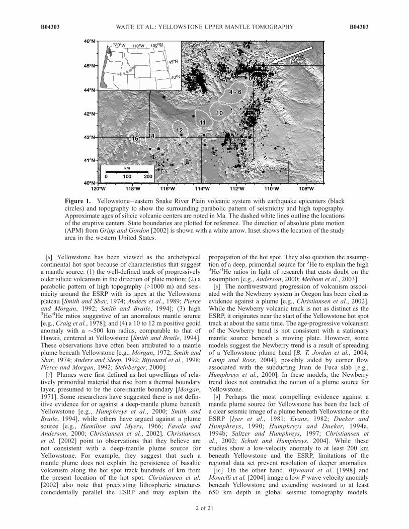
[6] Yellowstone has been viewed as the archetypicalcontinental hot spot because of characteristics that suggesta mantle source: (1) the well-defined track of progressivelyolder silicic volcanism in the direction of plate motion; (2) aparabolic pattern of high topography (>1000 m) and seis-micity around the ESRP with its apex at the Yellowstoneplateau [Smith and Sbar, 1974; Anders et al., 1989; Pierceand Morgan, 1992; Smith and Braile, 1994]; (3) high3He/4He ratios suggestive of an anomalous mantle source[e.g., Craig et al., 1978]; and (4) a 10 to 12 m positive geoidanomaly with a �500 km radius, comparable to that ofHawaii, centered at Yellowstone [Smith and Braile, 1994].These observations have often been attributed to a mantleplume beneath Yellowstone [e.g., Morgan, 1972; Smith andSbar, 1974; Anders and Sleep, 1992; Bijwaard et al., 1998;Pierce and Morgan, 1992; Steinberger, 2000].[7] Plumes were first defined as hot upwellings of rela-

tively primordial material that rise from a thermal boundarylayer, presumed to be the core-mantle boundary [Morgan,1971]. Some researchers have suggested there is not defin-itive evidence for or against a deep-mantle plume beneathYellowstone [e.g., Humphreys et al., 2000; Smith andBraile, 1994], while others have argued against a plumesource [e.g., Hamilton and Myers, 1966; Favela andAnderson, 2000; Christiansen et al., 2002]. Christiansenet al. [2002] point to observations that they believe arenot consistent with a deep-mantle plume source forYellowstone. For example, they suggest that such amantle plume does not explain the persistence of basalticvolcanism along the hot spot track hundreds of km fromthe present location of the hot spot. Christiansen et al.[2002] also note that preexisting lithospheric structurescoincidentally parallel the ESRP and may explain the

propagation of the hot spot. They also question the assump-tion of a deep, primordial source for 3He to explain the high3He/4He ratios in light of research that casts doubt on theassumption [e.g., Anderson, 2000; Meibom et al., 2003].[8] The northwestward progression of volcanism associ-

ated with the Newberry system in Oregon has been cited asevidence against a plume [e.g., Christiansen et al., 2002].While the Newberry volcanic track is not as distinct as theESRP, it originates near the start of the Yellowstone hot spottrack at about the same time. The age-progressive volcanismof the Newberry trend is not consistent with a stationarymantle source beneath a moving plate. However, somemodels suggest the Newberry trend is a result of spreadingof a Yellowstone plume head [B. T. Jordan et al., 2004;Camp and Ross, 2004], possibly aided by corner flowassociated with the subducting Juan de Fuca slab [e.g.,Humphreys et al., 2000]. In these models, the Newberrytrend does not contradict the notion of a plume source forYellowstone.[9] Perhaps the most compelling evidence against a

mantle plume source for Yellowstone has been the lack ofa clear seismic image of a plume beneath Yellowstone or theESRP [Iyer et al., 1981; Evans, 1982; Dueker andHumphreys, 1990; Humphreys and Dueker, 1994a,1994b; Saltzer and Humphreys, 1997; Christiansen etal., 2002; Schutt and Humphreys, 2004]. While thesestudies show a low-velocity anomaly to at least 200 kmbeneath Yellowstone and the ESRP, limitations of theregional data set prevent resolution of deeper anomalies.[10] On the other hand, Bijwaard et al. [1998] and

Montelli et al. [2004] image a low P wave velocity anomalybeneath Yellowstone and extending westward to at least650 km depth in global seismic tomography models.

Figure 1. Yellowstone–eastern Snake River Plain volcanic system with earthquake epicenters (blackcircles) and topography to show the surrounding parabolic pattern of seismicity and high topography.Approximate ages of silicic volcanic centers are noted in Ma. The dashed white lines outline the locationsof the eruptive centers. State boundaries are plotted for reference. The direction of absolute plate motion(APM) from Gripp and Gordon [2002] is shown with a white arrow. Inset shows the location of the studyarea in the western United States.

B04303 WAITE ET AL.: YELLOWSTONE UPPER MANTLE TOMOGRAPHY

2 of 21

B04303

Bijwaard et al. [1998] interpret the anomaly as a plume.Montelli et al. [2004], seeing no evidence for continuationof the anomaly through the lower mantle to the core-mantleboundary do not interpret the Yellowstone anomaly as aplume. The regional and global seismic tomography studiesagree that the Yellowstone hot spot has a shallow, <300 km,upper mantle low-velocity anomaly on the order of �2% to�5% for VP and VS. However, these studies have someuncertainty in the depth extent of the anomaly. In addition,there has not been a regional-scale mantle shear wavetomography study of Yellowstone.[11] Since Morgan [1971], researchers have defined

plumes variously based on seismic, chemical and thermalproperties. The lack of consistency in defining plumes hasled to confusion. Catalogs of proposed plume-induced hotspots vary depending on what criteria are used to define theplume [e.g., Courtillot et al., 2003] and numerical modelingreveals a range of possible plume shapes and sizes [Farnetaniand Samuel, 2005]. In order to avoid similar confusion in thispaper we use a general plume definition that does not definethe source depth, size, or chemical composition: a plume is anear-vertical, approximately axisymmetric, buoyant upwell-ing of hot or wet material. We are not able to resolve lowermantle seismic velocities with this study, so we cannotaddress the proposed core-mantle boundary source of aYellowstone plume. Likewise, the term hot spot refers to apersistent mantle melting anomaly that produces concen-trated volcanism, but does not presuppose a deep mantleorigin.[12] The continental setting of Yellowstone affords a

unique opportunity to study a hot spot with a large-scalepassive-source seismology experiment. We modeled tele-seismic delay time data from a 500 km by 600 km array of86 broadband three-component seismograph stations. Theaverage station spacing is 50 km NW–SE and 75 km NE–SW. The array aperture and station spacing provide higherresolution in the upper mantle than global tomographicmodels and over a larger area and to greater depths thanhas been imaged in the previous regional studies. These datafacilitate the imaging of a continuous low P and S waveanomaly that extends from Yellowstone Plateau to the top ofthe mantle transition zone [M. Jordan et al., 2004; Smith etal., 2003; Waite et al., 2003; Yuan and Dueker, 2005].

2. Traveltime Data for the Yellowstone Hot SpotExperiment

2.1. Earthquake Data Selection and Processing

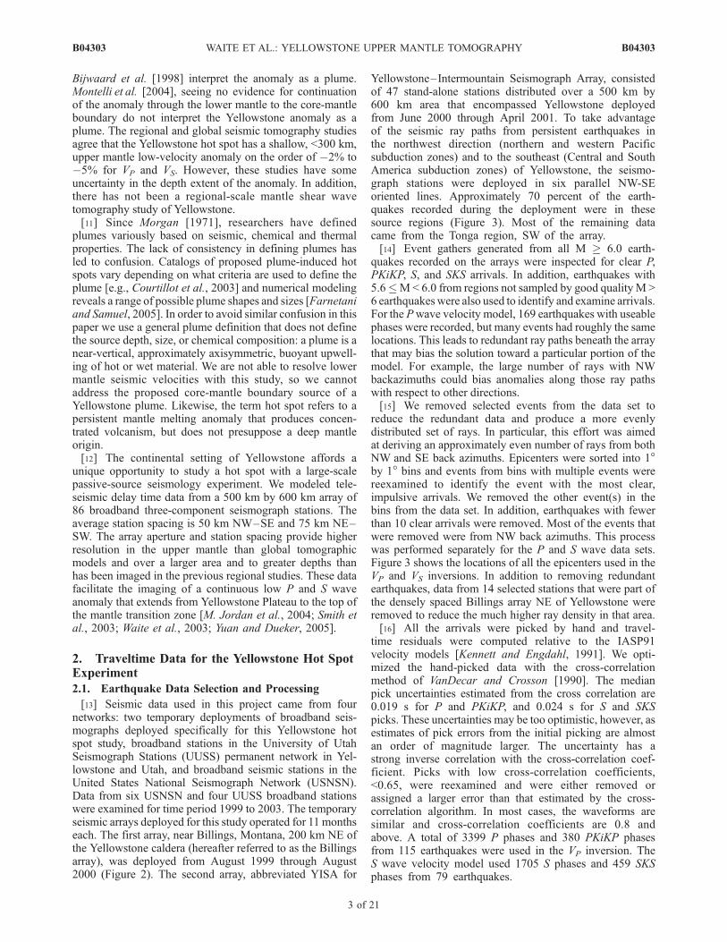
[13] Seismic data used in this project came from fournetworks: two temporary deployments of broadband seis-mographs deployed specifically for this Yellowstone hotspot study, broadband stations in the University of UtahSeismograph Stations (UUSS) permanent network in Yel-lowstone and Utah, and broadband seismic stations in theUnited States National Seismograph Network (USNSN).Data from six USNSN and four UUSS broadband stationswere examined for time period 1999 to 2003. The temporaryseismic arrays deployed for this study operated for 11 monthseach. The first array, near Billings, Montana, 200 km NE ofthe Yellowstone caldera (hereafter referred to as the Billingsarray), was deployed from August 1999 through August2000 (Figure 2). The second array, abbreviated YISA for

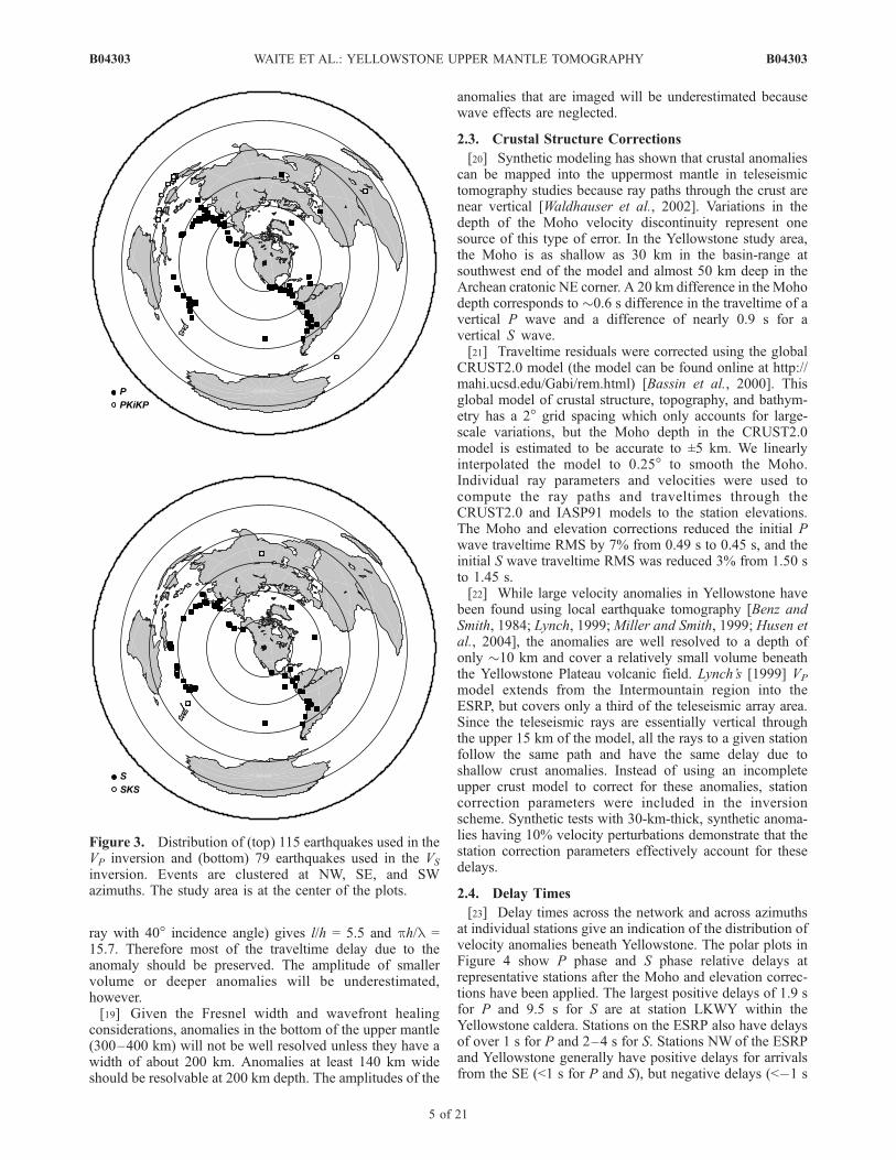
Yellowstone–Intermountain Seismograph Array, consistedof 47 stand-alone stations distributed over a 500 km by600 km area that encompassed Yellowstone deployedfrom June 2000 through April 2001. To take advantageof the seismic ray paths from persistent earthquakes inthe northwest direction (northern and western Pacificsubduction zones) and to the southeast (Central and SouthAmerica subduction zones) of Yellowstone, the seismo-graph stations were deployed in six parallel NW-SEoriented lines. Approximately 70 percent of the earth-quakes recorded during the deployment were in thesesource regions (Figure 3). Most of the remaining datacame from the Tonga region, SW of the array.[14] Event gathers generated from all M � 6.0 earth-

quakes recorded on the arrays were inspected for clear P,PKiKP, S, and SKS arrivals. In addition, earthquakes with5.6�M< 6.0 from regions not sampled by good quality M >6 earthquakeswere also used to identify and examine arrivals.For the Pwave velocity model, 169 earthquakes with useablephases were recorded, but many events had roughly the samelocations. This leads to redundant ray paths beneath the arraythat may bias the solution toward a particular portion of themodel. For example, the large number of rays with NWbackazimuths could bias anomalies along those ray pathswith respect to other directions.[15] We removed selected events from the data set to

reduce the redundant data and produce a more evenlydistributed set of rays. In particular, this effort was aimedat deriving an approximately even number of rays from bothNW and SE back azimuths. Epicenters were sorted into 1�by 1� bins and events from bins with multiple events werereexamined to identify the event with the most clear,impulsive arrivals. We removed the other event(s) in thebins from the data set. In addition, earthquakes with fewerthan 10 clear arrivals were removed. Most of the events thatwere removed were from NW back azimuths. This processwas performed separately for the P and S wave data sets.Figure 3 shows the locations of all the epicenters used in theVP and VS inversions. In addition to removing redundantearthquakes, data from 14 selected stations that were part ofthe densely spaced Billings array NE of Yellowstone wereremoved to reduce the much higher ray density in that area.[16] All the arrivals were picked by hand and travel-

time residuals were computed relative to the IASP91velocity models [Kennett and Engdahl, 1991]. We opti-mized the hand-picked data with the cross-correlationmethod of VanDecar and Crosson [1990]. The medianpick uncertainties estimated from the cross correlation are0.019 s for P and PKiKP, and 0.024 s for S and SKSpicks. These uncertainties may be too optimistic, however, asestimates of pick errors from the initial picking are almostan order of magnitude larger. The uncertainty has astrong inverse correlation with the cross-correlation coef-ficient. Picks with low cross-correlation coefficients,<0.65, were reexamined and were either removed orassigned a larger error than that estimated by the cross-correlation algorithm. In most cases, the waveforms aresimilar and cross-correlation coefficients are 0.8 andabove. A total of 3399 P phases and 380 PKiKP phasesfrom 115 earthquakes were used in the VP inversion. TheS wave velocity model used 1705 S phases and 459 SKSphases from 79 earthquakes.


3 of 21

B04303

2.2. Limitations of Ray-Theoretical Tomography

[17] We expect that there is little difference betweenresults obtained with our 1-D ray tracing and 3-D raytracing [e.g., Saltzer and Humphreys, 1997; Yuan andDueker, 2005]. However, the use of ray theory will under-estimate the true amplitude of seismic anomalies by ignor-ing the Fresnel volume. The width of the Fresnel volumedepends on the total distance between the source andreceiver, L, the distance from the source, d, and thewavelength, l. The variable f, is given by Spetzler andSnieder [2004] as

f ¼ 2ld L� dð Þ

L

� �12

: ð1Þ

The wavelengths of teleseismic P and S waves used in thisstudy are about 20 km given periods of 2 and 4 s,respectively, and upper mantle velocities. For a ray pathlength of 104 km, the maximum Fresnel width (at the

midpoint) is 450 km. This is a factor of 22 times larger thanthe wavelength. For smaller (or larger) d, the Fresnel widthis smaller. For example, at the 410 km discontinuity, a raywith an incidence angle of 40� from vertical will be about d =550 km away from the receiver. This gives f� 200 km for thesame l and L as above, so anomalies much smaller than about200 kmwide may not expected to be well resolved at the baseof the upper mantle (410 km depth). At 200 km depth, f �140 km.[18] The effects of wavefront healing, the diffraction of a

wavefront around a low-velocity anomaly [Wielandt, 1987],are also unaccounted for with ray theory. Nolet and Dahlen[2000] found that anomalies can be resolved with high-frequency rays when l/h ph/l, where l is the distancefrom the anomaly, h is the half width of the anomaly, l isthe wavelength of the seismic wave and the source is atinfinity. The amplitude of the recovered anomaly will bedecreased as d increases. The wavefront will ‘‘heal’’ (i.e.,the traveltimes will not be delayed) when l/h ph/l Forteleseismic wavelengths on the order of 20 km, an anomalywith 100 km half width at 400 km depth (l = 550 km for a

Figure 2. Seismographs used in the study. Billings array stations are the tight array in the NE. TheYellowstone–Intermountain Seismic Array (YISA) array consists of five lines of stations oriented NW-SE. Additional stations are part of USNSN and UUSS permanent networks. Symbols indicate stationowner and are shaded by sensor type. State boundaries, Yellowstone National Park boundary, selectedcities, and the 0.6 Ma caldera are shown for reference.


4 of 21

B04303

ray with 40� incidence angle) gives l/h = 5.5 and ph/l =15.7. Therefore most of the traveltime delay due to theanomaly should be preserved. The amplitude of smallervolume or deeper anomalies will be underestimated,however.[19] Given the Fresnel width and wavefront healing

considerations, anomalies in the bottom of the upper mantle(300–400 km) will not be well resolved unless they have awidth of about 200 km. Anomalies at least 140 km wideshould be resolvable at 200 km depth. The amplitudes of the

anomalies that are imaged will be underestimated becausewave effects are neglected.

2.3. Crustal Structure Corrections

[20] Synthetic modeling has shown that crustal anomaliescan be mapped into the uppermost mantle in teleseismictomography studies because ray paths through the crust arenear vertical [Waldhauser et al., 2002]. Variations in thedepth of the Moho velocity discontinuity represent onesource of this type of error. In the Yellowstone study area,the Moho is as shallow as 30 km in the basin-range atsouthwest end of the model and almost 50 km deep in theArchean cratonic NE corner. A 20 km difference in the Mohodepth corresponds to �0.6 s difference in the traveltime of avertical P wave and a difference of nearly 0.9 s for avertical S wave.[21] Traveltime residuals were corrected using the global

CRUST2.0 model (the model can be found online at http://mahi.ucsd.edu/Gabi/rem.html) [Bassin et al., 2000]. Thisglobal model of crustal structure, topography, and bathym-etry has a 2� grid spacing which only accounts for large-scale variations, but the Moho depth in the CRUST2.0model is estimated to be accurate to ±5 km. We linearlyinterpolated the model to 0.25� to smooth the Moho.Individual ray parameters and velocities were used tocompute the ray paths and traveltimes through theCRUST2.0 and IASP91 models to the station elevations.The Moho and elevation corrections reduced the initial Pwave traveltime RMS by 7% from 0.49 s to 0.45 s, and theinitial S wave traveltime RMS was reduced 3% from 1.50 sto 1.45 s.[22] While large velocity anomalies in Yellowstone have

been found using local earthquake tomography [Benz andSmith, 1984; Lynch, 1999;Miller and Smith, 1999; Husen etal., 2004], the anomalies are well resolved to a depth ofonly �10 km and cover a relatively small volume beneaththe Yellowstone Plateau volcanic field. Lynch’s [1999] VP

model extends from the Intermountain region into theESRP, but covers only a third of the teleseismic array area.Since the teleseismic rays are essentially vertical throughthe upper 15 km of the model, all the rays to a given stationfollow the same path and have the same delay due toshallow crust anomalies. Instead of using an incompleteupper crust model to correct for these anomalies, stationcorrection parameters were included in the inversionscheme. Synthetic tests with 30-km-thick, synthetic anoma-lies having 10% velocity perturbations demonstrate that thestation correction parameters effectively account for thesedelays.

2.4. Delay Times

[23] Delay times across the network and across azimuthsat individual stations give an indication of the distribution ofvelocity anomalies beneath Yellowstone. The polar plots inFigure 4 show P phase and S phase relative delays atrepresentative stations after the Moho and elevation correc-tions have been applied. The largest positive delays of 1.9 sfor P and 9.5 s for S are at station LKWY within theYellowstone caldera. Stations on the ESRP also have delaysof over 1 s for P and 2–4 s for S. Stations NW of the ESRPand Yellowstone generally have positive delays for arrivalsfrom the SE (<1 s for P and S), but negative delays (<�1 s

Figure 3. Distribution of (top) 115 earthquakes used in theVP inversion and (bottom) 79 earthquakes used in the VS

inversion. Events are clustered at NW, SE, and SWazimuths. The study area is at the center of the plots.


5 of 21

B04303

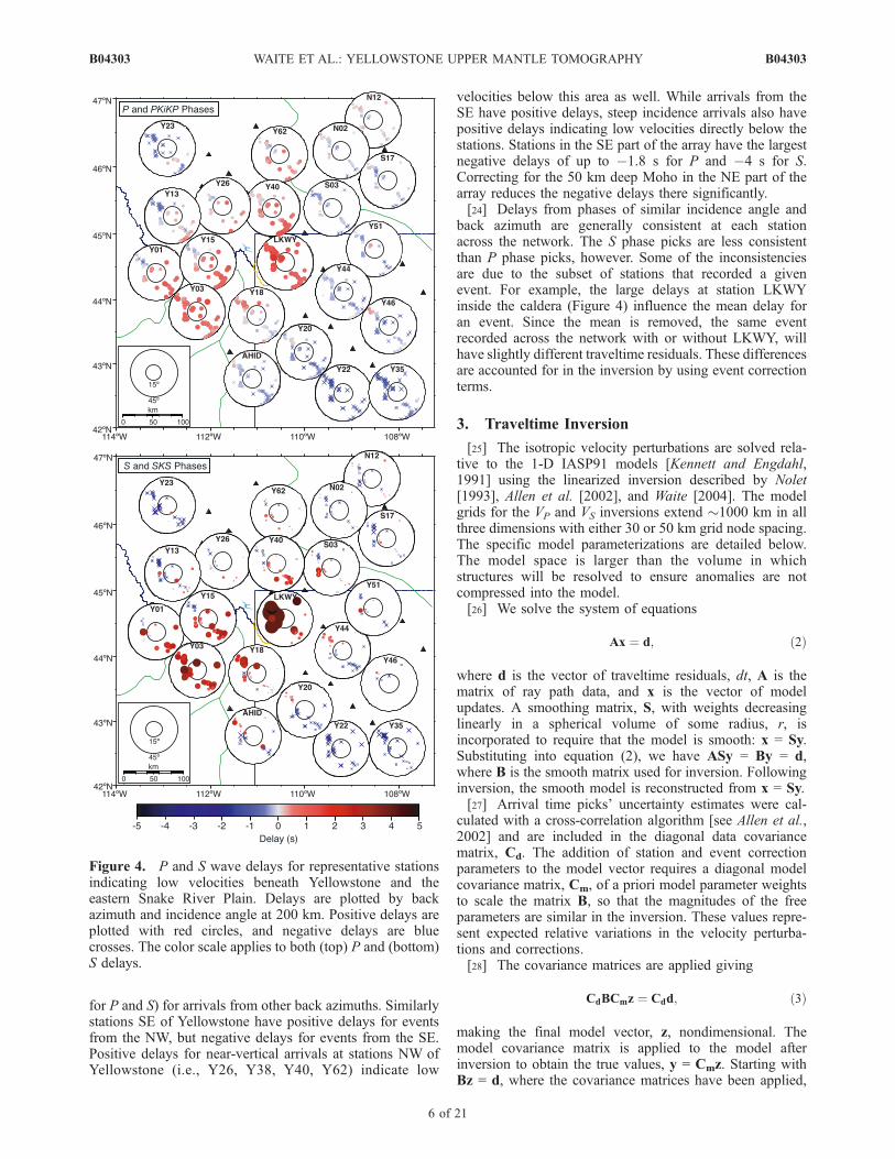
for P and S) for arrivals from other back azimuths. Similarlystations SE of Yellowstone have positive delays for eventsfrom the NW, but negative delays for events from the SE.Positive delays for near-vertical arrivals at stations NW ofYellowstone (i.e., Y26, Y38, Y40, Y62) indicate low

velocities below this area as well. While arrivals from theSE have positive delays, steep incidence arrivals also havepositive delays indicating low velocities directly below thestations. Stations in the SE part of the array have the largestnegative delays of up to �1.8 s for P and �4 s for S.Correcting for the 50 km deep Moho in the NE part of thearray reduces the negative delays there significantly.[24] Delays from phases of similar incidence angle and

back azimuth are generally consistent at each stationacross the network. The S phase picks are less consistentthan P phase picks, however. Some of the inconsistenciesare due to the subset of stations that recorded a givenevent. For example, the large delays at station LKWYinside the caldera (Figure 4) influence the mean delay foran event. Since the mean is removed, the same eventrecorded across the network with or without LKWY, willhave slightly different traveltime residuals. These differencesare accounted for in the inversion by using event correctionterms.

3. Traveltime Inversion

[25] The isotropic velocity perturbations are solved rela-tive to the 1-D IASP91 models [Kennett and Engdahl,1991] using the linearized inversion described by Nolet[1993], Allen et al. [2002], and Waite [2004]. The modelgrids for the VP and VS inversions extend �1000 km in allthree dimensions with either 30 or 50 km grid node spacing.The specific model parameterizations are detailed below.The model space is larger than the volume in whichstructures will be resolved to ensure anomalies are notcompressed into the model.[26] We solve the system of equations

Ax ¼ d; ð2Þ

where d is the vector of traveltime residuals, dt, A is thematrix of ray path data, and x is the vector of modelupdates. A smoothing matrix, S, with weights decreasinglinearly in a spherical volume of some radius, r, isincorporated to require that the model is smooth: x = Sy.Substituting into equation (2), we have ASy = By = d,where B is the smooth matrix used for inversion. Followinginversion, the smooth model is reconstructed from x = Sy.[27] Arrival time picks’ uncertainty estimates were cal-

culated with a cross-correlation algorithm [see Allen et al.,2002] and are included in the diagonal data covariancematrix, Cd. The addition of station and event correctionparameters to the model vector requires a diagonal modelcovariance matrix, Cm, of a priori model parameter weightsto scale the matrix B, so that the magnitudes of the freeparameters are similar in the inversion. These values repre-sent expected relative variations in the velocity perturba-tions and corrections.[28] The covariance matrices are applied giving

CdBCmz ¼ Cdd; ð3Þ

making the final model vector, z, nondimensional. Themodel covariance matrix is applied to the model afterinversion to obtain the true values, y = Cmz. Starting withBz = d, where the covariance matrices have been applied,

Figure 4. P and S wave delays for representative stationsindicating low velocities beneath Yellowstone and theeastern Snake River Plain. Delays are plotted by backazimuth and incidence angle at 200 km. Positive delays areplotted with red circles, and negative delays are bluecrosses. The color scale applies to both (top) P and (bottom)S delays.


6 of 21

B04303

the system of equations is solved by minimizing the leastsquares misfit function, with the LSQR algorithm [Paigeand Saunders, 1982] after modification to includedamping, l:

k Bz� d k2 þ l k z k2 : ð4Þ

Several combinations of model grid spacing (30, 40, 50,60 km), smoothing lengths (0 up to 90 km) and dampingwere tested to explore the sensitivity of the invertedmodel velocity perturbations to model parameterization.Synthetic data and real data were used in these tests. Theprincipal features of the model are persistent in everysolution, although the amplitudes vary by up to a fewpercent in the VS models. Many small features areinconsistent and are not interpreted. As expected,smoothing tends to reduce the amplitude of small volumeanomalies, but spreads them out over a larger volume.[29] An alternative type of smoothing uses grid offset and

averaging [Evans and Zucca, 1988]. Two grids are used inthis procedure: a coarse grid for inversion, and a second finegrid with spacing some fraction of the inversion grid. Thelatter grid is used to shift the inversion grid. The grids arenot shifted vertically. The procedure is as follows: inversionis performed using a coarse model grid; the grid is thenshifted horizontally 10 km (e.g., to the east) and theinversion is performed with this new coarse model grid.The shifting and inversion is continued until a coarse gridnode has occupied the each node of the fine grid. Finally,the average value of each node in the fine grid is computedfrom the value of the velocity at each of the 25 fine gridnodes that surround it in a 5 node by 5 node square.[30] We present results of inversion with both linear

smoothing and multimodel average for comparison. Themodels with linear smoothing imposed in the inversion havegrid node spacing of 30 by 30 by 30 km and 70 kmsmoothing in both the horizontal and vertical directions.The smoothed VP and VS models are designated S30VP andS30VS, respectively. The offset-and-average models have acoarse grid spacing of 50 km by 50 km in horizontal and thefine grid node spacing is 10 km by 10 km in horizontal.Both grids have 50 km spacing in the vertical as discussedabove. The offset-and-average VP and VS models are calledOSA50VP and OSA50VS. Including two models for boththe VP and VS inversions is useful for interpreting theresults. For example, higher confidence is afforded toanomalies that are consistent between the models.[31] Higher damping was used for the OSA models

than for the corresponding S30 models because therewere fewer grid nodes in the OSA models. Similarly,the model covariance values were chosen so that thestation and event corrections computed with the twomethods would be equivalent. The station correctionscomputed in the inversions vary from �0.8 to 0.7 s(�1.2 to 1.5 s) in the VP (VS) models. Event correctionsvary from �0.2 to 0.2 s (�0.5 to 0.8 s) in the VP (VS)models. The final RMS and total variance reduction ofthe corresponding OSA and S30 models for VP and VS

are equivalent (see results below). While the damping andweighting of station and event corrections contributes tothe variations in the structure and amplitude of the seismicanomalies in the models, we attribute most of the differences

between the models to the different types of smoothingemployed.

4. Results of the P and S Wave TomographicInversion

[32] The P and S wave velocity models were solvedindependently as described above. The VP and VS modelsshow strong low-velocity anomalies in the upper 200 kmbeneath Yellowstone. In addition, the VP and VS modelshave a smaller-amplitude low-velocity anomaly extendingfrom 250 km depth to the top of the midmantle transitionzone �100 km NNW of the caldera. The locations of thelower VP and VS anomalies are slightly different.

4.1. P Wave Velocity Structure

[33] The VP models are constructed from 3779 P andPKiKP rays and traveltimes. The initial RMS residual is0.45 s and the final RMS residual is 0.17 s for both theS30VP and OSA50VP models. This is an order of magni-tude higher than the pick uncertainty estimate after crosscorrelation and roughly equal to the estimated medianuncertainty in the handpicked data. The data variancereductions are 77% for S30VP and 78% for OSA50VP.[34] Plots of the ray density through slices of the S30VP

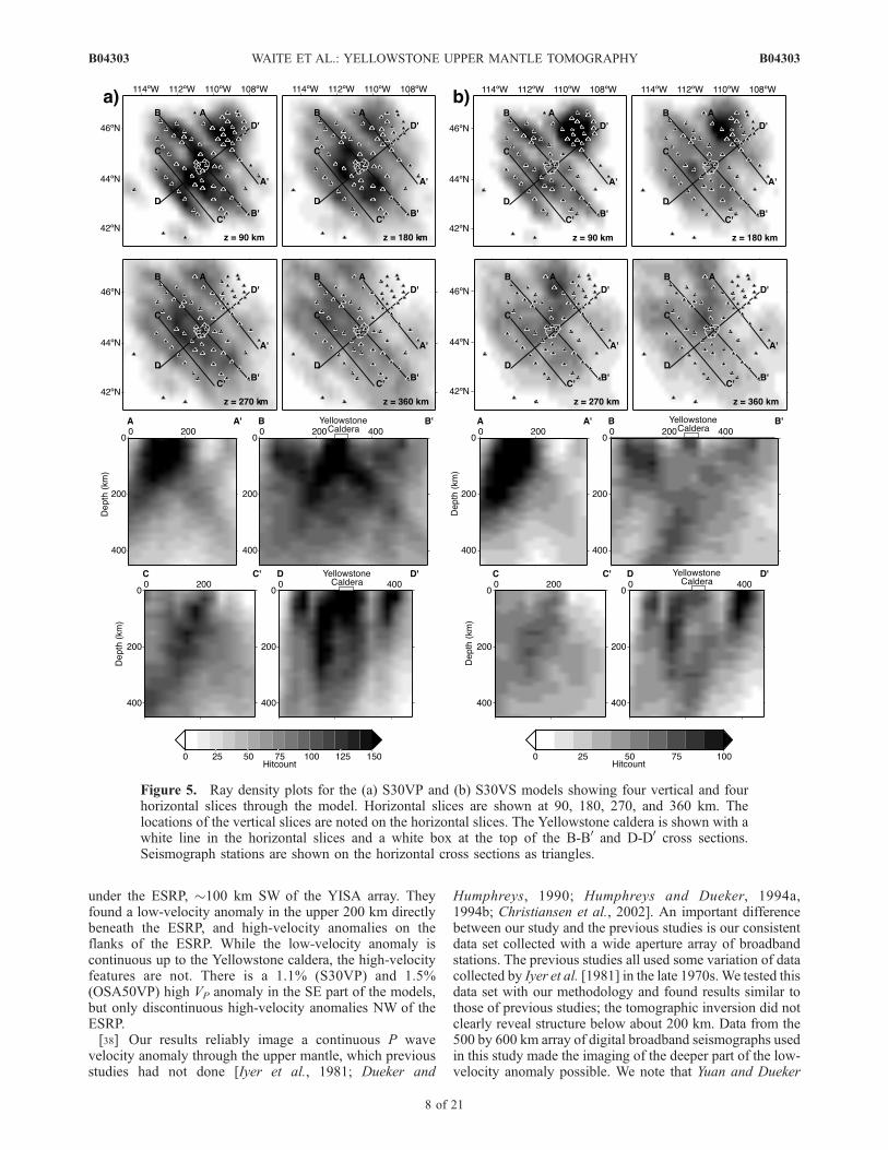
model are shown in Figure 5. These plots give a roughestimate of the model resolution since they do not take intoaccount the orientation of the rays, but they provide a wayto quickly estimate areas of good and poor data coverage.For example, note the high density of rays beneath theYellowstone caldera and the Billings array. The predomi-nance of rays arriving from NW and SE back azimuths isdemonstrated by the volumes of high ray density to the NWand SE of the caldera. In the 90 km depth slice, there is ahigh density under the NW-SE lines of stations, but lowdensity in between the lines. This results in less resolutionin the NE-SW direction at shallow depths, but the effect issmaller in deeper parts of the model.[35] The ray density plots do not demonstrate the vertical

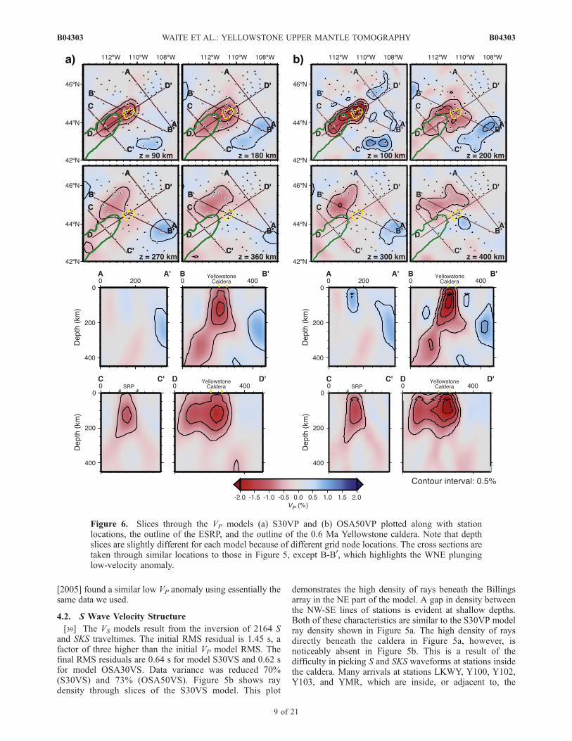
resolution problem inherent in this type of regional tele-seismic tomography study [see, e.g., Keller et al., 2000;Wolfe et al., 2002a, 2002b]. The angles of the incoming raysin the middle upper mantle (�200 km) are between �45�and vertical. The ray paths through the model to a givenstation define a cone that opens with depth. There arecrossing rays in the middle of the model down to at leastthe 410 km discontinuity, so reasonable resolution isexpected to about that depth. Smearing is expected to bestrongest at the sides and bottom of the model where therays are parallel. Resolution information obtained from thesynthetic tests described below is more useful.[36] The P wave models (Figure 6) are dominated by a

tilted low VP anomaly that extends from directly beneathYellowstone through the upper mantle to the 410 kmdiscontinuity 100 km WNW of Yellowstone. The anomalyhas peak amplitudes of �2.0% (S30VP) and �2.3%(OSA50VP) above 200 km and �1.0% (S30VP andOSA50VP) from 250 to 400 km depth. The shallow portionof the anomaly continues down the ESRP to the SW butdecreases in amplitude. It is roughly the width of the ESRP.[37] Schutt and Humphreys [2004] used a similar tele-

seismic tomography technique to image the upper mantle


7 of 21

B04303

under the ESRP, �100 km SW of the YISA array. Theyfound a low-velocity anomaly in the upper 200 km directlybeneath the ESRP, and high-velocity anomalies on theflanks of the ESRP. While the low-velocity anomaly iscontinuous up to the Yellowstone caldera, the high-velocityfeatures are not. There is a 1.1% (S30VP) and 1.5%(OSA50VP) high VP anomaly in the SE part of the models,but only discontinuous high-velocity anomalies NW of theESRP.[38] Our results reliably image a continuous P wave

velocity anomaly through the upper mantle, which previousstudies had not done [Iyer et al., 1981; Dueker and

Humphreys, 1990; Humphreys and Dueker, 1994a,1994b; Christiansen et al., 2002]. An important differencebetween our study and the previous studies is our consistentdata set collected with a wide aperture array of broadbandstations. The previous studies all used some variation of datacollected by Iyer et al. [1981] in the late 1970s. We tested thisdata set with our methodology and found results similar tothose of previous studies; the tomographic inversion did notclearly reveal structure below about 200 km. Data from the500 by 600 km array of digital broadband seismographs usedin this study made the imaging of the deeper part of the low-velocity anomaly possible. We note that Yuan and Dueker

Figure 5. Ray density plots for the (a) S30VP and (b) S30VS models showing four vertical and fourhorizontal slices through the model. Horizontal slices are shown at 90, 180, 270, and 360 km. Thelocations of the vertical slices are noted on the horizontal slices. The Yellowstone caldera is shown with awhite line in the horizontal slices and a white box at the top of the B-B0 and D-D0 cross sections.Seismograph stations are shown on the horizontal cross sections as triangles.


8 of 21

B04303

[2005] found a similar low VP anomaly using essentially thesame data we used.

4.2. S Wave Velocity Structure

[39] The VS models result from the inversion of 2164 Sand SKS traveltimes. The initial RMS residual is 1.45 s, afactor of three higher than the initial VP model RMS. Thefinal RMS residuals are 0.64 s for model S30VS and 0.62 sfor model OSA30VS. Data variance was reduced 70%(S30VS) and 73% (OSA50VS). Figure 5b shows raydensity through slices of the S30VS model. This plot

demonstrates the high density of rays beneath the Billingsarray in the NE part of the model. A gap in density betweenthe NW-SE lines of stations is evident at shallow depths.Both of these characteristics are similar to the S30VP modelray density shown in Figure 5a. The high density of raysdirectly beneath the caldera in Figure 5a, however, isnoticeably absent in Figure 5b. This is a result of thedifficulty in picking S and SKS waveforms at stations insidethe caldera. Many arrivals at stations LKWY, Y100, Y102,Y103, and YMR, which are inside, or adjacent to, the

Figure 6. Slices through the VP models (a) S30VP and (b) OSA50VP plotted along with stationlocations, the outline of the ESRP, and the outline of the 0.6 Ma Yellowstone caldera. Note that depthslices are slightly different for each model because of different grid node locations. The cross sections aretaken through similar locations to those in Figure 5, except B-B0, which highlights the WNE plunginglow-velocity anomaly.


9 of 21

B04303

caldera, have broad, distorted waveforms that do not corre-late with arrivals at stations outside the caldera. A combi-nation of scattering by small-scale heterogeneities andattenuation directly beneath the caldera affects the wave-forms recorded there.[40] The geometries of the anomalies in the VS models

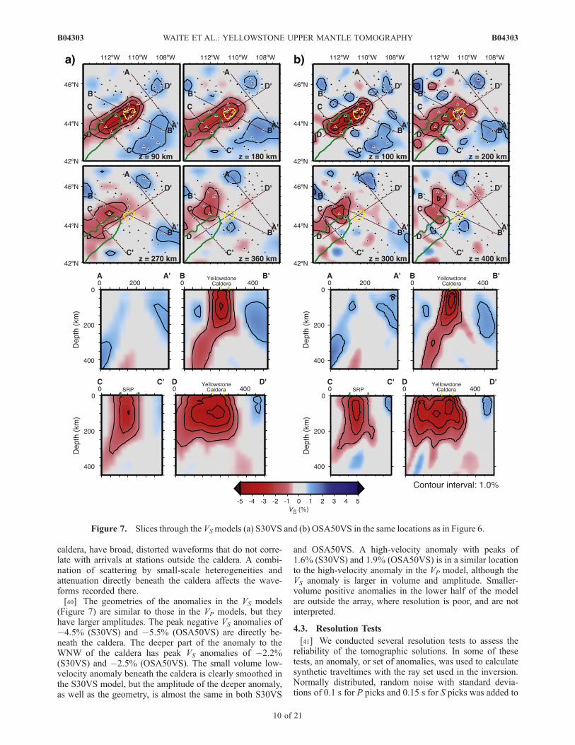
(Figure 7) are similar to those in the VP models, but theyhave larger amplitudes. The peak negative VS anomalies of�4.5% (S30VS) and �5.5% (OSA50VS) are directly be-neath the caldera. The deeper part of the anomaly to theWNW of the caldera has peak VS anomalies of �2.2%(S30VS) and �2.5% (OSA50VS). The small volume low-velocity anomaly beneath the caldera is clearly smoothed inthe S30VS model, but the amplitude of the deeper anomaly,as well as the geometry, is almost the same in both S30VS

and OSA50VS. A high-velocity anomaly with peaks of1.6% (S30VS) and 1.9% (OSA50VS) is in a similar locationto the high-velocity anomaly in the VP model, although theVS anomaly is larger in volume and amplitude. Smaller-volume positive anomalies in the lower half of the modelare outside the array, where resolution is poor, and are notinterpreted.

4.3. Resolution Tests

[41] We conducted several resolution tests to assess thereliability of the tomographic solutions. In some of thesetests, an anomaly, or set of anomalies, was used to calculatesynthetic traveltimes with the ray set used in the inversion.Normally distributed, random noise with standard devia-tions of 0.1 s for P picks and 0.15 s for S picks was added to

Figure 7. Slices through the VSmodels (a) S30VS and (b) OSA50VS in the same locations as in Figure 6.


10 of 21

B04303

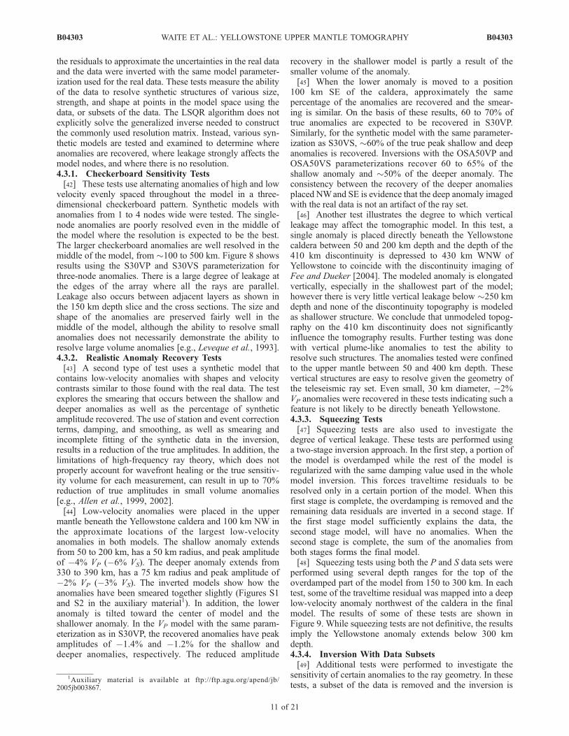
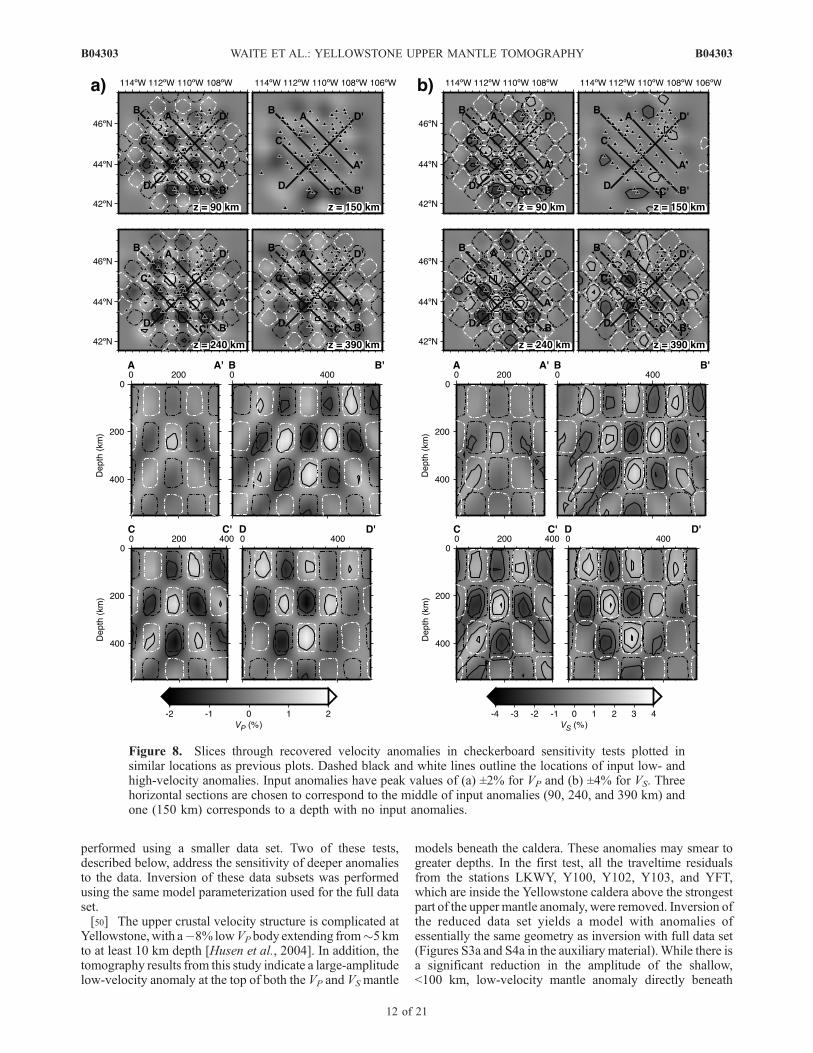
the residuals to approximate the uncertainties in the real dataand the data were inverted with the same model parameter-ization used for the real data. These tests measure the abilityof the data to resolve synthetic structures of various size,strength, and shape at points in the model space using thedata, or subsets of the data. The LSQR algorithm does notexplicitly solve the generalized inverse needed to constructthe commonly used resolution matrix. Instead, various syn-thetic models are tested and examined to determine whereanomalies are recovered, where leakage strongly affects themodel nodes, and where there is no resolution.4.3.1. Checkerboard Sensitivity Tests[42] These tests use alternating anomalies of high and low

velocity evenly spaced throughout the model in a three-dimensional checkerboard pattern. Synthetic models withanomalies from 1 to 4 nodes wide were tested. The single-node anomalies are poorly resolved even in the middle ofthe model where the resolution is expected to be the best.The larger checkerboard anomalies are well resolved in themiddle of the model, from �100 to 500 km. Figure 8 showsresults using the S30VP and S30VS parameterization forthree-node anomalies. There is a large degree of leakage atthe edges of the array where all the rays are parallel.Leakage also occurs between adjacent layers as shown inthe 150 km depth slice and the cross sections. The size andshape of the anomalies are preserved fairly well in themiddle of the model, although the ability to resolve smallanomalies does not necessarily demonstrate the ability toresolve large volume anomalies [e.g., Leveque et al., 1993].4.3.2. Realistic Anomaly Recovery Tests[43] A second type of test uses a synthetic model that

contains low-velocity anomalies with shapes and velocitycontrasts similar to those found with the real data. The testexplores the smearing that occurs between the shallow anddeeper anomalies as well as the percentage of syntheticamplitude recovered. The use of station and event correctionterms, damping, and smoothing, as well as smearing andincomplete fitting of the synthetic data in the inversion,results in a reduction of the true amplitudes. In addition, thelimitations of high-frequency ray theory, which does notproperly account for wavefront healing or the true sensitiv-ity volume for each measurement, can result in up to 70%reduction of true amplitudes in small volume anomalies[e.g., Allen et al., 1999, 2002].[44] Low-velocity anomalies were placed in the upper

mantle beneath the Yellowstone caldera and 100 km NW inthe approximate locations of the largest low-velocityanomalies in both models. The shallow anomaly extendsfrom 50 to 200 km, has a 50 km radius, and peak amplitudeof �4% VP (�6% VS). The deeper anomaly extends from330 to 390 km, has a 75 km radius and peak amplitude of�2% VP (�3% VS). The inverted models show how theanomalies have been smeared together slightly (Figures S1and S2 in the auxiliary material1). In addition, the loweranomaly is tilted toward the center of model and theshallower anomaly. In the VP model with the same param-eterization as in S30VP, the recovered anomalies have peakamplitudes of �1.4% and �1.2% for the shallow anddeeper anomalies, respectively. The reduced amplitude

recovery in the shallower model is partly a result of thesmaller volume of the anomaly.[45] When the lower anomaly is moved to a position

100 km SE of the caldera, approximately the samepercentage of the anomalies are recovered and the smear-ing is similar. On the basis of these results, 60 to 70% oftrue anomalies are expected to be recovered in S30VP.Similarly, for the synthetic model with the same parameter-ization as S30VS, �60% of the true peak shallow and deepanomalies is recovered. Inversions with the OSA50VP andOSA50VS parameterizations recover 60 to 65% of theshallow anomaly and �50% of the deeper anomaly. Theconsistency between the recovery of the deeper anomaliesplaced NWand SE is evidence that the deep anomaly imagedwith the real data is not an artifact of the ray set.[46] Another test illustrates the degree to which vertical

leakage may affect the tomographic model. In this test, asingle anomaly is placed directly beneath the Yellowstonecaldera between 50 and 200 km depth and the depth of the410 km discontinuity is depressed to 430 km WNW ofYellowstone to coincide with the discontinuity imaging ofFee and Dueker [2004]. The modeled anomaly is elongatedvertically, especially in the shallowest part of the model;however there is very little vertical leakage below �250 kmdepth and none of the discontinuity topography is modeledas shallower structure. We conclude that unmodeled topog-raphy on the 410 km discontinuity does not significantlyinfluence the tomography results. Further testing was donewith vertical plume-like anomalies to test the ability toresolve such structures. The anomalies tested were confinedto the upper mantle between 50 and 400 km depth. Thesevertical structures are easy to resolve given the geometry ofthe teleseismic ray set. Even small, 30 km diameter, �2%VP anomalies were recovered in these tests indicating such afeature is not likely to be directly beneath Yellowstone.4.3.3. Squeezing Tests[47] Squeezing tests are also used to investigate the

degree of vertical leakage. These tests are performed usinga two-stage inversion approach. In the first step, a portion ofthe model is overdamped while the rest of the model isregularized with the same damping value used in the wholemodel inversion. This forces traveltime residuals to beresolved only in a certain portion of the model. When thisfirst stage is complete, the overdamping is removed and theremaining data residuals are inverted in a second stage. Ifthe first stage model sufficiently explains the data, thesecond stage model, will have no anomalies. When thesecond stage is complete, the sum of the anomalies fromboth stages forms the final model.[48] Squeezing tests using both the P and S data sets were

performed using several depth ranges for the top of theoverdamped part of the model from 150 to 300 km. In eachtest, some of the traveltime residual was mapped into a deeplow-velocity anomaly northwest of the caldera in the finalmodel. The results of some of these tests are shown inFigure 9. While squeezing tests are not definitive, the resultsimply the Yellowstone anomaly extends below 300 kmdepth.4.3.4. Inversion With Data Subsets[49] Additional tests were performed to investigate the

sensitivity of certain anomalies to the ray geometry. In thesetests, a subset of the data is removed and the inversion is

1Auxiliary material is available at ftp://ftp.agu.org/apend/jb/2005jb003867.


11 of 21

B04303

performed using a smaller data set. Two of these tests,described below, address the sensitivity of deeper anomaliesto the data. Inversion of these data subsets was performedusing the same model parameterization used for the full dataset.[50] The upper crustal velocity structure is complicated at

Yellowstone,with a�8% lowVP body extending from�5 kmto at least 10 km depth [Husen et al., 2004]. In addition, thetomography results from this study indicate a large-amplitudelow-velocity anomaly at the top of both the VP and VSmantle

models beneath the caldera. These anomalies may smear togreater depths. In the first test, all the traveltime residualsfrom the stations LKWY, Y100, Y102, Y103, and YFT,which are inside the Yellowstone caldera above the strongestpart of the upper mantle anomaly, were removed. Inversion ofthe reduced data set yields a model with anomalies ofessentially the same geometry as inversion with full data set(Figures S3a and S4a in the auxiliary material).While there isa significant reduction in the amplitude of the shallow,<100 km, low-velocity mantle anomaly directly beneath

Figure 8. Slices through recovered velocity anomalies in checkerboard sensitivity tests plotted insimilar locations as previous plots. Dashed black and white lines outline the locations of input low- andhigh-velocity anomalies. Input anomalies have peak values of (a) ±2% for VP and (b) ±4% for VS. Threehorizontal sections are chosen to correspond to the middle of input anomalies (90, 240, and 390 km) andone (150 km) corresponds to a depth with no input anomalies.


12 of 21

B04303

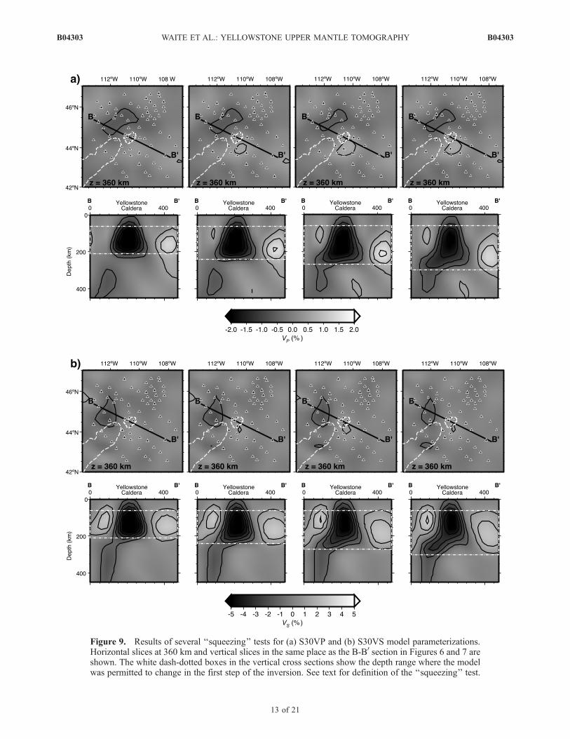
Figure 9. Results of several ‘‘squeezing’’ tests for (a) S30VP and (b) S30VS model parameterizations.Horizontal slices at 360 km and vertical slices in the same place as the B-B0 section in Figures 6 and 7 areshown. The white dash-dotted boxes in the vertical cross sections show the depth range where the modelwas permitted to change in the first step of the inversion. See text for definition of the ‘‘squeezing’’ test.


13 of 21

B04303

the caldera, this is expected since there are few raysremaining in this part of the model. The deeper anomaly,however, is not significantly affected by the smaller dataset.[51] In the other test, data from earthquakes to the NW

(i.e., earthquakes from azimuths between 300� and 360�from the caldera) were removed from the data set. While theanomalies have different shapes than those imaged with thefull data set, they are generally in the same positions(Figures S3b and S4b in the auxiliary material). The deep,300–400 km depth anomaly is clear although it is nearlyseparated from the shallow anomaly. This is an importantdifference from the inversion of the entire data set thatshows a continuous low-velocity feature from near thesurface to�400 km depth. Taken together, these tests provideconfidence that the deeper, 250–400 km portion of the low-velocity anomaly imaged with the full inversion is not a resultof smearing of shallow anomalies.

5. Discussion of the Yellowstone Hot Spot VP andVS models

[52] The interpretation of seismic tomography requiresknowledge of the effects of temperature, anisotropy, andcomposition including the presence of water or partial melt.Forward modeling of seismic velocity for a large number ofupper mantle thermal and compositional parameters showsthat variations in temperature have the largest effect [e.g.,Goes et al., 2000; Goes and van der Lee, 2002]. Exceptionsmay include regions where plumes or small-scale convec-tion may produce volumes of different composition throughmelting, hydration and dehydration. For example, Schuttand Humphreys [2004] interpret velocity variations acrossthe ESRP, �100 km SW of the YISA array, primarily interms compositional heterogeneity. The low-velocity anom-aly beneath the ESRP is attributed to up to 1% partial melt.The high-velocity bodies on the flanks of the ESRP areinterpreted to be only 80 K cooler, but 5% depleted inbasaltic component.[53] Seismic anisotropy has largely been ignored in veloc-

ity tomography studies although it can effect on the ability toresolve velocities [e.g., Levin et al., 1996]. The anisotropiccontribution to the traveltime delay depends on the amplitudeof the anisotropy, direction of propagation and polarization,and thickness of the anisotropic medium. Schutt andHumphreys [2004] used a correction for the anisotropybeneath the ESRP [Schutt and Humphreys, 2001] to removethe effect of anisotropy in their study. The simple anisotropicstructure of the upper mantle beneath the ESRP, with roughlyparallel directions of fast anisotropy everywhere, allowedcorrections to bemadewith reasonable assumptions about themean direction of fast anisotropy and thickness of the aniso-tropic layer. However, they found little difference betweentheir tomography results, which include correction for an-isotropy and those that did not. Keyser et al. [2002] found nofirst-order effect of S wave anisotropy in their shear wavetomography of the Eifel hot spot, despite a complex pattern ofshear wave splitting fast directions [Walker, 2004]. Since thedistribution of fast S wave polarization directions at Yellow-stone is comparable or simpler than at Eifel, we do not expectthat accounting for anisotropywill have a significant effect onthe tomography results.

[54] Some additional items should be considered wheninterpreting the seismic anomalies in terms of thermal andcompositional variations. First, recognizing that not all ofthe true anomaly amplitude is recovered with the inversion,the modeled anomalies should be considered as minimums.The relative seismic anomalies contribute the primarysource of uncertainty in the interpretation. Second, theexcess temperature estimates are relative to a mantle thatis warmer than average. Goes and van der Lee [2002]estimate a temperature anomaly of 200 K to at least250 km depth beneath the active basin-range province.Third, no significant chemical anomalies are interpreted tobe in this region [Godey et al., 2004]; however, anomalieson the scale of a narrow upwelling may not appear in thesurface wave tomography used by Godey et al. [2004] toestimate temperatures and chemical variations. Finally, asrevealed by the synthetic testing, some vertical leakage ofseismic anomalies occurs in the inversion. In particular, thedepths of the velocity anomalies may be overestimated.[55] To aid in interpreting the anomalies, three-dimen-

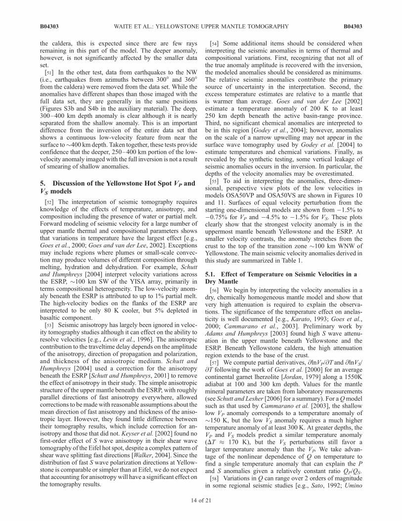
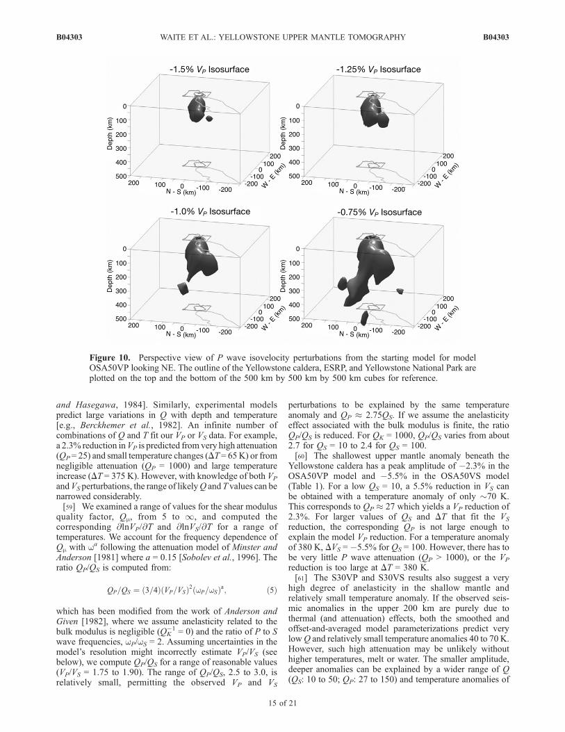
sional, perspective view plots of the low velocities inmodels OSA50VP and OSA50VS are shown in Figures 10and 11. Surfaces of equal velocity perturbation from thestarting one-dimensional models are shown from �1.5% to�0.75% for VP and �4.5% to �1.5% for VS. These plotsclearly show that the strongest velocity anomaly is in theuppermost mantle beneath Yellowstone and the ESRP. Atsmaller velocity contrasts, the anomaly stretches from thecrust to the top of the transition zone �100 km WNW ofYellowstone. The main seismic velocity anomalies derived inthis study are summarized in Table 1.

5.1. Effect of Temperature on Seismic Velocities in aDry Mantle

[56] We begin by interpreting the velocity anomalies in adry, chemically homogeneous mantle model and show thatvery high attenuation is required to explain the observa-tions. The significance of the temperature effect on anelas-ticity is well documented [e.g., Karato, 1993; Goes et al.,2000; Cammarano et al., 2003]. Preliminary work byAdams and Humphreys [2003] found high S wave attenu-ation in the upper mantle beneath Yellowstone and theESRP. Beneath Yellowstone caldera, the high attenuationregion extends to the base of the crust.[57] We compute partial derivatives, @lnVP/@T and @lnVS/

@T following the work of Goes et al. [2000] for an averagecontinental garnet lherzolite [Jordan, 1979] along a 1550Kadiabat at 100 and 300 km depth. Values for the mantlemineral parameters are taken from laboratory measurements(see Schutt and Lesher [2006] for a summary). For aQmodelsuch as that used by Cammarano et al. [2003], the shallowlow VP anomaly corresponds to a temperature anomaly of�150 K, but the low VS anomaly requires a much highertemperature anomaly of at least 300 K. At greater depths, theVP and VS models predict a similar temperature anomaly(DT � 170 K), but the VS perturbations still favor alarger temperature anomaly than the VP. We take advan-tage of the nonlinear dependence of Q on temperature tofind a single temperature anomaly that can explain the Pand S anomalies given a relatively constant ratio QP/QS.[58] Variations in Q can range over 2 orders of magnitude

in some regional seismic studies [e.g., Sato, 1992; Umino


14 of 21

B04303

and Hasegawa, 1984]. Similarly, experimental modelspredict large variations in Q with depth and temperature[e.g., Berckhemer et al., 1982]. An infinite number ofcombinations of Q and T fit our VP or VS data. For example,a 2.3% reduction inVP is predicted from very high attenuation(QP= 25) and small temperature changes (DT = 65K) or fromnegligible attenuation (QP = 1000) and large temperatureincrease (DT = 375 K). However, with knowledge of both VP

andVS perturbations, the range of likelyQ and T values can benarrowed considerably.[59] We examined a range of values for the shear modulus

quality factor, Qm, from 5 to 1, and computed thecorresponding @lnVP/@T and @lnVS/@T for a range oftemperatures. We account for the frequency dependence ofQm with wa following the attenuation model of Minster andAnderson [1981] where a = 0.15 [Sobolev et al., 1996]. Theratio QP/QS is computed from:

QP=QS ¼ 3=4ð Þ VP=VSð Þ2 wP=wSð Þa; ð5Þ

which has been modified from the work of Anderson andGiven [1982], where we assume anelasticity related to thebulk modulus is negligible (QK

�1 = 0) and the ratio of P to Swave frequencies, wP/wS = 2. Assuming uncertainties in themodel’s resolution might incorrectly estimate VP/VS (seebelow), we compute QP/QS for a range of reasonable values(VP/VS = 1.75 to 1.90). The range of QP/QS, 2.5 to 3.0, isrelatively small, permitting the observed VP and VS

perturbations to be explained by the same temperatureanomaly and QP � 2.75QS. If we assume the anelasticityeffect associated with the bulk modulus is finite, the ratioQP/QS is reduced. For QK = 1000, QP/QS varies from about2.7 for QS = 10 to 2.4 for QS = 100.[60] The shallowest upper mantle anomaly beneath the

Yellowstone caldera has a peak amplitude of �2.3% in theOSA50VP model and �5.5% in the OSA50VS model(Table 1). For a low QS = 10, a 5.5% reduction in VS canbe obtained with a temperature anomaly of only �70 K.This corresponds to QP � 27 which yields a VP reduction of2.3%. For larger values of QS and DT that fit the VS

reduction, the corresponding QP is not large enough toexplain the model VP reduction. For a temperature anomalyof 380 K, DVS = �5.5% for QS = 100. However, there has tobe very little P wave attenuation (QP > 1000), or the VP

reduction is too large at DT = 380 K.[61] The S30VP and S30VS results also suggest a very

high degree of anelasticity in the shallow mantle andrelatively small temperature anomaly. If the observed seis-mic anomalies in the upper 200 km are purely due tothermal (and attenuation) effects, both the smoothed andoffset-and-averaged model parameterizations predict verylowQ and relatively small temperature anomalies 40 to 70 K.However, such high attenuation may be unlikely withouthigher temperatures, melt or water. The smaller amplitude,deeper anomalies can be explained by a wider range of Q(QS: 10 to 50; QP: 27 to 150) and temperature anomalies of

Figure 10. Perspective view of P wave isovelocity perturbations from the starting model for modelOSA50VP looking NE. The outline of the Yellowstone caldera, ESRP, and Yellowstone National Park areplotted on the top and the bottom of the 500 km by 500 km by 500 km cubes for reference.


15 of 21

B04303

30 to 120 K. The upper ends of these ranges may be realisticfor the lower part of the upper mantle indicating the deeper(300 km) seismic velocity anomalies may not require com-positional anomalies to explain them.

5.2. Effects of Compositional Variations on SeismicVelocities

[62] The presence of melt can reduce seismic velocities,but the strong dependence on melt geometry makes predict-ing melt percent from seismic velocity perturbations diffi-cult [Goes et al., 2000]. In addition to reducing seismicvelocities, the orientation of these lenses can cause stronganisotropy [Kendall, 1994], further complicating the inter-pretation. Faul et al. [1994] found the addition of 1% partialmelt distributed in ellipsoidal lenses can lower VP by 1.8%and VS by 3.3%. Hammond and Humphreys [2000] calcu-lated a larger reduction of 3.6% and 7.9% in VP and VS,respectively, per 1% partial melt distributed in geometriesinferred from laboratory experiments. If this is correct,velocity reductions due to less than 1% partial melt couldexplain all of the observed shallow anomaly in the models.Importantly, because a small amount of partial melt primar-ily affects the shear modulus, the percent reduction in VS ismuch greater than the reduction in VP. This is consistentwith our models where the percent reduction in VS is morethan a factor of two greater than the percent reduction in VP.[63] If water is present, the melting temperature may be

700 K lower than the melting temperature of a dry mantle at200 km depth [Thompson, 1992]. Water may be present inhydrated minerals or possibly as free water [Kawamoto and

Holloway, 1997] and has been shown to reduce seismicvelocities through enhanced anelasticity [Karato and Jung,1998]. As with partial melt, the reduction of seismicvelocities due to the presence of water is greater for VS

than VP. Water may be transported up through the uppermantle within an upwelling of hotter, buoyant material.Transition zone minerals can dissolve 2 to 3% water[Kohlstedt et al., 1996]. Therefore the upwelling materialmay have a higher concentration of water than the surround-ing mantle. However, in addition to lowering the seismicvelocities, the water could lower the solidus enough toproduce melt to depths of 250 km [Kawamoto and Holloway,1997]. Since water is preferentially removed by melting,anomalies in the upper 250 km of the mantle are more likelydue to partial melt than water.[64] Mineralogical heterogeneity can also produce seis-

mic velocity variations. Melt depletion (i.e., preferentialremoval of iron-rich olivines with respect to magnesium-rich olivines) was predicted to increase seismic velocities[Jordan, 1979] and has been used to explain high seismicvelocities in some areas. However, recent work on the effectof melt depletion on velocities based on new laboratory

Figure 11. Perspective view of S wave isovelocity perturbations from the starting model for modelOSA50VS looking NE as in Figure 10.

Table 1. Peak Seismic Velocity Anomalies

Depth ofAnomaly, km S30VP OSA50VP S30VS OSA50VS

50–200 �2.0% �2.3% �4.5% �5.5%250–400 �1.0% �1.0% �2.2% �2.5%100–250 1.1% 1.5% 1.6% 1.9%


16 of 21

B04303

observations, suggests earlier estimates may have been toohigh [Schutt and Lesher, 2006]. Finally, Faul and Jackson[2005] demonstrate the correlation of grain size with seis-mic velocity and Q and suggest grain size increases withdepth in the upper mantle. While these results suggestintriguing new models to test, we assume constant grainsize in our interpretations.

5.3. Interpretation of Velocity Perturbations atYellowstone

[65] The modeled low-velocity anomalies are likely dueto a combination of temperature and compositional anoma-lies. The shallower, 50 to 200 km part of the low-velocityanomaly can be interpreted to consist of lowQmaterial (QS <100),with a temperature anomaly of <100K, and less than 1%partial melt. The Q estimates are comparable to those asso-ciated with the Eifel plume [Keyser et al., 2002], but largerthan values inferred for the shallow upper mantle beneathESRP (QS� 20) [Schutt and Humphreys, 2004]. The deeper,250 to 400 km, part of the anomaly can be explained by lowQ material with a temperature anomaly of up to 120 K. Ifwater is present between 250 and 400 km, such low valuesfor Q are not necessary to explain the seismic anomalies. Acombination of slightly higher temperatures, concentrationsof water, and/or melt is likely in both depth ranges since thetrue amplitude of the anomalies is underestimated by theinversion.[66] At 200 to 250 km depth beneath Yellowstone, the

anomaly is slightly weaker. The decrease in the amplitudeof the anomalies may be due to melting. Karato and Jung[1998] suggest that partial melting will increase seismicvelocities through the removal of water. A similar decreasein the amplitude of the Eifel plume was found near 200 kmdepth [Keyser et al., 2002]. The following scenario, mod-ified from the work of Keyser et al. [2002] may explain thezone of weaker anomaly in the Yellowstone plume: upwell-ing material moving from the transition zone could have ahigher concentration of water than the surrounding uppermantle; with enough water in the upwelling, melting couldinitiate at 200 to 250 km depth [Kawamoto and Holloway,1997]; as the melt rises buoyantly, the seismic velocity ofthe material left behind will increase. The melt may pond atshallower depths reducing the velocities and increasing theattenuation there.[67] Unlike the two-dimensional tomography results of

Schutt and Humphreys [2004] across the ESRP 200 kmsouthwest of Yellowstone, our Yellowstone tomographyresults do not reveal symmetric high-velocity volumes onboth sides of the low-velocity anomaly. The VP and VS

models do show strong high velocities �200 km SE of theYellowstone caldera from 100 to 300 km depth. The depthextent of this anomaly is overestimated because it is at theedge of the seismograph array. The anomaly is outside theseismic and topographic parabola and is probably too farfrom the caldera to be interpreted as buoyant melt residuum.It may represent a downwelling of colder mantle, possiblyto accommodate new material that has moved up throughthe plume [Yuan and Dueker, 2005].

5.4. Comparison With Other Hot Spots

[68] Regional tomographic imaging studies conducted atother hot spots have revealed structures that are unlike the

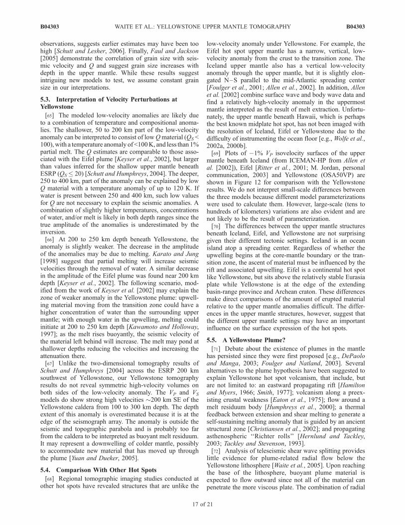
low-velocity anomaly under Yellowstone. For example, theEifel hot spot upper mantle has a narrow, vertical, low-velocity anomaly from the crust to the transition zone. TheIceland upper mantle also has a vertical low-velocityanomaly through the upper mantle, but it is slightly elon-gated N–S parallel to the mid-Atlantic spreading center[Foulger et al., 2001; Allen et al., 2002]. In addition, Allenet al. [2002] combine surface wave and body wave data andfind a relatively high-velocity anomaly in the uppermostmantle interpreted as the result of melt extraction. Unfortu-nately, the upper mantle beneath Hawaii, which is perhapsthe best known midplate hot spot, has not been imaged withthe resolution of Iceland, Eifel or Yellowstone due to thedifficulty of instrumenting the ocean floor [e.g., Wolfe et al.,2002a, 2000b].[69] Plots of �1% VP isovelocity surfaces of the upper

mantle beneath Iceland (from ICEMAN-HP from Allen etal. [2002]), Eifel [Ritter et al., 2001; M. Jordan, personalcommunication, 2003] and Yellowstone (OSA50VP) areshown in Figure 12 for comparison with the Yellowstoneresults. We do not interpret small-scale differences betweenthe three models because different model parameterizationswere used to calculate them. However, large-scale (tens tohundreds of kilometers) variations are also evident and arenot likely to be the result of parameterization.[70] The differences between the upper mantle structures

beneath Iceland, Eifel, and Yellowstone are not surprisinggiven their different tectonic settings. Iceland is an oceanisland atop a spreading center. Regardless of whether theupwelling begins at the core-mantle boundary or the tran-sition zone, the ascent of material must be influenced by therift and associated upwelling. Eifel is a continental hot spotlike Yellowstone, but sits above the relatively stable Eurasiaplate while Yellowstone is at the edge of the extendingbasin-range province and Archean craton. These differencesmake direct comparisons of the amount of erupted materialrelative to the upper mantle anomalies difficult. The differ-ences in the upper mantle structures, however, suggest thatthe different upper mantle settings may have an importantinfluence on the surface expression of the hot spots.

5.5. A Yellowstone Plume?

[71] Debate about the existence of plumes in the mantlehas persisted since they were first proposed [e.g., DePaoloand Manga, 2003; Foulger and Natland, 2003]. Severalalternatives to the plume hypothesis have been suggested toexplain Yellowstone hot spot volcanism, that include, butare not limited to: an eastward propagating rift [Hamiltonand Myers, 1966; Smith, 1977]; volcanism along a preex-isting crustal weakness [Eaton et al., 1975]; flow around amelt residuum body [Humphreys et al., 2000]; a thermalfeedback between extension and shear melting to generate aself-sustaining melting anomaly that is guided by an ancientstructural zone [Christiansen et al., 2002]; and propagatingasthenospheric ‘‘Richter rolls’’ [Hernlund and Tackley,2003; Tackley and Stevenson, 1993].[72] Analysis of teleseismic shear wave splitting provides

little evidence for plume-related radial flow below theYellowstone lithosphere [Waite et al., 2005]. Upon reachingthe base of the lithosphere, buoyant plume material isexpected to flow outward since not all of the material canpenetrate the more viscous plate. The combination of radial


17 of 21

B04303

spreading with plate motion will produce a parabolic flowpattern in the asthenosphere and a similar pattern ofanisotropy. However, split S waves show little to no signof contribution from radially spreading plume material,indicating the contribution of gravitationally spreading

plume material beneath Yellowstone is undetectably smallwith respect to the plate motion velocity.[73] The phase changes that are primarily responsible for

the 410 and 660 km discontinuities have opposite Cla-peyron (dP/dT) slopes so thermal anomalies that cross thetransition zone should have opposite effects on the discon-tinuity topography [Bina and Helffrich, 1994]. The 15 kmincrease in the depth of the 410 km discontinuity observed�100 km WNW of Yellowstone implies a positive thermalanomaly of �200 K at that depth [Fee and Dueker, 2004].However, the 660 km discontinuity topography is notcorrelated with the deep 410 km discontinuity in that area.The thermal anomaly may not continue downward throughthe transition zone to 660 km depth, or the 660 kmdiscontinuity is more complex than Bina and Helffrich’s[1994] estimate and involves multiple phase transitions[Vacher et al., 1998; Simmons and Gurrola, 2000]. Thetopography on the 410 and 660 km discontinuities else-where in the western U.S. varies by 20–30 km and is alsouncorrelated in general [Gilbert et al., 2003].[74] While the shear wave anisotropy pattern does not

favor a buoyant plume beneath Yellowstone the disconti-nuity imaging is consistent with our tomography results thatimage a continuous low-velocity feature through the uppermantle. This anomaly is a plume by our general definition.In order to reconcile the seismic tomography with theobservations cited as against a mantle plume we employ aplume-fed upper mantle small-scale convection model. Thismodel follows the work of Saltzer and Humphreys [1997],Humphreys et al. [2000], and Hernlund and Tackley [2003],which suggests that a plume may fuel small-scale uppermantle convection.[75] Numerical modeling demonstrates that longitudinal,

small-scale, convection cells can develop spontaneously inthe upper mantle where there is available partial melt from,for example, an upwelling plume [Hernlund and Tackley,2003; Tackley and Stevenson, 1993]. Density differencesbetween buoyant mantle containing partial melt and densermantle with no melt, initiates convection. Decompression ofascending mantle results in more melting. This causes alarger density contrast and the result is a positive feedback.Melt residuum, which is also lower in density than normalmantle, accumulates on the sides of the convection cells.These convection cells could be aligned by the moving plateto mimic linear hot spot trends. The accumulation of meltresiduum at the sides of the cells would eventually haltconvection, but the addition of hot and/or wet material froma plume could sustain the melting anomaly. In addition,basin-range extension above this type of system would thinthe upper mantle and encourage upwelling and melt pro-duction [Saltzer and Humphreys, 1997].[76] It is plausible that the tilt of the plume may be due to

upper mantle convection. For example, if a Yellowstoneplume is advected in the eastward mantle flow [Bunge andGrand, 2000; Steinberger, 2000], it should be plunging tothe west, similar to the WNW plunge of the low-velocityfeature imaged in the tomography models. When combinedwith plate motion, Steinberger’s [2000; personal communi-cation, 2003] models predict a Yellowstone hot spot tracknorth of the ESRP. The location of the hot spot track,however, is also likely to be influenced by the linearlithospheric anomaly it seems to follow [e.g., Eaton et al.,

Figure 12. Perspective plots of �1% VP perturbationsurfaces of models of the upper mantle beneath of other hotspots: Iceland, Eifel, and Yellowstone. The scale of each400 km by 400 km by 400 km cube is the same. Whiledifferent model parameterizations used to construct themodels may affect the amplitude of the anomalies, andtherefore the shape of the isovelocity surface, the plotsclearly show differences between the upper mantle structuresbeneath these three hot spots.


18 of 21

B04303

1975; Smith, 1977]. Dueker et al. [2001] imply the NE-SWProterozoic Madison mylonite zone, interpreted as a deep,ancient shear zone [Erslev and Sutter, 1990], just NE ofYellowstone may provide a favorable guide for small-scaleconvection. Magnetic and gravity anomalies associated withthis shear zone suggest it is a continuous, deep lithosphericstructure [Lemieux et al., 2000]. It is reasonable that as thehot spot encountered thicker lithosphere on its NE progres-sion, the plume found the path of least resistance to thesurface.[77] We favor a combination plume-fed upper mantle

convection model to reconcile the geologic as well as theseismic observations. While the plume is capable of trans-porting material up from the transition zone, the volumemay not be large enough to sustain the energetic volcanismat Yellowstone alone. A lineation of weak lithosphericstructure may be important in guiding the hot spot byallowing melt to penetrate into the crust more easily. Thepersistence of magmatism along the ESRP may be attribut-ed to continued convection millions of years after the platehas passed the plume. The complex upper mantle flow fieldexpected for longitudinal rolls can explain why evidence fora parabolic flow pattern is not seen in the shear wavesplitting data.

6. Concluding Remarks

[78] Tomographic inversions of traveltime delays acrossthe Yellowstone region provide an image of a low VP and VS

anomaly at the bottom of the upper mantle and the unusualfinding of a low-velocity body tilted �30� from vertical andextending laterally more than 100 km northwest of Yellow-stone. We interpret this structure as an upper mantle plume.In addition, the modeling reveals a low VP and VS anomalydirectly beneath the Yellowstone caldera extending to 200–250 km depth. This shallow feature is continuous, with asmaller amplitude, to the SW beneath the ESRP to the edgeof the model.[79] Yellowstone has a plume source, although it is not

necessarily deep plume that originates at the core-mantleboundary. In fact, there is no evidence to show that the low-velocity anomaly continues through the transition zone tothe lower mantle. As such, it may be strictly an uppermantle feature. The coincidence of Yellowstone with theboundary of the Archean craton and basin-range as well asstructural trends that parallel the hot spot track indicatelithosphere features may be important in guiding the hotspot.[80] Upper mantle convection models are not contra-

dicted by a plume model. Rather, convection, lithosphereextension, and upwelling from below likely work togetherat Yellowstone. Small-scale convection helps explain thestrong low-velocity anomaly beneath Yellowstone and theSnake River Plain to �200 km depth. The high topog-raphy on both sides of the ESRP may be supported bymelt residuum that has been pushed away from theupwelling zone under the ESRP. The possible eastwardmigration of the basin-range extensional regime is apartly a consequence of the active system moving in thedirection opposite plate motion. Without all three mecha-nisms, Yellowstone volcanism may not have persisted for�16 million years.

[81] Acknowledgments. This project was part of the collaborativeNSF Continental Dynamics project: Geodynamics of the Yellowstone Hotspot from Seismic and GPS Imaging. Collaborators included GeneHumphreys, Jason Crosswhite of the University of Oregon; Paul Tackleyand John Hernlund of UCLA; and Ken Dueker and Derek Schutt of theUniversity of Wyoming. We are especially appreciative of the dedicatedfield support teams that advised, installed, and maintained the instrumentsincluding J. Crosswhite, Dave Drobeck, K. Dueker, D. Schutt, and BrianZurek. The seismographs were provided by the PASSCAL facility of IRISthrough the PASSCAL Instrument Center. Data collected from this exper-iment are available at the IRIS Data Management Center. The IRISConsortium is supported by the NSF. Additional data were acquired fromthe USGS National Seismograph Network and University of Utah Seismo-graph Network. John Evans provided the teleseismic picks from earlierUSGS field experiments in Yellowstone. We appreciate discussions withUli Achauer, Thorsten Becker, Robert Christiansen, Gillian Foulger,Michael Jordan, Rafaella Montelli, Richard O’Connell, Christine Puskas,and Bernard Steinberger. The NSF Continental Dynamics Program grantsEAR-CD-9725431 and 0314237 provided support. The University of Utahsupported computational aspects of the project.

ReferencesAdams, D. C., and E. D. Humphreys (2003), Q tomography in the Yellow-stone region: Effects of mantle water content, Eos Trans. AGU, 84, FallMeet. Suppl., Abstract S21A-05.

Allen, R. M., et al. (1999), The thin hot plume beneath Iceland, Geophys.J. Int., 137, 51–63.

Allen, R. M., et al. (2002), Imaging the mantle beneath Iceland usingintegrated seismological techniques, J. Geophys. Res., 107(B12), 2325,doi:10.1029/2001JB000595.

Anders, M. H., and N. H. Sleep (1992), Magmatism and extension: Thethermal and mechanical effects of the Yellowstone hotspot, J. Geophys.Res., 97, 15,379–15,393.

Anders, M. H., J. W. Geissman, L. A. Piety, and J. T. Sullivan (1989),Parabolic distribution of circumeastern Snake River Plain seismicity andlatest Quaternary faulting, migratory pattern and association with theYellowstone hotspot, J. Geophys. Res., 94, 1589–1621.

Anderson, D. L. (2000), The statistics and distribution of helium in themantle, Int. Geol. Rev., 42, 289–311.

Anderson, D. L. (2001), Top down tectonics?, Science, 293, 2016–2018.

Anderson, D. L., and J. W. Given (1982), Absorption band Q model for theEarth, J. Geophys. Res., 87, 3893–3904.

Bassin, C., G. Laske, and G. Masters (2000), The current limits of resolu-tion for surface wave tomography in North America, Eos Trans. AGU,81(48), Fall Meet. Suppl., Abstract S12A-03.

Benz, H. M., and R. B. Smith (1984), Simultaneous inversion for lateralvelocity variations and hypocenters in the Yellowstone region usingearthquake and refraction data, J. Geophys. Res., 89, 1208–1220.

Berckhemer, H., W. Kampfman, E. Aulbach, and H. Schmeling (1982),Shear modulus and Q of forsterite and dunite near partial melting fromforced oscillation experiments, Phys. Earth Planet. Inter., 29, 30–41.

Bijwaard, H., W. Spakman, and E. R. Engdahl (1998), Closing the gapbetween regional and global travel time tomography, J. Geophys. Res.,103, 30,055–30,078.

Bina, C. R., and G. Helffrich (1994), Phase transition Clapeyron slopes andtransition zone seismic discontinuity topography, J. Geophys. Res., 99,15,853–15,860.

Blackwell, D. D. (1969), Heat-flow determinations in the northwesternUnited States, J. Geophys. Res., 74, 992–1007.

Bunge, H.-P., and S. P. Grand (2000), Mesozoic plate-motion history belowthe northeast Pacific Ocean from seismic images of the subducted Far-allon slab, Nature, 405, 337–340.

Cammarano, F., S. Goes, P. Vacher, and D. Giardini (2003), Inferring upper-mantle temperatures from seismic velocities, Phys. Earth Planet. Inter.,138, 197–222.

Camp, V. E., and M. E. Ross (2004), Mantle dynamics and genesis of maficmagmatism in the intermontane Pacific Northwest, J. Geophys. Res., 109,B08204, doi:10.1029/2003JB002838.

Christiansen, R. L. (2001), The Quaternary and Pliocene Yellowstone Pla-teau volcanic field of Wyoming, Idaho, and Montana, U.S. Geol. Surv.Prof. Pap., 729-G.

Christiansen, R. L., and R. S. Yeats (1992), Post-Laramide geology of theU.S. Cordilleran region, in The Geology of North America, vol. G3, TheCordilleran Orogen: Conterminous U.S., edited by B. C. Burchfiel, P. W.Lipman, and M. L. Zoback, pp. 261–406, Geol. Soc. of Am., Boulder,Colo.

Christiansen, R. L., G. R. Foulger, and J. R. Evans (2002), Upper-mantleorigin of the Yellowstone hotspot, Geol. Soc. Am. Bull., 114, 1245–1256.


19 of 21

B04303

Courtillot, V., A. Davaille, J. Besse, and J. Stock (2003), Three distincttypes of hotspots in the Earth’s mantle, Earth Planet. Sci. Lett., 205,295–308.

Craig, H., J. E. Lupton, J. A. Welhan, and R. Poreda (1978), Helium isotoperatios in Yellowstone and Lassen Park volcanic gases, Geophys. Res.Lett., 5, 897–900.

DePaolo, D. J., and M. Manga (2003), Deep origin of hotspots: The mantleplume model, Science, 300, 920–921.

Dueker, K. G., and E. D. Humphreys (1990), Upper-mantle velocity struc-ture of the Great Basin, Geophys. Res. Lett., 17, 1327–1330.

Dueker, K., H. Yuan, and B. Zurek (2001), Thick-structured Proterozoiclithosphere of the Rocky Mountain region, GSA Today, 11, 4–9.

Eaton, G. P., R. L. Christiansen, H. M. Iyer, A. M. Pitt, D. R. Mabey, H. R.Blank Jr., I. Zietz, andM. E. Gettings (1975), Magma beneath YellowstoneNational Park, Science, 188, 787–796.

Erslev, E. A., and J. F. Sutter (1990), Evidence for Proterozoic mylonitiza-tion in the northwestern Wyoming province, Geol. Soc. Am. Bull., 102,1681–1694.

Evans, J. R. (1982), Compressional wave velocity structure of the upper350 km under the eastern Snake River Plain near Rexburg, Idaho, J. Geo-phys. Res., 87, 2654–2670.

Evans, J. R., and J. J. Zucca (1988), Active high-resolution seismic tomo-graphy of compressional wave velocity and attenuation structure at Med-icine Lake Volcano, northern California Cascade Range, J. Geophys.Res., 93, 15,016–15,036.

Farnetani, C. G., and H. Samuel (2005), Beyond the thermal plume para-digm, Geophys. Res. Lett., 32, L07311, doi:10.1029/2005GL022360.

Faul, U. H., and I. Jackson (2005), The seismological signature of tempera-ture and grain size variations in the upper mantle, Earth Planet. Sci. Lett.,234, 119–134.

Faul, U. H., D. R. Toomey, and H. S. Waff (1994), Intergranular basaltic meltis distributed in thin, elongated inclusions,Geophys. Res. Lett., 21, 29–32.

Favela, J., and D. L. Anderson (2000), Extensional tectonics and globalvolcanism, in Problems in Geophysics for the New Millennium, edited byE. Boschi, G. Ekstrom, and A. Morelli, pp. 463–498, Compositori, Bo-logna, Italy.

Fee, D., and K. Dueker (2004), Mantle transition zone topography andstructure beneath the Yellowstone hotspot, Geophys. Res. Lett., 31,L18603, doi:10.1029/2004GL020636.

Foulger, G. R., and J. H. Natland (2003), Is ‘‘hotspot’’ volcanism a con-sequence of plate tectonics?, Science, 300, 921–922.

Foulger, G. R., et al. (2001), Seismic tomography shows that upwellingbeneath Iceland is confined to the upper mantle, Geophys. J. Int., 146,504–530.

Gilbert, H. J., A. F. Sheehan, K. G. Dueker, and P. Molnar (2003), Receiverfunctions in the western United States, with implications for upper mantlestructure and dynamics, J. Geophys. Res., 108(B5), 2229, doi:10.1029/2001JB001194.

Godey, S., F. Deschamps, and J. Trampert (2004), Thermal and composi-tional anomalies beneath the North American continent, J. Geophys. Res.,109, B01308, doi:10.1029/2002JB002263.

Goes, S., and S. van der Lee (2002), Thermal structure of the North Amer-ican uppermost mantle inferred from seismic tomography, J. Geophys.Res., 107(B3), 2050, doi:10.1029/2000JB000049.

Goes, S., R. Govers, and P. Vacher (2000), Shallow mantle temperaturesunder Europe from P and S wave tomography, J. Geophys. Res., 105,11,153–11,169.

Gripp, A. E., and R. G. Gordon (2002), Young tracks of hotspots andcurrent plate velocities, Geophys. J. Int., 150, 321–361.

Hamilton, W. B., and W. B. Myers (1966), Cenozoic tectonics of thewestern United States, Rev. Geophys., 4, 509–549.

Hammond, W. C., and E. D. Humphreys (2000), Upper mantle seismicwave velocity: Effects of realistic partial melt geometries, J. Geophys.Res., 105, 10,975–10,986.

Hernlund, J. W., and P. J. Tackley (2003), Post-Laramide volcanism andupper mantle dynamics in the western US: Role of small-scale convec-tion, Eos Trans. AGU, 84(46), Fall Meet. Suppl., Abstract V31F-07.

Humphreys, E. D., and K. G. Dueker (1994a), Physical state of the westernU.S. upper mantle, J. Geophys. Res., 99, 9635–9650.

Humphreys, E. D., and K. G. Dueker (1994b), Western U.S. upper mantlestructure, J. Geophys. Res., 99, 9615–9634.

Humphreys, E. D., K. G. Dueker, D. L. Schutt, and R. B. Smith (2000),Beneath Yellowstone; evaluating plume and nonplume models using tel-eseismic images of the upper mantle, GSA Today, 10, 1–7.

Husen, S., R. B. Smith, and G. P. Waite (2004), Evidence for gas andmagmatic sources beneath the Yellowstone Volcanic Field from seismictomographic imaging, J. Volcanol. Geotherm. Res., 131, 397 –410,doi:10.1016/S0377-0273(03)00416-5.

Iyer, H. M., J. R. Evans, G. Zandt, R. M. Stewart, J. M. Coakley, and J. N.Roloff (1981), A deep low-velocity body under the Yellowstone caldera,

Wyoming: Delineation using teleseismic P-wave residuals and tectonicinterpretation: Summary, Geol. Soc. Am. Bull., 92, 792–798, 1471–1646.

Jordan, B. T., A. L. Grunder, R. A. Duncan, and A. L. Deino (2004),Geochronology of age-progressive volcanism of the Oregon High LavaPlains: Implications for the plume interpretation of Yellowstone, J. Geo-phys. Res., 109, B10202, doi:10.1029/2003JB002776.

Jordan, M., R. B. Smith, and G. P. Waite (2004), Tomographic images ofthe Yellowstone hotspot structure, Eos Trans. AGU, 85, Fall Meet.Suppl., Abstract V51B-0556.

Jordan, T. H. (1979), Mineralogies, densities and seismic velocities ofgarnet lherzolites and their geophysical implications, in The Mantle Sam-ple: Inclusions in Kimberlites and other Volcanics, edited by F. R. Boydand H. O. A. Meyer, pp. 1–14, AGU, Washington, D. C.

Karato, S.-I. (1993), Importance of anelasticity in the interpretation ofseismic tomography, Geophys. Res. Lett., 20, 1623–1626.

Karato, S.-I., and H. Jung (1998), Water, partial melting and the origin ofthe seismic low velocity and high attenuation zone in the upper mantle,Earth Planet. Sci. Lett., 157, 193–207.

Kawamoto, T., and J. R. Holloway (1997), Melting temperature and partialmelt chemistry of H2O-saturated mantle peridotite to 11 gigapascals,Science, 276, 240–243.

Keller, W. R., D. L. Anderson, and R. W. Clayton (2000), Resolution oftomographic models of the mantle beneath Iceland, Geophys. Res. Lett.,27, 3993–3996.

Kendall, J. M. (1994), Teleseismic arrivals at a mid-ocean ridge; effects ofmantle melt and anisotropy, Geophys. Res. Lett., 21, 301–304.

Kennett, B. L. N., and E. R. Engdahl (1991), Traveltimes for globalearthquake location and phase identification, Geophys. J. Int., 105,429–465.

Keyser, M., J. R. R. Ritter, and M. Jordan (2002), 3D shear-wave velocitystructure of the Eifel Plume, Germany, Earth Planet. Sci. Lett., 203, 59–82.

Kohlstedt, D. L., H. Keppler, and D. C. Rubie (1996), Solubility of water inthe a, b and g phases of (Mg,Fe)2SiO4, Contrib. Mineral. Petrol., 123,345–357.

Lehman, J. A., R. B. Smith, M. M. Schilly, and L. W. Braile (1982), Uppercrustal structure of the Yellowstone caldera from delay time analyses andgravity correlations, J. Geophys. Res., 87, 2713–2730.

Lemieux, S., G. Ross, and F. A. Cook (2000), Crustal geometry and tec-tonic evolution of the Archean crystalline basement beneath the southernAlberta Plains, from new seismic reflection and potential-field studies,Can. J. Earth Sci., 37, 1473–1491.

Leveque, J., L. Rivera, and G. Wittlinger (1993), On the use of the checker-board test to assess the resolution of tomographic inversions, Geophys. J.Int., 115, 313–318.

Levin, V., W. Menke, and A. Lerner-Lam (1996), Seismic anisotropy in thenorth-eastern US as a source of significant teleseismic P traveltimeanomalies, Geophys. J. Int., 126, 593–603.

Lynch, D. P. (1999), Three-dimensional finite difference tomography of theBasin and Range-Colorado Plateau-Rocky Mountain transition usingearthquake and controlled source data, M.S. thesis, Univ. of Utah, SaltLake City.

Meibom, A., D. L. Anderson, N. H. Sleep, R. Frei, C. P. Chamberlain, M. T.Hren, and J. L. Wooden (2003), Are high 3He/4He ratios in oceanicbasalts an indicator of deep-mantle plume components?, Earth Planet.Sci. Lett., 208, 197–204, doi:10.1016/S0012-821X(03)00038-4.

Miller, D. S., and R. B. Smith (1999), P and S velocity structure of theYellowstone volcanic field from local earthquake and controlled-sourcetomography, J. Geophys. Res., 104, 15,105–15,121.

Minster, J. B., and D. L. Anderson (1981), A model of dislocation-con-trolled rheology for the mantle, Philos. Trans. R. Soc. London, 299, 319–356.

Montelli, R., G. Nolet, F. A. Dahlen, G. Masters, E. R. Engdahl, and S.-H.Hung (2004), Finite-frequency tomography reveals a variety of plumes inthe mantle, Science, 303, 338–343, doi:10.1126/science.1092485.

Morgan, W. J. (1971), Convection plumes in the lower mantle, Nature, 230,42–43.

Morgan, W. J. (1972), Deep mantle convection plumes and plate motions,Am. Assoc. Pet. Geol. Bull., 56, 203–213.

Nolet, G. (1993), Solving large linearized tomographic problems, in SeismicTomography: Theory and Practice, edited by H. M. Iyer and K. Hirahara,CRC Press, Boca Raton, Fla.

Nolet, G., and F. A. Dahlen (2000), Wavefront healing and the evolution ofseismic delay times, J. Geophys. Res., 105, 19,043–19,054.

Paige, C. C., and M. A. Saunders (1982), LSQR: An algorithm for sparselinear equations and sparse least squares, Trans. Math. Software, 8, 43–71.

Pelton, J. R., and R. B. Smith (1982), Contemporary vertical surface dis-placements in Yellowstone National Park, J. Geophys. Res., 87, 2745–2761.


20 of 21

B04303

Perkins, M. E., and B. P. Nash (2002), Explosive silicic volcanism of theYellowstone hotspot: The ashfall tuff record, Geol. Soc. Am. Bull., 114,367–381.

Pierce, K. L., and L. A. Morgan (1992), The track of the Yellowstone hotspot; volcanism, faulting, and uplift, in Regional Geology of EasternIdaho and Western Wyoming, edited by P. K. Link, M. A. Kuntz, andL. B. Platt, Mem. Geol. Soc. Am., 179, 1–53.

Puskas, C. M., R. B. Smith, and C. M. Meertens (2002), GPS-derivedmodels of intraplate deformation of the Yellowstone Hotspot, Eos Trans.AGU, 83(47), Fall Meet. Suppl., Abstract F1037.

Ritter, J. R. R., M. Jordan, U. R. Christensen, and U. Achauer (2001), Amantle plume below the Eifel volcanic fields, Germany, Earth Planet.Sci. Lett., 186, 7–14.

Saltzer, R. L., and E. D. Humphreys (1997), Upper mantle P wave velocitystructure of the eastern Snake River Plain and its relationship to geody-namic models of the region, J. Geophys. Res., 102, 11,829–11,841.

Sato, H. (1992), Thermal structure of the mantle wedge beneath northeast-ern Japan: Magmatism in an island arc from the combined data of seismicanelasticity and velocity and heat flow, J. Volcanol. Geotherm. Res., 51,237–252.

Schutt, D. L., and E. D. Humphreys (2001), Evidence for a deep astheno-sphere beneath North America from western United States SKS splits,Geology, 29, 291–294.

Schutt, D. L., and E. D. Humphreys (2004), P and S wave velocity and VP/VS in the wake of the Yellowstone hot spot, J. Geophys. Res., 109,B01305, doi:10.1029/2003JB002442.

Schutt, D. L., and C. E. Lesher (2006), Effects of melt depletion on thedensity and seismic velocity of garnet and spinel lherzolite, J. Geophys.Res., doi:10.1029/2003JB002950, in press.

Simmons, N. A., and H. Gurrola (2000), Multiple seismic discontinuitiesnear the base of the transition zone of the Earth’s mantle, Nature, 405,559–562, doi:10.1038/35014589.

Smith, R. B. (1977), Intraplate tectonics of the western North AmericanPlate, Tectonophysics, 37, 323–336.

Smith, R. B., and L. W. Braile (1994), The Yellowstone hotspot, J. Volcanol.Geotherm. Res., 61, 121–187.

Smith, R. B., and M. L. Sbar (1974), Contemporary tectonics and seismicityof the western United States with emphasis on the Intermountain SeismicBelt, Geol. Soc. Am. Bull., 85, 1205–1218.

Smith, R. B., G. P. Waite, C. M. Puskas, D. L. Schutt, and E. D. Humphreys(2003), Dynamic and kinematic models of the Yellowstone Hotspot con-strained by seismic anisotropy, GPS measurements and fault slip rates,Eos Trans. AGU, 84(46), Fall Meet Suppl., Abstract T51G-05.

Sobolev, S. V., H. Zeyen, G. Stoll, F. Werling, R. Altherr, and K. Fuchs(1996), Upper mantle temperatures from teleseismic tomography ofFrench Massif Central including effects of composition, mineral reac-tions, anharmonicity, anelasticity and partial melt, Earth Planet. Sci. Lett.,139, 147–163.

Spetzler, J., and R. Snieder (2004), The Fresnel volume and transmittedwaves, Geophysics, 69, 653–663, doi:10.1190/1.1759451.

Steinberger, B. (2000), Plumes in a convecting mantle; models andobservations for individual hotspots, J. Geophys. Res., 105, 11,127–11,152.

Tackley, P. J., and D. J. Stevenson (1993), A mechanism for spontaneousself-perpetuating volcanism on the terrestrial planets, in Flow and Creepin the Solar System: Observations, Modeling and Theory, edited by D. B.Stone and S. K. Runcorn, pp. 307–322, Springer, New York.

Thompson, A. B. (1992), Water in the Earth’s upper mantle, Nature, 358,295–302.

Umino, N., and A. Hasegawa (1984), Three-dimensional QS structure in thenortheastern Japan arc, J. Seismol. Soc. Jpn., 37, 217–228.

VanDecar, J. C., and R. S. Crosson (1990), Determination of teleseismicrelative phase arrival times using multi-channel cross-correlation andleast squares, Bull. Seismol. Soc. Am., 80, 150–159.

Vacher, P., A. Mocquet, and C. Sotin (1998), Computation of seismicprofiles from mineral physics: The importance of the non-olivine compo-nents for explaining the 660 km depth discontinuity, Phys. Earth Planet.Inter., 106, 275–298.

Waite, G. P. (2004), Upper mantle structure of the Yellowstone hotspot fromteleseismic body-wave velocity tomography and shear-wave anisotropy,Ph.D. thesis, Univ. of Utah, Salt Lake City.

Waite, G. P., and R. B. Smith (2002), Seismic evidence for fluid migrationaccompanying subsidence of the Yellowstone caldera, J. Geophys. Res.,107(B9), 2177, doi:10.1029/2001JB000586.

Waite, G. P., R. B. Smith, C. M. Puskas, D. L. Schutt, and R. M. Allen(2003), Kinematics of the Yellowstone hotspot derived from seismicanisotropy, tomography, and GPS, Geophys. Res. Abstr., 5, 00670.

Waite, G. P., D. L. Schutt, and R. B. Smith (2005), Models of lithosphereand asthenosphere anisotropic structure of the Yellowstone hotspot fromshear wave splitting, J. Geophys. Res., 110, B11304, doi:10.1029/2004JB003501.

Waldhauser, F., R. Lippitsch, E. Kissling, and J. Ansorge (2002), High-resolution teleseismic tomography of upper-mantle structure using an apriori three-dimensional crustal model, Geophys. J. Int., 150, 403–414.

Walker, K. T. (2004), Exploring Problems in Tectonics and Geodynamicswith Seismology, Ph.D. thesis, Stanford Univ., Palo Alto, Calif.

Wicks, C. W. J., W. R. Thatcher, and D. Dzurisin (1998), Migration offluids beneath Yellowstone caldera inferred from satellite radar interfero-metry, Science, 282, 458–462.

Wielandt, E. (1987), On the validity of the ray approximation for interpret-ing delay times, in Seismic Tomography, edited by G. Nolet, pp. 85–98,Springer, New York.

Wolfe, C. J., I. T. Bjarnason, J. C. VanDecar, and S. C. Solomon (2002),Assessing the depth resolution of tomographic models of upper mantlestructure beneath Iceland, Geophys. Res. Lett., 29(2), 1015, doi:10.1029/2001GL013657.

Wolfe, C. J., S. C. Solomon, P. G. Silver, J. C. VanDecar, and R. M. Russo(2002), Inversion of body-wave delay times for mantle structure beneaththe Hawaiian islands: Results from the PELENET experiment, EarthPlanet. Sci. Lett., 198, 129–145.

Yuan, H., and K. Dueker (2005), Teleseismic P-wave tomogram of theYellowstone plume, Geophys. Res. Lett., 32, L07304, doi:10.1029/2004GL022056.

��R. B. Smith, Department of Geology and Geophysics, University of Utah,

135 S. 1460 E., Salt Lake City, UT 84112, USA.G. P. Waite, U.S. Geological Survey, 345 Middlefield Road, MS-910,

Menlo Park, CA 94025, USA. ([email protected])R. M. Allen, Seismological Laboratory, Department of Earth and

Planetary Science, University of California, 215 McCone Hall, Berkeley,CA 94720, USA.


21 of 21

B04303

vp and vs structure of the yellowstone hot spot from teleseismic

Documents