introduction nuclear physics chapter 2

8/2/2019 Introduction Nuclear Physics Chapter 2

http://slidepdf.com/reader/full/introduction-nuclear-physics-chapter-2 1/26

Chapter 1 Basic Concepts in Nuclear Physics

Chapter 2.

Nuclear models and stability

The aim of this chapter is to understand how certain combinations of N neutrons and Z

protons form bound states and to understand the masses, spins and parities of those states.

The great majority of nuclear species contain excess neutrons or protons and are therefore

β-unstable. Many heavy nuclei decay by α-particle emission or by other forms of

spontaneous fission into lighter elements.

Another aim of this chapter is to understand why certain nuclei are stable against these

decays and what determines the dominant decay modes of unstable nuclei.

A. Mean potential model

The mean potential model relies on the observation that, to good approximation,

individual nucleons behave inside the nucleus as independent particles placed in a mean

potential (or mean field) due to the other nucleons. In order to obtain a qualitative

description of this mean potential ( )r V , we write it as the sum of potentials ( )'r r v −

between a nucleon at r and a nucleon at 'r :

( ) ( ) ( )∫ −= ''' r d r r r vr V ρ

In this equation, the nuclear density ( )'r ρ , is proportional to the probability per unit

volume to find a nucleus in the vicinity of 'r . It is precisely that function in the case of

protons.

We now recall what we know about v and ρ. The strong nuclear interaction ( )'r r v − is

attractive and short range. It falls to zero rapidly at distances larger than fm2≈ , while the

typical diameter on a nucleus is “much” bigger, of the order of 6 fm for a light nucleus

such as oxygen and of 14 fm for lead. In order to simplify the expression, let us

approximate the potential v by a delta function (i.e. a point-like interaction)

( ) ( )'' r r vr r v −≈− δ

The constant ov can be taken as a free parameter but we would expect that the integral of

this potential be the same as that of the original two-nucleon potential (Table 2.1):

Introduction to Nuclear Physics 21




( ) 33 200 fm MeV r vr d vo ≈= ∫ where we have used the values from Table 2.1.

The mean potential is then simply

( ) ( )r vr V o ρ −=

Using315,0 −≈ fm ρ we expect to find a potential depth of roughly

( ) MeV Rr V 30−≈<

where R is the radius of the nucleus.

Figure 2.1. Experimental charge density ( )3− fme as a function of r (fm) as determined in

elastic electron–nucleus scattering

The shapes of charge densities in Fig. 2.1 suggest that in first approximation the mean

potential has the shape shown in Fig. 2.2a. A much-used analytic expression is the Saxon–

Woods potential





( ) R Rr

V r V o

/)exp(1 −+−=

where oV is a potential depth of the order of 30 to 60 MeV and R is the radius of the

nucleus fm A R3

1

2,1≈ .

Figure 2.2. The mean potential and its approximation by a harmonic potential

An even simpler potential which leads to qualitatively similar results is the harmonic

oscillator potential drawn on Fig. 2.2b.

( ) 22

2

2

11 r M V

R

r V r V oo ω +−=

−−= r < R

With 22

21 R M V o ω = , and ( ) 0=> Rr V . Contrary to what one could believe from Fig.

2.2, the low-lying wave functions of the two potential wells (a) and (b) are very similar.

Quantitatively, their scalar products are of the order of 0.9999 for the ground state and

0.9995 for the first few excited states for an appropriate choice of the parameter ω in b.

The first few energy levels of the potentials a and b hardly differ.

In this model, where the nucleons can move independently from one another, and where

the protons and the neutrons separately obey the Pauli principle, the energy levels and

configurations are obtained in an analogous way to that for complex atoms in the Hartree

approximation. As for the electrons in such atoms, the proton and neutron orbitals are

independent fermion levels.

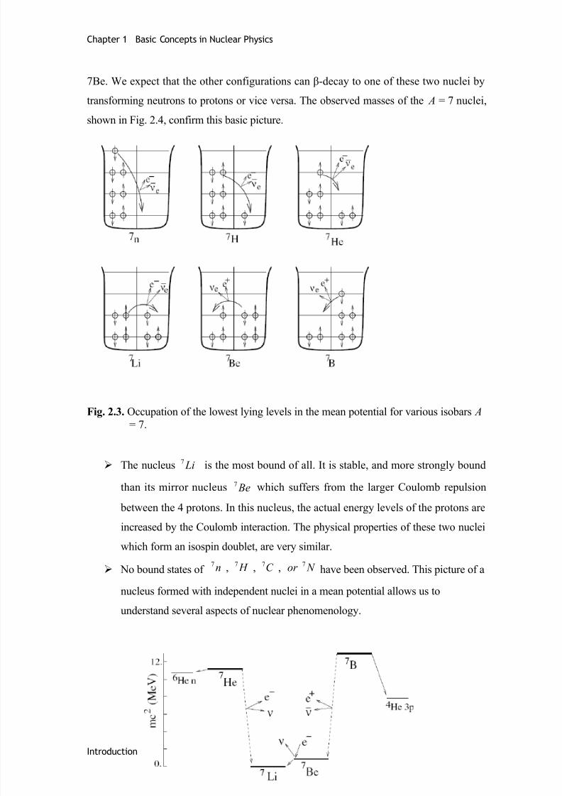
It is instructive, for instance, to consider, within the mean potential notion, the stability of

various A = 7 nuclei, schematically drawn on Fig. 2.3. The figure reminds us that, because

of the Pauli principle, nuclei with a large excess of neutrons over protons or vice versa

require placing the nucleons in high-energy levels. This suggests that the lowest energy

configuration will be the ones with nearly equal numbers of protons and neutrons, 7Li or





7Be. We expect that the other configurations can β-decay to one of these two nuclei by

transforming neutrons to protons or vice versa. The observed masses of the A = 7 nuclei,

shown in Fig. 2.4, confirm this basic picture.

Fig. 2.3. Occupation of the lowest lying levels in the mean potential for various isobars A

= 7.

The nucleus Li7 is the most bound of all. It is stable, and more strongly bound

than its mirror nucleus Be7 which suffers from the larger Coulomb repulsion

between the 4 protons. In this nucleus, the actual energy levels of the protons are

increased by the Coulomb interaction. The physical properties of these two nuclei

which form an isospin doublet, are very similar.

No bound states of N or C H n 7777 ,,, have been observed. This picture of a

nucleus formed with independent nuclei in a mean potential allows us to

understand several aspects of nuclear phenomenology.





Fig. 2.4. Energies of the A=7 isobars. Also shown are two unbound A=7 states n He6

and p He 34

For a given A, the minimum energy will be attained for optimum numbers of

protons and neutrons. If protons were not charged, their levels would be the sameas those of neutrons and the optimum would correspond to

Aodd for Z or Z N 1±= . This is the case for light nuclei, but as A increases,

the proton levels are increased compared to the neutron levels owing to Coulomb

repulsion, and the optimum combination has N > Z . For mirror nuclei, those

related by exchanging N and Z , the Coulomb repulsion makes the nucleus N >Z

more strongly bound than the nucleus Z >N .

The binding energies are stronger when nucleons can be grouped into pairs of

neutrons and pairs of protons with opposite spin. Since the nucleon–nucleon force

is attractive, the energy is lowered if nucleons are placed near each other but,

according to the Pauli principle, this is possible only if they have opposite spins.

There are several manifestations of this pairing effect. Among the 160 even-A, β -

stable nuclei, only the four light nuclei, N B Li H 141062 ,,, are “odd-odd”, the

others being all “even-even”.

The Pauli principle explains why neutrons can be stable in nuclei while free

neutrons are unstable. Possible β -decays of neutrons in

Liand He H n 7777 ,,, are indicated by the arrows in Fig. 2.3. In order for a

neutron to transform into a proton by β -decay, the final proton must find an

energy level such that the process eve pn ++→ −is energetically possible. If all

lower levels are occupied, that may be impossible. This is the case for Li

7





because the Coulomb interaction raises the proton levels by slightly more than

( ) MeV cmmm e P N 78,02 =−− . Neutrons can therefore be “stabilized ” by the

Pauli principle.

Conversely, in a nucleus a proton can be “destabilized” if the reaction

even p ++→ +can occur. This is possible if the proton orbitals are raised, via

the Coulomb interaction, by more than ( ) MeV cmmm P e N 80,12 =−+ with

respect to the neutron orbitals. In the case of Li7 and Be7 shown in Fig. 2.4, the

proton levels are raised by an amount between ( ) 2cmmm P e N −+ and

( )

2

cmmm P e N −− so that neither nucleus can β -decay. (The atom Be7

is

unstable because of the electron-capture reaction of an internal electron of the

atomic cloud ev Lie Be +→+ − 77).

We now back to: ( ) 22

2

2

11 r M V

R

r V r V oo ω +−=

−−= to to determine what value should be

assigned to the parameter ω so as to reproduce the observed characteristics of nuclei.

Equating the two forms in this equation we find

( ) 12

1

2 −

= R

M

V A oω

Equation ( ) MeV Rr V 30−≈< , suggests that oV independent of A while empirically we

know that R is proportional to 31

A . So ω is proportional to 31−

A . To get the

phenomenologically correct value, we take MeV V o 20= and 31

12,1 A R = which

yields

312

1

235

2 −×≈

= A MeV

R

c

cm

V

P

o

ω

We can now calculate the binding energy ( ) Z N A B 22 == in this model. The levels of

the three-dimensional harmonic oscillator are ( ω 2

3+= n E n with a degeneracy

( )( ) 2/21 ++= nn g n . The levels are filled up to maxnn = such that

3/2 3

max

0

max

n g An

n

n∑=

≈= i.e. ( ) 31

max 23 An ≈ .

The corresponding energy is





( )∑=

+−≈++−=max

0

4

max

2234

n

n

ono

nV An g V A E

ω ω

Using the expressions for ω and maxn , we find:

A MeV E ×−≈ 8

i.e. the canonical binding energy of 8 MeV per nucleon

B. The Liquid-Drop Model

One of the first nuclear models, proposed in 1935 by Bohr, is based on the short range of

nuclear forces, together with the additivity of volumes and of binding energies. It is called

the liquid-drop model .

Nucleons interact strongly with their nearest neighbors, just as molecules do in a drop of

water. Therefore, one can attempt to describe their properties by the corresponding

quantities, i.e. the radius, the density, the surface tension and the volume energy.

The Bethe–Weizsäcker mass formula

An excellent parametrization of the binding energies of nuclei in their ground state

was proposed in 1935 by Bethe and Weizsäcker. This formula relies on the liquid-drop

analogy but also incorporates two quantum ingredients we mentioned in the previous

section. One is an asymmetry energy which tends to favor equal numbers of protons and

neutrons. The other is a pairing energy which favors configurations where two identical

fermions are paired. The mass formula of Bethe and Weizsäcker is

( )( ) ( ) ( )

−+−+

−−−−=

21

2

31

2

32

2

11,

Aa

A

N Z a

A

Z a Aa Aa Z A B

N Z

P AC S V

The coefficients ai are chose so as to give a good approximation to the observed binding

energies. A good combination is the following, the values of the parameters aV , aS , aC , a A ,

a P , are

MeV a

MeV a

MeV a

MeV a

MeV a

P

A

C

S

V

0,12

285,23

697,0

23,17

56,15

=====





The existence of the Coulomb term and the asymmetry term means that for each A

there is a nucleus of maximum binding energy found by setting 0=∂∂

Z B . As we will

see below, the maximally bound nucleus has 2/ A N Z == for low A where theasymmetry term dominates but the Coulomb term favors N >Z for large A.

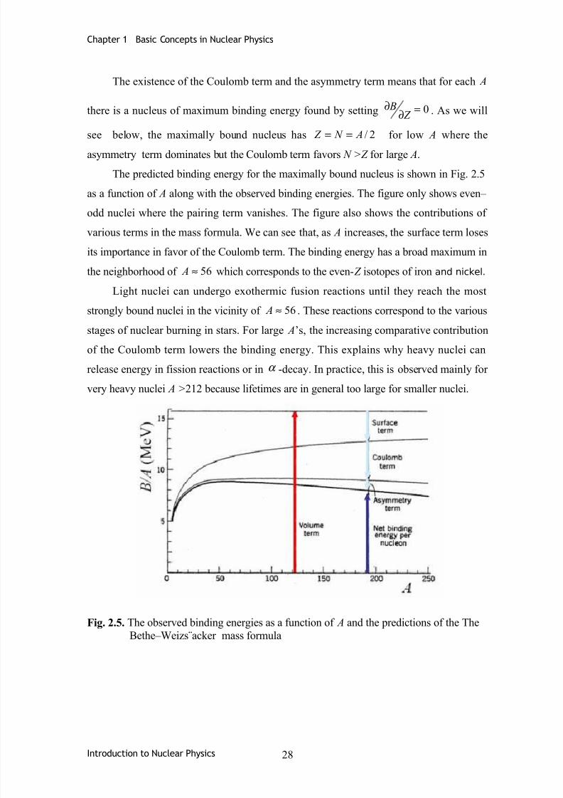
The predicted binding energy for the maximally bound nucleus is shown in Fig. 2.5

as a function of A along with the observed binding energies. The figure only shows even–

odd nuclei where the pairing term vanishes. The figure also shows the contributions of

various terms in the mass formula. We can see that, as A increases, the surface term loses

its importance in favor of the Coulomb term. The binding energy has a broad maximum in

the neighborhood of 56≈ A which corresponds to the even- Z isotopes of iron and nickel.

Light nuclei can undergo exothermic fusion reactions until they reach the most

strongly bound nuclei in the vicinity of 56≈ A . These reactions correspond to the various

stages of nuclear burning in stars. For large A’s, the increasing comparative contribution

of the Coulomb term lowers the binding energy. This explains why heavy nuclei can

release energy in fission reactions or in α -decay. In practice, this is observed mainly for

very heavy nuclei A >212 because lifetimes are in general too large for smaller nuclei.

Fig. 2.5. The observed binding energies as a function of A and the predictions of the The

Bethe–Weizs¨acker mass formula





For the even–odd nuclei, the binding energy follows a parabola in Z for a given A.

An example of this is given on Fig. 2.6 for A = 111. The minimum of the parabola, i.e. the

number of neutrons and protons which corresponds to the maximum binding energy of the

nucleus gives the value Z ( A) for the most bound isotope :

( )3

23

2

0075,01

2

22

0 A

A

a Aa

A A Z

Z

B

a

c +≈

+

=⇒=∂∂

This value of Z is close to, but not necessarily equal to the value of Z that gives the stable

isobar for a given A. This is because one must also take into account the neutron–proton

mass difference in order to make sure of the stability against β -decay. The only stable

nuclei for odd A are obtained by minimizing the atomic mass ( ) e Zm Z Am +, (we neglect

the binding energies of the atomic electrons). This leads to a slightly different value for

the Z ( A) of the stable atom:

( )( )

323/2

0075,01

201,1

41

41

2

A

A

a Aa

a A

A Z

a

c

a

ne

+≈

+

+

=

δ

Where MeV mmm

e P N NPe

75,0

=−−=δ

. This formula shows that light nuclei have aslight preference for protons over neutrons because of their smaller mass while heavy

nuclei have an excess of neutrons over protons because an extra amount of nuclear

binding must compensate for the Coulomb repulsion.

For even A, the binding energies follow two parabolas, one for even–even nuclei,

the other for odd–odd ones. The more massive of the two β -stable nuclei can decay via

β 2 -decay to the less massive. The lifetime for this process is generally of order or greater

than yr 2010 so for practical purposes there are often two stable isobars for even A.

The Bethe–Weizsacker formula predicts the maximum number of protons for a given N

and the maximum number of neutrons for a given Z . The limits are determined by

requiring that the last added proton or last added neutron be bound, i.e.

( ) ( ) ( ) ( ) 0,1,,0,,1 >−+>−+ N Z B N Z B N Z B N Z B

or equivalently:( )

0,

>∂

∂ Z

N Z B ( )0

,>

∂∂

N

N Z B





The locus of points ( Z,N ) where these inequalities become equalities establishes

determines the region where bound states exist. The limits predicted by the mass formula

are shown in Fig. 2.1. These lines are called the proton and neutron drip-lines. As

expected, some nuclei just outside the drip-lines are observed to decay rapidly by nucleon

emission. Combinations of ( Z,N ) far outside the drip-lines are not observed.

C The Fermi Gas Model

The Fermi gas model is a quantitative quantum-mechanical application of the mean

potential model discussed qualitatively in Ch2 Sect. A. It allows one to account semi-

quantitatively for various terms in the Bethe–Weizs¨acker formula. In this model, nuclei

are considered to be composed of two fermion gases, a neutron gas and a proton gas. The

particles do not interact, but they are confined in a sphere which has the dimension of the

nucleus. The interactions appear implicitly through the assumption that the nucleons are

confined in the sphere.

The liquid-drop model is based on the saturation of nuclear forces and one relates the

energy of the system to its geometric properties. The Fermi model is based on the

quantum statistics effects on the energy of confined fermions. The Fermi model provides

a means to calculate the constants V a , S a and aa in the Bethe–Weizsacker formula,

directly from the density ρ of the nuclear matter. Its semi-quantitative success further

justifies for this formula.

The Fermi model is based on the fact that a spin 21 particle confined to a volume V can

only occupy a discrete number of states. In the momentum interval pd 3 , the number of

states is

( )

( )

3

3

2

12

π

pVd sd +=Ν

with 21= s . This will be derived below for a cubic container but it is, in fact, generally

true. It corresponds to a density in phase space of 2 states per 32 π of phase-space

volume.

We now place N particles in the volume. In the ground state, the particles fill up the

lowest single-particle levels, i.e. those up to a maximum momentum called the Fermi

momentum, F p , corresponding to a maximum energym

p F F 2

2

=ε . The Fermi

momentum is determined by





32

3

3 π

F

p p

pV d

F

=Ν=Ν ∑<

This detemines the Fermi energy

( ) 32222

322

nmm

p F F π ε ==

Where n is the number density, V n /Ν= . The total (kinetic) energy Ε of the system is:

∑<

Ν==Ε F p p

F

m pε

5

322

In a system of A=Z+n nucleons, the densities of nucleons and protons are respestively

( A

N no and ( A

Z no where315,0 −≈ fmn is nucleon density. The total energy kinetic is

then:

+

=Ε+Ε=Ε

32

223

2

22

32

325

3 A

Nn

m N

A

Zn

m Z oo

N Z π π

In the approximation 2/ A N Z ≈≈ , this value of the nuclear density corrsponds to a

fermi energy for protons and neutrons of:

MeV F 35=ε

which corresponds to a momentum and a wave number:

c MeV p F 265= 133,1 −== fm

pk F

F

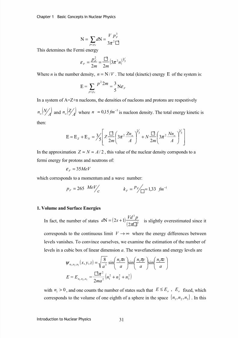
1. Volume and Surface Energies

In fact, the number of states ( )( ) 3

3

212

π

pVd sd +=Ν is slightly overestimated since it

corresponds to the continuous limit ∞→V where the energy differences between

levels vanishes. To convince ourselves, we examine the estimation of the number of

levels in a cubic box of linear dimension a. The wavefunctions and energy levels are

( )

( )2

3

2

2

2

12

22

,,

111

3,,

2

sinsinsin8

,,

321

321

nnnma

E E

a

z n

a

yn

a

xn

a z y x

nnn

nnn

++==

=

π

π π π ψ

with 0>in , and one counts the number of states such that oo E E E ,≤ fixed, which

corresponds to the volume of one eighth of a sphere in the space { }321 ,, nnn . In this





counting, one should not take into account the three planes 0,0 21 == nn and

03 =n for which the wavefunction is identically zero, which does not correspond to a

physical situation. When the number of states under consideration is very large, such

as in statistical mechanics, this correction is negligible. However, it is not negligible

here. The corresponding excess in32

3

3 π

F

p p

pV d

F

=Ν=Ν ∑<

can be calculated in an

analogous way to ( )( ) 3

3

212

π

pVd sd +=Ν ; one obtains

22

2

48 π

ε

π

S mS p F F ==∆Ν

where S is the external area of the volume V (S=6a2 for a cube,24 or S π = for a

sphere.

The expression32

3

3 π

F

p p

pV d

F

=Ν=Ν ∑<

, after correction for this effect, becomes

2

2

32

3

43 π π

F F pS pV −=Ν

The corresponding energy is:

2

2

22

3

0

2

85)(2 π

ε

π

ε F F F F

p pS pV

pd m

p F

−=Ν=Ε ∫ The first term is a volume energy, the second term is a surface correction, or a

surface-tension term.

To first order in S/V the kinetic energy per particle is therefore

++=

ΝΕ

...8

15

3

F

F pV

S π ε

In the approximation 2/ A N Z ≈≈ , the kinetic energy is of the form :3

2

Aa Aa E soc +=

with:

MeV a F o 215

3== ε MeV

pr a

F o

F S 1,168

3

5

3==

π ε

The second term is the surface coefficient, in good agreement with the experimental

value. The mean energy per particle is the sum U aa oV −= of oa and of a potential

energy U which can be determined experimentally by neutron scattering on nuclei(this is analogous to the Ramsauer effect). Experiment gives MeV U 40−≈ , i.e.





MeV aV 19≈

2. The asymmetry energy

Consider now the system of the two Fermi gases, with N neutrons and Z protons

inside the same sphere of radius R. The total energy of the two gases is

+

=

32

32

22

5

3

A

Z Z

A

N N E F ε

where we neglect the surface energy. Expanding this expression in the neutron excess

Z N −=∆ , we obtain, to first order in A∆ ,

This is precisely the form of the asymmetry energy in the Bethe–Weizsacker formula.

However, the numerical value of the coefficient MeV aa 12≈ is half of the empirical

value. This defect comes from the fact that the Fermi model is too simple and does not

contain enough details about the nuclear interaction.

D The shell model and magic numbers

In atomic physics, the ionization energy I E , i.e. the energy needed to extract an electron

from a neutral atom with Z electrons, displays discontinuities around Z = 2 , 10 , 18 , 36 , 54

and 86, i.e. for noble gases. These discontinuities are associated with closed electron

shells.

An analogous phenomenon occurs in nuclear physics. There exist many experimental

indications showing that atomic nuclei possess a shell-structure and that they can be

constructed, like atoms, by filling successive shells of an effective potential well. For

example, the nuclear analogs of atomic ionization energies are the “separation energies”

S n and S p which are necessary in order to extract a neutron or a proton from a nucleus

( ) ( )1,, −−= N Z B N Z BS n ( ) ( ) N Z B N Z BS p ,1, −−=

These two quantities present discontinuities at special values of N or Z , which are

called magic numbers. The most commonly mentioned are: 2 8 20 28 50 82 126





The discontinuity in the separation energies is due to the excess binding energy for

magic nuclei as compared to that predicted by the semi-empirical Bethe–Weizsacker mass

formula.

Just as the energy necessary to liberate a neutron is especially large at magic

numbers, the difference in energy between the nuclear ground state and the first excited

state is especially large for these nuclei. Only even–even nuclei are considered since these

all have similar nucleon structures with the ground state having += 0 P J and a first

excited state generally having += 2 P J . The table shows a strong peak at the doubly

magic 126

208

82 Pb .

1. The shell model and the spin-orbit interaction

It is possible to understand the nuclear shell structure within the framework of a modified

mean field model. If we assume that the mean potential energy is harmonic, the energy

levels are

( ),...3,2,1,0

23

=++=

+=

z y X

n

nnnn

n E ω

where z y xn ,, are the quantum numbers for the three orthogonal directions and can take on

positive semi-definite integers. If we fill up a harmonic well with nucleons, 2 can be

placed in the one n = 0 orbital, i.e. the ( ( )0,0,0,, = z y x nnn . We can place 6 in the n = 1

level because there are 3 orbitals, (1 , 0 , 0), (0 , 1 , 0) and (0 , 0 , 1). The number N (n) are

listed in the third row of Table 2.2.

We note that the harmonic potential, like the Coulomb potential, has the peculiarity that

the energies depend only on the principal quantum number n and not on the angular

momentum quantum number l . The angular momentum states, [ )ml n ,, can be constructed

by taking linear combinations of the z y z nnn ,, states. The allowed values of l for each n

are shown in the second line of Table 2.2.





The magic numbers corresponding to all shells filled below the maximum n, as shown on

the fourth line of Table 2.2, would then be 2, 8, 20, 40, 70, 112 and 168 in disagreement

with observation. It might be expected that one could find another simple potential that

would give the correct numbers. In general one would find that energies would depend on

two quantum numbers: the angular momentum quantum number l and a second giving the

number of nodes of the radial wavefunction. Unfortunately, it turns out that there is no

simple potential that gives the correct magic numbers.

The solution to this problem, found in 1949 by M. G¨oppert Mayer, and by D. Haxel J.

Jensen and H. Suess, is to add a spin orbit interaction for each nucleon:

( )2

ˆ

sl r V H

OS •= −

Without the spin-orbit term, the energy does not depend on whether the nucleon spin is

aligned or anti-aligned with the orbital angular momentum. The spin orbit term breaks the

degeneracy so that the energy now depends on three quantum numbers, the principal

number n , the orbital angular momentum quantum number l and the total angular

momentum quantum number 21±= l j . We note that the expectation value of sl • is

given by

( ) ( ) ( )2

1112

+−+−+=

• s sl l j j sl

2

1= s

2l = for 2

1+= l j

( )2

1+−= l for 2

1−= l j

For a given value of n , the energy levels are then changed by an amount proportional to

this function of j and l . For 0<−OS V the states with the spin aligned with the orbital





angular momentum (2

1+= l j have their energies lowered while the states with the spin

anti-aligned 21−= l j have their energies raised.

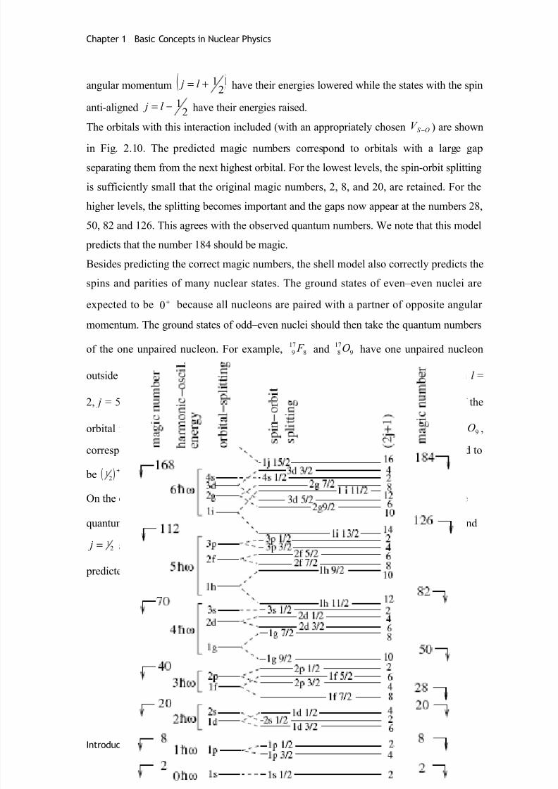
The orbitals with this interaction included (with an appropriately chosen OS V − ) are shown

in Fig. 2.10. The predicted magic numbers correspond to orbitals with a large gap

separating them from the next highest orbital. For the lowest levels, the spin-orbit splitting

is sufficiently small that the original magic numbers, 2, 8, and 20, are retained. For the

higher levels, the splitting becomes important and the gaps now appear at the numbers 28,

50, 82 and 126. This agrees with the observed quantum numbers. We note that this model

predicts that the number 184 should be magic.

Besides predicting the correct magic numbers, the shell model also correctly predicts the

spins and parities of many nuclear states. The ground states of even–even nuclei are

expected to be +0 because all nucleons are paired with a partner of opposite angular

momentum. The ground states of odd–even nuclei should then take the quantum numbers

of the one unpaired nucleon. For example, 8

17

9 F and 9

17

8 O have one unpaired nucleon

outside a doubly magic 8

8

8 O core. Figure 2.10 tells us that the unpaired nucleon is in a l =

2, j = 5 / 2. The spin parity of the nucleus is predicted to by ( ) +2

5 since the parity of the

orbital is ( ) l 1− . This agrees with observation. The first excited states of 8

17

9 F and 9

17

8 O ,

corresponding to raising the unpaired nucleon to the next higher orbital, are predicted to

be ( ) +21 , once again in agreement with observation.

On the other hand, 8

15

7 N and 7

15

8 O have one “hole” in their O16 core. The ground state

quantum numbers should then be the quantum numbers of the hole which are 1=l and

21= j according to Fig. 2.10. The quantum numbers of the ground state are then

predicted to be ( ) −2

1 , in agreement with observation.





Fig. 2.10. Nucleon orbitals in a model with a spin-orbit interaction

2. Some consequences of nuclear shell structure

Nuclear shell structure is reflected in many nuclear properties and in the relative natural

abundances of nuclei. This is especially true for doubly magic nuclei like He4

2 , O16

8 and

Ca40

20 all of which have especially large binding energies. The natural abundances of

Ca40 is 97% while that of Ca40

20 is only 2% in spite of the fact that the semi-empirical





mass formula predicts a greater binding energy for Ca44 . The doubly magic Sn100

50 is far

from the stability line ( Ru100

56 ) but has an exceptionally long half-life of 0.94 s. The same

can be said for , Ni48

28 , the mirror of Ca48

20 which is also doubly magic.

The Ni48

28 is the final nucleus produced in stars before decaying to Co56 and then Fe56

Fe56 . Finally, 126

208

82 Pb is the only heavy double-magic. It, along with its neighbors

Pb206 and Pb207 , are the final states of the three natural radioactive chains.

Nuclei with only one closed shell are called “semi-magic”:

• isotopes of nickel, Z = 28;

• isotopes of tin, Z = 50;

• isotopes of lead, Z = 82;

• isotones N = 28 ( ( ,,,,,52525150 etc FeCr V Ti

• isotones N = 50 ( ( )etc Zr V Sr Rb Kr ,,,,, 9059888786

• isotones N = 82 ( ).Pr,,,,, 141140139138136 etcCe La Ba Xe

These nuclei have

• a binding energy greater than that predicted by the semi-empirical mass formula,

• a large number of stable isotopes or isotones,

• a large natural abundances,

• a large energy separation from the first excited state,

• a small neutron capture cross-section (magic-N only).

The exceptionally large binding energy of doubly magic He4 makes α decay the

preferred mode of A non-conserving decays. Nuclei with 240209 << A all cascade via a

series of β and α decays to stable isotopes of lead and thallium. Even the light nuclei

,,, 855 Be Li He decay by α emission with lifetimes of order 1610− s.

While He5 rapidly α decays, He6 has a relatively long lifetime of 806ms. This nucleus

can be considered to be a three-body state consisting of 2 neutrons and an α particle.

This system has the peculiarity that while being stable, none of the two-body subsystems

(n-n or n-α) are stable. Such systems are called “Borromean” after three brothers from the





Borromeo family of Milan. The three brothers were very close and their coat-of-arms

showed three rings configured so that breaking any one ring would separate the other two.

Fig. 2.11. Nuclear energies as a function of deformation

Shell structure is a necessary ingredient in the explanation of nuclear deformation. We

note that the Bethe–Weizs¨acker mass formula predicts that nuclei should be spherical,

since any deformation at constant volume increases the surface term. This can be

quantified by a “deformation potential energy”. In the liquid-drop model a local minimum

is found at vanishing deformation corresponding to spherical nuclei. If the nucleus is

unstable to spontaneous fission, the absolute minimum is at large deformation

corresponding to two separated fission fragments.

Since the liquid-drop model predicts spherical nuclei, observed deformation must be due

to nuclear shell structure. Deformations are then linked to how nucleons fill available

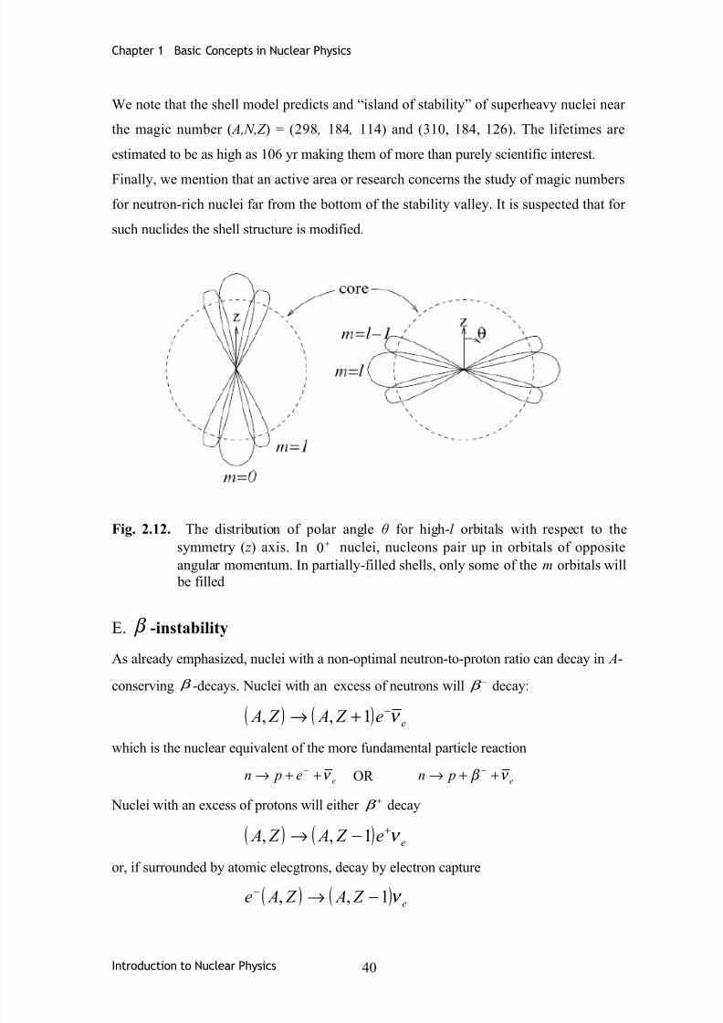
orbitals. For instance, even–even nuclei have paired nucleons. As illustrated in Fig. 2.12,

if the nucleons tend to populate the high-m orbitals of the outer shell of angular

momentum l , then the nucleus will be oblate. If they tend to populate low-m orbitals, the

nucleus will be prolate. Which of these cases occurs depends on the details of the

complicated nuclear Hamiltonian. The most deformed nuclei are prolate.

Because of these quantum effects, the deformation energy in Fig. 2.11 will have a local

minimum at non-vanishing deformation for non-magic nuclei. It is also possible that a

local minimum occurs for super-deformed configurations. These metastable

configurations are seen in rotation band spectra.





We note that the shell model predicts and “island of stability” of superheavy nuclei near

the magic number ( A,N,Z ) = (298 , 184 , 114) and (310, 184, 126). The lifetimes are

estimated to be as high as 106 yr making them of more than purely scientific interest.

Finally, we mention that an active area or research concerns the study of magic numbers

for neutron-rich nuclei far from the bottom of the stability valley. It is suspected that for

such nuclides the shell structure is modified.

Fig. 2.12. The distribution of polar angle θ for high-l orbitals with respect to the

symmetry ( z ) axis. In +0 nuclei, nucleons pair up in orbitals of opposite

angular momentum. In partially-filled shells, only some of the m orbitals will

be filled

E. β -instability

As already emphasized, nuclei with a non-optimal neutron-to-proton ratio can decay in A-

conserving β -decays. Nuclei with an excess of neutrons will −β decay:

( ) ( ) ee Z A Z A ν −

+→ 1,,

which is the nuclear equivalent of the more fundamental particle reaction

ee pn ν ++→ −OR e pn ν β ++→ −

Nuclei with an excess of protons will either +β decay

( ) ( ) ee Z A Z A ν +−→ 1,,

or, if surrounded by atomic elecgtrons, decay by electron capture

( ) ( ) e Z A Z Ae ν 1,, −→−





These two reactions are the nuclear equivalents of the particle reactions

evn pe +→+−or even p ++→ +

In order to conserve energy-momentum, proton+β -decay is given by

( ) ( ) em Z Am Z AmQ −+−=− 1,,β

( ) ( ){ } ( e pn mmm Z A B Z A B −−+−+= ,1,

While that in+β -decay is

( ) ( ) em Z Am Z AmQ −+−=+1,,

β

( ) ( ){ } ( e pn mmm Z A B Z A B −−−−−= ,1,

The energy release in electron capture is larger than that in+β -decay

eec mQQ 2+= +β

so electron capture is the only decay mode available for neighboring nuclei separated by

less than em in mass.

The energy released in β -decay can be estimated from the semi-empirical mass formula.

For moderately heavy nuclei we can ignore the Coulomb term and the estimate is

A

MeV A Z A

aQ a 100

2

8≈−≈

β

As with all reactions in nuclear physics, the Q values are in the MeV range.

β -decays and electron captures are governed by the weak interaction. One of the results

will be that for emQ >>β , the decay rate is proportional to the fifth power of β Q

5

1452

110

≈∝ −−

MeV

Q sQG F

β

β β λ 2cmQ e>>β

where the Fermi constant F G , given by ( )25

3 10166,1−−

×= GeV c

G F

, is the effective

coupling constant for low-energy weak interactions. The constant of proportionality

depends in the details of the initial and final state nuclear wavefunctions. In the most

favorable situations, the constant is of order unity.

F. α -instability





Because nuclear binding energies are maximized for 60≈ A , heavy nuclei that are β -

stable (or unstable) can generally split into more strongly bound lighter nuclei. Such

decays are called “spontaneous fission.” The most common form of fission is α -decay:

( ) ( ) He Z A Z A 422,4, +−−→

For example

MeV RaTh 08,4228

88

232

90 ++→ α : yr t 10

21 104,1 ×=

MeV RaTh 31,7220

88

224

90 ++→ α : st 05,12

1 =

MeV BaCe 45,1138

56

142

58 ++→ α : yr t 15

21 105×≈

MeV Pb Po 95,8208

82

212

84 ++→ α : st

7

21 103

−

×=We see that most nuclei with A > 140 are potential α -emitters. However, naturally

occurring nuclides with α-half-lives short enough to be observed have either A > 208 or

145≈ A with Ce142 being lightest.

The most remarkable characteristic of α -decay is that the decay rate is an exponentially

increasing function of α Q . This important fact is spectacularly demonstrated by

comparing the lifetimes of various uranium isotopes:

MeV ThU 19,4234238 ++→ α : st 17

21 104,1 ×=

MeV ThU 45,4232236 ++→ α : st 14

21 103,7 ×=

MeV ThU 70,4230234 ++→ α : st 12

21 108,7 ×=

MeV ThU 21,5228232 ++→ α : st 9

21 103,2 ×=

MeV ThU 60,5226230 ++→ α : st 6

2

1 108,1 ×=

MeV ThU 59,6224228 ++→ α : st 2

21 106,5 ×=

The lifetimes of other α -emitters are shown in Fig. 2.13.

This strong α Q dependence can be understood within the framework of a model

introduced by Gamow in 1928. In this model, a nucleus is considered to contain α -

particles bound in the nuclear potential. If the electrostatic interaction between an α and

the rest of the nucleus is “turned off,” the α ’s potential is that of Fig. 2.14a. As usual, the





potential has a range R and a depth oV . Its binding energy is called α E . In this situation,

the nucleus is completely stable against α -decay.

Fig. 2.13. The half-lives vs. α Q for selected nuclei. The half-lives vary by 23 orders of

magnitude while α Q varies by only a factor of two

Fig. 2.14. Gamow’s model of α -decay in which the nucleus contains a α -particle

moving in a mean potential. If the electromagnetic interactions are “turned

off”, the α -particle is in the state shown on the left.





If we now “turn on” the electrostatic potential between the α and the rest of the nucleus,

α E increases because of the repulsion. For highly charged heavy nuclei, the increase in

α E can be sufficient to make α E > 0, a situation shown in Fig. 2.16b. Such a nucleus,

classically stable, can decay quantum mechanically by the tunnel effect. The tunneling

probability could be trivially calculated if the potential barrier where a constant energy V

of width ∆

∆−∝ K e P 2 ,

( )2

2

α E V m K

−=

To calculate the tunneling probability for the potential of Fig. 2.14b, it is sufficient to

replace the potential with a series of piece-wise constant potentials between Rr = and

br = and then to sum:

γ 2−∝ e P ,( ){ }

dr c

mc E r V b

R

∫ −

=22

22

α γ

where ( )r V is the potential in Fig. 2.14b.

The integral can be simplified by defining the dimensionless variable

( ) ( ) c Z

E r

r V

E u

α 22 −==

We then have

( )du

u E

me Z

MIN uo∫ −

−=

12

112

4

22 α

πε γ

For large Z , suggests that it is a reasonably good approximation to take 0= MIN u in which

case the integral is π/ 2. This gives

( )υ

α π γ c

Z 22 −=

whereα

υ m

E 2= is the velocity of the α -particle after leaving the nucleus. For U 238

we have 1722 ≈γ while for U 228 we have 1362 ≈γ . We see how the small difference in

energy leads to about 16 orders of magnitude difference in tunneling probability and,

therefore, in lifetime.





Chapter 3

Nuclear decays and fundamental interactions

Chapter 4

Radioactivity

Chapter 5

Fission

Chapter 6

Fusion


introduction nuclear physics chapter 2

Documents