HYDRODYNAMIC MODES ANDNONEQUILIBRIUM STEADY STATES

Pierre GASPARDBrussels, Belgium

J. R. Dorfman, College Park

S. Tasaki, Tokyo

T. Gilbert, Brussels

• INTRODUCTION: POLLICOTT-RUELLE RESONANCES

• DIFFUSION IN SPATIALLY PERIODIC SYSTEMS

• FRACTALITY OF THE RELAXATION MODES OF DIFFUSION

• NONEQUILIBRIUM STEADY STATES

• CONCLUSIONS

ERGODIC PROPERTIES AND BEYOND

€

Ergodicity (Boltzmann 1871, 1884): time average = phase-space average

€

limT →∞

1

T A(Φ tΓ0) dt

0

T

∫ = A(Γ∫ ) Ψ0 Γ( ) dΓ = A = A Ψ0

€

pt = ˆ U t p0 = e i ˆ G t p0 ˆ G = i ˆ L

stationary probability density representing the equilibrium statistical ensemble

€

ˆ G Ψ0 = 0

Mixing (Gibbs 1902):

Spectrum of unitary time evolution:

Ergodicity: The stationary probability density is unique:The eigenvalue is non-degenerate.

€

A(t)B(0) = A(Φ tΓ∫ ) B(Γ) Ψ0 Γ( ) dΓ →t →∞

A B

€

limt →∞

μ(Φ−tA ∩B ) = μ(A ) μ(B )

€

z = 0

Mixing: The non-degenerate eigenvalue is the only one on the real-frequency axis.The rest of the spectrum is continuous.

€

z = 0

€

Ψ0

Statistical average of a physical observable A():

€

At

= A(Φ tΓ0∫ ) p0 Γ0( ) dΓ0 = A(Γ∫ ) p0 Φ−tΓ( ) dΓ ≡ A(Γ∫ ) eˆ L t p0 Γ( ) dΓ

POLLICOTT-RUELLE RESONANCESgroup of time evolution: ∞ < t < ∞ <A>t = <A|exp(L t)| p0 > = ∫ A(x) p0(t x) dx

analytic continuation toward complex frequencies: L |Ψ> = s |Ψ> , < | L = s < |

s = i z• forward semigroup ( 0 < t < ∞): asymptotic expansion around t = ∞ :

<A>t = <A|exp(L t)| p0> ≈ ∑ <A|Ψ> exp(s t) <| p0> + (Jordan blocks)

• backward semigroup (∞ < t < ): asymptotic expansion around t = ∞ :

<A>t = <A|exp(L t)| p0> ≈ ∑ <A|Ψ°> exp(s t) <°| p0> + (Jordan blocks)

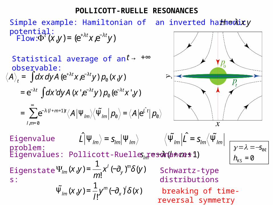
POLLICOTT-RUELLE RESONANCES

€

Simple example: Hamiltonian of an inverted harmonic potential:

€

H = λ x y

€

ˆ L Ψlm = slm Ψlm ˜ Ψ lm ˆ L = slm˜ Ψ lm

Flow:

€

Ψlm (x,y) =1

m!x l (−∂y )mδ(y)

˜ Ψ lm (x,y) =1

l!ym (−∂x )lδ(x)

Statistical average of an observable:

€

At= dx dy A(e+λt x,e−λ t y) p0∫ (x,y)

= e−λ t dx 'dy A(x ',e−λ t y) p0∫ (e−λ t x', y)

= e−λ ( l +m +1)t A Ψlm

l,m= 0

∞

∑ ˜ Ψ lm p0 = A eˆ L t p0

€

slm = −λ (l + m +1)

€

t (x, y) = (e+λt x,e−λ t y)

Eigenvalue problem:

Eigenvalues: Pollicott-Ruelle resonances:

Eigenstates:

€

t → +∞

breaking of time-reversal symmetry

Schwartz-type distributions

€

γ=λ =−s00

hKS = 0

TIME-REVERSAL SYMMETRY & ITS BREAKING

Hamilton’s equations are time-reversal symmetric:

€

ot oΘ = Φ−t

If the phase-space curve

is solution of Hamilton’s equation, then the time-reversed curve

is also solution of Hamilton’s equation.

Typically, the solution breaks the time-reversal symmetry:

Liouville’s equation is also time-reversal symmetric.

Equilibrium state:

Relaxation modes:

Nonequilibrium steady state:

Spontaneous or explicit breaking of time-reversal symmetry

€

C = Γ = Φ t (Γ0) : t ∈ R{ }

€

(C) = Γ'= Φ t '(ΘΓ0) : t '∈ R{ }

€

C ≠ Θ(C)

€

μeq (A ) = μ eq (ΘA )

€

μnoneq (A ) ≠ μnoneq (ΘA )

€

Ψ ≠Ψ o (α ≠ 0)

€

Ψ0 = Ψ0 oΘ

RELAXATION MODES OF DIFFUSION

special solutions of Liouville’s equation:

€

p(r,v, t) = C exp(sk t) Ψk (r,v)

€

ˆ L Ψk = sk Ψk

eigenvalue = dispersion relation of diffusion:

wavenumber: k

sk = D k2 + O(k4)

diffusion coefficient: Green-Kubo formula

time

space

c

once

ntra

tion

wavelength = 2/k

€

D = vx (0)vx (t) 0

∞

∫ dt

€

∂p

∂t= H, p{ } = ˆ L p

generalized eigenstate of Liouvillian operator:

€

Ψk (r,v)∝ exp(ik ⋅r)

spatial periodicity

MOLECULAR DYNAMICS SIMULATION OF DIFFUSION

J. R. Dorfman, P. Gaspard, & T. Gilbert, Entropy production of diffusion in spatiallyperiodic deterministic systems, Phys. Rev. E 66 (2002) 026110

Hamiltonian dynamics with periodic boundary conditions.N particles with a tracer particle moving on the whole lattice.The probability distribution of the tracer particle thus extends non-periodically over the whole lattice.

lattice Fourier transform:

€

G(Γ,l) =1

Bdk e i k⋅l ˜ G (Γ,k)

B

∫ first Brillouin zone of the lattice:

€

B

initial probability density close to equilibrium:

€

p0(Γ,l) = peq[1+ R0(Γ,l)]

time evolution of the probability density:

€

pt (Γ,l) = peq[1+ Rt (Γ,l)]

€

Rt (Γ,l) =1

Bdk Fk exp i k ⋅ l + d(Γ, t)[ ]{ }

B

∫

€

d(Γ, t) lattice distance travelled by the tracer particle:

lattice vector:

€

l ∈ L

DIFFUSIVE MODES IN SPATIALLY PERIODIC SYSTEMS

The Perron-Frobenius operator is symmetric under the spatial translations {l} of the (crystal) lattice:

common eigenstates:

eigenstate = hydrodynamic mode of diffusion:

€

ˆ P t = exp( ˆ L t)

€

ˆ P t , ˆ T l[ ] = 0

€

ˆ P t Ψk = exp(sk t) Ψk

ˆ T l Ψk = exp(ik ⋅l) Ψk

€

Ψk

€

⎧ ⎨ ⎩

eigenvalue = Pollicott-Ruelle resonance = dispersion relation of diffusion:

(Van Hove, 1954) wavenumber: k

sk = lim t∞ (1/t) ln <exp[ i k•(rt r0)]>

= D k2 + O(k4)

diffusion coefficient: Green-Kubo formula

time

space

c

once

ntra

tion

wavelength = 2/k

€

D = vx (0)vx (t) 0

∞

∫ dt

CUMULATIVE FUNCTION OF THE DIFFUSIVE MODES

The eigenstate Ψk is a distribution which is smooth in Wu but singular in Ws.

= breaking of time-reversal symmetry since Wu = (Ws) but Wu ≠ Ws .

cumulative function:

fractal curve in complex plane because Ψk is singular in Ws

S. Tasaki & P. Gaspard, J. Stat. Phys 81 (1995 935.P. Gaspard, I. Claus, T. Gilbert, & J. R. Dorfman, Phys. Rev. Lett. 86 (2001) 1506.

€

Fk (θ) = Ψk (rθ ',vθ ')dθ '

0

θ

∫ = limt →∞

dθ ' exp[ik ⋅(rt − r0)θ ' ]0

θ

∫

dθ ' exp[ik ⋅(rt − r0)θ ' ]0

2π

∫

eigenvalue = leading Pollicott-Ruelle resonance

sk = D k2 + O(k4) = lim t∞ (1/t) ln <exp[ i k•(rt r0)]> (Van Hove, 1954)

sk is the continuation of the eigenvalue s0 = 0 of the microcanonical equilibrium state and is not the next-to-leading Pollicott-Ruelle resonance.

MULTIBAKER MODEL OF DIFFUSION

€

φ(l,x,y) =l −1,2x,

y

2

⎛

⎝ ⎜

⎞

⎠ ⎟, 0 ≤ x ≤

1

2

l +1,2x −1,y +1

2

⎛

⎝ ⎜

⎞

⎠ ⎟,

1

2< x ≤1

⎧

⎨ ⎪ ⎪

⎩ ⎪ ⎪

€

singular diffusive modes :

de Rham cumulative functions :

Fk (y) =

α Fk (2y),

for 0 < y <1

2,

(1−α )Fk (2y −1) + α ,

for 1

2< y <1.

⎧

⎨

⎪ ⎪ ⎪

⎩

⎪ ⎪ ⎪

α =exp(ik)

2cosk

φ. . . . . .

ll-1 l+1. . . . . .

€

Hausdorff dimension : DH =ln2

ln(2cosk)

€

dispersion relation of diffusion : sk = lncosk

€

top. pressure : P(β ) = (1− β ) ln2

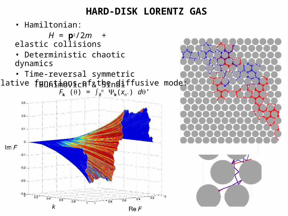
HARD-DISK LORENTZ GAS• Hamiltonian: H = p2/2m + elastic collisions• Deterministic chaotic dynamics• Time-reversal symmetric (Bunimovich & Sinai 1980)

cumulative functions of the diffusive mode: Fk () = ∫0

Ψk(x’) d’

YUKAWA-POTENTIAL LORENTZ GAS• Hamiltonian:

H = p2/2m i exp(ari)/ri

• Deterministic chaotic dynamics• Time-reversal symmetric (Knauf 1989)

cumulative functions of the diffusive mode: Fk () = ∫0

Ψk(x’) d’

HAUSDORFF DIMENSION OF THE DIFFUSIVE MODES

Proof of the formula for the Hausdorff dimension

cumulative function:

polygonal approximation of the fractal curve:

Hausdorff dimension:

Ruelle topological pressure:

€

Fk (θ) = limt →∞

dθ ' exp[ik ⋅(rt − r0)θ ']0

θ

∫

dθ ' exp[ik ⋅(rt − r0)θ ']0

2π

∫

€

P(DH) = DH Re sk

€

Fk (θ) = limn →∞

1

Λ(ω)

exp[ik ⋅(rt − r0)ω ]

exp(sk nτ )ω

∑ = limn →∞

ΔFk (ω)ω

∑

€

ΔFk (ω)ω

∑DH

∝1 for n → ∞

P. Gaspard, I. Claus, T. Gilbert, & J. R. Dorfman, Phys. Rev. Lett. 86 (2001) 1506.

Hausdorff dimension:

€

P(β ) ≡ limn →∞

1

nτ ln Λ(ω)

−β

ω

∑

Generalization of the Bowen-Ruelle formula for the Hausdorff dimension of Julia sets.

DIFFUSION COEFFICIENT FROM THE HAUSDORFF DIMENSION

low-wavenumber expansion:

€

P(DH) = DH Re sk

€

DH(k) =1+D

λk2 + O(k4 )

€

D =λ limk →0

DH(k) −1

k2

€

Re sk = −Dk2 + O(k4 )

Hausdorff dimension:

P. Gaspard, I. Claus, T. Gilbert, & J. R. Dorfman, Phys. Rev. Lett. 86 (2001) 1506.

probability measure:

€

μβ (ω) ≅Λ(ω)

−β

Λ(ω)−β

ω

∑

average Lyapunov exponent:

€

λ(β ) ≡ limn →∞

1

nτμβ (ω) ln Λ(ω)

ω

∑

€

h(β ) = β λ (β ) + P(β ) entropy per unit time:

€

−Re sk = −P(DH)

DH

= λ (DH) −h(DH)

DH

≈ λ 1−1

DH

⎛

⎝ ⎜

⎞

⎠ ⎟Hausdorff dimension:

dispersion relation of diffusion:

diffusion coefficient:

FRACTALITY OF THE DIFFUSIVE MODES

Hausdorff dimension:

large-deviation dynamical relationship:

P. Gaspard, I. Claus, T. Gilbert, & J. R. Dorfman, Phys. Rev. Lett. 86 (2001) 1506.

€

Dk2 ≈ −Re sk = −P(DH)

DH

= λ (DH) −h(DH)

DH

€

DH(k) =1+D

λk2 + O(k4 )

hard-disk Lorentz gas

Yukawa-potential Lorentz gas

Re sk

€

h(DH)

DH

€

λ(DH)

NONEQUILIBRIUM STEADY STATES

Steady state of gradient g=(p+p)/L in x:

pnoneq() = (p++ p)/2 + g [ x() + ∫0T() vx(t ) dt ]

pnoneq() = (p++ p)/2 + g [ x() + x(T() ) x() ]

pnoneq() = (p++ p)/2 + (p+p) x(T() ) /L

pnoneq() = p± for x(T() ) ±L/2

Ψg.() = g [ x() + ∫0 ∞ vx(t ) dt ]

= i g•∂k Ψk()|k=0

Green-Kubo formula: D = ∫0∞ <vx(0)vx(t)>eq dt

Fick’s law: <vx>neq= g [<vx x>eq + ∫0 ∞ <vx(0)vx(t)>eqdt ] = D g

p+ p

tx

SINGULAR CHARACTER OF THENONEQUILIBRIUM STEADY STATES

cumulative functions Tg () = ∫0 Ψg(’) d’

hard-disk Lorentz gas Yukawa-potential Lorentz gas

(generalized Takagi functions)

CONCLUSIONS

Breaking of time-reversal symmetry in the statistical description

Nonequilibrium transients:

Spontaneous breaking of time-reversal symmetry for the solutions of Liouville’s equation corresponding to the Pollicott-Ruelle resonances. The associated eigenstates are singular distributions with fractal cumulative functions.

Nonequilibrium modes of diffusion:

relaxation rate sk, Pollicott-Ruelle resonance

reminiscent of the escape-rate formula:

€

Dk2 ≈ −Re sk = λ (DH) −h(DH)

DH

€

D /L( )2

≈ γ = λ − hKS( )L

(1/2) wavelength = L = /k

CONCLUSIONS (cont’d)

€

D /L( )2

≈ γ = λ i

λ i >0

∑ − hKS

⎛

⎝ ⎜ ⎜

⎞

⎠ ⎟ ⎟L

Escape-rate formalism: nonequilibrium transients

fractal repeller

http://homepages.ulb.ac.be/~gaspard

diffusion D : (1990)

viscosity : (1995)

€

/χ( )2

≈ γ = λ i

λ i >0

∑ − hKS

⎛

⎝ ⎜ ⎜

⎞

⎠ ⎟ ⎟L

€

γ= λi

λ i >0

∑ − hKS = − λ i

λ i <0

∑ − hKS

€

λi

i=1

2 f

∑ = 0Hamiltonian systems: Liouville theorem:

€

σ =− λi

i=1

2 f

∑ = − λ i

λ i <0

∑ − λ i

λ i >0

∑ = − λ i

λ i <0

∑ − hKS

thermostated systems: no Liouville theorem

volume contraction rate:

€

hKS = λ i

λ i >0

∑Pesin’s identity on the attractor:

CONCLUSIONS (cont’d)

http://homepages.ulb.ac.be/~gaspard

Nonequilibrium steady states:

Explicit breaking of the time-reversal symmetry by the nonequilibrium boundary conditions imposing net currents through the system.

For reservoirs at finite distance of each other, the invariant probability measure is still continuous with respect to the Lebesgue measure, but it differs considerably from an equilibrium measure. Considering the invariant probability measure as the solution of Liouville’s equation with nonequilibrium boundary conditions imposed at the contacts with the reservoirs, the invariant probability density takes its value at the reservoir from which the trajectory is coming.

In the large-system limit at constant gradient, the phase-space regions coming from either one reservoir or the other alternate more and more densely so that the invariant probability measure soon becomes singular with respect to the Lebesgue measure.

€

μnoneq (A ) ≠ μnoneq (ΘA )