IT 16 074

Examensarbete 15 hpSeptember 2016

Hybrid Machine Translation

Choosing the best translation with Support

Vector Machines

Hannes Karlbom

Institutionen för informationsteknologiDepartment of Information Technology

Teknisk- naturvetenskaplig fakultet UTH-enheten Besöksadress: Ångströmlaboratoriet Lägerhyddsvägen 1 Hus 4, Plan 0 Postadress: Box 536 751 21 Uppsala Telefon: 018 – 471 30 03 Telefax: 018 – 471 30 00 Hemsida: http://www.teknat.uu.se/student

Abstract

Hybrid Machine Translation

Hannes Karlbom

In the field of machine translation there are various systems available which have different strengths and weaknesses. This thesis investigates the combination of two systems, a rule based one and a statistical one, to see if such a hybrid system can provide higher quality translations. The classification approach was taken, where a support vector machine is used to choose which sentences from each of the two systems result in the best translation. To label the sentences from the collected data a new method of simulated annealing was applied and compared to previously tried heuristics. The results show that a hybrid system has an increased average BLEU score of 6.10% or 1.86 points over the single best system, and that using the labels created through simulated annealing, over heuristic rules, gives a significant improvement in classifier performance.

Tryckt av: Reprocentralen ITCIT 16 074Examinator: Justin PearsonÄmnesgranskare: Olle GällmoHandledare: Aaron Smith

Contents

1 Introduction 51.1 Context . . . . . . . . . . . . . . . . . . . . . . . . . . . . . 51.2 Motivation and Goal . . . . . . . . . . . . . . . . . . . . . . 61.3 Scope . . . . . . . . . . . . . . . . . . . . . . . . . . . . . . 61.4 Related Work . . . . . . . . . . . . . . . . . . . . . . . . . . 7

2 Background 72.1 Machine Translation . . . . . . . . . . . . . . . . . . . . . . 8

2.1.1 Linguistic Approaches . . . . . . . . . . . . . . . . . 82.1.2 Rule Based Machine Translation . . . . . . . . . . . . 102.1.3 Statistical Machine Translation . . . . . . . . . . . . 11

2.2 BLEU Score . . . . . . . . . . . . . . . . . . . . . . . . . . . 12

3 Theory 133.1 Preprocessing . . . . . . . . . . . . . . . . . . . . . . . . . . 14

3.1.1 Tokenization, Stemming and Lemmatisation . . . . . 143.1.2 POS Tagging . . . . . . . . . . . . . . . . . . . . . . 153.1.3 Dependency Parsing . . . . . . . . . . . . . . . . . . 153.1.4 Universal Dependencies . . . . . . . . . . . . . . . . . 163.1.5 Normalization and Scaling . . . . . . . . . . . . . . . 16

3.2 Simulated Annealing . . . . . . . . . . . . . . . . . . . . . . 183.3 Machine Learning . . . . . . . . . . . . . . . . . . . . . . . . 20

3.3.1 Supervised Learning . . . . . . . . . . . . . . . . . . 203.3.2 Unsupervised Learning . . . . . . . . . . . . . . . . . 213.3.3 Reinforcement Learning . . . . . . . . . . . . . . . . 22

3.4 Support Vector Machines . . . . . . . . . . . . . . . . . . . . 233.4.1 Kernel Trick . . . . . . . . . . . . . . . . . . . . . . . 263.4.2 Parameters . . . . . . . . . . . . . . . . . . . . . . . 27

3.5 Model Evaluation . . . . . . . . . . . . . . . . . . . . . . . . 283.5.1 Training set and Test set holdout . . . . . . . . . . . 283.5.2 Cross-validation . . . . . . . . . . . . . . . . . . . . . 293.5.3 Bootstrap Sampling . . . . . . . . . . . . . . . . . . . 30

4 Method 304.1 DataSet . . . . . . . . . . . . . . . . . . . . . . . . . . . . . 304.2 System Overview . . . . . . . . . . . . . . . . . . . . . . . . 314.3 Potential Gain . . . . . . . . . . . . . . . . . . . . . . . . . . 32

4.3.1 Local Search . . . . . . . . . . . . . . . . . . . . . . . 334.4 Feature Extraction . . . . . . . . . . . . . . . . . . . . . . . 36

4.4.1 Basic . . . . . . . . . . . . . . . . . . . . . . . . . . . 364.4.2 Dependency Parsing . . . . . . . . . . . . . . . . . . 374.4.3 Part of Speech . . . . . . . . . . . . . . . . . . . . . . 39

2

4.5 Feature Selection . . . . . . . . . . . . . . . . . . . . . . . . 394.6 Model . . . . . . . . . . . . . . . . . . . . . . . . . . . . . . 404.7 Tools . . . . . . . . . . . . . . . . . . . . . . . . . . . . . . . 41

5 Results 435.1 Experimental Setup . . . . . . . . . . . . . . . . . . . . . . . 435.2 Simulated Annealing . . . . . . . . . . . . . . . . . . . . . . 435.3 Support Vector Machine . . . . . . . . . . . . . . . . . . . . 46

6 Discussion 49

7 Future Work 51

8 Conclusions 51

3

List of Figures

1 Bernard Vauquois’ pyramid [12] . . . . . . . . . . . . . . . . 82 Transfer learning for one language pair and two modules. . . 93 Interlingua model for one language pair. . . . . . . . . . . . 104 Dependency parsing of a short sentence [48]. . . . . . . . . . 155 Example of global/local maxima/minima using the cos(3πx)

xfunction [11] . . . . . . . . . . . . . . . . . . . . . . . . . . . 19

6 Approximately linear data which is noisy, fitted to both lin-ear and polynomial functions [14] . . . . . . . . . . . . . . . 21

7 Support vector machine where the elements on the dottedlines are the support vectors [13] . . . . . . . . . . . . . . . . 23

8 Mapping data from input space to feature space so it can beseparated linearly [10] . . . . . . . . . . . . . . . . . . . . . 27

9 An overview of the system architecture . . . . . . . . . . . . 32

List of Tables

1 Short example to demonstrate BLEU score . . . . . . . . . . 132 The three most common SVM kernel functions . . . . . . . . 273 Universal dependency relations . . . . . . . . . . . . . . . . 384 Universal Part of Speech tags . . . . . . . . . . . . . . . . . 395 BLEU score for different parameter combinations . . . . . . 456 BLEU score for different parameter combinations . . . . . . 467 Evaluation of the SVM given norm = �1 and SVM penalty

= �1 . . . . . . . . . . . . . . . . . . . . . . . . . . . . . . . 488 Evaluation of the SVM given norm = �2 and SVM penalty

= �1. . . . . . . . . . . . . . . . . . . . . . . . . . . . . . . . 489 Evaluation of the SVM given norm = �1 and SVM penalty

= �2. . . . . . . . . . . . . . . . . . . . . . . . . . . . . . . . 4810 Evaluation of the SVM given norm = �2 and SVM penalty

= �2. . . . . . . . . . . . . . . . . . . . . . . . . . . . . . . . 4911 Evaluation of the SVM given norm = �1 and no feature se-

lection . . . . . . . . . . . . . . . . . . . . . . . . . . . . . . 4912 Evaluation of the SVM given norm = �1 and SVM penalty=

�2 with no universal dependencies features (UD). . . . . . . . 49

4

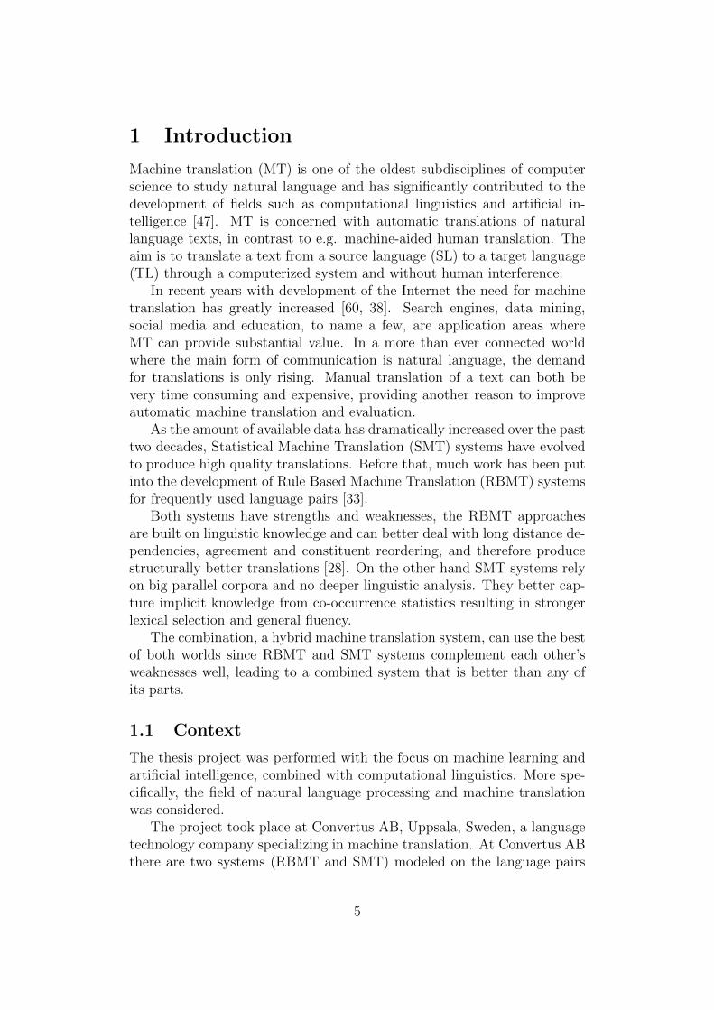
1 Introduction

Machine translation (MT) is one of the oldest subdisciplines of computerscience to study natural language and has significantly contributed to thedevelopment of fields such as computational linguistics and artificial in-telligence [47]. MT is concerned with automatic translations of naturallanguage texts, in contrast to e.g. machine-aided human translation. Theaim is to translate a text from a source language (SL) to a target language(TL) through a computerized system and without human interference.

In recent years with development of the Internet the need for machinetranslation has greatly increased [60, 38]. Search engines, data mining,social media and education, to name a few, are application areas whereMT can provide substantial value. In a more than ever connected worldwhere the main form of communication is natural language, the demandfor translations is only rising. Manual translation of a text can both bevery time consuming and expensive, providing another reason to improveautomatic machine translation and evaluation.

As the amount of available data has dramatically increased over the pasttwo decades, Statistical Machine Translation (SMT) systems have evolvedto produce high quality translations. Before that, much work has been putinto the development of Rule Based Machine Translation (RBMT) systemsfor frequently used language pairs [33].

Both systems have strengths and weaknesses, the RBMT approachesare built on linguistic knowledge and can better deal with long distance de-pendencies, agreement and constituent reordering, and therefore producestructurally better translations [28]. On the other hand SMT systems relyon big parallel corpora and no deeper linguistic analysis. They better cap-ture implicit knowledge from co-occurrence statistics resulting in strongerlexical selection and general fluency.

The combination, a hybrid machine translation system, can use the bestof both worlds since RBMT and SMT systems complement each other’sweaknesses well, leading to a combined system that is better than any ofits parts.

1.1 Context

The thesis project was performed with the focus on machine learning andartificial intelligence, combined with computational linguistics. More spe-cifically, the field of natural language processing and machine translationwas considered.

The project took place at Convertus AB, Uppsala, Sweden, a languagetechnology company specializing in machine translation. At Convertus ABthere are two systems (RBMT and SMT) modeled on the language pairs

5

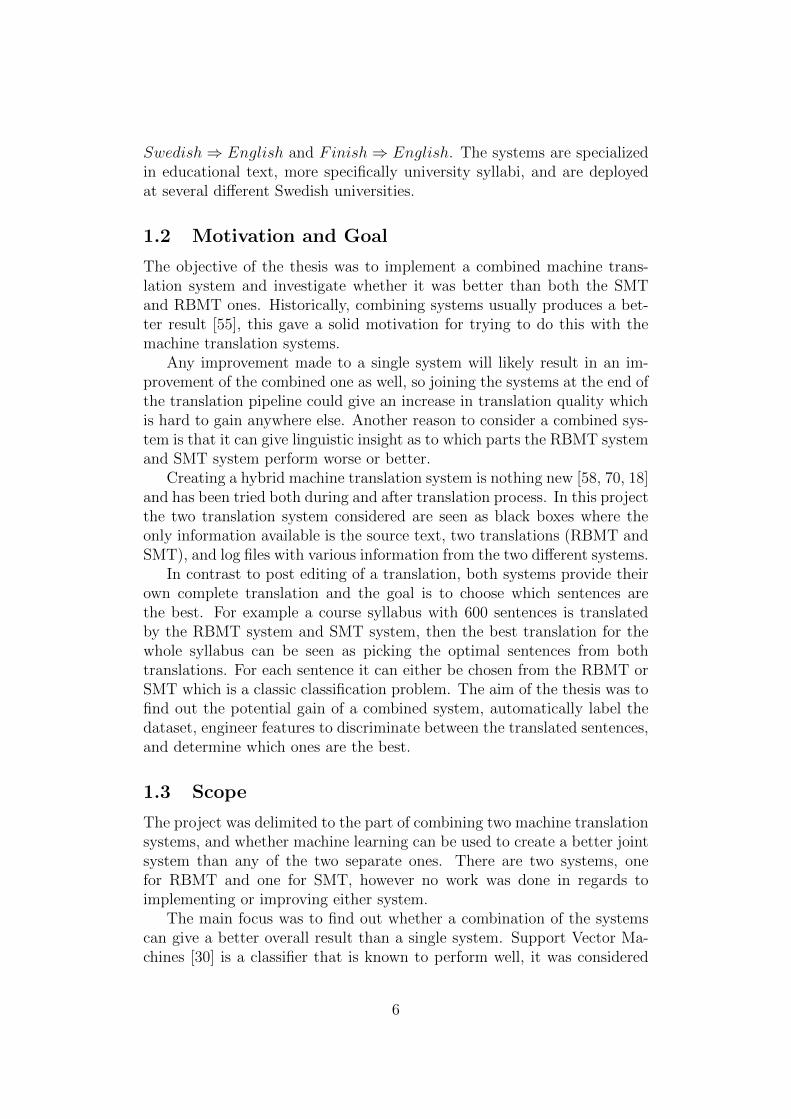
Swedish ⇒ English and Finish ⇒ English. The systems are specializedin educational text, more specifically university syllabi, and are deployedat several different Swedish universities.

1.2 Motivation and Goal

The objective of the thesis was to implement a combined machine trans-lation system and investigate whether it was better than both the SMTand RBMT ones. Historically, combining systems usually produces a bet-ter result [55], this gave a solid motivation for trying to do this with themachine translation systems.

Any improvement made to a single system will likely result in an im-provement of the combined one as well, so joining the systems at the end ofthe translation pipeline could give an increase in translation quality whichis hard to gain anywhere else. Another reason to consider a combined sys-tem is that it can give linguistic insight as to which parts the RBMT systemand SMT system perform worse or better.

Creating a hybrid machine translation system is nothing new [58, 70, 18]and has been tried both during and after translation process. In this projectthe two translation system considered are seen as black boxes where theonly information available is the source text, two translations (RBMT andSMT), and log files with various information from the two different systems.

In contrast to post editing of a translation, both systems provide theirown complete translation and the goal is to choose which sentences arethe best. For example a course syllabus with 600 sentences is translatedby the RBMT system and SMT system, then the best translation for thewhole syllabus can be seen as picking the optimal sentences from bothtranslations. For each sentence it can either be chosen from the RBMT orSMT which is a classic classification problem. The aim of the thesis was tofind out the potential gain of a combined system, automatically label thedataset, engineer features to discriminate between the translated sentences,and determine which ones are the best.

1.3 Scope

The project was delimited to the part of combining two machine translationsystems, and whether machine learning can be used to create a better jointsystem than any of the two separate ones. There are two systems, onefor RBMT and one for SMT, however no work was done in regards toimplementing or improving either system.

The main focus was to find out whether a combination of the systemscan give a better overall result than a single system. Support Vector Ma-chines [30] is a classifier that is known to perform well, it was considered

6

good enough for testing out the hypothesis that a joint system is better, andtherefore chosen as the main method for classification. There was no con-sideration to evaluate different classifiers, however parameter and featureselection were methods used to improve performance.

Finally only translations of syllabi from Swedish to English were used,although all ideas are applicable to other language pairs as well. The reas-oning was to keep the size of the project reasonable, and that it was easierto acquire good quality data for only one language pair.

1.4 Related Work

In 2002 Papineni et al. introduced one of the most widely used metricsfor evaluating how good a machine translation is, called BLEU [53]. SimonZwarts and Mark Dras suggested a combination of two SMT systems in backoff fashion, where one of them acted as a base line and the other one wasonly considered if better, to get an improved BLEU score [70]. Choosing thebest subset of machine translation systems by using only source languageinformation was investigated by Sanchez-Martinez et al. [58].

Machine translation evaluation is closely related to the task of choosingthe best translation since if a translation could be determined to be goodor bad, then this is a short step from choosing which translation to usefrom multiple systems. Finch, Yang and Sumita used standard MT evalu-ation techniques to build a classifier to determine sentence-level semanticequivalence [22]. The task of evaluating quality and fluency of a sentencein the absence of a reference translation was studied by Gamon et al. [26].Corston et al. presented a machine learning approach to evaluation of theoutput in the sense of well-formedness, and used classification to distinguishmachine translations from human reference ones [15].

Marta R. Costa-jussa and Jose A.R. Fonollosa reviewed the latest trendsin hybrid machine translation systems (2015) and concluded that hybridmachine translation has helped to advance the field of machine translationand is a promising line of research [18].

2 Background

Relevant information concerning machine translation systems, approachesand techniques are described. The commonly used translation quality met-ric, BLEU score, is explained in detail, as it is used as the main evaluationmethod in the project.

7

2.1 Machine Translation

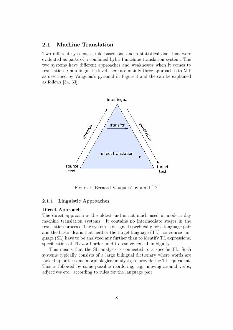
Two different systems, a rule based one and a statistical one, that wereevaluated as parts of a combined hybrid machine translation system. Thetwo systems have different approaches and weaknesses when it comes totranslation. On a linguistic level there are mainly three approaches to MTas described by Vauguois’s pyramid in Figure 1 and the can be explainedas follows [34, 33]:

Figure 1: Bernard Vauquois’ pyramid [12]

2.1.1 Linguistic Approaches

Direct ApproachThe direct approach is the oldest and is not much used in modern daymachine translation systems. It contains no intermediate stages in thetranslation process. The system is designed specifically for a language pairand the basic idea is that neither the target language (TL) nor source lan-guage (SL) have to be analyzed any further than to identify TL expressions,specification of TL word order, and to resolve lexical ambiguity.

This means that the SL analysis is connected to a specific TL. Suchsystems typically consists of a large bilingual dictionary where words arelooked up, after some morphological analysis, to provide the TL equivalent.This is followed by some possible reordering, e.g. moving around verbs,adjectives etc., according to rules for the language pair.

8

Transfer ApproachIn contrast to the direct approach, the transfer approach aims to first con-vert the SL to anything from a semantic representation to a syntactic one,e.g. a parse tree. This representation is then converted to a similar onefor the TL, and finally the translation is generated from the TL represent-ation. In the transfer approach both the TL and SL representations aredependent on their respective languages, and the rules used to transfer theinformation between language representations are as well.

Figure 2: Transfer learning for one language pair and two modules.

Typically the the SL text is converted to its representation through mor-phological analysis, syntactic analysis and semantic analysis, then rules forthe language pair are used to map the representation to the TL represent-ation. The final translation is produced by generation of text from the TLrepresentation where possibly some structures are altered as dictated bythe constraints of the TL.

Interlingua ApproachIn the interlingua approach the SL, similarly to the transfer approach, istransformed into an intermediate state. The difference is that the inter-mediate representation is independent of any language and the TL textgeneration happens directly from it. Because of the independence a mod-ule only has to translate from the abstract representation to the TL withoutknowing anything about the SL. In reverse, languages only have to converttext to the intermediate representation for it to be translated to every TLthat has a text generation module.

9

Figure 3: Interlingua model for one language pair.

This is clearly better for multilingual systems than the transfer ap-proach, however in practice it is very hard to define a universal abstractrepresentation and convert languages to it, even for similar ones, e.g. Ro-mance languages: French, Portuguese, Italian, Spanish. In practice thetransfer method is often preferred over the interlingua approach, both be-cause of the difficulty to create an independent language representation andto reduce the complexity of grammar generation.

2.1.2 Rule Based Machine Translation

Rule based machine translation systems use the transfer approach or theinterlingua approach to the translation of a text from SL to TL. Rulesare designed and used throughout the process of translating the text. Therules cover e.g. lexical selection, morphology analysis, syntactic analysis,syntactic generation, semantic analysis, etc. In general they cover the partsdiscussed in the linguistic approaches, which are analysis, transfer and gen-eration. The systems make use of a large bilingual dictionary and a gram-mar which has to be designed by linguists.

An example of how a rule base machine translation system could workis: given a SL text, it first divides it into segments which are looked upin a dictionary. This step returns the base form of the words and theirtags, and is a part of the morphological analysis. Next, to resolve anyambiguities between the segments, a part of speech tagger can be used, aswell as lexical selection to chose between alternate meanings. The next stepis to convert this representation to the TL by using structural and lexicaltransfer rules. Finally morphological generators and a post generator canbe used to produce the TL text [17].

All the steps described requires linguistic knowledge about both the SLand the TL to develop the specific rules for each part, and it is necessaryto get good translations. For this reason the construction of rule basedmachine translations systems can be both time consuming and expensive.

10

2.1.3 Statistical Machine Translation

Statistical machine translation (SMT) systems, as opposed to rule basedones, do not necessarily require much linguistic knowledge. The main isidea is, given a sentence in the SL, to find the translation to the TL thathas highest probability. There are three steps which SMT systems are con-cerned with: modeling, training and decoding. The modeling is about howto define a method for calculating the probability of a TL sentence having aSL language sentence. The training step is to use a corpus to estimate theparameters of the model which was defined. Lastly the decoding problemfocuses on the search to find the sentence which has the highest probabilityamong all the candidate translations.

More formally, given a sequence of words in the SL fJ1 = f1, . . . , fj . . . , fJ ,

finding the most probable sequence in the TL eI1 = e1, . . . , ei . . . , eI can be

formulated using Bayes decision rule [5]:

eI1 = argmax

eI1

{Pr(eI1 | fJ1 )}

= argmaxeI1

{Pr(eI1)Pr(fJ1 | eI1)}

(1)

Given the target language model Pr(eI1) and the translation modelPr(fJ

1 | eI1), the optimal translations is the product of their probabilit-

ies. The language model is formulated as a probability distribution overstrings in a language, with the aim of reflecting how likely a certain stringis to occur in the language. This is useful as deformed sentences are lesslikely to occur than well formed ones, and as such it represents the fluencyof the target sentence. Language models normally are a form of smoothedn-gram models where the probability of a word P (wn

1 ) is conditional on theprevious ones seen in the sentence, written as:

P (wn1 ) = P (wn

1 ).P (w2 | w1).P (w3 | w21) . . . P (wn | wn−1

1 )

=n�

i=1

P (wi | wi−1i )

(2)

The translation model Pr(eI1) assigns probabilities to the set of pos-sible translations for any target sentence. This model has to learn from aparallel corpora where source text and their corresponding gold standardtranslation is available.

In modern SMT systems the Bayes approach has been expanded to amore general one where maximum entropy with a log-linear combination offeature functions are used [51]. This maximization of the feature functionscan be written as:

11

�t = argmaxt

�M�

m=1

λmhm(eI1, f

J1 )

�. (3)

where hm(eI1, fJ1 ) ∀ m ∈ {1 . . .M} is a set of M feature functions, and there

exists a model parameter λm for every feature function.

2.2 BLEU Score

BLEU (BiLingual Evaluation Understudy) is the most widely used methodfor automatic evaluation of machine translation quality. It was introducedin 2002 by Papineni et al. [53] and has been frequently employed since.Given a machine translated sentence and set of reference sentences, whichare considered as a set of gold standard translations, the BLEU score givesa measurement of how good the translation is. The definition of quality, inthis context, is considered to be ‘how close the translation is to a profes-sional human’s translation’, and BLEU was shown, in the original article,to have high correlation with human judgments of quality.

The metric relies on what is called modified n-gram precision, and abrevity penalty to calculate the final score. A short example of two differentcandidate translations together with two references is shown i Table 1, andit van be used to illustrate how the BLEU score is derived.

Using normal precision and calculating the unigram precision forcandidate1, it can be seen that every word (7 occurrences of ‘the’) is presentin the both the reference translations. Hence the precision will be 7

7 =1, which is a perfect score, although only little content is present in thecandidate translation. The modified n-gram precision, which is used byBLEU, is defined such that the n-gram counts in the candidate translationare clipped at the max number found in the references. Applied to theexample in Table 1, there are 2 ‘the’ in reference1 and 1 in reference2,which results in clipping the 7 to 2. The modified unigram precision thenbecomes 2

7 since it is still divided by all the unigrams in the candidatetranslation.

By using the modified n-gram precision candidate translations that arelonger than the references are punished, however shorter ones can still pro-duce a high score using modified n-gram precision while still not being verysimilar to the references. Looking at candidate2, the modified unigram pre-cision becomes 1

2 + 12 = 1, since both ‘the’ and ‘cat’ are present in the

references. In addition the modified bigram precision also becomes 11 = 1

since ‘the cat’ is present in the references, and the candidate only has onebigram.

12

Candidate1 the the the the the the theCandidate2 the catReference1 the cat is on the matReference2 there is a cat on the mat

Table 1: Short example to demonstrate BLEU score

To account for this, a brevity penalty is used (as defined in equation (4))to punish candidate translations which are shorter than the reference trans-lations. The brevity penalty is applied over the whole document, not ona sentence level, and this is to allow for deviation in sentence length asotherwise shorter sentences would be punished to harshly. To calculate themodified n-gram precision for a whole document, sum the n-gram counts(clipped) for all sentences in the candidate translation then divide by thenumber of n-grams in the whole candidate translation.

Let c be the length of the candidate translation, and r be the effectivereference corpus length, then the brevity penalty BP is defined as:

BP =

�1 if c > r

exp(1− rc ) if c ≤ r

(4)

Finally the n-gram precision decays roughly exponentially with n and toaccount for this a geometric mean is used to arrive at the complete BLEUvalue. The score is given by equation (5), where the geometric mean of themodified n-gram precision from n = {1 . . . N} is multiplied by the positiveweights wn (which sum to 1), and then multiplied with the brevity penalty.

BLEU = BP · exp� N�

n=1

wn log pn

�(5)

Where wn = 1N and N = 4 was found to have the best correlation with

mono-lingual human judgments [53]. BLEU has been questioned as towhether it is the best method for automatically evaluating translations,and if it actually correlates as well with human judgments of translationquality [7]. As such there are many different ways, although not used inthis project, to evaluate translations, e.g. NIST, TER and METEOR [1].

3 Theory

The theory behind the techniques and algorithms used in the project areexplained in detail. Natural language processing is used to preprocess dataand extract features, machine learning, more specifically support vectormachine, is used to for classification, and different ways to evaluate a modelare described.

13

3.1 Preprocessing

Preprocessing is an important step in machine learning, where the datais transformed to have the right shape, size, features are extracted fromraw data etc., before the information can be passed on and utilized by theclassifier.

3.1.1 Tokenization, Stemming and Lemmatisation

TokenizationTokenization is the task of cutting a text into meaningful pieces to befurther processed [41]. It is used as a preprocessing step in most textanalysis tasks, but how a text should be divided is not always obvious.An intuitive way is to split a text on white spaces and possibly removepunctuation. However that does not cover all the cases, e.g. the desired

token or tokens for the word ‘aren’t’ could be: aren�t , arent , aren t

or are n�t . Other cases are when there is a natural white space in what

could considered two words but one token such as ‘San Francisco’, as wellas hyphenated words, and if they should be one or multiple tokens.

The different cases to be considered when doing tokenization can betreated as a classification problem, but is most commonly dealt with byapplying some heuristic rules for the language at hand [41].

Stemming and LemmatisationDifferent texts can have different forms of the same base word for gram-matical reasons, but sometimes it can be useful to consider all of them asthe same word. The purpose of both lemmatisation and stemming is toreduce a word to its basic form by removing inflectional forms and some-times derivationally related forms. An example would be:

am, are, is → becar, car’s, cars’, cars → car

The difference between them is that lemmatisation uses morphologicalanalysis and a dictionary of words to return their base form, also known asthe lemma. Lemmatisation aims only at removing the inflectional endingsof words, whilst stemming can also remove derivationally related forms.The processes of stemming is less complex and only involves chopping offthe last part of a word [41]. This is done by applying heuristic rules withthe most popular algorithm for the English language being Porter’s al-gorithm [56].

14

3.1.2 POS Tagging

Part of speech (POS) tagging is the process of assigning different tags towords in a text corresponding to parts of speech, such as nouns, verbs, ad-jectives etc. All the categories follow a universal tagset, that is independentof language, as shown in Table 4. POS tagging is used to disambiguate themeaning of words, e.g. the text ‘flies like a flower’. Looking at the wordsindividually, ‘flies’, ‘like’ and ‘flower’ can all be a verbs, but looking at itas sequence it is very unlikely that flower is a verb since it is preceded by‘a’.

Most approaches to sequence problems take a unidirectional way to doinference along the sequence. Different techniques such as hidden Markovmodels (HMM), maximum entropy conditional sequence models and de-cision trees take the unidirectional approach, which have been the mostsuccessful in recent years [64]. In HMM the word would be the observationand the tag the hidden state. Take the short example ‘the can’, an obser-vation of the word ‘can’ might have a certain probability to be classified asa noun, but with a preceding ‘the’ the chance increases.

3.1.3 Dependency Parsing

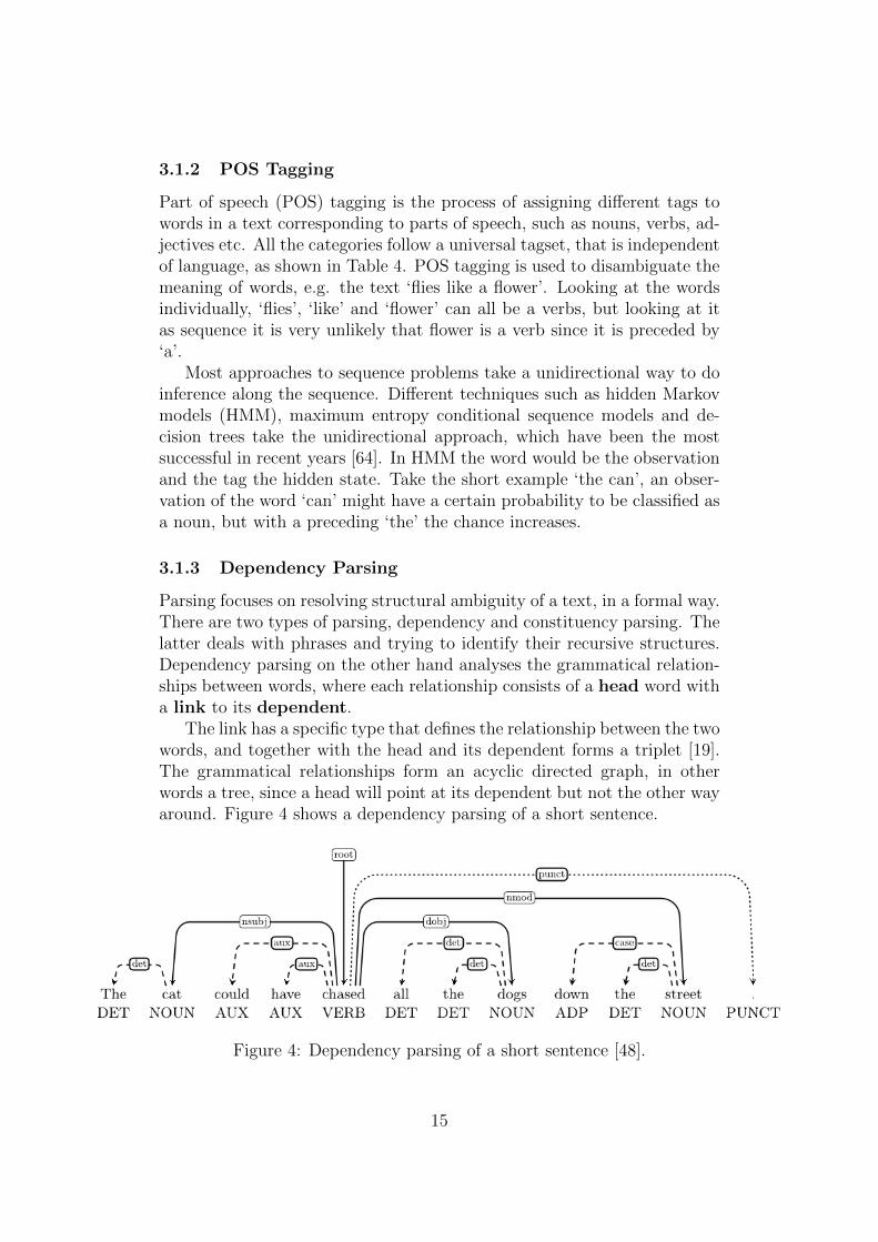
Parsing focuses on resolving structural ambiguity of a text, in a formal way.There are two types of parsing, dependency and constituency parsing. Thelatter deals with phrases and trying to identify their recursive structures.Dependency parsing on the other hand analyses the grammatical relation-ships between words, where each relationship consists of a head word witha link to its dependent.

The link has a specific type that defines the relationship between the twowords, and together with the head and its dependent forms a triplet [19].The grammatical relationships form an acyclic directed graph, in otherwords a tree, since a head will point at its dependent but not the other wayaround. Figure 4 shows a dependency parsing of a short sentence.

Figure 4: Dependency parsing of a short sentence [48].

15

The dependency parsers used in this projects (Maltparser and Stan-fordNLP parser as described in section 4.7) both use greedy transitionbased parsing. Transition based parsing works by performing a linear timescan over a sentence and then maintaining a partial parse while using astack for words being processed and a queue for words to be processed.The parsing works by applying transitions and as such changing its stateuntil the complete dependency graph is built and the queue is empty.The initial state starts with all the words words in the queue and with anempty dummy node on the stack, where the transitions can be describedas follows: [9, 49].

• LEFT-ARC: The second token on the stack becomes the dependentof the first one and is then the removed from the stack, with theprerequisite that the stack has at least two items.

• RIGHT-ARC: The first token on the stack becomes the dependentof the second one and is then the removed from the stack, with theprerequisite that the stack has at least two items.

• SHIFT: De-queues a token from the queue and pushes it onto thestack, with the prerequisite that the queue is not empty.

With three different transitions for typed parses, the dependency parserhas to decide which type of relationship should exist between the head andthe dependent, and which transition to take. Both the decision of whichtype should be used and which transition is to be taken can be decided bya classifier e.g. support vector machines or artificial neural networks (forthe Stanford parser) [9]. To make make these decisions, features such asthe first token in the buffer and its POS tag, the first word in the stackand its POS tag, can be used.

3.1.4 Universal Dependencies

In both the case of POS tags and the dependency relation types, a univer-sal dependencies (UD) [43] annotation was chosen. UD is a project whichaims at developing a cross-linguistically consistent treebank annotations fordifferent languages. The goal is to ‘facilitate multilingual parser develop-ment, cross-lingual learning, and parsing research from a language typologyperspective’ 1.

3.1.5 Normalization and Scaling

Normalizing or scaling the dataset is an important preprocessing step inmany machine learning applications, including text classification [36, 57].

1http://universaldependencies.org/introduction.html

16

The reason for this is that every feature should implicitly have the sameweight in their representation. If the scales between the features are big,then it may be the case that the big values will end up as the main predictorsof the classifier.

In some algorithms such as KNN, where Euclidean distance is used,having a variable measured in e.g. millimeters instead of meters can havean impact on the result. In the case of support vector machines, they arenot affine transformation invariant so multiplying a features by a factorwould completely change the solution.

Two common ways to normalize a dataset are to scale each feature tohave zero mean and unit variance, or to scale features or individual samplesto unit length. They both can allow for a classifier to converge faster butsince different features will be normalized more or less it can result in themaffecting the classifier to a greater extent.

Z-score scalingThe Z-score of a datapoint x is the distance from the mean, measured instandard deviations. The set of Z-scores for a whole dataset is called thestandardized dataset and has unit variance and zero mean. The normal-ization is normally done over the features, e.g. the mean and standarddeviation of the feature ‘height’ would be used to scale new data accordingto the definition:

Given a random variable or a feature vector with mean µ and standarddeviation σ, the z-score z of a value x is:

z =x− µ

σ(6)

Unit length normalizationVector length normalization can be done in different ways, a commonly usedone is to normalize the samples independently of each other, according toa �1 or �2 norm. Let the vector �x = (x1 . . . xi) be a datapoint, then thenormalized vector �xnorm is achieved by dividing �x by the Euclidean lengthof the vector, given by equation (9), for the �2 norm, or the Manhattandistance, given by equation (8), for the �1 norm.

��x�norm =�x

��x� (7)

��x��1 =N�

i=1

|xi| (8)

��x��2 =�x21 + · · ·+ x

2i (9)

17

Scaling datapoints to unit length has been shown to increase perform-ance for text classification and information retrieval [36, 57].

3.2 Simulated Annealing

Simulated annealing (SA) is probabilistic technique to used to find a goodenough solution to an optimization problem [37]. SA falls into the categoryof local search, which is a meta heuristic that aims to find a global optimumby making state transitions in a local neighborhood. It is not guaranteedto find the globally best max or min value 2, however in practice it worksvery well at finding a good value for the cost function [31].

The algorithm comes from the process of physical annealing, where asolid material is heated past its melting point, and is then cooled backdown into a minimum energy crystalline structure. The properties of thefinal structure of the material depends strongly on how fast it was cooled.A fast cooling scheme results in a high energy state, and crystals withimperfections, whilst a slow cooling scheme leads to a low energy statewith large crystals. The original Metropolis algorithm [45] from 1953 wassuggested as a way to find the equilibrium configuration of atoms at a giventemperature, and in 1983 Kirkpatrick et al. [37] presented how it could formthe basis for solving optimization problems.

Continuing the physical analogy, the change in energy between thestates of a material corresponds to moving between neighboring solutions inthe optimization problem. The cost function, to be optimized, is analogousto the energy of the system, and when the system reaches a frozen statethat will be close to a optimal solution. SA is a general model and as suchparameters, representations, and functions have to be defined specificallyfor the problem at hand, before the algorithm can be applied.

• Solution representation

• New solution generator

• Cost evaluation function

• Annealing schedule

The solution representation must be defined, and it has to be possible toevaluate it according to some cost function, which is what will be maximizedor minimized. The solution generator applies some random changes to acurrent solution which leads to a set of new solutions, also known as theneighborhood, to where a transition is possible.

2In theory a logarithmic cooling scheme with infinite time limit will lead the systemto the global optimum state [29], although this not feasible in practice

18

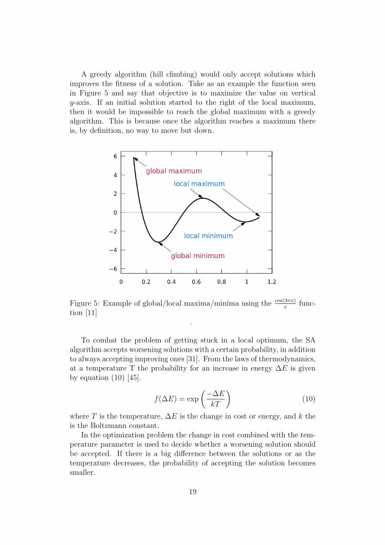
A greedy algorithm (hill climbing) would only accept solutions whichimproves the fitness of a solution. Take as an example the function seenin Figure 5 and say that objective is to maximize the value on verticaly-axis. If an initial solution started to the right of the local maximum,then it would be impossible to reach the global maximum with a greedyalgorithm. This is because once the algorithm reaches a maximum thereis, by definition, no way to move but down.

Figure 5: Example of global/local maxima/minima using the cos(3πx)x func-

tion [11].

To combat the problem of getting stuck in a local optimum, the SAalgorithm accepts worsening solutions with a certain probability, in additionto always accepting improving ones [31]. From the laws of thermodynamics,at a temperature T the probability for an increase in energy ∆E is givenby equation (10) [45].

f(∆E) = exp

�−∆E

kT

�(10)

where T is the temperature, ∆E is the change in cost or energy, and k theis the Boltzmann constant.

In the optimization problem the change in cost combined with the tem-perature parameter is used to decide whether a worsening solution shouldbe accepted. If there is a big difference between the solutions or as thetemperature decreases, the probability of accepting the solution becomessmaller.

19

3.3 Machine Learning

Machine learning (ML) is a subfield of computer science and has evolvedfrom the branch of artificial intelligence (AI). It can be defined as a set ofmethods that automatically detect patterns in data, and use the uncoveredpatterns to predict future data, or to perform other kinds of decision mak-ing under uncertainty [46]. ML is typically categorized into three differenttypes, supervised learning, unsupervised learning and reinforcement learn-ing. Classification the best translated sentences is a task mainly concernedwith supervised learning methods.

3.3.1 Supervised Learning

In supervised learning the objective is to learn a mapping from a set ofinput-output pairs, �x = �x1 . . . xk� to an output vector �y = �y1 . . . ym�. Tolearn this mapping a training set Dtrain is needed where each sample isan vector of inputs, also known as features, and its corresponding output,Dtrain = {(�xi, �yi)}Ni=1, where N is the number of samples [46]. The �y vectoris usually either categorical with each value belonging to a finite set, ∀yi ∈{1 . . . C}, or a real valued scalar, ∀yi ∈ IR. If �y is a vector of categoricalvalues then C is the number of different classes or labels, and the problemis called classification (or binary classification if C = 2). The differentlabels could be e.g. ‘cat’, ‘dog’, and ‘elk’ if the task is to classify an animal,given a set of input features. When �y is a vector of scalar values then theproblem is called regression and can be used for e.g. predicting a person’sincome or in general any function approximation.

The feature vector �x = �x1 . . . xk� represents attributes of the inputside used to predict �y. The idea is to choose features that differentiate wellbetween the different classes ∀yi ∈ {1 . . . C} when learning a mapping frominput to output. In the case of ∀yi ∈ {cat, dog, elk} then the features �x =�weight, height� could probably separate the classes pretty well. Howevergiven the weight and height of a chihuahua the algorithm could not possiblydiscern it from a cat, so additional features have to be considered. Featurescan also be more complicated such as whole images, where the featurevector consists of the intensity values of each pixel [3]. In machine learningconstructing and selecting features is key to having a good classificationperformance.

The name supervised learning comes from the fact that the groundtruth is available for every feature vector, which means that it is possibleto have a feedback loop for the learning algorithm. Since all the data points�y1 . . . �yi are known for their corresponding inputs �x1 . . . �xi, an error can bemeasured by how many were correctly predicted in the training set Dtrain.This error is used by e.g. a neural network classifier to adjust its weightswith the goal to minimize the error.

20

The error in this case is referred to as the objective function to beoptimized by a optimization method. In neural networks the most commontechnique is backpropagation where the error signal is propagated throughthe network and gradient descent is used to minimize the error function [21].

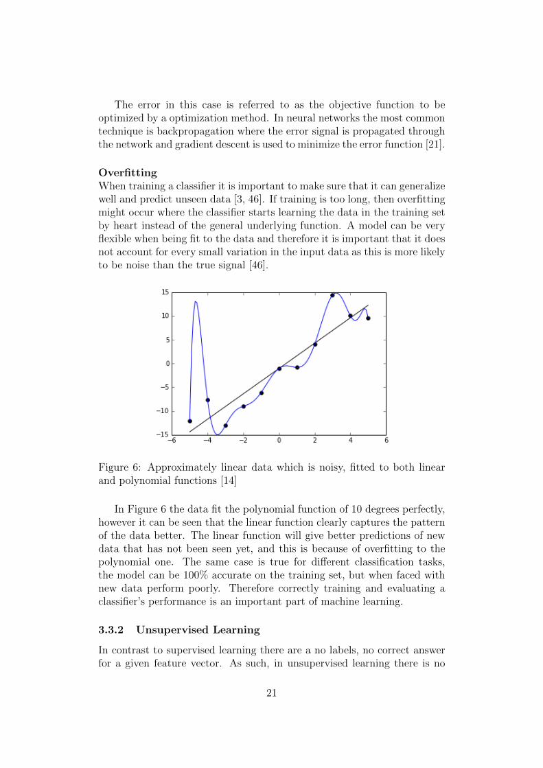
OverfittingWhen training a classifier it is important to make sure that it can generalizewell and predict unseen data [3, 46]. If training is too long, then overfittingmight occur where the classifier starts learning the data in the training setby heart instead of the general underlying function. A model can be veryflexible when being fit to the data and therefore it is important that it doesnot account for every small variation in the input data as this is more likelyto be noise than the true signal [46].

Figure 6: Approximately linear data which is noisy, fitted to both linearand polynomial functions [14]

In Figure 6 the data fit the polynomial function of 10 degrees perfectly,however it can be seen that the linear function clearly captures the patternof the data better. The linear function will give better predictions of newdata that has not been seen yet, and this is because of overfitting to thepolynomial one. The same case is true for different classification tasks,the model can be 100% accurate on the training set, but when faced withnew data perform poorly. Therefore correctly training and evaluating aclassifier’s performance is an important part of machine learning.

3.3.2 Unsupervised Learning

In contrast to supervised learning there are a no labels, no correct answerfor a given feature vector. As such, in unsupervised learning there is no

21

error or feedback signal and the problem to be solved is not as well-posedas in supervised learning. Sometimes unsupervised learning is referred toas knowledge discovery because the goal is to find patterns and features inthe data, D = {�xi}Ni=1 , without any teacher or supervision [21, 46].

Unsupervised learning can be used to group similar points of data to-gether by clustering or projecting data from high dimensional space into2 or 3 dimensions for visualization purposes [3]. It is also closely relatedto density estimation from statistics where the distribution of data withinthe input space is determined [3, 65]. An example where clustering can beuseful is recommender systems: Say that �x = �year, pages, genre� is a fea-ture vector describing books in a store. Then it is possible to use clusteringalgorithms to group similar books together, the same can be done for usersbuying books, and this information can be combined to suggest what bookcould be a good next purchase.

3.3.3 Reinforcement Learning

The reinforcement learning technique [61] is concerned with taking theoptimal action in a given state in order to maximize a reward. Contrary tosupervised learning, the learner is not given a set of optimal outputs, insteadit has to learn these by trial and error. A learning agent interacts with itsenvironment through different actions, resulting in different states [3].

An example of this would be when a neural network combined witha reinforcement learning algorithm was trained to play backgammon atmaster’s level [63], or more recently, together with deep learning to masterthe game of Go [59]. In the backgammon case the network is given theboard position and dice throw as the current state, and has to produce astrong action as output. This was done playing a copy of it self millionsof times, and only at the end of a game is a reward signal given. Thismeans that all the moves that contributed to a win must be attributedappropriately, even though not necessarily all of them were good moves.

In one game there can be a long sequence of moves and states, howeverin the end there is only one simple reward signal, win or lose. To make surethat the learning algorithm does well it has to balance the exploration andexploitation [3]. The exploration part is to make sure that even though amove is currently known to not produce the higher expected reward it ischosen anyway because it could be a better move. The exploitation partmeans that the algorithm uses its current knowledge and thereby choosesthe move that has the highest expected reward. The balance betweenexploration and exploitation is a fine line, and if there is too much focuson either the reinforcement algorithm will not yield good results.

22

3.4 Support Vector Machines

Support vector machines (SVMs) [20], originally introduced by Vapnik etal. [68, 4], are supervised learning models for binary classification and re-gression. SVMs are a popular classifier and perform well on a number ofdifferent applications, including text categorization, because they are ro-bust when dealing with noise and sparse features [25, 36].

They are both able to separate classes linearly, and non-linearly byusing a kernel trick (described in section 3.4.1). Similarly to a multilayerperceptron (a type of neural network) [21], SVMs try to separate the classesy ∈ {−1, 1} by using a hyperplane. A difference is that the SVM aims tofind the hyperplane that optimally separates the classes, by maximizingthe margin between the support vectors. The support vectors are the datapoints which are the hardest ones to classify, the ones closest to the decisionboundary.

When searching for an optimal hyperplane, only the support vectorsare the ones that influence optimality. This is in contrast to other methodssuch as linear regression and naıve Bayes where instead of only a few, allthe data points are contributing. As seen in Figure 7, the points on thedotted lines are support vectors, and only the removal of these changes howthe separating line would be placed.

Figure 7: Support vector machine where the elements on the dotted linesare the support vectors [13]

The task of find the optimal hyperplane to separate two classes is an

23

optimization problem that can be solved by using different techniques, acommon one being Lagrangian multipliers to get it to a form that can besolved analytically [6]. Given the training data Dtrain = {(xi, yi)}Ni=1 wherex ∈ IRk and that there is a hyperplane separating the negative labels fromthe positive ones.

The hyperplane’s equation is given by the equation w · x+ b = 0 where< · > represents the inner product, b the bias or offset of the plane from theorigin in the input space. The normal and its orientation to the hyperplaneis determined by the weight vector w and the vector x are the points locatedwithin the plane [8]. The perpendicular distance from the origin to thehyperplane is b

�w� where �w� is the Euclidean norm of w. Let d+ and d−

be the distances from the positive and negative classes respectively. In thecase that the classes are linearly separable then the SVM looks for the forthe hyperplane with largest margin d

+ + d−. More formally formulated,

given that all the training data satisfy the following constraints [6]:

xi · w + b ≥ +1 for yi = +1 (11)

xi · w + b ≤ −1 for yi = −1 (12)

Which can be combined into:

yi(xi · w + b)− 1 ≥ 0 ∀i (13)

The points for which equation (11) hold are located within the hyper-plane H1 = xi · w + b = 1 with a distance |1−b|

�w� perpendicular from the

origin and the normal w. Similarly, equation (12) lies within the hyper-plane H2 = xi · w + b = −1, that has a normal w and a perpendicualardistance to the origin |−1−b|

�w� . The total length of the margins d+ = d− = 1

�w�between the support vectors and the dividing hyperplane can then be sum-marized as: d

+ + d− = 2

�w� . Given the constraints in equation (13) whichsays there can be no data points between H1 and H2, it is possible to findthe hyperplanes H1, H2 which maximizes the margin, by minimizing �w�2.In Figure 7 the expected result of the SVM algorithm is shown for the2-dimensional case [6].

The task of minimizing �w� can be formulated using Lagrangian mul-tipliers and then solved by using quadratic programming [24]. Introducingthe Lagrangian variables α1 . . .αN , the Lagrangian formulation of the SVMproblem, also known as the primal problem[6], becomes:

LP =1

2�w�2 −

N�

i=1

αiyi(xi · w + b) +N�

i=1

αi

αi ≥ 0∀i(14)

24

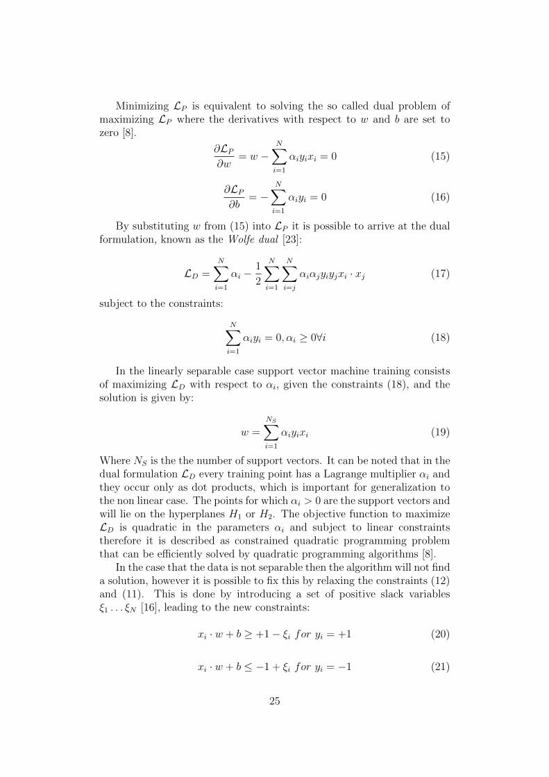
Minimizing LP is equivalent to solving the so called dual problem ofmaximizing LP where the derivatives with respect to w and b are set tozero [8].

∂LP

∂w= w −

N�

i=1

αiyixi = 0 (15)

∂LP

∂b= −

N�

i=1

αiyi = 0 (16)

By substituting w from (15) into LP it is possible to arrive at the dualformulation, known as the Wolfe dual [23]:

LD =N�

i=1

αi −1

2

N�

i=1

N�

i=j

αiαjyiyjxi · xj (17)

subject to the constraints:

N�

i=1

αiyi = 0,αi ≥ 0∀i (18)

In the linearly separable case support vector machine training consistsof maximizing LD with respect to αi, given the constraints (18), and thesolution is given by:

w =NS�

i=1

αiyixi (19)

Where NS is the the number of support vectors. It can be noted that in thedual formulation LD every training point has a Lagrange multiplier αi andthey occur only as dot products, which is important for generalization tothe non linear case. The points for which αi > 0 are the support vectors andwill lie on the hyperplanes H1 or H2. The objective function to maximizeLD is quadratic in the parameters αi and subject to linear constraintstherefore it is described as constrained quadratic programming problemthat can be efficiently solved by quadratic programming algorithms [8].

In the case that the data is not separable then the algorithm will not finda solution, however it is possible to fix this by relaxing the constraints (12)and (11). This is done by introducing a set of positive slack variablesξ1 . . . ξN [16], leading to the new constraints:

xi · w + b ≥ +1− ξi for yi = +1 (20)

xi · w + b ≤ −1 + ξi for yi = −1 (21)

25

ξi ≥ 0∀i (22)

Including the sum of the errors in the objective function, which in thelinearly separable cases consisted of minimizing 1

2�w�2, it can be formulated

as [6, 62]:

1

2�w�2 + C(

N�

i

ξi)k (23)

where C is a parameter that the user has to decide and tune for optimalperformance. To ensure that condition (22) is fulfilled, additional Lagrangemultipliers has to be introduced, however this can be avoided by choosingk = 1. By doing this neither ξi or its multipliers will show up in theWolfe dual problem, and it will become a quadratic programming problemin addition to being a convex one, which is easier to solve [6]. The dualoptimization problem to be maximized, similarly to before, becomes:

LD =N�

i=1

αi −1

2

N�

i=1

N�

i=j

αiαjyiyjxi · xj (24)

subject to:N�

i=1

αiyi = 0 (25)

0 ≤ αi ≤ C ∀i (26)

3.4.1 Kernel Trick

In the case that the classes y ∈ {−1, 1} are not linearly separable then itpossible to use a ‘kernel trick’ to map the input space I ∈ IRd into a, usuallyhigher dimensional, feature space F where a hyperplan can separate theclasses. This is an old trick [2] and Boser et al. [4] showed that this couldbe applied to SVMs in a rather simple way. Figure 8 shows an examplewhere the datapoints in the 2D input space are not linearly separable, butwhen mapped into a 3D space by some function ϕ : I → F they can beseparated by a hyperplane.

26

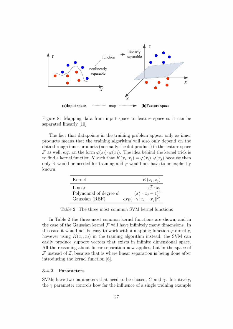
Figure 8: Mapping data from input space to feature space so it can beseparated linearly [10]

The fact that datapoints in the training problem appear only as innerproducts means that the training algorithm will also only depend on thedata through inner products (normally the dot product) in the feature spaceF as well, e.g. on the form ϕ(xi) ·ϕ(xj). The idea behind the kernel trick isto find a kernel function K such that K(xi, xj) = ϕ(xi) ·ϕ(xj) because thenonly K would be needed for training and ϕ would not have to be explicitlyknown.

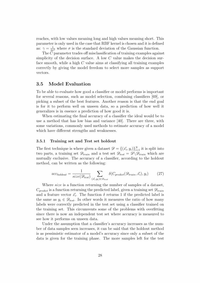
Kernel K(xi, xj)

Linear xTi · xj

Polynomial of degree d (xTi · xj + 1)d

Gaussian (RBF) exp(−γ�xi − xj�2)

Table 2: The three most common SVM kernel functions

In Table 2 the three most common kernel functions are shown, and inthe case of the Gaussian kernel F will have infinitely many dimensions. Inthis case it would not be easy to work with a mapping function ϕ directly,however using K(xi, xj) in the training algorithm instead, the SVM caneasily produce support vectors that exists in infinite dimensional space.All the reasoning about linear separation now applies, but in the space ofF instead of I, because that is where linear separation is being done afterintroducing the kernel function [6].

3.4.2 Parameters

SVMs have two parameters that need to be chosen, C and γ. Intuitively,the γ parameter controls how far the influence of a single training example

27

reaches, with low values meaning long and high values meaning short. Thisparameter is only used in the case that RBF kernel is chosen and it is definedas: γ = 1

2σ2 where σ is the standard deviation of the Gaussian function.The C parameter trades offmisclassification of training examples against

simplicity of the decision surface. A low C value makes the decision sur-face smooth, while a high C value aims at classifying all training examplescorrectly by giving the model freedom to select more samples as supportvectors.

3.5 Model Evaluation

To be able to evaluate how good a classifier or model performs is importantfor several reasons, such as model selection, combining classifiers [69], orpicking a subset of the best features. Another reason is that the end goalis for it to perform well on unseen data, so a prediction of how well itgeneralizes is in essence a prediction of how good it is.

When estimating the final accuracy of a classifier the ideal would be touse a method that has low bias and variance [40]. There are three, withsome variations, commonly used methods to estimate accuracy of a modelwhich have different strengths and weaknesses.

3.5.1 Training set and Test set holdout

The first technique is where given a dataset D = {(�xi, yi)}Ni=1 it is split intotwo parts, a training set Dtrain and a test set Dtest = D\Dtrain which aremutually exclusive. The accuracy of a classifier, according to the holdoutmethod, can be written as the following:

accholdout =1

size(Dtest)

�

(�xi,yi)∈Dtest

δ(Cpredict(Dtrain, �xi), yi) (27)

Where size is a function returning the number of samples of a dataset,Cpredict is a function returning the predicted label, given a training set Dtrain

and a feature vector �xi. The function δ returns 1 if the predicted label isthe same as yi ∈ Dtest. In other words it measures the ratio of how manylabels were correctly predicted in the test set using a classifier trained onthe training set. This circumvents some of the problems with overfittingsince there is now an independent test set where accuracy is measured tosee how it performs on unseen data.

Under the assumption that a classifier’s accuracy increases as the num-ber of data samples seen increases, it can be said that the holdout methodis as pessimistic estimator of a model’s accuracy since only a subset of thedata is given for the training phase. The more samples left for the test

28

partition, the more biased estimation, and if fewer test instances are keptthen the confidence interval for the accuracy will be wider [40].

When the data set D is divided into a training set and a test set thesplit, for example 2

3 training and 13 test, will be randomly chosen, and

the holdout estimation will depend on this division. It’s possible to userandom subsampling where the processes is repeated k times for k differenttrainingtest splits. The mean accuracy and standard deviation can then becalculated from the results of the iterations. However this violates the basicassumption that the instances in the training and test set are independentfrom each other [40].

Finally, in many cases gathering and labeling good quality data canbe both time consuming and expensive, thefore it is important to utilizethe data as well as possible. The holdout method is inefficient in this waybecause a subset of the data is not used to train the classifier.

3.5.2 Cross-validation

In this method the data D = {(�xi, yi)}Ni=1 is partitioned into k complement-ary subsets D1 . . .Dk, also known as the k folds of k-fold cross-validation.The subsets are of approximately equal in size and the classifier is trainedand tested using every fold. The training set is given by D\Dt wheret ∈ {1 . . . k} such that every subset acts as the test set Dt once and then asa part of the training set for the remaining k− 1 folds [40]. The estimatedaccuracy of the model can be expressed similarly as the holdout method(equation 27), as follows:

acccv =1

N

�

(�xi,yi)∈D

δ(Cpredict(D\Di, �xi), yi) (28)

The choice of how the folds are split is decided by a random number,and repeating the cross-validation multiple times and averaging the resultsprovides a better Monte-Carlo estimate to a complete cross-validation [40].A complete one would need to run through all the possible splits

�N

N/k

�,

choosing Nk samples from all N, which is usually computationally too costly

to calculate. It is also possible to do a leave-one-out cross-validation whichis always complete.

In stratified k-fold cross-validation the subsets are partitioned in such asway that they preserve the same class proportions as the original completedataset. In a study, Kohavi et al. recommended the 10-fold stratifiedcross-valdidation scheme as a good way to estimate accuracy and select amodel [40].

29

3.5.3 Bootstrap Sampling

From statistics, bootstrap sampling is a method which relies on randomsampling with replacement, meaning that an element may occur multipletimes in a sample. Given the dataset DN , where N is the number ofsamples, a bootstrap sample can be created by sampling uniformly N timesfrom the dataset. Because of the fact that it is sampled with replacement,the chance of an element not being chosen after N samples is: (1− 1

N )N =e−1 = 0.368 as N → ∞ therefore the expected number of unique elementspresent in the test set from the original dataset will be 0.632 ·N [40].

To estimate the accuracy � of a bootstrap sample the 0.632N uniqueelements from the original dataset, together with the replacement samples,are used as the training set whilst the 0.368 remaining elements are usedas a test set. The 0.632 bootstrap estimate for a set of bootstrap samplesb can be expressed as:

accboot =1

b

s�

i=1

(0.632 · �i + 0.368 · acctrain) (29)

where �i is the estimated accuracy for a bootstrap sample bi, and acctrain

is the accuracy on the training set, alternatively the re-substitution ac-curacy on the complete dataset D . The variance of the estimate can becomputed by calculating it for the estimate of every sample [40].

4 Method

It is explained how the algorithms and methods were applied to differentparts of the hybrid machine translation system, including data labeling,feature extraction, feature selection and model selection.

4.1 DataSet

The dataset was collected by processing various course syllabi from Stock-holm University. Only course syllabi with a corresponding English transla-tion were considered. The Swedish source texts and their translations weremanually inspected and were deemed to have good quality. The Swedishtext was considered as the source and the translation its reference. Thesource text was sent as input to the RBMT and SMT systems, and theiroutput corresponded to the translated text from each system. There wasalso a log file available that allowed for counting how many unknown wordsthere were, meaning Swedish words for which no translation was found.

In total there were 731 sentences in the complete document with equallymany sentences in the reference and the two translations. The sentences

30

were given in a tokenized lower case format as this was required to evaluatethem according to BLEU score.

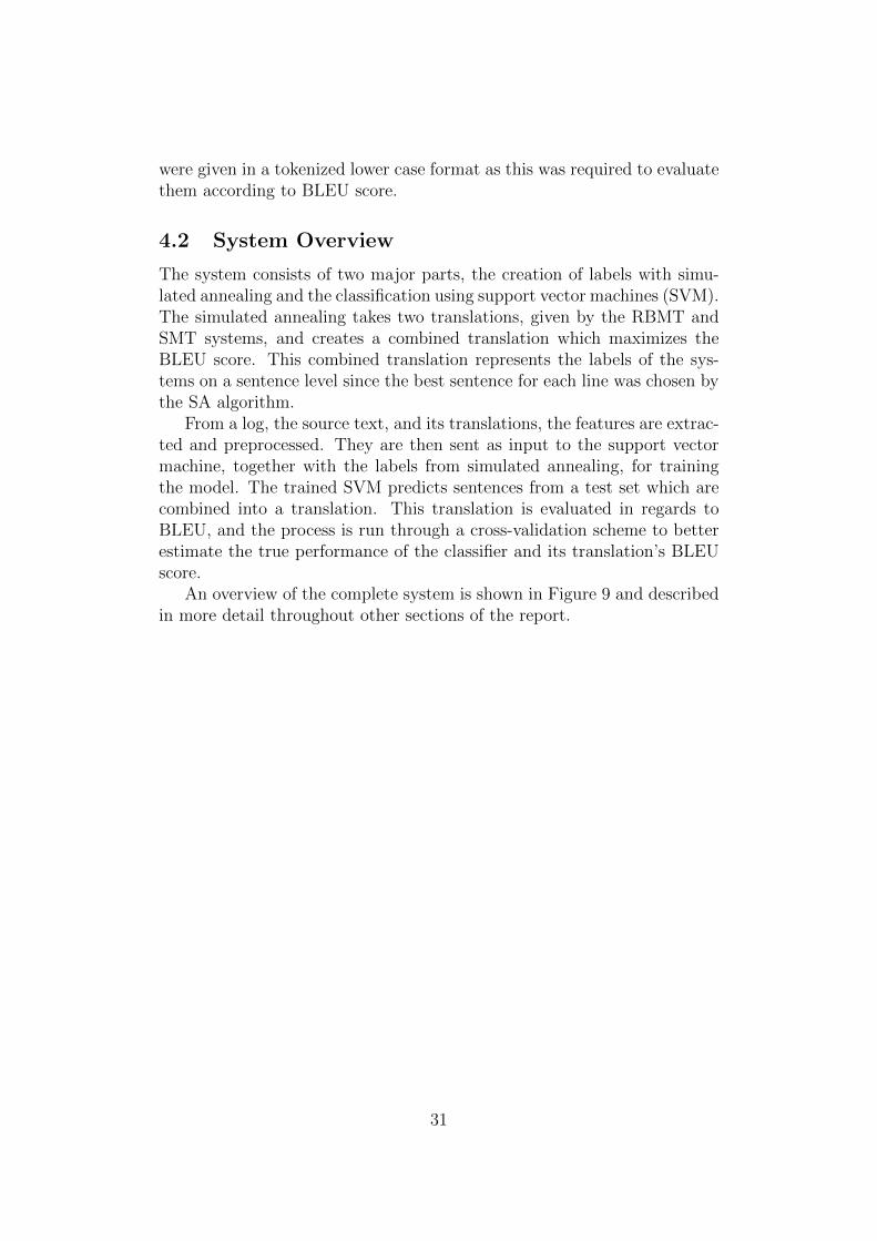
4.2 System Overview

The system consists of two major parts, the creation of labels with simu-lated annealing and the classification using support vector machines (SVM).The simulated annealing takes two translations, given by the RBMT andSMT systems, and creates a combined translation which maximizes theBLEU score. This combined translation represents the labels of the sys-tems on a sentence level since the best sentence for each line was chosen bythe SA algorithm.

From a log, the source text, and its translations, the features are extrac-ted and preprocessed. They are then sent as input to the support vectormachine, together with the labels from simulated annealing, for trainingthe model. The trained SVM predicts sentences from a test set which arecombined into a translation. This translation is evaluated in regards toBLEU, and the process is run through a cross-validation scheme to betterestimate the true performance of the classifier and its translation’s BLEUscore.

An overview of the complete system is shown in Figure 9 and describedin more detail throughout other sections of the report.

31

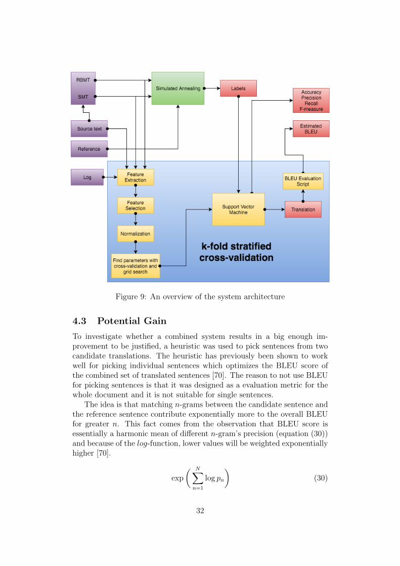
Figure 9: An overview of the system architecture

4.3 Potential Gain

To investigate whether a combined system results in a big enough im-provement to be justified, a heuristic was used to pick sentences from twocandidate translations. The heuristic has previously been shown to workwell for picking individual sentences which optimizes the BLEU score ofthe combined set of translated sentences [70]. The reason to not use BLEUfor picking sentences is that it was designed as a evaluation metric for thewhole document and it is not suitable for single sentences.

The idea is that matching n-grams between the candidate sentence andthe reference sentence contribute exponentially more to the overall BLEUfor greater n. This fact comes from the observation that BLEU score isessentially a harmonic mean of different n-gram’s precision (equation (30))and because of the log-function, lower values will be weighted exponentiallyhigher [70].

exp

� N�

n=1

log pn

�(30)

32

A n-gram will always be less frequent than a n− 1-gram by definition,e.g. a trigram match will have 2 bigram and 3 unigram matches as itssubset, and therefore have lower precision.

The heuristic picks the sentences from the candidate translations whichhave the highest n-values, of the n-gram matches with the reference sen-tences. As this can result result in two sentences having the same matchingresults, the method was tested with three different fall back cases whenthere was an equal match. The fall back was done by randomly keepingone of the sentences, choosing the RMBT system, or choosing the SMT sys-tem. All of them performed very similarly with SMT being slightly betterto keep as a fallback.

4.3.1 Local Search

Finding the best possible combined translation is important since it is usedas the gold standard when training the classifier. By using the the reference,RBMT and SMT translations, then the labels of which sentences belong inthe combined translation is only as good as the heuristic, and it might notcapture the best possible BLEU score. To see if it is possible to find an evenbetter translation than the heuristic one, the problem can be reformulatedso that a local search algorithm can be applied.

The choice of k sentences from two systems can be seen as combinatorialoptimization problem where there are 2k possible translations and BLEUis the objective function to be maximized. Finding the optimal translationby exhaustive search is unfeasible due to the exponential growth of possibletranslations as the number of sentences k increases.

A common approach to intractable optimization problems is to use localsearch algorithms [31], such as simulated annealing [37]. Before the al-gorithm can be applied to find a solution to the translation problem, a fewfunctions and parameters has to be defined:

• Initialization

• Neighborhood function

• Cost function

• Acceptance probability function

• Annealing schedule

– Start temperature

– Stopping condition

– Number of iterations at each temperature

33

– Temperature reduction factor

Since the search is local and that it is not guaranteed to find the optimalsolution (in practice), it can be relevant where the search starts. It isprobably more important for e.g. a greedy hill climb algorithm to have agood starting solution than simulated annealing because it is easier for it toget stuck in a local minimum. To see how different initialization performed,three possible starting translations were considered.

The first one was to use random selection, meaning that for every sen-tence from both the RBMT and SMT systems were picked with a 0.5 prob-ability. The second initialization was to pick all the sentences from thesystem that had the best translation. Finally the translation that wasfound through the n-gram heuristic matching was considered as a start-ing solution. As can be seen in Table 5 in the results section on page 48,starting off with the heuristic translation leads to a better final solution,although very minor. From the results it can be concluded that, in thiscase, it was not very important to pick a good initial starting solution.

The neighborhood of the current solution can be defined in differentways but it falls naturally to define it as all the solutions created by swap-ping different sentences. A sentence has been translated by either theRBMT system or the SMT one, therefore there are 2k possible swaps, orcandidate solutions. An alternative definition was was also investigated,where n different sentences’ translations, instead of one, were swapped forthe other system’s translation. The best method was to swap one or twosentences, which could be because swapping only a few sentences can tweakthe final solutions better. However swapping multiple sentences could bemore beneficial for larger datasets since it can explore the search spacefaster with the backside of possibly missing good solutions.

The cost function that should be optimized is defined as the BLEUscore over the whole document. After a candidate solution is chosen itis evaluated according to the cost function. If the score of the candidatesolution is greater than the current solution then it is accepted as the newsolution and the process repeats. If the score is worse then there is a chancethat it will be accepted as the new solution according to the acceptanceprobability function(10). This function is generally the same for differentproblems because it depends on the relative change between the currentsolution and the candidate solutions, as well as the temperature.

The starting temperature T0 is important - if too small, and the al-gorithm is not allowed to explore enough, if too big it becomes a ran-dom walk. The choice of T0 was done, as suggested by Kirkpatrick etal. [37], by taking the maximal cost between any two neighboring solutionsT0 = ∆Scoremax. However there is large amount of neighbors, thereforea subset of 100 were sampled and ∆Scoremax was calculated using thesesolutions. Another method to choose T0 would be to find a temperature

34

where the probability of accepting a solution equals to some predeterminednumber χ.

The temperature reduction can be done in many different ways [50]where three well known ones are:

• Linear, Tt = T0 − η · tFor η close to 0.

• Geometric, Tt = T0 · αt

Where values 0.8 ≤ α ≤ 0.99 are commonly used.

• Logarithmic, Tt =C

log(t+d)Normally where d = 1 and C is a constant.

The geometric cooling schedule was chosen and different values of αwere investigated, as shown in Table 5 and 6 in the results section onpage 48, to see which gave the best performance. The cooling parameteris connected to how many iterations k are being run at each temperature.If the cooling is fast and few temperatures are being used then it is betterto iterate longer at each one, and vice versa for the opposite case. In ageometric cooling schedule the cooling is not that fast, especially with α

close to 1, so not as many iterations at each temperature is needed.It could also be the case that it is more important to iterate longer on

lower temperatures, and that this parameter k would dynamically changeas T changed. There could alternatively be a criteria set on how manytransitions (accepted solutions) are needed at each temperature. In theend a constant value of 100 iterations at each temperature was chosen,through trial and error, as it gave good results and was not a hindrance tothe running time.

Finally the stopping criterion had to be decided, as with the otherparameters there are many different ways to choose it. The minimum tem-perature can be set together with α and k so that a set number of solutionsare generated or a number of set temperatures are used. Another method isto stop when there is no improvement, combined with the acceptance ratiofalling below a certain threshold χ. The stopping temperature was chosenby simulating the process for different values, together with different valuesfor α, to see which ones worked best, results are presented in Table 5 and 6in the results section on page 48.

The algorithm was implemented in python and the code can be seen inlisting 1, with some minor changes to make it more readable.

35

1 de f anneal ( rbmt , smt , r e f e r e n c e ) :2 # I n i t i a l i z e3 combined = i n i t ( rbmt , smt )4

5 # Evaluate the cur rent s o l u t i o n6 o l d s c o r e = eva luate ( r e f e r en c e , combined )7

8 T = getTZero ( rbmt , smt , r e f e r enc e , combined )9 T min = 0.0001

10 alpha = 0.9511

12 whi le T > T min :13 i = 014 whi le i < 100 :15 # Generate a candidate s o l u t i o n16 new so lut i on = neighbor ( rbmt , smt , combined )17 # Evaluate the candidate s o l u t i o n18 new score = eva luate ( r e f e r enc e , new so lut i on )19 # Probab i l i t y o f accept ing the new s o l u t i o n20 a = ac c ep t an c e p r obab i l i t y ( o l d s c o r e , new score , T)21 i f a > random ( ) :22 # Update s co r e and s o l u t i o n23 combined = new so lut i on24 o l d s c o r e = new score25 i += 126 # Decrease temperature27 T ∗= alpha

Listing 1: General python code for Simulated Annealing

4.4 Feature Extraction

Feature extraction is an important part of machine learning where the rawdata, in this case, text in the form of sentences, is transformed into valuesthat describe it. These features of the data can be picked in many differentways and it is usually hard to find the perfect way. The goal is to findfeatures that help to discriminate between the classes as much as possible,making it easier for the classifier to separate them. The features chosento determine the best sentence from the two MT systems were determinedfrom being used before or inspired by similar features [70, 15, 58, 22, 26].The features are each shortly defined in the following sections.

4.4.1 Basic

The basic features {f1 . . . f5} are simple to extract and understand, yetwork very well in improving classification.

1. Sentence length

36

2. Average token length

3. Difference in sentence length, compared to the source text

4. Difference in average token length, compared to the source text

5. Number of unknown words in the dictionary for SMT

The first feature f1 is the sentence length and it is counted in tokens, notcharacters. This feature is applied to every text, the source, as well as theRBMT and SMT translations. The second feature f2 is counted as howmany characters there are in every token divided by the number of tokensin that sentence. This feature is also applied to all the three texts.

Third and fourth features f3,f4 are already implied as the average tokenlength and sentence length are known through features f1 and f2. Howeversometimes a classifier can benefit from implicit information being statedas it does not have to learn it, especially in the case of less training data.These features are, as given by their definition, applied only to the RBMTand SMT translated sentences.

The last of the basic features f5 is extracted from the log files created bythe SMT system. Knowing the number of words that could not be trans-lated by the SMT system results in a good indication whether it succeed increating a good translation or not, and if not possibly picking RBMT one in-stead. In total the basic features consists of f1·3+f23+f3·2+f4·2+f5·1 = 11features.

4.4.2 Dependency Parsing

The next set of features are extracted by using a dependency parser, theparsed output is given in the form of universal grammatical relations, alsoknown as universal dependencies3. The different categories of dependenciesbetween words can be seen in Table 3, and the feature vector is created asthe frequency of each type.

These are extracted by reading the parsed files into a data structurecalled a DependencyGraph from the python NLTK (described in section 4.7).The DependecyGraph object makes it easy to get triplets, that is, two wordsand the dependency relations between them, as such the dependency typesare counted by iterating through all the triplets in the graph. Since thereare many different dependency relation types, this results in a sparse featurevector.

The dependency graph is an acyclic directed graph, in other words it isa tree, and the last feature in this category was chosen as the height of thetree. All of the the features described were extracted from both the sourcetext its two translations.

3http://universaldependencies.org/

37

acl clausal modifier of noun (adjectival clause)advcl adverbial clause modifieradvmod adverbial modifieramod adjectival modifierappos appositional modifieraux auxiliaryauxpass passive auxiliarycase case markingcc coordinating conjunctionccomp clausal complementcompound compoundconj conjunctcop copulacsubj clausal subjectcsubjpass clausal passive subjectdep unspecified dependencydet determinerdiscourse discourse elementdislocated dislocated elementsdobj direct objectexpl expletiveforeign foreign wordsgoeswith goes withiobj indirect objectlist listmark markermwe multi-word expressionname nameneg negation modifiernmod nominal modifiernsubj nominal subjectnsubjpass passive nominal subjectnummod numeric modifierparataxis parataxispunct punctuationremnant remnant in ellipsisreparandum overridden disfluencyroot rootvocative vocativexcomp open clausal complement

Table 3: Universal dependency relations

38

4.4.3 Part of Speech

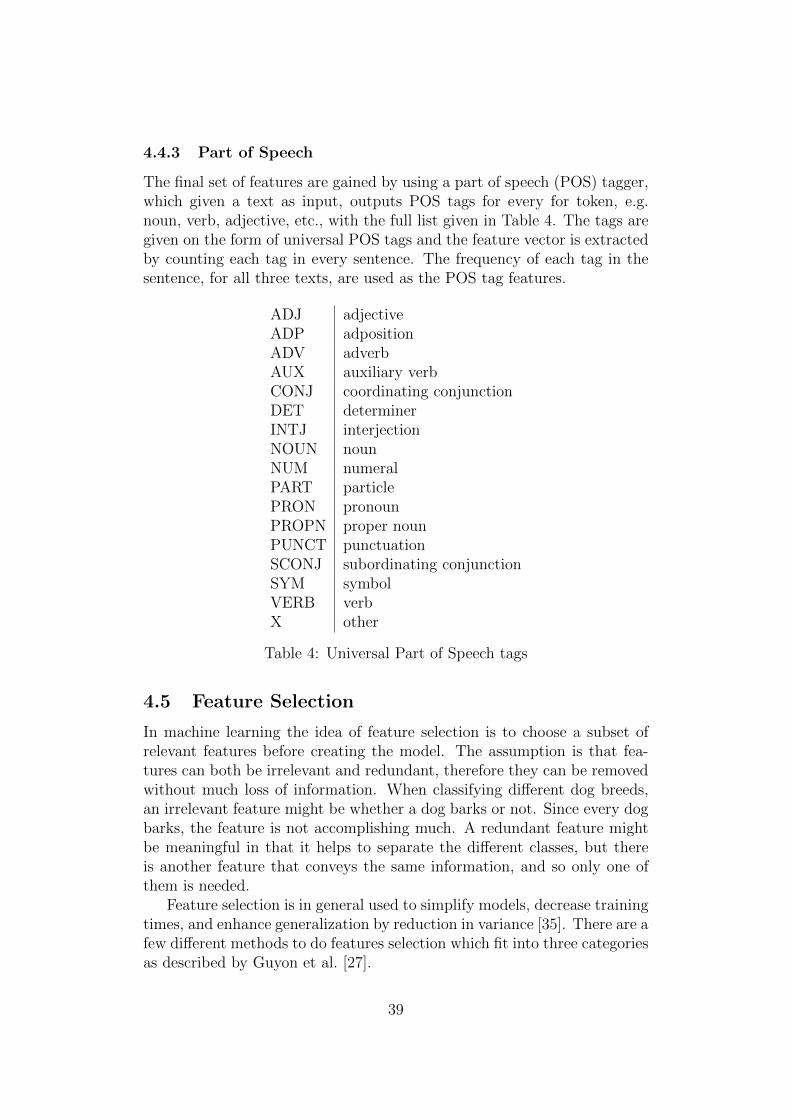
The final set of features are gained by using a part of speech (POS) tagger,which given a text as input, outputs POS tags for every for token, e.g.noun, verb, adjective, etc., with the full list given in Table 4. The tags aregiven on the form of universal POS tags and the feature vector is extractedby counting each tag in every sentence. The frequency of each tag in thesentence, for all three texts, are used as the POS tag features.

ADJ adjectiveADP adpositionADV adverbAUX auxiliary verbCONJ coordinating conjunctionDET determinerINTJ interjectionNOUN nounNUM numeralPART particlePRON pronounPROPN proper nounPUNCT punctuationSCONJ subordinating conjunctionSYM symbolVERB verbX other

Table 4: Universal Part of Speech tags

4.5 Feature Selection

In machine learning the idea of feature selection is to choose a subset ofrelevant features before creating the model. The assumption is that fea-tures can both be irrelevant and redundant, therefore they can be removedwithout much loss of information. When classifying different dog breeds,an irrelevant feature might be whether a dog barks or not. Since every dogbarks, the feature is not accomplishing much. A redundant feature mightbe meaningful in that it helps to separate the different classes, but thereis another feature that conveys the same information, and so only one ofthem is needed.

Feature selection is in general used to simplify models, decrease trainingtimes, and enhance generalization by reduction in variance [35]. There are afew different methods to do features selection which fit into three categoriesas described by Guyon et al. [27].

39

Filter MethodsThe filter methods apply a statistical measure, e.g. a χ

2 test, and usesthis to rank the features. The methods are usually univariate, meaningthat they consider the features independently with regard to the dependentvariable. The features are chosen according to some threshold, e.g. keepthe top k ranked features.

Wrapper MethodsWrapper methods approach feature selection as combinatorial optimizationproblem, where the goal is the find the subset of features that minimizes theclassifier’s error. An example of an algorithm would be recursive featureelimination, but any local search algorithm, such greedy hill climb, best fitfirst, simulated annealing, etc. can be used to find the optimal subset offeatures.

Embedded MethodsThe final methods learn the features which contribute the most to themodel’s accuracy, while the model is being created. Most common modelsare regularization ones such as LASSO, Ridge regression and SVMs. Thesemodels introduce additional regularization or penalization variables as con-straints to the optimization problem of the classification algorithm, whichgives the model a bias towards lower complexity.

The embedded method was chosen because it is easy to use and workswell with support vector machines, which were also used to perform themain classification. The features are in this case assigned weights fromthe coefficients of the SVM’s primal problem LP , shown in equation (14)which is described in the SVM section on page 24, and they can be used tochoose which features to keep or to throw away according to a threshold.This threshold can be calculated through the median or mean values, al-ternatively it can be picked manually. This was done with a linear SVMusing C = 0.01 and a penalty (see section 5), the parameters were chosenby trial and error.

4.6 Model

The final model is not set in stone as k-fold cross-validation was used toestimate its performance, which means that for every fold in the cross-validation, new parameters has to be chosen. The SVM has two mainparameters, the kernel and C, with an additional one γ, if a RBF kernelis used. One way would be to choose constant values, say a linear kernelwith C = 1, and then use that when training the SVM for every fold.This is bad since there is no good indication what parameters are good

40

for a particular dataset, and choosing at random will likely end with asuboptimal performance.

Instead there is a technique to more intelligently pick which paramet-ers to use, and that is by using a combination of cross-validation and gridsearch. The search is an exhaustive search of all the parameters and thebest ones are chosen by their cross-validation score. Deciding what values toconsider in the search is not obvious but a exponentially growing sequencehas previously been shown to work well at estimating the parameters [32].Given this fact, two kernels and values were chosen by following this reas-oning:

Linear kernel:C ∈ {1, 10, 100, 1000}

RBF kernel:C ∈ {1, 10, 100, 1000}γ ∈ {0.001, 0.0001}

In this case a 5-fold cross-validation will run with a Linear kernel forall the C values, followed by a RBF kernel with all values from the crossproduct of C and γ. Then the set of parameters with highest estimatedperformance (by cross-validation) will be picked, and used to train the finalmodel.

4.7 Tools

PythonPython [67] was chosen as the main programming language because offamiliarity and the fact that there are many libraries available, which makeshandling data and machine learning much easier. More specifically, the onesused were:

• Numpy

• Pandas

• Scikit learn

• NLTK

Numpy [66] adds support for big n-dimensional matrices and arrays,together with a large library of high-level mathematical functions whichcan be used in conjunction with such arrays and matrices. Pandas [44] islibrary that is used primarily for data manipulation and analysis, and it ishighly optimized for performance.

41

Sci-kit [54] learn is a library built upon scientific python (SciPy) andprovides various different clustering, regression and classification algorithms.It also supports many other techniques used together with machine learn-ing, such as cross-validations, feature selection, dimensionality reduction,parameter tuning etc. Finally NLTK, short for Natural Language Toolkit,is a gathering of libraries and programs that are used to do natural languageprocessing.

Stanford Core NLPThe Standford core NLP [42] is suit a of natural language analysis tools,where it was mainly the part-of-speech (PoS) tagger and dependency parserthat were used. The PoS tagger is a Java implementation of the log-linearone describe by Kristina Toutanova et al. [64], and it reads text as inputand assigns parts of speech (e.g. noun, verb, etc.) to each word.

The parser uses a transition based dependency parsing and is poweredby a neural network [9], it produces typed dependency parses of naturallanguage sentences. It supports English with universal dependencies whichis the type used in the feature extraction step.

Multi-BLEU perl scriptThe statistical machine translation system called Moses [39] provides, assupport software, a script called ‘multi-bleu.perl’ 4. It is a perl script forevaluation of a translation given one or multiple reference translations, withoutput as BLEU score.

efselab Swedish pipelineefselab Swedish pipeline a Swedish annotation pipeline which was createdat Uppsala University by Filip Salomonsson, it supports the following (asstated on their git repository5):

• Tokenization (using a Python tokenizer by Filip Salomonsson)

• POS tagging (using efselab with a SUC + SIC model)

• Conversion to Universal PoS tags (using efselab trained on Universal

• Dependencies data plus some postprocessing heuristics by Aaron Smith)

• Lemmatization (using the lexicon-based lemmatizer in lemmatize.pyx)

• Named Entity Recognition (using efselab with a SUC + SIC model)

• Dependency prasing (using MaltParser by Joakim Nivre et al. [49])4https://github.com/moses-smt/mosesdecoder/blob/master/scripts/generic/multi-

bleu.perl5https://github.com/robertostling/efselab

42

5 Results

Simulations were run for the two major parts of the project, simulatedannealing and SVM classification, and the results are summarized in tablesshowing which models performed the best.

5.1 Experimental Setup

The experiments were run under OS X Yosemite Version 10.10.5 (64 bit)on an Intel Core i7 950 of 1.7 GHz with a 256Kb L2 cache per core, 4Mb L3cache and 8 GB RAM. They consisted of two major parts where the firstwas to create optimal labels for the data by using a reference translationand simulated annealing. The algorithm has a few different parametersthat are possible to tweak, and they are also problem dependent. Thismeans that there is no out of the box set of parameters that is good forevery problem, instead it has to be discovered by educated guesses andexperimentation.

The second part consists of extracting features and using a SVM toclassify which sentences, from the two machine translation systems, makeup the best solution. There are parameters during the preprocessing stepsuch as normalization and feature selection that can be chosen in differentways, which in turn affect the result. The method to evaluate the classifier,as well as the kernel and parameters for the SVM can heavily influence thefinal performance, therefore these factors were also taken into considerationwhen performing the experiments.

The dataset, described in section 4.1, and the tools described in sec-tion 4.7 were used in the various simulations.

5.2 Simulated Annealing

Using different parameters for SA is something that can noticeably changethe result and any improvement that can be gained is very important sincethe algorithm is used to generate a gold standard. The classifier can onlybe as good as its labeled data, so any gain in the creation of the trainingdata is propagated to the classification step.

The parameters that were investigated are shown at the top of Table 5and 6. The reason not to run for more values is that every simulation takestime and because the parameters are run as combinations of each other,resulting in an exponential time increase when adding extra ones. Thedifferent variables were chosen in such a way that were believed to impactthe results the most, e.g. the α parameter was considered more impactfulthan the number of iterations k at each temperature level.

Initial guesses of the values such as α were decided by reading literature,

43

whilst the designed neighborhood function was specific to the problem andtherefore was constructed in such way that some insight could be gained,whether a higher or lower number of sentences swapped was better. Thestarting temperature was calculated as the difference between the best andworst neighboring solutions, to the initial solution. However because theneighborhood is very large, 100 random samples were taken, and the start-ing temperature was calculated using these instead.

The results from the simulations can be seen in Table 5 and 6, resultsover 36.10 BLEU score are marked in bold text for clarity. In Table 6,the 4-swap of sentences is no longer considered since it consistently per-formed worse for all instances, as seen in Table 5. It can be noted that thetype of initialization had very little impact on the final result, instead theparameters T-min and α clearly improved the result if chosen correctly.

The best instance in Table 6, marked in green, reaches a BLEU score of36.14 which compared to the n-gram heuristic score of 35.51 is a significantimprovement of 0.63 BLEU. This confirms that simulated annealing is aviable method for creating a labeled set for the combination of machinetranslation systems, given a set of translations and a reference.

44

T-start T-min Initialization α k Neighbors BLEU

20 0.01 Random 0.8 100 1 35.9119 0.01 Random 0.8 100 2 36.0230 0.01 Random 0.8 100 4 35.8413 0.01 Random 0.9 100 1 36.1019 0.01 Random 0.9 100 2 36.0827 0.01 Random 0.9 100 4 35.9816 0.01 Random 0.95 100 1 36.1226 0.01 Random 0.95 100 2 36.1121 0.01 Random 0.95 100 4 36.1014 0.01 n-gram 0.8 100 1 35.8619 0.01 n-gram 0.8 100 2 35.9320 0.01 n-gram 0.8 100 4 35.8914 0.01 n-gram 0.9 100 1 36.1021 0.01 n-gram 0.9 100 2 36.0923 0.01 n-gram 0.9 100 4 36.019 0.01 n-gram 0.95 100 1 36.119 0.01 n-gram 0.95 100 2 36.1023 0.01 n-gram 0.95 100 4 36.0716 0.01 SMT 0.8 100 1 36.0917 0.01 SMT 0.8 100 2 35.9626 0.01 SMT 0.8 100 4 35.8313 0.01 SMT 0.9 100 1 36.0820 0.01 SMT 0.9 100 2 36.0620 0.01 SMT 0.9 100 4 35.9920 0.01 SMT 0.95 100 1 36.1017 0.01 SMT 0.95 100 2 36.1128 0.01 SMT 0.95 100 4 36.07

Table 5: BLEU score for different parameter combinations

45

T-start T-min Initialization α k Neighbors BLEU

15 0.0001 Random 0.8 100 1 36.1024 0.0001 Random 0.8 100 2 36.0823 0.0001 Random 0.9 100 1 36.1217 0.0001 Random 0.9 100 2 36.1112 0.0001 Random 0.95 100 1 36.1320 0.0001 Random 0.95 100 2 36.1312 0.0001 n-gram 0.8 100 1 36.0717 0.0001 n-gram 0.8 100 2 36.0513 0.0001 n-gram 0.9 100 1 36.1117 0.0001 n-gram 0.9 100 2 36.1216 0.0001 n-gram 0.95 100 1 36.1216 0.0001 n-gram 0.95 100 2 36.1415 0.0001 SMT 0.8 100 1 36.1117 0.0001 SMT 0.8 100 2 36.0919 0.0001 SMT 0.9 100 1 36.1317 0.0001 SMT 0.9 100 2 36.1216 0.0001 SMT 0.95 100 1 36.1317 0.0001 SMT 0.95 100 2 36.12

Table 6: BLEU score for different parameter combinations

5.3 Support Vector Machine

Training and estimating the performance of the support vector machineinvolves a few different parameters which can influence the performance.The first concern was that the training set is not big, < 1000 sentences, andfor this a simple training/test split is not sufficient to estimate how goodthe model is. This was tried as a first approach but the variance betweenthe results, as the split is random, was too large to draw any conclusionsabout the result. Instead a stratified k-fold cross-validation scheme (withk = 10) was used as discussed in section 3.5.

This also involves a random element which is how the k folds are split,and since it is unfeasible to do a complete cross-validation where everysplit is run, a subset of 25 different ones were considered instead. Thevalue 25 was deemed sufficiently large to provide the better estimate whilststill being computationally reasonable to run, also at 25 the BLEU scorefor the RBMT and SMT systems resembles their original score (SMT:32.24and RBMT:32.28) for the whole document.

Another cross-validation (k = 5) is used on the training data (as splitby the ‘outer’ cross-validation loop) in conjunction with a grid search tofind optimal parameters for the SVM. The parameters found in this wayare: which kernel to use, the error penalty parameter C, and in case of a

46

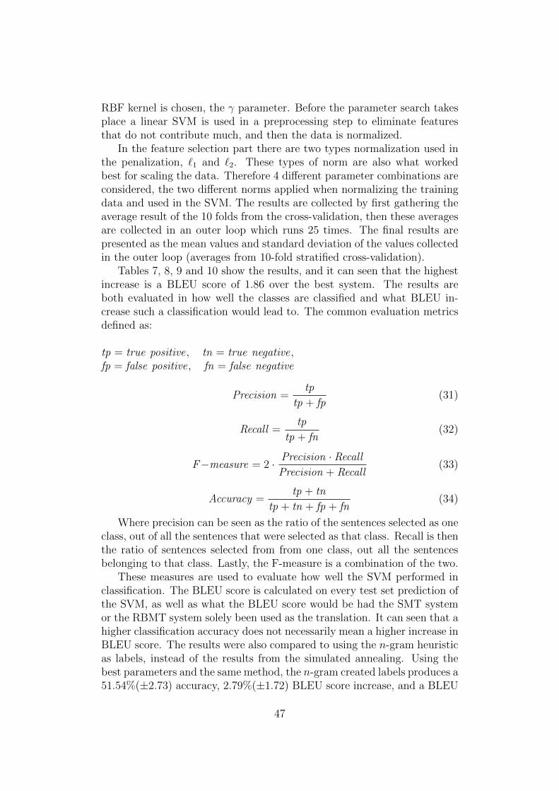
RBF kernel is chosen, the γ parameter. Before the parameter search takesplace a linear SVM is used in a preprocessing step to eliminate featuresthat do not contribute much, and then the data is normalized.

In the feature selection part there are two types normalization used inthe penalization, �1 and �2. These types of norm are also what workedbest for scaling the data. Therefore 4 different parameter combinations areconsidered, the two different norms applied when normalizing the trainingdata and used in the SVM. The results are collected by first gathering theaverage result of the 10 folds from the cross-validation, then these averagesare collected in an outer loop which runs 25 times. The final results arepresented as the mean values and standard deviation of the values collectedin the outer loop (averages from 10-fold stratified cross-validation).

Tables 7, 8, 9 and 10 show the results, and it can seen that the highestincrease is a BLEU score of 1.86 over the best system. The results areboth evaluated in how well the classes are classified and what BLEU in-crease such a classification would lead to. The common evaluation metricsdefined as:

tp = true positive, tn = true negative,

fp = false positive, fn = false negative

Precision =tp

tp + fp(31)

Recall =tp

tp + fn(32)

F−measure = 2 · Precision · RecallPrecision + Recall

(33)

Accuracy =tp + tn

tp + tn + fp + fn(34)

Where precision can be seen as the ratio of the sentences selected as oneclass, out of all the sentences that were selected as that class. Recall is thenthe ratio of sentences selected from from one class, out all the sentencesbelonging to that class. Lastly, the F-measure is a combination of the two.

These measures are used to evaluate how well the SVM performed inclassification. The BLEU score is calculated on every test set prediction ofthe SVM, as well as what the BLEU score would be had the SMT systemor the RBMT system solely been used as the translation. It can seen that ahigher classification accuracy does not necessarily mean a higher increase inBLEU score. The results were also compared to using the n-gram heuristicas labels, instead of the results from the simulated annealing. Using thebest parameters and the same method, the n-gram created labels produces a51.54%(±2.73) accuracy, 2.79%(±1.72) BLEU score increase, and a BLEU

47

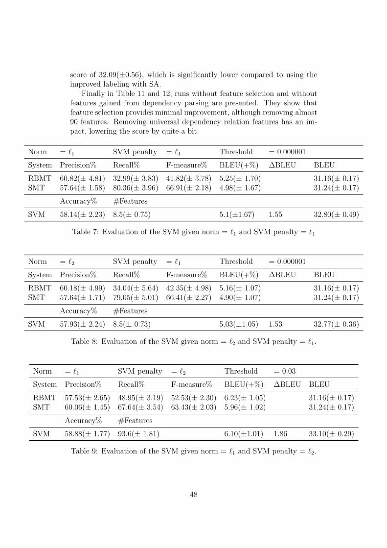
score of 32.09(±0.56), which is significantly lower compared to using theimproved labeling with SA.

Finally in Table 11 and 12, runs without feature selection and withoutfeatures gained from dependency parsing are presented. They show thatfeature selection provides minimal improvement, although removing almost90 features. Removing universal dependency relation features has an im-pact, lowering the score by quite a bit.

Norm = �1 SVM penalty = �1 Threshold = 0.000001

System Precision% Recall% F-measure% BLEU(+%) ∆BLEU BLEU

RBMT 60.82(± 4.81) 32.99(± 3.83) 41.82(± 3.78) 5.25(± 1.70) 31.16(± 0.17)SMT 57.64(± 1.58) 80.36(± 3.96) 66.91(± 2.18) 4.98(± 1.67) 31.24(± 0.17)

Accuracy% #Features

SVM 58.14(± 2.23) 8.5(± 0.75) 5.1(±1.67) 1.55 32.80(± 0.49)

Table 7: Evaluation of the SVM given norm = �1 and SVM penalty = �1

Norm = �2 SVM penalty = �1 Threshold = 0.000001

System Precision% Recall% F-measure% BLEU(+%) ∆BLEU BLEU

RBMT 60.18(± 4.99) 34.04(± 5.64) 42.35(± 4.98) 5.16(± 1.07) 31.16(± 0.17)SMT 57.64(± 1.71) 79.05(± 5.01) 66.41(± 2.27) 4.90(± 1.07) 31.24(± 0.17)

Accuracy% #Features

SVM 57.93(± 2.24) 8.5(± 0.73) 5.03(±1.05) 1.53 32.77(± 0.36)

Table 8: Evaluation of the SVM given norm = �2 and SVM penalty = �1.

Norm = �1 SVM penalty = �2 Threshold = 0.03

System Precision% Recall% F-measure% BLEU(+%) ∆BLEU BLEU

RBMT 57.53(± 2.65) 48.95(± 3.19) 52.53(± 2.30) 6.23(± 1.05) 31.16(± 0.17)SMT 60.06(± 1.45) 67.64(± 3.54) 63.43(± 2.03) 5.96(± 1.02) 31.24(± 0.17)

Accuracy% #Features

SVM 58.88(± 1.77) 93.6(± 1.81) 6.10(±1.01) 1.86 33.10(± 0.29)

Table 9: Evaluation of the SVM given norm = �1 and SVM penalty = �2.

48

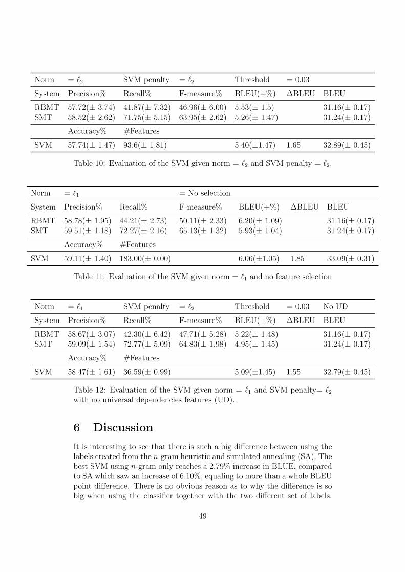
Norm = �2 SVM penalty = �2 Threshold = 0.03

System Precision% Recall% F-measure% BLEU(+%) ∆BLEU BLEU

RBMT 57.72(± 3.74) 41.87(± 7.32) 46.96(± 6.00) 5.53(± 1.5) 31.16(± 0.17)SMT 58.52(± 2.62) 71.75(± 5.15) 63.95(± 2.62) 5.26(± 1.47) 31.24(± 0.17)

Accuracy% #Features

SVM 57.74(± 1.47) 93.6(± 1.81) 5.40(±1.47) 1.65 32.89(± 0.45)

Table 10: Evaluation of the SVM given norm = �2 and SVM penalty = �2.

Norm = �1 = No selection

System Precision% Recall% F-measure% BLEU(+%) ∆BLEU BLEU

RBMT 58.78(± 1.95) 44.21(± 2.73) 50.11(± 2.33) 6.20(± 1.09) 31.16(± 0.17)SMT 59.51(± 1.18) 72.27(± 2.16) 65.13(± 1.32) 5.93(± 1.04) 31.24(± 0.17)

Accuracy% #Features

SVM 59.11(± 1.40) 183.00(± 0.00) 6.06(±1.05) 1.85 33.09(± 0.31)

Table 11: Evaluation of the SVM given norm = �1 and no feature selection

Norm = �1 SVM penalty = �2 Threshold = 0.03 No UD

System Precision% Recall% F-measure% BLEU(+%) ∆BLEU BLEU

RBMT 58.67(± 3.07) 42.30(± 6.42) 47.71(± 5.28) 5.22(± 1.48) 31.16(± 0.17)SMT 59.09(± 1.54) 72.77(± 5.09) 64.83(± 1.98) 4.95(± 1.45) 31.24(± 0.17)

Accuracy% #Features

SVM 58.47(± 1.61) 36.59(± 0.99) 5.09(±1.45) 1.55 32.79(± 0.45)

Table 12: Evaluation of the SVM given norm = �1 and SVM penalty= �2

with no universal dependencies features (UD).

6 Discussion

It is interesting to see that there is such a big difference between using thelabels created from the n-gram heuristic and simulated annealing (SA). Thebest SVM using n-gram only reaches a 2.79% increase in BLUE, comparedto SA which saw an increase of 6.10%, equaling to more than a whole BLEUpoint difference. There is no obvious reason as to why the difference is sobig when using the classifier together with the two different set of labels.

49

In comparison the score of the potential gain between the two methodsis smaller, being 0.63 BLEU versus the 1.01 BLEU of the classificationdifference.

It could be that the SA algorithm can find more complex patterns oftranslated sentences which produces a higher BLEU and in addition areeasier to find an underlying function for. According to the n-gram heuristic,almost half of the sentences are considered equal and in this case they arepicked at random, this is in contrast to SA where every sentence has itsplace specifically chosen to maximize BLEU.

Furthermore in section 5 it can observed that accuracy of the classifierdoes not always equal to an increase in BLEU score. The main goal ofthe combined system is to increase BLEU, and as such this goal is notcompletely in line with goal of the classifier. The SVM tries to separatethe classes y ∈ {RBMT, SMT} as well as possible, however it pays noattention to how much a sentence is ‘worth’ in terms of BLEU. This canexplain the differences in e.g. Table 10 and 12 which might otherwise lookstrange.

It can also be noted that leaving out the dependency parsing featuresresult in a similar classification performance for the classifier but a lowervalue in BLEU score, the reason for this could be that dependency relationsbetween words capture relevant features of text fluency. This in turn couldhelp to better classify the sentences which more strongly impact the overallBLEU score.

The BLEU score increase in the classification was also worse when therecall between the classes was skewed more in favor to one of them (inthis case SMT) as seen in Table 7 compared to Table 9. This resonateswith the fact the systems were equally good to begin with and complementeach other well, also as a result from the simulated annealing the optimalsplit between the systems were close to 50% for each system. It is thenreasonable to assume that if the classifier picks a ratio that resembles this,then it will result in a greater BLEU score.

Feature selection did not offer much improvement, however it removedalmost half the features which noticeably reduced the training time. Boththe part-of-speech tags and dependency parsing features were very sparsewith many zero frequencies, which were most likely ended up being removedby the feature selection process. Although in the case that too many fea-tures were cut, as in the case of the �1 penalty normalization, there was aclear decrease in performance.

The reason to use BLEU score as the main and only evaluation of thetranslated sentences was that it is the most known and commonly usedevaluation metric in regards to machine translation, as well as the fact thatthe main focus is one the relative difference between the system, and notthe evaluation in it self. The methods used could easily be applied using

50

other machine translation evaluation as well.

7 Future Work

As further work more features can be devised to increase the classifier per-formance. Using Giza++ [52] features concerning word positions, shiftand alignment in all the different sentences can used. More features de-rived from the tree of the dependency parsing could be investigated asthese proved to be important to capturing certain elements important toimproving the BLEU score. It could also be investigated how importantfeatures of the source and target language sides were, as currently featuresare being applied to all the texts.

Another direction to continue the work would be to see how well theclassifier performed if sentences that were very similar or had a low BLEUimpact were removed from the training data. This could be done by e.g.trying to remove each sentence from the SA solution and see which oneresults in the lowest decrease in BLEU, and then perform a greedy hillclimb from there to reach a new set of training data. The reasoning beingthat sentences that do not influence BLEU much are not important to getright during the classification, and might at worst mislead the classifierfrom more important sentences.

Lastly an extension to the system’s pipeline where other language pairsare considered, however in that case two similarly performing machinetranslations systems are needed for the new language pairs. More systemscan also be introduced to see if the results improve further for Swedish ⇒English, with the caveat that the combined systems works best if the sys-tems to be combined are originally close to each other in performance.

8 Conclusions

The thesis project set out with four main objectives:

• Investigate the potential gain of hybrid machine translation system

• Create training data by using a reference translation to automaticallylabel sentences

• Engineer good features given the source text and a set of translatedsentences

• Construct a SVM classifier and estimate its performance and gener-alization capabilities

51

The first objective was necessary to see if a combined system was worthpursuing, and to provide a soft upper bound of what could be gained.This was done by n-gram heuristic that had previously been shown to besuccessful, as discussed in section 4.3. The potential gain was tied in withcreating labels for the sentences, since the best sentences chosen were giventhe label from the system that they were picked.

This part was deemed to be important, and the heuristic left roomfor improvement, therefore a novel method of creating the best combinedtranslation, with respect to BLEU score, was introduced. The simulatedannealing algorithm is nothing new but it has never been used in the contextof labeling machine translation sentences as done in this project6. It hasbeen shown that simulated annealing has given a significant improvementin creating a combined translation that is optimized for BLEU score.

Different parameters, initializations and neighborhood functions havebeen explored to find a simulated annealing algorithm optimal for thisproblem. Results from the various simulations conclude that, as expected,parameter choice is very important with the biggest difference being al-most half of the improvement gained over the n-gram heuristic. The SAalgorithm is flexible and could easily be extended to pick sentences frommore systems and alternatively maximize according to another metric, in-stead of BLEU. The conclusion is that simulated annealing is very goodlocal search optimization technique and it works very well in creating agold standard translation, given multiple machine translation systems anda reference translation.

The third of objective was to engineer features that could discriminatewell between the classes y ∈ {RBMT, SMT}. The only information wasgiven by a set of source sentences and the sentences produced by theirrespective systems. Proven features, as seen in other text classificationsystems, such as sentence length and token length were used, but also newand unproved features were investigated.

The universal dependencies (UD) that can used to capture any depend-ency relation between words in any language was an interesting feature totry out as there was access to both the source sentence and its translationsby the different systems. It was shown that dependency parsing relationsdoes improve the BLEU score of the classifier by a percentage unit in itssimplest form, which is only the frequencies of each dependency relation.This suggests that it could be worthwhile to develop more complex featuresusing dependency parsing and UD as they capture a part of translation thatthe other features could not.

In general, what features were used and the normalization had a bigimpact on the result, in addition feature selection as preprocessing stepbefore training slightly helped to improve the performance of the classifier,

6To the author’s best knowledge.

52

and significantly reduced the training time.Using a SVM as a classifier, there are no one set of parameters which are

the best for every problem and they therefore have to picked for the probleminstance. The report has provided a good way to find parameters by usinggrid search in conjunction with 5-fold cross-validation. Furthermore a 10-fold stratified cross-validation was shown to work well at estimating theoverall performance of the SVM model. The presented results give at bestan estimated BLEU increase of 1.86 or 6.1% over the single best system.This is a significant increase and can be considered a very good result, andas such it can be concluded that using a hybrid machine translation system,as presented in this report, is a good idea.

References

[1] A. Agarwal and A. Lavie. Meteor, m-bleu and m-ter: Evaluation met-rics for high-correlation with human rankings of machine translationoutput. In Proceedings of the Third Workshop on Statistical Machine

Translation, pages 115–118. Association for Computational Linguist-ics, 2008.

[2] A. Aizerman, E. M. Braverman, and L. Rozoner. Theoretical founda-tions of the potential function method in pattern recognition learning.Automation and remote control, 25:821–837, 1964.

[3] C. M. Bishop. Pattern recognition. Machine Learning, 2006.

[4] B. E. Boser, I. M. Guyon, and V. N. Vapnik. A training algorithm foroptimal margin classifiers. In Proceedings of the fifth annual workshop

on Computational learning theory, pages 144–152. ACM, 1992.

[5] P. F. Brown, J. Cocke, S. A. D. Pietra, V. J. D. Pietra, F. Jelinek,J. D. Lafferty, R. L. Mercer, and P. S. Roossin. A statistical approachto machine translation. Computational linguistics, 16(2):79–85, 1990.

[6] C. J. Burges. A tutorial on support vector machines for pattern re-cognition. Data mining and knowledge discovery, 2(2):121–167, 1998.

[7] C. Callison-Burch, C. Fordyce, P. Koehn, C. Monz, and J. Schroeder.(meta-) evaluation of machine translation. In Proceedings of the Second

Workshop on Statistical Machine Translation, pages 136–158. Associ-ation for Computational Linguistics, 2007.

[8] C. Campbell and Y. Ying. Learning with support vector machines.Synthesis lectures on artificial intelligence and machine learning,5(1):1–95, 2011.

53

[9] D. Chen and C. D. Manning. A fast and accurate dependency parserusing neural networks. In EMNLP, pages 740–750, 2014.

[10] C.-T. Cheng, Z.-K. Feng, W.-J. Niu, and S.-L. Liao. Heuristic methodsfor reservoir monthly inflow forecasting: A case study of xinfengjiangreservoir in pearl river, china. Water, 7(8):4477–4495, 2015.

[11] W. Commons. Global/local maxima/minima — wikimedia commons,the free media repository. https://commons.wikimedia.org/wiki/

File:Extrema_example.svg, 2007. [Online; accessed 2-July-2016].

[12] W. Commons. Direct translation and transfer transla-tion pyramind.svg — wikimedia commons, the free mediarepository. https://commons.wikimedia.org/wiki/File:

Direct_translation_and_transfer_translation_pyramind.svg,2015. [Online; accessed 23-May-2016].

[13] W. Commons. Svm max sep hyperplane with margin.png — wikimediacommons, the free media repository. https://commons.wikimedia.

org/wiki/File:Svm_max_sep_hyperplane_with_margin.png, 2015.[Online; accessed 23-May-2016].

[14] W. Commons. Overfitted data.png — wikimedia commons, the freemedia repository. https://commons.wikimedia.org/wiki/File:

Overfitted_Data.png, 2016. [Online; accessed 23-May-2016].

[15] S. Corston-Oliver, M. Gamon, and C. Brockett. A machine learningapproach to the automatic evaluation of machine translation. In Pro-

ceedings of the 39th Annual Meeting on Association for Computational

Linguistics, pages 148–155. Association for Computational Linguistics,2001.

[16] C. Cortes and V. Vapnik. Support-vector networks. Machine learning,20(3):273–297, 1995.

[17] M. R. Costa-Jussa, M. Farrus, J. B. Marino, and J. A. Fonollosa. Studyand comparison of rule-based and statistical catalan-spanish machinetranslation systems. Computing and informatics, 31(2):245–270, 2012.

[18] M. R. Costa-Jussa and J. A. Fonollosa. Latest trends in hybrid ma-chine translation and its applications. Computer Speech & Language,32(1):3–10, 2015.

[19] M. A. Covington. A fundamental algorithm for dependency parsing.In Proceedings of the 39th annual ACM southeast conference, pages95–102. Citeseer, 2001.

54

[20] N. Cristianini and J. Shawe-Taylor. An introduction to support vector

machines and other kernel-based learning methods. Cambridge univer-sity press, 2000.

[21] A. P. Engelbrecht. Computational intelligence: an introduction. JohnWiley & Sons, 2007.

[22] A. Finch, Y.-S. Hwang, and E. Sumita. Using machine translation eval-uation techniques to determine sentence-level semantic equivalence.In Proceedings of the Third International Workshop on Paraphrasing

(IWP2005), pages 17–24, 2005.

[23] R. Fletcher. Practical methods of optimization. John Wiley & Sons,2013.

[24] M. Frank and P. Wolfe. An algorithm for quadratic programming.Naval research logistics quarterly, 3(1-2):95–110, 1956.

[25] T. S. Furey, N. Cristianini, N. Duffy, D. W. Bednarski, M. Schummer,and D. Haussler. Support vector machine classification and validationof cancer tissue samples using microarray expression data. Bioinform-

atics, 16(10):906–914, 2000.

[26] M. Gamon, A. Aue, and M. Smets. Sentence-level mt evaluationwithout reference translations: Beyond language modeling. In Pro-

ceedings of EAMT, pages 103–111, 2005.

[27] I. Guyon and A. Elisseeff. An introduction to variable and featureselection. The Journal of Machine Learning Research, 3:1157–1182,2003.

[28] N. Habash, B. Dorr, and C. Monz. Symbolic-to-statistical hybrid-ization: extending generation-heavy machine translation. Machine

Translation, 23(1):23–63, 2009.

[29] B. Hajek. Cooling schedules for optimal annealing. Mathematics of

operations research, 13(2):311–329, 1988.

[30] M. A. Hearst, S. T. Dumais, E. Osman, J. Platt, and B. Scholkopf.Support vector machines. Intelligent Systems and their Applications,

IEEE, 13(4):18–28, 1998.

[31] H. H. Hoos and T. Stutzle. Stochastic local search: Foundations &

applications. Elsevier, 2004.

[32] C.-W. Hsu, C.-C. Chang, C.-J. Lin, et al. A practical guide to supportvector classification. 2003.

55

[33] W. J. Hutchins. Machine translation: A brief history. Concise history

of the language sciences: from the Sumerians to the cognitivists, pages431–445, 1995.

[34] W. J. Hutchins and H. L. Somers. An introduction to machine trans-

lation, volume 362. Academic Press London, 1992.

[35] G. James, D. Witten, T. Hastie, and R. Tibshirani. An introduction

to statistical learning, volume 112. Springer, 2013.

[36] T. Joachims. Text categorization with support vector machines: Learn-

ing with many relevant features. Springer, 1998.

[37] S. Kirkpatrick, M. P. Vecchi, et al. Optimization by simmulated an-nealing. science, 220(4598):671–680, 1983.

[38] P. Koehn. Statistical machine translation. Cambridge University Press,2009.

[39] P. Koehn, H. Hoang, A. Birch, C. Callison-Burch, M. Federico, N. Ber-toldi, B. Cowan, W. Shen, C. Moran, R. Zens, et al. Moses: Opensource toolkit for statistical machine translation. In Proceedings of the

45th annual meeting of the ACL on interactive poster and demonstra-

tion sessions, pages 177–180. Association for Computational Linguist-ics, 2007.

[40] R. Kohavi et al. A study of cross-validation and bootstrap for accuracyestimation and model selection. In Ijcai, volume 14, pages 1137–1145,1995.

[41] C. D. Manning, P. Raghavan, H. Schutze, et al. Introduction to in-

formation retrieval, volume 1. Cambridge university press Cambridge,2008.

[42] C. D. Manning, M. Surdeanu, J. Bauer, J. Finkel, S. J. Bethard, andD. McClosky. The Stanford CoreNLP natural language processingtoolkit. In Association for Computational Linguistics (ACL) System

Demonstrations, pages 55–60, 2014.

[43] R. T. McDonald, J. Nivre, Y. Quirmbach-Brundage, Y. Goldberg,D. Das, K. Ganchev, K. B. Hall, S. Petrov, H. Zhang, O. Tackstrom,et al. Universal dependency annotation for multilingual parsing. InACL (2), pages 92–97. Citeseer, 2013.

[44] W. McKinney. Data structures for statistical computing in python. InS. van der Walt and J. Millman, editors, Proceedings of the 9th Python

in Science Conference, pages 51 – 56, 2010.

56

[45] N. Metropolis, A. W. Rosenbluth, M. N. Rosenbluth, A. H. Teller, andE. Teller. Equation of state calculations by fast computing machines.The journal of chemical physics, 21(6):1087–1092, 1953.

[46] K. P. Murphy. Machine learning: a probabilistic perspective. MITpress, 2012.

[47] S. Nirenburg and H. L. Somers. Readings in machine translation. MITPress, 2003.

[48] J. Nivre. Towards a universal grammar for natural language pro-cessing. In International Conference on Intelligent Text Processing

and Computational Linguistics, pages 3–16. Springer, 2015.

[49] J. Nivre, J. Hall, J. Nilsson, A. Chanev, G. Eryigit, S. Kubler,S. Marinov, and E. Marsi. Maltparser: A language-independent systemfor data-driven dependency parsing. Natural Language Engineering,13(02):95–135, 2007.

[50] Y. Nourani and B. Andresen. A comparison of simulated annealingcooling strategies. Journal of Physics A: Mathematical and General,31(41):8373, 1998.

[51] F. J. Och. Minimum error rate training in statistical machine trans-lation. In Proceedings of the 41st Annual Meeting on Association for

Computational Linguistics-Volume 1, pages 160–167. Association forComputational Linguistics, 2003.

[52] F. J. Och and H. Ney. A systematic comparison of various statisticalalignment models. Computational Linguistics, 29(1):19–51, 2003.

[53] K. Papineni, S. Roukos, T. Ward, and W.-J. Zhu. Bleu: a methodfor automatic evaluation of machine translation. In Proceedings of

the 40th annual meeting on association for computational linguistics,pages 311–318. Association for Computational Linguistics, 2002.

[54] F. Pedregosa, G. Varoquaux, A. Gramfort, V. Michel, B. Thirion,O. Grisel, M. Blondel, P. Prettenhofer, R. Weiss, V. Dubourg,J. Vanderplas, A. Passos, D. Cournapeau, M. Brucher, M. Perrot,and E. Duchesnay. Scikit-learn: Machine learning in Python. Journalof Machine Learning Research, 12:2825–2830, 2011.

[55] R. Polikar. Ensemble based systems in decision making. IEEE Circuits

and systems magazine, 6(3):21–45, 2006.

[56] M. F. Porter. An algorithm for suffix stripping. Program, 14(3):130–137, 1980.

57

[57] G. Salton and C. Buckley. Term-weighting approaches in automatictext retrieval. Information processing & management, 24(5):513–523,1988.

[58] F. Sanchez Martınez et al. Choosing the best machine translation sys-tem to translate a sentence by using only source-language information.2011.

[59] D. Silver, A. Huang, C. J. Maddison, A. Guez, L. Sifre, G. VanDen Driessche, J. Schrittwieser, I. Antonoglou, V. Panneershelvam,M. Lanctot, et al. Mastering the game of go with deep neural net-works and tree search. Nature, 529(7587):484–489, 2016.

[60] J. Slocum. A survey of machine translation: its history, current status,and future prospects. Computational linguistics, 11(1):1–17, 1985.

[61] R. S. Sutton and A. G. Barto. Reinforcement learning: An introduc-

tion. MIT press, 1998.

[62] J. A. Suykens and J. Vandewalle. Least squares support vector machineclassifiers. Neural processing letters, 9(3):293–300, 1999.

[63] G. Tesauro. Td-gammon, a self-teaching backgammon program,achieves master-level play. Neural computation, 6(2):215–219, 1994.

[64] K. Toutanova, D. Klein, C. D. Manning, and Y. Singer. Feature-rich part-of-speech tagging with a cyclic dependency network. In Pro-

ceedings of the 2003 Conference of the North American Chapter of

the Association for Computational Linguistics on Human Language

Technology-Volume 1, pages 173–180. Association for ComputationalLinguistics, 2003.

[65] A. B. Tucker. Computer science handbook. CRC press, 2004.

[66] S. Van Der Walt, S. C. Colbert, and G. Varoquaux. The numpy array:a structure for efficient numerical computation. Computing in Science

& Engineering, 13(2):22–30, 2011.

[67] G. VanRossum and F. L. Drake. The Python Language Reference.Python software foundation Amsterdam, Netherlands, 2010.

[68] V. N. Vapnik and V. Vapnik. Statistical learning theory, volume 1.Wiley New York, 1998.

[69] D. H. Wolpert. Stacked generalization. Neural networks, 5(2):241–259,1992.

58

[70] S. Zwarts and M. Dras. Choosing the right translation: A syntactic-ally informed classification approach. In Proceedings of the 22nd In-

ternational Conference on Computational Linguistics-Volume 1, pages1153–1160. Association for Computational Linguistics, 2008.

59