Forecasting the long-run potential

of the Scottish economy March 2018

© Crown copyright 2018

This publication is licensed under the terms of the Open Government Licence v3.0

except where otherwise stated. To view this licence, visit:

http://www.nationalarchives.gov.uk/doc/open-government-licence/version/3/ or write

to the Information Policy Team, The National Archives, Kew, London TW9 4DU, or

email: psi@nationalarchives.gsi.gov.uk

Where we have identified any third party copyright information you will need to obtain

permission from the copyright holders concerned.

This publication is available at www.fiscalcommission.scot

Any enquiries regarding this publication should be sent to us at: Scottish Fiscal

Commission, Governor’s House, Regent Road, Edinburgh EH1 3DE

Published by the Scottish Fiscal Commission, March 2018

ISBN: 978-1-9998487-6-7

Forecasting the long-run potential of

the Scottish economy

Contents Section 1: Introduction ..................................................................................................... 1

Section 2: General approach to forecasting the economy ............................................ 2

Section 2: What is potential output? ............................................................................... 5

Section 4: Forecasting the components of potential output ......................................... 8

Section 5: Forecasts of potential output ....................................................................... 28

Section 6: The output gap .............................................................................................. 30

Annex 1: Generation of industry productivity figures ................................................. 34

1

Section 1: Introduction The Scottish Fiscal Commission is committed to being open and transparent 1.1

in our approach to forecasting. We are publishing a series of technical papers

to enable further understanding of the methodology behind our main

forecasts. One area of particular interest is how we forecast the economy over

the long-run, and in particular our view on productivity.

This paper focuses on our methods for forecasting the long-run underlying 1.2

trends in the Scottish economy, putting to one side shorter-term volatility or

cyclicality. We forecast the long-run total potential capacity of the Scottish

economy, considering broad changes in supply side conditions. This helps to

shape our forecasts over the full six year period for which we create forecasts,

with other models forecasting the fluctuations in the demand side of the

economy over the short to medium term.

We set out our first economic forecast in our publication in December 2017, 1.3

Scotland’s Economic and Fiscal Forecasts (SEFF December 2017).1 This

paper explains the Commission’s methodology for modelling and projecting

potential output and the output gap in Scotland in further detail. Illustrative

projections of potential output and its components are provided using the

same methodology as in December but based on the latest available data,

which will include some historic revisions.

Our forecast in December was based on the approach set out in this paper to 1.4

forecasting the economy. The Commission will continue to consider all

available data, evidence and information in producing its future forecast

publications and may continue to make changes to both its methodology and

its key judgements. We will provide updates on changes to methodology and

judgements over time where appropriate.

1 SFC (2017) Scotland’s Economic and Fiscal Forecasts (link)

2

Section 2: General approach to forecasting

the economy 2.1 In September 2017 the Commission published a paper explaining at a high

level our approach to economic forecasting.2 We use a range of different

models for forecasting the economy. The models can be broadly grouped into

short, medium and long run forecasting models.

2.2 The main components of our current forecasting process are shown in Figure

2.1.

Figure 2.1: Schematic representation of economic forecasting process

Source: Scottish Fiscal Commission

2.3 The current steps taken by the Commission to creating an economic forecast

are:

I. Short-run forecasts: Official economic statistics by their nature are

only available with a lag. Timely surveys of the Scottish economy can

2 SFC (2017) Current Approach to Forecasting (link)

II. Long run

labour force

I Short run

forecasts

III. Long run

potential GDP

IV. OBR forecasts

V. Trade VI. Public

sector output

VII. Labour

market

Stand-alone models

All feeds into

VIII. SGGEM model

IX. Forecast diagnostics tool

SGGEM, diagnostics

and judgement

X. Income tax forecasting system

3

be analysed alongside other alternative sources of data to build up a

picture of what is happening today and the likely pathway in the near

future. Statistical models are used to create short-run forecasts for

up to two quarters ahead. For each key variable, a number of ARIMA

models are created, each with a single exogenous predictor variable.

These are then averaged together using their relative predictive

power, based on historic fit, to create short-run forecasts of selected

key variables.

II. Long-run labour force: The potential labour force consists of

people either in employment or actively searching for employment.

The starting point for the long-run forecast of the labour force is the

ONS/NRS population projections with detailed age and gender

demographics. Forecasts for labour force participation rates are then

applied by age and gender, to create total trend labour force levels.

As well as feeding into the rest of the economic forecasts, this

projection of the labour force is used in the income tax forecasting

system.

III. Long-run potential output: Over our forecast horizon of five years,

forecasts of GDP are anchored to our forecasts of potential output –

the maximum capacity the economy can sustain to produce goods

and services. This depends primarily on growth in productivity: the

amount of goods and services that can be produced for a given

amount of labour input. The forecast of potential output is produced

by combining forecasts of the size of the labour force with forecasts

of productivity and applying assumptions about trends in

unemployment and average hours worked.

IV. OBR forecasts: The UK economy affects Scotland in two main

ways: firstly, through a number of economic variables that Scotland

shares with the UK as a whole, such as interest rates and exchange

rates; and secondly, through trade as Scotland’s largest trade

partner. The starting point for these elements of the forecast is to

consider the latest available OBR forecasts for the UK.

V. Trade model: Trade is challenging to forecast. Trade between

Scotland and the rest of the UK is modelled based on growth in

demand in both economies. Trade between Scotland and the rest of

the world is then based on the OBR’s UK trade forecasts, with some

adjustment for Scottish circumstances.

VI. Public sector output: Government spending is a significant

component of GDP. Public sector output is forecast by considering

the available information on spending plans of both the Scottish and

UK Governments in Scotland.

4

VII. Labour market adjustments: Combining the short-run forecasts

and the long-run trend forecasts of the labour force, we create a

medium term adjustment pathway for employment and

unemployment. A long-run trend rate of unemployment is targeted in

the forecast, with additional judgement applied based on available

intelligence on the state of the Scottish labour market

VIII. SGGEM model: The SGGEM model sits at the core of the economic

forecasting process. It is an extension to NIESR’s long-established

NiGEM macroeconometric model.3 All of the above projections are

fed into SGGEM which is then used to create forecasts for remaining

variables and time periods.

IX. Forecast diagnostics tool: Forecasts from SGGEM are then

analysed in a separate diagnostics tool. This is to check the

characteristics of the forecast and allow the Commission to hone and

sense-check key judgements. The steps above can be repeated to

tweak the forecast and apply further judgement as necessary. These

diagnostic checks include the ratio productivity to wages, the savings

ratio and net trade as a share of GDP.

X. Income tax forecasting system: Once the economic forecasts are

complete, the forecasts of wages, employment and hours worked are

fed into the income tax forecasting system.

2.4 In this paper, we set out in more detail our approach to forecasting the

economy over the longer-term mentioned in steps II and III. In the context of

our forecasts, the longer term is considered to be the next six years. This

approach primarily considers the supply side of the economy, with other

models forecasting the pathway of the demand side of the economy over the

short to medium term. Potential output – or the trend amount of goods and

services the economy can sustainably produce – is estimated and projected.

This requires modelling of population, the labour market and labour

productivity to generate potential output.

2.5 Models provide insight and guidance, but judgement plays an important role.

Judgment is required in both how the models are operated, and how the

results from different models are used and combined. Ultimately, the forecast

will be driven by the judgements of the Commission, rather than depending

mechanically on the output of any one model.

3 NIESR – The National Institute of Economic and Social Research, a charity and Britain’s longest established

independent research institute (link). For further information on the NiGEM model see (link)

5

Section 3: What is potential output? Overview

3.1 Potential output is the estimated amount of goods and services the economy

can sustainably produce without inducing excess price inflation in the

economy. In the short term actual output can deviate from potential output,

but over the longer term the economy is assumed to be subject to the supply

constraint of potential output.

3.2 Estimation of potential output is crucial for forecasting the economy for two

reasons:

The capacity of an economy to generate sustainable growth

determines structural growth

The output gap is the relationship between potential and actual

output and this implicitly determines the cyclical position of the

economy

3.3 One of the main challenges in projecting potential output is that the supply

capacity of an economy is not observable. Instead, we capture the underlying

trends by decomposing output by supply factors, as well as incorporating the

best available intelligence for estimating potential output. Judgement is

inevitably needed to incorporate the available qualitative and quantitative

intelligence into our potential output projections.

3.4 This part of the forecasting process is therefore heavily influenced by the

judgement of the Commission. We use a variety of models and techniques to

identify the underlying trends in the supply side of the economy, but our

forecast of potential output is ultimately a judgement about how these trends

will evolve in the future.

Production function methodology

3.5 We build up our view of potential output by estimating historic trends and

projecting its individual components: population; the labour market and;

productivity. By forecasting each of these individually, a picture of total

potential output in the future can be constructed. A schematic representation

of this is provided in Figure 3.1 This methodology is widely used for

forecasting potential output, notably by the OBR, the European Commission

and the OECD. 4 5 6

4 OBR, 2014, Working paper No.5: Output gap measurement: judgement and uncertainty (link)

5 D’Auria, F., Denis, C., Havik, K., McMorrow, K., Planas, C., Raciborski, R., Roger, W., and Rossi, A., 2014.

“The production function methodology for calculating potential growth rates and output gaps”, European

Economy- Economic Paper No.420, European Commission, (link)

6

Figure 3.1: Schematic representation of forecast of potential output

Source: Scottish Fiscal Commission

3.6 The Commission does not consider capital – for example plant and machinery

– or other factors of production as part of this process, leaving labour input as

the only factor of production. One of the reasons is because capital stock and

business investment data for Scotland are limited and generally heavily

modelled. Potential output is determined by the combination of total labour

input and labour productivity. The implication is that our estimates of labour

productivity reflect changes not only in total factor productivity, but also

changes in capital stock on production.

3.7 The Commission’s methodology for projecting potential output consists of a

bottom-up approach for projecting and combining labour input and

productivity. In general, the process can be described as follows:

I. Decompose each factor to incorporate the underlying trends to our

projections. For factors associated with labour markets, we

6 Beffy, P.O., Ollivaud, P., Richardson, P. and Sedillot, F., 2006. New OECD methods for supply-side and

medium-term assessments: a capital services approach. OECD Economics Department Working Paper No.482,

(link)

= Total potential hours worked, multiplied by

Multiplied by

= Potential output

Population 16+ population

Labour Market

Labour supply Trend

unemployment Average hours

worked

Productivity output per

hour worked

7

decompose by age ranges and gender. For output variables, we

decompose by production industry.

II. Remove any cyclicality, volatility and noise from our variables

through trending and filtering techniques. This enables us to capture

the long run trends of the historic data and filter out shorter term

noise and volatility. This process also makes some judgements

about identify the underlying trends.

III. Project the path for each smoothed component. This is based on

observing recent growth in the series, judgement and any external

information, such as population projections. Largely this is an

empirically driven approach.

IV. Combine the factors to obtain potential output.

3.8 This bottom-up approach enables us to identify the contribution of different

factors to potential output growth, as well as assessing the sensitivity of the

forecast to variations in these factors.

3.9 One limitation to this approach is that it is a combination of stand-alone

models, so this modelling framework does not automatically incorporate

feedback effects between factors. The Commission applies additional

judgement to control for this.

8

Section 4: Forecasting the components of

potential output 4.1 The following section illustrates our approach, providing details about the

projection of the individual factors: population, participation, unemployment,

average hours worked, which make up labour input, and labour productivity.

The projections published in our Scottish Economic and Fiscal Forecasts

(December 2017) and some of the detail of the calculations behind them are

provided in a workbook published alongside this paper.7

Population

4.2 Population growth is a fundamental determinant of growth in the economy. All

else being equal, the larger the population, the larger the economy. As well as

the total size of the population, it is also important to understand how the age

and gender structure of the population may change, as labour market trends

vary by groups.

Historic trends

4.3 We start by considering detailed population forecasts broken down by age

and gender. For this we use the National Records of Scotland (NRS) mid-year

population data and 2016 based ONS/NRS population projections.

4.4 Historically, Scotland has had slower population growth than the UK as a

whole. This has been due in part to lower levels of net migration, with net

outflows of population from Scotland for much of the 1970s, 1980s and 1990s.

Figure 4.1 shows net migration per capita in Scotland and the UK.

7 Scottish Fiscal Commission (2018) Potential output calculation detailed workbook (link)

9

Figure 4.1: Net migration per capita, Scotland and UK

Source: Scottish Fiscal Commission

4.5 Since the early 2000s, Scotland has had higher levels of net inward migration

than observed historically. The level of this has been comparable in relative

terms to levels of net migration into the UK.

4.6 Scotland also has an ageing population, with the number of individuals aged

over 65 increasing relative to the population as a whole. Growth in the 16 to

64 year old population, those with the highest labour market participation, has

slowed significantly in recent years.

Our judgement

4.7 The ONS and NRS produce a range of variants of their population forecasts

based on varying assumptions around fertility, mortality and migration. On

fertility and mortality, the Commission uses the principal projections.

4.8 Migration is a key uncertainty, particularly with the prospect of the changing

relationship between the UK and the EU. As Figure 4.1 shows, Scotland has

moved from having negative net migration for most of the period 1971 to 1999

to a period of strong positive net migration. There are two aspects to the

Commission’s judgement on migration:

I. Aside from the impact of UK-EU exit, would more recent levels of

positive net migration have been sustained or would Scotland have

returned towards longer-term historic trends?

II. How will UK-EU exit affect future Scottish migration?

-0.006

-0.004

-0.002

0

0.002

0.004

0.006

1971 1975 1979 1983 1987 1991 1995 1999 2003 2007 2011 2015

UK Scotland

10

4.9 Figure 4.2 shows the range of available migration variants from the ONS

population projections.

Figure 4.2: Scottish net migration historic data and projections with migration

variants, thousands

Source: NRS (2017) total migration to or from Scotland (link), ONS/NRS (2017) 2016-based population

projections (link)

4.10 All of these variants assume that current high levels of net migration will not

be sustained and that net migration will gradually reduce.

4.11 For our December 2017 forecasts, the Commission judged the 50 per cent EU

migration scenario to best describe the context in Scotland because of the

potential impacts of the changing UK-EU relationship on net migration.

4.12 The Commission will closely monitor forthcoming migration data releases and

update our assumption if necessary.

Forecast

4.13 As shown in Figure 4.3, the Commission’s population forecasts show modest

population growth amongst those aged 16 plus, albeit slower than the growth

forecast by the OBR for the UK. The 16 to 64 year old population is expected

to start to shrink in Scotland within the next five years.

0

5

10

15

20

25

30

35

2005-06 2008-09 2011-12 2014-15 2017-18 2020-21

Net migration Principal Low High

0% EU 50% EU 150% EU

11

Figure 4.3: Scottish total population and 16 to 64 year old population,

thousands

Source: NRS (2017) mid-year population estimates (link), ONS/NRS (2017) 2016-based population projections

(link)

Participation

4.14 Labour force measures engagement in the labour market: it is the total

number of individuals who are either in work or are actively looking for work.

Together with population and demographics, participation determines the size

of the labour supply.

Historic trends

4.15 The Commission uses participation data from the Labour Force Survey (LFS)

as the basis for our forecasts, which are decomposed between males and

females aged over 16 years.

4.16 Historically labour market participation rates have varied between different

age groups and genders. For example, participation rates amongst those

aged 16 to 24 have declined steadily since 2004, in line with a gradual

increase in participation in further education. The 16 to 24 age group has also

seen strong convergence of participation rates between males and females,

with men and women having broadly similar labour market participation at this

age.

4.17 Another strong feature of recent trends in the labour market has been the

increasing participation of those aged 55 to 64 and over 65s. There are a

number of contributing factors including longer healthy working lives and slow

growth in real incomes since 2008 leading to later retirement.

3,350

3,450

3,550

3,650

3,750

3,850

5,050

5,150

5,250

5,350

5,450

5,550

2006 2008 2010 2012 2014 2016 2018 2020 2022

Total population (LHS) 16-64 population (RHS)

12

Our judgement

4.18 Our forecasts are primarily based on assuming that the trends observed in

each age group and gender continue in the near future. This empirical

approach would not be appropriate for a forecast horizon longer than five

years. For example, it is unlikely that participation amongst those aged 16 to

24 will continue to decline at the same rates observed since 2004, and that

this trend is likely to flatten out over a longer time horizon. We judge this

approach to be appropriate for the time horizons we are forecasting.

Our forecasts

4.19 Our projections for labour market participation rates, broken down by age and

gender, are shown in Figures 4.4 to 4.9.

Figure 4.4: Participation of 16-24,% Figure 4.5: Participation of 25-34,%

Figure 4.6: Participation of 35-44,% Figure 4.7: Participation of 45-54,%

55

60

65

70

75

80

2004 2008 2012 2016 2020

75

80

85

90

95

2004 2008 2012 2016 2020

75

80

85

90

95

2004 2008 2012 2016 2020

75

80

85

90

95

2004 2008 2012 2016 2020

13

Figure 4.8: Participation of 55-64,% Figure 4.9: Participation of 65+,%

Source: Scottish Fiscal Commission

4.20 The projections in Figures 4.4 to 4.9 show that participation rates are

expected to continue to decline for those aged 16 to 24, be flat for individuals

aged 25 to 34 and 35 to 44, and to increase for all individuals over the age of

45.

4.21 The Commission combines the decomposed participation projections with

their respective population shares and applies this projection to our historic

participation estimates from the Labour Force Survey (LFS). As shown in

Figure 4.10, this displays a mild trend for gender participation rate

convergence, as well as a slightly decreasing participation rate of all

individuals aged 16 and over.

Figure 4.10: Labour market participation rates for the population aged 16 and

over, %

Source: Scottish Fiscal Commission

45

50

55

60

65

70

75

80

2004 2008 2012 2016 2020

2

4

6

8

10

12

14

2004 2008 2012 2016 2020

50%

55%

60%

65%

70%

75%

1992 1995 1998 2001 2004 2007 2010 2013 2016 2019 2022

Males actual Males projected Females actual

Females projected Total projected

14

4.22 Figure 4.11 shows that despite a forecast of a slightly decreasing participation

rate, the participation level is expected to continue to increase as the Scottish

population grows, albeit at a slower rate than in the recent past.

Fig 4.11: 16+ participation level, thousands

Source: ONS (2017) Regional labour market statistics in the UK (link), Scottish Fiscal Commission

Unemployment

4.23 Unemployment describes those individuals who are not currently in

employment but are actively looking for and available to start work. They are

considered part of the available labour supply.

4.24 A small amount of short-term unemployment will mean firms have a pool of

available labour from which to hire. If unemployment becomes too low, firms

will struggle to recruit and this can place upwards pressure on wages, leading

to inflation. When the economy is operating at its potential, we would expect

unemployment to be low and stable, but not so low that excess wage

pressures are generated. This point is known as the Non-Accelerating

Inflation Rate of Unemployment (NAIRU) – the trend rate of unemployment

consistent with low inflation.

4.25 To forecast employment over the longer-term, the Commission produces a

forecast of the NAIRU.

Historic trends

4.26 The Commission bases its unemployment forecasts on data from the LFS.

The LFS unemployment rate data are shown in Figure 4.12.

2,400

2,500

2,600

2,700

2,800

1992 1995 1998 2001 2004 2007 2010 2013 2016 2019 2022

Actual data Projection

15

Figure 4.12: Scottish 16+ unemployment rate, %

Source: ONS (2017) Regional labour market statistics in the UK (link)

4.27 Since the early 1990s, unemployment has gone through two main phases. In

the period leading up to the financial crisis around 2008, unemployment rates

decreased significantly and this seems to imply a systematic decline in the

NAIRU over this period of time. The financial crisis caused the unemployment

rate to increase dramatically to a peak of 9 per cent, following which

unemployment rates have decreased to the currently observed historic lows of

around 4.0 per cent.

Our judgement

4.28 The Commission does not rely on the output of any specific model for

determining the NAIRU. Instead, we incorporate the available evidence and

intelligence to form a judgement about trend unemployment both during the

historic period and the forecast.

4.29 The Commission judges that the trend unemployment rate in Scotland

declined steadily from 1992 to 2008. Had the financial crisis not occurred, we

would have seen this decline start to level off. Whilst the financial crisis

caused a strong cyclical increase in the unemployment rate, it does not

appear to have had a long-run impact on the NAIRU, with unemployment

rates rapidly declining to levels of 4.0 to 4.5 per cent in recent years.

4.30 In its December 2017 forecast, the Commission judged the NAIRU to be 4.5

per cent. This is lower than the unemployment rate observed in much of the

period preceding the financial crisis. We see several reasons for a reduced

NAIRU:

0

2

4

6

8

10

12

1992 1994 1996 1998 2000 2002 2004 2006 2008 2010 2012 2014 2016

16

Low pressures on wages: Wage pressures appear generally weak

despite low unemployment. This may be due to: business uncertainty

following the financial crisis and with the changing relationship

between the UK and the EU; slow wage growth in the public sector;

and more strongly anchored inflation expectations than in the past.

Demographic composition of the labour market: The share of the

labour force aged between 16 and 24 years old is decreasing over

time. Because this age range has the highest unemployment rates, a

decline in its share of the labour force contributes toward a reduced

rate of unemployment. Similarly, women have lower rates of

unemployment, and the increasing share of women in the labour

market has increased over time. This has arithmetically reduced

average unemployment rates.

Individuals may be more willing to relocate for work than in the past

because of improved connectivity and communication

New technology allows for more flexible and remote working

New technology allows for quicker and more efficient job market

matching

Increases in self-employment and “gig-economy” work

Our forecasts

4.31 The Commission’s judgement on NAIRU is that it will remain at 4.5 per cent

over the forecast period.

Average hours worked

4.32 We use total hours worked as our measure of total labour input. This is a

multiple of the number of people in employment and the number of hours

each person works on average. Our forecasts of population, participation and

unemployment allow us to produce a forecast of trend employment. This

section provides details on how we forecast average hours worked and how

this leads to our forecast of total hours worked.

Historic data

4.33 The Commission uses Annual Population Survey (APS) as its source of data

on hours worked. In order to project the path for average hours per worker,

average hours are decomposed by different working patterns for males and

females.

4.34 The historic data show:

In both Scotland and the UK as a whole, average hours worked has

been steadily declining for some time. In the UK, average hours

17

worked has declined from around 36 hours a week in the 1970s, to

around 32 hours a week today, and Scotland has followed similar

trends in the shorter series of data available. However, this process

of gradual decline appears to be slowing and levelling off.

On average, men work more hours than women. This is in part the

result of women being more likely to work part-time, but even within

full-time work, men work more hours on average. This gap has been

gradually closing over time, with women starting to increase their

average hours worked in recent years, and a slight but persistent

decrease in average hours worked amongst men.

The financial crisis led to a sharp increase in the proportion of both

men and women in part-time work. This was due to low demand in

the economy and a lack of availability of full-time jobs. For women,

following this shock, the share in part-time work has unwound to

previous levels, but there appears to be a more permanent shift in

the proportion of men working part-time. It appears that the shock of

the financial crisis had a permanent effect on part-time work amongst

men.

Judgement

4.35 The Commission takes a largely empirical approach to forecasting average

hours worked. In most cases, we assume that the recent trends we have

observed by gender and working pattern will continue.

4.36 The financial crisis appears to have generated a small but permanent shift in

men’s working patterns. This view is supported by the data on involuntary

part-time working. Figure 4.13 illustrates that while the number of part time

workers has stayed high since the beginning of the crisis, the fraction of those

that would like to switch to full time has significantly decreased since 2013,

indicating that, over time, more individuals have decided that they would like

to work part-time.

18

Figure 4.13: Level of part time employment and involuntary part time

employment, thousands

Source: ONS (2017) Regional labour market statistics in the UK (link)

Forecasts

4.37 Figures 4.14 to 4.19 show our estimated historic trends and forecasts of

average hours worked by gender and working pattern.

Figure 4.14: FT hours worked Figure 4.15: PT hours worked

40

60

80

100

120

140

160

580

600

620

640

660

680

700

2004 2006 2008 2010 2012 2014 2016

PT employment (LHS) Involuntary PT employment (RHS)

32

34

36

38

40

2004 2008 2012 2016 2020

15.5

16.0

16.5

17.0

17.5

2004 2008 2012 2016 2020

19

Figure 4.16: Share of males PT, % Figure 4.17: Share of females PT, %

Figure 4.18: Second jobs hours

worked

Figure 4.19: Fraction of second jobs,

%

Source: Scottish Fiscal Commission

4.38 Combining the forecasts for average hours worked and their respective

shares of employed people, we obtain the projection path for our average

hours worked for males and females. These are shown in figures 4.20 to 4.21.

The Commission projects males average hours per worker to slightly

decrease, while females average hours worked are projected to increase over

the forecast horizon. This results in a broadly constant profile for average

hours worked in Scotland over the forecast horizon.

7%

9%

11%

13%

15%

2004 2008 2012 2016 2020

38%

40%

42%

44%

46%

2004 2008 2012 2016 2020

8

9

10

11

12

2004 2008 2012 2016 20202%

3%

4%

5%

6%

2004 2008 2012 2016 2020

20

Figure 4.20: Average hours worked by males

Figure 4.21: Average hours worked by females

Source: Scottish Fiscal Commission

4.39 The Commission uses data from APS for hours worked, but data from the LFS

for employment. These two different surveys of the labour market introduce a

slight inconsistency. Whilst we utilise information on disaggregated average

hours worked from the APS, we are ultimately more interested in total hours

worked.

4.40 To get a value for total hours worked that is consistent with our underlying

APS analysis of average hours worked, but also consistent with our LFS

employment values, we apply the following process:

1. Generate our underlying forecasts of average hours worked from

APS as described above

2. Take data on total hours worked from the APS and divide this by LFS

employment. This creates a slightly different series for average hours

worked than the APS estimate.

3. Grow this average hours worked estimate in line with our APS based

projection of average hours worked derived in step 1.

4. Multiply back up by our LFS employment forecast to estimate total

hours worked.

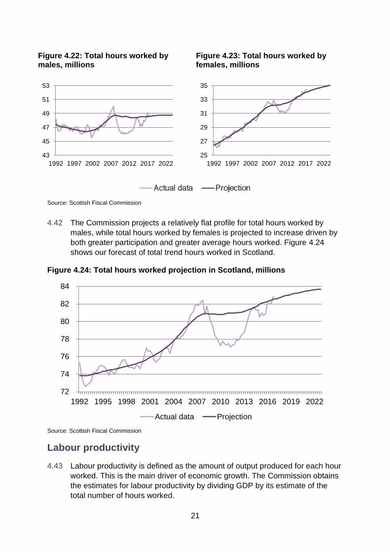
4.41 Figures 4.22 to 4.23 show our forecasts of trend total hours worked.

34

35

36

37

38

2002 2006 2010 2014 2018 2022

24

25

26

27

28

2002 2006 2010 2014 2018 2022

21

Figure 4.22: Total hours worked by males, millions

Figure 4.23: Total hours worked by females, millions

Source: Scottish Fiscal Commission

4.42 The Commission projects a relatively flat profile for total hours worked by

males, while total hours worked by females is projected to increase driven by

both greater participation and greater average hours worked. Figure 4.24

shows our forecast of total trend hours worked in Scotland.

Figure 4.24: Total hours worked projection in Scotland, millions

Source: Scottish Fiscal Commission

Labour productivity

4.43 Labour productivity is defined as the amount of output produced for each hour

worked. This is the main driver of economic growth. The Commission obtains

the estimates for labour productivity by dividing GDP by its estimate of the

total number of hours worked.

43

45

47

49

51

53

1992 1997 2002 2007 2012 2017 2022

25

27

29

31

33

35

1992 1997 2002 2007 2012 2017 2022

72

74

76

78

80

82

84

1992 1995 1998 2001 2004 2007 2010 2013 2016 2019 2022

Actual data Projection

22

4.44 The projections for productivity are heavily influenced by judgment.

4.45 Productivity growth has been slowing in a number of developed economies

over the last decade. The reasons for this are a matter of debate, with no

emerging consensus. Whilst the Commission does not seek to explain the

fundamental reasons why productivity growth has slowed, we do have to

make a judgement on whether this slow growth is a temporary phenomenon

driven by one-off factors or a new normal.

Historic data

4.46 The Commission uses productivity estimates that come from dividing real

GDP indices by APS total hours worked. Productivity growth in Scotland

appears to have been slowing since around 2004. This is part of a global

phenomenon in advanced economies, with the productivity puzzle not yet well

understood.

4.47 It is useful to look at productivity by industry. The construction industry in

Scotland recently went through a period of boom that has supported Scottish

GDP growth. However, this increase in construction sector output was

accompanied by an equivalent increase in employment and does not appear

to be a sustained effect. This has created a somewhat artificial increase in

productivity in Scotland. If we expect construction productivity to return to

trend in the following quarters, we need to control for this effect in generating

appropriate productivity projections.

4.48 Figures 4.25 to 4.26 show the Commission’s decomposition of productivity for

the construction and the non-construction industries. Further detail of this

analysis is provided in Annex 1.

Figure 4.25: Productivity excluding the construction industry, index

Figure 4.26: Productivity in the construction industry, index

Source: Scottish Fiscal Commission

80

85

90

95

100

105

1998 2002 2006 2010 2014

65

75

85

95

105

1998 2002 2006 2010 2014

23

4.49 In the Commission’s view, stripping out the effect of the construction industry,

productivity growth in Scotland has been weaker than suggested by the

headline figures.

4.50 The Commission’s estimates of historic trend productivity are shown in Figure

4.27. Prior to 2008, the average annual growth in productivity was 1.6 per

cent, since 2008 it has averaged 0.5 per cent.

Figure 4.27: Actual and trend productivity, Index 2014 = 100

Source: Scottish Fiscal Commission

Judgement

4.51 There are a number of factors considered to explain the slowdown in

productivity observed since the onset of the financial crisis. Some evidence

supports the argument for a temporary slowdown in productivity growth whilst

other evidence supports the argument for a more permanent slowdown.

4.52 Factors lending support to the view of a temporary slowdown in productivity

growth include:

I. Tight credit conditions: Following the financial crisis credit conditions

were tightened. Banks were less willing to lend to smaller firms and,

despite low central bank interest rates, effective interest rates

increased. This restricted the ability of firms to grow and invest in new

capital, R&D, training etc. This has had a knock on effect on

productivity growth. However, this effect will unwind as credit

conditions normalise.

70

75

80

85

90

95

100

105

1992 1995 1998 2001 2004 2007 2010 2013 2016

Actual data Projected data

24

II. Low capital investment: Because of tight credit conditions, low

consumer demand, low business confidence and a weak outlook for

profitability, firms scaled back on capital investment. A falling level of

the quantity and quality of capital would limit growth in labour

productivity.

III. Particularly low investment in R&D: Investment in intangibles – a

driver of long term productivity growth - was further reduced and

postponed in favour of investment in tangibles. Tangibles investment

is most profitable for short term needs and firm survival. R&D

investment may also have suffered from tighter credit market

conditions because investment in intangibles does not have collateral

value.

IV. Misallocation of resources: One common narrative following the 2008

shock was around so-called “zombie firms” and “labour hoarding”.

Both would be examples of a misallocation of resources. Firms that

had otherwise failed but were being artificially propped up by banks

would divert the supply of credit away from otherwise potentially

successful firms. Similarly, firms that were performing poorly but

expected profitability to return soon would hold onto the labour it

currently had to avoid a loss of human capital that it would have to

later rebuild. Again, if this restricted the supply of labour to potentially

more profitable firms, this could have held back GDP and productivity

growth.

V. Labour market structure and low productivity jobs: The initial shock to

demand in the economy in 2008 led to an increase in unemployment.

Labour market flexibility has allowed employment to return to high

levels despite subsequent slow economic growth. However, this

appears to be associated with individuals moving into low

productivity and low-wage jobs, with some degree of skills

underemployment. This structural issue in itself will hold back growth

in the short term, before the labour market gradually readjusts to

close the underemployment gap. Longer-term, a highly skilled

employee working in a low skill job made lead to an erosion of skills

over time, and reduce incentives for capital investment , which may

both hold back productivity growth.

VI. Sector specific issues: Financial services made significant direct

contributions to GDP growth in both Scotland and the UK prior to

2008. Subsequent weakness in this sector may explain some of the

lack of GDP growth, and therefore productivity growth.

VII. On-going lack of external and domestic demand: Following 2008

consumer confidence has been weak and export demand from the

UK and Scotland’s trade partners has also been weak. In addition,

25

lower public sector spending as a result of the austerity programme

of the UK government will have directly reduced consumption and

GDP.

4.53 Explanations I – V represent temporary supply-side issues. Explanations VI

and VII are more demand side and would imply that a lack of demand has

held back GDP growth, but that the output gap is larger than expected and

trend productivity is some way above observed productivity.

4.54 On the other hand, viewing the observed slow growth in productivity being a

more permanent feature of the economy would be explained by:

I. Technological change and measuring GDP: historical significant

technological progress such as motors and cars, the advancement of

computers, cheap air travel, mass globalised production resulted in

the production of “normal” well understood goods and services that

are easily measured. More recent technological innovation, such as

digital innovation, is harder for GDP to capture, may not be captured

in GDP at all, or may even replace previous activities that were

counted in GDP (for example online travel booking replacing travel

agents). Whilst there is some activity going on that provides utility to

consumers, this is not captured in GDP.

II. Slower technological growth: Productivity will be driven by, amongst

other things, growth in technology. Despite obvious technological

developments of the last decade such as smart phones, tablets,

digital services etc., the growth rate of technology is actually slowing.

This may be due to the increasingly high costs of technological

innovation.

III. Some historic growth may have been higher due to one-off factors: A

slowdown in productivity growth may have been happening longer

than currently understood but GDP was kept artificially high during

the late 1990’s and early 2000’s thanks to rapid globalisation. Both on

the supply side and demand side, rapid globalisation would have

provided many new consumers for Scottish and UK goods and also

provided cheap labour, keeping wages low. This may have allowed

growth rates to be sustained at a higher rate than would otherwise

have been the case. Now that globalisation may be going into

reverse, these opportunities may be absent in the coming decade,

with less support for the Scottish economy from trade.

4.55 Whilst we can do more research into both of these broad narratives, there is

no fixed view within the community of economists. Ultimately our choice of

narrative, and therefore pathway of GDP, will come down to judgement, and

which narrative we find more compelling.

26

4.56 Beyond these global factors driving slower productivity growth, there are some

Scottish specific factors that could be amplifying the “productivity puzzle” in

Scotland.

I. The slowdown has been happening for longer than widely believed:

Our analysis shows that the slowdown in productivity growth actually

happened around 2004, rather than simply following the 2008

recession. Whilst the 2008 recession will have had an impact, there

may be more fundamental changes occurring.

II. The oil and gas industry: The oil and gas industry contributed to

Scottish growth, but after prices plummeted in 2015, greatly reducing

demand for goods and services in the onshore supply chain. While

Scottish productivity performed relatively better than UK productivity

during the first years after the financial crisis (2008 to 2014), Scottish

productivity performance has been relatively poor since 2015. Part of

this could be explained by the Oil and Gas sector.

III. Changing UK-EU relationship: All else equal, trade and international

competition are recognised to support growth in productivity. This

could act as a drag for productivity in Scotland.

4.57 On balance, the Commission believes that the slowdown in productivity

growth observed since 2004 is becoming a long-term feature of the Scottish

economy. Whilst this does not necessarily mean that productivity growth will

be permanently lower in Scotland, we do not see this trend reversing rapidly

within our five year forecast horizon. Broadly, we assume that the trends in

productivity growth observed over the last seven years will continue in the

next five years.

4.58 The Commission’s forecast is a balance between recent observations and

longer-term trends. Our judgment is that trend productivity growth will

gradually increase from an annual 0.5 per cent in 2018-19 to 1.0 per cent in

2022-23.

Forecast

4.59 Based on our judgement, Figure 4.28 shows the Commission’s forecast of

productivity.

27

Figure 4.28: Scottish trend productivity projection, Index 2014 = 100

Source: Scottish Fiscal Commission

65

75

85

95

105

115

1992 1995 1998 2001 2004 2007 2010 2013 2016 2019 2022

Pre crisis rates Post crisis rates SFC forecast

28

Section 5: Forecasts of potential output

5.1 Once all the components of potential output have been forecast, the last step

is to bring the components together as described in Figure 3.1. Figure 5.1

shows the resulting forecast of potential output.

Figure 5.1: Potential output projections, Index (2014 = 100)

Source: Scottish Fiscal Commission

Decomposition of potential output growth

5.2 Given our forecasting approach, it is possible to decompose growth in

potential output by each of the components described above: population,

participation rate, unemployment rate, average hours and labour productivity.

This decomposition is shown in Figure 5.2.

5.3 The main drivers of growth in potential output in our forecast of Scotland are

productivity and population. The remaining components have a relatively

smaller effect and are expected to be more stable over the forecast horizon.

65

75

85

95

105

115

1992 1995 1998 2001 2004 2007 2010 2013 2016 2019 2022

Actual GDP Potential output

29

Figure 5.2: Potential output growth decomposition, %

Source: Scottish Fiscal Commission

5.4 While participation and unemployment rates have positively contributed to

growth in potential output since the 1990s, they are not expected to positively

contribute to potential output in our forecast period. We do not expect the

trend unemployment rate to continue to decrease and participation rates are

expected to slightly decrease because of the ageing of the Scottish

population.

-1.0%

0.0%

1.0%

2.0%

3.0%

4.0%

1994 1998 2002 2006 2010 2014 2018 2022

Population Participation rate Unemployment rate

Average hours worked Productivity Potential output

30

Section 6: The output gap

Overview

6.1 The output gap is the difference between estimated potential output and the

actual level of output at a point in time. This is an indication of the degree of

overheating or slack of the economy relative to its productive capacity. One

general forecasting judgement is that the output gap should close over the

long-run as markets adjust.

6.2 If the economy is operating below capacity with a negative output gap, there

is room for faster growth in the short-term to catch-up with potential. If on the

other hand the economy is already operating above capacity, this will restrict

the outlook for growth.

6.3 The output gap is not observable and its estimation is subject to uncertainty.

There are multiple methodologies for estimating the output gap for an

economy. These range from simple empirical based univariate methods to

richer multivariate methods incorporating a range of economic variables.

6.4 The Commission obtains its primary estimates of the output gap through

comparing actual output relative to our potential output estimates outlined

above. We consider various business surveys covering spare capacity in the

economy, and combine these indicators together to provide a secondary

estimate of the output gap, which we call our cyclical indicators approach.

Production function approach

6.5 With this approach, the output gap is the percentage difference between the

Commission’s estimates of potential and actual GDP.

6.6 This approach incorporates a number of important and emerging economic

trends that feed in to our wider approach to forecasting. By producing such a

bottom-up estimate of potential output we are able to identify and decompose

how the various components of potential output contribute to our output gap.

Figure 6.1 shows how participation, unemployment, average hours and

productivity all contribute to the estimated output gap.

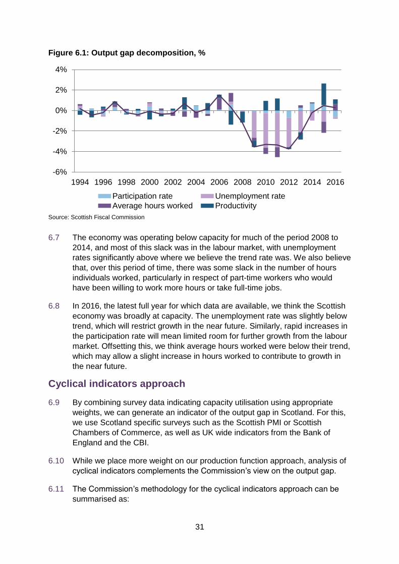
31

Figure 6.1: Output gap decomposition, %

Source: Scottish Fiscal Commission

6.7 The economy was operating below capacity for much of the period 2008 to

2014, and most of this slack was in the labour market, with unemployment

rates significantly above where we believe the trend rate was. We also believe

that, over this period of time, there was some slack in the number of hours

individuals worked, particularly in respect of part-time workers who would

have been willing to work more hours or take full-time jobs.

6.8 In 2016, the latest full year for which data are available, we think the Scottish

economy was broadly at capacity. The unemployment rate was slightly below

trend, which will restrict growth in the near future. Similarly, rapid increases in

the participation rate will mean limited room for further growth from the labour

market. Offsetting this, we think average hours worked were below their trend,

which may allow a slight increase in hours worked to contribute to growth in

the near future.

Cyclical indicators approach

6.9 By combining survey data indicating capacity utilisation using appropriate

weights, we can generate an indicator of the output gap in Scotland. For this,

we use Scotland specific surveys such as the Scottish PMI or Scottish

Chambers of Commerce, as well as UK wide indicators from the Bank of

England and the CBI.

6.10 While we place more weight on our production function approach, analysis of

cyclical indicators complements the Commission’s view on the output gap.

6.11 The Commission’s methodology for the cyclical indicators approach can be

summarised as:

-6%

-4%

-2%

0%

2%

4%

1994 1996 1998 2000 2002 2004 2006 2008 2010 2012 2014 2016

Participation rate Unemployment rate

Average hours worked Productivity

32

The results from each indicator of capacity surveys are standardised

so that they can be consistently combined. This is done respective to

the historic average and standard errors.

These standardised indicators of capacity are then combined using

appropriate weights. This includes industry weights or whether the

survey refers to labour or capital shares. This results in an aggregate

standardised indicator for the output gap.

Finally, the Commission determines the mean and standard

deviation to impose to the standardised indicator of the output gap.

The Commission considers the distribution of the production function

output gap estimates over the same time frame provides the most

appropriate indicator.

6.12 The surveys used collect qualitative rather than quantitative information,

usually based on the number of firms responding to binary questions on

capacity shortage. This gives an indication of the number of firms facing

capacity shortages, but it does not necessarily indicate the intensity of the

shortage. The surveys are also somewhat limited in scope for Scotland. We

therefore use evidence from the cyclical indicators approach as an additional

source of information to complement our production function derived

estimates.

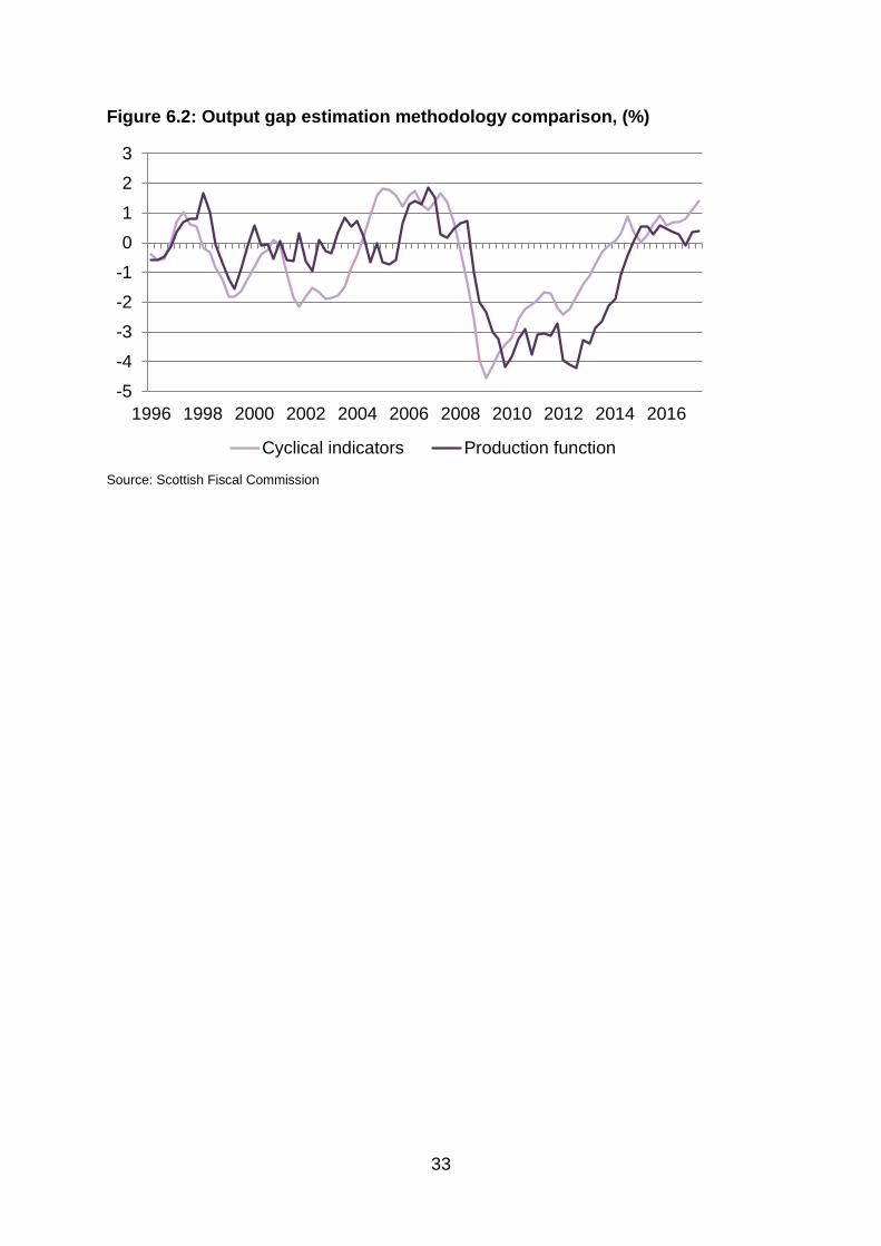
6.13 Figure 6.2 compares the two estimates of the output gap in Scotland. Whilst

derived from different methodologies and data, the two approaches provide

broadly similar estimates. This gives us greater confidence in our production

function approach to estimating potential output. Whilst our production

function approach suggests that the Scottish economy was broadly on trend

in the latest quarter with a small but positive output gap of +0.4 per cent,

surveys of the Scottish economy are suggesting that the economy is now over

capacity, with an output gap of +1.4 per cent.

6.14 Both approaches indicate a positive output gap for Scotland, implying that

there has been a structural slowdown in economic growth.

33

Figure 6.2: Output gap estimation methodology comparison, (%)

Source: Scottish Fiscal Commission

-5

-4

-3

-2

-1

0

1

2

3

1996 1998 2000 2002 2004 2006 2008 2010 2012 2014 2016

Cyclical indicators Production function

34

Annex 1: Generation of industry

productivity figures

A.1 The Commission decomposes its productivity figures between the

construction and non-construction industries. Through this decomposition, the

Commission aims to account for the temporary boom in the construction

industry in 2014.

A.2 For this, the Commission decomposes and combines the trend component of

both the construction and non-construction industries. The methodology for

obtaining this is described below.

1. Generate weighted industry GDP series

A.3 We multiply the construction and non-construction output indices with their

respective weights in total output. These weighted indices are shown in Figure

A.1.

Figure A.1: Weighted industry GDP, Index (2014 Total GDP = 100)

Source: Scottish Fiscal Commission

A.4 Figure A.1 illustrates how the construction industry significantly supported

GDP growth in 2014, but it has acted as a drag to GDP growth since then.

2. Generate quarterly industry hours series

A.5 Total APS hours are combined with the industry shares of total hours worked

given by the ONS regional productivity hours series. This is shown Figure A.2.

5

7

9

11

13

15

86

88

90

92

94

96

2009 2011 2013 2015 2017

Non-construction (LHS) Construction (RHS)

35

Figure A.2: Total hours worked in the Construction and non-construction

industry, millions

Source: Scottish Fiscal Commission

3. Generate productivity series that are comparable across industries

A.6 We divide weighted industry GDP series by the industry hours series for both

the construction and non-construction industries. These are the actuals values

in Figures A.3 and A.4.

4. Generate trend values for productivity across industries

A.7 We use an HP filter – a way of smoothing data - for the non-construction

industry productivity, while we apply a constant productivity during and after

the construction boom, as indicated by the trend lines in Figures A.3 and A.4.

5

7

9

11

13

69

71

73

75

77

2009 2011 2013 2015 2017

Non-construction (LHS) Construction (RHS)

36

Figure A.3: Productivity excluding the construction industry

Figure A.4: Productivity in the construction industry

Source: Scottish Fiscal Commission

5. Generate industry productivity weights

A.8 We calculate the productivity weights of the construction industry productivity

that allow us to combine the construction and non-construction industry into

aggregate productivity. These weights come from the following expression.

( ) ( ) ( ) ( ( )) ( )

A.9 This gives us:

( ) ( ) ( )

( ) ( )

6. Generate trend productivity series:

A.10 We combine the construction and non-construction industry productivity

figures with their respective weights to obtain the aggregate trend productivity

series illustrated in Figure A.5.

80

85

90

95

100

105

1998 2001 2004 2007 2010 2013 2016

65

75

85

95

105

1998 2001 2004 2007 2010 2013 2016

37

Figure A.5: Actual and trend productivity, Index 2014 = 100

Source: Scottish Fiscal Commission

70

75

80

85

90

95

100

105

1992 1995 1998 2001 2004 2007 2010 2013 2016

Actual data Projected data

38

© Crown copyright 2018

This publication is available at www.fiscalcommission.scot

ISBN: 978-1-9998487-6-7

Published by the Scottish Fiscal Commission, March 2018