Discrete Mathematics 104 (1992) 99-110

North-Holland

99

Fast Lagrange inversion, with an application to factorial numbers

Heinrich Niederhausen Florida Atlantic University, Boca Raton, FL 33486, USA

Received 10 May 1990

Abstract

Niederhausen, H., Fast Lagrange inversion, with an application to factorial numbers, Discrete

Mathematics 104 (1992) 99-110.

Suppose /3(t) and y(t) are a pair of compositional inverse formal powerseries. Lagrange

inversion expresses the coefficient oft” in y(t)” in terms of the coefficient of tC” in /c?(t)-“. ‘Fast

Lagrange inversion’ calculate the latter for invertible power series with nonzero quadratic

term, using only positive powers of /?. The result is given for multivariate series, and illustrated by a bivariate generalization of Stirling numbers.

1. Introduction

A delta series is a formal power series of the form P(t) = Pit + &t2 + . . . ,

PI # 0, and any delta series has a compositional inverse y(t), say, where

B(y(t)) = t. It 1s well known that the coefficient ( yk), of t” in y(t)” equals

(k/n)( p-“) _-k for all integers k c n # 0 (see [3]). This Lagrange inversion

procedure is usually not attractive, because the coefficients of negative powers of

P(t) are difficult to obtain in many applications. For example, let a and b be two

different real or complex numbers, and define P(t) := ear - ebr. For nonnegative

integers m, P(t)” has the coefficients

where F(k, m) belongs to the family of factorial number of the second kind

(0 c m c k). Best known members are the Stirling numbers, where a = 1, b = 0,

and the central factorial numbers of the second kind (a = l/2 = -b). (There are

combinatorial interpretations of factorial numbers for a large class of integer

values of a and b [IS].) Applying the binomial theorem to (e”’ - ebr)m for positive

integers m is straightforward, giving

m! F(k, m) = 2 (“)(-l)“-‘(ja + (m -j)b)k. j=O I

0012-365X/92/$05.00 fQ 1992 - Elsevier Science Publishers B.V. All rights reserved

brought to you by COREView metadata, citation and similar papers at core.ac.uk

provided by Elsevier - Publisher Connector

100 H. Niederhausen

But how can we obtain the coefficients of negative powers, where the binomial

theorem does no longer apply? We begin by defining for 1~ k s n the factorial

numbers of the first kind as

fapb(n, k):=(k _ l)!

(n - 1Y (/y_,.

That they are not so easily expressed in terms of powers and factorials, we know

already from the Stirling numbers of the first kind. Yet, such expressions exist,

and Lagrange inversion is still practical because of the following observation.

There is a large class of invertible power series, where the coefficients (pi)k are

actually values of some polynomials Ej(X), deg 5j =i. More precisely, (pi)k =

/3:GkJi) for all integers k > i, positive or negative! In that case it is easy to find

(p-“) _+ just be extrapolation,

(fib”j-k= (“,“I,“) 2 (” T k)(_ly~B~'-~(Bi),+.-,.

For the factorial numbers of the first kind, this ‘fast’ Lagrange inversion gives

(a - b)n-kfa,b(n, n -k)

This is well known for Stirling numbers, and can be found in [2] for central

factorial numbers.

Exactly which delta series have coefficients such that extrapolation can be used

for fast Lagrange inversion? To answer that question we have to introduce

polynomials of binomial type. A sequence {p,(x) 1 n = 0, 1, . . .} of polynomials

is of binomial type, iff degp, = n, p,,(x) = 1, and

Pntx +Y)=~oPi(x)Pn-i(Y)

for all n = 0, 1, . . . The answer to the

from results on polynomials of binomial

above question can be directly derived

type with polynomial coefficients [6].

Theorem 1. Let P(t) be a delta series. There exists a sequence {Gn(x) ( n =

0, 1, . . .} of binomial type such that (a’), = /3fbk_i(i) for all integers i s k iff pz,

the coefficient of the quadratic term in #l(t), is different from zero.

Whereas the theory of multivariate Lagrange inversion is very similar to the

univariate case, the actual calculation of an inverse may be tedious. Therefore,

‘fast’ Lagrange inversion can be especially helpful in the presence of several

variables. For that reason we prove Theorem 1’ in Section 3, the multivariate

version of Theorem 1, and present the whole theory in the multivariate setting.

As a reference frame for multivariate Lagrange inversion and Umbra1 Calculus,

Fast Lagrange inversion 101

we have chosen the paper ‘Dual Operators and Lagrange Inversion in Several Variables’ by Verde-Star [7]. Other approaches we want to mention are [l, 4, 8-91.

Not every invertible multivariate series /3 is a delta series as defined in the next section. But there always exists an invertible transformation which carries B into a delta series. As an example, we invert (em - ebr, ecs - ed’), ad # bs, in Section 4. This formal power series can be seen as a bivariate version of the factorial generating function ear - eb’. Its compositional inverse has relatively simple coefficients, which are just products of two factorial powers.

2. Multivariate Lagrange inversion

In most aspects, our notation follows closely the ‘Dual operators an Lagrange inversion in several variables’ Verde-Star [7]. Let r be a positive integer. On Z we consider the natural (componentwise) partial order. (In [7], other orders are also considered.) Let K be a field of characteristic 0, and 9 be the ring of all Laurent series C,, k,t”, where the support of the coefficients k, is bounded from below, i.e., there exists an m E z’ such that k, # 0 implies n 3 m. If k, # 0, we

say that the series is of order m. The Laurent series whose coefficients have a support bounded by 0 constitute a subring s0 of 9. Define %:= { cp E s0 1 q(O) =

l}, so all elements of 2 are of order 0. We are mainly interested in vectors

p = (Bl($ . . . f /$(t)) where /Ip(t)/tp is in 2 for all p = 1, . . . , r. The set of all such vectors is denoted by 3. If p E ‘3, we call /3 a normed delta series. /3 is a delta series, if P(t,/a,, . . . , &/a,) E 52 for some constant vector u with non-zero components. Every delta series has a compositional inverse, which is another delta series y such that /3,(r(t)) = tP for all p = 1, . . . , r.

Boldfacing of vectors indicates products, i.e., if y = (yl, . . . , yr) we use the notation y :=y, x . . . x y,, so t” = t~‘t~’ x . . . x t:, but t” = (t;‘, t;*, . _ . , t:‘). Also, n! = n,! x . . - x n,!, and

n 0 n! =

i i! (n - i)! .

To indicate the coefficient of f’ in a single Laurent series q(t) we write ( q)i, or simply vi if no confusion can occur. In this notation, an inverse pair can be expressed as an orthogonality relation on the coefficients. p and y are inverse delta series iff for all p = 1, . . . , r, j E Zp

where eP E z’ has the pth component equal to 1, and all others equal to 0.

102 H. Niederhamen

Denote the Jacobian determinant of /3 by J/3, and the vector of all ones in z’ by e:=(l,. . . , 1). If y is the compositional inverse of some delta series p, then the coefficient ( yk),, of f” in yk equals the coefficient (/3-“-‘J/3_k_e of tmkdC in jP-‘J~, where -n -e = (-n, - 1) x * . . x (-n, - 1) for all k, n E z’ [7].

The differentiation rules for multivariate power series allows us to write the Jacobian of j3” as

Hence, we can rephrase the Lagrange inversion result as follows.

If y ks the compositional inverse of /3, then the coeficient ( yk),, of t” in yk equals the coefficient of tCkme in (11 - n)J/F, if all components of n are different from zero.

We now explore that last coefficient.

So far, we assumed that n has no zero component. Suppose, 0 6 k s n, and n, = 0 is the only vanishing component of n. Then k, = 0, and

(Ykjn = (s-“-eJ~)-k-e = (--&- det(8,,,),,,=~,...,r)_k_e. Y

where fiP,O = DPPanO if o # Y, and bP,V = /3;1DP/?y. For p # Y one obtains bP,V= Dp log@&/t,) and by,,,= t;’ + D, log(/3,,/t,) as in [l, p. 3201. Note that fiy,y is the only element of (~P,O)P,O=l,,..,P that contains a negative power of t,,. But the vth component of -k - e equals - 1, so

(r”>n =( _,l+, t;’ det(Dpaan,)p,o=l,...,p;p2v20 Y > -k-e'

In other words, (r*)” still equals

if we eliminate all components in the latter expression for which n has a zero component.

Fast Lagrange inversion 103

Proposition 1. Zf y is the compositional inverse of a delta series /?, then the coeficient of t” in yk equals

(Y”>n = -& j,+,,,~,=_k (Cl (B~““)iJdet(i3 for all 0 s k s n, if n has no zero component. lf n has vanishing components,

compress all vectors on the right-hand side by eliminating those components,

where n is zero.

Of course, for r = 1 this specializes to the well-known result

(Y”L =x WLk.

If one is interested in yP only (k = e,), the formula slightly simplifies. For r = 2

we obtain the following.

Corollary 1. Zf y = (yl(s, t), y&, 4) is the compositional inverse of a delta series

j3 = (~76, t), ~6, t)), then:

(YlLo=; (ds, VL

for all positive integers m and n.

Example. Let /3(s, t) = stesr/(l + s + t) = Q)(s, t)q(s, t), where Q)(s, t) = sesf, and

+(s, t) = t/(1 + s + t). So we find

( c.p-“)i,j = (-my/j! ifj>Oandi=j-m,

and

( q-“);,j = n! (_j_i)!i!(j+n)! ifi~Oand-z~~~-n-

104 H. Niederhausen

Corollary 1 gives for positive m and n

(YlL.” = - c (-my’(n - l)!

j j!(2j+3-m)!(m-j-2)!(n-l-j)!’

where the summation index j takes all integer values such that the factorials are defined in the usual sense. Hence,

y,(s, t) =s -,g (&)j i: ‘--&;?;-‘sm+j+l m=O .

and

3. Sequences of binomial type

Denote by K[x,, . . . , x,] the algebra of polynomials over K in the variables

Xl, . . . , x,. A polynomial sequence {b,(x) ( n 3 0} has coefficients bnFi, where

b”(X) = i b”,i$ i=O

with b,,, # 0. The range of the summation i = 0, . . . , n stands for all integer vectors i such that 0 s i G n. The generating function of a polynomial sequence is a formal power series in K[x][[t]].

A polynomial sequence {b,(x) ( it 3 0} is of binomial type iff

W + Y) = i: W)b,-i(y) i=O

for all it E W. Note that b,(O) = do,,. Polynomials of binomial type can also be characterized by their coefficients:

b”,, f 0 and b,+i+j.i+j= 2 bk+i,ibn-k+j,j (1) k=O

for all i, j, n l FV.

Definition. The polynomial sequence {b,(x) ) II 2 0} has polynomial coefficients iff there exists a polynomial sequence {6a(~) 1 n 2 0} such that b,,i = 6,-i(i) for all 0 G i S n.

Fast Lagrange inversion 105

In order to see which sequences of binomial type have polynomial coefficients,

we need a few results from the Umbra1 Calculus.

Proposition 2 [7, Proposition

sequence, and let

&At) = c bv,,f” n=rJ

(p = 1, . . . , r). {b,(x) 1 n SO}

B(t)” = c b,,,t” n3m

for all m E IV.

4.3(i)]. Suppose, {b,(x) 1 n 20} is a polynomial

is of binomial type iff p, is of order e,,, and

Lemma 1 [7, (4.15)]. The polynomial sequence {b,(x) 1 n 2 0} is of binomial

type iff

& bJW = exp[x . PWL

where B(t)+ = pp(t) has order eP (p = 1, . . . , r).

Proposition 2 shows us how a sequence {b,,,,, 1 n > e,,, p = 1, . . . , r} of

scalars determines the whole sequence of binomial type. In the following lemma

we show that the same is true for the scalar sequence {b,(eP) 1 n 3 eP, p = 1, . _ . , r}.

Lemma 2. Let an,p E K for all n E N’, p = 1, . . , r. There exists a sequence {b,(x) 1 n 3 0} of binomial type such that b,(e,) = an,p for all n E N’, P= 1 , . . . , riffa,,,=landa,p,,#Oforallp=l ,... ,r.

Proof. If {b,(x)} is of binomial type, then we know from Lemma 1 that for

x=e P

by Proposition 2. So we see that ao,P = b,,,, = 1, and ae,,p = b+O + be,,,+ = bpp,e,, Z 0. Vice versa, if b,(e,) = an,p we have to find a power series /3,,(t) of order ep, the

‘logarithm’ of CnaO b,(e,)t”, such that

nzobn(ep)t” = Lz &(t)‘Ih!-

Let &(t) = CnzO d,$‘. Choosing L = 1 gives de0 = b,(e,) = ae,,P # 0, so &p(t) will

be of order ep. For n > eP we calculate an,p = d,, + sum of products of coefficients

106 H. Niederhausen

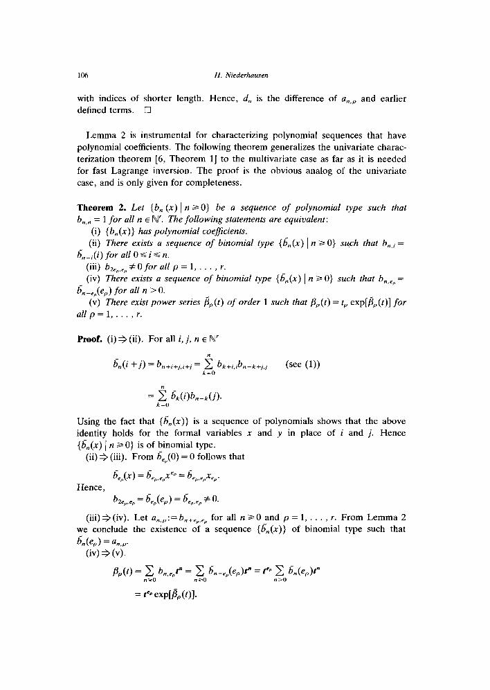
with indices of shorter length. Hence, d, is the difference of CZ~,~ and earlier defined terms. 0

Lemma 2 is instrumental for characterizing polynomial sequences that have polynomial coefficients. The following theorem generalizes the univariate charac- terization theorem [6, Theorem 11 to the multivariate case as far as it is needed for fast Lagrange inversion. The proof is the obvious analog of the univariate case, and is only given for completeness.

Theorem 2. Let {b, (x) ) n > 0) be a sequence of polynomial type such that b,,, = 1 for all n E N’. The following statements are equivalent:

(i) {b,(x)} has polynomial coeficients. (ii) There exists a sequence of binomial type {by 1 n 2 0} such that b,,i =

bn_i(i) for all 0 6 i S n.

(iii) bsep,e, # 0 for all p = 1, . . . , r. (iv) There exists a sequence of binomial type {bn(x) 1 n 2 0} such that b,,ep =

b”__,(e,) for all n > 0. (v) There exist power series &,(t) of order 1 such that rBp(t) = tP exp[&,(t)] for

all p = 1, . . , , r.

Proof. (i) + (ii). For all i, j, n E N’

bn(i +f) = b,+i+i,i+j = i bkti,ibn-k+j,j (see (1)) k=O

= k$o &k(i)bn--k(j),

Using the fact that {sn(x)} . IS a sequence of polynomials shows that the above identity holds for the formal variables x and y in place of i and j. Hence {bn(x) ( n SO} is of binomial type.

(ii) + (iii). From sC,p(0) = 0 follows that

&P&,(-4 = &&,&-,xeP = &,,&O. Hence,

b bP,eP = be&e,) = b+.Cp # 0.

(iii)+(iv). Let a,,P:= b,,+eP,eP for all n ~0 and p = 1, . . . , r. From Lemma 2 we conclude the existence of a sequence {hn(x)} of binomial type such that

&(e,) = a,,,. (iv) 3 (v).

/3,,(t) = c b,,,t” = c bn_,(eP)t” = tep c &(e,)t" ?I*0 IIS- n>O

= teP exp[&(t)].

Fast Lagrange inversion 107

(v) j (i). By Proposition 2,

c b,,,t” = p(t)” = t” exp[m * b(t)] = c 6n(m)t”cm “3l?l n=rl

Comparing coefficients shows that b,,, = 6,_,(m). 0

(Lemma 1).

The multivariate generalization of Theorem 1 is a simple consequence of

Theorem 2.

Theorem 1’. If /3(t) . 1s a delta series such that (/3, )2e, # 0 for all p = 1, . . . , r, then

there exists a sequence {ha(x) 1 n 2 0} of polynomial type such that

<P9>n = &-kpJkpe,)

for all integers k,,, and n E N’ + kpe,, p = 1, . , . , r. Furthermore,

nzO ~Ak,e,)t” = (PP(t)ltJkP.

Proof. By Proposition 2, (&,);?e, = b2ep,ep, where {b,(n) 1 n 20} is the cor-

responding sequence of binomial type. Hence, we know from Theorem 2 that

&,(t)krl = t2 exp[k,&(t)] = tk exp[k,e, . B(t)]

for some delta series fi. Let {sn(x) 1 n 2 0} be the corresponding sequence of

binomial type. Then

(P,(W,)“p = nTO &(k,e,)t”. q

4. Example

A bivariate generalization of ear - ebr can be constructed as the pair ,u,(s, t) :=

ear - ebr, and pZ(s, t) : = ecS - edt. ~1 has a compositional inverse iff ad - bc # 0, but

p is not a delta series. Hence, we transform ~1 into a delta series by considering

&:=~ro~ and /&:=y201z, where &(s, t):=ds + bt, and &(s, t):=cs +at. This

gives

pl(s, t) = eobr(eadF - ebcs), and &(s, t) = ecds(ebcr - eadr).

The transformed series factors, which simplifies our calculations! For positive

integers m, n, i and j,

(/I??)~,~= ((e’“-ebcS).“)j~=m!~~,~yFI(i, m), . .

and

108 H. Niederhausen

where F,(i, m) and F,(j, n) are the factorial numbers of the second kind as

defined in the introduction, corresponding to (en& - ehcs)m and (ebrr - endon,

respectively. Thus, F,(j, n) = (-l)“F,(j, n). By Theorem l’, the coefficients

(&) i.i are values of a sequence {&_(x) 1 m, 12 2 0} of binomial type, so that for

all integers i, 2 m, j, 3 0, i2 a n, jz 2 0

(ad - bC)-“(PT)il,j, = 6i,-,,j,(m, 0)

and therefore

(P;l)i,,j, = 6f,-,(m) F, (PZ)i,,j, = y 6,2,-n(n),

where the univariate sequences {6:(x) 1 n E N} and {d:(n) 1 n E N} have gener-

ating functions ((eadS - ebC*)/S)x and ((ehCf - eadf)t)x, respectively. In terms of

factorial numbers of the first kind (as defined in the introduction),

We find the inverse y of /3 from Proposition 1. For positive integers IZ and m, and

Oslsrn, Oskcn,

X 6~_,_j(-n)(l(k + j) + ik)

= $$ z: IzI (1 + i - l)! fadShc(m, 1 + i)

x (-abmY j!

. (k +j - l)!fudSbc(n, k + j) q (I(k + j) + ik),

and

- eadr)-n)_k = (-1)” i!++‘~bc(n, k).

The above expression for ( y{ Y$)~,+ can be simplified, using an identity which

is easily derived as follows. The factorial numbers of the first kind are the

connection coefficients between the powers E” and the polynomials of binomial

type MC) I y = 0, 1, . . . } (see [S]), satisfying th e system of difference equations

p,(E + ~4 -py(E + bc) =py--1(E), y = I, 2, . . .

Fast Lagrange inversion 109

where

q;d:d’bc(Q = (ad - bc)-“+ vjj; (E - iad - (Y - i)bc).

From qy ad+u’v~bc+u”‘( 5) = q$bc( 5 - u) follows that

f ad+ulm,bc+ulm(‘, 1) = 5’ (I + i - ‘)f od,bccm, [ + i)(_u)-i.

i=O

To shorten the notation, we think of ad and bc as fixed, u, m, and 1 as variable, and write f (m, I; u) for the above factorial number. In this notation,

(y:YL, = (-1)“~. [f h 1; CdnIf (n, k; abm) . .

- abm f (m, 1; cdn)f(n, k + 1; abm) - cdn f (m, I+ 1; cdn)f (n, k; abm)].

Especially,

abm f (m, 1; cdn)f (n, 1; abm)

= (- l)“-‘abm q zdpbc( -abm)q”,d~bc(-cdn),

(y2)m.n = (-I)“-‘cdn 4 ~d*bc(-abm)q~~bc(-cdn),

and ( Y,),,,.o = q~bc(o), (YZ)~,~ = (-l)“qtd,bc(0). Hence, cdn(y,),,, =

ah ( ydm,n. The compositional inverse of p is now obtained as (A,0 y, A20 y),

where

(Q ~>m,n = (dy, + by,),,,

= (-l)“-‘bd(am + cn)q”,“~b’(-abm)q~~bC(-cdn),

(&0YLV = (CY, + aYA.n

= (- l)“-‘ac(bm + dn)qz”*““(-ubm)q”,““‘( -cdn).

References

[l] A. Brini, Higher dimensional recursive matrices and diagonal delta sets of series, .I. Combin.

Theory Ser. A 36 (1984) 315-331. [2] P.L. Butzer, M. Schmidt, E.L. Stark and L. Vogt, Central factorial numbers; their main

properties and some applications, Numer. Funct. Anal. Optim. 10 (1989) 419-488.

[3] P. Henrici, Applied and Computational Complex Analysis, Vol. 1 (Wiley, New York, 1974).

[4] .I. Hofbauer, A short proof of the Lagrange-Good formula, Discrete Math. 25 (1979) 135-139.

110 H. Niederhausen

[5] H. Niederhausen, Colorful partitions, permutations, and trigonometric functions, Congr. Numer.,

77 (1990) 187-194.

[6] H. Hiederhausen, Sequences of binomial type with polynomial coefficients, Discrete Math. 50

(1984) 271-284. [7] L. Verde-Star, Dual operators and Lagrange inversion in severable variables, Adv. Math. 58

(1985) 89-108. [S] T. Watanabe, On dual relations for addition formulas for additive groups, I, Nagoya Math. J. 94

(1984) 171-191. [9] T. Watanabe, On dual relations for addition formulas for additive groups, II, Nagoya Math. J. 97

(1985) 95-135.