applications of ^-lagrange inversion to basic ... · we have seen that theorem 1.2 is the ^-analog...

transactions of theamerican mathematical societyVolume 277, Number 1, May 1983

APPLICATIONS OF ^-LAGRANGE INVERSION

TO BASIC HYPERGEOMETRIC SERIES

BY

IRA GESSEL1 AND DENNIS STANTON2

Abstract. A family of g-Lagrange inversion formulas is given. Special cases include

quadratic and cubic transformations for basic hypergeometric series. The g-analogs

of the so-called "strange evaluations" are also corollaries. Some new Rogers-

Ramanujan identities are given. A connection between the work of Rogers and

Andrews, and ^-Lagrange inversion is stated.

1. Introduction. The Lagrange inversion formula solves the following problem:

Given

y = y(x) — bxx + b2x2 + ■ ■ ■ , bx ¥= 0,

and

f(x)=f0+fx+f2x2+---

as formal power series in x, find the constants ak so that

f(x) = a0 + axy + a2y2+ •■-.

The special casef(x) = x gives the inverse function of y(x). Recently, ^-analogs of

this problem have been studied by Andrews [4], Gessel [23], and Garsia [22]. As

Garsia shows, they are equivalent to finding the constants ak for

(1.1) f(x) =a0 + axy(x) + a2y(x)y(xq) + ■■■ .

Unfortunately, there are very few examples for which this beautiful theory applies

easily. (The case y(x) = x/(l — x) works and was considered by Carlifz [15].) In

this paper we give many examples of ^-analogs of Lagrange inversion.

However, our examples do not satisfy (1.1). Instead, we concentrate on ^-analogs

of Lagrange inversion for y - x/(l - jc)*+1. We state here an example (b = 1) of

such a ^-Lagrange inversion. Throughout this paper we consider only formal power

series in x whose coefficients are rational functions of q. We use the customary

notation, (a)x = II^oO _ a4') and (a>* = (ö)»/**?*)»-

Received by the editors March 3, 1982.

1980 Mathematics Subject Classification. Primary 33A35; Secondary 05A19, 10A45.Key words and phrases. Lagrange inversion, basic hypergeometric series, Rogers-Ramanujan identities.

'Partially supported by NSF grant MCS 8105188.2Partially supported by NSF grant MCS 8102237.

©1983 American Mathematical Society

O0O2-9947/82/00OO-0395/$O6.50

173

License or copyright restrictions may apply to redistribution; see https://www.ams.org/journal-terms-of-use

174 IRA GESSEL AND DENNIS STANTON

Theorem 1.2. Letf(x) = If=0fkxk. If

n }~ (*)« ¿o k(Ax)k(l-x/q)---(l-x/qkY

thenfn = 2¡5=05„A:aA:' and vice versa, ak — 2k=0Bkjf,, where

_(Aq2k)n.k

a«if

„-i _ (Aq)2k-i(l - Aq2') ,k-,tu+k,( ,k-iBki -—T~\—m-a (~l) ■

(q)k-i(M)k+i

This theorem explicitly solves for the aks in terms of the//s by giving the entries of

the inverse matrix Bkj. It is somewhat related to (1.1). If we put A = 1, yx(x) —

1/(1 — xq), and y2(x) = 1/(1 — x/q), then we are solving for the constants ak in

(1.3)

f(x) = a0 + q-xaxxyx(x)y2(x) + q-4a2x2yx(x)yx(xq)y2(x)y2(xq-x) + ■■■ .

So the shifting in q occurs in both directions, not just one as in (1.1).

Theorem 1.2 has some far-reaching consequences. It can be used to give a

systematic approach to ^-analogs of quadratic transformations. There is a scattering

of such results in the literature [3,16,27,29,33]. However, the techniques are

verifications by manipulating sums. With Theorem 1.2 we can systematically con-

sider the "correct" series.

Perhaps the first ^-quadratic transformation was Sears' [29, Equation (4.1)] ^-ana-

log (see also [16]) of the well-poised 3F2 quadratic transformation. It follows from

Theorem 1.2. Moreover, we derive Watson's transformation of a very well-poised

8$7 [11, Equation 8.5(2)] from this transformation. It is well known that Watson's

transformation implies the Rogers-Ramanujan identities. Other ^-quadratic transfor-

mations will imply identities that are similar to the Rogers-Ramanujan identities.

Some of these are new, while others appear on Slater's hst [31]. This is no accident.

G. Andrews has commented [6] that much of Rogers' work was based upon the

"Bailey transform". He then inverted the transform by finding the inverse of a

certain matrix. That matrix is exactly our matrix B in Theorem 1.2. So it is fair to

say that Rogers' work was really a hidden special case of <¡r-Lagrange inversion.

We have seen that Theorem 1.2 is the ^-analog of Lagrange inversion for

x/(l — x)b+ ', b = 1. We also give ^-analogs of Lagrange inversion for a general b in

Theorem 3.7. The theorems for b = 2,0, -2, -3, and 1/2 are also explicitly stated in

§3. We concentrate on these values in §§5 and 6. In particular, we give more

(7-quadratic and ^f-cubic transformations in these cases.

In [24], we derived new evaluations of hypergeometric series by applying the

Lagrange inversion formula to the q = 1 version of these transformations. So in this


APPLICATIONS OF ^-LAGRANGE INVERSION 175

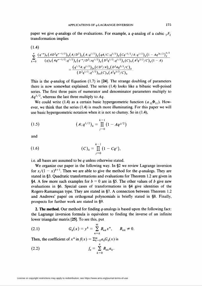
paper we give ^-analogs of the evaluations. For example, a ^-analog of a cubic 3F2

transformation implies

(1.4)

¿o («)*(^í"+1/I;«1/2)*(í-Vfl2wI/2)*(DV/2;íI/2)*(c)t(/<V/1/c)4(i - >o

_(<?'/2^<?'/2)2„(coV^)n(P2^3/2/c)n

(oV/2;?,/2)2„(c)„(¿y/Vc)„ ■

This is the çr-analog of Equation (1.7) in [24]. The strange doubling of parameters

there is now somewhat explained. The series (1.4) looks like a bibasic well-poised

series. The first three pairs of numerator and denominator parameters multiply to

Aqx/2, whereas the last three multiply to Aq.

We could write (1.4) as a certain basic hypergeometric function (a ,2$,,). How-

ever, we think that the series (1.4) is much more illuminating. For this paper we will

use basic hypergeometric notation when it is not so clumsy. So in ( 1.4),

(1.5) (A;qX/2)k = k][(l-Aq"2)

7 = 0

and

(1.6) (nk= n (i-<v),7 = 0

i.e. all bases are assumed to be q unless otherwise stated.

We organize our paper in the following way. In §2 we review Lagrange inversion

for x/(l — x)b+x. Then we are able to give the method for the g-analogs. They are

stated in §3. Quadratic transformations and evaluations for Theorem 1.2 are given in

§4. A few more such examples for b = 0 are in §5. The other values of b give new

evaluations in §6. Special cases of transformations in §4 give identities of the

Rogers-Ramanujan type. They are stated in §7. A connection between Theorem 1.2

and Andrews' paper on orthogonal polynomials is briefly stated in §8. Finally,

prospects for further work are stated in §9.

2. The method. Our method for finding ^-analogs is based upon the following fact:

the Lagrange inversion formula is equivalent to finding the inverse of an infinite

lower triangular matrix [25]. To see this, put

CO

(2.1) Gk(x)=yk= ^Bnkx", Bkk*0.n = k

Then, the coefficient of x" inf(x) = 1f=0akGk(x) is

(2.2) /„= 2 BHkak.k = 0



To solve for the ak's in terms of the/„'s is equivalent to finding the inverse of the

matrix B,

n

(2.3) an= 2 B-Xkfk.k=0

The Lagrange inversion formula solves for B~l in terms of the coefficients

[bx,b2,_} that define the power series for y. The generalized inversion problem

defines Gk(x) by (2.1) for some lower triangular matrix Bnk. Then one wants to find

the inverse matrix B~xk. This process gives our examples of q-Lagrange inversion.

First we consider the example of the usual Lagrange inversion formula upon

which our ^-analogs are based. We take

00

(2.4) f(x) = 2 fkxkk = 0

and try to expand

00

(2.5) f(x)-(l-xya2ak[x/(l-x)b+x]

So, the function Gk(x) here is

(2.6) Gk(x) = xk(l-xy-k{b+X\

which, fora = 0, isyk,y = x/(l - x)b+x. Thus

(a + (b + l)k)n_k(2.7) Bnk = (n-k)\

(In this section we adopt the usual q — 1 notation: (A)n — T(A + n)/T(A).) By the

Lagrange inversion formula (see [33]), we see that an is the coefficient of x" in

(1 + bx)(l - x)a-x+n(b+X)f(x), so

hM „-i _(l-a- n(b+ l)),,,^,, ,.,.,.,(2-8) Bnk-(n-k)\-(~a-(b+l)k).

To find a ^-analog of (2.7) and (2.8), we consider the orthogonality relations

(2.9) Sn/= ÍBn-xBklk = l

" (l-a-n(b+ !))„_,_, UL.A°+(b+l)l)k-,~l-Ô^ï)i-[-a-(fc + 1)*] (k-iy. '

(2.10) 8nl = 2 5n,B;;*=/

" (a + (b+ \)k)H.k(\ -a-(b+ l)k)k_,_x r.,n/1"J,-(«-*)!(*-/)!-[hi-(»+1W-


APPLICATIONS OF ?-LAGRANGE INVERSION 177

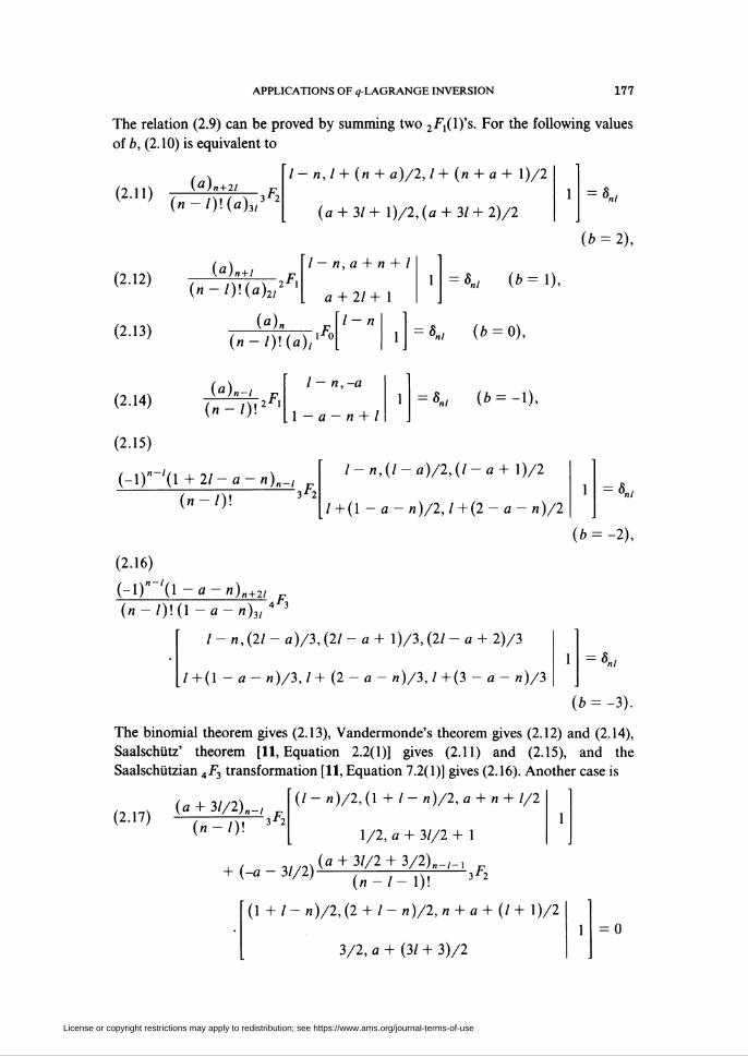
The relation (2.9) can be proved by summing two 2.F,(l)'s. For the following values

of b, (2.10) is equivalent to

(a)n+i

I- n,l+ (n + a)/2,1 + (n + a + l)/2

(a+ 31+ l)/2,(a + 3/+ 2)/2= «„/

(b = 2),

(2.12)

(2.13)

(2.14)

(2.15)

(n-l)\(a)2l

(a)n

2*1

I — n, a + n + I

a+ 21+ I

l-n

(n-iy.(a)l'O 1

--S„, (b=l),

*„/ (* = 0),

(n-/)!2 '

I — n,-a

I-a-n+l"nl (A = -l),

(-l)"-'(l+2/-fl-n)B.

(»-/)!

(2.16)

(-l)--'(l - « - h).

3r2

l-n,(l-a)/2,(l-a+ l)/2

/ +(1 - a - «)/2, / +(2 - a - n)/2= «„/

(¿ = -2),

+ 2/

(«-/)!(l-a-«)3/4*3

l-n,(21- a)/3, (21 - a + l)/3, (2/ - a + 2)/3

/ +(1 - a - n)/3, / + (2 - a - n)/3,1 +(3 - a - n)/3

= 8,nl

(b = -3).

The binomial theorem gives (2.13), Vandermonde's theorem gives (2.12) and (2.14),

Saalschütz' theorem [11, Equation 2.2(1)] gives (2.11) and (2.15), and the

Saalschiitzian 4F3 transformation [11, Equation 7.2(1)] gives (2.16). Another case is

(2.17) ^+3//,2>;-

(«-/)!3 *2

(I- n)/2,(l + I- n)/2,a + n + 1/2

1/2, a + 31/2 + 1

+ (-a - 31/2)-{n_l_l)l-3^2

(1 + I - n)/2,(2 + I - n)/2, n + a + (I + l)/2

3/2, a + (31 + 3)/2



for / < n (b = 1/2). Both of the 3F2's in (2.17) can be evaluated by Saalschütz'

theorem.

We find the ^-analogs of Bnk by finding the ^-analogs of (2.11)—(2.17). The

<7-analogs of (2.11)—(2.17) are easily written down by considering the ^-analogs of

the appropriate summation theorems (see [31, Appendix]). The ^-analog of (2.9) is

the sum of two terminating 2$,'s. It is

(2.18)n ( l-a-(b+\)n\ ( a + (b+l)l\

y V»_Jfl-/c-lV7_lk-l -(k-l)(n + nb + a)

k=l («)«-*(?)«-/

• [(1 - q-a-b'-')(l - q"-') - (1 - i<»-'X*+«))(l - qk-i)] = 0, l< n.

Nevertheless, we do not use (2.18) in this paper. In order to write (2.18) as an

orthogonality for Bnk and Bkj, we need to separate the n and / dependence. We find

it more convenient to use (2.11)—(2.17) for this purpose. Fields and Ismail [21] had

previously given (2.9). They also considered inverting an infinite upper triangular

matrix, but did not mention the connection with Lagrange inversion.

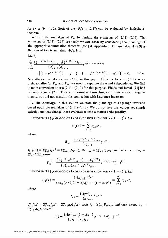
3. The (7-analogs. In this section we state the ^-analogs of Lagrange inversion

based upon the ^-analogs of (2.11)—(2.17). We do not give the tedious yet simple

calculations that change those evaluations into a matrix orthogonahty.

Theorem 3.1 (^-analog of Lagrange inversion for x/(l — x)3). Let

CO

Gk(x) = 2 Bnkx",

where

nkJ

n = k

( Aa3k/2. \/2\R - \ q ,q >n-k -nk

{l)n-k

V f(x) = lf=ofkxk = lf=0akGk(x), then f„ = lnk=0Bnkak, and vice versa, ak

2k=oBklfi, where

(Aqx;2;qx'2)3k_x(l-Aq^2) t t_,

(q)k-t(Aqx/2;qx^2)2k+¡ ? l / . "

Theorem 3.2 (^-analog of Lagrange inversion for x/(l — x)2). Let

_(Ax)xq-k2xk_ "

Gk(X) ' (x)x(Ax)k(l - x/q) ••• (1 - x/qk) " ¿f«* '

where

(M2k)n-k „-kn

Bnk - / \ <?(q)n-k

If f(x) = If=0fkxk = Z%=0akGk(x), then f„ = !U0Bnkak, and vice versa, ak

2k=oBüft> where

„-i _ (^g)2t-i(l -Aq21) (k-,v,+kl( sk-t

Bk'~ (d)k-,(Aq)k+, q (_1) •



Theorem 3.3 (¿/-analog of Lagrange inversion for x/(l - x)). Let

G(x) =_(Ax)xg-k2xk_= ZB x„

Gk{X) (xUl~x/q)...(l-x/qk) ¿kB"kX>

where

Bnk--(Aqk)n-k .

(<l)n-k

If fix) = 2f=ofkXk = 2k=0akGk(x), then /„ = 2"k=0B„kak, and vice versa, ak

2f=oBufi> where

B i = (Aq')k-lqik-,V)+lk{_l)k-t

(q)k-t

Theorem 3.4 (^-analog of Lagrange inversion for .x(1 — x)). Let Gk(x)

l^kBnkx", where

(Aqk/2;q-X/2)n-k _nk

(q)n-k

n _ V t 'T Jn-k „-nkBnk--¡—\-q ■

If fix) = 2T=ofkxk = If^afi^x), then /„ = 2nk=0Bnkak, and vice versa, ak -

2*=rA~///, where

( Aa(k+\)/2. l/2\

**; = —— 'g ^-^'(î-v^K-i) q( >')+lk-(q)k-i

Theorem 3.5 (<?-analog of Lagrange inversion for x(l - x)2). Let Gk(x) =

2%kBnkxn, where

( Aa2k/3-a-x/3)R - \Aq ,q In-k-kn

(q)n-k

If fix) = 2f=ofkXk = 2k=0akGk(x), then /„ = l"k=0Bnkak, and vice versa, ak =

2k=oBk¡fi, where

( a (2t+l)/3. l/3\

B-k)=^±- 'q ^-/-■(l-i4g2//3)g(*-?-) + */(.i)*-/-

(q)k-t

Theorem 3.6 (^-analog of Lagrange inversion for x/(l — x)3/2). Let Gk(x)

= l?=kBnkx», where

. „ _ (Aq3k/2)„-k kn/2

nk W/2W/2)n-kq '

If fix) = 2f=ofkxk = 2k=0akGk(x), ¡hen fn = 2nk=0Bnkak, and vice versa, ak =

2/=ofi*///> where

( Ân3k/2-l.n-l\»-1 -±2l_'q )k-l-\(, _ A 3//2\fl[(*-'2+,) + t/]/2/_,\*-'

The matrices in Theorems 3.1-3.6 are so much alike that one could hope for a

general theorem. Al-Salam and Verma [3] have given such a matrix. It is equivalent

to the following theorem.



Theorem 3.7 (q-analog of Lagrange inversion for x/(l - x)b+x). Let

Gkix) = ^=kBnkx", where

„ _(Apkqk;p)„-k k

ß"k ~-7~7\-q ■(q)n-k

If fix) = 2T=ofkxk = 2f=QakGk(x), then /„ = 2k=0B„kak, and vice versa, ak =

2k=oBklft, where

B~k) = (A«kpk~YX)k-'-l(l -Ap'q')qk'^-'^(-Dk-.

Note that by choosing p — qx/b, we retain Theorems 3.1-3.6. If A — qa/b, and

q -> 1, we have

Gk(x)->xk(l-x/by°-k(b+n.

We have stated Theorems 3.1-3.6 because these are the special cases of Theorem 3.7

that give identities for basic hypergeometric series.

We did not state the formulas coming from the ^-analog of (2.14). These are just

multiplying/(x) by (x)00/(Ax)x. In Theorems 3.2 and 3.3 we used the ¿/-binomial

theorem to explicitly sum Gk(x) = 2n°=kBnkx". For example, in Theorem 3.2 we

have

(3.8) Gk(x)=xkq-k2l A^i-i-^-*)".„=o yq)n

The <7-binomial theorem implies that, as formal power series in x with coefficients

that are rational functions of q,

(3.9) Gk(x) = xkq-k2(Axqk)00/(xq-k)00.

However, we can also write

, °° f^j-U-ZAr. -1\(3.10) Gk(x) = xkqkl 2 y . \ \ h(Axqk-xy,

„=0 (q'l;q'x)„

so that

(3.11) Gk(x)^xkq-k\xq-k~x;q-x)ao/(Axqk-x;q-x)00.

Equations (3.9) and (3.11) are not contradictory. They are merely two different ways

to express Gk(x) as a formal power series in x with coeffficients that are rational

functions of q. This allows us the freedom to "change q to q'x". We have chosen

(3.9) for Theorem 3.2.

There is a general theorem of which (3.8) and (3.10) are special cases. Let C[[x]] be

the ring of formal power series in x with coefficients in C. Similarly, define formal

power series rings C(<?)[[*]], C((í7))[[x]], and C((<7"'))[[;c]], whose coefficients are

rational functions of q, Laurent series in q, and Laurent series in q~x, respectively.

For the Laurent series in q, C((q)), we allow only a finite number of negative powers


APPLICATIONS OF ç-LAGRANGE INVERSION 181

of q. The coefficients in C((<¡r')) are restricted similarly. Note that C(q) C C((q)) n

C((q-X)). Then for any/(x) G C\[x]] with/(0) = 1, we see that

00

(3.12) F(x)= ][f(xqk)eC(q)[[x]].k=Q

Next we state a theorem of Garsia [22, Proposition 2.2] which tells us how to

interpret F(x) as an element of C((í7_1))[[jc]] via C(í¡r)[[*]].

Theorem 3.13. Letf(x) G C[[x]] withf(0) = 1. Then00

][f(xqk)EC(q)[[x}].k = 0

Moreover, as an element ofC((q'x))[[x]],

00 00

n f(xqk) = 1/ II f(xq~k).k=0 k=\

Proof. Letf(x) = exp(I°°=xbjXJ). Then

00 / oo \

Il f(xqk) = exp 2 bjXW (1 - qi)\ G C(q)[[x]].k=0 \j=l I

The second statement follows from

bjXJ/ (1 - qJ) = -bj(xq-l)J/ (1 - q-J). D

When necessary, we will freely use this q -» q~x idea.

In Theorems 3.1 and 3.4-3.6, we cannot express the function Gk(x) as an infinite

product. This is disappointing. However, we will find many new results from these

theorems. Also in these cases Gk(x) does not approach x*(l — x)'"~(b+X)k as q -» 1.

The limit is given in the discussion following Theorem 3.7. When q = 1 the scaling

factor of b is not important.

Carlitz [15] had given Theorem 3.3 previously, although he stated it in another

way.

For each of our theorems, we can state a natural "derivative form". For q = 1 this

is the expansion

(3.14) /(*) = (1 + bx)(l - x)'" 2 akxk/ (1 - x)($b+$k

k = 0

The derivative of x/(l — x)b+x is (1 + bx)/(l — x)b+2. In [24] we showed that any

expansion of type (2.5) naturally gives an expansion of type (3.14). We called the

latter the companion formula. The ¿¡r-analog of this procedure is to take the linear

factor from Bk) and attach it to Bnk. We illustrate this technique on Theorem 3.2.

Theorem 3.15 (q-analog of derivative form of Lagrange inversion for

x/(l - x)2). Let

G (x) - í-ííWl - .Ax2) q-k2xk(l - Aq2k) _ Sb^x)--^ (I qAx )—— - — j TJ\- L L„kx ,

(*)» (Ax)k+2(l-x/q)--- (I-x/qk) n=k



where

Cnk={A(q2P"-kq-kn(l-Aq2»y(q)n-k

If f{x) = 2?=ofkxk = lf=0akGk(x), then f„ = 2nk=0Cnkak, and vice versa, ak =

2k=tfk~}fh where

r-\ _ (Aq)2k^xj-l) (k-'ï<) + lk

CkI (q)k-,(Aq)k+l q

As a prelude to §§4-6, we give an application of Theorem 3.7 to Abel's [2]

generalization of the binomial theorem. If we let b -> oo (p = 1) in Theorem 3.7, we

find a ¿/-analog of Gk(x) = xkekßx. Lagrange inversion for Gk(x) — xkekßx yields

Abel's formula. So Theorem 3.7 should give a ¿/-analog. First we review the q = 1

case.

If Gk(x) — xkekßx, we have

nun b -îëûl!(3-16) B»k-(n-k)\

and

(3,7) ,,- - i-vwr-'ki (k-iy.

The choices of

(3-18) fu = fx

and

a(a-ßk)k '

(3.19) ak = -±-fr^-

give [1]

(3.20) e"*= 2 aia~*k)k~\xe*)k

k=o k-

and

„,n a"_ " aia-ßk)k-lißk)n-k

If we multiply eax ■ eyx and use (3.20), we find one form of Abel's formula [2],

/- M, (q + y)(« + y-/8ri)"-' - «(« - /tt)*~'y(Y - ß(n - k))n~

{ ] »' "¿o *!(«-*)!

For the ¿/-analog, we putp = 1 in Theorem 3.7 and choose

(3.23) ,,-*,.



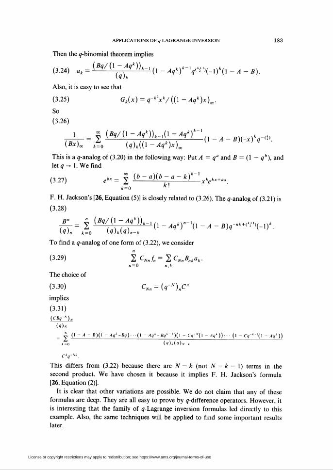
Then the ¿/-binomial theorem implies

(3.24) ak={Bq/{l-.Aqk))k-x(l-AqkrXq^(-l)k(l-A-B).

\q)k

Also, it is easy to see that

(3.25) Gk(x) = q-k\k/((l-Aqk)x)x.

So

(3.26)

1 _ - (Bq/(l-Aqk))k^x(l-Aqk)k-l_n _ , _ ,„ ^fc-_(J)= 2 x \ , „,:„ , (i-¿-g)(-*)v

(^)co *=o (i)*((i-VR

This is a ¿7-analog of (3.20) in the following way: Put A = qa and B = (1 - ¿7a), and

let q ^ 1. We find

v*-l, jb-a)(b-a-k)

k\(3.27) ebx= 2 -

A: = 0

F. H. Jackson's [26, Equation (5)] is closely related to (3.26). The ¿7-analog of (3.21) is

(3.28)

B- £ (*/0 - V))»-, (1 -¿«*)-'(1 -^ - B)q-"k^X-l)k.(q)n /t = 0 (íM?)»-*

To find a ¿7-analog of one form of (3.22), we consider

n

(3-29) 2 CNnfn = 2 CNnBnk^k-n = 0 n,k

The choice of

(3.30) CNn = (q-N)nC"

implies

(3.31)jeer")»

= y C -A -B)(\ - V -Bg).. •(! -V-y-'Hl -Cg-W(l - V))- ■(! -CV^'O ~ V))

This differs from (3.22) because there are N — k (not N — k — 1) terms in the

second product. We have chosen it because it implies F. H. Jackson's formula

[26, Equation (2)].

It is clear that other variations are possible. We do not claim that any of these

formulas are deep. They are all easy to prove by ¿7-difference operators. However, it

is interesting that the family of ¿7-Lagrange inversion formulas led directly to this

example. Also, the same techniques will be applied to find some important results

later.



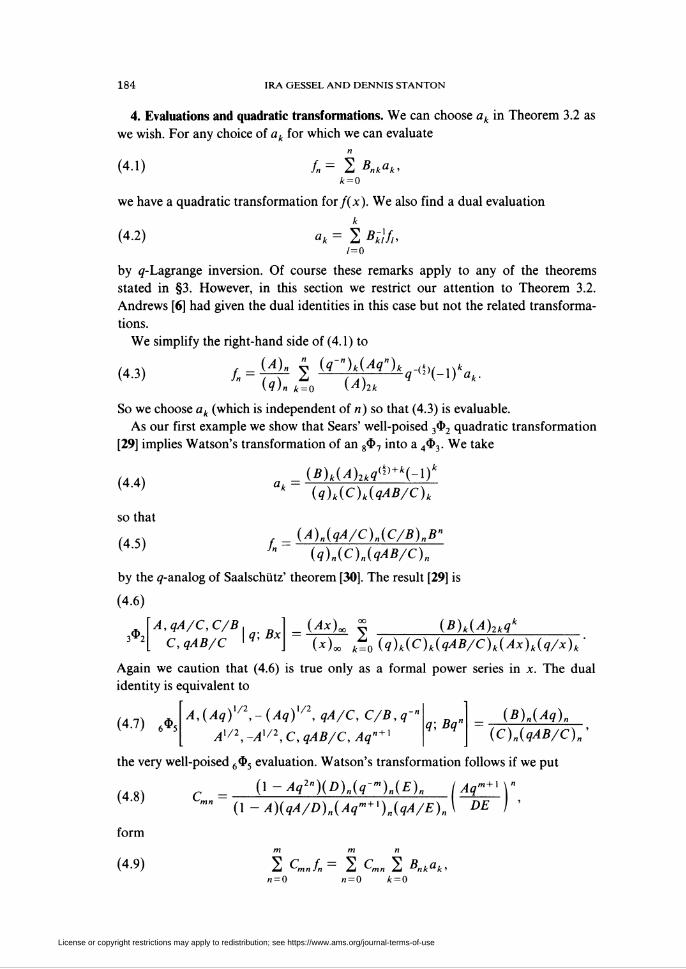
4. Evaluations and quadratic transformations. We can choose ak in Theorem 3.2 as

we wish. For any choice of ak for which we can evaluate

(4.1) /,= 2«, kuk,

k = 0

we have a quadratic transformation îoxf(x). We also find a dual evaluation

(4.2) ak - 2 Bk)fi,1=0

by ¿7-Lagrange inversion. Of course these remarks apply to any of the theorems

stated in §3. However, in this section we restrict our attention to Theorem 3.2.

Andrews [6] had given the dual identities in this case but not the related transforma-

tions.

We simplify the right-hand side of (4.1) to

(4.3) fn(A)n £ (q-")k(Aq")k

(q)n k=0 (A)2k

■q<H-l)kah

So we choose ak (which is independent of n) so that (4.3) is évaluable.

As our first example we show that Sears' well-poised 3$2 quadratic transformation

[29] implies Watson's transformation of an 807 into a 403. We take

(4.4)

so that

(4.5)

(B)k(A)2kq^+k(-l)k

(q)k(C)k(qAB/C)k

= (A)n(qA/C)n(C/B)nBn

(q)n(C)n(qAB/C)n

by the ¿7-analog of Saalschütz' theorem [30]. The result [29] is

(4.6)

3*2A,qA/C,C/B¡

C, qAB/Cq;Bx

_ (Ax)a (B)k(A)2kq"

(*)« k% (q)k(C)k(qAB/C)k(Ax)k(q/x)k

Again we caution that (4.6) is true only as a formal power series in x. The dual

identity is equivalent to

(4-7) 6*A,(Aq)X/2,-(Aq)X/1, qA/C, C/B,q~"

Ax/1, -AX/2,C, qAB/C, Aqn+Xq;Bq"

(B)ÁAq)„

(C)niqAB/C)n'

the very well-poised 6<£>5 evaluation. Watson's transformation follows if we put

(l-Aq2»)(D)„(q-m)n(E)n I Aqm+^n

(4.8)

form

(4.9)

C(1 - A)(qA/D)n(Aqm+')n(qA/E)n \ »E

2d t-mnJn Zi ^mn Z Bnkak,« = 0 n = 0 k = 0



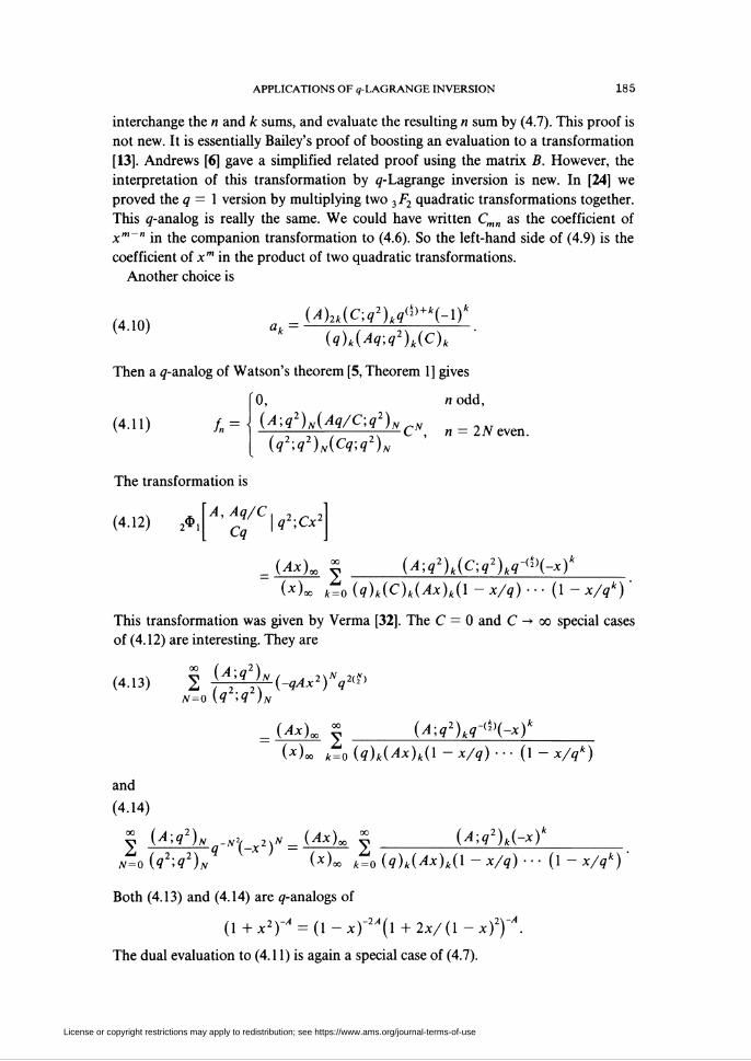
interchange the n and k sums, and evaluate the resulting n sum by (4.7). This proof is

not new. It is essentially Bailey's proof of boosting an evaluation to a transformation

[13]. Andrews [6] gave a simphfied related proof using the matrix B. However, the

interpretation of this transformation by ¿7-Lagrange inversion is new. In [24] we

proved the ¿7 = 1 version by multiplying two 3F2 quadratic transformations together.

This ¿7-analog is really the same. We could have written Cmn as the coefficient of

xm~" in the companion transformation to (4.6). So the left-hand side of (4.9) is the

coefficient of xm in the product of two quadratic transformations.

Another choice is

(4.10) at =(A)2k(C;q2)kq^+k(-l)k

(q)k(Aq;q2)k(C)k

Then a ¿7-analog of Watson's theorem [5, Theorem 1] gives

(4.11) u0,

(A;q2)N(Aq/C;g2)N

(q2;q2)N(Cq;q2)N

CN,

n odd,

n = 2N even.

The transformation is

A,Aq/C(4.12) 2*. Cq

\q2;Cx:

(Ax)x (A;q2)k(C;q2)kq-<H-x)1

(*)» k% (q)k(C)k(Ax)k(l - x/q) • ■ • (l - x/qk) '

This transformation was given by Verma [32]. The C = 0 and C -» 00 special cases

of (4.12) are interesting. They are

(4.13) 5 ¥Ñ^(-qAx2)Nq2^n=o (q ,q )N

_ (Ax)x - (A;q2)kq-^(-x)h

(*)» k% (q)k(Ax)k(l - x/q) ■ • • (l - x/qk)

and

(4.14)

(A;q2)k(-x)hy (A;q )n -N2t 2\N _(Ax)x y _

N=o(q2;q2)N (*)■» k=0(q)k(Ax)k(l- x/q)

Both (4.13) and (4.14) are ¿/-analogs of

(1 + x2yA = (1 - Xy2A(l + 2x/ (1 - x)2)"^.

The dual evaluation to (4.11) is again a special case of (4.7).

(1 - x/qk)



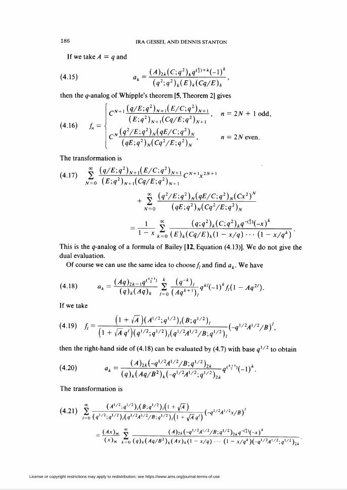
If we take A — q and

(4.15)(A)2k(C;q2)kq^+k(-lY

k (q2;q2)k(E)k(Cq/E)k '

then the ¿7-analog of Whipple's theorem [5, Theorem 2] gives

'cN+Aq/E;q2)N+ÁE/C;q2)N+x ^ n = 2N+lodd

(E;q2)N+i(Cq/E;q2)N+x

^(q2/E;q2)N(qE/C;q2)N(4.16) /„

C(qE;q2)N(Cq2/E;q2)N '

n = 2N even.


(q/E;q2)N+l(E/C;q2)N+XcN+Xx2N+x

¿v=o (E;q2)N+x(Cq/E;q2)

+ 2N = 0

(q2/E;q2)N(qE/C;q2)N(Cx2)N

(qE;q2)N(Cq2/E;q2)N

_ 1 I (q;q2)k(C;q2)kq-^(-x)k

1 - x ¿0 (E)k(Cq/E)k(l - x/q) • • • (l - x/qk) '

This is the ¿7-analog of a formula of Bailey [12, Equation (4.13)]. We do not give the

dual evaluation.

Of course we can use the same idea to choose// and find ak. We have

(4.18)

If we take

(4.19) f,

_(iik-^^JC^^(_1)V/(l_^2/).(q)k(Aq)k ,%(Aqk + x),

(l + ^)(A^2;q^2)l(B;q^2)l(-qx/2Ax/2/B)',

[l + {Xq,)W/2;qX/2)tW/1Ax/2/B;qx/2)l

then the right-hand side of (4.18) can be evaluated by (4.7) with base qx/2 to obtain

(A)2k(-qx/2Ax^2/B;qx/2)2

(4.20)(q)k(Aq/B2)k(-qx^2Ax^2;qx/2) T^^H)'

2 A


(¿,/2;í"2),(*í,/2)i(i+/<")

(4-21) ¿(^■^^/»Ao/w^'^^(^(V^Vn;^2)»^^-*)*(A*)x y _

(*)«= iéoíí^í^/a2)*^)^!-*/*)■■■ 0-V?*)(V/2¿l/2;<71/2)»


APPLICATIONS OF q-LAGRANGE INVERSION

The dual evaluation is equivalent to

¿7"", Aq", -Ax/2qx/2/B, -Ax/2q/B

187

(4.22) 4$: Aq/B2,-Ax^2qx^,-Ax/2q q; q

(-qX/2;qX/2)n(B;q1/2)n(l + {A-)

(-Ax'2;qx'2)n(qX/2Ax'2/B;qx/2)n[l + U q")(-qx/2Ax/2/B)\

Andrews had previously given (4.22) in [6, Equation (4.3)]. His identities [6, Equa-

tions (4.5) and (4.7)] also follow in this way.

For [6, Equation (4.5)] we take

(4-23)Ml/3;g1/3)f(i-^)(i-^V,/3)r y/3

'' (¿7'/3;í7'/3)/(l-J4¿72'Kl-^/3) '

then again the right-hand side of (4.18) can be evaluated by (4.7) with base ¿7I/3 to

obtain

_(i-^'/y/^'/3)3^'>(-i)'

()~Aq2k)(q)k


00 (y4'/3;gl/3);(1_^l/3^2//3)

ío W/3;ql/3),(i-Af)

(4.24)

(4.25) ^(A^q^x)1

_ (Ax)c(Ax/3;qx/i)ik+>q-(H-x)f

(*)» ¿0 (q)k(l - Aq2k)(Ax)k(l - x/q) • • • (l - x/qk)

The dual evaluation is [6, Equation (4.5)], namely,

(426) ¿ (q-n)k(Aq")k(Ax/y/3;qx/3)3kqk

k = Q (q)k(qA)2k

_ (q)n(Ax^qx^;qx^)n_x(l-Ax/Y"/3)(Aq)n/3

(qx^;qx^)n(Aq)n.x(l-Aq2")

For [6, Equation (4.8)] we take

0, /20(mod3),

(4-2?) /i= i^£k^, ,= 3L.

(q3;q3)L

Again, (4.7) with base ¿73 implies

(4-28) «,=i4#^+,)(-i)A.(q)k




(4.29)

^ (A;q3),c=o (q3;q3)t

-(Ax3)'-{Ax) (A;q3)kq<H-xf

(*)« k% (q)k(Ax)k(l - x/q) • ■ ■ (l - x/qk)

However, the left-hand side of (4.29) can be evaluated by the ¿7-binomial theorem to

obtain

(A;q3)kq<H-xY (A2x';q')Jx)0

k% (q)k(Ax)k(l - x/q) ■ • (l - x/qk) (Ax^q^jAx^ '

The above equation is the ¿7-analog of

(4.31) (l + 3x/ (1 - x)2)'" = (1 - x)3û(l - x3)'".

We had previously stated (4.30) in [24, Equation (6.7)] and commented that it should

be related to a ¿7-Lagrange inversion proof of

u „x v (q-")k(Aq")k(A;q3)k(4-32) 2-7ZVTT\-qk~

(q)k(A)2kfc=0

0, n SO (mod3),

(A;q3)N(qyNA

(A),N(q3;q3)N

Indeed (4.32) is the dual evaluation.

We give only one more example in this section. As Andrews [6] has indicated,

there are other examples involving only ¿7. They could quite possibly lead to

interesting transformations. Also, we could give the "derivative form" of Theorem

3.15 for each transformation in this section. We combine these two possibihties into

one example. Andrews [6, Equation (4.9)] allows

(4.33)

(4.34) (-1)7* =

g^+k(-l)k

"" (l-¿72*+1)'

?(3ní+7»-2)/2) k = 3n~l,

,(3«2-«)/2 k — 3n,

-(l+¿72"+,)¿7(3"2+7"+2>/2, k = 3n+l,

and A = ¿7, in Theorem 3.15. The transformation is

00 00

(4.35) 2 (-l)n + y"2+7"-2>/V-1 + 2 (-l)nq^2-"^2x3"

n=\ n=0

+ 2 (-l)"(l+92»+1)i<3"2+7,,+2)/2*3"+1

n = 0

(l-q2x2) ~ -(!)i-xY(! - *) *=o (qx)k+2(l - x/q) ■■■ (I- x/qk) '



Equation (4.35) is the ¿7-analog of

(4.36)(1 +x)_(1 +x)_

1+*3 ' (l-x)2(l +x/(l-xf)

5. More tranformations. In §4 we carefully considered Theorem 3.2. In this section

we find transformations and evaluations for Theorem 3.3.

For Theorem 3.3 we are trying to evaluate

(5.1)(q)n k=0 \A)k

So any evaluation in which the terminating parameter occurs exactly once will give a

transformation. It is easy to see that the terminating 2<I>, evaluation and

(5.2)

imply

(5.3)

(q)k(C)k

,(A)n(ß)n

}" (q)AC)n '

The resulting transformation is the ¿7-analog of the hnear 2FX tranformation [31]. A

nontrivial result is obtained if we take

(5.4)(A)k(C;q2)k k k

k 1 \ tr.„\ q '(q)k(C;q)k

and use a ¿7-analog of a terminating 2P'i(2) evaluation [7, Equation (1.8)] to find

0, n odd,

(A)2NCN(5.5) /„ =

(¿72;¿72)/,(C¿7;¿72)iV'

n = 2N even.

The tranformation is

A,Aq(5.6) 2$, Cq \q2;Cx:

(Ax)0 (A)k(C;q2)kq-<H-xY

(*)°o k% (q)k(C)k(l - x/q) ■•• (1 - x/qk) '

This is the ¿7-analog of Equation (17) in [20, p. 112]. Jain [27, Equation (3.1)] has

previously stated it. The dual evaluation follows from the ¿7-analog of Vandermonde's

theorem. In fact, it can be used to give another transformation. Put

0, A: odd,

iA)2Kq^

(¿72;¿72UC¿/;¿72)/k = 2 K even,

so

(5.8)(AUC;q2)

;" (q)ÁC)n q



and

(5.9) 2 ̂ iw'fv^"„=o (q)n(C)„

_ (¿*). V (A)2kq-^x2k

(x)x k% (q2;q2)k(Cq;q2)k(l - x/q) • • • (l - x/q2k)

The ¿7 ̂ 1 limit of (5.9) is Equation (4) of [20, p. 111],

2*i¿j,c/2.

(5.10)

We can also take

(5.11)

to find

(5.12)

Thus

(5.13)

2 a- (\-x)-\Fxa/2,(a+ l)/2,_x^

c/2 (i-xY

_ (A)kq^2(-l)k

ük (^2;qx^)k(-C;qx^2)k

(A)n(C;gx'2)2 ,

J"~ (q)ÁC2)n q (~>-

2 {A]ic;q'2?2"q-"2/2i-xy

„ = 0 (q)n(C )„

_ U*)oo_ (^),¿7-^+'»(-x¿7>/2)'

(*)« (¿72;Í72),(-C;¿7,/2),(1 - x/q) ••• (1 - x/q')

The dual evaluation is

(514) 4. (g-k)i(cW/2)2iqtk-i^t 0< - (V/2;g'/2)y*/2

1 ' io (q)t(C2), ' ( } (-C;qx'2)k * '

By writing (5.14) on base ¿7"', changing C"1 to C and ¿7"1 to ¿7 we see that (5.14)

really is

(5.15) 3*2

q~k,C,Cqx/2

C2,0q;q

(-qX/2;qX/2)k ck

(-c;qx/2)k

Equation (5.15) is not new. The 3$2 can be transformed to a well-poised 2<P,.

Nevertheless, we can use (5.15) to choose

(5.16)

and

(5.17)

(A)k(C;qx/2)2kq^

(q)k(C2)ki-iy

fn =(A)nC

(¿71/2;¿71/2)„(-C;¿7'/2)„


APPLICATIONS OF 9-LAGRANGE INVERSION 191


(5.18)

2*.

Al/2y_AV2

-Cqx/2;Cx

(Ax)0 (A)k(C;qx'2)2kq-*\-x)k

(*)« k=o (q)k(C2)k(l - x/q) •■•(!- x/qk) '

The appropriate ¿7 -» 1 limits of (5.13) and (5.18) are factorizations involving the

binomial theorem.

One may feel that the ¿/"<5) factor does not belong in (5.9). In fact, writing the

factors on base ¿7"1 will eliminate this term. We would like to change ¿7"1 to ¿7

throughout (5.9). This process is justified by Theorem 3.13. The resulting transfor-

mation is

g (A)n(B;q2)n n _ (Ay)x " (A)2kq^+k(By2)k

[ } ¿0 (q)n(ß)n y ' (y)~ ¿o(q2;q2)k(Bq;q2)k(Ay)2k-

We could change any of the transformations of §§4 and 5 in this way.

6. More evaluations. Finally we come to Theorems 3.1 and 3.4-3.6. In these cases

we cannot sum Gk(x), so that the resulting transformations are less interesting.

Hence, we concentrate on the evaluations. In particular we give ¿7-analogs of the

strange evaluations (1.2)-(1.5), (1.7), and (1.8) of [24].

First, for Theorem 3.4 if we put

(6.1)(B)k(A2qx/'-/B)k^)+k{_i)k^

L

k (q)k(Aqx'2;qx/2)k

then the ¿/-analog of Saalschütz' theorem imphes

(B/A;q^)m(Aq^/B;q^)m

(q)n(AqX/2;qX/1)n


¿7"*/2, -q-k/1, B/A, Aqx/2/B

-qx^2,qx/2-k/A,A

(6.2)

(6.3) 4$;

(-A)"q%-i/2(2)

¿7'/2;¿71/2(B)k(A2qx^2/B),

(A;qx'2)2 k

This is the c = q k terminating version of the ¿/-analog of Whipple's theorem

[5,Theorem 2]. If A = q"/2, and ¿7 -» 1, then Gk(x) -> xk(l + x/2)a+k. So our

transformation is a ¿7-analog of Equation (22) in [20, p. 112],

(6.4) 2FXa, I + a — b i ̂

1+ a ' 2

= (1 + V2)a2p-, b/2,a + (l-b)/2l_2x{l+x/2)1 + a

Next, we take Theorem 3.1. If A = ¿7a/2 and ¿7 -> 1, then

Gkix) -* xkil - x/2)-a-3k



So any pair (/„, ak) gives a ¿7-analog of a cubic transformation. We see that

« sï , - (A>qW2)n V (Mn/2;qX/2)2k(q-")k rikM Ukn(6-5) /„--7-T- ¿ -. , 2,-q l2,(-l) a*-

U)„ *=o (A;qX/2hk

Choosing

(6.6)

again we find

(6-7) /„

a v =

_ (A;qx^2)3kq^+k(-l)k

(q)k(C)k(A2q3/2/C)k'

(A;qx^2)n(Aq/CW/2)n(C/AqX/2;qX/2)n

(q)n(C)n(A2q3/2/C)nqWV)AH.


(6.8)

2* = 0

$ (q-")k(A;qx/2)k(Aq/C;qX/2)k(C/AqX/2;qX/2)k^ ~ Aq3k/2) nk+x/2^ k

(Aq"^2;qx^2)k(q)k(C)k(A2q^2/C)k(l - A)

_ (AqX/2;qX/2)2„

ic)n(A2q3/2/c)n'

This is the ¿7-analog of the strange 5FA[l/4,) evaluation [24, Equation (1.9)]. The

transformation is a ¿7-analog of [12, Equation (4.05)],

(6.9) 3^2

a, a + 2 — 2c,2c — a — liX

c, a - c + 3/2 I "8

(1 - x/2)-\F2a/3, a + 1/3, a + 2/3 -27x

c,a-c + 3/2 '8(l-x/2)3J'

Just as we derived Watson's tranformation from (4.7), we can derive the ¿7-analog of

the strange 7F6(1) evaluation [24, Equation (1.7)] from (6.8). This time take

(q-")k(AD2q"+x/2)k(A/D2)kA-kq-x/2^ (l - Aq3^2)

y' } "k (Aq»^2;qxS2)k(q-"/D2;qxS2)k(D2qx/2;qx/2)k (\ - A) "

Again, in 2¡J=0C„¿/¿ = 1jikCnkBkJaj, the k-suxn can be evaluated by the reversal of

(6.8). The result is precisely (1.4).

For Theorem 3.6 we see that if A = qa, Gk(x) -» x^l - 2x)~a~3k/2. So we can

find ¿7-analogs of (1.3) and (1.8) in [24]. This time

Í0. kodd,

UW/2(¥)+*(6.11)

yields

(6.12)

(q)K(B)K(Aqy2/B)K

k — 2 AT even,

/■ =(A)n(Bq^2)n(qA/B)nq

1/2(5)

(¿71/2;¿7'/2)„(73¿7-'/2;¿71/2)n(¿7^/5;¿71/2)„




(6.13)

y (q-"/2;qx'2)k(A)k(Bq-x^2)k(qA/B)k(l - Aq3k^2) [n,_(*)]/2

¿0 (qX/2;qX/2)k(Aqx^2)k(Bq-x/2;qx/2)k(qA/B;qx/2)k(l--A)q

0, n odd,(Aq)N(qX/2)N

(B)N(Aqy2/B)N

, n — 27V even.

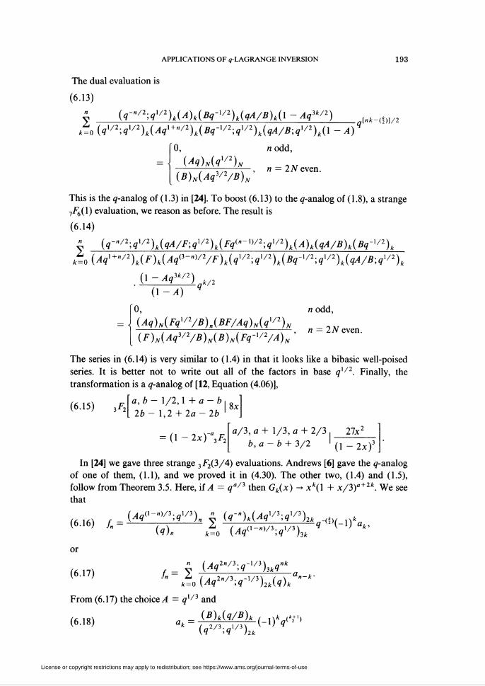
This is the ¿7-analog of (1.3) in [24]. To boost (6.13) to the ¿7-analog of (1.8), a strange

7F6(1) evaluation, we reason as before. The result is

(6.14)

y (q-»/2;qx/2)k(qA/F;qx/2)k(Fq(»-xV2;qx'2)k(A)^^

L(Aqx^2)k(F)k(Aq*-"y2/F)k(qx'2;qx'2)k^^

,k/2(l-Aq3k'2)

(I -A) "

0, n odd,

(Aq)N(Fqx/2/B)n(BF/Aq)N(qx'2)N

(F)N(Aq3/2/B)N(B)N(Fq~x/2/A)N 'n = 2/V even.

The series in (6.14) is very similar to (1.4) in that it looks like a bibasic well-poised

series. It is better not to write out all of the factors in base ¿71/2. Finally, the

transformation is a ¿7-analog of [12, Equation (4.06)],

~a,b- 1/2,1 + a-b ,(6.15) 3F2 2b- 1,2 +2a-2b

= (1 - 2x)-"3F2

8x

a/3, a + 1/3, a + 2/3 27.x2

b,a 3/2 (1-2*)J

In [24] we gave three strange 3 F2(3/4) evaluations. Andrews [6] gave the ¿7-analog

of one of them, (1.1), and we proved it in (4.30). The other two, (1.4) and (1.5),

follow from Theorem 3.5. Here, if A = qa/3 then Gk(x) -> jc*(1 + x/3)a+2k. We see

that

(6.16) /„ =(^(,-„)/3;i,/3)n „ iq->)k(AqVW/3)

(q), ¿0 (^(,-fl)/V/3k2^q-'H-l)kak,

or

(6.17)" (Aq2^3;q^3)3kq"k

f„= 1-—-———a„k%(Aq2^3;q-x^)2k(q)k""'k-

From (6.17) the choice/! = qx/3 and

(6.18) at = (B)k(q/B)k ( \\kn(kv

(q2/3W/3)2k '(-l)V



gives (by the ¿7-analog of Saalschütz' theorem)

(B)n(q/B)n(Bq<»-2V3;qVi)2n(6.19) /, = ' (-l)"q

n (n+lCI')(q2/3;qX/3)2n(Bq-l;q-')2n


,6 2Ç)) y (q-n)k(Bq-X/3;qX/3)k(q2/3/B;qX/3)kkn = (B)n(q/BUq)n

[' } ¿0 W/3;q2/i)2k(q-W/3)k q W/3;ql/3)3n '

This is the ¿7-analog of the 3F2(3/4) in [24, Equation (1.4)]. The tranformation is a

¿7-analog of

6,1-0, -9x(l + x/3)2(6.21) 2* 1

3b- 1,2- 36

3/2= (l+x/3)2Fx

3/2

Another choice for (6.17) is A = 1 and

(6.22) c

Then we have

(B)k(B~X)k (_t)fc («,+ ■)_

(qX/3;qX/3)2 k

(6.23) fn(B)n(B-x)n(Bq^-x^3;q^3)2n_

InCV) (-1)".(?1/3;i,/3k(^-,;?-,k-1


(,^ y (q-")k(ql/3B-l;qX/3)k(Bq]/3;qX/3)k k/3_(Bq)n(qB-x)n(g)n

(0.Z4J 2d / 9/1 1/1\ / -„-1/1 1/1\ 1(q2/3;qi/3)2k(q-n-,/3;qi/3)i(qk=o \h ,h >2k\H ,h )k \^2/3',qi/3)i„

This is the ¿7-analog of the 3F2(3/4) in [24, Equation (1.5)]. The transformation is a

¿7-analog of

-.2

2*i

36,-36, £

1/2 I 4(6.25)

For the dual form if we put

(6.26) /,

then

(6.27)

The evaluation is

:2^16,-6. -9x(l + x/3)

1/2 I 4

g-Ü)-//3(_1)'

(¿7-'/3;¿7-,/3)/(/l-1;¿7-1/3)/(l-^2//3)

(A3q2k-x;q-x)k(-l)kq^

(6.28) 2(í")*M3W

k%(q)k(A3)k(Aq<x-"V3;qx/3)3k

_^-''''(-l)"(l-^)(g),

(q-X/3;q-X/3)n(A-X;q-X/3)„(AqiX-")/3;qX/3)n(l-Aq2"/3)

This is an evaluation of a special balanced 5$4.



7. Identities of Rogers-Ramanujan type. It is well known that Watson's transfor-

mation implies the Rogers-Ramanujan identities,

00 ¿7*2 1

(7'° SoTqTk = (q;q5Uq4;q5L

and

oo k2 + k ,

(7.2) 2 'o (*)* (q2;q5)Jq3;q5)x'

We proved Watson's transformation in §4. Because Rogers' technique was really

Theorem 3.2, we can expect other identities of the Rogers-Ramanujan type to follow

from the quadratic transformations in §4. In this section we give several examples.

In (4.13) replace x by x/A and let ̂ 4 -» oo. We have

oo 2n2-n 2n oo nC2)rk

(7-3) 2 i-Hv- = (*)» 2 q~^«=o (q2;q2)n xk=o(q)k(x)k'

We see that (7.3) converges as a formal power series in ¿7. Changing ¿7 to ¿72,

replacing x by ¿7 and ¿73, and using (7.1) and (7.2) we find

(7-4) 2 "*-k%(q\k (q;q2Uq4;q20UqX6;q2°)0

and

00 ^Ar2 + 2A: ,

(7-5) 2£0(«W. (q;q2UqW°Uqn;q20L'

These are Rogers' identities of modulus 20 [31, Equations (79), (96)]. Another

interesting choice in (7.3) is x = -q.

In (4.21) let B ~* 00, replace x by x/A, let A -» 00, replace ¿7 by ¿72 and x by -xq2

to find

00 t2xi « qk2%k

(7.6) 2 j-r = (-xq2;q2)oc 2 , 2 2W 2—rr-1=0(9)1 k=o(q ,q )k(-q x;q2)k

This time the choices of x = 1 and ¿7 result in

¿7*2 1(7-7)

k%(q4;q*)k (-q2;q2)Jq;q5)Jq4;q5h

and

co yk2+k j

(7"8) Jo (q2;q2)k(-q3;q2)k = (V;*2UiVU9V).

These are Equations (20) and (17) of [31].



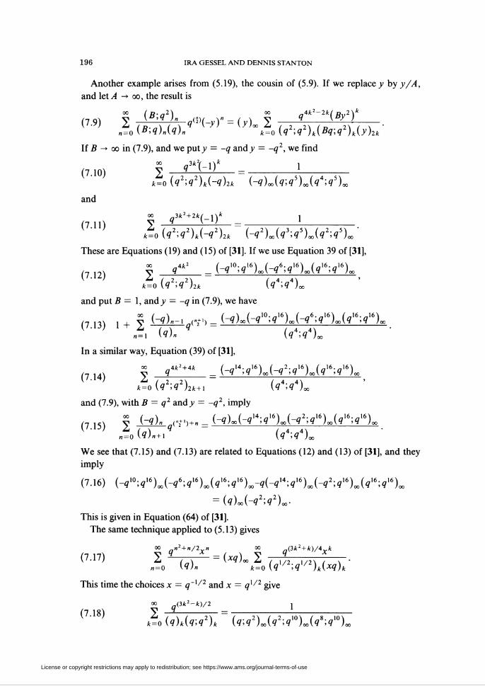
Another example arises from (5.19), the cousin of (5.9). If we replace y by y/A,

and let A -* oo, the result is

If 73 — oo in (7.9), and we put y = -¿7 and y = -q2,v/e find

00 a3k2(-l)k 1

(7.10) 2 — — =-k=o (q2;q2)k(-q)2k (-?)«,(?;î5)oo(«74;«75)»

and

00 3*2 + 2*/_i)* j

(7'U) Jo (q2;q2)k(-q2)2k = (~q2Uq3;q5Uq2;q5L '

These are Equations (19) and (15) of [31]. If we use Equation 39 of [31],

,.„, S <?4*2 _ (V0;g'6UV;<?16U<716;g,6LV ' ^ / 2 2\ / 4 4\ '

* = 0 U Î0 )2* (9 '9 )oo

and put 7? = 1, and y = -¿7 in (7.9), we have

,71-x , . y (-g)»-. ^M_(^L(V°:g1<L(V;g16),(g16;g16),(7.13) 1+2—7-^—9 -/ 4 4\-•

„=i («7)» (q ;q)x

In a similar way, Equation (39) of [31],

, g4t»+4t _ (-¿7^;¿7^)oo(-¿72;¿7^)Jg^;¿7^)oo

*=o U »Í )2*+i («7;?)«

and (7.9), with B = q2 and y = -q2, imply

/71S, £ izik <•*•>+. = (^)-(V4;g").(-g2:g"l(qw;g16)..i^/.ijj ¿ . . ¿7 . .

We see that (7.15) and (7.13) are related to Equations (12) and (13) of [31], and they

imply

(7.16) (V0;9,6)co(V;9,6).(9,6;í,6)..-«(V4;í,í)»(V;í,6).(9,6;9,6)ao

= (qU-q2;q2L-

This is given in Equation (64) of [31].

The same technique apphed to (5.13) gives

Jn2 + n/2Y.n oo n(îk2 + k)/A kn" T"/ if" n^

(7.17) 2 q , / = (*g), 2 7-^»=0 (?)» *=o U 7 ,<7 /2M*?)*

This time the choices * = ¿7"1/2 and x = qx/1 give

(7.18) 200 0lc2-k)/2 j

*t0 (q)k(q;q2)k (qrfUWUWl



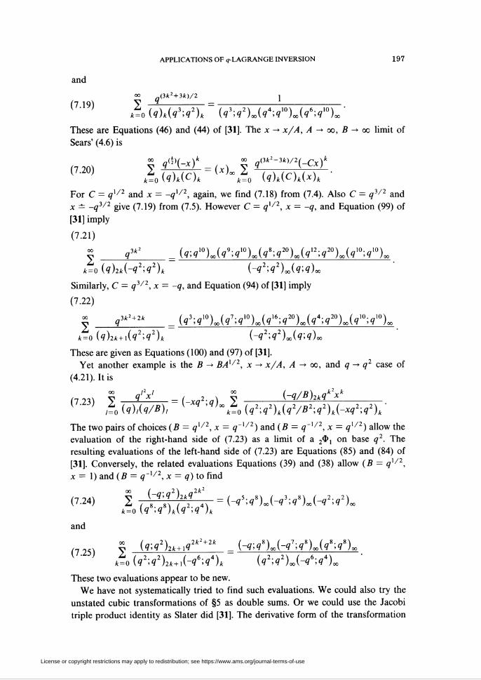
and

(3*:2 + 3*:)/2 1

(7J9) Jo (q)k(q3;q2)k {«WUl^UM0)* '

These are Equations (46) and (44) of [31]. The x -» x/A, A -> oo, B -» oo limit of

Sears' (4.6) is

00 a(k)(-x)k °° a(3k2~3k)/2(-Cx)k

¿=0 U)*(C)* ^=o (?)*(£)*(*)*

For C = ¿71/2 and x = -qx/2, again, we find (7.18) from (7.4). Also C = q3/2 and

x — -q3/1 give (7.19) from (7.5). However C = ¿7I/2, x = -q, and Equation (99) of

[31] imply

(7.21)oo „3it2 / ^,. „10\ f„9._10\ (ni.n2Q\ /■_12._20\ /_10._10\V _q - (q'q )°°(q >q )™(q 'q )°o(q >q )°°(q >q )oo

*=o (q)2k(-q2;q2)k (-q2;q2)x(q;q)x

Similarly, C = q3/2, x = -¿7, and Equation (94) of [31] imply

(7.22)

| g3kl+2k _ (g3;g10).(g7;g10),(gl<;g20),(g4;g20L(g'0;g10),,

fc=o (q)2k+\(q2;q2)k (-q2;q2)x(q;q)oo

These are given as Equations (100) and (97) of [31].

Yet another example is the B -» BAX/2, x -» jc/j4, /I -* 00, and q ^ q2 case of

(4.21). It is

r7^ ? <?'v ( 2 x v (^/*W**1 J A (9),(*/*), l * ,í;-¿o U2;92)*(<77*2;<,2)*(-V;<72)* ■

The two pairs of choices (B — qx/1, x = q~x/2) and (t3 = ¿7"1/2, x = qx/2) allow the

evaluation of the right-hand side of (7.23) as a limit of a 24>, on base q2. The

resulting evaluations of the left-hand side of (7.23) are Equations (85) and (84) of

[31]. Conversely, the related evaluations Equations (39) and (38) allow (B = qx/2,

x = 1) and (73 = q'x/2, x = q) to find

(7-24) 1, {?\t]2k?k*\ = (-q5>q*u-q3>q*u-q2>q2)~k=o (q ,q)k(q ,q )k

and

v (q;q2)2k+iq2k2+2k _ (-ï;î8U-îVU*V)»(7.25)

k%(q2;q2)2k+Á-q6;q4)k («VUV;«4).

These two evaluations appear to be new.

We have not systematically tried to find such evaluations. We could also try the

unstated cubic transformations of §5 as double sums. Or we could use the Jacobi

triple product identity as Slater did [31]. The derivative form of the transformation



would insert a linear term, as in Theorem 3.15. Also we did not state any

transformations with ¿7 as the only parameter. In any case it is clear that identities of

the Rogers-Ramanujan type are related to ¿7-Lagrange inversion.

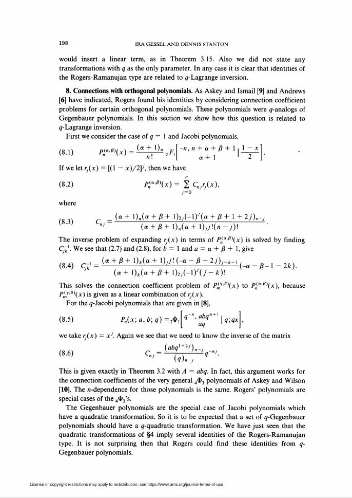
8. Connections with orthogonal polynomials. As Askey and Ismail [9] and Andrews

[6] have indicated, Rogers found his identities by considering connection coefficient

problems for certain orthogonal polynomials. These polynomials were ¿7-analogs of

Gegenbauer polynomials. In this section we show how this question is related to

¿7-Lagrange inversion.

First we consider the case of ¿7 = 1 and Jacobi polynomials,

-n, n + a + ß + 1 ■ 1 -.

a+\ '2

If we let rj(x) = [(1 — x)/2\>, then we have

(8.1) P^ß\x) = -^-^ 2F,

(8-2) Pf-'Kx) = 2 Cnñ(x),7=0

where

,R -, (a + l)„(a + ß + 1K,(-I)y(a + jB +1 + 2j)„-j

[ ' "J (a + ß+l)n(a+l)jj$n-j)l

The inverse problem of expanding rj(x) in terms of P^a'ß\x) is solved by finding

Cj-n\ We see that (2.7) and (2.8), for 6 = 1 and a = a + ß + 1, give

(8.4) c-, = (■ + /> + ■).(« + ■)//' H - ß - 27).-.- ( , _ lk(a+$k(a + ß+\)2,{-\)'{j-k)\

This solves the connection coefficient problem of P^,S)(x) to P^a'ß)(x), because

Bm'S)ix) is given as a linear combination of ry(x).

For the ¿7-Jacobi polynomials that are given in [8],

■ q~">abq"+],q-,qx

we take ry(x) = xJ. Again we see that we need to know the inverse of the matrix

(¿V+2;)n_,(8.6) C"7= L q'"J-

\q)n-j

This is given exactly in Theorem 3.2 with A — abq. In fact, this argument works for

the connection coefficients of the very general 403 polynomials of Askey and Wilson

[10]. The «-dependence for those polynomials is the same. Rogers' polynomials are

special cases of the 44>3's.

The Gegenbauer polynomials are the special case of Jacobi polynomials which

have a quadratic transformation. So it is to be expected that a set of ¿7-Gegenbauer

polynomials should have a ¿7-quadratic transformation. We have just seen that the

quadratic transformations of §4 imply several identities of the Rogers-Ramanujan

type. It is not surprising then that Rogers could find these identities from ¿7-

Gegenbauer polynomials.



It would be very interesting to find some orthogonal polynomials based upon our

other examples of ¿7-Lagrange inversion, e.g. Theorem 3.1. However, this is not even

known for ¿7 = 1. Some new identities of the Rogers-Ramanujan type might result.

9. Concluding remarks. F. H. Jackson [26] gave the first example of ¿7-Lagrange

inversion. It is a ¿7-analog of Abel's generalization of the binomial theorem. His

example is a special case of Theorem 3.7. Recently, J. Cigler [17,18,19] has also been

finding other examples. It would be very interesting to incorporate any of these

examples, or, for example, Theorem 1.2, into a general theory. For Theorem 1.2 the

work of Gessel [23] and Garsia [22] would appear to be promising.

There are many directions open for the quadratic transformations. Verma and

Jain have begun this program. We have indicated a systematic approach. However,

the evaluations that we used were the standard ones—Vandermonde's theorem,

Saalschütz' theorem, and the very well-poised 6<ï>5. It is quite possible that other

evaluations could give other transformations [3, Equation (3.3)]. Verma and Jain

have given several bibasic evaluations which might work [28]. In this regard, again,

we caution that all transformations stated here are formal power series identities,

and not identities for complex-valued functions. If the series do converge (or

terminate), we could integrate against a ¿/-beta function. This would boost the

transformations to transformations of series of higher order. We have not done these

calculations. They could quite possibly be related to [28].

We do not claim to have found all of the ¿7-analogs of the matrices in §2. It is

possible that (2.9) gives a non trivial matrix that is different from (2.10). Rather, we

were interested in those values of 6 which occurred in [24]. We wanted to find

¿7-analogs of those strange evaluations. Other values for 6 (e.g. p = 0) could be

interesting. Also, a basis for formal power series different from {xk}f=0 could be

necessary for other matrices.

Perhaps the most intriguing part of this paper is the connection between ¿7-Lagrange

inversion and identities of the Rogers-Ramanujan type. In §4 we indicated how

Sears' quadratic transformation implies Watson's transformation and thus the

Rogers-Ramanujan identities. Can one avoid Watson's transformation altogether, as

we have in §7? Bressoud [14] has shown how to derive these identities from

terminating evaluations. For the Rogers-Ramanujan identities, he used the terminat-

ing 6$5 evaluation. This is given exactly by ¿7-Lagrange inversion on Sears' transfor-

mation. This indicates that our new evaluations in §6 could lead to new identities of

the Rogers-Ramanujan type. It is easy to modify the Bailey transform as given by

Bressoud to fit §6, but we have not carried out any of these calculations.

The transformations implicit in §6 could also give new identities, as in §7. They

are ¿7-analogs of cubic transformations, written as double sums equal to single sums.

We fould that an analog of Watson's transformation for a cubic transformation was

the evaluation (1.4). A better analog might be a transformation of a double sum into

a single sum. This could lead to double sum Rogers-Ramanujan identities, as in [28].

Another direction that we hope to pursue is the connection of the matrices with

bilateral series. By extending the definition of Bnk properly to negative values of n

and k, this can be done.



Finally, it is possible to systematically study the transformations which arise just

as Watson's theorem did in §4. There we found the coefficient of x" in the product

of a transformation and its derivative form. In fact, there is a general theorem that

does this which is the ¿7-analog of Theorem 2 in [24, §4]. We state one version here.

Theorem 9.1. Let Bnk and Gk(x) be defined as in Theorem 3.7. Put Hj(x) =

2^jB'njx", where

Ki = (*r'j>-^';jO-,-,(1 _ Bq-np-n)qC-^-nJ{B/AyS{_x)n-J\q)n-j

Suppose 2?=0akGk(x) = lf=0bkxk and 1%0CjHj(x) = If^djxK Then, if B =

Ap"q",p = ¿7'/*, and 8(1 + 1/6) = 1, 2U0akcn_kqk" = 2nk=0bkdn_k.

Added in Proof. A formula equivalent to Theorem 3.7 was given by L. Carhtz,

Some inverse relations, Duke Math. J. 40 (1973), 893-901.

References

1. N. Abel, Sur les fonctions generatrices et leurs déterminantes, Ouvres Complètes, vol. 2, Grondahl &

Son, Christiania, 1881, pp. 67-81.

2. _, Beweis eines Ausdruckes, von welchem die Binomial-Formel ein einzelner Fall ist, J. Reine

Angew. Math. 1 (1826), 159-160.

3. W. Al-Salam and A. Verma, On quadratic transformations for basic series, preprint.

4. G. Andrews, Identities in combinatorics. II: A q-analog of the Lagrange inversion theorem, Proc.

Amer. Math. Soc. 53 (1975), 240-245.5. _, On q-analogues of the Watson and Whipple summations, SIAM J. Math. Anal. 7 (1976),

332-336.6. _, Connection coefficient problems and partitions (D. Ray-Chaudhuri, ed.), Proc. Sympos. Pure

Math., vol. 34, Amer. Math. Soc., Providence, R. I., 1979, pp. 1-24.

7._, On the q-analog of Kummer 's theorem and applications, Duke Math. J. 40 ( 1973), 525-528.

8. G. Andrews and R. Askey, Enumeration of partitions: The role of Eulerian series and q-orthogonal

polynomials, Higher Combinatorics (M. Aigner, ed.), Reidel, Dordrecht, 1977, pp. 3-26.

9. R. Askey and M. Ismail, A generalization of ultraspherical polynomials, Studies in Analysis (to

appear).

10. R. Askey and J. Wilson, Some basic hypergeometric orthogonal polynomials that generalize Jacobi

polynomials, preprint.

11. W. Bailey, Generalized hypergeometric series, Cambridge Univ. Press, Cambridge, 1935.

12. _, Products of generalized hypergeometric series, Proc. London Math. Soc. 28(1928), 242-254.

13. _, Some identities involving generalized hypergeometric series, Proc. London Math. Soc. 29

(1929), 503-516.14. D. Bressoud, Some identities for terminating q-series, Math. Proc. Cambridge Philos. Soc. 89 (1981),

211-223.

15. L. Carlitz, Some q-expansion formulas, Glas. Mat. Ser. Ill 8 (1973), 205-214.

16._Some formulas of F. H. Jackson, Monatsh. Math. 73 (1969), 193-198.17. J. Cigler, Operatormethoden für q-Identitäten, Monatsh. Math. 88 (1980), 87-105.

18. _, Operatormethoden für q-Identitäten. II. q-Laquerre-Polynome, Monatsh. Math. 91 (1981),

105-117.

19. _, Operatormethoden für q-Identitäten. III: Umbrale Inversion und die Lagrangesche Formel,

Arch. Math. (Basel) 35 (1980), 533-543.

20. A. Erdelyi, Higher transcendental functions. Vol. 1, McGraw-Hill, New York, 1953.

21. J. Fields and M. Ismail, Polynomial expansions, Math. Comp. 29 (1975), 894-902.

22. A. Garsia, A q-analogue of the Lagrange inversion formula, Houston J. Math. 7 (1981), 205-237.

23. I. Gessel, A noncommutative generalization and q-analog of the Lagrange inversion formula, Trans.

Amer. Math. Soc. 257 (1980), 455-482.



24. I. Gessel and D. Stanton, Strange evaluations of hypergeometric series, SIAM J. Math. Anal. 13

(1982), 295-308.25. P. Henrici, Applied and computational complex analysis, Vol. 1, Interscience, New York, 1977.

26. F. Jackson, A q-generalization of Abel's series, Rend. Palermo 29 (1910), 340-346.

27. V. Jain, Some transformations of basic hypergeometric functions. Part II, SIAM J. Math. Anal. 12

(1981), 957-961.28. V. Jain and A. Verma, Transformations between basic hypergeometric series on different bases and

identities of Rogers-Ramanujan type, J. Math. Anal. Appl. 76 (1980), 230-269.

29. D. Sears, Transformations of basic hypergeometric functions of special type, Proc. London Math. Soc.

52 (1951), 467-483.30. L. Slater, Generalized hypergeometric functions, Cambridge Univ. Press, Cambridge, 1966.

31. _, Further identities of the Rogers-Ramanujan type, Proc. London Math. Soc. 54 (1952),

147-167.

32. A. Verma, A quadratic transformation of a basic hypergeometric series, SIAM J. Math. Anal. 11

(1980), 425-427.33. E. Whittaker and G. Watson, A course of modern analysis, Cambridge Univ. Press, Cambridge, 1927.

Department of Mathematics, Massachusetts Institute of Technology, Cambridge, Mas-

sachusetts 02139

School of Mathematics, University of Minnesota, Minneapolis, Minnesota 55455


applications of ^-lagrange inversion to basic ... · we have seen that theorem 1.2 is the ^-analog...

Documents