1

Fast Intra- and Inter-Prediction Mode Decision

in H.264 Advanced Video Coding Mehdi Jafari Shohreh Kasaei Islamic Azad University, S and R Branch Sharif University of Technology Department of Communication Engineering Department of Computer Engineering P.O.Box 14515-775, Tehran, Iran P.O.Box 11365-9517, Tehran, Iran mjafari@mail.uk.ac.ir skasaei@sharif.edu Abstract

H.264/AVC, the latest video coding standard, achieves better video compression rates since it supports new features such as a large number of intra- and inter- prediction candidate modes. H.264/AVC adopts rate-distortion optimization (RDO) technique to obtain the best intra- and inter-prediction, while maximizing visual quality and minimizing the required bit rate. However, the RDO reduces the encoding speed via the exhaustive evaluation of all candidate modes. In this paper, in conjunction with an overview of proposed algorithms for fast intra-mode decision in H.264/AVC encoders, we decrease the encoding time by reducing the computational complexity of the cost function and the number of candidate modes. Also, a new algorithm based on the properties of similar predicted pixels and the feature of reference pixels is proposed. The proposed algorithms use spatial and transform domain features (such as edge information, simple directional properties of intra-mode, feature of reference pixels and adjacent blocks information in the intra- and inter-frame) to select a subset of all candidate modes. Subsequently, the RDO procedure uses the reduced subset of all candidate modes for extracting the final mode. Experimental results show that our algorithm, compared to the RDO and some other fast algorithms, reduces the total encoding time with negligible loss in PSNR and a slightly increased bitrate.

Keywords: H.264/AVC, Intra-prediction, RDO, similar predicted-pixels.

1. Introduction

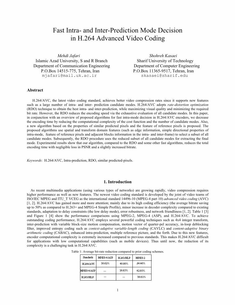
As recent multimedia applications (using various types of networks) are growing rapidly, video compression requires higher performance as well as new features. The newest video coding standard is developed by the joint of video teams of ISO/IEC MPEG and ITU_T VCEG as the international standard 14496-10 (MPEG-4 part 10) advanced video coding (AVC) [1, 2]. H.264/AVC has gained more and more attention; mainly due to its high coding efficiency (the average bitrate saving up to 50% as compared to H.263+ and MPEG-4 Simple Profile), minor increase in decoder complexity compared to existing standards, adaptation to delay constraints (the low delay mode), error robustness, and network friendliness [1, 2]. Table 1 [3] and Figure 1 [4] show the performance comparisons using MPEG-2, MPEG-4 (ASP), and H.264/AVC. To achieve outstanding coding performance, H.264/AVC employs several powerful coding techniques such as 4x4 integer transform, inter-prediction with variable block-size motion compensation, motion vector of quarter-pel accuracy, in-loop deblocking filter, improved entropy coding such as context-adaptive variable-length coding (CAVLC) and content-adaptive binary arithmetic coding (CABAC), enhanced intra-prediction, multiple reference picture, and the forth. Due to this new features, encoder computational complexity is extremely increased compared to previous standards. This makes H.264/AVC difficult for applications with low computational capabilities (such as mobile devices). Thus until now, the reduction of its complexity is a challenging task in H.264/AVC.

Table 1: Average bit-rate reduction compared to prior coding schemes.

2

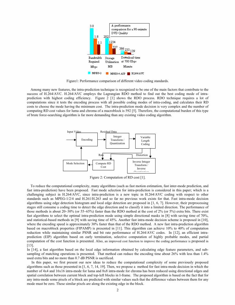
Figure1: Performance comparison of different video coding standards.

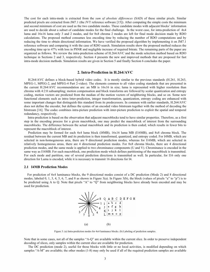
Among many new features, the intra-prediction technique is recognized to be one of the main factors that contribute to the success of H.264/AVC. H.264/AVC employs the Lagrangian RDO method to find out the best coding mode of intra-prediction with highest coding efficiency. Figure 2 [1] shows the RDO process. RDO technique requires a lot of computations since it tests the encoding process with all possible coding modes of intra-coding, and calculates their RD costs to choose the mode having the minimum cost. The intra-prediction mode decision is very complex and the number of computing RD cost values for luma and chroma of a macroblock is 592 [5]. Therefore, the computational burden of this type of brute force-searching algorithm is far more demanding than any existing video coding algorithm.

Input Video Residual Data

Rate Distortion

Figure 2: Computation of RD cost [1].

To reduce the computational complexity, many algorithms (such as fast motion estimation, fast inter-mode prediction, and fast intra-prediction) have been proposed. Fast mode selection for intra-prediction is considered in this paper; which is a challenging subject in H.264/AVC, since intra-prediction is a new topic in H.264/AVC coding with respect to other standards such as MPEG-1/2/4 and H.261/H.263 and so far no previous work exists for that. Fast intra-mode decision algorithms using edge detection histogram and local edge detection are proposed in [1, 6, 7]. However, their preprocessing stages still consume a coding time to detect the edge direction and to classify it into a limited direction. The performance of those methods is about 20~30% (or 55~65%) faster than the RDO method at the cost of 2% (or 5%) extra bits. There exist fast algorithms to select the optimal intra-prediction mode using simple directional masks in [8] with saving time of 70%, and statistical-based methods in [9] with saving time of 45%. Another fast intra-mode decision scheme is proposed in [10], where the encoding speed is approximately 30% faster than that of the RDO method. A new fast intra-prediction algorithm based on macroblock properties (FIPAMP) is presented in [11]. This algorithm can achieve 10% to 40% of computation reduction while maintaining similar PSNR and bit rate performance of H.264/AVC codes. In [12], an efficient intra-prediction (EIP) algorithm based on early termination, selective computation of highly probable modes, and partial computation of the cost function is presented. Also, an improved cost function to improve the coding performance is proposed in [13]. In [14], a fast algorithm based on the local edge information obtained by calculating edge feature parameters, and sub-sampling of matching operations is presented. That method can reduce the encoding time about 26% with less than 1.4% used extra bits and no more than 0.7 dB PSNR is sacrificed. In this paper, we first present our new ideas to reduce the computational complexity of some previously proposed algorithms such as those presented in [1, 6, 7, 14, 19]. Then, we propose a method for fast intra-mode decision in which the number of 4x4 and 16x16 intra-mode for luma and 8x8 intra-mode for chroma has been reduced using directional edges and spatial correlation between current block and top-left blocks in I-frame. The proposed algorithm is based on the fact that for any intra-mode some pixels of a block are predicted with similar values such that the difference values between them for any mode must be zero. These similar pixels are along the existing edge in the block.

Encoding

Variable Length Coding

Integer Transform / Quantization

Inverse Integer Transform /

Inverse Quantization

Compute RD Cost

Mode Selection

3

The cost for each intra-mode is extracted from the sum of absolute differences (SAD) of these similar pixels. Similar predicted pixels are extracted from JM7.1 (the JVT reference software [15]). After computing the simple costs the minimum and second minimum of cost are used as the two candidate modes. These candidate modes with adjacent blocks’ information are used to decide about a subset of candidate modes for the final challenge. In the worst case, for intra-prediction of 4x4 luma and 16x16 luma only 3 and 2 modes, and for 8x8 chroma 2 modes are left for final mode decision made by RDO calculations. The proposed method consumes less encoding time by reducing the number of RDO computations and by reducing the time to obtain directional information. We have verified the proposed algorithm by implementing it on JM7.1 reference software and comparing it with the case of RDO search. Simulation results show the proposed method reduces the encoding time up to 47% with loss in PSNR and negligible increase of required bitrate. The remaining parts of the paper are organized as follows. We review the intra-prediction scheme of H.264/AVC and the mode selection method based on RDO technique in Sections 2 and 3, respectively. Section 4 presents the new and improved methods that are proposed for fast intra-mode decision methods. Simulation results are given in Section 5 and finally Section 6 concludes the paper.

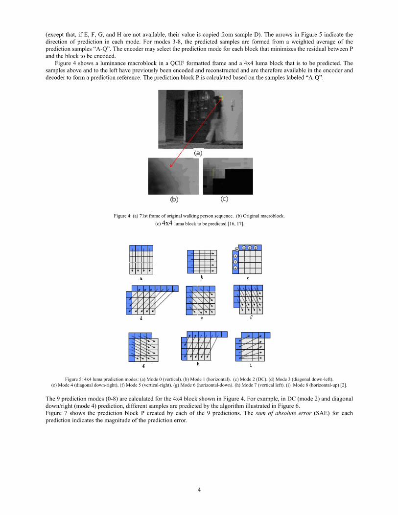
2. Intra-Prediction in H.264/AVC H.264/AVC defines a block-based hybrid video codec. It is mostly similar to the previous standards (H.261, H.263, MPEG-1, MPEG-2, and MPEG-4 Part 2-video). The elements common to all video coding standards that are presented in the current H.264/AVC recommendation are: an MB is 16x16 in size; luma is represented with higher resolution than chroma with 4:2:0 subsampling; motion compensation and block transforms are followed by scalar quantization and entropy coding, motion vectors are predicted from the median of the motion vectors of neighboring blocks, and so on. Some new functional elements such as intra-/inter-prediction, integer transformation, quantization, entropy coding are enhanced with some important changes that distinguish this standard from its predecessors. In common with earlier standards, H.264/AVC does not define the encoder, but defines the syntax of an encoded video bitstream together with the method of decoding the bitstream [16]. The codec combines intra-picture prediction with inter-picture prediction to exploit the spatial and temporal redundancy, respectively. Intra-prediction is based on the observation that adjacent macroblocks tend to have similar properties. Therefore, as a first step in the encoding process for a given macroblock, one may predict the macroblock of interest from the surrounding macroblocks. The difference between the actual macroblock and its prediction is then coded; which results in fewer bits to represent the macroblock of interest. Prediction may be formed for each 4x4 luma block (I4MB), 16x16 luma MB (I16MB), and 8x8 chroma block. The residual between the current MB and its prediction is then transformed, quantized, and entropy coded. For I4MB, which are selected in non-homogeneous area, there are 9 directional prediction modes, whereas for I16MB, which are selected in relatively homogeneous areas, there are 4 directional prediction modes. For 8x8 chroma blocks, there are 4 directional prediction modes, and the same mode is applied to two chrominance components (U and V). Chrominance is encoded in the same way as I16MB. For each macroblock, one prediction mode which defines partitioning of the macroblock is transmitted. For each mode and partition, one of several prediction directions is transmitted as well. In particular, for I16 only one direction for Luma is encoded, while it is necessary to transmit 16 directions for I4. 2.1 I4MB Prediction Modes For prediction of 4x4 luminance blocks, the 9 directional modes consist of a DC prediction (Mode 2) and 8 directional modes; labeled 0, 1, 3, 4, 5, 6, 7, and 8 as shown in Figure 3(a). In Figure 3(b), the block (values of pixels “a” to “p”) is to be predicted using A to Q. Note that pixels “A” to “Q” from neighboring blocks have already been encoded and may be used for prediction.

(a) (b)

Figure 3: (a) Intra-prediction modes for 4x4 luminance blocks. (b) Labeling of prediction samples. Note that in some cases, not all of the samples “A-Q” are available within the current slice. In order to preserve independent decoding of slices, only samples within the current slice are available for prediction. The DC prediction (mode 2), useful for those blocks with little or no local activities, is modified depending on which samples “A-M” are available; the other modes (1-8) may only be used if all of the required prediction samples are available

4

(except that, if E, F, G, and H are not available, their value is copied from sample D). The arrows in Figure 5 indicate the direction of prediction in each mode. For modes 3-8, the predicted samples are formed from a weighted average of the prediction samples “A-Q”. The encoder may select the prediction mode for each block that minimizes the residual between P and the block to be encoded. Figure 4 shows a luminance macroblock in a QCIF formatted frame and a 4x4 luma block that is to be predicted. The samples above and to the left have previously been encoded and reconstructed and are therefore available in the encoder and decoder to form a prediction reference. The prediction block P is calculated based on the samples labeled “A-Q”.

Figure 4: (a) 71st frame of original walking person sequence. (b) Original macroblock. (c) 4x4 luma block to be predicted [16, 17].

Figure 5: 4x4 luma prediction modes: (a) Mode 0 (vertical). (b) Mode 1 (horizontal). (c) Mode 2 (DC). (d) Mode 3 (diagonal down-left). (e) Mode 4 (diagonal down-right), (f) Mode 5 (vertical-right). (g) Mode 6 (horizontal-down). (h) Mode 7 (vertical left). (i) Mode 8 (horizontal-up) [2].

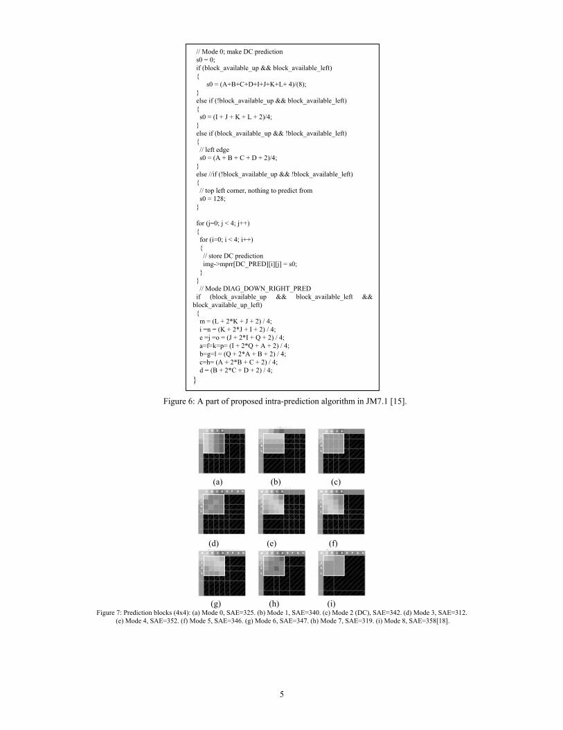
The 9 prediction modes (0-8) are calculated for the 4x4 block shown in Figure 4. For example, in DC (mode 2) and diagonal down/right (mode 4) prediction, different samples are predicted by the algorithm illustrated in Figure 6. Figure 7 shows the prediction block P created by each of the 9 predictions. The sum of absolute error (SAE) for each prediction indicates the magnitude of the prediction error.

5

Figure 6: A part of proposed intra-prediction algorithm in JM7.1 [15].

(a) (b) (c)

(d) (e) (f)

(g) (h) (i)

Figure 7: Prediction blocks (4x4): (a) Mode 0, SAE=325. (b) Mode 1, SAE=340. (c) Mode 2 (DC), SAE=342. (d) Mode 3, SAE=312. (e) Mode 4, SAE=352. (f) Mode 5, SAE=346. (g) Mode 6, SAE=347. (h) Mode 7, SAE=319. (i) Mode 8, SAE=358[18].

// Mode 0; make DC prediction s0 = 0; if (block_available_up && block_available_left) { s0 = (A+B+C+D+I+J+K+L+ 4)/(8); } else if (!block_available_up && block_available_left) { s0 = (I + J + K + L + 2)/4; } else if (block_available_up && !block_available_left) { // left edge s0 = (A + B + C + D + 2)/4; } else //if (!block_available_up && !block_available_left) { // top left corner, nothing to predict from s0 = 128; } for (j=0; j < 4; j++) { for (i=0; i < 4; i++) { // store DC prediction img->mprr[DC_PRED][i][j] = s0; } } // Mode DIAG_DOWN_RIGHT_PRED if (block_available_up && block_available_left && block_available_up_left) { m = (L + 2*K + J + 2) / 4; i =n = (K + 2*J + I + 2) / 4; e =j =o = (J + 2*I + Q + 2) / 4; a=f=k=p= (I + 2*Q + A + 2) / 4; b=g=l = (Q + 2*A + B + 2) / 4; c=h= (A + 2*B + C + 2) / 4; d = (B + 2*C + D + 2) / 4; }

6

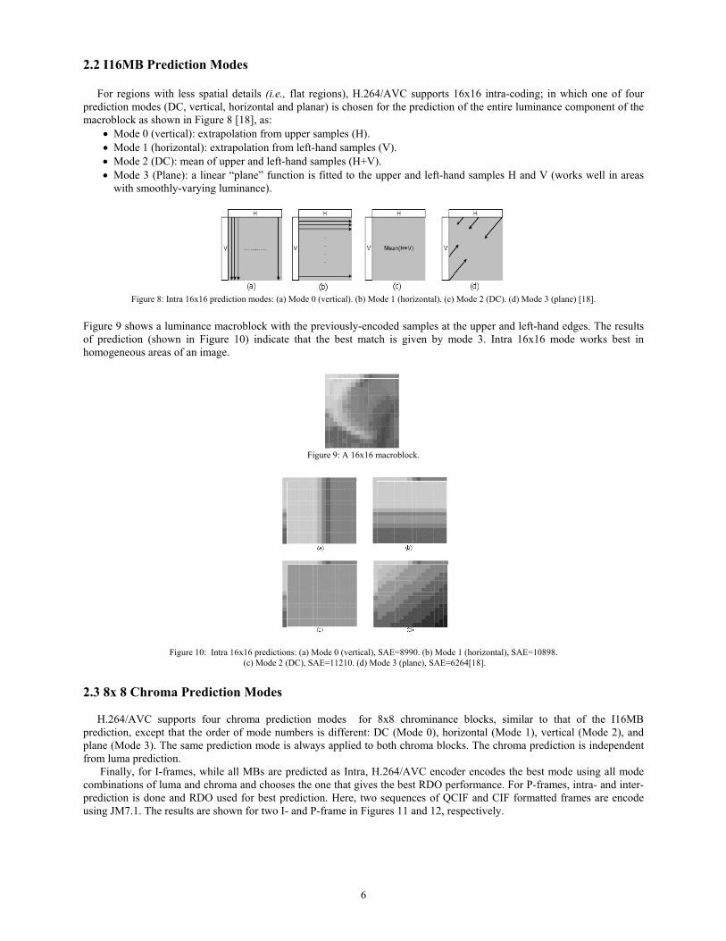
2.2 I16MB Prediction Modes For regions with less spatial details (i.e., flat regions), H.264/AVC supports 16x16 intra-coding; in which one of four prediction modes (DC, vertical, horizontal and planar) is chosen for the prediction of the entire luminance component of the macroblock as shown in Figure 8 [18], as:

• Mode 0 (vertical): extrapolation from upper samples (H). • Mode 1 (horizontal): extrapolation from left-hand samples (V). • Mode 2 (DC): mean of upper and left-hand samples (H+V). • Mode 3 (Plane): a linear “plane” function is fitted to the upper and left-hand samples H and V (works well in areas

with smoothly-varying luminance). JA B C D E F G H

J Figure 8: Intra 16x16 prediction modes: (a) Mode 0 (vertical). (b) Mode 1 (horizontal). (c) Mode 2 (DC). (d) Mode 3 (plane) [18].

Figure 9 shows a luminance macroblock with the previously-encoded samples at the upper and left-hand edges. The results of prediction (shown in Figure 10) indicate that the best match is given by mode 3. Intra 16x16 mode works best in homogeneous areas of an image.

Figure 9: A 16x16 macroblock.

Figure 10: Intra 16x16 predictions: (a) Mode 0 (vertical), SAE=8990. (b) Mode 1 (horizontal), SAE=10898. (c) Mode 2 (DC), SAE=11210. (d) Mode 3 (plane), SAE=6264[18].

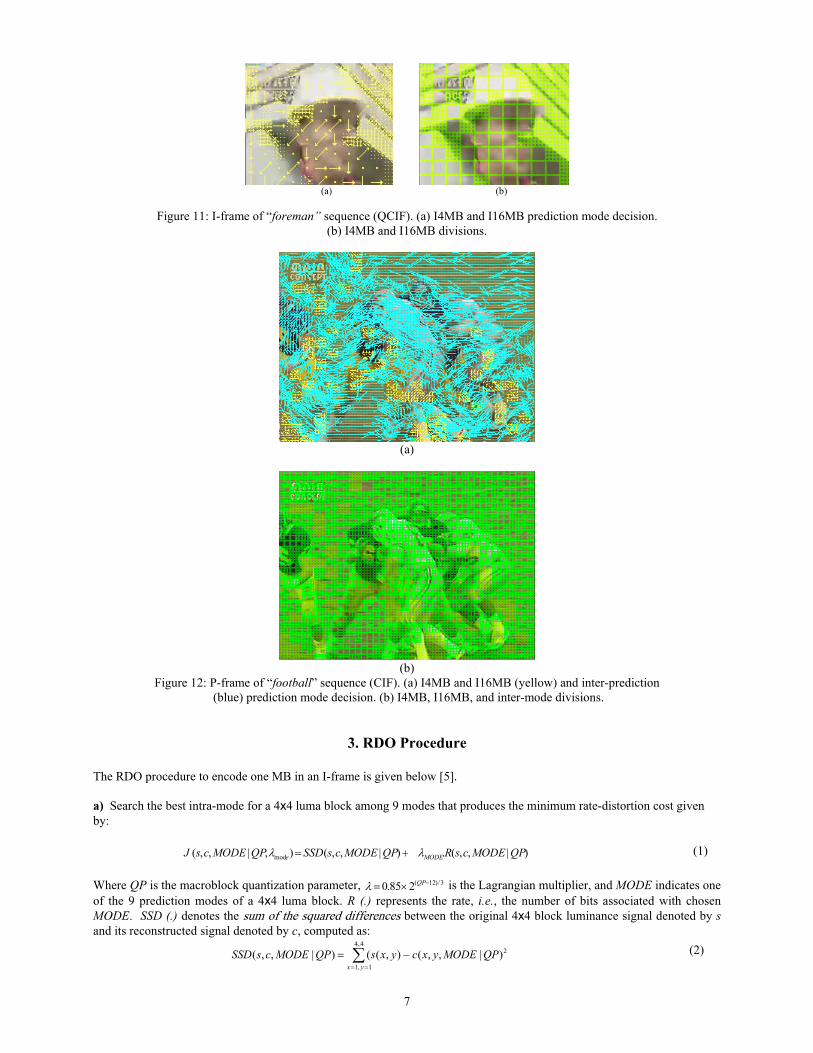
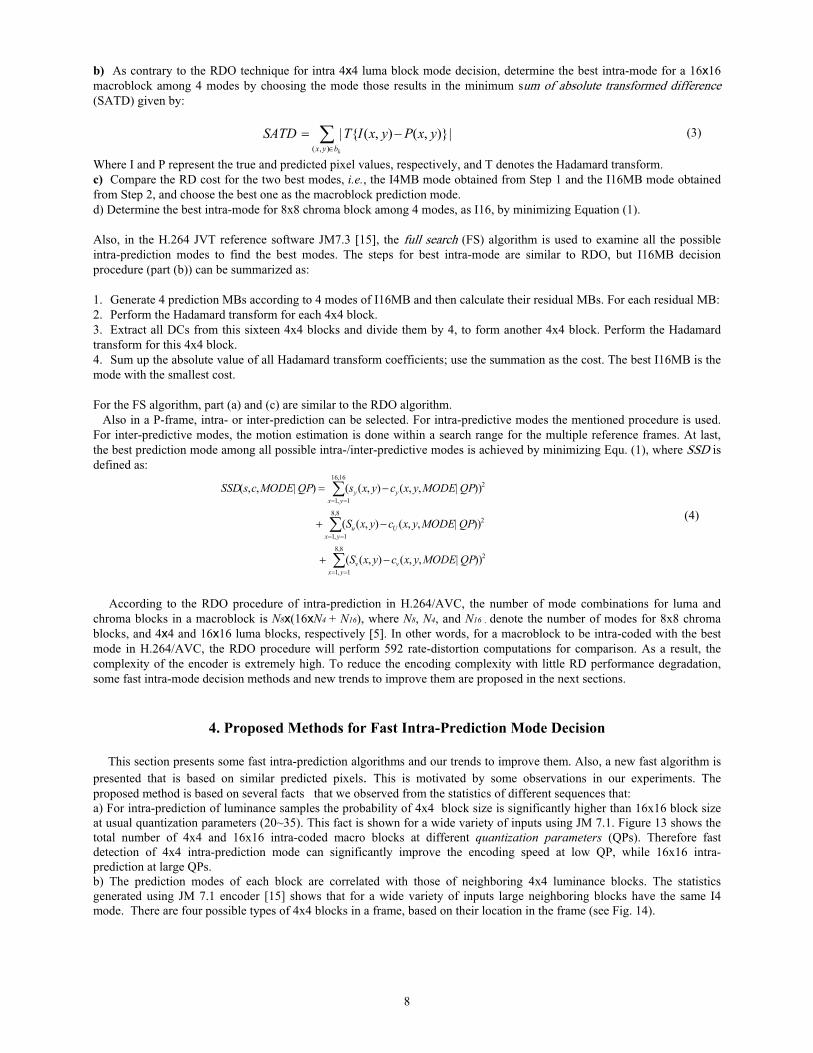
2.3 8x 8 Chroma Prediction Modes H.264/AVC supports four chroma prediction modes for 8x8 chrominance blocks, similar to that of the I16MB prediction, except that the order of mode numbers is different: DC (Mode 0), horizontal (Mode 1), vertical (Mode 2), and plane (Mode 3). The same prediction mode is always applied to both chroma blocks. The chroma prediction is independent from luma prediction. Finally, for I-frames, while all MBs are predicted as Intra, H.264/AVC encoder encodes the best mode using all mode combinations of luma and chroma and chooses the one that gives the best RDO performance. For P-frames, intra- and inter-prediction is done and RDO used for best prediction. Here, two sequences of QCIF and CIF formatted frames are encode using JM7.1. The results are shown for two I- and P-frame in Figures 11 and 12, respectively.

7

(a) (b)

Figure 11: I-frame of “foreman” sequence (QCIF). (a) I4MB and I16MB prediction mode decision. (b) I4MB and I16MB divisions.

(a)

(b)

Figure 12: P-frame of “football” sequence (CIF). (a) I4MB and I16MB (yellow) and inter-prediction (blue) prediction mode decision. (b) I4MB, I16MB, and inter-mode divisions.

3. RDO Procedure The RDO procedure to encode one MB in an I-frame is given below [5]. a) Search the best intra-mode for a 4x4 luma block among 9 modes that produces the minimum rate-distortion cost given by:

)|,,(.)|,,(),|,,( mod QPMODEcsRQPMODEcsSSDQPMODEcsJ MODEe λλ += (1)

Where QP is the macroblock quantization parameter, 3/)12(285.0 −×= QPλ is the Lagrangian multiplier, and MODE indicates one of the 9 prediction modes of a 4x4 luma block. R (.) represents the rate, i.e., the number of bits associated with chosen MODE. SSD (.) denotes the sum of the squared differences between the original 4x4 block luminance signal denoted by s and its reconstructed signal denoted by c, computed as:

∑==

−=4,4

1,1

2)|,,(),(()|,,(yx

QPMODEyxcyxsQPMODEcsSSD (2)

8

b) As contrary to the RDO technique for intra 4x4 luma block mode decision, determine the best intra-mode for a 16x16 macroblock among 4 modes by choosing the mode those results in the minimum sum of absolute transformed difference (SATD) given by:

∑∈

−=kbyx

yxPyxITSATD),(

|)},(),({| (3)

Where I and P represent the true and predicted pixel values, respectively, and T denotes the Hadamard transform. c) Compare the RD cost for the two best modes, i.e., the I4MB mode obtained from Step 1 and the I16MB mode obtained from Step 2, and choose the best one as the macroblock prediction mode. d) Determine the best intra-mode for 8x8 chroma block among 4 modes, as I16, by minimizing Equation (1). Also, in the H.264 JVT reference software JM7.3 [15], the full search (FS) algorithm is used to examine all the possible intra-prediction modes to find the best modes. The steps for best intra-mode are similar to RDO, but I16MB decision procedure (part (b)) can be summarized as: 1. Generate 4 prediction MBs according to 4 modes of I16MB and then calculate their residual MBs. For each residual MB: 2. Perform the Hadamard transform for each 4x4 block. 3. Extract all DCs from this sixteen 4x4 blocks and divide them by 4, to form another 4x4 block. Perform the Hadamard transform for this 4x4 block. 4. Sum up the absolute value of all Hadamard transform coefficients; use the summation as the cost. The best I16MB is the mode with the smallest cost. For the FS algorithm, part (a) and (c) are similar to the RDO algorithm. Also in a P-frame, intra- or inter-prediction can be selected. For intra-predictive modes the mentioned procedure is used. For inter-predictive modes, the motion estimation is done within a search range for the multiple reference frames. At last, the best prediction mode among all possible intra-/inter-predictive modes is achieved by minimizing Equ. (1), where SSD is defined as:

28,8

1,1

28,8

1,1

16,16

1,1

2

))|,,(),((

))|,,(),((

))|,,(),(()|,,(

QPMODEyxcyxS

QPMODEyxcyxS

QPMODEyxcyxsQPMODEcsSSD

yxvv

Uyx

u

yxyy

∑

∑

∑

==

==

==

−+

−+

−=

(4)

According to the RDO procedure of intra-prediction in H.264/AVC, the number of mode combinations for luma and chroma blocks in a macroblock is N8x(16xN4 + N16), where N8, N4, and N16 , denote the number of modes for 8x8 chroma blocks, and 4x4 and 16x16 luma blocks, respectively [5]. In other words, for a macroblock to be intra-coded with the best mode in H.264/AVC, the RDO procedure will perform 592 rate-distortion computations for comparison. As a result, the complexity of the encoder is extremely high. To reduce the encoding complexity with little RD performance degradation, some fast intra-mode decision methods and new trends to improve them are proposed in the next sections.

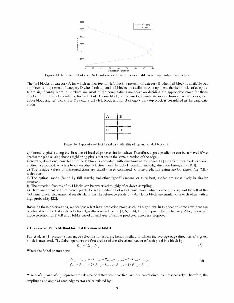
4. Proposed Methods for Fast Intra-Prediction Mode Decision This section presents some fast intra-prediction algorithms and our trends to improve them. Also, a new fast algorithm is presented that is based on similar predicted pixels. This is motivated by some observations in our experiments. The proposed method is based on several facts that we observed from the statistics of different sequences that: a) For intra-prediction of luminance samples the probability of 4x4 block size is significantly higher than 16x16 block size at usual quantization parameters (20~35). This fact is shown for a wide variety of inputs using JM 7.1. Figure 13 shows the total number of 4x4 and 16x16 intra-coded macro blocks at different quantization parameters (QPs). Therefore fast detection of 4x4 intra-prediction mode can significantly improve the encoding speed at low QP, while 16x16 intra-prediction at large QPs. b) The prediction modes of each block are correlated with those of neighboring 4x4 luminance blocks. The statistics generated using JM 7.1 encoder [15] shows that for a wide variety of inputs large neighboring blocks have the same I4 mode. There are four possible types of 4x4 blocks in a frame, based on their location in the frame (see Fig. 14).

9

10 15 20 25 30 35 40 45 500

1000

2000

3000

4000

5000

6000

Quantization Parameter

Num

ber o

f MB

16x16 MB4x4 MB

Figure 13: Number of 4x4 and 16x16 intra-coded macro blocks at different quantization parameters

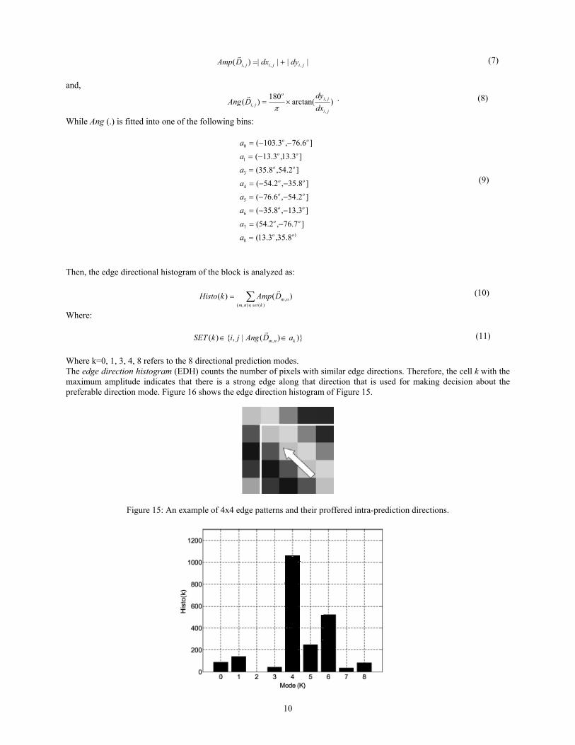
The 4x4 blocks of category A for which neither top nor left block is present, of category B when left block is available but top block is not present, of category D when both top and left blocks are available. Among these, the 4x4 blocks of category D are significantly more in numbers and most of the computations are spent on deciding the appropriate mode for these blocks. From these observations, for each 4x4 D luma block, we obtain two candidate modes from adjacent blocks, i.e., upper block and left block. For C category only left block and for B category only top block is considered as the candidate mode.

Figure 14: Types of 4x4 block based on availability of top and left 4x4 blocks[9].

c) Normally, pixels along the direction of local edge have similar values. Therefore, a good prediction can be achieved if we predict the pixels using those neighboring pixels that are in the same direction of the edge. Generally, directional correlation of each block is consistent with directions of the edges. In [1], a fast intra-mode decision method is proposed, which is based on edge detection using the Sobel operation and edge direction histogram (EDH). d) The residue values of intra-prediction are usually large compared to inter-prediction using motion estimation (ME) techniques. e) The optimal mode (found by full search) and other “good” (second or third best) modes are most likely in similar directions. f) The direction features of 4x4 blocks can be preserved roughly after down-sampling. g) There are a total of 13 reference pixels for intra prediction of a 4x4 luma block, which locate at the up and the left of the 4x4 luma block. Experimental results show that the reference pixels of a 4x4 luma block are similar with each other with a high probability [22]. Based on these observations, we propose a fast intra-prediction mode selection algorithm. In this section some new ideas are combined with the fast mode selection algorithms introduced in [1, 6, 7, 14, 19] to improve their efficiency. Also, a new fast mode selection for I4MB and I16MB based on analyses of similar predicted pixels are proposed. 4.1 Improved Pan’s Method for Fast Decision of I4MB Pan et al. in [1] present a fast mode selection for intra-prediction method in which the average edge direction of a given block is measured. The Sobel operators are first used to obtain directional vector of each pixel in a block by:

},{ ,,, jijiji dydxD =v (5)

Where the Sobel operator are:

1,1,11,11,1,11,1,

1,11,1,11,11,1,1,

22

22

+−−−−+++−+

−+−−−++++−

−×−−+×+=

−×−−+×+=

jijijijijijiji

jijijijijijiji

PPPPPPdy

PPPPPPdx (6)

Where jidx , and jidy , represent the degree of difference in vertical and horizontal directions, respectively. Therefore, the amplitude and angle of each edge vector are calculated by:

10

||||)( ,,, jijiji dydxDAmp +=

r (7) and,

)arctan(180)(,

,,

ji

jio

ji dxdy

DAng ×=π

r . (8)

While Ang (.) is fitted into one of the following bins:

)8

7

6

5

4

3

1

0

8.35,3.13(

]7.76,2.54(

]3.13,8.35(

]2.54,6.76(

]8.35,2.54(

]2.54,8.35(

]3.13,3.13(

]6.76,3.103(

oo

oo

oo

oo

oo

oo

oo

oo

a

a

a

a

a

a

a

a

=

−=

−−=

−−=

−−=

=

−=

−−=

(9)

Then, the edge directional histogram of the block is analyzed as:

∑∈

=)(),(

, )()(ksetnm

nmDAmpkHistor (10)

Where:

)})(|,{)( , knm aDAngjikSET ∈∈r (11)

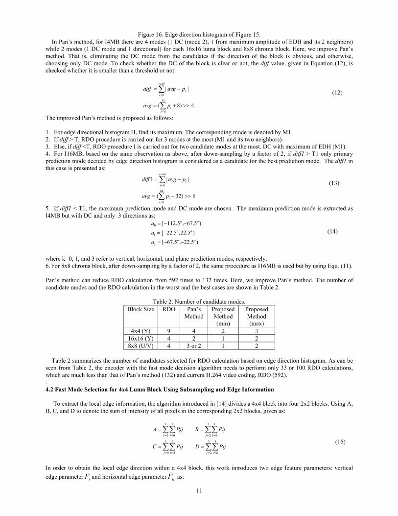
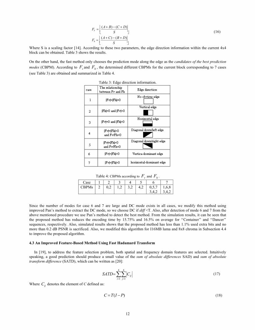
Where k=0, 1, 3, 4, 8 refers to the 8 directional prediction modes. The edge direction histogram (EDH) counts the number of pixels with similar edge directions. Therefore, the cell k with the maximum amplitude indicates that there is a strong edge along that direction that is used for making decision about the preferable direction mode. Figure 16 shows the edge direction histogram of Figure 15.

Figure 15: An example of 4x4 edge patterns and their proffered intra-prediction directions.

11

Figure 16: Edge direction histogram of Figure 15. In Pan’s method, for I4MB there are 4 modes (1 DC (mode 2), 1 from maximum amplitude of EDH and its 2 neighbors) while 2 modes (1 DC mode and 1 directional) for each 16x16 luma block and 8x8 chroma block. Here, we improve Pan’s method. That is, eliminating the DC mode from the candidates if the direction of the block is obvious, and otherwise, choosing only DC mode. To check whether the DC of the block is clear or not, the diff value, given in Equation (12), is checked whether it is smaller than a threshold or not:

4)8(

||

15

0

15

0

>>+=

−=

∑

∑

=

=

=

ii

i

ii

pavg

pavgdiff (12)

The improved Pan’s method is proposed as follows: 1. For edge directional histogram H, find its maximum. The corresponding mode is denoted by M1. 2. If diff > T, RDO procedure is carried out for 3 modes at the most (M1 and its two neighbors). 3. Else, if diff <T, RDO procedure I is carried out for two candidate modes at the most. DC with maximum of EDH (M1). 4. For I16MB, based on the same observation as above, after down-sampling by a factor of 2, if diff1 > T1 only primary prediction mode decided by edge direction histogram is considered as a candidate for the best prediction mode. The diff1 in this case is presented as:

6)32(

||1

64

0

64

0

>>+=

−=

∑

∑

=

=

=

ii

i

ii

pavg

pavgdiff (13)

5. If diff1 < T1, the maximum prediction mode and DC mode are chosen. The maximum prediction mode is extracted as I4MB but with DC and only 3 directions as:

)5.22,5.67[

)5.22,5.22[

)5.67,5.112[

3

1

0

oo

oo

oo

a

a

a

−−=

−=

−−= (14)

where k=0, 1, and 3 refer to vertical, horizontal, and plane prediction modes, respectively. 6. For 8x8 chroma block, after down-sampling by a factor of 2, the same procedure as I16MB is used but by using Equ. (11). Pan’s method can reduce RDO calculation from 592 times to 132 times. Here, we improve Pan’s method. The number of candidate modes and the RDO calculation in the worst and the best cases are shown in Table 2.

Table 2. Number of candidate modes. Block Size RDO Pan’s

Method Proposed Method (min)

Proposed Method (max)

4x4 (Y) 9 4 2 3 16x16 (Y) 4 2 1 2 8x8 (U/V) 4 3 or 2 1 2

Table 2 summarizes the number of candidates selected for RDO calculation based on edge direction histogram. As can be seen from Table 2, the encoder with the fast mode decision algorithm needs to perform only 33 or 100 RDO calculations, which are much less than that of Pan’s method (132) and current H.264 video coding, RDO (592). . 4.2 Fast Mode Selection for 4x4 Luma Block Using Subsampling and Edge Information To extract the local edge information, the algorithm introduced in [14] divides a 4x4 block into four 2x2 blocks. Using A, B, C, and D to denote the sum of intensity of all pixels in the corresponding 2x2 blocks, given as:

∑∑∑∑

∑∑∑∑

= == =

= == =

==

==

3

2

3

2

1

0

3

2

3

2

1

0

1

0

1

0

j ij i

j ii ii

PijDPijC

PijBijPA

(15)

In order to obtain the local edge direction within a 4x4 block, this work introduces two edge feature parameters: vertical

edge parameter vF and horizontal edge parameter hF as:

12

+−+

=

+−+

=

SDBCAF

SDCBAF

h

V

)()(

)()( (16)

Where S is a scaling factor [14]. According to these two parameters, the edge direction information within the current 4x4 block can be obtained. Table 3 shows the results.

On the other hand, the fast method only chooses the prediction mode along the edge as the candidates of the best prediction modes (CBPM). According to vF and hF , the determined different CBPMs for the current block corresponding to 7 cases (see Table 3) are obtained and summarized in Table 4.

Table 3: Edge direction information.

Table 4: CBPMs according to vF and hF .

Case 1 2 3 4 5 6 7 CBPMs 2 0,2 1,2 3,2 4,2 0,5,7

3,4,2 1,6,8 3,4,2

Since the number of modes for case 6 and 7 are large and DC mode exists in all cases, we modify this method using improved Pan’s method to extract the DC mode, so we choose DC if diff <T. Also, after detection of mode 6 and 7 from the above mentioned procedure we use Pan’s method to detect the best method. From the simulation results, it can be seen that the proposed method has reduces the encoding time by 15.75% and 16.5% on average for ‘‘Container’’ and ‘‘Dancer’’ sequences, respectively. Also, simulated results shows that the proposed method has less than 1.1% used extra bits and no more than 0.2 dB PSNR is sacrificed. Also, we modified this algorithm for I16MB luma and 8x8 chroma in Subsection 4.4 to improve the proposed algorithm. 4.3 An Improved Feature-Based Method Using Fast Hadamard Transform In [19], to address the feature selection problem, both spatial and frequency domain features are selected. Intuitively speaking, a good prediction should produce a small value of the sum of absolute differences SAD) and sum of absolute transform difference (SATD), which can be written as [20]:

∑∑= =

=4

1

4

1i jijCSATD (17)

Where ijC denotes the element of C defined as:

)( PITC −= (18)

13

where I and P denote the current block and its prediction, respectively, and T is a certain 2D orthonormal transform. In this work, for computational simplicity, T is chosen to be the separable Hadamard transform with 4-point along each dimension as:

−−−−

−−=

111111111111

1111

T (19)

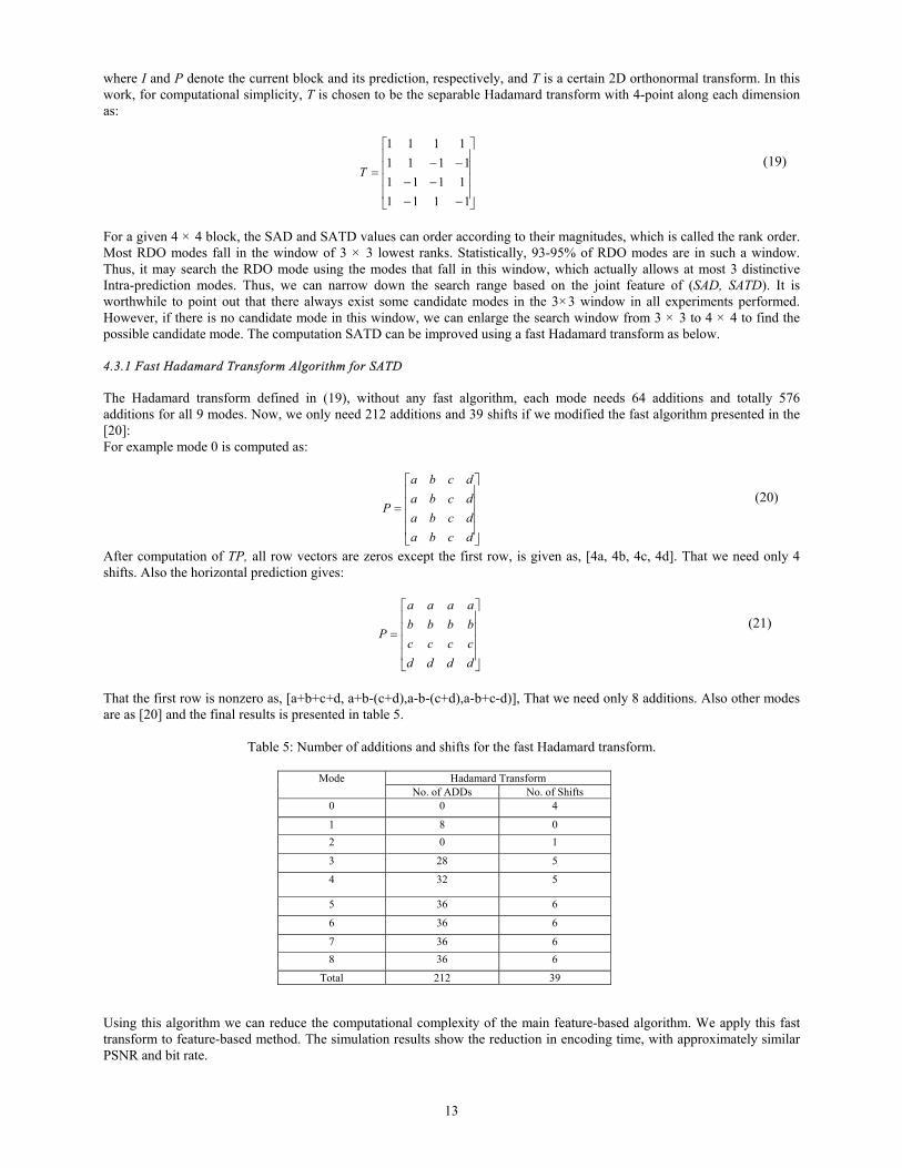
For a given 4 × 4 block, the SAD and SATD values can order according to their magnitudes, which is called the rank order. Most RDO modes fall in the window of 3 × 3 lowest ranks. Statistically, 93-95% of RDO modes are in such a window. Thus, it may search the RDO mode using the modes that fall in this window, which actually allows at most 3 distinctive Intra-prediction modes. Thus, we can narrow down the search range based on the joint feature of (SAD, SATD). It is worthwhile to point out that there always exist some candidate modes in the 3×3 window in all experiments performed. However, if there is no candidate mode in this window, we can enlarge the search window from 3 × 3 to 4 × 4 to find the possible candidate mode. The computation SATD can be improved using a fast Hadamard transform as below. 4.3.1 Fast Hadamard Transform Algorithm for SATD The Hadamard transform defined in (19), without any fast algorithm, each mode needs 64 additions and totally 576 additions for all 9 modes. Now, we only need 212 additions and 39 shifts if we modified the fast algorithm presented in the [20]: For example mode 0 is computed as:

=

dcbadcbadcbadcba

P (20)

After computation of TP, all row vectors are zeros except the first row, is given as, [4a, 4b, 4c, 4d]. That we need only 4 shifts. Also the horizontal prediction gives:

=

ddddccccbbbbaaaa

P (21)

That the first row is nonzero as, [a+b+c+d, a+b-(c+d),a-b-(c+d),a-b+c-d)], That we need only 8 additions. Also other modes are as [20] and the final results is presented in table 5.

Table 5: Number of additions and shifts for the fast Hadamard transform.

Mode Hadamard Transform

No. of ADDs No. of Shifts 0 0 4

1 8 0 2 0 1

3 28 5

4 32 5

5 36 6

6 36 6

7 36 6 8 36 6

Total 212 39 Using this algorithm we can reduce the computational complexity of the main feature-based algorithm. We apply this fast transform to feature-based method. The simulation results show the reduction in encoding time, with approximately similar PSNR and bit rate.

14

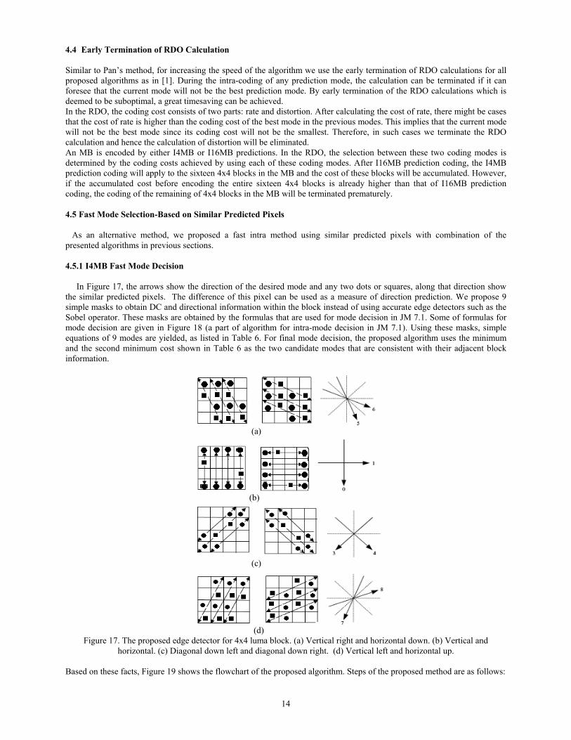
4.4 Early Termination of RDO Calculation Similar to Pan’s method, for increasing the speed of the algorithm we use the early termination of RDO calculations for all proposed algorithms as in [1]. During the intra-coding of any prediction mode, the calculation can be terminated if it can foresee that the current mode will not be the best prediction mode. By early termination of the RDO calculations which is deemed to be suboptimal, a great timesaving can be achieved. In the RDO, the coding cost consists of two parts: rate and distortion. After calculating the cost of rate, there might be cases that the cost of rate is higher than the coding cost of the best mode in the previous modes. This implies that the current mode will not be the best mode since its coding cost will not be the smallest. Therefore, in such cases we terminate the RDO calculation and hence the calculation of distortion will be eliminated. An MB is encoded by either I4MB or I16MB predictions. In the RDO, the selection between these two coding modes is determined by the coding costs achieved by using each of these coding modes. After I16MB prediction coding, the I4MB prediction coding will apply to the sixteen 4x4 blocks in the MB and the cost of these blocks will be accumulated. However, if the accumulated cost before encoding the entire sixteen 4x4 blocks is already higher than that of I16MB prediction coding, the coding of the remaining of 4x4 blocks in the MB will be terminated prematurely. 4.5 Fast Mode Selection-Based on Similar Predicted Pixels As an alternative method, we proposed a fast intra method using similar predicted pixels with combination of the presented algorithms in previous sections. 4.5.1 I4MB Fast Mode Decision In Figure 17, the arrows show the direction of the desired mode and any two dots or squares, along that direction show the similar predicted pixels. The difference of this pixel can be used as a measure of direction prediction. We propose 9 simple masks to obtain DC and directional information within the block instead of using accurate edge detectors such as the Sobel operator. These masks are obtained by the formulas that are used for mode decision in JM 7.1. Some of formulas for mode decision are given in Figure 18 (a part of algorithm for intra-mode decision in JM 7.1). Using these masks, simple equations of 9 modes are yielded, as listed in Table 6. For final mode decision, the proposed algorithm uses the minimum and the second minimum cost shown in Table 6 as the two candidate modes that are consistent with their adjacent block information.

(a)

(b)

(c)

(d)

Figure 17. The proposed edge detector for 4x4 luma block. (a) Vertical right and horizontal down. (b) Vertical and horizontal. (c) Diagonal down left and diagonal down right. (d) Vertical left and horizontal up.

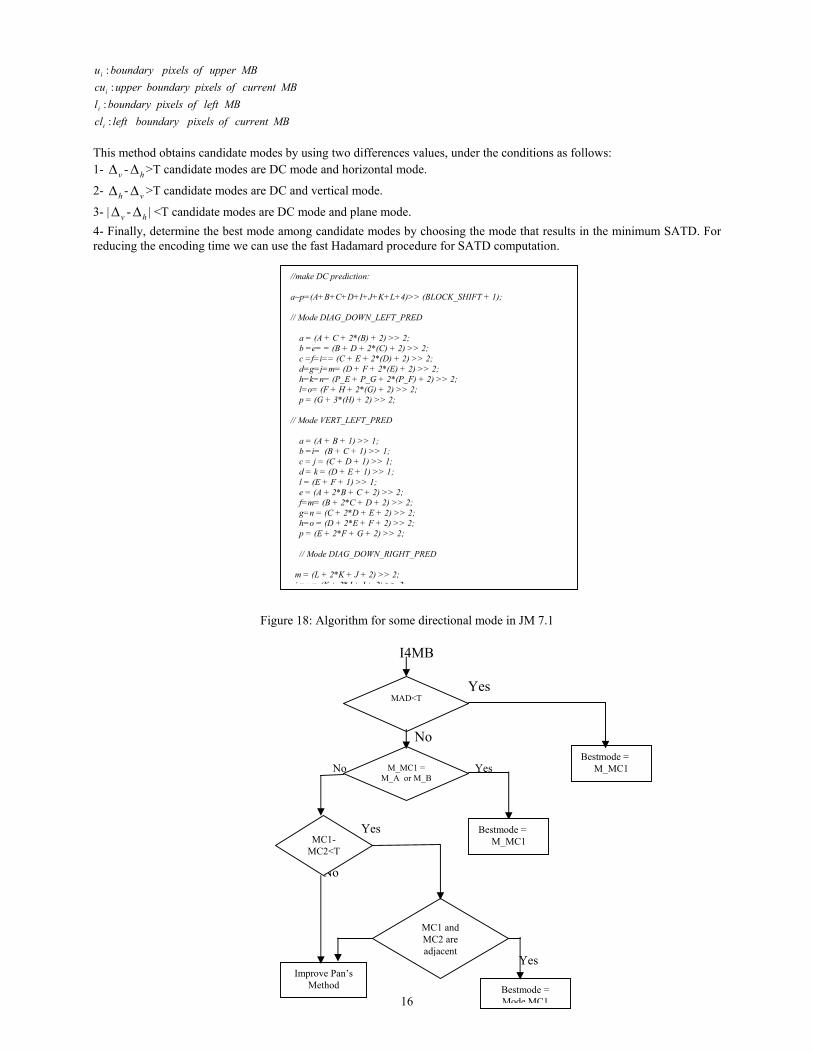
Based on these facts, Figure 19 shows the flowchart of the proposed algorithm. Steps of the proposed method are as follows:

15

1. Calculate the two most probable intra-prediction modes. These are the minimum (First Minumum Cost=MC1, mode MC1=M_MC1) and the second minimum (MC2, M_MC2) of costs evaluated by Table 6. 2. For 4x4 luma block, MAD (mean of absolute difference) of its reference pixels is computed, if it is smaller than a threshold, M_MC1 is selected. Go to step 10. This result is yielded from this fact that if the similarity of reference pixels of a block is high, the difference between different prediction modes will be very small. For this case, it is not necessary to check all 9 prediction modes, but only one prediction mode is enough [22]. 4. If MADH (mean of absolute difference of horizontal references) is less than a threshold and M_MC1 is a member of set {mode 0, mode 3, mode 7}, then M_MC1 is selected. Go to step 10. 5. Also, if MADV (mean of absolute difference of vertical references) is less than a threshold and M_MC1 is a member set of {mode 1, mode 8}, then M_MC1 is selected. Go to step 10. It is obvious that if the similarity of horizontal reference pixels of a block is high, the difference between prediction results obtained with prediction modes 0, 3 and 7 will be very small. Also, if the similarity of vertical reference pixels of a block is high, the similarity between modes 1 and 8 is high.

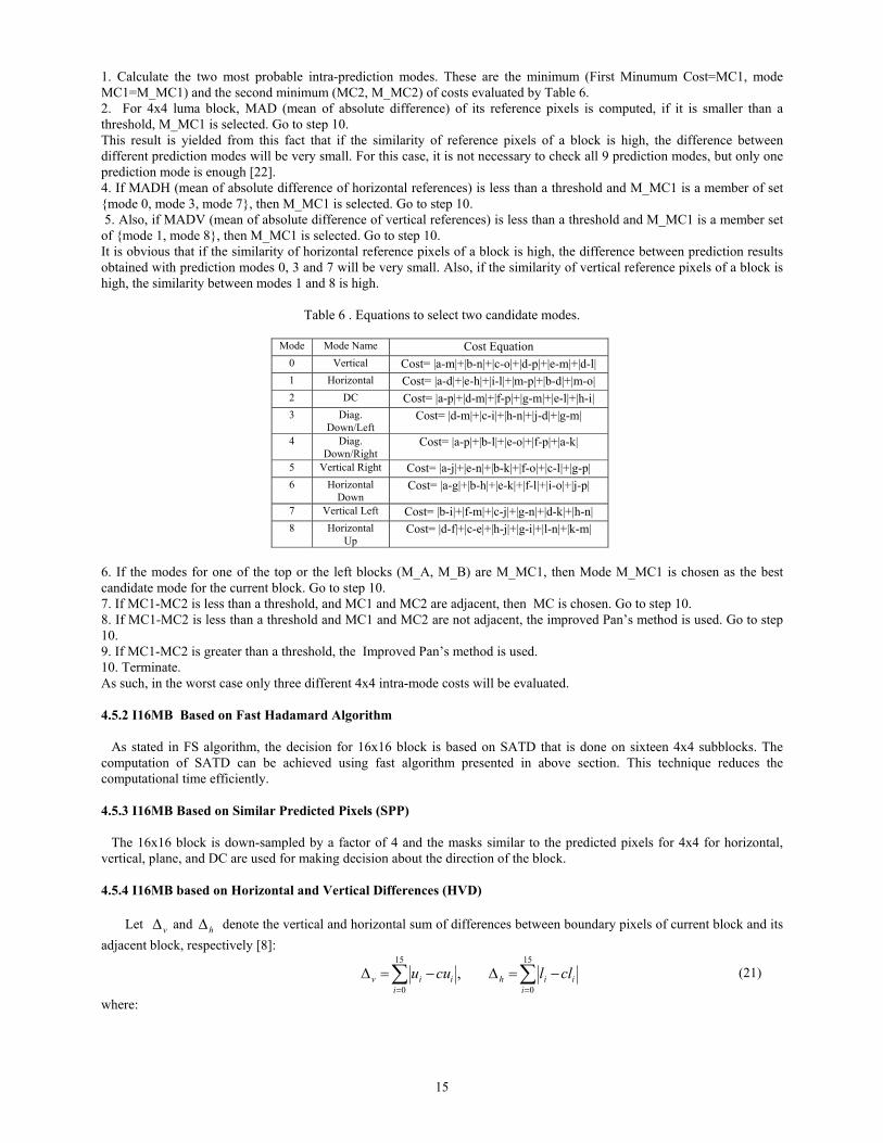
Table 6 . Equations to select two candidate modes.

Mode Mode Name Cost Equation

0 Vertical Cost= |a-m|+|b-n|+|c-o|+|d-p|+|e-m|+|d-l| 1 Horizontal Cost= |a-d|+|e-h|+|i-l|+|m-p|+|b-d|+|m-o| 2 DC Cost= |a-p|+|d-m|+|f-p|+|g-m|+|e-l|+|h-i|3 Diag.

Down/Left Cost= |d-m|+|c-i|+|h-n|+|j-d|+|g-m|

4 Diag. Down/Right

Cost= |a-p|+|b-l|+|e-o|+|f-p|+|a-k|

5 Vertical Right Cost= |a-j|+|e-n|+|b-k|+|f-o|+|c-l|+|g-p|6 Horizontal

Down Cost= |a-g|+|b-h|+|e-k|+|f-l|+|i-o|+|j-p|

7 Vertical Left Cost= |b-i|+|f-m|+|c-j|+|g-n|+|d-k|+|h-n|8 Horizontal

Up Cost= |d-f|+|c-e|+|h-j|+|g-i|+|l-n|+|k-m|

6. If the modes for one of the top or the left blocks (M_A, M_B) are M_MC1, then Mode M_MC1 is chosen as the best candidate mode for the current block. Go to step 10. 7. If MC1-MC2 is less than a threshold, and MC1 and MC2 are adjacent, then MC is chosen. Go to step 10. 8. If MC1-MC2 is less than a threshold and MC1 and MC2 are not adjacent, the improved Pan’s method is used. Go to step 10. 9. If MC1-MC2 is greater than a threshold, the Improved Pan’s method is used. 10. Terminate. As such, in the worst case only three different 4x4 intra-mode costs will be evaluated.

4.5.2 I16MB Based on Fast Hadamard Algorithm As stated in FS algorithm, the decision for 16x16 block is based on SATD that is done on sixteen 4x4 subblocks. The computation of SATD can be achieved using fast algorithm presented in above section. This technique reduces the computational time efficiently. 4.5.3 I16MB Based on Similar Predicted Pixels (SPP) The 16x16 block is down-sampled by a factor of 4 and the masks similar to the predicted pixels for 4x4 for horizontal, vertical, plane, and DC are used for making decision about the direction of the block. 4.5.4 I16MB based on Horizontal and Vertical Differences (HVD) Let v∆ and h∆ denote the vertical and horizontal sum of differences between boundary pixels of current block and its adjacent block, respectively [8]:

∑∑==

−=∆−=∆15

0

15

0,

iiih

iiiv cllcuu (21)

where:

16

MBcurrentofpixelsboundaryleftclMBleftofpixelsboundaryl

MBcurrentofpixelsboundaryuppercuMBupperofpixelsboundaryu

i

i

i

i

::

::

This method obtains candidate modes by using two differences values, under the conditions as follows: 1- v∆ - h∆ >T candidate modes are DC mode and horizontal mode.

2- h∆ - v∆ >T candidate modes are DC and vertical mode.

3- | v∆ - h∆ | <T candidate modes are DC mode and plane mode. 4- Finally, determine the best mode among candidate modes by choosing the mode that results in the minimum SATD. For reducing the encoding time we can use the fast Hadamard procedure for SATD computation.

that is used for mask extraction. For each 4x4 luma block

Figure 18: Algorithm for some directional mode in JM 7.1

I4MB Yes

No No Yes

Yes

No

Yes

//make DC prediction: a~p=(A+B+C+D+I+J+K+L+4)>> (BLOCK_SHIFT + 1); // Mode DIAG_DOWN_LEFT_PRED a = (A + C + 2*(B) + 2) >> 2; b =e= = (B + D + 2*(C) + 2) >> 2; c =f=i== (C + E + 2*(D) + 2) >> 2; d=g=j=m= (D + F + 2*(E) + 2) >> 2; h=k=n= (P_E + P_G + 2*(P_F) + 2) >> 2; l=o= (F + H + 2*(G) + 2) >> 2; p = (G + 3*(H) + 2) >> 2; // Mode VERT_LEFT_PRED

a = (A + B + 1) >> 1; b =i= (B + C + 1) >> 1; c = j = (C + D + 1) >> 1; d = k = (D + E + 1) >> 1; l = (E + F + 1) >> 1; e = (A + 2*B + C + 2) >> 2; f=m= (B + 2*C + D + 2) >> 2; g=n = (C + 2*D + E + 2) >> 2; h=o = (D + 2*E + F + 2) >> 2; p = (E + 2*F + G + 2) >> 2; // Mode DIAG_DOWN_RIGHT_PRED m = (L + 2*K + J + 2) >> 2; i =n = (K + 2*J + I + 2) >> 2;

M_MC1 = M_A or M_B

MC1-MC2<T

Improve Pan’s Method Bestmode =

Mode MC1

MAD<T

Bestmode = M_MC1

Bestmode = M_MC1

MC1 and MC2 are adjacent

17

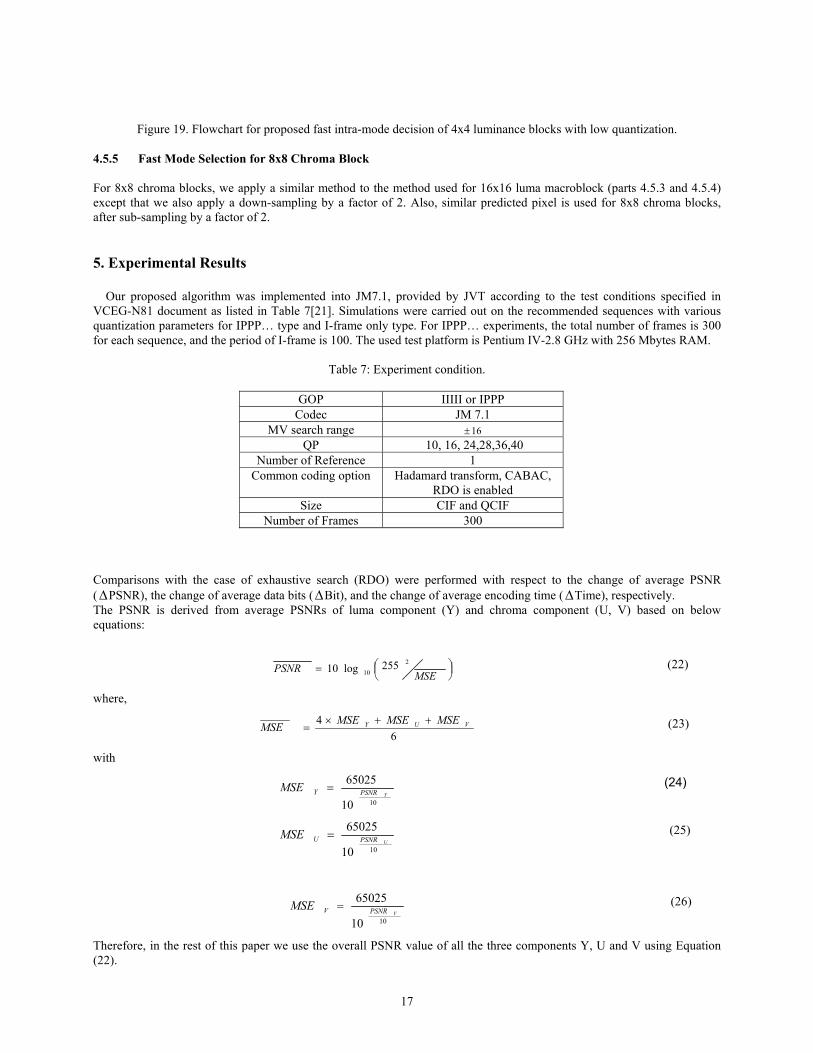
Figure 19. Flowchart for proposed fast intra-mode decision of 4x4 luminance blocks with low quantization. 4.5.5 Fast Mode Selection for 8x8 Chroma Block For 8x8 chroma blocks, we apply a similar method to the method used for 16x16 luma macroblock (parts 4.5.3 and 4.5.4) except that we also apply a down-sampling by a factor of 2. Also, similar predicted pixel is used for 8x8 chroma blocks, after sub-sampling by a factor of 2. 5. Experimental Results Our proposed algorithm was implemented into JM7.1, provided by JVT according to the test conditions specified in VCEG-N81 document as listed in Table 7[21]. Simulations were carried out on the recommended sequences with various quantization parameters for IPPP… type and I-frame only type. For IPPP… experiments, the total number of frames is 300 for each sequence, and the period of I-frame is 100. The used test platform is Pentium IV-2.8 GHz with 256 Mbytes RAM.

Table 7: Experiment condition.

GOP IIIII or IPPP Codec JM 7.1

MV search range 16±QP 10, 16, 24,28,36,40

Number of Reference 1 Common coding option Hadamard transform, CABAC,

RDO is enabled Size CIF and QCIF

Number of Frames 300 Comparisons with the case of exhaustive search (RDO) were performed with respect to the change of average PSNR (∆PSNR), the change of average data bits (∆Bit), and the change of average encoding time (∆Time), respectively. The PSNR is derived from average PSNRs of luma component (Y) and chroma component (U, V) based on below equations:

=

MSEPSNR

2

10255log10 (22)

where,

6

4 VUY MSEMSEMSEMSE ++×= (23)

with

1010

65025YPSNRYMSE = (24)

1010

65025UPSNRUMSE = (25)

1010

65025VPSNRVMSE = (26)

Therefore, in the rest of this paper we use the overall PSNR value of all the three components Y, U and V using Equation (22).

18

Also, in order to evaluate the time saving of the proposed fast intra-mode decision algorithm, the following calculation is defined to find the time differences. Let refT denote the coding time used by JM7.1 encoder and propT be the time taken by

the faster intra-prediction algorithm, and time∆ be defined as:

100% ×−

=∆ref

refprop

TTT

Time (27)

Also, bitrate increase is defined as:

100% ×−

=∆ref

refprop

bitratebitratebitrate

Bitrate (28)

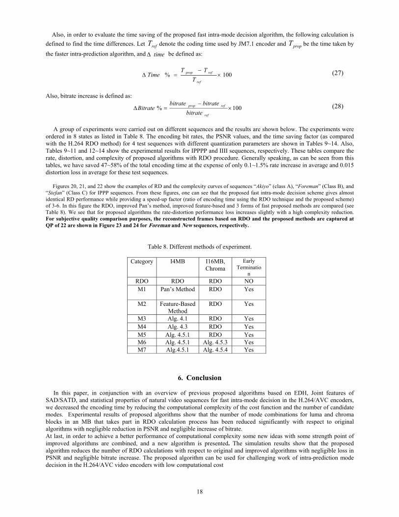
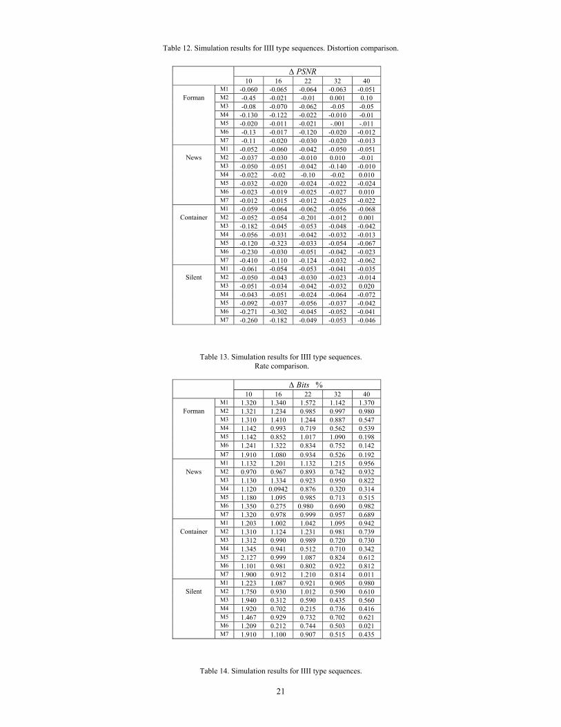
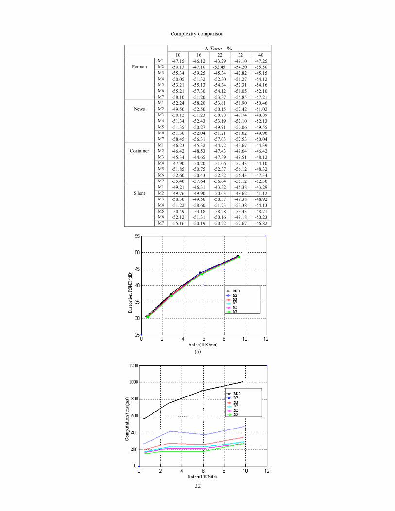
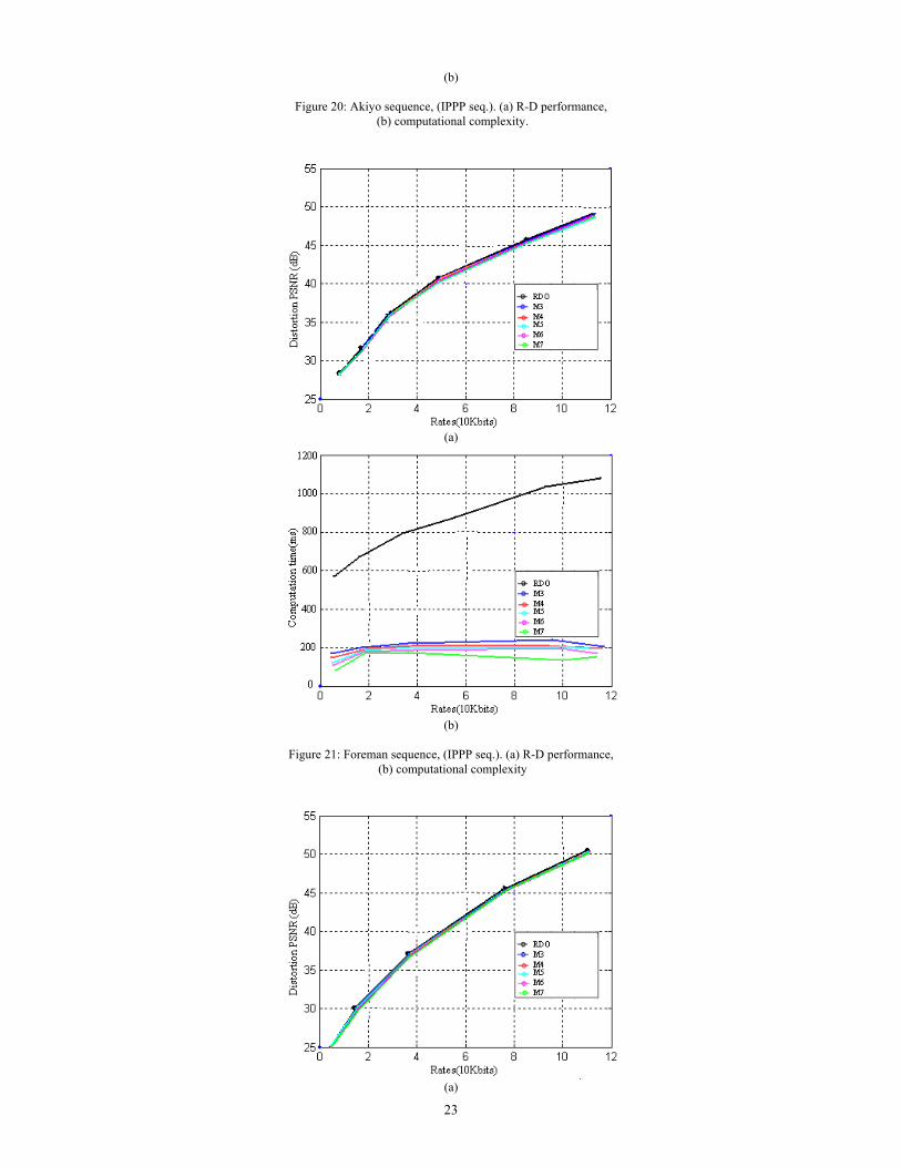
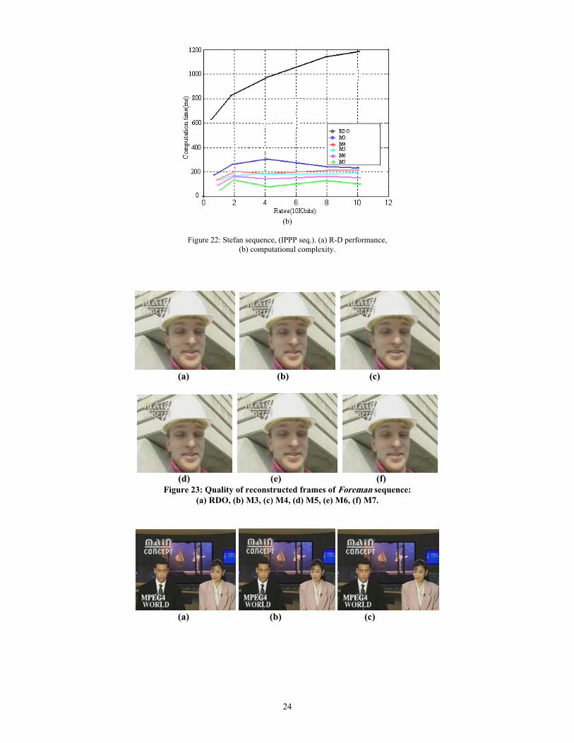
A group of experiments were carried out on different sequences and the results are shown below. The experiments were ordered in 8 states as listed in Table 8. The encoding bit rates, the PSNR values, and the time saving factor (as compared with the H.264 RDO method) for 4 test sequences with different quantization parameters are shown in Tables 9~14. Also, Tables 9~11 and 12~14 show the experimental results for IPPPP and IIII sequences, respectively. These tables compare the rate, distortion, and complexity of proposed algorithms with RDO procedure. Generally speaking, as can be seen from this tables, we have saved 47~58% of the total encoding time at the expense of only 0.1~1.5% rate increase in average and 0.015 distortion loss in average for these test sequences. Figures 20, 21, and 22 show the examples of RD and the complexity curves of sequences “Akiyo” (class A), “Foreman” (Class B), and “Stefan” (Class C) for IPPP sequences. From these figures, one can see that the proposed fast intra-mode decision scheme gives almost identical RD performance while providing a speed-up factor (ratio of encoding time using the RDO technique and the proposed scheme) of 3-6. In this figure the RDO, improved Pan’s method, improved feature-based and 3 forms of fast proposed methods are compared (see Table 8). We see that for proposed algorithms the rate-distortion performance loss increases slightly with a high complexity reduction. For subjective quality comparison purposes, the reconstructed frames based on RDO and the proposed methods are captured at QP of 22 are shown in Figure 23 and 24 for Foreman and New sequences, respectively.

Table 8. Different methods of experiment.

Category I4MB I16MB, Chroma

Early Terminatio

n RDO RDO RDO NO M1 Pan’s Method RDO Yes

M2 Feature-Based

Method RDO Yes

M3 Alg. 4.1 RDO Yes M4 Alg. 4.3 RDO Yes M5 Alg. 4.5.1 RDO Yes M6 Alg. 4.5.1 Alg. 4.5.3 Yes M7 Alg.4.5.1 Alg. 4.5.4 Yes

6. Conclusion In this paper, in conjunction with an overview of previous proposed algorithms based on EDH, Joint features of SAD/SATD, and statistical properties of natural video sequences for fast intra-mode decision in the H.264/AVC encoders, we decreased the encoding time by reducing the computational complexity of the cost function and the number of candidate modes. Experimental results of proposed algorithms show that the number of mode combinations for luma and chroma blocks in an MB that takes part in RDO calculation process has been reduced significantly with respect to original algorithms with negligible reduction in PSNR and negligible increase of bitrate. At last, in order to achieve a better performance of computational complexity some new ideas with some strength point of improved algorithms are combined, and a new algorithm is presented. The simulation results show that the proposed algorithm reduces the number of RDO calculations with respect to original and improved algorithms with negligible loss in PSNR and negligible bitrate increase. The proposed algorithm can be used for challenging work of intra-prediction mode decision in the H.264/AVC video encoders with low computational cost

19

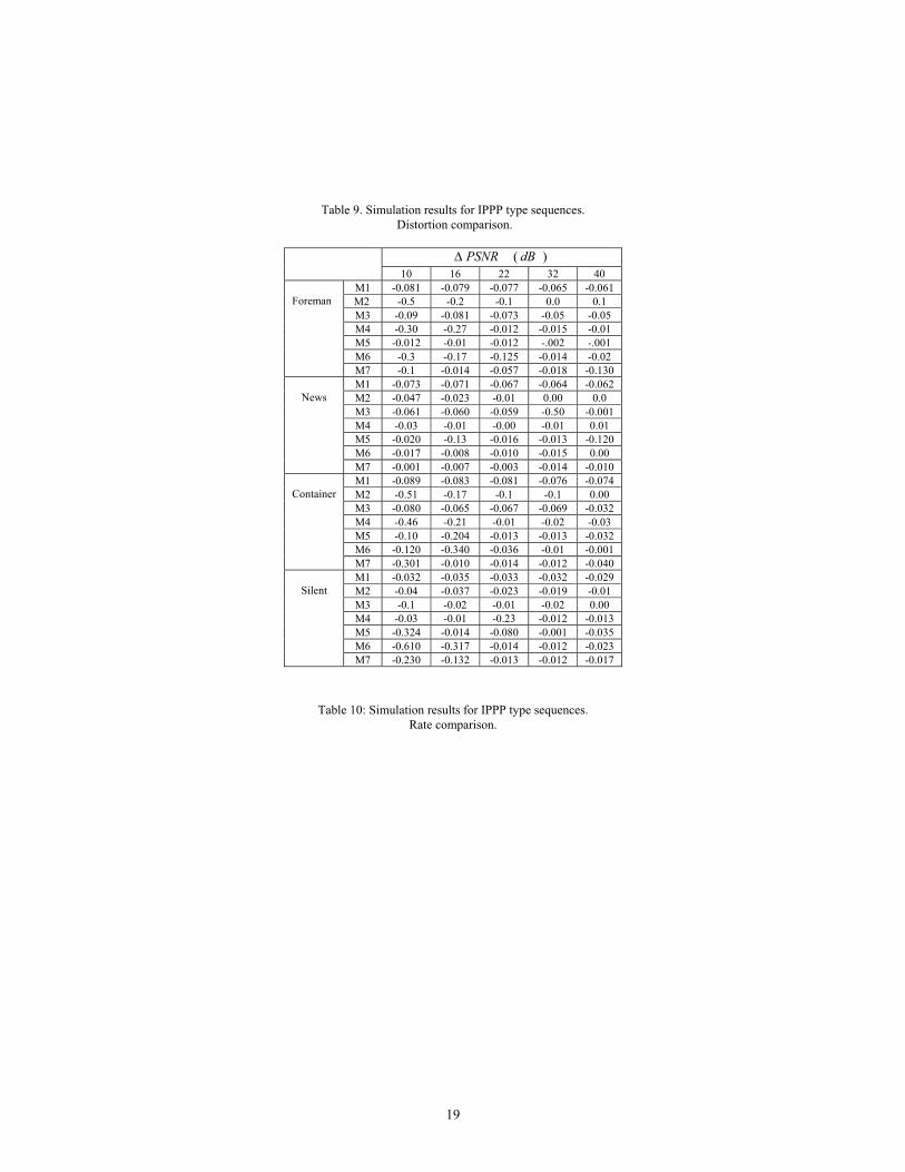
Table 9. Simulation results for IPPP type sequences. Distortion comparison.

Table 10: Simulation results for IPPP type sequences. Rate comparison.

)( dBPSNR∆ 10 16 22 32 40

Foreman

M1 -0.081 -0.079 -0.077 -0.065 -0.061 M2 -0.5 -0.2 -0.1 0.0 0.1 M3 -0.09 -0.081 -0.073 -0.05 -0.05 M4 -0.30 -0.27 -0.012 -0.015 -0.01 M5 -0.012 -0.01 -0.012 -.002 -.001 M6 -0.3 -0.17 -0.125 -0.014 -0.02 M7 -0.1 -0.014 -0.057 -0.018 -0.130

News

M1 -0.073 -0.071 -0.067 -0.064 -0.062 M2 -0.047 -0.023 -0.01 0.00 0.0 M3 -0.061 -0.060 -0.059 -0.50 -0.001 M4 -0.03 -0.01 -0.00 -0.01 0.01 M5 -0.020 -0.13 -0.016 -0.013 -0.120 M6 -0.017 -0.008 -0.010 -0.015 0.00 M7 -0.001 -0.007 -0.003 -0.014 -0.010

Container

M1 -0.089 -0.083 -0.081 -0.076 -0.074 M2 -0.51 -0.17 -0.1 -0.1 0.00 M3 -0.080 -0.065 -0.067 -0.069 -0.032 M4 -0.46 -0.21 -0.01 -0.02 -0.03 M5 -0.10 -0.204 -0.013 -0.013 -0.032 M6 -0.120 -0.340 -0.036 -0.01 -0.001 M7 -0.301 -0.010 -0.014 -0.012 -0.040

Silent

M1 -0.032 -0.035 -0.033 -0.032 -0.029 M2 -0.04 -0.037 -0.023 -0.019 -0.01 M3 -0.1 -0.02 -0.01 -0.02 0.00 M4 -0.03 -0.01 -0.23 -0.012 -0.013 M5 -0.324 -0.014 -0.080 -0.001 -0.035 M6 -0.610 -0.317 -0.014 -0.012 -0.023 M7 -0.230 -0.132 -0.013 -0.012 -0.017

20

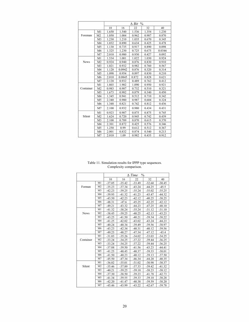
Table 11. Simulation results for IPPP type sequences. Complexity comparison.

%Time∆

10 16 22 32 40

Forman M1 -37.05 -35.42 -33.49 -32.60 -30.45 M2 -35.23 -37.34 -43.24 -44.25 -45.5 M3 -42.23 -39.25 -35.24 -35.02 -35.25 M4 -39.95 -41.32 -41.23 -43.47 -44.32 M5 -43.50 -42.23 -42.12 -40.25 -38.25 M6 -48.31 -47.6 -45.25 -42.25 -42.12 M7 -49.21 -43.32 -44.23 -47.25 -48.10

News

M1 -41.32 -38.24 -35.24 -31.12 -31.10 M2 -38.45 -39.25 -40.25 -42.13 -43.23 M3 -43.25 -41.50 -40.21 -39.34 -38.22 M4 -41.25 -42.02 -43.02 -43.24 -44.23 M5 -40.24 -40.34 -39.49 -39.56 -38.97 M6 -43.23 -42.34 -40.31 -40.12 -39.56 M7 -49.25 -48.27 -47.34 -47.12 -43.4

Container

M1 -31.03 -35.26 -34.02 -33.03 -34.25 M2 -33.24 -34.25 -37.22 -39.44 -36.25 M3 -33.24 -34.25 -37.22 -39.44 -36.25 M4 -37.88 -39.50 -41.56 -43.23 -44.41 M5 -41.25 -40.45 -40.37 -39.33 -38.01 M6 -41.50 -40.23 -40.12 -39.13 -37.50 M7 -45.50 -47.34 -46.34 -44.20 -40.35

Silent

M1 -36.02 -35.01 -31.02 -30.98 -30.37 M2 -35.46 -37.89 -37.33 -39.42 -41.32 M3 -40.21 -39.25 -39.10 -38.23 -38.12 M4 -37.30 -38.50 -39.23 -41.78 -42.73 M5 -41.34 -39.55 -39.33 -39.10 -38.28 M6 -42.20 -41.47 -40.38 -39.59 -38.20 M7 -45.46 -43.99 -43.22 -42.67 -39.78

%Bit∆ 10 16 22 32 40

Foreman

M1 1.650 1.540 1.536 1.354 1.230 M2 1.050 1.004 0.962 0.987 0.870 M3 1.230 1.210 1.035 0.670 0.345 M4 1.032 0.890 0.634 0.425 0.478 M5 1.130 0.735 0.917 0.890 0.098 M6 1.325 1.230 0.725 0.675 0.0346 M7 2.010 0.980 0.930 0.427 0.092

News

M1 1.534 1.001 1.022 1.030 0.924 M2 0.924 0.940 0.876 0.830 0.910 M3 1.021 0.932 0.982 0.760 0.567 M4 1.120 0.0942 0.876 0.320 0.314 M5 1.098 0.954 0.897 0.830 0.210 M6 2.010 0.0845 0.872 0.828 0.621 M7 2.120 0.932 0.489 0.762 0.412

Container

M1 1.803 1.902 1.090 0.950 0.921 M2 0.983 0.987 0.732 0.510 0.321 M3 1.673 0.982 0.879 0.340 0.450 M4 1.345 0.941 0.512 0.710 0.342 M5 2.340 0.980 0.987 0.604 0.324 M6 1.348 0.821 0.742 0.812 0.436 M7 2.100 0.932 0.980 0.434 0.431

Silent

M1 0.923 0.987 0.875 0.875 0.745 M2 1.624 0.720 0.945 0.742 0.439 M3 2.100 0.789 0.870 0.615 0.370 M4 2.301 0.872 0.425 0.576 0.346 M5 1.250 0.99 0.612 0.512 0.367 M6 2.001 0.832 0.874 0.540 0.213 M7 2.010 1.09 0.982 0.435 0.912

21

Table 12. Simulation results for IIII type sequences. Distortion comparison.

PSNR∆ 10 16 22 32 40

Forman

M1 -0.060 -0.065 -0.064 -0.063 -0.051 M2 -0.45 -0.021 -0.01 0.001 0.10 M3 -0.08 -0.070 -0.062 -0.05 -0.05 M4 -0.130 -0.122 -0.022 -0.010 -0.01 M5 -0.020 -0.011 -0.021 -.001 -.011 M6 -0.13 -0.017 -0.120 -0.020 -0.012 M7 -0.11 -0.020 -0.030 -0.020 -0.013

News

M1 -0.052 -0.060 -0.042 -0.050 -0.051 M2 -0.037 -0.030 -0.010 0.010 -0.01 M3 -0.050 -0.051 -0.042 -0.140 -0.010 M4 -0.022 -0.02 -0.10 -0.02 0.010 M5 -0.032 -0.020 -0.024 -0.022 -0.024 M6 -0.023 -0.019 -0.025 -0.027 0.010 M7 -0.012 -0.015 -0.012 -0.025 -0.022

Container

M1 -0.059 -0.064 -0.062 -0.056 -0.068 M2 -0.052 -0.054 -0.201 -0.012 0.001 M3 -0.182 -0.045 -0.053 -0.048 -0.042 M4 -0.056 -0.031 -0.042 -0.032 -0.013 M5 -0.120 -0.323 -0.033 -0.054 -0.067 M6 -0.230 -0.030 -0.051 -0.042 -0.023 M7 -0.410 -0.110 -0.124 -0.032 -0.062

Silent

M1 -0.061 -0.054 -0.053 -0.041 -0.035 M2 -0.050 -0.043 -0.030 -0.023 -0.014 M3 -0.051 -0.034 -0.042 -0.032 0.020 M4 -0.043 -0.051 -0.024 -0.064 -0.072 M5 -0.092 -0.037 -0.056 -0.037 -0.042 M6 -0.271 -0.302 -0.045 -0.052 -0.041 M7 -0.260 -0.182 -0.049 -0.053 -0.046

Table 13. Simulation results for IIII type sequences. Rate comparison.

%Bits∆

10 16 22 32 40

Forman M1 1.320 1.340 1.572 1.142 1.370 M2 1.321 1.234 0.985 0.997 0.980 M3 1.310 1.410 1.244 0.887 0.547 M4 1.142 0.993 0.719 0.562 0.539 M5 1.142 0.852 1.017 1.090 0.198 M6 1.241 1.322 0.834 0.752 0.142 M7 1.910 1.080 0.934 0.526 0.192

News

M1 1.132 1.201 1.132 1.215 0.956 M2 0.970 0.967 0.893 0.742 0.932 M3 1.130 1.334 0.923 0.950 0.822 M4 1.120 0.0942 0.876 0.320 0.314 M5 1.180 1.095 0.985 0.713 0.515 M6 1.350 0.275 0.980 0.690 0.982 M7 1.320 0.978 0.999 0.957 0.689

Container

M1 1.203 1.002 1.042 1.095 0.942 M2 1.310 1.124 1.231 0.981 0.739 M3 1.312 0.990 0.989 0.720 0.730 M4 1.345 0.941 0.512 0.710 0.342 M5 2.127 0.999 1.087 0.824 0.612 M6 1.101 0.981 0.802 0.922 0.812 M7 1.900 0.912 1.210 0.814 0.011

Silent

M1 1.223 1.087 0.921 0.905 0.980 M2 1.750 0.930 1.012 0.590 0.610 M3 1.940 0.312 0.590 0.435 0.560 M4 1.920 0.702 0.215 0.736 0.416 M5 1.467 0.929 0.732 0.702 0.621 M6 1.209 0.212 0.744 0.503 0.021 M7 1.910 1.100 0.907 0.515 0.435

Table 14. Simulation results for IIII type sequences.

22

Complexity comparison.

(a)

%Time∆ 10 16 22 32 40

Forman

M1 -47.15 -46.12 -43.29 -49.10 -47.25 M2 -50.13 -47.10 -52.45. -54.20 -55.50 M3 -55.34 -59.25 -45.34 -42.82 -45.15 M4 -50.05 -51.32 -52.30 -51.27 -54.12 M5 -53.21 -55.13 -54.34 -52.31 -54.16 M6 -55.21 -57.30 -54.12 -51.05 -52.10 M7 -58.10 -51.20 -53.37 -55.85 -57.21

News

M1 -52.24 -58.20 -53.61 -51.90 -50.46 M2 -49.50 -52.50 -50.15 -52.42 -51.02 M3 -50.12 -51.23 -50.78 -49.74 -48.89 M4 -51.34 -52.43 -53.19 -52.10 -52.13 M5 -51.35 -50.27 -49.91 -50.06 -49.55 M6 -51.30 -52.04 -51.21 -51.62 -49.96 M7 -58.45 -56.31 -57.03 -52.53 -50.04

Container

M1 -46.23 -45.32 -44.72 -43.67 -44.39 M2 -46.42 -48.53 -47.43 -49.64 -46.42 M3 -45.34 -44.65 -47.39 -49.51 -48.12 M4 -47.90 -50.20 -51.06 -52.43 -54.10 M5 -51.85 -50.75 -52.37 -56.12 -48.32 M6 -52.60 -50.43 -52.32 -56.43 -47.34 M7 -55.40 -57.64 -56.04 -55.12 -52.30

Silent

M1 -49.21 -46.31 -43.32 -45.38 -43.29 M2 -49.76 -49.90 -50.03 -49.62 -51.12 M3 -50.30 -49.50 -50.37 -49.38 -48.92 M4 -51.22 -58.60 -51.73 -53.38 -54.13 M5 -50.49 -53.18 -58.28 -59.43 -58.71 M6 -52.12 -51.31 -50.16 -49.18 -50.23 M7 -55.16 -50.19 -50.22 -52.67 -56.82

23

(b)

Figure 20: Akiyo sequence, (IPPP seq.). (a) R-D performance, (b) computational complexity.

(a)

(b)

Figure 21: Foreman sequence, (IPPP seq.). (a) R-D performance,

(b) computational complexity

(a)

24

(b)

Figure 22: Stefan sequence, (IPPP seq.). (a) R-D performance,

(b) computational complexity.

(a) (b) (c)

(d) (e) (f)

Figure 23: Quality of reconstructed frames of Foreman sequence: (a) RDO, (b) M3, (c) M4, (d) M5, (e) M6, (f) M7.

(a) (b) (c)

25

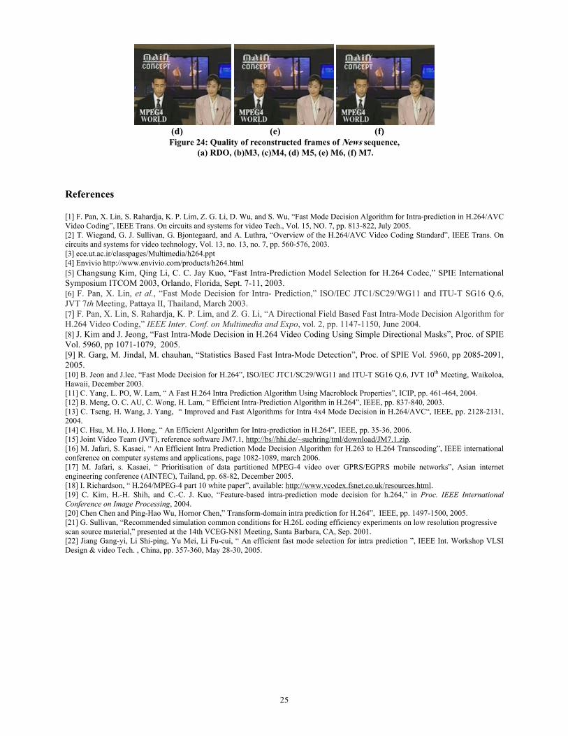
(d) (e) (f)

Figure 24: Quality of reconstructed frames of News sequence, (a) RDO, (b)M3, (c)M4, (d) M5, (e) M6, (f) M7.

References [1] F. Pan, X. Lin, S. Rahardja, K. P. Lim, Z. G. Li, D. Wu, and S. Wu, “Fast Mode Decision Algorithm for Intra-prediction in H.264/AVC Video Coding”, IEEE Trans. On circuits and systems for video Tech., Vol. 15, NO. 7, pp. 813-822, July 2005. [2] T. Wiegand, G. J. Sullivan, G. Bjontegaard, and A. Luthra, “Overview of the H.264/AVC Video Coding Standard”, IEEE Trans. On circuits and systems for video technology, Vol. 13, no. 13, no. 7, pp. 560-576, 2003. [3] ece.ut.ac.ir/classpages/Multimedia/h264.ppt [4] Envivio http://www.envivio.com/products/h264.html [5] Changsung Kim, Qing Li, C. C. Jay Kuo, “Fast Intra-Prediction Model Selection for H.264 Codec,” SPIE International Symposium ITCOM 2003, Orlando, Florida, Sept. 7-11, 2003. [6] F. Pan, X. Lin, et al., “Fast Mode Decision for Intra- Prediction,” ISO/IEC JTC1/SC29/WG11 and ITU-T SG16 Q.6, JVT 7th Meeting, Pattaya II, Thailand, March 2003. [7] F. Pan, X. Lin, S. Rahardja, K. P. Lim, and Z. G. Li, “A Directional Field Based Fast Intra-Mode Decision Algorithm for H.264 Video Coding,” IEEE Inter. Conf. on Multimedia and Expo, vol. 2, pp. 1147-1150, June 2004. [8] J. Kim and J. Jeong, “Fast Intra-Mode Decision in H.264 Video Coding Using Simple Directional Masks”, Proc. of SPIE Vol. 5960, pp 1071-1079, 2005. [9] R. Garg, M. Jindal, M. chauhan, “Statistics Based Fast Intra-Mode Detection”, Proc. of SPIE Vol. 5960, pp 2085-2091, 2005. [10] B. Jeon and J.lee, “Fast Mode Decision for H.264”, ISO/IEC JTC1/SC29/WG11 and ITU-T SG16 Q.6, JVT 10th Meeting, Waikoloa, Hawaii, December 2003. [11] C. Yang, L. PO, W. Lam, “ A Fast H.264 Intra Prediction Algorithm Using Macroblock Properties”, ICIP, pp. 461-464, 2004. [12] B. Meng, O. C. AU, C. Wong, H. Lam, “ Efficient Intra-Prediction Algorithm in H.264”, IEEE, pp. 837-840, 2003. [13] C. Tseng, H. Wang, J. Yang, “ Improved and Fast Algorithms for Intra 4x4 Mode Decision in H.264/AVC“, IEEE, pp. 2128-2131, 2004. [14] C. Hsu, M. Ho, J. Hong, “ An Efficient Algorithm for Intra-prediction in H.264”, IEEE, pp. 35-36, 2006. [15] Joint Video Team (JVT), reference software JM7.1, http://bs//hhi.de/~suehring/tml/download/JM7.1.zip. [16] M. Jafari, S. Kasaei, “ An Efficient Intra Prediction Mode Decision Algorithm for H.263 to H.264 Transcoding”, IEEE international conference on computer systems and applications, page 1082-1089, march 2006. [17] M. Jafari, s. Kasaei, “ Prioritisation of data partitioned MPEG-4 video over GPRS/EGPRS mobile networks”, Asian internet engineering conference (AINTEC), Tailand, pp. 68-82, December 2005. [18] I. Richardson, “ H.264/MPEG-4 part 10 white paper”, available: http://www.vcodex.fsnet.co.uk/resources.html. [19] C. Kim, H.-H. Shih, and C.-C. J. Kuo, “Feature-based intra-prediction mode decision for h.264,” in Proc. IEEE International Conference on Image Processing, 2004. [20] Chen Chen and Ping-Hao Wu, Hornor Chen,” Transform-domain intra prediction for H.264”, IEEE, pp. 1497-1500, 2005. [21] G. Sullivan, “Recommended simulation common conditions for H.26L coding efficiency experiments on low resolution progressive scan source material,” presented at the 14th VCEG-N81 Meeting, Santa Barbara, CA, Sep. 2001. [22] Jiang Gang-yi, Li Shi-ping, Yu Mei, Li Fu-cui, “ An efficient fast mode selection for intra prediction ”, IEEE Int. Workshop VLSI Design & video Tech. , China, pp. 357-360, May 28-30, 2005.