evaluating transportation land use impacts · 2019-03-19 · evaluating transportation land use...
TRANSCRIPT

www.vtpi.org
250-360-1560
Todd Alexander Litman © 1995-2019 You are welcome and encouraged to copy, distribute, share and excerpt this document and its ideas, provided
the author is given attribution. Please send your corrections, comments and suggestions for improvement.
Evaluating Transportation Land Use Impacts Considering the Impacts, Benefits and Costs of Different Land Use
Development Patterns
18 March 2019
Todd Litman Victoria Transport Policy Institute
Suburban Residential Urban Commercial Center
Abstract This report examines ways that transportation decisions affect land use patterns, and the resulting economic, social and environmental impacts. These include direct impacts on land used for transportation facilities, and indirect impacts caused by changes to land use development patterns. In particular, certain transportation planning decisions tend to increase sprawl (dispersed, urban-fringe, automobile-dependent development), while others support smart growth (more compact, infill, multi-modal development). These development patterns have various economic, social and environmental impacts. This report describes specific methods for evaluating these impacts in transport planning.
Originally published as “Land Use Impact Costs of Transportation,”
World Transport Policy & Practice, Vol. 1, No. 4, 1995, pp. 9-16.

Evaluating Transportation Land Use Impacts Victoria Transport Policy Institute
1
Contents
Introduction ................................................................................................................. 2
Evaluation Framework ................................................................................................. 5
Land Use Categories .................................................................................................. 7
How Transportation Planning Decisions Affect Land Use ............................................ 11
Direct Impacts – Land Devoted To Transportation Facilities ....................................... 13 Roads ............................................................................................................................. 13 Parking ............................................................................................................................ 14 Total Amount Of Land Devoted to Transportation .......................................................... 15
Indirect Impacts – How Transport Affects Land Use Development .............................. 16
Costs and Benefits Of Different Land Use Patterns .................................................... 20 Accessibility and Transportation Costs ........................................................................... 20 Household Affordability ................................................................................................... 22 Infrastructure and Public Service Costs ......................................................................... 23 Safety and Health ........................................................................................................... 28 Economic Productivity and Development ....................................................................... 30 Social Inclusion ............................................................................................................... 32 Community Cohesion ..................................................................................................... 33 Environmental Impacts ................................................................................................... 35 Energy Consumption and Pollution Emissions ............................................................... 39 Aesthetic Impacts ........................................................................................................... 40 Cultural Preservation ...................................................................................................... 40
Consumer and Economic Impacts ............................................................................... 41
Optimal Level of Sprawl .............................................................................................. 42
Evaluation Techniques ................................................................................................ 44 Comprehensive Project Analysis .................................................................................... 45 Monetized Impact Evaluation .......................................................................................... 46 Planning Objectives ........................................................................................................ 47
Examples and Case Studies ....................................................................................... 48 ASSET ........................................................................................................................... 50 Vision California - Charting Our Future ........................................................................... 51
Conclusions ................................................................................................................ 52
References And Resources For More Information ...................................................... 52

Evaluating Transportation Land Use Impacts Victoria Transport Policy Institute
2
Introduction Land use development patterns (also called urban form, built environment, community design, spatial development, and urban geography) refer to human use of the earth’s surface, including the location, type and design of infrastructure such as roads and buildings. Land use patterns can have diverse economic, social and environmental impacts: some some require less impervious surface (buildings and pavement, also called sealed soil) per capita and so preserve more openspace (gardens, farmland and natural habitat), and some are more accessible and so reduce transportation costs to businesses and consumers. Transportation planning decisions influence land use directly, by affecting the amount of land used for transport facilities, and indirectly, by affecting the location and design of development. For example, expanding urban highways increases pavement area, and encourages more dispersed, automobile-oriented development (sprawl), while walking, cycling and public transit improvements encourage compact, infill development (smart growth).
Planning Decision (development practices, infrastructure investment, zoning, development fees, etc.)
Urban Forum Patterns (density, mix, connectivity, parking supply, etc.)
Travel Behavior Land Use (amount and type of walking, cycling, (Impervious surface coverage,
public transit and automobile travel) greenspace, public service costs)
Economic, Social and Environmental Impacts (consumer costs, public service costs, physical fitness, crashes, pollution emissions, etc.)
There may be several steps between a transport planning decision, its impacts on urban form and travel behavior, and its ultimate economic, social and environmental impacts. These relationships are complex. There may be several steps between a transport planning decision and its ultimate effects, and a particular planning deicison can have a variety of impacts and costs, as illustrated above. Table 1 summarizes these impacts. Table 1 Transport Planning Land Use Impacts and Costs
Increased Pavement Area More Dispersed Development
Reduced openspace (gardens, parks, farmlands and wildlife habitat).
Increased flooding and stormwater management costs.
Reduced groundwater recharge.
Aesthetic degradation.
Reduced openspace (farmlands and wildlife habitat).
Longer travel distances, more total vehicle travel.
Reduced accessibility for non-drivers, which is inequitable (harms disadvantaged people).
Increased vehicle traffic and resulting external costs (congestion, accident risk, energy consumption, pollution emissions).
This table summarizes various land use impacts and costs from transport planning decisions.

Evaluating Transportation Land Use Impacts Victoria Transport Policy Institute
3
Historical Context During the last century, many transportation and land use planning practices reinforced a cycle of increased automobile dependency and sprawl, as illustrated in Figure 1. This was generally unintended, reflecting a lack of consideration of the full impacts of these decisions. For example, when deciding how much parking to require for a particular type of land use, traffic engineers were probably not thinking about the additional sprawl that would result from a more generous standard, they simply wanted to ensure motorist convenience. Similarly, planning decisions that affect roadway supply, transit service quality or roadway user fees often overlooked various land use impacts. Figure 1 Cycle of Automobile Dependency and Sprawl
This figure illustrates the self-reinforcing cycle of increased automobile dependency and sprawl.
Smart growth can provide various economic, social and environmental benefits. As a result, many professional organizations, jurisdictions and government agencies have adopted smart growth planning objectives, as summarized in the box on the next page.

Evaluating Transportation Land Use Impacts Victoria Transport Policy Institute
4
Smart Growth Endorsements
Various professional, academic and government organizations have adopted Smart Growth principles and support its implementation. Below are a few examples.
AASHTO Center for Environmental Excellence (www.environment.transportation.org), American Association of State Highway and Transportation Officials. Promotes Smart Growth practices.
AIA (2005), What Makes a Community Livable? Livability 101, American Institute of Architects (www.aia.org); at www.aia.org/aiaucmp/groups/aia/documents/pdf/aias077949.pdf.
APA (2002), Smart Growth Legislative Guidebook and User Manual: Model Statutes for Planning and the Management of Change, American Planning Association (www.planning.org).
CITE (2004), Canadian Guide to Promoting Sustainable Transportation Through Site Design, Canadian Institute of Transportation Engineers (www.cite7.org).
Reid Ewing, Keith Bartholomew, Steve Winkelman, Jerry Walters and Don Chen (2007), Growing Cooler: The Evidence on Urban Development and Climate Change, Urban Land Institute and Smart Growth America (www.smartgrowthamerica.org/gcindex.html).
ITE (2003), Smart Growth Transportation Guidelines, Institute of Transport. Engineers (www.ite.org).
NALGEP (2004), Smart Growth is Smart Business: Boosting the Bottom Line and Community Prosperity, National Association of Local Government Environmental Professionals, (www.nalgep.org).
NAR (2004), Creating Great Neighborhoods: Density in Your Community, National Association of Realtors (www.realtor.org).
NEMO Project (www.canr.uconn.edu/ces/nemo) helps communities reduce impervious surface area and associated infrastructure and environmental costs.
SGN (2002 and 2004), Getting To Smart Growth: 100 Policies for Implementation, and Getting to Smart Growth II: 100 More Policies for Implementation, Smart Growth Network (www.smartgrowth.org); at www.epa.gov/dced/getting_to_sg2.htm.
Land Use and Transportation Research Website (www.lutr.net), European Commission.
Smart Growth Leadership Institute (www.sgli.org) supported by the National Realtors Association (www.realtor.org) and Smart Growth America (www.smartgrowthamerica.org).
TRB (2009), Driving and the Built Environment: The Effects of Compact Development on Motorized Travel, Energy Use, and CO2 Emissions, Special Report 298, Transportation Research Board (www.trb.org); at http://onlinepubs.trb.org/Onlinepubs/sr/sr298prepub.pdf.
Urban Land Institute (www.uli.org) is a professional organization for developers which provides practical information on innovative development practices, including smart growth.
USEPA Smart Growth Website (www.epa.gov/smartgrowth) provides information on Smart Growth strategies to reduce environmental impacts.

Evaluating Transportation Land Use Impacts Victoria Transport Policy Institute
5
Evaluation Framework An evaluation framework specifies the basic structure of an analysis, including which impacts are considered and how they are measured and compared (Litman, 2001). A framework usually identifies:
Evaluation method, such as cost-effectiveness, benefit-cost, lifecycle cost analysis, etc.
Evaluation criteria are the factors and impacts considered in a particular analysis. Table 2 lists various land use impact evaluation criteria.
Table 2 Land Use Impact Evaluation Criteria
Economic Social Environmental
Value of land devoted to transportation facilities.
Land use accessibility.
Transportation costs.
Property values.
Crash damages.
Costs to provide public services.
Economic development and productivity.
Stormwater management costs.
Relative accessibility for different groups of people – impacts on equity and opportunity.
Community cohesion.
Housing affordability.
Cultural resources (e.g., heritage buildings).
Traffic accidents.
Public health (physical fitness).
Aesthetic impacts.
Greenspace and wildlife habitat.
Hydrologic impacts.
Heat island effects.
Energy consumption.
Pollution emissions.
This table lists various types of land use impacts that may be affected by transport planning decisions. These impacts are described in more detail in this report.
Modeling techniques, which predict how a policy change or program will affect travel behavior and land use patterns, and measure the incremental benefits and costs that result.
A Base Case (also called do nothing), the conditions that would occur without the proposed policy or program.
Reference units, such as costs per lane-mile, vehicle-mile, passenger-mile, incremental peak-period trip, etc.
Base year and discount rate, indicating how costs are adjusted to reflect the time value of money.
Perspective and scope, such as the geographic range of impacts to consider.
Dealing with uncertainty, such as sensitivity analysis and statistical tests.
How results are presented, so that the results of different evaluations are easy to compare.
Impacts are evaluated using a with-and-without test, which reflects the conditions that would occur with or without a particular policy or project. For example, the impacts of a roadway widening are the incremental changes that would occur if the project is implemented. This analysis requires defining the base case, the conditions that would otherwise occur if the proposed policy or project were not implemented.

Evaluating Transportation Land Use Impacts Victoria Transport Policy Institute
6
Impacts can be evaluated from various perspectives, such as a particular geographic area, group, or time period. For example, residents of an area or group tend to evaluate policies based on their own benefits and costs, and may consider it desirable to externalize costs and exclude people they consider undesirable, but more comprehensive evaluation would consider these economic transfers (one person or group gains at another’s expense) rather than net gains. It is usually best to consider all impacts, including those affecting other areas and times, although impacts to a particular group can be identified and highlighted.
Figure 2 Analysis Perspectives
Impacts may be evaluated from various perspectives and scales. Generally, all impacts should be considered with more condiseration to those that are more local.
Some analyses are concerned with impacts within a given area, measured per acre or square kilometer, while others are concerned with impacts per capita. For example, smart growth policies that encourage more compact, infill development tend to increase impervioius surface coverage (the portion of land covered with buildings or paved for roads and parking facilities) within existing urban areas, but tends to reduces per capita and total regional impervious surface area. Most analysis is primarily concerned with net impacts to society rather than the effects of self selection (the tendency of certain types of people to locate in certain areas). For example, it would generally be considered a benefit if a particular land use pattern increases accessibility and opportunity for disadvantaged people, and not a cost if that attracts disadvantaged people, and associated economic and medical problems to a particular area, because that is an economic transfer not a net cost (the total number of disadvantaged people does not increase, in fact, it may decline as more poor people are able to get jobs and mentally ill people are better able to access mental health services). However, policies that attract disadvantaged people to a particular area may seem undesirable to local residents and should be considered in equity analysis and as an impact that may require mitigation.

Evaluating Transportation Land Use Impacts Victoria Transport Policy Institute
7
Land Use Categories The earth’s surface, called the landscape, is a unique and valuable resource. The landscape affects and is affected by most economic, social and environmental activities. Major land use categories are listed below. Table 3 Land Use Categories
Built Environment Openspace
Residential (single- and multi-family housing)
Commercial (stores and offices)
Institutional (schools, public offices, etc.)
Industrial
Brownfields (old, unused and underused facilities)
Transportation facilities (roads, paths, parking lots, etc.)
Parkland
Agricultural
Forests, chaparral, grasslands
Wildlands (undeveloped lands)
Shorelines
Land use patterns can be evaluated based on the following attributes:
Density - the number of people, jobs or housing units in an area.
Clustering - whether related destinations are located close together (e.g., commercial centers, residential clusters, urban villages, etc.).
Mix - whether different land use types (commercial, residential, etc.) are located together.
Connectivity – the number of connections within the street and path systems.
Impervious surface – land covered by buildings and pavement, also called the footprint.
Greenspace – the portion of land used for lawns, gardens, parks, farms, woodlands, etc. The Green Area Factor or Green Area Ratio (GAR) refers to the portion of land that is greenspace.
Accessibility – the ability to reach desired activities and destinations.
Nonmotorized accessibility – the quality of walking and cycling conditions.
Land use attributes can be evaluated at various scales:
Site – an individual parcel, building, facility or campus.
Street – the buildings and facilities along a particular street or stretch of roadway.
Neighborhood or center – a walkable area, typically less than one square mile.
Local – a small geographic area, often consisting of several neighborhoods.
Municipal – a town or city jurisdiction.
Region – a geographic area where residents share services and employment options. A metropolitan region typically consists of one or more cities and various suburbs, smaller commercial centers, and surrounding semi-rural areas.

Evaluating Transportation Land Use Impacts Victoria Transport Policy Institute
8
Geographic areas are often categorized in the following ways:
Village – Small urban settlement (generally less than 10,000 residents).
Town – Medium size urban settlement (generally less than 50,000 residents).
City – is a large settlement (generally more than 50,000 residents).
Metropolitan region or metropolis – a large urban region (generally more than 500,000 residents) that usually consists of one or two large cities, and various smaller cities and towns (called suburbs). This development pattern is considered a polycentric.
Urban – relatively high density (10+ residents and 5+ housing units per acre), mixed-use development, multi-modal transportation system.
Suburban – medium density (2-10 residents, 1-5 housing units per acre), segregated land uses, and an automobile-dependent transportation system.
Central business district (CBD) – the main commercial center in a town or city.
Exurban – low density (less than 2 residents or 1 housing unit per acre), mostly farms and undeveloped lands, located near enough to an urban area that residents often commute, shop and use services there.
Rural – low density (less than 2 residents or 1 housing unit per acre), mostly farms and undeveloped lands.
Common Issues of Confusion in Land Use Evaluation The terms city and urban can refer to just a dense central businss district and its immediate residential neighborhoods, or a central city, or to an entire urban region, including suburbs. For example, when people claim that “more than a third of the land in cities is paved” or “urban housing is primarily highrise” they are usually referring to central business districts and possibly inner neighborhoods. Pavement area and highrise housing rates are much lower for an entire city or urban region. Density refers to people, jobs or housing per unit of land area (acre, hectare, square-kilometer or -mile). Density can be measured net (only developable land, excluding roads, parks and utility rights-of-way) or gross (all land). Density is generally associated with other land use factors including centricity, mix, roadway connectivity, transport diversity (good walking, cycling and public transit service), and efficient parking management. Together these are called compact development or urbanization. Because density is relatively easy to measure, it is often used as an indicator of this set of factors. Analysis can vary depending on scale, location and time. For example, some studies evaluate land use factors (such as the relationships between density and annual vehicle travel) at the neighborhood level and others at the county or regional level. Smaller scale analysis tends to be more difficult but accurate. Self-selection can affect land use patterns. For example, people who, due to necessity or preference, rely on alternative modes, tend to locate in more urban, multi-modal locations, so part of the differences in per capita automobile travel between urban and suburban locations may reflect self-selection. It would therefore be inappropriate to assume that an individual who shifts from a suburban to an urban location will change their travel patterns to reflect local averages: a car enthusiast who moves to a transit-oriented neighborhood may continue to drive and avoid using public transit.

Evaluating Transportation Land Use Impacts Victoria Transport Policy Institute
9
Housing can be categorized in various ways: Small lot – less than 7,000 square feet.
Medium lot – 7,000 to 12,000 square feet.
Large lot – more than 12,000 squre feet (0.3 acres)
Figure 3 Housing Types (Metropolitan Design Center 2005)
This illustrates various housing types. There are often debates about different development patterns, generally termed sprawl and smart growth (Aurbach 2003; Litman 2003). Table 4 compares these patterns. There is often confusion about exactly how these patterns should be defined and measured. For example, some analyses only consider density, while others only consider population growth outside of existing cities, neither of which accurately reflects the full set of relevant factors. Table 4 Comparing Sprawl and Smart Growth (SGN 2011)
Attribute Sprawl Smart Growth
Density Lower-density Higher-density.
Growth pattern Urban periphery (greenfield) development. Infill (brownfield) development.
Activity Location Commercial and institutional activities are dispersed.
Commercial and institutional activities are concentrated into centers and downtowns.
Land use mix Homogeneous land uses. Mixed land use.
Scale
Large scale. Larger buildings, blocks, wide roads. Less detail, since people experience the landscape at a distance, as motorists.
Human scale. Smaller buildings, blocks and roads, care to design details for pedestrians.
Transportation Automobile-oriented transportation, poorly suited for walking, cycling and transit.
Multi-modal transportation that support walking, cycling and public transit use.
Street design Streets designed to maximize motor vehicle traffic volume and speed.
Streets designed to accommodate a variety of activities. Traffic calming.
Planning process Unplanned, with little coordination between jurisdictions and stakeholders.
Planned and coordinated between jurisdictions and stakeholders.
Public space Emphasis on the private realm (yards, shopping malls, gated communities, private clubs).
Emphasis on the public realm (streetscapes, sidewalks, public parks, public facilities).
This table compares Sprawl and Smart Growth land use patterns.

Evaluating Transportation Land Use Impacts Victoria Transport Policy Institute
10
Most metropolitan regions are polycentric, with a central business district surrounded by smaller commercial centers, and a central city surrounded by smaller cities and towns. Sprawl refers to dispersed development in low-density, single-use, automobile-dependent areas outside of any city or town; population growth in cities and towns outside existing cities is not necessarily sprawl if the development pattern reflects smart growth principles. Figure 4 Development Patterns (Meijers and Burger 2009)
Most metropolitan regions are polycentric, with various business districts, cities and towns. Sprawl consists of dispersed, low-density, automobile-dependent development outside any urban area.
As urban areas grow in population and economic activity they can either increase density or expand in area (Angel 2011; Bertaud 2012; EEA 2016; Rogers 2016), as illustrated in Figure 5 Figure 5 Development Patterns (Yglesias 2016)
As cities grow in population and economic activity, they can either increase density (grow upward) or expand geographically (grow outward).

Evaluating Transportation Land Use Impacts Victoria Transport Policy Institute
11
How Transportation Planning Decisions Affect Land Use Transportation planning decisions affect land use, both directly by determining which land is devoted to transport facilities such as roads, parking lots, and ports, and indirectly by affecting the relative accessibility and development costs in different locations (Kelly 1994; Boarnet, Greenwald and McMillan 2008; OTREC 2009). In general, policies that reduce the generalized cost (financial costs, travel time, discomfort, risk) of automobile travel tend to increase total traffic and sprawl, while those that improve nonmotorized and transit travel tend to support Smart Growth, as summarized in Table 5. Table 5 Transportation Policy and Program Land Use Impacts
Encourages Sprawl Encourages Smart Growth
Increased roadway capacity and speeds
Generous minimum parking requirements.
Free or subsidized parking.
Low vehicle operating costs.
Inferior public transit service.
Poor walking and cycling conditions.
Reduced roadway capacity and speeds.
Reduced parking supply.
Parking pricing and management.
Road pricing and distance-based vehicle fees.
Transit service improvements and encouragement strategies.
Pedestrian and cycling improvements.
Traffic calming and traffic speed reductions.
Access management and streetscape improvements.
Some types of transport planning decisions tend to support sprawl, others support Smart Growth. Planning decisions often involve trade-offs between mobility (physical movement of people and goods) and accessibility (the ability to reach desired goods and activities). Incremental increases in road and parking supply create more dispersed land use patterns, increasing the travel distances required to achieve a given level of accessibility. This favors automobile travel and reduces the utility and efficiency of other transport modes. By increasing the amount of land required for a given amount of development, higher road and parking requirements favor urban fringe development, where land prices are lower. As a result, automobile-oriented planning is self-fulfilling: practices to make driving more convenient make alternatives less convenient and increase automobile-oriented sprawl. Figure 6 Land Used for Roads and Parking
Automobile transport requires relatively large amounts of land for roads and parking, which reduces the amount of land available for other activities. This tends to disperse destinations.

Evaluating Transportation Land Use Impacts Victoria Transport Policy Institute
12
During much of the last century, many common planning practices, such as using roadway Level-of-Service to evaluate transportation system quality (as opposed to indicators that reflect multi-modal mobility or land use accessibility), and generous minimum parking requirements, unintentionally encouraged sprawl and automobile dependency. Many of these policies can be considered market distortions because they underprice vehicle travel (“Market Principles,” VTPI, 2005). Smart Growth and TDM strategies can offset these trends, many of which are considered market reforms that increase economic efficiency. It can be difficult to determine the exact land use impacts of a particular transport planning decision, particularly indirect, long-term impacts. Impacts are affected by factors such as the relative demand for different types of development, the degree to which a particular transportation project will improve accessibility and reduce costs, and how a transportation policy or project integrates with other factors. For example, if there is significant unmet demand for urban fringe development, expanding roadway capacity in that area will probably stimulate a significant amount of sprawl. Conversely, if there is significant unmet demand for transit-oriented development, improving transit service and implementing supportive land use policies (encouraging compact development around transit stations, improving area walking conditions, managing parking more efficiently, etc.) will probably stimulate Smart Growth. However, the exact impacts of a particular policy or project can be difficult to predict. Land use models can predict some but not all effects. Analysis therefore requires professional judgment.

Evaluating Transportation Land Use Impacts Victoria Transport Policy Institute
13
Direct Impacts – Land Devoted To Transportation Facilities This section investigates the amount of land devoted to transportation facilities. Also see Litman (2009 and 2011); Manville and Shoup (2005); and Woudsma, Litman and Weisbrod (2006). Roads
Most roads have two to four lanes, each 10-14 feet wide, plus shoulders, sidewalks, drainage ditches and landscaping area, depending on conditions, so typical urban roads with two traffic and two parking lanes have 30-40 foot total widths. Road rights-of-way (land legally devoted to roads) usually range from 24 to 64 feet wide. In high density urban areas road pavement often fills the entire right-of-way, but in other areas there is often an unpaved shoulder that may be planted or left in its natural condition. The amount of land devoted to roads is affected by:
Projected vehicle traffic demand (which determine the number of traffic lanes).
Design standards that determine lane and shoulder widths, drainage and landscaping.
On-street parking practices (whether streets have parking lanes).
Additional design features, such as shoulders, sidewalks, ditches and landscaping.
Figure 7 shows the relationship between per capita lane-miles (and herefore roadway area) and density in U.S. urban regions: per captia road area declines with density. This indicates that in U.S. cities there are between 150 and 1,200 square feet of road space (assuming 15-foot average lane width), with higher rates in sprawled areas and lower rates in compact cities. Figure 7 Urban Density Versus Roadway Supply (FHWA 2012, Table HM72)
Per capita roadway supply declines with density (Each dot represents a U.S. urban region.)
A vehicle’s road space requirements tend to increase with its size and speed. For example, a vehicle traveling on an urban arterial at 30 miles-per-hour (mph) requires about 12 feet of lane width and 60 feet of lane length, or about 720 square feet in total, but at 60 mph this increases to 15 feet of lane width and 140 feet of length, or about 2,100 square feet in total. A bus requires about three times a much road space (measured as “passenger car equivalents”) but typically carries 10-20 times as many passengers under urban-peak conditions.

Evaluating Transportation Land Use Impacts Victoria Transport Policy Institute
14
Parking
A parking space is typically 8-10 feet wide and 18-20 feet deep, totaling 144 to 200 square feet (“Parking Costs,” Litman 2009). Off-street parking requires about twice this amount (300+ square feet per space) for driveways and access lanes. Public policies affect the amount of land devoted to parking facilities. Most urban streets have one or two parking lanes that typically represent 20-30% of their width, and rural roads often have shoulders intended, in part, to provide parking. Some off-street parking facilities are provided by local governments, usually with direct or indirect subsidy (indirect subsidies include free land and property tax exemption). Most jurisdictions have zoning codes with minimum parking requirements. These minimum parking requirements are similar to a property tax to fund public parking facilities, although the owner captures any long-term capital gain if the property appreciates in value. Various studies have investigated the amount of land used for parking facilities. Davis, et al. (2010) used detailed aerial photographs to estimate the number of surface parking spaces in Illinois, Indiana, Michigan, and Wisconsin. They identified more than 43 million parking spaces in these four states, which averages approximately 2.5 to 3.0 off-street, non-residential parking spaces per vehicle. They estimate that these four states allocate 1260 km
2 of land to parking
lots, with a lower bound estimate of 976 km2
and an upper bound of 1,745 km2. This accounts
for approximately 4.97% of urban land, with higher rates in more sprawled areas. Chester, et al. (2015) estimate parking in Los Angeles County (CA) from 1900 to 2010 and how parking infrastructure evolves, affects urban form, and relates to changes in automobile travel. They estimate that since 1975 the ratio of residential off-street parking spaces to automobiles in is close to 1.0, with the greatest density of parking spaces is in the urban core, while most new growth in parking occurs outside of the core. In total, 14% of Los Angeles County’s incorporated land is committed to parking. Pijanowski (2007) found approximately three non-residential off-street parking spaces per vehicle in Tippecanoe County, a typical rural county. Using GIS datasets, Hulme-Moir (2010) calculated that in Porirua, New Zealand, 24% of the central city land area is devoted to parking facilities, 7% to green space and 4% to recreation. McCahill and Garrick (2012) compared 12 U.S. cities to evaluate the relationships between parking supply, population density and commute mode share. The findings suggest that on average each increase of 10 percentage points in the portion of commuters traveling by automobile is associated with an increase of more than 2,500 m2 of parking per 1,000 people and a decrease of 1,700 people/km2. Even for shorter trips within each city had much higher automobile mode share in cities with more parking supply. Analysis by Shin, Vuchic and Bruun (2009) indicates that automobile-oriented transport improvements tend to cause more dispersed, lower-denstiy development than high quality public transit. This suggests that there are typically between two and six off-street parking spaces per vehicle. Structured parking reduces land requirements, and underground parking requires almost no additional land, but these facilities are costly and therefore uncommon. Estimates of on-street parking spaces are somewhat arbitrary since most suburban and rural roads have shoulders on which vehicles can park, but located where there is modest parking demand. The number of parking spaces per vehicle tends to be lower in urban areas where shared parking is common, and higher in suburban and rural areas where each destination has its own parking lot.

Evaluating Transportation Land Use Impacts Victoria Transport Policy Institute
15
Total Land Devoted to Transportation
Some studies using various assumtions and methods estimate the total amount of land devoted to different transport modes (Bruun 2014; Manville and Shoup 2005; Litman 2006d). Table 6 Space Required By Travel Mode (based on Bruun and Vuchic 1995)
Mode Average Speed Moving Area Parking Area
Miles/Hr Sq. Feet Sq. Feet
Walking 3 12 Not Appropriate
Bicycling 10 60 32
Motorcycle 30 720 150
Bus Transit 20 50 Not Appropriate
Solo Driving – Urban Arterial 30 720 300
Solo Driving - Highway 60 2,100 300
The space required to travel and park varies significantly by mode.
Figure 8 illustrates the total travel and parking space required for typical 20-minute commutes by various modes, measured in square-feet-minutes, based on values from Table 6. Figure 8 Space Required By Travel Mode
0
50,000
100,000
150,000
200,000
250,000
Walking Bicycling Public Transit Solo Driving -
Urban Arterial
Solo Driving -
Highway
Sq
ua
re-F
eet-
Min
ute
s P
er
Co
mm
ute
Parking Area
Travel Area
Automobile travel requires far more space for travel and parking than other modes.
Figure 9 illustrates this in a slightly different way: it shows the number of passengers that can be carried by various modes by a four-meter lane. Figure 9 Typical Maximum Passengers Per 4-Meter Lane-Hour
Arterial Freeway HOV Bike Lane Walkway Arterial
Bus Lane Bus Rapid
Transit Rail Line
800-
1,100 1,800- 2,400
4,000- 8,000
5,000- 10,000
5,000- 10,000
8,000- 12,000 20,000- 30,000 40,000 - 60,000
Roadway capacity varies by mode. (= 1,000 people)

Evaluating Transportation Land Use Impacts Victoria Transport Policy Institute
16
In practice, automobile transport does not necessarily increase transport land requirements 15-100 times since cities require roads wide enough to accommodate large vehicles (such as fire, garbage and freight trucks) and provide sunlight. Newman and Kenworthy (1999, Table 3.9) found that automobile dependent cities have 3 to 5 times as much land devoted to roads and parking as more multi-modal cities. Put differently, 66% to 80% of the land devoted to roads and parking facilities in modern cities results from the greater space requirements of automobile transport. Motor vehicle traffic also tends to reduce development density indirectly by increasing the need for sidewalk and building setbacks to avoid traffic noise and dust, so larger boulevards, highways shoulders and front lawns can be considered, in part, a cost of motor vehicle traffic. Figure 10 illustrates one analysis of urban impervious surface coverage. It suggests that 5-10% of suburban land, 20-30% of urban land, and 40-60% of commercial center land is devoted to roads and parking. This is the single largest category of impervious surface, covering twice as much land as the next category, building roofs. Ebrahimian, Gulliver and Wilson (2015), develop a method for measuring “effective” impervious area (EIA), which refers to the portion of impervious area that is connected to the storm sewer system, as opposed to areas where stormwater runoff flows into local ground or surface water. For information on impervious surface measureing methods see Janke, Gulliver and Wilson (2011) and DG Environment (2012). Figure 10 Surface Coverage (Arnold and Gibbons 1996)
0%
10%
20%
30%
40%
50%
60%
Low Density Residential High Density Residential Multifamily Commercial
Eff
ecti
ve C
ov
era
ge
Streets
Sidewalks
Parking/ Driveways
Roofs
Lawns/Landscaping
This figure illustrates land coverage in various urban conditions. The table below summarizes total estimated roadway and parking facility land consumption per U.S. urban automobile, based on previously described data sources. This suggests that, for automobile travel to be convenient a typical vehicle requires about 2,400 square feet of space. Where land is very expensive, some parking, and even some roadways can be structured or underground, reducing land consumption, but this is very expensive, adding $20,000 to $60,000 per parking space, and greatly increasing urban roadway construction costs, so in most situations motor vehicle space requiements translate into land consumption.

Evaluating Transportation Land Use Impacts Victoria Transport Policy Institute
17
Table 7 Averge Land Consumption Per Automobile
Factor Low Average High
Square feet of road space per capita (Figure 2) 150 675 1,200
Square feet of road space per vehicle @ 0.8 vehicle per capita 188 844 1,500
Off-street parking spaces per vehicle 2 4 6
Square feet per off-street parking space 300 350 400
Square feet parking per vehicle 600 1,500 2,400
Total road and parking square feet per vehicle 788 2,344 3,900
This table summarizes various factors that affect parking demand and optimal parking supply. Compare this with other urban land uses. A typical urban resident consumes about 1,250 square feet of residential land if they live in a house with four occupants on a 5,000 square-foot parcel, and less if they occupy more compact housing types (townhouses and apartments). A typical office employee needs about 200 square feet of building space, or just 50 square feet of land in a four-story building. This indicates that an automobile requires about twice as much land as a typical urban resident uses for housing and employment, and so approximately triples the amount of urban land required per capita. As a result, the number of people who can comfortably live in a given urban area declines rapidly as per capita vehicle ownership increases.

Evaluating Transportation Land Use Impacts Victoria Transport Policy Institute
18
Indirect Impacts – How Transport Affects Land Development
As previously described, automobile-oriented transport planning tends to cause more dispersed, automoible-oriented development (sprawl) by increasing the amount of land required for development (particularly roads and parking facilities), by improving accessibility to urban-fringe locations, and by degrading urban environments, as summarized in the table below (Leo Tidd, et al. 2013). Walking and transit improvements tend to have opposite effects, encouraging more compact, mixed, multi-modal development. Table 8 Automobile Transportation Land Use Impacts
Land Use Factors Impact
Impervious surface Portion of land area that is paved for transportation facilities.
Density Reduces density. Requires more land for roads and parking facilities.
Dispersion Allows more dispersed urban-fringe destinations.
Mix Allows single-use development where common services are unavailable in neighborhoods.
Scale Requires large-scale roads and blocks.
Street design Roads emphasize vehicle traffic flow, de-emphasize pedestrian activities.
Pedestrian travel Degrades pedestrian environment by increasing air and noise pollution, and risk.
This table identifies how automobile-oriented transport planning supports sprawl. One study calculates that, had the interstate highway system not been built, the aggregate population of 1950 geography central cities would have grown by 8% between 1950 and 1990 rather than declined, as observed, by 17% (Baum-Snow 2007). The tendency of automobile transportation to cause sprawl is widely acknowledged. The Transportation and Traffic Engineering Handbook states, “Although there are other factors that play a role [in urban sprawl], reliance on the automobile has been most significant... (Edwards, 1982, p. 401). Another transport engineering text states:
“Automotive transportation allowed and encouraged radical changes in the form of cities and the use of land. Cheap land in the outer parts of cities and beyond became attractive to developers, much of it being converted from agricultural uses. Most of the new housing was in the form of single-family homes on generously sized lots. There is no reason to doubt that this trend will continue... Automobiles were easily able to serve such residential areas, while walking became more difficult, given the longer distances involved, and mass transportation found decreasing numbers of possible patrons per mile of route.” (Homberger, Kell and Perkings 1982 p. 2-8)
It can be argued that sprawl is a land use issue rather than a transport issue, since it can be controlled by land use policies such as development restrictions and zoning codes. But such policies are often ineffective at controlling development (Knapp and Nelson, 1992). Few governments can establish and enforce effective land use controls where undeveloped land is easily accessible to urban areas. Impacts should be evaluated using a with-and-without test: the difference in development with and without a policy or project.

Evaluating Transportation Land Use Impacts Victoria Transport Policy Institute
19
Sprawl impacts can be evaluated based on the amount of impervious surface (or footprint), the loss of openspace (particularly wildlands that provide ecological services such as wildlife habitat), and other disturbance activities, such as noise and dispersion of harmful chemicals which affect ecological integrity and agriculture activity. Table 9 Development Footprint (Square Feet)
Location Building Parking Driveway Total
1,250 sq. ft. Residential
Sprawl, single story, 3 parking spaces. 1,500 540 540 2,580
Sprawl, 2-story, 2 parking spaces. 750 360 360 1,470
Urban, 3-story, 1 off-street, one on-street parking space. 500 360 180 1,040
Urban, 3-story, one on-street parking space. 500 180 680
Urban, 5-story, underground parking. 300 300
1,000 sq. ft. Commercial
Sprawl, single story, 4 parking spaces. 1,200 720 720 2,640
Sprawl, 2-story, 2 parking spaces. 600 360 360 1,320
Urban, 3-story, 1 off-street, one on-street parking space. 400 360 180 880
Urban, 3-story, 1 on-street parking 400 180 580
Urban, 5-story, underground parking. 240 240
This table compares the footprint of sprawl and urban development. (Assumes gross footprint is 120% of net floor area, 180 sq. ft. per parking space, driveway area equals parking area.) Table 9 and Figure 11 compare the footprints of different types of development. Sprawl uses two to four times as much land as medium-density urban development to provide the same amount of interior space. Even relatively modest changes in development style, from single-story suburban structures with maximum amount of parking to medium-density, 2-3 story buildings with more moderate parking supply can reduce land consumption by half. Urban fringe development impacts tend to be much larger than just the build footprint, including noise and introduced species. Residential development in an area can lead to restrictions on farming activities (called an urban shadow). A single large building in an otherwise natural area can reduce its aesthetic value. Figure 11 Footprint by Development Style (from Table 8)
0
500
1,000
1,500
2,000
2,500
3,000
Single story, 3
parking spaces
2-story, 2 parking
spaces
3-story, 1 off-street,
one on-street
parking spaces
3-story, one on-
street parking
space
5-story,
underground
parking
Sq
uare
Feet
of
Lan
d
Driveway
Parking
Building
The amount of land area required for a 1,250 sq. ft unit varies by development type.

Evaluating Transportation Land Use Impacts Victoria Transport Policy Institute
20
Costs and Benefits Of Different Land Use Patterns This section identifies economic, social and environmental impacts affected by land use patterns, particularly the costs and benefits of sprawl and Smart Growth. For more discussion see Burchell, et al. (2002), Ewing and Hamidi 2014, and Litman (2004a). Accessibility and Transportation Costs
People sometimes assume that by increasing development density smart growth increases traffic congestion (Melia, Parkhurst and Barton 2011), but this is not necessarily true. A study by the Arizona Department of Transportation found less traffic congestion on roads in more compact urban neighborhoods than in lower density suburban neighborhoods due to more mixed land use (particularly more retail in residential areas) which reduces trip lengths, more nonmotorized and public transport use, and a more connected street networks which substantially reduced vehicle travel on major roadways (Kuzmyak 2012). Analysis of the number of destinations that can be reached within a given travel time by mode (automobile and transit) and purpose (work and non-work trips) for about 30 US metropolitan areas indicates that increased proximity from more compact and centralized development is about ten times more influential than vehicle traffic speed on a metropolitan area’s overall accessibility (Levine, et al. 2012). Residents of smart growth communities tend to own fewer vehicles, drive less and rely more on alternative modes which reduces total transport costs, including internal costs (borne directly by users) and external costs (borne by other people) (Miller 2003; USEPA 2004; Litman 2005). The magnitude of these savings depends on specific conditions and the scope of analysis. Smart growth community residents typically own 10-30% fewer vehicles and drive 20-40% fewer annual miles than in automobile-dependent communities. Although fuel prices, insurance premiums. parking fees and transit subsidies tend to be higher in urbanized areas, residents generally have substantial net consumer savings (CNT 2010). Similarly, road and parking facilities tend to have higher unit costs (per space or lane-mile), but this is generally offset by fewer parking spaces and lane-miles per capita, resulting in lower total infrastructure costs (Woudsma, Litman and Weisbrod 2006). The Housing + Transportation Index (H+T Index) calculates the combined housing and transportation expenditures for various locations in 337 U.S. metropolitan regions (CNT 2008). It indicates that households in more compact neighborhoods enjoy combined housing and transport cost savings that average from $1,580 annually in lower-priced markets such as Little Rock up to $3,850 annually in higher-priced markets such as Boston (CNT 2010). For a typical household this is equivalent to a 10-20% increase in pre-tax income. McCann (2000) found that households in automobile dependent areas devote more than 20% of household expenditures to transport (over $8,500 annually), while those in smart growth communities spend less than 17% (under $5,500 annually), and because vehicles tend to depreciate much more than housing, housing expenditures provide greater long-term value: after a decade, $10,000 spent on housing is worth $4,730 compared with just $910 from the same investment on motor vehicles. In addition to these direct transportation cost savings, smart growth can provide indirect savings and financial benefits. For example, smart growth policies include parking requirement reductions which can typically saves $500 to $1,500 annually per parking space reduced, and

Evaluating Transportation Land Use Impacts Victoria Transport Policy Institute
21
cashing out employee parking subsidies (employees who commute by alternative modes receive the cash value of the parking space they do not use), which typically provides $400 to $1,000 annually in additional employee benefits. Smart growth is particularly beneficial to physically, economically and socially disadvantaged people who tend to be constrained in their ability to drive. Smart growth improves nondrivers overall accessibility and reduces the portion of lower-income household budgets devoted to transportation, as illustrated in Figure 12. Figure 12 Share of Income Spent on Housing and Transport (Lipman 2006)
The portion of income devoted to combined housing and transportation by lower and moderate income households is much lower for residents of more central locations. Because transit services and pedestrian facilities experience economies of scale (unit costs decline as use increases), smart growth tends to increase service quality and reduce unit costs. Conversely, sprawl harms people with physical disabilities by reducing their mobility and accessibility options, as described by (Schneider and McClelland 2005).
Sprawling communities, automobile dependence, a lack of curb cuts on sidewalks, and strip mall stores separated from bus stops by oceans of parking: All form significant barriers to basic mobility for many people with disabilities. Worse, sprawl’s rush to the suburbs is decaying the urban core, often the only place people with disabilities can find affordable housing. This raises significant safety issues for people with certain kinds of disabilities. It raises sizeable employment issues, too, as jobs move to the suburbs, where they are out of reach of people who cannot drive and lack access to good public transit… We need communities that are compact and equipped with readily accessible sidewalks, public transportation, and affordable housing. A community that works well for people with disabilities works extraordinarily well for everyone.

Evaluating Transportation Land Use Impacts Victoria Transport Policy Institute
22
Household Affordability
Land use patterns affect housing costs (“Affordability,” VTPI 2005). Sprawl reduces unit land costs (dollars per acre) and so reduces costs for larger-lot homes, while Smart Growth reduces land requirements per housing unit, reduces parking requirements, and expands housing types, but may require structured parking and increase other building costs. As a result, overall cost impacts depend on how the question is framed. Sprawl reduces housing costs for households that demand larger-lot single-family homes and generous parking supply, but Smart Growth reduces housing costs for households with more flexible housing and parking preferences (they would consider a smaller-lot or multi-family home). Research indicates that many households would choose more urban locations if they had security, quality public services (such as schools) and other social attributes currently associated with suburbs (Eppli and Tu 2000; Litman 2004a). Table 10 Smart Growth Housing Cost Impacts
Reduces Affordability Increases Affordability
Urban growth boundaries reduce developable land supply, increasing unit land costs (dollars per acre).
Increases some building costs (structure parking, curbs, sidewalks, sound barriers, etc.).
Increased density, reduced parking requirements and setback, reduces land requirements per housing unit.
More diverse, affordable housing options (secondary suites, apartments over shops, loft apartments).
Smart Growth market reforms provide financial savings for reduced parking demand and more compact development.
Many Smart Growth strategies can increase housing affordability. Combined transportation and housing costs (an Affordability Index) are lowest on average in more urban locations (Ewing and Hamidi 2014; Lipman 2006). Lower-income households that live in sprawled locations face financial risks due to their high transportation costs. The figure below illustrates these costs (Dodson and Sipe 2006). Figure 13 Affordability Index (CTOD 2006)
$0
$200
$400
$600
$800
$1,000
$1,200
$1,400
$1,600
$1,800
Urban Inner Suburb Outer Suburb Exurban
Mo
nth
ly E
xp
en
dit
ure
s
Transport
Housing
Although housing costs vary little, transportation costs increase significantly in less urban areas.

Evaluating Transportation Land Use Impacts Victoria Transport Policy Institute
23
Infrastructure and Public Service Costs
Increasing density tends to increase the cost efficiency of providing public infrastructure and services by reducing road and utility line lengths, and travel distances required for services such as garbage collection and emergency response (Blais 2010; Burchell, et al. 2002; CUSP 2016; IBI 2008; Muro and Puentes 2004; Newport Patners 2008; Stantec 2013). As a result, the per capita costs of providing a given level of services tends to decline with more compact, mixed and connected development. Computer models can calculate development costs in specific situations (CMHC 2008; SGA and RCLCO 2015a & b; Utah’s Governor’s Office 2003), although these generally focus capital costs and often overlook other public service costs that increase with sprawl, such as emergency response and school busing. Figure 14 illustrates how capital costs increase with development dispersion. Figure 14 Residential Service Costs (Frank 1989, p. 40)
Public infrastructure costs are far higher for lower density, dispersed development. A major study found that in Perth, Australia, the costs to governments of providing infrastructure such as roads, water, communications, power, emergency services, health and education to greenfield sites costs $150,389 per lot, about three times higher than the $55,828 costs in infill sites. Increasing Perth’s infill target from 47% to 60% (the original target under the previous Network City plan) would save $23 billion to 2050. Burchell and Mukherji (2003) found that sprawl increases local road lane-miles 10%, annual public service costs about 10%, and housing costs about 8%, increasing total costs an average of $13,000 per dwelling unit. A major study for Halifax, Nova Scotia (Stantec 2013) found that more compact development, which increased the portion of new housing located in existing urban centers from 25% to 50% reduced infrastructure and transporta costs by about 10%, and helped achieve other social and environmental objectives including improved public fitness and health, and reduced pollution emissions. Table 11 indicates that more compact development can provide significat savings to utilities, government services and transportation infrastructure in the Toronto region.

Evaluating Transportation Land Use Impacts Victoria Transport Policy Institute
24
Table 11 Public Costs of Three Development Options (Blais 1995)
Central Nodal Spread
Residents per Ha 152 98 66
Capital Costs (billion C$1995) 39.1 45.1 54.8
O&M Costs (billion C$1995) 10.1 11.8 14.3
Total Costs 49.2 56.9 69.1
Percent Savings over “Spread” option 40% 16% NA
More spread development substantially increases public service costs. More compact development could save Calgary, Canada about a third in capital costs and 14% in operating costs for roads, transit services, water and wastewater, emergency response, recreation services and schools (IBI 2008). A Charlotte, North Carolina study found that lower density neighborhoods with disconnected streets require four times the number of fire stations at four times the cost compared with more compact and connected neighborhoods (CDOT 2012). A study for the City of Madison, Wisconsin (SGA and RCLCO 2015a) found that annual net fiscal impacts (incremental tax revenues minus incremental local government and school district costs) are $6.8 million net revenue ($203 per capita and $4,534 per acre), compared with $4.4 million ($185 per capita and $1,286 per acre) for the low density scenario. A similar study for West Des Moines, Iowa predicts that, to accommodate 9,275 new housing units, compact development designed to maximize neighborhood walkability would generate a total annual net fiscal impact of $11.2 million ($417 per capita and $17,820 per acre), about 50% more than the $7.5 million ($243 per capita and $2,700 per acre) generated by the least dense scenario (SGA and RCLCO 2015b). Figure 15 illustrates how school transportation costs tend to decline with increased population, due to reductions in the need to provide school bus services. Figure 15 Transportation Costs Per Student (SGA 2015, p. 11)
Wisconsin Department of Public Instruction data show that school transport costs are high for low-density development (under 50 school pupils per square mile) and decline with density.
The same pattern is found in developing countries. Detailed analysis of 2,500 Spanish municipal budgets found that lower-density development increases per capita local service costs: in municipalities with less than 25 residents per acre, each 1% increase in urban land area per capita increases municipal costs by 0.11% (Rico and Solé-Ollé 2013). Of this, 21% is for basic infrastructure, 17% for culture and sport programs, 13% for housing and community development, 12% for community facilities, 12% for general administration, and 6% due to

Evaluating Transportation Land Use Impacts Victoria Transport Policy Institute
25
increased local policing costs. Similarly, de Duren and Compeán (2015) found that in 8,600 municipalities of Brazil, Chile, Ecuador and Mexico, municipal service efficiencies are optimized at about 90 residents per hectare, which jusitifies densification policies, particularly in medium-sized cities of developing countries (Figure 16).
Figure 16 Municipal Service Costs By Urban Density (de Duren and Compeán 2015)
All else being equal, the annual costs of providing public water, sewage, garbage collection by municipal governments in Brazil, Chile, Ecuador, and Mexico range from more than $150 in very low density areas to about $50 per capita.
Using data from three U.S. case studies, the study, Smart Growth & Conventional Suburban Development: Which Costs More? (Ford 2010) found that more compact residential development can reduce infrastructure costs by 30-50% compared with conventional suburban development. Building Better Budgets: A National Examination of the Fiscal Benefits of Smart Growth Development (SGA 2013) found that Smart Growth development costs one-third less for upfront infrastructure costs and saves an average of 10% of ongoing public services costs. Rural residents traditionally accepted lower quality public services such as unpaved road, voluntary emergency response, and fewer parks. Sprawl encourages residents who demand higher quality services to locate in exurban areas. Impact fees can internalize some of these costs but are seldom adequate (Sorensen and Esseks 1998). As a result, households in older urban areas tend to subsidize suburban residents’ public costs (Guhathakurta 1998). Lancaster, California established development impact fees that reflect the infrastructure costs of a particular location, calculated by a civil engineering firm (New Rules 2002). A typical new house is charged $5,500 if located near the city and $10,800 if located a mile away. Since this fee structure was implemented, most new development located close to the city. Table 12 Public Services Capital Costs, Billions (IBI 2008)
Dispersed Compact Difference
Roadways $17.6 $11.2 $6.4 (-36%)
Transit $6.8 $6.2$ 0.6 (-9%)
Water and Wastewater $5.5 $2.5 $3.0 (-54)
Fire Stations $0.5 $0.3 $0.2 (-46%)
Recreation Centers $1.1 $0.9 $0.2 (-19%)
Schools $3.0 $2.2 $0.8 (-27%)
Totals $34.5 $23.3 $11.2 (-33%)
Public services infrastructure costs tend to be higher for more dispersed development.

Evaluating Transportation Land Use Impacts Victoria Transport Policy Institute
26
The Calgary Plan-it program compared infrastructure and public service costs of compact and dispersed development patterns. More compact development saves about a third in capital costs and 14% in operating costs for roads, transit services, water and wastewater, emergency response, recreation services and schools, as summarized in tables 12 and 13. Table 13 Public Services Operating Costs, Annual Millions (IBI 2008)
Dispersed Compact Difference
Roadways $230 $190 $40 (-18%)
Transit $300 $300 $0 (0%)
Water and Wastewater $60 $30 $30 (-55%)
Fire Stations $280 $230 $50 (-18%)
Recreation Centers $230 $190 $40 (-18%)
Totals $990 $860 $130 (-14%)
Public services operating costs tend to be higher for more dispersed development.
The City of Calgary (2016) applies development fees based on detailed and transparent
accounting of the costs of providing public infrastructure and services (water, sewage, roads,
etc.). The resulting fees are significantly higher in sprawled locations to reflect the higher costs
of serving those areas. Fees range from $2,593 per multi-unit unit and $6,267 for per single
family home in urban areas up to $422,073 to $464,777 per hectare (about $45,000 for a
quarter-acre lot) in suburban locations.
The Utah’s Governor’s Office (2003), developed the Municipal Infrastructure Planning and Cost Model User’s Manual (MIPCOM), a spreadsheet model that estimates infrastructure construction and operation for new development, and how development density and location affect these costs. These costs include:
Regional infrastructure, including regional roads, transit, and water supply facilities.
Subregional (off-site) infrastructure, including water and waste water treatment facilities and distribution networks, storm drain lines and basins, and minor arterial roads.
On-site infrastructure, including local roads, water transmission lines, sewer transmission lines, dry utilities (telephone, electric, etc.), and storm drains.
Analyzing per capita municipal spending on public services in 8,600 municipalities of Brazil, Chile, Ecuador and Mexico, de Duren and Compeán (2015) found that municipal service efficiencies are optimized at densities close to 9,000 residents per square kilometre (90 residents per hectare), of which 85% of municipalities are below. They conclude that this justifies policies that encourage densification, particularly in medium-sized cities of developing countries, which are currently absorbing most of the world’s urban population growth. The MIPCOM analysis indicates that development impact fees should typically be discounted 20% for infill development. A study by the City of Charlotte, North Carolina found that a fire station in a low-density neighborhood with disconnected streets serves one-quarter the

Evaluating Transportation Land Use Impacts Victoria Transport Policy Institute
27
number of households and at four times the cost of an otherwise identical fire station in a less spread-out and more connected neighborhood (CDOT 2012). The relationships between density and public costs are, of course, complex. Actual costs depend on the specific services and conditions. There are can be costs associated with density including increased congestion and friction between activities, special costs for infill development, and higher design standards. Ewing (1997) concludes that costs are:
Lowest in rural areas where households provide their own services.
Increase in suburban areas where services are provided to dispersed development
Decline with clustering, as densities increase from low to moderate.
Are lowest for infill redevelopment in areas with adequate infrastructure capacity.
Increase at very high densities due to congestion and high land costs.
Much of the public savings in rural areas are actually costs shifted from public to private budgets, or reduced service quality. Rural households devote a larger portion of their budgets to utilities and public services (8.1%) than average (7.2%), and large city residents spend least (6.6%-6.8%), but the higher costs in rural areas do not show up in public budgets (BLS 2013). Cost reductions associated with increased density are true efficiency gains (lower costs to provide a given level of service) rather than cost shifts.
Evaluating Transportation Land Use Impacts Victoria Transport Policy Institute
28
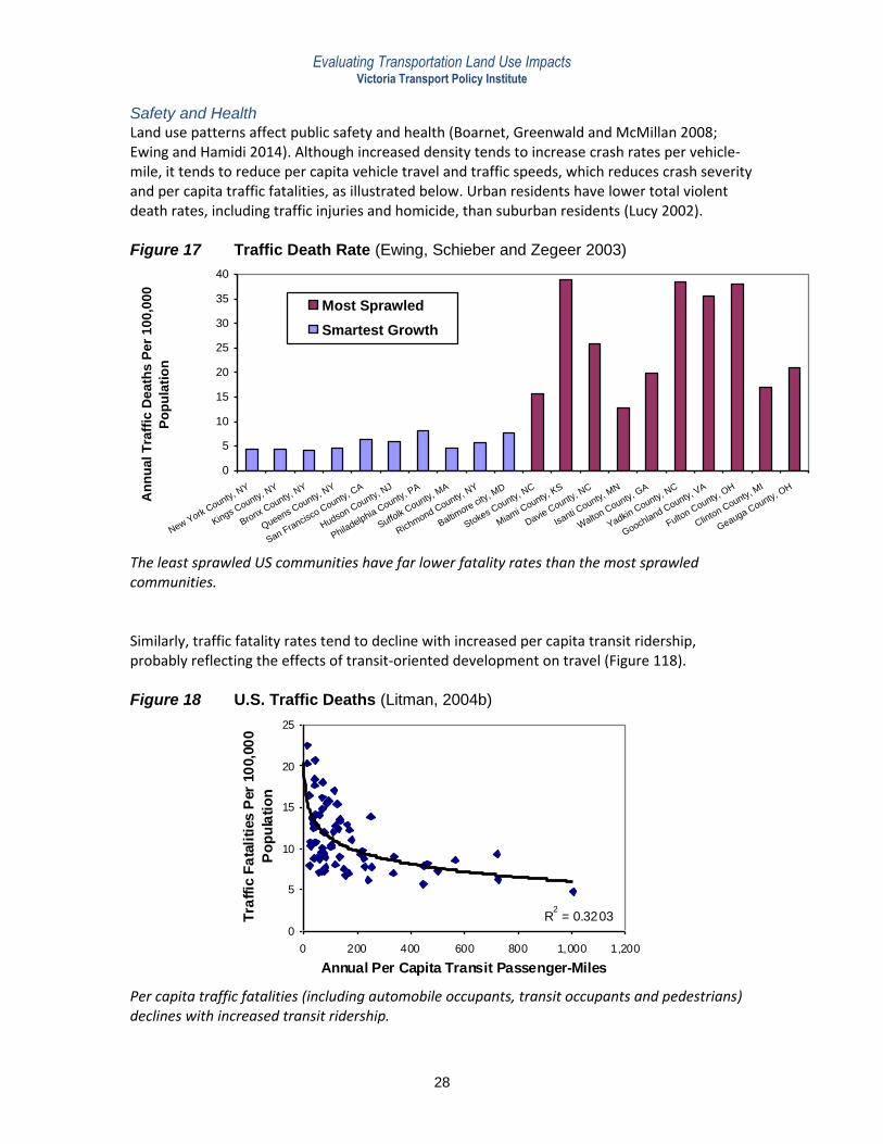
Safety and Health
Land use patterns affect public safety and health (Boarnet, Greenwald and McMillan 2008; Ewing and Hamidi 2014). Although increased density tends to increase crash rates per vehicle-mile, it tends to reduce per capita vehicle travel and traffic speeds, which reduces crash severity and per capita traffic fatalities, as illustrated below. Urban residents have lower total violent death rates, including traffic injuries and homicide, than suburban residents (Lucy 2002). Figure 17 Traffic Death Rate (Ewing, Schieber and Zegeer 2003)
0
5
10
15
20
25
30
35
40
New York C
ounty, NY
Kings County, N
Y
Bronx County, N
Y
Queens County, N
Y
San Francisco County, C
A
Hudson County, N
J
Philadelphia C
ounty, PA
Suffolk C
ounty, MA
Richmond County, N
Y
Baltimore city
, MD
Stokes County, N
C
Miami County, K
S
Davie County, N
C
Isanti County, M
N
Walto
n County, G
A
Yadkin County, N
C
Goochland County, V
A
Fulton C
ounty, OH
Clinton C
ounty, MI
Geauga County, O
H
An
nu
al T
raff
ic D
ea
ths P
er
10
0,0
00
Po
pu
lati
on
Most Sprawled
Smartest Growth
The least sprawled US communities have far lower fatality rates than the most sprawled communities. Similarly, traffic fatality rates tend to decline with increased per capita transit ridership, probably reflecting the effects of transit-oriented development on travel (Figure 118). Figure 18 U.S. Traffic Deaths (Litman, 2004b)
R2 = 0.3203
0
5
10
15
20
25
0 200 400 600 800 1,000 1,200
Annual Per Capita Transit Passenger-Miles
Tra
ffic
Fa
tali
ties
Per
10
0,0
00
Po
pu
lati
on
Per capita traffic fatalities (including automobile occupants, transit occupants and pedestrians) declines with increased transit ridership.

Evaluating Transportation Land Use Impacts Victoria Transport Policy Institute
29
The American Academy of Pediatrics (2009) argues that conventional, sprawled community design is unhealthy, particularly for children, because it discourages physical activity. Research by Lawton (2001), Khattak and Rodriguez (2003), and Gehling (illustrated in the Figure 19) indicate that residents of more urban, walkable communities are more likely to achieve recommended levels of physical activity than residents of more automobile-oriented, sprawled communities. For more discussion see Litman, 2005. Figure 19 Portion of Population Walking & Cycling 30+ Minutes Daily (Unpublished Analysis of 2001 NHTS by William Gehling)
0%
5%
10%
15%
20%
25%
30%
0-100 100-500 500-1,000 1,000-
2,000
2,000-
4,000
4,000-
10,000
10,000-
25,000
25,000-
100,000Po
rtio
n E
xe
rcis
ing
30+
Min
ute
s D
aily
The portion of people who exercise sufficiently by active transport increases with density. Lawton also found that increased urbanization (increased land use density, mix and roadway connectivity) increases minutes of nonmotorized travel, illustrated below. Figure 20 Urbanization Impact On Mode Split (Lawton, 2001)
0
10
20
30
40
50
60
70
80
Least Urban Mixed Most Urban
Urban Index Rating
Da
ily
Min
ute
s o
f T
rav
el
Automobile
Transit
Walk
Ewing, Frank, and Kreutzer (2006) identify a variety of specific ways that land use patterns can affect public health. Forsyth, Slotterback and Krizek (2010) discuss how Health Impact Assessments (HIAs) can be used to evaluate the public health impacts of specific planning decisions. Frank, et al (2006) developed a walkability index that reflects the quality of walking conditions, taking into account residential density, street connectivity, land use mix and retail floor area

Evaluating Transportation Land Use Impacts Victoria Transport Policy Institute
30
ratio (the ratio of retail building floor area divided by retail land area). In King County, Washington a 5% increase in this index is associated with a 32.1% increase in time spent in active transport (walking and cycling), a 0.23 point reduction in body mass index, a 6.5% reduction in VMT, and similar reductions in air pollution emissions. Economic Productivity and Development
Land use patterns affect economic productivity and development. All else being equal, greater accessible and lower transport costs increase economic productivity (Donovan and Munro 2013; Litman 2010b). More accessible land use that reduces consumers’ vehicle and fuel expenditures tends to increase regional employment and business activity, as illustrated in Table 14. Table 14 Regional Economic Impacts Of $1 Million Expenditure (MRL 1999)
Expenditure Category Regional Income Regional Jobs
Automobile Expenditures $307,000 8.4
Non-automotive Consumer Expenditures $526,000 17.0
Transit Expenditures $1,200,000 62.2
This table shows economic impacts of consumer expenditures in Texas.
Many economic activities, particularly finance, education and creative industries, experience agglomeration efficiencies; they are more efficient when located close together, because this facilitates interaction, trade and cooperation (Bettencourt, et al. 2007). Although difficult to measure these impacts appear to be large (Anas, Arnott and Small 1997; Lee 1999; Muro and Puentes 2004; Graham 2007; Sohn and Moudon 2008). More accessible, compact, mixed, connected land use patterns tend to increase employment, economic productivity, land values and tax revenues (IEDC 2006). One published study found that doubling county-level density index is associated with a 6% increase in state-level productivity (Haughwout 2000; also see discussion in Muro and Puentes 2004), although Gordon (2012) emphasizes that land use density is a surrogate for complex relationship networks that are only partly geographic. Meijers and Burger (2009) found that metropolitan region labor productivity declines with population dispersion (a higher proportion of residents live outside urban centres), and generally increases with polycentric development (multiple business districts, cities and towns within a metropolitan region, rather than a single large central business district and central city). This suggests that in growing regions, suburbanization is not economically harmful if new cities and towns reflect smart growth principles, but dispersed, automobile-dependent sprawl reduces economic productivity. This suggests that regional rail transit systems with transit oriented development around stations tends to support regional economic development by encouraging efficient polycentric land use development patterns. More compact development, including reductions in the amount of land required for transport facilities such as roads and parking, frees up land for other productive uses, including businesses, housing, farmlands, and recreation. The box on the following page describes how this can increase regional economic productivity.

Evaluating Transportation Land Use Impacts Victoria Transport Policy Institute
31
Transportation Policy Impacts On Farm Productivity This example describes how transport land use impacts can affect agricultural productivity. The Netherlands and Southern California (Los Angeles, Ventura, Orange, and eastern Riverside and San Bernardino counties) are similar in area (~ 16 thousand square miles) and population (~16 million residents). Both have significant agricultural potential. The Netherlands produces more than $40 billion annually in agricultural products. Farming was once major industry in Southern California, but it is now minor, accounting for less than a billion dollars in direct economic productivity. Several factors account for this differences, including topography (much of Southern California is hilly), water supply (Los Angeles has less) and economic policy (agricultural industry is well supported by the Dutch government), but a major factor is land use policy, which in turn is affected by transport policy. The Netherlands encourages compact development, with minimal per capita land consumption for housing, parking and roads, which leaves more land for farming. The following table compares the amount of land required for 16 million residents with multi-modal and automobile-oriented transport systems. Automobile dependency encourages larger building footprints, more surface parking and roads. Typical Land Consumption Per Capita (Square Feet)
Multi-Modal Auto-Oriented
Housing (1,200 sq. ft. interior space per capita) (Three stories) 400 (One-story) 1,200
Parking (300 sq. ft. per space) (2 spaces) 600 (6 spaces) 1,800
Roads (15 foot right-of-way width per lane)1 (30 lane-feet) 450 (100 lane-feet) 1,500
Impervious surface per capita (sq. ft) 1,450 4,500
Total impervious surface (sq. miles) 832 2,582
Portion of 16 thousand sq. miles 5% 16%
In the multi-modal community residents consume about 5% of the land base for buildings, parking and roads, compared with 16% in automobile-oriented areas, leaving about 11% more land available for productive uses such as agricultural. Of course, actual impacts depend on factors, including other land uses (such as residential lawns, parks and industrial facilities) and the quality of land displaced. Urban development often occurs on agricultural lands (valleys and deltas) which reduces farm production. This example illustrates how transportation policies can significantly affect per capita land consumption, which can have significant economic impacts. This indicates that transportation policies that encourage more compact development and reduce the amount of land required for roads and parking facilities can increase the productivity of farming or other land-intensive industries.
1 Federal Highway Statistics, Table 71 (www.fhwa.dot.gov/policyinformation/statistics/2008/hm71.cfm) provides data on road miles in various cities, suggesting that per capita lane-miles range from about 30 in multi-modal communities up to about 100 in
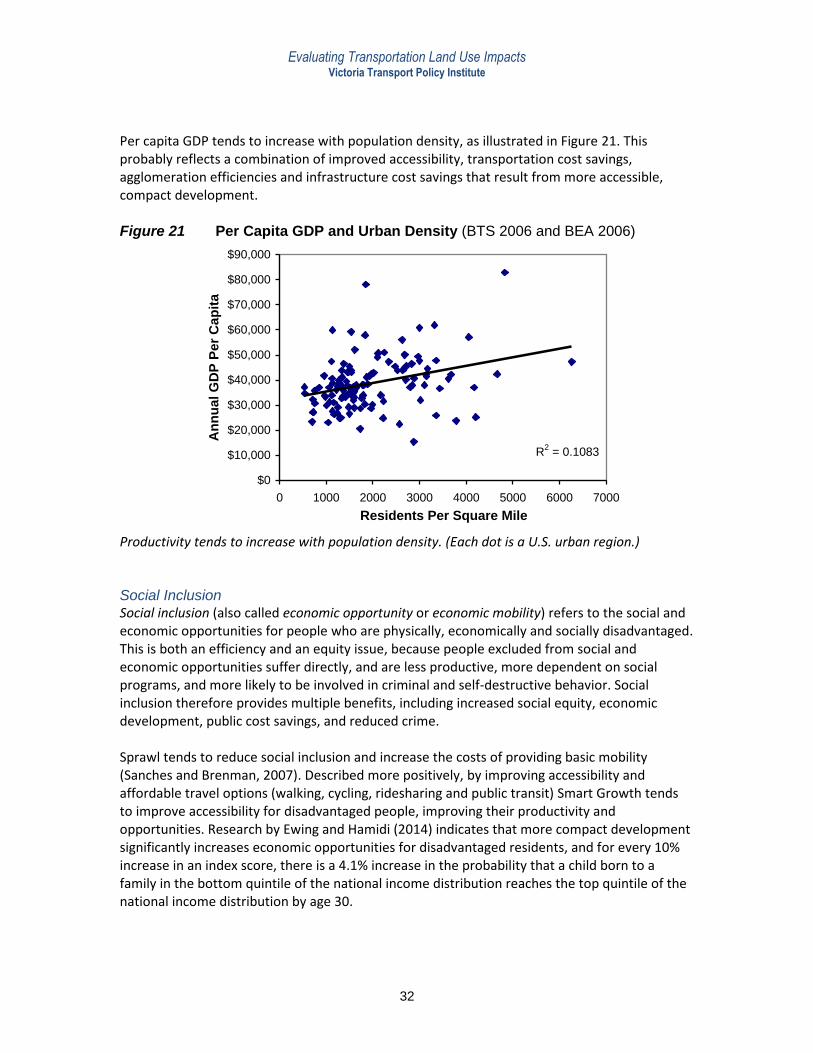
Evaluating Transportation Land Use Impacts Victoria Transport Policy Institute
32
Per capita GDP tends to increase with population density, as illustrated in Figure 21. This probably reflects a combination of improved accessibility, transportation cost savings, agglomeration efficiencies and infrastructure cost savings that result from more accessible, compact development. Figure 21 Per Capita GDP and Urban Density (BTS 2006 and BEA 2006)
R2 = 0.1083
$0
$10,000
$20,000
$30,000
$40,000
$50,000
$60,000
$70,000
$80,000
$90,000
0 1000 2000 3000 4000 5000 6000 7000
Residents Per Square Mile
An
nu
al G
DP
Per
Ca
pit
a
Productivity tends to increase with population density. (Each dot is a U.S. urban region.) Social Inclusion
Social inclusion (also called economic opportunity or economic mobility) refers to the social and economic opportunities for people who are physically, economically and socially disadvantaged. This is both an efficiency and an equity issue, because people excluded from social and economic opportunities suffer directly, and are less productive, more dependent on social programs, and more likely to be involved in criminal and self-destructive behavior. Social inclusion therefore provides multiple benefits, including increased social equity, economic development, public cost savings, and reduced crime. Sprawl tends to reduce social inclusion and increase the costs of providing basic mobility (Sanches and Brenman, 2007). Described more positively, by improving accessibility and affordable travel options (walking, cycling, ridesharing and public transit) Smart Growth tends to improve accessibility for disadvantaged people, improving their productivity and opportunities. Research by Ewing and Hamidi (2014) indicates that more compact development significantly increases economic opportunities for disadvantaged residents, and for every 10% increase in an index score, there is a 4.1% increase in the probability that a child born to a family in the bottom quintile of the national income distribution reaches the top quintile of the national income distribution by age 30.

Evaluating Transportation Land Use Impacts Victoria Transport Policy Institute
33
Community Cohesion
Community cohesion (also called social capital) refers to the quality of relationships among people in a community, as indicated by the frequency of positive interactions, the number of neighborhood friends and acquaintances, and their sense of community connections, particularly among people of different economic classes and social backgrounds (Forkenbrock and Weisbrod, 2001, pp. 97-106; Litman, 2007; CTE, 2008). Land use patterns affect community cohesion in various ways. Suburban locations are often considered highly livable because they are physically segregated from disruptive activities, traffic, poverty and crime. However, the automobile travel they generate tends to reduce community cohesion overall, by increasing vehicle traffic impacts through neighborhoods, degrade walking and cycling conditions, and reducing opportunities for neighborhood interaction. Many suburban neighborhoods lack sidewalks, neighborhoods shops and other public places where neighbors naturally congregate. Researcher Donald Appleyard (1981) reported a negative correlation between vehicle traffic and measures of neighborly interactions, including number of friends and acquaintances residents had on their street, and the area they consider “home territory.” He comments (1981, p. 35):
“The activities in which people engage or desire to engage in may affect their vulnerability to traffic impact. So many of these activities have been suppressed that we sometimes forget they exist...Children wanting to play, and people talking, sitting, strolling, jogging, cycling, gardening, or working at home and on auto maintenance are all vulnerable to interruption [by traffic]...One of the most significant and discussed aspects of street life is the amount and quality of neighboring. Its interruption or ‘severance’ has been identified as one of the primary measures of transportation impact in Britain.”
Many households prefer lower-density, suburban neighborhoods, but this partly reflects social attributes such as security, quality schools and prestige, rather than unique physical attributes, such as larger lawns (NAHB 1999). This suggests that some households would choose Smart Growth locations if they had such amenities. Demand for New Urbanist communities, loft apartments and urban infill is strong where they offer personal security, school quality and prestige comparable to suburbs. Eppli and Tu (2000) found that New Urbanist community homes sold for an average of $20,189 more than otherwise comparable homes in more conventional communities, an 11% increase in value. Heart and Biringer (2000) calculate that 43% of homebuyers who currently choose rural and suburban locations are good candidates for higher density, traditional neighborhood developments. This suggests that, although urban neighborhoods often have more social problems than suburban neighborhoods, urbanization does not cause social problems. Rather, these problems reflect the tendency of automobile dependent suburbs to offload social problems onto more accessible, multi-modal urban neighborhoods. Total regional social problems are likely to decline if Smart Growth can improve overall social inclusion in a region, helping disadvantaged people access education and employment. Freeman (2001) analyzed data from a cross-sectional survey of adults in Atlanta, Boston, and Los Angeles concerning their social interactions. The analysis indicates that, although the rate of

Evaluating Transportation Land Use Impacts Victoria Transport Policy Institute
34
neighborhood social tie formation was unrelated to land use density alone, it was significantly and substantially related to the degree to which residents of a neighborhood relied on their automobiles. Similarly, Leyden (2003) found that people living in walkable, mixed-use neighborhoods have higher levels of social capital compared with those living in car-oriented suburbs. Walkable neighborhood residents were more likely to know their neighbors, participate politically, trust others and be socially engaged, suggesting that polices and projects that support walking and public transit use, and increase land use mix, tend to increase community cohesion.

Evaluating Transportation Land Use Impacts Victoria Transport Policy Institute
35
Environmental and Ecological Impacts
Road and sprawl environmental impacts are widely recognized by land use planners and ecologists (Noonan 1996; Flad 1997; Forman, et al. 2003; White 2007). Ecologically active lands such as wetlands, forests, farms, and parks (collectively called greenspace or openspace) provide external benefits, including wildlife habitat, air and water quality, and beauty (Brabec 1992; Hawkes 2016; Kauffman 2001; Ewing and Kostyack 2005). Urban areas often contain high value habitate and species. For example, Ives, et al. (2016) found that Australian cities support substantially more nationally threatened animal and plant species than all other non-urban areas on a unit-area basis, and thirty per cent of threatened species were found to occur in cities. These external benefits of ecologically-active lands exist in addition to direct benefits to landowners and are not reflected in land’s market value (Knaap and Nelson 1992, p. 126). Some of these benefits result from the contribution that an ecological system makes toward market goods, such as fishery production or water quality. Other values are reflected in the tendency of greenspace to increase nearby property values and tourism, and in existence, option, and bequest values (Kopp and Smith 1993; Munasinghe and McNeely 1995; Sherer 2006). Banzhaf and Jawahar (2005) identify the following benefits of openspace preservation:
1. Protecting groundwater. 2. Protecting wildlife habitat. 3. Preserving natural places. 4. Providing local food. 5. Keeping farming as a way of life.
6. Preserving rural character. 7. Preserving scenic quality. 8. Slowing development. 9. Providing public access.
Ecological value refers to the contribution land makes toward various environmental functions such as wildlife habitat, and surface and groundwater recharge. Roads and parking facilities have hydrologic impacts (changes to surface and groundwater flows) that tend to concentrate stormwater, increase flooding, scouring and siltation, and reduce dry season supply, and create barriers to fish (Litman 2005). These impose both economic and ecological costs. Paved surfaces create heat islands, causing ambient summer temperatures to rise 2-8° F in urban areas, which increases energy demand, smog, human discomfort and health problems (Stone, Hess, Frumkin 2010; USEPA 2011). Transportation policies and projects are ecologically harmful if they disturb or divide habitat, convert natural habitat to gardens, farms or lawns, or increase impervious surface area. Parks, gardens, farms and lawns generally provide moderate to minimal wildlife habitat, particularly for larger animals, and although they allow surface and groundwater recharge, this often carries significant pollution loads from fertilizers, pesticides and other sources. From an ecological perspective, pavement is generally least beneficial land use since it provides no habitat, prevents groundwater recharge, increases stormwater management costs, and tends to concentrate water pollution. As a result, transport policies provide ecological benefits to the degree that they help reduce wildlife habitat fragmentation, preserves wildlife habitat, discourages lower-density development, or reduces impervious surface. This analysis depends on how impacts are

Evaluating Transportation Land Use Impacts Victoria Transport Policy Institute
36
measured: higher density urban development tends to have poorer ecological effects within a given area (measured per acre or square mile) but have better effects per capita (Arnold and Gibbons 1996; USEPA 2006). Some studies have valued open space (EDRG 2007; McConnel and Walls 2005; Tagliafierro, et al. 2013). The box below ranks of these values. Impervious surfaces such as buildings, parking lots and roadways generally provide the least environmental benefits, and they increase stormwater management costs and heat island effects (higher ambient temperatures from sunlight). These negative impacts can be reduced somewhat with design features such as rooftop gardens, street trees and pervious pavements, but this does not eliminate the value of open space preservation.
External Values Ranked (McConnel and Walls 2005) 1. Shorelands and wetlands such as lake and marshes. 2. Unique natural and cultural lands such as forests, deserts and heritage sites 3. Farmlands 4. Parks and gardens 5. Lawns
6. Impervious surfaces (buildings, parking lots and roads)
Some land use types, such as shorelines, unique natural and cultural lands, and high value farmlands, provide significant external benefits that justify their preservation.
Table 15 summarizes one estimate of various economic, social and environmental values of openspace in Washington State’s Puget Sound region. Many are indirect, and so tend to be undervalued by stakeholders. For example, area residents may be unaware that openspace reduces disaster risks, maintains water quality and supports local industries. Table 15 Puget Sound Openspace Values (Chadsey, Christin and Fletcher 2015)
Low Range High Range
Total (m) Per Acre Total (m) Per Acre
Aesthetic (perceived beauty and higher property values)
$2,294 $655 $9,510 $2,717
Air quality protection $422 $121 $529 $151
Food production (farm and aquaculture) $13 $4 $86 $25
Shelter (wildlife habitat) $74 $21 $111 $32
Water quality and percolation $63 $18 $1,925 $550
Health (exercise and mental health) $41 $12 $50 $14
Play (outdoor recreation and related industries) $2,633 $752 $4,133 $1,181
Disaster mitigation (e.g., flood protection) $1,860 $532 $4,194 $1,199
Raw materials (lumber, stone, etc.) $23 $7 $155 $44
Waste and pollution transformation $4,034 $1,153 $4,569 $1,306
Totals $11,458 $3,274 $25,264 $7,219
This study indicates that openspace provides diverse economic, social and environmental benefits. A number of studies indicate that proximity to high traffic roads reduces residential property values due to noise and air pollution effects, while proximity to greenspace tendst to increase property values. Kang and Cervero (2008) studied how the Cheong Gye Cheon (CGC) project in Seoul, Korea, which involved converting a freeway into an urban park, affected property values.

Evaluating Transportation Land Use Impacts Victoria Transport Policy Institute
37
They found that freeway proximity reduced residential property values and increased non-residential property values, and that both residential non-residential properties within 500 meter were generally worth more when the freeway was replaced by an urban stream/linearpark. While proximity to freeway on-ramps was valued by residential properties, this benefit was offset by nuisance effects of noise, dust, fumes, and visual blight for residences within several kms of the structure. Forman and Deblinger (2000) studied the ecological effects of a 25-kilometer stretch of four-lane highway through urban, suburban and rural areas, taking into account roadkills, habitat loss, traffic noise, barrier effects to wildlife, introduction of exotic species, water pollution and hydrologic impacts (such as changes in wetlands drainage). They found that the road-effect zone averages 600 meters wide, with some effects being even more dispersed. Extrapolating these results the researchers calculated that roads influence approximately 20% of continental United States. Brady and Jonathan L Richardson (2017), Noss (1995), Havlick (2002), and Forman, et al (2003) identify various types of ecological damages caused by roads, listed below. Forman, et al (2003, p. 136) identifies road density thresholds (maximum road-miles per square mile) for various habitats.
Roadkills: Animals killed directly by motor vehicles. More than 1 million large animals are killed annually on U.S. highways, representing more than 8% of all reported crashes (Hughes and Saremi, 1995). Roadkills increase with traffic speeds and volumes. Road kills are a major cause of death for many large mammals, including several threatened species.
Road Aversion and other Behavioral Modifications: Some animals have an aversion to roads, which may affect their behavior and movement patterns. For example, black bears cannot cross highways with guardrails. Other species, on the other hand, become accustomed to roads, and are therefore more vulnerable to harmful interactions with humans.
Population Fragmentation and Isolation: By forming a barrier to species movement, roads prevent interaction and cross breeding between population groups of the same species. This reduces population health and genetic viability.
Pollution: Road construction and use introduce a variety of noise, air and water pollutants.
Habitat Impacts: This includes loss of habitat, invasion of exotic species, and other effects.
Impacts on Hydrology and Aquatic Habitats: Road construction alters watersheds through changes in water quality and water quantity, stream channels, and groundwater.
Access to Humans: This includes hunters, poachers, and irresponsible visitors.
Some land use impacts, such as wetlands losses and endangered species threats, receive considerable attention and can influence planning decisions, but this requires evaluating each impact individually. A better approach applys a general model for valuing each land use type. Various techniques can be used to estimate the overall environmental value of different land use categories and specific sites (Johansson 1987; Kopp and Smith 1993). The US Forest Services’ Urban Forest Effects (UFORE) Model (www.fs.fed.us/ne/syracuse/About/about.htm) can be used to define and quantify various forest functions and values of urban trees air pollution, greenhouse gases and global warming, and building energy use.

Evaluating Transportation Land Use Impacts Victoria Transport Policy Institute
38
Jacob and Lopez (2009) calculated how land use development density affects stormwater runoff volumes, and the amount of phosphorous, nitrogen and suspended solid water pollution. They found that these impacts increase per acre but declined per capita. For a constant or given population, higher density development tends to dramatically reduce loadings compared with diffuse suburban densities. Their model showed that doubling standard suburban densities [from 3-5 up to 8 dwelling units per acre can usually achieve more contaminant loading reductions than many traditional stormwater best management practices (BMPs), and that higher densities such as those associated with transit-oriented development outperform almost all traditional BMPs in reduced loadings per capita. A major Swiss government research program on transporation costs included a study of habitat loss and fragmentation caused by road and railroad infrastructure (Swiss ARE 2005). The calculated external cost throughout Switzerland totaled 765 million Swiss Francs (CHFs) in 2000, of which habitat loss comprises CHF 179-337 million/year and habitat fragmentation CHF 264-746 million/year. Around 86% is caused and the rest by rail infrastructure. This is calculated to aveage:
1.2 centimes per vehicle-km for automobiles 0.7 centimes per passenger-km for rail transport 2.6 centimes per vehicle-km for trucks 3.4 centimes per vehicle-km for heavy articulated vehicles 1.2 centimes per tonne-km for rail freight transport.
Table 16 shows one evaluation of environmental benefits provided by selected land uses. Table 16 Environmental Benefits By Land Use Category (Bein 1997) Air
Quality
Water
Quality
Eco-
logica Flood
Control
Recrea-
tionb Aes-
thetic
Cul-
turalc Eco-
nomicd
Wetlands High High High High High High High High
Pristine Wildlands High High High Varies High High High Variese
Urban Greenspace High High Medium Medium High High High Variese
2nd Growth Forest High High Medium High High Varies Medium Medium
Farmland Medium Medium Low Medium Low Varies Medium Varies
Pasture/Range Low Medium Low Low Low Varies Medium Low
Mixed Urban Low Low Low Low Varies Varies Varies High
Highway Buffer Low High Low Low Low Low Low Low
Pavement None None None None None None None Varies
Notes a. Include wildlife habitat, species preservation and support for ecological systems. b. Includes hunting, fishing, wildlife viewing, hiking, horse riding, bicycling, etc. c. Includes preservation of culturally significant sites, and traditional activities such as harvesting resources. d. Includes economic benefits to people who do not own the land, such as tourism, fishing and hunting. e. Reflected in tourism and recreational expenditures, increased adjacent property values, water resources quality and availability, and fisheries.

Evaluating Transportation Land Use Impacts Victoria Transport Policy Institute
39
Energy Consumption and Pollution Emissions
Smart Growth tends to reduce per capita energy consumption and pollution emissions by reducing vehicle travel and supporting other energy conservation strategies such as shared building walls and district heating (Mindali, Raveh and Salomon 2004; Ewing, et al. 2007; Glaeser and Kahn 2008; Mehaffy, Cowan and Urge-Vorsatz 2009), although it can increase exposure to local emissions such as carbon monoxide, particulates and noise. The following land use factors can affect energy consumption and emissions:
Density (number of people and businesses in a given area) and clustering (common destinations located close together) affects travel mode and trip distance.
Land use mix (the diversity of land uses in an area) affects trip distances and the feasibility of nonmotorized transportation.
Major activity centers (locate employment, retail and public services close together in walkable commercial centers) increases walking, cycling and public transit travel.
Parking management (sharing, pricing and regulations to encourage efficient use of parking facilities) affects land use density, and automobile ownership and use.
Street connectivity (the degree to which streets connect to each other, rather than having deadends or large blocks) affects accessibility, including the amount of travel required to reach destinations and the relative speed and convenience of cycling and walking.
Transit Oriented Development (locating high-density development around transit stations) makes transit relatively more convenient, and can be a catalyst for other land-use changes.
Pedestrian Accessibility and traffic calming affect the relative speed, convenience and safety of nonmotorized transportation.
Although individually each of these factors has relatively modest travel impacts, residents of traditional communities that incorporate most or all of these factors tend to drive 20-40% less than otherwise comparable residents of automobile-dependent communities (Litman, 2005; Norman, MacLean and Kennedy 2006). A USEPA study (2004) found that regardless of population density, transportation system design features such as greater street connectivity, a more pedestrian-friendly environment, shorter route options, and more extensive transit service tend to reduce per-capita vehicle travel, pollution emissions, congestion delays and traffic accidents. Figure 22 compares per capita emissions between various cities.
Figure 22 Climate Change Emissions By City (Vancouver 2008)
0 2 4 6 8 10 12 14 16 18 20
Calgary
Austin
Portland
San Francisco
Seattle
Toronto
London
Vancouver
Barcelona
Oslo
Annual Tonnes CO2 Per Capita
Per capita energy consumption and climate change emissions vary significantly depending on a city’s transportation and land use patterns.

Evaluating Transportation Land Use Impacts Victoria Transport Policy Institute
40
Aesthetic Impacts
Roads and traffic also reduce natural environmental beauty and cause urban blight (Hoyle and Knowles 1992; Passonneau 1996). The Transportation and Traffic Engineering Handbook, (Edwards 1982, p. 396), the USDOT’s Environmental Assessment Notebook (USDOE 1997, p. 29-4) all cite visual aesthetic degradation as major negative impacts of roads. William Shore argues that an automobile oriented urban area is inherently ugly because retail businesses must “shout” at passing motorists with raucous signs, because so much of the land must be used for automobile parking, and because the settlement pattern has no clear form. The value of attractive landscapes is indicated by their importance in attracting tourism and increasing adjacent property values. Segal estimates that a 3/4 mile stretch of Boston’s Fitzgerald Expressway reduced downtown property values by the equivalent of $600 million by blocking waterfront views (Segal, 1981). Amortized, this cost averages $1.30 to $2.30 per expressway vehicle trip. This is an extreme case, but indicates that aesthetic degradation from roads may impose significant aesthetic costs. Public and professional surveys can be used to evaluate such aesthetic impacts on the landscape (Huddart 1978). When such techniques were used in a survey visual quality ratings consistently declined as the size of the road construction increased. In a study by Professor Wolf (2002), consumers were shown photos of retail streets with and without trees to residents in various US cities and asked how much they would pay various items at each location. Participants indicated that they were willing to pay nearly 12% more to shop on treed streets than on treeless ones. They perceived shops on tree-lined streets as better maintained, having a more pleasant atmosphere, and as likely having higher quality products. Participants also indicated that they were willing to travel farther to those shops (expanding the customer pool) and to pay more for parking. The study, Measuring the Economic Value of a City Park System (Harnik and Welle 2009) describes numerous benefits from urban parks and openspace, and identifies the following as suitable for quantification:
Increased property values
Tourism value
Direct use value
Public fitness and health value
Community cohesion value
Reducing urban stormwater management costs
Reduced air pollution
Cultural Preservation
Transportation facilities and sprawl sometimes threaten unique cultural resources, such as historic buildings, sacred land areas, neighborhood parks, older neighborhoods and towns, and traditional building styles. By reducing per capita land requirements and providing greater design flexibility, Smart Growth can avoid or reduce these impacts, allowing cultural preservation. Smart Growth also supports urban redevelopment, which helps preserve existing towns and cities, and urban neighborhoods.

Evaluating Transportation Land Use Impacts Victoria Transport Policy Institute
41
Consumer and Economic Impacts Critics argue that smart growth harms consumers and the economy by reducing housing options and restricting automobile travel. Table 17 evaluates the consumer and economic efficiency impacts of various smart growth strategies. Most of these strategies directly benefit the people affected by improving their housing and transport options and increasing efficiency. Many strategies correct existing market distortions that reduce housing and transportation options. Table 17 Smart Growth Consumer Impacts (Litman 2010a)
Strategy Examples Consumer Impacts Economic Impacts
More integrated transport and land use planning
Better sidewalks and bikelanes around schools. Commercial development concentrated along transit routes.
Most consumers benefit from improved accessibility and transport options.
Tends to reflect good planning and increase overall efficiency.
Location-efficient development
More affordable housing located in accessible areas.
Benefits lower-income residents who choose such housing.
Responds to consumer demand and increases efficiency.
More flexible zoning codes
Allow more compact and mixed development.
Benefits consumers who prefer more compact, affordable housing options.
Responds to consumer demands and increases efficiency.
Reduced and more flexible parking requirements.
Reduced parking requirements in response to geographic, demographic and management factors (more sharing and pricing of parking)
Benefits consumers who prefer more compact, affordable housing options, particularly those who own fewer than average cars.
Responds to consumer demands and increases efficiency. Can provide significant savings and benefits.
Growth control
Urban growth boundaries that limit urban fringe development.
Harms consumers who demand large-lot housing where supply is inadequate.
Increases automobile-dependency and associated costs.
Transportation funding shifts
Reduced funding for roadway expansion and increased funding for walking and cycling facilities and public transit service improvements.
People who prefer alternative modes benefit directly. Motorists may have less capacity, but can benefit from reduced chauffeuring requirements, and reduced congestion if better alternatives cause mode shifts.
Can increase efficiency if there is demand for alternative modes and if mode shifting reduces problems such as congestion and accidents.
Most smart growth strategies directly benefit consumers and increase economic efficiency.
Two strategies may harm some consumers. Growth controls can prevent some consumers who want large-lot homes from obtaining the housing option they prefer, if there is a significant shorting of supply. However, there is currently an oversupply of such housing across North America and no indication that shortages will develop in the future (Leinberger 2008). Similarly, shifting funding from highways to other modes can harm motorists who care nothing about other travel options, if the investments are inefficient and so do nothing to reduce congestion or accident risk, but if such investments are efficient even people who continue driving may benefit overall.

Evaluating Transportation Land Use Impacts Victoria Transport Policy Institute
42
Optimal Level of Sprawl There is often debate about the desirability of development patterns, generally termed sprawl and smart growth (Aurbach 2003; Litman 2003). Critics argue that sprawl imposes numerous economic, social and environmental costs, and that smart growth development is desirable. Smart growth critics argue that sprawl provides benefits that offset these costs, and meets consumer demands (Cox 2001; see box below).
Environmental and Social Benefits? A 1978 report by Gamble and Davinroy argues that highways provide environmental and social benefits. Here are typical quotations from the report:
Aesthetics: “The freeway can provide open space, reduce or replace displeasing land uses, enhance visual quality through design standards and controls, reduce headlight glare, and reduce noise.” and “Regarding the visual quality of the highway and highway structures, freeways may create a sculptural form of art in their own right. Some authors note that the undulating ribbons of pavement possessing both internal and external harmony are a basic tool of spatial expression.”
Wildlife: “Freeway rights-of-way may be beneficial to wildlife in both rural and urban environments...”
Wetlands: “The intersection of an aquifer by a highway cut may interrupt the natural flow of groundwater and thus may draw down an aquifer, improving the characteristics of the land immediately adjacent to the highway.”
Native plants: “Roadside rights-of-way can be among the last places where native plants can grow.”
Neighborhood Benefits: “Highways, if they are concentrated along the boundary of the neighborhood, can promote neighborhood stability.” and “Old housing of low quality occupied by poor people often serves as a reason for the destruction of that housing for freeway rights of way.”
Social Benefits: “Highways can increase the frequency of contact among individuals...” and “Good highways facilitate church attendance.”
Recreation: “Freeways cutting across, through, under, and around the cities afford an excellent opportunity for innovations in recreation planning and design.”
Additional claimed environmental benefits include improved air quality, energy savings, and reduce traffic noise. Urban benefits include removal of blighted housing and slums, support of mass transit, reduced accidents, greater safety for pedestrians – particularly school children, improved community values, civic pride, increased social contacts between diverse social groups, increased upward social mobility, in-migration of better educated families, and increased housing opportunities for racial minorities. Land use benefits include suburban growth, decentralization, industrial parks, shopping malls, commercial development at freeway interchanges, and drive-in businesses.
This debate often depends on how sprawl and smart growth are defined and measured. For example, critics often define smart growth as “high density development” or “population growth in existing cities,” although smart growth includes other factors, and allows development in new cities and towns, provided it reflects smart growth principles.

Evaluating Transportation Land Use Impacts Victoria Transport Policy Institute
43
Changing consumers appear to be increasing demand for smart growth (Nelson 2006; Litman 2010a). Market research indicates that an increasing portion of households want good accessibility (indicated by shorter commutes), land use mix (indicated by nearby shops and services), and diverse transport options (indicated by good walking conditions and public transit services) and will often choose small-lot and attached homes with these features. Demographic and economic trends are increasing smart growth demand, causing a shortage of such housing. Demand for sprawl housing is declining, resulting in oversupply and reduced value. Various studies, described in this report, indicates that lower-density, urban-fringe development imposes various economic, social and environmental costs. Many of these costs tend to be overlooked or undervalued in the planning process, and are seldom incorporated into pricing, which results in economically excessive levels of sprawl and automobile use (Litman, 2001; Lewyn, 2005). An efficient land market would therefore require the following features to determine the optimal level of sprawl:
Improved housing options, including more affordable housing developed in accessible, smart growth areas.
Policies that favor compact development to achieve agglomeration efficiencies and cost savings.
Development and utility fees, and taxes that reflect the lower costs of providing public services in more accessible, compact locations, so smart growth residents would save money.
Improved public services (particularly schools and public safety) in smart growth communities.
Land use policies that protect environmental amenties, including encouragement of more compact development and openspace protection.
These policies would test the true level of consumer demand for large-lot, urban fringe housing. Although some households would probably still choose such housing, even if faced with better and more affordable alternatives, it is likely that a significant portion of the market would shift to smarter growth locations, reducing the need for additional sprawl.

Evaluating Transportation Land Use Impacts Victoria Transport Policy Institute
44
Evaluation Techniques It would be inaccurate to say that current transport planning totally ignores land use impacts. Many projects undergo extensive review to identify, and if possible mitigate, negative impacts (FHWA, 1999; Forkenbrock and Weisbrod, 2001). However, current planning practices have several weaknesses:
Little or not analysis is performed for many transportation decisions. For example, no environmental analysis is required when minimum parking requirements are raised.
Many impacts are outside the scope of standard analysis. For example, impacts on accessibility, community cohesion and housing affordability are often overlooked.
Environmental analysis tends to focus on special, individual values and impacts, such as risks to a unique environmental or cultural resource. Damage to more common habitats or features are often given little consideration even if cumulative impacts are large.
Land use impacts are generally only evaluated during project planning. There is seldom review of existing policies and facilities. For example, there is no system to convert existing, underutilized roads and parking facilities back to greenspace.
As described earlier, comprehensive evolution of land use requires several steps, as summarized in the table below. The following pages describe techniques for evaluating land use impacts in transportation planning. For more information see Litman, 2001. These techniques are not mutually exclusive, they can be applied in combinations as appropriate. Table 18 Steps Between A Decision And Its Ultimate Effects
Physical Effects Impacts
1. Direct impacts of transportation facilities
Amount of land paved for transportation facilities
Greenspace preservation
Stormwater management costs
Heat Island effect
Transportation facility land values.
Development costs and affordability
Adjacent property values
Aesthetics
2. Changes in development patterns
Location, density and mix of development (degree of sprawl or Smart Growth).
Greenspace preservation
Public service costs
3. Land use accessibility and transport diversity
Dispersion of common destinations, and quality of travel options.
Changes in per capita vehicle travel
Equity and opportunity
Area property values
4. Quality of public realm Quality of sidewalk environment, and other places where people often interact.
Quality of community cohesion
Certain economic activities
5. Travel activity
Per capita motor vehicle ownership and use.
Consumer transportation costs
Accidents
Energy and pollution impacts
Physical fitness and public health
There may be several steps between a transport planning decision and some of its ultimate effects.

Evaluating Transportation Land Use Impacts Victoria Transport Policy Institute
45
Comprehensive Project Analysis
One approach is to improve existing evaluation practices is to expand the range of land use impacts considered in planning (“Comprehensive Transport Planning,” VTPI, 2005). This gives more consideration to the land use impacts identified in this report. Each impact can be described, and as much as possible quantified and monetized. Below is a list of impacts to consider and potential indicators. Table 19 Land Use Impact Checklist
Impact Examples of Indicators
Economic
Land value Amount of land used for transportation facilities and its estimated value.
Land use accessibility Number of public services and jobs within 30-minute travel time.
Transportation costs Household expenditures on transportation.
Crash damages Number of traffic crashes, injuries and deaths. Economic value of crash damages.
Public service costs Costs of providing public services, including roads, utilities, garbage collection, emergency response, school transportation, etc.
Economic development Economic productivity, employment, business activity, property values and tax revenues. Costs to governments and businesses, and agglomeration efficiencies.
Stormwater management Costs of providing stormwater management.
Others
Social
Equity of opportunity Relative level of accessibility and transport affordability for disadvantaged people (e.g., non-drivers and low income people) relative to more advantaged people.
Community cohesion Quality of public realm (sidewalks, streets, parks, etc.), and frequenty of positive interactions among community residents.
Housing affordability Amount of affordable housing available or planned.
Cultural resources Preserviation of heritage buildings, historic sites, etc.
Public health Traffic safety (per capita injuries and deaths), physical fitness (portion of the population that achieves minimal levels of daily physical activity) and pollution exposure (portion of population exposed to unacceptable levels of pollutants).
Aesthetic impacts. Aesthetic quality of the landscape.
Others
Environmental
Impervious surface Amount of land paved for transport facilities, and resulting environmental effects.
Openspace preservation Quantity and quality of greenspace (farms, forests, parks, etc.) and wildlife habitat.
Energy consumption and pollution emissions Per capita energy consumption and emissions of air, water and noise pollution.
Others
This table lists various land use impacts often resulting from transportation planning decisions.

Evaluating Transportation Land Use Impacts Victoria Transport Policy Institute
46
Monetized Impact Evaluation
It is often possible to monetize (measure in monetary units) nonmarket impacts such as aesthetics and safety, so they can be incorporated in economic analysis along with market impacts (Banzhaf and Jawahar 2005; Litman 2010a). Such values can be used to calculate the external benefits provided by greenspace, and therefore the costs of developing or paving such land (TPL 2007). These include environmental and aesthetic benefits to nearby residents (reflected in 5-20% increase in nearby property values and tax revenues) and avoided public service costs (compared with the land being developed), additional farmland productivity, improved air and water quality, and support for certain businesses (such as tourism and fisheries). Table 20 illustrates a generic cost structure. For each hectare of land converted from its current use (left column) to another use (top row), the dollar value in the intersection cell indicates the change in external environmental benefits. For example, converting land from second-growth forest to pavement hass an environmental cost valued at $60,000 per hectare. Indirect impacts (traffic noise, pollution, introduced species) to land within 500 meters of a road can be considered to impose half these cost. Table 20 Land Conversion Costs (1994 CA$/hectare; Bein 1997)
Land Use
Categories
Wetlands
Pristine Wildland/
Urban Greenspace
Second
Growth
Pasture/
Farmland
Settlement
/ Buffer
Pavement
Wetlands 0 -20,000 -40,000 -60,000 -80,000 -100,000
Wildland/Urban Greenspace 20,000 0 -20,000 -40,000 -60,000 -80,000
Second Growth Forest 40,000 20,000 0 -20,000 -40,000 -60,000
Pasture/Farmland 60,000 40,000 20,000 0 -20,000 -40,000
Settlement / Buffer 80,000 60,000 40,000 20,000 0 -20,000
Pavement 100,000 80,000 60,000 40,000 20,000 0
Using this table: For each hectare of land converted from its current use (left column) to another use (top row), the dollar amount in the intersection cell indicates the change in environmental value. For example, a proposed road project requires paving 20 hectares of farmland and 10 acres of second growth forest, will lead to development on 10 hectares of second growth forest, and will cause noise and pollution impacts to 5 hectares of wetland, 20 hectares of second growth forest and 30 hectares of farmland. Table 21 summarizes these costs. Table 21 External Environmental Costs Calculation Example
Land Use Impact
Hectares
Cost Per Hectare (From Table 14)
Half Cost for
Indirect Impacts
Totals
Farmland to Pavement 20 $40,000 -- $800,000
Second Growth Forest to Pavement 10 $60,000 -- $600,000
Second Growth Forest to Settlement 10 $40,000 -- $400,000
Wetland noise and pollution 5 $80,000 x 0.5 $200,000
Second Growth noise and pollution 20 $40,000 x 0.5 $400,000
Farmland noise and pollution 30 $20,000 x 0.5 $300,000
Totals 95 -- $2,700,000
This table illustrates an example of calculating the environmental costs of a roadway project.

Evaluating Transportation Land Use Impacts Victoria Transport Policy Institute
47
Planning Objectives
Another method, called Multiple Accounts Evaluation, is to rate and compare options relative to specific planning objectives, as illustrated in the tables below. Ratings can be developed by technical experts, a public survey or an advisory committee. Table 22 Evaluation Matrix Example
Improved
Accessibility
Reduced
Crashes
Improved Mobility
for Non-drivers
Reduced Pollution
Emissions
Option 1 High High Medium High
Option 2 Medium Very Harmful High Medium
Option 3 High Medium High Low
Option 4 Low High Harmful High
Each option is evaluated according to how well it helps achieve each objective. A more quantitative system can be used. For example, each option can be rated from 5 (best) to -5 (worst) for each objective. These ratings are then summed to create total points for each project, as illustrated in Table 23. This gives each objective equal weight. Table 23 Evaluation Matrix Example – With Point Ratings
Improved
Accessibility
Reduced
Crashes
Improved Mobility
for Non-drivers
Reduced Pollution
Emissions
Total
Points
Option 1 4 4 3 4 16
Option 2 3 -4 5 3 7
Option 3 5 3 4 1 13
Option 4 2 4 -3 5 8
Each option is evaluated according to how well it helps achieve each objective. The objectives can be weighted, as shown in Table 24. The weight factors are multiplied times each rating, which are summed to give weighted total points. This approach begins to converge with standard Benefit-Cost analysis if points are considered to represent dollar values. Table 24 Evaluation Matrix Example – With Weighted Points
Improved
Accessibility
Reduced
Crashes
Improved Mobility
for Non-drivers
Reduced Pollution
Emissions
Total
Points
Weight 5 4 2 5
Option 1 4 (20) 4 (16) 3 (6) 4 (20) 62
Option 2 3 (15) -4 (-16) 5 (10) 3 (15) 24
Option 3 5 (25) 3 (12) 4 (16) 1 (5) 50
Option 4 2 (10) 4 (16) -3 (-6) 5 (25) 40
Each option is evaluated according to each objective, and each objective is assigned a weight. These are multiplied (values in parenthesis) and summed to obtain total points for each option.

Evaluating Transportation Land Use Impacts Victoria Transport Policy Institute
48
Examples and Case Studies Measuring Sprawl (Ewing and Hamidi 2014)
The report, Measuring Sprawl assigned a Sprawl Index score to 221 metropolitan areas and 994 counties in the U.S. according to four primary factors: density (people and jobs per square mile), mix (whether neighborhoods had a mix of homes, jobs and services), centricity (the strength of activity centers and downtowns) and roadway connectivity (the density of connections in the roadway network). The index averages 100, meaning that scores lower than 100 indicate more sprawl and scores higher than 100 indicate smart growth. The table below summarizes the study’s key results. Table 25 Summary of Sprawl Outcomes (Ewing and Hamidi 2014)
Outcome Relationship to Sprawl Impact of 10% Index Score
Housing affordability Positive and significant 1.1% increase in housing costs relative to income.
Transportation affordability Negative and significant 3.5% decrease in transportation costs relative to income
Upward mobility (probability a child born in the bottom income quintile reaches the top quintile by age 30) Negative and significant
4.1% increase
Average household vehicle ownership Positive and significant 0.6% decline
Percentage of commuters walking to Work Negative and significant 3.9% increase
Percentage of commuters using public transit Negative and significant 11.5% increase
Average journey-to-work drive time Positive and significant 0.5% decline
Traffic crash rate per 100,000 population Negative and significant
Injury crash rate per 100,000 population Negative and significant
Fatal crash rate per 100,000 population Positive and significant 15% decline
Body mass index Positive and significant
Obesity Positive and significant
Any physical activity Positive and significant
Diagnosed high blood pressure Positive and significant
Diagnosed heart disease Not significant
Diagnosed diabetes Positive and significant
Average life expectancy Negative and significant 0.4% increase
This table summarizes various impacts of sprawl based on a comprehensive study. Municipal Fisical Impact Analysis (SGA and RCLCO 2015)
The report, Fiscal Implications Of Development Patterns A Model For Municipal Analysis, provides an analysis tool to help municipalities understand the financial performance of development patterns, and how to improve this performance. It estimates the incremental costs of roads, water/wastewater, stormwater management, fire protection, school transport and solid waste collection, and compares that with the incremental revenues of new development. The report, Fiscal Implications of Development Patters – Madison, WI (SGA 2015) applies the model to a specific city.

Evaluating Transportation Land Use Impacts Victoria Transport Policy Institute
49
Making the Land Use Connection
Many communities have implemented planning studies which evaluate the impacts of various transportation and land use policies. The DVRPC (2008) is a good example. Table 26 summarizes its analysis results. Table 26 Indicator Recentralization Trend Sprawl
Recentralization Trend Sprawl
Core Cities Population 1,880,000 1,690,000 1,100,000
Core Cities Employment 948,000 844,000 595,000
Vehicles 3,530,000 3,600,000 3,910,000
Average Vehicles per Household 1.5 1.5 1.7
Percent Households in Core and Developed Communities 67.6% 61.3% 45.7%
Percent of Jobs within Core Cities 30.1% 26.8% 18.9%
New Acres of Development from 2005 to 2035 5,800 169,000 478,000
Percent of Region Developed 39.4% 46.1% 58.8%
Average Acres per Household 0.28 0.34 0.45
Change in the Number Households with Transit Access 190,000 92,400 (159,000)
Change in the Number of Jobs with Transit Access 257,000 192,000 (83,500)
Annual Vehicle Miles Traveled (billions of VMT) 47.0 48.7 50.0
Annual Vehicle Hours Traveled (billions of VHT) 1.53 1.59 1.64
Annual VMT per Capita 7,650 7,920 8,120
Annual VHT per Capita 248 258 266
Annual Vehicle Trips (billions) 7.60 7.80 8.29
Annual Crashes 62,400 64,600 66,600
Average Peak Period Roadway Speed (mph) 30.2 29.7 28.6
Annual Vehicle Hours of Delay (millions) 124 144 171
Annual Hours of Delay per Capita 23.8 27.7 32.9
Annual Transit Trips (millions of unlinked trips) 4187 367.9 256.7
Annual Pedestrian Trips (millions) 590.4 554.3 465.0
Residential & Transport Energy Use Per Household (m BTUs) 331 339 349
Residential & Transport CO2 Emissions per Capita (tons) 8.1 8.3 8.5
Annual Household Automobile & Utility Expenses (2008 $) $ 14,770 $ 15,070 $16,060
Infrastructure Costs per New Housing Unit (2008 $s) $ 28,600 $ 37,400 $ 53,300
Jobs Added to Environmental Justice Communities 79,400 17,300 (151,000)
This analysis indicates that smart growth development can provide the following benefits:
Openspace (farm and woodlands) preservation.
Reduced per capita automobile travel resulting in reduced traffic congestion delay, energy consumption, pollution emissions and traffic accidents.
Increased portion of household and jobs with access to public transportation.
Increased walking and cycling activity.
Reduced utility and transportation costs.
More jobs located in economically disadvanted communities.

Evaluating Transportation Land Use Impacts Victoria Transport Policy Institute
50
Sprawl Index Analysis
Researchers Reid Ewing and Shima Hamidi (2014) used sophisticated statistical analysis and extensive data sets to measure how various aspects of sprawl affect motor vehicle ownership, travel activity, and resulting health and safety, economic and environmental outcomes, as described in their report, Measuring Sprawl 2014. They assigned a Sprawl Index (although, since it increases with smart growth attributes, it is better to think of it as a Compactness Index) score to 221 U.S. metropolitan areas and 994 counties based on four primary factors: density (people and jobs per square mile), mix (whether neighborhoods had a mix of homes, jobs and services), roadway connectivity (the density of road network connections), and centricity (the portion of jobs in major activity centers). Table 27 summarizes key results. Table 27 Impacts of More Compact Development (Ewing and Hamidi 2014)
Outcome Relationship to Compactness Impact of 10% Score Increase
Average household vehicle ownership Negative and significant 0.6% decline
Vehicle miles traveled Negative 7.8% to 9.5% decline
Walking commute mode share Positive and significant 3.9% increase
Public transit commute mode share Positive and significant 11.5% increase
Average journey-to-work drive time Negative and significant 0.5% decline
Traffic crashes per 100,000 population Positive and significant 0.4% increase
Injury crash rate per 100,000 pop. Positive and significant 0.6% increase
Fatal crash rate per 100,000 population Negative and significant 13.8% decline
Body mass index Negative and significant 0.4% decline
Obesity Negative and significant 3.6% decline
Any physical activity Not significant 0.2% increase
Diagnosed high blood pressure Negative and significant 1.7% decline
Diagnosed heart disease Negative and significant 3.2% decline
Diagnosed diabetes Negative and significant 1.7% decline
Average life expectancy Positive and significant 0.4% increase
Upward mobility (probability a child born in a bottom-income-quintile family reaches the top quintile by age 30) Positive and significant 4.1% increase
Transportation affordability Positive and significant 3.5% decrease in transport costs relative to income
Housing affordability Negative and significant 1.1% increase in housing costs relative to income.
This table summarizes economic, health and environmental impacts from compact development. These results validate previous research indicating that more compact development reduces motor vehicle travel and associated costs. This disaggregated analysis of sprawl factors is useful because it is possible to have dense sprawl (for example, dispersed high-rise development in an automobile-dependent area) and rural smart growth (development concentrated in villages with commonly used services within walking distance of most households, connected to larger urban centers with convenient public transit services). This expands the range of policy tools that can be used to increase transport system efficiency, for example, even if a city cannot increase development density it may be able to increase mix, road connectivity, and the quality of resource-efficient travel modes (walking, cycling and public transport).

Evaluating Transportation Land Use Impacts Victoria Transport Policy Institute
51
ASSET (www.asset-eu.org)
ASSET (ASsessing SEnsitiveness to Transport) is a new European Community funded project which aims to develop the scientific and methodological capabilities to implement European policies aiming at balancing the protection of environmentally Sensitive Areas (SA) with the provision of an efficient transport system. Although the concept of sensitive areas has been repeatedly evoked in the context of EU transport policies, there is to date no scientific and no political agreement on a definition, nor is there an agreed approach to address the specific concerns associated to transport related SA (TSA). The first part of the project defines a set of sensitiveness criteria to identify TSA and apply these in a mapping of TSAs across the EU, allowing for the identification and prioritisation of critical sustainability issues geared to the development of the Trans-European Transport Networks (TEN-T). The second part of the project concentrates on analysing policy instruments with regard to their applicability to different categories of TSA and the identification of adequate policy packages with a focus on market-based instruments. The proposed methodology and the policy instruments will be assessed in detail in 10 case studies covering (i) mountainous areas, (ii) urban/metropolitan areas, (iii) natural/protected areas, and (iv) coastal areas, as well as different modes, types of traffic and geographical situations. Finally, policy and operational guidelines for TSA will be developed, notably building on the cross site evaluation of the case studies. The project involves a consortium of 11 partners in 9 countries, thus covering all relevant disciplines (natural scientists, economists, transport policy, social policy experts) and a wide geographical scope in Europe.
Evaluating The Fiscal Impacts Of Development (www.costofsprawl.org)
The New Hampshire Cost of Sprawl Impact Model is designed as a decision-support tool for New Hampshire's dedicated local and regional planners, to provide a mechanism to evaluate the financial impact on local governments related to new development. Vision California - Charting Our Future (www.visioncalifornia.org).
Vision California uses the new Rapid Fire Model, a user-friendly spreadsheet tool that evaluates regional and statewide land use and transportation scenarios, including various combinations of land use density, mix, building types and transport policies, and predicts their impacts on vehicle travel, pollution emissions, water use, building energy use, transportation fuel use, land consumption, and public infrastructure costs. All assumptions are clearly identified and can be easily modified.

Evaluating Transportation Land Use Impacts Victoria Transport Policy Institute
52
Conclusions Transportation planning decisions can have many direct and indirect land use impacts. These impacts are often significant and should be considered when evaluating a particular policy or project. Conventional transport planning often overlooks some of these impacts, particularly when evaluating a single policy or project. The relationships between transportation and land use are complex. Comprehensive analysis of transportation land use impacts includes consideration of:
Impacts of lands used for transportation facilities.
Impacts on the location, type and cost of development.
Impacts on accessibility and travel options.
Impacts on travel behavior. Table 26 lists various types of impacts to consider. Many of these categories have various subcategories. Table 26 Transport Land Use Impacts
Economic Social Environmental
Value of land devoted to transportation facilities
Land use accessibility
Transportation costs
Property values
Crash damages
Costs to provide public services
Economic development
Stormwater management costs
Equity and opportunity
Community cohesion
Housing affordability
Cultural resources
Public fitness and health
Aesthetic impacts
Greenspace and wildlife habitat
Hydrologic impacts
Heat island effects
Energy consumption
Pollution emissions
This table lists various types of land use impacts that should be considered in transport planning. More comprehensive analysis of these impacts can help integrate transportation and land use planning, resulting in transport decisions that better support land use objectives, and land use decisions that support transport objectives. For example, it can help planners determine which congestion reduction strategies support strategic community development objectives, and therefore help reduce infrastructure costs, improve accessibility for non-drivers and preserve openspace.
Acknowledgements Thanks to David Morley for his sharp editing.

Evaluating Transportation Land Use Impacts Victoria Transport Policy Institute
53
References And Resources For More Information Hashem Akbari, L. Shea Rose and Haider Taha (2003), “Analyzing The Land Cover Of An Urban Environment Using High-Resolution Orthophotos,” Landscape and Urban Planning (www.sciencedirect.com/science/journal/01692046), Vol. 63, Issue 1, pp. 1–14. American Academy of Pediatrics (2009), “The Built Environment: Designing Communities to Promote Physical Activity in Children,” Pediatrics Vol. 123 No. 6, June, pp. 1591-1598; at http://aappolicy.aappublications.org/cgi/content/full/pediatrics;123/6/1591. Alex Anas, Richard Arnott and Kenneth Small (1997), Urban Spatial Structure, University of California Transportation Center (www.uctc.net), No. 357. Shlomo Angel (2011), Making Room for a Planet of Cities, Lincoln Institute (www.lincolninst.edu); at www.lincolninst.edu/pubs/1880_Making-Room-for-a-Planet-of-Cities-urban-expansion. Alain Bertaud (2012), Average Built-up Densities in 58 Metropolis, Urban Spatial Structures and Urban Planning; at http://alainbertaud.com/wp-content/uploads/2013/08/AB_Average_densities.pdf. American Forests (www.americanforests.org) provides tools for evaluating forest values, including CITYgreen software that monetizes forest benefits under specific circumstances. Donald Appleyard (1981), Livable Streets, University of California Press. Chester Arnold and James Gibbons (1996), “Impervious Surface Coverage: The Emergence of a Key Environmental Indicator,” American Planning Association Journal, Vol. 62, No. 2, Spring, pp. 243-258; at http://nemo.uconn.edu/publications/tech_papers/IS_keyEnvironmental_Ind.pdf. ASSET (www.asset-eu.org) is a European Union project to develop practical tools for balancing environmental protection with the provision of efficient transport systems. Laurence Aurbach (2003), “Debate between Wendell Cox and Andrés Duany (at the Preserving the American Dream Conference)” The Town Paper, (www.tndtownpaper.com/CoxDuany.htm). H. Spencer Banzhaf and Puja Jawahar (2005), Public Benefits of Undeveloped Lands on Urban Outskirts: Non-Market Valuation Studies and their Role in Land Use Plans, Resources for the Future (www.biodiversitypartners.org/econ/assessingwealth). Nathaniel Baum-Snow (2007), “Did Highways Cause Suburbanization?,” Quarterly Journal of Economics, Vol. 122, No. 2, pp. 775-805; at www.econ.brown.edu/fac/Nathaniel_Baum-Snow/hwy-sub.pdf. For more discussion of this issue see “Reply to Cox, Gordon, and Redfearn’s Comment on “Did Highways Cause Suburbanization?,” Econ Journal Watch, Vol. 5, No. 1, January 2008, pp 46-50; at www.econjournalwatch.org/pdf/Baum-SnowReplyJanuary2008.pdf.

Evaluating Transportation Land Use Impacts Victoria Transport Policy Institute
54
Peter Bein (1997), Monetization of Environmental Impacts of Roads, B.C. Ministry of Transportation and Highways; at http://trid.trb.org/view.aspx?type=MO&id=537883. Luís Bettencourt, José Lobo, Dirk Helbing, Christian Kühnert, and Geoffrey West (2007), “Growth, Innovation, Scaling, and the Pace of Life in Cities,” Proceedings of the National Academy of Sciences 104, no. 17 (www.pnas.org/content/104/17/7301.abstract). Pamela Blais (1995), The Economics of Urban Form, in Appendix E of Greater Toronto, Greater Toronto Area Task Force (Toronto); at http://perversecities.ca/?page_id=285. Pamela Blais (2010) Perverse Cities: Hidden Subsidies, Wonky Policy, and Urban Sprawl, UBC Press (www.ubcpress.ca); summarized at www.perversecities.ca. BLS (2013), “Table 2400; Population Size of Area of Residence,” Consumer Expenditure Survey, Bureau of Labor Statistics (www.bls.gov); at www.bls.gov/cex/22013/midyear/population.pdf. Marlon G. Boarnet, Michael Greenwald and Tracy E. McMillan (2008), “Walking, Urban Design, and Health: Toward a Cost-Benefit Analysis Framework,” Journal of Planning Education and Research, Vol. 27, No. 3, pp. 341-358; at http://jpe.sagepub.com/cgi/content/abstract/27/3/341. E. Brabec (1992), The Value of Preserving Open Land, Technical Information Series Vol. 1, No. 2, Scenic America (www.scenic.org). Steven P. Brady and Jonathan L. Richardson (2017), Road Ecology: Shifting Gears Toward Evolutionary Perspectives, Frontiers in Ecology and the Environment (DOI: 10.1002/fee.1458). Eric Bruun and Vukan Vuchic (1995), “The Time-Area Concept: Development, Meaning and Applications,” Transportation Research Record 1499, TRB (www.trb.org), pp. 95-104; at http://pubsindex.trb.org/view.aspx?id=452722. Eric Christian Bruun (2014), Better Public Transit Systems: Analyzing Investments and Performance, Earthscan (www.routledge.com/sustainability). Robert Burchell, et al (2002), The Costs of Sprawl – 2000, TCRP Report 74, TRB (www.trb.org); at http://onlinepubs.trb.org/Onlinepubs/tcrp/tcrp_rpt_74-a.pdf. Robert W. Burchell, Anthony Downs, Barbara McCann, and Sahan Mukherji (2005), Sprawl Costs: Economic Impacts Of Unchecked Development, Island Press (www.islandpress.org). Robert W. Burchell and Sahan Mukherji (2003), “Conventional Development Versus Managed Growth: The Costs of Sprawl,” American Journal of Public Health, Vol. 93, No. 9 (www.ajph.org), Sept., pp. 1534-1540; at www.ncbi.nlm.nih.gov/pmc/articles/PMC1448006. Marcy Burchfield, Henry Overman, Diego Puga and Matthew Turner (2006), “Causes of Sprawl: A Portrait from Space,” The Quarterly Journal of Economics (http://diegopuga.org/papers/sprawl.pdf), May 2006.

Evaluating Transportation Land Use Impacts Victoria Transport Policy Institute
55
Calgary (2016), Off-site Levy Calculation, City of Calgary (www.calgary.ca); at www.calgary.ca/PDA/pd/Documents/fees/off-site-levy-calculation.pdf. Calthorpe Associates (2010), Vision California - Charting Our Future, Strategic Growth Council Objectives (www.visioncalifornia.org). Julie Campoli and Alex MacLean (2002), Visualizing Density: A Catalog Illustrating the Density of Residential Neighborhoods, Lincoln Institute of Land Policy (www.lincolninst.edu); at www.lincolninst.edu/subcenters/visualizing-density. CDOT (2012), Effect of Connectivity on Fire Station Service Area & Capital Facilities Planning: Looking at Connectivity from an Emergency Response Perspective, Charlotte Department of Transportation; presentation at www.charlotteobserver.com/static/images/pdf/CNUPresentation.pdf. CEE (1999), Two Roads Diverge: Analyzing Growth Scenarios for the Twin Cities, Center for Energy and Environment, Minnesotans for an Energy-Efficient Economy (www.me3.org); at www.mncee.org/pdf/tech_pubs/finalreport.pdf. Center for Watershed Protection (www.cwp.org) provides information on ways to protection watersheds. Matt Chadsey, Zachary Christin, and Angela Fletcher (2015), Open Space Valuation for Central Puget Sound, Earth Economics (www.eartheconomics.org); at www.eartheconomics.org/FileLibrary/file/Reports/Earth%20Economics%20ROSS%20ESV%202015.pdf. Mikhail Chester, et al. (2015), “Parking Infrastructure: A Constraint on or Opportunity for Urban Redevelopment? A Study of Los Angeles County Parking Supply and Growth, Journal of the American Planning Association, Vol. 81, No. 4, pp. 268-286 (doi: 10.1080/01944363.2015.1092879); at http://www.tandfonline.com/doi/pdf/10.1080/01944363.2015.1092879; also see www.transportationlca.org/losangelesparking. CMHC (2008), Life Cycle Costing Tool for Community Infrastructure Planning, Canada Mortgage and Housing Corporation (www.cmhc-schl.gc.ca); at www.cmhc-schl.gc.ca/en/inpr/su/sucopl/licycoto/index.cfm. Steven Cochrun (1994), “Understanding and Enhancing Neighborhood Sense of Community,” Journal of Planning Literature, Vol. 9, No. 1, August 1994, p. 92-99. Community Impact Assessment Website (www.ciatrans.net), sponsored by the U.S. Federal Highway Administration, provides information on methods for evaluating the impacts of transportation projects and programs on communities. CNT (2008), Housing + Transportation Index, Center for Neighborhood Technology (www.cnt.org); at http://htaindex.cnt.org.

Evaluating Transportation Land Use Impacts Victoria Transport Policy Institute
56
CNT (2010), Penny Wise, Pound Fuelish: New Measures of Housing + Transportation Affordability, Center for Neighborhood Technology (www.cnt.org); at www.cnt.org/repository/pwpf.pdf. Randall Crane and Daniel G. Chatman (2003), “Traffic and Sprawl: Evidence from U.S. Commuting, 1985 To 1997,” Planning and Markets, Vol. 6, Issue 1 (www-pam.usc.edu). CTE (Center for Transportation and the Environment) (2008), Improved Methods For Assessing Social, Cultural, And Economic Effects Of Transportation Projects, NCHRP Project 08-36, Task 66, TRB (www.trb.org), American Association of State Highway and Transportation Officials (AASHTO); at www.statewideplanning.org/_resources/234_NCHRP-8-36-66.pdf. CTOD (2006), The Affordability Index: A New Tool for Measuring the True Affordability of a Housing Choice, Center for Transit-Oriented Development and the Center for Neighborhood Technology, Brookings Institute (www.brookings.edu/metro/umi/20060127_affindex.pdf). Amélie Y. Davis, Bryan C. Pijanowski, Kimberly D. Robinson and Paul B. Kidwell (2010), “Estimating Parking Lot Footprints In The Upper Great Lakes Region Of The USA” Landscape and Urban Planning, Vol. 96, Issue 2, May, Pages 68-77; at www.citeulike.org/article/6869205. Nora Libertun de Duren and Roberto Guerrero Compeán (2015), “Growing resources for growing cities: Density and the cost of municipal public services in Latin America,” Urban Studies, (DOI: 20150042098015601579); abstract at http://usj.sagepub.com/content/early/2015/09/15/0042098015601579.abstract. Mark Delucchi (1998), “Motor Vehicle Infrastructure and Services Provided by the Public Sector,” Annualized Social Cost of Motor-Vehicle Use in the U.S., 1990-1991, Vol. 7, Institute of Transportation Studies (www.engr.ucdavis.edu/~its), 1996, UCD-ITS-RR-96-3 (7). Jago Dodson and Neil Sipe (2006), Shocking the Suburbs: Urban Location, Housing Debt and Oil Vulnerability in the Australian City, Research Paper 8, Urban Research Program, Griffith University (www98.griffith.edu.au); at www98.griffith.edu.au/dspace/bitstream/10072/12665/1/41353.pdf. Stuart Donovan and Ian Munro (2013), Impact Of Urban Form On Transport And Economic Outcomes, Research Report 513, NZ Transport Agency (www.nzta.govt.nz); at www.nzta.govt.nz/resources/research/reports/513/docs/513.pdf. DoW (2006), Assessing the Wealth of Nature: Using Economic Studies to Promote Land Conservation Instead of Sprawl, Defenders of Wildlife (www.biodiversitypartners.org/econ/assessingwealth). Nora Libertun de Duren and Roberto Guerrero Compeán (2015), “Growing Resources for Growing Cities: Density and the Cost of Municipal Public Services in Latin America,” Urban Studies, (DOI: 20150042098015601579); at http://bit.ly/1oFPBdM.

Evaluating Transportation Land Use Impacts Victoria Transport Policy Institute
57
John Edwards (1982), Transportation and Traffic Engineering Handbook, Institute of Transportation Engineers/Prentice Hall (Englewood Cliffs), 1982. Mark Eppli and Charles C. Tu (2000), Valuing the New Urbanism; The Impact of New Urbanism on Prices of Single-Family Homes, Urban Land Institute (www.uli.org). DG Environment (2012), Soil Sealing, Science for Environment Policy, European Commission’s Directorate-General Environment (http://ec.europa.eu/environment); at http://ec.europa.eu/environment/archives/soil/pdf/sealing/Soil%20Sealing%20In-depth%20Report%20March%20version_final.pdf. J. Dixon Esseks, Harvey E. Schmidt and Kimberly L. Sullivan (1999), Fiscal Costs and Public Safety Risks of Low-Density Residential Development on Farmland, Center for Agriculture in the Environment, American Farmland Trust (www.aftresearch.org). DVRPC (2008), Making the Land Use Connection: Regional What-If Scenario Analysis, Deleware Valley Regional Planning Commission (www.dvrpc.org); at www.dvrpc.org/asp/pubs/reports/08059.pdf. EDRG (2007), Monetary Valuation of Hard-to-Quantify Transportation Impacts: Valuing Environmental, Health/Safety & Economic Development Impacts, NCHRP 8-36-61, TRB (www.trb.org); at http://tinyurl.com/l7y4ots. EEA (2016), Urban Sprawl in Europe, European Environmental Agency (www.eea.europa.eu) and FOEN; at www.eea.europa.eu/publications/urban-sprawl-in-europe. Reid Ewing, Best Development Practices (1996), Planners Press (www.planning.org). Reid Ewing (1997), “Is Los Angeles-Style Sprawl Desirable?” in Journal of the American Planning Association, Vol. 63, No. 1, Winter 1997, pp. 95-126. Reid Ewing, Rolf Pendall and Don Chen (2002), Measuring Sprawl and Its Impacts, Smart Growth America (www.smartgrowthamerica.org). Reid Ewing, et al. (2003), “Relationship Between Urban Sprawl and Physical Activity, Obesity, and Morbidity,” American Journal of Health Promotion, Vol. 18, No. 1 (www.healthpromotionjournal.com), Sept/Oct. 2003, pp. 47-57, at www.smartgrowth.umd.edu/pdf/JournalArticle.pdf. Reid Ewing, Richard A. Schieber, Charles V. Zegeer (2003), “Urban Sprawl As A Risk Factor In Motor Vehicle Occupant And Pedestrian Fatalities,” American Journal of Public Health, Vol. 93, No. 9 (www.ajph.org), Sept. 2003, pp. 1541-1545. Reid Ewing and John Kostyack (2005), Endangered By Sprawl: How Runaway Development Threatens America’s Wildlife, Smart Growth America, (www.smartgrowthamerica.org), National Wildlife Federation and Nature Serve.

Evaluating Transportation Land Use Impacts Victoria Transport Policy Institute
58
Reid Ewing, Keith Bartholomew, Steve Winkelman, Jerry Walters and Don Chen (2007), Growing Cooler: The Evidence on Urban Development and Climate Change, Urban Land Institute and Smart Growth America (www.smartgrowthamerica.org/gcindex.html). Reid Ewing, Lawrance Frank, and Richard Kreutzer (2006), Understanding The Relationship Between Public Health And The Built Environment: A Report Prepared For The LEED-ND Core Committee, US Green Building Council (www.usgbc.org); at www.usgbc.org/DisplayPage.aspx?CMSPageID=77. Reid Ewing and Shima Hamidi (2014), Measuring Urban Sprawl and Validating Sprawl Measures, Metropolitan Research Center at the University of Utah for the National Cancer Institute, the Brookings Institution and Smart Growth America (www.smartgrowthamerica.org); at www.arch.utah.edu/cgi-bin/wordpress-metroresearch. FWHA (2012), Highway Statisics, Federal Highway Administration (www.fhwa.dot.gov); at www.fhwa.dot.gov/policyinformation/statistics.cfm. Harvey Flad (1997), “Country Clutter; Visual Pollution and the Rural Landscape, Annals, AAPSS, 553, September, pp. 117-129. Jonathan Ford (2009), Smart Growth & Conventional Suburban Development: Which Costs More? USEPA (www.epa.gov/smartgrowth/sg_business.htm); at http://bit.ly/1EN0Fud. David Forkenbrock and Glen Weisbrod (2001), Guidebook for Assessing the Social and Economic Effects of Transportation Projects, NCHRP Report 456, TRB (www.trb.org). David Forkenbrock, Sondip Mathur and Lisa Schweitzer (2001), Transportation Investment Policy and Urban Land Use Patterns, University of Iowa Public Policy Center (www.uiowa.edu). Richard Forman and Robert Deblinger (2000), “The Long Reach of Asphalt,” Conservation Biology (http://conbio.rice.edu/scb/journal), February 2000. Richard T.T. Forman (2003), et al, Road Ecology: Science and Solutions, Island Press (www.islandpress.com). James Frank (1989), The Costs of Alternative Development Patterns, Urban Land Institute (www.udi.org). Lawrence Frank, Sarah Kavage and Todd Litman (2006), Promoting Public Health Through Smart Growth: Building Healthier Communities Through Transportation And Land Use Policies, Smart Growth BC (www.smartgrowth.bc.ca). Lawrence Frank, et al (2006), “Many Pathways From Land Use To Health: Associations Between Neighborhood Walkability and Active Transportation, Body Mass Index, and Air Quality,” Journal of the American Planning Association, Vol. 72/1 (www.planning.org), Winter, pp. 75-87.

Evaluating Transportation Land Use Impacts Victoria Transport Policy Institute
59
Lance Freeman (2001), The Effects of Sprawl on Neighbourhood Social Ties, American Planning Association Journal, Winter 2001, Vol. 67 No. 1. Bruce Friedman, Stephen Gordon, John Peers (1995), “Effect of Neotraditional Neighborhood Design on Travel Characteristics,” Transportation Research Record 1466, TRB (www.trb.org), pp. 63-70. Howard Frumkin, Lawrence Frank and Richard Jackson (2005), Urban Sprawl and Public Health: Designing, Planning, and Building For Healthier Communities, Island Press (www.islandpress.org). George Galster, et al. (2001), “Wrestling Sprawl to the Ground: Defining and Measuring an Elusive Concept,” Housing Policy Debate, Vol. 12, Issue 4, Fannie Mae Foundation (www.fanniemaefoundation.org/programs/hpd/pdf/HPD_1204_galster.pdf), pp. 681-717. Hays Gamble and Thomas Davinroy (1978), Beneficial Effects Associated with Freeway Construction, Transportation Research Board (www.trb.org), Report 193. Edward L. Glaeser and Matthew E. Kahn (2008), The Greenness Of Cities: Carbon Dioxide Emissions And Urban Development, Working Paper 14238, National Bureau Of Economic Research; at www.nber.org/papers/w14238; summarized in http://mek1966.googlepages.com/greencities_final.pdf. Daniel J. Graham (2007), Agglomeration, Productivity And Transport Investment, 11th World Conference on Transport Research, Berkeley, California (www.wctrs.org); www.internationaltransportforum.org/jtrc/DiscussionPapers/DiscussionPaper11.pdf. Peter Gordon (2012), Thinking About Economic Growth: Cities, Networks, Creativity And Supply Chains For Ideas, presented at the Western Regional Science Association; at www-bcf.usc.edu/~pgordon/pdf/THINKING_ABOUT_GROWTH_BLINDED_MS_JUNE_26.pdf. Stefan Grudemo, Pernilla Ivehammar and Jessica Sandström (2002), Calculation Model For Encroachment Costs Of Infrastructure Investments, Swedish National Road and Transport Research Institute (www.vti.se/PDF/reports/M939.pdf). Subhrait Guhathakurta (1998), “Who Pays for Growth in the City of Phoenix? An Equity-Based Perspective on Suburbanization,” Urban Affairs Review, Vol. 33, No. 5 (www.urbanfutures.org/j102898.html), July 1998, pp. 813-838. Peter Harnik and Ben Welle (2009), Measuring the Economic Value of a City Park System, The Trust for Public Land's Center for City Park Excellence (www.tpl.org); at www.tpl.org/content_documents/ccpe_econvalueparks_rpt.pdf. William Haskins and David Mayhood (1997), Stream Crossing Density as a Predictor of Watershed Impacts, Proceedings of the Seventeenth Annual ESRI User Conference, Paper 457, (www.rmec.org/science/crossg.html).

Evaluating Transportation Land Use Impacts Victoria Transport Policy Institute
60
Andrew F. Haughwout (2000), “The Paradox of Infrastructure Investment,” Brookings Review, Summer 2000, pp. 40-43; www.brook.edu/press/REVIEW/summer2000/haughwout.htm. David Havlick (2002), No Place Distant: Roads and Motorized Recreation on America's Public Lands, Island Press (www.islandpress.org). Logan Hawkes (2016), “Urban Sprawl Threatens Texas Farm Leases,” Southwest Farm Press, (http://southwestfarmpress.com); at http://southwestfarmpress.com/management/urban-sprawl-threatens-texas-farm-leases. Bennet Heart and Jennifer Biringer (2000), The Smart Growth - Climate Change Connection, Conservation Law Foundation (www.tlcnetwork.org). John Holtzclaw (1994), Using Residential Patterns and Transit to Decrease Auto Dependence and Costs, National Resources Defense Council (www.nrdc.org). Homberger, Kell and Perkings (1982), Fundamentals of Traffic Engineering, 13 Edition, Institute of Transportation Studies, UCB (www.uctc.net). Richard Horner, Derek Booth, Amanda Azous, and Christopher May (1996), “Watershed Determinates of Ecosystem Functioning,” Effects of Watershed Development and Management on Aquatic Ecosystems, L.A. Roesner Ed., American Society of Civil Engineers (New York). B.S. Hoyle and R.D. Knowles (1992), Modern Transport Geography, Belhaven (London), p. 54-57. L. Huddart (1978), “Evaluation of the Visual Impacts of Rural Roads and Traffic,” TRRL, Report 355. Warren Hughes and Reza Saremi (1995), Investigation of Crashes With Animals, Highway Safety Information System, FHWA, No. FHWA-RD-94-156. Angus Hulme-Moir (2010), Making Way for the Car: Minimum Parking Requirements and Porirua City Centre, Thesis, School of Geography, Environment and Earth Sciences, Victoria University of Wellington (http://researcharchive.vuw.ac.nz/handle/10063/1458). IBI (2008), Implications Of Alternative Growth Patterns On Infrastructure Costs, Plan-It Calgary, City of Calgary (www.calgary.ca); at www.calgary.ca/docgallery/BU/planning/pdf/plan_it/plan_it_calgary_cost_study_analysis_april_third.pdf. IEDC (2006), Economic Development and Smart Growth: Case Studies on the Connections Between Smart Growth Development and Jobs, Wealth, and Quality of Life in Communities, International Economic Development Council (www.iedconline.org); at www.iedconline.org/Downloads/Smart_Growth.pdf. Gregory K. Ingram and Yu-Hung Hong (2009), Evaluating Smart Growth: State and Local Policy Outcomes, Lincoln Institute for Land Policy (www.lincolninst.edu); at www.lincolninst.edu/pubs/PubDetail.aspx?pubid=1572.

Evaluating Transportation Land Use Impacts Victoria Transport Policy Institute
61
Christopher Ives, et al. (2016), “Cities are Hotspots for Threatened Species,” Global Ecology and Biogeography, Vol. 25, Is. 1, pp. 117-126 (DOI:10.1111/geb.12404); summary at www.sciencedaily.com/releases/2015/12/151207164339.htm. John S. Jacob and Ricardo Lopez (2009), “Is Denser Greener? An Evaluation Of Higher Density Development As An Urban Stormwater-Quality Best Management Practice,” Journal of the American Water Resources Association (JAWRA), Vol. 45, No. 3, pp. 687-701; at www.urban-nature.org/publications/documents/jawr_316.pdf. Ben Janke, John S. Gulliver and Bruce N. Wilson (2011), Development of Techniques to Quantify Effective Impervious Cover, Center for Transportation Studies, University of Minnesota (www.cts.umn.edu); at www.cts.umn.edu/Publications/ResearchReports/reportdetail.html?id=2058. Johansson (1987), Economic Theory and Measurement of Environmental Benefits, Cambridge. Chang Deok Kang and Robert Cervero (2008), From Elevated Freeway to Linear Park: Land Price Impacts of Seoul, Korea’s CGC Project, UCB-ITS-VWP-2008-7, Volvo Center for Future Urban Transport, University of California Berkeley (www.its.berkeley.edu/volvocenter); at http://repositories.cdlib.org/cgi/viewcontent.cgi?article=1019&context=its/future_urban_transport. Rea Janise Kauffman (2001), Paving The Planet: Cars and Crops Competing For Land, Alert, Worldwatch Institute (www.worldwatch.org). Eric Damian Kelly (1994), “The Transportation Land-Use Link,” Journal of Planning Literature, Vol. 9, No. 2, Nov. 1994, pp. 128-145. Maureen Kennedy and Paul Leonard (2001), Dealing With Neighborhood Change: A Primer on Gentrification and Policy Choices, Brookings Institute Center on Urban and Metropolitan Policy (www.brookings.edu/urban). Asad J. Khattak and Daniel Rodriguez (2005), “Travel Behavior in Neo-Traditional Neighborhood Developments: A Case Study In USA,” Transportation Research A, Vol. 39, No. 6 (www.elsevier.com/locate/tra), July 2005, pp. 481-500. G. Knaap & A. Nelson (1992), The Regulated Landscape, Lincoln Inst. (www.lincolninst.edu). Kopp and Smith (1993), Valuing Natural Assets, Resources for the Future (www.rff.org). J. Richard Kuzmyak (2012), Land Use and Traffic Congestion, Report 618, Arizona Department of Transportation (www.azdot.gov); at www.azdot.gov/TPD/ATRC/publications/project_reports/PDF/AZ618.pdf. Richard J. Kuzmyak and Richard H. Pratt (2003), Land Use and Site Design: Traveler Response to Transport System Changes, Chapter 15, Report 95, Transit Cooperative Research Program; Transportation Research Board (www.trb.org).

Evaluating Transportation Land Use Impacts Victoria Transport Policy Institute
62
Land Use and Transportation Research Website (www.lutr.net), sponsored by the European Commission, provides information and resources for more integrated transport and land use planning, to support sustainability objectives. Keith T. Lawton (2001), The Urban Structure and Personal Travel: an Analysis of Portland, Oregon Data and Some National and International Data, E-Vision 2000 Conference (www.rand.org/scitech/stpi/Evision/Supplement/lawton.pdf). Douglass Lee (1992), An Efficient Transportation and Land Use System, Volpe National Transportation Research Center (www.volpe.dot.gov). Douglass Lee (1995), Full Cost Pricing of Highways, Volpe National Transportation Research Center (www.volpe.dot.gov). Douglass Lee (1999), The Efficient City: Impacts of Transportation on Urban Form, Volpe Transportation Center (www.volpe.dot.gov), presented at ACSP Annual Conference. Christopher B. Leinberger (2008), “The Next Slum,” Atlantic Monthly, March 2008; at www.theatlantic.com/doc/200803/subprime. Jonathan Levine (2006), Zoned Out: Regulation, Markets, and Choices in Transportation and Metropolitan Land-Use, Resources for the Future (www.rff.org). Jonathan Levine, Joe Grengs, Qingyun Shen and Qing Shen (2012), “Does Accessibility Require Density or Speed?” Journal of the American Planning Association, Vol. 78, No. 2, pp. 157-172, http://dx.doi.org/10.1080/01944363.2012.677119; at www.connectnorwalk.com/wp-content/uploads/JAPA-article-mobility-vs-proximity.pdf. Additional research results at Metropolitan Accessibility: Comparative Indicators for Policy Reform, at www.umich.edu/~umaccess/index.html. Michael Lewyn (2002), “Suburban Sprawl: Not Just An Environmental Issue,” Marquette Law Review, Vol. 84, No. 2, Marquette University (http://law.marquette.edu), Winter, pp. 301-382. Michael Lewyn (2005), “How Overregulation Creates Sprawl (Even in a City without Zoning),” Wayne Law Review, Vol. 50, p. 1171; at http://ssrn.com/abstract=837244. Kevin M. Leyden (2003), “Social Capital and the Built Environment: The Importance of Walkable Neighborhoods,” American Journal of Public Health, Vol. 93, No. 9 (www.ajph.org), Sept. 2003, pp. 1546-1551. Lincoln Institute (1994), “Restructuring our Car-Crazy Society,” Land Lines, Lincoln Institute (www.lincolninst.org), March 1994. Barbara Lipman (2006), A Heavy Load: The Combined Housing and Transportation Burdens of Working Families, Center for Housing Policy (www.nhc.org/pdf/pub_heavy_load_10_06.pdf).

Evaluating Transportation Land Use Impacts Victoria Transport Policy Institute
63
Todd Litman (1995), Evaluating Transportation Land Use Impacts, World Transport Policy & Practice, Vol. 1, No. 4, pp. 9-16; at www.eco-logica.co.uk/pdf/wtpp01.4.pdf. Todd Litman (2001), What’s It Worth: Economic Evaluation For Transportation Decision-Making, TAC Symposium on Benefit-Cost Analysis; at www.vtpi.org/worth.pdf. Todd Litman (2003), Evaluating Criticism of Smart Growth, Victoria Transport Policy Institute (www.vtpi.org); at www.vtpi.org/sgcritics.pdf. Todd Litman (2004a), Understanding Smart Growth Savings, Victoria Transport Policy Institute (www.vtpi.org); at www.vtpi.org/sg_save.pdf. Todd Litman (2004b), Rail Transit In America: Comprehensive Evaluation of Benefits, VTPI (www.vtpi.org); at www.vtpi.org/railben.pdf. Todd Litman (2005), Land Use Impacts on Transport: How Land Use Factors Affect Travel Behavior, Victoria Transport Policy Institute (www.vtpi.org); at www.vtpi.org/landtravel.pdf. Todd Litman (2006a), Parking Management: Strategies, Evaluation and Planning, Victoria Transport Policy Institute (www.vtpi.org); at www.vtpi.org/park_man.pdf. Todd Litman (2006b), Planning Principles and Practices, Victoria Transport Policy Institute (www.vtpi.org); at www.vtpi.org/planning.pdf. Todd Litman (2006c), Smart Growth Policy Reforms, VTPI (www.vtpi.org); at www.vtpi.org/smart_growth_reforms.pdf. Todd Litman (2006d), Pavement Buster’s Guide: Why and How to Reduce the Amount of Land Paved for Roads and Parking Facilities, VTPI (www.vtpi.org); at www.vtpi.org/pavbust.pdf. Todd Litman (2007), Community Cohesion As A Transport Planning Objective, VTPI (www.vtpi.org); and www.vtpi.org/cohesion.pdf. Todd Litman (2008), Evaluating Accessibility for Transportation Planning, Victoria Transport Policy Institute (www.vtpi.org); at www.vtpi.org/access.pdf; originally published as, “Measuring Transportation: Traffic, Mobility and Accessibility,” ITE Journal (www.ite.org), Vol. 73, No. 10, October 2003, pp. 28-32, at www.vtpi.org/measure.pdf. Todd Litman (2009), Transportation Cost and Benefit Analysis: Techniques, Estimates and Implications, Victoria Transport Policy Institute (www.vtpi.org/tca). Todd Litman (2010a), Where We Want To Be: Household Location Preferences And Their Implications For Smart Growth, VTPI (www.vtpi.org); and www.vtpi.org/sgcp.pdf. Todd Litman (2010b), Evaluating Transportation Economic Development Impacts, VTPI (www.vtpi.org); at www.vtpi.org/econ_dev.pdf.

Evaluating Transportation Land Use Impacts Victoria Transport Policy Institute
64
Todd Litman (2011), “Why and How to Reduce the Amount of Land Paved for Roads and Parking Facilities,” Environmental Practice, Vol. 13, No. 1, March, pp. 38-46 (http://journals.cambridge.org/action/displayJournal?jid=ENP); at www.vtpi.org/EP_Pav.pdf. Todd Litman (2011b), “Can Smart Growth Policies Conserve Energy and Reduce Emissions?” Portland State University’s Center for Real Estate Quarterly (www.pdx.edu/realestate/research_quarterly.html), Vol. 5, No. 2, Spring, pp. 21-30; at www.vtpi.org/REQJ.pdf. Also see, Critique of the National Association of Home Builders’ Research On Land Use Emission Reduction Impacts, Victoria Transport Policy Institute (www.vtpi.org); at www.vtpi.org/NAHBcritique.pdf. Todd Litman (2014), Analysis of Public Policies That Unintentionally Encourage and Subsidize Urban Sprawl, commissioned by LSE Cities (www.lsecities.net), for the Global Commission on the Economy and Climate (www.newclimateeconomy.net); at http://bit.ly/1EvGtIN. Todd Litman and Steven Fitzroy (2005), Safe Travels: Evaluating Mobility Management Traffic Safety Impacts, Victoria Transport Policy Institute (www.vtpi.org); at www.vtpi.org/safetrav.pdf Louis Berger Inc. (1998), Guidance for Estimating the Indirect Effects of Proposed Transportation Projects, NCHRP Report 403, TRB (www.trb.org). Also see Louis Berger Group (2001), Guidance for Assessing Indirect and Cumulative Impacts of Transportation Projects in North Carolina, Project 81777722, North Carolina Department of Transportation (www.ncdot.org/~research). William Lucy (2002), Danger in Exurbia: Outer Suburbs More Dangerous Than Cities, University of Virginia (www.virginia.edu); summarized in www.virginia.edu/topnews/releases2002/lucy-april-30-2002.html. William Lucy and David L. Phillips (2006), Tomorrow’s Cities, Tomorrow’s Suburbs, Planners Press (www.planning.org). Michael Manville and Donald Shoup (2005), “People, Parking, and Cities,” Journal Of Urban Planning And Development, American Society of Civil Engineers (www.asce.org), pp. 233-245; at http://shoup.bol.ucla.edu/People,Parking,CitiesJUPD.pdf. Christopher McCahill and Norman Garrick (2012), “Automobile Use And Land Consumption: Empirical Evidence From 12 Cities,” Urban Design International, Vol. 17, Autumn, pp. 221-227 (doi:10.1057/udi.2012.12); summarized in “Cars and Robust Cities Are Fundamentally Incompatible,” The Atlantic Cities, www.theatlanticcities.com/commute/2013/02/cars-and-robust-cities-are-fundamentally-incompatible/4651. Barbara McCann (2000), Driven to Spend; The Impact of Sprawl on Household Transportation Expenses, Surface Transportation Policy Project (www.transact.org). Virginia McConnell and Margaret Walls (2005), The Value of Open Space: Evidence from Studies of Nonmarket Benefits, Resources for the Future (www.rff.org); at https://bit.ly/1SjCvfI.

Evaluating Transportation Land Use Impacts Victoria Transport Policy Institute
65
Michael Mehaffy, Stuart Cowan and Diana Urge-Vorsatz (2009), Factors of Urban Morphology in Greenhouse Gas Emissions: A Research Overview, presented at the Scientific Congress on Climate Change, 10 March 2009; at www.tectics.com/IARU.htm. Evert J. Meijers and Martijn J. Burger (2009), Urban Spatial Structure and Labor Productivity in U.S. Metropolitan Areas, presented at the 2009 Regional Studies Association annual conference ‘Understanding and Shaping Regions: Spatial, Social and Economic Futures’, Leuven, Belgium, April 6-8; at www.regional-studies-assoc.ac.uk/events/2009/apr-leuven/papers/Meijers.pdf. Steve Melia, Graham Parkhurst and Hugh Barton (2011), “The Paradox of Intensification,” Transport Policy, Vol. 18, No. 1, pp. 46-52 (http://dx.doi.org/10.1016/j.tranpol.2010.05.007); at
http://eprints.uwe.ac.uk/10555/2/melia-barton-parkhurst_The_Paradox_of_Intensification.pdf. Eric Miller (2003), Travel and Housing Costs in the Greater Toronto Area: 1986-1996, Neptis Foundation (www.neptis.org). Orit Mindali, Adi Raveh and Ilan Salomon (2004), “Urban Density and Energy Consumption: A New Look At Old Statistics,” Transportation Research A, Vol. 38, No. 2 (www.elsevier.com/locate/tra), Feb. 2004, pp. 143-162. Montana Transportation and Land Use Toolkit (www.mdt.mt.gov/research/toolkit/default.shtml) provides best practices for better coordinating transportation and land use decisions. MoTH (1994), British Columbia Scenic Highways Program Study, Ministry of Transportation and Highways (www.th.gov.bc.ca/bchighways). MRL (1999), Estimating Important Transportation-Related Regional Economic Relationships in Bexar County, Texas, VIA Transit (www.viainfo.net). Anne Vernez Moudon, et al. (2003), Strategies and Tools to Implement Transportation-Efficient Development: A Reference Manual, Washington State Department of Transportation, WA-RD 574.1 (http://depts.washington.edu/trac/bulkdisk/pdf/574.1.pdf). Mohan Munasinghe and Jeffrey McNeely (1995), “Key Concepts and Terminology of Sustainable Development,” Defining and Measuring Sustainability, World Bank (www.worldbank.org). Mark Muro and Robert Puentes (2004), Investing In A Better Future: A Review Of The Fiscal And Competitive Advantages Of Smarter Growth, Brookings Institute (www.brookings.edu); at www.brookings.edu/reports/2004/03metropolitanpolicy_muro.aspx. Dowell Myers and Elizabeth Gearin (2001), Current Preferences and Future Demand for Denser Residential Environments, Housing Policy Debate, Vol. 12, Issue 4, Fannie Mae Foundation (www.fanniemaefoundation.org/programs/hpd/v12i4-myers.shtml). NAHB (1999), Consumer Survey on Growth Issues, National Association of Home Builders (www.nahb.com).

Evaluating Transportation Land Use Impacts Victoria Transport Policy Institute
66
National Center for Smart Growth Research and Education (www.smartgrowth.umd.edu) is a non-partisan research center on Smart Growth and related land use issues. Arthur C. Nelson (2000), “Effects of Urban Containment on Housing Prices and Landowner Behavior,” LandLines, Lincoln Institute (www.lincolninst.edu), May 2000, p. 1-3. Arthur C. Nelson (2006), “Leadership in a New Era,” Journal of the American Planning Association, Vol. 72, No. 4 (www.planning.org); at http://bit.ly/1UKiUJe. Arthur C. Nelson, et al. (2008), A Guide to Impacts Fees and Housing Affordability, Island Press (www.islandpress.org); at http://islandpress.org/ip/books/book/islandpress/G/bo8018008.html. NEMO Project (www.canr.uconn.edu/ces/nemo) provides information on impervious surface economic and environmental impacts. Peter Newman and Jeff Kenworthy (1999), Sustainability and Cities; Overcoming Automobile Dependence, Island Press (www.islandpress.org). New Rules (2002), Distance-Based Impact Fees - Lancaster, CA, New Rules: Designing Rules As If Community Matters (www.newrules.org): at www.newrules.org/environment/rules/land-use-policy/distancebased-impact-fees-lancaster-ca. Newport Partners and Virginia Polytechnic Institute (2008), Impact Fees and Housing Affordability: A Guidebook for Practitioners, U.S. Department of Housing and Urban Development (www.huduser.gov); at www.huduser.gov/portal/publications/impactfees.pdf. Henry Diamond Patrick Noonan (1996), Land Use in America: Report of the Sustainable Use of Land Project, Lincoln Institute (www.lincolninst.org). Jonathan Norman, Heather L. MacLean and Christopher A. Kennedy (2006), Comparing High and Low Residential Density: Life-Cycle Analysis of Energy Use and Greenhouse Gas Emissions, Journal of Urban Planning and Development, March, pp. 10-21. Northwest Design Center (2005), Housing Types, Northwest Corridor Design Approach (www.housinginitiative.org) at www.housinginitiative.org/pdfs/Housing%20Types/Housing_Types_Sheets.pdf. Reed Noss (1995), Ecological Effects of Roads; or The Road To Destruction, Wildland CPR (www.wildrockies.org); at www.eco-action.org/dt/roads.html. OEP (2012), Evaluating The Fiscal Impacts Of Development, Part I - Final Report and User’s Manual, New Hampshire Office of Energy and Planning (www.nh.gov/oep); at www.costofsprawl.org/Evaluating-Fiscal-Impacts-of-Development-Part-I.pdf.

Evaluating Transportation Land Use Impacts Victoria Transport Policy Institute
67
OTREC (2009), Co-Evolution of Transportation and Land Use: Modeling Historical Dependencies in Land Use and Transportation Decision Making, OTREC-RR-09-08, Oregon Transportation Research and Education Consortium (www.otrec.us); at www.otrec.us/project/68. Joseph Passonneau (1996), “Aesthetics and Other Community Values in Design of Roads,” Transportation Research Record 1549, TRB (www.trb.org), pp. 69-74. PCJ (2008), Sprawl & Growth: articles from the Planning Commissioners Journal, Planners Web: City & Regional Planning Resources (www.plannersweb.com); at www.plannersweb.com/articles/sprawl-articles.html. Bruce Pond and Maurice Yeates (1993), “Rural/Urban Land Conversion I: Estimating Direct and Indirect Impacts,” Urban Geography, Vol. 14, pp. 323-347. David Popenoe (1997), “Urban Sprawl: Some Neglected Sociological Consideration,” Sociology and Social Research, Vol. 63, p. 255-268. Miriam Hortas-Rico and Albert Solé-Ollé (2010), “Does Urban Sprawl Increase the Costs of Providing Local Public Services? Evidence from Spanish Municipalities,” Urban Studies, Vol. 47. pp. 1513-1540 (doi:10.1177/0042098009353620). Paul Rogers (2016), “America's Vanishing West: California Losing Most Land To Development,” Mercury News (www.mercurynews.com); at www.mercurynews.com/california/ci_29902724/americas-vanishing-west-california-losing-most-land-development. Thomas W. Sanches and Marc Brenman (2007), The Right To Transportation: Moving To Equity, Planners Press (www.planning.org). Keith Schneider and Mac McClelland (2005), Follow The Money: Citizens Pay Heavy Price For State’s Sprawl Subsidies, Michigan Land Use Institute (www.mlui.org). Segal (1981), The Economic Benefits of Depressing an Urban Expressway. SFLCV (2003), This View of Density Calculator, San Francisco League of Conservation Voters (www.sflcv.org/density). Predicts the effects of clustering on land consumption and travel behavior, and the website discusses various issues related to higher density development. SGA (2014), Measuring Sprawl, Smart Growth America (www.smartgrowthamerica.org); at www.smartgrowthamerica.org/documents/measuring-sprawl-2014.pdf. SGA and RCLCO (2015a), The Fiscal Implications for Madison, Wisconsin, Smart Growth America (www.smartgrowthamerica.org); at http://bit.ly/1PSiARH. SGA and RCLCO (2015b), The Fiscal Implications for West Des Moines , Iowa, Smart Growth America (www.smartgrowthamerica.org); at http://bit.ly/1PC1wVp.

Evaluating Transportation Land Use Impacts Victoria Transport Policy Institute
68
SGN (2011), What is Smart Growth?, Smart Growth Network and US Environmental Protection Agency (www.epa.gov/smartgrowth/about_sg.htm). Paul M. Sherer (2006), The Benefits of Parks: Why America Needs More City Parks and Open Space, Trust for Public Lands (www.tpl.org); at www.tpl.org/content_documents/parks_for_people_Jul2005.pdf. Yong Eun Shin, Vukan R. Vuchic and Eric Christian Bruun (2009), “Land Consumption Impacts of a Transportation System on a City: An Analysis,” Transportation Research Record 2110, Transportation Research Board (www.trb.org), pp. 69-77; summary at http://pubsindex.trb.org/view/2009/C/881313. William Shore (1995), “Recentralization; The Single Answer to More Than a Dozen United States Problems and A Major Answer to Poverty,” American Planning Assoc. Journal, Vol. 61, No. 4, Summer 1995, 496-503. Michael L. Siegel (2000), Developments and Dollars: An Introduction to Fiscal Impact Analysis in Land Use Planning, National Resources Defense Council (www.nrdc.org/cities/smartgrowth/dd/acknow.asp). Sierra Club (2005), Healthy Growth Calculator: Where Do You Want to Live?, Sierra Club (www.sierraclub.org/sprawl/density/choose_density.asp). Robert Smythe (1986), Density-Related Public Costs, American Farmland Trust (www.farmland.org); at www.farmlandinfo.org/sites/default/files/Density-Related_Public_Costs_1.pdf. Dong-Wook Sohn and Anne V. Moudon (2008), “The Economic Value of Office Clusters: An Analysis of Assessed Property Values, Regional Form, and Land Use Mix in King County, Washington,” Journal of Planning Education and Research, Vol. 28, No. 1, pp. 86-99; http://jpe.sagepub.com/content/28/1/86.abstract. Stantec (2013), Quantifying the Costs and Benefits to HRM, Residents and the Environment of Alternate Growth Scenarios, Halifax Regional Municipality (www.halifax.ca); at www.halifax.ca/boardscom/documents/HRMGrowthScenariosFinalReportApril292013.pdf. Daniel Solomon (1986), “Fixing Suburbia,” in Sustainable Communities; A New Design Synthesis for Cities, Sim Van der Ryn and Peter Calthorpe, Sierra Club Books. Brian Stone, Jeremy J. Hess, Howard Frumkin (2010), “Urban Form and Extreme Heat Events: Are Sprawling Cities more Vulnerable to Climate Change than Compact Cities?,” Environmental Health Perspectives; at http://ehp03.niehs.nih.gov/article/info:doi/10.1289/ehp.0901879. STPP (2001), Easing the Burden: A Companion Analysis of the Texas Transportation Institute's Congestion Study, Surface Transportation Policy Project (www.transact.org).
Evaluating Transportation Land Use Impacts Victoria Transport Policy Institute
69
SUFR (2005), STRATUM; A Practical Approach to Assessing Structure, Function, and Value of Street Tree Populations in Small Communities, Center for Urban Forest Research (www.fs.fed.us/psw/programs/cufr/stratum.shtml). Surface Transportation Environment and Planning Cooperative Research Program (www.fhwa.dot.gov/hep/step/index.htm) provides research information in the area of Planning, Environment and Land Use. Swiss ARE (2005), External Costs of Traffic in Nature and Landscape (Externe Kosten des Verkehrs im Bereich Natur und Landschaft; Monetarisierung der Verluste und Fragmentierung von Habitaten), report for The External Cost of Transport In Switzerland, Swiss Federal Office of Spatial Development (www.are.admin.ch); at www.are.admin.ch/themen/verkehr/00252/00472/index.html?lang=en. Carolina Tagliafierro, et al. (2013), “Landscape Economic Valuation By Integrating Landscape Ecology Into Landscape Economics,” Environmental Science & Policy, Vol. 32, pp. 26-36; www.sciencedirect.com/science/article/pii/S1462901112002286. TCRP (2012), Assessing and Comparing Environmental Performance of Major Transit Investments, Transit Cooperative Research Program (www.tcrponline.org); at http://onlinepubs.trb.org/onlinepubs/tcrp/tcrp_w55.pdf. David Thompson (2013), Suburban Sprawl: Exposing Hidden Costs, Identifying Innovations, Sustainable Propserity (www.sustainableprosperity.ca); at http://thecostofsprawl.com/report/SP_SuburbanSprawl_Oct2013_opt.pdf. Leo Tidd, et al. (2013), Assessing the Extent and Determinates of Induced Growth, The Montana Department of Transportation (www.mdt.mt.gov); at www.mdt.mt.gov/other/research/external/docs/research_proj/growth/final_report_jun13.pdf. TPL (2007), Economic Benefits of Land Conservation, Trust for Public Lands (www.tpl.org); at www.tpl.org/content_documents/econbens_landconserve.pdf. TPL (2009), Conservation: An Investment That Pays: The Economic Benefits of Parks and Open Space, Trust For Public Lands (www.tpl.org); at www.tpl.org/content_documents/EconBenefitsReport_7_2009.pdf. TRANSPLUS (2003), Achieving Sustainable Transport and Land Use with Integrated Policies, European Commission (www.transplus.net). TRB (2009), Driving and the Built Environment: The Effects of Compact Development on Motorized Travel, Energy Use, and CO2 Emissions, Special Report 298, Transportation Research Board (www.trb.org); at http://onlinepubs.trb.org/Onlinepubs/sr/sr298prepub.pdf. Richard Untermann and Anne Vernez Moudon (1989), Street Design: Reassessing the Safety, Sociability, and Economics of Streets, University of Washington (Seattle).

Evaluating Transportation Land Use Impacts Victoria Transport Policy Institute
70
USEPA (1992), Cooling Our Communities, USEPA (www.epa.gov), GPO#055-000-00371-8. USEPA (1999), Indicators of the Environmental Impacts of Transportation, Office of Policy and Planning, USEPA (www.itre.ncsu.edu/cte). USEPA (2004), Characteristics and Performance of Regional Transportation Systems, Smart Growth Program, US Environmental Protection Agency (www.epa.gov); summary at www.urbanstreet.info/2nd_sym_proceedings/Volume%202/Santore.pdf. USEPA (2006), Growing Toward More Efficient Water Use: Linking Development, Infrastructure, and Drinking Water Policies, Development, Community, and Environment Division (DCED); U.S. Environmental Protection Agency (www.epa.gov). USEPA (2006), Smart Growth Scorecards, U.S. Environmental Protection Agency (www.epa.gov/smartgrowth/scorecards/component.htm). Provides scorecards for evaluating communities and projects in terms of Smart Growth objectives. USEPA (2009), WaterQuality Scorecard: Incorporating Green Infrastructure Practices at the Municipal, Neighborhood, and Site Scales, U.S. Environmental Protection Agency (www.epa.gov); at www.epa.gov/dced/pdf/2009_1208_wq_scorecard.pdf. USEPA (2011), Heat Island Effect, U.S. Environmental Protection Agency (www.epa.gov); at www.epa.gov/heatisld. USEPA (2013), Our Built and Natural Environments: A Technical Review of the Interactions Among Land Use, Transportation, and Environmental Quality, U.S. Environmental Protection Agency (www.epa.gov); at www.epa.gov/smartgrowth/pdf/b-and-n/b-and-n-EPA-231K13001.pdf. USEPA (2013), Smart Growth and Economic Success: The Business Case, U.S. Environmental Protection Agency (www.epa.gov); at www.epa.gov/smartgrowth/economic_success.htm. Utah’s Governor’s Office (2003), Municipal Infrastructure Planning and Cost Model User’s Manual, Utah Governor’s Office of Planning and Budget (www.governor.state.ut.us); at www.governor.state.ut.us/planning/mipcom.htm. Also see www.fhwa.dot.gov/planning/toolbox/utah_methodology_infrastructure.htm.
Vancouver (2008), EcoDensity: How Density, Design, and Land Use will Contribute to Environmental Sustainability, Affordability, and Livability, EcoDensity Program, City of Vancouver (www.vancouver-ecodensity.ca). Alfredo Sanchez Vicente and Clara Zamorano Martin (2006), “Geographic Information System Analysis of Accessibility as Indicator of Potential Land Use Changes and of Induced Impacts on the Environment: Application to the Pyrenean Area of France and Spain,” Transportation Research Record 1983, Transportation Research Board (www.trb.org), pp. 24-32. VTPI (2005), Online TDM Encyclopedia, Victoria Transport Policy Institute (www.vtpi.org).

Evaluating Transportation Land Use Impacts Victoria Transport Policy Institute
71
Patricia White (2007), Getting Up To Speed: A Conservationist’s Guide to Wildlife and Highways, Defenders of Wildlife (www.GettingUpToSpeed.org). Kathleen Wolf (2002), Retail And Urban Nature: Creating A Consumer Habitat, People/Plant Symposium, Amsterdam; at www.plants-in-buildings.com/documents/symposium-wolf.pdf. Clarence Woudsma, Todd Litman, and Glen Weisbrod (2006), A Report On The Estimation Of Unit Values Of Land Occupied By Transportation Infrastructures In Canada, Transport Canada (www.tc.gc.ca); at www.tc.gc.ca/pol/en/aca/fci/transmodal/menu.htm. Matthew Yglesias (2016), Seattle and Portland Are Showing How Cities Can Grow Without Sprawl, Vox (www.vox.com); at www.vox.com/2016/5/19/11713668/growth-and-sprawl. CUSP (2016), Design Perth: A Joint Vision for a Connected, Liveable and Sustainable Perth, Office of Senator Scott Ludlam, the Property Council of Australia, CODA Architecture and Urban Design, and the Curtin University Sustainability Policy Institute (www.curtin.edu.au/research/cusp); at http://greens.org.au/sites/greens.org.au/files/DESIGN_PERTH_FINAL_REPORT.pdf. Based on Roman Trubka, Peter Newman and Darren Bilsborough (2009) “Assessing the Costs of Alternative Development Paths in Australian Cities,” Parsons Brinckerhoff Australia (http://www.reconnectingamerica.org/assets/Uploads/pb_cusp_urban_v_fringe_research.pdf) www.vtpi.org/landuse.pdf