DETECTING, EVALUATING, AND MONITORING LAND-USE

CHANGE ON THE SOUTHERN HIGH PLAINS OF TEXAS

by

CHARLES EDWARD AULBACH, II, B.S., M.S., M.S.

A DISSERTATION

IN

LAND-USE PLANNING, MANAGEMENT, AND DESIGN

Submitted to the Graduate Faculty of Texas Tech University in

Partial Fulfillment of the Requirements for

the Degree of

DOCTOR OF PHILOSOPHY

May, 1991

go) 9^/?^

T3

Charles Edward Aulbach II, 1991

ACKNOWLEDGEMENT S

I wish to thank my Chairman, Dr. Ernest B. Fish, for

his patience and professional guidance during these past

several years; I have learned much from him. I also wish

to recognize the assistance of the other members of my

committee; their unique perspectives provided me with

valuable insights that helped me understand the human

environment on the Southern High Plains. Likewise, I am

grateful to the Elo and Olga Urbanovsky Endowed

Fellowship, which provided funds to purchase several of

the Landsat data tapes used in the study. Recognition is

also due Mr. David McGaughey of the Advanced Technology

Learning Center; without his programming expertise,

assistance with computer system interfaces and willingness

to help, it would have been physically impossible to

complete the research. Finally, and most importantly, I

wish to thank my wife, Carol, and my children; without

their support, encouragement and forebearance I would

never have been able to start this dissertation, much less

to complete it.

1 1

CONTENTS

ACKNOWLEDGEMENTS ii

ABSTRACT v

TABLES vii

FIGURES viii

CHAPTER

I. INTRODUCTION 1

Objectives 4

Study Area 8

II . REVIEW OF LITERATURE 12

Background 12

Traditional Data Sources 16

Remote Sensing Data Sources 20

Geographic Information Systems 27

III. METHODOLOGY 31

Data Collection and Organization 32

Data Layers 33

Spatial Reference Frame 36

Data Cell Size 38

Surface Reflectance Data 39

Land-Use Data 41

Soils Data 42

Elevation of Land Surface Data 44

Hydrologic Data 45

iii

Analysis, Modelling and Forecasting 47

IV. RESULTS AND DISCUSSION 50

V. CONCLUSIONS 82

LITERATURE CITED 84

APPENDICES

A. Soils Data Layer Production Techniques 95

B. List of Maps 99

C. Selected Hydrologic Data and Programs 100

IV

ABSTRACT

The study used remote sensing data and a geographic

information system (GIS) to investigate relationships

between changes in groundwater levels and changes in

irrigated and non-irrigated land use in Hockley County,

Texas from 1974 through 1982. The goal was to produce

information for use in regional planning activities and to

develop forecasting models. Objectives were detection of

irrigated land use locations, identification of patterns

of change in irrigated and non-irrigated land use, and

forecasting locations and time frames of future changes.

Data were organized as cells representing areas of 67m x

67m within GIS layers that contained Landsat data values,

classified land uses, soil mapping units, surface

elevation, depth to water and depth to base of the

aquifer. Eight main classes of land-use change patterns

across the study period were identified and compared with

underlying saturated thicknesses using mean separation

tests. These classes were tested for sensitivity to

surface conditions, energy costs associated with pumping

lift and artifacts produced by interpolation algorithims.

Additional classes of change out of irigated land use at

intervals of 2, 4, 6 and 8 years were related to saturated

thicknesses; regression models were produced for each

V

class. Conclusions were that irrigated land use is most

closely related to saturated thicknesses of the underlying

aquifer. Regression models for 1974 through 1980

indicated that the percentage of land irrigated over a

given saturated thickness could be predictive of land use

over the same thickness in a future year. Land use in

1982 could not be predicted. Inspection of Landsat and

classified data suggested that the introduction of center

pivot irrigation technology accounted for twenty-five

percent of land that was not irrigated previously becoming

irrigated. This distinctly affected the relationship that

existed between saturated thickness and land use under row

irrigation technology. Reliable forecasting models could

not be developed without a longer time series that would

permit evaluation of effects of this innovation on the

aquifer-land use relationship.

V I

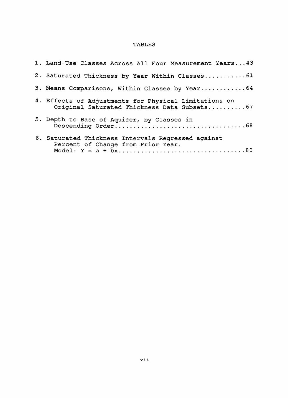
TABLES

1. Land-Use Classes Across All Four Measurement Years...43

2. Saturated Thickness by Year Within Classes 61

3. Means Comparisons, Within Classes by Year 64

4. Effects of Adjustments for Physical Limitations on Original Saturated Thickness Data Subsets 67

5. Depth to Base of Aquifer, by Classes in Descending Order 68

6. Saturated Thickness Intervals Regressed against Percent of Change from Prior Year. Model: Y = a + bx 80

V l l

FIGURES

1. Hockley County, Texas 9

2. Estimates of Irrigation in

Hockley County: 1969-1983 19

3. Land Use 1974 51

4 . Land Use 1978 52

5 . Land Use 1980 53

6. Land Use 1982 54

7. Land Use Classes Across All Four Measurement Years..55

8 . Soil Mapping Units 56

9. Saturated Thickness of the Aquifer 1974 57

10. Saturated Thickness of the Aquifer 1978 58

11. Saturated Thickness of the Aquifer 1980 59

12. Saturated Thickness of the Aquifer 1982 60

13. Mean Saturated Thicknesses by Class 63

14 . Depths to Base of the Aquifer 69

15. Land Irrigated in 1974 but not in 197 8 71

16. Land Irrigated in 1974 but not in 1980 72

17. Land Irrigated in 1974 but not in 1982 73

18. Land Irrigated in 1978 but not in 1980 74

19. Land Irrigated in 1978 but not in 1982 75

20. Land Irrigated in 1980 but not in 1982 76

21. Regression Model: Percent of Land not Irrigated in 197 8 but which was Irrigated in 1974 Regressed on Saturated Thickness Intervals in 1974 77

Vlll

22. Regression Model: Percent of Land not Irrigated in 1980 but which was Irrigated in 1974 Regressed on Saturated Thickness Intervals in 1974 77

23. Regression Model: Percent of Land not Irrigated in 1982 but which was Irrigated in 1974 Regressed on Saturated Thickness Intervals in 1974 78

24. Regression Model: Percent of Land not Irrigated in 1980 but which was Irrigated in 197 8 Regressed on Saturated Thickness Intervals in 1978 78

25. Regression Model: Percent of Land not Irrigated in 1982 but which was Irrigated in 1978 Regressed on Saturated Thickness Intervals in 197 8 7 9

26. Regression Model: Percent of Land not Irrigated in 1982 but which was Irrigated in 1980 Regressed on Saturated Thickness Intervals in 1980 7 9

IX

CHAPTER I

INTRODUCTION

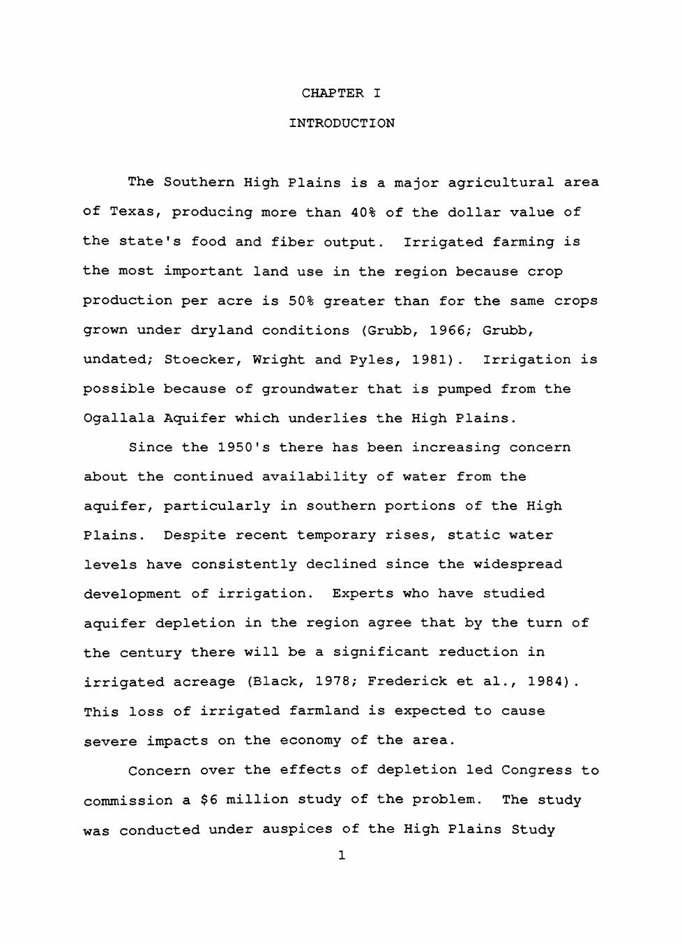
The Southern High Plains is a major agricultural area

of Texas, producing more than 40% of the dollar value of

the state's food and fiber output. Irrigated farming is

the most important land use in the region because crop

production per acre is 50% greater than for the same crops

grown under dryland conditions (Grubb, 1966; Grubb,

undated; Stoecker, Wright and Pyles, 1981). Irrigation is

possible because of groundwater that is pumped from the

Ogallala Aquifer which underlies the High Plains.

Since the 1950's there has been increasing concern

about the continued availability of water from the

aquifer, particularly in southern portions of the High

Plains. Despite recent temporary rises, static water

levels have consistently declined since the widespread

development of irrigation. Experts who have studied

aquifer depletion in the region agree that by the turn of

the century there will be a significant reduction in

irrigated acreage (Black, 1978; Frederick et al., 1984).

This loss of irrigated farmland is expected to cause

severe impacts on the economy of the area.

Concern over the effects of depletion led Congress to

commission a $6 million study of the problem. The study

was conducted under auspices of the High Plains Study

Council (HPSC). The Council's final report in 1982

determined that there were no feasible alternative sources

of water for the region (HPSC, 1982; Sweazy, 1983). In

the absence of a long-term solution to the depletion

problem, the Council recommended that water conservation

practices be encouraged as a way to keep irrigation

farmers in business during the near-term. One response to

this recommendation has been a program implemented by the

Texas Legislature to foster conservation by providing low-

interest loans to farmers to purchase and install water

conserving equipment, particularly center-pivot irrigation

systems (The Cross Section, 1985). However, even with

conservation, useable water supplies from the Ogallala are

expected to be extended for relatively few years more than

they would without conservation efforts (HPSC, 1982).

The Council forecast that over the next thirty years

more than one million acres of land on the Southern High

Plains of Texas can be expected to be converted from

irrigated farming to less productive agricultural uses,

such as dryland farming and rangelands. Increasingly

severe economic impacts and difficult land-use decisions

are expected to accompany reduced productivity which will

follow as groundwater supplies in the Ogallala decline

(Osborn, Harris and Owens, 1974; Baird, 1978; High Plains

Associates, 1982; HPSC, 1982; Matthews, Ethridge and

Stoecker, 1984; Stoecker et al., 1981).

Because reduced irrigation is inevitable, it would be

prudent to develop strategies to manage its impacts. A

prerequisite to management is planning information that is

both accurate and current. Types of information that

would be needed should address water quality, water

quantity, local patterns of water use, implications of

aquifer depletion, and changing patterns of water use and

development. The information should also be generated on

a continuing basis, be capable of being updated quickly,

and be produced at a scale which will meet the needs of

local, state and regional managers working within five to

ten year planning horizons (HPSC, 1982; Supalla, Lansford

and Gollehon, 1982). Such information is not available

(Texas Department of Water Resources, 1981; Frederick and

Hanson, 1982).

This research addresses some of these information

needs, particularly those that deal with land use and

changes in land use, specifically those involving

irrigated acreage. The aim of the research was to develop

a technique to give public and private managers

information that would permit them to make informed

decisions precipitated by changes in agricultural land

use.

Such changes, particularly those involving

irrigation, have both social and economic implications.

With past changes identified, future changes can be

predicted with acceptable accuracy. Managers could then

anticipate impacts associated with change in the resource

base and act in advance to mitigate its effects rather

than react to events after they have occurred (Mead, 1981;

HPSC, 1982; Johnson, 1982).

Objectives

The goal of the research was to develop a natural

resource data base that could be used to produce

information which would achieve the following objectives:

(1) locate and inventory selected land uses,

primarily irrigated cropland

(2) identify patterns of land-use change associated

with aquifer decline

(3) forecast locations where irrigation can be

expected to terminate

(4) forecast the time frame during which such

changes are likely to occur.

The study focuses on a single county as a site to

develop and test a system of techniques for collection,

classification and analysis of natural resource and land-

use data. The study was focused on a single county to

reduce computational workload and to minimize expenses

related to data acquisition and manipulation. The

methodology used in the study is flexible enough that it

can be applied with minor changes to other areas.

A major assumption in the study was that natural

resources are primary determinants of land use, and that

as resources are depleted land-use options are

constrained. The specific hypothesis tested was that

irrigated acreage declines as groundwater supplies are

depleted. Factors other than natural resource

availability--such as costs of energy to pump groundwater,

market prices of crops, expenses of applying agricultural

chemicals and personal preferences for specific crops and

agricultural practices--also affect decisions whether or

not to irrigate. The scope of the study did not include

identifying effects on land use of these and other socio­

economic factors. It was expected that their effect would

be to produce anomalies within areas dominated by a

specific resource and land-use situation; for example, if

pumping costs are too high a farmer may decide not to

irrigate even though he has sufficient groundwater

available; his farm then would appear as a non-irrigated

field within an irrigated area with which he shares

similar quantities of groundwater.

Three phases of activity were conducted to accomplish

the objectives. In the first phase an automated

geographic information system (GIS) was created for

Hockley County, Texas. The GIS was the vehicle for data

organization, analysis and information production. Four

digital data bases were produced:

(1) spatial location data

(2) natural resource data

(3) land-use information

(4) change information.

The spatial data base is a base map of the county.

It is not a separate data layer; rather it is a reference

frame or grid into which data cells are placed. This

frame was digitized from maps at a scale of 1:24000 in the

Universal Transverse Mercator (UTM) projection. This

digital base map was the locational reference for all data

bases.

The natural resource data base contained five layers:

soil type, digitized as soil mapping units from the Soil

Survey of Hockley County; and four hydrologic data layers

for well locations, surface elevation, depth to base of

the aquifer, and depth to water from the surface.

The land-use data base contained four layers, one for

each year for which Landsat satellite imagery data were

obtained. Land uses were determined by applying spectral

7

pattern recognition techniques to classify the data, then

verifying classifications. Landsat data were obtained in

digital format; the size of areas imaged by satellite

scanners was resampled into a standardized cell size (67m

X 67m).

The change data base had sixteen layers divided into

two categories: water level change and land-use change;

each category contained information on changes that

occurred at intervals of two, four, six and eight years.

The second phase of the study involved applying

analytical techniques to data to produce information about

land use and its correlation with different soil

associations and various hydrologic conditions. The aim of

this phase was to determine soil and groundwater

conditions coincident with land uses, as well as changes

in these resources which correspond to changes in land

use.

The third phase involved information output in both

tabular and graphic formats. The intent was to produce

information about and to forecast changes in the location

and type of agricultural land uses that could be expected

to occur with aquifer decline. Again, no attempt was made

to assess effects on land use of socio-economic factors,

such as government programs; nor was the information

designed to assess the suitability of land for specific

8

uses, although such factors could be used in later studies

to develop a more comprehensive change forecasting model.

Study Area

Hockley County, Texas was selected as the study area.

It is one of several counties on the Southern High Plains

having significant aquifer depletion. A sufficient amount

of land had also been converted from irrigated farming to

other uses to make change detection likely: the

Agricultural Census indicated that approximately 50% of

the 1969 irrigated acreage had been converted to other

uses by 1983, a situation which also occurred in eight of

the 22 Southern High Plains counties with most of their

land area over the Ogallala.

Hockley County is in northwest Texas (Figure 1); it

has an area of 581,000 acres (Texas Crop and Livestock

Reporting Service, 1983). The 1980 population of 23,230

is concentrated in three towns: Levelland, the county

seat (13,804), Sundown (1,511) and Anton (1,180) (U.S

Bureau of the Census, 1983). Principal economic

activities are farming, ranching and mining (petroleum and

natural gas).

Topography is relatively flat, with a gradual slope

from 3700 feet elevation in the northwest to 3300 feet in

the southeast. The climate is semiarid; annual

Hockley County

Ogallala Aquifer

Texas -New Mexico

State Line

County Boundaries

Approximate Limit Northern & Southern High Plains of Texas and New Mexico

Figure 1. Hockley County, Texas

10

precipitation averages 17.5 inches. Drainage is primarily

internal; precipitation collects in numerous temporary,

shallow lakes locally called playas. There are no

perennial streams; the largest external drainage net is

associated with Yellow House Draw in the northern quarter

of the county; this stream drains eastward into the Brazos

River system.

Precipitation is bimodal: the maximum occurs during

spring and summer months as a result of frontal passage

and thunderstorm activity; during fall and winter

precipitation is generally less intense, occurring either

as light rain or snowfall. Summers are hot with typically

high evapo-transpiration rates which greatly exceed

precipitation. The growing season extends from mid-April

through October (Bonnen, 1960; Knowles, Nordstrom and

Kent, 1982).

Soils in Hockley County are mainly sandy loams which

are highly susceptible to wind erosion if not protected.

There are two major soil associations in the county:

Amarillo fine sandy loam, found in 65% of the county, and

Amarillo-Olton loams, which are hardlands that make up 20%

of the county in its eastern portions (Grice, Green and

Richardson, 1965).

Land use is overwhelmingly agricultural: more than

94% of the land is in farms and ranches; two thirds of the

11

county is cropland, while about one fifth is pasture and

range. The principal crops are cotton, wheat and sorghum

(TCLRS, 1984). Petroleum and natural gas extraction is

concentrated in southwest and west-central portions of the

county, with three smaller fields located in the north­

west, north-central and east-central portions.

The availability of groundwater from the Ogallala is

important to the county economy; most crop production is

attributable to irrigation with groundwater. Since the

mid 1940's problems with aquifer decline have become more

apparent as groundwater withdrawl has greatly exceeded

recharge (Bell and Morrison, 1977). Irrigated acreage has

declined since the late 1960's. In 1974 nearly all the

county overlaid portions of the Ogallala which had a

potential to yield water at rates in excess of 100 gallons

per minute; by the year 2000, nearly half the county is

expected to depend on supplies which will yield less than

100 gallons per minute (Bell and Morrison, 1977; Wyatt,

Bell and Morrison, two undated maps).

CHAPTER II

REVIEW OF LITERATURE

Background

Development of irrigated farming in Hockley County

occurred as part of regional agricultural development

throughout the Southern High Plains of Texas. This major

change in land use from ranching to irrigated farming has

been chronicled by Green (1973) and Firey (1960).

Development of large-scale irrigated agriculture in the

region began during the late 1930's as farmers started to

recover from the drought conditions of the Dust Bowl.

Irrigation expanded rapidly with improvements in pumping

technology, lower energy prices and the increased

availability of capital, particularly after World War II.

By the 1970's most land that could be irrigated easily had

been developed (Young and Coomer, 1980; Dregne, 1983).

Total acreage under irrigation remained relatively

constant until the 1980's, although throughout development

areas of concentrated irrigation gradually shifted from

south to north as economically useable water reserves were

exhausted and new areas were drilled. By the 1980's total

irrigated acreage in the Southern High Plains began to

decline as widespread aquifer exploitation caused water

levels to drop in many locations (TDWR, 1981).

12

13

During the late 1940's and early 1950's economic

consequences associated with declining aquifer levels

became apparent. Public recognition of these

consequences, as well as legislative initiatives to

regulate groundwater, gave rise to water conservation

efforts and resulted in creation of the High Plains

Underground Water Conservation District No. 1 (HPUWCD) for

the Southern High Plains.

Creation of the district marks the start of serious

attempts to find ways to reduce agricultural demand for

water while maintaining the viability of irrigated

farming. The district has focused on conserving water by

eliminating tailwater waste, reducing evaporation losses

by eliminating open ditches, controlling well spacing to

reduce drawdown effects, encouraging development and use

of crop varieties that require less water, educating

potential and actual water users about conservation

techniques, and most recently by administering a state

loan program to finance purchases and installation of

agricultural water conserving equipment such as center

pivot irrigation systems.

Land-use changes that have been associated with

declining groundwater levels are adjustments which farmers

have made in an attempt to maintain irrigation but with

less water. Hughes and Magee (1960) studied adjustments

14

that farmers made when water levels declined precipitously

during the drought of the 1950's. They found that farmers

tended to irrigate land with progressively less water

until at last they were forced to take the drastic step of

reducing the number of acres under irrigation. Although

the study did not address the uses of land once it is

removed from irrigation, one can hypothesize an initial

conversion to dryland farming and then to rangeland, these

being the more profitable agricultural land uses after

irrigation.

Hughes and Magee (1960) also investigated natural

resource situations which were associated with various

conservation activities and with removal of land from

irrigation. They found that "...[t]he number, types and

extent of adjustments are closely related to physical

conditions [major soil types, initial thickness of the

water-bearing strata, permeability of water-bearing

materials] and to the degree of depletion in specific

hydrologic situations." They identified eleven hydrologic

situations within the High Plains study area; these were

defined by various combinations of intervals of decline in

static water levels and intervals of original (1938)

thickness in water-bearing strata. The proportion of

overlying cropland that was irrigated was found to be

related to hydrologic conditions.

15

Taylor (1979) related hydrologic situations to

economic factors when he observed that "...the decline in

water levels is a principal cause of increased pumping

cost, decreased well yields, and abandonment of shallower

wells." Knowles (1981) agreed with Taylor (1979)and

reported that irrigation tends to be discontinued when

saturated thickness of the aquifer reaches five feet.

Young and Coomer (1980) examined effects of energy

costs on irrigation activities. They concluded that costs

of energy for pumping may be a more restrictive factor in

irrigated farming than quantity of water available.

Slogett (1981) essentially concurred with their

conclusion, but he attributed increased costs of

irrigation not to rising energy prices, but rather to

declining water levels which result in increased pumping

lifts and longer pumping times to extract a given volume

of water.

Each of these studies implied that there is a

relationship between groundwater availability and the

occurrence of irrigated farming on the surface. None,

however, was able to confirm the strength of this

relationship, primarily because, as Young and Coomer

(1980) observed, there are "...no recorded statistics

available on the precise number of irrigated and dryland

crop acres overlying each saturated thickness category."

16

Likewise, there are no statistics available that document

the locations or current uses of land which is no longer

under irrigation. One goal of this research was to

produce this kind of information.

Traditional Data Sources

Many sources of data about agricultural land use and

irrigation may be classified as traditional data sources,

that is, inventories or censuses in which standard methods

of data collection such as sample surveys, expert

estimations, questionnaires or similar techniques are used

to develop a statistical description of an area of

interest. "Traditional" is used here to distinguish these

methods from those that use remote sensing techniques

(Estes et al., 1980).

An exhaustive review of these data sources would not

be especially productive since the research is not

intended to compare relative merits and efficiencies of

traditional data sources. There are, however,

similarities between various traditional sources of

agricultural data which provide insight about the

characteristics of information they provide planners and

managers.

Traditional data sources typically report two

categories of information: (1) farm production.

17

especially acreages of crops grown and volumes of

production; (2) acreage which is in uses that can be

related to broad levels of productivity, such as irrigated

cropland, dryfarmed cropland, pasture and rangeland,

wasteland, and land in non-productive uses. One-time

surveys serve little purpose other than to describe the

land situation at a particular moment in time, while

surveys that are conducted at intervals over a period of

years provide a longitudinal component to data. Available

data sources provide little information about land use

within a county because data is aggregated at the county

level. Most data sources present aggregated data for

counties, but generally leave analysis to users.

Each data source makes some claim to accuracy;

typical claims range between 90 and 97 percent, although

actual accuracy may be closer to 80 percent (Tullos,

1982). In an excellent review of major sources of data on

irrigation in the Western United States Frederick and

Hanson (1982) point out that a significant data problem is

that various sources do not agree on how much acreage is

irrigated. This lack of agreement is attributed to three

possible causes: (1) use of different definitions of

irrigation in different surveys; (2) absence of clear

guidelines or reliable primary data for estimates made by

local "experts"; and (3) bias caused by misstatements made

18

by respondents. These are typical difficulties

encountered when using traditional data collection methods

(Tullos, 1982). Although effects of these sources of

variation are thought to diminish as data are aggregated

over progressively more sampling units, validity of data

within any one unit remains uncertain. Disagreement

between data sources is illustrated by the variety of

estimates made for irrigated acreage in Hockley County

from 1969 to 1983 (Figure 2). Not only do differences

occur between estimates in any given year, but different

trends in irrigation also appear. Variability found in

traditional inventories of irrigated acreage is also

characteristic of other data categories (Lindenlaub and

Davis, 1978; Martinko et al., 1981; Tullos, 1982).

Data about groundwater availability on the Southern

High Plains, and in Hockley County, are more precise than

land-use data gathered by traditional methods. This is

primarily because groundwater data are based on physical

measurements collected at specific sites; when data are

reported these two components are reported together.

Consequently data can be related to distinct locations

within a county and estimates can be made of the water

resource between known points rather than averaged for the

entire county.

19

275000 -

/ c r

t 225000 -s

I r r i / / / e d

175000 -

125000

75000

* data unavailable

-+-1969 1970 1971 1972 1973 1974 1975 1976 1977 1978 1979 1980 1982 1983

• Texas Oeparlmenl ol O Texas Counly Slalislics * AQricultural Census ^ Ifigh Plains lingalion Water Resources Survey

Figure 2. Estimates of Irrigated Acreage in Hockley County, 1969— 1983.

Another factor which improves groundwater data

quality is standardization of collection techniques by

data gathering agencies. The High Plains Undergound Water

Conservation District Number 1 (HPUWCD) and the Texas

Department of Water Resources (TDWR), for example,

routinely perform water level measurements during December

and January to reduce drawdown effects caused by pumping;

drawdown would more likely affect measurements taken

immediately before, during or immediately after the

growing season.

The main source of groundwater data for Hockley

County is the HPUWCD; this agency and the TDWR operate an

extensive network of water level observation wells and

20

maintain well logs for large portions of the High Plains

(Taylor, 1979; Knowles et al., 1982). Data from these

agencies, along with studies by the U.S. Geological Survey

(Luckey et al., 1981; Weeks and Gutentag, 1981), have

produced copiously documented estimates of amounts and

locations of groundwater in the Southern High Plains.

State agencies also apply analytical models to data to

determine rates and locations of groundwater depletion.

This information provides a basis for aquifer management

and water conservation activities (Knowles, et al., 1982;

The Cross Section, 1985).

One aim of this research was to collect land-use data

with a degree of spatial accuracy comparable to that of

groundwater data. Improved accuracy made it possible to

relate surface land use to subsurface groundwater.

Rather than depend upon traditional techniques for

land-use data collection, this study used earth resource

data collected by the Landsat series of satellites using

remote sensing technology.

Remote Sensing Data Sources

The large area coverage of remote sensing data

acquisition systems makes it feasible to directly measure

acreages in different land uses and at various levels of

detail (Jensen, 1983). The scale and accuracy with which

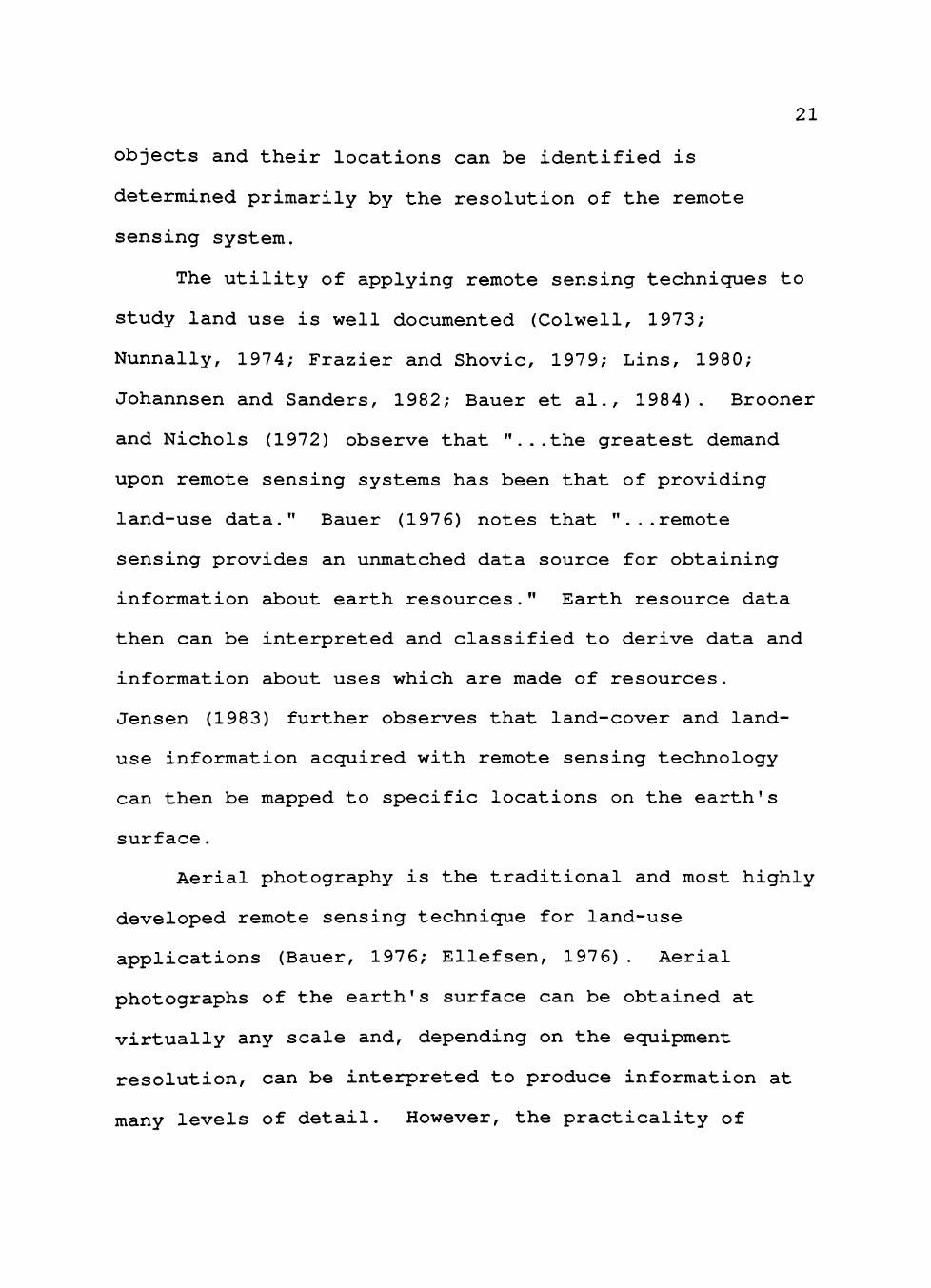
21

objects and their locations can be identified is

determined primarily by the resolution of the remote

sensing system.

The utility of applying remote sensing techniques to

study land use is well documented (Colwell, 1973;

Nunnally, 1974; Frazier and Shovic, 1979; Lins, 1980;

Johannsen and Sanders, 1982; Bauer et al., 1984). Brooner

and Nichols (1972) observe that "...the greatest demand

upon remote sensing systems has been that of providing

land-use data." Bauer (1976) notes that "...remote

sensing provides an unmatched data source for obtaining

information about earth resources." Earth resource data

then can be interpreted and classified to derive data and

information about uses which are made of resources.

Jensen (1983) further observes that land-cover and land-

use information acquired with remote sensing technology

can then be mapped to specific locations on the earth's

surface.

Aerial photography is the traditional and most highly

developed remote sensing technique for land-use

applications (Bauer, 1976; Ellefsen, 1976). Aerial

photographs of the earth's surface can be obtained at

virtually any scale and, depending on the equipment

resolution, can be interpreted to produce information at

many levels of detail. However, the practicality of

22

applying photogrammetric techniques to studies of land use

is limited by costs of obtaining repetitive imagery over

large areas (Schecter, 1976; Milazzo, 1980).

The first of the Landsat series of earth observation

satellites was launched in 1972. It provided the basis

for a new data collection system to study dynamics and

trends in land use (Anderson et al., 1976). The Landsat

system made it feasible to obtain repetitive coverage over

large areas of the earth's surface. However, these

capabilities were acquired by trading off higher

resolutions that could be obtained with aerial

photography. Nevertheless, Landsat multispectral scanners

are capable of producing imagery suitable for mapping

surficial phenomena at levels of detail sufficient for

many land-use and land-cover applications (Anderson et

al., 1976; Bauer, 1976; Fitzpatrick-Lins, 1978; Lee,

1982).

Landsat data are available in two basic formats:

photograph-like images, and digital data stored on

computer tapes. Although visual imagery has the

appearance of a photograph, it is produced from digital

data using computer, mechanical and photographic

processes. Because satellite remote sensing developed

from photogrammetry, interpretive techniques borrowed from

photogrammetry were first applied to visually or manually

23

interpret images produced by Landsat satellites (Bauer,

1976; Merchant, 1981). Ellefrits et al. (1978), for

example, proposed a visual interpretation methodology that

could be applied as a relatively inexpensive way to obtain

information about general land-cover types from Landsat

imagery. Christian (197 9) reported using visual

interpretation to delineate areas of pasture and cropland

as a part of the Australian National Mapping Division's

operations. The level of accuracy with which surficial

features can be mapped using visual interpretation

techniques, while adequate for most projects at regional

scales, is too general for investigations of relatively

small areas. Gordon (1980), for example, found that land

uses could not be classified reliably with visual

interpretation techniques when applied to areas of

approximately 75 square kilometers; considerably smaller

areas would be of interest in investigations of land use

in a county-sized area.

By the mid 1970's, computer processing of

multispectral data was used frequently to manipulate

Landsat data (Landgrebe, 1976). Bauer (1976) observed

that numerical (digital) analysis of Landsat data became

more widely used because of the need to obtain information

from the large quantities of data produced by Landsat and

because of the potential to improve on the identification

24

performance of manual methods. Merchant (1981) argues

that digital data obtained from Landsat are fundamentally

different from data obtained by photographic methods and

thus require different methods of analysis to derive

information about the land surface.

Taranik (1978) describes data produced by Landsat

multispectral scanners (MSS) as an ordered array of

numbers which are measurements of the average intensity of

electromagnetic radiation reflected from identifiable

portions of the earth's surface with an area of

approximately 1.1 acre. A more detailed description of

the characteristics of MSS data can be found in Swain and

Davis (1978), Taranik (1978) and Short (1982). It is

sufficient here to note that MSS data consist not of

representations of objects, but rather of measurements of

reflected light that are integrated (or averaged) for an

area. The measured frequency (color) of the light is

determined by electro-optical characteristics of the

scanner. The Landsat MSS's measure in four different

frequency ranges or bands: visible green (band 4),

visible red (band 5), invisible reflected infrared (bands

6 and 7). Measurements are recorded as digital values,

ranging from 1 to 128, which represent the intensity of

light in a given band that is reflected from the surface.

By combining measurements from each of the four bands a

25

spectral signature can be determined for each element of

the picture (pixel).

Numerical approaches to analysis of Landsat data

employ statistical pattern recognition techniques to

classify pixels into homogeneous groups; two main

approaches are supervised and unsupervised classification

(Estes et al., 1983). Supervised techniques base

classification of digital values on the range of

reflectances for sample sets of known land covers

associated with pixels in an image; other pixels in the

image are then classified into categories which correspond

to the sample set ranges into which they fall (Robinove,

1981). The accuracy of classifications obtained using

this technique is heavily dependent on the quality of

sample data; constraints on gathering data in the field

often preclude collection of a truly representative sample

(Swain and Davis, 1978; Estes et al., 1983).

Unsupervised classification approaches attempt to

overcome this disadvantage by identifying groupings

inherent in the reflectance values themselves; this is

accomplished by estimating the number of likely groupings

in the data and applying cluster analysis techniques to

find them (Swain and Davis, 1978). Robinove (1981)

observes that the logical difference between these two

approaches is that "...supervised classification uses the

26

analyst's knowledge of the terrain to guide the logical

division of the data into discrete clusters, whereas

unsupervised classification utilizes only the analyst's

estimate of the number, type, and statistical range of

clusters desired."

In both classification approaches the fundamental

problem is how to relate spectral reflectance data to

land-cover types (Robinove, 1981). In supervised

approaches, categories of land cover are determined by

using sample sets prior to classification of reflectance

data; in unsupervised approaches the reflectance data are

first classified independently, then sources of

reflectances are checked to determine what land covers

gave rise to them. Robinove (1981) observes that the

latter approach to classification results in higher

accuracy.

Three techniques have been used to verify the

relationship between reflectance measurements and land

cover; these techniques are referred to in the literature

as ground truthing or, more recently, as surface checking.

One technique is to physically evaluate actual conditions

at the point on the earth's surface to which a given pixel

or group pixels correspond. Another is to verify the

surface cover using larger scale imagery such as aerial

photographs. A third is to check classifications against

27

previously developed maps and other data. Each method

uses sampling techniques to determine classification

accuracy over large areas (Robinove, 1981; Dozier and

Strahler, 1983).

Geographic Information Systems

The sheer mass of data produced by the Landsat

satellites, as well as the specificity and level of detail

in the data, led to many new developments in fields such

as natural resource management, urban planning and

geology. The combined effect of voluminous satellite

data, the need for new analytical models, growing

complexity of land management activities, and rapid

development of computer technology resulted in development

of spatially arrayed computer databases and management

systems as preferred tools for land-use analysis

(Johannsen and Barney, 1981; Short, 1982); such systems

are generally referred to as geographic information

systems (GIS) (Gates and Heil, 1980).

Geographic information systems are a technology to

produce information about spatial processes. This

technology may be either manual or automated. Early

GIS's, such as the land evaluation technique advocated by

McHarg (1969), were manual systems. In these systems data

are typically stored on several transparent map overlays.

28

each of which portrays some characteristic of the land at

various locations. Analysis generally involves laying

transparencies over a base map, then identifying areas

that have the appropriate occurrence or absence of

characteristics of interest. Information produced by such

techniques is usually qualitative and not readily updated

or combined with other data bases. More recent GIS's

employ similar techniques, but are automated systems which

include spatially arrayed computer data bases, as well as

capabilities for input, integration, manipulation and

quantitative analysis of data (Cicone, 1977; McFarland,

1982; Walsh, 1985).

Gates and Heil (1980) and Berry (1981) attribute the

proliferation of automated GIS's to the failure of

traditional manual techniques to meet increasingly complex

needs of planners, engineers and managers who deal with

land based activities. Gates and Heil (1980) also

observed that GIS technology does not represent a single

technological approach, rather the "... field is so newly

developed that it has not yet evolved into an ordered

discipline."

GIS technology is heavily weighted toward system

design and system performance considerations (Gates and

Heil, 1980). Three functions are basic to a GIS: (1)

input and storage of geographically referenced data, with

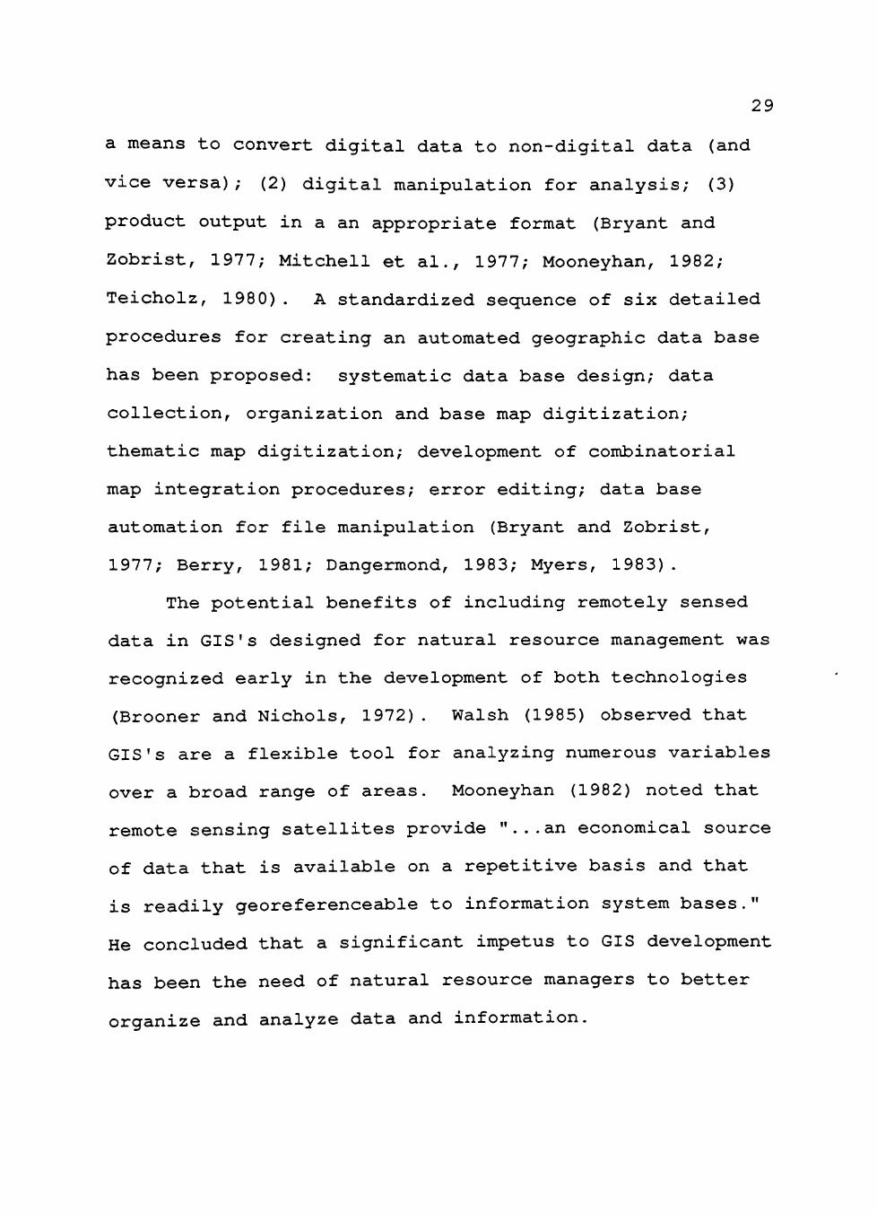
29

a means to convert digital data to non-digital data (and

vice versa); (2) digital manipulation for analysis; (3)

product output in a an appropriate format (Bryant and

Zobrist, 1977; Mitchell et al., 1977; Mooneyhan, 1982;

Teicholz, 1980). A standardized sequence of six detailed

procedures for creating an automated geographic data base

has been proposed: systematic data base design; data

collection, organization and base map digitization;

thematic map digitization; development of combinatorial

map integration procedures; error editing; data base

automation for file manipulation (Bryant and Zobrist,

1977; Berry, 1981; Dangermond, 1983; Myers, 1983).

The potential benefits of including remotely sensed

data in GIS's designed for natural resource management was

recognized early in the development of both technologies

(Brooner and Nichols, 1972). Walsh (1985) observed that

GIS's are a flexible tool for analyzing numerous variables

over a broad range of areas. Mooneyhan (1982) noted that

remote sensing satellites provide "...an economical source

of data that is available on a repetitive basis and that

is readily georeferenceable to information system bases."

He concluded that a significant impetus to GIS development

has been the need of natural resource managers to better

organize and analyze data and information.

30

GIS's that use remotely sensed data have been used to

analyze many different natural resource problems, such as

change on the land surface (Patterson and McAdams, 1981)

and to develop change forecasting models (Short, 1982).

Westin et al. (1981) combined mapped soil data with land-

use data derived from Landsat imagery and transferred them

to new maps that displayed soil units subdivided into

land-use classes. Henderson (1981) reported the

successful integration of Landsat and traditional data

into a multi-agency GIS for monitoring land-use change in

the San Francisco Bay Area.

Landsat data have also been successfully employed to

develop state and county-level GIS's (Sturdevant, 1981;

Wood and Beck, 1982). Loveland and Johnson (1981)

reported successful employment of a GIS using spatial data

to evaluate irrigation and design a predictive model for

forecasting water and energy requirements in the Umatilla

River Basin of Oregon.

Some of the foregoing techniques were used to

evaluate land-use change in Hockley County and to

determine if changes in the natural resource base are

related to changes in land use, and if so, to identify

spatial and temporal patterns associated with these

changes.

CHAPTER III

METHODOLOGY

Analysis of relationships between aquifer decline and

subsequent changes in amounts of irrigated cropland

involved evaluating temporal as well as a natural resource

factors. The spatial time series approach (Bennett, 1979)

was used in part to guide the analysis. Groundwater

resources and land use were viewed as components of a

physical system; socio-economic forces power the system

within the physical limits of the natural resource base.

A primary assumption was that owners and users of land act

through time to balance consumption of natural resources

against economic and market pressures which encourage them

to exploit their resources for crop production (see Firey,

1960). Within this context the research focused not on

crops produced as system output, but rather on a

surrogate: irrigated acreage.

The research was not designed to identify those

socio-economic forces that govern relationships between

resources and land use, other than to assume that socio­

economic forces would generally operate to insure that

users of agricultural land irrigate crops if enough water

is available. If the system functions in this manner,

then irrigation should stop in nearly all cases only when

groundwater is depleted. It is recognized that irrigation

31

32

also may be discontinued for economic reasons, such as

increasing costs of energy to pump, relative to the return

expected from the crops produced; decreasing commodity

prices; or conversion of land into more lucrative non-

agricultural uses. However, these situations were expected

to be exceptions rather than the rule, appearing as

anomalies within areas of irrigated or irrigable cropland;

they would thus contribute to error in the modeling

process.

In system analysis terms, operation of a transfer

function (socio-economic forces) modifies inputs

(groundwater and soil resources) to produce an output

(irrigated acreage). The transfer function was assumed to

operate as a constant throughout the period of

observation.

The investigation was undertaken in three phases:

data collection and organization; analysis, modelling and

forecasting; information production and presentation.

Data Collection and Organization

The principal data organization technique was to

structure data layers in automated data bases. To

accomplish this, data were digitized for computer

manipulation. Automation was initially very time

consuming; however, it ultimately expedited data handling

33

operations during the second and third phases of the

study. From an operational perspective, automation

simplified editing data, adding new data and testing

modeling parameters.

Data Layers

Data were organized as component layers within two

larger databases: land-use and natural resources. The

land-use data base contained the following layers:

1) Surface Reflectance Data by year:

a) 1974,

b) 1978,

c) 1980,

d) 1982;

2) Land-Use/Land-Cover Classification by year:

a) 1974,

b) 1978,

c) 1980,

d) 1982;

3) Change in Land-Use/Land-Cover Classification:

a) 1974-1978,

b) 1974-1980,

c) 1974-1982,

d) 1978-1980,

e) 1978-1982,

34

f) 1980-1982,

g) Combined Land-use Changes, all four years.

The layers that contain the natural resource data

were:

1) Soils;

2) Elevation of the Land Surface;

3) Hydrologic Measurement Data, which include:

a) Elevation of the Base of the Aquifer;

b) Elevation of the Head of the Aquifer by year:

(1) 1974,

(2) 1978,

(3) 1980,

(4) 1982;

4) Derived Hydrologic Data, which include:

a) Depth to Water by year:

(1) 1974,

(2) 1978,

(3) 1980,

(4) 1982;

b) Saturated Thickness of the Aquifer by year:

(1) 1974,

(2) 1978,

(3) 1980,

(4) 1982;

35

5) Change in Hydrologic Characteristics of the

Aquifer, which include:

a) Change in Head Elevation:

(1) 1974-1978,

(2) 1974-1980,

(3) 1974-1982,

(4) 1978-1980,

(5) 1978-1982,

(6) 1980-1982;

b) Change in Saturated Thickness:

(1) 1974-1978,

(2) 1974-1980,

(3) 1974-1982,

(4) 1978-1980,

(5) 1978-1982,

(6) 1980-1982;

c) Change in Depth to Water:

(1) 1974-1978,

(2) 1974-1980,

(3) 1974-1982,

(4) 1978-1980,

(5) 1978-1982,

(6) 1980-1982.

36 Spatial Reference Frame

Both system input and output data have locational

attributes; that is, they occur at specific locations.

These locations must be identifiable through time if

spatial change patterns are to be detected. The spatial

domain of the system is the Hockley County study area.

Locational data for the county were digitized from 1:24000

scale U.S.G.S. 7.5-minute maps of Hockley County, using

ERDAS Polygon Digitizing software and a GTCO Digi-Pad 5A-

2436 digitizing tablet.

The locational data are not a separate data layer.

Rather, they can be thought of as a reference frame into

which all data layers are resampled and which identifies

data cells in each layer, thus permitting the same

location to be identified in different data layers.

Two locational attributes are assigned to each data

layer: the size in meters of all data cells, and the UTM

coordinates of the upper left-hand corner data cell (the

cell at the origin of the data layer, i.e., in the 1,1

position). The coordinates of a given cell can then be

calculated by multiplying data cell size by the number of

data cells between the cell of interest and the origin,

then adding the product to the coordinates of the origin.

Each data layer is a rectangular array of pixels that

has 7 67 columns and 741 rows. Pixels that fall within the

37

boundaries of Hockley County lie within this array but do

not fill it. Because the county boundaries are based on

the Latitude and Longitude projection they are not

coincident with UTM grid lines; when the area of the

county is transposed to the UTM projection it appears as a

parallelogram, but is not rectangular. Thus each array

contains a series of edge or fill pixels needed to

maintain a uniform, rectangular matrix (data frame) in UTM

coordinates. Pixels which fall within the boundaries of

the county are data pixels (525,290 pixels), while those

that fall between the county boundaries and the edges of

the data frame are zero-coded as fill (43,057 pixels) and

are not used in analytical calculations. All data layers

in the database were sized to these dimensions; each layer

has the same northwest corner coordinates; data and fill

areas also corresponded precisely from one layer to

another.

When each data layer was constructed, care was taken

to identify the coordinates of data cells as accurately as

possible. Several techniques were used to do this; a

description of each technique is provided below as the

creation of each data layer is discussed.

38 Data Cell Size

Data layers are composed of arrays of data cells,

each of which represents an area on the Earth's surface.

Compatibility between data layers required that a standard

size be selected for data cells. Cells had to have metric

dimensions to conform to the UTM map projection and to

reduce error when resampling Landsat data into the UTM

locational reference frame. A cell size of 67m x 67m was

used for databases. The selection was made in the

following manner.

First, it was determined that the cell size for data

layers should meet the following criteria:

a) Data cells should be of equal dimensions in both

north-south and east-west directions to simplify

measurement of distance in output databases;

b) Cell size should be changed as little as possible

from that of original Landsat data to minimize relative

positional error when pixels of source datasets are

resampled into output data layers;

c) Differences between original data and data layer

cells should be identical in both directions to equalize

positional distortion;

d) Data layer cells should have metric dimensions

that, when multiplied by integer values, produce

measurements that approximate American Standard

39

measurements as closely as possible; this will increase

convergence between metric units of input datasets and

land survey measurement units on the surface.

Next, optimum cell size selection was made as

follows:

a) Landsat pixels have resampled nominal dimensions

of 7 9m in the along-track direction (roughly north-south)

and 56m in the cross-track direction (roughly east-west).

Half of the difference between these dimensions is 11.5m.

Reducing the along-track dimension by 12m and increasing

the cross-track dimension by 11m would produce changes of

-15.2% and +19.6% respectively;

b) This resulted in an output cell size of 67m x 67m.

Using a conversion factor of 39.37 inches per meter, one

data cell would have dimensions of 2,637.79 inches. Thus,

12.01 data cells are equivalent to one-half mile (31,680

inches), which was observed to be a dominant land survey

measurement in Hockley County.

Surface Reflectance Data

Landsat spectral reflectance values, were obtained in

digital image format on computer compatible tapes. The

image tapes were obtained from two sources: the EOSAT

Corporation and the Texas Natural Resources Information

System (TNRIS). The surface reflectance data base

40

contains four layers, each of which has four sublayers.

Layers are the Landsat digital data for an imagery year:

1974, 197 8 and so forth. Sublayers (bands) within each

layer contain data from each of four spectral bands for

which the satellite has recorded spectral reflectances.

The approximate position of the study area was

located within the data matrix of the computer data tape.

An array that included the county and surrounding area was

then extracted from the tape data. The area was displayed

on the ERDAS image processor screen. Points, such as road

and highway intersections, and landmarks, such as lakes

and other large surface features, were located on aerial

photographs and 7.5 minute topographic maps. Those which

could be located in the image processor display were used

as referents to locate the boundaries of the County and to

insure that all of the study area available on the data

tape had been obtained.

This image was then rectified to the UTM projection.

Twelve to eighteen ground control points were located in

both the U.S.G.S. quadrangles and in the images. A least

squares algorithm was then used to resample the image

pixels into the 67m X 67m spatial reference frame. The

coordinates of the county cornerpoints were then used to

extract the area of the county from the larger image. The

pixel having coordinates that most closely approximated

41

the northing of the northmost and easting of the westmost

corners of the county was selected as the northwest corner

of the data layer and assigned a value in the data array

of 1,1 (UTM Zone 13, 720703m E, 3746330m N).

Land-Use Data

Land use data were derived from the Landsat

reflectance data. These constitute the inventory of land

use in each image year. They were produced by supervised

signature classification techniques using all four bands

of the Landsat image data for any given year. Pixels were

classified into various categories of land use until an

acceptable degree of separability could be obtained

between those categories of use that were considered

irrigated farming and those which were considered non-

irrigated uses.

The classified images for 1974 and 1982 required

adjustment due to minor anomalies. The 1974 image

contained patches of small clouds and shadows in the

eastern portion of the county. Once these pixels were

identified they were replaced by substituting the

classified land uses from the cloud free 197 8 image; this

affected 14,052 pixels, less than three percent of the

image. The 1982 image did not include data for a wedge

shaped area of 2,964 pixels in the northeast corner of the

42

county; 1980 land-use classifications were substituted for

these pixels.

The several signature classes were then receded and

combined into two land-use classes: irrigated farming and

non-irrigated land uses. Verification of land use was

based on visual comparisons of classifications to the

apparent degree of infrared reflectance evidenced by the

same areas on the original unclassified Landsat imagery.

After reflectance data for each year had been

acceptably classified a binary encoding scheme was used to

assign a unique value to irrigated and to non-irrigated

land use in each year. All four classified data sets were

then combined into a single data set containing sixteen

classes or patterns of land use across all four years.

Thus, each pixel was classified into one of the classes

listed at Table 1.

Soils Data

Soils data were digitized from the Soil Survey of

Hockley County (Grice et al., 1965). The Survey data are

in the form of a 1:20000 scale semicontrolled mosaic of

aerial photographs; the locations of soil mapping units

are delineated on the mosaic. For the purposes of this

study soil type was considered a fixed attribute of

43

Table 1. Land-use Classes Across All Four Measurement Years.

Class Number

0 1 2 3 4 5 6 7 8 9

10 11 12 13 14 15 16

1974

Background N I N I N I N I N I N I N I N I

1978

(fill N N I I N N I I N N I I N N I I

1980

data) N N N N I I I I N N N N I I I I

1982

N N N N N N N N I I I I I I I I

I - Land was irrigated in this year N - Land was not irrigated in this year

location and assumed to have changed insignificantly since

the Survey was published.

Creation of the Soils Data Layer required the

transfer of soils mapping units from the 1:20000 scale,

Lambert conformal conic projection of the Soil Survey,

into the UTM projection of the spatial reference frame.

Soils mapping units on the aerial photographs were

digitized as a series of points and captured initially in

a file of Latitude-Longitude coordinate pairs, which were

44

then resampled into the spatial reference frame. The

procedures followed in creating the Soils Data Layer are

discussed in detail at Appendix A.

Elevation of Land Surface Data

Data for the elevation of the land surface were taken

from 1:24000 scale U.S.G.S 7.5 minute quadrangles covering

Hockley County (see Appendix B). Contours on each

quadrangle were digitized as a series of points identified

by UTM coordinates. One file was created for each

quadrangle.

The procedure used to identify and digitize the

contours was similar to that used for the soil data layer.

The elevation data points captured in this file were used

to estimate elevations between points of known elevation

by interpolation using the ERDAS routine SURFACE. The

interpolated image was resampled into the 67m X 67m data

reference frame; the pixel in the output surface image

that most closely approximated the coordinates of the 1,1

position in the spatial reference frame was then

reassigned the UTM coordinates of that pixel. The

interpolated file was then trimmed to include only data

points within the boundaries of the county, and fill

pixels between the county and the edges of the frame.

45

Seventy-six data pixels within the study area that

were not assigned a value by the interpolation algorithm

were manually assigned a value determined by duplicating

the elevations of adjacent pixels.

Hydrologic Data

Hydrologic data (Appendix C) were obtained from the

High Plains Underground Water Conservation District Number

1 (HPUWCD), the Texas Department of Water Resources (TDWR)

and the Texas Natural Resources Information System

(TNRIS). These data sources provide the location of wells

(Latitude and Longitude coordinates), the surface

elevation of wells and measured attributes of the aquifer

beneath the well site. Attributes include the elevations

of the base of the aquifer and the elevations of the head

of the aquifer in each year for which measurements were

recorded. The data are in several formats; well locations

are identified on maps, by TDWR well number or by latitude

and longitude coordinates. Some of these data are

recorded in tabular form; some are on computer tapes

(TNRIS, 1982; TDWR, 1981).

Latitude and longitude well coordinates were

recalculated to UTM coordinates. The files of UTM

coordinates were then processed to produce an interpolated

46

surface of aquifer characteristics for locations in

Hockley County.

Attribute data were recorded by assigning the various

measurements of the aquifer as class values. Each

attribute was recorded in a separate data layer: one for

the elevation of the base of the aquifer, and one of the

elevation of the head of the aquifer for each measurement

year. Interpolation and other processing for these data

layers were the same as those for the elevation of the

land surface data layer.

Although points outside the county were used in the

interpolation process, some editing was needed for those

areas outside the search radius of the algorithm. Fewer

than 100 pixels were inserted manually to complete the

data array of any one layer.

Additional hydrologic data layers were

computationally derived from these attribute layers. For

example, the data layers for saturated thickness were

derived by subtracting the elevation of the base of the

aquifer data layer from the respective elevation of the

head of the aquifer layers.

In some cases subtraction of the data layers produced

zero data values. These values conflicted with the coding

for fill pixels, which were also coded as zero. Conse­

quently these zero data pixels were manually receded to

47

the value one. Fewer than 8,000 data cells were recoded

on any one layer.

Analysis, Modelling and Forecasting

The initial analytical approach was to determine if a

relationship existed through time between the occurrence

of irrigation on the surface and the saturated thickness

of the aquifer beneath. Subsets of the saturated

thickness datasets were produced which depicted saturated

thickness beneath land that was classified either as

irrigated or as not irrigated.

Additional subsets were produced by successively

receding the sixteen unique classes of the combined land-

use data set; the class of interest was recoded to one and

the remaining classes were recoded to zero. This recoded

land-use data layer was then "overlaid" onto the saturated

thickness layer for each year. Zero valued data cells

masked out corresponding data cells in the saturated

thickness subsets. Thus, only those data cells passed

through which represented the saturated thicknesses of the

aquifer under data cells exhibiting the land-use

classification of interest. As a result, the output data

subset contained saturated thickness data only for those

cells from the selected year and land use which were

members of the class chosen.

48

Soils data were used in an attempt to further refine

the land-use/saturated thickness data. It was conjectured

that errors in classifying land uses as irrigated or

nonirrigated may have resulted in land being classified as

irrigated when in fact it could not have been because of

physically limiting factors, such as submerged land,

caliche pits and steeply sloped land.

Soil capability units (Grice et al., 1965) were used

to identify non-irrigable soil mapping units, which were

then zero coded in the soils data subset. This subset was

then used to mask out pixels of the saturated thickness

subsets for years during which the land represented by the

pixels was classified as irrigated.

Other data subsets were also generated in the process

of developing a model of the relation between land use and

changes in the aquifer. The modelling effort focused on

identifying the characteristics of pixels irrigated in one

measurement year but not in a subsequent one. Six data

subsets were constructed which reflected this condition:

1) land irrigated in 1974 but not in 1978

2) land irrigated in 1974 but not in 1980

3) land irrigated in 1974 but not in 1982

4) land irrigated in 1978 but not in 1980

5) land irrigated in 1978 but not in 1982

6) land irrigated in 1980 but not in 1982

49

These data subsets were produced by 'overlaying' the

classified land-use data sets for the two years of

interest. Each set was recoded to select for pixels

classified as irrigated in the data set for the first year

and not irrigated in the data set for the second year.

The resultant data subset contained only those pixels

classified as irrigated in the first year but not in the

second. Each of these data subsets was then overlaid to

the data set of saturated thicknesses of the aquifer

during the first year of the two year sequence. The

output of this operation was another data subset which

contained the saturated thickness of the aquifer under

each pixel classified as irrigated that year but which

went out of irrigation in the second year. The goal of

the analysis was to identify characteristics of land which

went out of irrigation. These then would be included in a

model that could be used to forecast the likelihood that

land over a given saturated thickness would no longer be

irrigated at some future year. The temporal component was

accounted for by using data sets of land-use change across

measurement years. The frequency of occurrence for each

saturated thickness interval in each data subset was

computed. These frequency data were then used in

regression equations to produce models of saturated

thicknesses associated with the termination of irrigation.

CHAPTER IV

RESULTS AND DISCUSSION

Results of the classification of spatial reflectance

data from Landsat digital imagery to produce land-use data

sets for 1974, 1978, 1980 and 1982 are presented in

Figures 3 through 6.

The combined land-use data set contains all sixteen

classes or pattern combinations of land use during the

study period; the data set is presented in Figure 7.

Figure 8 presents the digitized soils data layer.

Saturated thickness of the aquifer data layers by

year (1974, 1978, 1980 and 1982) are presented in Figures

9 through 12.

Land-use datasets were combined with saturated

thickness datasets to identify trends and patterns of

change in the aquifer associated with changes in irrigated

land use. Eight major classes of interest, which

represented clearly distinct sequences of irrigated and

non-irrigated land use across the period of the study,

were selected from the combined patterns of land-use

change data set. Mean saturated thicknesses, standard

errors of the mean and numbers of pixels for each

measurement year within each class are listed in Table 2.

50

51

3 7 4

0 0 0 ffl N

3 7 2

-0-0 0 0

3 7 0

0 0 0

720000«E 730000 740000 75o'oOO 76o'oOO 77o'oOO

720,000 730.000 740 000 _ _ J I I

\

750000 760000 770000«E

3 7 4 -0-0 0 0

3 7 2 -0-0 0 0

3 7 0 -0-0 0 0 m

N

Not Irrigated Irr igated

Figure 3. Land Use 1974.

52

3 7 4

-0-0 0 0 m N

3 7 2

0 0 0

3 7 0

0 0 0

720000«E 730000 74o'oOO 750i 000 760000 770000

*••• •Tgaa.T *'i>^^ -..\'". '.r^-L .-"J A

I^^^K If ^ . . * . - _i 0 • . * ^ ^ . ^ '̂ 'S I . i_ cr - •• • . \Mm • '

I

• J 111

720.000 730000 740000 750.000 760000

I 770.000mE

3 7 4

-0-0 0 0

3 7 2

-0-0 0 0

3 7 0

0 0 0 m N

j^Not Irrigated Irr igated^1

Figu re 4 . Land Use 1978.

53

720000«E 730000 740000 750000 760i

3 7 4

-0-0 0 0

3 7 2

-0-0 0 0

3 7 0

-0-0 0 0

000 770000

720.000 730000 740000 I

750000 760.000 770000«E

3 7 4

-0-0 0 0

3 7 2

-0-0 0 0

3 7 0

-0-0 0 0

^Not Irrigated Irr igatedJ

Figure 5. Land Use 1980.

54

7 2 0 0 0 0 « E 7 3 0 0 0 0 74o'oOO 75o'oOO 760 i 000 770000

760000 770.000mE

k Not Irrigated Irr igated

\ Figure 6. Land Use 1982

55

720000<nE

3 7 4

0

tf 3 7 2

-OH 0 0 0

3 7 0

-0-0 0 0 t *

N

000 730:000 740000 750'000 760'000 770000mE

C I A S S PCT. O F A R E I CIASS PCT. OF PREA

N N N N I N N N N I N N I I N N N N I N I N I N N I I N I I I N

41 6 1 2 3 2 1 4

N N N I N N

I I

13

N I I I N N

N I N I

I I

I N I I N I I I I I I I 10

Figure Land Use Classes Across All Four Measurement Years.

56

720000mE 730000 740000 750000 760000 770000

f^iftfBfC A m a r i l l o f i n e sandy loam A1A,B A m a r i l l o Loam AmB A m a r i l l o Loamy H n e sand jAn Arch f i n e sandy loam Ar Arch c lay loam AvA, B Arvanna f s l AxA,B Arvanna f s l , shal low BIC Berthoud-Mansker Loams BnB Bippus c l a y loam Br B r o u n f i e l d f i n e sand |Ch Church c l a y loam |DrB,C Drake so iLs 1-5'^ s lope |DrD Drake, 5-20>i s lope [Km Kimbrough s o i l s

(fsl) i M f A ^ B Mansker f s l | l 1 k A , B hansker loam ^'OtA 01 ton loam BJPfA^B P o r t a l e s Loam BPmA^B Por t a l e s Loam • P S Po t te r s o i l s | R a Randal l cLay

Rf Randal l f s l • S l S t e g a l l - L e a loams | S p Spur and Bippus s o i l s H T V T i v o l i f i n e sand • Z f A Z i ta f s l | Z m A Zi ta loam ^ | | N O Data Submergedxcaliche p i t s

Figure 8. Soil Mapping Units|

57

58

720000«E 730000 74o'oOO 750000 760i 000 770000

O F H R E A

81 - 90 91 - 100

101 - 110 111 - 120 121 - 130

2 <1 <1 <1 <1

I Figure 10. Saturated Thickness of the Aquifer 1978

59

720000-.E 730000 74o'oOO 750000 760000 770000

3 7 4

-0-0 0 0

3 7 2

-0-0 0 0

3 7 0

-0-0 0 0

770000«»E

FEET

1-10 11-20 21-30 31-40 41-50 51-60 61-70

PCT. OF PREA

<1 2

10 25 25 16 11

:ET PCT. OF P R E A

71-80 81-90 31-100

101-110 111-120 121-130

6 3 1

<1 <1 <1

Figure 11. Saturated Thickness of the Aquifer 1980.

60

720000mE 730:000 74o'oOO 750000 760000 770000

720000 730.000 740000 I

750.000 760000 770000«E

:ET CT. O F P R E . F E E T PCT. O F P R E A

1-10 11-20 21-30 31-40 41-50 51-60 61-70

3 6

16 24 20 14

9

71-80 81-90 91-100

101-110 111-120 121-130

5 2 1

<1 <1 <1

Figure 12. Satura ted Thickness of the Aquifer 1982.

61

Table 2. Saturated Thicknesses by Year Within Classes

Mean Class: I I I I

1974 59.05 1978 55.05 1980 58.54 1982 55.14

Class: I I I N 1974 56.62 1978 53.48 1980 57.11 1982 53.81

Class: N I I I 1974 52 1978 49 1980 53 1982 49

Class I I N N 1974 48 1978 44 1980 48 1982 45

Class: N N I I 1974 48 1978 44 1980 49 1982 44

Class: I N N N 1974 45.04 1978 42.19 1980 46.39 1982 42.97

Class: N N N I 1974 42.84 1978 38.38 1980 44.90 1982 38.75

Class: N N N N 1974 42.31 1978 39.28 1980 44.43 1982 38.16

95 53 12 08

13 32 09 31

26 92 40 41

SEM

0.08 0.08 0.07 0.08

0.14 0.13 0.12 0.13

0.20 0.19 0.17 0.19

0.15 0.14 0.14 0.14

0.15 0.14 0.13 0.14

0.09 0.09 0.09 0.09

0.07 0.07 0.06 0.07

0.04 0.04 0.03 0.04

Number of Pixels

52172 52172 52172 52172

21572 21572 21572 21572

8710 8710 8710 8710

12712 12712 12712 12712

15209 15209 15209 15209

32542 32542 32542 32542

69208 69208 69208 69208

212909 212909 212909 212909

62

Graphic analysis of mean saturated thickness values

in each class indicated an overall decrease through time

within classes, with the exception of 1980 (Figure 13).

All classes exhibited an increase in mean saturated

thickness in this year. A rise in elevation of the head

of the aquifer, thus a saturated thickness increase, in

Hockley County was reported by the HPUWCD (1980), which

attributed it to above normal precipitation in 1979. By

1982 the mean saturated thicknesses had returned to

approximately the same levels as in 1978.

The results of comparisons of means within classes to

determine if changes in saturated thickness differed

significantly (alpha = .05) from one measurement year to

the next are listed at Table 3. All means within classes

were significantly different from one measurement year to

the next.

There was also a noticeable difference between

classes. Land which was continuously irrigated throughout

the period of the study exhibited mean saturated

thicknesses that in each year were significantly (alpha =

.05) higher than those of any other class.

Land which was continuously irrigated for three of

the four measurement years exhibited mean saturated

thickness values significantly (alpha = .05) lower than

those of land irrigated for four consecutive measurement

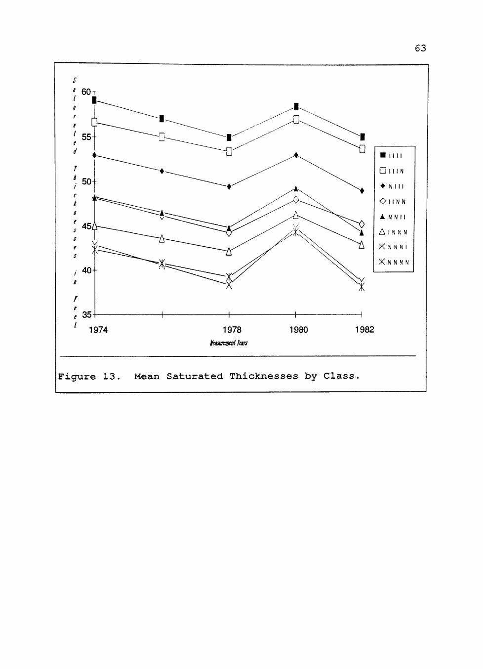
63

1974 1978 Measaraml Utars

1980

• 1111

D I I I N

• \M I I

O I I N N

• N M I

A I N N N

X N N N I

X N N »J N

1982

Figure 13. Mean Saturated Thicknesses by Class

Table 3. Mean Comparisons, Within Classes by Year

64

Class Year Mean ±1.96 SEM

I I I I 74 59.05 0.16 vs.

78 55.05 0.15 vs.

80 58.54 0.14 vs.

Year Mean +1.96 SEM

78 55.05 0.15

80 58.54 0.14

82 55.14 0.15

I

N

1

N

I

N

N

I I N

I I I

I N N

N i l

N N N

N N I

N N N

74

78

80

74

78

80

74

78

80

74

78

80

74

78

80

74

78

80

74

78

80

56.62

53.48

57.11

52.95

49.53

53.12

48.13

44.32

48.09

48.26

44.92

49.40

45.04

42.19

46.39

42.84

38.38

44.90

42.31

39.28

44.43

0.28

0.26

0.24

0.39

0.37

0.33

0.29

0.28

0.27

0.30

0.28

0.26

0.18

0.18

0.17

0.13

0.13

0.12

0.07

0.07

0.07

vs.

vs.

vs.

vs.

vs.

vs.

vs.

vs.

vs.

vs.

vs.

vs.

vs.

vs.

vs.

vs.

vs.

vs.

vs.

vs.

vs.

78

80

82

78

80

82

78

82

82

78

80

82.

78

80

82

78

80

82

78

80

82

53.48

57.11

53.81

49.53

53.12

49.08

44.32

45.31

45.31

44.92

49.40

44.41

42.19

46.39

42.97

38.38

44.90

38.75

39.28

44.43

38.16

0.26

0.24

0.25

0.37

0.33

0.37

0.28

0.28

0.28

0.28

0.26

0.27

0.18

0.17

0.18

0.13

0.12

0-13

0.07

0.07

0.07

*

*

*

*

*

*

*

*

*

*

*

•

*

*

*

*

•

*

*

*

*

* Means signi ificantly different at alpha = .05

65

years, but higher than those of land irrigated for two

consecutive years.

Land continuously irrigated for two consecutive

measurement years (classes IINN and NNII) did not exhibit

as clear a separation as the foregoing four and three year

land-use classes. Both two year classes had essentially

the same mean saturated thicknesses in 1978, although

class NNII had a mean which was slightly higher. Class

NNII maintained a progressively higher mean until 1982,

when it dropped to a value that was significantly (alpha =

.05) lower than that of class IINN. One would not have

expected irrigated land to have a mean saturated thickness

significantly lower than that of non-irrigated land.

Land which was not irrigated for three consecutive

measurement years had means significantly (alpha = .05)

lower than land not irrigated for two consecutive years

but generally higher than those of land that was never

irrigated. In 197 8 class NNNI had a lower mean saturated

thickness than class NNNN; in subsequent years, however,

it continued to exhibit higher thicknesses.

The patterns of change in saturated thickness were

inspected for a specific mean value at which land use

could be expected to change from irrigated to non-

irrigated. None was detected; in one class (IINN), land

ee

went out of irrigation in 1980 despite an increase in

saturated thickness to the 1974 level.

Adjusting the land-use/saturated-thickness data for

physical limitations on irrigability with soils data

produced insignificant changes in the means and standard

error of the means of the irrigated data subsets (Table

4) . This indicates that the original land-use

classifications accurately identified land uses for those

areas which could not have been irrigated. The adjustment

did not provide any new information that would improve

identification of patterns of land-use change associated

with changes in the aquifer.

Depth to the base of the aquifer (surface elevation

less the elevation of the base of the aquifer) was also

examined to determine if this hydrologic attribute could

provide additional information to help characterize

aquifer dynamics and irrigated land use. It was assumed

that most irrigation wells in the county are drilled to

the base of the aquifer to maximize the supply of water

available. At this depth the well can draw from the

maximum volume of saturated thickness and thus operate for

the longest period of time before pumping rates are

reduced below practical levels.

Depth to the base of the aquifer can also be regarded

as a surrogate for the cost of pumping water: lift

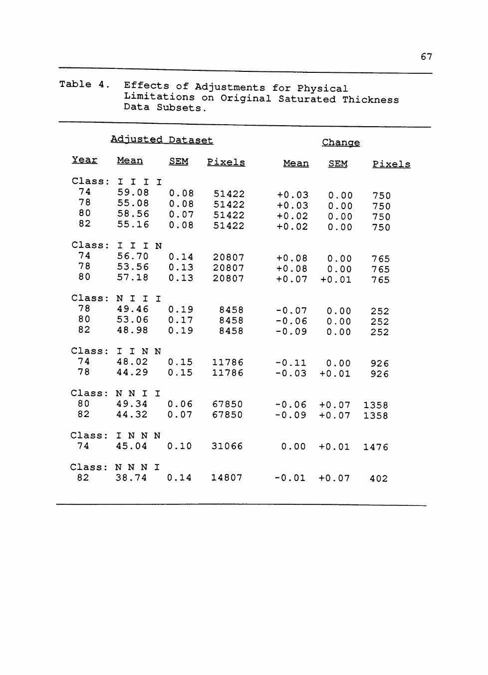
67

Table 4 Effects of Adjustments for Physical Limitations on Original Saturated Thickness Data Subsets.

Year

Class: 74 78 80 82

Class: 74 78 80

Class: 78 80 82

Class: 74 78

Class: 80 82

Class: 74

Class: 82

Adiusted

Mean

I I I 59.08 55.08 58.56 55.16

I I I 56.70 53.56 57.18

N i l 49.46 53.06 48.98

I I N 48.02 44.29

N N I 49.34 44.32

I N N 45.04

N N N 38.74

I

N

I

N

I

N

I

Dataset

SEM

0.08 0.08 0.07 0.08

0.14 0.13 0.13

0.19 0.17 0.19

0.15 0.15

0.06 0.07

0.10

0.14

Pixels

51422 51422 51422 51422

20807 20807 20807

8458 8458 8458

11786 11786

67850 67850

31066

14807

Mean

+ 0.03 +0.03 + 0.02 + 0.02

+ 0.08 + 0.08 +0.07

-0.07 -0.06 -0.09

-0.11 -0.03

-0.06 -0.09

0.00

-0.01

Chanae

SEM

0.00 0.00 0.00 0.00

0.00 0.00

+0.01

0.00 0.00 0.00

0.00 + 0.01

+ 0.07 + 0.07

+ 0.01

+ 0.07

Pixels

750 750 750 750

765 7 65 7 65

252 252 252

926 926

1358 1358

1476

402

68

increases with depth, requiring more energy to raise a

given volume of water a greater distance, thus the cost of

pumping increases. One would expect to find irrigation

discontinued first at locations with thin saturated

thicknesses at great depths. A summary of depth to base

of the aquifer data is presented in Table 5 and Figure 14.

Depth to base of the acjuifer data confirmed the

saturated thickness patterns, but yielded no new

information. Ranks of class means were essentially the

same as those obtained from the saturated thickness data.

The only difference involved the mean depth to base of the

aquifer for classes NNII and INNN; these classes tested to

be essentially the same; transposing the two would

Table 5. Depth to Base of Acjuifer, by Classes in Descending Order.

Class

I I I I I I I N N I I I I I N N N N I I I N N N N N N I N N N N

Note: Classes NNII and INNN tested the same at alpha = .05.

Mean

196.64 189.49 181.08 171.06 167.01 167.85 162.57 159.83

SEM

0.15 0.26 0.41 0.31 0.32 0.20 0.13 0.09

Number of Pixels

52172 21572 8710

12712 15209 32542 69208

212909

69

T E E T rc T. OF R E A • - 'FgeT' "PcT.lffT P̂ ffTTS

1-20 21-40 41-60 61-80 81-100

101-120 121-140

<1 <1

1 <1

2 7 7

141-160 161-180 181-200 201-220 221-240 241-260 261-280

16 16 19 16

7 1

< 1 I

70

reproduce the 1982 rank order of the saturated thickness

data.

Figures 15 through 20 present specific subsets of the

combined land-use data set depicting land irrigated in an

initial year but not irrigated in a subsecjuent year.

These data sets represented the amount of change across

periods of two years: 1978-1980 and 1980-1982; four years:

1974-1978 and 1978-1982; six years: 1974-1980; and eight

years: 1974-1982.

The percentages of pixels in each interval that had

passed out of irrigation were then regressed against the

initial saturated thickness intervals. Results of these

regressions are presented in Figures 21-26 and Table 6.

The data sets were also examined for sensitivity to

possible artifacts attributable to data production

techniques. For example the prior year data subset may

show some land under irrigation with a saturated thickness

of 5 feet or less. If one considers that the typical well

drawdown when pumping is ten feet, it is unlikely that

irrigation could occur. Likewise, some saturated

thicknesses underlay fewer than 100 irrigated pixels in

the prior year; it was suspected that such a low frequency

of occurrence might have resulted from spurious

classification. Removing these data from the subsets did

71

T T 720-000*E 730'000 74o'oOO 75o'oOO 76o' " ^ 1000 770000

3 7 4

0 0 0 m N

3 7 2

0 0 0

3 7 0 -0-0 0 0

720000 730000 740000 750000 760000 770p00«E

3 7 4

0 0 0

3 7 2

0 0 0

3 7 0

0 0 0 m N

Figure 15. Land Irrigated in 1974 but not in 1978

72

3 7 4

0 0 0 m N

3 7 2

0 0 0

3 7 0 -0-0 0 0

7 2 0 0 0 0 M E 730*000

720.000 730000

3 7 4 -0-0 0 0

3 7 2

0 0 0

3 7 0 -0-0 0 0 m N

740000

I 750.000 760000 770.000«E

Figure 16. Land Irrigated in 1974 but not in 1980

73

720000mE 730000 740000 750000 760000 770000

3 7 4 -0-0 0 0 m N

3 7 2 -0-0 0 0

3 7 0

h-O-0 0 0

3 7 4 -0-0 0 0

3 7 2 -0-0 0 0

3 7 0 -0-0 0 0 m N

720000 730000 740000 750000 760000 770000mE

Figure 17. Land Irrigated in 1974 but not in 1982

720000«E 730000 74o'oOO 750i

3 7 4

-0-0 0 0 M

N

3 7 2

-0-0 0 0

3 7 0

-0-0 0 0

000 760000 770000

(••• t-^t^rm^r"'^.

V

f l I -

<

*

• • • r

1?^ ia^ - ' - •, J4' ' , r f<. . " • ' • 4 v ; . - H - . > , j ••!?-»^ir.^

720000 730000 740000 I

750.000 760000

74

3 7 4

-0-0 0 0

3 7 2

-0-0 0 0

3 7 0

-0-0 0 0 M

N

770.000mE

Figure 18. Land Irrigated in 1978 but not in 1980.

75

I n 1 1 — 720000mE 730000 740000 750000

3 7 4 -0-0 0 0 m N

3 7 2 -0-0 0 0

3 7 0 -0-0 0 0

760000 770000

•t^-f' .* I

— , 1 1 I • . • * » * ' ^ i - •<*>'.,••> '

•7 .'•-•'.K,

>'. \ - • • "

*••.•• r . r

; If.

3 7 4 -0-0 0 0

3 7 2 -0-0 0 0

3 7 0 -0-0 0 0 ttt

N

720000 730000 740000 750000 760000 770000«.E

Figure 19. Land Irrigated in 1978 but not in 1982

76

720000mE 730000 74o'oOO 75o'oOO

3 7 4 -0-0 0 0 m N

3 7 2 -0-0 0 0

3 7 0 -0-0 0 0

760000 770000

720.000 730000 740000

3 7 4 -0-0 0 0

3 7 2 -0-0 0 0

3 7 0 -0-0 0 0 m N

750000 760.000 770000«.E

Figure 20. Land Irrigated in 1980 but not in 1982.

77

60 80

Saturated TJi/ckness in Feet

Figure 21 Regression Model: Percent of Land not Irrigated in 1978 but which was Irrigated in 1974 Regressed on Saturated Thickness Intervals in 1974.

100 n

90 -

80 -

P 70-e

'' 60 -c

' 50 -n

' 40-a

^ 30 -e

20 -

10 -

0 H

(

F i g u r e 22

Model Y = 77-0.61 X

- " ~ ^ ^ ^ ^ • " " • - "

w^^^%t ^ ^ ^ ^ ^

1 1 1 1 1 1 ^"^^ 1 1 1 1 1 1 1 1 1

) 20 40 60 80 100 120 140

Saturated JTiickness in Feet

. Reg re s s ion Model: P e r c e n t of Land not I r r i g a t e d i n 1980 but which was I r r i g a t e d i n 1974 Regressed on S a t u r a t e d Thickness I n t e r v a l s i n 1974.

78

p e r c e n t a

i e

100 n

9 0 -

80 -

70-

60 -

50-

40 -

30 -

2 0 -

10 -

0

(

F i g u r e 23

Model Y = 52-0.11X

• ~ „

^ ' ^ ^ ^ ^ ' ^ ^ ^ - ^ ^

1 1 1 1 _ . ,. , | . . . j — . . . 1

3 20 40 60 80 100 120 140 Saturated Tiic/cness in Feet

\. R e g r e s s i o n M o d e l : P e r c e n t o f L a n d n o t I r r i g a t e d i n 1 9 8 2

b u t w h i c h w a s I r r i g a t e d i n 1 9 7 4 R e g r e s s e d o n S a t u r a t e d

T h i c k n e s s I n t e r v a l s i n 1 9 7 4 .

100-|-

90 -

80 -

' 7 0 . e '' 60 -c

' 5 0 -n

' 4 0 . a

^ 30 -e

20 -

10 -

-

- -

0 - | —

0

F i g u r e 2 4 .

Model Y=63-0.55X

_

-

"" -̂-v^^ i*

1 1 1 1 . . . . 4 7 ^ ^ ^ ^ 1 1 ( - 1 1 1 1 1 1

20 40 60 80 100 120 140

Saturated fiiciness in Feet

R e g r e s s i o n M o d e l : P e r c e n t o f L a n d n o t I r r i g a t e d i n 1 9 8 0

b u t w h i c h w a s I r r i g a t e d i n 1 9 7 8 R e g r e s s e d o n S a t u r a t e d

T h i c k n e s s I n t e r v a l s i n 1 9 7 8 .

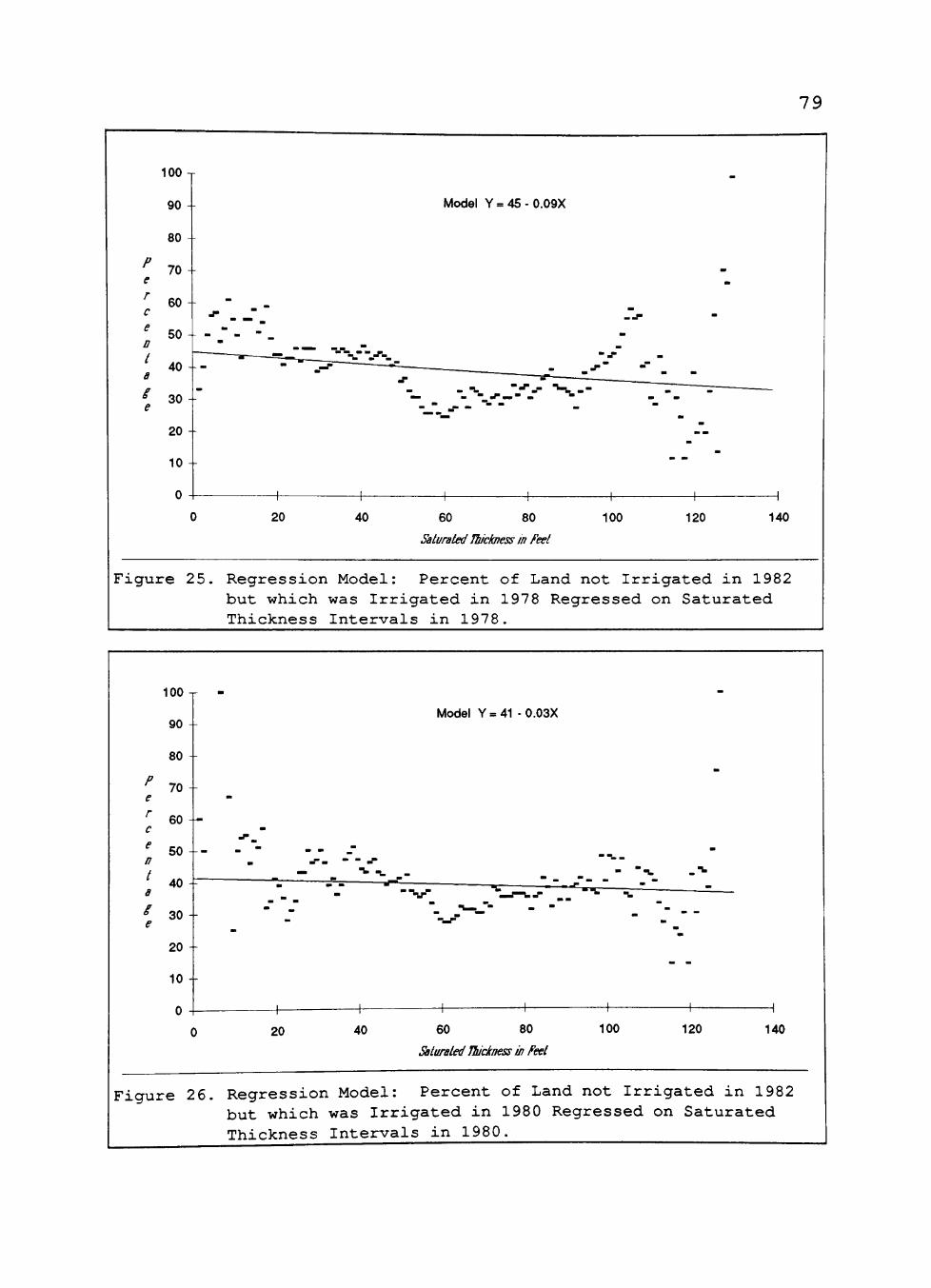
79

20 40 60 80

Saturated Itickness in Feel

100 120 140

Figure 25. Regression Model: Percent of Land not Irrigated in 1982 but which was Irrigated in 1978 Regressed on Saturated Thickness Intervals in 1978.

p e r c e n t a i e

100 -r

90

80 -

70

60 -

50

40 -

30 -

20

10 -

0 \

^

0

Figure 26.

^

.r_

• ^ >

^

. •

1 20

Model Y = 41 - 0.03X

- _ - _ _ • ' • ^ _ " ^

-̂v _ -̂-̂ -- -/"=—^

1 1 1 . - .+ . - -1 1 1 1

40 60 80 100

Saturated Itickness in Feet

^

1 1

120 140

Regression Model: Percent of Land not I r r i g a t e d in 1982 but which Thickness

was I r r i g a t e d in 1980 Regressed I n t e r v a l s in 1980.

on Sa tura ted

80

Table 6. Saturated Thickness Intervals Regressed against Percent of Change from Prior Year. Model: Y = a + bx

Interval

2 Years

4 Years

6 Years

8 Years

Years

1978-1980 1980-1982

1974-1978 1978-1982

1974-1980

1974-1982

a

63 41

76 45

77

52

S.E.

±1.56 ±2.39

±1.47 ±2.10

±1.34

±2.03

b

-0.55 -0.03

-0.53 -0.09

-0.61

-0.11

S.E.

±0.02 ±0.03

±0.53 ±0.09

±0.02

±0.03

R-Sq

0.84 0.01

0.85 0.07

0.90

0.13

not significantly affect either the intercept, the

coefficient of the independent variable or the correlation

coefficient.

Inspection of the regression statistics indicated, as

expected, that the likelihood of irrigation continuing

over time is less for areas with lower saturated

thicknesses. The relationship was strongest and most

consistent for years prior to 1982. The relationship was

minimal for intervals involving 1982 data. It was

surmised that some factor other than natural resources

became operative in the 1982 data. Previously published

information from the Texas Crop and Livestock Reporting

Service indicated an increase in irrigated acreage during

1982. Inspection of Landsat imagery for the period 1974

through 1982 showed a persistent increase in the number of

81

center pivot irrigation systems from 1978 through 1982.

As center pivot irrigation systems proliferated from 1980

to 1982, irrigated acreage also increased. It appears

that introduction of this "new" technology accounts for

the discontinuity in the data. Three effects could be

expected: first, acreage which previously had not been

irrigated, particularly in the northwest portions of the

county, could now be irrigated; second, marginal areas

which had previously been row irrigated and could have

been expected to pass out of irrigation, were able to

remain irrigated using this water conserving technology;

third, fields which had been completely irrigated using

row irrigation techniques, now became partially non-

irrigated in the corners of rectangular fields not reached

by the circular irrigation pattern of the center pivot

system. A review of data contained in Table 2 shows that

282,117 pixels (Class NNNI and Class NNNN) were

consistently not irrigated during the early years of this

study, but that 24.5% of these (Class NNNI) were classed

as irrigated in 1982. This is a significant change in the

otherwise general trend for certain land to remain out of

irrigation. The change which occurred in irrigation

technology from row irrigation to center pivot systems

severely limits the usefulness of the prediction model

established for the years 1974 through 1980.

CHAPTER V

CONCLUSIONS

This study demonstrates the feasibility of using

remotely sensed data in conjunction with other data

collected by more traditional means, such as soils data

and aquifer measurements to provide land-use managers with

improved information for decision making. Organizing the

data within the framework of a geographic information

system (GIS) for manipulation and analysis also proved

useful. The GIS format of the data structure permitted a

high degree of flexibility in reformatting, combining and

comparing datasets to derive new information and to

perform analytical operations on the data. It also

allowed comparisons to be made through time for any given

point (acre) within the study area.

It is apparent that the dominant influence on

irrigated land use is the availability of groundwater in

terms of saturated thickness; other factors, such as

soils, depth to water and depth to the base of the

aquifer, do not significantly improve the ability to

determine whether or not the land surface will be

irrigated.

A pattern of change in land use was found to be

consistent from 1974 through 1980: as saturated thickness

82

83

declined, more pixels (acres) were found to pass from

irrigated to non-irrigated land use. Higher amounts of

change were associated with the lower saturated

thicknesses, while less change was associated with greater

saturated thicknesses. This pattern did not, however

continue as strongly into 1982. While the general trend

of decline was still discernible, the relationship between

specific saturated thicknesses and land passing out of

irrigation was disrupted. This disruption appears to have

been associated with the introduction of center pivot

irrigation systems, located mainly in the northwestern and

north central portions of the county. Because of the

discontinuity in the data it was not possible to use

regression models to reliably forecast land use into 1982.

Center pivot irrigation represents the introduction of a

step function into the relationship between irrigation and

consumption of the groundwater resource. Further study,

using data obtained for periods after the introduction of

center pivot irrigation, is needed to identify the impact

of this technology on both aquifer decline and changes in

irrigated land use.

LITERATURE CITED

Anderson, J. R. , E. E. Hardy, J. T. Roach and R. E. Witmer, 1976. A land use and land cover classification system for use with remote sensor data. Professional Paper 964, U. S. Geological Survey, U. S. Government Printing Office, Washington, D. C , 28 p.

Baird, F. L. (Ed.), 1978. The Multi-faceted Water Crisis of West Texas. Proceedings of a Symposium Held November 8 and 9, 1978. Texas Tech University, Division of Continuing Education and Center for Public Service, Lubbock, Texas, 2 99 p.

Bauer, E. H., J. D. Baggett, S. L. Wall, R. W. Thomas and C. E. Brown, 1984. Results of an irrigated land assessment for water management in California. IEEE Transactions on Geoscience and Remote Sensing, GE-22(6):536-539.

Bauer, M. E., 1976. Technological basis and applications of remote sensing of the earth's resources. IEEE Transactions on Geoscience Electronics, GE-14(1):3-9.

Bell, A. E. and S. Morrison, 1977. Analytical Study of the Ogallala Aquifer in Hockley County, Texas. Report 214, Texas Department of Water Resources, Austin, Texas, 63 p.

Bennett, R. J., 1979. Spatial Time Series. Pion Ltd., London, U. K., 564 p.

Berry, J. K., 1981. Cartographic modeling: procedures for extending the utility of remotely sensed data. In B. F. Richason, Jr., 1982. PECORA VII Symposium on Remote Sensing: An Input to Geographic Information Systems in the 1980's. American Society of Photogrammetry, Falls Church, Virginia, pp. 414-424.

Black, A. L., 1978. The High Plains Ogallala study. In F. L. Baird (Ed.), 1978. The Multi-faceted Water Crisis of West Texas. Proceedings of a Symposium Held November 8 and 9, 1978. Texas Tech University, Division of Continuing Education and Center for Public Service, Lubbock, Texas, pp. 144-159.

84

85 Bonnen, C. A., 1960. Types of farming in Texas. Bulletin

964, Texas Agricultural Experiment Station, College Station, Texas, 27 p.

Brooner, W. G. and D. Nichols, 1972. Considerations and techniques for incorporating remotely sensed imagery into the land resource management process. Remote Sensing of Environment, pp. 1:1-24.

Bryant, N. A. and A. L. Zobrist, 1977. IBIS: A geographic information system based on digital image processing and image raster data type. IEEE Transactions on Geoscience Electronics, GE-15(3):152-159.

Christian, C. S., 1979. The Australian approach to environmental mapping. In F. C. Whitmore, Jr. and M. E. Williams (Eds.), 1982. Resources for the Twenty-First Century. Professional Paper 1193, U. S. Geological Survey, U. S. Government Printing Office, Washington, D. C , pp. 298-316.

Cicone, R. C , 1977. Remote sensing and geographically based information systems. In Proceedings of the 11th International Symposium on Remote Sensing of Environment. University of Michigan, Ann Arbor, pp. 1-127 - 1-137.

Colwell, R. N., 1973. Remote sensing as an aid to the management of earth resources. American Scientist, 61(2):175-183.

Cross Section, The, 1985. Monthly newsletter published by the High Plains Underground Conservation District No. 1, Lubbock, Texas.

Dangermond, J., 1983. Description of techniques for automation of regional natural resource inventories. In P. F. Hopkins (Ed.), 1983. Extraction of Information from Remotely Sensed Images. American Society of Photogrammetry, Falls Church, Virginia, pp. 135-152.

Dozier, J. and A. H. Strahler, 1983. Ground investigations in support of remote sensing. Chapter 23 in R. N. Colwell (Ed.), 1983. Manual of Remote Sensing, Second Edition, Vol. I. American Society of Photogrammetry, Falls Church Virginia, pp. 959-98 6.

86 Dregne, H. E., 1983. Desertification of Desert Lands.

Harwood Academic Publishers, N. Y., 242 p.

Ebert, J. I. and T. R. Lyons, 1983. Archaeology, anthropology, and cultural resources management. Chapter 26 in R. N. Colwell (Ed.), 1983. Manual of Remote Sensing, Second Edition, Vol. II. American Society of Photogrammetry, Falls Church Virginia, pp.1233-1304.

Ellefrtis, D. C , T. W. Baryen, D. J. Barr and C. J. Johnson, 1978. Mapping land cover from satellite images: a basic, low cost approach. Contractor Report 2 952, NASA contract NAS 8-317 67, George C. Marshall Space Flight Center, Scientific and Technical Information Office, 18 p.

Ellefsen, R. 1976. Computer-aided mapping of land use. In R. S. Williams and W. D. Carter (Eds.), 1976. ERTS-1 A New Window on Our Planet, Professional Paper 92 9, U. S. Government Printing Office, Washington, D. C , pp. 234-242.

Estes, J. E., E. J. Hajic and L. R. Tinney, 1983. Fundamentals of image analysis: analysis of visible and thermal infrared data. Chapter 24 in R. N. Colwell (Ed.), 1983. Manual of Remote Sensing, Second Edition, Vol. I. American Society of Photogrammetry, Falls Church Virginia, pp. 987-1118.

Estes, J. E., J. R. Jensen and D. Simonett, 1983. Impacts of remote sensing on U. S. geography. Remote Sensing of Environment, 10:43-80.

Firey, W., 1960. Man, Mind and Land: A Theory of Resource Use. The Free Press of Glencoe, Illinois, 256 p.

Fitzpatrick-Lins, K., 1978. Accuracy and consistency comparisons of land use and land cover maps made from high altitude photographs and Landsat multispectral imagery. Journal of Research, U. S. Geological Survey, 6(1):23-40.

Frazier, B. E. and H. F. Shovic, 1979. Sampling land use changes on prime agricultural land in western Watcom County, Washington. Journal of Soil and Water Conservation, 34(l):25-27.

87 Frederick, K. D. and J. C. Hanson, 1982. Water for

Western Agriculture. Resources for the Future, Inc., Washington, D. C , 241 p.

Frederick, K. D., J. c. Hanson, J. Pagano, R. N. Shulstad, R. D. May, B. E. Harrington and J. M. Erstine, 1984. Trends in U. S. irrigation: three regional studies. Project summary. Environmental Research Laboratory, U. S. Environmental Protection Agency, Athens, Georgia, 6 p.

Gates, W. E. and R. J. Heil, 1980. Geographic information systems. Proceedings of the American Society of Civil Engineers, Journal of the Surveying and Mapping Division, 106(SUl):105-117.

Gordon, S. I., 1980. Utilizing Landsat imagery to monitor land-use change: a case study in Ohio. Remote Sensing of Environment, 9:183-196.

Green, D. E., 1973. Land of the Underground Rain: Irrigation on the Texas High Plains, 1910-1970. University of Texas Press, Austin, Texas, 295 p.

Grice, D. G., W. Green and W. Richardson, 1965. Soil Survey, Hockley County, Texas. U. S. Department of Agriculture, Soil Conservation Service, U. S. Government Printing Office, Washington, D. C , 65 p.

Grubb, H. W. , undated. A fact sheet on the economy of the Texas High Plains. High Plains Underground Water Conservation District No. 1, Lubbock, Texas, 5 p.

Grubb, H. W., 1966. Importance of irrigation water to the economy of the Texas High Plains. Report 11, Texas Water Development Board, Austin, Texas, 25 p.

Henderson, C. E., 1981. Sub-regional information system formation using multi-resolution remote sensing products. In B. F. Richason, Jr., 1982. PECORA VII Symposium on Remote Sensing: An Input to Geographic Information Systems in the 1980's. American Society of Photogrammetry, Falls Church, Virginia, pp. 114-123.

88 High Plains Associates, 1982. Six-state High Plains

Ogallala Aquifer regional resources study - summary: a report to the U. S. Department of Commerce and the High Plains Study Council. High Plains Associates: Camp, Dresser & McKee, Inc.; Black & Veatch; Arthur D. Little, Inc., Austin, Texas, 46 p.

High Plains Study Council, 1982. A summary of results of the Ogallala Aquifer regional study, with recommendations to the Secretary of Commerce and Congress. Economic Development Administration, Washington, D. C , 60 p.

Hughes, W. F. and A. C. Magee, 1960. Some economic effects of adjusting to a changing water supply, Texas High Plains. Bulletin 966, Texas Agricultural Experiment Station, The Agricultural and Mechanical College of Texas, College Station, Texas, 27 p.

Jensen, J. R., 1983. Biophysical remote sensing. Annals of the Association of American Geographers, 73(1):111-132.

Johannsen, C. J. and T. W. Barney, 1981. Remote sensing applications for resource management. Journal of Soil and Water Conservation, 36(3) : 128-133.

Johannsen, C. J. and J. L. Sanders (Eds.), 1982. Remote Sensing for Resource Management. Soil Conservation Society of America, Arkeny, Iowa, 665 p.

Johnson, W. M. , 1982. Some information needs for USDA agencies in decision-making. In C. J. Johannsen and J. L. Sanders (Eds.), 1982. Remote Sensing for Resource Management. Soil Conservation Society of America, Arkeny, Iowa, pp. 493-500.

Knowles, T., 1981. Evaluating the ground-water resources of the High Plains of Texas, GWSIM-III Ground-water simulation program, program documentation and user's manual. UM-36, Texas Department of Water Resources, Austin, Texas, 84 p.

Knowles, T., P. Nordstrom and W. B. Kent, 1982. Evaluating the ground-water resources of the High Plains of Texas, Final Report, Vol. 1. Report No. LP-173, Texas Department of Water Resources, Austin, Texas, 179 p.

89 Landgrebe, D., 1976. Computer-based remote sensing

technology - a look to the future. Remote Sensing of Earth Resources, 5:229-246.

Lee, J. S., 1982. Remote sensing applications to national soil and water resource inventories. In C. J. Johannsen and J. L. Sanders (Eds.), 1982. Remote Sensing for Resource Management. Soil Conservation Society of America, Arkeny, Iowa, pp. 502-505.

Lindenlaub, J. C. and S. M. Davis, 1978. Applying the quantitative approach. In P. H. Swain and S. M. Davis (Eds.), 1978. Remote Sensing: The Quantitative Approach. McGraw-Hill, N. Y., pp. 290-335.

Lins, H. F., Jr., 1980. Patterns and trends of land use and land cover on Atlantic and Gulf Coast barrier islands. Professional Paper 1156, U. S. Geological Survey, U. S. Government Printing Office, Washington, D. C., 11 p.

Loveland, T. R. and G. E. Johnson, 1918. The role of remotely sensed and other spatial data for predictive modeling - the Umatilla, Oregon example. In B. F. Richason, Jr., 1982. PECORA VII Symposium on Remote Sensing: An Input to Geographic Information Systems in the 1980's. American Society of Photogrammetry, Falls Church, Virginia, pp. 442-454.

Luckey, R. R., E. D. Gutentag and J. B. Weeks, 1981. Water-level and saturated thickness changes, predevelopment to 1980, in the High Plains Aquifer in parts of Colorado, Kansas, Nebraska, New Mexico, Oklahoma, South Dakota, Texas and Wyoming. Hydrologic Investigations Atlas, HA-652, U. S. Geological Survey, Denver, Colorado, 2 sheets.

Martinko, E. A., J. Poracsky, E. R. Kipp, H. Krieger, K. Gunn, 1981. Crop phenology and Landsat-based irrigated lands inventory in the High Plains. Final report. Grant No. NAG 2-57, NASA, Office of University Affairs, Ames Research Center, Moffett Field, California. Space Technology Center, The University of Kansas, Lawrence, Kansas, 129 p.

90 Matthews, K. H., D. E. Ethridge and A. L. Stoecker, 1984.

Effects of aquifer and other characteristics on land values in the Texas High Plains. MP-1558, Texas Agricultural Experiment Station, College Station, Texas, 12 p.

McFarland, W. D., 1982. Geographic data bases for natural resources. In C. J. Johannsen and J. L. Sanders (Eds.), 1982. Remote Sensing for Resource Management. Soil Conservation Society of America, Arkeny, Iowa, pp. 41-50.

McHarg, I. L., 1969. Design with Nature. Natural History Press, Philadelphia, Pennsylvania, 198 p.

Mead, D. A., 1981. State-wide natural resource information systems - a status report. Journal of Forestry, 79(6):369-372.

Merchant, J. W., 1981. Employing Landsat MSS in land use mapping: observations and considerations. In B. F. Richason, Jr., 1982. PECORA VII Symposium on Remote Sensing: An Input to Geographic Information Systems in the 1980's. American Society of Photogrammetry, Falls Church, Virginia, pp. 71-91.

Milazzo, V. A., 1980. A review and evaluation of alternatives for updating U. S. Geological Survey land use and land cover maps. Circular 82 6, U. S. Geological Survey, Denver, Colorado, 19 p.

Miller, L. D., Y. K. Yang, T. Cheng, M. J. Unverferth, M. G. Kim, 1983. 7 1/2' map image extraction from precision processed Landsat multi-spectral scanner (MSS) and Thematic Mapper (TM) imagery using a microcomputer and EROS computer compatible tapes. In P. F. Hopkins (Ed.), 1983. Extraction of Information from Remotely Sensed Images. American Society of Photogrammetry, Falls Church, Virginia, pp. 115-125.

Mitchell, W. B., S. C. Guptill, K. E. Anderson, R. C. Fegeas and C. A. Hallam, 1977. GIRAS: A geographic information retrieval and analysis system for handling land use and land cover data. USGS Professional Paper 1059, U. S. Government Printing Office, Washington, D. C , 16 p.

91 Mooneyhan, D. W., 1982. Organizing information for

effective resource management. In C. J. Johannsen and J. L. Sanders (Eds.), 1982. Remote Sensing for Resource Management. Soil Conservation Society of America, Arkeny, Iowa, pp. 30-40.

Myers, V. I., 1983. Remote sensing applications in agriculture. Chapter 33 in R. N. Colwell (Ed.), 1983. Manual of Remote Sensing, Second Edition, Vol. II. American Society of Photogrammetry, Falls Church Virginia, pp. 2111-2228.

Nunnally, Nelson R., 1974. Interpreting land use from remote sensor imagery. In J. E. Estes and L. W. Senger (Eds.), 1974. Remote sensing: Techniques for Environmental Analysis. John Wiley & Sons, N. Y., pp. 167-187.

Osborn, J. E., T. R. Harris and T. R. Owens, 1974. Impact of groundwater and petroleum on the economy of the Texas High Plains. Final report to the Texas Department of Water Resources, Department of Agricultural Economics, College of Agricultural Sciences, Texas Tech University, Lubbock, Texas, 87 P-

Patterson, F. A. and P. McAdams, 1981. The use of Landsat MSS data and ancillary data to produce erosion hazard potential maps. In P. A. Moore (Ed.), 1981. Computer Mapping of Natural Resources and the Environment, Vol. 15, Harvard Library of Computer Graphics/1981 Mapping Collection, Laboratory for Computer Graphics and Spatial Analysis, Harvard Graduate School of Design, Cambridge, Massachusetts, pp. 131-138.

Robinove, C. J., 1981. The logic of multispectral classification and mapping of land. Remote Sensing of Environment, 11:231-244.

Schecter, R. N., 1976. Resource inventory using Landsat data for areawide water quality planning. In Machine Processing of Remotely Sensed Data, June 29-July 1, 1976. The Laboratory for Applications of Remote Sensing, Purdue University, IEEE Catalog No. 7 6CH1103-1MPRSD, pp. 4B-41 - 4B-51.

92 Short, M. M., 1982. The Landsat Tutorial Workbook. NASA

Reference Publication 1078, Scientific and Technical Information Branch, National Aeronautics and Space Administration, Washington, D. C , 533 p.

Sloggett, G., 1981. Prospects for ground-water irrigation: declining levels and rising energy costs. Agricultural Economic Report No. 47 8, Natural Resource Economics Division, Economic Research Service, U. S. Department of Agriculture, Washington, D. C., 43 p.

Stoecker, A. L., M. L. Wright and D. A. Pyles, 1981. An input-output model of the Texas High Plains economy in 1977. Publication No. T-1-199, Department of Agricultural Economics, College of Agricultural Sciences, Texas Tech University, Lubbock, Texas, 187 P-

Sturdevant, J. A., 1981. The development and application of a county-level geographic data base. In B. F. Richason, Jr., 1982. PECORA VII Symposium on Remote Sensing: An Input to Geographic Information Systems in the 1980's. American Society of Photogrammetry, Falls Church, Virginia, pp. 114-123.

Swain, P. H. and S. M. Davis (Eds.), 1978. Remote Sensing: the Quantitative Approach. McGraw-Hill, N. Y., 396 p.

Supalla, R. J., R. R. Lansford and N. R. Gollehon, 1982. Is the Ogallala going dry? Journal of Soil and Water Conservation, 37 (6) :310-314.

Sweazy, R. M. , 1983. West Texas water resources: beyond 2000. In I. R. Traylor and J. R. Goodin (Eds.), 1983. West Texas Natural Resources: Economic Perspectives for the Future. Conference proceedings. International Center for Arid and Semiarid Land Studies, Texas Tech University, Lubbock, Texas, pp. 29-40.

Taranick, J. V., 1978. Characteristics of the Landsat multispectral data system. Open File Report 78-187, U. S. Geological Survey. Reprinted in R. K. Holz, 1985. The Surveillant Science: Remote Sensing of the Environment, John Wiley & Sons, N. Y., pp. 328-380.

93 Taylor, H. D., 1979. Water-level data from observation

wells m the Southern High Plains of Texas, 1971-1977. Report 228, Texas Department of Water Resources, Austin, Texas, 484 p.

Teicholz, E., 1980. Geographic information systems: The ODYSSEY Project. Journal of the Surveying and Mapping Division, Proceedings of the ASCE, 106(SU 1):119-135.

Texas Crop and Livestock Reporting Service, various years. Texas County Statistics. Bulletin 214, U. S. Department of Agriculture and Texas Department of Agriculture, Austin, Texas.

Texas Department of Water Resources, 1981. Inventories of irrigation in Texas 1958, 1964, 1969, 1974 and 1979. Report 2 63, Texas Department of Water Resources, Austin, Texas, 295 p.

Texas Natural Resources Information System, 1982. Texas Natural Resources Information System, file description report. First edition, second revision. Texas Natural Resources Information System, Austin, Texas, 33 p. plus file descriptions.

Tullos, E. J., 1982. A Landsat-based, automated cotton acreage inventory system. In C. J. Johannsen and J. L. Sanders (Eds.), 1982. Remote Sensing for Resource Management. Soil Conservation Society of America, Arkeny, Iowa, pp. 470-478.

U. S. Bureau of the Census, 1983. City and County Data Book. U. S. Department of Commerce, Bureau of the Census, U. S. Government Printing Office, Washington, D. C., 996 p.

Walsh, S. J., 1985. Geographic information systems for natural resource management. Journal of Soil and Water Conservation, 40 (2) :202-205.

Weeks, J. B. and E. D. Gutentag, 1981. Bedrock geology, altitude of base, and 1980 saturated thickness of the High Plains Aquifer in parts of Colorado, Kansas, Nebraska, New Mexico, Oklahoma, South Dakota, Texas and Wyoming. Hydrologic Investigations Atlas, HA-648, U. S. Geological Survey, Denver, Colorado, 2 sheets.

94 Westin, F. C , T. M. Brander and M. E. Wehde, 1981.

Combining land use data acquired from Landsat with soil map data using an information system. In B. F. Richason, Jr., 1982. PECORA VII Symposium on Remote Sensing: An Input to Geographic Information Systems in the 1980's. American Society of Photogrammetry, Falls Church, Virginia, pp. 114-123.

Wood, B. L. and L. H. Beck, 1982. A geographic information system for Colusa County, California. In Proceedings of the Eighth International Symposium on Machine Processing of Remotely Sensed Data. Laboratory for Applications of Remote Sensing, Purdue University, IEEE Catalog No. 82 CH 1776-4 MPSRD, West Lafayette, Indiana, pp. 394-401.

Wyatt, A. W., A. E. Bell and S. Morrison, undated. Potential capacity of Ogallala Aquifer to yield water to wells - 1974. Map prepared by the Texas Department of Water Resources, High Plains Underground Water Conservation District No. 1, Lubbock, Texas, 1 sheet.

Wyatt, A. W., A. E. Bell and S. Morrison, undated. Potential capacity of Ogallala Aquifer to yield water to wells - 2000. Map prepared by the Texas Department of Water Resources, High Plains Underground Water Conservation District No. 1, Lubbock, Texas, 1 sheet.

Young, K. B. and J. M. Coomer, 1980. Effects of natural gas price increases on Texas High Plains irrigation, 1976-2025. Agricultural Economic Report No. 448, Natural Resource Economics Division, Economics, Statistics and Cooperatives Service, U. S. Department of Agriculture, Washington, D. C , 32 p.

APPENDIX A: SOILS DATA LAYER

PRODUCTION TECHNIQUES

This appendix describes the procedures used to

digitize the data in the soils data layer. The procedures

provide detail about the controls on the data transfer

techniques to insure that soils mapping units were

accurately digitized, and on the geographic grid locations

of the mapping to insure that positional accuracy within

the grid was maintained.

First, paper copies were made of each page of the

Soil Survey which contained aerial photographs taken over

Hockley County. Adjacent photo sheets were then aligned

with each other and taped together; usually four at a time

(only two adjacent sheets were needed for areas along the

eastern edge of the county). Two reference points which

could be identified on corresponding 7.5-minute

quadrangles were then selected at the left and right edges

of the photo sheet; four test points located near the

corners of the photo sheet were also identified; each set

of points was then marked on both media.

Next, the appropriate 7.5-minute quadrangles were

affixed to the digitizing tablet and the Latitude-

Longitude coordinates of each point were measured using

the MSTEST routine of the ERDAS Polygon Digitizing module.

95

96

The measured map coordinates were then recorded, the 7.5-

minute quadrangles were removed from the digitizing tablet

and the photo sheet was affixed.

The two reference points were used to set up the

coordinate frame for the photo sheet. The accuracy of the

setup was tested by comparing the coordinate measurements

for the test points on the photo sheet to those previously

obtained from the 7.5-minute quadrangles. This procedure

was repeated until coordinate differences representing

less than 100m (.001096 degree of longitude and .000918

degree of latitude at the center of the county) on the

1:24000 quadrangles were obtained.

Once the locational reference setup was complete the

soil traces were digitized. The paper photo sheet was

covered with frosted mylar that had been gridded into

four-inch squares. Soil units were then highlighted on

the mylar using a felt-tipped, water-soluble coloring pen.

One soil unit at a time was highlighted, searching

one four-inch grid block at a time, beginning at the upper

left-hand corner of the photo sheet and proceeding along a

row to the right, then continuing down the sheet in a

plow-row pattern. After the entire sheet was searched, it

was reviewed to identify traces that might have been

missed. All the areas for the one soil unit were then

digitized by passing the cursor crosshairs over the trace.

97

The digitized data were then visually inspected to

insure that all soil mapping units had been recorded and

that designations were correct. Corrections to the

digital data were made as needed at this time. The water

colors were then wiped from the mylar and the procedure

was repeated for the next soil type.

After all mapping units had been digitized from the

photo sheet the digitized file was "island sorted". The

effect of this procedure was to sort coordinate pairs by

the size of the area enclosed by the outline of the soil

mapping unit, placing the larger areas first in the file

and the smaller ones last. This procedure was needed

because the graphics software writes areas to the display

screen in sequential order as they are digitized. A

smaller area written before a larger one and enclosed

within it would be overwritten by the larger one; thus the

data of the smaller area would be lost when the data layer

was created from the graphic display.

After all of the photo sheets were completed the

files of coordinate pairs were converted from Latitude-

Longitude coordinates to UTM coordinates using the ERDAS

routine CCVRT. The files were then combined and resampled

into 67m x 67m cells of the data array. The resampled

data layer was then corrected by adding or deleting pixels

at the edges so locations of data in the soil layer would

98

exactly correspond with data locations in the rectified

and registered Landsat imagery. Fewer than 100 pixels

were manually recoded for this purpose.

There are 37 soil mapping units identified in the

Soil Survey of Hockley County. To reduce the number of

units for analytical purposes some were combined into one

unit. The combinations were achieved by grouping together

all mapping units of one type and ignoring classification

differences attributable to slope of the land, so long as

the range of differences in slope did not exceed five

percent. For example, three mapping units identify

Amarillo fine sandy loam: AfA, AfB and AfC; they are

distinct only because they have slopes of 0 to 1 percent,

1 to 3 percent and 3 to 5 percent respectively; all three

were digitized as one unit--Amarillo fine sandy loam--

with slopes of from 1 to 5 percent. On the other hand,

there are three units of Drake soils: DrB, DrC and DrD,

with slopes of 1 to 3 percent, 3 to 5 percent and 5 to 20

percent; in this case the first two units were digitized

together, while the third was digitized separately as a

Drake soil with 5 to 20 percent slopes. An additional

mapping unit was created for areas not classified in the

Soil Survey; these are areas of "no data"; they are

generally locations where the soil is inundated or where

there is no soil, such as perennial lakes or gravel pits.

APPENDIX B: LIST OF MAPS

The following is a list of the maps that were used to

determine the latitude/longitude and UTM coordinate

locations of features in the landsat satellite imagery, to

locate the boundaries of Hockley County in these

coordinate systems and to establish the reference frame of

the data layers. All maps are published by the U. S.

Geological Survey and are in the 7.5 minute map series at

a scale of 1:24000. The maps are listed in the order in

which they occurr in one degree block 33102 of the U. S.

Geological Survey index to topographic and other map

coverage for Texas, 1984 Edition

Ouadrangle Name

Busterville Ropesville Lockettville Sundown Plains 1 NE Wollforth Smyer Levelland East Levelland West Whiteface Wollforth NE Wollforth NW Whitharral Hester Ranch Pettit Roundup Anton Lums Chapel Oklahoma Flat Pep

Year of Publication

1985 1985 1965 1965 1965 1985 1985 1965 1965 1965 1985 1985 1965 1965 1965 1985 1985 1964 1964 1964

(Provisional) (Provisional)

(Provisional) (Provisional)

(Provisional) (Provisional)

(Provisional) (Provisional)

99

APPENDIX C: SELECTED HYDROLOGIC

DATA AND PROGRAMS

This appendix contains hydrologic data used in the

study, as well as computer programs used to extract data

from various sources, to combine them into a single file

and to reconfigure them into a format suitable for use in

a GIS data layer. Data were obtained for nine counties:

Bailey, Lamb, Hale, Hockley, Lubbock, Yoakum, Terry and

Lynn. All wells are located in one degree quadrangle 24

of the Texas State Well Numbering System (TDWR,

1979,1984). The only data file reproduced here is from an

undated, untitled printout obtained from the HPUGWD No. 1.

The other data files (referenced in the study) are not

included in this appendix because they are available to

the public from the State of Texas Department of Water

Resources and the Texas Natural Resources Information

Service.

Four programs (one main program and three modules)

that were used to extract and reformat data from the files

are included because they contain corrections to errors

found in the data source files. These are SAS

(Statistical Analysis System) source code files with

input-output statements for use on a VAX 8 650 operating

under VMS.

100

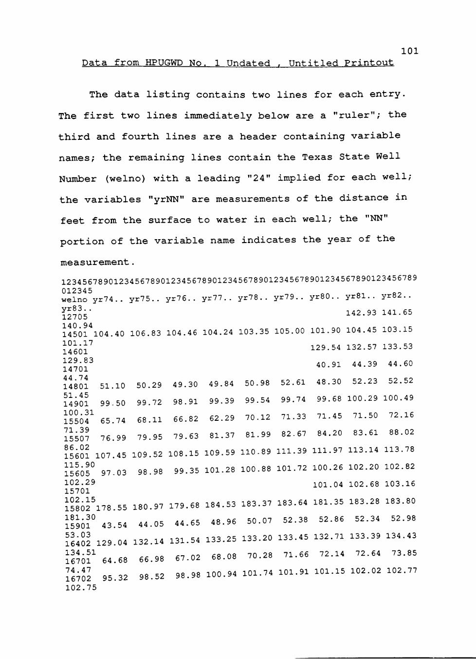
101 Data from HPUGWD No. 1 Undated ^ Untitled Printout

The data listing contains two lines for each entry.

The first two lines immediately below are a "ruler"; the

third and fourth lines are a header containing variable

names; the remaining lines contain the Texas State Well

Number (welno) with a leading "24" implied for each well;

the variables "yrNN" are measurements of the distance in

feet from the surface to water in each well; the "NN"

portion of the variable name indicates the year of the

measurement.

123456789012345678901234567890123456789012345678901234567890123456789

012345 „^ „., -^ welno yr74.. yr75.. yr76.. yr77.. yr78.. yr79.. yr80.. yrSl.. yr82.. If^l- 142.93 141.65

1450^104.40 106.83 104.46 104.24 103.35 105.00 101.90 104.45 103.15

^^.I'r}'^ 129.54 132.57 133.53 14601

\1^QI'^ 40.91 44.39 44.60

14801 51.10 50.29 49.30 49.84 50.98 52.61 48.30 52.23 52.52

14901 99.50 99.72 98.91 99.39 99.54 99.74 99.68 100.29 100.49

issif 65.74 68.11 66.82 62.29 70.12 71.33 71.45 71.50 72.16

llsll 76.99 79.95 79.63 81.37 81.99 82.67 84.20 83.61 88.02

^560? 107.45 109.52 108.15 109.59 110.89 111.39 111.97 113.14 113.78

15605° 97.03 98.98 99.35 101.28 100.88 101.72 100.26 102.20 102.82 102.29 101.04 102.68 103.16

i5862'l78.55 180.97 179.68 184.53 183.37 183.54 181.35 183.28 183.80

ilaif 43.54 44.05 44.65 48.96 50.07 52.38 52.86 52.34 52.98

I64S2 129.04 132.14 131.54 133.25 133.20 133.45 132.71 133.39 134.43

lliol^ 64.68 66.98 67.02 68.08 70.28 71.66 72.14 72.64 73.85

^6702 95.32 98.52 98.98 100.94 101.74 101.91 101.15 102.02 102.77

102.75

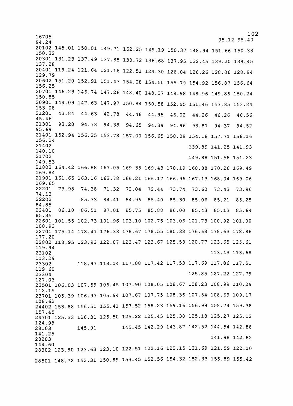
16705 94.24 20102 145, 150.32 20301 131, 137.28 20401 119, 129.79 20602 151, 156.25 20701 146, 150.85 20901 144, 153-08 21201 43, 45.46 21301 93, 95.69 21401 152, 156.24 21402 140.10 21702 149.53 21803 164, 169.84 21901 161, 169.65 22201 73, 74.13 22202 84.85 22401 86, 85.35 22601 101, 100.93 22701 175. 177.20 22802 118, 119.94 23102 113.29 23302 119.60 23304 127.03 23501 106. 112.15 23701 105. 108.62 24402 153. 157.45 24701 125. 124.98 28103 141.25 28203 144.60 28302 123.

28501 148.

.01

.23

.24

.20

.23

.09

.84

.20

.94

.42

.65

.98

.10

.55

.14

.95

.03

,39

,88

,33

80

72

150

137

121,

152,

146,

147,

44,

94,

156,

166,

163,

74,

85,

86,

102,

178.

123.

118,

107.

106,

156,

126.

145.

123.

152.

.01

.49

.64

.91

.74

.63

.63

.73

.25

.88

.16

.38

.33

.51

.73

.47

.93

.97

,59

,93

,51

,31

,91

63

31

149

137

121

151

147

147,

42,

94,

153,

167,

163,

71,

84.

87.

101.

176,

122,

118,

106.

105.

155.

125.

123.

150.

.71

.85

.16

.47

.26

.97

.78

.38

.78

.05

.78

.32

.41

.01

.96

.33

,07

,14

,45

94

41

50

10

89

152

138

122

154

148

150

44

94,

157,

169,

166,

72.

84.

85.

103.

178.

123.

117.

107.

107,

157.

125.

145.

122.

153.

.25

.72

.51

.08

.40

.84

.46

.65

.00

.38

.21

.04

.96

.75

.10

,67

,47

,08

,90

,67

,52

,22

,45

,51

,45

149

136

124

154

148

150

44,

94,

156,

169.

166.

72.

85.

85.

102.

178.

123,

117,

108.

107.

158.

125.

142.

122.

152.

.19

.68

.30

.50

.37

.58

.95

.39

.65

.43

.17

.44

.40

.88

,75

,55

,67

,42

,05

,75

,23

,45

,29

,16

,56

150

137

126

155

148

152,

46,

94,

158.

170.

166.

73.

85.

86.

103.

180.

125.

117.

108.

108.

159.

125.

143.

122.

154.

.37

.95

.04

.79

.98

.95

.02

.96

.09

,19

,96

,74

,30

00

06

38

53

53

67

36

16

38

87

15

32

148

132

126

154

148

151,

44,

93,

154.

139.

149.

168,

167.

73.

85.

85.

101.

176.

120.

117.

125.

108.

107.

156.

125.

142.

121.

152,

.94

.45

.26

.92

.96

.46

.26

.87

.18

,89

,88

,88

,13

,60

06

43

73

68

77

69

85

23

54

99

18

52

,69

,33

95.12 95

151.66

139.20

128.06

156.87

149.86

153.35

46.26

94.37

157.71

141.25

151.58

170.26

168.04

73.43

85.21

85.13

100.92

178.63

123.65

113.43

117.86

127.22

108.99

108.69

158.74

125.27

144.54

141.98

121.59

155.89

150

139

128

156

150

153

46,

94.

156.

141.

151.

169.

169.

73.

85.

85.

101.

178.

125.

113.

117.

127.

110.

109.

159.

125.

142.

142.

122.

155.

102 .40

.33

-45

.94

.64

.24

.84

.56

.52

.16

.93

,23

,49

,06

96

25

64

00

86

61

68

51

79

29

17

38

,12

,88

,82

.10

.42

103 154.87 28601 140.07 141.74 143.70 139.39 28901 167.23 169.65 166.13 168.74 168.81 169.27 169.03 172.27 172.00 168.90 29308 146.57 150.07 148.67 150.62 151.26 152.67 151.58 154.15 154.06 153.73 29312 137.47 139.00 139.72 138.96 29401 140.41 141.09 140.45 141.66 141.67 142.54 141.57 142.60 142.03 141.23 29603 135.22 135.76 135.60 135.13 29901 197.60 196.04 196.35 193.55 193.54 190.42 194.08 193.63 187.99 30102 138.20 141.69 139.79 139.71 140.26 141.09 138.61 139.57 140.05 138.48 30304 107.38 108.68 107.93 109.17 109.62 110.38 110.15 110.74 110.89 110.02 30401 129.48 131.54 128.56 130.48 129.82 130.08 127.90 128.42 128.60 30502 136.42 133.60 30801 174.17 176.49 175.65 177.77 177.92 179.23 178.20 179.39 181.47 178.79 30901 156.32 159.31 157.82 159.72 160.37 160.65 158.87 159.89 159.52 157.74 31101 70.22 71.23 71.24 69.20 31203 104.70 105.20

31401 130.56 135.24 132.00 136.19 136.56 138.09 134.42 135.08 134.10 128 39 3 1 5 0 1 7 8 . 1 5 7 9 . 3 1 7 6 . 8 6 7 7 . 6 1 7 9 . 0 2 7 9 . 6 6 7 9 . 0 8 8 0 - 1 4 8 0 . 2 4 7 7 . 9 1 31601 116.42 123.00 116.72 117.64 117.66 118.78 116.55 117.63 116.43 115.15 31801 146.67 147.51 147.67 148.23 148.68 149.67 149.57 150.33 150.69 149.87 31902 127.24 127.16 126.65 125 27 32401 102.24 105.09 104.14 106.04 106.26 106.43 104.87 106.46 104.32 101.34 32701 115.07 117.19 116.82 117.81 118.25 118.84 117.79 118.36 117.63 116.33

36302 172.64 174.12 173.49

36601 146.62 147.53 146.89 148.64 148.10 149.57 150.46 149.54 149.86

37101 150.54 152.38 153.92 153.83 154.55 155.16 155.64 157.24 161.23 158 94

37204 151.30 153.98 152.90 154.04 153.96 155.25 153.57 156.10 155.91

37368^^146.75 148.57 147.10 147.66 146.15 147.16 146.08 147.89 149.49

llloV 137.77 139.75

37701 152.30 152.02 152.22 152.24 151.36 150.87 150.63 150.54 150.36

38201^172.49 174.79 174.20 175.87 176.75 177.09 176.74 177.44 177.00

175.89

38403 163. 166.25 38501 128.60 38602 120.64 38801 163. 160.85 39101 155. 152.64 39302 146. 148.45 39501 135. 134.10 39701 115. 105.72 39901 95. 95.94 40401 141. 146.59 40403 146. 149.98 40702 113.02 10201 110. 114.56 10303 126.34 11201 106. 101.05 11202 84.82 11402 126.45 11701 125, 126.39 11801 106, 109.00 11802 110 114.36 11803 130.51 19201 147 150.09 19301 166 170.87 19403

154.89 19502 169 174.41 19601 166 160.15 19701 151.00 19801 164 167.60 19902 129 130.24 20103 145 145.34 20402 151

54

60

14

23

67

66

57

24

36

,22

.19

.52

.50

.87

.49

.86

.19

.98

.18

.11

.07

.78

164.

167.

156.

149.

136.

120.

95.

142.

149.

116.

141,

104.

127,

107,

113,

147

176

171

166

158

169

130

150

150

36

14

76

27

55

96

88

98

32

,36

.25

.11

.28

.39

.73

.75

.17

.78

.80

.17

.82

.20

.57

.27

163.

164.

156.

148.

135.

114.

95.

143.

148.

110.

135.

102.

126,

106,

113,

148,

172

173

156

154

166

129

147

149

61

93

08

72

39

84

11

24

09

,29

,03

,22

.01

.62

.50

.11

.25

.28

.52

.31

.28

-34

.17

.57

164.

164.

157.

150.

134.

117.

95.

143.

149.

114.

141,

103,

126.

107,

115,

148,

173

176

157

154

171

130

151

150

84

40

17

24

42

36

89

60

,94

,91

,78

.71

.66

.97

.82

.57

.11

.42

.62

.79

.44

.27

.62

.40

164.

163.

156.

150.

135.

116.

96.

144.

150.

114.

139.

102.

126.

108,

116,

149

169

176

157

154

171

129

147

150

49

65

83

27

03

92

80

50

52

,28

,08

,39

.38

.62

.18

.13

.25

.14

.78

.23

.25

.82

.48

.89

165.

163.

157.

151.

135.

118.

97.

145.

151.

116.

142.

103.

127.

109.

115.

149,

170.

176

161

153

169

129

147

152

78

99

49

25

84

99

56

72

64

15

23

,05

,07

.01

.79

.44

.04

.43

.52

.19

.89

.80

.92

.08

167.

162,

155.

149.

135.

113.

97.

145.

149.

112.

113.

135.

102.

84,

126.

126.

108.

114.

148,

164

176

157

153

166

129

147

153

,05

44

,24

62

20

,27

70

,74

59

,49

,14

,66

,42

,80

.61

.85

.49

.54

.67

.82

.86

.88

.16

.82

.59

.94

.06

167.

129,

123,

163.

156.

150.

135.

117.

97.

146.

151.

114.

117.

137.

102.

85.

127.

126,

109.

115.

131,

148,

168,

155

176

159

151

169

130

147

154

,13

,02

,29

,99

43

65

10

36

76

26

33

00

05

22

36

,04

,18

,41

,31

.54

.16

.07

.24

.90

.04

.43

.95

.88

.66

.97

.32

168,

129.

124.

163.

155.

150.

134.

112.

97.

147.

151.

114.

115.

131.

101.

84.

126.

126.

109,

114.

148,

167,

174

159

151

169

130

145

104 .86

,41

,79

,05

,62

49

91

48

11

42

10

10

21

92

97

95

,79

,55

,39

,54

.82

.76

.83

.80

.78

.89

.55

.58

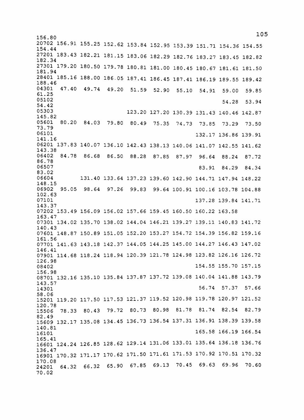
156.80 20702 154.44 27201 182.34 27301 181.94 28401 188.46 04301 61.25 05102 54.42 05303 145.82 05601 73.79 06101 141.16 06201 143.38 06402 86.78 06507 83.02 06604 148.15 06902 102.63 07101 143.37 07202 163.47 07301 140.43 07601 161.56 07701 146.41 07901 126.98 08402 156.98 08701 143.57 14301 58.06 15201 120.78 15506 82.49 15609 140.81 16101 165.41 16601 136.47 16901 170.08 24201 70.02

105 156.91

183.43

179.20

185.16

47.40

155.25

182.21

180.50

188.00

49.74

152.62

181.15

179.78

186-05

49.20

8 0 . 2 0 8 4 . 0 3 7 9 . 8 0

137.83

84.78

95.05

153.49

134.02

148.87

141.63

114.68

140.07

86.68

131.40

98.64

156.09

135.70

150.89

143.18

118.24

136.10

86.50

133.64

97.26

156.02

138.02

151.05

142.37

118.94

153.84

183.06

180.81

187.41

51.59

123.20

80.49

142.43

88.28

137.23

99.83

157.66

144.04

152.20

144.05

120.39

152.95

182.29

181.00

186.45

52.90

127.20

75.35

138.13

87.85

139.60

99.64

159.45

146.21

153.27

144.25

121.78

153

182,

180,

187.

55.

130.

74.

140.

87.

142.

100.

160.

139.

154.

145.

124.

39 151.71 154.36 154.55

76 183.27 183.45 182.82

45 180.67 181.61 181.50

132.16 135.10 135.84 137.87 137.72 139

119.20

78.33

132.17

124.24

170.32

64.32

117.50

80.43

135.08

126.85

171.17

66.32

117.53

79.72

134.45

128.62

170.62

65.90

121.37

80.73

136.73

129.14

171.50

67.85

119.52

80.98

136.54

131.06

171.61

69.13

120

81

137

133

171

70

41 186

10 54,

39 131,

73 73,

132.

06 141.

97 96.

83.

90 144.

91 100.

137.

50 160.

27 139.

72 154.

00 144.

98 123.

154.

08 140.

56.

98 119.

78 81.

31 136.

165,

01 135.

53 170.

45 69.

19 189.55 189.42

91 59.00 59.85

54.28 53.94

43 140

85 73

17 136

07 142,

64 88,

91 84,

71 147,

16 103.

28 139.

22 163.

11 140.

39 156.

27 146.

82 126.

55 155.

04 141.

74 57.

78 120.

74 82,

91 138,

58 166,

64 136,

92 170

63 69

46 142.87

29 73.50

86 139.91

55 141.62

24 87.72

29 84.34

94 148.22

78 104.88

84 141.71

58

83 141.72

82 159.16

43 147.02

16 126.72

70 157.15

88 143.79

37 57.66

97 121.52

54 82.79

39 139.58

19 166.54

18 136.76

51 170.32

96 70.60

24301 132 135.83 24501 137

24602 80 86.50 24901 160 170.43 24902 101 123.51 32201 103.63 32303 119.28 32304 140 145.95 32501 122

32601 128 134.53 40201 143 134.92 40301 143 146.97 40601 121 126.65 40603 88.28 40901 66. 69.93 48201 99-100.06 48203 92.51 48302 106 107.05 48601 88 87.75

76 135.94

09 139.56

75 84.29

00 164.61

63 100.86

134.32

139.12

82.84

166.40

102.35

136.56 137

140.95 141

84.75 85

168

121

34 136

29 142

28 86

97 171

65 126

39 143.18

03 124.47

52 131.56

30 138.76

27 146.40

38 124.85

,52 68.94

58 101.36

06 109.04

80 89.96

141.52

123.13

131.10

136.75

144.98

123.50

67.56

99.64

106.89

86.76

143.62 144,

124.75 125,

133.19 134,

138.30 138,

146.95 146,

125.48 125,

68.18 69

99.75 99

108.39 109

86.79 88

08 145

28 125

14 134

48 138

48 148

62 129

87

40 70

74 101

05 111

15 89

93 136.64

53 141.67

50 86.34

33 169.52

06 123.19

103.72

119.39

15 145.24

57 124.90

80 134.86

65 135.75

21 147.26

03 125.10

83 87.77

86 68.83

26 99.91

91 108.99

77 88.80

106

137.43 137.02

142.66 143.12

86.95 87.80

172.14 172.69

126.47 126.15

104.62 103.92

120.06 119.80

147.60 146.80

136.25 135.34

138.68 136.20

148.78 148.60

129.94 128.43

88.80 89.30

70.79 71.85

101.42 101.32

94.96

111.20 111.00

89.82 89.52

Main Program

infile 'work$area:[adgfy]well228.dat' firstobs=4;

107

@23 ms72_28 044 ms75 28

input @1 wno2_28 $ 2. @3 wno3_28 $ 3 els_28 4.

@16 ms71_28 6. @37 ms74_28 6. @58 ms77_28 6.; wnol_28 = '24';

tswn = wnol_28||'-'||wno2_28||'-'||wno3_28; ins70_28 ms78_28 ms7 9_28 ms80_28 ms81_28 ms82_28 ms83_28 ms84_28 ms85_28 ins86_28 itis87_28 ms88_28

proc sort; by tswn; data well_po;

infile 'work$area:[adgfy]wellpo.dat' firstobs=4; input @1 wno2_po $ 2. @3 wno3_po $ 3.

014 ms75_po 6. @21 ms76_po 6 @42 ms79_po 6. @49 ms80_po 6 070 ms83 po 6.;

07 msdp_28 3. 011

030 ms73_28 6. 051 ms76 28 6.

028 ms77_po 056 ms81_po

07 ms74_po 6. 035 ms78_po 6. 063 ms82_po 6. wnol_po = '24 ' ; tswn = wnol_po||'-'I|wno2_po||'-'I|wno3_po; ms70_po = ms71_po = ms72_po = ms73_po = ms84_po = ms85_po = nis86_po = ms87_po = ins88_po =

proc sort; by tswn; data well288;

infile 'work$area:[adgfyjwell288.dat' firstobs=14; input 01 wnol_88 $ 2. 03 wno2_88 $ 2. 05 wno3_88 $ 3.

08 lah_88 $ 1. 09 lad_88 2. 011 lain_88 2. 013 las_88 2. 015 loh~88 $ 1. 016 lod_88 3. 019 loxn_88 2. 021 los_88 2. 023 els~88 4. 027 elbaq_88 4. 031 ms80_88 6. 037 yitid_88 6 tswn = wnol 88 I I'-' I |wno2_88| I'-'I |wno3_88;

6 6

'N'; •W;

if lah_88='' then lah_88 if loh_88=" then loh 88 ms70_88 ms71_88 ms72_88 ms73_88 ms74_88 ms75_88 ms76_88 ms77_88 ms78_88 ms79_88 ms81_88 ms82_88 ms83_88 ms84_88 ms85_88 ms86_88 ms87_88 ms88_88

proc sort; by tswn; data welltap;

infile 'work$area:[adgfy]welltap.dat input 01 cocoden 3.

0 0 0 0

108

06 wno2_tp $ 2 02 9 lam_tp 2. 037 lom_tp 2. 061 insbaq;_tp 4

04 wnol_tp $ 2. 027 lad_tp 2. 034 lod_tp 3. 044 els_tp 6. if cocoden ne 110 then delete;

else if cocoden eq 110 then do; tswn = wnol_tp||'-'t |wno2_tp||'-'| ms_tp = ms_tp/100; if -l<ms_tp<l then ms_tp = . ; if 791221 <= measdt <= 800116 then if 700106 <= measdt <= 700114 then if 710108 <= measdt <= 710115 then if 720103 <= measdt <= 720107 then if 730117 <= measdt <= 730202 then if 730228 <= measdt <= 730301 then if 740111 <= measdt <= 740117 then if 750104 <= measdt <= 750110 then if 760107 <= measdt <= 760112 then if 770103 <= measdt <= 770204 then if 780103 <= measdt <= 780204 then if 790109 <= measdt <= 790111 then if 791226 <= measdt <= 800116 then if 810116 <= measdt <= 810123 then if 820106 <= measdt <= 820114 then if 830214 <= measdt <= 830218 then if 840105 <= measdt <= 840125 then

8 wno3_tp $ 3 31 las_tp 2. 39 los_tp 2. 65 msdp tp 4.

011 measdt 6. 033 lah_tp $ 1 041 loh_tp $ 1 082 ms tp 6.;

|wno3_tp; els_tp = els_tp/100;

do do do do do do do do do do do do do do do do do

ms ms ms ms ms ms ms ms ms ms ms ms ms ms ms ms ms

80_tp = 70_tp = 71_tp = 72_tp = 73_tp = 73L_tp 7 4_tp = 75_tp = 7 6_tp = 77_tp = 78_tp = 7 9_tp = 80_tp = 81_tp = 82_tp = 83_tp = 84 tp =

ms_tp ; ms_tp; ms_tp; ms_tp; ms_tp; = ms_tp; ms_tp ms_tp ms_tp ms_tp ms_tp ms_tp ms_tp ms_tp ms_tp ms_tp ms tp

end; end; end; end; end; end;

end; end; end; end; end; end; end; end; end; end; end;

850108 <= 860114 <= 861209 <= 880112 <= lah_tp=' ' loh_tp='•

measdt <= 850117 measdt <= 860120 measdt <= 870128 measdt <= 880120 then lah_tp = 'N' then loh_tp = 'W

then then then then

1 . 1

r .

do; do; do; do;

ms85 ms86 ms87_ ms88_

_tP _tP _tP .tp

=

=

=

=

ms ms ms ms

_tp; _tp; _tp; _tp;

end; end; end; end;

109 if if if if if if

end; proc sort; by tswn; data all_four;

merge well228 well_po well288 welltap; by tswn; %include 'work$area:[adgfy]wella.sas';/* NOTE: At this point any */

/* other module may be */ /* called; run statements */ /* are in the modules. */;

110 First Program Module: WELLA

/* This is module wella of well.sas. The purpose of this module is to determine if the following variables have the same values despite their coming from different data sets.

data well228

msdp_28 els 28

ms71_28 ms72_28 ms73_28 ms74_28 ms7 5_28 ms7 6_28 ms77 28

data well po

ms7 4_po ms75_po ms 7 6_po ms77_po ms7 8_po ms 7 9_po ms80_po ms81_po ms82_po ms83_po ms84_po ms 8 5_po ms 8 6_po ms 8 7_po ms88_po

* * * * * * * * * * * * * * * * * * * * * * * * * * * * * * * * * *

data well288 lah_88 lad_88 lam_88 las_88 loh_88 lod_88 iom_88 los_88

els_88 elbaq_88

data welltap lah_tp lad_tp lam_tp las_tp ioh_tp lod_tp lom_tp los_tp msdp_tp els_tp elbaq^tp ms70_tp ms71_tp ms72_tp ms73_tp ms74_tp ms 7 5_tp ms 7 6_tp ms7 7_tp ms78_tp ms7 9_tp ms80_tp ms81_tp ms82_tp ms83_tp ms84_tp ms85_tp ms86_tp ms87_tp ms88_tp

******************************/;

ms 0 88

data welllalo; /********** This data set checks latitude and longitude.********/;

set all four(keep = tswn lah_88 lah_tp ~ lad 88 lad_tp

file 'work$area:[adgfy]we

lam_88 lam_tp las_88 las_tp loh_88 loh_tp lod_88 lod_tp lom_88 lom_tp los_88 los_tp); lllalo.daf header=puthead;

Ill '* I!;̂ 'dif-..' variables created in the following steps identify the

occurrence Of a difference between the values for latitude ...la. and longitude (...lo.) in the degrees ( d) , minutes

I;;;"! T9S« T""""^^ ^ '̂ variables for each well in the data setswell288.dat (..._88) andwelltap.dat (..._tp).***************/;

if lah_88 ne •' and lah_tp ne •' then do;

If lah_88 ne 'N- and lah_tp ne 'N- then diflah = ^(:i<::i^; end;

if lad_88 ne . and lad_tp ne . then do; if lad_88 ne lad_tp then diflad = 'QQ';

end;

if lam_88 ne . and lam_tp ne . then do; if lam_88 ne lam_tp then diflam = 'QQ';

end;

if las_88 ne . and las_tp ne . then do; if las_88 ne las_tp then diflas = 'QQ';

end;

if loh_88 ne '' and loh_tp ne '' then do; if loh_88 ne 'W and loh_tp ne 'W then difloh = 'QQ';

end;

if lod_88 ne . and lod_tp ne . then do; if lod_88 ne lod_tp then diflod = 'QQ';

end;

if lom_88 ne . and lom_tp ne . then do; if lom_88 ne lom_tp then diflom = 'QQ';

end;

if los_88 ne . and los_tp ne . then do; if los_88 ne los_tp then diflos = 'QQ';

end;

if lah_88 = '' and loh_88 = '' and lad_88 = . and lod_88 = . and lah_tp = ' ' and loh_tp = ' ' and lad_tp = . and lod_tp = . then no_l_l = 'lat/lon not available';

put 01 tswn 013 lah_88 015 lad_88 018 lam_88 Z2. 021 las_88 Z2. 026 lah_tp 028 lad_tp 031 lam_tp Z2. 034 las_tp Z2. 038 diflah 041 diflad 044 diflam 047 diflas 060 loh_88 062 lod_88 066 lom_88 Z2. 069 los_88 Z2. 074 loh_tp 076 lod_tp 080 lom_tp Z2. 084 los_tp Z2. 087 difloh 090 diflod 093 diflom 096 diflos 0100 no_l_l 0125 _N_ ;

return;

112 puthead:

put

put

put; return;

013 026 038 060 074 087 01 013 026 038 060 074 087

'Lat-288 'Lat-tape

1

1

'Check Lat' 'Lon-288 'Lon-tape

?

1

'Check Lon'; 'tswn' 'H' 015 'H' 028 'H' 041 'H' 062 'H' 076 'H' 090

'D' 'D' 'D' 'D' 'D' 'D'

018 031 044 066 080 093

'M' 'M' 'M' 'M' 'M' 'M'

021 034 047 069 084 096

'S' S' S' S' S' S'

data els_msdp; /****** This data set checks elevation of surface and depth to well-bottom.***/;

set all_four (keep = tswn msdp_28 msdp_tp els_28 els_88 els_tp );

file 'work$area:[adgfy3well_elsmsdp.dat' header=eldphead;

/* The 'd ' variables created below indicate the occurrence of a difference between the values for elevation of surface (.els....) and measurements of the depth to the bottom (dif_msdp) of a well as found in files well228.dat, well288.dat and well.tap.***************/;

if msdp_28 ne . or msdp_tp ne . then dif_msdp = msdp_28 - msdp_tp;

if els_28 ne . and els_88 ne . then do;

if els_28 ne els_88 then dels2888 = els_28 - els_88 ; end;

if els_28 ne . and els_tp ne . then do;

if els_28 ne els_tp then dels28tp = els_28 - els_tp ;

end;

if els_tp ne . and els_88 ne . then do;

if els tp ne els_88 then delstp88 = els_tp - els_88 ;

end;

put 01 tswn 012 msdp_28 020 msdp_tp 028 dif_msdp 050 els_28 058 els_88 066 els_tp 075 dels2888 083 dels28tp 091 delstp88;

return;

eldphead: put 01 'tswn'

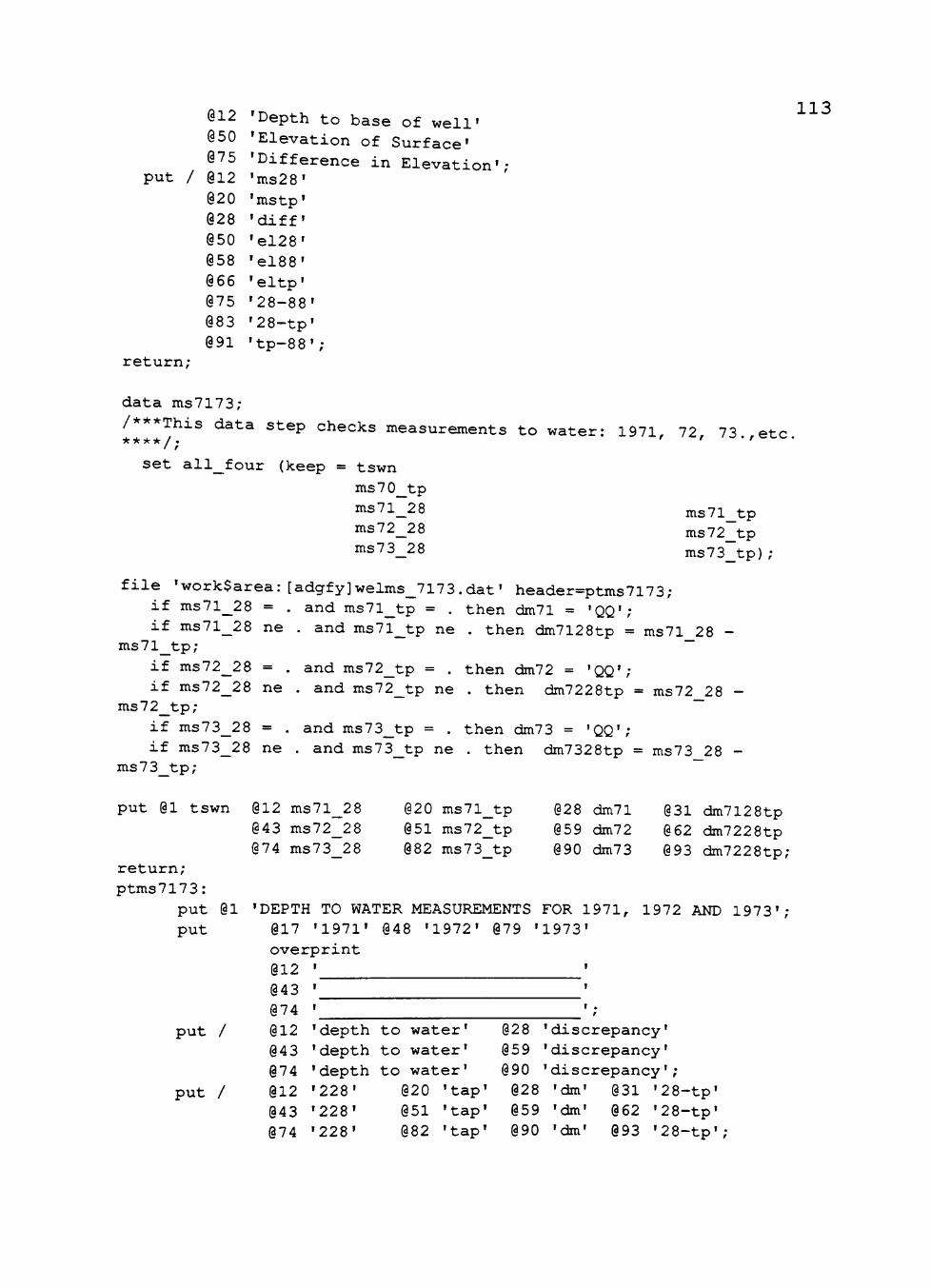
put

return

/

L;

012 ' 050 ' 075 ' 012 • 020 ' 028 ' 050 ' 058 ' 066 • 075 • 083 • 091 •

Depth to base of well' Elevation of Surface' Difference in Elevation'; ms28' mstp' diff el28' el88' eltp' 28-88' 28-tp' tp-88';

113

data ms7173;

/***This data step checks measurements to water; **** /.

set all_four (keep = tswn

ms70_tp ms71_28 ms72_28 ms73 28

1971, 72, 73.,etc

ms71_tp ms72_tp ms73_tp);

file 'work$area:[adgfy]welms_7173.dat' header=ptms7173; if ms71_28 = . and ms71_tp = . then dm71 = 'QQ';

and ms71 tp ne if ms71_28 ne ms 7l_tp;

if ms72_28 = if ms72_28 ne

ms72_tp; if ms73_28 = if ms73_28 ne

ms 7 3 tp;

and ms72_tp = . , and ms72_tp ne

and ms73_tp = . and ms73 tp ne

. then dm7128tp = ms71_28 -

then dm72 = 'QQ'; . then dm7228tp = ms72_28 -

then dm73 = 'QQ'; . then c3m7328tp = ms73 28 -

put 01 tswn

return; ptms7173:

put put

01

put /

put /

012 ms71_28 020 ms71_tp 028 dm71 043 ms72_28 051 ms72_tp 059 dm72 074 ms73_28 082 ms73 tp 090 dm73

'DEPTH TO WATER MEASUREMENTS FOR 1971, 017 '1971' 048 '1972' 079 '1973' overprint 012 ' '

043 074 012 043 074 012 043 074

031 dm7128tp 062 dm7228tp 093 dm7228tp;

1972 AND 1973';

'depth to water' 'depth to water' 'depth to water' '228' 020 'tap' '228' 051 'tap' '228' 082 'tap'

028 'discrepancy' 059 'discrepancy' 090 'discrepancy'; 028 'dm' 031 '28-tp' 059 'cim' 062 '28-tp' 090 'dm' 093 •28-tp';

114 put;

return;

data ms7475;

/*** This data step checks measurements for 1974 andl975 *********/; set all_four (keep = tswn ms74_28 ms74_po ms74 tp ms75 28 ms75 po

ms75_tp) ; — _ _

file 'work$area:[adgfy3welms_7475.dat' header=ptms7475; if ms74_28 = . and ms74_po = . and ms74_tp = . then dm74 = 'QQ'; if ms74_28 ne . and ms74_po ne . then dm7428po = ms74_28 -

ms74_po;

if ms74_28 ne . and ms74_tp ne . then dm7428tp = ms74_28 -ms74_tp;

if ms74_po ne . and ms74_tp ne . then dm74potp = ms7 4_po -ms74_tp;

if ms75_28 = . and ms75_po = . and ms75_tp = . then dm75 = 'QQ'; if ms75_28 ne . and ms75_po ne . then dm7528po = ms75_28 -

ms75_po;

if ms75_28 ne . and ms75_tp ne . then dm7528tp = ms75_28 -ms75_tp;

if ms75_po ne . and ms75_tp ne . then dm75potp = ms75_po -ms 7 5_tp;

put 01 tswn 012 ms74_28 020 ms74_po 028 ms74_tp 036 dm74 039 dm7428po 047 dm7428tp 055 dm74potp 066 ms75_28 074 ms75_po

082 ms75_tp 090 dm75 093 dm7528po 0101 dm7528tp 0109 dm75potp; return;

ptms7475: put 01 'DEPTH TO WATER MEASUREMENTS FOR 1974 AND 1975'; put 017 '1974' 070 '1975'

overprint 012 ' ' 066 ' ';

put 012 'Depth to Water' 036 'Discrepancies' 066 'Depth to Water' 090 'Discrepancies' overprint 012 ' ' 036

put 012 '228' 020 'p/o' 028 'tap' 036 'dm' 039 '28-po' 047 •28-tp' 055 'po-tp' 066 '228' 074 'p/o' 082 'tap' 090

'dm' 093 '28-po' 0101 '28-tp' 0109 'po-tp'; put;

return;

data ms7677; /*** This data step checks measurements for 1976 and 77 ***********/;

set all four (keep = tswn ms76_28 ms76_po ms76_tp ms77_28 s77_po ~ ms77 tp);

115 file 'work$area:[adgfy]welms_7677.dat' header=ptms7677;

If ms76_28 = . and ms76_po = . and ms76_tp = . then dm76 = 'QQ'; If ms76_28 ne . and ms76_po ne . then dm7628po = ms76 28 -

ms7 6_po; ~

if ms7 6_28 ne . and ms7 6_tp ne . then dm7 628tp = ms7 6 28 -ms 7 6_tp; ~

if ms7 6_po ne . and ms7 6_tp ne . then dm7 6potp = ms7 6 po -ms7 6_tp;

if ms77_28 = . and ms77_po = . and ms77_tp = . then dm77 = 'QQ'; if ms77_28 ne . and ms77_po ne . then dm7728po = ms77_28 -

ms77_po;

if ms77_28 ne . and ms77_tp ne . then cim7728tp = ms77_28 -ms77_tp;

if ms77_po ne . and ms77_tp ne . then dm77potp = ms77_po -ms77_tp;

put 01 tswn 012 ms76_28 020 ms76_po 028 ms76_tp 036 dm76 039 dm7628po 047 dm7628tp 055 dm76potp 066 ms77_28 074 ms77_po 082 ms77_tp 090 dm77 093 dm7728po 0101 dm7728tp 0109 dm77potp;

return;

ptms7 677:

put 01 'DEPTH TO WATER MEASUREMENTS FOR 197 6 AND 1977'; put 017 '1976' 070 '1977'

overprint 012 ' ' 066 ' ';

put 012 'Depth to Water' 036 'Discrepancies' 066 'Depth to Water' 090 'Discrepancies' overprint 012 ' • 036

put 012 '228' 020 'p/o' 028 'tap' 036 'dm' 039 '28-po' 047 '28-tp' 055 'po-tp' 066 '228' 076 'p/o' 082 'tap' 090 'dm' 093 '28-po' 0101 '28-tp' 0109 'po-tp';

put; return;

data ms7879;

/***This data step checks measurements to water: 1978, 79. ******/;

set all four (keep = tswn ms78_28 ms78_tp ms79_28 ms7 9_tp) ; file 'work$area:[adgfy]welms_7879.dat' header=ptms7879;

if ms78_28 = . and ms78_tp = . then dm78 = 'QQ'; if ms78_28 ne . and ms78_tp ne . then dm7828tp = ms78_28 -

ms7 8_tp; if ms79_28 = . and ms79_tp = . then dm79 = 'QQ';

if ms79_28 ne . and ms79_tp ne . then dm7928tp = ms79_28 -

ms7 9_tp;

116 put 01 tswn 012 ms78_28 020 ms78_tp 028 dm78 031 dm7828tp

043 ms79_28 051 ms79_tp 059 dm79 062 dm7928tp; return; ptms7879:

put 01 'DEPTH TO WATER MEASUREMENTS FOR 1978 AND 1979'; put 017 '1978' 048 '1979'

overprint 012 ' I 043 ' " ' I.

put / 012 'depth to water' 028 'discrepancy' 043 'depth to water';

put / 012 '228' 020 'tap' 028 'dm' 031 '28-tp'; put;

return;

data ms8000;

/*** This data step checks measurements for 1980. ************/; set all_f our (keep = tswn ms80_po ms80_88 ms80_tp) ; file 'work$area:[adgfy]welms_8000.dat' header=ptms8000;

if ms80_po = . and ms80_88 = . and ms80_tp = . then dm80 = 'QQ'; if ms80_po ne . and ms80_88 ne . then dm80po88 = ms80_po -

ms80_88; if ms80_po ne . and ms80_tp ne . then c3m80potp = ms80_po -

ms80_tp; if ms80_88 ne . and ms80_tp ne . then cim8088tp = ms80_88 -

ms 8 0_tp;

put 01 tswn 012 ms80_po 020 ms80_88 028 ms80_tp 036 dm80 039 dm80po88 047 dm80potp 055 dm8088tp;

return;

ptms8000:

put 01 'DEPTH TO WATER MEASUREMENTS FOR 1980'; put 017 '1980'

overprint 012 ' '

put 012 'Depth to Water' 036 'Discrepancies' overprint @12 ' ' 036

I

put 012 'p/o' 020 '288' 028 'tap' 036 'dm' 039 'po-88' 047 'po-tp' 055 '88-tp';

put; return;

data ms8184; /***This data step checks measurements to water: 1981, 82, 83 and 84 ******/•

set all_four (keep = tswn ms81_po ms81_tp ms82_po ms82_tp ms83_po ms83_tp ms84_po ms84_tp);

file •work$area:[adgfy]welms_8184.dat' header=ptms8184; if ms81_po = . and ms81_tp = . then dm81 = 'QQ';

. then dmSlpotp = ms81_po -

1 1 7

i f ms81_po ne ms 8 l _ t p ;

if ms82_po = if ms82_po ne

ms82_tp; if ms83_po = if ms83_po ne

ms83_tp; if ms84_po = if ms84_po ne

ms84 tp;

and ms81_tp ne

and ms82_tp = . , and ms82_tp ne

and ms83_tp = . , and ms83_tp ne

and ms84_tp = . , and ms84 tp ne

then dm82 = 'QQ'; . then dm82potp = ms82_po -

then dm83 = 'QQ'; . t h e n c3m83potp = ms83_po -

t h e n dm84 = ' Q Q ' ; . then dm84potp = ms84_po -

put 01 tswn 012 ms8l_po 043 ms82_po 074 ms83_po

0106 ms84 po

020 ms81_tp 051 ms82_tp 082 ms83_tp

0114 ms84 tp

028 dm81 059 dm82 090 cim83

0122 dm84

031 dm81potp 062 cam82potp 093 dm83potp

0125 dm84potp; return;

ptms8184: put

1984'; put

01

put /

put /

•DEPTH TO WATER MEASUREMENTS FOR 1981, 1982, 1983

017 '1981' 048 '1982' 079 '1983' 0111 '1984' overprint 012 • ' 043 • ' 074 • '

0106 ' •; 012 043 074

0106 012 043 074

0106

AND

'depth to water' 'depth to water' •depth to water' •depth to water' 'p/o' 'p/o' 'p/o' 'p/o'

020 051 082

0114

'tap' 'tap' 'tap' 'tap'

028 059 090

0122 028 059 090 0122

'discrepancy' 'discrepancy' 'discrepancy' 'discrepancy'; 'dm' 'dm' 'dm' 'dm'

031 062 093 0125

'po-tp' 'po-tp' 'po-tp• 'po-tp';

put; return;

data ms8588; /***This data step checks measurements to water: 1985, 86, 87 and 88 ******/;

set all four (keep = tswn ms85_po ms85_tp ms86_po ms86_tp ~ ms87_po ms87_tp ms88_po ms88_tp) ;

file 'work$area:[adgfyjwelms_8588.dat' header=ptms8588;

if ms85_po = . and ms85_tp = . then dm85 = 'QQ';

if ms85_po ne . and ms85_tp ne . then dm85potp = ms85_po -

ms 8 5 tp;

if ms86_po = . if ms8 6_po ne

ms 8 6_tp; if ms87_po = , if ms87_po ne

ms87_tp; if ms88_po = , if ms88_po ne

ms88_tp;

118

put 01 tswn

and ms86_tp = . and ms8 6_tp ne

and ms87_tp = . , and ms87_tp ne

and ms88_tp = . , and ms88 tp ne

t h e n dm86 = ' Q Q ' ; . t h e n dm86potp = ms86_po -

t h e n citi87 = ' Q Q ' ; . t h e n cim87potp = ms87_po -

t h e n dm88 = ' Q Q ' ; . then dm88potp = ms88 po -

return;

012 ms85_po 04 3 ms86_po 074 ms87_po 0106 ms88_po

020 ms85_tp 051 ms86_tp 082 ms87_tp 0114 ms88 tp

028 dm85 059 dm86 090 dm87

0122 dm88

031 dm85potp 062 dm86potp 093 dm8 7potp 0125 dm88potp;

ptms8588:

put 01 'DEPTH TO WATER MEASUREMENTS FOR 1985, 1986, 1987 AND 1988' ;

put

put /

put /

put, return; run;

017 '1985' overprint 012 '

048 '1986' 079 '1987' 0111 '1988

043 074

0106 012 043 074 0106 012 043 074 0106

'depth to water' 'depth to water' 'depth to water' 'depth to water' 'p/o' 'p/o' •p/o' 'p/o'

020 051 082

0114

'tap' 'tap' 'tap' 'tap'

028 059 090

0122 028 059 090 0122

'discrepancy' 'discrepancy' 'discrepancy' 'discrepancy'; 'dm' 'dm' 'dm' 'dm'

031 062 093

0125

'po-tp' 'po-tp' 'po-tp' 'po-tp';

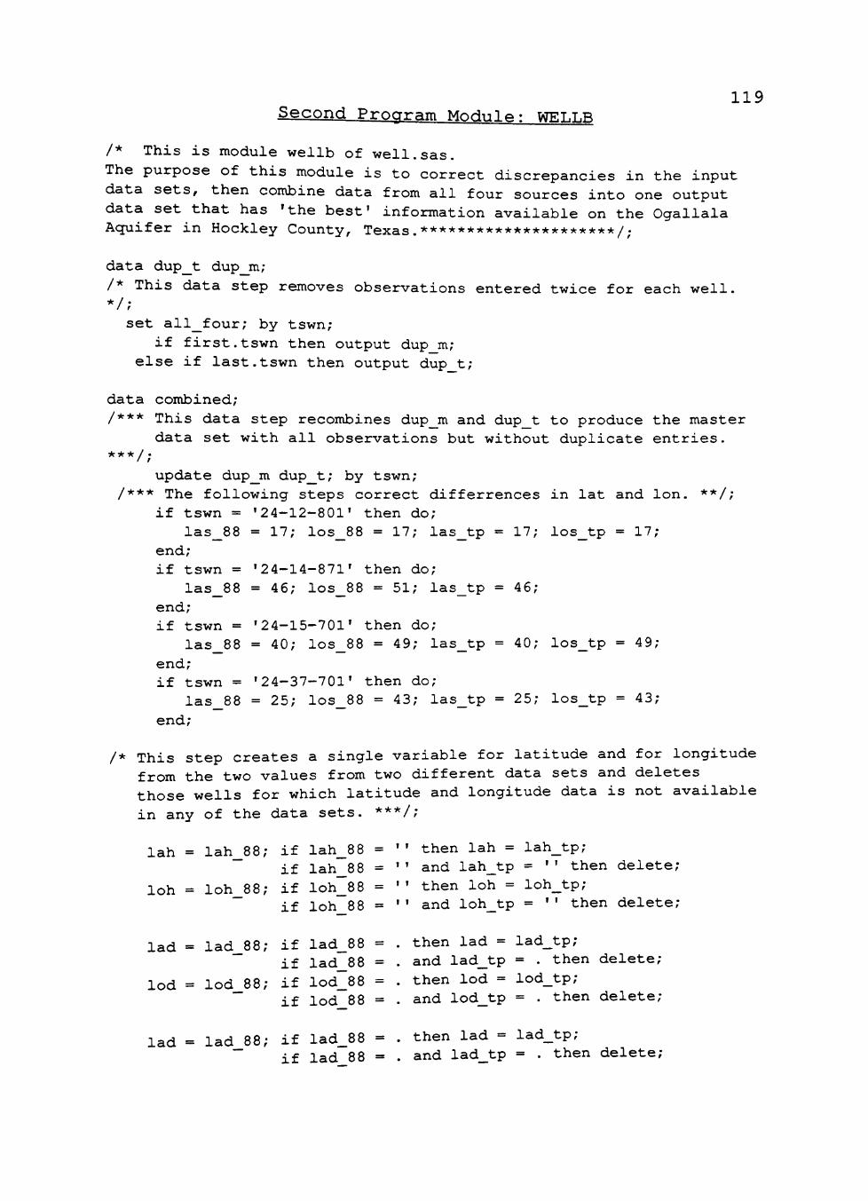
119 Second Program Module: WELLB

/* This is module wellb of well.sas.

The purpose of this module is to correct discrepancies in the input data sets, then combine data from all four sources into one output data set that has 'the best' information available on the Ogallala Acjuifer in Hockley County, Texas.*********************/.

data dup_t dup_m;

/* This data step removes observations entered twice for each well. */;

set all_four; by tswn; if first.tswn then output dup_m;

else if last.tswn then output dup_t;

data combined; /*** This data step recombines dup_m and dup_t to produce the master

data set with all observations but without duplicate entries. ***/;

update dup_m dup_t; by tswn; /*** The following steps correct differrences in lat and lon. **/;

if tswn = '24-12-801' then do; las_88 = 17; los_88 = 17; las_tp = 17; los_tp = 17;

end; if tswn = '24-14-871' then do;

las_88 = 46; los_88 = 51; las_tp = 46; end; if tswn = '24-15-701' then do;

las_88 = 40; los_88 = 49; las_tp = 4 0 ; los_tp = 4 9; end; if tswn = '24-37-701' then do;

las_88 = 25; los_88 = 4 3 ; las_tp = 2 5 ; los_tp = 4 3 ;

end;

/* This step creates a single variable for latitude and for longitude from the two values from two different data sets and deletes those wells for which latitude and longitude data is not available in any of the data sets. ***/;

lah = lah_88; if lah_88 = " then lah = lah_tp; if lah_88 = '' and lah_tp = '' then delete;

loh = loh_88; if loh_88 = '' then loh = loh_tp; if loh_88 = '' and loh_tp = '' then delete;

lad = lad_88; if lad_88 = . then lad = lad_tp; if lad_88 = . and lad_tp = . then delete;

lod = lod_88; if lod_88 = . then lod = lod_tp; if lod_88 = . and lod_tp = . then delete;

lad = lad 88; if lad_88 = . then lad = lad_tp; if lad 88 = . and lad_tp = . then delete;

120 lod = lod_88; if lod_88 = . then lod = lod_tp;

if lod_88 = . and lod_tp = . then delete; lam = lam_88; if lam_88 = . then lam = lam_tp;

if lam_88 = . and lam_tp = . then delete; lorn = lom_88; if lom_88 = . then lorn = lom_tp;

if lom_88 = . and lom_tp = . then delete; las = las_88; if las_88 = . then las = las_tp;

if las_88 = . and las_tp = . then delete; los = los_88; if los_88 = . then los = los_tp;

if los_88 = . and los_tp = . then delete;

/** The following steps correct for elevation of surface differrences. The corrected output variable is 'els'. **/;

if els_28 ne . and els_tp = . then els = els_28; else if els_28 = . and els_tp ne . then els = els_tp; else if els_28 ne . and els_tp ne . then do;

if els_28 = els_tp then els = els_tp; else if tswn = '24-15-507' then els = els_tp; else if tswn = '24-24-401' then els = els_tp; end;

/** The following steps use the corrected elevation of surface data to produce variables that express the depth to water in terms of the elevation of the head of the ac^uifer. The output variables created are 'hdyy' where 'yy' represents the measurement year. **/;

/** Produce a single value for depth to water (msyy, yy = year). **/;

ms70 = ms70_tp; /*** in the data sets being used there is ***/; ms84 = ms84_tp; /*** only one value for these years. ***/; ms85 = ms85_tp; ms8 6 = ms86_tp; ms87 = ms87_tp; ms88 = ms88_tp;

do count = 1 to 13 by 1;

if count = 1 then do; x28 = ms71_28; xpo = ms71_po; x88 = ms71_88; xtp = ms71_tp;

goto cases; end; else if count = 2 then do;

x28 = ms72_28; xpo = ms72_po; x88 = ms72_88; xtp = ms72_tp;

goto cases; end; else if count = 3 then do;

x28 = ms73_28; xpo = ms73_po; x88 = ms73_88; xtp = ms73_tp; goto cases;

end; else if count = 4 then do;

x28 = ms74 28; xpo = ms74_po; x88 = ms74_88; xtp = ms74_tp;

121 goto cases;

end;

else if count = 5 then do;

x28 = ms75_28; xpo = ms75_po; x88 = ms75 88; xtp = ms75 tp; goto cases; — _ -f

end;

else if count = 6 then do; x28 = ms76_28; xpo = ms76_po; x88 = ms76 88; xtp = ms76 tp; goto cases; ~ -

end;

else if count = 7 then do;

x28 = ms77_28; xpo = ms77_po; x88 = ms77_88; xtp = ms77 tp; goto cases; ~

end;

else if count = 8 then do;

x28 = ms78_28; xpo = ms78_po; x88 = ms78_88; xtp = ms78 tp; goto cases; ~

end;

else if count = 9 then do; x28 = ms79_28; xpo = ms79_po; x88 = ms79_88; xtp = ms79_tp; goto cases;

end; else if count = 1 0 then do;

x28 = ms80_28; xpo = ms80_po; x88 = ms80_88; xtp = ms80_tp; goto cases;

end; else if count = 11 then do;

x28 = ms81_28; xpo = ms81_po; x88 = ms8l_88; xtp = ms81_tp; goto cases;

end; else if count = 12 then do;

x28 = ms82_28; xpo = ms82_po; x88 = ms82_88; xtp = ms82_tp; goto cases;

end; else if count = 13 then do;

x28 = ms83_28; xpo = ms83_po; x88 = ms83_88; xtp = ms83 tp; goto cases;

end;

cases

/** CaseO: All annual measurements are missing for a given well. **/ if x28 = . and xpo = . and x88 = . and xtp = . then msyr = .

/* Casel: Only one annual measurement is present for a given well.*/ else if x28 = . and xpo = . and x88 = . and xtp ne . then msyr =

xtp; else if x28 ne . and xpo = . and x88 = . and xtp = . then msyr

x28; else if x28 = . and xpo ne . and x88 = . and xtp = . then msyr =

xpo;

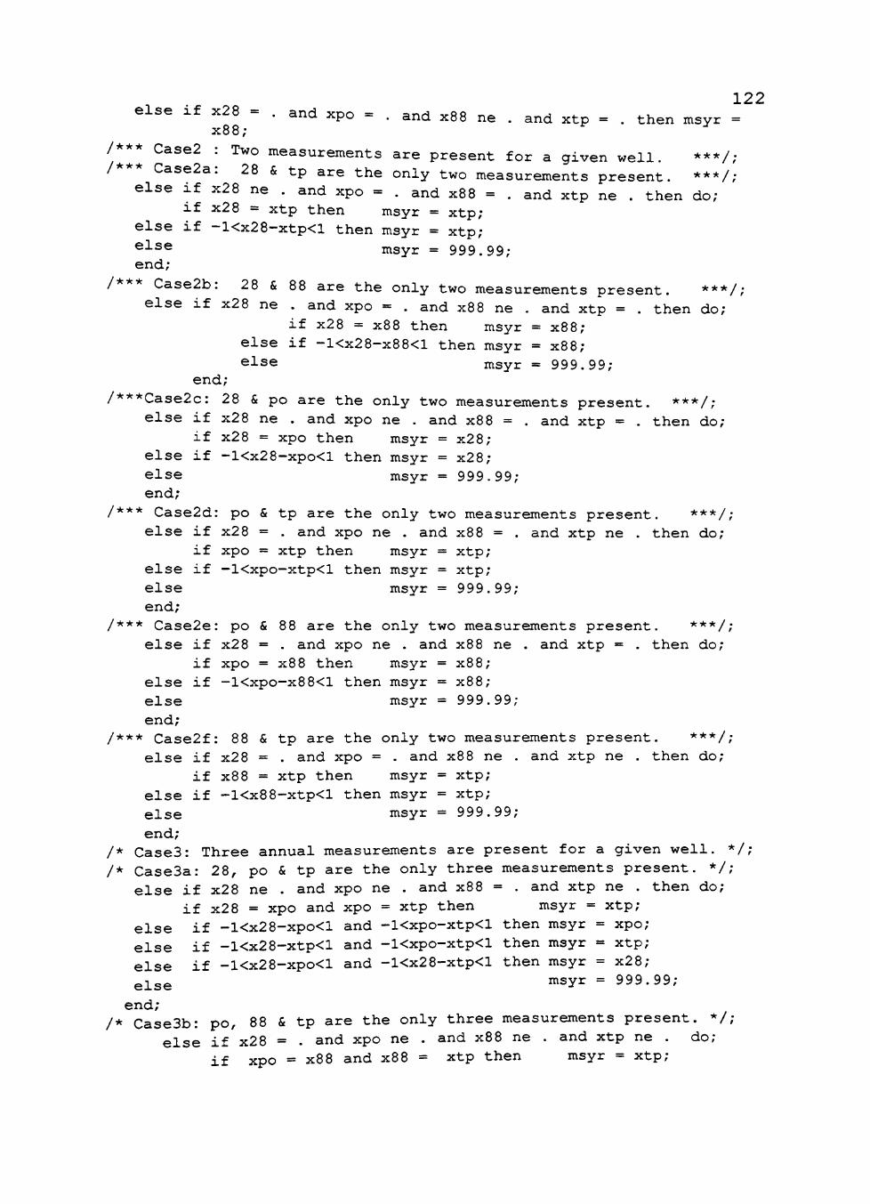
122 else If x28 - . and xpo = . and x88 ne . and xtp = . then msyr =

x88; ^

/*** Case2 : Two measurements are present for a given well. ***/; /*** Case2a: 28 & tp are the only two measurements present. ***/;

else if x28 ne . and xpo = . and x88 = . and xtp ne . then do; if x28 = xtp then msyr = xtp;

else if -l<x28-xtp<l then msyr = xtp;

else msyr = 999.99; end;

/*** Case2b: 28 & 88 are the only two measurements present. ***/; else if x28 ne . and xpo = . and x88 ne . and xtp = . then do;

if x28 = x88 then msyr = x88; else if -I<x28-x88<l then msyr = x88; else msyr = 999.99;

end;

/***Case2c: 28 & po are the only two measurements present. ***/; else if x28 ne . and xpo ne . and x88 = . and xtp = . then do;

if x28 = xpo then msyr = x28; else if -l<x28-xpo<l then msyr = x28; else msyr = 999.99;

end;

/*** Case2d: po & tp are the only two measurements present. ***/; else if x28 = . and xpo ne . and x88 = . and xtp ne . then do;

if xpo = xtp then msyr = xtp; else if -l<xpo-xtp<l then msyr = xtp; else msyr = 999.99; end;

/*** Case2e: po & 88 are the only two measurements present. ***/; else if x28 = . and xpo ne . and x88 ne . and xtp = . then do;

if xpo = x88 then msyr = x88; else if -Kxpo—x88<l then msyr = x88; else msyr = 999.99; end;

/*** Case2f: 88 & tp are the only two measurements present. ***/; else if x28 = . and xpo = . and x88 ne . and xtp ne . then do;

if x88 = xtp then msyr = xtp; else if -l<x88-xtp<l then msyr = xtp; else msyr = 999.99;

end; /* Case3: Three annual measurements are present for a given well. */; /* Case3a: 28, po & tp are the only three measurements present. */;

else if x28 ne . and xpo ne . and x88 = . and xtp ne . then do; if x28 = xpo and xpo = xtp then msyr = xtp;

else if -l<x28-xpo<l and -l<xpo-xtp<l then msyr = xpo; else if -l<x28-xtp<l and -l<xpo-xtp<l then msyr = xtp; else if -l<x28-xpo<l and -l<x28-xtp<l then msyr = x28; else ^sy^ = 999.99;

end; /* Case3b: po, 88 & tp are the only three measurements present. */;

else if x28 = . and xpo ne . and x88 ne . and xtp ne . do; if xpo = x88 and x88 = xtp then msyr = xtp;

. and xtp msyr =

then msyr = then msyr = then msyr =

msyr =

ne . xtp; = x28; = xtp; = x88; = 999.

then

99;

do;

123 else if -l<x88-xpo<l and -l<xpo-xtp<l then msyr = xpo; else if -l<x88-xtp<l and -l<xpo-xtp<l then msyr = xtp; else if -l<x88-xpo<l and -l<x88-xtp<l then msyr = x88; ^Ise insyr = 999.99; end;

/* Case3c: 28, 88 & tp are the only three measurements present. */; else if x28 ne . and xpo = . and x88 ne

if x28 = x88 and x88 = xtp then else if -I<x88-x28<l and -l<x28-xtp<l else if -l<x88-xtp<l and -l<x28-xtp<l else if -I<x88-x28<l and -l<x88-xtp<l else end;

/* Case3d: 28, po & 88 are the only three measurements present. */; else if x28 ne . and xpo ne . and x88 ne . and xtp = . then do;

if xpo = x88 and x88 = x28 then msyr = x28; else if -l<x88-xpo<l and -l<xpo-x28<l then msyr = xpo; else if -I<x88-x28<l and -l<xpo-x28<l then msyr = x28; else if -l<x88-xpo<l and -I<x88-x28<l then msyr = x88; else msyr = 999.99;

end; if count = 1 then ms71 = msyr;

else if count = 2 then ms72 = msyr; else if count = 3 then ms7 3 = msyr; else if count = 4 then ms74 = msyr; else if count = 5 then ms75 = msyr; else if count = 6 then ms7 6 = msyr; else if count = 7 then ms77 = msyr; else if count = 8 then ms7 8 = msyr; else if count = 9 then ms7 9 = msyr; else if count = 10 then ms80 = msyr; else if count = 1 1 then ms81 = msyr; else if count = 12 then ms82 = msyr; else if count = 13 then ms83 = msyr;

/* This step corrects for unicjue discrepancies between data sets. */; if tswn = '24-14-901' then ms76 = 97.61; if tswn = '24-15-504' then ms77 = 69.29; if tswn = '24-20-701' then ms75 = 147.74;

/* This step converts depth-to-water values into elevation above msl

values.*/; ms 7 0; ms71; ms 72; ms 7 3; ms74; ms75; ms 7 6; ms77; ms78; ms7 9; ms80;

hd70 hd71 hd72 hd73 hd74 hd75 hd7 6 hd77 hd78 hd7 9 hd80

=

=

=

=

=

=

=

=

=

=

=

els els els els els els els els els els els

124 hd81 hd82 hd83 hd84 hd85 hd86 hd87 hd88

end;

=

=

=

=

=

=

=

=

els els els els els els els els

—

—

—

—

—

—

—

—

ms81 ms82 ms83 ms84 ms85 ms86 ms87 ms88

/*** This step creates a single variable for the elevation of the base of the acjuifer. It first coverts the depth-to-base-of-the-aquifer measurement in welltap.dat to elevation above msl; then compares the two elevation values from well288.dat and welltap.dat; if there is a difference it prints out the difference. ***/;

elbaq_tp = els - msbaq_tp; if elbac3_88 = . and elbaq^tp = . then elbaq = .;

else if elbac^88 ne . and elbaq_tp = . then elbaq = elbaq_88; else if elbaq_88 = . and elbaq_tp ne . then elbaq = elbaq_tp; else if elbaq_88 ne . and elbaq^tp ne . then do;

if elbaq_88 = elbaq_tp then elbaq = elbaq^tp; else if l<elbaq_88-elbaq_tp<-l then elbaq = 999.99; else if -l<elbaq_88-elbac3^tp<l then elbaq = elbaq_tp;

end; /***

proc print; var tswn lah lad lam las loh lod lorn los elbaq; proc print; var tswn hd70 hd71 hd72 hd73 hd74 hd75 hd7 6 hd77 hd78 hd7 9; proc print; var tswn hd80 hdSl hd82 hd83 hd84 hd85 hd86 hd87 hd88;

***/;

/**** This datastep creates an output datafile with basic information for all wells for which a latitude and longitude are recorded. ***/;

data master; set combined (keep = tswn lah lad lam las loh lod lom los els elbaq

hd70 hd71 hd72 hd73 hd74 hd75 hd76 hd77 hd78 hd7 9 hd80 hd81 hd82 hd83 hd84 hd85 hd86 hd87 hd88);

file •work$area:[adgfy]well_master.dat•;

put #1 01 tswn $9. 010 lah $1. 011 lad z2. 013 lam z2. 015 las z2 017 loh $1. 018 lod z3. 021 lom z2. 023 los z2. 025 els 4 029'elbaq 4. 033 hd70 7.2 040 hd71 7.2 047 hd72 7.2 054 hd73 7.2 061 hd74 7.2 068 hd75 7.2 075 hd76 7.2 082 hd77 7.2 089 hd78

7.2 096 hd79 7.2

#2 033 hd80 7.2 040 hd81 7.2 047 hd82 7.2 054 hd83 7.2 061

hd84 7.2 068 hd85 7.2 075 hd86 7.2 082 hd87 7.2 089 hd88 7.2;

run;

Third Program Module: WF.T.T.M

/* This is module wellm of well.sas.*/; /* It checks for unique errors and creates a master

output file in ERDAS .DIG file format. */;

data master;

infile 'userl:[adgfy.data]well_master.dat'; missing _ ;

input #1 01 tswn $9. 010 lah $1. 0li lad 2 017 loh $1. 018 lod 3. 021 lom 2. 025 els 4. 029 elbaq 4. 033 hd70 7.2

054 hd73 7.2 061 hd74 7.2 068 hd75 7.2 089 hd78 7.2 096 hd79 7.2

#2 033 hd80 7.2 040 hd81 7.2 047 hd82 7.2 054 hd83 7.2 061 hd84 7.2 068 hd85 7.2 075 hd86 7.2 082 hd87 7.2 089 hd88 7.2;

125

013 lam 2. 015 las 2. 023 los 2. 040 hd71 7.2 047 hd72 7.2

075 hd76 7.2 082 hd77 7.2

/*** Round all integer.**/;

if hd70 ne if hd71 ne '_ if hd72 ne ̂ if hd73 ne ̂ if hd74 ne if hd75 ne if hd7 6 ne if hd77 ne ' if hd78 ne '_ if hd79 ne if hd80 ne if hd81 ne if hd82 ne if hd83 ne if hd84 ne if hd85 ne if hd8 6 ne if hd87 ne if hd88 ne

decimal values to the nearest whole foot; convert to

then then then then then then then then then then then then then then then then then then then

hd70 hd71 hd72 hd73 hd74 hd75 hd7 6 hd77 hd78 hd79 hd80 hd81 hd82 hd83 hd84 hd85 hd86 hd87 hd88

round round round round round round round round round round round round round round round round round round round

(hd70,l (hd71,l (hd72,l (hd73,l (hd74,l (hd75,l (hd76,l (hd77,l (hd78,l (hd79,l (hd80,l (hd81,l (hd82,l (hd83,l (hd84,l (hd85,l (hd86,l (hd87,l (hd88,l

/** Convert standard latitude and longitude to decimal degrees. **/; las)/3600); = laddecl *

laddecl = lad + (((lam * 60) + if lah = •N^ then laddec

else if lah = 'S' then laddec = laddecl * loddecl = lod + (((lom * 60) + los)/3600);

if loh = 'E' then loddec = loddecl *

1; -1;

1; else if loh = 'W' then loddec = loddecl * -1;

/*** Determine the ranges of values for each variable. ***/;

proc means n min max range; var laddec loddec els elbaq hd70 hd71

hd72 hd73 hd74 hd75 hd76 hd77 hd78 hd79 hd80 hd81 hd82 hd83 hd84 hd85

hd8 6 hd87 hd88;

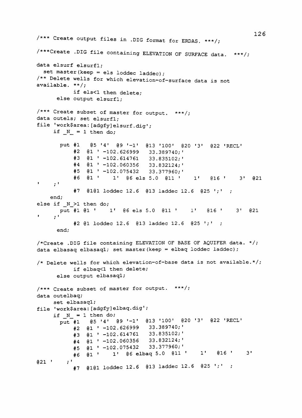
/*** Create output files in .DIG format for ERDAS. ***/;

/***Create .DIG file containing ELEVATION OF SURFACE data. ***/;

data elsurf elsurfl;

set master(keep = els loddec laddec); /** Delete wells for which elevation-of-surface data is not available. **/;

if els<l then delete; else output elsurfl;

126

/*** Create subset of master for output, data outels; set elsurfl; file 'work$area: [adgfy]elsurf.dig';

if _N_ = 1 then do;

*** / • /;

put #1 05 #2 01 #3 01 #4 01 #5 01 #6 01

'4' 09 '-1' 013 '100' 020 '3' 022 'RECL' -102.626999 33.389740;' -102.614761 33.835102, -102.060356 33.832124, -102.075432 33.377960,

1' 06 els 5.0 011 ' 1' 016 021

#7 0101 loddec 12.6 013 laddec 12.6 025 ';' end;

else if _N_>1 then do; put #1 01 ' 1̂ 06 els 5.0 011 • 1' 1' 016 •

#2 01 loddec 12.6 013 laddec 12.6 025 ';' end;

021

/*Create .DIG file containing ELEVATION OF BASE OF AQUIFER data. */; data elbasaq elbasaql; set master(keep = elbaq loddec laddec);

/* Delete wells for which elevation-of-base data is not available.*/; if elbaq<l then delete;

else output elbasaql;

/*** Create subset of master for output

data outelbaq; set elbasaql;

file 'work$area: [adgfy]elbaq.dig'; if N = 1 then do;

:**/;

put #1 05 » A » 09 '-1' 013 '100' 020 '3' 022 'RECL'

#2 01 #3 01 #4 01 #5 01 #6 01

-102.626999 -102.614761 -102.060356 -102.075432

33.389740 33.835102 33.832124 33.377960

1' 06 elbaq 5.0 011 • 016

021 #7 0101 loddec 12.6 013 laddec 12.6 025 •;'

127 end;

else if _N_>1 then do;

put #1 01 ' !• @6 elbaq 5.0 011 ' i' @16 ' 3' 021 ' ;'

#2 01 loddec 12.6 013 laddec 12.6 025 ';' ; end;

/***Create .DIG file containing ELEVATION OF 1974 HEAD OF AQUIFER data. ***/;

data elhd74 elhd741; set master(keep = hd74 loddec laddec);

/*** Delete wells for which elevation-of-1974 head data is not available. ***/;

if hd7 4<l then delete; else output elhd741;

/*** Create subset of master for output. ***/; data outhd74;

set elhd741;file 'work$area: [adgfy]elhd74.dig'; if _N_ = 1 then do;

put #1 05 '4' 09 '-1' 013 '100' 020 '3' 022 'RECL' -102.626999 33.389740 -102.614761 33.835102 -102.060356 33.832124 -102.075432 33.377960

1' 06 hd74 5.0 011

#2 01 #3 01 #4 01 #5 01 #6 01 ' 1' 06 hd74 5.0 011 ' 1' 016 ' 3'

021 ' ; '

#7 0101 loddec 12.6 013 laddec 12.6 025 ';' ; end;

else if _N_>1 then do; put #1 01 ' 1' 06 hd74 5.0 011 ' 1' 016 ' 3' 021

I . t r

#2 01 loddec 12.6 013 laddec 12.6 025 ';' ; end;

/***Create .DIG file containing ELEVATION OF 1978 HEAD OF AQUIFER data. ***/;

data elhd78 elhd781; set master(keep = hd78 loddec laddec);

/*** Delete wells for which elevation-of-1978 head data is not

available.***/; if hd78<l then delete;

else output elhd781;

/*** Create subset of master for output. ***/; data outhd78; set elhd781; file 'work$area:[adgfy]elhd78 .dig';

if _N_ = 1 then do; put #1 05 '4' 09 '-1' 013 '100' 020 '3' 022 'RECL'

#2 #3 #4 #5 #6

01 ' 01 • 01 • 01 ' 01 •

-102.626999 -102.614761 -102.060356 -102.075432

33.389740 33.835102 33.832124 33.377960

128

021

#7 end;

1' 06 hd78 5.0 011 '

0101 loddec 12.6 013 laddec 12.6 025

016

I . I

else if _N_>1 then do;

put #1 01 • 1. @6 hd78 5.0 011 •

end;

1' 016 ' 3' 021

#2 01 loddec 12.6 013 laddec 12.6 025 ';' ;

dltl^""***/."^^^ ^^^^ containing ELEVATION OF 1980 HEAD OF AQUIFER

data elhd80 elhd801;

set master(keep = hd80 loddec laddec) ;

/*** Delete wells for which elevation-of-1980 head data is not available.***/;

if hd80<l then delete; else output elhd801;

/*** Create subset of master for output. ***/; data outhd80; set elhd801; file 'work$area: [adgfy]elhdSO.dig';

if _N_ = 1 then do; put #1 05 '4' 09 '-1' 013 '100' 020 '3' 022 'RECL'

#2 01 ' -102.626999 #3 01 ' -102.614761 #4 01 ' -102.060356 #5 01 ' -102.075432

33.389740 33.835102 33.832124 33.377960

021 #6 01 •

#7

06 hd80 5.0 011

0101 loddec 12.6 013 laddec 12.6 025 end;

else if _N_>1 then do; put #1 01 • 1' 06 hd80 5.0 011 ' l'

016

» . I

end;

1' 016 '

#2 01 loddec 12.6 013 laddec 12.6 025 ';' ;

021

/***Create .DIG file containing ELEVATION OF 1982 HEAD OF AQUIFER data. ***/; data elhd82 elhd821; set master (keep = hd82 loddec laddec);

/*** Delete wells for which elevation-of-1982 head data is not

129 available.***/;

if hd82<l then delete; else output elhd821;

/*** Create subset of master for output. ***/; data outhd82; set elhd821; file 'work$area: [adgfy]elhd82.dig';

if _N_ = 1 then do; put #1 05 '4' 09 '-1' 013 '100' 020 '3' 022 'RECL'

#2 01 ' -102.626999 33.389740, #3 01 ' -102.614761 33.835102, #4 01 ' -102.060356 33.832124, #5 01 ' -102.075432 33.377960, #6 01 ' 1' 06 hd82 5.0 011 ' 1' 016 ' 3'

021 ' ; ' #7 0101 loddec 12.6 013 laddec 12.6 025 ';' ;

end; else if _N_>1 then do;

put #1 01 ' 1' 06 hd82 5.0 011 ' 1' 016 ' 3' 021 I . I

r

#2 01 loddec 12.6 013 laddec 12.6 025 ';' ; end;

run;