1

Evaluating the impact of CAP reforms on land use and the environment: a

two-step estimation with multiple selection rules and panel data.

François Bel(1), Anne Lacroix(2), François Salanié(3) and Alban Thomas(4)

This version January 30, 2006 Abstract. The latest reform of the Common Agricultural Policy (CAP) aims at making subsidies independent from crops and crop yields, so as to avoid distorsions in production choices. This evolution is likely to have important consequences on both the land use and the yields, and ultimately on water quality and soil contamination. Indeed nitrogen run-off depends not only on nitrogen application, but also on crops and crop yields. Consequently a detailed evaluation of environmental impacts of CAP reforms in the arable crop sector must take into account the multi-output nature of farms. In this paper, we estimate a microeconomic multi-output production model that is coupled to an environmental simulator for nitrate concentration in the soil. We propose a simple procedure for estimating a multi-output profit function, from which elasticities of land use, variable inputs and crop yields are easily computed as functions of prices and crop-specific subsidies. The estimation procedure addresses corner solutions in land use, the role of agricultural rotation dynamics in crop choice, and unobserved heterogeneity in structural and crop selection equations. The profit function with multiple selection rules and panel data is estimated on French FADN data for the years 1995-2001. Estimated elasticities are used to simulate the productive and environmental impacts of the current CAP reform. (1), (2): INRA-GAEL, University of Grenoble. (3), (4): INRA-LERNA, University of Toulouse. Corresponding author: Alban Thomas, thomas@toulouse.inra.fr

2

1. Introduction In the last 15 years, the Common Agricultural Policy (CAP) has experienced major structural changes. Concerning the most important crops, one of the most consequential evolution has made agricultural subsidies more lump-sum (decoupling), so as to avoid distortions in production choices. This evolution has been progressive: starting from a system in which interior prices were rigid, in 1992 prices were reduced and crop-specific subsidies based on land use were introduced (the so-called MacSharry Plan). This tendency was reinforced Agenda 2000; finally the recent Luxembourg compromise imposes a complete decoupling of subsidies and crop choices, since subsidies will no more be crop-specific in 2007.1 This final step will significantly impact agricultural land use and productions. It will also have important consequences on the environment since fertiliser and pesticide run-offs are likely to be affected by both changes in land use and intensification. These evolutions call for the development of models able to evaluate these different effects. Most existing models rely on aggregate data, and indeed allow to recover total demand and supplies as a function of the full price system, using a dual approach (see for example Guyomard et al., 1996). However, they do not allow for a discussion of regional effects. Such effects are important both because they condition the redistributive effect of the reform, and because the environmental damage associated with the use of nitrogen fertilisers is a local damage. Moreover, the relationship between input use and the final emission causing damage to the environment is far from direct, involving in particular climate and soil variables, but also cropping practices. For example, nitrogen concentration in groundwater depends not only on fertiliser application, but also on land use decisions and crop yields because part of the nitrogen applied is used by the plant itself and does not pollute2. As a result, two farmers with the same total nitrogen use may cause different environmental impacts, depending among other things on their allocation of crop land and ultimate crop yields. A last reason for using micro-economic data is that one would like to precisely take into account the role of history in crop choices; it is well-known that agricultural rotations constrain the farmers’ choices. Therefore this paper aims at developping a microeconomic multi-output production models for assessing the productive and environmental impacts of policy reforms. The need for such a model is widely acknowledged in the agricultural economics literature, as technological substitution and jointness patterns are particularly important in this sector, especially when environmental effects are at stake. In order to better capture the different technical aspects of production at work without resorting to an unduly sophisticated bio-physical model of crop growth, our approach follows two steps. First, the farmer production plan is defined from a micro-economic neo-classical model taking as exogenous variables, the whole system of prices and relevant policy instruments (subsidies) affecting private production. The impact of a policy reform can then be evaluated using standard tools from the duality principle applied to production. Second, an environmental impact simulator has been developped and linked to this economic model, that will compute a predicted environmental outcome taking as input parameters the control variables of the producer, such as land allocation, input use, etc. This paper focusses on the first stage; concerning the second stage we will only present a simple simulation experiment to illustrate the potential of the model regarding policy evaluation. 1 In the case of France, the decoupling will be incomplete since 25% of payments shall remain crop-specific. 2 Each crop has a characteristic content in nitrogen summarized in well-known crop-specific nitrogen uptake coefficients.

3

Applications closely related to our micro-economic model of production (Guyomard et al., 1996; Moro and Sckokai, 1999; Gullstrand, 2003) are concerned with the effect of decoupling aids from production, and not so much on environmental impacts of policy reforms. Guyomard et al. (1996) estimate a quadratic profit function with several crop groups and inputs on French aggregate data; hence the issue of crop rotation patterns and corner solutions in production is not discussed. Moro and Sckokai (1999), also with a normalised quadratic multi-output profit function but on Italian FADN data, do not exploit the panel data structure of their (individual) data set. Moreover, although they recognise the presence of possible sample selection in dealing with multiple crop groups, they do not control for these sample selection effects in an adequate fashion. Instead, Moro and Sckokai include in their profit share equations, dummy variables for the presence of other crops for the same year and the same farmer, as a crude way of considering multiple selection rules. Finally, Gullstrand (2003) uses FADN individual data over the period 1997-2000 without considering a panel data approach for estimating a quadratic profit function. To deal with censored dependent variables (shares), Gullstrand employs the partial Shonkwiler and Yen (1999) technique. To summarise on this selection of empirical applications, no prior work seems to have jointly considered multivariate selection problems with panel data (and possibly the associated endogeneity problem related to unobserved heterogeneity) in the case of agricultural production. We propose in this paper a simple procedure for estimating a multi-output profit function, from which elasticities of land, variable input and crop yield are easily computed as functions of output and input prices, and crop-specific subsidy rates. The estimation procedure addresses two important issues: the role of dynamics in crop choice (rotations), and the treatment of corner solutions in land use decisions. Instead of implementing a direct maximum likelihood approach for dealing with multivariate sample selection, we suggest a two-step approach based on a conditional mean independence assumption between selection equations. In this procedure, dynamics in crop rotation patterns are also implicitly accounted for by conditioning techniques for the treatment of unobserved heterogeneity (Wooldridge, 1995). By extending the Wooldridge approach to simultaneous equations while assuming conditional mean independence on the set of selection equations, we show that a two-step estimation procedure can produce consistent estimates while dealing with multivariate sample selection in cases where unobserved heterogeneity can be correlated with explanatory variables in structural equations. As an empirical application, we consider a flexible profit function with multiple selection rules and panel data, where crop output, land, and input expenditures define a system of equations to be estimated jointly with the multi-output profit function. The advantage of exploiting this system is the ability to identify elasticities of land but also crop yield for each crop in the system. We estimate the system of simultaneous equations on French FADN data for the years 1995-2001, that is, up to five years before enforcement of the latest round of CAP reforms for the case of France. Estimation results are compared with the standard single-selection rule procedure of Shonkwiler and Yen (1999), and elasticity estimates are used to simulate the environmental impacts of the current CAP (Common Agricultural Policy) reforms in the case of France. The paper proceeds as follows. In section 2, we present a comparison between the Translog and the quadratic multi-output profit functions. The environmental impact simulator is also briefly introduced. Data description is in Section 3, where we focus on input and output

4

prices, and CAP subsidy calculation. Section 4 first describes the standard econometric procedures based on single sample selection rules. We then introduce our two-step multivariate sample selection estimation method with fixed effects, and we briefly discuss the treatment of dynamic selection equations. Section 5 presents and discusses estimation results, which are used to simulate the environmental impact of the 2003 Luxembourg compromise on the CAP in terms of nitrogen concentration. Section 6 concludes.

2. The model We first present in this section the economic model of land allocation and input use decisions for a representative farmer. Using the dual approach with a flexible-form for a multi-output profit function, we compute land, crop yield and input elasticities with respect to output prices and subsidies. We then briefly present the environmental impact simulator ultimately used in connection with the economic model. A multi-output profit function for land use and input choice Consider a price-taker farmer with total land denoted L. The farmer allocates L to a set of possible crops, each entailing a positive subsidy payment proportional to land. Let

, 1,2,c c C= … denote the crop index, cl is land used for crop c, and c cp τ are respectively output production price and unit subsidy rate (per hectare), cq is crop yield (per hectare), W is the K-vector of variable inputs, and r is the corresponding vector of input prices. We denote

and , 1,2, ,k kW r k K= … respectively the k-th component of the input vector and the corresponding unit input price. The profit function is thus

[ ]1 1

,C K

c c c c k kc k

l p q r Wτ

= =

Π = + −∑ ∑ (1)

whose maximisation yields functions ( , , ), ( , , ) and ( , , ),c c kl p r q p r W p rτ τ τ where , and p rτ are output price, unit subsidy and input price vectors respectively. While a primal approach implies specifying crop yield functions, the dual approach on the contrary is based on the specification of a flexible form for profit, ( , , ).p rτΠ For the profit function to be homogeneous with respect to prices and land, conditions have typically to be imposed on

parameters, so that the constraint on total land 1

C

cc

l L=

=∑ gives3

1 1 1

0 , .C C C

c c c

c c cc c k

l l l c kp rτ= = =′ ′

∂ ∂ ∂′= = = ∀ ∀

∂ ∂ ∂∑ ∑ ∑ (2)

Consider for instance the parametric Translog functional form involving the whole set of prices and subsidy rates:

3 If total land is included in the profit functional form, we have, in addition,

1

/ 1.C

cc

l L=

∂ ∂ =∑

5

01 1 1 1 1

' ' ' '1 1 1 ' 1 1 ' 1

' ' '1 ' 1

log log log log log log

1 1log log log log log log2 2

1log log2

C C K C Kp r pr

c c c c k k ck c kc c k c k

C K C C C Cr pp

ck c k cc c c cc c cc k c c c cC C

p rcc c c kk

c c

p r p r

r p p

p

τ

τ ττ

τ

β β β τ β β

β τ β β τ τ

β τ β

= = = = =

= = = = = =

= =

Π = + + + +

+ + +

+ +

∑ ∑ ∑ ∑∑

∑∑ ∑∑ ∑∑

∑∑ '1 ' 1

log log .K K

rk k

k kr r

= =

∑∑

(3)

We introduce three types of profit shares: relative to production ( p

cw ), subsidies ( cwτ ), and variable inputs ( kw ), the latter being negative. Combining (1) and (3), we have

' ' ' '1 ' 1 ' 1

log log log loglog

K C Cp p pr pp pc c cc c ck k cc c cc c

k c cc

l p qw r pp

τβ β β β τ= = =

∂ Π= = = + + +

Π ∂∑ ∑ ∑ (4)

' ' ' '1 ' 1 ' 1

log log log loglog

K C Cr pc c

c c ck k cc c cc ck c cc

lw r pτ τ τ τ τττ

β β β β ττ

= = =

∂ Π= = = + + +

Π ∂∑ ∑ ∑ (5)

' '1 1 ' 1

log log log loglog

C C Kr pr r rrk k

k k ck c ck c kk kc c kk

r Ww p rr

τβ β β τ β= = =

∂ Π= − = = + + +

Π ∂∑ ∑ ∑ (6)

The system of 2 1C K+ + equations (3)-(4)-(5)-(6) can be used to compute analytical elasticity expressions of , , 1,2, , and , 1,2, ,c c kl q c C W k K= =… … with respect to , ,c c kp rτ . Differentiating the log of profit shares with respect to the log of prices and unit subsidy rates, and solving the resulting system of equations yields the price and subsidy elasticities of land and crop yield with respect to output prices and unit subsidy rates (1l denotes the indicator function):

log ,loglog 1l( ),log

log 1l( ),log

log 1l( ), , 1,2, , .log

plp c cccc c

c c

l c cccc c

c cpp p

qp c cc cccc p

c c cp

q c cc cccc p

c c c

l wp wl w c c

wq c cp w wq c c c c C

w w

τ

τ

τ

ττ

τ τ

τ

τ

τ

τ ττ

τ

τ

βε

βε

τ

β βε

β βε

τ

′

′ ′

′

′

′ ′

′

′ ′

′

′

′ ′

′

′

∂= = +

∂

∂′= = + − =

∂

∂′= = − − =

∂

∂′ ′= = − + = =

∂…

(7)

Furthermore, the impact of prices and subsidy rates on the demand for variable inputs kW , is computed as follows:

log log, ,log log

log 1l( ),log

r prWp p Xk ck k ckkc c kc cp

c c c crr

Wr rk kkkk kr

k k

W Ww wp w w

W w k kr w

τ

τ τ

τ

β βε ε

τ

βε ′

′

′

∂ ∂= = + = = +∂ ∂

∂′= = + − =

∂

(8)

1,2, , ; 1, 2, , .c C k K∀ = =… …

6

An interesting aspect of this model is the fact that crop yield sensitivity to price and subsidy can be estimated without additional data on production (output supply and input quantities in particular). Hence, the Translog profit function is useful in circumstances where only price and expenditures data are available. On the other hand, homogeneity of profit with respect to land is not easily imposed, as associated conditions are not translated into functions of parameters only, but also of observed prices. For this reason, the normalised quadratic form for profit is often preferred, also on the grounds of negative profit values being easily dealt with, but the current practice of complementing profit with a system of supply and demand equations requires knowledge of output and input quantities, on top of price information. An important advantage of the quadratic profit function, however, is the fact that land homogeneity constraints are directly imposed on the system to be estimated. The quadratic profit function reads

01 1 1 1 1

' ' ' '1 1 1 ' 1 1 ' 1

' ' ' '1 ' 1 1 ' 1

1 12 2

1 ,2

C C K C Kp r pr

c c c c k k ck c kc c k c k

C K C C C Cr pp

ck c k cc c c cc c cc k c c c cC C K K

p rrcc c c kk k k

c c k k

p r p r

r p p

p r r

τ

τ ττ

τ

β β β τ β β

β τ β β τ τ

β τ β

= = = = =

= = = = = =

= = = =

Π = + + + +

+ + +

+ +

∑ ∑ ∑ ∑∑

∑∑ ∑∑ ∑∑

∑∑ ∑∑

(9)

where the upper bar indicates normalised profit and price variables, i.e., 0 0 0 0/ , / , / , / ,c c c c k kp p p p p r r pτ τΠ = Π = = = and 0p is the numeraire.

Differentiating profit with respect to prices and unit subsidy rates yields

' ' ' '1 ' 1 ' 1

K C Cp pr pp p

c c c ck k cc c cc ck c cc

l q r pp

τβ β β β τ= = =

∂Π= = + + +∂

∑ ∑ ∑ (10)

' ' ' '1 ' 1 ' 1

K C Cr p

c c ck k cc c cc ck c cc

l r pτ τ τ ττβ β β β ττ

= = =

∂Π= = + + +∂

∑ ∑ ∑ (11)

' '1 1 ' 1

C C Kr pr r rr

k k ck c ck c kk kc c kk

W p rr

τβ β β τ β= = =

∂Π− = = + + +

∂∑ ∑ ∑ , (12)

from which elasticities are straightforwardly computed as

( ) ( ), , , ,

, 1,2, , .

lp p l lq p pp lq pc c c ccc cc cc cc cc cc cc cc

c c c c c c

p p pl l l q l q

c c C

τ τ ττ τ ττ

ε β ε β ε β ε β′ ′ ′ ′

′ ′ ′ ′ ′ ′ ′ ′= × = × = × = ×

′ = …

Converting output to crop yield elasticities is immediate, by noting that a percent change in crop yield can be written

1 1 0 0 1 0/

0 0 0 1

/ / 11 1,/ 1

QQ l c c c c c c cc l

c c c c c

Q l Q l Q lQ l Q l− ∆ +

∆ = = × − = −∆ +

where 1 0 and c cQ Q denote output of crop c in cases 1 and 0 respectively, and lc and Q

c∆ ∆ denote percent change in output and land for crop c, respectively.

7

Homogeneity of profit with respect to land is thus easily transcribed into the following set of parametric constraints:

2 2 2

1 1 1 1 1 1

0 0, , .C C C C C C

p rcc cc ck

c c k c c cc c c c c k

c kl p l l r

τ ττ τ

β β βτ

′ ′

′ ′ ′ ′ ′= = = = = =′ ′

∂ Π ∂ Π ∂ Π= = = ⇔ = = = ∀ ∀

∂ ∂ ∂ ∂ ∂ ∂∑ ∑ ∑ ∑ ∑ ∑ (13)

The reaction of land and crop yield to policy variables is expected to be the following. First, when the crop-specific subsidy per unit of land increases, we expect the farmer to increase the proportion of total arable land to that crop accordingly. This does not necessarily mean that all other crops will experience a decrease in land allocation however. Nevertheless, the crop yield is at the same time expected to decrease for that crop, as the farmer will use the extensive margin as a consequence of the first effect. Second, as far as output prices are concerned, things are less clear because a farmer may find it more profitable to intensify his production by using, e.g., more inputs on the same land. However, a reaction of crop yield in the opposite direction to the one on land should be experienced, whether the intensive or extensive margin is used. The environmental impact simulator In order to assess the impact of recent agricultural policy reforms on the environment, we consider a simple agronomic model that takes as inputs control variables whose equilibrium levels originate from the production model above. We concentrate here on the impact of cropping practices on nitrogen concentration in the soil, for the following reasons. First, nitrate contamination of surface and ground water has become a major environmental issue in many developed countries. Other inputs such as pesticides are also jeopardising the quality of groundwater used for human consumption, but the variety of such inputs and of their application methods makes empirical applications more difficult than in the nitrogen fertiliser case. Second, the impact of the CAP reforms on nitrogen concentration through changes in land use and crop yields is more easily identified, because a vast biophysical and agronomical literature exists on the relationship between crop growth, fertiliser input, and soil and climate characteristics. Third, environmental impacts on ground water quality is particularly difficult to evaluate, essentially because of the existence of lags in the transmission of nitrate from the soil to the water source. The duration of this transmission depends among other things of soil texture and climatic conditions, and hence is greatly heterogeneous across farmers. For this reason, we consider only a potential pollution indicator, not an actual pollution one, and concentrate on nitrogen emission in the so-called “below the root” zone. Runoff is interpreted as the excess nitrogen available in the soil after harvest, which depends on soil and climate conditions, and of course of the three main variables that are determined from the profit maximising behaviour formalised above: land use, nitrogen input level, and crop yield at the end of the growing season. The simulation model, of the emission indicator category, was developed in collaboration with agronomists. Its purpose is to conduct pollution diagnosis on limited geographical areas by mobilising standard individual farmer data, as well as simulating the impact of agri-environmental policies on nitrate concentration in the soil (Lacroix et al., 2005). The model first computes the nitrogen and water balance for a given climatic year, and for the entire land cover (land plots) of the farm. Annual nitrogen and water balance figures are then used to evaluate the risk of nitrogen runoff below the plant root zone.

8

The total nitrogen balance E results from the difference between nitrogen inputs (mineral fertiliser and organic nitrogen from cattle present on the farm) and nitrogen exports (nitrogen contained in harvested crops). We define

c c j j c c cc j c

E d S a N b Y S= + −∑ ∑ ∑ , (14)

where dc is the mineral nitrogen application per hectare for crop c, Sc is the land allocated to crop c (in hectare), aj is the average nitrogen supplied by livestock of type j, Nj is the livestock population of type j, bc is the average nitrogen exported content per unit of yield for crop c, and Yc is the crop yield (per hectare) of crop c.

The water balance is combined to the soil water capacity to estimate the winter runoff which ultimately results in nitrogen runoff:

1( )

n

tD P ETP RU

=

= − −∑ , (15)

where P is the 30-year average of rainfall in the region, ETP is the potential evapo-transpiration over the 30-year period, t is the index of the month during which excess water balance occurs, and RU is the soil water capacity, computed from average soil texture characteristics.

Runoff from crops is evaluated with an estimated equation from experiment results (see Lacroix et al., 2005) using various pedological, climatic and soil conditions:

8.64 0.39 41.18 0.13 * 0.27 ,L E TR E TR IN= − + + − + (16) where L is the nitrogen runoff outside the root zone, TR is the water repletion rate in the soil (the ratio between water drained and water kept in the soil, i.e., TR=D/2RU), and IN is the inter-crop duration (the ``naked soil’’ duration). In the simulation experiment to follow, only one climatic scenario is used but regional differences are expected to be limited, in particular because a 30-year period is used to compute average climatic conditions. Two soil types are nevertheless considered: silt and gravelly soil.

3. The data The sample consists of 602 farmers included in the French RICA (FADN, Farm Accounting Data Network) over the period 1995-2001, from three administrative regions: Midi-Pyrénées, Pays de Loire, and Rhône-Alpes. The total number of yearly observations is 2820. Farmers have been selected on the basis of their main production output in arable crops. Hence, cattle breeding and animal production are not considered here, which implies that the destination of some vegetable productions is not explained by the model (either for on-the-farm animal feed or for market sales). Four production groups are considered: corn for grain, other cereals (wheat, durum wheat, oats, barley, …), oilseeds and protein crops, to which we add land set-aside. The sample is typically unbalanced in several dimensions: with respect to year (presence of the farmer in the sample for less than 7 years in total), and to crop (output and land variables are zero for some crops in a given year and for a given farmer). Output price indices (except for land set-aside) are computed directly from the FADN dataset by dividing annual crop sales by produced (not sold) quantities, a unit value approach. These

9

price indices are therefore producer-specific, except when the crop is not produced in a given year. In this case, price is replaced by the mean output price in the same administrative district for the same year.4 Final output price indices for the four groups of crops (excluding land set-aside) are then computed as surface-weighted averages of unit crop price indices. During the period considered, the role of the CAP price support policy for the productions considered was not as significant as it used to be before the 1992 CAP reform, because international market prices were most of the time higher than the intervention price. For this reason, the proportion of compensatory payments in the final price to the farmer is limited, and was not accounted for in the data computation. We construct unit subsidy rates for each production group (including land set-aside) from the FADN database, and we check again obtained values by comparing to official data obtained from local Chambers of Agriculture, for the years 1995 to 2001. Because some crops have different subsidy rates depending on irrigation use, we compute an average subsidy rate as the mean between irrigated and non-irrigated (rainfed) crops in this case, as the FADN database does not record irrigation at the crop level. As our main interest lies in production decisions concerning nitrogen fertiliser as a potentially polluting input, we consider two kinds of variable inputs: chemical fertiliser on one hand, and other variable inputs on the other. For the latter, we consider an aggregate input consisting of labour, pesticide, seed, irrigation water and energy. We use the regional general input price index for agriculture (IPAMPA, Scees) to construct Tornqvist price indices at the district level. To do this, yearly average input cost shares (excluding fertiliser) are computed at the district level from FADN, and are used in the Tornqvist formula as follows:

( )00

1log log2

jtjt jt j

j

pp w w

p

= +

, (17)

where 0 and jt jp p are respectively the regional price of aggregate input j for year t and for base year 0; 0 and jt jw w are respectively the district cost share of aggregate input j for year t and base year 0. In practice, the base year values will in fact be replaced by the empirical average over the period 1995-2001. As noted above, physical quantities of inputs need to be observed to augment the system of equations (profit and land). Because the FADN data do not contain such information for all inputs, we do not consider the aggregate input variable as part of the system of equations, and use the corresponding price as the numeraire. As far as fertiliser input is concerned, we convert fertiliser expenditures to nitrogen fertiliser quantity by using district-level average nitrogen application rates and regional-level nitrogen fertiliser unit prices. Consequently, nitrogen fertiliser is the only input considered in our system of equations to be estimated. Finally, crop output and land c c cl q l are obtained directly from the FADN database. Note that, because of the mandatory land set-aside mechanism requiring farmers to ``freeze’’ a minimum proportion of land every year, as a fixed percentage of land allocated to corn, cereals, oilseed and protein crops, one may conclude that there is a direct relationship between land set-aside and other land surfaces. This is true in fact for medium- and large-size farms, whereas small farms are exempted from such requirement. However, a voluntary set-aside 4 We check that unit output prices obtained from the French FADN are reliable enough for the analysis, by comparing with ``exogenous’’, official statistical price data.

10

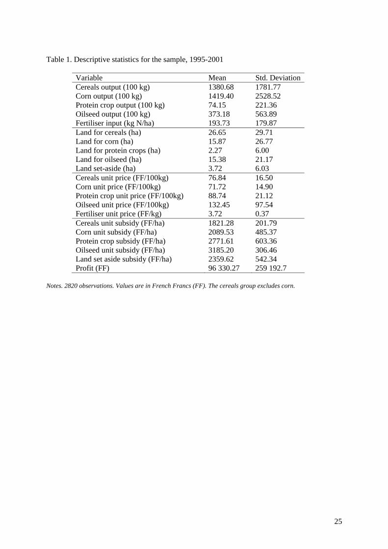
system also exists, by which farmers are compensated for hectares set-aside, on top of the mandatory mechanism. To deal with both sources of land set-aside (mandatory and voluntary), we proceed as follows. For observed land set-aside greater than the mandatory rate, we assume that the difference consists in voluntary land set-aside, and retain only this land surface in the land set-aside equation. When observed land set-aside is less than the mandatory rate, we consider that mandatory set-aside scheme does not apply, and the reported land set-aside consists of voluntary set-aside only. Hence, the original value is used in the land set-aside equation. Finally, when the proportion of land set-aside is exactly equal to the mandatory rate, we consider that there is no incentive-driven mechanism underlying the farmer’s decision, and we set the land set-aside to zero. Table 1 presents descriptive statistics on our sample: output, fertiliser input, land areas, unit prices and subsidy rates between 1995 and 2001. Concerning land, as we are only considering farmers with arable crops as the main production orientation, and hence limited livestock, the average number of hectares is highest for cereals (26.65), followed by corn (15.87) and oilseed (15.38). Protein crops are associated with only limited land, about 4 ha on average. The average land for set-aside is rather low (3.72), but this is due to the fact that the variable that we actually consider for land set-aside is associated with voluntary set-aside only. As a result, to obtain the total land set-aside (both mandatory and voluntary), the mandatory rate can be applied to the sum of land for corn, cereals, oilseed and protein crops, and the obtained figure added to the voluntary land set-aside. As far as unit output price and subsidies are concerned, oilseed and protein crops are the crop groups that seem the most valuable ones, on the gross benefit side (i.e., without accounting for operating costs). Finally, average nitrogen fertiliser input per hectare is particularly large in the three regions considered, and in any case above the national average nitrogen application rate.

4. Econometric considerations The model to be estimated consists in the system of equations (10)-(11)-(12) augmented with the profit equation (9). To accommodate for corner solutions in the analysis, the equation in the system associated to a single dependent variable ictw (either crop output or land), can be rewritten as a Tobit Type II model (see Amemiya, 1985):

* *

*

*

, 1l( 0),

,,

1,2, , ; 1,2, , ; 1,2, , ,

ict ict ict ict ict

ict ict c ic ict

ict ict c ic ict

i

w d w d dw Xd Z ui N c C t T

β α ε

δ η

= × = >

= + +

= + +

= = =… … …

(18)

where *

ictw is the latent variable corresponding to output or land, *ictd is the latent variable for

the selection equation with positivity indicator ictd . ictX is the vector of explanatory variables (output prices, input prices and unit subsidy rates), and ictZ is a vector of explanatory variables with possibly common elements with ictX . icα and icη are farmer- and crop-specific individual effects, and ictε and ictu are i.i.d. error terms. The indices are the following: i for the farmer, c for the crop and t for the period (year).

11

Three major issues call for particular attention when considering estimation. First, unobserved individual heterogeneity is likely to be present in structural equations, but also in the probability of crop selection (equivalently, the selection equation). In the latter case, wiping out individual effects requires a particular treatment analogous to the fixed effects (within-group) transformation in the linear regression model. Note that several interpretations of unobserved heterogeneity in land and output equations may be suggested. A first interpretation arises from the error-in-variables problem, where farm- and crop-specific permanent effects would possibly be correlated with price data. A second interpretation has to do with the fact that the individual-specific intercept in structural equations is restricted to be equal to own-price parameters in the profit equation, hence giving rise to a random-coefficients specification. Allowing for this parameter alone to be varying across producers and crops seems to be a restrictive assumption, however. Besides, although individual effects are typically restricted to have zero mean across the whole sample, a non-zero expected value of the effect for a given producer and crop would indicate systematic allocative inefficiency. Second, because of crop rotation systems in particular, there is a large proportion of censored dependent variables (land and output associated with crops). Crop rotations are motivated on agronomic grounds for pest control and soil fertility management, and not so much for smoothing farm income over time or for risk diversification purposes. Whatever the estimation technique used, the probability of a crop being planted needs to be considered, requiring the specification of a selection equation which, in the simplest case, reduces to a Tobit equation with the same regressors as in the structural equation being censored. The question of multiple selection rules naturally arises in our case, although previous empirical studies have either considered two-step estimation with single selection rules, or structural estimation of the full system within a single step. If two-step estimation procedures a la Heckman are easily implemented compared to one-step maximum-likelihood system estimation when the number of equations is large (involving in particular multiple integration and estimation of the full error-component variance-covariance matrix), selection bias is likely to occur however, when single selection rules are considered. We will come to that point later. Third, parametric constraints for symmetry and homogeneity are easily incorporated during estimation, but profit convexity in prices is another matter as it requires that the matrix of cross-derivatives be semi-positive definite. Imposing such condition is usually done through a Cholesky decomposition of the cross-product matrix of coefficients. However, convergence of the numerical optimisation algorithm is not guaranteed in this case. Moschini (1998) provides a solution to this problem in the way of a rank-reduction technique. By lowering the dimension of the matrix to which the semi-definite positiveness condition is imposed, convexity in prices is guaranteed, at the cost of destroying flexibility of the functional form for profit. Crop rotations and model dynamics As the latent variable *

ictd determines the presence or absence of crop c at date t, past land use decisions are obvious candidates for inclusion in ictZ , as well as price and subsidy variables already contained in ictX . When land plot specific data are not available, the set of lagged relative land areas devoted to each crop can be used to proxy the pattern of crop rotation through time, at the farm level. Let ( )1, 1 , 1, , 'i t iC ts s

− −

… denote the vector of lagged land relative

12

surfaces. Because 1

1C

ictc

s=

=∑ , ,i t∀ , we drop one component, say , 1ic ts−

, and define

( )1, 1 ( 1), 1 ( 1), 1 , 1, , , , ,ict i t i c t i c t iC tS s s s s− − − + − −

′= … … . The latent variable *

ictd is then rewritten as

* ,ict ict c ict c ic ictd S X uπ γ η= + + + (19) where the vector of parameters cπ captures the influence of the crop system (crop rotation) on the latent variable *

ictd , which is then interpreted as a profitability differential: crop c will be considered at time t only if * 0ictd > . When the number of time periods is limited, parameter estimates of the probability that

* 0ictd > are likely to be biased due to the incidental parameter problem, see Lancaster (2000). In usual estimation procedures, the effect of unobserved heterogeneity can be taken care of by conditioning techniques (estimation of fixed effects Logit probabilities) or by linear independence assumptions a la Chamberlain (1984). For example, in a fixed-effects Probit context, icη in Equation (19) would be “regressed” on the whole vector of lags and leads of explanatory variables and ict ictS X . In other words, icη is replaced by a linear projection on

the full iT vector ( ) ( )*1 1 1, , , , , , ,

i i iic ic icT ic icT ic icTZ Z Z S S X X′ ′= =… … … , which does not depend on

time, and which captures any form of correlation between the individual effect and the explanatory variables. This is the approach used by Wooldridge (1995) as an analogue to the fixed effects procedure in a nonlinear parametric context. Assume the regression function of

* on ic icZη is linear:

*1 1 ,

i iic ic c icT cT ic ic c icZ Z Zη λ λ ν λ ν= + + + = +… (20) where icν is a random component and is assumed distributed 2

,(0, )ctNν

σ . We further assume

ict ic ictuκ ν= + is independent of *icZ and is distributed 2

,(0, )ctNκ

σ . However, implementing this procedure amounts in our case to specifying *

ictd as a linear combination of the whole sequence (including leads and lags) of relative land surfaces in each period, as ictS then expands into

( )*11 1 ( 1),1 ( 1), ( 1)1 ( 1) 1, , , , , , , , , , , , ,

i i i iic i i T i c i c T i c i c T iC iCTS s s s s s s s s− − − −

′= … … … … … … .

Hence, the individual effect icη specific to farmer i and crop c can be interpreted as the permanent component picking up the influence of the crop system on the probability of growing this particular crop whatever the time period. As a consequence, it is not necessary to explicitly consider dynamic terms in the selection equation, as those terms are embedded in the set of explanatory variables anyway, through *

icS . Similarly, individual unobserved heterogeneity can be controlled for in the main equation, by considering the following regression equation of icα on the sequence over time of the ictX ’s:

13

*

1 1 ,i iic ic c icT cT ic ic c icX X Xα ψ ψ τ τ= + + + = Ψ +… (21)

where icτ is a random component, and is assumed distributed 2,(0, )ctN

τσ . We assume further

that ict ic ictω τ ε= + is independent of *icX .

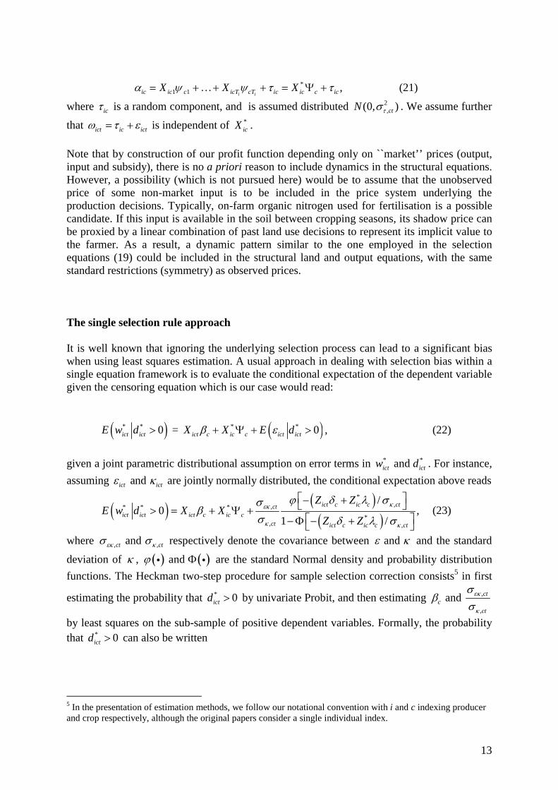
Note that by construction of our profit function depending only on ``market’’ prices (output, input and subsidy), there is no a priori reason to include dynamics in the structural equations. However, a possibility (which is not pursued here) would be to assume that the unobserved price of some non-market input is to be included in the price system underlying the production decisions. Typically, on-farm organic nitrogen used for fertilisation is a possible candidate. If this input is available in the soil between cropping seasons, its shadow price can be proxied by a linear combination of past land use decisions to represent its implicit value to the farmer. As a result, a dynamic pattern similar to the one employed in the selection equations (19) could be included in the structural land and output equations, with the same standard restrictions (symmetry) as observed prices. The single selection rule approach It is well known that ignoring the underlying selection process can lead to a significant bias when using least squares estimation. A usual approach in dealing with selection bias within a single equation framework is to evaluate the conditional expectation of the dependent variable given the censoring equation which is our case would read:

( )* * 0ict ictE w d > = ( )* * 0ict c ic c ict ictX X E dβ ε+ Ψ + > , (22)

given a joint parametric distributional assumption on error terms in * *and ict ictw d . For instance, assuming and ict ictε κ are jointly normally distributed, the conditional expectation above reads

( )( )

( )

*,,* * *

*, ,

/0 ,

1 /ict c ic c ctct

ict ict ict c ic cct ict c ic c ct

Z ZE w d X X

Z Zκ

εκ

κκ

ϕ δ λ σσβ

σ δ λ σ

− + > = + Ψ + −Φ − +

(23)

where , , and ct ctεκ κσ σ respectively denote the covariance between and ε κ and the standard

deviation of κ , ( ) ( ) and ϕ Φi i are the standard Normal density and probability distribution functions. The Heckman two-step procedure for sample selection correction consists5 in first

estimating the probability that * 0ictd > by univariate Probit, and then estimating ,

,

and ctc

ct

εκ

κ

σβ

σ

by least squares on the sub-sample of positive dependent variables. Formally, the probability that * 0ictd > can also be written

5 In the presentation of estimation methods, we follow our notational convention with i and c indexing producer and crop respectively, although the original papers consider a single individual index.

14

( )*

* *

,

Pr ( 0) ,ict c ic cict ct ict c ic c

ct

Z Zob d Z Zκ

δ λδ λ

σ

+> = Φ = Φ +

(24)

where heteroskedasticity is explicitly accounted for by indexing the probability by time. This is different from the cross-sectional context, where ,ctκ

σ would be normalised to 1. Two more

assumptions are that the regression function of *ict on and ic ic ic ictX uα κ ν= + is linear with

( )ic ict ct ictE α κ φ κ= × , (25) and that

( ) ( )* ,ict ic ict ict ict ct ictE Z Eε κ ε κ ρ κ= = × , (26)

where and ct ctφ ρ are time-varying correlation parameters. Although mean independence and linearity are assumed, no assumptions are made on the dependence of ictε on time, nor on ( , ),ict icscorr s tε κ ≠ . With these assumptions, we obtain that

( ) ( ) ( )* * *, 1 , 1 .ic ict ic ict ic c ct ct ict ic ictE Z d X E Z dα ε φ ρ κ+ = = Ψ + + = (27)

Estimation can then proceed in two steps. In the first one, estimates of the conditional expectation ( )* , 1ict ic ictE Z dκ = are obtained on a year-by-year basis, by a series of cross-

sectional maximum-likelihood Probit runs. In the second step, consistent estimates of ( ) and c ct ctβ φ ρ+ are obtained with the ``fixed effects’’ procedure (under the conditional

mean independence assumption) )applied to the structural equation for ictw . Once the selection term in (27) is computed, estimation can also proceed on the whole sample by considering

( ) ( )

( ) ( )

* * * *

, * *

,

ˆ ˆ, 1 ( )

ˆ ˆ ˆ ˆ0 ,

ict ict ic ct ict c ic c ict c ic c

ctct ict c ic c ct ict c ic c

ct

E w X X Z Z X X

Z Z Z Zεκ

κ

δ λ β

σϕ δ λ δ λ

σ

= −Φ − + × + Ψ

+ − + + ×Φ − +

(28)

where c

ˆ and cδ λ refer to first-step (Probit) estimates. This is the single-selection rule proposed by Shonkwiler and Yen (1999), which is particularly suited for large dimension problems such as demand systems with many corner solutions. The advantage of the method is that, in concentrating on single selection rules, it completely avoids multiple integral problems and rests on standard procedures found in most statistical software packages. Other methods involving a selection rule within a single equation context include Kyriazidou (1997) and Rochina-Barrachina (1999). The first one considers differences over time for individuals satisfying 1,ict icsd d s t= = ≠ . Since the selection effect for periods t and s is the same when and 1ict c ics c ict icsZ Z d dδ δ= = = , differencing between these two periods eliminates both the individual effect icα and the selection problem. To ensure that selection

15

effects are indeed equal, Kyriazidou imposes a conditional exchangeability condition of the form:

( ) ( ), , , , , , , , , , , , , , , ,ict ics ict ics ict ics ict ics ic ic ics ict ics ict ict ics ict ics ic icdist u u Z Z X X dist u u Z Z X Xε ε α η ε ε α η=

and a smoothness condition on selection correction terms (a Lipschitz continuity property). This is the only method (among the ones presented here) that does not impose a parametric distribution on the selection terms. Selection probability can be estimated in a first step (conditional Logit or fixed-effects Probit a la Wooldridge for example), to form a weighted least squares criterion based upon those pairs of (t,s) for which and ict c ics cZ Zδ δ are “close”:

( )( )

( )( )

1

,

,

ˆ ˆ( 1)

ˆ( 1) ,

ict ic ict ics ict ics ict icsi c t s t

ict ic ict ics ict ics ict icsi c t s t

d X X X X d d

d X X w w d d

β

−

<

<

′= − Ω × − −

′× − Ω × − −

∑ ∑ ∑

∑ ∑ ∑

(29)

where ( ) ˆ1ˆ ict ics c

icn n

Z ZK

h hδ −

Ω =

, K(.) is a kernel density function with bandwidth nh and

first-step parameter estimate cδ . Rochina-Barrachina (1999) on the other hand, does not impose conditional exchangeability, but her estimator relies on a parameterisation of the difference between selection correction terms (between any set of periods t and s). More precisely, the distribution assumption is the following one:

( ) * *, , ,ict ics ic ict ic ics ic icu u Z Xε ε ν ν − + + are trivariate normally distributed.

See Dustmann and Rochina-Barrachina (2000) for a comparison between these three estimators. Multiple selection rules Procedures described above all apply to a single selection rule, i.e., the probability that

* 0ic td′> for c c′≠ is not accounted for in the determination of the conditional expectation of

*ictw . It is however likely that omitting multiple selection rules will lead to sample selection

bias if correlation exists between and ,ict ic t c cε κ′

′≠ . In our case, as cropping systems involve specific relationships between land use across time periods, the single selection rule is difficult to justify. In other words, non-zero correlations between and , , 1, ,ict ic t c c Cε κ

′′ = … ,

should be considered, essentially because land is allocated to crops in a non-random fashion. For example, the expectation of a particular dependent variable conditional on all structural equations being positive is:

16

( )

( )

* * * *1

* * * *1 1 1 1 1

0, , 0, , 0

, , , , ,

ict i t ict iCt

ict i t i t i ict ict c ic c iCt C iC CiCt

E w d d d

E w Z Z Z Z Z Zκ δ λ κ δ λ κ δ λ

> > >

= > − − > − − > − −

… …

… …

, 1, 2, ,c c C′∀ = … , (30) and is in general different from ( )* * 0ict ictE w d > , even if ( ) 0ict ic tE c cκ κ

′′= ∀ ≠ , unless

( ) 0ict ic tE c cε κ′

′= ∀ ≠ . In practice, a great variety of selection rules are of course applicable, as any combination of censored land and output equations can apply. A first possibility for dealing with multivariate sample selection of general form is to solve the system of positive structural equations as functions of negative or zero latent variables, ending up with a multivariate sample-selection model (see Yen, 2005, and Chakir and Thomas, 2003, for an extension of Lee-Pitt approach to panel data). To simplify both notation and the analysis, we consider here the model for a given producer and a particular year, hence dropping indexes i and t, and concentrate upon the single index c for crop. Recall that after conditioning on * * and c cX Z , the error terms in compact form are

and c c c c c cuω τ ε κ ν= + = + for the structural equation and the selection equation respectively.

Assume the vector ( ) ( )1 1, , , , , ,C Cκ ω κ κ ω ω′ ′′ ′ = … … is distributed 2C-normal with zero mean

and variance-covariance matrix 11 12

21 22

Σ Σ Σ = Σ Σ

, where * *c c c cd Z Zκ δ λ= − − ,

*c c c cw X Xω β= − − Ψ , and let * * *

1( , , )Cd d d ′= … . Let ( )g ω denote the marginal probability

density functional of 22: (0, )Nω Σ , and let ( )h κ ω be the conditional probability density

function of κ ω : ( )1 112 22 11 12 22 21;N

κ ω κ ωµ ω

− −

=

Σ Σ Σ = Σ −Σ Σ Σ .

The sample likelihood function is the product of likelihood contributions for three possible regimes across observations, depending on the regime for each observation (see Yen, 2005): a) Outcomes are all positive.

( ) ( ) ( ) ( )*

*1 ; ,C

Z Z

L g h d g Z Zκ ω κ ω

κ δ λ

ω κ ω κ ω δ λ µ

>− −

= × = ×Φ + + Σ∫

where CΦ is the C-variate normal cumulative distribution function. b) All outcomes negative.

( ) ( )*

*2 11 11; , .C

Z Z

L f d Z Zκ δ λ

κ κ δ λ

≤− −

= Σ = Φ − − Σ∫

c) Mixed regime. Order structural equations such that the first l are not censored, and the rest

(C-l) are zero. Let ω be the l-vector containing the first elements of ω , so that ( ),κ ω′′ ′ is

(C+l)-variate normal with zero mean and variance-covariance matrix Σ . The likelihood contribution is then

17

( ) ( ) ( ) ( )*3 1 1, , ; ,C C CL g h d d g D Z Z D D

κ ω κ ωω κ κ ω κ κ ω δ λ µ ′= = ×Φ + + Σ

∫ ∫ … … …

where 1(2 1, ,2 1)CD diag d d= − −… . When the number of goods (or crops, in our case) is large, numerical approximation of multiple integrals is usually performed through the use of a fast simulation procedure (GHK in particular). With this structural estimation approach, the number of parameters is maximum, as all variance-covariance components have to be estimated. In a panel data context, this involves the variance-covariance matrix of structural equations, as well as the covariance of individual effects (random effects). The approach of Lee and Pitt (1986) is a special case of the likelihood above, where selection equations are directly obtained from the output and land structural equations. More precisely, corner solutions such as zero expenditures on a demand system are used to solve for the positive equations, under a inequality condition between virtual (unobserved) and actual prices. A ``poor-man’s method’’ for dealing with multivariate sample selection The procedure we consider here has the advantage of simplicity, as it completely avoids multiple integration. We consider the panel data approach suggested by Wooldridge (1995) and extend it to the case of multiple selection rules by assuming that we can find explanatory variables in the selection equations such that, conditional on these observed factors, the error terms in these equations are uncorrelated. On the other hand, correlation pattern are unrestricted between a particular structural equation and the set of selection equations for the same time period. Formally, we extend the assumptions in Wooldridge (1995) to the multivariate selection case:

( ) ,ic ic t cc t ic tE α κ φ κ′ ′ ′

= × , (31)

( ) , , , 1, ,ict ic t cc t ic tE c c Cε κ ρ κ′ ′ ′

′= × ∀ = … , (32)

with and ict ictε κ jointly normally distributed, but we add the important restrictions that

( )* *, 0ict ic t ic icE Z Z c cκ κ′ ′

′= ∀ ≠ , (33)

( )* *, 0ict ics ic icE X Z s tε κ = ∀ ≠ . (34)

Assumption (33) states that one can find two sets of conditioning variables in any pair of selection equations, to ensure that the remaining unobserved heterogeneity terms will be uncorrelated. This implies in particular that permanent components such as and ic icν ν

′ are

also uncorrelated for the same individual. As a result, the probability of a given set of censored equations is simply equal to the product of crop-specific probability terms. Assumption (34) is stronger than in Wooldridge (1995), as it requires that for a given pair of

18

output or land, and selection equations (for the same c), error terms and κ ε only exhibit contemporaneous correlation. Consider first the multiple selection rule of Catsiapis and Robinson (1982), where the dependent variable is observed only if all latent variables underlying the selection equations are positive. Given the assumption of joint normality of the error terms, we have

( )* * * *1 1 1 1 1

*,

1

, , , ,

,

ict i t i t i ict ict c ic c iCt iCt C iC C

C

ict c ic c cj t jtj

E w Z Z Z Z Z Z

X X

κ δ λ κ δ λ κ δ λ

β π λ=

> − − > − − > − −

= + Ψ +∑

… …

(35)

where ,cj tπ is proportional to , ,cj t cj tρ φ+ , the correlation coefficient between and ict ijtω κ , and

( )( )( )

**

*.

1jt ijt j ij j

jt ijt j ij jjt ijt j ij j

Z ZZ Z

Z Zϕ δ λ

λ δ λδ λ

− −− − =

−Φ − − (36)

Note that in Equation (36), we maintain the notation with density and probability distribution functions depending on time and on structural equation, as an indication that the sample selection correction term is obtained as in Wooldridge (1995), see Equation (24) above. Equation (35) can be estimated on the sub-sample of observations for which 1ictd = (as in a univariate Tobit). Another possibility is to consider the following equation:

( ) ( )

( )

( ) ( )

* * * * * * *1 1

* * * *1

* * * * *1 ,

1

0, , , , 0 Pr 0, , 0, 0

0, , 0, , 0 0

Pr 0, , 0, 0 ,

ict i t ict iCt i t ict iCt

ict i t ict iCt

C

i t ict iCt ict c ic c cj t jt ijt j ij jj

E w d d d ob d d d

E w d d d

ob d d d X X Z Zβ π λ δ λ=

> > = > > >

× > > > +

= > > > × + Ψ + − −

∑

… … … …

… …

… …

(37)

which allows one to use all observations for equation c when estimating the system. However, the sub-sample corresponding to (35) remains limited to equations such that * 1,ic td c c

′′= ≠ . In

order to exploit all observations in the sample, we augment the above sub-sample (in Equation (37)) by stacking observations corresponding to other positivity regimes. For example, the regime associated with all dependent variables equal to zero except equation c corresponds to the conditional expectation:

( ) ( )

( )

( )

* * * * * * *1 1

* * * *1

* * * * *1 ,

1

0, , , , 0 Pr 0, , 0, , 0

0, , , , 0 0

Pr 0, , 0, , 0 ,

ict i t ict iCt i t ict iCt

ict i t ict iCt

C

i t ict iCt ict c ic c cj t jtj

E w d d d ob d d d

E w d d d

ob d d d X Xβ π λ=

< < = < > <

× < < +

= < > < × + Ψ +

∑

… … … …

… …

… …

(38)

where ( )( )

**

*.jt ijt j ij j

jtjt ijt j ij j

Z ZZ Z

ϕ δ λλ

δ λ

− −= −

Φ − − (39)

It is of course necessary to integrate equality restrictions between parameters across the different selection regimes, but imposing these restrictions through a Minimum Distance

19

procedure is not necessary: observations are simply pooled together, and the probability corresponding to the relevant selection regime is applied to each. In our case, as the subsidy associated to a given crop is zero when the crop is not grown (planted), we only need to consider a single selection equation by crop (both for the output and the land equation). Our procedure for the full model can be compared with the single selection approach of Shonkwiler and Yen (1999), in which only the positivity condition for the same dependent variable is considered. In this special case, only the index j c= is maintained in the sample selection correction term (see equations (35) and (38) as two examples). A priori, if selection terms between the main structural (c) and selection equations for other crops are not all zero, the procedure of Shonkwiler and Yen will produce biased parameter estimates, because of the omitted-variable problem. The estimation method proceeds in two steps. In the first stage, we estimate the selection equations by Probit, and check that the no-correlation conditions (33) are satisfied. To do this, we run a set of bivariate Probit estimation steps for each pair of crops when selection is present, and compute the test statistic for the null hypothesis of no correlation. The advantage of the two-step method is that condition (33) is easily tested by augmenting the sets of explanatory variables * * and Zic icZ

′ until correlation between selection equations and c c′ is

tested to be not significantly different from zero. When this is the case, the probability associated with each selection regime is easily computed as the product of the crop-specific probabilities. In a second stage, the system of structural equations (output and land, and nitrogen fertiliser) is estimated on the full sample, where the right-hand side is the conditional expectation of the dependent variable multiplied by the probability of the corresponding regime, as indicated above. In total, when C=5 (corn, cereals, oilseed, protein crops, land set-aside) and with a single input (nitrogen fertiliser), we have C+(C-1)+1=10 equations in the system, which can be estimated by Iterated Three-Stage Least Squares or by Maximum Likelihood estimation. The latter is preferred in practice, as the property of global convexity of the profit function with respect to prices is imposed by restricting the matrix of (second-order) cross-product coefficients to be semi-definite positive. In addition to this restriction, we also impose the homogeneity condition for land, by restricting one price or subsidy parameter in each equation to be equal to minus the sum of all other parameters in the same equation, see condition (13) above.

5. Estimation results The validity of our approach relies heavily on the assumption that conditioning variables *

icZ can be found such that selection equations are not correlated between each other (although they can be correlated with structural equations). By using the Wooldridge fixed-effects approach consisting in specifying the individual effect icα in the structural equation as a linear combination of the full sequence over time of explanatory variables in *

ictw , and similarly for icη in the selection equation, the complete sequence of output prices, input prices, unit subsidy rates and relative land surface are used. In practice of course, some

20

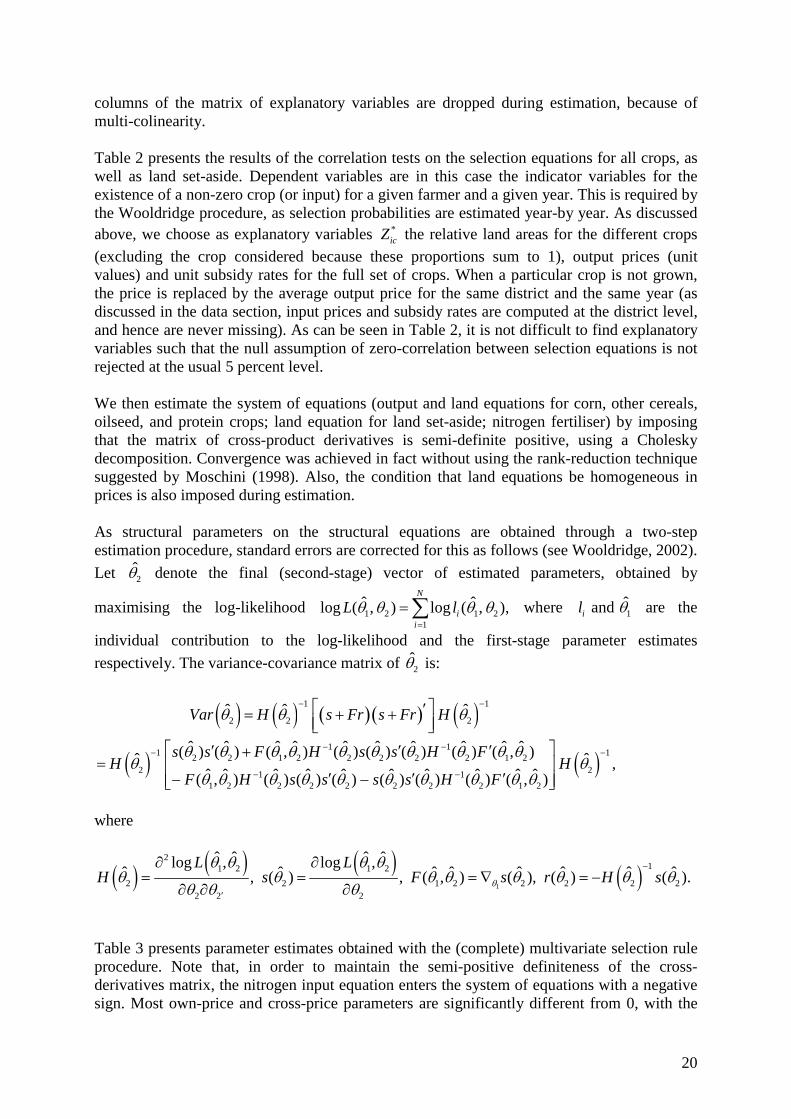
columns of the matrix of explanatory variables are dropped during estimation, because of multi-colinearity. Table 2 presents the results of the correlation tests on the selection equations for all crops, as well as land set-aside. Dependent variables are in this case the indicator variables for the existence of a non-zero crop (or input) for a given farmer and a given year. This is required by the Wooldridge procedure, as selection probabilities are estimated year-by year. As discussed above, we choose as explanatory variables *

icZ the relative land areas for the different crops (excluding the crop considered because these proportions sum to 1), output prices (unit values) and unit subsidy rates for the full set of crops. When a particular crop is not grown, the price is replaced by the average output price for the same district and the same year (as discussed in the data section, input prices and subsidy rates are computed at the district level, and hence are never missing). As can be seen in Table 2, it is not difficult to find explanatory variables such that the null assumption of zero-correlation between selection equations is not rejected at the usual 5 percent level. We then estimate the system of equations (output and land equations for corn, other cereals, oilseed, and protein crops; land equation for land set-aside; nitrogen fertiliser) by imposing that the matrix of cross-product derivatives is semi-definite positive, using a Cholesky decomposition. Convergence was achieved in fact without using the rank-reduction technique suggested by Moschini (1998). Also, the condition that land equations be homogeneous in prices is also imposed during estimation. As structural parameters on the structural equations are obtained through a two-step estimation procedure, standard errors are corrected for this as follows (see Wooldridge, 2002). Let 2θ denote the final (second-stage) vector of estimated parameters, obtained by

maximising the log-likelihood 1 2 1 21

ˆ ˆlog ( , ) log ( , ),N

ii

L lθ θ θ θ

=

=∑ where 1 and il θ are the

individual contribution to the log-likelihood and the first-stage parameter estimates respectively. The variance-covariance matrix of 2θ is:

( ) ( ) ( )( ) ( )1 1

2 2 2ˆ ˆ ˆVar H s Fr s Fr Hθ θ θ

− − ′= + +

( ) ( )1 11 12 2 1 2 2 2 2 2 1 2

2 21 11 2 2 2 2 2 2 2 1 2

ˆ ˆ ˆ ˆ ˆ ˆ ˆ ˆ ˆ ˆ( ) ( ) ( , ) ( ) ( ) ( ) ( ) ( , )ˆ ˆ ,ˆ ˆ ˆ ˆ ˆ ˆ ˆ ˆ ˆ ˆ( , ) ( ) ( ) ( ) ( ) ( ) ( ) ( , )

s s F H s s H FH H

F H s s s s H F

θ θ θ θ θ θ θ θ θ θθ θ

θ θ θ θ θ θ θ θ θ θ

− −

− −

− −

′ ′ ′+=

′ ′ ′− −

where

( )( ) ( )

( )1

211 2 1 2

2 2 1 2 2 2 2 22 2 2

ˆ ˆ ˆ ˆlog , log ,ˆ ˆ ˆ ˆ ˆ ˆ ˆ ˆ, ( ) , ( , ) ( ), ( ) ( ).L L

H s F s r H sθ

θ θ θ θ

θ θ θ θ θ θ θ θθ θ θ

−

′

∂ ∂

= = = ∇ = −∂ ∂ ∂

Table 3 presents parameter estimates obtained with the (complete) multivariate selection rule procedure. Note that, in order to maintain the semi-positive definiteness of the cross-derivatives matrix, the nitrogen input equation enters the system of equations with a negative sign. Most own-price and cross-price parameters are significantly different from 0, with the

21

exception of corn price and subsidy in the oilseed equation, own- and oilseed subsidy in protein equation, and protein subsidy in land set-aside equation. Considering first price effects in output supply equations (the upper left part of Table 3), we see that cross-price effects are negative except between corn and protein crops, and oilseed and protein crops. Note also that own-price effects in land equations (upper right part of Table 3) are not always positive. This is the case of corn and oilseed own prices in land equations, which are associated with negative parameters. Turning then to subsidy effects in land equations, corn and cereals, and oilseed and protein crops, have positive cross-subsidy effects, indicating some degree of complementary in the factor land between these two crops. Land set-aside is shown to be substitute to corn, cereals and protein crops, but (significantly) complementary to oilseed crops. As far as nitrogen fertiliser is concerned, it has to be remembered that the equation enters the system with a minus sign, so that parameters in the last column of Table 3 have to be interpreted with the opposite sign to the ones reported. Considering now sample selection correction terms, it can be seen that almost all are significant, except cereals in oilseed equation, protein crops in cereals output equation, land set-aside in cereals and set-aside land equations, cereals in land set-aside equation, and corn in fertiliser input equation. For price and subsidy equations, coefficients on Mills ratios (in the lower left part of Table 3) for the same crop are all positive. From parameter estimates in Table 3, we compute land, crop output and fertiliser input elasticities from expressions given below Equation (12). Results are gathered in Table 4. Note that elasticity of crop yield for land set-aside is obviously not reported, as the corresponding output sales equation is missing. As the second-order cross-derivative terms are restricted to be positive, own-price elasticities of output, and own-subsidy elasticities of land are all positive. And because the profit function is quadratic, as land and output are linear functions of prices and subsidy rates, elasticities have the same sign as estimated parameters in Table 3, except for fertiliser input, as described above. Own- and cross-price output elasticities refer to change in total crop output and not crop yield; in output equations, own-price elasticities range from 0.0959 for oilseed to 3.3871 for protein crops, and cross-elasticities from -4.5822 for cereal price in protein output equation to 1.8020 for corn price in protein output equation. Land own-subsidy elasticities range from 0.2095 for corn to 2.3723 for protein, the latter being not significant. As mentioned before, concerning cross-subsidy effects in land equations, corn and cereals, oilseed and land set-aside, and oilseed and protein crops are complementary (positive cross-subsidy effect), while all other land uses are substitutes. Finally, the last row of Table 3 contains price and subsidy elasticities of fertiliser input. The latter varies negatively with its own price (elasticity of -0.2754, significantly different from 0) and most other prices and land subsidies; fertiliser input demand varies positively with oilseed output price, oilseed and protein unit subsidy rates. Environmental simulation experiment We now exploit estimated elasticities discussed above to simulate the impact of the most recent reform of the Common Agricultural Policy (CAP) concerning arable crops. Let us briefly recall that the Luxembourg compromise of June 2003 (European Regulation EC 1782/2003) allows member States to choose a partial decoupling of subsidies from production. This is the case for France, for which only a partial decoupling is to apply from

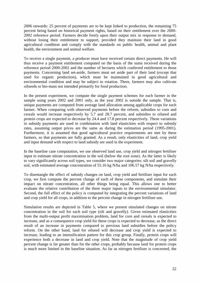
22

2006 onwards: 25 percent of payments are to be kept linked to production, the remaining 75 percent being based on historical payment rights, based on their entitlement over the 2000-2002 reference period. Farmers decide freely upon their output mix in response to demand, without losing their entitlement to support, provided they maintain their land in good agricultural condition and comply with the standards on public health, animal and plant health, the environment and animal welfare. To receive a single payment, a producer must have received certain direct payments. He will thus receive a payment entitlement computed on the basis of the sums received during the reference period 2000-2002 and the number of hectares which conferred entitlement to those payments. Concerning land set-aside, farmers must set aside part of their land (except that used for organic production), which must be maintained in good agricultural and environmental condition and may be subject to rotation. There, farmers may also cultivate oilseeds or bio-mass not intended primarily for food production. In the present experiment, we compute the single payment schemes for each farmer in the sample using years 2002 and 2001 only, as the year 2002 is outside the sample. That is, unique payments are computed from average land allocation among applicable crops for each farmer. When comparing with observed payments before the reform, subsidies to corn and cereals would increase respectively by 5.7 and 28.7 percent, and subsidies to oilseed and protein crops are expected to decrease by 24.4 and 17.8 percent respectively. These variations in subsidy payments are used in combination with land elasticities with respect to subsidy rates, assuming output prices are the same as during the estimation period (1995-2001). Furthermore, it is assumed that good agricultural practice requirements are met by these farmers, so that payments are fully granted. As a result, only elasticities of land, crop yield and input demand with respect to land subsidy are used in the experiment. In the baseline case computation, we use observed land use, crop yield and nitrogen fertiliser input to estimate nitrate concentration in the soil (below the root zone). As the latter is likely to vary significantly across soil types, we consider two major categories: silt soil and gravelly soil, with estimated average concentration of 55.16 kg N/ha and 106.57 kg N/ha respectively. To disentangle the effect of subsidy changes on land, crop yield and fertiliser input for each crop, we first compute the percent change of each of these components, and simulate their impact on nitrate concentration, all other things being equal. This allows one to better evaluate the relative contribution of the three major inputs to the environmental simulator. Second, the full effect of the policy is computed by integrating the percent variations of land and crop yield for all crops, in addition to the percent change in nitrogen fertiliser use. Simulation results are depicted in Table 5, where we present simulated changes on nitrate concentration in the soil for each soil type (silt and gravelly). Given estimated elasticities from the multi-output profit maximisation problem, land for corn and cereals is expected to increase, and as a consequence crop yield for these crops is expected to decrease, as the direct result of an increase in payments compared to previous land subsidies before the policy reform. On the other hand, land for oilseed will decrease and crop yield is expected to increase, leading to an intensification pattern for this crop group. Finally, protein crops will experience both a decrease in land and crop yield. Note that the magnitude of crop yield percent change is far greater than for the other crops, probably because land for protein crops is much more limited in the baseline situation. As far as nitrogen fertiliser is concerned, the

23

impact of subsidy changes for the four crop groups considered would lead to a decrease of about 11 percent for that input. In the case of silt soil, the contribution of corn and protein crops to the change in total nitrate concentration is negative, while it is positive for cereals and oilseed. The most important effects seem to be the change in land for oilseed and protein crop yield (respectively, 8.95 percent decrease and 6.46 percent increase in nitrate concentration). Cereals is characterised by a rather limited impact on total nitrate concentration, and the same can be said of corn. With an estimated change of -10.84 percent, nitrogen fertiliser will have a contribution of -6.18 percent to total emissions. The overall effect of the policy reform when only subsidy changes are simulated, is an expected reduction in nitrate concentration of 9.09 percent. The picture is somewhat different when gravelly soil is considered. It can be seen from the lower panel of Table 5 that there are significant differences in magnitude but also in the sign of crop contributions to the change in total nitrate concentration, compared to silt soil. The impact of a change in crop yield is now much smaller than it was in the previous case, with a mere 1.34 percent increase in nitrate concentration associated to a large variation in protein crop yield. Given that land and crop yield move in opposite directions except for protein crops, and also because changes in land for crops have a larger impact on emissions than changes in crop yields, the contribution of corn is now positive, while the one for oilseed is now negative. Cereals and oilseed have the most important contributions to changes in nitrate concentration: 4.01 percent and -9.68 percent respectively. This type of soil also seems to be less affected by a change in nitrogen fertiliser use, with a contribution of -1.29 percent compared to -9.09 percent in the case of silt soil. The overall effect of the policy reform when only subsidy changes are simulated, is an expected reduction in nitrate concentration of 3.51 percent. It is clear that the decoupled payment scheme to be implemented in France in 2006 is leading towards a reduction in non-point source nitrogen pollution, essentially because payments to cereals are expected to increase, relative to the pre-2003 period. Such a reduction in nitrate emissions results from the combination of changes in key variables decided upon by the farmer (land use, crop yield, nitrogen input demand), but the results seem to depend much on the soil type, although the overall trend for nitrate concentration is basically the same. The fact that output price variations are not considered in the experiment is an obvious limitation to the policy reform assessment. The linkage between the economic model of production and the environmental impact simulator behind easily implemented through output and land elasticities, a wide variety of scenarios can be considered, in addition to the one presented here.

6. Conclusion In this paper, we provide a methodology for dealing with multi-output production and land allocation decisions in the presence of corner solutions, when the objective is to evaluate the environmental impact of agricultural policy reforms. We claim that disaggregate data at the farm level is better suited to a problem in which crop-specific parameters play an important role in the final emission level. As agricultural policy reform is ultimately converting changes in output price and land subsidy into farmers’ reactions in terms of crop yield, input use and

24

land allocation among crops, we consider first a multi-crop microeconomic model of production for deriving price and subsidy elasticities. In the estimation stage, a particular attention is paid to the issue of corner solutions in land allocation. The probability of observing a positive land area for a given crop has to account for crop rotation patterns, in an observation framework where land plot data are not available. Besides, with repeated observations for the same farmer, unobserved heterogeneity in selection equations (determining whether a particular crop will be planted) and structural equations (crop output supply and land for crop) has to be accounted for. We deal with this issue by considering a panel data model with multivariate sample selection rule, where sample selection correction terms can be made independent from each other, using a conditional mean independence assumption among selection equations. This procedure is expected to provide consistent and efficient parameter estimates, contrary to usual, single selection rule techniques. The estimated system of equations originates from a normalised quadratic profit function including output prices, crop subsidies per unit of land, and variable inputs. Elasticities of crop output, land and nitrogen fertiliser are derived, and used as input parameters to an environmental impact simulator for predicting nitrate concentration in the soil. The interesting feature of such a coupling between a microeconomic production model and a bio-physical simulator, is the ability to simulate a wide range of policy reforms impacting output and input prices, as well as subsidies. As an empirical illustration, we simulate the impact of the 2003 Luxembourg compromise as the final step in the series of Common Agricultural Policy reforms, in the case of France. We start by computing equivalent variations of crop land subsidy rates, with respect to the 2000-2002 period, as the latter will be used for Single Payment Schemes in the future. Changes in crop yield, land for crops and fertiliser input are then simulated from estimated elasticities. In our case, the CAP reform will lead to an increase in subsidy payments for cereals and corn, and a decrease in payments for oilseed and protein crops, with respect to the baseline case. We find that the environmental impact of such a reform, assuming that output and input prices will remain constant, will be characterised by a decrease in nitrate concentration in the soil, as cereal and corn will experience extensification. However, this impact is depending on the type of soil (silt or gravelly soil), as well as on the initial land allocation patterns used to compute changes in subsidy payments. Nevertheless, the procedure we consider for simulating environmental impacts can be extended to other regions and productions, and used to simulate a wider range of scenarios impacting prices and subsidies.

25

Table 1. Descriptive statistics for the sample, 1995-2001

Variable Mean Std. Deviation Cereals output (100 kg) 1380.68 1781.77 Corn output (100 kg) 1419.40 2528.52 Protein crop output (100 kg) 74.15 221.36 Oilseed output (100 kg) 373.18 563.89 Fertiliser input (kg N/ha) 193.73 179.87 Land for cereals (ha) 26.65 29.71 Land for corn (ha) 15.87 26.77 Land for protein crops (ha) 2.27 6.00 Land for oilseed (ha) 15.38 21.17 Land set-aside (ha) 3.72 6.03 Cereals unit price (FF/100kg) 76.84 16.50 Corn unit price (FF/100kg) 71.72 14.90 Protein crop unit price (FF/100kg) 88.74 21.12 Oilseed unit price (FF/100kg) 132.45 97.54 Fertiliser unit price (FF/kg) 3.72 0.37 Cereals unit subsidy (FF/ha) 1821.28 201.79 Corn unit subsidy (FF/ha) 2089.53 485.37 Protein crop subsidy (FF/ha) 2771.61 603.36 Oilseed unit subsidy (FF/ha) 3185.20 306.46 Land set aside subsidy (FF/ha) 2359.62 542.34 Profit (FF) 96 330.27 259 192.7

Notes. 2820 observations. Values are in French Francs (FF). The cereals group excludes corn.

26

Table 2. Correlation test statistics between selection equations (bivariate Probit)

1995 1996 Corn Cereals Oilseed Protein Corn Cereals Oilseed Protein Corn - Corn - Cereals 0.0536 - Cereals 0.2752 - Oilseed 0.1125 0.0566 - Oilseed 0.1105 0.0005 - Protein 0.0751 0.1307 0.5585 - Protein 0.3969 0.2129 0.8533 - Set-aside 0.3723 0.1051 0.0652 0.2062 Set-aside 0.6187 0.1353 0.0756 0.7726 1997 1998 Corn Cereals Oilseed Protein Corn Cereals Oilseed Protein Corn - Corn - Cereals 0.4073 - Cereals 0.0714 - Oilseed 0.0834 0.1600 - Oilseed 0.2847 0.3400 - Protein 0.2724 0.1041 0.9025 - Protein 0.1195 0.0812 0.4013 - Set-aside 0.0648 0.0786 0.5726 0.0738 Set-aside 0.2111 0.0830 0.2156 0.5909 1999 2000 Corn Cereals Oilseed Protein Corn Cereals Oilseed Protein Corn - Corn - Cereals 0.2213 - Cereals 0.2393 - Oilseed 0.5628 0.3251 - Oilseed 0.9299 0.1054 - Protein 0.4206 0.0618 0.0735 - Protein 0.0776 0.1550 0.1070 - Set-aside 0.0701 0.0534 0.0540 0.1402 Set-aside 0.1421 0.0936 0.2418 0.0823 2001 Corn Cereals Oilseed Protein Corn - Cereals 0.1110 - Oilseed 0.2097 0.0766 - Protein 0.8245 0.0538 0.0706 - Set-aside 0.1814 0.1192 0.4902 0.0690

Notes. The table reports the p-value of the Wald test statistics associated to the null hypothesis of zero correlation between two crops (plus land set-aside), for a given year.

27

Table 3. Multiple selection rule estimation results p

cornw pcerealw

poilseedw

pproteinw cornwτ

cerealwτ

oilseedwτ

proteinwτ

set asidewτ

−

fertw

12.0343*** -0.9643*** -0.0580*** 2.7973*** -0.0078*** -0.0192*** 0.0064 0.0130** 0.0077* 63.4159*** cornp

(3.2569) (-9.3288) (-3.7325) (4.8590) (-6.8218) (-3.6934) (1.4103) (2.4176) (1.9417) (8.4319) 33.0118*** -46.4026*** -47.3389*** 1.3548* 1.4317*** 0.2046*** -1.8206*** -1.1705*** 70.1532**

cerealp (5.2856) (-19.0162) (-3.3936) (1.8301) (6.2875) (7.5049) (-15.3069) (-8.0986) (2.2167) 37.3037*** 35.0535*** -0.8839*** 1.4727** -1.1208** 1.0772*** -0.5452* -30.6171**

oilseedp (4.2219) (3.4414) (-4.1208) (2.0093) (-2.0763) (5.8168) (-1.8692) (-2.2538) 14.4022*** -9.3152** -11.6475*** 7.0526** 11.5251* 2.3849*** 26.9380***

proteinp (3.8884) (-2.1856) (-5.7767) (2.2403) (1.7214) (4.7078) (4.1252) 0.1388*** 0.1538* -0.1398 -0.1238*** -0.0290*** 34.0296**

cornτ (5.3908) (1.6989) (-1.5312) (-17.4433) (-3.9164) (2.2674) 0.5454*** -0.4778*** -0.0221*** -0.1993*** 51.0311*

cerealτ (2.7429) (-12.5577) (-14.7615) (-9.9745) (1.8508) 0.4340*** 0.0094 0.1742*** -68.3576**

oilseedτ (2.8035) (1.6133) (5.9603) (-2.6679) 0.1721 -0.0356 -26.3844**

proteinτ (1.2942) (-1.4740) (-2.1041) 0.0897** 9.6813**

set asideτ−

(2.2916) (2.5497) 2.4821**

fertr (2.0929) 5.3688*** -6.6618*** 4.2525*** 3.8235* 5.4182*** -2.6917*** 0.4456** -2.8851** 0.2181*** 34.2161 Mills ratio

corn (3.3815) (-4.4638) (4.1956) (1.6433) (-9.3610) (-3.4980) (2.4844) (-2.2960) (4.5041) (1.2054) -7.2114*** -97.2037** 2.7455*** -87.9891** 0.3328*** 1.0171*** -1.7455 7.7665*** -0.4497 -12.1280*** Mills ratio

cereal (-3.4011) (-2.1536) (4.3693) (-2.58877) (-6.9742) (7.8082) (-0.2475) (2.8720) (-1.5568) (-3.0987) -5.7174*** 1.4644*** 1.6431*** 2.3804*** -4.7699*** -3.9034*** 12.6489** 7.1408*** -1.0557 -74.8654** Mills ratio oilseed (-4.0285) (11.9090) (11.6158) (4.1912) (6.6121) (-4.6530) (2.0302) (8.2999) (-0.4109) (-2.4283) 8.3119** -6.3528 5.8731* 3.3250*** 0.8315*** 0.4758*** 2.2873*** 22.9945* -0.1480*** 30.8460*** Mills ratio

protein (2.1514) (-1.2392) (1.7437) (4.4202) (-6.8314) (3.2280) (6.0919) (1.8176) (-12.4462) (2.9925) 2.4544*** 1.3179*** 10.9512*** -2.1891* 1.8271*** 2.7950 1.5140** -2.2681*** 2.1558 -13.2269*** Mills ratio

set-aside (3.5925) (3.0184) (2.8801) (-1.8816) (-3.7862) (0.8065) (1.9991) (-11.3623) (1.2731) (-6.3210) Notes. 2820 observations. Standard errors (obtained by the Delta method) are in parentheses. *, ** and ***: parameter significant at 10, 5 and 1 percent level respectively.

28

Table 4. Multiple selection rule elasticities of land, crop yield and variable inputs with respect to output price and land subsidy.

cornp cerealp oilseedp proteinp cornτ cerealτ oilseedτ proteinτ set asideτ−

Fertiliser price

0.4050*** -0.4877*** -0.0392*** 0.3437*** -0.1320*** -0.2477*** 0.1442 0.2863** 0.1301* -0.4562*** Corn output (3.2569) (-9.3288) (-3.7325) (4.8590) (-6.8218) (-3.6934) (1.4103) (2.4176) (1.9417) (-8.4319) -0.0334 0.1716*** -0.0322*** -0.0598*** 0.0235* 0.0190*** 0.0048*** -0.0413*** -0.0203*** -0.0052** Cereal

output (-1.2460) (5.2856) (-19.0162) (-3.3936) (1.8301) (6.2875) (7.5049) (-15.3069) (-8.0986) (-2.2167) -0.0074* -0.0893*** 0.0959*** 0.0164*** -0.0567*** 0.0722** -0.0966** 0.0904*** -0.0350* 0.0008** Oilseed

output (-1.7300) (-16.6612) (4.2219) (3.4414) (-4.1208) (2.0093) (-2.0763) (5.8168) (-1.8692) (2.2538) 1.8020*** -4.5822* 0.4534 3.3871*** -3.0088** -2.8736*** 3.0591** 4.8687* 0.7707*** -0.0371*** Protein

output (3.9917) (-1.9207) (1.5847) (3.8884) (-2.1856) (-5.7767) (2.2403) (1.7214) (4.7078) (-4.1252) -0.0235** 0.0613** -0.0534*** -0.1024*** 0.2095*** 0.1773* -0.2834 -0.2444*** -0.0437*** -0.0219** Land for

corn (-2.5253) (2.3732) (-4.7253) (-6.0387) (5.3908) (1.6989) (-1.5312) (-17.4433) (-3.9164) (-2.2674) -0.0344*** 0.0386*** 0.0530** -0.0762*** 0.1382*** 0.3744*** -0.5766*** -0.0260*** -0.1792*** -0.0195* Land for

cereals (-2.6972) (5.0601) (2.2959) (-3.6943) (5.3020) (2.7429) (-12.557)7 (-14.7615) (-9.9745) (-1.8508) 0.0198 0.0095* -0.0699*** 0.0800*** -0.2177*** -0.5682*** 0.9074** 0.0192 0.2713*** 0.0454** Land for

oilseeds (1.0713) (1.7819) (-3.4818) (15.6212) (-7.6105) (-5.3248) (2.8035) (1.6133) (5.9603) (2.6679) 0.2727*** -0.5751* 0.4547 0.8846*** -1.3051*** -0.1779*** 0.1334** 2.3723 -0.3754 0.1186** Land for

proteins (4.6259) (-1.8074) (1.3590) (4.6114) (-7.0379) (-3.5795) (2.5680) (1.2942) (-1.4740) (2.1041) 0.0988*** -0.2256*** -0.1404* 0.1117** -0.1863*** -0.9792** 1.5048*** -0.2995 0.5769** -0.0265** Land set-

aside (3.0582) (-3.5687) (-1.7372) (2.6194) (-4.0117) (-2.5099) (4.7561) (-1.3609) (2.2916) (-2.5497) -0.3292*** -0.0547*** 0.0032* -0.0051** -0.0886*** -0.1015*** 0.2389* 0.0898*** -0.0252*** -0.2754** Fertiliser (-3.7398) (-4.6055) (1.7815) (-2.3365) (-9.0262) (-4.9954) (1.8294) (45.3526) (-5.7125) (-2.0929)

Notes. Standard errors (obtained by the Delta method) are in parentheses. *, ** and *** : parameter significant at 10, 5 and 1 percent level respectively.

29

Table 5. Contribution of each crop (land and crop yield) and total nitrogen to changes from baseline case. a) Silt soil Input variable Percent

change Nitrogen Runoff (kg N/ha)

Nitrogen runoff change (percent)

Corn land 17.54 56.6510 2.69 Corn yield -28.53 54.3240 -1.52 Total corn 55.8549 1.25 Cereals land 26.06 54.8251 -0.61 Cereals yield -19.30 55.2308 0.12 Total cereals 54.8865 -0.50 Oilseed land -40.03 50.2230 -8.95 Oilseed yield 79.06 55.2070 0.07 Total oilseed 50.2659 -8.88 Protein crop land -57.99 53.8860 -2.31 Protein crop yield -821.96 58.7304 6.46 Total protein crops 56.6956 2.77 Fertiliser use -10.84 51.7512 -6.18 Total crops & fert. 50.1476 -9.09 Baseline case - 55.1650 - b) Gravelly soil Input variable Percent

change Nitrogen Runoff (kg N/ha)

Nitrogen runoff change (percent)

Corn land 17.54 110.4053 3.59 Corn yield -28.53 106.2360 -0.32 Total corn 110.0844 3.29 Cereals land 26.06 110.8321 3.99 Cereals yield -19.30 106.6016 0.02 Total cereals 110.8569 4.01 Oilseed land -40.03 96.7003 -9.70 Oilseed yield 79.06 106.5920 0.01 Total oilseed 96.2542 -9.68 Protein crop land -57.99 103.9017 -2.50 Protein crop yield -821.96 108.0126 1.34 Total protein crops 105.2345 -1.44 Fertiliser use -10.84 105.1987 -1.29 Total crops & fert. 102.8298 -3.51 Baseline case - 106.5751 -

30

References Amemiya, T., 1985. Advanced Econometrics. Harvard University Press, Cambridge. Bourguignon, F., M. Fournier and M. Gurgand, 2004. Selection bias corrections based on the Multinomial Logit model: Monte-Carlo comparisons. Working Paper. Catsiapis, G. and C. Robinson, 1982. Sample selection bias with multiple selection rules. Journal of Econometrics 18, 351-368. Chakir, R. and A. Thomas, 2003. Simulated Maximum Likelihood estimation of firms demand systems with corner solutions and panel data: Application to industrial energy demand. Revue d’Economie Politique 6. 773-799. Chamberlain, G., 1984. Panel data. In Handbook of Econometrics, ed. Z. Griliches and M.D. Intriligator, vol.2, pp. 1247-1317. North-Holland, Amsterdam. Diewert, W.E. and T.J. Wales, 1995. Flexible functional forms and tests of homogeneous separability. Journal of Econometrics 67, 259-302. Diewert, W.E. and T.J. Wales, 1997. Flexible functional forms and global curvature conditions. Econometrica 55, 43-68. Diewert, W.E. and T.J. Wales, 1995. Flexible functional forms and tests of homogeneous separability. Journal of Econometrica 67, 259-302. Dustmann, C. and M.E. Rochina-Barrachina, 2000. Selection correction in panel data models: An application to labour supply and wages. IZA Discussion Paper N° 162. Gullstrand, J., 2003. Decoupling: The case of Swedish crop production. SLI working paper N° 2003:1. Guyomard, H., M. Baudry and A. Carpentier, 1996. Estimating crop supply response in the presence of farm programmes: Application to the CAP. European Journal of Agricultural Economics 23, 401-420. Heien, D. and C.R. Wessells, 1990. Demand system estimation with microdata: A censored regression approach. Journal of Business and Economics Statistics 8, 365-371. Kapteyn, A. and T.J. Wansbeek, 1985. Estimation in a linear model with serially correlated errors when observations are missing. International Economic Review 26, 469-490. Kyriazidou, E., 2001. Estimation of dynamic panel data sample selection models. Review of Economic Studies 68, 543-572. Kyriazidou, E., 1997. Estimation of a panel data sample selection model. Econometrica 65, 1335-1364.

31

Lacroix, A., F. Laurent, Ruelland, D. and E. Sauboua, 2005. Nitrate pollution risk assessment : From the model to the indicator. International Journal of Agricultural Resources Governance and Ecology, forthcoming. Lancaster, T., 2000. The incidental parameter problem since 1948. Journal of Econometrics 95, 391-413. Lee, L.-F. and M.M. Pitt, 1987. Microeconometric models of rationing, imperfect markets and non-negativity constraints. Journal of Econometrics 36. 89-110. Lee, L.-F. and M.M. Pitt, 1986. Microeconometric demand systems with binding constraints: The dual approach. Econometrica 54. 1237-1242. Lee, L.-F., 1983. Generalized econometrics models with selectivity. Econometrica 51, 507-512. Moro, D. and P. Sckokai, 1999.Modelling the CAP arable crop regime in Italy: Degree of decoupling and impact of Agenda 2000. Cahiers d’Economie et Sociologie Rurales 53, 50-73. Moschini, G., 1998. The semiflexible almost ideal demand system. European Economic Review 42, 349-364. Rochina-Barrachina, M.E., 1999. A new estimator for panel data sample selection models. Annales d’Economie et de Statistique 55/56, 153-181. Shonkwiler, J.S. and S.T. Yen, 1999. Two-step estimation of a censored system of equations. American Journal of Agricultural Economics 81, 972-982. Wooldridge, J.M., 1995. Selection corrections for panel data models under conditional mean independence assumptions. Journal of Econometrics 68, 115-132. Yen, S.T., 2005. A multivariate sample-selection model: Estimating cigarette and alcohol demands with zero observations. American Journal of Agricultural Economics 87, 453-466.