The Pennsylvania State University

The Graduate School

College of Information Sciences and Technology

USING BAYESIAN NETWORKS FOR ENTERPRISE NETWORK

SECURITY ANALYSIS

A Dissertation in

Information Sciences and Technology

by

Xiaoyan Sun

© 2016 Xiaoyan Sun

Submitted in Partial Fulfillment

of the Requirements

for the Degree of

Doctor of Philosophy

August 2016

The dissertation of Xiaoyan Sun was reviewed and approvedú by the following:

Peng Liu

Professor of Information Sciences and Technology

Dissertation Advisor, Chair of Committee

John Yen

Professor of Information Sciences and Technology

Dinghao Wu

Assistant Professor of Information Sciences and Technology

George Kesidis

Professor of Computer Science and Engineering

Professor of Electrical Engineering

Andrea Tapia

Associate Professor of Information Sciences and Technology

Director of Graduate Programs, College of Information Sciences and Tech-

nology

úSignatures are on file in the Graduate School.

ii

Abstract

Achieving complete and accurate cyber situation awareness (SA) is crucial for

security analysts to make right decisions. A large number of algorithms and

tools have been developed to aid the cyber security analysis, such as vulnerability

analysis, intrusion detection, network and system monitoring and recovery, and so

on. Although these algorithms and tools have eased the security analysts’ work

to some extent, their knowledge bases are usually isolated from each other. It’s a

very challenging task for security analysts to combine these knowledge bases and

generate a wholistic understanding towards the enterprise networks’ real situation.

To address the above problem, this paper takes the following approach. 1)

Based on existing theories of situation awareness, a Situation Knowledge Reference

Model (SKRM) is constructed to integrate data, information, algorithms/tools, and

human knowledge into a whole stack. SKRM serves as an umbrella model that

enables e�ective analysis of complex cyber-security problems. 2) The Bayesian

Network is employed to incorporate and fuse information from di�erent knowledge

bases. Due to the overwhelming amount of alerts and the high false rates, digging

out real facts is di�cult. In addition, security analysis is usually bound with a

number of uncertainties. Hence, Bayesian Networks is an e�ective approach to

iii

leverage the collected evidence and eliminate uncertainties.

With SKRM as the guidance, two independent security problems are identified:

the stealthy bridge problem in cloud and the zero-day attack path problem. This

paper will demonstrate how these problems can be analyzed and addressed by

constructing proper Bayesian Networks on top of di�erent layers from SKRM.

First, the stealthy bridge problem. Enterprise network islands in cloud are

expected to be absolutely isolated from each other except for some public services.

However, current virtualization mechanism cannot ensure such perfect isolation.

Some “stealthy bridges” may be created to break the isolation due to virtual

machine image sharing and virtual machine co-residency. This paper proposes to

build a cloud-level attack graph to capture the potential attacks enabled by stealthy

bridges and reveal possible hidden attack paths that are previously missed by

individual enterprise network attack graphs. Based on the cloud-level attack graph,

a cross-layer Bayesian network is constructed to infer the existence of stealthy

bridges given supporting evidence from other intrusion steps.

Second, the zero-day attack path problem. A zero-day attack path is a multi-

step attack path that includes one or more zero-day exploits. This paper proposes

a probabilistic approach to identify the zero-day attack paths. An object instance

graph is first established to capture the intrusion propagation. A Bayesian network is

then built to compute the probabilities of object instances being infected. Connected

through dependency relations, the instances with high infection probabilities form

a path, which is viewed as the zero-day attack path.

iv

Contents

List of Figures viii

List of Tables x

List of Symbols xi

Acknowledgments xii

Chapter 1Introduction 11.1 Cyber Situation Awareness . . . . . . . . . . . . . . . . . . . . . . . 11.2 Two Identified Problems . . . . . . . . . . . . . . . . . . . . . . . . 31.3 A Common Tool: Bayesian Networks . . . . . . . . . . . . . . . . . 5

Chapter 2SKRM: Where Security Techniques Talk to Each Other 82.1 Basic Concepts of Situation Awareness . . . . . . . . . . . . . . . . 82.2 A Model of Cyber Situation Knowlege Abstraction: the Application

of SA to Cyber Field . . . . . . . . . . . . . . . . . . . . . . . . . . 102.3 SKRM Framework . . . . . . . . . . . . . . . . . . . . . . . . . . . 13

2.3.1 Why do we need SKRM? . . . . . . . . . . . . . . . . . . . . 132.3.2 What is the main structure of SKRM? . . . . . . . . . . . . 142.3.3 How can SKRM enable cyber situation awareness? . . . . . 17

2.4 Case Study . . . . . . . . . . . . . . . . . . . . . . . . . . . . . . . 182.4.1 Implementation . . . . . . . . . . . . . . . . . . . . . . . . . 182.4.2 Capability 1: Mission Asset Identification and Classification 202.4.3 Capability 2: Mission Damage and Impact Assessment . . . 23

2.4.3.1 The System Object Dependency Graph . . . . . . . 272.4.3.2 Mission-Task-Asset Map . . . . . . . . . . . . . . . 312.4.3.3 MTA based Bayesian Networks . . . . . . . . . . . 33

v

2.5 Related Work . . . . . . . . . . . . . . . . . . . . . . . . . . . . . . 392.6 Discussion . . . . . . . . . . . . . . . . . . . . . . . . . . . . . . . . 402.7 Conclusion . . . . . . . . . . . . . . . . . . . . . . . . . . . . . . . . 41

Chapter 3Inferring the Stealthy Bridges between Enterprise Network Is-

lands in Cloud Using Cross-Layer Bayesian Networks 423.1 Introduction . . . . . . . . . . . . . . . . . . . . . . . . . . . . . . . 423.2 Cloud-level Attack Graph Model . . . . . . . . . . . . . . . . . . . 46

3.2.1 Logical Attack Graph . . . . . . . . . . . . . . . . . . . . . . 473.2.2 Cloud-level Attack Graph . . . . . . . . . . . . . . . . . . . 49

3.3 Bayesian Networks . . . . . . . . . . . . . . . . . . . . . . . . . . . 533.4 Cross-layer Bayesian Networks . . . . . . . . . . . . . . . . . . . . . 55

3.4.1 Identify the Uncertainties . . . . . . . . . . . . . . . . . . . 563.5 Implementation . . . . . . . . . . . . . . . . . . . . . . . . . . . . . 62

3.5.1 Cloud-level Attack Graph Generation . . . . . . . . . . . . . 623.5.2 Construction of Bayesian Networks . . . . . . . . . . . . . . 64

3.6 Experiment . . . . . . . . . . . . . . . . . . . . . . . . . . . . . . . 653.6.1 Attack Scenario . . . . . . . . . . . . . . . . . . . . . . . . . 653.6.2 Experiment Result . . . . . . . . . . . . . . . . . . . . . . . 68

3.6.2.1 Experiment 3.1: Probability Inferring . . . . . . . . 693.6.2.2 Experiment 3.2: Impact of False Alerts . . . . . . . 733.6.2.3 Experiment 3.3: Impact of Evidence Confidence

Value . . . . . . . . . . . . . . . . . . . . . . . . . 733.6.2.4 Experiment 3.4: Impact of Evidence Input Order . 753.6.2.5 Experiment 3.5: Mitigate Impact of False Alerts

by Tuning Evidence Confidence Value . . . . . . . 763.6.2.6 Experiment 3.6: Complexity . . . . . . . . . . . . . 77

3.7 Related Work . . . . . . . . . . . . . . . . . . . . . . . . . . . . . . 783.8 Conclusion and Discussion . . . . . . . . . . . . . . . . . . . . . . . 80

Chapter 4ZePro: Probabilistic Identification of Zero-day Attack Paths 824.1 Introduction . . . . . . . . . . . . . . . . . . . . . . . . . . . . . . . 824.2 Rationales and Models . . . . . . . . . . . . . . . . . . . . . . . . . 86

4.2.1 System Object Dependency Graph . . . . . . . . . . . . . . 864.2.2 Why use Bayesian Network? . . . . . . . . . . . . . . . . . . 884.2.3 Problems of Constructing BN based on SODG . . . . . . . . 904.2.4 Object Instance Graph . . . . . . . . . . . . . . . . . . . . . 91

4.3 Instance-graph-based Bayesian Networks . . . . . . . . . . . . . . . 95

vi

4.3.1 The Infection Propagation Models . . . . . . . . . . . . . . . 954.3.2 Evidence Incorporation . . . . . . . . . . . . . . . . . . . . . 97

4.4 System Design . . . . . . . . . . . . . . . . . . . . . . . . . . . . . . 994.5 Implementation . . . . . . . . . . . . . . . . . . . . . . . . . . . . . 1014.6 Experiments . . . . . . . . . . . . . . . . . . . . . . . . . . . . . . . 104

4.6.1 Attack Scenario . . . . . . . . . . . . . . . . . . . . . . . . . 1044.6.2 Experiment Results . . . . . . . . . . . . . . . . . . . . . . . 106

4.6.2.1 Correctness . . . . . . . . . . . . . . . . . . . . . . 1064.6.2.2 Size of Instance Graph and Zero-day Attack Paths 1124.6.2.3 Influence of Evidence . . . . . . . . . . . . . . . . . 1164.6.2.4 Influence of False Alerts . . . . . . . . . . . . . . . 1174.6.2.5 Sensitivity Analysis and Influence of · and fl . . . . 1184.6.2.6 Complexity and Scalability . . . . . . . . . . . . . 119

4.7 Related Work . . . . . . . . . . . . . . . . . . . . . . . . . . . . . . 1214.8 Limitation and Conclusion . . . . . . . . . . . . . . . . . . . . . . . 122

Chapter 5Conclusion 123

Bibliography 126

vii

List of Figures

2.1 A Model of Cyber Situation Knowledge Abstraction [12] . . . . . . 112.2 The Situation Knowledge Reference Model (SKRM) [11] . . . . . . 152.3 The Testbed Network and Attack Scenario [12] . . . . . . . . . . . . 192.4 Mission Asset Identification and Classification [12] . . . . . . . . . . 212.5 The Dependency Attack Graph [12] . . . . . . . . . . . . . . . . . . 222.6 Mission Damage and Impact Assessment [12] . . . . . . . . . . . . . 242.7 The SODG as the Construct between Attack and Mission [13] 1 . . 272.8 An example SODG built from the simplified system call log [13] . . 302.9 Mission-Task-Asset Map [13] 2 . . . . . . . . . . . . . . . . . . . . . 322.10 An Example of Benign Mission Dependency Graph [13] . . . . . . . 352.11 An Example of Tainted Mission Dependency Graph [13] . . . . . . . 362.12 An Example of MTA-based BN [13] . . . . . . . . . . . . . . . . . . 38

3.1 The Stealthy Bridges between Enterprise Network Islands in Cloud [14] 433.2 A Portion of an Example Logical Attack Graph [14] . . . . . . . . . 483.3 Features of the Public Cloud Structure [14] . . . . . . . . . . . . . . 503.4 An Example Cloud-level Attack Graph Model [14] . . . . . . . . . . 513.5 A Portion of Bayesian Network with associated CPT [14] . . . . . . 543.6 A Portion of Bayesian Network with AAN node [14] . . . . . . . . . 583.7 The Evidence-Condidence Pair [14] . . . . . . . . . . . . . . . . . . 613.8 The Attack Scenario [14] . . . . . . . . . . . . . . . . . . . . . . . . 663.9 The Cross-Layer Bayesian Network Constructed for the Attack

Scenario [14] . . . . . . . . . . . . . . . . . . . . . . . . . . . . . . . 723.10 Time Used for BN Compilation . . . . . . . . . . . . . . . . . . . . 793.11 Memory Used for BN Compilation . . . . . . . . . . . . . . . . . . 80

4.1 An SODG. An SODG generated by parsing an example set ofsimplified system call log. The label on each edge shows the timeassociated with the corresponding system call. . . . . . . . . . . . . 87

4.2 An Example Bayesian Network. . . . . . . . . . . . . . . . . . . . . 89

viii

4.3 An Instance Graph. An instance graph generated by parsing thesame set of simplified system call log as in Figure 4.1a. The labelon each edge shows the time associated with the correspondingsystem call operation. The dotted rectangle and ellipse are newinstances of already existed objects. The solid edges and the dottededges respectively denote the contact dependencies and the statetransition dependencies. . . . . . . . . . . . . . . . . . . . . . . . . 94

4.4 The Infection Propagation Models. . . . . . . . . . . . . . . . . . . 954.5 Local Observation Model. . . . . . . . . . . . . . . . . . . . . . . . 984.6 System Design. . . . . . . . . . . . . . . . . . . . . . . . . . . . . . 1074.7 Attack Scenario. . . . . . . . . . . . . . . . . . . . . . . . . . . . . . 1074.8 The zero-day Attack Path in the Form of an Instance Graph for

Experiment 4.1. . . . . . . . . . . . . . . . . . . . . . . . . . . . . . 1094.9 The zero-day Attack Path in the Form of an Instance Graph for

Experiment 4.2. . . . . . . . . . . . . . . . . . . . . . . . . . . . . . 1104.10 The Object-level Zero-day Attack Path in Experiment 4.1. . . . . . 1144.11 The Object-level Zero-day Attack Path in Experiment 4.2. . . . . . 115

ix

List of Tables

2.1 System Call Dependency Rules . . . . . . . . . . . . . . . . . . . . 292.2 CPT of Mission 1 in the Figure 2.12 [13] . . . . . . . . . . . . . . . 372.3 Modified CPT of Mission 1 in the Figure 2.12 [13] . . . . . . . . . . 38

3.1 CPT for Node Evidence [14] . . . . . . . . . . . . . . . . . . . . . . 623.2 A Sample Set of Interaction Rules [14] . . . . . . . . . . . . . . . . 633.3 Network Deployment [14] . . . . . . . . . . . . . . . . . . . . . . . . 703.4 Collected Evidence Corresponding to Attack Steps [14] . . . . . . . 713.5 Results of experiment 3.1 [14] . . . . . . . . . . . . . . . . . . . . . 733.6 Results of experiment 3.2 [14] . . . . . . . . . . . . . . . . . . . . . 743.7 Results of Experiment 3.3 [14] . . . . . . . . . . . . . . . . . . . . . 743.8 Results of experiment 3.4 . . . . . . . . . . . . . . . . . . . . . . . . 753.9 Results of experiment 3.5 . . . . . . . . . . . . . . . . . . . . . . . . 763.10 Size of Bayesian Networks . . . . . . . . . . . . . . . . . . . . . . . 78

4.1 CPT for Node p2 in Figure 4.2 . . . . . . . . . . . . . . . . . . . . . 904.2 CPT for Node sink

j+1 . . . . . . . . . . . . . . . . . . . . . . . . . 964.3 The Impact of Pruning the Instance Graphs . . . . . . . . . . . . . 1114.4 The Collected Evidence . . . . . . . . . . . . . . . . . . . . . . . . . 1124.5 The Influence of Evidence in Experiment 4.1 . . . . . . . . . . . . . 1164.6 The Influence of Evidence in Experiment 4.2 . . . . . . . . . . . . . 1164.7 The Influence of False Alerts . . . . . . . . . . . . . . . . . . . . . . 118

x

List of Symbols

SA Situation Awareness

SKRM Situation Knowledge Reference Model

AAN Attacker Action Node

AC Access Complexity

AMI Amazon Machine Image

BN Bayesian Network

CVSS Common Vulnerability Scoring System

CPT Conditional Probability Table

IDS Intrusion Detection System

OS Operating System

SODG System Object Dependency Graph

VMI Virtual Machine Image

xi

Acknowledgments

My first thanks go to my doctoral advisor, Prof. Peng Liu, for his endless support

and help throughout my entire PhD study. He spent countless hours meeting with

me for every detail of the projects and papers. With his brilliance, creativeness,

insights, diligence and patience, he guides and inspires me to discover and tackle

research problems in the wonderland of cyber security. He is my role model. What

I learned from him will benefit my entire life.

In addition, I want to express my sincere thanks to my doctoral committee

members, Prof. John Yen, Prof. Dinghao Wu and Prof. George Kesidis. They

are all amazing and successful professors, and also the sources of strong support,

prompt feedback and invaluable comments for the work presented in this paper.

I also would like to thank my collaborator, Dr. Anoop Singhal at National

Institute of Standards and Technology (NIST). His insightful comments in numerous

discussions are always important inputs to my work.

I also want to thank my labmates and friends here at Pennsylvania State

University. We share similar dreams, goals, interests, and experience. Their help

and support is always there whenever needed.

Finally, I feel very grateful to my parents, my husband and my son. They

xii

are the ones with warmest words, unconditional understanding, and sometimes

surprises. Life with them is so gorgeous.

xiii

Chapter 1 |Introduction

1.1 Cyber Situation Awareness

To better secure a network, human decision makers should clearly know and

understand what is going on in the network. This is basically what we call

cyber situation awareness (cyber SA). Human is the key role of cyber SA because

only human can be “aware”. Technologies regarding cyber security have made

remarkable progress in the past decades. A lot of algorithms and tools are developed

for vulnerability analysis, detection of attacks, damage and impact assessment, and

system recovery, etc. These technologies have significantly enhanced human analysts’

cyber situation awareness and facilitated their network security management. Attack

graph is one typical example. By combining vulnerabilities in the network, potential

attack paths can be automatically generated with attack graph tools. Through

generated attack paths, security analysts can clearly know how the attackers may

exploit the network. Without attack graph, it is very di�cult for them to construct

reasonable attack scenarios for even a small network only by reading the vulnerability

scan results, let alone for large scale enterprise network with hundreds to thousands

1

of hosts. In addition, due to the information asymmetry between security defenders

and attackers, defenders have to deploy a number of security sensors to monitor

the enterprises’ IT infrastructure. The main responsibility of security analysts is to

go through all types of reports from the security sensors to generate a wholistic

understanding towards the enterprise networks’ real situation. Although these

algorithms, tools, and security sensors have greatly eased the analysts’ work in

some aspects, they usually have di�erent knowledge bases. These knowledge bases

are isolated from each other. It is very challenging for security analysts to combine

the isolated information together to reveal real facts and achieve correct situation

awareness, especially when the amount of information is overwhelming.

To enhance human analysts’ situation awareness in cyber space, some existing

theories in situation awareness are applied into the cyber security field. A new

reference model called SKRM (Situation Knowledge Reference Model) is established

in Chapter 2. SKRM is a model that integrates cyber knowledge from di�erent

perspectives by coupling data, information, algorithms and tools, and human

knowledge, to enhance cyber analysts’ situation awareness. It mainly contains

four abstraction layers of cyber situation knowledge, including Workflow Layer,

App/Service Layer, Operating System Layer and Instruction Layer. These four

layers are generated by abstracting isolated situation knowledge from di�erent

perspectives of network. In addition to these four layers, attack graph is also an

essential part of SKRM. Attack Graph is not a specific layer in this stack, but

rather an interconnection technique between App/Service Layer and Operating

System Layer. Attack graph can generate potential attack paths in the network by

analyzing the vulnerabilities existing in the applications and services. These attack

paths can reveal which hosts are likely to be compromised. The lower level system

2

objects related to these hosts can then be scrutinized.

1.2 Two Identified Problems

SKRM model is not simply of a mapping of situation knowledge in di�erent spaces

to the four abstraction layers. It integrates data, information, algorithms and

tools, and human knowledge into a whole stack. Each abstraction layer generates a

graph that covers the entire enterprise network. In addition, each abstraction layer

views the same network from a di�erent perspective and at a di�erent granularity.

Most importantly, each abstraction layer leverages current available algorithms,

tools, and techniques in its corresponding area to extract the most critical and

useful information to present to human security analysts. Hence, SKRM serves as

an umbrella model that could enable solutions to di�erent security problems. In

this paper, two independent problems are identified on di�erent layers of SKRM,

including the stealthy bridge problem in cloud and the zero-day attack path problem.

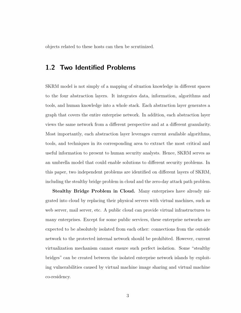
Stealthy Bridge Problem in Cloud. Many enterprises have already mi-

grated into cloud by replacing their physical servers with virtual machines, such as

web server, mail server, etc. A public cloud can provide virtual infrastructures to

many enterprises. Except for some public services, these enterprise networks are

expected to be absolutely isolated from each other: connections from the outside

network to the protected internal network should be prohibited. However, current

virtualization mechanism cannot ensure such perfect isolation. Some “stealthy

bridges” can be created between the isolated enterprise network islands by exploit-

ing vulnerabilities caused by virtual machine image sharing and virtual machine

co-residency.

3

Stealthy bridges are stealthy information tunnels existing between disparate

networks in cloud, through which information (data, commands, etc.) can be

acquired, transmitted or exchanged maliciously. However, these stealthy bridges are

inherently unknown or hard to detect: they either exploit unknown vulnerabilities,

or cannot be easily distinguished from authorized activities by security sensors.

For example, side-channel attacks extract information by passively observing the

activities of resources shared by the attacker and the target virtual machine (e.g.

CPU, cache), without interfering the normal running of the target virtual machine.

Similarly, the activity of logging into an instance by leveraging intentionally left

credentials (passwords, public keys, etc.) also hides in the authorized user activities.

The stealthy bridges are usually used for constructing a multi-step attack and

facilitate subsequent intrusion steps across enterprise network islands in cloud. By

taking advantage of the stealthy bridges, attackers can carry on the malicious

activities from one enterprise network to another. The stealthy bridges per se are

di�cult to detect, but the intrusion steps before and after the construction of stealthy

bridges may trigger some abnormal activities. Human administrators or security

sensors like IDS could notice such abnormal activities and raise corresponding

alerts, which can be collected as the evidence of attack happening. However, due to

the overwhelming amount of alerts and the high false rates, human analysts cannot

easily achieve accurate situation awareness. They may not even be aware of the

existence of such stealthy bridges, let alone the exact locating and analyzing of the

stealthy bridges. Therefore, a solution should be proposed to save human analysts

from the sea of alerts and infer the existence of stealthy bridges.

Zero-day Attack Path Problem. Zero-day attacks continue to challenge

the enterprise network security defense. They are usually enabled by unknown

4

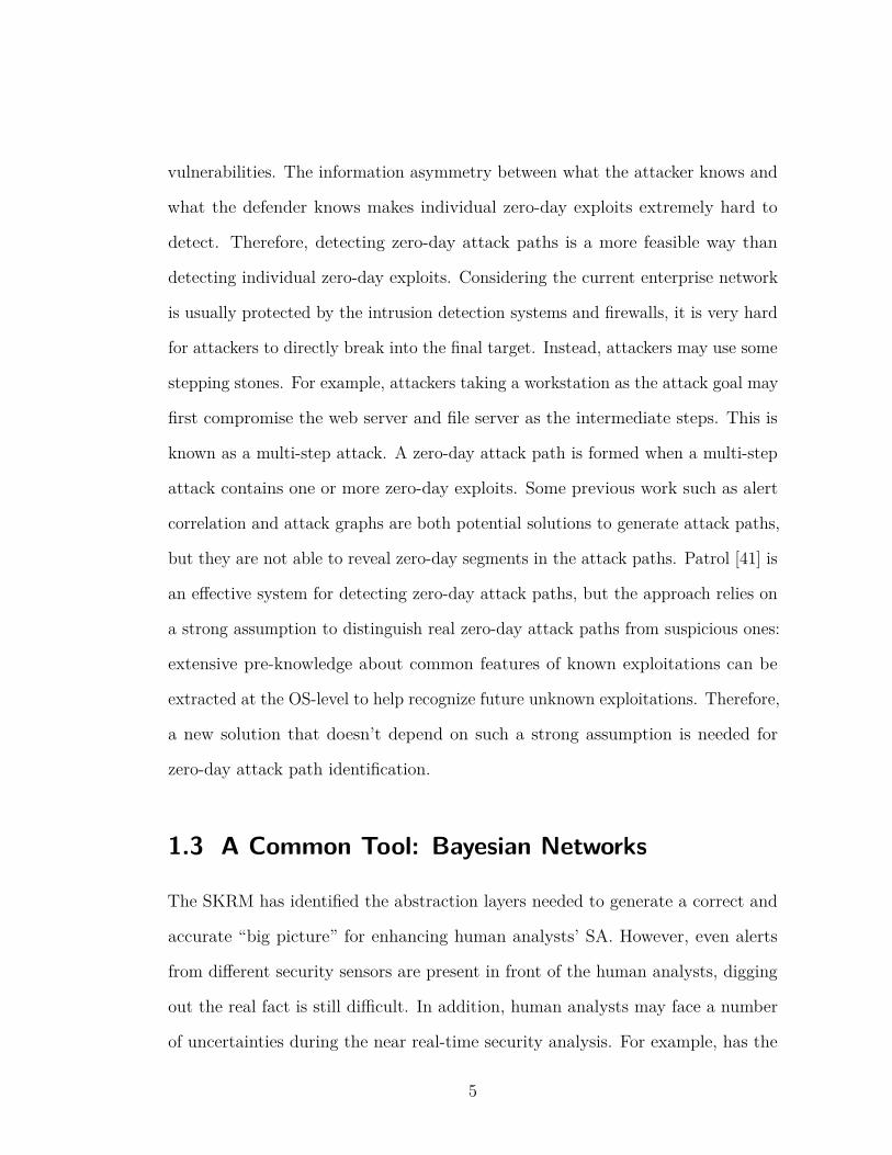
vulnerabilities. The information asymmetry between what the attacker knows and

what the defender knows makes individual zero-day exploits extremely hard to

detect. Therefore, detecting zero-day attack paths is a more feasible way than

detecting individual zero-day exploits. Considering the current enterprise network

is usually protected by the intrusion detection systems and firewalls, it is very hard

for attackers to directly break into the final target. Instead, attackers may use some

stepping stones. For example, attackers taking a workstation as the attack goal may

first compromise the web server and file server as the intermediate steps. This is

known as a multi-step attack. A zero-day attack path is formed when a multi-step

attack contains one or more zero-day exploits. Some previous work such as alert

correlation and attack graphs are both potential solutions to generate attack paths,

but they are not able to reveal zero-day segments in the attack paths. Patrol [41] is

an e�ective system for detecting zero-day attack paths, but the approach relies on

a strong assumption to distinguish real zero-day attack paths from suspicious ones:

extensive pre-knowledge about common features of known exploitations can be

extracted at the OS-level to help recognize future unknown exploitations. Therefore,

a new solution that doesn’t depend on such a strong assumption is needed for

zero-day attack path identification.

1.3 A Common Tool: Bayesian Networks

The SKRM has identified the abstraction layers needed to generate a correct and

accurate “big picture” for enhancing human analysts’ SA. However, even alerts

from di�erent security sensors are present in front of the human analysts, digging

out the real fact is still di�cult. In addition, human analysts may face a number

of uncertainties during the near real-time security analysis. For example, has the

5

attacker launched the attack? If he launched it, did he succeed to compromise the

host? How confident are we towards a certain alert? Obviously, a powerful tool

is needed to aid the near real-time security analysis by leveraging the collected

evidence and eliminating the uncertainties. Bayesian Network is such a tool that

we are looking for.

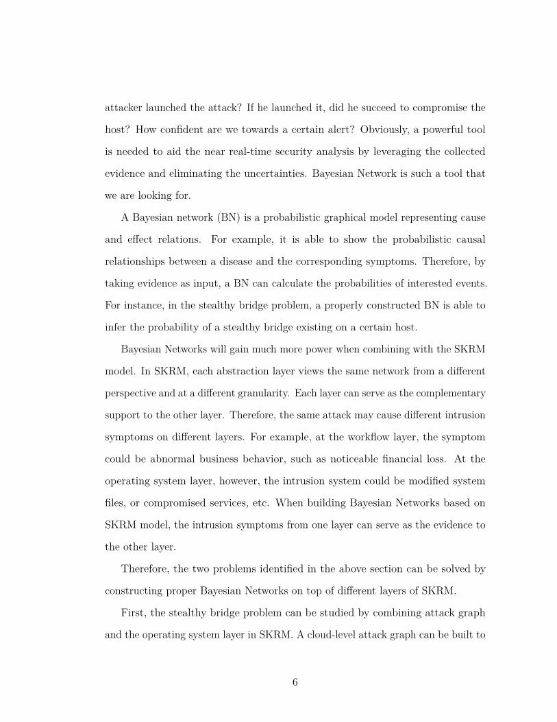
A Bayesian network (BN) is a probabilistic graphical model representing cause

and e�ect relations. For example, it is able to show the probabilistic causal

relationships between a disease and the corresponding symptoms. Therefore, by

taking evidence as input, a BN can calculate the probabilities of interested events.

For instance, in the stealthy bridge problem, a properly constructed BN is able to

infer the probability of a stealthy bridge existing on a certain host.

Bayesian Networks will gain much more power when combining with the SKRM

model. In SKRM, each abstraction layer views the same network from a di�erent

perspective and at a di�erent granularity. Each layer can serve as the complementary

support to the other layer. Therefore, the same attack may cause di�erent intrusion

symptoms on di�erent layers. For example, at the workflow layer, the symptom

could be abnormal business behavior, such as noticeable financial loss. At the

operating system layer, however, the intrusion system could be modified system

files, or compromised services, etc. When building Bayesian Networks based on

SKRM model, the intrusion symptoms from one layer can serve as the evidence to

the other layer.

Therefore, the two problems identified in the above section can be solved by

constructing proper Bayesian Networks on top of di�erent layers of SKRM.

First, the stealthy bridge problem can be studied by combining attack graph

and the operating system layer in SKRM. A cloud-level attack graph can be built to

6

capture the potential attacks enabled by stealthy bridges and reveal possible hidden

attack paths that are previously missed by individual enterprise network attack

graphs. Based on the cloud-level attack graph, a cross-layer Bayesian network is

constructed to infer the existence of stealthy bridges given supporting evidence

from other intrusion steps.

Second, the zero-day attack path problem is addressed on the operating system

layer of SKRM. An object instance graph is first built from system calls to capture

the intrusion propagation. To further reveal the zero-day attack paths hiding in

the instance graph, the proposed ZePro system constructs an instance-graph-based

Bayesian network. By leveraging intrusion evidence, the Bayesian network can

quantitatively compute the probabilities of object instances being infected. The

object instances with high infection probabilities reveal themselves and form the

zero-day attack paths.

In the following chapters, Chapter 2 briefly introduces the SKRM model. Chap-

ter 3 presents the stealthy bridge problem in cloud and a cross-layer Bayesian

Network to infer the existence of stealthy bridges. Chapter 4 mainly focuses on

the ZePro system for detecting zero-day attack paths at operating system level.

Chapter 5 concludes the whole paper.

7

Chapter 2 |SKRM: Where Security Tech-niques Talk to Each Other

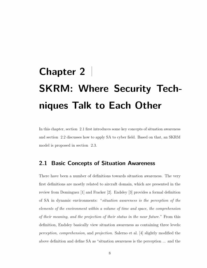
In this chapter, section 2.1 first introduces some key concepts of situation awareness

and section 2.2 discusses how to apply SA to cyber field. Based on that, an SKRM

model is proposed in section 2.3.

2.1 Basic Concepts of Situation Awareness

There have been a number of definitions towards situation awareness. The very

first definitions are mostly related to aircraft domain, which are presented in the

review from Dominguez [1] and Fracker [2]. Endsley [3] provides a formal definition

of SA in dynamic environments: “situation awareness is the perception of the

elements of the environment within a volume of time and space, the comprehension

of their meaning, and the projection of their status in the near future.” From this

definition, Endsley basically view situation awareness as containing three levels:

perception, comprehension, and projection. Salerno et al. [4] slightly modified the

above definition and define SA as “situation awareness is the perception ... and the

8

projection of their status in order to enable decision superiority.” Salerno’s definition

implies the importance of situation awareness to the decision process. McGuinness

and Foy [5] add a fourth level to Endsley’s definition named resolution, which tries

to identify the best path to follow to achieve the desire state change to the current

situation. Resolution does not directly make decisions for humans regarding what

should be done, but provides available options and the corresponding impact of

these options to the environment. To help understand the four levels of SA, we use

the analogy made by McGuinness and Foy to explain them: perception represents

“What are the current facts?” Comprehension means, “What is actually going on?”

Projection asks, “What is most likely to happen if ...?” And Resolution means,

“What exactly shall I do?”

Alberts et al. [6] provides another definition of situation awareness, which

“describes the awareness of a situation that exists in part or all of the battle space

at a particular point in time”. For situation, they identify three main components:

missions and constraints on missions, capabilities and intentions of relevant forces,

and key attributes of the environment. For awareness, they say “awareness exists

in the cognitive domain” and awareness is “the result of a complex interaction

between prior knowledge and current perceptions of reality”. This definition basically

emphasizes the role of cognition in awareness and uncovers a fact that awareness

is not just perceptions of reality, but also includes prior knowledge as a crucial

factor. This explains why experienced analysts usually gain situation awareness

more rapidly and accurately than novice analysts. Actually all the above definitions

consider time as a basic element of SA. Decision makers rely on previous experience

and prior knowledge to keep aware of changing environment, make decisions, and

perform actions. As in the OODA (Observe, Orient, Decision, Act) loop [7],

9

decisions and actions provide feedback to the environment again and a new cycle

will start. Therefore, time is an essential element of SA.

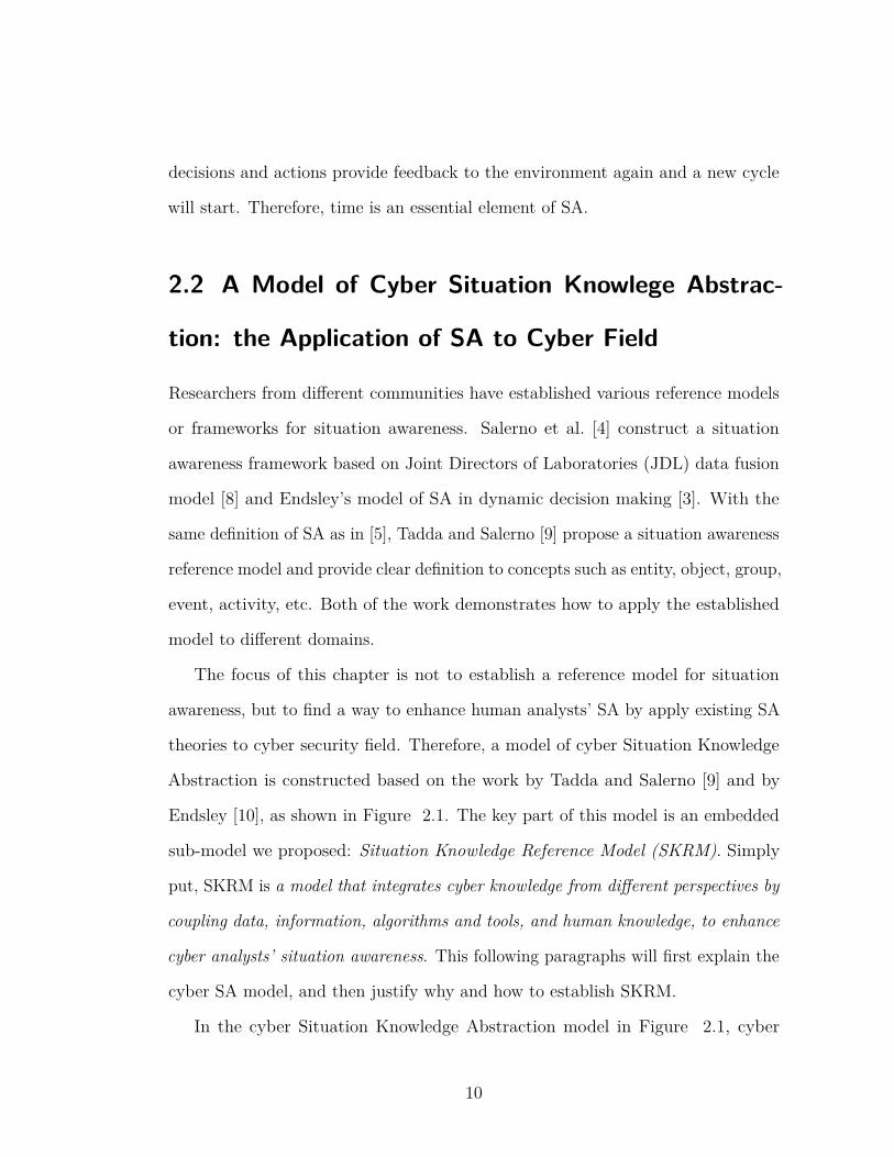
2.2 A Model of Cyber Situation Knowlege Abstrac-

tion: the Application of SA to Cyber Field

Researchers from di�erent communities have established various reference models

or frameworks for situation awareness. Salerno et al. [4] construct a situation

awareness framework based on Joint Directors of Laboratories (JDL) data fusion

model [8] and Endsley’s model of SA in dynamic decision making [3]. With the

same definition of SA as in [5], Tadda and Salerno [9] propose a situation awareness

reference model and provide clear definition to concepts such as entity, object, group,

event, activity, etc. Both of the work demonstrates how to apply the established

model to di�erent domains.

The focus of this chapter is not to establish a reference model for situation

awareness, but to find a way to enhance human analysts’ SA by apply existing SA

theories to cyber security field. Therefore, a model of cyber Situation Knowledge

Abstraction is constructed based on the work by Tadda and Salerno [9] and by

Endsley [10], as shown in Figure 2.1. The key part of this model is an embedded

sub-model we proposed: Situation Knowledge Reference Model (SKRM). Simply

put, SKRM is a model that integrates cyber knowledge from di�erent perspectives by

coupling data, information, algorithms and tools, and human knowledge, to enhance

cyber analysts’ situation awareness. This following paragraphs will first explain the

cyber SA model, and then justify why and how to establish SKRM.

In the cyber Situation Knowledge Abstraction model in Figure 2.1, cyber

10

sensors

tools&algorithms

Level 1: Perception

Human Analysts

real world

Level 2: ComprehensionDamage Assessment

Level 3: ProjectionImpact Assessment

Level 4: ResolutionSecurity Measure Options

&Consequence

Automation System

data

Information

System Interface

Cyber Situation Awareness

Instruction Layer

App/Service Layer

Workflow Layer

Operating System Layer

t5

t3 *a node is a task

*a green dotted line is a control dependency*a red line is a data dependency

t6

t4

t2t1

*a blue line is an execution path*a yellow line is an unexecuted path

*a rectangle node is a primitive fact node*an edge is a causality relation

*a node is an application or service

*a line is a service dependency

*a node is a system object(file, process, socket ...)*an edge is a dependency (7 types)

*a node is a register, memory cell, or instruction*an edge is a data/control dependency

Mem addr[4bf0000,4K], [4bff000, 4K]/bin/gzip process: loads

/etc/group, /etc/ld.so.cache, etc

Mem addr[4b92000,12K], [4bcf000,4K]tar process:

loads /lib/libc.so.6, /etc/selinux/config,, etc

Sector(268821, 120), ...

file system info sector

t7

22:RULE3(remote exploit of a server program)

24:RULE7(direct network access )

25:hacl(internet,webServer,tcp,22)

23:netAccess(webServer,tcp,22)

19:attackerLocated(internet)

26:networkServiceInfo(webServer,openssl,tcp,22,root)

27:vulExists(webServer,‘CVE-2008-0166’,openssl,remoteExploit ,privEscalation )

Avactis Server

(172.18.34.4, 3306, tcp)

(192.168.101.5, 80, tcp)

(192.168.101.*, 53, tcp)

(*, 80, tcp)

Database Server

Web Server3rd Party Web Server

DNS Server

service dependencynetwork connection

14:execCoce(webServer, )

31:hacl(webServer,fileServer,nfsProtocol,nfsPort)

32:nfsExportInfo(fileServer,‘/export’,write, webServer)

30:RULE18(NFS shell)

6:accessFile(fileServer,write, ‘/export’) *an ellipse node is a rule node

*a diamond node is a derived fact node

execve/root/.ssh/authorized_keys

/etc/passwd/etc/ssh/ssh_host_rsa_key

...

clone

exit

/usr/sbin/sshd

execveclone exit/usr/sbin/sshd

…(repeat )

/mnt/wunderbar_emporium.tar.gz /usr/bin/ssh

…

mountd

/export/wunderbar_emporium.tar.gz on NFS Server

/etc/exports

/mnt/wunderbar_emporium.tar.gz on Workstation

/mnt/wunderbar_emporium.tar.gz

on Web Server 36038-4execve wunderbar_em

porium

Files in /home/workstation/workstation_attack

Exploit .sh

Workstation

...

execve

/home/workstation/wunderbar_emporium.tar.gz

/mnt/wunderbar_emporium.tar.gz

execve

/bin/cp

/bin/sh /bin/tar /bin/gzip

NFS ServerWeb Server

… *a blue arrow is an extension from host to network

Dependency Attack Graph

NFS4 Server

(192.168.101.5, 798, tcp/udp)

(172.18.34.5, 2049, tcp/udp)

(10.0.0.3, 973, tcp)

NFS Server

Financial Workstation

SKRM

Data flow

Output of SKRM Information Source of Human Analysts

Input of SKRM

Figure 2.1: A Model of Cyber Situation Knowledge Abstraction [12]

situation awareness consists of four levels: perception, comprehension, projection,

and resolution. The basic idea of this model is: taking input from data, information,

tools and algorithms, and intelligence of human experts from di�erent areas, SKRM

enables the four levels of situation awareness. On the other hand, the output of

11

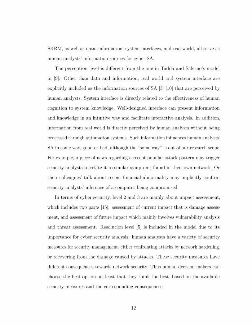
SKRM, as well as data, information, system interfaces, and real world, all serve as

human analysts’ information sources for cyber SA.

The perception level is di�erent from the one in Tadda and Salerno’s model

in [9]: Other than data and information, real world and system interface are

explicitly included as the information sources of SA [3] [10] that are perceived by

human analysts. System interface is directly related to the e�ectiveness of human

cognition to system knowledge. Well-designed interface can present information

and knowledge in an intuitive way and facilitate interactive analysis. In addition,

information from real world is directly perceived by human analysts without being

processed through automation systems. Such information influences human analysts’

SA in some way, good or bad, although the “some way” is out of our research scope.

For example, a piece of news regarding a recent popular attack pattern may trigger

security analysts to relate it to similar symptoms found in their own network. Or

their colleagues’ talk about recent financial abnormality may implicitly confirm

security analysts’ inference of a computer being compromised.

In terms of cyber security, level 2 and 3 are mainly about impact assessment,

which includes two parts [15]: assessment of current impact that is damage assess-

ment, and assessment of future impact which mainly involves vulnerability analysis

and threat assessment. Resolution level [5] is included in the model due to its

importance for cyber security analysis: human analysts have a variety of security

measures for security management, either confronting attacks by network hardening,

or recovering from the damage caused by attacks. These security measures have

di�erent consequences towards network security. Thus human decision makers can

choose the best option, at least that they think the best, based on the available

security measures and the corresponding consequences.

12

2.3 SKRM Framework

To better present SKRM framework, three questions should be answered: 1) Why

do we need SKRM? 2) What is the main structure of SKRM? 3) How can SKRM

enable cyber situation awareness?

2.3.1 Why do we need SKRM?

We need SKRM for several reasons. First, the isolation between di�erent knowledge

bases. Cyber security has made significant advancement in a variety of areas, but

these areas rarely “talk” to each other. When it comes to cyber SA, we have

experts from di�erent areas working on the same topic, but they cannot e�ectively

communicate with each other. For example, system experts exactly know which file

is stolen or modified, but they hardly know how this can impact the business level.

On the other hand, business managers can rapidly notice a suspicious financial loss,

but they won’t relate it to an unallowed system call parameter inside the operating

system. This is one reason for constructing SKRM: we need a model to integrate

knowledge from di�erent areas to break the isolation between them.

Second, the isolation between techniques and human. Human intelligence is the

most powerful and valuable resource that needs to be well utilized in security analysis.

Many microscopic tools, algorithms, and techniques are developed for specific

purposes, but few macroscopic models or framework are provided to synthesize

functions of these techniques, reduce the complexity of security problems and

ease the cognition of human analysts. Therefore, we need to couple the available

techniques to enhance cyber SA and construct a bridge between techniques and

human analysts.

13

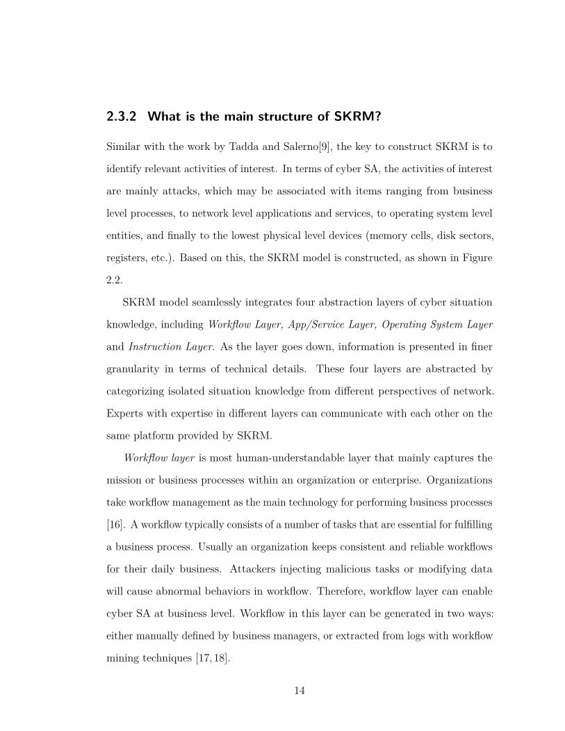
2.3.2 What is the main structure of SKRM?

Similar with the work by Tadda and Salerno[9], the key to construct SKRM is to

identify relevant activities of interest. In terms of cyber SA, the activities of interest

are mainly attacks, which may be associated with items ranging from business

level processes, to network level applications and services, to operating system level

entities, and finally to the lowest physical level devices (memory cells, disk sectors,

registers, etc.). Based on this, the SKRM model is constructed, as shown in Figure

2.2.

SKRM model seamlessly integrates four abstraction layers of cyber situation

knowledge, including Workflow Layer, App/Service Layer, Operating System Layer

and Instruction Layer. As the layer goes down, information is presented in finer

granularity in terms of technical details. These four layers are abstracted by

categorizing isolated situation knowledge from di�erent perspectives of network.

Experts with expertise in di�erent layers can communicate with each other on the

same platform provided by SKRM.

Workflow layer is most human-understandable layer that mainly captures the

mission or business processes within an organization or enterprise. Organizations

take workflow management as the main technology for performing business processes

[16]. A workflow typically consists of a number of tasks that are essential for fulfilling

a business process. Usually an organization keeps consistent and reliable workflows

for their daily business. Attackers injecting malicious tasks or modifying data

will cause abnormal behaviors in workflow. Therefore, workflow layer can enable

cyber SA at business level. Workflow in this layer can be generated in two ways:

either manually defined by business managers, or extracted from logs with workflow

mining techniques [17,18].

14

Instruction Layer

App/Service Layer

Workflow Layer

Operating System Layer

t5

t3 *a node is a task

*a green dotted line is a control dependency*a red line is a data dependency

t6

t4

t2t1

*a blue line is an execution path*a yellow line is an unexecuted path

*a rectangle node is a primitive fact node*an edge is a causality relation

*a node is an application or service

*a line is a service dependency

*a node is a system object(file, process, socket ...)*an edge is a dependency (7 types)

*a node is a register, memory cell, or instruction*an edge is a data/control dependency

Mem addr[4bf0000,4K], [4bff000, 4K]/bin/gzip process: loads

/etc/group, /etc/ld.so.cache, etc

Mem addr[4b92000,12K], [4bcf000,4K]tar process:

loads /lib/libc.so.6, /etc/selinux/config,, etc

Sector(268821, 120), ...

file system info sector

t7

22:RULE3(remote exploit of a server program)

24:RULE7(direct network access)

25:hacl(internet,webServer,tcp,22)

23:netAccess(webServer,tcp,22)

19:attackerLocated(internet)

26:networkServiceInfo(webServer,openssl,tcp,22,root)

27:vulExists(webServer,�CVE-2008-0166�,openssl,remoteExploit,privEscalation)

Avactis Server

(172.18.34.4, 3306, tcp)

(192.168.101.5, 80, tcp)

(192.168.101.*, 53, tcp)

(*, 80, tcp)

Database Server

Web Server3rd Party Web Server

DNS Server

service dependencynetwork connection

14:execCoce(webServer, )

31:hacl(webServer,fileServer,nfsProtocol,nfsPort)

32:nfsExportInfo(fileServer,�/export�,write, webServer)

30:RULE18(NFS shell)

6:accessFile(fileServer,write, �/export�) *an ellipse node is a rule node

*a diamond node is a derived fact node

execve/root/.ssh/authorized_keys

/etc/passwd/etc/ssh/ssh_host_rsa_key

...

clone

exit

/usr/sbin/sshd

execveclone exit/usr/sbin/sshd

…(repeat)

/mnt/wunderbar_emporium.tar.gz /usr/bin/ssh

…

mountd

/export/wunderbar_emporium.tar.gz on NFS Server

/etc/exports

/mnt/wunderbar_emporium.tar.gz on Workstation

/mnt/wunderbar_emporium.tar.gz

on Web Server 36038-4execve wunderbar_emporium

Files in /home/workstation/workstation_attack

Exploit.sh

Workstation

...

execve

/home/workstation/wunderbar_emporium.tar.gz

/mnt/wunderbar_emporium.tar.gz

execve

/bin/cp

/bin/sh /bin/tar /bin/gzip

NFS ServerWeb Server

… *a blue arrow is an extension from host to network

Dependency Attack Graph

NFS4 Server

(192.168.101.5, 798, tcp/udp)

(172.18.34.5, 2049, tcp/udp)

(10.0.0.3, 973, tcp)

NFS Server

Financial Workstation

Figure 2.2: The Situation Knowledge Reference Model (SKRM) [11]

The function of business process relies on a variety application and services.

A workflow can be divided into block tasks [19], which is actually a sub-workflow

containing a set of atomic tasks. Therefore, the execution of a workflow depends

on the execution of tasks, which then relies on corresponding application software.

These applications have further dependence relationship on a set of services, such

as web service, DNS service, etc. Therefore, App/Service Layer is incorporated into

15

SKRM to capture the required applications and services for workflow execution,

and the dependency relationship between them as well. Service discovery and

dependency analysis techniques [20] can be applied to App/Service Layer.

Attackers compromise network by exploiting security holes existing in applica-

tions and services. These attacks will leave trace inside operating system, which

could be deleted logs, prohibited access to password files, or abnormal system

call patterns, etc. All these operating system objects, processes and files, as well

as the dependency relationship between them, are included in Operating System

(OS) Layer. Operating system layer usually adopts techniques of system level taint

tracking [21] and intrusion recovery [22].

Instruction Layer can identify missed intrusions in operating system layer, and

assist taint analysis and attack recovery at instruction level. Instruction layer maps

the entities and relationships on OS layer to memory cells, disk sectors, registers,

kernel address space, and other devices. Techniques of intrusion harm analysis [23],

including taint tracking and intrusion recovery, are often involved in instruction

layer.

Attack Graph is not a specific layer in this stack, but rather an interconnection

technique between App/Service Layer and Operating System Layer. By analyzing

the vulnerabilities exist in the applications and services, attack graph can generate

potential attack paths for the entire network. Through the attack paths, security

analysts will know which hosts are most dangerous and need to be further scrutinized.

Moreover, the corresponding system objects related to the vulnerable services or

applications will be highlighted.

16

2.3.3 How can SKRM enable cyber situation awareness?

SKRM model is not simply a mapping of situation knowledge in di�erent areas

to the above abstraction layers. It is in fact an integration of data, information,

algorithms and tools, and human knowledge through cross-layer interaction. It

interconnects the perception level elements to elevate awareness to comprehension,

projection, and resolution levels. SKRM model has the following characteristics

that could enable the four levels of situation awareness:

1) Each abstraction layer generates a graph that covers the entire enterprise

network. This ensures completeness of the overall network environment awareness.

2) Each abstraction layer views the same network from a di�erent perspective

and at a di�erent granularity. These perspectives complement, assist and confirm

each other for more accurate situation awareness.

3) Each abstraction layer leverages current available algorithms, tools, and

techniques in its corresponding area to extract the most critical and useful informa-

tion to present to human security analysts. Such techniques include but are not

limited to workflow mining and attack recovery, service discovery and dependency

analysis, system level taint tracking and recovery, and instruction level intrusion

harm analysis, etc. Future developed algorithms, tools, or techniques can also be

incorporated into SKRM to elevate its capability.

4) Cross-layer analysis is the “soul” of SKRM. SKRM captures cross-layer

relationships by mapping, translating, bridging semantic gaps, and utilizing existing

techniques such as attack graph. Performing top-down, bottom up, and U-shape

cross-layer analysis can enhance the comprehension, projection and resolution

levels of security analysts’ SA. For example, when business level abnormality such

as financial loss is noticed, top-down analysis could find the damage caused by

17

attackers in each abstraction layer: which service is compromised, which system

file is deleted, or which memory cell is tainted, etc. This is an instance of damage

assessment, corresponding to comprehension level SA. On the other hand, if an

IDS alert is raised from operating system layer, a bottom-up analysis will find

out how could the attack have future impact on the business level. This can be

viewed as example of impact assessment or threat assessment, corresponding to

projection level SA. If options of security measures and their corresponding impact

are obtained through either bottom up or U-shape analysis, resolution level SA is

achieved.

2.4 Case Study

A case study is presented to demonstrate that the SKRM graph stack is useful

to enable capabilities toward holistic perception and comprehension. It is also

an illustration of the practical generation of the SKRM graph stack to perform

cross-layer analysis.

2.4.1 Implementation

To illustrate the application of SKRM framework to cyber security analysis, we

implement a web-shop in our test-bed which uses a business scenario similar

as the one described in [16]. To observe the network under cyber-attack, we

further implement a 3-step attack scenario as in [50,51] with di�erent vulnerability

choices (CVE-2008-0166-OpenSSL brute force key guessing attack, NFS mount

misconfiguration, CVE-2009-2692-bypassing mmap_min_addr). The test-bed

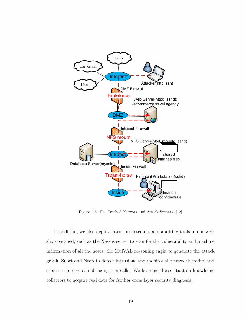
business and attack scenario is shown in Figure 2.3.

18

V. Case Study The security analyst needs to leverage information across different abstraction layers to diagnose an attack and assess its impact in an enterprise network. Business-level symptoms (alerts raised by human managers at high layer) or system level events (alerts provided by security monitoring systems like Snort, tripwire, anti-virus, etc.) are all invaluable to compensate the situation awareness of each other.

Since SKRM is proposed to break stovepipes through cross-layer diagnosis, we present the following case study to demonstrate that the SKRM graph stack is useful to enable capabilities toward holistic perception and comprehension. It is also an illustration of the practical generation of the SKRM graph stack to perform cross-layer analysis.

A. Implementation To illustrate the application of SKRM framework to cyber security analysis, we implement a web-shop in our test-bed which uses a business scenario similar as the one described in [30]. To observe the network under cyber-attack, we further implement a 3-step attack scenario as in [21, 28] with different vulnerability choices (CVE-2008-0166-OpenSSL brute force key guessing attack, NFS mount misconfiguration, CVE-2009-2692-bypassing mmap_min_addr). The test-bed business and attack scenario is shown in Fig. 7.

In addition, we also deploy intrusion detectors and auditing tools in our web-shop test-bed, such as the Nessus server to scan for the vulnerability and machine information of all the hosts, the MulVAL reasoning engin to generate the attack graph, Snort and Ntop to detect intrusions and monitor the network traffic, and strace to intercept and log system calls. We leverage these situation knowledge collectors to acquire real data for further cross-layer security diagnosis.

InternetAttacker(http, ssh)

DMZ Firewall

Web Server(httpd, sshd):-ecommerce travel agency

Financial Workstation(sshd)

Intranet Firewall

NFS Server(nfsd, mountd, sshd)

financial confidentials

shared binaries/files

Hotel

Car Rental

Bank

Bruteforce

DMZ

Intranet

Database Server(mysqld)

Inside

NFS mount

Trojan-horse

Inside Firewall

Fig. 7 The test-bed network and attack scenario

B. Capability: Mission Asset Identification and Classification

Usually an obvious intrusion symptom of an enterprise is the business level financial loss. The responsibility of security analysts is to reason over such symptoms so as to identify the exact intrusion root and all the infected mission assets, for better protection and recovery. That is, the capability of mission asset

identification and classification is required. As shown in Fig. 8, top-down cross-layer SKRM diagnosis will enable this capability.

Workflow Layer

App/Service Layer

OS Layer

dependency AG

12

downward traversing cross-layer edges

3

forward inter-host dependency/taint tracking

t2 is responsible for changing the execution path from non-member service path P1 to member service path P2

Host-switch level mission assets (Web Server, NFS Server and Workstation) are classified to be “clean but in danger” because they are critical for transactions about t2.

financial loss

Application level mission assets (tikiwiki and sshd for the Web Server, samba and unfsd for NFS Server and Linux kernel (2.6.27) for the Workstation) are classified to be “clean but in danger” because they are involved in the attack paths.

4

OS-object level mission assets (process - /usr/sbin/sshd and files - /root/.ssh/authorized_keys, /etc/passwd, /etc/ssh/ssh_host_rsa_key for the Web Server) are classified to be “clean but in danger” because they are mapped to the above-tagged applications/services.

5

The above-mentioned OS objects are updated to be “polluted” because of the mapping between the “repeating” dependency pattern on OS Layer graph and a vulnerability exploitation in dependency AG .

Corresponding mission assets at different levels are updated from the status of “clean but in danger” to “polluted” by reverse tracking.

OS-object level mission assets (/mnt/wunderbar_emporium.tar.gz on Web Server, /export on NFS Server, /mnt/wunderbar_emporium.tar.gz, /home/workstation/workstation_attack/wunderbar_emporium and /home/workstation on Workstation) are classified to be “polluted” because of the propagation of pollution.

Fig. 8 Mission asset identification and classification

Generally, mission asset identification and prioritization achieves at the identification and classification of host-switch level, application level and OS-object level mission critical assets into such classes as “polluted”, “clean but in danger”, and “clean and safe”. For example, the business managers of the web-shop found the profit much lower than expected. Through analysis on the Workflow Layer (Fig. 2), the security analysts suspected that non-member attackers cheated by getting service from the web-shop via the member service path P2. According to the control dependence relation in the workflow, they found that task t2 is responsible for changing the execution path from P1 to P2 (step 1). So they tracked down the cross-layer edges between Workflow Layer and App/Service Layer, with particular inspection on task t2 (step 2). Such cross-layer edges revealed the critical host-switch level mission assets involved in transactions about t2: Web Server, NFS Server and Workstation. Hence, as the most possible attack goals, these assets were tagged into “clean but in danger”. The analysts further tracked down the cross-layer edges between App/Service Layer and OS Layer (step 3), and found that there were four possible attack paths in the dependency AG: {23, 14, 6, 4, 1}, {16, 14, 11, 9, 6, 4, 1}, {16, 14, 6, 4, 1} and {23, 14, 11, 9, 6, 4, 1}. The four paths all lead to the compromise of Web Server, NFS Server, and Workstation, but exploit vulnerabilities of different applications/services. Fig. 6 differentiates the paths with red, blue, purple and green colors respectively. All the application level mission assets involved in the four attack paths were regarded as “clean but in danger”: tikiwiki and sshd for the Web Server, samba and unfsd for NFS Server and Linux kernel (2.6.27) for the Workstation.

The analysts continued to track down the cross-layer edges from dependency AG to OS Layer, and identified fine-grained OS-object level mission assets: process - /usr/sbin/sshd and files - /root/.ssh/authorized_keys, /etc/passwd, /etc/ssh/ssh_host_rsa_key for the Web Server (step 4). These objects were considered as “clean but in danger”. The mapping between the “repeating” dependency pattern on OS Layer graph (Fig. 4) and Node 27 in dependency AG (Fig. 6) confirmed the exploitation of CVE-2008-0166. Therefore, the above-mentioned OS objects related to this vulnerability on Web Server could be determined as “polluted”.

Figure 2.3: The Testbed Network and Attack Scenario [12]

In addition, we also deploy intrusion detectors and auditing tools in our web-

shop test-bed, such as the Nessus server to scan for the vulnerability and machine

information of all the hosts, the MulVAL reasoning engin to generate the attack

graph, Snort and Ntop to detect intrusions and monitor the network tra�c, and

strace to intercept and log system calls. We leverage these situation knowledge

collectors to acquire real data for further cross-layer security diagnosis.

19

2.4.2 Capability 1: Mission Asset Identification and Classifica-

tion

Usually an obvious intrusion symptom of an enterprise is the business level financial

loss. The responsibility of security analysts is to reason over such symptoms so as

to identify the exact intrusion root and all the infected mission assets, for better

protection and recovery. That is, the capability of mission asset identification and

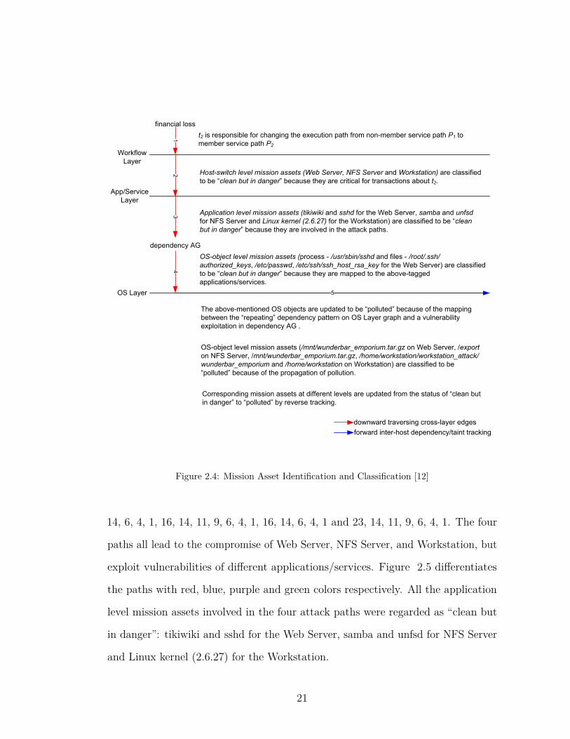
classification is required. As shown in Figure 2.4, top-down cross-layer SKRM

diagnosis will enable this capability.

Generally, mission asset identification and prioritization achieves at the iden-

tification and classification of host-switch level, application level and OS-object

level mission critical assets into such classes as “polluted”, “clean but in danger”,

and “clean and safe”. For example, the business managers of the web-shop found

the profit much lower than expected. Through analysis on the Workflow Layer

Figure 2.2, the security analysts suspected that non-member attackers cheated

by getting service from the web-shop via the member service path P2. According

to the control dependence relation in the workflow, they found that task t2 is

responsible for changing the execution path from P1 to P2 (step 1). So they tracked

down the cross-layer edges between Workflow Layer and App/Service Layer, with

particular inspection on task t2 (step 2). Such cross-layer edges revealed the critical

host-switch level mission assets involved in transactions about t2: Web Server, NFS

Server and Workstation. Hence, as the most possible attack goals, these assets

were tagged into “clean but in danger”. The analysts further tracked down the

cross-layer edges between App/Service Layer and OS Layer (step 3), and found

that there were four possible attack paths in the dependency AG (Figure 2.5), 23,

20

5. Case Study The security analyst needs to leverage information across different abstraction layers to diagnose an attack and assess its impact in an enterprise network. Business-level symptoms (alerts raised by human managers at high layer) or system level events (alerts provided by security monitoring systems like Snort, tripwire, anti-virus, etc.) are all invaluable to compensate the situation awareness of each other.

Since SKRM is proposed to break stovepipes through cross-layer diagnosis, we present the following case study to demonstrate that the SKRM graph stack is useful to enable capabilities toward holistic perception and comprehension. It is also an illustration of the practical generation of the SKRM graph stack to perform cross-layer analysis.

5.1 Implementation To illustrate the application of SKRM framework to cyber security analysis, we implement a web-shop in our test-bed which uses a business scenario similar as the one described in [30]. To observe the network under cyber-attack, we further implement a 3-step attack scenario as in [21, 28] with different vulnerability choices (CVE-2008-0166-OpenSSL brute force key guessing attack, NFS mount misconfiguration, CVE-2009-2692-bypassing mmap_min_addr). The test-bed business and attack scenario is shown in Fig. 7.

In addition, we also deploy intrusion detectors and auditing tools in our web-shop test-bed, such as the Nessus server to scan for the vulnerability and machine information of all the hosts, the MulVAL reasoning engin to generate the attack graph, Snort and Ntop to detect intrusions and monitor the network traffic, and strace to intercept and log system calls. We leverage these situation knowledge collectors to acquire real data for further cross-layer security diagnosis.

InternetAttacker(http, ssh)

DMZ Firewall

Web Server(httpd, sshd):-ecommerce travel agency

Financial Workstation(sshd)

Intranet Firewall

NFS Server(nfsd, mountd, sshd)

financial confidentials

shared binaries/files

Hotel

Car Rental

Bank

Bruteforce

DMZ

Intranet

Database Server(mysqld)

Inside

NFS mount

Trojan-horse

Inside Firewall

Fig. 7 The test-bed network and attack scenario

5.2 Capability: Mission Asset Identification and Classification Usually an obvious intrusion symptom of an enterprise is the business level financial loss. The responsibility of security analysts is to reason over such symptoms so as to identify the exact intrusion root and all the infected mission assets, for better protection and recovery. That is, the capability of mission asset

identification and classification is required. As shown in Fig. 8, top-down cross-layer SKRM diagnosis will enable this capability.

Workflow Layer

App/Service Layer

OS Layer

dependency AG

12

downward traversing cross-layer edges

3

forward inter-host dependency/taint tracking

t2 is responsible for changing the execution path from non-member service path P1 to member service path P2

Host-switch level mission assets (Web Server, NFS Server and Workstation) are classified to be “clean but in danger” because they are critical for transactions about t2.

financial loss

Application level mission assets (tikiwiki and sshd for the Web Server, samba and unfsd for NFS Server and Linux kernel (2.6.27) for the Workstation) are classified to be “clean but in danger” because they are involved in the attack paths.

4

OS-object level mission assets (process - /usr/sbin/sshd and files - /root/.ssh/authorized_keys, /etc/passwd, /etc/ssh/ssh_host_rsa_key for the Web Server) are classified to be “clean but in danger” because they are mapped to the above-tagged applications/services.

5

The above-mentioned OS objects are updated to be “polluted” because of the mapping between the “repeating” dependency pattern on OS Layer graph and a vulnerability exploitation in dependency AG .

Corresponding mission assets at different levels are updated from the status of “clean but in danger” to “polluted” by reverse tracking.

OS-object level mission assets (/mnt/wunderbar_emporium.tar.gz on Web Server, /export on NFS Server, /mnt/wunderbar_emporium.tar.gz, /home/workstation/workstation_attack/wunderbar_emporium and /home/workstation on Workstation) are classified to be “polluted” because of the propagation of pollution.

Fig. 8 Mission asset identification and classification

Generally, mission asset identification and prioritization achieves at the identification and classification of host-switch level, application level and OS-object level mission critical assets into such classes as “polluted”, “clean but in danger”, and “clean and safe”. For example, the business managers of the web-shop found the profit much lower than expected. Through analysis on the Workflow Layer (Fig. 2), the security analysts suspected that non-member attackers cheated by getting service from the web-shop via the member service path P2. According to the control dependence relation in the workflow, they found that task t2 is responsible for changing the execution path from P1 to P2 (step 1). So they tracked down the cross-layer edges between Workflow Layer and App/Service Layer, with particular inspection on task t2 (step 2). Such cross-layer edges revealed the critical host-switch level mission assets involved in transactions about t2: Web Server, NFS Server and Workstation. Hence, as the most possible attack goals, these assets were tagged into “clean but in danger”. The analysts further tracked down the cross-layer edges between App/Service Layer and OS Layer (step 3), and found that there were four possible attack paths in the dependency AG: {23, 14, 6, 4, 1}, {16, 14, 11, 9, 6, 4, 1}, {16, 14, 6, 4, 1} and {23, 14, 11, 9, 6, 4, 1}. The four paths all lead to the compromise of Web Server, NFS Server, and Workstation, but exploit vulnerabilities of different applications/services. Fig. 6 differentiates the paths with red, blue, purple and green colors respectively. All the application level mission assets involved in the four attack paths were regarded as “clean but in danger”: tikiwiki and sshd for the Web Server, samba and unfsd for NFS Server and Linux kernel (2.6.27) for the Workstation.

The analysts continued to track down the cross-layer edges from dependency AG to OS Layer, and identified fine-grained OS-object level mission assets: process - /usr/sbin/sshd and files - /root/.ssh/authorized_keys, /etc/passwd, /etc/ssh/ssh_host_rsa_key for the Web Server (step 4). These objects were considered as “clean but in danger”. The mapping between the “repeating” dependency pattern on OS Layer graph (Fig. 4) and Node 27 in dependency AG (Fig. 6) confirmed the exploitation of CVE-2008-0166. Therefore, the above-mentioned OS objects related to this vulnerability on Web Server could be determined as “polluted”.

Figure 2.4: Mission Asset Identification and Classification [12]

14, 6, 4, 1, 16, 14, 11, 9, 6, 4, 1, 16, 14, 6, 4, 1 and 23, 14, 11, 9, 6, 4, 1. The four

paths all lead to the compromise of Web Server, NFS Server, and Workstation, but

exploit vulnerabilities of di�erent applications/services. Figure 2.5 di�erentiates

the paths with red, blue, purple and green colors respectively. All the application

level mission assets involved in the four attack paths were regarded as “clean but

in danger”: tikiwiki and sshd for the Web Server, samba and unfsd for NFS Server

and Linux kernel (2.6.27) for the Workstation.

21

B. Cross-layer Interconnection Cross-layer diagnosis is critical for SKRM model, as traversing from one layer to another layer along the edges would lead to expected new information and ultimately a holistic understanding of the whole scenario. However, it cannot be achieved without the fulfillment of cross-layer interconnection. Only with inter-compartment interconnection we still lack the capture of cross-layer relationships that can break horizontal stovepipes.

1) Cross-layer Semantics Bridging

Basically, cross-layer relationships are captured by semantics bridging (specifically, mapping, translation, etc.) in-between the adjacent two abstraction layers of computer and information system semantics. In specific, association between the workflow tasks at Workflow Layer and the particular applications at App/Service Layer can be mined from the network traces with workflow logs, and can be used to create bi-directional mappings between them. The mappings between OS level objects and instruction level objects can be achieved by developing a reconstruction engine such as the one presented in [31]. The purple bi-directional dotted lines between adjacent layers in Fig. 1 illustrate such mappings.

2) Attack Graph Representation and Generation

Specially, we interconnect the App/Service Layer and OS Layer by vertically inserting a dependency Attack Graph between them. This enables the causality representation and tracking between App/Service Layer pre-conditions (network connection, machine configuration and vulnerability information) and OS Layer symptoms/patterns of successful exploits.

! Definition 5 (dependency Attack Graph): The dependency Attack Graph (AG) can be represented with a directed graph G(V,E), where V is the set of nodes and E is the set of directed edges. There are two

kinds of nodes in the attack graph (refer to the attack graph of Fig. 6): derivation nodes (represented with ellipses) and fact nodes. The fact nodes could be further classified into primitive fact nodes (represented with rectangles) and derived fact nodes (represented with diamonds). The directed edges represent the causality relationships between the nodes.

In the dependency Attack Graph, one or more fact nodes could serve as the preconditions of a derivation node and cause it to take effect. One or more derivation nodes could further cause a derived fact node to become true. Each derivation node represents an application of an interaction rule given in [28] that yields the derived fact. Let’s take our generated attack graph (Fig. 6) for example: Node 26, 27 (primitive fact node) and Node 23 (derived fact node) could cause Node 22 (derivation node) to take effect, and Node 22 could further cause Node 14 (derived fact node) to be valid. Besides, a derived fact node may have different ways to become true.

Fig. 1 illustrates a subset of Fig. 6. Fig. 1 also illustrates the interconnection of the dependency Attack Graph with its adjacent two layers. The conversion from App/Service Layer information (network connection, host configuration, scanned vulnerability) to the primitive nodes in Attack Graph is resulting from the Datalog representation before attack graph generation [28]. The mapping from the derived fact nodes in Attack Graph to the OS Layer intrusion symptoms (such as the system call sequence [10], intrusion pattern, signature, etc.) can be achieved by bi-directional inter-host OS level dependency tracking proposed above, using the OS level instances of host or service configuration as input. For example, the process “/usr/sbin/sshd” instantiates sshd, and “/etc/exports” instantiates unfsd. Tracking “/usr/sbin/sshd” would reveal the repeated pattern of accessing sshd-related processes and files, indicating the occurrence of Node 14 in the dependency AG.

18:hacl(internet,webServer,http,80):1

17:RULE 7 (direct network access):0

19:attackerLocated(internet):1 25:hacl(internet,webServer,tcp,22):1

24:RULE 7 (direct network access):0

16:netAccess(webServer,http,80):0

20:networkServiceInfo(webServer,tikiwiki,http,80,_):1

21:vulExists(webServer,'CVE-2007-5423',tikiwiki,remoteExploit,privEscalation):1

23:netAccess(webServer,tcp,22):0

26:networkServiceInfo(webServer,openssl,tcp,22,_):1

27:vulExists(webServer,'CVE-2008-0166',openssl,remoteExploit,privEscalation):1

15:RULE 3 (remote exploit of a server program):0 22:RULE 3 (remote exploit of a server program):0

13:hacl(webServer,fileServer,tcp,139):1 14:execCode(webServer,_):0 31:hacl(webServer,fileServer,nfsProtocol,nfsPort):1

32:nfsExportInfo(fileServer,'/export',write,webServer):1

12:RULE 6 (multi-hop access):0 30:RULE 18 (NFS shell):0

9:execCode(fileServer,_):0

28:networkServiceInfo(fileServer,samba,tcp,139,_):1

29:vulExists(fileServer,'CVE-2007-2446',samba,remoteExploit,privEscalation):1

10:RULE 3 (remote exploit of a server program):0

8:canAccessFile(fileServer,_,write,'/export'):1

7:RULE 11 (execCode implies file access):0

6:accessFile(fileServer,write,'/export'):0

33:nfsMounted(workStation,'/mnt/share',fileServer,'/export',read):1

5:RULE 17 (NFS semantics):0

4:accessFile(workStation,write,'/mnt/share'):0

3:vulExists(workStation,'CVE-2009-2692',kernel,localExploit,privEscalation):1

2:RULE 5 (Corresponding Trojan horse installation):0

1:execCode(workStation,root):0

11:netAccess(fileServer,tcp,139):0

Fig. 6 The dependency Attack Graph

Figure 2.5: The Dependency Attack Graph [12]

The analysts continued to track down the cross-layer edges from dependency AG

to OS Layer, and identified fine-grained OS-object level mission assets, including

process /usr/sbin/sshd and files /root/.ssh/authorized_keys, /etc/passwd, and

/etc/ssh/ssh_host_rsa_key for the Web Server (step 4). These objects were consid-

ered as “clean but in danger”. The mapping between the “repeating” dependency

pattern on OS Layer graph and Node 14 in dependency AG confirmed the exploita-

tion of CVE-2008-0166. Therefore, the above-mentioned OS objects related to this

vulnerability on Web Server could be determined as “polluted”. Further forward

dependency tracking on the dependency graph discovered a file named /mnt/wun-

derbar_emporium.tar.gz was created and thus “polluted” on the Web Server (step

5). Inter-host OS dependency tracking helped reveal the propagation of such pollu-

tion: the file sharing directory /export on NFS Server was “polluted”; the files or

22

directories named /home/workstation/workstation_attack/wunderbar_emporium,

/mnt/wunderbar_emporium.tar.gz, and /home/workstation on Workstation were

all “polluted”. In a similar way, the memory cells or disk sectors at Instruction Layer

corresponding to the system objects could also be classified into these categories.

Through reverse tracking to the upper layers, the status of Web Server and

its service sshd, NFS Server and its services unfsd, mountd, Workstation and its

service sshd were all updated from “clean but in danger” to “polluted”. In a word,

through such top-down cross-layer SKRM-based analysis, mission assets at the

host-switch level, application/service level and OS-object level could all be identified

and further classified into such classes as “polluted”, “clean but in danger” and

“clean and safe”.

2.4.3 Capability 2: Mission Damage and Impact Assessment

Defending missions in cyber space from various attacks continues to be a chal-

lenge. An e�ective attack can lead to great loss in the confidentiality, integrity, or

availability to the missions, and even cause some to abort in extreme cases [90].

When an attack happens, one major concern to the security administrators is how

the attack could possibly impact related missions. Specifically, they may ask the

questions such as 1) How likely is a mission a�ected? 2) To what extent is the

mission influenced? Which tasks are already tainted, and which are untouched?

Continuous e�orts have been made to construct high-level models that aid the

mission impact analysis, but concrete methods that achieve accurate quantitative

assessment are rare. Jackobson [90] constructs an impact dependency graph (IDG)

for mission situation assessment. Nevertheless, the paper doesn’t specify detailed

method for generating the dependencies in the IDG. The impact assessment provided

23

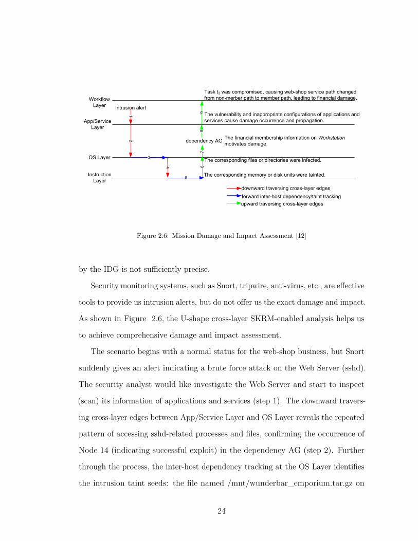
Further forward dependency tracking on the dependency graph discovered a file named /mnt/wunderbar_emporium.tar.gz was created and thus “polluted” on the Web Server (step 5). Inter-host OS dependency tracking helped reveal the propagation of such pollution: the file sharing directory /export on NFS Server was “polluted”; the files or directories named /home/workstation/workstation_attack/wunderbar_emporium, /mnt/wunderbar_emporium.tar.gz, and /home/workstation on Workstation were all “polluted”. In a similar way, the memory cells or disk sectors at Instruction Layer corresponding to the system objects could also be classified into these categories.

Through reverse tracking to the upper layers, the status of Web Server and its service sshd, NFS Server and its services unfsd, mountd, Workstation and its service sshd were all updated from “clean but in danger” to “polluted”. In a word, through such top-down cross-layer SKRM-based analysis, mission assets at the host-switch level, application/service level and OS-object level could all be identified and further classified into such classes as “polluted”, “clean but in danger” and “clean and safe”.

5.3 Capability: Mission Damage and Impact Assessment Security monitoring systems, such as Snort, tripwire, anti-virus, etc., are effective tools to provide us intrusion alerts, but do not offer us the exact damage and impact. As shown in Fig. 9, the U-shape cross-layer SKRM-enabled analysis helps us to achieve comprehensive damage and impact assessment.

Workflow Layer

App/Service Layer

OS Layer

Instruction Layer

dependency AG

12

downward traversing cross-layer edges

4

3

forward inter-host dependency/taint tracking6

upward traversing cross-layer edges7

Task t2 was compromised, causing web-shop service path changedfrom non-merber path to member path, leading to financial damage.

The vulnerability and inappropriate configurations of applications and services cause damage occurrence and propagation.

The financial membership information on Workstation motivates damage.

The corresponding memory or disk units were tainted.5

9

The corresponding files or directories were infected.

Intrusion alert

8

Fig. 9 Mission damage and impact assessment

The scenario begins with a normal status for the web-shop business, but Snort suddenly gives an alert indicating a brute force attack on the Web Server (sshd). The security analyst would like investigate the Web Server and start to inspect (scan) its information of applications and services (step 1). The downward traversing cross-layer edges between App/Service Layer and OS Layer reveals the repeated pattern of accessing sshd-related processes and files, confirming the occurrence of Node 14 (indicating successful exploit) in the dependency AG (step 2). Further through the process, the inter-host dependency tracking at the OS Layer identifies the intrusion taint seeds: the file named /mnt/wunderbar_emporium.tar.gz on the Web Server, the directory named /export on the NFS Server and the files or directories named /mnt/wunderbar_emporium.tar.gz, /home/workstation/workstation_attack/wunderbar_emporium and /home/workstation on the Workstation (step 3). Using these as input, downward traversing the cross-layer edges between OS Layer and Instruction Layer helps to identify the tainted memory and disk units (step 4). The forward inter-host taint tracking at the Instruction Layer located the fine-grained impacts on victim hosts (step 5). At this point, the OS-level and Instruction-level damage has been identified: the above files and directories were all infected and performing malicious actions at the OS Layer and their memory or disk space were therefore tainted on Instruction

Layer. This triggered the analyst to perform another round of bottom-up analysis to comprehend the damage at other layers. The analyst tracks upward along the cross-layer edges between OS Layer and dependency AG, and determined the attack path (step 6 and 7). The attack path, combined with the abnormal behavior on OS Layer, led the analyst to the missing intrusion intent of the attacker: the financial membership information under the directory named /home/workstation on Workstation is the evidence of the root cause of the damage. The mappings between dependency AG and App/Service Layer show the specific pre-conditions of the exploits (step 8). The vulnerabilities and inappropriate configurations at App/Service Layer allow the damage to be caused. Finally, the analyst tracks upward to the cross-layer relationships between App/Service Layer and Workflow Layer (step 9), and finds that: task t2 was compromised, so the web-shop’s service path was changed from non-member service path {t1, t2, t3, t4, t6, t7} to the member service path {t1, t2, t5, t6, t7} at Workflow Layer and enables significant financial damage to occur.

In a word, SKRM enables a U-shape cross-layer analysis, as illustrated in Fig. 9, to assess systematic damage and its impact from multi-layer semantics.

6. Discussion From the case study above, we identify that SKRM-enabled analytics can exceed the reach of intrusion detection and attack graph analysis, through inter-compartment awareness and cross-layer analysis (top-down, bottom-up, U-shape, etc.). SKRM actually has the potential to enable other capabilities. For example, attack path determination and attack intent identification were also involved in the above U-shape cross-layer diagnosis. The potential capabilities would be explored in future work, including but not limited to:

• U-shape cross-layer diagnosis may help us understand the adversary activity, including the attack path determination and attack intent identification.

• Bottom-up cross-layer analysis may help evaluate mission impact.

• Cross-layer Bayesian networks could be constructed to reason about uncertainty.

• Top-down cross-layer analysis may help us construct mission asset map based on asset classification.

• Comprehensive analysis may help us simulate different strategic mitigation plans.

• Comprehensive analysis may provide insights for intrusion recovery.

• Knowledge representation could be enabled for cognitive engineering.

In addition to the potentials, the current SKRM and SKRM-enabled analytics have some limitations. Although some tools have been developed to generate parts of the SKRM graph stack, the current version of SKRM is still semi-automatic, gaining computer-aided human centric cyber SA. Additional work is still required to evaluate the utility of SKRM in the scale of a real enterprise and more complex scenarios. Our future work will focus on addressing such limitations.

7. Conclusion Current cyber SA based on the technologies in intrusion detection and attack graphs lack the capability to address the needs of mission damage and impact assessment and asset identification (and prioritization). This paper proposes a cross-layer Situation

Figure 2.6: Mission Damage and Impact Assessment [12]

by the IDG is not su�ciently precise.

Security monitoring systems, such as Snort, tripwire, anti-virus, etc., are e�ective

tools to provide us intrusion alerts, but do not o�er us the exact damage and impact.

As shown in Figure 2.6, the U-shape cross-layer SKRM-enabled analysis helps us

to achieve comprehensive damage and impact assessment.

The scenario begins with a normal status for the web-shop business, but Snort

suddenly gives an alert indicating a brute force attack on the Web Server (sshd).

The security analyst would like investigate the Web Server and start to inspect

(scan) its information of applications and services (step 1). The downward travers-

ing cross-layer edges between App/Service Layer and OS Layer reveals the repeated

pattern of accessing sshd-related processes and files, confirming the occurrence of

Node 14 (indicating successful exploit) in the dependency AG (step 2). Further

through the process, the inter-host dependency tracking at the OS Layer identifies

the intrusion taint seeds: the file named /mnt/wunderbar_emporium.tar.gz on

24

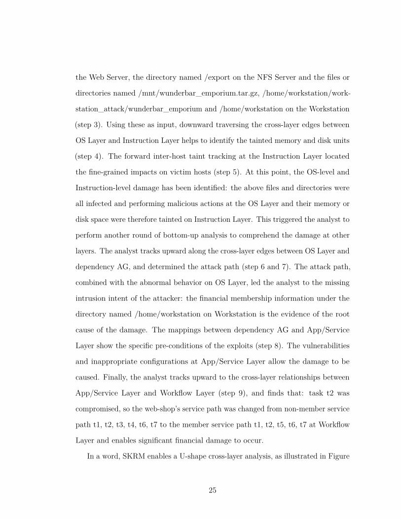
the Web Server, the directory named /export on the NFS Server and the files or

directories named /mnt/wunderbar_emporium.tar.gz, /home/workstation/work-

station_attack/wunderbar_emporium and /home/workstation on the Workstation

(step 3). Using these as input, downward traversing the cross-layer edges between

OS Layer and Instruction Layer helps to identify the tainted memory and disk units

(step 4). The forward inter-host taint tracking at the Instruction Layer located

the fine-grained impacts on victim hosts (step 5). At this point, the OS-level and

Instruction-level damage has been identified: the above files and directories were

all infected and performing malicious actions at the OS Layer and their memory or

disk space were therefore tainted on Instruction Layer. This triggered the analyst to

perform another round of bottom-up analysis to comprehend the damage at other

layers. The analyst tracks upward along the cross-layer edges between OS Layer and

dependency AG, and determined the attack path (step 6 and 7). The attack path,

combined with the abnormal behavior on OS Layer, led the analyst to the missing

intrusion intent of the attacker: the financial membership information under the

directory named /home/workstation on Workstation is the evidence of the root

cause of the damage. The mappings between dependency AG and App/Service

Layer show the specific pre-conditions of the exploits (step 8). The vulnerabilities

and inappropriate configurations at App/Service Layer allow the damage to be

caused. Finally, the analyst tracks upward to the cross-layer relationships between

App/Service Layer and Workflow Layer (step 9), and finds that: task t2 was

compromised, so the web-shop’s service path was changed from non-member service

path t1, t2, t3, t4, t6, t7 to the member service path t1, t2, t5, t6, t7 at Workflow

Layer and enables significant financial damage to occur.

In a word, SKRM enables a U-shape cross-layer analysis, as illustrated in Figure

25

2.6, to assess systematic damage and its impact from multi-layer semantics.

The rest of this section will introduce a concrete approach for mission impact

assessment. The approach is to 1) build a System Object Dependency Graph

(SODG) so that the intrusion propagation process is captured at the system object

level; 2) construct a Mission-Task-Asset (MTA) map to associate the missions and

composing tasks with corresponding assets, which are namely the system objects

such as processes, files, etc. The MTA map is naturally connected to the SODG

through shared system objects; 3) establish a Bayesian network based on the MTA

map and the SODG to leverage the collected intrusion evidence and infer the

probabilities of interested events, such as a system object or a mission task being

tainted.

The approach is proposed on the basis of the following supporting rationales.

First, the SODG is a proper construct connecting the attack and the missions, as

shown in Figure 2.7. From the attack side, an attack’s impact towards the operating

systems can be reflected on the SODG. System objects that are manipulated directly

or indirectly by attackers have the possibility of being tainted. From the mission

side, a mission is fulfilled through a sequence of operations towards system objects.

These operations are caught by the SODG. As a result, the impact of an attack to

the missions can be evaluated by leveraging the SODG as the intermediate bridge.

Second, the SODG is able to capture the intrusion propagation process, which

is critical for correct mission impact assessment. An attack’s impact towards a

mission may not be explicit when they have no common associated assets. The

attack-associated assets refer to the system objects that are directly related to the

attack activities (e.g. a modified file in a Tripwire [60] alert), while the mission-

associated assets refer to the system objects that are involved in the mission

26

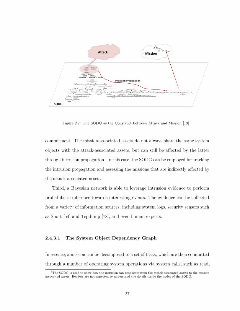
Attack

SODG

Intrusion Propagation

Mission

Figure 2.7: The SODG as the Construct between Attack and Mission [13] 1

commitment. The mission-associated assets do not always share the same system

objects with the attack-associated assets, but can still be a�ected by the latter

through intrusion propagation. In this case, the SODG can be employed for tracking

the intrusion propagation and assessing the missions that are indirectly a�ected by

the attack-associated assets.

Third, a Bayesian network is able to leverage intrusion evidence to perform

probabilistic inference towards interesting events. The evidence can be collected

from a variety of information sources, including system logs, security sensors such

as Snort [54] and Tcpdump [78], and even human experts.

2.4.3.1 The System Object Dependency Graph

In essence, a mission can be decomposed to a set of tasks, which are then committed

through a number of operating system operations via system calls, such as read,1The SODG is used to show how the intrusion can propagate from the attack associated assets to the mission

assocaited assets. Readers are not expected to understand the details inside the nodes of the SODG.

27

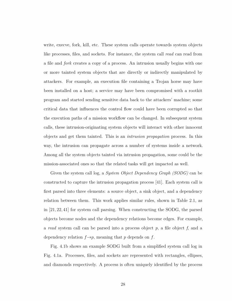
write, execve, fork, kill, etc. These system calls operate towards system objects

like processes, files, and sockets. For instance, the system call read can read from

a file and fork creates a copy of a process. An intrusion usually begins with one

or more tainted system objects that are directly or indirectly manipulated by

attackers. For example, an execution file containing a Trojan horse may have

been installed on a host; a service may have been compromised with a rootkit

program and started sending sensitive data back to the attackers’ machine; some

critical data that influences the control flow could have been corrupted so that

the execution paths of a mission workflow can be changed. In subsequent system

calls, these intrusion-originating system objects will interact with other innocent

objects and get them tainted. This is an intrusion propagation process. In this

way, the intrusion can propagate across a number of systems inside a network.

Among all the system objects tainted via intrusion propagation, some could be the

mission-associated ones so that the related tasks will get impacted as well.

Given the system call log, a System Object Dependency Graph (SODG) can be

constructed to capture the intrusion propagation process [41]. Each system call is

first parsed into three elements: a source object, a sink object, and a dependency

relation between them. This work applies similar rules, shown in Table 2.1, as

in [21, 22, 41] for system call parsing. When constructing the SODG, the parsed

objects become nodes and the dependency relations become edges. For example,

a read system call can be parsed into a process object p, a file object f, and a

dependency relation fæp, meaning that p depends on f .

Fig. 4.1b shows an example SODG built from a simplified system call log in

Fig. 4.1a. Processes, files, and sockets are represented with rectangles, ellipses,

and diamonds respectively. A process is often uniquely identified by the process

28

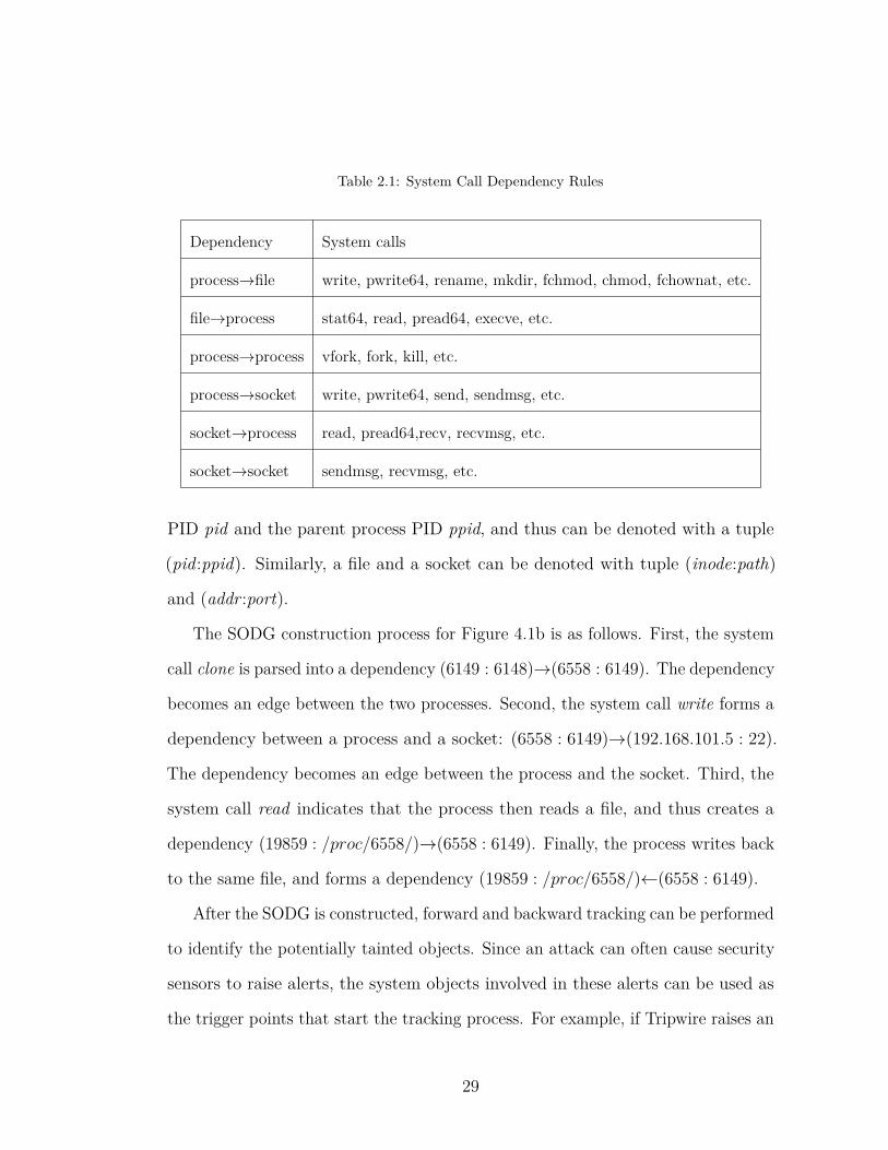
Table 2.1: System Call Dependency Rules

Dependency System calls

processæfile write, pwrite64, rename, mkdir, fchmod, chmod, fchownat, etc.

fileæprocess stat64, read, pread64, execve, etc.

processæprocess vfork, fork, kill, etc.

processæsocket write, pwrite64, send, sendmsg, etc.

socketæprocess read, pread64,recv, recvmsg, etc.

socketæsocket sendmsg, recvmsg, etc.

PID pid and the parent process PID ppid, and thus can be denoted with a tuple

(pid:ppid). Similarly, a file and a socket can be denoted with tuple (inode:path)

and (addr :port).

The SODG construction process for Figure 4.1b is as follows. First, the system

call clone is parsed into a dependency (6149 : 6148)æ(6558 : 6149). The dependency

becomes an edge between the two processes. Second, the system call write forms a

dependency between a process and a socket: (6558 : 6149)æ(192.168.101.5 : 22).

The dependency becomes an edge between the process and the socket. Third, the

system call read indicates that the process then reads a file, and thus creates a

dependency (19859 : /proc/6558/)æ(6558 : 6149). Finally, the process writes back

to the same file, and forms a dependency (19859 : /proc/6558/)Ω(6558 : 6149).

After the SODG is constructed, forward and backward tracking can be performed

to identify the potentially tainted objects. Since an attack can often cause security

sensors to raise alerts, the system objects involved in these alerts can be used as

the trigger points that start the tracking process. For example, if Tripwire raises an

29

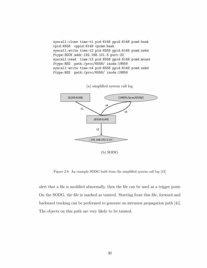
syscall:clone time:t1 pid:6149 ppid:6148 pcmd:bashcpid:6558 cppid:6149 cpcmd:bashsyscall:write time:t2 pid:6558 ppid:6149 pcmd:sshdftype:SOCK addr:192.168.101.5 port:22syscall:read time:t3 pid:6558 ppid:6149 pcmd:mountftype:REG path:/proc/6558/ inode:19859syscall:write time:t4 pid:6558 ppid:6149 pcmd:sshdftype:REG path:/proc/6558/ inode:19859

(a) simplified system call log

(6149:6148)

(6558:6149)

（192.168.101.5:22）

(19859:/proc/6558/)

t1

t2

t3

t4

(b) SODG

Figure 2.8: An example SODG built from the simplified system call log [13]

alert that a file is modified abnormally, then the file can be used as a trigger point.

On the SODG, the file is marked as tainted. Starting from this file, forward and

backward tracking can be performed to generate an intrusion propagation path [41].

The objects on this path are very likely to be tainted.

30

2.4.3.2 Mission-Task-Asset Map

Constructing Mission-Task-Asset (MTA) map is to relate the system objects with

the tasks and missions. An intuitive solution is to decompose the missions into

tasks, and further associate the tasks with system objects. However, this top-down

decomposing approach requires the prior knowledge of a mission workflow. In cases

when attackers are able to insert malicious tasks into the workflow, these inserted

tasks could be missed by the MTA map.

In this work, we propose a bottom-up extraction approach that extracts the

tasks from the SODG, and then relates the tasks with specific missions, as shown

in Figure 2.9. Since the SODG captures what actually happens in the network,

extraction from the SODG accurately reflects which tasks are actually committed.

Considering the manageable number of missions and tasks an enterprise network

could deal with, relating tasks with missions is not a real issue. The key di�culty

lies in how to extract tasks from the SODG due to its daunting size. However, the

extraction is ensured to be feasible by the following principles.

First, a mission task can be viewed as an instantiation of several services that

have dependency relations. In enterprise networks, the normal function of a service

may depend on one or more other services. These services and applications often

interact and work together to accomplish specific tasks. For example, a user’s

login request requires web service from a web server, which further relies on au

authentication service to verify the user’s legitimacy. The authentication will

then depend on the database service to access the users’ account information.

In this example, a single task “user login” can be viewed as the instantiation of

combined web service, authentication service, and database service. Therefore,2Again, readers are not expected to understand the details inside the nodes of the SODG.

31

t1

t2 t3t4

t5 t6

t7t8

t9

Mission 1 Mission 2

Service Dependency Graph Pattern Matching

Mission

Task

Asset: SODG

Service Dependency

Graph Pattern

Repository

Figure 2.9: Mission-Task-Asset Map [13] 2

if such dependency relations among services can be discovered and represented

with specific graphs, then a task can be viewed as the instantiation of a service

dependency graph.

Second, through service discovery, the service dependency graphs (SDGs) can be

established at the system object level. Service discovery has been studied intensively

in previous work [91–94]. Dai [95] proposed to infer the service dependency through

identifying OS-level causal paths. Therefore, the service dependencies can be

represented with OS-level dependency graphs, such as the SODGs. Each service

dependency graph has a pattern that can be used to identify the corresponding SDG.

The patterns could be defined from the perspective of both text and graph-topology.

For example, a file node with name config and an out degree of n can be one feature

32

for a specific pattern, indicating that file config is accessed n times. Since servers

in an enterprise network often fulfill routine responsibilities, the common patterns

can be extracted to form an SDG pattern repository.

Third, the system assets can be linked to tasks automatically by matching

the SODG against the SDG patterns. Although the SODG is usually not human-

readable, it can be annotated with specific SDGs through pattern matching. For

example, if the pattern for combined web service, authentication service, and

database service appears in the SODG for several times, then as the instantiations

of these services, several “user login” tasks can be linked to the system objects

involved in these patterns.

2.4.3.3 MTA based Bayesian Networks

To perform probabilistic mission impact assessment, the Bayesian networks can be

constructed based on the established MTA maps. The Bayesian network is a type

of Directed Acyclic Graph that can be used to model the cause and e�ect relations.

In a BN, the nodes represent the variables of interest, and the edges represent the

causality relations between nodes. The strength of such causality relations can be

specified with conditional probability tables (CPT). When evidence is provided, a

properly constructed BN can infer the probabilities of interesting variables.

In this section, we propose to construct an MTA-based BN, whose input is

the intrusion evidence collected from various security sensors, and output is the

probabilities of interesting security events, such as a system object or a task being

tainted. The graphical feature of MTA enables and facilitates the construction of

MTA-based BN. With CPT tables specified and the evidence incorporated, the

33

MTA-based BN is able to infer the probabilities of tasks and missions being tainted,

and thus evaluate the impact of attacks towards interesting missions.

To build the MTA-based BN, the dependency relations existing in the MTA

map need to be well modeled. Each MTA map implies certain dependency relations

among the missions, tasks, and system objects. Such dependency relations can

be represented with certain mission dependency graphs by interpreting the MTA

maps. In the mission dependency graph, the status of a mission depends on the

status of the composing tasks, while the status of a task depends on the status of

the relevant system objects. We provide two example mission dependency graphs

based on the same MTA map to illustrate how the dependency relations can be

interpreted.

Figure 2.10 is an example of benign mission dependency graph by interpreting

an MTA map. In this graph, a mission is composed of several tasks. For each

mission to be benign, all of its composing tasks should be benign. In addition, all

the tasks should be committed in the correct sequence. Similarly, each task is also

composed of several system level operations. To ensure the task is benign, the

related system objects should be benign and the operations should be performed in

the right sequence. Therefore, all of the parent nodes have the “AND” relation for

the child node to be true. In Figure 2.10, Node 5 “Task 1 is benign” should have

4 preconditions satisfied in order to be true: Node 1, F1 is benign; Node 2, P1 is

benign; Node 3, F2 is benign; Node 4, “Process P1 reads File F1” happens before

“Process P1 writes File F2”, meaning that the read operation is executed before

the write operation. In this example, in order for Node 5 to become true, all the

relevant system objects are benign and all the system operations are performed

in the right sequence. The relationship between these conditions (Node 1 to 4) is

34

1: F1 is benign

2: P1 is benign

3: F2 is benign

4: F1-> P1 is before P1->F2

5: Task 1 is benign

6: P1 is benign

7: F2 is benign

8: Task 2 is benign

10: Mission 1 is benign

9: Task 1 is before Task 2

AND

AND

AND

Figure 2.10: An Example of Benign Mission Dependency Graph [13]

“AND”.

Figure 2.11 is an example of a tainted mission dependency graph by interpreting

the same MTA map as in Figure 2.10. In this graph, if any of the system objects are

tainted or the system operations are not performed in the right order, the associated

task can be marked as tainted. Similarly, if any of the tasks are tainted or not

committed in the correct sequence, the associated mission is tainted. Therefore, all

the parent nodes have the “OR” relation for the child node to be true, meaning

any of the preconditions being true could cause the post-condition e�ective. For

example, even if only F1 in Node 1 is tainted while F2 and P1 are still benign, Task

1 will get tainted, which will further impacts Mission 1.

35

1: F1 is tainted

2: P1 is tainted

3: F2 is tainted

4: F1-> P1 is NOT before P1->F2

5: Task 1 is tainted

6: P1 is tainted

7: F2 is tainted

8: Task 2 is tainted

10: Mission 1 is tainted

9: Task 1 is NOT before Task 2

OR

OR

OR

Figure 2.11: An Example of Tainted Mission Dependency Graph [13]

To model the above “AND” and “OR” relations, a MTA-based BN can be

constructed as shown in Figure 2.12. Instead of specifying the taint status of

objects, tasks, and missions in the nodes directly, the MTA-based BN specify the

states in the CPT tables. For example, the CPT table for Mission 1 in Figure 2.12

is shown in Table 2.2. In this table, Mission 1, Task 1, and Task 2 have possible

states of “tainted” and “not tainted”. The operation sequence “Task 1 is before

Task 2” in Node 9 has the states of “true” and “false”. Other potential states,

such as “clear but in danger”, or “not sure”, etc, could also be assigned for system

objects depending on specific situations.

In addition, the numbers in Table 2.2 modeled the “AND” and “OR” relations.

36

Table 2.2: CPT of Mission 1 in the Figure 2.12 [13]

Mission1Task 1=Tainted Task 1=Untainted

Task 2=Tainted Task 2=Untainted Task 2=Tainted Task 2=Untainted

C = True C = False C = True C = False C = True C = False C = True C = False

Tainted 1 1 1 1 1 1 1 0

Untainted 0 0 0 0 0 0 0 1

Note: C represents the condition “Task 1 is committed before Task 2”

For example, to get “mission 1 = not tainted” the probability of 1, all the three

conditions “Task 1 is tainted”, “Task 2 is tainted”, and “Task 1 is before Task 2”

have to be false. As long as any of these three conditions are true, the probability

for “mission 1 = tainted” will become 1. If the three conditions have di�erent

impact on the mission’s taint status, the numbers in the CPT table can be modified

accordingly to reflect such di�erence. For example, in Table 2.3, “Task 1 is tainted”

has greater impact on missions than the other two conditions. When “Task 1 is

tainted”, the probability for the mission being tainted is bigger than 0.9, no matter

if the other conditions are true or false. When Task 1 is not tainted, the probability

for the mission being tainted is very low, even if task 2 is tainted or the operation

sequence is incorrect. The CPT table can also be modified to accommodate other

noise factors that cannot be completely taken into consideration. For example, in

Table 2.3, even if all the three conditions are true, the probability of mission 1

being tainted may not be 1, but a number very close to 1, such as 0.99.

After the BN is constructed, the taint status of system objects is input into BN

as evidence. The BN then computes the probabilities of missions being infected

based on the given evidence.

37

1: F1

2: P1

3: F2

4: F1-> P1 is before P1->F2

5: Task 1 6: P1

7: F2

8: Task 2

10: Mission 1

9: Task 1 is before Task 2

Figure 2.12: An Example of MTA-based BN [13]

Table 2.3: Modified CPT of Mission 1 in the Figure 2.12 [13]

Mission1Task 1=Tainted Task 1=Untainted

Task 2=Tainted Task 2=Untainted Task 2=Tainted Task 2=Untainted

C = True C = False C = True C = False C = True C = False C = True C = False

Tainted 0.99 0.9 0.9 0.9 0.2 0.2 0.2 0.01

Untainted 0.01 0.1 0.1 0.10 0.8 0.8 0.8 0.99

Note: C represents the condition “Task 1 is committed before Task 2”

38

2.5 Related Work

Mission Impact Assessment. Some high level frameworks and models have

been established in recent studies to enable qualitative evaluation towards cyber

attacks’ impact on missions. Alberts et al. [97] proposed a Mission Assurance

Analysis Protocol (MAAP) to determine how the current conditions can a�ect

a project. Watters et al. [98] proposed a Risk-to-Mission Assessment Process to

map the network nodes to the business objectives. Musman et al. [96] clarified the

cyber mission impact assessment framework and related the business processes with

technology capacities. Dai et al. [11] proposed a Situation Knowledge Reference

Model (SKRM) that enables capabilities such as asset classification, mission damage

and impact assessment. [90] is one of the few works that explore quantitative mission

impact assessment. It presented an impact-oriented cyber attack model, where an

attack has an impact factor and the asset is measured with operational capacity.

The assets’ operational capacity will be a�ected by the attack’s impact factor. The

paper then briefly introduced the impact dependency graph (IDG), but didn’t

provide details for the construction method.

Bayesian Network. Bayesian networks have been employed in a number of

studies for cyber security defense. [55] presented a BN modeling approach which

modeled three uncertainty types in the security analysis process. The BN was

constructed on top of the logical attack graphs [50,51]. [14] proposed to construct a

cross-layer Bayesian network to infer stealthy bridges existing between the enterprise

network islands in cloud. [99] described a mission-impact-based approach to correlate

the security alarms collected from di�erent sensors using Bayesian networks. An

incident rank tree was built to calculate the rank of each security alert, which

39

combines the incident’s impact towards the mission, and the success probability of

the activity reported in the alert. Our work also applies Bayesian networks, but

targets a di�erent problem.

2.6 Discussion

From the case study above, we identify that SKRM-enabled analytics can exceed the

reach of intrusion detection and attack graph analysis, through inter-compartment

awareness and cross-layer analysis (top-down, bottom-up, U-shape, etc.). SKRM

actually has the potential to enable other capabilities. For example, attack path

determination and attack intent identification were also involved in the above

U-shape cross-layer diagnosis. The potential capabilities would be explored in

future work, including but not limited to:

1) U-shape cross-layer diagnosis may help us understand the adversary activity,

including the attack path determination and attack intent identification.

2) Bottom-up cross-layer analysis may help evaluate mission impact.

3) Cross-layer Bayesian networks could be constructed to reason about uncer-

tainty.

4) Top-down cross-layer analysis may help us construct mission asset map based

on asset classification.

5) Comprehensive analysis may help us simulate di�erent strategic mitigation

plans.

6) Comprehensive analysis may provide insights for intrusion recovery.

7) Knowledge representation could be enabled for cognitive engineering.

In addition to the potentials, the current SKRM and SKRM-enabled analytics

have some limitations. Although some tools have been developed to generate parts

40

of the SKRM graph stack, the current version of SKRM is still semi-automatic,

gaining computer-aided human centric cyber SA. Additional work is still required

to evaluate the utility of SKRM in the scale of a real enterprise and more complex

scenarios. Our future work will focus on addressing such limitations.

2.7 Conclusion

To achieve cyber situation awareness, the role of human cyber analysts should be

considered explicitly into the design of security tools, algorithm, and techniques,

such as attack graph. Therefore, based on existing theories of situation awareness, a

cyber Situation Knowledge Abstraction model and an embedded SKRM model are

constructed to enhance the coupling of current techniques to situation awareness

to enable security analysts’ e�ective analysis of complex cyber-security problems.

Current and future work is to demonstrate the potential capabilities of SKRM

model for enabling cyber situation awareness.

41

Chapter 3 |Inferring the Stealthy Bridgesbetween Enterprise Network Is-lands in Cloud Using Cross-LayerBayesian Networks

3.1 Introduction

Enterprises have begun to move parts of their networks (such as web server, mail

server, etc.) from traditional infrastructure into cloud computing environments.

Cloud providers such as Amazon Elastic Compute Cloud (EC2) [33], Rackspace [34],

and Microsoft’s Azure cloud platform [35] provide virtual servers that can be rented

on demand by users. This paradigm enables cloud customers to acquire computing

resources with high e�ciency, low cost, and great flexibility. However, it also

introduces some security issues that are yet to be solved.

42

!!!!!!!!!!!!!!

Enterprise!A!

Enterprise!B!

Cloud&

A!Stealthy!Bridge!

Figure 3.1: The Stealthy Bridges between Enterprise Network Islands in Cloud [14]

A public cloud can provide virtual infrastructures to many enterprises. Except

for some public services, enterprise networks are expected to be like isolated islands

in the cloud: connections from the outside network to the protected internal

network should be prohibited. Consequently, an attack path that shows the multi-

step exploitation sequence in an enterprise network should also be confined inside

this island. However, as enterprise networks migrate into the cloud and replace

traditional physical hosts with virtual machines, some “stealthy bridges” could

be created between the isolated enterprise network islands, as shown in Fig. 3.1.

Moreover, with the stealthy bridges, the attack path confined inside an enterprise

network is able to traverse to another enterprise network in cloud.

The creation of such “stealthy bridges” is enabled by two unique features of the

public cloud. First, cloud users are allowed to create and share virtual machine

images (VMIs) with other users. Besides, cloud providers also provide VMIs with

43

pre-configured software, saving users’ e�orts of installing the software from scratch.

These VMIs provided by both cloud providers and users form a large repository. For

convenience, users can take a VMI directly from the repository and instantiate it

with ease. The instance virtual machine inherits all the security characteristics from

the parent image, such as the security configurations and vulnerabilities. Therefore,

if a user instantiates a malicious VMI, it’s like moving the attacker’s machine

directly into the internal enterprise network, without triggering the Intrusion

Detection Systems (IDSs) or the firewall. In this case, a “stealthy bridge” can be

created via security holes such as backdoors. For example, in Amazon EC2, if an

attacker intentionally leaves his public key unremoved when publishing an AMI

(Amazon Machine Image), the attacker can later login into the running instances

of this AMI with his own private key.

Second, virtual machines owned by di�erent tenants may co-reside on the same

physical host machine. To achieve high e�ciency, customer workloads are multi-

plexed onto a single physical machine utilizing virtualization. Virtual machines

on the same host may belong to unrelated users, or even rivals. Thus co-resident

virtual machines are expected to be absolutely isolated from each other. However,

current virutalization mechanisms cannot ensure perfect isolation. The co-residency

relationship can still enable security problems such as information leakage, per-

formance interference [36], or even co-resident virtual machine crashing. Previous

work [37] has shown that it is possible to identify on which physical host a target

virtual machine is likely to reside, and then intentionally place an attacker virtual

machine onto the same host in Amazon EC2. Once the co-residency is achieved, a

“stealthy bridge” can be further established, such as a side-channel for passively

observing the activities of the target machine to extract information for credential

44

recovering [38], or a covert-channel for actively sending information from the target

machine [40].

Stealthy bridges are stealthy information tunnels existing between disparate

networks in cloud, that are unknown to security sensors and should have been

forbidden. Stealthy bridges are developed mainly by exploiting vulnerabilities that

are unknown to vulnerability scanners. Isolated enterprise network islands are

connected via these stealthy tunnels, through which information (data, commands,

etc.) can be acquired, transmitted or exchanged maliciously. Therefore stealthy

bridges pose very severe threats to the security of public cloud. However, the

stealthy bridges are inherently unknown or hard to detect: they either exploit

unknown vulnerabilities, or cannot be easily distinguished from authorized activities

by security sensors. For example, side-channel attacks extract information by

passively observing the activities of resources shared by the attacker and the target

virtual machine (e.g. CPU, cache), without interfering the normal running of

the target virtual machine. Similarly, the activity of logging into an instance by

leveraging intentionally left credentials (passwords, public keys, etc.) also hides in

the authorized user activties.

The stealthy bridges can be used to construct a multi-step attack and facilitate

subsequent intrusion steps across enterprise network islands in cloud. By taking

advantage of the stealthy bridges, attackers can carry on the mailicious activities

from one enterprise network to another. The stealthy bridges per se are di�cult to

detect, but the intrusion steps before and after the construction of stealthy bridges

may trigger some abnormal activities. Human administrators or security sensors

like IDS could notice such abnormal activities and raise corresponding alerts, which

can be collected as the evidence of attack happening1. So our approach has two1In our trust model, we assume cloud providers are fully trusted by cloud customers. In

45

insights: 1) It is quite straightforward to build a cloud-level attack graph to capture

the potential attacks enabled by stealthy bridges. 2) To leverage the evidence

collected from other intrusion steps, we construct a cross-layer Bayesian Network

(BN) to infer the existence of stealthy bridges. Based on the inference, security

analysts will know where stealthy bridges are most likely to exist and need to be

further scrutinized.

The main contributions of this chapter are as follows:

First, a cloud-level attack graph is built by crafting new interaction rules in

MulVAL [50], an attack graph generation tool. The cloud-level attack graph can

capture the potential attacks enabled by stealthy bridges and reveal possible hidden

attack paths that are previously missed by individual enterprise network attack

graphs.

Second, based on the cloud-level attack graph, a cross-layer Bayesian network

is constructed by identifying four types of uncertainties. The cross-layer Bayesian

network is able to infer the existence of stealthy bridges given supporting evidence

from other intrusion steps.

3.2 Cloud-level Attack Graph Model

A Bayesian network is a probabilistic graphical model that is applicable for real-time

security analysis. Prior to the construction of a Bayesian Network, an attack graph

should be built to reflect the attacks enabled by stealthy bridges.

addition to security alerts generated at cloud level, such as alerts from hypervisors or cachemonitors, the cloud providers also have the privilege of accessing alerts generated by customers’virtual machines.

46

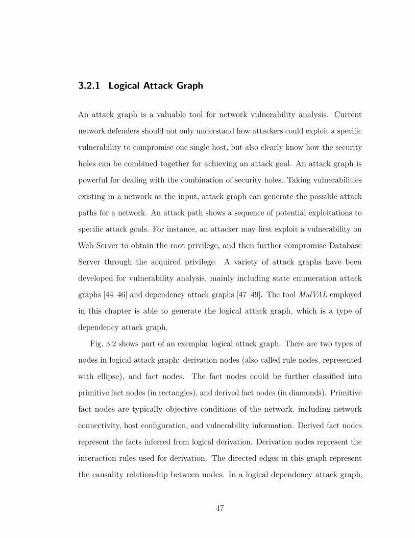
3.2.1 Logical Attack Graph

An attack graph is a valuable tool for network vulnerability analysis. Current

network defenders should not only understand how attackers could exploit a specific

vulnerability to compromise one single host, but also clearly know how the security

holes can be combined together for achieving an attack goal. An attack graph is

powerful for dealing with the combination of security holes. Taking vulnerabilities

existing in a network as the input, attack graph can generate the possible attack

paths for a network. An attack path shows a sequence of potential exploitations to

specific attack goals. For instance, an attacker may first exploit a vulnerability on

Web Server to obtain the root privilege, and then further compromise Database

Server through the acquired privilege. A variety of attack graphs have been

developed for vulnerability analysis, mainly including state enumeration attack

graphs [44–46] and dependency attack graphs [47–49]. The tool MulVAL employed

in this chapter is able to generate the logical attack graph, which is a type of

dependency attack graph.

Fig. 3.2 shows part of an exemplar logical attack graph. There are two types of

nodes in logical attack graph: derivation nodes (also called rule nodes, represented

with ellipse), and fact nodes. The fact nodes could be further classified into

primitive fact nodes (in rectangles), and derived fact nodes (in diamonds). Primitive

fact nodes are typically objective conditions of the network, including network

connectivity, host configuration, and vulnerability information. Derived fact nodes

represent the facts inferred from logical derivation. Derivation nodes represent the

interaction rules used for derivation. The directed edges in this graph represent

the causality relationship between nodes. In a logical dependency attack graph,

47

26:networkServiceInfo(webServer,openssl,tcp,22,_)

27:vulExists(webServer,’CVE-2008-0166’,openssl,remoteExploit,privEscalation)

22:Rule(remote exploit of a server program)

14:execCode(webServer,root)

23:netAccess(webServer,tcp,22)

...

...

Figure 3.2: A Portion of an Example Logical Attack Graph [14]

one or more fact nodes could serve as the preconditions of a derivation node and

cause it to take e�ect. One or more derivation nodes could further cause a derived

fact node to become true. Each derivation node represents the application of an

interaction rule given in [51] that yields the derived fact.

For example, in Fig. 3.2, Node 26, 27 (primitive fact nodes) and Node 23 (derived

fact node) are three fact nodes. They represent three preconditions respectively:

Node 23, the attacker has access to the Web Server; Node 26, Web Server provides

OpenSSL service; Node 27, Openssl has a vulnerability CVE-2008-0166. With the

three preconditions satisfied simultaneously, the rule of Node 22 (derivation node)

can take e�ect, meaning the remote exploit of a server program could happen. This

derivation rule can further cause Node 14 (derived fact node) to be valid, meaning

attacker can execute code on Web Server.

48

3.2.2 Cloud-level Attack Graph

In the cloud, each enterprise network can scan its own virtual machines for existing

vulnerabilities and then generate an attack graph. The individual attack graph

shows how attackers could exploit certain vulnerabilities and conduct a sequence

of attack steps inside the enterprise network. However, such individual attack

graphs are confined to the enterprise networks without considering the potential

threats from cloud environment. The existence of stealthy bridges could activate the

prerequisites of some attacks that are previously impossible in traditional network

environment and thus enable new attack paths. These attack paths are easily

missed by individual attack graphs. For example, in Fig. 4.7, without assuming

the stealthy bridge existing between enterprise A and B, the individual attack

graph for enterprise B can be incomplete or even not established due to lack of

exploitable vulnerabilities. Therefore, a cloud-level attack graph needs to be built

to incorporate the existence of stealthy bridges in the cloud. By considering the

attack preconditions enabled by stealthy bridges, the cloud-level attack graph can

reveal hidden potential attack paths that are missed by individual attack graphs.

The cloud-level attack graph should be modeled based on the cloud structure.

Due to the VMI sharing feature and the co-residency feature of cloud, a public cloud

has the following structural characteristics. First, virtual machines can be created

by instantiating VMIs. Therefore virtual machines residing on di�erent hosts may

actually be instances of the same VMI. In simple words, they could have the same

VMI parents. Second, virtual machines belong to one enterprise network may be

assigned to a number of di�erent physical hosts that are shared by other enterprise

networks. That is, the virtual machines employed by di�erent enterprise networks

49

vm11 vm12 vm1i

Hypervisor 1

... vm21 vm2j vm2k

Hypervisor 2

...

Host 1 Host 2

May be instantiated from the same virtual machine image

May belong to the same enterprise network

Figure 3.3: Features of the Public Cloud Structure [14]

are likely to reside on the same host. As shown in Fig. 3.3, the vm11 on host 1

and vm2j on host 2 may be instances of the same VMI, while vm12 and vm2k could

belong to the same enterprise network. Third, the real enterprise network could be

a hybrid of a cloud network and a traditional network. For example, the servers

of an enterprise network could be implemented in the cloud, while the personal

computers and workstations could be in the traditional network infrastructure.

Due to the above characteristics of cloud structure, the model for the cloud-level

attack graph should have the following corresponding characteristics.

1) The cloud-level attack graph is a cross-layer graph that is composed of three

layers: virtual machine layer, VMI layer, and host layer, as shown in Fig. 3.4.

2) The virtual machine layer is the major layer in the attack graph stack.

This layer reflects the causality relationship between vulnerabilities existing inside

the virtual machines and the potential exploits towards these vulnerabilities. If

stealthy bridges do not exist, the attack graph generated in this layer is scattered:

each enterprise network has an individual attack graph that is isolated from

50

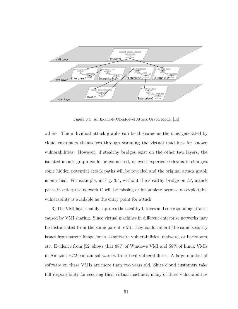
VM Layer

Host Layer

VMI Layer

Host h1

Enterprise A

Image v1

Enterprise CEnterprise B

Enterprise C

Enterprise D

Figure 3.4: An Example Cloud-level Attack Graph Model [14]

others. The individual attack graphs can be the same as the ones generated by

cloud customers themselves through scanning the virtual machines for known

vulnerabilities. However, if stealthy bridges exist on the other two layers, the

isolated attack graph could be connected, or even experience dramatic changes:

some hidden potential attack paths will be revealed and the original attack graph

is enriched. For example, in Fig. 3.4, without the stealthy bridge on h1, attack

paths in enterprise network C will be missing or incomplete because no exploitable

vulnerability is available as the entry point for attack.

3) The VMI layer mainly captures the stealthy bridges and corresponding attacks

caused by VMI sharing. Since virtual machines in di�erent enterprise networks may

be instantiated from the same parent VMI, they could inherit the same security

issues from parent image, such as software vulnerabilities, malware, or backdoors,

etc. Evidence from [52] shows that 98% of Windows VMI and 58% of Linux VMIs

in Amazon EC2 contain software with critical vulnerabilities. A large number of

software on these VMIs are more than two years old. Since cloud customers take

full responsibility for securing their virtual machines, many of these vulnerabilities

51

remain unpatched and thus pose great risks to cloud. Once a vulnerability or an

attack type is identified in the parent VMI, the attack graph for all the children

virtual machine instances may be a�ected: a precondition node could be activated,

or a new interaction rule should be constructed in attack graph generation tool.

The incorporation of the VMI layer provides another benefit to the subsequent

Bayesian network analysis. It enables the interaction between the virtual machine

layer and the VMI layer. On one hand, the probability of a vulnerability existence

on a VMI will a�ect the probability of the vulnerability existence on its children

instance virtual machines. On the other hand, if new evidence is found regarding

the vulnerability existence on the children instances, the probability change will

in turn influence the parent VMI. If the same evidence is observed on multiple

instances of the VMI, this VMI is very likely to be problematic.

4) The host layer is able to reason exploits of stealthy bridges caused by virtual

machine co-residency. Exploits on this layer could lead to further penetrations on

the virtual machine layer. In addition, this layer actually captures all attacks that

could happen on the host level, including those on pure physical hosts with no

virtual machines. Hence it provides a good interface to hybrid enterprise networks

that are implemented with partial cloud and partial traditional infrastructures.

The potential attack paths identified on the cloud part could possibly extend to

traditional infrastructures if all prerequisites for the remote exploits are satisfied,

such as network access being allowed, and exploitable vulnerabilities existing, etc.

As in Fig. 3.4, the attack graph for enterprise C extends from virtual machine layer

to host layer.

52

3.3 Bayesian Networks

As stated in [24] by Judea Pearl, the study for Bayesian Network was motiviated

by “attempts to devise a computational model for humans’ inferential reasoning,

namely, the mechanism by which people integrate data from various sources and

generate a coherent interpretation of the data.” This motivation well describes the

main function and potential applications of Bayesian networks.

A Bayesian network (BN) is a probabilistic graphical model representing cause

and e�ect relations. For example, it is able to show the probabilistic causal

relationships between a disease and the corresponding symptoms. Formally, a

Bayesian network is a Directed Acyclic Graph (DAG) that contains a set of nodes

and directed edges. The nodes represent random variables of interest and the

directed edges represent the causal influence among the variables. The strength

of such influence is represented with a conditional probability table (CPT). For

example, Fig. 3.5 shows a portion of a BN constructed directly from the attack

graph in Fig. 3.2 by removing the rule Node 22. Node 14 can be associated with

the CPT as shown. This CPT means that if all of the preconditions of Node 14 are

satisfied, the probability of Node 14 being true is 0.9. Node 14 is false in all other

cases.

Pearl summarized the properties of Bayesian networks in [25]. After that,

Bayesian networks have been studied widely by researchers. Heckerman et al.

describe a Bayesian approach in [26] for learning Bayesian networks from a combi-

nation of prior knowledge and statistical data. Bayesian networks are applied to

many fields of study, such as biology, artifical intelligence, and computer sciences,

to name a few. Friedman et al. use Bayesian Networks to describe the interactions

53

26_networkServiceInfo

27_vulExists

...

...

23_netAccess

14_execCode

Inferring the Stealthy Bridges in Cloud 7

a precondition node could be activated, or a new interaction rule should beconstructed in attack graph generation tool.

The incorporation of VMI layer provides another benefit to the subsequentBayesian network analysis. It enables the interaction between virtual machinelayer and VMI layer. On one hand, the probability of a vulnerability existenceon a VMI will a�ect the probability of the vulnerability existence on its chil-dren instance virtual machines. On the other hand, if new evidences are foundregarding the vulnerability existence on the children instances, the probabilitychange will in turn influence the parent VMI. If the same evidences are observedon multiple instances of the VMI, this VMI is very likely to be problematic.

4) The host layer is able to reason exploits of stealthy bridges caused byvirtual machine co-residency. Exploits on this layer could lead to further pene-trations on the virtual machine layer. In addition, this layer actually capturesall attacks that could happen on the host level, including those on pure physicalhosts with no virtual machines. Hence it provides a good interface to hybridenterprise networks that are implemented with partial cloud and partial tradi-tional infrastructures. The potential attack paths identified on cloud part couldpossibly extend to traditional infrastructures if all prerequisites for the remoteexploits are satisfied, such as network access being allowed, and exploitable vul-nerabilities existing, etc. As in Fig. 4, the attack graph for enterprise C extendsfrom virtual machine layer to host layer.

3 Cross-layer Bayesian Networks

Bayesian network is a probabilistic graphical model representing the cause ande�ect relations. For example, it is able to show the probabilistic causal relation-ships between a disease and the corresponding symptoms. Formally, a Bayesiannetwork is a Directed Acyclic Graph (DAG) that contains a set of nodes anddirected edges. The nodes represent random variables of interest and the di-rected edges represent the causal influence among the variables. The strengthof such influence is represented with a conditional probability table (CPT). Forexample, Fig. 5 shows a portion of Bayesian network constructed directly fromthe attack graph shown in Fig. 2 by removing the rule Node 22, Node 14 can beassociated with a CPT as shown in Table 1. This CPT means that if all of thepreconditions of Node 14 are satisfied, the probability of Node 14 being true is0.9. Node 14 is false in all other cases.

Table 1. a simple CPT table

26 27 23 14T T T 0.9otherwise 0

Bayesian network can be used to compute the probabilities of interested vari-ables. It is especially powerful for diagnosis and prediction analysis. For example,in diagnosis analysis, given the symptoms being observed, the network can calcu-late the probability of the causing fact (respresented with P(cause—symptom=True)).

Figure 3.5: A Portion of Bayesian Network with associated CPT [14]

between genes and describe a method for recovering gene interactions using tools

from learning Bayesian networks [27]. Jansen et al. provide another study for using

Bayesian networks to predict protein-protein interactions genome-wide in yeast [28].

Charniak explains the Bayesian Networks in a way that is easy to understand for

AI researchers with a limited grounding in probability theory [29].

Bayesian Networks have recently been applied to the field of cyber security. One

main direction is using Bayesian networks for network security metrics. Frigault et

al propose to measure the network security using Bayesian networks [30] and one

of it variants, dynamic Bayesian networks [31]. Dynamic Bayesian network is able

to incoporate time information into the inference process.

Due to Bayesian networks’ graphical property, many studies propose to combine

Bayesian network and attack graph for security analysis. Liu and Man [32] uses

Bayesian networks to perform network vulnerability assessment by modeling poten-

tial attack paths in a so-called “Bayesian attack graph”. [55] is another work that

54

analyzes which hosts are likely to be compromised based on known vulnerabilities

and observed alerts. Our work lands on a di�erent cloud environment and takes a

reverse strategy by using BN to infer the stealthy bridges, which are unknown in

nature. In the future, the inference of stealthy bridges can be further extended to

identify the zero-day attack paths in cloud, as in [41] for traditional networks.

Bayesian networks is also applied to intrusion detection. The main approaches

employed in current intrusion detection systems (IDSs) are misuse-based IDS and

anomaly-based IDS. Anomaly detection can detect previously unknown attacks,

but su�er from high false rate due to false classification of normal and abnormal

behaviors. Kruegel et al. proposes to a new event classification scheme based on

Bayesian networks [67]. The results show that the accuracy of classification is

greatly improved by using Bayesian networks.

3.4 Cross-layer Bayesian Networks

A Bayesian network can be used to compute the probabilities of variables of interest.

It is especially powerful for diagnosis and prediction analysis. For example, in

diagnosis analysis, given the symptoms being observed, a BN can calculate the

probability of the causing fact (respresented with Pr(cause | symptom = True)).

While in prediction analysis, given the causing fact, a BN will predict the probability

of the corresponding symptoms showing up (Pr(symptom|cause = True)). In the

cybersecurity field, similar diagnosis and prediction analysis can also be performed,

such as calculating the probability of an exploitation happening if related IDS alerts

are observed(Pr(exploitation|IDSalert = True)), or the probability of the IDS

raising an alert if an exploitation already happened (Pr(IDSalert|exploitation =

55

True)). This chapter mainly carries out a diagnosis analysis that computes the

probability of stealthy bridge existence by collecting evidence from other intrusion

steps. Diagnosis analysis is a kind of “backward” computation. In the cause-

and-symptom model, a concrete evidence about the symptom could change the

posterior probability of the cause by computing Pr(cause|symptom = True). More

intuitively, as more evidence is collected regarding the symptom, the probability of

the cause will become closer to reality if the BN is constructed properly.

3.4.1 Identify the Uncertainties

Inferring the existence of stealthy bridges requires real-time evidence being collected

and analyzed. BN has the capability, which attack graphs lack, of performing such

real-time security analysis. Attack graphs correlate vulnerabilities and potential

exploits in di�erent machines and enables determinstic reasoning. For example,

if all the preconditions of an attack are satisfied, the attacker should be able to

launch the attack. However, in real-time security analysis, there are a range of

uncertainties associated with this attack that cannot be reflected in an attack graph.

For example, has the attacker chosen to launch the attack? If he launched it, did

he succeed to compromise the host? Are the Snort [54] alerts raised on this host

related to the attack? Should we be more confident if we got other alerts from

other hosts in this network? Such uncertainty aspects should be taken into account

when performing real-time security analysis. BN is a valuable tool for capturing

these uncertainties.

One non-trivial di�culty for constructing a well functioning BN is to identify

and model the uncertainty types existing in the attack procedure. In this chapter,

56

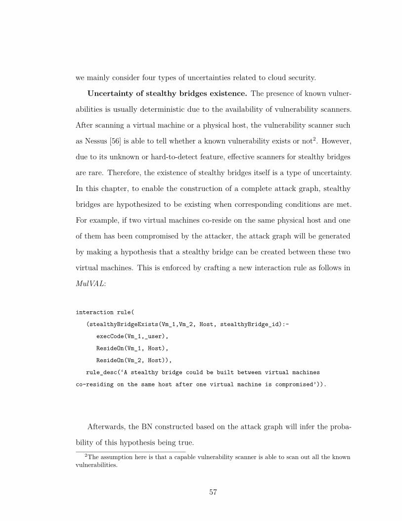
we mainly consider four types of uncertainties related to cloud security.

Uncertainty of stealthy bridges existence. The presence of known vulner-

abilities is usually deterministic due to the availability of vulnerability scanners.

After scanning a virtual machine or a physical host, the vulnerability scanner such

as Nessus [56] is able to tell whether a known vulnerability exists or not2. However,

due to its unknown or hard-to-detect feature, e�ective scanners for stealthy bridges

are rare. Therefore, the existence of stealthy bridges itself is a type of uncertainty.

In this chapter, to enable the construction of a complete attack graph, stealthy

bridges are hypothesized to be existing when corresponding conditions are met.

For example, if two virtual machines co-reside on the same physical host and one

of them has been compromised by the attacker, the attack graph will be generated

by making a hypothesis that a stealthy bridge can be created between these two

virtual machines. This is enforced by crafting a new interaction rule as follows in

MulVAL:

interaction rule(

(stealthyBridgeExists(Vm_1,Vm_2, Host, stealthyBridge_id):-

execCode(Vm_1,_user),

ResideOn(Vm_1, Host),

ResideOn(Vm_2, Host)),

rule_desc(‘A stealthy bridge could be built between virtual machines

co-residing on the same host after one virtual machine is compromised’)).

Afterwards, the BN constructed based on the attack graph will infer the proba-

bility of this hypothesis being true.2The assumption here is that a capable vulnerability scanner is able to scan out all the known

vulnerabilities.

57

...

...23 26 27 AAN

14

Inferring the Stealthy Bridges in Cloud 9

cedure. In this paper, we mainly consider four types of uncertainties related tocloud security.

Uncertainty of stealthy bridges existence. Vulnerability existence isusually deterministic due to the availability of vulnerability scanners. Afterscanning a virtual machine or a physical host, the vulnerability scanner likeNessus[24] is able to tell whether a vulnerability exists or not2. However, dueto the unknown or hard-to-detect feature of stealthy bridges, e�ective scan-ners for this kind of vulnerability are rare. Therefore, the existence of stealthybridges itself is a type of uncertainty. In this paper, to enable the construction ofa complete attack graph, stealthy bridges are hypothesized to be existing whencorresponding conditions are met. For example, if two virtual machines co-resideon the same physical host, the attack graph will be generated by making a hy-pothesis that a stealthy bridge exists between these two virtual machines. Thisis enforced by crafting a new interaction rule as follows in MulVAL:

interaction rule((stealthyBridgeExists(Vm_1,Vm_2, Host, stealthyBridge_id):-

execCode(Vm_1,_user),ResideOn(Vm_1, Host),ResideOn(Vm_2, Host)),

rule_desc(‘A stealthy bridge could be built between virtual machines co-residing onthe same host after one virtual machine is compromised’)).

Afterwards, the Bayesian network constructed based on this attack graphwill infer the probability of this hypothesis being true.

Uncertainty of attacker action. Uncertainty of attacker action is firstidentified by [23]. As pointed out in [23], even if all the prerequsites for anattack are satisfied, the attack may not happen because the attacker may evennot take action. Therefore, a kind of Attack Action Node (AAN) is added intoBayesian network to model the attackers’ actions. An AAN node is introducedas an additional parent node for the attack. For example, the Bayesian networkshown in Fig. 5 is changed to Fig. 6 after adding the AAN node. Correspondingly,the CPT table shown in Table 1 is modified into Table 2. This means “attackerstaking action” is another prerequisite to be satisfied for the attack to happen.

Table 2. a CPT table with AAN node

26 27 23 AAN 14T T T T 0.9

otherwise 0

AAN node is not added for all attacks. They are needed only for importantattacks such as the very first intrustion steps in a multi-step attack, or attacksthat need attackers’ action. Since an AAN node represents the primitive fact ofwhether an attacker taking action and it has no parent node, a prior probabilityshould be assigned to an AAN node to indicate the likelihood of attack. Theposterior probability of AAN will change as more evidences are collected.

2 The assumption here is that a capable vulnerability scanner is able to scan outall the known vulnerabilities. The unknown vulnerabilities are ruled out and notconsidered in this paper.

Figure 3.6: A Portion of Bayesian Network with AAN node [14]

Uncertainty of attacker action. Uncertainty of attacker action is first

identified by [55]. Even if all the prerequsites for an attack are satisfied, the attack

may not happen because attackers may not take action. Therefore, a kind of Attack

Action Node (AAN) is added to the BN to model attackers’ actions. An AAN node

is introduced as an additional parent node for the attack. For example, the BN

shown in Fig. 3.5 is changed to Fig. 3.6 after adding an AAN node. Correspondingly,

the CPT is modified as in Fig. 3.6. This means “attacker taking action” is another

prerequisite to be satisfied for the attack to happen.

An AAN node is not added for all attacks. They are needed only for important

attacks such as the very first intrustion steps in a multi-step attack, or attacks

that need attackers’ action. Since an AAN node represents the primitive fact of

whether an attacker taking action and has no parent nodes, a prior probability

distribution should be assigned to an AAN to indicate the likelihood of an attack.

58

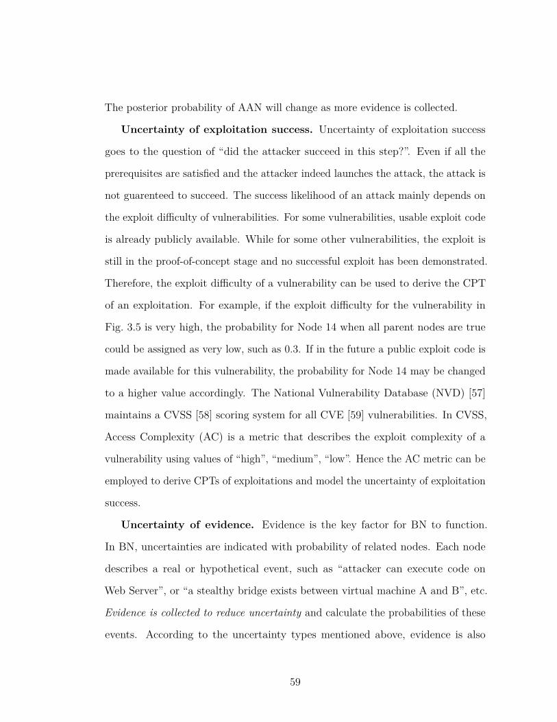
The posterior probability of AAN will change as more evidence is collected.

Uncertainty of exploitation success. Uncertainty of exploitation success

goes to the question of “did the attacker succeed in this step?”. Even if all the

prerequisites are satisfied and the attacker indeed launches the attack, the attack is

not guarenteed to succeed. The success likelihood of an attack mainly depends on

the exploit di�culty of vulnerabilities. For some vulnerabilities, usable exploit code

is already publicly available. While for some other vulnerabilities, the exploit is

still in the proof-of-concept stage and no successful exploit has been demonstrated.

Therefore, the exploit di�culty of a vulnerability can be used to derive the CPT

of an exploitation. For example, if the exploit di�culty for the vulnerability in

Fig. 3.5 is very high, the probability for Node 14 when all parent nodes are true

could be assigned as very low, such as 0.3. If in the future a public exploit code is

made available for this vulnerability, the probability for Node 14 may be changed

to a higher value accordingly. The National Vulnerability Database (NVD) [57]

maintains a CVSS [58] scoring system for all CVE [59] vulnerabilities. In CVSS,

Access Complexity (AC) is a metric that describes the exploit complexity of a

vulnerability using values of “high”, “medium”, “low”. Hence the AC metric can be

employed to derive CPTs of exploitations and model the uncertainty of exploitation

success.

Uncertainty of evidence. Evidence is the key factor for BN to function.

In BN, uncertainties are indicated with probability of related nodes. Each node

describes a real or hypothetical event, such as “attacker can execute code on

Web Server”, or “a stealthy bridge exists between virtual machine A and B”, etc.

Evidence is collected to reduce uncertainty and calculate the probabilities of these

events. According to the uncertainty types mentioned above, evidence is also

59

classified into three types: evidence for stealthy bridges existence, evidence for

attacker action, and evidence for exploitation success. Therefore, whenever a piece

of evidence is observed, it is assigned to one of the above evidence types to support

the corresponding event. This is done by adding evidence as the children nodes to

the event nodes related to uncertainty. For example, an IDS alert about a large

number of login attempts can be regarded as evidence of attacker action, showing

that an attacker could have tried to launch an attack. This evidence is then added

as the child node to an AAN, as exemplified in Fig. 3.7. For another example, the

alert “system log is deleted” given by Tripwire [60] can be the child of the node

“attacker can execute code”, showing that an exploit has been successfully achieved.

However, evidence per se contain uncertainty. The uncertainty is twofold. First,

the support of evidence to an event is uncertain. For analogy, a symptom of

coughing cannot completely prove the presence of lung disease. In the above

examples, could the multiple login attempts testify that attackers have launched

the attack? How likely is it that attackers have succeeded in compromising the

host if a system log deletion is observed? Second, evidence from security sensors is

not 100% accurate. IDS systems such as Snort, Tripwire, etc. su�er a lot from a

high false alert rate. For example, an event may trigger an IDS to raise an alert

while actually no attack happens. In this case, the alert is a false positive. The

reverse case is a false negative, that is, when an IDS should have raised an alarm

but doesn’t. Therefore, we propose to model the uncertainty of evidence with an

Evidence-Confidence(EC) pair as shown in Fig. 3.7. The EC pair has two nodes, an

Evidence node and an Evidence Confidence Node (ECN). An ECN is assigned as

the parent of an Evidence node to model the confidence level of the evidence. If the

confidence level is high, the child evidence node will have larger impact on other

60

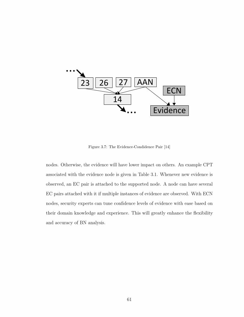
26 27...

...

23

14

AAN

Evidence

ECN

Figure 3.7: The Evidence-Condidence Pair [14]

nodes. Otherwise, the evidence will have lower impact on others. An example CPT

associated with the evidence node is given in Table 3.1. Whenever new evidence is

observed, an EC pair is attached to the supported node. A node can have several

EC pairs attached with it if multiple instances of evidence are observed. With ECN

nodes, security experts can tune confidence levels of evidence with ease based on

their domain knowledge and experience. This will greatly enhance the flexibility

and accuracy of BN analysis.

61

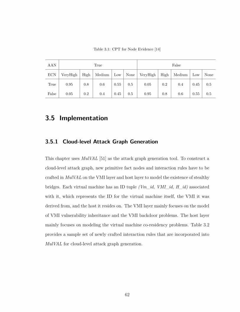
Table 3.1: CPT for Node Evidence [14]

AAN True False

ECN VeryHigh High Medium Low None VeryHigh High Medium Low None

True 0.95 0.8 0.6 0.55 0.5 0.05 0.2 0.4 0.45 0.5

False 0.05 0.2 0.4 0.45 0.5 0.95 0.8 0.6 0.55 0.5

3.5 Implementation

3.5.1 Cloud-level Attack Graph Generation

This chapter uses MulVAL [51] as the attack graph generation tool. To construct a

cloud-level attack graph, new primitive fact nodes and interaction rules have to be

crafted in MulVAL on the VMI layer and host layer to model the existence of stealthy

bridges. Each virtual machine has an ID tuple (Vm_id, VMI_id, H_id) associated

with it, which represents the ID for the virtual machine itself, the VMI it was

derived from, and the host it resides on. The VMI layer mainly focuses on the model

of VMI vulnerability inheritance and the VMI backdoor problems. The host layer

mainly focuses on modeling the virtual machine co-residency problems. Table 3.2

provides a sample set of newly crafted interaction rules that are incorporated into

MulVAL for cloud-level attack graph generation.

62

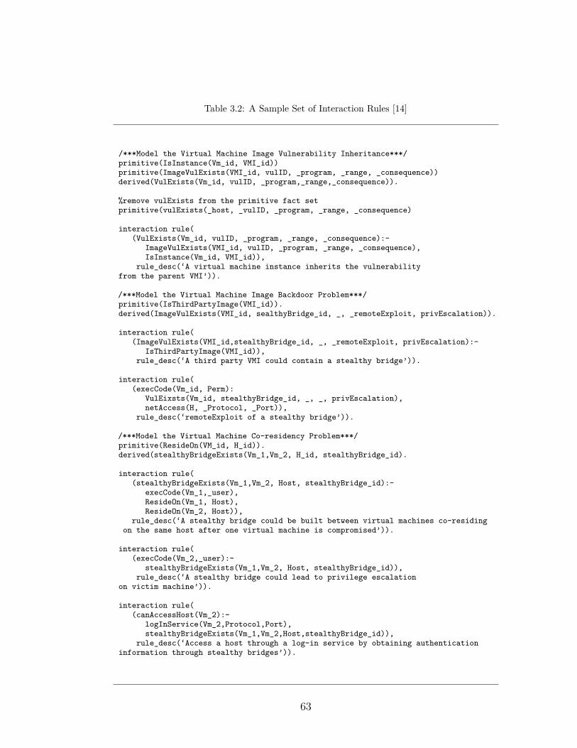
Table 3.2: A Sample Set of Interaction Rules [14]

/***Model the Virtual Machine Image Vulnerability Inheritance***/primitive(IsInstance(Vm_id, VMI_id))primitive(ImageVulExists(VMI_id, vulID, _program, _range, _consequence))derived(VulExists(Vm_id, vulID, _program,_range,_consequence)).

%remove vulExists from the primitive fact setprimitive(vulExists(_host, _vulID, _program, _range, _consequence)

interaction rule((VulExists(Vm_id, vulID, _program, _range, _consequence):-

ImageVulExists(VMI_id, vulID, _program, _range, _consequence),IsInstance(Vm_id, VMI_id)),

rule_desc(‘A virtual machine instance inherits the vulnerabilityfrom the parent VMI’)).

/***Model the Virtual Machine Image Backdoor Problem***/primitive(IsThirdPartyImage(VMI_id)).derived(ImageVulExists(VMI_id, sealthyBridge_id, _, _remoteExploit, privEscalation)).

interaction rule((ImageVulExists(VMI_id,stealthyBridge_id, _, _remoteExploit, privEscalation):-

IsThirdPartyImage(VMI_id)),rule_desc(‘A third party VMI could contain a stealthy bridge’)).

interaction rule((execCode(Vm_id, Perm):

VulEixsts(Vm_id, stealthyBridge_id, _, _, privEscalation),netAccess(H, _Protocol, _Port)),

rule_desc(‘remoteExploit of a stealthy bridge’)).

/***Model the Virtual Machine Co-residency Problem***/primitive(ResideOn(VM_id, H_id)).derived(stealthyBridgeExists(Vm_1,Vm_2, H_id, stealthyBridge_id).

interaction rule((stealthyBridgeExists(Vm_1,Vm_2, Host, stealthyBridge_id):-

execCode(Vm_1,_user),ResideOn(Vm_1, Host),ResideOn(Vm_2, Host)),

rule_desc(‘A stealthy bridge could be built between virtual machines co-residingon the same host after one virtual machine is compromised’)).

interaction rule((execCode(Vm_2,_user):-

stealthyBridgeExists(Vm_1,Vm_2, Host, stealthyBridge_id)),rule_desc(‘A stealthy bridge could lead to privilege escalation

on victim machine’)).

interaction rule((canAccessHost(Vm_2):-

logInService(Vm_2,Protocol,Port),stealthyBridgeExists(Vm_1,Vm_2,Host,stealthyBridge_id)),

rule_desc(‘Access a host through a log-in service by obtaining authenticationinformation through stealthy bridges’)).

63

3.5.2 Construction of Bayesian Networks

Deriving Bayesian networks from cross-layer attack graphs consists of four ma-

jor components: removing rule nodes in the attack graph, adding new nodes,

determining prior probabilities, and constructing CPTs.

Remove rule nodes of attack graph.

In an attack graph, the rule nodes imply how postconditions are derived from

preconditions. The derivation is deterministic and contains no uncertainty. There-

fore, these rule nodes have no e�ect on the reasoning process, and thus can be

removed when constructing the BN. To remove a rule node, its preconditions are

connected directly to its postconditions. For example, in Fig. 3.2, Node 26, 27, and

23 will be connected directly to Node 14 by removing Node 22.

Adding new nodes.

New nodes are added to capture the uncertainty of attacker action and the

uncertainty of evidence. To capture the uncertainty of attacker action, each step

has a separate AAN node as the parent, rather than sharing the same AAN

among multiple steps. The AAN node models attacker action at the granularity of

attack steps, and thus reflects the actual attack paths. To model the uncertainty

of evidence, whenever new evidence is observed, an EC pair is constructed and

attached to the supported node with uncertainty.

Determining prior probabilities.

Prior probability distributions should be determined for all root nodes that have

no parents, such as the vulnerability existence nodes, the network access nodes, or

the AAN nodes.

64

Constructing CPTs.

Some CPTs can be determined according to a standard, such as the the AC

metric in CVSS scoring system. The AC metric describes the exploit complexity

of vulnerabilities and thus can be used to derive the CPTs for corresponding

exploitations. Some other CPTs may involve security experts’ domain knowledge

and experience. For example, the VMIs from a trusted third party may have lower

probability of containing security holes such as backdoors, while those created and

shared by individual cloud users may have higher probability.

The constructed BN should be robust against small changes in prior probabilities

and CPTs. To ensure such robustness, we use SamIam [65] for sensitivity analysis

when constructing and debugging the BN. By specifying the requirements for an

interested node’s probability, SamIam will check the associated CPTs and provide

suggestions on feasible changes. For example, if we want to change P (N5 =

True) from 0.34 to 0.2, SamIam will provide two suggestions, either changing

P (N5 = True|N2 = True, N3 = True) from 0.9 to <= 0.43, or changing P (N3 =

True|N1 = True) from 0.3 to <= 0.125.

3.6 Experiment

3.6.1 Attack Scenario

Fig. 4.7 shows the network structure in our attack scenario. We have 3 major

enterprise networks: A, B, and C. A and B are all implemented within the cloud,

while C is implemented by partially cloud, and partially traditional network (the

65

Attacker

Web Server

File Server

Database Server

DNS Server

Email Server

Web Server

File Server SSH Server

Database Server

DNS Server

Email Server

VMI repository

Web Server

NFS Server SSH

Server

Database Server

DNS Server

Email Server

Enterprise A

Enterprise B Enterprise C

Cloud

Other Enterprise networks

Figure 3.8: The Attack Scenario [14]

servers are located in the cloud and the workstations are in a traditional network).

The attack includes several steps conducted by attacker Mallory.

Step 1, Mallory first publishes a VMI that provides a web service in the cloud.

This VMI is malicious in that it contains a security hole that Mallory knows how

to exploit. For example, this security hole could be an SSH user authentication

key (the public key located in .ssh/authorized_keys) that is intentionally left in

the VMI by Mallory. The leftover creates a backdoor that allows Mallory to login

into any instances derived from this malicious VMI using his own private key. The

security hole could also be an unknown vulnerability that is not yet publicly known.

To make the attack scenario more generic, we choose a vulnerability CVE-2007-

2446 [61], existing in Samba 3.0.0 [62], as the one imbedded in the malicious VMI,

but assume it as unknown for the purpose of simulation.

Step 2, the malicious VMI is then adopted and instantiated as a web server by

66

an innocent user from A. Mallory now wants to compromise the live instances, but

he needs to know which instances are derived from his malicious VMI. [52] provides

three possible ways for machine fingerprinting: ssh matching, service matching,

and web matching. Through ssh key matching, Mallory finds the right instance in

A and completes the exploitation towards CVE-2007-2446 [61].

Step 3, enterprise network B provides web services to a limited number of

customers, including A. With the acquired root privilege from A’s web server,

Mallory is able to access B’s web server, exploit one of its vulnerabilities CVE-

2007-5423 [63] from application tikiwiki 1.9.8 [64], and create a reverse shell.

Step 4, Mallory notices that enterprise B and C has a special relationship:

their web servers are implemented with virtual machines co-residing on the same

host. C is a start-up company that has some valuable information stored on its

CEO’s workstation. Mallory then leverages the co-residency relationship of the

web servers and launches a side-channel attack towards C’s web server to extract

its password. Mallory obtains user privilege through the attack. Mallory also

establishes a covert channel between the co-resident virtual machines for convenient

information exchange.

Step 5, the NFS server in C has a directory that is shared by all the servers and

workstations inside the company. Normally C’s web server should not have write

permission to this shared directory. But due to a configuration error of the NFS

export table, the web server is given write permission. Therefore, if Mallory can

upload a Trojan horse to the shared directory, other innocent users may download

the Trojan horse from this directory and install it. Hence Mallory crafts a Trojan

horse management_tool.deb and uploads it into the shared NSF directory on web

server.

67

Step 6, The innocent CEO from C downloads management_tool.deb and installs

it. Mallory then exploits the Trojan horse and creats a unsolicited connection back

to his own machine.

Step 7, Mallory’s VMI is also adopted by several other enterprise networks, so

Mallory compromises their instances using the same method in Step 2.

In this scenario, two stealthy bridges are established3: one is from Internet to

enterprise network A through exploiting an unknown vulnerability, the other one is

between enterprise network B and C by leveraging virtual machine co-residency.

The attack path crosses over three enterprise networks that reside in the same

cloud, and extends to C’s traditional network.

3.6.2 Experiment Result

The purpose of our experiment is to check whether the BN-based tool is able to

infer the existence of stealthy bridges given the evidence. The Bayesian network

has two inputs: the network deployment (network connection, host configuration,

and vulnerability information, etc.) and the evidence. The output of BN is the

probability of specific events, such as the probability of stealthy bridges being

established, or the probability of a web server being compromised. We view the

attackers’ sequence of attack steps as a set of ground truth. To evaluate the

e�ectiveness of the constructed BN, we compare the output of the BN with the

ground truth of the attack sequence. For example, given the ground truth that a

stealthy bridge has been established, we will check the corresponding probability

provided by the BN to see whether the result is convincible.3The enterprise networks in Step 7 are not key players, so we do not analyze the stealthy

bridges established in this step, but still use the raised alerts as evidence.

68

For the attack scenario illustrated in Fig. 4.7, the cross-layer BN is constructed

as in Fig. 3.9. By taking into account the existence of stealthy bridges, the cloud-

level attack graph has the capability of revealing potential hidden attack paths.

Therefore, the constructed BN also inherits the revealed hidden paths from the

cloud-level attack graph. For example, the white part in Fig. 3.9 shows the hidden

paths enabled by the stealthy bridge between enterprise network B and C. These

paths will be missed by individual attack graphs if the stealthy bridge is not

considered. The inputs for this BN are respectively the network deployment shown

in Table 3.34 and the collected evidence is shown in Table 3.4. Evidence is collected

against the attack steps described in our attack scenario. Not all attack steps have

corresponding observed evidence.

We conducted six sets of simulation experiments, each with a specific purpose.

For simplicity, we assume all attack steps are completed instantly with no time delay.

The ground truth in our attack scenario tells that one stealthy bridge between

attacker and enterprise A is established in attack step 2, and the other one between

B and C is established in step 4. By taking evidence with a certain order as input,

the BN will generate a corresponding sequence of probabilities for events of interest.

The probabilities are compared with the ground truth to evaluate the performance

of the BN.

3.6.2.1 Experiment 3.1: Probability Inferring

In experiment 3.1, we assume all the evidence is observed in the order of the

corresponding attack steps. We are interested in four events, a stealthy bridge4Aws,Bws,Cws,Cnfs,Cworkstation denote A’s web server, B’s web server, C’s web server, C’s

NFS server, C’s workstation respectively.

69

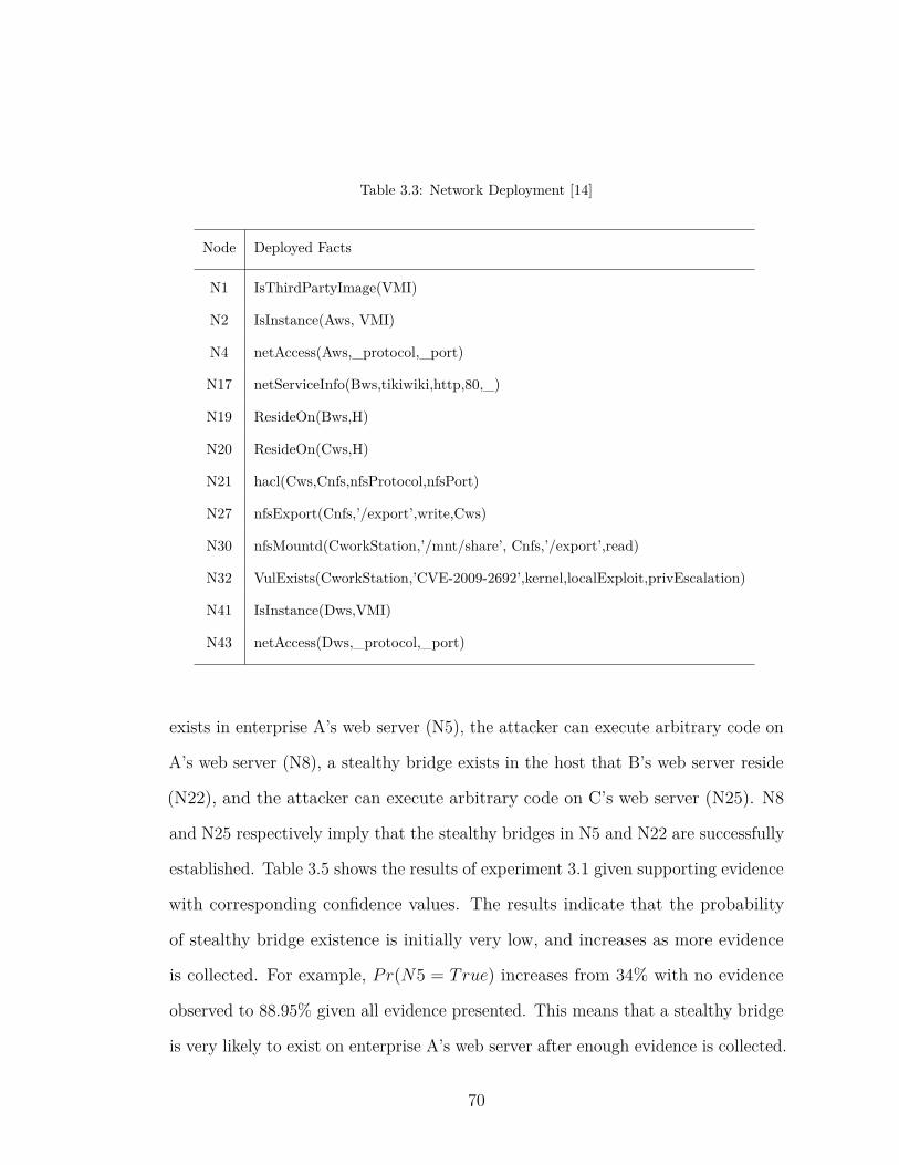
Table 3.3: Network Deployment [14]

Node Deployed Facts

N1 IsThirdPartyImage(VMI)

N2 IsInstance(Aws, VMI)

N4 netAccess(Aws,_protocol,_port)

N17 netServiceInfo(Bws,tikiwiki,http,80,_)

N19 ResideOn(Bws,H)

N20 ResideOn(Cws,H)

N21 hacl(Cws,Cnfs,nfsProtocol,nfsPort)

N27 nfsExport(Cnfs,’/export’,write,Cws)

N30 nfsMountd(CworkStation,’/mnt/share’, Cnfs,’/export’,read)

N32 VulExists(CworkStation,’CVE-2009-2692’,kernel,localExploit,privEscalation)

N41 IsInstance(Dws,VMI)

N43 netAccess(Dws,_protocol,_port)

exists in enterprise A’s web server (N5), the attacker can execute arbitrary code on

A’s web server (N8), a stealthy bridge exists in the host that B’s web server reside

(N22), and the attacker can execute arbitrary code on C’s web server (N25). N8

and N25 respectively imply that the stealthy bridges in N5 and N22 are successfully

established. Table 3.5 shows the results of experiment 3.1 given supporting evidence

with corresponding confidence values. The results indicate that the probability

of stealthy bridge existence is initially very low, and increases as more evidence

is collected. For example, Pr(N5 = True) increases from 34% with no evidence

observed to 88.95% given all evidence presented. This means that a stealthy bridge

is very likely to exist on enterprise A’s web server after enough evidence is collected.

70

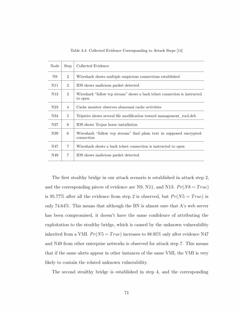
Table 3.4: Collected Evidence Corresponding to Attack Steps [14]

Node Step Collected Evidence

N9 2 Wireshark shows multiple suspicious connections established

N11 2 IDS shows malicious packet detected

N13 2 Wireshark “follow tcp stream” shows a back telnet connection is instructedto open

N23 4 Cache monitor observes abnormal cache activities

N34 5 Tripwire shows several file modification toward management_tool.deb

N37 6 IDS shows Trojan horse installation

N39 6 Wireshark “follow tcp stream” find plain text in supposed encrypted-connection

N47 7 Wireshark shows a back telnet connection is instructed to open

N49 7 IDS shows malicious packet detected

The first stealthy bridge in our attack scenario is established in attack step 2,

and the corresponding pieces of evidence are N9, N11, and N13. Pr(N8 = True)

is 95.77% after all the evidence from step 2 is observed, but Pr(N5 = True) is

only 74.64%. This means that although the BN is almost sure that A’s web server

has been compromised, it doesn’t have the same confidence of attributing the

exploitation to the stealthy bridge, which is caused by the unknown vulnerability

inherited from a VMI. Pr(N5 = True) increases to 88.95% only after evidence N47

and N49 from other enterprise networks is observed for attack step 7. This means

that if the same alerts appear in other instances of the same VMI, the VMI is very

likely to contain the related unknown vulnerability.

The second stealthy bridge is established in step 4, and the corresponding

71

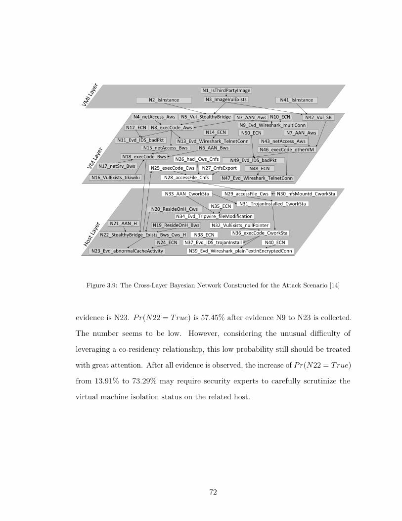
VM La

yer

VMI L

ayer N1_IsThirdPartyImage

N2_IsInstance N3_ImageVulExists N41_IsInstance

N5_Vul_StealthyBridgeN4_netAccess_Aws

N8_execCode_Aws

N18_execCode_Bws

N15_netAccess_Bws

N7_AAN_Aws

N12_ECN

N11_Evd_IDS_badPkt N13_Evd_Wireshark_TelnetConn

N9_Evd_Wireshark_multiConnN10_ECN

N14_ECN

N17_netSrv_Bws

N16_VulExists_tikiwiki

N6_AAN_Bws

N19_ResideOnH_Bws

N20_ResideOnH_Cws

N22_StealthyBridge_Exists_Bws_Cws_H

N25_execCode_Cws

N21_AAN_H

N23_Evd_abnormalCacheActivityN24_ECN

N26_hacl_Cws_Cnfs

N27_CnfsExport

N28_accessFile_Cnfs

N29_accessFile_Cws N30_nfsMountd_CworkSta

N31_TrojanInstalled_CworkSta

N32_VulExists_nullPointer

N33_AAN_CworkSta

N34_Evd_Tripwire_fileModification

N35_ECN

N36_execCode_CworkSta

N37_Evd_IDS_trojanInstallN38_ECN

N39_Evd_Wireshark_plainTextInEncryptedConnN40_ECN

N42_Vul_SB

N43_netAccess_AwsN46_execCode_otherVM

N7_AAN_AwsN50_ECN

N49_Evd_IDS_badPkt

N47_Evd_Wireshark_TelnetConn

N48_ECN

Host

Laye

r

Figure 3.9: The Cross-Layer Bayesian Network Constructed for the Attack Scenario [14]

evidence is N23. Pr(N22 = True) is 57.45% after evidence N9 to N23 is collected.

The number seems to be low. However, considering the unusual di�culty of

leveraging a co-residency relationship, this low probability still should be treated

with great attention. After all evidence is observed, the increase of Pr(N22 = True)

from 13.91% to 73.29% may require security experts to carefully scrutinize the

virtual machine isolation status on the related host.

72

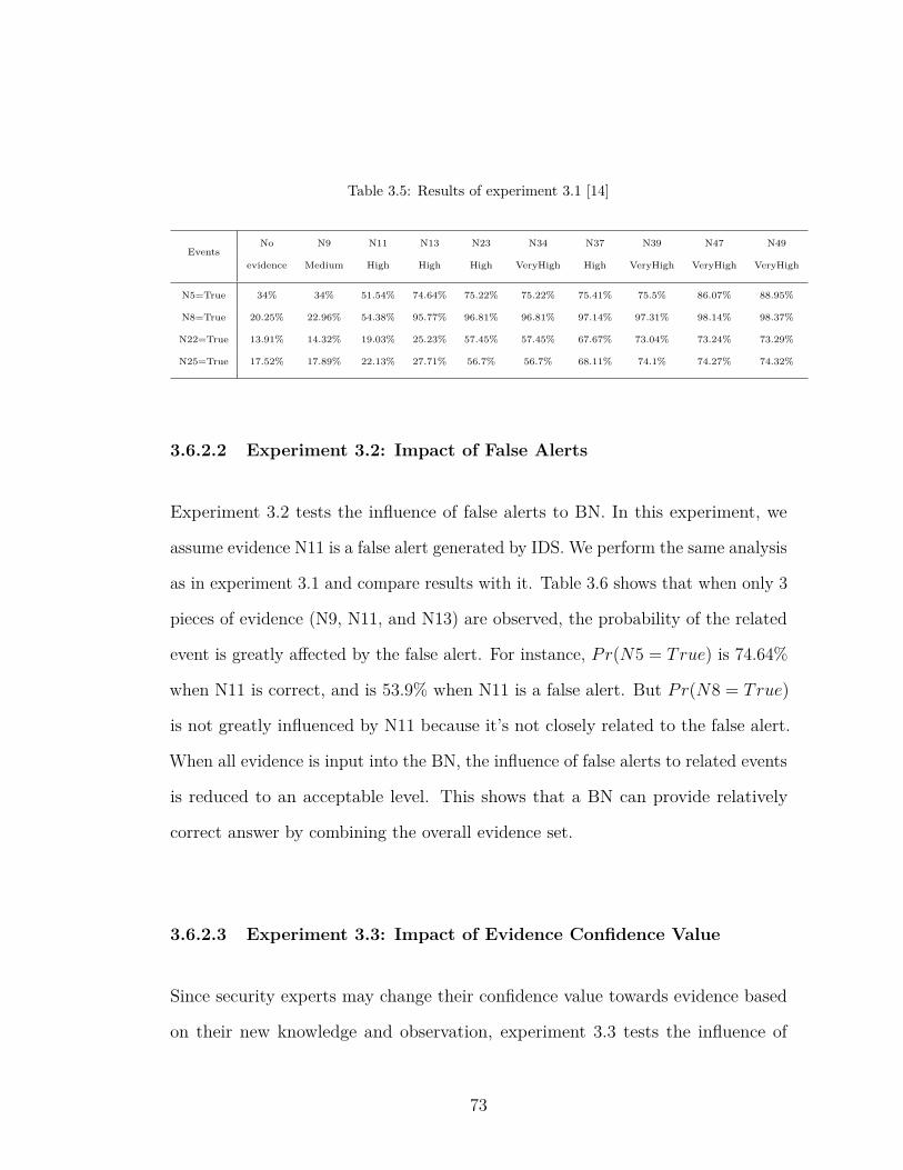
Table 3.5: Results of experiment 3.1 [14]

EventsNo N9 N11 N13 N23 N34 N37 N39 N47 N49

evidence Medium High High High VeryHigh High VeryHigh VeryHigh VeryHigh

N5=True 34% 34% 51.54% 74.64% 75.22% 75.22% 75.41% 75.5% 86.07% 88.95%

N8=True 20.25% 22.96% 54.38% 95.77% 96.81% 96.81% 97.14% 97.31% 98.14% 98.37%

N22=True 13.91% 14.32% 19.03% 25.23% 57.45% 57.45% 67.67% 73.04% 73.24% 73.29%

N25=True 17.52% 17.89% 22.13% 27.71% 56.7% 56.7% 68.11% 74.1% 74.27% 74.32%

3.6.2.2 Experiment 3.2: Impact of False Alerts

Experiment 3.2 tests the influence of false alerts to BN. In this experiment, we

assume evidence N11 is a false alert generated by IDS. We perform the same analysis

as in experiment 3.1 and compare results with it. Table 3.6 shows that when only 3

pieces of evidence (N9, N11, and N13) are observed, the probability of the related

event is greatly a�ected by the false alert. For instance, Pr(N5 = True) is 74.64%

when N11 is correct, and is 53.9% when N11 is a false alert. But Pr(N8 = True)

is not greatly influenced by N11 because it’s not closely related to the false alert.

When all evidence is input into the BN, the influence of false alerts to related events

is reduced to an acceptable level. This shows that a BN can provide relatively

correct answer by combining the overall evidence set.

3.6.2.3 Experiment 3.3: Impact of Evidence Confidence Value

Since security experts may change their confidence value towards evidence based

on their new knowledge and observation, experiment 3.3 tests the influence of

73

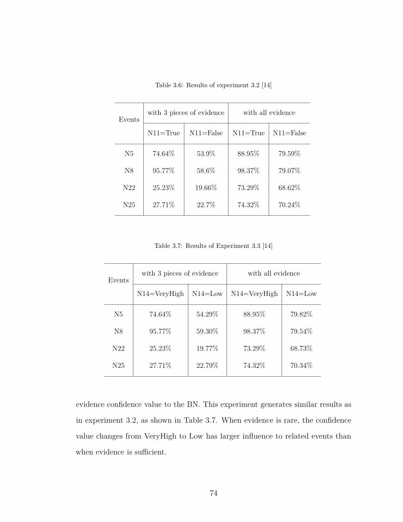
Table 3.6: Results of experiment 3.2 [14]

Eventswith 3 pieces of evidence with all evidence

N11=True N11=False N11=True N11=False

N5 74.64% 53.9% 88.95% 79.59%

N8 95.77% 58.6% 98.37% 79.07%

N22 25.23% 19.66% 73.29% 68.62%

N25 27.71% 22.7% 74.32% 70.24%

Table 3.7: Results of Experiment 3.3 [14]

Eventswith 3 pieces of evidence with all evidence

N14=VeryHigh N14=Low N14=VeryHigh N14=Low

N5 74.64% 54.29% 88.95% 79.82%

N8 95.77% 59.30% 98.37% 79.54%

N22 25.23% 19.77% 73.29% 68.73%

N25 27.71% 22.79% 74.32% 70.34%

evidence confidence value to the BN. This experiment generates similar results as

in experiment 3.2, as shown in Table 3.7. When evidence is rare, the confidence

value changes from VeryHigh to Low has larger influence to related events than

when evidence is su�cient.

74

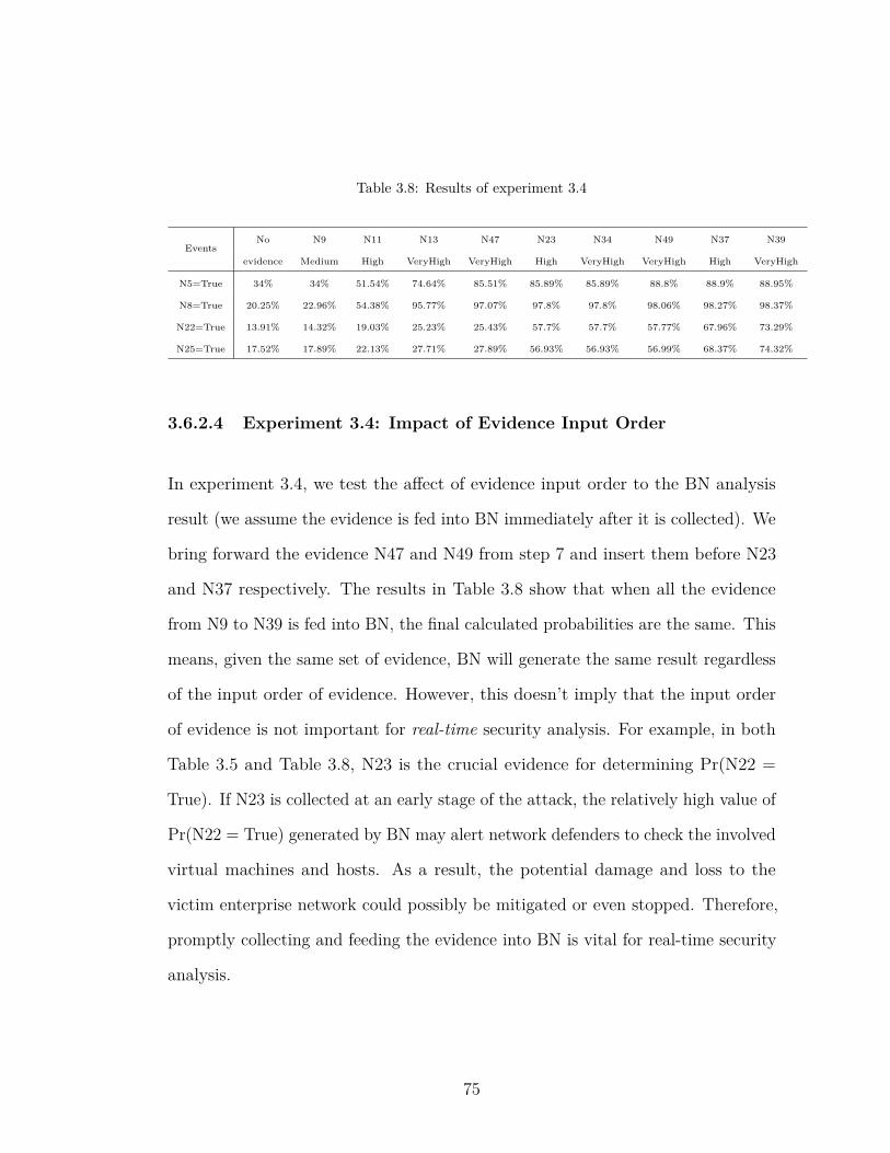
Table 3.8: Results of experiment 3.4

EventsNo N9 N11 N13 N47 N23 N34 N49 N37 N39

evidence Medium High VeryHigh VeryHigh High VeryHigh VeryHigh High VeryHigh

N5=True 34% 34% 51.54% 74.64% 85.51% 85.89% 85.89% 88.8% 88.9% 88.95%

N8=True 20.25% 22.96% 54.38% 95.77% 97.07% 97.8% 97.8% 98.06% 98.27% 98.37%

N22=True 13.91% 14.32% 19.03% 25.23% 25.43% 57.7% 57.7% 57.77% 67.96% 73.29%

N25=True 17.52% 17.89% 22.13% 27.71% 27.89% 56.93% 56.93% 56.99% 68.37% 74.32%

3.6.2.4 Experiment 3.4: Impact of Evidence Input Order

In experiment 3.4, we test the a�ect of evidence input order to the BN analysis

result (we assume the evidence is fed into BN immediately after it is collected). We

bring forward the evidence N47 and N49 from step 7 and insert them before N23

and N37 respectively. The results in Table 3.8 show that when all the evidence

from N9 to N39 is fed into BN, the final calculated probabilities are the same. This

means, given the same set of evidence, BN will generate the same result regardless

of the input order of evidence. However, this doesn’t imply that the input order

of evidence is not important for real-time security analysis. For example, in both

Table 3.5 and Table 3.8, N23 is the crucial evidence for determining Pr(N22 =

True). If N23 is collected at an early stage of the attack, the relatively high value of

Pr(N22 = True) generated by BN may alert network defenders to check the involved

virtual machines and hosts. As a result, the potential damage and loss to the

victim enterprise network could possibly be mitigated or even stopped. Therefore,

promptly collecting and feeding the evidence into BN is vital for real-time security

analysis.

75

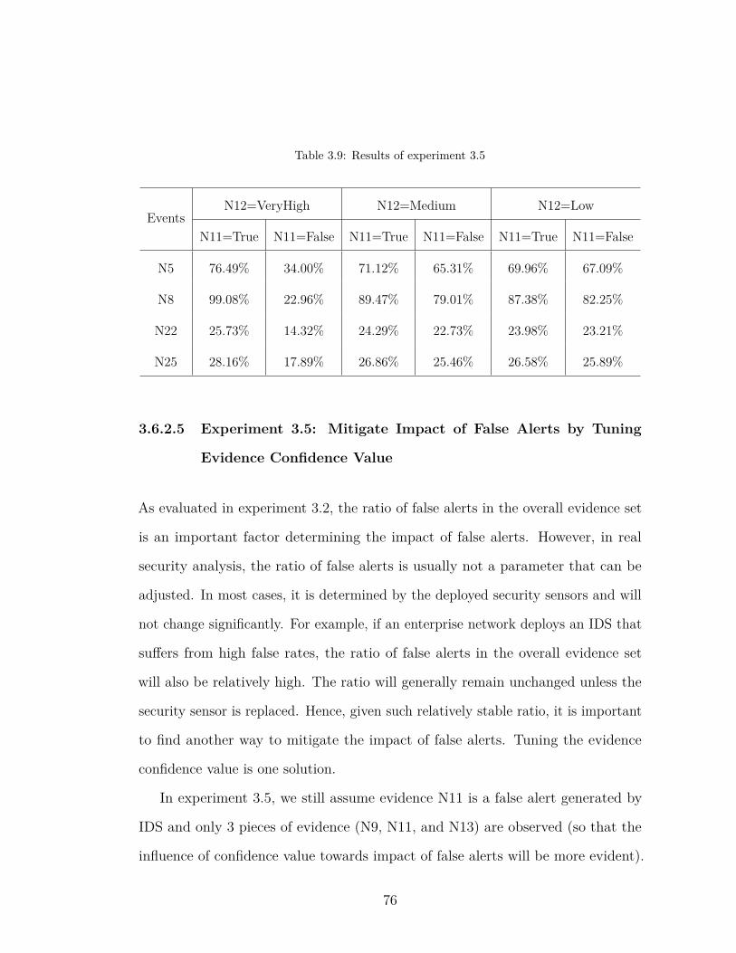
Table 3.9: Results of experiment 3.5

EventsN12=VeryHigh N12=Medium N12=Low

N11=True N11=False N11=True N11=False N11=True N11=False

N5 76.49% 34.00% 71.12% 65.31% 69.96% 67.09%

N8 99.08% 22.96% 89.47% 79.01% 87.38% 82.25%

N22 25.73% 14.32% 24.29% 22.73% 23.98% 23.21%

N25 28.16% 17.89% 26.86% 25.46% 26.58% 25.89%

3.6.2.5 Experiment 3.5: Mitigate Impact of False Alerts by Tuning

Evidence Confidence Value

As evaluated in experiment 3.2, the ratio of false alerts in the overall evidence set

is an important factor determining the impact of false alerts. However, in real

security analysis, the ratio of false alerts is usually not a parameter that can be

adjusted. In most cases, it is determined by the deployed security sensors and will

not change significantly. For example, if an enterprise network deploys an IDS that

su�ers from high false rates, the ratio of false alerts in the overall evidence set

will also be relatively high. The ratio will generally remain unchanged unless the

security sensor is replaced. Hence, given such relatively stable ratio, it is important

to find another way to mitigate the impact of false alerts. Tuning the evidence

confidence value is one solution.

In experiment 3.5, we still assume evidence N11 is a false alert generated by

IDS and only 3 pieces of evidence (N9, N11, and N13) are observed (so that the

influence of confidence value towards impact of false alerts will be more evident).

76

Table 3.9 shows the computed probabilities when the confidence value (specified in

N12) for false alert N11 is “VeryHigh”, “Medium”, and “Low” respectively. When

the confidence value is “VeryHigh”, the false alert can generate great impact on

the final results (e.g. Pr(N5 = True) is 76.49% when N11 is “True”, and 34.00%

when N11 is “False”). When the confidence value for false alert N11 is “Low”, the

false alert has little impact on the final result (e.g. the results for Pr(N5 = True)

are very close: 69.96% when N11 is “True”, and 67.09% when N11 is “False”).

Therefore, the impact of false alerts can be mitigated by tuning the corresponding

confidence value for the evidence. In practical application, if a security sensor su�er

from high false rates, the evidence generated by this sensor should have a relatively

low confidence value. Similarly, evidence generated by security sensors with low

false rates should have a relatively high confidence value. In such a way, the impact

of false alerts can be mitigated in BN analysis.

3.6.2.6 Experiment 3.6: Complexity

Since the BN is constructed on the basis of an attack graph, the size of BN mainly

depends on the size of attack graph. According to Theorem 2 in [50], the logical

attack graph for a network with N machines has a size at most O(N2). As we apply

logical attack graph to cloud, we consider both virtual machines and physical hosts

and regard them as normal hosts having special connections between each other.

For a cloud with n virtual machines and m physical hosts, the corresponding attack

graph has a size at most O((n + m)2). Considering n >> m in a normal cloud, the

size should be at most O(n2).

To further investigate the inference costs for BNs, we constructed 11 Bayesian

77

Table 3.10: Size of Bayesian Networks

BN 1 2 3 4 5 6 7 8 9 10 11

# of nodes 39 49 520 745 1069 1589 2068 2588 3082 5150 10300

# of edges 37 48 668 968 1244 1912 2545 3213 3854 6399 12798

networks with di�erent size (Table 3.10) in SamIam. For most exact inference

algorithms, the complexity of inference is mainly determined by the treewidth of

the network. Nevertheless, determining the treewidth is also di�cult. While we

cannot explore all di�erent tree structures and inference algorithms in this limited

space, we provide the compilation costs for the BNs we constructed, as shown in

Fig. 3.10 and Fig. 3.11, to give readers a sense regarding the time and memory

cost. The experiment was conducted in SamIam, with recursive conditioning as

the inference algorithm adopted.

3.7 Related Work

We explore the literature for the following topics that are related to this chapter.

VMI sharing. [66] explores a variety of attacks that leverage the virtual

machine image sharing in Amazon EC2. Researchers were able to extract highly

sensitive information from publicly available VMIs. The analysis revealed that 30%

of the 1100 analyzed AMIs (Amazon Machine Images) at the time of the analysis

contained public keys that are backdoors for the AMI Publishers. The backdoor

problem is not limited to AMIs created by individuals, but also a�ects those from

78

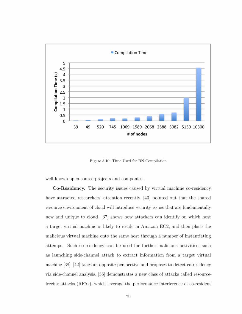
0"0.5"1"

1.5"2"

2.5"3"

3.5"4"

4.5"5"

39" 49" 520" 745" 1069" 1589" 2068" 2588" 3082" 5150" 10300"

Compila(o

n*Time*(s)*

#*of*nodes*

Compila4on"Time"

Figure 3.10: Time Used for BN Compilation

well-known open-source projects and companies.

Co-Residency. The security issues caused by virtual machine co-residency

have attracted researchers’ attention recently. [43] pointed out that the shared

resource environment of cloud will introduce security issues that are fundamentally

new and unique to cloud. [37] shows how attackers can identify on which host

a target virtual machine is likely to reside in Amazon EC2, and then place the

malicious virtual machine onto the same host through a number of instantiating

attemps. Such co-residency can be used for further malicious activities, such

as launching side-channel attack to extract information from a target virtual

machine [38]. [42] takes an opposite perspective and proposes to detect co-residency

via side-channel analysis. [36] demonstrates a new class of attacks called resource-

freeing attacks (RFAs), which leverage the performance interference of co-resident

79

0"

5"

10"

15"

20"

25"

30"

35"

39" 49" 520" 745" 1069" 1589" 2068" 2588" 3082" 5150" 10300"

Mem

ory'Used'(M

b)'

#'of'nodes'

Memory"Used"

Figure 3.11: Memory Used for BN Compilation

virtual machine. [40] presents a tra�c analysis attack that can initiate a covert

channel and confirm co-residency with a target virtual machine instance. [39] also

considers attacks towards hypervisor and propose to eliminate the hypervisor attack

surface through new system design.

3.8 Conclusion and Discussion

This chapter identifies the problem of stealthy bridges between isolated enterprise

networks in the public cloud. To infer the existence of stealthy bridges, we propose a

two-step approach. A cloud-level attack graph is first built to capture the potential

attacks enabled by stealthy bridges. Based on the attack graph, a cross-layer

80

Bayesian network is constructed by identifying uncertainty types existing in attacks

exploiting stealthy bridges. The experiments show that the cross-layer Bayesian

network is able to infer the existence of stealthy bridges given supporting evidence

from other intrusion steps. However, one challenge posed by cloud environments

needs further e�ort. Since the structure of cloud is very dynamic, generating the

cloud-level attack graph from scratch whenever a change happens is expensive

and time-consuming. Therefore, an incremental algorithm needs to be developed

to address such frequent changes such as virtual machine turning on and o�,

configuration changes, etc.

81

Chapter 4 |ZePro: Probabilistic Identifica-tion of Zero-day Attack Paths

4.1 Introduction

Defending against zero-day attacks is one of the most fundamentally challenging

security problems yet to be solved. Zero-day attacks are usually enabled by

unknown vulnerabilities. The information asymmetry between what the attacker

knows and what the defender knows makes zero-day exploits extremely hard to

detect. Signature-based detection assumes that a signature is already extracted

from detected exploits. Anomaly detection [68–70] may detect zero-day exploits,

but this solution has to cope with high false positive rates.

Considering the extreme di�culty of detecting individual zero-day exploits, a

substantially more feasible strategy is to identify zero-day attack paths. In real

world, to achive the attack goal, attack campaigns rely on a chain of attack actions,

which forms an attack path. Each attack chain is a partial order of exploits and

82

each exploit is exploiting a particular vulnerability. A zero-day attack path is a

multi-step attack path that includes one or more zero-day exploits. A key insight

in dealing with zero-day attack paths is to analyze the chaining e�ect. Typically, it

is not very likely for a zero-day attack chain to be 100% zero-day, namely having

every exploit in the chain be a zero-day exploit. Hence, defenders can assume that

1) the non-zero-day exploits in the chain are detectable; 2) these detectable exploits

have certain chaining relationships with the zero-day exploits in the chain. As a

result, connecting the detected non-zero-day segments through a path is an e�ective

way of revealing the zero-day segments in the same chain.

Both alert correlation [71, 72] and attack graphs [47, 48, 50, 51] are possible

solutions for generating potential attack paths, but they are limited in revealing the

zero-day ones. They both can identify the non-zero-day segments (i.e., “islands”)

of a zero-day attack path; however, none of them can automatically bridge all

segments into a meaningful path and reveal the zero-day segments, especially when

di�erent segments may belong to totally irrelevant attack paths.

To address these limitations, Dai et al. proposed a system called Patrol [41]

to identify real zero-day attack paths from a large set of suspicious intrusion

propagation paths generated through tracking dependencies between OS-level

objects. The set of suspicious dependency paths is usually very huge or even

su�ers from serious path explosion problem. A root cause for such explosion is that

dependencies introduced by legitimate activities and dependencies introduced by

zero-day attacks are often tangled together. Hence, Patrol made an assumption

that extensive pre-knowledge are available to distinguish real zero-day attack paths

from suspicious ones: common features or attack patterns of known exploitations

can be extracted at the OS-level to help recognize future unknown exploitations

83

if similar features appear again. However, this assumption is too strong in that

1) the acquirement of such pre-knowledge is quite di�cult. It is a very ad hoc

and e�ort consuming process. It relies heavily on the availability of the history for

known vulnerability exploitations. Even if the history is available, investigating

and crafting the common features at OS-level for all types of exploitations requires

immeasurable amount of human analysts’ e�orts or even the whole community’s

e�orts; 2) future zero-day exploits do not necessarily share similar attack patterns

with previous known exploitations.

Therefore, in this chapter, we propose a probabilistic approach to identify the

zero-day attack paths. Our approach is to 1) establish an object instance graph to

capture the intrusion propagation, where an instance of an object is a “version” of

the object with a specific timestamp; 2) build a Bayesian network (BN) based on the

instance graph to leverage the intrusion evidence collected from various information

sources. Intrusion evidence can be the abnormal system and network activities

that are noticed by human admins or security sensors such as Intrusion Detection

Systems (IDSs). With the evidence, the instance-graph-based BN can quantitatively

compute the probabilities of object instances being infected. Connected through

dependency relations, the instances with high infection probabilities form a path,

which can be viewed as a zero-day attack path. Such paths are of manageable size

as the instance-graph-based BN can significantly narrow down the set of suspicious

objects.

Our new insights are as follows. First, due to path explosion, deterministic

dependency analysis is not adequate and will fall short. Innovative ways are

required to help separate the dependency paths introduced by legitimate activities

and dependency paths introduced by zero-day attacks. Second, through Bayesian

84

networks, a key di�erence between the two types of dependency paths becomes

visible. In a Bayesian network, a dependency path becomes a causality path

associated with the probabilities of system objects being infected. Typically the

infection probabilities for system objects involved in a zero-day dependency path are

substantially higher than the infection probabilities of objects involved in legitimate

paths. Therefore, our approach does not require any pre-knowledge to distinguish

the real zero-day attack paths from the legitimate ones.

This approach is supported based on the following rationales. First, a BN

is able to capture cause-and-e�ect relations, and thus can be used to model the

infection propagation among instances of di�erent system objects: the cause is

an already infected instance of one object, while the e�ect is its infection to an

innocent instance of another object. We name this cause-and-e�ect relation as a

type of infection causality, which is formed due to the information flow between

the two objects in a system call operation. Second, an instance graph can reflect

the infection propagation process by capturing the dependencies among instances

of di�erent system objects. Third, a BN can be constructed on top of the instance

graph because they couple well with each other: the dependencies among instances

of di�erent system objects can be directly interpreted into infection causalities in

the BN. The BN’s graphical nature makes it fit well with an instance graph.

The significance of our approach is as follows:

1) Our approach is systematic because Bayesian networks can incorporate

literally all kinds of knowledge the defender has about the zero-day attack paths.

The knowledge includes but is not limited to alerts generated by security sensors

such as IDS and Tripwire, reports provided by vulnerability scanners, system logs,

or even human inputs.

85

2) Our approach does not rely on particular assumptions or preconditions.

Therefore, it is applicable to almost all kinds of enterprise networks.

3) Our approach is elastic. Whenever new knowledge is gained about zero-

day attacks, such new knowledge can be incorporated and the e�ectiveness of

our approach can be enhanced. Whenever erroneous knowledge is identified, our

approach can easily get rid of the negative e�ects of the wrong knowledge.

4) The tool we built is automated. Today’s security analysis relies largely on

the manual work of human security analysts. Our automated tool can significantly

save security analysts’ time and address the human resource challenge.

To summarize, we made the following contributions.

• To the best of our knowledge, this work is the first probabilistic approach

towards zero-day attack path identification.

• We proposed constructing Bayesian network at the system object level by

introducing the object instance graph.

• We have designed and implemented a system prototype named ZePro, which

can e�ectively and automatically identify zero-day attack paths.

4.2 Rationales and Models

4.2.1 System Object Dependency Graph

This work classifies OS-level entities in UNIX-like systems into three types of objects:

processes, files and sockets. The operating system performs a set of operations

86

1

t1: process A reads file 1t2: process A creates process Bt3: process A creates process Ct4: process B writes file 2t5: process C writes file 1t6: process B reads file 3

(a) Simplified System Call Log in Time-order

process Afile 3

file 1

process Cprocess B

file 2

t1

t5t3t2

t4

t6

(b) SODG

Figure 4.1: An SODG. An SODG generated by parsing an example set of simplified system calllog. The label on each edge shows the time associated with the corresponding system call.

towards these objects via system calls such as read, write, etc. For instance, a

process can read from a file as input, and then write to a socket. Such interactions

among system objects enable intrusions to propagate from one object to another.

Generally an intrusion starts with one or several seed objects that are created

directly or indirectly by attackers. The intrusion seeds can be processes such as

compromised service programs, or files such as viruses, or corrupted data, etc. As

the intrusion seeds interact with other system objects via system call operations,

the innocent objects can get infected. We call this process as infection propagation.

87

Therefore the intrusion will propagate throughout the system, or even propagate

to the network through socket communications.

To capture the intrusion propagation, previous work [21, 22] has explored

constructing system level dependency graphs by parsing system call traces. This

type of dependency graph is known as System Object Dependency Graphs (SODGs).

Each system call is interpreted into three parts: a source object, a sink object, and a

dependency relation between them. The objects and the dependencies respectively

become nodes and directed edges in SODGs. For example, a process reading a file

in the system call read indicates that the process (sink) depends on the file (source).

The dependency is denoted as fileæprocess. Similar rules as in Table 2.1 as used in

previous work [21,22] can be adopted to generate such dependencies. Figure 4.1b

is an example SODG generated by parsing the simplified system call log shown in

Figure 4.1a.

4.2.2 Why use Bayesian Network?

The BN is a probabilistic graphical model that represents the cause-and-e�ect

relations. It is formally defined as a Directed Acyclic Graph (DAG) that contains

a set of nodes and directed edges, where a node denotes a variable of interest,

and an edge denotes the causality relations between two nodes. The strength of

such causality relation is indicated using a conditional probability table (CPT).

Figure 4.2 shows an example BN. Table 4.1 is the CPTs associated with p2. Given

p1 is true, the probability of p2 being true is 0.9, which can be represented with

P (p2 = T |p1 = T ) = 0.9. Similarly, the probability of p4 can be determined by

the states of p2 and p3 according to a CPT at p4. BN is able to incorporate the

88

...

...

p1

p2 p3

p4

Figure 4.2: An Example Bayesian Network.

collected evidence by updating the posterior probabilities of interested variables.

For example, after evidence p2 = T is observed, it can be incorporated by computing

probability P (p1 = T |p2 = T ).

The BN is applied on top of the system level dependency graph for the following

benefits. First, BN is an e�ective tool to incorporate intrusion evidence from a

variety of information sources. Alerts generated by di�erent security sensors are

usually isolated from each other. As a unified platform, BN is able to leverage these

alerts as attack evidence to aid the security analysis. Second, BN can quantitatively

compute the probabilities of objects being infected. The inferred probabilities are

the key guidance to identify zero-day attack paths. By only focusing on the objects

with high infection probabilities, the set of suspicious objects can be significantly

narrowed down. The zero-day attack paths formed by the high-probability objects

through dependency relations is thus of manageable size.

89

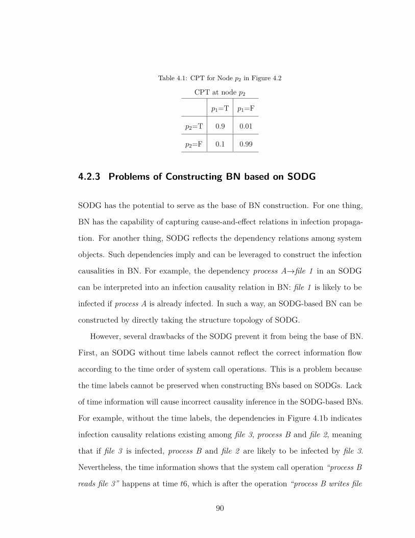
Table 4.1: CPT for Node p2 in Figure 4.2

CPT at node p2

p1=T p1=F

p2=T 0.9 0.01

p2=F 0.1 0.99

4.2.3 Problems of Constructing BN based on SODG

SODG has the potential to serve as the base of BN construction. For one thing,

BN has the capability of capturing cause-and-e�ect relations in infection propaga-

tion. For another thing, SODG reflects the dependency relations among system

objects. Such dependencies imply and can be leveraged to construct the infection

causalities in BN. For example, the dependency process Aæfile 1 in an SODG

can be interpreted into an infection causality relation in BN: file 1 is likely to be

infected if process A is already infected. In such a way, an SODG-based BN can be

constructed by directly taking the structure topology of SODG.

However, several drawbacks of the SODG prevent it from being the base of BN.

First, an SODG without time labels cannot reflect the correct information flow

according to the time order of system call operations. This is a problem because

the time labels cannot be preserved when constructing BNs based on SODGs. Lack

of time information will cause incorrect causality inference in the SODG-based BNs.

For example, without the time labels, the dependencies in Figure 4.1b indicates

infection causality relations existing among file 3, process B and file 2, meaning

that if file 3 is infected, process B and file 2 are likely to be infected by file 3.

Nevertheless, the time information shows that the system call operation “process B

reads file 3” happens at time t6, which is after the operation “process B writes file

90

2” at time t4. This implies that the status of file 3 has no direct influence on the

status of file 2.

Second, the SODG contains cycles among nodes. For instance, file 1, process A

and process C in Figure 4.1b form a cycle. By directly adopting the topology of

SODG, the SODG-based BN inevitably inherits cycles from SODG. However, the

BN is an acyclic probabilistic graphical model that does not allow any cycles.

Third, a node in an SODG can end up with having too many parent nodes,

which will render the CPT assignment di�cult and even impractical in the SODG-

based BN. For example, if process B in Figure 4.1b continuously reads hundreds

of files (which is normal in a practical operating system), it will get hundreds of

file nodes as its parents. In the corresponding SODG-based BN, if each file node

has two possible states that are “infected” and “uninfected”, and the total number

of parent file nodes are denoted as n, then the CPT at process B has to assign

2n numbers in order to specify the infection causality of the parent file nodes to

process B. This is impractical when n is very large.

Therefore, in this chapter we propose a new type of dependency graph, the

object instance graph, to address the above problems.

4.2.4 Object Instance Graph

In the object instance graph, each node is not an object, but an instance of the

object with a specific timestamp. Di�erent instances are di�erent “versions” of the

same object at di�erent time points, and can thus have di�erent infection status.

Definition 1. Object Instance Graph

If the system call trace in a time window T [tbegin

, tend

] is denoted as �T

and the

91

set of system objects (mainly processes, files or sockets) involved in �T

is denoted

as OT

, then the object instance graph is a directed graph GT

(V , E), where:

• V is the set of nodes, and initialized to empty set ?;

• E is the set of directed edges, and initialized to empty set ?;

• If a system call syscall œ �T

is parsed into two system object instances srci

,

sinkj

, i, j Ø 1, and a dependency relation depc

: srci

æsinkj

(according to

dependency rules in Table 2.1), where srci

is the ith instance of system object

src œ OT

, and sinkj

is the jth instance of system object sink œ OT

, then

V = V fi {srci

, sinkj

}, E = E fi {depc

}. The timestamps for syscall, depc

,

srci

, and sinkj

are respectively denoted as t_syscall, t_depc

, t_srci

, and

t_sinkj

. The t_depc

inherits t_syscall from syscall. The indexes i and j

are determined before adding srci

and sinkj

into V by:

– For ’ srcm

, sinkn

œ V , m, n Ø 1, if imax

and jmax

are respectively the

maximum indexes of instances for object src and sink, and;

– If ÷ srck

œ V , k Ø 1, then i = imax

, and t_srci

stays the same; Otherwise,

i = 1, and t_srci

is updated to t_syscall;

– If ÷ sinkz

œ V , z Ø 1, then j = jmax

+1; Otherwise, j = 1. In both

cases t_sinkj

is updated to t_syscall; If j Ø 2, then E = E fi {deps

:

sinkj≠1æsink

j

}.

• If aæb œ E and bæc œ E, then c transitively depends on a.

According to Definition 1, for src object, a new instance is created only when

no instances of src exist in the instance graph. For sink object, however, a new

92

instance is created whenever a srcæsink dependency appears. The underlying

insight is that the status of the src object will not be altered by srcæsink, while

the status of sink will be influenced. Hence a new instance for an object should be

created when the object has the possibility of being a�ected. A dependency depc

is

added between the most recent instance of src and the newly created instance of

sink. We name depc

as contact dependency because it is generated by the contact

between two di�erent objects through a system call operation.

In addition, when a new instance is created for an object, a new dependency

relation deps

is also added between the most recent instance and the new instance

of the same object. This is necessary and reasonable because the status of the new

instance can be influenced by the status of the most recent instance. We name deps

as state transition dependency because it is caused by the state transition between

di�erent instances of the same system object.

The instance graph can well tackle the problems existing in the SODG for

constructing BNs. It can be illustrated using Figure 4.3, an instance graph created

for the same simplified system call log as in Figure 4.1a. First, the instance graph

is able to reflect correct information flows by implying time information through

creating object instances. For example, instead of parsing the system call at time t6

directly into file 3æprocess B, Figure 4.3 parsed it into file 3 instance 1æprocess B

instance 2. Comparing to Figure 4.1b in which file 3 has indirect infection causality

on file 2 through process B, the instance graph in Figure 4.3 indicates that file 3

can only infect instance 2 of process B but no previous instances. Hence in this

graph file 3 does not have infection causality on file 2.

Second, instance graphs can break the cycles contained in SODGs. Again, in

Figure 4.3, the system call at time t5 is parsed into process C instance 1æfile 1

93

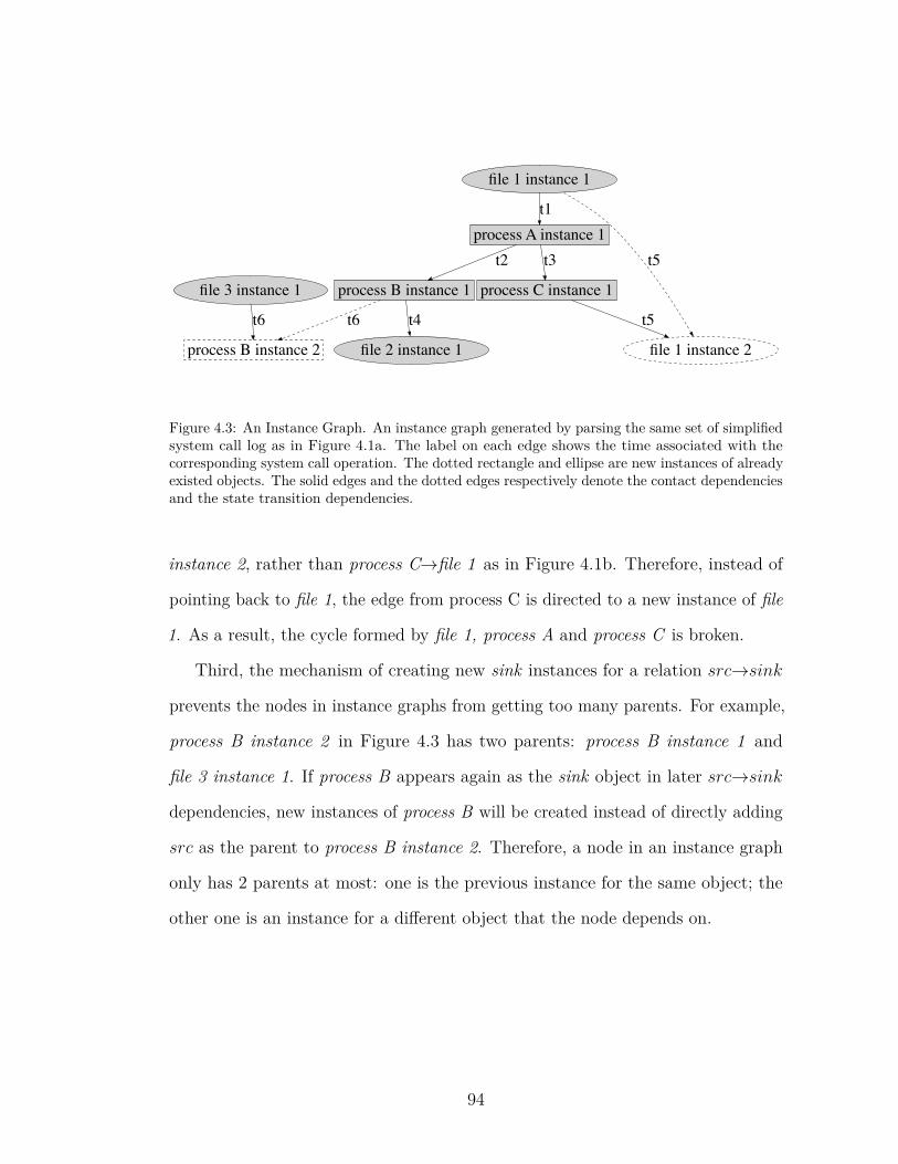
file 3 instance 1

process B instance 2

t6

file 1 instance 1

process A instance 1t1

file 1 instance 2

t5

process C instance 1

t3

process B instance 1

t2

t5

file 2 instance 1

t4t6

Figure 4.3: An Instance Graph. An instance graph generated by parsing the same set of simplifiedsystem call log as in Figure 4.1a. The label on each edge shows the time associated with thecorresponding system call operation. The dotted rectangle and ellipse are new instances of alreadyexisted objects. The solid edges and the dotted edges respectively denote the contact dependenciesand the state transition dependencies.

instance 2, rather than process Cæfile 1 as in Figure 4.1b. Therefore, instead of

pointing back to file 1, the edge from process C is directed to a new instance of file

1. As a result, the cycle formed by file 1, process A and process C is broken.

Third, the mechanism of creating new sink instances for a relation srcæsink

prevents the nodes in instance graphs from getting too many parents. For example,

process B instance 2 in Figure 4.3 has two parents: process B instance 1 and

file 3 instance 1. If process B appears again as the sink object in later srcæsink

dependencies, new instances of process B will be created instead of directly adding

src as the parent to process B instance 2. Therefore, a node in an instance graph

only has 2 parents at most: one is the previous instance for the same object; the

other one is an instance for a di�erent object that the node depends on.

94

...

...

sinkj srci

sinkj+1

...

Figure 4.4: The Infection Propagation Models.

4.3 Instance-graph-based Bayesian Networks

To build a BN based on an instance graph and compute probabilities for interested

variables, two steps are required. First, the CPTs have to be specified for each

node via constructing proper infection propagation models. Second, evidence

from di�erent information sources has to be incorporated into BN for subsequent

probability inference.

4.3.1 The Infection Propagation Models

In instance-graph-based BNs, each object instance has two possible states, “infected”

and “uninfected”. The strength of the infection causalities among the instances has

to be specified in corresponding CPTs. Our infection propagation models in this

work deal with two types of infection causalities, contact infection causalities and

state transition infection causalities, which correspond to the contact dependencies

and state transition dependencies in instance graphs.

Contact Infection Causality Model. This model captures the infection

95

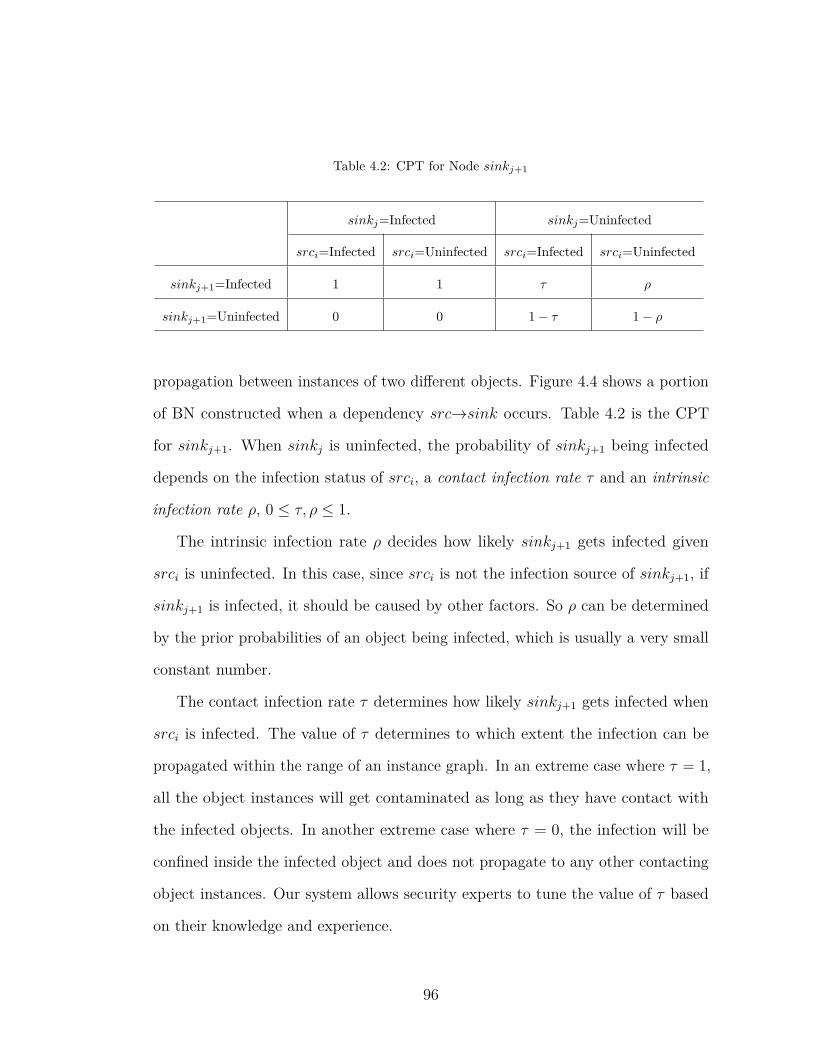
Table 4.2: CPT for Node sinkj+1

sinkj=Infected sinkj=Uninfected

srci=Infected srci=Uninfected srci=Infected srci=Uninfected

sinkj+1=Infected 1 1 · fl

sinkj+1=Uninfected 0 0 1 ≠ · 1 ≠ fl

propagation between instances of two di�erent objects. Figure 4.4 shows a portion

of BN constructed when a dependency srcæsink occurs. Table 4.2 is the CPT

for sinkj+1. When sink

j

is uninfected, the probability of sinkj+1 being infected

depends on the infection status of srci

, a contact infection rate · and an intrinsic

infection rate fl, 0 Æ ·, fl Æ 1.

The intrinsic infection rate fl decides how likely sinkj+1 gets infected given

srci

is uninfected. In this case, since srci

is not the infection source of sinkj+1, if

sinkj+1 is infected, it should be caused by other factors. So fl can be determined

by the prior probabilities of an object being infected, which is usually a very small

constant number.

The contact infection rate · determines how likely sinkj+1 gets infected when

srci

is infected. The value of · determines to which extent the infection can be

propagated within the range of an instance graph. In an extreme case where · = 1,

all the object instances will get contaminated as long as they have contact with

the infected objects. In another extreme case where · = 0, the infection will be

confined inside the infected object and does not propagate to any other contacting

object instances. Our system allows security experts to tune the value of · based

on their knowledge and experience.

96

Since a large number of system call traces with ground truths are often un-

available, currently it is very unlikely to learn the parameters of · and fl using

statistical techniques. Hence, now these parameters have to be assigned by security

experts. Security experts can assign parameters in batch mode or provide di�erent

parameters for specific nodes based on their knowledge. We will evaluate the impact

of · and fl in Section 4.6. Bayesian network training and parameter learning is

beyond the scope of this chapter and will be investigated in future work.

State Transition Infection Causality Model. This model captures the

infection propagation between instances of the same objects. We follow one rule to

model this type of causalities: an object will never return to the state of “uninfected”

from the state of “infected”1. That is, once an instance of an object gets infected,

all future instances of this object will remain the infected state, regardless of

the infection status of other contacting object instances. This rule is enforced in

the CPT exemplified in Table 4.2. If sinkj

is infected, the infection probability

of sinkj+1 keeps to be 1, no matter whether src

i

is infected or not. If sinkj

is

uninfected, the infection probability of sinkj+1 is decided by the infection status of

srci

according to the contact infection causality model.

4.3.2 Evidence Incorporation

BN is able to incorporate security alerts from a variety of information sources

as the evidence of attack occurrence. Numerous ways have been developed to

capture intrusion symptoms, which can be caused by attacks exploiting both known1This rule is formulated based on the assumptions that no intrusion recovery operations are

performed and attackers only conduct malicious activities.

97

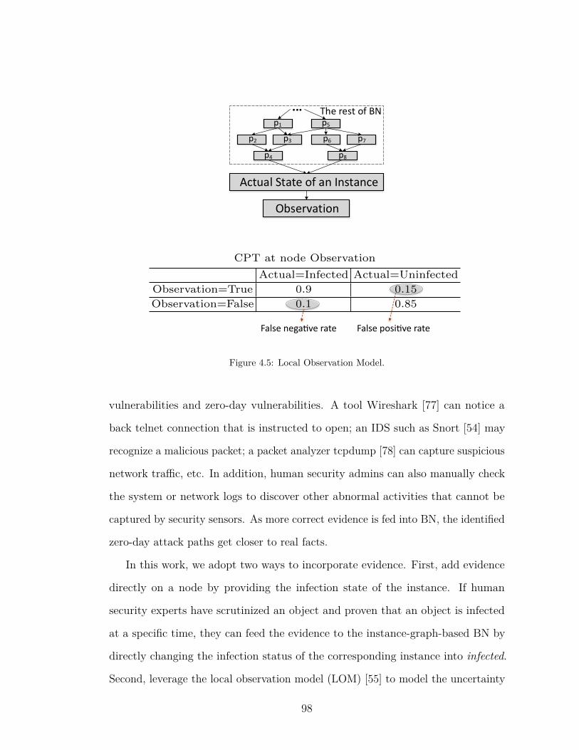
p1

p2 p3

p4

...p5

p6 p7

p8

Actual State of an Instance

Observation

The rest of BN

!!!!!!!

!!!

1

CPT at node Observation

Actual=Infected Actual=Uninfected

Observation=True 0.9 0.15

Observation=False 0.1 0.85

!

!

False&nega)ve&rate False&posi)ve&rate

Figure 4.5: Local Observation Model.

vulnerabilities and zero-day vulnerabilities. A tool Wireshark [77] can notice a

back telnet connection that is instructed to open; an IDS such as Snort [54] may

recognize a malicious packet; a packet analyzer tcpdump [78] can capture suspicious

network tra�c, etc. In addition, human security admins can also manually check

the system or network logs to discover other abnormal activities that cannot be

captured by security sensors. As more correct evidence is fed into BN, the identified

zero-day attack paths get closer to real facts.

In this work, we adopt two ways to incorporate evidence. First, add evidence

directly on a node by providing the infection state of the instance. If human

security experts have scrutinized an object and proven that an object is infected

at a specific time, they can feed the evidence to the instance-graph-based BN by

directly changing the infection status of the corresponding instance into infected.

Second, leverage the local observation model (LOM) [55] to model the uncertainty

98

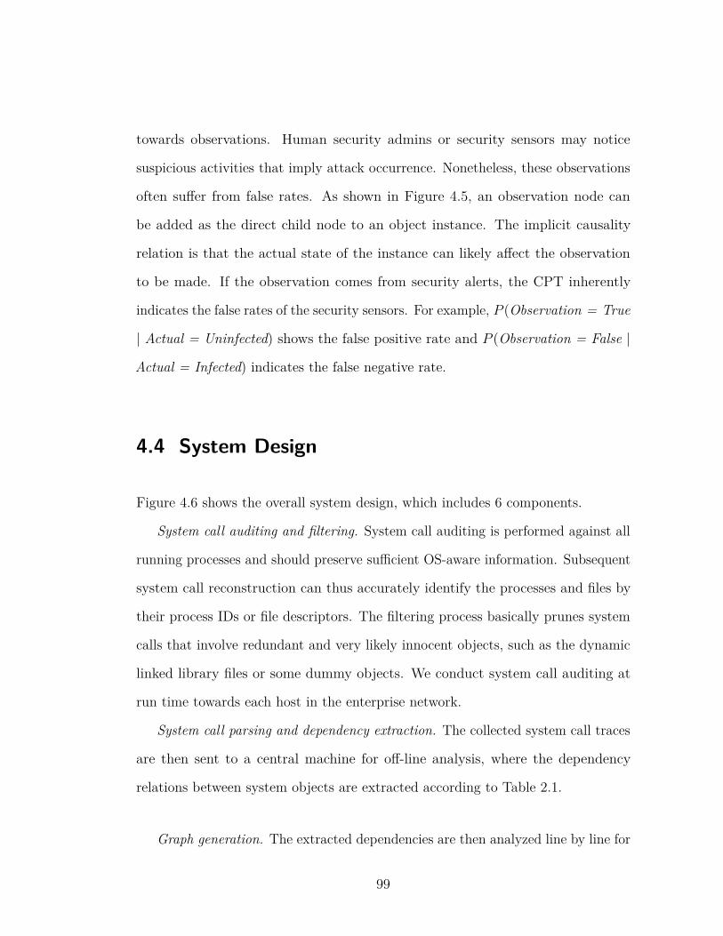
towards observations. Human security admins or security sensors may notice

suspicious activities that imply attack occurrence. Nonetheless, these observations

often su�er from false rates. As shown in Figure 4.5, an observation node can

be added as the direct child node to an object instance. The implicit causality

relation is that the actual state of the instance can likely a�ect the observation

to be made. If the observation comes from security alerts, the CPT inherently

indicates the false rates of the security sensors. For example, P (Observation = True

| Actual = Uninfected) shows the false positive rate and P (Observation = False |

Actual = Infected) indicates the false negative rate.

4.4 System Design

Figure 4.6 shows the overall system design, which includes 6 components.

System call auditing and filtering. System call auditing is performed against all

running processes and should preserve su�cient OS-aware information. Subsequent

system call reconstruction can thus accurately identify the processes and files by

their process IDs or file descriptors. The filtering process basically prunes system

calls that involve redundant and very likely innocent objects, such as the dynamic

linked library files or some dummy objects. We conduct system call auditing at

run time towards each host in the enterprise network.

System call parsing and dependency extraction. The collected system call traces

are then sent to a central machine for o�-line analysis, where the dependency

relations between system objects are extracted according to Table 2.1.

Graph generation. The extracted dependencies are then analyzed line by line for

99

Algorithm 1 Algorithm of Object Instance Graph GenerationRequire: set D of system object dependenciesEnsure: the instance graph G(V , E)

1: for each dep: srcæsink œD do2: look up the most recent instance src

k

of src, sinkz

of sink in V3: if sink

z

/œV then4: create new instances sink15: V Ω V fi { sink1}6: if src

k

/œV then7: create new instances src18: V Ω V fi { src1}9: E Ω E fi { src1æsink1}

10: else11: E Ω E fi { src

k

æsink1}12: end if13: end if14: if sink

z

œV then15: create new instance sink

z+116: V Ω V fi { sink

z+1}17: E Ω E fi { sink

z

æsinkz+1}

18: if srck

/œV then19: create new instances src120: V Ω V fi { src1}21: E Ω E fi { src1æsink

z+1}22: else23: E Ω E fi { src

k

æsinkz+1}

24: end if25: end if26: end for

graph generation. The generated graph can be either host-wide or network-wide,

depending on the analysis scope. A network-wide instance graph can be constructed

by concatenating individual host-wide instance graphs through instances of the

communicating sockets. Algorithm 1 is the base algorithm for instance graph

generation, which is designed according to the logic in Definition 1.

BN construction. The BN is constructed by taking the topology of an instance

graph. The instances and dependencies in an instance graph become nodes and

100

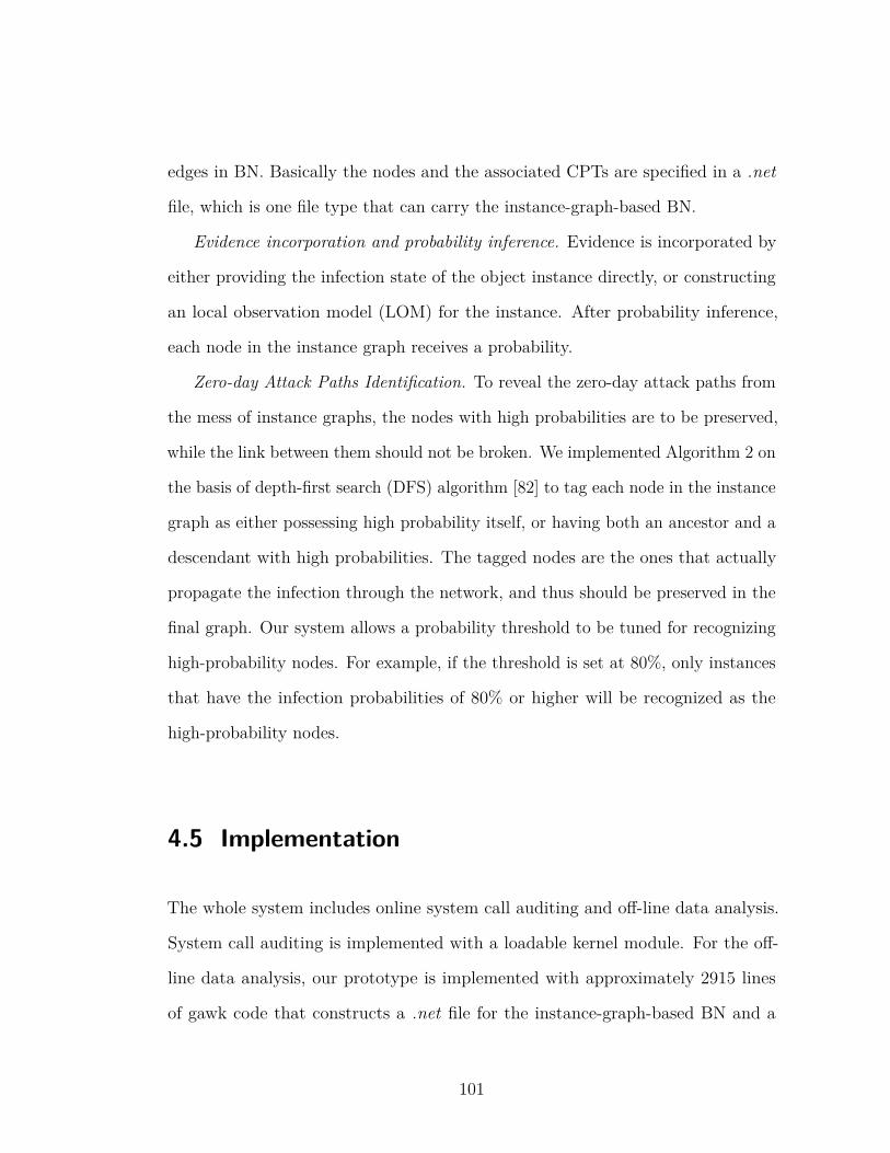
edges in BN. Basically the nodes and the associated CPTs are specified in a .net

file, which is one file type that can carry the instance-graph-based BN.

Evidence incorporation and probability inference. Evidence is incorporated by

either providing the infection state of the object instance directly, or constructing

an local observation model (LOM) for the instance. After probability inference,

each node in the instance graph receives a probability.

Zero-day Attack Paths Identification. To reveal the zero-day attack paths from

the mess of instance graphs, the nodes with high probabilities are to be preserved,

while the link between them should not be broken. We implemented Algorithm 2 on

the basis of depth-first search (DFS) algorithm [82] to tag each node in the instance

graph as either possessing high probability itself, or having both an ancestor and a

descendant with high probabilities. The tagged nodes are the ones that actually

propagate the infection through the network, and thus should be preserved in the

final graph. Our system allows a probability threshold to be tuned for recognizing

high-probability nodes. For example, if the threshold is set at 80%, only instances

that have the infection probabilities of 80% or higher will be recognized as the

high-probability nodes.

4.5 Implementation

The whole system includes online system call auditing and o�-line data analysis.

System call auditing is implemented with a loadable kernel module. For the o�-

line data analysis, our prototype is implemented with approximately 2915 lines

of gawk code that constructs a .net file for the instance-graph-based BN and a

101

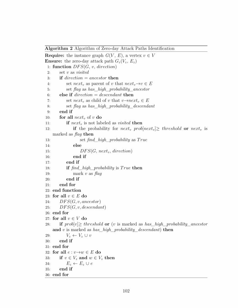
Algorithm 2 Algorithm of Zero-day Attack Paths IdentificationRequire: the instance graph G(V , E), a vertex v œ VEnsure: the zero-day attack path G

z

(Vz

, Ez

)1: function DFS(G, v, direction)2: set v as visited3: if direction = ancestor then4: set next

v

as parent of v that nextv

æv œ E5: set flag as has_high_probability_ancestor6: else if direction = descendant then7: set next

v

as child of v that vænextv

œ E8: set flag as has_high_probability_descendant9: end if

10: for all nextv

of v do11: if next

v

is not labeled as visited then12: if the probability for next

v

prob[nextv

]Ø threshold or nextv

ismarked as flag then

13: set find_high_probability as True14: else15: DFS(G, next

v

, direction)16: end if17: end if18: if find_high_probability is True then19: mark v as flag20: end if21: end for22: end function23: for all v œ E do24: DFS(G, v, ancestor)25: DFS(G, v, descendant)26: end for27: for all v œ V do28: if prob[v]Ø threshold or (v is marked as has_high_probability_ancestor

and v is marked as has_high_probability_descendant) then29: V

z

Ω Vz

fi v30: end if31: end for32: for all e : væw œ E do33: if v œ V

z

and w œ Vz

then34: E

z

Ω Ez

fi e35: end if36: end for

102

dot-compatible file for visualizing the zero-day attack paths in Graphviz [83], and

145 lines of Java code for probability inference, leveraging the API provided by the

BN tool SamIam [65].

An instance graph can be very large due to the introduction of instances.

Therefore, in addition to system call filtering, we also develop several ways to prune

that instance graphs while not impede reflecting the major infection propagation

process.

One helpful way is to ignore the repeated dependencies. It is common that

the same dependency may happen between two system objects for a number of

times, even through di�erent system call operations. For example, process A may

write file 1 for several times. In such cases, each time the write operation occurs,

a new instance of file 1 is created and a new dependency is added between the

most recent instance of process A and the new instance of file 1. If the status of

process A is not a�ected by any other system objects during this time period, the

infection status of file 1 will not change neither. Hence the new instances of file 1

and the related new dependencies become redundant information in understanding

the infection propagation. Therefore, a repeated srcæsink dependency can be

ignored if the src object is not influenced by other objects since the last time that

the same srcæsink dependency appeared.

Another way to simplify an instance graph is to ignore the root instances whose

original objects have never appear as the sink object in a srcæsink dependency

during the time period of being analyzed. For instance, file 3 in Figure 4.3 only

appears as the src object in the dependencies parsed from the system call log in

Figure 4.1a, so file 3 instance 1 can be ignored in the simplified instance graph.

Such instances are not influenced by other objects in the specified time window,

103

and thus are not manipulated by attackers, neither. Hence ignoring these root

instances does not break any routes of intrusion sequence and will not hinder the

understanding of infection propagation. This method is helpful for situations such

as a process reading a large number of configuration or header files.

A third way to prune an instance graph is to ignore some repeated mutual

dependencies, in which two objects will keep a�ecting each other through creating

new instances. One situation is that a process can frequently send and receive

messages from a socket. For example, in one of our experiments, 107 new instances

are created respectively for the process (pid:6706, pcmd:sshd) and the socket

(ip:192.168.101.5, port: 22 ) due to their interaction. Since no other objects are

involved during this procedure, the infection status of these two objects will keep

the same through all the new instances. Thus a simplified instance graph can

preserve the very first and last dependencies while neglect the middle ones. Another

situation is that a process can frequently take input from a file and then write the

output to it again after some operations. The middle repeated mutual dependencies

could also be ignored in a similar way.

4.6 Experiments

4.6.1 Attack Scenario

To demonstrate the merits of our system and compare experiment results with

Patrol [41], we implemented a similar attack scenario as in Patrol. We built a

test-bed network and launched a three-step attack towards it. Figure 4.7 illustrates

the attack scenario. Step 1, the attacker exploits vulnerability CVE-2008-0166 [75]

104

to gain root privilege on SSH Server through a brute-force key guessing attack. Step

2, since the export table on NFS Server is not set up appropriately, the attacker can

upload a malicious executable file to a public directory on NFS. The malicious file

contains a Trojan-horse that can exploit a vulnerability on a specific workstation.

The public directory is shared among all the hosts in the test-bed network so that a

workstation may access and download this malicious file. Step 3, once the malicious

file is mounted and installed on the workstation, the attacker is able to execute

arbitrary code on workstation.

To verify the e�ectiveness of our approach, we conducted two major sets of

experiments by providing di�erent vulnerabilities in step 3. In experiment 4.1, the

malicious file contains a Trojan-horse that exploits CVE-2009-2692 [73] existing in

the Linux kernel of workstation 3. CVE-2009-2692 is a vulnerability that allows local

users to gain privileges by triggering a NULL pointer dereference. In experiment

4.2, the malicious file contains another Trojan-horse leveraging CVE-2011-4089 [74]

on workstation 4. This vulnerability allows local users to execute arbitrary code by

precreating a temporary directory. Our goal is to test whether ZePro can reveal

both of the attack paths enabled by di�erent vulnerabilities.

Since zero-day exploits are not readily available, we emulate zero-day vulner-

abilities with known vulnerabilities. For example, we treat CVE-2009-2692 and

CVE-2011-4089 as zero-day vulnerabilities by assuming the current time is Dec

31, 2008. In addition, the configuration error on NFS is also viewed as a special

type of unknown vulnerability because it is ruled out by vulnerability scanners like

Nessus [56]. The strategy of emulation also brings another benefit. The information

for these “known zero-day” vulnerabilities can be available to verify the correctness

of our experiment results.

105

To capture the intrusion evidence for subsequent BN probability inference,

we deployed security sensors in the test-bed, such as firewalls, Snort, Tripwire,

Wireshark, Ntop [84] and Nessus. For sensors that need configuration, we tailored

their rules or policy files to match our hosts.

4.6.2 Experiment Results

While simultaneously logging the system calls on each host and collecting the

security alerts, we conducted the described three-step attacks. In experiment 4.1,

after analyzing a total number of 143120 system calls generated by three hosts, we

constructed an instance-graph-based BN with 1853 nodes and 2249 edges. Since

experiment 4.2 just di�ers from experiment 4.1 in attack step 3, in experiment 4.2

we only analyzed 54998 system calls generated by workstation 4. The constructed

BN contains 911 nodes and 1214 edges. The evidence as in Table 4.4 is collected

and fed into the two BNs respectively. We will present evaluation results for both

experiments in terms of correctness, size of zero-day attack paths and influence

of evidence. For other metrics, we only discuss experiment 4.1 because the two

experiments share similar evaluation conclusions.

4.6.2.1 Correctness

Given the evidence, Figure 4.8 and Figure 4.9 respectively illustrate the identified

zero-day attack paths for experiment 4.1 and 2 in the form of instance graphs. The

processes, files, and sockets are denoted with rectangles, ellipses, and diamonds

respectively. For both experiments, the intrinsic infection rate fl is set as 0.0001,

106

Syst

em C

all A

uditi

ng

and

Filte

ring

Syst

em C

all T

race

s

Grap

h Ge

nera

tion

Syst

em C

all P

arsin

g and

De

pend

ency

Ext

ract

ion

BN C

onst

ruct

ion

Evid

ence

Inco

rpor

atio

n an

d Pr

obab

ility

Infe

renc

eZe

ro-d

ay A

ttac

k Pa

th

Iden

tifica

tion

Depe

nden

cies

Inst

ance

Gra

phs

Inst

ance

-gra

ph-b

ased

BN

Inst

ance

Gra

phs w

ith P

roba

bilit

ies

Zero

-day

Att

ack

Path

s

Syst

em C

ompo

nent

s

Inte

rim O

utpu

tsIn

put

Outp

ut

Figu

re4.

6:Sy

stem

Des

ign.

Intr

anet

Att

acke

rSS

H S

erve

rD

atab

ase

Serv

er

Web

Ser

ver

Emai

l Ser

ver

NFS

Ser

ver

Wo

rkst

atio

n 3

Oth

er u

sers

in w

ild

DM

Z Fi

rew

all

Intr

anet

Fir

ewal

lIn

side

Fir

ewal

l

Wo

rkst

atio

n 1

Wo

rkst

atio

n 2

Bru

tefo

rce

key

gues

sing

NFS

mo

unt

Tro

jan

hor

se d

own

load

DM

ZInternet

Wo

rkst

atio

n 4

Insi

de

Figu

re4.

7:A

ttac

kSc

enar

io.

107

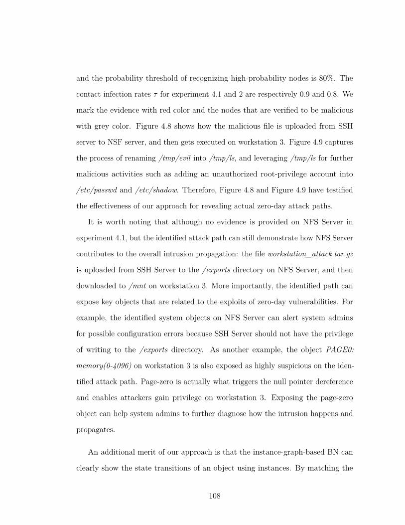
and the probability threshold of recognizing high-probability nodes is 80%. The

contact infection rates · for experiment 4.1 and 2 are respectively 0.9 and 0.8. We

mark the evidence with red color and the nodes that are verified to be malicious

with grey color. Figure 4.8 shows how the malicious file is uploaded from SSH

server to NSF server, and then gets executed on workstation 3. Figure 4.9 captures

the process of renaming /tmp/evil into /tmp/ls, and leveraging /tmp/ls for further

malicious activities such as adding an unauthorized root-privilege account into

/etc/passwd and /etc/shadow. Therefore, Figure 4.8 and Figure 4.9 have testified

the e�ectiveness of our approach for revealing actual zero-day attack paths.

It is worth noting that although no evidence is provided on NFS Server in

experiment 4.1, but the identified attack path can still demonstrate how NFS Server

contributes to the overall intrusion propagation: the file workstation_attack.tar.gz

is uploaded from SSH Server to the /exports directory on NFS Server, and then

downloaded to /mnt on workstation 3. More importantly, the identified path can

expose key objects that are related to the exploits of zero-day vulnerabilities. For

example, the identified system objects on NFS Server can alert system admins

for possible configuration errors because SSH Server should not have the privilege

of writing to the /exports directory. As another example, the object PAGE0:

memory(0-4096) on workstation 3 is also exposed as highly suspicious on the iden-

tified attack path. Page-zero is actually what triggers the null pointer dereference

and enables attackers gain privilege on workstation 3. Exposing the page-zero

object can help system admins to further diagnose how the intrusion happens and

propagates.

An additional merit of our approach is that the instance-graph-based BN can

clearly show the state transitions of an object using instances. By matching the

108

Workstation 3

NFS Server

SSH Server

x350.1: Snort Brute Force Alert

x4.1:(6560:6559:mount.nfs)

x4.2:(6560:6559:mount.nfs)

x10.1:(/etc/mtab:8798397) x1007.1:(172.18.34.5:2049)

x142.25:(192.168.101.5:22)

x253.3:(6706:6703:sshd)

x253.4:(6706:6703:sshd)

x253.5:(6706:6703:sshd)

x253.6:(6706:6703:sshd)

x253.7:(6706:6703:sshd)

x253.8:(6706:6703:sshd)

x254.1:(6707:6706:sshd)

x254.2:(6707:6706:sshd)

x254.3:(6707:6706:bash)

x254.4:(6707:6706:bash)

x254.5:(6707:6706:bash)

x254.6:(6707:6706:bash)

x254.7:(6707:6706:scp)

x259.1:(/mnt/workstation_attack.tar.gz:9453574)

x260.1:(/mnt:)

x1008.1:(5118:1:unfsd)

x1007.6:(172.18.34.5:2049)

x2006.2:(6737:6736:mount)

x1008.2:(5118:1:unfsd)

x1008.3:(5118:1:unfsd)

x1008.4:(5118:1:unfsd)

x1008.5:(5118:1:unfsd)

x1017.1:(/exports/workstation_attack.tar.gz:9453574)

x2006.3:(6737:6736:mount.nfs)

x2061.1:(/etc/mtab:1493088)

x2083.1:(/mnt/workstation_attack.tar.gz:9453574)

x2078.6:(6761:6719:cp)

x2082.2:(/home/user/test-bed/workstation_attack.tar.gz:1384576)

x2086.4:(6763:6719:tar)

x2086.5:(6763:6719:tar)

x2102.1:(/home/user/test-bed/workstation_attack/exploit.sh:1540318) x2107.1:(/home/user/test-bed/workstation_attack/wunderbar_emporium/exploit.c:1548376)x2108.1:(/home/user/test-bed/workstation_attack/wunderbar_emporium/wunderbar_emporium.sh:1548377)

x2114.1:(/home/user/test-bed/workstation_attack/wunderbar_emporium/pwnkernel.c:1548383)

x2144.2:(6781:6285:bash) x2311.3:(6794:6793:cc1)

x2147.2:(6783:6781:exploit.sh)

x2114.2:(/home/user/test-bed/workstation_attack/wunderbar_emporium/pwnkernel.c:1548383)

x2153.4:(6787:6783:sed)

x2114.3:(/home/user/test-bed/workstation_attack/wunderbar_emporium/pwnkernel.c:1548383)

x2157.1:(/home/user/test-bed/workstation_attack/wunderbar_emporium/pwnkernel2.c:1548383)

x2144.3:(6781:6285:exploit.sh)

x2144.4:(6781:6285:exploit.sh)

x2147.1:(6783:6781:exploit.sh)

x2152.1:(/home/user/test-bed/workstation_attack/wunderbar_emporium/pwnkernel1.c:1548396) x2153.1:(6787:6783:wunderbar_empor) x2154.1:(6788:6783:wunderbar_empor)x2158.1:(6789:6783:wunderbar_empor) x2308.1:(6793:6783:wunderbar_empor)

x2383.1:(6798:6783:wunderbar_empor)

x2397.1:(6803:6783:wunderbar_empor) x2460.1:(6812:6783:wunderbar_empor)

x2152.2:(/home/user/test-bed/workstation_attack/wunderbar_emporium/pwnkernel1.c:1548396)

x2152.3:(/home/user/test-bed/workstation_attack/wunderbar_emporium/pwnkernel1.c:1548396)

x2160.1:(/home/user/test-bed/workstation_attack/wunderbar_emporium/pwnkernel.c:1548396)

x2153.2:(6787:6783:wunderbar_empor)

x2153.3:(6787:6783:sed)

x2154.2:(6788:6783:wunderbar_empor)

x2154.3:(6788:6783:mv)

x2154.4:(6788:6783:mv)

x2154.5:(6788:6783:mv)

x2157.2:(/home/user/test-bed/workstation_attack/wunderbar_emporium/pwnkernel2.c:1548383)

x2158.2:(6789:6783:wunderbar_empor)

x2158.3:(6789:6783:mv)

x2158.4:(6789:6783:mv)

x2158.5:(6789:6783:mv)

x2385.3:(6799:6798:cc1)

x2308.2:(6793:6783:wunderbar_empor)

x2308.3:(6793:6783:cc)

x2310.1:(/tmp/cccXQxZn.s:2984222) x2311.4:(6794:6793:cc1)x2372.1:(/tmp/ccfRR34r.o:2984223)

x2373.5:(6795:6793:as)

x2310.2:(/tmp/cccXQxZn.s:2984222)

x2310.3:(/tmp/cccXQxZn.s:2984222)

x2373.3:(6795:6793:as)

x2311.5:(6794:6793:cc1)

x2311.6:(6794:6793:cc1)

x2311.7:(6794:6793:cc1)

x2311.8:(6794:6793:cc1)

x2311.9:(6794:6793:cc1)

x2311.10:(6794:6793:cc1)

x2311.11:(6794:6793:cc1)

x2311.12:(6794:6793:cc1)

x2311.13:(6794:6793:cc1)

x2311.14:(6794:6793:cc1)

x2311.15:(6794:6793:cc1)

x2311.16:(6794:6793:cc1)

x2311.17:(6794:6793:cc1)

x2311.18:(6794:6793:cc1)

x2311.19:(6794:6793:cc1)

x2311.20:(6794:6793:cc1)

x2311.21:(6794:6793:cc1)

x2311.22:(6794:6793:cc1)

x2311.23:(6794:6793:cc1)

x2311.24:(6794:6793:cc1)

x2311.25:(6794:6793:cc1)

x2311.26:(6794:6793:cc1)

x2311.27:(6794:6793:cc1)

x2311.28:(6794:6793:cc1)

x2311.29:(6794:6793:cc1)

x2311.30:(6794:6793:cc1)

x2311.31:(6794:6793:cc1)

x2311.32:(6794:6793:cc1)

x2311.33:(6794:6793:cc1)

x2311.34:(6794:6793:cc1)

x2311.35:(6794:6793:cc1)

x2311.36:(6794:6793:cc1)

x2311.37:(6794:6793:cc1)

x2311.38:(6794:6793:cc1)

x2311.39:(6794:6793:cc1)

x2311.40:(6794:6793:cc1)

x2311.41:(6794:6793:cc1)

x2311.42:(6794:6793:cc1)

x2311.43:(6794:6793:cc1)

x2311.44:(6794:6793:cc1)

x2311.45:(6794:6793:cc1)

x2311.46:(6794:6793:cc1)

x2311.47:(6794:6793:cc1)

x2311.48:(6794:6793:cc1)

x2311.49:(6794:6793:cc1)

x2311.50:(6794:6793:cc1)

x2311.51:(6794:6793:cc1)

x2311.52:(6794:6793:cc1)

x2311.53:(6794:6793:cc1)

x2311.54:(6794:6793:cc1)

x2311.55:(6794:6793:cc1)

x2311.56:(6794:6793:cc1)

x2311.57:(6794:6793:cc1)

x2311.58:(6794:6793:cc1)

x2311.59:(6794:6793:cc1)

x2311.60:(6794:6793:cc1)

x2311.61:(6794:6793:cc1)

x2311.62:(6794:6793:cc1)

x2311.63:(6794:6793:cc1)

x2311.64:(6794:6793:cc1)

x2372.2:(/tmp/ccfRR34r.o:2984223)

x2373.4:(6795:6793:as)

x2383.2:(6798:6783:wunderbar_empor)

x2383.3:(6798:6783:cc)

x2384.1:(/tmp/ccQXpwLK.s:2984226) x2385.4:(6799:6798:cc1)x2388.1:(/tmp/ccUZcd3t.o:2984227)

x2389.5:(6800:6798:as)

x2384.2:(/tmp/ccQXpwLK.s:2984226)

x2384.3:(/tmp/ccQXpwLK.s:2984226)

x2389.3:(6800:6798:as)

x2385.5:(6799:6798:cc1)

x2385.6:(6799:6798:cc1)

x2385.7:(6799:6798:cc1)

x2385.8:(6799:6798:cc1)

x2385.9:(6799:6798:cc1)

x2385.10:(6799:6798:cc1)

x2385.11:(6799:6798:cc1)

x2385.12:(6799:6798:cc1)

x2385.13:(6799:6798:cc1)

x2385.14:(6799:6798:cc1)

x2385.15:(6799:6798:cc1)

x2385.16:(6799:6798:cc1)

x2385.17:(6799:6798:cc1)

x2385.18:(6799:6798:cc1)

x2385.19:(6799:6798:cc1)

x2385.20:(6799:6798:cc1)

x2385.21:(6799:6798:cc1)

x2385.22:(6799:6798:cc1)

x2385.23:(6799:6798:cc1)

x2385.24:(6799:6798:cc1)

x2385.25:(6799:6798:cc1)

x2385.26:(6799:6798:cc1)

x2385.27:(6799:6798:cc1)

x2385.28:(6799:6798:cc1)

x2385.29:(6799:6798:cc1)

x2385.30:(6799:6798:cc1)

x2385.31:(6799:6798:cc1)

x2385.32:(6799:6798:cc1)

x2385.33:(6799:6798:cc1)

x2385.34:(6799:6798:cc1)

x2385.35:(6799:6798:cc1)

x2388.2:(/tmp/ccUZcd3t.o:2984227)

x2389.4:(6800:6798:as)

x2397.2:(6803:6783:wunderbar_empor)

x2397.3:(6803:6783:pwnkernel)

x2397.4:(6803:6783:pulseaudio)

x2397.5:(6803:6783:pulseaudio)

x2397.6:(6803:6783:pulseaudio)

x2397.7:(6803:6783:pulseaudio)

x2397.8:(6803:6783:pulseaudio)

x2397.9:(6803:6783:pulseaudio)

x2404.1:(/tmp/pulse-cart/pid:2984081)

x2397.10:(6803:6783:pulseaudio)

x2397.11:(6803:6783:pulseaudio)

x2409.1:(/home/cart/.esd_auth:974883)

x2397.12:(6803:6783:pulseaudio)

x2411.1:(/home/cart/.pulse-cookie:974885)

x2397.13:(6803:6783:pulseaudio)

x2397.14:(6803:6783:pulseaudio)

x2397.15:(6803:6783:pulseaudio)

x2397.16:(6803:6783:pulseaudio)

x2397.17:(6803:6783:pulseaudio)

x2397.18:(6803:6783:pulseaudio)

x2397.19:(6803:6783:pulseaudio)

x2397.20:(6803:6783:pulseaudio) x2421.1:(PAGE0:memory(0-4096))

x2397.21:(6803:6783:pulseaudio) x2423.1:(/tmp/sendfile.p4lbtq:2984231)

x2429.1:(6811:6803:sh)

x2429.2:(6811:6803:sh)

x2429.3:(6811:6803:useradd)

x2429.4:(6811:6803:useradd)

x2429.5:(6811:6803:useradd)

x2429.6:(6811:6803:useradd)

x2429.7:(6811:6803:useradd)

x2429.8:(6811:6803:useradd)x2433.1:(/etc/.pwd.lock:1491065) x2434.1:(/etc/passwd.6811:1493103)

x2429.9:(6811:6803:useradd)

x2429.10:(6811:6803:useradd)x2437.1:(/etc/shadow.6811:1493104)

x2429.11:(6811:6803:useradd)x2440.1:(/etc/group.6811:1493105)

x2429.12:(6811:6803:useradd)x2443.1:(/etc/gshadow.6811:1493106)

x2429.13:(6811:6803:useradd)

x2429.14:(6811:6803:useradd)

x2448.1:(/etc/passwd-:1491134)x2449.1:(/etc/passwd+:1493107) x2451.1:(/etc/shadow-:1491147) x2452.1:(/etc/shadow+:1493108)x2454.1:(/etc/group-:1491089)x2455.1:(/etc/group+:1493109) x2457.1:(/etc/gshadow-:1491091) x2458.1:(/etc/gshadow+:1493110)

x2450.1:(/etc/passwd:1493107) x2453.1:(/etc/shadow:1493108)

x2524.4:(6828:6815:cat)

x2456.1:(/etc/group:1493109) x2459.1:(/etc/gshadow:1493110)

x2460.2:(6812:6783:wunderbar_empor)

x2460.3:(6812:6783:mv)

x2460.4:(6812:6783:mv)

x2460.5:(6812:6783:mv)

x2493.7:(6815:6813:sshd)

x2493.8:(6815:6813:bash)

x2493.9:(6815:6813:bash)

x2493.10:(6815:6813:bash)

x2493.11:(6815:6813:bash)

x2493.12:(6815:6813:bash)x2503.1:(6818:6815:bash)

x2522.1:(6827:6815:bash)x2524.1:(6828:6815:bash) x2525.1:(6829:6815:bash)x2527.1:(6830:6815:bash) x2530.1:(6831:6815:bash) x2532.1:(6832:6815:bash) x2534.1:(6833:6815:bash) x2536.1:(6834:6815:bash) x2538.1:(6835:6815:bash)x2540.1:(6836:6815:bash) x2541.1:(6837:6815:bash)

x2522.2:(6827:6815:bash)

x2522.3:(6827:6815:ls)

x2522.4:(6827:6815:ls)

x2524.2:(6828:6815:bash)

x2524.3:(6828:6815:cat)

x2525.2:(6829:6815:bash)

x2525.3:(6829:6815:ls)

x2525.4:(6829:6815:ls)

x2527.2:(6830:6815:bash)

x2527.3:(6830:6815:touch)

x2529.1:(/virus:24610)

x2530.2:(6831:6815:bash)

x2530.3:(6831:6815:whoami)

x2530.4:(6831:6815:whoami)

x2532.2:(6832:6815:bash)

x2532.3:(6832:6815:ls)

x2532.4:(6832:6815:ls)

x2534.2:(6833:6815:bash)

x2534.3:(6833:6815:ls)

x2534.4:(6833:6815:ls)

x2536.2:(6834:6815:bash)

x2536.3:(6834:6815:rm)

x2538.2:(6835:6815:bash)

x2538.3:(6835:6815:ls)

x2538.4:(6835:6815:ls)

x2540.2:(6836:6815:bash)

x2540.3:(6836:6815:rm)

x2541.2:(6837:6815:bash)

x2541.3:(6837:6815:rm)

Figure 4.8: The zero-day Attack Path in the Form of an Instance Graph for Experiment 4.1.

109

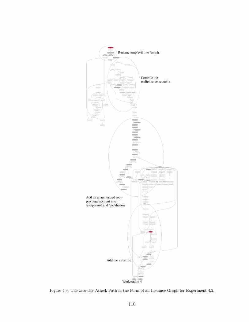
Workstation 4

x2075.2:(22826:21856:bash)

x2075.3:(22826:21856:symlinkattack.o)

x2078.1:(/tmp/evil:565696)x2079.1:(/tmp/ls:565697)

x2227.1:(22868:22826:symlinkattack.o)

x2076.1:(./symlinkattack.o:null)

x2079.2:(/tmp/ls:565696)

x2079.3:(/tmp/ls:565704)

x2115.2:(22843:22829:ls)

x2218.5:(22861:22852:ln)

x2115.36:(22843:22829:ls) x2221.2:(22864:22852:ls)

...

x2115.7:(22843:22829:ls)

...

x2118.1:(/tmp/sh.c:565699) x2115.11:(22843:22829:ls)

... x2123.1:(22844:22843:ls)

x2115.17:(22843:22829:ls)

... x2189.1:(22849:22843:ls)

x2115.23:(22843:22829:ls)

... x2195.1:(22850:22843:ls)

x2115.35:(22843:22829:ls)

x2208.1:(22852:22843:ls)

x2132.10:(22845:22844:cc1)

...

x2123.11:(22844:22843:cc)

x2131.1:(/tmp/ccQAkM1b.s:565700)

x2132.1:(22845:22844:cc1)

x2141.1:(/tmp/ccMBTbmh.o:565701)

x2143.5:(22846:22844:as) x2150.1:(22847:22844:collect2)

x2131.2:(/tmp/ccQAkM1b.s:565700)

x2143.8:(22846:22844:as)

...

x2141.2:(/tmp/ccMBTbmh.o:565701)

x2143.7:(22846:22844:as)

x2141.3:(/tmp/ccMBTbmh.o:565701)

x2181.7:(22848:22847:ld)

x2143.6:(22846:22844:as)

x2148.2:(/etc/passwd:6072405)

x2291.9:(22912:4837:sshd)

x2302.3:(22921:22912:sshd)

x2305.1:(4766:1:dbus-daemon)

x2307.6:(22922:5037:hal-acl-tool)

x2315.1:(5033:1:hald)

x2317.6:(22923:22922:polkit-read-aut)

x2319.6:(22924:5037:hal-acl-tool)

x2321.6:(22925:22924:polkit-read-aut)

x2323.6:(22926:5037:hal-acl-tool)

x2334.10:(22928:22927:id)

x2337.6:(22929:22926:polkit-read-aut)

x2361.13:(22934:22921:vi)

x2368.13:(22936:22921:vi)

x2149.2:(/etc/group:6072409)

x2291.33:(22912:4837:sshd)

x2302.7:(22921:22912:sshd)

x2305.2:(4766:1:dbus-daemon) x2315.2:(5033:1:hald) x2317.5:(22923:22922:polkit-read-aut) x2321.5:(22925:22924:polkit-read-aut)

x2334.11:(22928:22927:id)

x2337.5:(22929:22926:polkit-read-aut)

...

x2150.33:(22847:22844:collect2)

x2181.2:(22848:22847:ld)

...

x2181.6:(22848:22847:ld)

x2182.2:(/tmp/sh:565706)

x2182.3:(/tmp/sh:565706)

x2182.4:(/tmp/sh:565706)

x2182.5:(/tmp/sh:565706)

x2195.5:(22850:22843:chmod)

x2229.2:(22870:22868:sh)

...

x2189.7:(22849:22843:chown)

......

x2208.4:(22852:22843:ls)

x2210.1:(22854:22852:ls)

x2213.1:(22856:22852:ls)

x2214.1:(22857:22852:ls)

x2218.1:(22861:22852:ls)

x2221.1:(22864:22852:ls)

...

x2210.10:(22854:22852:tempfile)

x2211.2:(/tmp/gztmpQw8u37:565704)

x2211.3:(/tmp/gztmpQw8u37:565704)

x2211.4:(/tmp/gztmpQw8u37:565704)

x2214.5:(22857:22852:chmod)

x2211.5:(/tmp/gztmpQw8u37:565704)

x2218.6:(22861:22852:ln)

...

...

...

x2221.8:(22864:22852:ls)

...

x2227.10:(22868:22826:sh)

x2229.1:(22870:22868:sh)

...

x2229.8:(22870:22868:sh)

x2265.1:(22909:22870:sh)

x2234.5:(172.18.34.5:22)

x2291.17:(22912:4837:sshd)

x2234.6:(172.18.34.5:22)

x2291.32:(22912:4837:sshd)

...

x2265.9:(22909:22870:useradd)

x2265.10:(22909:22870:useradd)

x2268.1:(/etc/passwd.22909:6072390)

x2265.11:(22909:22870:useradd)

x2265.12:(22909:22870:useradd)

x2271.1:(/etc/shadow.22909:6072394)

x2265.13:(22909:22870:useradd)

x2265.14:(22909:22870:useradd)

x2274.1:(/etc/group.22909:6072402)

x2265.15:(22909:22870:useradd)

x2276.1:(/etc/gshadow.22909:6072404)

...

x2265.18:(22909:22870:useradd)

x2265.19:(22909:22870:useradd)

x2280.1:(/etc/passwd-:6070462)

x2265.20:(22909:22870:useradd)

x2281.1:(/etc/passwd+:6072405)

x2265.21:(22909:22870:useradd)

x2282.1:(/etc/shadow-:6070475)

x2265.22:(22909:22870:useradd)

x2283.1:(/etc/shadow+:6072408)

x2265.23:(22909:22870:useradd)

x2284.1:(/etc/group-:6070417)

x2265.24:(22909:22870:useradd)

x2285.1:(/etc/group+:6072409)

x2265.25:(22909:22870:useradd)

x2286.1:(/etc/gshadow-:6070419)

x2265.26:(22909:22870:useradd)

x2287.1:(/etc/gshadow+:6072410)

x2273.2:(/etc/shadow:6072408)

x2291.30:(22912:4837:sshd)

...

x2291.16:(22912:4837:sshd)

...

x2294.1:(22913:22912:sshd)

x2291.31:(22912:4837:sshd)

...

x2291.38:(22912:4837:sshd)

x2302.1:(22921:22912:sshd)

x2302.2:(22921:22912:sshd)

...

...

x2302.25:(22921:22912:bash)

x2302.26:(22921:22912:bash)x2329.1:(22927:22921:bash)

...

x2302.39:(22921:22912:bash)

x2302.40:(22921:22912:bash)

x2355.1:(22932:22921:bash)

...

x2302.44:(22921:22912:bash)

x2361.1:(22934:22921:bash)x2368.1:(22936:22921:bash)

x2317.1:(22923:22922:hal-acl-tool)

x2317.2:(22923:22922:polkit-read-aut)

x2317.3:(22923:22922:polkit-read-aut)

x2317.4:(22923:22922:polkit-read-aut)

x2321.1:(22925:22924:hal-acl-tool)

x2321.2:(22925:22924:polkit-read-aut)

x2321.3:(22925:22924:polkit-read-aut)

x2321.4:(22925:22924:polkit-read-aut)

x2337.1:(22929:22926:hal-acl-tool)

...

x2329.6:(22927:22921:bash)

x2334.1:(22928:22927:bash)

...

...

...

x2355.4:(22932:22921:touch)

x2356.1:(/virus:24580)

x2356.2:(/virus:24580)

x2361.5:(22934:22921:vi)x2368.5:(22936:22921:vi)

...

...

x2361.14:(22934:22921:vi)

x2365.1:(/.virus.swp:24581)

x2366.1:(/.virus.swpx:24582)

x2361.15:(22934:22921:vi)

x2361.16:(22934:22921:vi)

x2365.2:(/.virus.swp:24581)

x2365.3:(/.virus.swp:24582)

x2365.4:(/.virus.swp:24582)

x2368.14:(22936:22921:vi)

x2365.5:(/.virus.swp:24582)

x2366.2:(/.virus.swpx:24583)

x2368.15:(22936:22921:vi)

...

...

x2368.16:(22936:22921:vi)

x2368.17:(22936:22921:vi)

Rename /tmp/evil into /tmp/ls

Compile the malicious executable

Add an unauthorized root-privilege account into /etc/passwd and /etc/shadow

Add the virus file

Figure 4.9: The zero-day Attack Path in the Form of an Instance Graph for Experiment 4.2.

110

Table 4.3: The Impact of Pruning the Instance Graphs

SSH Server NFS Server Workstation 3

before after before after before after

number of syscalls in raw datatrace

82133 14944 46043

size of raw data trace (MB) 13.8 2.3 7.9

number of extracted object de-pendencies

10310 11535 17516

number of objects 349 20 544

number of instances(nodes) ininstance graph

10447 745 11544 39 17849 1069

number of dependencies(edges)in instance graph

20186 968 19863 37 34549 1244

number of contact dependen-cies

9888 372 8329 8 17033 508

number of state transition de-pendencies

10298 596 11534 29 17516 736

average time for graph genera-tion(s)

14 11 6 5 13 11

.net file size(KB) 2000 123 2200 8 3600 180

instances and dependencies back to the system call traces, it can even find out

the exact system call that causes the state-changing of the object. For example,

the node x2086.4:(6763:6719:tar) in Figure 4.8 represents the fourth instance of

process (pid:6763, pcmd:tar). Previous instances of the process are considered as

innocent because of their low infection probabilities. The process becomes highly

suspicious only after a dependency occurs between node x2082.2:(/home/user/test-

111

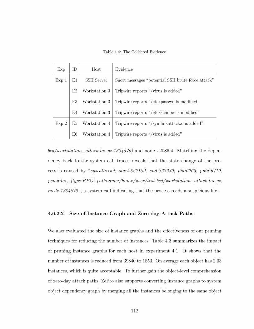
Table 4.4: The Collected Evidence

Exp ID Host Evidence

Exp 1 E1 SSH Server Snort messages “potential SSH brute force attack”

E2 Workstation 3 Tripwire reports “/virus is added”

E3 Workstation 3 Tripwire reports “/etc/passwd is modified”

E4 Workstation 3 Tripwire reports “/etc/shadow is modified”

Exp 2 E5 Workstation 4 Tripwire reports “/symlinkattack.o is added”

E6 Workstation 4 Tripwire reports “/virus is added”

bed/workstation_attack.tar.gz:1384576) and node x2086.4. Matching the depen-

dency back to the system call traces reveals that the state change of the pro-

cess is caused by “syscall:read, start:827189, end:827230, pid:6763, ppid:6719,

pcmd:tar, ftype:REG, pathname:/home/user/test-bed/workstation_attack.tar.gz,

inode:1384576”, a system call indicating that the process reads a suspicious file.

4.6.2.2 Size of Instance Graph and Zero-day Attack Paths

We also evaluated the size of instance graphs and the e�ectiveness of our pruning

techniques for reducing the number of instances. Table 4.3 summarizes the impact

of pruning instance graphs for each host in experiment 4.1. It shows that the

number of instances is reduced from 39840 to 1853. On average each object has 2.03

instances, which is quite acceptable. To further gain the object-level comprehension

of zero-day attack paths, ZePro also supports converting instance graphs to system

object dependency graph by merging all the instances belonging to the same object

112

into one node. Zero-day attack paths in SODG contain only objects and can be used

for verification when details regarding instances are not needed. Figure 4.10 and

Figure 4.11 are respectively the SODG form of zero-day attack paths for Figure 4.8

and Figure 4.9.

The experiment results have demonstrated that our system ZePro substantially

outperforms Patrol. Without any pre-knowledge towards known vulnerability

exploits and OS-level exploitation features (which are mandatory information for

Patrol to work), Zepro generates much better results than Patrol. In experiment 4.1,

the zero-day attack path identified by Patrol contains 175 objects, while the path by

our system is composed of only 77 objects (Figure 4.10). Considering that the total

number of objects involved in original instance graph is only 913, the 56% reduction

of path size is substantial. In experiment 4.2, the size of zero-day attack paths

revealed by Patrol and ZePro are very close: the path by Patrol has 60 nodes and

the path by ZePro has 61 nodes (Figure 4.11). This is because the objects involved

in these paths are already the smallest set of suspicious objects to constitute the

paths. Further reduction of objects will hurt the completeness of revealed zero-day

attack paths. More importantly, when the extensive pre-knowledge is not available

(which is usual), ZePro remains as e�ective, but Patrol will result in a large number

of suspicious intrusion propagation paths and is incapable of recognizing real attack

paths hiding in these candidates. For example, in Patrol’s dataset where SSH server

takes a workload of 1 request per 5 seconds, a 15-minute system call log generates

180 candidate paths that tangle with the real zero-day attack paths.

113

Wor

ksta

tion

3

NFS

Ser

ver

SSH

Ser

ver

x4.2

:(656

0:65

59:m

ount

.nfs

)

x10.

1:(/e

tc/m

tab:

8798

397)

x100

7.6:

(172

.18.

34.5

:204

9)

x142

.25:

(192

.168

.101

.5:2

2)

x350

.1: S

nort

Bru

te F

orce

Ale

rt

x253

.8:(6

706:

6703

:ssh

d) x254

.7:(6

707:

6706

:scp

)

x259

.1:(/

mnt

/wor

ksta

tion_

atta

ck.ta

r.gz:

9453

574)

x260

.1:(/

mnt

:)

x100

8.5:

(511

8:1:

unfs

d)x2

006.

3:(6

737:

6736

:mou

nt.n

fs)

x101

7.1:

(/exp

orts

/wor

ksta

tion_

atta

ck.ta

r.gz:

9453

574)

x206

1.1:

(/etc

/mta

b:14

9308

8)x2

083.

1:(/m

nt/w

orks

tatio

n_at

tack

.tar.g

z:94

5357

4)

x207

8.6:

(676

1:67

19:c

p)

x208

2.2:

(/hom

e/us

er/te

st-b

ed/w

orks

tatio

n_at

tack

.tar.g

z:13

8457

6)

x208

6.5:

(676

3:67

19:ta

r)

x210

2.1:

(/hom

e/us

er/te

st-b

ed/w

orks

tatio

n_at

tack

/exp

loit.

sh:1

5403

18)

x210

7.1:

(/hom

e/us

er/te

st-b

ed/w

orks

tatio

n_at

tack

/wun

derb

ar_e

mpo

rium

/exp

loit.

c:15

4837

6)x2

108.

1:(/h

ome/

user

/test

-bed

/wor

ksta

tion_

atta

ck/w

unde

rbar

_em

poriu

m/w

unde

rbar

_em

poriu

m.sh

:154

8377

)

x211

4.3:

(/hom

e/us

er/te

st-b

ed/w

orks

tatio

n_at

tack

/wun

derb

ar_e

mpo

rium

/pw

nker

nel.c

:154

8383

)

x214

4.4:

(678

1:62

85:e

xplo

it.sh

)

x231

1.64

:(679

4:67

93:c

c1)

x214

7.2:

(678

3:67

81:e

xplo

it.sh

)

x215

3.4:

(678

7:67

83:s

ed)

x215

7.2:

(/hom

e/us

er/te

st-b

ed/w

orks

tatio

n_at

tack

/wun

derb

ar_e

mpo

rium

/pw

nker

nel2

.c:1

5483

83)

x215

2.3:

(/hom

e/us

er/te

st-b

ed/w

orks

tatio

n_at

tack

/wun

derb

ar_e

mpo

rium

/pw

nker

nel1

.c:1

5483

96)

x215

4.5:

(678

8:67

83:m

v)x2

158.

5:(6

789:

6783

:mv)

x230

8.3:

(679

3:67

83:c

c)

x238

3.3:

(679

8:67

83:c

c)

x239

7.21

:(680

3:67

83:p

ulse

audi

o)x2

460.

5:(6

812:

6783

:mv)

x216

0.1:

(/hom

e/us

er/te

st-b

ed/w

orks

tatio

n_at

tack

/wun

derb

ar_e

mpo

rium

/pw

nker

nel.c

:154

8396

)

x238

5.35

:(679

9:67

98:c

c1)

x231

0.3:

(/tm

p/cc

cXQ

xZn.

s:29

8422

2)

x237

2.2:

(/tm

p/cc

fRR

34r.o

:298

4223

)

x237

3.5:

(679

5:67

93:a

s)

x238

4.3:

(/tm

p/cc

QX

pwLK

.s:29

8422

6)

x238

8.2:

(/tm

p/cc

UZc

d3t.o

:298

4227

)

x238

9.5:

(680

0:67

98:a

s)

x240

4.1:

(/tm

p/pu

lse-

cart/

pid:

2984

081)

x240

9.1:

(/hom

e/ca

rt/.e

sd_a

uth:

9748

83)

x241

1.1:

(/hom

e/ca

rt/.p

ulse

-coo

kie:

9748

85)

x242

1.1:

(PA

GE0

:mem

ory(

0-40

96))

x242

3.1:

(/tm

p/se

ndfil

e.p4

lbtq

:298

4231

)x2

429.

14:(6

811:

6803

:use

radd

)

x243

3.1:

(/etc

/.pw

d.lo

ck:1

4910

65)

x243

4.1:

(/etc

/pas

swd.

6811

:149

3103

)x2

437.

1:(/e

tc/s

hado

w.68

11:1

4931

04)

x244

0.1:

(/etc

/gro

up.6

811:

1493

105)

x244

3.1:

(/etc

/gsh

adow

.681

1:14

9310

6)x2

448.

1:(/e

tc/p

assw

d-:1

4911

34)

x244

9.1:

(/etc

/pas

swd+

:149

3107

)x2

451.

1:(/e

tc/s

hado

w-:1

4911

47)

x245

2.1:

(/etc

/sha

dow

+:14

9310

8)x2

454.

1:(/e

tc/g

roup

-:149

1089

)x2

455.

1:(/e

tc/g

roup

+:14

9310

9)x2

457.

1:(/e

tc/g

shad

ow-:1

4910

91)

x245

8.1:

(/etc

/gsh

adow

+:14

9311

0)

x245

0.1:

(/etc

/pas

swd:

1493

107)

x245

3.1:

(/etc

/sha

dow

:149

3108

)

x252

4.4:

(682

8:68

15:c

at)

x245

6.1:

(/etc

/gro

up:1

4931

09)

x245

9.1:

(/etc

/gsh

adow

:149

3110

)x2

493.

12:(6

815:

6813

:bas

h)

x250

3.1:

(681

8:68

15:b

ash)

x252

2.4:

(682

7:68

15:ls

)x2

525.

4:(6

829:

6815

:ls)

x252

7.3:

(683

0:68

15:to

uch)

x253

0.4:

(683

1:68

15:w

hoam

i)x2

532.

4:(6

832:

6815

:ls)

x253

4.4:

(683

3:68

15:ls

)x2

536.

3:(6

834:

6815

:rm)

x253

8.4:

(683

5:68

15:ls

)x2

540.

3:(6

836:

6815

:rm)

x254

1.3:

(683

7:68

15:rm

)

x252

9.1:

(/viru

s:24

610)

Figu

re4.

10:

The

Obj

ect-

leve

lZer

o-da

yA

ttac

kPa

thin

Expe

rimen

t4.

1.

114

Workstation 4

x2075.3:(22826:21856:symlinkattack.o)

x2078.1:(/tmp/evil:565696)

x2079.3:(/tmp/ls:565704) x2227.10:(22868:22826:sh)

x2076.1:(./symlinkattack.o:null)

x2115.36:(22843:22829:ls)

x2218.6:(22861:22852:ln)

x2221.8:(22864:22852:ls)

x2118.1:(/tmp/sh.c:565699) x2123.11:(22844:22843:cc)

x2189.7:(22849:22843:chown)

x2195.5:(22850:22843:chmod)

x2208.4:(22852:22843:ls)

x2132.10:(22845:22844:cc1)

x2131.2:(/tmp/ccQAkM1b.s:565700)

x2141.3:(/tmp/ccMBTbmh.o:565701)

x2143.8:(22846:22844:as)

x2150.33:(22847:22844:collect2)

x2181.7:(22848:22847:ld)

x2148.2:(/etc/passwd:6072405)

x2291.38:(22912:4837:sshd)

x2302.44:(22921:22912:bash)

x2305.2:(4766:1:dbus-daemon) x2307.6:(22922:5037:hal-acl-tool)x2315.2:(5033:1:hald)

x2317.6:(22923:22922:polkit-read-aut)

x2319.6:(22924:5037:hal-acl-tool)

x2321.6:(22925:22924:polkit-read-aut)

x2323.6:(22926:5037:hal-acl-tool)

x2334.11:(22928:22927:id)

x2337.6:(22929:22926:polkit-read-aut)

x2361.16:(22934:22921:vi)

x2368.17:(22936:22921:vi)

x2149.2:(/etc/group:6072409)

x2182.5:(/tmp/sh:565706)

x2229.8:(22870:22868:sh)

x2210.10:(22854:22852:tempfile) x2213.1:(22856:22852:ls)

x2214.5:(22857:22852:chmod)

x2211.5:(/tmp/gztmpQw8u37:565704)

x2265.26:(22909:22870:useradd)

x2234.6:(172.18.34.5:22)

x2268.1:(/etc/passwd.22909:6072390) x2271.1:(/etc/shadow.22909:6072394) x2274.1:(/etc/group.22909:6072402) x2276.1:(/etc/gshadow.22909:6072404) x2280.1:(/etc/passwd-:6070462) x2281.1:(/etc/passwd+:6072405) x2282.1:(/etc/shadow-:6070475)x2283.1:(/etc/shadow+:6072408) x2284.1:(/etc/group-:6070417)x2285.1:(/etc/group+:6072409) x2286.1:(/etc/gshadow-:6070419) x2287.1:(/etc/gshadow+:6072410)

x2273.2:(/etc/shadow:6072408)

x2294.1:(22913:22912:sshd)

x2329.6:(22927:22921:bash) x2355.4:(22932:22921:touch)

x2356.2:(/virus:24580)

x2365.5:(/.virus.swp:24582)

x2366.2:(/.virus.swpx:24583)

Figure 4.11: The Object-level Zero-day Attack Path in Experiment 4.2.

115

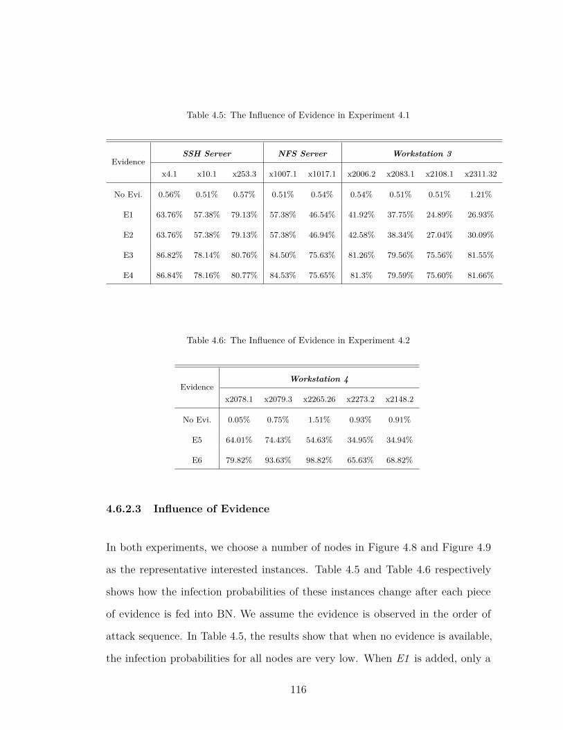
Table 4.5: The Influence of Evidence in Experiment 4.1

Evidence

SSH Server NFS Server Workstation 3

x4.1 x10.1 x253.3 x1007.1 x1017.1 x2006.2 x2083.1 x2108.1 x2311.32

No Evi. 0.56% 0.51% 0.57% 0.51% 0.54% 0.54% 0.51% 0.51% 1.21%

E1 63.76% 57.38% 79.13% 57.38% 46.54% 41.92% 37.75% 24.89% 26.93%

E2 63.76% 57.38% 79.13% 57.38% 46.94% 42.58% 38.34% 27.04% 30.09%

E3 86.82% 78.14% 80.76% 84.50% 75.63% 81.26% 79.56% 75.56% 81.55%

E4 86.84% 78.16% 80.77% 84.53% 75.65% 81.3% 79.59% 75.60% 81.66%

Table 4.6: The Influence of Evidence in Experiment 4.2

Evidence

Workstation 4

x2078.1 x2079.3 x2265.26 x2273.2 x2148.2

No Evi. 0.05% 0.75% 1.51% 0.93% 0.91%

E5 64.01% 74.43% 54.63% 34.95% 34.94%

E6 79.82% 93.63% 98.82% 65.63% 68.82%

4.6.2.3 Influence of Evidence

In both experiments, we choose a number of nodes in Figure 4.8 and Figure 4.9

as the representative interested instances. Table 4.5 and Table 4.6 respectively

shows how the infection probabilities of these instances change after each piece

of evidence is fed into BN. We assume the evidence is observed in the order of

attack sequence. In Table 4.5, the results show that when no evidence is available,

the infection probabilities for all nodes are very low. When E1 is added, only a

116

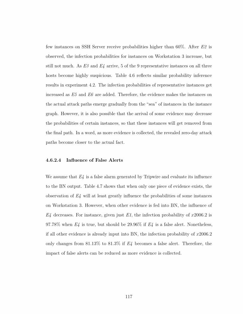
few instances on SSH Server receive probabilities higher than 60%. After E2 is

observed, the infection probabilities for instances on Workstation 3 increase, but

still not much. As E3 and E4 arrive, 5 of the 9 representative instances on all three

hosts become highly suspicious. Table 4.6 reflects similar probability inference

results in experiment 4.2. The infection probabilities of representative instances get

increased as E5 and E6 are added. Therefore, the evidence makes the instances on

the actual attack paths emerge gradually from the “sea” of instances in the instance

graph. However, it is also possible that the arrival of some evidence may decrease

the probabilities of certain instances, so that these instances will get removed from

the final path. In a word, as more evidence is collected, the revealed zero-day attack

paths become closer to the actual fact.

4.6.2.4 Influence of False Alerts

We assume that E4 is a false alarm generated by Tripwire and evaluate its influence

to the BN output. Table 4.7 shows that when only one piece of evidence exists, the

observation of E4 will at least greatly influence the probabilities of some instances

on Workstation 3. However, when other evidence is fed into BN, the influence of

E4 decreases. For instance, given just E1, the infection probability of x2006.2 is

97.78% when E4 is true, but should be 29.96% if E4 is a false alert. Nonetheless,

if all other evidence is already input into BN, the infection probability of x2006.2

only changes from 81.13% to 81.3% if E4 becomes a false alert. Therefore, the

impact of false alerts can be reduced as more evidence is collected.

117

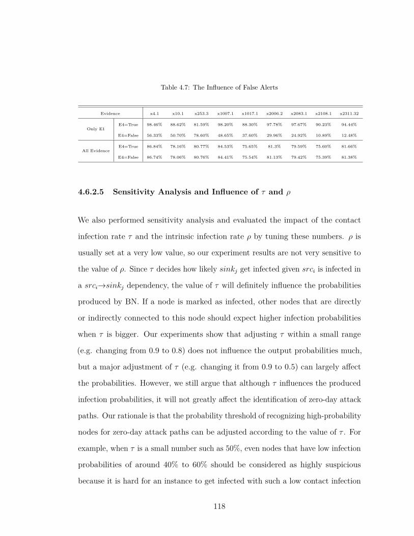
Table 4.7: The Influence of False Alerts

Evidence x4.1 x10.1 x253.3 x1007.1 x1017.1 x2006.2 x2083.1 x2108.1 x2311.32

Only E1E4=True 98.46% 88.62% 81.59% 98.20% 88.30% 97.78% 97.67% 90.23% 94.44%

E4=False 56.33% 50.70% 78.60% 48.65% 37.60% 29.96% 24.92% 10.89% 12.48%

All EvidenceE4=True 86.84% 78.16% 80.77% 84.53% 75.65% 81.3% 79.59% 75.60% 81.66%

E4=False 86.74% 78.06% 80.76% 84.41% 75.54% 81.13% 79.42% 75.39% 81.38%

4.6.2.5 Sensitivity Analysis and Influence of · and fl

We also performed sensitivity analysis and evaluated the impact of the contact

infection rate · and the intrinsic infection rate fl by tuning these numbers. fl is

usually set at a very low value, so our experiment results are not very sensitive to

the value of fl. Since · decides how likely sinkj

get infected given srci

is infected in

a srci

æsinkj

dependency, the value of · will definitely influence the probabilities

produced by BN. If a node is marked as infected, other nodes that are directly

or indirectly connected to this node should expect higher infection probabilities

when · is bigger. Our experiments show that adjusting · within a small range

(e.g. changing from 0.9 to 0.8) does not influence the output probabilities much,

but a major adjustment of · (e.g. changing it from 0.9 to 0.5) can largely a�ect

the probabilities. However, we still argue that although · influences the produced

infection probabilities, it will not greatly a�ect the identification of zero-day attack

paths. Our rationale is that the probability threshold of recognizing high-probability

nodes for zero-day attack paths can be adjusted according to the value of · . For

example, when · is a small number such as 50%, even nodes that have low infection

probabilities of around 40% to 60% should be considered as highly suspicious

because it is hard for an instance to get infected with such a low contact infection

118

rate.

As mentioned before, due to constraints of data and ground truths, it is possible

but currently very di�cult to automatically learn the parameters of · and fl using

statistical techniques. The parameter learning and Bayesian network training is

beyond the scope of this chapter and will be investigated in future works.

4.6.2.6 Complexity and Scalability

We evaluated the time cost for o�-line data analysis, which includes the time

for instance-graph-based BN generation, BN probability inference and zero-day

attack path identification. The time cost for probability inference depends on

the algorithm employed in SamIam. The time complexity can be O(|V |2) for

both instance-graph-based BN generation and zero-day attack path identification,

because the DFS algorithm is applied towards every node in the instance graph.

For our experiments that conduct the o�-line analysis on a host with 2.4 GHz

Intel Core 2 Duo processor and 4G RAM, Table 4.3 shows the time required for

constructing the instance-graph-based BN for each host, so the total time of BN

construction comes to around 27 seconds. For a BN with approximately 1854

nodes, assuming that the evidence is already fed into BN and the algorithm used is

recursive conditioning, the average time cost is 1.57 seconds for BN compilation

and probability inference, and 59 seconds for zero-day attack path identification.

Combining all the time required together, the average data analysis speed is 280

KB/s, which is quite reasonable. The average memory used for compiling the BN is

4.32 Mb. As for the run-time performance overhead, the overall system slow-down

caused by the system call logging component is around 15% to 20% according to

119

the measurement with UnixBench and kernel compilation.

The scalability of the approach proposed in this chapter can be ensured by the

following aspects. First, the time window of collecting system call logs for analysis

can be adjusted. For example, individual systems can collect system calls and send

the logs to central machine for analysis every 30 or 40 minutes. In our experiments,

a 40-minute system call log generates a BN with 1854 nodes. Smaller time window

usually generates smaller BN size, but not always. The BN size mainly depends on

the actual behavior of system call logs and cannot be estimated in a determined

way. Second, although an enterprise network may contain a large number of hosts,

the instance graphs generated by the individual hosts are not necessarily connected

to each other. An actual network-wide instance graph often contains one or several

isolated instance graphs. This also limits the size of individual BNs. Third, both

instance graph generation and zero-day attack path identification can be conducted

with parallel computing. Taking the current experiment results for estimation, if an

enterprise network contains 10000 hosts and an analysis cluster with 512 processors,

the time for instance graph generation and zero-day attack path identification

could be 2.93 minutes and 6.3 minutes respectively. In addition, intensive research

has been conducted towards the scalability of BN compilation and probability

inference [86,87]. A scalable parallel implementation using junction tree has been

developed for exact inference in BN [88]. The recursive conditioning [89] algorithm

we employed in this work even o�ers a smooth tradeo� between time and space,

which also enhances the scalability of BN inference.

120

4.7 Related Work

The work that is most related to us is the Patrol system designed by Dai et

al. [41]. It touches the zero-day attack path problem at operating system level. Our

work also aims at addressing the zero-day attack path problem, but our approach

is substantially di�erent from Patrol in several aspects. First, Patrol relies on

extensive pre-knowledge regarding known vulnerability exploitations to distinguish

zero-day attack paths from the huge number of candidate paths. However, such

pre-knowledge is extremely di�cult to acquire and may not be useful when zero-day

exploits do not share common features with previous exploits at OS-level. Instead,

our approach does not require any pre-knowledge, and reveals the zero-day attack

paths solely based on collected intrusion evidence. Second, Patrol only conducts

qualitative analysis and treats every object on the identified paths as having the

same malicious status. Compared to Patrol, our approach quantifies the infection

status of each system object with probabilities. By only focusing on system objects

with relatively high probabilities, the set of suspicious objects can be significantly

narrowed down and the size of revealed zero-day attack path is relatively small.

Third, Patrol performs reachability analysis through tracking and thus generates a

huge candidate pool for zero-day attack paths. In contrast, our system does not

conduct tracking, but relies on the computed probabilities. The paths containing

highly suspicious objects reveal themselves automatically. The dependency paths

introduced by legitimate activities and the dependency paths introduced by zero-day

attacks are therefore separated with ease.

Other related work includes system call dependency tracking and zero-day attack

identification. System call dependency tracking is first proposed in [21] to help the

121

understanding of intrusion sequence. It is then applied for alert correlation in [71,72].

Instead of directly correlating these alerts, our system takes the alerts as evidence

and quantitatively computes the infection probabilities of system objects. [85]

conducts an empirical study to reveal the zero-day attacks by identifying the

executable files that are linked to exploits of known vulnerabilities. A zero-day

attack is identified if a malicious executable is found before the corresponding

vulnerability is disclosed. Attack graphs have been employed to measure the

security risks caused by zero-day attacks [79–81]. Nevertheless, the metric simply

counts the number of required unknown vulnerabilities for compromising an asset,

rather than detects the actually occurred zero-day exploits. Our system takes an

approach that is quite di�erent from the above work.

4.8 Limitation and Conclusion

The current system still has some limitations. For example, when some attack

activities evade the system calls (it’s di�cult, but possible), or the attack time span

is much longer than the analyzed time period, the constructed instance graphs may

not reflect the complete zero-day attack paths. In such cases, our system can only

reveal parts of the paths.

In conclusion, this chapter proposes to use Bayesian networks to identify the

zero-day attack paths. For this purpose, an object instance graph is built to serve

as the basis of Bayesian networks. By incorporating the intrusion evidence and

computing the probabilities of objects being infected, the implemented system

ZePro can successfully reveal the zero-day attack paths.

122

Chapter 5 |Conclusion

Achieving cyber situation awareness is the key prerequisite for human decision

makers to make right decisions. In cyber security field, a number of tools, algorithm,

and techniques are developed to monitor and protect the enterprise networks.

These tools and techniques are able to generate information and alerts to help

with the human administrators’ analysis, but in di�erent knowledge bases. These

knowledge bases are usually isolated from each other. It’s very di�cult for human

administrators to combine the information from di�erent knowledge bases to

generate a wholistic understanding towards the networks’ real situation. Therefore,

to achieve correct cyber situation awareness, a Situation Knowledge Reference

Model (SKRM) is constructed to couple the current techniques to enable security

analysts’ e�ective analysis of complex cyber-security problems.

SKRM identifies the situation knowledge from di�erent areas, but it is not just a

mapping of knowledge to four abstraction layers. In SKRM, each abstraction layer

generates a graph that covers the entire enterprise network and views the same

network from a di�erent perspective and at a di�erent granularity. In addition,

each abstraction layer leverages current available algorithms, tools, and techniques

in its corresponding area to extract the most critical and useful information to

123

present to human security analysts. SKRM actually integrates data, information,

algorithms and tools, and human knowledge into a whole stack. Hence, SKRM

serves as an umbrella model that enables solutions to di�erent cyber security

problems. In this paper, two independent problems are identified in di�erent layers

of SKRM, including the stealthy bridge problem in cloud and the zero-day attack

path problem.

With the abstraction layers from SKRM, the Bayesian network is employed

to incorporate information and dig out real facts. Bayesian network has two

capabilities. First, it is able to leverage relevant evidence to infer the facts. Second,

it is able to reduce the uncertainties faced by human analysts in security analysis.

As more evidence is collected, the analysts get closer to real facts.

Bayesian Networks gains more power when combined with the SKRM model.

In SKRM, each abstraction layer represents a di�erent perspective. Each layer

can serve as the complementary support to the other layer. Therefore, the same

attack may cause di�erent intrusion symptoms on di�erent layers. For example,

at the workflow layer, the symptom could be abnormal business behavior, such

as noticeable financial loss. At the operating system layer, however, the intrusion

system could be modified system files, or compromised services, etc. When building

Bayesian Networks based on SKRM model, the intrusion symptoms from one layer

can serve as the evidence to the other layer and confirm each other.

Therefore, this paper demonstrates how the two identified security problems

can be addressed by constructing proper Bayesian Networks on top of di�erent

layers of SKRM.

First, the stealthy bridge problem is investigated by combining the operating

system layer and the attack graph in SKRM. Chapter 3 identifies the problem

124

of stealthy bridges between isolated enterprise networks in the public cloud. To

infer the existence of stealthy bridges, the paper proposes a two-step approach.

A cloud-level attack graph is first built to capture the potential attacks enabled

by stealthy bridges. Based on the attack graph, a cross-layer Bayesian network is

constructed by identifying uncertainty types existing in attacks exploiting stealthy

bridges. The experiments show that the cross-layer Bayesian network is able to infer

the existence of stealthy bridges given supporting evidence from other intrusion

steps.

Second, the zero-day attack path is identified and addressed in the operating

system layer. Chapter 4 introduces a ZePro system, which is able to identify the

zero-day attack paths on OS-level. It first constructs an object instance graph to

capture the intrusion propagation, and then establishes a Bayesian network on

top of the instance graph to leverage the evidence collected from security sensors.

The Bayesian network computes the infection probabilities of object instances. By

connecting the instances with high probabilities, the zero-day attack paths are

formed and revealed. This paper conducted two sets of experiments to demonstrate

the e�ectiveness and performance of the ZePro system.

To sum up, the Bayesian network is a powerful tool for cyber security analysis.

When combined with SKRM, it has even more potentials. For complex security

problems, SKRM can inspire the problem identification and serve as the guidance

for solution development; Bayesian network is able to incorporate information from

relevant abstraction layers of SKRM to reveal the real facts. This can significantly

enhance human analysts’ situation awareness towards the enterprise networks’

security status.

125

Bibliography

[1] Dominguez, Cynthia. “Can SA be defined.” Situation awareness: Papers andannotated bibliography (1994): 5–15.

[2] Fracker, Martin L. “A theory of situation assessment: Implications for measur-ing situation awareness.” Proceedings of the Human Factors and ErgonomicsSociety Annual Meeting. Vol. 32. No. 2. SAGE Publications, 1988.

[3] Endsley, Mica R. “Toward a theory of situation awareness in dynamic systems.”Human Factors: The Journal of the Human Factors and Ergonomics Society37.1 (1995): 32–64.

[4] Salerno, John J., Michael L. Hinman, and Douglas M. Boulware. “A situ-ation awareness model applied to multiple domains.” Defense and Security.International Society for Optics and Photonics, 2005.

[5] McGuinness, Barry, and Louise Foy. “A subjective measure of SA: the CrewAwareness Rating Scale (CARS).” Proceedings of the first human performance,situation awareness, and automation conference, Savannah, Georgia. 2000.

[6] Alberts, David S., John J. Garstka, Richard E. Hayes, and David A. Sig-nori. “Understanding information age warfare.” Assistant Secretary of Defense(C3I/Command Control Research Program) Washington DC, 2001.

[7] Boyd, John R. “The essence of winning and losing.” Unpublished lecture notes(1996).

[8] Witthen, I., and Eibe Frank. “Data Mining-Practical Machine Learning Toolsand Techniques With Java Implementations.” (2000).

[9] Tadda, George P., and John S. Salerno. “Overview of cyber situation awareness.”Cyber Situational Awareness. Springer US, 2010. 15–35.

[10] Endsley, Mica R. “Theoretical underpinnings of situation awareness: A criticalreview.” Situation awareness analysis and measurement (2000): 3–32.

126

[11] Jun Dai, Xiaoyan Sun, Peng Liu, Nicklaus Giacobe. “Gaining Big PictureAwareness through an Interconnected Cross-layer Situation Knowledge Refer-ence Model.” 2012 ASE International Conference on Cyber Security, Washing-ton DC, 2012

[12] Xiaoyan Sun, Jun Dai, and Peng Liu. “SKRM: Where security techniques talkto each other.” In Cognitive Methods in Situation Awareness and DecisionSupport (CogSIMA), 2013 IEEE International Multi-Disciplinary Conferenceon, pp. 163-166. IEEE, 2013.

[13] Xiaoyan Sun, Anoop Singhal, and Peng Liu. “Who Touched My Mission:Towards Probabilistic Mission Impact Assessment.” In Proceedings of the2015 Workshop on Automated Decision Making for Active Cyber Defense(SafeConfig), pp. 21-26. ACM, 2015.

[14] Xiaoyan Sun, Jun Dai, Anoop Singhal, Peng Liu. “Inferring the StealthyBridges between Enterprise Network Islands in Cloud Using Cross-LayerBayesian Networks.” 10th International Conference on Security and Privacy inCommunication Networks (SecureComm 2014), Beijing, China

[15] Barford, Paul, Marc Dacier, Thomas G. Dietterich, Matt Fredrikson, JonGi�n, Sushil Jajodia, Somesh Jha et al. “Cyber SA: Situational awareness forcyber defense.” In Cyber Situational Awareness, pp. 3–13. Springer US, 2010.

[16] Yu, Meng, Peng Liu, and Wanyu Zang. “Self-healing workflow systems underattacks.” In Proceedings of 24th IEEE International Conference on DistributedComputing Systems. pp. 418–425. 2004.

[17] van der Aalst, Wil MP, Boudewijn F. van Dongen, Joachim Herbst, LauraMaruster, Guido Schimm, and Anton JMM Weijters. “Workflow mining: Asurvey of issues and approaches.” Data & knowledge engineering 47, no.2(2003):237–267.

[18] van der Aalst, Wil MP, A. J. M. M. Weijters, and Laura Maruster. “Workflowmining: Which processes can be rediscovered.” Beta working paper series, wp74, Eindhoven University of Technology, Eindhoven, 2002.

[19] Van der Aalst, Wil, Ton Weijters, and Laura Maruster. “Workflow mining:Discovering process models from event logs.” Knowledge and Data Engineering,IEEE Transactions on 16, no. 9 (2004): 1128–1142.

[20] Chen, Xu, Ming Zhang, Zhuoqing Morley Mao, and Paramvir Bahl. “Automat-ing Network Application Dependency Discovery: Experiences, Limitations,and New Solutions.” In USENIX Symposium on Operating Systems Designand Implementation (OSDI), vol. 8, pp. 117–130. 2008.

127

[21] King, Samuel T., and Peter M. Chen. “Backtracking intrusions.” In ACMSIGOPS Operating Systems Review, vol. 37, no. 5, pp. 223–236. ACM, 2003.

[22] Xiong, Xi, Xiaoqi Jia, and Peng Liu. “Shelf: Preserving business continuityand availability in an intrusion recovery system.” In Annual Computer SecurityApplications Conference (ACSAC), 2009. pp. 484–493.

[23] Zhang, Shengzhi, Xiaoqi Jia, Peng Liu, and Jiwu Jing. “Cross-layer compre-hensive intrusion harm analysis for production workload server systems.” InProceedings of the 26th Annual Computer Security Applications Conference(ACSAC), pp. 297–306. ACM, 2010.

[24] Pearl, Judea. “Bayesian Networks: A Model of Self-activated Memory forEvidential Reasoning.” 1985.

[25] Pearl, Judea. “Probabilistic reasoning in intelligent systems: networks ofplausible inference.” Morgan Kaufmann, 1988.

[26] Heckerman, David, Dan Geiger, and David M. Chickering. “Learning Bayesiannetworks: The combination of knowledge and statistical data.” Machine learn-ing 20, no. 3 (1995): 197-243.

[27] Friedman, Nir, Michal Linial, Iftach Nachman, and Dana Pe’er. “UsingBayesian networks to analyze expression data.” Journal of computationalbiology 7, no. 3-4 (2000): 601-620.

[28] Jansen, Ronald, Haiyuan Yu, Dov Greenbaum, Yuval Kluger, Nevan J. Krogan,Sambath Chung, Andrew Emili, Michael Snyder, Jack F. Greenblatt, andMark Gerstein. “A Bayesian networks approach for predicting protein-proteininteractions from genomic data.” Science 302, no. 5644 (2003): 449-453.

[29] Charniak, Eugene. “Bayesian networks without tears.” AI magazine 12, no. 4(1991): 50.

[30] Frigault, Marcel, and Lingyu Wang. “Measuring network security usingbayesian network-based attack graphs.” In 32nd Annual IEEE InternationalComputer Software and Applications Conference, Turku, 2008. pp. 698-703.

[31] Frigault, Marcel, Lingyu Wang, Anoop Singhal, and Sushil Jajodia. “Measuringnetwork security using dynamic bayesian network.” In Proceedings of the 4thACM workshop on Quality of protection, pp. 23-30. ACM, 2008.

[32] Liu, Yu, and Hong Man. “Network vulnerability assessment using Bayesiannetworks.” In Defense and Security, pp. 61-71. International Society for Opticsand Photonics, 2005.

128

[33] Amazon Elastic Compute Cloud (EC2). http://aws.amazon.com/ec2/

[34] Rackspace. http://www.rackspace.com/

[35] Windows Azure. https://www.windowsazure.com/en-us/

[36] V. Varadarajan, T. Kooburat, B. Farley, T. Ristenpart, and M. M. Swift,“Resource-freeing attacks: improve your cloud performance (at your neighbor’sexpense),” in Proceedings of the 2012 ACM conference on Computer andcommunications security (CCS), 2012, pp. 281–292.

[37] T. Ristenpart, E. Tromer, H. Shacham, and S. Savage, “Hey, you, get o� ofmy cloud: exploring information leakage in third-party compute clouds,” inProceedings of the 16th ACM conference on Computer and communicationssecurity (CCS), 2009, pp. 199–212.

[38] D. X. Song, D. Wagner, and X. Tian, “Timing Analysis of Keystrokes andTiming Attacks on SSH.,” in USENIX Security Symposium, 2001.

[39] J. Szefer, E. Keller, R. B. Lee, and J. Rexford, “Eliminating the HypervisorAttack Surface for a More Secure Cloud,” in Proceedings of the 18th ACMConference on Computer and Communications Security (CCS), New York,NY, USA, 2011, pp. 401–412.

[40] A. Bates, B. Mood, J. Pletcher, H. Pruse, M. Valafar, and K. Butler, “Detectingco-residency with active tra�c analysis techniques,” in Proceedings of the 2012ACM Workshop on Cloud computing security workshop (CCSW), 2012, pp.1–12.

[41] J. Dai, X. Sun, and P. Liu. “Patrol: Revealing Zero-Day Attack Paths throughNetwork-Wide System Object Dependencies.” In Computer Securityâ��Eu-ropean Symposium on Research in Computer Security (ESORICS) 2013, pp.536-555. Springer Berlin Heidelberg, 2013.

[42] Y. Zhang, A. Juels, A. Oprea, and M. K. Reiter. HomeAlone: Co-residencyDetection in the Cloud via Side-Channel Analysis. in Proceedings of 2011IEEE Symposium on Security and Privacy (S&P), 2011.

[43] Y. Chen, V. Paxson, and R. H. Katz, What’s new about cloud computingsecurity. University of California, Berkeley Report No. UCB/EECS-2010-5January, 2010.

[44] O. Sheyner, J. Haines, S. Jha, R. Lippmann, and J. M. Wing, “Automatedgeneration and analysis of attack graphs,” in Proceedings of 2002 IEEESymposium on Security and Privacy (S&P). pp. 273–284.

129

[45] C. R. Ramakrishnan, R. Sekar, and others, “Model-based analysis of config-uration vulnerabilities,” Journal of Computer Security, vol. 10, no. 1/2, pp.189–209, 2002.

[46] C. Phillips and L. P. Swiler, “A graph-based system for network-vulnerabilityanalysis,” in Proceedings of the 1998 workshop on New security paradigms,1998, pp. 71–79.

[47] S. Jajodia, S. Noel, and B. O’Berry, “Topological analysis of network attackvulnerability,” Managing Cyber Threats, pp. 247–266, 2005.

[48] P. Ammann, D. Wijesekera, and S. Kaushik, “Scalable, graph-based networkvulnerability analysis,” in Proceedings of the 9th ACM conference on Computerand communications security (CCS), 2002, pp. 217–224.

[49] K. Ingols, R. Lippmann, and K. Piwowarski, “Practical attack graph genera-tion for network defense,” in 22nd Annual Computer Security ApplicationsConference,(ACSAC), 2006, pp. 121–130.

[50] X. Ou, W. F. Boyer, and M. A. McQueen, “A scalable approach to attackgraph generation,” in Proceedings of the 13th ACM conference on Computerand communications security (CCS), 2006, pp. 336–345.

[51] X. Ou, S. Govindavajhala, and A. W. Appel, “MulVAL: A logic-based networksecurity analyzer,” in Proceedings of the 14th conference on USENIX SecuritySymposium. Volume 14, 2005.

[52] M. Balduzzi, J. Zaddach, D. Balzarotti, E. Kirda, and S. Loureiro, “A securityanalysis of amazon’s elastic compute cloud service,” in Proceedings of the 27thAnnual ACM Symposium on Applied Computing, 2012, pp. 1427–1434.

[53] K. Lazri, S. Laniepce, and J. Ben-Othman, “Reconsidering Intrusion Monitor-ing Requirements in Shared Cloud Platforms,” in 2013 Eighth InternationalConference on Availability, Reliability and Security (ARES), 2013, pp. 630–637.

[54] http://www.snort.org/.

[55] Peng Xie, Jason Li, Xinming Ou, Peng Liu, and Renato Levy. “Using Bayesiannetworks for cyber security analysis.” In 2010 IEEE/IFIP International Con-ference on Dependable Systems and Networks (DSN), 2010.

[56] http://www.tenable.com/products/nessus.

[57] http://nvd.nist.gov/.

[58] http://nvd.nist.gov/cvss.cfm.

130

[59] http://cve.mitre.org/.

[60] http://www.tripwire.com/.

[61] http://cve.mitre.org/cgi-bin/cvename.cgi?name=CVE-2007-2446.

[62] https://www.samba.org.

[63] http://cve.mitre.org/cgi-bin/cvename.cgi?name=CVE-2007-5423.

[64] https://info.tiki.org/.

[65] http://reasoning.cs.ucla.edu/samiam/.

[66] S. Bugiel, S. Nurnberger, T. Poppelmann, A.-R. Sadeghi, and T. Schneider,“AmazonIA: when elasticity snaps back.” in Proceedings of the 18th ACMconference on Computer and communications security (CCS), 2011, pp. 389–400.

[67] C. Kruegel, D. Mutz, W. Robertson, and F. Valeur. “Bayesian event classi-fication for intrusion detection.” In Annual Computer Security ApplicationsConference, ACSAC 2003.

[68] V. Chandola, A. Banerjee, and V. Kumar. “Anomaly detection: A survey.” InACM Computing Surveys (CSUR), 2009.

[69] C. Kruegel, D. Mutz, F. Valeur, and G. Vigna. “On the detection of anomaloussystem call arguments.” In Computer Security - European Symposium onResearch in Computer Security (ESORICS)2003, pp. 326-343. Springer BerlinHeidelberg, 2003.

[70] S. Bhatkar, A. Chaturvedi, and R. Sekar. “Dataflow anomaly detection.” InProceedings of 2006 IEEE Symposium on Security and Privacy. pp. 15-pp.2006.

[71] S. T. King, Z. M. Mao, D. G. Lucchetti, P. M. Chen. “Enriching intrusion alertsthrough multi-host causality.” in Network and Distributed System Security(NDSS) Symposium, 2005.

[72] Y. Zhai, P. Ning, J. Xu. “Integrating IDS alert correlation and OS-Leveldependency tracking.” in IEEE Intelligence and Security Informatics, 2006.

[73] “https://cve.mitre.org/cgi-bin/cvename.cgi?name=CVE-2009-2692”

[74] “https://cve.mitre.org/cgi-bin/cvename.cgi?name=CVE-2011-4089”

[75] “https://cve.mitre.org/cgi-bin/cvename.cgi?name=CVE-2008-0166”

131

[76] Symantec Corporation. Internet Security Threat Report 2014, Volume19. http://www.symantec.com/content/en/us/enterprise/other_resources/b-istr_main_report_v19_21291018.en-us.pdf

[77] Wireshark. “https://www.wireshark.org/.”

[78] Tcpdump. “http://www.tcpdump.org/.”

[79] L. Wang, S. Jajodia, A. Singhal, and S. Noel. “k-zero day safety: Measuringthe security risk of networks against unknown attacks.” In Computer Security-European Symposium on Research in Computer Security (ESORICS) 2010,pp. 573-587. Springer Berlin Heidelberg, 2010.

[80] M. Albanese, S. Jajodia, A. Singhal, and L. Wang. “An E�cient Approach toAssessing the Risk of Zero-Day Vulnerabilities.” In Security and Cryptography(SECRYPT), 2013 International Conference on, pp. 1-12. IEEE, 2013.

[81] L. Wang, S. Jajodia, A. Singhal, P. Cheng, and S. Noel. “k-Zero day safety: Anetwork security metric for measuring the risk of unknown vulnerabilities.” inIEEE Transactions on Dependable and Secure Computing (TDSC), 2014.

[82] R. Tarjan. “Depth-first search and linear graph algorithms.” in SIAM journalon computing 1, 1972.

[83] GraphViz. “http://www.graphviz.org/.”

[84] Ntop. “http://www.ntop.org/.”

[85] L. Bilge, and T. Dumitras. “Before we knew it: an empirical study of zero-dayattacks in the real world.” In Proceedings of the 2012 ACM conference onComputer and communications security, pp. 833-844. ACM, 2012.

[86] Ole J. Mengshoel. “Understanding the scalability of Bayesian network inferenceusing clique tree growth curves.” Artificial Intelligence 174.12 (2010): 984-1006.

[87] Ole J. Mengshoel. “Designing resource-bounded reasoners using Bayesiannetworks: System health monitoring and diagnosis.” In 18th InternationalWorkshop on Principles of Diagnosis, 2007.

[88] V. Krishna Namasivayam, V. K. Prasanna. “Scalable parallel implementation ofexact inference in Bayesian networks.” In 12th IEEE International Conferenceon Parallel and Distributed Systems(ICPADS), 2006.

[89] Adnan Darwiche. “Recursive conditioning.” Artificial Intelligence 126. 1 (2001):5-41.

132

[90] Gabriel Jakobson. “Mission Cyber Security Situation Assessment Using ImpactDependency Graphs.”

[91] A. Natarajan, P. Ning, Y. Liu, S. Jajodia, and S.E. Hutchinson. “NSDMiner:Automated discovery of Network Service Dependencies.” In Proceeding ofIEEE International Conference on Computer Communications, 2012.

[92] Barry Peddycord III, Peng Ning, and Sushil Jajodia. “On the accurate identi-fication of network service dependencies in distributed systems.” In USENIXAssociation Proceedings of the 26th international conference on Large Installa-tion System Administration: strategies, tools, and techniques, 2012.

[93] Rodrigo Fonseca, George Porter, Randy H. Katz, Scott Shenker, and Ion Stoica.“X-trace: A pervasive network tracing framework.” In USENIX AssociationProceedings of the 4th USENIX conference on Networked systems design andimplementation, 2007.

[94] Paul Barham, Richard Black, Moises Goldszmidt, Rebecca Isaacs, John Mac-Cormick, Richard Mortier, and Aleksandr Simma. “Constellation: automateddiscovery of service and host dependencies in networked systems.” In TechRe-port MSR-TR-2008-67, 2008.

[95] Jun Dai. “Gaining Big Picture Awareness in Enterprise Cyber Security Defense.”Ph.D. dissertation, 2014.

[96] S. Musman, A. Temin, M. Tanner, D. Fox, and B. Pridemore. “Evaluating theImpact of Cyber Attacks on Missions.” MITRE Technical Paper 09-4577, July2010.

[97] Alberts C., et al. (2005). “Mission Assurance Analysis Protocol (MAAP): As-sessing Risk in Complex Environments.” CMU/SEI-2005-TN-032. Pittsburgh,PA: Carnegie Mellon University.

[98] Watters J., et al. (2009). “The Risk-to-Mission Assessment Process (RiskMAP):A Sensitivity Analysis and an Extension to Treat Confidentiality Issues.”

[99] M. Fong, P. Porras, and A. Valdes. “A Mission-Impact-Based Approach toINFOSEC Alarm Correlation.” Proceedings Recent Advances in IntrusionDetection. Zurich, Switzerland, October 2002.

133

Xiaoyan Sun

RESEARCH INTERESTS• Enterprise-level Network/Distributed System Security, Cloud Security, Cyber Situational Awareness• Information Flow Tracking, Vulnerability Analysis, Uncertainty Analysis, Bayesian Networks• Vehicular Ad hoc Network (VANET), Intelligent Transportation System (ITS)

EDUCATIONAL BACKGROUND

The Pennsylvania State University August 2011 - May 2016

Ph.D., Information Sciences and TechnologyThe Pennsylvania State University August 2010 - August 2011

Ph.D. Student, Civil EngineeringUniversity of Science and Technology of China (USTC) September 2007 - June 2010

Master of Engineering, College of Information Science and TechnologyShandong Normal University September 2003 - June 2007

Bachelor, Electrical and Information Engineering

PUBLICATIONS

1. Xiaoyan Sun, Anoop Singhal, Peng Liu, “Who Touched My Mission: Towards Probabilistic MissionImpact Assessment”, SafeConfig: Automated Decision Making for Active Cyber Defense (Collocatedwith ACM CCS 2015), Denver, Colorado, USA, 2015.

2. Xiaoyan Sun, Jun Dai, Anoop Singhal, Peng Liu, “Enterprise-level Cyber Situation Awareness”, In P.Liu, S. Jajodia, and C. Wang (Eds.), Recent Advances in Cyber Situation Awareness, Springer, Dec.2016, forthcoming. Book Chapter. To Appear.

3. Xiaoyan Sun, Jun Dai, Anoop Singhal, Peng Liu, “Inferring the Stealthy Bridges between EnterpriseNetwork Islands in Cloud Using Cross-Layer Bayesian Networks”, 10th International Conference onSecurity and Privacy in Communication Networks (SecureComm), Beijing, China, 2014. SpringerInternational Publishing. (Best Paper Award Nomination.)

4. Jun Dai, Xiaoyan Sun, Peng Liu, “Patrol: Revealing Zero-day Attack Paths through Network-wideSystem Object Dependencies”, 18th European Symposium on Research in Computer Security (ES-ORICS), RHUL, Egham, U.K., Springer Berlin Heidelberg, 2013. (Acceptance ratio: 17.8%)

5. Xiaoyan Sun, Jun Dai, Peng Liu, “SKRM: Where Techniques Talk to Each Other”, IEEE InternationalMulti-Disciplinary Conference on Cognitive Methods in Situation Awareness and Decision Support(CogSIMA), San Diego, USA, 2013. Short Paper.

6. Jun Dai, Xiaoyan Sun, Peng Liu, Nicklaus Giacobe, “Gaining Big Picture Awareness through anInterconnected Cross-layer Situation Knowledge Reference Model”, 2012 ASE International Confer-ence on Cyber Security, Washington DC, USA, 2012 (Acceptance ratio: 9.6%).

7. Xiaoyan Sun, Yuanlu Bao, Wei Lu, Jun Dai, Zhe Wang, “A Study on Performance of Inter-VehicleCommunications in Bidirectional Traffic Streams”, International Conference on Future Networks(ICFN), Sanya, China, 2010.

8. Xiaoyan Sun, Yuanlu Bao, Jun Dai, Wei Lu, Zhe Wang, “Performance Analysis of Inter-vehicleCommunications in Multilane Dynamic Traffic Streams”, IEEE Vehicular Networking Conference(VNC), Tokyo, Japan, 2009.

9. Wei Lu, Yuanlu Bao, Xiaoyan Sun, Zhe Wang, “Performance Evaluation of Inter-vehicle Communi-cation in a Unidirectional Dynamic Traffic Flow with Shockwave”, International Workshop on Com-munication Technologies for Vehicles, Oct 2009.

10. Xiaoyan Sun, Ping Huang, “Class Teaching of Electronic Circuits Based on Multisim”, Modern Elec-tronics Technique, Issue 24, 2006. Journal Paper. In Chinese.

11. Yanjun Liu, Zhen’an Liu, Xiaoyan Sun, “C Programming Language Practice Tutorial”, China Ma-chine Press. ISBN: 7111250532, 9787111250531 2009. Book. In Chinese.

12. Xiaoyan Sun, “A Study on Performances of Bidirectional and Multilane Inter-vehicle CommunicationNetworks”, Thesis for Master’s Degree, 2010.

13. Xiaoyan Sun, “Tire Pressure Monitoring System”, Thesis for Bachelor’s Degree, 2007.