Chapter 0

PRELIMINARIES

The purpose of this chapter is to fix some terminology that will be usedthroughout the book, and to present a few analytical tools which are notincluded in the prerequisites. It is intended mainly as a reference ratherthan as a systematic text.

A. Notations and Definitions

Points and sets in Euclidean space

lR will denote the real numbers, C the complex numbers. We will beworking in IRn, and n will always denote the dimension. Points in lR n willgenerally be denoted by X) y, C T/; the coordinates of x are (Xl, ... , xn ).

Occasionally Xl, X2, ... will denote a sequence of points in lR n rather thancoordinates, but this will always be clear from the context. Once in a whilethere will be some confusion as to whether (Xl, ... , x n ) denotes a point inlR n or the n-tuple of coordinate functions on lR n . However, it would betoo troublesome to adopt systematically a more precise notation; readersshould consider themselves warned that this ambiguity will arise when weconsider coordinate systems other than the standard one.

If U is a subset of JR n , U will denote its closure and aU its boundary.The word do=ain will be used to mean an open set n c JR n , not necessarilyconnected, such that an =8(JRn \ IT). (That is, all the boundary points ofn are "accessible from the outside.")

If X and yare points of JRn or en, we set

n

x· y = 2'=>jYj,1

2 Chapter 0LI Preliminaries 3

so the Euclidean norm of x is given by

Ixl = (x . X)1/2 (= (X, x)1/2 if x is real.)

for derivatives on lR n . Higher-order derivatives are then conveniently ex­pressed by multi-indices:

n

and for x E lR n ,

aFu(X) = F(x)· \7u(x) = LFj(x)aju(x).1

n ( {J ) exj alexl{Jex = __ = ° ° .If ax; ax1' ... {JXn"

that is, if u is a differentiable function on 0,

{JF=F·\7,

For our purposes, a vector field on a set 0 E lRn is simply an lR n•

valued function on O. If F is a vector field on an open set 0, we define thedirectional derivative aF by

\7u = (a1u, ... , anu) .

Note in particular that if a = 0, aex is the identity operator. With thisnotation, it would be natural to denote by au the n-tuple of functions(a1u, ... , anu) when u is a differentiable function; however, we shall useinstead the more common notation

n

Function spaces

If 0 is a subset oflRn , C(O) will dente the space of continuous complex­valued functions on 0 (with respect to the relative topology on 0). If 0 isopen and k is a positive integer, Ck (0) will denote the space of functionspossessing continuous derivatives up to order k on 0, and Ck(ri') will denotethe space of all u E Ck(O) such that {J°u extends continuously to theclosure n for 0 ::::; lal ::::; k. Also, we set COO(O) =n~ Ck(O) and COO(n) =n~ Ck(n).

We next define the Holder or Lipschitz spaces Cex(O), where 0 is anopen set and 0 < a < 1. (Here 0: is a real number, not a multi-index; theuse of the letter "0:" in both these contexts is standard.) Co (0) is the spaceof continuous functions on 0 that satisfy a locally uniform Holder conditionwith exponent 0:. That is, U E Ca(O) if and only iffor any compact V C 0there is a constant c> 0 such that for all y E lR n sufficiently close to 0,

i~

!f

,i

II

III

\

(f Ig) =Jfg,(f,g) =JIg,

5r (x) = {y E lR n : Ix - yl =r},

Br(x) = {y ElR n: Ix-yl < r}.

We will generally use the shorthand

Multi-indices and derivatives

An n-tuple a = (a1, ... an) of nonnegative integers will be' called amulti-index. We define

where 9 is the complex conjugate of g. The Hermitian pairing (JIg) willbe used only when we are working with the Hilbert space L 2 or a variantof it, whereas the bilinear pairing (f, g) will be used more generally.

We use the following notation for spheres and (open) balls: if x E lR n andr> 0,

Measures and integrals

The integral of a function lover a subset 0 of lRn with respect toLebesgue measure will be denoted by In I(x) dx or simply by In I. If nosubscript occurs on the integral sign, the region of integration is understoodto be lRn . If 5 is a smooth hypersurface (see the next section), the naturalEuclidean surface measure on 5 will be denoted by d(f; thus the integral oflover S is Is f(x) d(f(x), or Is f d(f, or just Is f. The meaning of d(f thusdepends on 5, but this will cause no confusion.

If f and 9 are functions whose product is integrable on lR n, we shall

sometimes write

{J{J. -­

1 - aXj sup lu(x + y) - u(x)1 ::::; elylo.xEV

4 Chapter 0 Preliminaries 5

x' -+ (x', "p(x' )).

This same neighborhood can also be represented in parametric form asthe image of an open set in IR n - 1 (with coordinate x') under the map

In this case, by the implicit function theorem we can solve the equationcjJ(x) = 0 near Xo for some coordinate Xi - for convenience, say i = n ­

to obtain

x n ="p(X1,"" Xn _1)

for some Ck function "p. A neighborhood of Xo in 5 can then be mappedto a piece of the hyperplane X n =0 by the C k transformation

(x' = (Xl,"" Xn -1)).x -+ (x', X n - "p(x' ))

(Note that C1 (0) C CO'(O) for all a < 1; by the mean value theorem.) Ifk is a positive integer, Ck+O'(O) will denote the set of all u E Ck(O) suchthat afJu E CO'(O) for all mull-indices fl with Ifll = k (or equivalently, withIfll S kj the lower-order derivatives are automatically in C 1(0) C CO'(O).).

The support of a function u, denoted by supp u, is the complement ofthe largest open set on which u =O. If 0 C IRn , we denote by C~(O) thespace of all Coo functions on lRn whose support is compact and containedin O. (In particular, if 0 is open such functions vanish near ao.)

The space Ck(IR n ) will be denoted simply by Ck. Likewise for Coo,Ck+O', and C~.

If 0 C IR n is open, a function u E Coo(O) is said to be analytic in 0if it can be expanded in a power series about every point of O. That is,u is analytic on 0 if for each x E 0 there exists r > 0 such that for ally E Br(x),

aO'u(x)u(y) = L -I-(Y - x)O',

(O'I~o a.

the series being absolutely and uniformly convergent on Br(x). When re­ferring to complex-analytic functions, we shall always use the word holo­morphic.

The Schwartz class S = S(IRn) is the space of all Coo functions on IRn

which, together with all their derivatives, die out faster than any power ofx at infinity. That is, u E S if and only if u E Coo and for all multi-indicesQ and fl,

sup IxO'a.au(x)1 < 00."EIllR

x' may be thought of as giving local coordinates on 5 near :1:0.

Similar considerations apply if "Ck" is replaced by "analytic."With 5, V, cjJ as above, the vector \1</>(x) is perpendicular to 5 at x

for every x E 5 n V. We shall always suppose that 5 is oriented, thatis, that we have made a choice of unit vector II(X) for'each xES, varyingcontinuously with x, which is perpendicular to S at x. II(X) will be calledthe normal to 5 at X; clearly on 5 n V we have

\1</>(x)II(X) = ± l\1cjJ(x) I'

Big 0 and little 0

We occasionally employ the big and little 0 notation for orders of mag­nitude. Namely, when we are considering the behavior of functions in aneighborhood of a point a (which may be 00), O(l(x)) denotes any func­tion g(x) such that Ig(x)1 :5 CI/(x)1 for x near a, and o(l(x)) denotes anyfunction h(x) such that h(x)/I(x) -+ 0 as x -+ a.

Thus II is a Ck-1 function on S. If S is the boundary of a domain 0, wealways choose the orientation so that II points out of n.

If u is a differentiable function defined near S, we can then define thenormal derivative of u on S by

avu = II' \1u.

B. Results from Advanced Calculus

We pause to compute the normal derivative on the sphere Sr (y). Sincelines through the center of a sphere are perpendicular to the sphere, wehave

We will use the following proposition several times in the sequel:

A subset S of IRn is called a hypersurface of class Ck(l ::; k ::; 00) if forevery Xo E S there is an open set Vel! n containing Xo and a real-valuedfunction <P E Ck (V) such that \1 <P is nonvanishing on S n V and

Snv= {XEV:</>(x)=O}.

(0.1)x-y

II(X) = --,r

on Sr (y).

6 Chapter 0

(0.2) Proposition.Let S be a compact oriented hypersurface of class C k , k ~ 2. There is aneighborhood V of S in R n and a number ( > 0 such that the map

F(x,t):::x+tv(x)

is a C k - l diffeomorphism of S x (-{, () onto V.

Proof (sketch): F is clearly C k - l . Moreover, for each xES itsJacobian matrix (with respect to local coordinates on S x R) at (x,O) isnonsingular since 11 is normal to S. Hence by the inverse mapping theorem,F can be inverted on a neighborhood W", of each (x,O) to yield a C k - l

mapFX-

l: Wx -> (SnWx) x (-{x, tx)

for some {x > O. Since S is compact, we can choose {x;}f" C S such thatthe WXj cover S, and the maps Fx-/ patch together to yield a C k - l inverseof F from a neighborhood V of S to S x (-{, () where { ::: min; {Xj' I

The neighborhood V in Proposition (0.2) is called a tubular neigh­borhood of S. It will be convenient to extend the definition of the normalderivative to the whole tubular neighborhood. Namely, if u is a differen­tiable function on V, for xES and -{ < t < ( we set

Preliminaries 7

The proof can be found, for example, in Treves [52, §10].Every x E ~n \ {O} can be written uniquely as x::: ry with r > 0 and

y E Sl(O) - namely, r::: Ixl and y ::: x/Ix!- The formula x == ry is calledthe polar coordinate representation of x. Lebesgue measure is given inpolar coordinates by

dx::: rn-

1 drder(y),

where dO' is surface measure on Sl(O). (See Folland [14, Theorem (2.49»).)For example, if 0 < a < b < 00 and>. E~, we have

if>' =I -n,if>' ::: -n,

where W n is the area of Sl(O) (which we shall compute shortly). As animmediate consequence, we have:

(0.5) Proposition.The function x -> Ixl" is integrable on a neighborhood of 0 if and onlyif>' > -n, and it is integrable outside a neighborhood of 0 if and only if>. < -no

As another application of polar coordinates, we can compute what isprobably the most important definite integral in mathematics:

If F ::: (Fl' ... , Fn ) is a differentiable vector field on a subset ofl~n, itsdivergence is the function

(0.3) allu(x +tv(x» ::: v(x)· \7u(x +tv(x». (0.6) Proposition.Je-,..Ixl' dx ::: 1.

Proof: Let In ::: JaR e-,..Ixl' dx. Since e-"'Ixl' = I1~ e-,..x1, Fubini'~

theorem shows that In = (Id n, or equivalently that In ::: (I2)n/2. But inpolar coordinates,

With this terminology, we can state the form of the general Stokes formulathat we. shall need.

(0.4) The Divergence Theorem.Let n eRn be a bounded domain with C l boundary S ::: an, and let Fbe a Cl vector field on n. Then

is F(y) . v(y) dO'(y) ::: l \7 . F(x) dx.

f·!

This trick works because we know that the measure of S1 (0) in ~ 2 is211". But now we can turn it around to compute the area W n of Sl(O) in ~nfor any n. Recall that the gamllla function res) is defined for Res> 0by

8 Chapter 0

One easily verifies that

Preliminaries 9

C. Convolutions

(Th~ first formula is obtained by integration by parts, and the last onereduces to (0.6) by a change of variable.) lIence, if k is a positive integer,

f(s + 1) =sf(s),

f(k) = (k -I)!,

f(l) = 1,

r(k +~) = (k - ~)(k -~) ... (~).j7r.

We begin with a general theorem about integral operators on a measurespace (X, j1.) which deserves to be more widely known than it is. In ourapplications, X will be either jRn or a smooth hypersurface in R.n.

(0.10) Generalized Young's Inequality.Let (X, j1.) be a u-finite measure space, and let 1 ~ p S; 00 and C > O.Suppose K is a measurable function on X x X such that

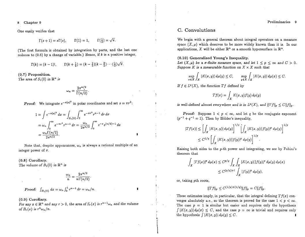
(0.7) Proposition.The area of 51 (0) in jRn is

21rn/2

W n = f(n/~)'

Proof: We integrate e-1rlxI2 in polar coordinates and set s =1rr2 :

Note that, despite appearances, W n is always a rational multiple of an

integer power of 1r.

(0.8) Corollary.The volume of Bl(O) in jRn is

W n 21rn/2

-;:; = nf(n/2)'

Proof: fB,(O) dx =Wn f: r n- l dr =wn/n.

(0.9) Corollary.For any x E jRn and any r > 0, the area of 5r(x) is rn-lwn and the volume

of Br(x) is rnwn/n.

I

sup r IK(x, y)/ dj1.(Y) S; C, sup r I[{(x, y)1 dj1.(x) S; C.xEX Jx yEX Jx

If f E VeX), the function Tf defined by

Tf(x) = fx K(x, y)f(y) dj1.(Y)

is well-defined almost everywhere and is in V(X), and IITfilp S; Cllfllp.

Proof: Suppose 1 < P < 00, and let q be the conjugate exponent(p-l + q-l = 1). Then by Holder's inequality,

ITf(x)1 S; [L I[{(x, y)1 dJ.l(Y)] l/q [L I[{(x, y)llf(y)IP dJ.l(Y)] IIp

S; Cl/q [L I[{(x, y)lIf(y)IP dJ.l(y)] IIp

Raising both sides to the p-th power and integrating, we see by Fubini'stheorem that

fx IT f(x)IP dJ.l(x) S; Cplq LLII«x, y)lIf(Y)IP dj1.(Y) dJ.l(x)

S; C(plq)+l LIf(y)IP dj1.(Y) ,

or, taking pth roots,

These estimates imply, in particular, that the integral defining T f( x) con­verges absolutely a.e., so the theorem is proved for the case 1 < p < 00.

The case p = 1 is similar but easier and requires only the hypothesisf IK(x, y)1 dj1.(x) S; C, and the case p = 00 is trivial and requires onlythe hypothesis f IK(x, y)1 dj1.(Y) S; C. I

10 Chapter 0

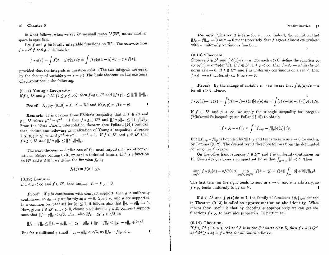
In what follows, when we say V we shall mean V (jRn) unless another

space is specified.Let f and 9 be locally integrable functions on jRn. The convolution

f * 9 of f and 9 is defined by

f * g(x) =Jf(x - y)g(y)dy =Jf(y)g(x - y) dy = 9 * f(x),

provided that the integrals in question exist. (The two integrals are equalby the change of variable y -> x - y.) The basic theorem on the existence

of convolutions is the following:

(0.11) Young's Inequality.If fELl and 9 E LP (1 ~ p ~ 00), then f*g E LP and IIf*gllp ~ IIflldlgllp·

Proof: Apply (0.10) with X =jRn and K(x, y) = f(x - y).

Remark: It is obvious from Holder's inequality that if f E Lq and9 E V where p-1 + q-l = 1 then f * 9 E L OO and Ilf * glloo ~ Ilfllqllgllp,From the Riesz-Thorin interpolation theorem (see F911and [14)) one canthen deduce the following generalization of Young's inequality: Suppose1 ~ p, q, r ~ 00 an,d p-1 + q-1 = r- 1 + 1. If f E Lq and 9 E LP then

f * gEL' and Ilf * gllr ::; IIfll qllgllp'

The next theorem underlies one of the most important uses of convo­lutions. Before coming to it, we need a technical lemma. If f is a functionon jRn and x E jRn, we define the function f:r: by

f",(y) = f(x + y).

(0.12) Lemma.If 1 ::; p < 00 and f E LP, then lim:r:_o life - flip = o.

Proof: If 9 is continuous with compact support, then 9 is uniformlycontinuous, so g:r: -> 9 uniformly as x -> O. Since g:r: and 9 are supportedin a common compact set for Ixl ::; I, it follows also that IIg:r: - gllp -> o.Now, given f E LP and f >0, choose a continuous 9 with compact support

such that IIf - gllp < [/3. Then also IIf:r: - g:r:llp < f/3, so

Ilf", - flip ~ Ilf:r: - gillp + IIg:r: - gllp + IIg - flip < IIg:r: - gllp + 2f/3.

But for x sufficiently small, IIg:r: - gllp < f/3, so IIf:r: - flip < f.

:j.

l

Preliminaries II

Remark: This result is false for p = 00. Indeed, the condition thatIIf:r: - flloo ..... 0 as x ..... 0 means precisely that f agrees almost everywherewith a uniformly continuous function.

(0.13) Theorem.Suppose rP E L1 and I rP(x) dx =a. For each f > 0, define the fune.tion rP,by rP,(x) =cnrP(c1x). If f E V, 1 ::; p < 00, then f * ¢h -> af in the LPnorm as f -> O. If f E L OO and f is uniformly continuous on a set V, thenf * rP, ..... af uniformly on V as f ..... O.

Proof: By the change of variable x -> [X we see that f rP,(x) dx = afor all f > O. Hence,

f*rP,(x)-af(x) = J[f(x-y)- f(x)]rP,(y) dy = J[f(x-[y)- f(x)];(y)dy.

If f E V and p < 00, we apply the triangle inequality for integrals(Minkowski's inequality; see Folland [14]) to obtain

IIf * 1;, - afllp ::; JIIf-,y - fll pl1;(y)1 dy.

But IIf-ty - flip is bounded by 211fllp and tends to zero as f -> 0 for each 'Ii,by Lemma (0.12). The desired result therefore follows from the dominatedconvergence theorem.

On the other hand, suppose f E Loo and f is uniformly continuous onV. Given 6> 0, choose a compact set W so that fJ?,n\w IrPl < o. Then

sup If * rP,(x) - af(x)l::; sup If(x - fY) - f(x)1 r 14>1 + 2l1fllooo.:r:EV :r:EV, yEW Jw

The first term on the right tends to zero as f ..... 0, and 0 is arbitrary, sof * ¢it tends uniformly to af on V. I

If 4> E L1 and fcP(x)dx = 1, the family of functions {cP,},>o definedin Theorem (0.13) is called an approximation to the identity. Whatmakes these useful is that by choosing rP appropriately we can get thefunctions f * cPt to have nice properties. In particular:

(0.14) Theorem.If f E LP (1 ::; p ~ 00) and cP is in the Schwartz class S, then f * rP is Cooand aa(f * 4» = f * oa4> for all multi-indices a.

12 Chapter 0 Preliminaries 13

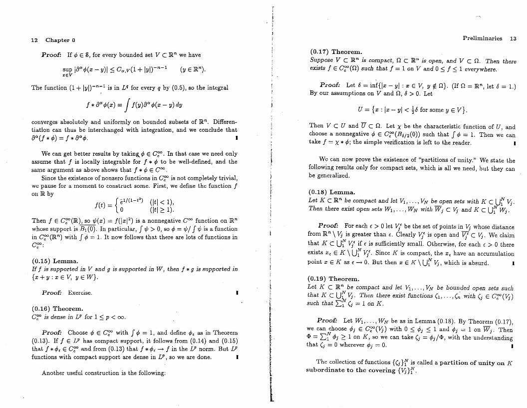
Proof: If rP E £, for every bounded set V C lRn we have

sup la"'rp(x - y)1 :s C",,v(l + lyl)-n-1:r:ev

(y E lR n).

(0.17) Theorem.Suppose V C lRn is compact, 11 C jRn is open, and V C 11. Then thereexists I E C':'(11) such that f == 1 on V and 0 :s f:S 1 everywhere.

The function (1 + !yl)-n-1 is in U for every q by (0.5), so the integral Proof: Let 8 = inf{lx - yl : x E V, y rt. 11}. (If 11 == jRn, let 8 == 1.)By our assumptions on V and 11, 8 > O. Let

u == {x : Ix - yJ < ~6 for some y E V}.

Another useful construction is the following:

(0.15) Lemma. .If f is supported in V and g is supported in W, then f * g is supported m{x + y : x E V, yEW}.

converges absolutely and uniformly on bounded subsets of lRn . Differen­tiation can thus be interchanged with integration, and we conclude thata"'(f*rP)==I*aarP . I

(0.18) Lemma.

Let J( C lRn be compact and let V1 , ... , VN be open sets with J( C ufl V;.Then there exist open sets W1 , ... , WN with Wj C Vi and J{ C ufl Wj.

We can now prove the existence of "partitions of unity." We state thefollowing results only for compact sets, which is all we need, but they canbe generalized.

Proof: For each f > 0 let v,< be the set of points in Vi whose distanceJ _

from lRn\ V; is greater than f. Clearly ~. is open and ~. C V;. We claim

that J{ C ufl ~. if f is sufficiently small. Otherwise, for each f > 0 there

exists x. E J( \ ufl ~'. Since J{ is compact, the x. have an accumulation

point x E J{ as f --> O. But then x E J( \ ufl Vi, which is absurd. I

Then V c U and U C 11. Let X be the characteristic function of U, andchoose a nonnegative rP E C':'(B6/ 2 (0» such that J¢ == 1. Then we cantake I = X * tP; the simple verification is left to the reader.

(0.19) Theorem.

Let J( C lRn be compact and let V1 , ... , VN be bounded open sets suchthat J{ C U~ V;. Then t~ere exist functions (1, ... , (n with (j E C':' (Vi)such that 2:1 (j = 1 on Ii. .

Proof: Let Wl, ... ,WN be as in Lemma (0.18). By Theorem (0.17),we can choose tPj E C':'(Vi) with 0 :s rPj :s 1 and tPj == 1 on W j. Then~ = 2:fI tPj ~ 1 on J(, so we can take (j = ¢j /41, with the understandingthat (j == 0 wherever ¢j = O. I

The collection of functions {(j}i" is called a partition of unity on J{

subordinate to the covering {Vi}i".

t,,!

IProof: Exercise.

(0.16) Theorem.C':' is dense in LP for 1 :s p < 00.

{e1f(1-t

2) (It I< 1),

I(t) == 0 CIt I~ 1).

Then f E COO(IR) , so 1/J(x) == f(JxI 2) is a nonnegative Coo function on jRn

whose supp;rt is Bl(O). In particular, J1/J > 0, so tP == 1/J/ J 'lj; is a functionin C':' (lRn) with J¢ = 1. It now follows that there are lots of functions inC':':

Proof: Choose tP E C':' with J tP == 1, and define ¢. as in Theorem(0.13). If f E LP has compact support, it follows from (0.14) and (0.15)that f *¢. E C':' and from (0.13) that f * tP. --> I in the LP norm. But LPfunctions with compact support are dense in LP, so we are done. I

We can get better results by taking, rP E C,:,. In that case we need onlyassume that f is locally integrable for f * rP to be well-defined, and thesame argument as above shows that I * rP E Coo. . .

Since the existence of nonzero functions in C':' is not completely trivIal,we pause for a moment to construct some. First, we define the function fon lR by

14 Chapter 0

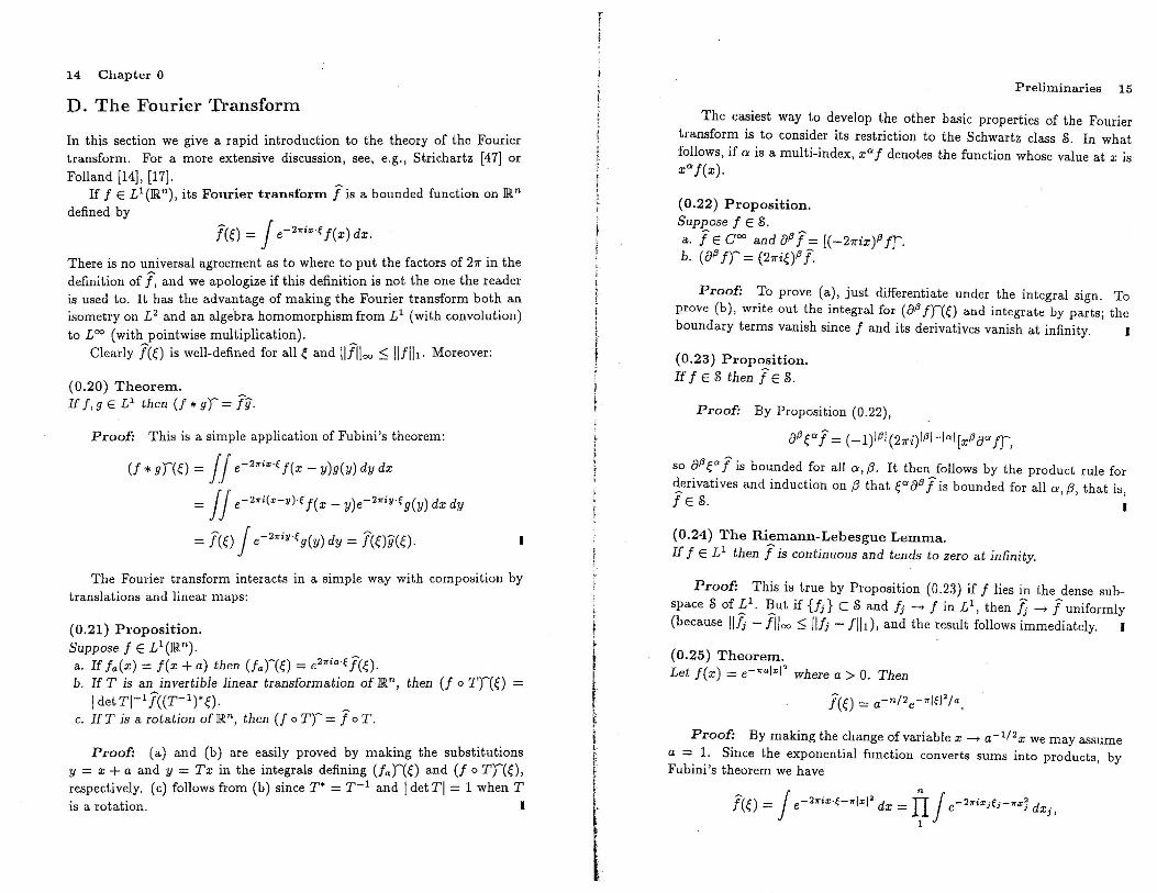
D. The Fourier Transform

In this section we give a rapid introduction to the theory of the Fouriertransform. For a more extensive discussion, see, e.g., Strichartz [47] or

Folland [14], [17]. ~ .If IE L1 (JR n ), its Fourier transform I is a bounded functlOn on JRn

defined by

lw =Je-27fix .€ I(x) dx.

There is no universal agreement as to where to put the factors of 271" in thedefinition of 1. and we apologize if this definition is not the one the readeris used to. It has the advantage of making the Fourier transform both anisometry on L 2 and an algehra homomorphism from L 1 (with convolution)

to L OO (with pointwise multiplication). ~

Clearly l(e) is well-defined for all e and 11/1100 ~ 11/1h. Moreover:

(0.20) Theorem. ~

If I, g E L 1 then (f * gf = n·Proof: This is a simple application of Fubini's theorem:

(f * gnO =JJe-2rrix

.{ I(x - y)g(y) dy dx

= JJe-2rriCx-y).{ I(x - y)e- 21riy .{g(y) dx dy

=l(e)Je-2rriY '€g(y) dy = 1(e)g(e).

The Fourier transform interacts in a simple way with composition bytranslations and linear maps:

(0.21) Proposition.Suppose f E L1 (JRn). . ~

a. If la(x) = I(x + a) then (JafW =e2na.{ I(e)·b. If T is an invertible linear transformation oflRn, then (J 0 Tne) =

IdetTI- 11«T-1)"e). ~c. 1fT is a rotation ofJRn, then (J 0 Tf = loT.

Proof: (a) and (b) are easily proved by making the substitutionsy = x + a and y = Tx in the integrals defining (Jane) and (J 0 Tne),respectively. (c) follows from (b) since T· = T- 1 and Idet TI = 1 when T. t t' IIS a ro a lOn.

Preliminaries 15

The easiest way to develop the other basic properties of the Fouriertransform is to consider its restriction to the Schwartz class S. In whatfollows, if a is a multi-index, x af denotes the function whose value at x isxaf(x).

(0.22) Proposition.Suppose I E S.

a. 1E coo and 8f31= [(-271"ix)f3 If.b. (8 f3 If = (271"ie)f3 f.

Proof: To prove (a), just differentiate under the integral sign. Toprove (b), write out the integral for (8f3 Ine) and integrate by parts; theboundary terms vanish since f and its derivatives vanish at infinity. I

(0.23) Proposition.If f E S then 1E S.

Proof: By Proposition (0.22),

8f3 ea1= (-1)1f31 (271"i)/f3I- la l[x f1 aaJf,

so af1 e"1 is bounded for all a, 13. It then follows by the product rule forderivatives and induction on 13 that e"8f11is bounded for all a, 13, that is,1E S. I

(0.24) The Riemann-Lebesgue Lemma.If J E L 1 then 1is continuous and tends to zero at infinity.

Proof: This is true by Proposition (0.23) if f lies in the dense sub­space S of L1. But if {Ji} C Sand Ij ---t I in L 1 , then l; ---t 1uniformly(because Ill; - 11/00 ~ IIJi - Illd, and the result follows immediately. I

(0.25) Theorem.Let J(x) = e-rra)x/' where a > O. Then

1(0 = a- n!2e-rrIW!a.

Proof: By making the change of variable x ---t a- 1!2 x we may assumea = 1. Since the exponential function converts sums into products, byFubini's theorem we have

ice) =Je- 2..ix ·{- 7f lxl' dx = ITJe-2rrixi{i-7fXJ dXj,1

16 Chapter 0

and it suffices to show that the jth factor in the product is e- 7f{} , i.e., toprove the theorem for n::;: 1. Now when n::;: 1 we have

Je- 27fi:Z:{-7f:Z:' dx::;: e- 7f{' Je- ..(:z:+iO' dx.

But I(z) ::;: e- 7fZ ' is an entire holomorphic function of z E C which dies outrapidly as IRe z I -> 00 when 11m zl reamins bounded. Hence by Cauchy's'theorem we can shift the contour of integration from 1m z ::;: 0 to 1m z ::;: -{,

which together with (0.6) yields

I

(0.26) Theorem.If I, g E 8 then J fY::;: J19.

Preliminaries 17

(0.28) Corollary.The Fourier transform is an isomorphism of S onto itself.

(0.29) The Plancherel Theorem.

The Fourier transform on S extends uniquely to a unitary isomorphism of£2 onto itself. .

Proof: Since S is d~nse in £2 (Theorem (0.16», by Corollary (0.28)it suffices to show that IIfll~::;: 11/112 for I E S. If IE S, set g(x)::;: I(-x).

One easily checks that g::;: 1. Hence by Theorems (0.20) and (0.27),

II/II~ ::;: JI(x)f(x) dx ::;: 1 * g(O)::;: J(f *gn~) d~::;: JfW1<~) d{

::;: 1Ij]1~·

Proof: By Fubini's theorem,

JIg::;: JJ l(x)g(y)e- 27fi :Z:. Y dydx::;: J19.

For I E £1, define the function r by

r(x)::;: Je27fi:Z:'{/(~)d~::;: l(-x).

(0.27) The Fourier Inversion Theorem.If I E S, (l)V ::;: I.

I

The results (0.20)-(0.29) are the fundamental properties of the Fouriertransform which we shall use repeatedly. We shall also sometimes need theFourier transform as an operator on tempered distributions, to be discussedin the next section, and the following result.

(0.30) Proposition.

IT I E L1

has compact support, then 1 extends to an entire holomorphicfunction on en. If I E C~, then 1(~) is rapidly decaying as IRe{1 -> 00

when IIm~1 remains bounded.

Proof: Given ( > 0 and x E jR", set 4J(~) ::;: e2.. i :z:·{- .. ,'j{I'. Then byTheorem (0.25),

'J(y)::;: Je- 27fi (Y-:z:H e- ... 'I{I' d~::;: (-"e- .. I:z:-Y1'j,'.

Thus,

'J(y) ::;: (-"g«(-l(x - y»::;: g,(x - y) where g(x) ::;: e- .. I:z: I'.

By (0.26), then,

Je- 7f ,'I{!' e27fi:Z:.{ 1(~) d~::;: J1¢;::;: JI'J::;: JI(X)gl(X-Y) dy::;: I*g,(x).

By (0.6) and (0.14), 1* g, -> I uniformly as ( -> 0 since functions in S areuniformly continuous. But clearly, for each x,

Je- 7f ,'I{I' e27fi :Z:.{1(0 d~ -> Je2.. i :z:.{ l(e) de::;: (l)V (x). I

Ili

tI,.IItt

t

Proof: The integral 1({) ::;: Je-27fi:z:.{ I(x) dx converges for every{ E C', and e- 2

..i:z:.{ is an entire function of ~ E C'. Hence one can

take complex derivatives of f simply by differentiating under the integral.Moreover, if f E C~ and 1 is supported in {x : Ixl ::; K}, for any multi­index ex we have

which yields the second assertion.

E. Distributions

We now outline the elements of the theory of distributions. The materialsketched here is covered in more detail in Folland [14] and Rudin [41], and a

18 Chapter 0 Preliminaries 19

(0.31)

(Tu,¢J) = (u,T'¢J).

I(u, ¢J)! ~ C L sup /8a¢J(:c)"lal:5N"'EO

(0.32)

I(u, ¢J)/ ~ On L lIaa (t/Jq)lloo.lal:5 No

Expanding aa(t/J¢J) by the product rule, we see that

This has two consequences. First, u is of "finite order": indeed, by (0.31)with K = IT,

needs to know that if {Va}aEA is a collection of open sets and u = 0 oneach Va, then u = 0 on UVa. But if ¢ E C,:,(U Va), supp ¢ is covered byfinitely many Va's. By means of a partition of unity on supp ¢ subordinateto this covering, one can write ¢J = Ef ¢Ji where each ¢Ji is supported insome Va. It follows that (u,¢J) = "fJu,¢Ji) = 0, as desired.)

The space of distributions on lR n whose support is a compact subset ofthe open set 0 is denoted by £'(0), and we set £' = £'(JRn).

Suppose u E £'. Let 0 be a bounded open set such that supp u CO, andchoose t/J E Cgo(O) with t/J = 1 on a neighborhood of supp u (by Theorem(0.17». Then for any ¢ E Cgo we have

where N = Nn and C depends only on Cn and the constants /18.0 t/J/loo,1.81 ~ N. Second, (u, t/J¢J) makes sense for all q) E Coo, compactly supportedor not, so if we define (u, q)) to be (u, t/J¢J) for all ¢ E Coo, we have anextension of u to a linear functional on Coo. This extension is clearlyindependent of the choice of t/J, and it is unique subject to the conditionthat (u, ¢J) = 0 whenever supp r/J and supp u are disjoint. Thus distributionswith compact support can be regarded as linear functionals on Coo thatsatisfy estimates of the form (0.32). Conversely, the restriction to C';"of any linear functional On Coo satisfying (0.32) is clearly a distributionsupported in IT.

The general philosophy for extending operations from functions to dis­tributions is the following. Let T be a linear operator on C~(O) that iscontinuous in the sense that if ¢i -+ q) in C';"(O) then T¢i -+ Tr/J in C';"(O).Suppose there is another such operator T' such that f(Tq)t/J = J¢(T't/J)for all r/J, 1/J E C';"(O). (We call T' the dual or transpose of T.) We canthen extend T to act on distributions by the formula

I(u, ¢J)I ~ CK L Ilaa¢Jlloo.lal:5NK

The space of distributions on 0 is denoted by 1)'(0), and we set 1)' =1)'(lRn). We put the weak topology on 1)'(0); that is, Uj -+ U in 1)'(0) ifand only if (ui' ¢J) -+ (u, ¢J) for every ¢J E C~(O). .

Every locally integrable function U on 0 can be regarded as a dIS­tribution by the formula (u, ¢J) = Ju¢J, which accords with the notationintroduced earlier. (The continuity follows from the Lebesgue dominatedconvergence theorem.) This correspondence is one-to-one if we regard twofunctions as the same if they are equal almost everywhere. Thus distribu­tions can be regarded as "generalized functions." Indeed, we shall oftenpretend that distributions are functions and write (u, ¢J) as Ju(:z:)¢J(:z:) d:Z:j

this is a useful fiction that makes certain operations involving distributionsmore transparent.

Every locally finite measure flo on n defines a distribution by the formula(p., ¢J) = J¢J dp.. In particular, if we take p. to be the point mass at 0, weobtain the gracldaddy of all distributions, the Dirac o-function 0 E 1)'defined by (0, ¢) = ¢(O). Theorem (0.13) implies that if u E £1, f U = a,and uf(:z:) = enu(r-I:z:), then U f -+ ao in 1)' when r -+ O.

If u, v E 1)'(0), we say that u = von an open set V COif (u, ¢) = (v, ¢)for all ¢J E C~(V). The support of a distribution u is the complement ofthe largest open set on which u = O. (To see that this is well-defined, one

more extensive treatment at an elementary level can be found in Strichartz[47J. Sea. also Treves [49] and Hormander [27, vol. I] for a deeper study ofdistributions.

Let 0 be an open set in lRn. We begin by defining a notion of sequentialconvergence in C~(O). Namely, we say that ¢Ji -+ ¢J in C~(O) if the ¢Jj'sare all supported in a common compact subset of 0 and aa¢Ji -+ aa¢Juniformly for every multi-index Of. (This notion of convergence comes froma locally convex topology on C~(O), whose precise description we shall notneed. See Rudin [41] or Treves [49].)

If u is a linear functional on the space C~(O), we denote the numberobtained by applying u to ¢J E C~(O) by (u, ¢J) (or sometimes by (¢J, u):it is convenient to maintain this flexibility). A distribution on 0 is alinear functional u on C~ (0) that is continuous in the sense that if ¢Ji -+ ¢Jin C~(O) then (u,¢Ji) -+ (u,¢J). A bit offunctional analysis (cf. Folland[14, Prop. (5.15)]) shows that this notion of continuity is equivalent to thefollowing condition: for every compact set J{ C 0 there is a constant CKand an integer N K such that for all ¢ E Cr;: (I<),

20 Chapter 0

The linear fllnctional Tu on C~(O) defined in this way is continuous onC~(O) since T' is assumed continuous. The most important examples arethe following; in all of them the verification of continuity is left as a simpleexercise.

1. Let T be multiplication by the function f E COO(O). Then T' = T,so we can multiply any distribution u by f E COO(O) by the formula(fu,¢J) = (u'/¢J).

2. Let T = 0"'. By integration by parts, T' = (-1)1"'10"'. Hence wecan differentiate any distribution as often as we please to obtain otherdistributions by the formula (o"'u, ¢J) = (-1)1"'1 (u, 0"'¢J).

3. We can combine (1) and (2). Let T = L:1"'I~k a",o'" be a differentialoperator of order k with Coo coefficients a",. Integration by parts showsthat the dual operator T' is given by T',p = I:laI9(-1)1 0 Ioo(aoc;6). Forany distribution u, then, we define Tu by (Tu,,p) = (u, T'¢).

Clearly, if u E Ck(O), the distribution derivatives of u of order:::; k arejust the pointwise derivatives. The converse is also true:

(0.33) Proposition.liu E C(O) and the distribution derivatives oOu are in C(O) for Jal :::; kthen u E Ck(O).

Proof: By induction it suffices to assume that k = 1. Since theconclusion is of a local nature, moreover, it suffices to assume that 0 is acube, say 0 = {x: maxlxj - Yjl:::; r} for some Y E lR n

. For x E 0, set

1""vex) = 01 u(t, X2,"" Xn ) dt +U(Y1, X2,.·., X n ).

!/,

It is easily checked that v and u agree as distributions on 0, hence v = uas functions on O. But 01 u is clearly a pointwise derivative of v. Likewisefor 02U, ... ,Onu; thus u E C 1 (11). I

We now continue our list of operations on distributions. In all of thefollowing, we take 0 = lRn

.

4. Given x E lRn, let T¢J = ¢:z:, where ¢",(y) = c;6(x + y). Then T'¢ = ¢-:r;.

Thus for any distribution u, we define its translate U:r; by. (u:r;, ¢) =(u, c;6-:r;).

5. Let Tc;6 = J;, where J;(x) = c;6(-x). Then T' = T, so for aEY distributionu we define its reflection in the origin ti by (ti, c;6) = (u, c;6).

[

II

Il

Preliminaries 21

6. Given 'rf; E C~, define T¢ = ¢ * 'rf;, whicE is in Cr by (0.14) and(0.15). It is easy to check that T'¢ = ¢ * 'rf;, where 'rf; is defined as in(5). Thus, if u is a distribution, we can define the distribution u * 'rf;by (u * 'rf;, ¢) = (u, ¢ * J;). On the other hand, notice that ¢ * 'rf;(x) =(¢, ('rf;:r;)l, so we can also define u*'rf; pointwise as a continuous functionby u * 'rf;(x) = (u, ('rf;:z:)l.

In fact, these two definitions agree. To see this, let ,p E C~, let J{ bea compact set containing supp('rf;:z:r for all x E supp,p, and let NK beas in (0.31). From the relation ¢ * J;(y) =Jc;6(x) ('rf;",nY) dx it is is nothard to see that there is a seque~ce of Riemann sums L ¢(Xj )('rf;:r;ir6..Xjthat converge uniformly to ¢ *'rf; together with their derivatives of order:::; NK. But then (0.31) implies that if u * 'rf; is defined as a continuousfunction, we have

(u * 'rf;, c;6) = lim L u * 'rf;(Xj ),p(Xj) 6..Xj

=lim L(u, ('rf;"'i)l¢(Xj) 6..Xj = (u, ¢ * J;),

which is the action of the distribution u * 'rf; on¢.

Moreover, by (2) and integration by parts, we see that the distributionOO(u * 'rf;) is given by

so 00

(u * 'rf;) = u *o°'rf; is a continuous function. Hence u * 'rf; is actuallya Coo function.

7. The same considerations apply when u E £' and 'rf; E Coo. That is, wecan define u * 'rf; either as a distribution by (u * 'rf;, ¢) = (u, ¢ * ;j), or asa Coo function by u * 'rf;(x) = (u, ('rf;:r;)l.

8. If u E £' and 'rf; E C~, as in (0.15) we see that u * 'rf; E Cr;'. Hencewe can consider the operator T'rf; = u * 'rf; on C~, whose dual is clearlyT'7/J = ti * 'rf;. It follows that if u E £' and v E 'n', u * v can bedefined as a distribution by the formula (u * v, 'rf;) = (v, ti * 'rf;). Weleave it as an exercise to verify that for any multi-index a we haveOO(u * v) = (OOu) * v = u * (OOv).

We shall also need to consider the class of "tempered distributions."We endow the Schwartz class S with the Frechet space topology defined bythe family of norms 11¢lko,p) = IJx o oPc;61J00. That is, ¢j --+ ¢ in S if andonly if

sup IxOoP(¢j - c;6)(x)l--+ 0 for all a,{3.:z:

22 Chapter 0

A tempered distribution is a continuous linear functional on S; the spaceof tempered distributions is denoted by S'. Since C~ is a dense subspace ofS in the topology of S, and the topology on C~ is stronger than the topologyon S, the re~trictionof every tempered distribution to C~ is a distribution,and this restriction map is one-to-one. Hence, every tempered distribution"is" a distribution. On the other hand, Proposition (0.32) shows thatevery distribution with compact support is tempered. Roughly speaking,the tempered distributions are those which "grow at most polynomially atinfinity." For example, every polynomial is a tempered distribution, butu(x) =elxl is not. (Exercise: prove this.)

One can define operations on tempered distributions as above, simplyby replacing Cr:' by S. For example, if u E S', then:

1. BOt'll is a tempered distribution for all multi-indices 0';

2. I'll is a tempered distribution for all I E Coo such that BOt I grows atmost polynomially at infinity for all a;

3. u * I/> is a tempered distribution, and also a Coo function, for any I/> E S.

The importance of tempered distributions lies in the fact that theyhave Fourier transforms. Indeed, since the Fourier transform maps S con­tinuously onto itself and is self-dual by Proposition (0.26), for any u E S'we can define u E S' by (u, ¢) = (u, ¢) (¢ E S), which is consistent withthe definition for functions. It is easy to see that Propositions (0.21) and(0.22) are still valid when I E S', as is the Fourier inversion theorem (0.27),provided r is defined by (r, ¢) = (1, ¢ V). Also, if u E S' and ¢ E S, wehave (u * ¢ j =¢u; the proof is left as an easy exercise.

For example, the Fourier transform of the Dirac 8-function is given by(8, ¢) = (8, ¢) = ¢(O) = f ¢(x) dx = (1, ¢), so 8' is the constant function 1.It then follows from the inversion theorem that 1 = 8, and from Proposition(0.22) that (B Ot8j= (27ri)IOtI~Ot and that (xOtj= (i/27l')I OtIB0t 8.

F. Compact Operators

Let X be a Banach space and let T be a bounded linear operator on X. Wedenote the nullspace and range of T by 'N(T) and :R(T). T is called com­pact if whenever {Xj} is a bounded sequence in X, the sequence {Txj} hasa convergent subsequence. Equivalently, T is compact if it maps boundedsets into sets with compact closure. T is said to be of finite rank if:R(T) is finite-dimensional. Clearly every bounded operator of finite rankis compact.

r.tt

r.t

III

ff

,.

Preliminaries 23

(0.34) Theorem.

The set of compact operators on X is a closed two-sided ideal in the algebraof bounded operators on X with the norm topology.

Proof: Suppose T1 and T2 are compact, and {Xj} C X is bounded.We can choose a subsequence {Yi} of {Xj} such that {T1Yi} converges, andthen choose a subsequence {Zj} of {Yj} such that {T2 zj } converges. Itfollows that G1 Tl +G2T2 is compact for all Gl, G2 E C. Also,"it is clear thatif T is compact and S is bounded, then TS and ST are compact. Thus theset of compact operators is a two-sided ideal.

Suppose {Tm } is a sequence of compact operators converging to a limitT in the norm topology. Given a seqence {Xj} C X with II xi 1/ :5 C for allj, choose a subsequence {Xli} such that {TlXlj} converges. Proceedinginductively, for m = 2,3,4, ..., choose a subsequence {xmj} of {X(m-l)j}

such that {Tmxmi} converges. Setting Yj = Xjj, one easily sees that {TmYj}converges for all m. But then

/ITYj - TY"I/ :51/(T - Tm)Yill + IjTm(Yj - Yk)11 + II(Tm - T)Ykl/

:5 2CI/T - Tmll + I/TmYj - TmY"II.Given c > 0, we can choose m so large that liT - Tmll :5 c/4C, and thenwith this choice of m we have I/TmYj - TmYk11 < c/2 when j and k aresufficiently large. Thus {TYi} is convergent, so T is compact. I

(0.35) Corollary.

1fT is a bounded operator on X and there is a sequence {Tm} of operatorsof finite rank such that IITm - TI/-> 0, then T is compact.

In case X is a Hilbert space, this corollary has a converse.

(0.36) Theorem.

IfT is a compact operator on a Hilbert space X, then T is the norm limitof operators of finite rank.

Proof: Suppose ( > 0, and let B be the unit ball in X. Since T(B)has compact closure, it is totally bounded: there is a finite set Yl, ... ,Ynof elements of T(E) such that every y E T(B) satisfies Ily - Yjl/ < c forsome j.Let p. be the orthogonal projection onto the space spanned byYl, ... , Yn, and set T. = P.T. Then T. is of finite rank. Also, since T.x isthe element closest to Tx in :R(p.), for X E B we have

I/Tx -T.xlI :5 lTi.¥n I/Tx - Yjll < c.-)-

In other words, liT - T.II < c, so T. -> T as c -> O.

24 Chapter 0Preliminaries 25

Remark: For many years it was an open question whether Theorem(0.36) were true ror general Banach spaces. The answer is negative evenfor some separable, reflexive Banach spaces; see Enflo [12].

(0.37) Theorem.The operator T on the Banach space X is compact if and only if the dualoperator T· on the dual space X· is compact.

Proof: Let Band B· be the unit balls in X and X·. Suppose T iscompact, and let {lj} be a bounded sequence in X·. Multiplying the Ji'sby a small constant, we may assume {lj} C B". The functions Ji : X -> I(:

are equicontinuous and uniformly bounded on bounded sets, so by theArzela.-Ascoli theorem there is a subsequence (still denoted by {Ji}) .whichconverges uniformly on the compact set T(B). Thus T· Ji(x) = Ji(Tx)converges uniformly for x E B, so {T· Ii} is Cauchy in the norm topologyof X·. Hence T" is compact.

Likewise, if T" is compact then T·· is compact on X... But X isisometrically embedded in X.. , and T is the restriction of T·· to X, so Tis compact. I

ti -•

~roof: (a) is equivalent to the following statement: For any f > 0,the lmear span of the spaces V>. with IAI 2: f is finite-dimensional. Supposet.o the c~ntrary that there exist E > 0 and an infinite sequence {x j} C X ofhnearly mdependent elements such that Tx· = >. .x· with IA" > r ~ all'S' I } }} } - < lor J.

mce >'j I~ IIT I/, by passing to a subsequence we can assume that {>..} isa Cauchy sequence. Let Xm be the linear span of Xl, ... , X m . For each mchoose Ym E Xm with IIYmll = 1 and Ym 1. X m - l . Then Ym = L:~ CmjX;for some scalars Cmj, so

m-l m-l

>,;lTYm = CmmXm + L CmjAj>.;l Xj =Ym + L Cmj(Aj>.;l - I)Xj1 1 •

= Ym (mod Xm-I).

If n < m, then,

Therefore, since Ym 1. Xm- 1, the Pythagorean theorem yields

(0.38) Fredholm's Theorem.Let T be a compact operator on a Hilbert space X with inner product (-1-).For each >. E 1(:, let

Then:a. The set of A E I(: for which V>. f= {O} is finite or countable, and in the

latter case its only accumulation point is O. Moreover, dim(VA) < 00

for all A f= o.b. If A f= 0, dim(VA) =dim(WI ).c. If A f= 0, ~(AI - T) is closed.

We now present the main structure theorem for compact operators.This theorem was first proved by I. Fredholm (by different methods) forcertain integral operators on L2 spaces. In the abstract Hilbert space set­ting it is due to F. Riesz, and it was later extended to arbitrary Banachspaces by J. Schauder. For this reason it is sometimes called the Riesz­Schauder theory. We shall restrict attention to the Hilbert space case,which is all we shall need, and for which the proof is easier; see Rudin [41]for the general case.

(XI - T")(Xl, - T{)-l =1- T;)

IITYn - TYmll 2: I>'ml-II- Am>.~lIIlTYnll.

As m. n -:'100 the second term on the ~ight tends to zero since IITYnil ~ IITIIand Am>'n -> 1. and the first term IS bounded below by E. Thus {TYm}has no convergent subsequence, contradicting compactness.

Now consider (b). Given A f= 0, by Theorem (0.36) we can writeT = To + T1 where To has finite rank and IITll1 < />./. The operatorAI - T1 = A(I - A-lTd is invertible (the inverse being given by the con­vergent geometric series L:':A-k - 1Tl'), and we have

or

But then

(0.39) (AI-TI}-l(Ai-T) = (AI-Td-1(AI-T1-To) = I-(AI-T1)-lTo.

Set T2 = (M - T1 )-lTo. Then clearly x E V>. if and only if x - T2x =o.

On the other hand, taking the adjoint of both sides of (0.39), we have

!!~.

f

I

,.'....

W>. = {x EX: T· x =AX}.V>. = (x EX: Tx = AX},

26 Chapter 0 Preliminaries 27

Set {3jl: = (Uj IVI:), and given x E X, set Cij = (x IVj). If x - T2x = 0, thenx = L~ Cij Uj, and we see by taking the scalar prodict with VI: that

so Y = (XI -Tn-Ix is in W:x if and only if x-Tix = O. We must thereforeshow that the equations x-T2x = 0 and x-Tix =0 have the same numberof independent solutions.

Since To has finite rank, so does T2 . Let Ul, ... , UN be an orthonormalbasis for :R(T2). Then for any x E X we have T2x = L~ /j(x)Uj whereL~ IJi(xW = IIT2 x11 2 . It follows that x -+ Ji(x) is a bounded linearfunctional on X, so there exist VI, ... ,VN such that

Conversely, if Cil, ... , Cin satisfy (0.40), then x = L CijUj satisfies X-T2X =O. On the other hand, one easily verifies that Ti x = L(X IUj )Vj, so by thesame reasoning, x - Tix = 0 if and only if x = LX CijVj, where

But the matrices (Djk - {3jk) and (Djk -7Jkj) are adjoints of each other andso have the same rank. Thus (0040) and (0.41) have the same number ofindependent solutions.

Finally, we prove (c). Suppose we have a sequence {Yj} C :R(>.! - T)which converges to an element Y E X. We can write Yj = (>.1 - T)xjfor some Xj E Xi if we set Xj = Uj + Vj where Uj E VA and Vj J.. VA'we have Yj= (>.1 - T)vj. We claim that {Vj} is a bounded sequence.Otherwise, by passing to a subsequence we may assume IIVj II -+ 00. SetWj =Vd II Vj II; then by passing to another subsequence we may assume that{Twj} converges to a limit z. Since the Yj'S are bounded and II Vj II -+ 00,

(0.40)

. (0.41)

N

T2x = L(x IVj)Uj1

Cik - L{3jkCij = 0,j

Cik - 2.:,7JkjCij = 0,j

(x EX).

k =1, . .. ,N.

k = 1, ... ,N.

so z E VA' This is a contradiction since we assume>. '# O.Now, since {Vj} is a bounded sequence, by passing to a subsequence we

may assume that {Tvj} converges to a limit x. But then

v} = >.-l(Yj +TVj) -+ A-l(y+ x),

soY = lim(>.! - T)vj = (>.! - T)A-l(y + x).

Thus Y E :R(>.! - T), and the proof is complete.

(0.42) Corollary.Suppose A '# O. Then:i. The equation (AI - T)x = y has a solution if and only if y ..L W-... , A11. AI - T is surjective if and only if it is injective.

Proof: (i) follows from part (c) of the theorem and the fact that:R(S) =N(S").L for any bounded operator S. (ii) then follows from (i) andpart (b) of the theorem. I

In general it may happen that the !ipaces VA are all trivial. (It is easyto construct an example from a weighted shift operator on [2.) However, ifT is self-adjoint, there are lots of eigenvectors.

(0.43) Lemma.If T is a compact self-adjoint operator on a Hilbert space X, then eitherIITII or -IITII is an eigenvalue for T.

Proof: Clearly we may assume T '# O. Let c = IITII (so c> 0), andconsider the operator A =c21- T 2

. For all x E X we have

(Ax Ix) = c211xII2 -IITxII2 ;:: O.

Choose a sequence {Xj} C X with IIXjl1 = 1 and IITxjll -+ c. Then(Axj IXj) -+ 0, so applying the Schwarz inequality to the nonnegativeHermitian form (u, v) -+ (Au Iv), we see that

(>.! - T)z =lim(>.! - T)>,wj = lim It~jll =0,

y'>'Wj =TWj + IIv~1I ..,.... z,

Thus z J.. V). and Ilzll = IAI, but also

(j -+ 00).IIAXjll2 = (Axj IAXj) ::; (Axj IXj)1/2(A2xj IAXj)1/2

::; (Axj IXj)1/2I1A2xjW/ 2 I1AxjW/ 2 ::; IIAI1 3/2(Axj IXj)1/2 -+ 0,

so AXj -+ 0. By passing to a subsequence we may assume that {Txj}converges to a limit Y, which satisfies

IlylI =limllTxjl1 =c > 0,' Ay =limATxj = limTAxj =O.

28 Chapter 0

In other words,

yiO and Ay=(cl+T)(cI-T)y=O.

Thus either Ty =cy or cy - Ty = z i 0 and Tz = -cz.

(0.44) The Spectral Theorem.1fT is a compact self-adjoint operator on a Hilbert space X, then X has anorthonormal basis consisting of eigenvectors for T.

Proof: It is a simple consequence of the self-adjointness of T that (i)eigenvectors for different eigenvalues are orthogonal to each other, and (ii)if 'd is a subspace of X such that TOn c 'd, then also T('dol) C 'dol. Inparticular, let 'd be the closed linear span of all the eigenvectors of T. If wepick an orthonormal basis for each eigenspace of T and take their union,by (i) we obtain an orthonormal basis for '0. By (ii), TI'Dol is a compactoperator on 'Dol, and it has no eigenvectors since all the eigenvectors of Tbelong to 'd. But this is impossible by Lemma (0.43) unless 'dol = {O}, so

'0 == X. I

We conclude by constructing a useful class of compact operators on£2(/;.), where p is a a-finite measure on a space S. To simplify the argumenta bit, we shall make the (inessential) assumption that L 2(p) is separable.If J{ is a measurable function on S x S, we formally define the operatorTK on functions on S by

TKf(x) = 1K(x, y)f(y) dp(y).

If K E £2(p x p), K is called a Hilbert-Schmidt kernel.

(0.45) Theorem.Let J{ be a Hilbert-Schmidt kernel. Then TK is a compact operator on

£2(p), and IITKII :::; IIK1I2.

Proof: First we show that TK is well-defined on £2(J-L) and boundedby IIKII2. By the Schwarz inequality,

Preliminaries 29

This shows that TK f is finite almost everywhere, and moreover

IITKfll~=1ITKf(xWdJ-L(x):s Ilfll~ 11 IK(x,yWdJ-L(y)dJ-L(~)

= IIKII~lIfllt

so IITKII :S IIKII2.Now let {¢iiH''' be an orthonormal basis for £2(J-L). It is an easy conse­

quence of Fubini's theorem that if 'l/Jii(x,y) = ¢ii(X)¢ii(y) , then {Wii}i,j=lis an orthonormal basis for £2(p x J-L)' Hence we can write K =L aii'I/Jii'For N = 1,2, ..., let

KN(X, y) = L aii!/Jii(x, y) = L aii¢ii(x)¢ii(Y)'i+i~N i+i~N

Then ~(TKN) lies in the span of ¢il,"" ¢iN, so TKN has finite rank. Onthe other hand,

11K - KNII~ = L la'i/ 2--+ 0 as N --+ 00,

i+i>N

so by the previous remarks,

By Corollary (0.35), then, TK is compact.