windfarmer - renewable energy software
TRANSCRIPT
WINDFARMERUSER MANUAL
SAFER, SMARTER, GREENER
Version: 5.3Date: January 2015DNV GL - Energy

DISCLAIMER
Garrad Hassan & Partners Ltd. accepts no liability for any loss or consequential damage arising directly or indirectly from the use of its products.
This document is subject to change without notice.
COPYRIGHT
All rights reserved. Duplications of this document in any form are not allowed unless agreed in writing by Garrad Hassan & Partners Ltd.
2015 Garrad Hassan & Partners Ltd.
Garrad Hassan & Partners Ltd., St Vincent's Works, Silverthorne Lane, Bristol, BS2 0QD England
www.dnvgl.com
WindFarmer User Manual (English) January 2015
CONTENTS
1 Introduction 1
1.1 Technical Support 1 1.2 Installation of WindFarmer 1 1.3 Quick Start 2
2 WindFarmer Interface 3 2.1 WindFarmer Workspace 3 2.2 Window Types and Associated Toolbars 4 2.3 Mapping Window Cursor Modes 6 2.4 Display, Control and Status Bar 11
3 Base Module 14 3.1 Base Module Interface 14 3.2 Input Files 17 3.3 WindFarmer Control Panel 42 3.4 Wind Studio 49 3.5 Calculating Wind Flow 55 3.6 Starting the wind flow model calculation 63 3.7 Modifying the wind flow model 63 3.8 Setting Site Constraints 63 3.9 Energy Yield Calculations 66 3.10 Use Existing Turbines as a Reference 72 3.11 Layout Optimisation 75 3.12 Exporting and Reporting 76 3.13 Noise Calculation 83 3.14 Graphical Representation of Results 86
4 MCP+ Module 88 4.1 Data Loader - Loading time series 89 4.2 Editing the masts, sensors and calibrations 95 4.3 Inspecting and cleaning the data 97 4.4 Data Summary Statistics 104 4.5 Data analysis 108 4.6 Application of MCP+ Module 116
5 Multiple Projects 117 5.1 Projects 117 5.2 Projects Tools Interface 117 5.3 Project Properties 119 5.4 Creating Multiple Projects 122 5.5 Cumulative Visual Impact 123 5.6 Cumulative Noise Impact 126
6 Visualisation Module 127 6.1 Visualisation Module Interface 127 6.2 Input Data 129 6.3 Creating a Wireframe Visualisation 129 6.4 Creating a Rendered Landscape Visualisation 132 6.5 Calculating a ZVI Map 134 6.6 Photomontage 135 6.7 Visualisation Features 136 6.8 Visual Layout Constraints 137 6.9 Radar Stations 137 6.10 Fly-throughs and Animation of Visualisations 140 6.11 Creating animated KML files 141 6.12 Troubleshooting 143
7 Financial Module 144 7.1 Financial Module Interface 144 7.2 Menus 145 7.3 Operating the Financial Module 145 7.4 Optimisation of a financial target 150
8 Turbulence Intensity Module 151 8.1 Flow and Performance Matrix 151 8.2 Advanced Turbulence Intensity Input 153
WINDFARMER USER MANUAL i
CONTENTS
8.3 Turbulence Intensity Experienced at Turbine Location 154 8.4 Estimated Design Equivalent Turbulence 154 8.5 Site Conditions Ranking Table 156
9 Electrical Module 157 9.1 Mouse Functions 157 9.2 Inputs 158 9.3 Outputs 160 9.4 Electrical Module Properties of Turbines & Cables Dialog (EMPTCD) 161 9.5 Caveats 165
10 Shadow Flicker Module 166 10.1 Shadow Flicker Module Interface 166 10.2 Calculating a Shadow Flicker Map 170 10.3 Displaying the Results of Shadow Flicker Calculation 171
A Supported File Formats 175 B Photomontage guidelines 177
B.1 Virtual Representation 177 B.2 Taking Photographs 178 B.3 How to create a Photomontage 178 B.4 Material Requirements 180 B.5 Viewpoint description form 181 B.6 Photographic Information 182
C Electrical Module Library 183 C.1 Dialog Controls 183 C.2 Launching 184
D Menu Structure 186 D.1 General Structure 186 D.2 Menus in the Mapping Window 189 D.3 Menus in the Graphing Window 193 D.4 Menus in the Visualisation Window 194 D.5 Menus in the Finance Window 196 D.6 MCP+ Menu 199
E Graphing 200 E.1 Titles (Graph Properties) 200 E.2 Axis (Graph Properties) 200 E.3 Fonts (Graph Properties) 202 E.4 Markers (Graph Properties) 202 E.5 Overlay (Graph Properties) 203 E.6 Background (Graph Properties) 204 E.7 Labels (Graph Properties) 204 E.8 Graph Labels Format 205
F Import/Export Data File Formats 206 G Indicative Power Curve Files 213 INDEX 214
WINDFARMER USER MANUAL ii

CHAPTER 1 INTRODUCTION
1 INTRODUCTION Welcome to WindFarmer, the most advanced wind farm design and optimisation software available. This application has been designed to be intuitive, customisable and above all powerful. WindFarmer simplifies working methods and increases the design control available to the operator. The result is a comprehensive integrated design studio that will enable the construction of wind farms that are both more productive and acceptable than would otherwise be possible. DNV GL, the developer of WindFarmer, is a trusted and active wind energy consultant. WindFarmer meets our demanding requirements and we hope that you find it as useful as we do. For the latest changes and new features please refer to the most recent User Manual Supplement”, accessed from Start > Programs > WindFarmer dropdown menu after installation of the CD.
1.1 Technical Support All WindFarmer users with valid technical support agreements are sent email bulletins with details of the latest upgrades, bug reports and user tips. To ensure that you are receiving these bulletins please email your name and email address to [email protected] If you have any queries regarding any aspect of the WindFarmer software package, or if you have encountered any technical difficulties with the software, please do not hesitate to contact DNV GL at: [email protected] Alternatively, please visit www.dnvgl.com/windfarmer-support for a list of DNV GL offices that provide technical support, in various languages, by telephone between 09:30 and 17:30 local time, on workdays Monday to Friday inclusive. We offer a range of training courses in the use of WindFarmer. For details, please visit www.dnvgl.com/renewables-training
1.2 Installation of WindFarmer Before you start:
You will require administrator rights on your computer when installing the software. Full version only: If you are installing WindFarmer, please DO NOT plug in the USB authentication device (dongle), before or during the installation.
How to install WindFarmer:
Insert the CD or double-click on the downloaded .exe file and follow the on-screen instructions. If the CD does not start automatically, please double-click the setup.exe file located on the CD. Please be sure to wait until the installation process has finished. Installation may take several minutes and it is important that the process is allowed to complete.
After the installation:
Full version only: After installation, plug the USB authentication device into a free USB port. Open WindFarmer using either the desktop icon or Start > Programs > WindFarmer menu, selecting WindFarmer icon.
WINDFARMER USER MANUAL 1
CHAPTER 1 INTRODUCTION
Demonstration data and textures are located in the Libraries\Documents\Public Documents folder for Windows 7 & Windows 8 users. A duplicate of this folder is also available in the Demodata folder of the installation directory. On-screen assistance is available by clicking on Help in the main menu, as well as by using the New Workbook Wizard. The User Manual, Theory Manual and Tutorials in PDF format are located in the installation directory and are accessed via Start menu > Programs > WindFarmer.
If you have problems:
Should you require any assistance with your installation, please email WindFarmer Technical Support: [email protected]
1.3 Quick Start The WindFarmer Workbook file (file extension *.WOW) contains all the information and files for the wind farm site that is to be designed. In this way, once a workbook has been created and saved for a specific site, it is all that needs to be opened to recreate your workspace. *.WOW files are in binary format and cannot be edited. To help the new user get started, WindFarmer has a Workbook Wizard to help you build a *.WOW file for the site and become familiar with the graphical user interface. The Workbook Wizard should start automatically, but can also be launched from the File Menu. The Wizard leads the user through the creation process of a WindFarmer Workbook loading the files that are necessary for the most commonly used functions. Example data can be found in the Demodata folder in Libraries\Documents\Public Documents (for Windows 7 & Windows 8 users) or the WindFarmer installation directory. All the files loaded via the Workbook Wizard can also be loaded by using the green Load File button located on the main toolbar. Saved Workbooks are opened using the yellow Open Workbook button, also on the main toolbar. There are several example workbooks located in the WindFarmer installation directory. Tutorials for all the modules are provided from the Start > Programs > WindFarmer dropdown, together with the Theory Manual, User Manual and other documents.
WINDFARMER USER MANUAL 2
CHAPTER 2 WINDFARMER INTERFACE
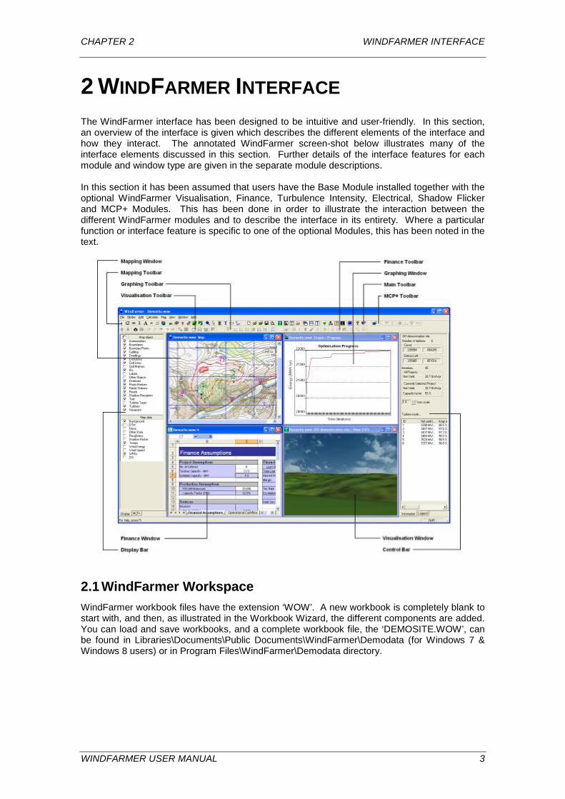
2 WINDFARMER INTERFACE The WindFarmer interface has been designed to be intuitive and user-friendly. In this section, an overview of the interface is given which describes the different elements of the interface and how they interact. The annotated WindFarmer screen-shot below illustrates many of the interface elements discussed in this section. Further details of the interface features for each module and window type are given in the separate module descriptions. In this section it has been assumed that users have the Base Module installed together with the optional WindFarmer Visualisation, Finance, Turbulence Intensity, Electrical, Shadow Flicker and MCP+ Modules. This has been done in order to illustrate the interaction between the different WindFarmer modules and to describe the interface in its entirety. Where a particular function or interface feature is specific to one of the optional Modules, this has been noted in the text.
2.1 WindFarmer Workspace WindFarmer workbook files have the extension ‘WOW’. A new workbook is completely blank to start with, and then, as illustrated in the Workbook Wizard, the different components are added. You can load and save workbooks, and a complete workbook file, the ‘DEMOSITE.WOW’, can be found in Libraries\Documents\Public Documents\WindFarmer\Demodata (for Windows 7 & Windows 8 users) or in Program Files\WindFarmer\Demodata directory.
WINDFARMER USER MANUAL 3
CHAPTER 2 WINDFARMER INTERFACE
WindFarmer requires the extents of a workspace to be defined so that positions can be referenced. This can be introduced in any one of four ways or by a combination of the four:
1. Load a Terrain Contour File, using File Menu, Load File or the green folder icon. Once loaded this file can be displayed by checking the “Terrain” tick box in the Display Bar. This method can be used for other types of contour file, with different file extension.
2. Load an image of the area. This could be a scanned map or aerial photograph of any type. These can be particularly useful for identifying ground features and placing design objects. This can be displayed by checking the “Background” tick box in the Display Bar.
3. Load a Terrain Grid File. This is required for using the visualisation options in WindFarmer Design Studio. The data can be displayed by checking the “DTM” tick box in the Display Bar. This method can be used for other types of DTM maps.
4. The co-ordinates of the workspace can be specified independently of any files being loaded. In this way it is possible to load a DTM covering a large area for visualisation purposes, while limiting the area over which, for instance, noise contours are calculated. To specify the co-ordinates of the workspace directly, select View menu, Workspace extents.
Once a wind farm has been designed, it can be saved through the File Menu. It will be saved as a *.WOW (WindFarmer workbook) file which contains all the information on the wind farm. It can be opened again at a later date for further modification. If required, WOW files can be saved in compressed format by ticking the box ‘Compress wow file on save’ in the Preferences page of the Control Panel. The workbook file then takes longer to save and to re-open but the size of the stored WOW file is reduced. The default is for the compression option to be switched off. How to load individual files and data is discussed in the individual module descriptions. To start with, the best way to build a simple workbook is to follow the Workbook Wizard which appears on the screen when WindFarmer is launched. This runs through step by step building a basic workbook. You can also call the Workbook Wizard from the File Menu, or refer to the Tutorials.
2.2 Window Types and Associated Toolbars In WindFarmer there are five distinct types of window that can be displayed and used. These are Mapping Window, Visualisation Window, Finance Window, Graphing Window and MCP+ Window. The Mapping and Graphing windows are integral to the Base Module, whilst the Visualisation, Finance and MCP+ windows require the Visualisation, Finance and MCP+ Modules. Each of these window types has its own menu and toolbar associated with it. The window specific menus and toolbars are only accessible when a window of the correct type is active (i.e. highlighted). If required, toolbars can be hidden using the View menu.
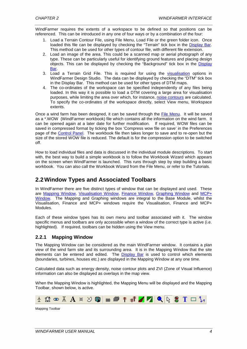
2.2.1 Mapping Window The Mapping Window can be considered as the main WindFarmer window. It contains a plan view of the wind farm site and its surrounding area. It is in the Mapping Window that the site elements can be entered and edited. The Display Bar is used to control which elements (boundaries, turbines, houses etc.) are displayed in the Mapping Window at any one time. Calculated data such as energy density, noise contour plots and ZVI (Zone of Visual Influence) information can also be displayed as overlays in the map view. When the Mapping Window is highlighted, the Mapping Menu will be displayed and the Mapping Toolbar, shown below, is active.
Mapping Toolbar
WINDFARMER USER MANUAL 4
CHAPTER 2 WINDFARMER INTERFACE
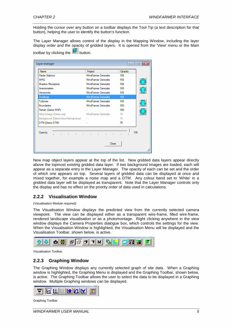
Holding the cursor over any button on a toolbar displays the Tool Tip (a text description for that button), helping the user to identify the button’s function. The Layer Manager allows control of the display in the Mapping Window, including the layer display order and the opacity of gridded layers. It is opened from the 'View' menu or the Main
toolbar by clicking the button.
New map object layers appear at the top of the list. New gridded data layers appear directly above the topmost existing gridded data layer. If two background images are loaded, each will appear as a separate entry in the Layer Manager. The opacity of each can be set and the order of which one appears on top. Several layers of gridded data can be displayed at once and mixed together, for example a noise map and a DTM. Any colour band set to 'White' in a gridded data layer will be displayed as transparent. Note that the Layer Manager controls only the display and has no effect on the priority order of data used in calculations.
2.2.2 Visualisation Window (Visualisation Module required)
The Visualisation Window displays the predicted view from the currently selected camera viewpoint. The view can be displayed either as a transparent wire-frame, filled wire-frame, rendered landscape visualisation or as a photomontage. Right clicking anywhere in the view window displays the Camera Properties dialogue box, which controls the settings for the view. When the Visualisation Window is highlighted, the Visualisation Menu will be displayed and the Visualisation Toolbar, shown below, is active.
Visualisation Toolbar
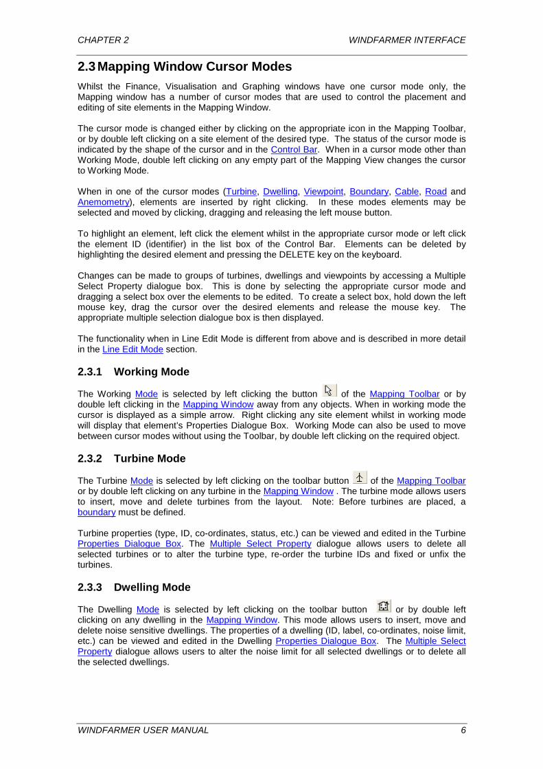
2.2.3 Graphing Window The Graphing Window displays any currently selected graph of site data. When a Graphing window is highlighted, the Graphing Menu is displayed and the Graphing Toolbar, shown below, is active. The Graphing Toolbar allows the user to select the data to be displayed in a Graphing window. Multiple Graphing windows can be displayed.
Graphing Toolbar
WINDFARMER USER MANUAL 5
CHAPTER 2 WINDFARMER INTERFACE
2.3 Mapping Window Cursor Modes Whilst the Finance, Visualisation and Graphing windows have one cursor mode only, the Mapping window has a number of cursor modes that are used to control the placement and editing of site elements in the Mapping Window. The cursor mode is changed either by clicking on the appropriate icon in the Mapping Toolbar, or by double left clicking on a site element of the desired type. The status of the cursor mode is indicated by the shape of the cursor and in the Control Bar. When in a cursor mode other than Working Mode, double left clicking on any empty part of the Mapping View changes the cursor to Working Mode. When in one of the cursor modes (Turbine, Dwelling, Viewpoint, Boundary, Cable, Road and Anemometry), elements are inserted by right clicking. In these modes elements may be selected and moved by clicking, dragging and releasing the left mouse button. To highlight an element, left click the element whilst in the appropriate cursor mode or left click the element ID (identifier) in the list box of the Control Bar. Elements can be deleted by highlighting the desired element and pressing the DELETE key on the keyboard. Changes can be made to groups of turbines, dwellings and viewpoints by accessing a Multiple Select Property dialogue box. This is done by selecting the appropriate cursor mode and dragging a select box over the elements to be edited. To create a select box, hold down the left mouse key, drag the cursor over the desired elements and release the mouse key. The appropriate multiple selection dialogue box is then displayed. The functionality when in Line Edit Mode is different from above and is described in more detail in the Line Edit Mode section.
2.3.1 Working Mode
The Working Mode is selected by left clicking the button of the Mapping Toolbar or by double left clicking in the Mapping Window away from any objects. When in working mode the cursor is displayed as a simple arrow. Right clicking any site element whilst in working mode will display that element’s Properties Dialogue Box. Working Mode can also be used to move between cursor modes without using the Toolbar, by double left clicking on the required object.
2.3.2 Turbine Mode
The Turbine Mode is selected by left clicking on the toolbar button of the Mapping Toolbar or by double left clicking on any turbine in the Mapping Window . The turbine mode allows users to insert, move and delete turbines from the layout. Note: Before turbines are placed, a boundary must be defined. Turbine properties (type, ID, co-ordinates, status, etc.) can be viewed and edited in the Turbine Properties Dialogue Box. The Multiple Select Property dialogue allows users to delete all selected turbines or to alter the turbine type, re-order the turbine IDs and fixed or unfix the turbines.
2.3.3 Dwelling Mode
The Dwelling Mode is selected by left clicking on the toolbar button or by double left clicking on any dwelling in the Mapping Window. This mode allows users to insert, move and delete noise sensitive dwellings. The properties of a dwelling (ID, label, co-ordinates, noise limit, etc.) can be viewed and edited in the Dwelling Properties Dialogue Box. The Multiple Select Property dialogue allows users to alter the noise limit for all selected dwellings or to delete all the selected dwellings.
WINDFARMER USER MANUAL 6
CHAPTER 2 WINDFARMER INTERFACE
2.3.4 Boundary Mode The Boundary Mode allows users to insert, move and delete site boundaries. Boundary properties (designation/label, co-ordinates, number of turbines, boundary type and minimum distance etc.) can be viewed and edited in the Boundary Properties Dialogue Box
It should be noted that there are two boundary modes: one for inserting new boundaries
and one for editing existing boundaries .
2.3.5 Viewpoint Mode (Visualisation Module required)
The Viewpoint Mode is selected by left clicking on the toolbar button or by double left clicking on any viewpoint in the Mapping Window. This mode allows users to insert, move and delete camera viewpoints. Viewpoint/camera properties (label, viewpoint co-ordinates, target co-ordinates, camera attributes) can be viewed and edited in the Camera Properties Dialogue Box. The Multiple Select Property dialogue allows users to alter a number of properties of all the selected viewpoints. (height settings for viewpoint and target, focal length, …).
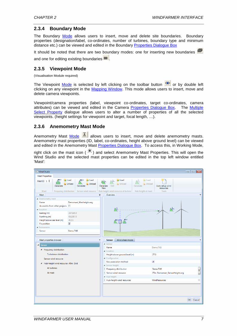
2.3.6 Anemometry Mast Mode
Anemometry Mast Mode allows users to insert, move and delete anemometry masts. Anemometry mast properties (ID, label, co-ordinates, height above ground level) can be viewed and edited in the Anemometry Mast Properties Dialogue Box. To access this, in Working Mode,
right click on the mast icon ( ) and select Anemometry Mast Properties. This will open the Wind Studio and the selected mast properties can be edited in the top left window entitled 'Mast':
WINDFARMER USER MANUAL 7
CHAPTER 2 WINDFARMER INTERFACE
Information on the wind regime is provided for each floating mast (a mast which is not spatially fixed). For each wind resource grid present above the mast location, information is given on the wind resource, TAB file (if associated), hub-height and mean free wind speed. For the wake affected wind speed to be calculated, you need to run an energy Test first. See the Wind Studio section for more details.
2.3.7 Text Label Mode
Text Label Mode allows users to insert, move and delete text labels. Text label properties (co-ordinates, text string, justification, font) can be viewed and edited in the Text Object Properties Dialogue Box.
2.3.8 Photo Marker Mode (Visualisation Module required)
Photo Marker Mode allows users to insert, move and delete reference markers, to assist in fitting photomontages. Photomontage marker properties (ID, label, co-ordinates, height) can be viewed and edited in the Photo Markers Properties Dialogue Box.
2.3.9 Shadow Receptor Mode (Shadow Flicker Module required)
Shadow Receptor Mode allows users to insert, move and delete locations for providing shadow flicker information. Shadow receptor properties (ID, label, co-ordinates and attributes) can be viewed and edited in the Shadow Receptor Properties Dialogue Box.
2.3.10 Road Mode Road Mode allows users to insert, move and delete site road/track layouts. Road properties (node ID, co-ordinates, width, road surface) can be viewed and edited in the Site Track Properties Dialogue Box. The length and type of the tracks are available as parameters in the Financial Module It should be noted that there are two road modes: one for inserting new roads
and one for editing existing roads .
2.3.11 Cabling Mode Cabling Mode allows users to insert, move and delete underground and overhead cable layouts. Cable properties can be viewed and edited in the Cable Line Properties dialogue box. The length and type of cables and nodes are available as parameters in the Financial Module.
It should be noted that there are two cable modes: one for inserting new cables and one
for editing existing cables .
2.3.12 Zoom Mode
The Zoom Mode allows users to zoom in and out of the Mapping View. A left mouse button click increases the magnification in the mapping window so that one click takes the magnification to 2:1 and fourteen clicks takes the magnification to 15:1. Clicking the Right mouse button zooms out in a similar manner. To zoom to a specific area, left click and drag a box over the extents you wish to appear in the Mapping View.
2.3.13 Radar Mode (Visualisation Module required)
Radar Mode allows users to insert, move and delete radar stations. Radar stations properties (label, associated viewpoint attributes, minimum radar elevation etc.) can be viewed and edited in the Radar Station Properties Dialogue Box.
WINDFARMER USER MANUAL 8
CHAPTER 2 WINDFARMER INTERFACE
2.3.14 Crop Mode
Crop Mode allows users to select an area of the Mapping View and delete the surrounding image to these new dimensions. Left click and drag brings up a window with the coordinates of the area to be cropped. These can then be edited before the crop is carried out. The crop tool operates on DTM, MAP and background BMP files only, not on inserted objects, and it only operates if they are visible in the Mapping View through checking the relevant Display Bar box. The cropped files can be saved through the Export option of the File Menu. Note that the crop action cannot be undone.
2.3.15 Line Edit Mode
Height and roughness contours can be created and edited in the Line Edit Mode . When selecting the Line Edit Mode in the Mapping Toolbar you are prompted to select “Terrain height” or “Roughness”, as the type of line you want to edit or create. The corresponding data layer is displayed in the Mapping Window. To exit the Line Edit Mode, switch to a different cursor mode.
Adding new lines
Method 1: If there are not yet any lines in your project, in Line Edit mode left click in the Mapping Window to define the first point of the line. Press OK to confirm you want to create a line and press “Apply” to set the first point. Method 2: When lines already exist, left click on any line to show the Line Edit menu. Select Edit Point -> New line. Add the points as in Method 1. The new line inherits the attributes of the currently selected line.
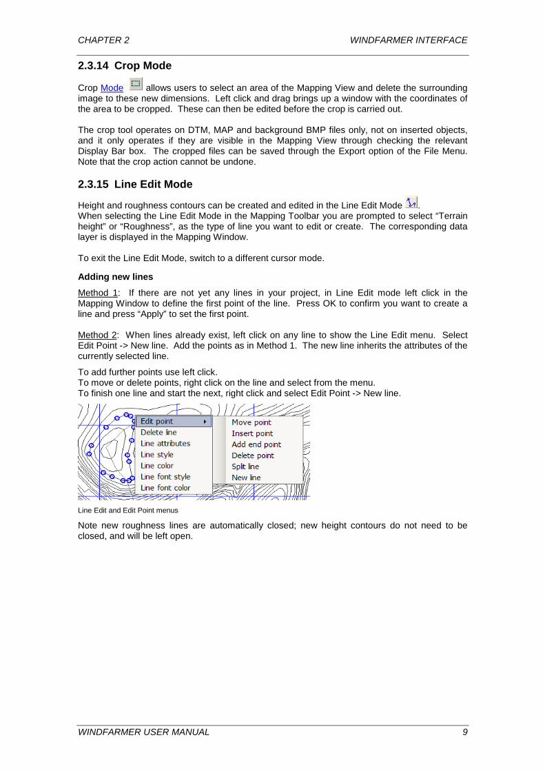
To add further points use left click. To move or delete points, right click on the line and select from the menu. To finish one line and start the next, right click and select Edit Point -> New line.
Line Edit and Edit Point menus
Note new roughness lines are automatically closed; new height contours do not need to be closed, and will be left open.
WINDFARMER USER MANUAL 9
CHAPTER 2 WINDFARMER INTERFACE
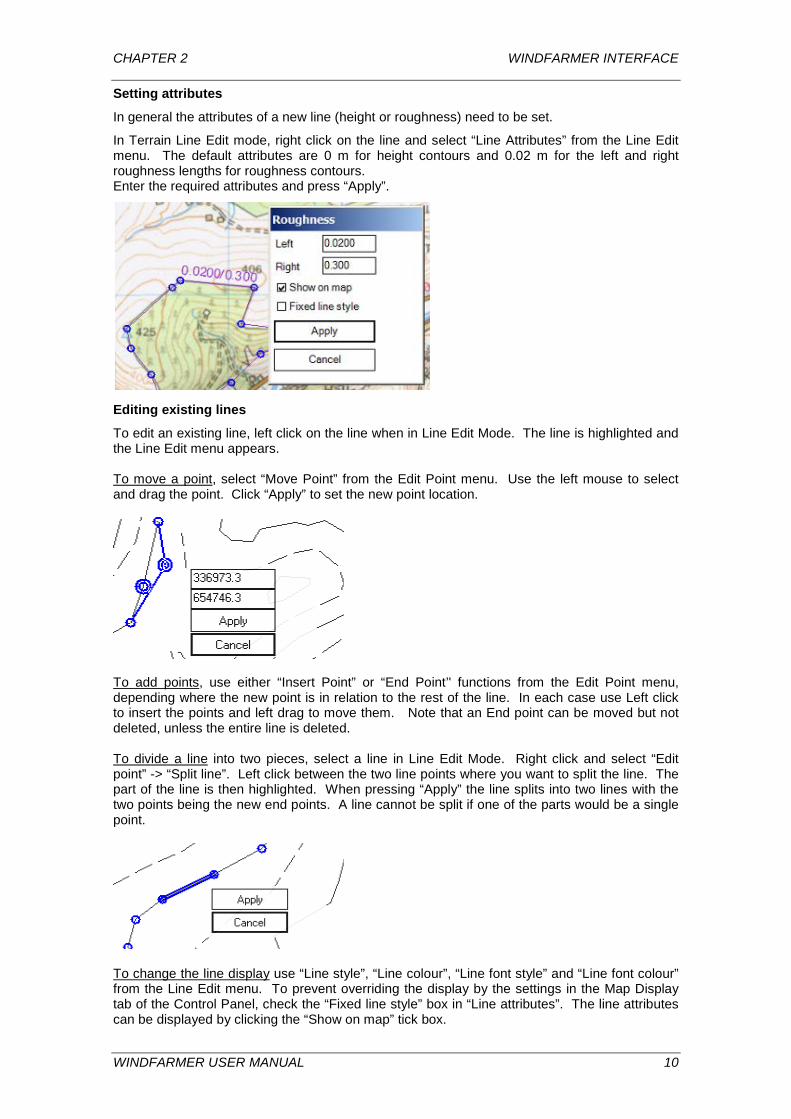
Setting attributes
In general the attributes of a new line (height or roughness) need to be set.
In Terrain Line Edit mode, right click on the line and select “Line Attributes” from the Line Edit menu. The default attributes are 0 m for height contours and 0.02 m for the left and right roughness lengths for roughness contours. Enter the required attributes and press “Apply”.
Editing existing lines
To edit an existing line, left click on the line when in Line Edit Mode. The line is highlighted and the Line Edit menu appears. To move a point, select “Move Point” from the Edit Point menu. Use the left mouse to select and drag the point. Click “Apply” to set the new point location.
To add points, use either “Insert Point” or “End Point’' functions from the Edit Point menu, depending where the new point is in relation to the rest of the line. In each case use Left click to insert the points and left drag to move them. Note that an End point can be moved but not deleted, unless the entire line is deleted. To divide a line into two pieces, select a line in Line Edit Mode. Right click and select “Edit point” -> “Split line”. Left click between the two line points where you want to split the line. The part of the line is then highlighted. When pressing “Apply” the line splits into two lines with the two points being the new end points. A line cannot be split if one of the parts would be a single point.
To change the line display use “Line style”, “Line colour”, “Line font style” and “Line font colour” from the Line Edit menu. To prevent overriding the display by the settings in the Map Display tab of the Control Panel, check the “Fixed line style” box in “Line attributes”. The line attributes can be displayed by clicking the “Show on map” tick box.
WINDFARMER USER MANUAL 10
CHAPTER 2 WINDFARMER INTERFACE
2.4 Display, Control and Status Bar The Display Bar and the Control Bar are Information Bars. All Information Bars are dockable and can be turned on and off through the View menu. However, if you are using two monitor screens, it is recommended to bring all the WindFarmer displays to the original screen before reverting to single screen use.
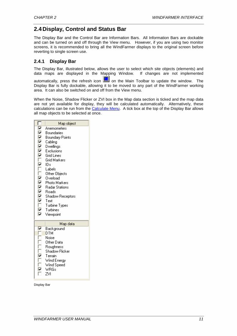
2.4.1 Display Bar The Display Bar, illustrated below, allows the user to select which site objects (elements) and data maps are displayed in the Mapping Window. If changes are not implemented
automatically, press the refresh icon on the Main Toolbar to update the window. The Display Bar is fully dockable, allowing it to be moved to any part of the WindFarmer working area. It can also be switched on and off from the View menu. When the Noise, Shadow Flicker or ZVI box in the Map data section is ticked and the map data are not yet available for display, they will be calculated automatically. Alternatively, these calculations can be run from the Calculate Menu. A tick box at the top of the Display Bar allows all map objects to be selected at once.
Display Bar
WINDFARMER USER MANUAL 11
CHAPTER 2 WINDFARMER INTERFACE
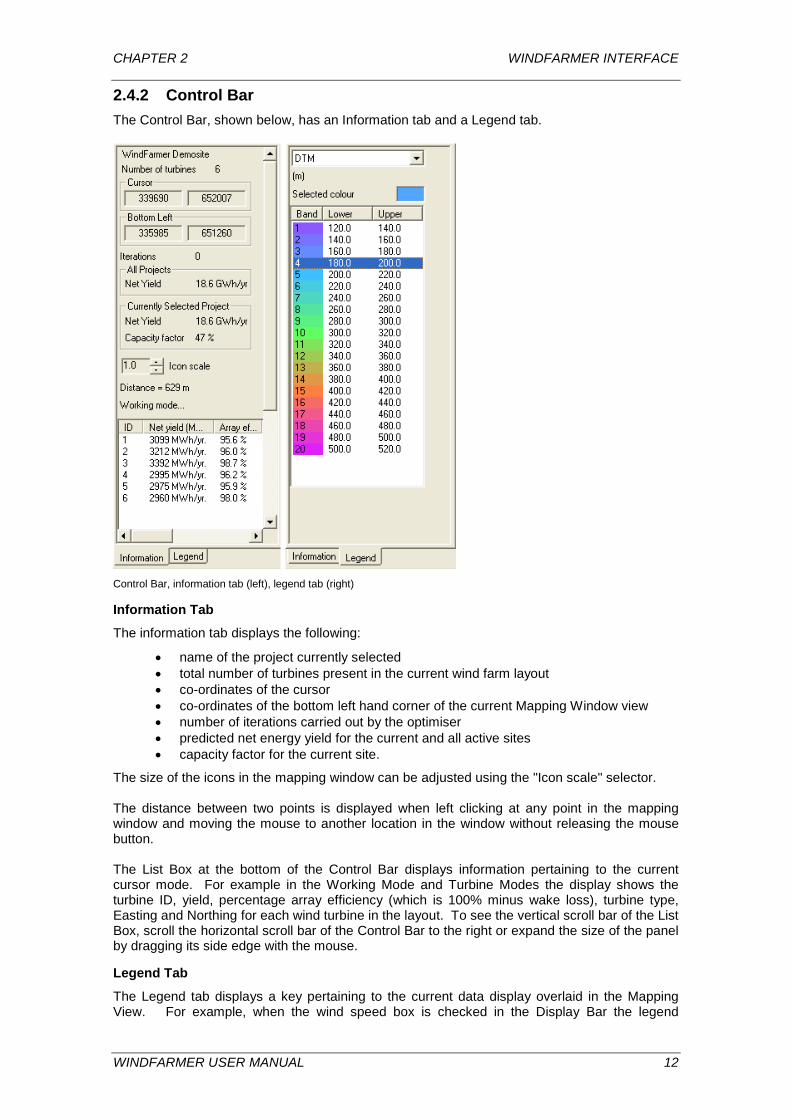
2.4.2 Control Bar The Control Bar, shown below, has an Information tab and a Legend tab.
Control Bar, information tab (left), legend tab (right)
Information Tab
The information tab displays the following:
• name of the project currently selected • total number of turbines present in the current wind farm layout • co-ordinates of the cursor • co-ordinates of the bottom left hand corner of the current Mapping Window view • number of iterations carried out by the optimiser • predicted net energy yield for the current and all active sites • capacity factor for the current site.
The size of the icons in the mapping window can be adjusted using the "Icon scale" selector. The distance between two points is displayed when left clicking at any point in the mapping window and moving the mouse to another location in the window without releasing the mouse button. The List Box at the bottom of the Control Bar displays information pertaining to the current cursor mode. For example in the Working Mode and Turbine Modes the display shows the turbine ID, yield, percentage array efficiency (which is 100% minus wake loss), turbine type, Easting and Northing for each wind turbine in the layout. To see the vertical scroll bar of the List Box, scroll the horizontal scroll bar of the Control Bar to the right or expand the size of the panel by dragging its side edge with the mouse.
Legend Tab
The Legend tab displays a key pertaining to the current data display overlaid in the Mapping View. For example, when the wind speed box is checked in the Display Bar the legend
WINDFARMER USER MANUAL 12
CHAPTER 2 WINDFARMER INTERFACE
contains the colour assigned to each wind speed range. Only a single legend can be displayed at a time. To select the legend for a specific layer, use the dropdown box above the legend. You can change the colour display, and save the settings into a BAN file which can be exported and imported into a different workbook. Double clicking anywhere in the text of the Legend window opens the bands setting window. This window is also accessed from the Control Panel, Map Data area wherever Band Settings is displayed.
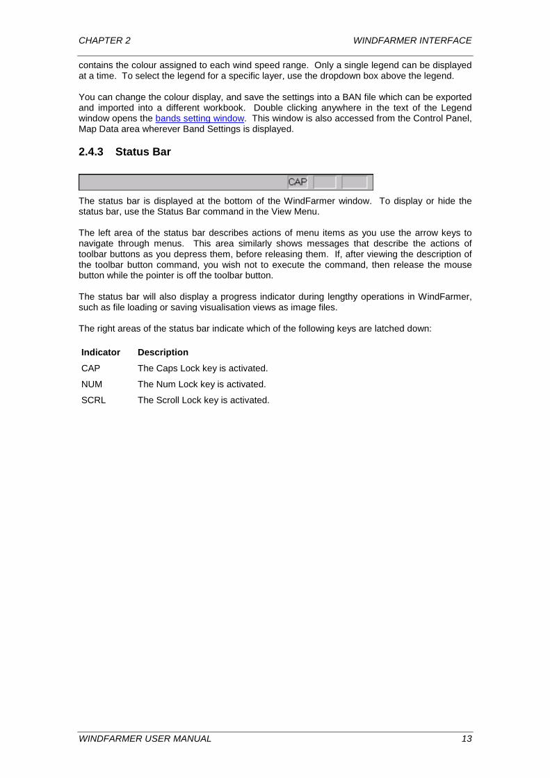
2.4.3 Status Bar
The status bar is displayed at the bottom of the WindFarmer window. To display or hide the status bar, use the Status Bar command in the View Menu. The left area of the status bar describes actions of menu items as you use the arrow keys to navigate through menus. This area similarly shows messages that describe the actions of toolbar buttons as you depress them, before releasing them. If, after viewing the description of the toolbar button command, you wish not to execute the command, then release the mouse button while the pointer is off the toolbar button. The status bar will also display a progress indicator during lengthy operations in WindFarmer, such as file loading or saving visualisation views as image files. The right areas of the status bar indicate which of the following keys are latched down: Indicator Description
CAP The Caps Lock key is activated.
NUM The Num Lock key is activated.
SCRL The Scroll Lock key is activated.
WINDFARMER USER MANUAL 13
CHAPTER 3 BASE MODULE
3 BASE MODULE The WindFarmer Base Module contains the core wind farm layout design and optimisation tools, including the wind farm energy calculation, noise modelling and turbine layout optimisation functions. Also featured in the Base Module are the WindFarmer Control Panel, the Turbine Studio, full data graphing facilities, file import and export functions, report generation and the interface control options.
3.1 Base Module Interface
3.1.1 Windows There are two windows associated with the Base Module: the Mapping window and the Graphing window.
3.1.1.1 Mapping Window
The Mapping Window displays a plan view of the working area. This plan view may consist of the following elements:
• digital contour map • digital terrain model (DTM) • background image • site boundaries • exclusion zone boundaries • photo markers • shadow receptors • wind turbine positions • house positions • viewpoint positions • radar stations • anemometry mast positions • wind resource file boundaries • map grid lines
All of these elements may be displayed or hidden by ticking the appropriate elements on or off in the Display Bar. Object ID and label display as well as the turbine type display can be switched on and off using the appropriate boxes in the Map object section. The size of icons in the Mapping Window can be changed using the Icon Scale feature in the middle of the Information tab of the Control Bar. Colour displays of ground heights (DTM), wind energy density and wind speed can be superimposed on the Map View by ticking the appropriate boxes in the Display Bar. The display parameters, including an option to display ground slope instead of height, can be selected in the Map Data page of the Control Panel. Display parameters can also be accessed through the Legend tab of the Control Bar. Please see Control Bar for further details. The Layer Manager allows control of the display in the Mapping Window, including the layer display order and the opacity of gridded layers. A list of digital contour and raster data and background image files can be inspected and unloaded from the workbook. This is done through the Workbook Files page in the Control Panel. Note that the Wind Energy map is read directly from the WRG file, whereas the Wind Speed map requires a calculation to have been performed and may therefore take a longer time to be displayed.
WINDFARMER USER MANUAL 14
CHAPTER 3 BASE MODULE
3.1.1.2 Graphing window
The Graphing Window is opened by selecting New Graph Window under the Window Menu. It is utilised to display any of the WindFarmer outputs and results in graphical form. A number of pre-set graph formats, selected through the Graphing Toolbar or through the View Menu (while the Graph Window is active), can be used for plotting:
• wind roses • optimisation progress charts • energy yield and wake losses by turbine or by sector • noise levels and limits at houses • power and thrust curves • design turbulence intensity vs wind speed (Turbulence Module required) • shadow flicker at receptors (Shadow Flicker Module required)
The wind rose requires a notional anemometry mast to be placed in the Mapping Window, and displays wind speed and direction information directly from the wind resource grid at the grid height. However, if a mast has been loaded using the association method, then the wind rose displayed will be at the mast location and height.
3.1.2 Toolbars Three toolbars are associated with the Base Module: the Main Toolbar, the Mapping Toolbar and the Graphing Toolbar.
3.1.2.1 Main Toolbar
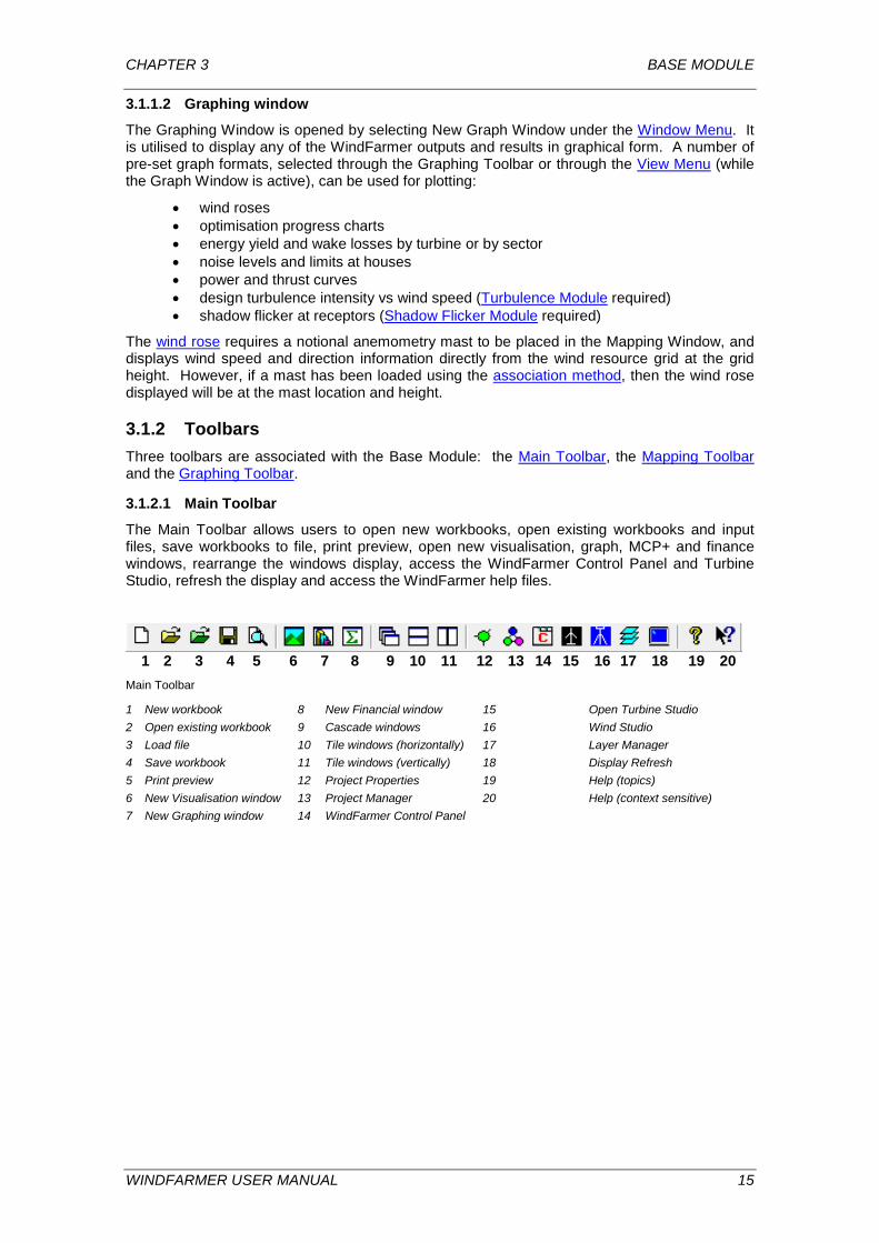
The Main Toolbar allows users to open new workbooks, open existing workbooks and input files, save workbooks to file, print preview, open new visualisation, graph, MCP+ and finance windows, rearrange the windows display, access the WindFarmer Control Panel and Turbine Studio, refresh the display and access the WindFarmer help files.
1 2 3 4 5 6 7 8 9 10 11 12 13 14 15 16 17 18 19 20
Main Toolbar
1 New workbook 8 New Financial window 15 Open Turbine Studio 2 Open existing workbook 9 Cascade windows 16 Wind Studio 3 Load file 10 Tile windows (horizontally) 17 Layer Manager 4 Save workbook 11 Tile windows (vertically) 18 Display Refresh 5 Print preview 12 Project Properties 19 Help (topics) 6 New Visualisation window 13 Project Manager 20 Help (context sensitive) 7 New Graphing window 14 WindFarmer Control Panel
WINDFARMER USER MANUAL 15
CHAPTER 3 BASE MODULE
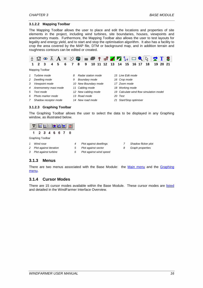
3.1.2.2 Mapping Toolbar
The Mapping Toolbar allows the user to place and edit the locations and properties of site elements in the project, including wind turbines, site boundaries, houses, viewpoints and anemometry masts. Furthermore, the Mapping Toolbar also allows the user to test layouts for legality and energy yield, and to start and stop the optimisation algorithm. It also has a facility to crop the area covered by the MAP file, DTM or background map, and in addition terrain and roughness contours can be edited or created.
1 2 3 4 5 6 7 8 9 10 11 12 13 14 15 16 17 18 19 20 21
Mapping Toolbar
1 Turbine mode 8 Radar station mode 15 Line Edit mode 2 Dwelling mode 9 Boundary mode 16 Crop mode 3 Viewpoint mode 10 New Boundary mode 17 Zoom mode 4 Anemometry mast mode 11 Cabling mode 18 Working mode 5 Text mode 12 New cabling mode 19 Calculate wind flow simulation model 6 Photo marker mode 13 Road mode 20 Test 7 Shadow receptor mode 14 New road mode 21 Start/Stop optimiser
3.1.2.3 Graphing Toolbar
The Graphing Toolbar allows the user to select the data to be displayed in any Graphing window, as illustrated below.
Graphing Toolbar
1 Wind rose 4 Plot against dwellings 7 Shadow flicker plot 2 Plot against iteration 5 Plot against sector 8 Graph properties 3 Plot against turbine 6 Plot against wind speed
3.1.3 Menus There are two menus associated with the Base Module: the Main menu and the Graphing menu.
3.1.4 Cursor Modes There are 15 cursor modes available within the Base Module. These cursor modes are listed and detailed in the WindFarmer Interface Overview.
WINDFARMER USER MANUAL 16
CHAPTER 3 BASE MODULE
3.2 Input Files The contents and origin of the principal input files are explained in this section. Examples of each of these file types are provided in the WindFarmer Demodata directory. All of the following input files are loaded through the Load File dialogue box that is opened by
clicking the Load File button on the Main Toolbar, using File menu -> Load File, or using File menu -> Load Online Data. Turbine Files (*.TRB and *.POW or *.WTG) can also be loaded
from the Turbine Studio .
3.2.1 Map Data and Conversions Map information is used in WindFarmer for orientation of the workspace and as a backdrop. WindFarmer uses for this purpose background images or height contour files. Workspace extents are set automatically, but can be changed by entering coordinates through View menu, Workspace extents. An additional format of terrain data file, the digital terrain model, is required for use in the Visualisation Module and Shadow Flicker Module, and can be used for noise calculations in the Base Module and electrical network calculations in the Electrical Module. A digital terrain model can also be used to display graphically the terrain relief in the Mapping Window. Within the Base Module is the facility to convert height contours into a digital terrain model, and vice versa. Both formats can then be exported. The area of a digital terrain model or height contour file can be reduced through the crop feature, if required.
3.2.1.1 Background image files
Reference maps are used to provide a graphical background in the Map View. The maps can show anything from a scale map, showing height contours, roads, forests, towns and individual residences, to an ecology map or even an aerial photograph. Reference maps can prove to be very useful when working in the Map View as they contain a large amount of site information. The demonstration WindFarmer workbook (WOW) file contains a 1:50,000 scanned reference map. WindFarmer allows you to import a number of background image formats. The image file types that can be imported include:
• BMP • JPG, including geo-referenced JPG • PNG • TIF, including geo-referenced TIFF and GEO-TIFF
When image files like BMP, JPG, PNG and TIF are loaded and the corresponding "World file" exists at the same location, then the image is loaded without the need for manual geo-referencing. However, in general, when inputting a background image file, the user must geo-reference the image in order to locate it within the co-ordinate system in WindFarmer. Background images are loaded using File menu > Load File. During the loading process, the Image Rectifier allows you to associate the pixel coordinates of the image with coordinates in the Mapping Window. The process allows the image to be rotated and stretched to take into account any distortions.
WINDFARMER USER MANUAL 17
CHAPTER 3 BASE MODULE
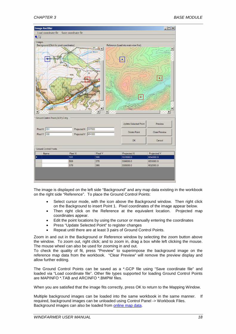
The image is displayed on the left side “Background” and any map data existing in the workbook on the right side “Reference”. To place the Ground Control Points:
• Select cursor mode, with the icon above the Background window. Then right click on the Background to insert Point 1. Pixel coordinates of the image appear below.
• Then right click on the Reference at the equivalent location. Projected map coordinates appear.
• Edit the point locations by using the cursor or manually entering the coordinates • Press “Update Selected Point” to register changes • Repeat until there are at least 3 pairs of Ground Control Points.
Zoom in and out in the Background or Reference window by selecting the zoom button above the window. To zoom out, right click; and to zoom in, drag a box while left clicking the mouse. The mouse wheel can also be used for zooming in and out. To check the quality of fit, press “Preview” to superimpose the background image on the reference map data from the workbook. “Clear Preview” will remove the preview display and allow further editing. The Ground Control Points can be saved as a *.GCP file using “Save coordinate file” and loaded via “Load coordinate file”. Other file types supported for loading Ground Control Points are MAPINFO *.TAB and ARCINFO *.BMPW files. When you are satisfied that the image fits correctly, press OK to return to the Mapping Window. Multiple background images can be loaded into the same workbook in the same manner. If required, background images can be unloaded using Control Panel -> Workbook Files. Background images can also be loaded from online map data.
WINDFARMER USER MANUAL 18

CHAPTER 3 BASE MODULE
3.2.1.2 MAP files (Contours)
Terrain data for input into the Base Module are contained in files with the extension MAP. The format of MAP files is the WAsP ASCII format (as opposed to the WAsP binary format) used in the WAsP wind flow analysis package. ASCII MAP files output by WAsP can be loaded directly into WindFarmer. ASCII MAP files are output from WAsP 4/5 using the command line DUM* in the OROgraphy menu. WAsP 6/7/8/9/10/11 users can use the "save as" option. For a full description of the ASCII WAsP MAP file format, please refer to the WAsP manual. The terrain data contained in a MAP file are used to define the workspace extents and its co-ordinate system. The terrain contours can also be used as a graphical backdrop in the Map View. MAP files can originate from several sources which are country specific. Normally the most accurate are those purchased directly as pre-digitised contour files which may require only minor conversion of headers. Alternatively they can be converted from DTM files using the Map Format Converter within WindFarmer. If no pre-digitised data are available, MAP files can be created in WindFarmer by digitising contour lines from a paper map. This method can be time consuming and laborious, although there is often no alternative where pre-digitised data are not available.
3.2.1.3 Import contour data
A much quicker method of creating a contour file is to purchase pre-digitised data from a national mapping authority. It is possible to buy pre-digitised contour data for many countries, although formats do differ significantly from country to country. WindFarmer allows you to import a number of contour formats: use File Menu > Load File, for importing contour data formats. The contour file types that can be imported include:
• NTF contour files (United Kingdom, Ireland) • DXF contour files (International) • DWG contour files (international) • ASCII MAP files (International) • SHP contour files (International)
If you are missing a specific file format, please let the WindFarmer support team know. We are working to expand this list for you. When loading more than one contour file the new files will be appended to the existing ones. Imported contour lines can be edited in the Line Edit Mode. Contour data can also be loaded from online map data.
3.2.1.4 DTM Digital Terrain Model data
DTM files contain spot-heights above sea level on a regular grid, with a grid resolution typically around 50 m. They are necessary in WindFarmer for the Visualisation Module and the Shadow Flicker Module. The data can also be used for noise calculations and Electrical Module calculations, as well as a visual backdrop in the Mapping Window where the relief is shaded. DTM’s can be converted within WindFarmer from MAP and WRG files as described below. Other sources of DTM data are covered in greater detail in the Visualisation Module.
WINDFARMER USER MANUAL 19
CHAPTER 3 BASE MODULE
3.2.1.5 Import DTM data
WindFarmer allows you to import a number of DTM formats: use File Menu > Load File, for importing DTM data. The DTM file types that can be imported include:
• NTF DTM files (United Kingdom, Ireland) • NTF Meridian2 format (United Kingdom) • SDTS, DEM files (USA) • Northwood or Surfer GRD files (International). • DGM50, DGM250 (Germany) • XYZ ASCII Import Wizard (International) • SRTM files in *.HGT, *.BIL or *.DT1 formats (International)
If you are missing a specific file format, please let the WindFarmer Support Team know. We are working to expand this list for you. When overlapping elevation grid files are loaded, the first file loaded has the highest priority and is employed in calculations that use elevation grid data, e.g. noise, ZVI and shadow flicker. When the grid files have different resolutions then all grids will be interpolated to match the file with the highest resolution. DTM data can also be loaded from online map data.
3.2.1.6 Map Format Converter
In the Mapping Window, Map menu several options for map data conversions are provided:
• MAP2DTM • WRG2DTM • DTM2MAP
These allow MAP files to be converted to *.DTM files, and vice versa through interpolation routines. The extraction of DTM data from WRG grid files is a further option. After conversion both the original and new files are retained within the workbook. To save the newly created files, use the File Menu > Export Mapping options. Please note that each conversion of map formats causes loss of information and should therefore be avoided where possible. It is essential that you check after the conversion that it was successful and no important detail has been lost in the process. To reduce the conversion time, it may be useful to crop the file before converting.
3.2.1.7 Map data projections
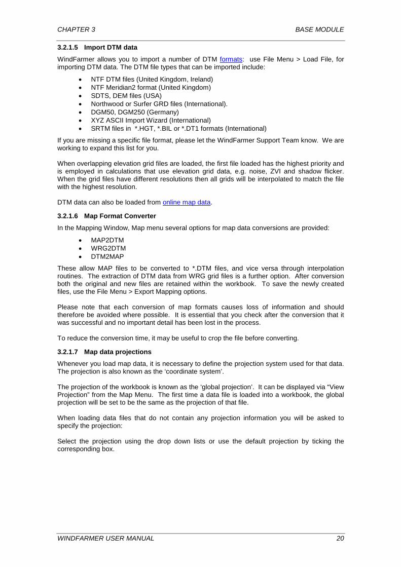
Whenever you load map data, it is necessary to define the projection system used for that data. The projection is also known as the ‘coordinate system’. The projection of the workbook is known as the ‘global projection’. It can be displayed via “View Projection” from the Map Menu. The first time a data file is loaded into a workbook, the global projection will be set to be the same as the projection of that file. When loading data files that do not contain any projection information you will be asked to specify the projection: Select the projection using the drop down lists or use the default projection by ticking the corresponding box.
WINDFARMER USER MANUAL 20
CHAPTER 3 BASE MODULE
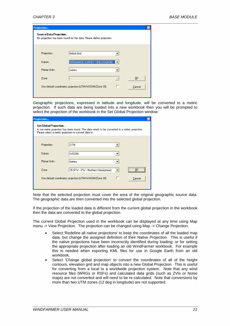
Geographic projections, expressed in latitude and longitude, will be converted to a metric projection. If such data are being loaded into a new workbook then you will be prompted to select the projection of the workbook in the Set Global Projection window:
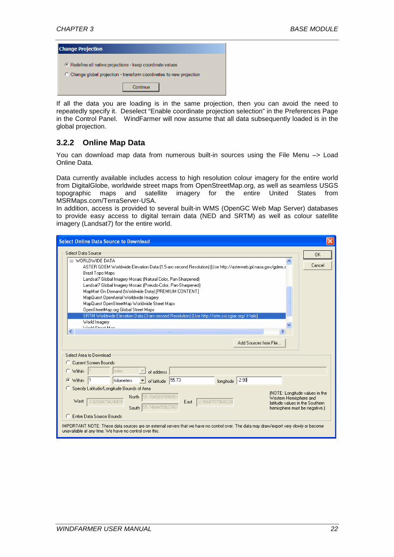
Note that the selected projection must cover the area of the original geographic source data. The geographic data are then converted into the selected global projection. If the projection of the loaded data is different from the current global projection in the workbook then the data are converted to the global projection. The current Global Projection used in the workbook can be displayed at any time using Map menu -> View Projection. The projection can be changed using Map -> Change Projection.
• Select 'Redefine all native projections' to keep the coordinates of all the loaded map data, but change the assigned definition of their Native Projection. This is useful if the native projections have been incorrectly identified during loading; or for setting the appropriate projection after loading an old WindFarmer workbook. For example this is needed when exporting KML files for use in Google Earth from an old workbook.
• Select 'Change global projection' to convert the coordinates of all of the height contours, elevation grid and map objects into a new Global Projection. This is useful for converting from a local to a worldwide projection system. Note that any wind resource files (WRGs or RSFs) and calculated data grids (such as ZVIs or Noise maps) are not converted and will need to be re-calculated. Note that conversions by more than two UTM zones (12 deg in longitude) are not supported.
WINDFARMER USER MANUAL 21
CHAPTER 3 BASE MODULE
If all the data you are loading is in the same projection, then you can avoid the need to repeatedly specify it. Deselect “Enable coordinate projection selection” in the Preferences Page in the Control Panel. WindFarmer will now assume that all data subsequently loaded is in the global projection.
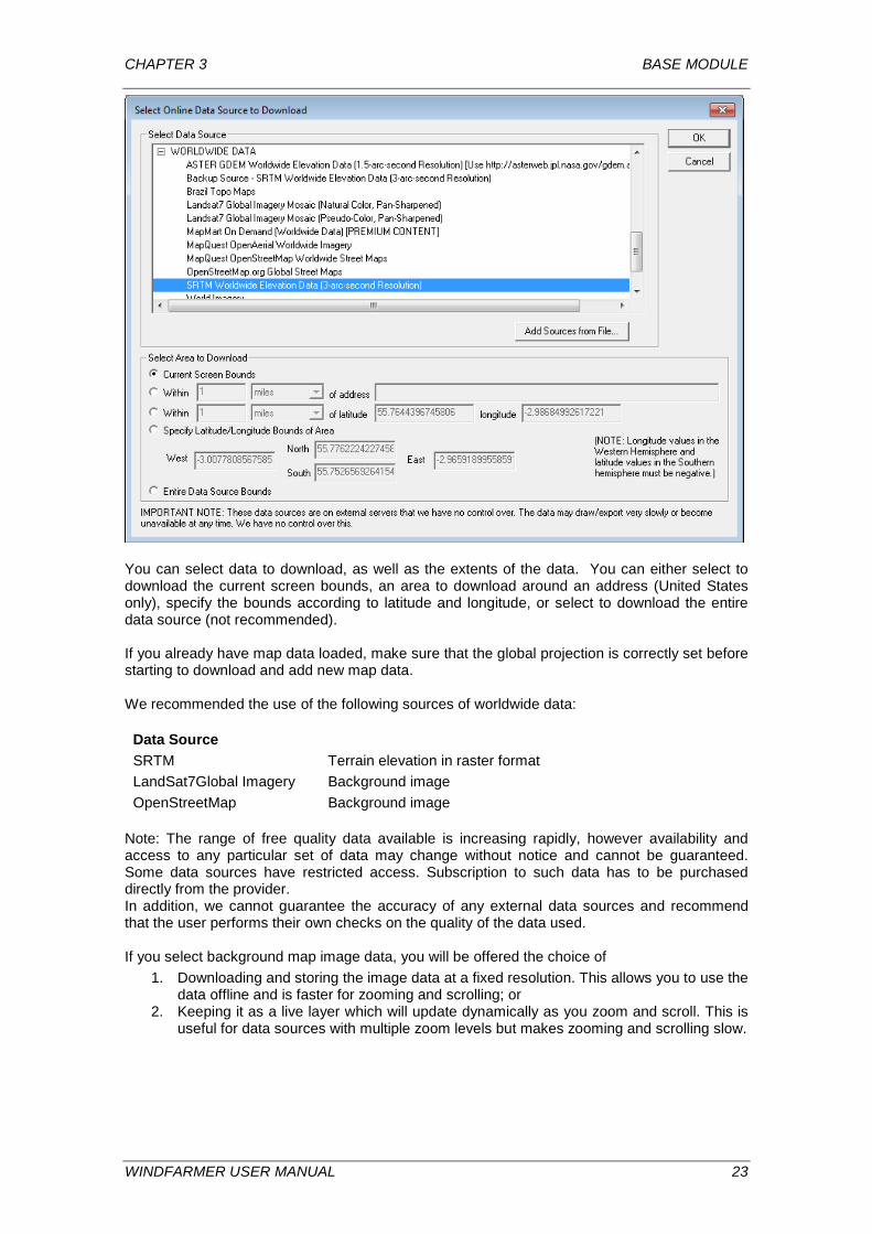
3.2.2 Online Map Data You can download map data from numerous built-in sources using the File Menu –> Load Online Data. Data currently available includes access to high resolution colour imagery for the entire world from DigitalGlobe, worldwide street maps from OpenStreetMap.org, as well as seamless USGS topographic maps and satellite imagery for the entire United States from MSRMaps.com/TerraServer-USA. In addition, access is provided to several built-in WMS (OpenGC Web Map Server) databases to provide easy access to digital terrain data (NED and SRTM) as well as colour satellite imagery (Landsat7) for the entire world.
WINDFARMER USER MANUAL 22
CHAPTER 3 BASE MODULE
You can select data to download, as well as the extents of the data. You can either select to download the current screen bounds, an area to download around an address (United States only), specify the bounds according to latitude and longitude, or select to download the entire data source (not recommended). If you already have map data loaded, make sure that the global projection is correctly set before starting to download and add new map data. We recommended the use of the following sources of worldwide data:
Data Source SRTM Terrain elevation in raster format LandSat7Global Imagery Background image OpenStreetMap Background image
Note: The range of free quality data available is increasing rapidly, however availability and access to any particular set of data may change without notice and cannot be guaranteed. Some data sources have restricted access. Subscription to such data has to be purchased directly from the provider. In addition, we cannot guarantee the accuracy of any external data sources and recommend that the user performs their own checks on the quality of the data used. If you select background map image data, you will be offered the choice of
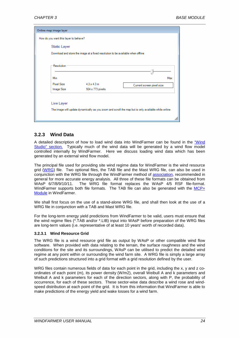
1. Downloading and storing the image data at a fixed resolution. This allows you to use the data offline and is faster for zooming and scrolling; or
2. Keeping it as a live layer which will update dynamically as you zoom and scroll. This is useful for data sources with multiple zoom levels but makes zooming and scrolling slow.
WINDFARMER USER MANUAL 23
CHAPTER 3 BASE MODULE
3.2.3 Wind Data A detailed description of how to load wind data into WindFarmer can be found in the “Wind Studio” section. Typically much of the wind data will be generated by a wind flow model controlled internally by WindFarmer. Here we discuss loading wind data which has been generated by an external wind flow model. The principal file used for providing site wind regime data for WindFarmer is the wind resource grid (WRG) file. Two optional files, the TAB file and the Mast WRG file, can also be used in conjunction with the WRG file through the WindFarmer method of association, recommended in general for more accurate energy analysis. All three of these file formats can be obtained from WAsP 6/7/8/9/10/11. The WRG file format replaces the WAsP 4/5 RSF file-format. WindFarmer supports both file formats. The TAB file can also be generated with the MCP+ Module in WindFarmer. We shall first focus on the use of a stand-alone WRG file, and shall then look at the use of a WRG file in conjunction with a TAB and Mast WRG file. For the long-term energy yield predictions from WindFarmer to be valid, users must ensure that the wind regime files (*.TAB and/or *.LIB) input into WAsP before preparation of the WRG files are long-term values (i.e. representative of at least 10 years' worth of recorded data).
3.2.3.1 Wind Resource Grid
The WRG file is a wind resource grid file as output by WAsP or other compatible wind flow software. When provided with data relating to the terrain, the surface roughness and the wind conditions for the site and its surroundings, WAsP can be utilised to predict the detailed wind regime at any point within or surrounding the wind farm site. A WRG file is simply a large array of such predictions structured into a grid format with a grid resolution defined by the user. WRG files contain numerous fields of data for each point in the grid, including the x, y and z co-ordinates of each point (m), its power density (W/m2), overall Weibull A and k parameters and Weibull A and k parameters for each of the direction sectors, along with P, the probability of occurrence, for each of these sectors. These sector-wise data describe a wind rose and wind-speed distribution at each point of the grid. It is from this information that WindFarmer is able to make predictions of the energy yield and wake losses for a wind farm.
WINDFARMER USER MANUAL 24

CHAPTER 3 BASE MODULE
3.2.3.2 Creation of WRG files
There are a few simple rules that should be observed by users when creating WRG files in WAsP for use in WindFarmer. The hierarchy structure in WAsP should contain as input a TAB file at the mast height and location, and a MAP file containing height and roughness contours extending typically to 10 or 20 km radius from the wind farm. Alternatively, a pre-calculated Atlas.LIB file and the MAP data can be used. A wind resource grid WRG is created in WAsP 6/7/8/9/10/11 by inserting a new wind resource grid into the hierarchy, defining its configuration and starting the calculation. Users of WAsP 4/5 should create a wind resource file (RSF) instead of a WRG file using the grid resource file option. WindFarmer calculates to an accuracy of 0.1m for the resolution of the grid. The WRG grid must cover the whole area that is available for turbine placement. The height above ground level at which the WRG is calculated must be within 0.5m of the hub-height of the wind turbine type to be analysed. Separate WRGs must be created for each hub height to be used in the wind farm. A single point WRG at the mast position may additionally be required. Furthermore, the WRG files should be created in WAsP without a WAsP format wind turbine power curve file (*.POW or *.WTG) being loaded.
3.2.3.3 Spatial resolution of the WRG file
A grid resolution of 10 to 25m is commonly used for the WRG, although the grid size is a compromise between file size and accuracy. Making the grid resolution coarser can lead to interpolation errors in moderately varying terrain, but will decrease run times and storage requirements. It should be noted that the turbine positions are not limited to the grid points of the WRG in WindFarmer. A turbine derives its wind regime by interpolating between the four nearest WRG grid points. A finer grid resolution reduces the impact of interpolation errors but can lead to very large WRG file sizes, which can be slow to load and run, and increased WAsP run-times. Where computer storage capacity and time permits, a 10m resolution is recommended. WRG files with a resolution of 10m have been shown to introduce negligible interpolation errors.
3.2.3.4 Multiple WRG files
Multiple WRG files, calculated at different heights above ground level, may be loaded into WindFarmer at any one time, hence permitting the analysis of wind turbines with different hub-heights within a single layout. WRGs which have been initiated in WAsP from more than one mast can also be loaded into WindFarmer, hence allowing the more accurate analysis of large or complex wind farms. Where more than one WRG is being used, it is permissible for the areas covered by these files to overlap.
3.2.3.5 Multiple projects
Users should note that if there is more than one project, the WRGs must be loaded separately into each project.
3.2.3.6 Giving priority to WRGs
In the Wind Resource Grid Priority page of Project Properties, buttons allow the priority of the highlighted WRG to be increased or decreased. These give the user control over which WRG is used when a turbine is covered by more than one WRG of the same height.
3.2.3.7 Discrete turbine wind resources
For a known turbine layout, WAsP can calculate the wind speed and direction frequency distribution at each exact turbine location. These discrete turbine wind resources are output as an *.RSF file. WindFarmer supports discrete RSF files written from WAsP version 8.1 and above. To calculate the discrete turbine wind resource, the “wind farm” option using the required turbine locations and hub height must be employed in WAsP. Turbine locations can be entered individually or loaded as a pre-prepared TXT file. Once the “wind farm” is created, choose ‘Calculate all sites data for wind farm (name)’. Then export the file in .RSF file format.
WINDFARMER USER MANUAL 25
CHAPTER 3 BASE MODULE
The advantages of this method are the time saved compared with calculating a wind resource grid (WRG) to cover the whole area and the improved accuracy of using a wind resource calculated by WAsP at the turbine itself. However, it is not a suitable method if turbines are to be moved within the WindFarmer workbook. In WindFarmer, the discrete RSF file can be used with or without association to a mast measurement. If the file is to be associated with the mast, two single point WRG files need also to be created in WAsP:
• one at the mast location and mast height • one at the mast location and turbine hub height
When a discrete wind resource file is loaded into WindFarmer, turbines are automatically created at the wind resource locations. It is not necessary to create a boundary that encompasses all turbine locations before loading the wind resource file. The turbines get automatically fixed and if they are inside an existing boundary, they are considered to belong to that boundary. For association, a frequency table corresponding to a mast, and the two single point WRGs are requested after loading the RSF. The association can also be made afterwards or changed through the Wind Studio. Once the discrete RSF has been loaded, turbine types must be assigned to each turbine location, of hub height matching the RSF height. All the turbines in each RSF must have the same hub height, but more than one RSF can be used in a Workbook.
3.2.4 Observed Wind Climate: the WindFarmer Association Method When measurements have been made at the wind farm site, in general we would recommend using the Association Method for improving the accuracy of wind energy predictions. With this method, it is possible to use a WRG file in conjunction with an Observed Wind Climate (TAB) file and a Mast WRG file. The principal reason for using these two additional files is to overcome the potential inaccuracies of Weibull curve fitting.
3.2.4.1 TAB file
The starting point for any WAsP or WindFarmer analysis is the TAB file, which may be generated using the MCP+ Module. This file is a wind speed and direction distribution which describes, in a tabular format, how often a given wind speed can be expected for a particular direction sector. Direction probabilities are given at the top of each column, with the first direction centred around North. Within the columns the data represent the frequency of occurrence for each wind speed bin. WindFarmer always uses relative probabilities in its calculations. The wind speed bin labels are given in the first column, and are usually based on a 1 m/s step size. In line with WAsP requirements, these wind speed bin labels denote the value at the top of the bin range. When the wind speed units are not in m/s, the wind speed scaling factor in line 3 of the TAB file can be used to convert the wind speed column to m/s. WindFarmer requires the TAB file to be in m/s for the energy calculation. For a full description of the TAB file format, please refer to the WAsP Help files. WAsP creates from this information (via a wind atlas *.LIB file) the wind resource (WRG) file. The empirical values for each wind speed bin in a direction sector, obtained from the TAB file, are converted into a pair of Weibull values (A and k, scale and shape respectively) and a probability of occurrence for that sector. However, it is not always possible to describe a wind distribution accurately using Weibull parameters. The Weibull method is restricted to describing relatively simple wind distributions. Measured data have proved beyond doubt that wind distributions are generally not Weibull over the full range of wind speeds and are often bi-modal and therefore cannot be accurately described by Weibull parameters. It is for this reason that TAB and Mast WRG files can be used to improve the accuracy of WindFarmer energy yield predictions.
WINDFARMER USER MANUAL 26
CHAPTER 3 BASE MODULE
3.2.4.2 Mast WRG file
When a TAB file and Mast WRG file are being used within WindFarmer, the wind regime information contained in the WRG is converted into a relative speed-up factor at each point in the WRG, relative to the site anemometer used to collect the data. To obtain the speed-up factor, the site anemometer is represented by the Mast WRG, which is a single point WRG calculated at the position and height above ground level of the site anemometer that was used to compile the TAB file. If the mast is located outside the grid WRG, then an additional single point WRG is required at mast location and turbine hub height. The creation of a WRG in WAsP 6/7/8/9/10/11 is described in the creation of WRG files section. The grid dimensions are set to calculate the required one-point Mast WRG file. Mast RSF files are created in WAsP 4/5 using the random RSF option. When using Association, for each turbine location, the wind speed distribution in each direction sector is taken from the values in the TAB file. This distribution is linearly factored to the turbine location using the relative speed-ups derived from the combined Weibull A and k values for the Mast WRG and the WRG. For the direction distribution there is a choice to use either that presented in the WRG, or that at the mast location. This is described in Project Properties.
3.2.4.3 Creating Wind Frequency Table Associations
Users are prompted to load the TAB and Mast WRG files upon loading of the WRG. TAB and Mast WRG files may also be loaded retrospectively at any time, although the Frequency Table must be associated with the appropriate WRG file afterwards. This is done for each project in the Wind Studio.
3.2.5 Wind Farm Boundaries Boundaries are inserted into the Mapping window either manually when in Boundary Mode or via a *.WOB or *.SHP file as a list of co-ordinates. See Setting Site Constraints for more detail. The *.WOB file may have been previously exported from WindFarmer or can be created by the Turbine Importer tool.
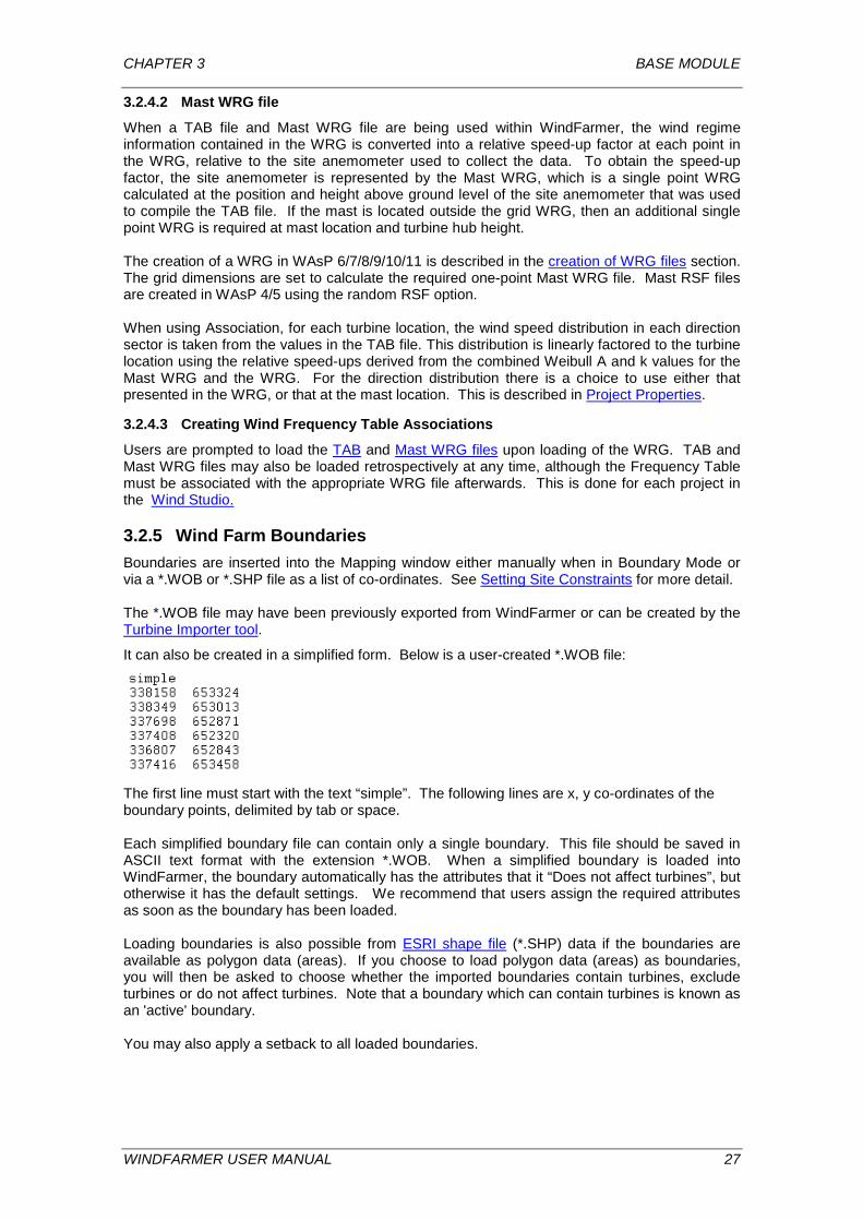
It can also be created in a simplified form. Below is a user-created *.WOB file:
The first line must start with the text “simple”. The following lines are x, y co-ordinates of the boundary points, delimited by tab or space. Each simplified boundary file can contain only a single boundary. This file should be saved in ASCII text format with the extension *.WOB. When a simplified boundary is loaded into WindFarmer, the boundary automatically has the attributes that it “Does not affect turbines”, but otherwise it has the default settings. We recommend that users assign the required attributes as soon as the boundary has been loaded. Loading boundaries is also possible from ESRI shape file (*.SHP) data if the boundaries are available as polygon data (areas). If you choose to load polygon data (areas) as boundaries, you will then be asked to choose whether the imported boundaries contain turbines, exclude turbines or do not affect turbines. Note that a boundary which can contain turbines is known as an 'active' boundary. You may also apply a setback to all loaded boundaries.
WINDFARMER USER MANUAL 27
CHAPTER 3 BASE MODULE
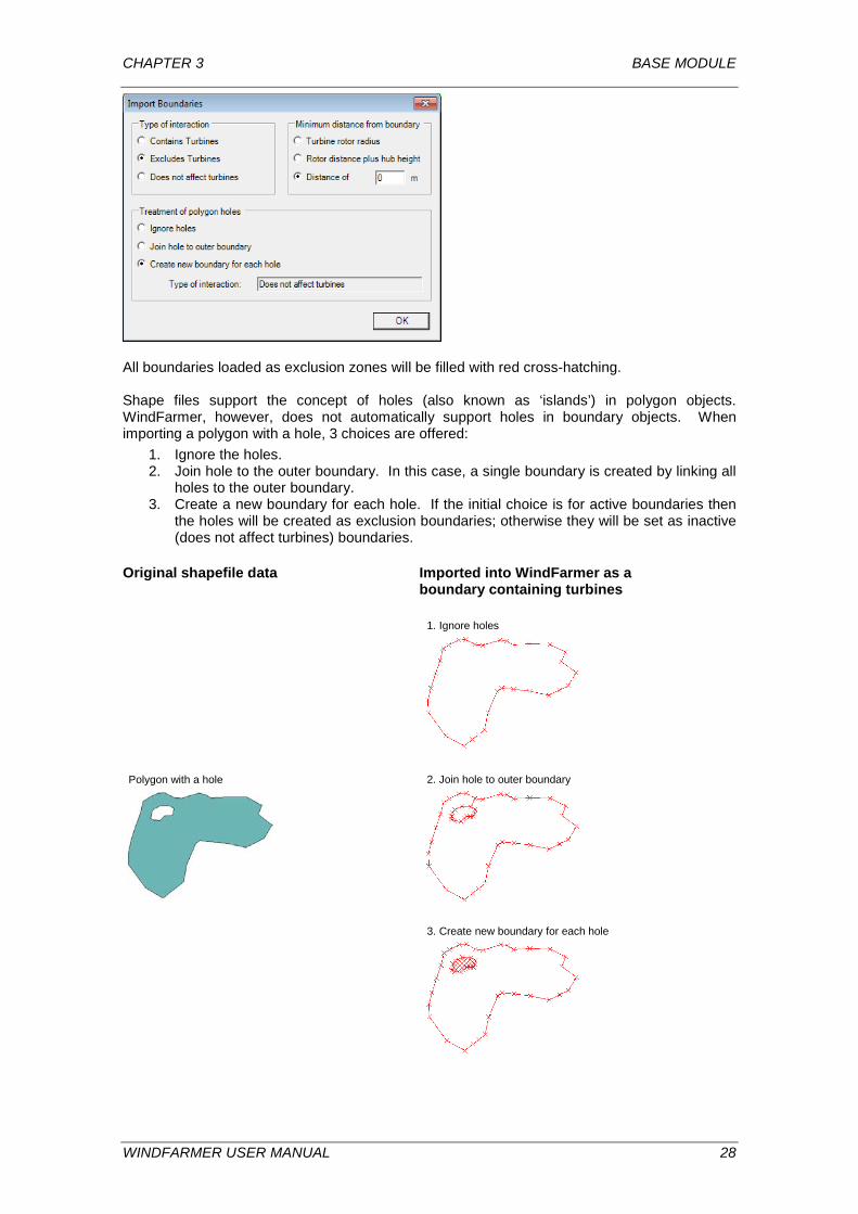
All boundaries loaded as exclusion zones will be filled with red cross-hatching. Shape files support the concept of holes (also known as ‘islands’) in polygon objects. WindFarmer, however, does not automatically support holes in boundary objects. When importing a polygon with a hole, 3 choices are offered:
1. Ignore the holes. 2. Join hole to the outer boundary. In this case, a single boundary is created by linking all
holes to the outer boundary. 3. Create a new boundary for each hole. If the initial choice is for active boundaries then
the holes will be created as exclusion boundaries; otherwise they will be set as inactive (does not affect turbines) boundaries.
Original shapefile data Imported into WindFarmer as a boundary containing turbines
1. Ignore holes
Polygon with a hole
2. Join hole to outer boundary
3. Create new boundary for each hole
WINDFARMER USER MANUAL 28
CHAPTER 3 BASE MODULE
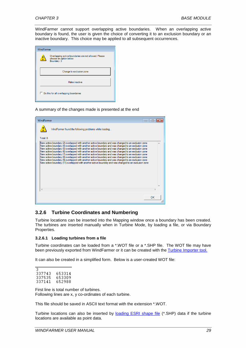
WindFarmer cannot support overlapping active boundaries. When an overlapping active boundary is found, the user is given the choice of converting it to an exclusion boundary or an inactive boundary. This choice may be applied to all subsequent occurrences.
A summary of the changes made is presented at the end
3.2.6 Turbine Coordinates and Numbering Turbine locations can be inserted into the Mapping window once a boundary has been created. The turbines are inserted manually when in Turbine Mode, by loading a file, or via Boundary Properties.
3.2.6.1 Loading turbines from a file
Turbine coordinates can be loaded from a *.WOT file or a *.SHP file. The WOT file may have been previously exported from WindFarmer or it can be created with the Turbine Importer tool. It can also be created in a simplified form. Below is a user-created WOT file:
First line is total number of turbines. Following lines are x, y co-ordinates of each turbine. This file should be saved in ASCII text format with the extension *.WOT. Turbine locations can also be inserted by loading ESRI shape file (*.SHP) data if the turbine locations are available as point data.
WINDFARMER USER MANUAL 29
CHAPTER 3 BASE MODULE
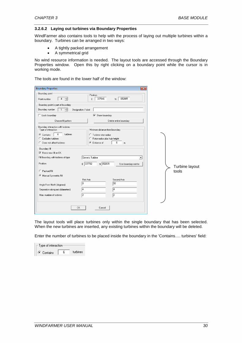
3.2.6.2 Laying out turbines via Boundary Properties
WindFarmer also contains tools to help with the process of laying out multiple turbines within a boundary. Turbines can be arranged in two ways:
• A tightly packed arrangement • A symmetrical grid
No wind resource information is needed. The layout tools are accessed through the Boundary Properties window. Open this by right clicking on a boundary point while the cursor is in working mode. The tools are found in the lower half of the window:
The layout tools will place turbines only within the single boundary that has been selected. When the new turbines are inserted, any existing turbines within the boundary will be deleted. Enter the number of turbines to be placed inside the boundary in the 'Contains…. turbines' field:
Turbine layout tools
WINDFARMER USER MANUAL 30
CHAPTER 3 BASE MODULE
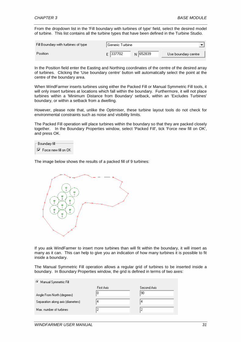
From the dropdown list in the 'Fill boundary with turbines of type' field, select the desired model of turbine. This list contains all the turbine types that have been defined in the Turbine Studio.
In the Position field enter the Easting and Northing coordinates of the centre of the desired array of turbines. Clicking the 'Use boundary centre' button will automatically select the point at the centre of the boundary area. When WindFarmer inserts turbines using either the Packed Fill or Manual Symmetric Fill tools, it will only insert turbines at locations which fall within the boundary. Furthermore, it will not place turbines within a 'Minimum Distance from Boundary' setback, within an 'Excludes Turbines' boundary, or within a setback from a dwelling. However, please note that, unlike the Optimiser, these turbine layout tools do not check for environmental constraints such as noise and visibility limits. The Packed Fill operation will place turbines within the boundary so that they are packed closely together. In the Boundary Properties window, select 'Packed Fill', tick 'Force new fill on OK', and press OK.
The image below shows the results of a packed fill of 9 turbines:
If you ask WindFarmer to insert more turbines than will fit within the boundary, it will insert as many as it can. This can help to give you an indication of how many turbines it is possible to fit inside a boundary. The Manual Symmetric Fill operation allows a regular grid of turbines to be inserted inside a boundary. In Boundary Properties window, the grid is defined in terms of two axes:
WINDFARMER USER MANUAL 31
CHAPTER 3 BASE MODULE
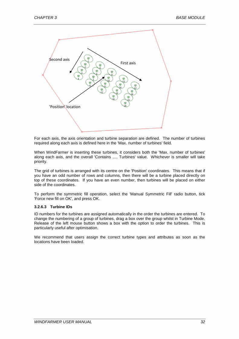
For each axis, the axis orientation and turbine separation are defined. The number of turbines required along each axis is defined here in the 'Max. number of turbines' field. When WindFarmer is inserting these turbines, it considers both the 'Max. number of turbines' along each axis, and the overall 'Contains …. Turbines' value. Whichever is smaller will take priority. The grid of turbines is arranged with its centre on the 'Position' coordinates. This means that if you have an odd number of rows and columns, then there will be a turbine placed directly on top of these coordinates. If you have an even number, then turbines will be placed on either side of the coordinates. To perform the symmetric fill operation, select the 'Manual Symmetric Fill' radio button, tick 'Force new fill on OK', and press OK.
3.2.6.3 Turbine IDs
ID numbers for the turbines are assigned automatically in the order the turbines are entered. To change the numbering of a group of turbines, drag a box over the group whilst in Turbine Mode. Release of the left mouse button shows a box with the option to order the turbines. This is particularly useful after optimisation. We recommend that users assign the correct turbine types and attributes as soon as the locations have been loaded.
First axis Second axis
'Position' location
WINDFARMER USER MANUAL 32
CHAPTER 3 BASE MODULE
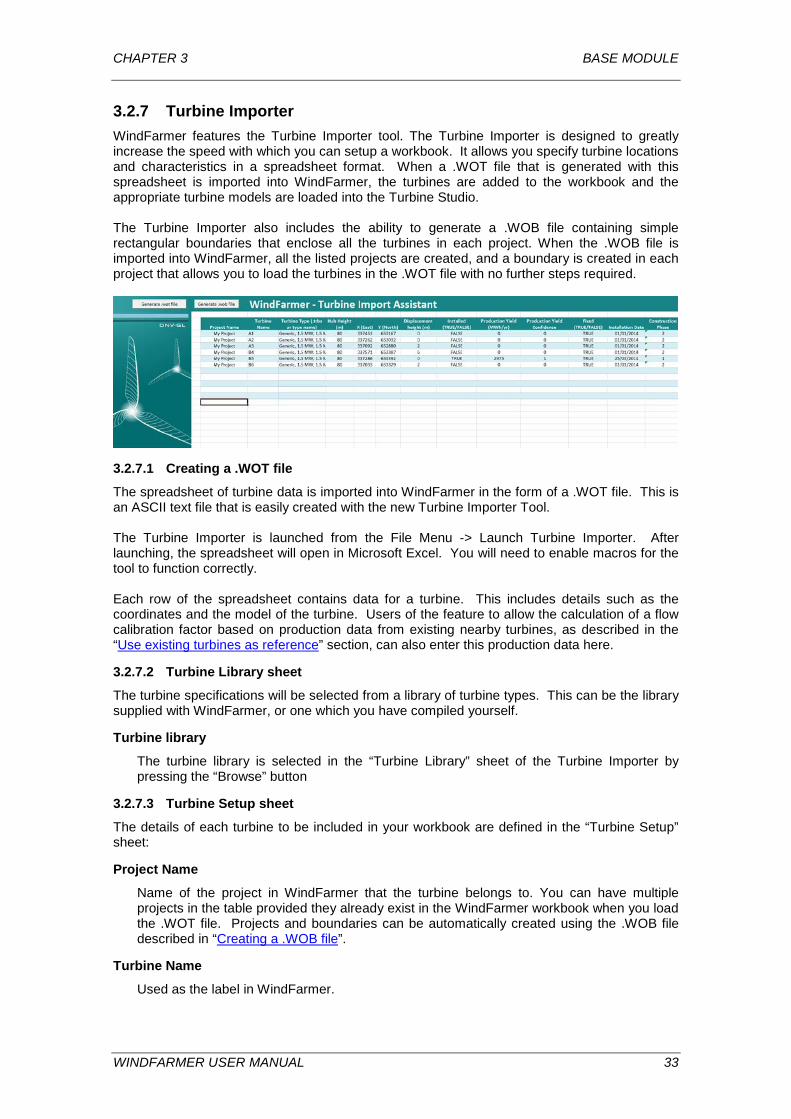
3.2.7 Turbine Importer WindFarmer features the Turbine Importer tool. The Turbine Importer is designed to greatly increase the speed with which you can setup a workbook. It allows you specify turbine locations and characteristics in a spreadsheet format. When a .WOT file that is generated with this spreadsheet is imported into WindFarmer, the turbines are added to the workbook and the appropriate turbine models are loaded into the Turbine Studio. The Turbine Importer also includes the ability to generate a .WOB file containing simple rectangular boundaries that enclose all the turbines in each project. When the .WOB file is imported into WindFarmer, all the listed projects are created, and a boundary is created in each project that allows you to load the turbines in the .WOT file with no further steps required.
3.2.7.1 Creating a .WOT file
The spreadsheet of turbine data is imported into WindFarmer in the form of a .WOT file. This is an ASCII text file that is easily created with the new Turbine Importer Tool. The Turbine Importer is launched from the File Menu -> Launch Turbine Importer. After launching, the spreadsheet will open in Microsoft Excel. You will need to enable macros for the tool to function correctly. Each row of the spreadsheet contains data for a turbine. This includes details such as the coordinates and the model of the turbine. Users of the feature to allow the calculation of a flow calibration factor based on production data from existing nearby turbines, as described in the “Use existing turbines as reference” section, can also enter this production data here.
3.2.7.2 Turbine Library sheet
The turbine specifications will be selected from a library of turbine types. This can be the library supplied with WindFarmer, or one which you have compiled yourself.
Turbine library
The turbine library is selected in the “Turbine Library” sheet of the Turbine Importer by pressing the “Browse” button
3.2.7.3 Turbine Setup sheet
The details of each turbine to be included in your workbook are defined in the “Turbine Setup” sheet:
Project Name
Name of the project in WindFarmer that the turbine belongs to. You can have multiple projects in the table provided they already exist in the WindFarmer workbook when you load the .WOT file. Projects and boundaries can be automatically created using the .WOB file described in “Creating a .WOB file”.
Turbine Name
Used as the label in WindFarmer.
WINDFARMER USER MANUAL 33
CHAPTER 3 BASE MODULE
Turbine Type
Select the turbine type from the library that is defined in the Turbine Library sheet.
Height
The hub height of the turbine. You can define different hub heights for the same turbine type.
X (East)
Turbine easting coordinate.
Y (North)
Turbine northing coordinate.
Displacement height:
This is an apparent vertical displacement of the wind profile. It is defined as a positive displacement in meters. When the flow model is run, the hub height is considered to be reduced by the displacement height. This can be used, for example, to improve the modelling of forestry in the wind flow calculation. Note that if a turbine is ever moved in the WindFarmer workbook, its displacement height is automatically reset to zero.
Is Installed
Enter TRUE for existing turbines and FALSE for proposed turbines. Existing turbines will be shown with blue turbine icons and new turbines with green icons in the Mapping Window. See "Use Existing Turbines as a Reference".
Production Yield
Annual energy yield in MWh for existing turbines. This can be used to define a correction factor for the flow model if there is a systematic over or under prediction of the energy yield. See "Use Existing Turbines as a Reference".
Production Yield Confidence
Weighting factor to be used when calculating the flow model correction. It gets rescaled based on all confidence values set at the turbines in a workbook. See "Use Existing Turbines as a Reference".
Fixed
TRUE/FALSE for turbines whose locations are fixed or not fixed.
Installation Date
Installation date for existing turbines. This is currently not used in any calculation.
Construction Phase
Construction phase for new turbines. This is currently not used in any calculation. You can save the spreadsheet at any time, and return to it later. When all the necessary data has been entered, press the “Generate .wot file” button.
3.2.7.4 Creating a .WOB file
When all the turbine data has been entered, as described above, simply press the “generate .wob file” button to export a WindFarmer boundary file containing simple rectangular boundaries that enclose all the turbines in each project.
3.2.7.5 Importing the .WOT and WOB files
Before importing the .WOT file into WindFarmer, you should load in some map data and create a boundary around the site. It is only possible to load turbines inside active boundaries. This can be achieved simply by loading the .WOB file exported from the spreadsheet.
WINDFARMER USER MANUAL 34
CHAPTER 3 BASE MODULE
Load the .WOB file from the File menu -> Load File, by pressing the green folder button in the Main Toolbar, or by dragging the file onto the map view. All projects are created, and an active boundary is created in each project enclosing the region occupied by the turbines specified in the spreadsheet. Load the .WOT file as for the .WOB file. The turbine type is automatically assigned to all the turbines and the turbine data are imported in the Turbine Studio. If there are turbines of the same type but with different hub heights, the turbine data become duplicated and the hub height is set automatically according to the hub height defined in the .WOT file. Please make sure that the turbine library that is defined in the .WOT file is accessible when loading the .WOT file.
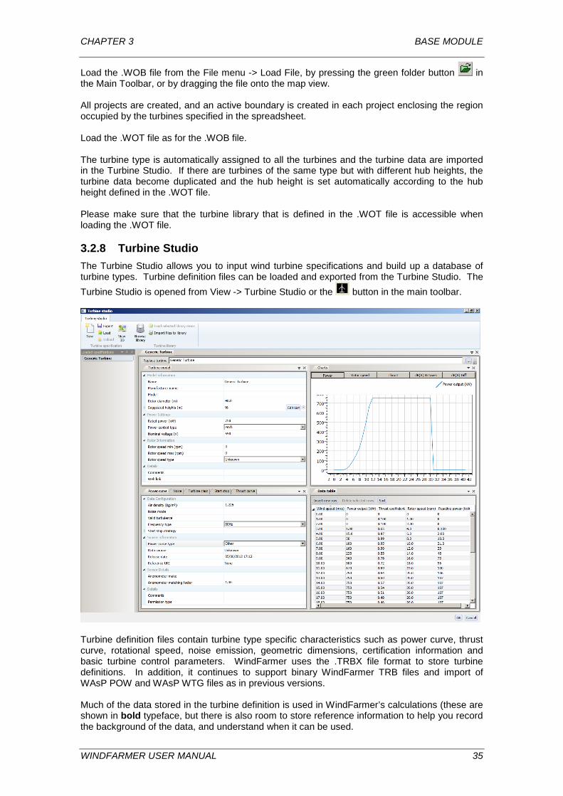
3.2.8 Turbine Studio The Turbine Studio allows you to input wind turbine specifications and build up a database of turbine types. Turbine definition files can be loaded and exported from the Turbine Studio. The Turbine Studio is opened from View -> Turbine Studio or the button in the main toolbar.
Turbine definition files contain turbine type specific characteristics such as power curve, thrust curve, rotational speed, noise emission, geometric dimensions, certification information and basic turbine control parameters. WindFarmer uses the .TRBX file format to store turbine definitions. In addition, it continues to support binary WindFarmer TRB files and import of WAsP POW and WAsP WTG files as in previous versions. Much of the data stored in the turbine definition is used in WindFarmer’s calculations (these are shown in bold typeface, but there is also room to store reference information to help you record the background of the data, and understand when it can be used.
WINDFARMER USER MANUAL 35
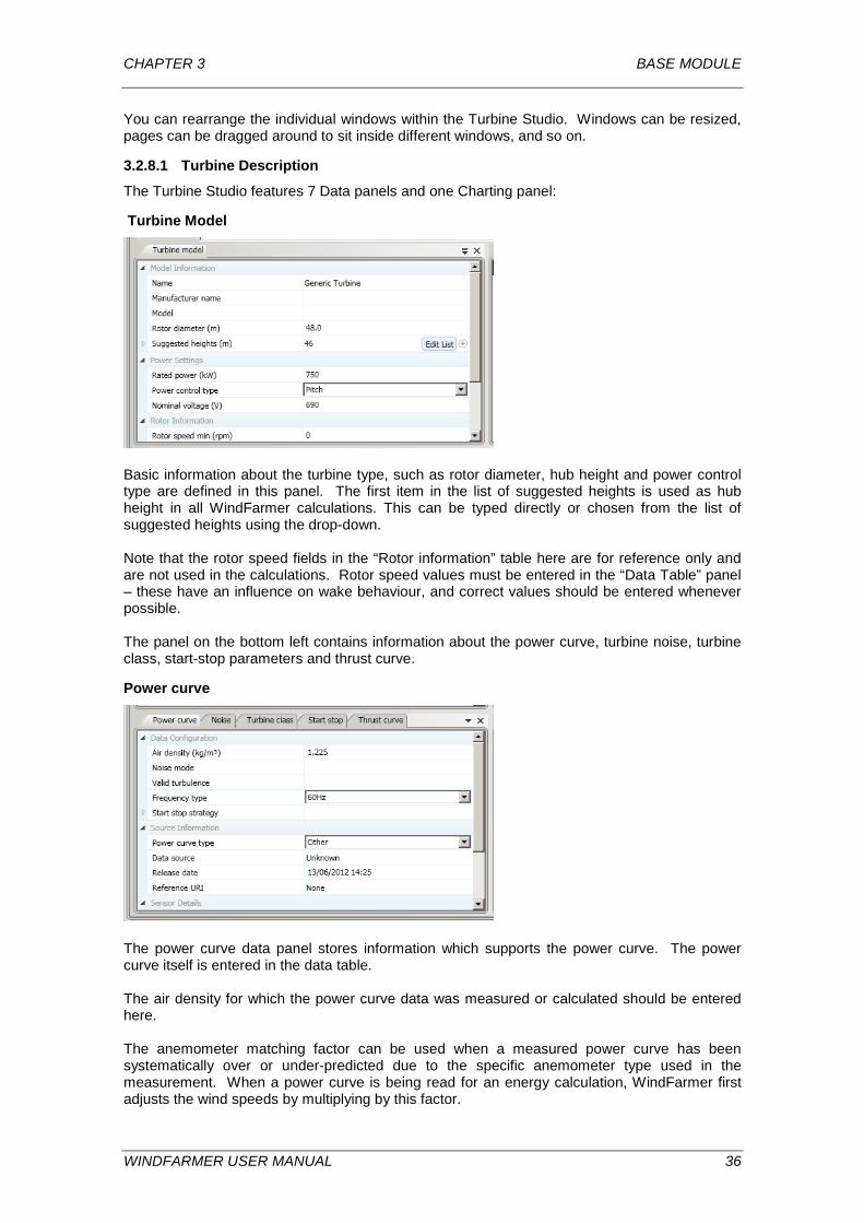
CHAPTER 3 BASE MODULE
You can rearrange the individual windows within the Turbine Studio. Windows can be resized, pages can be dragged around to sit inside different windows, and so on.
3.2.8.1 Turbine Description
The Turbine Studio features 7 Data panels and one Charting panel:
Turbine Model
Basic information about the turbine type, such as rotor diameter, hub height and power control type are defined in this panel. The first item in the list of suggested heights is used as hub height in all WindFarmer calculations. This can be typed directly or chosen from the list of suggested heights using the drop-down. Note that the rotor speed fields in the “Rotor information” table here are for reference only and are not used in the calculations. Rotor speed values must be entered in the “Data Table” panel – these have an influence on wake behaviour, and correct values should be entered whenever possible. The panel on the bottom left contains information about the power curve, turbine noise, turbine class, start-stop parameters and thrust curve.
Power curve
The power curve data panel stores information which supports the power curve. The power curve itself is entered in the data table. The air density for which the power curve data was measured or calculated should be entered here. The anemometer matching factor can be used when a measured power curve has been systematically over or under-predicted due to the specific anemometer type used in the measurement. When a power curve is being read for an energy calculation, WindFarmer first adjusts the wind speeds by multiplying by this factor.
WINDFARMER USER MANUAL 36
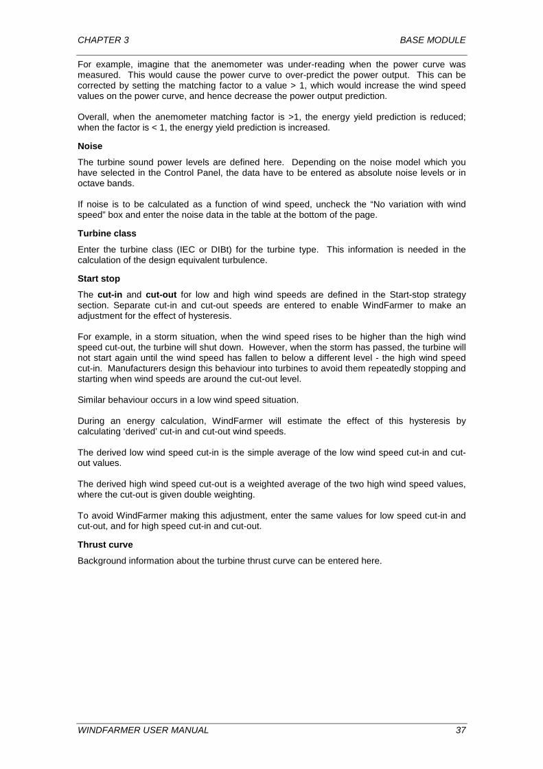
CHAPTER 3 BASE MODULE
For example, imagine that the anemometer was under-reading when the power curve was measured. This would cause the power curve to over-predict the power output. This can be corrected by setting the matching factor to a value > 1, which would increase the wind speed values on the power curve, and hence decrease the power output prediction. Overall, when the anemometer matching factor is >1, the energy yield prediction is reduced; when the factor is < 1, the energy yield prediction is increased.
Noise
The turbine sound power levels are defined here. Depending on the noise model which you have selected in the Control Panel, the data have to be entered as absolute noise levels or in octave bands. If noise is to be calculated as a function of wind speed, uncheck the “No variation with wind speed” box and enter the noise data in the table at the bottom of the page.
Turbine class
Enter the turbine class (IEC or DIBt) for the turbine type. This information is needed in the calculation of the design equivalent turbulence.
Start stop
The cut-in and cut-out for low and high wind speeds are defined in the Start-stop strategy section. Separate cut-in and cut-out speeds are entered to enable WindFarmer to make an adjustment for the effect of hysteresis. For example, in a storm situation, when the wind speed rises to be higher than the high wind speed cut-out, the turbine will shut down. However, when the storm has passed, the turbine will not start again until the wind speed has fallen to below a different level - the high wind speed cut-in. Manufacturers design this behaviour into turbines to avoid them repeatedly stopping and starting when wind speeds are around the cut-out level. Similar behaviour occurs in a low wind speed situation. During an energy calculation, WindFarmer will estimate the effect of this hysteresis by calculating ‘derived’ cut-in and cut-out wind speeds. The derived low wind speed cut-in is the simple average of the low wind speed cut-in and cut-out values. The derived high wind speed cut-out is a weighted average of the two high wind speed values, where the cut-out is given double weighting. To avoid WindFarmer making this adjustment, enter the same values for low speed cut-in and cut-out, and for high speed cut-in and cut-out.
Thrust curve
Background information about the turbine thrust curve can be entered here.
WINDFARMER USER MANUAL 37
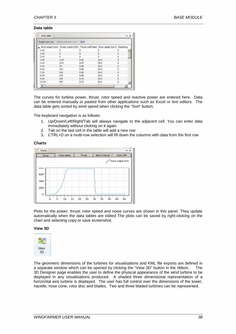
CHAPTER 3 BASE MODULE
Data table
The curves for turbine power, thrust, rotor speed and reactive power are entered here. Data can be entered manually or pasted from other applications such as Excel or text editors. The data table gets sorted by wind speed when clicking the “Sort” button. The keyboard navigation is as follows:
1. Up/Down/Left/Right/Tab will always navigate to the adjacent cell. You can enter data immediately without clicking on it again
2. Tab on the last cell in the table will add a new row 3. CTRL+D on a multi-row selection will fill down the columns with data from the first row
Charts
Plots for the power, thrust, rotor speed and noise curves are shown in this panel. They update automatically when the data tables are edited The plots can be saved by right-clicking on the chart and selecting copy or save screenshot.
View 3D
The geometric dimensions of the turbines for visualisations and KML file exports are defined in a separate window which can be opened by clicking the “View 3D” button in the ribbon. The 3D Designer page enables the user to define the physical appearance of the wind turbine to be displayed in any visualisations produced. A shaded three dimensional representation of a horizontal axis turbine is displayed. The user has full control over the dimensions of the tower, nacelle, nose cone, rotor disc and blades. Two and three bladed turbines can be represented.
WINDFARMER USER MANUAL 38
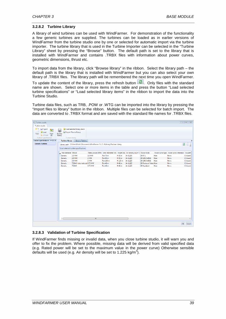
CHAPTER 3 BASE MODULE
3.2.8.2 Turbine Library
A library of wind turbines can be used with WindFarmer. For demonstration of the functionality a few generic turbines are supplied. The turbines can be loaded as in earlier versions of WindFarmer from the turbine studio one by one or selected for automatic import via the turbine importer. The turbine library that is used in the Turbine Importer can be selected in the “Turbine Library” sheet by pressing the “Browse” button. The default path is set to the library that is installed with WindFarmer and contains .TRBX files with information about power curves, geometric dimensions, thrust etc. To import data from the library, click “Browse library” in the ribbon. Select the library path – the default path is the library that is installed with WindFarmer but you can also select your own library of .TRBX files. The library path will be remembered the next time you open WindFarmer. To update the content of the library, press the refresh button . Only files with the standard name are shown. Select one or more items in the table and press the button “Load selected turbine specifications” or “Load selected library items” in the ribbon to import the data into the Turbine Studio. Turbine data files, such as TRB, .POW or .WTG can be imported into the library by pressing the “Import files to library” button in the ribbon. Multiple files can be selected for batch import. The data are converted to .TRBX format and are saved with the standard file names for .TRBX files.
3.2.8.3 Validation of Turbine Specification
If WindFarmer finds missing or invalid data, when you close turbine studio, it will warn you and offer to fix the problem. Where possible, missing data will be derived from valid specified data (e.g. Rated power will be set to the maximum value in the power curve) Otherwise sensible defaults will be used (e.g. Air density will be set to 1.225 kg/m3).
WINDFARMER USER MANUAL 39
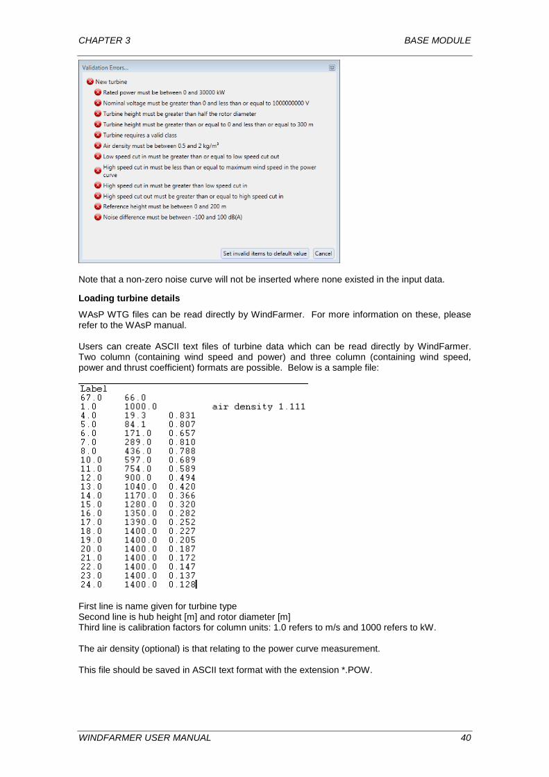
CHAPTER 3 BASE MODULE
Note that a non-zero noise curve will not be inserted where none existed in the input data.
Loading turbine details
WAsP WTG files can be read directly by WindFarmer. For more information on these, please refer to the WAsP manual. Users can create ASCII text files of turbine data which can be read directly by WindFarmer. Two column (containing wind speed and power) and three column (containing wind speed, power and thrust coefficient) formats are possible. Below is a sample file:
First line is name given for turbine type Second line is hub height [m] and rotor diameter [m] Third line is calibration factors for column units: 1.0 refers to m/s and 1000 refers to kW. The air density (optional) is that relating to the power curve measurement. This file should be saved in ASCII text format with the extension *.POW.
WINDFARMER USER MANUAL 40
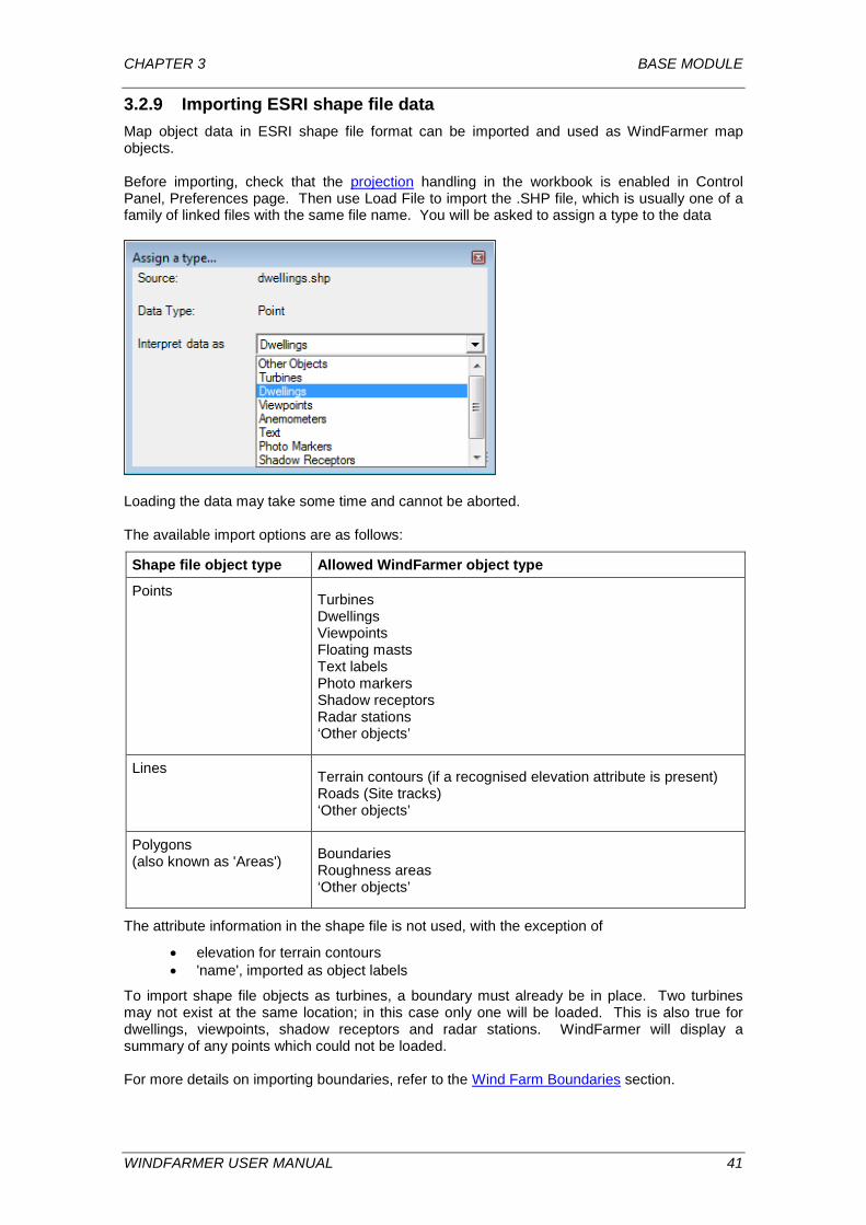
CHAPTER 3 BASE MODULE
3.2.9 Importing ESRI shape file data Map object data in ESRI shape file format can be imported and used as WindFarmer map objects. Before importing, check that the projection handling in the workbook is enabled in Control Panel, Preferences page. Then use Load File to import the .SHP file, which is usually one of a family of linked files with the same file name. You will be asked to assign a type to the data
Loading the data may take some time and cannot be aborted. The available import options are as follows:
Shape file object type Allowed WindFarmer object type
Points Turbines Dwellings Viewpoints Floating masts Text labels Photo markers Shadow receptors Radar stations ‘Other objects’
Lines Terrain contours (if a recognised elevation attribute is present) Roads (Site tracks) ‘Other objects’
Polygons (also known as 'Areas') Boundaries
Roughness areas ‘Other objects’
The attribute information in the shape file is not used, with the exception of
• elevation for terrain contours • 'name', imported as object labels
To import shape file objects as turbines, a boundary must already be in place. Two turbines may not exist at the same location; in this case only one will be loaded. This is also true for dwellings, viewpoints, shadow receptors and radar stations. WindFarmer will display a summary of any points which could not be loaded. For more details on importing boundaries, refer to the Wind Farm Boundaries section.
WINDFARMER USER MANUAL 41
CHAPTER 3 BASE MODULE
3.3 WindFarmer Control Panel
The WindFarmer Control Panel is accessed by clicking the Control Panel button . Each of the pages controls settings and parameters for a distinct part of the software. The Control Panel does not have to be closed before changes become applied. With any page open, changes will be implemented after clicking ‘Apply’. The Control Panel consists of the following pages:
Map Objects Optimiser Preferences Map Printing Visualisation Printing Energy Energy Reports ZVI Noise Model Shadow Model Workbook Files MCP+ Map Data Uncertainty Flow model
3.3.1 Map Objects display options The Map Objects page of the Control Panel is used to set the Mapping Window display settings. Definable settings include the colour of site object icons, grid line spacing and cursor appearance. The object settings can be transferred into other WindFarmer workbooks using the Copy and Paste buttons at the foot of the page. To do this:
• decide the settings for your first workbook, then press Copy • open a second workbook • open the Control Panel for this workbook, and press Paste to replace the settings
with the copied settings.
3.3.2 Optimiser The Optimiser page of the control panel is split into three sections: Convergence Energy capture Constraints The Convergence settings control the stopping criteria for the optimisation algorithm and determine how many attempts the algorithm should make to place turbines in a constrained layout. Increasing the “fruitless iterations” number is recommended for large wind farms with many constraints. If a financial target has been selected in the Financial Module the Optimiser can be set to seek the turbine layout that maximises the target cell value rather than the net energy production of all turbines in the workbook. The Energy capture settings allow users to choose the wind speed range and step size over which an optimisation is carried out, and the option to use distance penalties as a constraint. Setting distance penalties during optimisation helps to consider infrastructure cost as an integral part of the wind farm design. A turbine away from the centre of the site will be penalised and more compact layouts favoured. This is of particular relevance for offshore wind farms where cabling costs are high. If needed, re-set the site centre in the Display Options page of the Project Properties for which the energy penalty will be zero.
WINDFARMER USER MANUAL 42
CHAPTER 3 BASE MODULE
The set energy penalty applies at the penalty distance. Between the site centre and the penalty distance the energy penalty is calculated depending on the penalty type. The algorithm can be linear, square, cube or exponential. For example, if the cost penalty is a function of the wind farm area, then square relation would be most appropriate; if it is a function of distance such as length of cable, then linear would be better. For each trial layout during optimisation, the appropriate penalty percentage is applied to the energy predicted at each turbine. This derives a weighted value according to distance that is used to judge improvement. When the optimiser is running, the penalties are taken into account to determine the optimum turbine layout. When the optimiser is stopped, the energy result does not include the penalties. The Constraints settings allow users to choose the level of constraint to be applied with regards to allowable inter-turbine distance and ground slope. The user can also choose to enable optimisation with respect to noise, intervisibility with radar stations and also visual impact, with the actual level of constraint being set in the individual Camera Properties dialogue box. The wind farm layout can also be forced to be symmetric. The user can choose between elliptical and circular exclusion zones around turbines and define the long and short axes of the exclusion zone in units of the rotor diameter (D) of the turbine. Elliptical exclusion zones around turbines can also be calculated based on a wind speed and direction distribution measured at a mast at the wind farm site. The user must define the length of the short axis of the ellipse, and WindFarmer will calculate the appropriate length and bearing of the long axis. More details about the calculation method can be found in the Theory Manual. To operate the tool, a wind resource (WRG or RSF) file and frequency distribution (TAB) file must be present and associated with a mast. Then to calculate the aspect ratio and orientation of the elliptical exclusion zone, enter the length of the short axis and click the 'Automatic Ellipse…' button. Select the turbine type from the dropdown, highlight the frequency distribution to be used in the calculation and click OK. WindFarmer calculates the length of the long axis of the ellipse and its bearing. These parameters are then shown in the parameter boxes for the definition of the elliptical exclusion zones. The parameters of the ellipse can still be edited by the user. See Layout Optimisation Section.
3.3.3 Energy The Energy Calculation settings control the number of hours in a year, the wake model to be used and the range of wind speed and wind direction bins over which the wind farm yield calculations are carried out. The parameters for the models are also defined here. It is recommended that the default settings are not changed. Further information on wake modelling is given in the Section on Energy Yield Calculations and in the Theory Manual. The design standard and calculation options for the estimation of the design equivalent turbulence can also be set here. An energy map can be displayed for the area covered by the *.WRG file by checking Wind Energy in the Display Bar. The presentation can be adjusted in the Map Data page. The information is taken from the *.WRG file.
3.3.4 Noise Model The Noise Model page of the Control Panel allows the user to select which noise model is to be used for all noise calculations: Simple, Complex (ISO9613) or Custom. The parameters of the noise models are defined here. Ground Effect settings are distinguished clearly for each the four choices of noise model. The Custom option allows freedom of these settings. Further information is given in the Theory Manual.
WINDFARMER USER MANUAL 43
CHAPTER 3 BASE MODULE
3.3.5 Shadow Model (Shadow Flicker Module required)
The parameters of the shadow flicker model are entered here by the user.
3.3.6 Map Printing This page allows the user to add text to be displayed on print-outs of the Mapping Window and to control the font settings.
3.3.7 Visualisation Printing (Visualisation Module required) Here the user can add text to be displayed on print-outs of the Visualisation window and to control the font settings. The view-specific text information, such as view point ID and distance to nearest turbine, to be included on print-outs can be defined here also.
3.3.8 ZVI The ZVI page allows the user to choose which ZVI information is displayed. This dialogue box also allows the user to set the parameters for the ZVI calculation.
3.3.8.1 ZVI Type
Use this section to select the current type of ZVI. The types available are Turbines or Radar Stations. For example, when “Turbine” is selected, WindFarmer will calculate the number of turbines visible from each point on the map viewed from a set height above the terrain. Changing the ZVI type will invalidate any previously calculated ZVI map.
3.3.8.2 Calculation Options
The fields in this section affect how the ZVI is calculated. Modifying any of these fields, and then pressing OK will invalidate any previously calculated ZVI map.
• The ‘Calculate Visual Impact up to’ field lets the user set the extent of the ZVI calculation. Increasing this field will increase computation time.
• The ‘Calculate from centre of project’ produces a ZVI centred on the project centre which can be re-defined in Display Options page of Project Properties. ‘Calculate from centre of turbine’ defines the area of the ZVI according to distance from each turbine.
• The ‘Visibility line of sight algorithm checks height every’ field sets the step size of the visibility test for an object, from the viewpoint to the object. A small step size increases resolution at the expense of speed of calculation. A step size of the order of magnitude of the DTM x,y grid spacing is appropriate.
• The ‘Height above the terrain’ field specifies the height of the viewpoint above the DTM terrain.
3.3.9 Preferences A number of miscellaneous preferences can be set on this page. WOW files can be saved in compressed format by ticking the box "Compress wow file on save". The workbook file then takes longer to save and to re-open but the size of the stored WOW file is reduced. The default is for the compression option to be switched off. The "Prompt to set mast turbulence after loading a single point WRG", is by default switched on. The option to exclude energy settings at 100% from reporting is by default switched off. These optional settings are entered in Project Properties > Energy Efficiencies page. Ticking the “Implement curvature of earth using simple spherical geoid” box affects visualisations and ZVI calculations as well as the calculation of number of hubs and tips visible at any viewpoint. It also affects radar visibility and shadow flicker calculations. By default it is
WINDFARMER USER MANUAL 44
CHAPTER 3 BASE MODULE
switched on. In all these cases the centre of the current mapping space is used as a reference and each point in the DTM is dropped by an amount ∆z where
R is the radius of the earth and ∆x and ∆y are the distances of a point from the centre of the mapping space. The “Enable coordinate projection selection” box instructs WindFarmer to work in a way which allows the user to define the coordinate projection system. This also allows the conversion of map data into other projections. "Parallel processing support" is by default switched on and enables WindFarmer to make use of the additional processing power in computers with several processing cores. Note that calculation speed does not increase linearly with the number of calculation cores available. Performance is improved particularly to give faster energy yield calculation and optimisation in large wind farms, and faster shadow flicker and noise mapping. The usage of additional cores can be disabled in the Preferences panel, for example if you want other applications to share the calculation cores with WindFarmer. The "Wind Rose Properties" button enables you to set the wind speed ranges on the directional bars of the wind rose outputs. The “Panorama lens rotation step size” affects the speed and quality of the panoramic views as well as what is seen when the arrow keys are used to pan left and right. Bigger step size gives a faster calculation but at the expense of quality. The "Number Format" (comma or point as decimal separator) of input files has to be set according to the format of the input files. This provides extra flexibility for allowing WindFarmer to handle files with these alternate formats. When files are to be loaded for the wind resource association method, all must have the same number format. This applies to both WRG and Discrete RSF routes. WindFarmer supports the import, export and usage of current spreadsheet formats. When working with the Finance module, select the format of your financial spreadsheet from the dropdown list. The entries depend on what Excel version is installed on your computer. Changing this setting in an old WindFarmer workbook permanently converts the sheet to the new format. The default transparency of map images can be set in the "Layer display options".
3.3.10 Workbook Files The list of DTM, MAP and background image files can be inspected and unloaded from the workbook. This feature operates with workbooks created in version 3.2.0 and above or with new files loaded into workbooks from previous versions of WindFarmer. Data in the MCP+ Module can be unloaded here. The most likely reason would be to reduce the workbook size.
RyxRz −∆−∆−=∆ 222
WINDFARMER USER MANUAL 45
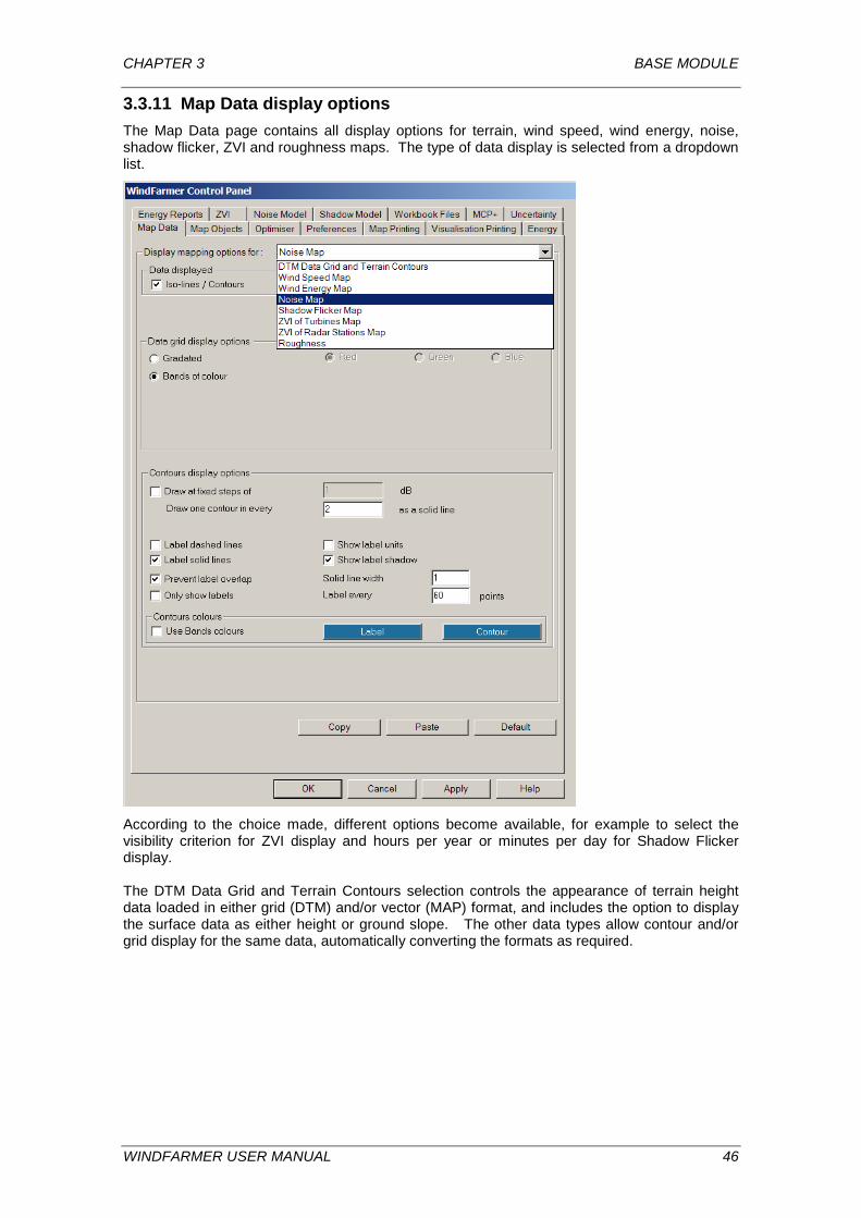
CHAPTER 3 BASE MODULE
3.3.11 Map Data display options The Map Data page contains all display options for terrain, wind speed, wind energy, noise, shadow flicker, ZVI and roughness maps. The type of data display is selected from a dropdown list.
According to the choice made, different options become available, for example to select the visibility criterion for ZVI display and hours per year or minutes per day for Shadow Flicker display. The DTM Data Grid and Terrain Contours selection controls the appearance of terrain height data loaded in either grid (DTM) and/or vector (MAP) format, and includes the option to display the surface data as either height or ground slope. The other data types allow contour and/or grid display for the same data, automatically converting the formats as required.
WINDFARMER USER MANUAL 46
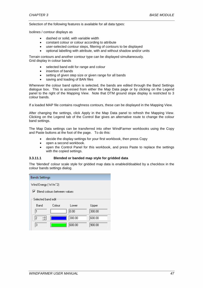
CHAPTER 3 BASE MODULE
Selection of the following features is available for all data types: Isolines / contour displays as
• dashed or solid, with variable width • constant colour or colour according to attribute • user-selected contour steps, filtering of contours to be displayed • optional labelling with attribute, with and without shadow and/or units
Terrain contours and another contour type can be displayed simultaneously. Grid display in colour bands
• selected band edit for range and colour • insertion of bands • setting of given step size or given range for all bands • saving and loading of BAN files
Whenever the colour band option is selected, the bands are edited through the Band Settings dialogue box. This is accessed from either the Map Data page or by clicking on the Legend panel to the right of the Mapping View. Note that DTM ground slope display is restricted to 3 colour bands. If a loaded MAP file contains roughness contours, these can be displayed in the Mapping View. After changing the settings, click Apply in the Map Data panel to refresh the Mapping View. Clicking on the Legend tab of the Control Bar gives an alternative route to change the colour band settings. The Map Data settings can be transferred into other WindFarmer workbooks using the Copy and Paste buttons at the foot of the page. To do this:
• decide the display settings for your first workbook, then press Copy • open a second workbook. • open the Control Panel for this workbook, and press Paste to replace the settings
with the copied settings.
3.3.11.1 Blended or banded map style for gridded data
The ‘blended’ colour scale style for gridded map data is enabled/disabled by a checkbox in the colour bands settings dialog.
WINDFARMER USER MANUAL 47
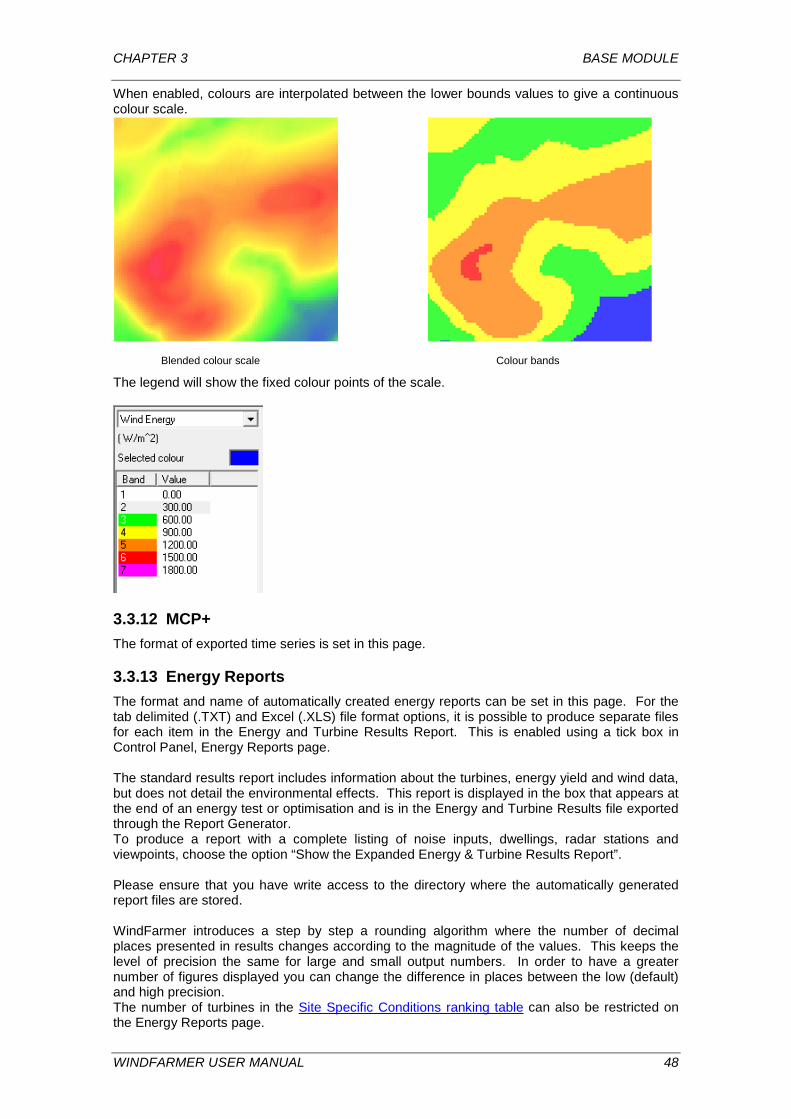
CHAPTER 3 BASE MODULE
When enabled, colours are interpolated between the lower bounds values to give a continuous colour scale.
Blended colour scale Colour bands
The legend will show the fixed colour points of the scale.
3.3.12 MCP+ The format of exported time series is set in this page.
3.3.13 Energy Reports The format and name of automatically created energy reports can be set in this page. For the tab delimited (.TXT) and Excel (.XLS) file format options, it is possible to produce separate files for each item in the Energy and Turbine Results Report. This is enabled using a tick box in Control Panel, Energy Reports page. The standard results report includes information about the turbines, energy yield and wind data, but does not detail the environmental effects. This report is displayed in the box that appears at the end of an energy test or optimisation and is in the Energy and Turbine Results file exported through the Report Generator. To produce a report with a complete listing of noise inputs, dwellings, radar stations and viewpoints, choose the option “Show the Expanded Energy & Turbine Results Report”. Please ensure that you have write access to the directory where the automatically generated report files are stored. WindFarmer introduces a step by step a rounding algorithm where the number of decimal places presented in results changes according to the magnitude of the values. This keeps the level of precision the same for large and small output numbers. In order to have a greater number of figures displayed you can change the difference in places between the low (default) and high precision. The number of turbines in the Site Specific Conditions ranking table can also be restricted on the Energy Reports page.
WINDFARMER USER MANUAL 48
CHAPTER 3 BASE MODULE
3.3.14 Uncertainty The types of measurement and modelling uncertainty to be calculated can be defined by the user. WindFarmer will derive project specific sensitivities for each of the areas and combine the uncertainties considering their respective importance for the wind farm energy yield. The statistical analysis considers variations in the past long term periods and future target periods. Outputs in terms of Confidence Limits or Exceedance Probabilities (P90 etc) can be selected according to user-defined future time periods to meet the requirements for financing. The absolute standard deviation of the expected energy yield is the difference between the outputs for the 50% and 84% Exceedance Probabilities. Sources of uncertainty are related in different ways (defined by the Type of Uncertainty) to the final net energy. The uncertainties are expressed in terms of percentage of the Type of Uncertainty and then linked to the energy production by a sensitivity factor, which can be either calculated by the software or estimated by the user. By using percentages to describe the relationships, the uncertainties and sensitivities in projects of different sizes can be directly compared. The default numbers for each source of uncertainty should be changed according to the specific wind farm being analysed and the method being used to derive the net energy yield. Further details about the calculation of uncertainty in WindFarmer are given in the Theory Manual.
3.3.15 Flow Model The flow model gives you the option of using the WAsP flow model or the simple flow model. The WAsP configuration can be set by clicking on "Edit WAsP parameters". For more information see the "Flow Model" section. This page of the Control Panel also allows you to enter the "Wind flow calibration factor". Here you can also select to "Generate reference heights" which is further explained in "Automatic setup of wind resource templates".
3.4 Wind Studio The Wind Studio is the tool for entering and changing wind climate data. In a typical case, you will have measured the wind climate at a meteorological mast. After processing the measured data with WindFarmer’s MCP+ module, you will have produced the long term wind statistics in the form of a TAB file. You can use the Wind Studio to load such a long term wind statistic TAB file into WindFarmer. If you are analysing a site where wind data has not yet been measured, and are working with simple mean wind speed information, you will use Wind Studio to enter that data. Even though no met. mast has been operated at the site, you create one in WindFarmer to indicate the location of the wind data you are entering. You can change the look of the Wind Studio. Windows can be resized, pages moved between windows, and so on.
3.4.1 Loading wind data for the integrated wind flow model WindFarmer is capable of calculating the wind flow across the site, as described in “Calculating Wind Flow”. It is supplied with a Simple wind flow model, and also has integrated control of the WAsP 10/11 wind flow model, so users who have also purchased a WAsP 10/11 licence can control it through WindFarmer. As with earlier versions, however, it is still possible to load in the results of an external wind flow calculation such as a CFD model, even WAsP CFD.
WINDFARMER USER MANUAL 49
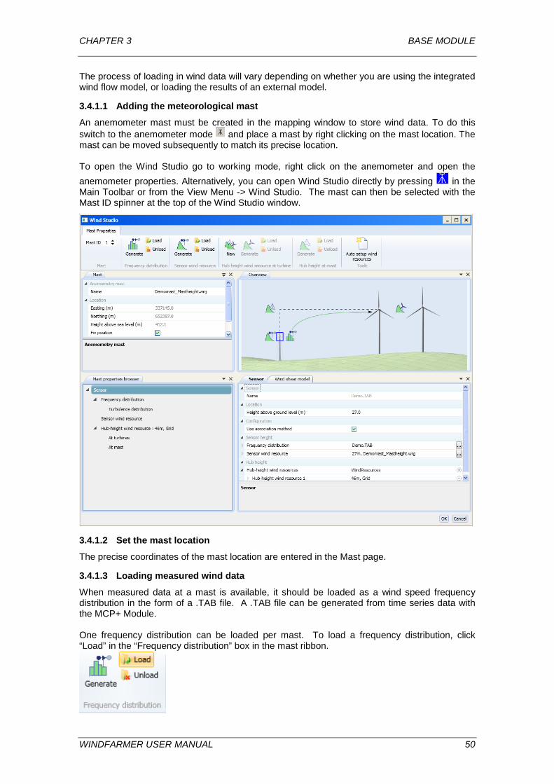
CHAPTER 3 BASE MODULE
The process of loading in wind data will vary depending on whether you are using the integrated wind flow model, or loading the results of an external model.
3.4.1.1 Adding the meteorological mast
An anemometer mast must be created in the mapping window to store wind data. To do this switch to the anemometer mode and place a mast by right clicking on the mast location. The mast can be moved subsequently to match its precise location. To open the Wind Studio go to working mode, right click on the anemometer and open the anemometer properties. Alternatively, you can open Wind Studio directly by pressing in the Main Toolbar or from the View Menu -> Wind Studio. The mast can then be selected with the Mast ID spinner at the top of the Wind Studio window.
3.4.1.2 Set the mast location
The precise coordinates of the mast location are entered in the Mast page.
3.4.1.3 Loading measured wind data
When measured data at a mast is available, it should be loaded as a wind speed frequency distribution in the form of a .TAB file. A .TAB file can be generated from time series data with the MCP+ Module. One frequency distribution can be loaded per mast. To load a frequency distribution, click “Load” in the “Frequency distribution” box in the mast ribbon.
WINDFARMER USER MANUAL 50
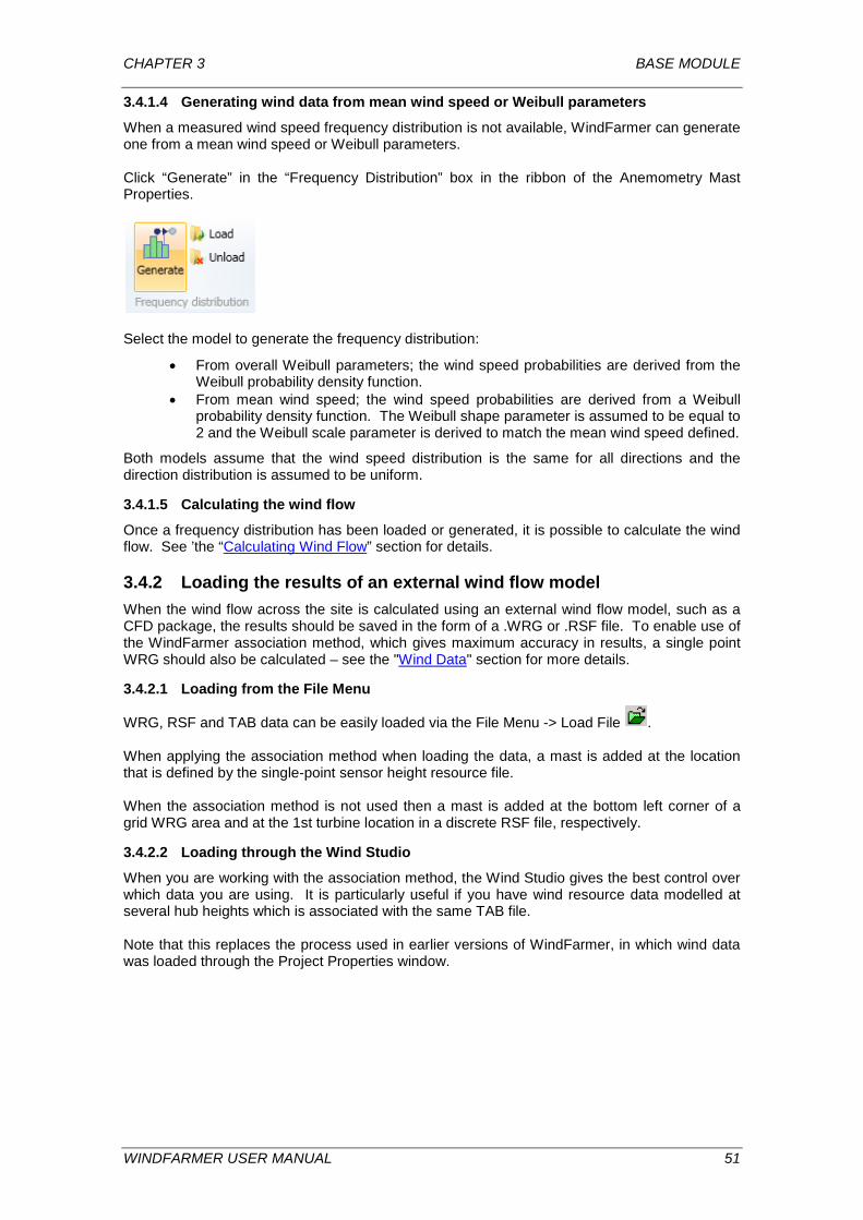
CHAPTER 3 BASE MODULE
3.4.1.4 Generating wind data from mean wind speed or Weibull parameters
When a measured wind speed frequency distribution is not available, WindFarmer can generate one from a mean wind speed or Weibull parameters. Click “Generate” in the “Frequency Distribution” box in the ribbon of the Anemometry Mast Properties.
Select the model to generate the frequency distribution:
• From overall Weibull parameters; the wind speed probabilities are derived from the Weibull probability density function.
• From mean wind speed; the wind speed probabilities are derived from a Weibull probability density function. The Weibull shape parameter is assumed to be equal to 2 and the Weibull scale parameter is derived to match the mean wind speed defined.
Both models assume that the wind speed distribution is the same for all directions and the direction distribution is assumed to be uniform.
3.4.1.5 Calculating the wind flow
Once a frequency distribution has been loaded or generated, it is possible to calculate the wind flow. See ’the “Calculating Wind Flow” section for details.
3.4.2 Loading the results of an external wind flow model When the wind flow across the site is calculated using an external wind flow model, such as a CFD package, the results should be saved in the form of a .WRG or .RSF file. To enable use of the WindFarmer association method, which gives maximum accuracy in results, a single point WRG should also be calculated – see the "Wind Data" section for more details.
3.4.2.1 Loading from the File Menu
WRG, RSF and TAB data can be easily loaded via the File Menu -> Load File . When applying the association method when loading the data, a mast is added at the location that is defined by the single-point sensor height resource file. When the association method is not used then a mast is added at the bottom left corner of a grid WRG area and at the 1st turbine location in a discrete RSF file, respectively.
3.4.2.2 Loading through the Wind Studio
When you are working with the association method, the Wind Studio gives the best control over which data you are using. It is particularly useful if you have wind resource data modelled at several hub heights which is associated with the same TAB file. Note that this replaces the process used in earlier versions of WindFarmer, in which wind data was loaded through the Project Properties window.
WINDFARMER USER MANUAL 51
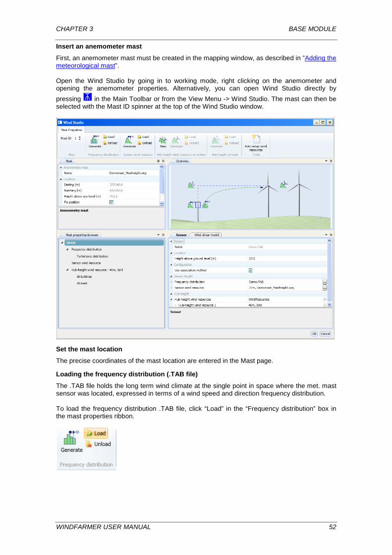
CHAPTER 3 BASE MODULE
Insert an anemometer mast
First, an anemometer mast must be created in the mapping window, as described in ”Adding the meteorological mast”. Open the Wind Studio by going in to working mode, right clicking on the anemometer and opening the anemometer properties. Alternatively, you can open Wind Studio directly by pressing in the Main Toolbar or from the View Menu -> Wind Studio. The mast can then be selected with the Mast ID spinner at the top of the Wind Studio window.
Set the mast location
The precise coordinates of the mast location are entered in the Mast page.
Loading the frequency distribution (.TAB file)
The .TAB file holds the long term wind climate at the single point in space where the met. mast sensor was located, expressed in terms of a wind speed and direction frequency distribution.
To load the frequency distribution .TAB file, click “Load” in the “Frequency distribution” box in the mast properties ribbon.
WINDFARMER USER MANUAL 52
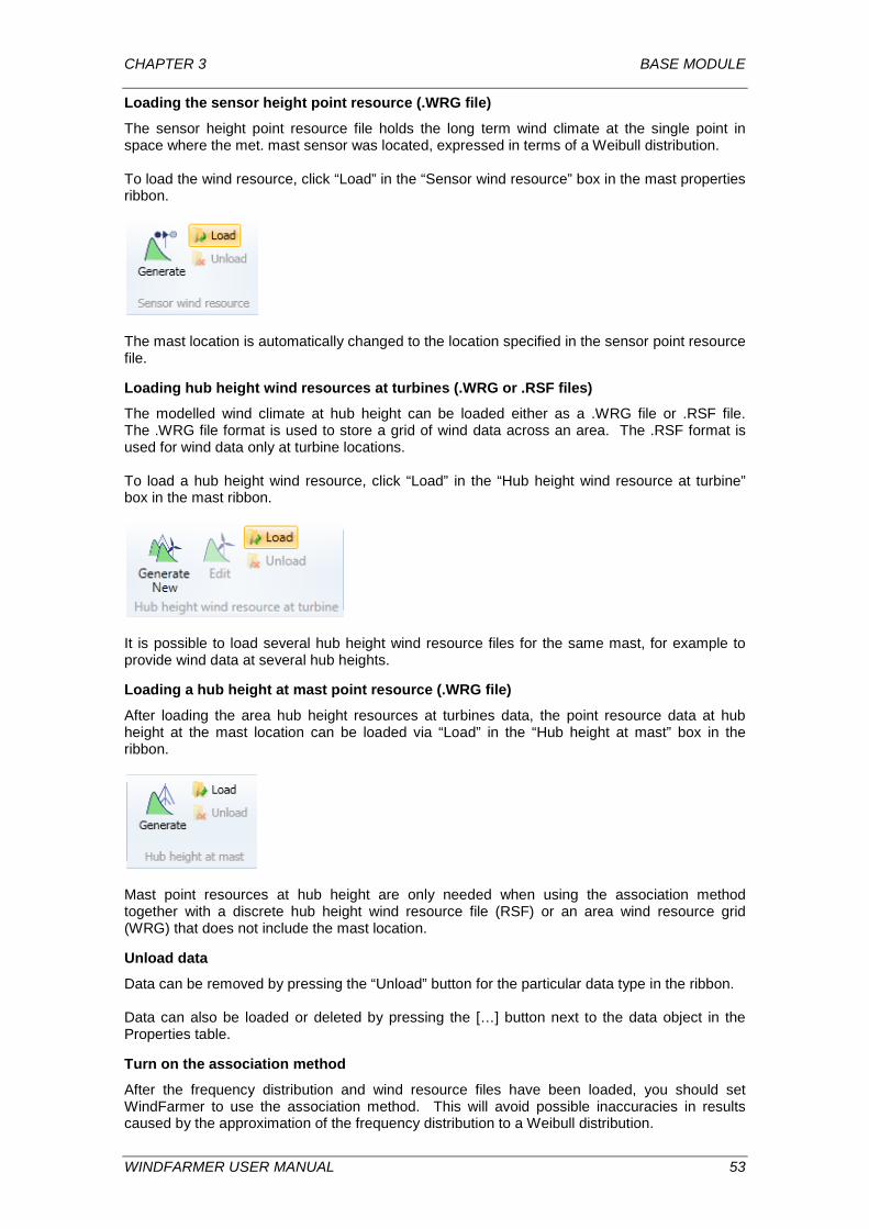
CHAPTER 3 BASE MODULE
Loading the sensor height point resource (.WRG file)
The sensor height point resource file holds the long term wind climate at the single point in space where the met. mast sensor was located, expressed in terms of a Weibull distribution. To load the wind resource, click “Load” in the “Sensor wind resource” box in the mast properties ribbon.
The mast location is automatically changed to the location specified in the sensor point resource file.
Loading hub height wind resources at turbines (.WRG or .RSF files)
The modelled wind climate at hub height can be loaded either as a .WRG file or .RSF file. The .WRG file format is used to store a grid of wind data across an area. The .RSF format is used for wind data only at turbine locations. To load a hub height wind resource, click “Load” in the “Hub height wind resource at turbine” box in the mast ribbon.
It is possible to load several hub height wind resource files for the same mast, for example to provide wind data at several hub heights.
Loading a hub height at mast point resource (.WRG file)
After loading the area hub height resources at turbines data, the point resource data at hub height at the mast location can be loaded via “Load” in the “Hub height at mast” box in the ribbon.
Mast point resources at hub height are only needed when using the association method together with a discrete hub height wind resource file (RSF) or an area wind resource grid (WRG) that does not include the mast location.
Unload data
Data can be removed by pressing the “Unload” button for the particular data type in the ribbon. Data can also be loaded or deleted by pressing the […] button next to the data object in the Properties table.
Turn on the association method
After the frequency distribution and wind resource files have been loaded, you should set WindFarmer to use the association method. This will avoid possible inaccuracies in results caused by the approximation of the frequency distribution to a Weibull distribution.
WINDFARMER USER MANUAL 53
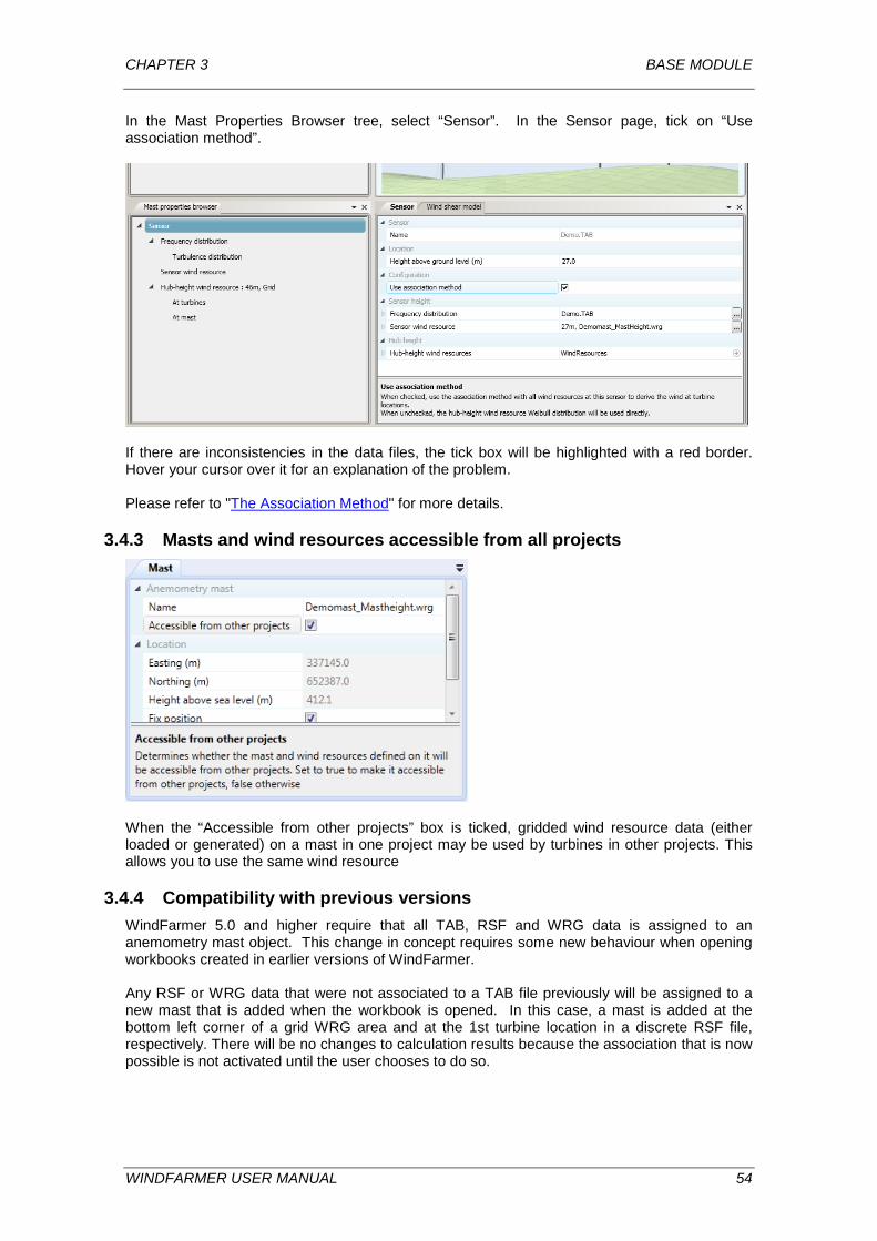
CHAPTER 3 BASE MODULE
In the Mast Properties Browser tree, select “Sensor”. In the Sensor page, tick on “Use association method”.
If there are inconsistencies in the data files, the tick box will be highlighted with a red border. Hover your cursor over it for an explanation of the problem. Please refer to "The Association Method" for more details.
3.4.3 Masts and wind resources accessible from all projects
When the “Accessible from other projects” box is ticked, gridded wind resource data (either loaded or generated) on a mast in one project may be used by turbines in other projects. This allows you to use the same wind resource
3.4.4 Compatibility with previous versions WindFarmer 5.0 and higher require that all TAB, RSF and WRG data is assigned to an anemometry mast object. This change in concept requires some new behaviour when opening workbooks created in earlier versions of WindFarmer. Any RSF or WRG data that were not associated to a TAB file previously will be assigned to a new mast that is added when the workbook is opened. In this case, a mast is added at the bottom left corner of a grid WRG area and at the 1st turbine location in a discrete RSF file, respectively. There will be no changes to calculation results because the association that is now possible is not activated until the user chooses to do so.
WINDFARMER USER MANUAL 54
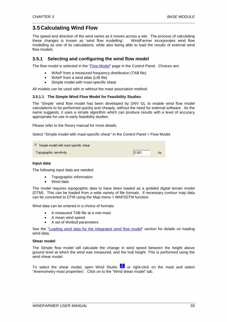
CHAPTER 3 BASE MODULE
3.5 Calculating Wind Flow The speed and direction of the wind varies as it moves across a site. The process of calculating these changes is known as ‘wind flow modelling’. WindFarmer incorporates wind flow modelling as one of its calculations, while also being able to load the results of external wind flow models.
3.5.1 Selecting and configuring the wind flow model The flow model is selected in the “Flow Model” page in the Control Panel. Choices are:
• WAsP from a measured frequency distribution (TAB file) • WAsP from a wind atlas (LIB file) • Simple model with mast-specific shear
All models can be used with or without the mast association method.
3.5.1.1 The Simple Wind Flow Model for Feasibility Studies
The ‘Simple’ wind flow model has been developed by DNV GL to enable wind flow model calculations to be performed quickly and cheaply, without the need for external software. As the name suggests, it uses a simple algorithm which can produce results with a level of accuracy appropriate for use in early feasibility studies. Please refer to the theory manual for more details. Select “Simple model with mast-specific shear” in the Control Panel > Flow Model.
Input data
The following input data are needed:
• Topographic information • Wind data
The model requires topographic data to have been loaded as a gridded digital terrain model (DTM). This can be loaded from a wide variety of file formats. If necessary contour map data can be converted to DTM using the Map menu > MAP2DTM function. Wind data can be entered in a choice of formats:
• A measured TAB file at a met mast • A mean wind speed • A set of Weibull parameters
See the ”Loading wind data for the integrated wind flow model” section for details on loading wind data.
Shear model
The Simple flow model will calculate the change in wind speed between the height above ground level at which the wind was measured, and the hub height. This is performed using the wind shear model. To select the shear model, open Wind Studio or right-click on the mast and select “Anemometry mast properties”. Click on to the “Wind shear model” tab.
WINDFARMER USER MANUAL 55
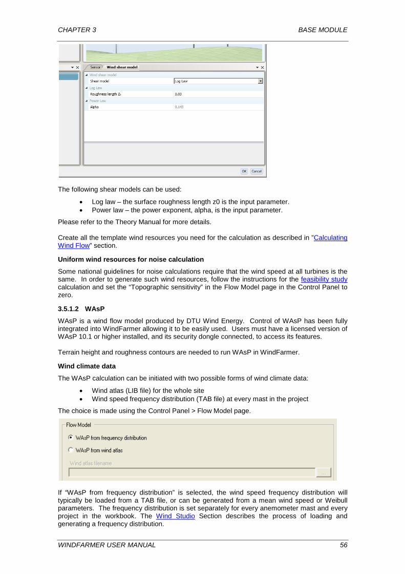
CHAPTER 3 BASE MODULE
The following shear models can be used:
• Log law – the surface roughness length z0 is the input parameter. • Power law – the power exponent, alpha, is the input parameter.
Please refer to the Theory Manual for more details. Create all the template wind resources you need for the calculation as described in ”Calculating Wind Flow” section.
Uniform wind resources for noise calculation
Some national guidelines for noise calculations require that the wind speed at all turbines is the same. In order to generate such wind resources, follow the instructions for the feasibility study calculation and set the “Topographic sensitivity” in the Flow Model page in the Control Panel to zero.
3.5.1.2 WAsP
WAsP is a wind flow model produced by DTU Wind Energy. Control of WAsP has been fully integrated into WindFarmer allowing it to be easily used. Users must have a licensed version of WAsP 10.1 or higher installed, and its security dongle connected, to access its features. Terrain height and roughness contours are needed to run WAsP in WindFarmer.
Wind climate data
The WAsP calculation can be initiated with two possible forms of wind climate data:
• Wind atlas (LIB file) for the whole site • Wind speed frequency distribution (TAB file) at every mast in the project
The choice is made using the Control Panel > Flow Model page.
If “WAsP from frequency distribution” is selected, the wind speed frequency distribution will typically be loaded from a TAB file, or can be generated from a mean wind speed or Weibull parameters. The frequency distribution is set separately for every anemometer mast and every project in the workbook. The Wind Studio Section describes the process of loading and generating a frequency distribution.
WINDFARMER USER MANUAL 56
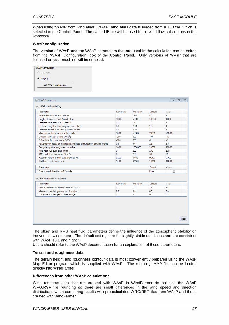
CHAPTER 3 BASE MODULE
When using “WAsP from wind atlas”, WAsP Wind Atlas data is loaded from a .LIB file, which is selected in the Control Panel. The same LIB file will be used for all wind flow calculations in the workbook.
WAsP configuration
The version of WAsP and the WAsP parameters that are used in the calculation can be edited from the “WAsP Configuration” box of the Control Panel. Only versions of WAsP that are licensed on your machine will be enabled.
The offset and RMS heat flux parameters define the influence of the atmospheric stability on the vertical wind shear. The default settings are for slightly stable conditions and are consistent with WAsP 10.1 and higher. Users should refer to the WAsP documentation for an explanation of these parameters.
Terrain and roughness data
The terrain height and roughness contour data is most conveniently prepared using the WAsP Map Editor program which is supplied with WAsP. The resulting .MAP file can be loaded directly into WindFarmer.
Differences from other WAsP calculations
Wind resource data that are created with WAsP in WindFarmer do not use the WAsP WRG/RSF file rounding so there are small differences in the wind speed and direction distributions when comparing results with pre-calculated WRG/RSF files from WAsP and those created with WindFarmer.
WINDFARMER USER MANUAL 57
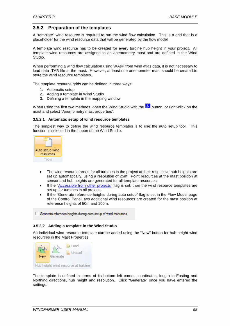
CHAPTER 3 BASE MODULE
3.5.2 Preparation of the templates A “template” wind resource is required to run the wind flow calculation. This is a grid that is a placeholder for the wind resource data that will be generated by the flow model. A template wind resource has to be created for every turbine hub height in your project. All template wind resources are assigned to an anemometry mast and are defined in the Wind Studio. When performing a wind flow calculation using WAsP from wind atlas data, it is not necessary to load data .TAB file at the mast. However, at least one anemometer mast should be created to store the wind resource templates. The template resource grids can be defined in three ways:
1. Automatic setup 2. Adding a template in Wind Studio 3. Defining a template in the mapping window
When using the first two methods, open the Wind Studio with the button, or right-click on the mast and select “Anemometry mast properties”.
3.5.2.1 Automatic setup of wind resource templates
The simplest way to define the wind resource templates is to use the auto setup tool. This function is selected in the ribbon of the Wind Studio.
• The wind resource areas for all turbines in the project at their respective hub heights are set up automatically, using a resolution of 25m. Point resources at the mast position at sensor and hub heights are generated for all template resources.
• If the “Accessible from other projects” flag is set, then the wind resource templates are set up for turbines in all projects.
• If the “Generate reference heights during auto setup” flag is set in the Flow Model page of the Control Panel, two additional wind resources are created for the mast position at reference heights of 50m and 100m.
3.5.2.2 Adding a template in the Wind Studio
An individual wind resource template can be added using the “New” button for hub height wind resources in the Mast Properties.
The template is defined in terms of its bottom left corner coordinates, length in Easting and Northing directions, hub height and resolution. Click “Generate” once you have entered the settings.
WINDFARMER USER MANUAL 58
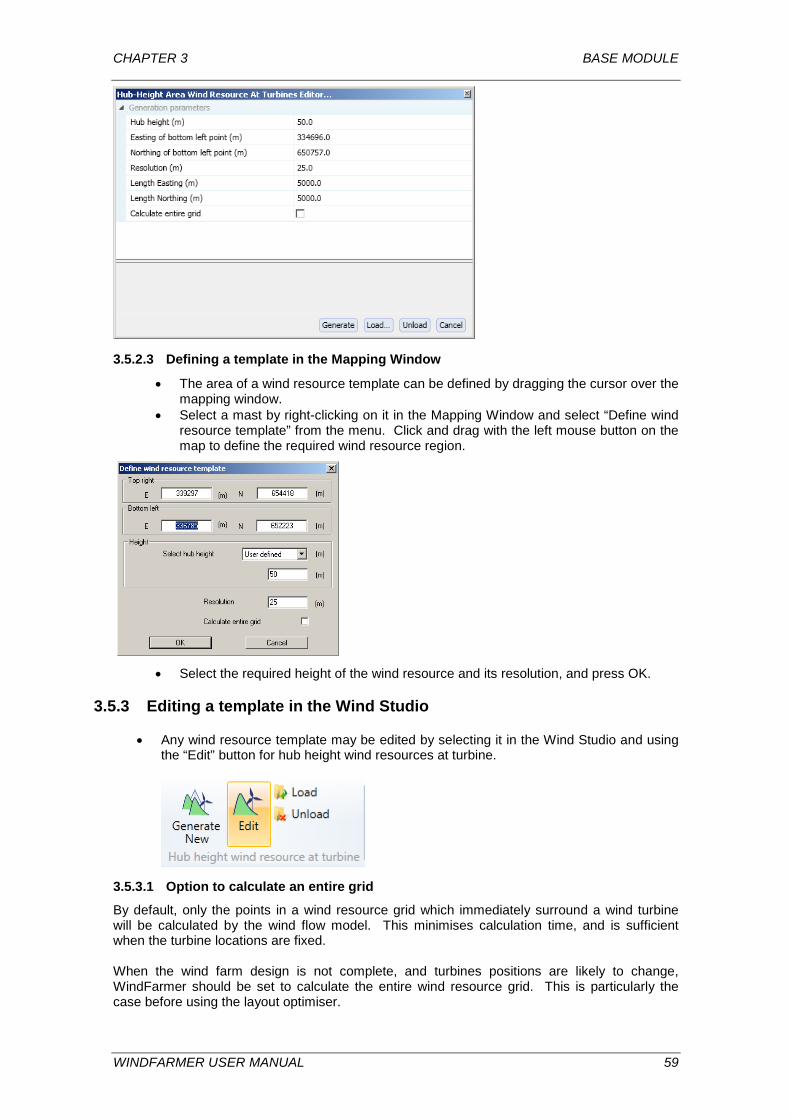
CHAPTER 3 BASE MODULE
3.5.2.3 Defining a template in the Mapping Window
• The area of a wind resource template can be defined by dragging the cursor over the mapping window.
• Select a mast by right-clicking on it in the Mapping Window and select “Define wind resource template” from the menu. Click and drag with the left mouse button on the map to define the required wind resource region.
• Select the required height of the wind resource and its resolution, and press OK.
3.5.3 Editing a template in the Wind Studio
• Any wind resource template may be edited by selecting it in the Wind Studio and using the “Edit” button for hub height wind resources at turbine.
3.5.3.1 Option to calculate an entire grid
By default, only the points in a wind resource grid which immediately surround a wind turbine will be calculated by the wind flow model. This minimises calculation time, and is sufficient when the turbine locations are fixed. When the wind farm design is not complete, and turbines positions are likely to change, WindFarmer should be set to calculate the entire wind resource grid. This is particularly the case before using the layout optimiser.
WINDFARMER USER MANUAL 59
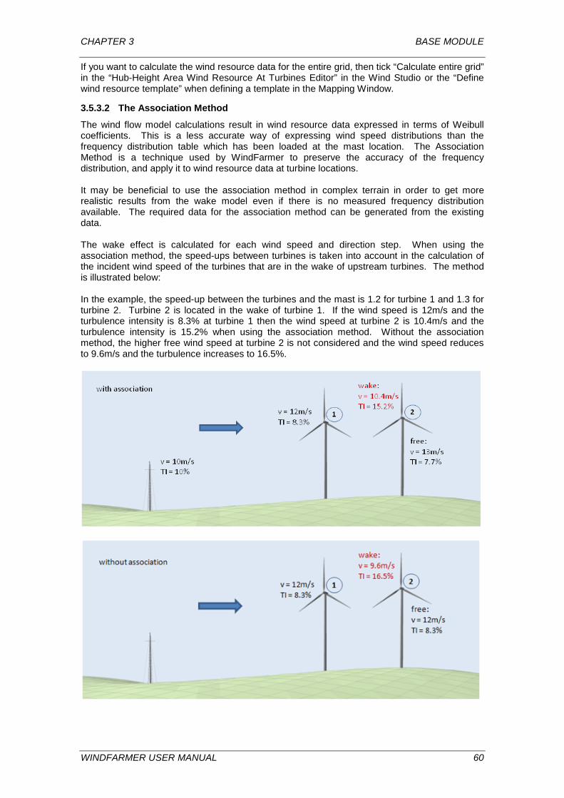
CHAPTER 3 BASE MODULE
If you want to calculate the wind resource data for the entire grid, then tick “Calculate entire grid” in the “Hub-Height Area Wind Resource At Turbines Editor” in the Wind Studio or the “Define wind resource template” when defining a template in the Mapping Window.
3.5.3.2 The Association Method
The wind flow model calculations result in wind resource data expressed in terms of Weibull coefficients. This is a less accurate way of expressing wind speed distributions than the frequency distribution table which has been loaded at the mast location. The Association Method is a technique used by WindFarmer to preserve the accuracy of the frequency distribution, and apply it to wind resource data at turbine locations. It may be beneficial to use the association method in complex terrain in order to get more realistic results from the wake model even if there is no measured frequency distribution available. The required data for the association method can be generated from the existing data. The wake effect is calculated for each wind speed and direction step. When using the association method, the speed-ups between turbines is taken into account in the calculation of the incident wind speed of the turbines that are in the wake of upstream turbines. The method is illustrated below: In the example, the speed-up between the turbines and the mast is 1.2 for turbine 1 and 1.3 for turbine 2. Turbine 2 is located in the wake of turbine 1. If the wind speed is 12m/s and the turbulence intensity is 8.3% at turbine 1 then the wind speed at turbine 2 is 10.4m/s and the turbulence intensity is 15.2% when using the association method. Without the association method, the higher free wind speed at turbine 2 is not considered and the wind speed reduces to 9.6m/s and the turbulence increases to 16.5%.
WINDFARMER USER MANUAL 60
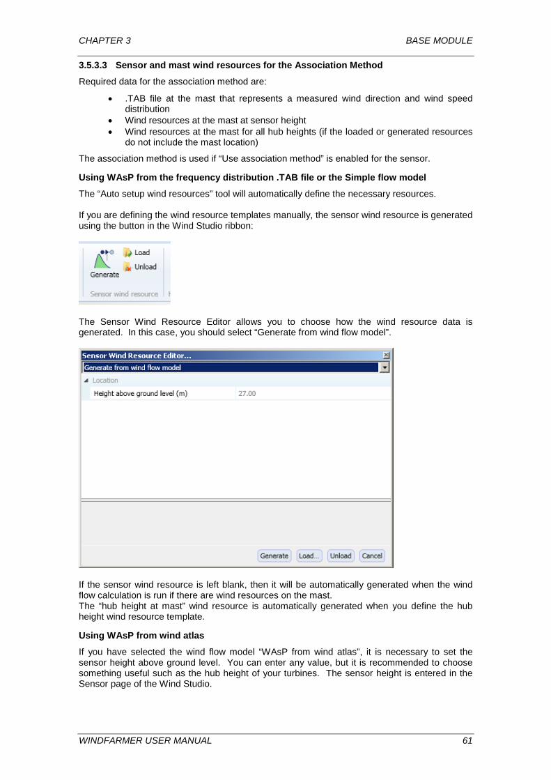
CHAPTER 3 BASE MODULE
3.5.3.3 Sensor and mast wind resources for the Association Method
Required data for the association method are:
• .TAB file at the mast that represents a measured wind direction and wind speed distribution
• Wind resources at the mast at sensor height • Wind resources at the mast for all hub heights (if the loaded or generated resources
do not include the mast location)
The association method is used if “Use association method” is enabled for the sensor.
Using WAsP from the frequency distribution .TAB file or the Simple flow model
The “Auto setup wind resources” tool will automatically define the necessary resources. If you are defining the wind resource templates manually, the sensor wind resource is generated using the button in the Wind Studio ribbon:
The Sensor Wind Resource Editor allows you to choose how the wind resource data is generated. In this case, you should select “Generate from wind flow model”.
If the sensor wind resource is left blank, then it will be automatically generated when the wind flow calculation is run if there are wind resources on the mast. The “hub height at mast” wind resource is automatically generated when you define the hub height wind resource template.
Using WAsP from wind atlas
If you have selected the wind flow model “WAsP from wind atlas”, it is necessary to set the sensor height above ground level. You can enter any value, but it is recommended to choose something useful such as the hub height of your turbines. The sensor height is entered in the Sensor page of the Wind Studio.
WINDFARMER USER MANUAL 61
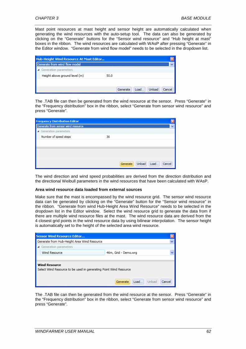
CHAPTER 3 BASE MODULE
Mast point resources at mast height and sensor height are automatically calculated when generating the wind resources with the auto-setup tool. The data can also be generated by clicking on the “Generate” buttons for the “Sensor wind resource” and “Hub height at mast” boxes in the ribbon. The wind resources are calculated with WAsP after pressing “Generate” in the Editor window. “Generate from wind flow model” needs to be selected in the dropdown list.
The .TAB file can then be generated from the wind resource at the sensor. Press “Generate” in the “Frequency distribution” box in the ribbon, select “Generate from sensor wind resource” and press “Generate”.
The wind direction and wind speed probabilities are derived from the direction distribution and the directional Weibull parameters in the wind resources that have been calculated with WAsP.
Area wind resource data loaded from external sources
Make sure that the mast is encompassed by the wind resource grid. The sensor wind resource data can be generated by clicking on the “Generate” button for the “Sensor wind resource” in the ribbon. “Generate from wind Hub-Height Area Wind Resource” needs to be selected in the dropdown list in the Editor window. Select the wind resource grid to generate the data from if there are multiple wind resource files at the mast. The wind resource data are derived from the 4 closest grid points in the wind resource data by using bilinear interpolation. The sensor height is automatically set to the height of the selected area wind resource.
The .TAB file can then be generated from the wind resource at the sensor. Press “Generate” in the “Frequency distribution” box in the ribbon, select “Generate from sensor wind resource” and press “Generate”.
WINDFARMER USER MANUAL 62
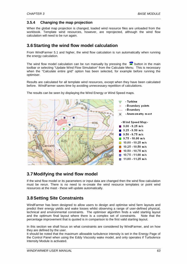
CHAPTER 3 BASE MODULE
3.5.4 Changing the map projection When the global map projection is changed, loaded wind resource files are unloaded from the workbook. Template wind resources, however, are reprojected, although the wind flow calculation will need to be run again.
3.6 Starting the wind flow model calculation From WindFarmer 5.1 and higher, the wind flow calculation is run automatically when running the energy calculation. The wind flow model calculation can be run manually by pressing the button in the main toolbar or selecting “Update Wind Flow Simulation” from the Calculate Menu. This is necessary when the “Calculate entire grid” option has been selected, for example before running the optimiser. Results are calculated for all template wind resources, except when they have been calculated before. WindFarmer saves time by avoiding unnecessary repetition of calculations. The results can be seen by displaying the Wind Energy or Wind Speed maps.
3.7 Modifying the wind flow model If the wind flow model or its parameters or input data are changed then the wind flow calculation must be rerun. There is no need to re-create the wind resource templates or point wind resources at the mast - these will update automatically.
3.8 Setting Site Constraints WindFarmer has been designed to allow users to design and optimise wind farm layouts and predict their energy yields and wake losses whilst observing a range of user-defined physical, technical and environmental constraints. The optimiser algorithm finds a valid starting layout and the optimum final layout where there is a complex set of constraints. Note that the percentage improvement that is quoted is in comparison to the first valid starting layout. In this section we shall focus on what constraints are considered by WindFarmer, and on how they are defined by the user. It should be noted that the maximum allowable turbulence intensity is set in the Energy Page of the Control Panel when using the Eddy Viscosity wake model, and only operates if Turbulence Intensity Module is activated.
WINDFARMER USER MANUAL 63
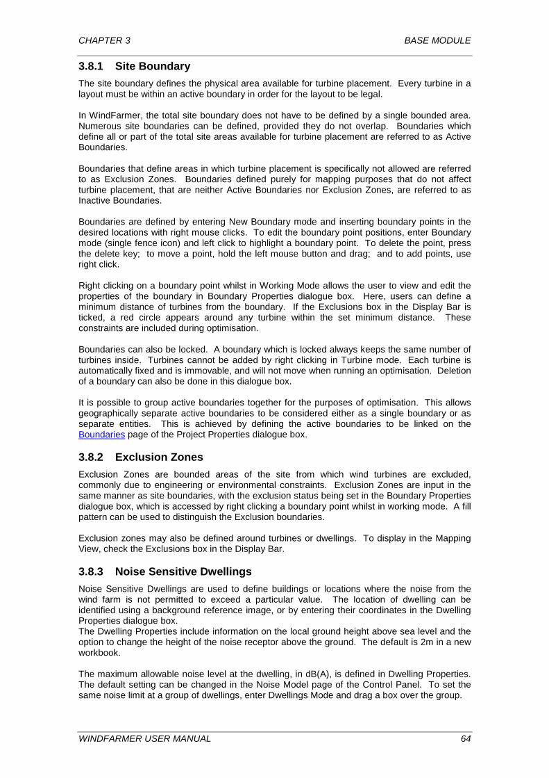
CHAPTER 3 BASE MODULE
3.8.1 Site Boundary The site boundary defines the physical area available for turbine placement. Every turbine in a layout must be within an active boundary in order for the layout to be legal. In WindFarmer, the total site boundary does not have to be defined by a single bounded area. Numerous site boundaries can be defined, provided they do not overlap. Boundaries which define all or part of the total site areas available for turbine placement are referred to as Active Boundaries. Boundaries that define areas in which turbine placement is specifically not allowed are referred to as Exclusion Zones. Boundaries defined purely for mapping purposes that do not affect turbine placement, that are neither Active Boundaries nor Exclusion Zones, are referred to as Inactive Boundaries. Boundaries are defined by entering New Boundary mode and inserting boundary points in the desired locations with right mouse clicks. To edit the boundary point positions, enter Boundary mode (single fence icon) and left click to highlight a boundary point. To delete the point, press the delete key; to move a point, hold the left mouse button and drag; and to add points, use right click. Right clicking on a boundary point whilst in Working Mode allows the user to view and edit the properties of the boundary in Boundary Properties dialogue box. Here, users can define a minimum distance of turbines from the boundary. If the Exclusions box in the Display Bar is ticked, a red circle appears around any turbine within the set minimum distance. These constraints are included during optimisation. Boundaries can also be locked. A boundary which is locked always keeps the same number of turbines inside. Turbines cannot be added by right clicking in Turbine mode. Each turbine is automatically fixed and is immovable, and will not move when running an optimisation. Deletion of a boundary can also be done in this dialogue box. It is possible to group active boundaries together for the purposes of optimisation. This allows geographically separate active boundaries to be considered either as a single boundary or as separate entities. This is achieved by defining the active boundaries to be linked on the Boundaries page of the Project Properties dialogue box.
3.8.2 Exclusion Zones Exclusion Zones are bounded areas of the site from which wind turbines are excluded, commonly due to engineering or environmental constraints. Exclusion Zones are input in the same manner as site boundaries, with the exclusion status being set in the Boundary Properties dialogue box, which is accessed by right clicking a boundary point whilst in working mode. A fill pattern can be used to distinguish the Exclusion boundaries. Exclusion zones may also be defined around turbines or dwellings. To display in the Mapping View, check the Exclusions box in the Display Bar.
3.8.3 Noise Sensitive Dwellings Noise Sensitive Dwellings are used to define buildings or locations where the noise from the wind farm is not permitted to exceed a particular value. The location of dwelling can be identified using a background reference image, or by entering their coordinates in the Dwelling Properties dialogue box. The Dwelling Properties include information on the local ground height above sea level and the option to change the height of the noise receptor above the ground. The default is 2m in a new workbook. The maximum allowable noise level at the dwelling, in dB(A), is defined in Dwelling Properties. The default setting can be changed in the Noise Model page of the Control Panel. To set the same noise limit at a group of dwellings, enter Dwellings Mode and drag a box over the group.
WINDFARMER USER MANUAL 64
CHAPTER 3 BASE MODULE
The acoustic porosity, or ground effect, can be defined for the surroundings of a dwelling as a Ground Effect parameter. Explanations and typical values for this parameter are given in the Theory Manual. The noise limits set at the dwelling locations must be adhered to in order for a turbine layout to be legal. When using noise limits including background noise the noise limit for each wind speed is checked by the code. The layout will only be defined as legal if no limit is exceeded at any dwelling and at any wind speed. The table in Dwelling Properties shows the wind turbine noise calculated according to the Noise Model and Turbine data entered, compared with the background noise and noise limit. In addition, a circular exclusion zone can be defined for each dwelling.
3.8.4 Inter-Turbine Separation Distance The minimum space allowable between any two turbines is defined by circular or elliptical exclusion zones around turbines in a wind farm. The distance is defined in the Optimiser page of the Control Panel as a multiple of D, the rotor diameter. For a layout to be legal, no two turbines may be closer than the minimum allowable separation distance. Where two turbine types with different rotor diameters are analysed on the same site, then the average of D for the turbines is used in the separation calculations. The separation calculations use coordinates in three dimensions.
3.8.5 Allowable Ground Slope The ground slope at a wind turbine location can have a significant effect on the ease of erection and performance of a wind turbine. It is therefore often necessary to control the maximum ground slope on which turbines are placed. In WindFarmer, the maximum allowable ground slope for turbine locations can be defined in degrees from horizontal in the Optimiser page of the Control Panel. The ground slope is calculated from the terrain values of z held in the WRG data. The maximum slope which is determined represents the maximum slope in any direction within the area bounded by the four nearest height points. Any turbine placed on a location that exceeds the maximum allowable ground slope will be deemed to be at an illegal position. Ground slopes over a DTM area can be displayed in the Mapping View. Settings for this are in the Map Data page of the Control Panel.
3.8.6 Optimisation of symmetrical layouts In addition to the optimisation of random wind farm layouts, WindFarmer also provides an optimisation for symmetrical layouts, of the kind that may be desired in simple terrain or offshore. To generate such a layout, tick the box 'Enable optimising using symmetrical layouts' in the Optimiser page in the Control Panel. The symmetrical layout will be generated inside a single active boundary in the current project. A suitable turbine type must be present and a wind resource file of matching height which is associated to a mast.
WINDFARMER USER MANUAL 65
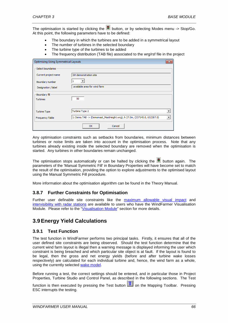
CHAPTER 3 BASE MODULE
The optimisation is started by clicking the button, or by selecting Modes menu -> Stop/Go. At this point, the following parameters have to be defined:
• The boundary in which the turbines are to be added in a symmetrical layout • The number of turbines in the selected boundary • The turbine type of the turbines to be added • The frequency distribution (TAB file) associated to the wrg/rsf file in the project
Any optimisation constraints such as setbacks from boundaries, minimum distances between turbines or noise limits are taken into account in the optimisation process. Note that any turbines already existing inside the selected boundary are removed when the optimisation is started. Any turbines in other boundaries remain unchanged. The optimisation stops automatically or can be halted by clicking the button again. The parameters of the 'Manual Symmetric Fill' in Boundary Properties will have become set to match the result of the optimisation, providing the option to explore adjustments to the optimised layout using the Manual Symmetric Fill procedure. More information about the optimisation algorithm can be found in the Theory Manual.
3.8.7 Further Constraints for Optimisation Further user definable site constraints like the maximum allowable visual impact and intervisibility with radar stations are available to users who have the WindFarmer Visualisation Module. Please refer to the “Visualisation Module” section for more details.
3.9 Energy Yield Calculations
3.9.1 Test Function The test function in WindFarmer performs two principal tasks. Firstly, it ensures that all of the user defined site constraints are being observed. Should the test function determine that the current wind farm layout is illegal then a warning message is displayed informing the user which constraint is being breached and which particular site object is at fault. If the layout is found to be legal, then the gross and net energy yields (before and after turbine wake losses respectively) are calculated for each individual turbine and, hence, the wind farm as a whole, using the currently selected wake model. Before running a test, the correct settings should be entered, and in particular those in Project Properties, Turbine Studio and Control Panel, as described in the following sections. The Test
function is then executed by pressing the Test button on the Mapping Toolbar. Pressing ESC interrupts the testing.
WINDFARMER USER MANUAL 66
CHAPTER 3 BASE MODULE
After performing an energy calculation, it is recommended that a report is immediately exported of the results and parameters employed. This can be done directly from the results panel which appears when the calculation is complete, or subsequently through the File menu using Generate Report. In addition to using the Report Generator, energy reports can be automatically exported through the options in the Energy Report page in the Control Panel. See Exporting and Reporting for further information.
3.9.2 Wake Models There are two main wake loss models available within WindFarmer as well as a method of calculating the energy yield before wake losses, each of which is explained below. The wake model to be used in the Test function and in the Optimisation algorithm is selected on the Energy page of the Control Panel dialogue box.
No Wake Losses
No Wake Losses, simply uses the turbine power curve and wind regime data to calculate the energy yield with no consideration given to wake interaction or losses.
Modified PARK
The Modified PARK model is a variation to the PARK model to achieve better agreement with experimental data for turbines in the second, third and following rows of a wind farm. Please refer to the WindFarmer Theory Manual for further details.
Eddy Viscosity
This is an implementation of the DNV GL Eddy Viscosity Wake model. This model has been tested against numerous wind farms and gives the most reliable results. Please refer to the WindFarmer Validation Report and Theory Manual for further details. Because this model is relatively time-consuming we recommend that the Modified PARK model is used for the optimisation of a wind farm layout and that the Eddy Viscosity Wake model is used for the final calculation of the energy yield.
Wake settings
The default roughness length value may be used to derive turbulence intensity but is only used in conjunction with the Eddy Viscosity model and if this derivation method is selected in Turbulence Intensity page of Project Properties. The wake decay constant is used in the Modified PARK model and is normally set at 0.07
Closely spaced turbines wake modification
This adjustment is applicable to wind farms with more than one row of turbines and with spacings of less than around two rotor diameters within each row. It can be selected in Energy page of the Control Panel. If the wind is blowing normal to the rows, then the wakes of adjacent turbines merge whilst they are still very near to the turbines. When these merged wakes are incident on the next row, they have a lower wind speed than predicted by the standard wake modelling method and the energy yield is less than predicted. The modified Eddy Viscosity wake model addresses this situation. Details of the modified wake model are given in the Theory Manual. Care is required in the application of the model to other layouts.
Large wind farm correction
The model is intended for application in wind farms with a dimension exceeding 40 x 40 rotor diameters where the surrounding roughness is low. Considerable caution is required when applying the large wind farm correction. The model has not yet been validated against a substantial number of wind farms. The number of sectors in the model is set to a minimum of 180 direction steps. Please note that this change substantially increases the processing time and memory requirements. For
WINDFARMER USER MANUAL 67
CHAPTER 3 BASE MODULE
application to a large onshore wind farm, the default parameter settings need to be changed. Please consult the Theory Manual for details. The large wind farm correction option for the energy assessments is not compatible with the large wind farm correction in the estimated design turbulence calculation.
3.9.3 Settings On the Energy page of the Control Panel dialogue box there are a number of other user definable settings, described below:
Leap Year
On the Energy Calculation page users may choose to tick the “Adjust annual energy yields to account of leap years”. When this option is selected it is assumed that there are 8766 hours in a year, to take account of the extra day every 4 years. When this option is not selected then all energy calculations are performed assuming 8760 hours in a year. This option is checked by default when opening a new workbook.
Energy Calculation
The parameters for maximum wind speed and number of direction steps determine the resolution and range in wind steps used in the energy calculation. Calculations are performed at wind speed steps of 1m/s. A maximum wind speed of 70 m/s is standard, which is sufficiently high to ensure the mean wind speed calculation takes all data into account; 72 direction steps are recommended for optimum precision of the wake calculations. The large wind farm correction is applicable to very large wind farms and in particular to those with turbines experiencing multiple wakes. Operational data indicate that turbines deep in such a wind farm produce lower energy than predicted using standard models. It is thought that the influence of such a large wind farm on the local wind regime is similar to an area of higher roughness. Users should be aware that the model for large wind farms is still in an experimental stage and is lacking validation with data from different wind farms.
Eddy Viscosity model
Although the user has the opportunity to change the model parameters, it is generally recommended that these parameters are not changed. The model is optimised for the default settings and care must be taken when making changes as this may lead to inaccurate results. The Maximum length of wake (Diameters) is a length from which the wake is assumed to have totally recovered. The Wake recovery (% at which to ignore wake) gives the value in percent at which the influence of the wake can be neglected in the calculation, normally a setting of 0.2 % is used.
Modified PARK model
Two further settings which have an impact on energy production figures, default surface roughness and wake decay constant, are input and edited from the Energy page of the dialogue box. Whilst the detailed surface roughness characteristics of the wind farm site, and their effect on wind flow, have been taken into account in the WAsP modelling, it is necessary to define a default site roughness length for the purposes of determining the wake decay constant in the modified PARK model. The option to Estimate Design Equivalent Turbulence is available only with the Turbulence Intensity Module and is described in that section.
WINDFARMER USER MANUAL 68

CHAPTER 3 BASE MODULE
3.9.4 Project Properties settings Frequency Table (TAB) Association
Both the Eddy Viscosity wake model and the Modified PARK model may be used in conjunction with the Frequency Table Association option.
Energy
On the Energy page of the Project Properties box there are a number of user definable settings, described below:
• Air Density
WindFarmer adjusts the power curve according to the air density at each individual turbine. In the Energy page, the site air density can be set either manually for a site reference height or derived for the site reference height from a meteorological station air density, met station height and a lapse rate. Heights for air density calculations should be those above sea level (ASL). The air density for which the turbine power curve is valid is defined in the Turbine Power Curve page of the Turbine Studio. If the site air density differs from this air density then adjustments are made to the turbine power curve data. The power regulation method of the wind turbine being analysed, i.e. pitch or stall regulation, determines the method used to adjust the power curve. The power regulation method is also set in the Turbine Power Curve page of the Turbine Studio. Air density changes at turbine positions in a large wind farm site with significant height differentials are calculated using the lapse rate. The power output of each turbine is then adjusted for the new air density. A typical value for the lapse rate is –0.113 (kg/m3)/km. If the lapse rate is set to zero, the same air density is assumed regardless of height differences between turbines.
• Direction shift of sector probabilities
This allows the user to adjust for wind direction probability changes that are predicted by the flow model over complex terrain. With TAB file association, the direction probabilities used in the energy calculations will be those at the mast if this box is unchecked.
Turbulence Intensity
Turbulence intensity data are input in the Turbulence Intensity page of the Project Properties box. Where ambient turbulence data are available, users should input the appropriate figure as a percentage turbulence at a height above ground level. Where Frequency Table Association has been selected, this height is taken as the mast height. Where no association has been made, the turbulence data estimated at the height of each wind resource grid, the hub height, should be entered. If turbulence intensity data are not available, it is possible to derive an estimate of the site ambient turbulence from the site roughness length, as defined on the Energy page of the Project Properties dialogue box. This setting affects the yield results of the Eddy Viscosity wake model only. Users of the WindFarmer Turbulence Intensity Module also have the possibility of entering turbulence intensity data as a function of wind direction or wind speed. Once entered, the matrix of data can be saved as a file with extension *.WTI, which can be imported into other projects. Users who additionally have the MCP+ Module can create WTI files directly from wind speed measurements, provided both mean and standard deviation of the wind speeds have been recorded. See also the sections on the Turbulence Intensity Module and the MCP+ Module
Display Options
The centre of the site can be set and concentric circles drawn around it. If a layout is optimised applying distance penalties the distance of the turbines are calculated from this reference point.
WINDFARMER USER MANUAL 69
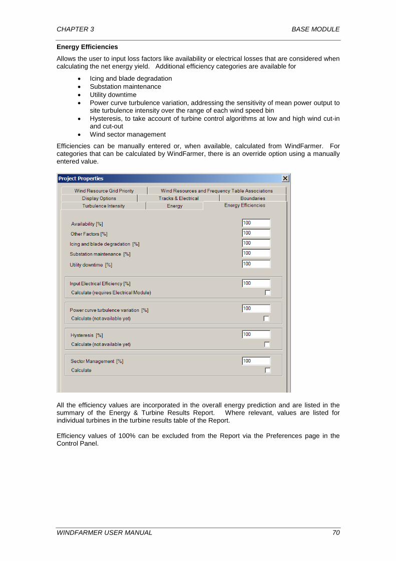
CHAPTER 3 BASE MODULE
Energy Efficiencies
Allows the user to input loss factors like availability or electrical losses that are considered when calculating the net energy yield. Additional efficiency categories are available for
• Icing and blade degradation • Substation maintenance • Utility downtime • Power curve turbulence variation, addressing the sensitivity of mean power output to
site turbulence intensity over the range of each wind speed bin • Hysteresis, to take account of turbine control algorithms at low and high wind cut-in
and cut-out • Wind sector management
Efficiencies can be manually entered or, when available, calculated from WindFarmer. For categories that can be calculated by WindFarmer, there is an override option using a manually entered value.
All the efficiency values are incorporated in the overall energy prediction and are listed in the summary of the Energy & Turbine Results Report. Where relevant, values are listed for individual turbines in the turbine results table of the Report. Efficiency values of 100% can be excluded from the Report via the Preferences page in the Control Panel.
WINDFARMER USER MANUAL 70
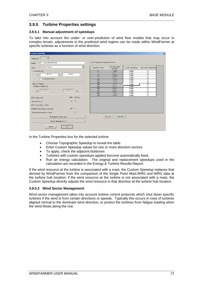
CHAPTER 3 BASE MODULE
3.9.5 Turbine Properties settings 3.9.5.1 Manual adjustment of speedups
To take into account the under- or over-prediction of wind flow models that may occur in complex terrain, adjustments to the predicted wind regime can be made within WindFarmer at specific turbines as a function of wind direction.
In the Turbine Properties box for the selected turbine
• Choose Topographic Speedup to reveal the table • Enter Custom Speedup values for one or more direction sectors • To apply, check the adjacent tickboxes • Turbines with custom speedups applied become automatically fixed. • Run an energy calculation. The original and replacement speedups used in the
calculation are recorded in the Energy & Turbine Results Report.
If the wind resource at the turbine is associated with a mast, the Custom Speedup replaces that derived by WindFarmer from the comparison of the Single Point Mast.WRG and WRG data at the turbine hub location; if the wind resource at the turbine is not associated with a mast, the Custom Speedup directly adjusts the wind resource in that direction at the turbine hub location.
3.9.5.2 Wind Sector Management
Wind sector management takes into account turbine control protocols which shut down specific turbines if the wind is from certain directions or speeds. Typically this occurs in rows of turbines aligned normal to the dominant wind direction, to protect the turbines from fatigue loading when the wind blows along the row.
WINDFARMER USER MANUAL 71
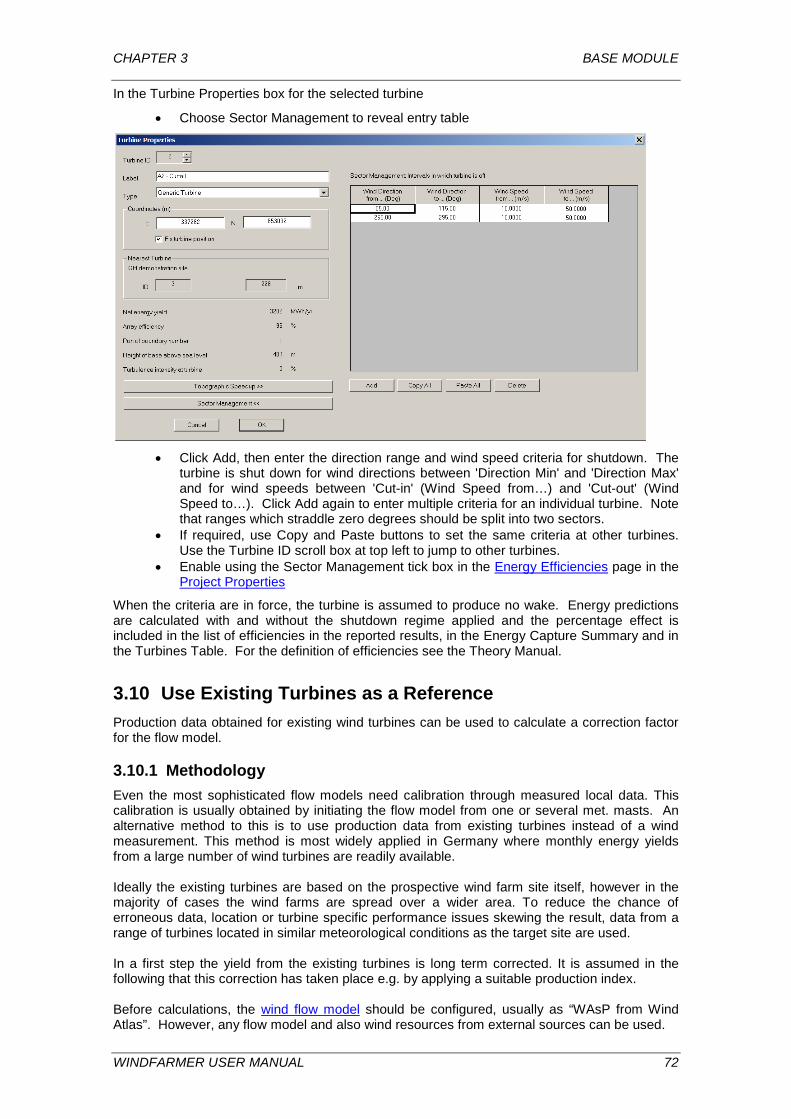
CHAPTER 3 BASE MODULE
In the Turbine Properties box for the selected turbine
• Choose Sector Management to reveal entry table
• Click Add, then enter the direction range and wind speed criteria for shutdown. The
turbine is shut down for wind directions between 'Direction Min' and 'Direction Max' and for wind speeds between 'Cut-in' (Wind Speed from…) and 'Cut-out' (Wind Speed to…). Click Add again to enter multiple criteria for an individual turbine. Note that ranges which straddle zero degrees should be split into two sectors.
• If required, use Copy and Paste buttons to set the same criteria at other turbines. Use the Turbine ID scroll box at top left to jump to other turbines.
• Enable using the Sector Management tick box in the Energy Efficiencies page in the Project Properties
When the criteria are in force, the turbine is assumed to produce no wake. Energy predictions are calculated with and without the shutdown regime applied and the percentage effect is included in the list of efficiencies in the reported results, in the Energy Capture Summary and in the Turbines Table. For the definition of efficiencies see the Theory Manual.
3.10 Use Existing Turbines as a Reference Production data obtained for existing wind turbines can be used to calculate a correction factor for the flow model.
3.10.1 Methodology Even the most sophisticated flow models need calibration through measured local data. This calibration is usually obtained by initiating the flow model from one or several met. masts. An alternative method to this is to use production data from existing turbines instead of a wind measurement. This method is most widely applied in Germany where monthly energy yields from a large number of wind turbines are readily available. Ideally the existing turbines are based on the prospective wind farm site itself, however in the majority of cases the wind farms are spread over a wider area. To reduce the chance of erroneous data, location or turbine specific performance issues skewing the result, data from a range of turbines located in similar meteorological conditions as the target site are used. In a first step the yield from the existing turbines is long term corrected. It is assumed in the following that this correction has taken place e.g. by applying a suitable production index. Before calculations, the wind flow model should be configured, usually as “WAsP from Wind Atlas”. However, any flow model and also wind resources from external sources can be used.
WINDFARMER USER MANUAL 72
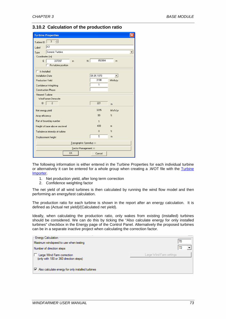
CHAPTER 3 BASE MODULE
3.10.2 Calculation of the production ratio
The following information is either entered in the Turbine Properties for each individual turbine or alternatively it can be entered for a whole group when creating a .WOT file with the Turbine Importer.
1. Net production yield, after long term correction 2. Confidence weighting factor
The net yield of all wind turbines is then calculated by running the wind flow model and then performing an energy/test calculation. The production ratio for each turbine is shown in the report after an energy calculation. It is defined as (Actual net yield)/(Calculated net yield). Ideally, when calculating the production ratio, only wakes from existing (installed) turbines should be considered. We can do this by ticking the “Also calculate energy for only installed turbines” checkbox in the Energy page of the Control Panel. Alternatively the proposed turbines can be in a separate inactive project when calculating the correction factor.
WINDFARMER USER MANUAL 73
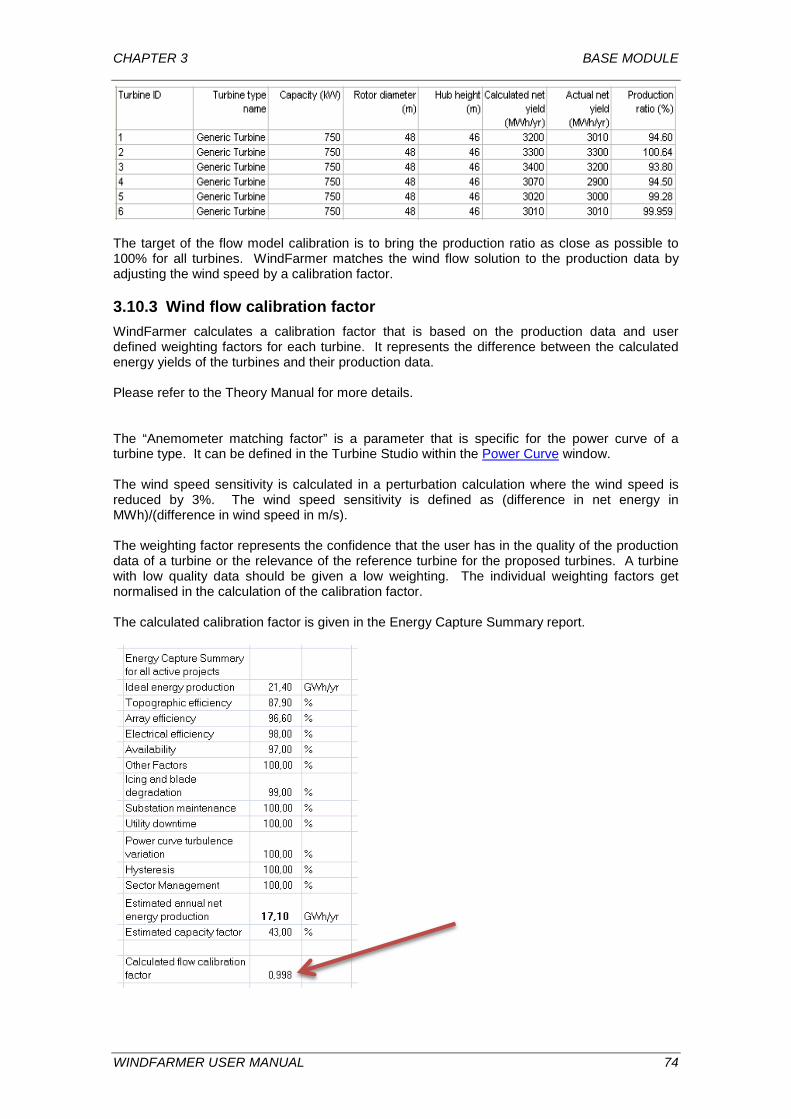
CHAPTER 3 BASE MODULE
The target of the flow model calibration is to bring the production ratio as close as possible to 100% for all turbines. WindFarmer matches the wind flow solution to the production data by adjusting the wind speed by a calibration factor.
3.10.3 Wind flow calibration factor WindFarmer calculates a calibration factor that is based on the production data and user defined weighting factors for each turbine. It represents the difference between the calculated energy yields of the turbines and their production data. Please refer to the Theory Manual for more details. The “Anemometer matching factor” is a parameter that is specific for the power curve of a turbine type. It can be defined in the Turbine Studio within the Power Curve window. The wind speed sensitivity is calculated in a perturbation calculation where the wind speed is reduced by 3%. The wind speed sensitivity is defined as (difference in net energy in MWh)/(difference in wind speed in m/s). The weighting factor represents the confidence that the user has in the quality of the production data of a turbine or the relevance of the reference turbine for the proposed turbines. A turbine with low quality data should be given a low weighting. The individual weighting factors get normalised in the calculation of the calibration factor. The calculated calibration factor is given in the Energy Capture Summary report.
WINDFARMER USER MANUAL 74

CHAPTER 3 BASE MODULE
Once the calibration factor has been calculated, it should be entered as the “Wind flow calibration” factor in the Control Panel > Flow Model page. It will then be used to scale the results of the flow model calculations, leading to a good match between calculated energy yields and measured production data.
Wind speed and wind energy maps are also scaled by the calibration factor.
3.11 Layout Optimisation The WindFarmer Base Module incorporates a unique algorithm for optimising the layout of a wind farm in order to obtain a maximum energy capture, whilst still observing the full range of user defined site constraints. The optimiser can consider noise limits at dwellings; boundaries; turbine separation distance; ground slope and visual impact. In addition a distance weighted energy penalty can be applied. Once all the required data have been loaded into a workbook, the Optimiser may be started at
any time by pressing the start/stop button on the Mapping Toolbar. Upon starting the Optimiser the user is asked to confirm the following settings: Noise model, wake model, visual and radar constraints, ground slope, separation distances, number of iterations and fruitless iterations. If the user is satisfied with the current set-up, then clicking YES will start the optimiser. Clicking NO returns the user to the Map View. On running the Optimiser, the turbines can be seen to be relocated to new positions and the energy yield to increase. The Optimiser continues to run until either the Start/Stop button is pressed, or until one of the stopping criteria is reached. In some circumstances, a message may be displayed on starting the optimiser indicating that it has not been possible to determine a legal starting layout. When this occurs, the user can either try again to determine a legal starting position with the current set-up by restarting the optimiser, change the Optimisation Settings to increase the number of attempts made to place the turbines or increase the tolerance for the site constraints. A backup file of the turbine layout, temp_turbines.WOT, is saved every 20 minutes during optimisation to the standard Windows TEMP directory of your computer. The location of this folder varies according to the operating system, usually: Windows XP: C:\Documents and Settings\$USER\Local Settings\Temp Windows Vista and Windows 7: C:\Users\$USER\AppData\Local\Temp If the file is not in the directories listed above, it can be set in Windows Control Panel > System > Advanced tab > Environmental Variables. After optimising, it is recommended that the new turbine layout be saved immediately. To save, choose File > Export.. > Export Data and select ‘Turbines’. The resulting file, with extension WOT, can be reloaded subsequently into WindFarmer if required.
WINDFARMER USER MANUAL 75
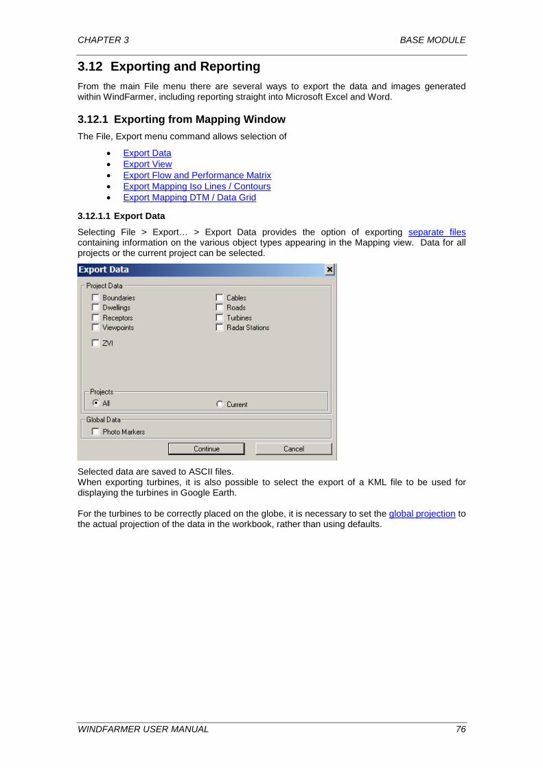
CHAPTER 3 BASE MODULE
3.12 Exporting and Reporting From the main File menu there are several ways to export the data and images generated within WindFarmer, including reporting straight into Microsoft Excel and Word.
3.12.1 Exporting from Mapping Window The File, Export menu command allows selection of
• Export Data • Export View • Export Flow and Performance Matrix • Export Mapping Iso Lines / Contours • Export Mapping DTM / Data Grid
3.12.1.1 Export Data
Selecting File > Export… > Export Data provides the option of exporting separate files containing information on the various object types appearing in the Mapping view. Data for all projects or the current project can be selected.
Selected data are saved to ASCII files. When exporting turbines, it is also possible to select the export of a KML file to be used for displaying the turbines in Google Earth. For the turbines to be correctly placed on the globe, it is necessary to set the global projection to the actual projection of the data in the workbook, rather than using defaults.
WINDFARMER USER MANUAL 76
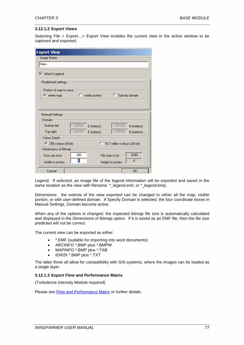
CHAPTER 3 BASE MODULE
3.12.1.2 Export Views
Selecting File > Export…> Export View enables the current view in the active window to be captured and exported.
Legend: If selected, an image file of the legend information will be exported and saved in the same location as the view with filename *_legend.emf, or *_legend.bmp. Dimensions: the extents of the view exported can be changed to either all the map, visible portion, or with user-defined domain. If Specify Domain is selected, the four coordinate boxes in Manual Settings, Domain become active. When any of the options is changed, the expected bitmap file size is automatically calculated and displayed in the Dimensions of Bitmap option. If it is saved as an EMF file, then the file size predicted will not be correct. The current view can be exported as either:
• *.EMF (suitable for importing into word documents) • ARCINFO *.BMP plus *.BMPW • MAPINFO *.BMP plus *.TAB • IDRISI *.BMP plus *.TXT
The latter three all allow for compatibility with GIS systems, where the images can be loaded as a single layer.
3.12.1.3 Export Flow and Performance Matrix
(Turbulence Intensity Module required) Please see Flow and Performance Matrix or further details.
WINDFARMER USER MANUAL 77
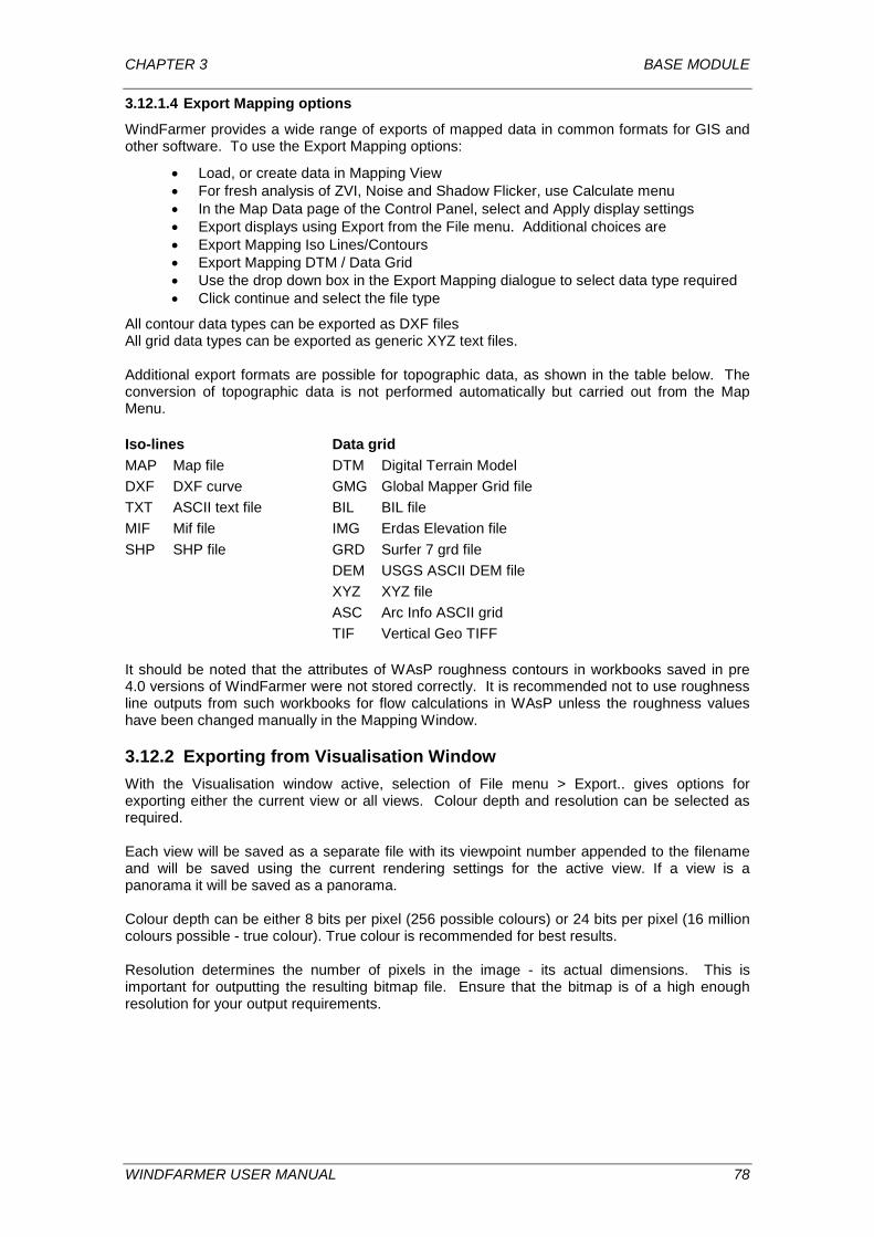
CHAPTER 3 BASE MODULE
3.12.1.4 Export Mapping options
WindFarmer provides a wide range of exports of mapped data in common formats for GIS and other software. To use the Export Mapping options:
• Load, or create data in Mapping View • For fresh analysis of ZVI, Noise and Shadow Flicker, use Calculate menu • In the Map Data page of the Control Panel, select and Apply display settings • Export displays using Export from the File menu. Additional choices are • Export Mapping Iso Lines/Contours • Export Mapping DTM / Data Grid • Use the drop down box in the Export Mapping dialogue to select data type required • Click continue and select the file type
All contour data types can be exported as DXF files All grid data types can be exported as generic XYZ text files. Additional export formats are possible for topographic data, as shown in the table below. The conversion of topographic data is not performed automatically but carried out from the Map Menu. Iso-lines Data grid MAP Map file DTM Digital Terrain Model DXF DXF curve GMG Global Mapper Grid file TXT ASCII text file BIL BIL file MIF Mif file IMG Erdas Elevation file SHP SHP file GRD Surfer 7 grd file DEM USGS ASCII DEM file XYZ XYZ file ASC Arc Info ASCII grid TIF Vertical Geo TIFF It should be noted that the attributes of WAsP roughness contours in workbooks saved in pre 4.0 versions of WindFarmer were not stored correctly. It is recommended not to use roughness line outputs from such workbooks for flow calculations in WAsP unless the roughness values have been changed manually in the Mapping Window.
3.12.2 Exporting from Visualisation Window With the Visualisation window active, selection of File menu > Export.. gives options for exporting either the current view or all views. Colour depth and resolution can be selected as required. Each view will be saved as a separate file with its viewpoint number appended to the filename and will be saved using the current rendering settings for the active view. If a view is a panorama it will be saved as a panorama. Colour depth can be either 8 bits per pixel (256 possible colours) or 24 bits per pixel (16 million colours possible - true colour). True colour is recommended for best results. Resolution determines the number of pixels in the image - its actual dimensions. This is important for outputting the resulting bitmap file. Ensure that the bitmap is of a high enough resolution for your output requirements.
WINDFARMER USER MANUAL 78
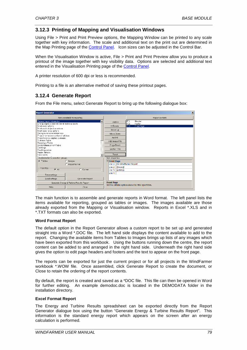
CHAPTER 3 BASE MODULE
3.12.3 Printing of Mapping and Visualisation Windows Using File > Print and Print Preview options, the Mapping Window can be printed to any scale together with key information. The scale and additional text on the print out are determined in the Map Printing page of the Control Panel. Icon sizes can be adjusted in the Control Bar. When the Visualisation Window is active, File > Print and Print Preview allow you to produce a printout of the image together with key visibility data. Options are selected and additional text entered in the Visualisation Printing page of the Control Panel. A printer resolution of 600 dpi or less is recommended. Printing to a file is an alternative method of saving these printout pages.
3.12.4 Generate Report From the File menu, select Generate Report to bring up the following dialogue box:
The main function is to assemble and generate reports in Word format. The left panel lists the items available for reporting, grouped as tables or images. The images available are those already exported from the Mapping or Visualisation window. Reports in Excel *.XLS and in *.TXT formats can also be exported.
Word Format Report
The default option in the Report Generator allows a custom report to be set up and generated straight into a Word *.DOC file. The left hand side displays the content available to add to the report. Changing the available items from Tables to Images brings up lists of any images which have been exported from this workbook. Using the buttons running down the centre, the report content can be added to and arranged in the right hand side. Underneath the right hand side gives the option to edit page headers and footers and the text to appear on the front page. The reports can be exported for just the current project or for all projects in the WindFarmer workbook *.WOW file. Once assembled, click Generate Report to create the document, or Close to retain the ordering of the report contents. By default, the report is created and saved as a *DOC file. This file can then be opened in Word for further editing. An example demodoc.doc is located in the DEMODATA folder in the installation directory.
Excel Format Report
The Energy and Turbine Results spreadsheet can be exported directly from the Report Generator dialogue box using the button “Generate Energy & Turbine Results Report”. This information is the standard energy report which appears on the screen after an energy calculation is performed.
WINDFARMER USER MANUAL 79
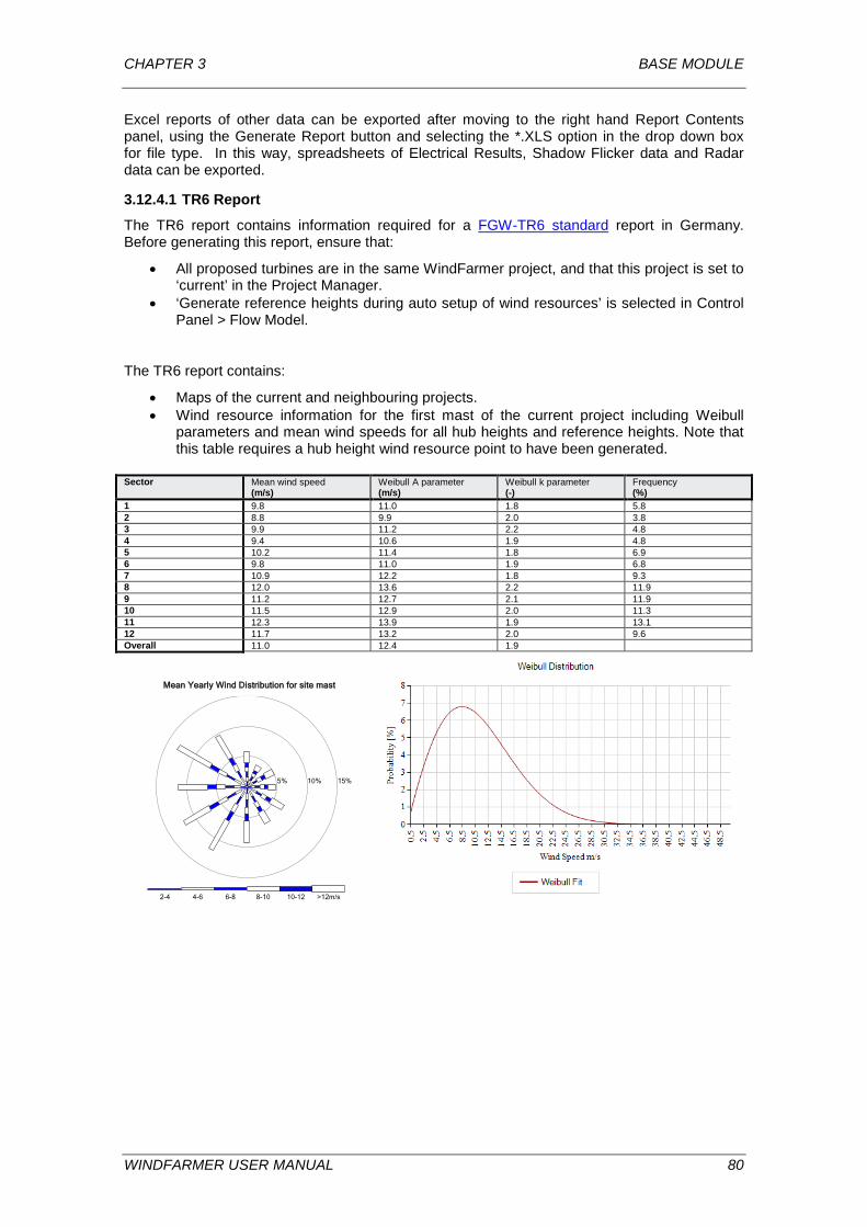
CHAPTER 3 BASE MODULE
Excel reports of other data can be exported after moving to the right hand Report Contents panel, using the Generate Report button and selecting the *.XLS option in the drop down box for file type. In this way, spreadsheets of Electrical Results, Shadow Flicker data and Radar data can be exported.
3.12.4.1 TR6 Report
The TR6 report contains information required for a FGW-TR6 standard report in Germany. Before generating this report, ensure that:
• All proposed turbines are in the same WindFarmer project, and that this project is set to ‘current’ in the Project Manager.
• ‘Generate reference heights during auto setup of wind resources’ is selected in Control Panel > Flow Model.
The TR6 report contains:
• Maps of the current and neighbouring projects. • Wind resource information for the first mast of the current project including Weibull
parameters and mean wind speeds for all hub heights and reference heights. Note that this table requires a hub height wind resource point to have been generated.
Sector Mean wind speed (m/s)
Weibull A parameter (m/s)
Weibull k parameter (-)
Frequency (%)
1 9.8 11.0 1.8 5.8 2 8.8 9.9 2.0 3.8 3 9.9 11.2 2.2 4.8 4 9.4 10.6 1.9 4.8 5 10.2 11.4 1.8 6.9 6 9.8 11.0 1.9 6.8 7 10.9 12.2 1.8 9.3 8 12.0 13.6 2.2 11.9 9 11.2 12.7 2.1 11.9 10 11.5 12.9 2.0 11.3 11 12.3 13.9 1.9 13.1 12 11.7 13.2 2.0 9.6 Overall 11.0 12.4 1.9
15%10%5%
2-4 4-6 6-8 8-10 10-12 >12m/s
Mean Yearly Wind Distribution for site mast
WINDFARMER USER MANUAL 80
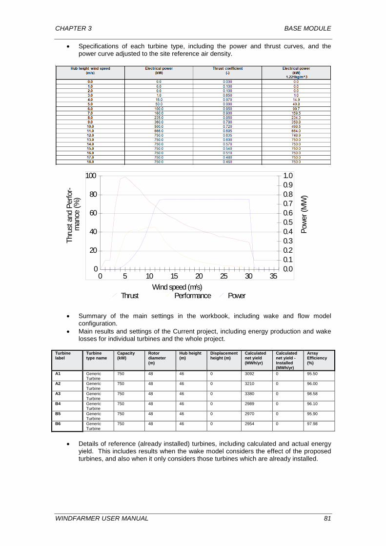
CHAPTER 3 BASE MODULE
• Specifications of each turbine type, including the power and thrust curves, and the power curve adjusted to the site reference air density.
• Summary of the main settings in the workbook, including wake and flow model configuration.
• Main results and settings of the Current project, including energy production and wake losses for individual turbines and the whole project.
Turbine label
Turbine type name
Capacity (kW)
Rotor diameter (m)
Hub height (m)
Displacement height (m)
Calculated net yield (MWh/yr)
Calculated net yield - Installed (MWh/yr)
Array Efficiency (%)
A1 Generic Turbine
750 48 46 0 3092 0 95.50
A2 Generic Turbine
750 48 46 0 3210 0 96.00
A3 Generic Turbine
750 48 46 0 3380 0 98.58
B4 Generic Turbine
750 48 46 0 2989 0 96.10
B5 Generic Turbine
750 48 46 0 2970 0 95.90
B6 Generic Turbine
750 48 46 0 2954 0 97.98
• Details of reference (already installed) turbines, including calculated and actual energy
yield. This includes results when the wake model considers the effect of the proposed turbines, and also when it only considers those turbines which are already installed.
Thrust Performance Power
Thru
st a
nd P
erfo
r-m
ance
(%)
Powe
r (M
W)
Wind speed (m/s)
0
20
40
60
80
100
0.00.10.20.30.40.50.60.70.80.91.0
0 5 10 15 20 25 30 35
WINDFARMER USER MANUAL 81

CHAPTER 3 BASE MODULE
3.12.4.2 Summary Report
With the “summary report” you can create a report that includes wind resource information as well as energy results for new and existing turbines. Click the “Generate Summary Report” to create a Word report that contains a report with the following data:
For the workbook:
• Energy calculation settings and projection information • Map including all turbine locations for all projects and legend • List of all turbines in all projects that appear in the map
For the current project:
• Map including all turbine locations for the current project area • Location of the first mast and directional Weibull parameters and mean wind speeds at
this mast for all hub heights and reference heights. Note that this table requires a hub height wind resource point to have been generated.
• Project calculation settings and energy capture summary • Energy production and wake losses for each turbine • Power and thrust curves for all turbine types for the reference air density in the project,
and the air density adjusted power curve for the site reference point interpolated to the original wind speed steps
For all non-current projects:
• Project calculation settings • Calculated and actual energy yield and their ratio for each turbine • Power and thrust curves for all turbine types in the project, including the air density
adjusted power curve for the site reference point interpolated to the original wind speed steps.
3.12.4.3 Precision of reported energy yields
The base precision of reported energy values can now be adjusted independently of other quantities. The setting is found in the Energy Report page of the Control Panel. The high precision setting will apply to energy values, up to a maximum of 8 significant figures
These precision settings are also applied to the reported perturbed energy results. They are not applied to the reported turbine rated power as there is no error level associated with this number – this is instead reported to its full accuracy.
WINDFARMER USER MANUAL 82
CHAPTER 3 BASE MODULE
3.13 Noise Calculation The modelling of the noise caused by wind turbines is based on the definition of source, receiver and transmission. All noise calculations consider the 3-dimensional distance between source and receiver and thus require terrain data in form of a DTM file to be loaded first. If no DTM file is loaded, WindFarmer will give you the option of using a flat-earth calculation. This option is also available by un-ticking the box at the foot of the Noise Model page in Control Panel, to provide compatibility with early versions of WindFarmer. Further information on the noise models and parameters is provided in the WindFarmer Theory Manual.
3.13.1 Noise Emission The noise data, as supplied by the turbine manufacturer, are defined in the Turbine Noise page of the Turbine Studio. Inputs include the sound power level of the turbine, tonal penalties and, when available, the octave-specific sound power levels for the turbine. The measured relation between sound power level and wind speed can be defined here to allow the user to model the turbine noise level at a range of hub height wind speeds. If octave bands are used together with the wind speed variation, it is assumed that the same variation occurs for each frequency band.
3.13.2 Noise Propagation The Noise Model page of the Control Panel allows the user to select which noise model is to be used for all noise calculations (Simple, Complex (ISO9613) General, Complex (ISO9613) Alternative or Custom). The parameters of the noise models are defined here. Please see ISO9613 and the Theory Manual for details on the noise model. The Simple model is the fastest. Please use it when running an automatic layout optimisation. It allows a conservative approximation of the expected noise level using a representative frequency of 500 Hz. The Complex model follows the recommendations of ISO9613 and always includes the analysis of octave bands and ground absorption. The Custom model allows you to choose freely between the different options available. Please note that prior to calculating the noise propagation in octave bands, you must define the octave band noise emissions for all turbines used.
WINDFARMER USER MANUAL 83
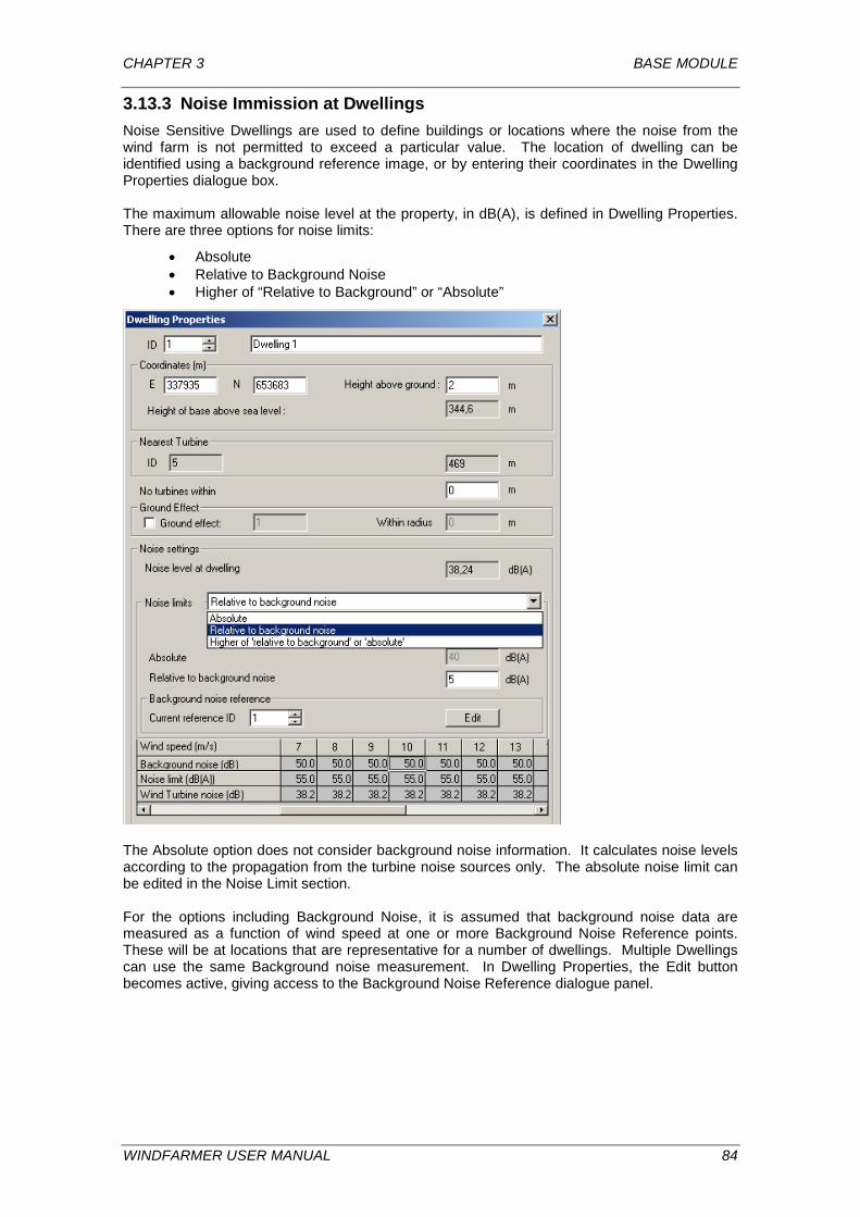
CHAPTER 3 BASE MODULE
3.13.3 Noise Immission at Dwellings Noise Sensitive Dwellings are used to define buildings or locations where the noise from the wind farm is not permitted to exceed a particular value. The location of dwelling can be identified using a background reference image, or by entering their coordinates in the Dwelling Properties dialogue box. The maximum allowable noise level at the property, in dB(A), is defined in Dwelling Properties. There are three options for noise limits:
• Absolute • Relative to Background Noise • Higher of “Relative to Background” or “Absolute”
The Absolute option does not consider background noise information. It calculates noise levels according to the propagation from the turbine noise sources only. The absolute noise limit can be edited in the Noise Limit section. For the options including Background Noise, it is assumed that background noise data are measured as a function of wind speed at one or more Background Noise Reference points. These will be at locations that are representative for a number of dwellings. Multiple Dwellings can use the same Background noise measurement. In Dwelling Properties, the Edit button becomes active, giving access to the Background Noise Reference dialogue panel.
WINDFARMER USER MANUAL 84
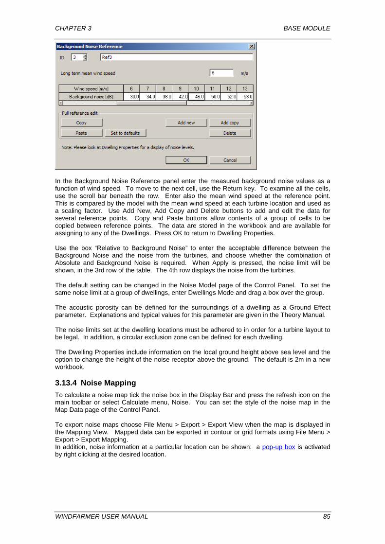
CHAPTER 3 BASE MODULE
In the Background Noise Reference panel enter the measured background noise values as a function of wind speed. To move to the next cell, use the Return key. To examine all the cells, use the scroll bar beneath the row. Enter also the mean wind speed at the reference point. This is compared by the model with the mean wind speed at each turbine location and used as a scaling factor. Use Add New, Add Copy and Delete buttons to add and edit the data for several reference points. Copy and Paste buttons allow contents of a group of cells to be copied between reference points. The data are stored in the workbook and are available for assigning to any of the Dwellings. Press OK to return to Dwelling Properties. Use the box “Relative to Background Noise” to enter the acceptable difference between the Background Noise and the noise from the turbines, and choose whether the combination of Absolute and Background Noise is required. When Apply is pressed, the noise limit will be shown, in the 3rd row of the table. The 4th row displays the noise from the turbines. The default setting can be changed in the Noise Model page of the Control Panel. To set the same noise limit at a group of dwellings, enter Dwellings Mode and drag a box over the group. The acoustic porosity can be defined for the surroundings of a dwelling as a Ground Effect parameter. Explanations and typical values for this parameter are given in the Theory Manual. The noise limits set at the dwelling locations must be adhered to in order for a turbine layout to be legal. In addition, a circular exclusion zone can be defined for each dwelling. The Dwelling Properties include information on the local ground height above sea level and the option to change the height of the noise receptor above the ground. The default is 2m in a new workbook.
3.13.4 Noise Mapping To calculate a noise map tick the noise box in the Display Bar and press the refresh icon on the main toolbar or select Calculate menu, Noise. You can set the style of the noise map in the Map Data page of the Control Panel. To export noise maps choose File Menu > Export > Export View when the map is displayed in the Mapping View. Mapped data can be exported in contour or grid formats using File Menu > Export > Export Mapping. In addition, noise information at a particular location can be shown: a pop-up box is activated by right clicking at the desired location.
WINDFARMER USER MANUAL 85

CHAPTER 3 BASE MODULE
3.14 Graphical Representation of Results The Graphing Window provides a choice of options for graphical representation of your results. As soon as a Graphing Window is opened through the Window menu or by clicking the Graphing window icon, the Graphing Toolbar becomes active.
3.14.1 Wind Rose
After opening a Graphing Window, select the symbol from the Graphing Toolbar to open the Wind Rose dialogue. This dialogue allows the user to choose the anemometry mast on which the wind rose will be based. The data required to draw the wind rose are taken from a wind resource grid (WRG file) by taking the sector P, A and k values at the anemometer’s position and reconstructing numbers of occurrences based on the Weibull equations. If the selected mast has been loaded using the association method, then the wind rose displayed will be at the mast location and height. Alternatively, a notional anemometry mast can be placed in the Mapping Window. The wind rose is then displayed using information read directly from the wind resource grid at the grid height. The Wind Rose Properties dialogue can be opened by right-clicking the Graphing Window when a wind rose is displayed or from the Graph Properties in the View menu. This dialogue allows the user to alter the appearance of the current wind rose:
• Maximum calm wind speed. All occurrences of wind speeds below this value are classed as calms. Calms have no direction and are combined in the centre of the wind rose. The radius of the central circle indicates the frequency of calms.
• Wind speed at top of …… These five edit boxes allow the user to determine how the wind distribution is displayed.
• Dimensions of saved bitmaps. The default size is the size of the wind rose window in pixels.
• Title Font. Press this button to activate a Choose Font dialog. • Font. Press this button to activate a Choose Font dialog.
You can also plot a wind rose from the MCP+ window.
3.14.2 Optimisation Progress
Selecting the symbol from the Graphing Toolbar opens the Progress Chart dialogue. With this dialogue you can watch and plot the progress of the automatic optimisation. It allows the user to select which data fields will be imported into the graph object. The two options are the Energy Yield or the Capacity Factor.
3.14.3 Turbine Performance
Selecting the symbol from the Graphing Toolbar opens the Plot Against Turbines dialogue. This allows you to plot the Net and Gross Energy Yields, the Array Efficiency i.e. Wake Loss and the Turbulence Intensity at each turbine over the turbine ID. This symbol also allows plotting the estimated design equivalent turbulence for a specific turbine as function of wind speed.
3.14.4 Noise at Dwellings
Selecting the symbol from the Graphing Toolbar opens the Plot Against Dwellings dialogue. This allows you to plot the noise level at the houses in your project and compare these with the limits at each dwelling.
3.14.5 Directional Response
Selecting the symbol from the Graphing Toolbar opens the Plot Against Sectors dialogue. This allows you to plot turbine yields against the wind direction sectors.
WINDFARMER USER MANUAL 86

CHAPTER 3 BASE MODULE
3.14.6 Turbine Characteristics
Selecting the symbol from the Graphing Toolbar opens the Plot Against Wind Speed dialogue. This allows you to plot turbine characteristics (power curve, thrust curve, performance curve)
3.14.7 Shadow Receptors
Selecting the symbol from the Graphing Toolbar opens the Shadow Plot dialogue. This allows you to plot the start and stop times of shadow flicker occurrence against the day of the year for the selected shadow receptor.
3.14.8 Changing the Graph Appearance
Selecting the symbol from the Graphing Toolbar opens the Graph Properties dialogue. You can access this dialogue also by right clicking on any graph displayed in the Graphing Window. This dialogue displays the editable properties of the current chart. After changing the appearance of the graph, use File menu, Export Template to save the settings. These can then be loaded back into a workbook using Load Template.
WINDFARMER USER MANUAL 87

CHAPTER 4 MCP+ MODULE
4 MCP+ MODULE The MCP+ Module contains the tools needed to take raw time series of wind speed and direction data through data assembly, cleaning, calibration and correlation to produce the wind regime at your site in the form of a wind speed and direction frequency distribution. To help determine the validity of the wind speed and direction data, other signals such as temperature, pressure and battery voltage can be loaded and analysed in parallel. Standard deviation data will also assist in determining the possibility of instruments malfunctioning, for example through icing. MCP (Measure-Correlate-Predict) techniques allow the derivation of a long term frequency distribution from short term data measured at your site. Outputs include multiple signal plots, wind roses, correlation plots, turbulence intensity results, data listings and reports. The frequency distribution outputs are in the TAB format, providing direct input to WAsP. The process is best treated in three parts:
• Loading the raw time series via the Data Loader. • Inspecting the data and defining data to be excluded from the subsequent analysis. • Data analysis – frequency distribution, wind roses and MCP options.
Once the data are loaded into MCP+ they are stored in a database. Any changes to the data are continuously saved as operations are performed: there is no explicit Save function within the MCP+ Module. However, after closing the MCP+ window, the workbook WOW file must be saved before closing WindFarmer completely. To explore the Module using the Demonstration CD, sample files are provided in the Demodata folder of the Libraries\Documents\Public Documents folder for Windows 7 & Windows 8 users. A duplicate of this folder is also available in the Demodata folder of the installation directory. Here can be found:
• Site.txt: time series (time history) data from a site mast • Reference.txt: long-term time series data from a reference station, including data
concurrent with the site mast • Demosite_MCP.wow: WindFarmer workbook pre-loaded with site and reference data
Interface
Logger data are imported into the Data Loader through Load MCP+ Data from the File Menu or
by clicking the blue folder icon in the MCP+ toolbar:
1 Load MCP+ data 6 'Windrose from TAB file' dialogue 2 'Edit masts' dialogue 7 'MCP' dialogue 3 'Edit sensors' dialogue 8 'Data cleaning' dialogue 4 'Edit calibration dialogue 9 'Exclude data by value' dialogue 5 'Frequency distribution' dialogue After loading, the data tree is presented and can be expanded in the MCP+ tab which alternates on the left of screen with the Display Bar. To inspect and analyse the data, functions can be selected in the toolbar or in the MCP+ menu.
WINDFARMER USER MANUAL 88
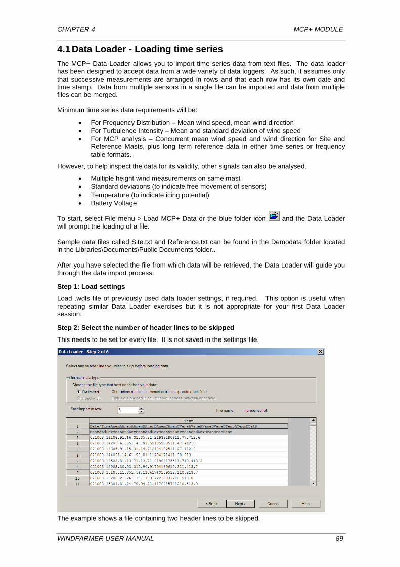
CHAPTER 4 MCP+ MODULE
4.1 Data Loader - Loading time series The MCP+ Data Loader allows you to import time series data from text files. The data loader has been designed to accept data from a wide variety of data loggers. As such, it assumes only that successive measurements are arranged in rows and that each row has its own date and time stamp. Data from multiple sensors in a single file can be imported and data from multiple files can be merged. Minimum time series data requirements will be:
• For Frequency Distribution – Mean wind speed, mean wind direction • For Turbulence Intensity – Mean and standard deviation of wind speed • For MCP analysis – Concurrent mean wind speed and wind direction for Site and
Reference Masts, plus long term reference data in either time series or frequency table formats.
However, to help inspect the data for its validity, other signals can also be analysed.
• Multiple height wind measurements on same mast • Standard deviations (to indicate free movement of sensors) • Temperature (to indicate icing potential) • Battery Voltage
To start, select File menu > Load MCP+ Data or the blue folder icon and the Data Loader will prompt the loading of a file. Sample data files called Site.txt and Reference.txt can be found in the Demodata folder located in the Libraries\Documents\Public Documents folder.. After you have selected the file from which data will be retrieved, the Data Loader will guide you through the data import process.
Step 1: Load settings
Load .wdls file of previously used data loader settings, if required. This option is useful when repeating similar Data Loader exercises but it is not appropriate for your first Data Loader session.
Step 2: Select the number of header lines to be skipped
This needs to be set for every file. It is not saved in the settings file.
The example shows a file containing two header lines to be skipped.
WINDFARMER USER MANUAL 89
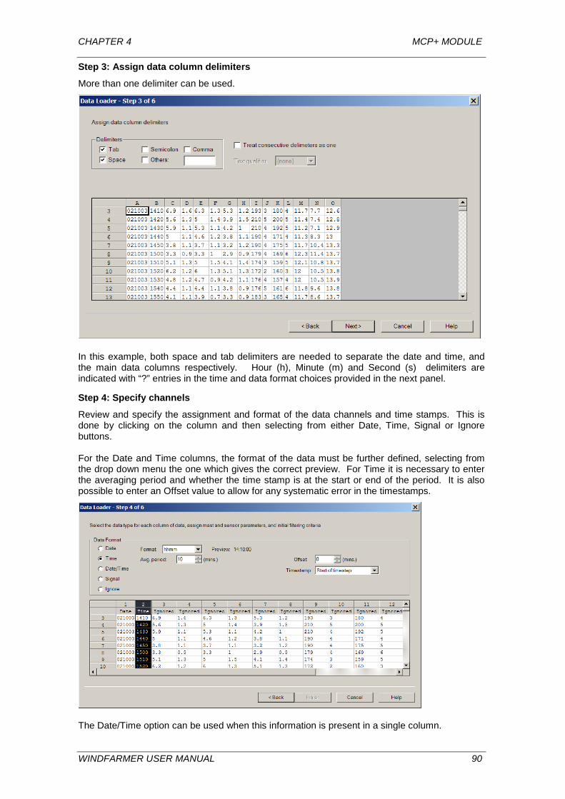
CHAPTER 4 MCP+ MODULE
Step 3: Assign data column delimiters
More than one delimiter can be used.
In this example, both space and tab delimiters are needed to separate the date and time, and the main data columns respectively. Hour (h), Minute (m) and Second (s) delimiters are indicated with “?” entries in the time and data format choices provided in the next panel.
Step 4: Specify channels
Review and specify the assignment and format of the data channels and time stamps. This is done by clicking on the column and then selecting from either Date, Time, Signal or Ignore buttons. For the Date and Time columns, the format of the data must be further defined, selecting from the drop down menu the one which gives the correct preview. For Time it is necessary to enter the averaging period and whether the time stamp is at the start or end of the period. It is also possible to enter an Offset value to allow for any systematic error in the timestamps.
The Date/Time option can be used when this information is present in a single column.
WINDFARMER USER MANUAL 90
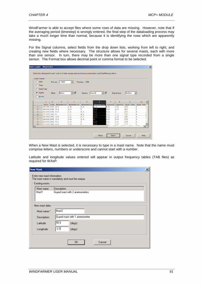
CHAPTER 4 MCP+ MODULE
WindFarmer is able to accept files where some rows of data are missing. However, note that if the averaging period (timestep) is wrongly entered, the final step of the dataloading process may take a much longer time than normal, because it is identifying the rows which are apparently missing. For the Signal columns, select fields from the drop down lists, working from left to right, and creating new fields where necessary. The structure allows for several masts, each with more than one sensor. In turn, there may be more than one signal type recorded from a single sensor. The Format box allows decimal point or comma format to be selected.
When a New Mast is selected, it is necessary to type in a mast name. Note that the name must comprise letters, numbers or underscore and cannot start with a number. Latitude and longitude values entered will appear in output frequency tables (TAB files) as required for WAsP.
WINDFARMER USER MANUAL 91
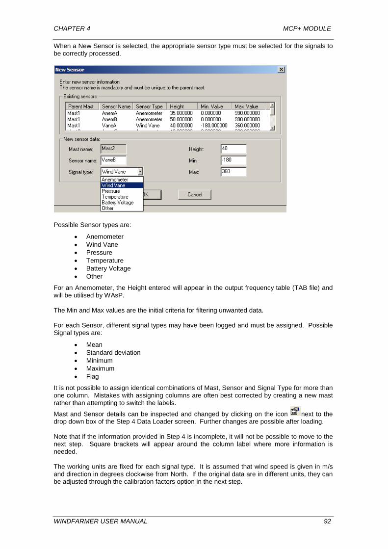
CHAPTER 4 MCP+ MODULE
When a New Sensor is selected, the appropriate sensor type must be selected for the signals to be correctly processed.
Possible Sensor types are:
• Anemometer • Wind Vane • Pressure • Temperature • Battery Voltage • Other
For an Anemometer, the Height entered will appear in the output frequency table (TAB file) and will be utilised by WAsP. The Min and Max values are the initial criteria for filtering unwanted data. For each Sensor, different signal types may have been logged and must be assigned. Possible Signal types are:
• Mean • Standard deviation • Minimum • Maximum • Flag
It is not possible to assign identical combinations of Mast, Sensor and Signal Type for more than one column. Mistakes with assigning columns are often best corrected by creating a new mast rather than attempting to switch the labels.
Mast and Sensor details can be inspected and changed by clicking on the icon next to the drop down box of the Step 4 Data Loader screen. Further changes are possible after loading. Note that if the information provided in Step 4 is incomplete, it will not be possible to move to the next step. Square brackets will appear around the column label where more information is needed. The working units are fixed for each signal type. It is assumed that wind speed is given in m/s and direction in degrees clockwise from North. If the original data are in different units, they can be adjusted through the calibration factors option in the next step.
WINDFARMER USER MANUAL 92
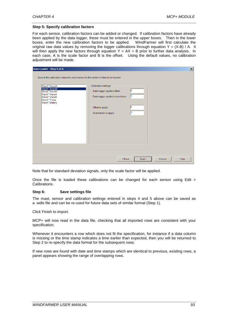
CHAPTER 4 MCP+ MODULE
Step 5: Specify calibration factors
For each sensor, calibration factors can be added or changed. If calibration factors have already been applied by the data logger, these must be entered in the upper boxes. Then in the lower boxes, enter the new calibration factors to be applied. WindFarmer will first calculate the original raw data values by removing the logger calibrations through equation Y = (X-B) / A. It will then apply the new factors through equation Y = AX + B prior to further data analysis. In each case, A is the scale factor and B is the offset. Using the default values, no calibration adjustment will be made.
Note that for standard deviation signals, only the scale factor will be applied. Once the file is loaded these calibrations can be changed for each sensor using Edit > Calibrations.
Step 6: Save settings file
The mast, sensor and calibration settings entered in steps 4 and 5 above can be saved as a .wdls file and can be re-used for future data sets of similar format (Step 1). Click Finish to import. MCP+ will now read in the data file, checking that all imported rows are consistent with your specification. Whenever it encounters a row which does not fit the specification, for instance if a data column is missing or the time stamp indicates a time earlier than expected, then you will be returned to Step 2 to re-specify the data format for the subsequent rows. If new rows are found with date and time stamps which are identical to previous, existing rows, a panel appears showing the range of overlapping rows.
WINDFARMER USER MANUAL 93
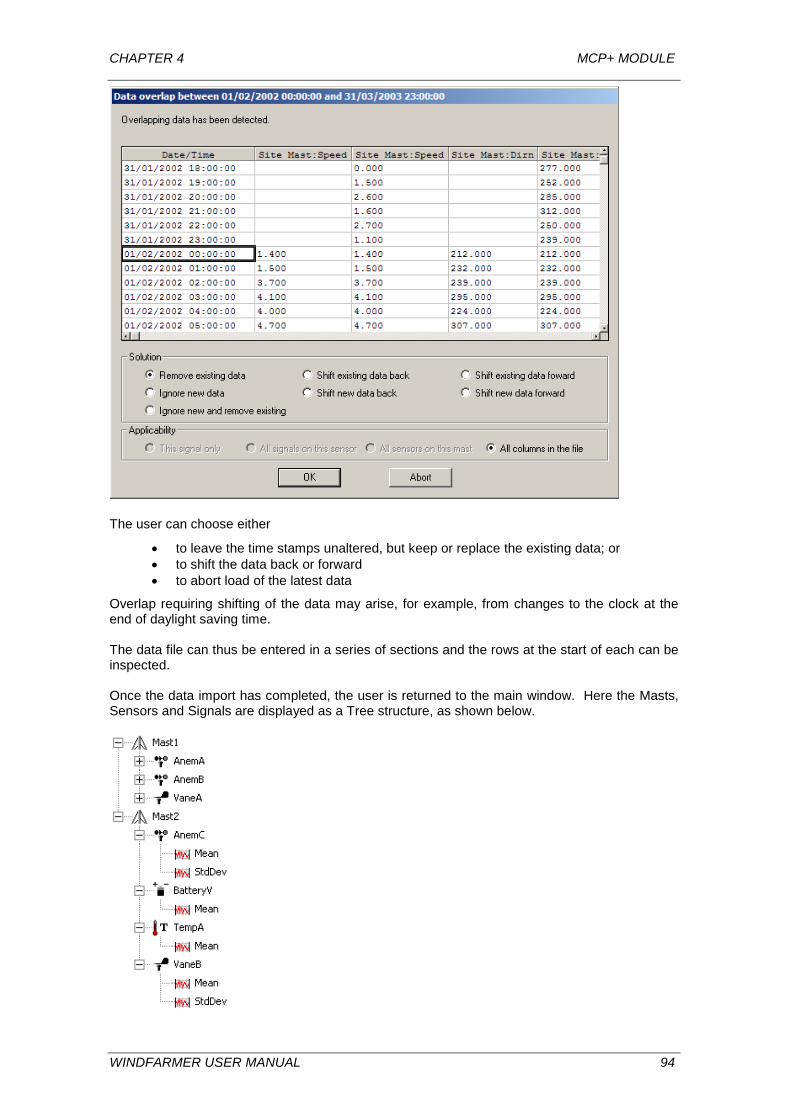
CHAPTER 4 MCP+ MODULE
The user can choose either
• to leave the time stamps unaltered, but keep or replace the existing data; or • to shift the data back or forward • to abort load of the latest data
Overlap requiring shifting of the data may arise, for example, from changes to the clock at the end of daylight saving time. The data file can thus be entered in a series of sections and the rows at the start of each can be inspected. Once the data import has completed, the user is returned to the main window. Here the Masts, Sensors and Signals are displayed as a Tree structure, as shown below.
WINDFARMER USER MANUAL 94
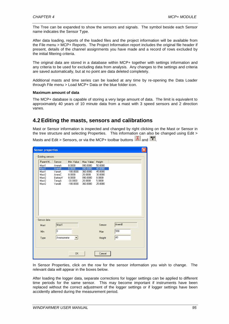
CHAPTER 4 MCP+ MODULE
The Tree can be expanded to show the sensors and signals. The symbol beside each Sensor name indicates the Sensor Type. After data loading, reports of the loaded files and the project information will be available from the File menu > MCP+ Reports. The Project Information report includes the original file header if present, details of the channel assignments you have made and a record of rows excluded by the initial filtering criteria. The original data are stored in a database within MCP+ together with settings information and any criteria to be used for excluding data from analysis. Any changes to the settings and criteria are saved automatically, but at no point are data deleted completely. Additional masts and time series can be loaded at any time by re-opening the Data Loader through File menu > Load MCP+ Data or the blue folder icon.
Maximum amount of data
The MCP+ database is capable of storing a very large amount of data. The limit is equivalent to approximately 40 years of 10 minute data from a mast with 3 speed sensors and 2 direction vanes.
4.2 Editing the masts, sensors and calibrations Mast or Sensor information is inspected and changed by right clicking on the Mast or Sensor in the tree structure and selecting Properties. This information can also be changed using Edit >
Masts and Edit > Sensors, or via the MCP+ toolbar buttons and .
In Sensor Properties, click on the row for the sensor information you wish to change. The relevant data will appear in the boxes below. After loading the logger data, separate corrections for logger settings can be applied to different time periods for the same sensor. This may become important if instruments have been replaced without the correct adjustment of the logger settings or if logger settings have been accidently altered during the measurement period.
WINDFARMER USER MANUAL 95
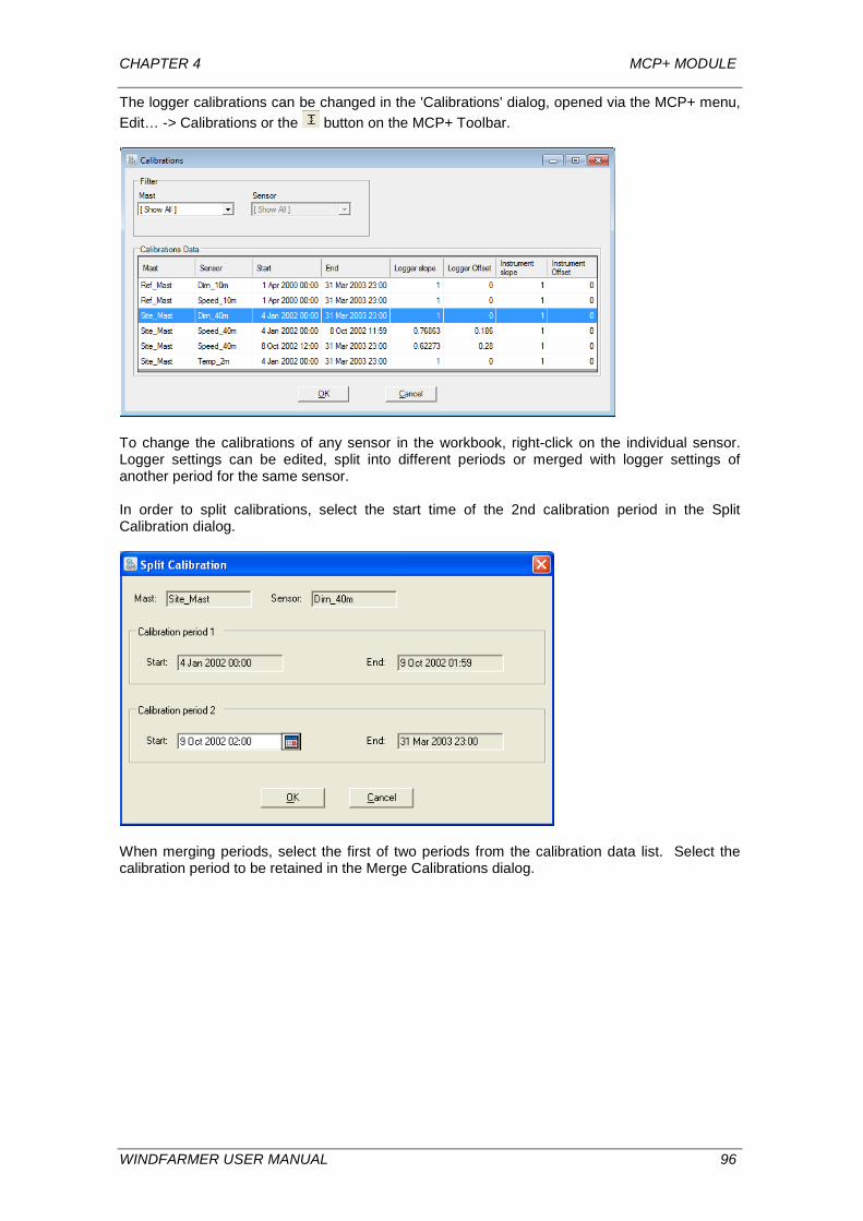
CHAPTER 4 MCP+ MODULE
The logger calibrations can be changed in the 'Calibrations' dialog, opened via the MCP+ menu, Edit… -> Calibrations or the button on the MCP+ Toolbar.
To change the calibrations of any sensor in the workbook, right-click on the individual sensor. Logger settings can be edited, split into different periods or merged with logger settings of another period for the same sensor. In order to split calibrations, select the start time of the 2nd calibration period in the Split Calibration dialog.
When merging periods, select the first of two periods from the calibration data list. Select the calibration period to be retained in the Merge Calibrations dialog.
WINDFARMER USER MANUAL 96
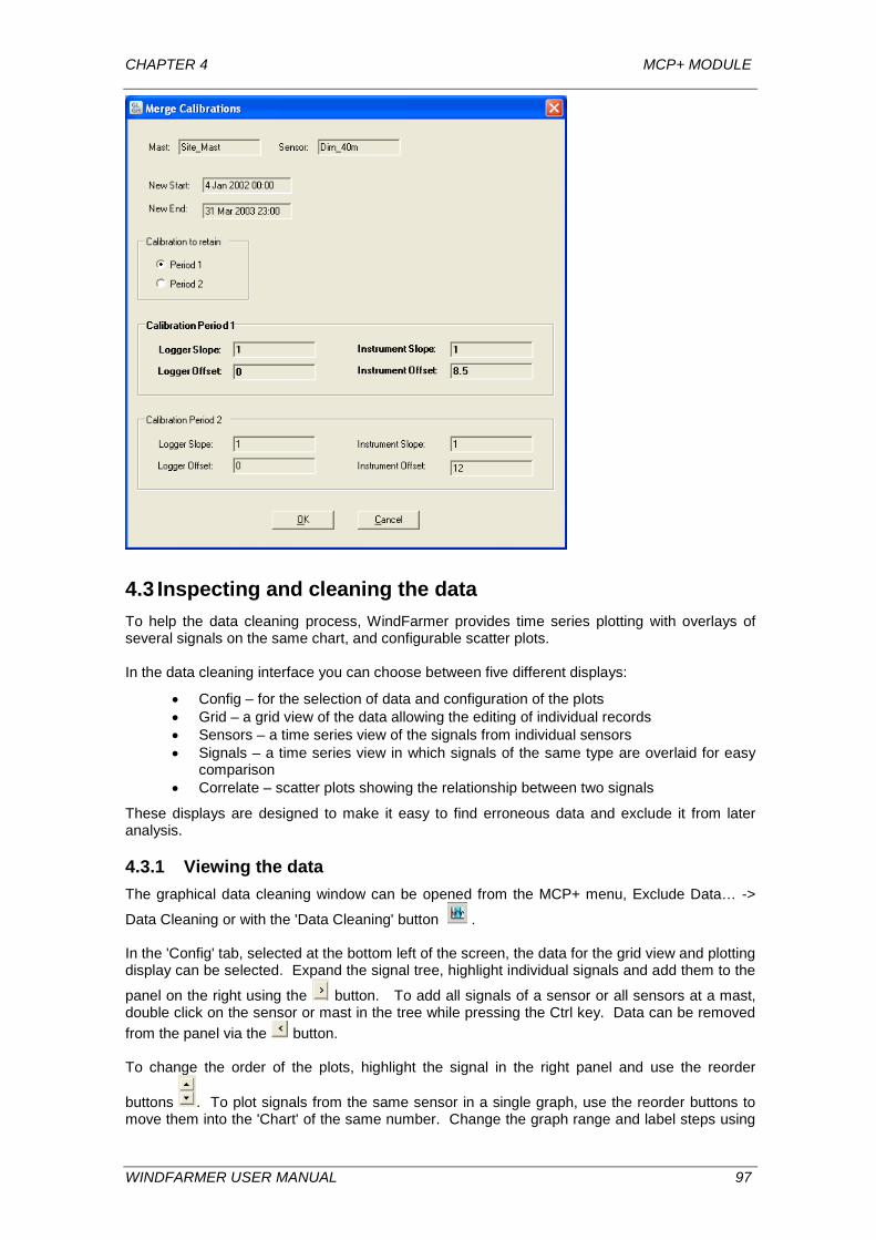
CHAPTER 4 MCP+ MODULE
4.3 Inspecting and cleaning the data To help the data cleaning process, WindFarmer provides time series plotting with overlays of several signals on the same chart, and configurable scatter plots. In the data cleaning interface you can choose between five different displays:
• Config – for the selection of data and configuration of the plots • Grid – a grid view of the data allowing the editing of individual records • Sensors – a time series view of the signals from individual sensors • Signals – a time series view in which signals of the same type are overlaid for easy
comparison • Correlate – scatter plots showing the relationship between two signals
These displays are designed to make it easy to find erroneous data and exclude it from later analysis.
4.3.1 Viewing the data The graphical data cleaning window can be opened from the MCP+ menu, Exclude Data… ->
Data Cleaning or with the 'Data Cleaning' button . In the 'Config' tab, selected at the bottom left of the screen, the data for the grid view and plotting display can be selected. Expand the signal tree, highlight individual signals and add them to the
panel on the right using the button. To add all signals of a sensor or all sensors at a mast, double click on the sensor or mast in the tree while pressing the Ctrl key. Data can be removed from the panel via the button. To change the order of the plots, highlight the signal in the right panel and use the reorder
buttons . To plot signals from the same sensor in a single graph, use the reorder buttons to move them into the 'Chart' of the same number. Change the graph range and label steps using
WINDFARMER USER MANUAL 97
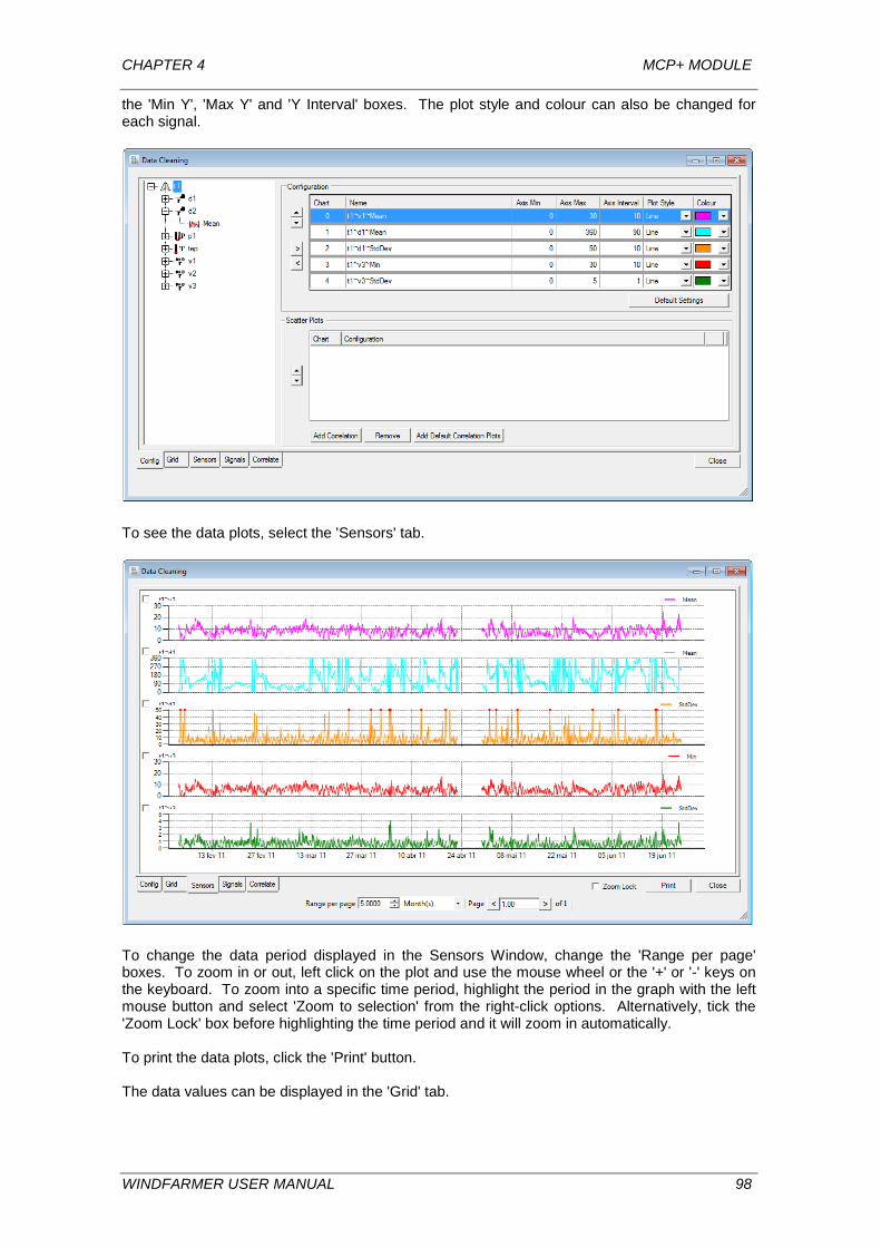
CHAPTER 4 MCP+ MODULE
the 'Min Y', 'Max Y' and 'Y Interval' boxes. The plot style and colour can also be changed for each signal.
To see the data plots, select the 'Sensors' tab.
To change the data period displayed in the Sensors Window, change the 'Range per page' boxes. To zoom in or out, left click on the plot and use the mouse wheel or the '+' or '-' keys on the keyboard. To zoom into a specific time period, highlight the period in the graph with the left mouse button and select 'Zoom to selection' from the right-click options. Alternatively, tick the 'Zoom Lock' box before highlighting the time period and it will zoom in automatically. To print the data plots, click the 'Print' button. The data values can be displayed in the 'Grid' tab.
WINDFARMER USER MANUAL 98
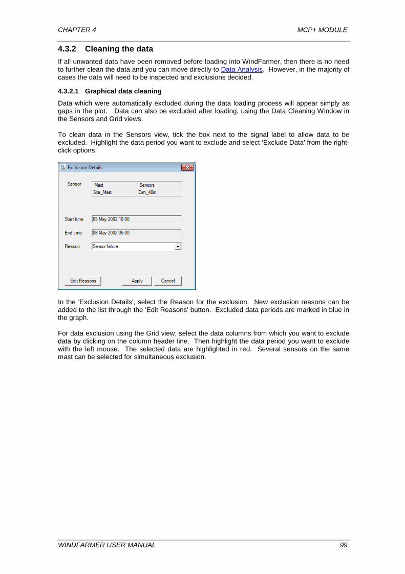
CHAPTER 4 MCP+ MODULE
4.3.2 Cleaning the data If all unwanted data have been removed before loading into WindFarmer, then there is no need to further clean the data and you can move directly to Data Analysis. However, in the majority of cases the data will need to be inspected and exclusions decided.
4.3.2.1 Graphical data cleaning
Data which were automatically excluded during the data loading process will appear simply as gaps in the plot. Data can also be excluded after loading, using the Data Cleaning Window in the Sensors and Grid views. To clean data in the Sensors view, tick the box next to the signal label to allow data to be excluded. Highlight the data period you want to exclude and select 'Exclude Data' from the right-click options.
In the 'Exclusion Details', select the Reason for the exclusion. New exclusion reasons can be added to the list through the 'Edit Reasons' button. Excluded data periods are marked in blue in the graph. For data exclusion using the Grid view, select the data columns from which you want to exclude data by clicking on the column header line. Then highlight the data period you want to exclude with the left mouse. The selected data are highlighted in red. Several sensors on the same mast can be selected for simultaneous exclusion.
WINDFARMER USER MANUAL 99
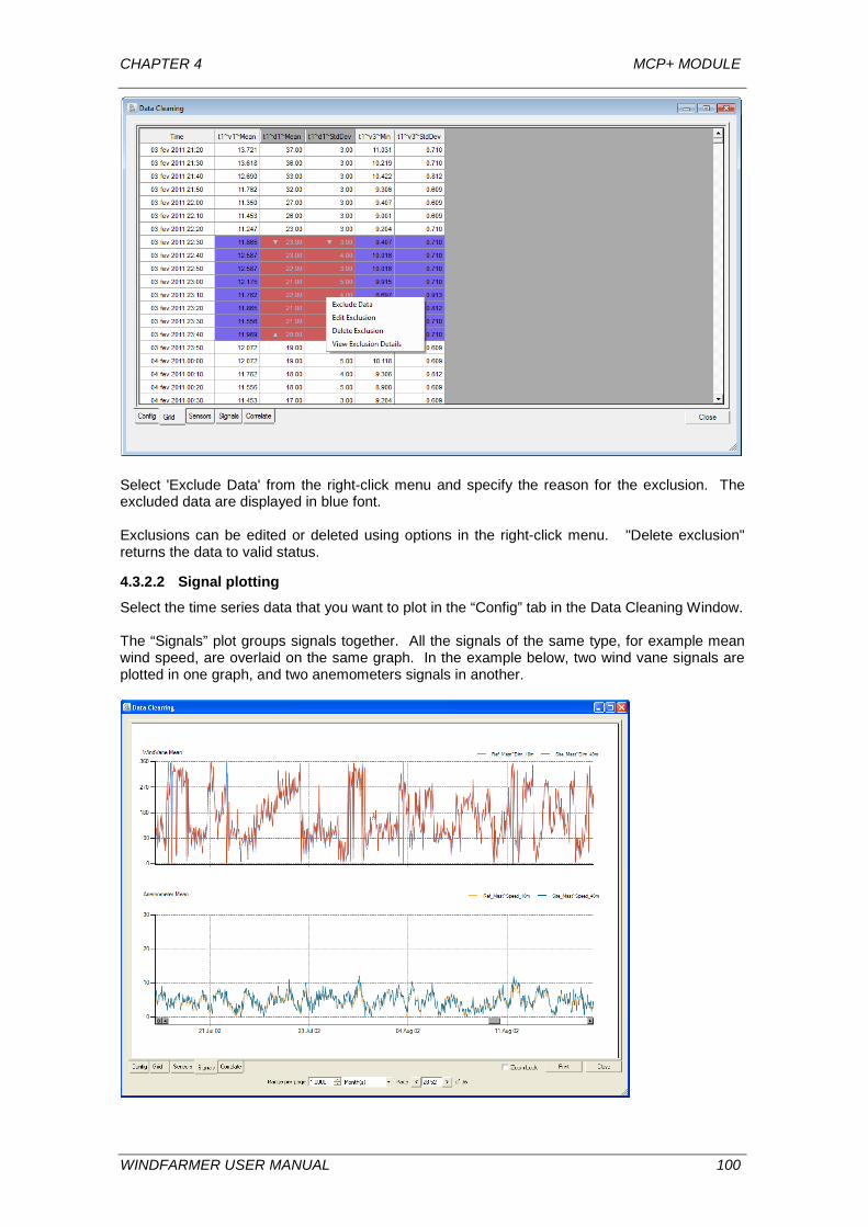
CHAPTER 4 MCP+ MODULE
Select 'Exclude Data' from the right-click menu and specify the reason for the exclusion. The excluded data are displayed in blue font. Exclusions can be edited or deleted using options in the right-click menu. "Delete exclusion" returns the data to valid status.
4.3.2.2 Signal plotting
Select the time series data that you want to plot in the “Config” tab in the Data Cleaning Window. The “Signals” plot groups signals together. All the signals of the same type, for example mean wind speed, are overlaid on the same graph. In the example below, two wind vane signals are plotted in one graph, and two anemometers signals in another.
WINDFARMER USER MANUAL 100
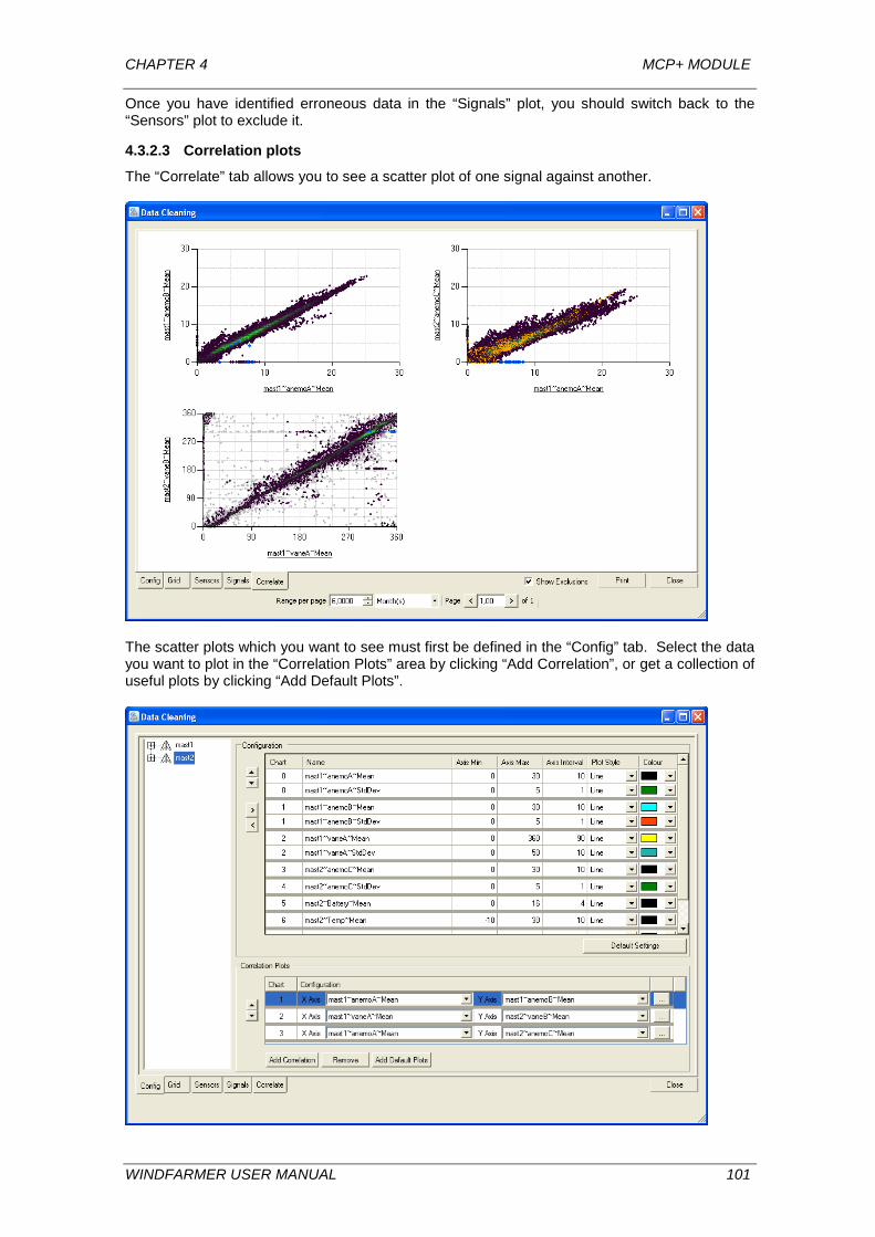
CHAPTER 4 MCP+ MODULE
Once you have identified erroneous data in the “Signals” plot, you should switch back to the “Sensors” plot to exclude it.
4.3.2.3 Correlation plots
The “Correlate” tab allows you to see a scatter plot of one signal against another.
The scatter plots which you want to see must first be defined in the “Config” tab. Select the data you want to plot in the “Correlation Plots” area by clicking “Add Correlation”, or get a collection of useful plots by clicking “Add Default Plots”.
WINDFARMER USER MANUAL 101
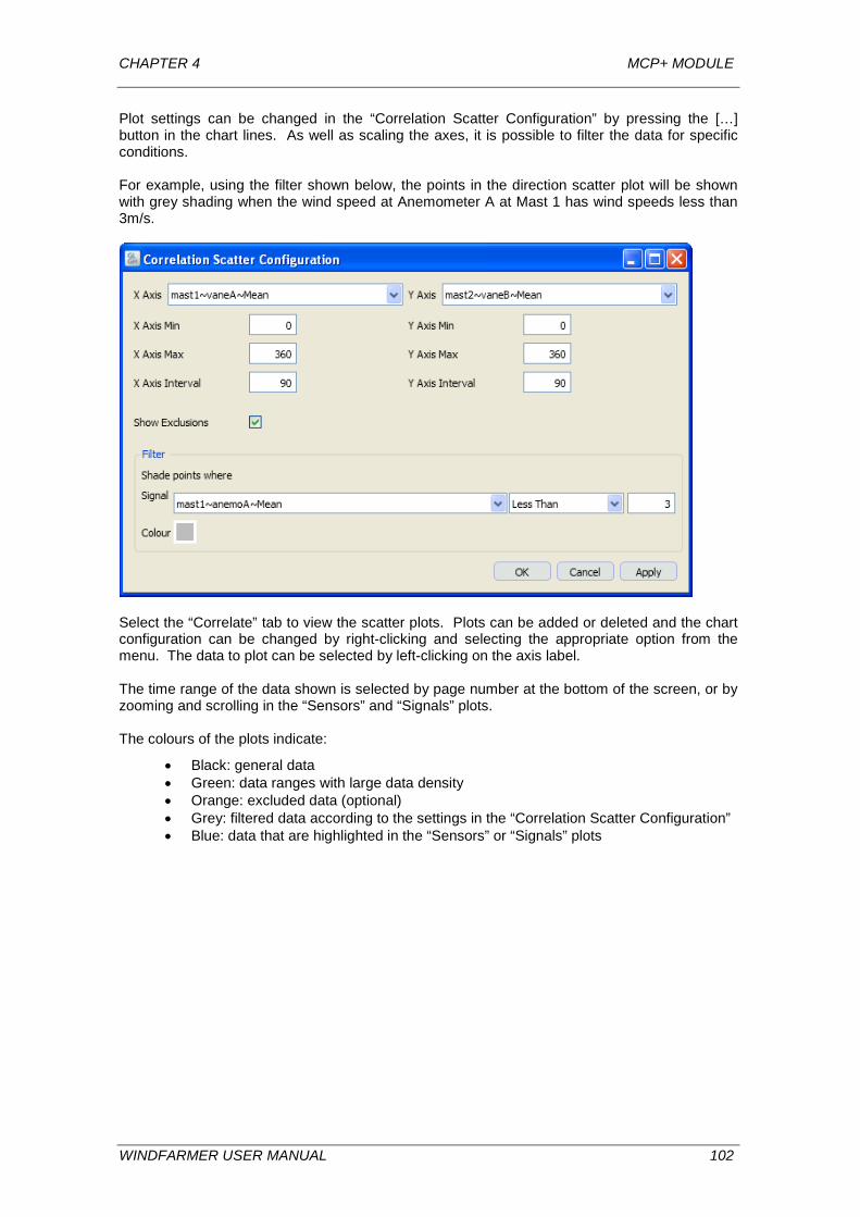
CHAPTER 4 MCP+ MODULE
Plot settings can be changed in the “Correlation Scatter Configuration” by pressing the […] button in the chart lines. As well as scaling the axes, it is possible to filter the data for specific conditions. For example, using the filter shown below, the points in the direction scatter plot will be shown with grey shading when the wind speed at Anemometer A at Mast 1 has wind speeds less than 3m/s.
Select the “Correlate” tab to view the scatter plots. Plots can be added or deleted and the chart configuration can be changed by right-clicking and selecting the appropriate option from the menu. The data to plot can be selected by left-clicking on the axis label. The time range of the data shown is selected by page number at the bottom of the screen, or by zooming and scrolling in the “Sensors” and “Signals” plots. The colours of the plots indicate:
• Black: general data • Green: data ranges with large data density • Orange: excluded data (optional) • Grey: filtered data according to the settings in the “Correlation Scatter Configuration” • Blue: data that are highlighted in the “Sensors” or “Signals” plots
WINDFARMER USER MANUAL 102
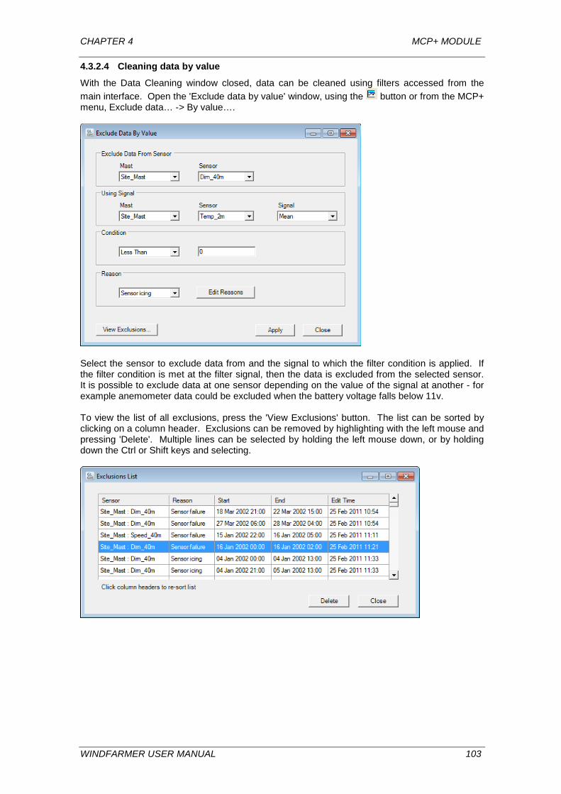
CHAPTER 4 MCP+ MODULE
4.3.2.4 Cleaning data by value
With the Data Cleaning window closed, data can be cleaned using filters accessed from the main interface. Open the 'Exclude data by value' window, using the button or from the MCP+ menu, Exclude data… -> By value….
Select the sensor to exclude data from and the signal to which the filter condition is applied. If the filter condition is met at the filter signal, then the data is excluded from the selected sensor. It is possible to exclude data at one sensor depending on the value of the signal at another - for example anemometer data could be excluded when the battery voltage falls below 11v. To view the list of all exclusions, press the 'View Exclusions' button. The list can be sorted by clicking on a column header. Exclusions can be removed by highlighting with the left mouse and pressing 'Delete'. Multiple lines can be selected by holding the left mouse down, or by holding down the Ctrl or Shift keys and selecting.
WINDFARMER USER MANUAL 103
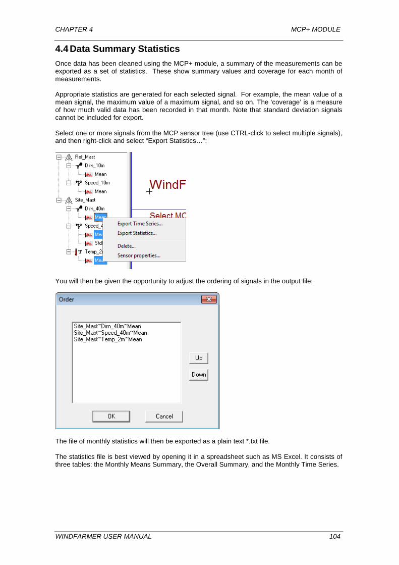
CHAPTER 4 MCP+ MODULE
4.4 Data Summary Statistics Once data has been cleaned using the MCP+ module, a summary of the measurements can be exported as a set of statistics. These show summary values and coverage for each month of measurements. Appropriate statistics are generated for each selected signal. For example, the mean value of a mean signal, the maximum value of a maximum signal, and so on. The ‘coverage’ is a measure of how much valid data has been recorded in that month. Note that standard deviation signals cannot be included for export. Select one or more signals from the MCP sensor tree (use CTRL-click to select multiple signals), and then right-click and select “Export Statistics…”:
You will then be given the opportunity to adjust the ordering of signals in the output file:
The file of monthly statistics will then be exported as a plain text *.txt file. The statistics file is best viewed by opening it in a spreadsheet such as MS Excel. It consists of three tables: the Monthly Means Summary, the Overall Summary, and the Monthly Time Series.
WINDFARMER USER MANUAL 104
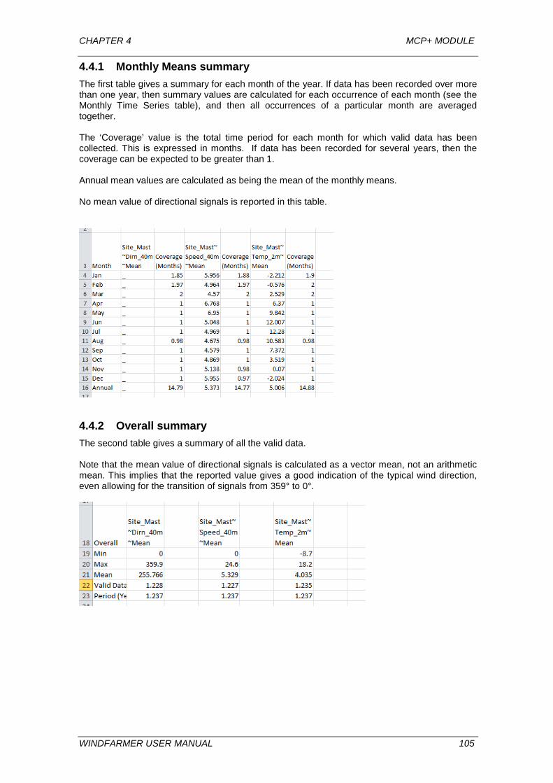
CHAPTER 4 MCP+ MODULE
4.4.1 Monthly Means summary The first table gives a summary for each month of the year. If data has been recorded over more than one year, then summary values are calculated for each occurrence of each month (see the Monthly Time Series table), and then all occurrences of a particular month are averaged together. The ‘Coverage’ value is the total time period for each month for which valid data has been collected. This is expressed in months. If data has been recorded for several years, then the coverage can be expected to be greater than 1. Annual mean values are calculated as being the mean of the monthly means. No mean value of directional signals is reported in this table.
4.4.2 Overall summary The second table gives a summary of all the valid data. Note that the mean value of directional signals is calculated as a vector mean, not an arithmetic mean. This implies that the reported value gives a good indication of the typical wind direction, even allowing for the transition of signals from 359° to 0°.
WINDFARMER USER MANUAL 105
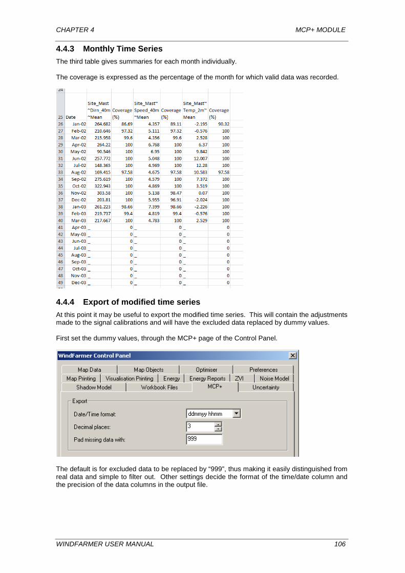
CHAPTER 4 MCP+ MODULE
4.4.3 Monthly Time Series The third table gives summaries for each month individually. The coverage is expressed as the percentage of the month for which valid data was recorded.
4.4.4 Export of modified time series At this point it may be useful to export the modified time series. This will contain the adjustments made to the signal calibrations and will have the excluded data replaced by dummy values. First set the dummy values, through the MCP+ page of the Control Panel.
The default is for excluded data to be replaced by “999”, thus making it easily distinguished from real data and simple to filter out. Other settings decide the format of the time/date column and the precision of the data columns in the output file.
WINDFARMER USER MANUAL 106
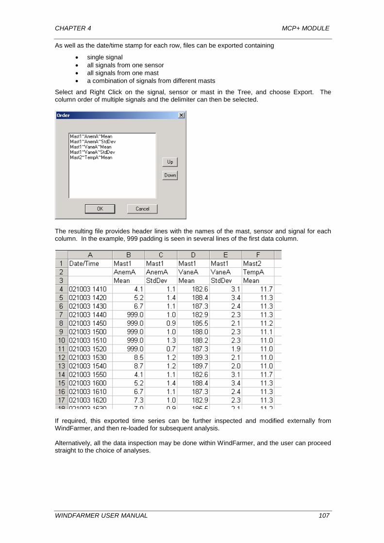
CHAPTER 4 MCP+ MODULE
As well as the date/time stamp for each row, files can be exported containing
• single signal • all signals from one sensor • all signals from one mast • a combination of signals from different masts
Select and Right Click on the signal, sensor or mast in the Tree, and choose Export. The column order of multiple signals and the delimiter can then be selected.
The resulting file provides header lines with the names of the mast, sensor and signal for each column. In the example, 999 padding is seen in several lines of the first data column.
If required, this exported time series can be further inspected and modified externally from WindFarmer, and then re-loaded for subsequent analysis. Alternatively, all the data inspection may be done within WindFarmer, and the user can proceed straight to the choice of analyses.
WINDFARMER USER MANUAL 107
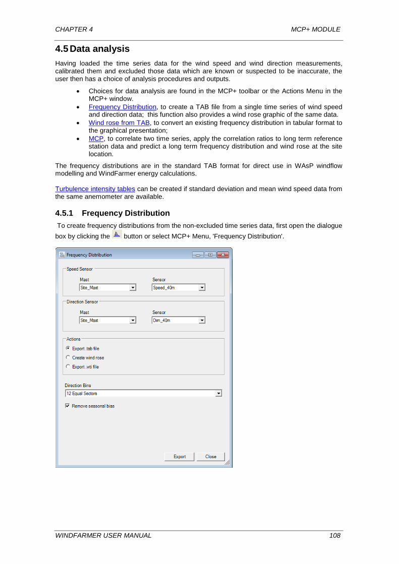
CHAPTER 4 MCP+ MODULE
4.5 Data analysis Having loaded the time series data for the wind speed and wind direction measurements, calibrated them and excluded those data which are known or suspected to be inaccurate, the user then has a choice of analysis procedures and outputs.
• Choices for data analysis are found in the MCP+ toolbar or the Actions Menu in the MCP+ window.
• Frequency Distribution, to create a TAB file from a single time series of wind speed and direction data; this function also provides a wind rose graphic of the same data.
• Wind rose from TAB, to convert an existing frequency distribution in tabular format to the graphical presentation;
• MCP, to correlate two time series, apply the correlation ratios to long term reference station data and predict a long term frequency distribution and wind rose at the site location.
The frequency distributions are in the standard TAB format for direct use in WAsP windflow modelling and WindFarmer energy calculations. Turbulence intensity tables can be created if standard deviation and mean wind speed data from the same anemometer are available.
4.5.1 Frequency Distribution To create frequency distributions from the non-excluded time series data, first open the dialogue box by clicking the button or select MCP+ Menu, 'Frequency Distribution'.
WINDFARMER USER MANUAL 108
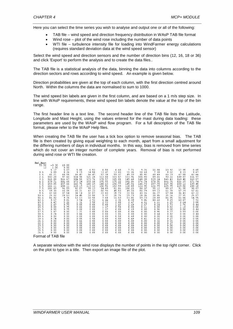
CHAPTER 4 MCP+ MODULE
Here you can select the time series you wish to analyse and output one or all of the following:
• TAB file – wind speed and direction frequency distribution in WAsP TAB file format • Wind rose – plot of the wind rose including the number of data points • WTI file – turbulence intensity file for loading into WindFarmer energy calculations
(requires standard deviation data at the wind speed sensor)
Select the wind speed and direction sensors and the number of direction bins (12, 16, 18 or 36) and click 'Export' to perform the analysis and to create the data files.. The TAB file is a statistical analysis of the data, binning the data into columns according to the direction sectors and rows according to wind speed. An example is given below. Direction probabilities are given at the top of each column, with the first direction centred around North. Within the columns the data are normalised to sum to 1000. The wind speed bin labels are given in the first column, and are based on a 1 m/s step size. In line with WAsP requirements, these wind speed bin labels denote the value at the top of the bin range. The first header line is a text line. The second header line of the TAB file lists the Latitude, Longitude and Mast Height, using the values entered for the mast during data loading: these parameters are used by the WAsP wind flow program. For a full description of the TAB file format, please refer to the WAsP Help files. When creating the TAB file the user has a tick box option to remove seasonal bias. The TAB file is then created by giving equal weighting to each month, apart from a small adjustment for the differing numbers of days in individual months. In this way, bias is removed from time series which do not cover an integer number of complete years. Removal of bias is not performed during wind rose or WTI file creation.
Format of TAB file A separate window with the wind rose displays the number of points in the top right corner. Click on the plot to type in a title. Then export an image file of the plot.
WINDFARMER USER MANUAL 109

CHAPTER 4 MCP+ MODULE
4.5.2 Turbulence Intensity Output For the Turbulence Intensity output, standard deviation and mean wind speed data from the same anemometer are required. If the “Export WTI file” is greyed out after selecting a wind speed sensor, this means either there are no associated standard deviation data, or you do not have the Turbulence Intensity Module activated in your WindFarmer licence. Four formats are possible for calculating the turbulence intensity of a time series.
OPTION OUTPUT Not enough data?
Single value Average turbulence intensity and standard deviation of the wind speed standard deviation for the whole time series.
Error message appears if there are less than 5 data points
Directional Average turbulence intensity and standard deviation of the wind speed standard deviation for each direction sector.
If there are less than 5 data points in any direction, the single average value is used
Speed Average turbulence intensity and standard deviation of the wind speed standard deviation for each integer wind speed.
If there are less than 5 data points in a wind speed bin, the single average value is used
Both Average turbulence intensity and standard deviation of the wind speed standard deviation for each wind speed on a directional basis.
If there are less that 5 data points in any one bin, the all-direction average for that wind speed is used; if there are less than 5 points at this wind speed, the single average is used.
The "low wind speed cut-off" setting determines what data are used in the analysis, when creating data that are averaged over wind speed. For each option a matrix of mean turbulence intensity, standard deviation of the wind speed standard deviation (Sigma-sigma) and of data coverage for direction and wind speed is output as an ASCII file with extension wti. These WTI files are designed to be loaded directly into the
WINDFARMER USER MANUAL 110
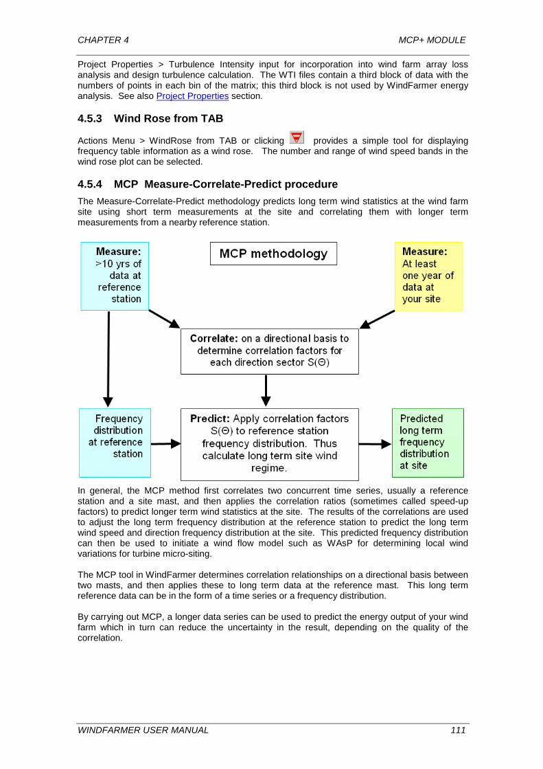
CHAPTER 4 MCP+ MODULE
Project Properties > Turbulence Intensity input for incorporation into wind farm array loss analysis and design turbulence calculation. The WTI files contain a third block of data with the numbers of points in each bin of the matrix; this third block is not used by WindFarmer energy analysis. See also Project Properties section.
4.5.3 Wind Rose from TAB
Actions Menu > WindRose from TAB or clicking provides a simple tool for displaying frequency table information as a wind rose. The number and range of wind speed bands in the wind rose plot can be selected.
4.5.4 MCP Measure-Correlate-Predict procedure The Measure-Correlate-Predict methodology predicts long term wind statistics at the wind farm site using short term measurements at the site and correlating them with longer term measurements from a nearby reference station.
In general, the MCP method first correlates two concurrent time series, usually a reference station and a site mast, and then applies the correlation ratios (sometimes called speed-up factors) to predict longer term wind statistics at the site. The results of the correlations are used to adjust the long term frequency distribution at the reference station to predict the long term wind speed and direction frequency distribution at the site. This predicted frequency distribution can then be used to initiate a wind flow model such as WAsP for determining local wind variations for turbine micro-siting. The MCP tool in WindFarmer determines correlation relationships on a directional basis between two masts, and then applies these to long term data at the reference mast. This long term reference data can be in the form of a time series or a frequency distribution. By carrying out MCP, a longer data series can be used to predict the energy output of your wind farm which in turn can reduce the uncertainty in the result, depending on the quality of the correlation.
WINDFARMER USER MANUAL 111
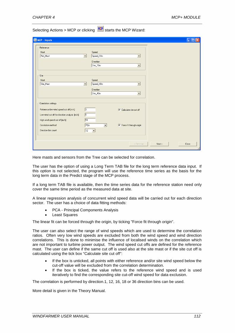
CHAPTER 4 MCP+ MODULE
Selecting Actions > MCP or clicking starts the MCP Wizard:
Here masts and sensors from the Tree can be selected for correlation. The user has the option of using a Long Term TAB file for the long term reference data input. If this option is not selected, the program will use the reference time series as the basis for the long term data in the Predict stage of the MCP process. If a long term TAB file is available, then the time series data for the reference station need only cover the same time period as the measured data at site. A linear regression analysis of concurrent wind speed data will be carried out for each direction sector. The user has a choice of data fitting methods:
• PCA - Principal Components Analysis • Least Squares
The linear fit can be forced through the origin, by ticking "Force fit through origin". The user can also select the range of wind speeds which are used to determine the correlation ratios. Often very low wind speeds are excluded from both the wind speed and wind direction correlations. This is done to minimise the influence of localised winds on the correlation which are not important to turbine power output. The wind speed cut offs are defined for the reference mast. The user can define if the same cut off is used also at the site mast or if the site cut off is calculated using the tick box “Calculate site cut off”:
• If the box is unticked, all points with either reference and/or site wind speed below the cut-off value will be excluded from the correlation determination.
• If the box is ticked, the value refers to the reference wind speed and is used iteratively to find the corresponding site cut-off wind speed for data exclusion.
The correlation is performed by direction.1, 12, 16, 18 or 36 direction bins can be used. More detail is given in the Theory Manual.
WINDFARMER USER MANUAL 112
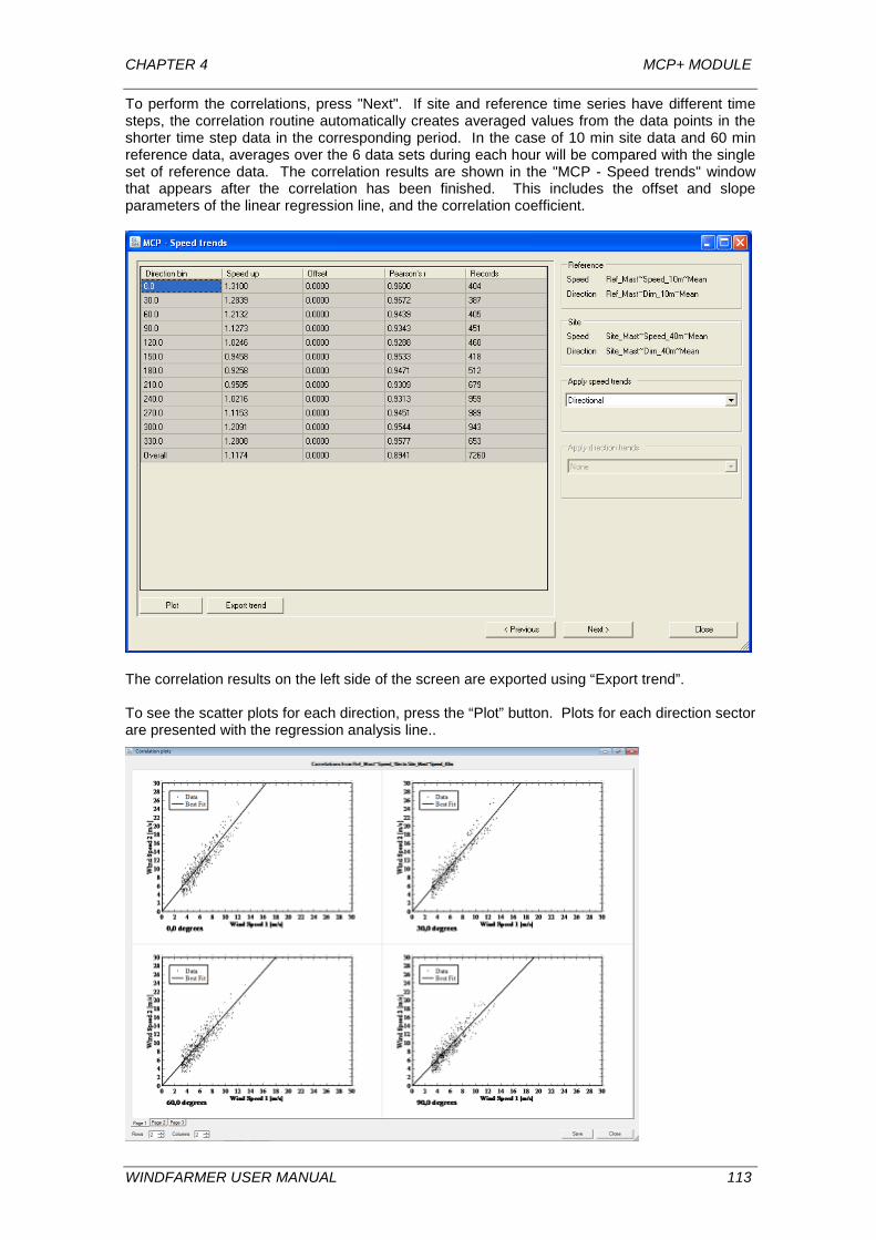
CHAPTER 4 MCP+ MODULE
To perform the correlations, press "Next". If site and reference time series have different time steps, the correlation routine automatically creates averaged values from the data points in the shorter time step data in the corresponding period. In the case of 10 min site data and 60 min reference data, averages over the 6 data sets during each hour will be compared with the single set of reference data. The correlation results are shown in the "MCP - Speed trends" window that appears after the correlation has been finished. This includes the offset and slope parameters of the linear regression line, and the correlation coefficient.
The correlation results on the left side of the screen are exported using “Export trend”. To see the scatter plots for each direction, press the “Plot” button. Plots for each direction sector are presented with the regression analysis line..
WINDFARMER USER MANUAL 113
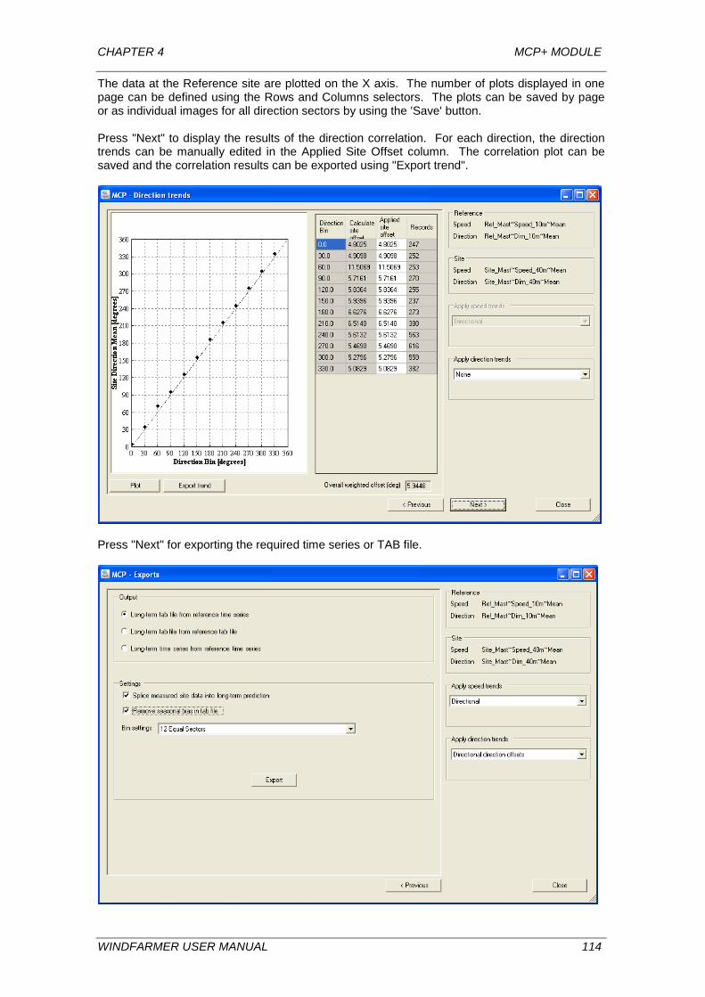
CHAPTER 4 MCP+ MODULE
The data at the Reference site are plotted on the X axis. The number of plots displayed in one page can be defined using the Rows and Columns selectors. The plots can be saved by page or as individual images for all direction sectors by using the 'Save' button. Press "Next" to display the results of the direction correlation. For each direction, the direction trends can be manually edited in the Applied Site Offset column. The correlation plot can be saved and the correlation results can be exported using "Export trend".
Press "Next" for exporting the required time series or TAB file.
WINDFARMER USER MANUAL 114
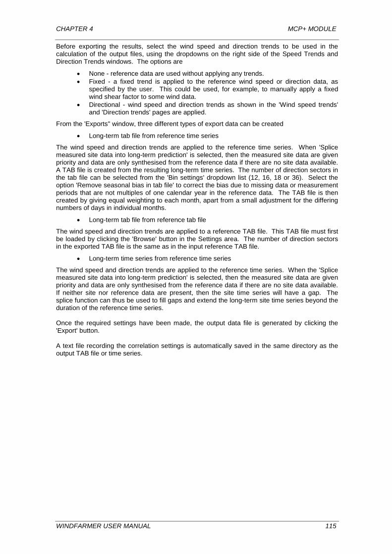
CHAPTER 4 MCP+ MODULE
Before exporting the results, select the wind speed and direction trends to be used in the calculation of the output files, using the dropdowns on the right side of the Speed Trends and Direction Trends windows. The options are
• None - reference data are used without applying any trends. • Fixed - a fixed trend is applied to the reference wind speed or direction data, as
specified by the user. This could be used, for example, to manually apply a fixed wind shear factor to some wind data.
• Directional - wind speed and direction trends as shown in the 'Wind speed trends' and 'Direction trends' pages are applied.
From the 'Exports" window, three different types of export data can be created
• Long-term tab file from reference time series
The wind speed and direction trends are applied to the reference time series. When 'Splice measured site data into long-term prediction' is selected, then the measured site data are given priority and data are only synthesised from the reference data if there are no site data available. A TAB file is created from the resulting long-term time series. The number of direction sectors in the tab file can be selected from the 'Bin settings' dropdown list (12, 16, 18 or 36). Select the option 'Remove seasonal bias in tab file' to correct the bias due to missing data or measurement periods that are not multiples of one calendar year in the reference data. The TAB file is then created by giving equal weighting to each month, apart from a small adjustment for the differing numbers of days in individual months.
• Long-term tab file from reference tab file
The wind speed and direction trends are applied to a reference TAB file. This TAB file must first be loaded by clicking the 'Browse' button in the Settings area. The number of direction sectors in the exported TAB file is the same as in the input reference TAB file.
• Long-term time series from reference time series
The wind speed and direction trends are applied to the reference time series. When the 'Splice measured site data into long-term prediction' is selected, then the measured site data are given priority and data are only synthesised from the reference data if there are no site data available. If neither site nor reference data are present, then the site time series will have a gap. The splice function can thus be used to fill gaps and extend the long-term site time series beyond the duration of the reference time series. Once the required settings have been made, the output data file is generated by clicking the 'Export' button. A text file recording the correlation settings is automatically saved in the same directory as the output TAB file or time series.
WINDFARMER USER MANUAL 115

CHAPTER 4 MCP+ MODULE
4.6 Application of MCP+ Module In summary, the MCP+ Module enables logger data to be inspected, adjusted and if necessary excluded from subsequent analysis. The user can then produce frequency tables and wind roses, analyse turbulence intensity, and predict long-term wind statistics through the Measure-Correlate-Predict process. The tools available can be used in many ways. For example, data inspection might include:
• Recalibration, to replace generic with individual calibration factors; • Filtering of signals using choice of logic to exclude unwanted data; • Synchronisation of signal plots, so standard deviation, battery or temperature values
can be used for diagnosing instrument malfunction; • Correlations to compare data from nearby instruments, helping to identify erroneous
signals such as incorrect wind vane alignment.
The primary outputs from the MCP+ Module are frequency distribution files in TAB format. These are obtained directly from wind speed and direction data measured at the site, or using MCP techniques for correlation with longer-term data from a nearby reference station. The TAB files are in the correct format for input into
• WAsP or other wind flow models, and • WindFarmer wind farm optimisation and energy analysis, using the Association
Method to enhance the wind flow prediction. See Theory Manual for more information.
For the association method, TAB files are loaded into WindFarmer
• During input of wind resource files (WRG or RSF) through the “Load File” menu item, or
• Through Project Properties > Wind Resources & Frequency Table Associations
If standard deviation wind speed data are available, turbulence intensities can be analysed. The WTI files provide input to the Eddy Viscosity wake model in the wind farm energy analysis, determining the wake dissipation behaviour for each direction and wind speed step of the calculation. WTI files can be created
• as a function of direction or wind speed or both, required for the most detailed energy analysis
WTI files are then loaded
• through Project Properties > Turbulence Intensity
Other outputs from the MCP+ Module are
• multiple signal plots showing data which have been excluded • wind roses, including wind roses directly from TAB files • scatter plots and correlation statistics • detailed data listings and reports
WINDFARMER USER MANUAL 116

CHAPTER 5 MULTIPLE PROJECTS
5 MULTIPLE PROJECTS WindFarmer allows the user to assess the effects of adjacent wind farm developments on the energy production and to study the cumulative and individual visual and acoustic impact of multiple wind farm projects in detail.
5.1 Projects WindFarmer Multiple Projects Tools work on the principle that the WindFarmer workbook (*.WOW) file contains the information that is to be shared by all of the wind farm projects being assessed. Typically this shared data will consist of a digital terrain model (DTM) for the area, a scanned background map and height contours in the form of a digital contour (MAP) file. These files can be thought of as the common framework into which site-specific project data are added. The WOW file will also contain one or more WindFarmer projects which describe project specific data and information. Project data stored within the WOW file can be exported and stored as separate WindFarmer Project (*.WPJ) files if required. Each WPJ file can contain only one project.
A WindFarmer WPJ file can contain the following site-specific information:
• the wind farm layout • wind farm boundary information • turbine specifications • wind resource information (*WRG and *RSF files) • reference anemometry mast locations • viewpoint locations • dwelling locations • road and cabling layouts • radar stations • text labels.
The Project Manager dialogue box allows individual wind farm projects to be included or excluded in the assessment, permitting different combinations of proposed and existing wind farms to be investigated. Each wind farm project also has an associated set of properties that influence a number of functions, principally ZVI map display, Finance Module labelling and boundary grouping for optimisation. The setting of these properties is described in the Project Properties section. It is also important to note that energy settings such as turbulence intensity, site air density and availability are associated with each project separately.
5.2 Projects Tools Interface The Multiple Projects Tools do not have a dedicated window, toolbar or menu associated with them. However, there are a number of toolbar buttons, dialogue boxes and pop-up menus associated with the cumulative impact tools.
5.2.1 Related Toolbar Buttons There are two toolbar buttons on the main WindFarmer toolbar that are used to access the
Projects Tool dialogue boxes. These are the Project Manager button and the Project
Properties button . Both dialogue boxes can also be accessed from the View options on the main WindFarmer menu.
WINDFARMER USER MANUAL 117
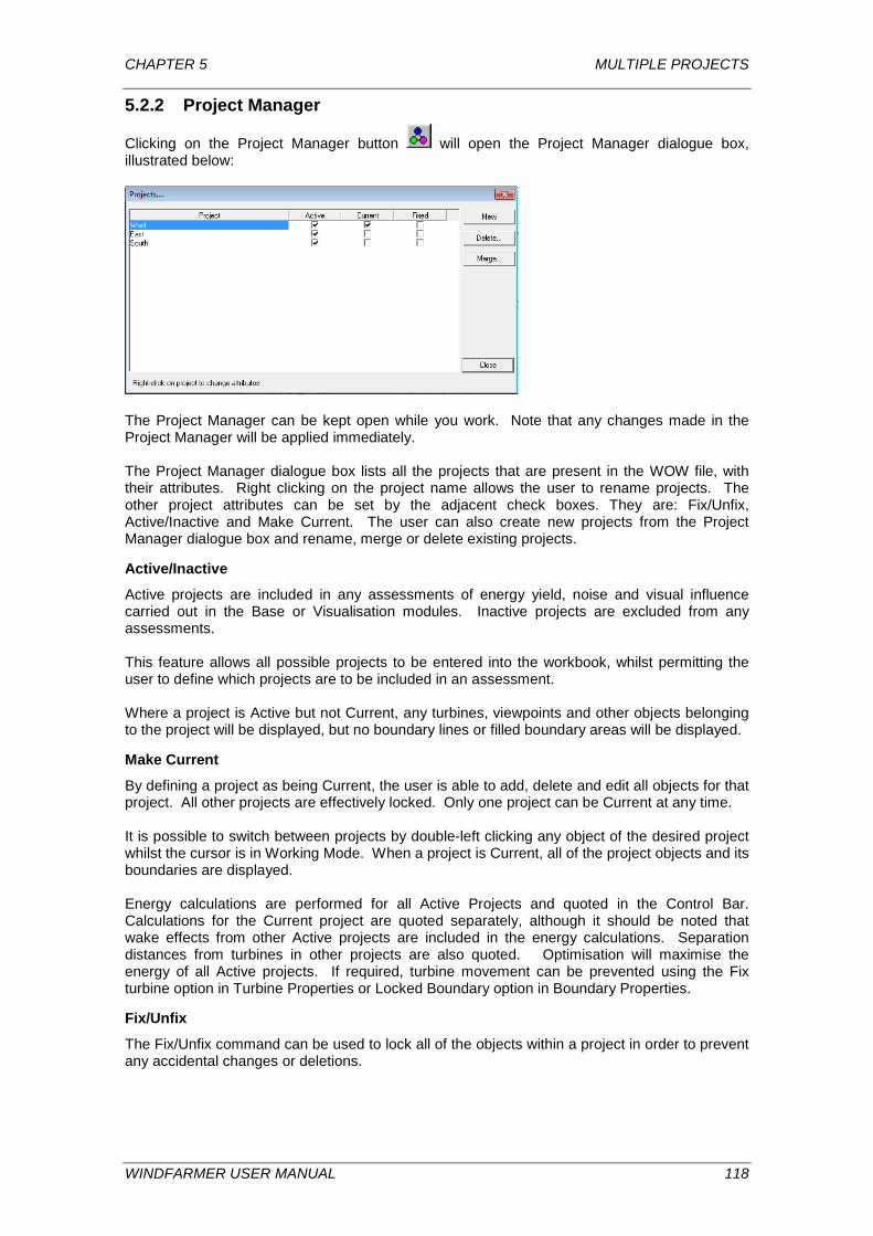
CHAPTER 5 MULTIPLE PROJECTS
5.2.2 Project Manager
Clicking on the Project Manager button will open the Project Manager dialogue box, illustrated below:
The Project Manager can be kept open while you work. Note that any changes made in the Project Manager will be applied immediately. The Project Manager dialogue box lists all the projects that are present in the WOW file, with their attributes. Right clicking on the project name allows the user to rename projects. The other project attributes can be set by the adjacent check boxes. They are: Fix/Unfix, Active/Inactive and Make Current. The user can also create new projects from the Project Manager dialogue box and rename, merge or delete existing projects.
Active/Inactive
Active projects are included in any assessments of energy yield, noise and visual influence carried out in the Base or Visualisation modules. Inactive projects are excluded from any assessments. This feature allows all possible projects to be entered into the workbook, whilst permitting the user to define which projects are to be included in an assessment. Where a project is Active but not Current, any turbines, viewpoints and other objects belonging to the project will be displayed, but no boundary lines or filled boundary areas will be displayed.
Make Current
By defining a project as being Current, the user is able to add, delete and edit all objects for that project. All other projects are effectively locked. Only one project can be Current at any time. It is possible to switch between projects by double-left clicking any object of the desired project whilst the cursor is in Working Mode. When a project is Current, all of the project objects and its boundaries are displayed. Energy calculations are performed for all Active Projects and quoted in the Control Bar. Calculations for the Current project are quoted separately, although it should be noted that wake effects from other Active projects are included in the energy calculations. Separation distances from turbines in other projects are also quoted. Optimisation will maximise the energy of all Active projects. If required, turbine movement can be prevented using the Fix turbine option in Turbine Properties or Locked Boundary option in Boundary Properties.
Fix/Unfix
The Fix/Unfix command can be used to lock all of the objects within a project in order to prevent any accidental changes or deletions.
WINDFARMER USER MANUAL 118
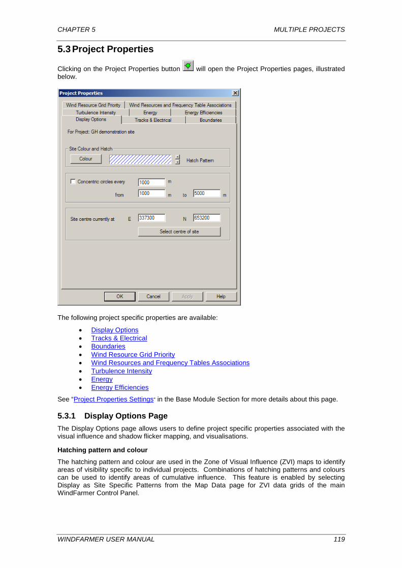
CHAPTER 5 MULTIPLE PROJECTS
5.3 Project Properties
Clicking on the Project Properties button will open the Project Properties pages, illustrated below.
The following project specific properties are available:
• Display Options • Tracks & Electrical • Boundaries • Wind Resource Grid Priority • Wind Resources and Frequency Tables Associations • Turbulence Intensity • Energy • Energy Efficiencies
See “Project Properties Settings” in the Base Module Section for more details about this page.
5.3.1 Display Options Page The Display Options page allows users to define project specific properties associated with the visual influence and shadow flicker mapping, and visualisations.
Hatching pattern and colour
The hatching pattern and colour are used in the Zone of Visual Influence (ZVI) maps to identify areas of visibility specific to individual projects. Combinations of hatching patterns and colours can be used to identify areas of cumulative influence. This feature is enabled by selecting Display as Site Specific Patterns from the Map Data page for ZVI data grids of the main WindFarmer Control Panel.
WINDFARMER USER MANUAL 119
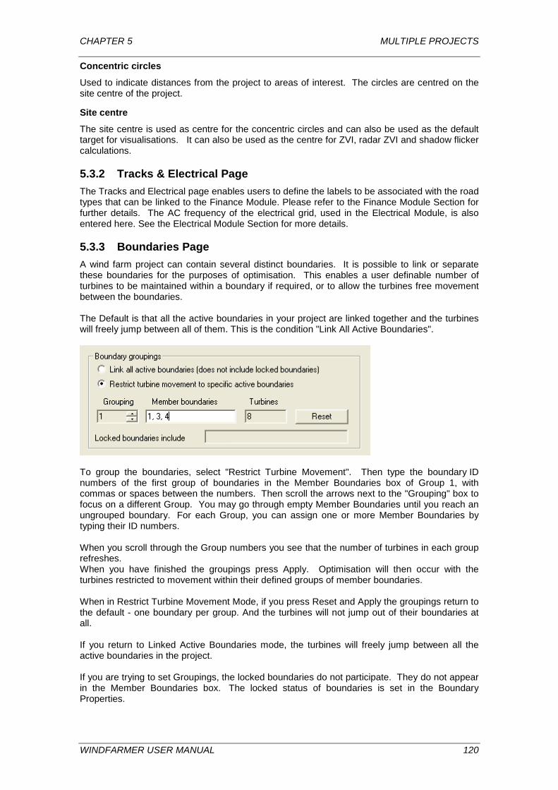
CHAPTER 5 MULTIPLE PROJECTS
Concentric circles
Used to indicate distances from the project to areas of interest. The circles are centred on the site centre of the project.
Site centre
The site centre is used as centre for the concentric circles and can also be used as the default target for visualisations. It can also be used as the centre for ZVI, radar ZVI and shadow flicker calculations.
5.3.2 Tracks & Electrical Page The Tracks and Electrical page enables users to define the labels to be associated with the road types that can be linked to the Finance Module. Please refer to the Finance Module Section for further details. The AC frequency of the electrical grid, used in the Electrical Module, is also entered here. See the Electrical Module Section for more details.
5.3.3 Boundaries Page A wind farm project can contain several distinct boundaries. It is possible to link or separate these boundaries for the purposes of optimisation. This enables a user definable number of turbines to be maintained within a boundary if required, or to allow the turbines free movement between the boundaries. The Default is that all the active boundaries in your project are linked together and the turbines will freely jump between all of them. This is the condition "Link All Active Boundaries".
To group the boundaries, select "Restrict Turbine Movement". Then type the boundary ID numbers of the first group of boundaries in the Member Boundaries box of Group 1, with commas or spaces between the numbers. Then scroll the arrows next to the "Grouping" box to focus on a different Group. You may go through empty Member Boundaries until you reach an ungrouped boundary. For each Group, you can assign one or more Member Boundaries by typing their ID numbers. When you scroll through the Group numbers you see that the number of turbines in each group refreshes. When you have finished the groupings press Apply. Optimisation will then occur with the turbines restricted to movement within their defined groups of member boundaries. When in Restrict Turbine Movement Mode, if you press Reset and Apply the groupings return to the default - one boundary per group. And the turbines will not jump out of their boundaries at all. If you return to Linked Active Boundaries mode, the turbines will freely jump between all the active boundaries in the project. If you are trying to set Groupings, the locked boundaries do not participate. They do not appear in the Member Boundaries box. The locked status of boundaries is set in the Boundary Properties.
WINDFARMER USER MANUAL 120
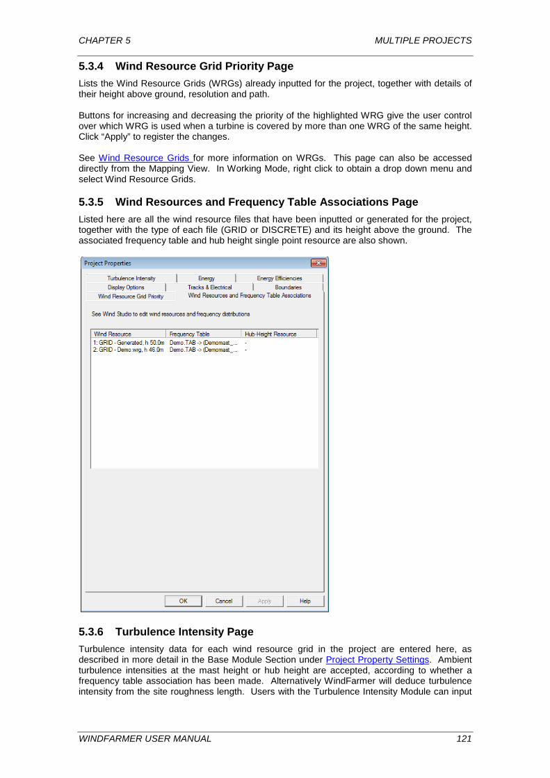
CHAPTER 5 MULTIPLE PROJECTS
5.3.4 Wind Resource Grid Priority Page Lists the Wind Resource Grids (WRGs) already inputted for the project, together with details of their height above ground, resolution and path. Buttons for increasing and decreasing the priority of the highlighted WRG give the user control over which WRG is used when a turbine is covered by more than one WRG of the same height. Click “Apply” to register the changes. See Wind Resource Grids for more information on WRGs. This page can also be accessed directly from the Mapping View. In Working Mode, right click to obtain a drop down menu and select Wind Resource Grids.
5.3.5 Wind Resources and Frequency Table Associations Page Listed here are all the wind resource files that have been inputted or generated for the project, together with the type of each file (GRID or DISCRETE) and its height above the ground. The associated frequency table and hub height single point resource are also shown.
5.3.6 Turbulence Intensity Page Turbulence intensity data for each wind resource grid in the project are entered here, as described in more detail in the Base Module Section under Project Property Settings. Ambient turbulence intensities at the mast height or hub height are accepted, according to whether a frequency table association has been made. Alternatively WindFarmer will deduce turbulence intensity from the site roughness length. Users with the Turbulence Intensity Module can input
WINDFARMER USER MANUAL 121

CHAPTER 5 MULTIPLE PROJECTS
turbulence intensity as a function of wind speed and direction. See also the Section on the Turbulence Intensity Module, Here the user can input the mean ambient turbulence intensity in percent. Numbers for the "Standard deviation of Sigma" are only required when the design equivalent turbulence intensity is calculated and have no impact on the calculation of the energy yield. More information about the calculation of the design equivalent turbulence is given in the Theory Manual.
5.3.7 Energy Page In the Energy page of Project Properties, data on the air density at the site should be entered. Variations in air density over a large site can be included in WindFarmer’s calculations using a specified lapse rate. Choices concerning adjustments for shifts in wind direction, and wake calculations in complex terrain are on this page. This page of Project Properties is described in more detail in Project Properties Settings.
5.3.8 Energy Efficiencies Page Availability, electrical efficiency and other factors leading to losses can be manually entered or selected for calculation by WindFarmer. This page of Project Properties is described in more detail in Project Properties Settings.
5.4 Creating Multiple Projects To create several Projects within a WOW file, the following actions need to be performed:
1. Load the required MAP, DTM and BMP files, as described for the Base Module. Save these files as a WOW file. Remember that these data will NOT form part of any project WPJ file.
2. Open the Project Manager dialogue box by clicking the Project Manager button . Right click on the Project Name field and select Rename. Type the name for the project (e.g. Wind Farm A).
3. Insert the required project elements, such as boundaries, wind resource files, turbines, viewpoints and houses. These elements belong to project Wind Farm A. All elements and files input by the user will belong to Wind Farm A until a new project is created or another project is made Current.
4. The project can be exported as a WPJ file by selecting “Save Current Project As” from File on the main menu. This file can be imported into other WOW files or sent to other WindFarmer users, i.e. planning authorities. Separate elements of individual projects can be exported with Export > Export Data and choose the current project.
5. To create a further new project within the same WOW file, open the Project Manager dialogue box again and click on New to create a new project.
6. Right click on the new project name and select Current. Any wind farm elements now entered will belong to the new project. Only the Current project can be edited; all other projects are locked.
Settings in Project Properties such as turbulence intensity, site air density and efficiency values must be entered separately for each project. Turbine types must also be entered for each project separately. It can be seen from the above example that the Projects Manager dialogue box is central to the multiple project tools and is used to create, select, control and delete projects.
WINDFARMER USER MANUAL 122
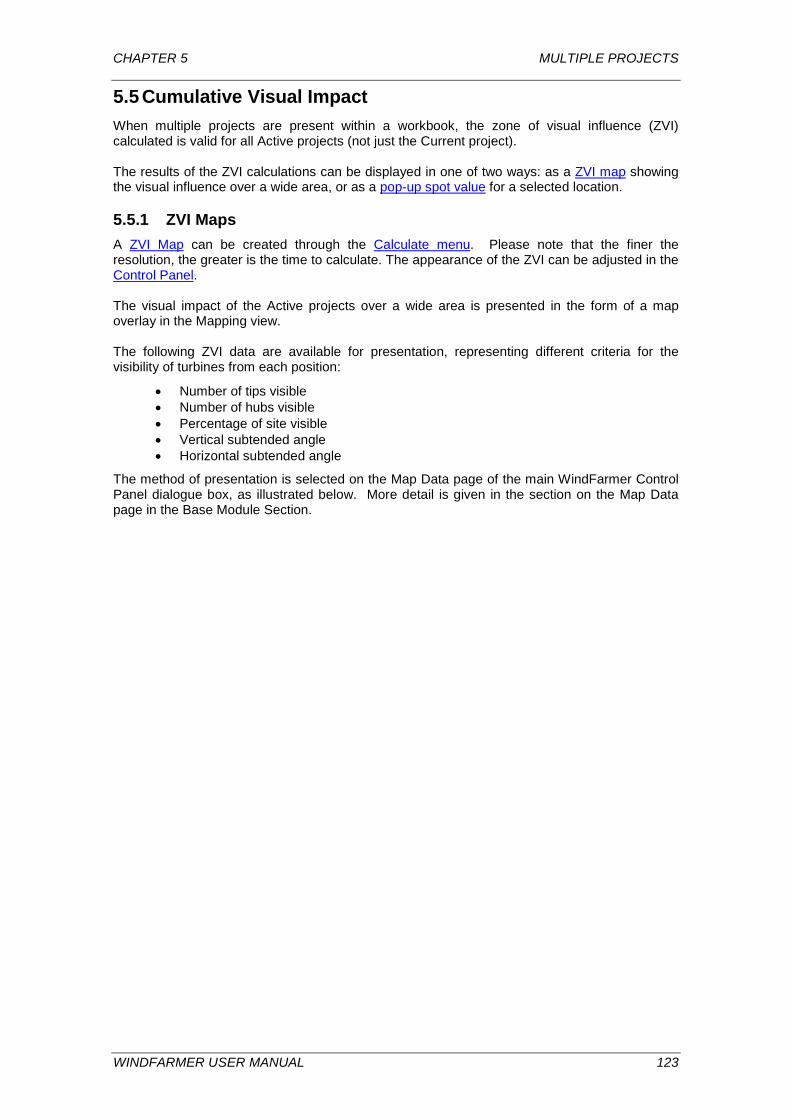
CHAPTER 5 MULTIPLE PROJECTS
5.5 Cumulative Visual Impact When multiple projects are present within a workbook, the zone of visual influence (ZVI) calculated is valid for all Active projects (not just the Current project). The results of the ZVI calculations can be displayed in one of two ways: as a ZVI map showing the visual influence over a wide area, or as a pop-up spot value for a selected location.
5.5.1 ZVI Maps A ZVI Map can be created through the Calculate menu. Please note that the finer the resolution, the greater is the time to calculate. The appearance of the ZVI can be adjusted in the Control Panel. The visual impact of the Active projects over a wide area is presented in the form of a map overlay in the Mapping view. The following ZVI data are available for presentation, representing different criteria for the visibility of turbines from each position:
• Number of tips visible • Number of hubs visible • Percentage of site visible • Vertical subtended angle • Horizontal subtended angle
The method of presentation is selected on the Map Data page of the main WindFarmer Control Panel dialogue box, as illustrated below. More detail is given in the section on the Map Data page in the Base Module Section.
WINDFARMER USER MANUAL 123
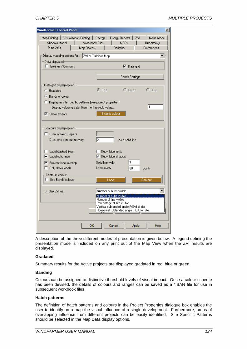
CHAPTER 5 MULTIPLE PROJECTS
A description of the three different modes of presentation is given below. A legend defining the presentation mode is included on any print out of the Map View when the ZVI results are displayed.
Gradated
Summary results for the Active projects are displayed gradated in red, blue or green.
Banding
Colours can be assigned to distinctive threshold levels of visual impact. Once a colour scheme has been devised, the details of colours and ranges can be saved as a *.BAN file for use in subsequent workbook files.
Hatch patterns
The definition of hatch patterns and colours in the Project Properties dialogue box enables the user to identify on a map the visual influence of a single development. Furthermore, areas of overlapping influence from different projects can be easily identified. Site Specific Patterns should be selected in the Map Data display options.
WINDFARMER USER MANUAL 124
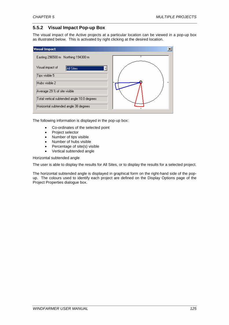
CHAPTER 5 MULTIPLE PROJECTS
5.5.2 Visual Impact Pop-up Box The visual impact of the Active projects at a particular location can be viewed in a pop-up box as illustrated below. This is activated by right clicking at the desired location.
The following information is displayed in the pop-up box:
• Co-ordinates of the selected point • Project selector • Number of tips visible • Number of hubs visible • Percentage of site(s) visible • Vertical subtended angle
Horizontal subtended angle
The user is able to display the results for All Sites, or to display the results for a selected project. The horizontal subtended angle is displayed in graphical form on the right-hand side of the pop-up. The colours used to identify each project are defined on the Display Options page of the Project Properties dialogue box.
WINDFARMER USER MANUAL 125
CHAPTER 5 MULTIPLE PROJECTS
5.6 Cumulative Noise Impact Similar to the cumulative visual impact, the noise assessment is made for all Active projects and can be displayed either as a map, or in a pop-up box for a selected location.
5.6.1 Noise Map A noise map is displayed for the noise attributable to the Active projects. The parameters for the noise propagation model are set in the main WindFarmer Control Panel, Noise Model page, whilst the parameters for the turbine sound characteristics are set in the Turbine Studio. Choice of display of the noise map is made in the Map Data page of the Control Panel.
5.6.2 Noise At Pop-Up Box The noise impact due to the Active projects at a particular location can be viewed in a pop-up box as illustrated below. Right clicking at the desired location activates this pop-up box.
The pop-up box contains the following information:
• Co-ordinates of the selected location • Noise level from all Active projects • Noise level from each individual project.
WINDFARMER USER MANUAL 126
CHAPTER 6 VISUALISATION MODULE
6 VISUALISATION MODULE The WindFarmer Visualisation Module contains the tools required to calculate and output wireframe and rendered landscape visualisations, zone of visual influence (ZVI) maps, photomontages and animations for wind energy projects. Animations, including fly-throughs and pans, can be exported as *.AVI movie files. Furthermore, the Visualisation Module allows visual impact to be set as a site constraint, allowing users to monitor and control the visual influence of a wind farm throughout the layout design and optimisation process. Radar stations can be included in the analysis, to define areas where turbines of a given height will be visible from the radar, and to use these areas as a constraint during optimisation. Viewpoints incorporated at the radar stations allow the sweep of weather radar to be superimposed on the visualisation. This Section has been designed to introduce users to the concepts surrounding the visual assessment of wind farms, and to describe the tools available within WindFarmer that allow users to carry out a full visual impact assessment. See the Exporting and Reporting section for information on image exports and printouts.
6.1 Visualisation Module Interface
6.1.1 Windows The outputs from the Visualisation Module are displayed in one of two windows. Wind farm visualisations (wire frames and photomontages) are displayed in a dedicated Visualisation Window. Zone of Visual Influence (ZVI) maps are displayed as overlays in the Mapping Window.
6.1.2 Opening a Visualisation Window There are two requirements before a Visualisation Window can be opened:
1. A DTM file must be loaded. This contains the digital terrain information that WindFarmer requires for a visualisation.
2. One or more Viewpoints must be inserted in the Mapview
A Visualisation Window can now be opened by left clicking the New Visualisation window button
on the main toolbar, or by selecting New Visualisation Window under the Window Menu. If after steps 1 and 2 above, the New Visualisation window button is greyed out and not available for selection, this means that your HASP software protection device has not been coded to enable the WindFarmer Visualisation Module to run on your system. Please contact WindFarmer technical support for more information.
WINDFARMER USER MANUAL 127
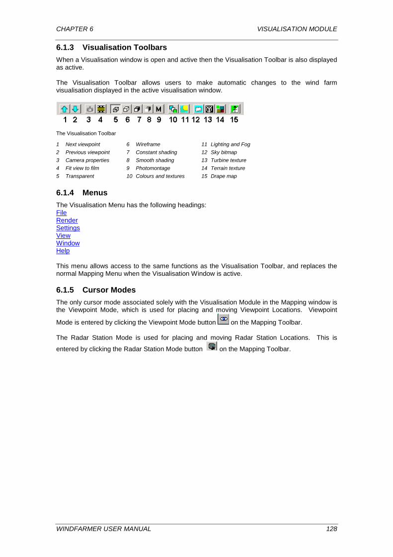
CHAPTER 6 VISUALISATION MODULE
6.1.3 Visualisation Toolbars When a Visualisation window is open and active then the Visualisation Toolbar is also displayed as active. The Visualisation Toolbar allows users to make automatic changes to the wind farm visualisation displayed in the active visualisation window.
The Visualisation Toolbar
1 Next viewpoint 6 Wireframe 11 Lighting and Fog 2 Previous viewpoint 7 Constant shading 12 Sky bitmap 3 Camera properties 8 Smooth shading 13 Turbine texture 4 Fit view to film 9 Photomontage 14 Terrain texture 5 Transparent 10 Colours and textures 15 Drape map
6.1.4 Menus The Visualisation Menu has the following headings: File Render Settings View Window Help This menu allows access to the same functions as the Visualisation Toolbar, and replaces the normal Mapping Menu when the Visualisation Window is active.
6.1.5 Cursor Modes The only cursor mode associated solely with the Visualisation Module in the Mapping window is the Viewpoint Mode, which is used for placing and moving Viewpoint Locations. Viewpoint
Mode is entered by clicking the Viewpoint Mode button on the Mapping Toolbar. The Radar Station Mode is used for placing and moving Radar Station Locations. This is
entered by clicking the Radar Station Mode button on the Mapping Toolbar.
WINDFARMER USER MANUAL 128
CHAPTER 6 VISUALISATION MODULE
6.2 Input Data
6.2.1 Digital Terrain Model (DTM) The principal data type required for carrying out a visual assessment of a wind energy project is a Digital Terrain Model (DTM) file, which contains spot-heights above sea level on a regular grid. WindFarmer supports a large number of file formats. Where DTM data is not available, it is possible to convert height contour data and WAsP .WRG data into DTM data within WindFarmer. This is done through the Map Menu. Please see Map Data and Conversions, for further information.
6.2.2 Turbine Appearance When creating visualisations of a wind farm, the appearance of the turbine can have a significant influence on the visual impact, particularly in close-up views. It is for this reason that WindFarmer allows users complete control over the appearance of the wind turbines in a visualisation. This is achieved by two methods: utilising the 3D Designer page of the Turbine Studio, and the Turbine page in the Colours and Textures window. This is accessed by clicking
on the Colours and Textures button on the Visualisation toolbar. In the 3D Designer page, mouse controlled sliders allow the various components of the turbine (tower, blades, nacelle, nose and disk) to be sized and adjusted. These settings can be saved in a turbine file (*.TRB) and transferred between projects. It should be noted that the overall tower height and rotor radius are set in the main Turbine Power Curve page of the Turbine Studio. The Colours and Textures button in the Visualisation toolbar allows the user to change the colour of the turbine (tower, blades and nacelle) and to apply a texture. The turbine colour is applied for transparent, wireframe and shaded modes. The colours of texture and turbine are applied using the methods:
• Modulate – turbine and texture colour combined • Blend – turbine and texture colour linear interpolation
6.3 Creating a Wireframe Visualisation
6.3.1 Viewpoints and Targets In order to create a visualisation of a wind farm, it is necessary to define the camera location and properties from which the visualisation is to be created. This is done by selecting Viewpoint Mode and right clicking on the desired viewpoint locations in the Map View. Viewpoints can be moved and deleted in the same manner used for any other element in the Map View. It is also possible to define the target point for the visualisation i.e. where the camera is pointing. By default this is the centre of your site. This can be changed in the Camera Properties window. Details of viewpoint locations and targets can be saved as a Viewpoints file from the mapping window by selecting File > Export > Export Data > Viewpoints. The resultant file (*.WOV) can be imported into other projects or workbooks.
6.3.2 Editing Viewpoint Properties (Camera Properties) Right clicking on a viewpoint icon in the Map View whilst in Working Mode displays the Camera Properties dialogue box, shown below: This dialogue box can also be accessed by right clicking anywhere in the Visualisation Window.
WINDFARMER USER MANUAL 129
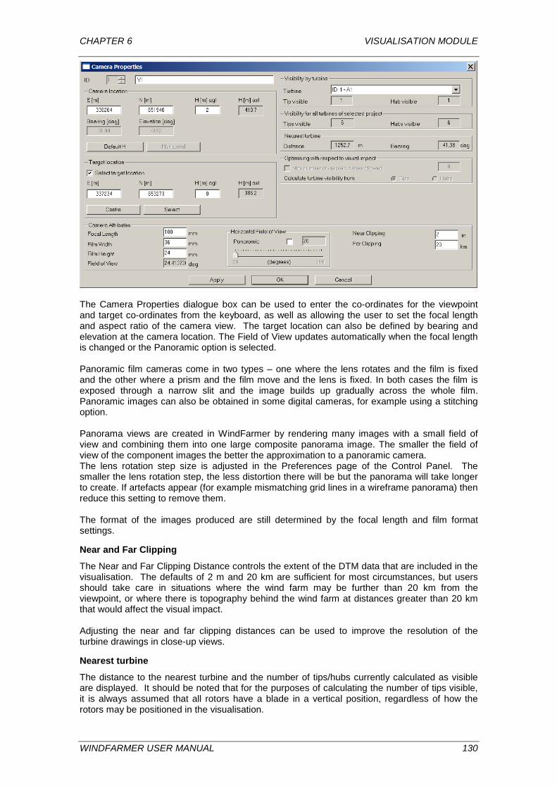
CHAPTER 6 VISUALISATION MODULE
The Camera Properties dialogue box can be used to enter the co-ordinates for the viewpoint and target co-ordinates from the keyboard, as well as allowing the user to set the focal length and aspect ratio of the camera view. The target location can also be defined by bearing and elevation at the camera location. The Field of View updates automatically when the focal length is changed or the Panoramic option is selected. Panoramic film cameras come in two types – one where the lens rotates and the film is fixed and the other where a prism and the film move and the lens is fixed. In both cases the film is exposed through a narrow slit and the image builds up gradually across the whole film. Panoramic images can also be obtained in some digital cameras, for example using a stitching option. Panorama views are created in WindFarmer by rendering many images with a small field of view and combining them into one large composite panorama image. The smaller the field of view of the component images the better the approximation to a panoramic camera. The lens rotation step size is adjusted in the Preferences page of the Control Panel. The smaller the lens rotation step, the less distortion there will be but the panorama will take longer to create. If artefacts appear (for example mismatching grid lines in a wireframe panorama) then reduce this setting to remove them. The format of the images produced are still determined by the focal length and film format settings.
Near and Far Clipping
The Near and Far Clipping Distance controls the extent of the DTM data that are included in the visualisation. The defaults of 2 m and 20 km are sufficient for most circumstances, but users should take care in situations where the wind farm may be further than 20 km from the viewpoint, or where there is topography behind the wind farm at distances greater than 20 km that would affect the visual impact. Adjusting the near and far clipping distances can be used to improve the resolution of the turbine drawings in close-up views.
Nearest turbine
The distance to the nearest turbine and the number of tips/hubs currently calculated as visible are displayed. It should be noted that for the purposes of calculating the number of tips visible, it is always assumed that all rotors have a blade in a vertical position, regardless of how the rotors may be positioned in the visualisation.
WINDFARMER USER MANUAL 130
CHAPTER 6 VISUALISATION MODULE
Optimising with respect to visual impact
The Optimising With Respect To Visual Impact controls are only accessible if this option is switched ON in the Optimiser page of the Control Panel dialogue box. The maximum allowable visual impact at the selected viewpoint is set in the Camera Properties dialogue box, in terms of numbers of tips or hubs permissible. This limit is then used as a constraint in the optimisation and testing functions of the Base Module.
6.3.3 Creating a Wireframe Once the viewpoint and target locations have been set and the camera properties defined, the
visualisation can be displayed simply by clicking the New Visualisation window button . On opening, the wireframe visualisations default to what is referred to as Transparent mode
(Transparent Mode button depressed), where hidden turbines are visible through the landscape to allow for easy identification of machines within the wind farm. The Wireframe
Mode button on the Visualisation Toolbar can be used to change the visualisation to the more common wireframe view with hidden lines removed. In both the Transparent and Wireframe views, it is possible to change the colour of the sky,
terrain and turbines by using the Colours and Textures button on the Visualisation Toolbar. To remove grey shadow which may appear on opening the wireframe, switch Sunlight off in the Lighting and Fog dialogue.
6.3.4 Adjusting the view In a wire frame visualisation, it is possible to yaw the turbine rotors to any desired position. The Insert and Delete keys on the keyboard can be used to yaw the turbines left and right. Alternatively all turbines can be yawed through a given angle by selecting Turbines in the Settings menu. This method may be preferable if there are large numbers of turbines. Furthermore, the rotor positions can be either displayed as being in random positions, or with each turbine having a blade in the vertical position. This function is controlled through the Visualisation Menu from Settings > Turbines > Random Rotors. It is often necessary to identify a turbine in a visualisation. In WindFarmer, if a turbine is highlighted in the Map View (by single left clicking whilst in Turbine mode), it is also highlighted in the Visualisation View. This function can be disabled by un-ticking Show Selected under Settings>Turbines. Where more than one viewpoint has been defined, the Next and Previous Viewpoint blue arrows on the Visualisation Toolbar can be used to toggle through the views. All WindFarmer visualisations, including wireframes, can either be printed direct to a printer or output to a graphics image file from the Export function on the File menu.
6.3.5 Turbine Nacelle Direction The direction the turbine nacelles and rotors face can be set by the user. Whilst in Visualisation Mode, select Settings > Turbines > Yaw Turbines and enter the angle and direction of rotation. The turbines can also be yawed using the Insert (clockwise) and Delete (counter-clockwise) keys on the keyboard. This affects all turbines – they will all always have the same orientation. The orientation is specific to each visualisation window, for example, three visualisation windows all showing the same viewpoint may have different turbine orientations. While the turbines are being rotated the terrain is not drawn. This allows easy, fast viewing of the turbines.
WINDFARMER USER MANUAL 131
CHAPTER 6 VISUALISATION MODULE
6.4 Creating a Rendered Landscape Visualisation Once a wireframe view has been created it is possible to then render the landscape to create a more realistic landscape. This section assumes a wireframe view has already been created, as just described.
6.4.1 Terrain and Sky Textures A Rendered Landscape Visualisation is a wind farm visualisation to which textures, colours and lighting effects have been added.
Shaded view Before adding textures to a visualisation, it is first necessary to shade the view. This is
achieved by depressing either the Constant Shading or the Smooth Shading button on the Visualisation Toolbar. These functions automatically add colour to the landscape and shade the views relative to a light source. Constant shading produces a slightly blocky effect but is relatively quick to update, whilst the Smooth Shading function produces a more realistic shading effect but takes slightly longer to calculate and update the view.
Colours and Textures
Textures are added to the sky or to the landscape by clicking on the Terrain Texture On/Off
button or the Sky Bitmap On/Off button on the Visualisation Toolbar. If no previous textures have been loaded, then the Colours and Textures Properties dialogue box will be displayed, through which bitmap Textures can be loaded. This dialogue box can also be used to set the colours used in constant and smooth shaded views where no textures are being used. When a texture has been loaded, the terrain texture and Sky Bitmap buttons can be used to
toggle the effect on and off and the Colours and Textures Toolbar buttons can be used to change the texture. A range of prepared textures are supplied with WindFarmer, although it is possible for users to create their own. The textures can be displayed using the options
Modulate: fragment and texture colour combined Blend: fragment colour linear interpolation between fragment and texture colour Contouring use texture to contour the terrain.
The terrain colour is used for rendering wire-frame grid lines and shaded modes. The Colours and Texture button allows combining a background colour for the terrain with a texture. Please select white if you desire to use the original colour of the texture. The colour and its brightness can be user defined from the Colours and Texture dialogue box.
WINDFARMER USER MANUAL 132

CHAPTER 6 VISUALISATION MODULE
6.4.2 Lighting and Fog The relative position of the sun in shaded views can be adjusted from the Lighting and Fog
Properties dialogue box, accessed by clicking the Lighting and Fog button on the Visualisation Toolbar. The available options on the Lighting and Fog toolbar are described below:
Adjusting Lighting
Sunlight on/off Lighting is only required for constant and smooth shading
Direction angles Specify direction to the sun
Intensity Specify intensity of each component of sunlight:
• Ambient: Scattered non-directional light. Uniform throughout the model.
• Diffuse: Directional light that scatters equally in all directions from surfaces.
• Specular: Directional light that reflects in a preferred direction. Shininess
Adjusting Fog
Fog on/off Fog is only for constant and smooth shading when lighting is enabled
Fog Type Choose an equation for combining fragment colour with fog colour:
• Clouds: Simulates cloudy day
• Haze: Simulates haze
• Distance: Simulates fade into distance
Density Density of fog
Colour Colour of fog to be combined with fragment colour
6.4.3 Drape Map The Drape Map option in WindFarmer allows users to drape a 2-dimensional scanned map or image onto a 3-dimensional wind farm visualisation. For instance, an aerial photograph of your
site could be draped over the DTM 3-D terrain data. The Drape Map button on the Visualisation Toolbar brings up an Open File dialogue box, where the bitmap image to drape over the landscape can be selected. The user is requested to enter the reference co-ordinates for the selected bitmap image. Alternatively, the image extents may be set to equal the DTM or workspace extents. On completion of the Reference Co-ordinates dialogue box, the view is updated and the draped map displayed in the Mapping window. Draped map views are likely to take longer to calculate and update than other types of view due to the nature of the data being processed. To remove a drape map, click the Drape Map button and select <none>. Note that the Drape Map is not retained when a Workbook is saved.
WINDFARMER USER MANUAL 133
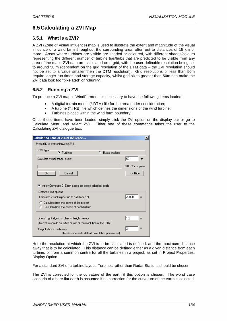
CHAPTER 6 VISUALISATION MODULE
6.5 Calculating a ZVI Map
6.5.1 What is a ZVI? A ZVI (Zone of Visual Influence) map is used to illustrate the extent and magnitude of the visual influence of a wind farm throughout the surrounding area, often out to distances of 15 km or more. Areas where turbines are visible are shaded or coloured, with different shades/colours representing the different number of turbine tips/hubs that are predicted to be visible from any area of the map. ZVI data are calculated on a grid, with the user-definable resolution being set to around 50 m (dependent on the grid resolution of the DTM data – the ZVI resolution should not be set to a value smaller then the DTM resolution). Grid resolutions of less than 50m require longer run times and storage capacity, whilst grid sizes greater than 50m can make the ZVI data look too “pixelated” or “chunky”.
6.5.2 Running a ZVI To produce a ZVI map in WindFarmer, it is necessary to have the following items loaded:
• A digital terrain model (*.DTM) file for the area under consideration; • A turbine (*.TRB) file which defines the dimensions of the wind turbine; • Turbines placed within the wind farm boundary;
Once these items have been loaded, simply click the ZVI option on the display bar or go to Calculate Menu and select ZVI. Either one of these commands takes the user to the Calculating ZVI dialogue box.
Here the resolution at which the ZVI is to be calculated is defined, and the maximum distance away that is to be calculated. This distance can be defined either as a given distance from each turbine, or from a common centre for all the turbines in a project, as set in Project Properties, Display Option. For a standard ZVI of a turbine layout, Turbines rather than Radar Stations should be chosen. The ZVI is corrected for the curvature of the earth if this option is chosen. The worst case scenario of a bare flat earth is assumed if no correction for the curvature of the earth is selected.
WINDFARMER USER MANUAL 134
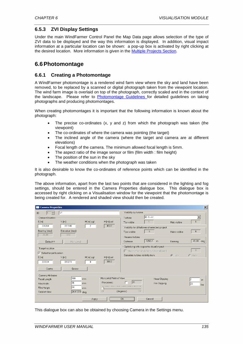
CHAPTER 6 VISUALISATION MODULE
6.5.3 ZVI Display Settings Under the main WindFarmer Control Panel the Map Data page allows selection of the type of ZVI data to be displayed and the way this information is displayed. In addition, visual impact information at a particular location can be shown: a pop-up box is activated by right clicking at the desired location. More information is given in the Multiple Projects Section.
6.6 Photomontage
6.6.1 Creating a Photomontage A WindFarmer photomontage is a rendered wind farm view where the sky and land have been removed, to be replaced by a scanned or digital photograph taken from the viewpoint location. The wind farm image is overlaid on top of the photograph, correctly scaled and in the context of the landscape. Please refer to Photomontage Guidelines for detailed guidelines on taking photographs and producing photomontages. When creating photomontages it is important that the following information is known about the photograph:
• The precise co-ordinates (x, y and z) from which the photograph was taken (the viewpoint)
• The co-ordinates of where the camera was pointing (the target) • The inclined angle of the camera (where the target and camera are at different
elevations) • Focal length of the camera. The minimum allowed focal length is 5mm. • The aspect ratio of the image sensor or film (film width : film height) • The position of the sun in the sky • The weather conditions when the photograph was taken
It is also desirable to know the co-ordinates of reference points which can be identified in the photograph. The above information, apart from the last two points that are considered in the lighting and fog settings, should be entered in the Camera Properties dialogue box. This dialogue box is accessed by right clicking on a Visualisation window for the viewpoint that the photomontage is being created for. A rendered and shaded view should then be created.
This dialogue box can also be obtained by choosing Camera in the Settings menu.
WINDFARMER USER MANUAL 135
CHAPTER 6 VISUALISATION MODULE
6.6.2 Loading a Photo
To load the scanned photograph or JPEG image, click on the photomontage button on the Visualisation Toolbar. This takes the user to an Open File dialogue box, through which the scanned bitmap image is loaded. Scanned photographs must be in 24 Bit uncompressed bitmap (*.BMP) or *.JPEG format. Upon loading the photograph, WindFarmer will display the photograph with the wind turbines superimposed on top. The image can be printed directly or output and saved as a bitmap image.
6.6.3 Adjustments Turbines may appear to be “floating” or “buried” due to discrepancies between the vertical camera angle as set in WindFarmer and as it was in reality when the photograph was taken. It may be necessary to adjust a photomontage image to make the turbines “sit” on the horizon. This is achieved by altering the target height or the viewpoint height in the Camera Properties dialogue box or by altering the inclination of the horizon. The target height can also be altered incrementally in steps of 10m using the up and down arrow keys on the keyboard and the inclination of the horizon using the Page Up and Page Down keys on the keyboard. The horizontal target can be altered using Left and Right Arrow keys and camera height using Home and End keys. In transparent or wireframe mode, the photo markers and terrain shape will be visible to assist in matching the photograph and visualisation.
6.7 Visualisation Features
6.7.1 Animated Turbines Turbines can be animated in any visualisation view; wireframe, rendered wireframe or photomontage. The speed of rotation of the turbine rotor is determined for each turbine type by the value defined for 20m/s in the RPM column of the Turbine Studio. Pressing the keyboard Space Bar toggles the turbine animation on and off. If no animation occurs, you may need to click first on the visualisation with the cursor.
6.7.2 360 degree View Pressing the keyboard left-arrow or the right-arrow cursor key activates the 360 degrees view. First a 360 degrees image is calculated. This facility may take some time for complex terrain and on less powerful computers. Once calculated, the view can be scrolled smoothly to the left or right using the cursor keys. Pressing the keyboard Space Bar returns the image to normal view.
6.7.3 Coloured Projects WindFarmer allows project-specific turbine colouring in visualisations and photomontages. The turbine colour is defined via the setting for the Site Colour in the Project Properties -> Display Options. In order to display the site-specific colours in visualisations and photomontages, select "Colour by project" for the turbines in the Colours and Textures dialogue .
WINDFARMER USER MANUAL 136
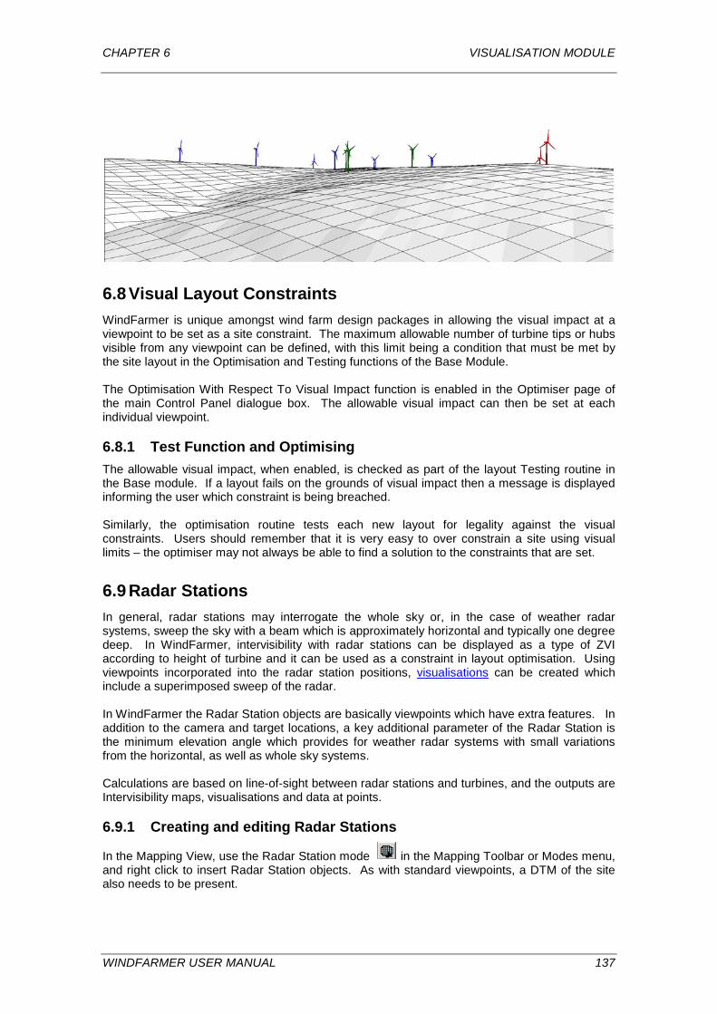
CHAPTER 6 VISUALISATION MODULE
6.8 Visual Layout Constraints WindFarmer is unique amongst wind farm design packages in allowing the visual impact at a viewpoint to be set as a site constraint. The maximum allowable number of turbine tips or hubs visible from any viewpoint can be defined, with this limit being a condition that must be met by the site layout in the Optimisation and Testing functions of the Base Module. The Optimisation With Respect To Visual Impact function is enabled in the Optimiser page of the main Control Panel dialogue box. The allowable visual impact can then be set at each individual viewpoint.
6.8.1 Test Function and Optimising The allowable visual impact, when enabled, is checked as part of the layout Testing routine in the Base module. If a layout fails on the grounds of visual impact then a message is displayed informing the user which constraint is being breached. Similarly, the optimisation routine tests each new layout for legality against the visual constraints. Users should remember that it is very easy to over constrain a site using visual limits – the optimiser may not always be able to find a solution to the constraints that are set.
6.9 Radar Stations In general, radar stations may interrogate the whole sky or, in the case of weather radar systems, sweep the sky with a beam which is approximately horizontal and typically one degree deep. In WindFarmer, intervisibility with radar stations can be displayed as a type of ZVI according to height of turbine and it can be used as a constraint in layout optimisation. Using viewpoints incorporated into the radar station positions, visualisations can be created which include a superimposed sweep of the radar. In WindFarmer the Radar Station objects are basically viewpoints which have extra features. In addition to the camera and target locations, a key additional parameter of the Radar Station is the minimum elevation angle which provides for weather radar systems with small variations from the horizontal, as well as whole sky systems. Calculations are based on line-of-sight between radar stations and turbines, and the outputs are Intervisibility maps, visualisations and data at points.
6.9.1 Creating and editing Radar Stations
In the Mapping View, use the Radar Station mode in the Mapping Toolbar or Modes menu, and right click to insert Radar Station objects. As with standard viewpoints, a DTM of the site also needs to be present.
WINDFARMER USER MANUAL 137
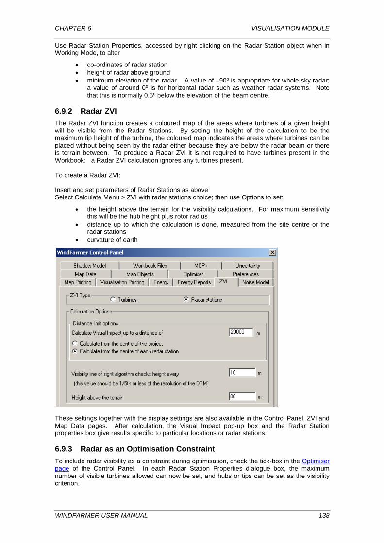
CHAPTER 6 VISUALISATION MODULE
Use Radar Station Properties, accessed by right clicking on the Radar Station object when in Working Mode, to alter
• co-ordinates of radar station • height of radar above ground • minimum elevation of the radar. A value of –90º is appropriate for whole-sky radar;
a value of around 0º is for horizontal radar such as weather radar systems. Note that this is normally 0.5º below the elevation of the beam centre.
6.9.2 Radar ZVI The Radar ZVI function creates a coloured map of the areas where turbines of a given height will be visible from the Radar Stations. By setting the height of the calculation to be the maximum tip height of the turbine, the coloured map indicates the areas where turbines can be placed without being seen by the radar either because they are below the radar beam or there is terrain between. To produce a Radar ZVI it is not required to have turbines present in the Workbook: a Radar ZVI calculation ignores any turbines present. To create a Radar ZVI: Insert and set parameters of Radar Stations as above Select Calculate Menu > ZVI with radar stations choice; then use Options to set:
• the height above the terrain for the visibility calculations. For maximum sensitivity this will be the hub height plus rotor radius
• distance up to which the calculation is done, measured from the site centre or the radar stations
• curvature of earth
These settings together with the display settings are also available in the Control Panel, ZVI and Map Data pages. After calculation, the Visual Impact pop-up box and the Radar Station properties box give results specific to particular locations or radar stations.
6.9.3 Radar as an Optimisation Constraint To include radar visibility as a constraint during optimisation, check the tick-box in the Optimiser page of the Control Panel. In each Radar Station Properties dialogue box, the maximum number of visible turbines allowed can now be set, and hubs or tips can be set as the visibility criterion.
WINDFARMER USER MANUAL 138
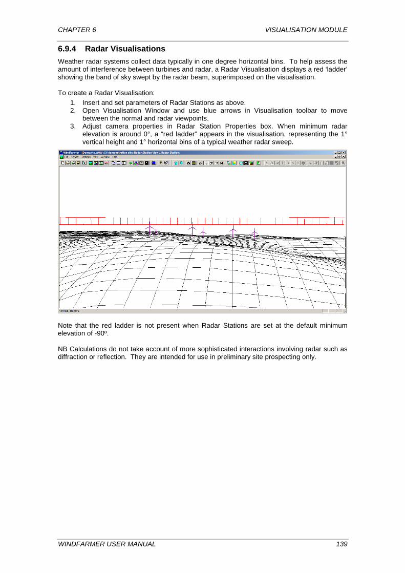
CHAPTER 6 VISUALISATION MODULE
6.9.4 Radar Visualisations Weather radar systems collect data typically in one degree horizontal bins. To help assess the amount of interference between turbines and radar, a Radar Visualisation displays a red ‘ladder’ showing the band of sky swept by the radar beam, superimposed on the visualisation. To create a Radar Visualisation:
1. Insert and set parameters of Radar Stations as above. 2. Open Visualisation Window and use blue arrows in Visualisation toolbar to move
between the normal and radar viewpoints. 3. Adjust camera properties in Radar Station Properties box. When minimum radar
elevation is around 0°, a “red ladder” appears in the visualisation, representing the 1° vertical height and 1° horizontal bins of a typical weather radar sweep.
Note that the red ladder is not present when Radar Stations are set at the default minimum elevation of -90º. NB Calculations do not take account of more sophisticated interactions involving radar such as diffraction or reflection. They are intended for use in preliminary site prospecting only.
WINDFARMER USER MANUAL 139
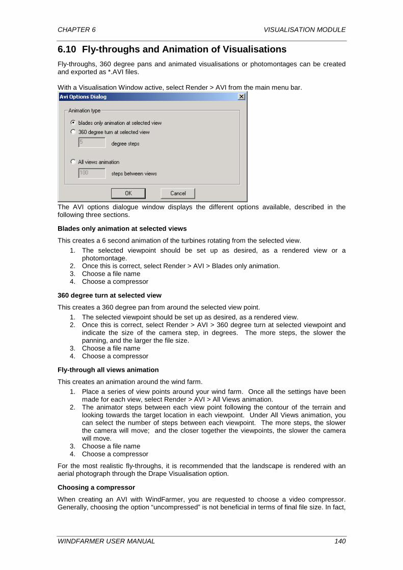
CHAPTER 6 VISUALISATION MODULE
6.10 Fly-throughs and Animation of Visualisations Fly-throughs, 360 degree pans and animated visualisations or photomontages can be created and exported as *.AVI files. With a Visualisation Window active, select Render > AVI from the main menu bar.
The AVI options dialogue window displays the different options available, described in the following three sections.
Blades only animation at selected views
This creates a 6 second animation of the turbines rotating from the selected view. 1. The selected viewpoint should be set up as desired, as a rendered view or a
photomontage. 2. Once this is correct, select Render > AVI > Blades only animation. 3. Choose a file name 4. Choose a compressor
360 degree turn at selected view
This creates a 360 degree pan from around the selected view point. 1. The selected viewpoint should be set up as desired, as a rendered view. 2. Once this is correct, select Render > AVI > 360 degree turn at selected viewpoint and
indicate the size of the camera step, in degrees. The more steps, the slower the panning, and the larger the file size.
3. Choose a file name 4. Choose a compressor
Fly-through all views animation
This creates an animation around the wind farm. 1. Place a series of view points around your wind farm. Once all the settings have been
made for each view, select Render > AVI > All Views animation. 2. The animator steps between each view point following the contour of the terrain and
looking towards the target location in each viewpoint. Under All Views animation, you can select the number of steps between each viewpoint. The more steps, the slower the camera will move; and the closer together the viewpoints, the slower the camera will move.
3. Choose a file name 4. Choose a compressor
For the most realistic fly-throughs, it is recommended that the landscape is rendered with an aerial photograph through the Drape Visualisation option.
Choosing a compressor
When creating an AVI with WindFarmer, you are requested to choose a video compressor. Generally, choosing the option “uncompressed” is not beneficial in terms of final file size. In fact,
WINDFARMER USER MANUAL 140
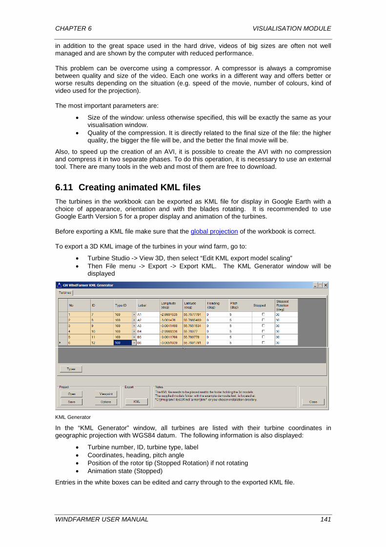
CHAPTER 6 VISUALISATION MODULE
in addition to the great space used in the hard drive, videos of big sizes are often not well managed and are shown by the computer with reduced performance. This problem can be overcome using a compressor. A compressor is always a compromise between quality and size of the video. Each one works in a different way and offers better or worse results depending on the situation (e.g. speed of the movie, number of colours, kind of video used for the projection). The most important parameters are:
• Size of the window: unless otherwise specified, this will be exactly the same as your visualisation window.
• Quality of the compression. It is directly related to the final size of the file: the higher quality, the bigger the file will be, and the better the final movie will be.
Also, to speed up the creation of an AVI, it is possible to create the AVI with no compression and compress it in two separate phases. To do this operation, it is necessary to use an external tool. There are many tools in the web and most of them are free to download.
6.11 Creating animated KML files The turbines in the workbook can be exported as KML file for display in Google Earth with a choice of appearance, orientation and with the blades rotating. It is recommended to use Google Earth Version 5 for a proper display and animation of the turbines. Before exporting a KML file make sure that the global projection of the workbook is correct. To export a 3D KML image of the turbines in your wind farm, go to:
• Turbine Studio -> View 3D, then select “Edit KML export model scaling” • Then File menu -> Export -> Export KML. The KML Generator window will be
displayed
KML Generator
In the “KML Generator” window, all turbines are listed with their turbine coordinates in geographic projection with WGS84 datum. The following information is also displayed:
• Turbine number, ID, turbine type, label • Coordinates, heading, pitch angle • Position of the rotor tip (Stopped Rotation) if not rotating • Animation state (Stopped)
Entries in the white boxes can be edited and carry through to the exported KML file.
WINDFARMER USER MANUAL 141
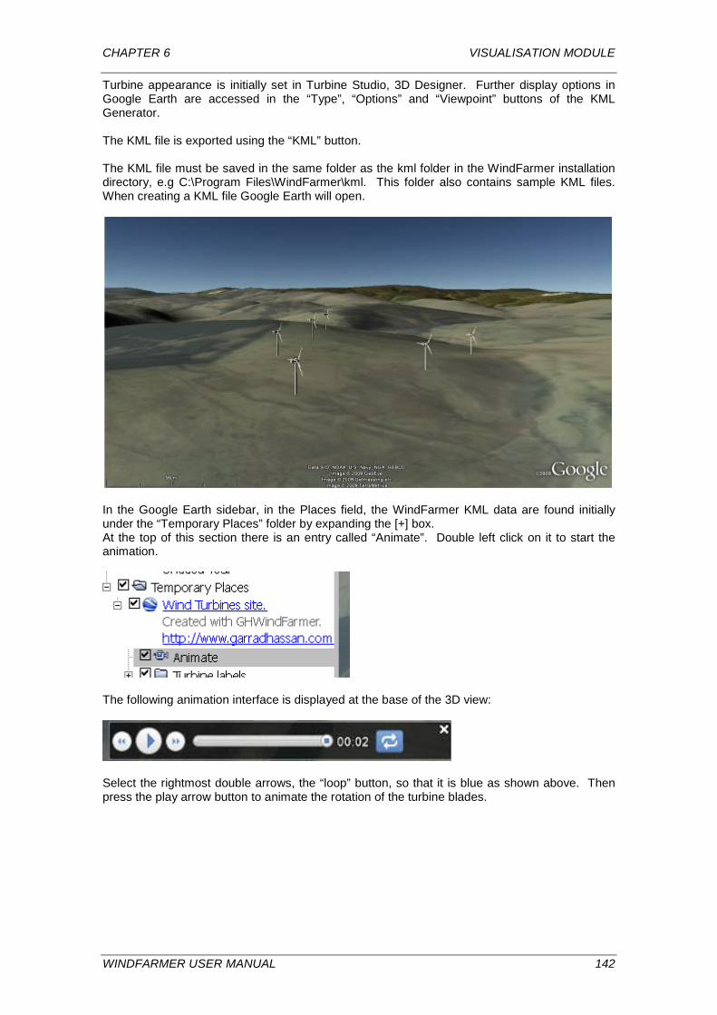
CHAPTER 6 VISUALISATION MODULE
Turbine appearance is initially set in Turbine Studio, 3D Designer. Further display options in Google Earth are accessed in the “Type”, “Options” and “Viewpoint” buttons of the KML Generator. The KML file is exported using the “KML” button. The KML file must be saved in the same folder as the kml folder in the WindFarmer installation directory, e.g C:\Program Files\WindFarmer\kml. This folder also contains sample KML files. When creating a KML file Google Earth will open.
In the Google Earth sidebar, in the Places field, the WindFarmer KML data are found initially under the “Temporary Places” folder by expanding the [+] box. At the top of this section there is an entry called “Animate”. Double left click on it to start the animation.
The following animation interface is displayed at the base of the 3D view:
Select the rightmost double arrows, the “loop” button, so that it is blue as shown above. Then press the play arrow button to animate the rotation of the turbine blades.
WINDFARMER USER MANUAL 142
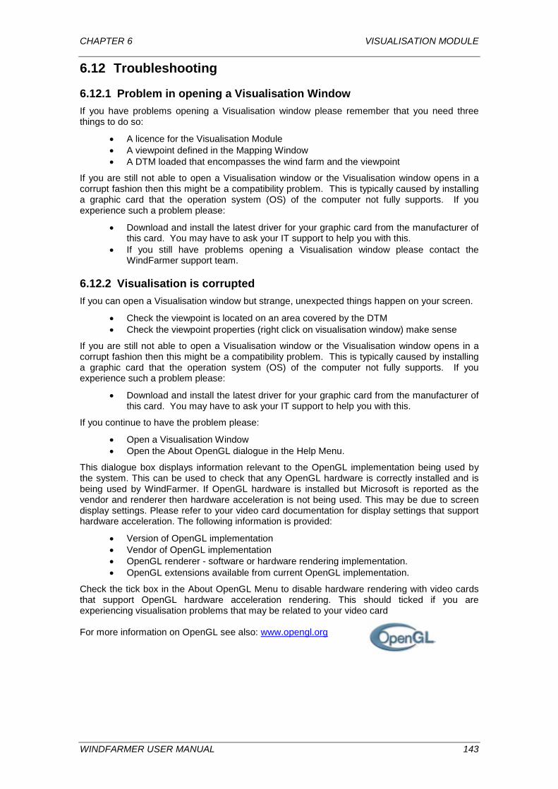
CHAPTER 6 VISUALISATION MODULE
6.12 Troubleshooting
6.12.1 Problem in opening a Visualisation Window If you have problems opening a Visualisation window please remember that you need three things to do so:
• A licence for the Visualisation Module • A viewpoint defined in the Mapping Window • A DTM loaded that encompasses the wind farm and the viewpoint
If you are still not able to open a Visualisation window or the Visualisation window opens in a corrupt fashion then this might be a compatibility problem. This is typically caused by installing a graphic card that the operation system (OS) of the computer not fully supports. If you experience such a problem please:
• Download and install the latest driver for your graphic card from the manufacturer of this card. You may have to ask your IT support to help you with this.
• If you still have problems opening a Visualisation window please contact the WindFarmer support team.
6.12.2 Visualisation is corrupted If you can open a Visualisation window but strange, unexpected things happen on your screen.
• Check the viewpoint is located on an area covered by the DTM • Check the viewpoint properties (right click on visualisation window) make sense
If you are still not able to open a Visualisation window or the Visualisation window opens in a corrupt fashion then this might be a compatibility problem. This is typically caused by installing a graphic card that the operation system (OS) of the computer not fully supports. If you experience such a problem please:
• Download and install the latest driver for your graphic card from the manufacturer of this card. You may have to ask your IT support to help you with this.
If you continue to have the problem please:
• Open a Visualisation Window • Open the About OpenGL dialogue in the Help Menu.
This dialogue box displays information relevant to the OpenGL implementation being used by the system. This can be used to check that any OpenGL hardware is correctly installed and is being used by WindFarmer. If OpenGL hardware is installed but Microsoft is reported as the vendor and renderer then hardware acceleration is not being used. This may be due to screen display settings. Please refer to your video card documentation for display settings that support hardware acceleration. The following information is provided:
• Version of OpenGL implementation • Vendor of OpenGL implementation • OpenGL renderer - software or hardware rendering implementation. • OpenGL extensions available from current OpenGL implementation.
Check the tick box in the About OpenGL Menu to disable hardware rendering with video cards that support OpenGL hardware acceleration rendering. This should ticked if you are experiencing visualisation problems that may be related to your video card For more information on OpenGL see also: www.opengl.org
WINDFARMER USER MANUAL 143
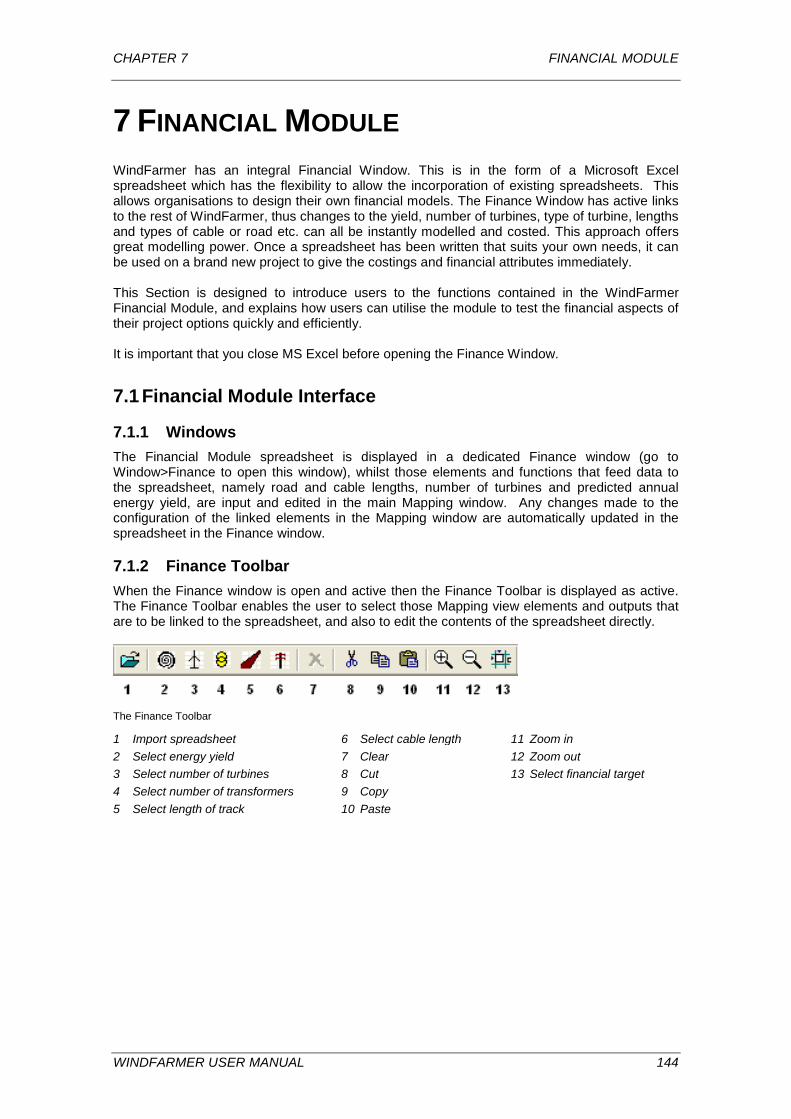
CHAPTER 7 FINANCIAL MODULE
7 FINANCIAL MODULE WindFarmer has an integral Financial Window. This is in the form of a Microsoft Excel spreadsheet which has the flexibility to allow the incorporation of existing spreadsheets. This allows organisations to design their own financial models. The Finance Window has active links to the rest of WindFarmer, thus changes to the yield, number of turbines, type of turbine, lengths and types of cable or road etc. can all be instantly modelled and costed. This approach offers great modelling power. Once a spreadsheet has been written that suits your own needs, it can be used on a brand new project to give the costings and financial attributes immediately. This Section is designed to introduce users to the functions contained in the WindFarmer Financial Module, and explains how users can utilise the module to test the financial aspects of their project options quickly and efficiently. It is important that you close MS Excel before opening the Finance Window.
7.1 Financial Module Interface
7.1.1 Windows The Financial Module spreadsheet is displayed in a dedicated Finance window (go to Window>Finance to open this window), whilst those elements and functions that feed data to the spreadsheet, namely road and cable lengths, number of turbines and predicted annual energy yield, are input and edited in the main Mapping window. Any changes made to the configuration of the linked elements in the Mapping window are automatically updated in the spreadsheet in the Finance window.
7.1.2 Finance Toolbar When the Finance window is open and active then the Finance Toolbar is displayed as active. The Finance Toolbar enables the user to select those Mapping view elements and outputs that are to be linked to the spreadsheet, and also to edit the contents of the spreadsheet directly.
The Finance Toolbar
1 Import spreadsheet 6 Select cable length 11 Zoom in 2 Select energy yield 7 Clear 12 Zoom out 3 Select number of turbines 8 Cut 13 Select financial target 4 Select number of transformers 9 Copy 5 Select length of track 10 Paste
WINDFARMER USER MANUAL 144

CHAPTER 7 FINANCIAL MODULE
7.2 Menus The Finance Menu has the following headings: File Edit Insert Format View Window Help This menu allows access to the same functions as the Finance Toolbar, and also additional formatting options which allow the user to control the appearance of the spreadsheet. The spreadsheet formatting options can also be accessed from a pop-up menu, activated by right clicking anywhere on the spreadsheet displayed in the Finance window. The tabs on this pop-up menu are Number, Alignment, Font, Borders and Patterns.
7.2.1 Cursor Modes When the Finance window is open, only one general cursor mode is available, where the cursor is displayed as a cross. This cursor mode is used to navigate around the spreadsheet and to select cells.
7.3 Operating the Financial Module The basic principle behind the effective use of the Financial Module is that the dynamic links between the Base Module and Finance Module are utilised so that the costs of the wind farm and the expected annual revenue of the wind farm are calculated and displayed in the spreadsheet. In simple terms, the capital cost of a wind farm is a function of the number of turbines in the project, the length of on and off-site cabling required and the length of roads to be constructed. Annual operating costs can be calculated as a function of the number of turbines in the project. The annual revenue of the wind farm will be a function of the predicted annual energy yield. By linking the appropriate Base Module outputs to a spreadsheet, which includes the figures by which these outputs should be factored (i.e. cost per turbine, cost per metre of cabling, price per unit of electricity generated), and other project costs that are not dependant on the linkable outputs, the Financial Module will calculate the cost and revenue streams for the project. However, please note that with the introduction of the Electrical Module it is no longer possible to link cable lengths into the finance spreadsheet unless you have both Financial and Electrical Modules. However, an alternative method is possible. The costs and revenue information calculated in the spreadsheet can be analysed by a financial model to determine the financial viability of the project using indicators, such as Internal Rate of Return (IRR) or Net Present Value (NPV). The spreadsheet supplied with WindFarmer contains both a capital cost sheet and a financial model, enabling users to calculate project cost and revenue streams and to perform financial analyses on them. The user is able to tailor the spreadsheet to match their needs or to replace it with their own.
WINDFARMER USER MANUAL 145
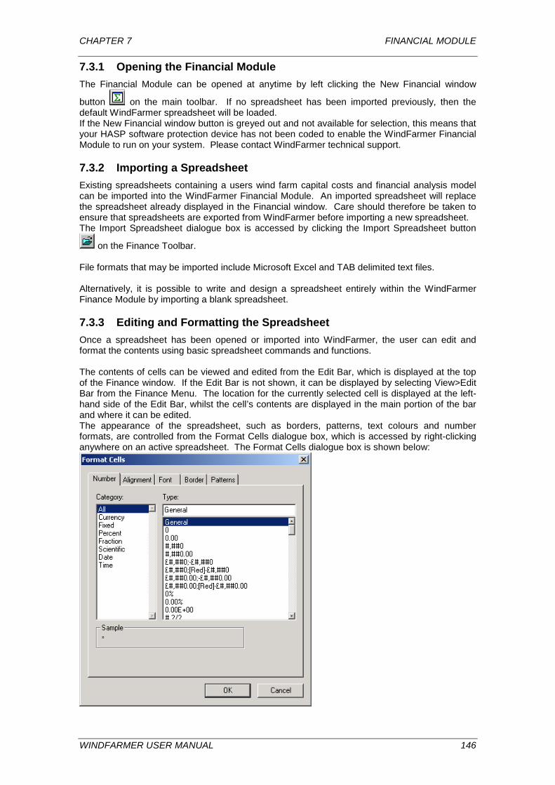
CHAPTER 7 FINANCIAL MODULE
7.3.1 Opening the Financial Module The Financial Module can be opened at anytime by left clicking the New Financial window
button on the main toolbar. If no spreadsheet has been imported previously, then the default WindFarmer spreadsheet will be loaded. If the New Financial window button is greyed out and not available for selection, this means that your HASP software protection device has not been coded to enable the WindFarmer Financial Module to run on your system. Please contact WindFarmer technical support.
7.3.2 Importing a Spreadsheet Existing spreadsheets containing a users wind farm capital costs and financial analysis model can be imported into the WindFarmer Financial Module. An imported spreadsheet will replace the spreadsheet already displayed in the Financial window. Care should therefore be taken to ensure that spreadsheets are exported from WindFarmer before importing a new spreadsheet. The Import Spreadsheet dialogue box is accessed by clicking the Import Spreadsheet button
on the Finance Toolbar. File formats that may be imported include Microsoft Excel and TAB delimited text files. Alternatively, it is possible to write and design a spreadsheet entirely within the WindFarmer Finance Module by importing a blank spreadsheet.
7.3.3 Editing and Formatting the Spreadsheet Once a spreadsheet has been opened or imported into WindFarmer, the user can edit and format the contents using basic spreadsheet commands and functions. The contents of cells can be viewed and edited from the Edit Bar, which is displayed at the top of the Finance window. If the Edit Bar is not shown, it can be displayed by selecting View>Edit Bar from the Finance Menu. The location for the currently selected cell is displayed at the left-hand side of the Edit Bar, whilst the cell’s contents are displayed in the main portion of the bar and where it can be edited. The appearance of the spreadsheet, such as borders, patterns, text colours and number formats, are controlled from the Format Cells dialogue box, which is accessed by right-clicking anywhere on an active spreadsheet. The Format Cells dialogue box is shown below:
WINDFARMER USER MANUAL 146

CHAPTER 7 FINANCIAL MODULE
7.3.3.1 Designing and Formatting Roads and Cabling
The lengths of roads and cables are two of the element properties that can be linked and output from the Base Module to the Financial Module. These elements are intended to allow users to design on-site turbine access tracks, site access tracks (both new and upgraded), on-site low voltage cabling and off-site high voltage grid connection cabling. Road and cable layouts are input in the Base Module, from the Mapping window. The mode for the desired element is made active by selecting the appropriate icon from the Mapping Toolbar, and the elements are input by right-clicking on the desired location in the Mapping View. If you do not have the Electrical Module, cable lengths can be linked into the spreadsheet by entering the cable layout as a type of road. When dealing with roads and cables, each input is a node, which can be defined as being the junction between two sections of road or cable (with the exception of the first and last points of a road or cable route). This node-based system allows the user to define layouts for different types of road and cabling, and allows the specification of roads and cables to be changed at any point along their length. The lengths of roads and cables of different types can therefore be output separately to the Finance Module, where different costs per metre can be associated with them. It should be noted that roads are not modified when the turbine layout is changed. Roads should therefore be laid out after the wind farm has been optimised. Although cables are linked to turbines, they also should be laid out after optimisation. To define the type of road or cable that you wish to enter, right click on the node following the road or cable to be modified, activating the pop-up properties dialogue box. The dialogue box for the road elements is shown below: The dialogue box for cables is shown in the section on the Electrical Module.
WINDFARMER USER MANUAL 147
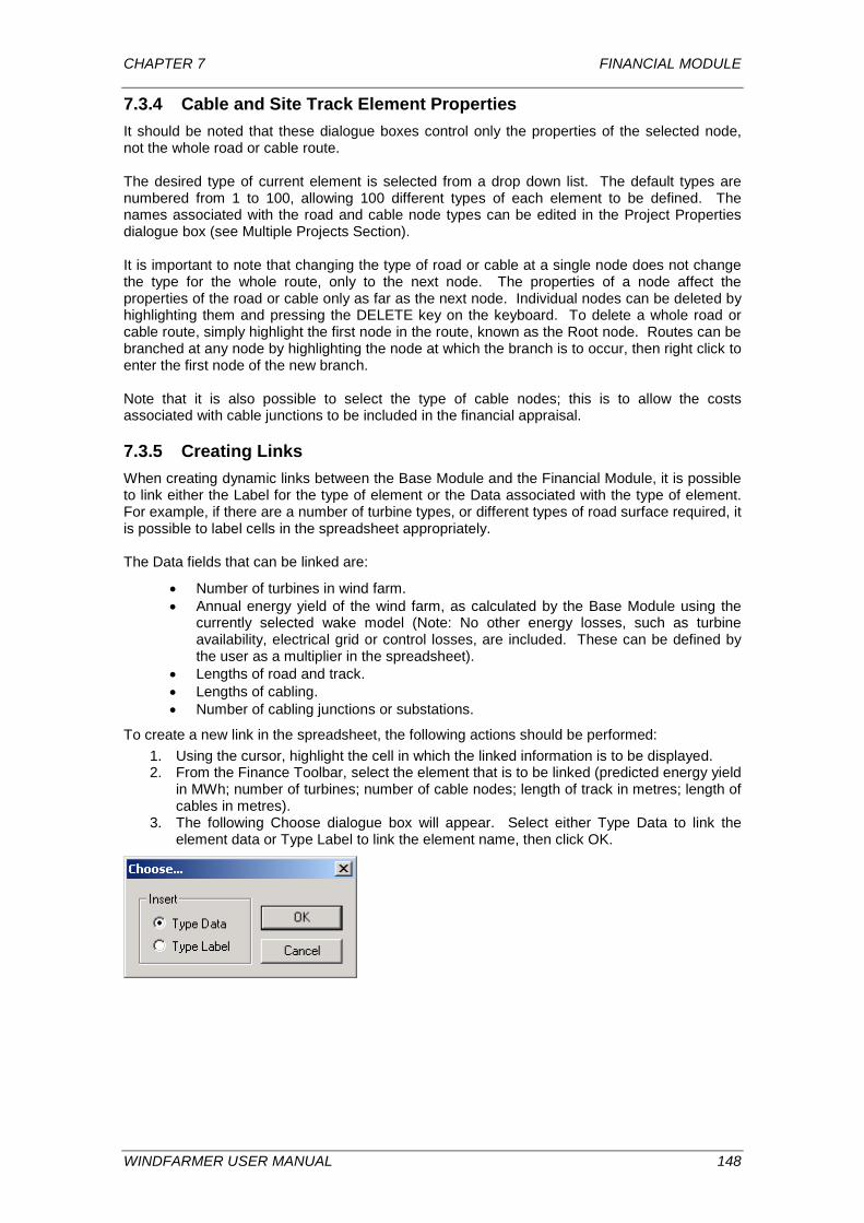
CHAPTER 7 FINANCIAL MODULE
7.3.4 Cable and Site Track Element Properties It should be noted that these dialogue boxes control only the properties of the selected node, not the whole road or cable route. The desired type of current element is selected from a drop down list. The default types are numbered from 1 to 100, allowing 100 different types of each element to be defined. The names associated with the road and cable node types can be edited in the Project Properties dialogue box (see Multiple Projects Section). It is important to note that changing the type of road or cable at a single node does not change the type for the whole route, only to the next node. The properties of a node affect the properties of the road or cable only as far as the next node. Individual nodes can be deleted by highlighting them and pressing the DELETE key on the keyboard. To delete a whole road or cable route, simply highlight the first node in the route, known as the Root node. Routes can be branched at any node by highlighting the node at which the branch is to occur, then right click to enter the first node of the new branch. Note that it is also possible to select the type of cable nodes; this is to allow the costs associated with cable junctions to be included in the financial appraisal.
7.3.5 Creating Links When creating dynamic links between the Base Module and the Financial Module, it is possible to link either the Label for the type of element or the Data associated with the type of element. For example, if there are a number of turbine types, or different types of road surface required, it is possible to label cells in the spreadsheet appropriately. The Data fields that can be linked are:
• Number of turbines in wind farm. • Annual energy yield of the wind farm, as calculated by the Base Module using the
currently selected wake model (Note: No other energy losses, such as turbine availability, electrical grid or control losses, are included. These can be defined by the user as a multiplier in the spreadsheet).
• Lengths of road and track. • Lengths of cabling. • Number of cabling junctions or substations.
To create a new link in the spreadsheet, the following actions should be performed: 1. Using the cursor, highlight the cell in which the linked information is to be displayed. 2. From the Finance Toolbar, select the element that is to be linked (predicted energy yield
in MWh; number of turbines; number of cable nodes; length of track in metres; length of cables in metres).
3. The following Choose dialogue box will appear. Select either Type Data to link the element data or Type Label to link the element name, then click OK.
WINDFARMER USER MANUAL 148
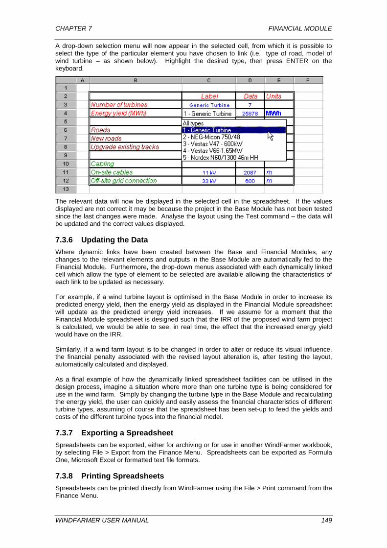
CHAPTER 7 FINANCIAL MODULE
A drop-down selection menu will now appear in the selected cell, from which it is possible to select the type of the particular element you have chosen to link (i.e. type of road, model of wind turbine – as shown below). Highlight the desired type, then press ENTER on the keyboard.
The relevant data will now be displayed in the selected cell in the spreadsheet. If the values displayed are not correct it may be because the project in the Base Module has not been tested since the last changes were made. Analyse the layout using the Test command – the data will be updated and the correct values displayed.
7.3.6 Updating the Data Where dynamic links have been created between the Base and Financial Modules, any changes to the relevant elements and outputs in the Base Module are automatically fed to the Financial Module. Furthermore, the drop-down menus associated with each dynamically linked cell which allow the type of element to be selected are available allowing the characteristics of each link to be updated as necessary. For example, if a wind turbine layout is optimised in the Base Module in order to increase its predicted energy yield, then the energy yield as displayed in the Financial Module spreadsheet will update as the predicted energy yield increases. If we assume for a moment that the Financial Module spreadsheet is designed such that the IRR of the proposed wind farm project is calculated, we would be able to see, in real time, the effect that the increased energy yield would have on the IRR. Similarly, if a wind farm layout is to be changed in order to alter or reduce its visual influence, the financial penalty associated with the revised layout alteration is, after testing the layout, automatically calculated and displayed. As a final example of how the dynamically linked spreadsheet facilities can be utilised in the design process, imagine a situation where more than one turbine type is being considered for use in the wind farm. Simply by changing the turbine type in the Base Module and recalculating the energy yield, the user can quickly and easily assess the financial characteristics of different turbine types, assuming of course that the spreadsheet has been set-up to feed the yields and costs of the different turbine types into the financial model.
7.3.7 Exporting a Spreadsheet Spreadsheets can be exported, either for archiving or for use in another WindFarmer workbook, by selecting File > Export from the Finance Menu. Spreadsheets can be exported as Formula One, Microsoft Excel or formatted text file formats.
7.3.8 Printing Spreadsheets Spreadsheets can be printed directly from WindFarmer using the File > Print command from the Finance Menu.
WINDFARMER USER MANUAL 149

CHAPTER 7 FINANCIAL MODULE
7.4 Optimisation of a financial target A financial target can be set in the spreadsheet. The optimiser will then seek the turbine layout that maximises the target cell value. In comparison, the standard optimisation method maximises the net energy production of all turbines in the workbook. To implement the function,
• first select the required financial target cell, which should contain a formula or variable;
• then select “Maximise in optimiser” from the Insert menu or use the target button in the Finance Toolbar. A pop-up box will appear to enter an appropriate label and units that will appear in the Optimisation Progress plot in the Graphing Window.
• to activate the new target during optimisation, check the tick box “Maximise Financial Target Value” in the Optimiser page in the Control Panel.
WINDFARMER USER MANUAL 150
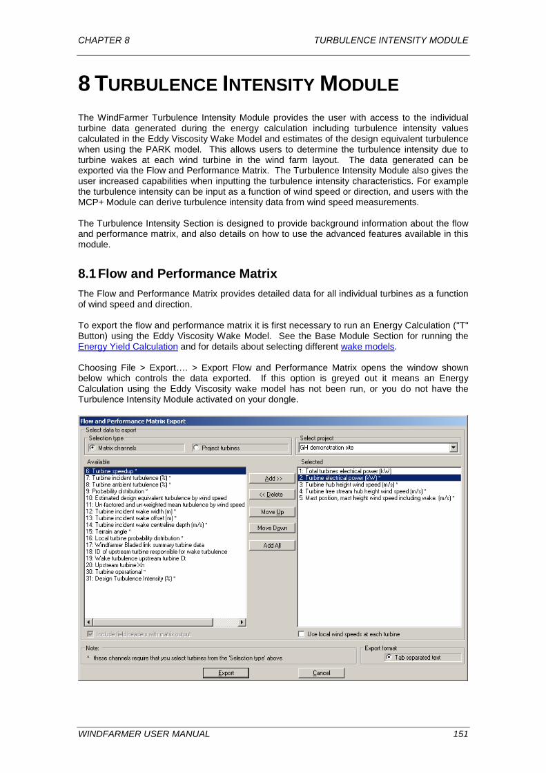
CHAPTER 8 TURBULENCE INTENSITY MODULE
8 TURBULENCE INTENSITY MODULE The WindFarmer Turbulence Intensity Module provides the user with access to the individual turbine data generated during the energy calculation including turbulence intensity values calculated in the Eddy Viscosity Wake Model and estimates of the design equivalent turbulence when using the PARK model. This allows users to determine the turbulence intensity due to turbine wakes at each wind turbine in the wind farm layout. The data generated can be exported via the Flow and Performance Matrix. The Turbulence Intensity Module also gives the user increased capabilities when inputting the turbulence intensity characteristics. For example the turbulence intensity can be input as a function of wind speed or direction, and users with the MCP+ Module can derive turbulence intensity data from wind speed measurements. The Turbulence Intensity Section is designed to provide background information about the flow and performance matrix, and also details on how to use the advanced features available in this module.
8.1 Flow and Performance Matrix The Flow and Performance Matrix provides detailed data for all individual turbines as a function of wind speed and direction. To export the flow and performance matrix it is first necessary to run an Energy Calculation ("T" Button) using the Eddy Viscosity Wake Model. See the Base Module Section for running the Energy Yield Calculation and for details about selecting different wake models. Choosing File > Export…. > Export Flow and Performance Matrix opens the window shown below which controls the data exported. If this option is greyed out it means an Energy Calculation using the Eddy Viscosity wake model has not been run, or you do not have the Turbulence Intensity Module activated on your dongle.
WINDFARMER USER MANUAL 151
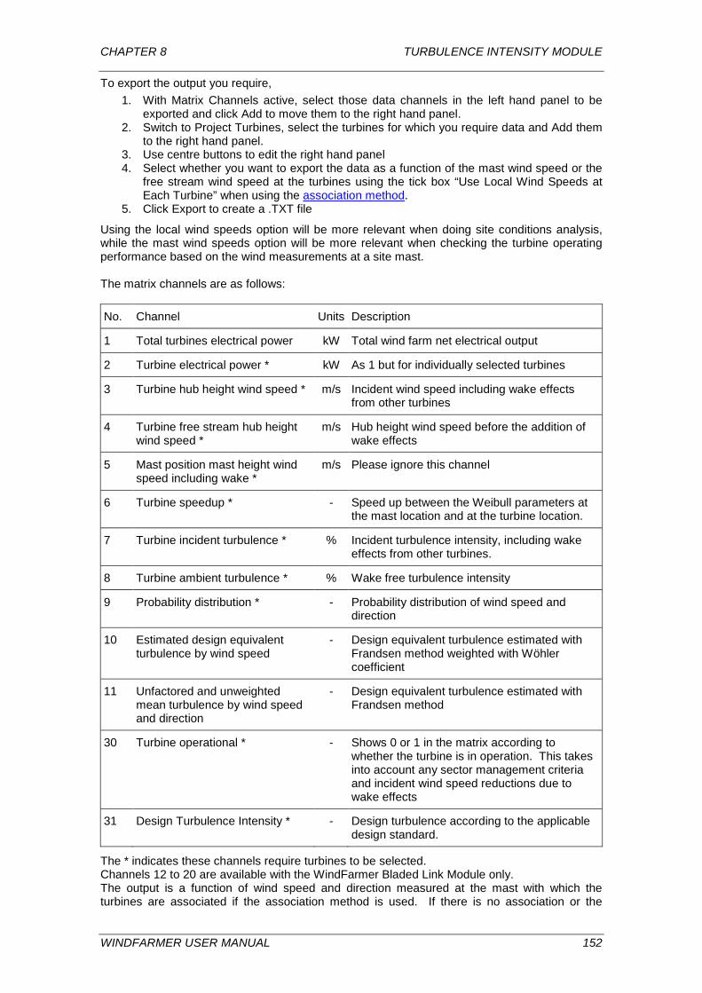
CHAPTER 8 TURBULENCE INTENSITY MODULE
To export the output you require, 1. With Matrix Channels active, select those data channels in the left hand panel to be
exported and click Add to move them to the right hand panel. 2. Switch to Project Turbines, select the turbines for which you require data and Add them
to the right hand panel. 3. Use centre buttons to edit the right hand panel 4. Select whether you want to export the data as a function of the mast wind speed or the
free stream wind speed at the turbines using the tick box “Use Local Wind Speeds at Each Turbine” when using the association method.
5. Click Export to create a .TXT file
Using the local wind speeds option will be more relevant when doing site conditions analysis, while the mast wind speeds option will be more relevant when checking the turbine operating performance based on the wind measurements at a site mast. The matrix channels are as follows: No. Channel Units Description
1 Total turbines electrical power kW Total wind farm net electrical output
2 Turbine electrical power * kW As 1 but for individually selected turbines
3 Turbine hub height wind speed * m/s Incident wind speed including wake effects from other turbines
4 Turbine free stream hub height wind speed *
m/s Hub height wind speed before the addition of wake effects
5 Mast position mast height wind speed including wake *
m/s Please ignore this channel
6 Turbine speedup * - Speed up between the Weibull parameters at the mast location and at the turbine location.
7 Turbine incident turbulence * % Incident turbulence intensity, including wake effects from other turbines.
8 Turbine ambient turbulence * % Wake free turbulence intensity
9 Probability distribution * - Probability distribution of wind speed and direction
10 Estimated design equivalent turbulence by wind speed
- Design equivalent turbulence estimated with Frandsen method weighted with Wöhler coefficient
11 Unfactored and unweighted mean turbulence by wind speed and direction
- Design equivalent turbulence estimated with Frandsen method
30 Turbine operational * - Shows 0 or 1 in the matrix according to whether the turbine is in operation. This takes into account any sector management criteria and incident wind speed reductions due to wake effects
31 Design Turbulence Intensity * - Design turbulence according to the applicable design standard.
The * indicates these channels require turbines to be selected. Channels 12 to 20 are available with the WindFarmer Bladed Link Module only. The output is a function of wind speed and direction measured at the mast with which the turbines are associated if the association method is used. If there is no association or the
WINDFARMER USER MANUAL 152
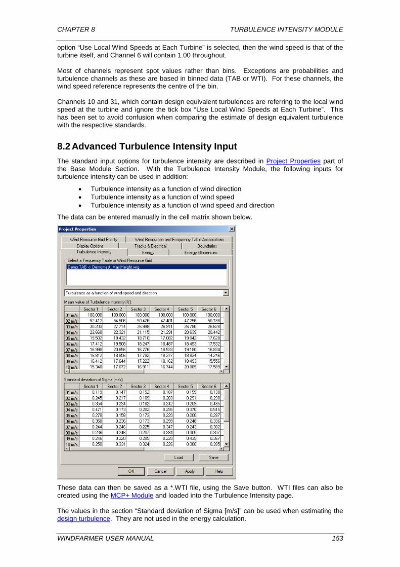
CHAPTER 8 TURBULENCE INTENSITY MODULE
option “Use Local Wind Speeds at Each Turbine” is selected, then the wind speed is that of the turbine itself, and Channel 6 will contain 1.00 throughout. Most of channels represent spot values rather than bins. Exceptions are probabilities and turbulence channels as these are based in binned data (TAB or WTI). For these channels, the wind speed reference represents the centre of the bin. Channels 10 and 31, which contain design equivalent turbulences are referring to the local wind speed at the turbine and ignore the tick box “Use Local Wind Speeds at Each Turbine”. This has been set to avoid confusion when comparing the estimate of design equivalent turbulence with the respective standards.
8.2 Advanced Turbulence Intensity Input The standard input options for turbulence intensity are described in Project Properties part of the Base Module Section. With the Turbulence Intensity Module, the following inputs for turbulence intensity can be used in addition:
• Turbulence intensity as a function of wind direction • Turbulence intensity as a function of wind speed • Turbulence intensity as a function of wind speed and direction
The data can be entered manually in the cell matrix shown below.
These data can then be saved as a *.WTI file, using the Save button. WTI files can also be created using the MCP+ Module and loaded into the Turbulence Intensity page. The values in the section “Standard deviation of Sigma [m/s]” can be used when estimating the design turbulence. They are not used in the energy calculation.
WINDFARMER USER MANUAL 153
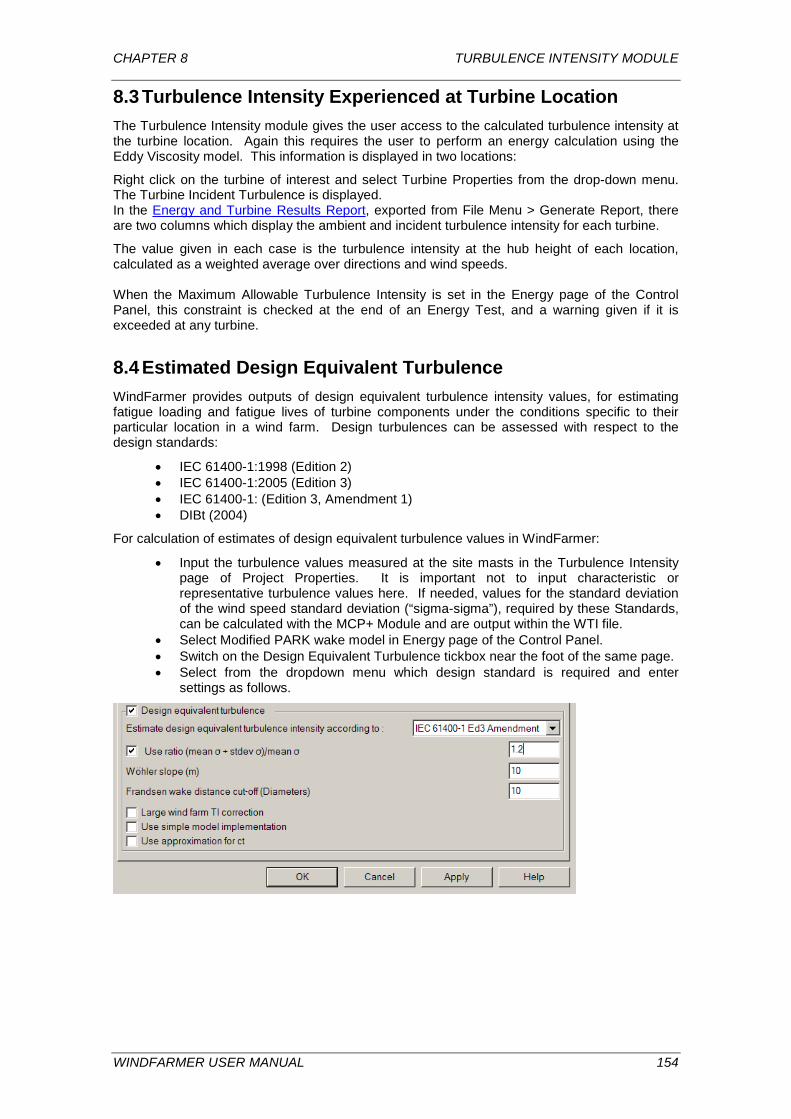
CHAPTER 8 TURBULENCE INTENSITY MODULE
8.3 Turbulence Intensity Experienced at Turbine Location The Turbulence Intensity module gives the user access to the calculated turbulence intensity at the turbine location. Again this requires the user to perform an energy calculation using the Eddy Viscosity model. This information is displayed in two locations:
Right click on the turbine of interest and select Turbine Properties from the drop-down menu. The Turbine Incident Turbulence is displayed. In the Energy and Turbine Results Report, exported from File Menu > Generate Report, there are two columns which display the ambient and incident turbulence intensity for each turbine.
The value given in each case is the turbulence intensity at the hub height of each location, calculated as a weighted average over directions and wind speeds. When the Maximum Allowable Turbulence Intensity is set in the Energy page of the Control Panel, this constraint is checked at the end of an Energy Test, and a warning given if it is exceeded at any turbine.
8.4 Estimated Design Equivalent Turbulence WindFarmer provides outputs of design equivalent turbulence intensity values, for estimating fatigue loading and fatigue lives of turbine components under the conditions specific to their particular location in a wind farm. Design turbulences can be assessed with respect to the design standards:
• IEC 61400-1:1998 (Edition 2) • IEC 61400-1:2005 (Edition 3) • IEC 61400-1: (Edition 3, Amendment 1) • DIBt (2004)
For calculation of estimates of design equivalent turbulence values in WindFarmer:
• Input the turbulence values measured at the site masts in the Turbulence Intensity page of Project Properties. It is important not to input characteristic or representative turbulence values here. If needed, values for the standard deviation of the wind speed standard deviation (“sigma-sigma”), required by these Standards, can be calculated with the MCP+ Module and are output within the WTI file.
• Select Modified PARK wake model in Energy page of the Control Panel. • Switch on the Design Equivalent Turbulence tickbox near the foot of the same page. • Select from the dropdown menu which design standard is required and enter
settings as follows.
WINDFARMER USER MANUAL 154

CHAPTER 8 TURBULENCE INTENSITY MODULE
8.4.1 Settings for estimated design turbulence Factoring of mean turbulence
If the box “Use ratio (mean σ + stdev σ)/mean σ” is unticked, then the sigma-sigma data entered using the advanced turbulence intensity input will be used. If it is ticked, then the mean ambient turbulence will be factored (default 1.2) to produce the characteristic or representative ambient turbulence according to whether using Edition 2 or 3 of IEC 61400-1 or DIBt respectively. The "Frandsen wake distance cut-off" determines when added turbulence is assumed negligible.
Large wind farm turbulence correction
The ambient turbulence level increases inside large wind farms and it is suggested in the design standards to adjust for this when calculating the estimated design equivalent turbulence. In the Control Panel, Energy page, tick the box “Apply large wind farm TI correction”. It is the user’s choice whether it is appropriate to apply this adjustment. More information is given in the Theory Manual. The new IEC61400-1 Edition 3 Amendment details that the large wind farm correction for turbulence is not used for directions where an upstream turbine wake is considered. This is applied for the Amendment only as follows: An increase in ambient turbulence is only applied in direction sectors that are not wake affected. In direction sectors with a wake from an upstream turbine that is closer than the wake distance cut-off, the correction is not applied. The cut-off is set to 10 rotor diameters by default. In the calculations with respect to the other design standards the correction is only applied in the direction sectors influenced by a wake.
Simple model implementation
WindFarmer provides the option for a simplified model to calculate the design equivalent turbulence. To activate this, check the tick box "Use simple model implementation". For more details, please refer to the Theory Manual.
Thrust coefficient
In performing the design equivalent turbulence calculation, WindFarmer can use either the actual thrust coefficient of the turbine, or an approximation of 7/(wind speed). The selection is made using the tick box "Use approximation for ct".
8.4.2 Calculation and reporting of estimated design turbulence Then
• After ensuring all other energy calculation settings are correct, run the energy calculation.
• Export the estimated turbulence values as a function of wind speed using File, Export, Export Flow and Performance Matrix, Channel 10 and Channel 11 for the selected turbine(s).
Channel 11 provides the effective turbulence information, excluding any Wöhler weighting or factoring with respect to the mean turbulence. Channel 10 provides the data after combination following the relevant standard. It includes Wöhler weighting over all directions and scaling. Channel 10 therefore corresponds to the characteristic or representative turbulence intensity that should be used for comparison with the allowable design levels. After calculating the design equivalent turbulence intensities, the values can be plotted in together with the design limits according to the Standard being followed. After running the energy calculation open a
Graphing Window, click the “Plot against turbines” icon or select View menu > Turbines. In the dialog box, activate “Selected turbine in active project” and select the individual turbine. Press OK to show the plot.
WINDFARMER USER MANUAL 155

CHAPTER 8 TURBULENCE INTENSITY MODULE
The specific estimated design equivalent turbulence of the selected turbine is plotted together with the design turbulence intensity level according to the turbine class defined in the Turbine Studio for that turbine type. If there is little difference between the two or the plots cross, then a more detailed analysis is needed. In particular, a site specific load calculation is required and use of WindFarmer Bladed Link is recommended. The estimated design equivalent turbulence is only available with the PARK model because both are related in their simplified description of the wake. The empirical expression used here contains factors to take into account the non-linear relationship between turbulence and load statistics, and follows the Frandsen method [IEC Standard 61400-1 ed. 3, Annex D]. To address the variation in fatigue life rather than just loading effects caused by the turbulence, outputs can be weighted according to the Wöhler index m. This index is specific to component material and geometry and is derived from the slope of the log-log plot of the S-N curve (magnitude of a cyclical stress (S) against the cycles to failure (N)), where the relation S ∝ N-1/m is assumed. Typical values for wind turbines range between 3 and 15 where 4 is appropriate for simple steel components and values 10 to 15 are suitable for simple composite components. The turbine manufacturer should be consulted for advice on an acceptable range of Wöhler indices for these calculations. More information and guidance on the calculations and requirements of the Standards is given in the Theory Manual. Note that the WindFarmer channels are expressed as turbulence intensities whereas the equations in the standard are expressed as standard deviations of wind speed.
8.5 Site Conditions Ranking Table WindFarmer provides the automatic ranking of turbine locations according to several key parameters. The primary use will be to readily compare the severity of the site conditions. To access this information select “Site Specific Conditions” in the Report Generator. In the Energy Reports page in the Control Panel it can be selected if all turbines are included in the report or if the ranking table is restricted to a maximum number of turbines. The information is provided for the hub height of each turbine listed, and depending on the parameter it is not always necessary to run an energy test calculation first. The information comprises:
• Air density • Mean free wind speed • Estimated design equivalent turbulence intensity • Maximum ground slope (needs presence of DTM) • The minimum, mean and maximum values are given in the upper table and below
the ranked values at the turbines in comparison with the target values from the Standards.
For completeness, extreme wind speed and shear coefficient are also presented. These are Project Specific values entered in the Project Properties, Energy page using the Site Condition Assessment button. At present the values are not used in any algorithms in WindFarmer.
WINDFARMER USER MANUAL 156

CHAPTER 9 ELECTRICAL MODULE
9 ELECTRICAL MODULE The Electrical Module allows you to design the electrical network for your proposed wind farm. Among its capabilities it will:
• Calculate lengths of underground cables and overhead lines, taking topography and gradients into account;
• Calculate annual electrical losses for cables, lines and transformers, and their annual value (requires the financial module);
• Calculate annual reactive power production and consumption, for turbines, cables, lines, power factor correction devices and transformers, and their annual value (requires the financial module);
• Check for overloading of transformers, cables and lines; • calculate Loss Capitalisation Factors for transformers (requires the financial
module); • Calculate the size of capacitor/reactor banks needed to correct the power factor at a
particular point. For simplicity, these devices will be referred as power factor correction devices (PFCD).
The Electrical Module is used to design the electrical infrastructure and perform its calculations once the wind farm layout has been fixed because moving turbines would require some repositioning of cable nodes.
9.1 Mouse Functions New Mouse Functions have been implemented in order to help the user to insert the cable nodes into the electrical infrastructure and amend it as required. The cursor should be in Cable Mode by clicking on Cable mode or New Cable mode button as required.
9.1.1 Adding Cable Nodes As with all other types of object in WindFarmer, cable nodes are added by right-clicking in the map view on the position the new object is to take. Cable nodes are part of cable networks which are group objects and as such, are similar to boundaries in that, once a workbook contains a cable network, you can either add to it or start another separate cable network by using the menu command or toolbar button.
9.1.2 Inserting Cable Nodes Additional cable nodes can be inserted into an already existing cable by holding down the shift key and right-clicking the mouse on the position of the new cable node. WindFarmer determines which cable to insert into by finding the nearest cable node and inserting the new cable node either before or after it depending on which option represents the shorter detour.
9.1.3 Lone Cable Nodes Initially unconnected cable nodes can be added to a site by holding down the control (Ctrl) key and right-clicking in the map view. This can be useful when placing the main components of the electrical network before linking everything together.
9.1.4 Redirecting Cable Route A cable route can be redirected by first selecting the cable node on the utility side of the stretch of cable to be redirected, then holding down the control (Ctrl) key and left-clicking on the node which you wish to redirect the cable to. This works both within a cable network as well as between separate cable networks. This merging of cable networks is particularly useful when merging two sites in order to analyse their combined performance.
WINDFARMER USER MANUAL 157

CHAPTER 9 ELECTRICAL MODULE
9.1.5 Connecting To Turbines Connecting a turbine to a cable network is very similar to redirecting a cable route. The user simply selects the cable node which the turbine should connect to then, holding down the control (Ctrl) key, left-click on the turbine and a line should appear connecting the turbine to the cable node. To ensure the connection has been achieved you can use the zoom facility. This connection can be edited in the cable properties dialog. However, unlike with a cable node object, this connection cannot contain a power factor compensation device (PFCD) or a meter. It can however, contain a transformer together with two cable components: one running from the turbine to the transformer; the other running from the transformer to the connecting cable node. If you need to have a meter or PFCD near the turbine then you should do this by placing a cable node which contains the desired components closer to the turbine and connecting from this.
9.1.6 Properties Properties of a cable node, along with any components owned by the node, can be edited by right-clicking on a cable node object whilst in Working Mode. A popup menu will appear and one of the options is Cable Properties.
9.2 Inputs
9.2.1 System Frequency 50 Hz, 60 Hz, or as specified by user (default 50 Hz). This is input in the Project Properties > Tracks and Electrical page.
9.2.2 Physical Layout of Electrical System The user must input the physical layout of the electrical network through the map view, using New Cable mode . The usual methods of adding, deleting and editing objects apply plus some New Mouse Functions, previously described, in order to facilitate easy re-routing of electrical networks. Each electrical (or cable) network has a Root node which represents a point of connection and, if deleted, deletes the entire network. There can be more than one network in a project. All the turbines in the currently selected project must be connected to an electrical network. The electrical network can be examined and edited through the Cable Properties dialogue box, labelled Electrical Module Properties of Turbines & Cables, which is accessed by right clicking on a cable node when in Working Mode. Further description of navigating around the network is given later in this Section. An electrical network is made up of cable node objects. These nodes define the large-scale topology of the electrical network. Each node is connected to one other node and is responsible for the connecting cable or overhead line. Branching is achieved by more than one node connecting to the branching node. In other words, a node can only connect to one other node but can be connected to by any number of nodes. The resulting tree-like structures can be likened to a river system in which turbines are the sources and the Root node becomes the river mouth. Because a node represents not only a point but also the line connecting it towards the point of connection, nodes are natural containers for any components which are to be situated at the node or at some point along the connecting line. The components that a node can contain include the following:
• a Transformer, which has primary (high-voltage) and secondary (low-voltage) sides • a Cable or Overhead Line (both referred to as cables for simplicity) • a PFCD • a Metering Point
Every node (with the exception of the Root) contains one cable component. The other components are optional. Components are added by the user through the Cable Properties Dialog. Only one of each component type can be added to any one cable node.
WINDFARMER USER MANUAL 158
CHAPTER 9 ELECTRICAL MODULE
Turbines can be thought of as a special form of cable node. The turbine’s electrical properties include a connection to a cable node (see Connecting to Turbines in New Mouse Functions section). Users cannot add components as they can with cable nodes. However, turbines can be configured to have a transformer outside the turbine terminals. This transformer can be inside or outside the turbine tower, its position being specified by a bearing and distance from the tower centre. The properties of the turbine transformer as well as the low and medium voltage cables are set in the Cable Properties Dialogue in the same way as for other electrical components. The user is able to supply text names for all components, or allow automatic naming. For components which are turbines, the component name shall be the turbine type identifier.
9.2.3 Cable and Line Data For each cable, the user needs to specify:
• AC Resistance per phase (ohms per km); • Reactance per phase (mH per km) (optional: zero if not stated); • Capacitance per phase (microF per km) (optional: zero if not stated). • Nominal Voltage (kV, phase to phase); • Ampacity or maximum continuous current rating (A) (optional: infinite if not stated);
Using the Copy and Paste options (see Electrical Module Properties of Turbines & Cables Dialog) cuts down on the amount of user input. Also, the Electrical Module Library Dialog, accessed via the Library button, allows saving of commonly used components for import into other workbooks. Libraries are saved with extension ELB. An example is provided with WindFarmer in the Demodata file.
9.2.4 Turbine/Substation Transformer Data For each turbine/substation transformer, the user needs to specify:
• Nominal Rating (kVA); • Nominal Primary Voltage (kV, phase to phase); • Nominal Secondary Voltage (kV, phase to phase); • No-Load Loss (‘Iron Loss’) (Watts); • Load Loss (‘Copper Loss’) at nominal rating (Watts); • Transformer Impedance (percent on transformer Nominal Rating) (optional: zero if
not stated); • Excitation Current (as a percentage of the nominal current of the transformer)
(optional: zero if not stated. WindFarmer then assumes then that the Magnetising Reactance is infinite, as shown in the Theory Manual)
Using the Copy and Paste options (see Electrical Module Properties of Turbines & Cables Dialog) cuts down on the amount of user input. Also, the Electrical Module Library Dialogue allows saving of commonly used components for import into other workbooks.
9.2.5 Turbine Data The following data fields have been added to turbine type definition and can be accessed via the Turbine Studio:
• Nominal Voltage of turbine terminals (kV, phase to phase); • Relationship between Active Power production (kW), Reactive Power
production/consumption (kVAr), and wind speed.
9.2.6 PFCD data Utilities are recently becoming more demanding in terms of power factor requirements for connection of new generation. Normally, capacitor banks (source of reactive power) can be installed to improve the power factor across the entire wind farm output power range, in particular for large outputs. In some cases, reactor banks (sinks of reactive power) can be installed to control power factor or voltage levels.
WINDFARMER USER MANUAL 159

CHAPTER 9 ELECTRICAL MODULE
PFCDs can be configured one of three ways:
• Fixed capacitance or reactance (constant value of kVAr) • Control power factor at some metering point nearer the point of connection by stating
the desired PF either capacitive (leading) or inductive (lagging) • Control power factor at the PFCD terminals as the previous case but introducing a
´dumb´ meter point upstream, i.e. towards the Root node, next to the PFCD terminals.
The PFCD step size can also been decided beforehand when inserting this device in the electrical network as shown in the Electrical Module Properties of Turbines and Cables Dialog. Only one PFCD can be inserted into one cable node object and associated with an upstream metering point.
9.2.7 Meter The Tariff Information required for each metering, which is used as input in the Financial Module, is as follows:
• Value of Energy Exported (currency unit/kWh) • Value of Energy Imported (currency unit/kWh) • Value of Reactive Energy Exported (currency unit/kVArh) • Value of Reactive Energy Imported (currency unit/kVArh)
Only one meter can be inserted into one cable node object.
9.3 Outputs To perform an electrical calculation and include the electrical losses for the wind farm in the net energy figure, tick “Calculate” under “Input Electrical Efficiency” in the “Energy Efficiencies” page of Project Properties. Then press the T test button on the Base Module toolbar to perform an energy calculation. After performing an energy calculation which includes the electrical model the electrical results can be exported either in Microsoft Word, Excel or Text format on generating the report. The calculated overall electrical efficiency also appears in the main energy report and is included in the net energy calculation. The outputs possible are grouped into electrical losses; active and reactive power; overloaded components; and cable lengths.
9.3.1 Electrical Losses The first output, Summarised Report, is a table for each metering point, showing electrical losses in kWh per year, and as a percentage of the ‘ideal’ annual energy output of the wind turbines associated with that metering point, subdivided as below:
• All transformers (no-load losses) summated; • All transformers (load losses) summated; • All cable and lines summated; • Total losses; • Total losses during periods of net export; • Total losses during periods of net import; • Peak loss, i.e. highest recorded value of total losses (in kW).
The ideal energy in this case is the sum of the energy generated at all the turbines connected to the utility through the metering point. The second output is a Detailed Report using the same format as above, but itemised for each electrical component.
WINDFARMER USER MANUAL 160

CHAPTER 9 ELECTRICAL MODULE
9.3.2 Reactive Power The output is a table for each metering point showing total annual reactive power consumption or generation (in kVArh), for:
• All turbines summated; • All cables and lines summated; • All transformers summated; • All PFCDs summated (if installed); • Total reactive losses; • The annual reactive power export of the metering point, i.e. the sum for all periods
where the metering point is a net exporter of reactive power (in kVArh). • The annual reactive power import of the metering point, i.e. the sum for all periods
where the metering point is a net importer of reactive power (in kVArh).
The second output is a Detailed Report using the same format as above, but itemised for each electrical component.
9.3.3 Overloading Displays a list of any transformers, cables and lines which will be overloaded at maximum wind turbine and/or wind farm output depending on the location of the component in question. Overloaded nodes are shown in the map view after performing the Electrical Module calculations (e.g. via the ‘T’ button). An overloaded cable node or turbine is indicated via a red circle. To turn on/off the display of overloading, change the state of the ‘Overload’ tick box in the display bar.
9.3.4 Calculated lengths Produces a table of calculated lengths for each cable and line segment, and a total for each cable and line type.
9.3.5 Power factor Results This output is included in the Electrical Module report if a PFCD is installed in the power collection system. The output is a table for any metering point which has a PFCD injecting a fix amount of reactive power or regulating the power factor, showing the following results as function of the Active Power (in terms of KW and percent):
• Size of the PFCD (Min and Max, kVAr) • Resulting Reactive Power (Min and Max, kVAr) • Resulting Power Factor Range
In the table, a positive amount of kVAr means a capacitor bank whereas a negative amount of KVAr means a reactor bank.
9.4 Electrical Module Properties of Turbines & Cables Dialog (EMPTCD)
This section provides a simple example of how to use the Electrical Module Properties of Turbines & Cables Dialog (EMPTCD) which acts as an interface between the user and WindFarmer to input all the electrical parameters of each component of the network.
9.4.1 Launching the EMPTCD from a turbine on the map view Select (left mouse click) the Working Mode mouse icon (the white arrow) from the main toolbar. Then right click the required Turbine Icon on the map, and select the menu item ‘Electrical properties of a turbine’.
WINDFARMER USER MANUAL 161
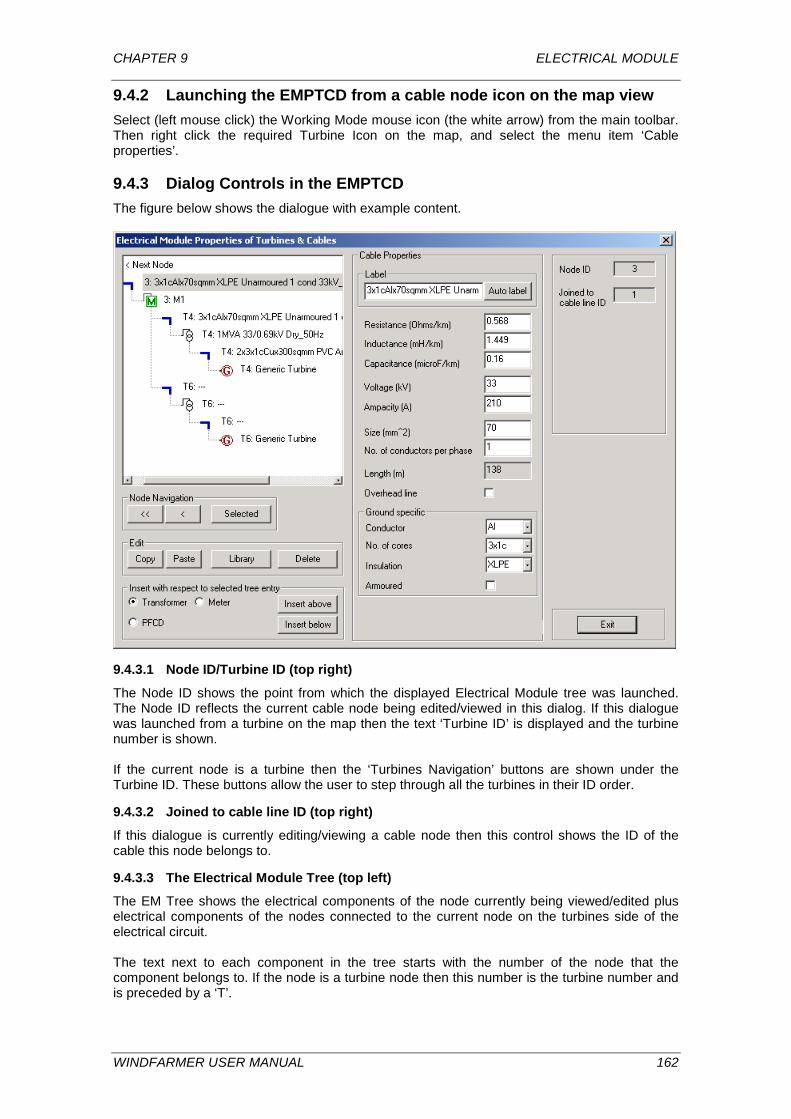
CHAPTER 9 ELECTRICAL MODULE
9.4.2 Launching the EMPTCD from a cable node icon on the map view Select (left mouse click) the Working Mode mouse icon (the white arrow) from the main toolbar. Then right click the required Turbine Icon on the map, and select the menu item ‘Cable properties’.
9.4.3 Dialog Controls in the EMPTCD The figure below shows the dialogue with example content.
9.4.3.1 Node ID/Turbine ID (top right)
The Node ID shows the point from which the displayed Electrical Module tree was launched. The Node ID reflects the current cable node being edited/viewed in this dialog. If this dialogue was launched from a turbine on the map then the text ‘Turbine ID’ is displayed and the turbine number is shown. If the current node is a turbine then the ‘Turbines Navigation’ buttons are shown under the Turbine ID. These buttons allow the user to step through all the turbines in their ID order.
9.4.3.2 Joined to cable line ID (top right)
If this dialogue is currently editing/viewing a cable node then this control shows the ID of the cable this node belongs to.
9.4.3.3 The Electrical Module Tree (top left)
The EM Tree shows the electrical components of the node currently being viewed/edited plus electrical components of the nodes connected to the current node on the turbines side of the electrical circuit. The text next to each component in the tree starts with the number of the node that the component belongs to. If the node is a turbine node then this number is the turbine number and is preceded by a ‘T’.
WINDFARMER USER MANUAL 162
CHAPTER 9 ELECTRICAL MODULE
The components of the currently viewed/edited node are always at the top of the tree, with the components of the connected node(s), branching of below. The example tree in the above figure shows the currently viewed/edited node is cable node 6, which has a cable, and a meter. Cable nodes always have a cable component that cannot be deleted. Connected to cable node 3 are turbines numbered T4 and T6. Both these turbines include a cable to a transformer, a transformer, and a cable from the transformer to the next node. The properties of the turbine relevant to the Electrical Module are represented by the ‘G’ or turbine generator component on the tree. T4 has had its components edited already, with each component having been named. T6 has not been edited yet. If you select the ‘< Next Node’ object at the top of the tree, then the state of the current node is saved, and the next node towards the utility is viewed as the new top node in the tree. If the top of the tree shows ‘Root Node’ rather than ‘Next Node’ then the current node is connected to the Root node of the cable. The Root node has no electrical properties, and is an artefact of representing cables by their end points. To move to an alternative branch connected directly to the Root node you must select a node of the alternative branch in the map view. If the Electrical Module properties of a turbine are being viewed, and the turbine is not connected to a cable network, then instead of ‘Next Node’ the top tree item shows the text ‘No Cable’. If you select an object not belonging to the current top node, but belonging to one of the lower node branches, then the current top node is saved, and the node of the selected object is then displayed as the new top node. If you select an EM component of the top node then the properties of that component are displayed in the central third of the dialog. In the above figure an example the cable component of cable node 6 has been selected in the tree, and so the ‘Cable Properties’ of this component are displayed in the centre of the dialog.
9.4.3.4 Node Navigation (centre left)
The buttons in this section are concerned with navigating the current cable within this dialog. The ‘<’ Button
The ‘<’ button has the same effect as selecting the ‘< Next Node’ object at the top of the EM Tree. Thus when you press this button the state of the current node is saved, and the next node towards the utility is viewed as the new top node in the tree. The ‘<<’ Button
The ‘<<’ button has the same effect as the ‘<’ button but it skips all nodes towards the utility, that only contain a cable component, and are only joined to one other node on the Turbine side. Thus it jumps to the next ‘significant’ node towards the utility. The ‘Selected’ Button
If you perform node navigation via the EM Tree or via the ‘<<’ or ‘<’ buttons then you can jump back to the node you selected to open this dialogue by pressing this button.
9.4.3.5 Edit (lower centre left)
The buttons in this section allow you to edit the contents of the selected EM Tree component, as displayed in the relevant component properties controls in the centre of the dialog. The component properties can also be edited directly. The ‘Copy’ and ‘Paste’ Buttons
WINDFARMER USER MANUAL 163
CHAPTER 9 ELECTRICAL MODULE
The ‘Copy’ button allows you to copy the contents of any component selected in the EM Tree. There is a temporary copy location reserved for each component type. When you press the ‘paste’ button the currently selected component type is detected and the contents of the corresponding temporary copy location are copied into the selected component. If the temporary copy location has not been previously populated via a ‘Copy’ then pressing paste will have the effect of clearing the contents of the selected component. The ‘Copy’ and ‘Paste’ operations are specific to each Workbook, so using this method to copy between Workbooks is not yet possible. To copy ALL the electrical components of a turbine select the Generator component, press the ‘Copy’ button, navigate to the turbine to be edited, and press the ‘Paste’ button. The ‘Delete’ button allows the selected EM component (if not a cable) to be deleted from the current node. The ‘Library’ button opens the ‘Electrical Module Library Dialog’ (EMLD). The EMLD provided the means to access and maintain a library of transformers, overhead lines and cables. If the currently selected component in the EM Tree is a transformer or cable/overhead line then when the ‘Library’ button is pressed the properties of the selected component are copied to the EMLD, to allow the addition of the selected component to the library.
9.4.3.6 Insert with respect to selected tree entry (bottom left)
The controls within this section allow the insertion of new EM components into the current node. Choose the type of component to insert via the ‘Transformer;’ ‘Meter’, and ‘PFCD’ buttons. Use the ‘Insert above’ button to insert the new component above the currently selected component. Use the ‘Insert below’ button to insert the new component below the currently selected component.
9.4.3.7 Cable Properties and Transformer Properties ‘Auto label’ button
If you select a cable or transformer within the tree then the properties of the selected component are displayed in the centre of the dialogue and includes an ‘Auto Label’ button. Pressing this button constructs a label using to the current status of the properties of the selected component. Text typed directly into the label control that begins with a ’_’ (underscore) is not deleted during the auto label but is instead appended to the end of the generated auto label text.
WINDFARMER USER MANUAL 164

CHAPTER 9 ELECTRICAL MODULE
9.5 Caveats The calculation methods used in the Electrical Module have sufficient accuracy to be used for outline design of wind farm three-phase AC electrical systems, and to calculate the cost of losses and of reactive power for budgeting purposes. For some projects, power-systems analysis packages may be necessary at the detail design stage, to achieve greater accuracy and to perform other calculations useful in electrical design. The major approximations in this module are:
• Ambient temperature is assumed to be constant, and assumed not to affect the thermal ratings of transformers, cables and lines.
• The resistance of cables and lines is assumed not to vary with load. Unless other information is available, it is suggested that as a conservative estimate the resistance appropriate to maximum conductor operating temperature is used.
• The resistance of transformers is assumed not to vary with load. The calculation method is based on the stated ‘load loss’ figure for the transformer, which is normally defined at the temperature appropriate to the nominal power of the transformer. In normal operation, transformers will usually be cooler than this, so the method slightly overestimates transformer resistance and losses.
• Nominal voltages are assumed throughout the system. • Transformer cooling fan loads are ignored. • Losses at the PFCD are ignored. This is not very accurate for a reactor bank device
where load losses can be quite significant. These losses should be included in the detailed design analysis in later stages.
• Parallel cables and lines for each phase and parallel transformers at the substation are permitted as long as the user provides the equivalent parameters; a method of automatic calculation of equivalent parameters for N identical/different electrical objects arranged in parallel is provided in the Theory Manual.
In addition, the following restriction applies:
• current paths are not permitted The electrical system must be a ‘tree’ structure rather than a ‘ring’ structure, i.e. alternative parallel.
WINDFARMER USER MANUAL 165

CHAPTER 10 SHADOW FLICKER MODULE
10 SHADOW FLICKER MODULE The WindFarmer Shadow Flicker Module contains the tools required to assess the potential period of shadow flicker caused by a wind turbine. The module allows you to create maps of shadow flicker occurrence and to analyse the shadow flicker at specific points, known as receptors. This information can be used to design and operate the wind farm in a way that minimises the annoyance to people. This Section introduces users to the functions contained in the WindFarmer Shadow Flicker Module, and explains how users can utilise the module in the design of wind farms.
10.1 Shadow Flicker Module Interface
10.1.1 Windows The Shadow Flicker module operates from the Mapping Window. The user defines the positions of the Shadow Receptors and displays results as shadow flicker maps and the shadow flicker at the receptors in the Mapping Window.
10.1.2 Toolbar Buttons When a Mapping Window is open and active then the Mapping toolbar is also displayed as active.
This toolbar allows users to enter the Shadow Receptor mode using the button and insert Shadow Receptors by right clicking in the Mapping View.
10.1.3 Inputs to Shadow Flicker The Shadow Flicker calculations require a DTM file to be loaded. WindFarmer derives the geographic coordinates for the shadow flicker calculation from the site centre of the current project (Project Properties, Display Options). To derive this correctly, make sure that the projection is correctly set in the workbook and the 'Enable coordinate projection selection' in Control Panel > Preferences is enabled.
WINDFARMER USER MANUAL 166
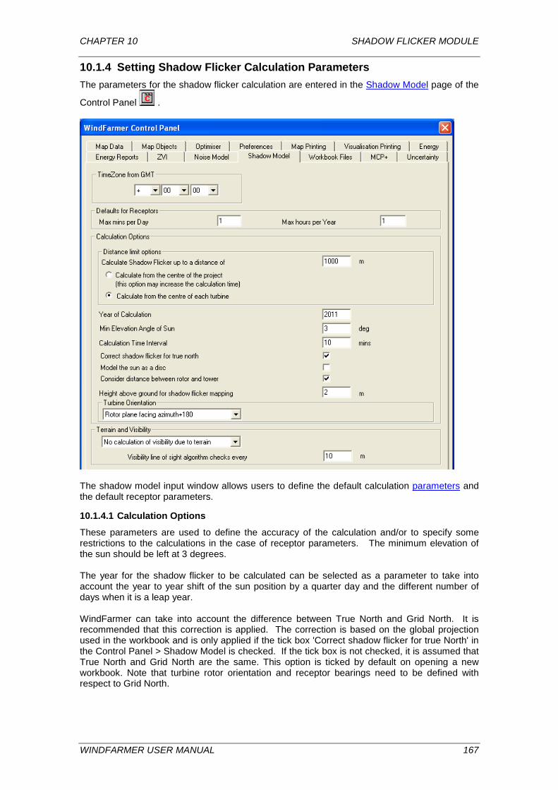
CHAPTER 10 SHADOW FLICKER MODULE
10.1.4 Setting Shadow Flicker Calculation Parameters The parameters for the shadow flicker calculation are entered in the Shadow Model page of the
Control Panel .
The shadow model input window allows users to define the default calculation parameters and the default receptor parameters.
10.1.4.1 Calculation Options
These parameters are used to define the accuracy of the calculation and/or to specify some restrictions to the calculations in the case of receptor parameters. The minimum elevation of the sun should be left at 3 degrees. The year for the shadow flicker to be calculated can be selected as a parameter to take into account the year to year shift of the sun position by a quarter day and the different number of days when it is a leap year. WindFarmer can take into account the difference between True North and Grid North. It is recommended that this correction is applied. The correction is based on the global projection used in the workbook and is only applied if the tick box 'Correct shadow flicker for true North' in the Control Panel > Shadow Model is checked. If the tick box is not checked, it is assumed that True North and Grid North are the same. This option is ticked by default on opening a new workbook. Note that turbine rotor orientation and receptor bearings need to be defined with respect to Grid North.
WINDFARMER USER MANUAL 167
CHAPTER 10 SHADOW FLICKER MODULE
The default in shadow flicker calculations is that the sun is assumed to be a point. There is an option to model the sun as a disc. This worst case option leads to higher shadow flicker times, especially close to the turbines. In this calculation no perception threshold is taken into account. It should be noted that many guidelines define limits that assume a point source. While more accurately representing theoretical shadow flicker, the option "Sun as disk", should not be selected if the result is to be compared with limits given by these guidelines. The calculation of shadow flicker automatically recognises the offset distance between the tower coordinates and the centre of the turbine rotor. This can be disabled if required. Additional flexibility and accuracy of the model is provided in the calculations by allowing the user to define the orientation of the turbine rotor and to model the rotor as a disk or as a sphere. The user has the choice between three calculation methods regarding the orientation of the turbine rotor orientation:
• Spherical model – using a sphere of radius equal to rotor radius to represent the area causing the potential shadow flicker.
• Rotor following the azimuth angle of the sun – where the rotor axis is 180° from the sun’s azimuth.
• Fixed rotor orientation for all turbines – where the rotor faces the defined wind direction.
As an additional option the distance between the turbine rotor and the turbine tower can be considered in the calculation. The worst case scenario occurs when both the spherical turbine rotor model with offset and the sun as a disk model is selected and the turbine rotor axis is aligned with the sun and the shadow receptor. Statistically this may not be the best representation of the actual wind direction distribution at the site and a calculation with other rotor orientations may be more relevant if not the worst case scenario but the probability of a given scenario is relevant. More details are given in the Theory Manual. Shadow flicker maps can be calculated at user-defined height above the ground, with a default of 2 m.
10.1.4.2 Terrain and Visibility
The Terrain and Visibility options allow you to decide if the calculation should consider that the view from the turbines to the sun or to the receptor can be obstructed by terrain features.
WINDFARMER USER MANUAL 168
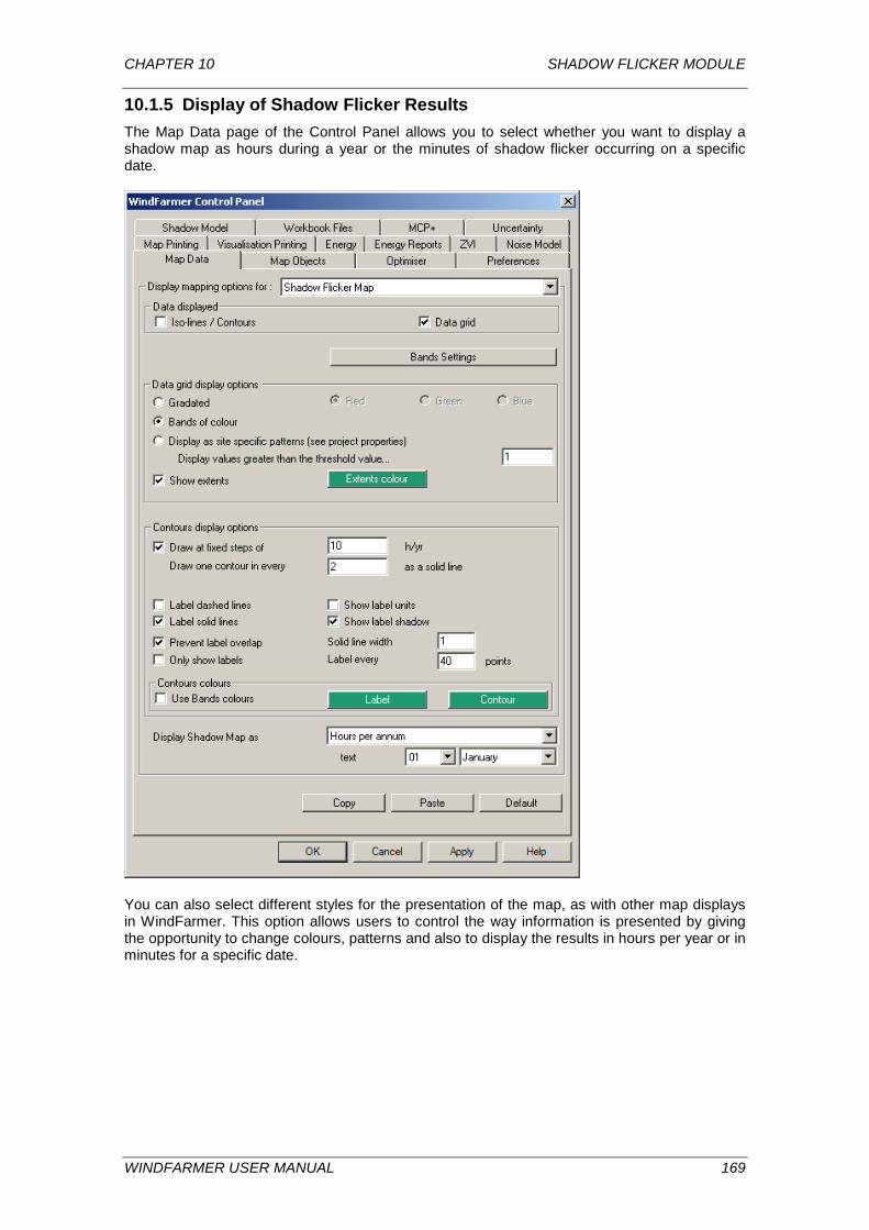
CHAPTER 10 SHADOW FLICKER MODULE
10.1.5 Display of Shadow Flicker Results The Map Data page of the Control Panel allows you to select whether you want to display a shadow map as hours during a year or the minutes of shadow flicker occurring on a specific date.
You can also select different styles for the presentation of the map, as with other map displays in WindFarmer. This option allows users to control the way information is presented by giving the opportunity to change colours, patterns and also to display the results in hours per year or in minutes for a specific date.
WINDFARMER USER MANUAL 169
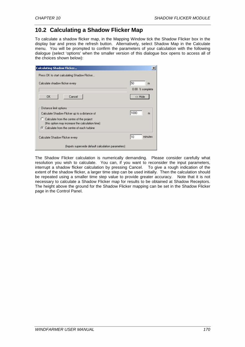
CHAPTER 10 SHADOW FLICKER MODULE
10.2 Calculating a Shadow Flicker Map To calculate a shadow flicker map, in the Mapping Window tick the Shadow Flicker box in the display bar and press the refresh button. Alternatively, select Shadow Map in the Calculate menu. You will be prompted to confirm the parameters of your calculation with the following dialogue (select ‘options’ when the smaller version of this dialogue box opens to access all of the choices shown below):
The Shadow Flicker calculation is numerically demanding. Please consider carefully what resolution you wish to calculate. You can, if you want to reconsider the input parameters, interrupt a shadow flicker calculation by pressing Cancel. To give a rough indication of the extent of the shadow flicker, a larger time step can be used initially. Then the calculation should be repeated using a smaller time step value to provide greater accuracy. Note that it is not necessary to calculate a Shadow Flicker map for results to be obtained at Shadow Receptors. The height above the ground for the Shadow Flicker mapping can be set in the Shadow Flicker page in the Control Panel.
WINDFARMER USER MANUAL 170
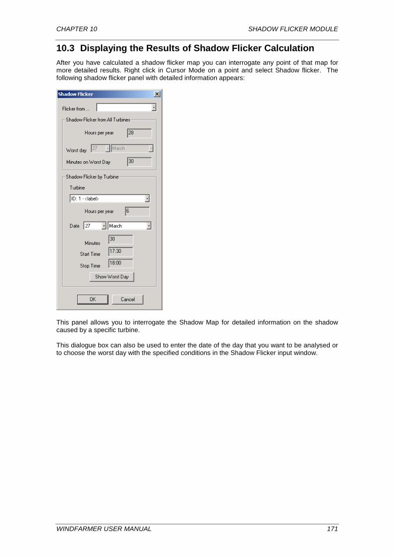
CHAPTER 10 SHADOW FLICKER MODULE
10.3 Displaying the Results of Shadow Flicker Calculation After you have calculated a shadow flicker map you can interrogate any point of that map for more detailed results. Right click in Cursor Mode on a point and select Shadow flicker. The following shadow flicker panel with detailed information appears:
This panel allows you to interrogate the Shadow Map for detailed information on the shadow caused by a specific turbine. This dialogue box can also be used to enter the date of the day that you want to be analysed or to choose the worst day with the specified conditions in the Shadow Flicker input window.
WINDFARMER USER MANUAL 171
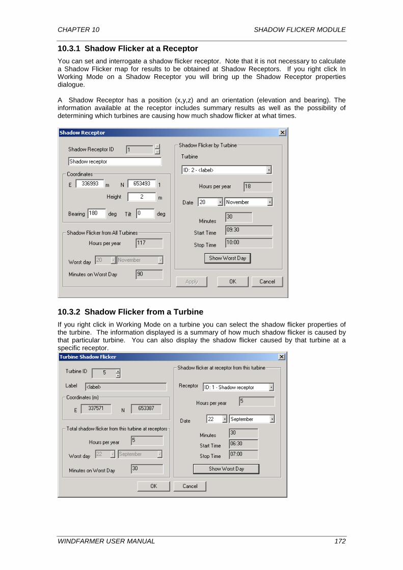
CHAPTER 10 SHADOW FLICKER MODULE
10.3.1 Shadow Flicker at a Receptor You can set and interrogate a shadow flicker receptor. Note that it is not necessary to calculate a Shadow Flicker map for results to be obtained at Shadow Receptors. If you right click In Working Mode on a Shadow Receptor you will bring up the Shadow Receptor properties dialogue. A Shadow Receptor has a position (x,y,z) and an orientation (elevation and bearing). The information available at the receptor includes summary results as well as the possibility of determining which turbines are causing how much shadow flicker at what times.
10.3.2 Shadow Flicker from a Turbine If you right click in Working Mode on a turbine you can select the shadow flicker properties of the turbine. The information displayed is a summary of how much shadow flicker is caused by that particular turbine. You can also display the shadow flicker caused by that turbine at a specific receptor.
WINDFARMER USER MANUAL 172
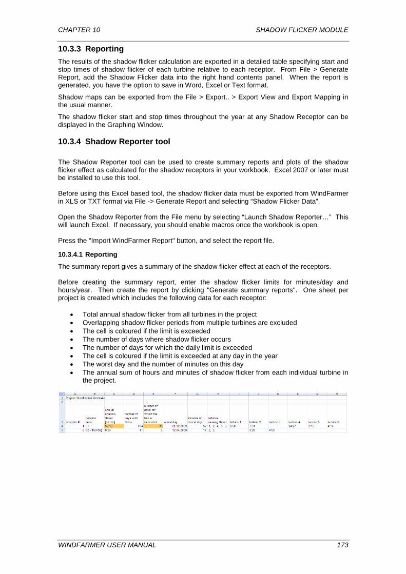
CHAPTER 10 SHADOW FLICKER MODULE
10.3.3 Reporting The results of the shadow flicker calculation are exported in a detailed table specifying start and stop times of shadow flicker of each turbine relative to each receptor. From File > Generate Report, add the Shadow Flicker data into the right hand contents panel. When the report is generated, you have the option to save in Word, Excel or Text format.
Shadow maps can be exported from the File > Export.. > Export View and Export Mapping in the usual manner.
The shadow flicker start and stop times throughout the year at any Shadow Receptor can be displayed in the Graphing Window.
10.3.4 Shadow Reporter tool The Shadow Reporter tool can be used to create summary reports and plots of the shadow flicker effect as calculated for the shadow receptors in your workbook. Excel 2007 or later must be installed to use this tool. Before using this Excel based tool, the shadow flicker data must be exported from WindFarmer in XLS or TXT format via File -> Generate Report and selecting “Shadow Flicker Data”. Open the Shadow Reporter from the File menu by selecting “Launch Shadow Reporter…” This will launch Excel. If necessary, you should enable macros once the workbook is open. Press the "Import WindFarmer Report" button, and select the report file.
10.3.4.1 Reporting
The summary report gives a summary of the shadow flicker effect at each of the receptors. Before creating the summary report, enter the shadow flicker limits for minutes/day and hours/year. Then create the report by clicking "Generate summary reports". One sheet per project is created which includes the following data for each receptor:
• Total annual shadow flicker from all turbines in the project • Overlapping shadow flicker periods from multiple turbines are excluded • The cell is coloured if the limit is exceeded • The number of days where shadow flicker occurs • The number of days for which the daily limit is exceeded • The cell is coloured if the limit is exceeded at any day in the year • The worst day and the number of minutes on this day • The annual sum of hours and minutes of shadow flicker from each individual turbine in
the project.
WINDFARMER USER MANUAL 173
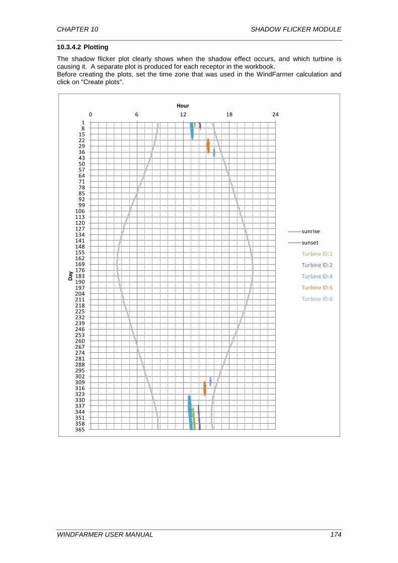
CHAPTER 10 SHADOW FLICKER MODULE
10.3.4.2 Plotting
The shadow flicker plot clearly shows when the shadow effect occurs, and which turbine is causing it. A separate plot is produced for each receptor in the workbook. Before creating the plots, set the time zone that was used in the WindFarmer calculation and click on "Create plots".
18
15222936435057647178859299
106113120127134141148155162169176183190197204211218225232239246253260267274281288295302309316323330337344351358365
0 6 12 18 24
Day
Hour
sunrise
sunset
Turbine ID:1
Turbine ID:2
Turbine ID:4
Turbine ID:5
Turbine ID:6
WINDFARMER USER MANUAL 174
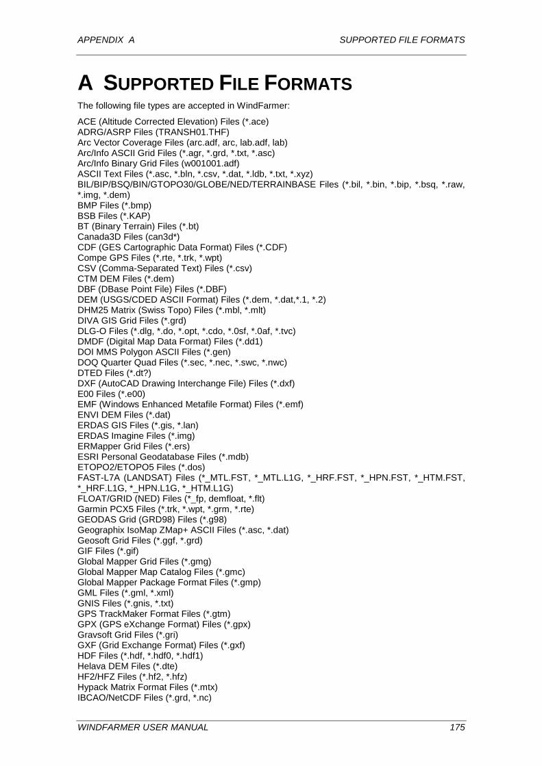
APPENDIX A SUPPORTED FILE FORMATS
A SUPPORTED FILE FORMATS The following file types are accepted in WindFarmer:
ACE (Altitude Corrected Elevation) Files (*.ace) ADRG/ASRP Files (TRANSH01.THF) Arc Vector Coverage Files (arc.adf, arc, lab.adf, lab) Arc/Info ASCII Grid Files (*.agr, *.grd, *.txt, *.asc) Arc/Info Binary Grid Files (w001001.adf) ASCII Text Files (*.asc, *.bln, *.csv, *.dat, *.ldb, *.txt, *.xyz) BIL/BIP/BSQ/BIN/GTOPO30/GLOBE/NED/TERRAINBASE Files (*.bil, *.bin, *.bip, *.bsq, *.raw, *.img, *.dem) BMP Files (*.bmp) BSB Files (*.KAP) BT (Binary Terrain) Files (*.bt) Canada3D Files (can3d*) CDF (GES Cartographic Data Format) Files (*.CDF) Compe GPS Files (*.rte, *.trk, *.wpt) CSV (Comma-Separated Text) Files (*.csv) CTM DEM Files (*.dem) DBF (DBase Point File) Files (*.DBF) DEM (USGS/CDED ASCII Format) Files (*.dem, *.dat,*.1, *.2) DHM25 Matrix (Swiss Topo) Files (*.mbl, *.mlt) DIVA GIS Grid Files (*.grd) DLG-O Files (*.dlg, *.do, *.opt, *.cdo, *.0sf, *.0af, *.tvc) DMDF (Digital Map Data Format) Files (*.dd1) DOI MMS Polygon ASCII Files (*.gen) DOQ Quarter Quad Files (*.sec, *.nec, *.swc, *.nwc) DTED Files (*.dt?) DXF (AutoCAD Drawing Interchange File) Files (*.dxf) E00 Files (*.e00) EMF (Windows Enhanced Metafile Format) Files (*.emf) ENVI DEM Files (*.dat) ERDAS GIS Files (*.gis, *.lan) ERDAS Imagine Files (*.img) ERMapper Grid Files (*.ers) ESRI Personal Geodatabase Files (*.mdb) ETOPO2/ETOPO5 Files (*.dos) FAST-L7A (LANDSAT) Files (*_MTL.FST, *_MTL.L1G, *_HRF.FST, *_HPN.FST, *_HTM.FST, *_HRF.L1G, *_HPN.L1G, *_HTM.L1G) FLOAT/GRID (NED) Files (*_fp, demfloat, *.flt) Garmin PCX5 Files (*.trk, *.wpt, *.grm, *.rte) GEODAS Grid (GRD98) Files (*.g98) Geographix IsoMap ZMap+ ASCII Files (*.asc, *.dat) Geosoft Grid Files (*.ggf, *.grd) GIF Files (*.gif) Global Mapper Grid Files (*.gmg) Global Mapper Map Catalog Files (*.gmc) Global Mapper Package Format Files (*.gmp) GML Files (*.gml, *.xml) GNIS Files (*.gnis, *.txt) GPS TrackMaker Format Files (*.gtm) GPX (GPS eXchange Format) Files (*.gpx) Gravsoft Grid Files (*.gri) GXF (Grid Exchange Format) Files (*.gxf) HDF Files (*.hdf, *.hdf0, *.hdf1) Helava DEM Files (*.dte) HF2/HFZ Files (*.hf2, *.hfz) Hypack Matrix Format Files (*.mtx) IBCAO/NetCDF Files (*.grd, *.nc)
WINDFARMER USER MANUAL 175
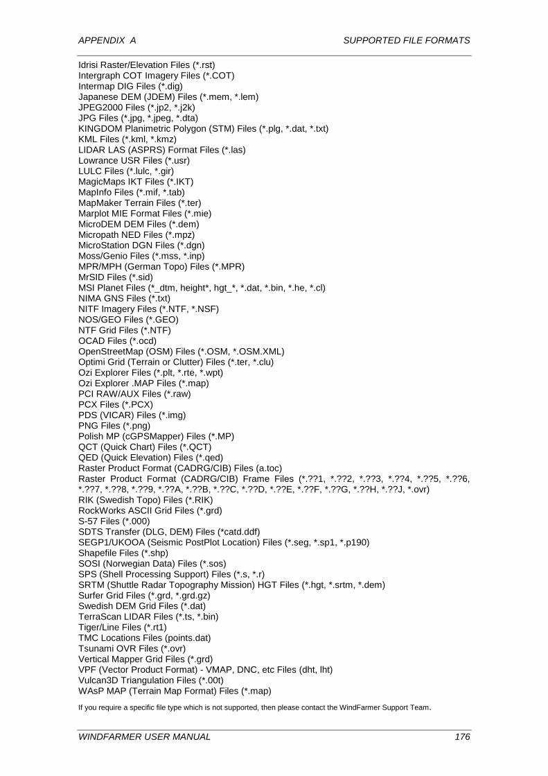
APPENDIX A SUPPORTED FILE FORMATS
Idrisi Raster/Elevation Files (*.rst) Intergraph COT Imagery Files (*.COT) Intermap DIG Files (*.dig) Japanese DEM (JDEM) Files (*.mem, *.lem) JPEG2000 Files (*.jp2, *.j2k) JPG Files (*.jpg, *.jpeg, *.dta) KINGDOM Planimetric Polygon (STM) Files (*.plg, *.dat, *.txt) KML Files (*.kml, *.kmz) LIDAR LAS (ASPRS) Format Files (*.las) Lowrance USR Files (*.usr) LULC Files (*.lulc, *.gir) MagicMaps IKT Files (*.IKT) MapInfo Files (*.mif, *.tab) MapMaker Terrain Files (*.ter) Marplot MIE Format Files (*.mie) MicroDEM DEM Files (*.dem) Micropath NED Files (*.mpz) MicroStation DGN Files (*.dgn) Moss/Genio Files (*.mss, *.inp) MPR/MPH (German Topo) Files (*.MPR) MrSID Files (*.sid) MSI Planet Files (*_dtm, height*, hgt_*, *.dat, *.bin, *.he, *.cl) NIMA GNS Files (*.txt) NITF Imagery Files (*.NTF, *.NSF) NOS/GEO Files (*.GEO) NTF Grid Files (*.NTF) OCAD Files (*.ocd) OpenStreetMap (OSM) Files (*.OSM, *.OSM.XML) Optimi Grid (Terrain or Clutter) Files (*.ter, *.clu) Ozi Explorer Files (*.plt, *.rte, *.wpt) Ozi Explorer .MAP Files (*.map) PCI RAW/AUX Files (*.raw) PCX Files (*.PCX) PDS (VICAR) Files (*.img) PNG Files (*.png) Polish MP (cGPSMapper) Files (*.MP) QCT (Quick Chart) Files (*.QCT) QED (Quick Elevation) Files (*.qed) Raster Product Format (CADRG/CIB) Files (a.toc) Raster Product Format (CADRG/CIB) Frame Files (*.??1, *.??2, *.??3, *.??4, *.??5, *.??6, *.??7, *.??8, *.??9, *.??A, *.??B, *.??C, *.??D, *.??E, *.??F, *.??G, *.??H, *.??J, *.ovr) RIK (Swedish Topo) Files (*.RIK) RockWorks ASCII Grid Files (*.grd) S-57 Files (*.000) SDTS Transfer (DLG, DEM) Files (*catd.ddf) SEGP1/UKOOA (Seismic PostPlot Location) Files (*.seg, *.sp1, *.p190) Shapefile Files (*.shp) SOSI (Norwegian Data) Files (*.sos) SPS (Shell Processing Support) Files (*.s, *.r) SRTM (Shuttle Radar Topography Mission) HGT Files (*.hgt, *.srtm, *.dem) Surfer Grid Files (*.grd, *.grd.gz) Swedish DEM Grid Files (*.dat) TerraScan LIDAR Files (*.ts, *.bin) Tiger/Line Files (*.rt1) TMC Locations Files (points.dat) Tsunami OVR Files (*.ovr) Vertical Mapper Grid Files (*.grd) VPF (Vector Product Format) - VMAP, DNC, etc Files (dht, lht) Vulcan3D Triangulation Files (*.00t) WAsP MAP (Terrain Map Format) Files (*.map)
If you require a specific file type which is not supported, then please contact the WindFarmer Support Team.
WINDFARMER USER MANUAL 176
APPENDIX B PHOTOMONTAGE GUIDELINES
B PHOTOMONTAGE GUIDELINES The task of creating photomontages of wind farms can be structured in three steps:
1. Virtual representations of the wind farm 2. Taking the actual photographs of site specific views 3. Producing photomontages for specific views
All information needed to produce a photomontage should be recorded in the lists of material and forms for viewpoint description and photographic information.
B.1 Virtual Representation Setting up a virtual wind farm model before taking any photographs allows the user to identify places where a photomontage may be required. It also allows the identification of information that needs to be confirmed during a site visit. The virtual wind farm model is used later to carry out the photomontage. The tasks required to generate a virtual wind farm model are described below:
1. Design virtual turbines in the Turbine Studio. 2. Load the digital terrain model and the wind turbine co-ordinates. 3. Locate the viewpoints on the large-scale map. 4. Locate reference points.
Create a rendered landscape visualisation (Render Wireframe)
Design Virtual Turbines
Wind turbines are designed in the Turbine Studio based on the physical dimensions of the wind turbines.
Terrain Data and Wind Farm Layout
Load the digital terrain model and design wind farm layout. Locate the required viewpoints on a large-scale map and input them in the WindFarmer model.
Locate Reference Points
Reference points on the map that are reproduced in the virtual view can be used to define a define the geometric relationship between the virtual view and the observer. To define this relationship a minimum of three (non-aligned) reference points is needed.
These reference points are marked in the virtual view by photo marker mode . Place the markers on the identified reference points, visualise and assess the viability of this specific view. Revise viewpoint if necessary. Reference points should, for an exact reproduction of the geometric configuration, cover both nearby objects such as houses, trees and roads, and objects close to the horizon which could for example be terrain features, church spires or other tall objects.
Create Virtual Images
The creation of a virtual image of the wind farm and its surroundings in a rendered landscape visualisation is described in the Visualisation Section. The rendered landscape visualisation is used here to get a first impression of the landscape and the visibility of the turbines in a photomontage.
WINDFARMER USER MANUAL 177

APPENDIX B PHOTOMONTAGE GUIDELINES
B.2 Taking Photographs Selecting the Viewpoints
The locations of viewpoints have to be clearly identified on a large-scale map, typically 1:25000 of the area and confirmed by GPS readings. The pre-selected viewpoint may not be suitable for a photograph because of unforeseen obstructions such as vegetation and buildings. In such circumstances the viewpoint should be moved to a more suitable location. To identify the exact orientation of the photograph, at least three key reference points need to be visible on each photograph that has been taken from a viewpoint.
Locating the Target Area
If the target area or the reference points are not obvious from the viewpoint they can be approximately located by using a compass bearing from the viewpoint.
Locating Reference Points
Reference points identified earlier on the map may have been moved, may no longer exist, or vegetation or new developments, built after the map was drawn, may obstruct the view. Once a suitable viewpoint has been identified the locations of the visible reference points need to be verified and compared to their location on the large-scale map. A GPS reading at key reference points is helpful.
Photographs
It is recommended that photographs are taken using a lens with a focal length of 50 mm. A focal length of around 50 mm gives the closest approximation to what the eye sees, but over a much smaller field of view. A tripod should be used and adjusted using a spirit level and care taken that the film is aligned horizontally. The height above ground at which the photograph is taken should be noted. A photograph should be taken with the proposed development in its centre. Where appropriate, panoramas created by joining a series of photographs or using a special camera may be very useful to set a development in the context of the surrounding landscape. All photographs for a viewpoint should be taken in similar light conditions. Time, date and bearing should be recorded with each photograph.
B.3 How to create a Photomontage Preparation of Photographs
The photographs have to undergo some processing before they are used for a photomontage. This is best done with a general purpose photo-editing program:
1. Scan photograph(s) at high resolution. The best results are achieved using a high resolution. The resolution will depend on:
• Resolution of the scanner • Graphic card and computer memory • Resolution of the output device
2. Load photographs in the general purpose graphic program. 3. If necessary, combine scanned photographs for each viewpoint taking care to smooth
transitions. 4. Save digital high resolution image of photograph.
The saved high-resolution image, which is later combined with the virtual image of the turbines, defines the quality of the photomontage that is produced.
WINDFARMER USER MANUAL 178

APPENDIX B PHOTOMONTAGE GUIDELINES
Matching Virtual Reality with Photograph
Identify the reference objects on the photograph and mark these (e.g. using a black arrow) on a copy of the high-resolution digital image. To speed up the process it is recommended, that the file size be reduced, by converting the image to a greyscale or black and white representation of the same dimensions. The high-resolution full colour image will be used for the final photomontage that is produced. The markings of the reference objects should still be visible after the conversion. This black and white image is now used to match virtual reality and photograph.
1. Open a Visualisation window in WindFarmer and set it to the specific viewpoint. 2. Disable auto-height, level view and target lock. 3. Set as far as possible the camera properties: target location, viewpoint location and focal
length to match those used to take the photograph. 4. Set aspect ratio of film to aspect ratio of photograph.
5. Load the black and white image using the photomontage option in a wireframe mode.
6. Match up virtual reality photo markers of the reference points with the markings on the digital image by adjusting the following values in the viewpoint properties box: Film size (the aspect ratio is given by the dimensions of your image), Target location (the centre of your image), viewpoint location. You can also tilt the virtual wind farm representation to adjust for non-horizontally aligned photos using the Page Up and Page Down keys.
Once the match between virtual reality and photograph image has been achieved switch to smooth shading mode and replace the black and white image with the digital high-resolution full colour photograph.
Fine Tuning
WindFarmer allows adjustment of the light conditions impacting on the virtual turbines to match the light conditions on the photograph. The effects of fog and clouds can also be included. After making any fine tuning adjustment the user considers appropriate the raw photomontage can be exported to a general-purpose graphic package where further adjustments can be made to account for vegetation that is hiding any turbines. Additional auxiliary buildings such as transformer stations can be included in the image at this stage.
Documentation of Results
The documentation accompanying the photomontage should include the following information:
• Grid co-ordinates for the location of turbines • Grid co-ordinates for the location of the viewpoint • Focal length of the lens used • Date and time of the photograph • Date of the photomontage • Author of the photomontage
It is often useful to provide guidance on the distance the photomontage should be viewed. The distance will be a function of the lens used to take the photograph. With a wide angle lens the photomontage will need to be viewed close up to obtain a realistic impression.
WINDFARMER USER MANUAL 179

APPENDIX B PHOTOMONTAGE GUIDELINES
B.4 Material Requirements Virtual Representation
1. WindFarmer software (Base and Visualisation Modules) 2. Detailed large-scale map (e.g. 1:25,000) 3. Digital terrain model (typical grid resolution 50m) 4. Co-ordinates for the wind farm layout 5. Turbine dimensions
• Tower height and width at top and base • Nacelle shape/height/width/length • Rotor diameter and number of blades • Blade chord at widest and narrowest section • Nose cone diameter • Diameter of ring-generator, if applicable
6. Viewpoint description form
Taking Photographs
1. Camera with a 50mm lens 2. Tripod 3. Spirit level 4. Detailed large scale map (e.g. 1:25000) 5. Compass 6. GPS 7. Viewpoint description form
Photomontage
1. Virtual representation 2. Viewpoint description form 3. Prints of photographs 4. General purpose graphic package 5. Colour scanner 6. Colour printer
WINDFARMER USER MANUAL 180
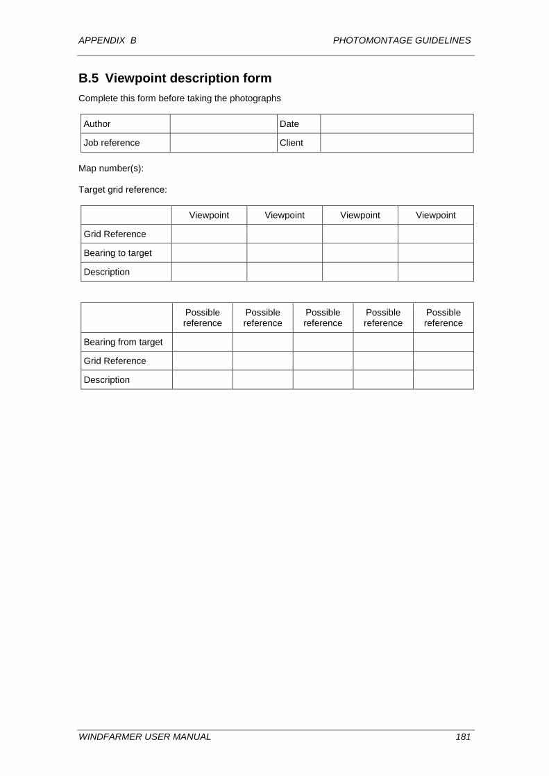
APPENDIX B PHOTOMONTAGE GUIDELINES
B.5 Viewpoint description form Complete this form before taking the photographs Author Date
Job reference Client Map number(s): Target grid reference:
Viewpoint Viewpoint Viewpoint Viewpoint
Grid Reference
Bearing to target
Description
Possible reference
Possible reference
Possible reference
Possible reference
Possible reference
Bearing from target
Grid Reference
Description
WINDFARMER USER MANUAL 181

APPENDIX B PHOTOMONTAGE GUIDELINES
B.6 Photographic Information
Camera make and model:
Focal length of lens: 50mm
Film make and type:
Film size: 35mm
Film ASA:
Details for panorama no: Camera location description:
Map no:
Grid reference:
Marked?
Ground elevation:
Height above ground level of camera:
Film reference no:
Centre frame no:
Left of centre frame no:
Right of centre frame no:
Lens F-stop:
Shutter speed:
Reference point: 1 2 3 4
Bearing:
X(Map)
Y(MAP)
X(GPS)
X(GPS)
Description Time of photos:
Cloud:
Light: Visited by:
WINDFARMER USER MANUAL 182
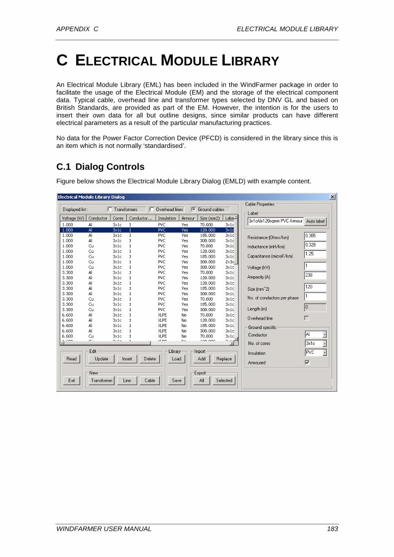
APPENDIX C ELECTRICAL MODULE LIBRARY
C ELECTRICAL MODULE LIBRARY An Electrical Module Library (EML) has been included in the WindFarmer package in order to facilitate the usage of the Electrical Module (EM) and the storage of the electrical component data. Typical cable, overhead line and transformer types selected by DNV GL and based on British Standards, are provided as part of the EM. However, the intention is for the users to insert their own data for all but outline designs, since similar products can have different electrical parameters as a result of the particular manufacturing practices. No data for the Power Factor Correction Device (PFCD) is considered in the library since this is an item which is not normally ‘standardised’.
C.1 Dialog Controls Figure below shows the Electrical Module Library Dialog (EMLD) with example content.
WINDFARMER USER MANUAL 183
APPENDIX C ELECTRICAL MODULE LIBRARY
C.2 Launching Press the ‘Library’ button within the ‘Electrical Module Properties of Turbines & Cables Dialog’ (EMPTCD). If the currently selected component in the EM Tree of the EMPTCD is a Transformer or Cable then when the ‘Library’ button is pressed the properties of the selected component are copied to the EMLD, to allow the addition of the selected component to the library. Under these circumstances when the EMLD is opened the Properties of the passed component are displayed on the right, and the library list corresponding to the passed components type is also displayed. In the example, a ground cable component was selected in the EMPTCD prior to pressing its ‘Library’ button so when the EMLD was opened the displayed properties on the right are those of the passed ground cable, and the displayed library list on the left is that of the ground cables.
C.2.1 Cable Properties/ Transformer Properties (right) The properties of the component currently selected for viewing/editing are displayed on the right of the dialog. In the above figure example the Cable Properties are shown for a ground cable (the Overhead line control in the Cable Properties is not ticked).
C.2.2 Displayed list (top left) Select the library list displayed via these radio buttons. Displayed list control (centre left) The list selected via the ‘Displayed list’ radio buttons is shown below the buttons. The contents of the list are sorted by column with the most significant column being to the leftmost. The list can be sorted by specific columns by mouse right clicking the relevant column header. When a component in the displayed list is selected then the full properties of that component are shown on the right of the dialog. When a list component is selected you can use the up/down arrow keys to navigate through the list, displaying the contents of each component on the left as encountered. The lists remember their selected rows when switched between via the list radio buttons.
C.2.3 Edit (lower left) The buttons in this section allow you to edit the contents of the displayed list.
• The ‘Update’ button updates the contents of the selected component in the displayed list with the current properties on the right of the dialog.
• The ‘Insert’ button inserts a new component in the displayed list that has the properties shown on the right of the dialog.
• The ‘Delete’ button deletes the selected component in the displayed list.
C.2.4 New (bottom left) The buttons in this section displays the properties of a new component of the selected type in the properties section on the right of the dialog.
WINDFARMER USER MANUAL 184
APPENDIX C ELECTRICAL MODULE LIBRARY
C.2.5 Library (bottom centre) • The buttons in this section allow you to load and save the entire library. • The ‘Load’ button loads the library of the Workbook from an Electrical Module Library
(extension ‘.elb’) file, replacing the current library contents. • The ‘Save’ button saves the library of the Workbook to an Electrical Module Library
(extension ‘.elb’) file.
C.2.6 Export (bottom centre) The buttons in this section allow you to export library components to a text file.
• The ‘All’ button exports the entire contents of the displayed list control. Thus, for example, to export all transformers to a text file, select (if not already selected) the transformers list via the Transformers radio button at the top left, and the press the ‘All’ button. This will result in a dialogue opening that allows you to select the name and location of the exported text file.
• The ‘Selected’ button allows you to export the component who’s properties are displayed on the right of the dialog. In the above figure the component on row 3 of the ‘ground cables’ list has been selected, with the corresponding properties of this component displayed on the right. These properties could be exported via the ‘Selected’ button. Pressing the ‘Select’ button will result in a dialogue opening that allows you to select the name and location of the exported text file.
Transformers text files begin with a line that only contains the word ’Transformers’. Overhead lines text files begin with a line that only contains the word ’Lines’. Ground cables text files begin with a line that only contains the word ’Cables’.
C.2.7 Import (lower centre) The buttons in this section allow you to import library components from a text file. The format of the text files has to mach that generated when exporting from this dialogue to a text file.
C.2.8 Read/Exit (bottom far left) • The ‘Read’ button closes the dialogue and passes the currently selected
components properties back to the EMPTCD. It is only enabled if the currently selected object is of the type (transformer or line/cable) that was selected in the EMPTCD when the Library dialogue was opened.
• The ‘Exit’ button closes the dialog.
WINDFARMER USER MANUAL 185
APPENDIX D MENU STRUCTURE
D MENU STRUCTURE The user interface of WindFarmer provides two options to access most of the control elements: via the toolbars or via the menu structure. With very few exceptions all functions are available from both. The menu structure is context sensitive and changes for each window.
D.1 General Structure Elements in the menu structure that are specific to a particular window are discussed in the section for the particular window. All WindFarmer menus have the following common elements: File Menu View Menu Window Menu Help Menu
D.1.1 File Menu The File Menu always contains the following items:
New
Creates a new workbook.
Open Workbook
Use this command to open an existing workbook in a new window. You can open multiple workbooks at once. Use the Window Menu to switch among the multiple open documents. You can create new documents with the New command.
Close
Closes an opened workbook. Use this command to close all windows containing the active document. WindFarmer suggests that you save changes to your document before you close it. If you close a document without saving, you lose all changes made since the last time you saved it. Before closing an untitled document, WindFarmer displays the Save As dialogue box and suggests that you name and save the document. You can also close a document by using the Close toolbar button on the document's window.
Save Workbook
Saves an opened workbook using the same file name. Use this command to save the active document to its current name and directory. When you save a document for the first time, WindFarmer displays the Save As dialogue box so you can name your document. If you want to change the name and directory of an existing document before you save it, choose the Save As command.
Save Workbook As
Saves an opened workbook to a specified file name. Use this command to save and name the active document. WindFarmer displays the Save As dialogue box so you can name your document. To save a document with its existing name and directory, use the Save Command.
Use this command to print a document. This command presents a Print dialogue box, where you may specify the range of pages to be printed, the number of copies, the destination printer, and other printer setup options. The Mapping Window can be printed to any scale under Print in the File menu (the Mapping Window must be active). The scale and text accompanying the print out is determined in the Control Panel .
WINDFARMER USER MANUAL 186
APPENDIX D MENU STRUCTURE
Print Preview
Displays the document on the screen, as it would appear printed and opens the print preview toolbar. The print preview toolbar offers you the following options:
Print: Bring up the print dialogue box, to start a print job. Next/Prev Page: Preview the next/previous printed page. One Page / Two Page: Preview one or two printed pages at a time. Zoom In/Out: Take a closer/larger look at the printed page. Close: Return from print preview to the editing window.
Page Setup
Selects a printer and printer connection.
Exit
Use this command to end your WindFarmer session. WindFarmer prompts you to save documents with unsaved changes
D.1.2 View Menu The View menu always offers the following commands: Tool Bars: Shows or hides a toolbar.
Main
Use this command to display and hide the Main Toolbar, which includes buttons for some of the most common commands in WindFarmer, such as File Open. A check mark appears next to the menu item when the Toolbar is displayed.
Mapping
Use this command to display and hide the Mapping Toolbar, which includes buttons for some of the most common commands in WindFarmer. A check mark appears next to the menu item when the Toolbar is displayed.
Visualisation
Use this command to display and hide the Visualisation Toolbar, which includes buttons for some of the most common commands in WindFarmer. A check mark appears next to the menu item when the Toolbar is displayed.
Graphing
Use this command to display and hide the Graphing Toolbar, which includes buttons for some of the most common commands in WindFarmer. A check mark appears next to the menu item when the Toolbar is displayed.
Finance
Use this command to display and hide the Finance Toolbar, which includes buttons for some of the most common commands in WindFarmer. A check mark appears next to the menu item when the Toolbar is displayed.
MCP+
Use this command to display and hide the MCP+ Toolbar, which includes buttons for some of the most common commands in WindFarmer. A check mark appears next to the menu when the Toolbar is displayed.
Status Bar
Use this command to display and hide the Status Bar, which describes the action to be executed by the selected menu item or depressed toolbar button, and keyboard latch state. A check mark appears next to the menu item when the Status Bar is displayed.
WINDFARMER USER MANUAL 187
APPENDIX D MENU STRUCTURE
Control Bar
This command shows or hides the Control Bar.
Display Bar
This command shows or hides the Display Bar. The display bar is initially docked at the left of the WindFarmer window and contains several check boxes that determine what information will be displayed next time the mapping window is updated.
D.1.3 Window Menu The Window Menu always offers the following commands,
New Visualisation Window
The Visualisation Window displays a 3-D representation of the terrain and turbines from a specific viewpoint in the Mapping window for visual impact assessment. The window title display the viewpoint number and the viewpoint, rendered landscape and photomontage are automated to allow easy, fast visualisation. Camera type, terrain, turbines and sky appearance are fully customisable by the user. The visualisations may be saved to image files or printed directly.
New Graphing Window
The Graphing Window allows various site data to be plotted automatically: Site yield, turbine statistics, wind rose, noise etc. The user can define the graph’s appearance. The graphs may be printed, saved to image files or pasted into the Finance window or other clipboard aware applications. Multiple graph windows may be opened.
Finance
The Finance Window allows costing and financial modelling of the wind farm site in a standard spreadsheet view. Site costs may be inserted and are updated automatically by WindFarmer allowing dynamic updating of costs as the optimisation and design process takes place. Full Microsoft Excel file loading and saving is supported. Only one Finance window may be opened.
Mapping
The Mapping Window is the basis of each workbook and only one Mapping window per workbook can be opened. WindFarmer does allow multiple workbooks to be opened and each Visualisation, Graphing or Finance window will have the appropriate window titles appended to allow identification of the workbook they relate to. The Mapping window is where site set-up, design and optimisation are performed. The other window types available basically display information relating to the site.
MCP Window
The MCP+ Module contains the tools needed to take raw time series of wind speed and direction data through data assembly, cleaning, calibration and correlation to produce the wind regime at your site in the form of a wind speed and direction frequency distribution.
Cascade
Arranges windows in an overlapped fashion.
Tile Vertically
Arranges windows in non-overlapped tiles.
Tile Horizontally
Arranges windows in non-overlapped tiles.
Arrange Icons
Use this command to arrange the icons for minimised windows at the bottom of the main window. If there is an open document window at the bottom of the main window, then some or all of the icons may not be visible because they will be underneath this document window..
WINDFARMER USER MANUAL 188

APPENDIX D MENU STRUCTURE
Minimise All Windows
Minimise all windows belonging to the current workbook.
Window 1, 2, ...
WindFarmer displays a list of currently open document windows at the bottom of the Window menu. A check mark appears in front of the document name of the active window. Choose a document from this list to make its window active.
D.1.4 Help Menu The Help Menu always offers you the following commands, which provide you assistance with this application:
Help Topics
Use this command to display the opening screen of Help. From the opening screen, you can jump to step-by-step instructions for using WindFarmer and various types of reference information. Once you open Help, you can click the Contents button whenever you want to return to the opening screen.
System Properties
This dialogue displays information about the current state of the system.
About WindFarmer
Displays the version number of this application.
D.2 Menus in the Mapping Window The menu is structured in levels. The user can access at the first level the following items: File Menu Modes Menu Add Menu Calculate Menu Map Menu MCP+ Menu View Menu Window Menu Help Menu Each of these items has a number of next level items.
D.2.1 File Menu in the Mapping Window The File menu of the Mapping Window offers the following specific commands beyond those listed for the general structure:
Workbook Wizard
Launches the Workbook Wizard. The wizard will take you through the steps involved in setting up a WindFarmer Workbook
Load File
This command activates the Load File dialogue to allow users to load data files into the current workbook.
Load MCP+ Data
Loads time series into the Data Loader for analysis in the MCP+ Module.
WINDFARMER USER MANUAL 189
APPENDIX D MENU STRUCTURE
Load Online Data
Opens a dialogue box with links to various online sources of mapping data, with options for specifying the location and extents of the data.
Launch Turbine Importer
Opens the Turbine Import Assistant in MS Excel (Excel 2007 or higher is required to use this tool). Allows the user to generate a .wot or .wob file for easy import of boundary and turbine data.
Save Current Project As
Saves the current project as a binary file, which can then be loaded into another workbook.
Generate Report
This command opens the Report Generator dialogue to specify report contents. The Report Generator dialogue allows the user to save WindFarmer results as a file. The file formats currently supported are Excel and Word.
MCP+ Report
Creates reports on Loaded Data and Project Information for the MCP+ Module.
Export
Displays the export dialogue. A detailed Flow and Performance Matrix, Data, Views, Iso Lines and Data grids can be exported.
Launch Shadow Reporter
Opens the Shadow Flicker Plot & Summary Tool in MS Excel (Excel 2007 or higher is required to use this tool). Allows the user to input the .xls or .txt shadow flicker file created in WindFarmer to create shadow flicker analyses as plots for each receptor, or summary reports showing where the shadow flicker limits have been exceeded.
1, 2, 3…
Use the numbers and filenames listed at the bottom of the File menu to open the last six documents you closed. Choose the number that corresponds with the document you want to open.
D.2.2 Modes Menu in the Mapping Window The Modes menu offers the following commands: Turbine: Place and edit turbines Dwelling: Place and edit dwellings Boundary: Place and edit boundary points. Viewpoint: Place and edit viewpoints. Shadow Receptor: Place and edit shadow receptors. Cabling: Place and edit cable nodes. Road: Place and edit road nodes. Anemometer Mast: Place and edit anemometry masts. Radar Stations Place and edit radar stations. Text Labels: Place and edit text labels. Photomontage Marker: Place and edit photomontage markers Zoom Zoom in (left mouse button) or out (right mouse button). Working: Default mode in which the properties of objects can be viewed and edited. Stop/Go: Toggles the optimiser on and off. Test: Tests the legality of the layout and updates the site yield. Crop: Deletes surrounding image Terrain line edit: Create and edit terrain contours
WINDFARMER USER MANUAL 190
APPENDIX D MENU STRUCTURE
D.2.3 Add Menu in the Mapping Window The Add Menu offers the following commands:
Grid Markers
This command activates the Grid Markers dialog. This dialogue allows the user to enter the left, top, right and bottom co-ordinates of a rectangle whose corners are marked with grid markers. Grid markers are small black crosses that can be used to position a transparent printout over a printed map.
New Boundary
This command adds a new boundary object to the current workbook. A boundary is a group object consisting of several boundary nodes. At least three boundary nodes must be inserted when a boundary object is created. This is done by three right mouse button clicks on the map at the desired locations.
Cable
This command adds a cable object to the current workbook. A cable is a group object consisting of several cable nodes. At least one cable node must be inserted when a cable object is created. This is done by a right mouse button click on the map at the desired location
Road
This command adds a new road object to the current workbook. A road is a group object consisting of several road nodes. At least one road node must be inserted when a road object is created. This is done by a right mouse button click on the map at the desired location.
D.2.4 Calculate Menu in the Mapping Window The Calculate Menu offers the following commands:
Calculate ZVI
Recalculates zones of visual influence map. To produce a ZVI map in WindFarmer, it is necessary to have the following items loaded: A digital terrain model (*.DTM) file loaded for the area under consideration; In the case of a Turbines ZVI, a turbine (*.TRB) file loaded ,which defines the dimensions of the wind turbine, and Turbines must be placed within a wind farm boundary(see Turbine Studio for how to change hub height and blade length); In the case of a Radars Stations ZVI, there must be Radar Stations placed on the map.
Calculate Noise
Recalculates the noise contours based on the present turbine positions and noise characteristics (see Turbine Studio and Control Panel).
Calculate Shadow Map
Recalculates shadow map based on the digital terrain model, the present turbine positions, hub heights and blade lengths (see Turbine Studio for how to change hub height and blade length).
Energy/Test
Tests the legality of the layout and Re-calculates the site yield.
Update Wind Flow Simulation
Calculates wind resources with the selected flow model for all wind resource templates for which data have not yet been calculated.
D.2.5 Map Menu in the Mapping Window The Map Menu offers the following commands:
MAP2DTM
Converts existing map into a DTM.
WINDFARMER USER MANUAL 191
APPENDIX D MENU STRUCTURE
WRG2DTM
Converts existing WRG into a DTM.
DTM2MAP
Converts existing DTM into MAP contours.
View Projection
To display the current global projection of the workbook
Change Projection
To change the current global projection of the workbook
D.2.6 View Menu in the Mapping Window The View menu offers the following specific commands beyond those listed for the general structure:
Turbine Studio
This command activates the Turbine Studio property sheet.
Wind Studio
This command opens the Wind Studio.
WF Control Panel
This command activates the Control Panel dialogue sheet.
Workspace Extents
This command activates the Workspace Extents dialog. Allows the user to view and change the extents of the mapping view. This is useful in limiting the extent of ZVI Shadow flicker or noise calculations
Project Properties
Displays the Project Property
Project Manager
Displays the Project Manager dialog
Layer Manager
Displays the Layer Manager dialog
Options…
Choose if you are prompted to set mast turbulence after loading a single point WRG file.
D.2.7 Window Menu in the Mapping Window The Window Menu of the Mapping View offers no specific commands beyond those listed under general structure.
D.2.8 Help Menu in the Mapping Window The Help Menu of the Mapping View offers no specific commands beyond those listed under general structure.
WINDFARMER USER MANUAL 192

APPENDIX D MENU STRUCTURE
D.3 Menus in the Graphing Window The following menus are available: File Menu View Menu Window Menu Help Menu
D.3.1 File Menu in the Graphing Window The File menu offers the following commands:
Load Template
Load a graph template into the current graph window. The graph template should be the same type as the one being displayed. Everything but the data will be updated with the new graph properties. New graphs will take on the appearance, but not type, of the graph template.
Export Template
Export current graph properties, but no data, to a graph template file.
Export Image
Saves an image file of a graph.
Export Image to Clipboard
Save a Graph Window to the clipboard as a windows metafile. From there it can be pasted into a spreadsheet cell in the Finance Window or into other clipboard aware applications.
D.3.2 View Menu in the Graphing Window The View menu offers the following specific commands beyond those listed for the general structure:
Wind rose
This dialogue allows the user to choose the anemometry mast on which the wind rose will be based. The data required to draw the wind rose is taken from a wind resource grid (WRG file) by taking the sector Weibull coefficients P, A and k at the anemometer’s position and reconstructing numbers of occurrences.
Progress Chart
Draw a chart showing the optimiser’s progress
Turbines
Draw a chart showing turbine statistics.
Dwellings
Draw a chart showing noise levels at dwellings.
Wind Speed
Draw a chart showing turbine statistics by wind speed.
Sectors
Draw a chart showing turbine statistics by sector.
Shadow plot
Draw a chart showing the periods with shadow flicker at shadow receptors.
Graph Properties
Manipulate the properties of the current chart.
WINDFARMER USER MANUAL 193
APPENDIX D MENU STRUCTURE
D.3.3 Window Menu in the Graphing Window The Window Menu of the Graphing Window does offer no specific commands beyond those listed under general structure.
D.3.4 Help Menu in the Graphing Window The Help Menu of the Graphing Window does offer no specific commands beyond those listed under general structure.
D.4 Menus in the Visualisation Window (Visualisation Module required) The Visualisation Menu has the following headings: File Render Settings View Window Help This menu allows access to the same functions as the Visualisation Toolbar, and replaces the normal Mapping Menu when the Visualisation Window is active.
D.4.1 File Menu in the Visualisation Window The File menu offers the following specific commands beyond those listed under general structure:
Generate Report
Opens the Report Generator dialogue to specify report contents.
Export
Visualisations can be exported as BMP and EMF files. Specify filename, colour depth and resolution.
D.4.2 Render Menu in the Visualisation Window The Render mode menu offers the following commands:
Transparent
Renders wireframe outline of object. Hidden lines are not removed from the view. Turbine positions can be seen through the terrain.
Wireframe
Renders wireframe outline of objects and fills solid objects with a colour. Hidden lines and surfaces are removed.
Constant
Renders the surfaces of objects and shades each polygon a constant colour. Hidden lines and surfaces are removed. Lighting must be enabled for shading.
Gouraud
Renders the surfaces of objects and shades across each polygon interpolating between the colours at the vertices of each polygon. Hidden lines and surfaces are removed. Lighting must be enabled for shading.
WINDFARMER USER MANUAL 194

APPENDIX D MENU STRUCTURE
Photomontage
Renders only the visible portion of turbines onto a selected background bitmap (scanned photograph) which should correspond to the current view. Use Fit to Film to correct the window aspect ratio after sizing the window.
Refresh
Manually executes all changes to view settings. Window redraws.
AutoRefresh
If Auto Refresh is on all changes to render settings are executed immediately and the window will redraw immediately. If Auto Refresh is off settings can be changed and then all updated once by clicking the left mouse button in the window.
AVI
Creates fly-throughs, 360 degree pans and animated visualisations or photomontages that can be exported as *.AVI files.
D.4.3 Settings Menu in the Visualisation Window The Visualisation Settings menu offers the following commands:
Camera
Specify viewpoint, target, camera attributes and optimisation with respect to visual influence parameters.
Roll…
Rotate the virtual image around the target.
Turbine Settings
Select: Texture on/off. Show Selected to highlight selected turbine in the visualisation window. Animate to animate the rotors. Set turbine option Random Rotors on to randomly set turbine rotor positions Yaw Turbines to turn the turbines to face the desired direction. Terrain Settings – The Terrain Settings allow to modify: Select Terrain texturing on/off. Select bitmap to drape over terrain for this viewpoint only. Applies only to current window. Normal: Terrain surface is created from triangle polygons at DTM resolution. Smooth: Terrain surface is created from non-uniform rational b-spline surface patches with an interpolated point between each DTM node Texture Scale: Changes the texture scaling co-ordinates on a logarithmic scale.
Sky Settings
Select Texture on/off for sky.
Colours and Textures
This command activates the Colours and Textures property sheet. For terrain, turbines and sky: select colours for all render modes. Select bitmaps for texturing.
Sunlight
Specify lighting and fogging parameters for shaded renderings.
WINDFARMER USER MANUAL 195

APPENDIX D MENU STRUCTURE
D.4.4 View Menu in the Visualisation Window The View menu offers the following specific commands beyond those listed for the general structure:
Fit to Film
Fit to Film resizes the window aspect ratio to equal the film aspect ratio specified in the Camera Properties dialogue box. This enables the view within the window to match the viewed area in a photograph. This command should be used to correct disjointed Panorama views if the user manually resizes them. When in Photomontage mode this command should be used after sizing the window to correctly place the turbines with reference to the background bitmap. The background bitmap will then only be scaled and not stretched.
Next
Display next viewpoint
Previous
Display previous viewpoint.
D.4.5 Window Menu in the Visualisation Window The Window menu of the Visualisation Window is identical to that of the Mapping Window.
D.4.6 Help Menu in the Visualisation Window The Help Menu of the Visualisation Window offers the following specific commands beyond those listed for the general menu structure, which provide you assistance with this application: About OpenGL Displays OpenGL implementation information.
D.5 Menus in the Finance Window (requires Finance Module) The Finance Window Menu has the following headings: File Edit Insert Format View Window Help This menu allows access to the same functions as the Finance Toolbar, and also additional formatting options which allow the user to control the appearance of the spreadsheet.
D.5.1 File Menu in the Finance Window The File menu offers the following specific commands beyond those listed under general structure:
Load Spreadsheet
Open a Microsoft Excel compatible file in the Finance window.
Export Spreadsheet
The financial model can be exported as a Microsoft Excel compatible Spreadsheet or as a text file under the File Menu.
Set Print Area
Allows the selection of an area of the spreadsheet with the mouse. This is the area that will be printed when Print is selected.
WINDFARMER USER MANUAL 196
APPENDIX D MENU STRUCTURE
D.5.2 Edit Menu in the Finance Window The Edit menu offers the following commands:
Cut
Cut the selected cells.
Copy
Copy the selected cells.
Paste
Paste the selected cells.
Paste Values
Paste value of cell in the clipboard into selected cell.
Clear
Clear the selected cells.
Fill Down
Fill cells selected down with clipboard contents.
Fill Right
Fill cells selected right with clipboard contents.
Cells Add
Select how to insert rows/columns into worksheet.
Cells Remove
Select how to delete rows/columns from worksheet.
Sheet Add
Add a new sheet to the spreadsheet
Sheet Remove
Delete the current sheet from the spreadsheet. All information in the sheet will be lost.
Find/Replace
Opens the find and replace dialog.
D.5.3 Insert Menu in the Finance Window The Insert menu offers the following commands:
Number of Turbines
Insert number of turbines in selected cell.
Length of Track
Insert length of track in selected cell.
Number of Transformers
Insert number of transformers in selected cell
Length of Cable
Insert length of cable in selected cell.
WINDFARMER USER MANUAL 197

APPENDIX D MENU STRUCTURE
Annual Yield
Insert annual energy yield in selected cell
Maximise in Optimiser…
Select a target for financial optimisation
D.5.4 Format Menu in the Finance Window The Format menu offers the following commands:
Sheet
Opens format sheet dialog: Type name for the sheet.
Cell Width
Opens format column width dialog: Select width of columns in characters, centimetres or inches.
Cell Height
Opens format row height dialog: Select height of rows in characters, centimetres or inches
Cell Appearance
Opens cell appearance dialog: Set data format, alignment, font, border and background pattern options for all selected cells.
D.5.5 View Menu in the Finance Window The View menu offers the following commands:
Zoom
Change magnification of spreadsheet in Finance window
Edit Bar
Shows or hides the formula bar.
D.5.6 Window Menu in the Finance Window The Window Menu of the Finance Window does offer no specific commands beyond those listed under general structure.
D.5.7 Help Menu in the Finance Window The Help Menu of the Finance Window does offer no specific commands beyond those listed under general structure.
WINDFARMER USER MANUAL 198
APPENDIX D MENU STRUCTURE
D.6 MCP+ Menu (requires MCP+ Module)
Edit
Masts…
Edit mast description, latitude and longitude of mast location.
Sensors…
Edit signal type, minimum and maximum values, height and plot style of sensors.
Calibrations…
Edit scale and offset applied by the logger and/or to be applied.
Exclude data…
Data cleaning…
Opens the Data Cleaning window for viewing and cleaning data.
By value…
Clean data by applying filters.
Frequency distribution…
Opens the Frequency Distribution dialog. Create frequency distribution of wind speed and direction, wind rose or summary tables of turbulence intensity of a time series.
MCP…
Opens the Measure Correlate Predict dialog. Correlate time series and export long-term time series or frequency distributions.
WindRose from .tab file…
Opens the WindRose from .tab file dialog. Create a wind rose plot from an existing TAB file.
WINDFARMER USER MANUAL 199
APPENDIX E GRAPHING
E GRAPHING Titles Axis Fonts Markers Overlay Background Labels Labels Format
E.1 Titles (Graph Properties) In this box, you can enter text for the top, bottom, right and left graph titles, which can be up to 80 characters in length. The top title appears centred at the top of the graphing window. When you enter text for a title, the Graph control adjusts the rest of the graphing window to provide space, either redrawing the graph and associated objects at a smaller size or decreasing the space between objects. When you clear the text box for a title, you disable it and provide more space for the rest of the graph. If you enter a title that is too long to appear in a single line, the Graph control automatically word-wraps it. If a title doesn't display at all, it's because the Graph control can't make the font small enough to fit all the text in the space provided. Increase the size of the graphing window to make the title appear.
E.2 Axis (Graph Properties) • X Select this option to view and/or change the settings for the X-axis. • Y Primary Select this option to view and/or change the settings for the primary Y-
axis. • Y Overlay Select this option to view and/or change the settings for the axis of an
overlay graph with a separate Y axis. • Variable When X is selected in the Apply to Axis group, select this option to draw
the X axis intersecting the Y origin, whether that's at the top, bottom, or middle of the graph. When Y Primary is selected in the Apply to Axis group, select this option to draw the primary Y axis intersecting the X origin, whether that's at the left, right, or middle of the graph.
• Left or Top When X is selected in the Apply to Axis group, select this option to draw the X-axis at the top of the graph, regardless of the location of the Y origin. When Y Primary is selected in the Apply to Axis group, select this option to draw the primary Y-axis at the left edge of the graph, regardless of the location of the X origin.
• Right or Bottom When X is selected in the Apply to Axis group, select this option to draw the X-axis at the bottom of the graph, regardless of the location of the Y origin. When Y Primary is selected in the Apply to Axis group, select this option to draw the primary Y-axis at the right edge of the graph, regardless of the location of the X origin.
• Zero Origin Select this option to draw the axis including the origin (zero) and extending far enough in the positive and negative directions to include all of the graph's values.
• Variable Origin Select this option to have the axis "zoom in" on the range of the graph's actual values, whether or not that range includes zero. For X and Z-axes, this option differs from Auto only if you specify X or Z values for data points.
• User-Defined Select this option to set your own values for the minimum, maximum, and number of ticks for the axis. When you select User-Defined, the settings in the Range group are enabled.
• Max (enabled by selecting User-Defined in the Scale group) The Max setting is generally the maximum point of the axis, with the following exceptions: If you have a
WINDFARMER USER MANUAL 200
APPENDIX E GRAPHING
positive Max with a negative Min, the Graph control may adjust the maximum or minimum point so that it lies on a tick.
• Min (enabled by selecting User-Defined in the Scale group) The Min setting is generally the minimum point of the axis, with the following exceptions: If you have a positive Max with a negative Min, the Graph control may adjust the maximum or minimum point so that it lies on a tick.
• Colour of Axes In this list box, you can choose a colour for axes from the current colour palette. The same colour is applied to all axes. To choose a colour palette, go to the Background property page.
• Show Select this option to enable grid lines for the axes. Clear the box for no grid lines
• Line In this list box, you can choose a style for grid lines. The same style is applied to both X and Y grids.
• Colour In this list box, you can choose a colour for grids from the current palette. The same colour is applied to both X and Y grids. To choose a colour palette, go to the Background property page.
• Ticks (enabled by selecting User-Defined in the Scale group) The Ticks setting determines the number of ticks along the selected axis. (Note that the setting here does not determine whether tick marks are displayed--see the Tick Marks group.) The effect depends on the axis and the nature of your data:
• For Y axes and X axes with specific X values the Ticks setting specifies the number of ticks from the origin to the setting of either Max or Min, whichever has the higher magnitude (distance from 0). For example, if you set Min to -50 and Max to 20, Ticks applies to the axis segment between 0 and -50.
• To determine the Ticks value you want to set, divide the length of the axis (or axis segment) by the desired interval between ticks. For the axis segment 0 to -50 we've just described (whose length is 50 units), if you want to place ticks 25 units apart, set Ticks to 2.
• Both the maximum and minimum points of an axis must fall on a tick. If you have a negative Min with a positive Max, the Graph control may have to move the minimum or maximum point to make this happen. In our example axis, ticks would be placed at -50, -25, 0, and 25--overriding the Max setting of 20.
• Show Check this box to draw tick marks along the axis. Clear the box for no tick marks. If you have a Y Overlay axis, the Show setting for Y Primary also applies to Y Overlay. Either both axes have tick marks or both don't.
• Minor Specify the number of minor tick marks to be drawn between pairs of major ticks.
• Through Axes Select this option if you want tick marks centred on the axis line.
• Inside Axes Select this option if you want tick marks to be drawn only on the graph side of the axes.
• Outside Axes Select this option if you want tick marks drawn outside the axes. Note: Your selection will apply to all axes for which tick marks have been enabled.
• Every If you select Zero Origin or Variable Origin in the Scale group, you can use the Every setting to specify the frequency with which tick marks are displayed along the X axis. An Every setting of 1 places a mark at each tick, a setting of 2 places a mark at every other tick, and so on. The X axis must end with a tick mark. If you set an Every value that doesn't include the last value on the axis, the Graph control will extend the axis so that it ends on a tick mark.
• Show Select this option to draw grid lines perpendicular to the axis, intersecting each tick mark. Clear the box for no grid lines.
WINDFARMER USER MANUAL 201
APPENDIX E GRAPHING
E.3 Fonts (Graph Properties) • Other Titles Select this option to apply font settings to the graph's left, right, and
bottom titles. The same settings apply to all three of these titles. • Graph Title Select this option to apply font settings to the graph's title, which
always appears centred at the top of the graphing window. • Labels Select this option to apply font settings to the graph's labels--including axis
labels (for graphs with X-Y-Z grids and polar graphs), pie chart labels, and data labels. The same settings apply to all labels in use in the graph.
• Legend Select this option to apply font settings to the graph's legend. • Name In this list box, you can choose any installed Windows font for the selected
text. • Italic Select this option to have the Graph control italicise the text. • Bold Select this option to have the Graph control display the text in boldface. • Underline Select this option to have the Graph control underline the text. • Smart Scale Check this box to have the Graph control automatically use smaller
type if the size you specify (using the Smaller-Bigger scroll bar) makes the text too large for the available space. If the Graph control can't make the type small enough to fit, the text won't display at all. If you do not check Smart Scale, the Graph control will not attempt to use type smaller than you specify with the Smaller-Bigger scroll bar. If the text is too large for the space available, it simply won't display.
• Smaller-Bigger This scroll bar lets you set the size of type. If Smart Scale is selected, the Graph control may override your setting to make the text small enough to fit in the graphing window. Each click on the smaller end of the scroll bar decreases the text size by 5 arbitrary units (to a minimum of 50), and each click on the Bigger end increases it by 5 units (to a maximum of 500). The initial size depends on which type of text you're sizing.
• Reset Click this button to reset the text size to the default.
E.4 Markers (Graph Properties) • Click to Select a Point or Set When you move the mouse pointer over the graph
drawing at the upper left of the Markers page, the pointer becomes a large arrow. Point and click on the marker you want to apply settings to.
• Apply To group This group shows you the point or set number of the graph object you've selected in the graph illustration.
• Set. For all graph types except pie, bubble, and bar graphs having one data set, a Set number is shown. Your settings apply to a particular data set.
• Point. For pie charts, bubble graphs, and bar graphs having one data set, a Point number is shown. Your settings apply to a particular data point.
• Reset All button Click this button to return all values in the Markers property page to their default.
• Colour In this list box, you can choose a colour for the selected marker from the current palette. To choose a colour palette, go to the Background property page. By default, the Graph control assigns an automatic series of colours to markers, chosen for variety. If you override this default by setting your own colour for one marker, you have to set colours for the remaining markers as well--otherwise, they'll be shown in black.
• Pattern Choose a pattern for the selected marker. If you don't choose one, the marker appears in a solid colour. The Pattern list box is enabled only for bar graphs.
• Symbol In this list box, you can choose one of 14 symbol options. By default, the Graph control automatically assigns symbols. If you override this default by setting your own symbol for one set, you have to set symbols for any remaining sets as well--otherwise, they'll all default to the first available symbol (+).
• Size This scroll bar sets the size for symbols, based on default of 100 arbitrary units. Each click to the left decreases the symbol size by 5 units (to a minimum of 10), and each click to the right increases it by 5 units (to a maximum of 1000).
• Thick Check this box to enable thick lines, which are three pixels thick by default. Clear the box for thin lines, which are one pixel thick. For line graphs, you can
WINDFARMER USER MANUAL 202

APPENDIX E GRAPHING
choose a line thickness of one to five pixels (overriding the default three pixels) in the list box. This setting applies to all lines in the graph. You can't set your own thickness for high-low-close or open-high-low-close markers, which are always three pixels thick when Thick is on.
• Patterned Check this box to enable patterned lines. Then, in the list box, choose a pattern for each line.
E.5 Overlay (Graph Properties) • Off Select this option for no overlay graph. • Shared Axis Select this option to draw an overlay graph using the same Y-axis as
the primary graph. • Second Axis Select this option to draw an overlay graph using a second Y-axis
that is always drawn at the right edge of the graph. • Data Values Click this button to enter values to be plotted against the overlay
graph's Y (vertical) axis. • X Position Click this button to enter values to be plotted against the overlay graph's
X (horizontal) axis. In most cases, X Position values are optional--you need them only if you want to set custom positions for data points along the X axis.
• Missing Data This dialogue presents a grid in which you can mark certain data points as "missing." Missing data points are not displayed in the graph, even if you have set a value for the point using the Data Values grid. When you place the cursor in a particular cell, the lower right corner of the dialogue displays a (set, point) indicator. Because overlay graphs have only one data set, the set indicator will always display 1. The point indicator will change depending on which cell the cursor is in. If the cursor is in the third cell, the indicator will display (1, 3), meaning Set 1, Point 3. To specify a data point as missing, enter a -1 in the corresponding cell. To display a data point, leave its cell blank or enter 0.
WINDFARMER USER MANUAL 203

APPENDIX E GRAPHING
• Colour In this list box, you can choose a colour for the overlay graph's markers from the selected colour palette. The default colour is automatic black or white, whichever provides the most contrast. To choose a colour palette, go to the Background property page.
• Symbol In this list box, you can choose one of 14 symbol options for the overlay graph.
• Thick Line Check this box to enable thick lines, which are three pixels thick by default. Clear the box for thin lines, which are one pixel thick. In the list box, you can choose a line thickness of one to five pixels, overriding the default three pixels.
• Patterned Line Check this box to enable patterned lines. Then, in the list box, choose a pattern for the line.
E.6 Background (Graph Properties) • Apply To Select the graph object to which you want to apply styles and colour. • No Style Select this option for no styling effect. • Border Select this option to draw a border around the object. • Drop Shadow Select this option to draw a black drop shadow behind the object. • Raised Select this option to draw a border with a "raised" appearance around the
object. • Lowered Select this option to draw a border with a "lowered" appearance around
the object. • Text Colour In this list box, you can choose a colour for the object's text from the
current palette. The default colour is automatic black or white, whichever provides the most contrast.
• Background In this list box, you can choose a background colour for the rectangular area surrounding a graph. The default colour is automatic black or white, whichever provides the most contrast.
• Background Colour In this list box, you can choose a background colour for the graphing window from the current colour palette.
• Backdrop This list box lets you choose a type of graphic image (bitmap or metafile) to use for the backdrop of the graphing window. You also choose how the image is displayed--centred, tiled, or stretched.
• File In this text box, you can enter the filename for the graph's backdrop image. If you don't include a path to the file as part of this string, the Graph control searches the current directory.
• Browse Click this button if you want to call up a standard Windows dialogue to select the file name and folder.
• Palette In this list box, you can choose a 16-color or 128-color palette for your screen. Whenever you have to set a colour in the Graph control, this palette determines the choices in the colour list box. 16-color palettes consist of 16 differentiated colours--default, pastel, or greyscale. 128-color palettes always consist of the 16 colours from the default palette, followed by 96 colours that vary according to the palette you select. The Graph control reserves 16 additional colours for special graphic needs, such as drawing the sides of 3D bars; you can't select these reserved colours yourself.
E.7 Labels (Graph Properties) • On Check this box to show labels along the axis. By default, axes are
automatically labelled with numbers determined by the scale and range of the data. You can enter your own text for labels by selecting Text Array from the Type list and then clicking the Label Text button. For the X axis, the Type list also includes a number of date/time options. If you select one of those, you must also enter a starting date or time and an increment.
• Vertical Check this box to display X or Z labels vertically (rotated 90 degrees counter-clockwise). Clear the box for horizontal labels. The Vertical option is normally used with text labels. It lets you use a larger font for labels because you don't need as much space horizontally (Available for X and Z axes only).
WINDFARMER USER MANUAL 204
APPENDIX E GRAPHING
• Every The Every setting determines the frequency with which labels are displayed. If you've defined text labels for the X-axis, they are displayed in the order you give them in the Label Text dialogue regardless of the Every setting (Available for X axis only)
• Type Select a label type from the list. Y and Z-axis labels can be either numeric or text. If you select numeric, labels will be calculated automatically from the scale and range of the graph's data. You can format numeric labels by selecting a string from the Format listbox. If you select text, the Label Text button is enabled so that you can enter a list of labels. Formatting is not available for text labels. X-axis labels can be numeric, text, or one of several date/time types.
• Label Text This button is disabled until you select "Text Array" from the Type drop-down list. When enabled, clicking on the Label Text button presents a dialogue with a grid in which you may enter text for labels along the selected axis.
• Start Enter a starting date/time. • Increment Enter the increment for each point label. • Format Applies formatting to numeric or date labels. Select a format from the
list. Label formatting is applied only when labels are generated automatically. • On Check this box to enable data labels. Unlike axis labels, which are associated
with tick marks along an axis, data labels are associated with individual data points. By default, points are labelled with their values. You can instead enter text for each point label by clicking on the Label Text button.
• Group Colour Select this option to have each data label match the colour of its associated marker.
• Uniform Colour Select this option if you want to apply the same colour (chosen from the list box) for all data labels. The default colour is automatic black or white, whichever provides the most contrast.
• Label Text Click this button to call up the Label Text dialog, which lets you specify text for each data label. If you don't define text labels, data points are labelled with their values.
E.8 Graph Labels Format
Number Format Displays as Date/Time Format Displays as
1000 0 1000 1997-03-01 m/d/yy 3/1/97
1000 0.00 1000.00 1997-03-01 d mmm yy 1 Mar 97
1000 #,##0 1,000 1997-03-01 d mmm 1 Mar
1000 \$#,##0 $1,000 1997-03-01 mmm yy Mar 97
1000 \$#,##0\k $1k 13-30-25 h:nn AM/PM 1:30 PM
0.10 0% 10% 13-30-25 h:nn:ss a/p 1:30:25 p
0.105 0.00% 10.50% 13-30-25 hh:nn 13:30
13-30-25 hh:nn:ss 13:30:25
13-30-25 nn:ss 30:25
WINDFARMER USER MANUAL 205
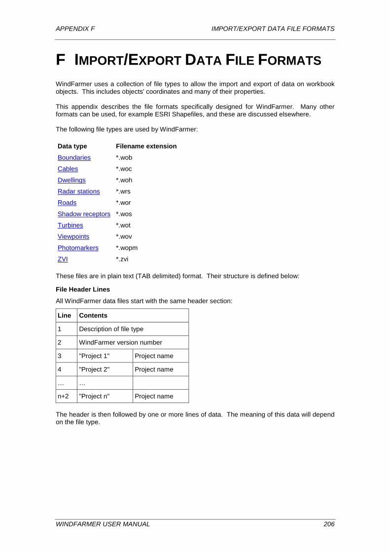
APPENDIX F IMPORT/EXPORT DATA FILE FORMATS
F IMPORT/EXPORT DATA FILE FORMATS WindFarmer uses a collection of file types to allow the import and export of data on workbook objects. This includes objects' coordinates and many of their properties. This appendix describes the file formats specifically designed for WindFarmer. Many other formats can be used, for example ESRI Shapefiles, and these are discussed elsewhere. The following file types are used by WindFarmer: Data type Filename extension Boundaries *.wob
Cables *.woc
Dwellings *.woh
Radar stations *.wrs
Roads *.wor
Shadow receptors *.wos
Turbines *.wot
Viewpoints *.wov
Photomarkers *.wopm
ZVI *.zvi These files are in plain text (TAB delimited) format. Their structure is defined below:
File Header Lines
All WindFarmer data files start with the same header section:
Line Contents
1 Description of file type
2 WindFarmer version number
3 "Project 1" Project name
4 "Project 2" Project name
… …
n+2 "Project n" Project name The header is then followed by one or more lines of data. The meaning of this data will depend on the file type.
WINDFARMER USER MANUAL 206
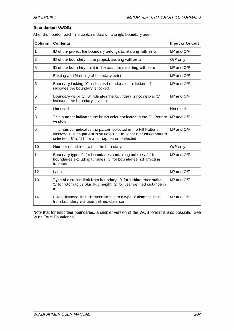
APPENDIX F IMPORT/EXPORT DATA FILE FORMATS
Boundaries (*.WOB)
After the header, each line contains data on a single boundary point:
Column Contents Input or Output
1 ID of the project the boundary belongs to, starting with zero I/P and O/P
2 ID of the boundary in the project, starting with zero O/P only
3 ID of the boundary point in the boundary, starting with zero I/P and O/P
4 Easting and Northing of boundary point I/P and O/P
5 Boundary locking: ‘0’ indicates boundary is not locked, ‘1’ indicates the boundary is locked
I/P and O/P
6 Boundary visibility: ‘0’ indicates the boundary is not visible, ‘1’ indicates the boundary is visible
I/P and O/P
7 Not used Not used
8 This number indicates the brush colour selected in the Fill Pattern window
I/P and O/P
9 This number indicates the pattern selected in the Fill Pattern window: ‘0’ if no pattern is selected, ‘1’ to ‘7’ for a brushed pattern selected, ‘8’ to ‘11’ for a bitmap pattern selected
I/P and O/P
10 Number of turbines within the boundary O/P only
11 Boundary type: ‘0’ for boundaries containing turbines, ‘1’ for boundaries excluding turbines, ‘2’ for boundaries not affecting turbines
I/P and O/P
12 Label I/P and O/P
13 Type of distance limit from boundary: ‘0’ for turbine rotor radius, ‘1’ for rotor radius plus hub height, ‘2’ for user defined distance in m
I/P and O/P
14 Fixed distance limit: distance limit in m if type of distance limit from boundary is a user defined distance
I/P and O/P
Note that for importing boundaries, a simpler version of the WOB format is also possible. See Wind Farm Boundaries
WINDFARMER USER MANUAL 207
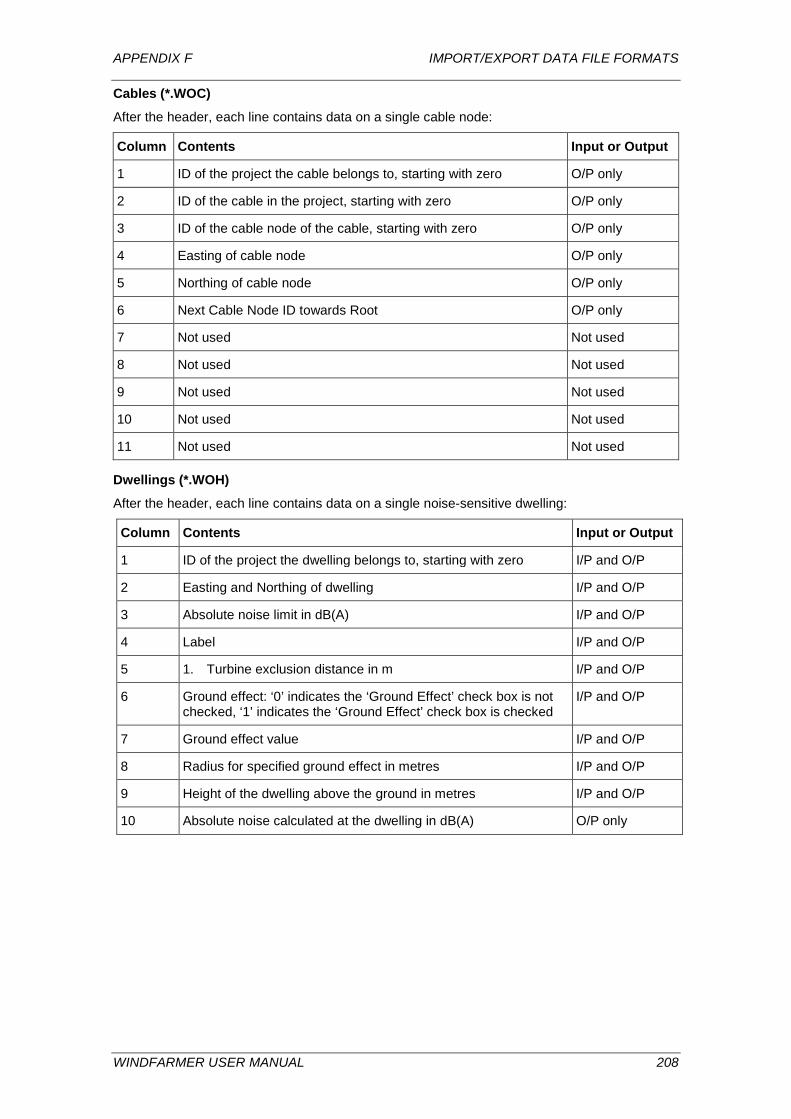
APPENDIX F IMPORT/EXPORT DATA FILE FORMATS
Cables (*.WOC)
After the header, each line contains data on a single cable node:
Column Contents Input or Output
1 ID of the project the cable belongs to, starting with zero O/P only
2 ID of the cable in the project, starting with zero O/P only
3 ID of the cable node of the cable, starting with zero O/P only
4 Easting of cable node O/P only
5 Northing of cable node O/P only
6 Next Cable Node ID towards Root O/P only
7 Not used Not used
8 Not used Not used
9 Not used Not used
10 Not used Not used
11 Not used Not used
Dwellings (*.WOH)
After the header, each line contains data on a single noise-sensitive dwelling:
Column Contents Input or Output
1 ID of the project the dwelling belongs to, starting with zero I/P and O/P
2 Easting and Northing of dwelling I/P and O/P
3 Absolute noise limit in dB(A) I/P and O/P
4 Label I/P and O/P
5 1. Turbine exclusion distance in m I/P and O/P
6 Ground effect: ‘0’ indicates the ‘Ground Effect’ check box is not checked, ‘1’ indicates the ‘Ground Effect’ check box is checked
I/P and O/P
7 Ground effect value I/P and O/P
8 Radius for specified ground effect in metres I/P and O/P
9 Height of the dwelling above the ground in metres I/P and O/P
10 Absolute noise calculated at the dwelling in dB(A) O/P only
WINDFARMER USER MANUAL 208
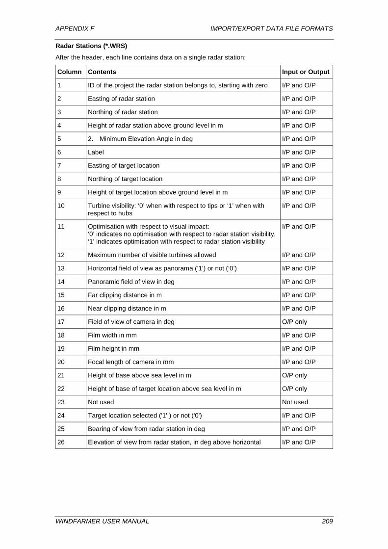
APPENDIX F IMPORT/EXPORT DATA FILE FORMATS
Radar Stations (*.WRS)
After the header, each line contains data on a single radar station:
Column Contents Input or Output
1 ID of the project the radar station belongs to, starting with zero I/P and O/P
2 Easting of radar station I/P and O/P
3 Northing of radar station I/P and O/P
4 Height of radar station above ground level in m I/P and O/P
5 2. Minimum Elevation Angle in deg I/P and O/P
6 Label I/P and O/P
7 Easting of target location I/P and O/P
8 Northing of target location I/P and O/P
9 Height of target location above ground level in m I/P and O/P
10 Turbine visibility: ‘0’ when with respect to tips or ‘1’ when with respect to hubs
I/P and O/P
11 Optimisation with respect to visual impact: ‘0’ indicates no optimisation with respect to radar station visibility, ‘1’ indicates optimisation with respect to radar station visibility
I/P and O/P
12 Maximum number of visible turbines allowed I/P and O/P
13 Horizontal field of view as panorama (‘1’) or not (‘0’) I/P and O/P
14 Panoramic field of view in deg I/P and O/P
15 Far clipping distance in m I/P and O/P
16 Near clipping distance in m I/P and O/P
17 Field of view of camera in deg O/P only
18 Film width in mm I/P and O/P
19 Film height in mm I/P and O/P
20 Focal length of camera in mm I/P and O/P
21 Height of base above sea level in m O/P only
22 Height of base of target location above sea level in m O/P only
23 Not used Not used
24 Target location selected ('1' ) or not ('0') I/P and O/P
25 Bearing of view from radar station in deg I/P and O/P
26 Elevation of view from radar station, in deg above horizontal I/P and O/P
WINDFARMER USER MANUAL 209
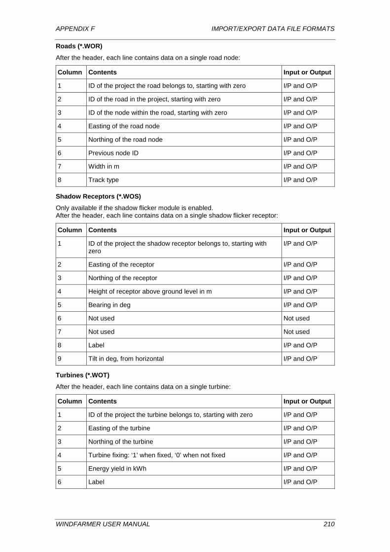
APPENDIX F IMPORT/EXPORT DATA FILE FORMATS
Roads (*.WOR)
After the header, each line contains data on a single road node:
Column Contents Input or Output
1 ID of the project the road belongs to, starting with zero I/P and O/P
2 ID of the road in the project, starting with zero I/P and O/P
3 ID of the node within the road, starting with zero I/P and O/P
4 Easting of the road node I/P and O/P
5 Northing of the road node I/P and O/P
6 Previous node ID I/P and O/P
7 Width in m I/P and O/P
8 Track type I/P and O/P
Shadow Receptors (*.WOS)
Only available if the shadow flicker module is enabled. After the header, each line contains data on a single shadow flicker receptor:
Column Contents Input or Output
1 ID of the project the shadow receptor belongs to, starting with zero
I/P and O/P
2 Easting of the receptor I/P and O/P
3 Northing of the receptor I/P and O/P
4 Height of receptor above ground level in m I/P and O/P
5 Bearing in deg I/P and O/P
6 Not used Not used
7 Not used Not used
8 Label I/P and O/P
9 Tilt in deg, from horizontal I/P and O/P
Turbines (*.WOT)
After the header, each line contains data on a single turbine:
Column Contents Input or Output
1 ID of the project the turbine belongs to, starting with zero I/P and O/P
2 Easting of the turbine I/P and O/P
3 Northing of the turbine I/P and O/P
4 Turbine fixing: ‘1’ when fixed, ‘0’ when not fixed I/P and O/P
5 Energy yield in kWh I/P and O/P
6 Label I/P and O/P
WINDFARMER USER MANUAL 210
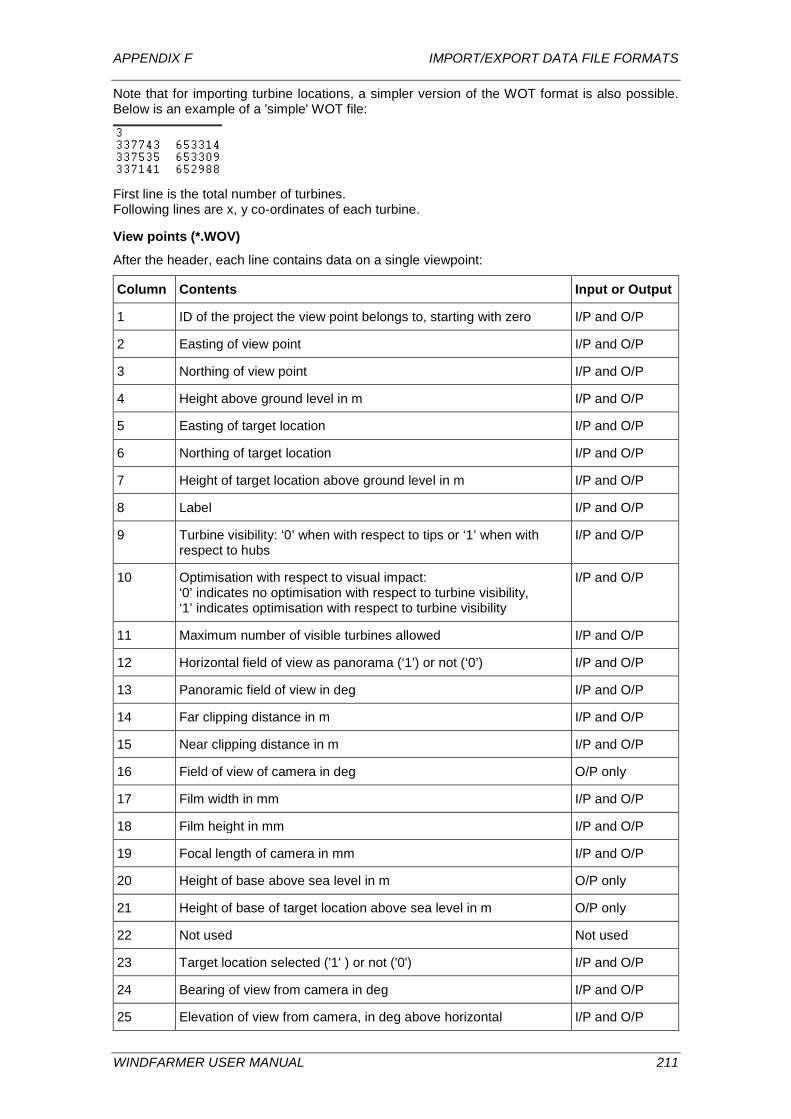
APPENDIX F IMPORT/EXPORT DATA FILE FORMATS
Note that for importing turbine locations, a simpler version of the WOT format is also possible. Below is an example of a 'simple' WOT file:
First line is the total number of turbines. Following lines are x, y co-ordinates of each turbine.
View points (*.WOV)
After the header, each line contains data on a single viewpoint:
Column Contents Input or Output
1 ID of the project the view point belongs to, starting with zero I/P and O/P
2 Easting of view point I/P and O/P
3 Northing of view point I/P and O/P
4 Height above ground level in m I/P and O/P
5 Easting of target location I/P and O/P
6 Northing of target location I/P and O/P
7 Height of target location above ground level in m I/P and O/P
8 Label I/P and O/P
9 Turbine visibility: ‘0’ when with respect to tips or ‘1’ when with respect to hubs
I/P and O/P
10 Optimisation with respect to visual impact: ‘0’ indicates no optimisation with respect to turbine visibility, ‘1’ indicates optimisation with respect to turbine visibility
I/P and O/P
11 Maximum number of visible turbines allowed I/P and O/P
12 Horizontal field of view as panorama (‘1’) or not (‘0’) I/P and O/P
13 Panoramic field of view in deg I/P and O/P
14 Far clipping distance in m I/P and O/P
15 Near clipping distance in m I/P and O/P
16 Field of view of camera in deg O/P only
17 Film width in mm I/P and O/P
18 Film height in mm I/P and O/P
19 Focal length of camera in mm I/P and O/P
20 Height of base above sea level in m O/P only
21 Height of base of target location above sea level in m O/P only
22 Not used Not used
23 Target location selected ('1' ) or not ('0') I/P and O/P
24 Bearing of view from camera in deg I/P and O/P
25 Elevation of view from camera, in deg above horizontal I/P and O/P
WINDFARMER USER MANUAL 211
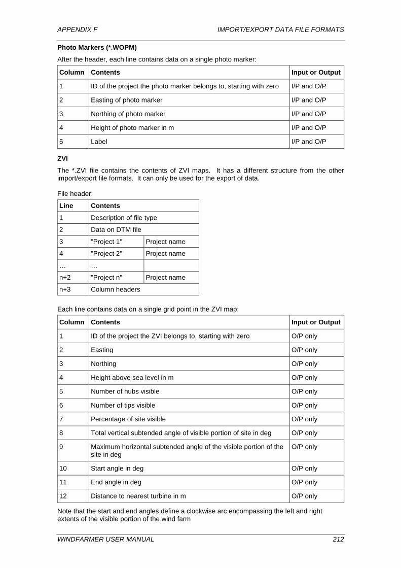
APPENDIX F IMPORT/EXPORT DATA FILE FORMATS
Photo Markers (*.WOPM)
After the header, each line contains data on a single photo marker:
Column Contents Input or Output
1 ID of the project the photo marker belongs to, starting with zero I/P and O/P
2 Easting of photo marker I/P and O/P
3 Northing of photo marker I/P and O/P
4 Height of photo marker in m I/P and O/P
5 Label I/P and O/P
ZVI
The *.ZVI file contains the contents of ZVI maps. It has a different structure from the other import/export file formats. It can only be used for the export of data. File header:
Line Contents
1 Description of file type
2 Data on DTM file
3 "Project 1" Project name
4 "Project 2" Project name
… …
n+2 "Project n" Project name
n+3 Column headers Each line contains data on a single grid point in the ZVI map:
Column Contents Input or Output
1 ID of the project the ZVI belongs to, starting with zero O/P only
2 Easting O/P only
3 Northing O/P only
4 Height above sea level in m O/P only
5 Number of hubs visible O/P only
6 Number of tips visible O/P only
7 Percentage of site visible O/P only
8 Total vertical subtended angle of visible portion of site in deg O/P only
9 Maximum horizontal subtended angle of the visible portion of the site in deg
O/P only
10 Start angle in deg O/P only
11 End angle in deg O/P only
12 Distance to nearest turbine in m O/P only
Note that the start and end angles define a clockwise arc encompassing the left and right extents of the visible portion of the wind farm
WINDFARMER USER MANUAL 212

APPENDIX G INDICATIVE POWER CURVE FILES
G INDICATIVE POWER CURVE FILES With future releases of WindFarmer Garrad Hassan & Partners Limited (DNV GL) intends to make available indicative power curve files provided to DNV GL by turbine manufacturers as examples of the power curve which the manufacturer might expect from their turbines. For existing users of WindFarmer we may also make indicative power curve files available in the download area for WindFarmer on the DNV GL website. If you choose to use indicative power curve files it is important that you use the latest files provided to DNV GL which are available in the download area for WindFarmer on the DNV GL website. WindFarmer is designed to be used without necessarily using the indicative power curve files (we may ask you to cease using any indicative power curve file, and the indicative power curve files may not be used except within WindFarmer5). The actual power curve of a wind turbine will be affected by many factors and users of WindFarmer must replace the indicative power curve files by such power curve as they agree with a turbine manufacturer (and which is applicable to the turbine’s intended installation and conditions), or use the actual (measured) power curve from the user’s existing installation. DNV GL makes indicative power curve files available on an “as is” basis without responsibility on the part of DNV GL or any of its affiliates (being any entity controlled by or under the same control, direct or indirect, as DNV GL, together with DNV GL being individually or collectively, the “DNV GL Group”) or their officers, employees and agents. The DNV GL Group and its officers, employees and agents neither assume nor accept any responsibility or liability (including for negligence) in relation to the indicative power curve files, and no action should be taken or omitted to be taken in reliance upon the indicative power curve files. In particular but without limiting the foregoing, neither the DNV GL Group or their officers, employees and agents shall be liable for any special, incidental, indirect, or consequential damages whatsoever (including, without limitation, damages for loss of business profits, business interruption, loss of business information, any other pecuniary loss, legal fees or court costs) howsoever arising (including without limitation negligence); however, none of the foregoing shall be taken to exclude liability for fraud, fraudulent misrepresentation or for negligence causing death or personal injury. By using WindFarmer you consent and agree to the above conditions and that these conditions (and any non-contractual obligations arising out of or in relation to the same) are governed by and shall be construed in accordance with English law and you irrevocably submit to the exclusive jurisdiction of the English courts to settle any suit, action or other proceedings relating to these conditions, save that nothing in these conditions shall prevent DNV GL from bringing proceedings against you in any jurisdiction.
WINDFARMER USER MANUAL 213
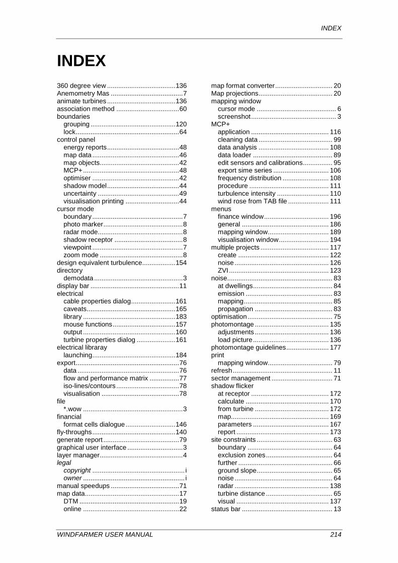
INDEX
INDEX 360 degree view ..................................... 136 Anemometry Mas ....................................... 7 animate turbines ..................................... 136 association method .................................. 60 boundaries
grouping .............................................. 120 lock ........................................................ 64
control panel energy reports ....................................... 48 map data ............................................... 46 map objects ........................................... 42 MCP+ .................................................... 48 optimiser ............................................... 42 shadow model ....................................... 44 uncertainty ............................................ 49 visualisation printing ............................. 44
cursor mode boundary ................................................. 7 photo marker ........................................... 8 radar mode .............................................. 8 shadow receptor ..................................... 8 viewpoint ................................................. 7 zoom mode ............................................. 8
design equivalent turbulence .................. 154 directory
demodata ................................................ 3 display bar ................................................ 11 electrical
cable properties dialog ........................ 161 caveats ................................................ 165 library .................................................. 183 mouse functions .................................. 157 output .................................................. 160 turbine properties dialog ..................... 161
electrical libraray launching ............................................. 184
export ........................................................ 76 data ....................................................... 76 flow and performance matrix ................ 77 iso-lines/contours .................................. 78 visualisation .......................................... 78
file *.wow ...................................................... 3
financial format cells dialogue ........................... 146
fly-throughs ............................................. 140 generate report ......................................... 79 graphical user interface .............................. 3 layer manager............................................. 4 legal
copyright .................................................. i owner ....................................................... i
manual speedups ..................................... 71 map data ................................................... 17
DTM ...................................................... 19 online .................................................... 22
map format converter ............................... 20 Map projections ........................................ 20 mapping window
cursor mode ........................................... 6 screenshot .............................................. 3
MCP+ application .......................................... 116 cleaning data ........................................ 99 data analysis ...................................... 108 data loader ........................................... 89 edit sensors and calibrations ................ 95 export sime series .............................. 106 frequency distribution ......................... 108 procedure ........................................... 111 turbulence intensity ............................ 110 wind rose from TAB file ...................... 111
menus finance window ................................... 196 general ............................................... 186 mapping window ................................. 189 visualisation window ........................... 194
multiple projects ..................................... 117 create ................................................. 122 noise ................................................... 126 ZVI ...................................................... 123
noise......................................................... 83 at dwellings ........................................... 84 emission ............................................... 83 mapping ................................................ 85 propagation .......................................... 83
optimisation .............................................. 75 photomontage ........................................ 135
adjustments ........................................ 136 load picture ......................................... 136
photomontage guidelines ....................... 177 print
mapping window ................................... 79 refresh ...................................................... 11 sector management ................................. 71 shadow flicker
at receptor .......................................... 172 calculate ............................................. 170 from turbine ........................................ 172 map..................................................... 169 parameters ......................................... 167 report .................................................. 173
site constraints ......................................... 63 boundary .............................................. 64 exclusion zones .................................... 64 further ................................................... 66 ground slope ......................................... 65 noise ..................................................... 64 radar ................................................... 138 turbine distance .................................... 65 visual .................................................. 137
status bar ................................................. 13
WINDFARMER USER MANUAL 214
INDEX
targets ..................................................... 129 test function .............................................. 66 toolbar
visualisation ........................................ 128 Turbine Importer ....................................... 33 turbine studio ............................................ 35 turbulence intensity
advanced input.................................... 153 at turbine ............................................. 154
visualisation ............................................ 127 menus ................................................. 128 radar .................................................... 139 radar ZVI ............................................. 138 shaded view ........................................ 132
turbine appearance ............................ 129 window ............................................... 127
wake models ............................................ 67 wind flow
modelling .............................................. 55 wind resource grid .................................... 24
creation ................................................. 25 resolution .............................................. 25 template ................................................ 58
window types ....................................................... 4 visualisation ........................................ 127
workbook workspace .............................................. 3
WINDFARMER USER MANUAL 215