what is the concentration footprint of a tall tower?

JOURNAL OF GEOPHYSICAL RESEARCH, VOL. 106, NO. D16, PAGES 17,831-17,840, AUGUST 27, 2001

What is the concentration footprint of a tall tower?

Manuel Gloor, •,e Peter Bakwin, 3 Dale Hurst, 4 Loreen Lock, 4 Roland Draxler, • and Pieter Tans •

Abstract. Studies that have attempted to estimate sources and sinks of trace gases such as COe with inverse calculations unanimously identify the lack of continental stations as a prime obstacle. Continental stations have traditionally been avoided because of the difficulty of interpretation due to large time-variability of trace substance mixing ratios. Large variability is caused by the proximity to the strongly variable sources in space and time and the complicated airflow within the lowermost 100-200 m of the planetary boundary layer. To address the need for continental stations and to overcome the problems associated with them, the National Oceanic and Atmospheric Administration Climate Monitoring and Diagnostics Laboratory started in 1992 to measure CO2 and other trace gases on tall television transmission towers [Bakwin et al., 1995]. An essential question in connection with these tower measurements is the area around the tower from which

fluxes substantially contribute to the observed short-term variability of trace gas mixing ratios. We present here a simple data and back trajectory-based method to estimate the fraction of the observed short-term variability explained by a localized flux around a tall television transmission tower in Wisconsin in dependence of its location relative to the tower (the concentration "footprint"). We find that the timescale over which the imprint of surface fluxes on air parcels before its arrival at the tower are still discernible in the mixing ratio variations observed at the tower is of the order of 1.5 days. Based on this timescale and the characteristics of air parcel trajectories, we infer a spatial extent of the footprint of the order of 106 km 2, or roughly a tenth of the area of the United States. This is encouraging evidence that tall tower measurements may be useful in global inversions and may also have implications for monitoring fluxes of anthropogenic trace substances on regional scales.

1. Introduction

There are at least two motivations to measure mixing ratios of carbon dioxide and other trace gases within continents. First, global inverse calculations that are currently strongly limited in longitudinal resolution of sources and sinks would greatly profit from such measurements, especially in the northern midlatitudes [Fan et al., 1998]. Global inverse calculations compare for- ward simulations of various surface flux scenarios with

observations to obtain the combination of surface fluxes

•Atmospheric and Oceanic Sciences Department, Prince- ton University, Princeton, New Jersey.

2Now at Max-Planck-Institut fiir Biogeochemie, Jena, Germany.

3Department of Commerce, Climate Monitoring and Di- agnostics Laboratory, NOAA, Boulder, Colorado.

4Cooperative Institute for Research in Environmental Sci- ences, University of Colorado, Boulder, Colorado.

5Air Resources Laboratory, NOAA, Silver Spring, Mary- land.

Copyright 2001 by the American Geophysical Union.

Paper number 2001JD900021. 0148-0227 / 01 / 2001JD900021 $09.00

that are most compatible with atmospheric observations [Bolin and Keeling, 1963; Enting and Mansbridge, 1989; Keeling et al., 1989]. The simulations are per- formed with atmospheric tracer transport models that integrate the tracer transport equation on a discrete

sphere. Second, monitoring of emissions of anthropogenic trace substances on a regional scale may be feasible with such measurements [Tans et al., 1996]. One concern, however, is that the area sampled by a tower may be small and thus may be poorly represented in global models that have horizontal resolution of hundreds of kilometers.

A helpful means to quantify from where and to which extent fluxes within the surroundings of a tower influence trace gas observations is the footprint concept. The concentration footprint of a tower, or synonymously transfer function or source weighting function, is defined as the conditional probability of observing a contribution f(F- F tower) to the observed short-term concentration variations at the tower given a flux T(• from location F [Schmid, 1997; $chmid and Oke, 1990; Horst and Well, 1992]. Short-term variations are those that oc- cur independently of the seasonal cycle and interannual trends; they are mostly tied to synoptic scale processes

17,831

17,832 GLOOR ET AL' CONCENTRATION FOOTPRINT OF A TALL TOWER

or variations of the surface fluxes. In a probabilistic sense the observed mixing ratio variations are given by the convolution of the footprint with the surface flux field

X(•tower) = / Ftower)T(•dxdy -]- Xtrend-

Note that the footprint of a tower is entirely determined by atmospheric transport. Note also that our definition differs slightly from $chmid's [1997] in that we disre- gard the seasonal and interannual variation of mixing ratio time-series. Since the timescale of the seasonal to

interannual variations approaches the timescale for in- terhemispheric exchange in the troposphere (-• I year [Maiss and Levin, 1994]), these variations are due to the integrated effect of fluxes from an area of roughly the size of a hemisphere and, in the case of weakly reactive trace substances like C2 C14, volume sinks. They therefore carry only very limited information on the distribution of surface fluxes on a regional scale.

The lowermost part of the planetary boundary layer (PBL) with 100 to 200 m height differs from the rest of the PBL. Over land, during night, stable stratifica- tion may develop such that near surface air masses are decoupled from the overlying air masses and thus trace substances emitted from the surface are trapped and accumulate. During day, within this lowermost part of the P BL mixing is caused by both convection and by shear generated turbulence. There trace substances with sources and sinks at the Earth surface typically are not homgeneously mixed but exhibit vertical gradients [$tull, 1988]. Within the layer of 1.5 to 2 km height ad- jacent to these lowermost 100 to 200 m in contrast air is vigorously mixed in the vertical by cloud convection during day. In this zone trace substances with sources and sinks at the Earth surface are typically well mixed. Exchange between the P BL and the overlying free troposphere above 1.5 to 2 km height finally is dominated by turbulent entrainment due to overshooting convec- tive plumes (thermals) and by synoptic events. This exchange between the PBL and the free troposphere acts to degrade the mixing ratio signal within the PBL caused by recent surface fluxes.

Because of the vigorous mixing within the layer above the lowermost 100 to 200 m of the PBL the variability of mixing ratios there is much less influenced by the spario- temporal variability of local surface sources and sinks. The footprint of measurements at the top of a tower that reaches into the well-mixed portion of the PBL is therefore expected to be substantially larger than the footprint of measurements close to the ground. How- ever, continuous measurements at a few hundred meters above ground are difficult to obtain becau•se of the ex- pense to construct and maintain such tall towers. In the United States, a number of towers up to 620 m height exist for television and radio transmission, and two such towers have been used for long-term measurements of atmospheric trace species [ Bakwin et al., 1995, 1998].

An alternative to tall tower measurement stations

may seem to be observation stations on mountain tops

such as Niwot Ridge, Colorado [Conway et al., 1994], and Schauinsland, Germany [Levin, 1987]. Such stations, however, sample mainly air from the free troposphere. Mixing ratios of nonreactive trace substances in the free troposphere that have been emitted from the Earth's surface exhibit only very weak gradients, particularly in longitudinal direction reflecting the strong zonality of the free tropospheric circulation [Gloor et al., 2000]. Such measurements thus carry only very limited information on surface sources and sinks. A second con-

cern with mountain top stations is the complicated atmospheric circulation in rugged topography that makes the interpretation of measurements difficult.

In this paper we develop a simple method to estimate the concentration footprint of anthropogenic trace gas species at 396 m above the ground on a tall tower in northern Wisconsin, up to a constant factor. We char- acterize the tower's footprint via a "backward look" in time along calculated airmass trajectories. To do so we examine the capability of reproducing the observed variability of C2C14 at the tower when cumulating population as a proxy for C2C14 emissions along back trajectories and when extending the trajectories gradually further backward in time. Based on the results obtained

and the statistics of back trajectory density within the surroundings of the tower, we then estimate the tower footprint. Before summarizing our results we present a few sensitivity studies that illustrate the possibilities and limitations of the approach. Our back trajectory- based analysis is motivated by the study of Vermeulen et al., A. T. [1997].

2. Derivation of the Footprint 2.1. Site and Measurements

The tower is located in northern Wisconsin (Figure 1). The site is described in detail by Bakwin et al. [1998]. The area within 50 km of the tower is mainly forested, with a population density of about 5 km -•'. The Minneapolis-St. Paul metropolitan area (1990 population 2.5 x 106, U.S. Census Bureau web site, 1999) lies about 250 km to the southwest.

The trace substance that we use for our analysis, C2C14, is measured every 60 min at 396 m height above the ground by automated, insitu gas chromatography (GC). The GC methods are as described by Hurst et al. [1997], and further analysis of the GC data is presented by Bakwin et al. [1997] and Hurst et al. [1998]. Our analysis uses data from the year 1998 and focuses on two periods, one with strong C2C14 signals and one with very weak signals. The juxtaposition of these two regimes illustrates the possibilities and limits of our approach.

The trace species C2C14 is exclusively of anthropogenic origin. It is used for dry cleaning and as an industrial degreasing agent [McCulloch and Midg- ley, 1996]. The atmospheric inventory of C2C14 has been roughly constant during 1995-1998 (S. Montzka, personal communication, 1999), though a large seasonal cycle and high degree of ambient variability make

GLOOR ET AL' CONCENTRATION FOOTPRINT OF A TALL TOWER 17,833

80N , , , 80 N

70 N 70 N

60 N 60 N

50 N 50 N

40 N 4O N

160 VV 120 VV 80 VV 40 VV 0 1 2 3 4 5

Height (km)

120 W 8O W 4O W o

16ow 16ow 12ow 8ow 4ow

Figure 1. Back trajectories arriving at the Wisconsin tower during October 1 to 10, 1998. Trajectories are calculated every 3 hours and exf, end 8 days backward in time. (a,b,c) kinematic trajectories and (d) isentropic trajectories.

trend detection difficult [Hurst et al., 1998]. Over the timescales considered here (several days), C2C14 may be considered as nonreactive: C2C14 reacts in the troposphere with OH with a lifetime of _< 0.5 year [Wang et al., 1995]. From all anthropogenic trace substances measured at the Wisconsin tower, the C2C14 signal in polluted air, while strongly correlated with the other anthropogenic trace substances, has the highest signal compared to its background value as well as to the magnitude of its small concentration fluctuations within background air [Bakwin et al., 1998]. The reasons are the low background concentration and high measurement precision. The substance C•C14 is therefore particularly suited for our purpose.

2.2. Region of Influence

We used the Hybrid Single-Particle Lagrangian In- tegrated Trajectory (HY-SPLIT4) model [Draxler and Hess, 1997; Draxler and Hess, 1998] to calculate back trajectories arriving at 396 m height at the tower. The model uses linearly interpolated (in space and time) wind fields from the National Centers for Environmen-

tal Prediction/National Oceanic and Atmospheric Ad- ministration (NCEP/NOAA) medium-range weather forecast model. The NCEP wind fields represent a compromise between available real-time observations

and the constraints of known physical laws [Kanamitsu, 1989]. From these wind fields back trajectories are obtained by integration of the differential equation

d•/dT: --•(•'(T), tar r -- T)

(which relates the rate of change of an air parcel's position vector F to the wind velocity •7 at time tarr--7 before the air parcel's arrival at t•rr) using a second- order accurate Runge-Kutta method. For reasons of economy the resolution of the forecast analysis fields is reduced before archiving. The original horizontal resolution is equivalent to 1 ø x 1 ø latitude by longitude, and 28 levels in the vertical are used. The near-surface zone

is highly resolved with eight layers between 1000 and 800 hPa. For archiving, 13 vertical layers are retained (lowest layers at 1000, 925, 850 and 700 hPa) and the horizontal resolution is degraded somewhat. With ex- ception of a sensitivity study (see section 3) we used in this paper these archived winds and a time step of 1 hour for the trajectory calculations.

A typical example of back trajectory paths from October I to 10, 1998, (Figure 1), reveals two main branches: one sweeping Alaska before arrival and one approaching the tower from the east via northeastern Canada, sometimes including a short southern loop shortly before arrival at the tower. The slope of air

17,834 GLOOR ET AL.. CONCENTRATION FOOTPRINT OF A TALL TOWER

! , ,

•4 a •2

•_•o

6

30

'--'10

0

!

i i i i i

100 , , ,

80

60

40 20

0 100 105 110 115 120

Day in Year (1998)

lOO

8O

•' 60 :• 40

20

0 240

i i i i i

d

250 260 270 280 290 300

Day in Year (1998)

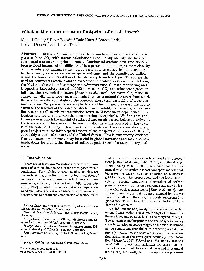
Figure 2. (a,b) Mixing ratios of C2C14 measured hourly at 396 m height on the Wisconsin tower and cumulative population underneath three-day back trajectories (c) during day 100 to 120 in 1998, (d) and during day 240 to 300 in 1998.

parcels with increasing latitude follows approximately the annual mean slope of isentropes. Air masses generally remain within the lowermost 2 km above ground within the last 4 days before arrival at the tower (Fig- ures lb and lc). Air parcels are found above the lowermost 2 km next to the ground mostly when they travel above the oceans or the high northern latitudes. A more detailed characterization of the vertical path of trajectories particularly in relation to the height of the PBL is given in section 3.

2.3. Demography

Because emissions of C2 C14 are proportional to population density [McCulloch et al., 1999], the interplay between atmospheric circulation and demography around the tower will predominantly shape the short-term variability of C2C14 at the tower. The demography [Andres et al., 1996] around the tower (Plate 1) has a strong gradient of higher density toward the southeast to lower density to the northwest, with pockets of high population density representing urban areas. Plate 2 shows the population density along each back trajectory that arrived at the tower during October 1998. The patterns of population density along the back trajectories are the result of synoptic scale variability. The highest population densities along the trajectories are generally not in the closest vicinity of the tower, reflecting the rural character of the area close to the tower.

2.4. Memory

We employ the population density distribution to- gether with the back trajectories to roughly reconstruct the structure of the C2C14 mixing ratio variations at the tower for two strongly contrasting periods: one with unusually weak C2C14 signals Figure 2a and one with strong signals (Figure 2b). For the reconstruction of the structure of the signals we simply sum the population

along the back trajectories over a period of 3 days backward in time (Figures 2c and 2d). This "reconstruction" of the tower signal correlates well with the observed C2C14 mixing ratios at 396 m height (Figures 2a and 2b) for the strong signal case and still fairly well for the weak signal case. The shape of the correlation between the reconstructed cumulative population density along back trajectories and the observed C2C14 mixing ratio time-series provides a measure of the "memory" timescale for the PBL in the region around the tower. The memory time scale is the period backwards in time over which the imprint of surface fluxes within the surroundings of the tower are discernible in the observed

0.8

0.7

.•-- 0.6

Q)0.5

•-0.4

0.2

0.1

i i [ i i [ i i [ t [ -I-- i i

Day 240-300 .............. , o Day100-120

/ --.. •.-7'""-"";"•'"" - ....................................... '•' .

/

..;, .•, _

?

,.i /

Backward extension of Trajectories (d)

Figure 3. Correlations between the observed C2C14 mixing ratio at 396 m height at the Wisconsin tower and the summed population over increasing periods in time along back trajectories for the time span from day 100 to 120 and day 240 to 300 in 1998. The dashed curves are fits of the function a(1 -e -t/z) to the correlations.

ß N Ir•N GLOOR ET AL CO CENTtLiT •,_ FOOTPRINT OF A TALL TOWER 17,855

mixing ratio signals at the tower. In both cases the correlation increases rapidly, then levels off after about 1.5 days (Figure 3), indicating that 1.5 days is a reasonable estimate for the memory timescale.

In the strong signal case there is only a small drop in correlation for long back trajectories because there are no sources of C2C14 at large distances from the tower. In contrast to the strong signal case for the low signal case the correlation drops after 3.5 days. The reason is likely that back trajectories from this period spend unusually long time over land.

2.5. Footprint Estimate

Since we use population density instead of C2C14 fluxes in our analysis, we can only estimate the tower footprint up to a constant (with dimensions of (C2C14 flux/population density)). We therefore choose here to normalize the footprint such that f•m•x y(s, •o)sdsd•o - emax, where s and •0 are polar coordinates with re- spect to the tower and emax is the largest value of the correlation, attained at s - smax, when gradually extending trajectories further away from the tower. With this normalization f(s,•o)sdsd•o is equal to the contribution of fluxes from (s,•0) to the maximal correlation emax- Now suppose we had no directional information on back trajectories and suppose we could express the correlation as a function of distance from the tower • - e(s) instead of time t before air parcel arrival at the tower. Then the most conservative

estimate of the angular distribution of the observed C2C14 variation de/ds explained by fluxes at a fixed distance so from the tower, de/ds(so), would be the uniform distribution: f(s0,•0) - 1/(2•rso)(de/ds)(so) (such that f f(so,•o)sod•o- (de/ds)(so)). However, fluxes along a circle with radius s around the tower contribute unevenly to the observed C2C14 variation

5

øoc• 4

Figure 4. Mean distance s = s(t) from Wisconsin tower and standard deviation of mean distance along back trajectories as a function of time before arrival at the tower for the periods from day 100 to 120 and from day 240 to 300 in 1998.

1.2

1.0

Eo.8

-•0.4

0.2

Day 100-120 (1998)

Day 240-300 (1998) "'•"x•\l\ --..

1

Distance from Tower (1000 km) Figure 5. Fraction de/ds of the observed C2C14 variability explained by fluxes located at distance s from the Wisconsin tower for the periods from day 100 to 120 and from da•v 240 to 300 in 1998.

depending on how often they are frequented by trajectories. For example, the footprint value f(s,p) of a location that is never passed by by a back trajectory is zero. A more accurate distribution of de/ds over the circle with radius s is obtained when weighing d•/ds proportionally to the number density n(s, •) of trajectories intersecting the circle with radius s when con- sidering trajectories from an extended period of time:

- )/f0 To dtr- mine f(s, •o) based on our analysis we need to translate de/dt into de/ds. For this purpose we use the approximation de/ds _• (de/dt)(dt/ds) where dt/ds(s) is the mean over the period in question of the inverse of the velocity of air parcels at distance s from the tower. As is evident from the variation of the distance of a large set

, i i i i i , i i i

Mean' day 100-120 std; day 100-120 ' ' ' -1 100 ..... - -• --•---r .... •---, ......

• Mean; day 240-300 . •' • std;__.day_2 •

90-

70

2 4 6 8

Backextension of Trajectories (day) 5o Backward Extension of Trajectory (d)

Figure 6. Fraction of back trajectories within mixed layer as a function of distance along trajectories from the tower during the period from day 240 to 300 in 1998.

17,836 GLOOR ET AL.: CONCENTRATION FOOTPRINT OF A TALL TOWER

0.8

•-0.4

0.2

0

Trajectory Hgt vs PBL Hgt

a

,J

1 2 3 4 5 6 7 8

0.8

'6 0.6

o

õ0.4 '• 0.2

o

Time Variation of Surface Flux

b

1 2 3

,-0.4 o

._

'• 0.2 o

o 0

Kinematic vs. Isentropic Traj.

1 2 3 4 5 6 7 8

Backward Extension (d)

0.8

•0.6 o

=0.4 o

'• 0.2 o

0

EDAS winds vs. FNL winds ,

d

Backward Extension (d)

Figure 7. Sensitivity of the correlation between observed C2C14 and cumulated population underneath trajectories to (a) exclusion of trajectories that leave the PBL, (b) selective accumulation of population depending on time of the day (no accumulation from midnight to six o'clock in the morning), (c) trajectory type (kinematic versus isentropic), and (d) resolution of winds used for the back trajectory calculations. The benchmark calculations use kinematic back trajectories, FNL winds, all trajectories (no selection), and are printed with dots (day 240-300, 1998) and diamonds (day 100-120, 1998). The sensitivity calculations are marked as lines (day 240-300) and dashed lines (day 100-120).

of air parcels with increasing time before arrival at the tower in Figure 4 this approximation is not fully satis- factory but suffices for an approximate estimate of the tower footprint. The final estimate of the concentration footprint provided by our analysis therefore is

n(s, •o) d• dt

To obtain a smooth estimate of the rate of change of the correlation d•/dt with time, we fit here the function a(1 -e -t/r) to the observed correlation up to time t = tmax where the correlation is maximal (Figure 3). The resulting functions d•/ds(s) for the weak and strong signal cases are displayed in Figure 5 and the footprint estimates for these two cases are displayed in Plate 3.

The footprints for both periods extend over hundreds of kilometers (the lateral dimensions of the grid cells are of the order of 100 km). This conclusion on the extent of the footprints is fairly independent from the time period chosen. For correlation functions • - •(t) for each of the six 2-months periods of the year 1998 we find •- - 26.2+ 7.6 days. The spatial distribution of the footprints

in contrast and as expected differs considerably between different time periods.

3. Sensitivity Analyses

3.1. Trajectory Height Relative to Mixed Layer Height

A concern with the footprint estimates presented in this paper is that data from all locations along trajectories are used independently from their vertical position relative to the PBL. It is therefore of interest to

determine the fraction of trajectories remaining within the PBL when gradually extending trajectories further backward in time and to determine how strongly the results of our analysis change if we use trajectories only as long as they reside in the PBL. We investigate the first of these questions for the strong signal case in Figure 6. Within the first day, 20% of back trajectories leave the mixed layer followed by a linear increase to 40% within the following 1.5 days. The percentage of trajectories remaining within the mixed layer then stabilizes at 60%. From the functional form of d•o/ds(s) (Figure 5) and the mean distance traveled by trajectories (Figure

GLOOR ET AL. CONCENTRATION FOOTPRINT OF A TALL TOWER 17,837

60N •

•40N

ON[

Population Density - GEIA 1990

=, ß

i

Ill

II

ß I

120W -i..,00w. Longitude

ß j 80W

>=5.0

4.0

- 3.0

2.0

1.0

Plate 1; Population density in North America (number of people x10 -6 within each 1 ø x 1 ø grid cell).

Population underneath Backtrajectory

30 _• ---_ •

0325 --- "" _ __:._

O ,• • • - _..- O20' -. -•.-•_- - . _ . •

- _

.• 15

o

•10 • "•_

5;

0 2 4 6

days before arrival

Plate 2. Population density underneath 8 day back trajectories (time backward along horizontal axis) that arrive at the Wisconsin tower during October 1998 rival time on the vertical axis). The color code is the same as in Plate 1.

't

50N

40N

Day 240 - Day 300 (1998)

100W 85W Longitude

0.05

0.04

I

0.03

0.02

0.01

<0.002

70N .-..---

Day 240 - Day 300 (1998)

40N

120W Longitude

80W

Day 100 - Day 120 (1998)

70N •

40N

120W 80W Longitude

Plate 3. (top) Footprint estimate f(s, •) for day 240 to 300 in 1998 and areas wherefrom fluxes contribute 25%, 50% and 75% to the correlation •max at the tower for (middle) day 240 to 300 in 1998 and (bottom) day 100 to 120 in 1998.


Table 1. Difference Statistics (Time Trends of Sample Mean and Sample Standard Deviation) of Back Trajectory Paths Calculated Using Two Different Trajectory Types (Kinematic and Isentropic) and Using Winds From Two Atmospheric Circulation Models With Different Resolution (FNL and EDAS)

Difference Statistics

Kinematic Versus Isentropic FNL Versus EDAS

0-24 hours 24-48 hours 48-72 hours 0-24 hours 24-48 hours 48-72 hours

Along, (deg d- •) 0.0 1.0 0.0 -0.2 0.0 1.2 Alat, (deg d- •) -0.1 0.7 0.6 -1.1 -1.1 -0.5 Az, (m d- •) -500 -200 300 50.0 100 0.0 std(Along), (deg d -•) 3.0 3.0 1.5 2.0 2.5 3.0 std(Alat), (deg d -•) 2.5 2.5 2.5 1.7 1.7 1.7 std(Az), (m d- •) 1000 300 0.0 400 400 200

The statistics axe determined for 0-24, 24-48, and 48-72 hours periods before the trajectories axrive at the tower. The sample consists of all trajectories from October 1998 with axrival times offset from each other by 3 hours.

4) it is expected that the exclusion of trajectories from the footprint estimation once they leave the mixed layer raises the level of correlation by 10 to 20%. However, when repeating our analysis and omitting data once trajectories leave the PBL, the correlation level does not rise (Figure 7a). It actually slightly decreases (by 3% in the high signal case). Apparently, our PBL height estimates are not reliable enough that their consideration would help improve our analysis.

3.2. Time Pattern of C2C14 Emissions

Since dry cleaning contributes strongly to C2 C14 emissions, there is likely a daily cycle in emissions which potentially should have been included in our analysis when cumulating population underneath backtrajecto- ries. Unfortunately, we do not have precise information on the daily cycle of these emissions. We may, however, estimate its impact on our analysis by investigating the scenario that assumes no emissions from midnight until 6 o'clock in the morning (Figure 7b). We find that the correlation relation with trajectory time before arrival at the tower degrades slightly (by 5-10% ). Our assumed cycle of C2C14 emissions is therefore on the one hand not confirmed by the data, and on the other hand the main conclusions of our analysis do not rely critically on the assumption of constant C2C14 emissions.

3.3. Kinematic Versus Isentropic Trajectories

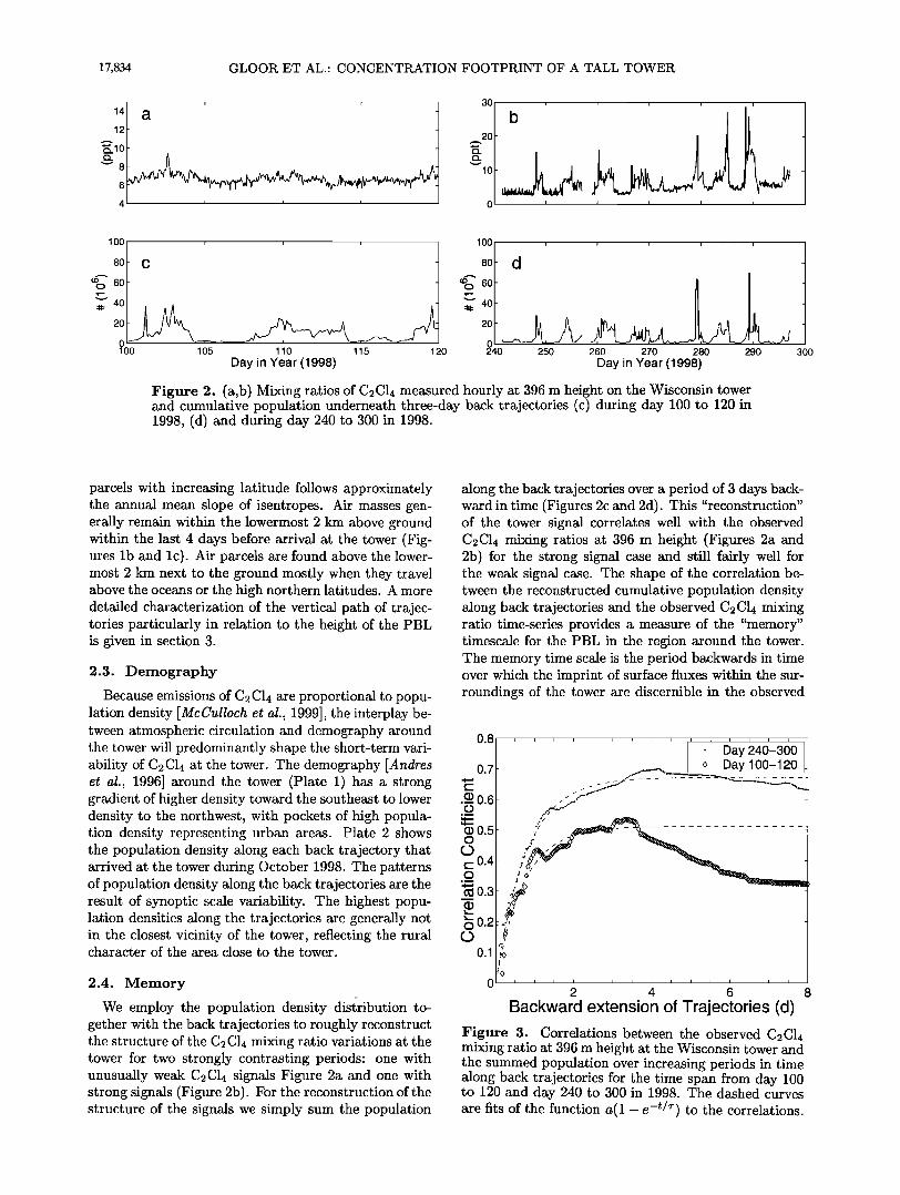
Isentropic trajectories differ from kinematic trajectories in their vertical velocity. The vertical velocity of isentropic back trajectories is chosen such that the air parcels remain on isentropic surfaces. A comparison of our analysis when based on kinematic and isentropic trajectories provides us with both a measure of which trajectory type is more suited for our purposes and a sensitivity test of our analysis to biases in trajectory paths. Kinematic and isentropic trajectory paths are compared in Figures la and ld, and differences are sum- marized in greater detail in Table 1. During the first 3

days before arrival of the trajectories the mean differences of the horizontal position are small compared to the distance traveled as well as compared to the 1øxl ø resolution of the population density distribution. Sim- ilarly, the mean difference of the vertical position compared to the P BL height remains small during the first 3 days. The scatter (standard deviation) of the trajectories in contrast is much larger and expected to lead to substantial errors in population accumulation and therefore in the footprint estimates. The resulting fractional differences in the footprints at fixed distance from the tower are quantified in Figure 8. To quantify the contribution of the fractional difference at distance s

from the tower to the total observed variation of C2C14 attributed differently when using the two types of tra-

0.8

0.6

0.2

Figure 8.

200 400 600 800 1000

Distance from Tower (km)

Angular mean of the relative difference of the footprints 1/27r 2• fo (f•i.(s,•p) - f•.(s,•p))/ [0.5(f•in(s, tp) +/isen(s, tp))]sdtp as a function of distance s from the tower for the period from day 240 to 300 (1998) when alternatively using kinematic and isentropic back trajectories.

GLOOR ET AL.: CONCENTRATION FOOTPRINT OF A TALL TOWER 17,839

jectories, the decrease of the footprim with increasing distance from the tower as in Figure 5 needs to be taken into account. The fractional differences are smallest

when their contribution to the footprint is largest and vice versa. The total differently attributed fraction, the product of the footprint with the fractional difference between footprints integrated over the distance from the tower to infinity is 30%.

As above we may use the level of correlation as a criterium which trajectory type to choose to estimate a footprint (Figure 7c). The correlation level for isentropic trajectories is approximately 20% less compared with kinematic trajectories, favoring kinematic trajectories.

3.4. Highly Resolved Versus Coarsely Resolved Winds

The hemispheric winds from NCEP's final (FNL) forecast step that we used solar in this paper are coarsely resolved, particularly in the vertical. Routinely highly resolved winds from NCEP's Eta Data Assimilation

System (EDAS), [Rogers et al., 1997]) are archived for later use in HY-SPLIT4 for a domain that covers the

United States, Mexico, and Southern Canada. The resolution of the archived winds is 22 levels in the vertical

(10 levels between the surface and 800 hPa) and the horizontal resolution is 80 km x 80 km. We did not

use these winds for the analysis in this paper because the domain for which the winds are available is too lim-

ited. Indeed some trajectories that extend backwards in time from the Wisconsin tower leave the domain al-

ready after I day. Nevertheless, as a means to evalu- ate the role played by the resolution of the winds in our analyses, the EDAS winds are helpful as long as we restrict ourselves to the first 1-1.5 days. The main substantial difference in the paths (FNL-EDAS, Table 1) is a northward bias of the EDAS trajectories during the last 2 days before arrival. Accordingly there are differences in the level of correlation attained (Figure 7d) when using the different winds. Higher levels of correlation are achieved when using the EDAS winds. The method developed in this paper therefore should preferably be applied with winds from highly resolved circulation models of the atmosphere.

4. Summary

We presented a simple, approximate approach to estimate the concentration footprint for trace gas mixing ratios observed at a tall tower. The area swept by back trajectories contributing significantly (75% of Pmax, the maximal level of correlation between signal reconstruction and observation attained when gradually extending trajectories further backward in time) to the observed short-term variability of trace gas mixing ratios at the tower is surprisingly large, of the order of 106 km 2, or approximately a tenth of the area of the United States. A sensitivity analyses demonstrates that this conclusion does not hinge on the simplifications inherent in our approach. The result on the footprint extent in-

dicates that exchange between the PBL and the free troposphere is slow enough for far-reaching reception of anthropogenic emissions of inert trace substances with tall tower observations. A minimal condition for any emission monitoring method is that flux signals from the entire area to be monitored may be received. The large area covered by the tower's footprint is encouraging evidence that for inert trace substances •- 10 strate- gically located towers within United States would fulfill this condition.

Acknowledgments. We thank the State of Wisconsin Educational Communications Board for use of the transmit- ter tower and facilities in Wisconsin, and R. Strand, chief engineer of WLEF-TV (Park Falls, Wisconsin), for valuable assistance and advice. R. Teclaw and A. Berger (U.S. De- partment of Agriculture Forest Service, Rhinelander, Wis- consin) assisted with maintenance of the analytical equip- ment at the tower. We are grateful to R. Myers, M. Pender, and S. Montzka of NOAA CMDL for preparation and cal- ibration of the gas standards. The critical comments from one reviewer helped to improve the manuscript. This work has been supported by NASA (NAG5-3510) and the NOAA Office of Global Programs (NA56GP0439). Measurements at the tower were supported by the Atmospheric Chem- istry Project of the Climate and Global Change Program of the National Oceanic and Atmospheric Administration. D. Hurst acknowledges support by the National Research Council Associateship program.

References

Andres, R. J., G. Marland, I. Fung, and E. Matthews, A 1øxl ø distribution of carbon dioxide emissions from fos- sil fuel consumption and cement manufacture, 1950-1990, Global Biogeochem. Cycles, 10, 419-429, 1996.

Bakwin, P.S., P. P. Tans, C. Zhao, W. Ussler, and E. Ques- nell, Measurements of carbon dioxide on a very tall tower, Tellus, Set. B., d?, 535-549, 1995.

Bakwin, P.S., D. F. Hurst, P. P. Tans, and J. W. Elkins, Anthropogenic sources of halocarbons, sulfur hexafiuo- ride, carbon monoxide, and methane in the southeastern United States, J. Geophys. Res., 102, 15915-15925, 1997.

Bakwin, P.S., P. P. Tans, D. Hurst, and C. Zhao, Measure- ments of carbon dioxide on very tall towers: Results of the NOAA/CMDL, Tellus, Set. B., 50, 401-415, 1998.

Bolin, B., and C. D. Keeling, Large-scale atmospheric mixing as deduced from the seasonal and meridional variations of carbon dioxide, J. Geophys. Res., 68, 3899-3920, 1963.

Conway, T. J., P. P. Tans, and L. S. Waterman, Atmospheric CO2 records from sites in the NOAA/CMDL air sampling network, in Trends '93: A Compendium of Data on Global Change, pp. 41-119, Carbon Dioxide Inf. Anal. Cent., Oak Ridge Nat. Lab., Oak Ridge, Tenn., 1994.

Draxler, R. R., and G. D. Hess, Description of the HYS- PLITJ modeling system, NOAA Tech. Mere., ERL ARL- 224, 1997.

Draxler, R. R., and G. D. Hess, An overview of the HYS- PLIT4 modelling system for trajectories, dispersion and deposition, Aust. Meteorol. May., J7, 295-308, 1998.

Enting, I. G., and J. V. Mansbridge, Latitudinal distribution of sources and sinks of atmospheric CO2: Direct inversion of filtered data, Tellus, Set. B., Jl, 111-126, 1989.

Fan, S., M. Gloor, J. Mahlman, S. Pacala, J. Sarmiento, T. Takahashi, and P. Tans, A large terrestrial carbon sink in North America implied by atmospheric and oceanic carbon dioxide data and models, Science, 282, 442-446, 1998.

Gloor, M., S.-M. Fan, S. W. Pacala, and J. L. Sarmiento,


Optimal sampling of the atmosphere for purpose of inverse modelling: A model study, Global Biogeochem. Cycles, 1.4, 407-428, 2000.

Horst, T. W., and J. C. Weil, Footprint estimation for scalar flux measurements in the atmospheric surface layer, Boundary Layer Meteorol., 59, 279-296, 1992.

Hurst, D. F., P.S. Bakwin, R. C. Myers, and J. W. Elkins, Behavior of trace gas mixing ratios at a very tall tower site in North Carolina, J. Geophys. Res., 102, 8825-8835, 1997.

Hurst, D. F., P.S. Bakwin, and J. W. Elkins, Recent trends in the variability of halogenated trace gases over the United States, J. Geophys. Res., 103, 25,299-25,306, 1998.

Kanamitsu, M., Description of the NMC global data assimilation and forecast system, Weather Forecasting, •, 335-342, 1989.

Keeling, C. D., S.C. Piper, and M. Heimann, A three di- mensional model of atmospheric CO2 transport based on observed winds, 4, Mean annual gradients and interannual variations, in Aspects of Climate Variability in the Pacific and the Western Americas, editor D. H. Peter- son, Geophys. Monogr. Set., vol. 55, pp. 305-363, AGU, Washington, D.C., 1989.

Levin, I., Atmospheric CO•. in continental Europe: An alternative approach to clean air CO2, Tellus, Set. B., 39B, 21-28, 1987.

Maiss, M., and I. Levin, Global increase of SF6 observed in the atmosphere, Geophys. Res. Left., 21, 569-572, 1994.

McCulloch, A., and P.M. Midgley, The production and global distribution of emissions of trichloroethene, tetrachloroethene and dichloromethane over the period 1988- 1992, Atmos. Environ., 30, 601-608, 1996.

McCulloch, A., M. L. Aucott, T. E. Graedel, G. Kleiman, P.M. Midgley, and Y.-F. Li, Industrial emissions of trichloroethene, tetrachloroethene, and dichloromethane: Reactive chlorine emissions inventory, J. Geophys. Res., 10•, 8417-8427, 1999.

Rogers, E. T., T. L. Black, D. Deaven, G. J. DiMego, Q. Zhao, M. Baldwin, N. Junker, and Y. Lin, Changes

to the operational "early" eta analysis/forecast system at the National Centers for Environmental Prediction, Wear. Forecasting, 11, 391-413, 1997.

Schmid, H. P., Experimental design for flux measurements: Matching scales of observations and fluxes, Agric. Mete- orol., 87, 179-200, 1997.

Schmid, H. P., and T. R. Oke, A model to estimate the source area contributing to turbulent exchange in the surface layer over patchy terrain, Q. J. R. Meteorol. Soc., 116, 965-988, 1990.

Stull, R. B., An Introduction to Boundary Layer Meteorlogy, Kluwer Acad., Norwell, Mass., 1988.

Tans, P. P., P.S. Bakwin, and D. W. Guenther, A feasible global carbon cycle observing system: a plan to decipher today's carbon cycle based on observations, Global Chem. Biol., 2, 309-318, 1996.

Vermeulen et al., A. T., Validation of methane emission in- ventories for NW-Europe, Final Tech. Rep., Energieon- derzoek Cent., Petten, Ned., ECN-C-96-088, 1997.

Wang, J.-L. C., D. R. Blake, and F. S. Rowland, Seasonal variations in the atmospheric distribution of a reactive chlorine compound, tetrachloroethene (CCI• = CCI•), Geophys. Res. Left., 22, 1097-1100, 1995.

P. Bakwin and P. Tans, Department of Commerce/NOAA CMDL, Mailstop R/CMDL1, 325 Broadway, Boulder, CO 80303. ([email protected]. gov; [email protected]. gov)

R. Draxler, NOAA Air Resources Laboratory, 1315 East West Hwy, Silver Spring, MD 20910. (r draxl er@arlrisc. arlh q. n oaa. gov )

M. Gloor, Max-Planck Institut fiir Biogeochemie, Post- fach 100164, D-07701 Jena, Germany. (mgloor@bgc- jena.mpg.de)

D. Hurst and L. Lock, Cooperative Institute for Research in Environmental Sciences, University of Colorado, Boulder, CO 80309. ([email protected]. gov)

(Received January 28, 2000; revised November 27, 2000; accepted December 5, 2000.)

what is the concentration footprint of a tall tower?

Documents