wave propagation in staggered-grid finite-difference models
TRANSCRIPT
Wave Propagation In Staggered-Grid
Finite-Difference Models With Boundaries
Muhamad Najib Bin Zakaria
Submitted in accordance with the requirements for
the degree of Doctor of Philosophy
The University of Leeds
School of Mathematics
June 2019


i
The candidate confirms that the work submitted is his own and that appropriate credit has
been given where reference has been made to the work of others.
This copy has been supplied on the understanding that it is copyright material and that no
quotation from the thesis may be published without proper acknowledgement.
ii
Acknowledgements
I would like to express my deepest gratitude to my supervisor, Dr. Stephen Griffiths for
his superb guidance and advice. I sincerely appreciate his patience, motivation and helps
offered in doing my research. His enthusiasm for this work and all things scientific has
been inspiring. Thanks also to my advisor, Prof Mark Kelmanson for his input, helpful
discussions and support in this research. Besides, I sincerely have to thank all those who
have supported and helped me in completing this thesis.
My special thanks to my lovely wonderful wife, Hazzirah Izzati Mat Hassim, for her uncon-
ditional love, understanding, sacrifice and endless moral support. I overwhelmingly owe a
lot to my sweet and precious son, Muhammad Zharif Daniel. Staying apart during final
year was the hardest thing but makes all of us stronger people.
Thanks also to my beloved parents, Zakaria Mohd Said and Sarah Ahmad, for being very
supportive and understanding. Not to be forgotten, I wish to express my appreciation to all
my siblings and friends for always being with me in undergo the hard times together.
iii
Abstract
Finite-difference numerical models are widely used in acoustics, electrodynamics and fluid
dynamics. In particular, the so-called C-grid (or Yee grid) is a popular staggered-grid for-
mulation, with excellent conservation properties and a natural positioning of nodes. How-
ever, domain boundaries are typically treated as staircases, and these degrade the accuracy
of the numerical solutions. Here that degradation is quantified for various linear wave
propagation problems in idealised geometries.
Here, the discrete solution is studied for three important models: (i) wave propagation
along a channel, (ii) wave reflection at a planar wall, (iii) the long-time dynamics of waves
sloshing in two simple closed domains (square and circle). The first two problems are
solved analytically, using asymptotics to examine the limit of small grid spacing h, with
expressions for the wavespeed reduction (in (i)) and a phase error (in (ii)) being derived.
The third problem is examined numerically, using a high-order time-stepping scheme so
that the effects of the staircase boundaries can be isolated. We typically find first-order
convergence in grid spacing h, although there are some variations, according to whether we
consider convergence in velocities or pressure, and also whether we use L2 or L∞-norm.
Some extensions to the propagation of internal waves in a density stratified medium are
also considered, which is a less standard scenario, but which has considerable significance
in geophysical fluid dynamics.
iv
Contents
Acknowledgements . . . . . . . . . . . . . . . . . . . . . . . . . . . . . . . . . ii
Abstract . . . . . . . . . . . . . . . . . . . . . . . . . . . . . . . . . . . . . . . iii
Contents . . . . . . . . . . . . . . . . . . . . . . . . . . . . . . . . . . . . . . . iv
List of figures . . . . . . . . . . . . . . . . . . . . . . . . . . . . . . . . . . . . ix
List of tables . . . . . . . . . . . . . . . . . . . . . . . . . . . . . . . . . . . . .xxviii
1 INTRODUCTION 1
1.1 Waves . . . . . . . . . . . . . . . . . . . . . . . . . . . . . . . . . . . . . 1
1.2 Mathematical modelling of waves . . . . . . . . . . . . . . . . . . . . . . 3
1.3 Numerical solutions of wave equations . . . . . . . . . . . . . . . . . . . . 6
1.4 Staggered-grid finite difference methods in two spatial dimensions . . . . . 8
1.5 Aims and outline of this thesis . . . . . . . . . . . . . . . . . . . . . . . . 11
2 MATHEMATICAL BACKGROUND: WAVES AND
STAGGERED FINITE-DIFFERENCE SCHEMES IN UN-
BOUNDED DOMAINS 15
2.1 Introduction . . . . . . . . . . . . . . . . . . . . . . . . . . . . . . . . . . 15
2.2 Physical Systems . . . . . . . . . . . . . . . . . . . . . . . . . . . . . . . 17
2.2.1 Acoustic waves . . . . . . . . . . . . . . . . . . . . . . . . . . . . 17
2.2.2 Electromagnetic waves . . . . . . . . . . . . . . . . . . . . . . . . 19
2.2.3 Shallow-water flows . . . . . . . . . . . . . . . . . . . . . . . . . 22
2.3 Conservation Laws . . . . . . . . . . . . . . . . . . . . . . . . . . . . . . 25
2.3.1 Conservation of mass . . . . . . . . . . . . . . . . . . . . . . . . . 26
v
2.3.2 Conservation of energy . . . . . . . . . . . . . . . . . . . . . . . . 27
2.4 Wave Propagation . . . . . . . . . . . . . . . . . . . . . . . . . . . . . . . 28
2.5 Finite-Difference Approximations . . . . . . . . . . . . . . . . . . . . . . 30
2.5.1 A-grid . . . . . . . . . . . . . . . . . . . . . . . . . . . . . . . . . 31
2.5.2 B-grid . . . . . . . . . . . . . . . . . . . . . . . . . . . . . . . . . 32
2.5.3 C-grid . . . . . . . . . . . . . . . . . . . . . . . . . . . . . . . . . 33
2.6 Discrete Conservation Laws . . . . . . . . . . . . . . . . . . . . . . . . . 33
2.6.1 Discrete Conservation of Mass . . . . . . . . . . . . . . . . . . . . 34
2.6.2 Discrete Conservation of Energy . . . . . . . . . . . . . . . . . . . 35
2.7 Discrete Waves . . . . . . . . . . . . . . . . . . . . . . . . . . . . . . . . 38
2.7.1 A-grid solutions . . . . . . . . . . . . . . . . . . . . . . . . . . . . 39
2.7.2 B-grid solutions . . . . . . . . . . . . . . . . . . . . . . . . . . . . 40
2.7.3 C-grid solutions . . . . . . . . . . . . . . . . . . . . . . . . . . . . 41
2.7.4 Comparison of discrete frequency on the A-, B-, and C-grid . . . . 42
2.8 Summary . . . . . . . . . . . . . . . . . . . . . . . . . . . . . . . . . . . 45
3 WAVE PROPAGATION ALONG A CHANNEL 49
3.1 Introduction . . . . . . . . . . . . . . . . . . . . . . . . . . . . . . . . . . 49
3.1.1 Nondimensional equations . . . . . . . . . . . . . . . . . . . . . . 52
3.2 Continuum Solutions . . . . . . . . . . . . . . . . . . . . . . . . . . . . . 52
3.3 Boundary Aligned with the Grid . . . . . . . . . . . . . . . . . . . . . . . 55
3.3.1 Numerical solutions . . . . . . . . . . . . . . . . . . . . . . . . . . 57
3.3.2 Analytical solutions . . . . . . . . . . . . . . . . . . . . . . . . . . 61
3.3.3 Asymptotic analysis as h→ 0 . . . . . . . . . . . . . . . . . . . . 63
3.4 Boundary aligned at 45◦ to the grid . . . . . . . . . . . . . . . . . . . . . . 64
3.4.1 Rotated coordinate system . . . . . . . . . . . . . . . . . . . . . . 65
3.4.2 Wavelike solutions . . . . . . . . . . . . . . . . . . . . . . . . . . 67
3.4.3 Numerical solutions . . . . . . . . . . . . . . . . . . . . . . . . . . 68
vi
3.4.4 Analytical solution . . . . . . . . . . . . . . . . . . . . . . . . . . 71
3.4.5 Behaviour as h→ 0 . . . . . . . . . . . . . . . . . . . . . . . . . . 75
3.4.6 Numerical verification . . . . . . . . . . . . . . . . . . . . . . . . 80
3.5 Summary . . . . . . . . . . . . . . . . . . . . . . . . . . . . . . . . . . . 81
4 WAVE REFLECTION AT A PLANAR WALL 85
4.1 Introduction . . . . . . . . . . . . . . . . . . . . . . . . . . . . . . . . . . 85
4.2 Boundary Aligned with the Grids . . . . . . . . . . . . . . . . . . . . . . . 88
4.2.1 Continuum solutions . . . . . . . . . . . . . . . . . . . . . . . . . 88
4.2.2 Discrete solutions . . . . . . . . . . . . . . . . . . . . . . . . . . . 91
4.2.3 Numerical visualisation . . . . . . . . . . . . . . . . . . . . . . . . 94
4.3 Tilted boundary: Continuum solution . . . . . . . . . . . . . . . . . . . . . 96
4.4 Tilted boundary: Discrete solution . . . . . . . . . . . . . . . . . . . . . . 99
4.4.1 Alternative derivation of amplitude error . . . . . . . . . . . . . . . 106
4.4.2 Spatial structure of discrete solution . . . . . . . . . . . . . . . . . 108
4.5 Summary . . . . . . . . . . . . . . . . . . . . . . . . . . . . . . . . . . . 112
5 NUMERICAL SOLUTIONS: THE EFFECT OF STAIRCASE BOUNDARY 121
5.1 Introduction . . . . . . . . . . . . . . . . . . . . . . . . . . . . . . . . . . 121
5.2 Numerical Methods . . . . . . . . . . . . . . . . . . . . . . . . . . . . . . 123
5.2.1 Spatial discretization . . . . . . . . . . . . . . . . . . . . . . . . . 123
5.2.2 Temporal discretization . . . . . . . . . . . . . . . . . . . . . . . . 127
5.3 Waves in an aligned square . . . . . . . . . . . . . . . . . . . . . . . . . . 128
5.3.1 Continuum solutions . . . . . . . . . . . . . . . . . . . . . . . . . 130
5.3.2 Numerical solutions . . . . . . . . . . . . . . . . . . . . . . . . . . 135
5.4 Waves in a square tilted at 45◦: perfect staircases . . . . . . . . . . . . . . 147
5.5 Effects of tilt angle on simulated waves . . . . . . . . . . . . . . . . . . . . 155
5.5.1 Quantification of spatial convergence . . . . . . . . . . . . . . . . 159
5.5.2 Frequency reduction . . . . . . . . . . . . . . . . . . . . . . . . . 161

vii
5.6 Waves in a circular domain . . . . . . . . . . . . . . . . . . . . . . . . . . 172
5.6.1 Continuum solutions . . . . . . . . . . . . . . . . . . . . . . . . . 172
5.6.2 Numerical solutions . . . . . . . . . . . . . . . . . . . . . . . . . . 175
5.6.3 Low resolution: h = 0.1 . . . . . . . . . . . . . . . . . . . . . . . 176
5.6.4 High resolution: h = 0.01 . . . . . . . . . . . . . . . . . . . . . . 177
5.6.5 The effect of circular mode . . . . . . . . . . . . . . . . . . . . . . 178
5.6.6 The effect of cell selection . . . . . . . . . . . . . . . . . . . . . . 190
5.7 Summary . . . . . . . . . . . . . . . . . . . . . . . . . . . . . . . . . . . 201
6 REFLECTION AND FOCUSSING OF INTERNAL GRAVITY WAVES 223
6.1 Introduction . . . . . . . . . . . . . . . . . . . . . . . . . . . . . . . . . . 223
6.2 Equations of Motion for Stratified Fluid . . . . . . . . . . . . . . . . . . . 229
6.3 Internal gravity waves in an unbounded domain . . . . . . . . . . . . . . . 233
6.3.1 Continuum internal waves . . . . . . . . . . . . . . . . . . . . . . 233
6.3.2 Discrete internal waves . . . . . . . . . . . . . . . . . . . . . . . . 235
6.4 Internal Gravity Waves at A Sloping Boundary . . . . . . . . . . . . . . . . 237
6.4.1 Continuum Solution . . . . . . . . . . . . . . . . . . . . . . . . . . 238
6.4.2 Discrete solution . . . . . . . . . . . . . . . . . . . . . . . . . . . 243
6.5 Internal Waves Attractor . . . . . . . . . . . . . . . . . . . . . . . . . . . 250
6.5.1 Numerical setting . . . . . . . . . . . . . . . . . . . . . . . . . . . 251
6.5.2 Freely evolving flow . . . . . . . . . . . . . . . . . . . . . . . . . 254
6.5.3 Parametric excitation . . . . . . . . . . . . . . . . . . . . . . . . . 257
6.6 Summary . . . . . . . . . . . . . . . . . . . . . . . . . . . . . . . . . . . 258
7 CONCLUSION 263
7.1 Summary . . . . . . . . . . . . . . . . . . . . . . . . . . . . . . . . . . . 263
7.2 Overview . . . . . . . . . . . . . . . . . . . . . . . . . . . . . . . . . . . 267
Appendices 275

viii
A Stability Testing . . . . . . . . . . . . . . . . . . . . . . . . . . . . . . . . 277
Bibliography 297
ix
List of Figures
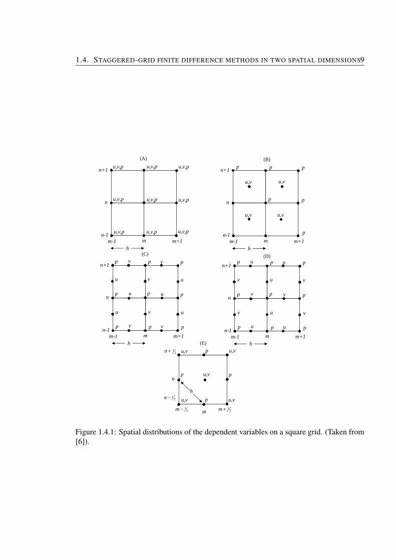
1.4.1 Spatial distributions of the dependent variables on a square
grid. (Taken from [6]). . . . . . . . . . . . . . . . . . . . . . . . . . . . 9
2.2.1 Electromagnetic waves propagate in a channel. . . . . . . . . . . . . . . . 21
2.2.2 Schematic showing a shallow water flow. . . . . . . . . . . . . . . . . . . 22
2.5.1 Distributions of the dependent variables on A-, B-, C-grids.
(The figure is reillustrated from [6]). . . . . . . . . . . . . . . . . . . . . 31
2.6.1 The arrangement of variables on a C-grid. . . . . . . . . . . . . . . . . . 34
2.7.1 (a) The frequency, (b) the wave speed, and (c) the group speed
for the case f = 0. . . . . . . . . . . . . . . . . . . . . . . . . . . . . . . 45
2.7.2 The dispersion relations for the continuum and finite-
difference approximation based on the A, B, and C-grids
without rotation effects, f = 0. . . . . . . . . . . . . . . . . . . . . . . . 46
2.7.3 The dispersion relations for the continuum and finite-
difference approximation based on the A, B, and C-grids with
the effects of rotation. The left column is for LD/h = 2, and
the right for LD/h = 0.1. . . . . . . . . . . . . . . . . . . . . . . . . . . 47
3.1.1 Wave propagation in a channel. . . . . . . . . . . . . . . . . . . . . . . . 53
3.3.1 (a) The Arakawa C-grid and (b) the configuration of aligned
boundaries for a channel. . . . . . . . . . . . . . . . . . . . . . . . . . . 55
x
3.3.2 The numerical solution v for wave propagation along the
aligned channel at different mode j = 1, 2, 3 with along chan-
nel wavenumber k = 1, and grid spacing h = 1/20. . . . . . . . . . . . . 59
3.3.3 The convergence plot of ωd for wave propagation along a
channel with aligned boundaries for mode j = 1, 2, 3 and
k = 1. The slope of the lines are 1.9992 (mode j = 1), 1.9971
(mode j = 2) and 1.9935 (mode j = 3), indicate second-order
convergence. . . . . . . . . . . . . . . . . . . . . . . . . . . . . . . . . . 59
3.3.4 The convergence plot of v for wave propagation along the
channel with aligned boundaries for mode j = 1, 2, 3 with
k = 1. The slope of the lines are 1.9907 (mode j = 1), 1.9659
(mode j = 1), and 1.9467 (mode j = 3), indicate second-
order convergence. . . . . . . . . . . . . . . . . . . . . . . . . . . . . . 60
3.3.5 The frequency ω for wave propagation along the channel with
aligned boundaries with horizontal wavenumber k = 1 and
modes j = 1, 2, 3 at various grid spacing h. Black represents
ω for j = 1, blue for j = 2, and red for j = 3. . . . . . . . . . . . . . . . 60
3.4.1 (a) The new indices in the transformation coordinate axes, and
(b) the computational domain of the tilted channel with stair-
case boundaries. . . . . . . . . . . . . . . . . . . . . . . . . . . . . . . . 65
3.4.2 The continuum and numerical solutions for P at four different
cross-channel modes j for along-channel wavenumber k = 1
with grid boxes across channel N∗ = 100, i.e., h =√
2/100. . . . . . . . 69
3.4.3 The differences in P for different cross-channel modes j for
along-channel wavenumber k = 1 with grid boxes across
channel N∗ = 100, i.e., h =√
2/100. . . . . . . . . . . . . . . . . . . . 70
xi
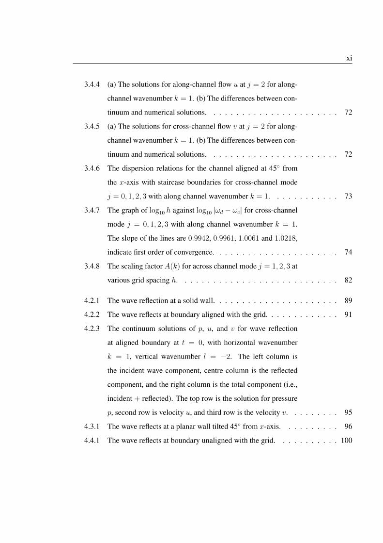
3.4.4 (a) The solutions for along-channel flow u at j = 2 for along-
channel wavenumber k = 1. (b) The differences between con-
tinuum and numerical solutions. . . . . . . . . . . . . . . . . . . . . . . 72
3.4.5 (a) The solutions for cross-channel flow v at j = 2 for along-
channel wavenumber k = 1. (b) The differences between con-
tinuum and numerical solutions. . . . . . . . . . . . . . . . . . . . . . . 72
3.4.6 The dispersion relations for the channel aligned at 45◦ from
the x-axis with staircase boundaries for cross-channel mode
j = 0, 1, 2, 3 with along channel wavenumber k = 1. . . . . . . . . . . . 73
3.4.7 The graph of log10 h against log10 |ωd − ωc| for cross-channel
mode j = 0, 1, 2, 3 with along channel wavenumber k = 1.
The slope of the lines are 0.9942, 0.9961, 1.0061 and 1.0218,
indicate first order of convergence. . . . . . . . . . . . . . . . . . . . . . 74
3.4.8 The scaling factor A(k) for across channel mode j = 1, 2, 3 at
various grid spacing h. . . . . . . . . . . . . . . . . . . . . . . . . . . . 82
4.2.1 The wave reflection at a solid wall. . . . . . . . . . . . . . . . . . . . . . 89
4.2.2 The wave reflects at boundary aligned with the grid. . . . . . . . . . . . . 91
4.2.3 The continuum solutions of p, u, and v for wave reflection
at aligned boundary at t = 0, with horizontal wavenumber
k = 1, vertical wavenumber l = −2. The left column is
the incident wave component, centre column is the reflected
component, and the right column is the total component (i.e.,
incident + reflected). The top row is the solution for pressure
p, second row is velocity u, and third row is the velocity v. . . . . . . . . 95
4.3.1 The wave reflects at a planar wall tilted 45◦ from x-axis. . . . . . . . . . 96
4.4.1 The wave reflects at boundary unaligned with the grid. . . . . . . . . . . 100
xii
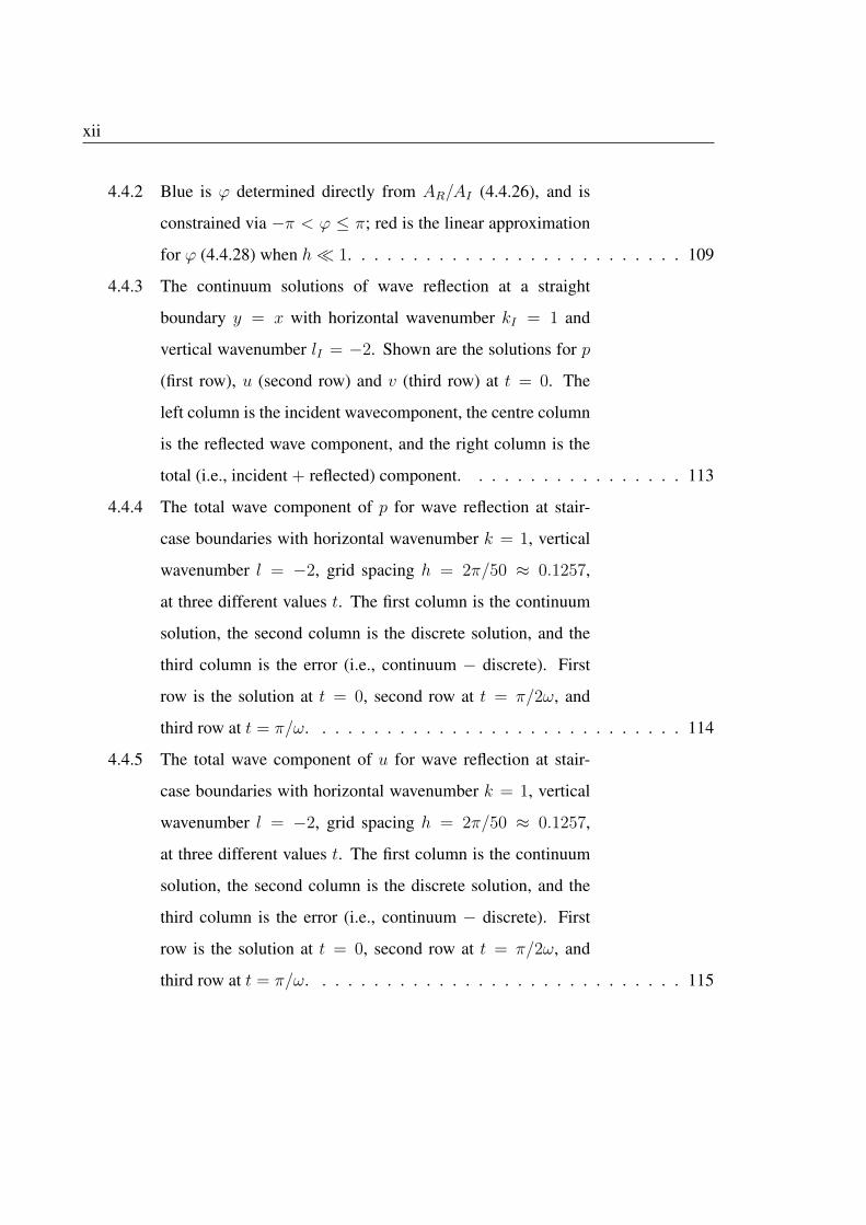
4.4.2 Blue is ϕ determined directly from AR/AI (4.4.26), and is
constrained via −π < ϕ ≤ π; red is the linear approximation
for ϕ (4.4.28) when h� 1. . . . . . . . . . . . . . . . . . . . . . . . . . 109
4.4.3 The continuum solutions of wave reflection at a straight
boundary y = x with horizontal wavenumber kI = 1 and
vertical wavenumber lI = −2. Shown are the solutions for p
(first row), u (second row) and v (third row) at t = 0. The
left column is the incident wavecomponent, the centre column
is the reflected wave component, and the right column is the
total (i.e., incident + reflected) component. . . . . . . . . . . . . . . . . 113
4.4.4 The total wave component of p for wave reflection at stair-
case boundaries with horizontal wavenumber k = 1, vertical
wavenumber l = −2, grid spacing h = 2π/50 ≈ 0.1257,
at three different values t. The first column is the continuum
solution, the second column is the discrete solution, and the
third column is the error (i.e., continuum − discrete). First
row is the solution at t = 0, second row at t = π/2ω, and
third row at t = π/ω. . . . . . . . . . . . . . . . . . . . . . . . . . . . . 114
4.4.5 The total wave component of u for wave reflection at stair-
case boundaries with horizontal wavenumber k = 1, vertical
wavenumber l = −2, grid spacing h = 2π/50 ≈ 0.1257,
at three different values t. The first column is the continuum
solution, the second column is the discrete solution, and the
third column is the error (i.e., continuum − discrete). First
row is the solution at t = 0, second row at t = π/2ω, and
third row at t = π/ω. . . . . . . . . . . . . . . . . . . . . . . . . . . . . 115
xiii
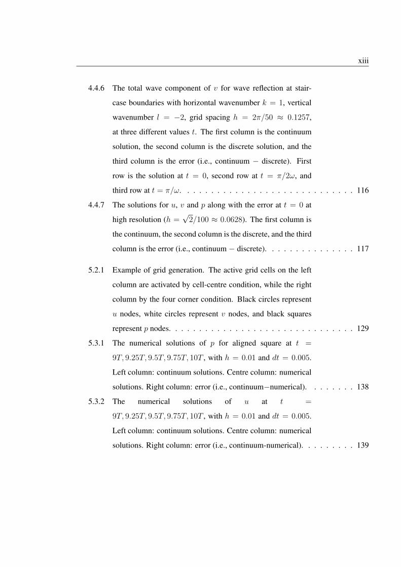
4.4.6 The total wave component of v for wave reflection at stair-
case boundaries with horizontal wavenumber k = 1, vertical
wavenumber l = −2, grid spacing h = 2π/50 ≈ 0.1257,
at three different values t. The first column is the continuum
solution, the second column is the discrete solution, and the
third column is the error (i.e., continuum − discrete). First
row is the solution at t = 0, second row at t = π/2ω, and
third row at t = π/ω. . . . . . . . . . . . . . . . . . . . . . . . . . . . . 116
4.4.7 The solutions for u, v and p along with the error at t = 0 at
high resolution (h =√
2/100 ≈ 0.0628). The first column is
the continuum, the second column is the discrete, and the third
column is the error (i.e., continuum − discrete). . . . . . . . . . . . . . . 117
5.2.1 Example of grid generation. The active grid cells on the left
column are activated by cell-centre condition, while the right
column by the four corner condition. Black circles represent
u nodes, white circles represent v nodes, and black squares
represent p nodes. . . . . . . . . . . . . . . . . . . . . . . . . . . . . . . 129
5.3.1 The numerical solutions of p for aligned square at t =
9T, 9.25T, 9.5T, 9.75T, 10T , with h = 0.01 and dt = 0.005.
Left column: continuum solutions. Centre column: numerical
solutions. Right column: error (i.e., continuum−numerical). . . . . . . . 138
5.3.2 The numerical solutions of u at t =
9T, 9.25T, 9.5T, 9.75T, 10T , with h = 0.01 and dt = 0.005.
Left column: continuum solutions. Centre column: numerical
solutions. Right column: error (i.e., continuum-numerical). . . . . . . . . 139
xiv
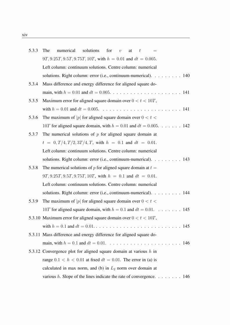
5.3.3 The numerical solutions for v at t =
9T, 9.25T, 9.5T, 9.75T, 10T , with h = 0.01 and dt = 0.005.
Left column: continuum solutions. Centre column: numerical
solutions. Right column: error (i.e., continuum-numerical). . . . . . . . . 140
5.3.4 Mass difference and energy difference for aligned square do-
main, with h = 0.01 and dt = 0.005. . . . . . . . . . . . . . . . . . . . . 141
5.3.5 Maximum error for aligned square domain over 0 < t < 10T ,
with h = 0.01 and dt = 0.005. . . . . . . . . . . . . . . . . . . . . . . . 141
5.3.6 The maximum of |p| for aligned square domain over 0 < t <
10T for aligned square domain, with h = 0.01 and dt = 0.005. . . . . . . 142
5.3.7 The numerical solutions of p for aligned square domain at
t = 0, T/4, T/2, 3T/4, T , with h = 0.1 and dt = 0.01.
Left column: continuum solutions. Centre column: numerical
solutions. Right column: error (i.e., continuum-numerical). . . . . . . . . 143
5.3.8 The numerical solutions of p for aligned square domain at t =
9T, 9.25T, 9.5T, 9.75T, 10T , with h = 0.1 and dt = 0.01.
Left column: continuum solutions. Centre column: numerical
solutions. Right column: error (i.e., continuum-numerical). . . . . . . . . 144
5.3.9 The maximum of |p| for aligned square domain over 0 < t <
10T for aligned square domain, with h = 0.1 and dt = 0.01. . . . . . . . 145
5.3.10 Maximum error for aligned square domain over 0 < t < 10T ,
with h = 0.1 and dt = 0.01. . . . . . . . . . . . . . . . . . . . . . . . . . 145
5.3.11 Mass difference and energy difference for aligned square do-
main, with h = 0.1 and dt = 0.01. . . . . . . . . . . . . . . . . . . . . . 146
5.3.12 Convergence plot for aligned square domain at various h in
range 0.1 < h < 0.01 at fixed dt = 0.01. The error in (a) is
calculated in max norm, and (b) in L2 norm over domain at
various h. Slope of the lines indicate the rate of convergence. . . . . . . . 146
xv
5.3.13 Error for u, v and p in aligned square domain at h = 0.01 and
dt = 0.01. . . . . . . . . . . . . . . . . . . . . . . . . . . . . . . . . . . 147
5.4.1 The solutions of p for square domain tilted at 45◦ at t =
0, T/4, T/2, 3T/4, T , with h = 0.1 and dt = 0.01. Left
column: continuum solutions. Centre column: numerical
solutions. Right column: error (i.e., continuum-numerical). . . . . . . . . 149
5.4.2 The solutions of p for square domain tilted at 45◦ at t =
9T, 9.25T, 9.5T, 9.75T, 10T , with h = 0.1 and dt = 0.01.
Left column: continuum solutions. Centre column: numerical
solutions. Right column: error (i.e., continuum-numerical). . . . . . . . . 150
5.4.3 The solutions of u for square domain tilted at 45◦ at t =
0, T/4, T/2, 3T/4, T , with h = 0.1 and dt = 0.01. Left
column: continuum solutions. Centre column: numerical
solutions. Right column: error (i.e., continuum-numerical). . . . . . . . . 151
5.4.4 The solutions of v for square domain tilted at 45◦ at t =
0, T/4, T/2, 3T/4, T , with h = 0.1 and dt = 0.01. Left
column: continuum solutions. Centre column: numerical
solutions. Right column: error (i.e., continuum-numerical). . . . . . . . . 152
5.4.5 The maximum of |p| over square domain tilted at 45◦ at h =
0.1, dt = 0.01 over 0 < t < 10T . . . . . . . . . . . . . . . . . . . . . . . 153
5.4.6 Maximum error over square domain tilted at 45◦, over 0 < t <
10T at h = 0.1, dt = 0.01. . . . . . . . . . . . . . . . . . . . . . . . . . 153
5.4.7 Mass and energy difference for square domain tilted at 45◦, at
h = 0.1, dt = 0.01. . . . . . . . . . . . . . . . . . . . . . . . . . . . . . 154
5.4.8 The solutions of p for square domain tilted at 45◦ at t =
9T, 9.25T, 9.5T, 9.75T, 10T , with h = 0.01 and dt = 0.005.
Left column: continuum solutions. Centre column: numerical
solutions. Right column: error (i.e., continuum-numerical). . . . . . . . . 156
xvi
5.4.9 The solutions of u for square domain tilted at 45◦ at t =
9T, 9.25T, 9.5T, 9.75T, 10T , with h = 0.01 and dt = 0.005.
Left column: continuum solutions. Centre column: numerical
solutions. Right column: error (i.e., continuum-numerical). . . . . . . . . 157
5.4.10 The solutions of v for square domain tilted at 45◦ at t =
9T, 9.25T, 9.5T, 9.75T, 10T , with h = 0.01 and dt = 0.005.
Left column: continuum solutions. Centre column: numerical
solutions. Right column: error (i.e., continuum-numerical). . . . . . . . . 158
5.4.11 The maximum |p| for square domain tilted at 45◦ with h =
0.01, dt = 0.005 over 0 < t < 10T . . . . . . . . . . . . . . . . . . . . . 159
5.4.12 Maximum error for square domain tilted at 45◦, at h = 0.01
and dt = 0.005 over 0 < t < 10T . . . . . . . . . . . . . . . . . . . . . . 159
5.4.13 Mass and energy difference for square domain tilted at 45◦,
with h = 0.01, dt = 0.005 over 0 < t < 10T . . . . . . . . . . . . . . . . 160
5.4.14 Convergence plot for square domain tilted at 45◦, at various
h in range 0.003 < h < 0.03 at fixed dt = 0.003. (a) is
convergence in max norm, and (b) in L2 norm over domain.
Slope of the lines indicate the rate of convergence. . . . . . . . . . . . . 160
5.4.15 Maximum error for u, v and p in square domain tilted at 45◦,
at h = 0.003 and dt = 0.003. . . . . . . . . . . . . . . . . . . . . . . . . 161
5.5.1 Maximum error for u, v and p in square domain tilted at 5◦, at
h = 0.003 and dt = 0.003. . . . . . . . . . . . . . . . . . . . . . . . . . 162
5.5.2 Maximum error for u, v and p in square domain tilted at 10◦,
at h = 0.003 and dt = 0.003. . . . . . . . . . . . . . . . . . . . . . . . . 162
5.5.3 Maximum error for u, v and p in square domain tilted at 15◦,
at h = 0.003 and dt = 0.003. . . . . . . . . . . . . . . . . . . . . . . . . 162
5.5.4 Maximum error for u, v and p in square domain tilted at 30◦,
at h = 0.003 and dt = 0.003. . . . . . . . . . . . . . . . . . . . . . . . . 163
xvii
5.5.5 Maximum error of u, v and p for square domain tilted at
various angle of rotation with grid spacing (a) h = 0.1, (b)
h = 0.01. The maximum error is calculated over 0 < t <
10T ≈ t = 9. . . . . . . . . . . . . . . . . . . . . . . . . . . . . . . . . 163
5.5.6 Convergence plot for square domain tilted at 5◦, at various
h in range 0.003 < h < 0.03 at fixed dt = 0.003. (a) is
convergence in max norm, and (b) in L2 norm over domain.
Slope of the lines indicate the rate of convergence. . . . . . . . . . . . . 165
5.5.7 Convergence plot for square domain tilted at 10◦, at various
h in range 0.003 < h < 0.03 at fixed dt = 0.003. (a) is
convergence in max norm, and (b) in L2 norm over domain.
Slope of the lines indicate the rate of convergence. . . . . . . . . . . . . 165
5.5.8 Convergence plot for square domain tilted at 15◦, at various
h in range 0.003 < h < 0.03 at fixed dt = 0.003. (a) is
convergence in max norm, and (b) in L2 norm over domain.
Slope of the lines indicate the rate of convergence. . . . . . . . . . . . . 166
5.5.9 Convergence plot for square domain tilted at 30◦, at various
h in range 0.003 < h < 0.03 at fixed dt = 0.003. (a) is
convergence in max norm, and (b) in L2 norm over domain.
Slope of the lines indicate the rate of convergence. . . . . . . . . . . . . 166
5.5.10 Time series of kinetic and potential energy for waves in a
square domain over 0 < t < 1. . . . . . . . . . . . . . . . . . . . . . . . 168
5.5.11 The frequency of wave in aligned square domain, and log-log
plot error in frequency at various h. The slope of the line is
1.80398 with 95% confidence interval (1.045, 2.563). . . . . . . . . . . . 169
5.5.12 The frequency of wave in square domain tilted at 5◦, and log-
log plot error in frequency at various h. The slope of the line
is 1.2491. . . . . . . . . . . . . . . . . . . . . . . . . . . . . . . . . . . 169
xviii
5.5.13 The frequency of wave in square domain tilted at 10◦, and log-
log plot error in frequency at various h. The slope of the line
is 1.0505. . . . . . . . . . . . . . . . . . . . . . . . . . . . . . . . . . . 170
5.5.14 The frequency of wave in square domain tilted at 15◦, and log-
log plot error in frequency at various h. The slope of the line
is 1.064. . . . . . . . . . . . . . . . . . . . . . . . . . . . . . . . . . . . 170
5.5.15 The frequency of wave in square domain tilted at 30◦, and log-
log plot error in frequency at various h. The slope of the line
is 1.0417. . . . . . . . . . . . . . . . . . . . . . . . . . . . . . . . . . . 171
5.5.16 The frequency of wave in square domain tilted at 45◦, and log-
log plot error in frequency at various h. The slope of the line
is 1.27522, with 95% confidence interval (0.9113, 1.639). . . . . . . . . 171
5.6.1 The solutions of p for circle domain at t =
0, T/4, T/2, 3T/4, T , with h = 0.1 and dt = 0.01 for
mode m = 1, n = 0. Left column: continuum solutions.
Centre column: numerical solutions. Right column: error
(i.e., continuum-numerical). . . . . . . . . . . . . . . . . . . . . . . . . . 179
5.6.2 The solutions of p for circle domain at t =
9T, 9.25T, 9.5T, 9.75T, 10T , with h = 0.1 and dt = 0.01
for mode m = 1, n = 0. Left column: continuum solutions.
Centre column: numerical solutions. Right column: error
(i.e., continuum-numerical). . . . . . . . . . . . . . . . . . . . . . . . . . 180
5.6.3 The maximum |p| over circle domain at h = 0.1, dt = 0.01
for mode m = 1, n = 0. . . . . . . . . . . . . . . . . . . . . . . . . . . . 181
xix
5.6.4 The solutions of u for circcle domain at t =
0, T/4, T/2, 3T/4, T , with h = 0.1 and dt = 0.01 for
mode m = 1, n = 0. Left column: continuum solutions.
Centre column: numerical solutions. Right column: error
(i.e., continuum-numerical). . . . . . . . . . . . . . . . . . . . . . . . . . 182
5.6.5 The solutions of u for circle domain at t =
9T, 9.25T, 9.5T, 9.75T, 10T , with h = 0.1 and dt = 0.01
for mode m = 1, n = 0. Left column: continuum solutions.
Centre column: numerical solutions. Right column: error
(i.e., continuum-numerical). . . . . . . . . . . . . . . . . . . . . . . . . . 183
5.6.6 The solutions of v for circle domain at t =
0, T/4, T/2, 3T/4, T , with h = 0.1 and dt = 0.01 for
mode m = 1, n = 0. Left column: continuum solutions.
Centre column: numerical solutions. Right column: error
(i.e., continuum-numerical). . . . . . . . . . . . . . . . . . . . . . . . . . 184
5.6.7 The solutions of v for circle domain at t =
9T, 9.25T, 9.5T, 9.75T, 10T , with h = 0.1 and dt = 0.01
for mode m = 1, n = 0. Left column: continuum solutions.
Centre column: numerical solutions. Right column: error
(i.e., continuum-numerical). . . . . . . . . . . . . . . . . . . . . . . . . . 185
5.6.8 Maximum error over domain for 0 < t < 17 ≈ 10T , at h =
0.1, dt = 0.01, for mode m = 1, n = 0. . . . . . . . . . . . . . . . . . . 186
5.6.9 Mass and energy difference for circle domain, at h = 0.1,
dt = 0.01 over 0 < t < 17 ≈ 10T , for mode m = 1, n = 0. . . . . . . . . 186
xx
5.6.10 The solutions p for circle domain at t =
9T, 9.25T, 9.5T, 9.75T, 10T , with h = 0.01 and dt = 0.005
for mode m = 1, n = 0. Left column: continuum solutions.
Centre column: numerical solutions. Right column: error
(i.e., continuum-numerical). . . . . . . . . . . . . . . . . . . . . . . . . . 187
5.6.11 The maximum of |p| over 0 < t < 17 ≈ 10T at h = 0.01 with
dt = 0.005 for circle domain mode m = 1, n = 0. . . . . . . . . . . . . . 188
5.6.12 Maximum error over domain at 0 < t < 17 ≈ 10T , h = 0.01,
dt = 0.005 for mode m = 1, n = 0. . . . . . . . . . . . . . . . . . . . . 188
5.6.13 Mass and energy difference for circle domain, at h = 0.01,
dt = 0.005 over 0 < t < 17 ≈ 10T , for mode m = 1, n = 0. . . . . . . . 189
5.6.14 Convergence plot for circle domain with mode m = 1, n = 0
at various h in range 0.2 < h < 0.02 at fixed dt = 0.02. The
error in (a) is calculated in max norm, and (b) in L2 norm over
domain. Slope of the line is summarised in Table 5.9, indicate
the rate of convergence. . . . . . . . . . . . . . . . . . . . . . . . . . . 189
5.6.15 The frequency of wave in circle domain with mode m =
1, n = 0, and log-log plot error in frequency at various h.
The slope of the line is 1.66158, with 95% confidence interval
(1.002, 2.321). The scaling factor is 1.00801. . . . . . . . . . . . . . . . 190
5.6.16 The solutions for p at t = 0, 0.25T, 0.5T, 0.75T, T with h =
0.1, dt = 0.05, for m = 1, n = 1. Left column: continuum
solutions. Centre column: numerical solutions. Right column:
error (i.e., continuum-numerical). . . . . . . . . . . . . . . . . . . . . . . 191
5.6.17 The solutions for p at t = 9T, 9.25T, 9.5T, 9.75T, 10T with
h = 0.1, dt = 0.05, for m = 1, n = 1. Left column: con-
tinuum solutions. Centre column: numerical solutions. Right
column: error (i.e., continuum-numerical). . . . . . . . . . . . . . . . . . 192
xxi
5.6.18 The solutions for u at t = 0, 0.25T, 0.5T, 0.75T, T with h =
0.1, dt = 0.05, for m = 1, n = 1. Left column: continuum
solutions. Centre column: numerical solutions. Right column:
error (i.e., continuum-numerical). . . . . . . . . . . . . . . . . . . . . . . 193
5.6.19 The solutions for u at t = 9T, 9.25T, 9.5T, 9.75T, 10T with
h = 0.1, dt = 0.05, for m = 1, n = 1. Left column: con-
tinuum solutions. Centre column: numerical solutions. Right
column: error (i.e., continuum-numerical). . . . . . . . . . . . . . . . . . 194
5.6.20 The solutions for v at t = 0, 0.25T, 0.5T, 0.75T, T with h =
0.1, dt = 0.05, for m = 1, n = 1. Left column: continuum
solutions. Centre column: numerical solutions. Right column:
error (i.e., continuum-numerical). . . . . . . . . . . . . . . . . . . . . . . 195
5.6.21 The solutions for v at t = 9T, 9.25T, 9.5T, 9.75T, 10T with
h = 0.1, dt = 0.05, for m = 1, n = 1. Left column: con-
tinuum solutions. Centre column: numerical solutions. Right
column: error (i.e., continuum-numerical). . . . . . . . . . . . . . . . . . 196
5.6.22 The maximum |p| for circle domain at h = 0.1 with dt = 0.01,
over 0 < t < 10T with mode m = 1, n = 1. . . . . . . . . . . . . . . . . 197
5.6.23 Maximum error over 0 < t < 10T for circle domain at h =
0.1, dt = 0.01 with mode m = 1, n = 1. . . . . . . . . . . . . . . . . . . 197
5.6.24 Mass and energy difference for circle domain, at h = 0.1,
dt = 0.01 over 0 < t < 10T ≈ t = 35, for mode m = 1, n = 1. . . . . . . 198
5.6.25 The solutions for p at t = 9T, 9.25T, 9.5T, 9.75T, 10T with
h = 0.01, dt = 0.005, for m = 1, n = 1. Left column: con-
tinuum solutions. Centre column: numerical solutions. Right
column: error (i.e., continuum-numerical). . . . . . . . . . . . . . . . . . 199
xxii
5.6.26 The solutions for u at t = 9T, 9.25T, 9.5T, 9.75T, 10T with
h = 0.01, dt = 0.005, for m = 1, n = 1. Left column: con-
tinuum solutions. Centre column: numerical solutions. Right
column: error (i.e., continuum-numerical). . . . . . . . . . . . . . . . . . 204
5.6.27 The solutions for v at t = 9T, 9.25T, 9.5T, 9.75T, 10T with
h = 0.01, dt = 0.005, for m = 1, n = 1. Left column: con-
tinuum solutions. Centre column: numerical solutions. Right
column: error (i.e., continuum-numerical). . . . . . . . . . . . . . . . . . 205
5.6.28 The maximum |p| for circle domain at h = 0.01 with dt =
0.005, over 0 < t < 10T with mode m = 1, n = 1. . . . . . . . . . . . . 206
5.6.29 Maximum error for u, v and p over 0 < t < 10T , for circle
domain, at h = 0.01, dt = 0.005 with mode m = 1, n = 1. . . . . . . . . 206
5.6.30 Mass and energy difference for circle domain, at h = 0.01,
dt = 0.005 over 0 < t < 10T ≈ t = 35, for mode m = 1, n = 1. . . . . . 207
5.6.31 Convergence plot for circle domain with mode m = 1, n = 1
at various h in range 0.2 < h < 0.02 at fixed dt = 0.02. The
error in (a) is calculated in max norm, and (b) in L2 norm over
domain. Slope of the lines is summarised in Table 5.10. . . . . . . . . . . 207
5.6.32 Maximum error in u, v and p for circle domain with mode
m = 1, n = 1, at h = 0.01 and dt = 0.01. . . . . . . . . . . . . . . . . . 208
5.6.33 The frequency of wave in circle domain with mode m =
1, n = 1 at various h, and log-log plot error in frequency at
various h. The slope of the line is 1.08843, with 95% confid-
ence interval (0.7236, 1.453). The scaling factor is 0.305429. . . . . . . . 208

xxiii
5.6.34 The solutions of p for circle domain at t =
0, 0.25T, 0.5T, 0.75T, T , with h = 0.1 and dt = 0.01,
with mode m = 1, n = 0 using 4 corners of cell activation.
Left column: continuum solutions. Centre column: numerical
solutions. Right column: error (i.e., continuum-numerical). . . . . . . . . 209
5.6.35 The solutions of p for circle domain at t =
9T, 9.25T, 9.5T, 9.75T, 10T , with h = 0.1 and dt = 0.01,
with mode m = 1, n = 0 using 4 corners of cell activation.
Left column: continuum solutions. Centre column: numerical
solutions. Right column: error (i.e., continuum-numerical). . . . . . . . . 210
5.6.36 The maximum |p| for circle domain at h = 0.1 with dt = 0.01,
over 0 < t < 10T with mode m = 1, n = 0. The active grid
is chosen according to 4 corners of each cells. . . . . . . . . . . . . . . . 211
5.6.37 Maximum error for u, v and p over 0 < t < 10T ≈ t = 17,
for circle domain, at h = 0.1, dt = 0.01 with mode m = 1,
n = 0. The active grid is chosen according to 4 corners of each cells. . . . 211
5.6.38 The solutions of u for circle domain at t =
0, 0.25T, 0.5T, 0.75T, T , with h = 0.1 and dt = 0.01,
with mode m = 1, n = 0 using 4 corners of cell activation.
Left column: continuum solutions. Centre column: numerical
solutions. Right column: error (i.e., continuum-numerical). . . . . . . . . 212
5.6.39 The solutions of v for circle domain at t =
0, 0.25T, 0.5T, 0.75T, T , with h = 0.1 and dt = 0.01,
with mode m = 1, n = 0 using 4 corners of cell activation.
Left column: continuum solutions. Centre column: numerical
solutions. Right column: error (i.e., continuum-numerical). . . . . . . . . 213
xxiv
5.6.40 The maximum |u| for circle domain at h = 0.1 with dt = 0.01,
over 0 < t < 10T with mode m = 1, n = 1. The active grid
is chosen according to 4 corners of each cells. . . . . . . . . . . . . . . . 214
5.6.41 The maximum |v| for circle domain at h = 0.1 with dt = 0.01,
over 0 < t < 10T with mode m = 1, n = 1. The active grid
is chosen according to 4 corners of each cells. . . . . . . . . . . . . . . . 214
5.6.42 Mass and energy difference for circle domain, at h = 0.1,
dt = 0.01 over 0 < t < 10T ≈ t = 17, for mode m = 1,
n = 0. The active grid is chosen according to 4 corners of each cells. . . . 215
5.6.43 The solutions of p for circle domain at t =
0, 0.25T, 0.5T, 0.75T, T , with h = 0.01 and dt = 0.005, with
mode m = 1, n = 0 using 4 corners of cell activation. Left
column: continuum solutions. Centre column: numerical
solutions. Right column: error (i.e., continuum-numerical). . . . . . . . . 216
5.6.44 The solutions of p for circle domain at t =
9T, 9.25T, 9.5T, 9.75T, 10T , with h = 0.01 and dt = 0.005,
with mode m = 1, n = 0 using 4 corners of cell activation.
Left column: continuum solutions. Centre column: numerical
solutions. Right column: error (i.e., continuum-numerical). . . . . . . . . 217
5.6.45 The maximum |p| for circle domain at h = 0.01 with dt =
0.005, over 0 < t < 10T with mode m = 1, n = 1. The
active grid is chosen according to 4 corners of each cells. . . . . . . . . . 218
5.6.46 Maximum error for u, v and p over 0 < t < 10T , for circle
domain, at h = 0.01, dt = 0.005 with mode m = 1, n = 0.
The active grid is chosen according to 4 corners of each cells. . . . . . . . 218

xxv
5.6.47 The solutions of u for circle domain at t =
9T, 9.25T, 9.5T, 9.75T, 10T , with h = 0.01 and dt = 0.005,
with mode m = 1, n = 0 using 4 corners of cell activation.
Left column: continuum solutions. Centre column: numerical
solutions. Right column: error (i.e., continuum-numerical). . . . . . . . . 219
5.6.48 The solutions of v for circle domain at t =
9T, 9.25T, 9.5T, 9.75T, 10T , with h = 0.01 and dt = 0.005,
with mode m = 1, n = 0 using 4 corners of cell activation.
Left column: continuum solutions. Centre column: numerical
solutions. Right column: error (i.e., continuum-numerical). . . . . . . . . 220
5.6.49 Mass and energy difference for circle domain, at h = 0.01,
dt = 0.005 over 0 < t < 10T ≈ t = 17, for mode m = 1,
n = 0. The active grid is chosen according to 4 corners of each cells. . . . 221
5.6.50 The log-log plot of maximum error over (a) 0 < t < 10T ≈
t = 17, and (b) 0 < t < t ≈ 2 > T , at various grid spacing
h. The slope of the lines indicate the rate of convergence. The
slope in (b) are: u and v are 0.905945, with 95% confidence
interval (0.8362, 0.9757), p is 0.5498, with 95% confidence
interval (0.5049, 0.5948). The active grid is chosen according
to 4 corners of each cells. . . . . . . . . . . . . . . . . . . . . . . . . . . 221
6.3.1 Different choice of variables staggering on a C-grid. . . . . . . . . . . . . 236
6.4.1 The mechanism of internal wave reflection at a sloping bound-
ary. (a) reflection at a shallow slope, (b) reflection at β > ϕ.
This figure is re-illustrated from [53]. . . . . . . . . . . . . . . . . . . . . 238
6.4.2 Internal wave reflection at staircase boundary on the C-grid. . . . . . . . . 243
xxvi
6.5.1 Evolution of buoyancy, b at t = 0, 100, 200, 300, 400, 500
(i.e.,0 < t < 50T ) with mode (l, n) = (1, 1) at h = 0.002,
dt = 0.05. The period of wave is T = 2π/ω = 2√
2π ≈
8.8858. . . . . . . . . . . . . . . . . . . . . . . . . . . . . . . . . . . . 255
6.5.2 Evolution of buoyancy, b at t =
1000, 1500, 2000, 2500, 3000, 3500 (i.e., 100T < t < 350T )
with mode (l, n) = (1, 1) at h = 0.002, dt = 0.05. . . . . . . . . . . . . 255
6.5.3 Evolution of buoyancy, b at t = 0, 100, 200, 300, 400, 500 (i.e.,
0 < t < 25T ) with mode (l, n) = (1, 3) at h = 0.002, dt =
0.05. The period is T = 2π/ω = 2√
10π ≈ 19.8692. . . . . . . . . . . . 256
6.5.4 Evolution of buoyancy, b at t =
1000, 1500, 2000, 2500, 3000, 3500 (i.e., 50T < t < 175T )
with mode (l, n) = (1, 3) at h = 0.002, dt = 0.05. . . . . . . . . . . . . . 256
6.5.5 The evolution of buoyancy b at t = 5, 50, 100, 150, 200 for
(l, n) = (1, 1), ω/Nf = 0.74. Gravity tilted at angle 7π/72.
The left column is the results using [11] attractor initial con-
dition. On the right column, the results with (6.5.5) normal
mode initial condition with parametric excitation. . . . . . . . . . . . . . 259
6.5.6 Energy analysis for the simulations on normal mode (right
column Figure 6.5.5), (l, n) = (1, 1), ωc = 1.55786, ωd =
1.50097, |ωc − ωd| = 0.056882. . . . . . . . . . . . . . . . . . . . . . . 260
6.5.7 The evolution of buoyancy b at t = 5, 50, 100, 150, 200 for
(l, n) = (1, 3), ω/Nf = 0.34. Gravity tilted at angle π/18.
The left column is the results with [11] attractor initial con-
dition. On the right column, the results with (6.5.5) normal
mode initial condition with parametric excitation. . . . . . . . . . . . . . 261
xxvii
6.5.8 Energy analysis for the simulations on normal mode (right
column Figure 6.5.7), (l, n) = (1, 3), ωc = 1.54485, ωd =
1.46097, |ωc − ωd| = 0.0838847. . . . . . . . . . . . . . . . . . . . . . . 262
A.0.1 Modulus of amplification factor for the Euler’s scheme as a
function of ∆t . . . . . . . . . . . . . . . . . . . . . . . . . . . . . . . . 280
A.0.2 Convergence plot for RK-2 method. . . . . . . . . . . . . . . . . . . . . 282
A.0.3 Modulus of amplification factor for the RK-4 scheme as a
function of ∆t. . . . . . . . . . . . . . . . . . . . . . . . . . . . . . . . 284
A.0.4 Convergence plot for RK-4 method. . . . . . . . . . . . . . . . . . . . . 285
A.0.5 Modulus of amplification factor for the AB-2 scheme as a
function of ∆t. . . . . . . . . . . . . . . . . . . . . . . . . . . . . . . . 287
A.0.6 Convergence plot for AB-2 method. . . . . . . . . . . . . . . . . . . . . 287
A.0.7 Convergence plot for Leapfrog method. . . . . . . . . . . . . . . . . . . 289
A.0.8 Modulus of amplification factor for the AB-3 scheme as a
function of ∆t. . . . . . . . . . . . . . . . . . . . . . . . . . . . . . . . 290
A.0.9 Convergence plot for AB-3 method. . . . . . . . . . . . . . . . . . . . . 291
xxviii
List of Tables
5.1 The convergence rate of u, v and p in max norm and L2 norm,
for aligned square domain. . . . . . . . . . . . . . . . . . . . . . . . . . . 142
5.2 The confidence interval of u, v and p in max norm for aligned
square domain. . . . . . . . . . . . . . . . . . . . . . . . . . . . . . . . . 142
5.3 The convergence rate of u, v and p in max norm and L2 norm,
for square domain tilted at 45◦. . . . . . . . . . . . . . . . . . . . . . . . . 155
5.4 The convergence rate of u, v and p in max norm and L2 norm,
for square domain tilted at 5◦. . . . . . . . . . . . . . . . . . . . . . . . . 163
5.5 The convergence rate of u, v and p in max norm and L2 norm,
for square domain tilted at 10◦. . . . . . . . . . . . . . . . . . . . . . . . . 164
5.6 The convergence rate of u, v and p in max norm and L2 norm,
for square domain tilted at 15◦. . . . . . . . . . . . . . . . . . . . . . . . . 164
5.7 The convergence rate of u, v and p in max norm and L2 norm,
for square domain tilted at 30◦. . . . . . . . . . . . . . . . . . . . . . . . . 164
5.8 The scaling factors C and scaling exponents n, along with 95%
confidence interval for error in frequency, at various θ. The val-
ues are numerically determined at fixed dt = 0.003 and grid
spacing 0.003 < h < 0.03. . . . . . . . . . . . . . . . . . . . . . . . . . . 168
5.9 The convergence rate of u, v and p in max norm and L2 norm,
for circle domain with mode m = 1, n = 0. The slope of the
lines in Figure 5.6.14. . . . . . . . . . . . . . . . . . . . . . . . . . . . . 178
xxix
5.10 The convergence rate of u, v and p in max norm and L2 norm,
for circle domain with mode m = 1, n = 1. The slope is for the
lines in Figure 5.6.31, indicate the rate of convergence. . . . . . . . . . . . 188
5.11 The convergence rate for u, v and p in max norm and L2 norm,
at various h for the specific domain. . . . . . . . . . . . . . . . . . . . . . 203
5.12 The convergence rate obtained by [67] for the case of wave re-
flection at specific domain in L2 norm. The convergence rate is
measured at three grid spacings. . . . . . . . . . . . . . . . . . . . . . . . 203
7.1 The relative error ∆ for wave propagation along a channel with
aligned boundaries and unaligned boundaries for j = 0, k = 1. . . . . . . . 271
7.2 The relative error ∆ for wave propagation along a channel with
aligned boundaries and unaligned boundaries for j = 0, k = 2. . . . . . . . 271
7.3 The relative error ∆ for wave propagation along a channel with
aligned boundaries and unaligned boundaries for j = 1, k = 1. . . . . . . . 272
7.4 The relative error ∆ for wave propagation along a channel with
aligned boundaries and unaligned boundaries for j = 5, k = 1. . . . . . . . 272
7.5 The convergence rate for u, v and p in max norm and L2 norm,
at various h for the specific domain. . . . . . . . . . . . . . . . . . . . . . 273

xxx
1
Chapter 1
INTRODUCTION
1.1 Waves
Wave phenomena are abundant in nature. They exist across a wide range of lengthscales and
timescales, from short wavelength electromagnetic waves moving at the speed of light, to
planetary-scale waves moving in the deep ocean at walking pace. Perhaps the most common
waves are water waves (visible on the surface of the sea), sound waves (or acoustic waves)
that we hear everyday, and light waves electromagnetic waves – all of them are around us.
Such waves have long been a phenomenon of great scientific interest. But they are not
only a curiosity for us, due to the fundamental role that they play in many systems, and the
possibility of exploiting their abundance. For example, waves have enabled us to infer the
structure of the Earth through seismology, and form the basis of modern communication.
Waves are generated by a disturbance of a material parcel around an equlibrium position.
In doing so, a so-called ‘restoring force’ is often generated, which pulls back the parcel
towards its original position. However, in the absence of friction or other damping, the
parcel overshoots in the opposite direction. The restoring force continues to act, but now to
reverse the direction of the original motion. This process continues, leading to an oscillatory
2 1. INTRODUCTION
motion of the material parcel. This well-understood mechanism is fundamental to almost
all waves, which can then be categorised by the different restoring forces that drive them.
In the case where the restoring force is induced by fluid pressure, the waves propagate as
regions of compression and rarefaction. In an elastic solid, these are the P-waves of seis-
mology; in a fluid, these are sound waves, first studied by [56]. These are examples of lon-
gitudinal waves, as particle movement is in the direction of wave travel (or the wavevector),
with an initial disturbance creating an area of high pressure. Particles are then forced out of
this region, only to ’bump’ into more particles, creating another high pressure area further
from the initial perturbation, and so on. They propagate through the Earth’s atmosphere
very quickly compared to other atmospheric effects such as the wind (at around 350 ms−1)
and through the ocean quicker still (around 1500 ms−1), owing to the higher density of the
water. They are also relatively small scale, compared with, say the familiar waves on a
beach; the wavelength of the sound of a typical human voice is around 3cm.
The restoring force can also be gravity. A displaced fluid parcel is forced back towards equi-
librium through gravitational buoyancy, leading to so-called gravity waves. These waves
which sometimes categorised as surface gravity waves can be observed on the surface of
the sea, where gravity playing a dominant role in the driving of the waves. In 1834, Scott
Russell observed a solitary wave propagating down a canal, maintaining its shape for ex-
tended periods of time [59]. These waves propagate at much slower speeds than sound
waves, typically at around 1-200 ms−1 compared to the 1500 ms−1 sound speed in water.
Another example of gravity waves is tsunami waves. These waves are a hundred kilometers
long which will propagate faster in the deep ocean. Surface tension can also contribute to
the restoring force of waves. The waves that travel by both the effects of surface tension
and gravity are called gravity-capillary waves. These waves are common in nature, and
are often referred to as ripples. Typically, the wavelength of these waves is less than the
wavelength of the gravity waves.
The other category of gravity wave is internal gravity wave, which occur within a fluid. The
1.2. MATHEMATICAL MODELLING OF WAVES 3
first internal waves were documented in 1792 by Benjamin Franklin, who conducted an ex-
periment with oil on water. Later, in 1898, Bjerknes attempted to explain the ‘dead water’
phenomenon using internal waves, which were subsequently investigated experimentally
by Ekman in 1904 [49]. These have also been observed in the ocean, with tracers or detect-
ors suspended in the fluid, or by using satellites such as the Earth Resources Technology
Satellite [5]. These waves arise in regions with changing bottom topography and tidal for-
cing [e.g.,[55, 9]]. Internal waves can also be found in the atmosphere. For example, the
so-called Morning Glory waves that are observed around 150m above the Australian coast,
first documented in the Royal Australian air force in 1942, travel at around 10 ms−1. As
well as travelling slower than sound waves, internal gravity waves also occur on much lar-
ger spatial scales: a crest of a wave in the Morning Glory wavetrain will have a wavelength
of approximately 10km, as documented by [18], compared to the 3cm wavelength of sound
waves.
There are many other examples of forces that give rise to waves; inertial waves, for example,
arise from the Coriolis force arising from the Earth’s rotation. Of course, when we say ‘the
restoring force’, we really mean the dominating restoring force; in reality this is not the only
force present on any system. For example, in the Earth’s oceans, typically both background
rotation and gravity simultaneously act, so that we are often interested in inertia-gravity
waves.
This thesis is concerned with waves in a quite general context, but we are mostly thinking
of applications to waves in fluids. So we are generally use terminology relating to sound
waves and gravity waves.
1.2 Mathematical modelling of waves
The mathematical modelling of waves date back to many scientists across many fields
across the centuries. Among many others, Daniel Bernoulli, Jean le Rond d’Alembert,

4 1. INTRODUCTION
Leonhard Euler, and Pierre-Simon Laplace realised that there was a similarity in the maths
of how to describe waves through solids and fluids. Common scientific concepts of wave
can connect seemingly disparate areas of science. In 1720s, Bernoulli, a Swiss mathem-
atician, applied Isaac Newton’s laws of motion to understand the propagation of waves in
the surrounding air which is interpreted as sound. He was a pioneer of the mathematical
theory of sound from vibrated violin string with fixed at each end.
For many systems, the waves are described by the wave equation
ηtt − c2∇2η = 0. (1.2.1)
Here η is a scalar representing a disturbance quantity (such as fluid pressure), t is time,
c is the (scalar) wave speed of the system, and ∇2 is the Laplacian operator (perhaps in
several spatial dimensions). In one spatial dimension x, (1.2.1) has the famous d’Alembert
solutions
η = A(x± ct), (1.2.2)
representing steady non-dispersive wave propagation in each direction. An underlying as-
sumption in (1.2.1) is that the waves can be modelled linearly, meaning that nonlinear terms
in the governing equations can be neglected. This is always the case for waves of suf-
ficiently small amplitude, but the assumption of linearity is often useful even for larger
amplitude waves, since it captures the restoring force that is fundamental to wave motion.
More generally, the waves will be governed by a system of partial differential equations
(PDEs), which will be more complicated than (1.2.1). However, again under the assumption
of linearity, these can often be reduced to an equation that is similar in form to (1.2.1). Such
equations are commonly analysed by seeking solutions∝ <(η exp(i(kx+ly−ωt))), where
ω is the frequency of the wave, and k and l are wavenumbers in the x and y directions –
here we are assuming just two dimensions, for simplicity, as in much of this thesis. The
governing PDE then only has non-trivial solutions, i.e., η 6= 0, when a so-called dispersion

1.2. MATHEMATICAL MODELLING OF WAVES 5
relation is satisfied:
ω = ω(k, l). (1.2.3)
For example, for (1.2.1) in two dimensions we obtain the simple dispersion relation ω2 =
c2(k2+l2). However, dispersion relations can be somewhat more complex. For example, for
internal gravity waves in 2D with x horizontal and y vertical, we obtain ω2 = N2k2/(k2 +
l2), where N is the buoyancy frequency of the fluid.
The above analysis ignores the presence of boundaries. Although these are usually irrel-
evant to the underlying restoring mechanism that drives the wave motion, their presence is
often critical in determining the spatial structure and frequency of the response. For ex-
ample, in a tubular music instrument, the boundaries lead to the possibility of musical tones
of discrete frequencies. In contrast, in the ocean, the boundaries can sometimes lead to the
existence of new classes of waves, such as the famous Kelvin wave that exists in coastal
waters. In all such examples, the governing PDEs must be solved subject to an approriate
boundary condition. This means we must impose a correct boundary conditions at every
point of our domain. For example, for a fluid medium and a solid boundary, there can be no
flow through it and thus the normal component of the velocity must be set to be zero. This is
commonly known as the no normal-flow boundary condition, and will be used throughout
this study.
When such boundaries are present, the dispersion relation is typically modified, in the form
ω = ω(kj, lj;L), (1.2.4)
where L encodes information about the shape and length of the domain, and the wavenum-
bers kj and lj now form a discrete set. For example, when solving (1.2.1) in a square
domain 0 < x < L and 0 < y < L, it is possible to show that there exist solutions
6 1. INTRODUCTION
η ∝ <(η sin kx sin ly exp(−iωt)) provided
ω2 = c2(k2m + l2n), where km =
mπ
Land ln =
nπ
L. (1.2.5)
1.3 Numerical solutions of wave equations
The solution of a wave equation is a main aim in any wave investigations. One can ob-
tain the solution by solving the equation analytically with the satisfied boundary condition.
However, the usefulness of these solutions is sometimes restricted to problems involving
shapes for which the boundary conditions can be satisfied. If this is the case, approximation
methods, whether analytical or numerical in character are the only means of solution, apart
from the use of analogue devices.
The oldest and most popular method to solve wave equation numerically is called finite-
difference method. It was first utilized by L. Euler in 1768 in one dimension, and was
extended to two dimensions by C. Runge in 1908 [14, 15]. The advent of the method in
real numerical calculations was documented by Lewis Fry Richardson in 1911 [57]. The
development of the method was stimulated by the emergence of computers that offered a
convenient framework for dealing with complex problems of science and technology. The
main principle in this method is the approximation of derivatives in the system of PDEs by
using the famous Taylor series expansion at the grid points. In this principle, the partial
derivatives are replaced by algebraic difference equations that are based on Taylor series
expansions. The set of continuum PDEs is totally converted into a large discrete system
of algebraic equations. For example, in one spatial dimension x, the Laplacian operator in
(1.2.4) is approximated at the grid point as
∂2η
∂x2=η(x+ h)− 2η + η(x− h)
h2+O(h2), (1.3.1)
where h is the grid spacing. The accuracy of (1.3.1) is second order accuracy since the
1.3. NUMERICAL SOLUTIONS OF WAVE EQUATIONS 7
leading order of error term is two.
Typically, the resulting of algebraic equations can be solved on a computer. For a certain
case, like a simple domain, these algebraic equations can be solved analytically, which
will give discrete solutions. Analogous to the continuum system, this algebraic system of
equations must be solved with an appropriate boundary condition. In a wave context, the
presence of boundaries will give discrete version of dispersion relations, which then will
be analysed by comparing with the continuum version in terms of accuracy and the rate of
convergence.
There are of course other existing numerical methods that can be used in approximating
the wave equation. Among of them are finite-element methods, finite-volume methods
and spectral methods. Finite-element methods have become popular in recent years espe-
cially when involving a complex domain. In all existing numerical methods, implementa-
tion of boundary conditions is very important. In the finite-difference method this can be
fiddly, and perhaps it is easy for finite-element and finite-volume method. All these methods
provide their own advantages and drawbacks in providing discrete solutions of any prob-
lems. However, in this thesis we only focus with the oldest and popular method which is
the finite-difference method which is still widely used today in many applications due to its
simplicity and robustness, and the ease in which it can handle things like spatially varying
coefficients.
8 1. INTRODUCTION
1.4 Staggered-grid finite difference methods in two spatial
dimensions
We consider a two-dimensional system (x, y, t), with horizontal flow (u, v) and a pressure
variable p, govern by
∂u
∂t= −∂p
∂x,
∂v
∂t= −∂p
∂y,
∂p
∂t+ c2
(∂u
∂x+∂v
∂y
)= 0. (1.4.1)
As discussed in chapter 2, these equations govern wave phenomena in a range of physical
systems.
To solve (1.4.1) using finite-differences, the arrangement of the grid points is a serious
matter. There are five different grids that were introduced by [6] to calculate different
variables in governing equations, namely A, B, C, D and E-grid. Of these grids, A is an
unstaggered grid where the dependent variables (which are u, v and p) are defined at the
same points. The B-grid through E are all staggered grids where the variables are defined
at different points. All of these grids are shown in Figure 1.4.1.
In B-grid, the velocities variables (u and v) are defined either at the center of a grid or at the
grid corner, while the pressure p is defined either at the corner or at the center of the grid. In
the C-grid, u and v are defined at the mid-point between grid cells while p is calculated at
the corner of a grid. In this research, we only focus on discretizing the governing equation
on grid A, B and C since grid D is a slight variation of grid C with the u and v variables
being oriented with a rotation of 90◦ while staggered grid E is rotated 45◦ relative to B-grid
[20].
As mentioned earlier, the most common finite-difference representations of derivatives are
based on Taylor series expansions. The equations are linked through Taylor expansions.
For example, on the C-grid, the spatial derivative u′(x) = ∂u/∂x is approximated by the
1.4. STAGGERED-GRID FINITE DIFFERENCE METHODS IN TWO SPATIAL DIMENSIONS9
u,v m-1
n+1
n
n-1m-1 m m+1
h
u,v,p u,v,p u,v,p
u,v,p u,v,p u,v,p
u,v,p u,v,p u,v,p
(A)
p
n+1
n
n-1m-1 m m+1
h
(C)
p
p
p
p
p
p
p
p
u
u
v
v
u
u
v
u
v
v
u
v
p
n+1
n
n-1m-1 m m+1
h
(D)p
p
p
p
p
p
p
p
v
v
u
u
v
v
u
v
u
u
v
u
p
(B)
p
p
p
u,v
p
p
p
p
p
u,v
u,v
u,v
n+1
n
n-1m-1 m m+1
h
p
12n
h
p
pp
p
u,v u,v
u,v
u,vu,v1
2n
12m 1
2m
n
m
(E)
u,vu,v
u,v u,v
Figure 1.4.1: Spatial distributions of the dependent variables on a square grid. (Taken from[6]).
10 1. INTRODUCTION
following second order central difference
∂u
∂x=u(x+ h/2)− u(x− h/2)
h+O(h2), (1.4.2)
with interval h. The accuracy of the above expression is second order since it is the leading
order error term in the Taylor series expansion.
Among these five finite-difference grids, the C-grid is widely used as the basis for hori-
zontal discretisations. This grid is also known as Yee grid in electromagnetism [71] and
the Arakawa C-grid in fluid dynamics [6]. The arrangement of the physical quantities on a
regular Cartesian grid made it special and becomes more popular in finite-difference study
[65, 4, 24]. The popularity of the C-grid in oceanography also increasing over the years
[19, 12]. Generally, the C-grid is commonly used by ocean modellers in terms of resol-
ution perspective either in the presence of boundaries or unbounded domains [30]. The
arrangement of the pressure p nodes at the centre of the grid gives a naturality to evaluate
derivatives using second-order centred differences. It is because∇p is easily evaluated at u
nodes, which is optimal for the discretised equations of motion. So that given (1.4.1), this
means that we need to evaluate ∂p/∂x on u nodes, ∂p/∂y on v nodes, and both ∂u/∂x and
∂v/∂y on p nodes, with all four operations are trivially achieved with second-order centred
differences using C-grid. Moreover, it is also easy to ensure that the resulting schemes con-
serve mass, and it is possible to conserve additional quantities such as energy and enstrophy
[7].
One aspect that always been discussed in finite-difference method is the implementation of
the boundaries when the domain is not smooth or unaligned with the grid [68, 67]. In the
presence of such irregular domain, the Cartesian structure of many finite-difference grids
lead to a so called staircase boundaries. It is the famous treatment to overcome the problem
of boundary implementation in the presence of irregular boundary where the basis of this
treatment is to introduce a numerical boundary that differs with the continuum boundary.
The nature of the C-grid means that nodes of the normal velocity may be chosen to lie on
1.5. AIMS AND OUTLINE OF THIS THESIS 11
the numerical boundary, which make the zero flux boundary condition easy to implement.
However, it is not clear how the resulting numerical solution will converge to the continuum
solution as the grid size h → 0. On the numerical boundary, the normal vector is nowhere
approaches the continuum boundary as h→ 0, so it is not obvious how the no flux boundary
condition may be applied correctly. One expects that such staircase boundaries can degrade
the accuracy of the numerical solutions [67]. However, it is not obvious how large the
degradation can be occured.
The numerical errors induced by staircase boundaries on the C-grid have been investigated
in various specific configurations. However in some of these studies there is no quantifica-
tion of the rate of convergence towards continuum solution, and in others the quantification
is insufficient to accurately determine the rate of convergence. For example, for electro-
magnetism reflection study with Maxwell’s equation, there is no quantification is reported
in [17]. For acoustic wave reflection problems, [67] estimate convergence rates between
0.5 and 1 for the pressure in L2 norm. And for the related problem of acoustic wave reflec-
tion in three dimensions, [33] report errors of O(√h) for pressure and velocity in the L2
norm. For a non-rotating shallow-water flow, [51] showed analytically that a gravity waves
reflected from a staircase boundary aligned at 45◦ to the grid inherits a phase-shift of O(h).
For the inviscid shallow-water model, it is shown in [32] that staircase boundary reduces
the approximation of the Kelvin wave speed down to the first order in h and degrades the
accuracy of numerical simulation of physical phenomena.
1.5 Aims and outline of this thesis
The aim of this thesis is to quantify the degradation caused by staircase boundaries on C-
grid finite-difference solutions of standard wave equations. We study a sequence of linear
problems in idealised geometries, so that the degradation can be studied thoroughly. For
most of the thesis we will focus on the standard set of acoustic wave equations (1.4.1),
12 1. INTRODUCTION
in part because they have wide application outside of acoustics – for example, they are
also equivalent to the non-rotating shallow-water equations, which describe the evolution
of long waves in a shallow fluid layer. However, in the final chapter, we do additionally
consider an internal gravity wave system, with different governing equations.
Wherever possible, we consider harmonic waves in time, so that the effects of time-
differencing are neglected, and we can thus exclusively focus on the effects spatial differ-
encing and staircase boundaries. In many cases, this enables to first find an exact analytical
solution for the continuum problem of interest – whether it be a dispersion relation for a
wave propagating along a channel, or a reflection coefficient – and then to solve an ana-
logous discrete problem on the C-grid. We then compare the discrete prediction (for wave
frequency or a reflection coefficient) with the continuum result, by performing asymptot-
ics in the limit of small grid spacing h. We can then assess whether the implied error is
second-order in h, or if there is degradation of order of convergence due to the staircasing.
We start, in Chapter 2, by reviewing well-known and standard (but essential) background
on wave equations, and their solution using staggered finite-difference schemes. Several
distinct physical systems that describe waves are discussed (acoustics, electromagnetics,
shallow-water), together with their governing equations, which are shown to be essentially
equivalent to (1.4.1). Various conservation laws (mass and energy) are discussed of these
continuum equations. We then examine the discrete version of both the governing equa-
tions and conservations laws on staggered grids, focussing on the Arakawa C-grid. Finally,
we discuss the representation of periodic travelling wave solutions in unbounded domains,
where there are no effects of staircase boundaries.
In Chapter 3, wave propagation along a channel is examined. We first derive the continuum
analytical solution, and the discrete solution in the case where the grid and boundary are
aligned. We then turn to the main question of interest, which is how the discrete solutions
are degraded when wave propagate along a channel with a staircase boundary, obtained by
tilting the boundaries of the channel by 45◦ relative to the grid. The staircase boundaries
1.5. AIMS AND OUTLINE OF THIS THESIS 13
are said to have a perfect staircase. The discrete solutions in this configuration are obtained
analytically and a discussion of the results is presented in terms of degradation of the rate
of convergence. Our focus is on the frequency of the waves for specified along-channel and
cross-channel wavenumbers.
In Chapter 4, wave reflection at a hard boundary is examined. Again, we first derive the
continuum analytical solution, and the discrete solution in the case where the grid and
boundary are aligned. We then calculate the discrete solution for waves reflecting from a
perfect staircase boundary, and quantify the degradation relative to the continuum solution.
Here of focus is on the (complex) reflection coefficient, and whether there are errors in
amplitude and/or phase of the reflected waves.
Chapter 5 brings together the results of Chapter 3 and 4, by finding solutions in vari-
ous bounded domains (squares, tilted squared, circles). Here, it is not possible to find the
discrete solutions analytically, so we resort to numerical simulations, using a high-order
time-stepping scheme, so that time-differencing errors remain much smaller than spatial-
differencing errors. However, continuum analytical solutions are available in these cases,
so that we can still quantify the errors of the discrete solutions for suitably chosen initial
conditions. Here we are interested in what happens after multiple wave reflections. For
example, does the discrete solution become incoherent? Or does it remain coherent but
perhaps evolve at a different frequency to the continuum solution?
In Chapter 6, we move onto the distinct problem of internal gravity waves, which are gov-
erned by a different set of equations. Our focus is on reflection of internal gravity waves,
and we are again able (as in chapter 4) to solve a wave reflection problem for a perfect
staircase boundary. Finally, we briefly discuss the possible effects of staircase boundaries
on internal gravity wave attractors, which are a special dynamical feature of internal gravity
waves in a closed domain.
We conclude in Chapter 7.

14 1. INTRODUCTION
15
Chapter 2
MATHEMATICAL BACKGROUND:
WAVES AND STAGGERED
FINITE-DIFFERENCE SCHEMES IN
UNBOUNDED DOMAINS
2.1 Introduction
In this chapter, we review standard background material relating to the issue of wave
propagating on staggered finite-difference schemes, in the absence of boundaries. These
ideas are fundamental to the remaining chapters, which contain new research on waves in
the presence of boundaries. We focus on waves in two space dimensions, and time.
We start, in section 2.2, by showing how several very different physical systems are gov-
erned by the same linear partial differential equations (PDEs):
∂u
∂t= −∂p
∂x,
∂v
∂t= −∂p
∂y,
∂p
∂t+ c2
(∂u
∂x+∂v
∂y
)= 0, (2.1.1)
162. MATHEMATICAL BACKGROUND: WAVES AND STAGGERED
FINITE-DIFFERENCE SCHEMES IN UNBOUNDED DOMAINS
involving u and v representing velocity, p the accompanying pressure, c is a constant
wavespeed of the system. By eliminating u and v, we can obtain a single equation for
p:
∂2p
∂t2= c2
(∂2p
∂x2+∂2p
∂y2
). (2.1.2)
This is the famous wave equation, which is hyperbolic. The meaning of u, v, and p varies
according the physical system, and we show how each of acoustic waves, electromagnetic
waves, and shallow-water waves fit in this framework.
The formulation of a problem requires a complete specification of the geometry with an
appropriate boundary conditions. In this section, we also will look at a standard ‘no normal
flow’ condition for fluid systems. For a closed domain D with no normal flow through it,
the boundary condition is mathematically written as
u · n = 0 on ∂D, (2.1.3)
where u = (u, v) and n is the unit vector perpendicular to the boundary.
In sections 2.3 and 2.4, we establish some key properties of the PDEs system (2.1.1). In
section 2.3, we establish some local conservation laws and global conserved properties, sub-
ject to (2.1.3): conservation of mass (which means slightly different things in each physical
system), and conservation of energy. In a possible situation, these conservation laws should
be respected by the discretized equations of motion. In section 2.4, we establish the fun-
damental wave dynamics of (2.1.1) in unbounded domains, and discuss the corresponding
phase and group velocities.
In section 2.5, we turn to finite-difference grids. We present three common spatial discret-
isations of (2.1.1), corresponding to the A, B and C grids of fluid dynamics. The A grid is
non-staggered, whilst the B and C grid, which is distinguished grid or staggered grid. As
discussed in previous chapter, the C-grid is the main subject of the remainder of this thesis.

2.2. PHYSICAL SYSTEMS 17
In section 2.6, we present discrete conservation laws which analogous to the continuum
conservation laws (section 2.3). In section 2.7, we derive the discrete dispersion relation-
ships for waves (in unbounded domains) on each of the A, B and C grids, and consider the
implied errors in the frequency and group velocities.
2.2 Physical Systems
In this section, we discuss system of equations that we use to analyse certain physical
systems. We will then show that each system of equations is governed by (2.1.1). We
establish this here because these equations will be heavily studied in later chapters.
2.2.1 Acoustic waves
The equations of acoustics may be used to describe the propagation of sound waves through
a compressible medium, such as air, a process which is important in various physical phe-
nomenon. For an inviscid fluid in (x, y, t) the equations of motion are
∂u
∂t+ u
∂u
∂x+ v
∂u
∂y= −1
ρ
∂p
∂x, (2.2.1a)
∂v
∂t+ v
∂v
∂y+ u
∂v
∂x= −1
ρ
∂p
∂y, (2.2.1b)
∂ρ
∂t+
∂
∂x(ρu) +
∂
∂y(ρv) = 0, (2.2.1c)
p = p (ρ, T ) , (2.2.1d)
where u and v are the velocity in the x and y directions, respectively, ρ is the density, p is
the pressure, T is the temperature. (2.2.1d) is an equation of state; for example, if we are
are dealing with a perfect gas, then (2.2.1d) would be p = ρRT where R is a perfect gas
constant. In (2.2.1a) - (2.2.1d), the temperature must be prescribed, otherwise we have five
182. MATHEMATICAL BACKGROUND: WAVES AND STAGGERED
FINITE-DIFFERENCE SCHEMES IN UNBOUNDED DOMAINS
unknown functions u, v, p, ρ and T with four equations which is overdetermined. However,
we will take T to be constant here.
We now take a basic state of rest u = v = 0, with constant density ρ0, constant temperature
T , and constant pressure p0 = p(ρ0, T ). We then consider small disturbances to this basic
state by writing u = 0 + u′, v = 0 + v′, ρ = ρ0 + ρ′, p = p0 + p′ with prescribed constant
T . Equations (2.2.1a)-(2.2.1d) then become
(ρ0 + ρ′)
(∂u′
∂t+ u′
∂u′
∂x+ v′
∂u′
∂y
)= − ∂
∂x(p0 + p′) , (2.2.2a)
(ρ0 + ρ′)
(∂v′
∂t+ v′
∂v′
∂y+ u′
∂v′
∂x
)= − ∂
∂y(p0 + p′) , (2.2.2b)
∂
∂t(ρ0 + ρ′) +
∂
∂x((ρ0 + ρ′)u′) +
∂
∂y((ρ0 + ρ′) v′) = 0, (2.2.2c)
(p0 + p′) = p (ρ0 + ρ′, T ) . (2.2.2d)
Waves can be identified by seeking small-amplitude disturbances u′, v′, ρ′ and p′. For suf-
ficiently small disturbances, the nonlinear terms that are products of disturbance quantities
can be neglected. To make this clear, we rewrite (2.2.2a)-(2.2.2d) as
ρ0∂u′
∂t+
[ρ′∂u′
∂t+ (ρ0 + ρ′)
(u′∂u′
∂x+ v′
∂u′
∂y
)]= −∂p
′
∂x,
ρ0∂v′
∂t+
[ρ′∂v′
∂t+ (ρ0 + ρ′)
(v′∂v′
∂x+ u′
∂v′
∂x
)]= −∂p
′
∂y,
∂ρ′
∂t+ ρ0
(∂u′
∂x+∂v′
∂y
)+
[∂
∂x(ρ′u′) +
∂
∂y(ρ′v′)
]= 0,
p0 + p′ = p (ρ0, T ) + ρ′∂p
∂ρ(ρ0, T ) +
[O(ρ′2) ].
These equations are linearised by neglecting the nonlinear terms in square brackets, yielding
2.2. PHYSICAL SYSTEMS 19
∂u′
∂t= − 1
ρ0
∂p′
∂x, (2.2.3a)
∂v′
∂t= − 1
ρ0
∂p′
∂y, (2.2.3b)
∂ρ′
∂t+ ρ0
(∂u′
∂x+∂v′
∂y
)= 0, (2.2.3c)
p′ = c2ρ′, (2.2.3d)
where c2 = ∂p(ρ0, T )/∂ρ. For example, for air c ≈ 285m s−1, and water, c ≈ 1500m s−1.
By writing P = p′/ρ0, we thus obtain
∂u′
∂t= −∂P
′
∂x,∂v′
∂t= −∂P
′
∂y,∂P ′
∂t+ c2
(∂u′
∂x+∂v′
∂y
)= 0. (2.2.4)
Equation (2.2.4) is a simply equations (2.1.1). These equations must be solved subject to
any initial conditions, plus the spatial boundary conditions that the normal component of
the flow must match that of the boundary. For a stationary boundary which we consider
here, we then have
u · n = 0 on ∂D, (2.2.5)
where n is the outward normal vector to the boundary. Note that, this boundary condition
is equivalent to (2.1.3).
2.2.2 Electromagnetic waves
The waves that can propagate in the vacuum are known as electromagnetic waves. The
waves consist of two waves propagating perpendicular; one of the wave is an oscillating
magnetic field and the other one is an oscillating electric field. Since both waves propag-
ate perpendicular with each other, they also are called transverse waves. The example of
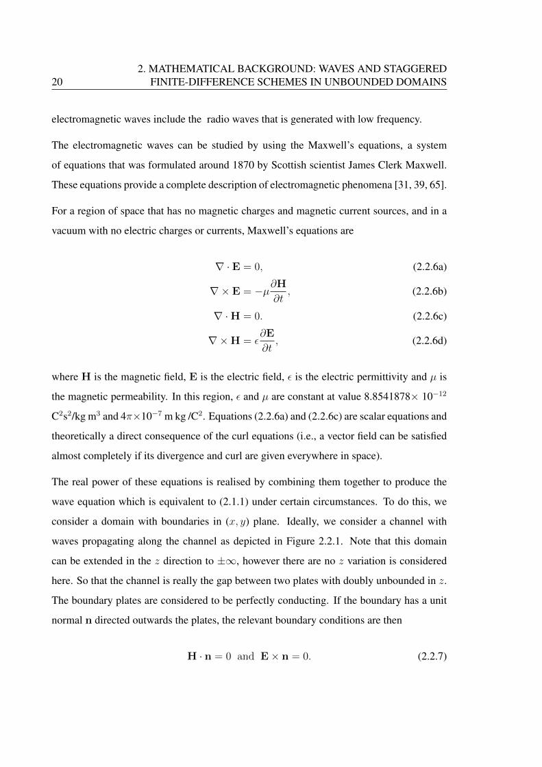
202. MATHEMATICAL BACKGROUND: WAVES AND STAGGERED
FINITE-DIFFERENCE SCHEMES IN UNBOUNDED DOMAINS
electromagnetic waves include the radio waves that is generated with low frequency.
The electromagnetic waves can be studied by using the Maxwell’s equations, a system
of equations that was formulated around 1870 by Scottish scientist James Clerk Maxwell.
These equations provide a complete description of electromagnetic phenomena [31, 39, 65].
For a region of space that has no magnetic charges and magnetic current sources, and in a
vacuum with no electric charges or currents, Maxwell’s equations are
∇ · E = 0, (2.2.6a)
∇× E = −µ∂H∂t
, (2.2.6b)
∇ ·H = 0. (2.2.6c)
∇×H = ε∂E
∂t, (2.2.6d)
where H is the magnetic field, E is the electric field, ε is the electric permittivity and µ is
the magnetic permeability. In this region, ε and µ are constant at value 8.8541878× 10⁻¹²
C2s2/kg m3 and 4π×10−7 m kg /C2. Equations (2.2.6a) and (2.2.6c) are scalar equations and
theoretically a direct consequence of the curl equations (i.e., a vector field can be satisfied
almost completely if its divergence and curl are given everywhere in space).
The real power of these equations is realised by combining them together to produce the
wave equation which is equivalent to (2.1.1) under certain circumstances. To do this, we
consider a domain with boundaries in (x, y) plane. Ideally, we consider a channel with
waves propagating along the channel as depicted in Figure 2.2.1. Note that this domain
can be extended in the z direction to ±∞, however there are no z variation is considered
here. So that the channel is really the gap between two plates with doubly unbounded in z.
The boundary plates are considered to be perfectly conducting. If the boundary has a unit
normal n directed outwards the plates, the relevant boundary conditions are then
H · n = 0 and E× n = 0. (2.2.7)
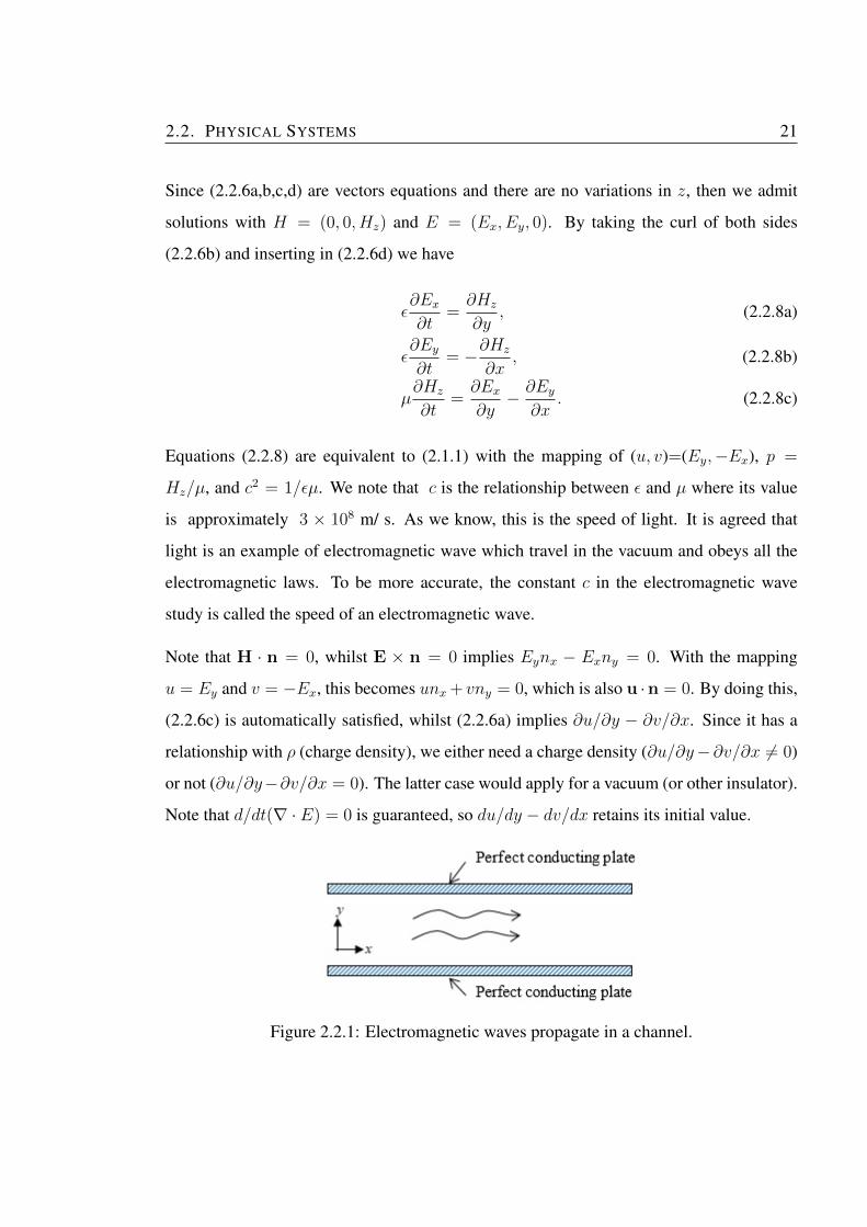
2.2. PHYSICAL SYSTEMS 21
Since (2.2.6a,b,c,d) are vectors equations and there are no variations in z, then we admit
solutions with H = (0, 0, Hz) and E = (Ex, Ey, 0). By taking the curl of both sides
(2.2.6b) and inserting in (2.2.6d) we have
ε∂Ex∂t
=∂Hz
∂y, (2.2.8a)
ε∂Ey∂t
= −∂Hz
∂x, (2.2.8b)
µ∂Hz
∂t=∂Ex∂y− ∂Ey
∂x. (2.2.8c)
Equations (2.2.8) are equivalent to (2.1.1) with the mapping of (u, v)=(Ey,−Ex), p =
Hz/µ, and c2 = 1/εµ. We note that c is the relationship between ε and µ where its value
is approximately 3 × 10⁸ m/ s. As we know, this is the speed of light. It is agreed that
light is an example of electromagnetic wave which travel in the vacuum and obeys all the
electromagnetic laws. To be more accurate, the constant c in the electromagnetic wave
study is called the speed of an electromagnetic wave.
Note that H · n = 0, whilst E × n = 0 implies Eynx − Exny = 0. With the mapping
u = Ey and v = −Ex, this becomes unx + vny = 0, which is also u ·n = 0. By doing this,
(2.2.6c) is automatically satisfied, whilst (2.2.6a) implies ∂u/∂y − ∂v/∂x. Since it has a
relationship with ρ (charge density), we either need a charge density (∂u/∂y−∂v/∂x 6= 0)
or not (∂u/∂y−∂v/∂x = 0). The latter case would apply for a vacuum (or other insulator).
Note that d/dt(∇ · E) = 0 is guaranteed, so du/dy − dv/dx retains its initial value.
Figure 2.2.1: Electromagnetic waves propagate in a channel.
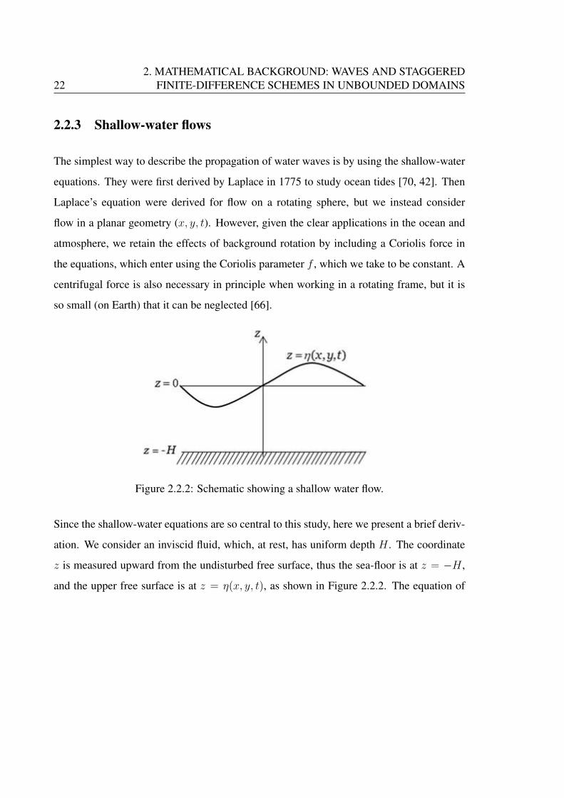
222. MATHEMATICAL BACKGROUND: WAVES AND STAGGERED
FINITE-DIFFERENCE SCHEMES IN UNBOUNDED DOMAINS
2.2.3 Shallow-water flows
The simplest way to describe the propagation of water waves is by using the shallow-water
equations. They were first derived by Laplace in 1775 to study ocean tides [70, 42]. Then
Laplace’s equation were derived for flow on a rotating sphere, but we instead consider
flow in a planar geometry (x, y, t). However, given the clear applications in the ocean and
atmosphere, we retain the effects of background rotation by including a Coriolis force in
the equations, which enter using the Coriolis parameter f , which we take to be constant. A
centrifugal force is also necessary in principle when working in a rotating frame, but it is
so small (on Earth) that it can be neglected [66].
Figure 2.2.2: Schematic showing a shallow water flow.
Since the shallow-water equations are so central to this study, here we present a brief deriv-
ation. We consider an inviscid fluid, which, at rest, has uniform depth H . The coordinate
z is measured upward from the undisturbed free surface, thus the sea-floor is at z = −H ,
and the upper free surface is at z = η(x, y, t), as shown in Figure 2.2.2. The equation of
2.2. PHYSICAL SYSTEMS 23
motions are
Du
Dt− fv = −1
ρ
∂p
∂x, (2.2.9a)
Dv
Dt+ fu = −1
ρ
∂p
∂y, (2.2.9b)
∂p
∂z= −ρg, (2.2.9c)
0 =∂u
∂x+∂v
∂y+∂w
∂z. (2.2.9d)
where g is the gravitational acceleration and the operator D/Dt is the material derivative
defined byD
Dt=
∂
∂t+ (u
∂
∂x+ v
∂
∂y+ w
∂
∂z).
Here we have taken hydrostatic balance in the vertical since the uniform depth is small
compared to the wavelength of the disturbance. Therefore, hydrostatic balance is consistent
with the shallowness of the water (p.80, [70]). Then, the pressure at the free surface is equal
to atmospheric pressure patm, (2.2.9c) implies
p(x, y, z, t) = patm + ρgη(x, y, t)− ρgz.
Thus,
−1
ρ
∂p
∂x= −g ∂η
∂x, −1
ρ
∂p
∂y= −g∂η
∂y,
are independent of z; it follows from (2.2.9a) and (2.2.9b) that if u and v are independent
of z at some instant, they will remain independent of z for all time. We thus seek solutions
u = u(x, y, t) and v = v(x, y, t) with
∂u
∂t+ u
∂u
∂x+ v
∂u
∂y− fv = −g ∂η
∂x, (2.2.10a)
∂v
∂t+ u
∂v
∂x+ v
∂v
∂y+ fu = −g∂η
∂y. (2.2.10b)

242. MATHEMATICAL BACKGROUND: WAVES AND STAGGERED
FINITE-DIFFERENCE SCHEMES IN UNBOUNDED DOMAINS
These are two equations, involving three unknowns u, v and η.
We now have to find an equation for η to close the system. We do this by integrating
equation (2.2.9d) over the layer we have
w(z = η) = −(∂u
∂x+∂v
∂y
)(η +H), (2.2.11)
since u and v are independent of z, and w = 0 at z = −H . The moving boundary condition
at the upper surface z = η(x, y, t), is given as
u · n = ub · n, (2.2.12)
where n is the normal vector to z = η(x, y, t). At the upper surface
ub =
(0, 0,
∂η
∂t
), (2.2.13)
and the surface z − η(x, y, t) = 0 has
n = ∇(z − η(x, y, t)) =
(−∂η∂x,−∂η
∂y, 1
). (2.2.14)
Then, by using (2.2.13) and (2.2.14), (2.2.12) gives
(u, v, w) ·(−∂η∂x,−∂η
∂y, 1
)=
(0, 0,
∂η
∂t
)·(−∂η∂x,−∂η
∂y, 1
)at z = η,
or
w =∂η
∂t+ u
∂η
∂x+ v
∂η
∂yat z = η. (2.2.15)
Substituting into equation (2.2.11) gives
∂η
∂t+
∂
∂x((η +H)u) +
∂
∂y((η +H)v) = 0. (2.2.16)
2.3. CONSERVATION LAWS 25
Equations (2.2.10a), (2.2.10b) and (2.2.16) are known as the shallow water equations.
We now assume that amplitudes of the disturbances are small. Thus, this allows the problem
to be linearised. To analyse this, a basic state of rest is taken where u = 0 with constant
depth H . So, we write u = 0 + u′, v = 0 + v′, η = 0 + η′, then equations (2.2.10a),
(2.2.10b) and (2.2.16) are linearised by neglecting the nonlinear terms that are products of
disturbance quantities, i.e., the second and third left-hand terms of the momentum equation
(2.2.10a), (2.2.10b). Then, the equations become
∂u′
∂t− fv′ = −g∂η
′
∂x, (2.2.17a)
∂v′
∂t+ fu′ = −g∂η
′
∂y, (2.2.17b)
∂η′
∂t+H
(∂u′
∂x+∂v′
∂y
)= 0. (2.2.17c)
Equations (2.2.17a,b,c) are called linear shallow water equations. These are exactly (2.1.1),
but with the effects of earth’s rotation f in the momentum equations (2.2.17a,b), c2 = gH ,
and p = gη. This system must be solved with boundary conditions where there can be no
flow across the boundary and thus the normal component of the velocity is always zero:
u · n = 0, on ∂D, (2.2.18)
where ∂D is the boundary of the domain D.
2.3 Conservation Laws
This section is devoted to discuss the conservation laws. These laws are important property
of mechanical systems. Typically, they express something fundamental about a property of
physical interest such as mass and energy. In fluid dynamics, a conservation laws takes the
262. MATHEMATICAL BACKGROUND: WAVES AND STAGGERED
FINITE-DIFFERENCE SCHEMES IN UNBOUNDED DOMAINS
form
∂A
∂t+∇ · J = 0. (2.3.1)
Over an arbitrary volume V we will see that J is the flux of quantity A across a surface.
While over the entire domain D, the quantity A is integrated and will give a conserved
quantity∫DA dV , if J · n = 0 on the boundary. We will work with quantities like A which
can be defined at points and are thus functions of x and t.
2.3.1 Conservation of mass
We now derive a conservation law for the mass. We can see that the third equation in (2.1.1)
is already in the form∂A
∂t+∇ · J = 0, (2.3.2)
with A = p and J = c2u. Since J · n is proportional to u · n = 0 on ∂D, we then will have
a conserved quantity ∫D
p dV. (2.3.3)
We call this the mass. In the acoustics, the mass is indeed proportional to the mass perturb-
ation which is the integral of perturbation density with units of kg s−1 for a flow through a
surface. In the shallow-water flow, the mass is the mass perturbation, since it is proportional
to surface displacement. While in electromagnetism the mass is proportional to an integral
of the z- component of the magnetic field, and is thus some sort of magnetic flux.

2.3. CONSERVATION LAWS 27
2.3.2 Conservation of energy
We now proceed with the conservation law of energy for equations (2.1.1). Analogous to
the continuum case the energy equation can be obtained by taking the dot product of the
momentum equation in (2.1.1) with velocity as
u∂u
∂t= −u∂p
∂x, v
∂v
∂t= −v∂p
∂y. (2.3.4)
Adding both equations in (2.3.4) yield
∂
∂t
(1
2(u2 + v2)
)= −u∂p
∂x− v∂p
∂y= −u · ∇p. (2.3.5)
By writing the right-hand side (2.3.5) as a divergence and using the third equation in (2.1.1)
yield
−u · ∇p = −∇ · (pu)− p∇ · u = −∇ · (pu)− ∂
∂t
(p2
2c2
). (2.3.6)
Substituting (2.3.6) into (2.3.5) we then have
∂E
∂t+∇ · J = 0, where E =
p2
2c2+
1
2(u2 + v2), and J = pu. (2.3.7)
This is the standard energy equation for (2.1.1). Over a fixed volume V , E is the conserved
quantity, and we call it energy. The wave energy E has two components which are kinetic
energy per unit volume (u2/2), and some kind internal energy per unit volume (p2/2c2).
The wave energy flux J tells us in what direction and at what rate wave energy is transferred
around the fluid by waves. For example, in the acoustic mode the energy is the summation of
velocity and the perturbation density. For shallow-water flow, the energy is the relationship
between gravity and surface displacement, since wave energy generated from fluctuation
below the surface.

282. MATHEMATICAL BACKGROUND: WAVES AND STAGGERED
FINITE-DIFFERENCE SCHEMES IN UNBOUNDED DOMAINS
2.4 Wave Propagation
We now examine wave propagation in our two-dimensional system of wave equations
∂u
∂t− fv = −∂p
∂x, (2.4.1a)
∂v
∂t+ fu = −∂p
∂y, (2.4.1b)
∂p
∂t+ c2
(∂u
∂x+∂v
∂y
)= 0. (2.4.1c)
Here, we are retaining Coriolis terms for greater generality and comparison with the great
literature from atmosphere-ocean dynamics, although for most of this thesis these terms
will be dropped.
For these rotationally-modified two-dimensional wave equations there is no d’Alembert
wave solution (like (1.2.2)). Instead, we seek solutions of the form
u = Re(uei(kx+ly−ωct)
), v = Re
(vei(kx+ly−ωct)
), p = Re
(pei(kx+ly−ωct)
), (2.4.2)
where u, v, and p are complex wave amplitudes, k is the wave number in the x-direction,
l is the wave number in y-direction, and ωc is the frequency (with the subscript c denoting
the continuum frequency, rather than the discrete frequency as obtained in a numerical
approximation). Then, by substituting (2.4.2) into (2.4.1a,b,c) we have
− iωcu− fv = −ikp, (2.4.3a)
− iωcv + fu = −ilp, (2.4.3b)
− iωcp+ c2 (iku+ ilu) = 0. (2.4.3c)
We wish to find solutions for which (u, v, p)T is not identically zero, and here we intro-
duce the matrix method which performs process of elimination. System (2.4.3a,b,c) can be
2.4. WAVE PROPAGATION 29
written as −iωc −f ik
f −iωc il
c2ik c2il −iωc
u
v
p
=
0
0
0
. (2.4.4)
For non-trivial solutions, the determinant of the matrix must be zero which gives
ωc(ω2c − f 2 − c2(k2 + l2)
)= 0.
The possible solutions are ωc = 0 which is non wave-like solution, or
ω2c = f 2 + c2(k2 + l2). (2.4.5)
Equation (2.4.5) is called dispersion relation and the wave-like solutions can only occur if
there is a particular relationship between the frequency, ωc, and wavenumbers, k, l. In the
special case where l = 0, the wave crests and troughs propagate at the phase speed, cp,
which from (2.4.5) is
cp =ωck
= ±c(
1 +f 2
c2k2
)1/2
. (2.4.6)
So the phase speed is a function of wavenumber, and waves of different wavenumbers move
at different speeds. However, in the absence of rotation effects (i.e., f = 0), one can have
dispersion relation for the acoustic and electromagnetic case. In that particular case, the
phase speed (2.4.6) now is
cp =ωck
= ±c. (2.4.7)
This shows that the wave move at speed c, independent of the wavenumber, k.
Another interesting property that can be derived from dispersion relation is called group
velocity. It is the speed of a compact group of waves. It is sometimes written as cg and is

302. MATHEMATICAL BACKGROUND: WAVES AND STAGGERED
FINITE-DIFFERENCE SCHEMES IN UNBOUNDED DOMAINS
defined as
cg(k) =
(∂ωc∂k
,∂ωc∂l
). (2.4.8)
So, from (2.4.5) we have
cg =
(∂ωc∂k
,∂ωc∂l
)= ± c2
[f 2 + (k2 + l2)]1/2(k, l) . (2.4.9)
In the absence of rotation effects, the group velocity is
cg = ± c
(k2 + l2)1/2(k, l) . (2.4.10)
We can see that the group velocity is in the same direcion as the wavevector k = (k, l).
2.5 Finite-Difference Approximations
The development of accurate numerical approximation scheme is an essential tool for ex-
tracting quantitative information for the deep understanding of the basic physical system.
Besides, we can accurately test a proposed numerical scheme by running it on a known
solution. Numerical methods also can provide us a better understanding of a given govern-
ing equations in their simplest form. So that, we will discuss the numerical approximation
by finite-difference method for the system of wave equations (2.4.1). As in section 2.4, we
retain the Coriolis terms to make a link to the important work on atmosphere-ocean fluid
dynamics, where many of these discretizations were first proposed.
A key issue is whether or not the three variables u, v, p are staggered. In Figure 1.4.1, five
possible arrangements were noted. Here, we will examine in detail the discretizations of
the so-called A-grid, B-grid and C-grid, as illustrated in Figure 2.5.1, using the terminology
of AL77 [6]. It remains to introduce discretizations in both space and time. The former are
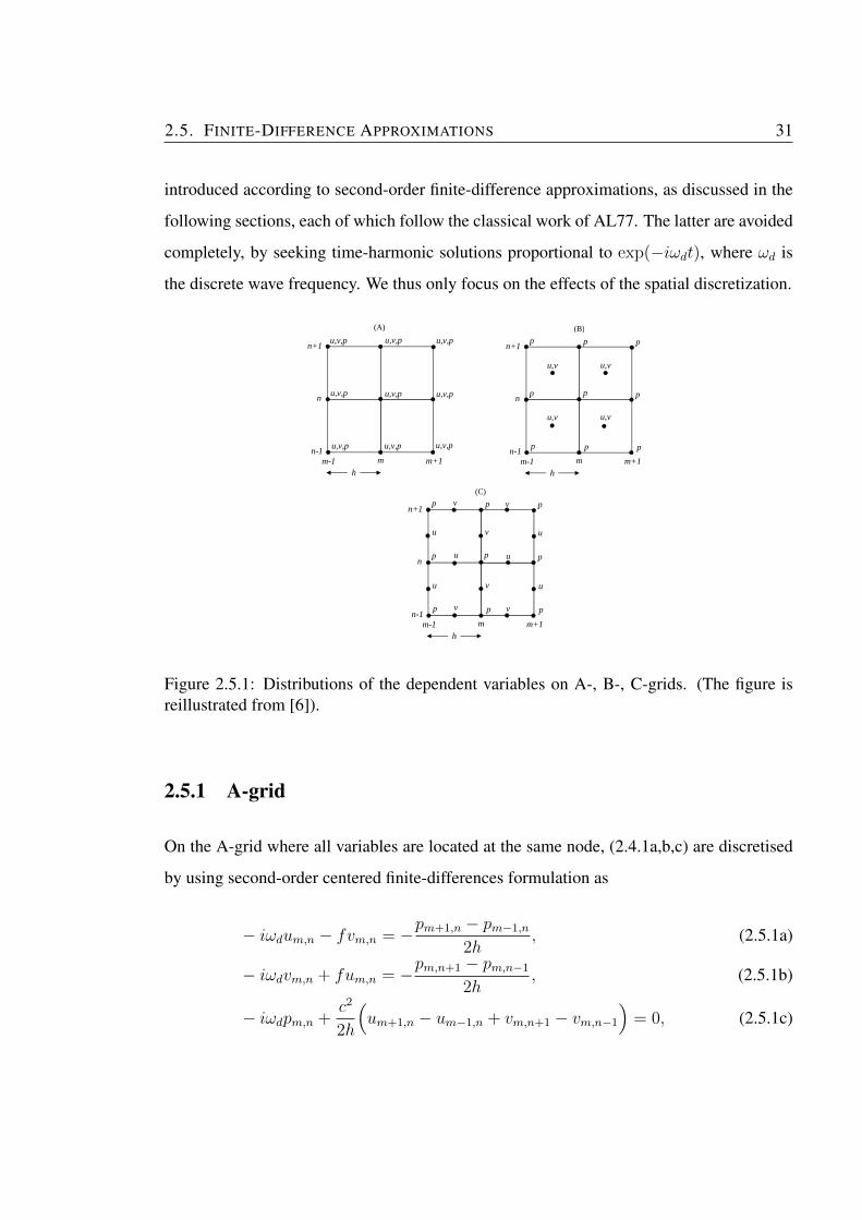
2.5. FINITE-DIFFERENCE APPROXIMATIONS 31
introduced according to second-order finite-difference approximations, as discussed in the
following sections, each of which follow the classical work of AL77. The latter are avoided
completely, by seeking time-harmonic solutions proportional to exp(−iωdt), where ωd is
the discrete wave frequency. We thus only focus on the effects of the spatial discretization.
u,v m-1
n+1
n
n-1m-1 m m+1
h
u,v,p u,v,p u,v,p
u,v,p u,v,p u,v,p
u,v,p u,v,p u,v,p
(A)
p
n+1
n
n-1m-1 m m+1
h
(B)
p
p
p
u,v
p
p
p
p
p
u,v
u,v
u,v
n+1
n
n-1m-1 m m+1
h
(C)
p
p
p
p
p
p
p
p
u
u
v
v
u
u
v
u
v
v
u
v
p
p
Figure 2.5.1: Distributions of the dependent variables on A-, B-, C-grids. (The figure isreillustrated from [6]).
2.5.1 A-grid
On the A-grid where all variables are located at the same node, (2.4.1a,b,c) are discretised
by using second-order centered finite-differences formulation as
− iωdum,n − fvm,n = −pm+1,n − pm−1,n
2h, (2.5.1a)
− iωdvm,n + fum,n = −pm,n+1 − pm,n−1
2h, (2.5.1b)
− iωdpm,n +c2
2h
(um+1,n − um−1,n + vm,n+1 − vm,n−1
)= 0, (2.5.1c)
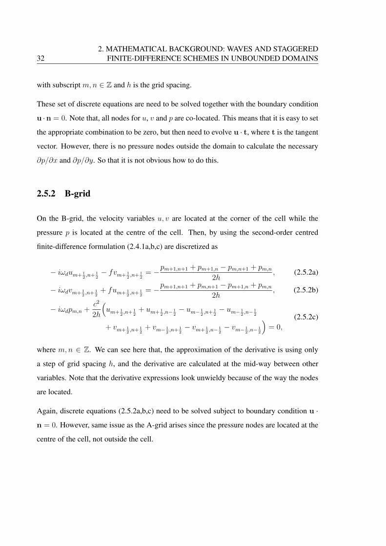
322. MATHEMATICAL BACKGROUND: WAVES AND STAGGERED
FINITE-DIFFERENCE SCHEMES IN UNBOUNDED DOMAINS
with subscript m,n ∈ Z and h is the grid spacing.
These set of discrete equations are need to be solved together with the boundary condition
u ·n = 0. Note that, all nodes for u, v and p are co-located. This means that it is easy to set
the appropriate combination to be zero, but then need to evolve u · t, where t is the tangent
vector. However, there is no pressure nodes outside the domain to calculate the necessary
∂p/∂x and ∂p/∂y. So that it is not obvious how to do this.
2.5.2 B-grid
On the B-grid, the velocity variables u, v are located at the corner of the cell while the
pressure p is located at the centre of the cell. Then, by using the second-order centred
finite-difference formulation (2.4.1a,b,c) are discretized as
− iωdum+ 12,n+ 1
2− fvm+ 1
2,n+ 1
2= −pm+1,n+1 + pm+1,n − pm,n+1 + pm,n
2h, (2.5.2a)
− iωdvm+ 12,n+ 1
2+ fum+ 1
2,n+ 1
2= −pm+1,n+1 + pm,n+1 − pm+1,n + pm,n
2h, (2.5.2b)
− iωdpm,n +c2
2h
(um+ 1
2,n+ 1
2+ um+ 1
2,n− 1
2− um− 1
2,n+ 1
2− um− 1
2,n− 1
2
+ vm+ 12,n+ 1
2+ vm− 1
2,n+ 1
2− vm+ 1
2,n− 1
2− vm− 1
2,n− 1
2
)= 0,
(2.5.2c)
where m,n ∈ Z. We can see here that, the approximation of the derivative is using only
a step of grid spacing h, and the derivative are calculated at the mid-way between other
variables. Note that the derivative expressions look unwieldy because of the way the nodes
are located.
Again, discrete equations (2.5.2a,b,c) need to be solved subject to boundary condition u ·
n = 0. However, same issue as the A-grid arises since the pressure nodes are located at the
centre of the cell, not outside the cell.
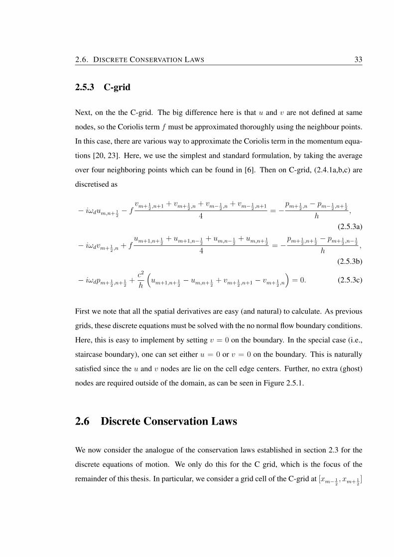
2.6. DISCRETE CONSERVATION LAWS 33
2.5.3 C-grid
Next, on the the C-grid. The big difference here is that u and v are not defined at same
nodes, so the Coriolis term f must be approximated thoroughly using the neighbour points.
In this case, there are various way to approximate the Coriolis term in the momentum equa-
tions [20, 23]. Here, we use the simplest and standard formulation, by taking the average
over four neighboring points which can be found in [6]. Then on C-grid, (2.4.1a,b,c) are
discretised as
− iωdum,n+ 12− f
vm+ 12,n+1 + vm+ 1
2,n + vm− 1
2,n + vm− 1
2,n+1
4= −
pm+ 12,n − pm− 1
2,n+ 1
2
h,
(2.5.3a)
− iωdvm+ 12,n + f
um+1,n+ 12
+ um+1,n− 12
+ um,n− 12
+ um,n+ 12
4= −
pm+ 12,n+ 1
2− pm+ 1
2,n− 1
2
h,
(2.5.3b)
− iωdpm+ 12,n+ 1
2+c2
h
(um+1,n+ 1
2− um,n+ 1
2+ vm+ 1
2,n+1 − vm+ 1
2,n
)= 0. (2.5.3c)
First we note that all the spatial derivatives are easy (and natural) to calculate. As previous
grids, these discrete equations must be solved with the no normal flow boundary conditions.
Here, this is easy to implement by setting v = 0 on the boundary. In the special case (i.e.,
staircase boundary), one can set either u = 0 or v = 0 on the boundary. This is naturally
satisfied since the u and v nodes are lie on the cell edge centers. Further, no extra (ghost)
nodes are required outside of the domain, as can be seen in Figure 2.5.1.
2.6 Discrete Conservation Laws
We now consider the analogue of the conservation laws established in section 2.3 for the
discrete equations of motion. We only do this for the C grid, which is the focus of the
remainder of this thesis. In particular, we consider a grid cell of the C-grid at [xm− 12, xm+ 1
2]

342. MATHEMATICAL BACKGROUND: WAVES AND STAGGERED
FINITE-DIFFERENCE SCHEMES IN UNBOUNDED DOMAINS
and [yn− 12, yn+ 1
2], as illustrated in Figure 2.6.1. Further, we perform our analysis for a sys-
tem where rotation is neglected. This is, of course, natural for acoustics or electromagnetic
waves. For shallow- water waves on a rotating planet, it can be justified when the Rossby
number of the flow is large. More precisely, for a representative lengthscale of motion L
and speed of flow U , the inertial terms are of size Ro = (U2/L)/(fU) = U/fL relative to
the Coriolis terms, and we demand Ro� 1.
Figure 2.6.1: The arrangement of variables on a C-grid.
2.6.1 Discrete Conservation of Mass
In this section, we will derive a discrete version of conservation of mass. We now recall
equation (2.5.3c) to begin the derivation. On the C-grid this equation is discretized as
∂
∂tpm+ 1
2,n+ 1
2+c2
h
(um+1,n+ 1
2− um,n+ 1
2+ vm+ 1
2,n+1 − vm+ 1
2,n
)= 0. (2.6.1)
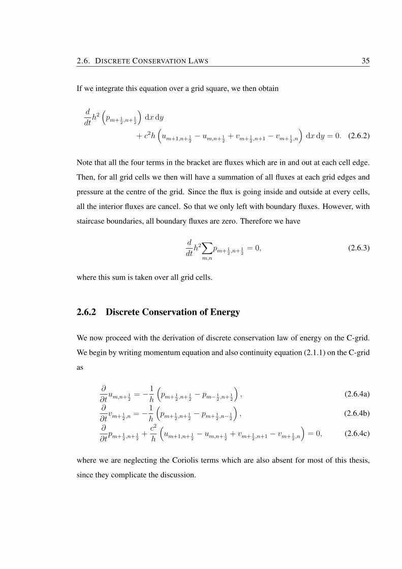
2.6. DISCRETE CONSERVATION LAWS 35
If we integrate this equation over a grid square, we then obtain
d
dth2(pm+ 1
2,n+ 1
2
)dx dy
+ c2h(um+1,n+ 1
2− um,n+ 1
2+ vm+ 1
2,n+1 − vm+ 1
2,n
)dx dy = 0. (2.6.2)
Note that all the four terms in the bracket are fluxes which are in and out at each cell edge.
Then, for all grid cells we then will have a summation of all fluxes at each grid edges and
pressure at the centre of the grid. Since the flux is going inside and outside at every cells,
all the interior fluxes are cancel. So that we only left with boundary fluxes. However, with
staircase boundaries, all boundary fluxes are zero. Therefore we have
d
dth2∑m,n
pm+ 12,n+ 1
2= 0, (2.6.3)
where this sum is taken over all grid cells.
2.6.2 Discrete Conservation of Energy
We now proceed with the derivation of discrete conservation law of energy on the C-grid.
We begin by writing momentum equation and also continuity equation (2.1.1) on the C-grid
as
∂
∂tum,n+ 1
2= −1
h
(pm+ 1
2,n+ 1
2− pm− 1
2,n+ 1
2
), (2.6.4a)
∂
∂tvm+ 1
2,n = −1
h
(pm+ 1
2,n+ 1
2− pm+ 1
2,n− 1
2
), (2.6.4b)
∂
∂tpm+ 1
2,n+ 1
2+c2
h
(um+1,n+ 1
2− um,n+ 1
2+ vm+ 1
2,n+1 − vm+ 1
2,n
)= 0, (2.6.4c)
where we are neglecting the Coriolis terms which are also absent for most of this thesis,
since they complicate the discussion.
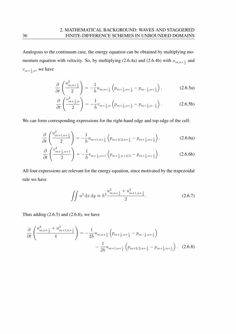
362. MATHEMATICAL BACKGROUND: WAVES AND STAGGERED
FINITE-DIFFERENCE SCHEMES IN UNBOUNDED DOMAINS
Analogous to the continuum case, the energy equation can be obtained by multiplying mo-
mentum equation with velocity. So, by multiplying (2.6.4a) and (2.6.4b) with um,n+ 12
and
vm+ 12,n, we have
∂
∂t
(u2m,n+ 1
2
2
)= −1
hum,n+ 1
2
(pm+ 1
2,n+ 1
2− pm− 1
2,n+ 1
2
), (2.6.5a)
∂
∂t
(v2m+ 1
2,n
2
)= −1
hvm+ 1
2,n
(pm+ 1
2,n+ 1
2− pm+ 1
2,n− 1
2
). (2.6.5b)
We can form corresponding expressions for the right-hand edge and top edge of the cell:
∂
∂t
(u2m+1,n+ 1
2
2
)= −1
hum+1,n+ 1
2
(pm+3/2,n+ 1
2− pm+ 1
2,n+ 1
2
), (2.6.6a)
∂
∂t
(v2m+ 1
2,n+1
2
)= −1
hvm+ 1
2,n+1
(pm+ 1
2,n+3/2 − pm+ 1
2,n+ 1
2
). (2.6.6b)
All four expressions are relevant for the energy equation, since motivated by the trapezoidal
rule we have
∫∫u2 dx dy ≈ h2
u2m,n+ 1
2
+ u2m+1,n+ 1
2
2. (2.6.7)
Thus adding (2.6.5) and (2.6.6), we have
∂
∂t
(u2m,n+ 1
2
+ u2m+1,n+ 1
2
4
)= − 1
2hum,n+ 1
2
(pm+ 1
2,n+ 1
2− pm− 1
2,n+ 1
2
)− 1
2hum+1,n+ 1
2
(pm+3/2,n+ 1
2− pm+ 1
2,n+ 1
2
). (2.6.8)
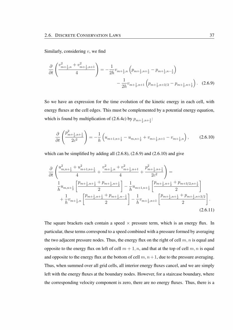
2.6. DISCRETE CONSERVATION LAWS 37
Similarly, considering v, we find
∂
∂t
(v2m+ 1
2,n
+ v2m+ 1
2,n+1
4
)= − 1
2hvm+ 1
2,n
(pm+ 1
2,n+ 1
2− pm+ 1
2,n− 1
2
)− 1
2hvm+ 1
2,n+1
(pm+ 1
2,n+3/2 − pm+ 1
2,n+ 1
2
). (2.6.9)
So we have an expression for the time evolution of the kinetic energy in each cell, with
energy fluxes at the cell edges. This must be complemented by a potential energy equation,
which is found by multiplication of (2.6.4c) by pm+ 12,n+ 1
2:
∂
∂t
(p2m+ 1
2,n+ 1
2
2c2
)= −1
h
(um+1,n+ 1
2− um,n+ 1
2+ vm+ 1
2,n+1 − vm+ 1
2,n
), (2.6.10)
which can be simplified by adding all (2.6.8), (2.6.9) and (2.6.10) and give
∂
∂t
(u2m,n+ 1
2
+ u2m+1,n+ 1
2
4+v2m+ 1
2,n
+ v2m+ 1
2,n+1
4+p2m+ 1
2,n+ 1
2
2c2
)=
1
hum,n+ 1
2
[pm+ 1
2,n+ 1
2+ pm+ 1
2,n+ 1
2
2
]− 1
hum+1,n+ 1
2
[pm+ 1
2,n+ 1
2+ pm+3/2,n+ 1
2
2
]+
1
hvm+ 1
2,n
[pm+ 1
2,n+ 1
2+ pm+ 1
2,n− 1
2
2
]− 1
hvm+ 1
2,n+1
[pm+ 1
2,n+ 1
2+ pm+ 1
2,n+3/2
2
].
(2.6.11)
The square brackets each contain a speed × pressure term, which is an energy flux. In
particular, these terms correspond to a speed combined with a pressure formed by averaging
the two adjacent pressure nodes. Thus, the energy flux on the right of cell m,n is equal and
opposite to the energy flux on left of cell m + 1, n, and that at the top of cell m,n is equal
and opposite to the energy flux at the bottom of cell m,n+1, due to the pressure averaging.
Thus, when summed over all grid cells, all interior energy fluxes cancel, and we are simply
left with the energy fluxes at the boundary nodes. However, for a staircase boundary, where
the corresponding velocity component is zero, there are no energy fluxes. Thus, there is a

382. MATHEMATICAL BACKGROUND: WAVES AND STAGGERED
FINITE-DIFFERENCE SCHEMES IN UNBOUNDED DOMAINS
discrete energy conservation law:
d
dt
∑m,n
(p2m+ 1
2,n+ 1
2
2c2+u2m,n+ 1
2
+ u2m+1,n+ 1
2
+ v2m+ 1
2,n
+ v2m+ 1
2,n+1
4
)= 0. (2.6.12)
2.7 Discrete Waves
To get an idea of the different performances of the grids, we consider waves propagating in a
doubly periodic domain (i.e., with no boundaries) and the analysis were done for equations
(2.4.3) on A-, B- and C-grid. Note that all calculations in this section also can be found in
[6]. On every grid, we used notation as in Figure 2.5.1 with
xm = mh, yn = nh.
The wave propagation on finite-difference grid can be seen by seeking discrete wavelike
solution of the form
um,n = Re(uei(kxm+lyn)
), vm,n = Re
(vei(kxm+lyn)
), pm,n = Re
(pei(kxm+lyn)
),
(2.7.1)
with time-periodicity assumed to be proportional to exp(−iωdt), where ωd is the discrete
wave frequency. Note that, in this section we again retain the Coriolis terms, to make a
connection to well-known results in atmosphere-ocean dynamics. Also note that we will
apply Euler’s formula exp(ikxm) = cos(kxm) + i sin(kxm) for the simplication of the
resulting discrete equations for each grids.
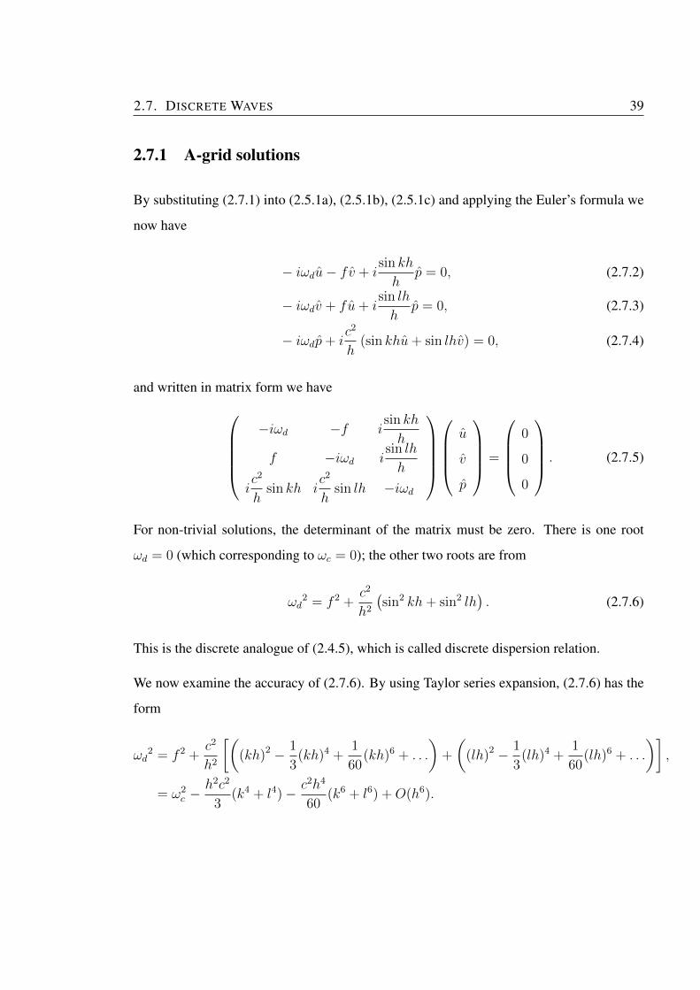
2.7. DISCRETE WAVES 39
2.7.1 A-grid solutions
By substituting (2.7.1) into (2.5.1a), (2.5.1b), (2.5.1c) and applying the Euler’s formula we
now have
− iωdu− fv + isin kh
hp = 0, (2.7.2)
− iωdv + fu+ isin lh
hp = 0, (2.7.3)
− iωdp+ ic2
h(sin khu+ sin lhv) = 0, (2.7.4)
and written in matrix form we have−iωd −f i
sin kh
h
f −iωd isin lh
h
ic2
hsin kh i
c2
hsin lh −iωd
u
v
p
=
0
0
0
. (2.7.5)
For non-trivial solutions, the determinant of the matrix must be zero. There is one root
ωd = 0 (which corresponding to ωc = 0); the other two roots are from
ωd2 = f 2 +
c2
h2
(sin2 kh+ sin2 lh
). (2.7.6)
This is the discrete analogue of (2.4.5), which is called discrete dispersion relation.
We now examine the accuracy of (2.7.6). By using Taylor series expansion, (2.7.6) has the
form
ωd2 = f 2 +
c2
h2
[((kh)2 − 1
3(kh)4 +
1
60(kh)6 + . . .
)+
((lh)2 − 1
3(lh)4 +
1
60(lh)6 + . . .
)],
= ω2c −
h2c2
3(k4 + l4)− c2h4
60(k6 + l6) +O(h6).
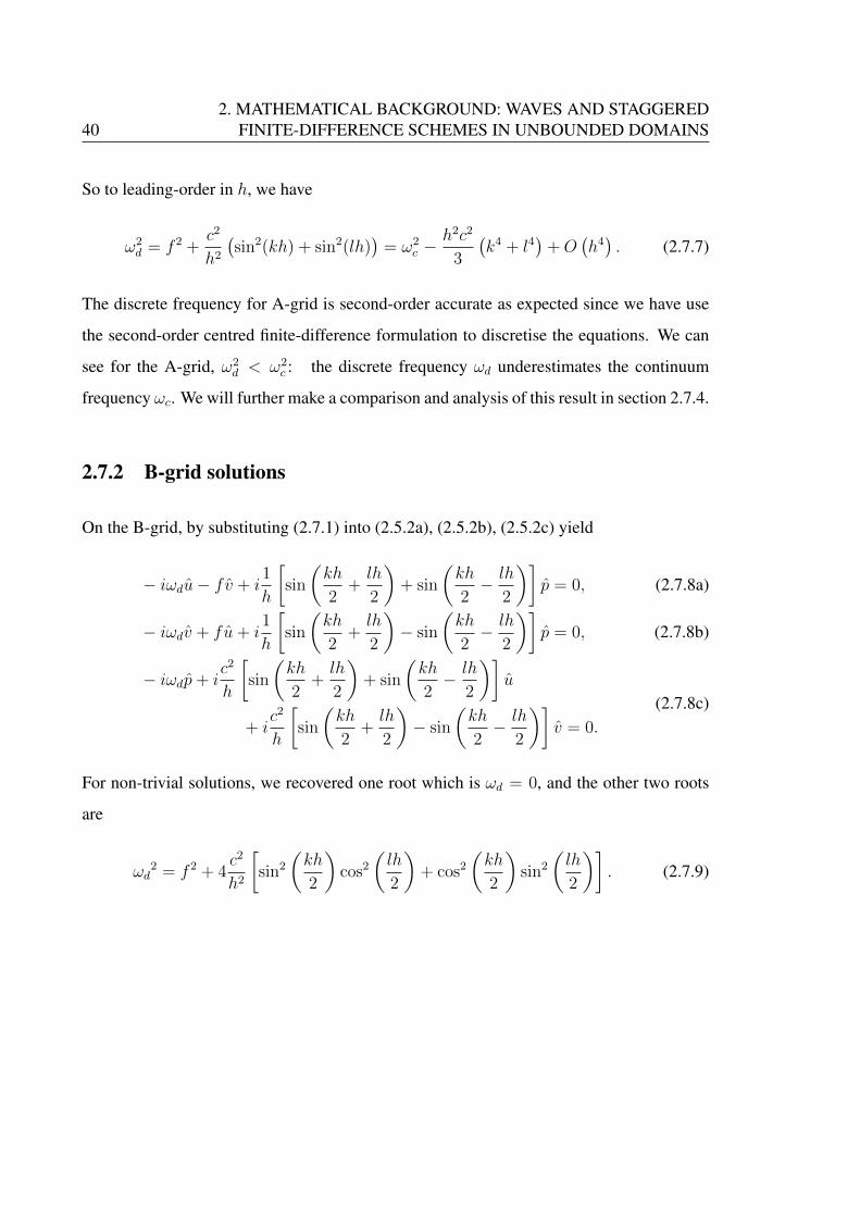
402. MATHEMATICAL BACKGROUND: WAVES AND STAGGERED
FINITE-DIFFERENCE SCHEMES IN UNBOUNDED DOMAINS
So to leading-order in h, we have
ω2d = f 2 +
c2
h2
(sin2(kh) + sin2(lh)
)= ω2
c −h2c2
3
(k4 + l4
)+O
(h4). (2.7.7)
The discrete frequency for A-grid is second-order accurate as expected since we have use
the second-order centred finite-difference formulation to discretise the equations. We can
see for the A-grid, ω2d < ω2
c : the discrete frequency ωd underestimates the continuum
frequency ωc. We will further make a comparison and analysis of this result in section 2.7.4.
2.7.2 B-grid solutions
On the B-grid, by substituting (2.7.1) into (2.5.2a), (2.5.2b), (2.5.2c) yield
− iωdu− fv + i1
h
[sin
(kh
2+lh
2
)+ sin
(kh
2− lh
2
)]p = 0, (2.7.8a)
− iωdv + fu+ i1
h
[sin
(kh
2+lh
2
)− sin
(kh
2− lh
2
)]p = 0, (2.7.8b)
− iωdp+ ic2
h
[sin
(kh
2+lh
2
)+ sin
(kh
2− lh
2
)]u
+ ic2
h
[sin
(kh
2+lh
2
)− sin
(kh
2− lh
2
)]v = 0.
(2.7.8c)
For non-trivial solutions, we recovered one root which is ωd = 0, and the other two roots
are
ωd2 = f 2 + 4
c2
h2
[sin2
(kh
2
)cos2
(lh
2
)+ cos2
(kh
2
)sin2
(lh
2
)]. (2.7.9)

2.7. DISCRETE WAVES 41
In order to examine the numerical error of (2.7.9), we applied the Taylor series expansion.
In the limit of small kh and lh (kh� 1, lh� 1), (2.7.9) has the form
ωd2 = f 2 + 4
c2
h2
[((kh
2
)2
− 1
3
(kh
2
)4
+ . . .
)(1−
(lh
2
)2
+1
3
(lh
2
)4
+ . . .
)][
+
(1−
(kh
2
)2
+1
3
(kh
2
)4
+ . . .
)((lh
2
)2
− 1
3
(lh
2
)4
+ . . .
)],
= ω2c −
c2h2
12
(k4 + l4 + 6k2l2
)+O(h4).
Therefore, discrete frequency for B-grid can be written as
ωd2 = f 2 + 4
c2
h2
[sin2
(kh
2
)cos2
(lh
2
)+ cos2
(kh
2
)sin2
(lh
2
)]= ωc
2 − c2h2
12
(k4 + l4 + 6k2l2
)+O(h4).
(2.7.10)
Again, on the B-grid ω2d < ω2
c : the discrete frequency underestimates the continuum fre-
quency.
2.7.3 C-grid solutions
On the C-grid, by substituting (2.7.1) into (2.5.3a), (2.5.3b), (2.5.3c) yields
− iωdu−f
2
[cos
(kh
2+lh
2
)+ sin
(kh
2− lh
2
)]v + i
2
hsin
(kh
2
)p = 0, (2.7.11a)
− iωdv +f
2
[cos
(kh
2+lh
2
)+ cos
(kh
2− lh
2
)]u+ i
2
hsin
(lh
2
)p = 0, (2.7.11b)
− iωdp+ 2ic2
h
[sin
(kh
2
)u+ sin
(lh
2
)v
]= 0. (2.7.11c)
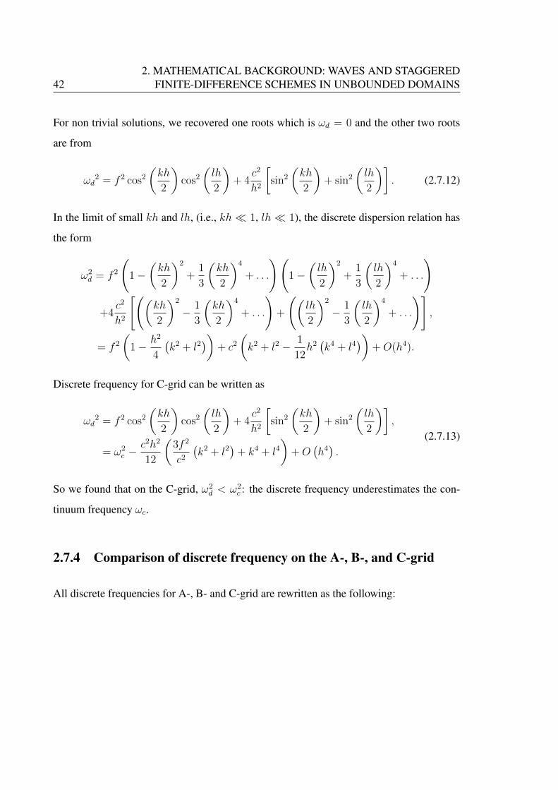
422. MATHEMATICAL BACKGROUND: WAVES AND STAGGERED
FINITE-DIFFERENCE SCHEMES IN UNBOUNDED DOMAINS
For non trivial solutions, we recovered one roots which is ωd = 0 and the other two roots
are from
ωd2 = f 2 cos2
(kh
2
)cos2
(lh
2
)+ 4
c2
h2
[sin2
(kh
2
)+ sin2
(lh
2
)]. (2.7.12)
In the limit of small kh and lh, (i.e., kh � 1, lh � 1), the discrete dispersion relation has
the form
ω2d = f 2
(1−
(kh
2
)2
+1
3
(kh
2
)4
+ . . .
)(1−
(lh
2
)2
+1
3
(lh
2
)4
+ . . .
)
+4c2
h2
[((kh
2
)2
− 1
3
(kh
2
)4
+ . . .
)+
((lh
2
)2
− 1
3
(lh
2
)4
+ . . .
)],
= f 2
(1− h2
4
(k2 + l2
))+ c2
(k2 + l2 − 1
12h2(k4 + l4
))+O(h4).
Discrete frequency for C-grid can be written as
ωd2 = f 2 cos2
(kh
2
)cos2
(lh
2
)+ 4
c2
h2
[sin2
(kh
2
)+ sin2
(lh
2
)],
= ω2c −
c2h2
12
(3f 2
c2
(k2 + l2
)+ k4 + l4
)+O
(h4).
(2.7.13)
So we found that on the C-grid, ω2d < ω2
c : the discrete frequency underestimates the con-
tinuum frequency ωc.
2.7.4 Comparison of discrete frequency on the A-, B-, and C-grid
All discrete frequencies for A-, B- and C-grid are rewritten as the following:
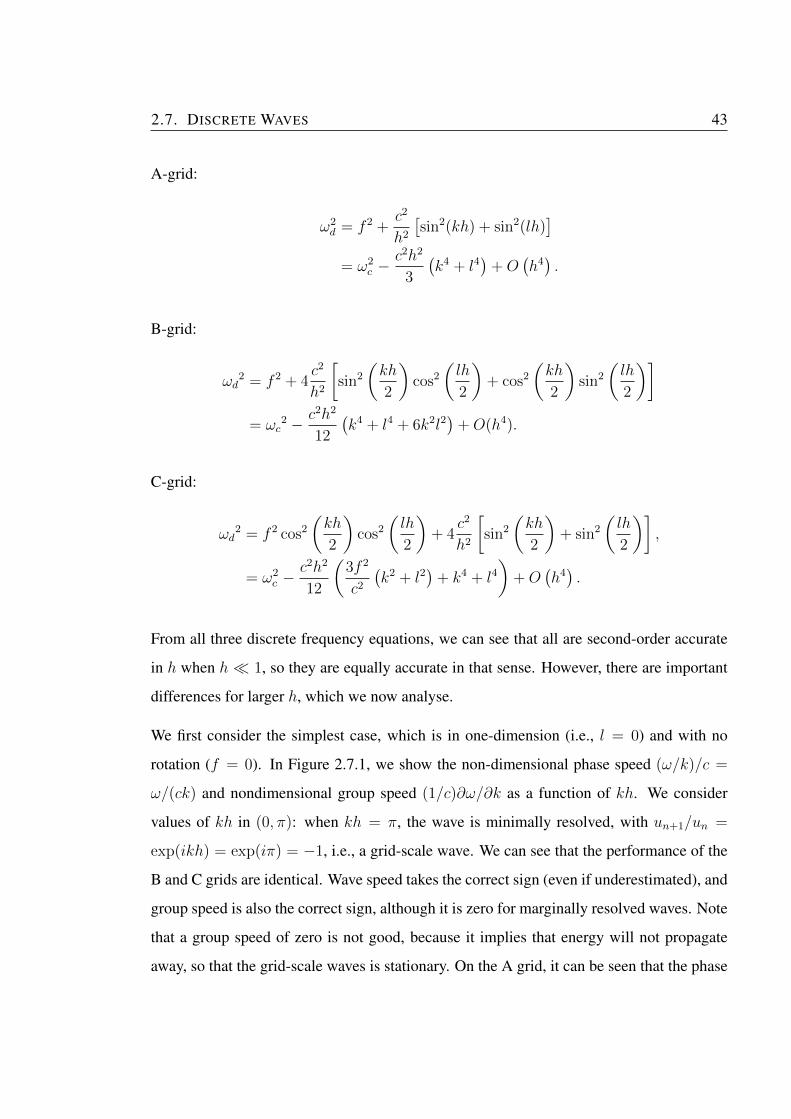
2.7. DISCRETE WAVES 43
A-grid:
ω2d = f 2 +
c2
h2
[sin2(kh) + sin2(lh)
]= ω2
c −c2h2
3
(k4 + l4
)+O
(h4).
B-grid:
ωd2 = f 2 + 4
c2
h2
[sin2
(kh
2
)cos2
(lh
2
)+ cos2
(kh
2
)sin2
(lh
2
)]= ωc
2 − c2h2
12
(k4 + l4 + 6k2l2
)+O(h4).
C-grid:
ωd2 = f 2 cos2
(kh
2
)cos2
(lh
2
)+ 4
c2
h2
[sin2
(kh
2
)+ sin2
(lh
2
)],
= ω2c −
c2h2
12
(3f 2
c2
(k2 + l2
)+ k4 + l4
)+O
(h4).
From all three discrete frequency equations, we can see that all are second-order accurate
in h when h � 1, so they are equally accurate in that sense. However, there are important
differences for larger h, which we now analyse.
We first consider the simplest case, which is in one-dimension (i.e., l = 0) and with no
rotation (f = 0). In Figure 2.7.1, we show the non-dimensional phase speed (ω/k)/c =
ω/(ck) and nondimensional group speed (1/c)∂ω/∂k as a function of kh. We consider
values of kh in (0, π): when kh = π, the wave is minimally resolved, with un+1/un =
exp(ikh) = exp(iπ) = −1, i.e., a grid-scale wave. We can see that the performance of the
B and C grids are identical. Wave speed takes the correct sign (even if underestimated), and
group speed is also the correct sign, although it is zero for marginally resolved waves. Note
that a group speed of zero is not good, because it implies that energy will not propagate
away, so that the grid-scale waves is stationary. On the A grid, it can be seen that the phase
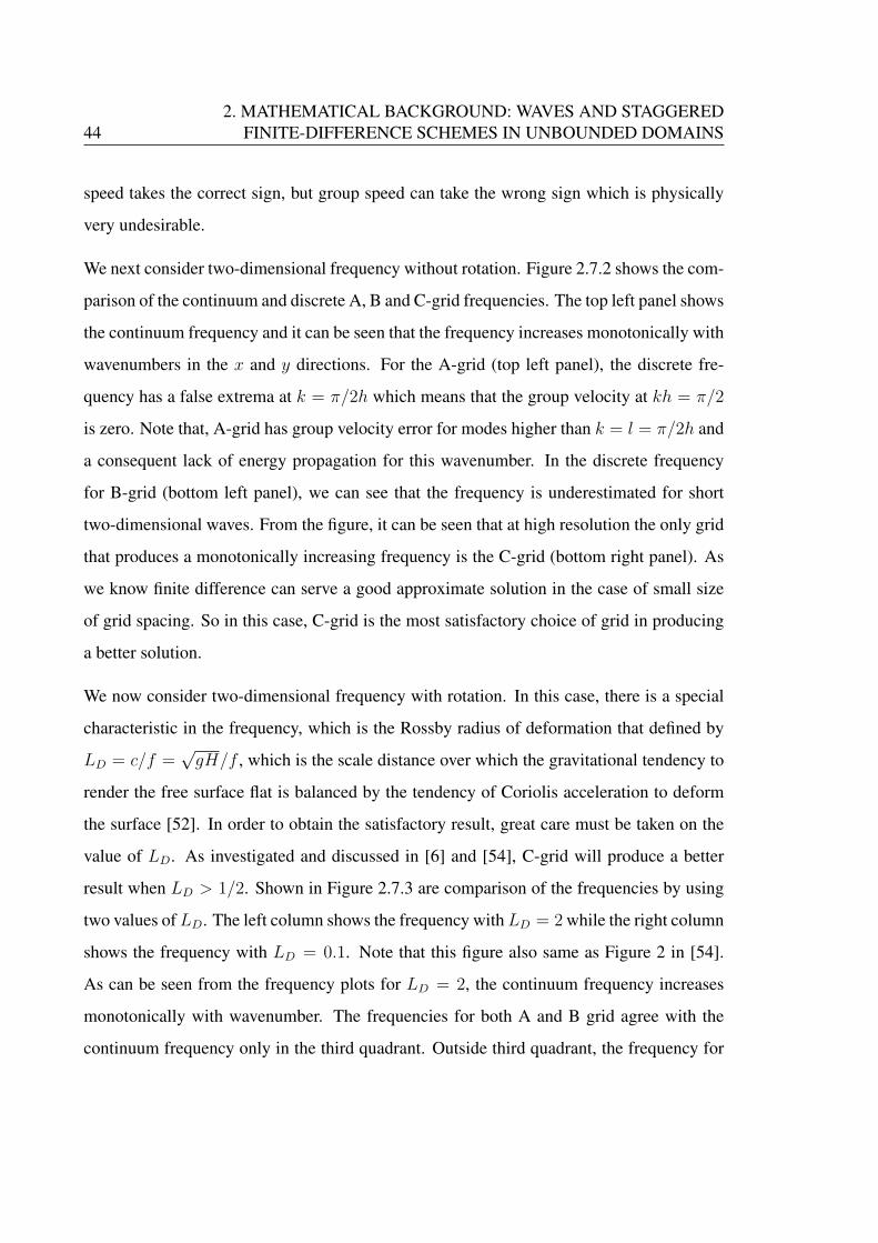
442. MATHEMATICAL BACKGROUND: WAVES AND STAGGERED
FINITE-DIFFERENCE SCHEMES IN UNBOUNDED DOMAINS
speed takes the correct sign, but group speed can take the wrong sign which is physically
very undesirable.
We next consider two-dimensional frequency without rotation. Figure 2.7.2 shows the com-
parison of the continuum and discrete A, B and C-grid frequencies. The top left panel shows
the continuum frequency and it can be seen that the frequency increases monotonically with
wavenumbers in the x and y directions. For the A-grid (top left panel), the discrete fre-
quency has a false extrema at k = π/2h which means that the group velocity at kh = π/2
is zero. Note that, A-grid has group velocity error for modes higher than k = l = π/2h and
a consequent lack of energy propagation for this wavenumber. In the discrete frequency
for B-grid (bottom left panel), we can see that the frequency is underestimated for short
two-dimensional waves. From the figure, it can be seen that at high resolution the only grid
that produces a monotonically increasing frequency is the C-grid (bottom right panel). As
we know finite difference can serve a good approximate solution in the case of small size
of grid spacing. So in this case, C-grid is the most satisfactory choice of grid in producing
a better solution.
We now consider two-dimensional frequency with rotation. In this case, there is a special
characteristic in the frequency, which is the Rossby radius of deformation that defined by
LD = c/f =√gH/f , which is the scale distance over which the gravitational tendency to
render the free surface flat is balanced by the tendency of Coriolis acceleration to deform
the surface [52]. In order to obtain the satisfactory result, great care must be taken on the
value of LD. As investigated and discussed in [6] and [54], C-grid will produce a better
result when LD > 1/2. Shown in Figure 2.7.3 are comparison of the frequencies by using
two values ofLD. The left column shows the frequency withLD = 2 while the right column
shows the frequency with LD = 0.1. Note that this figure also same as Figure 2 in [54].
As can be seen from the frequency plots for LD = 2, the continuum frequency increases
monotonically with wavenumber. The frequencies for both A and B grid agree with the
continuum frequency only in the third quadrant. Outside third quadrant, the frequency for

2.8. SUMMARY 45
A and B grid decreases as the wavenumber increasing which contradict with the continuum
frequency. Unlike the other frequencies, the freuency for C grid shows the same monotonic
increase of frequency as the continuum frequency. For LD = 0.1, both frequencies for A
and B grid show the same distortion as LD = 2. However, the C-grid frequency now shows
a monotonic decrease with increasing wavenumber. Hence all discrete frequencies contrary
to the continuum frequency. Thus, for the two dimensional case with rotation C-grid is the
most satisfactory choice of grid in producing a better solution with an appropriate value of
LD.
0 0.5 1 1.5 2 2.5 3 3.5
kh
0
0.5
1
1.5
2
2.5
3
3.5
ω
ContinuumA-gridB-gridC-grid
(a)
0 0.5 1 1.5 2 2.5 3 3.5
kh
0
0.2
0.4
0.6
0.8
1
ω /
ck (
wav
e sp
eed)
ContinuumA-gridB-gridC-grid
(b)
0 0.5 1 1.5 2 2.5 3 3.5
kh
-1
-0.8
-0.6
-0.4
-0.2
0
0.2
0.4
0.6
0.8
1
∂ ω
/ ∂ k
(gr
oup
spee
d)
ContinuumA-gridB-gridC-grid
(c)
Figure 2.7.1: (a) The frequency, (b) the wave speed, and (c) the group speed for the casef = 0.
2.8 Summary
The chapter began with a review of a standard set of two-dimensional wave equations and
showed that three different physical systems (i.e., acoustic, electromagnetism, shallow-
water flow) has equivalent equations. We also reviewed some important conservation laws
for this equations. We next examined wave propagation using the standard set of wave
equations by looking at the frequency and property related to it: phase speed and group
velocity.
Then, we have reviewed a numerical scheme by finite-differene methods on three different
finite-difference grids, namely A, B, and C-grid. We also have reviewed some discrete
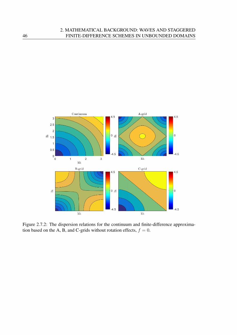
462. MATHEMATICAL BACKGROUND: WAVES AND STAGGERED
FINITE-DIFFERENCE SCHEMES IN UNBOUNDED DOMAINS
Figure 2.7.2: The dispersion relations for the continuum and finite-difference approxima-tion based on the A, B, and C-grids without rotation effects, f = 0.
2.8. SUMMARY 47
Figure 2.7.3: The dispersion relations for the continuum and finite-difference approxim-ation based on the A, B, and C-grids with the effects of rotation. The left column is forLD/h = 2, and the right for LD/h = 0.1.
482. MATHEMATICAL BACKGROUND: WAVES AND STAGGERED
FINITE-DIFFERENCE SCHEMES IN UNBOUNDED DOMAINS
conservation laws that are discrete mass and energy conservation laws on the C-grid. By
using second-order centred finite-difference formulation, the equations are discretized and
we showed that there are three different sets of discrete equations, correspond for each
grid. Analogous to the continuum domain, we reviewed some works done in [6]; wave
propagation in a doubly periodic domain. We analysed the performance of each grid in
terms of discrete frequency. For all grids, we recovered second-order discrete frequency,
and the discrete frequency underestimated by continuum frequency. So they are equally
accurate as grid spacing h→ 0. However, there is important differences for larger h.
We then reviewed some works done in [54] on performance of discrete frequency on the
finite-difference grids. We showed that by retaining the Earth’s rotation effects in the wave
equations, Rossby radius of deformation takes account in the discrete frequency, and great
care must be taken in producing discrete solution. We have compared all discrete frequen-
cies with the continuum frequency. We showed that discrete frequency on the C-grid is the
most satisfactory grid to represent the discrete frequency. For the rest of this thesis, we only
consider discrete solution on the C-grid. As the variables on this grid are staggered, the
spatial derivatives are evaluating naturally on this grid, which is optimal for the discretized
of equations of motion. It is also easy to ensure that the mass and energy quantities are
conserved.
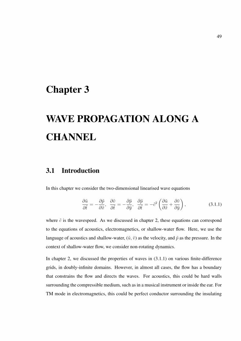
49
Chapter 3
WAVE PROPAGATION ALONG A
CHANNEL
3.1 Introduction
In this chapter we consider the two-dimensional linearised wave equations
∂u
∂t= −∂p
∂x,∂v
∂t= −∂p
∂y,∂p
∂t= −c2
(∂u
∂x+∂v
∂y
), (3.1.1)
where c is the wavespeed. As we discussed in chapter 2, these equations can correspond
to the equations of acoustics, electromagnetics, or shallow-water flow. Here, we use the
language of acoustics and shallow-water, (u, v) as the velocity, and p as the pressure. In the
context of shallow-water flow, we consider non-rotating dynamics.
In chapter 2, we discussed the properties of waves in (3.1.1) on various finite-difference
grids, in doubly-infinite domains. However, in almost all cases, the flow has a boundary
that constrains the flow and directs the waves. For acoustics, this could be hard walls
surrounding the compressible medium, such as in a musical instrument or inside the ear. For
TM mode in electromagnetics, this could be perfect conductor surrounding the insulating
50 3. WAVE PROPAGATION ALONG A CHANNEL
di-electric in the plate geometry illustrated in Figure 2.2.1. For shallow-water flow, this
could be the banks of a river, or the coastline of an ocean. In this chapter, we consider the
discuss the effects of such boundaries upon the discrete wave propagation, albeit it in the
simplest possible case of wave propagation along an infinitely long channel with parallel
and straight side walls.
As in the rest of this thesis, we now focus on the C grid that was introduced in chapter 2.
The standard treatment in this method to approximate the complex boundaries is introduce a
numerical boundary that differ from the real boundary which typically contains staircases.
Such staircase boundaries might be expected to reduce the accuracy of the resulting nu-
merical solution, because the numerical boundary deviates from the continuum boundary
by a distance of O(h). However, it is not clear how the resulting numerical solution will
converge to the continuum solution as the grid size h → 0. Further, if the solution does
converge, then at what rate does this happen? This chapter is devoted to quantifying the
convergence rate – analytically in the limit h → 0 – for wave propagation along staircase
boundaries.
There are a handful of studies on the effects of staircase boundaries on wave propagation.
The most relevant example is [51], who studied system (3.1.1) on the C-grid for a channel
with a perfect staircase boundaries (i.e., boundaries aligned at 45◦ to grid). By using the
standard centred second order finite-difference formulation in space, he derived the discrete
dispersion relation for waves propagation along the channel and he showed that the nondi-
mensional phase speed, i.e., (1 + 1/m)−1/2 – Eq. (34) in [51], is reduced to first-order
accuracy in grid spacing. He also concluded that the waves in the channel propagate with
the criss-cross form which then give delay with a first-order accuracy in the phase-shift.
This first-order phase shift error is comfirmed in the wave reflection analysis which will be
discussed in the next chapter. However, this result does not apparently apply to the main
problem of interest, which is what happens when h → 0 but with m → ∞, so that the
width of the channel remains finite. Further, it does not apparently distinguish between

3.1. INTRODUCTION 51
waves with different cross-channel wavenumbers.
In a more specific application, the propagation of Kelvin wave along straight boundar-
ies in C-grid finite-difference models has been studied by [32]. By considering the two-
dimensional shallow-water equations with the effects of Earth’s rotation, he showed analyt-
ically that the frequency and horizontal structure of the discrete Kelvin wave on the C-grid
with staircase boundary converge at first order in h. The results also are verified numer-
ically at other angle θ between the coastline and the grid, and the solution remain at first
order accurate. In the limit of h→ 0, he showed that the discrete solutions of frequency and
horizontal velocity converge towards the continuum solutions along the straight and stair-
case boundary. He concluded that the discrete solutions induced by the staircase boundaries
degrade the accuracy of the discrete solutions. However, Kelvin wave existence relies upon
a coastline and the derived solutions may not be appropriate for the bounded problem, i.e.
channel. The effects of rotation may be one of the factor of degradation of the accuracy.
In this chapter we adopt many of the methods introducing in [32] to the non-rotating chan-
nel problem, as partially studied by [51]. We start, in Section 3.1.1, by introducing a non-
dimensional set of governing equations, involving a non-dimensional frequency ω, which
is the main quantity of interest. In Section 3.2, we derive the continuum solution, which
provides the benchmark for the discrete calculations to follow. The first of those, in Sec-
tion 3.3, is for the case with boundary-aligned grids, where we confirm that second-order
accuracy can be achieved. The second of those calculations, in Section 3.4, is for the case
of a perfect staircase (i.e., with boundary aligned at 45◦ to the grid). In both cases we use
both numerical and asymptotic methods.

52 3. WAVE PROPAGATION ALONG A CHANNEL
3.1.1 Nondimensional equations
Suppose that the channel has width L, which we use as our lengthscale, in which case the
corresponding timescale is L/c. We thus introduce nondimensional coordinates
x =x
L, y =
y
L, t =
tc
L, (u, v) =
(u, v)
U, p =
p
U c. (3.1.2)
We then seek solutions of the form
u = URe (u(x, y) exp(−iωt)) ,
v = URe (v(x, y) exp(−iωt)) ,
p = U cRe (p(x, y) exp(−iωt)) , (3.1.3)
where U is an arbitrary dimensional amplitude of motion. Then (3.1.1) become
−iωu = −∂p∂x, (3.1.4a)
−iωv = −∂p∂y, (3.1.4b)
−iωp+∂u
∂x+∂v
∂y= 0. (3.1.4c)
The boundary conditions of no normal flow at the upper and lower channel are
v(x, 0) = 0, and v(x, 1) = 0. (3.1.5)
3.2 Continuum Solutions
Here, we derive the continuum solutions of our problem which will be used to assess our
discrete solutions in further discussions. Let us consider the periodic unbounded channel
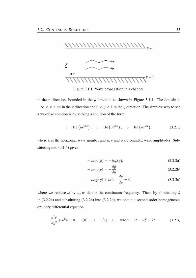
3.2. CONTINUUM SOLUTIONS 53
Figure 3.1.1: Wave propagation in a channel.
in the x direction, bounded in the y direction as shown in Figure 3.1.1. The domain is
−∞ < x <∞ in the x direction and 0 < y < 1 in the y direction. The simplest way to see
a wavelike solution is by seeking a solution of the form
u = Re(ueikx
), v = Re
(veikx
), p = Re
(peikx
), (3.2.1)
where k is the horizontal wave number and u, v and p are complex wave amplitudes. Sub-
stituting into (3.1.4) gives
− iωcu(y) = −ikp(y), (3.2.2a)
− iωcv(y) = −dpdy, (3.2.2b)
− iωcp(y) + iku+dv
dy= 0, (3.2.2c)
where we replace ω by ωc to denote the continuum frequency. Then, by eliminating u
in (3.2.2c) and substituting (3.2.2b) into (3.2.2c), we obtain a second-order homogeneous
ordinary differential equation
d2v
dy2+ κ2v = 0, v(0) = 0, v(1) = 0, where κ2 = ω2
c − k2, (3.2.3)
54 3. WAVE PROPAGATION ALONG A CHANNEL
where we have added the boundary condition (3.1.5) in that equation. We notice that this is
an eigenvalue problem for ωc and v(y). We need to find the special values of ωc for which
non-zero solutions exist for v(y). There are three cases to be considered.
1. κ = 0. Then v = Ay + B, for some constant A and B. Then, v(0) = 0 implies
B = 0; and v(1) = 0 implies A = 0. So v(y) = 0, which is not a solution of interest.
2. κ < 0. Then v = A exp(κy) + B exp(−κy), for some constant A and B. Then,
v(0) = 0, implies B = −A, so that v = A(exp(κ)y − exp(−κ)y). Then, v(1) = 0
implies A = 0. So v(y) = 0, which is not a solution of interest.
3. κ > 0. Then, v = A cosκy + B sinκy, for some constant A and B. Then v(0) = 0
implies A = 0, so that v = B sinκy. Then v(1) = 0 implies B sinκ = 0, so either
B = 0 but then gives v(y) = 0, which is not a solution of interest, or sinκ = 0,
which implies κ = jπ, for some positive integer j.
Thus, we only obtained non-trivial solutions when κ = jπ, so that
κ2 = j2π2 ⇒ ω2c − k2 = j2π2 ⇒ ω2
c = k2 + j2π2, (3.2.4)
where j ∈ N. Since sinκy = sin jπy, the corresponding solution for v is
v(y) = B sin(jπy) ⇒ v(x, y) = Re(B sin(jπy) e(ikx)
). (3.2.5)
This is the standard well-known solution for channel waves with modenumber j. To com-
plete all the solutions, we also calculate p and u from (3.2.2a), (3.2.2c), which then simply
give the full solutions of wave in the channel (3.2.1). They are written as
u(y) =Bkω
jπcos(jπy) ⇒ u(x, y) = Re
(Bkω
jπcos(jπy) e(ikx)
)=Bkω
jπcos(jπy) cos(kx),
(3.2.6)
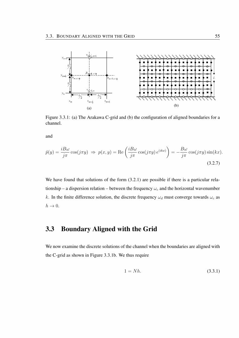
3.3. BOUNDARY ALIGNED WITH THE GRID 55
(a)(b)
Figure 3.3.1: (a) The Arakawa C-grid and (b) the configuration of aligned boundaries for achannel.
and
p(y) =iBω
jπcos(jπy) ⇒ p(x, y) = Re
(iBω
jπcos(jπy) e(ikx)
)= −Bω
jπcos(jπy) sin(kx).
(3.2.7)
We have found that solutions of the form (3.2.1) are possible if there is a particular rela-
tionship – a dispersion relation – between the frequency ωc and the horizontal wavenumber
k. In the finite difference solution, the discrete frequency ωd must converge towards ωc as
h→ 0.
3.3 Boundary Aligned with the Grid
We now examine the discrete solutions of the channel when the boundaries are aligned with
the C-grid as shown in Figure 3.3.1b. We thus require
1 = Nh. (3.3.1)
56 3. WAVE PROPAGATION ALONG A CHANNEL
As discussed in previous chapter, we use the popular staggered C-grid where all variables
in our system of equations are distributed in every cells as demonstrated in Figure 3.3.1a.
Then, for every discrete points in computational domain we have index m for the x variable
and index n for the y variable. So that we have point xm which represents the mth grid
point in space and yn represents nth grid point in space and discrete coordinates at any
point m and n are xm = mh and yn = nh, where m,n ∈ Z. By using second-order centred
finite-difference formulation, our system of equations which are (3.1.4a,b,c) are discretised
as
− iωdum,n+ 12
= −pm+ 1
2,n+ 1
2− pm− 1
2,n+ 1
2
h, (3.3.2a)
− iωdvm+ 12,n = −
pm+ 12,n+ 1
2− pm+ 1
2,n− 1
2
h, (3.3.2b)
− iωdpm+ 12,n+ 1
2+
1
h
(um+1,n+ 1
2− um,n+ 1
2+ vm+ 1
2,n+1 − vm+ 1
2,n
)= 0, (3.3.2c)
where ωd now is the discrete frequency and we will assess the rate of convergence of this
unknown. The discrete boundary conditions of no normal flow at the upper and lower
channel are
vm+ 12,0 = vm+ 1
2,N = 0. (3.3.3)
The easiest way to derive the discrete solution for this problem is by seeking wavelike
solutions of the form
um,n+ 12
= Re(un+ 1
2eikxm
),
vm+ 12,n = Re
(vne
ikxm+1
2
),
pm+ 12,n+ 1
2= Re
(pn+ 1
2eikx
m+12
).
3.3. BOUNDARY ALIGNED WITH THE GRID 57
By substituting these ansatz into (3.3.2a,b,c) we have
− iωdun+ 12
= −2i
hsin
(kh
2
)pn+ 1
2, (3.3.4a)
− iωdvn = −1
h
(pn+ 1
2− pn− 1
2
), (3.3.4b)
− iωdpn+ 12
+1
h
(2i sin
(kh
2
)un+ 1
2+ vn+1 − vn
)= 0. (3.3.4c)
With a straightforward elimination of un+ 12
in (3.3.4c) using (3.3.4a), and eliminating pn+ 12
and pn− 12
in (3.3.4b) using (3.3.4c), we then obtain a linear second-order difference equation
for v written as
vn+1 − 2(1− µ)vn + vn−1 = 0, where µ =h2
2
(ω2d −
4 sin2 kh2
h2
), (3.3.5)
together with the boundary conditions
v0 = vN = 0. (3.3.6)
Again, this is an eigenvalue problem for ωd and vn and we need to find the special values
of ωd for which non-zero solutions exist for vn.
We notice that the non-zero solution of vn can be found by solving (3.3.5) either analytic-
ally or numerically. Therefore, we will discuss both solutions followed by the asymptotic
solutions as h→ 0 for the analytical case.
3.3.1 Numerical solutions
There are many existing numerical methods for solving second order linear boundary value
problem and the common method is shooting method. Shooting method works by reducing
the boundary value problem to an iterative sequence of initial value problems. The shooting
method is initialised with an initial guess ω1 for ωd, and then stepping (3.3.5) across the

58 3. WAVE PROPAGATION ALONG A CHANNEL
domain from n = 0 to n = N subject to v0 = 0 and v1 = 1 (the latter being an arbitrary
choice for this homogeneous and linear problem). This leads to some value vN , which is
required to be zero for the actual eigenvalue, but which is generally non-zero for any guess;
we thus call this a residual, R1. Next, the initial guess ω1 is changed by a small amount
to give ω2, and the shooting process is repeated, leading to another residual R2. In order
to obtain a residual of 0, the guess for ω must be sensibly updated. This can be done by
implementing Newton-Raphson iterations method using
ωnew = ω1 −R1
R′1, where R′1 =
(R2 −R1)
(ω2 − ω1). (3.3.7)
With this new value of ωnew, the process is repeated until a chosen stopping convergence is
satisfied. Here we choose (ω2 − ω1)� 10−8 and |R1| � 10−8 as our stopping criteria.
When the convergence is satisfied, we now have the value of ωd in (3.3.5), and the numerical
solutions of (3.3.5) can be obtained. Note that we can solve for different cross-channel
modes by choosing our initial guess ω1 to be close to the known-continuum value, with
a chosen value of j. In Figure 3.3.2, we are showing solutions of vn for the case of grid
spacing h = 0.05 (i.e., N = 20) for corresponding wavenumber along the channel k = 1 to
values j = 1, 2, 3, where the solutions have been normalised to max |v| = 1.
We can check the rate of convergence of this plot by plotting the log-log plot of the dif-
ferences between continuum frequency ωc and numerical frequency ωd versus grid spacing
h as can be seen in Figure 3.3.3. In this figure, we are showing slope of convergence for
mode j = 2. We note that, the plot has a straight line with slope two which means the rate
of convergence of our numerical frequency is second-order as expected, since we have used
second order finite-difference formulation to discretise equations of motion.
One can also measure the convergence in vn. This is shown in Figure 3.3.4, where we
measure the slope of log-log plot of the error in v at various grid spacing for mode j = 2.
It can be seen that the slope of the line is two which indicates second-order convergence as
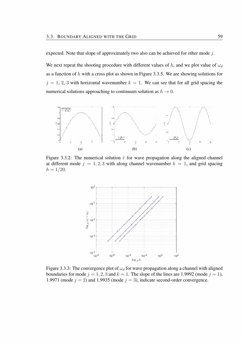
3.3. BOUNDARY ALIGNED WITH THE GRID 59
expected. Note that slope of approximately two also can be achieved for other mode j.
We next repeat the shooting procedure with different values of h, and we plot value of ωd
as a function of h with a cross plot as shown in Figure 3.3.5. We are showing solutions for
j = 1, 2, 3 with horizontal wavenumber k = 1. We can see that for all grid spacing the
numerical solutions approaching to continuum solution as h→ 0.
(a) (b) (c)
Figure 3.3.2: The numerical solution v for wave propagation along the aligned channelat different mode j = 1, 2, 3 with along channel wavenumber k = 1, and grid spacingh = 1/20.
Figure 3.3.3: The convergence plot of ωd for wave propagation along a channel with alignedboundaries for mode j = 1, 2, 3 and k = 1. The slope of the lines are 1.9992 (mode j = 1),1.9971 (mode j = 2) and 1.9935 (mode j = 3), indicate second-order convergence.

60 3. WAVE PROPAGATION ALONG A CHANNEL
Figure 3.3.4: The convergence plot of v for wave propagation along the channel withaligned boundaries for mode j = 1, 2, 3 with k = 1. The slope of the lines are 1.9907(mode j = 1), 1.9659 (mode j = 1), and 1.9467 (mode j = 3), indicate second-orderconvergence.
Figure 3.3.5: The frequency ω for wave propagation along the channel with aligned bound-aries with horizontal wavenumber k = 1 and modes j = 1, 2, 3 at various grid spacing h.Black represents ω for j = 1, blue for j = 2, and red for j = 3.
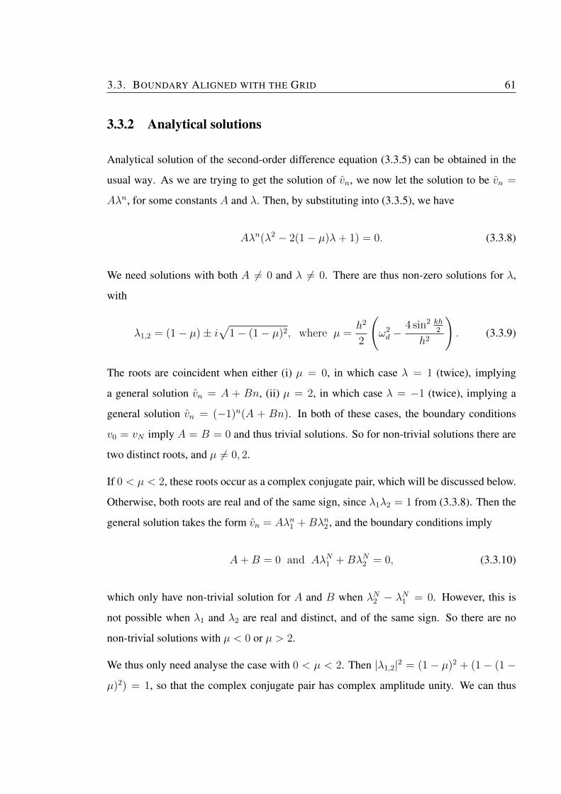
3.3. BOUNDARY ALIGNED WITH THE GRID 61
3.3.2 Analytical solutions
Analytical solution of the second-order difference equation (3.3.5) can be obtained in the
usual way. As we are trying to get the solution of vn, we now let the solution to be vn =
Aλn, for some constants A and λ. Then, by substituting into (3.3.5), we have
Aλn(λ2 − 2(1− µ)λ+ 1) = 0. (3.3.8)
We need solutions with both A 6= 0 and λ 6= 0. There are thus non-zero solutions for λ,
with
λ1,2 = (1− µ)± i√
1− (1− µ)2, where µ =h2
2
(ω2d −
4 sin2 kh2
h2
). (3.3.9)
The roots are coincident when either (i) µ = 0, in which case λ = 1 (twice), implying
a general solution vn = A + Bn, (ii) µ = 2, in which case λ = −1 (twice), implying a
general solution vn = (−1)n(A + Bn). In both of these cases, the boundary conditions
v0 = vN imply A = B = 0 and thus trivial solutions. So for non-trivial solutions there are
two distinct roots, and µ 6= 0, 2.
If 0 < µ < 2, these roots occur as a complex conjugate pair, which will be discussed below.
Otherwise, both roots are real and of the same sign, since λ1λ2 = 1 from (3.3.8). Then the
general solution takes the form vn = Aλn1 +Bλn2 , and the boundary conditions imply
A+B = 0 and AλN1 +BλN2 = 0, (3.3.10)
which only have non-trivial solution for A and B when λN2 − λN1 = 0. However, this is
not possible when λ1 and λ2 are real and distinct, and of the same sign. So there are no
non-trivial solutions with µ < 0 or µ > 2.
We thus only need analyse the case with 0 < µ < 2. Then |λ1,2|2 = (1 − µ)2 + (1− (1 −
µ)2) = 1, so that the complex conjugate pair has complex amplitude unity. We can thus
62 3. WAVE PROPAGATION ALONG A CHANNEL
write
λ1,2 = cos θ ± i sin θ = exp(±iθ), (3.3.11)
where cos θ = 1 − µ and sin θ =√
(1− (1− µ)2) =√
(2µ− µ2), enabling θ to be
uniquely determined from µ, and vice-versa. Then
vn = A exp(inθ) +B exp(−inθ) = C cosnθ +D sinnθ. (3.3.12)
But v0 = 0 implies C = 0, and then vN = 0 implies sinNθ = 0 (since D 6= 0), i.e.,
Nθ = jπ for some positive integer j. Thus
µ = 1− cos θ = 1− cos
(jπ
N
)= 2 sin2
(jπ
2N
)= 2 sin2
(jπh
2
), (3.3.13)
since h = 1/N , from (3.3.1).
With a straightforward algebraic manipulation, we obtained a discrete dispersion relation,
ωd, as
ω2d =
4
h2
(sin2 kh
2+ sin2 jπh
2
), where j ∈ N. (3.3.14)
The solutions for p and u also can be calculated. From (3.3.4c), we obtain the discrete
solutions for pressure as
pn+ 12
=iωdD
h(ω2d − 4
h2sin2 kh
2
) [2 sin jπnh sin2 jπh
2− sin jπh cos jπnh
], (3.3.15)
where the expressions in the square bracket are obtain from the discrete solution of v. And
from (3.3.4a) the solution of the horizontal velocity u is obtain as
un+ 12
=2
ωhsin
kh
2pn+ 1
2, (3.3.16)
where pn+ 12
is given in (3.3.15).
3.3. BOUNDARY ALIGNED WITH THE GRID 63
3.3.3 Asymptotic analysis as h→ 0
The accuracy of ωd is then assessed by comparing the discrete solution with the continuum
solution (3.2.4). By using Taylor series expansion, (3.3.14) now is written as
ω2d =
4
h2
((kh
2
)2
+
(jπh
2
)2
− 1
3
((kh
2
)4
+
(jπh
2
)4))
+ · · ·
= k2 + j2π2 − 1
12h2(k4 + j4π4
)+ · · ·
= ω2c −
1
12h2(k4 + j4π4
)+ · · · . (3.3.17)
It is found that in the limit of h→ 0, the discrete frequency ωd is second order accurate in h
and ω2d is always underestimates ω2
c . This behaviour is show in Figure 3.3.5 where we plot
both continuum and discrete frequency for three different modes j against various values
of grid spacing h. It can be seen that, for every mode j, the discrete frequency ωd is always
underestimates the continuum frequency ωc and as the grid size decreases (i.e., h→ 0), the
discrete solutions are approaching continuum solutions as expected from (3.3.17).
The analytical discrete solution that has been derived in this section has been shown to agree
with the numerical solutions and both solutions are approaching to the continuum solutions
as the grid spacing h → 0. The rate of convergence for numerical and analytical discrete
solutions also agree with each other with both being second-order accurate in h. This is
desired results in the case of the channel boundaries and grid are aligned. However, we
cannot easily assume that same accuracy can be recovered when the channel’s boundaries
are not aligned with the grids. Therefore, in the next section, we will discuss its effect
where we considered the same channel rotated 45◦ from the axis.
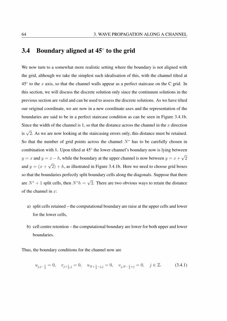
64 3. WAVE PROPAGATION ALONG A CHANNEL
3.4 Boundary aligned at 45◦ to the grid
We now turn to a somewhat more realistic setting where the boundary is not aligned with
the grid, although we take the simplest such idealisation of this, with the channel tilted at
45◦ to the x axis, so that the channel walls appear as a perfect staircase on the C grid. In
this section, we will discuss the discrete solution only since the continuum solutions in the
previous section are valid and can be used to assess the discrete solutions. As we have tilted
our original coordinate, we are now in a new coordinate axes and the representation of the
boundaries are said to be in a perfect staircase condition as can be seen in Figure 3.4.1b.
Since the width of the channel is 1, so that the distance across the channel in the x direction
is√
2. As we are now looking at the staircasing errors only, this distance must be retained.
So that the number of grid points across the channel N∗ has to be carefully chosen in
combination with h. Upon tilted at 45◦ the lower channel’s boundary now is lying between
y = x and y = x− h, while the boundary at the upper channel is now between y = x+√
2
and y = (x +√
2) + h, as illustrated in Figure 3.4.1b. Here we need to choose grid boxes
so that the boundaries perfectly split boundary cells along the diagonals. Suppose that there
are N∗ + 1 split cells, then N∗h =√
2. There are two obvious ways to retain the distance
of the channel in x:
a) split cells retained – the computational boundary are raise at the upper cells and lower
for the lower cells,
b) cell centre retention – the computational boundary are lower for both upper and lower
boundaries.
Thus, the boundary conditions for the channel now are
uj,j− 12
= 0, vj+ 12,j = 0, uN+ 1
2−j,j = 0, vj,N− 1
2+j = 0, j ∈ Z. (3.4.1)
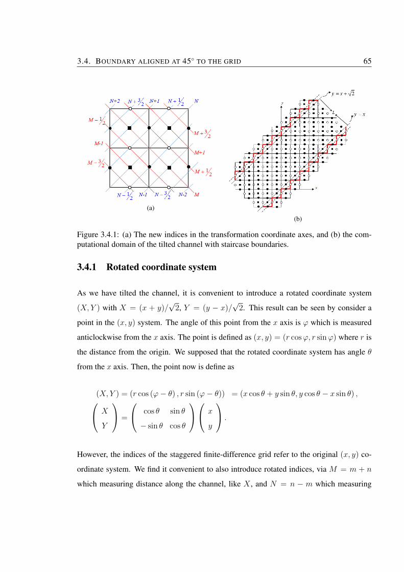
3.4. BOUNDARY ALIGNED AT 45◦ TO THE GRID 65
(a)
(b)
Figure 3.4.1: (a) The new indices in the transformation coordinate axes, and (b) the com-putational domain of the tilted channel with staircase boundaries.
3.4.1 Rotated coordinate system
As we have tilted the channel, it is convenient to introduce a rotated coordinate system
(X, Y ) with X = (x + y)/√
2, Y = (y − x)/√
2. This result can be seen by consider a
point in the (x, y) system. The angle of this point from the x axis is ϕ which is measured
anticlockwise from the x axis. The point is defined as (x, y) = (r cosϕ, r sinϕ) where r is
the distance from the origin. We supposed that the rotated coordinate system has angle θ
from the x axis. Then, the point now is define as
(X, Y ) = (r cos (ϕ− θ) , r sin (ϕ− θ)) = (x cos θ + y sin θ, y cos θ − x sin θ) , X
Y
=
cos θ sin θ
− sin θ cos θ
x
y
.
However, the indices of the staggered finite-difference grid refer to the original (x, y) co-
ordinate system. We find it convenient to also introduce rotated indices, via M = m + n
which measuring distance along the channel, like X , and N = n − m which measuring
66 3. WAVE PROPAGATION ALONG A CHANNEL
distance across the channel, like Y . By using these new indices, any variable in the system
now written as
um,n = UM,N , vm,n = VM,N , pm,n = PM,N ,
where (M,N) in terms of (m,n). Then, equations (3.1.4a,b,c) are discretized by using
second-order centred finite difference as
− iωUM− 12,N− 1
2= −1
h(PM,N−1 − PM−1,N) , (3.4.2a)
− iωVM− 32,N− 1
2= −1
h(PM−1,N − PM−2,N−1) , (3.4.2b)
− iωPM−1,N +1
h
(UM− 1
2,N− 1
2− UM− 3
2,N+ 1
2+ VM− 1
2,N+ 1
2− VM− 3
2,N− 1
2
)= 0, (3.4.2c)
which is equivalent to
− iωUM,N = −1
h
(PM+ 1
2,N− 1
2− PM− 1
2,N+ 1
2
), (3.4.3a)
− iωVM,N = −1
h
(PM+ 1
2,N+ 1
2− PM− 1
2,N− 1
2
), (3.4.3b)
− iωPM,N +1
h
(UM+ 1
2,N− 1
2− UM− 1
2,N+ 1
2+ VM+ 1
2,N+ 1
2− VM− 1
2,N− 1
2
)= 0. (3.4.3c)
Note that, this is the same system used in [32] but with the Coriolis terms omitted. This
system needs to be solved together with the boundary conditions. At the lower channel,
for both ways of cell retain (a) and (b) we obtain N = −1/2 as the boundary nodes from
(3.4.1). So that boundary conditions at the lower channel for both cases in the rotated
system are
UM,−1/2 = VM,−1/2 = 0, for all M. (3.4.4)
At the upper channel, the boundary conditions are
UM,N∗± 12
= 0, and VM,N∗± 12
= 0, (3.4.5)
3.4. BOUNDARY ALIGNED AT 45◦ TO THE GRID 67
where N∗ being the total number of grid across the channel defined by
N∗ =
√2
h. (3.4.6)
3.4.2 Wavelike solutions
We seek solutions that are periodic in the along-channel directionX . We thus seek solutions
of the form
UM,N = UNeiMθ, VM,N = VNe
iMθ, PM,N = PNeiMθ. (3.4.7)
If we suppose that there is a spatial wavenumber k in the along channel, then increasing M
by unity at fixed N increases the phase by kh/√
2, where the moving distance of this phase
is h/√
2. So that we set
θ =kh√
2. (3.4.8)
By substituting (3.4.7) into equations (3.4.3a,b,c) with some algebraic manipulation we
then have
− iωUN = −1
h
(PN− 1
2eiθ2 + PN+ 1
2e−i
θ2
), (3.4.9a)
− iωVN = −1
h
(PN+ 1
2eiθ2 − PN− 1
2e−i
θ2
), (3.4.9b)
− iωPN +1
h
(UN− 1
2eiθ2 − UN+ 1
2e−i
θ2 + VN+ 1
2eiθ2 − VN− 1
2e−i
θ2
)= 0. (3.4.9c)
By eliminating UN−1/2, UN+1/2, VN−1/2, VN+1/2 in (3.4.9c), we then obtain a single second-
order difference equation for P as
PN+2 + µPN+1 + PN = 0, where µ =ω2dh
2 − 4
2 cos θ, and θ =
kh√2. (3.4.10)

68 3. WAVE PROPAGATION ALONG A CHANNEL
As before, this is an eigenvalue problem for ωd and PN . So that we need to find the special
values of ωd for which non-zero solutions for PN exist. We are now in peculiar situation
since our boundary conditions (3.4.4) are in terms of U and V . However, we can derive a
relevant boundary conditions in terms of P nodes near the boundary. We do this by first
setting N = 0 in (3.4.9c) giving
−iωP0 +1
h
(V 1
2eiθ2 − U 1
2e−i
θ2
)= 0. (3.4.11)
We then set N = 1/2 into (3.4.9a,b) yielding
U 12
= − i
ωh
(eiθ2 − P1e
−i θ2
), (3.4.12)
V 12
= − i
ωh
(P1e
i θ2 − e−i
θ2
). (3.4.13)
Eliminating U 12
and V 12
in (3.4.11) by using (3.4.12), (3.4.13) and P0 = 1 (linearity) to set
some boundary values to 0, we obtained
P1 = αP0 where α =2− ω2
dh2
2 cos θ= −µ− 1
cos θ. (3.4.14)
Performing a corresponding manipulation near the other boundary we obtain
PM−1 = αPM . (3.4.15)
With N∗ cells across the channel, so that we might take M = N∗ (split cells retained) or
M = N∗ − 1 (cell centre retention), where N∗ is defined by (3.4.6).
3.4.3 Numerical solutions
In this section, we are going to solve (3.4.10) subject to (3.4.14) and (3.4.15) using the
shooting method. Note that we could do either case a) or b), however we just give numerical
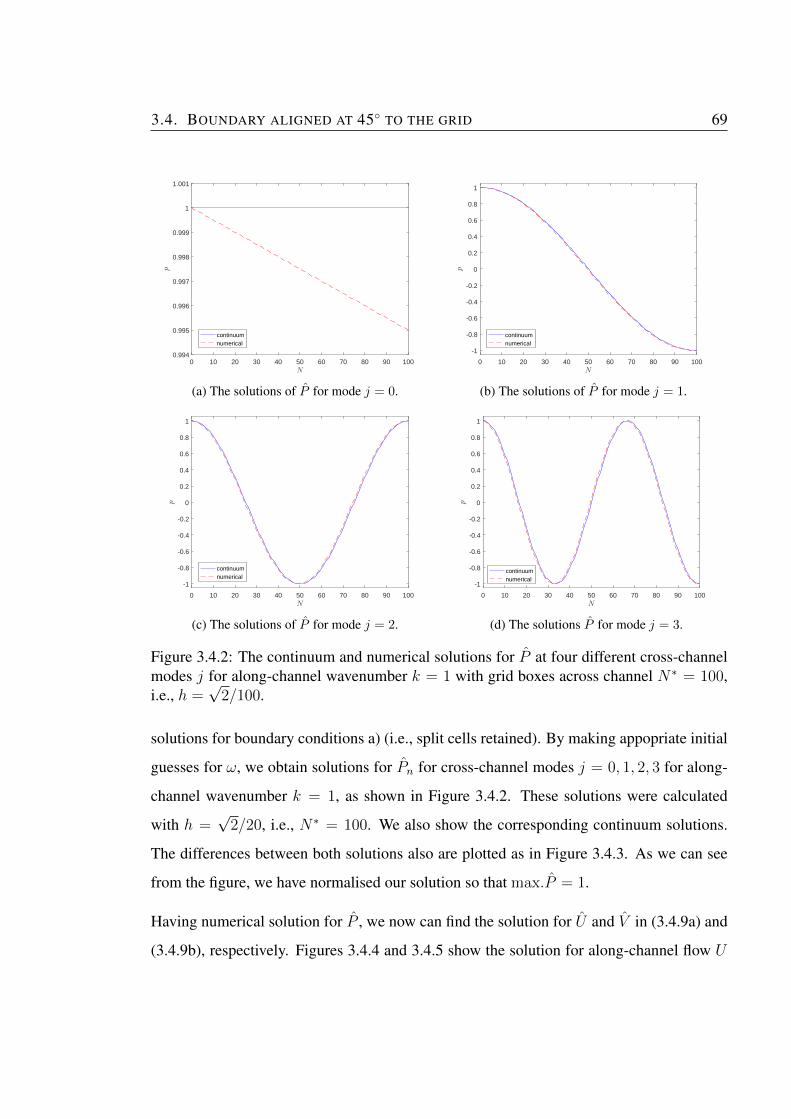
3.4. BOUNDARY ALIGNED AT 45◦ TO THE GRID 69
0 10 20 30 40 50 60 70 80 90 100N
0.994
0.995
0.996
0.997
0.998
0.999
1
1.001
p
continuumnumerical
(a) The solutions of P for mode j = 0.
0 10 20 30 40 50 60 70 80 90 100N
-1
-0.8
-0.6
-0.4
-0.2
0
0.2
0.4
0.6
0.8
1
p
continuumnumerical
(b) The solutions of P for mode j = 1.
0 10 20 30 40 50 60 70 80 90 100N
-1
-0.8
-0.6
-0.4
-0.2
0
0.2
0.4
0.6
0.8
1
p
continuumnumerical
(c) The solutions of P for mode j = 2.
0 10 20 30 40 50 60 70 80 90 100N
-1
-0.8
-0.6
-0.4
-0.2
0
0.2
0.4
0.6
0.8
1
p
continuumnumerical
(d) The solutions P for mode j = 3.
Figure 3.4.2: The continuum and numerical solutions for P at four different cross-channelmodes j for along-channel wavenumber k = 1 with grid boxes across channel N∗ = 100,i.e., h =
√2/100.
solutions for boundary conditions a) (i.e., split cells retained). By making appopriate initial
guesses for ω, we obtain solutions for Pn for cross-channel modes j = 0, 1, 2, 3 for along-
channel wavenumber k = 1, as shown in Figure 3.4.2. These solutions were calculated
with h =√
2/20, i.e., N∗ = 100. We also show the corresponding continuum solutions.
The differences between both solutions also are plotted as in Figure 3.4.3. As we can see
from the figure, we have normalised our solution so that max.P = 1.
Having numerical solution for P , we now can find the solution for U and V in (3.4.9a) and
(3.4.9b), respectively. Figures 3.4.4 and 3.4.5 show the solution for along-channel flow U
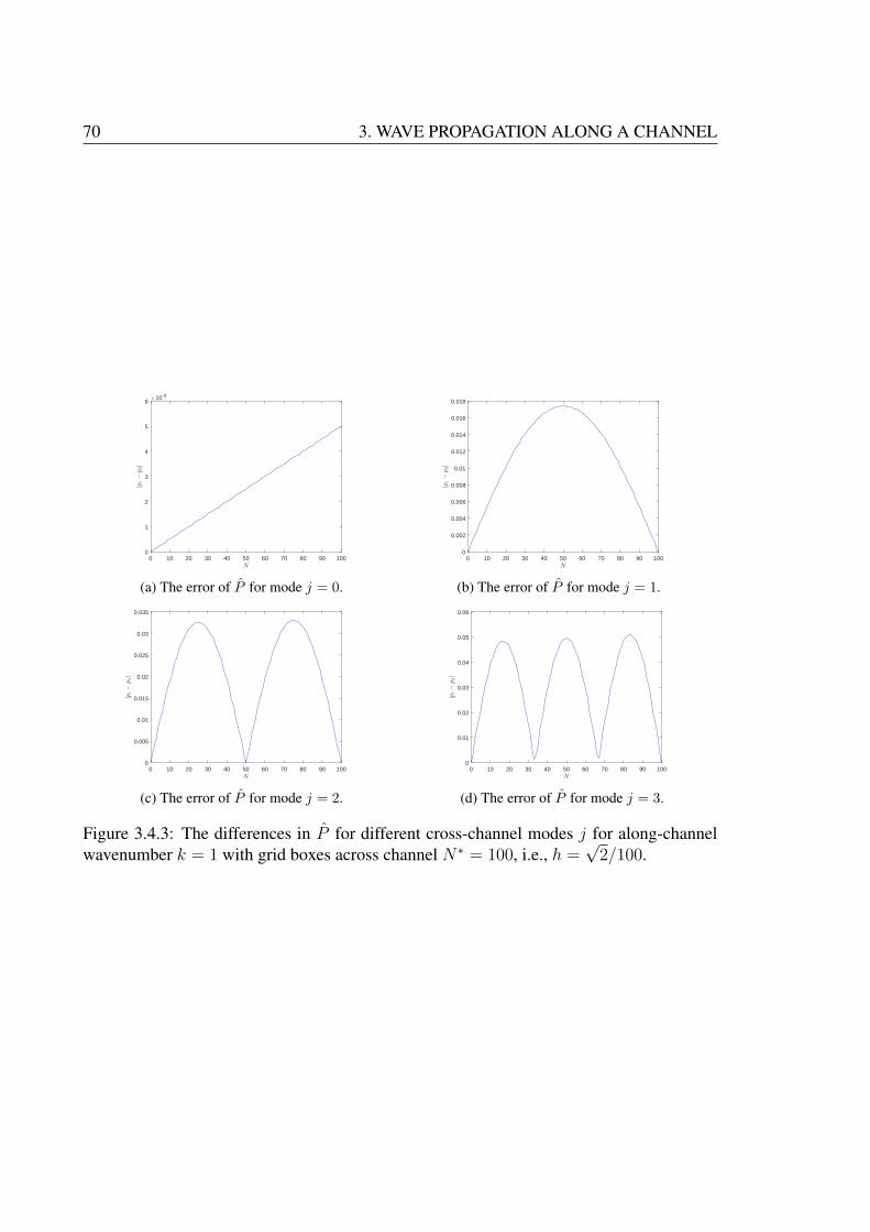
70 3. WAVE PROPAGATION ALONG A CHANNEL
0 10 20 30 40 50 60 70 80 90 100N
0
1
2
3
4
5
6
|pc−pd|
×10-3
(a) The error of P for mode j = 0.
0 10 20 30 40 50 60 70 80 90 100N
0
0.002
0.004
0.006
0.008
0.01
0.012
0.014
0.016
0.018
|pc−pd|
(b) The error of P for mode j = 1.
0 10 20 30 40 50 60 70 80 90 100N
0
0.005
0.01
0.015
0.02
0.025
0.03
0.035
|pc−pd|
(c) The error of P for mode j = 2.
0 10 20 30 40 50 60 70 80 90 100N
0
0.01
0.02
0.03
0.04
0.05
0.06
|pc−pd|
(d) The error of P for mode j = 3.
Figure 3.4.3: The differences in P for different cross-channel modes j for along-channelwavenumber k = 1 with grid boxes across channel N∗ = 100, i.e., h =
√2/100.

3.4. BOUNDARY ALIGNED AT 45◦ TO THE GRID 71
and cross-channel flow V for the cross-channel mode j = 2 for along-channel wavenumber
k = 1, with N∗ = 20. We also calculated the error between continuum and numerical
solutions. From the figures we can clearly see that there is large disagreement for the
solutions at the boundary as illustrated in Figures 3.4.4b and 3.4.5b. This large error arise
because the velocity at the boundary in numerical calculations is set to be zero since they
are on the staircase. We have put the no normal flow boundary condition at staircase in the
numerical computation while the continuum boundary is not exactly zero.
We now vary h from 0.1171 to 0.0001, and track the corresponding changes in eigenvalue
or discrete frequency ωd, for along-channel wavenumber k = 1. The results are shown in
Figure 3.4.6, for cross-channel modes j = 0, 1, 2, 3, which thus have continuum frequencies
ωc =√
12 + j2π2, i.e., ωc ≈1, 3.2969, 6.3623, and 9.4777. These continuum frequencies
– which are independent of h – are shown as solid lines. The numerical results, shown
as crosses, show that ωd < ωc, but that ωd → ωc as h → 0. The rate of convergence is
quantified via log-log plot of the error |ωd−ωc| against h, as can be seen in Figure 3.4.7 for
cross-channel mode j = 0, 1, 2, 3. The slope is 0.9942, 0.9961, 1.0061 and 1.0218 for each
j, respectively, indicating first-order convergence in h. This means that there is reduction
of order in the numerical solutions since we have used the second-order finite-difference
formulation to discretise the equations. This also means that the staircase boundaries has
degraded the order of numerical solution from second-order to first-order accurate in h.
3.4.4 Analytical solution
We now derive the analytical solution for the problem with staircase boundaries by solving
the linear second-order difference equation (3.4.10) with boundary conditions (3.4.14) and
(3.4.15). The analytical solution for the problem is derived analagous to the problem in the
section 3.3.2. In this section we provide both boundary conditions cases a) and b). We first
let Pn = λn to be a solution, for some constant λ. Following the same procedure in the
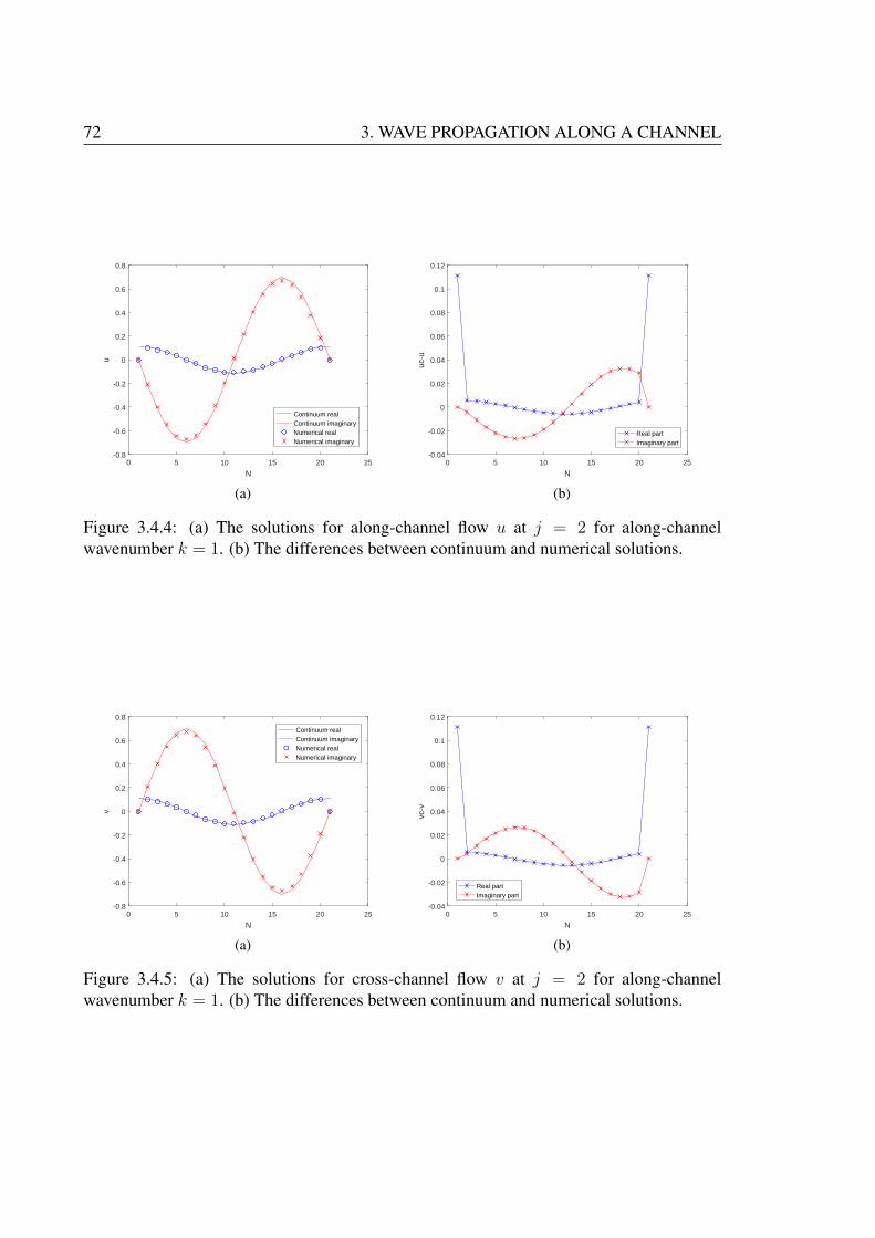
72 3. WAVE PROPAGATION ALONG A CHANNEL
0 5 10 15 20 25
N
-0.8
-0.6
-0.4
-0.2
0
0.2
0.4
0.6
0.8
u
Continuum realContinuum imaginaryNumerical realNumerical imaginary
(a)
0 5 10 15 20 25
N
-0.04
-0.02
0
0.02
0.04
0.06
0.08
0.1
0.12
uc-u
Real partImaginary part
(b)
Figure 3.4.4: (a) The solutions for along-channel flow u at j = 2 for along-channelwavenumber k = 1. (b) The differences between continuum and numerical solutions.
0 5 10 15 20 25
N
-0.8
-0.6
-0.4
-0.2
0
0.2
0.4
0.6
0.8
v
Continuum realContinuum imaginaryNumerical realNumerical imaginary
(a)
0 5 10 15 20 25
N
-0.04
-0.02
0
0.02
0.04
0.06
0.08
0.1
0.12
vc-v
Real partImaginary part
(b)
Figure 3.4.5: (a) The solutions for cross-channel flow v at j = 2 for along-channelwavenumber k = 1. (b) The differences between continuum and numerical solutions.
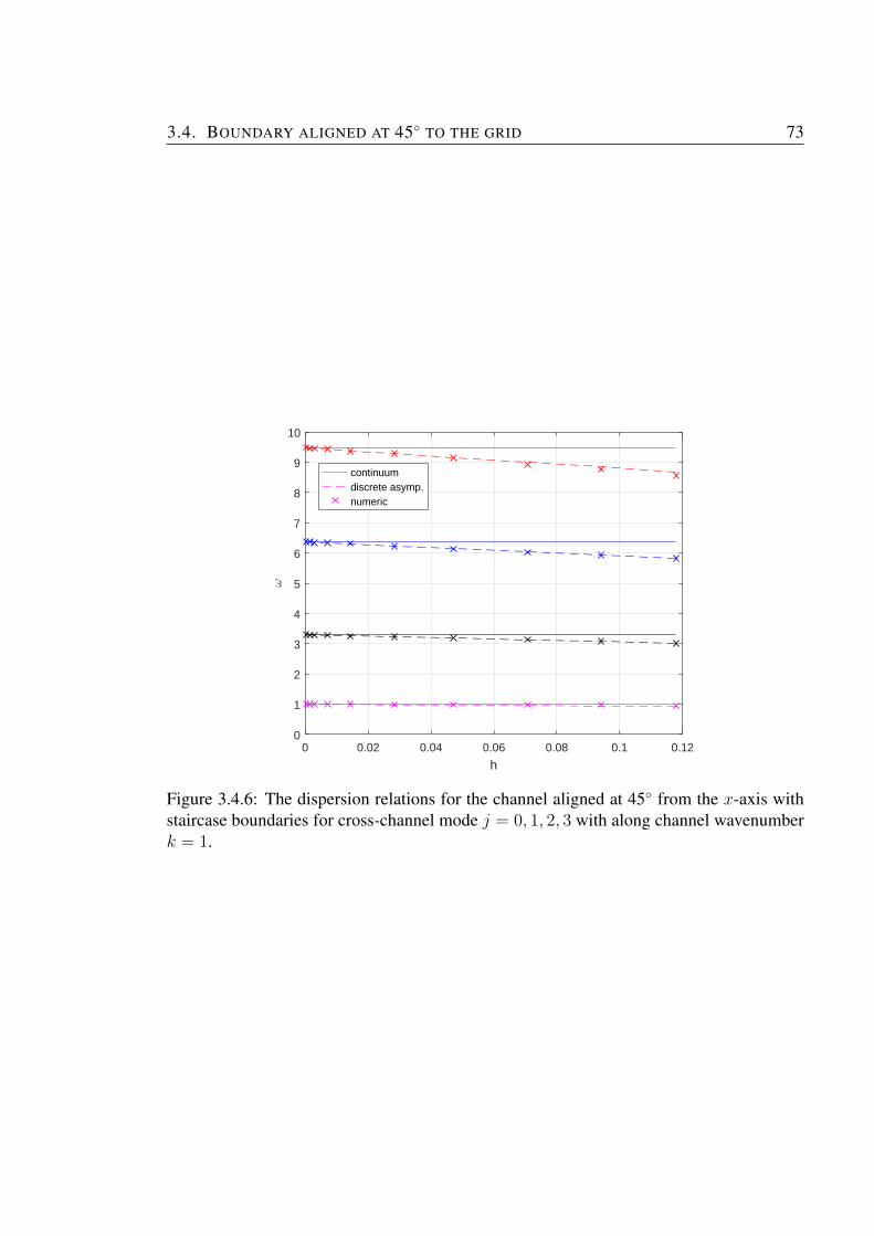
3.4. BOUNDARY ALIGNED AT 45◦ TO THE GRID 73
0 0.02 0.04 0.06 0.08 0.1 0.12
h
0
1
2
3
4
5
6
7
8
9
10
ω
continuumdiscrete asymp.numeric
Figure 3.4.6: The dispersion relations for the channel aligned at 45◦ from the x-axis withstaircase boundaries for cross-channel mode j = 0, 1, 2, 3 with along channel wavenumberk = 1.
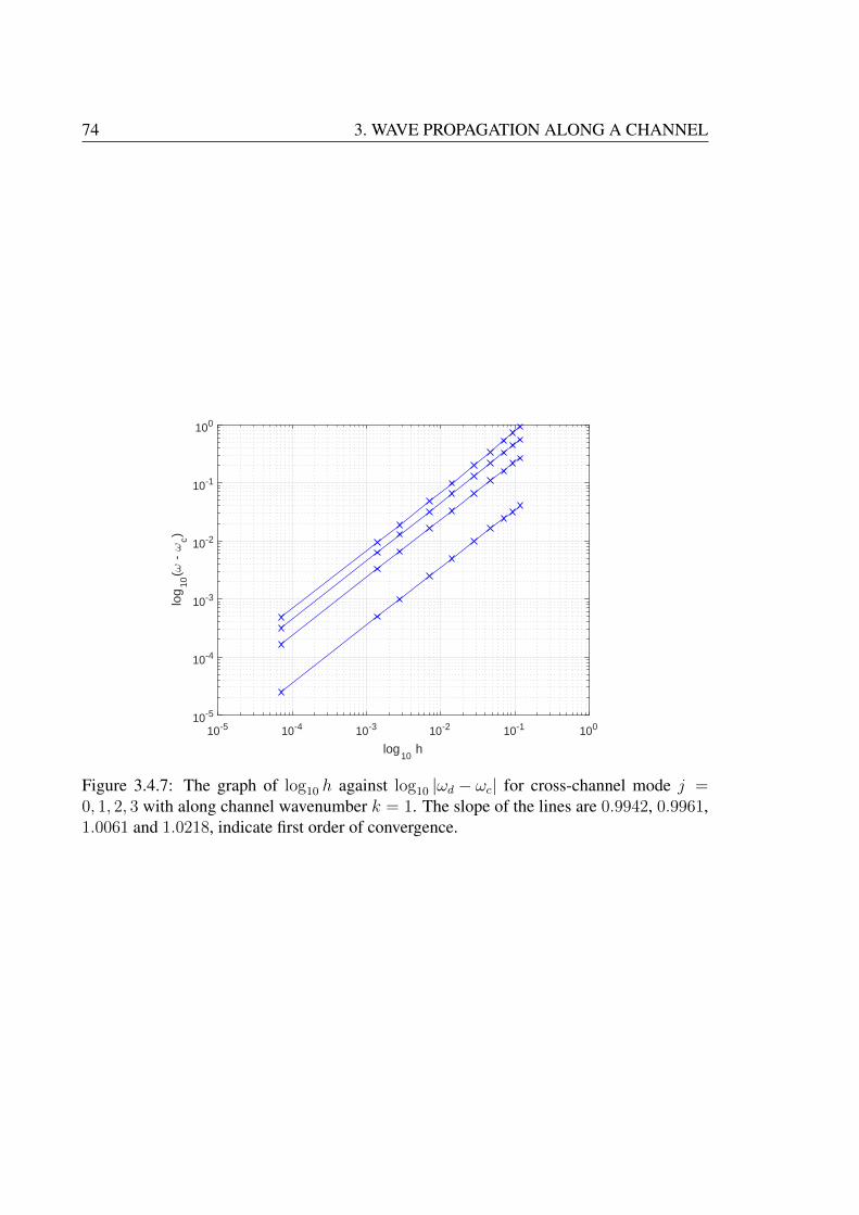
74 3. WAVE PROPAGATION ALONG A CHANNEL
10-5 10-4 10-3 10-2 10-1 100
log10
h
10-5
10-4
10-3
10-2
10-1
100
log
10(ω
- ω
c)
Figure 3.4.7: The graph of log10 h against log10 |ωd − ωc| for cross-channel mode j =0, 1, 2, 3 with along channel wavenumber k = 1. The slope of the lines are 0.9942, 0.9961,1.0061 and 1.0218, indicate first order of convergence.
3.4. BOUNDARY ALIGNED AT 45◦ TO THE GRID 75
early section 3.3.2, the general solution (3.4.10) is
Pn = A1λn1 + A2λ
n2 , where λ2 + µλ+ 1 = 0 ⇒ λ =
−µ±√µ2 − 4
2, (3.4.16)
µ =ω2dh
2 − 4
2 cos θ, (3.4.17)
and θ =kh√
2. (3.4.18)
The boundary conditions (3.4.14) and (3.4.15) then imply
A1λ1 + A2λ2 = αA1 + αA2, A1λM−11 + A2λ
M−12 = αA1λ
M1 + αA2λ
M2 ,
⇒
λ1 − α λ2 − α
αλM1 − λM−11 αλM2 − λM−1
2
A1
A2
= 0.
For nontrivial solutions we require
(λM1 − λM2
)α2 − 2
(λM−1
1 − λM−12
)α +
(λM−2
1 − λM−22
)= 0, (3.4.19)
where we have used λ1λ2 = 1, which follows from (3.4.16). Equation (3.4.19) is an implicit
relation for ωd, which appears directly via α, and indirectly via λ1,2, which depend upon µ,
which in turn depends on ωd via (3.4.17).
3.4.5 Behaviour as h→ 0
We anticipate that the waves are retarded from the continuum frequency ωc as h→ 0, where
ω2c = k2 + j2π2, with j an integer. We thus write
ω2d = ω2
c − a1h− a2h2 + · · · = k2 + j2π2 − a1h− a2h
2 + · · · . (3.4.20)
We wish to find a1 (and perhaps a2).
76 3. WAVE PROPAGATION ALONG A CHANNEL
As h→ 0, (3.4.17) and (3.4.18) imply
µ =
(−2 +
ω2dh
2
2
)(1 +
k2h2
4+O(h4)
)= −2 +
h2(ω2d − k2)
2+O(h4) (3.4.21)
⇒ µ2 − 4 = −2h2(ω2d − k2) +O(h4) = −2h2j2π2 + 2a1h
3 +O(h4). (3.4.22)
So the discriminant µ2 − 4 in (3.4.16) is thus negative (at least when j > 0), implying
complex roots for λ:
λ1 = exp(+iϕ), λ2 = exp(−iϕ), where exp(iϕ) =−µ+ i
√4− µ2
2, (3.4.23)
⇒ cosϕ = −µ2
= 1− h2(ω2d − k2)
4+O(h4) = 1− h2j2π2
4+a1h
3
4+O(h4), (3.4.24)
sinϕ =
√1− µ2
4=
√h2j2π2
2− a1h3
2+O(h4) =
jπh√2− a1h
2
2√
2jπ+O(h3). (3.4.25)
With this assumption of complex conjugate roots for λ1,2, the eigenvalue condition (3.4.19)
becomes
(sinMϕ)α2 − 2(sin(M − 1)ϕ)α + sin(M − 2)ϕ = 0 (3.4.26)
⇒ α =sin(M − 1)ϕ±
√sin2(M − 1)ϕ− (sinMϕ)(sin(M − 2)ϕ)
sinMϕ. (3.4.27)
But
2 sinMϕ sin(M − 2)ϕ = cos 2ϕ− cos 2(M − 1)ϕ = 1− 2 sin2 ϕ− 1 + 2 sin2(M − 1)ϕ
⇒ sin2(M − 1)ϕ− sinMϕ sin(M − 2)ϕ = sin2 ϕ,
so that the square root in (3.4.27) simplifies, and we have
α =sin(M − 1)ϕ± sinϕ
sinMϕ. (3.4.28)
This is our modified eigencondition, which is valid whenever λ1,2 are complex (e.g., as
3.4. BOUNDARY ALIGNED AT 45◦ TO THE GRID 77
h→ 0 with j > 0).
It is possible to simply expand all terms in (3.4.28) to find the frequency reduction coeffi-
cient a1. However, further trigonometrical expansions reduce the burden. Using boundary
conditions (3.4.14) and (3.4.15), and (3.4.24) to write α = 2 cosϕ − 1/ cos θ, (3.4.28)
becomes1
cos θ=
2 cosϕ sinMϕ− sin(M − 1)ϕ± sinϕ
sinMϕ.
But 2 cosϕ sinMϕ = sin(M + 1)ϕ+ sin(M − 1)ϕ, so there is a further reduction:
1
cos θ=
sin(M + 1)ϕ± sinϕ
sinMϕ. (3.4.29)
We now split into two cases, using sinA+ sinB = 2 sin A+B2
cos A−B2
:
• taking the positive root in (3.4.29) gives
1
cos θ=
2 sin((M + 2)ϕ/2) cos(Mϕ/2)
2 sin(Mϕ/2) cos(Mϕ/2)=
sin((M + 2)ϕ/2)
sin(Mϕ/2)
= cosϕ+cos(Mϕ/2) sinϕ
sin(Mϕ/2).
As h → 0, we can write 1/ cos θ = 1 + k2h2/4 + · · · , and use the expansions in
(3.4.24) and (3.4.25) for cosϕ and sinϕ to obtain
1 +k2h2
4+ · · · −
(1− h2j2π2
4+ · · ·
)=jπh/
√2 + · · ·
tan(Mϕ/2)
⇒ tanMϕ
2=
2√
2jπ
h(k2 + j2π2)+ · · · . (3.4.30)
We will be choosing M = N∗ =√
2/h, or M = N∗ − 1. Also using (3.4.25), we
78 3. WAVE PROPAGATION ALONG A CHANNEL
thus write
Mϕ = (N∗ + (M −N∗))ϕ =
(√2
h+ (M −N∗)
)(jπh√
2− a1h
2
2√
2jπ+ · · ·
)=
(1 +
h(M −N∗)√2
)(jπ − a1h
2jπ+ · · ·
)= jπ+h
((M −N∗)jπ√
2− a1
2jπ
)+· · · .
(3.4.31)
A balance in (3.4.30) is thus possible if j is odd, since then tan(Mϕ/2) approaches
tan(jπ/2). More precisely,
tanMϕ
2=
sin(jπ/2)(1 + · · · )
− sin(jπ/2) sin(h2
[(M−N∗)jπ√
2− a1
2jπ
]+ · · ·
) = − 2
h[
(M−N∗)jπ√2
− a12jπ
]+· · ·
So (3.4.30) becomes
− 2
h[
(M−N∗)jπ√2
− a12jπ
] + · · · = 2√
2jπ
h(k2 + j2π2)+ · · ·
⇒ (M −N∗)jπ√2
− a1
2jπ= −k
2 + j2π2
√2jπ
⇒ a1 =√
2(k2 + (M −N∗ + 1)j2π2
).
We can now analyse our two cases of interest:
a) whenM = N∗ (i.e., split cell retention), we have a1 =√
2(k2 +j2π2) =√
2ω2c ,
so that
ω2d = ω2
c −√
2hω2c + · · · =
(1−√
2h+ · · ·)ω2c
⇒ ωd =
(1− h√
2+ · · ·
)ωc. (3.4.32)
Thus, the frequency is reduced by a factor of√
2h: this, of course, is a first-order
error in h.
3.4. BOUNDARY ALIGNED AT 45◦ TO THE GRID 79
b) When M = N∗ − 1 (i.e., cell-centre retention), we have a1 =√
2k2, so that
ω2d = ω2
c −√
2k2h+ · · · = ω2c
(1−√
2
(k2
k2 + j2π2
)h+ · · ·
)⇒ ωd = ωc
(1−
(k2
k2 + j2π2
)h√2
+ · · ·). (3.4.33)
The relative error now is always less than h/√
2. Further, the relative error
becomes much smaller than h/√
2 when j � k/π, i.e., for modes with large
cross-channel wavenumber j.
• Alternatively, taking the negative root in (3.4.29) gives
1
cos θ=
2 sin(Mϕ/2) cos((M + 2)ϕ/2)
2 sin(Mϕ/2) cos(Mϕ/2)=
cos((M + 2)ϕ/2)
cos(Mϕ/2)
= cosϕ− sin(Mϕ/2) sinϕ
cos(Mϕ/2).
In the same way that we found (3.4.30), we now find
1 +k2h2
4+ · · · −
(1− h2j2π2
4+ · · ·
)= −jπh√
2tan
Mϕ
2+ · · ·
⇒ tanMϕ
2= −h(k2 + j2π2)
2√
2jπ+ · · · . (3.4.34)
We again have (3.4.31) for Mϕ. A balance in (3.4.34) is thus possible if j is even,
since then tan(Mϕ/2) approaches tan(jπ/2) = 0. More precisely,
tanMϕ
2=
cos(jπ/2) sin(h2
[(M−N∗)jπ√
2− a1
2jπ
]+ · · · )
cos(jπ/2) (1 + · · · )
=h
2
[(M −N∗)jπ√
2− a1
2jπ
]+ · · · .
80 3. WAVE PROPAGATION ALONG A CHANNEL
So (3.4.34) becomes
h
2
[(M −N∗)jπ√
2− a1
2jπ
]+ · · · = −h(k2 + j2π2)
2√
2jπ+ · · ·
⇒ (M −N∗)jπ√2
− a1
2jπ= −k
2 + j2π2
√2jπ
⇒ a1 =√
2(k2 + (M −N∗ + 1)j2π2
),
which is exactly the result that we derived before, when j was odd. So our approx-
imate discrete dispersion relations (3.4.32) and (3.4.33) for all modes with j 6= 0.
3.4.6 Numerical verification
We now confirm the analysis of the relative error numerically. Note that we only verified the
relative error for boundary conditions a) (i.e., split cell retention). As discussed in section
3.4.3, we have obtained the eigenvalue ωd using a shooting method. Further, from both the
existing numerics and our asymptotics, we have shown that |ωc − ωd| = A(k)h for some
A(k) as h → 0. Our asymptotics imply that ωd = ωc(1 − h/√
2 · · · ) (via (3.4.32)) as
h→ 0, and so that
A(k) =ωc√
2=
√k2 + j2π2
2. (3.4.35)
We now verify that this is consistent with the numerical results of section 3.4.3.
Numerically, the scaling factor is determined by calculating ωd and ωc at various values of
h (bearing in mind that we need h =√
2/N∗, via (3.4.6)), and then fitting a straight line to
log10 |ωc − ωd| versus log10 h. The intercept is then A. By repeating for different values of
k, we can numerically construct A(k), for a given cross-channel mode j.
Figure 3.4.8a shows the scaling factor A(k) determined both numerically and analytically,
for j = 1, 2, 3. The numerical results have been determined taking 6 values of h with√
2/1000 ≤ h ≤√
2/20 (i.e., each cross in the figure requires 6 separate shooting cal-
culations, followed by a straight line fit). The agreement between the asymptotics and the
numerical results is good for j = 1 and small k, but worsens as j and k both increase.
3.5. SUMMARY 81
However, better agreement can be found by considering yet smaller values of h, where the
numerical results should be increasingly in line with the asymptotic predictions. Shown in
Figure 3.4.8b and 3.4.8c are results calculated with 6 values of h over each of√
2/10000 <
h <√
2/500 and√
2/29000 < h <√
2/5000. One can see that the agreement between
the asymptotics and the numerics improves in each case, and we can be confident (from
Figure 3.4.8c) that the asymptotics is indeed correct. So, in Figure 3.4.8a, the number of
grid points was insufficient to resolve the wave structure, especially at j = 3.
3.5 Summary
Building upon previous studies in [51, 32], we have examined the accuracy of discrete
wave solutions in a straight channel with perfect staircase walls. Here we have considered
standard non-rotating shallow-water waves (or acoustic waves), and the staggered C-grid.
We have shown that the staircase boundaries mean that the discrete wave frequency is only
determined at first order in grid spacing h, despite the second-order finite difference for-
mulations used in the interior of the domain. This convergence is to be contrasted with
solutions for which the channel’s boundaries and grid are aligned, where we proved that the
frequency is obtained at second-order in h.
Our main calculations were asymptotics for the two cases of an aligned channel and
a perfect staircase channel. In the former case, the relative error ∆ =|ωd − ωc||ωc|
=
h2/12(k4 + j4π4)/(k2 + j2π2), from (3.3.17), which is second-order accurate in h. In
the latter case, the relative error is ∆ = h/√
2, (via (3.4.32)), for the boundary condition
choice a) (i.e., split cell retention), and ∆ = (k2/k2 + j2π2)h/√
2, (via (3.4.32)) for the
boundary condition choice b) (i.e., cell-centre retention), as h → 0. We note that the relat-
ive error for aligned boundaries is dependent of k. While the relative error for the unaligned
boundaries is independent of k for the split cell retention boundary condition choice and de-
pendent of k for the cell-centre retention staircase boundary conditions. For the unaligned
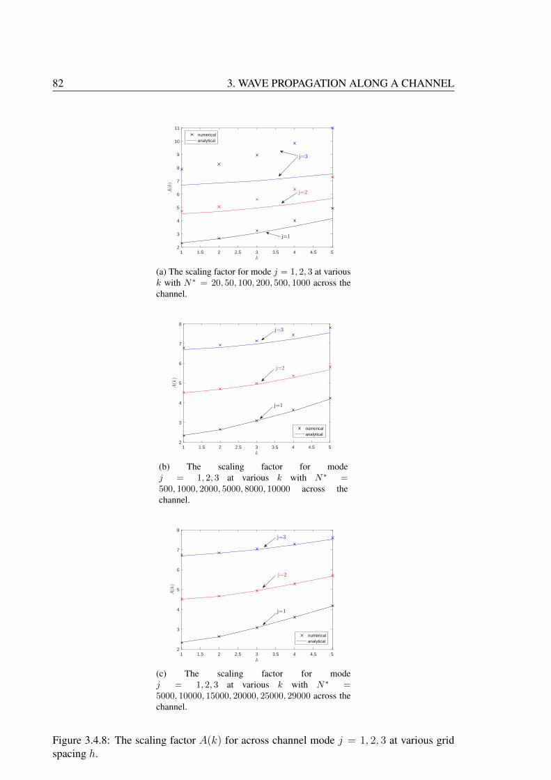
82 3. WAVE PROPAGATION ALONG A CHANNEL
1 1.5 2 2.5 3 3.5 4 4.5 5k
2
3
4
5
6
7
8
9
10
11
A(k)
numericalanalytical
j=1
j=3
j=2
(a) The scaling factor for mode j = 1, 2, 3 at variousk with N∗ = 20, 50, 100, 200, 500, 1000 across thechannel.
1 1.5 2 2.5 3 3.5 4 4.5 5k
2
3
4
5
6
7
8
A(k)
numericalanalytical
j=3
j=2
j=1
(b) The scaling factor for modej = 1, 2, 3 at various k with N∗ =500, 1000, 2000, 5000, 8000, 10000 across thechannel.
1 1.5 2 2.5 3 3.5 4 4.5 5k
2
3
4
5
6
7
8
A(k)
numericalanalytical
j=1
j=2
j=3
(c) The scaling factor for modej = 1, 2, 3 at various k with N∗ =5000, 10000, 15000, 20000, 25000, 29000 across thechannel.
Figure 3.4.8: The scaling factor A(k) for across channel mode j = 1, 2, 3 at various gridspacing h.
3.5. SUMMARY 83
case both relative errors have a staircasing error. For the split cell retention choice, there is
geometrical error generated – as the channel is widen by O(h).
So for the case of mode j = 0, to obtain the frequency accurate to within 1% (i.e., ∆ <
0.01), we need kh =√
0.12 or 18 grid points per along-channel wavelength for the case
of aligned boundaries. On the other hand, for the case of unaligned boundaries we need
h =√
2, or 71 grid boxes across the channel, for both boundary condition (a) and (b).
To obtain the frequency accurate to within 10% (i.e., ∆ < 0.1), we need 6 grid points
per along-channel for the aligned boundaries, and 7 grid boxes across the channel for the
unaligned case.
For the case of mode j = 1, in order to obtain the frequency accurate to within 1%, we
need 9 grid boxes across the channel for the aligned boundary. For the case of unaligned
boundary, again we need 71 grid boxes across the channel for split cell retention boundary
condition. However, for cell-centre retention boundary condition we need only 7 grid boxes
across the channel.
Thus, we have been able to make a clear conclusion about the influence of staircase bound-
aries on wave propagation along a channel. In particular, the formula for the relative error
∆ =h√2
and ∆ =
(k2
k2 + j2π2
)h√2,
allows a quick estimation of the degradation due to staircase error, in this ‘worst-case’
scenario where the channel and grid are aligned at 45◦. From the results of [32] for Kelvin
waves, we can anticipate that the error would be reduced as the angle between walls and
grid is reduced, whilst remaining first order.
Most of these results are new. Presumably the grid-aligned analysis leading to (3.3.17)
exists somewhere in the vast research literature covering acoustics, electromagnetic waves
and shallow-water waves, but we have not found it. However, the perfectly-aligned staircase
analysis is completely original, as far as we can tell. The closest study is that of [51], but
84 3. WAVE PROPAGATION ALONG A CHANNEL
he used rather different methods and gave no results for h→ 0 at fixed channel width, and
thus gave nothing analogous to our main results (3.4.32) and (3.4.33). The study of [32]
used similar methods to here, but was completely focussed on the case of Kelvin waves for
an unbounded channel and shallow-water dynamics. Those results rely upon rotation, and
cannot be converted to our results here for non-rotating dynamics.
However, what we have not done is examine the spatial structure of the solution. In par-
ticular, we know that the continuum solution has along channel flow even at the walls (i.e.,
tangential flow), even though the normal flow vanishes. Of course, both components of
the flow of the discrete solution are forced to vanish at the staircase wall via (3.4.5), and
it would be interesting to calculate how these flow change from zero to something close to
the continuum values as we move away from the wall. In [32], it was shown that there was
a thin computational boundary layer of width h2 (see Eq. (31) of [32]).
85
Chapter 4
WAVE REFLECTION AT A PLANAR
WALL
4.1 Introduction
In this chapter, we consider the linearised wave equations
∂u
∂t= −∂p
∂x,
∂v
∂t= −∂p
∂y,
∂p
∂t+∂u
∂x+∂v
∂y= 0, (4.1.1)
where (u, v) is the velocity vector, p is the pressure, following the same notation of acoustic
and shallow-water flow.
In chapter 3, we discussed the propagation of waves on the C grid along a channel with
two boundaries. However, when waves propagate through a medium, they also can reflect
at a boundary. In many cases, waves propagate carrying information from the source and
are reflected back to the source region. The information from the reflected component
can then be analysed. For example, acoustic wave reflection is used to explore oil and
gas reservoirs under the sea. The human hearing mechanism also uses a similar process
that often relies upon sound wave reflection. In classical electrodynamics, electromagnetic
86 4. WAVE REFLECTION AT A PLANAR WALL
waves also propagate and reflect at surfaces. For shallow-water flow, ocean waves can
propagate to the coast and be completely or partially reflected at boundaries such as cliffs
or seawalls. These wave reflections can be important for the behaviour of coastal waves.
The nature of the wave reflection depends upon the structure of the boundary, and any nu-
merical solutions will be sensitive to how this boundary is represented. Study of reflection
at a straight wall is possible even in a finite-difference model, because the straight bound-
ary can be aligned with the finite-difference grid. However, on a non-planar boundary
the accuracy of the resulting numerical solutions is not clear. As mentioned in chapter 3,
the classic technique in finite-difference methods based on the staggered C-grid to repres-
ent the non-smooth boundary is to introduce a numerical boundary that contain staircases.
Typically, these staircases introduce an error and may reduce the accuracy of the numerical
solution. The aim of this chapter is to study this numerical error for wave reflection at a
planar boundary.
Analysis of the error induced by staircase boundaries on wave reflection is not a new sub-
ject. For example, [17] studied the error of electromagnetic wave reflection on a hard wall
with staircase boundary. The error analysis was performed using the two-dimensional Max-
well’s equations. There are two different waves that propagate in electromagnetism: one
corresponds to electric field, and the other one corresponds to magnetic field. These waves
propagate perpendicular to each other, and are thus a type of transverse wave. The er-
ror analysis of [17] was performed for both transverse electric (TEz) and magnetic (TMz)
modes subject to a perfect conductor boundary condition. By assuming a total solution of
incoming and reflected wave at the boundary, the reflection coefficient was derived for both
modes. From the analysis of the reflection coefficient for TMz mode, they showed graphic-
ally that there is phase error generated upon reflection at the staircase boundary, depending
on the angle of incident wave with respect to the normal. They also showed graphically
that the phase error increased as the angle of incident wave increased. However, there is no
obvious phase error from the analysis of the reflection coefficient in TEz mode. In the study,
4.1. INTRODUCTION 87
they also analysed the discrete dispersion relation for waves propagating along the bound-
ary x = y. From the analysis, they concluded that the presence of the staircase boundary
decreased the phase velocity and one can expect to see a delay in a travelling pulse. The
analysis was verified by using two time-dependent numerical experiments and they showed
that there was a delay for a wave pulse traveling with the rotated boundary for the TMz
mode, but there was no delay in the TEz mode, as expected from their analyses. Further-
more, they concluded that the phase errors in the TEz mode are significantly greater than
those in the TMz mode, which supported their analysis.
The above study implies that the staircase approximation could generate a significant error.
However, these errors are not quantified via a rate of convergence. In this chapter, we study
wave reflection at a staircase boundary for (4.1.1), which is equivalent to the equations in
[17]. The study will provide more detail about the wave reflection at staircase boundary.
In other studies, analysis of wave reflection at a boundary for one-dimensional equations by
using staggered grid finite-difference method was discussed in [68]. The acoustic wave for-
mulations involving pressure p and velocity u and v, has been used in the study instead of
the Maxwell’s electromagnetism formulation. Note that, the equations are also equivalent
to the non-rotating shallow water dynamics used for water wave applications. In the study,
the hard boundary condition which is equivalent to no normal flow boundary conditions in
fluid dynamics was used to investigate the effects of the reflection. From the analysis, they
showed that both velocity and pressure has first-order of accuracy in the size of grid spa-
cing. The analysis was verified numerically with a test wave function propagating against a
boundary. In the experiment, they quantified the error numerically by measuring the max-
imum error at three different grid spacings. They showed that the accuracy of numerical
solutions for pressure and velocity degraded from second-order to first-order when the wave
reflects at the boundary.
In a subsequent study, numerical investigations of two-dimensional wave reflection against
an inclined boundary and a solid circle were given in [67]. The study was the continuation
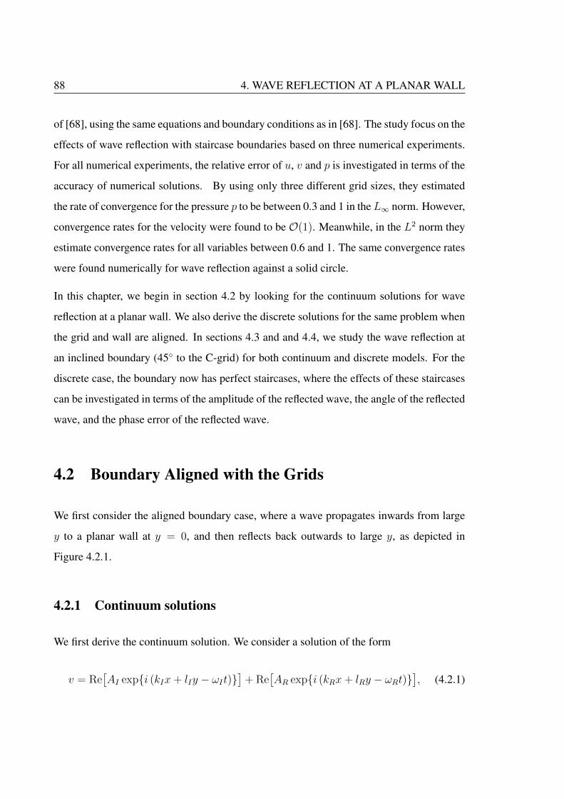
88 4. WAVE REFLECTION AT A PLANAR WALL
of [68], using the same equations and boundary conditions as in [68]. The study focus on the
effects of wave reflection with staircase boundaries based on three numerical experiments.
For all numerical experiments, the relative error of u, v and p is investigated in terms of the
accuracy of numerical solutions. By using only three different grid sizes, they estimated
the rate of convergence for the pressure p to be between 0.3 and 1 in the L∞ norm. However,
convergence rates for the velocity were found to be O(1). Meanwhile, in the L2 norm they
estimate convergence rates for all variables between 0.6 and 1. The same convergence rates
were found numerically for wave reflection against a solid circle.
In this chapter, we begin in section 4.2 by looking for the continuum solutions for wave
reflection at a planar wall. We also derive the discrete solutions for the same problem when
the grid and wall are aligned. In sections 4.3 and and 4.4, we study the wave reflection at
an inclined boundary (45◦ to the C-grid) for both continuum and discrete models. For the
discrete case, the boundary now has perfect staircases, where the effects of these staircases
can be investigated in terms of the amplitude of the reflected wave, the angle of the reflected
wave, and the phase error of the reflected wave.
4.2 Boundary Aligned with the Grids
We first consider the aligned boundary case, where a wave propagates inwards from large
y to a planar wall at y = 0, and then reflects back outwards to large y, as depicted in
Figure 4.2.1.
4.2.1 Continuum solutions
We first derive the continuum solution. We consider a solution of the form
v = Re[AI exp{i (kIx+ lIy − ωIt)}
]+ Re
[AR exp{i (kRx+ lRy − ωRt)}
], (4.2.1)
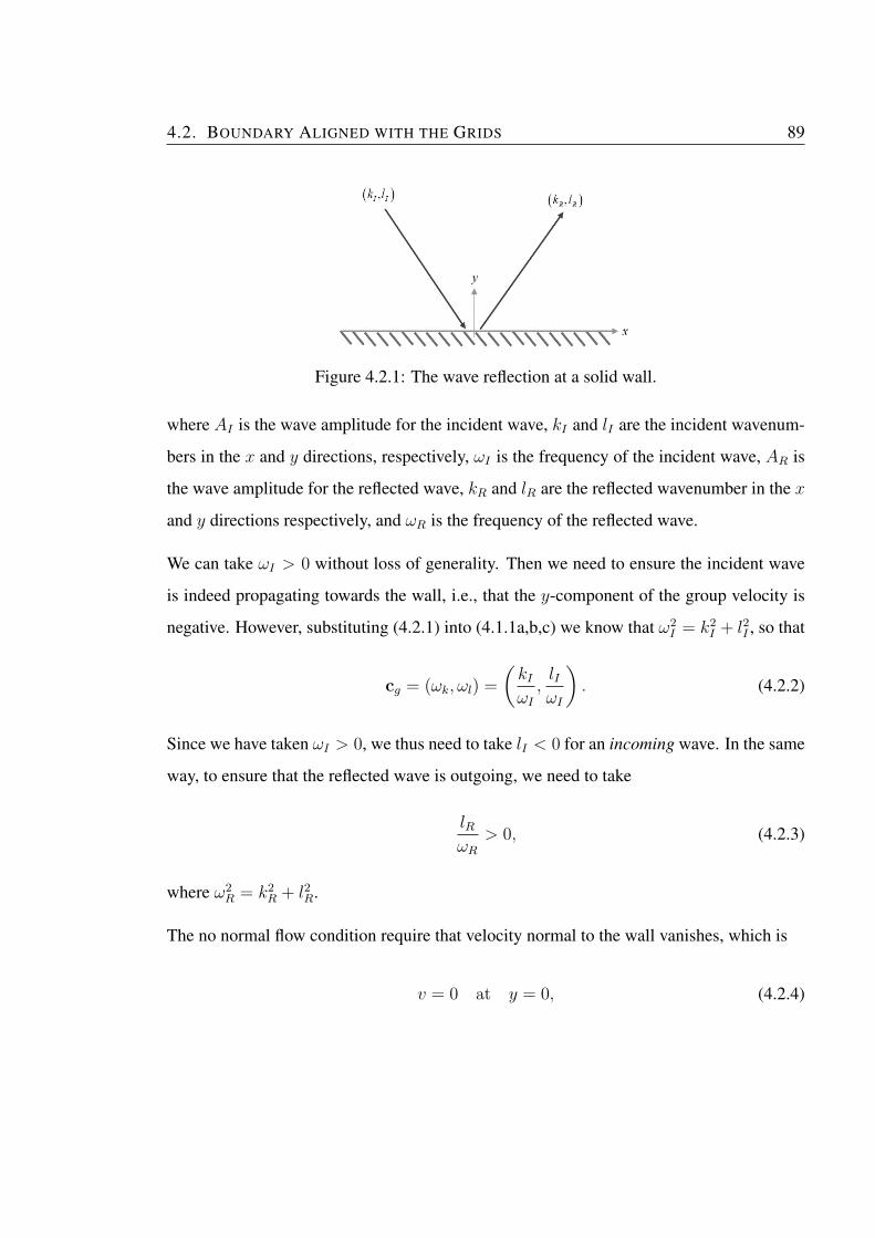
4.2. BOUNDARY ALIGNED WITH THE GRIDS 89
Figure 4.2.1: The wave reflection at a solid wall.
where AI is the wave amplitude for the incident wave, kI and lI are the incident wavenum-
bers in the x and y directions, respectively, ωI is the frequency of the incident wave, AR is
the wave amplitude for the reflected wave, kR and lR are the reflected wavenumber in the x
and y directions respectively, and ωR is the frequency of the reflected wave.
We can take ωI > 0 without loss of generality. Then we need to ensure the incident wave
is indeed propagating towards the wall, i.e., that the y-component of the group velocity is
negative. However, substituting (4.2.1) into (4.1.1a,b,c) we know that ω2I = k2
I + l2I , so that
cg = (ωk, ωl) =
(kIωI,lIωI
). (4.2.2)
Since we have taken ωI > 0, we thus need to take lI < 0 for an incoming wave. In the same
way, to ensure that the reflected wave is outgoing, we need to take
lRωR
> 0, (4.2.3)
where ω2R = k2
R + l2R.
The no normal flow condition require that velocity normal to the wall vanishes, which is
v = 0 at y = 0, (4.2.4)

90 4. WAVE REFLECTION AT A PLANAR WALL
and gives
Re[AI exp{i (kIx− ωIt)}+ AR exp{i (kRx− ωRt)}
]= 0
⇒ AR exp{i(kI − kR)x} = −AI exp{i(ωI − ωR)t}. (4.2.5)
This can only be true if the function of x on the left-hand side and the function of t on the
right hand side are both constants, which requires
kI = kR and ωI = ωR. (4.2.6)
Then we also require
AR = −AI . (4.2.7)
It remains to find lR. But, l2R = ω2R − k2
R = ω2I − k2
I = l2I , so lR = ±lI . Since lI < 0, and
we require lR to take the same sign as ωR = ωI (which is positive), we thus need lR = −lI .
Hence the full solution for v is
v(x, y, t) = Re[AI exp{i (kIx+ lIy − ωIt)}
]− Re
[AI exp{i (kIx− lIy − ωIt)}
]= Re
[AI exp{i(kIx− ωIt)}
](exp{ilIy} − exp{−ilIy})
= 2 sin(lIy)Re[iAI exp{i (kIx− ωIt)}
]. (4.2.8)
To complete the solution, we also calculate p and u. By looking at (4.1.1b), differentiating
(4.2.8) with respect to t we have
∂v
∂t= Re (−iωIAI exp(i(kIx+ lIy − ωIt)) + iωIAI exp(i(kIx− lIy − ωIt))) = −∂p
∂y,
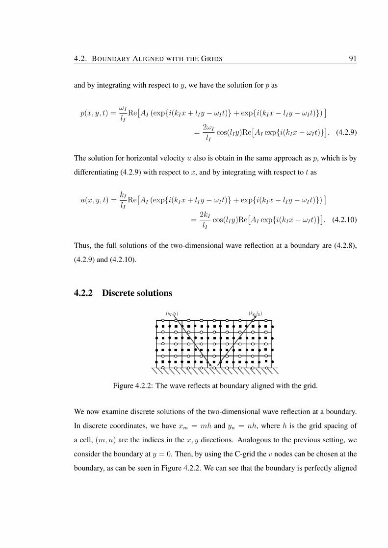
4.2. BOUNDARY ALIGNED WITH THE GRIDS 91
and by integrating with respect to y, we have the solution for p as
p(x, y, t) =ωIlI
Re[AI (exp{i(kIx+ lIy − ωIt)}+ exp{i(kIx− lIy − ωIt)})
]=
2ωIlI
cos(lIy)Re[AI exp{i(kIx− ωIt)}
]. (4.2.9)
The solution for horizontal velocity u also is obtain in the same approach as p, which is by
differentiating (4.2.9) with respect to x, and by integrating with respect to t as
u(x, y, t) =kIlI
Re[AI (exp{i(kIx+ lIy − ωIt)}+ exp{i(kIx− lIy − ωIt)})
]=
2kIlI
cos(lIy)Re[AI exp{i(kIx− ωIt)}
]. (4.2.10)
Thus, the full solutions of the two-dimensional wave reflection at a boundary are (4.2.8),
(4.2.9) and (4.2.10).
4.2.2 Discrete solutions
Figure 4.2.2: The wave reflects at boundary aligned with the grid.
We now examine discrete solutions of the two-dimensional wave reflection at a boundary.
In discrete coordinates, we have xm = mh and yn = nh, where h is the grid spacing of
a cell, (m,n) are the indices in the x, y directions. Analogous to the previous setting, we
consider the boundary at y = 0. Then, by using the C-grid the v nodes can be chosen at the
boundary, as can be seen in Figure 4.2.2. We can see that the boundary is perfectly aligned
92 4. WAVE REFLECTION AT A PLANAR WALL
with the grid (the optimal choice), so that our boundary condition is
vm,0 = 0 for all m. (4.2.11)
Analogous to the derivation of the continuum solutions, we consider a discrete free wave
solution of the form
vm,n = Re[AI exp{i(kIxm + lIyn − ωIt)}
]+ Re
[AR exp{i(kRxm + lRyn − ωRt)}
].
(4.2.12)
Then by using the boundary condition (4.2.11), we obtain
AI exp{i(kImh− ωIt)}+ AR exp{i(kRmh− ωRt)} = 0
⇒ AI exp{i(kI − kR)mh}+ AR exp{i(ωI − ωR)t} = 0. (4.2.13)
If this is to be true for all m and t, then the exponential terms must be equal to zero, i.e.,
(kI − kR)mh = 0, ∀h ⇒ kI = kR, and (4.2.14)
(ωI − ωR)t = 0, ∀t ⇒ ωI = ωR. (4.2.15)
Then, (4.2.13) will give
AR = −AI . (4.2.16)
This means that the amplitude of the reflected wave is perfectly reproduced, and is unaffac-
ted by the finite-difference approximation. The solution now is
v = Re[AI exp{i(kIxm + lIyn − ωIt)}
]− Re
[AI exp{i(kRxm + lRyn − ωRt)}
].
(4.2.17)
4.2. BOUNDARY ALIGNED WITH THE GRIDS 93
It remains to find lR. There are two considerations here. First, we need to ensure that the
incident wave is indeed incident, and the outgoing wave is indeed outgoing. To do this, we
consider the discrete dispersion relation, i.e., equation (2.7.12) with f = 0 and c = 1
ω2 =4
h2
(sin2 kh
2+ sin2 lh
2
). (4.2.18)
Thus,
2ωωl =
(4
h2
)2
(h
2
)cos
(lh
2
)sin
(lh
2
)=
(2
h
)sin(lh)
⇒ ωl =sin(lh)
hω≈ l
ωwhen lh� 1. (4.2.19)
We take ωI > 0, without loss of generality. Thus, for the incoming wave we need lI/ωI < 0,
so that lI < 0 (at least when h� 1). For the reflected wave, we need 0 < lR/ωR = lR/ωI ,
so that lR > 0.
The second consideration is that both incident and reflected waves satisfy the discrete dis-
persion relation. So
4
h2
(sin2 kIh
2+ sin2 lIh
2
)=
4
h2
(sin2 kRh
2+ sin2 lRh
2
),
⇒ sin2(lIh)− sin2(lRh) = 0, since kI = kR by 4.2.14
⇒ cos (lIh)− cos (lRh) = 0,
⇒ sin
((lI + lR)h
2
)sin
((lI − lR)h
2
)= 0.
Thus (lI + lR)h/2 = nπ or (lI − lR)h/2 = nπ. At least as h→ 0, the only possibilities are
lI + lR = 0 or lI − lR = 0. But, since we know that lI and lR take opposite signs, we must
have
lR = −lI . (4.2.20)
94 4. WAVE REFLECTION AT A PLANAR WALL
Thus, the full discrete solution for wave reflection at a boundary is
vm,n = Re[AI exp{i(kIxm + lIyn − ωIt)}
]− Re
[AI exp{i(kIxm − lIyn − ωIt)}
]= 2 sin(lIyn)Re
[iAI exp{i (kIxm − ωIt)}
]. (4.2.21)
We can see that discrete solution (4.2.21) is exactly same as continuum solution (4.2.8)
without any error terms. Therefore, the discrete solution is as good a solution as the con-
tinuum solution, which shows perfect reflection at the boundary. However, note that the
discrete solution is not perfect, simply because there is a small error in the discrete fre-
quency, via (4.2.18).
4.2.3 Numerical visualisation
In this section, we visualised the solution of wave reflection at a planar wall. We consider
incident wave traveling towards a planar wall with incident wavenumber kI = 1 and lI =
−2 in the x and y direction, respectively. There is no normal flow at the wall, so that when
hitting the wall the wave reflects and traveling away from the wall. Figure 4.2.3 shows
the solutions for pressure p along the first row, and velocity (u, v) along the second and
third row, for wave reflection at the planar wall. The wall and grid are aligned at y = 0.
The wave incident component is given in column one, the reflected wave component in
second column, and the total solution (incident + reflected) in third column. From all the
figures, we can see that the wave is traveling towards the boundary and then reflected back
propagates away from the boundary. In the total solutions, there is a complete wave with
wavelength 2π in x direction which represents wavenumber kI = 1, and two complete wave
in y direction which illustrated lI = −2. Note that, the negative value in lI represents the
direction of wave propagation.
In the above discussion, we have focused on the solution where planar boundary at y =
0, which implies that boundary is aligned with the grid in discrete solution. In further

4.2. BOUNDARY ALIGNED WITH THE GRIDS 95
discussion, the effect of unaligned boundary with the grid will be discussed.
Figure 4.2.3: The continuum solutions of p, u, and v for wave reflection at aligned boundaryat t = 0, with horizontal wavenumber k = 1, vertical wavenumber l = −2. The left columnis the incident wave component, centre column is the reflected component, and the rightcolumn is the total component (i.e., incident + reflected). The top row is the solution forpressure p, second row is velocity u, and third row is the velocity v.
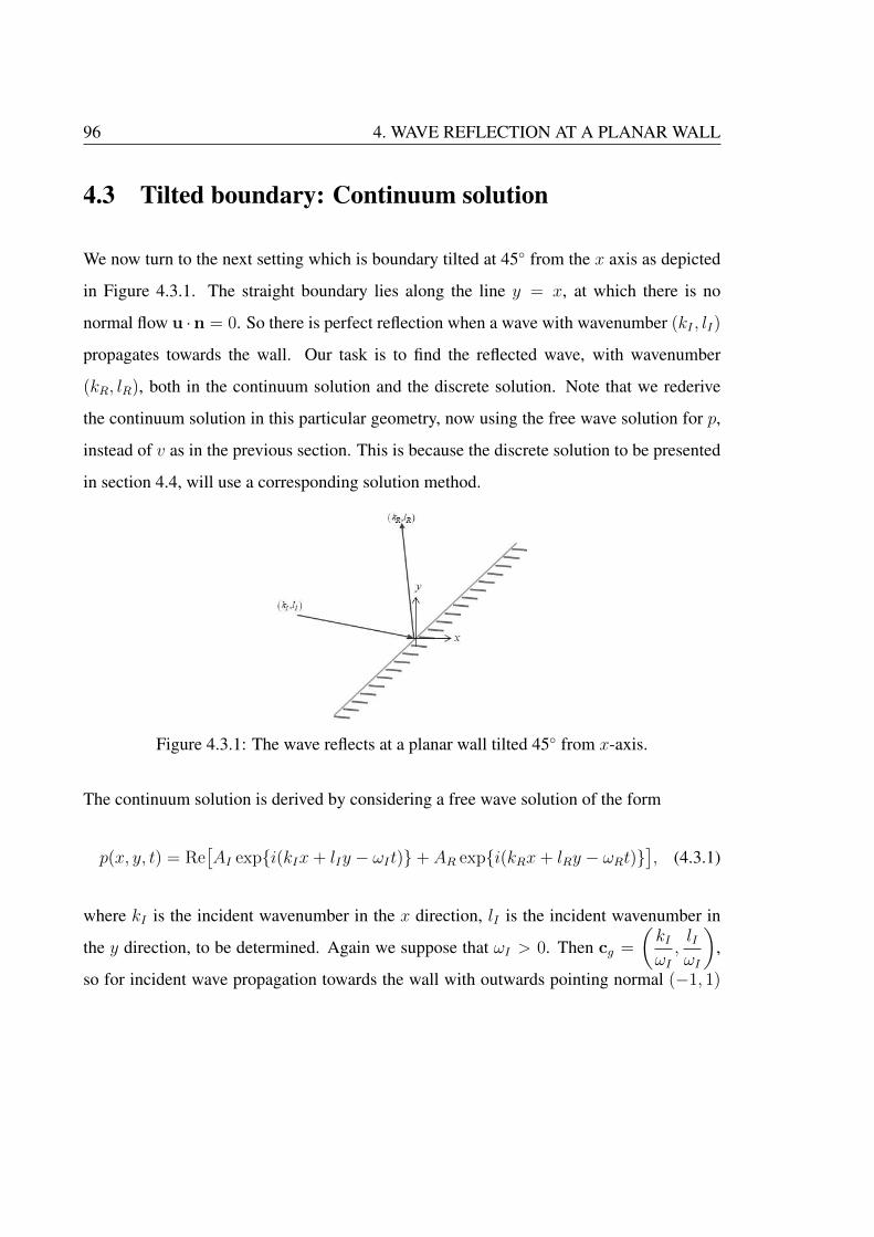
96 4. WAVE REFLECTION AT A PLANAR WALL
4.3 Tilted boundary: Continuum solution
We now turn to the next setting which is boundary tilted at 45◦ from the x axis as depicted
in Figure 4.3.1. The straight boundary lies along the line y = x, at which there is no
normal flow u ·n = 0. So there is perfect reflection when a wave with wavenumber (kI , lI)
propagates towards the wall. Our task is to find the reflected wave, with wavenumber
(kR, lR), both in the continuum solution and the discrete solution. Note that we rederive
the continuum solution in this particular geometry, now using the free wave solution for p,
instead of v as in the previous section. This is because the discrete solution to be presented
in section 4.4, will use a corresponding solution method.
Figure 4.3.1: The wave reflects at a planar wall tilted 45◦ from x-axis.
The continuum solution is derived by considering a free wave solution of the form
p(x, y, t) = Re[AI exp{i(kIx+ lIy − ωIt)}+ AR exp{i(kRx+ lRy − ωRt)}
], (4.3.1)
where kI is the incident wavenumber in the x direction, lI is the incident wavenumber in
the y direction, to be determined. Again we suppose that ωI > 0. Then cg =
(kIωI,lIωI
),
so for incident wave propagation towards the wall with outwards pointing normal (−1, 1)
4.3. TILTED BOUNDARY: CONTINUUM SOLUTION 97
we need
cg · (−1, 1) < 0 ⇒ (lI − kI)ωI
< 0 ⇒ lI − kI < 0. (4.3.2)
Conversely, for the reflected wave to be propagating away from the wall we need
(lR − kR)
ωR< 0. (4.3.3)
To proceed, we also calculate the corresponding expressions for u and v. Substituting
(4.3.1) into (4.1.1) we have
− iωu = −ikp ⇒ u =k
ωp, (4.3.4)
− iωv = −ilp ⇒ v =l
ωp, (4.3.5)
− iωp+ iku+ ilv = 0. (4.3.6)
At the boundary y = x, the no normal flow boundary condition u · n = 0 will give u = v.
With this condition, (4.3.4) and (4.3.5) are equal and we have
kIωIAI exp(i(kIx+ lIx− ωIt)) +
kRωR
AR exp(i(kRx+ lRx− ωRt))
=lIωIAI exp(i(kIx+ lIx− ωIt)) +
lRωR
AR exp(i(kRx+ lRx− ωRt)),
⇒ exp(i(kIx+ lIx− ωIt))AIωI
(kI − lI) = exp(i(kRx+ lRx− ωRt))ARωR
(lR − kR) ,
⇒ exp(i(kI − kR + lI − lR)x)AIωI
(kI − lI) = exp(−i(ωR − ωI)t)ARωR
(lR − kR) .
(4.3.7)
98 4. WAVE REFLECTION AT A PLANAR WALL
Thus, (4.3.7) is only true for all x and all t if
kI − kR + lI − lR = 0, (4.3.8a)
ωR − ωI = 0, (4.3.8b)
andAIωI
(kI − lI) =ARωR
(lR − kR) . (4.3.8c)
Finally, the dispersion relation must be satisfied for both incident and reflected waves. Thus
ω2I =
(k2I + l2I
), and ω2
R =(k2R + l2R
).
Since ωR = ωI by (4.3.8b), it follows that
k2I + l2I = k2
R + l2R ⇒ k2I − k2
R = l2R − l2I . (4.3.9)
Substituting (4.3.8a) into (4.3.9) we have
(kI + kR) (lR − lI) = (lR + lI) (lR − lI) ⇒ (lR − lI) (kI + kR − lR − lI) = 0.
(4.3.10)
There are two possibilities. First, lR = lI , which then implies kI = kR by (4.3.8a), and
then AI = −AR by (4.3.8c), (since kI 6= lI by (4.3.2)). However, this is a trivial solution
(p = 0). So we must have the other possibility, i.e.,
kI + kR − lR − lI = 0 ⇒ kI − lI = lR − kR, (4.3.11)
in which case (4.3.8c) gives
AR = AI . (4.3.12)
It remains to find kR and lR. From (4.3.8a) , we have kR = lR + lI − kI , and substituting
4.4. TILTED BOUNDARY: DISCRETE SOLUTION 99
into (4.3.11) yields
kI − lR − lI + kI + lI − lR = 0 ⇒ 2kI = 2lR ⇒ lR = kI , and kR = lI . (4.3.13)
Note that this reflected wave is indeed ‘reflected’, since
cg · (−1, 1) =
(kRωR
,lRωR
)· (−1, 1) =
(lIωI,kIωI
)· (−1, 1) =
kI − lIωI
> 0, (4.3.14)
by (4.3.2).
Therefore, the full solution of wave reflection at the boundary y = x is
p(x, y, t) = Re[AI exp{i(kIx+ lIy − ωIt)}+ AI exp{i(lIx+ kIy − ωIt)}
]. (4.3.15)
We can calculate the solutions for u and v. By substituting (4.3.15) into (4.3.4), we obtain
the solution for u as
u(x, y, t) = Re
[kIωIAI exp{i(kIx+ lIy − ωIt)}+
lIωIAI exp{i(lIx+ kIy − ωIt)}
].
(4.3.16)
While the solution for v is obtain by substituting (4.3.15) into (4.3.5) which is written as
v(x, y, t) = Re
[lIωIAI exp{i(kIx+ lIy − ωIt)}+
kIωIAI exp{i(lIx+ kIy − ωIt)}
].
(4.3.17)
4.4 Tilted boundary: Discrete solution
We now examine the discrete solutions for wave reflected at a boundary tilted at 45◦, where
we have chosen to align the grid so that the continuum boundary y = x passes through p
nodes, as shown in Figure 4.4.1. These cut cells are retained in the computational domain,
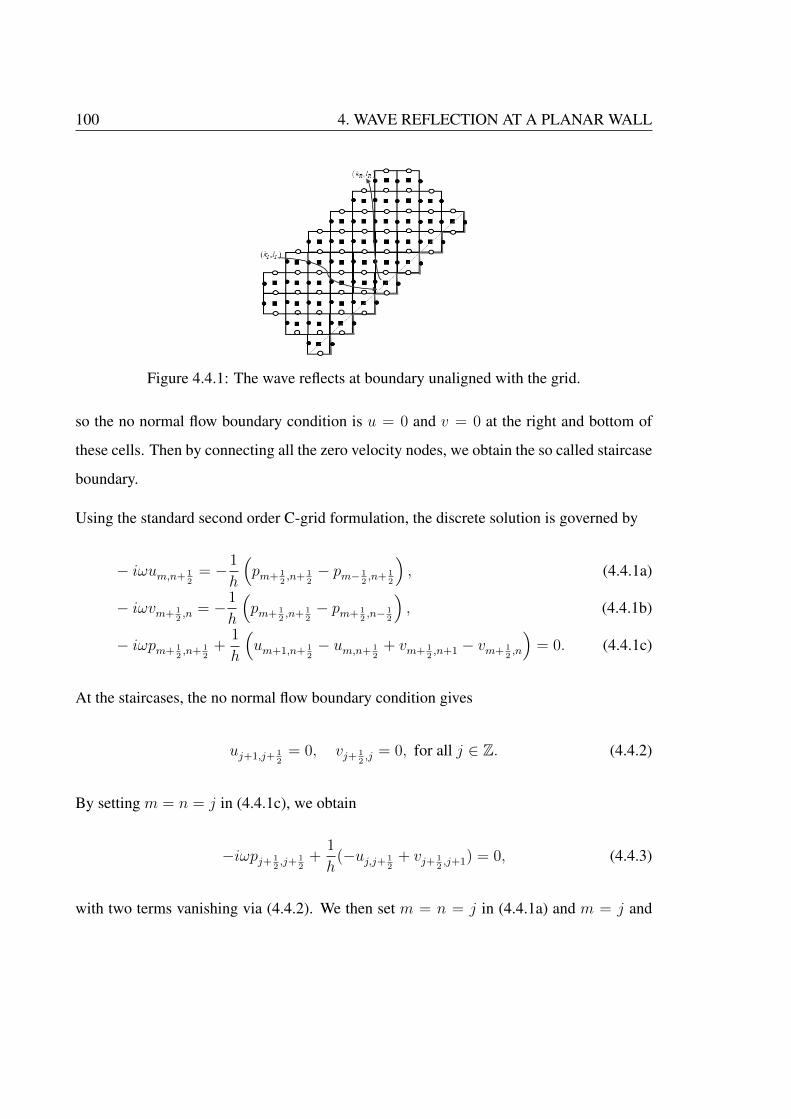
100 4. WAVE REFLECTION AT A PLANAR WALL
Figure 4.4.1: The wave reflects at boundary unaligned with the grid.
so the no normal flow boundary condition is u = 0 and v = 0 at the right and bottom of
these cells. Then by connecting all the zero velocity nodes, we obtain the so called staircase
boundary.
Using the standard second order C-grid formulation, the discrete solution is governed by
− iωum,n+ 12
= −1
h
(pm+ 1
2,n+ 1
2− pm− 1
2,n+ 1
2
), (4.4.1a)
− iωvm+ 12,n = −1
h
(pm+ 1
2,n+ 1
2− pm+ 1
2,n− 1
2
), (4.4.1b)
− iωpm+ 12,n+ 1
2+
1
h
(um+1,n+ 1
2− um,n+ 1
2+ vm+ 1
2,n+1 − vm+ 1
2,n
)= 0. (4.4.1c)
At the staircases, the no normal flow boundary condition gives
uj+1,j+ 12
= 0, vj+ 12,j = 0, for all j ∈ Z. (4.4.2)
By setting m = n = j in (4.4.1c), we obtain
−iωpj+ 12,j+ 1
2+
1
h(−uj,j+ 1
2+ vj+ 1
2,j+1) = 0, (4.4.3)
with two terms vanishing via (4.4.2). We then set m = n = j in (4.4.1a) and m = j and
4.4. TILTED BOUNDARY: DISCRETE SOLUTION 101
n = j + 1 in (4.4.1b) to eliminate u and v, to obtain
pj+ 12,j+ 3
2+ (ω2h2 − 2)pj+ 1
2,j+ 1
2+ pj− 1
2,j+ 1
2= 0. (4.4.4)
This equation links the pressure node pj+1/2,j+1/2 at the centre of a boundary cell, to pres-
sure nodes at the centre of two cells away from the boundary pj−1/2,j+1/2 and pj+1/2,j+3/2
(i.e., to the left and above the boundary cell). In (4.4.4), j is taken to be an integer, but we
can rewrite it as
pj,j+1 +(ω2h2 − 2
)pj,j + pj−1,j = 0, (4.4.5)
where j will now be an integer plus half.
We now assume a discrete solution of the form
pm,n = Re[AI exp{i(kIxm + lIyn − ωIt)}
]+ Re
[AR exp{i(kRxm + lRyn − ωRt)}
].
(4.4.6)
As before, we can take ωR > 0 without loss of generality, and there is a condition on
(kR, lR) to ensure propagation towards the wall. Substituting (4.4.6) in (4.4.5) then gives
AI exp(i (kIjh+ lI (j + 1)h− ωIt)) + AR exp(i (kRjh+ lR (j + 1)h− ωRt))
+(ω2h2 − 2
)(AI exp(i (kIjh+ lIjh− ωIt)) + AR exp(i (kRjh+ lRjh− ωRt)))
+AI exp{i (kI (j − 1)h+ lIjh− ωIt)}+AR exp{i (kR (j − 1)h+ lRjh− ωRt)} = 0.
(4.4.7)
With a straightforward factorising the common terms we have
AI exp{i ((kI + lI)jh− ωIt)}(exp{−ikIh}+ ω2h2 − 2 + exp{ilIh}
)= −AR exp{i ((kR + lR)jh− ωRt)}
(exp{−ikRh}+ ω2h2 − 2 + exp{ilRh}
), (4.4.8)
102 4. WAVE REFLECTION AT A PLANAR WALL
or we can simply write as
AR = −AI exp{i(kI + lI − kR − lR)jh− (ωI − ωR)t}(e−ikIh + ω2h2 − 2 + eilIh
)(e−ikRh + ω2h2 − 2 + eilRh)
.
(4.4.9)
This equation, (4.4.9), has some similarities to equation (7) of [17]. The first main dif-
ference arises because they analysed the problem in a specific time-stepping framework,
so that their expression also involved a time step δ. Here we simply assume time-periodic
waves, the frequency of which will be consistent with the discrete dispersion relation. The
second main difference arises because they made an assumption about the values of kR and
lR, without deriving them from kI and lI . Here we make no such assumption, and rather
determine kR and lR from kI and lI , leading to (4.4.15).
If (4.4.9) is to be true for all j and t, then
kI + lI − kR − lR = 0, (4.4.10)
ωI − ωR = 0, (4.4.11)
AI(e−ikIh + ω2
Ih2 − 2 + eilIh
)= −AR
(e−ikRh + ω2
Rh2 − 2 + eilRh
). (4.4.12)
Since we know all the components for the incident wave, (i.e., kI , lI , AI , and ωI), the
remaining task is to find all the reflected wave components, (i.e., kR, lR, AR, and ωR).
Of course, we also know that the discrete dispersion relation (4.2.18) must be satisfied by
4.4. TILTED BOUNDARY: DISCRETE SOLUTION 103
the incident and reflected waves, that is
ω2I =
4
h2
(sin2
(kIh
2
)+ sin2
(lIh
2
))=
4
h2
(sin2
(kRh
2
)+ sin2
(lRh
2
))= ω2
R,
⇒ 1− cos (kIh)
2+
1− cos(lIh)
2=
1− cos kRh
2+
1− cos lRh
2
cos (kIh) + cos (lIh) = cos (kRh) + cos (lRh) ,
2 cos
((kI + lI)h
2
)cos
((kI − lI)h
2
)= 2 cos
((kR + lR)h
2
)cos
((kR − lR)h
2
).
However, using (4.4.10) we have
cos
((kR + lR)h
2
)cos
((kI − lI)h
2
)= cos
((kR + lR)h
2
)cos
((kR − lR)h
2
).
⇒ cos
((kR + lR)h
2
)[cos
((kI − lI)h
2
)− cos
((kR − lR)h
2
)]= 0,
⇒ cos
((kR + lR)h
2
)sin
((kI−lI)h
2+ (kR−lR)h
2
2
)sin
((kI−lI)h
2− (kR−lR)h
2
2
)= 0.
At least as h → 0, the first term cannot vanish, so we either need(kI − lI)h
2+
(kR − lR)h
2= 0 or
(kI − lI)h2
− (kR − lR)h
2= 0 (again as h → 0). In terms of the
wavenumbers, these options are
kI − lI + kR − lR = 0 or kI − lI − kR + lR = 0. (4.4.13)
Using (4.4.10), the second of these gives lR = lI and then kR = kI , and then AI = −ARfrom (4.4.12); this corresponds to a trivial solution with p = 0. So we are left (which would
also fail to satisfy the group velocity condition) with
kI − lI + kR − lR = 0. (4.4.14)
104 4. WAVE REFLECTION AT A PLANAR WALL
Combining with (4.4.10) then gives
kR = lI , lR = kI . (4.4.15)
So we have found the discrete reflected wavenumbers in term of the incident wavenumbers.
It shows the surprising result that there is no error in the reflected wavenumber, i.e., we
exactly recover the continuum reflection relationship (4.3.13). This appears to arise by
some special chance, perhaps because of the simple form of the discrete dispersion relation,
or because of its symmetry between k and l, i.e., ω2 = (4/h2)(sin2(kh/2) + sin2(lh/2)).
Indeed, as shown in section 6.4.2 for a case with internal waves, there is no necessity for
a continuum (reflection) result to be recovered exactly in a discrete approximation. The
result (4.4.15) was simply assumed in [17], which is one of the key differences between
their study and this one. We should also note that if we were to generalise the problem and
consider reflection at a non-perfect staircase (i.e., one not-aligned at 45 degrees to the grid),
then this perfect reflection property may be lost.
It remains to find AR. Expanding (4.4.12) with Taylor Series, we find
AI
[{1 + ilIh−
1
2(lIh)2 − i
6(lIh)3 +O(h4)}+ ω2
Ih2 − 2
+ {1− ikIh−1
2(kIh)2 +
i
6(kIh)3 +O(h4)}
]
= −AR
[{1 + ilRh−
1
2(lRh)2 − i
6(lRh)3 +O(h4)}+ ω2
Rh2 − 2
+ {1− ikIRh−1
2(kRh)2 +
i
6(kRh)3 +O(h4)}
], (4.4.16)
4.4. TILTED BOUNDARY: DISCRETE SOLUTION 105
By rearranging the common terms we have
AI
[i (lI − kI) + h
(ω2I −
k2I
2− l2I
2
)+ih2
6
(k3I − l3I
)+O(h3)
]= −AR
[i (lR − kR) + h
(ω2R −
l2R2− k2
R
2
)+ih2
6
(k3R − l3R
)+O(h3)
], (4.4.17)
and substituting (4.4.11) and (4.4.15) into (4.4.17) and multiplying by (−1) both side gives
AI
[i (kI − lI)− h
(ω2I −
k2I
2− l2I
2
)− ih2
6
(k3I − l3I
)+O(h3)
]= AR
[i (kI − lI) + h
(ω2R −
k2I
2− l2I
2
)+ih2
6
(l3I − k3
I
)+O(h3)
]. (4.4.18)
By making AR as a subject we have
AR = AI
[i (kI − lI)−
h
2(k2I + l2I)−
ih2
6(k3I − l3I) +O(h3)
][i (kI − lI) +
h
2(k2I + l2I) +
ih2
6(l3I − k3
I ) +O(h3)
] (4.4.19)
= AI
i (kI − lI)[1− h (k2
I + l2I)
2i (kI − lI)− ih2(kI − lI)
6i (kI − lI)(k2I + kI lI + l2I) +O(h3)
]i (kI − lI)
[1 +
h (k2I + l2I)
2i (kI − lI)− ih2(kI − lI)
6i (kI − lI)(k2I + kI lI + l2I) +O(h3)
] .(4.4.20)
Note that the case kI = lI is excluded, since this corresponds to wave propagation along
the wall. So we may cancel that factor, and obtain
AR = AI
[1 +
ih (k2I + l2I)
2 (kI − lI)− h2 (k2
I + kI lI + l2I)
6+O(h3)
][1− ih (k2
I + l2I)
2 (kI − lI)− h2 (k2
I + kI lI + l2I)
6+O(h3)
] . (4.4.21)
106 4. WAVE REFLECTION AT A PLANAR WALL
Finally, using the binomial series on the denominator gives
AR = AI
(1 +
ih (k2I + l2I)
(kI − lI)− h2(k2
I + l2I)2
2(kI − lI)2
)+O(h3). (4.4.22)
This is a key result. The corresponding continuum result was (4.3.12) AR = AI . However,
we have not recovered that. Instead, we find a first-order in h phase error in the complex
amplitude: this is solely due to the staircase boundary.
It is then of interest to ask if there is solely a phase error, or whether there is also an
amplification (or suppression) upon reflection. To do this, we calculate
|AR|2 = |AI |2(
1 +ih (k2
I + l2I)
(kI − lI)− h2(k2
I + l2I)2
2(kI − lI)2+O(h3)
)(
1− ih(k2I + l2I)
(kI − lI)− h2(k2
I + l2I)2
2(kI − lI)2+O(h3)
), (4.4.23)
which gives
|AR|2 = |AI |2(1 +O(h3)
). (4.4.24)
So we cannot detect any change in the magnitude of the reflected wave from the incident
wave. This analysis does not prove that |AR| = |AI |, other than up to O(h2).
4.4.1 Alternative derivation of amplitude error
We can improve upon (4.4.22) and (4.4.23) by returning to (4.4.12). Using (4.4.15) to
substitute kR = lI and lR = kI gives
ARAI
= −exp(−ikh) + exp(+ilh)− 2 + ω2h2
exp(+ikh) + exp(−ilh)− 2 + ω2h2, where ω2 =
4
h2
(sin2 kh
2+ sin2 lh
2
).
(4.4.25)
4.4. TILTED BOUNDARY: DISCRETE SOLUTION 107
This expression takes the form
ARAI
= − a
a∗, where a = exp(−ikh) + exp(+ilh)− 2 + 4
(sin2 kh
2+ sin2 lh
2
). (4.4.26)
Since |a/a∗| = 1, it follows that |AR/AI | = 1. So everything is contained in the (complex)
phase function ϕ, i.e., AR/AI = exp(iϕ). If we write a = r exp(i(π/2 + θ)), then
exp(iϕ) =ARAI
= − r exp(i(π/2 + θ))
r exp(−i(π/2 + θ))= − exp(i(π + 2θ)) = exp(2iθ) ⇒ ϕ = 2θ.
It remains to determine θ, which we find by rewriting a as
a = r exp(i(π/2 + θ)) = r (cos(π/2 + θ) + i sin(π/2 + θ)) = r(− sin θ + i cos θ).
But from (4.4.26), we can rewrite a as
a = cos kh+ cos lh− 2 + 4
(sin2 kh
2+ sin2 lh
2
)+ i(sin lh− sin kh)
= 2
(sin2 kh
2+ sin2 lh
2
)+ i(sin lh− sin kh)
⇒ r cos θ = sin lh− sin kh and r sin θ = −2
(sin2 kh
2+ sin2 lh
2
)⇒ tan θ = 2
(sin2 kh
2+ sin2 lh
2
sin kh− sin lh
). (4.4.27)
For example,
• if h� 1, then
tan θ ≈ 2
(k2h2/4 + l2h2/4
kh− lh
)=
(k2 + l2
2(k − l)
)h
⇒ θ ≈(k2 + l2
2(k − l)
)h ⇒ ϕ = 2θ ≈
(k2 + l2
k − l
)h, (4.4.28)
in agreement with the existing result (4.4.22) for small h.
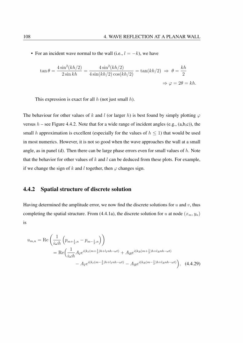
108 4. WAVE REFLECTION AT A PLANAR WALL
• For an incident wave normal to the wall (i.e., l = −k), we have
tan θ =4 sin2(kh/2)
2 sin kh=
4 sin2(kh/2)
4 sin(kh/2) cos(kh/2)= tan(kh/2) ⇒ θ =
kh
2
⇒ ϕ = 2θ = kh.
This expression is exact for all h (not just small h).
The behaviour for other values of k and l (or larger h) is best found by simply plotting ϕ
versus h – see Figure 4.4.2. Note that for a wide range of incident angles (e.g., (a,b,c)), the
small h approximation is excellent (especially for the values of h ≤ 1) that would be used
in most numerics. However, it is not so good when the wave approaches the wall at a small
angle, as in panel (d). Then there can be large phase errors even for small values of h. Note
that the behavior for other values of k and l can be deduced from these plots. For example,
if we change the sign of k and l together, then ϕ changes sign.
4.4.2 Spatial structure of discrete solution
Having determined the amplitude error, we now find the discrete solutions for u and v, thus
completing the spatial structure. From (4.4.1a), the discrete solution for u at node (xm, yn)
is
um,n = Re
(1
iωh
(pm+ 1
2,n − pm− 1
2,n
))= Re
( 1
iωhAIe
i(kI(m+ 12
)h+lInh−ωt) + ARei(kR(m+ 1
2)h+lRnh−ωt)
− AIei(kI(m− 12
)h+lInh−ωt) − ARei(kR(m− 12
)h+lRnh−ωt)), (4.4.29)
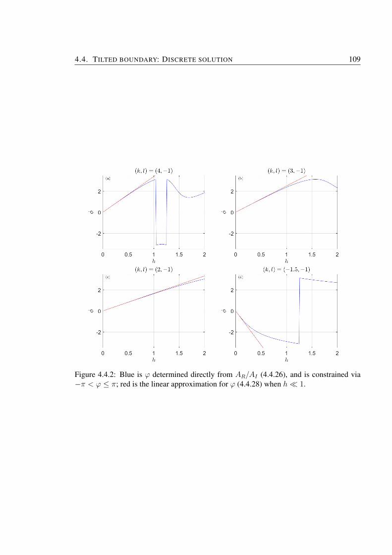
4.4. TILTED BOUNDARY: DISCRETE SOLUTION 109
Figure 4.4.2: Blue is ϕ determined directly from AR/AI (4.4.26), and is constrained via−π < ϕ ≤ π; red is the linear approximation for ϕ (4.4.28) when h� 1.

110 4. WAVE REFLECTION AT A PLANAR WALL
which is simplified as
um,n = Re
(2
ωh
(AIe
i(kImh+lInh−ωt) sinkIh
2+ ARe
i(kRmh+lRnh−ωt) sinkRh
2
)). (4.4.30)
Then, in the limit of h→ 0, and by substituting AR and kR, lR using (4.4.24) and (4.4.15),
respectively, we obtain
um,n = Re
(AIω
[kI exp(i(kImh+ lInh− ωt)) + lI exp(i(lImh+ kInh− ωt))(
1 +ih(k2
I + l2I)
(kI − lI)
)])+O(h3). (4.4.31)
Similarly, the structure of discrete solution for v also can be calculated. From (4.4.1b), the
discrete solution for v at (xm, yn) is
vm,n = Re
(1
iωh
(pm,n+ 1
2− pm,n− 1
2
))= Re
( 1
iωhAIe
i(kImh+lI(n+ 12
)h−ωt) + ARei(kRmh+lR(n+ 1
2)h−ωt)
− AIei(kImh+lI(n− 12
)h−ωt) − ARei(kRmh+lR(n− 12
)h−ωt)), (4.4.32)
which is simplified as
vm,n = Re
(2
ωh
(AIe
i(kImh+lInh−ωt) sinlIh
2+ ARe
i(kRmh+lRnh−ωt) sinlRh
2
)). (4.4.33)
Again, as h→ 0 we obtain
vm,n = Re
(AIω
[lI exp(i(kImh+ lInh− ωt)) + kI exp(i(lImh+ kInh− ωt))(
1 +ih(k2
I + l2I)
(kI − lI)
)])+O(h3). (4.4.34)
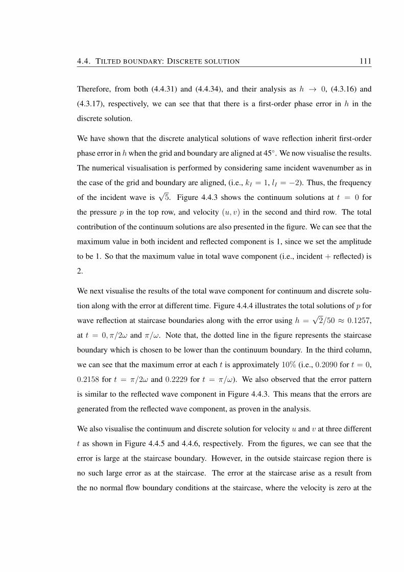
4.4. TILTED BOUNDARY: DISCRETE SOLUTION 111
Therefore, from both (4.4.31) and (4.4.34), and their analysis as h → 0, (4.3.16) and
(4.3.17), respectively, we can see that that there is a first-order phase error in h in the
discrete solution.
We have shown that the discrete analytical solutions of wave reflection inherit first-order
phase error in hwhen the grid and boundary are aligned at 45◦. We now visualise the results.
The numerical visualisation is performed by considering same incident wavenumber as in
the case of the grid and boundary are aligned, (i.e., kI = 1, lI = −2). Thus, the frequency
of the incident wave is√
5. Figure 4.4.3 shows the continuum solutions at t = 0 for
the pressure p in the top row, and velocity (u, v) in the second and third row. The total
contribution of the continuum solutions are also presented in the figure. We can see that the
maximum value in both incident and reflected component is 1, since we set the amplitude
to be 1. So that the maximum value in total wave component (i.e., incident + reflected) is
2.
We next visualise the results of the total wave component for continuum and discrete solu-
tion along with the error at different time. Figure 4.4.4 illustrates the total solutions of p for
wave reflection at staircase boundaries along with the error using h =√
2/50 ≈ 0.1257,
at t = 0, π/2ω and π/ω. Note that, the dotted line in the figure represents the staircase
boundary which is chosen to be lower than the continuum boundary. In the third column,
we can see that the maximum error at each t is approximately 10% (i.e., 0.2090 for t = 0,
0.2158 for t = π/2ω and 0.2229 for t = π/ω). We also observed that the error pattern
is similar to the reflected wave component in Figure 4.4.3. This means that the errors are
generated from the reflected wave component, as proven in the analysis.
We also visualise the continuum and discrete solution for velocity u and v at three different
t as shown in Figure 4.4.5 and 4.4.6, respectively. From the figures, we can see that the
error is large at the staircase boundary. However, in the outside staircase region there is
no such large error as at the staircase. The error at the staircase arise as a result from
the no normal flow boundary conditions at the staircase, where the velocity is zero at the

112 4. WAVE REFLECTION AT A PLANAR WALL
staircase boundary. Meanwhile, in the continuum solutions they are not exactly zero. As
in p, the error in velocity are also arise from the reflected components. Undoubtedly, the
error in the solutions are minimised when we reduced the size of grid spacing h to be√
2/100 ≈ 0.0141, as illustrated in Figure 4.4.7. It can be seen that the error is improved
by 5% error, since the maximum error is approximately 0.1046 .
4.5 Summary
In this chapter, we have studied reflection of waves (meaning acoustic waves or non-rotating
shallow-water waves) at a straight boundary. In the underlying continuum problem, the
(complex) wave amplitude of the reflected wave is the same as that of the incoming wave,
the along-boundary wavenumber remains unchanged, and the across-boundary wavenum-
ber changes sign.
We studied two versions of the discrete problem. In the first of these, the grid and boundary
were aligned, at y = 0. We showed that the reflected amplitude was recovered exactly, as
were the two components of the reflected wavenumber. The solution is ‘exact’ in this sense.
However, we should remember that there is a second-order error in the wave frequency of
both incident and reflected waves, as occurs for any wave problem on the C-grid, with or
without boundaries.
In the second discrete problem, the boundary (at y = x) was aligned at 45◦ to the grid,
thus forming a perfect staircase boundary. Here we showed that the wavenumbers of the
reflected wave were recovered exactly, which is perhaps surprising. However, the (complex)
amplitude AR of the reflected wave was not recovered exactly. Even though its magnitude
was recovered correctly, i.e., |AR| = |AI |, there was a phase error, i.e., AR/AI had non-
zero imaginary part. We derived an expression for AR/AI (which was previously given by
[17]), and analysed it in some detail. In particular, we showed that there is first-order error
4.5. SUMMARY 113
Figure 4.4.3: The continuum solutions of wave reflection at a straight boundary y = x withhorizontal wavenumber kI = 1 and vertical wavenumber lI = −2. Shown are the solutionsfor p (first row), u (second row) and v (third row) at t = 0. The left column is the incidentwavecomponent, the centre column is the reflected wave component, and the right columnis the total (i.e., incident + reflected) component.
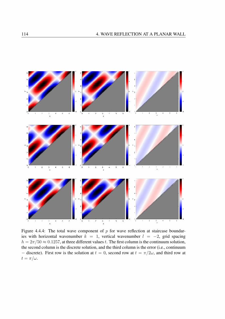
114 4. WAVE REFLECTION AT A PLANAR WALL
Figure 4.4.4: The total wave component of p for wave reflection at staircase boundar-ies with horizontal wavenumber k = 1, vertical wavenumber l = −2, grid spacingh = 2π/50 ≈ 0.1257, at three different values t. The first column is the continuum solution,the second column is the discrete solution, and the third column is the error (i.e., continuum− discrete). First row is the solution at t = 0, second row at t = π/2ω, and third row att = π/ω.
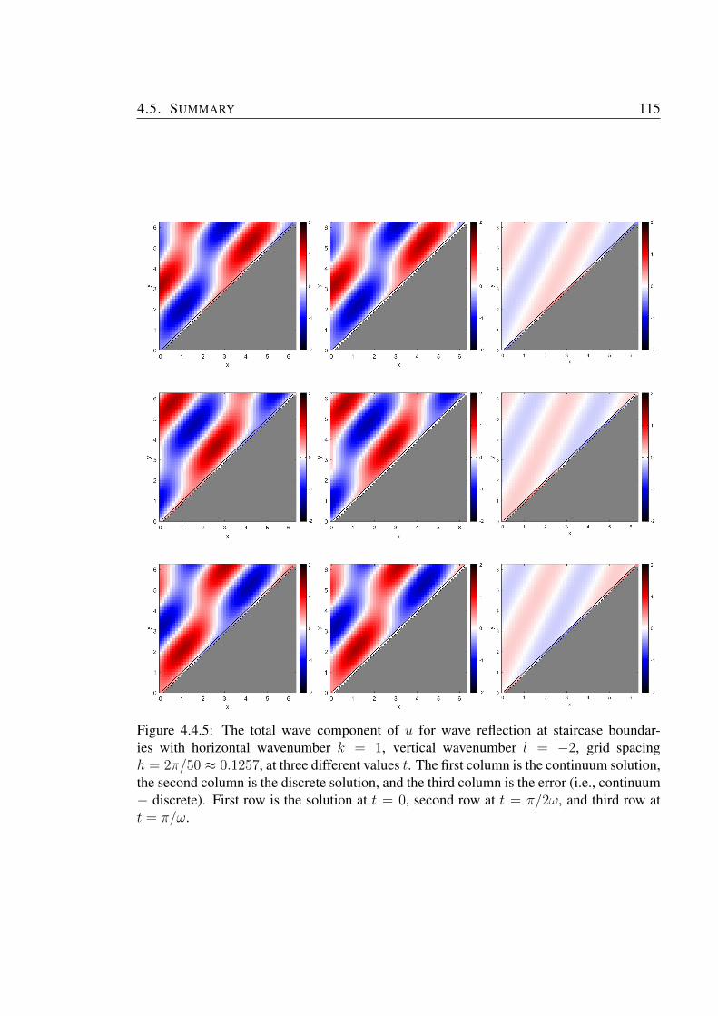
4.5. SUMMARY 115
Figure 4.4.5: The total wave component of u for wave reflection at staircase boundar-ies with horizontal wavenumber k = 1, vertical wavenumber l = −2, grid spacingh = 2π/50 ≈ 0.1257, at three different values t. The first column is the continuum solution,the second column is the discrete solution, and the third column is the error (i.e., continuum− discrete). First row is the solution at t = 0, second row at t = π/2ω, and third row att = π/ω.
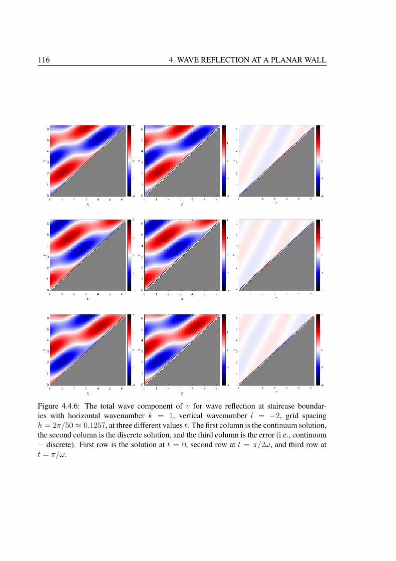
116 4. WAVE REFLECTION AT A PLANAR WALL
Figure 4.4.6: The total wave component of v for wave reflection at staircase boundar-ies with horizontal wavenumber k = 1, vertical wavenumber l = −2, grid spacingh = 2π/50 ≈ 0.1257, at three different values t. The first column is the continuum solution,the second column is the discrete solution, and the third column is the error (i.e., continuum− discrete). First row is the solution at t = 0, second row at t = π/2ω, and third row att = π/ω.
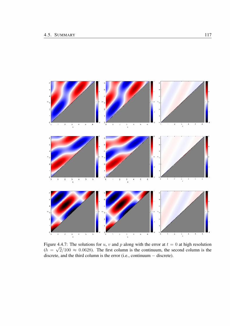
4.5. SUMMARY 117
Figure 4.4.7: The solutions for u, v and p along with the error at t = 0 at high resolution(h =
√2/100 ≈ 0.0628). The first column is the continuum, the second column is the
discrete, and the third column is the error (i.e., continuum − discrete).
118 4. WAVE REFLECTION AT A PLANAR WALL
ϕ in the phase, in terms of the grid spacing h, with
ϕ = (k2 + l2)h/(k − l),
where (k, l) is the wavevector of the incident wave. By comparison with evaluations of the
exact phase error at finite h, we showed that our first-order asymptotic scaling for the phase
error is remarkably accurate when h . 0.5, provided that the incident wave direction is not
close to being parallel with the boundary. In that case, the phase errors are much larger (see
Figure 4.4.2).
Consider, for example, the case when the incident wave is normal to the boundary, i.e.,
l = −k. Then the phase error ϕ = kh (a result which we showed to be exact, even at finite
h). For a minimally resolved wave with 4 grid points per wavelength (i.e., 4h = 2π/k ⇒
kh = π/2), the phase error upon reflection is then π/2. So if the wave were to reflect
off two such boundaries, then the phase error would be π (assuming that the phase errors
were additive), and the wave would become completely out of phase with its continuum
counterpart. However, note that the error in the wave frequency here would only be 19%
(i.e., this might be considered to be an adequately resolved wave on the C-grid), since the
continuum frequency ω2c = 2k2 and discrete frequency
ω2d = (8/h2) sin2(kh/2) = (8k2/(kh2)) sin2(kh/2)
= (8k2)/(π/2)2 sin2(π/4) = 2k2(8/π2) = (8/π2)ω2c .
For what might be considered as a well-resolved wave with 16 grid points per wavelength
(i.e., 16h = 2π/k ⇒ kh = π/8), the phase error upon reflection is then π/8. This is clearly
better, but only 8 reflections would be required for the wave to become completely out of
phase with its continuum counterpart. The error in the wave frequency here would only be
1.3% (i.e., this might be considered to be a well resolved wave on the C-grid), since the
4.5. SUMMARY 119
discrete frequency would be
ω2d = (8/h2) sin2(kh/2) = (8k2/(kh2)) sin2(kh/2)
= (8k2)/(π/8)2 sin2(π/16) = 2k2(256/π2) sin2(π/16) = (8/π2)ω2c .
The extension to better resolved waves is obvious. So, the effects of staircasing are clear,
and how they could lead to serious errors in the phase of the wave after 1 (or, more likely,
multiple) reflections.

120 4. WAVE REFLECTION AT A PLANAR WALL
121
Chapter 5
NUMERICAL SOLUTIONS: THE
EFFECT OF STAIRCASE BOUNDARY
5.1 Introduction
This chapter is devoted to understanding possible implications of the previous mathematical
analysis of the linearised wave equations
∂u
∂t= −∂p
∂x,∂v
∂t= −∂p
∂y,∂p
∂t+∂u
∂x+∂v
∂y= 0. (5.1.1)
Here, we choose the same notation as in the chapters 3 and 4, where (u, v) denoted velocity
of the flow while p the pressure.
In chapter 3, we discussed the wave propagation along a channel bounded by two parallel
walls in the y direction. While in chapter 4, we discussed the waves reflection at a boundary.
As we know, there are different kinds of error can be arise from the presented discrete
solutions. As discussed chapter 3, we know that if wave goes along the boundary, it will
slow down. And from chapter 4, we know that there could be a phase error from the
reflection of wave at a boundary. But, the solution remains ‘good’, and just experiences
122 5. NUMERICAL SOLUTIONS: THE EFFECT OF STAIRCASE BOUNDARY
some effect of displacement. In this chapter, we investigate what will happen when both of
these possible errors are combined together, from two numerical experiments on the C grid.
In the chapter 3 and 4, as grid spacing h→ 0, the discrete solutions were assessed with the
continuum solutions in terms of the convergence. Here, the numerical experiments will be
conducted and the error measurement is calculated from the continuum solution. For this
reason, our numerical experiments are focused on the square and circular domain, since the
continuum solution for these domains can be derived. Of course, numerical simulations can
also be conducted for arbitrary domains, but this will not be discussed in this thesis.
The equations are discretised using the finite-difference method. It is arguably the simplest,
easiest and efficient method to implement on the regular-spaced grid. However, this advant-
age offset by the curved boundaries and complex geometries where the finite-difference grid
does not coincide with the boundary, i.e., staircases. As shown in previous two chapters,
staircase boundaries introduce errors that affect the numerical solutions. However, those
calculations were performed for time-harmonic oscillations. Thus, the emphasis of this
chapter is to examine how does the error generated from the staircase boundaries influence
the long-time dynamics of a wave sloshing in a closed domain.
Numerical simulations with staircase boundaries have been performed in various complex
geometries. However, in such studies there is little or no quantification of the rate of con-
vergence towards the continuum solution. For example, [13] has presented numerical simu-
lations of room acoustic modelling over various complex geometries. By comparing finite-
difference with staircase boundary and finite-volume method with fitted boundary, it was
found that finite-volume method gave results much better than finite-difference method.
However, at only one fixed resolution it is impossible to reach a conclusion on the rate of
convergence of every method that has been performed. For electromagnetic waves, [67]
studied two-dimensional wave reflection at a straight boundary tilted at some angle relative
to x axis and a cylinder domain. Based on experiments at three different resolutions, con-
vergence rates between 0.5 and 1 for the pressure in the L2 norm is obtained. In the same
5.2. NUMERICAL METHODS 123
setting, [27, 33] reported errors of O(h1/2) for pressure and velocity in the L2 norm. In a
different application, [29] estimate the rate of convergence for pressure in a linear wind-
driven ocean circulation is between 1 and 2 in L2 norm. By revisiting these problems we
hope that we can understand how the model resolution effects on the staircase boundary,
and reveal the convergence rate of finite-difference method as grid spacing h→ 0.
In setting up numerical solutions of two-dimensional acoustic wave equations, the equations
are discretised such that finite-differencing is applicable to the Arakawa C-grid [6]. The
analogous grid which is known as Yee-grid [71] is widely used in the modelling of acoustic
and electromagnetic waves [34, 17]. The simplest application of this grid is to acoustic
wave equations where velocity vector u = (u, v) is located at the boundary of a finite-
difference cell and pressure p is located at the centre of cell. With this grid, it is easy to
ensure that the resulting schemes conserve the fluid dynamics properties such as mass and
energy, as discussed in Chapter 2.
5.2 Numerical Methods
We consider the same equations of motion (5.1.1) as considered in chapters previous two
chapters and we solve these subject to u · n = 0 and a specified initial condition, using a
numerical method that works for an arbitrary closed domain.
5.2.1 Spatial discretization
As in previous chapters, we use the Arakawa C-grid, with nodes (u,v,p) staggered as shown
in Figure 2.5.1. We choose the grid spacings dx= dy = h for all experiments. We consider an
arbitrary domain placed on top of this grid, and we then construct a grid on a quadrilateral
of extend 2lx × 2ly that just extends beyond the specified domain, where 2lx = nxh and
2ly = nyh for some integers nx and ny.
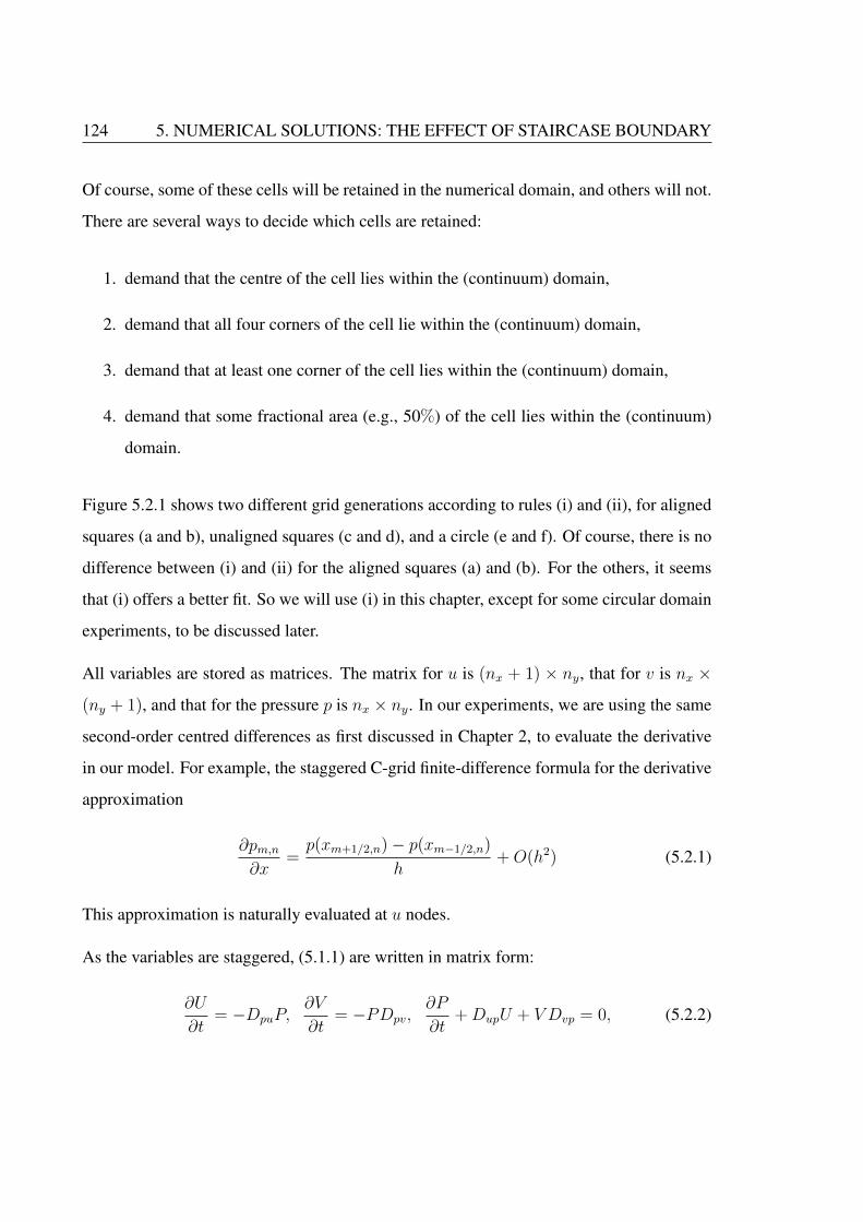
124 5. NUMERICAL SOLUTIONS: THE EFFECT OF STAIRCASE BOUNDARY
Of course, some of these cells will be retained in the numerical domain, and others will not.
There are several ways to decide which cells are retained:
1. demand that the centre of the cell lies within the (continuum) domain,
2. demand that all four corners of the cell lie within the (continuum) domain,
3. demand that at least one corner of the cell lies within the (continuum) domain,
4. demand that some fractional area (e.g., 50%) of the cell lies within the (continuum)
domain.
Figure 5.2.1 shows two different grid generations according to rules (i) and (ii), for aligned
squares (a and b), unaligned squares (c and d), and a circle (e and f). Of course, there is no
difference between (i) and (ii) for the aligned squares (a) and (b). For the others, it seems
that (i) offers a better fit. So we will use (i) in this chapter, except for some circular domain
experiments, to be discussed later.
All variables are stored as matrices. The matrix for u is (nx + 1) × ny, that for v is nx ×
(ny + 1), and that for the pressure p is nx × ny. In our experiments, we are using the same
second-order centred differences as first discussed in Chapter 2, to evaluate the derivative
in our model. For example, the staggered C-grid finite-difference formula for the derivative
approximation
∂pm,n∂x
=p(xm+1/2,n)− p(xm−1/2,n)
h+O(h2) (5.2.1)
This approximation is naturally evaluated at u nodes.
As the variables are staggered, (5.1.1) are written in matrix form:
∂U
∂t= −DpuP,
∂V
∂t= −PDpv,
∂P
∂t+DupU + V Dvp = 0, (5.2.2)
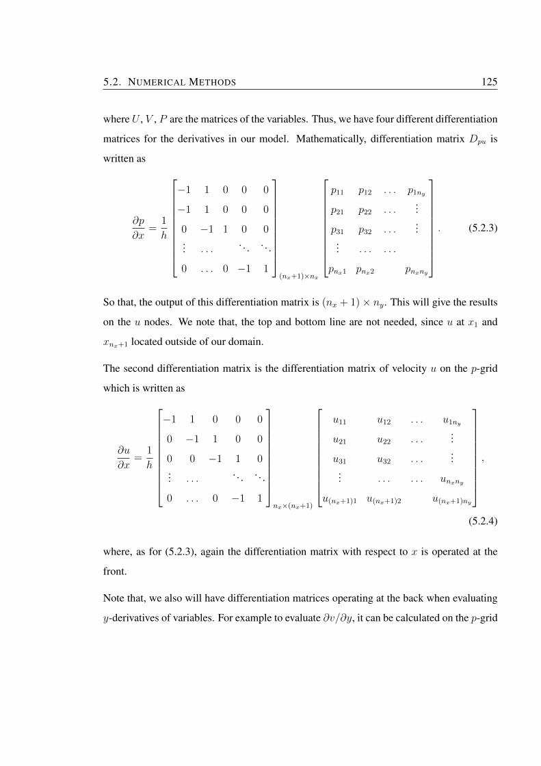
5.2. NUMERICAL METHODS 125
where U , V , P are the matrices of the variables. Thus, we have four different differentiation
matrices for the derivatives in our model. Mathematically, differentiation matrix Dpu is
written as
∂p
∂x=
1
h
−1 1 0 0 0
−1 1 0 0 0
0 −1 1 0 0... . . .
. . . . . .
0 . . . 0 −1 1
(nx+1)×nx
p11 p12 . . . p1ny
p21 p22 . . ....
p31 p32 . . ....
... . . . . . .
pnx1 pnx2 pnxny
. (5.2.3)
So that, the output of this differentiation matrix is (nx + 1)× ny. This will give the results
on the u nodes. We note that, the top and bottom line are not needed, since u at x1 and
xnx+1 located outside of our domain.
The second differentiation matrix is the differentiation matrix of velocity u on the p-grid
which is written as
∂u
∂x=
1
h
−1 1 0 0 0
0 −1 1 0 0
0 0 −1 1 0... . . .
. . . . . .
0 . . . 0 −1 1
nx×(nx+1)
u11 u12 . . . u1ny
u21 u22 . . ....
u31 u32 . . ....
... . . . . . . unxny
u(nx+1)1 u(nx+1)2 u(nx+1)ny
,
(5.2.4)
where, as for (5.2.3), again the differentiation matrix with respect to x is operated at the
front.
Note that, we also will have differentiation matrices operating at the back when evaluating
y-derivatives of variables. For example to evaluate ∂v/∂y, it can be calculated on the p-grid
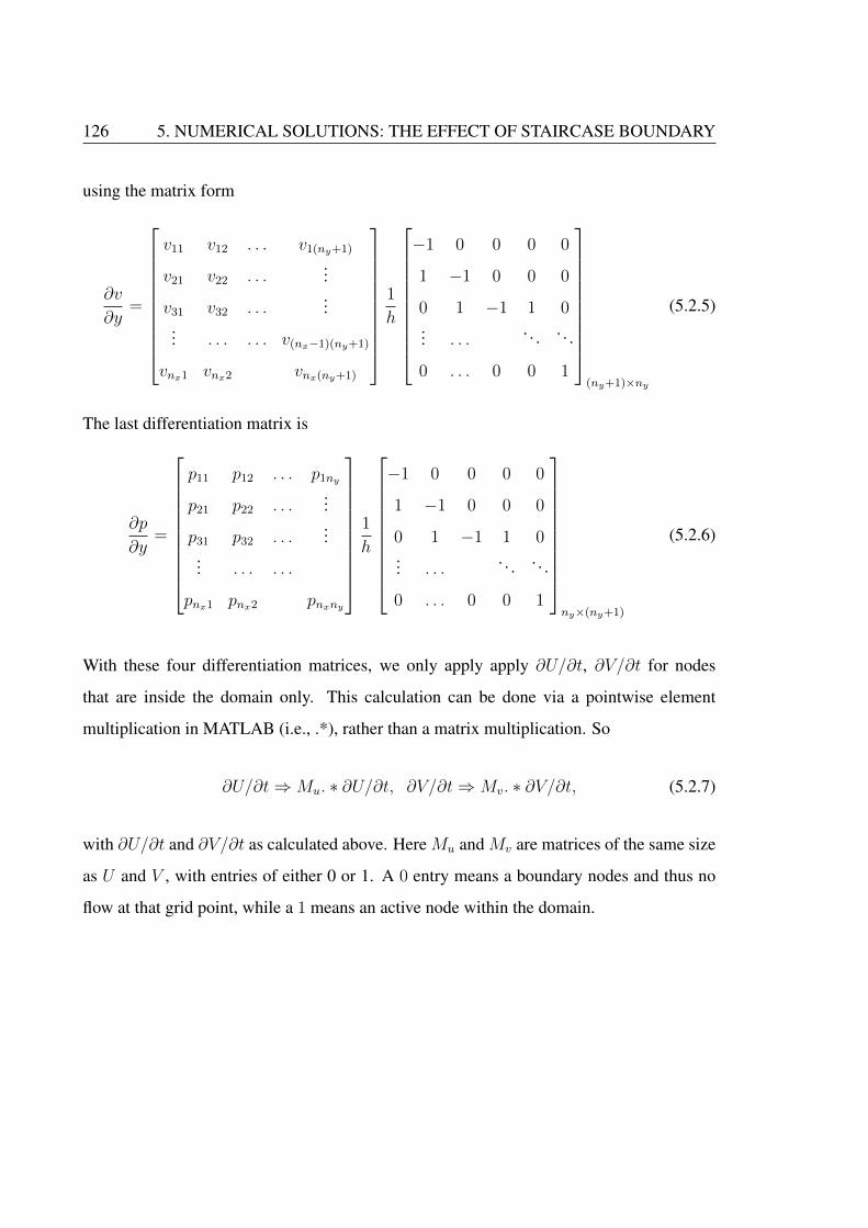
126 5. NUMERICAL SOLUTIONS: THE EFFECT OF STAIRCASE BOUNDARY
using the matrix form
∂v
∂y=
v11 v12 . . . v1(ny+1)
v21 v22 . . ....
v31 v32 . . ....
... . . . . . . v(nx−1)(ny+1)
vnx1 vnx2 vnx(ny+1)
1
h
−1 0 0 0 0
1 −1 0 0 0
0 1 −1 1 0... . . .
. . . . . .
0 . . . 0 0 1
(ny+1)×ny
(5.2.5)
The last differentiation matrix is
∂p
∂y=
p11 p12 . . . p1ny
p21 p22 . . ....
p31 p32 . . ....
... . . . . . .
pnx1 pnx2 pnxny
1
h
−1 0 0 0 0
1 −1 0 0 0
0 1 −1 1 0... . . .
. . . . . .
0 . . . 0 0 1
ny×(ny+1)
(5.2.6)
With these four differentiation matrices, we only apply apply ∂U/∂t, ∂V/∂t for nodes
that are inside the domain only. This calculation can be done via a pointwise element
multiplication in MATLAB (i.e., .*), rather than a matrix multiplication. So
∂U/∂t⇒Mu. ∗ ∂U/∂t, ∂V/∂t⇒Mv. ∗ ∂V/∂t, (5.2.7)
with ∂U/∂t and ∂V/∂t as calculated above. Here Mu and Mv are matrices of the same size
as U and V , with entries of either 0 or 1. A 0 entry means a boundary nodes and thus no
flow at that grid point, while a 1 means an active node within the domain.
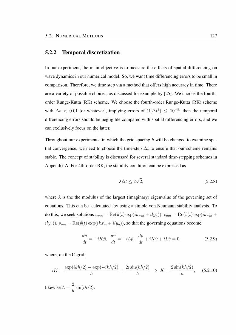
5.2. NUMERICAL METHODS 127
5.2.2 Temporal discretization
In our experiment, the main objective is to measure the effects of spatial differencing on
wave dynamics in our numerical model. So, we want time differencing errors to be small in
comparison. Therefore, we time step via a method that offers high accuracy in time. There
are a variety of possible choices, as discussed for example by [25]. We choose the fourth-
order Runge-Kutta (RK) scheme. We choose the fourth-order Runge-Kutta (RK) scheme
with ∆t < 0.01 [or whatever], implying errors of O(∆t4) ≤ 10−8; then the temporal
differencing errors should be negligible compared with spatial differencing errors, and we
can exclusively focus on the latter.
Throughout our experiments, in which the grid spacing h will be changed to examine spa-
tial convergence, we need to choose the time-step ∆t to ensure that our scheme remains
stable. The concept of stability is discussed for several standard time-stepping schemes in
Appendix A. For 4th-order RK, the stability condition can be expressed as
λ∆t ≤ 2√
2, (5.2.8)
where λ is the the modulus of the largest (imaginary) eigenvalue of the governing set of
equations. This can be calculated by using a simple von Neumann stability analysis. To
do this, we seek solutions umn = Re(u(t) exp(ikxm + ilyn)), vmn = Re(v(t) exp(ikxm +
ilyn)), pmn = Re(p(t) exp(ikxm + ilyn)), so that the governing equations become
du
dt= −iKp, dv
dt= −iLp, dp
dt+ iKu+ iLv = 0, (5.2.9)
where, on the C-grid,
iK =exp(ikh/2)− exp(−ikh/2)
h=
2i sin(kh/2)
h⇒ K =
2 sin(kh/2)
h; (5.2.10)
likewise L =2
hsin(lh/2).
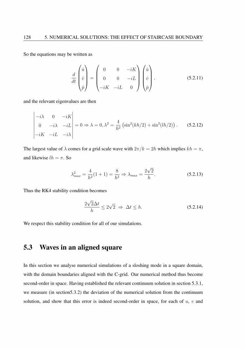
128 5. NUMERICAL SOLUTIONS: THE EFFECT OF STAIRCASE BOUNDARY
So the equations may be written as
d
dt
u
v
p
=
0 0 −iK
0 0 −iL
−iK −iL 0
u
v
p
, (5.2.11)
and the relevant eigenvalues are then∣∣∣∣∣∣∣∣∣−iλ 0 −iK
0 −iλ −iL
−iK −iL −iλ
∣∣∣∣∣∣∣∣∣ = 0⇒ λ = 0, λ2 =4
h2
(sin2(kh/2) + sin2(lh/2)
). (5.2.12)
The largest value of λ comes for a grid scale wave with 2π/k = 2h which implies kh = π,
and likewise lh = π. So
λ2max =
4
h2(1 + 1) =
8
h2⇒ λmax =
2√
2
h. (5.2.13)
Thus the RK4 stability condition becomes
2√
2∆t
h≤ 2√
2 ⇒ ∆t ≤ h. (5.2.14)
We respect this stability condition for all of our simulations.
5.3 Waves in an aligned square
In this section we analyse numerical simulations of a sloshing mode in a square domain,
with the domain boundaries aligned with the C-grid. Our numerical method thus become
second-order in space. Having established the relevant continuum solution in section 5.3.1,
we measure (in section5.3.2) the deviation of the numerical solution from the continuum
solution, and show that this error is indeed second-order in space, for each of u, v and
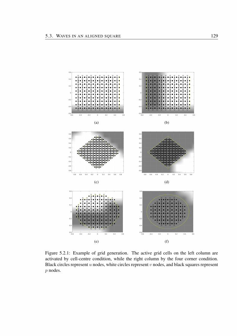
5.3. WAVES IN AN ALIGNED SQUARE 129
-0.6 -0.4 -0.2 0 0.2 0.4 0.6-0.6
-0.4
-0.2
0
0.2
0.4
0.6
(a)
-0.6 -0.4 -0.2 0 0.2 0.4 0.6-0.6
-0.4
-0.2
0
0.2
0.4
0.6
(b)
-0.8 -0.6 -0.4 -0.2 0 0.2 0.4 0.6 0.8
-0.8
-0.6
-0.4
-0.2
0
0.2
0.4
0.6
0.8
(c)
-0.8 -0.6 -0.4 -0.2 0 0.2 0.4 0.6 0.8
-0.8
-0.6
-0.4
-0.2
0
0.2
0.4
0.6
0.8
(d)
-0.6 -0.4 -0.2 0 0.2 0.4 0.6-0.6
-0.4
-0.2
0
0.2
0.4
0.6
(e)
-0.6 -0.4 -0.2 0 0.2 0.4 0.6-0.6
-0.4
-0.2
0
0.2
0.4
0.6
(f)
Figure 5.2.1: Example of grid generation. The active grid cells on the left column areactivated by cell-centre condition, while the right column by the four corner condition.Black circles represent u nodes, white circles represent v nodes, and black squares representp nodes.

130 5. NUMERICAL SOLUTIONS: THE EFFECT OF STAIRCASE BOUNDARY
p. These results, although not unexpected, set the context for the numerical simulations
of section 5.4 (tilted square) and section 5.6 (circle) where the boundary and grid are not
aligned.
5.3.1 Continuum solutions
We consider the acoustic wave equations (5.1.1) (or non-rotating shallow water equations).
We consider time-harmonic solutions of the form
(u, v, p) = Re ((u, v, p)exp(−iωt)) , (5.3.1)
for which we obtain
−iωu = −∂p∂x, −iωv = −∂p
∂y, −iωp+
∂u
∂x+∂v
∂y= 0. (5.3.2)
We solve these in a square domain −lx < x < lx, −ly < y < ly, subject to u = 0 at −lx, lx
and v = 0 at −ly, ly.
Eliminating u and v, we obtain
p+1
ω2
(∂2p
∂x2+∂2p
∂y2
)= 0. (5.3.3)
To solve this equation, we will apply a famous and useful method which is separation of
variables. We first write the solution of (5.3.3) in the form
p(x, y) = X(x)Y (y), (5.3.4)
where X is a function of only x, and Y is a function of only y. By substituting (5.3.4) into
5.3. WAVES IN AN ALIGNED SQUARE 131
(5.3.3), we have
X(x)Y (y) +1
ω2(X ′′Y (y) +X(x)Y ′′) = 0, (5.3.5)
and dividing by XY yield
ω2 +X ′′
X+Y ′′
Y= 0. (5.3.6)
The next step is the key in the process of separation of variables. We are going to say that
each of the terms in (5.3.6) is a constant because the second term is a function of only x
and the third term is a function of only y. The basis of the process in separation of variables
is the equation f(x) = g(y), with x and y independent variables, is an identity if both
functions are the same constant. Thus, we must have
X ′′
X= −k2 ⇒ Y ′′
Y= k2 − ω2 = −l2. (5.3.7)
The constant k2 is called a separation constant. Now, we need to solve the ordinary dif-
ferential equation (ODEs) (5.3.7) separately. We solve the ODE for x first. The general
solution of (5.3.7) for X is
X(x) = A cos (k(x+ lx)) +B sin (k(x+ lx)) . (5.3.8)
The boundary conditions are u = 0 at x = −lx and x = lx. Imposing the condition at
x = −lx gives
u = 0⇒ u = 0⇒ ∂p
∂x= 0⇒ X ′Y = 0⇒ X ′(−lx) = 0. (5.3.9)
From (5.3.8) we also have
X ′(x) = −Ak sin (k(x+ lx)) +Bk cos (k(x+ lx)) , (5.3.10)
132 5. NUMERICAL SOLUTIONS: THE EFFECT OF STAIRCASE BOUNDARY
and with x = −lx we get B = 0. So, the general solution now is
X(x) = A cos (k(x+ lx)) . (5.3.11)
Imposing u = 0 at x = lx, imply
u = 0⇒ u = 0⇒ ∂p
∂x= 0⇒ X ′Y = 0⇒ X ′(lx) = 0, (5.3.12)
and from (5.3.11) we have
X ′(x) = −Ak sin (k(x+ lx)) , (5.3.13)
and to satisfies the boundary condition X ′(lx) = 0 we now have eigenvalue condition, i.e.,
X ′(lx) = 0⇒ −Ak sin (2klx) = 0⇒ sin (2klx) = mπ ⇒ k =mπ
2lx, (5.3.14)
where m is an integer. Thus, the final solution of (5.3.7) for X(x) is
Xm(x) = Am cos (k(x+ lx)) ,where k =mπ
2lx, (5.3.15)
Now, lets solve (5.3.7) for y variable. The ODE now is rewritten as
Y ′′ + l2Y = 0, where l2 =ω2
c2− k2. (5.3.16)
The general solution of this ODE is
Y (y) = C cos (l(y + ly)) +D sin (l(y + ly)) . (5.3.17)
The no normal flow boundary condition at the upper and lower wall imply that v = 0 at
5.3. WAVES IN AN ALIGNED SQUARE 133
y = −ly and ly. Then, imposing the lower wall boundary condition we have
v = 0 ⇒ v = 0 ⇒ ∂p
∂y= 0 ⇒ XY ′ = 0 ⇒ Y ′(−ly) = 0, (5.3.18)
which give
Y ′(−ly) = −Cl sin (l(−ly + ly)) +Dl cos (l(−ly + ly)) = 0 ⇒ D = 0. (5.3.19)
Then, the solution now becomes
Y (y) = C cos (l(y + ly)) . (5.3.20)
Next, imposing the upper wall boundary condition, i.e., v = 0 at y = ly, we have Y ′(ly) =
0, implies
Y ′(ly) = −Cl sin (l(2ly)) = 0 ⇒ sin (l(2ly)) = sin(nπ) ⇒ l =nπ
2ly, (5.3.21)
where n is an integer. Thus, the solution for (5.3.7) for Y (y) is
Yn(y) = C cos
(nπ
2ly(y + ly)
), (5.3.22)
Combining (5.3.15) and (5.3.22) into (5.3.6) yield
p = XY = A cos
(mπ
2lx(x+ lx)
)· C cos
(nπ
2ly(y + ly)
)= F cos (k (x+ lx)) · cos (l (y + ly)) , (5.3.23)
where F = AC is an arbitrary constant. By differentiating (5.3.23) with respect to x and y,
134 5. NUMERICAL SOLUTIONS: THE EFFECT OF STAIRCASE BOUNDARY
we have
∂p
∂x= −Fk sin (k(x+ lx)) cos (l(y + ly)) , and (5.3.24)
∂p
∂y= −Fl cos (k(x+ lx)) sin (l(y + ly)) . (5.3.25)
By using (5.3.1), we can derive the solution for u and v. The solution of u is
− iωu = −∂p∂x
= Fk sin (k (x+ lx)) cos (l (y + ly)) ,
⇒ u =iFk
ωsin (k (x+ lx)) cos (l (y + ly)) , (5.3.26)
while solution of v is
− iωv = −∂p∂y
= Fl cos (k (x+ lx)) sin (l (y + ly)) ,
⇒ v =iF l
ωcos (k (x+ lx)) sin (l (y + ly)) . (5.3.27)
Thus, the full solution for a time harmonic standing wave in a rectangle is
u(x, y, t) = Re
(iFk
ωsin (k (x+ lx)) cos (l (y + ly)) exp(−iωt)
), (5.3.28a)
v(x, y, t) = Re
(iF l
ωcos (k (x+ lx)) sin (l (y + ly)) exp(−iωt)
), (5.3.28b)
p(x, y, t) = Re(F cos (k (x+ lx)) cos (l (y + ly)) exp(−iωt)
), (5.3.28c)
with ω satisfies the dispersion relation between k and l, which is written as
ω2 = k2 + l2, where k =mπ
2lx, and l =
nπ
2ly. (5.3.29)
5.3. WAVES IN AN ALIGNED SQUARE 135
5.3.2 Numerical solutions
We now present and analyse numerical solutions of (5.1.1). We initialise, at t = 0, with
the solution (5.3.28) with u = v = 0 but p 6= 0. This leads to a freely oscillating mode,
bouncing back and forth between the domain boundaries. We also
• choose a domain with lx = ly = 1/2 (i.e., −1/2 < x < 1/2, −1/2 < y < 1/2);
• choose mode m = 2 in x, so that k = 2π, and mode n = 1 in y, so that l = π,
(although we also checked the behaviour for other values of m and n);
• the frequency ω =√
5π;
• set the arbitrary constant F = 1;
• note that the amplitude of the oscillation in u is Fk/ω = 2π/√
5π = 2/√
5 ≈ 0.8944
and that in v is Fl/ω = π/√
5π = 1/√
5 ≈ 0.4472.
Since ω =√
5π, the period of the wave is T = 2/√
5 ≈ 0.8944. The simulations are
performed up to t = 10T , and with grid spacings h = 0.1, 0.05, 0.02, 0.01 and 0.005, which
correspond to 10, 20, 50, 100 and 200 grid cells in the x- and y-direction. The time-step is
adjusted to satisfy (5.2.14).
Some typical solutions – at h = 0.01 and dt = 0.005 – are shown in Figures 5.3.1 (for
p), 5.3.2 (for u), and 5.3.3 (for v). We are showing the last oscillation period, i.e., 9T <
t < 10T . It is clear that the numerical solutions remain in excellent agreement with the
continuum solutions, at least out to t = 10T . It is also the case, as shown in Figure 5.3.4,
that the code is also conserving energy and mass to a very high degree, as expected.
We can measure the error in each of (u, v, p) by calculating
E(t) = max |µ− µnum| , (5.3.30)
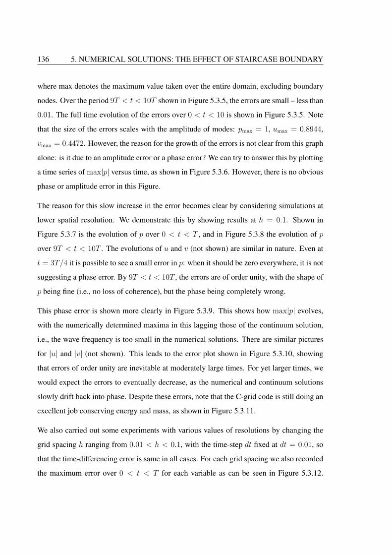
136 5. NUMERICAL SOLUTIONS: THE EFFECT OF STAIRCASE BOUNDARY
where max denotes the maximum value taken over the entire domain, excluding boundary
nodes. Over the period 9T < t < 10T shown in Figure 5.3.5, the errors are small – less than
0.01. The full time evolution of the errors over 0 < t < 10 is shown in Figure 5.3.5. Note
that the size of the errors scales with the amplitude of modes: pmax = 1, umax = 0.8944,
vmax = 0.4472. However, the reason for the growth of the errors is not clear from this graph
alone: is it due to an amplitude error or a phase error? We can try to answer this by plotting
a time series of max|p| versus time, as shown in Figure 5.3.6. However, there is no obvious
phase or amplitude error in this Figure.
The reason for this slow increase in the error becomes clear by considering simulations at
lower spatial resolution. We demonstrate this by showing results at h = 0.1. Shown in
Figure 5.3.7 is the evolution of p over 0 < t < T , and in Figure 5.3.8 the evolution of p
over 9T < t < 10T . The evolutions of u and v (not shown) are similar in nature. Even at
t = 3T/4 it is possible to see a small error in p: when it should be zero everywhere, it is not
suggesting a phase error. By 9T < t < 10T , the errors are of order unity, with the shape of
p being fine (i.e., no loss of coherence), but the phase being completely wrong.
This phase error is shown more clearly in Figure 5.3.9. This shows how max|p| evolves,
with the numerically determined maxima in this lagging those of the continuum solution,
i.e., the wave frequency is too small in the numerical solutions. There are similar pictures
for |u| and |v| (not shown). This leads to the error plot shown in Figure 5.3.10, showing
that errors of order unity are inevitable at moderately large times. For yet larger times, we
would expect the errors to eventually decrease, as the numerical and continuum solutions
slowly drift back into phase. Despite these errors, note that the C-grid code is still doing an
excellent job conserving energy and mass, as shown in Figure 5.3.11.
We also carried out some experiments with various values of resolutions by changing the
grid spacing h ranging from 0.01 < h < 0.1, with the time-step dt fixed at dt = 0.01, so
that the time-differencing error is same in all cases. For each grid spacing we also recorded
the maximum error over 0 < t < T for each variable as can be seen in Figure 5.3.12.
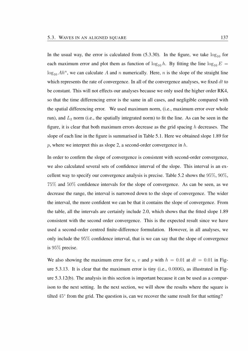
5.3. WAVES IN AN ALIGNED SQUARE 137
In the usual way, the error is calculated from (5.3.30). In the figure, we take log10 for
each maximum error and plot them as function of log10 h. By fitting the line log10E =
log10Ahn, we can calculate A and n numerically. Here, n is the slope of the straight line
which represents the rate of convergence. In all of the convergence analyses, we fixed dt to
be constant. This will not effects our analyses because we only used the higher order RK4,
so that the time differencing error is the same in all cases, and negligible compared with
the spatial differencing error. We used maximum norm, (i.e., maximum error over whole
run), and L2 norm (i.e., the spatially integrated norm) to fit the line. As can be seen in the
figure, it is clear that both maximum errors decrease as the grid spacing h decreases. The
slope of each line in the figure is summarised in Table 5.1. Here we obtained slope 1.89 for
p, where we interpret this as slope 2, a second-order convergence in h.
In order to confirm the slope of convergence is consistent with second-order convergence,
we also calculated several sets of confidence interval of the slope. This interval is an ex-
cellent way to specify our convergence analysis is precise. Table 5.2 shows the 95%, 90%,
75% and 50% confidence intervals for the slope of convergence. As can be seen, as we
decrease the range, the interval is narrowed down to the slope of convergence. The wider
the interval, the more confident we can be that it contains the slope of convergence. From
the table, all the intervals are certainly include 2.0, which shows that the fitted slope 1.89
consistent with the second order convergence. This is the expected result since we have
used a second-order centred finite-difference formulation. However, in all analyses, we
only include the 95% confidence interval, that is we can say that the slope of convergence
is 95% precise.
We also showing the maximum error for u, v and p with h = 0.01 at dt = 0.01 in Fig-
ure 5.3.13. It is clear that the maximum error is tiny (i.e., 0.0006), as illustrated in Fig-
ure 5.3.12(b). The analysis in this section is important because it can be used as a compar-
ison to the next setting. In the next section, we will show the results where the square is
tilted 45◦ from the grid. The question is, can we recover the same result for that setting?
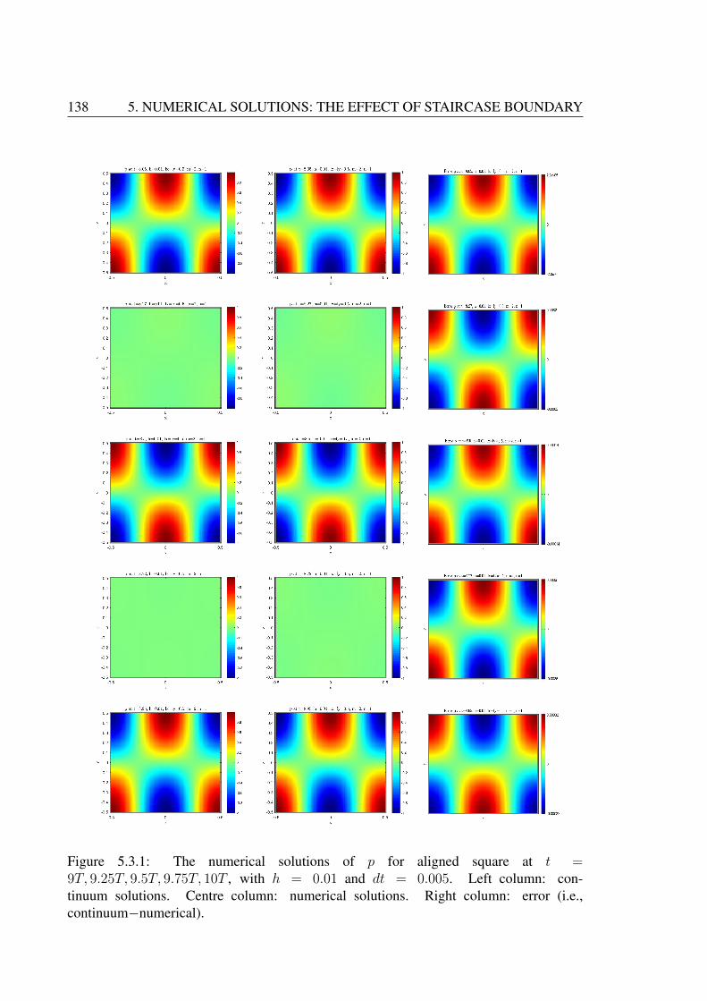
138 5. NUMERICAL SOLUTIONS: THE EFFECT OF STAIRCASE BOUNDARY
Figure 5.3.1: The numerical solutions of p for aligned square at t =9T, 9.25T, 9.5T, 9.75T, 10T , with h = 0.01 and dt = 0.005. Left column: con-tinuum solutions. Centre column: numerical solutions. Right column: error (i.e.,continuum−numerical).
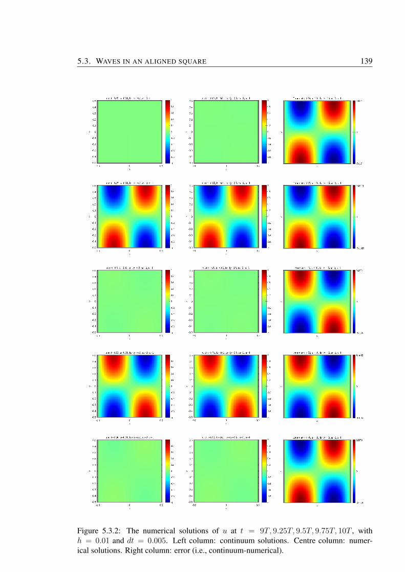
5.3. WAVES IN AN ALIGNED SQUARE 139
Figure 5.3.2: The numerical solutions of u at t = 9T, 9.25T, 9.5T, 9.75T, 10T , withh = 0.01 and dt = 0.005. Left column: continuum solutions. Centre column: numer-ical solutions. Right column: error (i.e., continuum-numerical).

140 5. NUMERICAL SOLUTIONS: THE EFFECT OF STAIRCASE BOUNDARY
Figure 5.3.3: The numerical solutions for v at t = 9T, 9.25T, 9.5T, 9.75T, 10T , withh = 0.01 and dt = 0.005. Left column: continuum solutions. Centre column: numer-ical solutions. Right column: error (i.e., continuum-numerical).

5.3. WAVES IN AN ALIGNED SQUARE 141
0 1 2 3 4 5 6 7 8 9-1
-0.5
0
0.5
1
1.5h=0.01
×10 -17 mass difference
0 1 2 3 4 5 6 7 8 9-6
-5
-4
-3
-2
-1
0
h=0.01
×10 -9 energy difference
Figure 5.3.4: Mass difference and energy difference for aligned square domain, with h =0.01 and dt = 0.005.
0 1 2 3 4 5 6 7 8 9time, t
0
1
2
3
4
5
6
7
8
9
max.error
×10 -3 maximum error plot with h=0.01, dt=0.005
uvp
Figure 5.3.5: Maximum error for aligned square domain over 0 < t < 10T , with h = 0.01and dt = 0.005.

142 5. NUMERICAL SOLUTIONS: THE EFFECT OF STAIRCASE BOUNDARY
0 1 2 3 4 5 6 7 8 9
time, t
0
0.2
0.4
0.6
0.8
1
1.2
max
abs
(p)
pc
pd
Figure 5.3.6: The maximum of |p| for aligned square domain over 0 < t < 10T for alignedsquare domain, with h = 0.01 and dt = 0.005.
Table 5.1: The convergence rate of u, v and p in max norm and L2 norm, for aligned squaredomain.
max norm L2 normslope scaling factor slope scaling factor
u 1.81706 18.7455 1.83682 9.87735v 1.88788 13.465 1.85756 5.39464p 1.88655 25.27 1.89323 11.2428
Table 5.2: The confidence interval of u, v and p in max norm for aligned square domain.
max norm confidence intervalslope 95% 90% 75% 50%
u 1.81706 (1.037, 2.597) (1.1720, 2.4621) (1.3736, 2.2605) (1.5598, 2.0743)v 1.88788 (1.073, 2.703) (1.2136, 2.5622) (1.4243, 2.3515) (1.6189, 2.1568)p 1.88655 (1.046, 2.727) (1.1913, 2.5818) (1.4085, 2.3646) (1.6092, 2.1639)
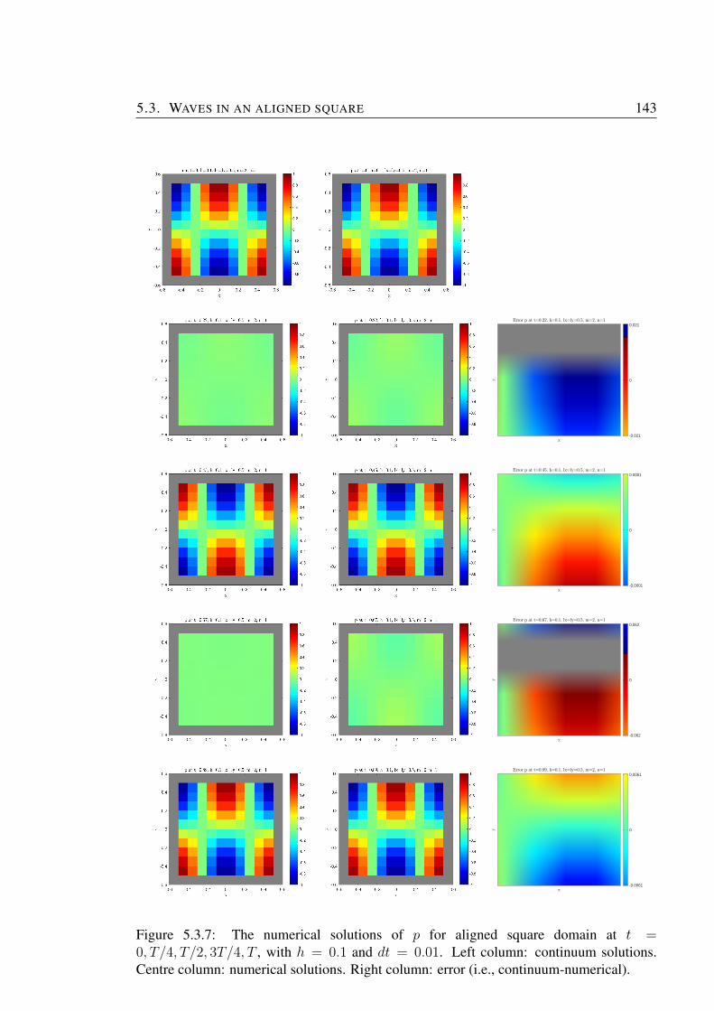
5.3. WAVES IN AN ALIGNED SQUARE 143
Error p at t=0.22, h=0.1, lx=ly=0.5, m=2, n=1
x
y
-0.021
0
0.021
Error p at t=0.45, h=0.1, lx=ly=0.5, m=2, n=1
x
y
-0.0001
0
0.0001
Error p at t=0.67, h=0.1, lx=ly=0.5, m=2, n=1
x
y
-0.062
0
0.062
Error p at t=0.89, h=0.1, lx=ly=0.5, m=2, n=1
x
y
-0.0061
0
0.0061
Figure 5.3.7: The numerical solutions of p for aligned square domain at t =0, T/4, T/2, 3T/4, T , with h = 0.1 and dt = 0.01. Left column: continuum solutions.Centre column: numerical solutions. Right column: error (i.e., continuum-numerical).
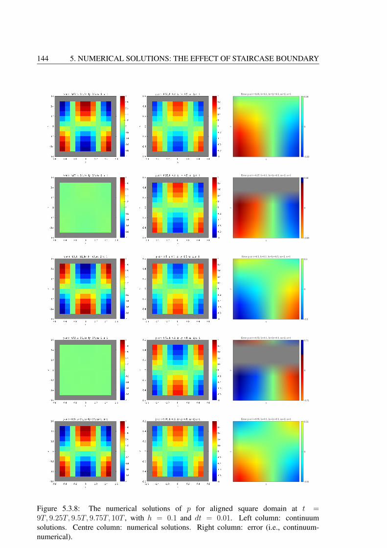
144 5. NUMERICAL SOLUTIONS: THE EFFECT OF STAIRCASE BOUNDARY
Error p at t=8.05, h=0.1, lx=ly=0.5, m=2, n=1
x
y
-0.28
0
0.28
Error p at t=8.27, h=0.1, lx=ly=0.5, m=2, n=1
x
y
-0.68
0
0.68
Error p at t=8.5, h=0.1, lx=ly=0.5, m=2, n=1
x
y
-0.3
0
0.3
Error p at t=8.72, h=0.1, lx=ly=0.5, m=2, n=1
x
y
-0.71
0
0.71
Error p at t=8.95, h=0.1, lx=ly=0.5, m=2, n=1
x
y
-0.31
0
0.31
Figure 5.3.8: The numerical solutions of p for aligned square domain at t =9T, 9.25T, 9.5T, 9.75T, 10T , with h = 0.1 and dt = 0.01. Left column: continuumsolutions. Centre column: numerical solutions. Right column: error (i.e., continuum-numerical).

5.3. WAVES IN AN ALIGNED SQUARE 145
0 1 2 3 4 5 6 7 8 9time, t
0
0.2
0.4
0.6
0.8
1
1.2
max.|p|
pc
pd
Figure 5.3.9: The maximum of |p| for aligned square domain over 0 < t < 10T for alignedsquare domain, with h = 0.1 and dt = 0.01.
0 1 2 3 4 5 6 7 8 9time, t
0
0.1
0.2
0.3
0.4
0.5
0.6
0.7
0.8
max.error
maximum error plot with h=0.1, dt=0.01
uvp
Figure 5.3.10: Maximum error for aligned square domain over 0 < t < 10T , with h = 0.1and dt = 0.01.
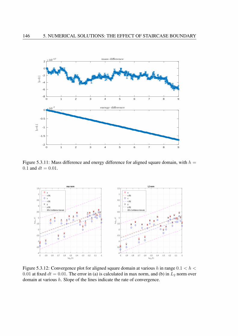
146 5. NUMERICAL SOLUTIONS: THE EFFECT OF STAIRCASE BOUNDARY
0 1 2 3 4 5 6 7 8 9-8
-6
-4
-2
0
2
h=0.1
×10 -17 mass difference
0 1 2 3 4 5 6 7 8 9-2
-1.5
-1
-0.5
0
h=0.1
×10 -7 energy difference
Figure 5.3.11: Mass difference and energy difference for aligned square domain, with h =0.1 and dt = 0.01.
-2 -1.9 -1.8 -1.7 -1.6 -1.5 -1.4 -1.3 -1.2 -1.1 -1log10(h)
-4
-3.5
-3
-2.5
-2
-1.5
-1
-0.5
0
0.5
1
1.5
log10E
max norm
u
u (fit)
v
v (fit)
p
p (fit)
95% Confidence Intervals
-2 -1.9 -1.8 -1.7 -1.6 -1.5 -1.4 -1.3 -1.2 -1.1 -1log10(h)
-4
-3.5
-3
-2.5
-2
-1.5
-1
-0.5
0
0.5
1
1.5
log10E
L2 norm
u
u (fit)
v
v (fit)
p
p (fit)
95% Confidence Intervals
Figure 5.3.12: Convergence plot for aligned square domain at various h in range 0.1 < h <0.01 at fixed dt = 0.01. The error in (a) is calculated in max norm, and (b) in L2 norm overdomain at various h. Slope of the lines indicate the rate of convergence.
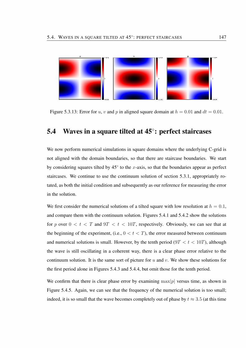
5.4. WAVES IN A SQUARE TILTED AT 45◦: PERFECT STAIRCASES 147
Figure 5.3.13: Error for u, v and p in aligned square domain at h = 0.01 and dt = 0.01.
5.4 Waves in a square tilted at 45◦: perfect staircases
We now perform numerical simulations in square domains where the underlying C-grid is
not aligned with the domain boundaries, so that there are staircase boundaries. We start
by considering squares tilted by 45◦ to the x-axis, so that the boundaries appear as perfect
staircases. We continue to use the continuum solution of section 5.3.1, appropriately ro-
tated, as both the initial condition and subsequently as our reference for measuring the error
in the solution.
We first consider the numerical solutions of a tilted square with low resolution at h = 0.1,
and compare them with the continuum solution. Figures 5.4.1 and 5.4.2 show the solutions
for p over 0 < t < T and 9T < t < 10T , respectively. Obviously, we can see that at
the beginning of the experiment, (i.e., 0 < t < T ), the error measured between continuum
and numerical solutions is small. However, by the tenth period (9T < t < 10T ), although
the wave is still oscillating in a coherent way, there is a clear phase error relative to the
continuum solution. It is the same sort of picture for u and v. We show these solutions for
the first period alone in Figures 5.4.3 and 5.4.4, but omit those for the tenth period.
We confirm that there is clear phase error by examining max|p| versus time, as shown in
Figure 5.4.5. Again, we can see that the frequency of the numerical solution is too small;
indeed, it is so small that the wave becomes completely out of phase by t ≈ 3.5 (at this time
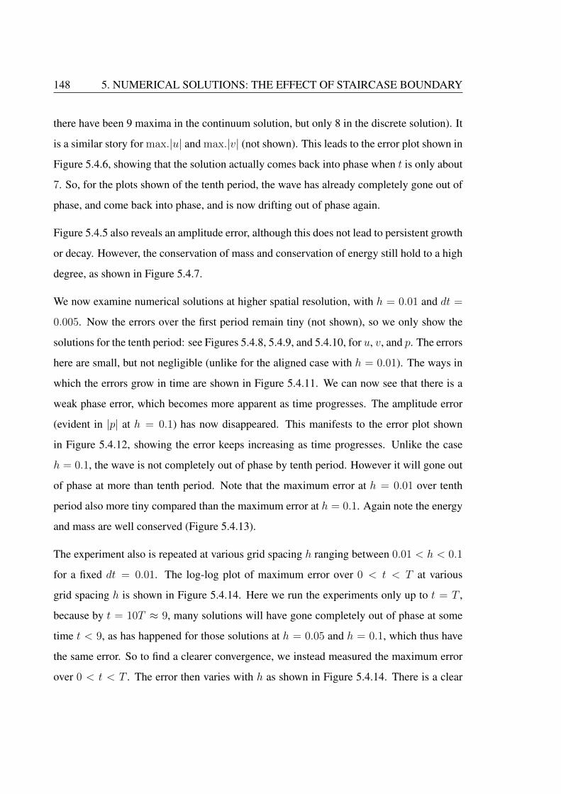
148 5. NUMERICAL SOLUTIONS: THE EFFECT OF STAIRCASE BOUNDARY
there have been 9 maxima in the continuum solution, but only 8 in the discrete solution). It
is a similar story for max.|u| and max.|v| (not shown). This leads to the error plot shown in
Figure 5.4.6, showing that the solution actually comes back into phase when t is only about
7. So, for the plots shown of the tenth period, the wave has already completely gone out of
phase, and come back into phase, and is now drifting out of phase again.
Figure 5.4.5 also reveals an amplitude error, although this does not lead to persistent growth
or decay. However, the conservation of mass and conservation of energy still hold to a high
degree, as shown in Figure 5.4.7.
We now examine numerical solutions at higher spatial resolution, with h = 0.01 and dt =
0.005. Now the errors over the first period remain tiny (not shown), so we only show the
solutions for the tenth period: see Figures 5.4.8, 5.4.9, and 5.4.10, for u, v, and p. The errors
here are small, but not negligible (unlike for the aligned case with h = 0.01). The ways in
which the errors grow in time are shown in Figure 5.4.11. We can now see that there is a
weak phase error, which becomes more apparent as time progresses. The amplitude error
(evident in |p| at h = 0.1) has now disappeared. This manifests to the error plot shown
in Figure 5.4.12, showing the error keeps increasing as time progresses. Unlike the case
h = 0.1, the wave is not completely out of phase by tenth period. However it will gone out
of phase at more than tenth period. Note that the maximum error at h = 0.01 over tenth
period also more tiny compared than the maximum error at h = 0.1. Again note the energy
and mass are well conserved (Figure 5.4.13).
The experiment also is repeated at various grid spacing h ranging between 0.01 < h < 0.1
for a fixed dt = 0.01. The log-log plot of maximum error over 0 < t < T at various
grid spacing h is shown in Figure 5.4.14. Here we run the experiments only up to t = T ,
because by t = 10T ≈ 9, many solutions will have gone completely out of phase at some
time t < 9, as has happened for those solutions at h = 0.05 and h = 0.1, which thus have
the same error. So to find a clearer convergence, we instead measured the maximum error
over 0 < t < T . The error then varies with h as shown in Figure 5.4.14. There is a clear
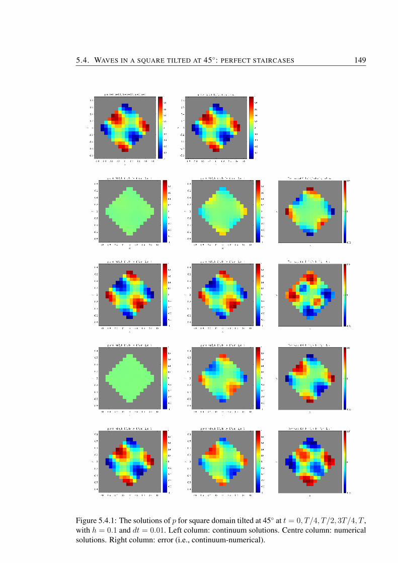
5.4. WAVES IN A SQUARE TILTED AT 45◦: PERFECT STAIRCASES 149
Figure 5.4.1: The solutions of p for square domain tilted at 45◦ at t = 0, T/4, T/2, 3T/4, T ,with h = 0.1 and dt = 0.01. Left column: continuum solutions. Centre column: numericalsolutions. Right column: error (i.e., continuum-numerical).
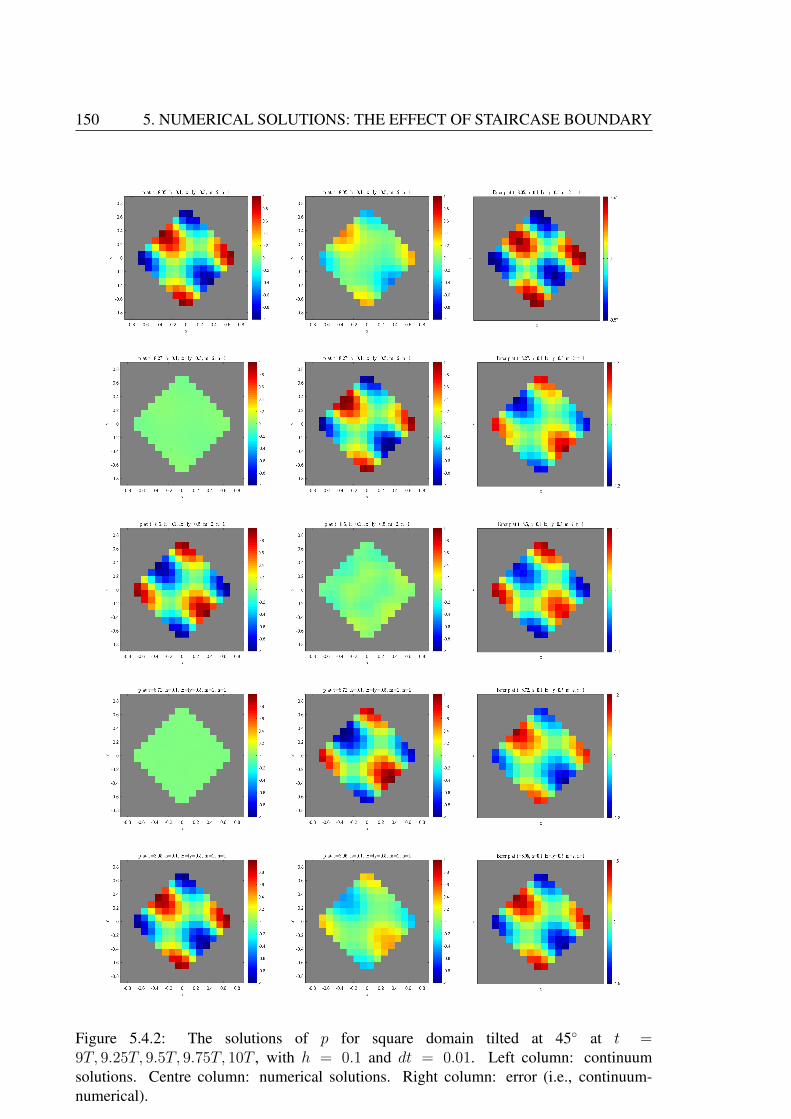
150 5. NUMERICAL SOLUTIONS: THE EFFECT OF STAIRCASE BOUNDARY
Figure 5.4.2: The solutions of p for square domain tilted at 45◦ at t =9T, 9.25T, 9.5T, 9.75T, 10T , with h = 0.1 and dt = 0.01. Left column: continuumsolutions. Centre column: numerical solutions. Right column: error (i.e., continuum-numerical).
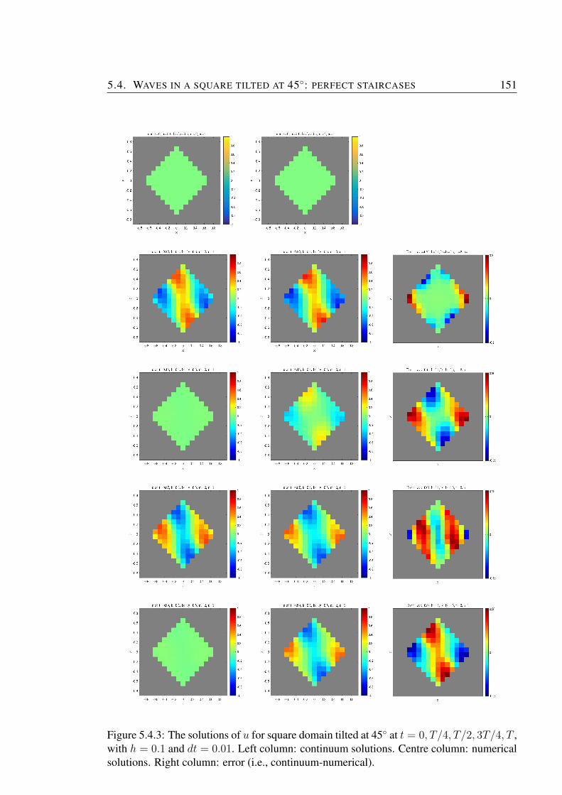
5.4. WAVES IN A SQUARE TILTED AT 45◦: PERFECT STAIRCASES 151
Figure 5.4.3: The solutions of u for square domain tilted at 45◦ at t = 0, T/4, T/2, 3T/4, T ,with h = 0.1 and dt = 0.01. Left column: continuum solutions. Centre column: numericalsolutions. Right column: error (i.e., continuum-numerical).

152 5. NUMERICAL SOLUTIONS: THE EFFECT OF STAIRCASE BOUNDARY
Figure 5.4.4: The solutions of v for square domain tilted at 45◦ at t = 0, T/4, T/2, 3T/4, T ,with h = 0.1 and dt = 0.01. Left column: continuum solutions. Centre column: numericalsolutions. Right column: error (i.e., continuum-numerical).
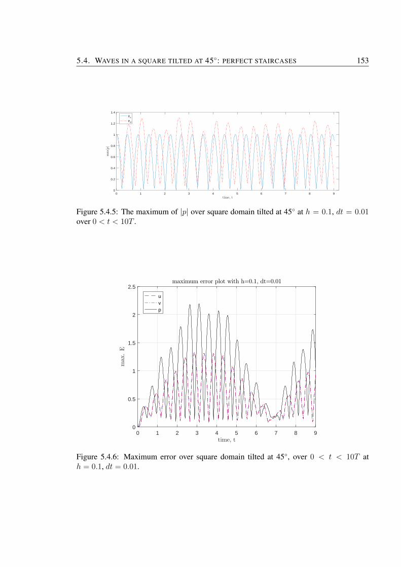
5.4. WAVES IN A SQUARE TILTED AT 45◦: PERFECT STAIRCASES 153
0 1 2 3 4 5 6 7 8 9time, t
0
0.2
0.4
0.6
0.8
1
1.2
1.4
max|p|
pc
pd
Figure 5.4.5: The maximum of |p| over square domain tilted at 45◦ at h = 0.1, dt = 0.01over 0 < t < 10T .
0 1 2 3 4 5 6 7 8 9time, t
0
0.5
1
1.5
2
2.5
max.E
maximum error plot with h=0.1, dt=0.01
uvp
Figure 5.4.6: Maximum error over square domain tilted at 45◦, over 0 < t < 10T ath = 0.1, dt = 0.01.
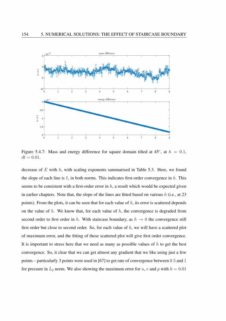
154 5. NUMERICAL SOLUTIONS: THE EFFECT OF STAIRCASE BOUNDARY
0 1 2 3 4 5 6 7 8 9-10
-5
0
5
h=0.1
×10-17 mass difference
0 1 2 3 4 5 6 7 8 9-2
-1.5
-1
-0.5
0
h=0.1
×10-7 energy difference
Figure 5.4.7: Mass and energy difference for square domain tilted at 45◦, at h = 0.1,dt = 0.01.
decrease of E with h, with scaling exponents summarised in Table 5.3. Here, we found
the slope of each line is 1, in both norms. This indicates first-order convergence in h. This
seems to be consistent with a first-order error in h, a result which would be expected given
in earlier chapters. Note that, the slope of the lines are fitted based on various h (i.e., at 23
points). From the plots, it can be seen that for each value of h, its error is scattered depends
on the value of h. We know that, for each value of h, the convergence is degraded from
second order to first order in h. With staircase boundary, as h → 0 the convergence still
first order but close to second order. So, for each value of h, we will have a scattered plot
of maximum error, and the fitting of these scattered plot will give first order convergence.
It is important to stress here that we need as many as possible values of h to get the best
convergence. So, it clear that we can get almost any gradient that we like using just a few
points – particularly 3 points were used in [67] to get rate of convergence between 0.5 and 1
for pressure in L2 norm. We also showing the maximum error for u, v and p with h = 0.01
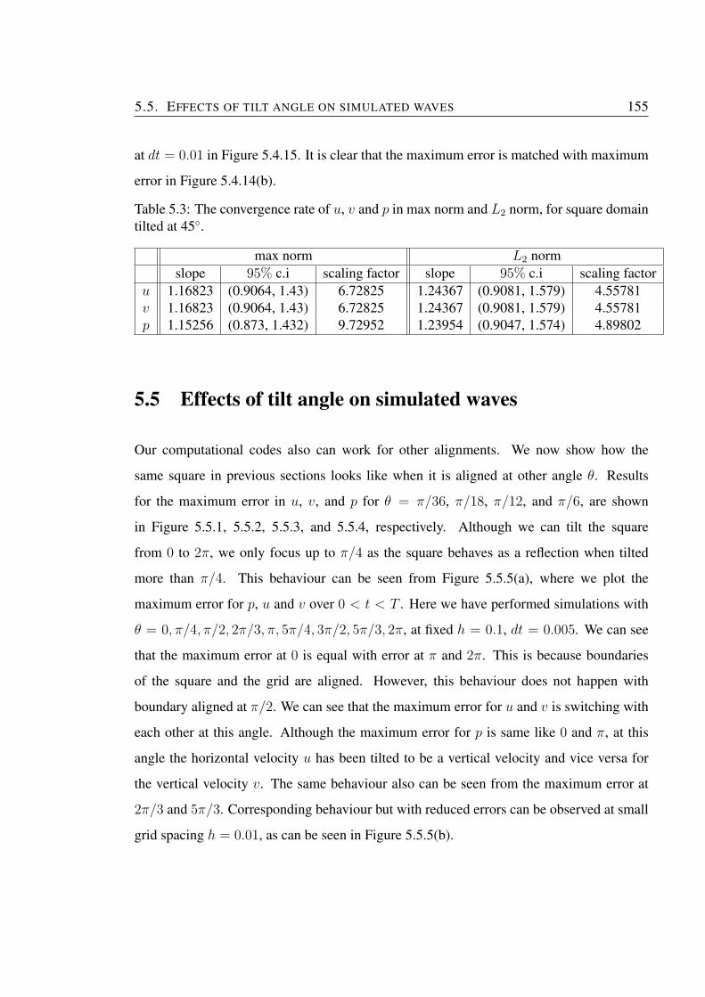
5.5. EFFECTS OF TILT ANGLE ON SIMULATED WAVES 155
at dt = 0.01 in Figure 5.4.15. It is clear that the maximum error is matched with maximum
error in Figure 5.4.14(b).
Table 5.3: The convergence rate of u, v and p in max norm and L2 norm, for square domaintilted at 45◦.
max norm L2 normslope 95% c.i scaling factor slope 95% c.i scaling factor
u 1.16823 (0.9064, 1.43) 6.72825 1.24367 (0.9081, 1.579) 4.55781v 1.16823 (0.9064, 1.43) 6.72825 1.24367 (0.9081, 1.579) 4.55781p 1.15256 (0.873, 1.432) 9.72952 1.23954 (0.9047, 1.574) 4.89802
5.5 Effects of tilt angle on simulated waves
Our computational codes also can work for other alignments. We now show how the
same square in previous sections looks like when it is aligned at other angle θ. Results
for the maximum error in u, v, and p for θ = π/36, π/18, π/12, and π/6, are shown
in Figure 5.5.1, 5.5.2, 5.5.3, and 5.5.4, respectively. Although we can tilt the square
from 0 to 2π, we only focus up to π/4 as the square behaves as a reflection when tilted
more than π/4. This behaviour can be seen from Figure 5.5.5(a), where we plot the
maximum error for p, u and v over 0 < t < T . Here we have performed simulations with
θ = 0, π/4, π/2, 2π/3, π, 5π/4, 3π/2, 5π/3, 2π, at fixed h = 0.1, dt = 0.005. We can see
that the maximum error at 0 is equal with error at π and 2π. This is because boundaries
of the square and the grid are aligned. However, this behaviour does not happen with
boundary aligned at π/2. We can see that the maximum error for u and v is switching with
each other at this angle. Although the maximum error for p is same like 0 and π, at this
angle the horizontal velocity u has been tilted to be a vertical velocity and vice versa for
the vertical velocity v. The same behaviour also can be seen from the maximum error at
2π/3 and 5π/3. Corresponding behaviour but with reduced errors can be observed at small
grid spacing h = 0.01, as can be seen in Figure 5.5.5(b).
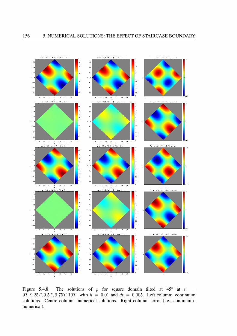
156 5. NUMERICAL SOLUTIONS: THE EFFECT OF STAIRCASE BOUNDARY
Figure 5.4.8: The solutions of p for square domain tilted at 45◦ at t =9T, 9.25T, 9.5T, 9.75T, 10T , with h = 0.01 and dt = 0.005. Left column: continuumsolutions. Centre column: numerical solutions. Right column: error (i.e., continuum-numerical).
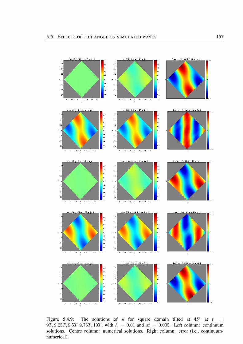
5.5. EFFECTS OF TILT ANGLE ON SIMULATED WAVES 157
Figure 5.4.9: The solutions of u for square domain tilted at 45◦ at t =9T, 9.25T, 9.5T, 9.75T, 10T , with h = 0.01 and dt = 0.005. Left column: continuumsolutions. Centre column: numerical solutions. Right column: error (i.e., continuum-numerical).
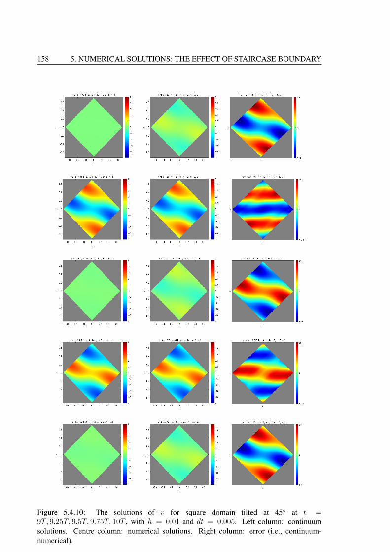
158 5. NUMERICAL SOLUTIONS: THE EFFECT OF STAIRCASE BOUNDARY
Figure 5.4.10: The solutions of v for square domain tilted at 45◦ at t =9T, 9.25T, 9.5T, 9.75T, 10T , with h = 0.01 and dt = 0.005. Left column: continuumsolutions. Centre column: numerical solutions. Right column: error (i.e., continuum-numerical).
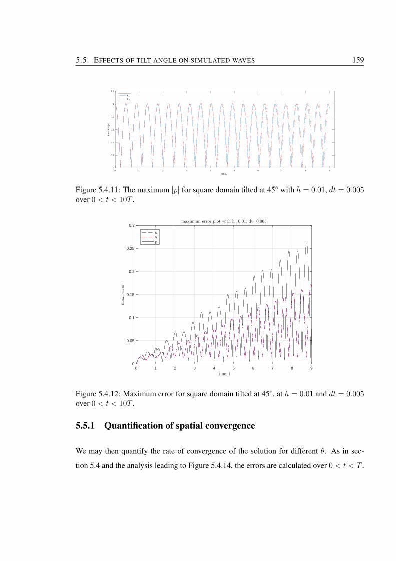
5.5. EFFECTS OF TILT ANGLE ON SIMULATED WAVES 159
0 1 2 3 4 5 6 7 8 9
time, t
0
0.2
0.4
0.6
0.8
1
1.2
max
abs
(p)
pc
pd
Figure 5.4.11: The maximum |p| for square domain tilted at 45◦ with h = 0.01, dt = 0.005over 0 < t < 10T .
0 1 2 3 4 5 6 7 8 9time, t
0
0.05
0.1
0.15
0.2
0.25
0.3
max.error
maximum error plot with h=0.01, dt=0.005
uvp
Figure 5.4.12: Maximum error for square domain tilted at 45◦, at h = 0.01 and dt = 0.005over 0 < t < 10T .
5.5.1 Quantification of spatial convergence
We may then quantify the rate of convergence of the solution for different θ. As in sec-
tion 5.4 and the analysis leading to Figure 5.4.14, the errors are calculated over 0 < t < T .
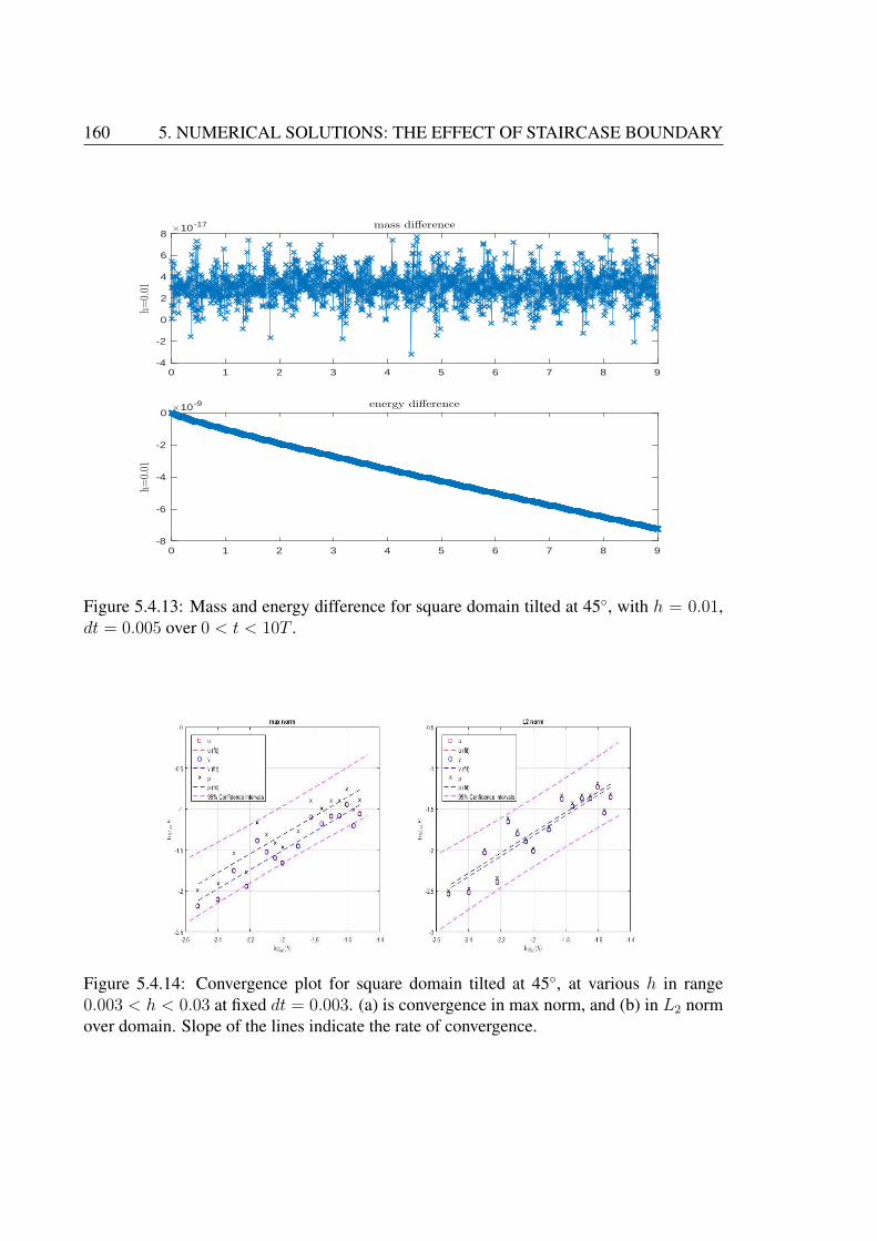
160 5. NUMERICAL SOLUTIONS: THE EFFECT OF STAIRCASE BOUNDARY
0 1 2 3 4 5 6 7 8 9-4
-2
0
2
4
6
8
h=0.01
×10 -17 mass difference
0 1 2 3 4 5 6 7 8 9-8
-6
-4
-2
0
h=0.01
×10 -9 energy difference
Figure 5.4.13: Mass and energy difference for square domain tilted at 45◦, with h = 0.01,dt = 0.005 over 0 < t < 10T .
Figure 5.4.14: Convergence plot for square domain tilted at 45◦, at various h in range0.003 < h < 0.03 at fixed dt = 0.003. (a) is convergence in max norm, and (b) in L2 normover domain. Slope of the lines indicate the rate of convergence.

5.5. EFFECTS OF TILT ANGLE ON SIMULATED WAVES 161
Figure 5.4.15: Maximum error for u, v and p in square domain tilted at 45◦, at h = 0.003and dt = 0.003.
We know that, the error can be expressed as
E = Bhn ⇒ log10E = log10B + n log10 h, (5.5.1)
where E = |pc − pd| and n represents the order of convergence with scaling factor B. The
order of convergence is quantified by fitting (5.5.1), in each case θ, as in Figures 5.5.6,
5.5.7, 5.5.8, and 5.5.9. The results are shown in Table 5.4, 5.5, 5.6, and 5.7. We found that
for each θ, first-order convergence is attained according to the scaling factor n. We also
examined the scaling factor B, for each θ. We can see that B increases with θ, as expected.
As we increase the θ the number of steps also increase, so thatB increase with θ. This result
agree with a channel flow with rotation effects in [32], where it was found that B increased
with θ, see Table 1 in [32]. However, it is important to mention here that the results that
we presented in this thesis are about wave sloshing in a closed domain, different from the
experiments in [32], i.e., waves in a semi-infinite channel.
5.5.2 Frequency reduction
In the past two sections, we have seen that the frequency of the sloshing mode is reduced
from the continuum value in our numerical experiments, that is ωd < ωc. Although we have
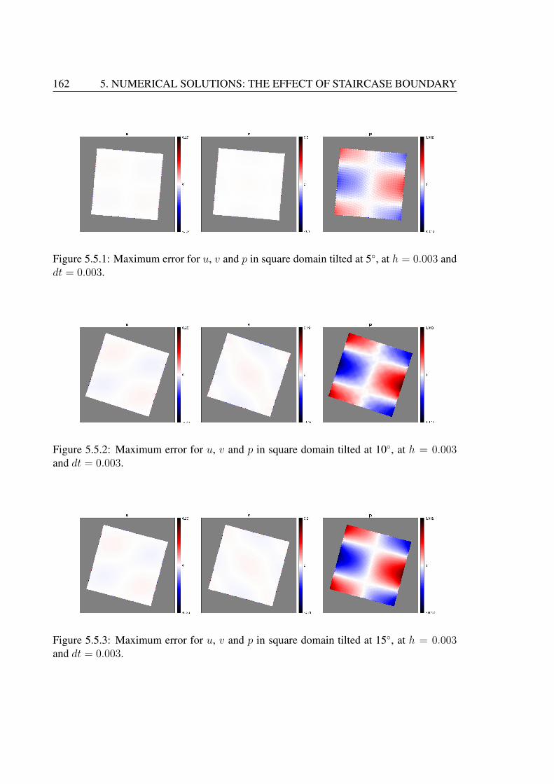
162 5. NUMERICAL SOLUTIONS: THE EFFECT OF STAIRCASE BOUNDARY
Figure 5.5.1: Maximum error for u, v and p in square domain tilted at 5◦, at h = 0.003 anddt = 0.003.
Figure 5.5.2: Maximum error for u, v and p in square domain tilted at 10◦, at h = 0.003and dt = 0.003.
Figure 5.5.3: Maximum error for u, v and p in square domain tilted at 15◦, at h = 0.003and dt = 0.003.

5.5. EFFECTS OF TILT ANGLE ON SIMULATED WAVES 163
Figure 5.5.4: Maximum error for u, v and p in square domain tilted at 30◦, at h = 0.003and dt = 0.003.
0 0.2 0.4 0.6 0.8 1 1.2 1.4 1.6 1.8 2θ/π
-1.6
-1.4
-1.2
-1
-0.8
-0.6
-0.4
-0.2
0
0.2
log10|m
ax.E
|
dt = 0.005, h =0.1
(a)
0 0.2 0.4 0.6 0.8 1 1.2 1.4 1.6 1.8 2θ/π
-3.5
-3
-2.5
-2
-1.5
-1
-0.5
log10|m
ax.E
|
dt = 0.005, h =0.01
(b)
Figure 5.5.5: Maximum error of u, v and p for square domain tilted at various angle ofrotation with grid spacing (a) h = 0.1, (b) h = 0.01. The maximum error is calculated over0 < t < 10T ≈ t = 9.
Table 5.4: The convergence rate of u, v and p in max norm and L2 norm, for square domaintilted at 5◦.
max norm L2 normslope 95% c.i scaling factor slope 95% c.i scaling factor
u -0.0403 (-0.0757, -0.0048) 0.3147 0.6337 (0.5735, 0.6939) 0.3725v -0.0069 (-0.0473, 0.0335) 0.4094 0.6441 (0.5851, 0.703) 0.3683p 0.9477 (0.9025, 0.9929) 5.1315 1.3523 (1.187, 1.517) 3.8090
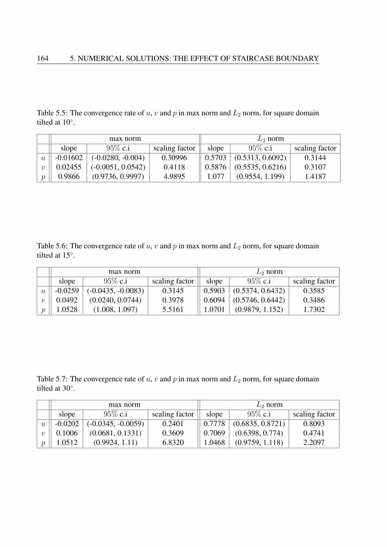
164 5. NUMERICAL SOLUTIONS: THE EFFECT OF STAIRCASE BOUNDARY
Table 5.5: The convergence rate of u, v and p in max norm and L2 norm, for square domaintilted at 10◦.
max norm L2 normslope 95% c.i scaling factor slope 95% c.i scaling factor
u -0.01602 (-0.0280, -0.004) 0.30996 0.5703 (0.5313, 0.6092) 0.3144v 0.02455 (-0.0051, 0.0542) 0.4118 0.5876 (0.5535, 0.6216) 0.3107p 0.9866 (0.9736, 0.9997) 4.9895 1.077 (0.9554, 1.199) 1.4187
Table 5.6: The convergence rate of u, v and p in max norm and L2 norm, for square domaintilted at 15◦.
max norm L2 normslope 95% c.i scaling factor slope 95% c.i scaling factor
u -0.0259 (-0.0435, -0.0083) 0.3145 0.5903 (0.5374, 0.6432) 0.3585v 0.0492 (0.0240, 0.0744) 0.3978 0.6094 (0.5746, 0.6442) 0.3486p 1.0528 (1.008, 1.097) 5.5161 1.0701 (0.9879, 1.152) 1.7302
Table 5.7: The convergence rate of u, v and p in max norm and L2 norm, for square domaintilted at 30◦.
max norm L2 normslope 95% c.i scaling factor slope 95% c.i scaling factor
u -0.0202 (-0.0345, -0.0059) 0.2401 0.7778 (0.6835, 0.8721) 0.8093v 0.1006 (0.0681, 0.1331) 0.3609 0.7069 (0.6398, 0.774) 0.4741p 1.0512 (0.9924, 1.11) 6.8320 1.0468 (0.9759, 1.118) 2.2097
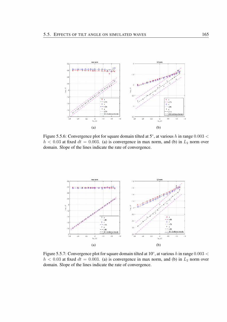
5.5. EFFECTS OF TILT ANGLE ON SIMULATED WAVES 165
(a) (b)
Figure 5.5.6: Convergence plot for square domain tilted at 5◦, at various h in range 0.003 <h < 0.03 at fixed dt = 0.003. (a) is convergence in max norm, and (b) in L2 norm overdomain. Slope of the lines indicate the rate of convergence.
(a) (b)
Figure 5.5.7: Convergence plot for square domain tilted at 10◦, at various h in range 0.003 <h < 0.03 at fixed dt = 0.003. (a) is convergence in max norm, and (b) in L2 norm overdomain. Slope of the lines indicate the rate of convergence.
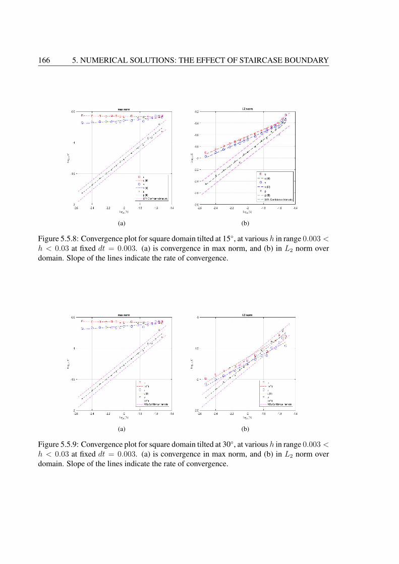
166 5. NUMERICAL SOLUTIONS: THE EFFECT OF STAIRCASE BOUNDARY
(a) (b)
Figure 5.5.8: Convergence plot for square domain tilted at 15◦, at various h in range 0.003 <h < 0.03 at fixed dt = 0.003. (a) is convergence in max norm, and (b) in L2 norm overdomain. Slope of the lines indicate the rate of convergence.
(a) (b)
Figure 5.5.9: Convergence plot for square domain tilted at 30◦, at various h in range 0.003 <h < 0.03 at fixed dt = 0.003. (a) is convergence in max norm, and (b) in L2 norm overdomain. Slope of the lines indicate the rate of convergence.
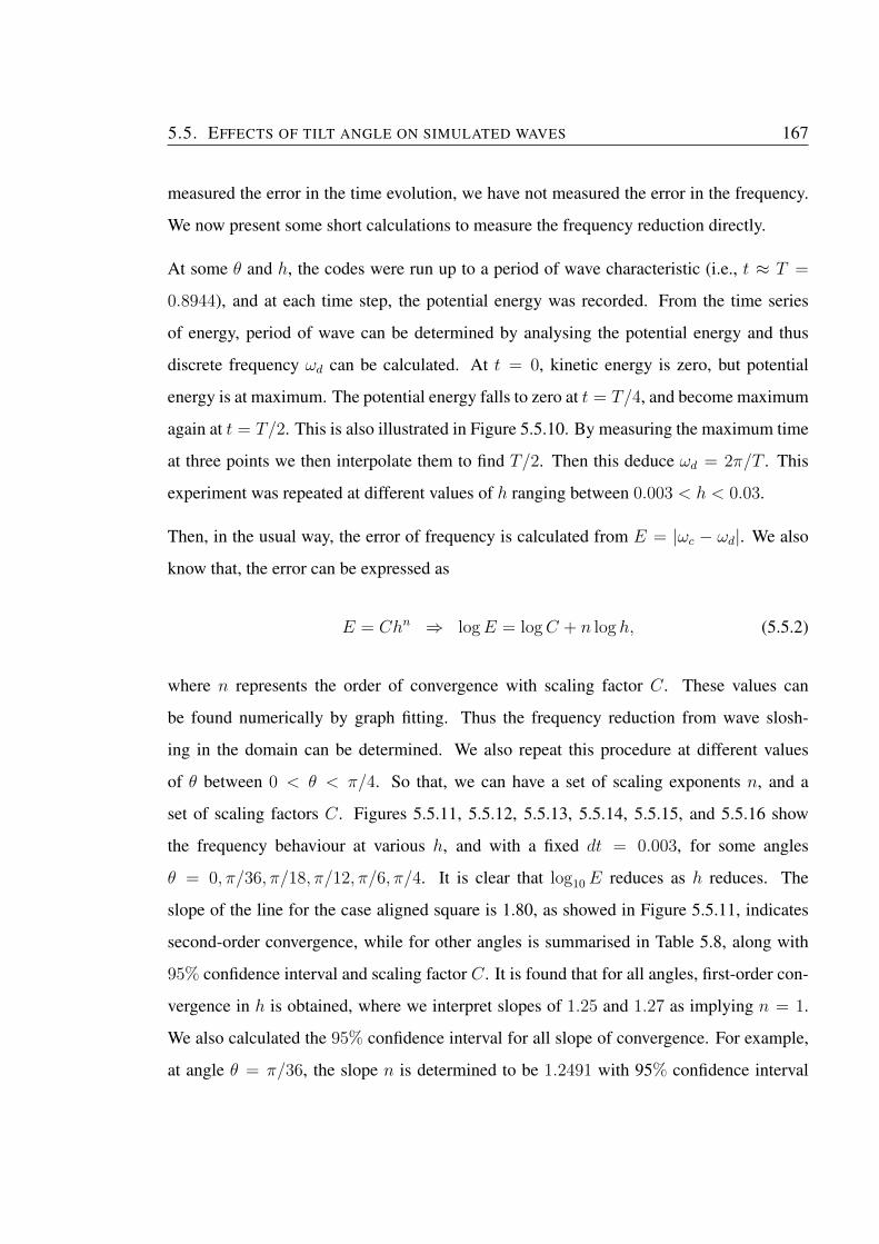
5.5. EFFECTS OF TILT ANGLE ON SIMULATED WAVES 167
measured the error in the time evolution, we have not measured the error in the frequency.
We now present some short calculations to measure the frequency reduction directly.
At some θ and h, the codes were run up to a period of wave characteristic (i.e., t ≈ T =
0.8944), and at each time step, the potential energy was recorded. From the time series
of energy, period of wave can be determined by analysing the potential energy and thus
discrete frequency ωd can be calculated. At t = 0, kinetic energy is zero, but potential
energy is at maximum. The potential energy falls to zero at t = T/4, and become maximum
again at t = T/2. This is also illustrated in Figure 5.5.10. By measuring the maximum time
at three points we then interpolate them to find T/2. Then this deduce ωd = 2π/T . This
experiment was repeated at different values of h ranging between 0.003 < h < 0.03.
Then, in the usual way, the error of frequency is calculated from E = |ωc − ωd|. We also
know that, the error can be expressed as
E = Chn ⇒ logE = logC + n log h, (5.5.2)
where n represents the order of convergence with scaling factor C. These values can
be found numerically by graph fitting. Thus the frequency reduction from wave slosh-
ing in the domain can be determined. We also repeat this procedure at different values
of θ between 0 < θ < π/4. So that, we can have a set of scaling exponents n, and a
set of scaling factors C. Figures 5.5.11, 5.5.12, 5.5.13, 5.5.14, 5.5.15, and 5.5.16 show
the frequency behaviour at various h, and with a fixed dt = 0.003, for some angles
θ = 0, π/36, π/18, π/12, π/6, π/4. It is clear that log10E reduces as h reduces. The
slope of the line for the case aligned square is 1.80, as showed in Figure 5.5.11, indicates
second-order convergence, while for other angles is summarised in Table 5.8, along with
95% confidence interval and scaling factor C. It is found that for all angles, first-order con-
vergence in h is obtained, where we interpret slopes of 1.25 and 1.27 as implying n = 1.
We also calculated the 95% confidence interval for all slope of convergence. For example,
at angle θ = π/36, the slope n is determined to be 1.2491 with 95% confidence interval

168 5. NUMERICAL SOLUTIONS: THE EFFECT OF STAIRCASE BOUNDARY
(1.058, 1.44). This means that, slope n = 1 lies within the interval that is consistent with
the analysis. Again, scaling factor C increase with θ. This is as expected, as increases in
θ lead to larger number of steps, thus C increases. This also based on theoretical approach
that we have discussed previously in Chapter 3, i.e., C ∼ h/√
2 as h→ 0. So, when θ � 1,
our domain may have just a single step, the convergence in the frequency is still reduced to
first order in h. This is a pretty robust upwards trend as θ gets larger. But of course that π/6
is not so much different from π/4 in terms of how the staircases operate, so it is fine that the
numbers are similar. For π/36, π/18, and π/12, all are pretty small angles, and indeed we
do see the scaling factor increase. So the staircases are less disruptive as θ becomes small,
as anticipated.
0 0.5 1 1.5t
0
0.02
0.04
0.06
0.08
0.1
0.12
0.14
0.16
KE
0 0.5 1 1.5t
0
0.02
0.04
0.06
0.08
0.1
0.12
0.14
0.16
PE
Figure 5.5.10: Time series of kinetic and potential energy for waves in a square domainover 0 < t < 1.
Table 5.8: The scaling factors C and scaling exponents n, along with 95% confidenceinterval for error in frequency, at various θ. The values are numerically determined at fixeddt = 0.003 and grid spacing 0.003 < h < 0.03.
θ n 95% c.i Cπ/36 1.2491 (1.058,1.44) 1.4128π/18 1.0505 (0.9128,1.188) 2.59302π/12 1.064 (0.9815,1.147) 3.29813π/6 1.0417 (0.972,1.111) 4.92095π/4 1.27522 (0.9113,1.639) 4.45275
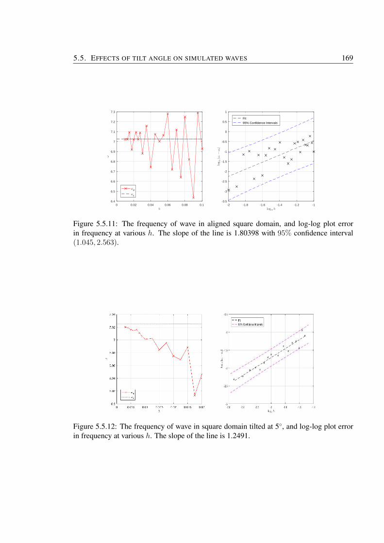
5.5. EFFECTS OF TILT ANGLE ON SIMULATED WAVES 169
0 0.02 0.04 0.06 0.08 0.1h
6.4
6.5
6.6
6.7
6.8
6.9
7
7.1
7.2
7.3
ω
ωd
ωc
-2 -1.8 -1.6 -1.4 -1.2 -1log10 h
-3.5
-3
-2.5
-2
-1.5
-1
-0.5
0
0.5
1
log10|ω
c−ωd|
Fit
95% Confidence Intervals
Figure 5.5.11: The frequency of wave in aligned square domain, and log-log plot errorin frequency at various h. The slope of the line is 1.80398 with 95% confidence interval(1.045, 2.563).
Figure 5.5.12: The frequency of wave in square domain tilted at 5◦, and log-log plot errorin frequency at various h. The slope of the line is 1.2491.
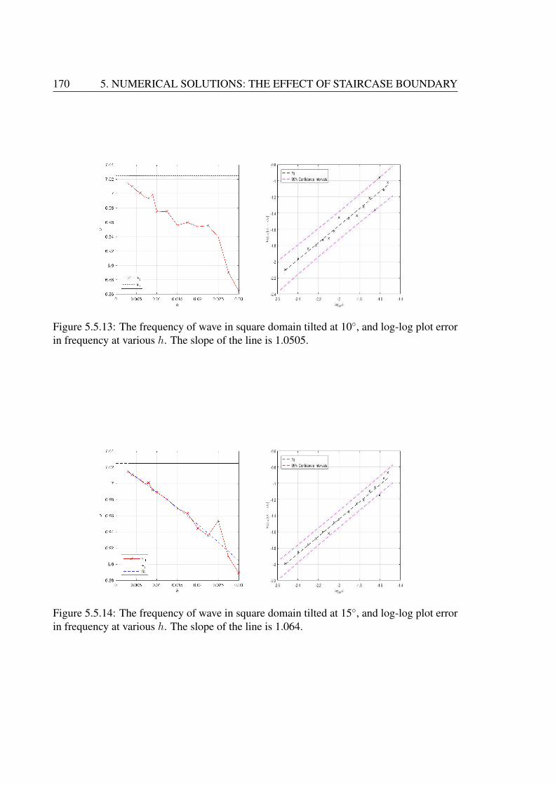
170 5. NUMERICAL SOLUTIONS: THE EFFECT OF STAIRCASE BOUNDARY
Figure 5.5.13: The frequency of wave in square domain tilted at 10◦, and log-log plot errorin frequency at various h. The slope of the line is 1.0505.
Figure 5.5.14: The frequency of wave in square domain tilted at 15◦, and log-log plot errorin frequency at various h. The slope of the line is 1.064.
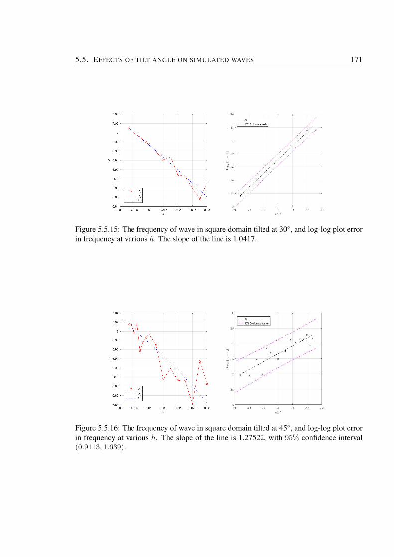
5.5. EFFECTS OF TILT ANGLE ON SIMULATED WAVES 171
Figure 5.5.15: The frequency of wave in square domain tilted at 30◦, and log-log plot errorin frequency at various h. The slope of the line is 1.0417.
Figure 5.5.16: The frequency of wave in square domain tilted at 45◦, and log-log plot errorin frequency at various h. The slope of the line is 1.27522, with 95% confidence interval(0.9113, 1.639).

172 5. NUMERICAL SOLUTIONS: THE EFFECT OF STAIRCASE BOUNDARY
5.6 Waves in a circular domain
In this section, we consider the two-dimensional wave equations in a circular domain. As in
the square domain, the equations are to be solved numerically with finite-difference method
on the staggered C-grid. The boundary conditions are simply the no-normal flow condition
at the circular wall. Unlike the square domain a staircase boundary for this domain is a
necessity. However, studying the effects of the staircase boundary in this domain is feasible
because we can find a continuum solution for various wave modes, which can be used as an
initial condition in the numerical experiments and also can be used to measure the numerical
error.
5.6.1 Continuum solutions
An analytical solution of the wave equations in a circular domain can be found by using the
method of separation variables. Since we are dealing with a circular domain, we write the
equations in polar coordinates as
∂2p
∂t2− ∂2p
∂r2− 1
r
∂p
∂r− 1
r2
∂2p
∂θ2= 0. (5.6.1)
This equation is to be solved with boundary conditions u · n = 0, which implies that
∂p/∂r = 0. By separating the variables in (5.6.1) as p(r, θ, t) = P (r, θ)T (t) and dividing
by PT , we then have
1
T
∂2T
∂t2− 1
P
(∂2P
∂r2+
1
r
∂P
∂r+
1
r2
∂2P
∂θ2
)= 0. (5.6.2)
Since the first term in (5.6.2) is a function of only t, we set it as separation constant −k2
which will give the general solution T (t) = A cos kt+ B sin kt, is to be found later. Then,
5.6. WAVES IN A CIRCULAR DOMAIN 173
(5.6.2) become
r2∂2P
∂r2+ r
∂P
∂r+∂2P
∂θ2+ r2k2P = 0. (5.6.3)
Again, we separate the variables in (5.6.3) by assuming P (r, θ) = R(r)Θ(θ) and dividing
by RΘ gives
1
Θ
d2Θ
dθ2+r2
R
d2R
dr2+r
R
dR
dr+ r2k2 = 0. (5.6.4)
As can be seen, from the first term in (5.6.4), we let −d2Θ/dθ2 = n2, where the separation
constant n2 must be an integer, because the angular solution Θ(θ) = einθ must be periodic
in the azimuthal angle. Now, we only left with radial, R-equation
d2R
dr2+
1
r
dR
dr+
(k2 − n2
r2
)R = 0. (5.6.5)
Equation (5.6.5) is known as Bessel’s ordinary differential equation. The constant n is
called the order of Bessel function R. The detailed solutions and properties of this equation
are discussed in [8]. We use the regular solution R(r) = Jn(kr) because the irregular
second independent solution is singular at the origin, which is unacceptable here. Thus, the
solution of (5.6.1) now is
p(r, θ, t) = Jn(kr)einθ (A cos kt+B sin kt) , (5.6.6)
where the constant k is determined from the boundary condition ∂p/∂r = 0 at the boundary
of the circular domain. Applying the boundary condition by differentiating (5.6.6) with
respect to r allow us to determine the possible values of k with
J ′n(kmn) = 0, (5.6.7)
174 5. NUMERICAL SOLUTIONS: THE EFFECT OF STAIRCASE BOUNDARY
with kmn the m-th zero of J ′n. The discrete values of kmn can be found in [1]. Hence, the
complete solution now is
p(r, θ, t) = Jn(kmnr)einθ (A cos kmnt+B sin kmnt) , (5.6.8)
where A and B are arbitrary constants.
We now need to determine the solution for u and v. We start from the polar velocity, ur and
uθ, which satisfy
∂ur∂t
= −∂p∂r
and∂uθ∂t
= −1
r
∂p
∂θ,
⇒ uθ =n
ωmnrJn(kmnr)e
inθ (A cos kmnt+B sin kmnt) ,
ur = −J ′n(kmnr)einθ (A cos kmnt+B sin kmnt) . (5.6.9)
The velocity u transforms into Cartesian coordinate using u = cos θur − sin θuθ and v =
sin θur + cos θuθ:
u = − cos θJ ′n(kmnr)einθ (A cos kmnt+B sin kmnt)
− n sin θ
kmnrJn(kmnr)e
inθ (A cos kmnt+B sin kmnt) , (5.6.10)
and
v = − sin θJ ′n(kmnr)einθ (A cos kmnt+B sin kmnt)
+n cos θ
kmnrJn(kmnr)e
inθ (A cos kmnt+B sin kmnt) . (5.6.11)
The solutions (5.6.8), (5.6.10) and (5.6.11) are the complete solutions of the wave equa-
tions for a circular domain which will be used as initial condition to initiate our numerical
computations in the next section. In all experiments, we choose A = 1 and B = 0, and use
5.6. WAVES IN A CIRCULAR DOMAIN 175
the particular solution
p = Jn(kmnr)einθ cos kmnt, (5.6.12)
u = −J ′n(kmnr)einθ cos θ cos kmnt−
n sin θ
kmnrJn(kmnr)e
inθ cos kmnt, (5.6.13)
v = −J ′n(kmnr)einθ sin θ cos kmnt+
n cos θ
kmnrJn(kmnr)e
inθ cos kmnt. (5.6.14)
5.6.2 Numerical solutions
As previously investigated for a square domain, we now present numerical solutions for a
circular domain at both low and high resolution. By considering a circular domain with
radius r = 1 as the continuum domain, grid cell is activated when the centre coordinate
(p-node) lies within the continuum domain. For all centre coordinates that are outside of
the continuum domain, they are inactive cells and will not be used in the numerical compu-
tations. Unlike square domain, staircase boundaries for a circular domain are automatically
generated with rectangular grid cells. Again we consider the two-dimensional acoustic
wave equations (5.1.1). The boundary condition at these staircases are similar to the square
experiment, where there will be no flow through these boundaries, i.e., u = 0 or v = 0.
The frequency of wave in the circle is define as ωmn = kmn, where kmn = zmn with zmn
the m-th zero of J ′n, as given previously in (5.6.7). Here, we start by presenting numerical
solutions for mode m = 1 and n = 0, so that the frequency now is ω10 = 3.8317. Note
that the value of 3.8317 is taken from the table of zero J ′0 [1]. As we are trying to see the
spatial effect of staircases after a certain period, the numerical solutions are performed up
to ten period. The period of wave is define as T = 2π/ω10 ≈ 1.6398. Here, we perfomed
the computations up to t = 17, the nearest integer after ten periods. Note that, in all
computations we use a high order time stepping scheme Runge-Kutta order 4, so that the
time-stepping errors can be minimised and we almost exclusively focus on the effect of
spatial errors. Analogous to the experiment of the square domain, in all figures we present
176 5. NUMERICAL SOLUTIONS: THE EFFECT OF STAIRCASE BOUNDARY
continuum solutions in the first column along with their numerical solutions in the second
column. In the third column, we present the error between both solutions.
5.6.3 Low resolution: h = 0.1
The numerical solutions of pressure p with grid spacing h = 0.1 at first and tenth period
of oscillation are showed in Figures 5.6.1 and 5.6.2, respectively. Despite a tiny error, it
can clearly be seen that the wave propagates outwords at the correct phase speed in the
first period; before moving back to the original starting point after hitting the boundary.
However, after the tenth period, there are differences between the continuum and numerical
solutions. The numerical solutions are slightly out of phase with the continuum solutions,
which presumably arises from the staircase boundaries.
This phase error is also clearly seen from |p|, as shown in Figure 5.6.3. We can see that
there is almost no difference between continuum and numerical solutions over 0 < t < T ≈
t = 1.64. However, after t = 3 the numerical solutions (red dashed line) start to diverge
from the continuum solutions. This divergence grows showing that the wave frequency is
too small.
We also present numerical solutions of the corresponding velocity u in Figures 5.6.4 and
5.6.5, for 0 < t < T and 9T < t < 10T , respectively. Over the first period, the behavior
is fine, although we can already see small errors near the boundaries. By tenth period,
although the shape is still fine, the wave is again out of phase. Note that we also observed
the same behavior in the vertical velocity v, as can be seen in Figures 5.6.6 and 5.6.7.
The ways in which the errors grow in time are shown in Figure 5.6.8. We can see that
the maximum errors at each time step generally keep increase over 0 < t < 10T . This is
consistent with an increasing phase error over this period, which would eventually reverse
as the waves come back into phase. Despite these errors, the C-grid code is still doing an
excellent job conserving energy and mass, as shown in Figure 5.6.9.

5.6. WAVES IN A CIRCULAR DOMAIN 177
5.6.4 High resolution: h = 0.01
We then repeat the same numerical experiments by reducing the grid spacing from h = 0.1
to h = 0.01. In order to ensure the numerical solution is always stable, we also change
the time step to be dt = 0.005, which obeys (5.2.14). Figures 5.6.10 shows the pressure p
for the tenth period: there is almost no error. This is because the waves now stay almost
perfectly in phase, as confirmed in Figure 5.6.11. Note that we also observed the same
behavior for u and v. These suggest that the waves can propagate at the correct speed and
remain coherent at this small grid spacing h = 0.01, despite having staircase boundaries.
We also note that unlike the square domain discussed in the previous section 5.4, there is
no amplitude error in the solutions.
The full time evolution of the maximum errors over 0 < t < 17 is shown in Figure 5.6.12.
It can be seen that the maximum error for p generally increase as time progresses, taking
account of the oscillation. It also has similar pattern to the experiment with h = 0.1 – see
Figure 5.6.8. However, the error patterns for u and v are different from the experiment with
h = 0.1. Note that, despite having these errors, the C-grid code is conserving energy and
mass to a very high degree as shown in Figure 5.6.13.
In order to quantify the rate of convergence, we repeat the same experiment at various grid
spacings h, ranging between 0.02 < h < 0.2, at a fixed dt = 0.02. Figure 5.6.14 shows
the log-log plot of maximum error in maximum and L2-norm for u, v and p. By fitting
the straight line log10E = log10Ahn, we obtained the value n and A numerically as in
Table 5.9. It is perhaps not surprising that we seen to have only first-order convergence in
both u and v, since, as we know, staircase boundaries lead to first-order errors. What is
surprising is that the convergence in p is so rapid (i.e., ≈ 1.6). This is in contrast to the
results of section 5.4, for the square domain tilted at 45◦, where p showed a convergence
rate of 1 – see Table 5.3. As in section 5.5.2, we next examined the frequency behaviour in
the circle at various h. Figure 5.6.15 shows the frequency behaviour along with the log-log
plot of |ωc − ωd|. Surprisingly, the slope of the line is obtained to be 1.67, contrast to the
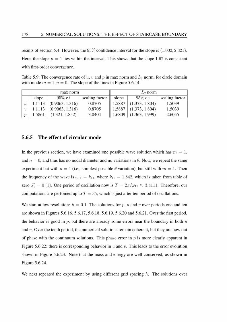
178 5. NUMERICAL SOLUTIONS: THE EFFECT OF STAIRCASE BOUNDARY
results of section 5.4. However, the 95% confidence interval for the slope is (1.002, 2.321).
Here, the slope n = 1 lies within the interval. This shows that the slope 1.67 is consistent
with first-order convergence.
Table 5.9: The convergence rate of u, v and p in max norm and L2 norm, for circle domainwith mode m = 1, n = 0. The slope of the lines in Figure 5.6.14.
max norm L2 normslope 95% c.i scaling factor slope 95% c.i scaling factor
u 1.1113 (0.9063, 1.316) 0.8705 1.5887 (1.373, 1.804) 1.5039v 1.1113 (0.9063, 1.316) 0.8705 1.5887 (1.373, 1.804) 1.5039p 1.5861 (1.321, 1.852) 3.0404 1.6809 (1.363, 1.999) 2.6055
5.6.5 The effect of circular mode
In the previous section, we have examined one possible wave solution which has m = 1,
and n = 0, and thus has no nodal diameter and no variations in θ. Now, we repeat the same
experiment but with n = 1 (i.e., simplest possible θ variation), but still with m = 1. Then
the frequency of the wave is ω11 = k11, where k11 = 1.842, which is taken from table of
zero J ′1 = 0 [1]. One period of oscillation now is T = 2π/ω11 ≈ 3.4111. Therefore, our
computations are perfomed up to T = 35, which is just after ten period of oscillations.
We start at low resolution: h = 0.1. The solutions for p, u and v over periods one and ten
are shown in Figures 5.6.16, 5.6.17, 5.6.18, 5.6.19, 5.6.20 and 5.6.21. Over the first period,
the behavior is good in p, but there are already some errors near the boundary in both u
and v. Over the tenth period, the numerical solutions remain coherent, but they are now out
of phase with the continuum solutions. This phase error in p is more clearly apparent in
Figure 5.6.22; there is corresponding behavior in u and v. This leads to the error evolution
shown in Figure 5.6.23. Note that the mass and energy are well conserved, as shown in
Figure 5.6.24.
We next repeated the experiment by using different grid spacing h. The solutions over
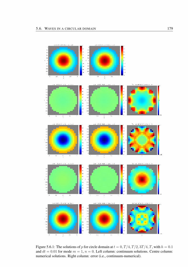
5.6. WAVES IN A CIRCULAR DOMAIN 179
Figure 5.6.1: The solutions of p for circle domain at t = 0, T/4, T/2, 3T/4, T , with h = 0.1and dt = 0.01 for mode m = 1, n = 0. Left column: continuum solutions. Centre column:numerical solutions. Right column: error (i.e., continuum-numerical).
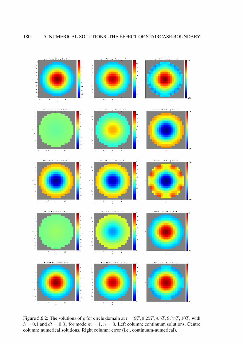
180 5. NUMERICAL SOLUTIONS: THE EFFECT OF STAIRCASE BOUNDARY
Figure 5.6.2: The solutions of p for circle domain at t = 9T, 9.25T, 9.5T, 9.75T, 10T , withh = 0.1 and dt = 0.01 for mode m = 1, n = 0. Left column: continuum solutions. Centrecolumn: numerical solutions. Right column: error (i.e., continuum-numerical).
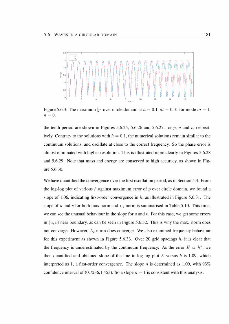
5.6. WAVES IN A CIRCULAR DOMAIN 181
0 2 4 6 8 10 12 14 16time, t
0
0.2
0.4
0.6
0.8
1
1.2
max
|p|
pc
pd
Figure 5.6.3: The maximum |p| over circle domain at h = 0.1, dt = 0.01 for mode m = 1,n = 0.
the tenth period are shown in Figures 5.6.25, 5.6.26 and 5.6.27, for p, u and v, respect-
ively. Contrary to the solutions with h = 0.1, the numerical solutions remain similar to the
continuum solutions, and oscillate at close to the correct frequency. So the phase error is
almost eliminated with higher resolution. This is illustrated more clearly in Figures 5.6.28
and 5.6.29. Note that mass and energy are conserved to high accuracy, as shown in Fig-
ure 5.6.30.
We have quantified the convergence over the first oscillation period, as in Section 5.4. From
the log-log plot of various h against maximum error of p over circle domain, we found a
slope of 1.06, indicating first-order convergence in h, as illustrated in Figure 5.6.31. The
slope of u and v for both max norm and L2 norm is summarised in Table 5.10. This time,
we can see the unusual behaviour in the slope for u and v. For this case, we get some errors
in (u, v) near boundary, as can be seen in Figure 5.6.32. This is why the max. norm does
not converge. However, L2 norm does converge. We also examined frequency behaviour
for this experiment as shown in Figure 5.6.33. Over 20 grid spacings h, it is clear that
the frequency is underestimated by the continuum frequency. As the error E ∝ hn, we
then quantified and obtained slope of the line in log-log plot E versus h is 1.09, which
interpreted as 1, a first-order convergence. The slope n is determined as 1.09, with 95%
confidence interval of (0.7236,1.453). So a slope n = 1 is consistent with this analysis.
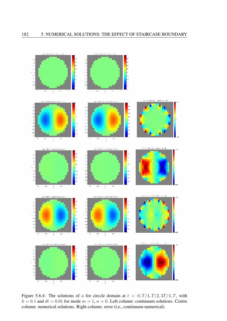
182 5. NUMERICAL SOLUTIONS: THE EFFECT OF STAIRCASE BOUNDARY
Figure 5.6.4: The solutions of u for circcle domain at t = 0, T/4, T/2, 3T/4, T , withh = 0.1 and dt = 0.01 for mode m = 1, n = 0. Left column: continuum solutions. Centrecolumn: numerical solutions. Right column: error (i.e., continuum-numerical).
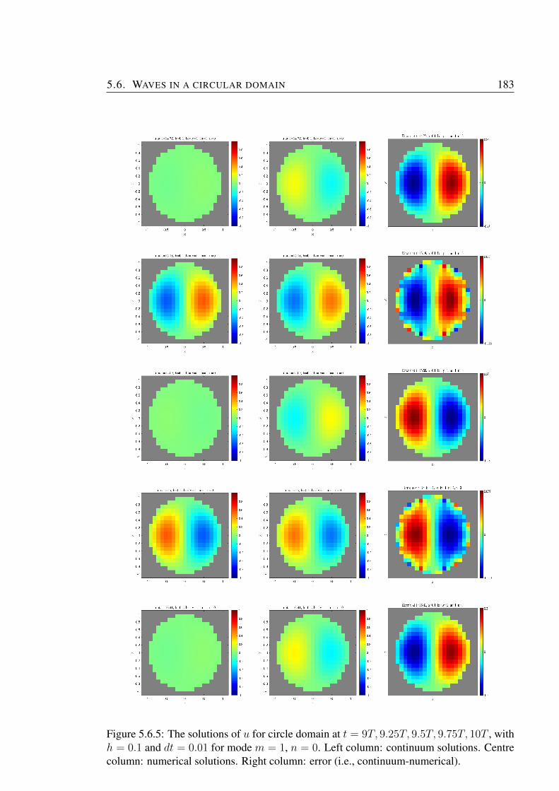
5.6. WAVES IN A CIRCULAR DOMAIN 183
Figure 5.6.5: The solutions of u for circle domain at t = 9T, 9.25T, 9.5T, 9.75T, 10T , withh = 0.1 and dt = 0.01 for mode m = 1, n = 0. Left column: continuum solutions. Centrecolumn: numerical solutions. Right column: error (i.e., continuum-numerical).
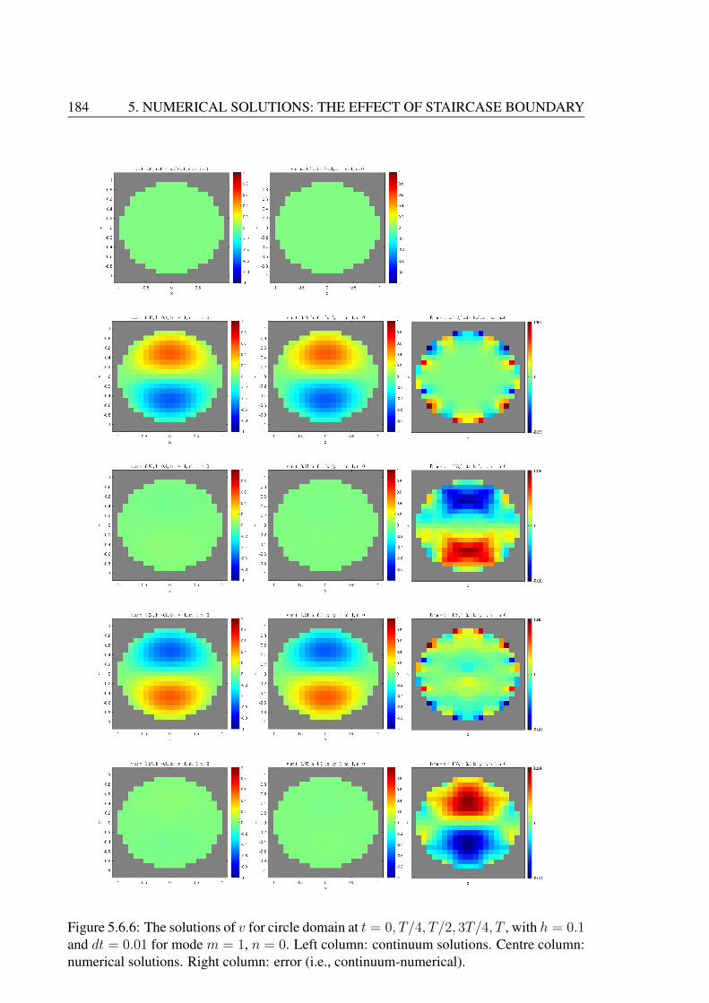
184 5. NUMERICAL SOLUTIONS: THE EFFECT OF STAIRCASE BOUNDARY
Figure 5.6.6: The solutions of v for circle domain at t = 0, T/4, T/2, 3T/4, T , with h = 0.1and dt = 0.01 for mode m = 1, n = 0. Left column: continuum solutions. Centre column:numerical solutions. Right column: error (i.e., continuum-numerical).
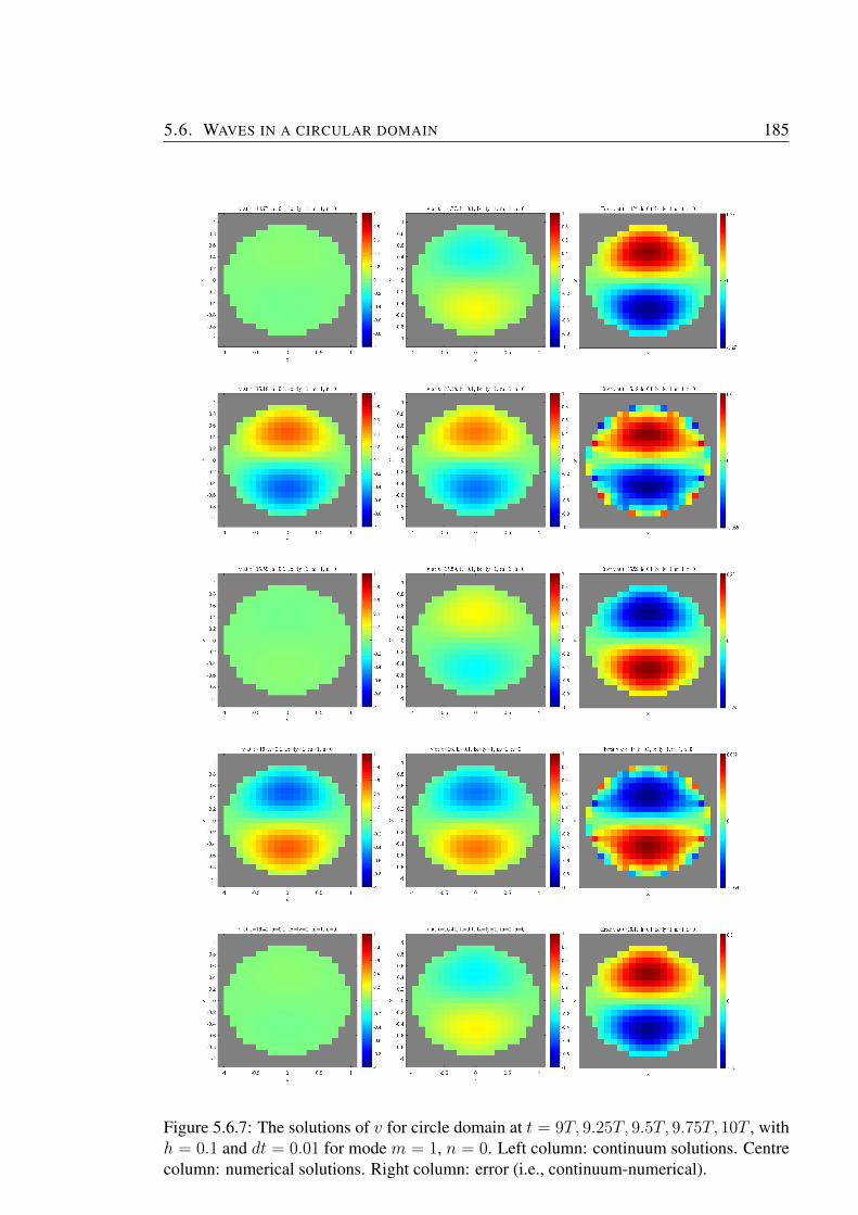
5.6. WAVES IN A CIRCULAR DOMAIN 185
Figure 5.6.7: The solutions of v for circle domain at t = 9T, 9.25T, 9.5T, 9.75T, 10T , withh = 0.1 and dt = 0.01 for mode m = 1, n = 0. Left column: continuum solutions. Centrecolumn: numerical solutions. Right column: error (i.e., continuum-numerical).
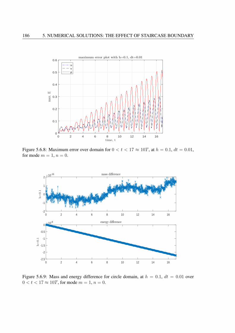
186 5. NUMERICAL SOLUTIONS: THE EFFECT OF STAIRCASE BOUNDARY
0 2 4 6 8 10 12 14 16time, t
0
0.1
0.2
0.3
0.4
0.5
0.6
max
.E
maximum error plot with h=0.1, dt=0.01
uvp
Figure 5.6.8: Maximum error over domain for 0 < t < 17 ≈ 10T , at h = 0.1, dt = 0.01,for mode m = 1, n = 0.
0 2 4 6 8 10 12 14 16-2
-1
0
1
2
h=0.1
×10-16 mass difference
0 2 4 6 8 10 12 14 16-2.5
-2
-1.5
-1
-0.5
0
h=0.1
×10-8 energy difference
Figure 5.6.9: Mass and energy difference for circle domain, at h = 0.1, dt = 0.01 over0 < t < 17 ≈ 10T , for mode m = 1, n = 0.
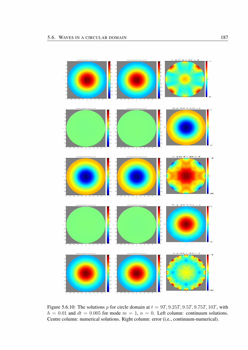
5.6. WAVES IN A CIRCULAR DOMAIN 187
p at t=14.76, dx=dy=0.01, lx=ly=1, m=1, n=0
x
y
−1 −0.8 −0.6 −0.4 −0.2 0 0.2 0.4 0.6 0.8 1−1
−0.8
−0.6
−0.4
−0.2
0
0.2
0.4
0.6
0.8
1
−1
−0.8
−0.6
−0.4
−0.2
0
0.2
0.4
0.6
0.8
1p at t=14.76, dx=dy=0.01, lx=ly=1, m=1, n=0
x
y
−1 −0.8 −0.6 −0.4 −0.2 0 0.2 0.4 0.6 0.8 1−1
−0.8
−0.6
−0.4
−0.2
0
0.2
0.4
0.6
0.8
1
−1
−0.8
−0.6
−0.4
−0.2
0
0.2
0.4
0.6
0.8
1
p at t=15.17, dx=dy=0.01, lx=ly=1, m=1, n=0
x
y
−1 −0.8 −0.6 −0.4 −0.2 0 0.2 0.4 0.6 0.8 1−1
−0.8
−0.6
−0.4
−0.2
0
0.2
0.4
0.6
0.8
1
−1
−0.8
−0.6
−0.4
−0.2
0
0.2
0.4
0.6
0.8
1p at t=15.17, dx=dy=0.01, lx=ly=1, m=1, n=0
x
y
−1 −0.8 −0.6 −0.4 −0.2 0 0.2 0.4 0.6 0.8 1−1
−0.8
−0.6
−0.4
−0.2
0
0.2
0.4
0.6
0.8
1
−1
−0.8
−0.6
−0.4
−0.2
0
0.2
0.4
0.6
0.8
1
p at t=15.59, dx=dy=0.01, lx=ly=1, m=1, n=0
x
y
−1 −0.8 −0.6 −0.4 −0.2 0 0.2 0.4 0.6 0.8 1−1
−0.8
−0.6
−0.4
−0.2
0
0.2
0.4
0.6
0.8
1
−1
−0.8
−0.6
−0.4
−0.2
0
0.2
0.4
0.6
0.8
1p at t=15.59, dx=dy=0.01, lx=ly=1, m=1, n=0
x
y
−1 −0.8 −0.6 −0.4 −0.2 0 0.2 0.4 0.6 0.8 1−1
−0.8
−0.6
−0.4
−0.2
0
0.2
0.4
0.6
0.8
1
−1
−0.8
−0.6
−0.4
−0.2
0
0.2
0.4
0.6
0.8
1
p at t=15.99, dx=dy=0.01, lx=ly=1, m=1, n=0
x
y
−1 −0.8 −0.6 −0.4 −0.2 0 0.2 0.4 0.6 0.8 1−1
−0.8
−0.6
−0.4
−0.2
0
0.2
0.4
0.6
0.8
1
−1
−0.8
−0.6
−0.4
−0.2
0
0.2
0.4
0.6
0.8
1p at t=15.99, dx=dy=0.01, lx=ly=1, m=1, n=0
x
y
−1 −0.8 −0.6 −0.4 −0.2 0 0.2 0.4 0.6 0.8 1−1
−0.8
−0.6
−0.4
−0.2
0
0.2
0.4
0.6
0.8
1
−1
−0.8
−0.6
−0.4
−0.2
0
0.2
0.4
0.6
0.8
1
p at t=16.4, dx=dy=0.01, lx=ly=1, m=1, n=0
x
y
−1 −0.8 −0.6 −0.4 −0.2 0 0.2 0.4 0.6 0.8 1−1
−0.8
−0.6
−0.4
−0.2
0
0.2
0.4
0.6
0.8
1
−1
−0.8
−0.6
−0.4
−0.2
0
0.2
0.4
0.6
0.8
1p at t=16.4, dx=dy=0.01, lx=ly=1, m=1, n=0
x
y
−1 −0.8 −0.6 −0.4 −0.2 0 0.2 0.4 0.6 0.8 1−1
−0.8
−0.6
−0.4
−0.2
0
0.2
0.4
0.6
0.8
1
−1
−0.8
−0.6
−0.4
−0.2
0
0.2
0.4
0.6
0.8
1
Figure 5.6.10: The solutions p for circle domain at t = 9T, 9.25T, 9.5T, 9.75T, 10T , withh = 0.01 and dt = 0.005 for mode m = 1, n = 0. Left column: continuum solutions.Centre column: numerical solutions. Right column: error (i.e., continuum-numerical).

188 5. NUMERICAL SOLUTIONS: THE EFFECT OF STAIRCASE BOUNDARY
0 2 4 6 8 10 12 14 16time, t
0
0.2
0.4
0.6
0.8
1
1.2
max
|p|
pc
pd
Figure 5.6.11: The maximum of |p| over 0 < t < 17 ≈ 10T at h = 0.01 with dt = 0.005for circle domain mode m = 1, n = 0.
0 2 4 6 8 10 12 14 16time, t
0
0.002
0.004
0.006
0.008
0.01
0.012
0.014
0.016
max
.E
maximum error plot with h=0.01, dt=0.005
uvp
Figure 5.6.12: Maximum error over domain at 0 < t < 17 ≈ 10T , h = 0.01, dt = 0.005for mode m = 1, n = 0.
Table 5.10: The convergence rate of u, v and p in max norm and L2 norm, for circle domainwith mode m = 1, n = 1. The slope is for the lines in Figure 5.6.31, indicate the rate ofconvergence.
max norm L2 normslope 95% c.i scaling factor slope 95% c.i scaling factor
u 0.0176 (-0.1418, 0.177) 0.13 0.9368 (0.7209, 1.153) 0.5071v -0.1816 (-0.3147, -0.0484) 0.07 0.6586 (0.5761, 0.7411) 0.1530p 1.0571 (0.8242, 1.29) 0.75 1.0789 (0.7508, 1.407) 0.6470

5.6. WAVES IN A CIRCULAR DOMAIN 189
0 2 4 6 8 10 12 14 16-4
-2
0
2
4h=0.01
×10-16 mass difference
0 2 4 6 8 10 12 14 16-8
-6
-4
-2
0
h=0.01
×10-10 energy difference
Figure 5.6.13: Mass and energy difference for circle domain, at h = 0.01, dt = 0.005 over0 < t < 17 ≈ 10T , for mode m = 1, n = 0.
Figure 5.6.14: Convergence plot for circle domain with mode m = 1, n = 0 at various h inrange 0.2 < h < 0.02 at fixed dt = 0.02. The error in (a) is calculated in max norm, and(b) in L2 norm over domain. Slope of the line is summarised in Table 5.9, indicate the rateof convergence.

190 5. NUMERICAL SOLUTIONS: THE EFFECT OF STAIRCASE BOUNDARY
0 0.05 0.1 0.15 0.2h
3.7
3.75
3.8
3.85
ω
ωd
ωc
Figure 5.6.15: The frequency of wave in circle domain with mode m = 1, n = 0, andlog-log plot error in frequency at various h. The slope of the line is 1.66158, with 95%confidence interval (1.002, 2.321). The scaling factor is 1.00801.
5.6.6 The effect of cell selection
In the previous two sections, we have discussed the numerical solutions of wave equations
in a circular domain, where the active cells are chosen according to condition (i) in sec-
tion 5.2. As discussed in that section, there are other possiblities to choose the active cells
for our numerical domain. In this section we repeat the experiment of section 5.6.2, but
cells are now retained if all the four corners of the cell lie within the continuum domain
(condition (ii) of section 5.2). With the mode m = 1 and n = 0, the frequency ω ≈ 3.8317,
and the period of the wave is T = 2π/ω ≈ 1.6398. As in previous sections, we perform
simulations up to t = 10T (i.e., t ≈ 17), and the time stepping stills need to satisfy the
condition (5.2.14). All solutions are recorded at every quarter period, but we only present
the solutions over one and ten wave periods.
We begin with the experiment with h = 0.1 and dt = 0.01. Shown in Figures 5.6.34 and
5.6.35 are the solutions for p over 0 < t < T and 9T < t < 10T , respectively. As we
can see in the solutions, there is a reasonably large error between continuum and numerical
solutions as early one period. The error then grows larger as the experiment continues.
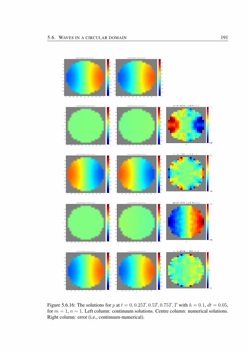
5.6. WAVES IN A CIRCULAR DOMAIN 191
p at t=0, dx=dy=0.1, lx=ly=1, m=1, n=1
x
y
−1 −0.8 −0.6 −0.4 −0.2 0 0.2 0.4 0.6 0.8 1
−1
−0.8
−0.6
−0.4
−0.2
0
0.2
0.4
0.6
0.8
1
−1
−0.8
−0.6
−0.4
−0.2
0
0.2
0.4
0.6
0.8
1p at t=0, dx=dy=0.1, lx=ly=1, m=1, n=1
x
y
−1 −0.8 −0.6 −0.4 −0.2 0 0.2 0.4 0.6 0.8 1
−1
−0.8
−0.6
−0.4
−0.2
0
0.2
0.4
0.6
0.8
1
−1
−0.8
−0.6
−0.4
−0.2
0
0.2
0.4
0.6
0.8
1
p at t=0.85, dx=dy=0.1, lx=ly=1, m=1, n=1
x
y
−1 −0.8 −0.6 −0.4 −0.2 0 0.2 0.4 0.6 0.8 1
−1
−0.8
−0.6
−0.4
−0.2
0
0.2
0.4
0.6
0.8
1
−1
−0.8
−0.6
−0.4
−0.2
0
0.2
0.4
0.6
0.8
1p at t=0.85, dx=dy=0.1, lx=ly=1, m=1, n=1
x
y
−1 −0.8 −0.6 −0.4 −0.2 0 0.2 0.4 0.6 0.8 1
−1
−0.8
−0.6
−0.4
−0.2
0
0.2
0.4
0.6
0.8
1
−1
−0.8
−0.6
−0.4
−0.2
0
0.2
0.4
0.6
0.8
1
p at t=1.71, dx=dy=0.1, lx=ly=1, m=1, n=1
x
y
−1 −0.8 −0.6 −0.4 −0.2 0 0.2 0.4 0.6 0.8 1
−1
−0.8
−0.6
−0.4
−0.2
0
0.2
0.4
0.6
0.8
1
−1
−0.8
−0.6
−0.4
−0.2
0
0.2
0.4
0.6
0.8
1p at t=1.71, dx=dy=0.1, lx=ly=1, m=1, n=1
x
y
−1 −0.8 −0.6 −0.4 −0.2 0 0.2 0.4 0.6 0.8 1
−1
−0.8
−0.6
−0.4
−0.2
0
0.2
0.4
0.6
0.8
1
−1
−0.8
−0.6
−0.4
−0.2
0
0.2
0.4
0.6
0.8
1
p at t=2.56, dx=dy=0.1, lx=ly=1, m=1, n=1
x
y
−1 −0.8 −0.6 −0.4 −0.2 0 0.2 0.4 0.6 0.8 1
−1
−0.8
−0.6
−0.4
−0.2
0
0.2
0.4
0.6
0.8
1
−1
−0.8
−0.6
−0.4
−0.2
0
0.2
0.4
0.6
0.8
1p at t=2.56, dx=dy=0.1, lx=ly=1, m=1, n=1
x
y
−1 −0.8 −0.6 −0.4 −0.2 0 0.2 0.4 0.6 0.8 1
−1
−0.8
−0.6
−0.4
−0.2
0
0.2
0.4
0.6
0.8
1
−1
−0.8
−0.6
−0.4
−0.2
0
0.2
0.4
0.6
0.8
1
p at t=3.41, dx=dy=0.1, lx=ly=1, m=1, n=1
x
y
−1 −0.8 −0.6 −0.4 −0.2 0 0.2 0.4 0.6 0.8 1
−1
−0.8
−0.6
−0.4
−0.2
0
0.2
0.4
0.6
0.8
1
−1
−0.8
−0.6
−0.4
−0.2
0
0.2
0.4
0.6
0.8
1p at t=3.41, dx=dy=0.1, lx=ly=1, m=1, n=1
x
y
−1 −0.8 −0.6 −0.4 −0.2 0 0.2 0.4 0.6 0.8 1
−1
−0.8
−0.6
−0.4
−0.2
0
0.2
0.4
0.6
0.8
1
−1
−0.8
−0.6
−0.4
−0.2
0
0.2
0.4
0.6
0.8
1
Figure 5.6.16: The solutions for p at t = 0, 0.25T, 0.5T, 0.75T, T with h = 0.1, dt = 0.05,for m = 1, n = 1. Left column: continuum solutions. Centre column: numerical solutions.Right column: error (i.e., continuum-numerical).
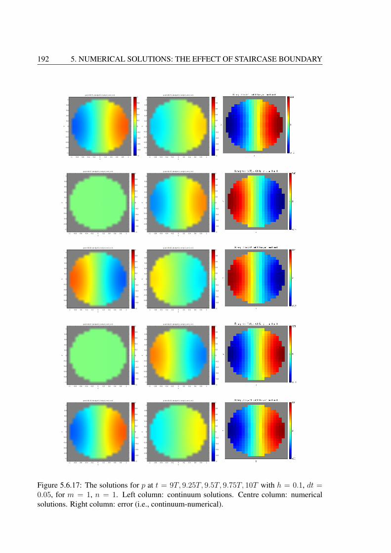
192 5. NUMERICAL SOLUTIONS: THE EFFECT OF STAIRCASE BOUNDARY
p at t=30.71, dx=dy=0.1, lx=ly=1, m=1, n=1
x
y
−1 −0.8 −0.6 −0.4 −0.2 0 0.2 0.4 0.6 0.8 1
−1
−0.8
−0.6
−0.4
−0.2
0
0.2
0.4
0.6
0.8
1
−1
−0.8
−0.6
−0.4
−0.2
0
0.2
0.4
0.6
0.8
1p at t=30.71, dx=dy=0.1, lx=ly=1, m=1, n=1
x
y
−1 −0.8 −0.6 −0.4 −0.2 0 0.2 0.4 0.6 0.8 1
−1
−0.8
−0.6
−0.4
−0.2
0
0.2
0.4
0.6
0.8
1
−1
−0.8
−0.6
−0.4
−0.2
0
0.2
0.4
0.6
0.8
1
p at t=31.57, dx=dy=0.1, lx=ly=1, m=1, n=1
x
y
−1 −0.8 −0.6 −0.4 −0.2 0 0.2 0.4 0.6 0.8 1
−1
−0.8
−0.6
−0.4
−0.2
0
0.2
0.4
0.6
0.8
1
−1
−0.8
−0.6
−0.4
−0.2
0
0.2
0.4
0.6
0.8
1p at t=31.57, dx=dy=0.1, lx=ly=1, m=1, n=1
x
y
−1 −0.8 −0.6 −0.4 −0.2 0 0.2 0.4 0.6 0.8 1
−1
−0.8
−0.6
−0.4
−0.2
0
0.2
0.4
0.6
0.8
1
−1
−0.8
−0.6
−0.4
−0.2
0
0.2
0.4
0.6
0.8
1
p at t=32.42, dx=dy=0.1, lx=ly=1, m=1, n=1
x
y
−1 −0.8 −0.6 −0.4 −0.2 0 0.2 0.4 0.6 0.8 1
−1
−0.8
−0.6
−0.4
−0.2
0
0.2
0.4
0.6
0.8
1
−1
−0.8
−0.6
−0.4
−0.2
0
0.2
0.4
0.6
0.8
1p at t=32.42, dx=dy=0.1, lx=ly=1, m=1, n=1
x
y
−1 −0.8 −0.6 −0.4 −0.2 0 0.2 0.4 0.6 0.8 1
−1
−0.8
−0.6
−0.4
−0.2
0
0.2
0.4
0.6
0.8
1
−1
−0.8
−0.6
−0.4
−0.2
0
0.2
0.4
0.6
0.8
1
p at t=33.27, dx=dy=0.1, lx=ly=1, m=1, n=1
x
y
−1 −0.8 −0.6 −0.4 −0.2 0 0.2 0.4 0.6 0.8 1
−1
−0.8
−0.6
−0.4
−0.2
0
0.2
0.4
0.6
0.8
1
−1
−0.8
−0.6
−0.4
−0.2
0
0.2
0.4
0.6
0.8
1p at t=33.27, dx=dy=0.1, lx=ly=1, m=1, n=1
x
y
−1 −0.8 −0.6 −0.4 −0.2 0 0.2 0.4 0.6 0.8 1
−1
−0.8
−0.6
−0.4
−0.2
0
0.2
0.4
0.6
0.8
1
−1
−0.8
−0.6
−0.4
−0.2
0
0.2
0.4
0.6
0.8
1
p at t=34.13, dx=dy=0.1, lx=ly=1, m=1, n=1
x
y
−1 −0.8 −0.6 −0.4 −0.2 0 0.2 0.4 0.6 0.8 1
−1
−0.8
−0.6
−0.4
−0.2
0
0.2
0.4
0.6
0.8
1
−1
−0.8
−0.6
−0.4
−0.2
0
0.2
0.4
0.6
0.8
1p at t=34.13, dx=dy=0.1, lx=ly=1, m=1, n=1
x
y
−1 −0.8 −0.6 −0.4 −0.2 0 0.2 0.4 0.6 0.8 1
−1
−0.8
−0.6
−0.4
−0.2
0
0.2
0.4
0.6
0.8
1
−1
−0.8
−0.6
−0.4
−0.2
0
0.2
0.4
0.6
0.8
1
Figure 5.6.17: The solutions for p at t = 9T, 9.25T, 9.5T, 9.75T, 10T with h = 0.1, dt =0.05, for m = 1, n = 1. Left column: continuum solutions. Centre column: numericalsolutions. Right column: error (i.e., continuum-numerical).
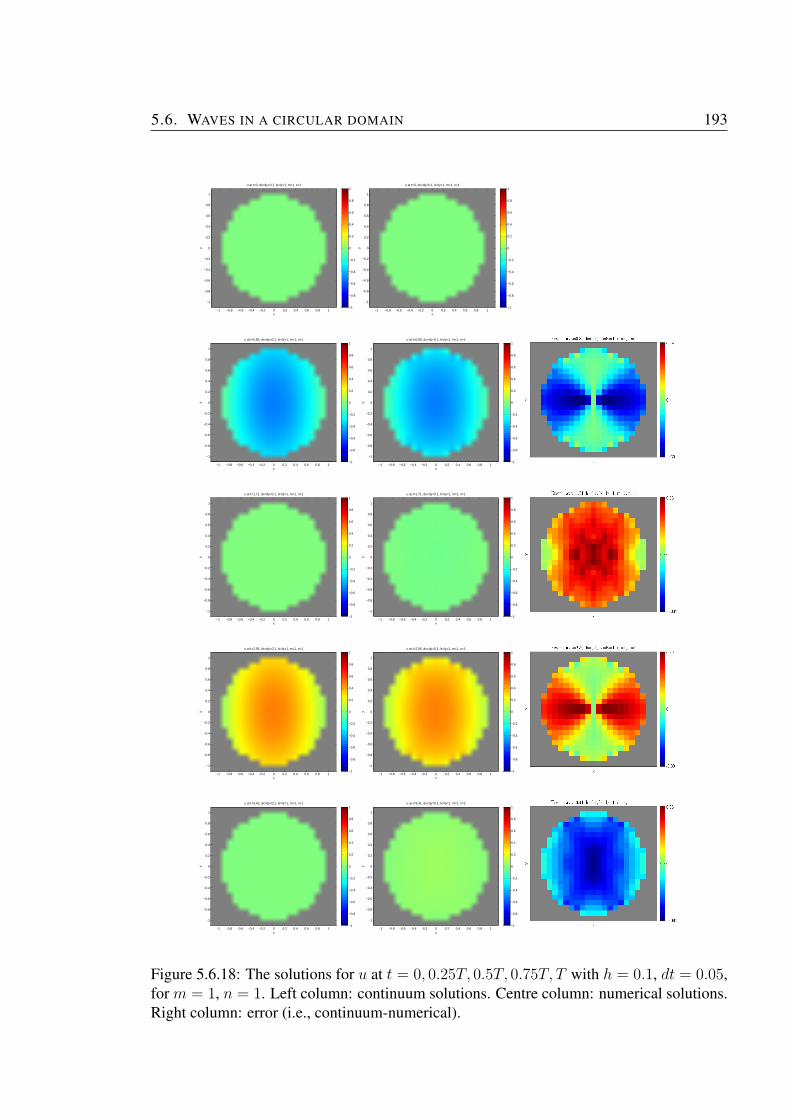
5.6. WAVES IN A CIRCULAR DOMAIN 193
u at t=0, dx=dy=0.1, lx=ly=1, m=1, n=1
x
y
−1 −0.8 −0.6 −0.4 −0.2 0 0.2 0.4 0.6 0.8 1
−1
−0.8
−0.6
−0.4
−0.2
0
0.2
0.4
0.6
0.8
1
−1
−0.8
−0.6
−0.4
−0.2
0
0.2
0.4
0.6
0.8
1u at t=0, dx=dy=0.1, lx=ly=1, m=1, n=1
x
y
−1 −0.8 −0.6 −0.4 −0.2 0 0.2 0.4 0.6 0.8 1
−1
−0.8
−0.6
−0.4
−0.2
0
0.2
0.4
0.6
0.8
1
−1
−0.8
−0.6
−0.4
−0.2
0
0.2
0.4
0.6
0.8
1
u at t=0.85, dx=dy=0.1, lx=ly=1, m=1, n=1
x
y
−1 −0.8 −0.6 −0.4 −0.2 0 0.2 0.4 0.6 0.8 1
−1
−0.8
−0.6
−0.4
−0.2
0
0.2
0.4
0.6
0.8
1
−1
−0.8
−0.6
−0.4
−0.2
0
0.2
0.4
0.6
0.8
1u at t=0.85, dx=dy=0.1, lx=ly=1, m=1, n=1
x
y
−1 −0.8 −0.6 −0.4 −0.2 0 0.2 0.4 0.6 0.8 1
−1
−0.8
−0.6
−0.4
−0.2
0
0.2
0.4
0.6
0.8
1
−1
−0.8
−0.6
−0.4
−0.2
0
0.2
0.4
0.6
0.8
1
u at t=1.71, dx=dy=0.1, lx=ly=1, m=1, n=1
x
y
−1 −0.8 −0.6 −0.4 −0.2 0 0.2 0.4 0.6 0.8 1
−1
−0.8
−0.6
−0.4
−0.2
0
0.2
0.4
0.6
0.8
1
−1
−0.8
−0.6
−0.4
−0.2
0
0.2
0.4
0.6
0.8
1u at t=1.71, dx=dy=0.1, lx=ly=1, m=1, n=1
x
y
−1 −0.8 −0.6 −0.4 −0.2 0 0.2 0.4 0.6 0.8 1
−1
−0.8
−0.6
−0.4
−0.2
0
0.2
0.4
0.6
0.8
1
−1
−0.8
−0.6
−0.4
−0.2
0
0.2
0.4
0.6
0.8
1
u at t=2.56, dx=dy=0.1, lx=ly=1, m=1, n=1
x
y
−1 −0.8 −0.6 −0.4 −0.2 0 0.2 0.4 0.6 0.8 1
−1
−0.8
−0.6
−0.4
−0.2
0
0.2
0.4
0.6
0.8
1
−1
−0.8
−0.6
−0.4
−0.2
0
0.2
0.4
0.6
0.8
1u at t=2.56, dx=dy=0.1, lx=ly=1, m=1, n=1
x
y
−1 −0.8 −0.6 −0.4 −0.2 0 0.2 0.4 0.6 0.8 1
−1
−0.8
−0.6
−0.4
−0.2
0
0.2
0.4
0.6
0.8
1
−1
−0.8
−0.6
−0.4
−0.2
0
0.2
0.4
0.6
0.8
1
u at t=3.41, dx=dy=0.1, lx=ly=1, m=1, n=1
x
y
−1 −0.8 −0.6 −0.4 −0.2 0 0.2 0.4 0.6 0.8 1
−1
−0.8
−0.6
−0.4
−0.2
0
0.2
0.4
0.6
0.8
1
−1
−0.8
−0.6
−0.4
−0.2
0
0.2
0.4
0.6
0.8
1u at t=3.41, dx=dy=0.1, lx=ly=1, m=1, n=1
x
y
−1 −0.8 −0.6 −0.4 −0.2 0 0.2 0.4 0.6 0.8 1
−1
−0.8
−0.6
−0.4
−0.2
0
0.2
0.4
0.6
0.8
1
−1
−0.8
−0.6
−0.4
−0.2
0
0.2
0.4
0.6
0.8
1
Figure 5.6.18: The solutions for u at t = 0, 0.25T, 0.5T, 0.75T, T with h = 0.1, dt = 0.05,for m = 1, n = 1. Left column: continuum solutions. Centre column: numerical solutions.Right column: error (i.e., continuum-numerical).
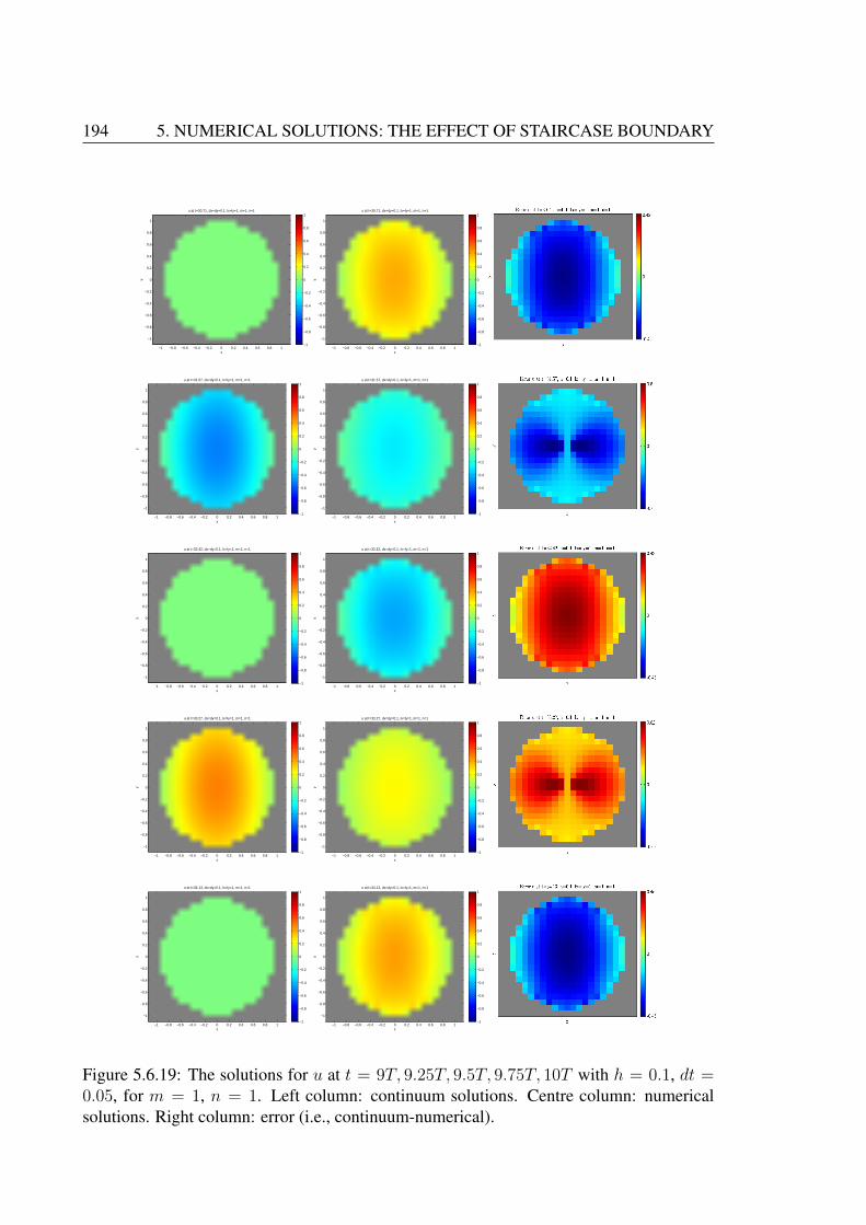
194 5. NUMERICAL SOLUTIONS: THE EFFECT OF STAIRCASE BOUNDARY
u at t=30.71, dx=dy=0.1, lx=ly=1, m=1, n=1
x
y
−1 −0.8 −0.6 −0.4 −0.2 0 0.2 0.4 0.6 0.8 1
−1
−0.8
−0.6
−0.4
−0.2
0
0.2
0.4
0.6
0.8
1
−1
−0.8
−0.6
−0.4
−0.2
0
0.2
0.4
0.6
0.8
1u at t=30.71, dx=dy=0.1, lx=ly=1, m=1, n=1
x
y
−1 −0.8 −0.6 −0.4 −0.2 0 0.2 0.4 0.6 0.8 1
−1
−0.8
−0.6
−0.4
−0.2
0
0.2
0.4
0.6
0.8
1
−1
−0.8
−0.6
−0.4
−0.2
0
0.2
0.4
0.6
0.8
1
u at t=31.57, dx=dy=0.1, lx=ly=1, m=1, n=1
x
y
−1 −0.8 −0.6 −0.4 −0.2 0 0.2 0.4 0.6 0.8 1
−1
−0.8
−0.6
−0.4
−0.2
0
0.2
0.4
0.6
0.8
1
−1
−0.8
−0.6
−0.4
−0.2
0
0.2
0.4
0.6
0.8
1u at t=31.57, dx=dy=0.1, lx=ly=1, m=1, n=1
x
y
−1 −0.8 −0.6 −0.4 −0.2 0 0.2 0.4 0.6 0.8 1
−1
−0.8
−0.6
−0.4
−0.2
0
0.2
0.4
0.6
0.8
1
−1
−0.8
−0.6
−0.4
−0.2
0
0.2
0.4
0.6
0.8
1
u at t=32.42, dx=dy=0.1, lx=ly=1, m=1, n=1
x
y
−1 −0.8 −0.6 −0.4 −0.2 0 0.2 0.4 0.6 0.8 1
−1
−0.8
−0.6
−0.4
−0.2
0
0.2
0.4
0.6
0.8
1
−1
−0.8
−0.6
−0.4
−0.2
0
0.2
0.4
0.6
0.8
1u at t=32.42, dx=dy=0.1, lx=ly=1, m=1, n=1
x
y
−1 −0.8 −0.6 −0.4 −0.2 0 0.2 0.4 0.6 0.8 1
−1
−0.8
−0.6
−0.4
−0.2
0
0.2
0.4
0.6
0.8
1
−1
−0.8
−0.6
−0.4
−0.2
0
0.2
0.4
0.6
0.8
1
u at t=33.27, dx=dy=0.1, lx=ly=1, m=1, n=1
x
y
−1 −0.8 −0.6 −0.4 −0.2 0 0.2 0.4 0.6 0.8 1
−1
−0.8
−0.6
−0.4
−0.2
0
0.2
0.4
0.6
0.8
1
−1
−0.8
−0.6
−0.4
−0.2
0
0.2
0.4
0.6
0.8
1u at t=33.27, dx=dy=0.1, lx=ly=1, m=1, n=1
x
y
−1 −0.8 −0.6 −0.4 −0.2 0 0.2 0.4 0.6 0.8 1
−1
−0.8
−0.6
−0.4
−0.2
0
0.2
0.4
0.6
0.8
1
−1
−0.8
−0.6
−0.4
−0.2
0
0.2
0.4
0.6
0.8
1
u at t=34.13, dx=dy=0.1, lx=ly=1, m=1, n=1
x
y
−1 −0.8 −0.6 −0.4 −0.2 0 0.2 0.4 0.6 0.8 1
−1
−0.8
−0.6
−0.4
−0.2
0
0.2
0.4
0.6
0.8
1
−1
−0.8
−0.6
−0.4
−0.2
0
0.2
0.4
0.6
0.8
1u at t=34.13, dx=dy=0.1, lx=ly=1, m=1, n=1
x
y
−1 −0.8 −0.6 −0.4 −0.2 0 0.2 0.4 0.6 0.8 1
−1
−0.8
−0.6
−0.4
−0.2
0
0.2
0.4
0.6
0.8
1
−1
−0.8
−0.6
−0.4
−0.2
0
0.2
0.4
0.6
0.8
1
Figure 5.6.19: The solutions for u at t = 9T, 9.25T, 9.5T, 9.75T, 10T with h = 0.1, dt =0.05, for m = 1, n = 1. Left column: continuum solutions. Centre column: numericalsolutions. Right column: error (i.e., continuum-numerical).
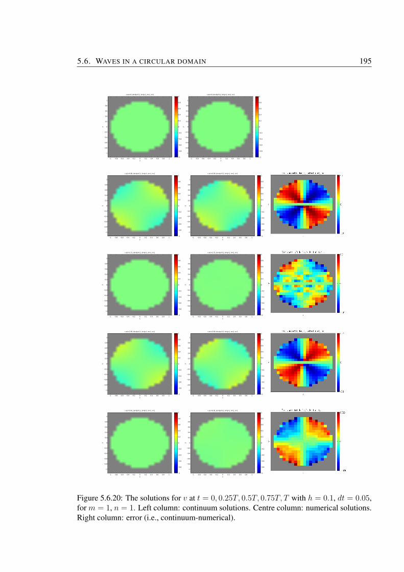
5.6. WAVES IN A CIRCULAR DOMAIN 195
v at t=0, dx=dy=0.1, lx=ly=1, m=1, n=1
x
y
−1 −0.8 −0.6 −0.4 −0.2 0 0.2 0.4 0.6 0.8 1
−1
−0.8
−0.6
−0.4
−0.2
0
0.2
0.4
0.6
0.8
1
−1
−0.8
−0.6
−0.4
−0.2
0
0.2
0.4
0.6
0.8
1v at t=0, dx=dy=0.1, lx=ly=1, m=1, n=1
x
y
−1 −0.8 −0.6 −0.4 −0.2 0 0.2 0.4 0.6 0.8 1
−1
−0.8
−0.6
−0.4
−0.2
0
0.2
0.4
0.6
0.8
1
−1
−0.8
−0.6
−0.4
−0.2
0
0.2
0.4
0.6
0.8
1
v at t=0.85, dx=dy=0.1, lx=ly=1, m=1, n=1
x
y
−1 −0.8 −0.6 −0.4 −0.2 0 0.2 0.4 0.6 0.8 1
−1
−0.8
−0.6
−0.4
−0.2
0
0.2
0.4
0.6
0.8
1
−1
−0.8
−0.6
−0.4
−0.2
0
0.2
0.4
0.6
0.8
1v at t=0.85, dx=dy=0.1, lx=ly=1, m=1, n=1
x
y
−1 −0.8 −0.6 −0.4 −0.2 0 0.2 0.4 0.6 0.8 1
−1
−0.8
−0.6
−0.4
−0.2
0
0.2
0.4
0.6
0.8
1
−1
−0.8
−0.6
−0.4
−0.2
0
0.2
0.4
0.6
0.8
1
v at t=1.71, dx=dy=0.1, lx=ly=1, m=1, n=1
x
y
−1 −0.8 −0.6 −0.4 −0.2 0 0.2 0.4 0.6 0.8 1
−1
−0.8
−0.6
−0.4
−0.2
0
0.2
0.4
0.6
0.8
1
−1
−0.8
−0.6
−0.4
−0.2
0
0.2
0.4
0.6
0.8
1v at t=1.71, dx=dy=0.1, lx=ly=1, m=1, n=1
x
y
−1 −0.8 −0.6 −0.4 −0.2 0 0.2 0.4 0.6 0.8 1
−1
−0.8
−0.6
−0.4
−0.2
0
0.2
0.4
0.6
0.8
1
−1
−0.8
−0.6
−0.4
−0.2
0
0.2
0.4
0.6
0.8
1
v at t=2.56, dx=dy=0.1, lx=ly=1, m=1, n=1
x
y
−1 −0.8 −0.6 −0.4 −0.2 0 0.2 0.4 0.6 0.8 1
−1
−0.8
−0.6
−0.4
−0.2
0
0.2
0.4
0.6
0.8
1
−1
−0.8
−0.6
−0.4
−0.2
0
0.2
0.4
0.6
0.8
1v at t=2.56, dx=dy=0.1, lx=ly=1, m=1, n=1
x
y
−1 −0.8 −0.6 −0.4 −0.2 0 0.2 0.4 0.6 0.8 1
−1
−0.8
−0.6
−0.4
−0.2
0
0.2
0.4
0.6
0.8
1
−1
−0.8
−0.6
−0.4
−0.2
0
0.2
0.4
0.6
0.8
1
v at t=3.41, dx=dy=0.1, lx=ly=1, m=1, n=1
x
y
−1 −0.8 −0.6 −0.4 −0.2 0 0.2 0.4 0.6 0.8 1
−1
−0.8
−0.6
−0.4
−0.2
0
0.2
0.4
0.6
0.8
1
−1
−0.8
−0.6
−0.4
−0.2
0
0.2
0.4
0.6
0.8
1v at t=3.41, dx=dy=0.1, lx=ly=1, m=1, n=1
x
y
−1 −0.8 −0.6 −0.4 −0.2 0 0.2 0.4 0.6 0.8 1
−1
−0.8
−0.6
−0.4
−0.2
0
0.2
0.4
0.6
0.8
1
−1
−0.8
−0.6
−0.4
−0.2
0
0.2
0.4
0.6
0.8
1
Figure 5.6.20: The solutions for v at t = 0, 0.25T, 0.5T, 0.75T, T with h = 0.1, dt = 0.05,for m = 1, n = 1. Left column: continuum solutions. Centre column: numerical solutions.Right column: error (i.e., continuum-numerical).
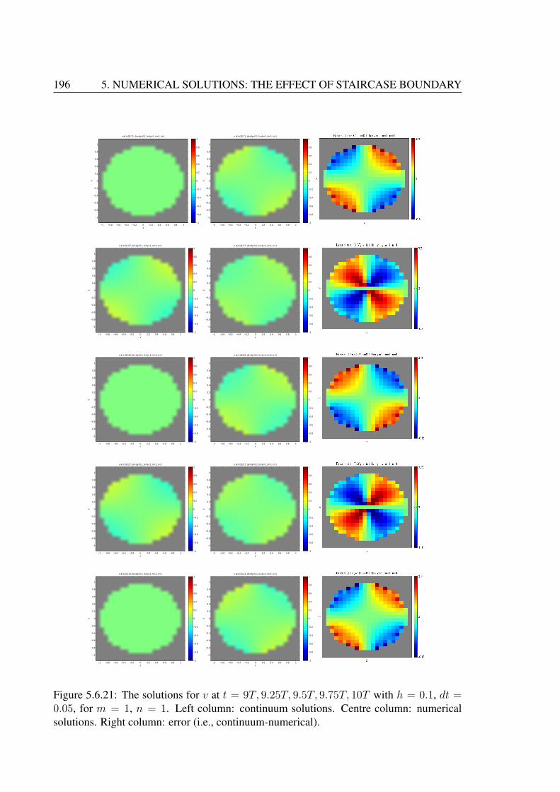
196 5. NUMERICAL SOLUTIONS: THE EFFECT OF STAIRCASE BOUNDARY
v at t=30.71, dx=dy=0.1, lx=ly=1, m=1, n=1
x
y
−1 −0.8 −0.6 −0.4 −0.2 0 0.2 0.4 0.6 0.8 1
−1
−0.8
−0.6
−0.4
−0.2
0
0.2
0.4
0.6
0.8
1
−1
−0.8
−0.6
−0.4
−0.2
0
0.2
0.4
0.6
0.8
1v at t=30.71, dx=dy=0.1, lx=ly=1, m=1, n=1
x
y
−1 −0.8 −0.6 −0.4 −0.2 0 0.2 0.4 0.6 0.8 1
−1
−0.8
−0.6
−0.4
−0.2
0
0.2
0.4
0.6
0.8
1
−1
−0.8
−0.6
−0.4
−0.2
0
0.2
0.4
0.6
0.8
1
v at t=31.57, dx=dy=0.1, lx=ly=1, m=1, n=1
x
y
−1 −0.8 −0.6 −0.4 −0.2 0 0.2 0.4 0.6 0.8 1
−1
−0.8
−0.6
−0.4
−0.2
0
0.2
0.4
0.6
0.8
1
−1
−0.8
−0.6
−0.4
−0.2
0
0.2
0.4
0.6
0.8
1v at t=31.57, dx=dy=0.1, lx=ly=1, m=1, n=1
x
y
−1 −0.8 −0.6 −0.4 −0.2 0 0.2 0.4 0.6 0.8 1
−1
−0.8
−0.6
−0.4
−0.2
0
0.2
0.4
0.6
0.8
1
−1
−0.8
−0.6
−0.4
−0.2
0
0.2
0.4
0.6
0.8
1
v at t=32.42, dx=dy=0.1, lx=ly=1, m=1, n=1
x
y
−1 −0.8 −0.6 −0.4 −0.2 0 0.2 0.4 0.6 0.8 1
−1
−0.8
−0.6
−0.4
−0.2
0
0.2
0.4
0.6
0.8
1
−1
−0.8
−0.6
−0.4
−0.2
0
0.2
0.4
0.6
0.8
1v at t=32.42, dx=dy=0.1, lx=ly=1, m=1, n=1
x
y
−1 −0.8 −0.6 −0.4 −0.2 0 0.2 0.4 0.6 0.8 1
−1
−0.8
−0.6
−0.4
−0.2
0
0.2
0.4
0.6
0.8
1
−1
−0.8
−0.6
−0.4
−0.2
0
0.2
0.4
0.6
0.8
1
v at t=33.27, dx=dy=0.1, lx=ly=1, m=1, n=1
x
y
−1 −0.8 −0.6 −0.4 −0.2 0 0.2 0.4 0.6 0.8 1
−1
−0.8
−0.6
−0.4
−0.2
0
0.2
0.4
0.6
0.8
1
−1
−0.8
−0.6
−0.4
−0.2
0
0.2
0.4
0.6
0.8
1v at t=33.27, dx=dy=0.1, lx=ly=1, m=1, n=1
x
y
−1 −0.8 −0.6 −0.4 −0.2 0 0.2 0.4 0.6 0.8 1
−1
−0.8
−0.6
−0.4
−0.2
0
0.2
0.4
0.6
0.8
1
−1
−0.8
−0.6
−0.4
−0.2
0
0.2
0.4
0.6
0.8
1
v at t=34.13, dx=dy=0.1, lx=ly=1, m=1, n=1
x
y
−1 −0.8 −0.6 −0.4 −0.2 0 0.2 0.4 0.6 0.8 1
−1
−0.8
−0.6
−0.4
−0.2
0
0.2
0.4
0.6
0.8
1
−1
−0.8
−0.6
−0.4
−0.2
0
0.2
0.4
0.6
0.8
1v at t=34.13, dx=dy=0.1, lx=ly=1, m=1, n=1
x
y
−1 −0.8 −0.6 −0.4 −0.2 0 0.2 0.4 0.6 0.8 1
−1
−0.8
−0.6
−0.4
−0.2
0
0.2
0.4
0.6
0.8
1
−1
−0.8
−0.6
−0.4
−0.2
0
0.2
0.4
0.6
0.8
1
Figure 5.6.21: The solutions for v at t = 9T, 9.25T, 9.5T, 9.75T, 10T with h = 0.1, dt =0.05, for m = 1, n = 1. Left column: continuum solutions. Centre column: numericalsolutions. Right column: error (i.e., continuum-numerical).
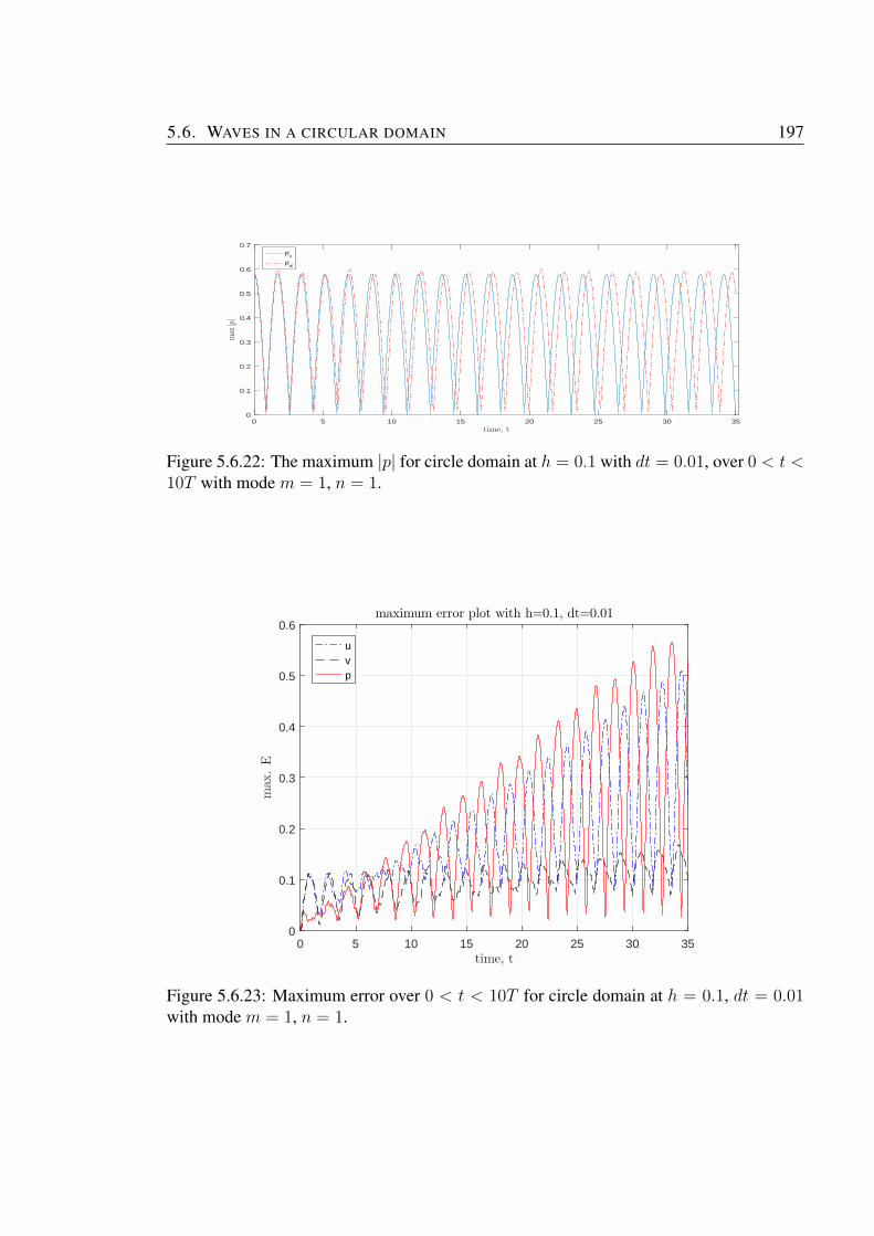
5.6. WAVES IN A CIRCULAR DOMAIN 197
0 5 10 15 20 25 30 35time, t
0
0.1
0.2
0.3
0.4
0.5
0.6
0.7
max
|p|
pc
pd
Figure 5.6.22: The maximum |p| for circle domain at h = 0.1 with dt = 0.01, over 0 < t <10T with mode m = 1, n = 1.
0 5 10 15 20 25 30 35time, t
0
0.1
0.2
0.3
0.4
0.5
0.6
max.E
maximum error plot with h=0.1, dt=0.01
uvp
Figure 5.6.23: Maximum error over 0 < t < 10T for circle domain at h = 0.1, dt = 0.01with mode m = 1, n = 1.
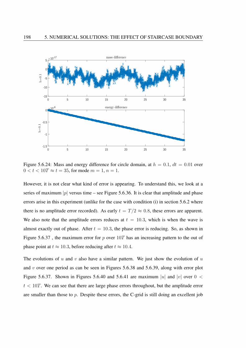
198 5. NUMERICAL SOLUTIONS: THE EFFECT OF STAIRCASE BOUNDARY
0 5 10 15 20 25 30 35-15
-10
-5
0
5
h=0.1
×10-17 mass difference
0 5 10 15 20 25 30 35-1.5
-1
-0.5
0
h=0.1
×10-8 energy difference
Figure 5.6.24: Mass and energy difference for circle domain, at h = 0.1, dt = 0.01 over0 < t < 10T ≈ t = 35, for mode m = 1, n = 1.
However, it is not clear what kind of error is appearing. To understand this, we look at a
series of maximum |p| versus time – see Figure 5.6.36. It is clear that amplitude and phase
errors arise in this experiment (unlike for the case with condition (i) in section 5.6.2 where
there is no amplitude error recorded). As early t = T/2 ≈ 0.8, these errors are apparent.
We also note that the amplitude errors reduces at t = 10.3, which is when the wave is
almost exactly out of phase. After t = 10.3, the phase error is reducing. So, as shown in
Figure 5.6.37 , the maximum error for p over 10T has an increasing pattern to the out of
phase point at t ≈ 10.3, before reducing after t ≈ 10.4.
The evolutions of u and v also have a similar pattern. We just show the evolution of u
and v over one period as can be seen in Figures 5.6.38 and 5.6.39, along with error plot
Figure 5.6.37. Shown in Figures 5.6.40 and 5.6.41 are maximum |u| and |v| over 0 <
t < 10T . We can see that there are large phase errors throughout, but the amplitude error
are smaller than those to p. Despite these errors, the C-grid is still doing an excellent job
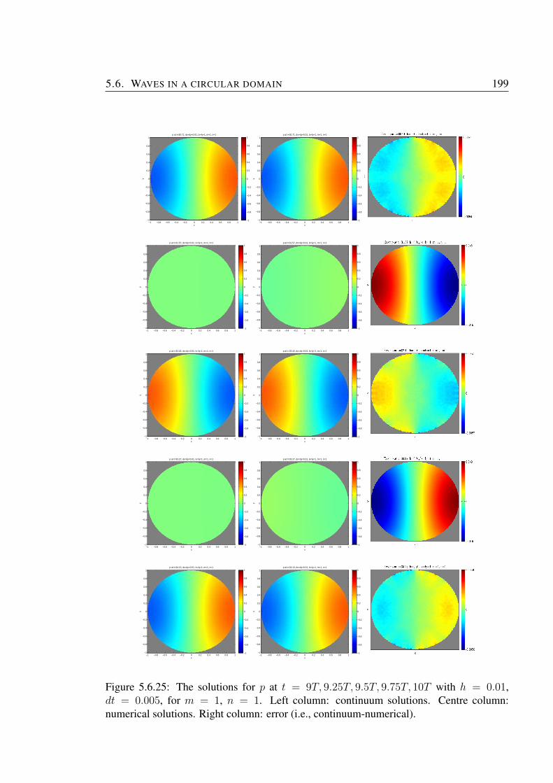
5.6. WAVES IN A CIRCULAR DOMAIN 199
p at t=30.71, dx=dy=0.01, lx=ly=1, m=1, n=1
x
y
−1 −0.8 −0.6 −0.4 −0.2 0 0.2 0.4 0.6 0.8 1−1
−0.8
−0.6
−0.4
−0.2
0
0.2
0.4
0.6
0.8
1
−1
−0.8
−0.6
−0.4
−0.2
0
0.2
0.4
0.6
0.8
1p at t=30.71, dx=dy=0.01, lx=ly=1, m=1, n=1
x
y
−1 −0.8 −0.6 −0.4 −0.2 0 0.2 0.4 0.6 0.8 1−1
−0.8
−0.6
−0.4
−0.2
0
0.2
0.4
0.6
0.8
1
−1
−0.8
−0.6
−0.4
−0.2
0
0.2
0.4
0.6
0.8
1
p at t=31.57, dx=dy=0.01, lx=ly=1, m=1, n=1
x
y
−1 −0.8 −0.6 −0.4 −0.2 0 0.2 0.4 0.6 0.8 1−1
−0.8
−0.6
−0.4
−0.2
0
0.2
0.4
0.6
0.8
1
−1
−0.8
−0.6
−0.4
−0.2
0
0.2
0.4
0.6
0.8
1p at t=31.57, dx=dy=0.01, lx=ly=1, m=1, n=1
x
y
−1 −0.8 −0.6 −0.4 −0.2 0 0.2 0.4 0.6 0.8 1−1
−0.8
−0.6
−0.4
−0.2
0
0.2
0.4
0.6
0.8
1
−1
−0.8
−0.6
−0.4
−0.2
0
0.2
0.4
0.6
0.8
1
p at t=32.42, dx=dy=0.01, lx=ly=1, m=1, n=1
x
y
−1 −0.8 −0.6 −0.4 −0.2 0 0.2 0.4 0.6 0.8 1−1
−0.8
−0.6
−0.4
−0.2
0
0.2
0.4
0.6
0.8
1
−1
−0.8
−0.6
−0.4
−0.2
0
0.2
0.4
0.6
0.8
1p at t=32.42, dx=dy=0.01, lx=ly=1, m=1, n=1
x
y
−1 −0.8 −0.6 −0.4 −0.2 0 0.2 0.4 0.6 0.8 1−1
−0.8
−0.6
−0.4
−0.2
0
0.2
0.4
0.6
0.8
1
−1
−0.8
−0.6
−0.4
−0.2
0
0.2
0.4
0.6
0.8
1
p at t=33.27, dx=dy=0.01, lx=ly=1, m=1, n=1
x
y
−1 −0.8 −0.6 −0.4 −0.2 0 0.2 0.4 0.6 0.8 1−1
−0.8
−0.6
−0.4
−0.2
0
0.2
0.4
0.6
0.8
1
−1
−0.8
−0.6
−0.4
−0.2
0
0.2
0.4
0.6
0.8
1p at t=33.27, dx=dy=0.01, lx=ly=1, m=1, n=1
x
y
−1 −0.8 −0.6 −0.4 −0.2 0 0.2 0.4 0.6 0.8 1−1
−0.8
−0.6
−0.4
−0.2
0
0.2
0.4
0.6
0.8
1
−1
−0.8
−0.6
−0.4
−0.2
0
0.2
0.4
0.6
0.8
1
p at t=34.13, dx=dy=0.01, lx=ly=1, m=1, n=1
x
y
−1 −0.8 −0.6 −0.4 −0.2 0 0.2 0.4 0.6 0.8 1−1
−0.8
−0.6
−0.4
−0.2
0
0.2
0.4
0.6
0.8
1
−1
−0.8
−0.6
−0.4
−0.2
0
0.2
0.4
0.6
0.8
1p at t=34.13, dx=dy=0.01, lx=ly=1, m=1, n=1
x
y
−1 −0.8 −0.6 −0.4 −0.2 0 0.2 0.4 0.6 0.8 1−1
−0.8
−0.6
−0.4
−0.2
0
0.2
0.4
0.6
0.8
1
−1
−0.8
−0.6
−0.4
−0.2
0
0.2
0.4
0.6
0.8
1
Figure 5.6.25: The solutions for p at t = 9T, 9.25T, 9.5T, 9.75T, 10T with h = 0.01,dt = 0.005, for m = 1, n = 1. Left column: continuum solutions. Centre column:numerical solutions. Right column: error (i.e., continuum-numerical).
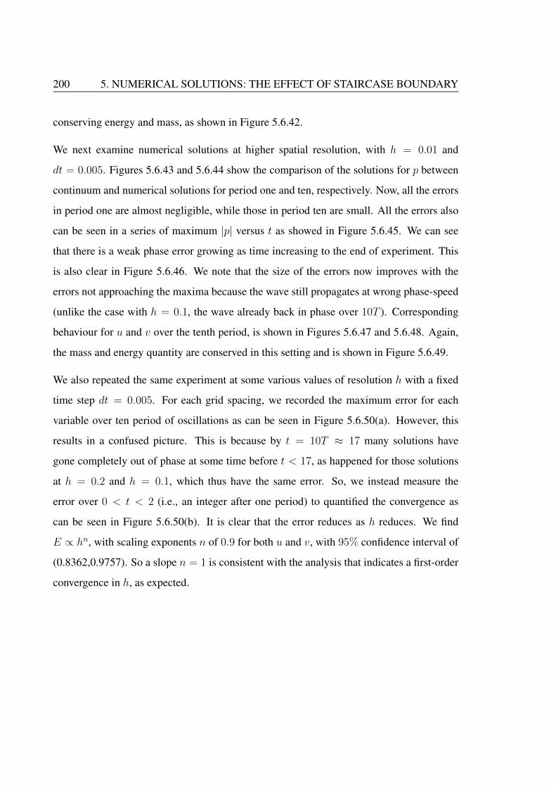
200 5. NUMERICAL SOLUTIONS: THE EFFECT OF STAIRCASE BOUNDARY
conserving energy and mass, as shown in Figure 5.6.42.
We next examine numerical solutions at higher spatial resolution, with h = 0.01 and
dt = 0.005. Figures 5.6.43 and 5.6.44 show the comparison of the solutions for p between
continuum and numerical solutions for period one and ten, respectively. Now, all the errors
in period one are almost negligible, while those in period ten are small. All the errors also
can be seen in a series of maximum |p| versus t as showed in Figure 5.6.45. We can see
that there is a weak phase error growing as time increasing to the end of experiment. This
is also clear in Figure 5.6.46. We note that the size of the errors now improves with the
errors not approaching the maxima because the wave still propagates at wrong phase-speed
(unlike the case with h = 0.1, the wave already back in phase over 10T ). Corresponding
behaviour for u and v over the tenth period, is shown in Figures 5.6.47 and 5.6.48. Again,
the mass and energy quantity are conserved in this setting and is shown in Figure 5.6.49.
We also repeated the same experiment at some various values of resolution h with a fixed
time step dt = 0.005. For each grid spacing, we recorded the maximum error for each
variable over ten period of oscillations as can be seen in Figure 5.6.50(a). However, this
results in a confused picture. This is because by t = 10T ≈ 17 many solutions have
gone completely out of phase at some time before t < 17, as happened for those solutions
at h = 0.2 and h = 0.1, which thus have the same error. So, we instead measure the
error over 0 < t < 2 (i.e., an integer after one period) to quantified the convergence as
can be seen in Figure 5.6.50(b). It is clear that the error reduces as h reduces. We find
E ∝ hn, with scaling exponents n of 0.9 for both u and v, with 95% confidence interval of
(0.8362,0.9757). So a slope n = 1 is consistent with the analysis that indicates a first-order
convergence in h, as expected.

5.7. SUMMARY 201
5.7 Summary
In this chapter, we have seen numerical solutions of waves equation sloshing in a square and
circle domain. For the square domain, we have seen the solutions at two particular cases:
(i) boundaries aligned with the grid, and (ii) boundaries unaligned with the grid. While for
the circle domain, we have seen the numerical solutions of two different wave modes (with
different azimuthal wavenumber) sloshing in the domain. The exact continuum solutions
is first derived to be used as an initial condition in the numerical experiment as well as to
compute the error of the solutions.
For the square domain boundaries aligned with the grid, we have shown that second-order
convergence in h is achieved, since central second-order finite-difference formulation is
used in the experiments. We thus confirmed that the rate of convergence will not be affected
as long as the boundaries aligned with the grid (second-order convergence in h is obtained
with angle θ = 90◦).
On the other hand, there is reduction of the order of accuracy for the case of unaligned
boundaries with staircase boundary. We have quantified this degradation in for u, v and
p. The quantification is obtained after one period of wave oscillation. We summarised all
the results in Table 5.11. It is shown that first-order convergence in h is obtained when the
square has staircase boundaries, which is consistent with the analysis in chapters 3 and 4.
We also have examined the effect of tilt angle. We have quantified the spatial convergence
rate at some angles. We found that the scaling factor for spatial error decrease with θ,
which as expected. This is agree with the results found in [32] for channel flow, where it
was showed that scaling factor for spatial error decrease with θ.
The solutions for waves sloshing in a circular domain are different. The investigation was
split into three experiments: (i) mode m = 1, n = 0, (ii) mode m = 1, n = 1, and (iii)
mode m = 1, n = 0. In experiments (i) and (ii), we used cell centre activation, while in (iii)
we used 4 corners of each cells as activation. Here, we also quantified the convergence rate
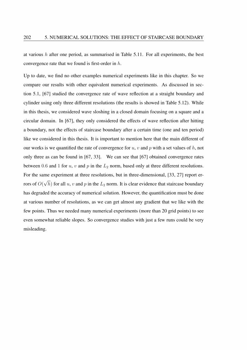
202 5. NUMERICAL SOLUTIONS: THE EFFECT OF STAIRCASE BOUNDARY
at various h after one period, as summarised in Table 5.11. For all experiments, the best
convergence rate that we found is first-order in h.
Up to date, we find no other examples numerical experiments like in this chapter. So we
compare our results with other equivalent numerical experiments. As discussed in sec-
tion 5.1, [67] studied the convergence rate of wave reflection at a straight boundary and
cylinder using only three different resolutions (the results is showed in Table 5.12). While
in this thesis, we considered wave sloshing in a closed domain focusing on a square and a
circular domain. In [67], they only considered the effects of wave reflection after hitting
a boundary, not the effects of staircase boundary after a certain time (one and ten period)
like we considered in this thesis. It is important to mention here that the main different of
our works is we quantified the rate of convergence for u, v and p with a set values of h, not
only three as can be found in [67, 33]. We can see that [67] obtained convergence rates
between 0.6 and 1 for u, v and p in the L2 norm, based only at three different resolutions.
For the same experiment at three resolutions, but in three-dimensional, [33, 27] report er-
rors of O(√h) for all u, v and p in the L2 norm. It is clear evidence that staircase boundary
has degraded the accuracy of numerical solution. However, the quantification must be done
at various number of resolutions, as we can get almost any gradient that we like with the
few points. Thus we needed many numerical experiments (more than 20 grid points) to see
even somewhat reliable slopes. So convergence studies with just a few runs could be very
misleading.
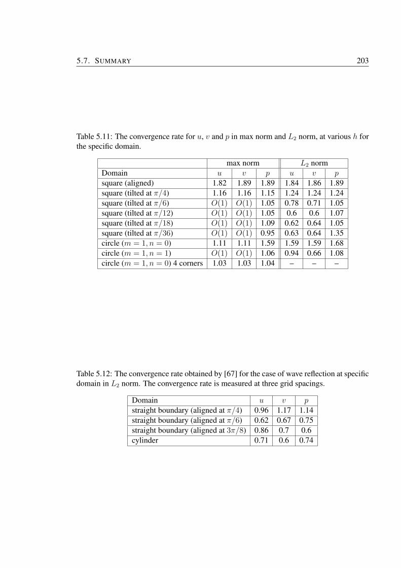
5.7. SUMMARY 203
Table 5.11: The convergence rate for u, v and p in max norm and L2 norm, at various h forthe specific domain.
max norm L2 normDomain u v p u v psquare (aligned) 1.82 1.89 1.89 1.84 1.86 1.89square (tilted at π/4) 1.16 1.16 1.15 1.24 1.24 1.24square (tilted at π/6) O(1) O(1) 1.05 0.78 0.71 1.05square (tilted at π/12) O(1) O(1) 1.05 0.6 0.6 1.07square (tilted at π/18) O(1) O(1) 1.09 0.62 0.64 1.05square (tilted at π/36) O(1) O(1) 0.95 0.63 0.64 1.35circle (m = 1, n = 0) 1.11 1.11 1.59 1.59 1.59 1.68circle (m = 1, n = 1) O(1) O(1) 1.06 0.94 0.66 1.08circle (m = 1, n = 0) 4 corners 1.03 1.03 1.04 – – –
Table 5.12: The convergence rate obtained by [67] for the case of wave reflection at specificdomain in L2 norm. The convergence rate is measured at three grid spacings.
Domain u v pstraight boundary (aligned at π/4) 0.96 1.17 1.14straight boundary (aligned at π/6) 0.62 0.67 0.75straight boundary (aligned at 3π/8) 0.86 0.7 0.6cylinder 0.71 0.6 0.74
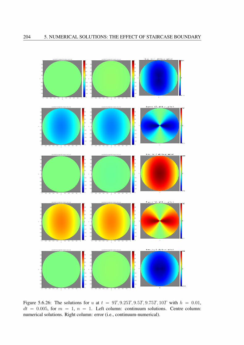
204 5. NUMERICAL SOLUTIONS: THE EFFECT OF STAIRCASE BOUNDARY
u at t=30.71, dx=dy=0.01, lx=ly=1, m=1, n=1
x
y
−1 −0.8 −0.6 −0.4 −0.2 0 0.2 0.4 0.6 0.8 1−1
−0.8
−0.6
−0.4
−0.2
0
0.2
0.4
0.6
0.8
1
−1
−0.8
−0.6
−0.4
−0.2
0
0.2
0.4
0.6
0.8
1u at t=30.71, dx=dy=0.01, lx=ly=1, m=1, n=1
x
y
−1 −0.8 −0.6 −0.4 −0.2 0 0.2 0.4 0.6 0.8 1−1
−0.8
−0.6
−0.4
−0.2
0
0.2
0.4
0.6
0.8
1
−1
−0.8
−0.6
−0.4
−0.2
0
0.2
0.4
0.6
0.8
1
u at t=31.57, dx=dy=0.01, lx=ly=1, m=1, n=1
x
y
−1 −0.8 −0.6 −0.4 −0.2 0 0.2 0.4 0.6 0.8 1−1
−0.8
−0.6
−0.4
−0.2
0
0.2
0.4
0.6
0.8
1
−1
−0.8
−0.6
−0.4
−0.2
0
0.2
0.4
0.6
0.8
1u at t=31.57, dx=dy=0.01, lx=ly=1, m=1, n=1
x
y
−1 −0.8 −0.6 −0.4 −0.2 0 0.2 0.4 0.6 0.8 1−1
−0.8
−0.6
−0.4
−0.2
0
0.2
0.4
0.6
0.8
1
−1
−0.8
−0.6
−0.4
−0.2
0
0.2
0.4
0.6
0.8
1
u at t=32.42, dx=dy=0.01, lx=ly=1, m=1, n=1
x
y
−1 −0.8 −0.6 −0.4 −0.2 0 0.2 0.4 0.6 0.8 1−1
−0.8
−0.6
−0.4
−0.2
0
0.2
0.4
0.6
0.8
1
−1
−0.8
−0.6
−0.4
−0.2
0
0.2
0.4
0.6
0.8
1u at t=32.42, dx=dy=0.01, lx=ly=1, m=1, n=1
x
y
−1 −0.8 −0.6 −0.4 −0.2 0 0.2 0.4 0.6 0.8 1−1
−0.8
−0.6
−0.4
−0.2
0
0.2
0.4
0.6
0.8
1
−1
−0.8
−0.6
−0.4
−0.2
0
0.2
0.4
0.6
0.8
1
u at t=33.27, dx=dy=0.01, lx=ly=1, m=1, n=1
x
y
−1 −0.8 −0.6 −0.4 −0.2 0 0.2 0.4 0.6 0.8 1−1
−0.8
−0.6
−0.4
−0.2
0
0.2
0.4
0.6
0.8
1
−1
−0.8
−0.6
−0.4
−0.2
0
0.2
0.4
0.6
0.8
1u at t=33.27, dx=dy=0.01, lx=ly=1, m=1, n=1
x
y
−1 −0.8 −0.6 −0.4 −0.2 0 0.2 0.4 0.6 0.8 1−1
−0.8
−0.6
−0.4
−0.2
0
0.2
0.4
0.6
0.8
1
−1
−0.8
−0.6
−0.4
−0.2
0
0.2
0.4
0.6
0.8
1
u at t=34.13, dx=dy=0.01, lx=ly=1, m=1, n=1
x
y
−1 −0.8 −0.6 −0.4 −0.2 0 0.2 0.4 0.6 0.8 1−1
−0.8
−0.6
−0.4
−0.2
0
0.2
0.4
0.6
0.8
1
−1
−0.8
−0.6
−0.4
−0.2
0
0.2
0.4
0.6
0.8
1u at t=34.13, dx=dy=0.01, lx=ly=1, m=1, n=1
x
y
−1 −0.8 −0.6 −0.4 −0.2 0 0.2 0.4 0.6 0.8 1−1
−0.8
−0.6
−0.4
−0.2
0
0.2
0.4
0.6
0.8
1
−1
−0.8
−0.6
−0.4
−0.2
0
0.2
0.4
0.6
0.8
1
Figure 5.6.26: The solutions for u at t = 9T, 9.25T, 9.5T, 9.75T, 10T with h = 0.01,dt = 0.005, for m = 1, n = 1. Left column: continuum solutions. Centre column:numerical solutions. Right column: error (i.e., continuum-numerical).
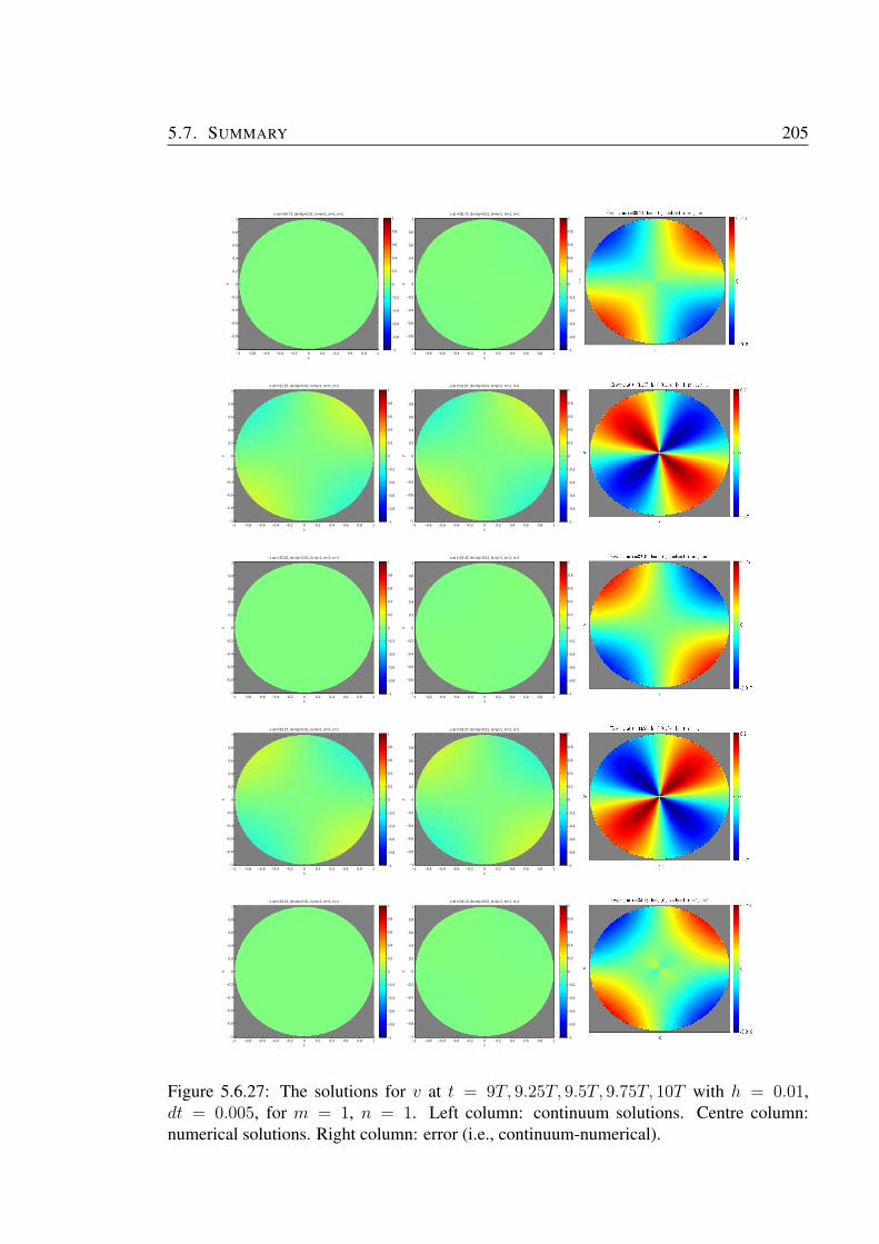
5.7. SUMMARY 205
v at t=30.71, dx=dy=0.01, lx=ly=1, m=1, n=1
x
y
−1 −0.8 −0.6 −0.4 −0.2 0 0.2 0.4 0.6 0.8 1−1
−0.8
−0.6
−0.4
−0.2
0
0.2
0.4
0.6
0.8
1
−1
−0.8
−0.6
−0.4
−0.2
0
0.2
0.4
0.6
0.8
1v at t=30.71, dx=dy=0.01, lx=ly=1, m=1, n=1
x
y
−1 −0.8 −0.6 −0.4 −0.2 0 0.2 0.4 0.6 0.8 1−1
−0.8
−0.6
−0.4
−0.2
0
0.2
0.4
0.6
0.8
1
−1
−0.8
−0.6
−0.4
−0.2
0
0.2
0.4
0.6
0.8
1
v at t=31.57, dx=dy=0.01, lx=ly=1, m=1, n=1
x
y
−1 −0.8 −0.6 −0.4 −0.2 0 0.2 0.4 0.6 0.8 1−1
−0.8
−0.6
−0.4
−0.2
0
0.2
0.4
0.6
0.8
1
−1
−0.8
−0.6
−0.4
−0.2
0
0.2
0.4
0.6
0.8
1v at t=31.57, dx=dy=0.01, lx=ly=1, m=1, n=1
x
y
−1 −0.8 −0.6 −0.4 −0.2 0 0.2 0.4 0.6 0.8 1−1
−0.8
−0.6
−0.4
−0.2
0
0.2
0.4
0.6
0.8
1
−1
−0.8
−0.6
−0.4
−0.2
0
0.2
0.4
0.6
0.8
1
v at t=32.42, dx=dy=0.01, lx=ly=1, m=1, n=1
x
y
−1 −0.8 −0.6 −0.4 −0.2 0 0.2 0.4 0.6 0.8 1−1
−0.8
−0.6
−0.4
−0.2
0
0.2
0.4
0.6
0.8
1
−1
−0.8
−0.6
−0.4
−0.2
0
0.2
0.4
0.6
0.8
1v at t=32.42, dx=dy=0.01, lx=ly=1, m=1, n=1
x
y
−1 −0.8 −0.6 −0.4 −0.2 0 0.2 0.4 0.6 0.8 1−1
−0.8
−0.6
−0.4
−0.2
0
0.2
0.4
0.6
0.8
1
−1
−0.8
−0.6
−0.4
−0.2
0
0.2
0.4
0.6
0.8
1
v at t=33.27, dx=dy=0.01, lx=ly=1, m=1, n=1
x
y
−1 −0.8 −0.6 −0.4 −0.2 0 0.2 0.4 0.6 0.8 1−1
−0.8
−0.6
−0.4
−0.2
0
0.2
0.4
0.6
0.8
1
−1
−0.8
−0.6
−0.4
−0.2
0
0.2
0.4
0.6
0.8
1v at t=33.27, dx=dy=0.01, lx=ly=1, m=1, n=1
x
y
−1 −0.8 −0.6 −0.4 −0.2 0 0.2 0.4 0.6 0.8 1−1
−0.8
−0.6
−0.4
−0.2
0
0.2
0.4
0.6
0.8
1
−1
−0.8
−0.6
−0.4
−0.2
0
0.2
0.4
0.6
0.8
1
v at t=34.13, dx=dy=0.01, lx=ly=1, m=1, n=1
x
y
−1 −0.8 −0.6 −0.4 −0.2 0 0.2 0.4 0.6 0.8 1−1
−0.8
−0.6
−0.4
−0.2
0
0.2
0.4
0.6
0.8
1
−1
−0.8
−0.6
−0.4
−0.2
0
0.2
0.4
0.6
0.8
1v at t=34.13, dx=dy=0.01, lx=ly=1, m=1, n=1
x
y
−1 −0.8 −0.6 −0.4 −0.2 0 0.2 0.4 0.6 0.8 1−1
−0.8
−0.6
−0.4
−0.2
0
0.2
0.4
0.6
0.8
1
−1
−0.8
−0.6
−0.4
−0.2
0
0.2
0.4
0.6
0.8
1
Figure 5.6.27: The solutions for v at t = 9T, 9.25T, 9.5T, 9.75T, 10T with h = 0.01,dt = 0.005, for m = 1, n = 1. Left column: continuum solutions. Centre column:numerical solutions. Right column: error (i.e., continuum-numerical).
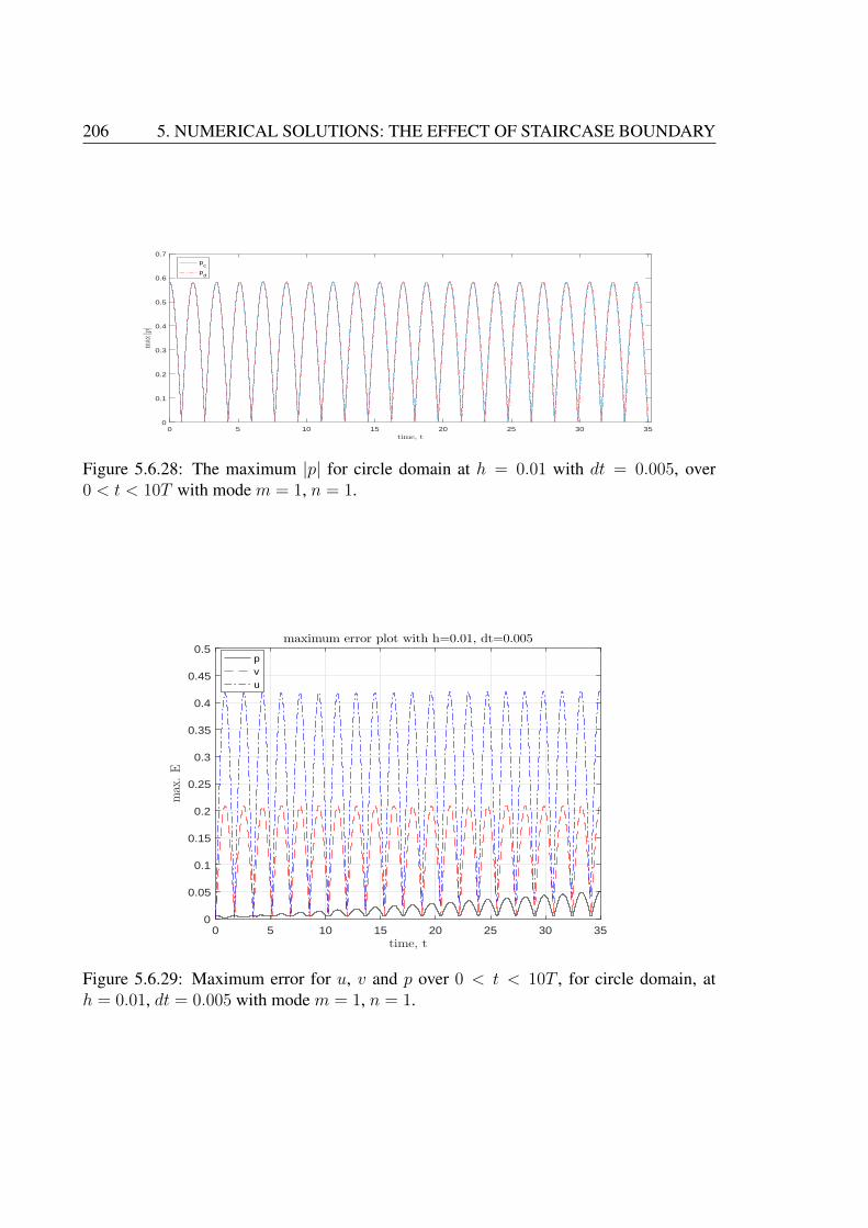
206 5. NUMERICAL SOLUTIONS: THE EFFECT OF STAIRCASE BOUNDARY
0 5 10 15 20 25 30 35time, t
0
0.1
0.2
0.3
0.4
0.5
0.6
0.7
max
|p|
pc
pd
Figure 5.6.28: The maximum |p| for circle domain at h = 0.01 with dt = 0.005, over0 < t < 10T with mode m = 1, n = 1.
0 5 10 15 20 25 30 35time, t
0
0.05
0.1
0.15
0.2
0.25
0.3
0.35
0.4
0.45
0.5
max
.E
maximum error plot with h=0.01, dt=0.005
pvu
Figure 5.6.29: Maximum error for u, v and p over 0 < t < 10T , for circle domain, ath = 0.01, dt = 0.005 with mode m = 1, n = 1.

5.7. SUMMARY 207
0 5 10 15 20 25 30 35-6
-4
-2
0
2
4h=0.01
×10-17 mass difference
0 5 10 15 20 25 30 35-1.5
-1
-0.5
0
h=0.01
×10-8 energy difference
Figure 5.6.30: Mass and energy difference for circle domain, at h = 0.01, dt = 0.005 over0 < t < 10T ≈ t = 35, for mode m = 1, n = 1.
-1.8 -1.6 -1.4 -1.2 -1 -0.8 -0.6log10(h)
-2.4
-2.2
-2
-1.8
-1.6
-1.4
-1.2
-1
-0.8
-0.6
-0.4
log10E
max norm
u
u (fit)
v
v (fit)
p
p (fit)
95% Confidence Intervals
-1.8 -1.6 -1.4 -1.2 -1 -0.8 -0.6log10(h)
-3
-2.5
-2
-1.5
-1
-0.5
0
log10E
L2 norm
u
u (fit)
v
v (fit)
p
p (fit)
95% Confidence Intervals
Figure 5.6.31: Convergence plot for circle domain with mode m = 1, n = 1 at various h inrange 0.2 < h < 0.02 at fixed dt = 0.02. The error in (a) is calculated in max norm, and(b) in L2 norm over domain. Slope of the lines is summarised in Table 5.10.
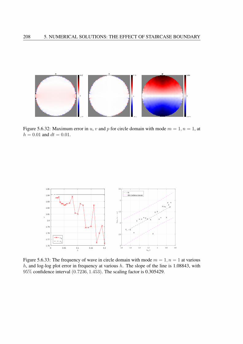
208 5. NUMERICAL SOLUTIONS: THE EFFECT OF STAIRCASE BOUNDARY
Figure 5.6.32: Maximum error in u, v and p for circle domain with mode m = 1, n = 1, ath = 0.01 and dt = 0.01.
0 0.05 0.1 0.15 0.2h
1.76
1.77
1.78
1.79
1.8
1.81
1.82
1.83
1.84
1.85
ω
ωd
ωc
-1.8 -1.6 -1.4 -1.2 -1 -0.8 -0.6log10 h
-3
-2.5
-2
-1.5
-1
-0.5
log10|ω
c−ωd|
Fit
95% Confidence Intervals
Figure 5.6.33: The frequency of wave in circle domain with mode m = 1, n = 1 at varioush, and log-log plot error in frequency at various h. The slope of the line is 1.08843, with95% confidence interval (0.7236, 1.453). The scaling factor is 0.305429.
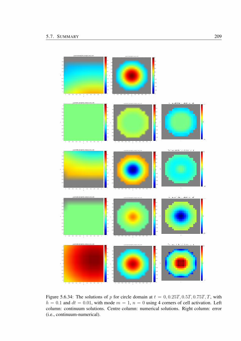
5.7. SUMMARY 209
p at t=0, dx=dy=0.1, lx=ly=1, m=1, n=0
-1 -0.8 -0.6 -0.4 -0.2 0 0.2 0.4 0.6 0.8 1
x
-1
-0.8
-0.6
-0.4
-0.2
0
0.2
0.4
0.6
0.8
1
y
-1
-0.8
-0.6
-0.4
-0.2
0
0.2
0.4
0.6
0.8
1 p at t=0, dx=dy=0.1, m=1, n=0
x
y
−1 −0.8 −0.6 −0.4 −0.2 0 0.2 0.4 0.6 0.8 1
−1
−0.8
−0.6
−0.4
−0.2
0
0.2
0.4
0.6
0.8
1
−1
−0.8
−0.6
−0.4
−0.2
0
0.2
0.4
0.6
0.8
1
p at t=0.41, dx=dy=0.1, lx=ly=1, m=1, n=0
-1 -0.8 -0.6 -0.4 -0.2 0 0.2 0.4 0.6 0.8 1
x
-1
-0.8
-0.6
-0.4
-0.2
0
0.2
0.4
0.6
0.8
1
y
-1
-0.8
-0.6
-0.4
-0.2
0
0.2
0.4
0.6
0.8
1 p at t=0.41, dx=dy=0.1, lx=ly=1, m=1, n=0
x
y
−1 −0.8 −0.6 −0.4 −0.2 0 0.2 0.4 0.6 0.8 1
−1
−0.8
−0.6
−0.4
−0.2
0
0.2
0.4
0.6
0.8
1
−1
−0.8
−0.6
−0.4
−0.2
0
0.2
0.4
0.6
0.8
1
p at t=0.82, dx=dy=0.1, lx=ly=1, m=1, n=0
-1 -0.8 -0.6 -0.4 -0.2 0 0.2 0.4 0.6 0.8 1
x
-1
-0.8
-0.6
-0.4
-0.2
0
0.2
0.4
0.6
0.8
1
y
-1
-0.8
-0.6
-0.4
-0.2
0
0.2
0.4
0.6
0.8
1 p at t=0.82, dx=dy=0.1, lx=ly=1, m=1, n=0
x
y
−1 −0.8 −0.6 −0.4 −0.2 0 0.2 0.4 0.6 0.8 1
−1
−0.8
−0.6
−0.4
−0.2
0
0.2
0.4
0.6
0.8
1
−1
−0.8
−0.6
−0.4
−0.2
0
0.2
0.4
0.6
0.8
1
p at t=1.23, dx=dy=0.1, lx=ly=1, m=1, n=0
-1 -0.8 -0.6 -0.4 -0.2 0 0.2 0.4 0.6 0.8 1
x
-1
-0.8
-0.6
-0.4
-0.2
0
0.2
0.4
0.6
0.8
1
y
-1
-0.8
-0.6
-0.4
-0.2
0
0.2
0.4
0.6
0.8
1 p at t=1.23, dx=dy=0.1, lx=ly=1, m=1, n=0
x
y
−1 −0.8 −0.6 −0.4 −0.2 0 0.2 0.4 0.6 0.8 1
−1
−0.8
−0.6
−0.4
−0.2
0
0.2
0.4
0.6
0.8
1
−1
−0.8
−0.6
−0.4
−0.2
0
0.2
0.4
0.6
0.8
1
p at t=1.64, dx=dy=0.1, lx=ly=1, m=1, n=0
-1 -0.8 -0.6 -0.4 -0.2 0 0.2 0.4 0.6 0.8 1
x
-1
-0.8
-0.6
-0.4
-0.2
0
0.2
0.4
0.6
0.8
1
y
-1
-0.8
-0.6
-0.4
-0.2
0
0.2
0.4
0.6
0.8
1 p at t=1.64, dx=dy=0.1, lx=ly=1, m=1, n=0
x
y
−1 −0.8 −0.6 −0.4 −0.2 0 0.2 0.4 0.6 0.8 1
−1
−0.8
−0.6
−0.4
−0.2
0
0.2
0.4
0.6
0.8
1
−1
−0.8
−0.6
−0.4
−0.2
0
0.2
0.4
0.6
0.8
1
Figure 5.6.34: The solutions of p for circle domain at t = 0, 0.25T, 0.5T, 0.75T, T , withh = 0.1 and dt = 0.01, with mode m = 1, n = 0 using 4 corners of cell activation. Leftcolumn: continuum solutions. Centre column: numerical solutions. Right column: error(i.e., continuum-numerical).
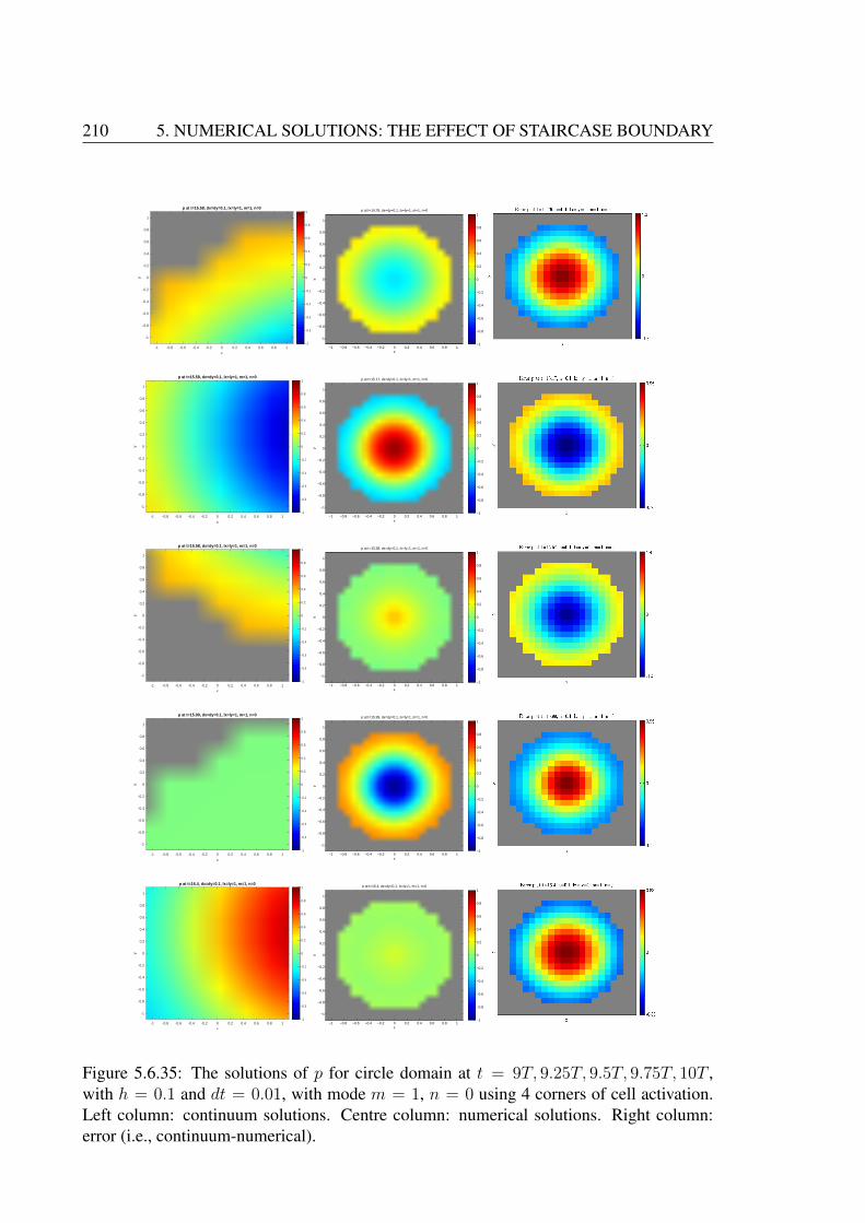
210 5. NUMERICAL SOLUTIONS: THE EFFECT OF STAIRCASE BOUNDARY
p at t=15.58, dx=dy=0.1, lx=ly=1, m=1, n=0
-1 -0.8 -0.6 -0.4 -0.2 0 0.2 0.4 0.6 0.8 1
x
-1
-0.8
-0.6
-0.4
-0.2
0
0.2
0.4
0.6
0.8
1
y
-1
-0.8
-0.6
-0.4
-0.2
0
0.2
0.4
0.6
0.8
1 p at t=14.76, dx=dy=0.1, lx=ly=1, m=1, n=0
x
y
−1 −0.8 −0.6 −0.4 −0.2 0 0.2 0.4 0.6 0.8 1
−1
−0.8
−0.6
−0.4
−0.2
0
0.2
0.4
0.6
0.8
1
−1
−0.8
−0.6
−0.4
−0.2
0
0.2
0.4
0.6
0.8
1
p at t=15.58, dx=dy=0.1, lx=ly=1, m=1, n=0
-1 -0.8 -0.6 -0.4 -0.2 0 0.2 0.4 0.6 0.8 1
x
-1
-0.8
-0.6
-0.4
-0.2
0
0.2
0.4
0.6
0.8
1
y
-1
-0.8
-0.6
-0.4
-0.2
0
0.2
0.4
0.6
0.8
1 p at t=15.17, dx=dy=0.1, lx=ly=1, m=1, n=0
x
y
−1 −0.8 −0.6 −0.4 −0.2 0 0.2 0.4 0.6 0.8 1
−1
−0.8
−0.6
−0.4
−0.2
0
0.2
0.4
0.6
0.8
1
−1
−0.8
−0.6
−0.4
−0.2
0
0.2
0.4
0.6
0.8
1
p at t=15.58, dx=dy=0.1, lx=ly=1, m=1, n=0
-1 -0.8 -0.6 -0.4 -0.2 0 0.2 0.4 0.6 0.8 1
x
-1
-0.8
-0.6
-0.4
-0.2
0
0.2
0.4
0.6
0.8
1
y
-1
-0.8
-0.6
-0.4
-0.2
0
0.2
0.4
0.6
0.8
1 p at t=15.58, dx=dy=0.1, lx=ly=1, m=1, n=0
x
y
−1 −0.8 −0.6 −0.4 −0.2 0 0.2 0.4 0.6 0.8 1
−1
−0.8
−0.6
−0.4
−0.2
0
0.2
0.4
0.6
0.8
1
−1
−0.8
−0.6
−0.4
−0.2
0
0.2
0.4
0.6
0.8
1
p at t=15.99, dx=dy=0.1, lx=ly=1, m=1, n=0
-1 -0.8 -0.6 -0.4 -0.2 0 0.2 0.4 0.6 0.8 1
x
-1
-0.8
-0.6
-0.4
-0.2
0
0.2
0.4
0.6
0.8
1
y
-1
-0.8
-0.6
-0.4
-0.2
0
0.2
0.4
0.6
0.8
1 p at t=15.99, dx=dy=0.1, lx=ly=1, m=1, n=0
x
y
−1 −0.8 −0.6 −0.4 −0.2 0 0.2 0.4 0.6 0.8 1
−1
−0.8
−0.6
−0.4
−0.2
0
0.2
0.4
0.6
0.8
1
−1
−0.8
−0.6
−0.4
−0.2
0
0.2
0.4
0.6
0.8
1
p at t=16.4, dx=dy=0.1, lx=ly=1, m=1, n=0
-1 -0.8 -0.6 -0.4 -0.2 0 0.2 0.4 0.6 0.8 1
x
-1
-0.8
-0.6
-0.4
-0.2
0
0.2
0.4
0.6
0.8
1
y
-1
-0.8
-0.6
-0.4
-0.2
0
0.2
0.4
0.6
0.8
1 p at t=16.4, dx=dy=0.1, lx=ly=1, m=1, n=0
x
y
−1 −0.8 −0.6 −0.4 −0.2 0 0.2 0.4 0.6 0.8 1
−1
−0.8
−0.6
−0.4
−0.2
0
0.2
0.4
0.6
0.8
1
−1
−0.8
−0.6
−0.4
−0.2
0
0.2
0.4
0.6
0.8
1
Figure 5.6.35: The solutions of p for circle domain at t = 9T, 9.25T, 9.5T, 9.75T, 10T ,with h = 0.1 and dt = 0.01, with mode m = 1, n = 0 using 4 corners of cell activation.Left column: continuum solutions. Centre column: numerical solutions. Right column:error (i.e., continuum-numerical).
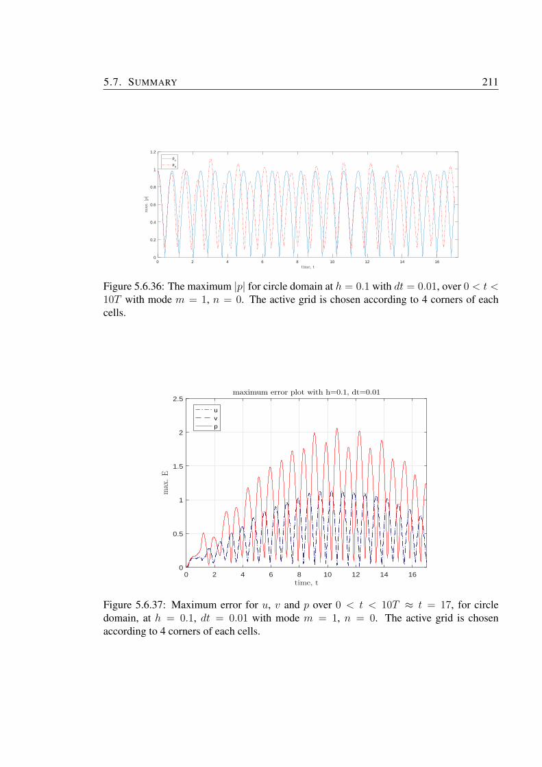
5.7. SUMMARY 211
0 2 4 6 8 10 12 14 16time, t
0
0.2
0.4
0.6
0.8
1
1.2
max.|p|
pc
pn
Figure 5.6.36: The maximum |p| for circle domain at h = 0.1 with dt = 0.01, over 0 < t <10T with mode m = 1, n = 0. The active grid is chosen according to 4 corners of eachcells.
0 2 4 6 8 10 12 14 16time, t
0
0.5
1
1.5
2
2.5
max
.E
maximum error plot with h=0.1, dt=0.01
uvp
Figure 5.6.37: Maximum error for u, v and p over 0 < t < 10T ≈ t = 17, for circledomain, at h = 0.1, dt = 0.01 with mode m = 1, n = 0. The active grid is chosenaccording to 4 corners of each cells.
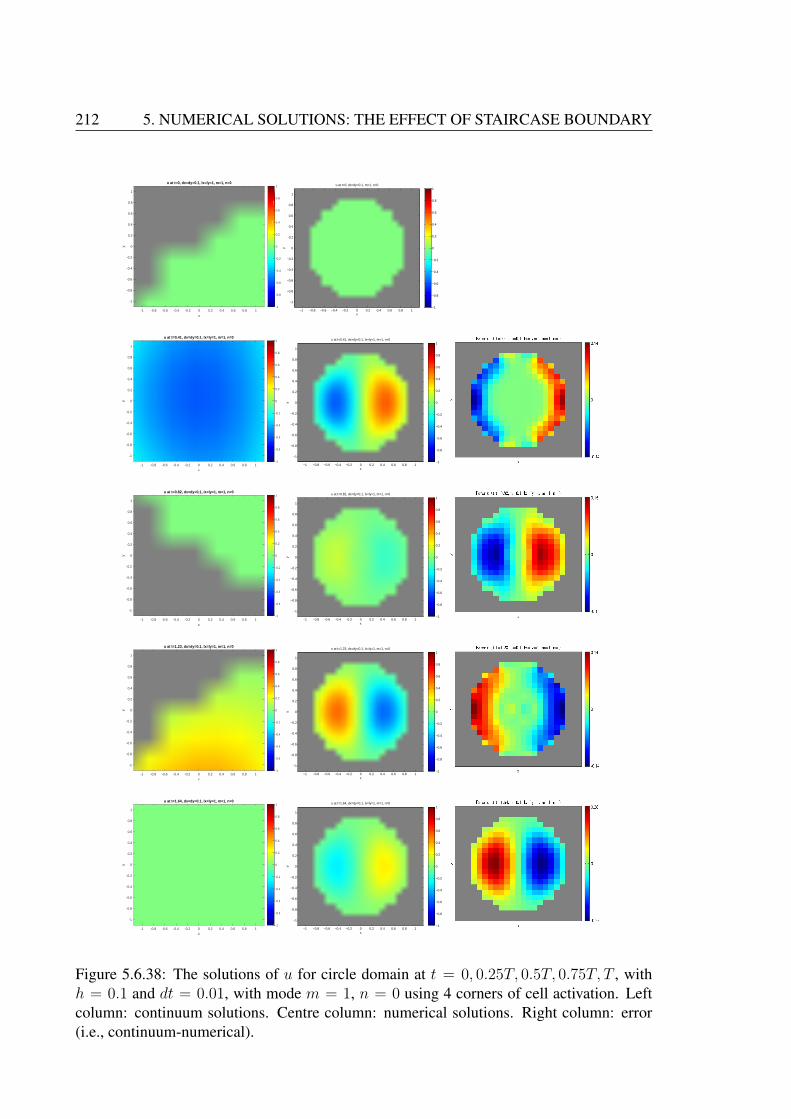
212 5. NUMERICAL SOLUTIONS: THE EFFECT OF STAIRCASE BOUNDARY
u at t=0, dx=dy=0.1, lx=ly=1, m=1, n=0
-1 -0.8 -0.6 -0.4 -0.2 0 0.2 0.4 0.6 0.8 1
x
-1
-0.8
-0.6
-0.4
-0.2
0
0.2
0.4
0.6
0.8
1
y
-1
-0.8
-0.6
-0.4
-0.2
0
0.2
0.4
0.6
0.8
1 u at t=0, dx=dy=0.1, m=1, n=0
x
y
−1 −0.8 −0.6 −0.4 −0.2 0 0.2 0.4 0.6 0.8 1
−1
−0.8
−0.6
−0.4
−0.2
0
0.2
0.4
0.6
0.8
1
−1
−0.8
−0.6
−0.4
−0.2
0
0.2
0.4
0.6
0.8
1
u at t=0.41, dx=dy=0.1, lx=ly=1, m=1, n=0
-1 -0.8 -0.6 -0.4 -0.2 0 0.2 0.4 0.6 0.8 1
x
-1
-0.8
-0.6
-0.4
-0.2
0
0.2
0.4
0.6
0.8
1
y
-1
-0.8
-0.6
-0.4
-0.2
0
0.2
0.4
0.6
0.8
1 u at t=0.41, dx=dy=0.1, lx=ly=1, m=1, n=0
x
y
−1 −0.8 −0.6 −0.4 −0.2 0 0.2 0.4 0.6 0.8 1
−1
−0.8
−0.6
−0.4
−0.2
0
0.2
0.4
0.6
0.8
1
−1
−0.8
−0.6
−0.4
−0.2
0
0.2
0.4
0.6
0.8
1
u at t=0.82, dx=dy=0.1, lx=ly=1, m=1, n=0
-1 -0.8 -0.6 -0.4 -0.2 0 0.2 0.4 0.6 0.8 1
x
-1
-0.8
-0.6
-0.4
-0.2
0
0.2
0.4
0.6
0.8
1
y
-1
-0.8
-0.6
-0.4
-0.2
0
0.2
0.4
0.6
0.8
1 u at t=0.82, dx=dy=0.1, lx=ly=1, m=1, n=0
x
y
−1 −0.8 −0.6 −0.4 −0.2 0 0.2 0.4 0.6 0.8 1
−1
−0.8
−0.6
−0.4
−0.2
0
0.2
0.4
0.6
0.8
1
−1
−0.8
−0.6
−0.4
−0.2
0
0.2
0.4
0.6
0.8
1
u at t=1.23, dx=dy=0.1, lx=ly=1, m=1, n=0
-1 -0.8 -0.6 -0.4 -0.2 0 0.2 0.4 0.6 0.8 1
x
-1
-0.8
-0.6
-0.4
-0.2
0
0.2
0.4
0.6
0.8
1
y
-1
-0.8
-0.6
-0.4
-0.2
0
0.2
0.4
0.6
0.8
1 u at t=1.23, dx=dy=0.1, lx=ly=1, m=1, n=0
x
y
−1 −0.8 −0.6 −0.4 −0.2 0 0.2 0.4 0.6 0.8 1
−1
−0.8
−0.6
−0.4
−0.2
0
0.2
0.4
0.6
0.8
1
−1
−0.8
−0.6
−0.4
−0.2
0
0.2
0.4
0.6
0.8
1
u at t=1.64, dx=dy=0.1, lx=ly=1, m=1, n=0
-1 -0.8 -0.6 -0.4 -0.2 0 0.2 0.4 0.6 0.8 1
x
-1
-0.8
-0.6
-0.4
-0.2
0
0.2
0.4
0.6
0.8
1
y
-1
-0.8
-0.6
-0.4
-0.2
0
0.2
0.4
0.6
0.8
1 u at t=1.64, dx=dy=0.1, lx=ly=1, m=1, n=0
x
y
−1 −0.8 −0.6 −0.4 −0.2 0 0.2 0.4 0.6 0.8 1
−1
−0.8
−0.6
−0.4
−0.2
0
0.2
0.4
0.6
0.8
1
−1
−0.8
−0.6
−0.4
−0.2
0
0.2
0.4
0.6
0.8
1
Figure 5.6.38: The solutions of u for circle domain at t = 0, 0.25T, 0.5T, 0.75T, T , withh = 0.1 and dt = 0.01, with mode m = 1, n = 0 using 4 corners of cell activation. Leftcolumn: continuum solutions. Centre column: numerical solutions. Right column: error(i.e., continuum-numerical).
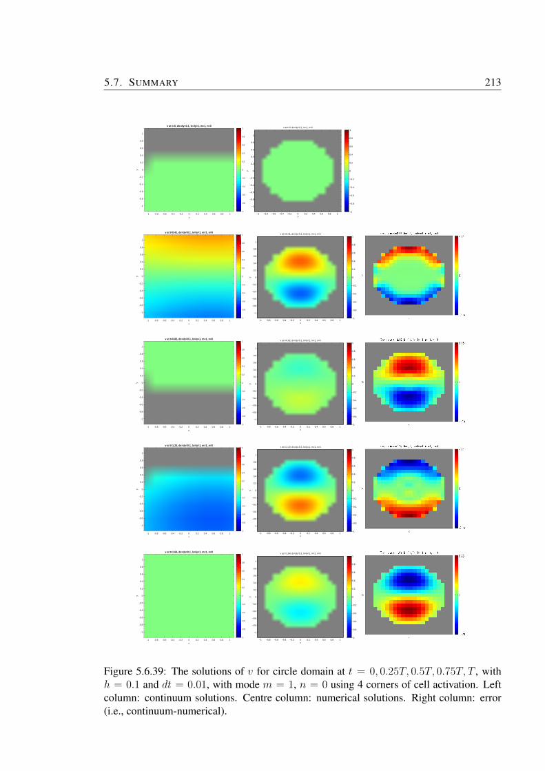
5.7. SUMMARY 213
v at t=0, dx=dy=0.1, lx=ly=1, m=1, n=0
-1 -0.8 -0.6 -0.4 -0.2 0 0.2 0.4 0.6 0.8 1
x
-1
-0.8
-0.6
-0.4
-0.2
0
0.2
0.4
0.6
0.8
1y
-1
-0.8
-0.6
-0.4
-0.2
0
0.2
0.4
0.6
0.8
1 v at t=0, dx=dy=0.1, m=1, n=0
x
y
−1 −0.8 −0.6 −0.4 −0.2 0 0.2 0.4 0.6 0.8 1
−1
−0.8
−0.6
−0.4
−0.2
0
0.2
0.4
0.6
0.8
1
−1
−0.8
−0.6
−0.4
−0.2
0
0.2
0.4
0.6
0.8
1
v at t=0.41, dx=dy=0.1, lx=ly=1, m=1, n=0
-1 -0.8 -0.6 -0.4 -0.2 0 0.2 0.4 0.6 0.8 1
x
-1
-0.8
-0.6
-0.4
-0.2
0
0.2
0.4
0.6
0.8
1
y
-1
-0.8
-0.6
-0.4
-0.2
0
0.2
0.4
0.6
0.8
1 v at t=0.41, dx=dy=0.1, lx=ly=1, m=1, n=0
x
y
−1 −0.8 −0.6 −0.4 −0.2 0 0.2 0.4 0.6 0.8 1
−1
−0.8
−0.6
−0.4
−0.2
0
0.2
0.4
0.6
0.8
1
−1
−0.8
−0.6
−0.4
−0.2
0
0.2
0.4
0.6
0.8
1
v at t=0.82, dx=dy=0.1, lx=ly=1, m=1, n=0
-1 -0.8 -0.6 -0.4 -0.2 0 0.2 0.4 0.6 0.8 1
x
-1
-0.8
-0.6
-0.4
-0.2
0
0.2
0.4
0.6
0.8
1
y
-1
-0.8
-0.6
-0.4
-0.2
0
0.2
0.4
0.6
0.8
1 v at t=0.82, dx=dy=0.1, lx=ly=1, m=1, n=0
x
y
−1 −0.8 −0.6 −0.4 −0.2 0 0.2 0.4 0.6 0.8 1
−1
−0.8
−0.6
−0.4
−0.2
0
0.2
0.4
0.6
0.8
1
−1
−0.8
−0.6
−0.4
−0.2
0
0.2
0.4
0.6
0.8
1
v at t=1.23, dx=dy=0.1, lx=ly=1, m=1, n=0
-1 -0.8 -0.6 -0.4 -0.2 0 0.2 0.4 0.6 0.8 1
x
-1
-0.8
-0.6
-0.4
-0.2
0
0.2
0.4
0.6
0.8
1
y
-1
-0.8
-0.6
-0.4
-0.2
0
0.2
0.4
0.6
0.8
1 v at t=1.23, dx=dy=0.1, lx=ly=1, m=1, n=0
x
y
−1 −0.8 −0.6 −0.4 −0.2 0 0.2 0.4 0.6 0.8 1
−1
−0.8
−0.6
−0.4
−0.2
0
0.2
0.4
0.6
0.8
1
−1
−0.8
−0.6
−0.4
−0.2
0
0.2
0.4
0.6
0.8
1
v at t=1.64, dx=dy=0.1, lx=ly=1, m=1, n=0
-1 -0.8 -0.6 -0.4 -0.2 0 0.2 0.4 0.6 0.8 1
x
-1
-0.8
-0.6
-0.4
-0.2
0
0.2
0.4
0.6
0.8
1
y
-1
-0.8
-0.6
-0.4
-0.2
0
0.2
0.4
0.6
0.8
1 v at t=1.64, dx=dy=0.1, lx=ly=1, m=1, n=0
x
y
−1 −0.8 −0.6 −0.4 −0.2 0 0.2 0.4 0.6 0.8 1
−1
−0.8
−0.6
−0.4
−0.2
0
0.2
0.4
0.6
0.8
1
−1
−0.8
−0.6
−0.4
−0.2
0
0.2
0.4
0.6
0.8
1
Figure 5.6.39: The solutions of v for circle domain at t = 0, 0.25T, 0.5T, 0.75T, T , withh = 0.1 and dt = 0.01, with mode m = 1, n = 0 using 4 corners of cell activation. Leftcolumn: continuum solutions. Centre column: numerical solutions. Right column: error(i.e., continuum-numerical).
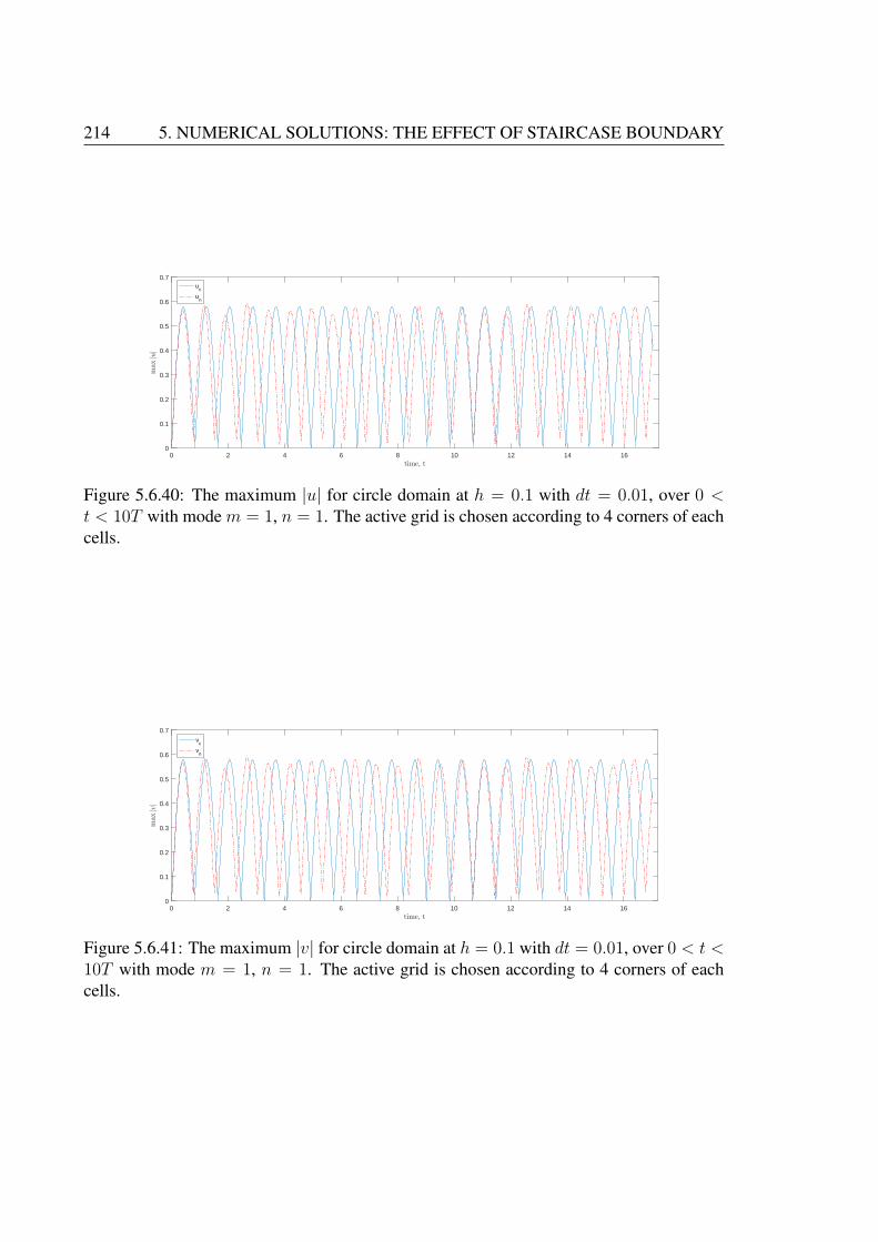
214 5. NUMERICAL SOLUTIONS: THE EFFECT OF STAIRCASE BOUNDARY
0 2 4 6 8 10 12 14 16time, t
0
0.1
0.2
0.3
0.4
0.5
0.6
0.7
max|u|
uc
un
Figure 5.6.40: The maximum |u| for circle domain at h = 0.1 with dt = 0.01, over 0 <t < 10T with mode m = 1, n = 1. The active grid is chosen according to 4 corners of eachcells.
0 2 4 6 8 10 12 14 16time, t
0
0.1
0.2
0.3
0.4
0.5
0.6
0.7
max|v|
vc
vn
Figure 5.6.41: The maximum |v| for circle domain at h = 0.1 with dt = 0.01, over 0 < t <10T with mode m = 1, n = 1. The active grid is chosen according to 4 corners of eachcells.
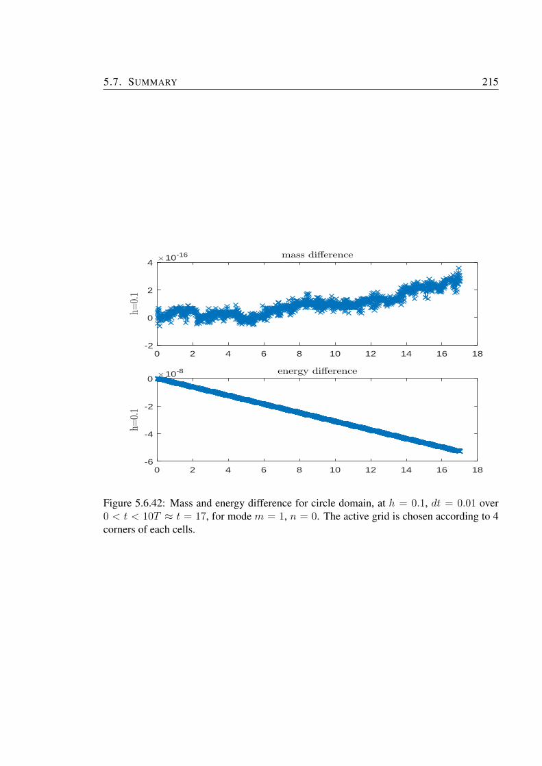
5.7. SUMMARY 215
0 2 4 6 8 10 12 14 16 18-2
0
2
4
h=0.1
×10-16 mass difference
0 2 4 6 8 10 12 14 16 18-6
-4
-2
0
h=0.1
×10-8 energy difference
Figure 5.6.42: Mass and energy difference for circle domain, at h = 0.1, dt = 0.01 over0 < t < 10T ≈ t = 17, for mode m = 1, n = 0. The active grid is chosen according to 4corners of each cells.

216 5. NUMERICAL SOLUTIONS: THE EFFECT OF STAIRCASE BOUNDARY
p at t=0, dx=dy=0.01, lx=ly=1, m=1, n=0
-1 -0.5 0 0.5 1
x
-1
-0.8
-0.6
-0.4
-0.2
0
0.2
0.4
0.6
0.8
1
y
-1
-0.8
-0.6
-0.4
-0.2
0
0.2
0.4
0.6
0.8
1p at t=0, dx=dy=0.01, lx=ly=1, m=1, n=0
-1 -0.5 0 0.5 1
x
-1
-0.8
-0.6
-0.4
-0.2
0
0.2
0.4
0.6
0.8
1
y
-1
-0.8
-0.6
-0.4
-0.2
0
0.2
0.4
0.6
0.8
1
p at t=0.41, dx=dy=0.01, lx=ly=1, m=1, n=0
-1 -0.5 0 0.5 1
x
-1
-0.8
-0.6
-0.4
-0.2
0
0.2
0.4
0.6
0.8
1
y
-1
-0.8
-0.6
-0.4
-0.2
0
0.2
0.4
0.6
0.8
1p at t=0.41, dx=dy=0.01, lx=ly=1, m=1, n=0
x
y
−1 −0.8 −0.6 −0.4 −0.2 0 0.2 0.4 0.6 0.8 1−1
−0.8
−0.6
−0.4
−0.2
0
0.2
0.4
0.6
0.8
1
−1
−0.8
−0.6
−0.4
−0.2
0
0.2
0.4
0.6
0.8
1
p at t=0.82, dx=dy=0.01, lx=ly=1, m=1, n=0
-1 -0.5 0 0.5 1
x
-1
-0.8
-0.6
-0.4
-0.2
0
0.2
0.4
0.6
0.8
1
y
-1
-0.8
-0.6
-0.4
-0.2
0
0.2
0.4
0.6
0.8
1p at t=0.82, dx=dy=0.01, lx=ly=1, m=1, n=0
x
y
−1 −0.8 −0.6 −0.4 −0.2 0 0.2 0.4 0.6 0.8 1−1
−0.8
−0.6
−0.4
−0.2
0
0.2
0.4
0.6
0.8
1
−1
−0.8
−0.6
−0.4
−0.2
0
0.2
0.4
0.6
0.8
1
p at t=1.23, dx=dy=0.01, lx=ly=1, m=1, n=0
-1 -0.5 0 0.5 1
x
-1
-0.8
-0.6
-0.4
-0.2
0
0.2
0.4
0.6
0.8
1
y
-1
-0.8
-0.6
-0.4
-0.2
0
0.2
0.4
0.6
0.8
1p at t=1.23, dx=dy=0.01, lx=ly=1, m=1, n=0
x
y
−1 −0.8 −0.6 −0.4 −0.2 0 0.2 0.4 0.6 0.8 1−1
−0.8
−0.6
−0.4
−0.2
0
0.2
0.4
0.6
0.8
1
−1
−0.8
−0.6
−0.4
−0.2
0
0.2
0.4
0.6
0.8
1
p at t=1.64, dx=dy=0.01, lx=ly=1, m=1, n=0
-1 -0.5 0 0.5 1
x
-1
-0.8
-0.6
-0.4
-0.2
0
0.2
0.4
0.6
0.8
1
y
-1
-0.8
-0.6
-0.4
-0.2
0
0.2
0.4
0.6
0.8
1p at t=1.64, dx=dy=0.01, lx=ly=1, m=1, n=0
x
y
−1 −0.8 −0.6 −0.4 −0.2 0 0.2 0.4 0.6 0.8 1−1
−0.8
−0.6
−0.4
−0.2
0
0.2
0.4
0.6
0.8
1
−1
−0.8
−0.6
−0.4
−0.2
0
0.2
0.4
0.6
0.8
1
Figure 5.6.43: The solutions of p for circle domain at t = 0, 0.25T, 0.5T, 0.75T, T , withh = 0.01 and dt = 0.005, with mode m = 1, n = 0 using 4 corners of cell activation. Leftcolumn: continuum solutions. Centre column: numerical solutions. Right column: error(i.e., continuum-numerical).
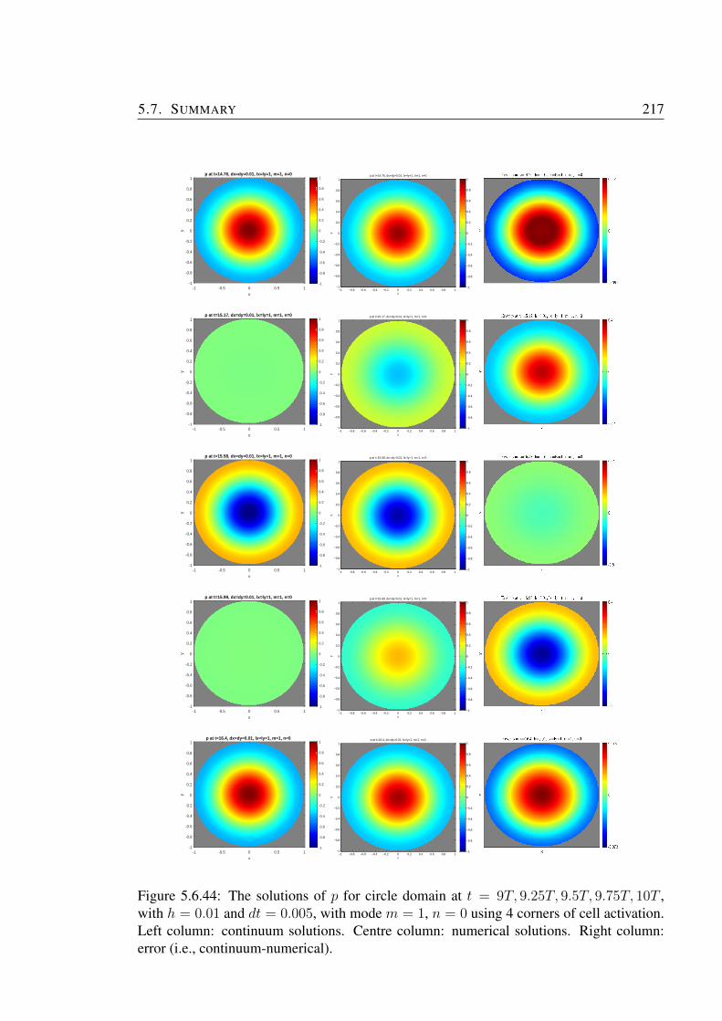
5.7. SUMMARY 217
p at t=14.76, dx=dy=0.01, lx=ly=1, m=1, n=0
-1 -0.5 0 0.5 1
x
-1
-0.8
-0.6
-0.4
-0.2
0
0.2
0.4
0.6
0.8
1y
-1
-0.8
-0.6
-0.4
-0.2
0
0.2
0.4
0.6
0.8
1p at t=14.76, dx=dy=0.01, lx=ly=1, m=1, n=0
x
y
−1 −0.8 −0.6 −0.4 −0.2 0 0.2 0.4 0.6 0.8 1−1
−0.8
−0.6
−0.4
−0.2
0
0.2
0.4
0.6
0.8
1
−1
−0.8
−0.6
−0.4
−0.2
0
0.2
0.4
0.6
0.8
1
p at t=15.17, dx=dy=0.01, lx=ly=1, m=1, n=0
-1 -0.5 0 0.5 1
x
-1
-0.8
-0.6
-0.4
-0.2
0
0.2
0.4
0.6
0.8
1
y
-1
-0.8
-0.6
-0.4
-0.2
0
0.2
0.4
0.6
0.8
1p at t=15.17, dx=dy=0.01, lx=ly=1, m=1, n=0
x
y
−1 −0.8 −0.6 −0.4 −0.2 0 0.2 0.4 0.6 0.8 1−1
−0.8
−0.6
−0.4
−0.2
0
0.2
0.4
0.6
0.8
1
−1
−0.8
−0.6
−0.4
−0.2
0
0.2
0.4
0.6
0.8
1
p at t=15.58, dx=dy=0.01, lx=ly=1, m=1, n=0
-1 -0.5 0 0.5 1
x
-1
-0.8
-0.6
-0.4
-0.2
0
0.2
0.4
0.6
0.8
1
y
-1
-0.8
-0.6
-0.4
-0.2
0
0.2
0.4
0.6
0.8
1p at t=15.58, dx=dy=0.01, lx=ly=1, m=1, n=0
x
y
−1 −0.8 −0.6 −0.4 −0.2 0 0.2 0.4 0.6 0.8 1−1
−0.8
−0.6
−0.4
−0.2
0
0.2
0.4
0.6
0.8
1
−1
−0.8
−0.6
−0.4
−0.2
0
0.2
0.4
0.6
0.8
1
p at t=15.99, dx=dy=0.01, lx=ly=1, m=1, n=0
-1 -0.5 0 0.5 1
x
-1
-0.8
-0.6
-0.4
-0.2
0
0.2
0.4
0.6
0.8
1
y
-1
-0.8
-0.6
-0.4
-0.2
0
0.2
0.4
0.6
0.8
1p at t=15.99, dx=dy=0.01, lx=ly=1, m=1, n=0
x
y
−1 −0.8 −0.6 −0.4 −0.2 0 0.2 0.4 0.6 0.8 1−1
−0.8
−0.6
−0.4
−0.2
0
0.2
0.4
0.6
0.8
1
−1
−0.8
−0.6
−0.4
−0.2
0
0.2
0.4
0.6
0.8
1
p at t=16.4, dx=dy=0.01, lx=ly=1, m=1, n=0
-1 -0.5 0 0.5 1
x
-1
-0.8
-0.6
-0.4
-0.2
0
0.2
0.4
0.6
0.8
1
y
-1
-0.8
-0.6
-0.4
-0.2
0
0.2
0.4
0.6
0.8
1p at t=16.4, dx=dy=0.01, lx=ly=1, m=1, n=0
x
y
−1 −0.8 −0.6 −0.4 −0.2 0 0.2 0.4 0.6 0.8 1−1
−0.8
−0.6
−0.4
−0.2
0
0.2
0.4
0.6
0.8
1
−1
−0.8
−0.6
−0.4
−0.2
0
0.2
0.4
0.6
0.8
1
Figure 5.6.44: The solutions of p for circle domain at t = 9T, 9.25T, 9.5T, 9.75T, 10T ,with h = 0.01 and dt = 0.005, with mode m = 1, n = 0 using 4 corners of cell activation.Left column: continuum solutions. Centre column: numerical solutions. Right column:error (i.e., continuum-numerical).

218 5. NUMERICAL SOLUTIONS: THE EFFECT OF STAIRCASE BOUNDARY
0 2 4 6 8 10 12 14 16time, t
0
0.2
0.4
0.6
0.8
1
1.2
max.|p|
pc
pn
Figure 5.6.45: The maximum |p| for circle domain at h = 0.01 with dt = 0.005, over0 < t < 10T with mode m = 1, n = 1. The active grid is chosen according to 4 corners ofeach cells.
0 2 4 6 8 10 12 14 16time, t
0
0.05
0.1
0.15
0.2
0.25
0.3
0.35
0.4
0.45
max
.E
maximum error plot with h=0.01, dt=0.005
uvp
Figure 5.6.46: Maximum error for u, v and p over 0 < t < 10T , for circle domain, ath = 0.01, dt = 0.005 with mode m = 1, n = 0. The active grid is chosen according to 4corners of each cells.
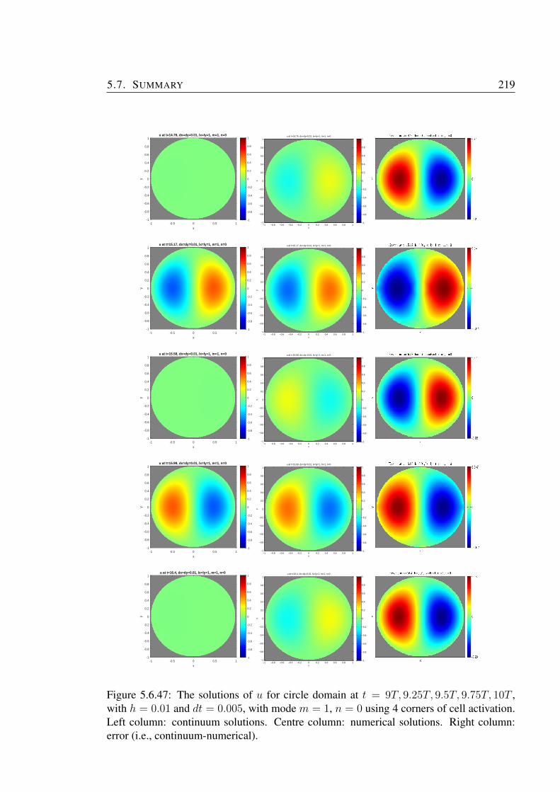
5.7. SUMMARY 219
u at t=14.76, dx=dy=0.01, lx=ly=1, m=1, n=0
-1 -0.5 0 0.5 1
x
-1
-0.8
-0.6
-0.4
-0.2
0
0.2
0.4
0.6
0.8
1y
-1
-0.8
-0.6
-0.4
-0.2
0
0.2
0.4
0.6
0.8
1u at t=14.76, dx=dy=0.01, lx=ly=1, m=1, n=0
x
y
−1 −0.8 −0.6 −0.4 −0.2 0 0.2 0.4 0.6 0.8 1−1
−0.8
−0.6
−0.4
−0.2
0
0.2
0.4
0.6
0.8
1
−1
−0.8
−0.6
−0.4
−0.2
0
0.2
0.4
0.6
0.8
1
u at t=15.17, dx=dy=0.01, lx=ly=1, m=1, n=0
-1 -0.5 0 0.5 1
x
-1
-0.8
-0.6
-0.4
-0.2
0
0.2
0.4
0.6
0.8
1
y
-1
-0.8
-0.6
-0.4
-0.2
0
0.2
0.4
0.6
0.8
1u at t=15.17, dx=dy=0.01, lx=ly=1, m=1, n=0
x
y
−1 −0.8 −0.6 −0.4 −0.2 0 0.2 0.4 0.6 0.8 1−1
−0.8
−0.6
−0.4
−0.2
0
0.2
0.4
0.6
0.8
1
−1
−0.8
−0.6
−0.4
−0.2
0
0.2
0.4
0.6
0.8
1
u at t=15.58, dx=dy=0.01, lx=ly=1, m=1, n=0
-1 -0.5 0 0.5 1
x
-1
-0.8
-0.6
-0.4
-0.2
0
0.2
0.4
0.6
0.8
1
y
-1
-0.8
-0.6
-0.4
-0.2
0
0.2
0.4
0.6
0.8
1u at t=15.58, dx=dy=0.01, lx=ly=1, m=1, n=0
x
y
−1 −0.8 −0.6 −0.4 −0.2 0 0.2 0.4 0.6 0.8 1−1
−0.8
−0.6
−0.4
−0.2
0
0.2
0.4
0.6
0.8
1
−1
−0.8
−0.6
−0.4
−0.2
0
0.2
0.4
0.6
0.8
1
u at t=15.99, dx=dy=0.01, lx=ly=1, m=1, n=0
-1 -0.5 0 0.5 1
x
-1
-0.8
-0.6
-0.4
-0.2
0
0.2
0.4
0.6
0.8
1
y
-1
-0.8
-0.6
-0.4
-0.2
0
0.2
0.4
0.6
0.8
1u at t=15.99, dx=dy=0.01, lx=ly=1, m=1, n=0
x
y
−1 −0.8 −0.6 −0.4 −0.2 0 0.2 0.4 0.6 0.8 1−1
−0.8
−0.6
−0.4
−0.2
0
0.2
0.4
0.6
0.8
1
−1
−0.8
−0.6
−0.4
−0.2
0
0.2
0.4
0.6
0.8
1
u at t=16.4, dx=dy=0.01, lx=ly=1, m=1, n=0
-1 -0.5 0 0.5 1
x
-1
-0.8
-0.6
-0.4
-0.2
0
0.2
0.4
0.6
0.8
1
y
-1
-0.8
-0.6
-0.4
-0.2
0
0.2
0.4
0.6
0.8
1u at t=16.4, dx=dy=0.01, lx=ly=1, m=1, n=0
x
y
−1 −0.8 −0.6 −0.4 −0.2 0 0.2 0.4 0.6 0.8 1−1
−0.8
−0.6
−0.4
−0.2
0
0.2
0.4
0.6
0.8
1
−1
−0.8
−0.6
−0.4
−0.2
0
0.2
0.4
0.6
0.8
1
Figure 5.6.47: The solutions of u for circle domain at t = 9T, 9.25T, 9.5T, 9.75T, 10T ,with h = 0.01 and dt = 0.005, with mode m = 1, n = 0 using 4 corners of cell activation.Left column: continuum solutions. Centre column: numerical solutions. Right column:error (i.e., continuum-numerical).
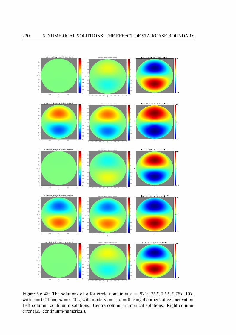
220 5. NUMERICAL SOLUTIONS: THE EFFECT OF STAIRCASE BOUNDARY
v at t=14.76, dx=dy=0.01, lx=ly=1, m=1, n=0
-1 -0.5 0 0.5 1
x
-1
-0.8
-0.6
-0.4
-0.2
0
0.2
0.4
0.6
0.8
1
y
-1
-0.8
-0.6
-0.4
-0.2
0
0.2
0.4
0.6
0.8
1v at t=14.76, dx=dy=0.01, lx=ly=1, m=1, n=0
x
y
−1 −0.8 −0.6 −0.4 −0.2 0 0.2 0.4 0.6 0.8 1−1
−0.8
−0.6
−0.4
−0.2
0
0.2
0.4
0.6
0.8
1
−1
−0.8
−0.6
−0.4
−0.2
0
0.2
0.4
0.6
0.8
1
v at t=15.17, dx=dy=0.01, lx=ly=1, m=1, n=0
-1 -0.5 0 0.5 1
x
-1
-0.8
-0.6
-0.4
-0.2
0
0.2
0.4
0.6
0.8
1
y
-1
-0.8
-0.6
-0.4
-0.2
0
0.2
0.4
0.6
0.8
1v at t=15.17, dx=dy=0.01, lx=ly=1, m=1, n=0
x
y
−1 −0.8 −0.6 −0.4 −0.2 0 0.2 0.4 0.6 0.8 1−1
−0.8
−0.6
−0.4
−0.2
0
0.2
0.4
0.6
0.8
1
−1
−0.8
−0.6
−0.4
−0.2
0
0.2
0.4
0.6
0.8
1
v at t=15.58, dx=dy=0.01, lx=ly=1, m=1, n=0
-1 -0.5 0 0.5 1
x
-1
-0.8
-0.6
-0.4
-0.2
0
0.2
0.4
0.6
0.8
1
y
-1
-0.8
-0.6
-0.4
-0.2
0
0.2
0.4
0.6
0.8
1v at t=15.58, dx=dy=0.01, lx=ly=1, m=1, n=0
x
y
−1 −0.8 −0.6 −0.4 −0.2 0 0.2 0.4 0.6 0.8 1−1
−0.8
−0.6
−0.4
−0.2
0
0.2
0.4
0.6
0.8
1
−1
−0.8
−0.6
−0.4
−0.2
0
0.2
0.4
0.6
0.8
1
v at t=15.99, dx=dy=0.01, lx=ly=1, m=1, n=0
-1 -0.5 0 0.5 1
x
-1
-0.8
-0.6
-0.4
-0.2
0
0.2
0.4
0.6
0.8
1
y
-1
-0.8
-0.6
-0.4
-0.2
0
0.2
0.4
0.6
0.8
1v at t=15.99, dx=dy=0.01, lx=ly=1, m=1, n=0
x
y
−1 −0.8 −0.6 −0.4 −0.2 0 0.2 0.4 0.6 0.8 1−1
−0.8
−0.6
−0.4
−0.2
0
0.2
0.4
0.6
0.8
1
−1
−0.8
−0.6
−0.4
−0.2
0
0.2
0.4
0.6
0.8
1
v at t=16.4, dx=dy=0.01, lx=ly=1, m=1, n=0
-1 -0.5 0 0.5 1
x
-1
-0.8
-0.6
-0.4
-0.2
0
0.2
0.4
0.6
0.8
1
y
-1
-0.8
-0.6
-0.4
-0.2
0
0.2
0.4
0.6
0.8
1v at t=16.4, dx=dy=0.01, lx=ly=1, m=1, n=0
x
y
−1 −0.8 −0.6 −0.4 −0.2 0 0.2 0.4 0.6 0.8 1−1
−0.8
−0.6
−0.4
−0.2
0
0.2
0.4
0.6
0.8
1
−1
−0.8
−0.6
−0.4
−0.2
0
0.2
0.4
0.6
0.8
1
Figure 5.6.48: The solutions of v for circle domain at t = 9T, 9.25T, 9.5T, 9.75T, 10T ,with h = 0.01 and dt = 0.005, with mode m = 1, n = 0 using 4 corners of cell activation.Left column: continuum solutions. Centre column: numerical solutions. Right column:error (i.e., continuum-numerical).
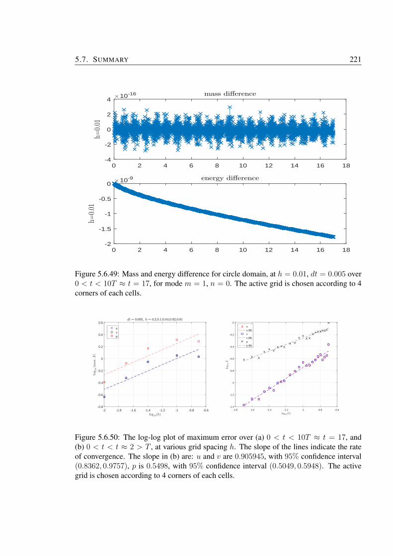
5.7. SUMMARY 221
0 2 4 6 8 10 12 14 16 18-4
-2
0
2
4h=
0.01
×10-16 mass difference
0 2 4 6 8 10 12 14 16 18-2
-1.5
-1
-0.5
0
h=0.01
×10-9 energy difference
Figure 5.6.49: Mass and energy difference for circle domain, at h = 0.01, dt = 0.005 over0 < t < 10T ≈ t = 17, for mode m = 1, n = 0. The active grid is chosen according to 4corners of each cells.
-2 -1.8 -1.6 -1.4 -1.2 -1 -0.8 -0.6log10(h)
-0.8
-0.6
-0.4
-0.2
0
0.2
0.4
0.6
log10|m
ax.E|
dt = 0.005, h = 0.2,0.1,0.04,0.02,0.01
uvp
-1.8 -1.6 -1.4 -1.2 -1 -0.8 -0.6log10(h)
-1.4
-1.2
-1
-0.8
-0.6
-0.4
-0.2
0
log10E
u
u (fit)
v
v (fit)
p
p (fit)
Figure 5.6.50: The log-log plot of maximum error over (a) 0 < t < 10T ≈ t = 17, and(b) 0 < t < t ≈ 2 > T , at various grid spacing h. The slope of the lines indicate the rateof convergence. The slope in (b) are: u and v are 0.905945, with 95% confidence interval(0.8362, 0.9757), p is 0.5498, with 95% confidence interval (0.5049, 0.5948). The activegrid is chosen according to 4 corners of each cells.

222 5. NUMERICAL SOLUTIONS: THE EFFECT OF STAIRCASE BOUNDARY

223
Chapter 6
REFLECTION AND FOCUSSING OF
INTERNAL GRAVITY WAVES
6.1 Introduction
Wave phenomena that we have discussed so far exist on the surface of a boundary. If
we look beneath the surface another kind of wave also can be discovered, which is internal
waves. They are mostly hidden for eyesight but it is very important. The main ingredient for
these waves to be generated is due to the density variations in a fluid. An obvious example
of fluid with density differences is the ocean. As we go down into the ocean, the density of
the water increase with light fluid overlying dense fluid. Such fluids are said to be stratified.
Waves in the fluids exist due to restoring forces; a fluid parcel moved vertically is pushed
back to its starting level, giving oscillations. It goes almost without saying that the same
mechanism is at work whenever two fluid densities differ. The oscillations in the stratified
fluid are normally called internal gravity waves. The main difference with the waves on the
surface is that internal waves are generally slower because they rely on a weaker density
difference and can propagate both vertically and horizontally.
224 6. REFLECTION AND FOCUSSING OF INTERNAL GRAVITY WAVES
Early investigation of internal gravity waves was motivated by F. Nansen in 1902 with an
observation of a phenomenon on the Arctic Ocean or the so called “Dead Water” [26]. The
phenomenon is one of the motivations for the waves in fluids that are stratified. The ocean
is an example of stratified fluid in which internal gravity waves can be found. The oceans
are stratified in density as a result of many geophysical processes, like evaporation, cool-
ing, and mixing with fresh meltwater [63]. In the ocean, it is speculated that these internal
waves may thus play an important role in maintaining the large-scale deep circulation, by
providing downward mixing heat [62]. Their mixing may also be relevant for marine eco-
systems by providing nutrients to the water column. These phenomena not only happen at
the ocean. It also can occur in the atmosphere which can lead to distinctive cloud patterns
that results from condensation of water vapour; rising air becomes cooler.
In a stratified medium, buoyancy forces arise subject to gravity. There is a special property
that ensure the oscillations mechanism. To illustrate, we suppose fluid to be at rest, with
vertical density stratification ρ = ρ0(z), and the corresponding hydrostatic balance for
pressure is
dp0
dz= −gρ0(z). (6.1.1)
By considering a small fluid parcel at z = z∗, and assumed the density on the fluid is
conserved such that dρ/dt = 0. On the stationary fluid parcel, there is a balance between
gravity and the pressure gradient
−dp0
dz= gρ0(z∗).
If we displace the fluid parcel vertically to z = z∗ + δ(t), we can use Newton’s 2nd law
6.1. INTRODUCTION 225
F = ma to determine the subsequent motion of the fluid parcel:
ρ0(z∗)d2δ
dt2= −gρ0(z∗)−
dp0
dz|z∗+δ
= −gρ0(z∗) + gρ0 (z∗ + δ) ,
= −gρ0(z∗) + g
(ρ0(z∗) + δ
dρ0
dz|z∗ +O(δ2)
),
⇒ d2δ
dt2≈(g
ρ0
dρ0
dz
)|z∗δ.
If dρ0/dz > 0, then δ(t) can grow exponentially in time: the configuration is unstable.
If dρ0/dz < 0, there is vertical oscillatory motion: d2δ/dt2 = −N2∗ δ which implies δ =
δ0 cos(N∗t), where N∗ = N(z∗) and
N2(z) = − g
ρ0
dρ0
dz. (6.1.2)
The quantity N(z) is known as the buoyancy frequency, or Brunt-Vaisala frequency. It
gives the theoretical frequency of vertical oscillations of a small parcel of fluid in a stratified
medium.
A typical dispersion relation of internal gravity waves is
ω2 =N2k2
k2 +m2, (6.1.3)
where k and m are wavenumbers in the horizontal and vertical, respectively, and N2 now
is assumed as a constant. It is clear that the dispersion relation has a relationship between
wavenumbers and wave frequency. Obviously, (6.1.3) is depends on N2. In general, for
m 6= 0, we have
ωc ≤ N. (6.1.4)
In the absence of vertical wavenumber (m = 0), we then have ω = N . The phase speed
226 6. REFLECTION AND FOCUSSING OF INTERNAL GRAVITY WAVES
then is cp = ω/k = N/k. This means that the particle motions are purely vertical; in
agreement with the definition of buoyancy frequency. On the other side, for the purely
vertical wavenumber (k = 0), the frequency then vanishes (ω = 0). The particle motions
are then horizontal, which implies that there is no wave propagation. Unlike surface wave
(acoustic), these waves are anisotropic because the frequency depends on the direction.
A further linear property of internal gravity waves is that if these wave reflect from a solid
boundary then in general the wavenumbers of incident and reflected waves are unequal
[53]. The consequence of this is that, after reflection the internal gravity waves change their
direction, but retain the same frequency. This can be illustrated from the dispersion relation
(6.1.3), which shows that the frequency of internal waves independent of the magnitude
wavenumber. To bring this out, it is useful to specify wavenumber (k,m) as
(k,m) = |κ|(cos θ, sin θ) ⇒ ω = N cos θ, (6.1.5)
where |κ| is the wave magnitude and θ is the angle between the horizontal and the resultant
wavenumber vector |κ|. This means that the frequency depends only on the angle θ.
Upon reflection, this angle must be the same since the frequency depends only on θ, re-
gardless of the angle of the bottom boundary, β. In other words, the angle of incident and
reflected to the vertical are equal. However, reflection at an inclined boundary with angle β
altered the angle of incident and reflected waves, which makes them unequal, as shown in
Figure 6.4.1. If β > ϕ, the wave is reflected back with horizontal component of group ve-
locity in the opposite direction to the incident wave. On the other hand, if β < ϕ, the wave
will have forward reflection. In the ocean, a shallow wedge acts as a perfect absorber of
internal gravity waves, as the waves propagate further. In a shallow wedge, the wavelength
will decrease with the change of magnitude of wave, in accord with [53]. Note that, in the
case of β = 0 or π/2, there is no change in wavenumber and perfect internal wave reflection
can occur.
6.1. INTRODUCTION 227
There are numerous investigations on the reflection of internal gravity waves in different
approaches and interest, either in analytically [10, 22], numerically [28, 40, 60], or experi-
mentally [16, 64]. Most of them are toward understanding the dynamical aspect of internal
wave during reflection. These include the interactions between incident and reflected waves
in the development of nonlinearities and topographic influences, and also towards under-
standing the dynamical aspects in the critical regime which is β = ϕ [22, 40, 21]. In the
critical regime, reflected internal wave is expected to have zero group velocity, infinite amp-
litude and infinite wavelength, which results incoming wave trap in the boundary region and
wave breaking [61]. In such a case, nonlinearities and turbulence must come into play. As
the investigation in this thesis rely on the linear theory, which focus on the reflection of the
incoming wave, there is no consideration for the case of the criticality. However, another
criterion for the internal wave reflection is the sloping boundary. So that we will focus on
this effect for the internal wave reflection with numerical approach.
The representation of an inclined boundary in finite-difference numerical model commonly
finished by staircase boundary. A comparison study of the boundary representation in geo-
physical numerical models was done by [60]. In the study, they compare two techniques
to approximate the bottom boundary which are the staircase and piecewise linear fashion,
which the performance of both techniques are predict using an analytical solution in Fourier
space. The main difference in these two techniques is the boundary condition implementa-
tion. In the staircase approximation, the no-flux boundary condition usually enforced on the
sidewall of the grid. While the boundary condition in the piecewise linear representation is
imposed directly on the linear approximation. Analysis in the study focus on the reflection
coefficient for linear internal wave in a rectangular channel containing a linearly stratified
fluid and Gaussian bump acts as bottom topography. From the analysis, they found that the
reflection coefficient behaviour with staircase Gaussian bump is not uniform towards the
analytical solution. There are aliasing effect which is the effect of discrete Fourier trans-
form. On the other hand, reflection coefficient with the piecewise linear approximation
behave with the analytical solution. However, the advantage of this technique also minimal
228 6. REFLECTION AND FOCUSSING OF INTERNAL GRAVITY WAVES
in the case of small grid size.
The linear approximation strategy for the bottom boundary is achieved using the terrain-
following coordinates, so that the thickness of the bottom topography is varied along the
topography. Moreover, the importance of gravity in the ocean may suffer with this tech-
nique since the approach only focus upon the effects of topography. Although the piecewise
linear fashion was showed to have a better solution than the staircase approximation [3], the
performance of the technique is limited to a few of sensitivity and may not be implemen-
ted to all types of flow. While in the staircase approximation, it is generally agree that the
smaller the grid size in the approximation, the more smooth the bottom topography, and
hence the more accurate the numerical solution. Therefore, it is agreed that the grid size in
the staircase approximation play an important role in the accuracy of numerical solution.
However, there is no sufficient quantification of the resulting scheme towards the analytical
solution as grid spacing tends to zero. It is thus desirable to quantify the effects of grid
spacing to the internal wave reflection at a sloping boundary.
Upon reflection at an inclined boundary, internal gravity waves preserve their frequency
and consequently their angle with respect to the gravitational direction [44]. These waves
also change their wavelength which resulting either focusing or defocusing when reflecting
from boundary. The situation where the waves become focused when reflecting from a
sloping boundary, and converge towards limit cycle is called wave attractor [46, 48]. Many
investigations have been performed to confirm this behavior, either analytically [46, 36, 35],
or in numerical experiments [11, 41]. Understanding the dynamical properties of internal
gravity waves in a bounded domain is important for explaining the mixing process in ocean
basins and lakes. It also has relation to astrophysics and fluid dynamics [50, 41].
For the analytical investigation, the usual governing equations that describe internal gravity
waves can be solved with appropriate initial and boundary conditions. However, it becomes
more difficult to solve directly because it involves with the initial boundary value problem
and the solutions are not easily be written in closed form [35]. Another handful laboratory

6.2. EQUATIONS OF MOTION FOR STRATIFIED FLUID 229
experiment is described in [58] where they showed that the waves defocusing when there is
no sloping boundaries. Thus, in this chapter we only focused on the numerical experiments
on internal gravity wave attractors. For the numerical experiment, we consider the fluid is
in the square geometry. This investigation is important since we can make further analysis
on the patterns of internal gravity wave attractors when the sloping wall is represented with
staircase configurations.
The aim of this chapter is to start extending some of the ideas from chapters 2-5 to internal
gravity waves. We start by introducing the equations of motion in section 6.2, and then
consider in section 6.3 how these equations may be configured on staggered grids, deriving
the relevant dispersion relation for internal gravity waves in an unbounded medium. In
section 6.4 we consider plane internal gravity wave reflection at a sloping boundary. The
classic continuum reflection is reviewed in section 6.4.1, before we present what is believed
to be a completely novel discrete reflection calculation in section 6.4.2. We will find an
error of O(h) in the discrete reflection problem, and this suggests that issues may then arise
in phenomena driven by internal gravity reflection. Thus, in section 6.5, we consider the
phenomena of internal wave focussing in closed domain, which is driven by a particular
property of internal gravity wave reflection. Our idea is that staircase boundaries may
prevent or alter the focussing phenomena. However, in section 6.5 we are only able to
present provisional calculations towards this end in rectangular domains, without staircase
boundaries.
6.2 Equations of Motion for Stratified Fluid
To study internal gravity waves, a few assumptions are necessary. Since internal gravity
waves generally can be found in the stratified fluid, it is worth to mention here that we
will focus on the internal gravity waves in the ocean. So that further simplification and
assumption is possible and desirable. In the ocean, the density variations are small when
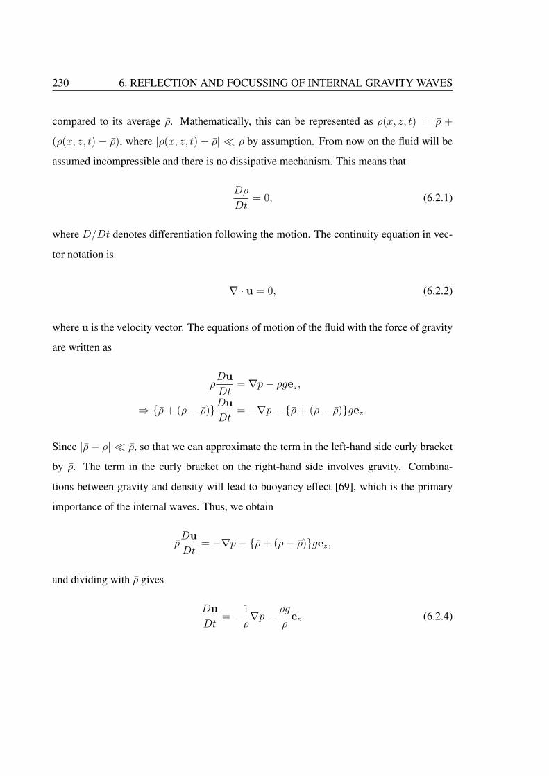
230 6. REFLECTION AND FOCUSSING OF INTERNAL GRAVITY WAVES
compared to its average ρ. Mathematically, this can be represented as ρ(x, z, t) = ρ +
(ρ(x, z, t) − ρ), where |ρ(x, z, t)− ρ| � ρ by assumption. From now on the fluid will be
assumed incompressible and there is no dissipative mechanism. This means that
Dρ
Dt= 0, (6.2.1)
where D/Dt denotes differentiation following the motion. The continuity equation in vec-
tor notation is
∇ · u = 0, (6.2.2)
where u is the velocity vector. The equations of motion of the fluid with the force of gravity
are written as
ρDu
Dt= ∇p− ρgez,
⇒ {ρ+ (ρ− ρ)}Du
Dt= −∇p− {ρ+ (ρ− ρ)}gez.
Since |ρ− ρ| � ρ, so that we can approximate the term in the left-hand side curly bracket
by ρ. The term in the curly bracket on the right-hand side involves gravity. Combina-
tions between gravity and density will lead to buoyancy effect [69], which is the primary
importance of the internal waves. Thus, we obtain
ρDu
Dt= −∇p− {ρ+ (ρ− ρ)}gez,
and dividing with ρ gives
Du
Dt= −1
ρ∇p− ρg
ρez. (6.2.4)
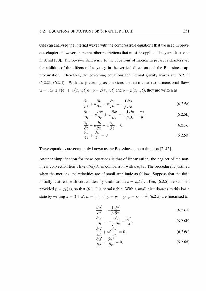
6.2. EQUATIONS OF MOTION FOR STRATIFIED FLUID 231
One can analysed the internal waves with the compressible equations that we used in previ-
ous chapter. However, there are other restrictions that must be applied. They are discussed
in detail [70]. The obvious difference to the equations of motion in previous chapters are
the addition of the effects of buoyancy in the vertical direction and the Boussinesq ap-
proximation. Therefore, the governing equations for internal gravity waves are (6.2.1),
(6.2.2), (6.2.4). With the preceding assumptions and restrict at two-dimensional flows
u = u(x, z, t)ex + w(x, z, t)ez, ρ = ρ(x, z, t) and p = p(x, z, t), they are written as
∂u
∂t+ u
∂u
∂x+ w
∂u
∂z= −1
ρ
∂p
∂x, (6.2.5a)
∂w
∂t+ u
∂w
∂x+ w
∂w
∂z= −1
ρ
∂p
∂z− gρ
ρ, (6.2.5b)
∂ρ
∂t+ u
∂ρ
∂x+ w
∂ρ
∂z= 0, (6.2.5c)
∂u
∂x+∂w
∂z= 0. (6.2.5d)
These equations are commonly known as the Boussinesq approximation [2, 42].
Another simplification for these equations is that of linearisation, the neglect of the non-
linear convection terms like u∂u/∂x in comparison with ∂u/∂t. The procedure is justified
when the motions and velocities are of small amplitude as follow. Suppose that the fluid
initially is at rest, with vertical density stratification ρ = ρ0(z). Then, (6.2.5) are satisfied
provided p = p0(z), so that (6.1.1) is permissable. With a small disturbances to this basic
state by writing u = 0 + u′, w = 0 + w′, p = p0 + p′, ρ = ρ0 + ρ′, (6.2.5) are linearised to
∂u′
∂t= −1
ρ
∂p′
∂x, (6.2.6a)
∂w′
∂t= −1
ρ
∂p′
∂z− gρ′
ρ, (6.2.6b)
∂ρ′
∂t+ w′
dρ0
dz= 0, (6.2.6c)
∂u′
∂x+∂w′
∂z= 0, (6.2.6d)
232 6. REFLECTION AND FOCUSSING OF INTERNAL GRAVITY WAVES
These equations are to be solved subject to any initial and boundary conditions. For simpli-
city in the further calculations, we first define a variable for buoyancy force to be substituted
in the vertical momentum equation. The variable is define as
b = −gρρ
⇒ ρ = − ρgb.
So that, the governing equations for the internal waves now become
∂u
∂t= −1
ρ
∂p
∂x, (6.2.7a)
∂w
∂t= −1
ρ
∂p
∂z+ b, (6.2.7b)
∂b
∂t+N2w = 0, (6.2.7c)
∂u
∂x+∂w
∂z= 0, (6.2.7d)
The emphasis of this study is to investigate the spatial effects of internal gravity waves.
We first describe wavelike solutions in the continuum space with a prescribe frequency. A
wavelike solution is assumed with all variables are proportional to exp(−iωt); the equations
then become
−iωu = −1
ρ
∂p
∂x, (6.2.8a)
−iωw = −1
ρ
∂p
∂z+ b, (6.2.8b)
−iωb+N2w = 0, (6.2.8c)
∂u
∂x+∂w
∂z= 0. (6.2.8d)
6.3. INTERNAL GRAVITY WAVES IN AN UNBOUNDED DOMAIN 233
6.3 Internal gravity waves in an unbounded domain
6.3.1 Continuum internal waves
We first consider internal gravity waves in unbounded domain. We suppose that N is
constant in unbounded x and z directions with horizontal wavenumber k, and vertical
wavenumber m. By considering wavelike solutions of the form
(u,w, p, b) = Re((u, w, p, b
)exp{i (kx+mz)}
), (6.3.1)
where u, w, p, b are complex constant, then (6.2.8) become
−iωcu = −ikρp, (6.3.2a)
−iωcw = −imρp+ b, (6.3.2b)
−iωcb+N2w = 0, (6.3.2c)
iku+ imw = 0. (6.3.2d)
Note that the component of Re(exp{i(kx+mz)}) are omitted since the complex relations
must be satisfied. (6.3.2a,b,c,d) may rewritten in matrix form as−iωc 0 0 ik
0 −iωc −1 im
0 N2 −iωc 0
ik im 0 0
u
w
b
p
=
0
0
0
0
. (6.3.3)
234 6. REFLECTION AND FOCUSSING OF INTERNAL GRAVITY WAVES
For non-trivial solution, determinant of the matrix must be zero, which implies that
detA = −iωc
∣∣∣∣∣∣∣∣∣−iωc −1 im
N2 −iωc 0
im 0 0
∣∣∣∣∣∣∣∣∣− 0 + 0− ik
∣∣∣∣∣∣∣∣∣0 −iωc −1
0 N2 −iωcik im 0
∣∣∣∣∣∣∣∣∣ ,= −iωc
(−iωcm2
)− ik
(−iω2
ck + iN2k)
= −ω2cm
2 − ω2ck
2 +N2k2.
As the determinant must be zero, then we obtain
ω2c =
N2k2
k2 +m2. (6.3.4)
This is the dispersion relation for internal gravity waves, where we now describe it as ωc as
continuum dispersion relation. It is a relationship of wavenumbers and buoyancy frequency.
Internal gravity waves can be visualised by assuming the lines of constant phase(wave-
crests and wave-troughs) to be constant. These lines have normal vector, i.e.,∇(kx+mz−
ωt) = (k, 0,m) where its direction is called wavevector k = (k, 0,m). The wave crests
appear to move in the direction k, i.e., the wave frequency ωc is independent of the wave
magnitude. In the absence of vertical wavenumber (m = 0), we then have ωc = N . The
phase speed then is cp = ωc/k = N/k. This means that the particle motions are purely
vertical; in agreement with the definition of buoyancy frequency. On the other side, for the
purely vertical wavenumber (k = 0), the frequency is then vanishes (ωc = 0). The particle
motions are then horizontally, which imply that there is no wave propagation.
We have seen that at fixed z, the phase lines move in the x-direction and vice versa.
However, for the full two-dimensional case of (6.1.3), the wave speed is not simply
cp = (ωc/k, ωc/m). Instead, it is
|cp| =|ωc||k|
. (6.3.5)
Furthermore, the group velocity cg which is the gradient of ωc with respect to the wavenum-
6.3. INTERNAL GRAVITY WAVES IN AN UNBOUNDED DOMAIN 235
ber is
cg =
(∂ω
∂k,∂ω
∂m
)=
(±Nm2
(k2 +m2)3/2,− ±Nkm
(k2 +m2)3/2
)=
±Nm(k2 +m2)3/2
(m,−k) .
(6.3.6)
There is a special property of internal gravity waves that can be illustrated from cp and cg.
The vector product of these two velocities is cp · cg = 0. This shows that the group velocity
direction is perpendicular to the phase velocity. When the group velocity has an upward
component, the phase velocity has a downward propagating component, and vice-versa.
This is the main difference between the surface waves that we have discussed in previous
chapters. Having all of these properties, we now can look further into the discrete version
of internal gravity waves in unbounded domain.
6.3.2 Discrete internal waves
The main purpose here is to examine the discrete solutions of waves in stratified fluid
without boundary. So, consider the staggered finite-difference C-grid, which means that
all variables are staggered. We know that, there are four dependent variables (u,w, p, b) to
be staggered on the C-grid. Following the same manner as in [6], the velocity nodes and
pressure are arrange at the same nodes. As the main ingredient in the internal gravity waves
is the buoyancy variable b, that generate the flow in the stratified fluid, this variable must be
located precisely on the C-grid to give an accurate numerical solutions. There are of course
various ways for this variable to be located on the grid [45, 38].
Since buoyancy is dependent on z, the variable can be located together on the pressure nodes
or vertical velocity nodes. In this study, the variable is to be located on the vertical velocity
nodes, as illustrated in Figure 6.3.1. Then, by using second-order centered differences the
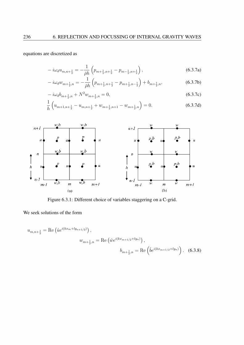
236 6. REFLECTION AND FOCUSSING OF INTERNAL GRAVITY WAVES
equations are discretized as
− iωdum,n+ 12
= − 1
ρh
(pm+ 1
2,n+ 1
2− pm− 1
2,n+ 1
2
), (6.3.7a)
− iωdwm+ 12,n = − 1
ρh
(pm+ 1
2,n+ 1
2− pm+ 1
2,n− 1
2
)+ bm+ 1
2,n, (6.3.7b)
− iωdbm+ 12,n +N2wm+ 1
2,n = 0, (6.3.7c)
1
h
(um+1,n+ 1
2− um,n+ 1
2+ wm+ 1
2,n+1 − wm+ 1
2,n
)= 0. (6.3.7d)
Figure 6.3.1: Different choice of variables staggering on a C-grid.
We seek solutions of the form
um,n+ 12
= Re(uei(kxm+lyn+1/2)
),
wm+ 12,n = Re
(wei(kxm+1/2+lyn)
),
bm+ 12,n = Re
(bei(kxm+1/2+lyn)
). (6.3.8)
6.4. INTERNAL GRAVITY WAVES AT A SLOPING BOUNDARY 237
Substituting into (6.3.7a), (6.3.7b), (6.3.7c), (6.3.7d) yields
− iωdu+2i
hsin
(kh
2
)p = 0, (6.3.9a)
− iωdw +2i
hsin
(lh
2
)p− b = 0, (6.3.9b)
− iωdb+N2w = 0, (6.3.9c)
2i
h
(sin
(kh
2
)u+ cos
(lh
2
)w
)= 0. (6.3.9d)
Rewritten in matrix form−iωd 0 0 2i
hsin(kh2
)0 −iωd −1 2i
hsin(lh2
)0 N2 −iωd 0
2ih
sin(kh2
)2ih
sin(lh2
)0 0
u
w
b
p
=
0
0
0
0
. (6.3.10)
The determinant of the matrix must be zero for non-trivial solution. So that, we recovered
the dispersion relation
ω2d =
N2 sin2(kh2
)sin2
(kh2
)+ sin2
(lh2
) . (6.3.11)
6.4 Internal Gravity Waves at A Sloping Boundary
We now turn to the next setting which is boundary tilted at 45◦ to the x axis. The straight
boundary lies along the line z = x, at which there is no normal flow u · n = 0. So there is
perfect reflection when a wave with wavenumber (kI ,mI) propagates towards the boundary.
Our task is to find the reflected wave, with wavenumber (kR,mR), both in the continuum
solution and discrete solution.
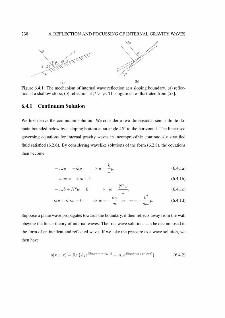
238 6. REFLECTION AND FOCUSSING OF INTERNAL GRAVITY WAVES
(a) (b)
Figure 6.4.1: The mechanism of internal wave reflection at a sloping boundary. (a) reflec-tion at a shallow slope, (b) reflection at β > ϕ. This figure is re-illustrated from [53].
6.4.1 Continuum Solution
We first derive the continuum solution. We consider a two-dimensional semi-infinite do-
main bounded below by a sloping bottom at an angle 45◦ to the horizontal. The linearised
governing equations for internal gravity waves in incompressible continuously stratified
fluid satisfied (6.2.6). By considering wavelike solutions of the form (6.2.8), the equations
then become
− iωu = −ikp ⇒ u =k
ωp, (6.4.1a)
− iωw = −iωp+ b, (6.4.1b)
− iωb+N2w = 0 ⇒ ib =N2w
ω, (6.4.1c)
iku+ imw = 0 ⇒ w = −kum⇒ w = − k2
mωp. (6.4.1d)
Suppose a plane wave propagates towards the boundary, it then reflects away from the wall
obeying the linear theory of internal waves. The free wave solutions can be decomposed in
the form of an incident and reflected wave. If we take the pressure as a wave solution, we
then have
p(x, z, t) = Re(AIe
i(kIx+mIz−ωI t) + ARei(kRx+mRz−ωRt)
), (6.4.2)
6.4. INTERNAL GRAVITY WAVES AT A SLOPING BOUNDARY 239
where the subscript I and R refer to the incident and reflected waves, respectively, k is the
horizontal wavenumber in the x direction, m is the vertical wavenumber in z direction, ω is
the wave frequency. At the boundary z = x, the wave has to satisfy the boundary condition
no normal flow, which is
u · n = 0 ⇒ −u+ w = 0. (6.4.3)
By substituting (6.4.1a) and (6.4.1d) into (6.4.3), and using (6.4.2) we have
− k
ω
(AIe
i(kIx+mIx−ωI t) + ARei(kRx+mRz−ωRt)
)− k2
mω
(AIe
i(kIx+mIz−ωI t) + ARei(kRx+mRx−ωRt)
)= 0,
− AIei((kI+mI)x−ωI t)(kIωI
+k2I
mIωI
)− ARei((kR+mR)x−ωRt)
(kRωR
+k2R
mRωR
)= 0,
− AIei((kI−kR+mI−mR)x−(ωI−ωR)t)
(kIωI
+k2I
mIωI
)− AR
(kRωR
+k2R
mRωR
)= 0.
(6.4.4)
If (6.4.4) to be true for all x and t, then the following 3 conditions must be satisfied:
kI − kR +mI −mR = 0, (6.4.5a)
ωI − ωR = 0, (6.4.5b)
−AI(kIωI
+k2I
mIωI
)− AR
(kRωR
+k2R
mRωR
)= 0. (6.4.5c)
The dispersion relation for the internal gravity waves in (6.1.3) must satisfied for both in-
cident and reflected waves. Thus, (6.4.5b) implies
ω2I =
N2k2I
(k2I +m2
I)=
N2k2R
(k2R +m2
R)= ω2
R. (6.4.6)
240 6. REFLECTION AND FOCUSSING OF INTERNAL GRAVITY WAVES
Some algebraic manipulations of (6.4.6) give
N2k2I
(k2I +m2
I)=
N2k2R
(k2R +m2
R)⇒ N2k2
I
(k2R +m2
R
)= N2k2
R
(k2I +m2
I
),
k2Ik
2R + k2
Im2R = k2
Rk2I + k2
Rm2I , ⇒ k2
Im2R = k2
Rm2I .
(6.4.7)
As the incident wave reflects at the boundary, the reflected wavenumber kR and mR must
be in terms of incident and AI . They can be obtained from (6.4.7). By eliminating mR in
(6.4.7) from (6.4.5a), we obtain
mR = kI +mI − kR ⇒ m2R = k2
I + 2kImI − 2kIkR − 2kRmI +m2I + k2
R,
and substituting into (6.4.7) gives
k2I
(k2I + 2kImI − 2kIkR − 2kRmI +m2
I + k2R
)= k2
Rm2I ,
k4I + 2k3
ImI − 2k3IkR − 2k2
IkRmI + k2Im
2I + k2
Rk2I − k2
Rm2I = 0,
k2R(k2
I −m2I)− 2k2
IkR(kI +mI) + k2I (k
2I + 2kImI +m2
I) = 0,
(kI +mI)[k2R(kI −mI)− 2k2
IkR + k2I (kI +mI)
]= 0.
An obvious possibility of reflected wavenumber is
kI +mI = 0 ⇒ kI = −mI , then (6.4.5a) gives kR = −mR.
This shows that the wave is not reflected. Otherwise, the wave is only propagates along the
boundary. So we must have the other possibility, i.e., k2R(kI−mI)−2k2
IkR+k2I (kI+mI) =
6.4. INTERNAL GRAVITY WAVES AT A SLOPING BOUNDARY 241
0. It implies
kR =2k2
I ±√
4k4I − 4k2
I (kI +mI)(kI −mI)
2(kI −mI),
=2k2
I ±√
4k4I − 4k4
I + 4k2Im
2I
2(kI −mI),
=k2I ± kImI
(kI −mI).
Here, if the negative sign is chosen, we then have
kR =kI(kI −mI)
(kI −mI)⇒ kR = kI , and (6.4.5a) gives mR = mI .
Again, this is not the interesting solution as there is no reflection occur at the boundary. So,
the only possibility left is
kR =kI(kI +mI)
kI −mI
⇒ mR = −mI(kI +mI)
kI −mI
. (6.4.9)
Note that, this is only true for the case of kI 6= mI , for which reflection to be occured.
Otherwise, we only have wave propagation along the boundary. The reflected wavenum-
ber (6.4.9) expresses the change in reflected wavenumber upon reflection. Both are con-
sistent with the well known result in [53] who written reflected wavenumber in terms of
trigometrical function. (6.4.9) also equivalent to equation (5) in [28], who consider three-
dimensional linearised inviscid Boussinesq incompressible motion in a uniformly stratified
rotating fluid.
Having these reflected wavenumber and same frequency during reflection, (6.4.5c) can be
242 6. REFLECTION AND FOCUSSING OF INTERNAL GRAVITY WAVES
solved to give reflected amplitude AR. We found the reflected amplitude as
−AIkI
mIωI(kI +mI)− AR
kRmRωR
(kR +mR) = 0,
−AIkI
mIωI(kI +mI) + AR
kImIωR
(kI +mI) = 0,
AI = AR.
(6.4.10)
With these expressions, the velocity field and buoyancy are found to be
u(x, y, t) = Re
(kI
ωAIe
i(kIx+m
Iz−ωt) +
kI(kI +mI)
ω(kI −mI)AIe
i(
(kI−mI )(kI−mI )
(kIx−mIz−ωt)))
,
(6.4.11)
w(x, y, t) = Re
(−
k2I
ωmI
AIei(kI x+m
Iz−ωt) +
k2I(kI +mI)
ωmI(kI −mI)
AIei(
(kI−mI )(kI−mI )
(kIx−mIz−ωt)))
,
(6.4.12)
b(x, y, t) = Re
(i (k2 +m2)
m
(AIei(kI x+m
Iz−ωt) − (k
I+m
I)
(kI−m
I)AIei
((kI+m
I)
(kI−m
I)(kIx−mIz−ωt)
)))(6.4.13)
Although we obtain different expression for the reflected amplitude as in equation (7) in
[28], we note that the second term in our velocity (6.4.11,6.4.12) and buoyancy (6.4.13)
components (i.e.,(kI +mI)
(kI −mI)AI) is similar to the reflected amplitude, AR, Eq. (7) in [28].
This is because we assume the pressure as our plane wave solution, instead of vertical
velocity as was done by [28]. So that, our continuum solutions are consistent with the well
known linear theory of internal waves. Having completed these continuum solutions, the
performance of the discrete solutions that will derive in the next section can be tested in the
limit of grid spacing tends to zero.
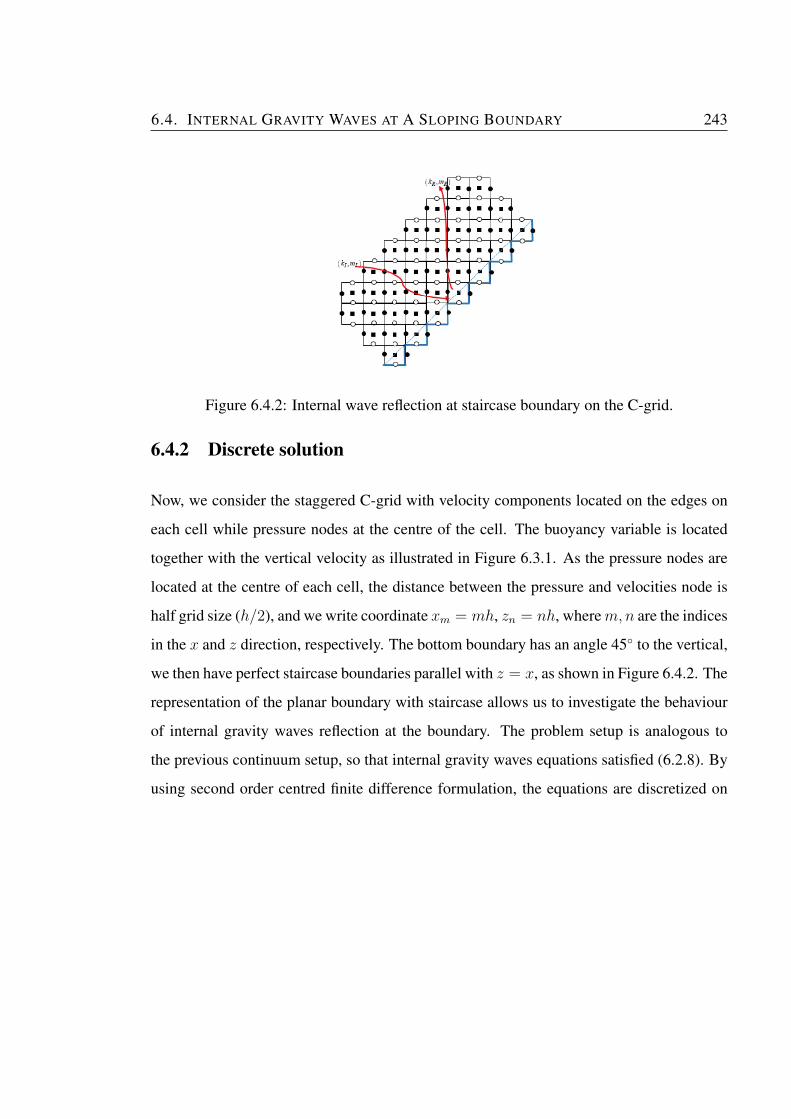
6.4. INTERNAL GRAVITY WAVES AT A SLOPING BOUNDARY 243
Figure 6.4.2: Internal wave reflection at staircase boundary on the C-grid.
6.4.2 Discrete solution
Now, we consider the staggered C-grid with velocity components located on the edges on
each cell while pressure nodes at the centre of the cell. The buoyancy variable is located
together with the vertical velocity as illustrated in Figure 6.3.1. As the pressure nodes are
located at the centre of each cell, the distance between the pressure and velocities node is
half grid size (h/2), and we write coordinate xm = mh, zn = nh, wherem,n are the indices
in the x and z direction, respectively. The bottom boundary has an angle 45◦ to the vertical,
we then have perfect staircase boundaries parallel with z = x, as shown in Figure 6.4.2. The
representation of the planar boundary with staircase allows us to investigate the behaviour
of internal gravity waves reflection at the boundary. The problem setup is analogous to
the previous continuum setup, so that internal gravity waves equations satisfied (6.2.8). By
using second order centred finite difference formulation, the equations are discretized on
244 6. REFLECTION AND FOCUSSING OF INTERNAL GRAVITY WAVES
the C-grid as
− iωdum,n+ 12
= −1
h
(pm+ 1
2,n+ 1
2− pm− 1
2,n+ 1
2
), (6.4.14a)
− iωdwm+ 12,n = −1
h
(pm+ 1
2,n+ 1
2− pm+ 1
2,n− 1
2
)+ bm+ 1
2,n, (6.4.14b)
− iωdbm+ 12,n +N2wm+ 1
2,n = 0, (6.4.14c)
1
h
(um+1,n+ 1
2− um,n+ 1
2+ wm+ 1
2,n+1 − wm+ 1
2,n
)= 0, (6.4.14d)
where ωd represents the discrete frequency. From (6.4.14c), we can have buoyancy as
bm+ 12,n = −iN
2
ωdwm+ 1
2,n,
and substituting into (6.4.14b) gives
−iωdwm+ 12,n = −
pm+ 12,n+ 1
2− pm+ 1
2,n− 1
2
h− iN2
ωdwm+ 1
2,n,(
−iωd +iN2
ωd
)wm+ 1
2,n = −1
h
(pm+ 1
2,n+ 1
2− pm+ 1
2,n− 1
2
),
wm+ 12,n =
iωdh (N2 − ωd)
(pm+ 1
2,n+ 1
2− pm+ 1
2,n− 1
2
).
(6.4.15)
Simplifying (6.4.14a) gives discrete horizontal velocity as
um,n+ 12
= − i
ωdh
(pm+ 1
2,n+ 1
2− pm− 1
2,n− 1
2
). (6.4.16)
We suppose that a free internal gravity wave propagates towards the sloping boundary and
reflects away. The wave solution is the combination of both incoming and reflected wave.
By assuming the pressure as our discrete solution, we have
pm+ 12,n+ 1
2= AI exp(i{kIxm+ 1
2+mIzn+ 1
2− ωdt})
+ AR exp(i{kRxm+ 12
+mRzn+ 12− ωdt}). (6.4.17)

6.4. INTERNAL GRAVITY WAVES AT A SLOPING BOUNDARY 245
At the boundary, the wave must satisfy the no normal flow boundary conditions
uj,j− 12
= 0, wj+ 12,j = 0, j ∈ Z. (6.4.18)
Substituting(6.4.15) and (6.4.16) into (6.4.14d) and imposing the boundary conditions gives
1
h
(i
ωdh
(pj+ 1
2,j+ 1
2− pj− 1
2,j+ 1
2
)+
iωdh (N2 − ω2
d)
(pj+ 1
2,j+ 3
2− pj+ 1
2,j+ 1
2
))= 0,
i
h2
((1
ωd− ωd
(N2 − ω2d)
)pj+ 1
2,j+ 1
2+
ωd(N2 − ω2
d)pj+ 1
2,j+ 3
2− 1
ωdpj− 1
2,j+ 1
2
)= 0,
substituting (6.4.17) gives
(1
ωd− ωd
(N2 − ω2d)
)(AIe
i(kI(j+ 12
)h+mI(j+ 12
)h−ωdt) + ARei(kR(j+ 1
2)h+mR(j+ 1
2)h−ωdt)
)+
ωd(N2 − ω2
d)
(AIe
i(kI(j+ 12
)h+mI(j+ 32
)h−ωdt) + ARei(kR(j+ 1
2)h+mR(j+ 3
2)h−ωdt)
)− 1
ωd
(AIe
i(kI(j− 12
)h+mI(j+ 12
)h−ωdt) + ARei(kR(j+ 1
2)h+mR(j+ 1
2)h−ωdt)
)= 0.
AIei((kI+mI−kR−mR)jh−(ωI−ωR)t)
[(− 1
ωI+
ωI(N2 − ω2
I )
)ei(kIh
2+mIh
2
)
− ωI(N2 − ω2
I )ei(kIh
2+
3mIh
2
)+
1
ωdei(mIh
2− kIh
2
)]
= AR
[(1
ωR− ωR
(N2 − ω2R)
)ei(kRh
2+mRh
2
)
+ωR
(N2 − ω2R)ei(kRh
2− 3mRh
2
)− 1
ωRei(mRh
2− kRh
2
)].
246 6. REFLECTION AND FOCUSSING OF INTERNAL GRAVITY WAVES
If this must be hold for all j and t, the following conditions must be satisfied:
kI +mI − kR −mR = 0, (6.4.19a)
ωI − ωR = 0, (6.4.19b)
AI
[(− 1
ωI+
ωI(N2 − ω2
I )
)ei(kIh
2+mIh
2
)− ωI
(N2 − ω2I )ei(kIh
2+
3mIh
2
)+
1
ωdei(mIh
2− kIh
2
)]
=AR
[(1
ωR− ωR
(N2 − ω2R)
)ei(kRh
2+mRh
2
)+
ωR(N2 − ω2
R)ei(kRh
2− 3mRh
2
)− 1
ωRei(mRh
2− kRh
2
)].
(6.4.19c)
Through the dispersion relation (6.3.11) and (6.4.19b), we have
N2 sin2
(kIh
2
)sin2
(kIh
2
)+ sin2
(mIh
2
) =
N2 sin2
(kRh
2
)sin2
(kRh
2
)+ sin2
(mRh
2
) ,sin2
(kIh
2
)[sin2
(kRh
2
)+ sin2
(mRh
2
)]= sin2
(kRh
2
)[sin2
(kIh
2
)+ sin2
(mIh
2
)],
sin2
(kIh
2
)sin2
(mRh
2
)= sin2
(kRh
2
)sin2
(mIh
2
),(
1− cos 2
(kIh
2
))2
·
(1− cos 2
(mRh
2
))2
=
(1− cos 2
(kRh
2
))2
·
(1− cos 2
(mIh
2
))2
,
(1− cos (kIh)) (1− cos (mRh)) = (1− cos (kRh)) (1− cos (mIh)) ,
− cos (mRh)− cos (kIh) + cos (kIh) cos (mRh) = − cos (mIh)− cos (kRh) + cos (kRh) cos (mIh) .
In the limit of h→ 0, Taylor series expansion gives
k2Im
2R = k2
Rm2I +O(h2), (6.4.20)
6.4. INTERNAL GRAVITY WAVES AT A SLOPING BOUNDARY 247
which is equivalent to equation (6.4.7) in the continuum case, with second order correction,
as expected due to the second order finite-differences. But, from (6.4.19a) we have
mR = kI +mI − kR ⇒ m2R = k2
I + 2kImI − 2kIkR − 2kRmI +m2I + k2
R.
This means that the reflected wavenumber kR can be found by eliminating mR from
(6.4.20). So that (6.4.20) gives
k2I
(k2I + 2kImI − 2kIkR − 2kRmI +m2
I + k2R
)= k2
Rm2I +O(h2),
k4I + 2k3
ImI − 2k3IkR − 2kRk
2ImI + k2
Im2I + k2
Ik2R − k2
Rm2I +O(h2) = 0,
k2R
(k2I −m2
I
)− 2kR
(k3I = k2
ImI
)+ k2
I
(m2I + k2
I + 2kImI
)+O(h2) = 0,
k2R(kI +mI)(kI −mI)− 2kRk
2I (kI +mI) + k2
I (kI +mI)2 +O(h2) = 0,
(kI +mI)[k2R(kI −mI)− 2kRk
2I + k2
I (kI +mI)]
+O(h2) = 0.
An obvious possibility is
kI +mI +O(h2) = 0 ⇒ kI = −mI +O(h2), which implies kR = −mR +O(h2).
248 6. REFLECTION AND FOCUSSING OF INTERNAL GRAVITY WAVES
However, this is impossible because this shows wave propagates along the boundary. If the
terms in the square bracket is possible, then we can have
k2R −
2kRk2I
kI −mI
+k2I (kI +mI)
kI −mI
+O(h2) = 0,
kR =1
2
[2k2
I
(kI −mI)±
√4k4
I
(kI −mI)2− 4(1)
(k2I (kI +mI)
(kI −mI)+O(h2)
)],
kR =k2I
(kI −mI)± 1
2
√4k4
I
(kI −mI)2− 4
(k2I (kI +mI)
(kI −mI)+O(h2)
),
kR =k2I
(kI −mI)± 1
2
√4k4
I
(kI −mI)2− 4
k2I (kI +mI)(kI −mI)
(kI −mI)2+O(h2),
kR =k2I
(kI −mI)± 1
2
√4k4
I − 4k4I + 4k2
Im2I +O(h2)
(kI −mI)2,
kR =k2I
(kI −mI)± kImI
(kI −mI)
(1 +O(h2)
),
which again gives another two possiblities of reflected wavenumber. On the first possibility
is rejected since there is no wave reflection occur at the boundary
kR =kI(kI +mI)
(kI −mI)+O(h2) or kR =
kI(kI −mI)
(kI −mI)+O(h2) = kI +O(h2). (6.4.21)
It is noted from (6.4.19a) that, the latter implies mR = mI + O(h2), which is impossible
because of the same wave. Hence, the former is the only possibility of kR. So that, we also
have
mR = −mI(kI +mI)
kI −mI
+O(h2). (6.4.22)
6.4. INTERNAL GRAVITY WAVES AT A SLOPING BOUNDARY 249
Now, we only need to find AR. From (6.4.19c), we have
AI
[2ω2
I −N2
ωI (N2 − ω2I )− ωIe
imIh
(N2 − ω2I )
+e−ikIh
ωI
]eih2
(kI+mI)
= AR
[N2 − 2ω2
R
ωR (N2 − ω2R)
+ωRe
imRh
(N2 − ω2R)− e−ikRh
ωR
]eih2
(kR+mR),
but, by using (6.4.19a) and (6.4.19b) we obtained
AI
[2ω2 −N2
ω (N2 − ω2)− ωeimIh
(N2 − ω2)+e−ikIh
ω
]= AR
[N2 − 2ω2
ω (N2 − ω2)+
ωeimRh
(N2 − ω2)− e−ikRh
ω
].
(6.4.23)
Factorising and canceling the denominator followed by the Taylor series expansion of the
exponential terms give
AI
[2ω2−N2 − ω2
(1 + imIh+O(h2)
)+ (N2 − ω2)
(1− ikIh+O(h2)
) ]
= AR
[N2 − 2ω2 + ω2
(1 + imRh+O(h2)
)− (N2 − ω2)
(1− ikRh+O(h2)
) ],
AI
[ω2(kI −mI)−N2kI −
ih
2
(ω2(k2
I +m2I)−N2k2
I
)+O(h2)
]
= AR
[ω2(mR − kR) +N2kR +
ih
2
(ω2(k2
R +m2R)−N2k2
R
)+O(h2)
],
250 6. REFLECTION AND FOCUSSING OF INTERNAL GRAVITY WAVES
and substituting the reflected wavenumber (6.4.21) yield
AI
[− N2kImI(kI +mI)
(k2I +m2
I)− ih
2
(N2
(k2I +m2
I)
)+O(h2)
]
= AR
[− N2kImI(kI +mI)
(k2I +m2
I)+ih
2
(N2(kI +mI)
2
(kI −mI)2(k2I +m2
I)
)+O(h2)
],
⇒ AR =
AI
[− N2kImI(kI+mI)
(k2I+m2I)
− ih2
(N2
(k2I+m2I)
)+O(h2)
][− N2kImI(kI+mI)
(k2I+m2I)
+ ih2
(N2(kI+mI)2
(kI−mI)2(k2I+m2I)
)+O(h2)
] .
Factorising the first term in bracket and simplifying, we obtained
AR = AI
(1 + ih
(k2I +m2
I)
kImI(kI −mI)2(kI +mI)
)+O(h2). (6.4.24)
It is found that the reflected amplitude of internal gravity wave has first-order (complex)
error. This is also known as the phase error. It is showed that the staircase boundaries give
influence to the internal wave speed.
6.5 Internal Waves Attractor
Now, we turn to more realistic or natural situation of the existing of internal gravity waves,
i.e., in a closed basin. It is important to consider such realistic situation of internal gravity
waves as it will give a key to understand the patterns of internal gravity wave in fluids.
In a closed basin, internal gravity waves propagate and reflect from the side of the basin.
In a closed domain with at least one sloping boundary, it has been proved that multiple
reflections of internal gravity wave will lead to a closed orbit that is called internal wave
attractor [47, 48]. Various theoretical and laboratory settings were assumed in order to
study the existence and the structure of the of the attractors as they varied the parameters
6.5. INTERNAL WAVES ATTRACTOR 251
of the geometry. In a numerical experiment context, one needs to consider a suitable nu-
merical scheme to investigate the existence of internal wave attractor since it will involve
large computational. As internal wave attractor could be existed upon multiples reflections,
boundary approximation also is a crucial issue in any numerical scheme. In this section we
will discuss a numerical experiment of internal gravity wave in a square domain.
As we know, internal wave attractor appearance depends on the angle of reflection. For a
square domain, internal gravity waves focusing only occurs when a boundary of the domain
is inclined with respect to gravity [47]. For this reason here we assumed our square domain
to be rotated through an angle 0 ≤ θ ≤ π/4. Then, the governing equations now satisfy
∂u
∂t= −∂p
∂x+ b sin θ, (6.5.1a)
∂w
∂t= −∂p
∂z+ b cos θ, (6.5.1b)
∂b
∂t+N2(u sin θ + w cos θ) = 0, (6.5.1c)
∂u
∂x+∂w
∂z= 0, (6.5.1d)
where θ is the angle of (x, z)-cooordinate system. This angle θ plays an important role in
the appearance of the internal gravity waves attractor. These equations cannot be solved
analytically if the square domain is tilted [11]. Thus, we only can compare the results of
numerical solutions qualitatively with other existing numerical solutions. These equations
have to be solved with the no normal flow boundary condition u · n = 0 on the square
domain.
6.5.1 Numerical setting
In setting up a numerical experiment of (6.5.1), the equations are discretised such that
finite-differencing is applicable to the C-grid. As discussed in section 6.3.2, on this grid the
velocity vector (u,w) is located at the boundary of a finite-difference cell, while pressure p

252 6. REFLECTION AND FOCUSSING OF INTERNAL GRAVITY WAVES
and buoyancy b are co-located at the centre of cell. We choose the grid spacings dx= dy =
h for all experiments. We consider a square domain placed on top of this grid, and we then
construct a grid on a quadrilateral of extend 2lx× 2ly that just extends beyond the specified
domain, where 2lx = nxh and 2ly = nyh for some integers nx and ny.
All variables are stored as matrices. In our experiments, we are using the same second-order
centred differences as first discussed in Chapter 2, to evaluate the derivative in our model.
Since all variables are staggered, (6.5.1) are written in matrix form as
∂U
∂t= −DpuP + sin θB, (6.5.2a)
∂W
∂t= −PDpw + cos θB, (6.5.2b)
∂B
∂t+N2 (sin θU + cos θW ) = 0, (6.5.2c)
DupU +WDwp = 0, (6.5.2d)
where U , V , P and B are the matrices of the variables. Thus, we have four different differ-
entiation matrices for the derivatives in our model. By adapting Crank-Nicolson scheme,
(6.5.2) become
Un+1 − Un
∆t= −Dpu
P n+1 + P n
2+ sin θ
Bn+1 +Bn
2, (6.5.3a)
W n+1 −W n
∆t= −P
n+1 + P n
2Dpw + cos θ
Bn+1 +Bn
2, (6.5.3b)
Bn+1 −Bn
∆t+N2
(sin θ
Un+1 + Un
2+ cos θ
W n+1 +W n
2
)= 0, (6.5.3c)
DupUn +W nDwp = 0. (6.5.3d)
where superscript n represents time step. Unlike in the previous chapter, here we are us-
ing Crank-Nicolson method, rather than RK4, so it is a second order scheme. The main
reason we are using this scheme is because it is a natural scheme for enforcing incompress-
ibility (6.5.2d) or (6.5.3d). As we know, RK4 is an explicit scheme, then the flow that
6.5. INTERNAL WAVES ATTRACTOR 253
is generated at tn+1 does not necessarily satisfy (6.5.3d), and a further projection step is
necessary to make it incompressible. The Crank Nicolson scheme has this projection step
embedded. The other reason is because of the accuracy requirement. In the earlier chapters
we were trying to measure spatial convergence, and thus absolutely needed to have the
time-discretization errors to be tiny, so that all that remained were the spatial-discretization
errors. However, in this chapter this same accuracy is not needed.
We can eliminate U and W in (6.5.3c) using (6.5.3a) and (6.5.3b), respectively. Then we
have
Bn+1
(1 +
N2∆2
4
)= Bn
(1− N2∆2
4
)−N2∆(sin θUn + cos θW n) +
N2∆2
4(sin θDpu + cos θDpw)
(P n+1 + P n
). (6.5.4)
In (6.5.4), we first solve for P and B by performing inversion on the right-hand side. In our
experiment, we used initial condition
u = Re [−A exp{−iωt} sin(kx) cos(my)] , (6.5.5a)
w = Re [A exp{−iωt} cos(kx) sin(my)] , (6.5.5b)
b = Re
[A exp{−iωt}iωm
kcos(kx) sin(my)
], (6.5.5c)
p = Re
[−A exp{−iωt}iN
2
ωcos(kx) sin(my)
], (6.5.5d)
where k = πl/2lx and m = πn/2ly, (l, n) is initial condition wavemode are chosen at two
different values: (i) (l, n) = (1, 1) and (ii) (1, 3). The initial condition (l, n) = (1, 1) is
expected to produce (1, 1) wave attractor while initial condition (l, n) = (1, 3) is expected
to produce (1, 3) wave attractor [11].
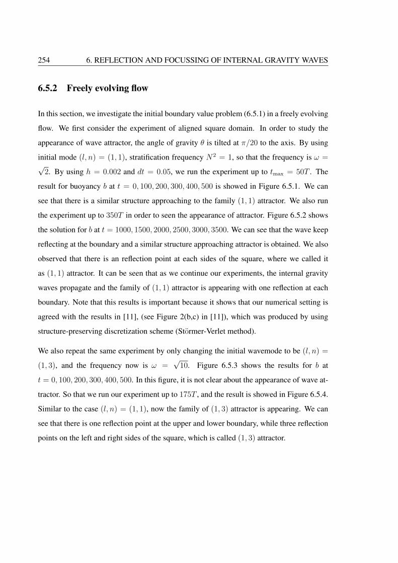
254 6. REFLECTION AND FOCUSSING OF INTERNAL GRAVITY WAVES
6.5.2 Freely evolving flow
In this section, we investigate the initial boundary value problem (6.5.1) in a freely evolving
flow. We first consider the experiment of aligned square domain. In order to study the
appearance of wave attractor, the angle of gravity θ is tilted at π/20 to the axis. By using
initial mode (l, n) = (1, 1), stratification frequency N2 = 1, so that the frequency is ω =√
2. By using h = 0.002 and dt = 0.05, we run the experiment up to tmax = 50T . The
result for buoyancy b at t = 0, 100, 200, 300, 400, 500 is showed in Figure 6.5.1. We can
see that there is a similar structure approaching to the family (1, 1) attractor. We also run
the experiment up to 350T in order to seen the appearance of attractor. Figure 6.5.2 shows
the solution for b at t = 1000, 1500, 2000, 2500, 3000, 3500. We can see that the wave keep
reflecting at the boundary and a similar structure approaching attractor is obtained. We also
observed that there is an reflection point at each sides of the square, where we called it
as (1, 1) attractor. It can be seen that as we continue our experiments, the internal gravity
waves propagate and the family of (1, 1) attractor is appearing with one reflection at each
boundary. Note that this results is important because it shows that our numerical setting is
agreed with the results in [11], (see Figure 2(b,c) in [11]), which was produced by using
structure-preserving discretization scheme (Stormer-Verlet method).
We also repeat the same experiment by only changing the initial wavemode to be (l, n) =
(1, 3), and the frequency now is ω =√
10. Figure 6.5.3 shows the results for b at
t = 0, 100, 200, 300, 400, 500. In this figure, it is not clear about the appearance of wave at-
tractor. So that we run our experiment up to 175T , and the result is showed in Figure 6.5.4.
Similar to the case (l, n) = (1, 1), now the family of (1, 3) attractor is appearing. We can
see that there is one reflection point at the upper and lower boundary, while three reflection
points on the left and right sides of the square, which is called (1, 3) attractor.
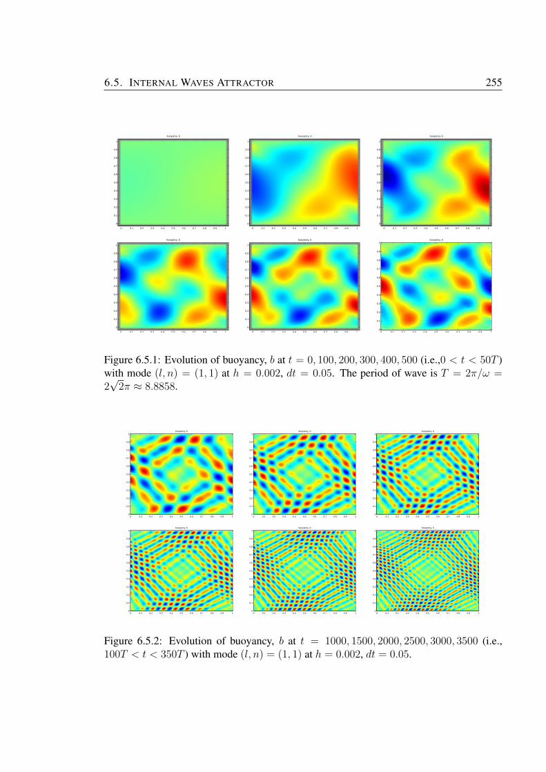
6.5. INTERNAL WAVES ATTRACTOR 255
buoyancy, b
0 0.1 0.2 0.3 0.4 0.5 0.6 0.7 0.8 0.9 1
0
0.1
0.2
0.3
0.4
0.5
0.6
0.7
0.8
0.9
1
buoyancy, b
0 0.1 0.2 0.3 0.4 0.5 0.6 0.7 0.8 0.9 1
0
0.1
0.2
0.3
0.4
0.5
0.6
0.7
0.8
0.9
1
buoyancy, b
0 0.1 0.2 0.3 0.4 0.5 0.6 0.7 0.8 0.9 1
0
0.1
0.2
0.3
0.4
0.5
0.6
0.7
0.8
0.9
1
buoyancy, b
0 0.1 0.2 0.3 0.4 0.5 0.6 0.7 0.8 0.9 1
0
0.1
0.2
0.3
0.4
0.5
0.6
0.7
0.8
0.9
1
buoyancy, b
0 0.1 0.2 0.3 0.4 0.5 0.6 0.7 0.8 0.9 1
0
0.1
0.2
0.3
0.4
0.5
0.6
0.7
0.8
0.9
1
buoyancy, b
0 0.1 0.2 0.3 0.4 0.5 0.6 0.7 0.8 0.9 10
0.1
0.2
0.3
0.4
0.5
0.6
0.7
0.8
0.9
1
Figure 6.5.1: Evolution of buoyancy, b at t = 0, 100, 200, 300, 400, 500 (i.e.,0 < t < 50T )with mode (l, n) = (1, 1) at h = 0.002, dt = 0.05. The period of wave is T = 2π/ω =2√
2π ≈ 8.8858.
buoyancy, b
0 0.1 0.2 0.3 0.4 0.5 0.6 0.7 0.8 0.9 10
0.1
0.2
0.3
0.4
0.5
0.6
0.7
0.8
0.9
1buoyancy, b
0 0.1 0.2 0.3 0.4 0.5 0.6 0.7 0.8 0.9 10
0.1
0.2
0.3
0.4
0.5
0.6
0.7
0.8
0.9
1buoyancy, b
0 0.1 0.2 0.3 0.4 0.5 0.6 0.7 0.8 0.9 10
0.1
0.2
0.3
0.4
0.5
0.6
0.7
0.8
0.9
1
buoyancy, b
0 0.1 0.2 0.3 0.4 0.5 0.6 0.7 0.8 0.9 10
0.1
0.2
0.3
0.4
0.5
0.6
0.7
0.8
0.9
1buoyancy, b
0 0.1 0.2 0.3 0.4 0.5 0.6 0.7 0.8 0.9 10
0.1
0.2
0.3
0.4
0.5
0.6
0.7
0.8
0.9
1buoyancy, b
0 0.1 0.2 0.3 0.4 0.5 0.6 0.7 0.8 0.9 10
0.1
0.2
0.3
0.4
0.5
0.6
0.7
0.8
0.9
1
Figure 6.5.2: Evolution of buoyancy, b at t = 1000, 1500, 2000, 2500, 3000, 3500 (i.e.,100T < t < 350T ) with mode (l, n) = (1, 1) at h = 0.002, dt = 0.05.

256 6. REFLECTION AND FOCUSSING OF INTERNAL GRAVITY WAVES
buoyancy, b
0 0.1 0.2 0.3 0.4 0.5 0.6 0.7 0.8 0.9 10
0.1
0.2
0.3
0.4
0.5
0.6
0.7
0.8
0.9
1buoyancy, b
0 0.1 0.2 0.3 0.4 0.5 0.6 0.7 0.8 0.9 10
0.1
0.2
0.3
0.4
0.5
0.6
0.7
0.8
0.9
1buoyancy, b
0 0.1 0.2 0.3 0.4 0.5 0.6 0.7 0.8 0.9 10
0.1
0.2
0.3
0.4
0.5
0.6
0.7
0.8
0.9
1
buoyancy, b
0 0.1 0.2 0.3 0.4 0.5 0.6 0.7 0.8 0.9 10
0.1
0.2
0.3
0.4
0.5
0.6
0.7
0.8
0.9
1buoyancy, b
0 0.1 0.2 0.3 0.4 0.5 0.6 0.7 0.8 0.9 10
0.1
0.2
0.3
0.4
0.5
0.6
0.7
0.8
0.9
1buoyancy, b
0 0.1 0.2 0.3 0.4 0.5 0.6 0.7 0.8 0.9 10
0.1
0.2
0.3
0.4
0.5
0.6
0.7
0.8
0.9
1
Figure 6.5.3: Evolution of buoyancy, b at t = 0, 100, 200, 300, 400, 500 (i.e., 0 < t < 25T )with mode (l, n) = (1, 3) at h = 0.002, dt = 0.05. The period is T = 2π/ω = 2
√10π ≈
19.8692.
buoyancy, b
0 0.1 0.2 0.3 0.4 0.5 0.6 0.7 0.8 0.9 10
0.1
0.2
0.3
0.4
0.5
0.6
0.7
0.8
0.9
1buoyancy, b
0 0.1 0.2 0.3 0.4 0.5 0.6 0.7 0.8 0.9 10
0.1
0.2
0.3
0.4
0.5
0.6
0.7
0.8
0.9
1buoyancy, b
0 0.1 0.2 0.3 0.4 0.5 0.6 0.7 0.8 0.9 10
0.1
0.2
0.3
0.4
0.5
0.6
0.7
0.8
0.9
1
buoyancy, b
0 0.1 0.2 0.3 0.4 0.5 0.6 0.7 0.8 0.9 10
0.1
0.2
0.3
0.4
0.5
0.6
0.7
0.8
0.9
1buoyancy, b
0 0.1 0.2 0.3 0.4 0.5 0.6 0.7 0.8 0.9 10
0.1
0.2
0.3
0.4
0.5
0.6
0.7
0.8
0.9
1buoyancy, b
0 0.1 0.2 0.3 0.4 0.5 0.6 0.7 0.8 0.9 10
0.1
0.2
0.3
0.4
0.5
0.6
0.7
0.8
0.9
1
Figure 6.5.4: Evolution of buoyancy, b at t = 1000, 1500, 2000, 2500, 3000, 3500 (i.e.,50T < t < 175T ) with mode (l, n) = (1, 3) at h = 0.002, dt = 0.05.

6.5. INTERNAL WAVES ATTRACTOR 257
6.5.3 Parametric excitation
It has been proved that wave attractors can be generated by periodically forcing a strati-
fied fluid in a domain with inclined boundaries. The appearance of wave attractor can be
found experimentally by vertically oscillating a container with a sloping wall [48, 37]. This
vertical oscillation also can be viewed as time-dependent modulation of the gravitational
parameter g, which originally enters the momentum equation [11]. So, by multipliying
momentum equation with a time-dependent function α(t), the vertical oscillation, which is
also called parametric excitation can be incorporated. A handful numerical study on the
appearance of internal wave attractor was done in [11]. By considering a tilted square do-
main, [11] studied the appearance of internal wave attractor on the staggered C-grid with
the parametric excitation effects. At a specific parameter values, they showed internal wave
attractor is appeared by using two initial wavemodes ((l, n) = (1, 1) and (l, n) = (1, 3)).
However, they focused on the energy preserving in the internal wave attractors. Unlike
them, our focus is on the effects of staircase boundaries. So, by following the same excita-
tion mode, the internal wave equations (6.5.1) now becomes
∂u
∂t= −α(t)
(∂p
∂x+ b sin θ
), (6.5.6a)
∂w
∂t= −α(t)
(∂p
∂z+ b cos θ
), (6.5.6b)
∂b
∂t+N2(u sin θ + w cos θ) = 0, (6.5.6c)
∂u
∂x+∂w
∂z= 0, (6.5.6d)
where α(t) = 1 − ε cos(2ωt), with a small positive constant ε and 2ω is the forcing fre-
quency.
We now examine internal wave attractor as an initial value problem with the parametric
excitation effects by solving (6.5.6) using our numerical setting. We consider forcing fre-
quency 2ω = π, so that the wave period is T = 4, ε = 0.1, gravity tilted at angle θ = 7π/72,
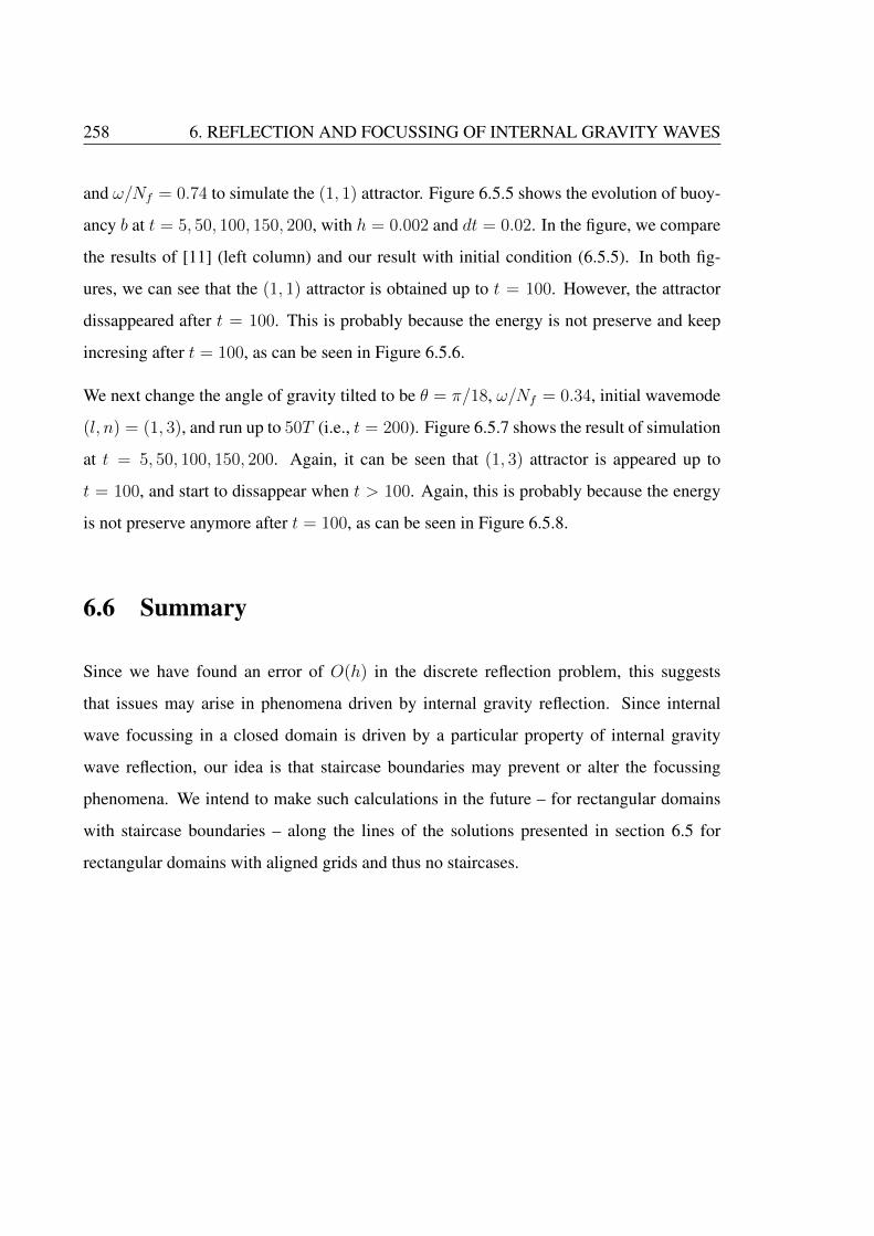
258 6. REFLECTION AND FOCUSSING OF INTERNAL GRAVITY WAVES
and ω/Nf = 0.74 to simulate the (1, 1) attractor. Figure 6.5.5 shows the evolution of buoy-
ancy b at t = 5, 50, 100, 150, 200, with h = 0.002 and dt = 0.02. In the figure, we compare
the results of [11] (left column) and our result with initial condition (6.5.5). In both fig-
ures, we can see that the (1, 1) attractor is obtained up to t = 100. However, the attractor
dissappeared after t = 100. This is probably because the energy is not preserve and keep
incresing after t = 100, as can be seen in Figure 6.5.6.
We next change the angle of gravity tilted to be θ = π/18, ω/Nf = 0.34, initial wavemode
(l, n) = (1, 3), and run up to 50T (i.e., t = 200). Figure 6.5.7 shows the result of simulation
at t = 5, 50, 100, 150, 200. Again, it can be seen that (1, 3) attractor is appeared up to
t = 100, and start to dissappear when t > 100. Again, this is probably because the energy
is not preserve anymore after t = 100, as can be seen in Figure 6.5.8.
6.6 Summary
Since we have found an error of O(h) in the discrete reflection problem, this suggests
that issues may arise in phenomena driven by internal gravity reflection. Since internal
wave focussing in a closed domain is driven by a particular property of internal gravity
wave reflection, our idea is that staircase boundaries may prevent or alter the focussing
phenomena. We intend to make such calculations in the future – for rectangular domains
with staircase boundaries – along the lines of the solutions presented in section 6.5 for
rectangular domains with aligned grids and thus no staircases.

6.6. SUMMARY 259
-0.5 0 0.5
x
-0.5
-0.4
-0.3
-0.2
-0.1
0
0.1
0.2
0.3
0.4
0.5
y
-0.5 -0.4 -0.3 -0.2 -0.1 0 0.1 0.2 0.3 0.4 0.5
x
-0.5
-0.4
-0.3
-0.2
-0.1
0
0.1
0.2
0.3
0.4
0.5
y
-0.5 0 0.5
x
-0.5
-0.4
-0.3
-0.2
-0.1
0
0.1
0.2
0.3
0.4
0.5
y
-0.5 -0.4 -0.3 -0.2 -0.1 0 0.1 0.2 0.3 0.4 0.5
x
-0.5
-0.4
-0.3
-0.2
-0.1
0
0.1
0.2
0.3
0.4
0.5
y
-0.5 0 0.5
x
-0.5
-0.4
-0.3
-0.2
-0.1
0
0.1
0.2
0.3
0.4
0.5
y
-0.5 -0.4 -0.3 -0.2 -0.1 0 0.1 0.2 0.3 0.4 0.5
x
-0.5
-0.4
-0.3
-0.2
-0.1
0
0.1
0.2
0.3
0.4
0.5
y
-0.5 0 0.5
x
-0.5
-0.4
-0.3
-0.2
-0.1
0
0.1
0.2
0.3
0.4
0.5
y
-0.5 -0.4 -0.3 -0.2 -0.1 0 0.1 0.2 0.3 0.4 0.5
x
-0.5
-0.4
-0.3
-0.2
-0.1
0
0.1
0.2
0.3
0.4
0.5
y
-0.5 0 0.5
x
-0.5
-0.4
-0.3
-0.2
-0.1
0
0.1
0.2
0.3
0.4
0.5
y
-0.5 -0.4 -0.3 -0.2 -0.1 0 0.1 0.2 0.3 0.4 0.5
x
-0.5
-0.4
-0.3
-0.2
-0.1
0
0.1
0.2
0.3
0.4
0.5
y
Figure 6.5.5: The evolution of buoyancy b at t = 5, 50, 100, 150, 200 for (l, n) = (1, 1),ω/Nf = 0.74. Gravity tilted at angle 7π/72. The left column is the results using [11]attractor initial condition. On the right column, the results with (6.5.5) normal mode initialcondition with parametric excitation.
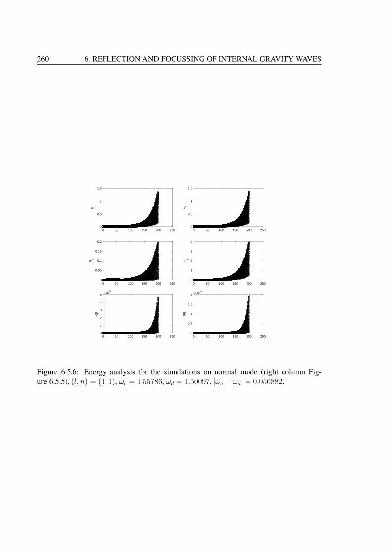
260 6. REFLECTION AND FOCUSSING OF INTERNAL GRAVITY WAVES
0 50 100 150 200 2500
0.5
1
1.5
Eu
0 50 100 150 200 2500
0.5
1
1.5
Ev
0 50 100 150 200 2500
0.05
0.1
0.15
0.2
Ep
0 50 100 150 200 2500
1
2
3
4
Eb
0 50 100 150 200 2500
0.5
1
1.5
2
PE
×106
0 50 100 150 200 2500
1
2
3
4
5
KE
×105
Figure 6.5.6: Energy analysis for the simulations on normal mode (right column Fig-ure 6.5.5), (l, n) = (1, 1), ωc = 1.55786, ωd = 1.50097, |ωc − ωd| = 0.056882.
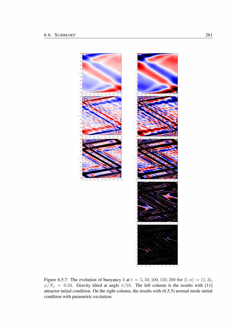
6.6. SUMMARY 261
-0.5 -0.4 -0.3 -0.2 -0.1 0 0.1 0.2 0.3 0.4 0.5
x
-0.5
-0.4
-0.3
-0.2
-0.1
0
0.1
0.2
0.3
0.4
0.5
y
-0.5 -0.4 -0.3 -0.2 -0.1 0 0.1 0.2 0.3 0.4 0.5
x
-0.5
-0.4
-0.3
-0.2
-0.1
0
0.1
0.2
0.3
0.4
0.5
y
-0.5 -0.4 -0.3 -0.2 -0.1 0 0.1 0.2 0.3 0.4 0.5
x
-0.5
-0.4
-0.3
-0.2
-0.1
0
0.1
0.2
0.3
0.4
0.5
y
-0.5 -0.4 -0.3 -0.2 -0.1 0 0.1 0.2 0.3 0.4 0.5
x
-0.5
-0.4
-0.3
-0.2
-0.1
0
0.1
0.2
0.3
0.4
0.5
y
-0.5 -0.4 -0.3 -0.2 -0.1 0 0.1 0.2 0.3 0.4 0.5
x
-0.5
-0.4
-0.3
-0.2
-0.1
0
0.1
0.2
0.3
0.4
0.5
y
-0.5 -0.4 -0.3 -0.2 -0.1 0 0.1 0.2 0.3 0.4 0.5
x
-0.5
-0.4
-0.3
-0.2
-0.1
0
0.1
0.2
0.3
0.4
0.5
y
-0.5 -0.4 -0.3 -0.2 -0.1 0 0.1 0.2 0.3 0.4 0.5
x
-0.5
-0.4
-0.3
-0.2
-0.1
0
0.1
0.2
0.3
0.4
0.5
y
-0.5 -0.4 -0.3 -0.2 -0.1 0 0.1 0.2 0.3 0.4 0.5
x
-0.5
-0.4
-0.3
-0.2
-0.1
0
0.1
0.2
0.3
0.4
0.5
y
Figure 6.5.7: The evolution of buoyancy b at t = 5, 50, 100, 150, 200 for (l, n) = (1, 3),ω/Nf = 0.34. Gravity tilted at angle π/18. The left column is the results with [11]attractor initial condition. On the right column, the results with (6.5.5) normal mode initialcondition with parametric excitation.
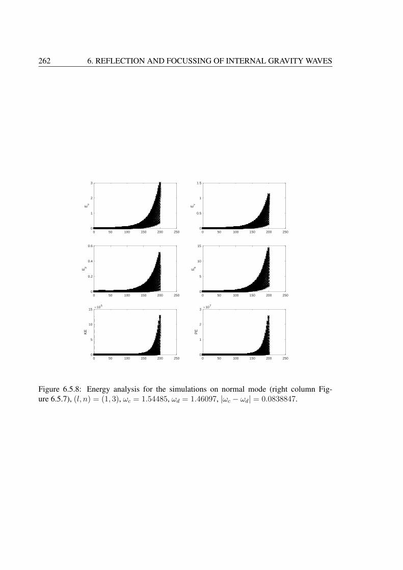
262 6. REFLECTION AND FOCUSSING OF INTERNAL GRAVITY WAVES
0 50 100 150 200 2500
1
2
3
Eu
0 50 100 150 200 2500
0.5
1
1.5
Ev
0 50 100 150 200 2500
0.2
0.4
0.6
Ep
0 50 100 150 200 2500
5
10
15
Eb
0 50 100 150 200 2500
1
2
3
PE
×107
0 50 100 150 200 2500
5
10
15
KE
×105
Figure 6.5.8: Energy analysis for the simulations on normal mode (right column Fig-ure 6.5.7), (l, n) = (1, 3), ωc = 1.54485, ωd = 1.46097, |ωc − ωd| = 0.0838847.
263
Chapter 7
CONCLUSION
7.1 Summary
The main aim of this thesis is to investigate the effects of staircase boundaries in finite-
difference models of wave propagation in several physical settings. For most of the thesis
we focused on the standard set two-dimensional wave equations that is widely used in some
applications such as acoustic, electromagnetism and shallow-water flow. In this thesis, we
also considered internal gravity wave equations for stratified flow that is slightly differ-
ent from the standard set wave equations. For most of our models, we have considered
harmonic waves in time, so that we can exclusively focused on the spatial effects of finite-
differencing. For all problems of interest, we first derived the continuum solutions followed
by discrete solutions on the C-grid. We then compared both solutions and assessed the con-
vergence rate of discrete solutions towards the continuum solutions.
In Chapter 2, we reviewed the two-dimensional wave equations and showed that three phys-
ical systems of wave propagation (i.e., acoustic, electromagnetism, shallow-water flow) also
has equivalent system of equations. We also reviewed some important conservation laws
for this equations. As our main aim is to investigate wave propagation on finite-difference
models, we then reviewed finite-difference scheme of system of wave equations on doubly
264 7. CONCLUSION
periodic domain on three different finite-difference grids which are A-, B- and C-grid. By
using second-order central finite-difference formulation, we showed that the discrete fre-
quency for each grids has second-order convergence in grid spacing h. However, the relat-
ive error for each grids behave differently. For each discrete frequencies, we discussed its
representation and we showed that C-grid is the most satisfactory grid.
In Chapter 3, we considered wave propagation along a channel. We first considered chan-
nel’s boundaries and grid are aligned, and we proved that the discrete frequency is obtained
at second-order in h. Then, we considered wave propagation along a channel with perfect
staircase boundaries. The perfect staircase boundaries is obtained by tilting the channel by
45◦ relative to the grid. This is our main problem of interest. By performing asymptotics
in the limit of small grid spacing h, the discrete solution is derived and compared with the
continuum solution. Unlike the aligned channel, we proved that there is degradation of or-
der of convergence due to the staircasing. The discrete frequency of this unaligned channel
converge towards the continuum values at first-order in grid spacing h, despite the second-
order finite-differences used within the domain. Further, we showed that for this unaligned
case there are two options of perfect staircase boundary condition can be selected. First is
called split centre retention where we showed that the relative error is purely depend on h,
the staircasing error. While the second is called cell-centre retention and we showed that the
relative error dependent on both across and along channel wavenumber j and k, respect-
ively, despite having staircasing error. We also visualised the discrete analytical solution
agreed with the numerical solution. In chapter 3, most of the results are new. Presumably
the grid-aligned analysis leading to (3.3.17) exists somewhere in the vast research literat-
ure covering acoustics, electromagnetic waves and shallow-water waves, but we have not
found it. However, the perfectly-aligned staircase analysis is completely original, as far as
we can tell. The closest study is that of [51], but he used rather different methods and gave
no results for h → 0 at fixed channel width, and thus gave nothing analogous to our main
results (3.4.32) and (3.4.33). The study of [32] used similar methods to here, but was com-
pletely focussed on the case of Kelvin waves for an unbounded channel and shallow-water

7.1. SUMMARY 265
dynamics. Those results rely upon rotation, and cannot be converted to our results here for
non-rotating dynamics.
In Chapter 4, we have studied reflection of waves at a straight boundary. In the continuum
solution, we found that the wave reflected amplitude is the same as that of the incom-
ing wave, the along-boundary wavenumber remains unchanged, and the across-boundary
wavenumber changes sign. For the discrete solutions, we studied two versions of the dis-
crete problem. For the first discrete problem we consider the grid and boundary were
aligned at y = 0. We showed that the reflected amplitude and reflected wavenumber re-
main unchanged as continuum amplitude. However, it is to be noted that there is a second-
order error in the wave frequency of both incident and reflected waves. For the second
discrete problem, we studied wave reflection upon a straight boundary tilted at 45◦ (i.e.,
y = x). In this problem, the boundary now is perfect staircase. Remarkably, we showed
that the reflected wavenumbers were recovered exactly. However, the reflected amplitude
was not recovered exactly. We showed that there was a phase-error which a first-order er-
ror in h. This is our new result. As the study in this chapter looks similar in [17], there
are some differences. The first main difference arises because they analysed the problem
in a specific time-stepping framework, so that their expression also involved a time step.
Here we simply assume time-periodic waves, the frequency of which will be consistent
with the discrete dispersion relation. The second main difference arises because they made
an assumption about the values of kR and lR, without deriving them from kI and lI . Here
we make no such assumption, and rather determine kR and lR from kI and lI , leading to
(4.4.15).
In Chapter 5, we studied numerical solutions of waves equation in two closed domains
which are square and circle. Here the numerical solutions that we obtained bring together
results of Chapter 3 and 4. For both domains, we first derived the continuum solutions,
and we initialised numerical computations by using the continuum solution up to a tenth
period. We studied numerical solutions after multiple reflections and analysed its maximum
266 7. CONCLUSION
error. Further, we quantified our numerical solutions at various grid spacings h, towards the
continuum solution to find convergence rate of physical quantity. For a square domain, we
have considered two separate experiments. In the first of these, the square boundary and
grid were aligned. We quantified the numerical solutions and found that there is a second-
order convergence in h, as expected. In the second experiment, the same square is tilted
at 45◦ so that the boundary has perfect staircases at various h (over 20). For this case, we
found that the rate of convergence for u, v, p, and discrete frequency, degraded to a first-
order in h over one period. We also quantified this domain when tilted at some angles (i.e.,
π/6, π/12, π/18, and π/20). We found that the convergence rate for u, v, p, and ω degraded
to a first-order in h in max. norm, and between 0.6 and 1 in L2 norm, over one period.
For a circular domain, we considered three separate experiments depending on the wave-
mode (m,n). First we considered numerical solution with mode (1, 0). Here, we found that
the rate of convergence for u and v is at first order in h, while for p is 1.6, after one period
in L2 norm, and convergence rate of 1.6 in max. norm. For the second experiment, we
considered wavemode (1, 1). We found that the rate of convergence in max. norm for p is
1.06, but there is no convergence was found (i.e., O(1)) for u and v. While in the L2-norm,
the rate of convergence of all u, v and p is between 0.6 and 1. For these two experiments of
circular wavemode we used cell centre node as activation cell to generate staircase bound-
ary. So, in the third experiment we considered same wavemode (1, 0) as in first, but with
four corner cell activation. Here, we showed that there is a first-order convergence in h for
u, v and p in max. norm. As far as we concern, we cannot find other examples of numer-
ical experiments of wave sloshing in a closed domain with staircase boundaries like in this
chapter. So that all works in chapter 5 are new.
In Chapter 6, in order to get some ideas to extend the results from chapters 2-5, we first
reviewed internal gravity wave equations by introducing the equations of motion and con-
figuring these equations on staggered grids. We then derived the relevant dispersion re-
lation for internal gravity waves in an unbounded medium. We next considered internal
7.2. OVERVIEW 267
wave reflection at a sloping boundary, and reviewed the classic continuum reflection. We
then presented what is believed to be a completely novel discrete reflection calculation on
the staggered grid. We found an error of O(h) in the discrete reflection problem and this
suggests that issues may arise in phenomena driven by internal gravity reflection. Since
internal wave focussing in a closed domain is driven by a particular property of internal
gravity wave reflection, our idea is that staircase boundaries may prevent or alter the fo-
cussing phenomena. We intend to make such calculations in the future – for rectangular
domains with staircase boundaries.
7.2 Overview
Throughout this thesis, we have studied the relative error of the discrete wave’s frequency
in each of our physical settings. Here, we summarised all results for Chapter 3 in Table 7.1-
7.4. As can be seen, the relative error for the case of channel with aligned boundary has
second-order convergence in h. While the relative error for the case of tilted channel at
45◦, has first-order convergence in h. For the case of split cell retention we found that the
relative error is purely from staircase boundaries. However, for the case cell-centre retention
the relative error consists of staircasing error and geometrical error which is manifested by
across channel wavenumber j and along-channel wavenumber k. For example, for the
case of mode j = 0, to obtain the frequency accurate to within 1% (i.e., ∆ < 0.01), we
need kh =√
0.12 or 18 grid points per along-channel wavelength for the case of aligned
boundaries. On the other hand, for the case of unaligned boundaries we need 71 grid-
boxes across the channel, for both split cell and cell centre retention boundary condition.
To obtain the frequency accurate to within 10% (i.e., ∆ < 0.1), we need 6 grid points
per along-channel for the aligned boundaries, and 7 grid-boxes across the channel for the
unaligned case.
For the case of mode j = 1 and k = 1 in order to obtain the frequency accurate to within
268 7. CONCLUSION
1%, we need 9 grid boxes across the channel for the aligned boundary. For the case of
unaligned boundary, again we need 71 grid boxes across the channel for split cell retention
boundary condition. However, for cell-centre retention boundary condition we only need 7
grid boxes across the channel. For the case of mode j = 5 and k = 1, in order to obtain
the frequency accurate to within 1%, we need 46 grid boxes across the channel for the
aligned boundary. For the case of unaligned boundary, again we need 71 grid boxes across
the channel for split cell retention boundary condition, but only 1 for cell-centre retention
boundary condition. Thus, we have been able to make a clear conclusion about the influence
of staircase boundaries on wave propagation along a channel.
In Chapter 4, we considered wave reflection at a straight wall aligned with grid and the wall
(at y = x) was aligned at 45◦ to the grid, thus forming a perfect staircase boundary. In
the discrete wave reflection at staircase boundary, we showed that the wavenumbers of the
reflected wave were recovered exactly, which is perhaps surprising. However, the (complex)
amplitude AR of the reflected wave was not recovered exactly. Even though its magnitude
was recovered correctly, i.e., |AR| = |AI |, there was a phase error, i.e., AR/AI had non-
zero imaginary part. We derived an expression for AR/AI (which was previously given by
[17]), and analysed it in some detail. In particular, we showed that there is first-order error
ϕ in the phase, in terms of the grid spacing h with ϕ = (k2 + l2)h/(k − l), where (k, l)
is the wavevector of the incident wave. For example, for the case when the incident wave
is normal to the boundary, i.e., l = −k. Then the phase error ϕ = kh (a result which we
showed to be exact, even at finite h). For a minimally resolved wave with 4 grid points per
wavelength (i.e., 4h = 2π/k ⇒ kh = π/2), the phase error upon reflection is then π/2.
So if the wave were to reflect off two such boundaries, then the phase error would be π
(assuming that the phase errors were additive), and the wave would become completely out
of phase with its continuum counterpart. However, note that the error in the wave frequency
here would only be 19% (i.e., this might be considered to be an adequately resolved wave
on the C-grid). So, the effects of staircasing are clear, and how they could lead to serious
errors in the phase of the wave after 1 (or, more likely, multiple) reflections.
7.2. OVERVIEW 269
In chapter 5, we have seen numerical solutions of waves equation sloshing in a square and
circle domain. For the square domain, we have seen the solutions at two particular cases:
(i) boundaries aligned with the grid, and (ii) boundaries unaligned with the grid. While for
the circle domain, we have seen the numerical solutions of two different wave modes (with
different azimuthal wavenumber) sloshing in the domain. The exact continuum solutions
is first derived to be used as an initial condition in the numerical experiment as well as to
compute the error of the solutions.
For the square domain boundaries aligned with the grid, we have shown that second-order
convergence in h is achieved, since central second-order finite-difference formulation is
used in the experiments. We thus confirmed that the rate of convergence will not be affected
as long as the boundaries aligned with the grid (second-order convergence in h is obtained
with angle θ = 90◦).
On the other hand, there is reduction of the order of accuracy for the case of unaligned
boundaries with staircase boundary. We have quantified this degradation in for u, v and p.
The quantification is obtained after one period of wave oscillation. We summarised all the
results in Table 7.5. It is shown that first-order convergence in h is obtained when the square
has staircase boundaries, which is consistent with the analysis in chapters 3 and 4. We also
have examined the effect of tilt angle. We have quantified the spatial convergence rate at
some angles. We found that the scaling factor for spatial error decrease with θ, which as
expected. This is agree with the results found in [32] for channel flow, where it was showed
that scaling factor for spatial error decrease with θ.
The solutions for waves sloshing in a circular domain are different. The investigation was
split into three experiments: (i) mode m = 1, n = 0, (ii) mode m = 1, n = 1, and (iii)
mode m = 1, n = 0. In experiments (i) and (ii), we used cell centre activation, while in
(iii) we used 4 corners of each cells as activation. Here, we also quantified the convergence
rate at various h after one period, as summarised in Table 7.5. For all experiments, the best
convergence rate that we found is first-order in h. It is clear evidence that staircase boundary
270 7. CONCLUSION
has degraded the accuracy of numerical solution. However, the quantification must be done
at many points to see a reliable slope of convergence (i.e., many numerical experiments at
many grid points). This has not been discussed to our knowledge, and, indeed, the standard
behaviour seems to be to take far fewer points – even as few as 3.

7.2.O
VE
RV
IEW
271
Table 7.1: The relative error ∆ for wave propagation along a channel with aligned boundaries and unaligned boundaries forj = 0, k = 1.
aligned boundaries staircase boundaries
∆ =h2
12
(k4 + j4π4
k2 + j2π2
)GPPW GPAC ∆ =
h√2
GPPW GPAC ∆ =h√2
(k2
k2 + j2π2
)GPPW GPAC
0.1% 57 9 0.1% 4443 708 0.1% 4443 7081% 18 3 1% 444 71 1% 444 7110% 6 1 10% 45 7 10% 45 7
Table 7.2: The relative error ∆ for wave propagation along a channel with aligned boundaries and unaligned boundaries forj = 0, k = 2.
aligned boundaries staircase boundaries
∆ =h2
12
(k4 + j4π4
k2 + j2π2
)GPPW GPAC ∆ =
h√2
GPPW GPAC ∆ =h√2
(k2
k2 + j2π2
)GPPW GPAC
0.1% 58 19 0.1% 2222 708 0.1% 556 1771% 19 6 1% 222 71 1% 56 1810% 6 2 10% 22 7 10% 6 2
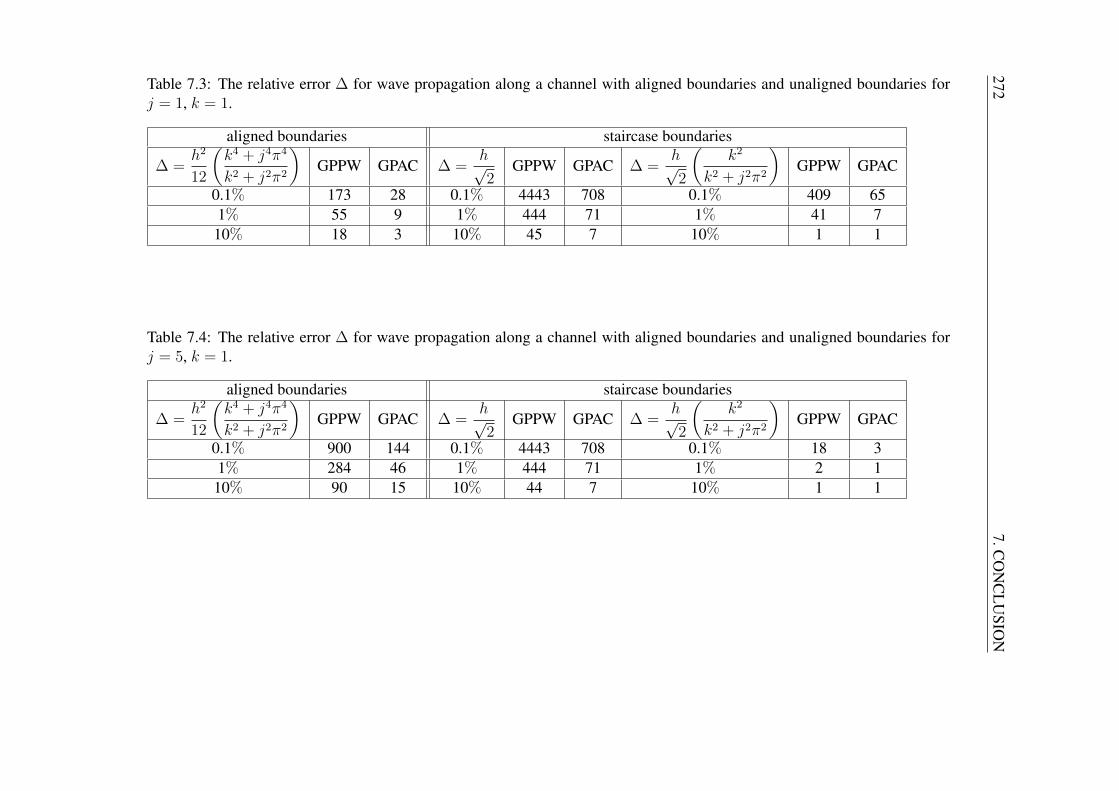
2727.C
ON
CL
USIO
N
Table 7.3: The relative error ∆ for wave propagation along a channel with aligned boundaries and unaligned boundaries forj = 1, k = 1.
aligned boundaries staircase boundaries
∆ =h2
12
(k4 + j4π4
k2 + j2π2
)GPPW GPAC ∆ =
h√2
GPPW GPAC ∆ =h√2
(k2
k2 + j2π2
)GPPW GPAC
0.1% 173 28 0.1% 4443 708 0.1% 409 651% 55 9 1% 444 71 1% 41 710% 18 3 10% 45 7 10% 1 1
Table 7.4: The relative error ∆ for wave propagation along a channel with aligned boundaries and unaligned boundaries forj = 5, k = 1.
aligned boundaries staircase boundaries
∆ =h2
12
(k4 + j4π4
k2 + j2π2
)GPPW GPAC ∆ =
h√2
GPPW GPAC ∆ =h√2
(k2
k2 + j2π2
)GPPW GPAC
0.1% 900 144 0.1% 4443 708 0.1% 18 31% 284 46 1% 444 71 1% 2 110% 90 15 10% 44 7 10% 1 1

7.2. OVERVIEW 273
Table 7.5: The convergence rate for u, v and p in max norm and L2 norm, at various h forthe specific domain.
max norm L2 normDomain u v p u v psquare (aligned) 1.82 1.89 1.89 1.84 1.86 1.89square (tilted at π/4) 1.16 1.16 1.15 1.24 1.24 1.24square (tilted at π/6) O(1) O(1) 1.05 0.78 0.71 1.05square (tilted at π/12) O(1) O(1) 1.05 0.6 0.6 1.07square (tilted at π/18) O(1) O(1) 1.09 0.62 0.64 1.05square (tilted at π/36) O(1) O(1) 0.95 0.63 0.64 1.35circle (m = 1, n = 0) 1.11 1.11 1.59 1.59 1.59 1.68circle (m = 1, n = 1) O(1) O(1) 1.06 0.94 0.66 1.08circle (m = 1, n = 0) 4 corners 1.03 1.03 1.04 – – –

274 7. CONCLUSION
275
Appendices

277
Appendix A
Stability Testing
We consider a system of first-order of linear with constant coefficient ordinary differential
equations (ODEs) of the form
a′ = La, a(0) = a0, (A.0.1)
where L is a constant matrix and a = a(t) is m-dimensional vector. We calculate a numer-
ical solution an = a(n∆t) by using some scheme.
To understand the stability of the scheme, we first consider the eigenvalues of matrix L in
the form
|L− λiI| = 0, (A.0.2)
where λi(i = 1, 2, ...,m) is the eigenvalue of matrix Lm×m and I is the identity matrix, and
every eigenvalues has corresponding eigenvectors xi which satisfy
Lxi = λixi. (A.0.3)
278 A. Stability Testing
Then, the solution of the system of ODEs can be written as
a(t) =m∑i=1
ci(t)xi. (A.0.4)
where ci(t) are fixed by the initial condition. Hence, (A.0.1) is satisfied if
m∑i=1
ci′(t)xi =
m∑i=1
ci(t)Lxi =m∑i=1
ci(t)λixi. (A.0.5)
It is easily seen from (A.0.5) that
c′i = λici, ordcidt
= λici, ci(0) = ci0 . (A.0.6)
Equation (A.0.6) is a scalar equation with eigenvalues of matrix L. O, understanding solu-
tion of (A.0.1) reduces to understanding solution of (A.0.5), and eigenvalues of L are the
key to understanding.
We are interested in wave equation for which the eigenvalue of L will be pure imaginary. It
is because wave oscillates with sin and cos function. To illustrate it, we give an example by
considering the system
du
dt= p,
dp
dt= −u. (A.0.7)
Then the system can be written as
d
dt
u
p
=
0 1
−1 0
u
p
. (A.0.8)
So, L =
0 1
−1 0
, and the eigenvalues are λ = ±i. The solution is ψ(t) = ψ0eit. The

279
remainder of the discussion will discuss about the stability of scheme to the test equation
dψ
dt= iψ, ψ(0) = ψ0. (A.0.9)
The stability of a numerical scheme can be determined by analyzing the amplification factor.
So, we now explicitly derive amplification factor for some standard numerical scheme.
They are all well known results that can be found in various books [25, 43]. The ampli-
fication factor, A, is defined as the ratio of the numerical solution ϕ, between two adjacent
times or mathematically in the form
A =ϕn+1
ϕn. (A.0.10)
where ϕn is the numerical approximation to the true solution at discrete time level tn =
n∆t. The numerical scheme is said stable if |A| ≤ 1 and unstable if |A| > 1. All schemes
that will be discussed will be examined based on this amplification factor. Note that, from
(A.0.10), we want |A| = 1 where A = ei∆t. If we expending the solution becomes
A = 1 + i∆t− ∆t2
2− i∆t
3
6+
1
24∆t4 + (O(∆t5)). (A.0.11)
For every numerical scheme, we also calculate numerical solution and consider the max-
imum error at t = 10.
A.0.1 Euler
The most famous and simple numerical scheme to approximate the derivative in equation
(A.0.9) is Euler’s scheme by using forward difference. When applied to the test equation
(A.0.9) the scheme reads
ϕn+1 − ϕn
∆t= iϕn. (A.0.12)

280 A. Stability Testing
0 0.5 1 1.5 2 2.5 30.5
1
1.5
2
2.5
3
∆t
|A|
EulerRK−2
Figure A.0.1: Modulus of amplification factor for the Euler’s scheme as a function of ∆t .
Dividing by ϕn gives
A = 1 + i∆t. (A.0.13)
So we get the first 2 terms in the right hand side of (A.0.11). This means that the scheme is
first-order accurate in ∆t. The modulus of the amplification factor can be written as
|A| =(1 + ∆t2
)1/2. (A.0.14)
It can be easily seen that, |A| > 1. Thus, this scheme is said unstable. The instability of
the scheme is graphically showed in Figure A.0.1. This scheme is not suitable because the
numerical solution will diverge from the true solution.
281
A.0.2 Runge-Kutta order 2
For the general problem dϕ/dt = F (ϕ), the Runge-Kutta order 2 scheme can be written as
ϕn+1 = ϕn + ∆tF (ϕn+1/2), (A.0.15a)
ϕn+1/2 = ϕn +1
2∆tF (ϕn). (A.0.15b)
When applying to the test equation (A.0.9), where F (ϕ) = iϕ it becomes
ϕn+1 = ϕn + i∆tϕn − 1
2∆t2ϕn =
(1 + i∆t− 1
2∆t2)ϕn.
Dividing by ϕn, yields
A = 1 + i∆t− 1
2∆t2. (A.0.16)
Here, we get first three terms of (A.0.11). So this scheme is second-order accurate in ∆t.
The modulus square of amplification factor (A.0.16) is
|A|2 =
(1− 1
2∆t2)2
+ ∆t2 = 1 +1
4∆t4, (A.0.17)
which also gives
|A| = 1 +1
8∆t4, as ∆t→ 0. (A.0.18)
It can be seen from (A.0.17) that the scheme is unstable for all ∆t since |A| > 1. This
instability is graphically shown in the Figure (A.0.1). Although this scheme is unstable, the
growth factor is of O(∆t4) which makes the amplification weak. This scheme can be used
in the limited length of time integration and the time stepping ∆t is sufficiently small.
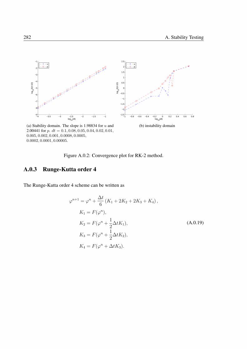
282 A. Stability Testing
−4 −3.5 −3 −2.5 −2 −1.5 −1−9
−8
−7
−6
−5
−4
−3
−2
−1
log10
(dt)
log 10
E(t
=10
)
up
(a) Stability domain. The slope is 1.98834 for u and2.00441 for p. dt = 0.1, 0.08, 0.05, 0.04, 0.02, 0.01,0.005, 0.002, 0.001, 0.0008, 0.0005,0.0002, 0.0001, 0.00005.
−1 −0.8 −0.6 −0.4 −0.2 0 0.2 0.4 0.6 0.8−2.5
−2
−1.5
−1
−0.5
0
0.5
1
1.5
2
2.5
log10
(dt)lo
g 10E
(t=
10)
up
(b) instability domain
Figure A.0.2: Convergence plot for RK-2 method.
A.0.3 Runge-Kutta order 4
The Runge-Kutta order 4 scheme can be written as
ϕn+1 = ϕn +∆t
6(K1 + 2K2 + 2K3 +K4) ,
K1 = F (ϕn),
K2 = F (ϕn +1
2∆tK1),
K3 = F (ϕn +1
2∆tK2),
K4 = F (ϕn + ∆tK3).
(A.0.19)
283
Applying to the test equation (A.0.9) where F (ϕ) = iϕ, the scheme reads
K1 = iϕn,
K2 = i
(ϕn +
1
2i∆tϕn
)= iϕn
(1 +
1
2i∆t
),
K3 = i
(ϕn +
1
2i∆tϕn{1 +
1
2∆t}
),
= iϕn(
1 +1
2i∆t− 1
4∆t2),
K4 = i
(ϕn + i∆tϕn{1 +
1
2i∆t− 1
4∆t2}
),
= iϕn(
1 + i∆t− 1
2∆t2 − 1
4i∆t3
).
(A.0.20)
Hence,
ϕn+1 = ϕn +i∆t
6ϕn(
6 + 3i∆t−∆t2 − 1
4i∆t3
). (A.0.21)
Dividing by ϕn gives
A =ϕn+1
ϕn= 1 + i∆t− 1
2∆t2 − 1
6i∆t3 +
1
24∆t4. (A.0.22)
For this scheme, we get first four terms of (A.0.11). So, this scheme is four order accurate
in ∆t. The modulus square of amplification factor (A.0.22) is
|A|2 =
(1− 1
2∆t2 +
1
24∆t4)2
+
(∆t− 1
6∆t3)2
,
= 1− 1
72∆t6 +O(∆t8).
(A.0.23)
which gives
|A| = 1− 1
144∆t6 +O(∆t8), as ∆t→ 0. (A.0.24)
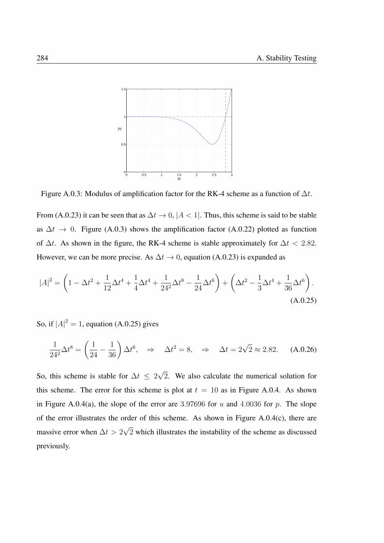
284 A. Stability Testing
0 0.5 1 1.5 2 2.5 30
0.5
1
1.5
∆t
|A|
Figure A.0.3: Modulus of amplification factor for the RK-4 scheme as a function of ∆t.
From (A.0.23) it can be seen that as ∆t→ 0, |A < 1|. Thus, this scheme is said to be stable
as ∆t → 0. Figure (A.0.3) shows the amplification factor (A.0.22) plotted as function
of ∆t. As shown in the figure, the RK-4 scheme is stable approximately for ∆t < 2.82.
However, we can be more precise. As ∆t→ 0, equation (A.0.23) is expanded as
|A|2 =
(1−∆t2 +
1
12∆t4 +
1
4∆t4 +
1
242∆t8 − 1
24∆t6)
+
(∆t2 − 1
3∆t4 +
1
36∆t6).
(A.0.25)
So, if |A|2 = 1, equation (A.0.25) gives
1
242∆t8 =
(1
24− 1
36
)∆t6, ⇒ ∆t2 = 8, ⇒ ∆t = 2
√2 ≈ 2.82. (A.0.26)
So, this scheme is stable for ∆t ≤ 2√
2. We also calculate the numerical solution for
this scheme. The error for this scheme is plot at t = 10 as in Figure A.0.4. As shown
in Figure A.0.4(a), the slope of the error are 3.97696 for u and 4.0036 for p. The slope
of the error illustrates the order of this scheme. As shown in Figure A.0.4(c), there are
massive error when ∆t > 2√
2 which illustrates the instability of the scheme as discussed
previously.
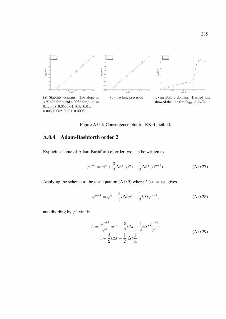
285
−3.5 −3 −2.5 −2 −1.5 −1−14
−13
−12
−11
−10
−9
−8
−7
−6
−5
log10
(dt)
log 10
E(t
=10
)
up
(a) Stability domain. The slope is3.97696 for u and 4.0036 for p. dt =0.1, 0.08, 0.05, 0.04, 0.02, 0.01,0.005, 0.002, 0.001, 0.0008.
−3.5 −3 −2.5 −2 −1.5 −1−14
−13
−12
−11
−10
−9
−8
−7
−6
−5
log10
(dt)
log 10
E(t
=10
)
up
(b) machine precision
−1 −0.5 0 0.5 1−5
0
5
10
15
20
log10
(dt)
log 10
E(t
=60
)
up
(c) instability domain. Dashed lineshowed the line for dtmax < 2
√2.
Figure A.0.4: Convergence plot for RK-4 method.
A.0.4 Adam-Bashforth order 2
Explicit scheme of Adam-Bashforth of order two can be written as
ϕn+1 = ϕn +3
2∆tF (ϕn)− 1
2∆tF (ϕn−1). (A.0.27)
Applying the scheme to the test equation (A.0.9) where F (ϕ) = iϕ, gives
ϕn+1 = ϕn +3
2i∆tϕn − 1
2i∆tϕn−1, (A.0.28)
and dividing by ϕn yields
A =ϕn+1
ϕn= 1 +
3
2i∆t− 1
2i∆t
ϕn−1
ϕn,
= 1 +3
2i∆t− 1
2i∆t
1
A,
(A.0.29)
286 A. Stability Testing
where 1/A in the right hand side of preceding equation is obtained by decreasing 1 step from
equation (A.0.10). Simplify equation (A.0.29) will give quadratic stability polynomial
A2 −(
1 +3
2i∆t
)A+
1
2i∆t = 0. (A.0.30)
Note that, this scheme is two level schemes which involve ϕn−1, ϕn and ϕn−1, and that is
why we have a quadratic of A, with two roots. The first root is represent physical mode and
the second root represent computational mode. So the two roots of the stability polynomial
(A.0.30) are
A± =1
2
(1 +
3
2i∆t±
(1 + i∆t− 9
4∆t2)1/2
). (A.0.31)
As ∆t→ 0, we obtain
A+ =1
2
(2 + 2i∆t−∆t2 +
1
2i∆t3 − 1
4∆t4)
+O(∆t5),
= 1 + i∆t− 1
2∆t2 +
1
4i∆t3 − 1
8∆t4 +O(∆t5),
(A.0.32)
A− =1
2
(i∆t+ ∆t2 − 1
2i∆t3
)+O(∆t4),
=1
2i∆t+
1
2∆t2 − 1
4i∆t3 +O(∆t4),
(A.0.33)
From (A.0.11), A+ is the physical mode and A− is the computational mode. The modulus
of amplification factor for both roots are
|A+| = 1 +1
4∆t4 + . . . ; |A−| =
1
2∆t+ . . . , as ∆t→ 0. (A.0.34)
From equation (A.0.34), the physical root is stable while the computational root is converge
as ∆t → 0. Also can be seen that, the O(∆t4) in the physical mode makes the growth of
the amplification weak. Thus, the AB-2 scheme is weakly stable with an O(∆t4) growth.
This scheme has the same case as in the Runge-Kutta of order two scheme. The stability

287
0 0.5 1 1.5 2 2.5 30
0.5
1
1.5
2
2.5
3
3.5
4
4.5
5
∆t
|A|
Figure A.0.5: Modulus of amplification factor for the AB-2 scheme as a function of ∆t.
behaviour of this scheme is graphically shown in Figure A.0.5.
−4 −3.5 −3 −2.5 −2 −1.5 −1−8
−7
−6
−5
−4
−3
−2
−1
log10
(dt)
log 10
E(t
=10
)
up
(a) Stability domain. The slope is 1.9926 for u and2.00302 for p. dt = 0.1, 0.08, 0.05, 0.04, 0.02, 0.01,0.005, 0.002, 0.001, 0.0008, 0.0005,0.0002, 0.0001, 0.00005.
−1 −0.8 −0.6 −0.4 −0.2 0 0.2 0.4 0.6 0.8−2
−1.5
−1
−0.5
0
0.5
1
1.5
2
2.5
log10
(dt)
log 10
E(t
=10
)
up
(b) instability domain
Figure A.0.6: Convergence plot for AB-2 method.
288 A. Stability Testing
A.0.5 Leapfrog
The Leapfrog scheme can be written as
ϕn+1 = ϕn−1 + 2∆tF (ϕn). (A.0.35)
Then, when applied to the test equation (A.0.9) will give
ϕn+1 = ϕn−1 + 2i∆tϕn, (A.0.36)
and dividing by ϕn gives the quadratic equation
A2 − 2i∆tA− 1 = 0. (A.0.37)
The two roots of equation (A.0.37) are
A± = i∆t±(1−∆t2
)1/2. (A.0.38)
As can be seen, the roots of this scheme have two different behaviour. When ∆t → 0, the
first root is A+ → 1 which represent physical mode and the second root is A− → −1 which
represent computational mode. If |∆t| < 1, then the second term in equation (A.0.38) is
real which will give
|A±| =((
1−∆t2)1/2)2
+ (∆t)2 = 1, (A.0.39)
which means that both physical and computational modes are stable. If ∆t = 1, then both
physical and computational modes are same, i.e., A+ = A− = i. This scheme is stable for
∆t = 1 because both roots represent the exact solution. If ∆t > 1, then the second term is

289
complex and we have
|A+| =∣∣∣i∆t+ i
(∆t2 − 1
)1/2∣∣∣ > |∆t| > 1, (A.0.40)
and the scheme is unstable.
−4 −3.5 −3 −2.5 −2 −1.5 −1−9
−8
−7
−6
−5
−4
−3
−2
−1
log10
(dt)
log 10
E(t
=10
)
up
(a) Stability domain. The slope is 2.00133 for u and1.99995 for p. dt = 0.1, 0.08, 0.05, 0.04, 0.02, 0.01,0.005, 0.002, 0.001, 0.0008, 0.0005,0.0002, 0.0001, 0.00005.
−1 −0.8 −0.6 −0.4 −0.2 0 0.2 0.4−3
−2
−1
0
1
2
3
log10
(dt)
log 10
E(t
=10
)
up
(b) instability domain. Dashed line showed the linefor dtmax < 1.
Figure A.0.7: Convergence plot for Leapfrog method.
A.0.6 Adam-Bashforth order 3
Explicit scheme of Adam-Bashforth of order three can be written as
ϕn+1 = ϕn +∆t
12
(23F (ϕn)− 16F (ϕn−1) + 5F (ϕn−2)
). (A.0.41)
Applying to the test equation gives
ϕn+1 = ϕn +∆t
12
(23iϕn − 16iϕn−1 + 5iϕn−2
). (A.0.42)
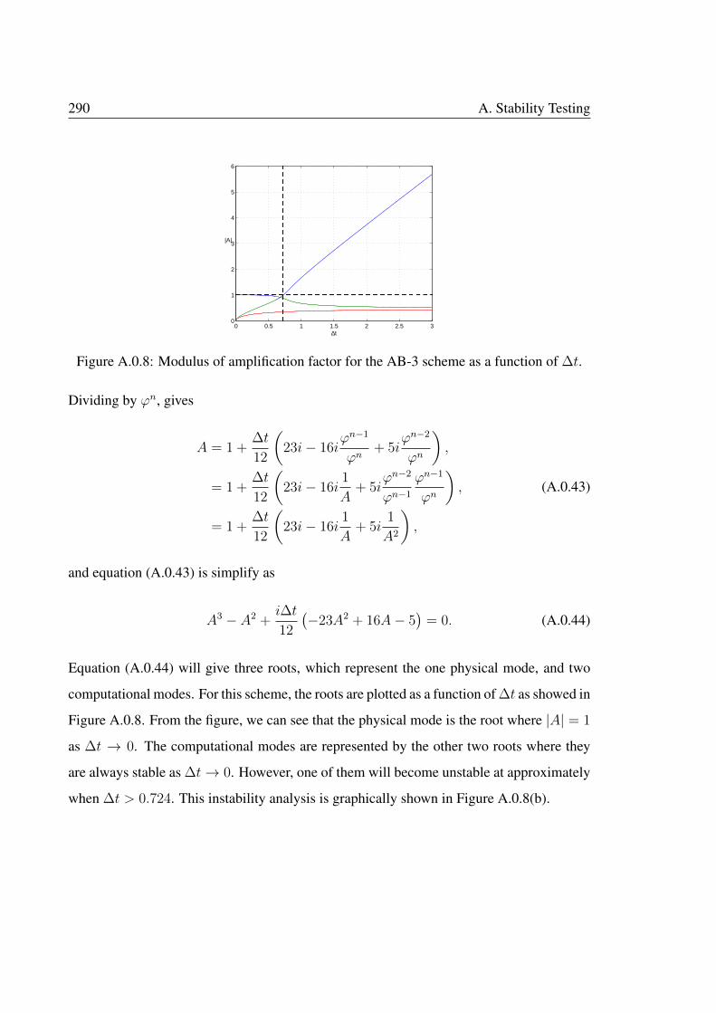
290 A. Stability Testing
0 0.5 1 1.5 2 2.5 30
1
2
3
4
5
6
∆t
|A|
Figure A.0.8: Modulus of amplification factor for the AB-3 scheme as a function of ∆t.
Dividing by ϕn, gives
A = 1 +∆t
12
(23i− 16i
ϕn−1
ϕn+ 5i
ϕn−2
ϕn
),
= 1 +∆t
12
(23i− 16i
1
A+ 5i
ϕn−2
ϕn−1
ϕn−1
ϕn
),
= 1 +∆t
12
(23i− 16i
1
A+ 5i
1
A2
),
(A.0.43)
and equation (A.0.43) is simplify as
A3 − A2 +i∆t
12
(−23A2 + 16A− 5
)= 0. (A.0.44)
Equation (A.0.44) will give three roots, which represent the one physical mode, and two
computational modes. For this scheme, the roots are plotted as a function of ∆t as showed in
Figure A.0.8. From the figure, we can see that the physical mode is the root where |A| = 1
as ∆t → 0. The computational modes are represented by the other two roots where they
are always stable as ∆t→ 0. However, one of them will become unstable at approximately
when ∆t > 0.724. This instability analysis is graphically shown in Figure A.0.8(b).
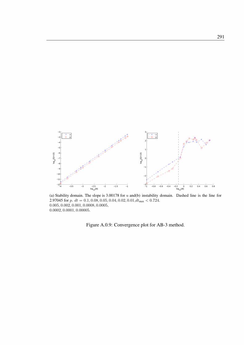
291
−4 −3.5 −3 −2.5 −2 −1.5 −1−12
−11
−10
−9
−8
−7
−6
−5
−4
−3
−2
log10
(dt)
log 10
E(t
=10
)
up
(a) Stability domain. The slope is 3.00178 for u and2.97045 for p. dt = 0.1, 0.08, 0.05, 0.04, 0.02, 0.01,0.005, 0.002, 0.001, 0.0008, 0.0005,0.0002, 0.0001, 0.00005.
−1 −0.8 −0.6 −0.4 −0.2 0 0.2 0.4 0.6 0.8−3
−2
−1
0
1
2
3
log10
(dt)
log 10
E(t
=10
)
up
(b) instability domain. Dashed line is the line fordtmax < 0.724.
Figure A.0.9: Convergence plot for AB-3 method.

292 A. Stability Testing
293
Bibliography
[1] M. Abramowitz and I. A. Stegun. Handbook of mathematical functions: with formu-las, graphs, and mathematical tables, volume 55. Courier Corporation, 1964.
[2] D. J. Acheson. Elementary fluid dynamics. Oxford University Press, 1990.
[3] A. Adcroft, C. Hill, and J. Marshall. Representation of topography by shaved cells ina height coordinate ocean model. Monthly Weather Review, 125(9):2293–2315, 1997.
[4] H. Aochi, T. Ulrich, A. Ducellier, F. Dupros, and D. Michea. Finite difference sim-ulations of seismic wave propagation for understanding earthquake physics and pre-dicting ground motions: Advances and challenges. In Journal of Physics: ConferenceSeries, volume 454, page 012010. IOP Publishing, 2013.
[5] J. R. Apel, H. M. Byrne, J. R. Proni, and R. L. Charnell. Observations of oceanicinternal and surface waves from the earth resources technology satellite. Journal ofGeophysical Research, 80(6):865–881, 1975.
[6] A. Arakawa and V. R. Lamb. Computational design of the basic dynamical processesof the UCLA general circulation model. Methods in Computational Physics, 17:173–265, 1977.
[7] A. Arakawa and V. R. Lamb. A potential enstrophy and energy conserving scheme forthe shallow water equations. Monthly Weather Review, 109(1):18–36, 1981.
[8] G. B. Arfken and H. J. Weber. Mathematical methods for physicists. AAPT, 1999.
[9] P. Baines. The generation of internal tides by flat-bump topography. In Deep SeaResearch and Oceanographic Abstracts, volume 20, pages 179–205. Elsevier, 1973.
[10] P. G. Baines. The reflexion of internal inertial waves from bumpy surfaces. Journal ofFluid Mechanics, 46(2):273–291, 1971.
[11] J. Bajars, J. Frank, and L. R. Maas. On the appearance of internal wave attractorsdue to an initial or parametrically excited disturbance. Journal of Fluid Mechanics,714:283–311, 2013.
294 BIBLIOGRAPHY
[12] W. Barham, S. Bachman, and I. Grooms. Some effects of horizontal discretization onlinear baroclinic and symmetric instabilities. Ocean Modelling, 125:106–116, 2018.
[13] S. Bilbao. Modeling of complex geometries and boundary conditions in finite dif-ference/finite volume time domain room acoustics simulation. IEEE Transactions onAudio, Speech, and Language Processing, 21(7):1524–1533, 2013.
[14] J. Blazek. Computational fluid dynamics: principles and applications. Butterworth-Heinemann, 2015.
[15] J. C. Butcher. The Numerical Analysis of Ordinary Differential Equations: Runge-Kutta and General Linear Methods. Wiley-Interscience, New York, NY, USA, 1987.
[16] D. Cacchione and C. Wunsch. Experimental study of internal waves over a slope.Journal of Fluid Mechanics, 66(2):223–239, 1974.
[17] A. C. Cangellaris and D. B. Wright. Analysis of the numerical error caused bythe stair-stepped approximation of a conducting boundary in FDTD simulationsof electromagnetic phenomena. IEEE Transactions on Antennas and Propagation,39(10):1518–1525, 1991.
[18] R. Clarke. The morning glory: An atmospheric hydraulic jump. Journal of AppliedMeteorology, 11(2):304–311, 1972.
[19] S. N. Collins, R. S. James, P. Ray, K. Chen, A. Lassman, and J. Brownlee. Gridsin numerical weather and climate models. In Climate Change and Regional/LocalResponses. IntechOpen, 2013.
[20] B. Cushman-Roisin and J.-M. Beckers. Introduction to geophysical fluid dynamics:physical and numerical aspects. Academic Press, 2011.
[21] T. Dauxois, A. Didier, and E. Falcon. Observation of near-critical reflection of in-ternal waves in a stably stratified fluid. Physics of Fluids, 16(6):1936–1941, 2004.
[22] T. Dauxois and W. R. Young. Near-critical reflection of internal waves. Journal ofFluid Mechanics, 390:271–295, 1999.
[23] S. Dobricic. An improved calculation of Coriolis terms on the C-grid. MonthlyWeather Review, 134(12):3764–3773, 2006.
[24] K. Dridi, J. S. Hesthaven, and A. Ditkowski. Staircase-free finite-difference time-domain formulation for general materials in complex geometries. IEEE Transactionson Antennas and Propagation, 49(5):749–756, 2001.
[25] D. R. Durran. Numerical methods for wave equations in geophysical fluid dynamics,volume 32. Springer Science & Business Media, 2013.
BIBLIOGRAPHY 295
[26] V. Ekman. On dead water: the norwegian north polar expedition 1893-1896. scientificresults. edited by f, 1904.
[27] B. Engquist, J. Häggblad, and O. Runborg. On energy preserving consistent boundaryconditions for the Yee scheme in 2D. BIT Numerical Mathematics, 52(3):615–637,2012.
[28] C. C. Eriksen. Observations of internal wave reflection off sloping bottoms. Journalof Geophysical Research: Oceans, 87(C1):525–538, 1982.
[29] D. A. Greenberg, F. Dupont, F. H. Lyard, D. R. Lynch, and F. E. Werner. Resolu-tion issues in numerical models of oceanic and coastal circulation. Continental ShelfResearch, 27(9):1317–1343, 2007.
[30] S. M. Griffies, C. Böning, F. O. Bryan, E. P. Chassignet, R. Gerdes, H. Hasumi,A. Hirst, A.-M. Treguier, and D. Webb. Developments in ocean climate modelling.Ocean Modelling, 2(3-4):123–192, 2000.
[31] D. J. Griffiths. Introduction to electrodynamics. Prentice Hall, 1962.
[32] S. D. Griffiths. Kelvin wave propagation along straight boundaries in C-grid finite-difference models. Journal of Computational Physics, 255, 2013.
[33] J. Häggblad and B. Engquist. Consistent modeling of boundaries in acoustic finite-difference time-domain simulations. The Journal of the Acoustical Society of America,132(3):1303–1310, 2012.
[34] J. Häggblad and O. Runborg. Accuracy of staircase approximations in finite-differencemethods for wave propagation. Numerische Mathematik, 128(4):741–771, 2014.
[35] U. Harlander. Towards an analytical understanding of internal wave attractors. Ad-vances in Geosciences, 15:3–9, 2008.
[36] U. Harlander and L. R. Maas. Two alternatives for solving hyperbolic boundary valueproblems of geophysical fluid dynamics. Journal of Fluid Mechanics, 588:331–351,2007.
[37] J. Hazewinkel, N. Grisouard, and S. B. Dalziel. Comparison of laboratory and nu-merically observed scalar fields of an internal wave attractor. European Journal ofMechanics-B/Fluids, 30(1):51–56, 2011.
[38] P. Héreil and R. Laprise. Sensitivity of internal gravity waves solutions to the time stepof a semi-implicit semi-lagrangian nonhydrostatic model. Monthly weather review,124(5):972–999, 1996.
[39] J. D. Jackson. Classical electrodynamics. Wiley, 1999.

296 BIBLIOGRAPHY
[40] A. Javam, J. Imberger, and S. Armfield. Numerical study of internal wave reflectionfrom sloping boundaries. Journal of Fluid Mechanics, 396:183–201, 1999.
[41] L. Jouve and G. I. Ogilvie. Direct numerical simulations of an inertial wave attractorin linear and nonlinear regimes. Journal of Fluid Mechanics, 745:223–250, 2014.
[42] P. K. Kundu. Fluid Mechanics. Elsevier Academic Press, 1990.
[43] J. Lambert. Numerical Methods for Ordinary Differential Systems: The Initial ValueProblem. Wiley, 1991.
[44] J. Lighthill. Waves in fluids. Cambridge university press, 1978.
[45] D. Lilly. A proposed staggered-grid system for numerical integration of dynamicequations. Mon. Wea. Rev, 89:59–65, 1961.
[46] L. Maas and F. Lam. Geometric focusing of internal waves. J. Fluid Mech., 300:1–41,1995.
[47] L. R. Maas. Wave attractors: linear yet nonlinear. International Journal of Bifurca-tion and Chaos, 15(09):2757–2782, 2005.
[48] L. R. Maas, D. Benielli, J. Sommeria, and F.-P. A. Lam. Observation of an internalwave attractor in a confined, stably stratified fluid. Nature, 388(6642):557, 1997.
[49] M. Mercier, R. Vasseur, and T. Dauxois. Resurrecting dead-water phenomenon. Non-linear Processes in Geophysics, 18:193–208, 2011.
[50] G. I. Ogilvie and D. Lin. Tidal dissipation in rotating giant planets. The AstrophysicalJournal, 610(1):477, 2004.
[51] G. Pedersen. On the effects of irregular boundaries in finite difference models. Inter-national Journal for Numerical Methods in Fluids, 6(8):497–505, 1986.
[52] J. Pedlosky. Geophysical fluid dynamics. Springer Science & Business Media, 2013.
[53] O. M. Phillips. The Dynamics of the Upper Ocean. Cambridge University Press, NewYork, 1966.
[54] D. A. Randall. Geostrophic adjustment and the finite-difference shallow-water equa-tions. Monthly Weather Review, 122(6):1371–1377, 1994.
[55] M. Rattray Jr. On the coastal generation of internal tides. Tellus, 12(1):54–62, 1960.
[56] J. W. S. B. Rayleigh. The theory of sound. Macmillan, 1896.
BIBLIOGRAPHY 297
[57] L. F. Richardson. The approximate arithmetical solution by finite differences of phys-ical problems involving differential equations, with an application to the stresses in amasonry dam. Philosophical Transactions of the Royal Society of London. Series A,307–357, 1911.
[58] F. S. Robert and S. B. Dalziel. Internal wave attractors without sloping boundaries.7th. Int. Symp. on Stratified Flows, Rome, Italy, August 22 - 26, 2011, 2011.
[59] J. Russell. Report of the committee on waves. report of the seventh meeting of thebritish association for the advancement of science, liverpool (murray j, 1838.
[60] M. Simanjuntak, J. Imberger, and K. Nakayama. Effect of stair-step and piecewiselinear topography on internal wave propagation in a geophysical flow model. Journalof Geophysical Research: Oceans, 114(C12), 2009.
[61] D. N. Slinn and J. Riley. Internal wave reflection from sloping boundaries. Submittedto J. Fluid Mech, 2001.
[62] L. St. Laurent and C. Garrett. The role of internal tides in mixing the deep ocean.Journal of Physical Oceanography, 32(10):2882–2899, 2002.
[63] B. R. Sutherland. Internal gravity waves. Cambridge university press, 2010.
[64] B. R. Sutherland, S. B. Dalziel, G. O. Hughes, and P. F. Linden. Visualization andmeasurement of internal waves by synthetic schlieren. part 1: Vertically oscillatingcylinder. Journal of Fluid Mechanics, 390:93 126, 1999.
[65] A. Taflove and S. C. Hagness. Computational electrodynamics. Artech house pub-lishers, 2000.
[66] F. D. Tombe. The centrifugal force and the coriolis force. 2014.
[67] A.-K. Tornberg and B. Engquist. Consistent boundary conditions for the Yee scheme.Journal of Computational Physics, 227(14):6922–6943, 2008.
[68] A.-K. Tornberg, B. Engquist, B. Gustafsson, and P. Wahlund. A new type of boundarytreatment for wave propagation. BIT Numerical Mathematics, 46(1):145–170, 2006.
[69] J. S. Turner. Buoyancy effects in fluids. Cambridge University Press, 1979.
[70] G. K. Vallis. Atmospheric and oceanic fluid dynamics: fundamentals and large-scalecirculation. Cambridge University Press, 2006.
[71] K. S. Yee. Numerical solution of initial boundary value problems involving Maxwell’sequations in isotropic media. IEEE Trans. Antennas Propag, 14(3):302–307, 1966.