propagation - unt digital library
TRANSCRIPT
PROPAGATIONB. S. BEPARTMENT OF COMMERCE
National Bureau of Standards
:O
C ~'>
UNITED STATES DEPARTMENT OF COMMERCE • John T. Connor, Secretary
NATIONAL BUREAU OF STANDARDS • A. V. Astin, Director
Ionospheric Radio Propagation
Kenneth Davies
National Bureau of Standards Monograph 80
Issued April 1, 1965
For sale by the Superintendent of Documents, U.S. Government Printing Office Washington, D.C., 20402 - Price $2.75
Library of Congress Catalog Card Number: 64-60061
IONOSPHERIC RADIO PROPAGATION
Contents
Chapter 1
The Earth's Atmosphere, Geomagnetism, and the Sun
Page1.1. Nomenclature. _________-_-___-__-„_.._---______-- _________________ 11.2. Pressure and Density Variations- __________________--__^_~__-_____-- 21.3. Chemical Composition__«______„__.____-__-______,_____^-__^_>_____ 51.4. Formation of Ionized Layers. ___.___„_„_- __________ _-_______«_______ 8
1.4.1. Ion Production- ____________ ____ _-.,._______-_ _ „-_ _. _________ 81.4.2. Ion Disappearance.__.__.,-_______~-___^_-__-____-_-__-____-__ 81.4.3. Formation of a Chapman Layer. ______ ________^____-__-______- 121.4.4. Electron Density Distribution. .____„__________, __.._-^_________ 17
1.5. The Earth's Magnetic Field___ a __ .... ... __„_____-_-____-_-________ 191.5.1. The Dipole Field. _„__„__-_-____-__________._,-__.-__-.______ 19L5.2. The Real Field. „.-_„__„-.„__-_„_-„-_-.-.-_„--_-„_„„-. 23L5.3. Magnetic Variations. ,_______._-__._-__-, ___.__-____________„__ 26L5.4. Magnetic Indices. ______________ _.__ ______________-__„____. ^_ 30
1.6. The Auroral Zones _ __.___________________-____--^-_~_-__-__,____ 361.7. The Sun. _.___,_„_._„___________.________________._.__-__,_,__ 36
1.7.1. Quiet Conditions- _________ _____ _-________---______-.______- 361.7.1.1. Structure. ___.________..--_______--___---_----,--__ 361.7.1.2. Ionizing Radiations.__________________________________ 371.7.1.3* Radio Emissions^... ______.____._.._-____--_________„_ 38
1.7.2. The Active Sun, „„„„_ _^> .___..-_ _._,...__ _.__ . .___„.._- 401.7.2.1. Sunspots. ____.____.____._______^____- _._____._.____ 401.7.2.2. The Sunspot Cycle. .. fc ___..._.___,„,_.__.._„.._._.__ 401.7.2.3. Flares--,--^-.--...--...-»...---.,.----...---.-..-.-- 411.7.2.4. Radio Emissions^ _________._-__. __^ ______ ^_-__________ 43
References.. . ___„.____._,_.___„______, .._.^_-___._,_.__._^,__. _„____- 44
Chapter 2
Theory of Wave Propagation
2.1. Purpose. _ _,-„_______________._____..__..___._._______-_-_-_____.__- 452.2. Electromagnetic Waves ____________________________ _.__._>_,.->_____ 45
2.2.L Electrostatics and Magnetostatics-^^__^_«..^___,^_-^__,..„.____ 452.2.2. Ampere's Circuital Law. __ ^_ ____^_ __________________ ^. _._.„__ 492.2.3. Faraday's Law. , ._____.__...„__.>-__-___,______..._,.__„_._. 49
in
2.2.4. The Displacement Current.___________________________________ 512.2.5. A Solution of Maxwell's Equations.____________________________ 532.2.6. Some Properties of Electromagnetic Waves_____________________ 56
2.3. Magneto-ionic Theory. __________________-,____^_______-____________ 592.3.1. Motion of Ions in Electric and Magnetic Fields-____________ _____ 59
2.3.1.1. Motion in an Electric Field. ___________________________ 592.3.1.2. Motion in a Magnetic Field___ _________________________ 612.3.1.3. Motion in Crossed Electric and Magnetic Fields. __ _______ 62
2.3.2. Derivation of the Appleton Formula. ______________ ___________ 632.3.3. Some Properties of the Appleton Formula . ____________________ 71
2.3.3.1. No Magnetic Field, No Collisions. _____________________ 712.3.3.2. Magnetic Field, No Collisions_____ _____________________ 732.3.3.3. No Magnetic Field, With Collisions.____________________ 802.3.3.4. Magnetic Field, With Collisions. _______________________ 82
2.3.4. Generalized Magneto-ionic Formulas____„____-_-_____________- 842.3.4.1. Collision Statistics. ___________________________________ 842.3.4.2. Dispersion ___________________________________________ 882.3.4.3. Absorption.__________________________________________ 88
2.4. Group Propagation________________________________________________ 892.4.1. Phase Velocity-______________________________________________ 892.4.2. Group Velocity. ________._____.____.___-.___-_ _____-_-__ ______ 91
2.5. Propagation in Anisotropic Media_ __________________________________ 932.5.1. Meaning of Anisotropy_______________________________________ 932.5.2. Angle Between Phase and Ray Directions. _____________________ 952.5.3. Phase and Group Paths_ __--_--___--_-____-_.__-____--____-.- 96
References. ________ ______-_______-_________-____-_^__--_______________ 99
Chapter 3
Synoptic Studies of the Ionosphere
3.1. Worldwide Soundings. _____ ______________________________ „____„ _ 1013.2. Experimental Techniques. __________________________________________ 103
3.2.1. Height Recorders.___________________________________________ 1033.2.1.1. The Ionosonde_____________________._________________ 1033.2.1.2. The Virtual Height-Time Recorder. .„_________________ 108
3.2.2. Absorption Measurements. ____________________________________ 1083.2.2.1. The Pulse Reflection Method. _________________________ 1083.2.2.2. Continuous-Wave Field-Intensity Recordings ____________ 1103.2.2.3. The Riometer Method. _______________________________ 1103.2.2.4. Minimum Frequency Observations_______________„____ 112
3.2.3. Phase Measurements_ ________________________________________ 1133.2.3.1. Relative Phase Changes. ______________________ „ _____ 1133.2.3.2. Frequency Changes.___________________________________ 113
3.2.4. Angle of Arrival. ____________________________________________ 1143.2.4.1. Direction Finding. ___________________________________ 1143.2.4.2. Vertical Angle. ______________________________________ 114
3.2.5. Rockets and Satellites. _______________________________________ 1163.3. The Quiet Ionosphere_____________________«____^_________________._ 117
3.3.1. Purpose_________^__________________________________________ 1173.3.2. lonograms and Their Interpretation.____ ___________________„__ 117
IV
3.3.3. Electron Density Profiles. ____„____-___._---____-___._________ 1243.3.3.1. Real Height Analysis. _______________________________ 1243.3.3.2. Diurnal Variations^.__. ________________ __________ _____ 1253.3.3.3. Seasonal Variations. ____________ ______________________ 1303.3.3.4. Solar Cycle Variations. _______________________ ________ _ 1303.3.3.5. Geographical Variation____ _______„_____________„______ 130
3.3.4. Model Layers.. ____________________________________________ 1343.3.4.1. Chapman Layer______ ________________________________ 1343.3.4.2. Parabolic Layer _ _____________________________________ 1343.3.4.3. Linear Layer. _________________________________________ 1363.3.4.4. Exponential Layer____________________________________ 136
3.3.5. Critical Frequency Variations_________________________________ 1363.3.5.1. General Features. _________ ______ _____________________ 1363.3.5.2. The E Layer__ _______________________________________ 1383.3.5.3. The Fi Layer. ______________________________________ 1403.3.5.4. The F2 Layer. _____________ ________ _________________ 142
3.3.6. Variations in Ionospheric Absorption. __________________________ 1443.3.6.1. Introductory Remarks. _______________________________ 1443.3.6.2. Frequency Dependence of Absorption. __________________ 1453.3.6.3. Solar Cycle Control--._________„»„____.-________________ 1473.3.6.4. Diurnal Variations._-________-__^_____________________ 1473.3.6.5. Seasonal Variations. __________________________________ 149
3.3.7. Sporadic £;________________-_____________ ______________ _____ 1503.3.8. Spread F___________________________________________________ 153
3.3.8.1. Description of Spread F_ ______________________________ 1533.3.8.2. Diurnal Variations.. __________________________________ 1533.3.8.3. Seasonal Variations-__________________________________ 1543.3.8.4. Solar Cycle Variations ________________________________ 1563.3.8.5. Correlation with Magnetic Activity. ___ _________________ 156
References-________________________________j__________________________ 156
Chapter 4
Oblique Propagation
4.1. Characteristics of HF Propagation.__________________________________ 1594.2. Equivalence Relationships.„_____-__________________________________ 160
4.2.1. Plane Earth and Plane Ionosphere. ____________________________ 1604.2.1.1. The "Secant Law"_____________._ _____________________ 1604.2.1.2. Breit and Tuve's Theorem,... _________________________ 1614.2.1.3. Martyn's (Equivalent Path) Theorem.__________________ 1624.2.1.4. Martyn's (Absorption) Theorem____________ ____________ 163
4.2.2. Effect of the Curvature of the Ionosphere_______________________ 1634.3. Calculation of Maximum Frequencies. ___________________„___________ 165
4.3.1. Plane Ionosphere. ___________________________________________ 1654.3.2. Curved Ionosphere.__________________________________________ 1694.3.3. The Parabolic-Layer Method.________ _________________________ 172
4.4. Oblique lonograms________________________________________________ 1734.4.1. Experimental Technique.. _____________„__„______,____________ 1734.4.2. Conversion from Vertical to Oblique Incidence __________________ 1744.4.3. Experimental Records. _______________________________________ 175
4.4.3.1. Medium Distances. __ _________________________________ 175
4.4.3.2. Long Distances.__._-_.____._-.-_-.__-______-______-_- 1784.5. Definitions of MUF..._..._____________________________________ 1794.6. Accuracy of MUF Calculations. __ „.____________________________„. 180
4.6.1. Effect of the Earth's Magnetic Field. __________________________ 1804.6.2. MUF Extention__-__________-__-____________________________ 1824.6.3. Sporadic £_________ ______________________________ ___________ 1824.6.4. Ionospheric Scatter. _.„______________________________________ 1844.6.5. Ground Scatter. __..__________________________________________ 1844.6.6. Ionospheric Tilts. .__.____ ___________________________________ 186
4.7. Some Problems in Long-Distance Transmission.____________„_„______ 1884.7.1. Path Identification... _._.___-_--_-____-______.- _-.___________.. 1884.7.2. E-Layer Cutoff Frequencies for F* Propagation._________________ 1904.7.3. Optimum Working Frequency.________________________________ 192
4.8. Multipath Propagation Times______ ____________„„ __„-._-_-___-____ 1924.9. Ray Paths_____-_-_-_---_.______^_--_______--_.--.----_~_-_--_____ 194
4.9.1. Without Magnetic Field. _____ ___________________ _ ____________ 1944.9.2. With Magnetic Field (Waves and Rays)__________„____________ 1974.9.3. Some Sample Ray Paths... _-___-______--___-__-_.-_--.-______-_ 198
4.9.3.1. Vertical Propagation._________________________________ 1984.9.3.2. ObHque Paths.......___.______________..._.____._._._ 2014.9.3.3. Topside Soundings._._____„__.______.«_-_-_.-___-_-___ 2044.9.3.4. Satellite-to-Ground Paths- _______________-__„____..___ 207
4.9.4. Propagation Effects Associated with Ray Paths______________„_ 2104.9.5. Faraday Rotation___________________________________________ 210
4.9.5.1. Rotation of the Plane of Polarization_______>____________ 2104.9.5.2. Some Results of Faraday-Rotation Experiments-_________ 213
References-___________________________________________________________ 214
Chapter 5
Signal Strength
5.1. Meaning of Signal Strength. __ _________ _______„____„__ ____________ 2175.2. Factors Affecting Signal Strength-_______„_____>______.._____________ 2175.3. Path Loss«»_________________________________^____________________ 222
5.3.1. Components of Path Loss, _____ ____________ ___________________ 2225.3.2. Spatial Loss_ .__.__ _______ ____________ __-__-_ _____________ 2235.3.3. Focusing. ___________________ _______________________________ 223
5.3.3.1. Effective Path Length___________ ____ _________________ 2235.3.3.2. Skip Distance Focusing__.___._________________________ 2265.3.3.3. Antipodal Focusing. __________________________________ 2295.3.3.4. Horizon Focusing___ ______ _„_____.__________________ 2295.3.3.5. Ionospheric Distortion.____________„__________________ 2295.3.3.6. Defocusing Due to Underlying lonization._______________ 230
5.3.4. Absorption._____________„___„___________„________________ 2315.3.4.1. The Absorption Coefficient,. _______ ___________________ 2315.3.4.2. Martyn's Absorption Theorem. ________________________ 2325.3.4.3. Variation of Absorption with Distance___________________ 2325.3.4.4. Deviative Absorption.________________________________ 2345.3.4.5. Geographic Considerations.____________________________ 235
5.3.5. Polarization Mismatch Factors._______________________________ 236VI
5.3.6. Antenna Gain-__________.____-__.-_-_..___-_.-______.____--.- 2415.4. Fading-___________-_-_-_-_.___.....-___-_____-„___-_„-.-_------- 242
5.4.1. General Characteristics. ___._____^_____. _-____.---__-._-__-.--- 2425.4.2. Interference Fading. _________________________________________ 2425.4.3. The Fading Power Spectrum. __-__„___-_____-_-___-_-_.____-- 2455.4.4. Scintillations- _____-_____„_____„____-__„__.____--__.__-.___ 2485.4.5. Fading Correlation Bandwidth__.________„.__._______________ 2535.4.6. Reciprocity. _-_„______________________-_-____.__-_-.___-__- 2535.4.7. Diversity____________________________________________________ 255
References. _ _________-_____-.___-____-___.____________».______-.-.__-_-_ 255
Chapter 6
Ionospheric Disturbances
6.1. Types of Disturbance. _ ________________________ __-.-___._____„„-__ 2576.2. Sudden Ionospheric Disturbances.____________________________________ 258
6.2.1. D-Region Absorption____ ______ _ __ _____________________ _______ 2586.2.2. Sudden Phase Anomalies_.__._.___„__________-______._„____„ 2626.2.3. Sudden Frequency Deviations.________________________________ 2626.2.4. Effects on Very High Frequencies. ________ ____________________ 265
6.3. Ionospheric Storms__„___-_-___________-_______-_-_________________ 2656.3.1. Association with Magnetic Storms. _____________________________ 2656.3.2. Depression of .Fa Critical Frequencies__________________________ 2666.3.3. Absorption..________________________________________________ 267
6.3.3.1. Blackout Statistics..-. _______________________________ 2676.3.3.2. Time of Maximum Occurrence.- ____________„_________ 2716.3.3.3. Total Time of Occurrence. __-____.„-__-_-_--___-______ 2726.3.3.4. Latitude Variation.___________________________________ 2746.3.3.5. Magnetic Correlation. __.--_______________________.„„ 2746.3.3.6. Sunspot Variation. _.____________„_____________„_.____ 274
6.3.4. Sporadic E- ______-______-„___.~_____--________~__-_________ 2766.4. Polar Cap Absorption._____________________________________________ 277
6.4.1. Duration.. .._.__„______.____________„______ ____„___.____ 2776.4.2. Temporal Variations. ____„___-_____„__.-__________.__-___.. 2786.4.3. Geographical Extent.______,-_,___-_--„__--_-.___-^^____-__,__ 2806.4.4. Frequency Dependence of the Absorption._________~_____.-.-___-~ 281
6.5. Effects on Radio Communications in High Latitudes. ________„_________ 2816.5.1. Some General Considerations. ____.. ________„-_.__. _„.„_.__. 2816.5.2. WWV Monitoring............_._._-___.__^._.________...____ 2826.5.3. Some Path-Loss Data___________„_______ __..^___.___________ 2826.5.4. Remedial Measures. _______________________._____^___________ 284
6.6. Radio Propagation Forecasting. ____________________________________ 285References..____„___.______-__.___^.._________________________________ 287
Chapter 7
Ionospheric Propagation Predictions
7.1. Aim of the Chapter. __,._._______________-______.___„__.-______._ 2897.2. Purposes of Predictions. „._..____.____.__»_.__.._„_.____„„. _______ 289
VII
7.3. Predictable Characteristics- ___________-_-____________--_--______-_- 2907.3.1. Sunspot Number. ___________________________ ________________ 29O7.3.2. Maximum Frequencies. _________ _ _ ___________________________ 2917.3.3. Radiation Angle__ ___________________ _____ ...... _______ _ _____ 2937.3.4. System LOSK_ _______________________________________________ 294
7.3.4.1. The Elements of System Loss. ___-__--_-__-_-_-_-___-__ 2947.3.4.2. Ground Loss. _____________________________________ 2947.3.4.3. Distance IX>HH _____________________________________ 2947.3.4.4. Ionospheric Absorption. ________________________________ 2977.3.4.5. Allowance for Fading, Polarization, Etc._ _______________ _ 3007.3.4.6. Antenna Ciairi. ________________________________________ 301
7.4. Frequency Prediction Systems. __„___________- ______________________ 3017.4.1. Monthly Predictions. _ _„___„_____„_„______--____---_-_____-__ 3017.4.2. Permanent Predictions. ______________________________________ 303
7.5. Radio Noise Predictions . .. -. _ ..____„____________ _ _____________________ 3107..5.1. Importance of Noise. ________________________________________ 3107.5.2. Presentation of Noise Data. __________________________________ 311
7.5.2.1. Lorig-Term Characteristics. ___________________________ 3117.5.2.2. Short-Term Characteristics_ ___________________________ 3147.5.2.3. Application of Noise Dala_ __ _ ^ __ _ „____„_______________ 314
7.6. Calculation Procedures for Distances Less Than 4OOO km__ __________„__ 3157.6.1. Introduction ________ __________^_____________________________ 3157.6.2. Problem 1 _________________________________________ _ ______ 3157.6.3. Determination of Optimum Frequency------------------------- 317
7.7. Calculation Procedures for Distances Greater Than 4OOO km. ___________ 3307.7.1. Control Points. ______________________________________________ 3307.7.2. Statement of Problem 2_ __________________________ _ __________ 3307.7.3. Control Points arid Midpoint _______„.. __^__________________^__ 3317.7.4. Frequency Calculations. _____________________________________ 3317.7.5. Path Structure.__ __________________________________________ 3357.7.6. System I.oss. _________________________________________________ 337
7.7.6.1. Path Loss. ____.__. ________._______.___._--_______--__ 3377.7.6.2. Antenna Loss_ ______________________________________ 3387.7.6.3. Total System Loss_ ___________________________________ 338
7.7.7. Noise Power______^_____________________________________ 3387.7.8. Kequireti Carrier Power at the Receiver. _________________^_____ 3397.7.9. Required Transmitter Power /*«_ ______________________________ 339
7.8. Choice of O|»eratiiirr Frequency __ „____._______________________________ 3397.8.1. Optimum IX'orkiiip: Frequency _________________________________ 3397.8.2. Lowest Usable Frequency. ____________________________________ 3407.8.3. Operating Frequency _ _ _ __ _ _ ____„____„________________________ 341
References._ __________________________________________________________ 341
Chapter 8
Scatter Propagation on Very High Frequencies
8.1. Scattering from Ionospheric Irregularities. ___________________________ 3438.2. Characteristics of Propagation 011 Very High Frequencies. _________ __ __ 3438.3. />-Region Scattering. ______________________________________________ 344
8.3.1. Scattering from Irregularities in the D Region. __________________ 344VIII
8.3.2. Height of Scattering. _______________________________ 3468.3.3. Signal Strengths in Middle and High Latitudes. ___ _ ____ _ _ _ _ ___ 347
8.3.3.1. Long-Term Variations_____ ___________________________ 3478.3.3.2. Frequency Dependence. ___________________ 3478.3.3.3. Short-term Variations. ___________________________ 348
8.3.3.3.1. Amplitude Distribution and Fading Rate_____ 3488.3.3.3.2. Space Correlation_________________ 3488.3.3.3.3. Frequency Correlation^ ______________________ 34*)
8.3.3.4. Geographical Variations. ____________________ 34*)8.3.4. Abnormal Behavior _ _____________________________ 349
8.3.4.1. Sudden Ionospheric Disturbances- _____________ 3498.3.4.2. Correlation with Auroral Phenomena. __________________ 3508.3.4.3. Sputter. _____________________________ 3518.3.4.4. Polar Cap Absorption Effects, ____________________ 351
8.4. Meteor Scatter. ___________________________________________ 3.118.4.1. lonization by Meteors _ _ _ . ______ ________________ 3518.4.2. Meteor Data. ________________________-___-„---___ 3538.4.3. Reflection from a Meteor Trail. _________________________ 356
8.4.3.1. Important Parameters. ___________________ 3568.4.3.2. Long Wavelength Reflections from Low-Density Trails____ 3578.4.3.3. Long Wavelength Reflections from High-Density Trails. __ 3598.4.3.4. Short Wavelength Reflections from Low-Density Trails..__ 3618.4.3.5. Short Wavelength Reflections from High-Density Trails. __ 363
8.4.4. Other Aspects of Reflections from Meteor loriizatiori- __________ 3638.4.4.1. Long Wavelength Reflections During Trail Formation..___ 3638.4.4.2. Trail Drift and Distortion ________________________ 3648.4.4.3. Diversity Effects. _____________„____________________ 365
8.4.5. Short-Term Statistical Characteristics. _________^__________^___ 3658.4.5.1. General Remarks. _ .. „ _____„___„_ _______ ____________ 3658.4.5.2. Peak Amplitude Distribution. _____________________ _ >_. 3668.4.5.3. Duty Cvcle versus Threshold _ ______^____ ______ _______„ 3678.4.5.4. Apparent Location of Trails. __________________________ 369
8.4.6. Long-Term Statistical Characteristics_____________„_„________ 3708.4.6.1. Diurnal Variations. ___.___________________„_____________ 37O8.4.6.2. Monthly Variations. _________________________________ 3728.4.6.3. Geographical Variation. ___________________ _ . _ ._ _ _ _____ 3748.4.6.4. Abnormal Absorption. ________ ____^___________________ 374
8.4.7. Use of Meteor Reflections for Intermittent Radio Communications. _ 3758.4.7.1. General Characteristics. _________________„_.._,.____--_ 3758.4.7.2. Channel Capacity ___________________________________ 376
8.4.8. Concluding Remarks on Meteor Propagation_____________„-__ 3768.5. Equatorial F Scatter- _____________________________________ 377
8.5.1. History ___________________________________________________ 3778.5.2. Characteristics of F Scatter. __________________________ 377
8.5.2.1. Diurnal Variation. ____________________________________ 3778.5.2.2. Seasonal Variation. _______ ____________ ______ 3778.5.2.3. Geographical Variation- _ ________________ ___ 3778.5.2.4. Fading. ___________________________________________ 3788.5.2.5. Geophysical Factors ______________________ 378
8.5.3. Flutter Fading. __________________________________________ 378IX
8.6. Auroral Scatter. _____________________________________ _____________ 3798.6.1. Radio Aurora. ......_______________________________________ 3798.6*2. Bistatic Observations________________________________________ 3808.6.3. Monostatic (Radar) Observations._____________________________ 381
8.7. Incoherent Scatter._________________________________________________ 3848.7.1. Historical Note______________________________________________ 3848.7.2. Scattering from an Individual Electron. ________________________ 3848.7.3. Electron Density Profiles. _______ _________________ ____________ 386
References..__________________________________________________________ 390
Chapter 9
Propagation of Low and Very Low Frequency Waves
9.1. Purpose.. ___________ ____________________________________________ 3939.2. Theoretical Considerations._________________________________________ 394
9.2.1. Ray Theory_______ __________________________________________ 3949.2.2. Waveguide Theory__________ _________________-______„________ 394
9.2.2.1. Meaning of Mode. _._-___„_-__--__-----_-_____-____-_ 3949.2.2.2. Basic Concepts.______________________________________ 3959.2.2.3. Modifications for Imperfect Reflection.__________________ 4009.2.2.4. Effect of Earth Curvature. . __________________ . ______ 4029.2.2.5. Effect of the Earth's Magnetic Field.___________________ 4049.2.2.6. Modes and Rays on Very Low Frequencies.. ____________ 4089.2.2.7. Effect of Ionospheric Stratification.____________________ 410
9.2.3. Ionospheric Coupling on Low Frequencies______________________ 4119.3. Sources of Very Low Frequency Signals ______________________________ 413
9.3.1. Atmospherics. _______..____________„___________„___________ 4139.3.2. Manmade Signals- _________ ___„__„__„___„__„_„..__„___ 4139.3.3. VLF Signals Associated with the Exosphere_ ____________________ 413
9.4. Phase Variations on Very Low Frequencies. __________________________ 4149.4.1. Method of Observing Phase Changes. __________________________ 4149.4.2. Regular Diurnal Changes Over Short Distances-__ __ __ __________ 4149.4.3. Regular Diurnal Changes Over Long Distances __________________ 4169.4.4. Influence of Geographical Location,_________________„__________ 4189.4.5. Determination of Phase Velocity______________________________ 4209.4.6. Effects of Meteors. _ _________________________________________ 4219.4.7. Effects of Solar Flares_____ ___________________________________ 4219.4.8. Effects of Magnetic Disturbance.______________________________ 421
9.4.8.1. Sudden Commencements. _____________________________ 4219.4.8.2. Magnetic Storm Effects. ______________________________ 423
9.5. Amplitude Variations on Very Low Frequencies. ______________________ 4239.5.1. Reflection Coefficients, _ ______________________________________ 4239.5.2. Amplitude. _________________________________________________ 4259.5.3. Attenuation Rate___________________________________________ 4259.5.4. Polarization. _______________________________________________ 427
9.6. Phase Variations on Low Frequencies ________________________________ 4279.6.1. Normal Behavior over Short Distances. ________________________ 4279.6.2. Normal Behavior over Long Distances _________________________ 4279.6.3. Effects of Solar Flares.______________________________^________ 4289.6.4. Polar Cap Disturbances. . ____________________________________ 429
x
9.7. Amplitude Variations on Low Frequencies-------__-___--„_______„__ 4299.7.1. Normal Behavior over Short Distances. _______.____-__--___--_ 4299.7.2. The Reflection Coefficient. ______-_-___„__-„_--„_______-_-_ 4319.7.3. Normal Behavior over Long Distances. _„__-____---„_„____--_- 433
9.7.3.1. Diurnal Variation. _______________ ______________„--__ 4339.7.3.2. Seasonal Variation--.----. _______--_____--„__________ 433
9.7.4. Effects of Solar Flares________ _„„_„__________-____-____-____ 4349.7.5. Polar Cap Disturbances- _____________________________________ 4359.7.6. Magnetic Storm Effects. ___________ _ ________________________ 4379.7.7. Nocturnal Anomalies-_-_--_-________-_--._.__________-___--__ 4379.7.8. The Winter Anomaly________________________________________ 4379.7.9. Variation of Amplitude with Distance__________________________ 438
9.7.9.1. Short Distances. _______________-_______„____________ 4389.7.9.2. Long Distances- -__-____________________-_____-„__.._ 438
9.8. Use of Very Low Frequencies in Frequency Comparison.-__-________.__ 4409.9. Uses of Very Low and Low Frequencies. --___-______---_____„____„- 441References_ -__________________________-__-_„__________-___-_________ 441
Index ________________________________________________________________ 445Author index»_________________________________________________________ 465Place index._________________________________________________________ 469
XI

IONOSPHERIC RADIO PROPAGATION
Preface
The purpose of this book is to replace, in part, a previous publication of the National Bureau of Standards (Circular 462) with the same title. Since the publication of the earlier work in 1948, the whole subject has undergone a considerable transformation. This is partly due to the special geophysical efforts known as the International Geophysical Year (1957—8) and the International Year of the Quiet Sun (1964—5) and to the advent of the Space Age. The scope of the present work has therefore been broadened to include aspects of ionospheric radio propagation which were not treated in the earlier publication.
Such topics as electron-layer production, the geomagnetic field, magneto-ionic theory, and oblique propagation have been expanded with respect to the earlier treatment. On the other hand, such topics as fre quency prediction and atmospheric noise have been less thoroughly dealt with because they have been well treated in other publications £1, 2, 3]. 1 Thus, those persons interested in the purely practical aspects of ionospheric radio communications should use this book in conjunction with these other publications.
The bulk of the material in the book is taken from the published liter ature. However, a certain amount has been based on, or taken verbatim from, certain of the lecture notes prepared by the CRPL staff for the courses in Radio Propagation held in Boulder, Colorado, during the summers of 1961 and 1962. Recognition of the sources of the material has been given in the text (or as footnotes). I wish to express my deepest appreciation to those lecturers who have given me permission to use their notes. Of course, it is impossible to list the names of all those who have contributed in an indirect manner and I apologize for any inadvertent omissions. My thanks are also expressed to the many authors and pub lishers who have given generous permission for the reproduction of their illustrations. The work of the following authors has been particularly helpful in the preparation of the respective chapters.
Chapter 1: S. Chapman, T. E. VanZandt.Chapter 3: J. S. Belrose, R. W. Knecht, J. M. Watts, J. W. Wright.Chapter 4: T. N. Gautier, R. S. Lawrence, R. K. Salaman.
Figures in brackets indicate the literature references on p. XIV.
XIII
Chapter 5: H. J. A. Chivers, T. N* Gautier.Chapter 6: V. Agy, R. W. Knecht, C. G. Little.Chapter 7: W. Q. Crichlow, G. W. Hay don, M. Leftin, S. Ostrow.Chapter 8: K. L. Bowles, R. S. Cohen, R. C. Kirby, G. Sugar.Chapter 9: J. S. Belrose, C. J. Chilton, J. H. Crary, D. D. Crombie,
A. Glenn Jean, W. L. Taylor, J. R. Wait.It is intended that the reader who wishes to pursue the subject further
will consult the references cited. To this end, whenever possible, the most recent references are cited, as the older (and sometimes more important) works are invariably listed therein. The reference lists are augmented by acknowledgments to the sources of published figures and the reader is advised to consult these references also. An excellent bibliography of ionospheric work has been compiled by Dr. L. A. Manning £4].
While the book is devoted mostly to the propagation of high-fre quency radio waves, two chapters have been included in order to give the reader a better perspective of the relationship of the high-frequency band to the lower frequency (LF and VL.F) bands and upper (VHF) frequency band.
The book was prepared during a visit to the Radio Research Station of the Department of Scientific and Industrial Research in Slough, England. I want to extend my appreciation to Mr. J. A. Ratcliffe, Di rector of the Radio Research Station, and his staff for their kindness and help in the preparation of the manuscript and in supplying certain illus trations. In particular, I should like to thank J. W. King, L. Thomas, and W. R. Piggott.
Finally, I should like to thank Mr. J. W. Finney, Mrs. T. Simpson, Dr. J. R. Lebsack, and the staffs of the Technical Information Office (NBS, Boulder) and of the Technical Publications Division (NBS, Washington) for their help in the preparation of the typescript, and my colleagues in the Central Radio Propagation Laboratory and the Uni versity of Colorado who kindly read and criticized the earlier versions.
It is hoped that the book will be of use both to research workers and to communications engineers who already have some background knowl edge of radio propagation via the ionosphere.
REFERENCES
[1] Haydon, G. W., and D. L. Lucas, Technical Considerations in the Selection ofOptimum Frequencies for High Frequency Sky Wave Communications Services(unpublished).
[2] World Distribution and Characteristics of Atmospheric Radio Noise (1964),CCIR Report 322.
[3] Radio Spectrum Conservation (Revised) (1964), IEEE and Joint TechnicalAdvisory Committee of IEEE and El A.
[4] Manning, L. A. (1962), Bibliography of the Ionosphere, Stanford University Press.xrv
CHAPTER 1
The Earth's Atmosphere,
Geomagnetism, and the Sun
1.1. NOMENCLATURE
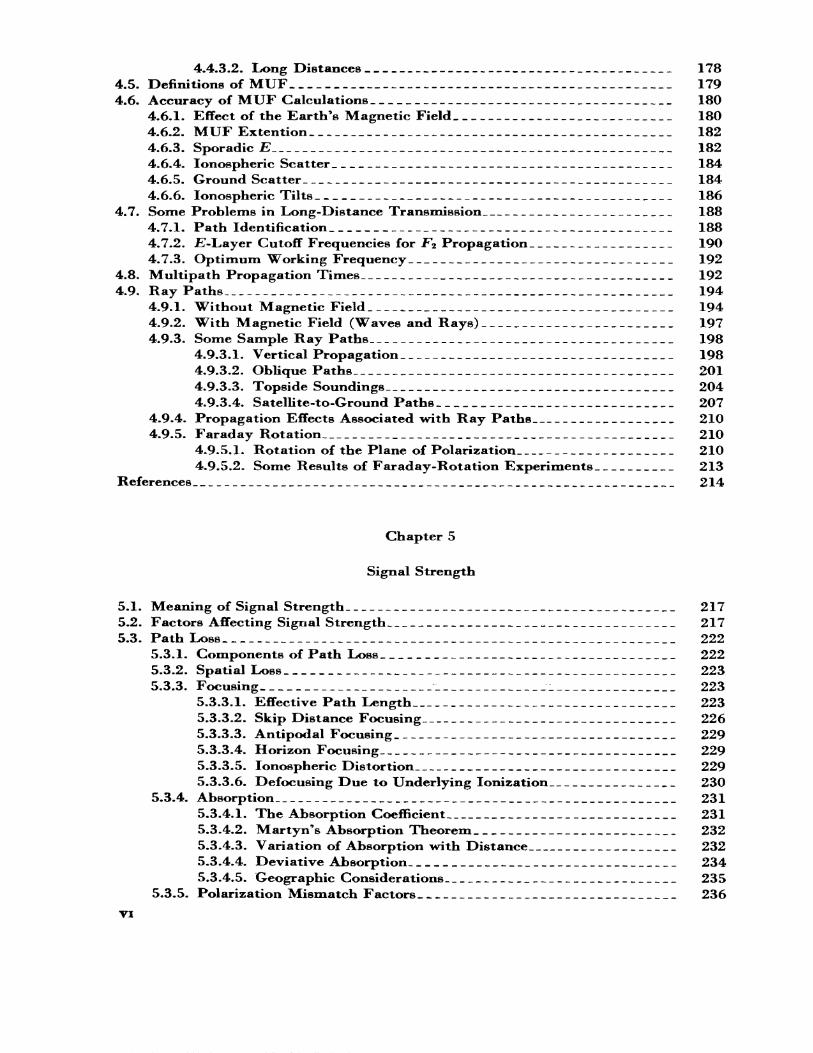
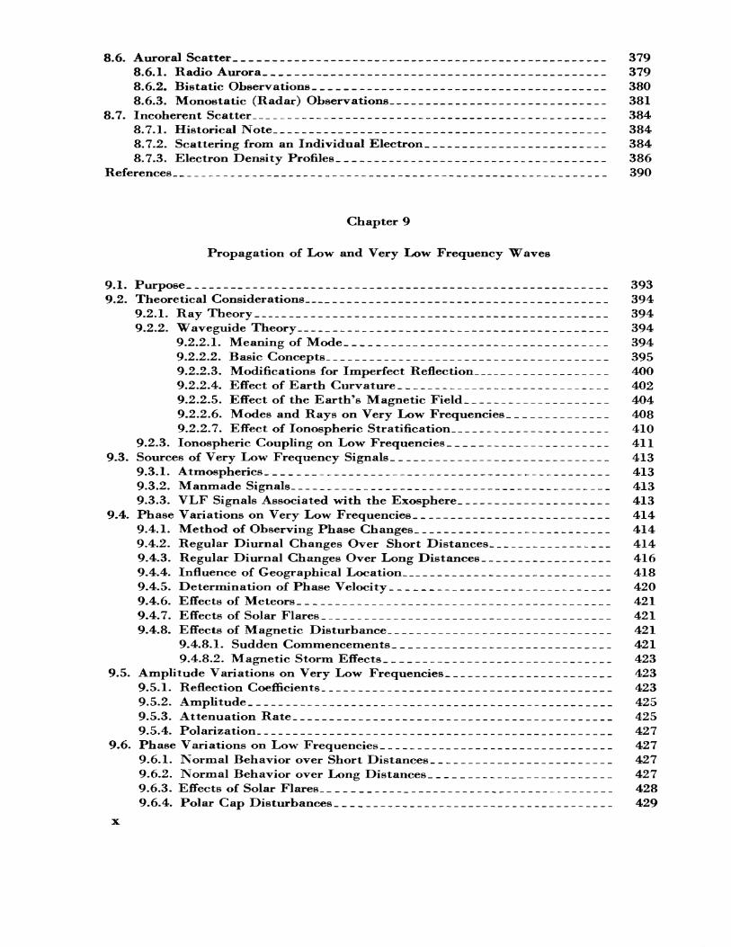
Throughout this book, the terminology used to describe the various regions of the upper atmosphere will be that based upon the temperature distribution of the neutral atmosphere Ql]. 1 This distribution is shown in figure 1.1, and the following terminology is widely used.
The mesosphere, which lies in the height range of 50 to 85 km, is a region of decreasing temperature with height.
The thermosphere, above 85 km, is a region in which the temper ature increases with height.
These "regions" are not well defined and the transition regions are called "pauses."
In addition to the terminology based on temperature, others have been devised based on alternative physical quantities and processes. Two of these are illustrated in figure 1.1. For example, one terminology is based on the fact that turbulence predominates below about 100 km, whereas diffusive separation sets in above about 110 km. Above about 500 km is a region called the exosphere.
The term ionosphere was first applied by Sir Robert Wat son-Watt to that part of the atmosphere in which free ions exist in sufficient quan tities to affect the propagation of radio waves. The ionosphere can, therefore, be considered as lying between about 40 to 50 km and several earth radii. This definition is essentially that adopted by the Institute of Radio Engineers Q2].
It is convenient to define a region as a section of the atmosphere within which there can exist ion distributions called layers. A division
1 Figures in brackets indicate the literature references on p. 44.
2 EARTH'S ATMOSPHERE, GEOMAGNETISM, AND THE SUN
of the ionosphere into regions is given in table 1.1 together with the layers which may exist within these regions. The electron distribution within a region may not contain a peak of electron density.
1.2* PRESSURE AND DENSITY VARIATIONS
The relationship between pressure p and density p at any height h is given by the ''barometric equation/' which is derived as follows: con-
TABLE 1.1. Ionospheric regions and layers
5000
2000
1000
500
200
100
50
Height range (km)
50-9090- (120-140)Above (120-140)
Region
DEF
Layers
DEii EZ, EsFi, Fa, F2
IONOSPHERE
PROTONOSPHERE
HELIOSPHERE
F2
Fl
E
D
NEUTRAL ATMOSPHERE
TEMPERATURE
THERMOSPHERE
-MESOPAUSE(85)
MESOSPHERE
___MESOPEAK(SO)J____I_________
PROCESSES
EXOSPHERE
(500-700) -
DIFFUSOSPHERE _
TURBOPAUSE (IOO-I2O) _
TURBOSPHERE-
2000
1000
500
200
100
50
LOG, 0 Ne (cm- 3 )
0 500 1000 1500
T (°K)
FIGURE 1.1. Atmospheric nomenclature.
(After T. E. VanZandt and R. W. Knecht. See fig. 1.3.)
PRESSURE AND DENSITY VARIATIONS 3
sider an elementary cylinder of height dh and unit cross section. The net pressure difference dp between the top and bottom surfaces must equal the downward force due to the weight of the fluid in the cylinder, and is given by
dp = —pgdh(1.1)
= — Ning dh^
where g is the acceleration due to gravity, TV is the number density of molecules and in is the mean molecular mass. It should be remembered that TV, in, and g are all functions of height; e.g., g varies inversely as the square of the radius vector.
The perfect gas law is
p = NkT, (1.2)
where k is Boltzmann's Constant ( = 1.372 X 10~16 erg/deg) and T is the absolute temperature.
From (1.1) and (1.2) we obtain
dp ine dh ^ -£ = _-| dA= __, (1.3)
where H=kT/mg is known as the ff scale height" of the atmosphere, which again is height dependent. At the earth's surface the value of H is about 8 km.
In an isothermal atmosphere, integration of (1.3) gives
/ h-h0\ p=po exp ( —— H~f (a)
or (1.4)
/ *-*o\ __= po exp I — 1, (b)
where p is the pressure at a height h corresponding to a pressure po at a height h0 . Similarly for the density p. The quantity (h — hQ)/H, which is the height difference in scale height units, is often denoted by z. Below about 100 km it is possible to measure T(h) and m(h) directly, by means of rockets, and hence to determine H. Above about 100 km, however, it is much easier to measure p(h) and determine H from (1.3) expressed
4 EARTH'S ATMOSPHERE, GEOMAGNETISM, AND THE SUN
in the form
/:The following formulas are useful in calculating the scale height at any altitude:
/ h\ 2 T °KH(km)= 0.848(1+-) ————-——— , (1.6) \ a/ jfll(gm/mole)
where a is the earth's radius (6370 km approximately). Equation (1.6) can be approximated by
#=0.93-^, (1.7)
which is correct to within 7.5 percent between 50 km and 500 km. It is exact at 300 km.
The temperature or scale height structure gives rise to the ter minology indicated in the column labeled ^temperature" in figure 1.1. Although the terminology is self-explanatory, the causes of the observed temperature structure deserve comment. The mesosphere is heated by the absorption by ozone of solar ultraviolet light with wavelengths be tween 2550 A and 1650 A. The thermosphere is heated by the dissociation and ionization of the atmospheric gases by solar ultraviolet light with wavelengths less than 1760 A. Up to about 100 km, heat is lost mainly by infrared radiation. Above 100 km, on the other hand, heat is lost mainly by conduction downward towards the mesopause.
Below about 100 km, the specific heat of the atmosphere is so large that even though the rate of heat input almost vanishes at night, the temperature changes very little. Above 100 km the temperature is in creasingly variable, both diurnally and with solar activity. For example, at 300 km the temperature decreases by about one third from day to night and probably by about half from sunspot maximum to sunspot minimum. The temperature may also increase by a factor of two during large iono spheric storms. These variations of the structure of the thermosphere are complex and poorly understood, but they are now the object of intensive research.
CHEMICAL COMPOSITION
1.3. CHEMICAL COMPOSITION
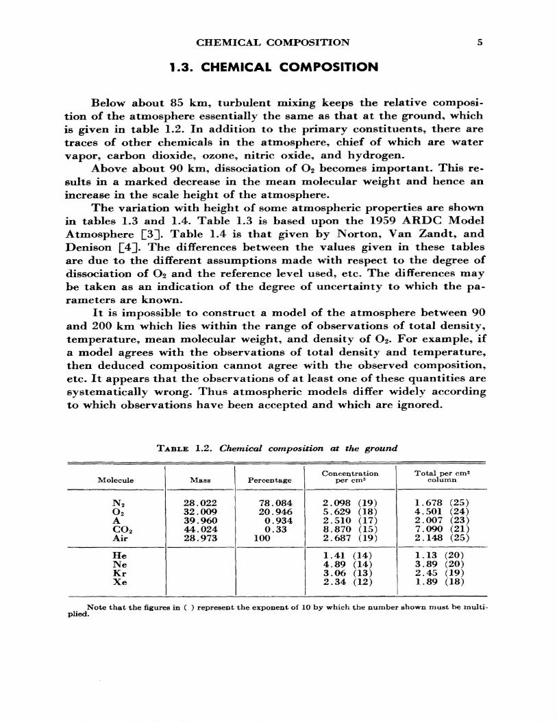
Below about 85 km, turbulent mixing keeps the relative composi tion of the atmosphere essentially the same as that at the ground, which is given in table 1.2. In addition to the primary constituents, there are traces of other chemicals in the atmosphere, chief of which are water vapor, carbon dioxide, ozone, nitric oxide, and hydrogen.
Above about 90 km, dissociation of C>2 becomes important. This re sults in a marked decrease in the mean molecular weight and hence an increase in the scale height of the atmosphere.
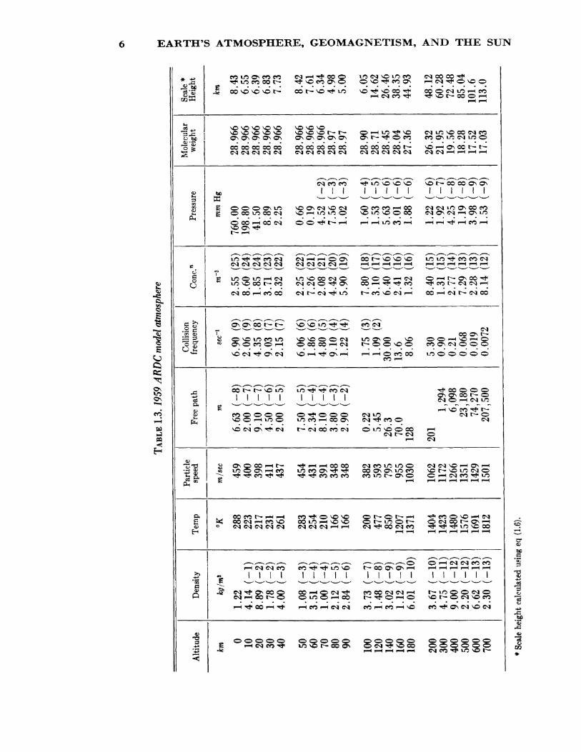
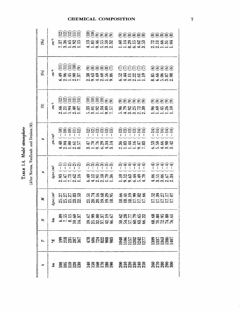
The variation with height of some atmospheric properties are shown in tables 1.3 and 1.4. Table 1.3 is based upon the 1959 ARDC Model Atmosphere C^H- Table 1.4 is that given by Norton, Van Zandt, and Denison [[4], The differences between the values given in these tables are due to the different assumptions made with respect to the degree of dissociation of C>2 and the reference level used, etc. The differences may be taken as an indication of the degree of uncertainty to which the pa rameters are known.
It is impossible to construct a model of the atmosphere between 90 and 200 km which lies within the range of observations of total density, temperature, mean molecular weight, and density of C>2. For example, if a model agrees with the observations of total density and temperature, then deduced composition cannot agree with the observed composition, etc. It appears that the observations of at least one of these quantities are systematically wrong. Thus atmospheric models differ widely according to which observations have been accepted and which are ignored.
TABLE 1.2. Chemical composition at the ground
Molecule
N2 02 A C02 Air
He Ne Kr Xe
Mass
28.022 32.009 39.960 44.024 28.973
Percentage
78.084 20.946 0.934 0.33
1OO
Concentration per cm3
2.098 (19) 5.629 (18) 2.510 (17) 8.870 (15) 2.687 (19)
1.41 (14) 4.89 (14) 3.06 (13) 2.34 (12)
Total per cm2 column
1.678 (25) 4.501 (24) 2.007 (23) 7.090 (21) 2.148 (25)
1.13 (20) 3.89 (20) 2.45 (19) 1.89 (18)
Note that the figures in ( ) represent the exponent of 10 by which the number shown must be multi plied.
TABL
E 1.
3.19
59 A
RDC
mode
l atm
osph
ere
Alti
tude
km
0 10 20 30 40 50 60 70 80 90 100
120
140
160
180
200
300
400
500
600
700
Den
sity
*»/m
»
1.22
4.14
(-1
)8.
89 (
-2)
1.78
(-2
)4.
00 (
-3)
1.08
(-3
)3.
51 (
-4)
1.00
(-4
)2.
12 (
-5)
2.84
(-6
)
3.73
(-7
)1.
48 (
-8)
3.02
(-9
)1.
12 (
-9)
6.01
(-1
0)
3.67
(-1
0)4.
75 (
-11)
9.00
(-1
2)2.
20 (
-12)
6.62
(-1
3)2.
30 (
-13)
Tem
p
"K 288
223
217
231
261
283
254
210
166
166
200
477
850
1207
1371
1404
1423
1480
1576
1691
1812
Parti
cle
spee
d
m/se
c
459
400
398
411
437
454
431
391
348
348
382
593
795
955
1030
1062
1172
1266
1351
1429
1501
Free
pat
h
m
6.63
(-8
)2.
00 (
-7)
9.10
(-7
)4.
50 (
-6)
2.00
(-5
)
7.50
(-5
)2.
34 (
-4)
8.10
(-4
)3.
80 (
-3)
2.90
(-2
)
0.22 5.45
26.3
70.0
128
201
1,29
46,
098
23,1
8074
,270
207,
500
Colli
sion
frequ
ency
sec"
1
6.90
(9)
2.06
(9)
4.35
(8)
9.03
(7)
2.15
(7)
6.06
(6)
1.86
(6)
4.80
(5)
9.10
(4)
1.22
(4)
1.75
(3)
1.09
(2)
30.0
013
.6 8.06
5.30
0.90
0.21
0.06
80.
019
0.00
72
Cone
."
wr>
2.55
(2
5)8.
60 (
24)
1.85
(24
)3.
71 (
23)
8.32
(22
)
2.25
(22
)7.
26 (
21)
2.08
(21
)4.
42 (
20)
5.90
(19
)
7.80
(18
)3.
10 (
17)
6.40
(16
)2.
41 (
16)
1.32
(16)
8.40
(15
)1.3
1 (1
5)2.
77 (
14)
7.29
(13
)2.
28 (
13)
8.14
(12
)
Pres
sure
mm H
g
760.
0019
8.80
41.5
08.
892.
25
0.66
0.19
4.52
(-2
)7.
56 (
-3)
1.02
(-3
)
1.60
(-4
)1.
53 (
-5)
5.63
(-6
)3.
01 (
-6)
1.88
(-6
)
1.22
(-6
)1.
92 (
-7)
4.25
(-8
)1.
19 (
-8)
3.98
(-9
)1.
53 (
-9)
Mol
ecul
ar
wei
ght
28.9
6628
.966
28.9
6628
.966
28.9
66
28.9
6628
.966
28.9
6628
.97
28.9
7
28.9
028
.71
28.4
528
.04
27.3
6
26.3
221
.95
19.5
618
.28
17.5
217
.03
Scale
*
Hei
ght
km 8.43
6.55
6.39
6.83
7.73
8.42
7.61
6.34
4.98
5.00
6.05
14.6
226
.46
38.3
544
.93
48.1
260
.28
72.4
885
.04
101.
611
3.0
w > c/ s o (/> ^ B B » B 0
2!
B
H M Cfl H
B
B
* Sca
le he
ight
calc
ulate
d us
ing
eq (
1.6).
CHEMICAL COMPOSITION
d-dd-dd- dd2^S^£ S£sSs52- SB-SSSS«L, t**— NO LO CS| *-O CO I-H vO uO O CSI O ^ ON LO CSf CO CSI r-H NO i—^ •*£* g CO CO NO ON r-< r—(OO^l-OLOCO VO i-H CSI r-H VO LO r~ f-H VO CO O
t**™ CO p'H CO ^"^ ^J* r^ ^?\ l-O CO CSI ^™H ^^ CO N^5 ^^ CO (^J CN| r^ ^~4 p^
r~H f*1^ ^H r1^ ^?\ ^y\ CO CO CO CO r^* t^* t"* t~*~ C^* C""* t^* Mu^ ^O N^^ NO N^^T ^-">——"^--^-^^-^ N.-'^——•'^ '^--V__^^_^ v_^s ->_^^^>__^>^^ S__^v__^^_^^_^^^
Q ^ ONvouoc^r- OOCOONONO'O c^^f-Hcqi-H o\ to NO NO r— co« ^JiO^^^ONCO CONONONOi-OCO i_O^p-*CS|NOi-H CONOOOCON
C^l C"^ F^H ^"H ^^ C^ ^^ ^^ *»J x"~^s^~-v /^~s. x-^v x^~s ^-~^. x^~^. x^^s ^-~*^. x"~^- ^"~*^ x"""*. *-^~^^•H ^^ r^ F1"H ^™H ^""^ ^~H ^"H ^^ ^?N (?"\ ON ^?N C^*1 ^?^ ^T^ ON C?N ON ON G^ ON
e^i-HLOC^|i-H UO CO r—f i—'I ON t— l-O-^COCOCMCSI T-Hr—Ir-Hr—(i—I
g 000-^ i—I f-4 i-H i
11111CL
*^ ^ OO ^^ f^^> p"H t^* t*1^* *^^> ^Q C?*^ ^^ ^^ N^^ CO ^SH ^O t~^" CO CO ^^ ^*O CO '
pa I 1 777^*7 ^«Y«J5^^^> I ! I I I 1 I 1 I t I.0 Q.
55 _ _ _EH fe ^^^^^^ ^t^ 0:^! 1^^•"^ CMi—< t— CM i-H NO '^ CSI CSi (—i I-H i—( ON ON NO i
CM CSI CSI CO UO
CSICSICSICMCSI cS|(MCS|f^Hf^-lf-H ^^p^^Hf-Hp-H
o r-4 C<t C<t CN| CO ^* VO t^- CO C^ O"\ <^ >™^ i"H C"<1 C^ CN1 CO CO CO <
O> LO O> O> O> OO^OOC^O O O> O> <O O O O O> O> O Oft C^ O> »™H CSI CO **T* LO NO t^" CO 0s t^ '"^ CS| CO ^^* l-O NO P~- CO ON O>
-« p—(,—(p^^^p^^ ,-^ r—i p—( ,—H ^—t ,-H CS|CSiCS|C^CSlCSl CS|CS|CS|eSlCO
8 EARTH'S ATMOSPHERE, GEOMAGNETISM, AND THE SUN
1.4. FORMATION OF IONIZED LAYERS
1.4.1. Ion Production
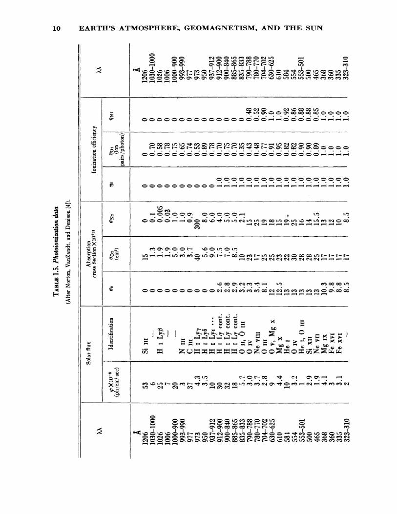
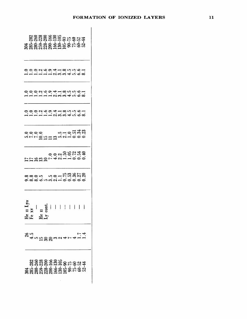
Ions are believed to be produced in the earth's atmosphere partly by cosmic rays but mostly by solar radiation. The latter may include particle radiation (during storm periods), ultraviolet light, and x rays. By far the predominant agent appears to be solar ultraviolet light and soft x rays. With a suitable atmospheric model together with a knowledge of the solar flux, absorption cross section, and ionization efficiency of the various constituents, it is possible to compute the rate of ion produc tion in the atmosphere. Some relevant photoionization data are included in table 1.5 for the major constituents of the E and F regions; i.e., O, O^ and N2 . The ionization efficiency (ion pairs per photon absorbed) is the ratio of the ionization cross section to the absorption cross section. For a more extensive discussion of this subject, the reader is referred else where Ql, 5, 6].
1.4.2. Ion Disappearance
When electrons are produced in the upper atmosphere, they tend to reunite with positive ions ("recombination) and to attach themselves to neutral molecules to form negative ions such as Q%~ (attachment). The O2~~ ion is later neutralized by further reactions. Electrons can also leave a given volume by moving out of it (diffusion and/or drift).
For our present purposes we shall consider recombination and at tachment only. Let the number densities of electrons, of positive ions, and of molecules to which attachment is possible be denoted by 7V(e), N(A+}, and N(A)* respectively* The rate at which electrons are lost by recombining with positive ions is given by
) 9 f 1.8)dt
where a is the recombination coefficient. If we assume that there are few negative ions compared with the electron concentration, we have
) so that
d.9)
FORMATION OF IONIZED LAYERS 9
Consider the process of attachment; the rate of disappearance will be proportional to both electron concentration and the neutral atom con centration, that is
= -bN(e)N(A), (1.10)dtwhere fc is a constant of proportionality. If we assume that the number of neutral molecules is enormously greater than the number of electrons, so that it does not change appreciably when a few of the atoms are con verted into negative ions, we may write
— 7V(e) = — /37V(e), (1.11)
where /3 is known as the attachment coefficient. For a fuller discussion of this subject, the reader is referred to other works on the subject H6]. The coefficients a and /3 may vary with height because the reactions usually involve three bodies rather than two.
The rate of change of electron density AT is, therefore, given by the following continuity equations for the cases of recombination and attachment, respectively:
^//v(1.12)
(1.13)
dt *
dN = dt
where q is the rate of electron production, i.e., number of electrons pro duced per second.
It should be noted here that if electrons are produced at a rate q and are lost by attachment to neutral atoms to form negative ions, and if these ions are subsequently lost by ionic recombination, it can be shown that the continuity equation assumes the form
(1.14)
where q^a and cee ff are effective rates of production and disappearance - Thus the net effect is to make the process appear as simple recom-
10 EARTH'S ATMOSPHERE, GEOMAGNETISM, AND THE SUN
J
T3ci
iiUO-5 gw r»j os ^•^ n H 5
I
§xU§
=3cc**ol
r 2 ft
g
x|
r-H
i \O O O CO--- C<l <
O O <
cc O oo i
> co oo o e^i _> co oo r- o > oo oo r- t— -> i-O lO. . , O O ^4" O O '
OO CO O*^ OO C^ cO I~H ^oo oo r- t- t- so ^o i > O vO vD *O (
oo c^i o e^ \o oo oo LO ^inoNOoaNCOcooocoO O O O O O O O O O O O O O O O O r-H •— I O O O O O
OOOOOOC3>OOOOOOOOOOOOOOOOOOOOOi— H»— If-Hi-Hi-Hi— tf-Hi-Hi— If— 1,-Hf-Hf— li-Hi-H^Hf— li— t
\o oo ON c^ co ^J* i— i oooooom
§ SS s85 S w .
CO LO - o r- oo ^J* CM
i-H CO CO i—I
N op co oo> co c^ < i o o < _ _5 CO CS|
CO CO CO CO
FORMATION OF IONIZED LAYERS 11
c^ o oo o ̂ o o LOCOVOCMO'sOeOOCSLO CMCSie^CSli—fi-Hi-HONt^V
i/SOONCOOvOOiOOiO
co vo t^- <^ ir3ecc<icsioooo
afi § i I I I I I ! iO
C^ O OO O ^Q O LOO^OCMO^OCOC^C^CSlCsli—Ip-Hr
i_cc>aNCoo>^ooi-ootn

12 EARTH'S ATMOSPHERE, GEOMAGNETISM, AND THE SUN
bination. The effective recombination coefficient c*c ff becomes relatively large in the lower (Z> and E) regions of the atmosphere.
Another set of reactions which is thought to be of importance in the upper atmosphere is electron disappearance first by atom -ion exchange between a neutral molecule (XY) and the positive ion (A +), followed by recombination between an electron and the XA+ ion:
Production ^4+photon — *A+ -\-e, (a)
, (b) (1.15)
(c)Loss
The primes indicate that the atoms X and A may be left in excited states. With these reactions it can be shown Q6] that, if the number density
of X Y is high in the F region and low in the E and D regions (as is thought to be the case if A represents atomic oxygen and XY molecular oxygen), the continuity equation takes the form
g-/WV, (1.16) a
where /8e ff is an effective attachment coefficient.We now see that the forms of the continuity equation may not be
those expected from simple recombination and attachment.
1.4.3. Formation of a Chapman Layer
The simplest type of ionized layer that can be deduced from theo retical considerations is known as a Chapman Layer C73- The derivation2 is based on the following assumptions:
(1) An atmosphere with only one type of gas.(2) Plane stratification.(3) A parallel beam of monochromatic ionizing radiation from the
sun.(4) An isothermal atmosphere.
To start with, let us invoke assumptions (1), (2), and (3) only. Let the ionizing radiation of intensity Sm be incident, at a zenith angle
2 Due to Dr. T. E. Van Zandt.
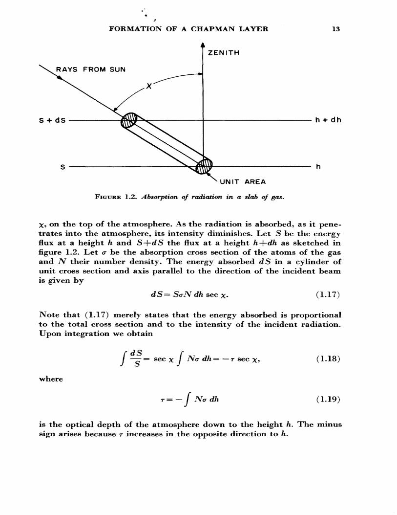
FORMATION OF A CHAPMAN LAYER
ZENITH
13
RAYS FROM SUN
S -I- dS
UNIT AREA
FIGURE 1.2. Absorption of radiation in a slab of gas.
X* on the top of the atmosphere. As the radiation is absorbed, as it pene trates into the atmosphere, its intensity diminishes. Let S be the energy flux at a height h and S-f-dS the flux at a height h-\-dh as sketched in figure 1.2. Let a be the absorption cross section of the atoms of the gas and TV their number density. The energy absorbed dS in a cylinder of unit cross section and axis parallel to the direction of the incident beam is given by
= StrTV dh sec (1.17)
Note that (1.17) merely states that the energy absorbed is proportional to the total cross section and to the intensity of the incident radiation. Upon integration vie obtain
r d $ rI —— = sec x I Ncr dh= —T sec x-> (1-18)
where
r=— / Nadh (1-19)
is the optical depth of the atmosphere down to the height h. The minus sign arises because r increases in the opposite direction to h.
14 EARTH'S ATMOSPHERE, GEOMAGNETISM, AND THE SUN
At great heights, S—»Sm as r—>0 and (1.18) gives
S=S^exp (-rsecx). (1-20)
The energy absorbed per unit volume is given by
dSdh sec
(-T sec x).
Let 77 be the number of ion pairs produced per unit quantity of energy absorbed, i.e., the ionization efficiency. The number of ion pairs pro duced per unit volume per second is
q(x* h) ^No-S^r) exp (—r sec x)* (1-22)
Now T is a function of x and h. Using (1.1), (1.2), and (1.3), we obtain
-cr f Ndh = ̂ - fdp = ̂ = ̂ ^ = aNH. (1.23) J mJ m mmg mg mg
Substitution of (1.23) into (1.22) yields
^»
q(x, h) =—-=17 exp (1 — T sec x), (1-24)
where e=2.718 • * *. Note that we have neglected the variation of g with height.
Notice that (1.24) holds for any temperature distribution. To obtain Chapman's formula we invoke assumption (4) , an isothermal atmosphere, where H is independent of height.
We can define a quantity z by the relation
z= — In T, (a)i.e., (1-25)
r= exp ( — z). (b)
Substitution of (1.25b) into (1.24) gives
^ q(x, z) = ~£7 exp {1 — z— sec x exp (— z) } (a)
FORMATION OF A CHAPMAN LAYER 15
(1.26) = <jr0 exp {1 — z — sec x exp ( — z) }, (b)
where
(1.27)
is the rate of production of ion pairs at the level z=0 when the sun is overhead, i.e., when TO = 1, and where TO is the value of r at the level z=0. From (1.23), (1.25b), and (1.4a) we get
r p exp (-*) ----- exp
i.e.,
The reference height hG is, therefore, the height of maximum ion pro duction when the sun is overhead.
If, in (1.26b), we replace z by z — In sec x and put x = Qi w^ obtain
9 z— In sec x) = sec x q(x* z) . (1-29)
Equation (1.29) gives us an important scaling rule. That is, the curve * z) has the same shape as g(0, z) , but is moved upwards by In sec x
and is diminished by cos x- The height of the peak of ion production Zm or hm is given by
Zm= In sec x. (a)or (1.30)
= hQ -t-Hln sec x- (b)
The variation of q(x) for various values of z is shown in figure 1.3. It can be seen that the use of a logarithmic scale for q makes the shapes of the q curves identical. The peak rate of production is given by
qm = qo cos x- (1-31)
The intensity of the ion production is determined by the flux of ionizing radiation and the efficiency 77. Changing the flux does not alter the height
16 EARTH'S ATMOSPHERE, GEOMAGNETISM, AND THE SUN
O.OI O.O2 0.05 O.2 0.5 I q(z)/qo
OJ O.I5 O.2 0.3 0.4 O.6 O.8 N(z)/Nc
FIGURE 1.3. Normalized rate of photoionization q(z)/q$ and electron density N(z)/Noaccording to Chapman theory.
(After T. E. VanZandt and R. W, Knecht, 1964 t Ch. 6, Space Physics, John Wiley & Sons.)
ELECTRON DENSITY DISTRIBUTION 17
of maximum production. Thus, if there are several wavelengths present in the incident radiation for which the ionization coefficients are markedly different, several distinct layers will result. The most strongly absorbed radiation produces the uppermost layer and vice versa. Likewise, different ionized layers would result with different gases in the atmosphere.
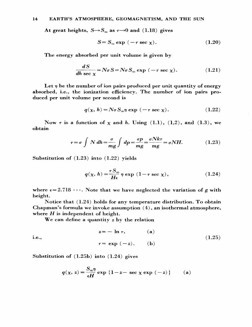
1.4.4. Electron Density Distribution
To determine the electron density distribution, we must assume some process of electron disappearance. Under certain circumstances the left- hand sides of (1.12) and (1.13) are small (quasi -equilibrium conditions). If, therefore, the loss of ions is due to a recombinationlike process, thenq=ctJ\?2 and
N=N0 exp £{1 — z— sec x exp (— *) K (1.32)
where at is independent of height and
CL
The peak density
(1.33)
Of.
and the height of the peak is given by (1.30).When the loss process is * fattachmentlike," which is independent of
height, we have
q=0N9 (1.35)
which gives
JV=JV'exp {1 — z— sec x exp (—*)}, (1.36)
where
JV-f. (1.37)
This gives
= |cos x. (1.38)
18 EARTH'S ATMOSPHERE, GEOMAGNETISM, AND THE SUN
If we assume that 0 depends directly on the molecular density,
-z), (1.39)
where (So is the value of 0 at the level h$. This gives, for the electron density distribution,
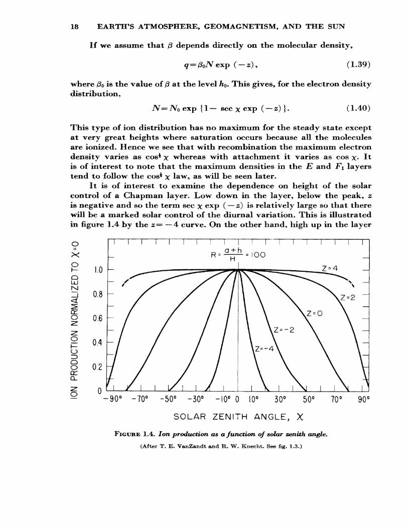
= 7V0 exp { 1 — sec x ( — 2) } • (1.40)
This type of ion distribution has no maximum for the steady state except at very great heights where saturation occurs because all the molecules are ionized. Hence we see that with recombination the maximum electron density varies as cos* x whereas with attachment it varies as cos x* It is of interest to note that the maximum densities in the E and JFi layers tend to follow the cos* x law, as will be seen later.
It is of interest to examine the dependence on height of the solar control of a Chapman layer. Low down in the layer, below the peak, z is negative and so the term sec x exP (— z) *s relatively large so that there will be a marked solar control of the diurnal variation. This is illustrated in figure 1.4 by the z= —4 curve. On the other hand, high up in the layer
O itXO
O UJ NJ
o 0.6
OI— O ID O O
o -90< •70 -50° -30° -10° 0 10° 30° 50°
SOLAR ZENITH ANGLE, X
70 l 90 C
FIGURE 1.4. Ion production as a function of solar zenith angle.
(After T. E. VanZandt and R. W. Knecht. See fig. 1.3.)
DIPOLE FIELD 19
where z is positive and large, the sec x exp ( — z) term is small and so the production increases rapidly near sunrise and remains almost constant until sunset, when it drops rapidly (fig- 1.4, curve jz=4). This is the type of diurnal variation to be expected when electron production is due to photodetachment of electrons from negative ions by visible light.
Although the theory given above is useful for purposes of discussion, it should be borne in mind that, in practice, almost all the basic assump tions need qualification. Thus the earth's atmosphere consists of several species of gases, and the incoming radiation has a broad spectrum. The assumption of an isothermal atmosphere is certainly invalid.
Cos x can be found for any location on the earth from the following equation:
cos x= sin 0 sin 5+ cos <£ cos 5 cos /*, (1,41)
where 0 is the geographic latitude, 5 is the solar declination, and h is the local hour angle of the sun measured westwards from apparent noon (mean noon corrected for the equation of time and the standard time used at the location). Tables of hourly values of cos x from sunrise to sunset for the fifteenth day of each month for most of the ionospheric vertical incidence sounding stations are giveij in the URSI Ionosphere Station Manual £8].
Near grazing incidence (x greater than about 80°), the assumption of plane stratification breaks down, and it is necessary to replace sec x by the Chapman function of Ch(R~}-z^ x)? where R= (a-\-h)/H. Tables of Ch(R-\-z, x) have been published by Wilkes Q9].
Finally, it should be realized that the recombination coefficient (effective) is not independent of height. In view of all the above qualifi cations, it is remarkable that the E and FI layers behave approximately as predicted.
1.5. THE EARTH'S MAGNETIC FIELD3
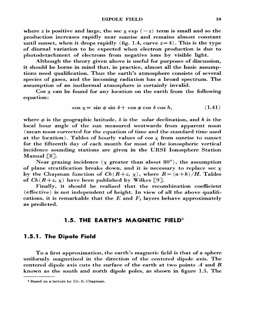
1.5.1. The Dipole Field
To a first approximation, the earth's magnetic field is that of a sphere uniformly magnetized in the direction of the centered dipole axis. The centered dipole axis cuts the surface of the earth at two points A and B known as the south and north dipole poles, as shown in figure 1.5. The
* Based on a lecture by Dr. S. Chapman.
20 EARTH'S ATMOSPHERE, GEOMAGNETISM, AND THE SUN
GEOMAGNETIC AXIS \ AXIS OF ROTATION
\BOREAL MAGNETIC POLE B
THE EARTH
A AUSTRAL MAGNETIC POLE\\FIGURE 1.5. Perth's dipole magnetic poles.
A—austral pole; B—boreal pole.
best fit between the earth-centered dipole and the actual magnetic field is obtained by taking A at 78.3°S, 111°E and B at 78.3°N, 69°W. It will be seen that the axis of the dipole does not coincide with the axis of rotation. The plane through the center of the earth O perpendicular to B A is called the dipole equatorial plane, and the circle in which it cuts the sphere is called the dipole equator. Dipole latitude & is reckoned relative to this equator. The semicircles joining B and A. are called the dipole meridians; the one passing through the dipole and south geo graphic pole is chosen as the zero of dipole longitude A. The relationships between the dipole coordinates (<£ the latitude and A the longitude) and the corresponding geographic coordinates (0, X) at a point P are given by
sin <£= sin <£ sin <£o+ cos <f> cos <£0 cos (X— X0 )
cos <f> sin (X—X0 )sin A =
cos
(1.42)
(1.43)
where <£0 and Xo are the geographical latitude and longitude of the north
DIPOLE FIELD 21
dipole pole (<fr>=78.3°N, X0 =291.0°E). The magnetic potential V of the dipole, of moment M at any point P -whose position vector relative to O is r, is given by
(1.44)
where <f> denotes the dipole latitude. This is also the potential of the external field of the uniformly magnetized sphere*
The radial (vertical) component Z of the field, reckoned positive when inward, is given by
dr
The horizontal (tangential) component H at P lies in the meridian through P and is directed towards B. It is given by
^rd3> r3 V '
The magnetic dip or inclination / is given hy
^tan / = — = 2 tan 3>. (1-47)
H
Because this is independent of r, the dip is the same at all points along any radius OP. Note that / is positive when the field direction is below the horizontal. Also,
(1.48)
At the pole B, F=Z<> and at the equator, F=H. Let HQ denote the equa torial value of H at the surface of the sphere (r — a). Then we have the following relationships:
/a\ 3 H=H0 l-} cos 3>, (a)
-\ sin*, (b) (1.49)
=ffr- {1 + 3 sin2 <£}*. (c)
22 EARTH'S ATMOSPHERE, GEOMAGNETISM, AND THE SUN
F ISOSURFACESLINES OF FORCE
FIGURE 1.6. Lines of force and of equal intensity of a uniformlymagnetized sphere.
(After S. Chapman, 1964, Geophysics—The Earth's Environment, Part III, Solar Plasma, Geomagnetism and Aurora, Gordon and Breach, N.Y.)
It will be seen, from (1.49), that the magnetic intensity at the poles is twice that at the same radial distance (height) at the equator.
The lines of force of the dipole field are given by dr/Z=rd&/H; hence their equation is
r= ka cos2 (1.50)
Here k is the equatorial radius measured in earth radii. The product ka is the distance at which the line of force crosses the equatorial plane. The points where it meets the sphere are given by <i> = 3>0 and <I> = — <l>o where cos <J>o = fc~~*.
The lines of force, together with the isosurfaces of F (on which F is constant), are given by
r = fc'a(l + 3 sin2 *)*, (1.51)
and are shown in figure 1.6. The parameter fe' of the F isosurface is thus
REAL FIELD 23
related to the value of F for the surface:
(1.52)
It is interesting to note that the strength of the magnetic field decreases as the cube of the distance from the earth's center. Thus at one earth radius above the surface, the field is only 0.125 of that at the surface. Thus it may be important to consider the variation of field strength when large distances are involved (e.g., earth-space propagation) .
1.5*2. The Real Field
The magnetic intensity F at any point F* on the earth's surface can be specified by its downward vertical component Z and its vector hori zontal component H, or by H and the angle / by which F dips below the horizontal. On the earth, the direction of H is specified by the angle D between H and the geographic north; D is called the magnetic (or com pass) declination and is reckoned positive if eastward. The northward and eastward components of H are denoted by X, Y, respectively, and
(1.53)
The seven quantities F, Z, H, /, Z), X, and Y are called the magnetic elements, and any set of three independent elements serves to specify F; i.e.,
F, /, Z>; H, /, D; H, Z, D; X, Y, Z. (1.54)
The elements F, J/, Z, and / are called intrinsic because their only refer ence to direction is to the natural direction characteristics of P^ namely, the vertical. The other three elements, Z), X, Y, are called relative be cause they are defined relative to the geographical (or rotational) axis TVS, which has no necessary relation to the geomagnetic field.
In geomagnetism, field intensity is measured in gauss units F, despite the internationally agreed use of the term oersted for intensity and gauss for induction. A smaller unit, the gamma (T), is used, especially in connection with the variations in the geomagnetic field where
(1.55)
24 EARTH'S ATMOSPHERE, GEOMAGNETISM, AND THE SUN
FIGURE 1.7. World map of total magnetic intensity (F).
(After J. C. Cain and J. R. Neilon, 1963, J. Geophys. Res. 68, 4689.)
REAL FIELD 25
FIGURE 1.8. World map of magnetic dip (1).
(After J. C. Cain and J. R. Neilon, 1963, J. Geophys. Res. 68, 4689.)
26 EARTH'S ATMOSPHERE, GEOMAGNETISM, AND THE SUN
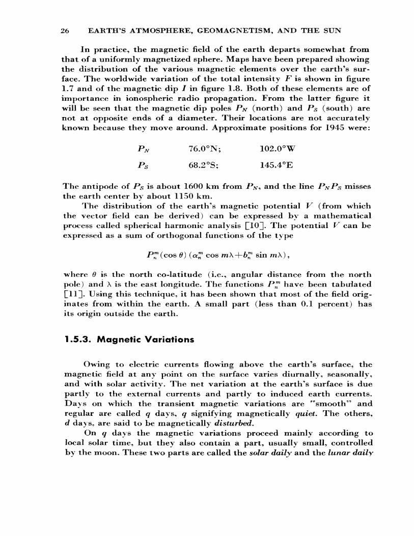
In practice, the magnetic field of the earth departs somewhat from that of a uniformly magnetized sphere. Maps have been prepared showing the distribution of the various magnetic elements over the earth's sur face. The worldwide variation of the total intensity F is shown in figure 1.7 and of the magnetic dip / in figure 1.8. Both of these elements are of importance in ionospheric radio propagation. From the latter figure it will be seen that the magnetic dip poles PN (north) and PS (south) are not at opposite ends of a diameter. Their locations are not accurately known because they move around. Approximate positions for 1945 were:
PN 76.0°N; 102.0°W
PS 68.2°S; 145.4°E
The antipode of PS is about 1600 km from PN^ and the line P^Ps misses the earth center by about 1150 km.
The distribution of the earth's magnetic potential V (from which the vector field can be derived) can be expressed by a mathematical process called spherical harmonic analysis Q10]. The potential V can be expressed as a sum of orthogonal functions of the type
P™(cos 0) (cC cos mX+fe™ sin mX),
where 6 is the north co-latitude (i.e., angular distance from the north pole) and X is the east longitude. The functions P™ have been tabulated Cll]- Using this technique, it has been shown that most of the field orig inates from writhin the earth. A small part (less than 0.1 percent) has its origin outside the earth.
1*5*3. Magnetic Variations
Owing to electric currents flowing above the earth's surface, the magnetic field at any point on the surface varies diurnally, seasonally, and with solar activity. The net variation at the earth's surface is due partly to the external currents and partly to induced earth currents. Days on which the transient magnetic variations are ffsmooth" and regular are called q days, q signifying magnetically quiet. The others, d days, are said to be magnetically disturbed.
On q days the magnetic variations proceed mainly according to local solar time, but they also contain a part, usually small, controlled by the moon. These two parts are called the solar daily and the lunar daily
MAGNETIC VARIATIONS 27
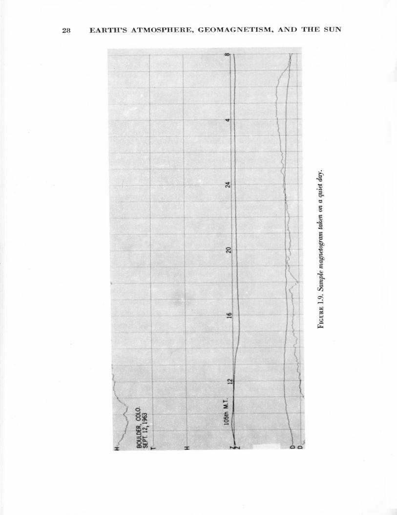
magnetic variations. They, and the fields of which they are the mani festation, are denoted by SQ and L ( S= solar, L = lunar). Both are caused by currents flowing in the ionosphere, mainly in the E layer. An example of a quiet day magnetogram for a middle latitude station is given in figure 1.9.
The Sq currents are stronger by day than by night, stronger in summer than in winter, and about 50 percent stronger at sunspot maxi mum than at sunspot minimum.
Of particular interest, from the point of view of the ionosphere, is the concentration of enhanced currents in a narrow strip along the mag netic equator which is known as the "equatorial electrojet."
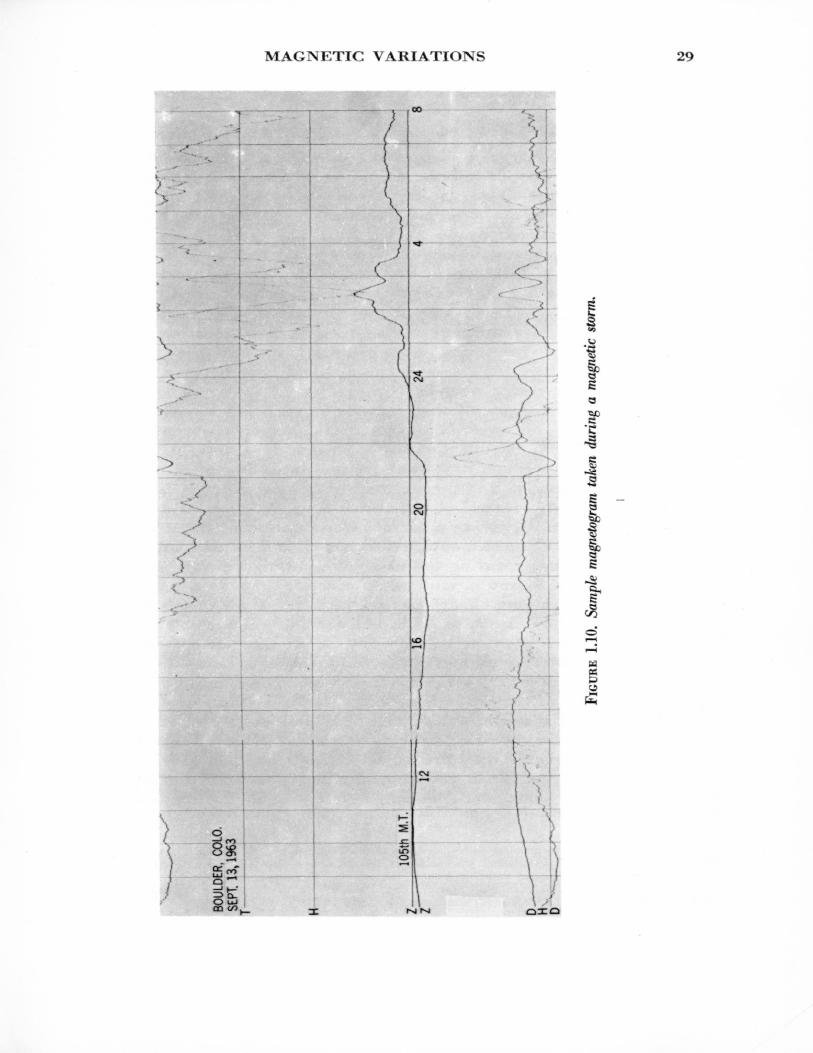
During a magnetic disturbance, additional currents circulate in the ionosphere. They are superposed on the Sq and L currents. Unlike the latter, they are strong in high latitudes and are often stronger over the night than over the day hemisphere. They are denoted by DP (/) = dis turbance, P= polar). They are especially concentrated along the auroral zones (i.e., the region of overhead visible aurora), and hence the currents there are called the auroral electrojet. A strong auroral electrojet may carry a current of the order of a million amperes. The return current flows mainly over the polar cap, but some flows between the north and south auroral zones. The DP currents are believed to be one of the many effects caused by the impact of a solar stream or cloud of ionized gas upon the earth's magnetic field. Some of the gas finds its way into the polar at mosphere and causes the luminescence of the aurora. A magnetogram taken during a magnetic storm is shown in figure 1.10.
Many magnetic storms, particularly the big storms, begin suddenly and almost simultaneously, to within a minute, all over the earth. The sudden commencement is ascribed to the impact of solar ionized gas on the outer part of the geomagnetic field, at a distance of several earth radii.
Though much of the solar gas is turned away from the earth, some is trapped by the field and the trapped particles spiral round the lines of force, between the northern and southern hemispheres; they also drift round the earth under the influence of the magnetic field. The total motion is equivalent to an electric current in the form of a ring around the earth. The net effect at the earth is to decrease the horizontal field, and in many storms the decrease soon overpowers the initial increase.
28 EARTH'S ATMOSPHERE, GEOMAGNETISM, AND THE SUN
V
/•
5
i
Ed
MAGNETIC VARIATIONS 29
Cd
oxo
30 EARTH'S ATMOSPHERE, GEOMAGNETISM, AND THE SUN
1.5.4. Magnetic Indices
The degree of magnetic disturbance during each Greenwich day is indicated by a variety of indices, according to internationally adopted plans. 4 Many magnetic observatories throughout the world take part in these plans. They assign local indices of magnetic activity. These are sent to an international center at De Bilt, The Netherlands. This is linked with a Permanent Service of Geomagnetic Indices at Gottingen, Germany.6 There the local indices are used as the basis for world indices.
Each participating observatory assigns to each Greenwich day its own "daily figure" C. This is one of the numbers 0, 1, or 2, to indicate ascending degrees of disturbance of its records. This local daily index is assigned by simple inspection of the records. Naturally there are many borderline cases where the choice between 0 and 1, or between 1 and 2, is difficult; but the choice is made.
The values of C from all observatories for each day are averaged to one decimal place. This gives d, the * finternational daily character figure." It provides a 21-fold classification of Greenwich days, from 0.0 on days of extreme calm, to 2.0 on days that are magnetically highly disturbed.
By a more detailed and precise method, a local index K is assigned to each three-hourly interval of Greenwich time, 0—3, 3—6, • • •; K is one of the integers 0 to 9, giving a tenfold classification of these intervals. The records of the three elements are examined, and for each an estimate is made of the range r during the interval, allowing for the part of the change caused by Sq and L and, when necessary, by SFE ( Sq current augmented by solar flare effect) and the recovery phase of the ring cur rent field. Such allowance calls for experience and judgment. The largest of the three ranges is taken as the basis for K^ the element concerned may vary from interval to interval, or from one observatory to another.
For each observatory a table is assigned, giving limits of r corre sponding to each of the ten values of K. The lower limit of r for K = 9 may have any of the values 300, 350, 500, 600, 750, 1000, 1200, 1500, and 2000 7. The first applies to very-low-latitude observatories (outside the belt of the equatorial electrojet; sec. 1.5.3). The last applies to the most disturbed stations, in the auroral zone. The limit 500 refers to stations in about geomagnetic latitude 50°. The table for this latitude is
4 The plans are under the auspices and supervision of the Committee on Characterization of Magnetic disturbances of IAGA (International Association of Geomagnetism and Aeronomy), a part of ITJGG (International Union of Geodesy and Geophysics); the present Chairman is J. Bartels.
5 Addresses: C +K Centre, Kon. Ned. Meteor. Inst., De Bilt, The Netherlands; and Geophysikalisches Institut, 180 Herzberger Landstr., (34) Gottingen, Germany.
MAGNETIC INDICES 31
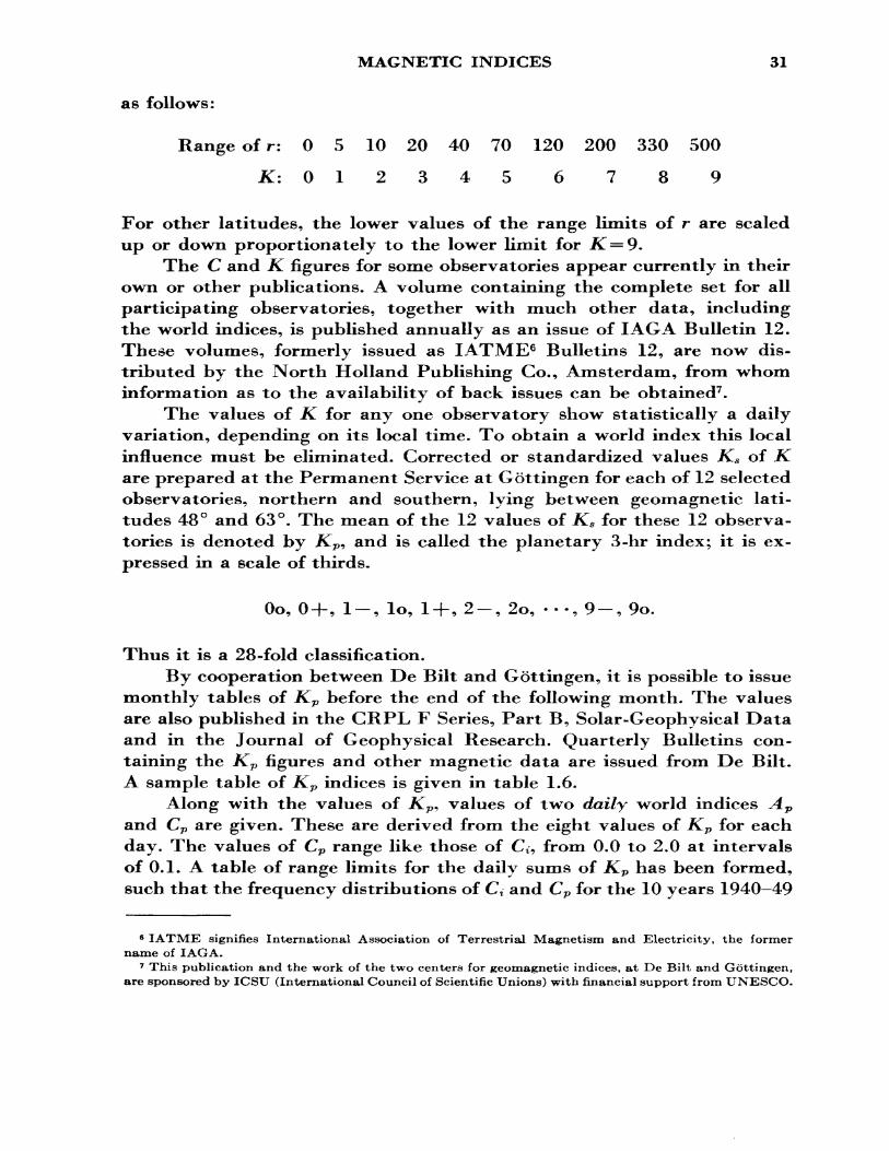
as follows:
Range of r: 0 5 10 20 40 70 120 200 330 500
A:-. 012345 6 7 8 9
For other latitudes, the lower values of the range limits of r are scaled up or down proportionately to the lower limit for jRC = 9.
The C and K figures for some observatories appear currently in their own or other publications. A volume containing the complete set for all participating observatories, together with much other data, including the world indices, is published annually as an issue of IAGA Bulletin 12. These volumes, formerly issued as IATME6 Bulletins 12, are now dis tributed by the North Holland Publishing Co., Amsterdam, from whom information as to the availability of back issues can be obtained7 .
The values of K for any one observatory show statistically a daily variation, depending on its local time. To obtain a world index this local influence must be eliminated. Corrected or standardized values Ks of K are prepared at the Permanent Service at Gottingen for each of 12 selected observatories, northern and southern, lying between geomagnetic lati tudes 48° and 63°. The mean of the 12 values of Ks for these 12 observa tories is denoted by Kp, and is called the planetary 3-hr index; it is ex pressed in a scale of thirds.
Oo, 0+, 1 — , lo, 1+, 2 — , 2o, • • •, 9 — , 9o.
Thus it is a 28-fold classification.By cooperation between De Bilt and Gottingen, it is possible to issue
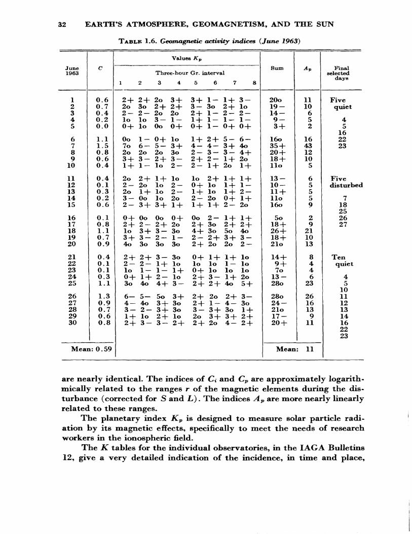
monthly tables of Kp before the end of the following month. The values are also published in the GRPL F Series, Part B, Solar-Geophysical Data and in the Journal of Geophysical Research. Quarterly Bulletins con taining the Kp figures and other magnetic data are issued from De Bilt. A sample table of Kp indices is given in table 1.6.
Along with the values of Kp, values of two daily world indices A p and Cp are given. These are derived from the eight values of Kp for each day. The values of Cp range like those of Ct, from 0.0 to 2.0 at intervals of 0.1. A table of range limits for the daily sums of Kp has been formed, such that the frequency distributions of C; and Cp for the 10 years 1940—49
6 IATME signifies International Association of Terrestrial Magnetism and Electricity, the former name of IAGA.
7 This publication and the work of the two centers for geomagnetic indices, at De Bilt and Gottingen, are sponsored by ICSU (International Council of Scientific Unions) with financial support from UNESCO.
32 EARTH'S ATMOSPHERE, GEOMAGNETISM, AND THE SUN
TABLE 1.6. Geomagnetic activity indices (June 1963)
June 1963
12345
6789
10
1112131415
1617181920
2122232425
2627282930
C
0.60.70.40.20.0
1.11.50.80.60.4
0.40.10.30.20.6
0.10.81.10.70.9
0.40.10.10.31.1
1.30.90.70.60.8
Mean: 0.59
Values Kp
Three-hour Gr. interval
1 2345678
2+ 2+ 2o 3+ 3+ 1- 1+ 3-2o 3o 2+ 2+ 3— 3o 2+ lo2-2- 2o 2o 2+1-2-2-lo lo 3-1- 1+1-1-1-0+ lo Oo 0+ 0+ 1— 0+ 0 +
Oo 1— 0+ lo 1+ 2+ 5— 6 —7o 6- 5- 3+ 4- 4- 3+ 4o2o 2o 2o 3o 2—3—3— 4+3+ 3- 2+ 3- 2+ 2- 1+ 2o1+1- lo 2- 2-1+ 2o 1 +
2o 2+ 1+ lo lo 2+ 1+ 1 +2- 2o lo 2- 0+ lo 1+1-2o 1+ lo 2— 1+ lo 1+ 2 —3— Oo lo 2o 2— 2o 0+ 1 +2- 3+ 3+ 1+ 1+ 1+ 2- 2o
0+ Oo Oo 0+ Oo 2— 1+ 1 +2+ 2- 2+ 2o 2+ 3o 2+ 2 +lo 3+3- 3o 4+ 3o 5o 4o3+ 3- 2- 1- 2- 2+ 3+ 3-4o 3o 3o 3o 2+ 2o 2o 2 —
2+ 2+ 3- 3o 0+ 1+ 1+ lo2-2-l+lo lo lo 1- lolo 1-1-1+ 0+ lo lo lo0+ 1+ 2- lo 2+ 3- 1+ 2o3o 4o 4+ 3- 2+ 2+ 4o 5 +
6— 5— 5o 3+ 2+ 2o 2+ 3 —4- 4o 3+ 3o 2+ 1- 4- 3o3- 2- 3+ 3o 3- 3+ 3o 1 +1+ lo 2+ lo 2o 3+ 3+ 2 +2+ 3- 3- 2+ 2+ 2o 4- 2 +
Sum
20o19-14-
Q __
3 +
16o35 +20 +18 +llo13-10-11 +llo16o
5o18 +26 +18 +21o
14 +9 +7o
13-28o
28o24-21o17-20 +
Ap
1110
652
16431210
5
65559
29
211013
8446
23
2616139
11
Mean: 11
Final selected
days
Fivequiet
45
162223
Fivedisturbed
718252627
Tenquiet
45
1011121314162223
are nearly identical. The indices of d and Cp are approximately logarith mically related to the ranges r of the magnetic elements during the dis turbance (corrected for S and L). The indices Ap are more nearly linearly related to these ranges*
The planetary index Kp is designed to measure solar particle radi ation by its magnetic effects, specifically to meet the needs of research workers in the ionospheric field.
The K tables for the individual observatories, in the IAGA Bulletins 12, give a very detailed indication of the incidence, in time and place,
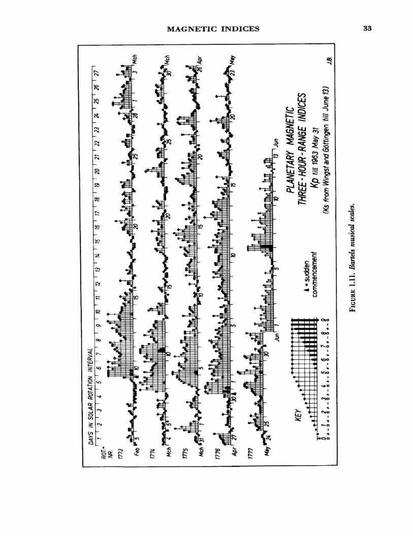
MAGNETIC INDICES 33
$KJ
CN
?2>
S*
<Z>
Si
^.
$
vo
^
^? S
is £
£3
8 i
«ON
0)0
(00
<v>o
0,0
w
W &
34 EARTH'S ATMOSPHERE, GEOMAGNETISM, AND THE SUN
FIGURE 1.12. Location of the northern zone of maximum frequency of occurrence of overhead aurora on magnetically quiet and on magnetically disturbed days*
(After Y. I. Feldstein, Investigations of the Aurora, Moscow, 1960.)
of the magnetic effects of the solar eruptions. The Kp, Cp, Ap, and d tables give a concise indication of the overall world effects ^llj. These tables are now available from the time of the Second International Polar Year (1932/3) to date. The tables of d go back still further. Details regarding these publications are given in Bulletin 12(1) (pp. iv and 268); see also IGY Annals, vol. 4, pp. 227-236, where also, on pp. 220—226, an account is given of the quarter-hourly indices Q to be issued, covering the period of the IGY. These will permit studies of correlations between magnetic disturbance and other phenomena in much more time detail than is possible with the daily and three-hourly indices.
MAGNETIC INDICES 35
WHITE & GEDDES (1939)-—•—^"-"v. VESTINE ft SNYDERO945)-^-~~"""- HULTQVIST (1958)_._.———- GARTLEIN. NACK a SPRAGUE (1959)
- BOND a JACKA (1959)QUENBY a WEBBER (1959)
0 0 0 VESTINE (I960)& KITAMURA (1958)U EVANS ft THOMAS (1959)C SCHNEIDER (1959]
GEOMAGNETtCO
FIGURE 1.13. South auroral zone.
(After O. Schneider, 1961, Institute Antarctic© Argentine 55, Buenos Aires.)
Finally, note in this connection the publication of diagrams (Bartels* ffmusical scales") graphically illustrating the sequence of the Kp values, figure 1.11. These are arranged in rows so as to show the 27-day recur rence tendency of magnetic disturbance, arising from the solar rotation. The diagrams are issued monthly along with the Kj, tables, in time to be helpful in making 27-day recurrence forecasts.
The monthly diagrams issued during the IGY have been combined into a diagram for the whole IGY period, and since then annual diagrams have been issued (see Bulletins 12 for further information).
36 EARTH'S ATMOSPHERE, GEOMAGNETISM, AND THE SUN
1.6. THE AURORAL ZONES
These regions of the earth where visible aurora occurs overhead are of particular importance to the radio communicator because of the fre quent occurrence there of ionospheric disturbance, as will be discussed in a later chapter.
As was mentioned in section 1.5.3 above, aurora is thought to be the result of the entry into the atmosphere of charged corpuscles. Owing to the interaction between the moving charges and the geomagnetic field, the corpuscles are deflected north and south of the equatorial plane and are deposited in a relatively narrow ring situated between dipole latitudes of about 64° and about 70°. Maps showing lines of constant frequency of occurrence (called isochasms) have been prepared for the northern and southern auroral zones and are shown in figures 1.12 and 1.13. The north auroral isochasms are not quite circular, but are elongated along the Siberia-North American axis. The geographical areas encV^sed by the auroral rings are often called "polar caps."
It should be borne in mind that the auroral zone is not fixed but moves with varying magnetic activity. Thus during strong magnetic storms the auroral zones, both north and south, move towards the equator. For example, a great aurora on September 25, 1909, was observed in Singapore, latitude 1°N. Even during magnetic storms of moderate strength there is a close connection between the position of the aurora and the strength of the magnetic disturbance.
In addition to the visible aurora, radio techniques have revealed the existence of enhanced ionization in the ionosphere in these latitudes |^12^]. This enhanced ionization is manifested as sporadic E (sec. 6.3.4), D-region absorption (sec. 6.3.3), and radio aurora (sec. 8.6.1). However, it may not necessarily follow that the various auroral zones coincide.
1.7. THE SUN
1.7.1. Quiet Conditions
1.7*1*1. Structure
For our present purposes it will be sufficient to consider the sun as made up of four parts:
QUIET CONDITIONS 37
(1) the interior;(2) the photosphere, or visible surface;(3) the chromosphere, the bright region above the photosphere,
seen during total solar eclipses; and(4) the corona, the outer atmosphere of the sun*
Although the various sections merge into one another, the radiation from the photosphere comes entirely from a layer about 400 km thick compared to a solar radius of about 700,000 km so that the concept of a solar surface has a fairly well-defined meaning. Approximate values of the heights and temperatures of the various regions are given in table 1.7. For further information the reader should consult frThe Sun" £13].
The sun is composed chiefly of the elements hydrogen and helium together with smaller amounts of the heavier elements, notably calcium.
TABLE 1.7. Approximate heights and temperatures of the suii*s outer layers
Solar layer h (km)
Outer corona Middle corona Inner corona Upper chromosphere Lower chromosphere Photosphere
1,400,000700,00021,OOO to 140,OOO7,OOO to 14,OOO1000
1,500,0001,50O,OOO1,OOO,OOO25,000 to 300,00053006OOO effective
1.7.1.2. Ionizing Radiations
To a first approximation, the quiet sun radiates as a blackbody at a temperature around 6000° Kelvin. Superimposed on the blackbody continuum are certain lines characteristic of the elements in the sun. Some of the more important lines are hydrogen a (6563 A), Lyman ot (1216 A), and helium I (584 A). These radiations are responsible for the ionization of the upper atmosphere discussed in section 1.4. A number of lines in the ultraviolet part of the solar spectrum are given in table 1.5. For example, it is thought that Lyman a radiation is the major source of ionization in the quiet D region. The quiet E region is believed to be produced by x rays (10-100 A), Lyman 0 (1025.7 A), Cm (977 A), and the Lyman continuum (910 to 980 A) £14], The primary source of ionization in the F region appears to be the Lyman continuum and the band 350 to 200 A (which includes the He m 304 A resonance line).
38 EARTH'S ATMOSPHERE, GEOMAGNETISM, AND THE SUN
The amount of visible light from the sun changes very little from one day to the next. On the other hand, the day to day variability of the quiet ionosphere suggests that the solar emissions in the ultraviolet and x-ray regions vary appreciably.
In addition to the wave radiations, the quiet sun emits a stream of charged corpuscles (mostly electrons and protons) which is called the "solar wind."
1.7.1.3. Radio Emissions
The sun is a source of radiation on radio frequencies. These emissions are caused by plasma oscillations (see sec. 2.3.1.1) and gyro-oscillations
FIGURE 1.14a. Photograph of the sun at sunspot minimum (1954).
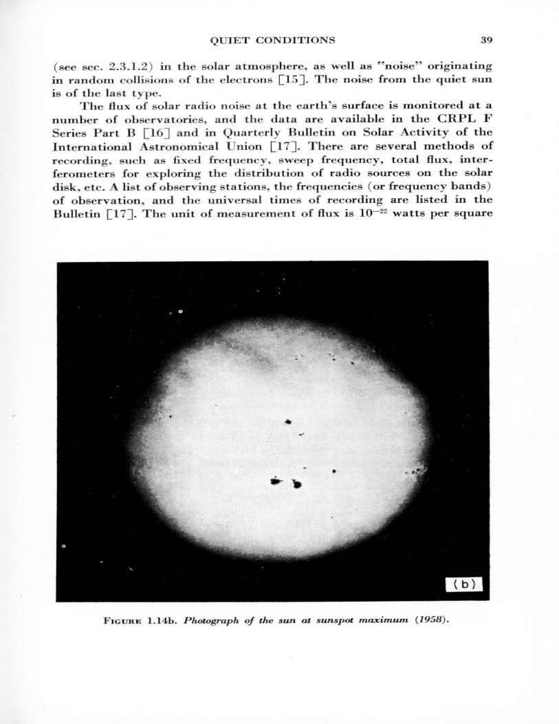
QUIET CONDITIONS 39
(see sec. 2.3.1.2) in the solar atmosphere, as well as "noise" originating in random collisions of the electrons C15J, The noise from the quiet sun is of the last type.
The flux of solar radio noise at the earth's surface is monitored at a number of observatories, and the data are available in the CRPL F Series Part B Cl^D and in Quarterly Bulletin on Solar Activity of the International Astronomical Union Q17]. There are several methods of recording, such as fixed frequencv, sweep frequency, total flux, inter ferometers for exploring the distribution of radio sources on the solar disk, etc. A list of observing stations, the frequencies (or frequency bands) of observation, and the universal times of recording are listed in the Bulletin Q17]. The unit of measurement of flux is 10~22 watts per square
FIGURE 1.14b. Photograph of the sun at sunspot maximum (1958).
40 EARTH'S ATMOSPHERE, GEOMAGNETISM, AND THE SUN
meter per cycle per second* In general, the flux increases with frequency in the range 100 Mc/s to 10,000 Mc/s, but the day to day variability is much greater on the lower frequencies as can be seen on pages 464—6 of the Bulletin [17].
1*7.2. The Active Sun
1.7.2.1. Sunspots
One of the most notable phenomena on the sun's surface is the ap pearance, and disappearance, of certain dark areas known as sunspots. The life of a sunspot is highly variable; some spots last only a few days, whereas a few may survive four or five solar rotations (of about 27 days each). Their exact nature is not known, but they appear to be vortices in the matter comprising the photosphere. Sunspots appear dark because the surface temperature is only about 3000 °K, compared with the 6000 °K of the quiet photosphere. Sunspots tend to group together. A group may contain a few isolated spots or dozens of spots.
One of the more interesting features of sunspots is their unusually strong magnetic fields. These may approach 0.4 Wb/m2 (weber per square meter) (4000 G) for the larger spots.
1.7.2.2. The Sunspot Cycle
The appearance of the sun in 1954 and in 1958 can be seen in figures 1.14a and 1.14b. Clearly, there is a variation in the sunspot ''activity." To measure this activity an index is required. The most common index of sunspot activity is the Wolf number R given by
« = fc(10g+s), (1.56)
where g is the number of groups and s is the number of observable indi vidual spots. The factor k is a correction factor to take into account the equipmental and observer characteristics. It will be seen that this number is weighted heavily in favor of groups, so that its value as an index of sunspot activity is questionable* Nevertheless, it is valuable because of its availability for a period of about 200 yr. It thus provides a large homogeneous sample of data. Sunspot numbers are available on a daily basis and as monthly and yearly averages.
ACTIVE SUN 41
When the yearly sunspot numbers are plotted, for a long period of time, such as is shown in figure 1.15, it is clear that the sunspot activity has a periodicity of about 11 yr. The duration of an individual cycle may vary over much wider limits; thus the periods between minima range from about 8.5 yr to about 14 yr and those between maxima range from 7.3 yr to about 17 yr. Furthermore, the annual minima of jR lie in the range 0 to 10, whereas the maxima range from about 50 to about 190. The daily values of /? vary between 0 and 355 or more.
In addition to the 11-yr period, there are periods, particularly near the 11-yr minima, when a 27-day (approximate) recurrence is evident. This period corresponds to a solar rotation.
Many attempts have been made to represent, analytically, the exist ing sunspot data with a view to the prediction of future cycles. The pre dictions have never been particularly successful.
In addition to the relatively dark sunspots, bright areas often appear on the solar disk. These areas, called plages, are observed in the light of calcium K and are intimately associated with sunspots. Plages are comparatively long-lived active regions; they precede in appearance the spots, which develop in them, and persist after the spots have disappeared.
1.7.2.3. Flares
A solar flare is a burst of frlight" occurring in the chromosphere near a sunspot. It is most easily observed in the Ho: light (6563 A), although, in some rare cases, flares have been seen in white light. At present, solar patrol observations are almost continuous and so most of the flares oc curring on the solar hemisphere facing the earth are detected. Flares are frequent occurrences, particularly at the peak of the sunspot cycle.
Flares are divided into classes of importance 1 —, 1, 1 + , 2, 2-f-, 3, and 3 + 9 according to area and brightness. The average duration of a flare increases with its importance; thus 1 flares last about 20 min, 2 flares last about 30 min, and 3 flares last about 60 min. Of course, the life of an individual flare may vary greatly from the mean value. Flares smaller than importance 1 are referred to as subflares.
The development of a flare is somewhat as follows: a rapid rise (flash) to peak intensity, a brief period of peak intensity, followed by a steady decline. There is a close statistical relation between the number of flares per solar rotation, TV/?, and the corresponding mean sunspot numbers R, given by
(1*57)
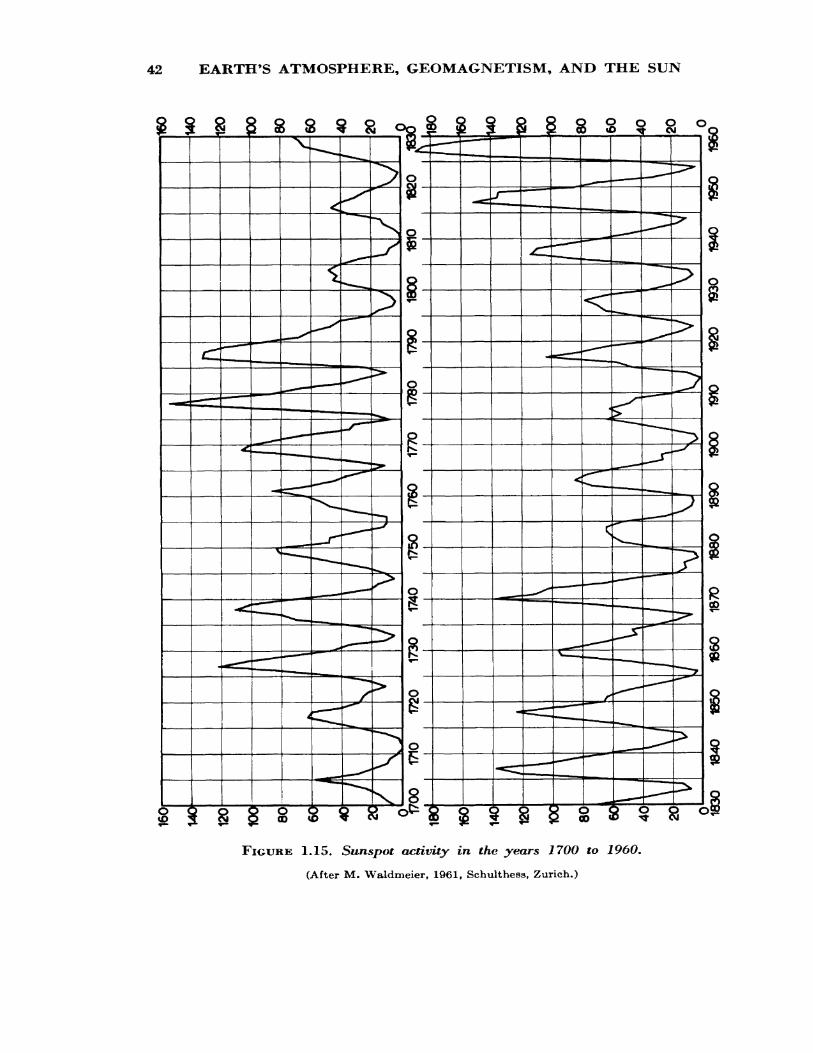
42 EARTH'S ATMOSPHERE, GEOMAGNETISM, AND THE SUN
FIGURE 1.15* Sunspot activity in the years 1700 to 1960.
(After M. Waldmeier, 1961, Schulthess, Zurich.)
ACTIVE SUN 43
The mean values of a for the sunspot cycles having peaks in 1937 and 1947 are 1.98 and 1.47 respectively [18].
During some flares there is a marked increase in the flux of solar ionizing radiation in the far ultraviolet and soft x-ray regions of the spectrum. This results in enhancements in the electron densities in the D and E regions, as will be seen later. Data on the duration and impor tance of flares, etc., can be found in the F Series Part B [16] and in the IATJ Bulletin [17].
1.7.2.4. Radio Emissions
The amplitude of the solar signals may remain relatively constant for long periods of time and then will be greatly enhanced during a efnoise storm." These storms are often associated with solar flares and certain geophysical disturbances and may last for a period of hours or days.
Noise bursts are categorized as follows:
Type /, or noise storms, occur most frequently on frequencies less than about 300 Mc/s. Type I bursts extend over a narrow frequency range, 5 to 30 Mc/s, for instance, while their lifetimes range from 0.2 sec to 1 min or so. During the lifetime of a single burst, the frequency of emission may drift with time to higher or to lower frequencies.
Certain outbursts, which last for the order of several minutes, are associated with the larger solar flares and may involve signal enhance ments of the order of a million times the quiet values.
The chief characteristic of Type II ( slow drift) and Type III (fast drift) bursts is the drift of the emission to lower frequency with time. This drift can be explained as due to a source moving outwards through the corona, emitting at the plasma frequency, which decreases as the electron density decreases (see sec. 2.3.1.1). Type III events are very frequent.
Type IV events are long-lived emissions emanating from a source of large extent that moves to heights of the order of a solar radius. Radi ation occurs over a broad band of frequencies at each height. The char acteristics of type IV radiation can be explained by synchrotron emission of electrons. From the point of view of sun-earth relationships, type IV events are particularly important because of the strong association with solar corpuscular radiation, evidenced by polar cap absorption events [19, ch. 6], ground-level cosmic ray increases, and great magnetic storms.
Type V is continuum emission of shorter duration, following a type III burst.
44 EARTH'S ATMOSPHERE, GEOMAGNETISM, AND THE SUN
A considerable amount of data is made available every month in the F Series Part B [16],
REFERENCES
[I] VanZandt, T. E., and R. W. Knecht (1964), The structure and physics of the upper atmosphere, Space Physics (ed. A. Rosen and D. P. LeGallery) (John Wiley & Sons).
[2] Standards on wave-propagation, definition of terms, (1950) Proc. IRE 38, 1264.[3] Minzner, R. A., K. S. W. Champion, and H.L . Pond (1959), The ARDC model
atmosphere, Air Force Surveys in Geophysics No, 115, Bedford, Mass.[4] Norton, R. B., T. E. VanZandt, and J. S. Denison (1962), A model of the atmos
phere, and ionosphere in the E and FI regions, Proc. Intern. Conf. on the Iono sphere, Inst. Phys. and Phys. Soc., London.
[5] Nawrocki, P. J., and R. Papa (1961), Atmospheric Processes, Geophysics Corpora tion of America, Bedford, Mass., AFCRL-595, GCA Number 61-37-A.
[6] Ratcliffe, J. A., and K. Weekes (1960), The Ionosphere, chap. 9, Physics of the Upper Atmosphere (ed. J. A. Ratcliffe) (Academic Press).
[7] Chapman, S. (1931), The absorption and dissociative or ionizing effect of mono chromatic radiation in an atmosphere on a rotating earth, Proc. Phys. Soc. 43, 26.
[8] Wright, J. W., R. W. Knecht, and K. Davies (1957), Annals of the International Geophysical Year, Vol. Ill, Part 1.
[9] Wilkes, M. V. (1954), A table of Chapman's grazing incidence integral Ch(jc, x)*Proc. Phys. Soc. 67B, 304.
[10] Chapman, S., and J. Bartels (1962), Geomagnetism, ch. 17 (Oxford Univ. Press).[II] Bartels, J. (1957), The geomagnetic measures for the time variations of solar
corpuscular radiation, described for use in correlation studies in other geo physical fields, IGY Annals 4, 227.
[12] Booker, H. G. (1960), Radar studies of the aurora, Physics of the Upper Atmos phere (ed. J. A. Ratcliffe) (Academic Press).
[13] The Sun (1953) (ed. G. P. Kuper) (Univ. of Chicago Press).[14] Friedman, H. (1960), The sun's ionizing radiations, Physics of the Upper Atmos
phere (ed. J. A. Ratcliffe) (Academic Press).[15] Pawsey, J. L., and S. F. Smerd (1953), Solar radio emission, The Sun (ed. G. P.
Kuper) (Univ. of Chicago Press).[16] CRPL F Series, Part B, Solar Geophysical Data, issued monthly by the National
Bureau of Standards, Boulder, Colo.[17] Quarterly Bulletin on Solar Activity, International Astronomical Union, (ed. M.
Waldmeier) (Schulthess and Co., Zurich).[18] Kiepenheuer, K. O. (1953), Solar activity, The Sun (ed. G. P. Kuper) (Univ. of
Chicago Press).[19] Athay, R. G., and C. S. Warwick (1961), Indices of solar activity, Advances in
Geophysics (ed. H. E. Landsberg and J, Van Mieghem), Vol. 8 (Academic Press).
CHAPTER 2
Theory of Wave Propagation
2.1. PURPOSE
The purpose of this chapter is to acquaint the reader with the basic ideas needed for an understanding of the propagation of radio waves in the ionosphere. In the presence of the earth's magnetic field, the ionosphere behaves as a birefringent medium and so it is necessary to discuss the properties of such a medium. These properties include the decomposition of a plane polarized wave into ordinary and extraordinary waves and the deviation of the direction of energy flow away from the direction of phase propagation.
We shall consider first the early history of the subject leading to the formulation of Maxwell's equations and their experimental verification by Hertz. Next we shall derive the Appleton formula for the complex refractive index of a magneto-ionic medium and consider its properties.
The weakness of the Appleton theory will be considered and more generalized formulas will be discussed. Finally, we shall discuss the propagation of wave packets in a magneto-ionic medium.
2.2. ELECTROMAGNETIC WAVES
2.2.1. Electrostatics and Magnetostatics
The principles underlying the propagation of radio waves are based on the relationships between electricity and magnetism which were dis covered in the eighteenth and nineteenth centuries. It is now generally known that the attractive and repulsive properties of electrified bodies and of lodestone were first recorded by the ancient Greeks. Little further progress was made until the eighteenth century, when attempts were made to establish laws of electrical and magnetic forces similar to the
45
46 THEORY OF WAVE PROPAGATION
gravitational law of Newton. This search bore fruit when, in 1785, the French scientist Coulomb, using a torsion balance, showed that the mechanical force between two small electrified spheres varies inversely as the square of the distance r between them. Later work showed that the force was proportional also to the amounts of charge q^ q% on the two bodies and so we obtain the relationship
(2-D
where to is the permittivity of free space (8.85X10"12 F/m) .A relationship similar to (2.1) was found to hold for the mutual
forces exerted by long bar magnets.It is useful to introduce the concept of electric field E at this point.
Let us assume that the charge q% produces an electric field E at the site of qi and that this field exerts the force F on qi where
F- giE. (2.2)
Thus the electric field E at a point may be defined as the force experienced by a small unit test charge. It is assumed that the test charge itself does not alter the field.
The field at a vector distance r from a point charge q is, therefore, given by
r, (2.3)
so that the vector E is in the direction of r. If the charge is distributed throughout a volume of space, we have
A' fdS, (2.4)47T€0
where dq is an element of charge and Ar is a unit vector in the direction from dq.
Many electrical and magnetic problems, particularly static field problems, are best tackled through the idea of potential difference. The potential difference between two points A and B can be defined as the work done by an external force on a unit test charge in moving it from A to B as shown in figure 2.1. The zero of potential is, therefore, arbitrary;
ELECTROSTATICS AND MAGNETOSTATICS
ELECTRIC FIELD E
47
FIGURE 2.1. Potential difference.
and it is sometimes convenient to define the zero at infinity. The work done on the test charge in moving it from A to B is
and hence
VB — VA — — I E cos <f> ds = — I E • ds,JA JA
dVE=- —-=-gradV. ds
(2.5)
(2-6)
Gauss showed that the integral of the electric field over a surface A enclosing a medium of permittivity e is given by
ef E-dA= fJ A J
(2.7)
where p is the charge density, V is the volume enclosed, and Q is the total charge enclosed.
Similarly, for a magnetic field of induction B Wb/m2 (webers per square meter),
B-dA = 0. (2.8)
This follows since there are no free magnetic poles.
48 THEORY OF WAVE PROPAGATION
Before proceeding to a consideration of current electricity let us consider some elementary properties of dielectrics. Consider a parallel plate capacitor with a large area of cross section (so that edge effects are negligible), and distance d between plates, connected to a voltage source V^ and let a be the charge density on one of the plates. From (2.7) we can show that the field E between the plates is given by
(2.9)
and, by definition,
VE=- . (2.10)
a
Now on the introduction of a slab of dielectric, of thickness d, be tween the plates, the positive nuclei in the atoms of the dielectric will tend to be displaced in the direction of smaller field while the negative charges (electrons) will tend to be displaced up the field, i.e., the medium becomes polarized. Thus a back electromotive force is set up which AVI 11 tend to decrease the field between the plates.
Now the total field E, as given by (2.10), is independent of the di electric. Hence, the charge density on the plates must increase by an amount <r t , for instance. We can regard the polarization of the dielectric as conferring on it an effective permittivity e so that from (2.7) we obtain
cE=<r + <n. (2.11)
Imagine a cylinder of dielectric of unit cross section with its axis perpendicular to the plates. At the end surfaces will be charges +<rt and — <T; at a distance d apart. Hence we have the equivalent of a dipole of moment en d. The electric moment per unit volume is, therefore, <n which is called the polarization P. The total quantity cr-f-o-; is known as the dis placement D. Hence we have the relationship
D = eGE+P. (2.12)
Now in certain media (anisotropic) the application of an electric field in one direction gives rise to a polarization in some other direction. Under these circumstances (2.12) has to be expressed as a vector equation:
(2.13)
FARADAY'S LAW 49
This relation is of great importance in ionospheric radio propagation as will be seen later.
2.2.2. Ampere's Circuital Law
One of the most important observations in the study of electro- magnetism was that of Oersted, who found, in 1819, that a pivyAed mag net was deflected when in the vicinity of an electric current. This experi ment demonstrated that a current of electricity produced a magnetic field. As in the case of static electricity and magnetism, it was found that the magnetic field produced by a current element decreased as the square of the distance from the element. This led Ampere to formulate his circuital law, namely, that the line integral of the tangential magnetic field H t taken around a current i was equal to the component of the current flowing normal to the surface A enclosed (see fig. 2.2),
= fJ A
(2.14)
where J is the current density through the surface A. enclosed by the path of integration S. Note that H refers to magnetic intensity which, in a medium of magnetic permeability ju, is related to magnetic induction B by the formula
(2.15)
2.2*3. Faraday's Law
Efforts to observe the electrical effects of magnetic fields bore fruit in 1831 when Faraday found that a current was produced in a coil of
CURRENT i = / J.dA
SURFACE A
CURRENT DENSITY J
PATH OF INTEGRATION
FIGURE 2.2. Ampere's circuital law.
50 THEORY OF WAVE PROPAGATION
wire by the following processes: (1) when a magnet was moving near it and/or (2) when a current in an adjacent coil was switched on and off.
Faraday carried out a large number of beautiful experiments to verify the phenomena of electromagnetic induction and the serious reader is recommended to read Faraday's account in his book Experimental Researches in Electricity El]- 1
Faraday's results may be summed up in the following two laws:(a) When the flux of magnetic induction through a coil is changing,
an electromotive force is induced in the circuit.(b) The magnitude of the emf S is proportional to the rate of change
of flux.The sign of the emf is given by Lenz's law, which states that it is
such that any current flow is in the direction which would oppose the flux change causing the emf.
Therefore
S=-^, (2.16)
where TV is the total flux through the coil, i.e., induction times area, normal to the surface, that is
N= f B-dA. (2.17)J A
Consider now the integral of the electric field round a loop which, as shown in figure 2.3, has a small gap CD and through which is threaded a time-varying magnetic field. The integral
DE-ds
c
is the total voltage between C and />, that is, the induced emf, S.Hence, when C and D are brought together we arrive at the formula
E-ds = ~jf B-dA. (2.18)
It must be stressed that this relationship is quite general in spite of the fact that we have derived it for a particular case only.
1 Figures in brackets indicate the literature references on p. 99.
DISPLACEMENT CURRENT 51
/B_.dA
NORMAL TO A
SURFACE A
ds
CHANGING MAGNETIC FIELDd R dt ~
E_ INDUCED ELECTRIC FIELD
FIGURE 2.3. Faraday's electromagnetic induction latv.
It is convenient, at this point, to summarize the essential equations obtained above. They are:
The electric field
The magnetic field
Magnetic field ofa current
Electromagnetic induction
e f E-rfA= fJ A J v
f B-</A = 0,J A
<f-£L-ds = f
<f> E-ds= —
pdV,
J-dA,
1 /"B.JA.dt J
(a)
(b)
(c)
(d)
(2.19)
2.2.4. The Displacement Current
It -would appear, at first sight, as if eqs (2.19) are complete in them selves and define the electromagnetic field uniquely. However, that this is not so was discovered by Maxwell in the course of his studies on the charging of a capacitor (Ley den jar).
52 THEORY OF WAVE PROPAGATION
Consider the charging of a parallel plate capacitor with an insulator as dielectric so that no current can flow between the plates. Let us apply (2.19c) to a closed loop around the wire to a plate. If the surface enclosed by the loop cuts the wire, then ^"H-dfs around the loop is non-zero. Now it is possible to construct a surface which envelopes the plate of the ca pacitor and which passes between the plates. Since there is no flow of electricity between the plates, application of (2.19c) shows that ^H«cfe around the loop is zero. We thus arrive at a contradiction. James Clerk Maxwell's great contribution to electromagnetic theory was his assertion that the circuit through a capacitor should be considered as closed. He showed, furthermore, that the current density through the insulator between the plates is due to the time rate of change of the displacement Z), i.e.,
r^Jl^JL^- l d f- . -N ^ dD J ~~A~A A A at (2.20)
where q is the charge on the plate.Maxwell maintained that as far as the electromagnetic field was con
cerned, the displacement current was just as important as a flow of elec tricity and that it must be added to the current on the right hand side of (2.19c). This enables us to write Maxwell's equations in integral form as follows:
/,'/,''
f
Jy P
B.A =0,
f d f
E-ds=- ^ f B>dA. dt J
(a)
(b)
L, (c)
(d)
(2.21)
For Maxwell's own account of the derivation of these formulas the reader should consult his f*A Treatise on Electricity and Magnetism
SOLUTION OF MAXWELL'S EQUATIONS
2.2.5. A Solution of Maxwell's Equations
53
In order to solve the set of eqs (2.21), it is necessary to express them in their differential forms. This can be achieved by means of the following two vector theorems:
Green's Theorem
Let F be any vector function and V a volume bounded by the closed surface A, then
f F-rfA= f diJ J divF dV. (2.22)
Stokes* Theorem
Let F be a vector function and A a surface (not closed) bounded by a simple closed curve S; then
f F-cfe= f curlF-dA.Js J A
Applying these transformations to (2.21) we obtain
(2.23)
divD = p,
div B = 0,
curlH = J+D,
curl E = — B = — Atfi,
(a)
(b)
(c)
(d)
(2.24)
where the dot signifies the time derivative.Let us consider a solution of these equations in a medium having the
folio wing properties:
(i) Magnetically and electrically isotropic, that is, having the same properties in all directions.
(ii) Electrically neutral, no net space charge so that p —0.(iii) Electrically nonconducting, i.e., */=0.(iv) A field varying in the 1-direction only in a right-handed orthog-
54 THEORY OF WAVE PROPAGATION
onal system of axes (1, 2, 3), so that
d d—=— = o.
With these restrictions, we obtain
curlH=+D, (a)
(b)(2.25)
Taking the curl of (2.25a) we have
curl curl H = +curl D
= +€ curl E (2.26)
Now it can be shown that, for any vector F,
curl curl F = grad div F — div grad F. (2.27)
Since div B = 0, then div H = 0 and hence grad div H = 0. Furthermore, under restriction (iv) we have
(2.28)div grad H = ——71 +——2 +
Equation (2.26) thus reduces to
Now
,. „ div H =dH3 = —— = 0,
i dxz 8x3 xi
and if we select the 2- and 3 -axes so that H2 = 0, we obtain
(2.29)
(2.30)
dt2 (2.31)
SOLUTION OF MAXWELL'S EQUATIONS 55
This is the equation of a plane transverse wave traveling in the 1- direction with a phase velocity v where
(2.32)
Note that this can be shown by substituting a wave of the form cos 27r£/t± (aci/X)] and remembering that v=f\. The — sign represents a wave traveling in the positive 1-direction and vice versa.
The free space velocity c is given by
(2.33)
Now the refractive index n of the medium is given by the ratio c/t>9 so that
C I JJL€rc--=A/ —— V * Mo^n
(2.34)
thenIn media which have no particular magnetic properties, M^MO and
(2.35)
where K is the dielectric constant of the medium.
The equation of such a wave may be written in several different forms, each of which has its peculiar advantages, such as
; = EQ cos
"= EQ COS k$(ct —
E= EQ exp i(a)t —
(a)
(b)
(c)
(d)
(2.36)
56 THEORY OF WAVE PROPAGATION
where Jfe = — the propagation factor,A
&o = — the phase constant,Xo
X0 = the free space wavelength,
X== actual wavelength in the medium,
It is of historical interest to note that Maxwell used a mixed (elec trostatic and electromagnetic) system of units and he found that the velocity c is given by the ratio of the electromagnetic to the electrostatic unit of charge. This ratio was known to be about 3 X 10⁸ m/sec, or close to the velocity of light. This agreement led Maxwell to claim that light was indeed an electromagnetic phenomenon.
The existence of electromagnetic waves was demonstrated conclu sively, around 1888, when Hertz |~33) showed that the disturbances gen erated by a spark coil could be reflected, refracted, focused, and polarized.
2.2.6. Some Properties of Electromagnetic Waves
Let us consider some of the properties of a plane electromagnetic wave propagating in an isotropic nonconducting medium. If the wave is traveling in the 1 -direction we have d/dx^=d/dx^ = Q^ since, for a given value of #1, the fields are constant over the whole 2—3 plane. Equation (2.25) can be written
dH3dx3 dt
(a)
(b)
(c)
(2.37)
PROPERTIES OF ELECTROMAGNETIC WAVES 57
= —Mo—r—, (a) 3 dt
(b)
(c)
(2.38)
Let us rotate our system of axes so that the 2-axis lies parallel to the E vector. Then Ez= E, and Es = Q. Since d/dx2 = d/dX3 = Q, (2.37) and (2.38) become
dEi dt
= 0,
dt *
(a)
(b)
dt= 0, (c)
(2.39)
dHldt
(a)
= _ MO——-± = 0, (b) ot
(c)/»* dt
(2.40)
58 THEORY OF WAVE PROPAGATION
From (2.39a) and (2.40a) we see that there is no time-vary ing component of E or H in the 1-direction. That is, the electromagnetic wave is entirely transverse.
Equations (2.39c) and (2.40b), respectively, tell us that H has no space- or time-varying components in the 2-direction* Hence E and H are perpendicular to each other and to the direction of propagation. We shall see later that this is not necessarily the case for propagation in the ionosphere.
To determine the phase relationship between E and U, substitute the expression £2 = E%0 cos (cot— kxi) in (2.39b) or (2.40c). This gives
cos o>£ — (a)
(b)
(2.41)
where
n_3o —
MO(2.42)
Equations (2.41) show that, if n is real, E and H are in phase. Equa tion (2.42) gives us the relationship between the peak amplitudes of E and H in terms of the refractive index n of the medium.
The energy density Ue in the electric field is given by
and in the magnetic field
Hence the ratio of the energy densities is given by
U
(2.43)
(2.44)
(2.45)
so that the energy is divided equally between the electric and magnetic fields.
MOTION OF IONS IN ELECTRIC AND MAGNETIC FIELDS 59
The flux of energy per unit area in the direction of propagation is given by the Poynting vector ^4],
S = EXH. (2.46)
For a sinusoidally varying wave, S has to be averaged over a com plete cycle. This gives
Sav=^ol*0. (2.47)
In general, the E and H vectors will be complex quantities and, in this case, it can be shown |j4] that the average of the complex Poynting vector is given by
(2.48)
where H* is the complex conjugate of H.
2.3. Magneto-Ionic Theory
2.3.1. Motion of Ions in Electric and Magnetic Fields
2.3.1.1. Motion in an Electric Field
It will be recalled that, in chapter 1, we discussed the existence of free electrons and ions in the earth's atmosphere (ionosphere) and, also, the existence of the earth's magnetic field. It is the purpose of this section to discuss the propagation of radio waves in a conducting medium in the presence of a superposed magnetic field.
First of all, let us examine the motions of ions in the presence of static fields.
The equation of motion of an ion of charge e and mass m in an elec tric field E V/m, in the 2 -direction, is
(2*49)
from which, by integration, we obtain the velocity
—Et (2.50) m
60 THEORY OF WAVE PROPAGATION
DISPLACEMENT
E = INDUCED ELECTRIC FIELD
-» 2-AXIS
FIGURE 2.4. Force on an electron due to plasma displacement.
assuming that the ion starts from rest.If the ion concentration is TV (per cubic meter), the current density
created is
Ne2r = Nex2 =——Et.
m(2.51)
Consider now a slab of plasma (a medium containing free charges) in which the light electrons and the heavy positive ions are displaced, as shown in figure 2.4, by a distance x%~ Such a displacement will produce charges on the surface of the slab and an electric field E will be set up in the slab as in the case of a parallel plate capacitor.
The surface charge density is Nex% so that from (2.9) the field is given by
(2.52)
The — sign arises because E is in the opposite direction to the displace ment x%. There will be a restoring force due to the electrostatic attraction; the equation of motion of an ion is
MOTION OF IONS IN ELECTRIC AND MAGNETIC FIELDS 61
or(2.53)
This is the equation of a simple harmonic motion with angular frequency given by
(2.54)
where cojy is called the angular plasma frequency.
2.3.1.2. Motion in a Magnetic Field
The force F exerted on an ion of charge e moving with velocity v in a magnetic field B Wb/m2 is
F = evXB,
F=evB sin 0,
(2.55)
(2.56)
where 6 is the angle between v and B. Equation (2.56) shows that the force on a moving charge is proportional to the component of the magnetic field transverse to the direction of motion. Thus, if we shoot an ion into a region where there is a magnetic field, the component of motion parallel to the field will be unaltered whereas there will be a force, and hence an acceleration, due to the component of motion perpendicular to the mag netic field. This acceleration tends to bend the path around the lines of force. The ion motion is, therefore, a helix. The projection on to a plane perpendicular to the magnetic field is a circle of radius r//, which is deter mined by balancing the centrifugal force mr//^^ against the centripetal force evrB. Here &H is the angular velocity and VT is the transverse compo nent of velocity rn&H- Now mrnu?H = ern^nB9 hence,
-1 m (a)
(2.57)
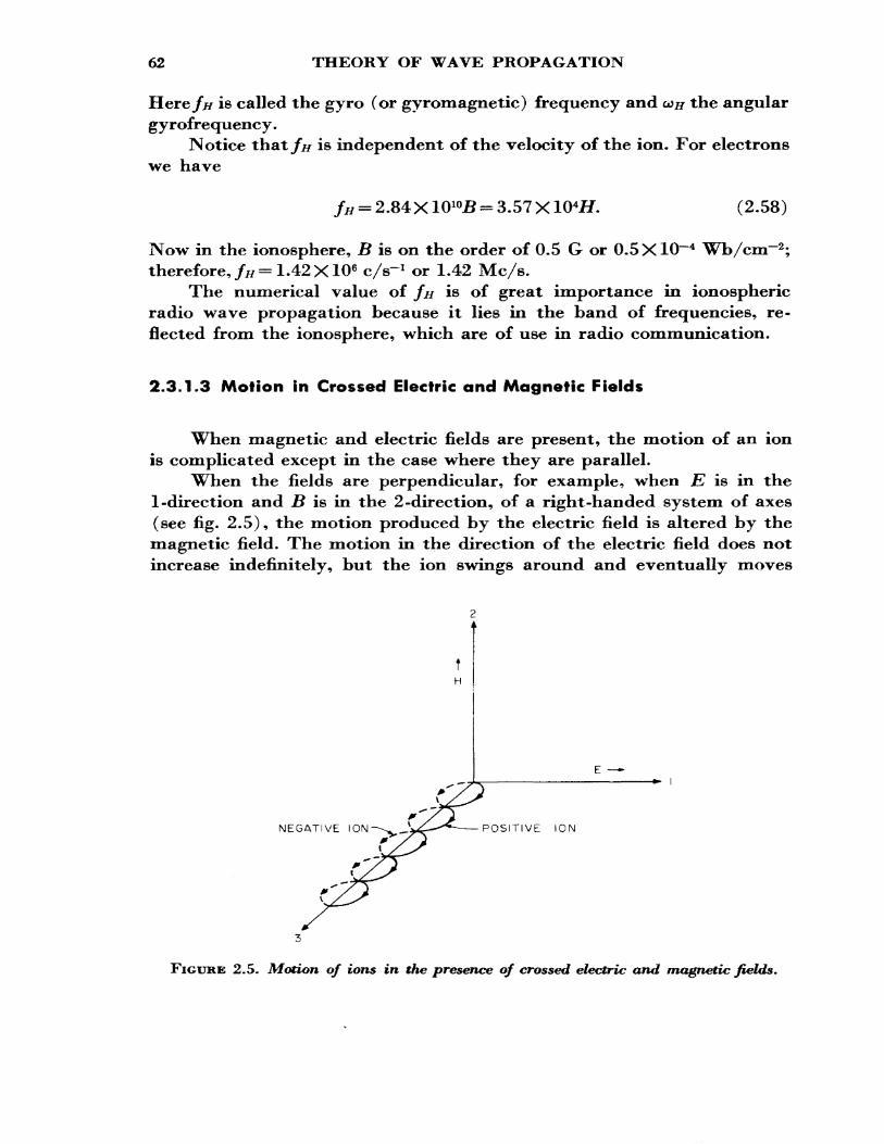
62 THEORY OF WAVE PROPAGATION
Here//r is called the gyro (or gyromagnetic) frequency and U>H the angular gy rofrequency.
Notice that/*/ is independent of the velocity of the ion. For electrons we have
= 2.84 X - 3. (2.58)
Now in the ionosphere, B is on the order of 0.5 G or 0.5X10"4 Wb/cm~2 ; therefore, /# = 1.42 XlO6 c/s"1 or 1.42 Mc/s.
The numerical value of fn is of great importance in ionospheric radio wave propagation because it lies in the band of frequencies, re flected from the ionosphere, which are of use in radio communication.
2.3.1.3 Motion in Crossed Electric and Magnetic Fields
When magnetic and electric fields are present, the motion of an ion is complicated except in the case where they are parallel.
When the fields are perpendicular, for example, when E is in the 1-direction and B is in the 2-direction, of a right-handed system of axes (see fig. 2.5), the motion produced by the electric field is altered by the magnetic field. The motion in the direction of the electric field does not increase indefinitely, but the ion swings around and eventually moves
TH
NEGATIVE POSITIVE ION
FIGURE 2.5. Motion of ions in the presence of crossed electric and magnetic fields.
DERIVATION OF THE APPLETON FORMULA 63
against the electric field, as illustrated in figure 2.5. The average ion motion is in the 3 -direction and is independent of the mass and charge of the ion and even of the sign of the charge, negative and positive ions both moving in the same direction. Hence, in an electrically neutral medium there is no resultant current in the 3 -direction, except insofar as these conditions may be altered by collisions,
2.3.2. Derivation of the Appleton Formula
The formulas for the complex refractive index of a medium such as the ionosphere were derived by a number of people during the 1920*s but the name most commonly associated with the theory is that of Sir Edward Appleton Q5].
In 1931, D. R. Hartree [_6^\ suggested that it was appropriate to include the Lorentz polarization term in the theory. Although the bulk of both theoretical and experimental evidence indicates that the inclusion of the term is unjustified, the formula for the complex refractive index is often referred to as the Appleton— Hartree formula.
The influence of heavy ions on the refractive index was considered by Goubau £7] in 1935, and since then more realistic distributions of collision statistics have been introduced by Phelps £8] and by Sen and Wyller [9].
In order to derive the formula for the refractive index it is necessary to define certain properties of both the wave and the medium. For our present purposes we shall assume the following properties:
Wave Properties(1) Simple harmonic progressive wave.(2) Steady -state solution.(3) Plane waves with given polarization. We shall call such waves
characteristic waves
Properties of the Medium(4) Electrically neutral.(5) Charges distributed with statistical uniformity so that there is
no resultant space charge.(6) Uniform external magnetic field.(7) Electrons only are effective.(8) Electronic collisions are independent of electron energy,(9) The thermal motions of the electrons are unimportant. Such a
medium is called a cold plasma.(10) The magnetic properties are those of free space.
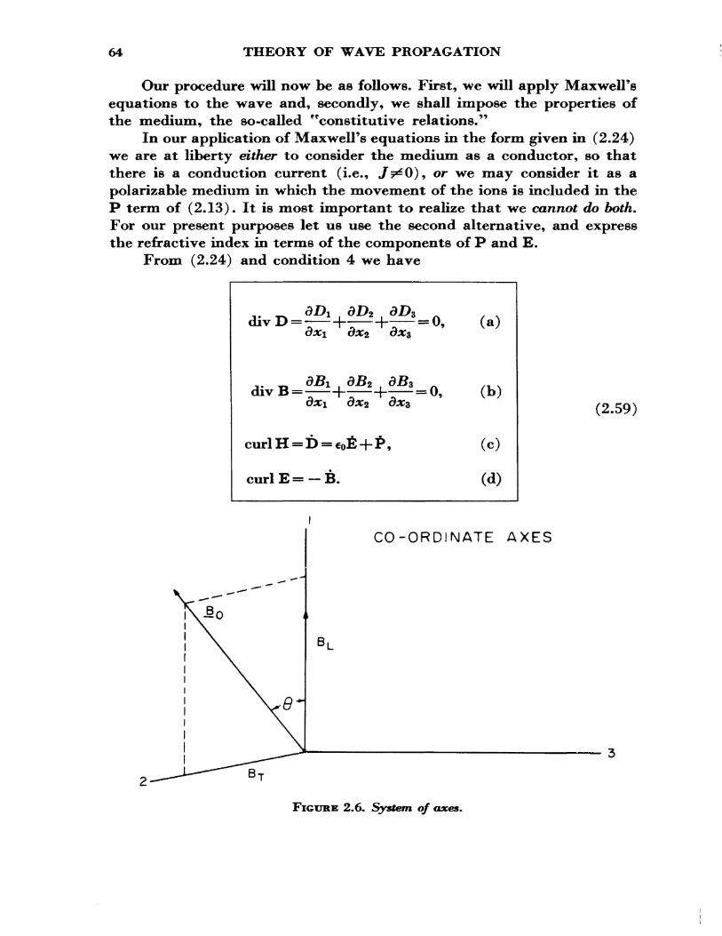
64 THEORY OF WAVE PROPAGATION
Our procedure will now be as follows. First, we will apply Maxwell's equations to the wave and, secondly, we shall impose the properties of the medium, the so-called "constitutive relations/'
In our application of Maxwell's equations in the form given in (2.24) we are at liberty either to consider the medium as a conductor, so that there is a conduction current (i.e., /^O), or we may consider it as a polarizable medium in which the movement of the ions is included in the P term of (2.13). It is most important to realize that we cannot do both. For our present purposes let us use the second alternative, and express the refractive index in terms of the components of P and E.
From (2.24) and condition 4 we have
,. -, i divB = -
curl E = — B.
= 0, (b)
(c)
(d)
(2.59)
CO-ORDINATE AXES
B,
B-
FIGURE 2.6. System, of axes.
DERIVATION OF THE APPLETON FORMULA 65
Consider a characteristic wave, having properties (1), (2), and (3) above, to be traveling along the 1-axis of a right-handed orthogonal system with axes 1, 2, and 3 as shown in figure 2.6. The components of the wave vary in time as exp (+£o>t) and in space as exp ( — ikx±) and do not vary in the 2- and 3 -directions.
Since we are considering the charge oscillation as a polarization of the medium then we have, from (2.13)
which expresses the electrical anisotropy of the medium. The magnetic properties, given by B = /zoH, are those of free space.
A plane wave traveling in the positive 1 -direction can be expressed by an equation of the form
(cct —
or E= EQ exp i(cot —
(a)
(b)(2.60)
Since the electric and magnetic vectors of the wave do not vary in the 2- and 3-directions we have, using the notation of (2.60b),
= ifc,
dxz
92
(a)
—— = 0, (b)
(c)
(d)
(2.61)
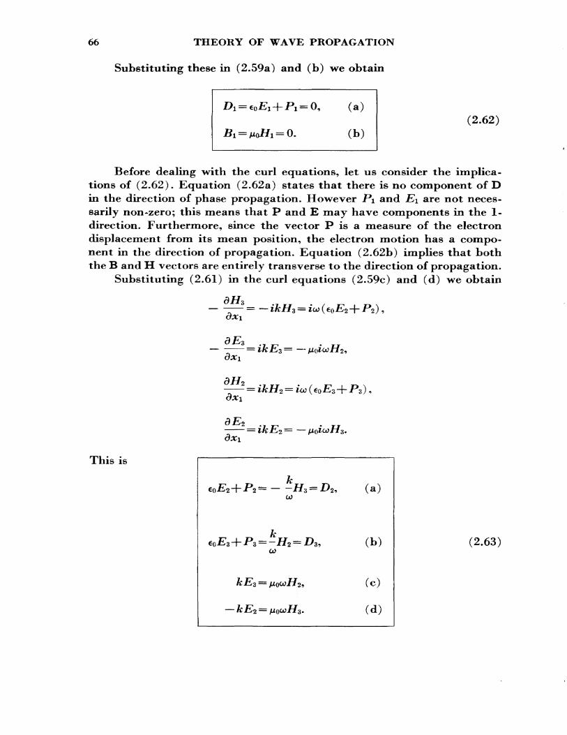
66 THEORY OF WAVE PROPAGATION
Substituting these in (2.59a) and (b) we obtain
(a)
(b)(2.62)
Before dealing with the curl equations, let us consider the implica tions of (2.62). Equation (2.62a) states that there is no component of D in the direction of phase propagation. However JPi and E\ are not neces sarily non-zero; this means that P and E may have components in the In direction. Furthermore, since the vector P is a measure of the electron displacement from its mean position, the electron motion has a compo nent in the direction of propagation. Equation (2.62b) implies that both the B and H vectors are entirely transverse to the direction of propagation.
Substituting (2.61) in the curl equations (2.59c) and (d) we obtain
— —— = £££'3 = —
= ikH<> = \ + P3 )
This is
*jCO
: *jCO
(a)
(b)
(c)
(d)
(2.63)
DERIVATION OF THE APPLETON FORMULA 67
Our next step is to express the refractive index in terms of the JP's and E*&. To do this we shall eliminate 7/3 from (2.63a) and (d). This gives
/
or
From the definitions of k, a;, and n it follows that
ck71 = ——
60
Hence
(2.64)
(2.65)
1/>2 f 1— -FT , (a)
similarly (2.66)
From these equations it follo\vs that
and \vith (2.63) we obtain
_ *____ T* (2.67)
>vhere R is called the wave polarization.
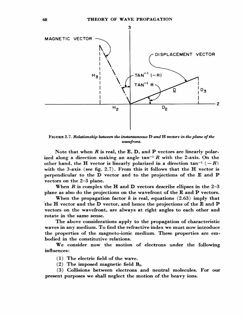
68 THEORY OF WAVE PROPAGATION
3
MAGNETIC VECTOR
\
DISPLACEMENT VECTOR
TAN" 1 (-R)
FIGURE 2.7. Relationship between the instantaneous D and H vectors in the plane of thetvavefront.
Note that when R is real, the E, D, and P vectors are linearly polar ized along a direction making an angle tan~J R with the 2-axis* On the other hand, the H vector is linearly polarized in a direction tan"1 ( — R} with the 3-axis (see fig. 2.7). From this it follows that the H vector is perpendicular to the D vector and to the projections of the E and P vectors on the 2—3 plane.
When R is complex the H and D vectors describe ellipses in the 2—3 plane as also do the projections on the wavefront of the E and P vectors.
When the propagation factor k is real, equations (2.63) imply that the H vector and the D vector, and hence the projections of the E and P vectors on the wavefront, are always at right angles to each other and rotate in the same sense.
The above considerations apply to the propagation of characteristic waves in any medium. To find the refractive index we must now introduce the properties of the magneto-ionic medium. These properties are em bodied in the constitutive relations.
We consider now the motion of electrons under the following influences:
(1) The electric field of the wave.(2) The imposed magnetic field B0 .(3) Collisions between electrons and neutral molecules. For our
present purposes we shall neglect the motion of the heavy ions.
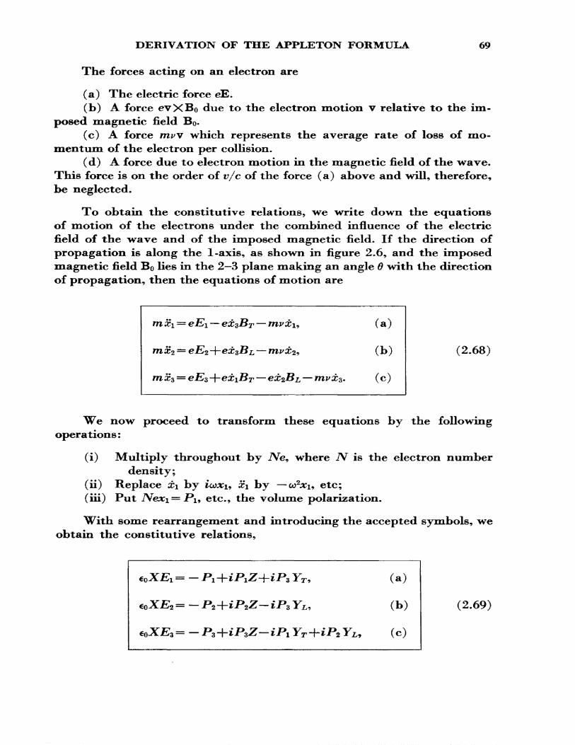
DERIVATION OF THE APPLETON FORMULA 69
The forces acting on an electron are
(a) The electric force eE.(b) A force evXBo due to the electron motion v relative to the im
posed magnetic field B0.(c) A force mw which represents the average rate of loss of mo
mentum of the electron per collision.(d) A force due to electron motion in the magnetic field of the wave.
This force is on the order of v/c of the force (a) above and will, therefore, be neglected.
To obtain the constitutive relations, we write down the equations of motion of the electrons under the combined influence of the electric field of the wave and of the imposed magnetic field. If the direction of propagation is along the 1-axis, as shown in figure 2.6, and the imposed magnetic field BO lies in the 2—3 plane making an angle 0 with the direction of propagation, then the equations of motion are
= eEi — ex$BT —
— mvx^ (b)
(c)
(2.68)
We now proceed to transform these equations by the following operations:
(i) Multiply throughout by TVe, where N is the electron numberdensity;
(ii) Replace x\ by i&x^ x\ by —<o2Jti, etc; (iii) Put Nex\= Pi9 etc., the volume polarization.
With some rearrangement and introducing the accepted symbols, we obtain the constitutive relations,
€QXEl = - (a)
(b)
(c)
(2.69)
70 THEORY OF WAVE PROPAGATION
where X=7Ve2/c0'nco2, Yz, = eBz, Arac*>, YT = eBT/m^^ and Z=v/&.The subscripts T and L refer to the transverse and longitudinal com
ponents of the imposed magnetic field with reference to the direction of the wave normal (i.e., phase propagation).
The next step in our derivation is to express the ratio Pz/E<t or Pz/Es in terms of the parameters X, Y, and Z. This is best done via the wave polarization term R as follows: From (2.62a),
eoX.c/1 = —
Substitution in (2.69a) gives
P! iYP3 1-X-i
(2.70)
From (2.67) it follows that P2E3 = P3E2 so that by multiplying (2.69b) by PS and (2.69c) by PZ and subtracting, we end up with
p\ YL = PiP2 YT -P\YL. (2.71 )
With a little rearrangement, and remembering that R = P3/P2, we have from (2.70) and (2.71) the following quadratic expression in R:
' . 7R+YL = 0. (2.72) — X— iZ
There are, in general, two solutions of this quadratic which are given by
(2.73)
For the propagation of high-frequency radio waves through the E and F regions of the ionosphere, Z is usually very small and can be neg lected. For instance, with a frequency of 10 Mc/s at the 100-km level (v= 1.75 X10³ from table 1.3) we have Z= 3 X 10~4 . Under these conditions R is given by
(2-74)This formula tells us that, in general, there are two, and only two, char-
PROPERTIES OF THE APPLETON FORMULA 71
acteristic waves capable of propagation in our magneto-ionic medium. From (2.69b) we obtain
(2.75)-iZ+iYLR*
which, on substituting, in (2.66a) gives
Y———— , (2.76)
/ V*/ ________ I T ___
\4(l-X-i
which is the Appleton formula.In the upper regions of the ionosphere the collision frequency is
sufficiently small so that, for frequencies greater than about 1 Mc/s, we may put Z=Q, and hence the real part2 // of the refractive index is given by
2X(1-X)v .
In the absence of an imposed magnetic field ( YT = YL = 0) and of colli sions (,Z=0) the refractive index is given by
l-k~ 9 (2.78)
where k= (e?/4<7r2€Qm) =80.5 and/ is in cycles per second.
2.3.3. Some Properties of the Appleton Formula
2.3.3.1. No Magnetic Field, No Collisions
In a discussion of the properties of the Appleton formula it is best to start with the simplest case, that is, with (2.78). First it will be seen that the square of the refractive index must be equal to or less than unity. Furthermore, for propagation of the wave, p, must be real so that AI must
3 Henceforth the symbol /A will be used in this sense and not for magnetic permeability.
72 THEORY OF WAVE PROPAGATION
lie between 0 and 1. Secondly, we see that, for a given wave frequency, the refractive index decreases with increase of electron density, and that, for a given electron density, the refractive effects decrease with increase of frequency but are independent of the amplitude of the wave.
Curves depicting the variation of y? (or /x) with X are often called dispersion curves. The simplest dispersion curve is that representing (2.78) and is shown in figure 2.8. This curve can be interpreted in terms of ionospheric propagation as follows:
Imagine a radio wave incident normally on a plane stratified iono sphere; at the bottom of the ionosphere (7V=0) IJL is unity. As we pene trate into levels of higher and higher electron concentration, ^ falls lower and lower. If the electron density is sufficiently high, then £i will go to zero. To find what happens when M reaches zero we apply SnelFs law to the wave. SnelFs law states that for a wave incident at an angle <£o to the normal, the angle <£ with the normal at a level where the refractive index is IJL is given by
sn <j> — sn (2.79)
Now MO= 1 outside the ionosphere and at reflection 0 must be 90° so that the refractive index at reflection jur must be equal to sin <£o- With normal incidence (0o = 0) the condition of reflection becomes /xr =0. Thus we see that if the electron density is sufficiently large to reduce IJL to zero then a wave (incident normally) will be reflected. Otherwise the wave will penetrate through the layer.
0
DISPERSION CURVE
= I-X
FIGURE 2.8. Dispersion curve (no field^ no collisions).
PROPERTIES OF THE APPLETON FORMULA 73
2.3.3.2. Magnetic Field, No Collisions
Dispersion. For a more complete discussion of the properties of the refractive index formula, the reader should consult the excellent books by J. A. Ratcliffe [lO], K. G. Budden [11], and J. M. Kelso [17]. However, we shall derive some formulas which will be needed in future chapters.
First consider the case of the reflection of a wave, of frequency /, incident normally in an ionospheric layer. Putting /x = 0 in (2.77) and solving for X we obtain the following:
With + sign X=l (2.80)
With - sign X=l- Y, (a)or
X=1+F. (b) (2.81)where
l. (c)
Equation (2.80) tells us that, for one of the magneto-ionic waves, the wave is reflected as in the absence of the magnetic field. This wave is called the ''ordinary" wave. Equations (2.81) show that the level of reflection of the other magneto-ionic wave (called the extraordinary) is dependent on the strength, but not on the direction, of the imposed magnetic field. For waves of frequency greater than the gyrofre- quency (fa) the usual level of reflection is given by X= 1— Y whereas on frequencies below fn (so that Y>1) the condition is X=l+ Y.
The dispersion curves corresponding to (2.77) are shown in figures 2.9a and b for values of Y=^ and Y=2, respectively, and for 0£^45 0 together with the limiting cases of longitudinal and transverse propaga tion. Note that these curves are not drawn to scale but are intended merely to illustrate the general shapes.
Approximate formulas. Even in the absence of electronic collisions, the refractive index formula (2.77) is complicated. There are certain practical conditions under which considerably simpler approximations are useful. Although, with the advent of electronic computers, the neces sity for using approximations in numerical work has decreased, there is still some need for them in practical work and, furthermore, they are widely used to simplify theoretical discussion.
The usual rules for determining whether the quasi-transverse (QT) or the quasi-longitudinal (QL) approximations hold are,
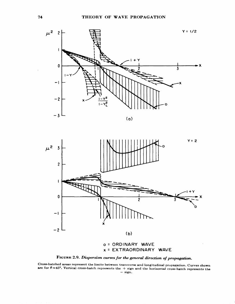
74 THEORY OF WAVE PROPAGATION
Y= 1/2
Y= 2
3 -
2 -
o = ORDINARY WAVEx = EXTRAORDINARY WAVE
FIGURE 2*9. Dispersion curves for the genercd direction of propagation.
Cross-hatched areas represent the limits between transverse and longitudinal propagation. Curves shown are for 0 «45°. Vertical cross-hatch represents the + sign and the horizontal cross-hatch represents the
— sign.
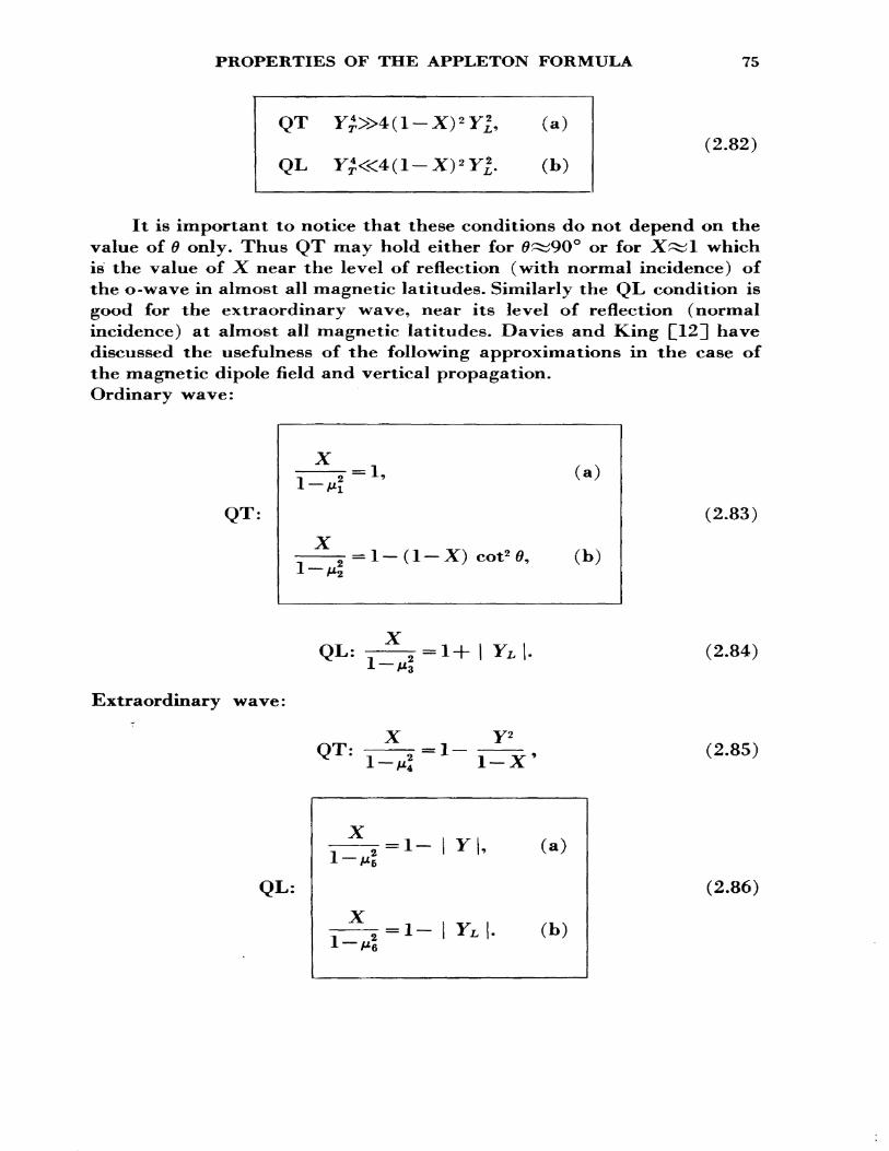
PROPERTIES OF THE APPLETON FORMULA 75
QT y*»4(l-X)*yl, (a)
QL y*«4(l-X)*y£ (b)(2.82)
It is important to notice that these conditions do not depend on the value of 6 only. Thus QT may hold either for 0^90° or for X~l which is the value of X near the level of reflection (with normal incidence) of the o-wave in almost all magnetic latitudes. Similarly the QL condition is good for the extraordinary wave, near its level of reflection (normal incidence) at almost all magnetic latitudes. Davies and King £12] have discussed the usefulness of the following approximations in the case of the magnetic dipole field and vertical propagation. Ordinary wave:
QT:
= 1—(1—X) cot2 0,
(a)
(b)
(2.83)
QL: \ Yz.\. (2.84)
Extraordinary wave:
(2.85)
QL:
X 1 1 V 1-, 2 L ~~ 1 * !' A M&
i i v i1_ U2 X 1 YL >•A Me
(a)
(b)
(2.86)
76 THEORY OF WAVE PROPAGATION
Care must be taken when using these approximations, as the range of validity may be very small. This is illustrated in figures 2.10a and b. Note that the extraordinary wave curves are plotted in terms of the parameter
The following are suitable formulas for the refractive indices near the levels of reflection with normal incidence. For the ordinary wave
M+ = (1 — i« cot2 0) cosec2 0,
where e = 1 — X, and for the extraordinary wave we have
(2.87)
-=>/=(l-F)(l+cos2 0)
tan2 $ /3+sec2 ~ e-+tan2 0
(2.88)
where ci = 1 — Y — X.For further details the reader is referred to Budden £11, Ch. 12).
Note that if Y is replaced by — Y in (2.88) the refractive index is that when X approaches 1 + Y.
Other approximations of interest are those applicable to audio fre quency waves (the whistler mode). When X^>Y^>1 and | Yi | > 1, Storey £13] has shown that the + sign in (2.77) reduces to the following approximations for a wide range of 0, not too near 90°:
X
or approximately Ai2 =
(a)
(b)
(2.89)
Wave polarization. One other aspect of the Appleton formula which is of interest is the wave polarization jR given by (2.74). This gives the amplitude ratio and the phase difference between the oscillations of the D, E, and P vectors along the 2- and 3-axes. In general, the tips of these vectors describe ellipses. The D ellipse is similar in shape to the projec tions of the E and P ellipses on to the 2-3 plane and the sense of rotation is the same. The H ellipse is similar to the D ellipse (and lies wholly in
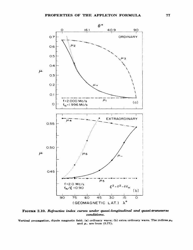
PROPERTIES OF THE APPLETON FORMULA 77
16.1 4O.9 9O
0.7
0.6
0.5
O.4
0.3
O.2
O.I
O
ORDINARY
f = 2.000 Mc/s fN = 1.996 Mc/s
0.55
O.5O
O.45
I I EXTRAORDINARY
- f =2.0 Mc/s f/€ =0.90
(b)
90 75 60 45 3O 15
(GEOMAGNETIC LAT.) X°
O
FIGURE 2.1O. Refractive index curves under quasi-longitudinal and quasi-transverseconditions.
Vertical propagation, dipole magnetic Held, (a) ordinary wave; (b) extra ordinary wave. The indices fJL+and fM— are from (2.77)*
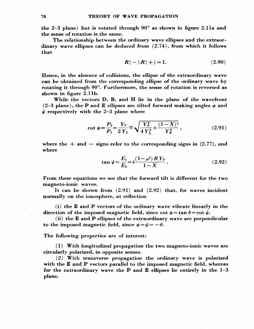
78 THEORY OF WAVE PROPAGATION
the 2—3 plane) but is rotated through 90° as shown in figure 2.1 la and the sense of rotation is the same.
The relationship between the ordinary wave ellipses and the extraor dinary wave ellipses can be deduced from (2.74), from which it follows that
/*(-)*( + )=!. (2.90)
Hence, in the absence of collisions, the ellipse of the extraordinary wave can be obtained from the corresponding ellipse of the ordinary wave by rotating it through 90°. Furthermore, the sense of rotation is reversed as shown in figure 2.lib.
While the vectors D, B, and H lie in the plane of the wavefront (2—3 plane), the P and E ellipses are tilted forward making angles 0 and ^ respectively with the 2—3 plane where
! 2 YL 4 Y(2-91)
where the + and — signs refer to the corresponding signs in (2.77), and where
(2.92)
From these equations we see that the forward tilt is different for the two magneto-ionic waves.
It can be shown from (2.91) and (2.92) that, for waves incident normally on the ionosphere, at reflection
(i) the E and P vectors of the ordinary wave vibrate linearly in the direction of the imposed magnetic field, since cot <£ = tan 6 = cot ^.
(ii) the E and P ellipses of the extraordinary wave are perpendicular to the imposed magnetic field, since <£ = ̂ = — 0.
The following properties are of interest:
(1) With longitudinal propagation the two magneto-ionic waves are circularly polarized, in opposite senses.
(2) With transverse propagation the ordinary wave is polarized with the E and P vectors parallel to the imposed magnetic field, whereas for the extraordinary wave the P and E ellipses lie entirely in the 1-3 plane.
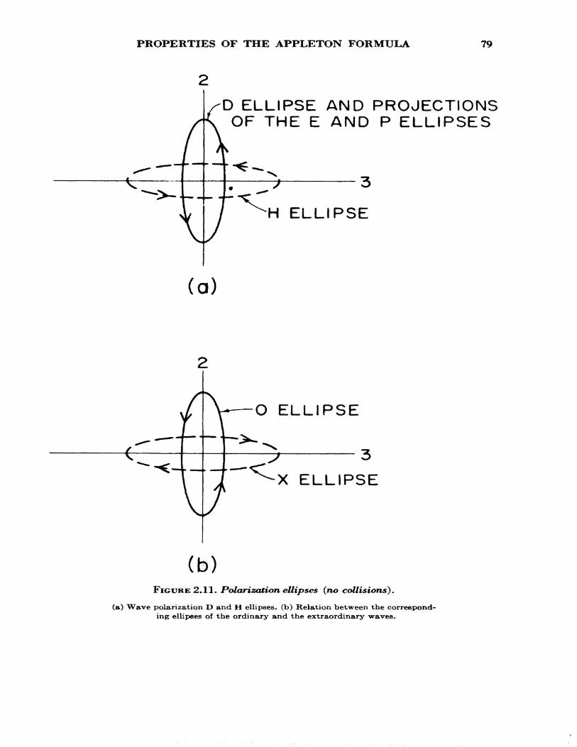
PROPERTIES OF THE APPLETON FORMULA 79
D ELLIPSE AND PROJECTIONS OF THE E AND P ELLIPSES
H ELLIPSE
(a)
O ELLIPSE
ELLIPSE
(b)FIGURE 2.11. ffolarization ellipses (no collisions).
(a) Wave polarization D and H ellipses, (b) Relation between the correspond ing ellipses of the ordinary and the extraordinary waves.
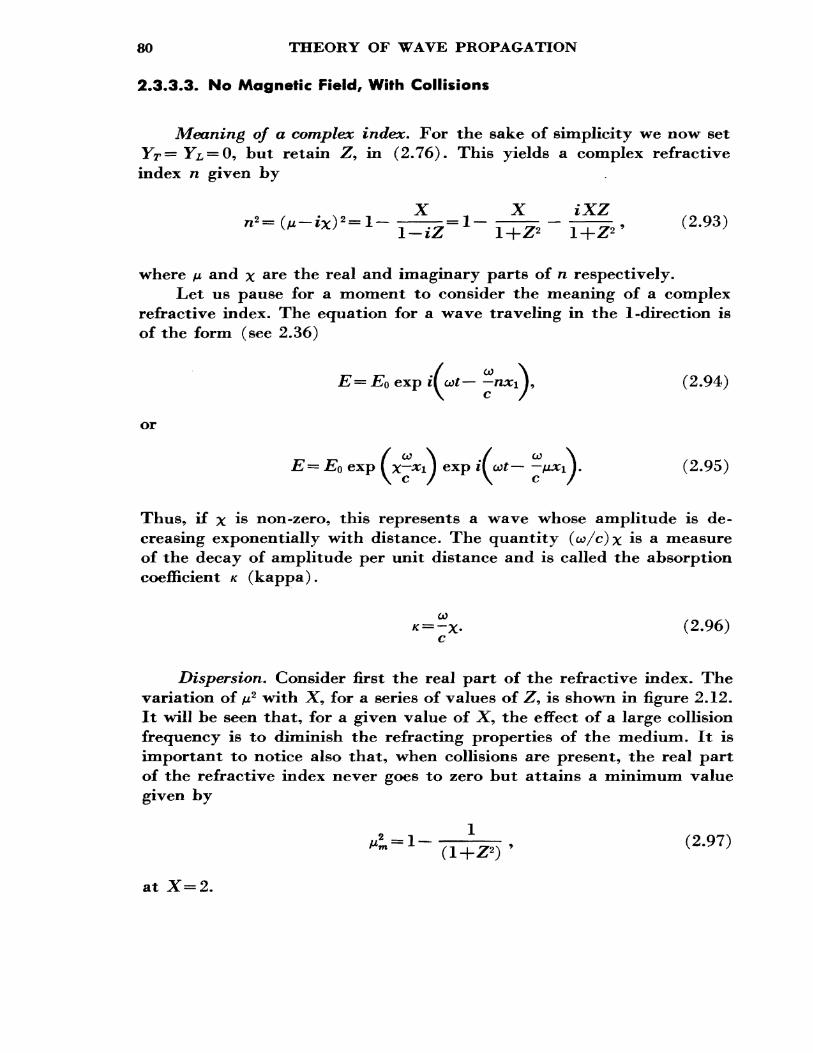
80 THEORY OF WAVE PROPAGATION
2.3.3.3. No Magnetic Field, With Collisions
Meaning of a complex index. For the sake of simplicity we now set YT= YL = Q* but retain Z, in (2.76). This yields a complex refractive index n given by
„_(„-*),_!____!_ -_. (2.93)
where M and x ar^ the real and imaginary parts of n respectively.Let us pause for a moment to consider the meaning of a complex
refractive index. The equation for a wave traveling in the 1 -direction is of the form (see 2.36)
or
= E0 exp i{ ut— -nxl ), (2.94)
(2.95)/ co \ / co \
= EQ exp f x— KI ) exp if &t— —fjLXi ].
Thus, if x is non-zero, this represents a wave whose amplitude is de creasing exponentially with distance. The quantity (o>/c)x is a measure of the decay of amplitude per unit distance and is called the absorption coefficient K (kappa).
* = -*. (2.96)C
Dispersion. Consider first the real part of the refractive index. The variation of M2 with X, for a series of values of Z, is shown in figure 2.12. It will be seen that, for a given value of X, the effect of a large collision frequency is to diminish the refracting properties of the medium. It is important to notice also that, when collisions are present, the real part of the refractive index never goes to zero but attains a minimum value given by
/£ = 1 — ——^- , (2.97)
at X=2.
PROPERTIES OF THE APPLETON FORMULA 81
NO MAGNETIC FIELD
0-5
O
Z=2-0
O-5 1-5 2'0
FIGURE 2.12. Variation of refractive index & with X for different collision frequencies (nomagnetic field) , Z^ = v/co.
This means that in a lossy medium total reflection <never really oc curs. However, strong reflections still occur near levels at which JJL is small.
Absorption. We shall return now to the absorption of the radio wave. From (2.93) and (2.96) we get
a; 1 XZ _____ c 2/u. 1+.Z2 2e0mc
e2 1 Nv(2.98)
This formula gives the absorption in nepers per meter, where 1 neper — 8.69 dB.
Equation (2.98) enables us to distinguish between two extreme types of absorption, namely:
Non-deviative absorption occurs in the D region of the ionosphere; it predominates when JJL is near unity and when the product Nv is large.
Deviation absorption occurs near the level of reflection and whenever there is marked bending of the ray, that is, when JJL tends to zero. For non-deviative absorption we have, when co is much greater than */,
Nvor
(2.99)
82 THEORY OF WAVE PROPAGATION
so that the absorption varies inversely as the square of the frequency. For deviative absorption we have
(2.100)
Note that this type of absorption does not, in general, vary inversely as the square of the frequency.
Let us consider now the case when the angular wave frequency is small compared with the collision frequency (i.e., o?2<S>2 ). With this condition we have from (2.98) for non-deviative absorption
e2 TV(2.101)
2e0mc v
Under these conditions, the absorption may actually decrease with in crease of collision frequency. The physical reason for this appears to be that the electronic motions are so confined that little energy is extracted from the wave. Absorption of this type is thought to occur during some polar cap absorption events and certain solar flare effects.
It is of interest to note that differentiation of (2.98) (for M~!) shows that a maximum of absorption occurs when v = o>.
2.3.3.4. Magnetic Field, With Collisions
Dispersion. With one exception, the inclusion of a magnetic field and collisions introduces great complication into the dispersion and ab sorption relationships. The one exception is that of transverse propaga tion of the ordinary wave which is the same as the **no field" case.
The dispersion curves for the general case of any angle of propaga tion are discussed usually in terms of the so-called critical collision fre quency vc where
Vc
0>
The curves are sketched in figure 2.13 and show how profound are the effects of collisions (in comparison with figure 2.9), especially near X=l. Collisions play an important part in modifying the QT and QL conditions. Thus QL conditions may hold even near X=l for the ordinary wave
PROPERTIES OF THE APPLETON FORMULA 83
DISPERSION CURVES WITH COLLISIONS Y <I Y>I
v < z/c
1.0
tp. 1.0
v =
1.0
If >
LO
Z/= Z/C
I/ > Z/c
1.0
0=* 20°ORDINARY
——— EXTRAORDINARY
FIGURE 2.13. Dispersion curves with magnetic field and collisions for a fixed 0=20°
84 THEORY OF WAVE PROPAGATION
whereas QT conditions may apply near X=1 =F Y for the X-wave. The interested reader can find more information on this in Mr. Ratcliffe's book [10].
Polarization. As far as polarization is concerned, the introduction of collisions causes the polarization ellipses (in the 2—3 plane) to rotate about the 1-axis. All the ellipses associated with one magneto-ionic wave rotate in the same direction and through the same angle as shown in figure 2.14a. The ellipses associated with the other wave rotate in the opposite direction through the same angle (figure 2.14b). Hence, for the projections of the ellipses onto the wavefront^ uue may deduce the ellipses of one magneto-ionic wave front that of the other as follows i Rotate the ellipse through 90° about the direction of phase propagation and then reflect in the magnetic meridian. It may be noted that one ellipse is the reflection of the other in the plane making an angle of 45° with the magnetic meridian.
Absorption. In principle it is possible to express the complex refrac tive index in terms of its real and imaginary parts and thus to obtain the absorption. In practice the expressions which would be obtained by this procedure are so complex as to be of little or no value. For a variety of conditions, however, the propagation conditions are quasi-longitudinal and the non-deviative absorption coefficient is then given, approximately, by
2e0mc(2.103)
The + and — signs refer to the ordinary and extraordinary waves re spectively. From this we see that the ordinary wave suffers less absorp tion, and the extraordinary suffers more absorption, than the correspond ing wave in the absence of a magnetic field.
2.3.4. Generalized Magneto-Ionic Formulas
2.3.4.1. Collision Statistics
In our derivation of the Appleton formula it was assumed that the electrons all possessed the same average velocity and that the collision frequency v was independent of the electron velocity. Now the question of finding an "average" velocity while not important in the upper regions of the ionosphere, where v is small, is of considerable importance in the D region where v may be equal to or greater than the angular wave
GENERALIZED MAGNETO-IONIC FORMULAS 85
D ELLIPSE AND PROJECTIONS OF THE E AND P ELLIPSES
H ELLIPSE
(a)
N
(b)FIGURE 2.14. Polarization ellipses with collisions.
(a) Polarization D and H ellipses, (b) Relation between the corresponding ellipses of ordinary andextraordinary waves.
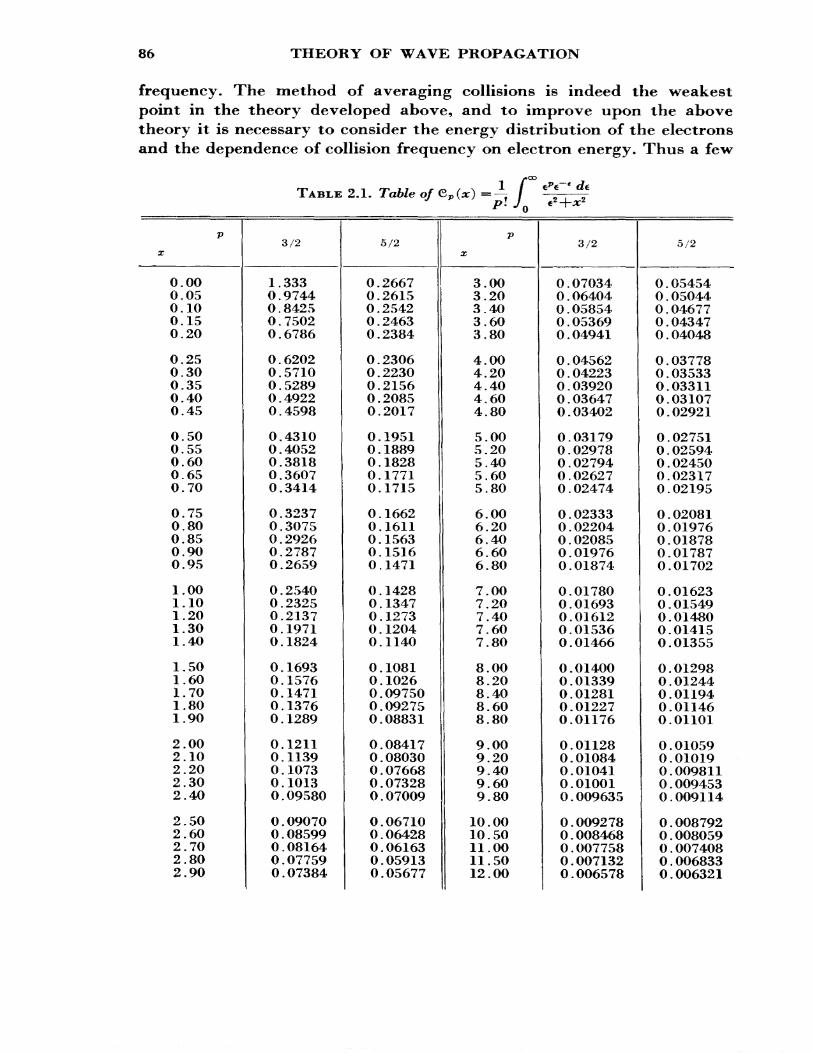
86 THEORY OF WAVE PROPAGATION
frequency. The method of averaging collisions is indeed the weakest point in the theory developed above, and to improve upon the above theory it is necessary to consider the energy distribution of the electrons and the dependence of collision frequency on electron energy. Thus a few
TABLE 2.1. Table ofe-' de
pX
0.000.050.100.150.20
0.250.300.350.400.45
0.500.550.600.650.70
0.750.800.850.900.95
1.001.101.201.301.40
1.501.601.701.801.90
2.002.102.202.302.40
2.502.602.702.802.90
3/2
1.3330.97440.84250 . 75020.6786
0.62020.57100 . 52890 . 49220 . 4598
0.43100.40520.38180 . 36070.3414
0.32370.30750.29260.27870.2659
0.25400.23250.21370.19710.1824
0.16930.15760.14710.13760 . 1289
0.12110.11390 . 10730.10130.09580
0.090700.085990.081640.077590 . 07384
5/2
0.26670.26150.25420.24630.2384
0.23060.22300.21560.20850.2017
0.19510 . 18890 . 18280.17710.1715
0.16620.16110.15630.15160.1471
0 . 14280.13470.12730 . 12040.1140
0.10810.10260.097500.092750.08831
0.084170 . 080300 . 076680.073280.07009
0.067100.064280.061630.059130.05677
pX
3.003.203.403.603.80
4.004.204.404,604.80
5.005.205.405.605.80
6.006.206.406.606.80
7,007.207.407.607.80
8.008.208.408.608.80
9.009.209.409.609.80
10.0010.5011.0011.5012.00
3/2
0.070340.064040.058540.053690.04941
0 . 045620 . 042230 . 039200.036470.03402
0.031790 . 029780 . 027940.026270 . 02474
0.023330.022040.020850.019760.01874
0.017800.016930.016120.015360.01466
0.014000.013390.012810.012270.01176
0.011280.010840.010410.010010.009635
0.0092780.0084680.0077580,0071320.006578
5/2
0 . 054540.050440.046770 . 043470 . 04048
0.037780.035330.033110.031070.02921
0.027510.025940 . 024500.023170.02195
0.020810.019760.018780.017870.01702
0.016230.015490.014800.014150.01355
0.012980.012440.011940.011460.01101
0.010590.010190.0098110.0094530.009114
0.0087920 . 0080590.0074080.0068330.006321
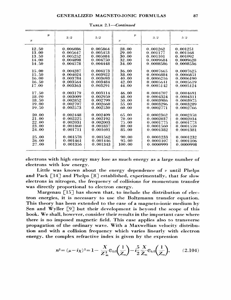
GENERALIZED MAGNETO-IONIC FORMULAS
TABLE 2.1—Continued
87
pX
12.50 13.00 13.50 14.00 14.50
15.00 15.50 16.00 16.50 17.00
17.50 18.00 18.50 19.00 19 . 50
20.00 21.00 22 . 00 23.00 24.00
25.00 26.00 27.00
3/2
0.006086 0 . 005647 0.005252 0.004898 0.004578
0.004287 0 . 004024 0.003784 0.003564 0.003363
0.003179 0 . 003009 0.002852 0.002707 0.002573
0.002448 0.002225 0.002031 0.001860 0.001711
0.001578 0.001461 0.001356
5/2
0.005864 0 . 005453 0 . 005084 0 . 004750 0 . 004448
0.004173 0.003922 0 . 003693 0.003484 0.003291
0.003114 0 . 002950 0.002799 0.002660 0.002530
0.002409 0.002192 0 . 002003 0.001837 0.001691
0.001562 0.001446 0.001343
pX
28.00 29.00 30.00 32,00 34.00
36.00 38.00 40.00 42.00 44,00
46.00 48.00 50.00 55 . 00 60.00
65.00 70.00 75.00 80.00 85.00
90.00 95.00 100 . 00
3/2
0.001262 0.001177 0.001101 0 . 0009684 0 . 0008586
0 . 0007665 0 . 0006884 0.0006216 0.0005641 0.0005142
0 . 0004707 0 . 0004324 0 . 0003986 0.0003296 0.0002771
0.0002362 0.0002037 0.0001775 0.0001560 0.0001382
0.0001233 0.0001107 0 . 0000999
5 /2
0.001251 0.001168 0.001092 0 . 0009620 0 . 0008536
0.0007625 0.0006851 0.0006190 O.OO05619 0.0005124
0.0004691 0.0004311 0 . 0003975 0 . 0003289 0.0002766
0.0002358 0 . 0002034 0.0001773 0.0001559 0.0001381
O.OO01232 0.0001106 0 . 0000998
electrons with high energy may lose as much energy as a large number of electrons with low energy.
Little was known about the energy dependence of v until Phelps and Pack £14] and Phelps £8] established, experimentally, that for slow electrons in nitrogen, the frequency of collisions for momentum transfer was directly proportional to electron energy.
Margenau £153 has shown that, to include the distribution of elec tron energies, it is necessary to use the Boltzmann transfer equation. This theory has been extended to the case of a magneto-ionic medium by Sen and Wyller £9] but their development is beyond the scope of this book. We shall, however, consider their results in the important case where there is no imposed magnetic field. This case applies also to transverse propagation of the ordinary wave. With a Maxwellian velocity distribu tion and with a collision frequency which varies linearly with electron energy, the complex refractive index is given by the expression
-i~G,~ (2.104)
88 THEORY OF WAVE PROPAGATION
in which Zm = vm/a). Here vm is the electron collision frequency associated with the most probable energy rather than with the mean energy.
exp ( — e) de (2.105)
The values of 63/2 (x) and 65/2 (#) given in table 2.1 are taken from Burke and Hara £16] and are published by permission of the Superintendent, Defence Research Telecommunications Establishment, Ottawa, Canada.
2.3.4.2. Dispersion
For the sake of simplicity let us consider the case where the absorp tion is relatively small so that x2<3^M2 - Under this condition we have
or (b)
(2.106)
From (2.105) it can be seen that when x is small, i.e., when 63/2(0) =£. Substitution of this value into (2.106) gives M2 = l— ( which is similar to (2.97) with 2^§>1. Thus it is possible to use the classical formula provided that v= (v5/2)^m . When x is large, i.e., when oC>>*>m, (2.106) reduces to (2.78).
2.3.4.3. Absorption
The non-deviative absorption per unit length (x2<$O*2 ) is obtained from the imaginary part of (2.104), namely
PHASE VELOCITY 89
5 o> 1 XK = o ~" 0~ ~T~ G6/5
2 C ZjJL Z,m
5 Ico2 /or K — 65/2!
4C (JL Vm \
f 1 }\z~J°
0,\1,J-(a)
(b)
(2.107)
To see how the absorption from the generalized theory compares with that from the Appleton equation, we need to compare the following function:
5 1' = ̂ ——^5/2
/o>\ ( — KVm/
(2.108)
with
(2.109)
This comparison is made in figure 2.15. As in the case of the dispersion curves, it is not possible to use a single effective collision frequency ^e ff across the entire frequency band. Nevertheless, on high frequencies the Appleton theory can be used with ^e ff = 2.5 ^m, whereas on low frequencies it is necessary to use *>e ff=l*5 */m. It must be realized, however, that on intermediate frequencies appreciable error is involved in using one or the other of these values of
2.4. GROUP PROPAGATION
2.4.1. Phase Velocity
From (2.78) it follows that the phase velocity (v) of a wave in a plasma containing no imposed magnetic field and in which electronic collisions are negligible is given by
c [ Ne2 ] v = - = c 1-———„ fji L me0^ J
(2.110)
90 THEORY OF WAVE PROPAGATION
IOO 8O6O
4O
8: 20 oCO CD< 10 UJ 8
LUcr
6
4
IO-l 10
v
2.IO9 z/=i/m 2.IO9 i/= l-5z/m 2.IO9 i/ = 2- 2.108
I IO-2 O-3 2O 3O
0-5 50
I-O IOO
Mc/s
345 IO
FIGURE 2.15. Comparison of absorption curves of Appleton theory and of generalizedtheory.
This indicates that the phase velocity, in the medium, is greater than that of light. It might be thought, at first sight, that this is a violation of the special theory of relativity. However, this is not so; all it means is that the wavelength (i.e., the distance between one wave crest and the next) is greater in the medium than in free space. It does not mean that energy is propagated faster than light.
The relationships between phase velocity (#), wavelength X, and refractive index p, are given by
GROUP VELOCITY 91
(a)
and — = — , (b) X X0
(2.111)
where Xo is the free space wavelength.
2.4.2. Group Velocity
When the phase velocity of a wave in a medium is a function of the wave frequency, the medium is said to be "dispersive." This term arose in the dispersion of colors by a prism. Inspection of (2.110) reveals that, for radio waves, the ionosphere is dispersive. This means that two waves differing slightly in frequency will travel with slightly different velocities. It is the interference pattern produced by two such waves that determines where, and with what velocity, the energy in the composite wave will travel. This is what happens when we modulate a wave and it introduces the concept of "group velocity" which, for our present purposes, may be regarded as the velocity with which the modulation envelope travels or the velocity of the energy. It should be realized that this concept is applicable only when the modulation envelope retains its shape. It is not applicable under conditions of severe distortion as can occur in highly dispersive media. For a more detailed discussion of this subject the reader should consult Stratton £4, sec. 5.1 7].
For our present purpose it will suffice to consider the superposition of two harmonic waves 1^1 and ^2 of equal amplitude which differ slightly in frequency and wave number.
= cos x\ —
= cos
= 2 cos %(xiSk — r&o) cos (^+v)^1 ~(^ +V/f r
fa)
(b)
(c)
(2.112)
92 THEORY OF WAVE PROPAGATION
FIGURE 2.16. Interference pattern produced by two tuaves of equal amplitudes and slightlydifferent frequencies.
This is shown diagrammatically in figure 2.16. The superposition pro duces a f*beat" signal, the envelope of which is given by
= 2 cos £<>i 8k —t Sco). (2.113)
It follows from (2.113) that the velocity of propagation of the envelope (i.e., the group velocity u) is given by
Scou = (2.114)
This contrasts with the phase velocity v given by
CO (2.115)
For a non-dispersive medium, in which a>/k is constant, u = v. In the limit as 5co—>0 and dk—K) we obtain the differential form
(2.116)_/u ~\dk k;
where ko is the value of k at which the gradient (dw/dk} is evaluated.It is convenient to define a group refractive index p' in a manner
similar to a phase index namely,
MEANING OF ANISOTROPY 93
It is important to remember that the group velocity as defined above is the component in the direction of phase propagation. Furthermore, under normal dispersion conditions, its magnitude is always less than the velocity of light. Substituting M =\/l — (/V/) 2 ™ (2.117) we find that
M' = -^(M/)=-. (2.118) df M
In the presence of an imposed magnetic field the group refractive index /i'(db) is given by substituting the expression for p from (2.77) in (2.117). This gives
x(2.119)
where the -f- and — signs refer to the ordinary and extraordinary waves respectively. The more complete expression, involving collisions, is given by Budden [11, ch. 12].
2.5. PROPAGATION IN ANISOTROPIC MEDIA
2.5.1. Meaning of Anisotropy
A homogeneous medium is said to be isotropic if the phase velocity at any given point in the medium is independent of the direction of propagation. A two-dimensional illustration of this is seen in figure 2.17. Consider a disturbance, originating at the origin 0; after a time t the wavefront will be a circle of radius r=vt. At a point P on the wave the wavefront is tangent to the circle and hence the wave normal np, which is perpendicular to the front, is radial. Now, since the disturbance is traveling out from O in all directions, it is not hard to see that the direc tion of energy flow (ray direction) is always radial. Hence, in an isotropic medium, the direction of phase propagation and of energy propagation coincide.
Now consider a magneto-ionic medium. Equation (2.77) shows that the refractive index p, depends upon YT and Yz,9 that is, upon the direction
94 THEORY OF WAVE PROPAGATION
WAVE DIRECTION
RAY DIRECTION
WAVE FRONT AT P
CIRCULAR WAVE FRONT
FIGURE 2.17. Wavefront in an isotropic medium.
WAVE FRONT AT P
n p NORMAL TO WAVE FRONT
;n r RAY DIRECTION (RADIAL)
B 0 REFERENCE AXIS
VNONCIRCULAR WAVE FRONT
FIGURE 2.18. Wavefront in an anisotropic medium.
of phase propagation with respect to the magnetic field. A medium such as this, in which the phase velocity at a point is a function of direction, is said to be "anisotropic." Again consider a disturbance originating at a point O in such a medium as illustrated in figure 2.18. Since the phase velocity is a function of the angle 0 made with the reference axis, the wavefront at a time t is not circular but shaped somewhat similar to that shown in figure 2.18. As before, the wavefront at a point P is tangential to the surface of constant phase and so the wave normal np is no longer radial. Since the energy is radiating from the point 0, the ray direction nr is still radial. Hence, in an anisotropic medium, the direction of phase propagation differs, in general, from that of energy propagation.
ANGLE BETWEEN PHASE AND RAY DIRECTIONS
2.5.2. Angle Between Phase and Ray Directions
95
Let ex be the angle measured from the wave normal np to the ray nr, i.e., in same sense as 0, as shown in figure 2.18. Our next step is to find a relationship for OL in terms of the refractive properties of the medium. Referring to the geometry in figure 2.19 we see that
\drtan a = — - —
and
(2.120)
(2.121)
It is now necessary to introduce the concept of ray velocity vr. The distance OP=r, in figure 2.18, is proportional to the velocity of P in the ray direction nr, whereas the phase velocity v is measured in the direction of phase propagation np. By letting the wavefront advance a short distance it can be seen that the relation between v and VT is
~Vr COS Of. (2.122)
Solution of (2.120), (2.121), and (2.122) gives
1 dv 1 dntan or = — - —- = H— —vde AI de (2.123)
WAVE FRONT AT P
RAY DIRECTION n, r
B 0 REFERENCE AXIS
FIGURE 2.19. Derivation of formula tan a
96 THEORY OF WAVE PROPAGATION
The sign convention used here is important because some authors use (2.123) with a reversal of sign. The convention used here is that angles measured in the same direction as 8 (i.e., from wave normal to magnetic field) are positive. It is important to remember also that in the above derivation of tan a, it was tacitly assumed that the medium was homo- geneous, that is the wave velocity in a given direction is independent of position in the medium. Hence no distortion of the wavefront is brought about by variations in the medium due to position.
2.5.3. Phase and Group Paths
For some purposes, it is convenient to use the concepts of phase and group paths which may be defined with reference to the transit times of a surface of constant phase and of a wave packet, respectively, between a sender and a receiver. It must be remembered that these are not paths in space but are distances which would have been covered if the wave (and wave packet) had traveled with the free space velocity.
Referring to the ray path between sender S and receiver R in figure 2.20, the time dTp required for a surface of constant phase (see fig. 2.20b) to travel from P to Q is given by
PM PQ dscoscx 1 , ,«,«^ds. (2.124)V Vr V C
The total transit time
Tp = - f /zco6«<fc=-, (2.125) cJs c
where
P= f M cos oc ds, (2.126)
is defined as the phase path.The quantity K= (2ir/\o)P is called the angular phase path length.
It is simply the number of radians of phase between sender and receiver. If K changes with time, either because of a change of real distance and/or a change in refractive index, the angular frequency of the received wave will differ from that transmitted by an amount Ao>. If K increases then the received frequency decreases because more radians are needed in the
PHASE AND GROUP PATHS 97
RAY PATH
(a)
Up WAVE NORMALn r RAY DIRECTION
FIGURE: 2.20. Phase and group paths in an anisatropic medium.
medium between S and R. Therefore the angular Doppler frequency Aco is
_Ato — — —— — — -—dt X0 dt
(2.127)
98 THEORY OF WAVE PROPAGATION
In terms of linear frequency the Doppler shift A/ is given by
1 dP fdP Af= — — —— = — - —— . X0 At c dt
(2.128)
The group path Pf may be defined in terms of the time of flight of a pulse. It will be recalled that in section 2.4.2 we defined the group velocity u in the direction of phase propagation. In an anisotropic medium the wave packet will, in general, have a velocity component parallel to the wavefront. The time dTg for the packet to travel from JP to Q (fig. 2.20) is given by
ds cosu
(2.129)
The quantity u sec a is called the ray group velocity and represents the velocity of the wave packet along the ray path.
The total time of flight between sender and receiver is:
Tf1 rR
= - / M' c J *
where
/>' =
cos a1= -P', c
(2.130)
Ri cos ot ds (2.131)
is called the group path. Another useful relationship between these quantities is
Ta = — ( W TP), (a)
or P' = — («P). (b) aco
(2.132)
REFERENCES 99
REFERENCES
[1] Faraday, M. (1855), Experimental Researches in Electricity, Vols. I, II, andIII (London).
[2] Maxwell, J. C. (1873), A Treatise on Electricity and Magnetism, Vols. I and II(Oxford).
[3] Hertz, H. (1892), Ausbreitung der Elektrischen (Kraft, Leipzig). [4] Stratton, J. (1941), Electromagnetic theory, sec. 2.19 (McGraw-Hill Book Co.,
Inc., New York).[5] Appleton, E. V. (1927), URSI Proc., Washington. [6] Hartree, D. R. (1931), The propagation of electro-magnetic waves in a refracting
medium in a magnetic field, Proc. Cambridge Phil. Soc. 27, 143.[7] Goubau, G. (1935), Dispersion in einem Electronen-Ionen-Gemisch dass unter
dem Einfluss eines ausseren Magnetfeldes staht, Hochfrequenz u. Electroakust 46, 37.
[8] Phelps, A. V. (1960), Propagation constants for electromagnetic waves in weaklyionized dry air, J. Appl. Phys. 31, 1723.
[9] Sen, H. K., and A. A. Wyller (1960), On the generalizations of the Appleton -Hartree magnetoionic formulas, J. Geophys. Res. 65, 3931.
[10] Ratcliffe, J. A. (1959), The magnetoionic theory (Cambridge Univ* Press)* [11] Budden, K. G. (1961), Radio waves in the ionosphere (Cambridge Univ. Press). [12] Davies, K., and G. A. M. King (1961), On the validity of some approximations to
the Appleton-Hartree formula, J. Res. NBS 65D, (Radio Prop.), No. 4, 323. [13] Storey, L. R. O. (1953), An investigation of whistling atmospherics, Phil. Trans.
Roy. Soc. London, A 246, 113. [14] Phelps, A. V., and J. L. Pack (1959), Electron collision frequencies in nitrogen and
in the lower ionosphere, Phys. Rev. Letters 3, 340.[15] Margenau, H. (1946), Conduction and dispersion of ionized gases at high fre
quencies, Phys. Rev. 69, 508.[16] Burke, M. J., and E. Hara (May 1963), A table of C—script integrals for use with
the generalized Appleton-Hartree magneto-ionic formulas, DRTE Report 1113. [17] Kelso, J. M. (1964), Radio Ray Propagation in the Ionosphere, (McGraw-Hill
Co., Inc., New York).

CHAPTER 3
Synoptic Studies of the Ionosphere
3.1. WORLDWIDE SOUNDINGS
For purposes of radio communications, it is necessary to have in formation about the ionosphere on a global scale. Since the spatial and temporal fluctuations in the ionosphere are so great, geographic coverage may be much more important than accuracy of measurement. This point should be borne in mind whenever one is judging the value of ionospheric data. For instance, the lack of accuracy to which a critical frequency can be measured may make it of little value to the scientist, yet it may be of value to the radio operator.
Before World War II, there were only a few sounding stations in existence, e.g., Slough, England; Washington, D.C., U.S.A.; Huancayo, Peru; Watheroo, Australia; and Slutsk, U.S.S.R. The need for more reliable high-frequency communications led to the installation of many more stations during the war (40 or 50). During the International Geo physical Year (IGY) still more stations were added, making a total of about 150. The distribution of stations during the IGY is shown in figure 3.1. During this latter period considerable uniformity was introduced into the scaling and reporting of ionospheric data Cl],1 which has turned out to be valuable from the point of view of both the radio communicator and the scientific worker.
Much of the impetus for ionospheric research has come from certain international organizations such as the International Scientific Radio Union (URSI) and the Consultative Committee on Ionospheric Radio (CCIR). These organizations have encouraged investigations into the spatial and temporal variations in the electron distribution in the iono sphere, the measurement of ionospheric absorption of radio waves, ionospheric movements, noise, and the scattering of radio waves from ionospheric irregularities.
1 Figures in brackets indicate the literature references on p. 156.
101
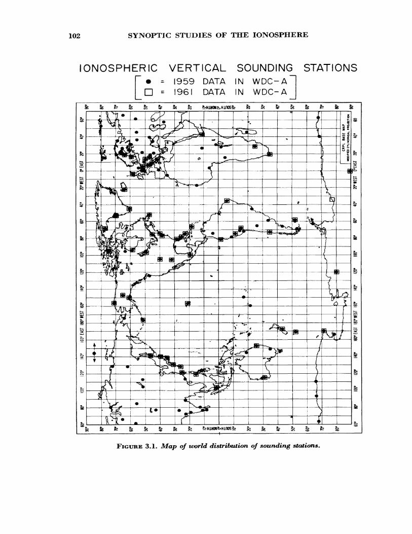
102 SYNOPTIC STUDIES OF THE IONOSPHERE
IONOSPHERIC VERTICAL SOUNDING STATIONS• = 1959 DATA IN WDC-AD = 1961 DATA IN WDC-A
FIGURE 3.1. Map q/" tvorld distribution of sounding stations.
EXPERIMENTAL TECHNIQUES 103
In the present chapter, we shall consider some of the techniques used in ionospheric investigations and a few of the results obtained.
When making measurements on a medium such as the ionosphere it is necessary to distinguish clearly between controlled experiments, such as can be carried out in a laboratory, and those over which we have no control. Except for certain modeling techniques involving laboratory plasmas and microwaves, ionospheric research must be carried out in its own environment and, hence, any control must be ffremote control,"
3.2. EXPERIMENTAL TECHNIQUES
There are many possible ways of classifying radio techniques for investigating the ionosphere. For instance, we can divide them into pulse versus continuous wave (CW) techniques, or into fixed frequency versus sweep frequency, or again into intermittent versus continuous methods and so on. In the present treatment, we shall start by studying the most widely used technique (the ionosonde) and follow in order of decreasing usage, such as the techniques for measuring absorption, phase, etc. It is not to be construed that this order is in any sense one of relative importance.
3.2.1. Height Recorders
3.2.1.1. The Ionosonde
The ionosonde is essentially a pulsed radar device in which the ex ploring frequency can be varied over a wide range from 1 Mc/s, say, up to 25 Mc/s. Of course the entire sweep may have to be covered in a series of frequency bands. A detailed description of ionosondes is given by Wright, Knecht, and Davies £2J. The equipment is designed to measure directly the time t taken for a pulse of radio waves to travel up to the ionosphere and back as a function of frequency. That is, it measures the group height h f of the ionosphere, where
fc' = ±e*=0.15f, (3.1)
t being in microseconds. This group height is also known as equivalent height and virtual height. The transmitter and receiver are kept in tune by suitable electronic or mechanical linkage and the receiver output is
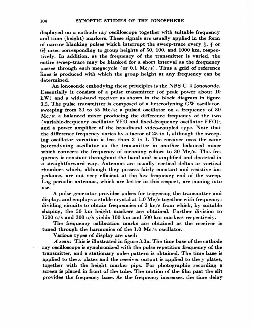
104 SYNOPTIC STUDIES OF THE IONOSPHERE
displayed on a cathode ray oscilloscope together with suitable frequency and time (height) markers. These signals are usually applied in the form of narrow blanking pulses which interrupt the sweep-trace every ^, f or 6f msec corresponding to group heights of 50, 100, and 1000 km, respec tively. In addition, as the frequency of the transmitter is varied, the entire sweep-trace may be blanked for a short interval as the frequency passes through each megacycle (or 0.1 Mc/s). Thus a grid of reference lines is produced with which the group height at any frequency can be determined.
An ionosonde embodying these principles is the NBS C-4 lonosonde. Essentially it consists of a pulse transmitter (of peak power about 10 kW) and a wide-band receiver as shown in the block diagram in figure 3.2. The pulse transmitter is composed of a heterodyning CW oscillator, sweeping from 31 to 55 Mc/s; a pulsed oscillator on a frequency of 30 Mc/s; a balanced mixer producing the difference frequency of the two (variable-frequency oscillator VFO and fixed-frequency oscillator FFO); and a power amplifier of the broadband video-coupled type. Note that the difference frequency varies by a factor of 25 to 1, although the sweep ing oscillator variation is less than 2 to 1. The receiver uses the same heterodyning oscillator as the transmitter in another balanced mixer which converts the frequency of incoming echoes to 30 Mc/s. This fre quency is constant throughout the band and is amplified and detected in a straightforward way. Antennas are usually vertical deltas or vertical rhombics which, although they possess fairly constant and resistive im pedance, are not very efficient at the low frequency end of the sweep. Log periodic antennas, which are better in this respect, are coming into use.
A pulse generator provides pulses for triggering the transmitter and display, and employs a stable crystal at 1.0 Mc/s together with frequency- dividing circuits to obtain frequencies of 3 kc/s from which, by suitable shaping, the 50 km height markers are obtained. Further division to 1500 c/s and 300 c/s yields 100 km and 500 km markers respectively.
The frequency calibration marks are obtained as the receiver is tuned through the harmonics of the 1.0 Mc/s oscillator.
Various types of display are used:A scan: This is illustrated in figure 3.3a. The time base of the cathode
ray oscilloscope is synchronized with the pulse repetition frequency of the transmitter, and a stationary pulse pattern is obtained. The time base is applied to the x plates and the receiver output is applied to the y plates, together with the height marker pips. For photographic recording a screen is placed in front of the tube. The motion of the film past the slit provides the frequency base. As the frequency increases, the time delay
TRANSMITTER
/\ PULSE
GENERATOR
SWEEP
16M
M M
OV
IE
CAM
ERA
VA
RIA
BLE
FREQ
UEN
CYO
SCIL
LATO
R
HEI
GH
T M
ARK
ER
FREQ
UEN
CY
MA
RKER
V M
MO
NIT
OR
RECO
RD35
MM
MOV
ING
FILM
CA
MER
A
w M 0 w H W 8 » 0 w
106 SYNOPTIC STUDIES OF THE IONOSPHERE
OSCILLOSCOPE
G = DIRECT PULSE, A,, A2 , A3 = ONCE, TWICE, THRICEREFLECTED SIGNALS
(0) A-SCANFIGURE 3.3a. Types of ionosonde display—A scan.
OSCILLOSCOPE
A, A 2 A
(b) B-SCANFIGURE 3.3b. Types of ionosonde display—B scan.
generally increases and the echo breaks in the time base move to the right. The cams controlling the frequency of the transmitter and receiver are suitably shaped so as to give the desired frequency scale on the film (e.g., linear or logarithmic).
B scan: This is similar to the A scan except that the receiver output and height pips are applied as blanking pulses to the oscilloscope and the y plates are grounded. The output is as shown in figure 3.3b.
HEIGHT RECORDERS 10'
MAY 3. 1962POINT BARROW
1345 (I5O° WMT)
1000 —
800
0 — •
2 346
MC/S
(C) PANORAMIC DISPLAY
FIGURE 3.3c. Types of ionosonde display—panoramic.
Panoramic displays'. The 13 scan is used with the time base applied to the y plates and a voltage applied to the x plates which is a function of transmitter frequency. The whole h f —f picture is photographed on a single frame of 16 mm movie film as illustrated in figure 3.3c.
The ionosonde is a versatile equipment and, in one form or another, is used at every ionospheric observatory. It has the advantage that the quantity measured (virtual height) does not depend upon the output of the transmitter or the gain of the receiver, which means that it can be operated by relativelv inexperienced operators. It is programmed, auto matically, to make sweeps at certain intervals (e.g., every 15 min). The duration of a sweep depends on the mechanical design of the ionosonde but there are practical limits. If the sweep is too fast, the receiver is out of tune with the echo which has been reflected from the ionosphere. Sweeps of duration less than about IS sec suffer from this. On the other hand, if the sweep takes too long, the ionosphere itself may have changed appreciably between the beginning and end of the sweep. Furthermore, the ionosonde may produce excessive interference with other radio systems.
108 SYNOPTIC STUDIES OF THE IONOSPHERE
3.2.1.2. The Virtual Height-Time Recorder
This is a fixed -frequency device using a B scan display which operates continuously. Provided that the signal does not penetrate the ionosphere, this system has the advantage of continuous monitoring of the ionosphere and is useful in detecting "one-shot " events such as the effect of a solar flare. It has the added advantage of extreme simplicity.
3.2.2. Absorption Measurements
The ionosonde gives very little information about the D region because reflections from this region tend to be of the partial type rather than the refractive type. Also, the lower frequencies are heavily absorbed in the lower ionosphere because of the high collision frequency there. This absorption is, of course, very important to the radio operator be cause it sets a lower limit to the power and/or the frequency with which he can operate. Thus absorption measurements are of practical importance and, in addition, they give information on the total electron content of the D region. Some of the methods used will be discussed below. These methods have been described, in more detail, by Piggott, Beynon, Brown, and Little
3.2.2.1. The Pulse Reflection Method
This method has been used extensively in England £4^ and elsewhere and involves the measurement of the amplitudes of successive echoes with an A scan display. The amplitudes are usually read off visually, either by noting the gain required to bring the tops of the oscilloscope traces to a fiduciary mark or else by calibrating the face of the oscilloscope.
It is convenient to express the amplitude ratios in terms of an ap parent reflection coefficient p. This parameter is the ratio of the amplitude / of a wave which is reflected once in the ionosphere to the amplitude /'o which would have been received in the absence of dissipative attenuation
7=/'0 exp(- f *ds} (3.2)
ds= — In p. (3.3)
ABSORPTION MEASUREMENTS 109
In practice, the absorption is usually measured in terms of a loss in decibels, L>, where
L= — 20 log p= —8.7 hi p. (3.4)
In the absence of absorption, the amplitude / of a wave reflected from a group height h' is given by
(3.5)
where /<> is the amplitude which would have been received if reflection had occurred at a standard height fee- When absorption is present the amplitudes of the first /i, second 72, and rth order Ir reflections are given by
ploh0 = pG, (a)
(b)
(c)
(3-6)
where pg is the apparent reflection coefficient of the ground and G( = /o/*o) may be regarded as a calibration constant.
The calibration factor, G, can be found by measuring the amplitudes of multiple reflected signals when the absorption is low (at night) and can then be used to measure p when the absorption is high, i.e., when there is one reflection only.
When G is known, p can be found from the group height and ampli tude of the reflected echo.
The chief practical problem in the measurement of absorption by this technique is that introduced by the continuous fading of the reflected signal. This question is too complex to be considered here but it requires that a suitable statistical sample be used to derive a mean amplitude. For vertical incidence measurements in the HF band, periods between 15 and 20 min are common, and it is desirable to average over such periods. Of course, if the averaging period is excessive, the absorption itself may have changed during the interval.
The chief disadvantage of this system is that the measurements are tedious to make and/or reduce to L values. Furthermore, inaccuracies arise because of noise and interference, polarization, pulse dispersion, partial reflection, and scattering (see ref.
110 SYNOPTIC STUDIES OF THE IONOSPHERE
3.2.2.2. Continuous-Wave Field-Intensity Recordings
In this method a continuous wave sender is used. A communications- type receiver is fed by a calibrated antenna and the output is registered on a pen recorder.
The CW recording method of measuring ionospheric absorption has the advantage of continuous recording, but it suffers from the dis advantage of not being able to separate the various echoes. The total field received at any instant is the resultant of different order echoes and of ordinary and extraordinary waves, all fading independently of each other. Approximately, the resultant median field intensity is the square root of the sum of the squares of the median values of all of its compo nents. From a knowledge of the differential absorption of the ordinary and extraordinary waves, and using the root-sum-square rule, the field intensity of the ordinary wave, first echo, can (in principle) be obtained.
If transmitter and receiver are close together, so that the incidence is essentially normal, it is possible to calibrate the equipment (roughly) by assuming that the nighttime signals are not absorbed in the ionosphere.
3.2.2.3. The Riometer Method
The riometer (rio = relative ionospheric opacity) is simply a receiver that measures the intensity of the random noise which impinges on the earth from deep space. The use of cosmic radio noise for the measurement of ionospheric absorption has been developed by Little £3] and his co- workers. The principle is as follows:
The radio noise power incident at a point outside the earth's atmos phere from a given direction in space is assumed to be constant with respect to time. The noise power received on a fixed receiving system at the earth's surface should, therefore, be a function of sidereal time only, since each day the aerial beam will explore the same strip of sky as the earth rotates. The transparency of the atmosphere at a particular in stant of time is, therefore, given by the ratio of the signal strength actually received to that received at the same sidereal time under conditions of little ionospheric absorption.
The simplest equipment capable of measuring cosmic noise consists of a gain stable receiver connected to an antenna (input) and a pen recorder (output), as illustrated in the block diagram in figure 3.4, to gether with a noise diode, for calibration purposes, and stabilized power
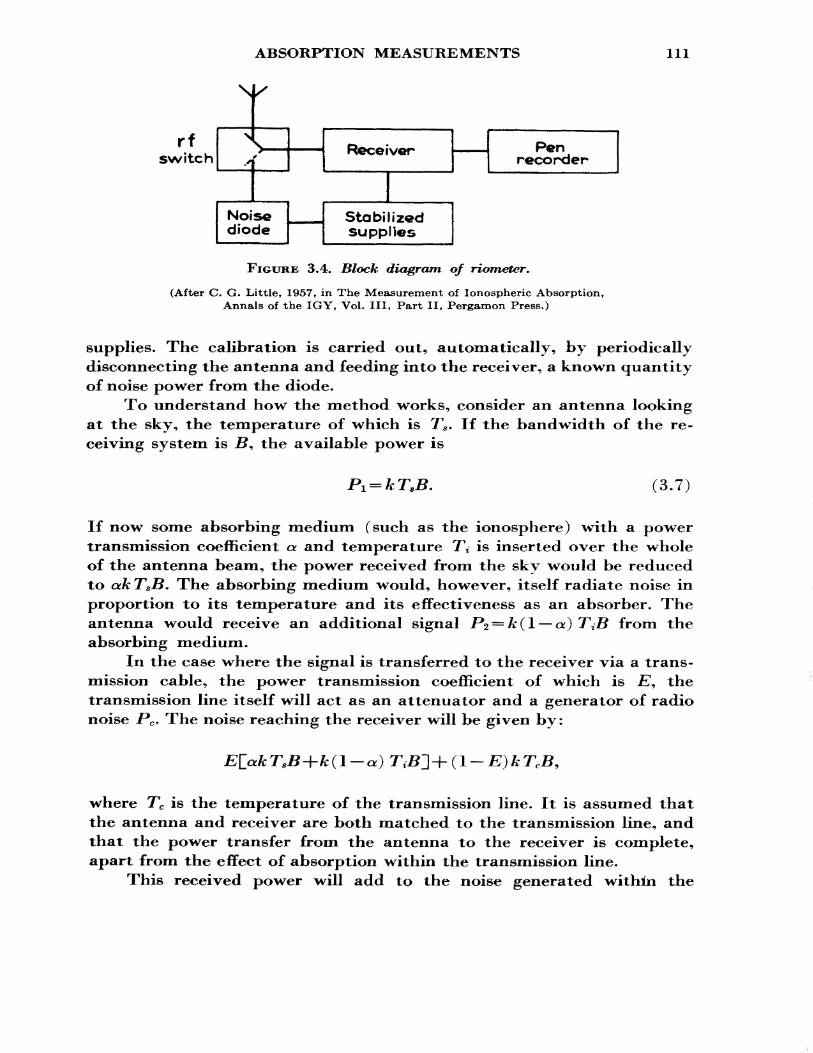
ABSORPTION MEASUREMENTS 111
rfswitch
\
\
X
^> ——^
HrNoise diode
Receiver
Stabilizedsupplies
P^»recorder
FIGURE 3.4. Block diagram of riometer.
(After C. G. Little, 1957, in The Measurement of Ionospheric Absorption, Annals of the IGY, Vol. Ill, Part II, Pergamon Press.)
supplies. The calibration is carried out, automatically, by periodically disconnecting the antenna and feeding into the receiver, a known quantity of noise power from the diode.
To understand how the method works, consider an antenna looking at the sky, the temperature of which is Ts . If the bandwidth of the re ceiving system is J5, the available power is
(3.7)
If now some absorbing medium (such as the ionosphere) with a power transmission coefficient a and temperature 7\ is inserted over the whole of the antenna beam, the power received from the sky would be reduced to oik TSB. The absorbing medium would, however, itself radiate noise in proportion to its temperature and its effectiveness as an absorber. The antenna would receive an additional signal />2 = fc(l — ex) 7YB from the absorbing medium.
In the case where the signal is transferred to the receiver via a trans mission cable, the power transmission coefficient of which is £*, the transmission line itself will act as an attenuator and a generator of radio noise _PC . The noise reaching the receiver will be given by:
where Tc is the temperature of the transmission line. It is assumed that the antenna and receiver are both matched to the transmission line, and that the power transfer from the antenna to the receiver is complete, apart from the effect of absorption within the transmission line.
This received power will add to the noise generated within the
112 SYNOPTIC STUDIES OF THE IONOSPHERE
receiver, which is given by
(3.8)
where T is the room temperature and F is the noise factor of the receiver. If the above system receives cosmic radio noise, the output power
jPo of the receiver may be written as
(3.9)
where Ps = noise power from theF*i= noise power from the ionosphere = E(l — oi) T
T8 ? Ti= effective temperatures of sky and ionosphere, Pc = noise power from cable = ( 1 — E) TckB9 Pr = noise power from receiver = (F — 1) TkB, /= interference, G = power gain of the receiver.
The problem introduced by interference can be partially removed by recording the minimum signal received while the receiver frequency is swept over a small frequency range (but many bandwidths) . Various other refinements are discussed in reference C3J.
It should be realized that the riometer is of use on frequencies above the penetration frequency only. A typical frequency is about 30 Mc/s. The disadvantage of such high frequencies is that the ionospheric ab sorption is low and it is necessary, therefore, to measure small changes in absorption. A riometer can usually measure absorption changes down to about 0.1 dB.
3.2.2.4. Minimum Frequency Observations
In (2.99) it was shown that non-deviative absorption varies in versely as the square of the wave frequency. Thus, when sounding the ionosphere with a conventional ionosonde, the minimum frequency ob served, /min* is roughly, a function of the ionospheric absorption. The characteristic/m i n has been used quite widely as an index of ionospheric absorption and its use is justified provided that the absorption changes are large compared with the other variable characteristics of the ionosphere.
PHASE MEASUREMENTS 113
3.2.3. Phase Measurements
3.2.3.1. Relative Phase Changes
Although it is not possible to determine the absolute phase of a reflected signal it is possible to measure, accurately, changes in phase. This can be done by mixing the incoming signal of frequency fe with a local oscillator signal of frequency fr of about the same amplitude and differing from it in frequency by a small amount (/«—/r ) - The phase of the signal from the reference oscillator must be highly stable or else must be locked to that of the radiated signal. With the advent of portable stable crystal oscillators and atomic frequency standards the former alternative is possible. The echo and the reference signal beat together in the detector stage of the receiver and give a beat signal of frequency (fe — fr)- This gives a sinusoidal trace on the screen of an oscilloscope when the output of the receiver is applied to the y plates and a linear time base is applied to the x plates. The movements of the sinusoidal trace depict the varying phase of the echo. Such a method has been described by Findlay Q5], Suitable modification of this arrangement enables the phase changes to be tracked electronically and displayed on a pen recorder instead of on photographic paper.
3.2.3.2. Frequency Changes
When the changes of phase with time are slow, the above method is very suitable; on the other hand, if the phase changes rapidly with time, there is a Doppler change in the received frequency and it is often con venient to measure frequency changes rather than phase changes. The technique is essentially the same as that described above; the beat fre quency signal may be recorded directly on a pen recorder and the fre quency changes determined by inspection. In a slight modification used by Ogawa \JbT\ and by Fen wick and Villard [1^ the beat frequency is fed to a frequency meter the output of which is recorded on an inked chart.
One disadvantage of both the above presentations is that they give the frequency variation of the composite sky wave. An improvement on this is the technique developed by Watts and Davies Q8] which is of interest also in that it provides one solution to a data storage problem. This method involves the spectral analysis of the beat signal. The beat signal is fed directly to the recording head of a magnetic tape recorder
114 SYNOPTIC STUDIES OF THE IONOSPHERE
the speed of which is 0.02 ips (inches per second). At this speed an 1800-ft roll of tape can store data continuously for more than one week, at the end of which the tape is played into an audio spectrum analyzer at a speed of 30 ips, say. This results in a frequency multiplication of 1500 and so converts the beat frequency of a few cycles per second into an audio tone. A commercial 420 channel analyzer having a total bandwidth of 10.5 kc/s and a channel bandwidth of 32 c/s is used for analysis; the output is displayed on a continuously fed facsimile attachment. With such a system the frequency resolution is about 0.2 c/s and the time reso lution is less than 1 min. This method of recording is suitable for study ing transient phenomena such as the ionospheric effects associated with solar flare and sudden magnetic commencements. A sample record taken during a solar flare is shown in figure 3.5.
3.2.4. Angle of Arrival
3.2.4.1. Direction Finding
Ionospheric tilts and irregularities give rise to radio rays which lie outside the great circle path through the transmitter, the receiver, and the center of the earth. Various techniques have been developed for measuring the azimuthal angles of arrival of signals and an account of the modern techniques used can be found in reference £9].
3.2.4.2. Vertical Angle
There are three principal methods of measuring vertical angle of arrival: (1) the phase measurement method, (2) the use of frmusa" or multi-unit steerable antenna, and (3) the use of two antennas having different radiation patterns in the vertical plane.
The most common system is (1) and depends on the fact that when a radio wave (of wavelength X) from a given direction arrives at two receiving antennas, separated by a known distance rf, the phase angle <j> between the induced voltages is
27T d<£ = —— cos A cos \l/ (3.10)
A
where A is the vertical angle measured from the horizontal and if/ is the
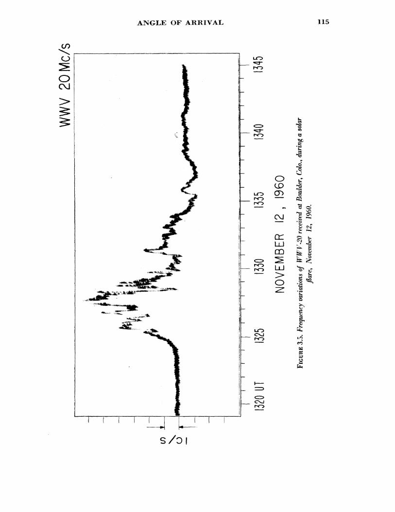
I/) \
WW
V 20
Mc/
s
—I—
i—i—
i—r~
1320 U
T 132
5"T
T'T
'T—
|——
I——
I
1330
1335
NOVE
MBER
12
, I9
60134
0134
5
0 5 $ F
FIGU
RE 3
.5. F
requ
ency
var
iatio
ns o
f W
WV-
2Q re
ceive
d at
Bou
lder
, Colo
., du
ring
a so
lar
flare
, No
vem
ber
12,
1960
.
116 SYNOPTIC STUDIES OF THE IONOSPHERE
azimuthal angle, measured from a line joining the centers of the two antennas.
In practice the antennas are oriented with their centers in the great circle plane passing through the transmitter and receiver so that ^£^0. For accurate measurements it is necessary to correct for the variation of if/.
The musa system for measuring a vertical angle consists of an antenna array having a very sharp lobe which can be steered up and down in the vertical plane. The vertical angle is determined by the position of the lobe at which the received signal is a maximum.
In the third system the antennas may be a pair of identical ones at different heights above ground or one can be a horizontal and the other a vertical. In either case the antenna patterns must be known. One useful application of this method is in normal incidence sounding where dipoles are located at such heights as to give (1) a maximum, (2) a null in the zenith direction. This arrangement enables a determination to be made of whether echoes are returned from overhead or scattered obliquely.
3.2.5. Rockets and Satellites
In recent years it has become possible to explore the ionosphere by sending up radio equipment in rockets and satellites. In particular, elec tron density profiles have been deduced from measurements in rockets of the differential absorption £10^] between ordinary and extraordinary waves. In 1961 an h't recorder was flown in a rocket to study the topside of the F region Qll^] and more recently an ionosonde has been flown in a satellite [[12] to study the same region.
By moving the observing stations to artificial satellites three im portant advantages are gained:
1. Probes can be used to measure some ionospheric parameters in situ, thereby checking previous radio measurements and adding new ones.
2. Radio soundings can be obtained from above the level of maximum density, thereby extending our knowledge greatly.
3. Geographic scanning of these parameters can be achieved to an extent and degree of detail never possible with scattered ground stations.
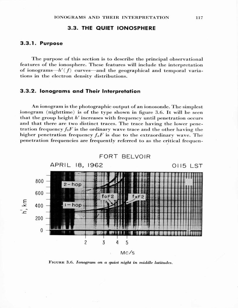
IONOGRAMS AND THEIR INTERPRETATION 117
3.3. THE QUIET IONOSPHERE
3.3.1. Purpose
The purpose of this section is to describe the principal observational features of the ionosphere. These features will include the interpretation of ionograms—h f ( f) curves—and the geographical and temporal varia tions in the electron density distributions.
3.3.2. Ionograms and Their Interpretation
An ionogram is the photographic output of an ionosonde. The simplest ionogram (nighttime) is of the type shown in figure 3.6. It will be seen that the group height h' increases with frequency until penetration occurs and that there are two distinct traces. The trace having the lower pene tration frequency foF is the ordinary wave trace and the other having the higher penetration frequency fxF is due to the extraordinary wave. The penetration frequencies are frequently referred to as the critical frequen-
FORT BELVOIR APRIL 18, 1962 OII5 LST
800
600
2 345
Mc/s
FIGURE 3.6. Ionogram on a quiet night in middle latitudes.
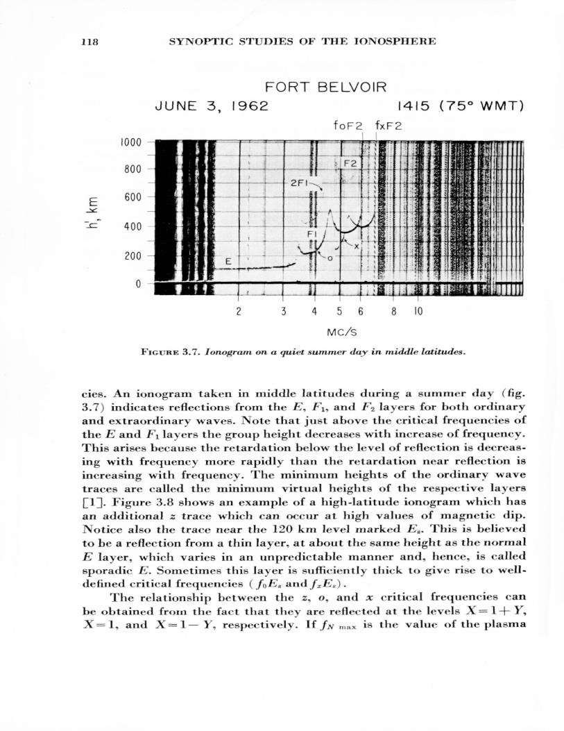
118 SYNOPTIC STUDIES OF THE IONOSPHERE
FORT BELVOIR JUNE 3, 1962 1415 (75° WMT)
foF2 fxF2
456 8 10
FIGURE 3.7, lonogram on a quiet summer day in middle latitudes.
cies. An ionogram taken in middle latitudes during a summer day (fig. 3.7) indicates reflections from the £", /*\, and Fz layers for both ordinary and extraordinary waves. IVote that just above the critical frequencies of the E and F\ layers the group height decreases with increase of frequency. This arises because the retardation below the level of reflection is decreas ing with frequency more rapidly than the retardation near reflection is increasing with frequency. The minimum heights of the ordinary wave traces are called the minimum virtual heights of the respective layers £1]. Figure 3.8 shows an example of a high-latitude ionogram which has an additional z trace which can occur at high values of magnetic dip. Notice also the trace near the 120 km level marked Es . This is believed to be a reflection from a thin layer, at about the same height as the normal E layer, which varies in an unpredictable manner and, hence, is called sporadic E, Sometimes this layer is sufficiently thick to give rise to well- defined critical frequencies (f^Es a.r\<\fx Es ).
The relationship between the z, o, and x critical frequencies can be obtained from the fact that they are reflected at the levels X=l-h Y, X=l, and X=l— 1% respectively. If /W max is the value of the plasma
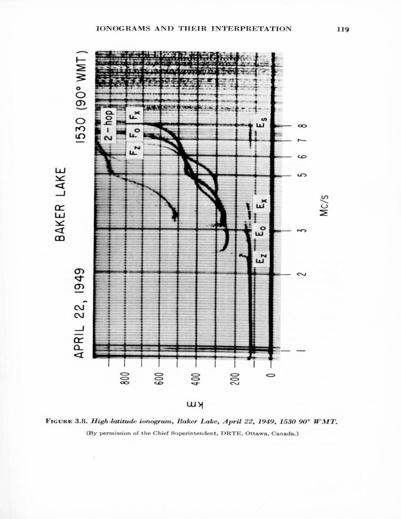
IONOGRAMS AND THEIR INTERPRETATION 119
<rGO
O r
orOm
CD ^f CD
OJ OJ
or o_
CVJ
UU>j
FIGURE 3.8. High-latitutle ionograrn. Baker Lake, April 22, 1949, 153O 9O° WMT.(By permission of the Chief Superintendent, DRTE, Ottawa, Canada.)
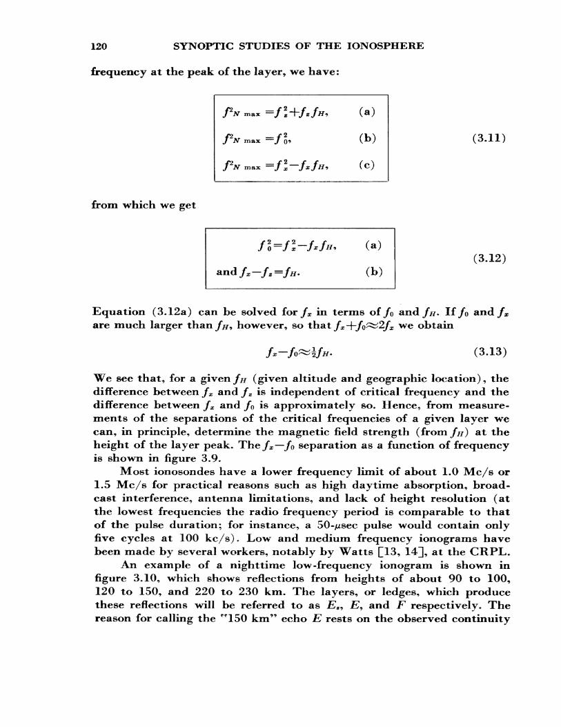
120 SYNOPTIC STUDIES OF THE IONOSPHERE
frequency at the peak of the layer, we have:
J N max —J z
J N max ==7 o
(a)
(b)
(c)
(3.11)
from which we get
and fx —f, =/H.
(a)
( b )(3.12)
Equation (3.12a) can be solved for fx in terms of/o and///. If/o and fx are much larger than///, however, so that/x +/o~2/x we obtain
_ / /-*^i/ /o i q\t —J®'~**-/ ~2j ff m ^O..LOy
We see that, for a given/// (given altitude and geographic location), the difference between fx and fz is independent of critical frequency and the difference between fx and /0 is approximately so. Hence, from measure ments of the separations of the critical frequencies of a given layer we can, in principle, determine the magnetic field strength (from///) at the height of the layer peak. The/x —/o separation as a function of frequency is shown in figure 3.9.
Most ionosondes have a lower frequency limit of about 1.0 Mc/s or 1.5 Mc/s for practical reasons such as high daytime absorption, broad cast interference, antenna limitations, and lack of height resolution (at the lowest frequencies the radio frequency period is comparable to that of the pulse duration; for instance, a 50-/zsec pulse would contain only five cycles at 100 kc/s). Low and medium frequency ionograms have been made by several workers, notably by Watts Q13, 14], at the CRPL.
An example of a nighttime low -frequency ionogram is shown in figure 3.10, which shows reflections from heights of about 90 to 100, 120 to 150, and 220 to 230 km. The layers, or ledges, which produce these reflections will be referred to as E8, JB, and F respectively. The reason for calling the "150 km" echo E rests on the observed continuity
IONOGRAMS AND THEIR INTERPRETATION 121
0-62 O-61 OCO O-50 0-58 0-571 O-56 0-55 O-5-4 0-53 0-52 0-51
1 8
H
FIGURE 3.9. Critical frequency separation bettvecn ordinary and extraordinary traces.
(After J. W. Wright, R. W. Knecht, and K. Davies, 1957, Annals of the IGY, Vol. III. Part I,Pergamon. Press.)
BOULDER,COLORADO
DECEMBER 2, 1959 225O (IO5° WMT)
0-1.0
MC/S
KlGURE 3.10. Loiv-frequency ionogram.
with the daytime E echo over the sunrise period. The E* layer appears to be patchy (transparent) and must be fairly thin because no group retardation is evident at its upper frequency limit. Note that the critical frequency of the extraordinary Z trace is less than that of the ordinary, which is to be expected on the theory given in sec. 2.3.3.2.
lonogranis vary in appearance depending upon the geographic location of the station. A great many more ionograms are available for study in the IGY Atlas of lonogranis C^^D and in the Annals of the IGY [2],
122 SYNOPTIC STUDIES OF THE IONOSPHEHE
g i tn ni ii iiiui] unit S3 Z K 53 s;
FIGURE 3.11 a. Sample f plot for Adak^ Alaska—summer.
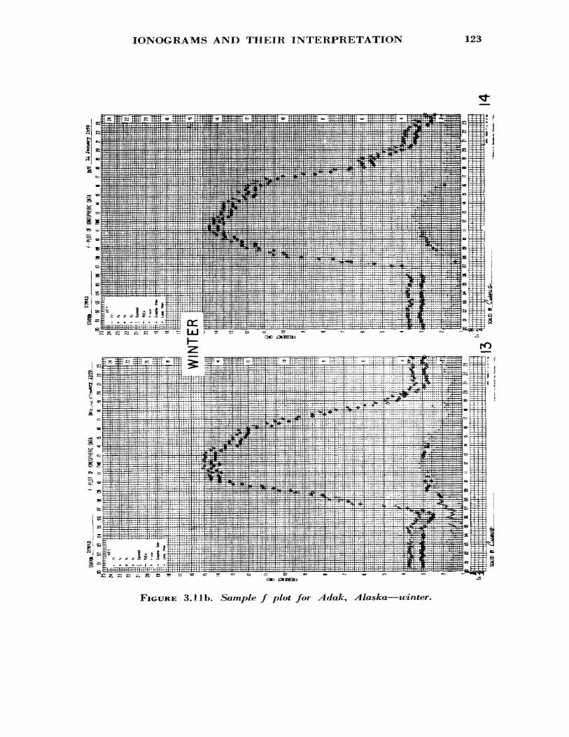
IONOGRAMS AND THEIR INTERPRETATION 123
FIGURE 3.lib. Sample f plot for Adak, Alaska—ivinter.
124 SYNOPTIC STUDIES OF THE IONOSPHERE
Ionospheric data are available, in several different forms, in one of the four World Data Centers. These forms may be the original ionograms or scaled hourly values of the various parameters (e.g., critical frequencies and minimum virtual heights) or simply monthly median values of these parameters as published in the CRPL F Series, Part A Q16]. The latter publication contains monthly medians of ionospheric parameters from about 80 stations in tabular and graphical form. Another form of presenta tion (due to J. H. Meek) is the/ plot. The/ plot is a daily graph of the frequency characteristics of the ionograms as a function of time, using internationally agreed conventions for interstation comparison. It was originally developed to enable the complicated and rapidly changing ionograms from high latitudes to be reduced with the minimum of inter pretation by the scaling individual. It was also introduced to obviate the necessity of repeated plotting from tabulated data. Its use has now be come worldwide. Some sample/ plots are shown in figure 3.11.
3.3*3. Electron Density Profiles
3.3.3.1. Real Height Analysis
Conventional ionograms contain a direct measure of the electron densities of the ionosphere within a range determined by the lowest and highest radio frequencies employed in the sounding. The total retardation depends upon the unknown electron density profile. However, it is not immediately obvious how the actual height of reflection of each frequency is to be determined, for the reason that the apparent (virtual) height depends in an involved way on the group retardation imposed on the probing pulses at each point below the level of reflection.
The group height h f is given by the integral of the group refractive index y! along the ray path. In the case of vertical propagation this is given by
/ hr f^r JJi v. f dh=\ p' — d^ (3.14) 0 J 0 <*<f>
where hr is the real height of reflection and <f> is an arbitrary monotonic function of the electron density distribution; for instance, in Budden's method £17] <t> is/v, whereas in King's method Q18] </> is log /AT. It is not possible to solve this integral analytically, except under certain limiting conditions (transverse and longitudinal). However, a solution can be
ELECTRON DENSITY PROFILES 125
found by dividing the range of integration into n small intervals within each of which dh/d$> is assumed constant. Equation (3.14) can then be replaced by
ffh\ r*™~) f »'d*. (3.15)d<Z>/ m J -
Since the integrals are now dependent on // and <£ and the interval width, they may be evaluated once and for all as a set of coefficients. Equation (3.15) then represents a set of linear equations in dh/d<f>. By dividing the observed h'f curve into intervals of equal ranges of <£, this system of equations can, in principle, be solved and the real height intervals obtained.
In the above theory, it was assumed that 0 increased monotonically with height. It does not give us any information about a ^valley" which may exist in the profile between the E and F layers, say. Some information on the existence of a valley can be inferred from the extraordinary wave trace []19 , 20]* Another limitation on the experimental data is that con ventional ionograms give no information on frequencies below about 1.0 Mc/s. Once again the extraordinary trace can sometimes be used to give information concerning unobserved ionization Q19, 21 ]. A good re vie w of this subject has been made by Thomas Q22].
3.3.3.2. Diurnal Variations
Sample day and night N(h) profiles for middle latitudes are shown in figures 3.12a and b respectively. Large diurnal changes occur particu larly in the lower ionosphere. The daytime structure may be thought of as a single bank of electrons beginning around 100 km and having a peak density around 300 km. The various lower fflayers" E and FI may be only inflections, or ledges, in the electron distribution.
At night, all vestige of the FI layer disappears and the E-layer densities drop by a factor of 100 or so, thus producing a simpler structure. The electron density in the D region is not directly observable by the conventional ionosonde and probably falls from about 103 per cm3 at 80 km at noon to less than 102 per cm3 at night. Some tentative 7V(/i) profiles (obtained from cross modulation experiments) for the D region are shown in figure 3.13.
Additional features of the diurnal variation in ionospheric structure are illustrated in figure 3*14. Note that the E layer appears promptly at
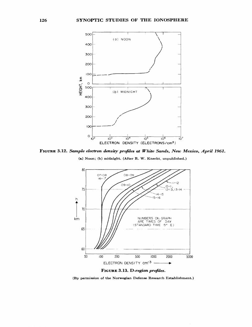
126 SYNOPTIC STUDIES OF THE IONOSPHERE
5OO
4OO
300
2OO
IOO
O 500
4OO
3OO
2OO
IOO
(a) NOON
(b) MIDNIGHT \
_)O^ IO3 IO4 IO5 IO€ !O r
ELECTRON DENSITY (ELECTRONS/cm3 )
FIGURE 3.12, Sample electron density profiles at White Sands, New Mexico, April 1961.
(a) Noon; (b) midnight. (After R. W. Knecht, unpublished.)
(STANDARD TIME 15° E)
100 200 500 1000
ELECTRON DENSITY Cm"3 —
2000 5000
FIGURE 3.13. D -region profiles.
(By permission of the Norwegian Defense Research Establishment.)
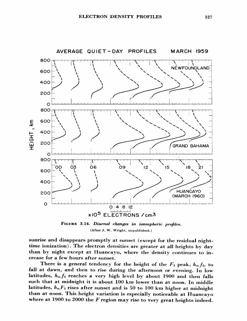
ELECTRON DENSITY PROFILES 127
AVERAGE QUIET-DAY PROFILES MARCH 1959
80O r—jn——i—!———j
NEWFOUNDLAND \
GRAND BAHAMAr. . . . . i . , . .
HUANCAYO (MARCH I960)
O 4 8 12
xlO 5 ELECTRONS /cm3
FICURE 3.14, Diurnal changes in ionospheric profiles.(After J. W. Wright, unpublished.)
sunrise and disappears promptly at sunset (except for the residual night- time ionization). The electron densities are greater at all heights by day than by night except at Huancayo, where the density continues to in crease for a few hours after sunset.
There is a general tendency for the height of the F% peak, fcm /2 , to fall at dawn, and then to rise during the afternoon or evening. In low latitudes, fcm/2 reaches a very high level by about 1900 and then falls such that at midnight it is about 100 km lower than at noon. In middle latitudes, hmFz rises after sunset and is 50 to 100 km higher at midnight than at noon. This height variation is especially noticeable at Huancayo where at 1900 to 2000 the .F region may rise to very great heights indeed.
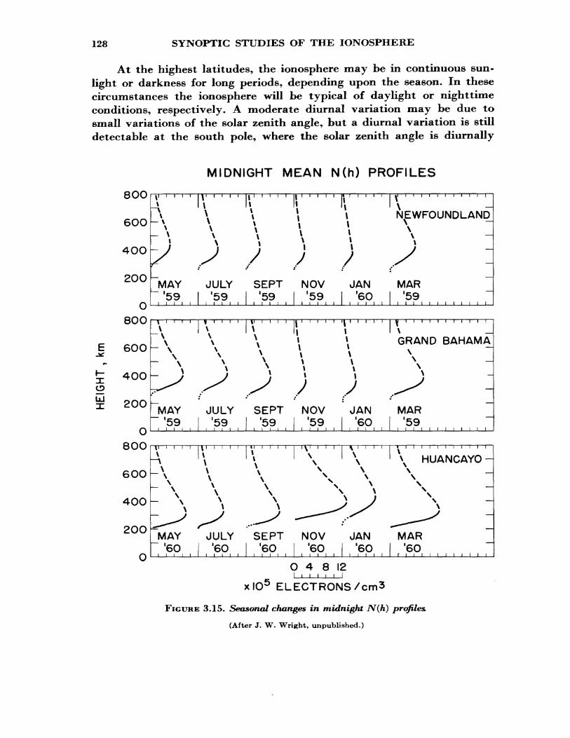
128 SYNOPTIC STUDIES OF THE IONOSPHERE
At the highest latitudes, the ionosphere may be in continuous sun light or darkness for long periods, depending upon the season. In these circumstances the ionosphere will be typical of daylight or nighttime conditions, respectively. A moderate diurnal variation may be due to small variations of the solar zenith angle, but a diurnal variation is still detectable at the south pole, where the solar zenith angle is diurnally
MIDNIGHT MEAN N(h) PROFILES
LUX
O\J\J
GOO
4OO
2OO
O8OO
600
400
2OO
O8OO
6OO
4OO
200
n
v i . , > v , , , , ,,,.,, | i . i i i .. , , ,4 » \ I '\-\ \ \ \ -\ \ \ \ \~S S / ) /
MAY JULY SEPT NOV JAN'59 '59 '59 '59 '6C
1 I I l i 1 t i i i l i i i i f i i i i ill
'' V '•' '•'•'•''
NEWFOUNDLAND^\ \ — t
y _
MAR) '5911 1 1 1 1 1 1 i 1 [ 1 1 L
^iiii i i i i i |i i i t J i i i i i i it i i i
v \ \ ', •~\ \ \ » » A \ \ \: \ \ \ \^^ ^ ,^ j j
El V l l l l l l [ I l l (
\ __
GRAND BAHAMA\ \ _ \\
^^
"MAY JULY SEPT NOV JAN MAR'59 '59 '59 '59 '6C
I 1 1 1 1 1 1 1 1 1 I ! 1 1 1 1 ! 1 1 i III
1 1 i I 1 1 | 1 1 1 1 f 1 1 1 1 ! 1 1 TT1 1 T ] \ 1 1
A \ \ \ \^\ ^ \ \ \
> '59II 1 1 1 1 1 ! J 1 ! 1 1 1
1 1 1 1 1 1 1 1 1 1 1 1 1 !
\ HUANCAYO -\ _
- \ \ \ \ \ \ -* V \ V \ ^\ \ \ XN - V
— * \ \ »
_ \ J ^) ^^ ' ̂
"MAY JULY SEPT NOV JAN'6O '60 '6O '6O '6C
/j
MAR) '6O
O 4 8 12I I I I I I I
xlO5 ELECTRONS/cm3
FIGURE 3.15. Seasoned changes in midnight N(h) profiles,
(After J. W. Wright, unpublished.)
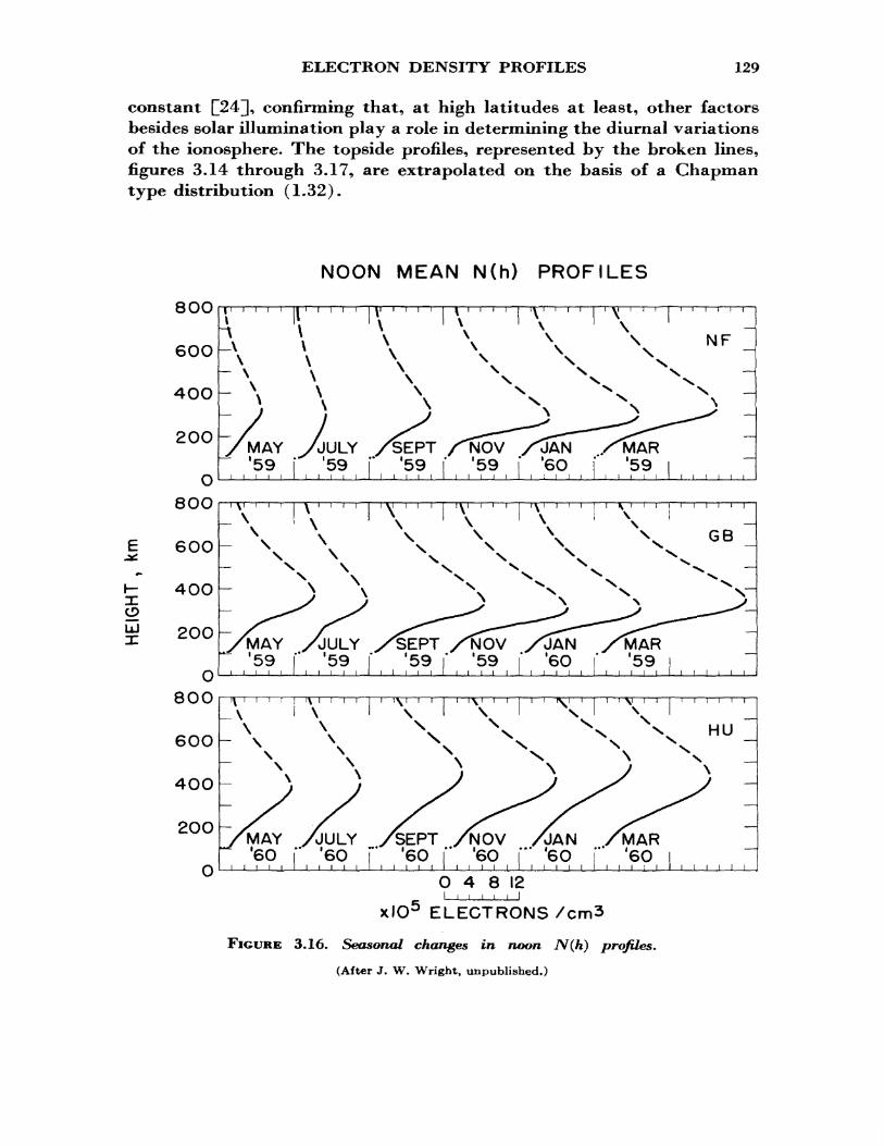
ELECTRON DENSITY PROFILES 129
constant C243i confirming that, at high latitudes at least, other factors besides solar illumination play a role in determining the diurnal variations of the ionosphere. The topside profiles, represented by the broken lines, figures 3.14 through 3.17, are extrapolated on the basis of a Chapman type distribution (1.32).
NOON MEAN N(h) PROFILES
LJX
8OO
60O
4OO
ZOO
A _\
\ — \
1 ' V ' ' ' ' V ' ' ' ' '\
MAY /JULY /SEPT /^MOV /JAN /MAR '59 ' '59 i" '59 I '59 ' '6O I '59
1 i I i I I i 1
JULY /SEPT'59 ' '59
O 4 8 12i i i i i i ixlO5 ELECTRONS /cm3
FIGURE 3.16. Seasonal changes in noon N(h) profiles.(After J. W. Wright, unpublished.)
130 SYNOPTIC STUDIES OF THE IONOSPHERE
3.3.3.3. Seasonal Variations
The seasonal variation in N(h) profiles is illustrated in figures 3.15 and 3.16 for midnight and noon conditions respectively. The nighttime F layer tends to be at higher heights in summer than in winter, the tendency being accentuated in lower latitudes. The nighttime F layer tends to be thicker when higher. In general, the maximum electron density and the total electron content of the nighttime F region are greater in summer than in winter. Turning to the noon profiles, the most distinctive feature is that the peak density is considerably larger in winter than in summer; this is called the seasonal anomaly. It is more evident at high latitudes than at low latitudes. In the summer months, in middle latitudes, the F layer bifurcates into the FI and F% layers. Under these conditions the F% peak density is fairly small and is located at a relatively great altitude. The FI layer is not so much a distinct layer but rather a minor inflection in the profile at about 200 to 220 km.
3.3.3.4. Solar Cycle Variations
In sec. 1.7.3 we discussed the long-term variation in sunspot activity. This variation has a profound effect on the noon electron distribution, as can be seen from figure 3.17. The graphs are arranged to show increments in ionization corresponding to increments of 100 in sunspot number. The electron densities above the peak are extrapolated. A striking feature of this variation is that the most significant increases in electron density occur at successively higher heights.
3.3.3.5. Geographical Variation
The expense of reducing all ionograms to N(h) profiles has meant that the worldwide distribution is not yet available. Some idea of the latitudinal variations can be obtained from the iso-ionic contours obtained at CRPL £24], examples of which are shown in figure 3.18. Profile data taken near the 75° west geographic meridian were used and the iso-ionic contours are for fixed values of plasma frequency. The height of the F^ maximum is shown by a dotted line. The following features are important:
(1) The F layer is much thicker near the magnetic equator than elsewhere.
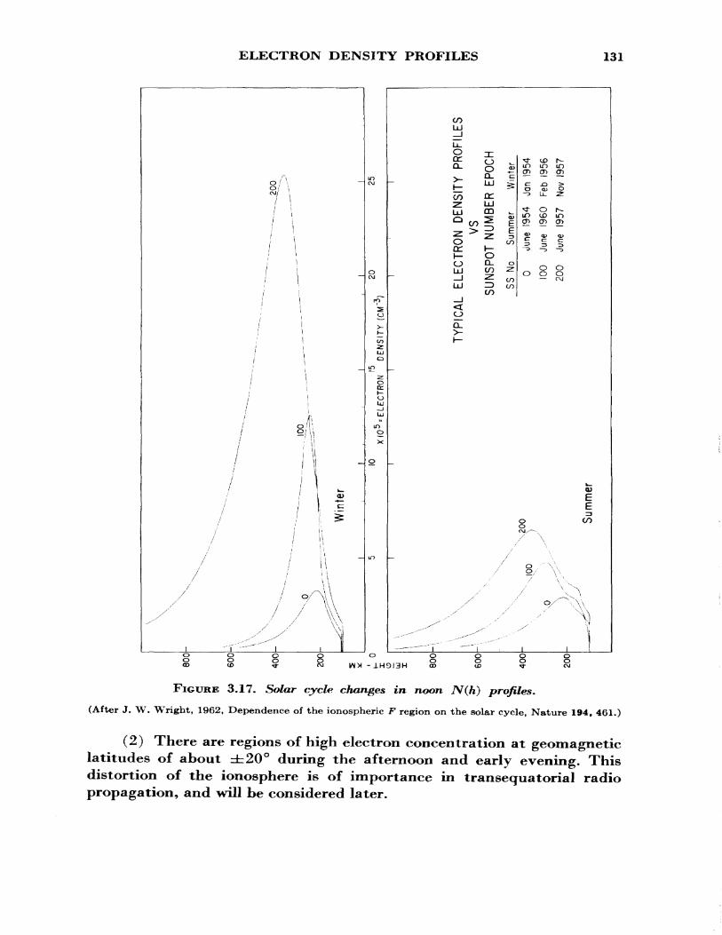
ELECTRON DENSITY PROFILES 131
o /q/ \
11
CO
o
LU
LU
O O.
^0 » Q. "c
co rcii i 00
oQ_ o CO ^
CO
a? h-LD IDCT> CTi
o r-o> mcr> 0s*
0 0000— rvJ
8
vE^
CO
o CD
t" i8
-1H9J3H
FIGURE 3.17. Solar cycle changes in noon N(h) profiles.
(After J. W. Wright, 1962, Dependence of the ionospheric F region on the solar cycle, Nature 194, 461.)
(2) There are regions of high electron concentration at geomagnetic latitudes of about ±20° during the afternoon and early evening. This distortion of the ionosphere is of importance in transequatorial radio propagation, and will be considered later.
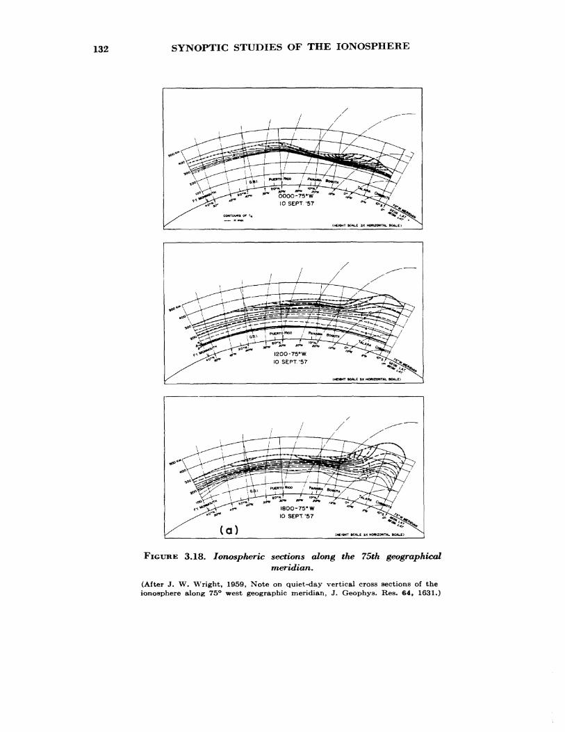
132 SYNOPTIC STUDIES OF THE IONOSPHERE
(HEFOHT SCALE 3X H04WZONTAL SCALE}
FIGURE 3.18. Ionospheric sections along the 75th geographicalmeridian.
(After J. W. Wright, 1959, Note on quiet-day vertical cross sections of the ionosphere along 75° west geographic meridian, J. Geophys. Res. 64, 1631.)
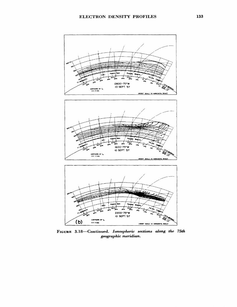
ELECTRON DENSITY PROFILES 133
FIGURE 3.18—Continued. Ionospheric sections along the 75thgeographic meridian.
134 SYNOPTIC STUDIES OF THE IONOSPHERE
3.3.4. Model Layers
For many purposes, particularly computational purposes, it is con venient to approximate the N(h) profile by analytical expressions which are amenable to integration, differentiation, etc. Various models can be used as approximations to the Chapman layer; for instance, near the peak the distribution is approximately parabolic, whereas high up in the layer the distribution is roughly exponential. Over short ranges of height it is often sufficiently accurate to assume a linear variation of TV with fc* Some relevant formulas derived from certain models are given below.
3.3.4.1. Chapman Layer
From (1.32) we have
A^= TVo exp ^ {1 — z— sec x exp (— z) } .
The total non-deviative absorption suffered by a wave of angular frequency o> in one complete vertical transit through the layer (in which o>2>>>*>2 ) is given by
L= J Kds= ° "°\/27rexp (l)-r——T^ - (3.16)
Here TVo is the electron concentration at the level of maximum electron production when x == 0 (i-e., at s=0), VQ is the collision frequency at the same height, and H is the constant scale height. It is assumed that the propagation conditions are quasi-longitudinal, toz, being the gyrofrequency corresponding to the component of the earth's magnetic field in the direc tion of phase propagation.
3.3.4.2. Parabolic Layer
When x and z are very small (1.32) reduces to
(3.17)
which is the equation of a parabola with semithickness (i.e., distance
MODEL LAYERS 135
from base to level of maximum density) of ym = 2H:
This can be written in terms of plasma frequency:
where /p is the penetration frequency of the layer.In the absence of an imposed magnetic field, the refractive index
within the layer is given by
The group height for reflection within the layer is given by
h>= f „' dh = h«-yrn + \yj- ln^±£ , (3.21) J JP Jp~J
and the phase height for the same conditions is
hp = f M dh = h0 -lym -lym(^ - £\ ln-^±f . (3 .22)J \J JP/ JP —— /
Note that h f = ho for a frequency 0.834 /p. This shows that the height of the maximum electron density is equal to the group height on a frequency of 0.834 /„.
For transmission through a layer, the contributions to the group and phase heights are
m , JP J~Jp
* fp\ 1 f*f*>
^- 7) 7^,'
136 SYNOPTIC STUDIES OF THE IONOSPHERE
3.3.4.3. Linear Layer
If TV increases linearly with height h from a base at 7*o above ground, since TV is proportional tof^ we have
f* = a(h-h0), (3.25)
where a is the constant height gradient of /£. The virtual and phase heights are given by
/»' = feo+-/2 (3.26) a
(3.27)
3.3.4.4. Exponential Layer
The equation for this layer can be written:
(az) (3.28)
where z= (h — h&) /H and F is the plasma frequency at the level HR. Note that, for propagation in the medium, the wave frequency must be greater than F. The group and phase heights are given by
and
2 F(3.30)
3.3*5. Critical Frequency Variations
3.3.5.1. General Features
For many purposes, including radio communication, the most im portant characteristics of the ionospheric layers are their critical fre-
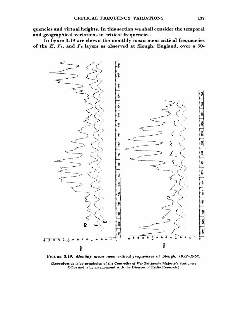
CRITICAL FREQUENCY VARIATIONS 137
quencies and virtual heights. In this section we shall consider the temporal and geographical variations in critical frequencies.
In figure 3.19 are shown the monthly mean noon critical frequencies of the E9 Fi9 and F% layers as observed at Slough, England, over a 30-
_I UJ
o
FIGURE 3.19. Monthly mean noon critical frequencies at Slough, 1932-1962.
(Reproduction is by permission of the Controller of Her Brittannic Majesty's Stationery Office and is by arrangement with the Director of Radio Research.)
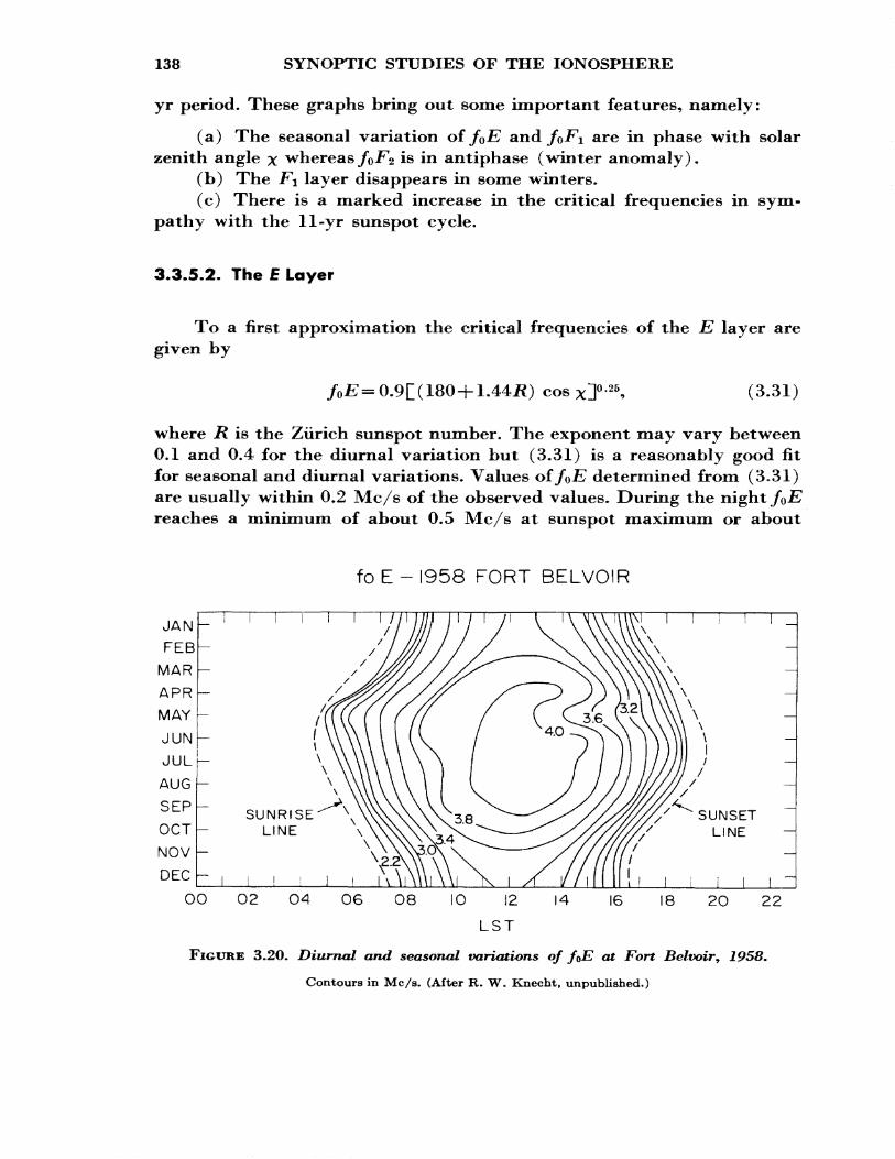
138 SYNOPTIC STUDIES OF THE IONOSPHERE
yr period. These graphs bring out some important features, namely:
(a) The seasonal variation of fQE and /o^i are in phase \vith solar zenith angle x whereas/o-Fs is in antiphase (winter anomaly).
(b) The FI layer disappears in some winters*(c) There is a marked increase in the critical frequencies in sym
pathy with the 11-yr sunspot cycle.
3*3.5.2. The £ Layer
To a first approximation the critical frequencies of the E layer are given by
= 0.9[( 180+ 1.447?) cos x]°-25, (3.31)
where R is the Zurich sunspot number. The exponent may vary between 0.1 and 0.4 for the diurnal variation but (3.31) is a reasonably good fit for seasonal and diurnal variations. Values of/oJS determined from (3.31) are usually within 0.2 Mc/s of the observed values. During the night fQE reaches a minimum of about 0.5 Mc/s at sunspot maximum or about
foE-1958 FORT BELVOIR
JANFEB
MAR
APR
MAY
JUN
JUL AUG -
SEP -
OCT -
NOV -
DEC
SUNRISE LINE
SUNSET LINE
OO 02 O4 06 O8 IO 12 14 16 18 20 22LST
FIGURE 3.20. Diurnal and seasonal variations of f$E at Fort Belvoir^ 1958.
Contours in Mc/s. (After R. W. Knecht, unpublished.)
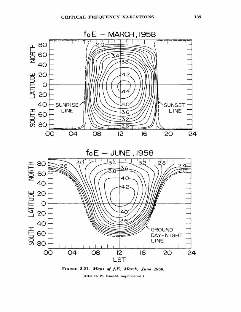
SOUTH
LATI
TUDE
NO
RTH
SOUTH
LATI
TUDE
NORTH
00
0)
-&o
o o
ro o o
no
^
O
Ooo o
oo o>
-P^ ro
oooo
no -^
0) oo
o o
o o
o
a n O i Co NO
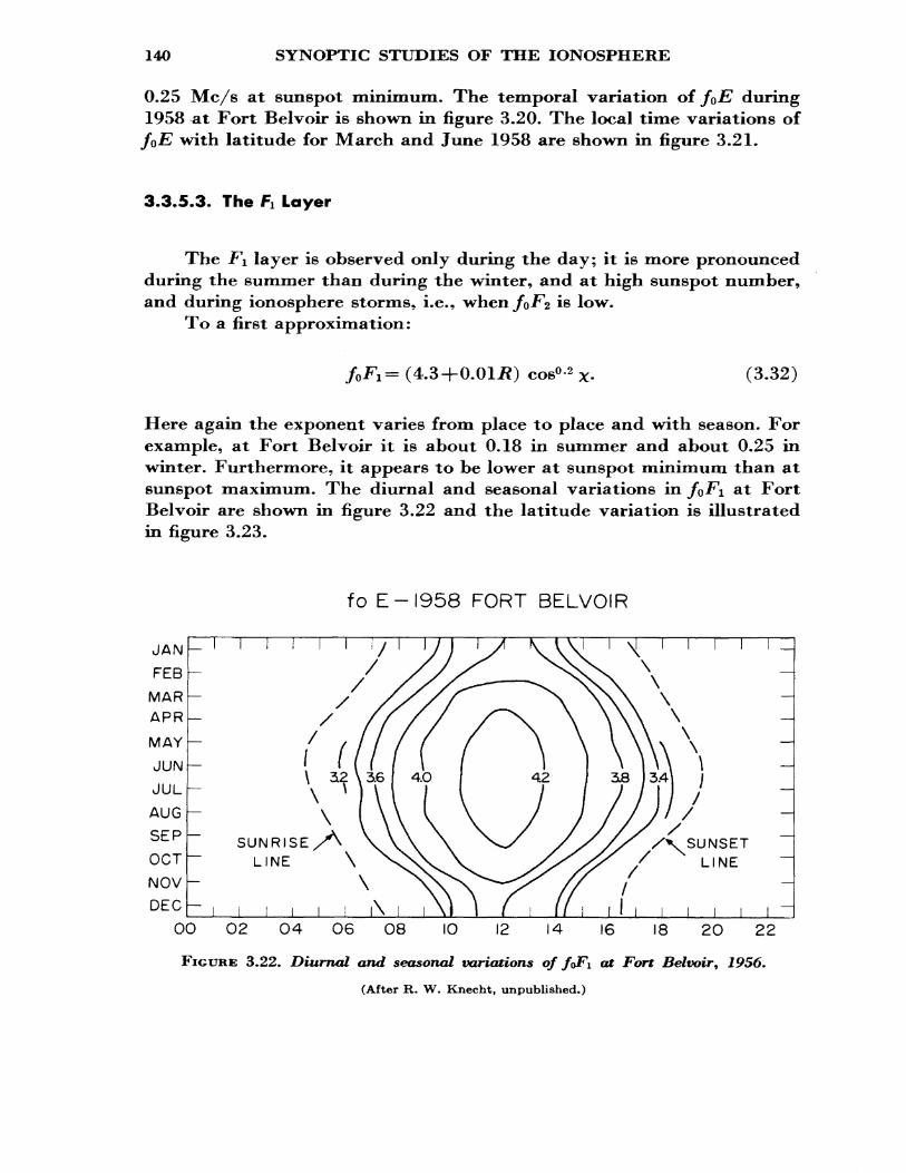
140 SYNOPTIC STUDIES OF THE IONOSPHERE
0.25 Mc/s at sunspot minimum. The temporal variation of f$E during 1958 at Fort Belvoir is shown in figure 3.20. The local time variations of foE with latitude for March and June 1958 are shown in figure 3.21.
3.3.5.3. The FI Layer
The -Fi layer is observed only during the day; it is more pronounced during the summer than during the winter, and at high sunspot number, and during ionosphere storms, i.e., when /o^2 is low.
To a first approximation:
r1= (4.3+0.01/J) cos0 - 2 X - (3.32)
Here again the exponent varies from place to place and with season. For example, at Fort Belvoir it is about 0.18 in summer and about 0.25 in winter. Furthermore, it appears to be lower at sunspot minimum than at sunspot maximum. The diurnal and seasonal variations in f<>Fi at Fort Belvoir are shown in figure 3.22 and the latitude variation is illustrated in figure 3.23.
fo E-1958 FORT BELVOIR
JAN
FEB
MAR APR
MAY
JUN
JUL
AUG
SEP
OCT
NOV
DEC
i r_
00 O2 O4 O6 08 10 12 14 16 18 20 22
FIGURE 3.22. Diurnal and seasonal variations of foFi at Fort Belvoir , 1956.
(After R. W. Knecht, unpublished.)
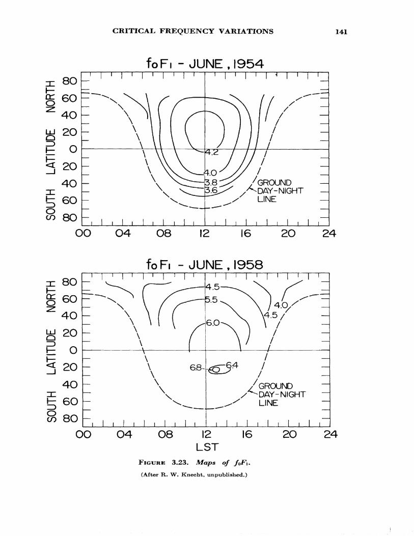
SOUT
H LA
TITU
DE
NORT
HSO
UTH
LATIT
UDE
NORT
H
ff e
^ »
td w
§ •g
"0 I «*,
CD I fc
O
,71
00
0)
-P>o
o o
ro ro
-^ o
oo
o8
8ro
-^ 0)
00 ooooo
ft W $ a o 2 en
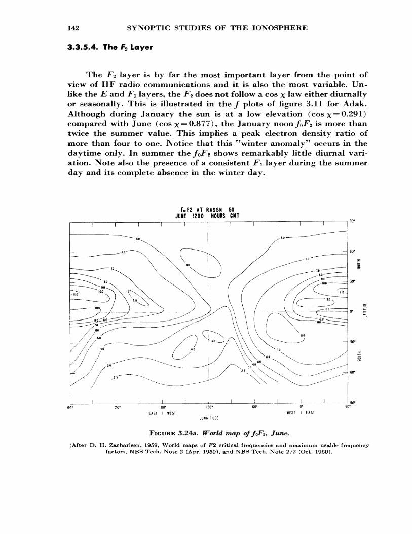
142 SYNOPTIC STUDIES OF THE IONOSPHERE
3.3*5.4. The F2 Layer
The F2 layer is by far the most important layer from the point of view of HF radio communications and it is also the most variable. Un like the E and Fl layers, the F2 does not follow a cos x law either diurnally or seasonally. This is illustrated in the / plots of figure 3.11 for Adak. Although during January the sun is at a low elevation (cos x = 0.291) compared with June (cos x = 0.877), the January noon/0F2 is more than twice the summer value. This implies a peak electron density ratio of more than four to one. Notice that this "winter anomaly" occurs in the daytime only. In summer the/0F2 shows remarkably little diurnal vari ation. Note also the presence of a consistent FI layer during the summer day and its complete absence in the winter day.
foF2 AT RASSN 50 JUNE 1200 HOURS GMT
60"
WEST i EAST
FIGURE 3.24a. World map o//0F2, June.
(After D. H. Zacharisen, 1959, World maps of F2 critical frequencies and maximum usable frequency factors, NBS Tech. Note 2 (Apr. 1959), and NBS Tech. Note 2/2 (Oct. 1960).
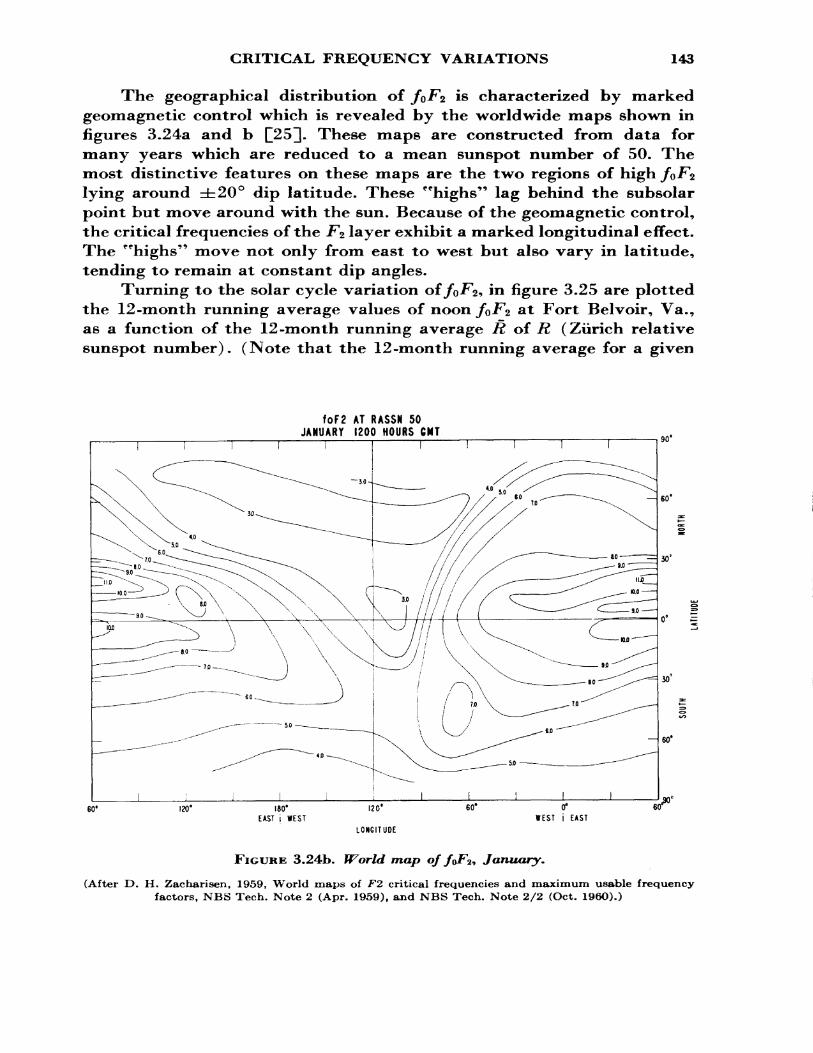
CRITICAL FREQUENCY VARIATIONS 143
The geographical distribution of fQ F2 is characterized by marked geomagnetic control which is revealed by the worldwide maps shown in figures 3.24a and b C25]. These maps are constructed from data for many years which are reduced to a mean sunspot number of 50. The most distinctive features on these maps are the two regions of high foF^ lying around ±20° dip latitude. These "highs" lag behind the subsolar point but move around with the sun. Because of the geomagnetic control, the critical frequencies of the F2 layer exhibit a marked longitudinal effect. The "highs" move not only from east to west but also vary in latitude, tending to remain at constant dip angles.
Turning to the solar cycle variation of/0F2, in figure 3.25 are plotted the 12-month running average values of noon foFz at Fort Belvoir, Va., as a function of the 12-month running average R of R (Zurich relative sunspot number). (Note that the 12-month running average for a given
foF2 AT RASSN 50 JANUARY 1200 HOURS GMT
»EST i EAST
FIGURE 3,24b. World map of /oF2, January.
(After D. H. Zacharisen, 1959, World maps of F2 critical frequencies and maximum usable frequency factors, NBS Tech. Note 2 (Apr. 1959), and NBS Tech, Note 2/2 (Oct. I960).)
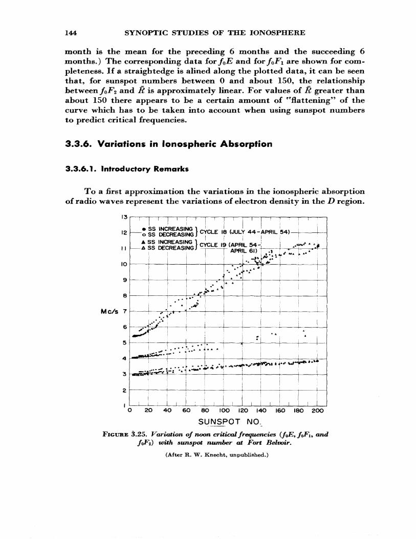
144 SYNOPTIC STUDIES OF THE IONOSPHERE
month is the mean for the preceding 6 months and the succeeding 6 months.) The corresponding data forfQE and forfQFi are shown for com pleteness. If a straightedge is alined along the plotted data, it can be seen that, for sunspot numbers between 0 and about 150, the relationship between/o/^ and R is approximately linear. For values of R greater than about 150 there appears to be a certain amount of ^flattening" of the curve which has to be taken into account when using sunspot numbers to predict critical frequencies.
3.3.6. Variations in Ionospheric Absorption
3.3.6.1. Introductory Remarks
To a first approximation the variations in the ionospheric absorption of radio waves represent the variations of electron density in the D region.
12
II
10
Mc/s 7
i I i
CYCLE 18 (JULY 44-APRIL• SS INCREASING ~oSS DECREASINGA SS INCREASING 1 CYC, E |9 (ApR, „ jA ss DECREASING) CYCLE l9 CAPRIL M
i
APRIL
"
i2O 4O 6O 80 IOO I2O I4O I6O ISO ZOO
SUNSPOT NCXFICURE 3.25. Variation of noon critical frequencies (f<J£9 foFi* and
tvith sunspot number at Fort Belvoir.
(After R. W. Knecht, unpubKshed.)
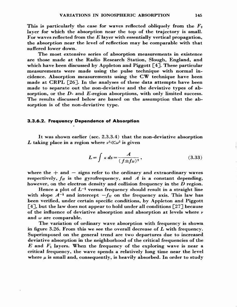
VARIATIONS IN IONOSPHERIC ABSORPTION 145
This is particularly the case for waves reflected obliquely from the F% layer for which the absorption near the top of the trajectory is small. For waves reflected from the E layer with essentially vertical propagation, the absorption near the level of reflection may be comparable with that suffered lower down.
The most extensive series of absorption measurements in existence are those made at the Radio Research Station, Slough, England, and which have been discussed by Appleton and Piggott Q4], These particular measurements were made using the pulse technique with normal in cidence. Absorption measurements using the CW technique have been made at GRPL £26]. In the analyses of these data attempts have been made to separate out the non-deviative and the deviative types of ab sorption, or the D- and jE-region absorptions, with only limited success. The results discussed below are based on the assumption that the ab sorption is of the non-deviative type.
3.3.6.2. Frequency Dependence of Absorption
It was shown earlier (sec. 2.3.3.4) that the non-deviative absorption L taking place in a region where *> 2<5Coo2 is given
f = I K ds = (3.33)
where the + and — signs refer to the ordinary and extraordinary waves respectively, fn is the gyrofrequency, and A is a constant depending, however, on the electron density and collision frequency in the D region.
Hence a plot of jL~* versus frequency should result in a straight line with slope A~~^ and intercept —/// on the frequency axis. This law has been verified, under certain specific conditions, by Appleton and Piggott £43, but the law does not appear to hold under all conditions £27] because of the influence of deviative absorption and absorption at levels where v and w are comparable.
The variation of ordinary wave absorption with frequency is shown in figure 3.26. From this we see the overall decrease of L with frequency. Superimposed on the general trend are two departures due to increased deviative absorption in the neighborhood of the critical frequencies of the E and FI layers. When the frequency of the exploring wave is near a critical frequency, the wave spends a relatively long time near the level where p, is small and, consequently, is heavily absorbed. In order to study
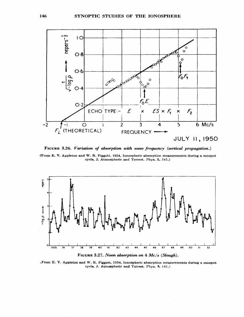
146 SYNOPTIC STUDIES OF THE IONOSPHERE
234FREQUENCY
6 Mc/s-2 f-l OFL (THEORETICAL)
JULY ||, 1950
FIGURE 3.26. Variation of absorption with wave frequency (vertical propagation.)
(From E. V. Appleton and W. R. Piggott, 1954, Ionospheric absorption measurements during a sunspotcycle, J. Atmospheric and Terrest. Phys. 5, 141.)
1935 3*> 37 3$ 39 4O 41 42 43 44 45 46 47 48 49 SO 51 52
FIGURE 3.27. Noon absorption on 4 Mc/s (Slough).
vFrom E. V. Appleton and W. R. Piggott, 1954, Ionospheric absorption measurements during a sunspotcycle, J. Atmospheric and Terrest. Phys. 5, 141.)
VARIATIONS IN IONOSPHERIC ABSORPTION 147
the D-region absorption, it is necessary first to remove from the total absorption that due to the upper layers. To a first approximation this can be done by taking a parabolic model of electron density as the E layer and an exponential height variation of collision frequency £28^- The total ordinary wave absorption is expressed in the form
(3'34)
where 0 represents some function of the ratio (foE/f), and //, is the longitudinal gyrofrequency.
The quantity A is the Z>-region absorption on an ''effective" fre quency /+/£. With oblique propagation the refractive index never falls to near zero (SnelFs law) and the last term in 3.34 is then generally small.
3*3.6*3. Solar Cycle Control
The ionospheric absorption, on 4 Mc/s, measured at Slough over the period 1935 to 1952 (fig. 3.27) exhibits a marked 11-yr solar cycle varia tion. The values plotted in figure 3.27 indicate a factor of about 2 between sunspot minimum and maximum. The dependence of absorption on sun- spot number is roughly linear, that is, of the form
L = a(\+bR). (3.35)
Although the value of b appears to vary from one location to another, the best experimental value seems to be about 0.004.
3.3.6.4. Diurnal Variations
For transmission through a Chapman-type layer which is situated at a level of low pressure, so that v* is very much less than (coico/,) 2, the dependence of absorption L on solar zenith angle x *s given by
L=Ccos3 '2 x , (3.36)
where C depends on the wave frequency, the peak electron density, and the collision frequency (see (3.16)).
Although (3.36) has been verified by Best and Ratcliffe £29] in
148 SYNOPTIC STUDIES OF THE IONOSPHERE
middle latitudes, a much better fit to the experimental data is given by
L= Ccosn (3.37)
where C depends on season, magnetic disturbance, etc., and where in middle latitudes the exponent n lies between 0.7 and 1.0. For large values of x(>80° say) the cosine function should be replaced by the inverse of the Chapman function Ch(x^ x)—see (1.42)—but for most practical purposes this is unimportant. From (3.37) we have
log L = log C+n log cos x- (3.38)
The slope and intercept of this line give the values of n and log C respectively.
In table 3.1 are listed some mean values of n for various locations. It will be seen that n falls sharply in high latitudes. While there is some evidence for a decrease in n in low latitudes, this cannot be considered conclusive.
Although (3.37) holds reasonably well around midday, it often breaks down near sunrise and sunset and so an alternative expression was developed at the CRPL, namely,
L = A+B cos x* (3.39)
which represents the diurnal variation somewhat more closely than (3.37) . Some theoretical justification for including the term A is provided by photodetachment processes (see fig. 1.4, z = 4). At first sight it might
TABL.E 3.1, Solar control of ionospheric absorption L = C cosnx
Location
Ibadan (Nigeria)Ah me dab ad (India)Delhi (India)Sydney (Australia) Tokyo (Japan) Washington, D.C. (U.S.A.)Genoa (Italy)Freiburg (Germany) Slough (England)Prince Rupert (Canada)Churchill (Canada)Baker Lake (Canada)Resolute Bay (Canada)
Geographic latitude0
72328
-34 35 394548 5254596475
n
0.630.730.620.83 0.87 0.830.970.63 0.750.500.270.180.07
VARIATIONS IN IONOSPHERIC ABSORPTION 149
60
50
40
~ 30 - 30
20
10
L = 43 COS*3* L- 21 + 24 COSX
CHURCHILL JUNE 1958
000
— L- 40 COS* 1 *-- L-50-M5 COSX
BAKER LAKE JULY 1957
06 24 00
90° WMT
06 12 18 24
FIGURE 3.28. Comparison between observed absorption and the formulasL=A-\-B coax*
cosnx and
appear that (3.37) and (3.39) would give very different variations but, as illustrated in figure 3.28, the differences are, generally, smaller than the scatter in the data. The sensitivity to solar control is determined by the value of B which falls off in high latitudes H30]. The empirical factor K used at the CRPL is
K = 0.142 +0.858 cos (3.40)
To get the total absorption, K has to be multiplied by other factors representing the seasonal, sunspot, and geometrical (path) variations.
3.3.6.5. Seasonal Variations
If monthly mean noon values of L are plotted against cos x ** is found that whereas the summer (and equinox) values tend to obey a linear law, the winter months exhibit unexpectedly high absorption, which is known as the "winter anomaly." The increased absorption does not occur uniformly over all days, but appears in the form of high ab sorption on certain groups of days. It appears primarily to be a middle latitude effect since it vanishes in polar regions where, in winter, the D region is in prolonged periods of darkness £30]]. From a comparison between Europe and America, or America and Western Russia, Thomas
150 SYNOPTIC STUDIES OF THE IONOSPHERE
has shown that days of enhanced anomalous absorption in one sector correspond to days of reduced anomalous absorption in the other. Days of anomalous absorption are also associated with reflections from the D region Q32]]. Fortunately, the winter anomaly is not a serious factor from the point of view of radio communications because the critical frequencies of the FZ layer are also higher in winter than in summer, so that higher frequencies can be used. The decrease of absorption due to the use of the higher frequency more than compensates for the higher absorption on a fixed frequency so that, in general, radio communications are better on winter days than on summer days.
3.3.7. Sporadic E
In addition to the regular layers of the ionosphere there are several of transient or irregular nature. The most important of these is the Bporadic-E layer, often designated as E8 . Some examples of sporadic-^ reflections on standard ionograms are shown in figure 3.29. It will be seen that the maximum frequency returned from the layer can be much greater than that from the normal E layer and, indeed, from any of the normal layers. Sometimes the Es traces show retardation near the maxi mum frequency, indicating a relatively thick layer with a well-defined maximum of electron density. Under other conditions the echoes exhibit no retardation, suggesting that the layer is extremely thin or else due to a sharp change in electron density gradient. On some occasions the Es layer is opaque and blankets the upper layers; on other occasions the upper layers can be seen through the E99 which suggests that the Es is patchy and that the radio waves are penetrating through the gaps. Sometimes magneto-ionic splitting is evident; at other times there is none.
Sporadic-£ echoes can occur over a range of heights from about 90 to 120 km or more, and evidence has been advanced by Helliwell for pre ferred heights []33]. There is some evidence also for believing that one type of Es is due to ionization by meteors. It is almost certain that several different physical phenomena are lumped together under the general heading of sporadic E. For the scaling of Es characteristics see reference
Because of its variable nature, sporadic E has been studied largely by statistical means Q34[], usually by computing the fraction of time that the maximum frequency fE* exceeds some reference value. Some results obtained in this way are shown in figure 3.30. Close to the equator, E8 is essentially a daytime phenomenon with little seasonal variation. On the
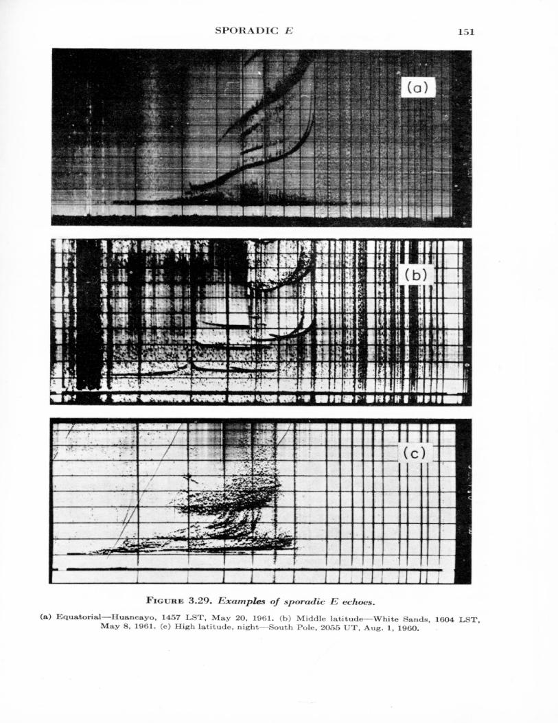
SPORADIC E 151
FIGURE 3.29. Examples of sporadic E echoes.
(a) Equatorial—Huancayo, 1457 LST, May 2O, 1961. (b) Middle latitude—White Sanda, 16O4 LST, May 8, 1961. (c) High latitude, night—South Pole, 2055 UT, Aug. 1, I960.
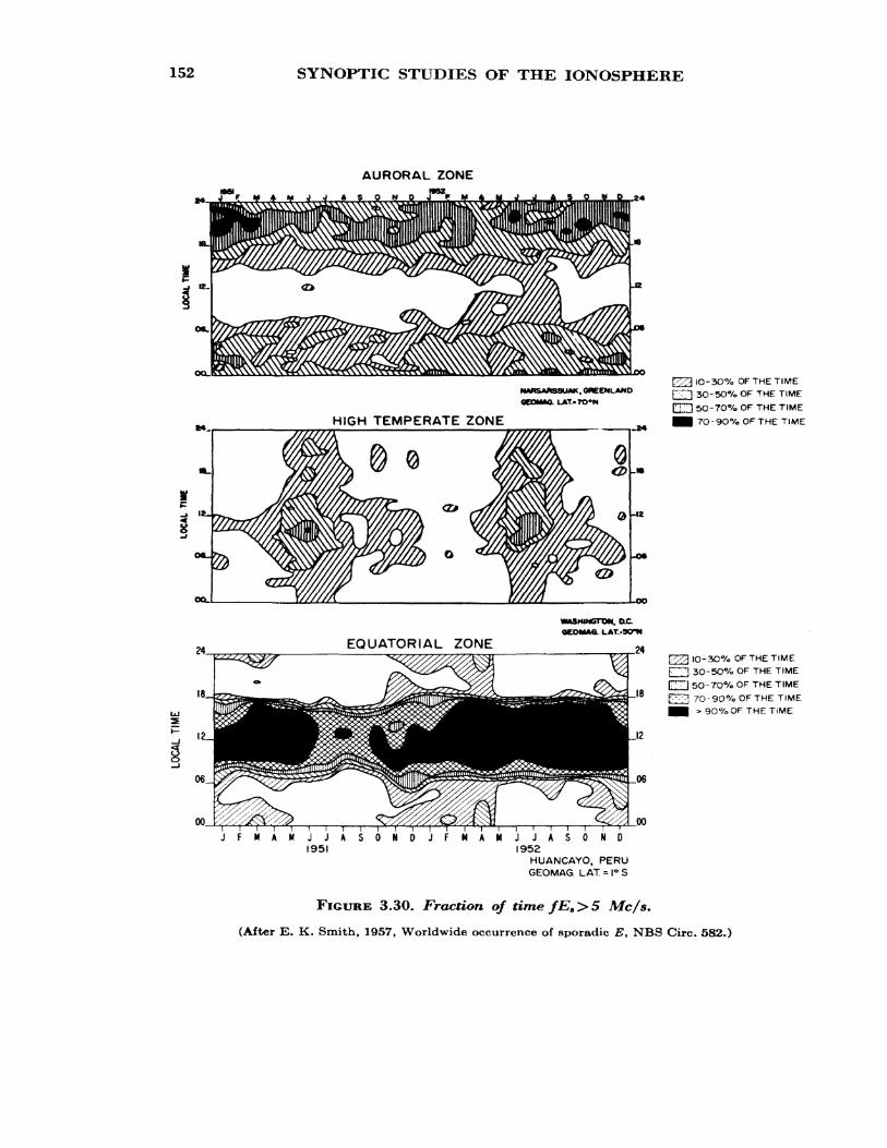
152 SYNOPTIC STUDIES OF THE IONOSPHERE
AURORAL ZONE
NAftSAMSSUAK, GREENLAND L LAT.-TO»N
H1GH TEMPERATE ZONE
EQUATORIAL ZONE
WASHINGTON. O.C. QEOMA& LAT.5CTN
¥Z\ (0-3O% OF THE TIME F\l 30-50% OF THE TIME
CUD 50-70% OF THE TIME
•• 70-90% OF THE TIME
-3O% OF THE TIME ] 3O-5O% OF THE TIME
[TH1! 50-70% OF THE TIME
70-9O% OF THE TIME 90% OF THE TiME
JFMAMJJASONDJFWAMJJASOND 1951 1952
HUANCAYO, PERU GEOMAG. LAT = 1° S
FIGURE 3.30. Fraction of time fEa >5 Mc/$.
(After E. K. Smith, 1957, Worldwide occurrence of sporadic E, NBS Circ. 582.)
SPREAD F 153
other hand, in the auroral zone, E* is most prevalent during the night hours but again there is little seasonal variation.
In middle latitudes fE8 is less than elsewhere and the occurrence is subject to diurnal and seasonal variations. In general, Es is more frequent in local summer than in winter and by day more than by night. Data on the occurrence of E8 are published monthly in the CRPL F Series, Part A.
3-3.8. Spread F
3.3.8.1. Description of Spread F
It is often observed that the echo pulse reflected from the F% layer has a much longer (10 times) duration than the transmitted pulse and this phenomenon is called spread F. Undoubtedly, spread F is caused by the scattering of the signal from irregularities embedded in the ionosphere both in depth and away from the zenith. Some examples of ionograms -with spread-J^ echoes are presented in figure 3.31 from which it is seen that the phenomenon occurs in high and low latitudes. A survey of the existing knowledge of spread F has been compiled by Glover £35]. The rules for scaling spread F are discussed in references [[1], C2D-» and Q36]. It should be noted that spread F is generally defined in terms of the ap pearance of an ionogram rather than in terms of the physical mechanism operative.
Several classifications for types of spread F have been suggested, such as high-, medium-, and low-latitude spread F []15], but this method is not entirely satisfactory. An alternative division into "range type" and ''frequency type" has been suggested C37^]- Frequency type spread refers to diffuseness near the critical frequency of the F% layer, whereas the range type refers to diffuseness near the horizontal part of the trace.
Some ionograms, such as that shown in figure 3.32a, exhibit spread only on the multiple echoes. This type is believed to be due to ground scatter, as illustrated in figure 3.32b.
3.3.8.2. Diurnal Variations
Spread F occurrence is essentially a statistical phenomenon, and maps have been prepared showing the probability of occurrence C383- It is essentially an evening and nighttime phenomenon. In low geomagnetic latitudes the most likely time of occurrence is between about 2100 local
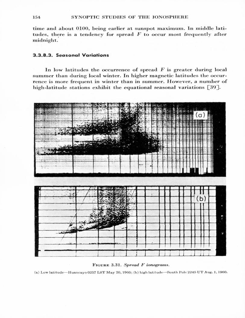
154 SYNOPTIC STUDIES OF THE IONOSPHERE
time and about 0100,, being earlier at sunspot maximum. In middle lati tudes, there is a tendency for spread F to occur most frequently after midnight.
3.3.8.3. Seasonal Variations
In low latitudes the occurrence of spread F is greater during local summer than during local winter. In higher magnetic latitudes the occur rence is more frequent in winter than in summer. However, a number of high-latitude stations exhibit the equational seasonal variations £39].
FIGURE 3.31. Spread F ionograms.
(a) Low latitude—Huancayo O257 LST May 20, I960; (b> high latitude—South Polo 2245 UT Aug. 1, 1960.
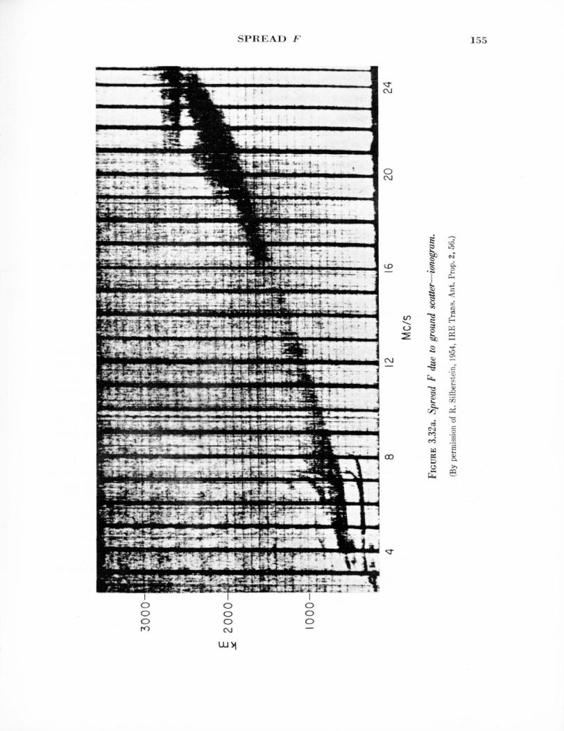
3000-
Mc/s
FIGU
RE 3
.32a
. Sp
read
F d
ue to
gro
und
scat
ter—
iono
gram
.
(By
perm
ission
of R
. Silb
erstei
n, 19
54, I
RE T
rans
. Ant.
Pro
p, 2,
56.)
Cft
en
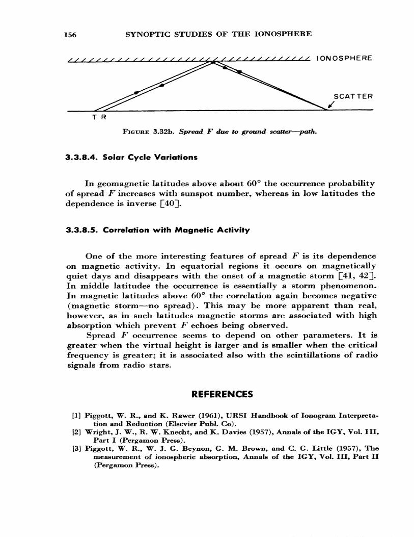
156 SYNOPTIC STUDIES OF THE IONOSPHERE
/s/s/ss/// IONOSPHERE
T R
FIGURE 3.32b. Sprecwf F due to ground scatter—path.
3.3.8.4. Solar Cycle Variations
In geomagnetic latitudes above about 60° the occurrence probability of spread F increases with sunspot number, whereas in low latitudes the dependence is inverse £40]].
3.3.8.5. Correlation with Magnetic Activity
One of the more interesting featurep of spread F is its dependence on magnetic activity. In equatorial regions it occurs on magnetically quiet days and disappears with the onset of a magnetic storm £41, 42]. In middle latitudes the occurrence is essentially a storm phenomenon. In magnetic latitudes above 60° the correlation again becomes negative (magnetic storm—no spread). This may be more apparent than real, however, as in such latitudes magnetic storms are associated with high absorption which prevent .F echoes being observed.
Spread F occurrence seems to depend on other parameters. It is greater when the virtual height is larger and is smaller when the critical frequency is greater; it is associated also with the scintillations of radio signals from radio stars.
REFERENCES
[1] Piggott, W. R., and K. Rawer (1961), URSI Handbook of lonogram Interpreta tion and Reduction (Elsevier Publ. Co).
[2] Wright, J. W., R. W. Knecht, and K. Davies (1957), Annals of the IGY, Vol. Ill, Part I (Pergamon Press).
13] Piggott, W, R., W. J. G. Beynon, G. M. Brown, and C. G. Little (1957), The measurement of ionospheric absorption, Annals of the IGY, VoL III, Part II (Pergamon Press).
REFERENCES 157
[4] Appleton, E. V., and W. R. Piggott (1954), Ionospheric absorption measurements during a sunspot cycle, J. Atmospheric and Terrest. Phys. 5, 141.
[5] Findlay, J. W. (1951), The phase and group paths of radio waves returned from region E of the ionosphere, J. Atmospheric and Terrest. Phys. 1, 353.
[6] Ogawa, T. (1958), Frequency variations in short wave propagation, Proc. IRE46. 1934.
[7] Fenwick, R. C., and O. G. Villard (1960), Continuous recordings of the frequency variation of the WWV-20 signal after propagation over a 40O km path, J. Geophys. Res. 65, 3249.
[8] Watts, J. M., and K. Davies (1960), Rapid frequency analysis of fading radiosignals, J. Geophys. Res. 65, 2295.
[9] Selected papers from J. Res. NBS 65D (Radio Prop.)* 197-311 (1961).[10] Seddon, J. C. (1953), Propagation measurements in the ionosphere with the aid of
rockets, J. Geophys. Res. 58, 323.[11] Knecht, R. W., T. E. VanZandt, and S. Russell (1961), First published radio
soundings of the topside of the ionosphere, J. Geophys. Res. 66, 3078.[12] Warren, E. S. (1963), Some preliminary results of sounding of the topside of the
ionosphere by radio pulses from a satellite, Nature 197, 636.[13] Watts, J, M., and J. N. Brown (1954), Some results of sweep frequency investiga
tions in the low -frequency band, J. Geophys. Res. 59, 71.[14] Watts, J. M. (1952), A note on the polarization of low -frequency ionospheric
echoes, J. Geophys. Res. 57, 287; (1958), The interpretation of nighttime low- frequency ionograms, ibid. 63, 19; and (1959), J. Atmospheric and Terrest. Phys. 15, 73.
[15] Wright, J. W. and R. W. Knecht (1957), IGY Atlas of lonograms.[16] NBS CRPL F Series, Part A, published monthly.[17] Budden, K. G. (1955), A method for determining the variation of electron density
with height from curves of equivalent height against frequency, Proc. Cam bridge Conf. on the Physics of the Ionosphere, Phys. Soc., 332.
[18] King, G. A. M. (1960), Use of logarithmic frequency spacing in ionogram analysis, J. Res. NBS 64D (Radio Prop.), 501.
[19] Titheridge, J. E. (1959), The use of the extraordinary ray in the analysis of iono spheric records, J. Atmospheric and Terrest. Phys. 17, 110.
[20] Davies, K., and A. K, Saha (1962), Study of the "valley problem" with a ray tracing program, Electron Density Profiles, p. 162 (Pergamon Press).
[21] Storey, L. R. O. (I960), The joint use of the ordinary and extraordinary virtual height curves in determining ionospheric layer profiles, J. Res. NBS 64D, (Radio Prop.), 111.
[22] Thomas, J. O. (1959), The distribution of electrons in the ionosphere, Proc. IRE47. 162.
[23] Knecht, R. W. (1959), Observations of the ionosphere over the south geographicpole, J. Geophys. Res. 64, 1243.
[24] Mean electron density variations of the quiet ionosphere (quarterly), NBS Tech.Notes 40-1, -2, -3, etc.
[25] Zacharisen, D. H. (1959), World maps of F2 critical frequencies and maximumusable frequency factors (Apr. 1959), NBS Tech. Note 2, and (Oct. 1960) NBSTech. Note 2-2.
[26] Taylor, E. W. (1948), Absorption of radio waves reflected at vertical incidence asa function of the sun's zenith angle, J. Res. NBS 41, 575.
[27] Davies, K., and E. L. Hagg (1955), Ionospheric absorption measurements atPrince Rupert, J. Atmospheric and Terrest. Phys. 6, 18.
158 SYNOPTIC STUDIES OF THE IONOSPHERE
[28] Bibl, K., A. Paul, and K. Rawer (1962), Absorption in the D and E regions andits time variations, Radio Wave Absorption in the Ionosphere, AGARDograph53 (Pergamon Press).
[29] Best, J. E., and J. A. Ratcliffe (1938), The diurnal variation of the ionosphericabsorption of wireless waves, Proc. Phys. Soc. 50, 233.
[30] Davies, K. (1960), A study of 2-Mc/s ionospheric absorption measurements athigh latitudes, J. Geophys. Res. 65, 2285.
[31] Thomas, L. (1962), The winter anomaly in ionospheric absorption, Radio WaveAbsorption in the Ionosphere (ed. N. C. Gerson) (Pergamon Press).
[32] Dieminger, W. (1952), On the causes of excessive absorption in the ionosphere onwinter days, J. Atmospheric and Terrest. Phys. 2, 340.
[33] Seddon, J. C. (1962), Sporadic E as observed with rockets, Ionospheric SporadicE (ed. Smith and Matsushita), p. 78 (Pergamon Press).
[34] Smith, E. K. (1957), Worldwide occurrence of sporadic E, NBS Circ. 582. [35] Glover, F. N. (1960), A study of spread F, NBS Tech. Note 82. [36] Hanson, G. H., E. L. Hagg, and D. Fowle (1953), The interpretation of ionospheric
records, DRTE Report R-2, Canada, [37] McNicol, R. W. E., H. C. Webster, and C. G. Bowman (1956), A study of spread-F
ionospheric echoes at night at Brisbane, I., Australian J. Phys. 9, 247. [38] Tao, K. (1962), On the theoretical study of F scatter, J. Geomagnetism and Geo-
eleclricity VIX, 71.[39] Reber, G. (1956), Worldwide spread F, J. Geophys. Res. 61, 157. [40] Shimazaki, T. (1959), A statistical study of worldwide occurrence probability of
spread F, J. Radio Res. Labs. (Tokyo) 6, 669. [41] Wright, R. W. (1959), The geomorphology of spread F and characteristics of
equatorial spread F, J. Geophys. Res. 64, 2203. [42] Wright, R. W., and N. J. Skinner (1959), Equatorial spread F, J. Atmospheric and
Terrest. Phys. 15, 121.
CHAPTER 4
Oblique Propagation
.1- CHARACTERISTICS OF HF PROPAGATION
High-frequency (3 to 30 Mc/s) radio waves have been and still are one of the basic vehicles for long-distance transmission of information. The reasons for this may be summarized as follows:
(a) Low cost of terminal equipment,(b) Low power requirements,(c) Adequate bandwidths,(d) Adequate signal strengths.
In contrast with the above, it may be noted that medium wave fre quencies (300 kc/s to 3 Mc/s) suffer very heavy absorption during the day, while on lower frequencies there is insufficient bandwidth for more than a few voice channels. Frequencies much above 30 Mc/s are not, normally, reflected from the ionosphere. For propagation over long dis tances the F% layer is of fundamental importance.
The disadvantages in using high frequencies are:
(1) The variability of propagation conditions which, for optimum results, requires frequent changes in the operating frequency. Even on the optimum frequency, communications are often subject to interrup tion by ionospheric storms,
(2) The large number of possible propagation paths and the re sulting time dispersion of a single signal.
(3) The large and rapid phase fluctuations,(4) The high interference.(5) Wide-band signals suffer from frequency distortion.
In the lower part of the high-frequency spectrum, refraction in and reflection from the E region (particularly E8 ) contribute to the com plexity of the echo structure.
159
160 OBLIQUE PROPAGATION
The range of high frequencies useful for medium and long distance radio communications is limited, on the upper end, by the height and maximum electron density in the controlling layer and, on the low-fre quency end, by absorption in the D region.
In this chapter we shall be concerned with methods of calculating the maximum frequency and with the identification of the structure of signals both by experiment and by means of ray tracing.
4.2. EQUIVALENCE RELATIONSHIPS
4.2.1. Plane Earth and Plane Ionosphere
4.2.1.1. The "Secant Law"
In this section we shall consider the relationships that exist between the frequencies, virtual paths, and absorptions of two waves, one reflected with oblique incidence and the other reflected with normal incidence from the same true height. For this purpose consider a ray incident on a plane ionosphere at an angle 0o, as shown in figure 4.1, in which the electron density is increasing with height so that total internal reflection takes place.
In the absence of both collisions and an imposed magnetic field, the refractive index jj, for a wave of frequency /, at a level where the plasma
T = TRANSMITTER R = RECEIVER
REAL PATH VIRTUAL PATH
T'R 1 T
FIGURE 4.1. Equivalence theorem for plane earth and planeionosphere*
PLANE EARTH AND PLANE IONOSPHERE 161
frequency IS/AT, is given by (2.78):
(4.1)
Application of SnelFs law (M — sin 00 ) gives, at the level of reflection,
/AT =/ cos 0o-
Now if /v is the frequency which is reflected with normal incidence from the same true height (i.e., same plasma frequency) as the frequency / with oblique incidence, then fv =/N- Therefore
0, (a)or (4.2)
f=fv sec 0o. (b)
The frequency fv is called the ''equivalent vertical -incidence frequency," corresponding to/. Equation (4.2b) is the so-called secant law. It shows that, with oblique incidence, the ionosphere can reflect much higher fre quencies than with normal incidence.
4.2.1.2. Breit and Tuve's Theorem [I] 1
Another relationship of importance is known as Breit and Tuve's theorem. It states that the group (or equivalent) path P' (see (2.130)), for transmission between a transmitter T and a receiver R (fig. 4.1), is given by the length of the equivalent triangle TAR. That is,
P' = TA+AR, (4.3)
which can be proved by the folio wing argument:
P, = r *_J MTBR
Note that the true height of reflection (at B) is always less than the equiv alent height at A.
Figures in brackets indicate the literature references on p. 214.
162 OBLIQUE PROPAGATION
It should be remembered that (4.3) applies only when sender and receiver are situated outside the ionosphere. If the transmitter and re ceiver are located within the ionosphere at a level where the refractive index is MI-> the right-hand side of (4.3) must be divided by m in order that Pr is still to mean the group propagation time multiplied by the free space velocity.
4.2.1*3. Martyn's (Equivalent Path) Theorem [2]
If / and fv are equivalent frequencies of waves reflected obliquely and vertically from the same real height, then the virtual height of re flection of fv is equal to the height of the equivalent triangular path for the oblique signal.
Consider the refractive indices /x0b and /JL V for the oblique and vertical waves, respectively, at the same real height at which the plasma fre quency IS/AT; we have
(a)
(4.4)
and by Snell's law ^ob sin <j> = sin 00 - Combining these equations we get
Mob COS 4> = Hv COS 0o- (4.5)
Now the group path for the oblique signal is
ds fhr dh 2 fhr dh 2[hr dh =
J t\ JLU <Mob •'o Mob COS <p COS <po •'o Mv COS <po
Hence
P'(f)=h'(fv ) sec 0o. (4.6)
This theorem expresses the important relationship that the virtual height of reflection of an obliquely incident wave is the same as that of the equivalent vertical wave.
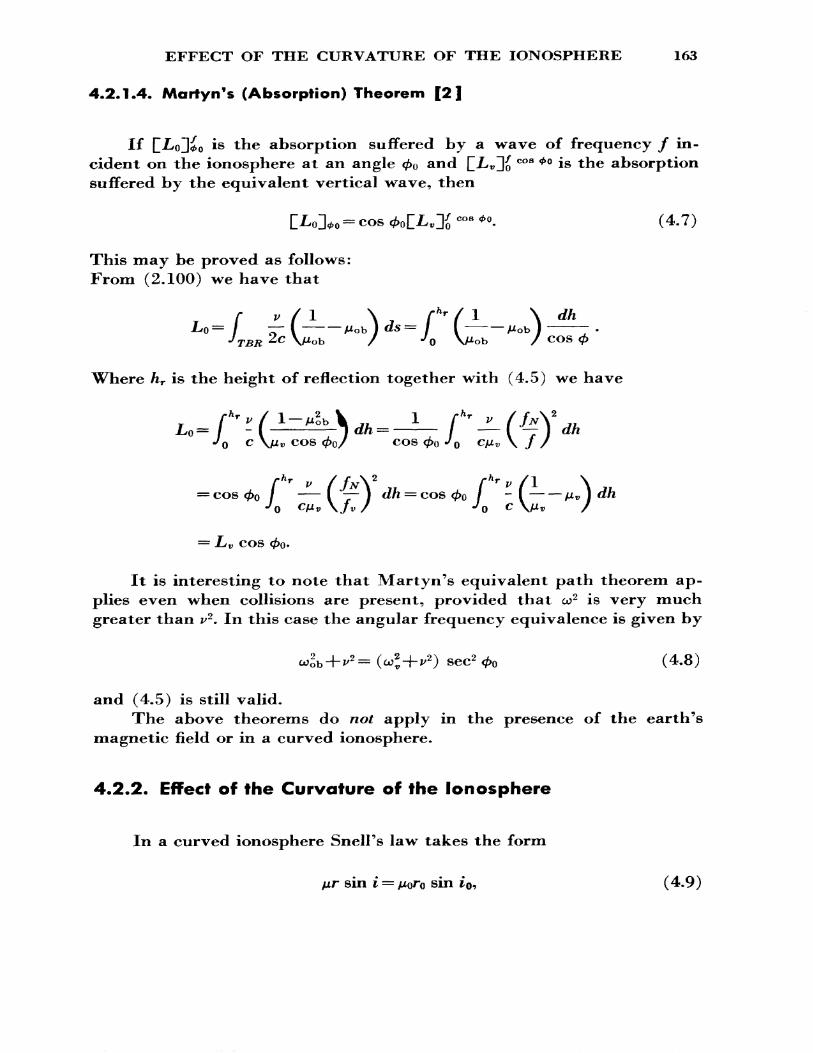
EFFECT OF THE CURVATURE OF THE IONOSPHERE 163
4.2.1.4. Martyn's (Absorption) Theorem [2]
If []i/oJ0o *s the absorption suffered by a wave of frequency / in cident on the ionosphere at an angle 00 and C^Do cos 00 *s the absorption suffered by the equivalent vertical wave, then
CLoIU = cos 0oLi.Di cos *°. (4.7)
This may be proved as follows: From (2.100) we have that
LQ= I — I————/nob )dfs=I (———— Mob)J TBR 2c \Mob / J Q XMob /
dh'TBR %c \Mob / •'o \Mob / cos 0
Where hr is the height of reflection together with (4.5) we have
C JULv COS 0o COS
hr= cos
fhr * //A2 /"Vj; /! \ / —— \ — ] dh = cos <^o / - I — — Mv I
^0 <Vt> \/v / ^o ^ VMr /
= Lv cos 0o.
It is interesting to note that Martyn's equivalent path theorem ap plies even when collisions are present, provided that co2 is very much greater than v^. In this case the angular frequency equivalence is given by
and (4.5) is still valid.The above theorems do not apply in the presence of the earth's
magnetic field or in a curved ionosphere.
4.2.2. Effect of the Curvature of the Ionosphere
In a curved ionosphere Snell's law takes the form
fir sin i = ^toJo sin i$, (4.9)
164 OBLIQUE PROPAGATION
REFLECTION
IONOSPHERE
EARTH
FIGURE 4.2. Ray geometry tuith oblique incidence.
where r is the length of the radius vector from the center of the earth to the level where the refractive index is n and the angle between the radius vector and the ray is £, as shown in figure 4.2.; p,$, TO, and £o are ar bitrary reference values. Let us take ground level as reference so that /zo=l, /o = a, and i0 = (ir/2)— A where A is the angle of elevation. Then
/xr sin i = a cos A. (4.10)
The relationship between a frequency / and the equivalent vertical fre- quency/t, which is reflected from the same real height hr is given by sub stituting (4.1) into (4.10) and replacing fN by fv . This gives
(4.11)
Now let <f>r be the angle between the continuation of the unrefracted ray and the radius vector at the level hr as shown in figure 4.2. From the ge-
PLANE IONOSPHERE 165
ometry we have that
(a+Ar) sin <£r = a cos A. (4.12)
Hence
r. (4.13)
From (4.11) and (4.13) it will be seen that the equivalent frequency depends not only on A but also on the height of reflection hr.
Instead of defining fv in terms of the height of reflection, it can be defined in terms of (4.6) or (4.7) but, unlike the plane ionosphere case, the values of fv will depend on the definition.
4.3. CALCULATION OF MAXIMUM FREQUENCIES
4.3.1. Plane Ionosphere
The theorems of Breit and Tuve and of Martyn stated above show that, for a plane ionosphere, the reflection process is equivalent to mirror- type reflection at a height equal to the virtual height h f of reflection of the equivalent vertical frequency. The variation of the latter with fre quency can be determined experimentally by means of a conventional sounder.
The relationship between oblique and equivalent-vertical frequencies, in the case of a plane reflector at an equivalent height h f ', for transmission over a distance D, is given by
/ob =/. sec ,=W'In the case of a curved earth and a plane ionosphere <£o is given by
sin i#tan 0o= , a ———— - , (4.15) 1 + (h /a) — cos %6
where a is the earth's radius (6370 km) and 6 is the angle at the center of the earth subtended by the transmission path.
To obtain /ob for a given value offv we need to know h f as a function of fv — from an ionogram — and the relationship between sec <£o and h'
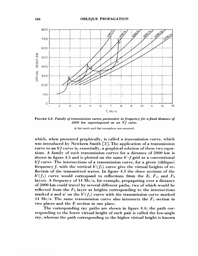
166 OBLIQUE PROPAGATION
8OO
TOO
FIGURE 4.3. Family of transmission curves parametric in frequency for a fixed distance of2000 km superimposed on an h ff curve.
A flat earth and flat ionosphere are assumed.
which, when presented graphically, is called a transmission curve, which was introduced by Newbern Smith [[3]. The application of a transmission curve to an h ff curve is, essentially, a graphical solution of these two equa tions. A family of such transmission curves for a distance of 2000 km is shown in figure 4.3 and is plotted on the same h'-f grid as a conventional h ff curve. The intersections of a transmission curve, for a given (oblique) frequency/, with the vertical h f (fv } curve give the virtual heights of re flection of the transmitted waves. In figure 4.3 the three sections of the ^'(/tO curve would correspond to reflections from the £", FI, and F2 layers. A frequency of 14 Mc/s, for example, propagating over a distance of 2000 km could travel by several different paths, two of which would be reflected from the F2 layer at heights corresponding to the intersections marked a and a' on the h'(fv ) curve with the transmission curve marked 14 Mc/s. The same transmission curve also intersects the FI section in two places and the E section in one place.
The corresponding ray paths are shown in figure 4.4; the path cor responding to the lower virtual height of each pair is called the low-angle ray, whereas the path corresponding to the higher virtual height is known
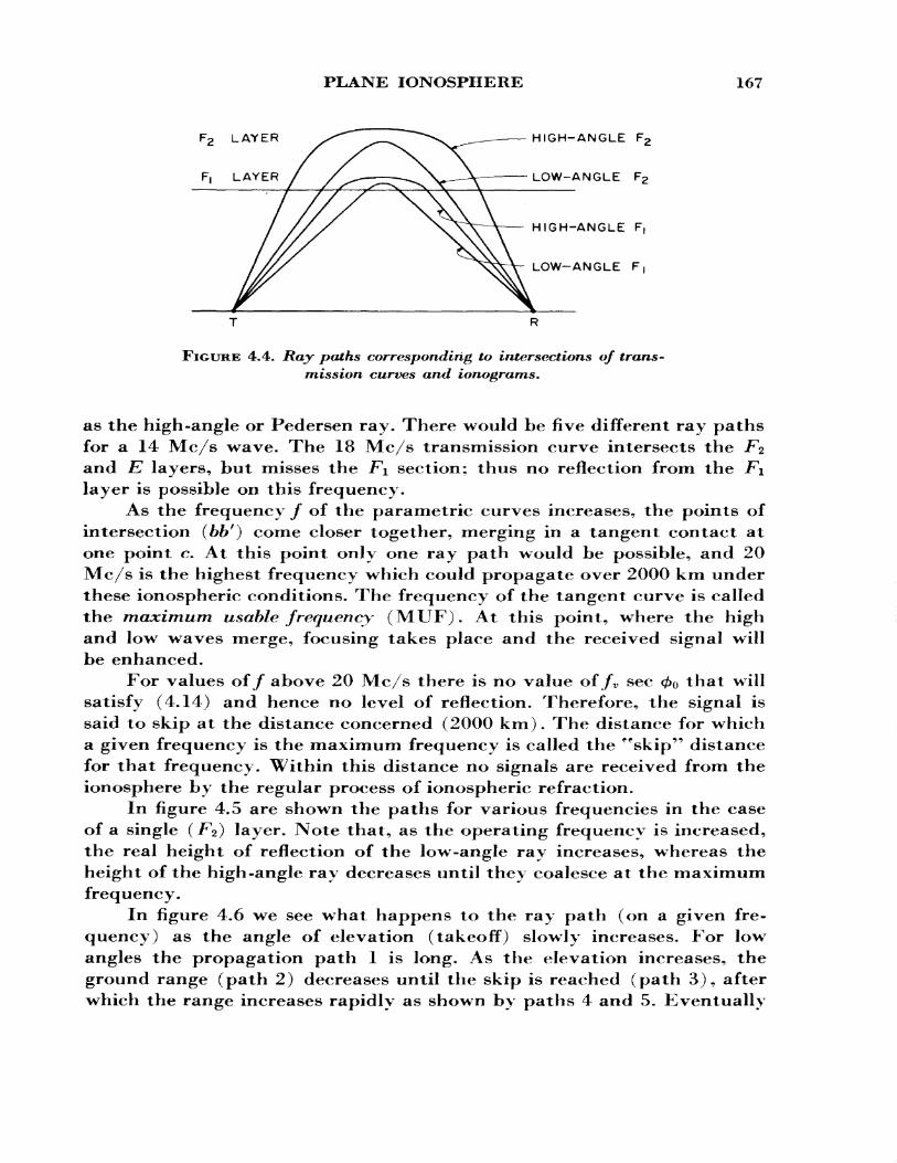
PLANE IONOSPHERE 167
HIGH-ANGLE F2
LOW-ANGLE F2
HIGH-ANGLE F,
LOW-ANGLE F,
FIGURE 4.4. Ray paths corresponding to intersections of trans mission curves and ionograms.
as the high-angle or Pedersen ray. There would be five different ray paths for a 14 Mc/s wave. The 18 Mc/s transmission curve intersects the FZ and E layers, but misses the F± section; thus no reflection from the FI layer is possible on this frequency.
As the frequency / of the parametric curves increases, the points of intersection (bb r) come closer together, merging in a tangent contact at one point c. At this point only one ray path would be possible, and 20 Mc/s is the highest frequency which could propagate over 2000 km under these ionospheric conditions. The frequency of the tangent curve is called the maximum usable frequency (MUF). At this point, where the high and low waves merge, focusing takes place and the received signal will be enhanced.
For values off above 20 Mc/s there is no value of fv sec 00 that will satisfy (4.14) and hence no level of reflection. Therefore, the signal is said to skip at the distance concerned (2000 km) . The distance for which a given frequency is the maximum frequency is called the ffskip" distance for that frequency. Within this distance no signals are received from the ionosphere by the regular process of ionospheric refraction.
In figure 4.5 are shown the paths for various frequencies in the case of a single (F%) layer. Note that, as the operating frequency is increased, the real height of reflection of the low-angle ray increases, whereas the height of the high-angle ray decreases until they coalesce at the maximum frequency.
In figure 4.6 we see w^hat happens to the ray path (on a given fre quency) as the angle of elevation (takeoff) slowly increases. For low angles the propagation path 1 is long. As the elevation increases, the ground range (path 2) decreases until the skip is reached (path 3), after which the range increases rapidly as shown by paths 4 and 5. Eventually
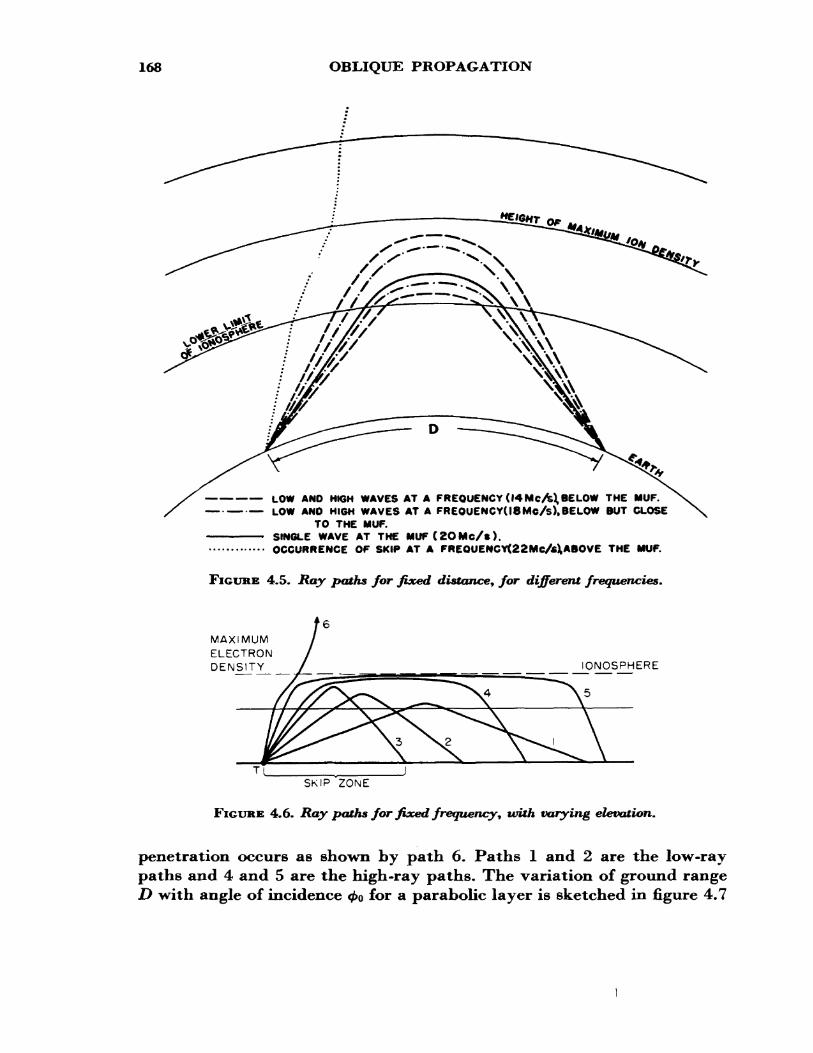
168 OBLIQUE PROPAGATION
LOW AND HIGH WAVES AT A FREQUENCY (14 Mc/s), BE LOW THE MUF. LOW AND HIGH WAVES AT A FR£OUENCY( 18 Mc/s), BELOW BUT CLOSE
TO THE MUF.SINGLE WAVE AT THE MUF(2OMc/t). OCCURRENCE OF SKIP AT A FR£OUENCY(22Mc/6XABOVE THE MUF.
FIGURE 4.5. Ray paths for fixed distance, for different frequencies.
MAXIMUMELECTRONDENSITY IONOSPHERE
SKIP ZONE
FIGURE 4.6. Ray paths for fixed frequency, with varying elevation.
penetration occurs as shown by path 6. Paths 1 and 2 are the low-ray paths and 4 and 5 are the high-ray paths. The variation of ground range D with angle of incidence <£o for a parabolic layer is sketched in figure 4.7
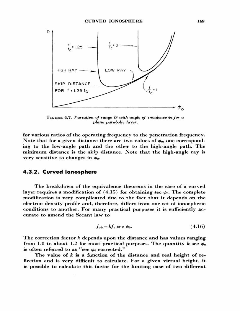
CURVED IONOSPHERE 169
D
SKJPJDI STANCE
FOR f = 1.25 fc
FIGURE 4.7. Variation, of range D with angle of incidence 4>ofor aplane parabolic layer.
for various ratios of the operating frequency to the penetration frequency. Note that for a given distance there are two values of <£o, one correspond ing to the low-angle path and the other to the high -angle path. The minimum distance is the skip distance. Note that the high -angle ray is very sensitive to changes in <£0 -
4.3.2. Curved Ionosphere
The breakdown of the equivalence theorems in the case of a curved layer requires a modification of (4.15) for obtaining sec <£o- The complete modification is very complicated due to the fact that it depends on the electron density profile and, therefore, differs from one set of ionospheric conditions to another. For many practical purposes it is sufficiently ac curate to amend the Secant law to
= kfv sec (4.16)
The correction factor k depends upon the distance and has values ranging from 1.0 to about 1.2 for most practical purposes. The quantity k sec <£o is often referred to as rfsec <£o corrected."
The value of A: is a function of the distance and real height of re flection and is very difficult to calculate. For a given virtual height, it is possible to calculate this factor for the limiting case of two different
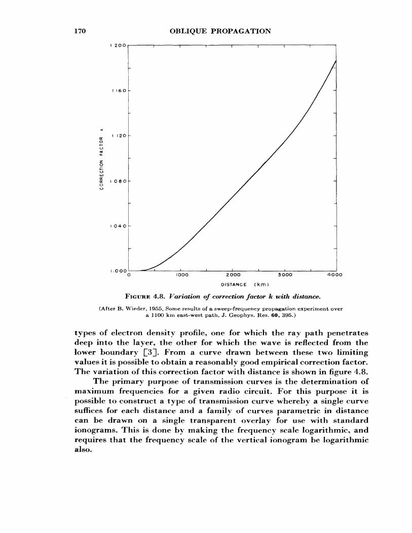
170 OBLIQUE PROPAGATION
t 200
160 -
<r oo<
or or O o
I I2O -
i.oeo -
I.O4 O -
.0004OOO
(km)
FIGURE 4.8. Variation of correction factor k with distance.
(After B. Wieder, 1955, Some results of a sweep-frequency propagation experiment over a 1100 km east-west path, J. Geophys. Res. 60, 395.)
types of electron density profile, one for which the ray path penetrates deep into the layer, the other for which the wave is reflected from the lower boundary £3]. From a curve drawn between these two limiting values it is possible to obtain a reasonably good empirical correction factor. The variation of this correction factor with distance is shown in figure 4.8.
The primary purpose of transmission curves is the determination of maximum frequencies for a given radio circuit. For this purpose it is possible to construct a type of transmission curve whereby a single curve suffices for each distance and a family of curves parametric in distance can be drawn on a single transparent overlay for use with standard ionograms. This is done by making the frequency scale logarithmic, and requires that the frequency scale of the vertical ionogram be logarithmic also.
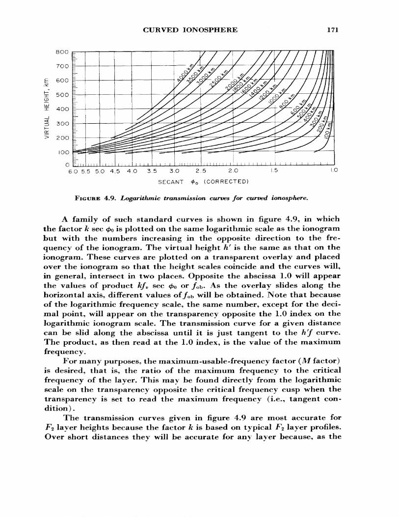
CURVED IONOSPHERE 171
O EL 6.0 5.5 5.0 4.5 4.O 3.5 3.O 2.5 2.Q
SECANT <£ 0 (CORRECTED)
FIGURE 4.9. Logarithmic transmission curves for curved ionosphere.
A family of such standard curves is shown in figure 4.9, in which the factor k sec <£0 is plotted on the same logarithmic scale as the ionogram but with the numbers increasing in the opposite direction to the fre quency of the ionogram. The virtual height h f is the same as that on the ionogram. These curves are plotted on a transparent overlay and placed over the ionogram so that the height scales coincide and the curves will, in general, intersect in two places. Opposite the abscissa 1.0 will appear the values of product kfv sec 00 or /ob - As the overlay slides along the horizontal axis, different values of/O b will be obtained. Note that because of the logarithmic frequency scale, the same number, except for the deci
mal point, will appear on the transparency opposite the 1.0 index on the logarithmic ionogram scale. The transmission curve for a given distance can be slid along the abscissa until it is just tangent to the h'f curve. The product, as then read at the 1.0 index, is the value of the maximum frequency.
For many purposes, the maximum-usable-frequency factor (TV/ factor) is desired, that is, the ratio of the maximum frequency to the critical frequency of the layer. This may be found directly from the logarithmic scale on the transparency opposite the critical frequency cusp when the transparency is set to read the maximum frequency (i.e., tangent con dition ).
The transmission curves given in figure 4.9 are most accurate for jp2 layer heights because the factor k is based on typical F% layer profiles. Over short distances they will be accurate for any layer because, as the
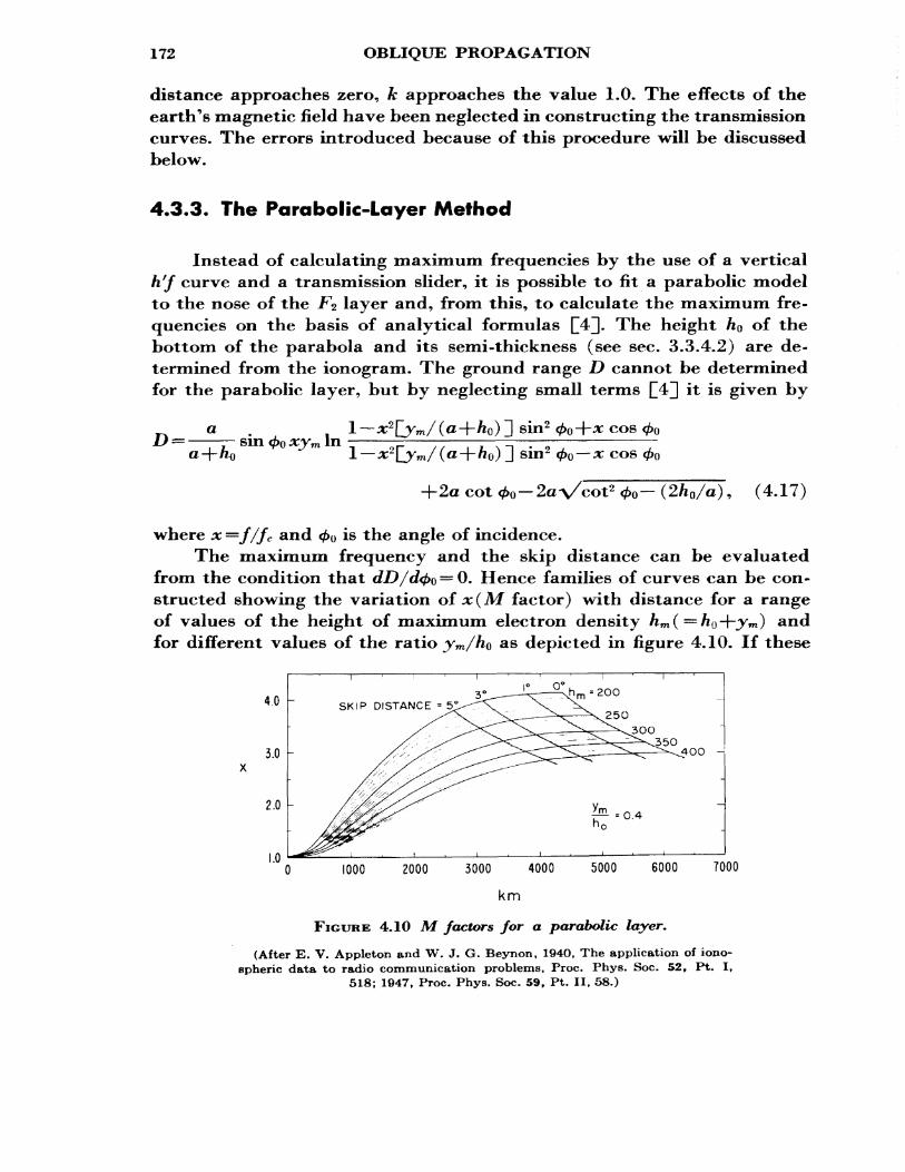
172 OBLIQUE PROPAGATION
distance approaches zero, k approaches the value 1.0. The effects of the earth's magnetic field have been neglected in constructing the transmission curves. The errors introduced because of this procedure will be discussed below.
4.3.3. The Parabolic-Layer Method
Instead of calculating maximum frequencies by the use of a vertical h'f curve and a transmission slider, it is possible to fit a parabolic model to the nose of the F* layer and, from this, to calculate the maximum fre quencies on the basis of analytical formulas Q4J. The height hQ of the bottom of the parabola and its semi-thickness (see sec. 3.3.4.2) are de termined from the ionogram. The ground range D cannot be determined for the parabolic layer, but by neglecting small terms £4] it is given by
asin <£0 xym In
sn cossn <£0 — x cos
+2a cot 0o — 2a A/cot2 <£0 — (2A 0/a), (4.17)
where x=f/fc and 00 is the angle of incidence.The maximum frequency and the skip distance can be evaluated
from the condition that dD/d<j>$ = 0. Hence families of curves can be con structed showing the variation of x(M factor) with distance for a range of values of the height of maximum electron density hm ( =/io+JKm) and for different values of the ratio ym/h0 as depicted in figure 4.10. If these
1000 2000 3000 4000
km
5000 6000 7000
FIGURE 4.10 M factors for a parabolic layer.
(After E. V. Appleton and W. J. G. Beynon, 1940, The application of iono spheric data to radio communication problems, Proc. Phys. Soc. 52, Pt. I,
518; 1947, Proc. Phys. Soc. 59, Pt. II, 58.)
EXPERIMENTAL TECHNIQUE 173
parameters are known, together with /c, it is possible to determine the maximum frequency by interpolation between curves. To get the most reliable estimate of the factor at any time, it is desirable that h$ and ym should be determined directly from ionograms at the midpoint of the path. Such a course is, however, rarely practicable, and it is necessary to predict the most probable values of ym and ft0 from past history. From the network of ionospheric sounding stations the diurnal, seasonal, and sunspot cycle variations of these parameters are known over most of the -world. Comparisons have shown that the results obtained by the para bolic method and by Smith's transmission curves are essentially the same. For two-hop propagation it is necessary to calculate the factor for half the distance.
The transmission theory presented above applies to the case of a spherically stratified ionosphere only. Now, over long transmission paths, the ionospheric parameters may vary appreciably and so the various hops will be of unequal length. The parabolic layer theory has been extended by Kift £5]] to include such variations and will be considered later.
4.4. OBLIQUE IONOGRAMS
4.4.1. Experimental Technique
The most convenient way of determining the echo structure of signals transmitted obliquely is by the ionosonde technique but with transmitter and receiver at different ends of the path. From the technical point of view this introduces two problems:
(a) The repetition frequencies at the sender and at the receiver must be very nearly the same; otherwise the received pulse will ff drift" along the time base of the display oscilloscope.
(b) The frequency of the receiver, as a function of time, must be kept in tune with the sender.
Pulse synchronization (a) is achieved by employing signals from in dependent stable crystal oscillators. The frequencies of such oscillators are normally in the range 100 kc/s to 5 Mc/s, and electronic frequency dividers are used to obtain the desired repetition frequency. The oscilla tors can be adjusted (in frequency) either independently with reference to an external standard (e.g., WWV), or else the oscillator at the receiver can be adjusted periodically until the drift of the pulses from the sender is reduced to a minimum. Other synchronization methods used have in-
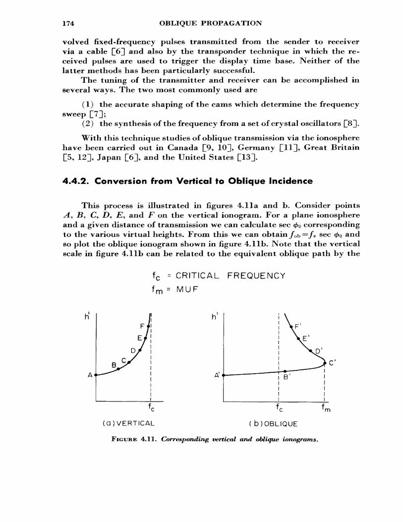
174 OBLIQUE PROPAGATION
volved fixed -frequency pulses transmitted from the sender to receiver via a cable Q6] and also by the transponder technique in which the re ceived pulses are used to trigger the display time base. Neither of the latter methods has been particularly successful.
The tuning of the transmitter and receiver can be accomplished in several ways. The two most commonly used are
(1) the accurate shaping of the cams which determine the frequency sweep []7]];
(2) the synthesis of the frequency from a set of crystal oscillators QJl.
With this technique studies of oblique transmission via the ionosphere have been carried out in Canada £9, 10], Germany CHU, Great Britain [5, 12], Japan Q6], and the United States [13].
4.4*2. Conversion from Vertical to Oblique Incidence
This process is illustrated in figures 4.1 la and b. Consider points A^ J5, C, D^ E, and F on the vertical ionogram. For a plane ionosphere and a given distance of transmission we can calculate sec 00 corresponding to the various virtual heights. From this we can obtain /Ob =fv sec <£ 0 and so plot the oblique ionogram shown in figure 4. lib. Note that the vertical scale in figure 4. lib can be related to the equivalent oblique path by the
fc - CRITICAL FREQUENCY
fm = MUF
m
(Q) VERTICAL ( b)OBLIQUE
FIGURE 4.11. Corresponding vertical and oblique ionograms.
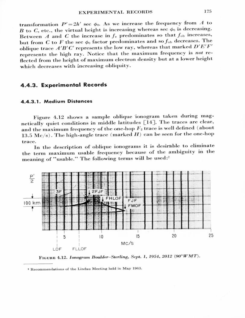
EXPERIMENTAL RECORDS 175
transformation P' = 2h f sec 00 . As we increase the frequency from A to
B to C, etc., the virtual height is increasing whereas sec </>« is decreasing.
Between A and C the increase in fv predominates so that /O b increases,
but from C to F the sec <£0 factor predominates and so/0b decreases. The
oblique trace A'B'C' represents the low ray, whereas that marked D f E''Ff
represents the high ray. Notice that the maximum frequency is not re
flected from the height of maximum electron density but at a lower height
which decreases with increasing obliquity.
4.4.3. Experimental Records
4.4.3.1. Medium Distances
Figure 4.12 showrs a sample oblique ionogram taken during mag
netically quiet conditions in middle latitudes Q14J. The traces are clear,
and the maximum frequency of the one-hop F2 trace is well defined (about
13.5 Mc/s) . The high-angle trace (marked JhT) can be seen for the one-hop
trace.In the description of oblique ionograms it is desirable to eliminate
the term maximum usable frequency because of the ambiguity in the
meaning of "usable." The following terms will be used: 2
1
15 20 25MC/S
LOF FLLOF
FIGURE 4.12. Ionogram Boulder-Sterling, Sept. 1, 1954, 2012 (9O°WMT}.
Recommendations of the Lindau Meeting held in May 1963.
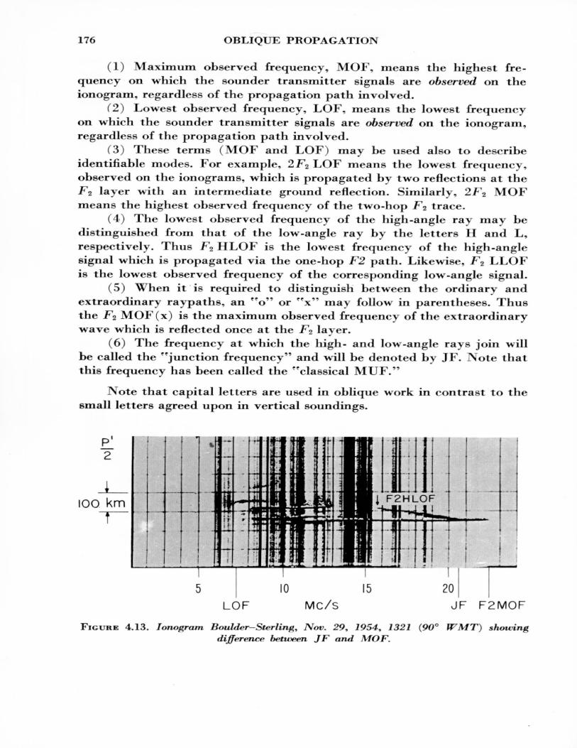
176 OBLIQUE PROPAGATION
(1) Maximum observed frequency, MOF, means the highest fre quency on which the sounder transmitter signals are observed on the ionogram, regardless of the propagation path involved.
(2} Lowest observed frequency, LOF, means the lowest frequency on which the sounder transmitter signals are observed on the ionogram, regardless of the propagation path involved.
(3) These terms (MOF and LOF) may be used also to describe identifiable modes. For example, 2F^ LOF means the lowest frequency, observed on the ionograms, which is propagated by two reflections at the FZ layer with an intermediate ground reflection. Similarly, 2F<t MOF means the highest observed frequency of the two-hop F? trace.
(4) The lowest observed frequency of the high-angle ray may be distinguished from that of the low-angle ray by the letters H and L, respectively. Thus Fz HLOF is the lowest frequency of the high-angle signal which is propagated via the one-hop F2 path. Likewise, F2 LLOF is the lowest observed frequency of the corresponding low-angle signal.
(5) Vt hen it is required to distinguish between the ordinary and extraordinary raypaths, an fpo" or "x" may follow in parentheses. Thus the F2 MOF(x) is the maximum observed frequency of the extraordinary wave which is reflected once at the FZ layer.
(6) The frequency at which the high- and low -angle rays join will be called the "junction frequency" and will be denoted by JF. Note that this frequency has been called the "classical MUF."
IVote that capital letters are used in oblique work in contrast to the small letters agreed upon in vertical soundings.
IOO km
LOF MC/S JF F2MOF
FIGURE 4.13. Ionogram Boulder-Sterling, Nov. 29, 1954, 1321 (90° WMT} showingdifference bettveen JF and
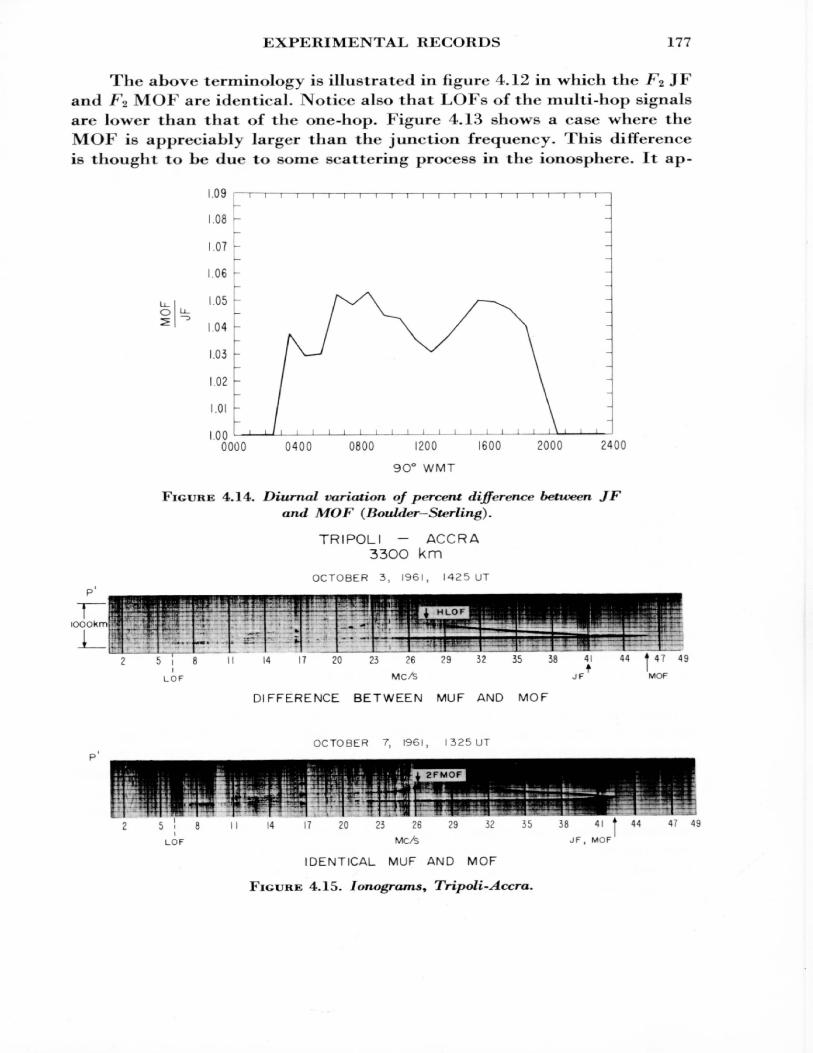
EXPERIMENTAL RECORDS 177
The above terminology is illustrated in figure 4.12 in which the F% JF and F2 MOF are identical. Notice also that LOFs of the multi-hop signals are lower than that of the one-hop. Figure 4.13 shows a case where the MOF is appreciably larger than the junction frequency. This difference is thought to be due to some scattering process in the ionosphere. It ap-
0000 0400 0800 1200 1600 2000 24009O° WMT
FIGURE 4.14. Diurnal variation of percent difference between JF and MOF (Boulder-Sterling).
TRIPOLI - ACCRA 33OO km
OCTOBER 3, 1961, 1425 UT
LOF MC/S
DIFFERENCE BETWEEN MUF AND MOF
OCTOBER 7, 1961, I 325 UT
1Ftf~»;^^^K
1 -• 3Bt*-4*l2
' Jmn*t. -- s. MJ -t.NM^ •&<•* '-.Tj J ' • ' " •• ^»aa-T-»i» . » i Jii f:ih 1 E^uJife^ifiiiySili^f^rr* : .^t^^.LL-__ ^-a.fc i:L.il"-!i"^B:'-rT3ilr "Jy^^i^T'mrf TiH ''V'"it'^r' TrT^t I — T — n —— TI^- i i | n 1~i —— Jt HlT'Tl jPmi^Tli-^K Haii fi ~fK~t- -| *'44n ' * ' !J ; Jf f 4-' -fm Jr^ y -jljBBE8|ia^aj»J Apiiii| JJJl^^^yj^-^ — — -34.-5_5-|
3)3 II 14 17 20 23 26 29 32 35 ?S 4i * 44 47 4Ji I
LOF MC/S JF , MOF
IDENTICAL MUF AND MOF
FIGURK 4.15. lonograms, Tripoli-Accra.
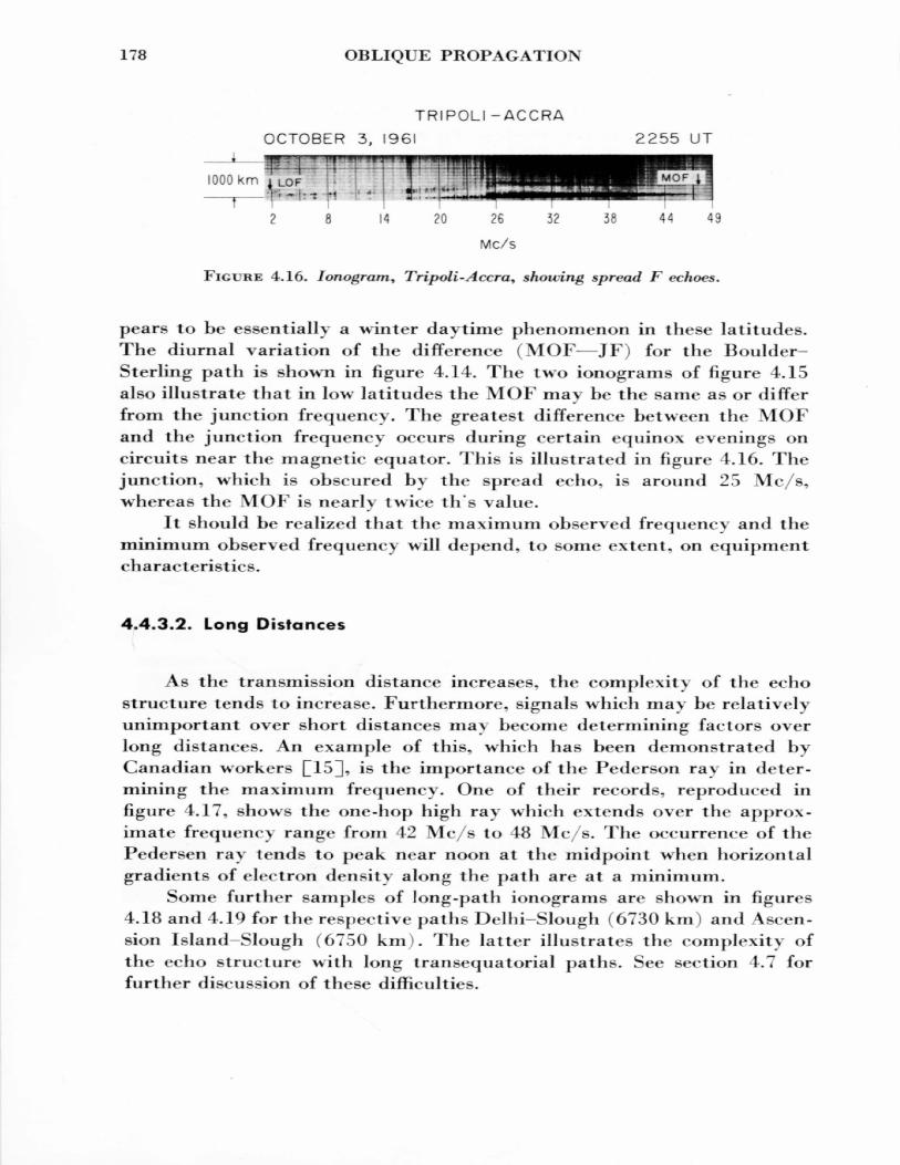
178 OBLIQUE PROPAGATION
TRIPOLI -ACCRA OCTOBER 3, (961 2255 UT
8 14 20 26 32 38 44 49
Mc/s
FIGURE 4,16. lonogram, Tripoli-Accra, showing spread F echoes.
pears to be essentially a winter daytime phenomenon in these latitudes. The diurnal variation of the difference (MOF—JF) for the Boulder- Sterling path is shown in figure 4.14. The two ionograms of figure 4.15 also illustrate that in low latitudes the MOF may be the same as or differ from the junction frequency. The greatest difference between the MOF and the junction frequency occurs during certain equinox evenings on circuits near the magnetic equator. This is illustrated in figure 4.16. The junction, which is obscured by the spread echo, is around 25 Mc/s, whereas the MOF is nearly twice th's value.
It should be realized that the maximum observed frequency and the minimum observed frequency will depend, to some extent, on equipment characteristics.
4.4.3.2. Long Distances
As the transmission distance increases, the complexity of the echo structure tends to increase. Furthermore, signals which may be relatively unimportant over short distances may become determining factors over long distances. An example of this, which has been demonstrated by Canadian workers [^15]], is the importance of the Pederson ray in deter mining the maximum frequency. One of their records, reproduced in figure 4.17, shows the one-hop high ray which extends over the approx imate frequency range from 42 Mc/s to 48 Mc/s. The occurrence of the Pedersen ray tends to peak near noon at the midpoint when horizontal gradients of electron density along the path are at a minimum.
Some further samples of long-path ioiiograms are shown in figures 4.18 and 4.19 for the respective paths Delhi—Slough (6730 km) and Ascen sion Island—Slough (6750 km). The latter illustrates the complexity of the echo structure wTith long transequatorial paths. See section 4.7 for further discussion of these difficulties.
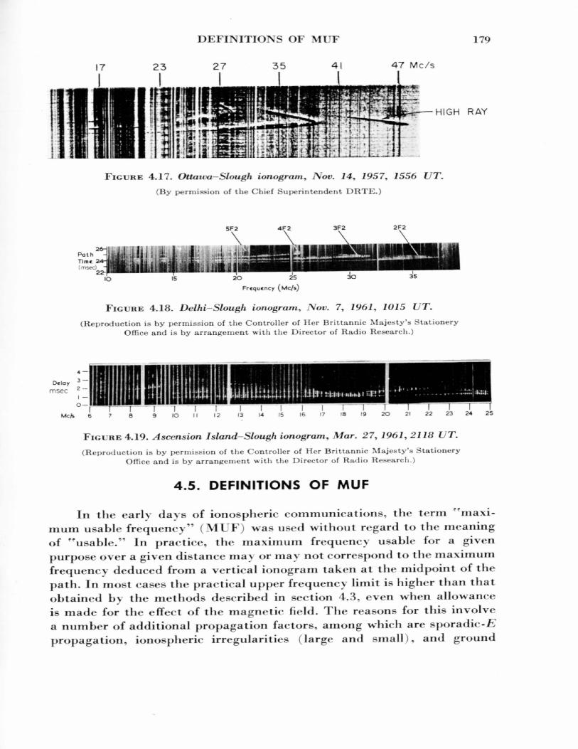
DEFINITIONS OF MUF 179
47 Mc/s
HIGH RAY
FIGURE 4.17. Ottawa-Slough ionogram* New. 14, 1957, 1556 UT.
(By permission of the Chief Superintendent DRTE.)
5F2 4F2 3F2
ID 20 25
Frequency (Me/*)
30 35
FIGURE 4.18. Delhi-Slough ionogram, Nov. 7, 1961, 1O15 VT.
(Reproduction is by permission of the Controller of Her Brittannic Majesty's Stationery Office and is by arrangement with the Director of Radio Research.)
Delaymsec
FIGURE 4.19. Ascension Island-Slough ionogram. Mar. 27, 1961, 2118 UT.
(Reproduction is by permission of the Controller of Her Brittannic Majesty's Stationery Office and is by arrangement with the Director of Radio Research.)
4.5. DEFINITIONS OF MUF
In the early days of ionospheric communications, the term ''maxi mum usable frequency" (MUF) was used without regard to the meaning of rr usable." In practice, the maximum frequency usable for a given purpose over a given distance may or may not correspond to the maximum frequency deduced from a vertical ionogram taken at the midpoint of the path. In most cases the practical upper frequency limit is higher than that obtained by the methods described in section 4.3. even w^heri allowance is made for the effect of the magnetic field. The reasons for this involve a number of additional propagation factors, among which are sporadic-/? propagation, ionospheric irregularities (large and small), and ground
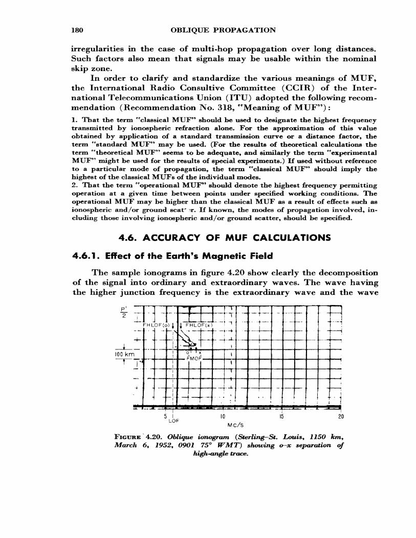
180 OBLIQUE PROPAGATION
irregularities in the case of multi-hop propagation over long distances. Such factors also mean that signals may be usable \vithin the nominal skip zone.
In order to clarify and standardize the various meanings of MTJF, the International Radio Consultive Committee (CCIR) of the Inter national Telecommunications Union (ITU) adopted the following recom mendation (Recommendation No. 318, "Meaning of MUF"):1. That the term "classical MUF" should be used to designate the highest frequency transmitted by ionospheric refraction alone. For the approximation of this value obtained by application of a standard transmission curve or a distance factor, the term ^standard MUF" may be used. (For the results of theoretical calculations the term "theoretical MUF" seems to be adequate, and similarly the term "experimental MUF" might be used for the results of special experiments.) If used without reference to a particular mode of propagation, the term "classical MUF" should imply the highest of the classical MUFs of the individual modes.2. That the term "operational MUF" should denote the highest frequency permitting operation at a given time between points under specified working conditions. The operational MUF may be higher than the classical MUF as a result of effects such as ionospheric and/or ground scat' :r. If known, the modes of propagation involved, in cluding those involving ionospheric and/or ground scatter, should be specified,
4.6. ACCURACY OF MUF CALCULATIONS
4.6.1. Effect of the Earth's Magnetic Field
The sample ionograms in figure 4.20 show clearly the decomposition of the signal into ordinary and extraordinary waves. The wave having the higher junction frequency is the extraordinary wave and the wave
P 1 ..2 !
-4-
100 kmT i**
4
H-HL
-
H3F(c
5
1
1)) J
1
sii
•• • '
[_1 FHLOF(x) * i
TA AO F
TT;'MOP
h
....—
_ — i
~1
I
T -*•
h-»-i
»
»
^
10
. ~ . ...
- A
j_.r tf—
IE
i
-i1
—— | •i *
•
?
i• 1
20LOF
MC/S
FIGURE 4.20. Oblique ionogram (Sterling-Si. Louis, 1150 km* March 6> 1952, 09O1 75° WMT) showing o-x separation of
high-angle trace.
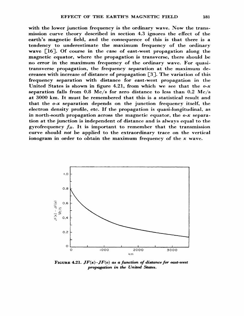
EFFECT OF THE EARTH'S MAGNETIC FIELD 181
with the lower junction frequency is the ordinary wave. Now the trans mission curve theory described in section 4.3 ignores the effect of the earth's magnetic field, and the consequence of this is that there is a tendency to underestimate the maximum frequency of the ordinary wave Cl^U- Of course in the case of east-west propagation along the magnetic equator, where the propagation is transverse, there should be no error in the maximum frequency of the ordinary wave. For quasi - transverse propagation, the frequency separation at the maximum de creases with increase of distance of propagation Q3]. The variation of this frequency separation with distance for east-west propagation in the United States is shown in figure 4.21, from which we see that the o-x separation falls from 0.8 Mc/s for zero distance to less than 0.2 Mc/s at 3000 km. It must be remembered that this is a statistical result and that the o-x separation depends on the junction frequency itself, the electron density profile, etc. If the propagation is quasi-longitudinal, as in north-south propagation across the magnetic equator, the o-x separa tion at the junction is independent of distance and is always equal to the gyrofrequency fn. It is important to remember that the transmission curve should not be applied to the extraordinary trace on the vertical ionogram in order to obtain the maximum frequency of the x wave.
LO
0.8
0.6
0.4
0.2
IOOO 2OOO 3OOOkm
FIGURE 4.21. JF(x)—JF(p) as a function of distance for east-west propagation in the United States.
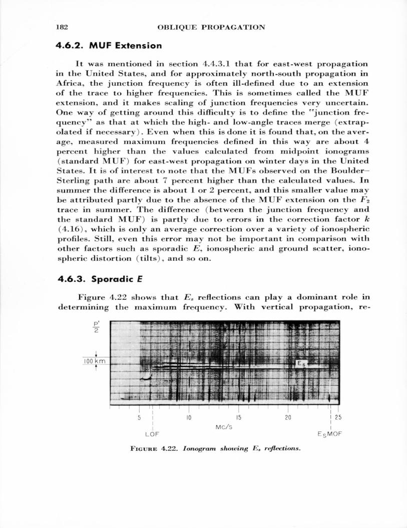
182 OBLIQUE PROPAGATION
4.6.2. MUF Extension
It was mentioned in section 4.4.3.1 that for east-west propagation in the United States, and for approximately north-south propagation in Africa, the junction frequency is often ill-defined due to an extension of the trace to higher frequencies. This is sometimes called the MUF extension, and it makes scaling of junction frequencies very uncertain. One way of getting around this difficulty is to define the "junction fre quency" as that at which the high- and low-angle traces merge (extrap olated if necessary). Kven when this is done it is found that, on the aver age, measured maximum frequencies defined in this way are about 4 percent higher than the values calculated from midpoint ionograms (standard MUF) for east-west propagation on winter days in the United States. It is of interest to note that the MUFs observed on the Boulder- Sterling path are about 7 percent higher than the calculated values. In summer the difference is about 1 or 2 percent, and this smaller value may be attributed partly due to the absence of the MUF extension on the F^ trace in summer. The difference (between the junction frequency and the standard MUF) is partly due to errors in the correction factor k (4.16), which is only an average correction over a variety of ionospheric profiles. Still, even this error may not be important in comparison with other factors such as sporadic £", ionospheric and ground scatter, iono spheric distortion (tilts), and so on.
4.6.3. Sporadic E
Figure 4.22 shows that Es reflections can play a dominant role in determining the maximum frequency. With vertical propagation, re-
LOF E S MOF
FIGURE 4.22. lonogram showing K, reflections.
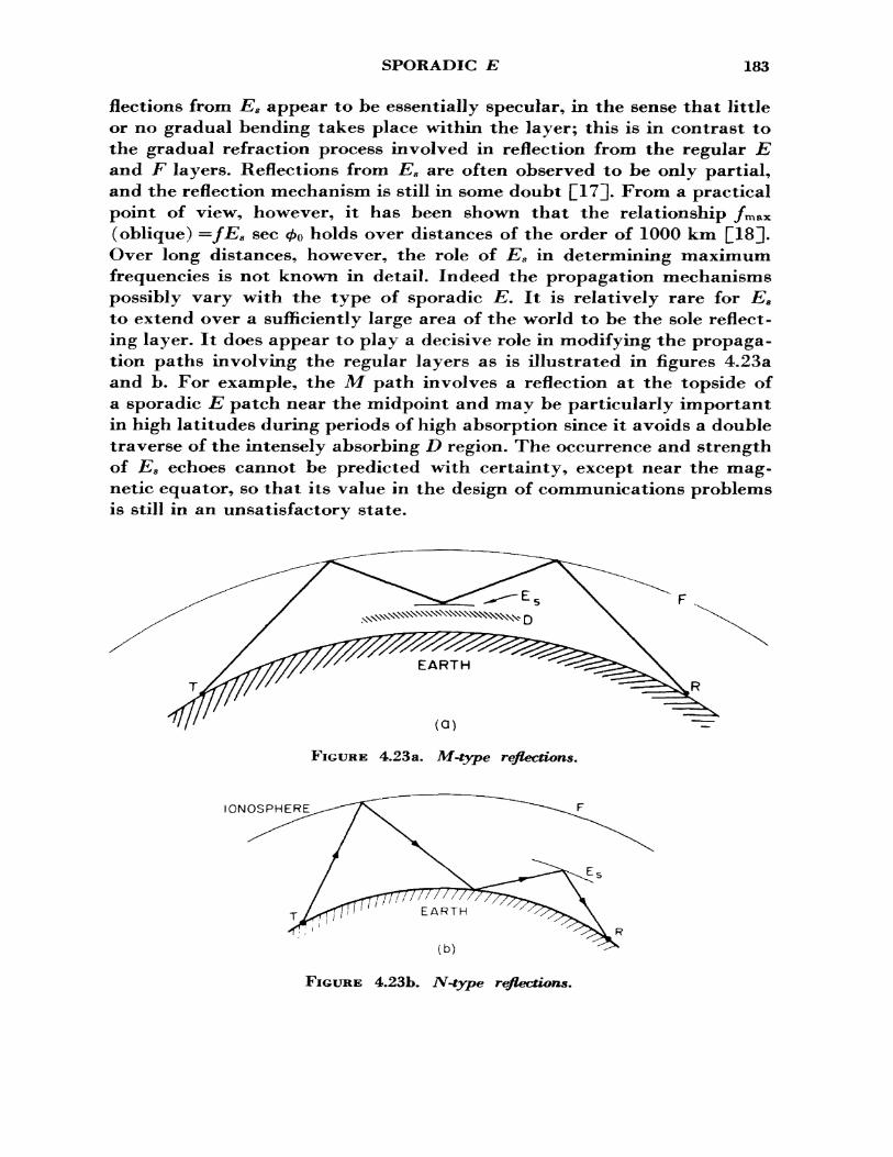
SPORADIC E 183
flections from E8 appear to be essentially specular, in the sense that little or no gradual bending takes place within the layer; this is in contrast to the gradual refraction process involved in reflection from the regular E and F layers. Reflections from Es are often observed to be only partial, and the reflection mechanism is still in some doubt C17J. From a practical point of view, however, it has been shown that the relationship (oblique) =fEs sec <£0 holds over distances of the order of 1000 km Over long distances, however, the role of Es in determining maximum frequencies is not known in detail. Indeed the propagation mechanisms possibly vary with the type of sporadic E, It is relatively rare for Es to extend over a sufficiently large area of the world to be the sole reflect ing layer. It does appear to play a decisive role in modifying the propaga tion paths involving the regular layers as is illustrated in figures 4.23a and b. For example, the M path involves a reflection at the topside of a sporadic E patch near the midpoint and may be particularly important in high latitudes during periods of high absorption since it avoids a double traverse of the intensely absorbing D region. The occurrence and strength of E8 echoes cannot be predicted with certainty, except near the mag netic equator, so that its value in the design of communications problems is still in an unsatisfactory state.
\\\\\^^^^^^ D
(a)
FIGURE 4.23a. M-type reflections.
IONOSPHERE
EARTH
(b)
FIGURE 4,23b. N-type reflections.
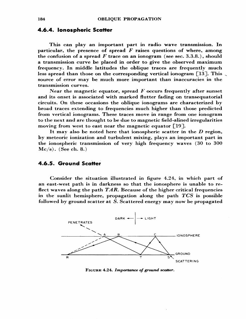
184 OBLIQUE PROPAGATION
4.6.4. Ionospheric Scoffer
This can play an important part in radio wave transmission. In particular, the presence of spread F raises questions of where, among the confusion of a spread F trace on an ionogram (see sec. 3.3.8.)* should a transmission curve be placed in order to give the observed maximum frequency. In middle latitudes the oblique traces are frequently much less spread than those on the corresponding vertical ionogram £13]. This source of error may be much more important than inaccuracies in the transmission curves.
Near the magnetic equator, spread .F occurs frequently after sunset and its onset is associated with marked flutter fading on transequatorial circuits. On these occasions the oblique ionograms are characterized by broad traces extending to frequencies much higher than those predicted from vertical ionograms. These traces move in range from one ionogram to the next and are thought to be due to magnetic field-alined irregularities moving from west to east near the magnetic equator []193-
It may also be noted here that ionospheric scatter in the D region, by meteoric ionization and turbulent mixing, plays an important part in the ionospheric transmission of very high frequency waves (30 to 300 Mc/s). (See ch. 8.)
4.6.5. Ground Scatter
Consider the situation illustrated in figure 4.24, in which part of an east -west path is in darkness so that the ionosphere is unable to re flect waves along the path TAR. Because of the higher critical frequencies in the sunlit hemisphere, propagation along the path TCS is possible followed by ground scatter at S. Scattered energy may now be propagated
DARKPENETRATES
LIGHT
.IONOSPHERE
GROUND
SCATTERING
FIGURE 4.24. Importance of ground scatter.
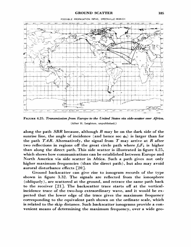
GROUND SCATTER
POSSIBLE PROPAGATION PATHS, GREENVILLE-MUNICH
185
FIGURE 4.25. Transmission from Europe to the United States via side-scatter over Africa.(After H. Leigh tori, unpublished.)
along the path SBR because, although B may be on the dark side of the sunrise line, the angle of incidence (and hence sec 0o) is larger than for the path TAR. Alternatively, the signal from T may arrive at R after two reflections in regions off the great circle path where foF2 is higher than along the direct path. This side scatter is illustrated in figure 4.25, which shows how communications can be established between Europe and North America via side scatter in Africa. Such a path gives not only higher maximum frequencies (than the direct path), but also may avoid auroral disturbance effects [[20].
Ground backscatter can give rise to ionogram records of the type shown in figure 3.32. The signals are reflected from the ionosphere (obliquely), are scattered at the ground, and retrace the same path back to the receiver [[21]. The backscatter trace starts off at the vertical- incidence trace of the two-hop extraordinary wave, and it would be ex pected that the lower edge of the trace gives the maximum frequency corresponding to the equivalent path shown on the ordinate scale, which is related to the skip distance. Such backscatter ionograms provide a con venient means of determining the maximum frequency, over a wide geo-
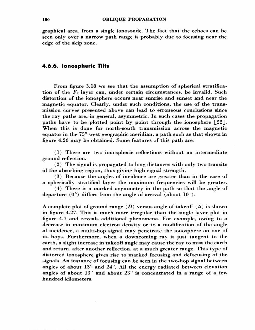
186 OBLIQUE PROPAGATION
graphical area, from a single ionosonde. The fact that the echoes can be seen only over a narrow path range is probably due to focusing near the edge of the skip zone.
4.6.6. Ionospheric Tilts
From figure 3.18 we see that the assumption of spherical stratifica tion of the Jp2 layer can, under certain circumstances, be invalid. Such distortion of the ionosphere occurs near sunrise and sunset and near the magnetic equator. Clearly, under such conditions, the use of the trans mission curves presented above can lead to erroneous conclusions since the ray paths are, in general, asymmetric. In such cases the propagation paths have to be plotted point by point through the ionosphere £22]. When this is done for north-south transmission across the magnetic equator in the 75° west geographic meridian, a path such as that shown in figure 4.26 may be obtained. Some features of this path are:
(1) There are two ionospheric reflections without an intermediate ground reflection.
(2) The signal is propagated to long distances with only two transits of the absorbing region, thus giving high signal strength.
(3) Because the angles of incidence are greater than in the case of a spherically stratified layer the maximum frequencies will be greater.
(4) There is a marked asymmetry in the path so that the angle of departure (0°) differs from the angle of arrival (about 10 ).
A complete plot of ground range (D) versus angle of takeoff (A) is shown in figure 4.27. This is much more irregular than the single layer plot in figure 4.7 and reveals additional phenomena. For example, owing to a decrease in maximum electron density or to a modification of the angle of incidence, a multi-hop signal may penetrate the ionosphere on one of its hops. Furthermore, when a downcoming ray is just tangent to the earth, a slight increase in takeoff angle may cause the ray to miss the earth and return, after another reflection, at a much greater range. This type of distorted ionosphere gives rise to marked focusing and defocusing of the signals. An instance of focusing can be seen in the two-hop signal between angles of about 13° and 24°. All the energy radiated between elevation angles of about 13° and about 23° is concentrated in a range of a few hundred kilometers.
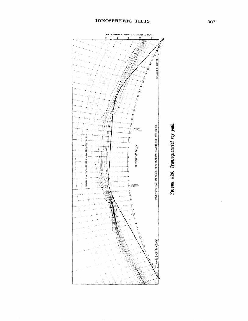
IONOSPHERIC TILTS 187
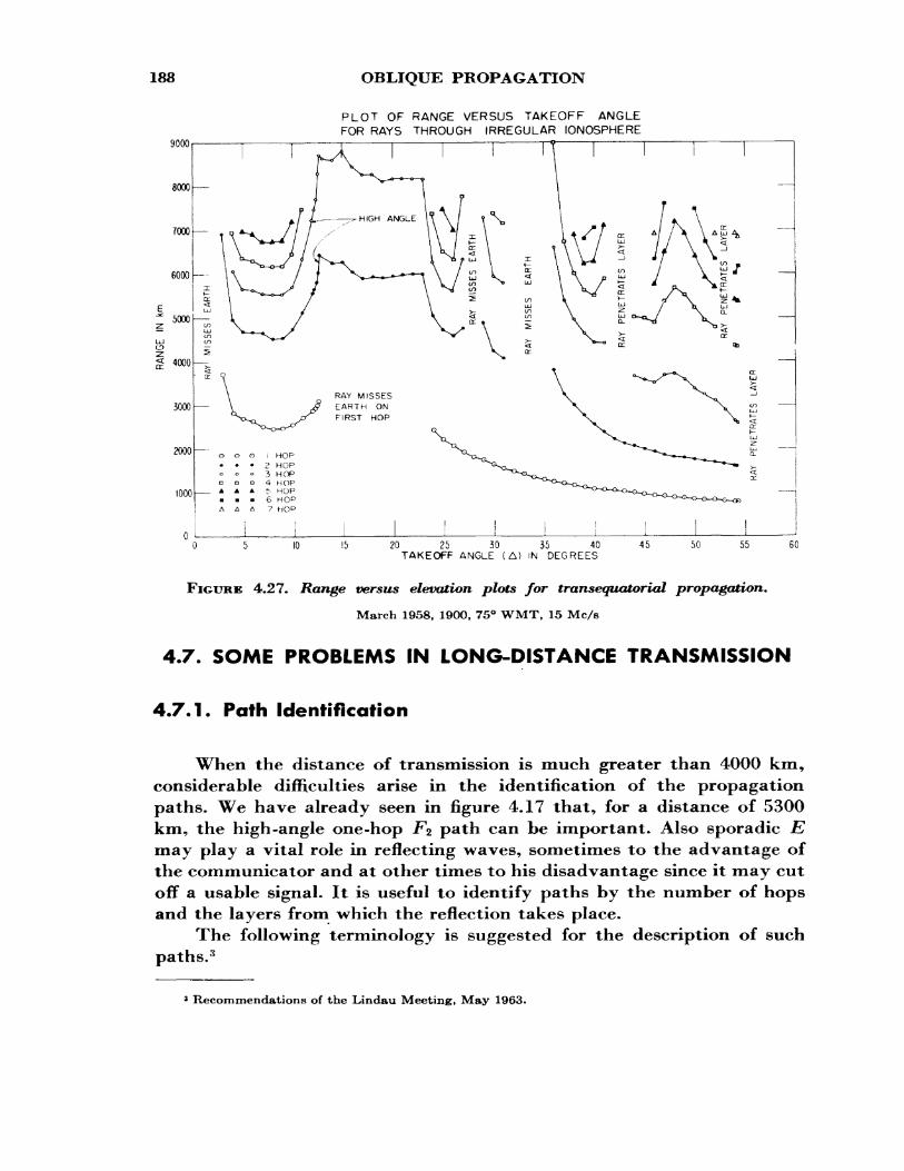
188
9000
8000
OBLIQUE PROPAGATION
PLOT OF RANGE VERSUS TAKEOFF ANGLE FOR RAYS THROUGH IRREGULAR IONOSPHERE
20 25 30 35 40 TAKEOFF ANGLE (A) IN DEGREES
45 50 55 60
FIGURE 4.27. Range versus elevation plots for transequatorial propagation.
March 1958, 1900, 75° WMT, 15 MC/B
4.7. SOME PROBLEMS IN LONG-DISTANCE TRANSMISSION
4.7.1. Path Identification
When the distance of transmission is much greater than 4000 km, considerable difficulties arise in the identification of the propagation paths. We have already seen in figure 4.17 that, for a distance of 5300 km, the high-angle one-hop F2 path can be important. Also sporadic E may play a vital role in reflecting waves, sometimes to the advantage of the communicator and at other times to his disadvantage since it may cut off a usable signal. It is useful to identify paths by the number of hops and the layers from which the reflection takes place.
The following terminology is suggested for the description of such paths. 3
3 Recommendations of the Lindau Meeting, May 1963.
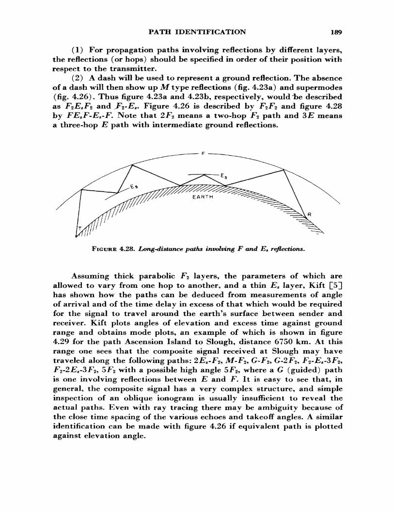
PATH IDENTIFICATION 189
(1) For propagation paths involving reflections by different layers, the reflections (or hops) should be specified in order of their position with respect to the transmitter.
(2) A dash will be used to represent a ground reflection. The absence of a dash will then show up M type reflections (fig. 4.23a) and supermodes (fig. 4.26). Thus figure 4.23a and 4.23b, respectively, would 'be described
and JFz-E8 . Figure 4.26 is described by -F2 F2 and figure 4.28asby FEsF-Es-F. Note that 2F2 means a two-hop F2 path and 3E means a three -hop E path with intermediate ground reflections.
FIGURE 4.28. Long-distance paths involving F and E9 reflections.
Assuming thick parabolic F% layers, the parameters of which are allowed to vary from one hop to another, and a thin E8 layer, Kift £5] has shown how the paths can be deduced from measurements of angle of arrival and of the time delay in excess of that which would be required for the signal to travel around the earth's surface between sender and receiver. Kift plots angles of elevation and excess time against ground range and obtains mode plots, an example of which is shown in figure 4.29 for the path Ascension Island to Slough, distance 6750 km. At this range one sees that the composite signal received at Slough may have traveled along the following paths: 2E& -F^ M-F2, G-F2, G-2F2, F2-1%-3F2, F2 -2£*S -3F2, 5F2 with a possible high angle 5F2, where a G (guided) path is one involving reflections between E and F. It is easy to see that, in general, the composite signal has a very complex structure, and simple inspection of an oblique ionogram is usually insufficient to reveal the actual paths. Even with ray tracing there may be ambiguity because of the close time spacing of the various echoes and takeoff angles. A similar identification can be made with figure 4.26 if equivalent path is plotted against elevation angle.
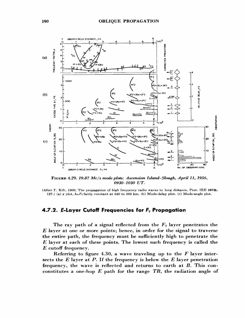
190 OBLIQUE PROPAGATION
T GREAT-CIRCLE DISTANCE , Km0123
/IF2 (2F2 13F2 (4F2 |Ce^I \ x. v v^ ! 7
GREAT-C (RCLE Dl STANCE O, Km
O 20 40 No OF OBSERVATIONS
FIGURE 4.29. 19.57 Mc/s mode plots: Ascension Island-Slough^ April 11, 1956,0930-1030 UT.
(After F. Kift T 1960, The propagation of high frequency radio waves to long distance, Proc. IEE 107B, 127.) (a) x plot, hmFi fairly constant at 340 to 360 km. (b) Mode-delay plot, (c) Mode-angle plot.
4.7.2. E-Layer Cutoff Frequencies for F2 Propagation
The ray path of a signal reflected from the F2 layer penetrates the E layer at one or more points; hence, in order for the signal to traverse the entire path, the frequency must be sufficiently high to penetrate the E layer at each of these points. The lowest such frequency is called the E cutoff frequency.
Referring to figure 4.30, a wave traveling up to the F layer inter sects the E layer at P. If the frequency is below the E layer penetration frequency, the wave is reflected and returns to earth at B. This con- constitutes a one-hop E path for the range 77?, the radiation angle of
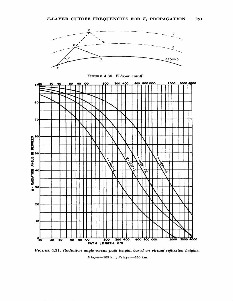
J£-LAYER CUTOFF FREQUENCIES FOR F2 PROPAGATION 191
P/
FIGURE 4.30. E layer cutoff.
io20 3O 4O *0 8O 100 COO 3OO 4OO 6OO SOO 1000 1
80
70
•0
5O
4O
30
to
IO
ft
S5•\-"" ««b-
^
•* •• •*^^"^
X
»*»*
Xs
^^"*•*s
"^
•x
S
V
•^
s,
^
s
s
s
^x
^
s
\
^*
X
S
\
»v
sv
\
x
\
s
s
s
s
^
s\
-
^
s
ss
\
9 t*J
v
\
\
\
s
sV
s
.s
\rO
ss
\iV
N
r*
s
\
*
\\
V,
\
\V
\
^
^
a
>
V
s
\
s
s
\^
\
s
\
9
\
\|
N
s
v̂\
ss
^
9
^
Ss
s
tOOO 30004000
\
N
^
\
\^
\
^
\
S^
L
^
>
Ul
30 40 60 80 KX> tOO SOO 4OO 6OO BOO JOOO 2OOO 3OOO 4OOO PATH LENGTH, km
FIGURE 4.31. Radiation angle versus path length, based on virtual reflection heights.
E layer—1Q5 km; F* layer—320 km.
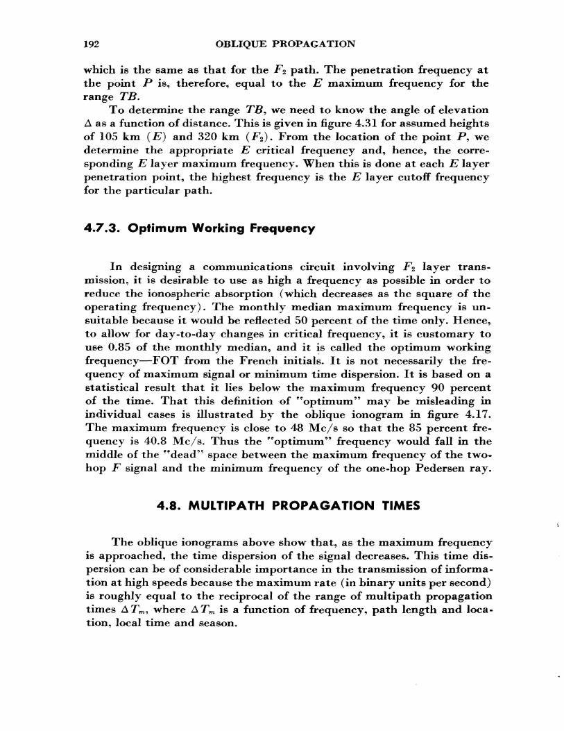
192 OBLIQUE PROPAGATION
which is the same as that for the F% path. The penetration frequency at the point P is, therefore, equal to the E maximum frequency for the range TB.
To determine the range TB, we need to know the angle of elevation A as a function of distance. This is given in figure 4.31 for assumed heights of 105 km (E) and 320 km (JPa). From the location of the point P, we determine the appropriate E critical frequency and, hence, the corre sponding E layer maximum frequency. When this is done at each E layer penetration point, the highest frequency is the E layer cutoff frequency for the particular path.
4.7.3. Optimum Working Frequency
In designing a communications circuit involving F* layer trans mission, it is desirable to use as high a frequency as possible in order to reduce the ionospheric absorption (which decreases as the square of the operating frequency). The monthly median maximum frequency is un suitable because it would be reflected 50 percent of the time only. Hence, to allow for day-to-day changes in critical frequency, it is customary to use 0.85 of the monthly median, and it is called the optimum working frequency—FOT from the French initials. It is not necessarily the fre quency of maximum signal or minimum time dispersion. It is based on a statistical result that it lies below the maximum frequency 90 percent of the time. That this definition of "optimum" may be misleading in individual cases is illustrated by the oblique ionogram in figure 4.17. The maximum frequency is close to 48 Mc/s so that the 85 percent fre quency is 40.8 Mc/s. Thus the "optimum" frequency would fall in the middle of the "dead" space between the maximum frequency of the two- hop F signal and the minimum frequency of the one-hop Pedersen ray.
4.8. MULTIPATH PROPAGATION TIMES
The oblique ionograms above show that, as the maximum frequency is approached, the time dispersion of the signal decreases. This time dis persion can be of considerable importance in the transmission of informa tion at high speeds because the maximum rate (in binary units per second) is roughly equal to the reciprocal of the range of multipath propagation times A Tm , where ATm is a function of frequency, path length and loca tion, local time and season.
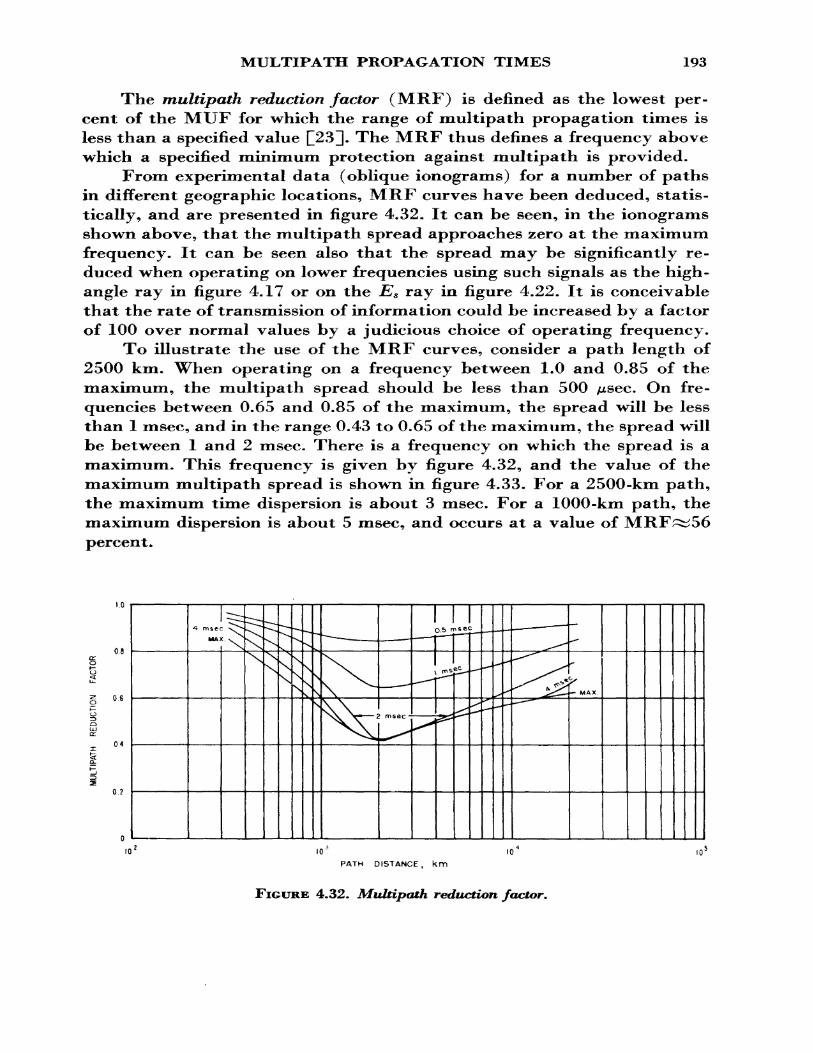
MULTIPATH PROPAGATION TIMES 193
The multipath reduction factor (MRF) is defined as the lowest per cent of the MUF for which the range of multipath propagation times is less than a specified value [J233- The MRF thus defines a frequency above which a specified minimum protection against multipath is provided.
From experimental data (oblique ionograms) for a number of paths in different geographic locations, MRF curves have been deduced, statis tically, and are presented in figure 4.32. It can be seen, in the ionograms shown above, that the multipath spread approaches zero at the maximum frequency. It can be seen also that the spread may be significantly re duced when operating on lower frequencies using such signals as the high- angle ray in figure 4.17 or on the E8 ray in figure 4.22. It is conceivable that the rate of transmission of information could be increased by a factor of 100 over normal values by a judicious choice of operating frequency.
To illustrate the use of the MRF curves, consider a path length of 2500 km. When operating on a frequency between 1.0 and 0.85 of the maximum, the multipath spread should be less than 500 /xsec. On fre quencies between 0.65 and 0.85 of the maximum, the spread will be less than 1 msec, and in the range 0.43 to 0.65 of the maximum, the spread will be between 1 and 2 msec. There is a frequency on which the spread is a maximum. This frequency is given by figure 4.32, and the value of the maximum multipath spread is shown in figure 4.33. For a 2500-km path, the maximum time dispersion is about 3 msec. For a 1000-km path, the maximum dispersion is about 5 msec, and occurs at a value of percent.
PATH DISTANCE, km
FIGURE 4.32. Multipath reduction factor*
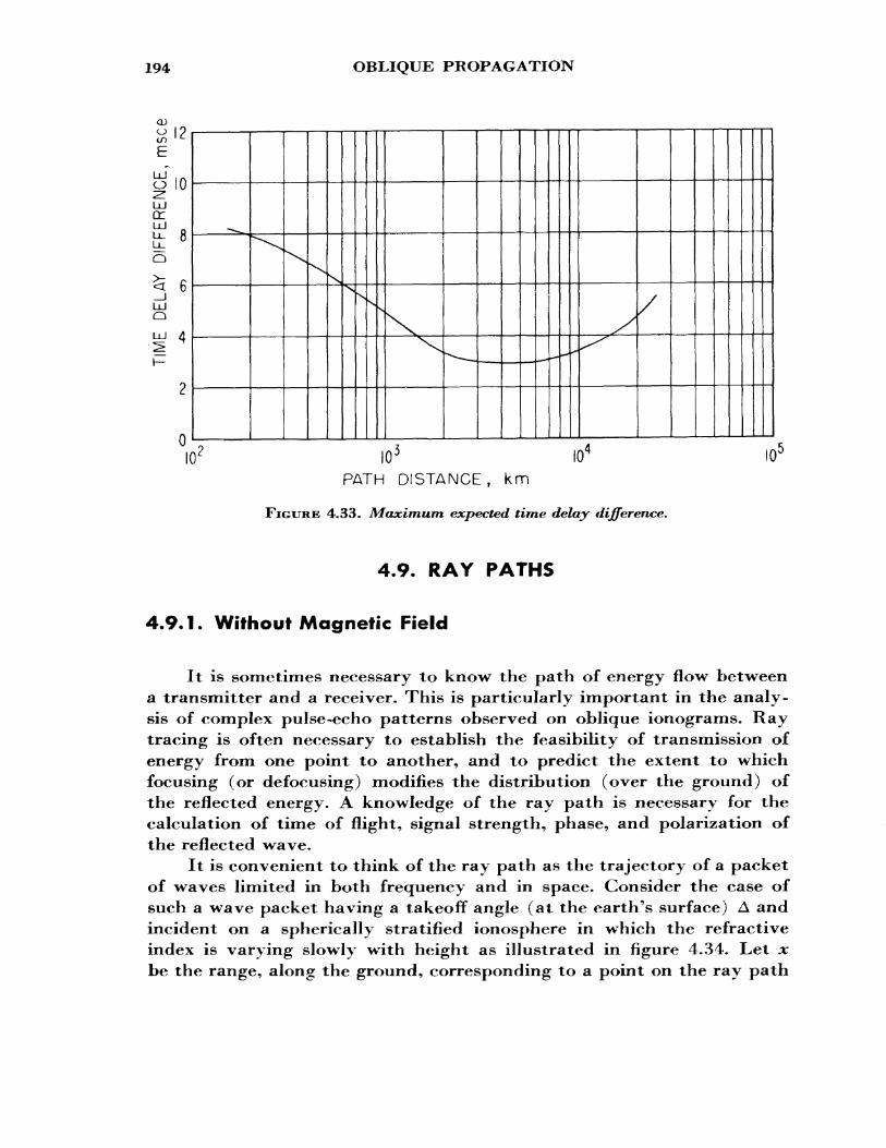
194 OBLIQUE PROPAGATION
CDin I*e
o~IO
LUor
t 8
— c*
LU 0
LU 4
2
n
"^^\
N ss
vk^_ p^. — * X-x^/
I0 3 I04
PATH DISTANCE, km
FIGURE 4.33. Maximum expected time delay difference.
4.9. RAY PATHS
10*
4.9.1. Without Magnetic Field
It is sometimes necessary to know the path of energy flow between a transmitter and a receiver. This is particularly important in the analy sis of complex pulse-echo patterns observed on oblique ionograms. Ray tracing is often necessary to establish the feasibility of transmission of energy from one point to another, and to predict the extent to which focusing (or defocusing) modifies the distribution (over the ground) of the reflected energy. A knowledge of the ray path is necessary for the calculation of time of flight, signal strength, phase, and polarization of the reflected wave.
It is convenient to think of the ray path as the trajectory of a packet of waves limited in both frequency and in space. Consider the case of such a wave packet having a takeoff angle (at the earth's surface) A and incident on a spherically stratified ionosphere in which the refractive index is varying slowly with height as illustrated in figure 4.34. Let x be the range, along the ground, corresponding to a point on the ray path
WITHOUT MAGNETIC FIELD 195
FIGURE 4.34. Ray path geometry for a spherically stratifiedionosphere.
at a height h above ground, and let x subtend an angle G at the center of the earth. From figure 4.34
(4.18)
(4.19)
(4.20)
together with SnelFs law (see 4.9)
this gives
e =
a+/i) sin i = a cos A,
a cos A dh
(o+A) ^- cos2 A
One solution to the problem of ray tracing is to approximate the electron density profile by a suitable model in order to evaluate, analytically,
196 OBLIQUE PROPAGATION
the integral for 0. This is relatively simple to do in the case of a plane earth and plane ionosphere when the ground range x is given by
cos A dh\//j?— cos2 A
(4.21)
The solutions of (4.21) for some of the more commonly used models are given by Budden £24, ch. 11].
When the curvature of the ionosphere is taken into account, the problem is more difficult, Appleton and Beynon £4] assumed a layer shape which is derived from a parabola by neglecting small terms, and they ob tained (4.17) for the ground range. In general, however, it is not possible to find suitable analytic functions which represent adequately the electron density profiles £25, 26]. Under such circumstances the ray path has to be computed by dividing the profile into a number of laminae and postu lating an analytic N(h) function within each lamina. As the number of laminae used is increased, the result becomes less and less dependent upon the form of the assumed distribution within each segment.
An interesting graphical method has been developed by Chvojkova £27] which is illustrated in figure 4.35 where, for clarity, the refracting shells are separated by infinitesimal non-refracting shells. From Snell's law (fjir sin r —a constant) we see that, outside the ionosphere, the ray direction must always be tangent to the surface of a sphere of radius r sin i0 ; and at any point inside the ionosphere at which the refractive index is ^ the ray is tangential to a sphere of radius (r//z) sin i0 -
FIGURE 4.35. Chvojkova9s construction.
WITH MAGNETIC FIELD (WAVES AND RAYS) 197
4.9.2. With Magnetic Field (Waves and Rays)
From the point of view of ray tracing, the main effects of the mag netic field are
(1) Ordinary and extraordinary waves are produced;(2) The direction of energy flow (ray direction) differs, in general,
from the phase normal;(3) The refractive index depends upon the angle of refraction, so that
it is not possible to solve SnelFs law directly.
The angle a. between the directions of phase propagation and energy propagation is given by (2.123), namely
1 dv 1 dfji , A ^^.tan <*= —— — = - -f . (4.22)v de fji de
Substituting the expression for /x(2.77) in (4.22) we obtain
(i>*-l-)YT YL(4.23)
The + and — signs refer to the ordinary and to the extraordinary rays respectively. Note that on is of opposite sign for the ordinary and extra ordinary waves except when the refractive index of one of the rays is greater than unity. Furthermore, the sign of tan a changes as 6 goes through 90°.
Bremmer C28] has summarized the ray behavior as follows:
(a) The wave normal is parallel to the plane of incidence and satis fies SnelFs law,
(b) The ray is situated in the plane through the wave normal and the earth's magnetic field.
(c) The angle a. measured from the wave normal to the ray, is given by (4.23).
Before considering some actual ray paths, it is of interest to consider the implications of these rules. First they imply that, as a wave packet penetrates into the ionosphere, it ffslips" sideways in a direction parallel to the magnetic meridian. For upgoing waves the extraordinary ray is (for /z<l) deflected towards the magnetic equator, whereas the ordinary ray is deflected away from the magnetic equator. Second, let us consider (4.23) in the case of waves propagating vertically. We see that tan ex is
198 OBLIQUE PROPAGATION
zero under the following conditions:
Y = 0, no magnetic field0 = 0°, 180° propagation at the magnetic poles0 = 90° propagation at the magnetic equator
At the levels of reflection, M = 0 and X=l for the ordinary wave and X = l± Y for the extraordinary waves. This gives
tan c*0 = —cot 6, (4.24)
sin 0 cos 6 sin 9 cos 8 , A _ Ntan ok = —:F= =—————— - (4.25) 7 " ' rt ' '^9 l+cos2 0
Hence, at reflection, the ordinary ray is perpendicular to the earth's magnetic field. Note that a* depends on the direction, but not on the magnitude, of the earth's magnetic field.
4.9.3. Some Sample Ray Paths
4.9.3.1. Vertical Propagation
Applying SnelFs law in a plane stratified ionosphere, we find that the wave normal is always vertical. The lateral deviation D at a height h is given by
D-/* n
htan a. dh. (4.26)
o
In the general case this expression is too complicated to solve analyti cally, but D can be found by dividing the electron density profile into a number of slabs and determining the mean value of tan a (tan a say) for each slab, then summing, i.e.,
(4.27)
where A/i t is the thickness of the £th slab.Ray paths over Boulder, Colo., which have been calculated by this
method, are shown in figures 4.36 and 4.37. Consider first the paths on frequencies greater than the gyrofrequency ( = 1.5 Mc/s approx.). The
ORDI
NARY BO
ULDE
R NO
V.
28,
1959
00
30
EXTR
AORD
INAR
Y
. I—
——
I——
—I
10
0 10
20
30
40
s km
N*
400
300
E
200
100
500
400
E * 3
00
200
\c\r\
\- J—
—l—
—I—
—l—
—l—
—I—
—L
8 20
10
0
10
20
30
40§•
»S
,
N*
s km
_______11)1
20
10 0
10 20
30
40
*s
km
N-
I lilt
20
10
0 10
20
30
40
*s
km
N-
I I
1 I
I I
I20
10
0
10
20
30
40*s
km
N
*2 9 B
200 OBLIQUE PROPAGATION
340
320
30O
280
260
24O
2 2O
2OO
ISO
160
I4O
120
ORDINARY ————— EXTRAORDINARY
100
BOULDER NOV. 28, 1959 OO3O 1.4 MC/S
^
O IO 2O 3O 4O 5O 6O 7O 8O 9O 1OO MO 12O I3O I4O ISO I6O I7O ISO I9Okm N^
BOULDER NOV. 28, 1959 OO3O280
260
24O
220
2OO
I8O
I6O
I4O
12O
inn
-
-
:\ :\\ \
\ '-
r \.
-iii
I.O MC/S
\\1
1 t 1 1
\\
\ 1.2 MC/S
\\\
^ — """"' J^^*****^ jS
s^ ''"''''- s *'"*''i-"'"
i t t i i i i i
km km
FIGURE 4.37. Some ray paths tuith normal incidence over Boulder on frequencies less thanthe gyrofrequency.
SAMPLE RAY PATHS 201
following features are of interest:
(1) The ray paths lie entirely in the magnetic meridian.(2) On a given frequency, less than the penetration frequency, the
deviation (to the north) of the o ray at reflection is always greater than that (to the south) of the extraordinary ray at its level of reflection.
(3) On a given frequency and for the same real height, the deviation of the extraordinary ray is greater than that of the ordinary ray.
(4) Most of the deviation of the ordinary ray takes place relatively close to the reflection level.
On a frequency less than the gyrofrequency, the situation is a little different. The ordinary wave behaves much the same as before, but the behavior of the extraordinary (z) wave is different. In figure 2.9 we see that, for 0<X<1, the refractive index of the extraordinary wave is greater than unity so that in this range /x2 —1 is positive and the ray is deflected to the north. For values of X between 1 and 1+ Y (reflection), /ji is less than unity and the ray veers to the south. Whether the point of reflection lies to the north or the south of the point of entry will depend on the frequency and on the profile. The path of the downcoming wave is identical with that of the upgoing wave. Owing to electron collisions, these paths will be modified slightly, the modification becoming more pro nounced as the wave frequency approaches the gyrofrequency.
On a frequency close to the penetration frequency of the F% layer, the ordinary ray may be deviated by 50 or 60 km; however, the deviation within the layer falls off rapidly as the frequency increases above /o^V For example, with fvFz— 10 Mc/s the deviation, with a complete passage through a Chapman layer on a frequency of 40 Mc/s, is of the order of 0.1 km.
Because of the lateral deviations, the ordinary and extraordinary rays, in practice, sample slightly different electron density profiles.
4.9.3*2. Oblique Paths
For fairly short distances of transmission, the plane containing the emergent ray is parallel to, but not necessarily coincident with, the great circle plane containing the incident ray. The incident and emergent planes are coincident for exactly east-west propagation in all latitudes and for north-south propagation in a magnetic meridian. Some ray paths have been calculated in the case of approximately east-west propagation in the United States with a parabolic distribution of electron density with height and the dipole approximation (earth centered) to the earth's
202 OBLIQUE PROPAGATION
LATERAL DEVIATION (METERS)
4OO -
2OO -
-200 -
-400 -
EXIT
DIPOLE FIELD,h 0 = 20O km, y m = IOO km
ELEVATION = 26.717°f = 14.t42 MC/S
EXTRAORDINARY^,
TRANS:
REC:
39° LAT.-75° LONG.
4O° LAT.-IO5° LONG
ENTRY
550
EXIT
35O RANGE FROM TRANSMITTERkm
6OO
NORTH
\
FIGURE 4.38. Horizontal projection of ray paths in a parabolic layer for geographicallyeast-ivest propagation in the United States.
magnetic field. The projections of the paths on to a horizontal plane are shown in figure 4.38. The paths are twisted, veering first in one direction and then in the other. The maximum deviations are about 0.3 km, and the net deviations, at the point of exit from the ionosphere, are only about 100 m. Furthermore, the ordinary and extraordinary rays are, roughly, mirror images of each other. The deviation tends to increase with operating frequency because of the increase in depth of penetration of the ray into the layer; however, the deviations with oblique propagation are much less than with vertical propagation.
With propagation in the magnetic meridian (north-south) there is no lateral displacement of the ray, but the point of energy reflection is, in general, displaced from the center of the path* The point of reflection of the ordinary wave is displaced to a higher magnetic latitude than the midpoint and vice versa for the extraordinary wave.
Ionospheric ray paths can be calculated in a variety of ways. Those more commonly used are the Booker quartic £29], the iterative method C^OJ, Haselgrove's equations pJl], Titheridge's approximate method []32]], and Poeverlein's graphical construction Q33]].
Poeverlein's method is of interest because it illustrates the existence of the "spitze." It is a graphical method and depends on the fact that, for a refractive index surface,4 the radius vector gives the wave normal
4 The refractive index surface is the locus of end points of a vector whose magnitude is the refractive index and whose direction is the direction of phase propagation.
SAMPLE RAY PATHS 203
jiirection and the normal to the surface is the ray direction, as shown in figure 4.39. The wave normal direction is known from Snell's law, so the ray direction can be obtained from the construction shown in figure 4.39. From this direction the next point on the ray is determined and the procedure is repeated. Note that the condition for energy reflection is given by a point such as A where the normal to the /x surface is horizontal, but where the wave normal is not, in general, horizontal.
DIRECTION OF EARTH'S MAGNETIC FIELD
FIGURE 4.39. Illustrating Poeverlein?s construction
Direction in which the ray R is normal to the refractive index surface. N, the wave normal, is given by the direction of the radius vector. Curves not drawn to scale.
Using this construction, with oblique propagation in the magnetic meridian, Poeverlein showed that, for angles of incidence less than a certain critical value 0t (where sin 0,; = A/C Y/ (1 + Y") D cos/, /=dip), the path of the ordinary ray never becomes horizontal, but has a cusp at the level X=l. This phenomenon, called the ffspitze," is illustrated by the ray paths in figure 4.40. An excellent description of the behavior of rays for many special cases is given by Budden Q24, ch. 13^ where he shows that on frequencies greater than the gyrofrequency the spitze is not exhibited by the extraordinary ray.
204 OBLIQUE PROPAGATION
DIRECTION OF MAGNETIC FIELD
EARTH
FIGURE 4.40. Sample ordinary ray paths for oblique propagation in magnetic meridian,, showing the Spitze.
Not drawn to scale.
4.9.3.3. Topside Soundings
With the advent of artificial earth satellites it is necessary to con sider reflections from the topside of the ionosphere and transmission be tween satellites and ground.
Some ray paths for waves having the vertical direction of phase propagation are shown in figure 4.41 for various heights above the peak of a Chapman layer in the northern hemisphere. Note that the ordinary ray is deviated to the south and the extraordinary ray is deviated to the north. As the height of the satellite decreases, i.e., as the surrounding electron density increases, first the extraordinary wave and second the ordinary wave get "imprisoned" in the satellite because the plasma is overdense to waves of that frequency (e.g., 5 Mc/s). When the satellite is near its reflection level, the ordinary wave energy slides almost side ways. An additional path (the z path) is possible, which may be under stood by reference to figure 2.9. For F<1 it will be seen that there is a branch of the extraordinary curve lying in the range
Normally this wave cannot originate except from a source embedded in
SAMPLE RAY PATHS 205
ORDINARYfUUU
700
400
300
1000
_*:
^ 700 0LU
400
300
1000
700
400
300 2
A 5 Mc/s/
/
_
—
i
__ _ .
>-<r
5Cd- § -01
LU
_
1
1 —— "1
trcr- S -oz
i
^_^-— - — »
i 1 i
— - — —— -
III.
>-
• ^0cr • oo. z:
1 , 100 20 40
- ——— N S ——— -
— — - EXTRAORDINARY
IO Mc/s
kmFIOURE 4.41. Some ordinary and extraordinary ray paths from a topside sounder located
at heights of 1000 fcro, 7OO km9 and 400 km in a Chapman layer.
Penetration frequency (o wave)=10 Mc/s/jyr=0.75 MC/S
Dip=72.9°.
206 OBLIQUE PROPAGATION
1000 r T
980
960 -
940 -
920
1000
980
960
940 -
2,236 MC/S
20 0 20 - — S N — -
40 60
920
2.242MC/S
60 40 20 0 80
Km
40
60
2.24O MC/S
20 0 20-—S N——
2.249 Mc/S ._
40 S
20
FIGURE 4.42. Some z ray paths from a topside sounder located at a height of1000 km in a Chapman layer.
Penetration frequency (o wave)=10 Mc/sfff=Q.75 Mc/s
Dip=72.9°
Q_ UJ Q
I F I I I 1 II.5 2.5 3.5 4.5 5.5 6.5 7.5 8.5 9.5 10.5
Mc/s
FIGURE 4.43. Topside ionogram, Singapore* Nov. 199 1962, 0810 UT.(Reproduction is by permission of the Controller of Her Brittannic Majesty's Stationery
Office and is by arrangement with the Director of Radio Research.)
SAMPLE RAY PATHS 207
the plasma. To get some idea of what the ray paths may look like we notice that /x2 >l near X= (1— Y2)/(l— Yf,) and M drops below 1 as it ap proaches reflection. The quantity (^2 —1) and, hence <*, will change sign. The ray path veers first to one side and then to the other, as illustrated in figure 4.42. The existence of the z-wave has been confirmed in recent soundings of the topside—see figure 4.43.
4.9*3.4. Satellite-to-Ground Paths
To a first approximation on very high frequencies, the effective ionosphere exists only within a definite range of heights, and we shall assume (for the sake of discussion only) that the refractive index is unity both above and below this range. Consider a wave of frequency consider ably greater than the critical frequency; at very oblique incidence the rays are reflected (see fig. 4.44) but within a cone of semiangle <f>o = sin""1 ^m all rays will penetrate the ionosphere. The refractive index Mm£ == "v 1 — (/c//) 2 H is the value at the height of maximum electron density in the absence of the earth's magnetic field and collisions. This blocking effect of the ionosphere for zenith angles greater than a critical value is sometimes called the ^iris" effect.
FIGURE 4.44. The iris effect (plane ionosphere).
208 OBLIQUE PROPAGATION
FIGURE 4.45. Effect of ionosphere curvature on angular error.
With angles less than <f>^ the ray is bent in the layer and so the angle of elevation at the ground is increased by an amount /3 as seen in figure 4.44. The angle (3 is called the "angular error at the observer" and, in this case, it is equal to —/?', the "angular error at the source."
The effects mentioned above for a plane-stratified ionosphere are modified slightly by the curvature of the ionosphere. The geometry is shown in figure 4.45 and shows that the total bending (i.e., the difference in direction of the ray at the source and at the observer), r = /3+/3 / , is no longer zero. Thus the total bending which occurs in a ray passing through the ionosphere is a second-order effect, since the bending of the ray on entering the ionosphere (from above) is compensated for (actually, over- compensated for) by the bending on leaving the ionosphere. With the exception of the special case of radio astronomy, where the source—observer distance is essentially infinity, the angular error at the observer generally differs from, and may be greater or less than, the total bending.
It can be seen that the overall effect of the refracting iris is to focus rays from a large section of the sky into a relatively narrow cone. From the point of view of signals received at the earth from a satellite, this means a smaller signal/noise ratio (see ref. £28J, ch. X, sec. 8).
The effect of the earth's magnetic field is to produce two images of the satellite—ordinary and extraordinary. In the general case of propa gation making an angle (non-zero) with a magnetic meridian, the two rays are deviated in opposite direction from the plane of incidence but the lateral deviation is much smaller than the refractive effects in the plane of incidence. Thus we get a good approximation to the actual ray
SAMPLE RAY PATHS 209
I2OO -
900 -
6OO -
3OO -
1324 MST, SEPT, t7 t 1958
AZIMUTH = 350°
foF2 = 9 Mc/5
x = 382 km
BOULDER
FIGURE 4.46. Ray paths (o and x) from satellite to ground near Boulder, Colo.
(By permission of R. S. Lawrence and E>. J. Posakony, 1962, A digital ray-tracing program for ionospheric research, Space Research II, Proc. 2d Intern. Space Sci. Symp., Florence, North Holland Publ. Co.)
path if we project the ray on to the vertical plane of incidence. In figure 4.46 is an example, projected on a vertical plane (not to scale), of ray paths from a 20 Mc/s satellite-borne transmitter near Boulder, Colo. The total bending along the extraordinary ray always exceeds the total bending along the ordinary ray. In figure 4.46, for example, the total bend ing of the extraordinary wave is 2°.73 while that of the ordinary wave is only 2°.61. Notice that this relationship does not necessarily mean that the angular errors at the observer are similarly related. Several methods are available for estimating the angular error at the observer in the absence of the earth's magnetic field £34, 35].
The above treatment assumes a spherically stratified ionosphere so that horizontal gradients in electron content are ignored. The treatment of refraction in the presence of ionospheric distortion is a complicated process, except in cases of simple models. One such model is that of a rfwedge" of electrons. For angles of incidence near the zenith the relation ship between the wedge refraction r and the horizontal gradient of total electron content is given by £36]]
Ndh. (4.28)
210 OBLIQUE PROPAGATION
Data on ionospheric irregularities can be obtained from measurements on radio-star signals £37, 38], and on satellite radio signals £38].
4.9.4. Propagation Effects Associated With Ray Paths
(a) Phase path P is given by
P=f Mcosads. (4.29)
(b) Group path Pf is given by
P> = f M' Cos a ds. (4.30)
(c) Total absorption L is given by
L= I K cos OL dfs, (4.31)
where /JL and // are the phase and group refractive indices respectively and K (kappa) is the absorption per unit length of path.
It is of interest to note that, when the magnetic field is absent, the relationship between //, yu', and L is given by
L = — (P'-P) (4.32)
provided that v (the collision frequency) is independent of height.
4.9.5. Faraday Rotation
4.9.5*1* Rotation of the Plane of Polarization
A linearly polarized wave can be considered as the resultant of two vectors, of equal amplitude, rotating in opposite senses with the same angular speed. In the case of quasi-longitudinal propagation in the ab sence of absorption, the two characteristic waves (ordinary and extra-
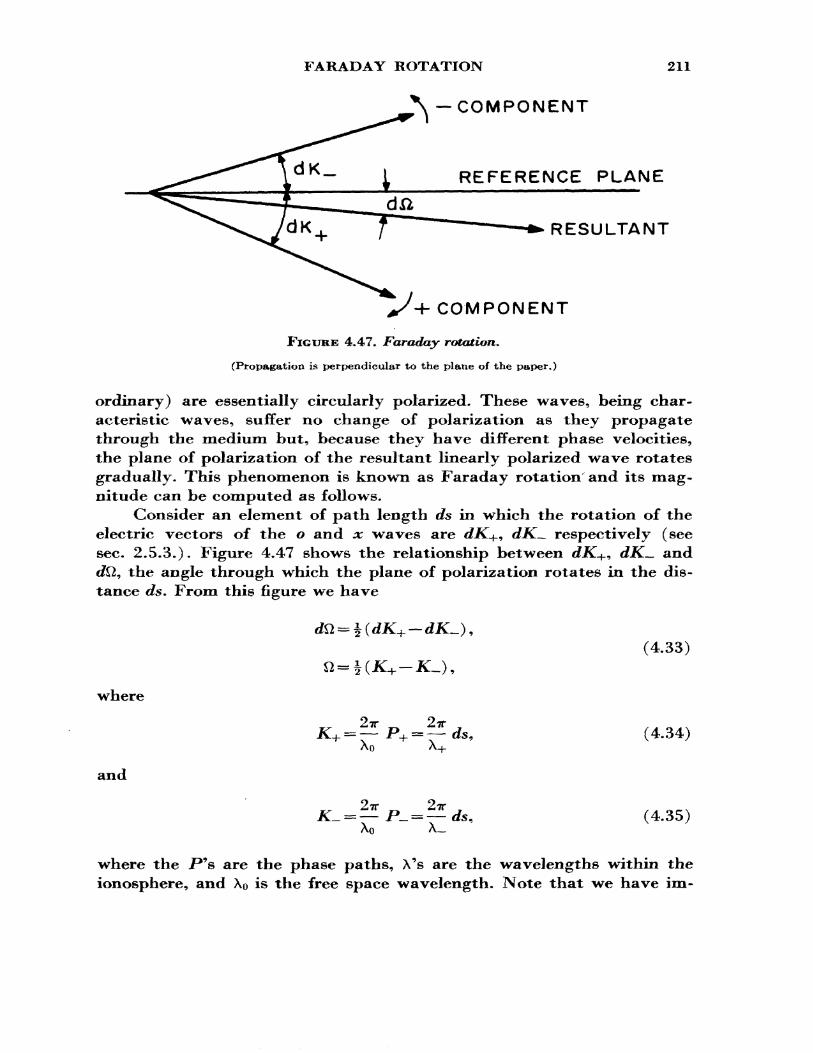
FARADAY ROTATION 211
—COMPONENT
REFERENCE PLANE
RESULTANT
COMPONENT
FIGURE 4,47. Faraday rotation*
(Propagation is perpendicular to the plane of the paper.)
ordinary) are essentially circularly polarized. These waves, being char acteristic waves, suffer no change of polarization as they propagate through the medium but, because they have different phase velocities, the plane of polarization of the resultant linearly polarized wave rotates gradually. This phenomenon is known as Faraday rotation and its mag nitude can be computed as follows.
Consider an element of path length ds in which the rotation of the electric vectors of the o and x waves are dK+, dK^ respectively (see sec. 2.5.3.). Figure 4.47 shows the relationship between dK+, dK— and d£2, the angle through which the plane of polarization rotates in the dis tance ds. From this figure we have
(4.33)
where
and
AO(4.34)
(4.35)
where the .P's are the phase paths, X's are the wavelengths within the ionosphere, and AO is the free space wavelength. Note that we have im-
212 OBLIQUE PROPAGATION
plicitly set cos a, = 1, which restricts the discussion to frequencies well above the plasma frequency.
From (4.33), (4.34), and (4.35) we obtain
n = f f (/4+-/O ds. (4.36) AO J
In the case of quasi-longitudinal propagation we have (sec. 2.3.3.2)
On very high frequencies /JL = 1 and, on expanding this expression, neg lecting the high order terms, and reducing, we get
M+ - M_^X YL = X Y cos e. (4.38)
In terms of the mks units, (4.36) now becomes
^ f NB0 cos 6 ds, (4.39)/ ^8
where (> = 2.97 X 10~2.It is important to remember that several approximations have been
made in deriving this expression and its validity becomes questionable as 6 increases and it breaks down completely when quasi-longitudinal propagation gives way to the quasi-transverse type. Nevertheless it has proven very valuable in the interpretation of 12 measurements in terms of the total electron content fN ds.
Measurements of Faraday rotation £2 have been made on signals from artificial satellites Q39] and from radar reflections from the moon Q403-
In moon echo experiments the frequencies are usually high enough (several hundred megacycles per second) so that (4.39) is accurate/To find the total electron content in a unit vertical column of the ionosphere it is possible to replace the path element ds by dh sec i where i is the local zenith angle (between the ray and the vertical) and dh is an element of height. In this case (4.39) becomes
Q I 7vr»,r JL ^
(4.40)
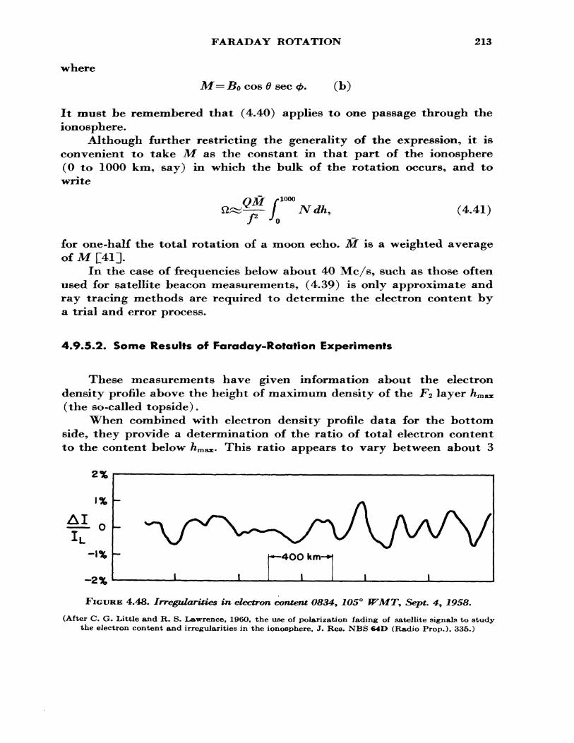
FARADAY ROTATION 213
•whereM= Bo cos 6 sec (b)
It must be remembered that (4.40) applies to one passage through the ionosphere.
Although further restricting the generality of the expression, it is convenient to take M as the constant in that part of the ionosphere (0 to 1000 km, say) in which the bulk of the rotation occurs, and to write
QM / 1000
.JNdh, (4.41)
for one-half the total rotation of a moon echo. M is a weighted average of M £411).
In the case of frequencies below about 40 Mc/s, such as those often used for satellite beacon measurements, (4.39) is only approximate and ray tracing methods are required to determine the electron content by a trial and error process.
4.9.5.2. Some Results of Faraday-Rotation Experiments
These measurements have given information about the electron density profile above the height of maximum density of the F$ layer hmax (the so-called topside).
When combined with electron density profile data for the bottom side, they provide a determination of the ratio of total electron content to the content below hmBX. This ratio appears to vary between about 3
2%
1%
AIIL
H%
-2%
-*—4OO km-
FIGURE 4.48. Irregularities in electron content 08349 105° WMT* Sept. 4, 1958.(After C. G. Little and R. S. Lawrence, 1960, the use of polarization fading of satellite signals to study
the electron content and irregularities in the ionosphere, J. Res. NBS 64O (Radio Prop.), 335.)
214 OBLIQUE PROPAGATION
and about 5 from day to night. The daytime peak in electron content is six to eight times greater than the nighttime minimum. Furthermore, the noontime content seems to be somewhat higher in winter than in summer. During magnetically disturbed conditions the total electron content appears to decrease.
Because of the high sensitivity inherent in this method, it is possible to observe the irregular structure in the electron content of the F% layer as shown in figure 4.48.
REFERENCES
[I] Breit, G., and M. A. Tuve (1926), A test of the existence of the conducting layer,Phys. Rev. 28, 554.
[2] Martyn, D. F. (1935), The propagation of medium radio waves in the ionosphere,Proc. Phys. Soc. 47, 323.
[3] Smith, N. (1939), The relation of radio sky wave transmission to ionospheremeasurements, Proc. IRE 27, 332.
[4] Appleton, E. V., and W. J. G. Beynon (1940), The application of ionospheric datato radio communications problems, Proc. Phys. Soc. 52, Pt. I, 518; (1947), Proc.Phys. Soc. 59, Pt. II, 58.
[5] Kift, F. (1960), The propagation of high frequency radio waves to long distances,Proc. IEE 107B, 127.
[6] Aono, Y. (1962), Study of radio wave propagation in sweep-frequency pulsetransmission tests in Japan, J. Radio Res. Lab. 9, 127.
[7] Sulzer, P. G. (1955), Sweep-frequency pulse-transmission measurements over a2400 km path, J. Geophys. Res. 60, 411.
[8] Hatton, W. L. (1961), Oblique sounding and H.F. radio communication, IRETrans. Commun. Syst. CS-9, 275.
[9] Cox, J. W., and K. Davies (1955), Oblique incidence pulse transmission, WirelessEng. 32, 35.
[10] Sandoz, O. A., E. E. Stevens, and E. S. Warren (1959), The development of radiotraffic frequency prediction techniques for use at high latitudes, Proc. IRE 47,681,
[II] M oiler, H. G. (1958), Further results of sweep frequency oblique-incidence meas urements, J. Atmospheric Terrest. Phys. 13, 173.
[12] Wilkins, A. F., and F. Kift (1957), Characteristics of H.F. signals, Electronic and Radio Eng. 34, 1.
[13] Agy, V., and K. Davies (1959), Ionospheric investigations using the sweep- frequency pulse technique at oblique incidence, J. Res. NBS 63D (Radio Prop.), 151.
[14] Agy, V., K. Davies, and R. Salaman (1959), An atlas of oblique-incidence iono- grams, NBS Tech. Note 31.
[15] Warren, E., and E. L. Hagg (1958), Single hop propagation of radio waves to a distance of 5300 km, Nature 181, 34.
[16] Davies, K. (1959), The effect of the earth's magnetic field on m.u.f. calculations, J. Atmospheric Terrest. Phys. 16, 187.
[17] Thomas, J. A., and E. K. Smith (1959), A survey of the present knowledge of sporadic E ionization, J. Atmospheric Terrest. Phys. 13, 295.
REFERENCES 215
[18] Wright, J. W., and T. N. Gautier (1960), Note on a test of the equivalence theorem for sporadic E propagation, J. Res. NBS 64D (Radio Prop.)* 347.
[19] Calvert, W., K. Davies, E. Stiltner, and J. T. Brown (1963), Equatorial spread-F motions, Proc. Intern. Conf. Ionosphere, p. 316 (The Institute of Physics and the Physical Society, London).
[20] Hagg, E. L., and W. Rolf (1963), A study of transatlantic radio propagation modes at 41.5 Mc/s, Can. J. Phys. 41, 220.
[21] Silherstein, R. (1954), Sweep-frequency backscatter——some observations and deductions, IRE Trans. Ant. Prop. AP—2, 56.
[22] Villard, O. G., S. Stein, and K, C. Yeh (1957), Studies of transequatorial iono spheric propagation by the scatter-sounding method, J. Geophys. Res. 62, 399.
[23] Bailey, D. K. (1959), The effect of multipath distortion on the choice of operating frequencies for high-frequency communications circuits, IRE Trans. Ant. Prop. AP-7, 398.
[24] Budden, K. G. (1961), Radio Waves in the Ionosphere (Cambridge Univ. Press).[25] De Voogt, A. H. (1960), Ionospheric models as an aid for the calculation of iono
spheric propagation quantities, Proc. IRE 48, 341.[26] Muldrew, D. R. (1959), An ionospheric ray-tracing technique and its application
to a problem in long distance radio propagation, IRE Trans, Ant. Prop. AP—7, 3939.
[27] Chvojkova (Woyk), E. (1959), The refraction of radio waves by a spherical ionized layer, J. Atmospheric Terrest. Phys. 16, 124.
[28] Bremmer, H. (1949), Terrestrial Radio Waves, Ch. XI (Elsevier Publ. Co.).[29] Booker, H. G. (1949), Application of magnetoionic theory to radio waves incident
obliquely upon a horizontally stratified ionosphere, J, Geophys. Res. 54, 243.[30] Lawrence, R. S., and D. J. Posakony (1962), A digital ray-tracing program for
ionospheric research, Space Research II, Proc. 2d Intern. Space. Sci. Symp., Florence (North Holland Publ. Co.).
[31] Ilaselgrove, J. (1955), Ray-theory and a new method for ray-tracing, Report on Conf. on Phys. of the Ionosphere, 355, Phys. Soc., London.
[32] Titheridge, J. E. (1959), Ray-paths in the ionosphere, J. Atmospheric Terrest. Phys. 14, 50.
[33] Poeverlein, H. (1949), Strahlweze von Radiowellen in der lonosphare, Z. angen Phys. 1, 517.
[34] Lawrence, R. S., C. G. Little, and H. J. A. Chivers (1964), A survey of ionospheric effects upon earth-space radio propagation, Proc. IEEE 52, No. 1, P. 4.
[35] Weisbrod, S., and L. J. Anderson (1959), Simple methods for computing tropo- spheric and ionospheric refraction effects on radio waves, Proc. IRE 47, 1770.
[36] Smith, F. G. (1952), Ionospheric refraction of 81.5 Mc/s radio waves from radio stars, J. Atmospheric Terrest. Phys. 2, 350.
[37] Komesaroff, M. M. (1960), Ionospheric refraction in radio astronomy. I. Theory, Australian J. Phys. 13, 153.
[38] Lawrence, R. S., and J. L. Jespersen (1961), Refraction effects of large scale iono spheric irregularities observed at Boulder, Colo., Space Research II, Proc. 2d Intern. Space. Sci. Symp., 277 (North Holland PubL Co.).
[39] Little, C. G., and R. S. Lawrence (1960), The use of polarization fading of satellite signals to study the electron content and irregularities in the ionosphere, J. Res. NBS 64D (Radio Prop.), 335.
[40] Evans, J. V. (1957), The electron content of the ionosphere, J* Atmospheric Terrest. Phys. 11, 259.
[41] Yeh, K. C., and V. H. Gonzales (1960), Note on the geometry of the earth magne tic field useful to Faraday effect experiments, J. Geophys. Res. 65, 3209.

CHAPTER 5
Signal Strength
5.1. MEANING OF SIGNAL STRENGTH
The instantaneous value of a sine wave function at a point is defined by the peak amplitude and the instantaneous phase at the point. The amplitude of a composite wave signal is given by the vector sum of its components; thus, if the components are in phase, the resultant amplitude will be the algebraic sum of the individual waves. If the phases of the separate components are varying randomly with respect to each other, the resultant signal power, averaged over many fading cycles, is given by the sum of the powers in the component waves. In this chapter the term "signal strength" will be used in a broad sense to mean either the amplitude (field strength) or the power received by an antenna.
The signal strength at any time depends upon absorption along the path, path focusing, polarization, and phase of the waves. In this chapter we shall discuss some aspects of these phenomena.
We shall discuss first the factors affecting the average power received (system loss) and then the factors which produce variations about the average (i.e., fading).
5.2. FACTORS AFFECTING SIGNAL STRENGTH
Consider a radio communications system which consists of a trans mitter, a transmission line, a transmitting antenna, the propagation medium, a receiving antenna, a receiver transmission line, and, finally a receiver. It is possible to consider the entire circuit between transmitter output terminals and the receiver input terminals as a ffblack box" as shown in figure 5.1. If pt is the power fed into the terminals of the feeder line from the transmitter and if pT is the signal power available from the terminals of the line from the receiving antenna, then the total system
217
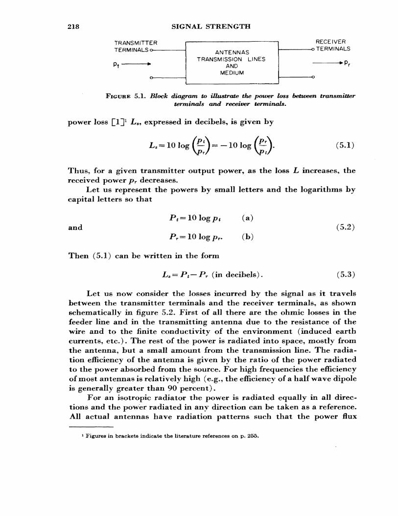
218 SIGNAL STRENGTH
TRANSMITTER TERMINALS o—
Pf
ANTENNAS TRANSMISSION LINES
AND MEDIUM
RECEIVER -o TERMINALS
FIGURE 5.1. Block diagram to illustrate the power loss between transmitter terminals and receiver terminals.
power loss Ql^]1 Ls , expressed in decibels, is given by
(5.1)
Thus, for a given transmitter output power, as the loss L increases, the received power pr decreases.
Let us represent the powers by small letters and the logarithms by capital letters so that
Pt =IQlogpt (a)and (5.2)
r. (b)
Then (5.1) can be written in the form
Ls =Pt —Pr (in decibels). (5.3)
Let us now consider the losses incurred by the signal as it travels between the transmitter terminals and the receiver terminals, as shown schematically in figure 5.2. First of all there are the ohmic losses in the feeder line and in the transmitting antenna due to the resistance of the wire and to the finite conductivity of the environment (induced earth currents, etc.). The rest of the power is radiated into space, mostly from the antenna, but a small amount from the transmission line. The radia tion efficiency of the antenna is given by the ratio of the power radiated to the power absorbed from the source. For high frequencies the efficiency of most antennas is relatively high (e.g., the efficiency of a half wave dipole is generally greater than 90 percent).
For an isotropic radiator the power is radiated equally in all direc tions and the power radiated in any direction can be taken as a reference. All actual antennas have radiation patterns such that the power flux
Figures in brackets indicate the literature references on p* 255.
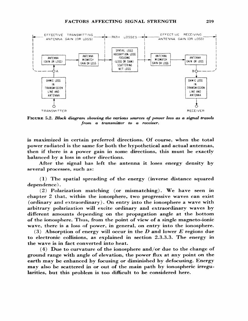
FACTORS AFFECTING SIGNAL STRENGTH 219
i EFFECTIVE TRANSMITTING 1J4 ~~ -~ANTENNA GAIN
ANTENNA(GAIN OR LOSS)
L_ JL
(OR LOSS)
ANTENNA— *• MISMATCH
GAIN OR LOSS
1 1 1 1 1
— r-~
PATH LOSSES
SPATIAL LOSS ABSORPTION LOSS
FOCUSING (LOSS OR GAIN)
SCATTERING NET LOSS
EFFECTIVE RECEIVING _|ANTENNA
ANTENNA——— (— *- MISMATCH
GAIN OR LOSS
GAIN (OR LOSS) j
11 I
ANTENNA |* GAIN OR LOSS j
^tr JOHMiC LOSS
INTRANSMISSION
LINE AND ANTENNAI
TRANSMITTER
____4____ OHMIC LOSS
IN TRANSMISSION
LINE AND ANTENNA
IRECEIVER
FIGURE 5.2. Block diagram showing the various sources of power loss as a signal travelsfrom a transmitter to a receiver*
is maximized in certain preferred directions. Of course, when the total power radiated is the same for both the hypothetical and actual antennas, then if there is a power gain in some directions, this must be exactly balanced by a loss in other directions.
After the signal has left the antenna it loses energy density by several processes, such as:
(1) The spatial spreading of the energy (inverse distance squared dependence^.
(2) Polarization matching (or mismatching). We have seen in chapter 2 that, within the ionosphere, two progressive waves can exist (ordinary and extraordinary). On entry into the ionosphere a wave with arbitrary polarization will excite ordinary and extraordinary -waves by different amounts depending on the propagation angle at the bottom of the ionosphere. Thus, from the point of view of a single magneto-ionic wave, there is a loss of power, in general, on entry into the ionosphere.
(3) Absorption of energy will occur in the D and lower E regions due to electronic collisions, as explained in section 2.3.3.3. The energy in the wave is in fact converted into heat.
(4) Due to curvature of the ionosphere and/or due to the change of ground range with angle of elevation, the power flux at any point on the earth may be enhanced by focusing or diminished by defocusing. Energy may also be scattered in or out of the main path by ionospheric irregu larities, but this problem is too difficult to be considered here.
220 SIGNAL STRENGTH
(5) On leaving the ionosphere the polarization for a particular magneto-ionic wave will have a certain configuration depending on the angle between the wave normal and the earth's magnetic field at the bottom of the ionosphere. Since the angle between the magnetic field and the emergent wave differs from the angle between the magnetic field and the incident wave, the polarization of the emergent wave will, in general, be different from the polarization of the incident wave. Further more, the polarization of the wave will not in general match that of the reqeiving antenna and there will therefore be a loss of received signal due to polarization mismatch. For certain directions there may be a gain due to the antenna pattern; in other directions there will be a loss.
Finally, there are ohmic losses in the receiving antenna and in its transmission line.
The polarization mismatch losses can be included with the antenna gain to give an "effective antenna gain" for the particular angle of takeoff and wave polarization. Our main concern, in this book, is with propaga tion in the medium between the antennas. The power losses along the propagation path, and which are not associated in any way with the antennas, will be called the "path loss."2
In what follows it will be assumed that the polarizations of the hypo thetical isotropic radiators are perfectly matched to the polarizations of the characteristic waves excited in the ionosphere.
Consider a single propagation path, with a given characteristic wave, between a transmitter and a receiver. With an actual antenna, let
Lia = the ohmic loss in the transmitting antenna and its transmissionline, in decibels,
L*p = the polarization mismatch loss of the transmitting antenna,G t = the gain of the transmitting antenna in the desired direction,Lp =the path loss in decibels,
Lrp—the polarization mismatch loss of the receiving antenna,Gr =the gain of the receiving antenna in the desired direction, and
Lra = the ohmic loss in the receiving antenna and its transmission line.
Then the system loss is given by
. (5.4)
Of course, it sould be remembered that the antenna gains Gt and Gr may be positive or negative depending on the direction of radiation.
2 CCIR Recommendation No. 241 defines a quantity called "basic transmission loss" and states that it is sometimes called path loss. It is important to note that our definition of path loss is not the same as that of basic transmission loss*
FACTORS AFFECTING SIGNAL STRENGTH 221
In practice, the total signal arriving at a receiver, after reflection at the ionosphere, is composed of individual signals which have traversed different paths and which have differing characteristic polarizations. To draw an electrical analogy, we can think of the component paths as a set of resistances in parallel. The presence of additional paths, although they involve losses, actually increases the received power and, therefore, diminishes the effective loss of the system. The ohmic losses in the an tennas and their transmission lines (see fig. 5.2) are the same for all paths. However, the effective antenna gain will depend on the particular propa gation path. Hence, the additional paths must be considered as parallel channels across the terminals A and B in figure 5.2.
Let LI represent, for channel 1, the sum of the losses (in decibels) given by (5.4), with the exclusion of the ohmic losses; that is,
£>i= Ltpi — Gti~{-Lpi-\-Lrpi — G>i> (5.5)
and, similarly, for L^ JL3, etc. To determine the manner in which the net loss between A and -B, which we may call LAB* is related to JLi, L^ La, etc., it is necessary to deal with the fraction / of the power which is lost along each path. That is,
Li =10 log Zi, etc. (5.6)
Invoking the analogy of parallel resistances, it will be seen that the net loss IAB is given by
IAB
and LAB by
= 10 log /A* =-10 log [7 +^+^ -fete. . (5.7)L*l *2 *3 J
To take a simple example, consider three possible paths for which the losses between A and B are Z>i = 50 dB, £,2 = 50 dB, and .£,3= 100 dB. The corresponding values of the Z's are: /i=106, /2 =105, and /3 =1010, so that the net loss /^B = 5X10⁴ and LAB = 47 dB, This shows that the con tribution to the total signal from path 3 is negligible, and that the con tributions from paths 1 and 2 give a net loss which is 3 dB less than that for either path 1 or path 2. Consider the case where Z/i = 50 dB, £2 = 60 dB, and jL3 = 70 dB, which gives /i = 10s, /2 = 106, and /3 = 107. The net loss IAB =
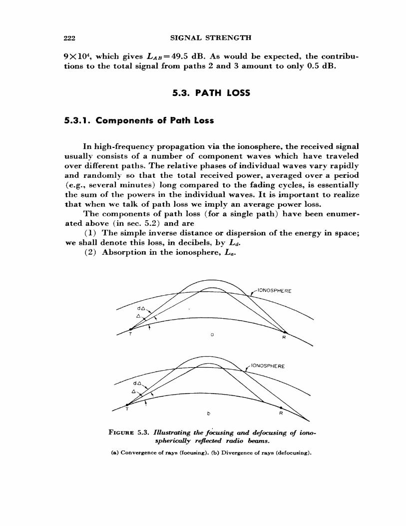
222 SIGNAL STRENGTH
9X10⁴, which gives 1/^ = 49.5 dB. As would be expected, the contribu tions to the total signal from paths 2 and 3 amount to only 0.5 dB.
5.3. PATH LOSS
5.3.1. Components of Path Loss
In high-frequency propagation via the ionosphere, the received signal usually consists of a number of component waves which have traveled over different paths. The relative phases of individual waves vary rapidly and randomly so that the total received power, averaged over a period (e.g., several minutes) long compared to the fading cycles, is essentially the sum of the powers in the individual waves. It is important to realize that when we talk of path loss we imply an average power loss.
The components of path loss (for a single path) have been enumer ated above (in sec. 5.2) and are
(1) The simple inverse distance or dispersion of the energy in space; we shall denote this loss, in decibels, by L,d-
(2) Absorption in the ionosphere, La.
IONOSPHERE
FIGURE 5.3. Illustrating the fwusing and defocusing of iono- spherically reflected radio beams.
(a) Convergence of rays (focusing), (b) Divergence of rays (defocusing).
FOCUSING 223
(3) Focusing or defocusing of power, Z//. Note that L/ will be posi tive for defocusing and negative for focusing.
The path loss, Z/p, in decibels, is given by the sum of its components, namely,
(5.8)
Let us now discuss these losses in more detail,
5*3.2. Spatial Loss
As a wave travels out from a small source, the power flux falls off inversely as the square of the distance s from the source, therefore,
(5.9)
5.3.3. Focusing
5.3.3.1. Effective Path Length
Focusing is the result of the convergence or divergence (defocusing) of originally neighboring rays (in addition to the divergence responsible for Ld) as illustrated in figure 5.3, for example. In practice it is very difficult to take into account the focusing of ionospherically reflected radio signals. In fact, it is necessary to have a detailed knowledge of the ionosphere along the ray path together with an elaborate ray-tracing program, as already discussed in section 4.6.6. Nevertheless, it is possible to consider the effect of focusing in terms of an effective path length se. The physical meaning of this effective path length can be seen from the following argument. In the absence of all other forms of energy loss the power flux at a distance s€ from an isotropic radiator, which radiates a total power p ta ^ is given by
(5.10)
Now let the energy radiated into the same cone by the antenna be de- focused as shown in figure 5.4. Let s be the distance from the antenna at which the area covered by the defocused rays is the same as that for
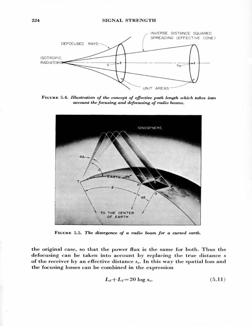
224 SIGNAL STRENGTH
INVERSE DISTANCE SQUARED SPREADING (EFFECTIVE CONE)
DEFOCUSED RAYS
ISOTROPIC RADIATOR
FIGURE 5.4. Illustration, of the concept of effective path length tvhich takes into account the focusing and defocusing of radio beams.
TO THE CENTER / OF EARTH
JFiGXJRE 5.5. The divergence of a radio beam for a curved earth.
the original case, so that the power flux is the same for both. Thus the defocusing can be taken into account by replacing the true distance s of the receiver by an effective distance se . In this way the spatial loss and the focusing losses can be combined in the expression
(5.11)
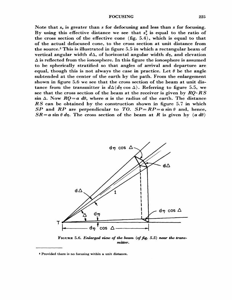
FOCUSING 225
Note that se is greater than s for defocusing and less than s for focusing. By using this effective distance we see that s\ is equal to the ratio of the cross section of the effective cone (fig. 5.4), which is equal to that of the actual defocused cone, to the cross section at unit distance from the source, 3 This is illustrated in figure 5.5 in which a rectangular beam of vertical angular width </A, of horizontal angular width dy, and elevation A is reflected from the ionosphere. In this figure the ionosphere is assumed to be spherically stratified so that angles of arrival and departure are equal, though this is not always the case in practice. Let 8 be the angle subtended at the center of the earth by the path. From the enlargement shown in figure 5.6 we see that the cross section of the beam at unit dis tance from the transmitter is dA(dij cos A). Referring to figure 5.5, we see that the cross section of the beam at the receiver is given by RQ • R S sin A. Now RQ = a dd, where a is the radius of the earth. The distance RS can be obtained by the construction shown in figure 5.7 in which Sf* and RP are perpendicular to TO. SP=RP = asin0 and, hence, SR = a sin 6 dij. The cross section of the beam at R is given by (a d0)
dA
FIGURE 5.6. Enlarged view of the beam (of fig. 5.5) near the trans mitter.
* Provided there is no focusing within a unit distance.
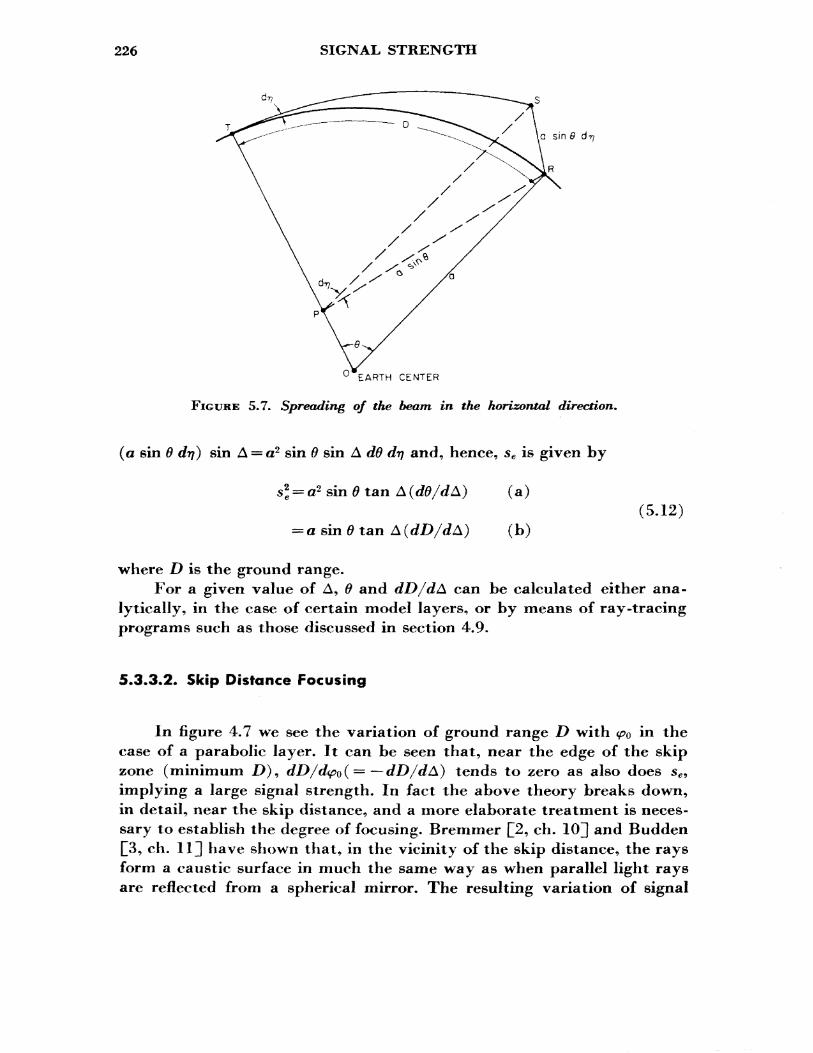
226 SIGNAL STRENGTH
a sin 8
0 EARTH CENTER
FIGURE 5.7. Spreading of the beam in the horizontal direction.
(a sin 6 dij) sin A = a2 sin 9 sin A d6 dij and, hence, se is given by
si = a2 sin 0 tan A (d9/dA) (a)(5.12)
= a sin 0 tan A (dD/dA) (b)
where Z) is the ground range.For a given value of A, 9 and dD/dA can be calculated either ana
lytically, in the case of certain model layers, or by means of ray-tracing programs such as those discussed in section 4.9.
5.3*3.2* Skip Distance Focusing
In figure 4.7 we see the variation of ground range D with (po in the case of a parabolic layer. It can be seen that, near the edge of the skip zone (minimum D), dD/d<po( = — dD/dA) tends to zero as also does sc , implying a large signal strength. In fact the above theory breaks down, in detail, near the skip distance, and a more elaborate treatment is neces sary to establish the degree of focusing. Bremmer £2, ch. 1CT) and Budden pi, ch. 11]] have shown that, in the vicinity of the skip distance, the rays form a caustic surface in much the same way as when parallel light rays are reflected from a spherical mirror. The resulting variation of signal
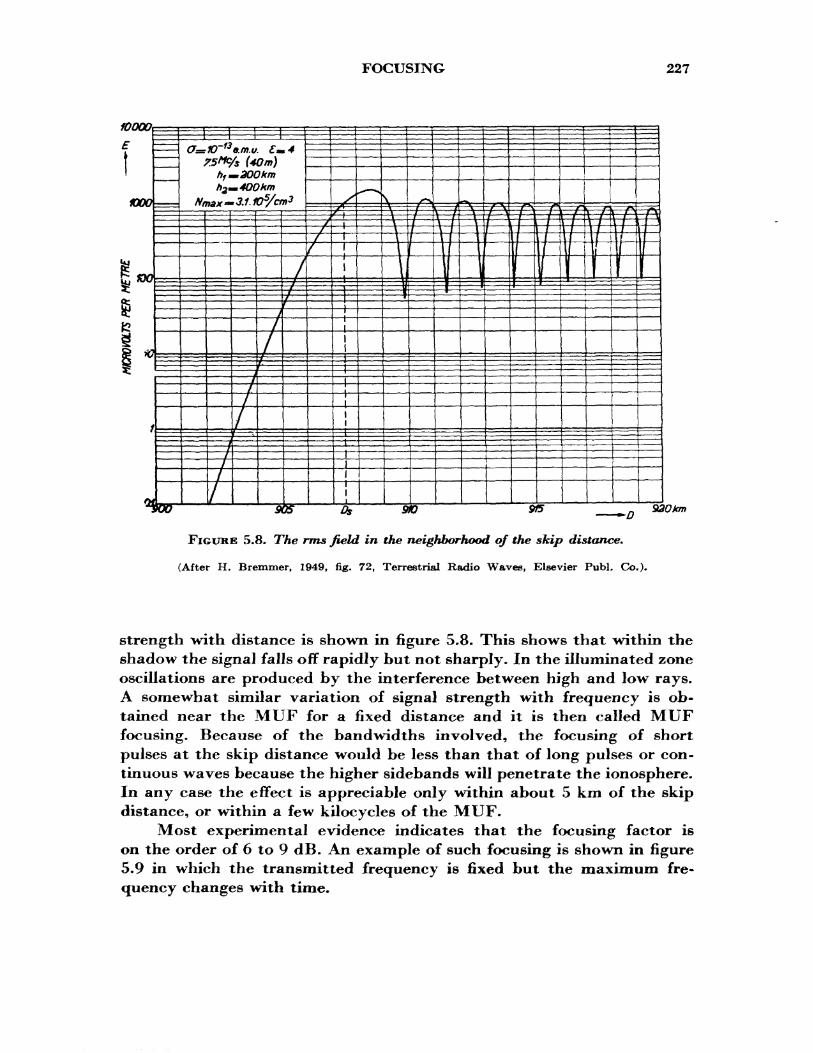
FOCUSING 227
920km
FIGURE 5.8. The rms field in the neighborhood of the skip distance*
(After H. Bremmer, 1949, fig. 72, Terrestrial Radio Waves, Elsevier Pubh Co.)-
strength with distance is shown in figure 5.8. This shows that within the shadow the signal falls off rapidly but not sharply. In the illuminated zone oscillations are produced by the interference between high and low rays. A somewhat similar variation of signal strength with frequency is ob tained near the MUF for a fixed distance and it is then called MUF focusing. Because of the bandwidths involved, the focusing of short pulses at the skip distance would be less than that of long pulses or con tinuous waves because the higher sidebands will penetrate the ionosphere. In any case the effect is appreciable only within about 5 km of the skip distance, or within a few kilocycles of the MUF.
Most experimental evidence indicates that the focusing factor is on the order of 6 to 9 dB. An example of such focusing is shown in figure 5.9 in which the transmitted frequency is fixed but the maximum fre quency changes with time.
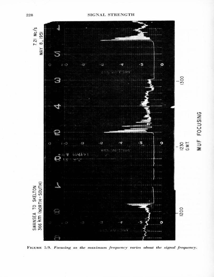
*J M 0 SB B \0 Si ft
SWAN
SEA
TO
SKEL
TON
366
km (
NO
RTH
-SO
UTH
)7.2
1 M
c/S
MAY
8, 1
951
oo CD M 0
1200
MUF
FO
CUSI
NG
FOCUSING 229
5*3.3.3* Antipodal Focusing
If the earth and ionosphere were perfectly smooth and concentric, energy could reach the antipode by all possible great circle paths £2]* However, because of the great geographic variations in ionospheric con ditions, such focusing does not appear to be of great practical importance.
5.3.3.4. Horizon Focusing
Putting A = 0 in (5.12) we see that s* goes to zero- This type of fo cusing is called rchorizon" focusing.
It is interesting to note that in multi-hop propagation, if the suc cessive hops are all alike, the degree of focusing in the vertical plane is the same as for the first hop. This can be proved as follows: Let SA be the effective distance taking account of spreading in the vertical plane only (see fig. 5.5). Then
SA-=asin A(rf0/rfA). (5.13)
The degree of focusing in the vertical plane may be denoted by the ratio of SA to the actual length of the ray path. If S' denotes the actual length of the ray path for the first hop, the actual ray path length for n hops is n S'. The value of S& n for the n hops is
c . A*5A = a sin A — - —— = noA% (5.14) dA
where SA' is the value of SA for the first hop. The degree of focusing for the n hops is thus nS& f/nS'= S&/Sr, which is the degree of focusing for the first hop.
5.3.3.5. Ionospheric Distortion
Focusing (or defocusing) due to ionospheric distortion can be very important, as was seen in section 4.6.6, where ionospheric curvature simulates convex or concave mirrors. This phenomenon is particularly important in transequatorial propagation during the afternoon and early evening because of the existence of a relatively stable deformation. Part of the long-period fading (half to one hour) of high-frequency sky waves
230 SIGNAL STRENGTH
is the result of focusing by transient deformations of the ionospheric layers. In particular, such distortions in the jF layer can produce focusing and defocusing of the reflected radio signal amounting to between 5 and 10 dB variation in the path loss.
5.3.3.6. Defocusing Due to Underlying lonization
Consider an electron density profile, such as shown in figure 5.10a, in which a block of electrons (simulating an E layer) is located below a sharply bounded reflecting F layer. Because of refraction in the lower layer the ray path (for /~1.5/jE) will be as shown in figure 5.10b. The effective path se to the same range will, therefore, be greater than it would be in the absence of the underlying ionization and, as a result, the path loss is increased.
km 400 300 200 100
\
(a)
F LAYER
E LAYER
GROUND
TO CENTER OF EARTH
(b)FIGURE 5.10. Defocusing due to underlying model E layer in which
the electron density is constant over the height range 100 to 300 km.
(a) Profile and ionogram. (b) Ray path for /=1.5 fE
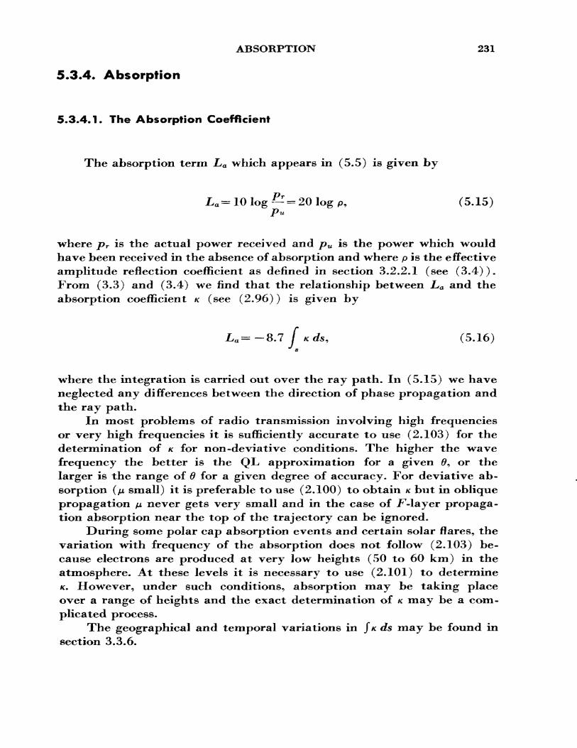
ABSORPTION 231
5.3.4* Absorption
5.3.4.1. The Absorption Coefficient
The absorption term La which appears in (5.5) is given by
La = 10 log -^ = 20 log p, (5.15)Pu
where pT is the actual power received and pu is the power which would have been received in the absence of absorption and where pis the effective amplitude reflection coefficient as defined in section 3.2.2.1 (see (3.4)). From (3.3) and (3.4) we find that the relationship between La and the absorption coefficient K (see (2.96)) is given by
E =—8.7 f Kds, (5.16)
where the integration is carried out over the ray path. In (5.15) we have neglected any differences between the direction of phase propagation and the ray path.
In most problems of radio transmission involving high frequencies or very high frequencies it is sufficiently accurate to use (2.103) for the determination of K for non-deviative conditions. The higher the wave frequency the better is the QL. approximation for a given 9, or the larger is the range of 6 for a given degree of accuracy. For deviative ab sorption (JJL small) it is preferable to use (2.100) to obtain K but in oblique propagation yu never gets very small and in the case of .F-layer propaga tion absorption near the top of the trajectory can be ignored.
During some polar cap absorption events and certain solar flares, the variation with frequency of the absorption does not follow (2.103) be cause electrons are produced at very low heights (50 to 60 km) in the atmosphere. At these levels it is necessary to use (2.101) to determine K. However, under such conditions, absorption may be taking place over a range of heights and the exact determination of K may be a com plicated process.
The geographical and temporal variations in J/c ds may be found in section 3.3.6.
232 SIGNAL STRENGTH
5.3.4.2. Martyn's Absorption Theorem
By analogy with (4.7) the absorption L, for a wave incident at an angle 0 on a plane ionosphere, is related to the absorption Lv of the equiv alent vertical wave, as defined in section 4.2.1, by the formula
L=Lt,cos0. (5.17)
This relation is not exact for the actual ionosphere with the earth's mag netic field, but it is a useful guide. An easy way to remember this theorem is to notice that the oblique path length is sec 0 times the vertical but that the equivalent vertical wave (of frequency / cos 0) suffers sec2 <f> more absorption because the absorption varies inversely as the square of the frequency, (2.99).
5.3.4.3. Variation of Absorption with Distance
Daytime absorption on high frequencies takes place mainly in the D region, between 80 and 100 km. The amount of absorption suffered by a high-frequency wave passing through this region is proportional to the length of the path in the region. Since the thickness of the region is very small compared to its radius of curvature (distance to the center of the earth), the length of the path in the region is very nearly equal to the secant of the angle of incidence <J>D at the mean height of the region multi plied by the thickness of the region.
On frequencies sufficiently far above the £-layer critical frequency, the ray path may be reasonably well represented by an equivalent tri angle like that depicted in figure 5.11. The variation of sec 0x> with dis tance for such a path is shown in figure 5.12 for four combinations of hn the mean height of the D region, and hf the height of the apex of the equivalent triangle. The two values of HD are 80 and 100 km, and the two values of h f are 250 and 500 km.
Beyond about 1000 km, these curves can be approximated by the straight dashed lines drawn through the origin, at least to the degree of accuracy normally attained in transmission loss determinations. All four curves bend over at the top, but the departure from the straight lines is not serious until the distance is greater than about 2600 km for the /i' = 250 km curves (departure angle ;^5°) and about 3800 km for the h 1 = 400 km curves (departure angle ~3°).
ABSORPTION 233
REFLECTION LEVEL
D REGION
FIGURE 5.11. Angle of incidence in the O region.
h = 25O km
h = 4OO k m
I IO 500 1000 1500 2000 25OO 3OOO 35OO 4OOO 45OO
PATH LENGTH IN k m
FIGURE: 5.12. Variation of sec <f>n with ground range for the model shoivn in figure 5.10.
(After T. N. Gautier, unpublished.)
234 SIGNAL STRENGTH
During daytime when there is an appreciable E layer present the ray paths will be modified as sketched in figure 5.10b. In general, the de viation in the E layer will decrease with increase of frequency for a given angle of elevation. It will decrease with increase in elevation on a given frequency.
5.3.4*4. Deviative Absorption
The calculation of deviative absorption is a difficult process depend ing on the details of ray path, electron density profile, and collision fre quency profile. In fact it is impossible, in practice, to determine just what is deviative and what is non -deviative since these terms are defined in terms of limiting conditions. Because the collision frequency v decreases rapidly with height, absorption tends to be concentrated in the lower regions of the ionosphere. Thus for waves reflected from the F region, deviative absorption tends to be greatest not near reflection but in the
1200
FIGURE 5.13. Variation of deviative absorption ivith frequency for various ground ranges (in km) and the electron density profile shown in figure 5,10.
XE=(fE/fi2. (After T. N. Gautier, unpublished.)
ABSORPTION 235
lower part of the E region except, possibly, at night. To determine the deviative absorption it is necessary either to choose suitable ionospheric models of N(h) and v(h} so that the integral J2* ds can be evaluated analytically, or to compute the absorption step by step in an actual N(h} profile with a computer (ray-tracing) program.
With an N(h) profile of the type shown in figure 5.10a and a v(h) profile given by
~ (5.18)
the variation of absorption with wave frequency for different distances is sketched in figure 5.13. At the right-hand side of the figure (large f/fE) where the curves are flat, the absorption is non -deviative. Deviative absorption is manifested by the upward bending of the curves to the left. The distance 3128 km corresponds to M^ = 0, that is, when a ray incident vertically on the 100 km level is refracted so as to be tangential. Under such conditions the absorption would be large. The 3836 km distance is the maximum one-hop distance achieved with no E layer refraction (i.e., fjiE= 1).
5.3.4.5* Geographic Considerations
Middle latitudes. The variations of non -deviative absorption in middle latitudes are fairly well-behaved and may be approximated by a formula given by Rawer
La = 430 (1+0.00357?) cos0 -75 x sec ^(/i/z,)-2 , (5,19)
in decibels per hop. Here R is the sunspot number, x is the solar zenith angle, and/ and//, are in megacycles per second. The numerical values in this formula are based on analyses of vertical incidence measurements at Slough, England.
The formula does not take account of the winter anomaly — section 3.3.6.5. To get an estimate of the absorption for the winter months, the values given by (5.19) should be multiplied by the factors in table 5.1. These numbers may be used in dipole latitudes of 40° to 70° north and south. It should be kept in mind that these are average values. On in dividual days the factor may vary from less than 1 to around 2.0. The value of the factor depends somewhat on the degree of geomagnetic activity
236 SIGNAL STRENGTH
TABLE 5.1. Absorption factors for winter months in northern and southern hemispheres
Month
Northernhemisphere
NovemberDecemberJanuary February
Southernhemisphere
MayJuneJuly August
Factor
1.21.51.5 1.2
High latitudes. In high latitudes the most important consideration in radio communications is the onset of radio blackouts rather than the average absorption. This subject will be dealt with in chapter 6.
Low latitudes. These latitudes have been discussed by Piggott Q6], who has listed the following characteristic features of low-latitude propa gation :
1. The relatively great importance of jE-layer trajectories,2. The variability of the .F-layer profile. This seriously limits the
practical value of jF-layer propagation at short ranges and makes the angle of elevation and path loss for F reflections at a given range excep tionally variable.
3. The absorption of the ordinary wave on a given frequency and trajectory is usually greater than at higher latitudes because/z, is smaller, other factors being the same.
4. Interference fading between modes having equal amplitudes is relatively more common since the differential absorption between the ordinary and extraordinary waves is smaller than in higher latitudes.
5.3.5* Polarization Mismatch Factors
When a wave propagates in the ionosphere it is polarized in a manner which depends primarily on the electron density, wave frequency, and di rection of propagation relative to the magnetic field. The polarization at the bottom of the ionosphere (where the electron density 7V—0) is called the limiting polarization.
To illustrate the effect of polarization mismatch on a wave, consider a ray incident at an angle of 45° on a plane ionosphere in the magnetic meridian as shown in figure 5.14a. Let the magnetic dip angle be 45° and the polarization of the transmitting antenna be such that the in-
POLARIZATION MISMATCH FACTORS 237
B IONOSPHERE
TRANSMITTING T ANTENNA
TRANSMITTING ANTENNA
RECEIVING ANTENNA
RECEIVING ANTENNA
FJOURE 5.14. Path losses due to polarization mismatch.(a) Transmitted wave linearly polarized, (b) Transmitted wave circularly
polarized.
cident wave is linearly polarized with the electric vector parallel to the magnetic field. On entry into the ionosphere at the point A^ all the in cident power is used in exciting the ordinary wave. Thus, for the ordinary wave, the loss 0Ltp is zero, whereas for the extraordinary wave xL tp is infinite. Now as the ordinary wave travels through the ionosphere, the propagation angle 0 varies continuously so that the wave polarization changes from linear to elliptical until it reaches J?, at which point the polarization is circular, because 0 = 0°. If the receiving antenna is linearly polarized it will pick up half the incident power, so that 0Lrp is 6 dB.
Next, consider the case in which the transmitting antenna radiates a circularly polarized wave (see fig* 5.14b) such that, on entry into the ionosphere at A 9 all the power is used in exciting the ordinary wave. Once again 0LtP is zero for the ordinary wave and ^Ltp is infinite for the extra ordinary wave. Within the ionosphere the wave polarization becomes elliptical until at B it is linearly polarized with the electric vector parallel to the magnetic field B0. Now if the receiving antenna is linearly polarized to pick up the ordinary wave 0Lrp is zero, whereas if it is polarized per pendicular to this direction the loss is infinite. If <p is the angle between the direction of the magnetic field and the direction of linear polarization of the receiving antenna the loss for the ordinary wave is given by 10 log cos2 <p = 2Q log cos <p. Of course if the transmitting antenna emits circularly polarized waves with the opposite sense of rotation, then the
238 SIGNAL STRENGTH
EXTRAORDINARY WAVE ELLIPSE
B0 (EARTHS MAGNETIC FIELD)
ORDINARY WAVE ELLIPSE
FIGURE 5.15. Limiting polarization ellipses produced by a horizontally polarized wave incident on the ionosphere in the magnetic meridian.
losses for the ordinary and extraordinary waves are reversed. If the in cident radiation, in the case of figure 5.14b, is linearly polarized, then the incident power is divided equally between the ordinary and extraordinary waves so that 0LtP ~xLtP :=6 dB. Of course the total power in the com posite wave may still be the same. We now have an extra wave to take into account.
To illustrate further what happens jwhen a radio wave enters the ionosphere, consider radiation from a horizontally polarized antenna in cident on the ionosphere in the magnetic meridian. On entering the ion osphere the wave is split up into two characteristic waves (see sec. 2.3.3.2) which are, in general, elliptically polarized with opposite senses of rota tion. Since the incident wave is horizontally polarized the vertical axes of the two polarization ellipses must just cancel, and so the ellipses must be as shown in figure 5.15. The shapes of the ellipses are given (approxi- imately) by the formula X=0 in (2.74) :
Now
2 YL ' A ~
(E3 ) 0 =R+(E2 ) (
(5.20)
POLARIZATION MISMATCH FACTORS 239
and
hence
Substituting from (2.90) we obtain
(EJo^RKEJ*, (a)or (5.21)
(Ed* = Rl(E£o. (b)
Equation (5.21) enables us to determine the way in which energy in the incident wave is distributed between the ordinary and extraordinary components. From then on the two components travel essentially in dependently until they emerge from the ionosphere. However, since the absorptions suffered by the two waves are unequal the emergent waves will not cancel out in the vertical plane and the resultant wave will, there fore, be elliptically polarized.
Substitution of numerical values of Y(0.1, say) and 0(45°, say) in (5.20) shows that /?^~^1 so that, except for nearly transverse propaga tion, the energy is divided almost equally between the two magneto-ionic components. On lower frequencies, however, this is not the case as can be seen by substituting Y=l and 0 = 45° in (5.20). This gives (E&) 0 = 2(E*) X .
When the propagation is nearly transverse, 0:~90°, so that /?_J~ ( YL/ y£) — >0 and /?_j_c^( Y%*/ Y%) — » o° . Hence the ellipses are very narrow. In the absence of collisions the major axis of the ordinary wave ellipse is parallel to the magnetic field, whereas that for the extraordinary wave ellipse is perpendicular to the magnetic field. In intermediate and high latitudes the ordinary wave ellipse has its major axis nearly vertical and the extraordinary wave ellipse has its major axis nearly horizontal. Except when 6 is within about 15° of the normal to the magnetic field the ellipses are so nearly circular that the differences between ordinary and extraordinary wave ellipses are unimportant on frequencies well above the gyrofrequency.
For east-west propagation along the magnetic equator, antennas should be horizontally polarized so as to excite the ordinary wave, whereas in high latitudes the ordinary wave is excited by a vertically polarized
240 SIGNAL STRENGTH
o° 30° 60°
AZIMUTH (p
90°
FIGURE 5.16. Directions for tuhich 6 (the propagation angle} =90° for different angles ofmagnetic dip *.
The azimuth <f> is measured from the magnetic meridian. (After W. R. Piggott, 1959, Radio Research Special Report No. 27, Her Majesty's Stationery Office, London.)
wave. The necessary conditions for polarization to be important are (a) that the propagation be quasi-transverse at the point of entry into or exit from the ionosphere (or both), and (b) that the differential absorp tion between the magneto-ionic waves be large. Polarization effects are, therefore, most important on frequencies in the vicinity of the gyro- frequency that is in the frequency band from 0.3 Mc/s to 3 Mc/s.
For the calculation of path loss it is necessary to know LtP (5.4) and this can be determined by the use of equations such as (5,21) and a knowledge of the polarization of the transmitted wave. Similarly Lrp can be determined from a knowledge of the emergent polarization and the antenna polarization, the angles of elevation and azimuth at which the polarization may become important can be seen in figure 5.16, which gives the angles of elevation and azimuth as a function of the dip angle near the transmitter or receiver as appropriate. The critical range of angles falls in the middle of the most important range of angles for practical com munications in temperate latitudes. Vertical polarization is preferable to horizontal whenever polarization is important in these latitudes.
ANTENNA GAIN 241
For short-range transmissions on the lower frequencies it is often convenient to use polarization as a method of discriminating against noise. Very considerable gains in signal/noise ratio are possible in the daytime by using antennas which are insensitive to vertical polarization on the frequencies where most of the interference is propagated via the iono sphere.
In multi-hop transmission, depolarization of a characteristic wave may occur after a ground reflection, especially if the magnetic dip is different for the two hops so that a downcoming ordinary wave may, after a ground reflection, give rise to ordinary and extraordinary waves.
5.3.6. Antenna Gain
A detailed discussion of antennas is beyond the scope of this book and so a few simple ideas will suffice for our present purposes.
It has become customary to specify the gain of an antenna in a given direction as the ratio of the power radiated in that direction to the power which would be radiated in the same direction by a standard reference antenna. Standard antennas used for this purpose are (1) an isotropic radiator, (2) a half-wave dipole (this has a power gain of 1.64 [J2.15 dB] relative to an isotropic radiator), and (3) a short electric dipole which has a maximum power gain of 1.5 (1.76 dB) over an isotropic radiator.
If PQ is the power radiated in kilowatts, the power p& radiated per unit solid angle at an elevation A is given by
pA=pogA (5.22)
where g& is the free space gain of the antenna at an elevation A over an isotropic radiator. The value of g& can be calculated from the geometry of the antenna. Note that />o is the actual power radiated (current squared times radiation resistance) and not the power output of the transmitter or the power input to the antenna.
For a short dipole (less than 0.1 wavelength), gA=l-5 sin2 A, where A is measured from the axis of the dipole. For a short vertical wire, one end of which is on a perfectly conducting ground, the gain is given by gA = 3 cos2 A. Part of the field intensity near the ground (Ac^0°) is due to the surface wave, which is negligible when the wave reaches the iono sphere. Consequently, the vertical directional pattern of an antenna, for sky wave calculations, may be considerably different from the pattern measured near the antenna.
242 SIGNAL STRENGTH
5.4. FADING
5.4.1* General Characteristics
In the above discussions of path loss we concerned ourselves with the average power received. Now the instantaneous field strength may fluctuate widely about the mean value and amplitude variations of the order of 10 to 1 can occur in the course of a few seconds. Fading may be caused by several different ionospheric phenomena, e.g., movements of the ionosphere causing interference fading, rotation of the axes of the polarization ellipses, time variations in ionospheric absorption, focusing, and skipping of the signal due to MUF failure. In the case of signals trans mitted from a moving source—e.g., a satellite—fading will result from the motion of the source relative to ionospheric irregularities. Fading of cos mic radio noise is often referred to as ^scintillation."
The period of a fading cycle depends largely on the cause of the fading. Thus the fading period of interference and polarization fading may vary from a fraction of a second to a few seconds, absorption fading may have a period of the order of an hour or longer, whereas focusing may be of the order of 15 to 30 min. Signals can fade in or fade out if the fre quency of the signal is near the maximum frequency and the critical frequency is changing with time (see fig, 5.9). It is, therefore, highly irregular as far as period is concerned and may occur only in the early morning and late afternoon (fade in and fade out).
In general, fading is faster on high frequencies than on low frequencies because a given movement in the ionosphere produces a greater phase shift on the shorter wavelengths. The fact that fading is frequency - dependent means that different sidebands in a modulated wave fade -differently. This gives rise to a distortion of the modulation envelope which is called selective fading.
5.4.2* Interference Fading
A beam of radio waves incident on the ionosphere is not reflected from a point but from an extended region. Small irregularities in electron density near the level of reflection give rise to individual reflected wavelets and the received signal is the vector sum of the individual signals at the receiving antenna. Movements of ionospheric irregularities give rise to variations in the relative phases of the individual wavelets and thus
INTERFERENCE FADING 243
produce interference fading. It is not uncommon for a received high- frequency signal to consist of a mixture of high- and low-angle rays, each having extraordinary and ordinary components; each such set may be combined with other sets corresponding to rays having different numbers of hops.
The resultant amplitude can vary over wide limits, the maximum value being when all the individual components are in phase. The root mean square value of the fluctuating signal is equal to the steady value of the field that would have existed had the ionosphere not broken it up into many components. Because it is impossible to determine the resultant amplitude at any given moment, the subject has to be treated on a statis tical basis. Such phenomena are said to be "stochastic."
The distribution of amplitude approximates the Rayleigh law when the various components are of approximately the same amplitude and the relative phases are varying randomly. For the Rayleigh distribution, the percentage of time p(A) that the amplitude exceeds the value A is
p(A) =exp C-^V^l), (5.23)
where A\ is the mean square value of A (i.e., proportional to the mean power) . Ionospheric signals are, often, better described by a Rice dis tribution £7] in which a wave of steady amplitude (specular component) is added to the randomly varying signals. If A 8 is the steady amplitude the distribution function is given by
where /o is the Bessel function of zero order and imaginary argument.For A S/AR<<^I^ the Rice distribution approaches the Rayleigh law,
For A S/AR^>TL it approaches a normal distribution with mean A s and standard deviation 0.707 AR.
The amplitude distribution of a continuous wave, and of trains of long pulses, involving several paths, is usually close to Rayleigh. In dividual modes resolved by short pulses often have shallower (and slower) fading corresponding to a substantial specular component, ^5/^4^ = 2 or more.
With a Rayleigh distribution, the median amplitude is equal to 0.832 times the rms value. For such a distribution the lower decile value, or the amplitude exceeded 90 percent of the time, is 0.39 of the median value. The upper decile value, that is the value exceeded 10 percent of the time, is 1.8 times the mean value.
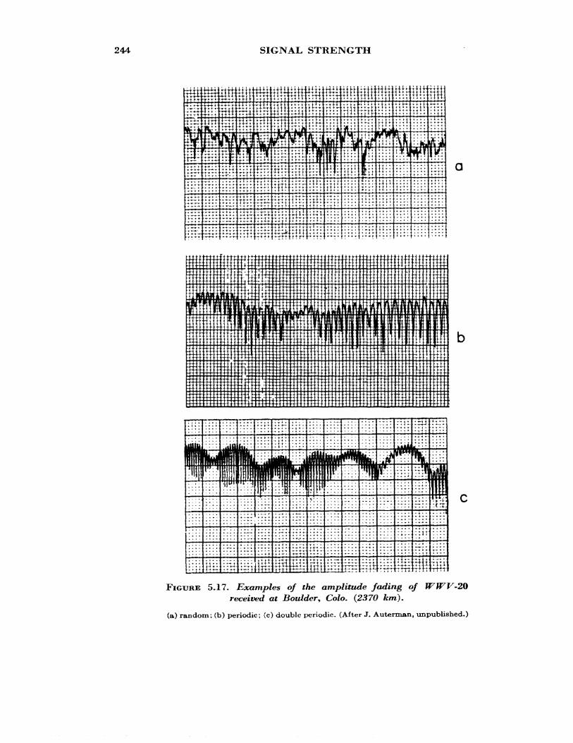
244 SIGNAL STRENGTH
[jjliiffiH ;ji iiiiiiiili i S j i jiiii III
imnmm sir si i! k\\ Bnil i^ip! il' 1 ^- 11 ^-; 1111 !)'-!iill! ! i 5 Hi !
l!!!g ! Mi S!iilfiliii I! '! 1 ill fill If! ii i! Ill
;»IH!HSi!i»HHiH»iS»l!lIt»millSHSiI:
of the amplitude fading of WWV , Colo. (2370 fern).
(b) periodic; (c) double periodic. (After J.(a)
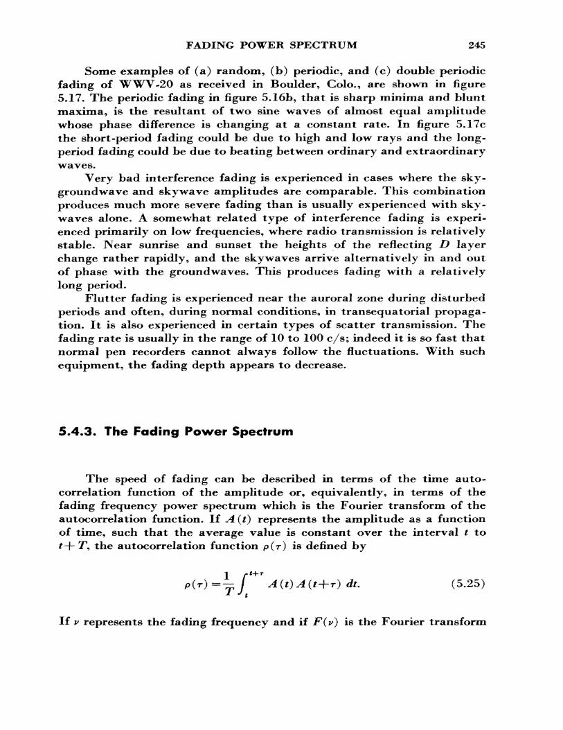
FADING POWER SPECTRUM 245
Some examples of (a) random, (b) periodic, and (c) double periodic fading of WWV-20 as received in Boulder, Colo., are shown in figure 5.17. The periodic fading in figure 5.16b, that is sharp minima and blunt maxima, is the resultant of two sine waves of almost equal amplitude whose phase difference is changing at a constant rate. In figure 5.17c the short-period fading could be due to high and low rays and the long- period fading could be due to beating between ordinary and extraordinary waves.
Very bad interference fading is experienced in cases where the sky- groundwave and skywave amplitudes are comparable. This combination produces much more severe fading than is usually experienced with sky- waves alone. A somewhat related type of interference fading is experi enced primarily on low frequencies, where radio transmission is relatively stable. Near sunrise and sunset the heights of the reflecting D layer change rather rapidly, and the skywaves arrive alternatively in and out of phase with the groundwaves. This produces fading with a relatively long period.
Flutter fading is experienced near the auroral zone during disturbed periods and often, during normal conditions, in transequatorial propaga tion. It is also experienced in certain types of scatter transmission. The fading rate is usually in the range of 10 to 100 c/s; indeed it is so fast that normal pen recorders cannot always follow the fluctuations. With such equipment, the fading depth appears to decrease.
5.4.3. The Fading Power Spectrum
The speed of fading can be described in terms of the time auto correlation function of the amplitude or, equivalently, in terms of the fading frequency power spectrum which is the Fourier transform of the autocorrelation function. If A (t) represents the amplitude as a function of time, such that the average value is constant over the interval t to
, the autocorrelation function p(r) is defined by
=- A(t)A(t+r) dt. (5.25)
If v represents the fading frequency and if F(v) is the Fourier transform
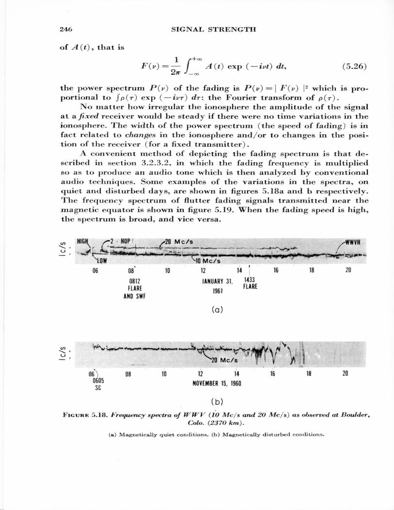
246 SIGNAL STRENGTH
of A(t) 9 that is1 r+°*
=— I A(i) exp ( — ivi) dt, (5.26) 2/r •>_<»
the power spectrum P(v} of the fading is ^(P) = | F(v) j 2 which is pro portional to Jp(r) exp ( — ivr) dr: the Fourier transform of p(r).
INo matter how irregular the ionosphere the amplitude of the signal at SL fixed receiver would be steady if there were no time variations in the ionosphere. The width of the power spectrum (the speed of fading) is in fact related to changes in the ionosphere and/or to changes in the posi tion of the receiver (for a fixed transmitter).
A convenient method of depicting the fading spectrum is that de scribed in section 3.2.3.2, in which the fading frequency is multiplied so as to produce an audio tone which is then analyzed by conventional audio techniques. Some examples of the variations in the spectra, on quiet and disturbed days, are shown in figures 5.18a and b respectively. The frequency spectrum of flutter fading signals transmitted near the magnetic equator is shown in figure 5.19- When the fading speed is high, the spectrum is broad, and vice versa.
WVH
(a)
0 ~ • MC/S f i yOB"; 08 10 12 14 16 18 20°^5 NOVEMBER 15. 1960
(b)FIGURE 5.18. Frequency spectra of WWV (10 Mc/s and 2O Mc/s} as observed at Boulder,
Co/o. (237O &m).
(a) Magnetically quiet conditions, (b) Magnetically disturbed conditions.
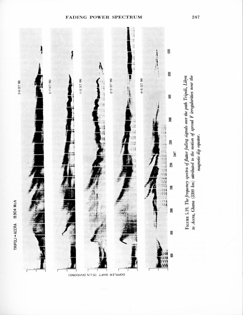
FADING POWER SPECTRUM 247
J
oQ_
i r
C 1 1 II:I; *
i
I1
m
. '•"•t t*.£;
&i
Jl|————————|————————I I I
(SNOISIAIQ S/39) J.JIHS
:t .-
1
i
J
i
S3
1-3•••* «- ^ a
-I 1.
"
•
t
e §
248 SIGNAL STRENGTH
5.4.4. Scintillations4
This refers to the amplitude and phase variations of high-frequency signals transmitted through the ionosphere from outside the earth. The two common sources are cosmic noise from outer space and signals from artificial satellites- When a radio wave travels through an irregular iono sphere the latter behaves as a diffraction grating so that there is a re distribution in the amplitude of the wave with position which results in fading due to ionospheric movement. There are also irregular fluctuations in the apparent position of a radio source viewed through the ionosphere. These two processes are usually described as amplitude and angular scin tillations, respectively £8].
The phenomenon can best be treated by reference to a thin phase - changing screen Q9, 10], Let us consider a plane wave incident upon the ionosphere such that no absorption of the wave takes place. Immediately below the region containing such irregularities the surface of constant phase in the emergent wave will be corrugated in an irregular way. The amplitude distribution will, however, still be uniform since no energy is extracted from the wave.
In order to investigate the process by which amplitude variations are built up from the pure phase-modulated wave, it is convenient to con sider the angular spectrum of the wave. The angular spectrum of a phase- changing screen is analogous to the frequency spectrum of a phase- modulated carrier wave, the deviation in angle of a particular component being equivalent to the shift in frequency of a particular side band with respect to the carrier wave. For the case of a phase-modulated carrier wave it is well known that the side bands occur not only at all the fre quencies in the Fourier analyis of the phase-modulation but also at sums and differences and multiples of these frequencies, and the relative mag nitude of these side bands depends on the phase deviation. By analogy it can be shown for the case of diffraction, without specifying the screen in any detail, that the total spread of the angular spectrum depends on the phase deviation as well as on the lateral scale of the phase variations.
Now the phase relationship between the components of the angular spectrum is such as to produce a pure phase modulation at the screen itself. As the wavefront leaves the screen, however, the relative phases will be changed owing to the different directions of propagation within the angular spectrum; and, in this way, amplitude variations will be
4 Taken from a lecture by Dr. H. J. A. Chivers.
SCINTILLATIONS 249
introduced into the diffraction pattern. The amplitude variations will grow in magnitude as the distance from the screen is increased until the initial phase relationship is entirely destroyed. The more deeply modu lated the screen, the wider will be the angular spectrum, and the finer the structure in the diffraction pattern.
As long as the average phase changes introduced by the diffracting screen are less than about 1 rad (radian), then the scale size of the ir regularities observed on the ground is the same as the scale of the irreg ularities in the ionosphere. If the average phase changes are greater than 1 rad, then the scale of the pattern observed at a distant plane is smaller than the scale size in the ionosphere by a factor equal in magnitude to the average phase change in radians.
Hence, in cases where the average phase changes are less than 1 rad, the scale of the irregular structure of the emergent radio wave is the same in all planes below the screen. In this case it has been shown £11]] that the amplitude variations become fully developed at a distance where an average irregularity in the ionosphere occupies about the size of the first Fresnel zone radius. For a screen viewed from a distance /?, observing at a wavelength X, the Fresnel zone radius is given by \/It.X.
In the case of a transmitting earth satellite, the radio wave incident on the ionosphere will have a spherical wavefront if the satellite is at a low altitude. Therefore, in the satellite case, we must consider the distance from the satellite to the irregular layer as well as the layer-to-earth dis tance. When the satellite is located at the bottom of the layer of irregu larities, then the Fresnel zone radius is only half the radio wavelength; and, to observe strong scintillations at the ground, there must be sub stantial phase changes over this order of distance in the ionosphere. Such a situation is unlikely, so scintillations will not be observed. As the dis tance from transmitter to the screen increases, the Fresnel zone radius increases so that, when the satellite-to-ionosphere and ionosphere-to- ground distances are equal (say /?), then the Fresnel zone radius is -\/R\/2. Hence for a given receiving station, the Fresnel zone distance is smaller for satellite observations than for radio star observations. Since the proportion of fluctuation in the observed signal depends on the average phase changes over distances comparable to the Fresnel zone distance, there will be proportionally smaller fluctuation in a satellite signal than in a radio star signal viewed through the same part of the ionosphere. The average voltage amplitude of the scintillations depends on the square of the average phase changes over the Fresnel zone distance £12 ]; there fore, the above calculation indicates that, when transmitter and receiver are equidistant from the ionosphere, the amount of scintillation is about
250 SIGNAL STRENGTH
one-half of that to be expected from a radio star observed at the same time and in the same direction.
In order to estimate the magnitude of the irregular component in electron density which is necessary to produce scintillations, we must first compute the total change in phase path length which is imposed on a radio wave in traversing the ionosphere, then consider the fractional variation in this path which will result in phase differences of about one radian in waves emerging at places separated by approximately the Fresnel zone radius.
The total phase path length P from source to receiver is given by
/ M ds,J
where JJL is the refractive index and s the source distance. Hence, the dif ference in phase path length introduced by the ionization is
f ds- f
Now, when the wave frequency is high compared with the plasma frequency (/jv) we have, from (2.78),
(5.27) V //
and hence
1 t* 40 S /"* W/^-TT/"*- (5.28)
Taking the typical value 1017 electrons/m2 column for JJV ds and assuming a radio wave frequency of 40 Mc/s (4X10⁷ c/s), we get AP» 2500 m. This corresponds to about 2000 rad at 40 Mc/s. Now, if we take as a typical value for the distance to the irregularities 400 km, then the Fresnel zone radius \//?X, for 40 Mc/s observations, is approximately 2000 m.
Since for strong scintillations we require changes in phase of about 1 rad over the Fresnel zone distance, the calculations show that on 40 Mc/s there must be differences in electron density of about 1 part in 2000 over distances of about 2000 m. Such variations can be expected
SCINTILLATIONS 251
to be quite common, indicating that scintillations on 40 Mc/s would be observed very frequently. This is, in fact, the case.
A similar calculation for a radio frequency of 400 Mc/s shows that electron density variations of 1 part in 200 are required over distances of about 500 m. Since this distance is of the same order as the mean free path for electrons in the ionosphere, it is unlikely that there would be sufficiently rapid density variations to cause scintillations at 400 Mc/s. Experimental observations support this conclusion; strong scintillations at 400 Mc/s are normally observed only during auroral disturbances or at the magnetic equator, where the horizontal field inhibits vertical diffusion.
Using the above approach, some idea can be obtained of the expected variation of scintillation activity with the elevation angle at which ob servations are made. With decreasing elevation angles, the effective thick ness of the ionosphere increases. In addition, the radius of the first Fresnel zone increases as the square root of the slant range. The two facts com bined mean that smaller fractional deviations in electron content oc curring over greater distances can cause scintillations at low elevations compared with variations necessary at high elevations. Thus it can be ex pected that, at low elevations, scintillations will be more common and more intense than at high elevations. Again this is supported by experi mental evidence.
Scintillations are apparent in both the amplitude and phase variations of the received signal. Amplitude variations are the more simple to ob serve and have consequently received the greater attention. In radio star work a moderately directional antenna system is required for straight forward observations of the brightest radio sources. The output of the second detector of a sensitive superheterodyne receiver is amplified and displayed on a pen recorder, and scintillations are revealed as a marked fluctuation of the recorded trace in excess of the smoothed noise fluctu ations normally seen at the output. Samples of the output of such a re ceiving system are shown in figure 5.20. The top trace (a) shows the re corded noise level in the absence of scintillations, the middle trace (b) shows moderate scintillations, while the lower trace (c) indicates very intense scintillations. The records were made using a radio frequency of 80 Mc/s by observing the intense radio source in Cassiopeia (23N5A).
In the case of satellite observations, the signal-to-noise ratio is usually higher than that from a radio star; hence a very simple antenna will suffice to give good records. A simple antenna has the advantage of ex tensive sky coverage, thus avoiding the necessity of steering the antenna to follow the satellite.
Simple amplitude experiments are usually confined to routine ob servations to investigate the diurnal, seasonal, and other time changes in
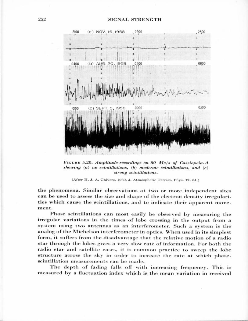
252 SIGNAL STRENGTH
2100 (a) NOV. 6, 1958 2200 23.00
0400 tb) AUG. 2O, 1958 0500 0600
0!00 (C) SEPT. 5, 1958 0200 0300
FIGURE 5.20. Amplitude recordings on ftO A/c/s of Cassiopvia-A. showing (a) no scintillations, (h) mot/crate scintillations^ find (c)
strong scintillations.
(After H. J. A. Chivers, 19CO, J. Atmospheric Terrest. Phys. 19, 54.)
the phenomena. Similar observations at two or more independent sites can be used to assess the size and shape of the electron density irregulari ties which cause the scintillations, and to indicate their apparent move ment.
Phase scintillations can most easily be observed by measuring the irregular variations in the times of lobe crossing in the output from a system using two antennas as an interferometer. Such a system is tin- analog of the IVlichelsoii interferometer in optics. When used in its simplest form, it suffers from the disadvantage that the relative motion of a radio star through the lobes gives a very slow rat*1 of information. For both the radio star and satellite cases, it is common practice to sweep the lobe structure across the sky in order to increase the rate at which phase- scin tillatioii measurements can be made.
The depth of fading falls off writh increasing frequency. This is measured by a fluctuation index which is the mean variation in received
RECIPROCITY 253
power relative to the average power. For normal scintillations, this index varies from about unity at 30 Mc/s to a small value at 300 Mc/s. Scintil lations have been reported on frequencies as high as 900 Mc/s, but tropo- spheric effects cannot be ruled out on this frequency.
The rate of scintillation, in the case of radio stars, varies from about 0.1 per minute to around 10 per minute. The scintillation rate appears to be independent of wave frequency down to about 30 Mc/s. When satel lites are used as sources, the scintillation rate depends mainly on the height and speed of the satellite and on the height of the irregularities. Sample values are around 10 fades per second.
The variation in angular position of a radio star is usually a few minutes of arc on 36 Mc/s with an observed upper limit of about 0.5°.
The diurnal variation of scintillations in temperate latitudes at low sunspot numbers shows a peak of occurrence at night but little by day. In high latitudes and during high solar activitv the distinction between day and night disappears. The seasonal variation is characterized by peaks during the equinoctial months. It is fairly closely correlated with the occurrence of spread F.
5.4.5. Fading Correlation Bandwidth
Because phase path differences in multipath propagation are a func tion of the wavelength, the fading on adjacent frequencies tends to be different. As the frequency difference 6co increases the correlation be tween fading on frequencies of oj0 and a?0 + 5aj will decrease and, at a suf ficiently large difference, the fading on the two channels will be unrelated. This selective fading can produce distortion in an amplitude modulated wave (double sideband) if the carrier fades to a level below that of the sidebands. This gives an effect similar to overmodulation. On high fre quencies, for a CW signal, the bandwidth of correlation is found to be around 3 kc/s and even less under severely disturbed conditions on arctic paths. Single pulse signals without overlapping time may have a correla tion bandwidth of 40 kc/s or so.
5.4.6. Reciprocity
A radio signal of given frequency traveling from A to B may be expected to exhibit the same fading as a similar signal received at A from B. Although this is true as far as paths and amplitudes are concerned,
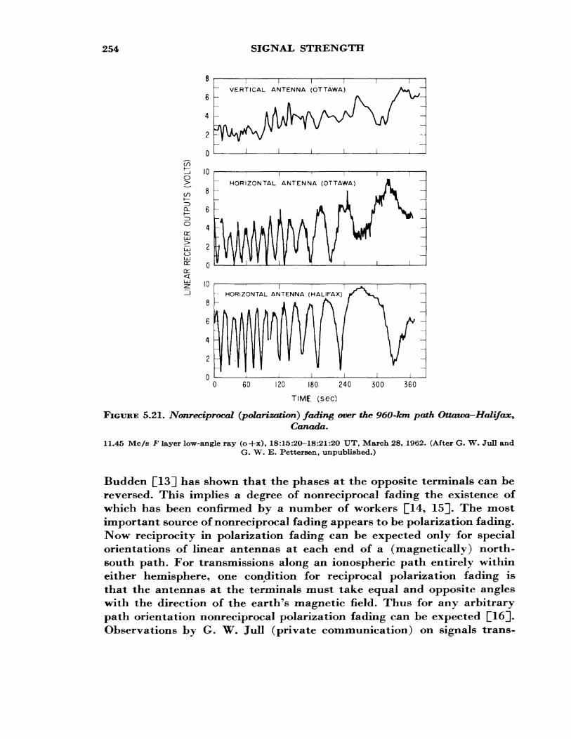
254 SIGNAL STRENGTH
§LO\— => CL f—
O
crLU
UJ O
I I I I VERTICAL ANTENNA (OTTAWA)
HORIZONTAL ANTENNA (OTTAWA)
HORIZONTAL ANTENNA (HALIFAX)
120 180 240
TIME (sec)
360
FIGURE 5.21. Nonreciprocal (polarization) fading over the 960-km path Ottawa-Halifax*Canada.
11.45 Mc/s F layer low-angle ray (o-fx), 18:15:20-18:21:20 UT, March 28, 1962. (After G. W. Jull andG. W. E. Pettersen, unpublished.)
Budden CIS] has shown that the phases at the opposite terminals can be reversed. This implies a degree of nonreciprocal fading the existence of which has been confirmed by a number of workers £14, 15], The most important source of nonreciprocal fading appears to be polarization fading. Now reciprocity in polarization fading can be expected only for special orientations of linear antennas at each end of a (magnetically) north- south path. For transmissions along an ionospheric path entirely within either hemisphere, one condition for reciprocal polarization fading is that the antennas at the terminals must take equal and opposite angles with the direction of the earth's magnetic field. Thus for any arbitrary path orientation nonreciprocal polarization fading can be expected £16]. Observations by G. W. Jull (private communication) on signals trans-
DIVERSITY 255
mitted over the east-west path Ottawa, Ontario, to Halifax, Nova Scotia (960 km) have shown that time displacements in polarization fading maxima can occur. Time displacements of up to one-half a fading cycle were observed (see fig. 5.21).
5.4.7. Diversity [17]
To minimize the effect of fading on quality of reception, use can be made of the fact that fading is correlated only over relatively small dis tances, and frequency bandwidths. Also signals from antennas having different polarizations may fade differently.
Space diversity is obtained by mixing signals from antennas separated by distances greater than the correlation distance. This is the distance beyond which the correlation coefficient of the fading falls to some speci fied value (e~l say).
Frequency diversity is obtained by transmitting and receiving on frequencies separated by more than the correlation bandwidth. This method is not recommended as it is wasteful of the usable frequency spectrum.
Polarization diversity is useful when there are two magneto-ionic waves present with essentially equal amplitudes. As discussed in section 4.9.5.1, the resultant of such waves is, approximately, a linearly polarized wave which rotates steadily so that sinusoidal (Faraday) fading would be observed with a linearly polarized antenna. Deep fading can be avoided by the use of two orthogonal antennas. There is little point in using po larization diversity when only one magneto-ionic component is likely to be present.
REFERENCES
[1] Norton, K. A, (1959), System loss in radio wave propagation, J* Res. NBS 63D(Radio Prop.), No. 1, 53.
[2] Bremmer, H. (1949), Terrestrial Radio Waves (Elsevier Publ. Co.). [3] Budden, K. G. (1961), Radio Waves in the Ionosphere (Cambridge Univ. Press). [4] Rawer, K. (1952), Calculation of sky-wave field strength, Wireless Engineer 29,
287. [5] Thomas, L. (1962), The winter anomaly in ionospheric absorption, Radio waves
absorption in the ionosphere, AGARDograph No. 53 (ed. N. C. Gerson)(Pergamon Press).
[6] Piggott, W. R. (1959), The calculation of the median sky wave field strength in
256 SIGNAL STRENGTH
tropical regions, Radio Research Special Report No. 27, Department of Scien tific and Industrial Research.
[7] Rice, S. O. (1944), Mathematical analysis of random noise, Bell Syst. Tech.J. 23, 282; (1945) 24, 46.
[8] Little, C. G., and A. C. B. Lovell (1951), The origin of the fluctuations in theintensity of radio 'waves from the galactic sources, Phil. Mag. 42, 267.
[9] Booker, H. G., J. A. Ratcliffe, and D. H. Shinn (1950), Diffraction from an ir regular screen with applications to ionospheric problems, Phil. Trans. Roy. Soc. (London) A242, 579.
[10] Bowhill, S. A. (1961), The scattering of radio waves by an extended randomly refracting medium, J. Atmospheric Terrest. Phys. 20, 9.
[11] Hewish, A. (1951), The diffraction of radio waves in passing through a phase changing ionosphere, Proc. Roy. Soc* (London) A209A, 81.
[12] Booker, H. G. (1958), The use of radio stars to study irregular refraction of radio waves in the ionosphere, Proc. IRE 46, 298.
[13] Budden, K. G. (1954), A reciprocity theorem on the propagation of radio waves via the ionosphere, Proc. Cambridge Phil. Soc. 50, Part IV, 604.
[14] Meadows, R. W. (1956), An experiment to test the reciprocal radio transmission conditions over an ionospheric path of 740 km, Proc. IEE (London) 103B, 224.
[15] Balser, M., W. B. Smith, and E. Warren (1958), On the reciprocity of HF iono spheric transmission, J. Geophys. Res. 63, 859.
[16] Budden, K. G. and G.W. Jull (1964),Reciprocity and non-reciprocity with magneto- ionic rays, Can. J. Phys. 42, 113.
[17] Baghdady, E. (1961), Lectures in communications systems theory, McGraw-Hill, New York.
CHAPTER 6
Ionospheric Disturbances
.1. TYPES OF DISTURBANCE
The term "ionospheric disturbance" is used to cover a wide variety of ionospheric conditions that show some departure from the usual state. Thus slight perturbations in the electron configuration that move with time are called traveling disturbances. These are usually localized in space. From the point of view of radio transmission, these traveling dis turbances are not nearly so important as the more (geographically) extensive disturbances which are all associated, in some way or another, with a flare on the sun (see section 1.7.6).
These solar flare associated effects may be classified as follows;
(1) Sudden ionospheric disturbances,(2) ionospheric storms,(3) polar cap absorption events (PCAs).
The reason these disturbances are important from the point of view of radio communications is that they often result in interruption of com munications. The absorption in the D region is enhanced so much that intelligible radio communications may be impossible for periods lasting from a few minutes to several days. Furthermore, the critical frequencies of the F% layer are sometimes depressed (ionospheric storms), resulting in loss of signal due to MUF failure. It is a very difficult matter to pre dict the onset of an ionospheric disturbance and since the ionospheric conditions can change rapidly from very quiet to highly disturbed, the idea of ''average" conditions (e.g., path loss, maximum frequency, etc.) tends to have only limited value. The purpose of this chapter is to out line the effects of these disturbances on radio signals and to discuss some ways of dealing with the problems.
Before discussing these various phenomena in detail, however, it is useful to consider the general pattern a little further. Although all the regular layers (£), E9 and jp) are affected, the E layer is not strongly affected except for the occurrence of sporadic E in certain ionospheric
257
258 IONOSPHERIC DISTURBANCES
storms. The D and F layers are subject to much stronger effects. The D region effects often occur simultaneously with the appearance of an optical solar flare, whereas the F region effects are often delayed by a day or more. These simultaneous and delayed effects are illustrated in figure 6.1.
We have seen (sec. 1.7.6) that the occurrence of a solar flare may be accompanied by the emission of radio waves, ultraviolet, and x rays, all of which arrive simultaneously at the earth because they travel with the free space velocity of light (essentially). Solar cosmic rays are also emitted with relativistic velocities and these may take 15 min to several hours to reach the earth, where they produce polar cap absorption. Slower particles, which have transit times of from 20 to 40 hr, result in iono spheric storms, magnetic storms, and visible displays of the aurora borealis. It should be remembered, of course, that not all the effects shown in figure 6.1 are associated with every flare.
6.2. SUDDEN IONOSPHERIC DISTURBANCES
6.2.1. D-Region Absorption
At times, communications on high frequencies by skywave propaga tion over the daylight hemisphere of the earth are "blacked out" by ab normally high absorption in the D region. The association between these shortwave fadeouts (SWF) and solar flares w^as discovered by Dellinger Cl]. 1 The condition of high absorption may last from a few minutes to several hours. Onset of this absorption is usually, but not always, very sudden (hence the name "sudden ionospheric disturbance," SID); it is followed by a relatively slow recovery, as shown in figure 6.2. Short wave fadeouts (SWFs) are sometimes accompanied by transient vari ations in the earth's magnetic field (fig. 6.2) indicating the existence of electric currents in the D region. Not all shortwave fadeouts are sudden and, at the National Bureau of Standards, SWFs are described as sudden, slow, or gradual, depending on the time variation of the recorded signal. Information on the occurrence of ionospheric effects of solar flares is given in CRPL F Series, B, Solar Geophysical Data, issued monthly by the National Bureau of Standards. The production of ionization in the D region gives rise to associated phenomena such as the sudden absorp tion of cosmic noise (SCNA) received on frequencies above the F2 layer
1 Figures in brackets indicate the literature references on p* 287.
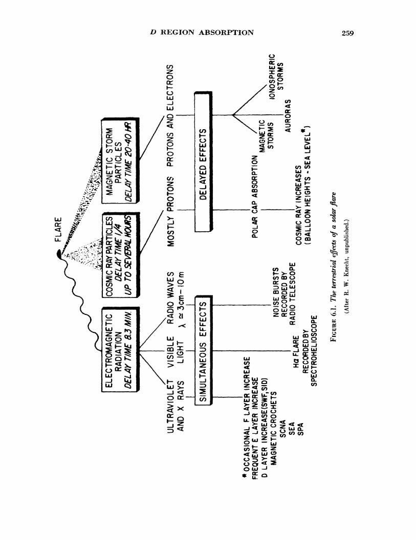
D REGION ABSORPTION 259
CO
jA,
,v>-«£*
J.v-.x*
£f
scr^cnC^Uj
00•-tUjOC§^<I^
^>T?".»r^
ui 5i- a: 3*
5/ ,,/ ..^v-v^
^/"^'S'^* *•"•'• \ V^\ """•'-•xV-'-iJ
VC/̂^<
ARTICLES 1 TIME 1/4 \
^•^£^otlSQ en8
&_0orH-O LU-JLU
. ^k
$§y %*\DELAYTI,
/ «^j Z <CO10r QC0.
en
P0QL
. d.
^
X.HJ
^ i
OH-LUTROMAGN
tADIATION
0^LU
LU
$5*•*>«e
1C:x̂
§
MOSTLY 1
enLUI
. o0,<t
/cr/
/ ^ / _j
\ cn >
I-UJ— 1o£ort~— ir^
£gcoP,x ^^ ^^
mmm
ent—
tfu.LU QLU
— 1 LU 0
//^
off
CO
(T
>v — CO ^\ {"•. 3E <t *
3J OCe>p ^co
0
CLa: oCO CD
CL
0
5CL
E 0
1
ofO21*<
h-Xo— 1
ensct: —
mamrn
enh- OLU U.U.LU
en0 LU
IZD
en
LU CO
UJgwg CO
LUKITLUO
x 5 ̂or
Q UL UJ^<^ ^—-51 ^3-^
O COuTCOUJCO
Ulcr0
SE BURSTS
o
CO
UJX0oo:
CO
INCREASE
>-or
CO O 0
Ul
IORDED BY ) TELESCOP
X-' CJLU^ ^3
cr
UJa:
u.
X
^̂̂ 4^ ^
—iLU
§UJ CO
lEIGHTS *
JC
0
CD
LUa. o
ECORDEDB^ FROHELIOS-
er oSCO
p
Jk.
ffects of a solaunpublished.)
*r"B 11 J^ P^
*ifH <J
<5 ^
Ctf
£
0 £5 uj QLy£<oco
cot o:UJ
o
O Ul
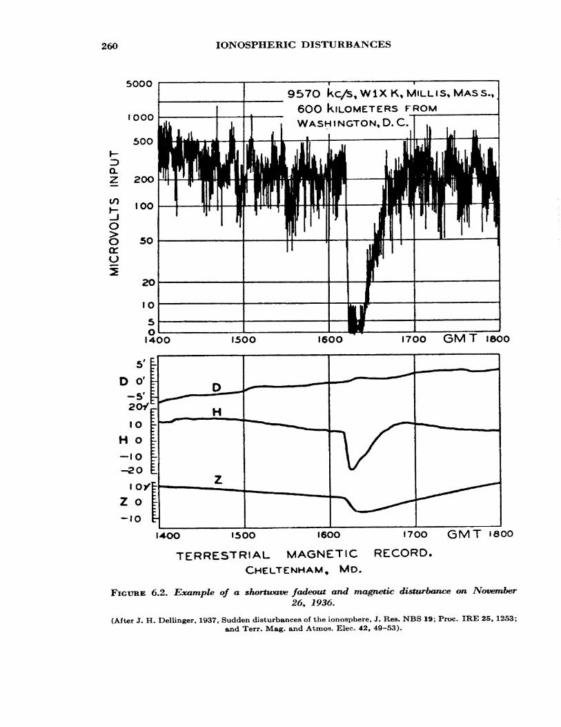
260 IONOSPHERIC DISTURBANCES
5OOO
O§cc
I-4OO
957O kc/s,WlXK, MILL is, MASS., 6OO KILOMETERS FROM WASH i NGTON. D. C.
1500 I6OO I7OO GMT I8OO
5'
D o'-5' 20/
10
H o-IO-20
IO/ Z O-IO
I4OO I5OO 1600 1700 GMT
TERRESTRIAL MAGNETIC RECORD. CHELTENHAM, MD.
FIGURE 6.2. Example of a shortwave fadeout and magnetic disturbance on November26, 1936.
(After J. H. Dellinger, 1937, Sudden disturbances of the ionosphere, J. Res. NBS 19; Proc. IRE 25, 1253;and Terr. Mag. and Atmos. Elec. 42, 49-53).
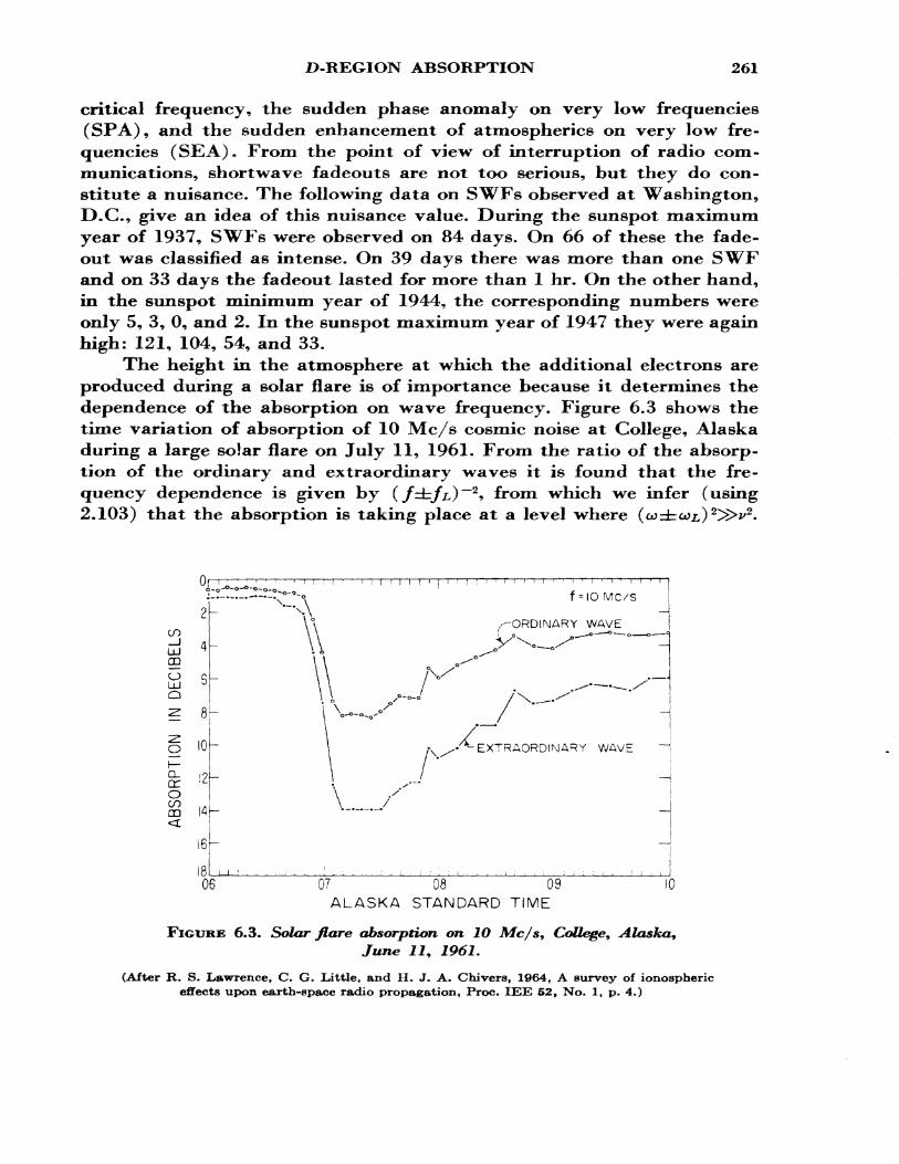
D-REGION ABSORPTION 261
critical frequency, the sudden phase anomaly on very low frequencies (SPA), and the sudden enhancement of atmospherics on very low fre quencies (SEA). From the point of view of interruption of radio com munications, shortwave fadeouts are not too serious, but they do con stitute a nuisance. The following data on SWFs observed at Washington, D.C., give an idea of this nuisance value. During the sunspot maximum year of 1937, SWFs were observed on 84 days. On 66 of these the fade- out was classified as intense. On 39 days there was more than one SWF and on 33 days the fadeout lasted for more than 1 hr. On the other hand, in the sunspot minimum year of 1944, the corresponding numbers were only 5, 3, 0, and 2. In the sunspot maximum year of 1947 they were again high: 121, 104, 54, and 33.
The height in the atmosphere at which the additional electrons are produced during a solar flare is of importance because it determines the dependence of the absorption on wave frequency. Figure 6.3 shows the time variation of absorption of 10 Mc/s cosmic noise at College, Alaska during a large solar flare on July 11, 1961. From the ratio of the absorp tion of the ordinary and extraordinary waves it is found that the fre quency dependence is given by (/±/z,)~2 > from which we infer (using 2.103) that the absorption is taking place at a level where
LO
UJCD
LU O
Q_cr oCO CD
06
f = IO MC/S
^-ORDINARY WAVE
'\.
EXTRAORDINARY WAVE
^
1
07 08 09 ALASKA STANDARD TIME
10
FIGURE 6.3. Solar flare absorption on 1O Mc/s, College, Alaska,June 11, 1961.
(After R. S. Lawrence, C. G. Little, and H. J. A. Chivers, 1964, A survey of ionospheric effects upon earth-space radio propagation, Proc. IEE 52, No. 1, p. 4.)
262 IONOSPHERIC DISTURBANCES
On the other hand, there is evidence which indicates that absorption can occur at low levels such that (coztco^) is comparable with v. It is of interest to note that during the flare of July 11, 1961, the absorption in the D region increased by a factor of the order of 10.
The vast majority of radio fadeouts is associated with solar flares. Therefore, they exhibit the same 11-yr occurrence cycle as do flares and sunspots. In general, the magnitude of the SID depends on the solar zenith angle.
Shortwave fadeouts have been studied using measurements of the minimum frequencies observed on ionograms Q3] (see sec. 3.2.2.4.) to give a synoptic picture of the worldwide distribution. It has been found that/m in varies as cos0 * 75 x* where x is the solar zenith angle.
6.2.2. Sudden Phase Anomalies
The increase of ionization in the D region produces an effect on the phase and amplitude of long and very long waves—usually a phase ad vance due to a lowering of the effective level of reflection. Changes in the effective height of reflection of from 0.9 to 15 km have been reported C4]. There appeared to be a threshold value of this height change of about 6 km, above which SPAs were accompanied by SWFs.
6.2.3. Sudden Frequency Deviations
During a solar flare, it is found that the frequency of a very stable radio signal, observed after reflection from the ionosphere, undergoes certain characteristic changes of a few cycles per second. The technique has already been described in section 2.5.3.
An increase in the electron content of the ionosphere usually brings about a decrease in the phase path of ionospherically reflected signals because of one or both of the following reasons:
(1) A lowering of the height of reflection, or(2) A lowering of the refractive index along the path below the level
of reflection.
It is possible to separate these two types of changes under the follow ing extreme conditions:
(a) When the height of the reflecting layer changes without change of layer shape, and/or the refractive index
M I =
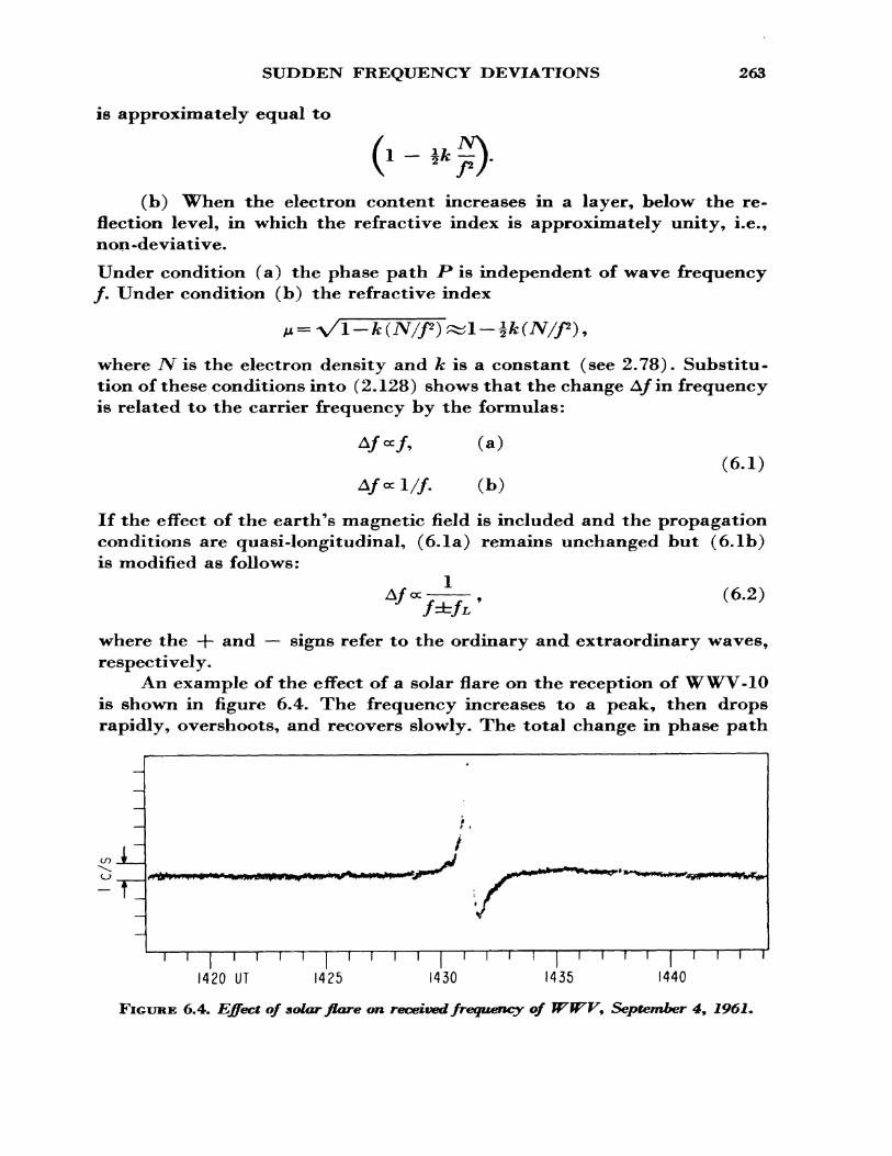
SUDDEN FREQUENCY DEVIATIONS 263
is approximately equal to
(b) When the electron content increases in a layer, below the re flection level, in which the refractive index is approximately unity, i.e., non-deviative.
Under condition (a) the phase path JP is independent of wave frequency /. Under condition (b) the refractive index
where TV is the electron density and A; is a constant (see 2.78). Substitu tion of these conditions into (2.128) shows that the change A/ in frequency is related to the carrier frequency by the formulas:
/, (a)(6.1)
I//. (b)
If the effect of the earth's magnetic field is included and the propagation conditions are quasi-longitudinal, (6. la) remains unchanged but (6.1b) is modified as follows:
* (6'2)
where the -f- and — signs refer to the ordinary and extraordinary waves, respectively.
An example of the effect of a solar flare on the reception of WWV-10 is shown in figure 6.4. The frequency increases to a peak, then drops rapidly, overshoots, and recovers slowly. The total change in phase path
I I 1 T I I I I I I I I I I I I I I I I 1 T 1420 UT 1425 1430 1435 1440
FIGURE 6.4. Effect of solar flare on received frequency of WWV+ September 49 1961.
264 IONOSPHERIC DISTURBANCES
AP can be determined from the area under the curve, i.e.,
AP=-Xo ( Afdt, (6.3)
-where X 0 is the free space wavelength. With the use of suitable models to represent the electron density profile, it is possible to convert the phase path changes into changes in total electron content or changes in height of reflection.
It is of interest to note that the following equivalence exists between frequency shifts on oblique and vertical paths [19].
A/* = A/v, (6.4)
where Af0b is the frequency shift on a wave transmitted over an oblique path and Afv is the frequency shift on the equivalent vertical wave (see 4.2).
In the case of changes below the level of reflection, it is possible to estimate the height at which the extra electrons are produced from simul taneous measurements of the changes in absorption A A of the signal and in phase path A.P. It can be shown (using (2.100) and the definition of phase path, P — /M ds) that for a thin layer, in which the ray path length is s, that
» (I \= KS = —— [ ——fJL ]2c\fji V
and
Hence AA = — — [ — + 1 ]A/jLStt — - AJJLS2c \j? c
and AP= A/JLS.
This gives — — = —— . (6.5)AP c
Knowing the variation with height of the collision frequency *>, it is pos sible to estimate an average height of electron production. Application of this theory to experimental data shows that, while no two flares pro duce identical results, most of the observed frequency changes are due to enhanced ionization in the E region C^D-
Flares that produce shortwave fadeouts are not necessarily those that produce the large frequency changes. Indeed some flares, which have
ASSOCIATION WITH MAGNETIC STORMS 265
produced large absorption by the creation of a relatively small number of electrons at levels where the collision frequency is high, produce little frequency change,
6.2.4. Effects on Very High Frequencies
Very high frequency waves (50 Mc/s) are propagated via the D region by scattering from ionospheric irregularities. During shortwave fadeouts it has been found that these signals are enhanced by as much as 9 dB and there is little evidence of any weakening of the signal (on 50 Mc/s) during an HF blackout £6]. However, on 27.7 Mc/s it was found that the signal enhancement lasted for a few minutes only and was fol lowed by marked attenuation £7], From these observations it would be concluded that the scattering occurred in the absorbing region and that the increased absorption was compensated for by increased scattering on the higher frequency but not on the lower frequency.
6.3. IONOSPHERIC STORMS
6.3.1. Association with Magnetic Storms
The term "ionospheric storm" is used to describe the conditions which may prevail for several days and which are accompanied by magnetic disturbances of the type referred to in section 1.5.3. It is, therefore, of interest to consider briefly the characteristics of magnetic storms.
Magnetic storms are disturbances of the earth's magnetic field lasting from a few hours to several days during which time the various components of the earth's field fluctuates over much wider limits (several percent of the total field in middle latitudes) than they do under normal conditions (a few tenths of one percent). In spite of the irregularity of the field the overall pattern can generally be classified into certain types.
One such type is that which begins with a sudden commencement (SC) which is essentially simultaneous all over the world. During the first few hours (the initial phase) the horizontal component remains above normal; then it drops rapidly to well below normal (the main or negative phase). After this a slow recovery takes place over several days and this is called the post-perturbation phase. Magnetic disturbance is usually most intense in the vicinity of the auroral zones.
Large magnetic storms with either sudden or gradual commence ment are accompanied by one or more of certain ionospheric phenomena
266 IONOSPHERIC DISTURBANCES
such as: a depression of the daytime critical frequencies of the F2 layer, radio blackout, enhanced spread F, and sporadic E. These ionospheric effects may last from 2 to 5 or more days. During sunspot maximum years there is a tendency for the effects to be shorter (2 to 3 days) and more severe while during sunspot minimum they tend to last longer (4 to 5 days) and are rather less intense.
6.3.2* Depression of F2 Critical Frequencies
The most prominent features of ionospheric storms are the reduction in the F% critical frequencies and the increase in D region absorption. The practical consequence of this lowering of the maximum usable fre quency and increase in the lowest usable frequency is a narrowing of the usable frequency spectrum. The effects of a magnetic storm on foF2 at a given location depend, in an involved way, upon the local time, season, magnetic latitude, and the storm time (that is, time measured from the onset of the storm).
Figure 6.5 shows the effect, on critical frequencies, of a storm in middle latitudes. The associated magnetic storm had the following time sequence:
Start—about 0400 LT, March 26;Maximum—morning, March 27 (J£=8 + ; see section 1.5.4.);End—late, March 29.
On the / plots for the second and third days, /oJ^2 is well below normal and the maximum electron density at noon is down by a factor of seven. Note also the appearance of the Fi layer. On the fourth day, the daytime /0 JP2S return towards normal, but depressed values and spread F (solid vertical lines in / plot) continue during the night hours for several ad ditional days (not shown). In certain latitudes, when the storm starts in the afternoon, the first effect on /o^s is an increase rather than a de crease. Later the usual decrease sets in.
Some results of a statistical study of the morphology (space and time variations) of ionospheric storms, by Matsushita £8^ are shown in figure 6.6. The world is divided into eight zones of geomagnetic latitude as follows: zone 1, 60° —55°; zone 2, 55° —50°; zone 3, 50° —45°; zone 4, 45°-40°; zone 5, 40°-29°; zone 6, 29°-20°; zone 7, 20°-9°; and zone 8, +9° to —9°. The results shown represent the average effects of 51 strong storms and 58 weak storms that occurred in the period 1946 through 1955. It will be seen that the most severe depressions in electron
ABSORPTION 267
density (and hence /o^) occur between about 20 and 40 hr storm time in geomagnetic latitudes of 45° and higher. In intermediate latitudes only a mild depression occurs, and in equatorial regions an actual increase is observed. Note also, that an initial increase tends to occur during the first 9 hr or so of the storm in all zones except those with the lowest lati tudes. Of course, it must be realized that this is the statistical picture and so an individual storm will not necessarily follow this pattern.
In addition to the storm time variations there are marked variations which depend on the local time. Thus the time of maximum depression of A^max depends on local time. Some useful factual data are presented in table 6.1 (after Matsushita) , showing how the times (local and storm) of maximum depression depend on magnetic latitude.
TABLE 6.1. Variation tvith geomagnetic latitude of times of peak depression of 7Vduring a storm
(A)
Zone
60°-55°55°-50°50°-45°45°-40°40°-29°
(B)
Decrease(%)
30-5030-4530-4515-2515-20
<C)
Ixjoal Time{Hours)
14-2222-0401-0703-1303-13
(I>)Storm Time
{Hours}
17-4210-4110-4219-5520-48
The table should be interpreted as follows: In the zone given in column (A) a maximum decrease of about the percentage shown in OB) will occur at about the local time shown in (C) during .the period after the onset of a strong magnetic storm with a sudden commencement indicated in
The fact that the statistical picture in figure 6.6 can be a little mis leading is shown by the seasonal variation of storm pattern in zone 6. The data shown would suggest that there is relatively little storm time variation in the F% layer in these latitudes. The results of a seasonal analysis, however, show that the electron density is depressed during the summer but enhanced in the winter. The overall average is, therefore, not representative of a single storm in either of those seasons.
6.3*3. Absorption
6.3*3.1. Blackout Statistics
During some magnetic storms, the absorption of radio waves in the D region is so intense that no detectable signals are reflected. This is
268 IONOSPHERIC DISTURBANCES
CO52;
PQ
O
CO
FIGURE 6.5. Ionospheric storm effects in middle latitudes.
ABSORPTION 269
FIGURE 6.5*—Continued. Ionospheric storm effects in middle latitudes*
270 IONOSPHERIC DISTURBANCES
STRONG STORMS WEAK STORMS
/\KyVu^\/v\ --1//W
O 12 24 36 48 60 72 0 12 24 36 48 6O 72
STORM TIME
FIGURE 6.6. Storm time variations of maximum electron densities (F%) in different latitudes.
(After S. Matsushita, 1959, A study of the morphology of ionospheric storms, J. Geophys Res. 64, 305.)
ABSORPTION 271
particularly true near the auroral zones and the absorption is often re ferred to as auroral absorption or auroral blackout. These blackouts have been studied statistically by several workers £9, 10, 11] to determine the geographic and time distributions in their occurrence. The procedure has been to count the occurrences of the no-echo condition on conven tional ionograms* This condition is denoted by the letter B on the hourly data sheets of ionospheric characteristics. Alternatively, a measure of absorption can be obtained from the minimum frequency/m in observed on ionograms (see sec. 3.2.2.4). The occurrence of high absorption can be determined from the occasions when/m in exceeds a certain frequency.
6.3.3.2. Time of Maximum Occurrence
The most probable time of occurrence of blackout is in the morning and the least probable in the evening. Furthermore, the most probable time is later as the latitude increases; for instance, it varies from about 0700 at Winnipeg to about 1300 at Resolute Bay. The geographical vari ation of the local time of maximum occurrence of blackout during the International Geophysical Year is shown in figure 6.7 for the northern
I50°E
ISO0
I5O° W
30° E
3O° W
I2O° 9O° W
FIGURE 6.7. Local mean time of maximum frequency of occurrence of blackout, northern hemisphere—IG Y.
(After V. Agy, unpublished.)
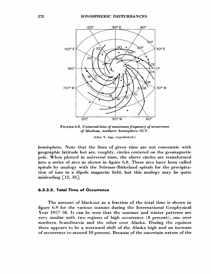
272 IONOSPHERIC DISTURBANCES
I2O° 9O°E
I50°E
180°
I50°W
30° E
30° W
I2O° 90° W
FIGURE 6.8. Universal time of maximum frequency of occurrence of blackout* northern hemisphere—IG Y.
(After V. Agy, unpublished.)
hemisphere. Note that the lines of given time are not concentric with geographic latitude but are, roughly, circles centered on the geomagnetic pole. When plotted in universal time, the above circles are transformed into a series of arcs as shown in figure 6.8. These arcs have been called spirals by analogy with the Stormer-Birkeland spirals for the precipita tion of ions in a dipole magnetic field, but this analogy may be quite misleading
6.3.3.3. Total Time of Occurrence
The amount of blackout as a fraction of the total time is shown in figure 6.9 for the various seasons during the International Geophysical Year 1957—58. It can be seen that the summer and winter patterns are very similar with two regions of high occurrence (8 percent), one over northern Scandinavia and the other over Alaska. During the equinox there appears to be a westward shift of the Alaska high and an increase of occurrence to around 10 percent. Because of the uncertain nature of the
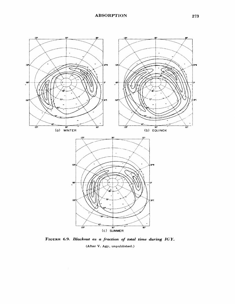
ABSORPTION 273
30f ISO*
90*
(a) WINTER90*
<b) EQUINOX
120*
(c) SUMMER
FIGURE 6,9. Blackout as a fraction of total time during IGY.
(After V. Agy, unpublished.)
274 IONOSPHERIC DISTURBANCES
data on which these maps are based, too much attention should not be paid to small variations. The average diurnal path of the blackout pattern for the equinox months is shown in figure 6.10. Notice that the blackout pattern moves around with the sun (shaded region represents darkness) and that the peak percentages vary with longitude. In all three seasons the maximum contour leads the sun by some 6 hr or so and the motion of the contours is relatively uniform except over Canada (£^90° west).
6.3.3.4. Latitude Variation
Maps such as those shown in figures 6*9 and 6.10 show that the maxi mum occurrence of blackout takes place in a ring similar to, but not necessarily identical with, the visual auroral zone. North of this zone there is a polar region in which the incidence of blackout is relatively low. The width of the absorption zone has not yet been established with certainty but appears to lie between about 6° £13J and about 15° Q14]. This difference may be brought about by an increase in both the radius of the ring (southward motion) and a broadening with increasing sunspot numbers.
Within the auroral ring the average incidence of blackout is of the order of 5 percent £15^], although at a small number of abnormally sensi tive stations in the ring the average may rise to 15 percent.
6.3.3.5. Magnetic Correlation
In relatively low latitudes, outside the absorption ring, there is a high correlation with the Kp index. In higher latitudes, however, the mag netic correlation is obscured by the presence of polar cap absorption C-^^H- There is also a marked 27-day recurrence tendency in the occurrence of auroral absorption similar to that in magnetic activity CM].
6.3.3.6. Sunspot Variation
There appears to be a strong association between the 11-yr sunspot cycle and the long-term cycle of auroral blackout occurrence Cl^J. The peak phases of the two cycles are displaced by 2 to 3 yr. The peak in blackout occurrence over Canada took place around 1950—51, whereas the sunspot numbers peaked in 1947 and reached a minimum in 1954 Q14]. This behavior is similar to that of moderate geomagnetic dis turbances, which also fail to show a clear decrease at sunspot minimum.
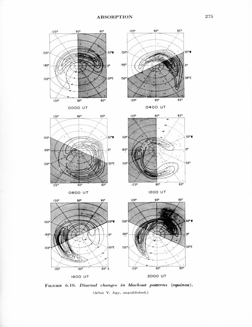
ABSORPTION 275
(20
ISO*
120" 90°
OOOO UT
120*
150*
150
ISO
150
30'* 150*
0 . 190*
3D'F 150*
60'
JO'W 150
60' 0
50*1
30'E 150
30*W ISO
30*E 150'
30* t
30'E
FIGURE 6.10. Diurnal changes in blackout patterns (equinox).
(After V. Agy, unpublished.)
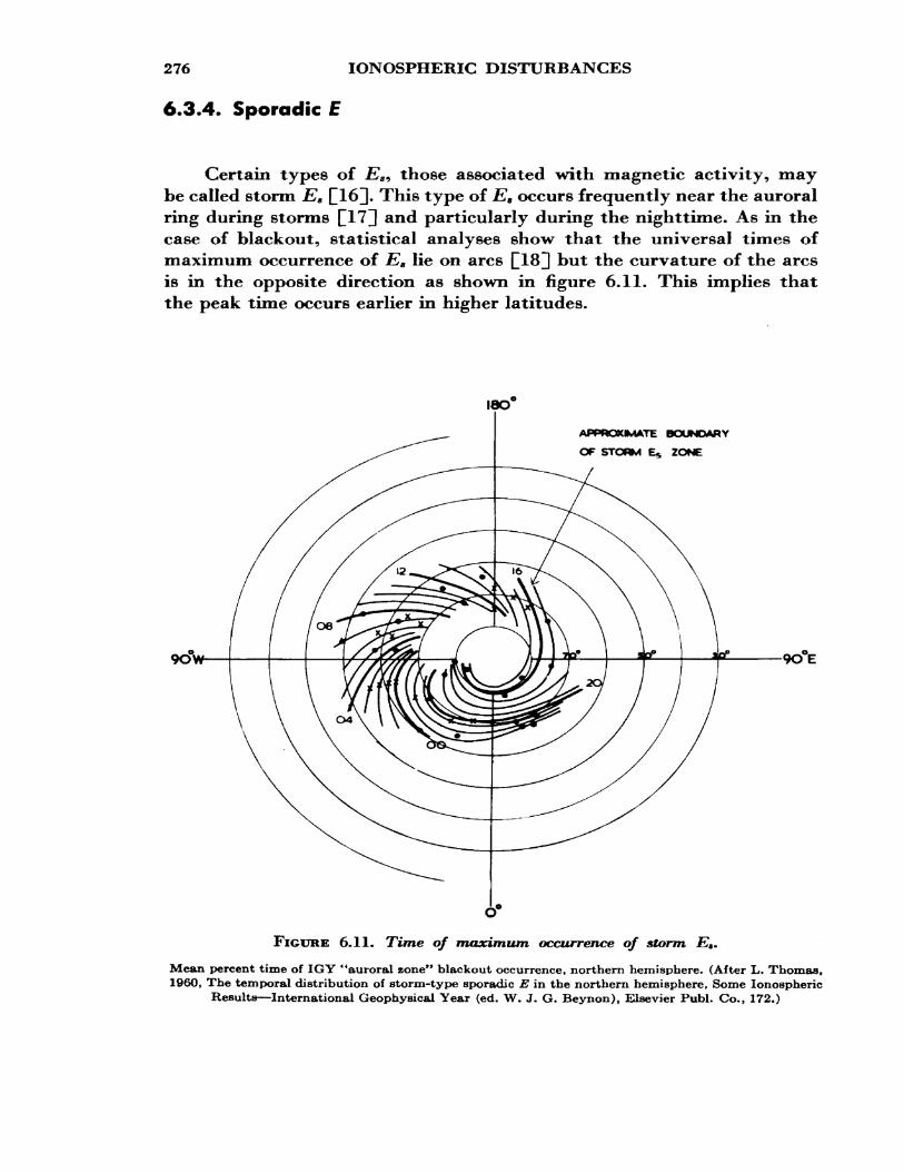
276 IONOSPHERIC DISTURBANCES
6.3.4. Sporadic E
Certain types of E8, those associated with magnetic activity, may be called storm Es £16]. This type of E8 occurs frequently near the auroral ring during storms Hi'71 and particularly during the nighttime. As in the case of blackout, statistical analyses show that the universal times of maximum occurrence of E8 lie on arcs Q18] but the curvature of the arcs is in the opposite direction as shown in figure 6.11. This implies that the peak time occurs earlier in higher latitudes.
180"
APPROtUMATE BOUNDARY
OF STORM ES ZONE
90°E
FIGURE 6.11. Time of maximum occurrence of storm E9.
Mean percent time of IGY "auroral zone" blackout occurrence, northern hemisphere. (After L. Thomas.1960, The temporal distribution of storm-type sporadic E in the northern hemisphere, Some Ionospheric
Results—International Geophysical Year (ed. W» J. G. Beynon), Elsevier Publ. Co,, 172.)
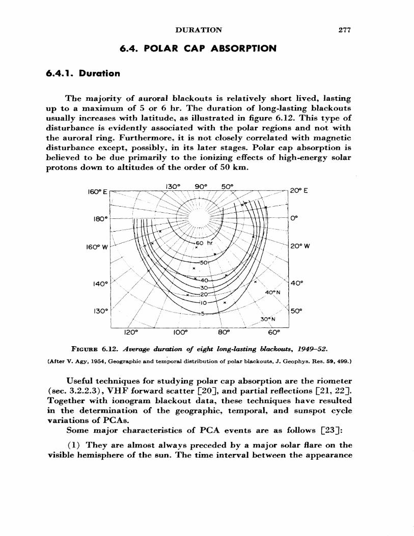
DURATION
6.4. POLAR CAP ABSORPTION
277
6.4.1* Duration
The majority of auroral blackouts is relatively short lived, lasting up to a maximum of 5 or 6 hr. The duration of long-lasting blackouts usually increases with latitude, as illustrated in figure 6*12. This type of disturbance is evidently associated with the polar regions and not with the auroral ring. Furthermore, it is not closely correlated with magnetic disturbance except, possibly, in its later stages. Polar cap absorption is believed to be due primarily to the ionizing effects of high-energy solar protons down to altitudes of the order of 50 km.
I6O°E
180°
I6O°W
!4O C
I3O C
130 50°20° E
2O° W
4O°
50°
120° too0 8O°
FIGURE 6.12. Average duration of eight long-lasting blackouts* 1949-52.
(After V. Agy, 1954, Geographic and temporal distribution of polar blackouts, J. Geophys. Res. 59, 499.)
Useful techniques for studying polar cap absorption are the riometer (sec. 3.2.2.3), VHF forward scatter £203, ancj partial reflections [21, 22]. Together with ionogram blackout data, these techniques have resulted in the determination of the geographic, temporal, and sunspot cycle variations of PCAs.
Some major characteristics of PCA events are as follows £23]:
(1) They are almost always preceded by a major solar flare on the visible hemisphere of the sun. The time interval between the appearance
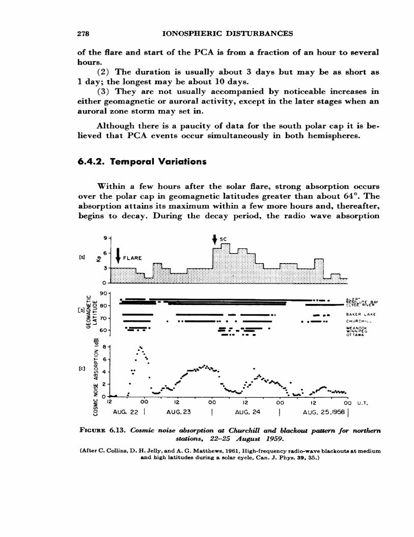
278 IONOSPHERIC DISTURBANCES
of the flare and start of the PCA is from a fraction of an hour to several hours.
(2) The duration is usually about 3 days but may be as short as 1 day; the longest may be about 10 days.
(3) They are not usually accompanied by noticeable increases in either geomagnetic or auroral activity, except in the later stages when an auroral zone storm may set in.
Although there is a paucity of data for the south polar cap it is be lieved that PCA events occur simultaneously in both hemispheres.
6.4.2. Temporal Variations
Within a few hours after the solar flare, strong absorption occurs over the polar cap in geomagnetic latitudes greater than about 64°. The absorption attains its maximum within a few more hours and, thereafter, begins to decay. During the decay period, the radio wave absorption
ffi
90
8O
7O
6O-
8H
CC] 1CD
y 12 00
8 AUG, 22 I
8AKER LAKE
CHURCHILL
MEANQOK WINMP£G OTTAWA
12 OO 12 OO 12 OO U.T.
AUG.23 I AUG. 24 I AUG. 25,1958 I
FIGURE 6.13. Cosmic noise absorption at Churchill and blackout pattern for northernstations* 22-25 August 1959.
(After C. Collins, D. H. Jelly, and A. G. Matthews, 1961, High-frequency radio-wave blackouts at medium and high latitudes during a solar cycle, Can. J. Phys. 39, 35.)
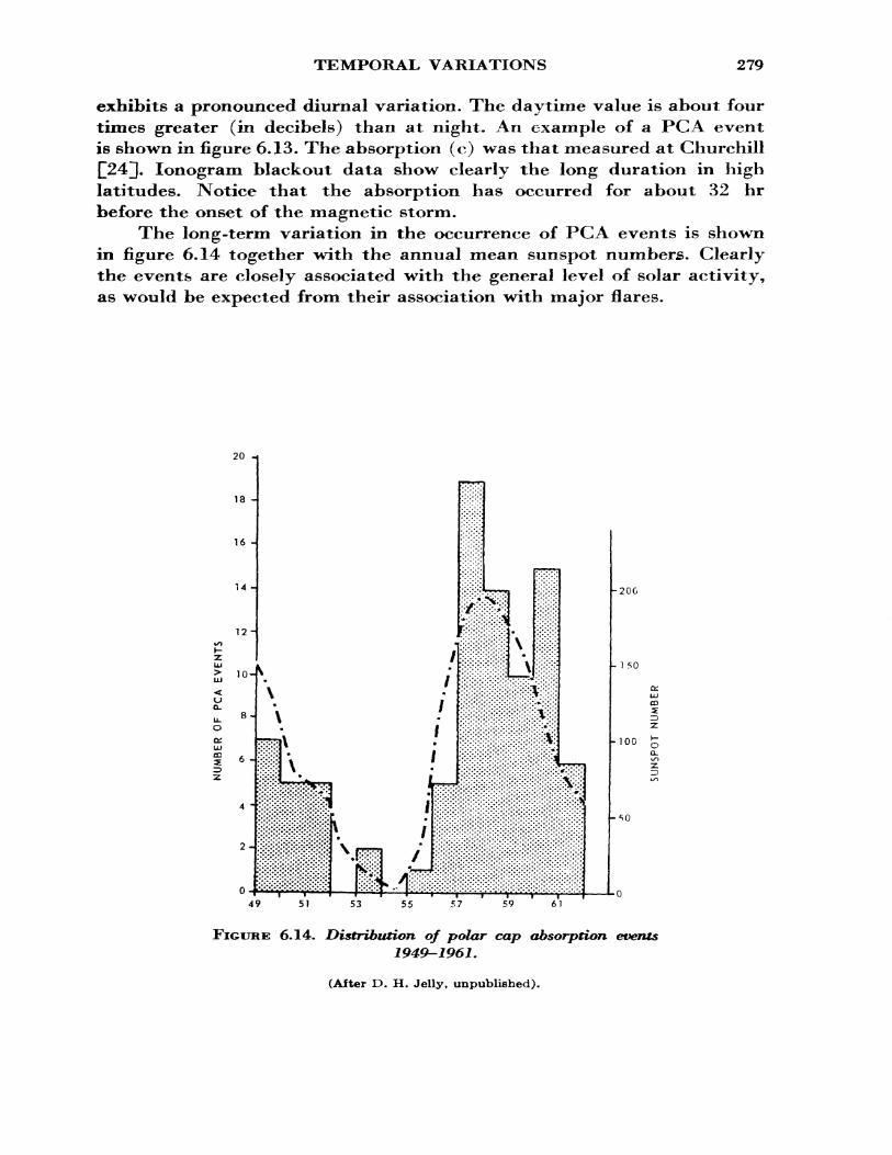
TEMPORAL VARIATIONS 279
exhibits a pronounced diurnal variation. The daytime value is about four times greater (in decibels) than at night. An example of a PCA event is shown in figure 6.13. The absorption (c) was that measured at Churchill [[24]. lonogram blackout data show clearly the long duration in high latitudes. Notice that the absorption has occurred for about 32 hr before the onset of the magnetic storm.
The long-term variation in the occurrence of PCA events is shown in figure 6.14 together with the annual mean sunspot numbers. Clearly the events are closely associated with the general level of solar activity, as would be expected from their association with major flares.
20 -«
18 J
h200
h 150
HOC oCL
49 51 53 55 57 59 6)
FIGURE 6.14. Distribution of polar cap absorption1949-1961.
(After E>. H. Jellyt unpublished).
events
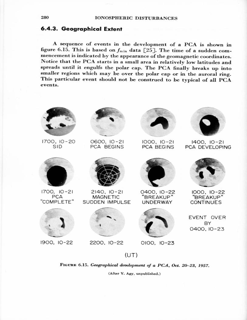
280 IONOSPHERIC DISTURBANCES
6.4.3. Geographical Extent
A sequence of events in the development of a PCA is shown in figure 6.15. This is based on/min data £25]. The time of a sudden com mencement is indicated by the appearance of the geomagnetic coordinates. Notice that the PCA starts in a small area in relatively low latitudes and spreads until it engulfs the polar cap. The PCA finally breaks up into smaller regions which may be over the polar cap or in the auroral ring. This particular event should not be construed to be typical of all PCA events.
I70O, IO-2O SID
06OO, 1O-2I PCA BEGINS
IOOO, IO-2I PCA BEGINS
I4OO. IO-2! PCA DEVELOPING
I70Q, IO-2IPCA
"COMPLETE"
I9OO. IO-22
214O, IO-2IMAGNETIC
SUDDEN IMPULSE
O4OO, IO-22 "BREAKUP"
UNDERWAY
220O, IO-22 OtOO. IO-23
(UT)
IOOO, IO-22 "BREAKUP"
CONTINUES
EVENT OVERBY
O4OO, IO-23
FIGURE 6.15. Geographical development of a PCA* Oct. 20—23, 1957.
(After V. Agy, unpublished.)
GENERAL CONSIDERATIONS 281
6*4*4. Frequency Dependence of the Absorption
If the absorption takes place high in the D region, where y<$Co>, we should expect the absorption to obey (2.99), whereas if it occurs very low down, where *C§>co, we should expect (2.101) to hold. The frequency de pendence can, therefore, be used to determine (at least roughly) the al titude at which the absorption takes place. This approach has been used by Little and Silberstein £26^ in an analysis of continuous wave trans missions between Barrow and Kenai, Alaska, on 5, 10, and 15 Mc/s along with riometer measurements on 50 Mc/s made by aiming the riometer antennas along the probable oblique HF paths at both ends. It was concluded that the inverse square law was inoperative on the lower frequencies and, therefore, that the absorption takes place at levels from 50 to 70 km.
6.5. EFFECTS ON RADIO COMMUNICATIONS IN HIGHLATITUDES
6.5.1. Some General Considerations
The effect of shortwave fadeouts on radio communications is so insignificant, especially in high latitudes where the solar zenith angle is large, that it will not be considered further. On the other hand, the effects brought about by storms and polar cap events are often catas trophic.
A lowering of the maximum frequency (due to depression of the critical frequency) and an increase in the lowest frequency (due to ab sorption) can occur separately or simultaneously* In all cases the effect is a narrowing of the usable frequency spectrum. The former often happens in middle latitudes and the latter has been observed near the auroral ring.
Ionospheric storms are frequently accompanied by spread F con stituting a breaking up of the reflecting layer. This in turn brings about rapid fading called ee auroral flutter/9 This flutter is disastrous to voice communication .
The combination of these effects makes HF communications via the auroral regions rather unreliable. Also, the southward extension of the auroral ring during storms disrupts communications between North America and Europe and relaying of the traffic through low-latitude stations is necessary. Thus, although ionospheric disturbance may last only 5 percent of the time, high-frequency communications cannot be used when 100 percent reliability is essential.
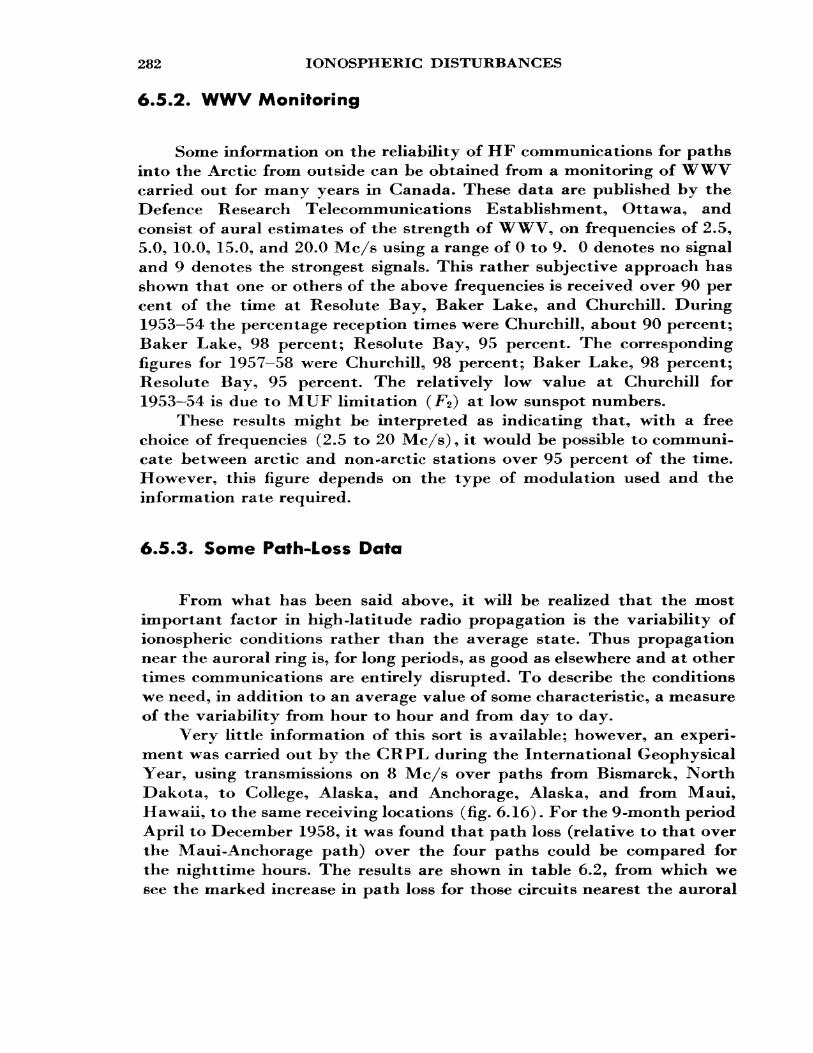
282 IONOSPHERIC DISTURBANCES
6.5.2. WWV Monitoring
Some information on the reliability of HF communications for paths into the Arctic from outside can be obtained from a monitoring of WWV carried out for many years in Canada. These data are published by the Defence Research Telecommunications Establishment, Ottawa, and consist of aural estimates of the strength of WWV, on frequencies of 2.5, 5.0, 10.0, 15.0, and 20.0 Mc/s using a range of 0 to 9. 0 denotes no signal and 9 denotes the strongest signals. This rather subjective approach has shown that one or others of the above frequencies is received over 90 per cent of the time at Resolute Bay, Baker Lake, and Churchill. During 1953—54 the percentage reception times were Churchill, about 90 percent; Baker Lake, 98 percent; Resolute Bay, 95 percent. The corresponding figures for 1957—58 were Churchill, 98 percent; Baker Lake, 98 percent; Resolute Bay, 95 percent. The relatively low value at Churchill for 1953—54 is due to MUF limitation (/^O at low sunspot numbers.
These results might be interpreted as indicating that, with a free choice of frequencies (2.5 to 20 Mc/s), it would be possible to communi cate between arctic and non-arctic stations over 95 percent of the time. However, this figure depends on the type of modulation used and the information rate required.
6.5.3. Some Path-Loss Data
From what has been said above, it will be realized that the most important factor in high-latitude radio propagation is the variability of ionospheric conditions rather than the average state. Thus propagation near the auroral ring is, for long periods, as good as elsewhere and at other times communications are entirely disrupted. To describe the conditions we need, in addition to an average value of some characteristic, a measure of the variability from hour to hour and from day to day*
Very little information of this sort is available; however, an experi ment was carried out by the CRPL during the International Geophysical Year, using transmissions on 8 Mc/s over paths from Bismarck, North Dakota, to College, Alaska, and Anchorage, Alaska, and from Maui, Haw^aii, to the same receiving locations (fig. 6.16). For the 9-month period April to December 1958, it was found that path loss (relative to that over the Maui-Anchorage path) over the four paths could be compared for the nighttime hours. The results are shown in table 6.2, from which we see the marked increase in path loss for those circuits nearest the auroral
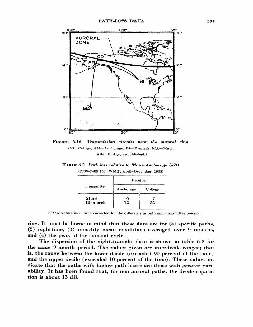
9O<I8O°
60*
30*
PATH-LOSS DATA
_________i2Oe________
283
6O°
AURORAL ZONE
MA
90 e
60°
30°
I8O° 60°
FIGURE 6.16. Transmission circuits near the auroral ring.CO—College, AN—Anchorage, BI—Bismark, MA—Maui.
(After V. Agy, unpublished.)
TABLE 6.2. Path loss relative to Maui-Anchorage (dB)(220CK2400 150° WMT; April-December, 1958)
Receiver
Transmitter
Maui Bismarck
Anchorage
0 12
College
7 22
(These values have been corrected for the difference in path and transmitter power).
ring. It must be borne in mind that these data are for (a) specific paths, (2) nighttime, (3) monthly mean conditions averaged over 9 months, and (4) the peak of the sunspot cycle.
The dispersion of the night-to-night data is shown in table 6.3 for the same 9-month period. The values given are interdecile ranges; that is, the range between the lower decile (exceeded 90 percent of the time) and the upper decile (exceeded 10 percent of the time). These values in dicate that the paths with higher path losses are those with greater vari ability. It has been found that, for non-auroral paths, the decile separa tion is about 13 dB.
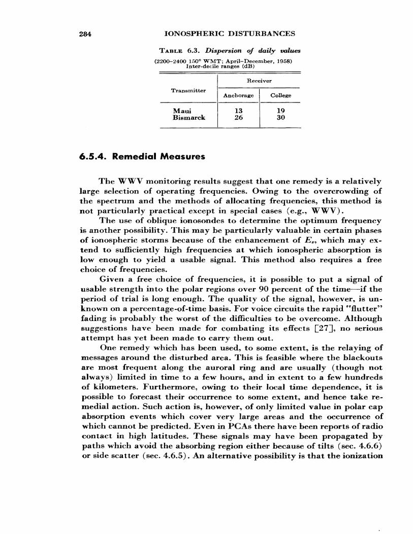
284 IONOSPHERIC DISTURBANCES
TABLE 6.3. Dispersion of daily values(220O-2400 150° WMT; April-December, 1958)
Inter-decile ranges (dB)
Transmitter
Maui Bismarck
Receiver
Anchorage
13 26
College
19 30
6.5.4* Remedial Measures
The WWV monitoring results suggest that one remedy is a relatively large selection of operating frequencies. Owing to the overcrowding of the spectrum and the methods of allocating frequencies, this method is not particularly practical except in special cases (e.g., WWV).
The use of oblique ionosondes to determine the optimum frequency is another possibility. This may be particularly valuable in certain phases of ionospheric storms because of the enhancement of Es, which may ex tend to sufficiently high frequencies at which ionospheric absorption is low enough to yield a usable signal. This method also requires a free choice of frequencies.
Given a free choice of frequencies, it is possible to put a signal of usable strength into the polar regions over 90 percent of the time—if the period of trial is long enough. The quality of the signal, however, is un known on a percentage-of-time basis. For voice circuits the rapid "flutter" fading is probably the worst of the difficulties to be overcome. Although suggestions have been made for combating its effects £27], no serious attempt has yet been made to carry them out.
One remedy which has been used, to some extent, is the relaying of messages around the disturbed area. This is feasible where the blackouts are most frequent along the auroral ring and are usually (though not always) limited in time to a few hours, and in extent to a few hundreds of kilometers. Furthermore, owing to their local time dependence, it is possible to forecast their occurrence to some extent, and hence take re medial action. Such action is, however, of only limited value in polar cap absorption events which cover very large areas and the occurrence of which cannot be predicted. Even in PC As there have been reports of radio contact in high latitudes. These signals may have been propagated by paths which avoid the absorbing region either because of tilts (sec. 4.6.6) or side scatter (sec. 4.6.5). An alternative possibility is that the ionization
RADIO PROPAGATION FORECASTING 285
is created very law down in the D region; under these conditions the ab sorption would not increase on the lower frequencies (see (2.101)) as much as it would if the absorption occurred at higher altitudes.
Other alternatives are the use of very low frequencies, very high frequencies (forward scatter, meteor scatter, etc.), and tropospheric scatter.
6.6. RADIO PROPAGATION FORECASTING
Forecasting of the probable occurrence of an ionospheric storm can be very useful from several points of view. For example, a communica tions operator is warned to transmit his essential messages before his circuit is blacked out; alternatively he may start up various relay links, or change his operating frequency.
The two radio forecasting centers of the Central Radio Propagation Laboratory regularly issue three types of forecasts of radio propagation conditions. These forecasts apply to sky wave propagation (usually within the frequency range 2 to 30 Mc/s) over certain particularly im portant radio paths. The North Atlantic Radio Warning Service is con cerned primarily with transmission over paths such as New York—London or Washington—Paris; their forecasts will apply to a lesser extent on nearby paths like Boston—North Africa, Maine—Greenland, etc. The North Pacific Radio Warning Service forecasts are designed for paths like Anchorage- Seattle, San Francisco—Fairbanks, or Tokyo—Anchorage; they can be given special interpretation, however, for others, such as short intra- Alaska circuits, but again with less reliability.
Average quality is forecast for a specified 6-, 12-, or 24-hr period. All times are Universal Time (UT or GCT). The CRPL radio quality scale is used in all instances:
1—Useless 6—Fair-to-good2—Very poor 7—Good3—Poor 8—Very good4—Poor-to-fair 9—Excellent.5—Fair
The average quality in the 2 hr preceding the issue time is expressed in the following letter code:
i W—disturbed (1 to 4)U—unsettled (5) N—normal (6 to 9).
286 IONOSPHERIC DISTURBANCES
The forecasts must be interpreted in the light of the user's own ex perience. A forecast of r*3" means that the conditions experienced should be relatively poor, but the operator must interpret this in terms of the expected performance of his circuit. If the forecast is correct, no more than 5 or 10 percent of all days should be so poor. There may be, however, a systematic difference between the word-descriptions used by the operator and by the forecaster, and the operator must take this into account in interpreting the forecast. For instance, he may be used to calling condi tions "very poor" when the forecaster calls them frpoor," or the operator of another, perhaps easier, circuit may never see conditions as worse than fffair." The forecasts are expressed on a scale which corresponds to the average experience reported on a typical circuit.
The estimate of present conditions (the letter) is made available to aid the user in interpreting the forecast (the number). For example, if an "N—5" is issued, and the operator is already at the time of the forecast experiencing what he would call unsettled (quality 5) conditions, then he would expect conditions to become even worse. The statement N—5 indicates that the forecaster looks for a deterioration of at least one grade during the forecast period. The value of this scheme rests on the fact that the operator is concerned with expected changes in conditions and so is given information to tie in with his current experience. If the "5" had been issued without the "N," the user would not have been prepared for a drop in quality since he was already experiencing what he called quality ff5" conditions, although the concensus available to the forecaster rated conditions ''normal."
A third forecast, the 24-hr forecast, is also available daily by telephone and teletype from the two forecasting centers. Separate quality estimates are issued for nighttime and daytime of the ensuing 24-hr period. The range of frequencies on which the predicted quality should be realized is also included.
Additional information concerning the radio forecasting services may be obtained from:
For the North Atlantic area:North Atlantic Radio Warning Service (or NARWS) National Bureau of Standards, Box 178, Fort Belvoir, Va.
(Telephone—Washington, B.C., 780-1436 or 780-1444)
For the North Pacific and Alaskan area:North Pacific Radio Warning Service (or NPRWS) National Bureau of Standards, Box 1119, Anchorage, Alaska
(Telephone—753-2211 or 753-7210)
REFERENCES 287
Past CRPL forecasts together with the actual conditions which developed are included in the CRPL F series, B, Solar Geophysical Data.
REFERENCES
[1] Dellinger, J. H. (1937), Sudden ionospheric disturbances, Terr. Mag. and Atmos.Elec. 42, 49.
[2] Ratcliffe, J. A. (1960), S.I.D.'s during the IGY, Some Ionospheric Results—International Geophysical Year (ed. W.J.G. Beynon), p. 124 (Elsevier PubL Co.)
[3] Kasuya, I., Y. Hakura, and H. Hojo, (1959), On the SWF phenomenon (Dellingereffect) andym in in the world-wide distribution, J. Radio Res. Labs. (Tokyo) 6,1.
[4] Bracewell, R. N., and T. W. Straker (1949), The study of solar flares by very longwaves, Monthly Not. Roy. Astron. Soc. 109, 28*
[5] Davies, K. (1963), Doppler studies of the ionospheric effects of solar flares, Proc.Int. Conf. on the Ionosphere, Inst. Phys. and Phys. Soc., 76.
[6] Bailey, IX K., R. Bateman, L. V. Berkner, H. G. Booker, G. F. Montgomery, E. M. Purcell, and W. W. Salisbury (1952), A new kind of radio propagation at very high frequencies observed over long distances, Phys. Rev. 86, 141.
[7] Bailey, D. K., R. Bateman, and R. C. Kirby (1955), Radio transmission at VHPby scattering and other processes in the lower ionosphere, Proc. IRE 43, 1181.
[8] Matsushita, S. (1959), A study of the morphology of ionospheric storms, J. Geo-phys. Res. 64, 305.
[9] Agy, V. (1954), Geographic and temporal distribution of polar blackouts, J.Geophys. Res. 59, 499.
[10] Cox, J. W., and K. Davies (1954), Statistical studies of polar radio blackouts, Can.J. Phys. 32, 743.
[11] Thomas, L., and W. R. Piggott (1960), Some aspects of the incidence of polar blackout during the IGY, Some Ionospheric Results—International Geo physical Year (ed. W. J. G. Beynon) (Elsevier Publ. Co.), 61.
[12] Agy, V. (1960), Spiral patterns in geophysics, J. Atmospheric and Terrest. Phys.19, 136.
[13] Agy, V. (1954), The location of the auroral absorption zone, J. Geophys. Res. 59,267.
[14] Collins, C., D. H. Jelly, and A. G. Matthews (1961), High-frequency radiowave blackouts at medium and high latitudes during a solar cycle, Can. J. Phys. 39, 35.
[15] Piggott, W. R., and L. Thomas (1960), Variations in the incidence of polar black out with magnetic activity, Some Ionospheric Results—International Geo physical Year (ed. W. J. G. Beynon) (Elsevier Publ. Co.), 72.
[16] Thomas, L. (1960), The temporal distribution of storm-type sporadic E in the northern hemisphere, Some Ionospheric Results—International Geophysical Year (ed. W. J. G. Beynon) (Elsevier Publ. Co.), 172.
[17] Hill, G. E. (1960), Ionospheric disturbances following a solar flare, J. Geophys.Res. 65, 3183.
[18] Hagg, E. L., D. Muldrew, and E. Warren (1959), Spiral occurrence of sporadic E9 J. Atmospheric Terrest. Phys. 14, 345.
288 IONOSPHERIC DISTURBANCES
[19] Agy, V., D. M. Baker, and R. M. Jones (1965), Studies of solar flare effects and other ionospheric disturbances with a high-frequency Doppler technique, NBS Tech. Note No. 306.
[20] Bailey, D. K. (1959), Abnormal ionization in the lower ionosphere associated with cosmic-ray flux enhancements, Proc. IRE 47, 255.
[21] Gregory, J. B. (1963), Particle influx at high latitudes, 1. Temporal and latitude variations, J. Geophys. Res. 68, 3087.
[22] Gregory, J. B. (1963), Particle influx at high latitudes, 2. Solar protons, J. Geo phys. Res. 68, 3097.
[23] Leinhach, H., and G. C. Reid (1960), VHF radio wave absorption in northern latitudes and solar particle emissions, Some Ionospheric Results—International Geophysical Year (ed. W. J. G. Beynon) (Elsevier Publ. Co.), 281.
[24] Jelly, D. H., A. G. Matthews, and C. Collins (1962), Study of polar cap and auroral absorption at HF and VHF frequencies, Radio Wave Absorption in the Iono sphere (ed. N. C. Gerson), AGARDograph No. 53 (Pergamon Press), 206.
[25] Agy, V., and K. Davies (1962), Worldwide patterns of ionospheric blackout occurrence, Radio Wave Absorption in the Ionosphere (ed. N. C. Gerson), AGARDograph No. 53 (Pergamon Press), 202.
[26] Little, C. G., and R. Silberstein (1961), A comparison of arctic HF transmission loss and VHF riometer data (private communication).
[27] Villard, O. G., and K. C. Yeh (1960), A proposed technique for improving the intelligibility of voice radio transmissions in the presence of auroral flutter fading, J. Res. NBS 64D (Radio Prop.), 79.
CHAPTER 7
Ionospheric Propagation Predictions
7.1. AIM OF THE CHAPTER
The aim of this chapter is to give the reader a brief idea of the way in which ionospheric data are applied to the problems of high-frequency communications via the ionosphere. The problems concerned with the prediction of optimum working frequencies (see sec. 4.7.3) and system loss are more adequately dealt with in another publication [[I]1 of the Central Radio Propagation Laboratory, and the reader of this chapter is urged to consult that work. Data on the world wide distribution of noise levels, which are required for the determination of required trans mitter power, are given in CGIR Report 322 P^U- These two documents will be extensively referenced in this chapter.
An outline will be given of the procedures used at CRPL in prepar ing predictions, and the application of the data to practical problems will be illustrated by some simple numerical examples.
7.2. PURPOSES OF PREDICTIONS
Because the ionosphere varies from hour to hour and from day to day, etc., it is necessary to have a knowledge of this variability in order to select the optimum frequency, required transmitter power, antenna configuration, and so on. Broadly speaking there are two types of pre dictions required.
(1) Relatively short-term frequency predictions are required by the circuit operator in order that he may be able to anticipate MUF failure and thus increase the circuit reliability.
(2) The long-term predictions are required for the planning of terminal installations. This involves both the circuit planner and the
L Figures in brackets indicate the literature references on p. 341.
289
290 IONOSPHERIC PROPAGATION PREDICTIONS
frequency allocator. The sort of questions they are faced with are: What will be the range of usable frequencies over the next sunspot cycle? What is the minimum power necessary to fulfill the requirements of the circuit? What elevation angles must be used in antenna design?
It might be noted here that yet another type of prediction, if it may be called a prediction, is the short-term information obtainable from oblique ionosondes (sec. 4.4.) or backscatter observations. This type is of importance primarily to traffic control centers and those concerned with circuit operation.
For the first type of prediction, the most accurate method is to pre dict median values of the required parameters month by month. Such monthly predictions are issued usually about 3 months in advance and include observed ionospheric data up to 1 year before the prediction is made. The solar cycle information required is usually based on even more recent data. Predictions of type (2) are needed over a complete sunspot cycle and normally include data over the solar cycle prior to that in which the prediction is made. The behavior of the E and FI layers of the iono sphere is so regular that permanent nomograms can be used for deter mining the required characteristics. On the other hand, the F-.% layer is very irregular, and since it is the most important from the point of view of high-frequency communications, maps have been prepared giving the variation of/o/^ and the M factor (sec. 4.3.2), etc., as a function of time of day, season, and sunspot number.
The purpose of the present chapter is to show how a prediction system can be used to give information about a specific circuit. The essential phenomena concerning the ionosphere and the underlying theory have already been discussed and will be considered only briefly below.
7.3. PREDICTABLE CHARACTERISTICS 2
7.3.1. Sunspot Number
The long-term variation of ionospheric parameters is tied closely to the sunspot cycle, and although no completely satisfactory measure of solar activity is available, the 12-month running average sunspot number is most widely used (see sec. 3.3.5.4), Normally, the most practical way for circuit operations and planners to determine the sunspot number is to use the predictions of others [~3[]. When predictions of future cycles are required, an average minimum of 10 and an average maximum of 130
2 Most of the figures in this section are from a lecture by G. W. Haydon.
MAXIMUM FREQUENCIES 291
are recommended as a rule of thumb. New indices, based upon other pa rameters (e.g., ionospheric and solar noise), are being investigated £4, 5]]-
7.3*2. Maximum Frequencies
The predictions of foF2 are based on the diurnal, seasonal, and geo graphical variations and/or sunspot number dependence established from previous data (see sec, 3.3.5.4). No attempt is made, in these long-term predictions, to estimate the day-to-day fluctuations in critical frequency since these are rather localized in both space and time. Furthermore, no account is taken of ionospheric disturbances, such as those discussed in chapter 6, as these constitute a relatively small percentage of the total time.
The basic ionospheric data used in predictions are the /?, FI, and F% layer ordinary -wave critical frequencies and the M (3000) F% (sec. 4.3.2) — that is, the M factor for a distance of 3000 km.
The behavior of the E and JPi layers is such that the critical fre quencies can be predicted, fairly accurately, in terms of solar zenith angle x and sunspot number R by means of (3.31) and (3.32) respec tively. Furthermore, the higher critical frequency and the lower Af factor for the FI layer are such that the product gives roughly the same maxi mum frequency as do the corresponding values for the E layer. The E layer is usually the controlling layer for distances up to about 2000 km and the FI layer for distances between 2000 km and 3000 km. Thus, from a knowledge of x and R, nomograms can be constructed to give/o^E- The use of these nomograms will be discussed below.
The behavior of the F% layer is more complicated than that of the E and FI layers and cannot be represented analytically. In the prepara tion of F2 predictions, the first step is to obtain the line of best fit of the monthly median values of /o^2 to the 12-month running average sunspot number. This is done for each hour (or each alternate hour) of the day and for all stations. The slopes and intercepts of these lines are then used to construct worldwide maps from which, with a knowledge of /£, it is possible to calculate fG F2. Sometimes, the value of foF2 at some specific <K( = 50, for example) is given instead of the intercept or together with it to give the slope. The predictions of the A/(3000)1^ are prepared in a similar manner. In those prediction methods (which are published monthly) the sunspot, seasonal, and diurnal variations are automatically taken into account £3^). Given the F% zero distance maximum frequency, MUF, (ZERO) F2 (=/XF2 ) and the 4000 km maximum frequency, it is
292 IONOSPHERIC PROPAGATION PREDICTIONS
I fcfr< = O 62137 mtl* =053961 nout. ml
I mil**: 6O935km«O 86836 naut mi
tnau».mi.-r3532Skm=l.l516 mi
DISTANCE IN KM
THAN 35 M C , MULTIPLY ALL MUF AND FOT SCALF ser 2
c o cll ss"^
^^
^
^^^
^
^
^
^^
^
>
.^~>v
s^
\
"V,
"v-
'~v^
"~-v.
K^-
K^.
h^v.
'"^N
""
^
^,
^^
4^"**"•
^^
I ^
^^
^
"S ^
^^
3 0
Jf
MUF FOT-35
^—33
^—32
^—30
^—29
"-— 28
^—2725 —
^—26
-1 25^-—24
^ — 23 .
^~ 22 20 —
^—21 -
^—20
^— 19 ~~
•-— 18 U_^) 15 —
^- 16 0O
x - ' ^
^ — 1 3 10 —^— 12 -
^— 10 "
5 —
^ — 6
^-5
10 *>% 0v O — i
— 25
—
-
— 20
-
-
-
— 15.
_
— IO
"~
—
-
-
-
— O
FIGURE 7.1, Nomogramfor transforming F2 (ZERO)MUF and F2 (400O)MUF to equiva lent maximum usable frequencies for intermediate transmission distances.
Also conversion scale for obtaining optimum working frequency (FOT). The nomogram can be used to find the skip distance for a given frequency from the MUF(ZERO)F2 and MUF(4000)F2.
RADIATION ANGLE 293
possible to interpolate for intermediate distances by means of figure 7.1. Note that the M(4000) F2 is obtained by multiplying M(3000) F2 by 1.1.
7.3.3. Radiation Angle
This depends on the height of reflection (assumed specular) of the waves. In the case of the E layer, it is sufficiently accurate to take the angles of elevation given in figure 4.31. This figure can also be used to give rough values in the case of F* layer propagation but, in general, it is more accurate, if the height of reflection is known, to determine the elevation angle from figure 7.2. The monthly median heights of the F% layer are given on a worldwide basis in reference [1].
200 300 400 500eooo
5000
3000
2000
1000
800
500
300
200
100
00
SO
J Ml |
(VERTICAL ftAOIATIOff ANGLE - DEGREES)H
87
5.00 400 3.50 3.00 M-4000 FACTOR
2.50 2,30
FIGURE 7.2. Radiation angle as a function of great circle distance and ionospheric layerheight.
294 IONOSPHERIC PROPAGATION PREDICTIONS
7.3.4. System Loss
7.3.4.1. The Elements of System Loss
The concepts of system loss and path loss have already been dis cussed in sections 5.2 and 5.3, respectively. In this section we shall con sider the various losses that occur between the transmitting and the re ceiving terminals.
We shall need to consider the following path losses:
(1) Ground loss which occurs on reflection in multi-hop propaga tion, L0 ;
(2) Distance loss due to spatial spreading of the wave, -L*P ;(3) Ionospheric absorption, Z/a ;(4) Fading and polarization factors;(5) Antenna gain, G.
7.3.4.2. Ground Loss
This depends on the conductivity of the ground and on the angle of elevation of the incident radiation. The losses for a good conducting surface (e.g., sea water) are less than for a poorly conducting surface such as bare rock or desert. For two types of surface the value of L0 (in decibels) can be obtained, with a knowledge of the wave frequency and the radiation angle A, from figures 7.3a and 7.3b.
7.3.4.3. Distance Loss
In general, it is too complicated to take into account the detailed effects of focusing, etc., so that the effective distance se (see (5.8)) is essentially the geometrical distance of the path which depends upon the ground range and height of reflection. For long distance transmission, involving single or multiple hops, the effective distance is, essentially, linearly related to the ground range. This is incorporated into the nomo- gram of figure 7.4 in which the distance attenuation has been combined with the frequency characteristics of an isotropic radiator for which the plane wave capture area in free space is given by c2/47rf2, where c is the free space velocity of height.
SYSTEM LOSS 295
DECIBELS PER GROUND REFLECTION
90
70
\ ir i i r i I I! I I I 1 / I ! I I
O.I DECIBELS PER SEA REFLECTION
3 5 15 20 MC/S
25 30
FIGURE 7.3. Potver loss at reflection.
(a) Poor earth, €—4, <J = 1O~J mho/m. (b) Sea water, €=80 P a—5 mho/m.
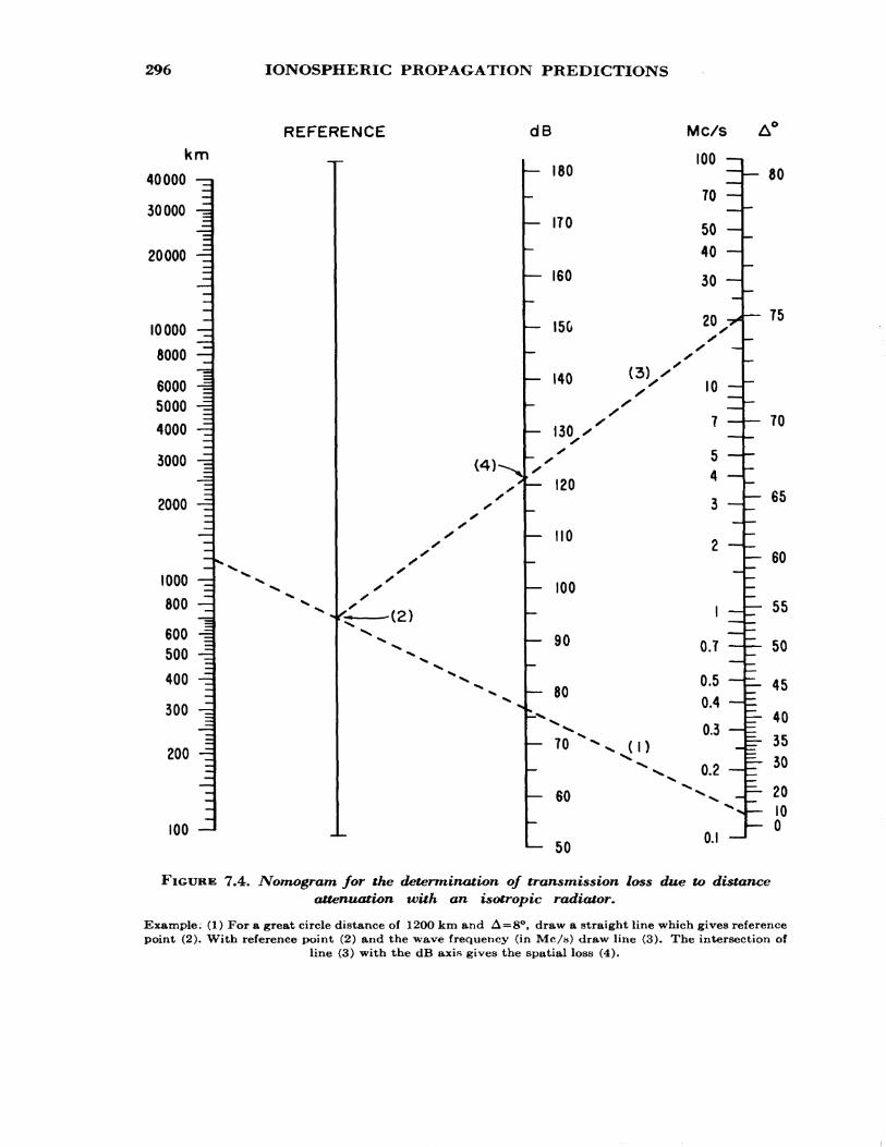
296 IONOSPHERIC PROPAGATION PREDICTIONS
REFERENCE dBkm
40000 -^—
30000 -|-=
20000 -=
—
10000 -^8000 -^
6000 -|5000 -=4000 -=
3000 -i"•3;
2000 -E—~*
——™
——
1000 -=800 -^
600 -1 500 -|400 -I
300 -i-=~
200 -5^™
-
100 —
s*X
X X
XX
X X •s
V^» * ^"""ssfc
>X
XX
XX
XX
XX
XX
^ —— -(2)X,
X.X
XX
X
%
— 180
— 170
— 160
— I5&
- 140
- I30x x xs - s
s- 120
- 110
- 100-
- 90
- 80"^^__ JQ -v.
—
- 60
— «in
Mc/s A"100 ^
70 -—
50 —40 —
30 —
20 * ss —
^y 10 =* _7 -
——
5 -4 -3 -
—
1 —i-
0.7 -
0.5 -0.4 —0.3 —
^^ 0.2 —
X •^
0.1 —
— 80
— 75
- 70
^
— 65
^- 60
r- 55_
5- soE- 45
|- 40^ 35=- 30=- 20— 10— 0
FIGURE 7.4. Nomogram for the determination of transmission /oss due to distance attenuation with an isotropic radiator.
Example. (1) For a great circle distance of 1200 km and A=8°, draw a straight line which gives reference point (2). With reference point (2) and the wave frequency (in Mc/s) draw line (3). The intersection of
line (3) with the dB axis gives the spatial loss (4).
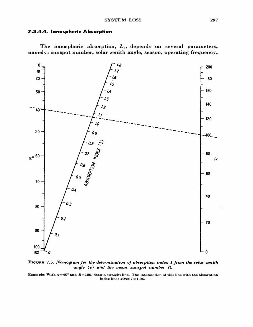
SYSTEM LOSS 297
7.3.4.4. Ionospheric Absorption
The ionospheric absorption, La-> depends on several parameters, namely: sunspot number, solar zenith angle, season, operating frequency,
200
180
160
140
- 120
•100....
-80R
- 60
-40
- 20
-0
FIGURE 7.5. Nomogram for the determination of absorption index I from the solar zenithangle (x) and the mean sunspot number R.
Example: With x =4O° and , draw a straight line. The intersection of this line with the absorption index lines gives 7 = 1.06.
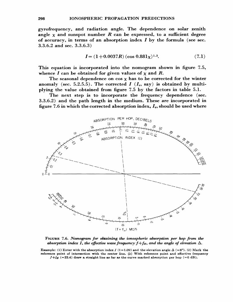
298 IONOSPHERIC PROPAGATION PREDICTIONS
gyrofrequency, and radiation angle. The dependence on solar zenith angle x and sunspot number R can be expressed, to a sufficient degree of accuracy, in terms of an absorption index / by the formula (see sec. 3.3.6.2 and sec. 3.3.6.3)
/= (1+0.0037J?) (cos (7.1)
This equation is incorporated into the nomogram shown in figure 7.5, whence / can be obtained for given values of x and JR.
The seasonal dependence on cos x has to be corrected for the winter anomaly (sec. 5.2.5.5). The corrected / (7C, say) is obtained by multi plying the value obtained from figure 7.5 by the factors in table 5.1.
The next step is to incorporate the frequency dependence (sec. 3.3.6.2) and the path length in the medium. These are incorporated in figure 7.6 in which the corrected absorption index, 7C, should be used where
PER HOP'
(f+f H > MC/5
FIGURE 7.6. Nomogram for obtaining the ionospheric absorption per hop from the absorption index /, the effective tvave frequency f+f&9 and the angle of elevation A.
Example: (1) Enter with the absorption index / (1 = 1.09) and the elevation angle A ( = 8°). (2) Mark thereference point of intersection with the center line. (3) With reference point and effective frequency
f-\-/H (=22.4) draw a straight line as far as the curve marked absorption per hop ( = 6 dB).
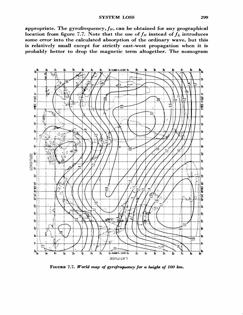
SYSTEM LOSS 299
appropriate. The gyrofrequency, /#, can be obtained for any geographical location from figure 7.7. Note that the use of fn instead of /z, introduces some error into the calculated absorption of the ordinary wave, but this is relatively small except for strictly east -west propagation when it is probably better to drop the magnetic term altogether. The nomogram
Boruuvi
FIGTJHE 7.7. World map of gyrofrequency for a height of WO km.
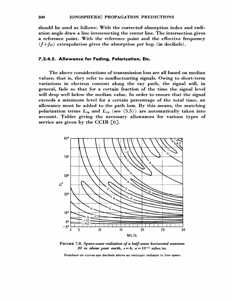
300 IONOSPHERIC PROPAGATION PREDICTIONS
should be used as follows: With the corrected absorption index and radi ation angle draw a line interesecting the center line. The intersection gives a reference point. With the reference point and the effective frequency
extrapolation gives the absorption per hop (in decibels).
7.3.4,5. Allowance for Fading, Polarization, Etc.
The above considerations of transmission loss are all based on median values; that is, they refer to nonfluctuating signals. Owing to short-term variations in electron content along the ray path, the signal will, in general, fade so that for a certain fraction of the time the signal level will drop well below the median value. In order to ensure that the signal exceeds a minimum level for a certain percentage of the total time, an allowance must be added to the path loss. By this means, the matching polarization terms Ltp and Lrp (see (5.5)) are automatically taken into account. Tables giving the necessary allowances for various types of service are given by the CCIR
-5
FIGURE 7.8. Space-wave radiation of a half-wave horizontal antenna 20 m above poor earth9 e = 4, <r = 10~3 mho/m.
Numbers on curves are decibels above an isotropic radiator in free space.
MONTHLY PREDICTIONS 301
7.3.4*6. Antenna Gain
In order to determine the system loss, it is essential to know the gains of the transmitting and receiving antennas at the appropriate radiation angles. Of course, this information can only be obtained from the ge ometry of the antennas. An example of the type of information required, for the case of a half-wave horizontal antenna, is shown in figure 7.8.
7.4. FREQUENCY PREDICTION SYSTEMS
7.4.1. Monthly Predictions3
A variety of ionospheric predictions is issued monthly by labora tories in a number of different countries, usually three months or so in advance. Many of them are for localized areas, but several attempt world wide predictions £3, 7^ While all prediction services use essentially the same ionospheric data and established physical relationships, there is considerable variation in the form of presentation and in the approxima tions used in applying the various predictions to propagation problems. The CRPL prediction system, based on a method of numerical mapping of ionospheric characteristics developed by Gallet and Jones £8, 9, 10J, using electronic computers, will be described briefly.
The term ''numerical map" is used to denote a function, F(X, 0, t) 9 of the three variables: latitude (X), longitude (0), and time (t) . The func tion F(X, 0, i) is obtained by fitting certain polynomial series of functions of the three variables to the basic ionospheric data. The general form of F(X, 0, t) is the Fourier time series
H
F(X, 0, i) ±a0 (X, 0) + X OX*, *) cos/e+6y(X, 0) sinyO» ( 7 - 2 )j— i
where H denotes the number of harmonics retained to represent the diurnal variation. The Fourier coefficients, ay(X, 0) and 6/(X, 0), which vary with the geographic coordinates, are represented by series of the form
>.*G*(X,0) (7.3)
where the G& (X, 6) are given in table 7.1. The index s denotes which Fourier
* This section was written by Mr. S. M. Ostrow.
302 IONOSPHERIC PROPAGATION PREDICTIONS
TABLE 7.1. Geographic functions Gfc(X, 6)
Main latitudinal variation
k
012
fco
GftCX, 0)
1 sin X sin2X
sin9°X
Mixed latitudinal and longitudinal variation
First order in longitude
k
k Q + l k»+2 A: 0 +3 fco+4
<7*(X, 0}
cosX cos0 cosX sin#
sinX cosX cos0 sinX cosX sin#
sin^X cosX cos# sin^X cosX sin#
Second order in longitude
k
&i + lfei+2 Ai+3 fci+4
K-l K
Gk (\, 8}
cos2 X cos 26 cos2X sin 20
sinX cos2 X cos 26 sinX cos2X sin 26
sin 92 X cos2 X cos 26 siii^X cos2 X sin 26
coefficient is represented, in the order given by
s = 2j\ foray (A, 0),/-0, 1, ••-, //, (a)
s = 2j-I, for fcy (X, 0), 7 = 1, 2, - - •, if. (b)(7.4)
A numerical map, F(X, 0, r), is completely defined by a relatively small table of coefficients, Dsk .
An important advantage of the numerical mapping method is that, as new data become available, the coefficients can be easily revised by the use of an electronic computer. Also, as additional physical relation ships are established, they can be incorporated readily into the mapping program. The value of the parameter mapped can be derived for any location, and graphical maps may be prepared by computations using the table of coefficients.
The numerical map is particularly useful when large numbers of propagation path computations are required. The use of a computer permits rapid and economical inclusion of all required propagation vari ables in routine computation. Tables of predicted coefficients may be ob tained in the form of tested sets of punched cards from the Prediction Services Section, CRPL. Users who do not have access to a computer, or whose requirements are not large enough to justify their own computer facility, may arrange to have ionospheric propagation calculations per formed at a reasonable cost by the Frequency Utilization Section, CRPL.
For those who do not have access to a computer, or require a manual solution to an ionospheric propagation problem for some other reason, the CRPL also issues a monthly publication, Ionospheric Predictions This bulletin contains the basic tables of predicted coefficients of fo
PERMANENT PREDICTIONS 303
and JVf (3000)^2 three months in advance, in addition to world maps of predicted MUF(ZERO) F2 and MUF(4000) F2 for every even hour of Universal Time. The predicted maps are calculated from the tables of predicted coefficients using the approximations:
MUF(ZERO)F2 =/0F2 +////2-/,F2, (7.5)
MUF(4000)F2 =/0 F2 XM(3000)F2 X1.1- (7.6)
Instructions for the use of these maps may be found in the National Bureau of Standards Handbook 90 Q113- Tables 7.2 and 7.3 give examples of tables of predicted coefficients Dsk defining the function F(X, #, t) for monthly median/0F2 and A/(3000)F2 for June 1963. Figures 7.9a and 7.9b show examples of world maps of MUF(ZERO) F2 and MUF(4000) F2 for the hour 1800 Universal Time, predicted for June 1963. These maps were derived from the predicted coefficients of tables 7.2 and 7.3.
7.4,2, Permanent Predictions
In contrast to the monthly prediction systems, permanent predic tions systems describe the variation of the ionosphere over a complete solar cycle. They are particularly useful for long-term frequency planning and communications equipment specification. Such systems have been issued by the CRPL, the United States £1^3; the Radio Research Station, England [[13]; The Defence Research Telecommunications Laboratory, Canada £14J; and the Radio Research Laboratories of Japan £15]. These are usually issued in the form of a set of maps for solar cycle minimum and maximum conditions, but may also be in the form of a set of maps for a specific level of solar activity accompanied by a set of maps showing the world variation of the dependence on solar activity. Permanent predictions in the form of numerical maps for solar cycle minimum and maximum are available from CRPL and are part of the current CRPL prediction system.
By applying a suitable index of solar activity to a permanent pre diction system, ionospheric characteristics may be obtained for any level of solar activity. They may be used as monthly predictions by using a pre dicted monthly index. The Zurich sunspot number has been the most commonly used index of solar activity. An index based on past ionospheric data, such as I(F2 ) of the Radio Research Station, is also sometimes used.
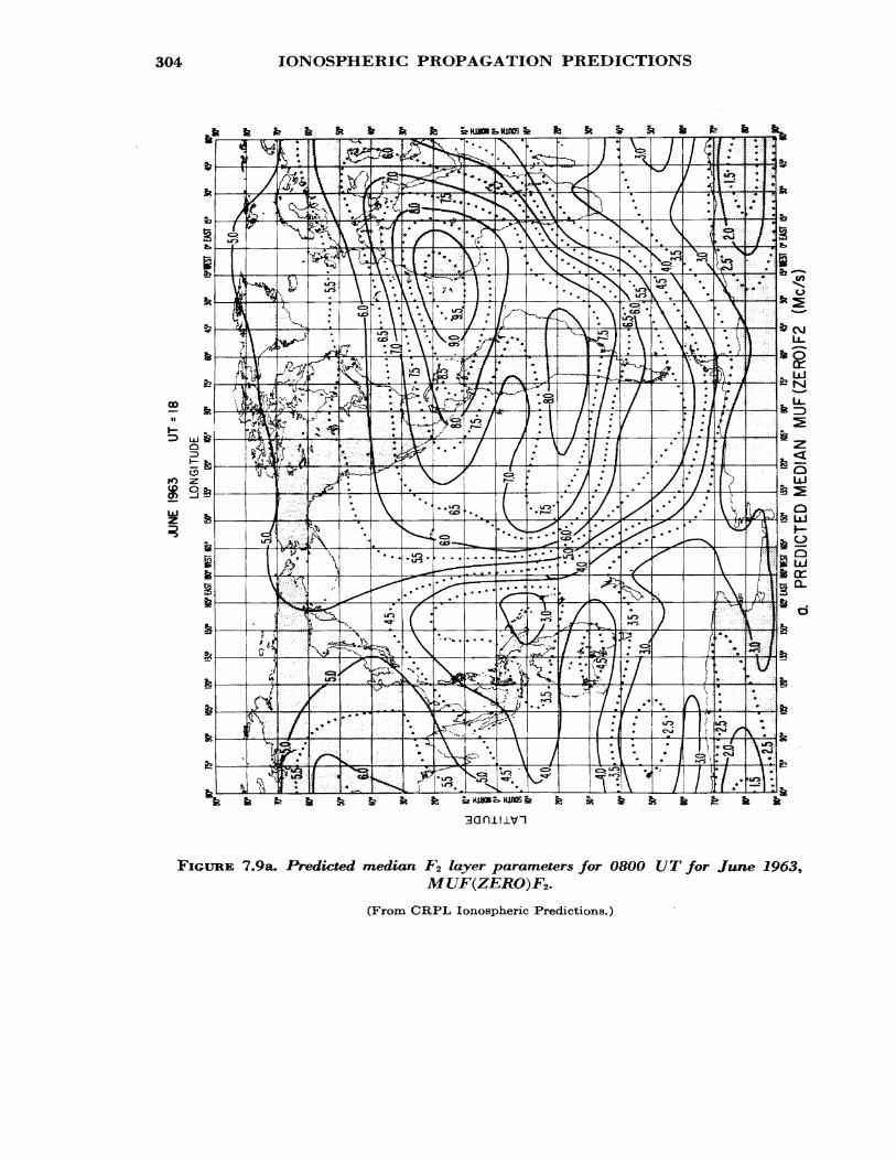
304 IONOSPHERIC PROPAGATION PREDICTIONS
3aruiivi
FIGURE 7.9a. Predicted median F2 layer parameters for 0800 UT for June 1963,MUF(ZERO)F2.
(From CRPL Ionospheric Predictions.)

MONTHLY PREDICTIONS 305
s HldQN£> KinOSe
3aniu\n
FIGURE 7.9b. Predicted median F2 layer parameters for 180O UT for June 19639
(From CRPL Ionospheric Predictions.)
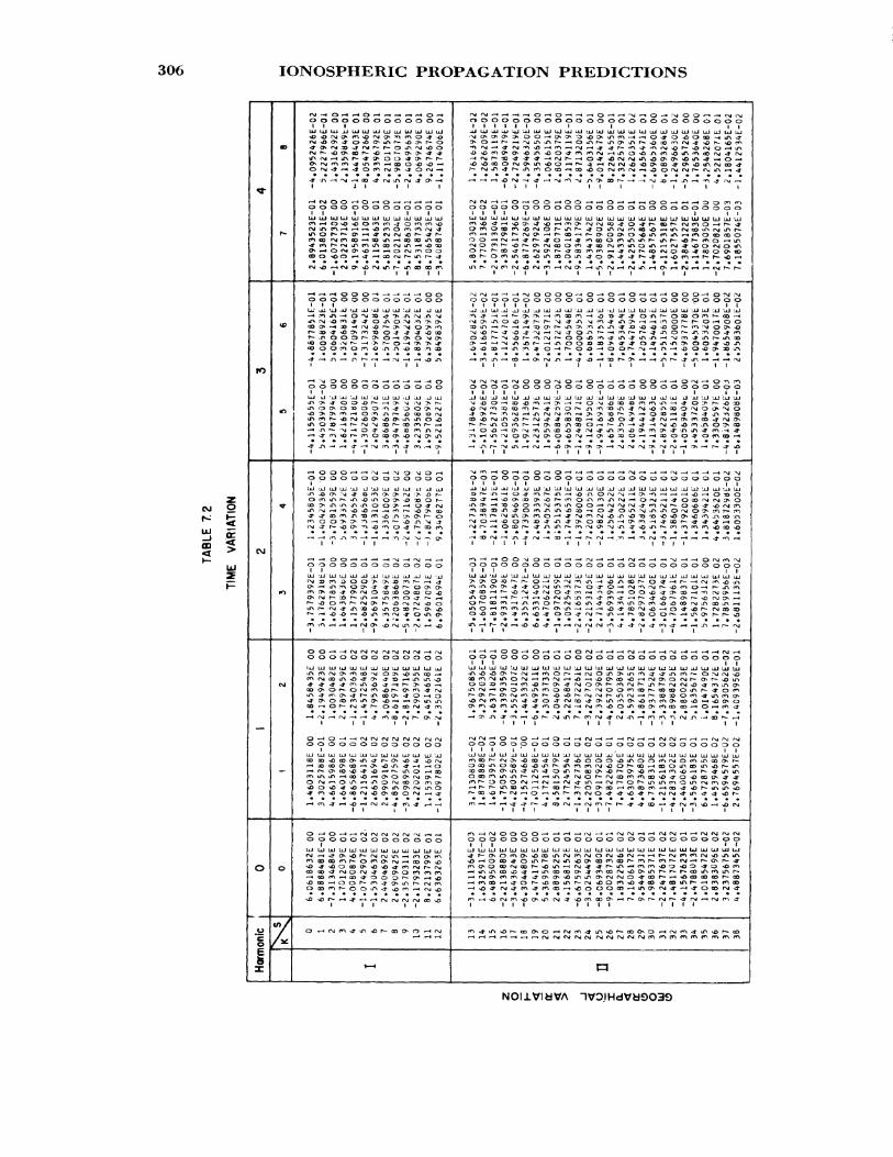
306 IONOSPHERIC PROPAGATION PREDICTIONS
^>
fO
CVJ
_
0
J£
I
a>
r-
(O
<r>
«•
fO
CJ
_
0
Xf ^
ooooooooooooo 1 1 1
r»ivOO.*o<OOiAi— sO:r>r- o
I a i ii i
ooooooooooooo 11 1 II
t*i co r^cicooHQirt^coaQtrhco
1 1 1 i t 1
OOOOOOOOOOOOO1 1 1
OOO-«aO-»rMsOr^3s>jo^m r-a>^%O?»r^TOo*-*-»OaO
t 11 II
OOOOOOOOOOOOO1 1
1 II II I
ooooooooooooo
£S£S£S22££S££
II II 111
ooooooooooooo
m :> en ** o r>j o co * o co o >o OrMf— 3)r-iA— • *n er\ O ^ r*~ ,-t
\ 11 1 1
ooooooo oooooo
{ II II 1
ooooooooo oo oo 1
ot^^OiA^kTiorsjcoo mo
It t ) 1
O — «O— «i— tfNirMfMrMrvirNtr-*.^ OOOOOOOOOOOOO
LU UJUJUJlJjUJljJUJLlJUJUJLlJljJ•M^H-j-o^or-ngrsjtri— imtTsto ^aococ^r-Ofior^i-Hcoo^vO>fr.X>OCOO>OvO<J-rr>fvr*-C^ coco-*oJOf>J>».*oan"if^on — tWrri^cD^J-OOor-C^— 1*0-fico— <OOfx-(T'i-3'O^U^r-»rvc*^ Oao<*\r— oOLr*-^-«or|>if-H{Nj^
1 11 1 1 "°
t— «
000000000000000000000000001 1 1 I 1 1 1 1 II
1 t 1 1 til 1 1 1 1 1
oo oooooooooooooooo oooooo oo 1 1 1 1 1 III
UJlUUJUJklJUJUJLULlJLUlJJLJJljJLULUUJLUUJljJLUUJUJLUUJtJJUJ
1111 t t t 1 11 1
oooooooooooooooooooooooooo 1 1 1 1 1 t It
oj^irvo^j-r^r-^i^^A^r^.* in^^^^or-i^o^oo soiT* — t r-. — t r-t "%} <y\ r- iT> *f< r<^inin ^JO sO>OO Or~-i»i"vJ OO^^O
III 1 1 1 t 1 11111
oooooooooooooooooooooooooo 1 1 1 1 1 1 1 III
III 1 1 1 1 1 lit) II
oooooooooooooooooooooooooo 1 1 1 1 1 1 It
rf\cOtD .TV ^ O m •/> vT» vO SO — « O^ OLn^vjiTiifxOry OO* fl r— m
i I i i i i i r i i t i I
OOOOOOOOOOOOOOOOOOOOOOOOOO
(ill 1(1) lilt i
oooooooooooooooooooooooooo lit IIUJUJuJ UJUjIUUJLlJLUUJUJLUIJJUJUJUJLiJLUliJLLi UJ aJ UJ Jj UJ UJ
1 1 1 1 111 1 t 1 1 II
OOOOOOOOOOOOOOOOOOOOOOOOOO1 1 t I • I , II
c>aoJ^CDeo^oo^^^p^J^p^^*^<^Jlfior^oo^-^^Olf^QO^r^JJr*•lr^
mr-ooo*M'— <<Ni»^oj^-Ln-— (csjr^of^-iniTic^OinfNi^o*^ r-»r^r^ir%Bj»rvi— ir-~oor~r^oo^ •— « m oo en <— i ao -4-^r~-«ir\ifv»o
1 1 1 1 1 1 1 1 1 1 1 1 1
p-k—irNtOOOO— «— <^-*-^rst—f^ioJfvj"i^HrgrM— »^-*r\|ivjrNtf\i OOOOOOC5OOOOOOOOOOOOOOOOOOOill t (^•r-c^OfT\ov^eoir>fv«*Pnif%JC3t\j^oj<-H <— (r-rsj(^fOp^»oir*tr\ >o— <Oco-*omr^tM»AsOO<»(^ico^rr>r— (*\r-«M^Hr-or*-^ «noo ooojoDf-^otrs'— «*\j^-«4-r^if\-*<*'ic<'i>oo «oo -*o >firo »^»riiricojj'Jf^^if>ooooo»-*-t<^oof^o&*trir^r^r*-«nirNr'iirHr---^rg(7scrr^<»-^rc^O>Otr>^OfNfMO-iraor-«-i'i>cDeDaor-oo --<t<^*^^-4-or-socoLrHr--f>j^Orn^o-*«-*coirir— «— «fornao-^sO-*f^-^tr»-*'^(T3'-^ <*OOOOO«-im<7i(M^-^-I^OCOrM^-
1 III ill! 1 1 1 1
p)
5
NOIlVldVA ~IVO.IHdVB9O39
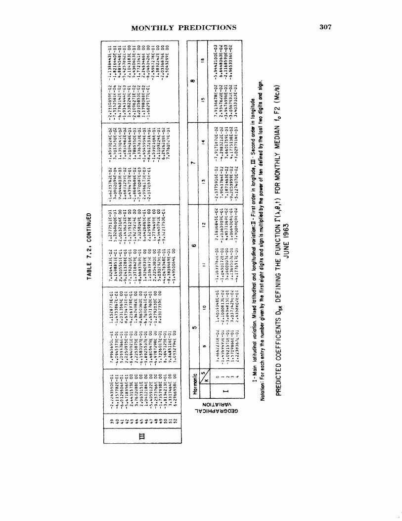
TABL
E 7.2
, CO
NTIN
UED
m
39 40 41 42 43 44 45 46 47 48 49 50 51 52
-2.2243550E-01
-4.1157782E-01
-6.0129504E-01
-5.4718356E-01
2,44
3157
3E 00
3B7672088E
002.0633151E 00
1.04
1218
4E 00
-5.4059122E
00-9.2573766E
00-1.7357938E
00-3.8134213E-01
3.33
1746
4E 00
6.296695BC 00
7.996b690t-0l
U152B773E-01
~4,Q945373E-01
-1.4
7338
67E-
013,Q9337b6E-01
2.Q3
1356
5E 00
2.0250975E-01
d.673473lE-Ol
-8.4
9409
21E-
01
-4-.
Z161
978E
-01
2.22
5387
5E 00
1.
3474
982E 00
-6.1580197E~01
-8,86503fcOE 00
-9.8925537E-01
-6»7690841E-Q1
-1.4805479E
00
-2.6571760E-01
-4.9787298E
00
-1.27920306
005.7236017E-01
8.03
1735
5E 00
8,b847125E"01
9»8485116E-01
3.0332
794E
00
7,82
64i8
3E-0
2 1.2777511E-01
3.14
9885
3E-0
1 5.3268600E-01
2*510556&E-01
-2.0&32316E
00-9.2413288E-01
-1 . 1436232E-01
-7»37926lOE-Oi
-1.5175129E
00-1.3718429E
00
-1.9275214E
00-d»6683769E-01
7.3258049E 00
1.92
6093
9E 00
6.
6426
a6bE
-Ol
1.0363975E 00
2.1299699E 00
2.2254380E 00
U7774499E 00
I>.030292bE-Ol
-6,b44l>79lE 00
-4.047834BE-01
-9 .52
2175
3E-0
1-8.3808469E-01
-1.49&0064E
00
-1.6233762E-02
-l.b59302«*E-02
3.Q6
0209
4E-0
4 3,
50l3
^50E
-Q'2
9.Q444803E-03
1.1353Q4i£-o2
1.68312S9E-02
7,^83i4B2E-02
1.4394707E-01
2.20
942&
dt-o
l-I,86896titiE'02
l,78
8535
0E-O
l-7.697QOB7E-03
1.3367633E-01
2.9966173E-03
-1.4545954E-Q1
-2.012Q531E-01
-8.i>61725it-0l
*-1.5392io6t-Ol
-2,1109224E-01
6.29
2620
BE-0
27,97605iVE-Ol
-2.Z310859E-02
-1.138&443t-0l
-7.315
2581E-04
-1.8216440E-01
-6,77b2142E-02
4.88
94548E-0
1-1
.914
1444
E-03
-5
.425
7692
t.-0
l1.5382243E-01
2.1043183E 00
-2.109
6271E-
02
5.43
6060
3E-0
1'8.
010&
853E
-Q2
-1.7723341E
001.1798088E-02
2.24
6346
6E 00
-1.6
8291
77E-
01
-6*0461426E
00-2.598727BE-01
U3832242E 00
-2.0336876E
004.5043299E 00
o z
CP < - 5
S 0
Horm
onlc
I
H 0 1 2 3 4
59
10
9*^6
6223
1E-Q
<!
1.4Q
!iS
34bE
-Ol
-1.4
y69493E
-01
-2.1
Q00
813E
-Q2
-3*0
9215
71E
-01
-3.8
494B
15E
-01
U&
709B
66E
-01
3.Q
37342bt-
Oi
2.2
238367t-
0i
^.43
5a«O
^E-O
l
611
12
-I.i6
3976
zc.-
0l
2,U
'J684
5E-O
ii -1
.045
0172
E-01
-1
.036
5909
E-01
5.
1000
007L
-01
4,«5
7136
9£-0
2 i.l
369b
Q7t
-Ol
U06
6430
&E-
01
-4.1
7765
t7E
-Oi
-7.9
006B
03t-
02
713
14
-2.3
7759
16E-
02
-7. 9
171b
70E-
02
7.90
4176
4E-0
2 -4
.298
32U
E-Q
2 7*
1871
463E
-02
3.66
0175
9E-Q
1 -9
.205
3959
E-02
4a
775l
3BE
-02
-5.1
2740
70E-
Q2
-3,0
25f7
91bE
-Ol
615
16
7.91
3667
8E-Q
2 -5
.944
21Q
OE-
03
2.93
4762
i!E-0
2 6.
6448
063E
-0^
-3.9
47&
99&
E-01
-2
.116
8590
E-03
-3
.036
7931
E-02
-6
t965
3336
E-02
3t
4033
103E
-01
I - M
ain
latitu
dinal
varia
tion.
Mixe
d lat
itudin
al an
d lon
gitud
inal v
ariat
ion:H
- Fi
rst o
rder
in lo
ngitu
de, H
I - S
econ
d or
der i
n lon
gitud
e No
tatio
n: F
or e
ach
entry
the
numb
er g
iven
by th
e fir
st e
ight d
igits
and
sign i
s m
ultipl
ied by
the
powe
r of t
en d
efine
d by
the
last
two
digi
ts a
nd s
ign,
PRED
ICTE
D CO
EFFI
CIEN
TS D
SK D
EFIN
ING
THE
FUN
CTIO
N r(
X,0
,t)
FOR
MON
THLY
MED
IAN
f0 F2
(M
c/s)
JUNE
196
3
s
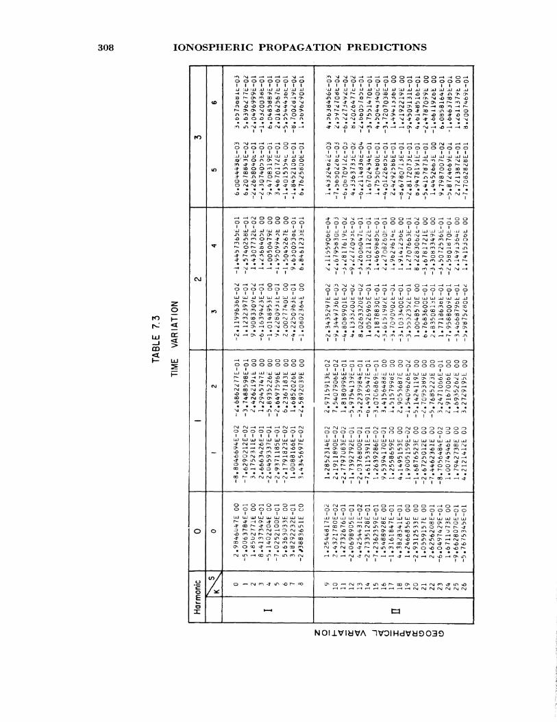
308 IONOSPHERIC PROPAGATION PREDICTIONS
otO H- rsJ <
ro
eg
—
0
oc.0Eo
*0
in
*
to
r\j
__
0
-/
O OOOOOOOO1 1 1 1 1 1 1 t 1
o -NJ ^ o so Ji -4* t> ~M
.0 ooooorir— n
it 11
O OOOOOOOO1 1 1 t 1 1 II
-U UJ Jj JJ UJ LU Jj Jj UJ
'i 1 II
0 OOOOOOOO111 11
11 41
ooooooooo till 1 tuJ LiJjJuJtjJaJLjJaJuJ
^rnaocn^-aorvj^so
t t 1 II
—t OOOOOOOO O OOOOOOOO
1 1uJ LU _LJ UJ ijj UJ UJ LU UJ
It 11 1
0 OOOOOOOO1 1 1 1 1 1 1 1 1
UJ UJ UJ UJ UJ UJ UJ UJ UJ
CO vO^^OOO—iO^t
II lit
O OOOOOOOO1 1 1 1
UJ UJ LLj UJ Lll UJ UJ ill UJ
S oS^SSSSS
i II 1
1— H
00000 00000000000001 t 1 I 1 1 1 1 II II 1
s?*s55?235Ssls352l
lilt 1 1 1 1
oooooooooooooooooo 1 1 1 1 1 1 1 1 1 1 1 t 1 till
^^ss^ss^^g^^^ss^^sIII 1 1 t 1 II
oooooooooooooooooo1 1 1 ! 1 1 1 1 14 II
H^fsiHH^sIsH;1 t 1 4 1 1 I 1 1
oooooooooooooooooo1 1 1 1 1 1 4 1 1 t 1 1 1 1 t t 1
m^a-mm^oo-torrt^cocnonoosjirk
lit fill III
rM r\j •— i — < — i— (^-HOOO~vJ O O O — « O O Ooooooooooooooooooo
1 1 1 1 1 f 1 1 tUJ UJ til til LlJ !lt Jl llj ill Lll LiJ 111 1 l_l 111 IjJ IjJ !lj -ll
?S2PSsl2-2g§5s332SS
1 1 1 1 1111
OOOOOOOOOOO OC3OOOOO1 1 1 1 1 1 1 1 1 1
UJ UJ UJ UJ UJ ii 1 LU UJ UJ UJUI LiJ UJ UJ tiJ .il UJn!
1 1 t 1 till
ooooooooooooooooooI 1 1 1 ! I 1 11 > 1 11
IssilsSissiSSSIslff1 1 1 1 t 111
t— i^-i^-it— «<—(,— ir-t.— <r— ir-ipgr\jrsj(NjrNjr\jf\j
a
NOUVIdVA ~tVOIHdVti9O39
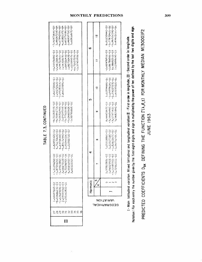
MONTHLY PREDICTIONS 309
Oo
•ro
UJ_jCD
.O O O O O O O I I I I I I IU UJ OJ LU JJ *-JJ UJ
o : sO rao .
ooooooooo I I t I i I I I I
UJ uU -U uJ !jJ UJ jJ 'jJ !JJ -
-o, ,"\j NJ r\j O O O O11(1
jJ uJ JJ aJ ^O OJ ^O CA
O O O O O O Ot ( t I ( I t
^o oO 33
o o o o o oJ 1 I I I I
LU UJ UJ UJ 'jj LU
0^1 r- j^> r- ^ oCD -H r- O L^ ror\j J1 ro. o r-< r\jCD r- o OD ^ O
^ -4- vQ sO -NJ — *
I I I I I I ELU ^jJ LU UJ UJ LU LU>3" O O i~sj o —* •—•
i •—• oj ro r>
<f- O
to
in
o
o E0X
CJ
_™*
0
0>
00
r-
CO //
L^
01
LU
^mOJ
^J
ol
'U
0r^
2*
J
sf0
1
sOJO,y
0
--oo
1LU
-0ro,
5*
13
0J
UJ•sDCO00
.-ou">ors^
OJ
o1
CO00r-»oCOr—
^
0
0 01 1
JJ UJ
-* -4O ~>J
OO f*-
* •
1 1
0 01 1
-U _U
X) OJQO O
2 500 70
i
o of ttJ LU
t> r-o o23 r-o o5 S
1 t
^j ro0 01 1UJ UJ
I s^r\ r*-
5 J* *
t 1
0 01 (
UJ LU0 f-
r*-^ --^^NJ Oo <oOJ 00• *
r\J -M'oj rxjO O
1 iLU jJ oj O
CO LHOsl CDLH J^-* OOO rvt
1
r~> OvJ
0*(J
AJ
O
x>5^
01
LiJ
u
5o5^
oi
r\JOL^
5
-
^J
0
LU
soOQ
r^
O1
0~gLO>.
LTV
_t1
^Jo
1!_,Orxj
'./>OJ
*
T
m
-
g.•as
«> o"O crt 3 -—'g1 ^
51
oO
CJLL.O O O ro
< O
X
oCCe
T? 0>w> ^: o ••-11"1 "o.
11
i S
O
P
O 2 ID U.UJ
LU
.^s
11 c " S>
-I ji.5 E
_ O>
LU Q
COO
iUJo
NOIlVmVA
— U_>* ii i^ Oa) O"§ Qo> LU
£ feg SI £
310 IONOSPHERIC PROPAGATION PREDICTIONS
7.5. RADIO NOISE PREDICTIONS
7.5.1. Importance of Noise
In every communications system (radio or otherwise) noise is the limiting factor which determines whether or not the signal is usable for the transmission of information. In principle, if all noise could be elimi nated from a system then only an infinitesimal transmitted power would be required and the amplification in the receiver could be unlimited. In the presence of noise, there is a limit to the amount of useful amplifi cation because both signal and noise are amplified to the same extent. Thus, in choosing a receiving site, it is very important to have a knowledge of the ambient noise with which the desired signal must compete so that sufficient power may be transmitted in order to override the noise.
Radio noise arises from a number of noise sources such as resistors, radio tubes, etc. (thermal noise), galactic noise (thermal) from outer space, atmospheric noise from lightning discharges (thermal and/or impulsive in nature), and from electrical machinery (impulsive or spikey) C16].
Noise internal to the receiving system is usually the dominant noise in systems operating on frequencies above about 300 Mc/s. In the high- frequency band (3 to 30 Mc/s), atmospheric and galactic noise usually determines the noise level at sites well removed from civilization. It is with these types of noise that we shall be concerned in this chapter.
Measurements of atmospheric noise levels have been made for many years by the Radio Noise Section of the Central Radio Propagation Labo ratory and the reader is referred to their publications Q17, 18, 19] for details on the method of noise measurement and the applications to the design of communications systems. These details need not concern us here; it will suffice to know that experience has shown that the noise power is generally the most significant single parameter in relating the interference effect of the noise to system performance.
The noise power is measured in terms of quantity, Fa * which is de fined as the external noise power available from a lossless antenna, ex pressed in decibels above A: TO, where k is Boltzmann's constant and TO = 288.39 °K is a reference temperature, which is the noise generated in a unit bandwidth by a thermal source at a temperature T0 . On the as sumption that noise power is proportional to the bandwidth b (in cycles per second) we have that the the total power (Pn in decibels above one watt) available at the terminals of a lossless antenna is given by
PRESENTATION OF NOISE DATA 311
- 204 dB/W (7.7)
where B = 10 log 6 and 10 log k TO = — 204. Notice that this is based on the assumption that the noise is incident on the antenna uniformly in all directions.
7.5.2* Presentation of Noise Data
7.5*2.1. Long-Term Characteristics
The noise power at any point on the earth's surface depends on the following:
(1) Geographic location;(2) Time of day;(3) Season of year;(4) Operating radio frequency;(5) Bandwidth of the receiving system.
Hourly noise data have been collected at a number of locations on a routine basis over several years. Any long-term variation appears, at present, to be small. The diurnal and seasonal variations of the noise parameters are represented by dividing the year into the following four seasons:
Months
December, January, February March, April, May June, July, August September, October, November
Seasons
Northern hemisphere
Winter Spring Summer Autumn
Southern hemisphere
Summer Autumn Winter Spring
The noise levels are presented as median values Farn of Fa for each of the following 4-hr periods of local time at the receiver: 00-04, 04—08, 08-12, 12-16, 16-20, and 20-24. The statistical distribution of the individual values Fa about the median Farn is given by the upper decile ratio Du ( = Fau — Fam ) where Fau is the value of Fa exceeded 10 percent of the time. When plotted on a normal probability graph (level in decibels), the am plitude distribution of the deviations, /), above the median can be repre-
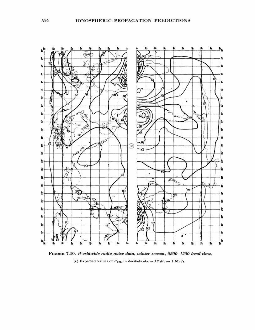
312 IONOSPHERIC PROPAGATION PREDICTIONS
FIGURE 7.10. Worldwide radio noise data, -winter season, 0800—1200 local time.
(a) Expected values of Fam , in decibels above kToB, on 1 Mc/s.
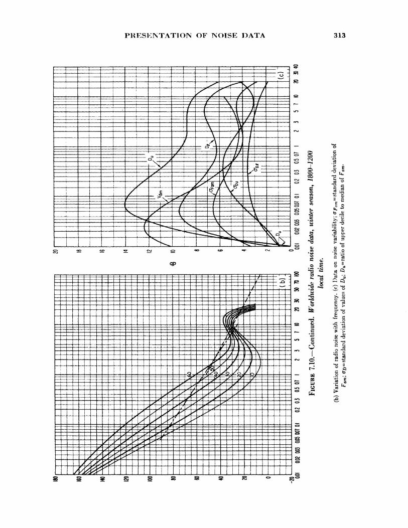
-2020 0,01
0.02 0
03 OJ05
007 0
.1 0.2
0.3
0,5 07
2 3
5 7
10 20
3040
H H O 2 B
FIGU
RE 7
.10.
— C
ontin
ued.
Wor
ldwi
de r
adio
noi
se d
ata,
win
ter
seas
on,
1800
-120
0lo
cal
time.
(b)
Var
iatio
n of
rad
io n
oise
with
fre
quen
cy,
(c) D
ata
on n
oise
var
iabi
lity;
ffFa
m^ s
tand
ard
devi
atio
n of
Fa
m\ c
r/)- s
tand
ard
devi
atio
n of
val
ues
of D
u\ Z)
u-ra
tio o
f upp
er d
ecile
to m
edia
n of
Fam
-
314 IONOSPHERIC PROPAGATION PREDICTIONS
sented with reasonable accuracy by a straight line through the median and upper decile value. A corresponding line through the median and lower decile value DI can be used to represent the deviations below the median. The lower decile is of little practical importance and will not be considered here.
The values of Fam presented in the maps are deduced from values taken at several geographical locations and on a number of frequencies. From the frequency dependence of Fam a reference value on an effective frequency of 1 Mc/s is obtained and this is plotted on the sample noise map in figure 7.10a. Of course, the data presented are smoothed values and the measurements on a specific frequency at a particular location will, in general, differ from the value deduced from the curves. A measure of the error introduced by the smoothing procedure is, therefore, given by the standard deviation of these differences <rpam. In a similar way, the standard deviations of £>w , <TZ>«, are measures of the difference to be ex pected between the values of Du obtained from the curves and the actual measured values. The variations with frequency of the above noise pa rameters are given in figures 7.10b and 7.10c. A complete set of these maps can be found in the CCIR Report 322.
7.5.2*2. Short-Term Characteristics
The parameters discussed above represent the fluctuations in the long-term character of the noise, that is, from one time block to the next and from season to season. To evaluate the effect of the noise on a com munications system, we need also some knowledge of the short-term char acter of the noise. This subject is dealt with fully in the publications of W. Q. Crichlow and his coworkers Q17, 18, 19] and the interested reader should consult those references. For many purposes, and particularly those involving subjective factors, the simplest procedure is to take the short-term effects into account by using the CCIR tables of signal/noise ratio [_6~].
7.5.2.3. Application of Noise Data
To understand how the information presented in figure 7.10 is applied to an actual problem, let us consider the following example.
Determine the noise level at Washington, D.C., on a frequency of 13 Mc/s in a 6 kc/s channel at 1400 UT in December 1963.
DISTANCES LESS THAN 40OO KM 315
From an atlas or some other source we determine the geographic coordinates of Washington, D.C.—39°North, 77°West and, hence, the local time is approximately 1400 — 0500=0900 hours. From the noise grade map of figure 7.10a we find that Fam on 1 Mc/s is about 32 dB. In order to determine the value of Fam on 13 Mc/s we locate the 32 dB point on the 1 Mc/s line in figure 7.10b and move up in frequency (keep ing just above the 30 dB line). On 13 Mc/s, we have Fafft~32 dB. To take into account the uncertainty in the value of Fam due to the spread of the data we add a correction o^om obtained from figure 7.10c. On 13 Mc/s we find that <rFam^6 dB. Hence the noise power on 13 Mc/s in an effective bandwidth of 1 c/s is 32+6 = 38 dB above the reference value of k TQ.
On the assumption that noise power is proportional to bandwidth we find that the noise power in a 6 kc/s channel is 38 + 10 log 6000 = 38 + 37.8 = 75.8 dB above kT0. Substitution in (7.7) gives Pn = — 128.2 dB above 1 W.
7.6. CALCULATION PROCEDURES FOR DISTANCESLESS THAN 4OOO km
7.6.1. Introduction
The average height of the F% layer (320 km) corresponds to a maxi mum one-hop distance of about 4000 km. Hence, this distance gives a convenient dividing line between long distance and intermediate distance transmission. In this section we shall discuss, by example, the procedure to be followed for transmission distances of less than 4000 km.
7.6.2. Problem 1
Part 1. Determine the optimum working frequency around noon in June 1963 for a transmitter in Boulder, Colo., and a receiver in Wash ington, D.C.
Part 2. Find the transmitter power required to ensure the following performance of an A3 telephony double sideband system with a band width of 6 kc/s. The required grade of service is marginally commercial for 90 percent of the hour and the antennas are half-wave horizontal dipoles at heights of 20 meters.
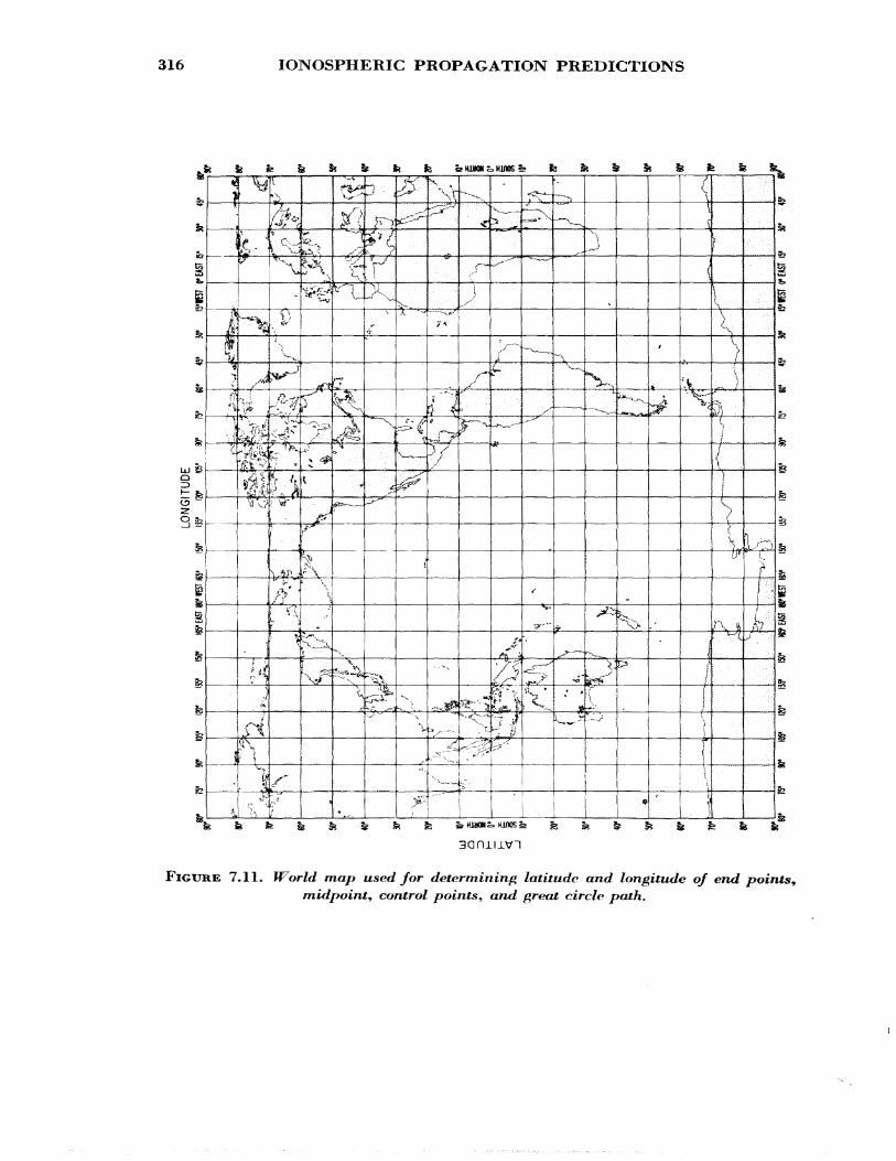
316 IONOSPHERIC PROPAGATION PREDICTIONS
Jk fe fe fe&fefe
t!3 ~"Z
Sis
M:.U£
^fe1—T
/?\
/X
=17
£
s
FIGURE 7.11. World map used for determining latitude and longitude of end points9 midpoint, control points, and great circle path.
DETERMINATION OF OPTIMUM FREQUENCY 317
Path Length^ Location of Midpoint, and Solar Angle
First we find the geographic coordinates of the end points, from a map (figure 7.11) or elsewhere:
Boulder 40°N 105°W Washington 38.9°N 77°W
To find the path length and midpoint we lay a sheet of transparent paper over the world map (fig. 7.11) and proceed as follows:
Step 1: Draw on it the equator and the 0° and 180° meridians.Step 2: Locate and mark the geographic coordinates of the transmitter
and receiver.Step 3: Transfer the transparency to the great circle chart (fig. 7,12)
and, with the equators coincident, slide the transparency along the equator until the terminals lie on the same great circle (solid lines) or a proportionate distance between adjacent great circles.
Step 4: Estimate the great circle distance from the hroken lines—this gives about 2400 km,
Step 5: Estimate the midpoint location from the broken lines—approx imately 40.4°N 91 °W—and mark on the transparency.
Step 6: Transfer the transparency to figure 7.13 and read the dipole latitude at the path midpoint—about 51°.
Step 7: Determine the appropriate universal time at the path midpoint. 1200 (90° WMT) corresponds to 1800 UT.
Step 8: Determine the sun's zenith angle x a^ follows. Place the trans parency over the chart in figure 7.14. Keeping the equators co incident make the zero meridian coincide with the universal time (1800) obtained in step 7. Then read off, by interpolation if necessary, the value of x at the midpoint of the path—about 18°. A complete set of maps of x is given in reference 1.
7.6.3. Determination of Optimum Frequency
Step 9: From figure 7.9a and b, respectively, we obtain
MUF (ZERO) F2 = 6.0 Mc/s
MUF (4000) F2 = 17.0 Mc/s.
Step 10: From the data obtained in step 9, we find, from figure 7.1, by
318 IONOSPHERIC PROPAGATION PREDICTIONS
FIGURE 7.12. Great circle chart centered on the geographic equator for use with figure 7.11.
The solid lines represent great circles. The numbered dot-dash lines indicate distance in thousands ofkilometers.
DETERMINATION OF OPTIMUM FREQUENCY 319
oCL
8UJ
60° 90° 120° 150° 180° 150° 120° 90° 60° 30° 0° 30° 60° EAST WEST WEST EAST
LONGITUDE
FIGURE 7,13. World map of magnetic dipole latitude.
interpolation, that the MUF and FOT for 2400 km are respec tively 13.8 Mc/s and 11.7 Mc/s. The FOT is 0.85 MUF (see sec. 4,7.3.).
It is now necessary to determine the effect of the E layer. Here there are three possibilities.
(1) The normal E layer will determine the MUF.(2) The sporadic E layer will determine the MUF.(3) That E layer cutoff will occur (sec. 4.7.2.).
Step 11: Determine the radiation angle for one-hop E propagation for a distance of 2400 km. From figure 4.31 we find that this is less than zero and so this possibility is eliminated.
Step 12: The angle of elevation A(jp2 ) for one-hop F2 propagation is found by first determining the height of the F layer from figure 7.15 as follows: Place the transparency over the appropriate chart and, keeping the equators coincident and with zero degree meridian coincident with the universal time (1800), read off the /'Vlayer height at the midpoint of the path. We find the height to be about 400 km. From figure 7.2 we obtain A (F2 ) = 13°. A complete set of maps for obtaining the F^-layer height is given in reference £1].
Step 13: To see whether the MUF for the two-hop E mode dominates we proceed as follows for a distance of 1200 km (half the path
320 IONOSPHERIC PROPAGATION PREDICTIONS
S33d93Q l OIHdVd9O39
o o
FIGURE 7.14. Solar zenith angle for June.
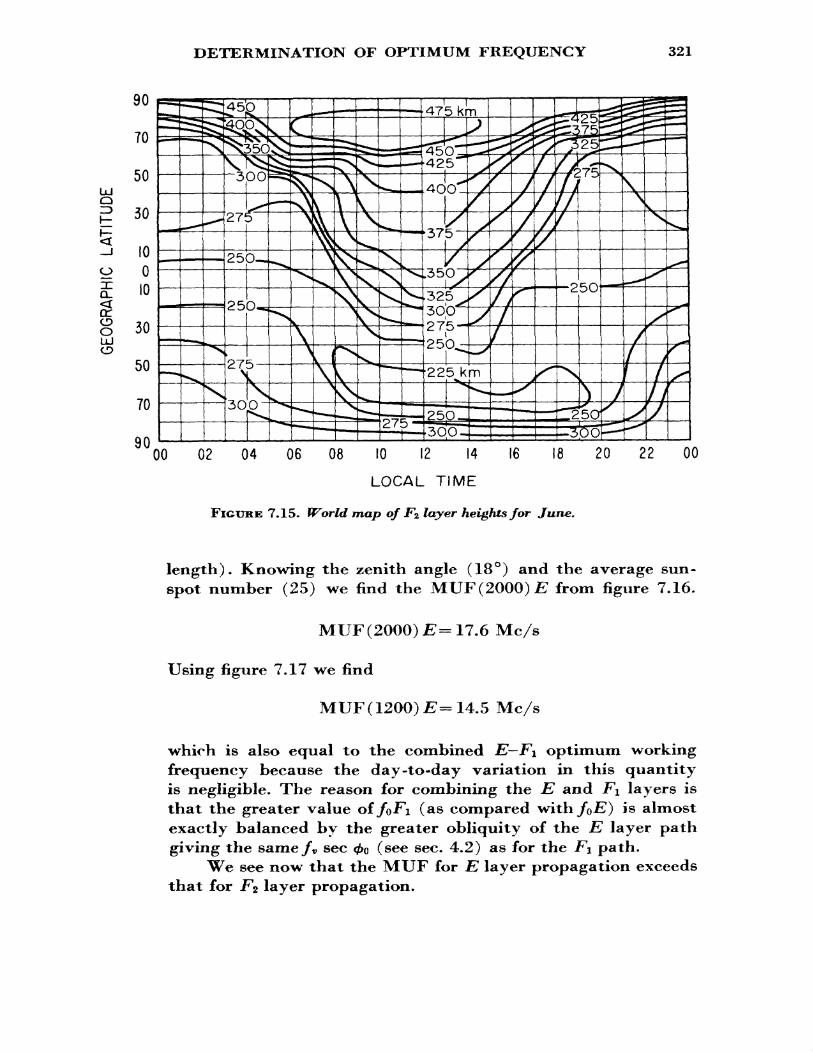
DETERMINATION OF OPTIMUM FREQUENCY 321
UJ O
oLiJ
00 02 04 06 08 10 12 14
LOCAL TIME
FIGURE 7.15. World map of F2 layer heights for June.
16 18 20 22 00
length). Knowing the zenith angle (18°) and the average sun- spot number (25) we find the MUF(2000) £ from figure 7.16.
MUF(2000) £=17.6 Mc/s
Using figure 7.17 we find
MUF(1200) £=14.5 Mc/s
which is also equal to the combined E—Fi optimum working frequency because the day-to-day variation in this quantity is negligible. The reason for combining the E and JF\ layers is that the greater value of/oFi (as compared with foE) is almost exactly balanced by the greater obliquity of the E layer path giving the same/v sec <£0 (see sec. 4.2) as for the FI path.
We see now that the MUF for E layer propagation exceeds that for F% layer propagation.
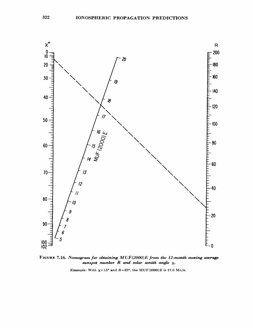
322 IONOSPHERIC PROPAGATION PREDICTIONS
010
20
30
40^
50-
60-
70-
\\\\\\
R •200
ISO
160
140
H20
HOO
^80
-60
-40
80-
90-
100-i 102
-20
FIGURE 7.16. Nomogram for obtaining MUF(2000)E from the 12-month moving average sunspot number R and solar zenith angle x*
Example: With x=15° and R=25°t the MUF(2000)£ is 17.6 Mc/s.

DETERMINATION OF OPTIMUM FREQUENCY 323
MUF(20OO)E, MC/S50 ^a45 -|40 -|35 -=
30 -i—
25 -r
20 -—
-15 —
~"
—
10 —9 —
__
7 —— un-
g _____
0 """""
MUF, MC/S50 -a
40 H=—
30 -f
20 -^
__ __ _____ __ 15-ri
10 ^w "^
—6 —5 -i4 -E
3 -=2.5 -|
2 -|
1.5 -E
1I •'•
DISTANCE, km,-2500-4000
iF 2000I- '500
r- 1000——
3- 800— 700—
— 600™*
— 500
— 400—
— 300
— 200
— 1000
4 —
3 —'
FIGURE 7.17. Nomogram for transforming MUF(2000)E to equivalent maximumfrequencies and optimum working frequencies due to combined effect of the E
layer and the FI layer for other distances.
Also from the MUF(2000)^ it is possible to find the skip distance corresponding to a given freQuency. Example: With MUF(2000)^ of 17.6 Me/a, the MUF(120O)E is 14.2 Mc/s.
Step 14: To see whether the sporadic E layer controls the maximum frequency we use figure 7.18. This gives the median fE& contours for the month of June. A set of 12 such maps (one for each month of the year) is given in reference £!]• Note that the solar cycle variation of Es has not been definitely established and so, for the time being, these charts may be considered as permanent. Furthermore, it will be seen that dipole latitudes
324 IONOSPHERIC PROPAGATION PREDICTIONS
NORTH GEOMAGNETIC LATITUDE SOUTHoooe
ooooooooo ooooooooo
FIGURE 7.18. Worldwide distribution of fE8 for June.
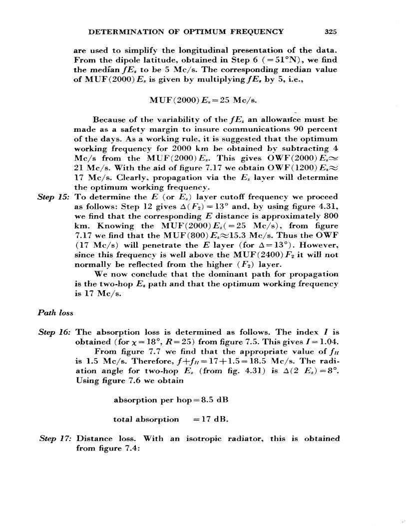
DETERMINATION OF OPTIMUM FREQUENCY 325
are used to simplify the longitudinal presentation of the data. From the dipole latitude, obtained in Step 6 ( = 51°N), we find the medfan fEs to be 5 Mc/s. The corresponding median value of MUF(2000)£;S is given by multiplying/^ by 5, i.e.,
MUF(2000)jEs -25 Mc/s.
Because of the variability of the fEs an allowaifce must be made as a safety margin to insure communications 90 percent of the days. As a working rule, it is suggested that the optimum working frequency for 2000 km be obtained by subtracting 4 Mc/s from the MUF(2000) £*. This gives OWF(2000) £s~ 21 Mc/s. With the aid of figure 7.17 we obtain OWF(1200) Es^ 17 Mc/s. Clearly, propagation via the Es layer will determine the optimum working frequency.
Step 15: To determine the E (or Es ) layer cutoff frequency we proceed as follows: Step 12 gives A(F%) ==13° and, by using figure 4.31, we find that the corresponding E distance is approximately 800 km. Knowing the MUF(2000) E8 ( =25 Mc/s), from figure 7.17 we find that the MUF(SOO) £^15.3 Mc/s. Thus the OWF (17 Mc/s) will penetrate the E layer (for A = 13°). However, since this frequency is well above the MUF(2400)7^ it will not normally be reflected from the higher (J^) layer.
We now conclude that the dominant path for propagation is the two-hop Es path and that the optimum working frequency is 17 Mc/s.
Path loss
Step 16: The absorption loss is determined as follows. The index / is obtained (for x= 18°, /? = 25) from figure 7.5. This gives /= 1.04.
From figure 7.7 we find that the appropriate value of /// is 1.5 Mc/s. Therefore,/+/// = 17+ 1.5 =18.5 Mc/s. The radi ation angle for two-hop Es (from fig. 4.31) is A(2 Es ) =8°. Using figure 7.6 we obtain
absorption per hop = 8.5 dB
total absorption =17 dB.
Step 17: Distance loss. With an isotropic radiator, this is obtained from figure 7.4:
326 IONOSPHERIC PROPAGATION PREDICTIONS
distance loss per hop = 120 dB
total distance loss = 120+6= 126 dB.
Step 18: Ground reflection loss. From figure 7.3b we obtain, for A = 8° a ground reflection loss = 3 dB.
Total path loss Lpath= 17 + 126+3 = 146 dB.
System Loss
Step 19: Antenna gain. From figure 7.8, with A —8°, the gain per antenna is 6 dB. Therefore, the antenna loss La — —12 dB. For informa tion on other types of antennas the reader may consult reference £20] and follow up the references cited therein.
Step 20: Total system loss L8 is given by
La = ipath H~ La
= 146-12 = 134dB.
Step 21: Required carrier/noise ratio. From the CCIR tables Q6J we find that the required value of peak RF signal/noise ratio under steady (nonfading) conditions for the specified performance is 27 dB. On the assumption of 100 percent depth of modulation this requires a median carrier/noise ratio of 21 dB. To allow for the random (Rayleigh) fading of the signal we must add 8 dB, i.e., the ratio of the value P exceeded 90 percent of the time to the median Pm * This is obtained from the formula
T= exp { -0.693P/Pm } (7.8)
where T is the fraction of time that the instantaneous value exceeds P.
For the upper decile value, 10 log P/Pmtt8 dB.
The required carrier/noise is, therefore, 21+8 = 29 dB. Step 22: Noise power. Following the procedure outlined in sec. 7.5*2.3,
we obtain from figure 7.19a
Fam on 1 Mc/s= 70 dB.
DETERMINATION OF OPTIMUM FREQUENCY 327
Together with figure 7.19b this gives
Fam on 17 Mc/s^33 dB.
This value of Fam^ being a median, gives the noise level exceeded 50 percent of the days. In order to find the level exceeded 10 per- cent we require the upper decile value Fau. This is obtained from Du ( = Fau — Fam) which is given, as a function of frequency, in figure 7.19c. On 17 Mc/s, 1>U~8 dB, therefore Fau = Fam + £>tt = 33+8 = 41 dB. Because of the spread in the data, from which Fam and Du are derived, there are inherent inaccuracies in the median values. These inaccuracies can be partially taken into account by the standard deviations o-jpatn and a^ respec tively which are given in figure 7.19c. From this figure we obtain crjpam^^4 dB; cT£>wc^3 dB. The total uncertainty aT is deduced on the basis that the errors are uncorrelated, i.e., 0'r = a"!*ma + <r|>tt , hence crr =5 dB. The effective upper decile is, therefore, Feff= Fau -\-o-T = 4<6 dB. When circuit operation is required for some percentage of the time other than 90 percent, Fau and Fam can be plotted on probability paper and the appropriate value of Fa obtained by linear interpolation (or extrapolation). A more complete account of this procedure is to be found in CGIR Report 322 pJJ- Furthermore, further corrections need to be made to obtain the true total uncertainty <TT but these are negligible and will not be considered here. The interested reader should consult CCIR Report 322 for a more detailed treatment.
The effective noise level for a 6 kc/s channel is given by substitution in (7.7).
Pn =Feff+B — 204 = 46+37.8 -204
= —120.2 dB above 1 W.
Step 23: Required carrier power Pr at receiver. From step 21 we have
Required carrier/noise = Pr — Pn = 29 dB
= 29 — 120.2=—91.2 dB above 1 W.
328 IONOSPHERIC PROPAGATION PREDICTIONS
FIGURE 7.19. Worldwide radio noise data, summer season, 1200—1600 local time.
(a) Expected values of Fam, in decibels above fcTob, on 1 Mc/s.
DETERMINATION OF OPTIMUM FREQUENCY 329
330 IONOSPHERIC PROPAGATION PREDICTIONS
Step 24: Required transmitter power Pt .
From step 19, £*=134 dB; and step 23, Pr = —91.2 dB.
P, = 42.8 dB above 1 W
^19,000 W-19 kW.
7.7. CALCULATION PROCEDURES FOR DISTANCES GREATER THAN 4OOO km
7.7.1. Control Points
As the distance of propagation is increased beyond the one-hop F% limit (around 4000 km) it has been found (empirically) that the propa gation is not suddenly cut off. Some physical reasons for this, discussed in section 4,6, are ionospheric and ground scatter, the high -angle ray, and ionospheric tilts. Empirically, it has been found that propagation did not appear to fail until the ionosphere failed to support the propagation at two ''control points" on the great circle path at 2000 km from each end. This was apparently true, within limits, over wide ranges of path lengths, geographical locations, and time.
In the practical solution of determining the MUF for F 2-layer propa gation, the control points 2000 km from each end are chosen. The MUF for the path is the lower of the two MUFs, for a distance of 4000 km, for each control point as the midpoint of the 4000 -km path.
When it is desired to apply the procedure to the £, £"«, and FI layers, an additional pair of control points 1000 km from each end may be used. However, there is less justification for this course than is the case with Fz propagation.
7.7.2. Statement of Problem 2
Determine the transmitter power requirements of the following circuit :
Transmitter location London 51.5°N 0°W Receiver location Washington 38.9°N 77°W
FREQUENCY CALCULATIONS 331
Month—December 1963 Time—1400 UTSunspot number 17 (CRPL Predictions)Frequency 13 Mc/sAntennas—half-wave horizontal antennas 20 meters high, A3telephony—good commercial quality, 90 percent of timeBandwidth 6 kc/s
7.7.3. Control Points and Midpoint
Mark a sheet of transparent paper, as in problem 1, and determine the coordinates of the midpoint and the two control points (2000 km from either end). Following the procedures outlined in problem 1 we obtain the following information:
Control point A:Control point B:Midpoint:Midpoint gyrofrequency:Path length
Geographic
55°N 30°W 50°N 57°W 52 °N 42 °W 1.4 Mc/s 5900 km
Geomagn etic
62 °N 60°N
30°W 57°W
7.7.4. Frequency Calculations
We follow the course outlined in problem 1, bearing in mind that the use of the control point method implies that the maximum frequency is that appropriate to a distance of 4000 km, i.e., zero angle of radiation. We obtain the following data.
Step
(1)(2)
(3)
(4)
(5)(6)
(7)(8)(9)
(10)
Parameter
Local timeSolar angle x
MUF(ZERO)F2(Mc/s)
MUF (4000)^2(Mc/s)
FZ layer height (km)Average F% height
(km)Absorption index IAverage ICorrected I
OWF(Mc/s)
Source
Step (1) and figure7.21
CRPL Predictions(fig. 7.20a)
CRPL Predictions(fig. 7.20b)
Figure 7.22Average of step (5)
Figure 7.5Average of step (7)Step (8) and table
5.10.85X21.5
A
120078°
6.5
22.5
225
0.28
Midpoint
111275°
—
—
220222
0.3330.300.46
18.3
B
101277°
6.2
21.5
220
0.30
332 IONOSPHERIC PROPAGATION PREDICTIONS
3aruu\n
FIGURE 7.20a. Predicted median F2 layer parameters for December 1963, UT=14009MUF(ZERO)F2
FREQUENCY CALCULATIONS 333
aaruuxn
FIGURE 7.20b. Predicted median F2 layer parameters for December 1963,MUF(4000)F2 .
14009
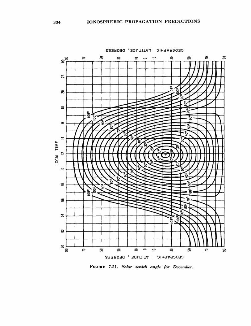
334 IONOSPHERIC PROPAGATION PREDICTIONS
S33d93Q €
FIGURE 7.21. Solar zenith angle for December.
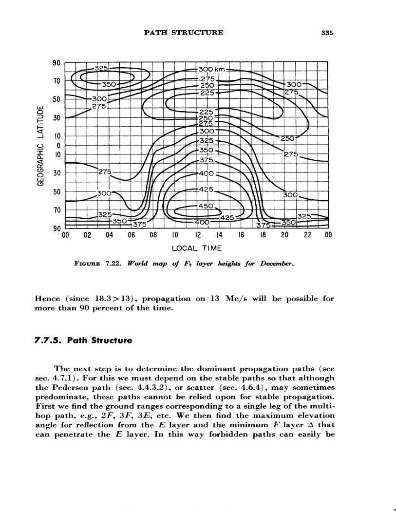
PATH STRUCTURE 335
CL<r cr e> oLU
00 04 06 08 16 18 20 22 0010 12 14
LOCAL TIME
FIGURE 7.22. World map of F2 layer heights for December.
Hence (since 18.3> 13), propagation on 13 Mc/s will be possible for more than 90 percent of the time.
7.7.5. Path Structure
The next step is to determine the dominant propagation paths (see sec. 4.7.1). For this we must depend on the stable paths so that although the Pedersen path (sec. 4.4.3.2), or scatter (sec. 4.6.4) 9 may sometimes predominate, these paths cannot be relied upon for stable propagation. First we find the ground ranges corresponding to a single leg of the multi- hop path, e.g., 2/% 37% 3£", etc. We then find the maximum elevation angle for reflection from the E layer and the minimum F layer A that can penetrate the E layer. In this way forbidden paths can easily be
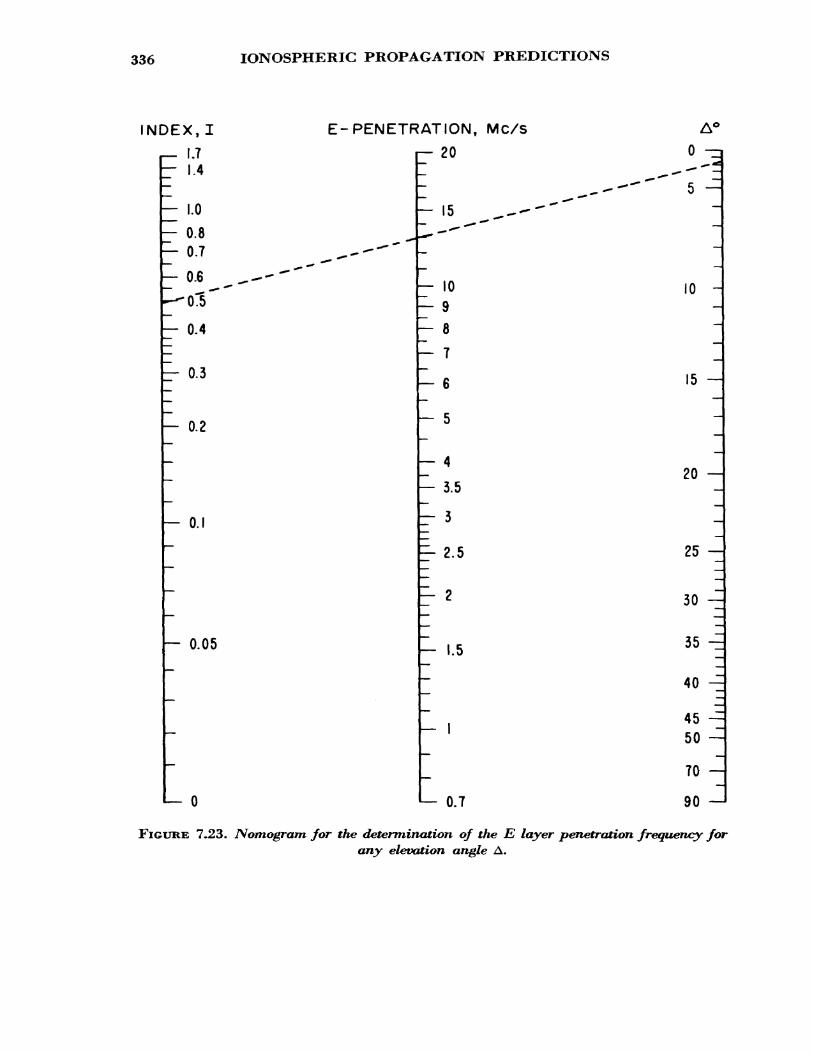
336 IONOSPHERIC PROPAGATION PREDICTIONS
INDEX, I- 1.7
z L0— 0.8— 0.7
— 0.6
— 0.4
E- 0-3
— 0.2
— O.I
— 0.05
l— 0
E-PENETRATION, Mc/S i— 20
- 15
10987
6
- 5
- 4
- 3.5- 3
E- 2-5
^- 2
— 1.5
A°0 -q
5 —
L— 0.7
10 -
15 —
20 —
25 —
30 -^
35 -E
40 -E
45 —_ 50 -
70 -
90 -
FIGURE 7.23. Nomogram for the determination of the E layer penetration frequency farany elevation angle A.
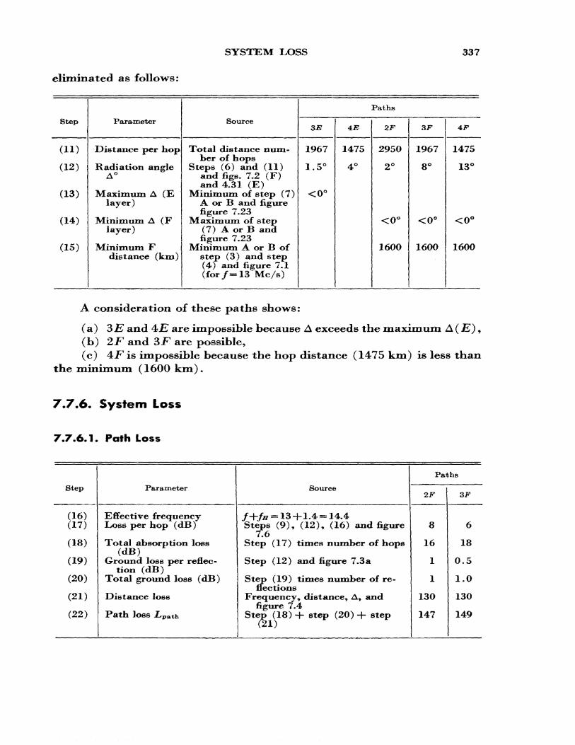
SYSTEM LOSS 337
eliminated as follows:
Step
(ID
(12)
(13)
(14)
(15)
Parameter
Distance per hop
Radiation angleA°
Maximum A (Elayer)
Minimum A (Flayer)
Minimum Fdistance (km)
Source
Total distance num-l>er of hops
Steps (6) and (11)and figs. 7.2 (F)and 4.31 (E)
Minimum of step (7)A or B and figurefigure 7.23
Maximum of step(7) A or B andfigure 7.23
Minimum A or B ofstep (3) and step(4) and figure 7.1(for/ =13 Mc/s)
Paths
3E
19671.5°
<0°
4E
14754°
2F
29502°
<0°
1600
3F
19678°
<0°
1600
4F
147513°
<0°
1600
A consideration of these paths shows:
(a) 3E and 4JE are impossible because A exceeds the maximum A ( E) ,(b) 2JP and 3JF are possible,(c) 4?F is impossible because the hop distance (1475 km) is less than
the minimum (1600 km).
7.7.6. System Loss
7.7.6.1. Path Loss
Step
(16)(17)
(18)
(19)
(20)
(21)
(22)
Parameter
Effective frequencyLoss per hop (dB)
Total absorption loss
Ground loss per reflec tion (dB)
Total ground loss (dB)
Distance loss
Path loss Z/path
Source
/+/* = 13+1.4 = 14-4Steps (9), (12), (16) and figure
7.6Step (17) times number of hops
Step (12) and figure 7*3 a
Step (19) times number of re flections
Frequency, distance, A, and figure 7.4
Step (18) + step (20) + step(21)
Paths
2F
s16
1
1
130
147
3F
6
18
0.5
1.0
130
149
338 IONOSPHERIC PROPAGATION PREDICTIONS
7.7.6.2. Antenna Loss
We shall assume that the appropriate antennas are perfectly matched to the transmitter and receiver* From figure 7.8 we obtain the following antenna gains relative to an isotropic radiator.
Step
(23)(24)(25)
Parameter
Transmitter antenna gainReceiver antenna gainTotal antenna loss JLantenna
Source
FigureFigure
7,8 and step (12)7.8 and step (12)
Paths
2F
-5-510
3F
44
— 8
7.7.6.3. Total System Loss
antenna
LS (2F)= 147 + 10- 157
Since the loss on the 2F path is very much larger than that on the 3-F1 path, the latter is the dominant path and it alone needs to be con sidered further.
7.7.7. Noise Power
From section 7.5.2.3 we see that, on 13 Mc/s, jFom = 32 dB and 0>am 6 dB. To find the effective upper decile value we proceed as follows:
Step
(26)(27)(28)(29)(30)
(31)
(32)
Parameter
Du<TDUUpper decile FauTotal uncertaintyEffective noise level
above kTJ>Correction for 6
kc/s bandwidthCorrection for kTo
Source
Figure 7.19cFigure 7.19cFau = Fam +Du =:32+9<TT= {<r2Fam+<rr>u\*Fan +0" T
Add 10 log 6000- +37.8 (see(7.7)-204
3F Value
9dB3 dB
41 dB6.7 dB
47.7 dB
85.5 dB
-118.5 dB/W
OPTIMUM WORKING FREQUENCY
7.7.8. Required Carrier Power at the Receiver
339
Step
(33)
(34)
(35)
(36)
(37)
Parameter
Peak RF signal/noise required
C arrier/noise(based on 100%modulation)
Allowance for Ray-leigh fading
Required carrier/noise
Required carrierpower f*r
Source
Reference [6]
Step (33) — 6 dB
Equation (7.8)
Step (34) + step (35)
Step (32)+ step (36)
3F Value
35 dB
29 dB
8dB
37 dB
-81.5 dB
7.7.9. Required Transmitter Power Pt
= —81.5+141 = 59.5 dB/W
This rather high value of required power will normally be reduced by the use of more highly directive antennas.
7.8. CHOICE OF OPERATING FREQUENCY
7.8.1. Optimum Working Frequency
The optimum working frequency (0.85 MUF) can be calculated for each hour of the day by the methods described above. In principle, it would be desirable to change the frequency slowly throughout the day in order to make use of the optimum conditions. However, in practice, this is both inconvenient and, in most cases, impossible because of inter national methods of allocating frequencies. In general, a user is allocated only two or three frequencies for use on a given circuit. A knowledge of the diurnal variation of the FOT will, however, aid the circuit operator in anticipating circuit failure due to penetration of the ionosphere by the signal.
340 IONOSPHERIC PROPAGATION PREDICTIONS
7.8.2. The Lowest Usable Frequency
For a given transmitter output power, as the operating frequency is decreased, the available power at the receiver normally decreases due to increased ionospheric absorption, etc. Furthermore, the noise power in creases so that the signal-to-noise ratio deteriorates and the circuit re liability decreases. The minimum frequency below which the reliability is unacceptable, is called the lowest useful high frequency (LUF). The LUF depends upon transmitter power, the factors that determine the path loss (frequency, season, geographical location, etc.), and the noise level (mainly frequency and receiver location). One of the main factors is ionospheric absorption and hence, since this normally varies with solar zenith angle, the LUF peaks around noon. Consequently, in
302826242220
o
I 10O
1 I I !_
CANARY ISLANDS — LONDON DECEMBER (R=29)
FOT
o
o
— o o o o o o
o o o o
O 00 O O ——
LUF
00 04 08 12 UT
16 20 00
Example: With /=0.49 and A=1.5° the E penetration frequency is 13 Mc/s.
FIGURE 7.24. Sample diurnal variation of the optimum u^orking frequency (FOT) and the lowest usable high frequency (LUF) to illustrate the selection of operating frequencies.
REFERENCES 341
selecting a frequency, it is necessary to ascertain whether the LUF ex ceeds this frequency.
7.8.3. Operating Frequency
The diurnal variations of the FOT and the LUF for a circuit between the Canary Islands and London in a December when the average sun- spot number is 29 are shown in figure 7.24. It will be seen that, during the night, it is necessary to use a frequency of around 6 Mc/s in order to ensure that the operating frequency does not exceed the FOT by an ap preciable amount for too long a time. The use of this frequency band during the day is impossible because it lies below the LUF. During the daytime it would be better to use a frequency around 15 Mc/s.
Of course, it should be realized that occasionally the MUF may drop to an exceptionally low value, as during a magnetic disturbance, or that increased D region absorption will raise the LUF* Under these circum stances even the FOT may be unusable.
REFERENCES
[1] Haydon, G. W. ? and IX L. Lucas, Theoretical considerations in the selection of optimum frequencies for high frequency sky-wave communication services (to be published).
[2] CCIR Report 322 (1964), World distributions and characteristics of atmospheric noise.
[3] CRPL Ionospheric Predictions, issued monthly, 3 months in advance, U.S. Government Printing Office, Washington, D.C. 20402,
[4] Bazzard, G. H. (1960), Short-term differences in the behavior of two daily indices of solar activity during the IGY, J. Atmospheric Terrest. Phys. 18, 290.
[5] Minnis, C. M., and G. H. Bazzard (1960), A monthly ionospheric index of solar activity based on F2 layer ionization at eleven stations, J. Atmospheric Terrest. Phys. 18, 297.
[6] CCIR (1959), Documents of the IX Plenary Assembly, Los Angeles, Recom mendation 161, Bandwidths and signal-to-noise ratios in complete systems, also Recommendation 164, Fading allowances for the various classes of service.
[7] Monthly predictions of radio propagation, Institute of Terrestrial Magnetism, Ionosphere, and Radio Propagation, Russia.
[8] Jones, W. B., and R. M. Gallet (1962), The representation of the diurnal and geo graphic variations of ionospheric data by numerical methods, J. Res. NBS BSD (Radio Prop.), 419.
[9] Jones, W. B., and R* M, Gallet (1962), Methods for applying numerical maps of ionospheric characteristics, J. Res. NBS 66D (Radio Prop.)* 649.
342 IONOSPHERIC PROPAGATION PREDICTIONS
[10] Jones, W. B., and R. M. Gallet, Representation of diurnal and geographic varia tions of ionospheric data by numerical methods, Part II, Control of Instability (private communication).
[11] Ostrow, S. M. (1962), Handbook for CRPL Ionospheric Predictions, Based on Numerical Methods of Mapping, NBS Handb. 90.
[12] Zacharisen, 13. H. (1959), World maps of F2 critical frequencies and maximum usable frequency factors, (April 1959) NBS Tech. Note 2, and (Oct. 1960) NBS Tech Note 2-2.
[13] Predictions of radio wave conditions using the index I(F2) and Bulletin A, Radio Research Laboratories of the Ministry of Posts and Telecommunications (1958).
[14] Prediction of optimum traffic frequencies in northern latitudes, Defence Research Board of Canada, December (1954).
[15] World maps of F2 critical frequencies and maximum usable frequencies for 400 km, Radio Research Laboratories of the Ministry of Posts and Telecommunica tions (1958).
[16] Bennett, W. R. (1960), Electrical Noise (McGraw-Hill Book Co., Inc., New York).[17] Crichlow, W. Q., D. F. Smith, R. N. Morton, and W. R. Corliss (1959), World
wide radio noise levels expected in the frequency band 10 kilocycles to 100 mega cycles, NBS Circ. 557.
[18] Crichlow, W. Q., C. J. Roubique, A. D. Spaulding, and W. M. Beery (1960), Determination of the amplitude-probability distribution of atmospheric radio noise from statistical moments, J. Res. NBS 64D (Radio Prop.), 49.
[19] Crichlow, W. Q., A. D. Spaulding, C. J. Roubique, and R. T. Disney (1960), Amplitude-probability distributions for atmospheric radio noise, NBS Mono. 23.
[20] Josik, H. (1961), Antenna Engineering Handbook (McGraw-Hill Book Co. Inc., New York).
CHAPTER 8
Scatter Propagation on Very High Frequencies
8.1. SCATTERING FROM IONOSPHERIC IRREGULARITIES
The very high frequency (VHF) band is usually defined as the fre quency range from 30 Mc/s to 300 Mc/s. Such a definition is of course purely arbitrary* From the point of view of magneto-ionic theory, the numerical values of Y (2.69) are very small and, in general, are negligible, except possibly for Faraday rotation effects (see sec. 4,9.5). Further more, the maximum electron densities in the ionosphere are rarely suf ficient to reflect waves on frequencies much above 30 Mc/s except for relatively short periods (e.g., in the equatorial regions near the peak of the sunspot cycle). Ionospheric transmission on VHF is, therefore, mainly the result of scattering of waves by irregularities in the electron density distribution in the ionosphere rather than by gradual refraction. If suf ficiently high transmitter powers are used the net scattering of energy from the individual electrons (qua si-incoherent scatter) can be detected.
The chief sources of irregularities in the ionosphere are:
(1) Irregularities due to turbulent mixing in the -D region.(2) Ionized trails due to the passage of meteors through the at
mosphere.(3) Spread ,F irregularities (cause unknown).(4) Sporadic E.(5) Individual electrons.
In this chapter we shall select a few of these topics for discussion.
8.2. CHARACTERISTICS OF PROPAGATION ON VERYHIGH FREQUENCIES
Ionospheric effects on frequencies above 100 Mc/s are small (but see sec. 4.9) and not particularly important from the point of view of
343
344 SCATTER PROPAGATION ON VERY HIGH FREQUENCIES
radio communications. We shall, therefore, concentrate our attention on the frequency band from 30 Mc/s to 100 Mc/s.
Ionospheric propagation in the 30 Mc/s to 100 Mc/s range is char acterized by the following features:
(a) Regular but weak scattering from the D region which is useful for continuous single-frequency communication in the 30 Mc/s to 60 Mc/s range over path lengths of the order of 1000 to 2000 km.
(b) Intermittent reflections from ionized meteor tracks which are useful for burst communications in the 40 Mc/s to 80 Mc/s range over path lengths up to 2000 km.
(c) Sporadic and intense reflections on frequencies which may be useful up to about 50 Mc/s to long distances (greater than 4000 km) via irregularities in the J^ region at times of high sunspot number.
(d) Reflections from patches of sporadic E are sometimes important (especially as a source of interference) up to distances of 2000 km or so and on frequencies as high as 80 Mc/s.
The chief disadvantages of VHF propagation, from the point of view of radio communications, are:
(1) Low signal strengths, because of the relative inefficiency of the scattering mechanism.
(2) Rapid fading.(3) Limited ground range (2000 km).(4) Mutual interference between channels normally independent.
8.3. D-REGION SCATTERING1
8.3.1. Scattering From Irregularities in the D Region
Irregularities are produced by the action of turbulence, wind shears, etc., on the electron distribution in the height range between about 70 km and about 90 km. These irregularities in electron density result in corresponding fluctuations in refractive index. Since turbulence merely brings about a redistribution of the electrons, these types of irregularities will exhibit marked solar control as does the overall electron content of the D region. There is also evidence for stratification in the D region which means that the refractive index changes abruptly with height.
1 This section is based on a lecture by R. C. Kirby.2 Figures in brackets indicate the literature references on p. 390.
SCATTERING FROM IRREGULARITIES IN THE D REGION 345
FIGURE 8.1. Geometry of forward scatter from the D region.
The effect of these rapid changes, both in time and space, on very- high-frequency waves is to scatter the energy out of the direction of the incident beam £2]. Since most of the energy is scattered in directions making small angles with that of the incident beam, the phenomenon is called **forward scatter."
The geometry of forward scatter is sketched in figure 8.1 in which a volume V of the ionosphere is illuminated by a transmitter. If pt is the power radiated in the direction of V, then the available power pa from a receiving antenna R is given by
r csc (7/2) (8.1)where
r0 is the electron radius (2.8X10~15 m),/ is the distance from V to /?,b is the thickness of the scattering volume,A T is the effective area of the receiving antenna,y is the angle through which scattering takes place,S(K) is the spectrum of turbulent irregularities,
and
= —~ sinA
(8.2)
where X is the wavelength. Equation (8.1) applies when single scattering is the dominant mechanism (i.e., the amplitude of a twice-scattered wave is negligible) and for isotropic irregularities*
346 SCATTER PROPAGATION ON VERY HIGH FREQUENCIES
The scattering process acts like a narrow band filter on the spectrum, emphasizing those irregularities of size X"1 , where K is given by (8.2). Notice that the isotropy assumption prevents the application of this theory to magnetic field-alined irregularities. Furthermore, we have neglected the effect of the polarization of the incident wave. The latter requires the inclusion, in (8.1), or a sin2 x term where x is the angle be tween the incident electric vector and the scattering direction. Equations (8.1) and (8.2) emphasize the joint frequency-distance dependence of received power which is characteristic of scatter propagation, and shows that the spectrum of irregularities is the basic description of the turbulent electron density variations which is required in electromagnetic theory. In the case of turbulent mixing it can be shown Q2] that
S(K)=K-"(dN/dh)\ (8.3)
where dN/dh is the electron density gradient.From (8.1), (8.2), and (8.3) we find that the relationship of system
loss to the frequency/ and geometry of the propagation path is given by
Pt/pa <*l2fn'(sw %v} n *~\ (8.4)
where n s (n 8 = n+2) is the frequency exponent for an antenna the gain of which is constant with respect to frequency. The use of ns allows for the frequency dependence of A T because the gain of the antenna increases as the square of the frequency.
8.3.2. Height of Scattering
Experimental evidence suggests that the scattering of VHF waves is produced primarily from two layers. During the daytime the predominant heights are around 70 km; this scattering layer is subject to solar control and, therefore, is thought to be due to turbulence. During nighttime the scattering appears to come from the 85 to 90 km region, the ionization in which is thought to be produced by the influx of meteors. Some observa tions seem to be best explained on the basis of simultaneous scattering from both layers.
SIGNAL STRENGTHS IN MIDDLE AND HIGH LATITUDES 347
8.3.3. Signal Strengths in Middle and High Latitudes
8.3.3*1. Long-Term Variations
From hourly median values of signal strengths it has been found that, in the frequency range from 25 to 108 Mc/s, over distances of from 1000 to 2000 km, the system loss ranges from about 140 dB to abtlut 210 dB. The loss depends on several factors such as wave frequency, type of an tenna, geography, and time.
Median values of system loss £3] indicate that on a frequency of about 50 Mc/s the diurnal variations of signal strength are as follows:
Middle latitudes: A maximum near noon and a minimum near 2000 hr local time with the diurnal curve broader in summer than in winter, as would be expected from the solar illumination.
High latitudes: The diurnal maximum is broader and tends to be centered earlier in the day as compared with middle latitudes. The system loss for a given hour varies considerably from day to day. This variation is greater in high latitudes than in middle latitudes.
In middle and high latitudes the seasonal variation is characterized by a strong maximum in summer for all hours of the day. No definite long-term (solar cycle) variation has been established.
The above results were obtained over paths of about 1200 km length and with narrow-beam (6°) rhombic antennas aimed along the great circle.
8.3.3.2. Frequency Dependence
According to (8.4) the system loss should vary with frequency to the power n s . Observations with narrow-beam (6°) antennas show that the values of n8 vary with time but that 90 percent of the observations give values in the range 7 to 9.5 with an overall median of 8. Daytime values are generally greater than nighttime by 1 or 2. Furthermore, summer values tend to be lower than those in other seasons, though winter daytime values are also lower than equinoctial daytime values. With wide beam (56°) antennas the values of n s are about \ to 1 less than with the narrow beam (6°) antennas.
The diurnal and seasonal variations of ns , and the beamwidth de pendence, have been interpreted as evidence of the combined effects of turbulence and meteoric ionization. The lower values of n s are associated
348 SCATTER PROPAGATION ON VERY HIGH FREQUENCIES
with dominant meteoric contributions to the received signal, and the higher values with turbulence.
A limited amount of data indicates that average values for frequency dependence for arctic paths are about the same as in middle latitudes, though less data are available. The measurement of frequency dependence in high latitudes is often complicated by the prevalence of high absorp tion on the lower frequencies.
The dependence of the intensity of the signal on scattering angle in the plane of the great circle has also been measured directly. Measure ments have been carried out in summer daytime, over short paths (500 to 800 km) using pulse transmissions to separate ionospheric and tropo- spheric returns. Values of n from 4 to 8 (corresponding to values from 6 to 10 for n«) have been obtained. These are not inconsistent with the values from frequency dependence measurements, but as very few observations have been made, the statistical significance of the frequency dependence measurements is much greater.
8.3.3.3. Short-Term Variations
8.3.3.3.1. Amplitude Distribution and Fading Rate
Observed amplitude distributions show that, during most of the day, the envelope is, essentially, distributed in a Rayleigh manner. The dis tributions are peaked somewhat at the high-signal end during the late night and early morning hours. Fading rates normally lie between 0.2 c/s and 3 c/s, the rate increasing with frequency. Most observations show that this rate depends on carrier frequency raised to a power between 0.75 and 1.25. One would expect a linear dependence (exponent = 1.0) if the drift speed of the scattering region were dominant compared to the changing structure of irregularities. This departure from linear dependence at times favors the idea of a turbulent D region as against meteor-pro duced ionization.
Fading rates are higher for broad-beam systems, and for off-great- circle paths, than for great-circle transmission with narrow beams.
8.3.3.3.2. Space Correlation
Correlation of signals received on antennas spaced in the great circle is much greater than for antennas spaced perpendicular to the path. Measurements on 50 Mc/s, with narrow-beam transmitting antennas, show that the correlation coefficient falls to 0.5 at 3.5 wavelengths normal to the path, while along the path the corresponding distance is about 40
ABNORMAL BEHAVIOR 349
wavelengths. In the analyses of these data, recognizable meteoric signals were excluded.
8.3.3.3.3. Frequency Correlation
The extent of correlation of fading across a frequency band affects the modulation bandwidth which may be usefully employed and, hence, the design of frequency diversity techniques. Using narrow-beam (6°) antennas on 50 Mc/s, the correlation coefficient has been found to fall to about 0.5 for frequency separations of 6 kc/s during the early morning hours; and near noon the corresponding (6 kc/s) correlation coefficient is 0.65, falling to 0.5 for about 7 kc/s separation. This correlation is poorer for broad-band systems and for off-great -circle paths.
8.3.3.4. Geographical Variations
Observations have shown that, except for paths near the equator, the transmission loss for paths in the arctic, the United States, and Europe differ by less than db5 dB from the overall median value. Within these limits, the signal strengths on the arctic paths are, statistically, higher than those in middle latitudes.
Near the magnetic equator the signal intensities are, on the whole, much higher than in the United States. The background scatter signal is about the same, but this is obscured for a large portion of the time by strong enhancements (up to 50 dB) which appear to be reflected from field-alined ionization in the E region £4Q. Rapid fading is often charac teristic of these enhancements.
It may be of interest to note here that there is little correlation be tween VHF transmission loss in temperate latitudes and/ofi, or HF at tenuation. There appears to be little variation of signal intensity with sunsport number but there is a statistical correlation (positive) with the magnetic K index
8.3.4. Abnormal Behavior
8.3.4.1. Sudden Ionospheric Disturbances
These have been discussed already in section 6.2.4, but a few more comments are appropriate as it appears that the behavior of the received VHF signal varies with frequency. The increased ionization created by
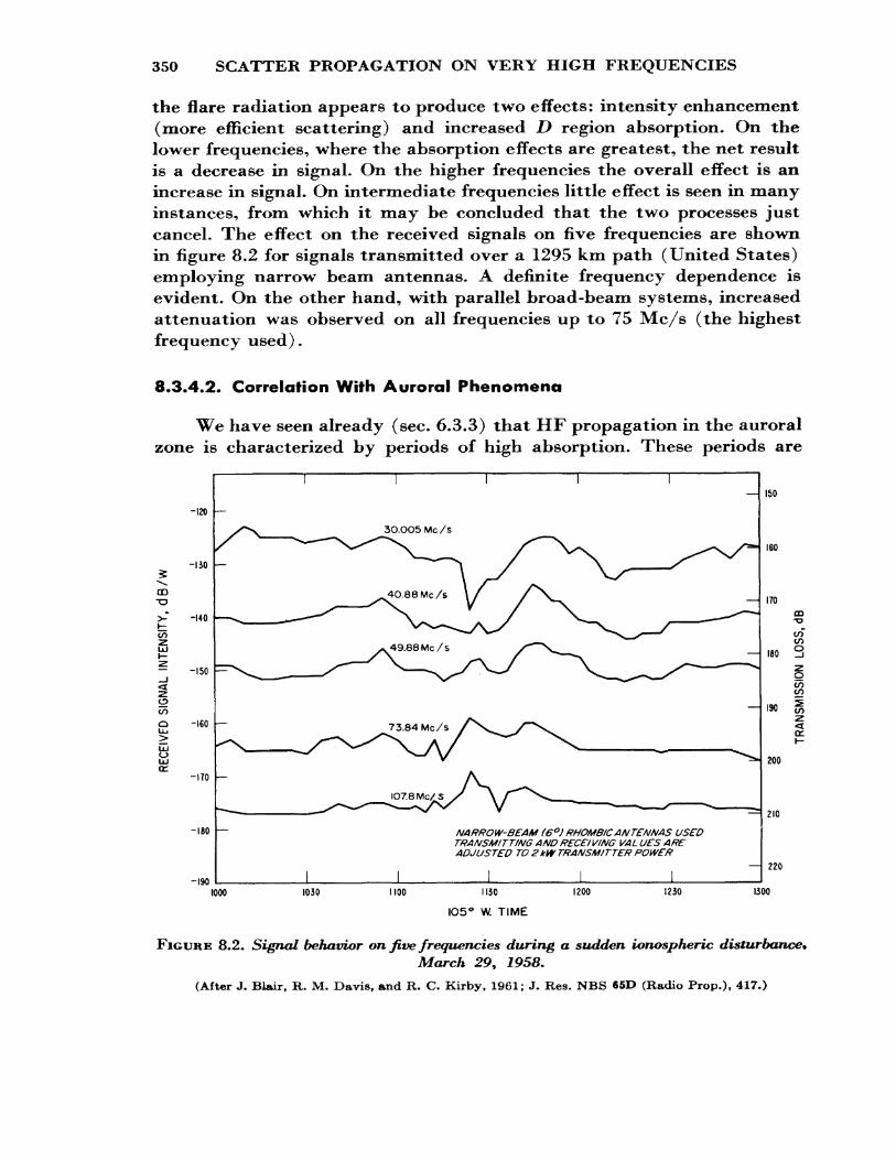
350 SCATTER PROPAGATION ON VERY HIGH FREQUENCIES
the flare radiation appears to produce two effects: intensity enhancement (more efficient scattering) and increased D region absorption. On the lower frequencies, where the absorption effects are greatest, the net result is a decrease in signal. On the higher frequencies the overall effect is an increase in signal. On intermediate frequencies little effect is seen in many instances, from which it may be concluded that the two processes just cancel. The effect on the received signals on five frequencies are shown in figure 8.2 for signals transmitted over a 1295 km path (United States) employing narrow beam antennas. A definite frequency dependence is evident. On the other hand, with parallel broad-beam systems, increased attenuation was observed on all frequencies up to 75 Mc/s (the highest frequency used).
8*3.4.2. Correlation With Auroral Phenomena
We have seen already (sec. 6.3.3) that HF propagation in the auroral zone is characterized by periods of high absorption. These periods are
$ \CD
-120
-130
-140
- -ISO
CO
O -160
-170
-180
-190
3O.OO5 Me /s
NARROW-BEAM (6°) RHOMBIC ANTENNAS USED TRANSMITTING AND RECEIVING VAL UES ARE ADJUSTED TO 2kW TRANSMITTER POWER
JL 1 I
150
160
170
ISO
130
ZOO
210
CD TJ
COtoO
CO CO
220
1000 1030 1100 1130
105° W TIME
1200 1230 1300
FIGURE 8.2. Signal behavior on five frequencies during a sudden ionospheric disturbance.March 29, 1958.
(After J. Blair t R. M. Davis, and R. C. Kirby, 1961; J. Res. NBS «5D (Radio Prop.), 417.)
IONIZATION BY METEORS 351
nof, in general, periods of high absorption of VHF waves. On the contrary, high signal intensities, on 50 Mc/s, are usually observed during periods of enhanced HF absorption and strong geomagnetic activity. It has been found also that marked increases in signal level often coincide with iso lated intervals of HF blackout
8.3.4.3. Sputter
An additional effect associated with aurorae is the occurrence of rapid fading called ''sputter," which is due to a multipath signal. There have been occasions when e*sputter" speeds of up to 200—300 c/s have been observed, i.e., about 100 times the normal fading rate. The effect is minimized with narrow-beam antennas. It may be observed, to some degree or other, 100 hr and more per year Q3].
8.3.4.4. Polar Cap Absorption Effects
Forward scatter signals are affected during PC A events (see sec. 6.4) in high latitudes. If the onset of the proton flux (which gives rise to the PC A) occurs at night , the VHF signals are enhanced (fairly abruptly) followed by strong absorption during the ensuing daylight. The fact that the scattered signals are absorbed during the PC A while en hanced during auroral blackouts indicates that the height at which scatter ing occurs lies below the region of auroral absorption (90 km) but above the height at which polar cap absorption occurs (60 km).
Polar cap absorption events are generally confined to paths with mid points at geomagnetic latitudes greater that about 60°. The onset of this absorption (in the lower latitudes) usually follows the onset of a magnetic storm and often at the time of a strong (Forbush) decrease in the intensity of cosmic rays which is, in general, many hours after the commencement of the PCA itself in higher latitudes.
8.4. METEOR SCATTER 3
8.4.1. lonization by Meteors
Mention has been made above to the fact that in VHF forward scatter strong bursts of signal are frequently superimposed on the background
* This section is based on a paper by G. R. Sugar (1964), Radio Propagation by Reflection from Meteor Trails, Proc. IEEE 52, No. 2, 116-135.
352 SCATTER PROPAGATION ON VERY HIGH FREQUENCIES
signal reflected from turbulent irregularities. These bursts are due to reflections from ionized "trails" produced by meteors mostly in the height range 80 to 120 km. Billions of these trails are produced daily; they diffuse rapidly and usually disappear within a few seconds. During their brief existence, however, these ionized columns will reflect VHF waves par ticularly in the frequency range 20 to 110 Mc/s. The lower frequency limit is set by the need to be above the regular maximum usable frequency and the upper limit is set by technical limitations, since reflections on the higher frequencies are relatively weak.
The ionized trail is the result of conversion of the kinetic energy of the meteor into potential energy of ionization as the meteor is slowed down by collisions with the neutral molecules. The ionization is distributed in the form of a long, thin paraboloid of revolution with the particle at the head of it. The electron density per unit length of the trail is propor tional to the mass of the particle.
The height distribution of trails varies with particle characteristics. The higher velocity particles (of a given mass) produce trails at the higher (120 km) heights, with the mean trail height increasing by about 10 km as the velocity increases from less than 15 km/s to greater than 60 km/s C^H- For a given velocity, particles of higher mass produce maximum trail ionization at lower heights. Over the mass range 10~7 to 10 3 g the height variation is around 44 km. There is also a height variation with the zenith angle (x) of the trail, larger angles corresponding to greater heights. A variation of about 13 km corresponds to the range of x from 0 to 90°.
The lengths of the trails depend primarily on the mass and zenith angle. Typical lengths range up to 50 km, the most probable value being 15 km, although this depends on the definition of rflength."
The initial radii of the trails are in the range 0 to 1.2 m (with a mean value of 0.65 m) based on visual studies, while radio observations give a range from 0.55 m to 4.35 m. The 0.55-m-radius is for a height of 81 km.
Let us consider now the dissipation of the ionization. Once the trail is formed it expands by diffusion at a relatively low rate, thus producing a radial distribution of material that is approximately Gaussian. After a time t the radius r is related to initial radius TO by the expression:
r2 = r*+4£>f, (8.5)
•where D is the diffusion coefficient of the electrons and varies from one m2/sec at 85 km to 140 m2/sec at 115 km. Hence, after 1 sec, a trail will have a radius in the range 2 to 20 m.
METEOR DATA 353
The practical lifetime of a trail depends, of course, on the means of detection. Most trails, detected by radio methods, are those resulting from small particles and last for a fraction of a second only. Larger meteors produce more densely ionized trails, and trails with durations of the order of 1 min are observed several times per day. Trails with durations of the order of an hour or more are extremely rare.
The dissipation of trails is complicated further by the action of winds in the 80 to 120 km region. At the time of formation, trails are quite straight but they are deformed rapidly by winds of the order of 25 m/sec and vertical wind shears with maxima of the order of 100 m/sec per km. A wind shear of this magnitude can rotate part of a trail through an angle of 5° in 1 sec.
8*4.2. Meteor Data
Before considering the reflection of radio waves from meteor trails, it will be useful to discuss some of the physical properties of meteors* Nearly all our knowledge in this field comes from visual and radio ob servations. The term rrmeteor" will be restricted to those particles enter ing the earth's atmosphere that are completely burned up by frictional heating.
Particles in the mass range of 10~7 to 103 g and dimensions in the range 40 p. to 8 cm are primarily responsible for radio reflections. Before being swept up by the earth's atmosphere these meteors move in elliptical orbits around the sun and they are thought to be of cometary origin.
Meteors can be divided into two classes:
Shower meteors are collections of particles all moving with the same velocity in fairly well-defined orbits around the sun. These meteors, while the most spectacular, account for only a small fraction of the total in cidence of meteors.
Sporadic meteors comprise nearly all those of interest to radio work. These meteors seem to move in random orbits so that, in contrast to the shower meteors which appear to come from a specific ^radiant" point in the sky, sporadic meteors have radiants that appear to be randomly dis tributed over the sky- It is of interest to note that a meteor shower is often named after the stellar constellation in which the radiant point lies, e.g., Leonid for Leo.
The radiants and times of occurrence of sporadic meteors are random and of course cannot be cataloged in this manner. Their radiant points are not, however, uniformly distributed in the sky but are for the most
354 SCATTER PROPAGATION ON VERY HIGH FREQUENCIES
part concentrated toward the ecliptic plane (the plane of the earth's orbit) and move in the same direction around the sun as the earth moves pl]. The orbits are not uniformly distributed along the earth's orbit but are concentrated so as to produce a maximum incidence of meteors at the earth in July and a minimum in February. This variation in the space density of meteors is shown in figure 8.3, which has been adapted from the data of Hawkins C^D-
The rate of incidence of sporadic meteors at the earth is further modi fied by two factors. The first of these, resulting in a regular diurnal vari ation in meteor rate, is illustrated in figure 8.4. On the morning side of
OCT NOV DEC JAN FEB MAR APR MAY JUN JUL AUG SEPT
MONTH
FIGURE 8.3. Variation of space density of meteors along the earth's orbit.
(After G. S, Hawkins, 1956, Monthly Notices Roy. Astron, Soc. 116, 103.)
METEORS SWEPT UP BY THE EARTH
MOTION OF EARTH AROUND SUN
METEORSOVERTAKING EARTH
TO THE SUN
FIGURE 8.4. Diurnal variation of meteor rates,
In the evening only meteors overtaking the earth are observed. In the morning meteors with orbital directions opposite to that of the earth and the slower ones with the same orbital direction are observed. (After G. R. Sugar, 1964, Radio propagation by reflection from meteor trails,
Proc. IEEE 52, No. 2, 116.)
METEOR DATA 355
the earth, meteors are swept up by the forward motion of the earth in its motion around the sun. On the evening side the only meteors reaching the earth are those which overtake it. This results in a maximum oc currence rate around 6 a.m. and a minimum rate around 6 p.m. The ratio of maximum to minimum depends on the latitude of the observer. A further minor seasonal variation is introduced because of the tilt of the earth^s axis relative to the ecliptic plane. This variation, also dependent on the latitude of the observer, can change the expected hourly rates by factors as large as 1.4.
The mass distribution of sporadic meteors is such that there are approximately equal total masses of each size of particle. There are, for example, 10 times as many particles of mass 10~~4 g as there are particles of mass 10~3 g. This approximate relation between particle mass and number is given in table 8.1. The mass distribution of shower meteors is somewhat similar to that for the sporadic meteors with the important
TABLE 8.1. Order-of-magnitude estimates of the properties of sporadic meteors
Particles passthrough the at mosphere and fallto the ground
Particles totallydisintegrated inthe upper atmos phere
Approximate limitof radar measure ments — »
Micrometeorites(Particles float down unchangedby atmospheric collisions)
Particles removedfrom the solarsystem by radia tion pressure
Mass(grams)
104
1C 3102101lo-110~210~ 3io-410~5io-*10~710~*
10-*10-io 10"1110~12
IO-13—
Visualmagnitude
-12.5
-10.0-7.5-5.0-2.5
0.02.55.07.5
10.012.515.017.5
20.022.5 25.027.5
30—
Radius
8 cm
4 cm2 cm0.8 cm0 .4 cm0.2 cmO.O8 cm0.04 cm0.02 cm
80 M40 ii20 fji
8 M
4 M2 M 0.8 M0.4 M
0.2 M—
Number ofthis massor greater
swept up bythe eartheach day
10
IO2IO 3IO 4IO5IO6IO7IO8IO9IO10IO11IO12
?
Total forthis group estimatedas high as 102°
——
Electronline density
(electronsper meter
of traillength)
——
__——
IO18IO17IO16IO15IO14IO13IO12IO11IO10
9
Practicallynone
——
356 SCATTER PROPAGATION ON VERY HIGH FREQUENCIES
difference that there are more large particles relative to the number of smaller ones than for the sporadic meteors £9],
The velocities of meteors approaching the earth are in the range 11.3 to 72 km/s. The lower limit is the escape velocity for a particle leaving the earth and is, therefore, the lowest velocity that a particle falling toward the earth can have. The upper limit is the sum of two components, a 30 km/s component associated with the velocity of the earth in its orbit around the sun, and a 42 km/s component associated with the meteor itself. This latter velocity is the escape velocity for a particle leaving the solar system. Nearly all observations indicate that meteor velocities fall in the above range, which suggests that meteors are members of the solar system.
8.4.3. Reflection From a Meteor Trail
8.4.3.1* Important Parameters
The distribution of energy reflected by a meteor trail is a function of many variables. The ionization density distribution across and along the trail, the orientation of the trail, the radio wavelength, the polariza tion of the incident wave relative to the trail, motion of the trail either as part of the process of formation or due to ionospheric winds, and the straightness of the trail are all significant. In discussing the reflection properties it is convenient to divide the trails into two classes—under- dense trails and overdense trails—and to examine the properties of each class independently. Underdense trails are those wherein the electron density is low enough so that the incident wave passes through the trail and the trail can be considered as an array of independent scatterers. Overdense trails are those wherein the electron density is high enough to prevent complete penetration of the incident wave and to cause reflection of waves in the same sense that the ordinary ionospheric reflections occur. A rough sorting of trails into these two categories can be done on the basis of trail lifetime or duration. On long wavelengths (relative to the VHF band) the underdense trails have durations of less than about 1 sec while the overdense trails have longer durations. The analysis can be further divided in terms of the radio wavelength. On long wavelengths the ef fective duration of a trail is large compared to the time it takes the trail to form, and the trail may be considered to have a cylindrical shape. On short wavelengths, however, the duration is much shorter and the column must be considered to be of the paraboloidal form previously indicated.
REFLECTION FROM A METEOR TRAIL 357
The solutions to be considered here are at best useful approximations to the physical problems. They will apply quite well to some of the trails observed and rather poorly to others. A complete analysis of the reflec tions from even a relatively simple trail would be far too complex to be of any practical use or interest. In the following treatment the terms long wavelength, etc., are used in a relative manner to indicate the lower frequency end of the VHF band, etc.
8*4.3*2. Long Wavelength Reflections From Low-Density Trails
On the assumption that the trail is an infinitely long right circular cylinder of electrons whose diameter is very small compared to the wave length, assume also that the trail electron density is low enough that the incident wave passes through the trail without major modification. Consider the case of radarlike reflections with transmitter and receiver at the same location. Figure 8.5a illustrates the reflection geometry and the trail model. Let R be the length of the perpendicular from the radar set to the trail. The signal received can be computed by summing the energy backscattered by each electron in the trail while taking proper account of the phase relations of these contributions. When this is done it is found that the principal contribution of energy from a trail is from its first Fresnel zone, a region of length \/2XJ?, centered at the point on the trail where the line from the radar is normal to the trail. For example, on 50 Mc/s a trail 200 km away will have a first Fresnel zone 1.6 km in length. As the trail expands by diffusion, the phase difference of the contributions from the electrons on opposite sides of the trail increases so that the received power decreases. The signal amplitude will have fallen to l/€ of its initial value (e = 2.718) at the time the radius of the trail is \/2w. On 50 Mc/s this radius is 1 m.
(a) (b)
FIGURE 8.5. Low-density long-wavelength reflections.
(a) Reflection geometry, (b) Variation of received signal with time. (After V. R. Eshleman, I960, Meteor scatter, The Radio Noise Spectrum, ch. 4 t Harvard Univ. Press.)
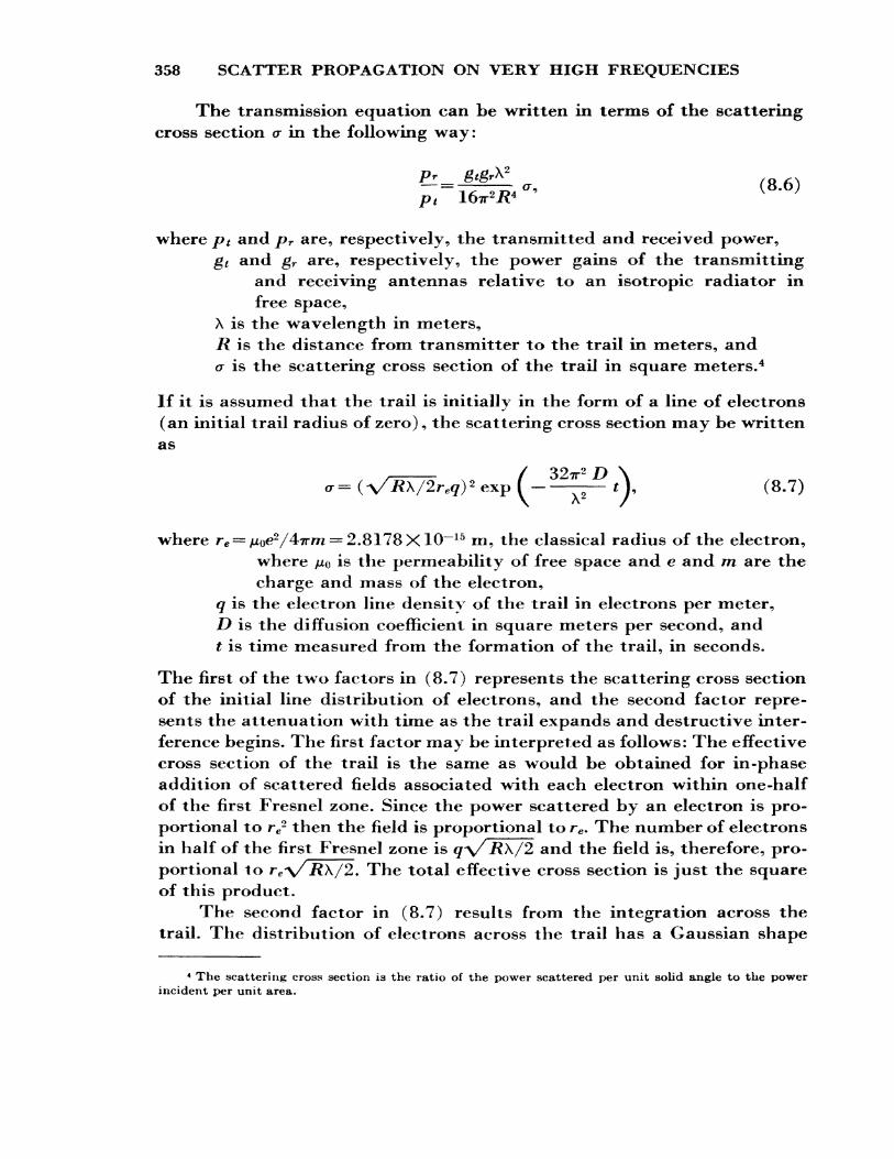
358 SCATTER PROPAGATION ON VERY HIGH FREQUENCIES
The transmission equation can be written in terms of the scattering cross section a in the following way:
Pr— -1 ^ 9 r>d -p t 167T2/?4
where />* and pr are, respectively, the transmitted and received power,gt and gr are, respectively, the power gains of the transmitting
and receiving antennas relative to an isotropic radiator infree space,
X is the wavelength in meters,R is the distance from transmitter to the trail in meters, and a is the scattering cross section of the trail in square meters. 4
If it is assumed that the trail is initially in the form of a line of electrons (an initial trail radius of zero) , the scattering cross section may be written as
/ ^9-^2 r> \(8.7)
where rc = Mo#2/47rm = 2.8178XlO~15 m, the classical radius of the electron, where /JLQ is the permeability of free space and e and m are the charge and mass of the electron,
q is the electron line density of the trail in electrons per meter, D is the diffusion coefficient in square meters per second, and t is time measured from the formation of the trail, in seconds.
The first of the two factors in (8.7) represents the scattering cross section of the initial line distribution of electrons, and the second factor repre sents the attenuation with time as the trail expands and destructive inter ference begins. The first factor may be interpreted as follows: The effective cross section of the trail is the same as would be obtained for in -phase addition of scattered fields associated with each electron within one-half of the first Fresnel zone. Since the power scattered by an electron is pro portional to re2 then the field is proportional to re . The number of electrons in half of the first Fresnel zone is q\/ R\/2 and the field is, therefore, pro portional to re\/R\/2. The total effective cross section is just the square of this product.
The second factor in (8.7) results from the integration across the trail. The distribution of electrons across the trail has a Gaussian shape
4 The scattering cross section is the ratio of the power scattered per unit solid angle to the power incident per unit area.
REFLECTION FROM A METEOR TRAIL 359
£9] with an effective radius of \/4Dt. Using this with (8.6) and (8*7) 5 it can be shown that the signal amplitude will fall to 1/c when the effective radius is \/2w.
If the initial radius is nonzero, the peak amplitude is reduced from that given by (8.6). The form of the time variation of received power is sketched in figure 8.5b.
In the above relation, since it was assumed that trails were of in finite length, every trail had a first Fresnel zone and therefore gave a reflection. In practice, however, since trails are of finite length, this zone may not lie on the trail but rather on an extension of it. In such a case the signal returned from the trail would be a relatively weak one, and in practice these returns are of little importance. Thus a radar can ff see" only a fraction of all the trails incident on the ionosphere within its range because most trails do not have the proper orientation for the line of sight to be perpendicular to the trail. The requirement for proper orienta tion can be restated as requiring that the trail be tangent to a sphere centered at the radar.
When the transmitter and receiver are separated, as in the case of point-to-point propagation, the reflection requirement is that the incident ray and reflected ray make equal angles with the trail axis. Geometrically this is equivalent to a requirement that the trail be tangent to an ellipsoid with foci at the transmitter and receiver. For this case two important changes take place because of the oblique geometry. First, the length of the first Fresnel zone increases and, therefore, more electrons contribute to the received signal. Second, the maximum possible propagation path difference over the cross section of the trail decreases with increasing obliquity. This decrease is equivalent to an increase in wavelength and results in both a larger initial signal and a slower rate of signal decay as the trail expands.
In this case it can be shown £10, 11J that the peak received power varies as X3g2 and the signal duration as X2 .
8*4.3*3* Long Wavelength Reflections From High-Density Trails
With high electron densities the assumption that the incident wave passes through the trail essentially unmodified is no longer valid. For this case it is assumed that the wave penetrates the trail until reaching a surface of sufficiently high electron density to be reflected. The model used is that of an expanding cylindrical reflector of radius rc, figure 8.6a. After a time the electron density everywhere within the trail falls below
360 SCATTER PROPAGATION ON VERY HIGH FREQUENCIES
>(a)
T '
FIGURE 8.6. High-density long-wavelength reflections.
(a) Reflection geometry, (b) Variation of received signal with time. (After V. R. Eshleman, 1960, Meteor scatter, The Radio Noise Spectrum, ch. 4, Harvard Univ. Press.)
the critical value and the underdense model is once more applicable. However, by this time the radius is quite large and the signal contribution is rather small.
In the case of backscatter, the transmission equation is based on reflection from a cylinder and is given by
and this applies until approximately the time when the second factor becomes zero. This occurs at a time
47T2 D '
after this time the relation for underdense trails is applicable Q12]. The form of the time dependence of received power predicted by (10*8) is illustrated in figure 8.6b.
For the overdense case the maximum received power varies as q* in contrast to the qr2 variation for the underdense case. The X3 dependence is the same as for the latter case.
The dividing line between low- and high -density trails is commonly taken to be for q in the range 1 to 2.4X10¹⁴ electrons per meter. If the transition value is taken at 0.75 X10¹⁴ electrons per meter, then the peak signals predicted by (8.8) will be equal; this is sometimes done for con venience D-2].
REFLECTION FROM A METEOR TRAIL 361
The extension of (8.8) to the forward scatter case has been done in a relatively simple manner £1.2]]* The derivation, as in the backscatter case, is based on a reflecting cylinder and the refractive effects of the electrons beyond the critical radius of the trail have been ignored. These refractive effects reduce the validity of the transmission equation £13], but their significance is uncertain.
The dividing line between low- and high -density trails is again at g=0.75Xl014 electrons per meter. The effect of the initial radius of the trail can be computed as in the backscatter case.
8.4.3.4. Short Wavelength Reflections From Low-Density Trails
In the previous two sections it has been assumed that the time of formation of a meteor trail is quite small compared to the total time that radio waves are scattered by the trail. The formation of the trail was in effect considered to be a transient state preceding the desired "steady state" trail and this transient was neglected. However, as the wavelength is decreased and the duration of this steady state decreases, the duration of the transient state tends to remain constant. For sufficiently short wavelengths only the transient state remains. In this section and the following one this transient state will be considered £14], first for under- dense trails, then for overdense trails.
Consider first the problem of estimating the shortest wavelength for which the long wavelength results are applicable. The time of formation of a trail is essentially the time required for the incoming particle to traverse one-half the first Fresnel zone as defined for the long wavelength case. A rough estimate of the transition wavelength between long- and shortwave cases may be obtained by equating the time of formation for a trail to the duration of a longwave echo and solving for the wave length. For example, consider backscatter reflections from an underdense trail. The time to traverse half the first Fresnel zone is (R\/2)*/v, where v is the meteor velocity, and the nominal echo duration (to the 1/e am plitude) is A2/167r2 Z)» Equating these and solving for ATS the transition wavelength, we obtain
\T = (128*-4 D2/?/^)*. (8.10)
Using as typical values 1? = 500 km, r=40 km/s, and Z> = 3 m2/&ec9 a transition wavelength of 3.3 m is obtained.
Since in practice there can be a wide variation in the values of the parameters in (8.10) it is necessary to evaluate XT for each specific case.
362 SCATTER PROPAGATION ON VERY HIGH FREQUENCIES
If the practical extremes of all of the variables for both the backscatter and forward scatter cases are investigated, it is found that the transitional wavelength can be anywhere in the range 0.1 to 100 m. For a random sample of meteors the transitional wavelength is likely to be near 2.9 m for backscatter and in the range 0.5 to 1.6 m for forward scatter.
The short wavelength case is treated by considering the effects of differential diffusion as the trail is being formed. Each part of the trail begins to diffuse as soon as it is formed, and thus the effective radius of the trail is smaller close to the meteor than farther back along the trail where diffusion has been going on for a longer time. The effective radius for any part of the trail is taken as r= \/4 Dt, the same value previously used for the whole trail. Now it can be shown that, except near the end of its path, the velocity of the meteor can be considered to be constant. Therefore position along the trail is proportional to t and the relation r— \/4 Dt indicates that the trail will have the form of a paraboloid of revolution.
The geometry is shown in figure 8.7a and the time variation in re ceived power is given in figure 8.7b. The time t = 0 is the instant of closest approach of the meteor.
In this case the peak power varies as q2 as was true in the long wave length underdense trail case. With decreasing wavelength the power falls as A6 is compared with X3 for the long wavelength underdense case. This rapid variation with wavelength is consistent with the fact that very few observations of meteor reflections have been made on frequencies above the VHF range.
SMALL REFLECTING REGION
FIGURE 8.7. Low-density short-wavelength reflections.
(a) Reflection geometry, (b) Variation of received signal with time. (After V. R. Eshleman, 1960, Meteor scatter, The Radio Noise Spectrum, ch. 4, Harvard Univ. Press.)
REFLECTIONS FROM METEOR IONIZATION 363
8.4.3.5. Short Wavelength Reflections From High-Density Trails
This case is of less practical interest than those discussed above and, consequently, will not be treated here. A brief discussion of this case is given in the paper by Sugar Ell], which should be consulted by the interested reader.
8.4.4. Other Aspects of Reflections From Meteor lonization
In the previous four sections, reflections from meteor trails have been considered from a relatively idealized viewpoint and many of the practical aspects have been ignored. In this section some of these will be discussed from a qualitative viewpoint. The discussion is directed toward the long wavelength cases, since relatively few observations on short wavelengths have been made and analyzed.
8.4.4.1. Long Wavelength Reflections During Trail Formation
The transient state associated with trail formation is of some interest since it accounts for some of the observed characteristics of trail reflections. As a trail is being formed, but before the meteor reaches the first Fresnel
1.2
1.0
^0.8
>5O.6
0.2
-5.0 -4.0 -3.0 -2.0 -1.0 O I.O 2.O 3.O RELATIVE POSITION OF HEAD OF TRAIL
4,0 5.0
FIGURE 8.8. Amplitude variation of received signal as trail lengthincreases.
The limits of the first Fresnel zone are at -f-1 and — 1. (After M. Lo wen thai, 1956, MIT Lincoln Laboratory Tech. Rept. 132.)
364 SCATTER PROPAGATION ON VERY HIGH FREQUENCIES
zone, a weak reflection is obtained from the incomplete trail. This comes primarily from the part of the trail corresponding to the shortest trans mission path at the instant; and. when, as is usually the case, this is the head of the trail, the reflected signal is shifted in frequency because of the motion of the effective reflecting point. As the meteor approaches the first Fresnel zone for the trail this frequency shift approaches zero, and thus the received frequency decreases with time. The observed frequency will of course depend on trail orientation, meteor velocity, and observing wavelength, A maximum shift of the order of 5 kc/s is possible on 50 Mc/s over a 1000 km path.
As the meteor crosses the first Fresnel zone, the specular reflection occurs, accompanied by a large signal enhancement. Then as the particle continues on, the additional ionization from the lengthening trail creates a minor fluctuation of the signal as shown in figure 8.8. Most trails do not have the proper orientation to produce a specular reflection and in these cases only the weak Doppler-shifted component is observed.
8.4.4.2. Trail Drift and Distortion
The effects of ionospheric winds are appreciable for trails which last for the order of a second or more. A Doppler shift of the received frequency will be associated wTith the average wind velocity at the trail. For a velocity of 25 m/s this ffbody Doppler" can be as large as 18 c/s for backscatter observations on 50 Mc/s and will be somewhat less for forward scatter observations.
The trail distortion resulting from wind shears can lead to the forma tion of several local first Fresnel zones for the trail since a distorted trail can have several points where the transmission path length has a local minimum. These local minima, or "glints" as they have been called, are strong scatters and the received signal is a composite of their contribu tions. Since they are moving at different velocities, the signals from each have different Doppler shifts and the resultant composite signal fades in an irregular manner. On 50 Mc/s the fading rates observed for forward scatter are of the order of 1 to 10 c/s. In addition to producing the fading observed for long-enduring trails, the wind shears can rotate a trail suf ficiently to produce reflections when the initial orientation was not suitable. Thus these trails lose their aspect sensitivity as time goes on, and if their life is of the order of 10 sec they will scatter in all directions.
SHORT-TERM STATISTICAL CHARACTERISTICS 365
8.4.4.3. Diversify Effects
As pointed out in section 8.4.3, underdense trails act as small co herent sources and, therefore, CW signals scattered by them exhibit good space and frequency correlation. Correspondingly, very little pulse broad ening is observed when pulse signals are used. The limited available data suggest that for a forward scatter path about 1000 km in length, operating near 50 Mc/s, the correlation coefficient observed for single jAiderdense trails will fall to 0.5 for antenna spacings of the order of 150 km along the path, for antenna spacings of the order of 30 km across the path, and for frequency separations greater than 5 Mc/s. Three-microsecond pulses show no appreciable broadening under these conditions.
Overdense trails, in contrast to the underdense trails, tend to act like relatively large sources and, therefore, exhibit much poorer space and frequency correlation properties. Again, as in the underdense case, specific data on these properties are not available. Available results £13] suggest that the correlation observed for single overdense trails will fall to 0.5 for antenna spacings of the order of 50 A. Measurements using short pulses over a 1000-km path indicate that the received composite signal can have a total time spread as large as 10 Atsec Cl^U*
8.4.5. Short-Term Statistical Characteristics
8.4.5.1. General Remarks
From the viewpoint of radio propagation it is the collective properties of trail reflections rather than the individual reflections that are of pri mary interest. These statistical characteristics can be divided into two classes. First there are the short -term properties, the ones which would be observed during a single hour or less. These can be thought of as being associated with a small but statistically significant sample of trails. Second are the long-term statistical characteristics of the reflections. These include the diurnal and seasonal variations, geographical factors, variations with systems parameters, etc. In the following sections the effects of the initial radii of the trails are ignored—the initial radii are assumed to be zero. This approach appears to be satisfactory since the simplified theory accounts satisfactorily for nearly all of the radio propa gation properties of meteor trails. Difficulties arise primarily when one tries to deduce properties of the meteors themselves from the radio ob servations. For example, when the initial radii are assumed not to be zero,
366 SCATTER PROPAGATION ON VERY HIGH FREQUENCIES
different height distributions and mass distributions are obtained than for the zero radius case. These differences will not be important here since the older theory is consistent with the observations and thus the initial radius problem can be avoided.
8.4.5.2. Peak Amplitude Distribution
The peak amplitude of the reflection from an underdense trail is proportional to the electron line density q and, hence, proportional to the mass of the meteor £9]]. For underdense trails the number N of signals observed with peak amplitudes greater than A is given by
NocA-1 . (8.11)
For overdense trails A is proportional to q* and so
N^A-*. (8.12)
In general, it is better to write the relationship in the form
7V= CA-" (8.13)
where C is a constant of proportionality and where a depends on the details of the observing system and in practice will be a function of the detection threshold A. If a very low threshold is used, then nearly all of the trails detected will be underdense and the exponent observed will be quite near a=l. If a very high threshold is used, nearly all of the trails detected will be overdense and the exponent will be near a = 4. Between these two conditions there will be a transition region where contributions from both overdense and underdense trails will be im portant, and in this region the exponent a will lie between 1 and 4. The extent of the transition region depends on path geometry, antenna di rectivity, etc. Observations of shower meteors made using backscatter with highly directive antennas and, therefore, concerned with trails localized in position and orientation, indicated that the transition was complete in a 2 to 1 amplitude range £9]. In contrast, forward scatter observations of sporadic meteors, which therefore include a wide variation of positions and orientations, indicated that the transition extended over a 10 to 1 amplitude range C16]. Figure 8.9 gives the relation between threshold and rate computed for one experimental path £16]. The system parameters were /»/= 100 W^ X = 7.5 m, gf = gr = 40; a transmitter-receiver
SHORT-TERM STATISTICAL CHARACTERISTICS 367
too
IO
LO
o en
1
O.I
O.OlO.I 1,0 IO
COUNTING LEVEL A c (yLiV)
FIGURE 8.9. Theoretical rate—amplitude relation computed for the following parameters: f*t = 10O W 9̂ X = 7.5 m, gt = gr = 40.
(After C. O. Mines, 1958, Can. J. Phys. 36, 549.)
separation of 1000 km was assumed and a mean trail height of 100 km was used. The upper and lower dashed lines in the figure have slopes of — 1 and —4 respectively, corresponding to the theoretical distributions for underdense and overdense trails.
8.4.5.3. Duty Cycle Versus Threshold
Duty cycle is defined as the fraction of time that a received signal exceeds a prescribed threshold. To a first approximation it is the fraction of time that the reception of messages will occur in a meteor-burst com munication system and it is an important parameter in systems work.
368 SCATTER PROPAGATION ON VERY HIGH FREQUENCIES
The relationship between duty cycle T and the threshold A\ for propagation by underdense trails is given by
T= (r/a) (8.14)
Here r is the time taken for the amplitude to fall to (1/2.78- • •) of its initial value and a and C are defined by (8.13). Note that since this can be written as T= (r/a)N9 the factor r/a is just the average duration of a burst. For underdense bursts a= 1 and since duty cycle P is proportional to T, then
P(A>A1 ) (8.15)
In practice, the presence of overdense trails increases the observed value
100
-40 -30 -2O -IO O IO
RELATIVE THRESHOLD IN DECIBELS
2O 3O
FIGURE 8.10. Duly cycle versus threshold.
(After G. R. Sugar, 1964, Radio propagation by reflection from meteor trails, Proc. IEEE 52, No. 2, 116.)
SHORT-TERM STATISTICAL CHARACTERISTICS 369
of a. Values commonly observed are in the range 1.1 to 3.5, with the large values apparently associated with a predominance of overdense trails. An example of the measured variation of duty cycle with threshold is shown in figure 8.10. Note that the slope of the curve increases at higher thresholds. The points at duty cycles higher than 10 percent include con tamination from receiver noise and ionospheric scatter transmission as well as signals from overlapping meteor trails. They should not, therefore, be expected to fit the distribution law derived here.
8.4.5.4. Apparent Location of Trails
The geometrical conditions required for strong reflections from a trail, combined with the radiant distribution for sporadic meteors, are such as to favor trails occurring in some parts of the sky and to discrimi nate against those in other parts of the sky. The result is that the meteors contributing to propagation over a particular path occur in a relatively small region of the sky, the so-called "hot spot." For the longer trans-
4OO
300
200
100
100 2OO 3OO 4OO 500x (km)
FIGURE 8.11. Relative signal contributions from various parts of the meteor region computed for a 100O km path.
The origin of coordinates represents the path midpoint, x and y are respectively displacements along and normal to great circle path. Results in the other quadrants are symmetrical to these. (After C. O. Hines, 1956, Can. J. Phys.
34, 1O13,)
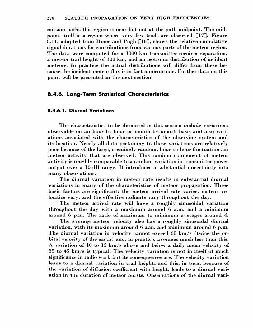
370 SCATTER PROPAGATION ON VERY HIGH FREQUENCIES
mission paths this region is near but not at the path midpoint. The mid point itself is a region where very few trails are observed Cl^H* Figure 8.11, adapted from Hines and Pugh ClS^, shows the relative cumulative signal durations for contributions from various parts of the meteor region. The data were computed for a 1000 km transmitter-receiver separation, a meteor trail height of 100 km, and an isotropic distribution of incident meteors. In practice the actual distributions will differ from these be cause the incident meteor flux is in fact nonisotropic. Further data on this point will be presented in the next section.
8*4.6. Long-Term Statistical Characteristics
8.4.6.1. Diurnal Variations
The characteristics to be discussed in this section include variations observable on an hour-by-hour or month-by-month basis and also vari ations associated with the characteristics of the observing system and its location. Nearly all data pertaining to these variations are relatively poor because of the large, seemingly random, hour-to-hour fluctuations in meteor activity that are observed. This random component of meteor activity is roughly comparable to a random variation in transmitter power output over a 10-dB range. It introduces a substantial uncertainty into many observations.
The diurnal variation in meteor rate results in substantial diurnal variations in many of the characteristics of meteor propagation. Three basic factors are significant: the meteor arrival rate varies, meteor ve locities vary, and the effective radiants vary throughout the day.
The meteor arrival rate will have a roughly sinusoidal variation throughout the day with a maximum around 6 a.m. and a minimum around 6 p.m. The ratio of maximum to minimum averages around 4.
The average meteor velocity also has a roughly sinusoidal diurnal variation, with its maximum around 6 a.m. and minimum around 6 p.m. The diurnal variation in velocity cannot exceed 60 km/s (twice the or bital velocity of the earth) and, in practice, averages much less than this. A variation of 10 to 15 km/s above and below a daily mean velocity of 35 to 45 km/s is typical. The velocity variation is not in itself of much significance in radio work but its consequences are. The velocity variation leads to a diurnal variation in trail height; and this, in turn, because of the variation of diffusion coefficient with height, leads to a diurnal vari ation in the duration of meteor bursts. Observations of the diurnal vari-
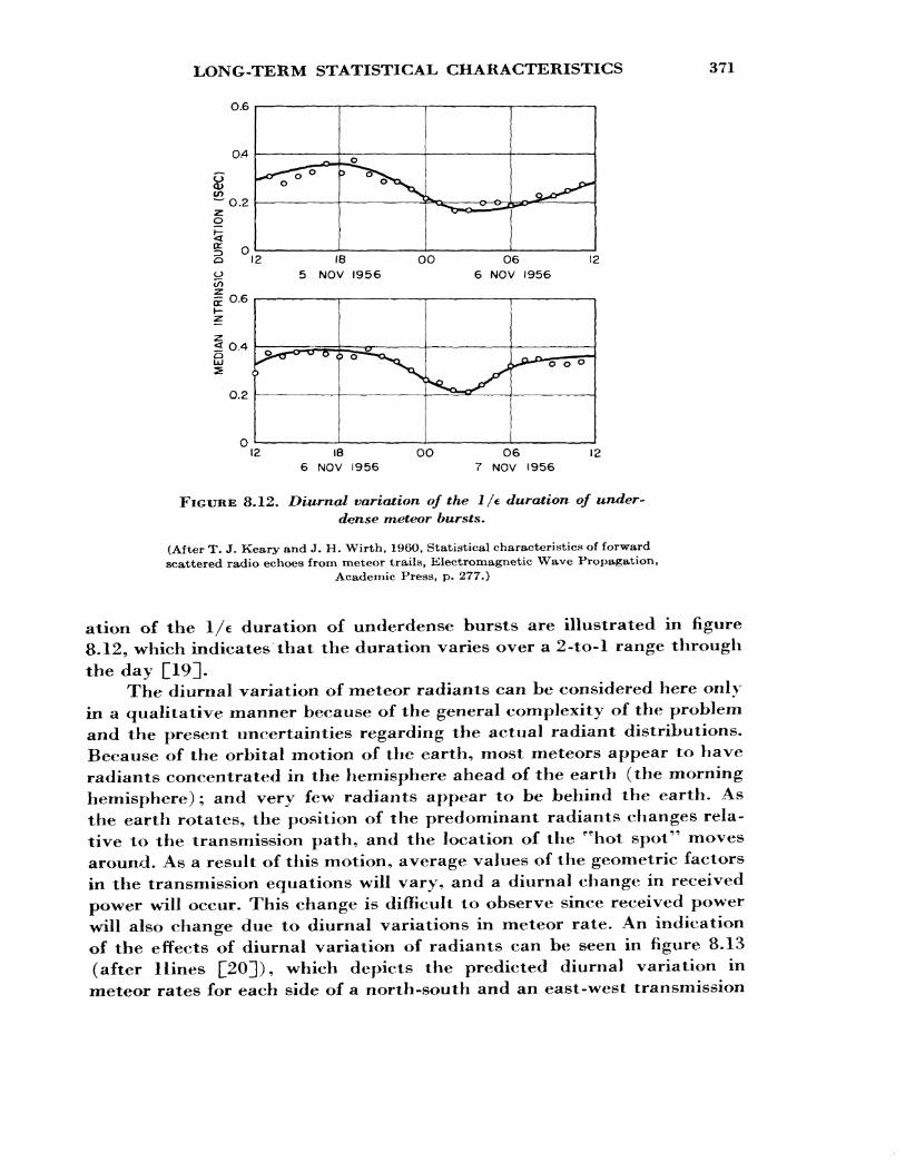
LONG-TERM STATISTICAL CHARACTERISTICS
0.6
371
166 NOV 1956
O6 7 NOV 1956
FIGURE 8.12. Diurnal variation of the 1/e duration of under- dense meteor bursts.
(After T. J. Keary and J. H. Wirth, 1960 t Statistical characteristics of forward scattered radio echoes from meteor trails, Electromagnetic Wave Propagation,
Academic Press, p. 277.)
ation of the 1/e duration of underdense bursts are illustrated in figure 8-12, which indicates that the duration varies over a 2-to-l range through the day [19].
The diurnal variation of meteor radiants can be considered here only in a qualitative manner because of the general complexity of the problem and the present uncertainties regarding the actual radiant distributions. Because of the orbital motion of the earth, most meteors appear to have radiants concentrated in the hemisphere ahead of the earth (the morning hemisphere) ; and very few radiants appear to be behind the earth. As the earth rotates, the position of the predominant radiants changes rela tive to the transmission path, and the location of the "hot spot" moves around. As a result of this motion, average values of the geometric factors in the transmission equations will vary, and a diurnal change in received power will occur. This change is difficult to observe since received power will also change due to diurnal variations in meteor rate. An indication of the effects of diurnal variation of radiants can be seen in figure 8.13 (after llines [20]), which depicts the predicted diurnal variation in meteor rates for each side of a north-south and an east-west transmission
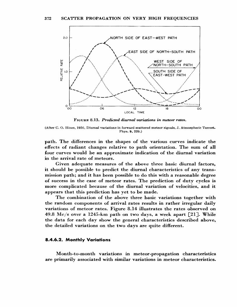
372 SCATTER PROPAGATION ON VERY HIGH FREQUENCIES
2.0
LU
5
<t_J LUo:
NORTH SIDE OF EAST-WEST PATH
,-EAST SIDE OF NORTH-SOUTH PATH
WEST SIDE OF ^XNORTH-SOUTH PATH /
SOUTH SIDE OF "EAST-WEST PATH /
~~~ s"/
oo 06 12 LOCAL TIME
18 OO
FIGURE 8.13. Predicted diurnal variations in meteor rates.
(After C. O. Hines, 1956, Diurnal variations in forward scattered meteor signals, J. Atmospheric Terrest.Phys. 9, 229.)
path. The differences in the shapes of the various curves indicate the effects of radiant changes relative to path orientation. The sum of all four curves "would be an approximate indication of the diurnal variation in the arrival rate of meteors.
Given adequate measures of the above three basic diurnal factors, it should be possible to predict the diurnal characteristics of any trans mission path; and it has been possible to do this with a reasonable degree of success in the case of meteor rates. The prediction of duty cycles is more complicated because of the diurnal variation of velocities, and it appears that this prediction has yet to be made.
The combination of the above three basic variations together with the random components of arrival rates results in rather irregular daily variations of meteor rates. Figure 8.14 illustrates the rates observed on 49.8 Mc/s over a 1245-km path on two days, a week apart Q21]. While the data for each day show the general characteristics described above, the detailed variations on the two days are quite different.
8.4*6.2. Monthly Variations
Month-to-month variations in meteor-propagation characteristics are primarily associated with similar variations in meteor characteristics.
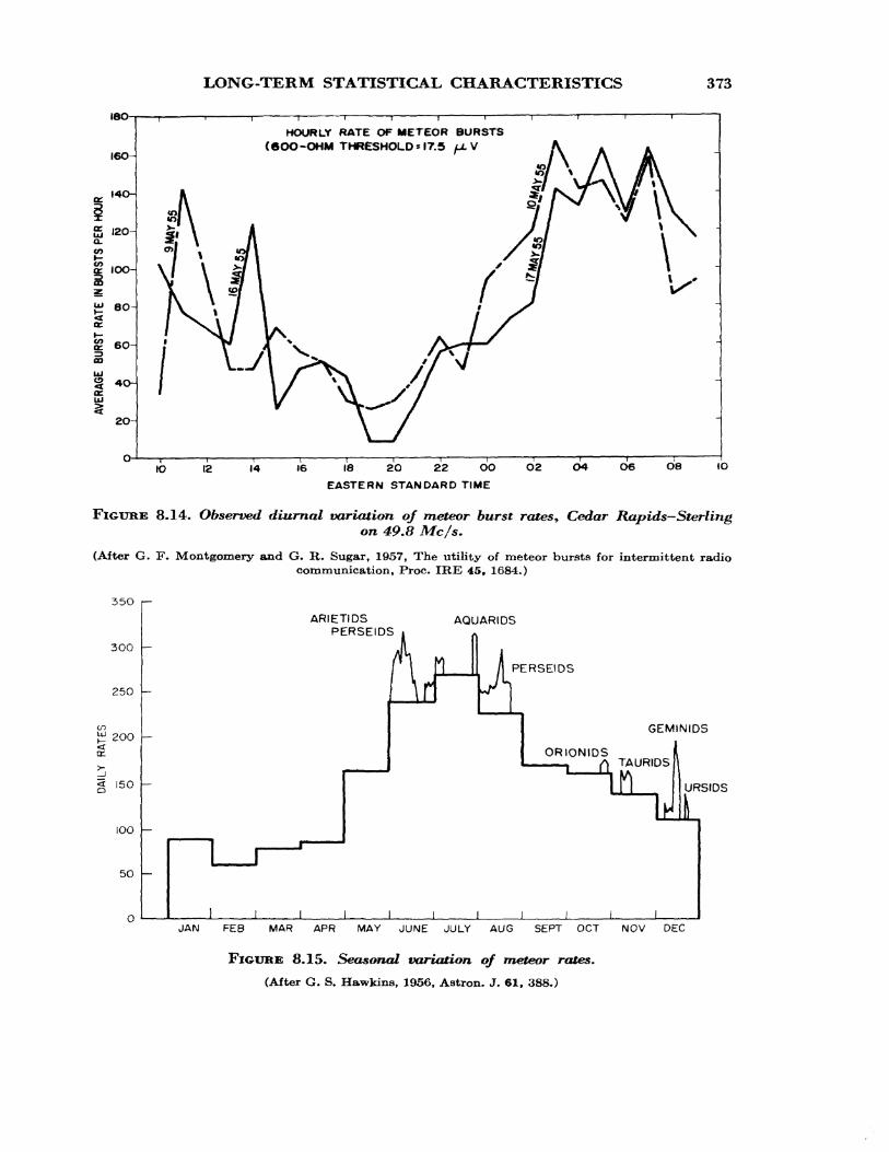
LONG-TERM STATISTICAL CHARACTERISTICS 373
180
160
I4O-
g .20H
CO
Vf1 io<H
S
80-
60-
20-
HOURLY RATE OF METEOR BURSTS (600-OHM THRESHOLD * 17.5 fJL V
IO 12 14 16 18 2O 22 OOEASTERN STANDARD TIME
O2 O4 O6 O8 IO
FIGURE
(After G.
35O
300
250
8.14. Observed diurnal variation of meteor burst rates* Cedar Rapids-Sterlingon 49.8 Mc/s.
F. Montgomery and G. K. Sugar, 1957, The utility of meteor bursts for intermittent radio communication, Proc. IRE 45, 1684.)
2OO<cc.
< 150 h
IOO
50
ARIETIDSPERSEIDS
AQUARIDS
PERSEIDS
GEMINIDS
ORIONIDSTAURIDS
_L _L _L JL _LJAN FEB MAR APR MAY JUNE JULY AUG SEPT OCT NOV DEC
FIGURE 8.15. Seasonal variation of meteor rates.(After G. S. Hawkins, 1956, Astron. J. 61, 388.)
374 SCATTER PROPAGATION ON VERY HIGH FREQUENCIES
There is little evidence that any of the normal month-to-month variations in ionospheric characteristics are reflected in meteor propagation char acteristics, with the possible exception of D region absorption. The seasonal variation of meteor rates is illustrated in figure 8.15 (after Hawkins £8]). The echo rates shown are for meteor trails with an electron line density of 2.75X10¹⁴ electrons per meter or greater. The contribu tions of shower meteors are shown above the histogram for the sporadic meteors. The relative contributions of shower meteors will decrease as the system sensitivity is raised, since the two types have a different mass distribution.
As yet there is no satisfactory answer to the question of year-to-year variations in meteor activity. Such variations have been observed but most workers who have observed them have attributed them to changes in equipment sensitivity.
8.4.6*3. Geographical Variation
As yet this has not been clearly defined. The geographical variations, if present, are masked by the random variations.
8*4*6.4. Abnormal Absorption
Since most meteor trails are produced at heights above the absorbing region, the meteor signals are absorbed in much the same way as HF signals. On frequencies much greater than 30 Mc/s, the normal D region absorption is negligible. During periods of high absorption in high lati tudes, the absorption can increase enormously and affect meteor propaga tion on frequencies as high as 100 Mc/s and more. During a major dis turbance the duty cycle on a meteor-burst communications circuit be tween Goose Bav, Labrador, and Ottawa, Canada dropped by a factor over 103, implying a signal attenuation of over 30 dB £22]]. Disturbances of this magnitude are relatively uncommon and are not important in terms of the average characteristics of meteor-burst propagation. They are an indication, however, that this mode of propagation, like most others, can be disrupted and is, therefore, not the basis of a completely reliable communication system.
METEOR REFLECTIONS FOR COMMUNICATIONS 375
8.4.7. Use of Meteor Reflections for Intermittent Radio Communications
8.4.7.1* General Characteristics
Before leaving meteor propagation let us consider an application to communication systems. Meteor-burst communication systems are basically weak signal systems because the signal loss associated with the meteor-trail reflection is relatively high* For example, a typical system £15] operating on 50 Mc/s over a 1300 km path with a transmitter power of 2 kW was commonly set to transmit messages whenever the signal at the receiver exceeded 2X10~14 W (2 ^V open-circuit voltage for a 50-Q source). This corresponds to a system loss of 170 dB—under similar circumstances ionospheric scatter propagation would exhibit a system loss of the order of 180 dB. Of this total about 90 dB represents the at tenuation associated with the length of the transmission path and 80 dB the scattering loss. Such a system was shown to be capable of a daily average teletypewriter transmission rate of 40 words per minute at a character error rate of 0.35 percent.
As is implied in the title of this section, meteor communication systems operate in an intermittent mode. They transmit messages only during the brief intervals when meteor propagation is present. Control of message transmission is achieved by providing for two-way transmission over the propagation path and transmitting only a control signal when a meteor trail is not present. When a meteor burst occurs, its presence is indicated by reception of the control signal, and message transmission can begin. These principles are incorporated in the JANET system [^23]. In the interval between suitable meteor signals a system accepts messages and stores them for subsequent transmission. The system is, in essence, one that adapts its operation to the conditions of the transmission me dium; it transmits only under favorable conditions. The aim is, of course, to obtain better overall transmission by avoiding the times when trans mission is poor. Whether or not the intermittent mode of operation re sults in an overall improvement over continuous operation depends on the details of the equipment and on the characteristics of the propaga tion medium.
376 SCATTER PROPAGATION ON VERY HIGH FREQUENCIES
8.4.7.2. Channel Capacity
For an intermittent system operated at a fixed transmitter output and with band-limited Gaussian noise interference, the relation between channel capacity M and system bandwidth B is given by C^lH
M=kB*-**\ (8.16)
where k is a constant of proportionality.From (8.16) we see that if a lies in the range 0 <a <2 then, for a given
transmitter output power, the channel capacity will increase as the signal ing bandwidth is increased. Early measurements indicated that 1.2 was a typical value for a, thus suggesting that meteor-burst communication might be feasible. It is likely that this result, more than any other, has provided the impetus for the development of meteor-burst communica tion systems.
8.4.8. Concluding Remarks on Meteor Propagation
At the present time there is a large amount of theoretical and ob servational material available on most aspects of meteor propagation in the lower VHF range. As has been suggested in the previous sections, the available information is most complete for long wavelength under- dense trails and least complete for the short wavelength overdense trails. Some of the areas where substantial work still remains to be done are studies of radiant distributions, properties of very small meteors, the effects of fragmentation, geographic factors, and the long-term fluctua tions in propagation characteristics.
The adequacy of the presently available data can be examined from the viewpoint of the communication system design and engineering. If this is done, it appears that the present uncertainty in predicting the trans mitter power required for a meteor communication circuit is probably of the order of 10 dB. At present it is not clear whether this number can be substantially reduced by further work. The whole field of system design is one where relatively little effort lias been expended, and it is likely that major improvements in systems can still be achieved.
CHARACTERISTICS OF F SCATTER 377
8.5. EQUATORIAL f SCATTER
8.5.1. History
Amateur radio operators had discovered that near the peak of the sunspot cycle (1947) they could communicate over long distances across the equatorial regions on frequencies (50 Mc/s) well above the maxi mum frequency to be expected for the distances involved. These radio contacts were most pronounced during nighttime in the equinoctial months.
During the International Geophysical Year more definite experi ments were carried out on this phenomenon in the Far East £24] and in South America £25], These experiments established that the enhanced signals were reflected from scattering centers located near the base of the F',2 layer.
8.5.2. Characteristics of F Scatter
8.5.2.1. Diurnal Variation
The signal appears usually during the evening and night when the signal level may rise 30 to 40 dB above the level produced by forward scatter.
8.5.2.2. Seasonal Variation
F scatter appears to be most prevalent around the autumnal equinox.
8.5.2.3. Geographical Variation
The echoes are aspect sensitive £25], so that the signal level depends on the orientation of the path relative to the earth's magnetic field. This also determines the direction of arrival of the signal. North-south paths, with midpoints within ±20° of the dip equator, are affected.
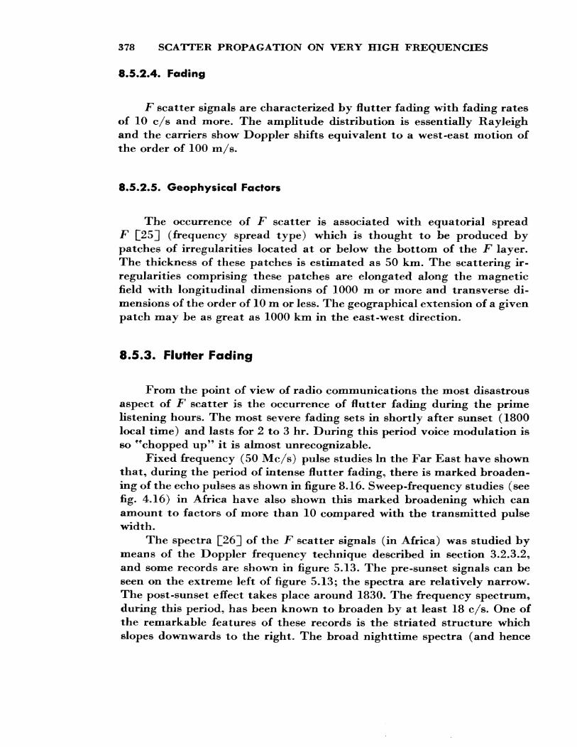
378 SCATTER PROPAGATION ON VERY HIGH FREQUENCIES
8.5.2.4. Fading
F scatter signals are characterized by flutter fading with fading rates of 10 c/s and more. The amplitude distribution is essentially Rayleigh and the carriers show Doppler shifts equivalent to a west-east motion of the order of 100 m/s.
8.5.2.5* Geophysical Factors
The occurrence of F scatter is associated with equatorial spread F [J253 (frequency spread type) which is thought to be produced by patches of irregularities located at or below the bottom of the F layer. The thickness of these patches is estimated as 50 km. The scattering ir regularities comprising these patches are elongated along the magnetic field with longitudinal dimensions of 1000 m or more and transverse di mensions of the order of 10 m or less. The geographical extension of a given patch may be as great as 1000 km in the east-west direction.
8.5.3. Flutter Fading
From the point of view of radio communications the most disastrous aspect of F scatter is the occurrence of flutter fading during the prime listening hours. The most severe fading sets in shortly after sunset (1800 local time) and lasts for 2 to 3 hr. During this period voice modulation is so **chopped up" it is almost unrecognizable.
Fixed frequency (50 Mc/s) pulse studies In the Far East have shown that, during the period of intense flutter fading, there is marked broaden ing of the echo pulses as shown in figure 8.16. Sweep-frequency studies (see fig. 4.16) in Africa have also shown this marked broadening which can amount to factors of more than 10 compared with the transmitted pulse width.
The spectra Q26]] of the jF scatter signals (in Africa) was studied by means of the Doppler frequency technique described in section 3.2.3.2, and some records are shown in figure 5.13. The pre-sunset signals can be seen on the extreme left of figure 5.13; the spectra are relatively narrow* The post-sunset effect takes place around 1830. The frequency spectrum, during this period, has been known to broaden by at least 18 c/s. One of the remarkable features of these records is the striated structure which slopes downwards to the right. The broad nighttime spectra (and hence
RADIO AURORA 379
Poro P. I. to Onna, Okinawa (837 mliea) markers are 1OO micro- Beeondo
Frequency: ^9.84 Mc/sPower : 2 k.wAntennas: 5 element H yagie
Pulse length: 5O micro-seconds Pulse repetition rate: lOO/second Rr-celver bandwldtn: 12O kc/s
Okinawa Standard Time (GOT + 9)
FIGURE 8.16. Range-time records showing pulse broadening of F-scatter echoes.
(After R. Bateman, J. W. Finney, E. K. Smith, L. H. Tveten, and J. M. Watts, 1959, IGY observations of .F-layer scatter in the far east, J. Geophys. Res. 64, 403.)
the associated flutter fading) may be attributed to the motion of scatter ing irregularities.
Since the spread F responsible for flutter fading is limited in space and in time, there is a possibility that its effects may be minimized by suitable relaying of radio signals.
8.6. AURORAL SCATTER
8.6.1. Radio Aurora
Radio aurora can be denned as "the ionospheric ionization, asso ciated with auroral disturbances, that gives rise to radio reflection" [J27J. While aurora itself may be defined as emitted radiation (visible and in visible) , radio aurora is ionization which reflects radio waves. Thus we should not expect a one-to-one correlation between the spatial and tem poral occurrences of one and those of the other. Radio aurora and visible aurora are separate phenomena with the same basic origin; that is, aurora is a manifestation of atomic excitation and ionization, and radio aurora
* Based on a lecture by R. Co hen.
380 SCATTER PROPAGATION ON VERY HIGH FREQUENCIES
is constituted of the electrons and ions separated during the ionization process. However, reflections from radio aurora usually depend not only on the presence of ionization but also on the geometry involved. These aspect-sensitive reflections will not be observed unless the radio aurora is in the right place with respect to the observer. Thus from a given loca tion one may see visible aurora but not radio aurora. On the other hand, radio aurora can be observed during the daytime when visible aurora cannot be seen.
A review of radio studies of the aurora has been made by Booker and this should be consulted b the interested reader.
8*6.2. Bistatic Observations
The term "bistatic" is used to contrast a two-station (transmitter and receiver separated) method of observation with a single -station or monostatic method (radar) . Auroral observations of this kind have always involved continuous -wave transmissions, so that the measurements of distances have had to be inferred from information on angles of arrival.
The most extensive bistatic studies of radio aurora are those of Collins and Forsyth £27], who have classified enhancements of the received signals into five categories:
(1) E events, which are strong reflections probably from sporadic E patches,
(2) S events, which are enhancements which are not accompanied by a magnetic disturbance.
The following A events are auroral phenomena closely associated with magnetic disturbance:
(3) AI exhibits rapid fading (100 c/s) and is strongly aspect sen sitive.
(4) A<z exhibits slow fading (1 cycle per 5 sec) and is slightly aspect sensitive.
(5) At exhibits slow fading and no aspect sensitivity, i.e., the signals arrive in the great circle.
This suggests that the A% signals are due to scattering from essentially isotropic irregularities.
Based on these results and some frequency-dependence measure ments, Collins and Forsyth conclude that the AI and A% events can be ascribed to field-alined irregularities above a height of 100 km, and the AZ events to more isotropic irregularities below that height. They also conclude from their frequency dependence measurements in the 32 to
MONOSTATIC (RADAR) OBSERVATIONS 381
50 Mc/s frequency range that the A% events can correspond to overdense irregularities with electron density as great as 3X107 cm~3, and that the usual electron density for the A\ events was between 1.3 and 1.9 XlO7 cm~3, corresponding to a plasma frequency range of about 32 to 39 Mc/s.
8.6.3. Monostatic (Radar) Observations
For localized observations of the radio aurora and the determination of its aspect sensitivity, radar methods are suitable. Furthermore, this method is useful in the study of movements. Numerous workers have con tributed to radar-auroral research in the past 30 years and reviews of this subject are available £28, 29, 30]. Although the results of the radar studies are not altogether conclusive, certain facts are generally agreed upon and these will be summarized below.
The determination of the spatial association between aurora and radio aurora is complicated by the aspect sensitivity requirements of the latter. By a comparison of the associated aurora with the radar echoes (at College, Alaska) Bowles obtained good correspondence as illustrated in figure 8.17. This figure shows, however, that radar echoes are obtained from only parts of the visual forms.
A striking demonstration of the aspect sensitivity of radio aurora has been given by Dyce £31], who operated a radar at Point Barrow, Alaska, located to the north of the visible aurora. The majority of radar echoes was obtained not from the south, but from the north.
The heights from which auroral radar echoes are reflected range from 75 to 135 km with a mean of about 110 km, which corresponds fairly well to the average height of the lower edge of most visual auroral forms.
Leadabrand et al. £52] also measured the azimuthal distribution and thence the aspect sensitivity of radar echoes on 398 Mc/s, and found that they could be obtained up to 10° away from the angle of perpen dicularity to the earth's magnetic field. Presnell et al. £33] show that this departure is 12° on 216 Mc/s and 6° on 780 Mc/s. Thus, aspect sensitivity becomes more stringent as the frequency increases. It has been observed £32] that echoes from radio aurora at lower heights are confined to a narrower departure from perpendicularity than those from greater heights.
The frequency dependence of radar echoes from radio aurora has not been definitely determined. It is clear that the scattering cross section diminishes with increasing frequency, and that it is small at all frequencies, corresponding, for example, to a power reflection coefficient of order 10~4 on 106 Mc/s.
382 SCATTER PROPAGATION ON VERY HIGH FREQUENCIES
6OO RANGE krn 4OOW-
SEPT 3O 1954
HIGH- LOW
345
RANGE
48O-32O
59O-420 -70O-52O 8OO-6I5 910-7 IO IO6O-790
km I I I 5°W N I5°E
GEOMAGNETIC AZIMUTH
GOO RANGE km 4OO 8OO
SEPT. 3O 1954
W
20 h 30 m
AST
HIGH-LOW
345
RANGE 48O- 320
59O-42O -70O-520 8OO - 6 5 9IO - 7IO IO6O-79O
km3O°W I5°W N 15°E
GEOMAGNETIC AZIMUTH
'IGUKK 8.17. Association bfticccn visible aurora and radio aurora.
(After K. L. Bowles. unpublished.)
MONOSTATIC (RADAR) OBSERVATIONS 383
A number of workers have measured the frequency spectrum of radar echoes from radio aurora. Some of the spectra obtained by Bowles [34] in Ithaca, N.Y., and in College, Alaska, are shown in figure 8.18. The Doppler shifts and spreads of these spectra correspond to the motion of the irregularities in the radio aurora, and range motions observed simultaneously do not always correlate with them in magnitude or di rection. Inasmuch as the range motions are probably spatial drifts re sulting from redirection of the source of ionization, this apparent dis crepancy is not surprising.
COLLEGE, ALASKA F0 = 25. 3 MC/S ITHACA, N.Y. F0 -49,78 MC/S
F0 +IOO F0 +2OO
=25.3 MC/SFo -!00 F.
COLLEGE, ALASKA
(C)
FREQUENCY, C/S
FIGURE 8.18. Spectra of VHF signals reflected from radio aurora.
(After K. L. Bowlea, unpublished.)
384 SCATTER PROPAGATION ON VERY HIGH FREQUENCIES
8*7. INCOHERENT SCATTER 6
8.7.1. Historical Note
It has been known for many years, especially in connection with x-ray scattering, that an individual electron has a cross section for the scattering of electromagnetic waves. In 1958, Professor W. E. Gordon [35] pointed out that with the existing radar sensitivities it should be feasible to measure ionospheric electron densities by detecting this weak Thomson scattering. Gordon pointed out that, from the theory, the Doppler spread (pressure broadening) imparted to the radiofrequency by the thermal motion of the electrons provided a means of measuring electron temperatures.
The existence of incoherent scatter was demonstrated in October 1958 by Bowles [36]] with a scatter-radar in Long Branch, 111. To obtain the high sensitivity required he used an antenna with a cross-sectional area of almost 5 acres and a pulse transmitter of about 1 M W peak power on a frequency near 40 Mc/s. The receiver bandwidth was of the order of 10 kc/s. Much to his surprise Bowles found that the line broadening was about 10 kc/s rather than the 100 kc/s predicted by Gordon. These results were corroborated, on a frequency of 440 Mc/s, at the Massachusetts Institute of Technology
8.7*2. Scattering From an Individual Electron
The reason for high equipment sensitivity is, of course, the small value of the Thomson scattering cross section a for a free electron (10~~28 m2). The echo amplitude to be expected from a single free electron can be calculated as follows: The incident power density is ptg/4wR2 where pt is the power transmitter, g is the antenna gain, and R is the range. The power absorbed (and re-emitted) is ptga/^irK* and the received power pr is (ptga/^wR2 } (a/4wR2 ) , where a is the antenna cross section. With a typical radar and scattering from the F region we assume the following values: />,= 106 W, g=104, a=104 m2, and /? = 3X10⁵ m. This gives pr =6X10~39 W. For unity signal/noise we need about 10~16 W so that the scattering volume must contain something like 1024 electrons. In the F region N is about 1012 per cubic meter so that the scattering
6 Based on a lecture by K. L. Bowles.
SCATTERING FROM AN INDIVIDUAL ELECTRON 385
volume required must be of the order of 1012 m3 (i.e., 10 km3). Thus a limit is set to the smallest volume that can be studied by a given radar system.
If the electrons are in thermal equilibrium with the ions and neutral molecules they will have, essentially, a Maxwellian distribution of ve-
4.0
3.0
0>Al
O
2.0
1.0
00
£ i-oOCOens
ui O.6 o
O.O
•X X
X X
00
T
X X
X X
X X
X
X )"
06 12 LOCAL TIME
18 24
FIGURE 8,19. Electron cross sections for incoherent scatter measured at Jicamarca, Peru.
(After K. L. Bowlee, G. R. Ochs, and J. 7^. Green, 1962, J. Res. NBS 66I> (Radio Prop.), No. 4f 395.)
386 SCATTER PROPAGATION ON VERY HIGH FREQUENCIES
locities and these motions will impose various Doppler shifts on the re- radiated waves. For an average F region temperature of 1500 °K one expects that the spectrum on 41 Mc/s should be about 100 kc/s wide. The experimental width turned out to be about one tenth this value and it was realized that something was wrong with the simple theory. The reason for this discrepancy has been found to lie in the long-range Coulomb interactions between the positive ions and the electrons. Because of their charges and motions, the ions and electrons produce statistical fluctua tions of charge density which almost cancel in space. If this were not so, strong space charges would develop, tending to restore neutrality. Be cause of this necessity to maintain electrical neutrality the motions of the electrons are constrained by those of the heavy ions. The observed line broadening is, therefore, not that due to the free electrons but rather to the ions wherein most of the momentum lies £36]. Because of this constraint it has been proposed to call the phenomenon "quasi-incoherent scatter." The theoretical implications of this idea have been studied by a number of workers [[38, 39, 40].
It turns out that, for thermal equilibrium between ions and electrons, the scattering cross section per free electron is just about one-half the classical Thomson cross section. In the more general case, when the elec tron and ion temperatures ( T€ and T\, respectively) differ, the relation ship between the measured cross section am and the classical value a is given approximately by
Measurements of am have been made by Bowles at the Jicamarca radar near Lima, Peru, and the results are shown in figure 8.19a. It will be seen that the values are all less than the theoretical value of 5X10~29 m2 . It is believed that during the middle of the day the dis crepancy is due to absorption in the D region (approximately 0.5 dB, as shown in figure 8.19b.). On the other hand, near sunrise it is thought that the electrons are in fact hotter than the ions.
8.7.3. Electron Density Profiles
We have seen above that the power received from a given volume in the ionosphere is proportional to the number of electrons present. The incoherent scatter technique thus provides a means of determining the
ELECTRON DENSITY PROFILES 387
electron density profile above the Fz peak provided that the geometry of propagation is known. The power pr received from a distance R is given by
(8.18)87TR2
where a is the antenna aperture area,cr is the cross section per unit volume, c is the velocity of light, r is the pulse duration in seconds,77 r, ?7 S , and 77^4 are factors to correct the aperture for the effects of
resistive losses, side lobes, and tapered feed, respectively.
The following features of (8.18) are worth noticing:
(1) pr is proportional to /?~~2 rather than R~4 as in the case of a single scatterer. From the divergence of the beam it can be seen that the scatter ing volume increases proportional to the square of the range; this removes a factor of R~2.
(2) The aperture a appears to the first power only. This is because increased aperture (i.e., increased gain) results in a smaller scattering volume.
Further corrections have to be made to (8.18), depending on the type of antenna used.
150 3OO 450 600 750km
FIGURE 8.20. Oscittogram showing echo power versus range made tvith scatter radar at Jicamarca* Peru.
(After K. L. Bowles, 1961, J. Res. NBS 65I> (Radio Prop.), No. 1, 1.)
388 SCATTER PROPAGATION ON VERY HIGH FREQUENCIES
LIMA, PERU 17 FEB. 1962
ELECTRON DENSITY (N/cm 3 )
FIGURE 8.21. Electron-density profile obtained from incoherent scatter measurements.(After K. L. Bowles, Mar. 1963, NBS Tech. Note 169.)
Turning to the experimental results, in figure 8.20 we see an actual oscilloscope photograph made with the radar. Each spot is the result of averaging the echo power taken over many radar sweeps and is thus a plot of power versus range. With a knowledge of the equipment charac teristics it is possible to determine the cross section per unit volume a from (10.18) and, hence, the electron concentration averaged over a cer-
ELECTRON DENSITY PROFILES 389
150
100) .
LIMA, PERU
A- 17 FEB.- 1515 EST
B-16 FEB.-2020 EST C- 25 APRIL- 0035 EST D-25 APRIL- I4O5 EST E-25 APRIL- 1925 EST F-26 APRIL-0615 EST
B
ELECTRON DENSITY10°
(N/cm 3 )IOC
FIGURE 8.22. Sample electron-density profiles obtained from incoherent scattermeasurements .
(After K. L. Bowles, 1964, Radio wave scattering in the ionosphere, Advances in Electronics and ElectronPhysics 19, 55, Academic Press.)
390 SCATTER PROPAGATION ON VERY HIGH PROPAGATION
tain volume and over a given time. A sample profile obtained with this technique is shown in figure 8.21. The curve has to be calibrated at least at one point and this is done at the peak of the F layer. The peak electron density is determined from the /o^2 as observed with a conventional ionosonde and substitution in the formula
JV=1.24X10¹⁰ (/0F)2 electrons per cubic meter.
Further sample profiles are shown in figure 8.22 from which we see that there are rather large variations in the shape of the profiles with time of day and from day to day. The daytime results for heights below about 200 km are probably too large by as much as a factor of two, due to the presence of weak coherent irregularities. At greater heights it has been verified that the echo power is proportional to electron density. One feature of particular interest is the abrupt change in electron-density gradient which often occurs on the topside. This change is probably as sociated with the changeover in atmospheric composition from one con stituent to another (e.g., oxygen to helium or helium to hydrogen).
REFERENCES
[I] Ellyett, C., and J. M. Watts (1959), Stratification in the lower ionosphere, J. Res.NBS 63D (Radio Prop.), 117.
[2] Wheelon, A. D. (1960), Relation of turbulence theory to ionospheric forwardscatter propagation experiments, J. Res. NBS 64D (Radio Prop.), 301.
[3] Bailey, D. K., R. Bateman, and R. C. Kirby (1955), Radio transmission at VHPby scattering and other processes in the lower ionosphere, Proc. IRE 43, 1181.
[4] Bowles, K. L., and R. S. Cohen (1962), A study of radio wave scattering fromsporadic -E near the magnetic equator, Ionospheric Sporadic -E (ed. Smith andMatsushita) (Pergamon Press), 51.
[5] Ellyett, C., and H. Leighton (1958), Solar cycle influence on the lower ionosphereand on VHF forward scattering, Proc. IRE 46, 711.
[6] Norwegian Defence Research Establishment, Report No. 27 (1958), A study ofVHF forward scattering in high latitudes.
[7] Greenhow, J. S., and J. E. Hall (1960), The variation of meteor heights withvelocity and magnitude, Monthly Notices Roy. Astron. Soc. 121, 174.
[8] Hawkins, G. S. (1956), A radio survey of sporadic meteor radiants, MonthlyNotices Roy. Astron. Soc. 116, 92.
[9] Kaiser, T. R. (1953), Radio echo studies of meteor ionization, Advances in Phys.2, 495.
[10] Manning, L. A., and V. R. Eshleman (1959), Meteors in the ionosphere, Proc.IRE 47, 186.
[II] Sugar, G. R. (1964), Radio propagation by reflection from meteor trails, Proc. IEEE 52, No. 2, 116.
REFERENCES 391
[12] Hines, C. O., and P. A. Forsyth (1957), The forward scattering of radio wavesfrom overdense meteor trails, Can. J. Phys. 35, 1033.
[13] Manning, L. A. (1959), Oblique echoes from overdense meteor trails, J. Atmos pheric Terrest. Phys. 14, 82.
[14] Eshleman, V. R. (1960), Meteor scatter, The Radio Noise Spectrum (ch. 4) (Har vard Univ. Press).
[15] Carpenter, R. J., and G. R. Ochs (1962), High resolution pulse measurements ofmeteor burst propagation at 41 Mc/s over a 1295 km path, J. Res, NBS 66D(Radio Prop.), 249.
[16] Hines, C. O. (1958), A theoretical rate-amplitude relation in meteoric forwardscattering, Can. J. Phys. 36, 539.
[17] McKinley, D. W. R., and A. G. McNamara (1956), Meteoric echoes observedsimultaneously by backscatter and forward scatter, Can. J. Phys. 34, 625.
[18] Hines, C, O., and R. E. Pugh (1956), The spatial distribution of signal sources inmeteoric forward scattering, Can. J. Phys. 34, 1005.
[19] Keary, T. J., and J. H. Wirth (1960), Statistical characteristics of forward scat tered radio echoes from meteor trails, Electromagnetic Wave Propagation,(Academic Press), 277.
[20] Hines, C. O. (1956), Diurnal variations in forward scattered meteor signals, J.Atmospheric Terrest. Phys., 9, 229.
[21] Montgomery, G. F., and G. R. Sugar (1957), The utility of meteor bursts forintermittent radio communication, Proc. IRE 45, 1684.
[22] Maynard, L. A. (1961), Propagation of meteor-burst signals during the polardisturbance of November 12-16, 1960, Can. J. Phys. 39, 628.
[23] Forsyth, R A., E. L. Vogan, D. R. Hansen, and C. O. Hines (1957), The principlesof JANET—A meteor-burst communications system, Proc. IRE 45, 1642.
[24] Bateman, R., J. W. Finney, E. K. Smith, L. H. Tveten, and J. M. Watts (1959),IGY observations of .F-layer scatter in the Far East, J. Geophys. Res. 64, 403.
[25] Cohen, R., and K. L. Bowles (1961), On the nature of equatorial spread JF, J.Geophys. Res. 66, 1081.
[26] Calvert, W., K. Davies, E. Stiltner, and J. T. Brown (1963), Equatorial spread-Fmotions, Proc. Int. Conf. lono., 316, Inst. of Phys. and Phys. Soc.
[27] Collins, C., and P. A. Forsyth (1959), A bistatic radio investigation of auroralionization, J. Atmospheric Terrest. Phys. 13, 315.
[28] Booker, H. G. (1960), Radar studies of the aurora, Physics of the Upper Atmos phere (ed. J. A. Ratclifle) (Academic Press).
[29] Chamberlain, J. R. (1961), Physics of the aurora and airglow (ch. 6), AcademicPress.
[30] Little, C. G., W. M. Rayton, and R. B. Roof (1956), Review of ionospheric effectsat VHF and UHF, Proc. IRE 44, 992.
[31] Dyce, R. (1955), More about VHF auroral propagation, J. Geophys. Res. 60, 317. [32] Leadabrand, R. L., L. Dolphin, and A. M* Peterson (1959), Preliminary results
of a 400 Me radar investigation of auroral echoes at College, Alaska, IRETrans. Ant. Prop. AP-7, 127.
[33] Presnell, R. I., R. L. Leadabrand, A. M. Peterson, R. B. Dyce, J. Schlobohm,and M. R. Berg, VHF and UHF radar observations of the aurora at College,Alaska, J. Geophys. Res. 64, 1179.
[34] Bowles, K. L. (1954), Doppler shifted radio echoes from aurora, J. Geophys. Res.59, 553.
[35] Gordon, W. E. (1958), Incoherent scattering of radio waves by free electrons withapplications to space exploration by radar, Proc. IRE 46, 1824.
392 SCATTER PROPAGATION ON VERY HIGH FREQUENCIES
[36] Bowles, K. L. (1961), Incoherent scattering by free electrons as a technique for studying the ionosphere and exosphere: Some observations and theoretical considerations, J. Res. NBS 65D (Radio Prop.), 1.
[37] Pineo, V. C., L. G. Kraft, and H. W. Briscoe (1960), Some characteristics of ionospheric backscatter observed at 440 Mc/s, J. Geophys. Res. 65, 2629.
[38] Dougherty, J. P., and D. T. Farley (1960), A theory of incoherent scattering of radio waves by a plasma, Proc. Roy. Soc. (London) A259, 79.
[39] Fejer, J. A. (1961), Scattering of radio waves by an ionized gas in thermal equili brium in the presence of a uniform magnetic field, Can. J. Phys. 39, 716.
[40] Salpeter, E. E. (1961), Effect of the magnetic field in ionospheric backscatter, J. Geophys. Res. 66, 982.
CHAPTER 9
Propagation of Low and Very Low Frequency Waves
9.1. PURPOSE
The aim of this chapter is to discuss, briefly, those lower frequency bands which provide alternatives to the use of high frequencies. It has been seen, in the previous chapters, that high frequency propagation is characterized by the following undesirable features:
(1) Unreliability during ionospheric disturbances.(2) Fairly rapid and deep fading.
The chief advantage of high frequencies is the relative simplicity of the terminal equipment required for long-distance communications.
These defects in high-frequency propagation can be largely overcome by the use of low and very low frequencies (LF and VLF). These waves, reflected from the lower boundary of the D layer, are not affected by ionospheric disturbances to the same degree as the HF waves, and are characterized by relatively slow fading rates. The chief disadvantages are the limited usable bandwidths and the relatively large, and hence expensive, transmitter installations which are required.
The VLF spectrum is nominally defined as 3 to 30 kc/s, but the usable band is confined to the range 10 to 30 kc/s. This is largely due to the difficulty in building efficient transmitting antennas for such wave lengths (10 km<X<30 km). The propagation is characterized by rela tively low path attenuation which is relatively stable with time. This feature, coupled with the fact that VLF energy is guided for long dis tances (5000 to 20,000 km) between the earth and ionosphere, makes the VLF spectrum attractive for long-distance paths when high reliability is important. In figure 7.10b we saw that the noise on VLF is very high and, as a result, large transmitter powers are required. This fact, together with narrow spectrum available, has resulted in most VLF systems having narrow bandwidths. In addition, the bandwidths of most VLF trans-
393
394 PROPAGATION OF LF AND VLF FREQUENCY WAVES
milling antennas are of the order of 20 to 150 c/s and their radiation efficiency is of the order of 10 to 20 percent only.
The low-frequency (LF) spectrum, 30 to 300 kc/s, is characterized by higher path attenuation, lower background noise levels, and more stable propagation time delays relative to VLF. As a result LF systems are usually used for intermediate ranges (1000 to 5000 km). Terminal equipment is usually cheaper than in the VLF case and, in addition, the available bandwidths are greater.
Our primary concern is with the propagation, rather than with the engineering uses, of low and very low frequencies. We shall first discuss some elementary theory and then consider the observational material.
9.2. THEORETICAL CONSIDERATIONS
9.2.1. Ray Theory
The concepts of geometrical ray theory break down in the case of low and very low frequencies because the wavelengths are comparable with the thickness of the D region. However, in some cases, geometrical ray theory is useful for describing certain phenomena. For example, it is convenient to describe the diurnal change A<£ in phase as due to changes in the height of a fictitious reflecting layer, the phase shift on reflection being assumed constant. For example, if h is the mean height of this fictitious layer, Ah the diurnal change in height, 2d the distance between transmitter and receiver, and X is the wavelength, then
where A0 is in radians.
9.2.2. Waveguide Theory
9.2.2.1. Meaning of Mode
The propagation of VLF waves between the earth and the iono sphere, over large distances, can be likened to the propagation of micro waves along a waveguide. The "mode theory", as it is called, has been
WAVEGUIDE THEORY 395
considered in detail by Budden Ql]1 and Wait p2j and a few simple ideas based on these works will be discussed here.
Let us consider first the meaning of the term "mode." The Inter national Dictionary of Physics and Mathematics (Van Nostrand) de fines mode of propagation as follows: "A form of propagation of waves that is characterized by a particular field pattern in a plane transverse to the direction of propagation, which field pattern is independent of position along the axis of the guide."
In this section it shall be assumed that the transmitted waves are vertically polarized, i.e., the electric vectors are vertical. Furthermore, we shall confine attention to /ong-distance propagation where a single mode predominates (see reference QlJ, sec. 9.13).
9.2*2.2. Basic Concepts
In the simple model shown in figure 9.1, the earth and ionosphere are represented by perfectly conducting planes. With respect to a cylindrical coordinate system (p, 0, 2), the ground is the plane z=0 and the lower
PHASE FRONT
IONOSPHERE 2 = h
-gh ';IMAGE ir
FIGURE 9.1, Ray geometry corresponding to the first mode between parallel conducting planes.
1 Figures in brackets indicate the literature references on p. 441.
396 PROPAGATION OF LF AND VLF FREQUENCY WAVES
boundary of the ionosphere is the plane z = ft, p is the radial coordinate in a horizontal plane and 0 is the azimuthal coordinate. Let the source be a vertical dipole located on the ground, at the origin. The electric field observed at some other point on the ground is in the vertical direc tion. To an observer on the ground, the signal would appear to come from the dipole plus a whole series of images in the ground and in the ionosphere £2^. The images are located just below the ground and at z = ±2fc, ±4/*, and so on, as shown in figure 9.1.
Consider the wavelets emanating from the images in the ionosphere. These will reinforce in a direction making an angle ft with the vertical (see fig. 9.1) such that
2h cos £ = 2feC= nX, (9.2)
where C=cos/3, which is a function of the integer n. Thus for a given value of n
Cn = . (9.3) 2n
The ground images will add up at an angle (IT — (3) with the vertical. Thus, for a given value of n, there are two families of waves which have the same horizontal component (c/ Sn) but which have opposing vertical components of velocity, where
S^l-C (9.4)
We can imagine the resultant of these two sets of waves as a single wave traveling parallel to the z=0 plane with a phase velocity vp — c/Sn.
Consider the wave directed broadside (n = 0). We can imagine this wave to originate in a line source in which the effective uniform current is Ia . Let s be the length of the transmitting dipole carrying a current /. Since images occur as pairs of dipoles all of the same strength (because of the perfect reflectors), and since they are separated by distances of 2h we have
/« = !/. (9-5)
The field Ez produced by such a line current is given by
Ez = iM<**/atfo(2) (kp) - jMow/fc-'sfio (2) ( jfep) , (9.6)
WAVEGUIDE THEORY 397
in which H^2) (kp) is the Hankel function of the second kind with argu ment Arp, MO is the permeability of free space, co is the angular frequency, and A; = 27r/X. At very great distances, i.e. when p^>>\, the Hankel func tion can be replaced by the first terms of its asymptotic expansion, giving
Ez = ~\— J — (Xp)~* exp i - exp ( — ikp). (9.7) 2 \ eo/ h 4
Note that this field corresponds to the mode obtained by putting n = 0 in (9.2). We shall call this, for convenience, the zero-order mode.
Next let us consider the mode produced by the pair of nth images (that is, those located at distances of 2nh above and below ground). Because of the obliquity of the rays the equivalent line current is / sin /3 ( =/Sn). Also the electric field at a point in the plane of the diagram will be perpendicular to the radius vector from the point to the image so that to obtain the vertical component of the electric field we must again mul tiply by Sn, so that, for the nth mode, the field is given by
(9.8) **n
Note that the factor 2 arises because of the two sets of images. For the zero-order mode we have only one set. The resultant field is obtained by summing over all modes for integral values of n from 0 to <x>. This gives
), (9.9)
where £0 = 1, fn = 2(n= 1, 2, 3, • • •)•For the far field (p>$>\) this expression reduces to
exp i £ fnSl exp (-ifcpSn ), (9.10)
where Sn = (1 — O* and Cn =It has been assumed above that the earth and the ionosphere are
perfect electrical conductors and that the reflection coefficients of the rays are always +1. In practice, for long-distance propagation the iono sphere behaves more like a perfect magnetic conductor with a reflection coefficient of — 1, while the ground still has a reflection of +1. In this case the images are located at z=2/r, db4fc, and so on, but now they al ternate in sign. If we write down the resonance condition similar to (9.2)
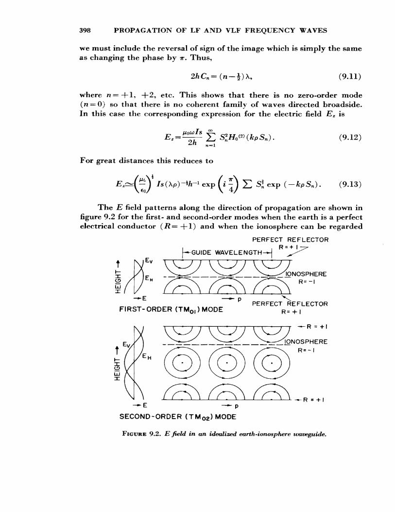
398 PROPAGATION OF LF AND VLF FREQUENCY WAVES
we must include the reversal of sign of the image "which is simply the same as changing the phase by TT. Thus,
(9.11)
where n=-f-l, +2, etc. This shows that there is no zero-order mode (n = 0) so that there is no coherent family of waves directed broadside. In this case the corresponding expression for the electric field Ez is
(9.12)
For great distances this reduces to
*fc-i exp (i * exp (-ApSB ). (9.13)
The E field patterns along the direction of propagation are shown in figure 9.2 for the first- and second-order modes when the earth is a perfect electrical conductor (R= +1) and when the ionosphere can be regarded
PERFECT REFLECTORi i R = +I:^[-^GUIDE WAVELENGTH— | ^>^
FIRST-ORDER (TMOI )MODEPERFECT REFLECTOR
R= + 1
R =
IONOSPHERE
— E —— p
SECOND-ORDER (TM O2 ) MODE
FIGURE 9.2. E field in an idealized earth-ionosphere waveguide.
WAVEGUIDE THEORY 399
as a perfect magnetic conductor (/?= — 1). Since we are dealing with waves polarized in the plane of incidence, the modes are transverse mag netic (TM). When the ionospheric reflection coefficient is — 1, the mode pattern can be obtained from the mode pattern of the same order for perfectly conducting boundaries by placing the ionosphere in the plane of the first null in the vertical electric field below the upper perfectly conducting boundary.
We have seen above that the phase velocity vp in the z-direction is given by
*»=-%-• (9-14)&n
If we let \g be the wavelength in the z direction we have that
X, = --, (9.15)
where X is the free space wavelength. Combining (9.2) and (9.15) we obtain £)'-©'-©-This shows that, for \<2/i/n, \ G is imaginary and, hence, the mode is evanescent. There is a minimum cutoff frequency fn below which waves will not propagate where
/.-=.The cutoff frequency for n = 1 is, therefore, /i = c/2h and, taking
h = 75 km for the height of the daytime D layer, we obtain /i £^2 kc/s.For the case of a magnetically conducting ionosphere, (9.11) and
(9.15) give, for the cutoff frequency,
It will be seen that the change of R from +1 to — 1 will change the cutoff frequency (for n— 1) from 2 kc/s to 1 kc/s. To be consistent with the mode-numbering system for perfectly conducting electrical walls,
4OO PROPAGATION OF LF AND VLF FREQUENCY WAVES
the idealized earth -ionosphere modes should be denoted by n — J rather than by n.
9*2*2.3. Modifications for Imperfect Reflection
Equations (9.2) and (9.11) are based on the establishment of a standing wave pattern. This can be interpreted as the condition for a wave to transverse the wave guide, thus suffering reflection at each boundary, and suffer a net phase change of 2irn radians, thus permitting the twice reflecting wave front to interfere constructively with the original wave front. This condition can be written as
exp (-i2khC)=exp (-£2ir/i), (9.19)
in which Rg ( C) and Ri ( C) are the reflection coefficients of the ground and ionosphere respectively for waves incident at an angle /3 where C=n\/2h. Note that by putting Rg (C) = Rt(C) = 1 we obtain (9.2) and by putting Ri(C) = —1 we obtain (9.11). In the case where Rg and /?* are not unity it is necessary to solve (9.19) for Cn for each mode and, hence, determine Sn = (1— C^)* for substitution in equations like (9.13). Now, in general, Rg and Rl will be complex so that Cn and Sn will be complex. The wave fields contain the term exp ( — ikpSn ) so that when Sn is complex it im plies attenuation (see also sec. 2.3.3.3). The absorption index (K) is given by the imaginary part of Sn, the guide wavelength Xn is given by
and the phase velocity vp is given by
p'Jtve on
where Im Sn and Re Sn represent the imaginary and real parts, respec tively, of Sn .
The numerical solution of the mode (9.19) is complicated when the reflection coefficients of the earth and of the ionosphere depart from unity, but some solutions have been given by Wait [}4j. When signals are propagated over long distances it must mean that the attenuation per unit distance is small and, thus, that the reflectivity of the boundaries must be relatively high. Also the angles of incidence must be large (near
WAVEGUIDE THEORY 401
90°). Under these conditions approximate solutions may be obtained as follows:
The Fresnel reflection coefficient R is given by
, 0 00 ,(9.22)
where JJL is the refractive index of the reflecting medium. For XLF waves in the ionosphere, o><$G>, and thus [J2]
• 2If2^^1 ____— I __ __*L /Q 03\ fJL /^^-L — -L . ^37.^0^
i j OJlf
Hence
Similarly for the ground
-- z -- lG*\*2 » (9-25)
where G = €oco/0-9 X=ee/€o, where € € and cr are the permittivity and con ductivity of the ground.
The value of L for very low frequencies is of the order of unity and, for long distances, Cn is small so that (9.24) reduces to
Note that at great distances it is sufficient to take the first-order mode only.
When the ground conductivity is large, G<5C1 and (9.25) reduces to
1 exp C£(7r/4)3. (9.27)
Now for low-order modes C^<KL and, assuming that L is real, (9.19) can be solved, approximately, using (9.26) and (9.27), which gives
Re Sn =5n +(2V27rC(VA)]^n)-1 C(Cn ) 2 (I>i -I,-i)+G^, (9.28)
Im Sn =-(2^27r\:(h/\)^Sn)-1 L(Cn) 2 (L^ + L^)+G^ (9.29)
402 PROPAGATION OF LF AND VLF FREQUENCY WAVES
where _i£„=(!-C«2)* and Cn" 2h
These two equations, together with (9.13), determine (approxi mately) the phase velocities and rates of attenuation of the modes for the simple case of a flat earth and a flat sharply bounded ionosphere, when the effect of the earth's magnetic field is neglected. It should be noted also that finite ground conductivity always affects the phase ve locity. The phase velocity is affected also by L except when JL=1. The rate of attenuation is a minimum when L~\ and it increases with de creasing ground conductivity. It will be seen also that the higher order modes are more highly attenuated than the first order.
The above presentation is intended to illustrate the application of waveguide theory to VLF ionospheric propagation rather than to de velop a quantitatively correct theory. It is defective, as it stands, in two major aspects:
(1) It neglects earth and ionosphere curvature.(2) It neglects the earth's magnetic field.
9.2.2.4. Effect of Earth Curvature
The most important influence of the curvature of the earth is that it prevents the angle of incidence at the ionosphere from becoming grazing while it can become grazing at the surface of the earth. If the radius of the earth is a, the height of reflection is /i, and <£' and <£ are the angles of incidence at the ionosphere and at the ground respectively we have, from (4.9), that
a sin 0= (a-h/i) sin <£'. (9.30)
Both the above effects tend to reduce the magnitude of the reflection coefficients of the ionosphere and earth. On the other hand, antipodal focusing (sec. 5.2.4.3) may modify the rate at which the signal amplitude decreases with distance.
A detailed theory of the modifications introduced by the earth's curvature has been worked out elsewhere £3] and a modified mode equa tion has been derived namely:
exp-2ik c2 +— s dz~ exp (-£2irw), (9.31)
WAVEGUIDE THEORY 403
CM O
CO
li
0.5
0.4
0.3
O.2
O.I
10FREQUENCY, kc/s
12 14 16 18 2O 22 24 IO 12 14 16 18 2O 22 24I VTI T I I I I I
B=0.05 n - I
———CURVED EARTH———FLAT EARTH—— -EXPERIMENTAL
DATA (Taylor)
i ! T I I
B = (X1O
——— CURVED EARTH -FLAT EARTH
3.5
3.0
2,5
2.O
1.5
1.0
O.5
O
H
FIGURE 9.3. Attenuation factor as a function of height.
M'ne upper and right-hand scales are specifically for fc=70 km, which is a typical daytime height (B=\L/h) (After J. R. Wait and K. Spies, 1960, Influence of earth curvature and terrestrial magnetic field on VLF
propagation, J. Geophys. Res. 65, 2325.)
where C=cos<£, C/ = cos0/ , and z is height. Since (a+fe) S' = aS, this reduces to the flat earth equivalent as h/a—K). Actually (9.31) is also an approximation and is strictly only valid if | (&a/2)*C |2£>1.
A higher degree of approximation has been used by Wait and Spies [[S]. Some numerical results of these authors-, given in figure 9.3a and 9.3b, indicate that the curvature of the earth can increase the attenuation by a factor of 3 above that calculated on the basis of a plane-earthplane - ionosphere model. Some curves showing the attenuation rate as a func tion of frequency are given in figure 9.4.
The effect of earth curvature on the phase velocity is of interest in that the velocity is reduced to less than c in most cases of interest as shown in figure 9.5. It will be seen that the effect of the curvature is greatest on the lowest order mode. This is to be expected since the higher order modes involve rays which are less grazing, and the differences between the angles of incidence for the flat- and curved-earth cases becomes smaller as the mode order increases.
Another effect of earth-ionosphere curvature is the efficiency with which a given mode can be launched into the waveguide (see page 221 of reference 2). For ionosphere heights of the order of 70 km and for fre-
404 PROPAGATION OF LF AND VLF FREQUENCY WAVES
CD -o
24 2& g 12
FREQUENCY, kc/S20 24
FIGURE 9.4. Attenuation rate as a function of frequency.
(After J. R. Wait and K. Spies, I960, Influence of earth curvature and terrestrial magnetic field on VLFpropagation, J. Geophys. Res. 65, 2325.)
quencies less than 16 kc/s, there is little difference but, for higher fre quencies or greater heights, the excitation of the first mode becomes rela tively weak. However, in a few cases the excitation factor may be greater than unity, particularly for the higher order modes.
9*2.2.5. Effect of the Earth's Magnetic Field
The chief effect of the earth's magnetic field is to make the ionosphere an anisotropic medium (see ch. 2). A wave polarized in the plane of incidence (E vector in the vertical plane) gives rise to two reflected waves and two transmitted waves. One of each of these is polarized in the plane of incidence, while the others are polarized normal to this plane (i.e..
WAVEGUIDE THEORY 405
0.010
0.006
1——X -V->r—Nc—'^Ki.——jV^i—TX-J—j—^afcj-j 1 —^——r~*afrra V r 'f>
' ~\^^^^^ ^X^^^1^^^.X. rxj^s^i ^<v^ ^*^:-,™T*HiPrri
0,016
-0,008
-0.010
0.012
26 FREQUENCY, kc/S
\ 7 'V V—1~~X3——; xT—""Xr-^—^xT——0.004
0.00?
0.000
- 0.002
-0.004
FIGURE 9.5. Phase velocity for a perfectly conducting earth and an imperfectly reflectingionosphere.
(After J. R. Wait and K. Spies, I960, Influence of earth curvature and terrestrial magnetic field on VLFpropagation, J. Geophys. Res. 65, 2325.)
horizontally). Thus, a vertically polarized wave incident on the ionosphere gives rise to a horizontally polarized component which, after a ground reflection and another ionospheric reflection, gives rise to further vertically and horizontally polarized waves. This results in polarized modes which are "coupled." However, the degree of coupling is usually small and will be ignored in this book.
In principle, the ray properties of VLF signals in the ionosphere can be determined from the complex refractive index (2.76)* It is much more convenient, however, to use the quasi-longitudinal and quasi- transverse approximations (sec. 2.3.3.2), retaining the collision term.
In order to take into account the double refraction in the ionosphere, it is convenient to use the two reflection coefficients \\R\\ and X/?JL to gether with two conversion coefficients \\R± and ±R\\- The first subscript denotes whether the electric field of the incident wave is parallel (| j)
406 PROPAGATION OF LF AND VLF FREQUENCY WAVES
to or perpendicular (J_) to the plane of incidence and the second subscript refers to the same characteristic in the reflected wave.
For details of the calculations of these reflection coefficients the interested reader can start with chapter IX of reference £2] and follow up the references given therein. It will be sufficient for our present purpose to note how the attenuation and phase velocity is affected by the inclu sion of the earth's magnetic field. Some results for the first-order mode are shown in figures 9.6 and 9.7 for attenuation and phase velocity respec tively for a real angle of incidence of 82 °, for various dip angles /, and with different directions of propagation <f>a (measured clockwise from the north). The attenuation results are presented in terms of the ratio
n _ Attenuation with magnetic field Attenuation without magnetic field
360
FIGURK 9.6. Ratios of attenuation (tvith and without the magnetic field) as a function ofazimuth.
(After J. R. Wait and K. Spies, 1960, Influence of earth curvature and terrestrial magnetic field on VLF propagation, J. Geophys. Res.
65, 2325,)
WAVEGUIDE THEORY 407
and, in figure 9.6, P is plotted for various dip angles and frequencies of 10 kc/s and 22 kc/s. In all these curves the electron density TV is 103 per cm3, *> = 2X10⁷ sec"1, and the strength of the earth's field is 0.5 G.
When the azimuth <f>a is 0° (propagation towards the north) or 180° (to the south) the magnetic field has little effect on the attenuation. For east-west and west-east propagation P departs significantly from unity. The effect becomes less noticeable as / approaches 90°. The effect of the magnetic field on the phase velocities of VLF waves is relatively small.
One feature, which is evident in both figures 9.6 and 9.7, is the non- reciprocity in P, and in velocity, for <£a = 90 0 and 270°. The difference in P has been observed experimentally £6, 7] and the physical explana tion involves the action of the transverse field component on the motion of the ionospheric electrons in the plane of incidence £6, 8]. These electron motions should not be confused with those giving rise to the ordinary
FIGURE 9.6b. Ratios of attenuation (with and without the magnetic field) as a function ofazimuth.
(After J. R. Wait and K. Spies, I960, Influence of earth curvature and terrestrial magnetic field on VL.F propagation, J. Geophys. Res.
65, 2325.)
408 PROPAGATION OF LF AND VLF FREQUENCY WAVES
Q _J LU
oX
FIGURE 9.7a. Differences between phase velocities (with and without the magnetic field).
(After J. R,. Wait and K, Spies, 1960, Influence of earth curvature and terrestrial magnetic field on VLF propagation, J. Geophys. Res.
65, 2325.)
and extraordinary waves which are in the plane transverse to the direction of propagation. It is important to notice that the results shown in figure 9.7 refer to a particular model and the results may be entirely different with a different model.
9.2.2.6. Modes and Rays on Very Low Frequencies
The question frequently arises as to (a) the relationship between mode and ray (or geometrical-optical) theories, and, sometimes, (b)
WAVEGUIDE THEORY 409
<r :Ex
o<r
FIGURE 9.7b. Differences between phase velocities (with and without the magnetic field).
(After J. R, Wait and K. Spies, I960, Influence of earth curvature and terrestrial magnetic field on VLF propagation, J. Geophys. Res.
65, 2325.)
whether one is more correct than the other.It has been shown £9] that for the case of propagation between per
fectly reflecting parallel planes, the series expansions based on ray and mode theory are related by a Fourier cosine transform. This suggests that, provided all modes and all rays are taken into account with appropriate corrections for losses, the results from both methods will be the same as has been demonstrated £10]. In fact the derivation of the mode formula given earlier is based on the ray approach. It is not uncommon, however, for a ray model of VLF propagation to be used which considers just one ray, reflected several times between earth and ionosphere, from the trans-
410 PROPAGATION OF LF AND VLF FREQUENCY WAVES
mitter to the receiver. A single ray model is satisfactory only at short distances.
The appropriate question to ask, then, is which method of calcula tion is simplest. On VLF, the wavelength and height of the ionosphere are such that only a few modes are important since the higher-order modes are attenuated at a much greater rate than that of the lowest mode. At great distances only one mode need be considered. In this case, how ever, many rays have to be considered. On the other hand, at short dis tances all propagating modes are comparable in amplitude and must be considered. Only a few rays need to be considered, however, since the higher-order rays are incident at smaller angles of incidence where the reflection coefficient is decreasing rapidly.
On higher frequencies (in the LF band) and at long distances many modes may be important, and the attenuation coefficients of many of the less attenuated modes may be comparable. Thus there is less advantage in using mode theory. Wait [[10] has given an account of ray theory for use at LF which takes account of the curvature of the earth, showing how the rays which are identifiable inside the horizon behave as the hori zon is passed.
9.2.2.7. Effect of Ionospheric Stratification
It has been assumed that the ionosphere is a sharply bounded, semi- infinite medium. This is only a first approximation because what little evidence we have suggests that the D layer is not sharply bounded. It has been found £2, 3, 11, 12J that a two-layered model is necessary to explain the observed attenuation rate in the frequency range from 500 c/s to 1.5 kc/s. For frequencies in the range 8 kc/s to about 20 kc/s, however, the sharply bounded model is convenient for a simple description of what must be a complicated reflection process. Extensive justifications for the idealized model have been given recently by Wait and Walters2 in a series of four papers dealing with the reflection of VLF waves from in- homogeneous ionospheric models.
2 Wait, J. R., and L. C. Walters (1963), Reflection of VLF radio waves from an inhomogeneous iono sphere, Parts I, II, III, and IV, J. Res. NBS 67D, and (1964) Radio Science.
IONOSPHERIC COUPLING ON LOW FREQUENCIES 411
9.2.3. Ionospheric Coupling on Low Frequencies 3
In our discussion of the propagation of waves in a magneto-ionic medium (ch. 2) we assumed that the ordinary and extraordinary waves are propagated independently. While this is substantially true on high frequencies, it is not so on low frequencies. Experimental studies have shown that the echo structure of low-frequency pulses is more complicated than that on high frequencies. One of the most interesting effects is known as coupling ^13^}, which has been studied extensively at the Pennsylvania State University on a frequency of 150 kc/s at night.
Coupling may be thought of as arising in the following way. In the case of long waves, propagation in an inhomogeneous medium must be considered. It is no longer possible to consider a purely progressive wave, because each point in the medium gives rise to a forward and a backward wave, and these two waves must be taken into account in describing the propagation. Furthermore, the component magneto-ionic waves no longer propagate independently; hence coupling occurs not only between magneto-ionic components but also between the progressive wave of one component and the backward wave of the other. For a detailed description of the propagation, a full wave theory is required. It has been shown ^13^ that when the level X = 1 occurs near the level where v = vc = COH sin2 6/cos 0, strong coupling can occur. This level depends on the strength and di rection of the magnetic field and on the collision frequency profile v(h). The sketch in figure 9.8 indicates, schematically, the reflection processes for long waves, including the possibility of coupling. Above the base of the ionosphere (where X=0), the two circularly polarized ordinary and extraordinary waves travel independently with different speeds. Near the level where coupling can occur, the upgoing extraordinary wave gives rise to a backscattered ordinary wave and to a progressive ordinary wave in addition to the progressive extraordinary wTave. This progressive extraordinary wave is known as the "whistler mode." Similarly the up- going o wave gives rise to a backwards x wave. These backward -moving waves combine to produce a downcoming coupling echo. The polarization of the coupling echo should be fairly constant, since the backscattering o and x waves should be in proportion. This is, in fact, observed. The polarization of the coupling echo is roughly constant and the same as
This section is taken verbatim from a lecture by Dr. J. S. Belrose.
412 PROPAGATION OF LF AND VLF FREQUENCY WAVES
+Y
X'
* Xo *
il ^ 0
xoCOUPLING
ECHO
MAIN ECHO
FIGURE 9.8. Sketch to illustrate the mechanism of reflection of LF waves from the ionosphere*
(After J. S. Belrose, 1964, unpublished.)
that transmitted. However the amplitude would depend markedly on how closely the X=l level approaches the v~vc level*
A second effect of coupling is concerned with the polarization of the main echo. The upgoing x, wave, in the region of coupling, gives rise to a forward-scattered o wave, which combines with the forward pro gressive o wave, and proceeds to the level X= 1+ Y, where it is reflected. Now, when this downcoming o wave reaches the coupling level, it gen erates a forward-scattered x wave which, when combined with the progressive o wave below this level, alters its polarization. In fact the resulting polarization ellipse, in the presence of strong coupling, may have its major axis outside the magnetic north-east south-west quadrants, that is, in a direction "forbidden" by simple magneto-ionic theory.
If the bottom of the ionosphere is "rippled" and these ripples pass over the level where v = vc so as to change the X=l level from below to above the "critical coupling" level, we would expect that the polarization could change rapidly £14]. This phenomenon has been observed by the Pennsylvania State University workers, who have called it "flip-overs," i.e., the polarization of the "main echo" can change from right-handed to left-handed depending on whether j>< or >vc at the level where X— 1, and in the case of "critical" coupling the polarization of the downcoming wave may be in the pair of "forbidden" quadrants mentioned in the previous paragraph.
VLF SIGNALS ASSOCIATED WITH THE EXOSPHERE 413
/^Coupling" effects, where studied, namely at Pennsylvania State University, are strongest on frequencies near 150 kc/s at night. No day time coupling effects have been observed, but if they were, the effect should be strongest for waves of frequency between 300 and 500 kc/s.
9.3* SOURCES OF VERY LOW FREQUENCY SIGNALS
9.3.1. Atmospherics
The majority of the energy in the VLF band comes from radiation due to lightning discharges (see sec. 7.2.2.2), which are called atmos pherics. A typical discharge radiates about 5X10⁴ joules £15, 163- A large part of this energy is radiated in the VLF band, with peaks near 10 kc/s. The transmitted waves are mostly vertically polarized and the field strengths produced by these discharges can be as great as several volts/meter at short distances. The energy level, at the receiver, is gen erally greatest between sunset and midnight and tapers off to a broad minimum after sunrise.
9.3.2. Man made Signals
These generally originate in transmitters with Morse code or pulsed CW carriers, and are spread through the range from 10 to 25 kc/s. Radi ated powders vary from a few kilowatts to more than a megawatt, and the signals are vertically polarized.
Another type of manmade radiation comes from nuclear explosions in the atmosphere.
9.3.3. VLF Signals Associated with the Exosphere
These signals are generated within or are propagated along paths in the outer atmosphere. The length of such a path may amount to 30,000 or 50,000 km. Whistlers £17]] are generated in lightning discharges and are guided along the earth's magnetic field to conjugate points. VLF emissions, chorus, hiss, etc., are believed to originate in the exosphere.
414 PROPAGATION OF LF AND VLF FREQUENCY WAVES
9.4. PHASE VARIATIONS ON VERY LOW FREQUENCIES
9.4.1. Method of Observing Phase Changes
This is, essentially, described in section 3.2.3.1. For short distances, up to about 200 km, the groundwave provides a suitable reference signal because it can be separated from the skywave signal £19]. For longer dis tances, the reference signal has to be transmitted by some other means, e.g. telephone line [J20]]. Both the above methods have the advantage that the actual frequency transmitted need not be very stable. This is not the case when a local reference oscillator is used. The latter is required for distances greater than about 200 km because of the difficulty of separating the groundwave from the skywave.
9.4.2. Regular Diurnal Changes Over Short Distances
It was pointed out above that an incident wave, polarized in the plane of incidence, will, after reflection, be elliptically polarized. This reflected wave can, therefore, be resolved into two components:
(a) the normal component, polarized in the plane of incidence;(b) the abnormal component, with its electric vector horizontal.
The abnormal component can be observed by the use of a loop an tenna set with its plane perpendicular to the plane of propagation. The normal component can be observed by means of a loop in the plane of propagation. In the latter case, the groundwave signal induced in the loop has to be cancelled by means of a signal received on a vertical whip antenna [21, 22].
In studies of the diurnal variations of phase, it has been found con venient to describe them in terms of changes Ah of height h of a fictitious mirror reflector. If the ground distance is 2d and the wavelength is X, then
(9.32)
where A<£ is the diurnal phase change in radians.The diurnal variation in the phase of WWVL (on 20 kc/s) over a 113
km path near Boulder, Colo., is shown in figure 9.9. The phase curves are dish -shaped with the deepest depression centered near local noon. The
I o o tr
DEGR
EES
PHAS
E LA
GCn
-d
. O
MIC
ROSE
COND
S PH
ASE
LAG
OJOJ o
N
U>r\>
ui
w o I ft a o M o H 0 M
CD n w CD
416 PROPAGATION OF LF AND VLF FREQUENCY WAVES
diurnal phase shifts in May 1961 were approximately 720°, corresponding to a height change of about 18 km. This result agrees well with similar ob servations in England £19] over a 90 km path. There, on 16 kc/s, phase changes varying from 430° in November to 600° in June were observed, which correspond to height changes of 13 km and 18 km respectively. The English results showed also that the effective height of reflection h(x) varied in a Chapman-like manner (see (1.29)), namely:
h( x)=H»+Hsec X > (9-33)
provided that x <85°. Here h Q is the effective height if the sun were over head, and H is the scale height of the atmosphere (sec. 1.2) at the height of reflection. It was found that the mean value of /IQ was about 69 km and that the values of H varied from 4 km in June and January to about 7 km in October and April with a mean value of around 5.5 km.
Observations of the abnormal component over a distance of 540 km £23] showed that the diurnal change starts about 1 hr before ground sunrise at the path midpoint, whereas at 90 km the change commences about 10 min after ground sunrise. Over this distance (540 km), the phase change reaches a maximum value near ground sunrise and then decreases for about 2 hr thereafter. This phase reversal, together with a much smaller one occurring during the main phase change (neither being ob served over 90 km), are thought to be due to reflections from different D layers £24]. It is possible, however, that these effects may be due to interference between multiple rays or modes.
9.4.3. Regular Diurnal Changes Over Long Distances
In these experiments, it is necessary to use a local reference oscillator and allowance must be made for oscillator drift. When this is done, it is found that, on an east-west path, the diurnal variation of phase com mences some half hour before sunrise at the eastern terminus and con tinues smoothly until just before sunrise at the western terminus £25]. The relative phase then remains constant until about a half hour after sunset at the eastern terminus when a smooth transition of nighttime conditions sets in. This trapezoidal diurnal variation is illustrated in figure 9.10. It must be remembered that this trapezoidal representation is highly idealized and, in practice, the diurnal pattern undergoes con siderable variation from day to day and from season to season.
Observations of the phase of the GBR (Rugby, England) signal in New Zealand £26] can be explained in terms of the times at which the
REGULAR DIURNAL CHANGES OVER LONG DISTANCES 417
I ——— OCTOBER(3 DAYS) S_____ _ _
I50C 18 20 22 00 02 04 06 08 (0 12 1500 I5CG 18 20 22 00 02 04 06 10 12 1500HOURS (UT)
FIGURK 9.10. Diurnal variation of phase of the GBR (Rugby* England, 16 kc/s) signalreceived in Boulder, Colo. (7400 km).
(After C. J. Chilton, F. K. Steele, and R. B. Norton, 1963, Very-low-trequency phase observations of solar flare ionization in the D region of the ionosphere, J. Geophys. Res. 68, 5421.)
sunrise or sunset line crossed the nearly north-south path, and the angle between these lines and the path. It is necessary to assume that the height changes suddenly from its daytime to its nighttime value at the time of sunset and vice versa at sunrise. The magnitude of the phase change can be explained in terms of a waveguide mode theory provided that the ionosphere is treated as a magnetic conductor C27J. To a first approxima tion, it has bfi<*n shown T-T] that the phase velocity vp in a curved earth- ionosphere \* n «pnii^f> i,s ^tv<2ji by
^T sc <, i —
so that for the first-order mode (n = 1) we have
(9.34)
418 PROPAGATION OF LF AND VLF FREQUENCY WAVES
x! - ,\+smaller terms
If the height h changes by an amount Aft, the corresponding phase change A<£ is given by
2ird[ h , , „— Ls+"* (9'35)
in which d is the great circle distance of the receiver from the transmitter and h is the mean height of reflection. Using this equation it has been shown [[2 7] that the diurnal height change (day to night) is about 16 km. Curves showing the phase velocity as a function of reflection height and wave frequency have been shown in figure 9.5. As a particular path is crossed by a day /night boundary, the relative phase seen at the receiver will depend on the relative amounts of the path which are in daylight and in darkness at the instant concerned. If dQ and dn are the distances in daylight and darkness, and j8o and /3n are the respective phase changes per unit length, the total phase lag <j> t between transmitter and receiver is given by
<t>t = dtfo + dn0n = di>(fa-0n)+0nd. (9.36)
For an east -west path this gives the trapezoidal variation noted above while for a north -south path they may tend to pass quickly from daylight to night giving a rectangular variation as illustrated in figure 9.11.
9.4*4. Influence of Geographical Location
The diurnal curves shown in figures 9.10 and 9.11 show up the effect on the phase of paths in high latitudes. The GBR-Boulder path lies in much higher latitudes than the NBA (Panama)-Boulder path. If one considers ground sunset and sunrise, the GBR-Boulder path becomes com pletely dark during June, but this is not reflected in the June curve. If we consider, however, sunset and sunrise at the level of the D region, then we see that the path never really becomes dark and, thus, we should not expect the full diurnal variation to develop. Examination of the diurnal phase changes during the months for which the path does become completely dark suggests that there is a seasonal change in the diurnal phase shift. In December and January, the mean phase change is 210° while in March it is 260°.
INFLUENCE OF GEOGRAPHICAL LOCATION 419
PANAMA - BOULDERMONTHLY - AVERAGES
18 kc/s 4258 km
< 24
OCT —— 21 DAYS FEB — - 8 DAYS
SEP—— 29 DAYS MAR-—— 6 DAYS
APR——— 2 DAYS AUG- — 26 DAYS
£ o
JAM ——— 23 DAYS NOV ——— 28 DAYS
DEC—— 31 DAYS JUN — -6 DAYS
MAY ——6 DAYS JULY --13 DAYS
1800 20 22 24 02 04 06 08 10 12 14 16 1800 1800 20 22 24 02 04 06HOURS UT
10 12 14 16 1800
FIGURE 9.11. Diurnal variation in the phase of NBS (Panama, 18 kc/s) signals asreceived in Boulder* Cola.
(After C. J. Chilton, F. K. Steele, and R. B. Norton, 1963, Very-low-frequency phase observations of solar flare ionization in the D region of the ionosphere, J. Geophys. Res. 68, 5421.)
Some observations of the relative phase of GBR as measured in Point Barrow, Alaska (6000 km) are shown in figure 9.12. This is a very northerly path and, ignoring the effect of flares, etc., it is seen that the diurnal phase shift (^^30°) is small. When allowance is made for the fact that two-thirds of the path is illuminated, the observed phase change represents an effective height change of 13 km for that portion of the path which changes from daylight to dark.
It is useful to note at this point that a phase change A<f> is sometimes measured in terms of a time delay At by the formula
(9.37)
It should be remembered that At is not the change in transmission time since the latter usually refers to group propagation time (see sec. 2.4.2).
420 PROPAGATION OF LF AND VLF FREQUENCY WAVES
CLASS n FLARE\PHASE SHIFT 11.5
TWO CLASS 1 FLARES- PHASE SHIFT 35
18 20 22 24 2 4 6 8 10 12 HOURS UT
FIGURE 9.12. Relative phase of GBR (Rugby* England* 16 kc/s) signals at Point Barrow*Alaska.
(After C. J. Chilton, D. D. Crombie, and A. G. Jean, 1963 t Phase variations in VLF propagation,AGARDograph 74, 257 1 Pergamon Press.)
9.4.5. Determination of Phase Velocity
The measurements, over long distances, of the diurnal variation of phase do not permit a determination of the actual phase velocity.* The latter requires the determination of the absolute phase change of a signal as it travels between points separated by a known distance. This in turn requires an independent link between the two points having a known phase shift.
Wait C28J has examined such experimental results and finds that the data fit waveguide theory if the reflection height is taken to be 70 km during the day and 90 km at night. Even better agreement is obtained when allowance is made for the finite conductivity of the ionosphere. These data, as given by Wait, show7 that on 10 kc/s the phase velocity is approximately equal to the free space velocity c during the night, while
* See Steele, F. K., and C. J. Chilton (1964), The measurement of the phase velocity of VLF propa gation in the earth-ionosphere waveguide, Radio Sci. J. Res. NBS/USNC-URSI 68D, 1269.
EFFECTS OF MAGNETIC DISTURBANCE 421
during the day it is approximately 0.3 percent higher than c. On 14 kc/s, the phase velocity is approximately equal to c during the day and about 0.2 percent smaller at night. On 16 kc/s the phase velocity is approxi mately 0.3 percent and 0.1 percent less than c by night and by day re spectively.
9.4.6. Effects of Meteors
Effects attributed to meteors have been observed both on VLF Q293 and on LF [30^. On VLF the effect is observed on the GBR-Boulder path as a delay in the onset of the sunrise advance of phase until the meteor shower has passed or until the entire path has become sunlit, at which time the phase returns to the normal daytime value. On low frequencies the diurnal phase curve is also unsymmetrical during meteor showers.
9.4.7. Effects of Solar Flares
In section 6.2.2, we mentioned the effect on VLF waves of a solar flare* These sudden phase anomalies build up rapidly (1 to 5 min) and recover slowly (30 min to 3 hr). The magnitude of the phase shift is related to the increase in the flux of the solar radiation, its angle of in cidence at the ionosphere and to the length of the circuit over which a lowering of the apparent reflection height occurs. Phase shifts of 30° to 60° are common for flares of importance 2.
Certain large flares which produce polar cap absorption events (sec. 6*1) produce also unusually large phase changes. A phase advance of 240° occurred on the GBR-Boulder circuit on May 4, 1960. Such events are, however, relatively rare; about 10 were observed during 1960, for ex ample. The larger sudden phase anomalies indicate changes in effective height of the order of 18 km whereas more moderate height changes are 7 km or less. There is no simple relationship between the optical im portance of flares and their ionizing effects in the ionosphere.
9.4.8. Effects of Magnetic Disturbance
9.4.8.1. Sudden Commencements
Phase advances have been observed during magnetic sudden com mencements on paths which traverse a certain range of geomagnetic
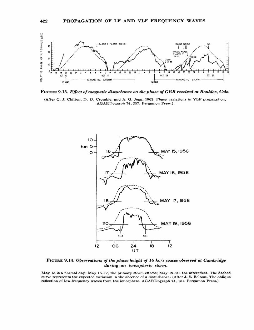
422 PROPAGATION OF LF AND VLF FREQUENCY WAVES
RADIO NOfSE
14 16 18 20 22 24 2 4 6 OCT. 26
8 K) (2 W 16 16 20 22 24 2 4 6 8 10 12 14 16 18 20 22 24 2 8 10 12 14OCT 27
MAGNETIC STORM -
OCT 29
- MAGNETIC STORM -
FIGURE 9.13. Effect of magnetic disturbance on the phase of GBR received at Boulder, Colo.
(After C. J. Chilton, D. D. Crombie, and A. G. Jean, 1963, Phase variations in VLF propagation,AGARDograph 74, 257, Pergamon Press.)
10-
Km 5 — O- MAY 15, 1956
\_ MAY I6 t 1956
ss
- MAY 17, 1956
MAY 19, 1956
12i
O6l
24 UT
i 18
I 12
FIGURE 9.14. Observations of the phase height of 16 kc/s -waves observed at Cambridgeduring an ionospheric storm.
May 15 is a normal day; May 16-17, the primary storm effects; May 19-20, the aftereffect. The dashed curve represents the expected variation in the absence of a disturbance. (After J. S. Belrose, The oblique reflection of low-frequency waves from the ionosphere, AGARDograph 74, 151, Pergamon Press.)
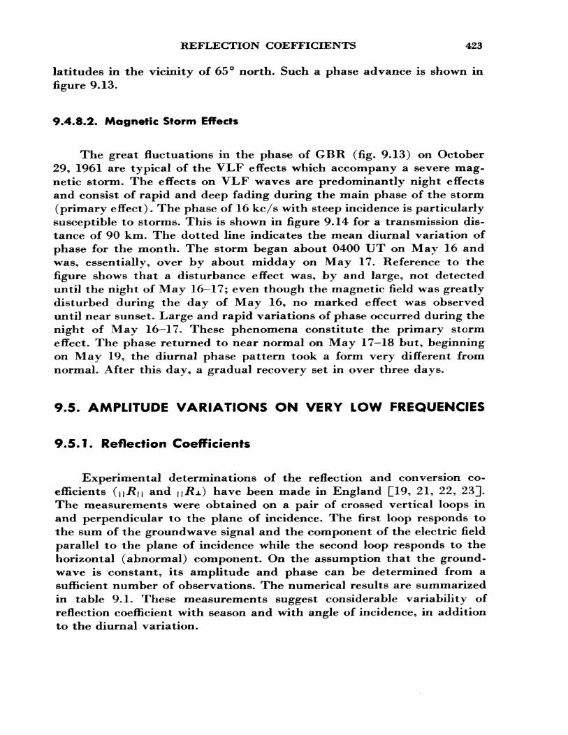
REFLECTION COEFFICIENTS 423
latitudes in the vicinity of 65° north* Such a phase advance is shown in figure 9.13.
9.4.8.2. Magnetic Storm Effects
The great fluctuations in the phase of GBR (fig. 9.13) on October 29, 1961 are typical of the VLF effects which accompany a severe mag netic storm. The effects on VLF waves are predominantly night effects and consist of rapid and deep fading during the main phase of the storm (primary effect). The phase of 16 kc/s with steep incidence is particularly susceptible to storms. This is shown in figure 9.14 for a transmission dis tance of 90 km. The dotted line indicates the mean diurnal variation of phase for the month. The storm began about 0400 UT on May 16 and was, essentially, over by about midday on May 17. Reference to the figure shows that a disturbance effect was, by and large, not detected until the night of May 16—17; even though the magnetic field was greatly disturbed during the day of May 16, no marked effect was observed until near sunset. Large and rapid variations of phase occurred during the night of May 16—17. These phenomena constitute the primary storm effect. The phase returned to near normal on May 17—18 but, beginning on May 19, the diurnal phase pattern took a form very different from normal. After this day, a gradual recovery set in over three days.
9.5. AMPLITUDE VARIATIONS ON VERY LOW FREQUENCIES
9.5.1. Reflection Coefficients
Experimental determinations of the reflection and conversion co efficients (ii/?n and \\RJL) have been made in England £19, 21, 22, 23]. The measurements were obtained on a pair of crossed vertical loops in and perpendicular to the plane of incidence. The first loop responds to the sum of the groundwave signal and the component of the electric field parallel to the plane of incidence while the second loop responds to the horizontal (abnormal) component. On the assumption that the ground- wave is constant, its amplitude and phase can be determined from a sufficient number of observations. The numerical results are summarized in table 9.1. These measurements suggest considerable variability of reflection coefficient with season and with angle of incidence, in addition to the diurnal variation.
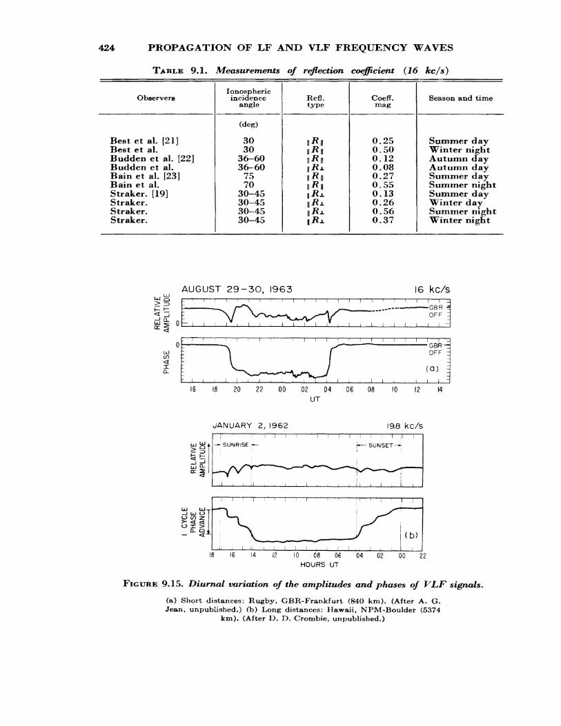
3 0 C/l I
>^M
S
'^*»
w
?3
R
n. t*
a' 5
c ST
c3^3-
«' 2
° a
ff^x
- 5,
"tb
x g*
I CY
CLE
PHAS
EAD
VANC
ERE
LATI
VE
AMPL
ITUD
E
5 5
j3 c '
c z 5 K "f fi H
J
.
PHAS
ERE
LATI
VE
AMPL
ITUD
E
SLS-
S-S-
s 3
00 W
Ctf
W
_.
_ "
OO
O<
J<
IOM
^-.
_
I I
I O
inT
T
00
en c
/i c/
i c/i
O O
oooooooooo
^—
^^^^-g
gj^
CsB
sggg
-^ag
Ff^
f^M
M
MU
C
rfw
•a
CL ts
o,
O a* SB;!
3?
J» » 03 ST. CD
ft 3 g 0 >• H M i o *j 5 > ;s *l 9 s 2 n̂
hM * g
8"
> C«
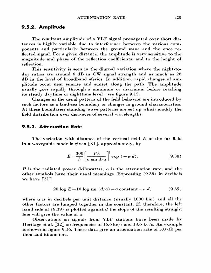
ATTENUATION RATE 425
9.5.2. Amplitude
The resultant amplitude of a VLF signal propagated over short dis tances is highly variable due to interference between the various com ponents and particularly between the ground wave and the once re flected signal. For a given distance, the amplitude is very sensitive to the magnitude and phase of the reflection coefficients, and to the height of reflection.
This sensitivity is seen in the diurnal variation where the night-to day ratios are around 6 dB in GW signal strength and as much as 20 dB in the level of broadband sferics. In addition, rapid changes of am plitude occur near sunrise and sunset along the path. The amplitude usually goes rapidly through a minimum or maximum before reaching its steady daytime or nighttime level—see figure 9.15.
Changes in the usual pattern of the field behavior are introduced by such factors as a land-sea boundary or changes in ground characteristics. At these boundaries standing wave patterns are set up which modify the field distribution over distances of several wavelengths.
9.5.3. Attenuation Rate
The variation with distance of the vertical field E of the far field in a waveguide mode is given Q31J, approximately, by
3001" P\^—— exp ( —«rf). (9.38) a/a Jh |_a sin
JP is the radiated power (kilowatts), OL is the attenuation rate, and the other symbols have their usual meanings. Expressing (9.38) in decibels we have £31]
20 log E-\-W log sin (d/a) =a constant — a. d, (9.39)
where OL is in decibels per unit distance (usually 1000 km) and all the other factors are lumped together in the constant. If, therefore, the left hand side of (9.39) is plotted against d the slope of the resulting straight line will give the value of OL.
Observations on signals from VLF stations have been made by Heritage et al. []32] on frequencies of 16.6 kc/s and 18.6 kc/s. An example is shown in figure 9.16. These data give an attenuation rate of 3.0 dB per thousand kilometers.
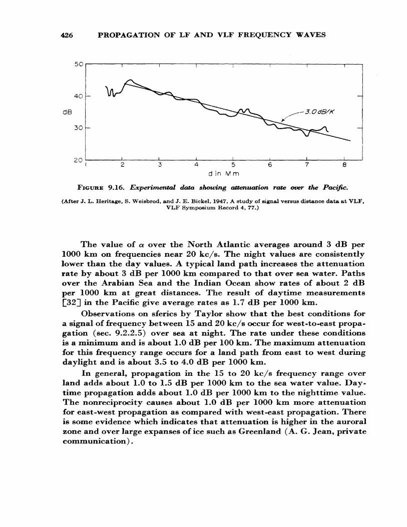
426 PROPAGATION OF LF AND VLF FREQUENCY WAVES
5C
40
dB
30
I 2345678d in M in
FIGURE 9.16. Experimental data showing attenuation rate over the Pacific.
(After J. L. Heritage, S. Weisbrod, and J. E. Bickel, 1947, A study of signal versus distance data at VLrF,VLF Symposium Record 4, 77.)
The value of a over the North Atlantic averages around 3 dB per 1000 km on frequencies near 20 kc/s. The night values are consistently lower than the day values. A typical land path increases the attenuation rate by about 3 dB per 1000 km compared to that over sea water. Paths over the Arabian Sea and the Indian Ocean show rates of about 2 dB per 1000 km at great distances. The result of daytime measurements £32]] in the Pacific give average rates as 1.7 dB per 1000 km.
Observations on sferics by Taylor show that the best conditions for a signal of frequency between 15 and 20 kc/s occur for west-to-east propa gation (sec. 9.2.2.5) over sea at night. The rate under these conditions is a minimum and is about 1.0 dB per 100 km. The maximum attenuation for this frequency range occurs for a land path from east to west during daylight and is about 3.5 to 4.0 dB per 1000 km.
In general, propagation in the 15 to 20 kc/s frequency range over land adds about 1.0 to 1.5 dB per 1000 km to the sea water value. Day time propagation adds about 1.0 dB per 1000 km to the nighttime value. The nonreciprocity causes about 1.0 dB per 1000 km more attenuation for east-west propagation as compared with west-east propagation. There is some evidence which indicates that attenuation is higher in the auroral zone and over large expanses of ice such as Greenland (A. G. Jean, private communication).
NORMAL BEHAVIOR OVER LONG DISTANCES 427
9.5*4. Polarization
Over short distances (100 to 300 km) the sky wave is essentially circularly polarized, that is, the ratio n/?j.r u J?u is approximately unity with a 90° phase shift. At longer distances (500 to 800 km), the polariza tion is approximately linear with \\R\\ being much larger than K/?JL. For distances over 1000 km, it appears that the polarization is essentially vertical during the daytime and that this changes to an elongated ellipse (10:1 axis ratio) at night. The polarization is highly variable during disturbed conditions for short and medium distances. Little is known, in general, about polarization for long distances.
9.6. PHASE VARIATIONS ON LOW FREQUENCIES
9.6.1. Normal Behavior Over Short Distances
Experimental data obtained by Belrose C33J indicates that the heights of reflections of waves, in the frequency range 70 kc/s to 245 kc/s, are roughly the same as those of VLF waves. For transmission distances of the order of 1000 km the heights of reflection change from about 90 km by night to about 72 km by day as sketched in figure 9.17. It will be seen also that the reflecting layer is closely controlled by the sun. When these frequencies are transmitted over shorter distances (less than about 300 km) they appear to be reflected at somewhat higher heights, namely 80 to 85 km by day and 90 to 100 km by night.
9*6.2. Normal Behavior Over Long Distances
When LF waves are propagated over distances of 2000 km and greater, the diurnal variation of phase is quite different from that for distances of around 1000 km and less. This is seen in figure 9.18, where the trapezoidal shape of the curve is emphasized by the dashed line. The fact that the phase changes during daylight are independent of solar zenith angle x has led to the suggestion that the height of reflection (zero phase) is less than 70 km (probably around 65 km). Note that the phase of LF signals appears to be highly variable at night over most paths. It is important to remember that the deductions about the height of re flection are made on the assumption that the one-hop signal predominates
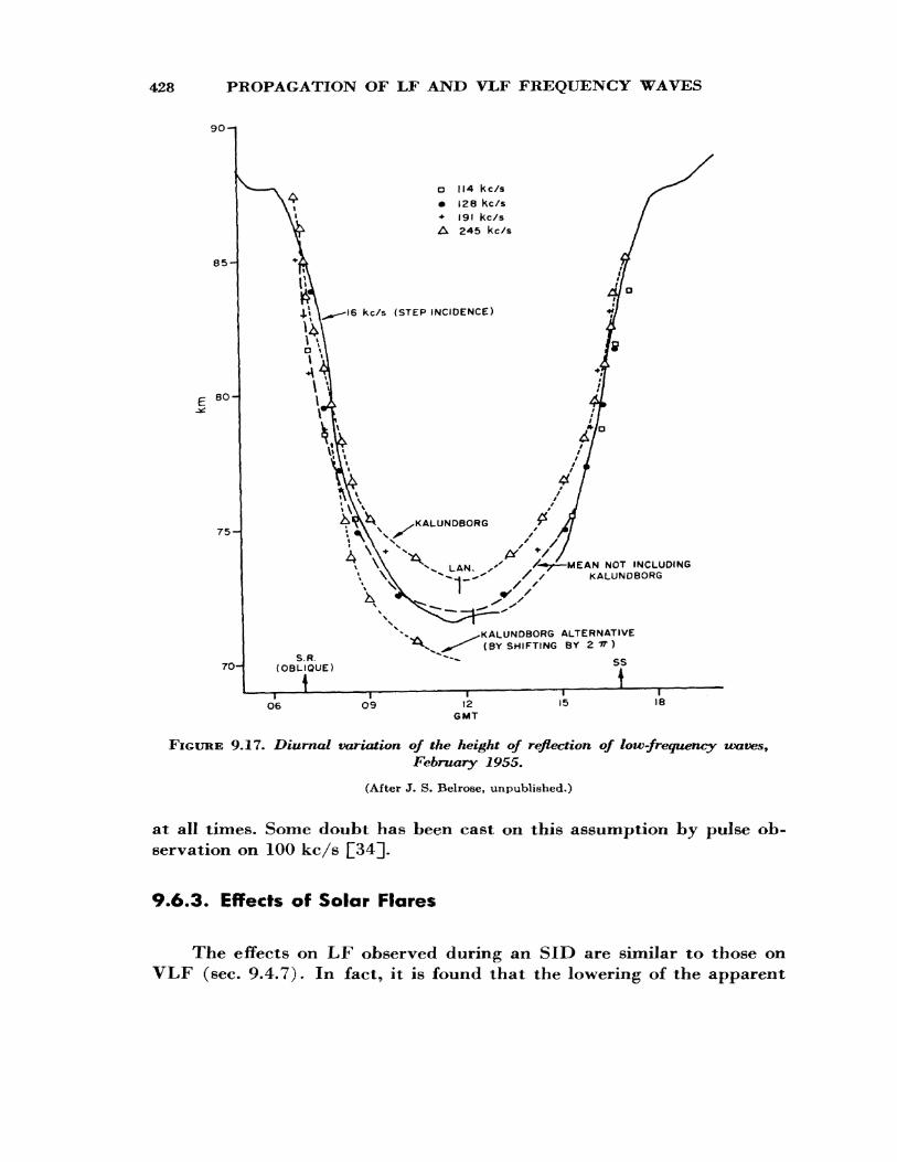
428 PROPAGATION OF LF AND VLF FREQUENCY WAVES
90-1
7O
D 114 kc/s
• 128 kc/s+ 191 kc/sA 245 kc/s
16 kc/s {STEP INCIDENCE)
rfEAN NOT INCLUDING KALUNDBORG
KALUNDBORG ALTERNATIVE (BY SHIFTING BY 2 TT }
SS
—I——
12 GMT
15 18
FIGURE 9.17. Diurnal variation of the height of reflection of low-frequency waves.February 1955.
(After J. S. Belrose, unpublished.)
at all times. Some doubt has been cast on this assumption by pulse ob servation on 100 kc/s []34]].
9.6.3. Effects of Solar Flares
The effects on LF observed during an SID are similar to those on VLF (sec. 9.4.7). In fact, it is found that the lowering of the apparent
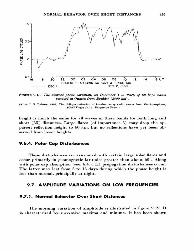
NORMAL BEHAVIOR OVER SHORT DISTANCES 429
I.O-i
CO 0.5-
CD
<tO_
0.516 18 2O 22 OO O2 O4 O6 O8 IO 12
BOULDER-OTTAWA 6O Kc/s AT 246O Km DEC. I —————H———————————————DEC. 2, 1959 ———
16 UT
FIGURE 9.18. The diurnal phase variation^ on December 1—2, 1959, of 60 kc/s wavesreceived at Ottawa from Boulder (240O km).
(After J. S. Belrose, 1963, The oblique reflection of low-frequency radio waves from the ionosphere,AGARDograph 74, Pergamon Press.)
height is much the same for all waves in these bands for both long and short p55] distances. Large flares (of importance 3) may drop the ap parent reflection height to 60 km, but no reflections have yet been ob served from lower heights.
9.6.4. Polar Cap Disturbances
These disturbances are associated with certain large solar flares and occur primarily in geomagnetic latitudes greater than about 60°. Along with polar cap absorption (sec. 6.4.), LF propagation disturbances occur. The latter may last from 5 to 15 days during which the phase height is less than normal, principally at night.
9.7. AMPLITUDE VARIATIONS ON LOW FREQUENCIES
9.7.1. Normal Behavior Over Short Distances
The morning variation of amplitude is illustrated in figure 9.19. It is characterized by successive maxima and minima. It has been shown
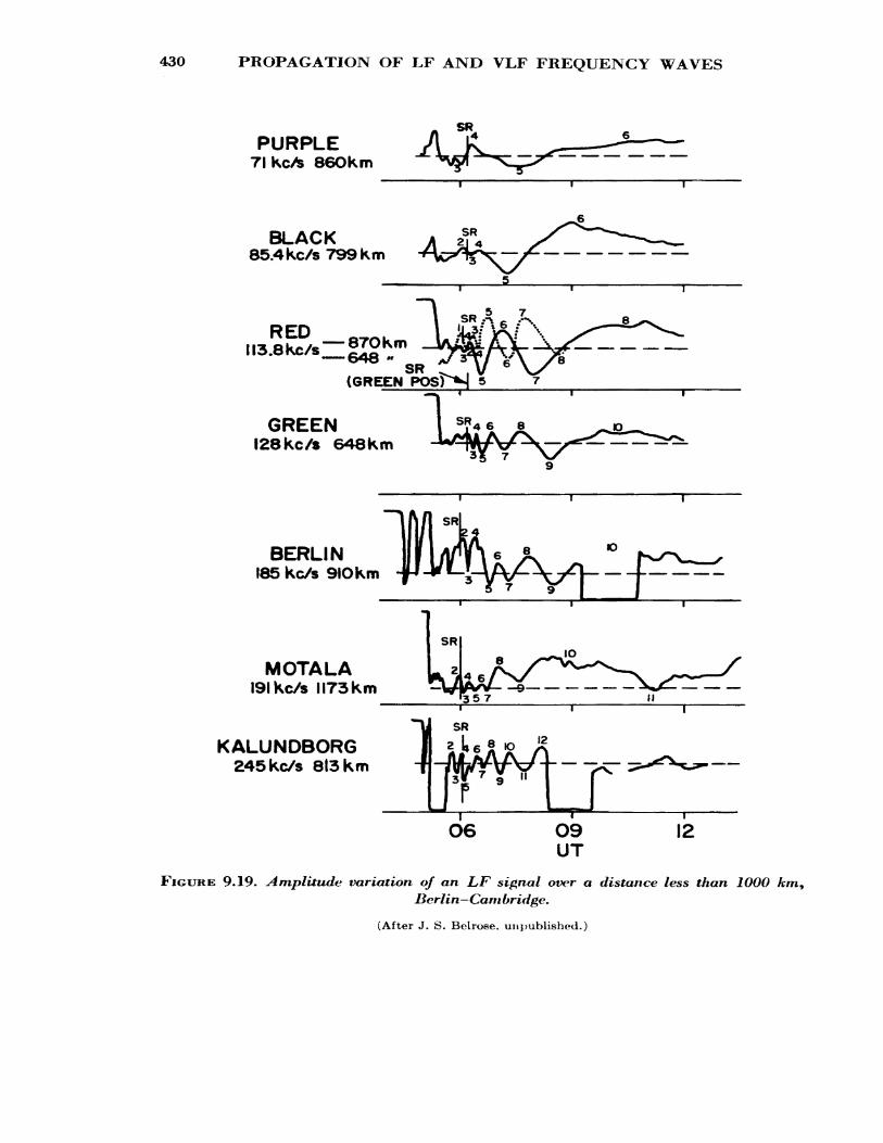
430 PROPAGATION OF LF AND VLF FREQUENCY WAVES
PURPLE 71 Kc/s 86OKm
BLACK 85.4Kc/s799km
\ ,f! A e r — 870Km _UiffiLO
GREENI28kc/s 648 Km
BERLIN 185 kc/s 9IOkm
MOTALA 191 Kc/s 1173 Km
KALUNDBORG 245Kc/s 813 Km
12
FIGURE 9.19. Amplitude variation of an LF signal over a distance less than 1000 km,Berlin— Cam bridge.
(After J. S. Belroee, unpublished.)
REFLECTION COEFFICIENT 431
£33] that, by starting at midday and working back towards sunrise, these maxima and minima can be explained in terms of the interference between a single skywave, the amplitude of which decreases with time of day, and the groundwave. If this analysis is continued earlier than ground sunrise, the results are no longer consistent and it is necessary to assume that more than one skywave is present. It appears unlikely that the ad ditional skywave is the two-hop signal because of the small magnitude of the reflection coefficient.
9.7.2. The Reflection Coefficient
The variation of \\R\\ with the equivalent vertical frequency (/cos 0, where <f> is the angle of incidence) is sketched in figure 9.20 for the months of November 1954, March 1955, and June 1955. Except in the case of
UJo ,OI
o o
oI— oUJ
tl1 -OOI-
.00 or
16 17
\ 'X-K\ \ "6X^ »C\I5 5* \
OUGHT
10 20 5O IOOf cos i Kc/s
2OO 500 1000
FIGURE 9.20. Variation of reflection coefficient \\R\\ with equivalent frequency.
(After J. S, Bclrose, The oblique reflection of low-frequency radio waves from the ionosphere, AGARDograph 74, 1963.)
432 PROPAGATION OF LF AND VLF FREQUENCY WAVES
June, the variations are essentially linear. It should be noted that, for short distances, since the downcoming wave is approximately circularly polarized, the reflection coefficient \\R\\ and the conversion coefficient I|1?-L are essentially equal. On the whole, the data from which figure 9.20 was constructed refer to sunspot minimum years.
Detailed studies Q36] on waves of frequency 245 kc/s over a distance of 180 km have shown that the difference in attenuation between sun- spot maximum and sunspot minimum is a function of solar zenith angle. There is a maximum difference in attenuation of 15 dB at x — 70°. Monthly mean values of log \\R\\ at constant x ar^ closely related to sunspot number
H <r
.OOOI
.OOI
FIGURE 9.21. Diurnal variation of \\R±for 245 kc/s over a distance of 180 km for 1954 (solid line) and 1956 (broken line).
(After J. S. Belroee, unpublished.)
NORMAL BEHAVIOR OVER LONG DISTANCES 433
up to a value of 150 above which there is little change. This "saturation" effect is also evident in the monthly mean curves of figure 9.21 giving the diurnal variation of \\R± (plotted from data in ref. C^7J). In winter and equinox months there is a difference in attenuation over the whole of the day. In summer the ionospheric absorption, during a year of high sunspot number, reaches a maximum soon after sunrise. This maximum is about the same as the midday value during a sunspot minimum year.
There is some evidence that suggests that the sunspot cycle effect on LF waves is opposite to that on VLF waves. Thus 16 kc/s waves are more strongly reflected at sunspot maximum than at sunspot minimum whereas on 245 kc/s the reverse appears to be true. The magnitude of the difference depends on the sunspot number and, in part, on the season (for instance on 245 kc/s a difference is found for equinoctial and winter months only) and is about 3 to 6 dB. On intermediate frequencies the effect "will be less.
9.7.3. Normal Behavior Over Long Distances
9.7.3.1. Diurnal Variation
The diurnal variation of the amplitude of waves of frequency 97 kc/s propagated between Ottawa and Goose Bay in Canada (1500 km) is shown in figure 9.22.
In summer the diurnal variation of amplitude is very regular and, to a first order, symmetrical about local noon. In winter the daytime amplitude is greater, and much less regular and the equinox months are erratic. Deep fluctuations are present near dawn. In these records the groundwave is negligible in comparison with the total skywave so that the fluctuation is due probably to the beating between two waves re flected from different heights.
9.7.3.2. Seasonal Variation
The seasonal variation of the signal strength on 80 kc/s over the 1910 km path from Ottawa to Churchill is shown in figure 9.23a. This shows the usual seasonal trend with winter signals stronger than the summer ones. The seasonal variation of the signal strength in the case of 70.4 kc/s waves over the 1700 km path from Comfort Cove, Newfoundland, to Ottawa is opposite to that obtained for all other transmissions as can be seen in figure 9.23b.
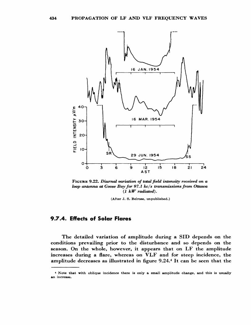
434 PROPAGATION OF LF AND VLF FREQUENCY WAVES
FIGURE 9.22. Diurnal variation of total field intensity received on a loop antenna at Goose Bay for 97.1 kc/s transmissions from Ottawa
(1 kW radiated).
(After J. S. Belrose, unpublished.)
9*7.4. Effects of Solar Flares
The detailed variation of amplitude during a SID depends on the conditions prevailing prior to the disturbance and so depends on the season. On the whole, however, it appears that on LF the amplitude increases during a flare, whereas on VLF and for steep incidence, the amplitude decreases as illustrated in figure 9.24.4 It can be seen that the
* Note that with oblique incidence there is only a small amplitude change, and this is usually an increase.
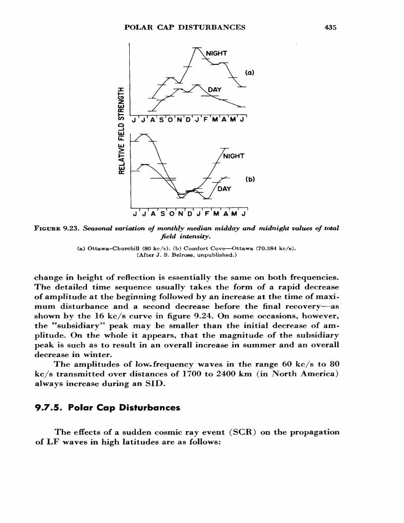
POLAR CAP DISTURBANCES 435
oUJorfeo
1UJor
NIGHT
N D J F M'A'M J
NIGHT
(b)
J'J'A'S'O'N'D'JV'M'A'M'j'
FIGURE 9.23. Seasonal variation of monthly median midday and midnight values of totalfield intensity.
(a) Ottawa-Churchill (80 kc/s). (b) Comfort Cove—Ottawa (70.384 kc/s). (After J. S. Belrose, unpublished.)
change in height of reflection is essentially the same on both frequencies. The detailed time sequence usually takes the form of a rapid decrease of amplitude at the beginning followed by an increase at the time of maxi mum disturbance and a second decrease before the final recovery—as shown by the 16 kc/s curve in figure 9.24. On some occasions, however, the ^subsidiary" peak may be smaller than the initial decrease of am plitude. On the whole it appears, that the magnitude of the subsidiary peak is such as to result in an overall increase in summer and an overall decrease in winter.
The amplitudes of low.frequency waves in the range 60 kc/s to 80 kc/s transmitted over distances of 1700 to 2400 km (in North America) always increase during an SID.
9.7.5. Polar Cap Disturbances
The effects of a sudden cosmic ray event (SGR) on the propagation of LF waves in high latitudes are as follows:
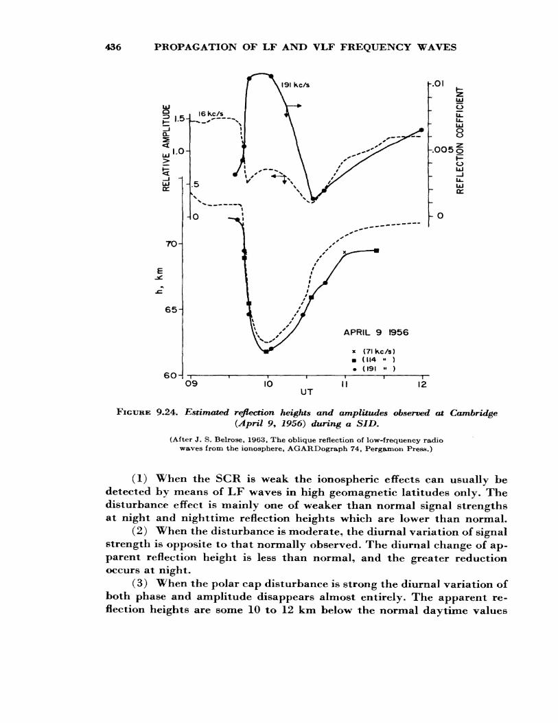
436 PROPAGATION OF LF AND VLF FREQUENCY WAVES
-.Ol
60 J
APRIL 9 1956
• (7lkc/s)• (114 » )• (191 '• )
UT11 12
FIGURE 9.24. Estimated reflection heights and amplitudes observed at Cambridge(April 9, 1956) during a SID.
(After J. S. Belrose, 1963, The oblique reflection of low-frequency radio waves from the ionosphere, AGARDograph 74, Pergamon Press.)
(1) When the SCR is weak the ionospheric effects can usually be detected by means of LF waves in high geomagnetic latitudes only* The disturbance effect is mainly one of weaker than normal signal strengths at night and nighttime reflection heights which are lower than normal.
(2) When the disturbance is moderate, the diurnal variation of signal strength is opposite to that normally observed. The diurnal change of ap parent reflection height is less than normal, and the greater reduction occurs at night.
(3) When the polar cap disturbance is strong the diurnal variation of both phase and amplitude disappears almost entirely. The apparent re flection heights are some 10 to 12 km below the normal daytime values
WINTER ANOMALY 437
(i.e., the waves may be reflected from heights between 50 and 55 km). The signal strengths are about the same as those on a normal day.
9.7.6* Magnetic Storm Effects
The behavior of LF waves during magnetic storm in middle latitudes has been summarized by Lauter C38J as follows:
(1) The sudden commencement was not associated with any change of amplitude;
(2) at night, rapid and deep fading accompanied the main phase af the storm (primary storm effect) ;
(3) daytime records were not usually disturbed during the main phase of the storm;
(4) when the storm was intense the signal strength during the night was unduly weak for a period which began about 3 to 4 days after the Btart of the storm and continued for several days (the after effect).
9.7.7. Nocturnal Anomalies [33, 38 ]
At night it is not uncommon to observe phase and amplitude anom alies lasting for about an hour or so. Both phase and amplitude changes occur together. The phase anomalies always correspond to a decrease in apparent height. Although they are somewhat similar to sudden phase anomalies, they frequently start more gradually. The decrease in ap parent height can be as great as 8 to 10 km, which is the size of a normal SPA. Furthermore, there is evidence to indicate that these nocturnal anomalies have spatial extents of at least 600 km.
Nocturnal anomalies are associated sometimes with magnetic vari ations, but not always. They are found both in middle and high latitudes and are usually accompanied by other ^auroral" type phenomena such as enhanced forward scatter of VHF signals, II F absorption, and so on.
9.7.8. The Winter Anomaly
During winter days of high absorption on II F (sec. 3.3.6.5), low- frequency waves appear to be reflected from heights lower than normal and the amplitude of waves transmitted over distances of 1000 to 2000 km is greater than normal. When these waves are propagated over short
438 PROPAGATION OF LF AND VLF FREQUENCY WAVES
distances their amplitudes may be greater or less than normal but, when the HF absorption is intense, their amplitudes are usually greater than normal.
9.7.9. Variation of Amplitude With Distance
9*7.9.1. Short Distances
At distances less than 100 km the variation is dominated by inter ference between the groundwave and the skywave* If the amplitude of the vertical electric field is measured on the ground, or in an airplane fly ing at a constant height, and allowance is made for the inverse distance attenuation, a pattern of the type shown in figure 9.25 is obtained. This pattern is called the Hollingworth pattern. From the positions and signal strengths of the turning points it is possible to deduce the characteristics of the downcoming wave.
9.7.9.2. Long Distances
Some idea of the decrease of amplitude with distance can be obtained from figure 9.26 which is based on data for 180 kc/s waves over land
300 400 500 600 Distance from sender,km
700 800
FIGURE 9.25. The Hollingtuorth interference pattern observed during the midday hours on85 kc/s on November 39 1949.
The full curve represents the calculated groundwave signal. (After R. N. Bracewell, K. G. Budden, J. A.Ratcliffe, T. W. Straker, and K. Weeks, 1951, The ionospheric propagation of low-frequency radio waves
over distances less than 1000 km, Proc. IEE 98, Pt. Ill, 221.)
VARIATION OF AMPLITUDE WITH DISTANCE 439
r>o
"
0? ^-v
-
LU IO ^^ S
co C•« I § £
oCO CO
CO
orCS
Cs3£2 O
IIPQCQ
AJLISN31NI QH3IJ
440 PROPAGATION OF LF AND VLF FREQUENCY WAVES
]. The following features are worthy of note:
(1) At the geometrical limits of the one-hop path (£^2000 km) there is no sharp drop in signal strength. This is in agreement with waveguide theory.
(2) The amplitudes fall off approximately exponentially with dis tance both by day and by night.
(3) The amplitudes are greater by night than by day.(4) The attenuation rate is somewhat greater by day than by night.
9.8. USE OF VERY LOW FREQUENCIES IN FREQUENCYCOMPARISONS
The relatively high phase stability of VLF signals propagated over long distances makes it possible to transmit reference frequencies to re mote parts of the world. For this purpose, the frequency of the trans mitter must be stabilized by means of a stable crystal oscillator or pref erably an atomic standard. Under these conditions the limitation on the accuracy to which a received frequency can be measured is determined by
(a) the relatively high atmospheric noise £39^ and(b) the phase fluctuations due to ionospheric changes E40]].
Frequency is essentially the time rate of change of phase (i.e., d<t>/dt} . It can be shown that if TV and C are the rms noise and signal powers respectively, then the standard deviation of phase <r(<f>) is given by
a(0)=^. (9.40)
If n cycles are observed in a time ( T) the error in n is l/27r<7(0) and thus the rms error E in the frequency (/) measurement is
1 <r(0) 1 TV 1 ~n 27T
Now the noise power TV is proportional to the bandwidth (6) of the re ceiving system, which can be made small (e.g., 0.01 c/s) by suitable in strumentation £413- Using such a system, a precision of 1 part in 109 has been achieved in an hour's observations over a distance of 19,000
REFERENCES 441
km. From this it will be seen that atmospheric noise will rarely be the limiting factor.
The effect of ionospheric height changes is more serious because the variations are so slow and, thus, long averaging times are required. If the phase of a VLF signal relative to that of a local oscillator changes by an amount <f> in a time T, then the angular frequency difference AOJ is given by
A<» = j.- (9.42)
If cr(<f>) is the standard deviation in the fluctuations of <£, the precision of the frequency measurement will be
<r(d>) *M=-^jr* (9.43)
provided that the phases at the beginning and end of the measurement are uncorrelated. Thus the precision increases linearly with the time of observation. Pierce gives values of <r(0) for GBR-Boston (16 kc/s) of 0.28 rad for quiet nights and 0.14 rad by day. For GBR—Boulder the day value of <r(<£) is 0.26 rad. The natural limit of frequency comparison over a north-Atlantic path is about 2 parts in 1011 for a 24-hr period C423-
9.9. USES OF VERY LOW AND LOW FREQUENCIES
The main uses of VLF are
(1) Long-distance communications (on -off keying) ,(2) Continuous-wave navigation systems,
and of LF,
(3) Broadcasting (e.g., Droitwich, 200 kc/s),(4) Communications (on-off keying and frequency shift-keying),(5) Continuous wave navigation systems (e.g., Decca),(6) Pulse navigation and timing systems (e.g., Loran C, 100 kc/s).
REFERENCES
[1] Budden, K. G. (1961), The Wave-Guide Mode Theory of Wave Propagation(Logos Press).
[2] Wait, J. R. (1962), Electromagnetic Waves in Stratified Media (Pergamon Press). [3] Wait, J. R. (1960), Terrestrial propagation of VLF radio waves, J. Res. NBS
G4D, (Radio Prop.)- 153.
442 PROPAGATION OF LF AND VLF FREQUENCY WAVES
[4] Wait, J. R. (1957), The mode theory of VLF ionospheric propagation for finiteground conductivity, Proc. IRE 45, 760.
[5] Wait,' J. R., and K. Spies (1960), Influence of earth curvature and terrestrialmagnetic field on VLF propagation, J. Geophys. Res. 65, 2325.
[6] Crombie, D. D. (1958), Differences between E-W and W-E propagation of VLFsignals over long distances, J, Atmospheric Terrest. Phys. 12, 110.
[7] Taylor, W. L. (1960), Daytime attenuation rates in the VLF band using atmos pherics, J. Res. NBS 64D (Radio Prop.), 349.
[8] Barber, N. F., and D. D. Crombie (1959), VLF reflections from the ionospheric in the presence of a transverse magnetic field, J. Atmospheric Terrest. Phys. 16, 37.
[9] Pekeris, C. L. (1950), Ray theory versus normal mode theory in wave propagationproblems, Proc. Sympl Appl. Math. 2, 61, Am. Math. Soc.
[10] Wait, J. R. (1961), A diffraction theory for LF sky wave propagation, J. Geophys.Res. 66, 1713.
[11] Barron, D. W. (1959), The waveguide mode theory of radio propagation whenthe ionosphere is not sharply bounded, Phil. Mag. 45, 1068.
[12] Johler, J. R., and J. D. Harper (1962), Reflection and transmission of radio waves at a continuously stratified plasma with arbitrary magnetic induction, J. Res. NBS 66D (Radio Prop.), 81.
[13] Parkinson, R. W. (1956), The nigh time lower ionosphere as deduced from theo retical and experimental study of coupling phenomena, J. Atmospheric Terrest. Phys. 7, 203; ibid. 8, 158 (1956).
[14] Ratcliffe, J. A. (1959), The Magneto-Ionic Theory and its Application to theIonosphere (Cambridge Univ. Press).
[15] Taylor, W. L., and A. G. Jean (1959), Very-low-frequency radiation spectra oflightning discharges, J. Res. NBS 63D (Radio Prop.), 199.
[16] Laby, T. IL, J. J. McNeill, F. G. Nicolls, and A. F. B. Nickson (1940), Waveform energy and reflection by the ionosphere of atmospherics, Proc. Roy. Soc. (London) A174, 145.
[17] Helliwell, R. A., and M. G. Morgan (1959), Atmospheric whistlers, Proc. IRE 47,200.
[18] Gallet, R. M. (1959), The very low-frequency emissions generated in the earth'sexosphere, Proc. IRE 47, 211.
[19] Straker, T. W. (1955), The ionospheric reflection of radio waves of frequency 16 kc/s over short distances, Proc. IEE 102, Pt. C, 396; Proc. IEE Monograph 144 (1955).
[20] Bracewell, R. N, (1952), The ionospheric propagation of radio waves of frequency16 kc/s over distances of about 200 km, Proc. IEE 99, Pt. IV, 217.
[21] Best, J. E., J. A. Ratcliffe, and M. V. Wilkes (1936), Experimental investigations of very long waves reflected from the ionosphere, Proc. Roy. Soc. (London) A156, 614.
[22] Budden, K. G., J. A. Ralcliffe, and M. V. Wilkes (1939), Further investigations of very long waves reflected from the ionosphere, Proc. Roy. Soc. (London) A171, 188.
[23] Bain, W. C., R. N. Bracewell, T. W. Straker, and C. IT. Westcott (1952), The ionospheric propagation of radio waves of frequency 16 kc/s over distances of about 540 km, Proc. IEE, Monograph 37R.
[24] Bracewell, R. N., and W. C. Bain (1952), An explanation of radio propagation at
REFERENCES 443
16 kc/s in terms of two layers below E layer, J. Atmospheric Terrest. Phys. 2,216.
[25] Pierce, J. A. (1955), The diurnal carrier phase variations of a 16 kc/s trans-Atlanticsignal, Proc. IRE 43, 584.
[26] Crombie, D. D., A. H. Alien, and N. Newman (1958), Phase variations of 16 kc/stransmissions from Rugby as received at New Zealand, Proc. IEE B, 301.
[27] Wait, J. R. (1959), Diurnal change of ionospheric heights deduced from phasevelocity measurements at VLF, Proc. IRE 47, 998.
[28] Wait, J. R. (1961), A comparison between the theoretical and experimental dataon phase velocity of VLF radio waves, Proc. IRE 49, 1089.
[29] Chilton, C. J. (1961), VLF phase perturbations associated with meteor showerionization, J. Geophys. Res. 66, 379.
[30] Cilliars, W. A. (1960), Changes in fading speed of LF radio waves, J. AtmosphericXerrest. Phys. 18, 339; also (1960) Irregularities in the lower ionosphere, Ph.D.Thesis, University of Cambridge.
[31] Wait, J. R. (1958), A study of VLF field strength data: both old and new, Geo-fisica Pura e Applicata 41, 73.
[32] Heritage, J. L., S. Weisbrod, and J. E. Bickel (1947), A study of signal versusdistance data at VLF, VLF Symposium Record 4, 77.
[33] Belrose, J. S. (1958), Some investigations of the lowest ionosphere, Ph.D. Thesis,Cambridge University.
[34] Doherty, R. H., G. Hefley, and R. F. Linfield, (1961), Timing potentials ofLoran-C, Proc. IRE 49, 1659.
[35] Bracewell, R. N., K. G. Budden, J. A. Ratcliffe, T. W. Straker, and K. Weekes(1951), The ionospheric propagation of low -frequency and very -low -frequencyradio waves over distances less than 1000 km, Proc. IEE 98, Pt. Ill, 221.
[36] Lauter, E. A., Some results of IGY low frequency absorption measurements,Symposium on ionospheric soundings in the IGY/IGC, Nice, France, December1961.
[37] Geophysikalische Messreihen des Observatorium fur lonospharen ForschungKuhlungsborn (monthly bulletins published by the Deutschen DemokratischenRepublik Observatorium Kuhlungsborn).
[38] Lauler, E. A., and K. Sprenger (1952), IVocturnal ionospheric disturbances in thelower ionosphere, Z. Met. 6, 161 (translation DSIS/DRB, Canada, TranslationT826).
[39] Watt, A. D., and R. W. Plush (1959), Power requirements and choice of an opti mum frequency for a worldwide standard frequency broadcasting station, J. Res.NBS 63D (Radio Prop.), 35.
[40] Pierce, J. A. (1957), Intercontinental frequency comparison by very low frequencyradio transmissions, Proc. IRE 45, 798.
[41] Alien, A. II., E). O. Crornbie, and W, A. Penton (1956), Frequency variations fromGBK, Rugby, Nature 177, 178.
[42] Pierce, J. A., G. M. R. Winkler, and R. L. Corke (1960), The GBR experiment:a trans-Atlanlic frequency comparison between cesium-con trolled oscillators,Nature 187, 914.
[43] Belrose, J. S., W. L. llatton, C. A. McKerrow, and R. S. Thain (1959), The en gineering of communications systems for low radio frequencies, Proc. IRE 47,661.

Index
A scan, 104, 108Abnormal component, 414, 416, 423Absorption, 81
anomalous, 150change A A, 112coefficient, 80, 82, 84, 89, 231cross section, 8, 10, 13Z>-region, 36, 108, 145, 147, 160, 219, 232, 234, 257, 258, 262, 265, 285, 374, 386deviative, 81, 82, 145, 231, 234, 235differential, 110, 116, 236, 240index, 82, 112, 297, 298, 300, 331, 400measurements, 103, 108, 109, 146, 271non-deviative, 81, 82, 84, 88, 112, 134, 145, 231, 234, 235of sun's radiation, 4, 13polar cap, 43, 82, 231, 257, 258, 274, 277, 278, 279, 280, 281, 284, 351variations, 112, 144, 147, 149, 232, 235, 261, 297, 374zone, 274
Aerials (see antennas). Ampere's circuital theorem, 49 Amplitude:
distribution, 243of wave, 108, 217, 248ratio, 108variations VLF, 244
Angle of:arrival, 114, 186, 189, 225departure, 186, 225elevation, 164, 167, 189, 192, 208, 219, 240, 290, 293, 294, 298incidence, 160, 163, 168, 185, 186, 203, 209, 232, 233, 400, 402, 403, 406, 423, 424,
431radiation, 190, 191, 292, 293, 294, 298, 300, 301, 331, 336
Angular error, 208, 209 Anisotropic medium, 48, 93, 94, 97, 404 Anistropy, 93 Anomalies:
LF phase, 421, 437winter, 130, 138, 149, 150, 235, 298, 437
Antennas:dipole, 241gain, 220, 221, 241, 294, 301, 338, 346ionosonde, 104loss, 218, 220, 221, 338lossless, 310radiation, 218radiation efficiency, 218, 394radiation pattern, 218
Apple ton formula, 71approximate formulas, 73
Appleton-Hartree formula, 63 Arcs, 272, 276ARDC Model Atmosphere, 5 Asymmetric raypaths, 186 Asymptotic expansion of Hankel function, 397
445
446 INDEX
Atmosphere, 8, 11, 413composition, 5constituents, 4, 5density, 5dissociation, 4heat conduction, 4heat loss, 4ionization, 3, 7, 8, 12isothermal, 3, 12layers, 1, 2, 17mean molecular weight, 3, 5models, 5neutral, 1nomenclature, 1numher density, 38region, 1, 8scale height, 3, 5specific heat, 4temperature structure, 4, 5temperature variations, 4, 5terminology, 1
Atmospherics (see spherics). Atmospheric noise, 440, 441 Atomic oxygen, 12 A torn-ion exchange, 12 Attachment, coefficient of, 12, 14, 17 Attenuation (see absorption):
rate, 374, 400, 402, 403, 406, 410, 425, 426, 432, 440 Axes, right-handed system, 412 Aurora:
frequency of occurrence, 34, 36luminescence of, 27origin of, 26, 27, 36
Aurora borealis, 258, 382 Auroral:
absorption, 271, 274, 351activity, 34, 278blackouts, 271, 274, 276, 277, 278, 279, 284, 351movement, 36ring, 274, 276, 277, 280, 281, 283, 284zone, 27, 35, 36, 153, 245, 265, 271, 274, 278, 350, 426
B
B scan, 106, 107, 108Back Electromotive force, 48Backscatter, 185, 290, 357, 360, 361, 362, 364, 366, 441Bandwidth, III, 159, 227, 253, 310, 331, 349, 393, 394Barometric equation, 2Bartel's '''musical scales," 33, 35Beat signal, 92, 113, 114Bi-refringent medium, 45Bistatic, 380Body Doppler, 364Boltzman's Constant, 3, 310Breit and Tuve's theorem, 161
Calibration, 104, 190, 110, 111 Capacitor, parallel plate, 48, 52 Carbon dioxide, 5 Carrier/noise ratio, 326, 339 Carrier wave, 248
INDEX 447
Cassiopeia, 251, 252Caustic surface, 226CCIR, 101, 180, 289, 290, 314, 326, 327Centrifugal force, 61Centripedal force, 61Chapman, 14, 16
formula, 14function, 19, 148layer, 18, 34, 147, 205, 206
formation of, 12height of maximum production, 18 limitations of, 18 solar control, 18
Characteristic waves, 65, 68, 70, 211, 220, 238 Charge:
density, 47, 48oscillation, 65surface, 48
Charges, moving, 36 Chorus, 413 Chromosphere, 37Circularly polarized components (resolution into), 211, 237 Cold plasma, 63 Collision frequency, 71, 80, 82, 84, 87, 108, 134, 145, 147, 210, 264, 265
critical, 82effective, 89profile, 234statistics, 63, 84
Collisions and group refractive index, 71, 73 Collisions, electronic, 63, 68, 69, 73, 88 Colors, 91 Communications:
high frequency, 159, 160, 281, 289, 290long distance, 159, 160, 188, 190, 281radio, 150, 217, 236, 257, 281, 310, 344, 374
CompJex group refractive index, 45, 63, 80, 84, 87 Complex Jroynting vector, 59 Computers, electronic, 73 Conduction current, 4 Constitutive relations, 64, 68, 69 Continuity equation, 9, 12, 52Continuous waves (CW), 103, 108, 110, 145, 365, 413, 440 Contour:
charts, 271, 273maps, 280
Control point, 330, 331 Controlled experiments, 102 Convergence, 222Conversion coefficients, 405, 423, 432, 441Conversion of ordinary to extraordinary wave (see coupling), 45 Coordinates:
dipole, 20geographic, 20
Corona, 37, 43 Cosmic rays, 8, 258, 351 Coupled modes, 405 Coupling, 411, 413
critical, 412ionospheric, 405, 411, 412level, 411LF, 410
CRPL (Central Radio Propagation Laboratory), XIII, 1, 24, 31, 39, 130, 145, 148, 149, 153, 258, 283, 285, 387, 289, 301, 302, 303, 304, 305, 310, 331
448 INDEX
Cross section:absorption, 8ionization, 8
Crossed vertical loops, 423 Curl equations, 53, 54, 66 Current density, 60 Currents:
atmospheric, 26DP, 27earth, 26electro jet, 27L, 27ring, 27, 36Sq, 27
Curvature of earth, 224Curved earth-ionosphere guide, 163, 165, 169 Cusp, ionogram, 203 Cut-off frequency, 190, 192, 399
Declination:magnetic, 23solar, 19
D-days, 26, 34, 246Defocusing, 194, 219, 222, 223, 224, 225, 230 Density:
atmosphere, 5electron, 2, 8, 9, 15, 16, 17,18, 28, 43, 72,124,130, 135,145, 147,160, 172, 175,178,
186, 207, 234, 236, 250, 251, 252, 263, 266, 270, 343, 344, 346, 352, 358, 359, 390molecular, 18
Departure, angle of, 186, 225 Depression in electron density, 266, 267 Deviation, lateral, 198, 208 Dielectric constant, 48 Dielectric polarization, 48 Diffraction, 248, 249 Diffusion, 8
coefficient, 352separation, 1
Dip:angles, 240, 407poles, 26
Dipole, 116, 218, 241coordinates, 20displaced, 26equator, 20, 21field, 19, 22field magnetic, 21latitude, 20, 21, 36, 235, 319lines of force, 22longitude, 20meridians, 20, 21poles, 19, 20vertical, 396
Direction:of energy flow, 45of phase propagation, 45, 97of propagation, 93, 94of ray, 94, 97of wave normal, 95, 96
Dispersion curves, 72, 73, 74, 80, 82, 83, 89 Dispersive medium, 91
INDEX 449
Displacement, 202Dissociation, 4, 5Distance factor, 180, 188, 294Disturbance, 257Diurnal phase variations, 18, 291, 347, 414, 416, 417, 419, 420, 423, 424, 427, 428, 429,
432, 433, 436 Divergence, 222, 224 Diversity:
frequency, 255polarization, 255space frequency, 255
D layer, 257, 258, 259, 391, 399, 410, 416, 418 Doppler shift, 97, 98, 364, 378, 383, 386 Double refraction, 405 Downcoming pattern, 186D region, 43, 84, 108, 125, 149, 150, 183, 184, 233, 258, 262, 264, 267, 281, 285, 294,
343 344 348absorption, 36, 1O8, 145, 145, 160, 219, 232, 234, 258, 262, 265, 285, 374, 386ionization, 37
Drift, 8, 43, 173, 364, 416
Earth's curvature, 224, 402, 403, 410, 417centered dipole, 19magnetic field, 19, 20, 21, 22, 23, 27, 45, 134, 163, 179, 180, 181, 2O1, 203, 377, 4O2,
404, 406, 407East-west propagation, 170, 181, 182, 201, 239, 254, 299, 407, 418, 426 Echoes, 151, 186, 189, 212, 213
LF, 412structure, 159, 173, 178, 410
Effective collision frequency, 147 Efficiency, launching, 403E layer, 18, 19, 27, 118, 125, 137, 138, 139, 145, 147, 150, 166, 167, 182, 190, 191, 192,
232, 234, 235, 236, 257, 259, 290, 291, 292, 234, 235, 236, 257, 259, 290, 291, 293, 314, 323, 325, 330, 335, 336, 337
X dependence, 138, 291 Electric:
field, 27, 46, 47, 51, 62moment per unit volume, 48
Electro-jet:auroral, 27equatorial, 27
Electromagnetic:induction, 50, 51units, 50, 56
Electromagnetic unit of charge, 56 Electromotive force (emf), 48, 5OElectron density, 2, 8, 9, 16, 17, 43, 72, 124, 130, 131, 135, 145, 147, 166, 178, 186, 207,
234, 236, 250, 251, 263, 266, 270, 407profiles, 124, 169, 181, 196, 198, 2O1, 264, 386, 387, 388, 389
D region, 12, 108, 126, 144 E region, 12, 150, 230 F region, 12, 117, 127, 230, 387
Electron energy, 87, 175, 195distribution of, 2, 87, 201
Electrons, 38, 259effective, 63motion of (see ion), 69number density, 8, 12, 18, 60, 117, 13O, 145, 150, 160, 204, 381rate of production, 9, 19, 134, 261, 264recombination, 8, 18slow, 87
450 INDEX
Electrostatic unit of change, 56 Eleven-year cycle, 262 Ellipses:
extra-ordinary wave, 78, 79, 85, 237, 238, 239ordinary, 78, 85, 237, 238, 239tilt of, 78
Emission, 38radio wave, 43ultra-violet, 38, 43x-ray, 38, 43
Energy:density, 219flow, 45, 194
direction of, 94, 194, 197 Equation:
of motion, 59, 61, 69 Equator:
(see dipole)magnetic, 19, 20, 22, 247
Equinox, 178, 272, 273, 275, 377month, 149, 253, 274
Equivalent frequency, 161, 162, 164, 165 Equivalent height, 103
in exponential profile, 136in linear profile, 136in parabolic profile, 135
Equivalent path, 161, 162, 163, 185 Equivalent vertical frequency, 161, 162, 164, 165 E region, 8, 37, 43, 118, 119, 120, 121, 159, 219, 235, 264 Excitation factor, 404 Exosphere, 12, 413Extraordinary wave, 45, 73, 75, 76, 77, 78, 79, 83, 84, 85, 93, 110, 117, 118, 121, 125,
145, 176, 180, 185, 197, 198, 199, 201, 202, 203, 204, 205, 408, 411
Fading, 217, 242, 344, 349absorption, 242double periodic, 244, 245frequency dependent, 245, 246, 281of HF, 393periodic, 242, 244, 245random, 244, 245rates, 245, 348, 351, 364, 378rotation, 210selective, 242, 253short period, 245spectrum, 245, 246
Faraday's law, 49, 211, 212 Far-field, 397Field alined irregularities, 184, 346 Field strength, 110, 217, 241, 242 Finite ground conductivity, 402 Fixed frequency techniques, 103, 108, 174 Flat earth, mode theory, 394F layer, 125, 130, 182, 190, 230, 231, 236, 254, 257, 258, 259, 319, 343, 355 Flip-overs, 412Flutter fading, 184, 245, 246, 247, 281, 284, 378, 379 Flux, 13, 15, 50, 59, 218, 223 /min, 112, 262, 271, 280 Focusing, 194, 208, 219, 223, 224, 228, 230, 242
antipodal, 229
INDEX 451
Focusing—Continuedeffect, merging of low and high waves, 186effect on field intensity, 217horizon, 229ionospheric, 186, 22, 226MUF, 227skip, 186
Force, on electron, 69 Forecasts, 35, 285, 286 Formation of layers, 8Forward scatter, 285, 344, 345, 361, 362, 366, 412 FOT, 192, 284, 289, 292, 319, 323, 325, 331, 339, 340 Fourier:
analysis, 248integral, 301time series, 301transforms, 245, 246, 4O9
F plots, 122, 123, 124, 266 Free space, 63, 65, 300
velocity, 162, 258, 294, 420wavelength, 264, 399
F region, 8, 37, 116, 119, 131, 247, 258, 344, 384, 386 Frequency, hand, 393
changes (Doppler) Af, 97, 113, 262, 263comparison, VLF, 440dependence of, 145, 261, 346, 347, 348, 350distortion, 159diversity, 255lowest useful, 340range, 410
Fresnel reflection coefficient, 401Fresnel zone, 249, 250, 357, 358, 359, 361, 365, 364 Fi-layer, 18, 19, 118, 119, 120, 125, 130, 137, 138, 140, 141, 144, 145, 146, 166, 167, 266,
268 290 291 321 323 325 330^Vlayer, 118, 127, 130, 137, 138, 140, 142, 143, 144, 146, 150, 153, 159, 166, 167, 175,
176, 177, 182, 186, 188, 189, 190, 192, 201, 214, 257, 258, 265, 267, 268, 270, 282, 390, 292, 293, 301, 303, 304, 3O5, 307, 309, 315, 319, 321, 330, 331, 332, 333, 335, 377
Galactic noise, 310Gamma, 23Gauss unit, 23GBR, 416, 418, 419, 420, 421, 422, 423, 424, 441Geomagnetic:
activity, 278, 351field, XIII, 20, 23, 27
Glints, 364 Gradient:
electron density, 346, 390horizontal, 178
Gradual commencement, 265 Grazing incident, 402 Great circle, 116
charts, 318path, 114, 184, 229, 296, 315, 330, 348, 418
Ground:backscatter, 185conductivity, 294, 401, 402range, 167, 186, 196, 219, 294scatter, 153, 155, 156, 180, 182, 185, 330sunset, 418wave, 414, 423, 431, 438
452 INDEX
Group:height, 103, 104, 109, 117, 118, 124, 135path, 96, 98, 161, 162, 210propagation, 89propagation time, 162, 419refractive index, 93, 125, 210retardation, 124velocity, 91, 93, 98
Gyrofrequency, 62, 73, 134, 145, 147, 181, 198, 200, 201, 203, 239, 240, 298, 299, 331 Gyro-oscillations, 38
H
Heliosphere, 2 Height:
apparent, 124, 436equivalent, 161, 165group, 103, 104, 109, 117, 118, 124, 135measurement of, 103minimum virtual, 118, 124of reflection, 124, 162, 163, 165, 293, 294, 416, 418, 427, 436phase, 136, 416, 422real or true, 124, 160, 161, 162, 293, 294, 416, 418, 427, 436phase, 136, 416, 422real or true, 124, 160, 161, 162, 165, 166, 171, 174, 175virtual, (see group height), 103, 107, 124,136, 137, 156, 162, 165, 166,171, 174, 175
Helium, 37High angle ray, 169, 175, 178, 300 Hiss, 413Hollingsworth pattern, 438 Hot-spot, 369, 371 Hour angle of sun, 18 Hydrogen, 5, 37
IGY (International Geophysical Year), XIII, 34, 35, 101, 121, 272, 273, 276, 283, 377Images, ground, 396Imperfect reflection, 400Imposed magnetic field, 68, 69, 70, 71, 134, 135
direction, 70 Impulsive noise, 310Incidence, angle of, 160, 163, 168, 185, 186, 203, 209, 232, 233 Incident beam, 13, 345 Inclination (see dip) Index:
absorption, 297, 298of refraction, 344refractive, 55, 63, 64, 67, 68, 71, 72, 73, 76, 77, 80, 81, 84, 87, 90, 92, 96, 135, 147,
160, 162, 164, 194, 196, 197, 201, 202, 203, 207, 210, 250, 262, 263, 294 Infrared radiation, 4 Inhomogeneous medium, 410, 411 Initial phase of magnetic storm, 265 International Astronomical Union, 39, 43 International Geophysical Year (See IGY) International daily character figure, 30 Inverse distance, 219
loss, 21Q, 221 Inverse square law, 281 Ion, concentration, 60
motion, 59
INDEX 453
lonization, 125, 23O, 284coefficient, 17cross section, 8efficiency, 8, 10meteoric, 184, 348, 352, 353, 356
Ionized trails, 343, 344, 352, 353, 356, 357, 358, 359, 360, 361, 362, 363, 364, 365, 366,369
lonogram, oblique, 174, 175, 180, 184, 189, 192, 193, 1941GY atlas of, 121
lonogram, vertical, 117, 118, 119, 121, 124, 125, 150, 170, 181, 184markers, 104
lonosonde, 103, 104, 105, 106, 107, 112, 117, 125antenna, 104blanking of display, 106C-4, 104interference, 107oblique, 284sweep frequency, 103, 104, 107
Ionosphere, 1, 59currents, 27curvature, 163, 169, 196, 208, 219, 229, 403electron distribution, 262, 343layers, 230, 291, 293model, 410movements, 101, 248quiet, 38, 117regions, 2storms, 101, 140, 159, 257, 258, 259, 265, 268, 269, 270, 285, 281, 422
Ions, 19, 61 Iris effect, 207, 208 Isochasms, 36 Isoionic contours, 130 Isosurface, 22 Isotropic radiator, 358 Isotropy, 346 IQSY, XIII
JANET system, 375Junction frequency (JF), 176, 177, 178, 180, 181, 182
k factor, 40, 56, 68, 169, 170, 171, 172, 182 ICinetic energy of electrons, 352
Land-sea boundary, 425Latitude:
dip, 143 dipoJe, 20, 319 geographic, 19, 20 geomagnetic, 20 magnetic, 20
Layer formation, 17 by attachment, 9 by recombination, 9
Layer model, 1, 226 shape, 196, 262
Levels of reflection, 76Ley den jar, 51
454 INDEX
Light, 90, 93Lightning discharges, 310, 413Linear:
polarization, 210, 237, 238, 255profile, 136
Line density, 366Lines of force (earth magnetic), 27 Local reference oscillator, 414 LOF (lowest observed frequency), 176, 177 Log-periodic antenna, 104 Longitude:
dipole, 20magnetic, 20
Longitudinal component:of imposed magnetic field, 69of Y, 70
Lorari C, 441Lorentz polarization term, 63 Loss:
absorption (La), 218, 222, 294, 297, 325antenna, 218, 220, 221, 338distance, 296distance (Ls/>), 294ground (Lg), 294, 327inverse square of distance, 219, 221, 281ohmic, 218, 220, 231path, 218, 219, 220, 221, 222, 223, 230, 237, 240, 281, 282, 283, 294, 337, 340power, 218, 294spatial, 218, 224
Low (angle) ray, 166, 169, 254 Lowest observable frequency, 266 Low frequency:
spectrum, XIII, 394, 410broadcasting, 441phase change diurnal, 428pulse observations, 141
Low latitude, 236LUF (lowest usable frequency), 281, 34O Lunar daily magnetic variation, 26 Lyman ex radiation, 37 Lyman £ radiation, 37
MMagnetic:
activity, 30, 31, 156, 274 conductor, 397, 399, 417 declination, 23 dip, 21, 25, 118, 236, 240 dipole field, 19, 20, 22, 75, 77, 272, 319 dip pole, 25, 118, 236, 240disturbances, 26, 27, 30, 35, 148, 214, 260, 277, 421, 422equator, 27, 130, 172, 178, 181, 183, 184, 186, 197, 198, 239, 246, 247, 265, 349 field of earth, 19, 20, 23, 36, 45, 47, 59, 134, 163, 179, 180, 181, 197, 198, 201, 203,
208, 209, 220, 236, 254, 263, 377of sunspots, 40
field of wave, 58, 96, 197 inclination, 21 indices, 30, 31, 32, 33
daily figure, 30, 34international daily character figure, 30local, 30local K index, 30, 31, 349
INDEX 455
Magnetic—Continuedindices—Continued
planetary, 31, 32 world, 30, 31
induction, 23intensity, 22intrinsic elements, 23isosurface, 22latitudes, 30, 31, 75, 202, 266, 267lines of force, 27maps, 24, 25meridian, 197, 201, 202, 203, 204, 208, 236, 238poles, 19, 20, 26, 198potentials, 26properties, 65relative elements, 346spherical harmonic analysis of, 26storms, 27, 28, 29, 36, 43, 156, 258, 259, 265, 267, 279, 351, 423
after effects, 265, 437 main phase, 265, 437 sudden commencements, 437
units, 23variations, 26, 437
Magnetogram, 27, 28, 29Magneto-ionic medium, 45, 69, 71, 410, 411 Magneto-ionic splitting, 150, 239 Magneto-ionic theory, XIII, 59, 412 Main phase, 265Maps, 24, 25, 301, 302, 316, 321, 335 Maximum frequencies, 160, 165, 170, 171, 172, 175, 184, 242, 281, 331
monthly median, 192Maximum observed frequency (MOF), 176, 177, 178 Maximum usable frequency (see MUF) Maxwellian velocity distribution, 87, 385 Maxwell's equations, 45, 52, 53 Medium:
anisotropic, 48, 65, 93, 94, 97, 98birefringenl, 45isotropic, 53, 56, 94neutral, 53, 63non conductive, 53, 56non dispersive, 92
Meridian:dipole (see dipole).
Mesopause, 2, 4 Mesosphere, 1, 2, 4 Mesopeak, 3 Meteor, 354, 355, 366, 372
activity, 150, 374bursts," 367, 368, 370, 371, 373, 374, 375, 376mass distribution, 335radiants, 371showers, 353, 421trails, 343, 344, 352, 353, 356, 357, 358, 359, 360, 361, 362, 363, 364, 365, 366, 369.
370VLF effects, 421
Middle latitude, 149, 235, 266, 347, 348 MKS units, 212 Mode, 180, 189, 401, 402, 409, 416
zero order, 297higher order, 410number, 395theory, 394, 408, 410
456 INDEX
Model:ionospheric, 102, 195sharply bounded, 410
Modulation envelope, 91, 92, 242 Molecular oxygen, 12 Momentum, transfer, 87 Monostatic (radar), 380, 381 Motions of electrons, 61MUF, 143, 167, 175, 176, 177, 179, 180, 182, 227, 242, 257, 266, 282, 289, 292, 319, 321,
322, 325, 331, 332, 339classical, 176, 180definitions, 167, 175experimental, 1804000 km, 292, 293, 317, 330, 331operational, 180standard, 180, 182theoretical, 180
M(2000) E, 321, 322, 323 M(2000) Eg, 325M(ZERO) F2, 291, 293, 303, 309 M(4000) F2, 292, 293, 303, 305, 317 Multipath reduction factor, 193
spread, 193transmission, radio waves, 186, 193, 253
Musa, 114, 116
N
N(h) profiles, 125, 128, 130, 134, 196, 235 National Bureau of Standards, XIII, 258, 303 Navigation systems, 441 Negative phase, 265 Neutral molecules, 8, 9, 12
number density, 8 No-echo conditions, 271 Noise:
atmospheric, XIII, 291, 310carrier/noise ratio, 241, 326data presentation, 311, 312, 313distribution, 311electrical, 310extraterrestrial, 110, 112galactic, 110, 248, 278, 310importance, 310impulse, 310ionosphere, 241level, 327maps, 311, 312, 314power, 110, 112, 310, 311, 326, 340radio, 39, 110, 111, 242resistor, 310solar, 259, 261source, 310thermal, 310
Non-conducting medium, 65Non-deviative absorption (see absorption), 81, 82, 84 Non-reciprocity:
in attenuation, 426in fading, 254
Normal component, 414Normal incidence, 72, 75, 76, 116, 145, 160, 161 Northern hemisphere, 236, 272, 276
INDEX 457
North-south, 417, 418propagation, 181, 201, 202 transmission, 182, 186
Numerical mapping, 301, 302
Oblique:incidence, 160, 161, 162, 164, 207, 397, 434paths, 201sounder, 176
Off-great-circle-paths, 185 One-hop:
path, 175, 178, 190, 294, 440signal, 235, 427
Operating frequency, 159, 167, 169, 192, 202, 284, 297 Operational MUF, 180 Optical:
depth, 13flares, 421
Optimum working frequency (FOT), 192, 284, 289, 292, 319, 323, 325, 331, 339, 340 Oscillations, 38
gyro, 38plasma, 38
Oscillator:drift, 416fixed frequency, 104variable frequency, 104
OWF (optimum working frequency) (see FOT). Oxygen, 5, 8, 12 Ozone, 4, 5
Parabolic:ionosphere, 135, 226profile, 173
Parabolic ray path, 168, 189 Parametric curve, 167 Partial reflections, E«, 277 Path:
effective length, 191, 223, 224, 330, 344great circle, 348group, 96, 97, 98, 161, 162long, 178loss, 218, 219, 220, 221, 222, 223, 230, 237, 240, 281, 282, 283, 294, 337, 340phase, 96, 97, 250virtual (see group path)
Pause, 1 PC A (polar cap absorption), 43, 82, 231, 257, 258, 274, 277, 278, 279, 280, 281, 284, 351,
421 Pederson:
path, 335ray, 167, 178
Penetration frequency, 192, 336, 340 Perfect gas law, 3Permanent Service of Geomagnetic Indices, 30, 31 Permeability, 297 Permittivity, 401 Permittivity of free space, 46 Phase:
advances, 421
458 INDEX
Phase—Continuedconstant, 96, 394 difference, 245, 414 measurements, 103, 112, 414 normal, 197 relative changes, 414
Phase height, 135, 136fluctuations, 159, 419, 440
Phase path, 96, 97, 210, 211, 250, 263 changes AP, 113, 264 measurements, 113 stability, 440
Phase propagation direction (see direction), 45, 93, 94, 95, 98, 134, 197 Phase velocity, determination, 89, 90, 94, 95, 399, 400, 401, 402, 408, 409 Photodetachment, 19, 148, 406 Photoionization, 8, 10, 16 Photosphere, 37, 40 Plage, 41Plane-earth, plane ionosphere model, 160, 165, 196 Plane polarized wave, 45, 210, 211Planes of incidence, 197, 208, 209, 399, 404, 406, 414, 423 Plane waves, 55 Plasma, 89, 103
cold, 63frequency, 43, 61, 135, 136, 160, 162, 211, 250 oscillations, 38 overdense, 204
Polar cap absorption (see PC A). Polar caps, 27, 36, 43, 280, 429, 435, 436 Polarization, 76, 217, 413, 414, 427
circular, 211, 411, 412, 427, 432 dielectric, 48ellipse, 84, 85, 237, 238, 239, 242 equation, 70 linear, 78, 237, 238 very low frequency, 427wave, 27, 76, 79, 211, 217, 220, 237, 346, 399, 405, 411
Polarized medium, 48 Polar region, 421Post perturbation phase (magnetic), 265 Potential difference, 46, 47 Poynting vector, 59 Precision, time of observation, 441 Prediction:
of long term frequencies, 289, 291, 301 of short term frequency, 289, 301 of solar cycle, 290, 303 optimum working frequency OWF, 289 problems, 289, 301 procedures, 289, 301, 302
Pressure, 2, 3 Profile:
electron density (see electron density profile), monotonic, 1, 2, 5
Propagation:constant, 56 direction of, 407 group, 89multi-hop, 189, 226, 294 of radio waves, 45, 394 of great distances, 159, 410
Proton, influx, 38, 259, 351
INDEX 459
Pulse:distortion, 91drift, 173reflection method, 108techniques, 103, 145transmitter, 104
Pulse navigation systems, 441 Pulse synchronization, 173
Qdays, 26, 34, 127, 132, 246
condition, 75, 76, 77, 82, 84, 134, 181, 310, 211, 212, 263 condition, 75, 77, 82, 84, 181, 212, 240
^uasi-incoherent scatter, 343, 386
R
Radar, 103, 212, 357, 380, 381, 383, 384, 385, 387, 388Radiant point, 353Radiation:
absorption, 13angle, 190, 191, 292, 294, 298, 300, 331, 336corpuscular, 38efficiency, 218, 394trapped, 27wave, 38
Radiator, isotropic, 218, 358 Radio astronomy, 208, 259 Radio:
aurora, 36star, 156, 210, 249, 251, 252, 253
Ray:direction, 94, 95, 196, 197, 203velocity, 95versus mode theory, 408, 409, 410
Ray group velocity, 98 Rayleigh distribution, 243, 348Ray path, 166, 167, 168, 186, 187, 190, 194, 195, 197, 198, 199, 200, 201, 202, 203, 208,
210, 223, 232, 234, 264in magnetic meridian plane, 201topside, 204, 207with oblique propagation, 164with vertical propagation, 208
Ray tracing, 160, 189, 194, 195, 197, 213, 223, 226, 235 Reactions, 8, 12 Receiving set noise, 111, 112 Reciprocity, 253, 254 Recombination, 8, 9 Recombination coefficient, 8, 10, 12
effective, 12, 19Reflection at vertical (or normal) incidence, 72, 73, 75, 78, 161, 162 Reflection coefficient, 108
of the ground, 109, 400of the ionosphere, 400, 423, 424
Reflection conditions, 72 Reflection height, LF, 161, 164, 191, 412 Reflection level, 167, 183, 201, 262, 293 Refraction, 159, 180, 183, 197, 209, 343Refractive index, 55, 63, 64, 67, 68, 71, 72, 73, 76, 77, 80, 81, 84, 87, 90, 92, 96, 135, 147,
160, 162, 164, 194, 196, 197, 201, 202, 203, 207, 210, 250, 262, 263, 394complex, 45, 63, 80, 84, 87group (see Group refractive index).surface, 203
460 INDEX
Relativity, 90, 258Relaying, 284Repetition frequency (pulse), 173Resonance- condition, 397Riometer, 110, 111, 112, 277, 281Rippled ionosphere, 412Rotation, sense of, 210
Satellite, 208, 210, 212, 213, 248, 249, 251, 252, 253topside sounder, 116, 204, 207
Scale height, 3, 4, 5, 6, 13 i Scatter, 153, 156, 184, 245
ground, 153, 155, 156, 180, 182, 185, 330side, 185
Scattering, 265forward, 285incoherent, 384
SCNA (sudden cosmic noise absorption), 258, 261 SEA (sudden enhancement of atmospherics), 259, 261 Seasonal variation:
of absorption, 149, 235, 297of LF amplitude, 433
Secant law, 160, 161, 169 Second International Polar Year, 34 Sec <£o corrected, 169 (see k factor) SEE (solar flare effect), 30, 259Short wave fadeout, 258, 259, 260, 261, 262, 264, 281 SID (sudden ionospheric disturbance), 257, 258, 259, 280, 349 Side scatter, 185, 284Signal strength, 110, 159, 186, 194, 217, 226, 227, 344, 347, 349, 439, 440 Simple harmonic motion, 61 Single frequency communications, 344 Skip distance, 167, 172, 185, 226, 227 Sky wave, 414, 427, 431, 433, 438Snell's law, 72, 147, 161, 162, 163, 195, 196, 197, 198, 203 Solar, 40
activity, 253, 279, 290, 303control, 148, 149, 344, 346cosmic rays, 258daily magnetic variation, 26flare, 41, 43, 82, 108, 114, 115, 231, 257, 258, 259, 261, 262, 263, 264, 277, 278, 421,
434flux, 8, 10protons, 277radiation, 8, 12, 13, 32radio emmission, 43rotation, 35, 41wind, 38zenith angle, 12, 13, 18, 128, 138, 147, 235, 262, 281, 291, 297, 317, 320, 322, 334,
340, 427, 432Solar flare disturbances, 41, 257, 258, 261, 262, 263, 278 Sounders, 165
topside, 116, 204, 205, 206, 207vertical, 19
Sounding stationsdistribution of, 19, 101, 102, 173
SPA (sudden phase anomoly), 259, 261, 262, 437 Space charge, 63 Space diversity, 255 Specular reflection, 183, 293 Spherical stratified ionosphere, 186, 194, 195, 209, 225
INDEX 461
Spherics, 261, 413, 426Spitze, 202, 203, 204Sporadic E9 36, 118, 15O, 151, 152, 153, 159, 179, 182, 183, 188, 189, 257, 266, 284, 324,
325, 330 Spread:
F, 153, 155, 156, 184, 247, 253, 266, 269, 281, 343, 378, 379echo, 153, 178
Sputter, 351Stable crystal oscillator, 113, 173 Static field, 46 Statistics collision, 84 Steady state solution, 63 Storm:
ES9 276geomagnetic, 156, 274, 281ionosphere, 4, 284noise, 43time, 266, 270, 271
Suhflare, 41 Subsidiary peak, 435Sudden commencement, 114, 261, 265, 267 Sudden frequencies deviations, 262 Sun:
declination of, 19hour angle of, 19
Sunspot, 40, 42, 130, 262cycle, 40, 41, 43, 130, 138, 146, 262, 274, 277, 290maximum, 27, 39, 41, 138, 140, 147, 261, 266, 274minimum, 27, 38, 41, 140, 147, 261, 266, 274number, 130, 143, 147, 253, 274, 279, 290, 291, 297, 298, 322
Sweep frequency, 103, 170System loss, 217, 218, 289, 294, 300, 337, 338, 347
Take-off angle, 167, 186, 189, 194 Temperature, 1, 3, 5
distribution, 1, 13variation, 4
Theorems:absorption, 163Breit and Tuve's, 161, 165equivalent height, 162Green^s, 53Martyn's, 162, 163, 165, 232Stokes', 53
Theoretical MUF, 180 Thermal equilibrium, 385, 386 Thermosphere, 1, 2, 4, 366, 368, 369 Threshold, 366 Tilt, 114, 182, 186
angle, 78ionospheric, 284, 330
Time, equation of, 19 Time of flight, 98 Time, recorder, 109Time of travel of wave crest or wave front, 90 Time, transmission, 192 Topside:
profiles, 129, 390soundings, 204, 205, 206, 207
Tolal bending of ray, 208 Total electron content, 209, 212, 213, 214
462 INDEX
Total internal reflection, 160Transequatorial propagation, 131, 178, 181, 184, 187, 229, 245Transfer, equation, 87Transmission:
curve, 166, 170, 171, 181distance, 174, 178, 188, 201, 439line, 217, 218path, 165, 166, 173
Transit time, 96 Transmitter, 162, 173, 345, 384 Transponder, 174 Transverse component of magnetic field, 70
propagation, 73, 74, 78, 87, 181, 239wave, 55, 58, 61, 70
Tropospheric scatter, 285 True height, 124, 160, 161 Turbulence, 1, 5, 344 Turbopause, turbosphere, 2 Two-hop path, 325
U
Ultra-violet, 4, 8, 37, 38, 43, 258, 259 Unreliability of HF propagation, 393 URSI (International Scientific Radio Union), 101
Valley, 125Variations of the ionosphere diurnal, 4, 18, 19, 125, 128, 138, 140, 147, 148, 153, 173,
253, 279, 291, 301, 340, 347, 364, 370, 371, 372, 377geographic, 130, 140, 229, 271, 349, 374, 377seasonal, 130, 138, 140, 149, 173, 253, 267, 291, 347, 364, 377solar cycle, 4, 131, 303, 323, 347sun-spot, 138, 140, 149, 173
Velocity:average, 84electron, 84phase, 90, 91wave, 96
Velocity distribution, 87Maxwellian, 87
Vertical dipole source, 396 Vertical polarization, 240, 395, 405VHF forward scatter, 265, 277, 343, 345, 346, 351, 437 VLF (very low frequency):
antennas, 393emissions, 413noise, 393spectrum, XIII, 393, 413uses of, 409, 440, 441
W
Warning service, 285Water vapor, 5Wave, composite harmonic, 91, 217Wave, guide theory, 394, 402, 417, 420, 440Wave:
backward, 411crest, 90
INDEX 463
W ave—Continuedextraordinary, 45, 73, 75, 76, 77, 78, 79, 83, 84, 85, 110, 117, 118, 121, 125, 145, 176,
180, 185, 197, 198, 199, 200, 201, 202, 203, 204, 205, 209, 210, 219, 236, 237, 238, 239, 243, 245, 261, 263
forward, 4, 11free space, 90, 91, 211front, 94, 95, 249height of reflection, 418length, 90normal, 70, 95, 96, 197, 198, 202, 203, 220ordinary, 73, 76, 77, 78, 79, 82, 83, 84, 85, 87, 93, 110, 116, 117, 118, 121, 125, 145,
176, 180, 181, 197, 198, 199, 200, 201, 202, 203, 204, 205, 209, 210, 219, 236, 237, 238, 239, 243, 245, 261, 263, 291, 299
packet, 96, 98, 194, 197plane polarized, 63, 210polarization, 67, 76, 79, 217, 220, 237, 346, 399, 405, 411properties, 63, 78
progressive, 63, 219, 411, 412velocity, 96
Wedge refraction, 209 ^West-east propagation, 407 Whistler mode, 76, 411 Whistlers, 413 Wind shear, 344, 353, 364"Wolf, sun spot number, (see Zurich), 40, 41 World data centers, 124WWV, 115, 173, 244, 245, 246, 263, 282, 284 WWVL, 414, 415
X-rays, 8, 37, 38, 43, 258, 384
Zenith angle of sun (x), 12, 13, 18, 262, 281, 291, 297, 317, 320, 427, 432Zero-muf (see MUF, M(ZERO) F2),Zero-order mode, 397, 398Zero of refractive index, 427^-trace, 118, 121Zurich relative sunspot numher, 138, 143, 144

Author Index
Agy, V., XIV, 214, 271, 272, 273, 275,277, 280, 283, 287, 288
Alien, A. H., 443 Anderson, L. J., 215 Aono, Y., 214 Appleton, E. V., 63, 99, 145, 146, 157,
172, 196, 214 Athay, R. G., 44 Auterman, J., 244
B
Baghdady, E., 256Bailey, D. K., 215, 287, 288, 39OBain, W. C., 442Baker, D. M., 287Balser, M., 256Barber, N. F., 442Barron, D. W., 442Bartels, J., 30, 33, 44Bateman, R., 287, 379, 390, 391Bazzard, G. H., 341Berry, W. M., 342Belrose, J. S., XIII, XIV, 411, 412, 422,
427, 428, 429, 430, 431, 432, 434, 435,436, 439, 443
Bennett, W, R., 342 Berg, M. R., 391 Berkner, L. V., 287 Best, J. E., 147, 158, 442 Beynon, W. J. G., 1O8, 156, 172, 196, 214,
276Bibl, K., 158 Bickle, J. E., 426, 443 Blair, J. C., 350 Booker, H. G., 44, 202, 215, 256, 287,
380, 391Bowhill, S. A., 256 Bowles, K. L., XIV, 382, 383, 384, 385,
387, 388, 389, 390, 391, 392 Bowman, C. G., 158 Bracewell, R. N., 287, 438, 442, 443 Breit, G., 214Bremmer, H., 197, 215, 227, 255 Briscoe, H, W., 392 Brown, G. M., 108, 156 Brown, J. N., 157 Brown, J. T., 215, 391 Budden, K. G., 73, 75, 93, 99, 124, 157,
196, 203, 215, 255, 256, 395, 438, 441,442, 443
Burke, M. J., 88, 99
Cain, J. C., 24, 25Calvert, W., 215, 391Carpenter, R. J., 391Chamberlain, J. R., 391Champion, K. S. W., 44Chapman, S., XIII, 19, 22, 44Chilton, C. J., XIV, 415, 417, 419, 420,
422, 443Chivers, H. J. A., XIV, 215, 248, 252, 261 Chvojkova (Woyk), E., 196, 215 Cilliars, W. A., 443 Cohen, R. S., XIV, 379, 390, 391 Collins, C., 278, 279, 287, 288, 380, 391 Corke, R. L., 443 Corliss, W. R., 342 Cox, J. W., 214, 287 Crary, J. H., XIV Crichlow, W. Q., XIV, 342 Crombie, D. D., XIV, 415, 420, 422,
424, 442, 443
Davies, K., 44, 74, 99, 103, 113, 121, 156,157, 158, 214, 215, 287, 288, 391
Davis, R. N., 350 Dellinger, J. H., 260, 287 Dennison, J. S., 5, 7, 10, 44 De Voogt, A. H., 215 Dieminger, W., 158 Dinsey, R. T., 342 Dolphin, L., 391 Dougherty, J. P., 392, 443 Dyce, R., 381, 391
Ellyett, C., 390Eshleman, V. R., 357, 360, 362, 390, 391Evans, J. V., 215
Faraday, M., 99 Farley, D. T., 392 Fejer, J. A., 392 Feldstein, Y. I., 34 Fenwick, R. C., 113, 157 FindJay, J. W., 157 Finney, J- W., 379, 391 Forsyth, P. A., 380, 391 Fowle, D., 158 Friedman, H., 44
465
466 AUTHOR INDEX
Gallet, R. M., 301, 341, 342, 442Gautier, T. N., XIII, XIV, 215, 233, 234Glover, F. N., 158Gonzales, V. H., 215Gordon, W. E., 384, 392Green, J. L., 385Greenhow, J. S., 390Goubau, G., 63, 99Gregory, J. B., 288
Hagg, E. L., 157, 158, 215, 287Hakura, Y., 287Hall, J. E., 390Hansen, D. R., 391Hanson, G. H., 158, 341Hanson, R. A., XIVHara, E., 87, 99Harper, J. D., 442Hartree, D. R., 63, 99Haselgrove, J., 202, 215Hatton, W. L., 214, 439, 443Hawkins, G. S., 354, 373, 374, 390Haydon, G. W., XIV, 290, 293, 341Hefly, G., 443Helliwell, R. A., 442Heritage, J. L., 425, 426, 443Hertz, H., 56, 99Hewish, A., 256Hill, G. E., 287Hines, C. CX, 367, 369, 370, 371, 372, 391Hojo, H., 287
Jean, A. G., XIV, 415, 420, 422, 424, 426,442
Jelly, D. H., 278, 279, 287, 288 Jespersen, J. L., 215 Johler, J. R,, 442 Jones, R, M., 287 Jones, W. B., 301, 341, 342 Josik, H., 342 Jul], G. W., 254, 256
Kaiser, T. R., 390Kasuya, I., 287Keary, T. J., 371, 391Kelso, J. M., 73, 99Kiepenheuer, K. O., 44Kift, F., 173, 214King, G. A. M., 75, 99, 124, 157King, J. W., XIVKirby, R. C., XIV, 287, 344, 350, 390Knecht, R. W., XIII, XIV, 16, 44, 103,
121, 126, 138, 139, 140, 141, 144, 156,157, 259
Komesaroff, M. M., 215 Kraft, L. G., 392 Kuper, G. P,, 44
Laby, T. H., 442Landsberg, H. E., 44Lauter, E. A., 437, 443Lawrence, R. S., XIII, 209, 213, 215,
261Leadabrand, R. L., 381, 391 Leftin, M., XIV Leighton, H., 370 Leinbach, H., 288 Linfield, R. F., 443 Little, C. G., XIV, 108, 111, 156, 213,
215, 256, 261, 281, 288, 391 Lovell, A. C. B., 256 Lowenthal, M., 363 Lucas, D. L., XIV, 341
M
Manning, L. A., XIV, 390, 391Margenau, H., 87, 99Martyn, D. F., 214Matsushita, S., 270, 287Matthews, A. G., 278, 279, 287, 288Maxwell, J. C., 99Maynard, L. A., 391McKerrow, C. A., 439, 443McKinley, D. W. R., 391McNamara, A. G., 391McNeill, J. J., 442McNicol, R. W. E., 158Meadows, R. W., 256Meek, J. H., 124Minnis, C. M., 341Minzner, R. A., 44Moller, H. G., 214Montgomery, C. F., 287, 373, 391Morgan, M. G., 442Morton, R. N., 342Muldrew, D. R., 215, 287
N
Nawrocki, P. J., 44Neilson, J. R., 24, 25Newman, N., 443Nickson, A. F. B., 442Nicolls, F. G., 442Norton, R. B., 5, 7, 10, 44, 255, 419
Ochs, G. R., 385, 391 Ogawa, T., 113, 157 Ostrow, S. M.,
Pack, J. L., 87, 99 Papa, R., 44 Parkinson, R. W., 442 Paul, A., 158
AUTHOR INDEX 467
Pawsey, J. L., 44Pekeris, C. L., 442Penton, W. A., 443Peterson, A. M., 391Petterson, G. W. E., 254Phelps, A. V., 63, 87, 99Pierce, J. A*, 443Piggott, W. R., 108, 145, 146, 156, 157,
236, 240, 255, 287 Pineo, V. C., 392 Plush, R. W., 443 Poverlein, H., 202, 215 Pond, H. L., 44 Posakony, D. J., 209, 215 Presnell, R. I., 381, 391 Pugh, R. E., 370, 291 Purcell, E. M., 287
Ratcliffe, J. A., 44, 73, 84, 99, 147, 158,256, 287, 438, 442, 443
Rawer, K., 156, 158, 235, 255 Rayton, W. M., 391 Reber, G., 158 Reid, G. C., 288 Rice, S. O., 243, 256 Rolf, W., 215 Roof, R. B., 391 Roubique, C. J., 342 Russell, S., 157
Saha, A. K., 157Salaman, R. K., XIII, 214Salisbury, W. W., 287Salpeter, E. E., 392Sandoz, O. A., 214Schlobohm, J., 391Schneider, O., 35Seddon, J. C., 157, 158Sen, H. K., 63, 87, 99Shimazaki, T., 158Shinn, IX H., 256Silberstein, R., 155, 215, 281, 288Skinner, IN. J., 158Smerd, S. F., 44Smith, D. F., 342Smith, E. K., 158, 214, 379, 391Smith, F. G., 215Smith, N., 166, 214Smith, W. B., 256Spauldiiig, A. D., 342Spies, K., 403, 404, 405, 406, 407, 408,
409, 410, 442 Sprenger, K., 443 Stein, S., 215 Steele, F. K., 417. 419 Stevens, E. E., 214 Stiltner, E., 215. 391
Storey, L. R. O., 75, 99, 157Straker, T. W., 287, 438, 442, 443Stratum, J., 99Sugar, G. R., XIV, 351, 354, 363, 368,
373, 390, 391 Sulzer, P. G., 214
Tao, K., 158 Taylor, E. W., 157 Taylor, W. L., XIV, 442 Thain, R. S., 439, 443 Thomas, J. O*, 125, 157, 158, 214 Thomas, L., 255, 276, 287 Titheridge, J. E., 157, 2O2, 215 Tuve, M. A., 214 Tveten, L. H., 379, 391
Van Mieghem, J., 44Van Zandt, T. E., XIII, 2, 5, 7, 10, 12,
16, 18, 44, 157Villard, O. G., 113, 157, 215, 288 Vogen, E. L., 391
W
Wait, J. R., XIV, 395, 403, 404, 405, 406, 407, 408, 420, 441, 442, 443
Waldmeier, M., 42, 44Walters, L. C., 410Warren, E. S., 157, 214, 256, 287Warwick, C. S., 44Watson-Watt, R., 1Watt, A. D., 443Watts, J. M., XIII, 113, 120, 157, 379,
390, 391Webster, H. C., 158Weekes, K., 44, 438, 443Weisbrod, S., 215, 426, 443Wescott, C. H., 442Wheelon, A. D., 390Wieder, B., 170Wilkes, M. V., 44, 442Wilkins, A. F., 214Winkler, G. M. R., 443Wirth, J. H., 371, 391Wright, J. W., XIII, 44, 103, 121, 127,
128, 129, 131, 132, 156, 157, 215Wright, R. W., 158Wyller, A. A., 63, 87, 99
Yeh, K. C., 215, 288
Zacharisen, D. H., 142, 143, 157, 342

Place Index
Accra 177, 247Adak (lonad) 122, 123Africa 182, 185Ahmedabad 148Alaska 122, 123, 261, 272, 278, 282, 286,
383, 419, 420 Alert 278America 148, 149, 185 Amsterdam 31Anchorage 282, 283, 284, 285, 286 Arabian Sea 426 Arctic 282, 349 Ascension Island 178, 179, 189, 192
B
Baker Lake 119, 148, 278, 282Barrow 281, 381, 421, 422Belgrano 35Berlin 430Bismarck 283, 284Boston 285, 441Boulder XIII, 115, 175, 176, 177, 178,
198, 199, 200, 209, 244, 245, 246, 315, 414, 417, 418, 419, 421, 422, 424, 429, 441
Bueno Aires 35
Cambridge 422, 430, 436Canada 119, 148, 174, 178, 274, 282Canary Islands 340, 341Cedar Rapids 373Cheltenham 260Churchill 148, 278, 279, 282, 433, 435Clyde River 278College 261, 282, 283, 284, 383, 381Comfort Cove 433, 435CRPL (Central Radio Propagation
Laboratory) XIII, XIV, 31, 39, 120, 124, 130, 145, 148, 149, 258, 282, 285, 287, 289, 301, 302, 303, 304, 305, 310, 331
DeBilt 30, 31Decca 441Delhi 148, 178, 179Droitwich 441DRTE (Defence Research Telecommuni
cations Establishment) 119, 179, 282, 303
England 108, 418, 423 Europe 149, 185, 281, 349
Fairbanks 285Far East 377, 378Fort Belvoir 118, 138, 140, 143, 144, 286Fort Monmouth 268, 269Frankfurt 424Freiburg 148
GBR 416, 418, 419, 420, 421, 422, 423,424, 441
Genoa 148 Germany 174 Goose Bay 374, 433, 434 Gottingen 30, 31, 33 Grand Bahama 128 Great Britain 174 Greenland 152, 285 Greenville 185 Greenwich 30
H
Halifax 254, 255Halley Bay 35Hawaii 282, 426Huancayo 101, 127, 128, 151, 152, 154
Ibadan 148 India 148 Indian Ocean 426 Ithaca 385
Japan 174 Jicamarca 386, 387
Kalundborg 428, 430 Kenai 278
Lima 386, 388, 389 Lindau 188London 240, 285, 330, 341 Long Branch 384 Loran C 441
469
470 PLACE INDEX
M
Maine 285 TMaui 282, 283, 284 Meanook 278 Millis (WIXK) 260MIT (Massachusetts Institute of Tech
nology) 384 Moscow 34 Motala 430 Munich 185
N
National Bureau of Standards XIII,258, 286, 303
NBA 418, 419 Newfoundland 128, 433 New York 285 New Zealand 418 Nigeria 148 North Africa 185, 285 North America 281, 435 North Atlantic 286, 426, 441 North Pacific 286 NPM 424
Onna (Okinawa) 379Ottawa 119, 179, 254, 255, 278, 282, 374,
429, 433, 434, 435
Pacific 286, 426Panama 418, 419Paris 285Pennsylvania State University 412, 413Point Barrow 281, 381, 419, 420Polo Geomagnetic 35Poro 379Prince Rupert 148
Radio Research Laboratories (Japan)303
Radio Research Station (England) XIV,137, 145, 179, 240, 303
Resolute Bay 148, 271, 278, 282 Rugby 416, 417, 424
St. Louis 180San Francisco 285Scandanavia 272Seattle 28575° geographic meridian 132, 133Shackleton 35Siberia 36Singapore 36, 206Skelton 228Slough XIV, 101, 137, 145, 146, 147, 148,
178, 179, 189, 192 Slutsk 101 South America 377 South Ice 35 South Pole 151, 154 Sterling 175, 176, 177, 178, 180 Swansea 228 Sydney 148 Syowa 35
Tokyo 148, 285 Tripoli 177, 247
U
United States 148, 149, 174, 181, 182, 202, 349, 350
W
Washington, D. C. 101, 148, 152, 260,261, 285, 314, 315, 330
Watheroo 101 Western Russia 149 White Sands 126, 151 Wingst 33 Winnipeg 271, 278 World Data Centers 124 WWV 115, 173, 224, 245, 246, 263, 282 WWVL 414, 415
Zurich 42, 138, 143, 303
U. S. GOVERNMENT PRINTING OFFICE : 1965 O - 737-179