PHYSICAL REVIEW E 91, 033207 (2015)

Staggered parity-time-symmetric ladders with cubic nonlinearity

Jennie D’Ambroise,1 P. G. Kevrekidis,2 and Boris A. Malomed3

1Department of Mathematics and Statistics, Amherst College, Amherst, Massachusetts 01002-5000, USA2Department of Mathematics and Statistics, University of Massachusetts, Amherst, Massachusetts 01003-9305, USA

3Department of Physical Electronics, School of Electrical Engineering, Faculty of Engineering, Tel Aviv University, Tel Aviv 69978, Israel(Received 30 September 2014; published 25 March 2015)

We introduce a ladder-shaped chain with each rung carrying a parity-time- (PT -) symmetric gain-loss dimer.The polarity of the dimers is staggered along the chain, meaning alternation of gain-loss and loss-gain rungs. Thisstructure, which can be implemented as an optical waveguide array, is the simplest one which renders the systemPT -symmetric in both horizontal and vertical directions. The system is governed by a pair of linearly coupleddiscrete nonlinear Schrodinger equations with self-focusing or defocusing cubic onsite nonlinearity. Starting fromthe analytically tractable anticontinuum limit of uncoupled rungs and using the Newton’s method for continuationof the solutions with the increase of the inter-rung coupling, we construct families of PT -symmetric discretesolitons and identify their stability regions. Waveforms stemming from a single excited rung and double ones areidentified. Dynamics of unstable solitons is investigated too.

DOI: 10.1103/PhysRevE.91.033207 PACS number(s): 05.45.Yv, 63.20.Ry

I. INTRODUCTION

A vast research area, often called discrete nonlinear optics,deals with evanescently coupled arrayed waveguides featuringmaterial nonlinearity [1]. Discrete arrays of optical waveguideshave drawn a great deal of interest not only because they intro-duce a vast phenomenology of the nonlinear light propagation,such as, e.g., the prediction [2] and experimental creation [3] ofdiscrete vortex solitons, but also due to the fact that they offera unique platform for emulating the transmission of electricsignals in solid-state devices, which is obviously interesting forboth fundamental studies and applications [1,4]. Furthermore,the flexibility of techniques used for the creation of virtual(photoinduced) [5] and permanently written [6] guiding arraysenables the exploration of effects which can be difficult todirectly observe in other physical settings, such as Andersonlocalization [7].

Another field in which arrays of quasidiscrete waveguidesfind a natural application is the realization of the optical PT(parity-time) symmetry [8]. On the one hand, a pair of couplednonlinear waveguides, which carry mutually balanced gainand loss, make it possible to realize PT -symmetric spatialor temporal solitons (if the waveguides are planar ones orfibers, respectively), which admit an exact analytical solution,including their stability analysis [9]. On the other hand, aPT -symmetric dimer, i.e., the balanced pair of gain and lossnodes, can be embedded, as a defect, into a regular guidingarray, with the objective to study the scattering of incidentwaves on the dimer [10,11,13]. We note here in passingthat sometimes, also the term “dipoles” may be used fordescribing such dimers; however, we will not make use ofit here, to avoid an overlap in terminology with classicaldipoles in electrodynamics as discussed, e.g., in [12]. Discretesolitons pinned to a nonlinearPT -symmetric defect have beenreported too [13]. Such systems, although governed by discretenonlinear Schrodinger (DNLS) equations corresponding tonon-Hermitian Hamiltonians, may generate real eigenvaluespectra (at the linear level), provided that the gain-loss strengthdoes not exceed a critical value, above which thePT symmetry

is broken [14] [self-defocusing nonlinearity with the localstrength growing, in a one-dimensional (1D) system, fromthe center to periphery at any rate faster that the distance fromthe center, gives rise to stable fundamental and higher-ordersolitons with unbreakable PT -symmetry [15]].

One- and two-dimensional (1D and 2D) lattices, built ofPTdimers, were introduced in Refs. [16,17] and [18], respectively.Discrete solitons, both quiescent and moving ones, were foundin these systems [16,18]. In the continuum limit, those solitonsgo over into those in the above-mentioned PT -symmetriccoupler [9]. Accordingly, a part of the soliton family is stable,and another part is unstable. Pairs of parallel and antiparallelcoupled dimers, in the form of PT -symmetric plaquettes(which may be further used as building blocks for 2D chains),were investigated too [19,20].

The objective of this work is to introduce a staggered chainof PT -symmetric dimers, with the orientations of the dimersalternating between adjacent sites of the chain. This can alsobe thought of as an extension of a plaquette from Refs. [19,20]towards a lattice. While this ladder-structured lattice is not afull 2D one, it belongs to a class of chain systems which maybe considered as 1.5D models [21].

As shown in Sec. II, where the model is introduced, thefundamental difference from the previously studied ones is thefact that such a system, although being nearly one dimensional,actually realizes the PT symmetry in the 2D form, withrespect to both horizontal and vertical directions. In Sec. III,we start the analysis from the solvable anticontinuum limit(ACL) [22], in which the rungs of the ladder are uncoupled(in the opposite continuum limit, the ladder degenerates into asingle NLS equation). Using parametric continuation from thislimit makes it possible to construct families of discrete solitonsin a numerical form. Such solution branches are initiated, inthe ACL, by a single excited rung, as well as by the excitationconfined to several rungs. The soliton stability is systematicallyanalyzed in Sec. III too and, if the modes are identified asunstable, their evolution is examined to observe the instabilitydevelopment. The paper is concluded by Sec. IV, where alsosome directions for future study are presented.

1539-3755/2015/91(3)/033207(11) 033207-1 ©2015 American Physical Society

D’AMBROISE, KEVREKIDIS, AND MALOMED PHYSICAL REVIEW E 91, 033207 (2015)

•Ψ−3

•Φ−3

κC

•Φ−2

•Ψ−2

•Ψ−1

•Φ−1

•Φ0

•Ψ0

•Ψ1

•Φ1

•Φ2

•Ψ2

•Ψ3

•Φ3

•Φ4

•Ψ4

FIG. 1. (Color online) The staggered ladder-shaped lattice withhorizontal (C) and vertical (κ) coupling constants. Red and bluedots designate sites carrying the mutually balanced gain and loss,respectively. The dashed lines designate the horizontal and verticalaxes of the PT symmetry.

II. THE MODEL

We consider the ladder configuration governed by theDNLS system with intersite coupling constant C,

id�n

dt+ C

2(�n+1 + �n−1 − 2�n) + σ |�n|2�n

= iγ�n − κ�n,(1)

id�n

dt+ C

2(�n+1 + �n−1 − 2�n) + σ |�n|2�n

= −iγ�n − κ�n,

where evolution variable t is the propagation distance, interms of the optical realization. Coefficients +iγ and −iγ

with γ > 0 represent PT -symmetric gain-loss dimers, whoseorientation is staggered (alternates) along the ladder, the sitescarrying gain and loss being represented by amplitudes �n(t)and �n(t), respectively. Cubic nonlinearity with coefficient σ

is present at every site, and κ > 0 accounts for the verticalcoupling along the ladder’s rungs, each representing a PT -symmetric dimer. The system is displayed in Fig. 1. As seenin the figure, the nearly 1D ladder realizes the PT symmetryin the 2D form, with respect to the horizontal axis, runningbetween the top and bottom strings, and, simultaneously, withrespect to any vertical axis drawn between adjacent rungs.

By means of obvious rescaling, we can fix |σ | = 1,hence, the nonlinearity coefficient takes only two distinctvalues, which correspond, respectively, to the self-focusingand defocusing onsite nonlinearity, σ = +1 and −1. The usualDNLS equation admits the sign reversal of σ by means of thewell-known staggering transformation [22]. However, oncewe fix γ > 0 (and also κ > 0) in Eq. (1), this transformationcannot be applied, as it would also invert the signs of γ and κ .

The single self-consistent continuum limit of system (1),corresponding to C → ∞, is possible for the fields relatedby � = eiδ�, with phase shift δ = γ /C. Replacing, in thislimit, the finite-difference derivative by the one with respectto the continuous coordinate x ≡ n/

√C yields the standard

NLS equation

i∂�

∂t+ 1

2

∂2�

∂x2+ σ |�|2� = −κ�. (2)

Given its “standard” nature, leading to a full mutual cancella-tion of the gain and loss terms, we will not pursue this limitfurther. Instead, as shown in the following, we will use as anatural starting point for examining nontrivial localized modes

in the discrete system (1) the opposite ACL, which correspondsto C → 0, i.e., the set of uncoupled rungs.

Stationary solutions to Eqs. (1) with real propagationconstant are sought in the usual form �n = eitun and�n = eitvn, where functions un and vn obey the stationaryequations

− un + C

2(vn+1 + vn−1 − 2un) + σ |un|2un = iγ un − κvn,

− vn + C

2(un+1 + un−1 − 2vn) + σ |vn|2vn = −iγ vn − κun.

(3)

Numerical solutions of these equations for discrete solitonsare produced in the next section. To analyze the stability of thesolutions, we add perturbations with an infinitesimal amplitudeε and frequencies ω:

�n(t) = [un + ε(aneiωt + bne

−iω∗t )]eit ,(4)

�n(t) = [vn + ε(cneiωt + dne

−iω∗t )]eit .

The linearization of Eq. (1) with respect to the small perturba-tions leads to the eigenvalue problem

M

⎡⎢⎢⎢⎣

an

b∗n

cn

d∗n

⎤⎥⎥⎥⎦ = ω

⎡⎢⎢⎢⎣

an

b∗n

cn

d∗n

⎤⎥⎥⎥⎦ , (5)

where M is a 4N × 4N matrix for the ladder of length N . Usingstandard indexing, N × N submatrices of M are defined as

M11 = diag(p∗n − − C),

M22 = diag( + C − pn),

M33 = diag(qn − − C),

M44 = diag( + C − q∗n ),

M12 = −M∗21 = diag(σu2

n), (6)

M34 = −M∗43 = diag(σv2

n),

M13 = M31 = −M24 = −M42 = C

2G + diag(κ),

pn ≡ iγ + 2σ |un|2,qn ≡ iγ + 2σ |vn|2, (7)

where G is an N × N matrix of zero elements, except for thesuperdiagonals and subdiagonals that contain all ones.

For the zero solution of the stationary equation (3), un =vn = 0, matrix M has constant coefficients, hence perturbationeigenmodes can be sought for as an = Aeikn, bn = 0, cn =Beikn, dn = 0. Then, Eq. (5) becomes a 2 × 2 system, whoseeigenvalues can be found explicitly:

ω = −( + C) ±√

(C cos k + κ)2 − γ 2, (8)

so that ω is real only for C � κ − γ . In other words, the PTsymmetry is broken, with iω acquiring a positive real part,which drives the exponential growth of the perturbations, at

γ > γ (1)cr (C) ≡ κ − C. (9)

033207-2

STAGGERED PARITY-TIME-SYMMETRIC LADDERS WITH . . . PHYSICAL REVIEW E 91, 033207 (2015)

It is interesting to observe here that the coupling between therungs decreases the size of the interval of the unbroken PTsymmetry of the single dimer [8,14].

In the stability region, Eq. (8) demonstrates that realperturbation frequencies take values in the following intervals:

−( + C) −√

(κ + C)2 − γ 2 < ω

< −( + C) −√

(κ − C)2 − γ 2,(10)

−( + C) +√

(κ − C)2 − γ 2 < ω

< −( + C) +√

(κ + C)2 − γ 2.

Similarly, for the perturbations in the form of an = 0, bn =Aeikn, cn = 0, dn = Beikn the negatives of expressions (8) arealso eigenvalues of the zero stationary solution, and at γ <

γ (1)cr (C), they fall into the negatives of intervals (10).

Simultaneously, Eq. (8) and its negative counterpart givethe dispersion relation for plane waves (“phonons”) in thelinearized version of Eq. (1). Accordingly, intervals (10), alongwith their negative counterparts, represent phonon bands of thelinearized system.

In Sec. III, we produce stationary solutions in the formof discrete solitons. This computation begins by findingexact solutions for the ACL, C = 0, and then continuing thesolutions numerically to C > 0, by means of the Newton’smethod for each C (i.e., utilizing the converging solutionobtained for a previous value of C as an initial seed for theNewton’s algorithm with C → C + �C). As suggested byEq. (9), we restrict the analysis to 0 < γ � κ , so as to remainwithin the PT -symmetric region at C = 0. Subsequently, thestability interval of the so constructed solutions is identified,in a numerical form too.

III. DISCRETE SOLITONS AND THEIR STABILITY

A. Anticontinuum limit (ACL) C = 0

To construct stationary localized solutions of Eqs. (1) atC = 0, when individual rungs are decoupled, we substitute

un = eiδnvn (11)

with real δn in Eq. (3), which yields relations

γ = −κ sin δn, σ |vn|2 = −κ cos δn + . (12)

For the uncoupled ladder, one can specify either a single-rungsolution, with fields at all sites set equal to zero exceptfor u1 satisfying Eq. (12), or a double-rung solution withnonzero fields u1 and u2 satisfying the same equations.We focus on these two possibilities in the ACL (althoughlarger-size solutions are obviously possible too). These are thedirect counterparts of the single-node and two-node solutionsthat have been extensively studied in 1D and 2D DNLSmodels [22].

We take parameters satisfying constraints

σ > 0, > κ (13)

to make the second equation (12) self-consistent. Then, twosolution branches for δn are possible. The first branch satisfies−π/2 � δin ≡ arcsin(−γ /κ) � 0 and cos(δin) � 0. Choosinga solution with δn = δin in the rung carrying nonzero fields, we

name it an in-phase rung, as the phase shift between the gainand loss poles of the respective dimer is smaller than π/2,namely, |arg(vu∗)| ∈ [0,π/2]. The second branch satisfies−π � δout ≡ −π + |δin| � −π/2 and cos δout � 0. The rungcarrying the solution with δn = δout is called an out-of-phaseone, as the respective phase shift between the elements exceedsπ/2, viz., |arg(vu∗)| ∈ [π/2,π ]. The two branches meet anddisappear at γ = κ , when δin = δout = −π/2. Recall thatγ = κ = γ (1)

cr (C = 0) [see Eq. (9)] is the boundary of thePT -symmetric region for C = 0. These branches can be alsobe considered as stemming from the Hamiltonian limit ofγ = 0, where δin = 0 and δout = π correspond, respectively, tothe usual definitions of the in- and out-of-phase Hamiltoniandimers.

The stability eigenfrequencies for stationary solitons at C =0 can be readily calculated analytically in the ACL [14]. In thiscase, M has the same eigenvalues as submatrices

m0 =

⎛⎜⎝

− − iγ 0 κ 00 − iγ 0 −κ

κ 0 − + iγ 00 −κ 0 + iγ

⎞⎟⎠ ,

which is associated with zero-amplitude (unexcited) rungs,and

mn =

⎛⎜⎜⎝

− + p∗n σu2

n κ 0−σ (u∗

n)2 − pn 0 −κ

κ 0 − + qn σv2n

0 −κ −σ (v∗n)2 − q∗

n

⎞⎟⎟⎠ ,

associated with the excited ones, which carry nonzero station-ary fields, with vn, un taken as per Eqs. (11) and (12). In otherwords, each of the four eigenvalues of m0,

ω = ± ±√

κ2 − γ 2, (14)

is an eigenvalue of M with multiplicity equal to the numberof zero-amplitude rungs, while each of the four eigenvalues ofmn,

ω = ±0, ± 2

√2α2∗ − α∗, (15)

appears as an eigenvalue of M with multiplicity equalto the number of excited rungs. Here, α∗ = αin =κ cos(δin)/ ≡

√(κ2 − γ 2)/2, and α∗ = αout = κ cos(δout)/

≡ −√

(κ2 − γ 2)/2 for an in- and out-of-phase rung,respectively.

Equation (15) shows that the out-of-phase excited rung isalways stable, as it has Re(iω) = 0. Similarly, the in-phaseexcited rung is stable for κ2 − γ 2 � 2/4, and unstable for0 < κ2 − γ 2 < 2/4. Thus, for solutions that contain anexcited in-phase rung in the initial configuration at C = 0,there are the two critical values, viz., γ (1)

cr (C = 0) = κ given byEq. (9), and the additional one, which designates the instabilityarea for the uncoupled in-phase rungs:

γ > γ (2)cr (C = 0) =

√κ2 − 2/4. (16)

A choice alternative to Eq. (13) is

σ < 0, < −κ. (17)

In this case, the analysis differs only in that the sign ofα∗ in Eq. (15) is switched. That is, the in-phase rung

033207-3

D’AMBROISE, KEVREKIDIS, AND MALOMED PHYSICAL REVIEW E 91, 033207 (2015)

is now associated to negative α∗ = αin = κ cos(δin)/ =−

√(κ2 − γ 2)/2, while the out-of-phase one to positive

α∗ = αout = κ cos(δout)/ ≡√

(κ2 − γ 2)/2. In this case,the in-phase rung is always stable, while its out-of-phasecounterpart is unstable at γ > γ (2)

cr (C = 0) [see Eq. (16)].

B. Discrete solitons at C > 0

To construct soliton solutions for coupling constant C

increasing in steps of �C, we write Eq. (3) as a systemof 4N equations for 4N real unknowns wn,xn,yn,zn, withun ≡ wn + ixn, vn ≡ yn + izn. Then, we apply the Newton’smethod with the initial guess at each step taken as the solitonsolution found at the previous value of C, as mentioned above.Thus, the initial guess at C = �C is the analytical solutionfor C = 0 given by Eqs. (11) and (12) with parameters takenaccording to either Eq. (13) or (17).

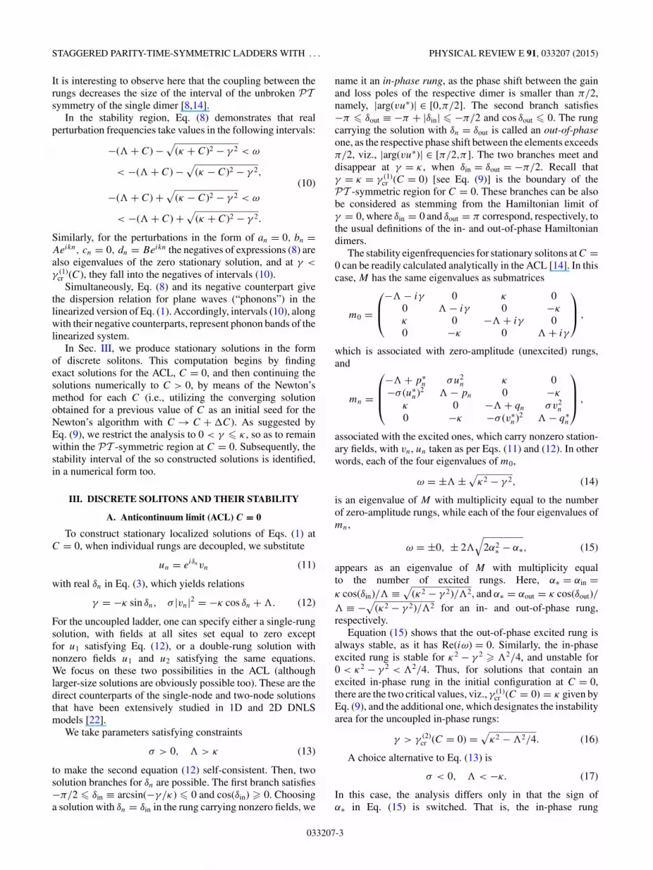
Figure 2 shows |un|2 for the solutions identified by thisprocess on a (base 10) logarithmic scale as a function ofC for parameters taken as per Eq. (13). The logarithmicscale is chosen, as it yields a clearer picture of the variationof the solution’s spatial width, as C varies. The differentsolutions displayed in Fig. 2 include those seeded by the singleexcited in- and out-of-phase rungs (the top row), and two-rungexcitations for which there are three possibilities: in-phase in

n

C

10 0 10

0

1

25

0

n

C

10 0 10

0

1

25

0

n

C

10 0 10

0

1

25

0

n

C

10 0 10

0

1

25

0

n

C

10 0 10

0

0.5

15

0

FIG. 2. (Color online) Plots of log10(|un|2), where un at C =0 is given by Eqs. (11) and (12), and at C > 0 the solitonsolutions un are obtained by the continuation in C (see the text).Common parameters are γ = 1, κ = 1.9, and σ = 1. The initialconfiguration of the excited rungs at C = 0 and parameters are asingle in-phase rung with δ1 = δin, = 2.5, N = 40, �C = 0.001(top left), a single out-of-phase rung with δ1 = δout, = 2.5,N =40, �C = 0.001 (top right), two in-phase rungs with δ1 = δ2 = δin, = 2, N = 80, �C = 0.001 (middle left), two out-of-phase rungswith δ1 = δ2 = δout, = 2.5, N = 80, �C = 0.001 (middle right),and, finally, a mixed state carried by two rungs with δ1 = δin,δ2 = δout, = 2.5, N = 80, �C = 0.000 01 (bottom center). Plotsof log10(|vn|2) are identical to those of log10(|un|2). As C increases,small amplitudes appear at adjacent rungs, and the soliton gains width.The corresponding second moment w(C), defined as per Eq. (18), isshown in Fig. 4. The stability of the solitons shown here is predictedby eigenvalue plots displayed in Fig. 12 for γ = 1.

20 10 0 100

1

2

n

|un|2 ,|v

n|2

20 10 0 100

5

n

|un|2 ,|v

n|2

20 10 0 100

0.5

n

|un|2 ,|v

n|2

20 10 0 100

5

n

|un|2 ,|v

n|2

20 10 0 100

5

n

|un|2 ,|v

n|2

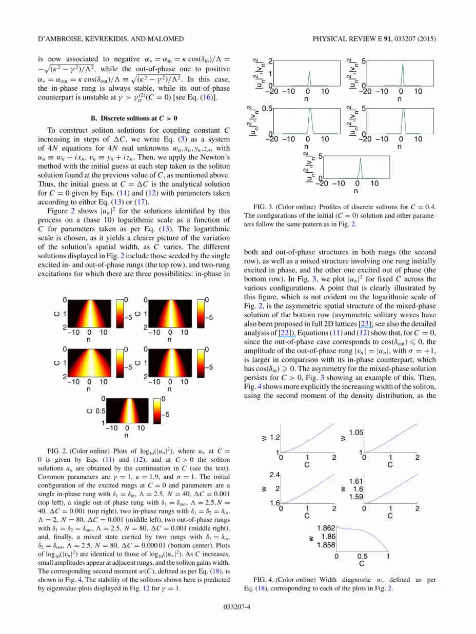
FIG. 3. (Color online) Profiles of discrete solitons for C = 0.4.The configurations of the initial (C = 0) solution and other parame-ters follow the same pattern as in Fig. 2.

both and out-of-phase structures in both rungs (the secondrow), as well as a mixed structure involving one rung initiallyexcited in phase, and the other one excited out of phase (thebottom row). In Fig. 3, we plot |un|2 for fixed C across thevarious configurations. A point that is clearly illustrated bythis figure, which is not evident on the logarithmic scale ofFig. 2, is the asymmetric spatial structure of the mixed-phasesolution of the bottom row (asymmetric solitary waves havealso been proposed in full 2D lattices [23]; see also the detailedanalysis of [22]). Equations (11) and (12) show that, for C = 0,since the out-of-phase case corresponds to cos(δout) � 0, theamplitude of the out-of-phase rung |vn| = |un|, with σ = +1,is larger in comparison with its in-phase counterpart, whichhas cos(δin) � 0. The asymmetry for the mixed-phase solutionpersists for C > 0, Fig. 3 showing an example of this. Then,Fig. 4 shows more explicitly the increasing width of the soliton,using the second moment of the density distribution, as the

0 1 21

1.2

C

w

0 1 21

1.05

C

w

0 1 21.6

2

2.4

C

w

0 1 2

1.591.6

1.61

C

w

0 0.5 1

1.8581.86

1.862

C

w

FIG. 4. (Color online) Width diagnostic w, defined as perEq. (18), corresponding to each of the plots in Fig. 2.

033207-4

STAGGERED PARITY-TIME-SYMMETRIC LADDERS WITH . . . PHYSICAL REVIEW E 91, 033207 (2015)

n

C

10 0 10

0

1

20.10.20.30.40.5

n

C

10 0 10

0

1

2 0

1

2

n

C

10 0 10

0

1

20.10.20.30.40.5

n

C10 0 10

0

1

2 0

1

2

n

C

10 0 10

0

0.5

1 0.511.522.5

FIG. 5. (Color online) The phase shift between two edges of therungs |arg(vnu

∗n)|, plotted as a function of C and n, where u is the

solution whose absolute value is presented in Fig. 2. The value of|arg(vnu

∗n)| is set to zero for any n at which log10(|u|2) � −6 in

Fig. 2. In other words, the phase shift is shown as equal to zerowhen the amplitude is too small. For the top left and middle leftplots, the soliton’s field is different from zero at one or two in-phase rung(s) when C = 0, and as C increases the solutions stay inphase. For the top right and middle right plots, the field at C = 0 isnonzero and out of phase at the one or two central rungs, and, as C

increases, the fields at these rungs, and at two rungs on either side ofthe central ones, tend to be out of phase, while the field at other rungs,located farther away, tend to be in phase. Similarly, in the bottom plot,where at C = 0 the n = 1 rung is in phase and the n = 2 one is outof phase, as C increases, most rungs tend to be in phase, exceptfor n = 2,3.

respective diagnostic,

w(C) ≡√∑

n n2|un|2∑n |un|2 (18)

versus C for the solutions shown in Fig. 2. It is relevant topoint out that the variation of this width-measuring quantity isfairly weak in the case of the out-of-phase solutions and mixedones, while it is more significant in the case of the single anddouble in-phase excited rungs.

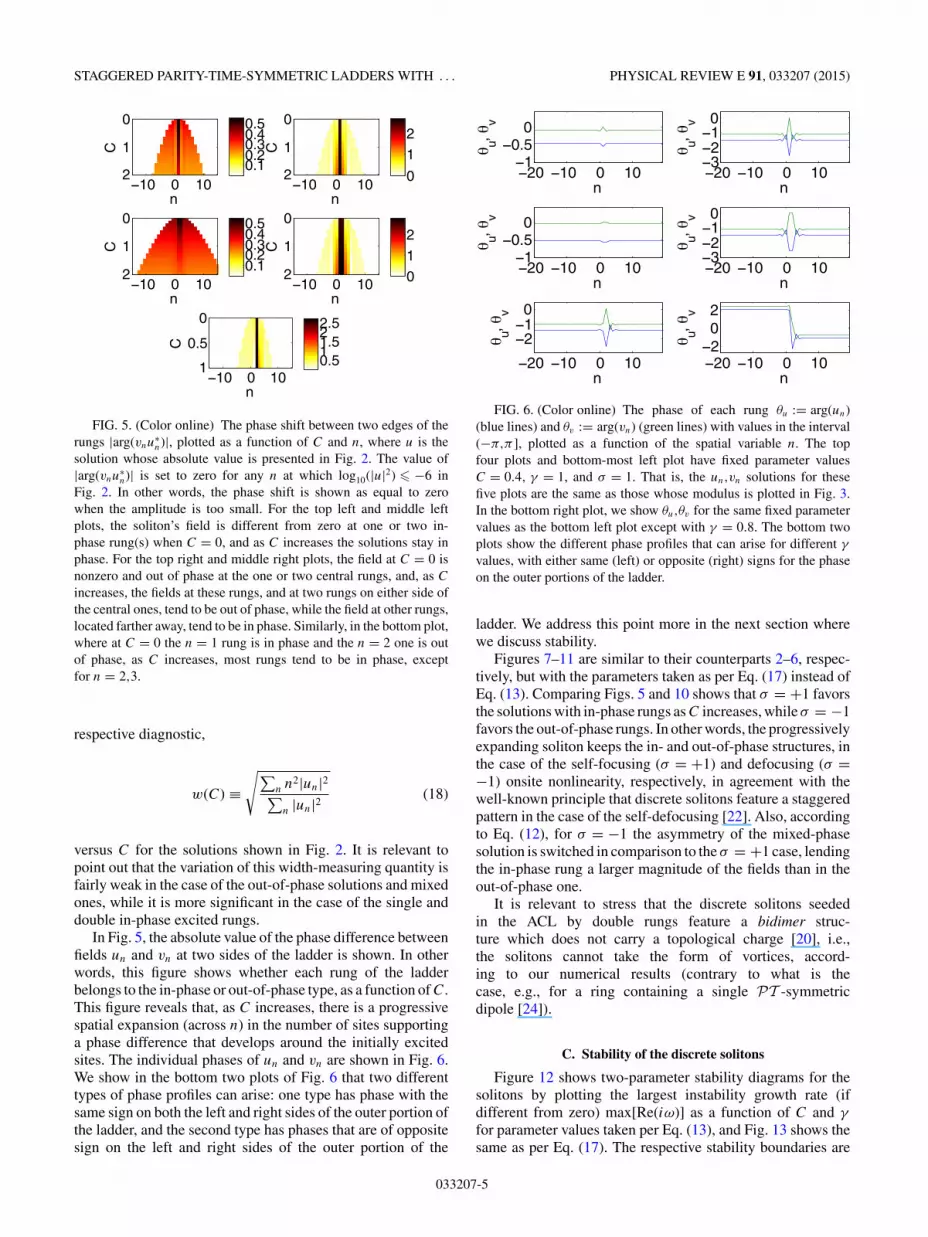
In Fig. 5, the absolute value of the phase difference betweenfields un and vn at two sides of the ladder is shown. In otherwords, this figure shows whether each rung of the ladderbelongs to the in-phase or out-of-phase type, as a function of C.This figure reveals that, as C increases, there is a progressivespatial expansion (across n) in the number of sites supportinga phase difference that develops around the initially excitedsites. The individual phases of un and vn are shown in Fig. 6.We show in the bottom two plots of Fig. 6 that two differenttypes of phase profiles can arise: one type has phase with thesame sign on both the left and right sides of the outer portion ofthe ladder, and the second type has phases that are of oppositesign on the left and right sides of the outer portion of the

20 10 0 101

0.50

n

u, v

20 10 0 103210

n

u, v

20 10 0 101

0.50

n

u, v

20 10 0 103210

n

u, v

20 10 0 10

210

n

u, v

20 10 0 10202

n

u, v

FIG. 6. (Color online) The phase of each rung θu := arg(un)(blue lines) and θv := arg(vn) (green lines) with values in the interval(−π,π ], plotted as a function of the spatial variable n. The topfour plots and bottom-most left plot have fixed parameter valuesC = 0.4, γ = 1, and σ = 1. That is, the un,vn solutions for thesefive plots are the same as those whose modulus is plotted in Fig. 3.In the bottom right plot, we show θu,θv for the same fixed parametervalues as the bottom left plot except with γ = 0.8. The bottom twoplots show the different phase profiles that can arise for different γ

values, with either same (left) or opposite (right) signs for the phaseon the outer portions of the ladder.

ladder. We address this point more in the next section wherewe discuss stability.

Figures 7–11 are similar to their counterparts 2–6, respec-tively, but with the parameters taken as per Eq. (17) instead ofEq. (13). Comparing Figs. 5 and 10 shows that σ = +1 favorsthe solutions with in-phase rungs as C increases, while σ = −1favors the out-of-phase rungs. In other words, the progressivelyexpanding soliton keeps the in- and out-of-phase structures, inthe case of the self-focusing (σ = +1) and defocusing (σ =−1) onsite nonlinearity, respectively, in agreement with thewell-known principle that discrete solitons feature a staggeredpattern in the case of the self-defocusing [22]. Also, accordingto Eq. (12), for σ = −1 the asymmetry of the mixed-phasesolution is switched in comparison to the σ = +1 case, lendingthe in-phase rung a larger magnitude of the fields than in theout-of-phase one.

It is relevant to stress that the discrete solitons seededin the ACL by double rungs feature a bidimer struc-ture which does not carry a topological charge [20], i.e.,the solitons cannot take the form of vortices, accord-ing to our numerical results (contrary to what is thecase, e.g., for a ring containing a single PT -symmetricdipole [24]).

C. Stability of the discrete solitons

Figure 12 shows two-parameter stability diagrams for thesolitons by plotting the largest instability growth rate (ifdifferent from zero) max[Re(iω)] as a function of C and γ

for parameter values taken per Eq. (13), and Fig. 13 shows thesame as per Eq. (17). The respective stability boundaries are

033207-5

D’AMBROISE, KEVREKIDIS, AND MALOMED PHYSICAL REVIEW E 91, 033207 (2015)

n

C

10 0 10

00.5

1 5

0

n

C

10 0 10

00.20.40.6

5

0

n

C

10 0 10

00.5

1 5

0

n

C10 0 10

00.20.40.6

5

0

n

C

10 0 10

0

0.2

0.45

0

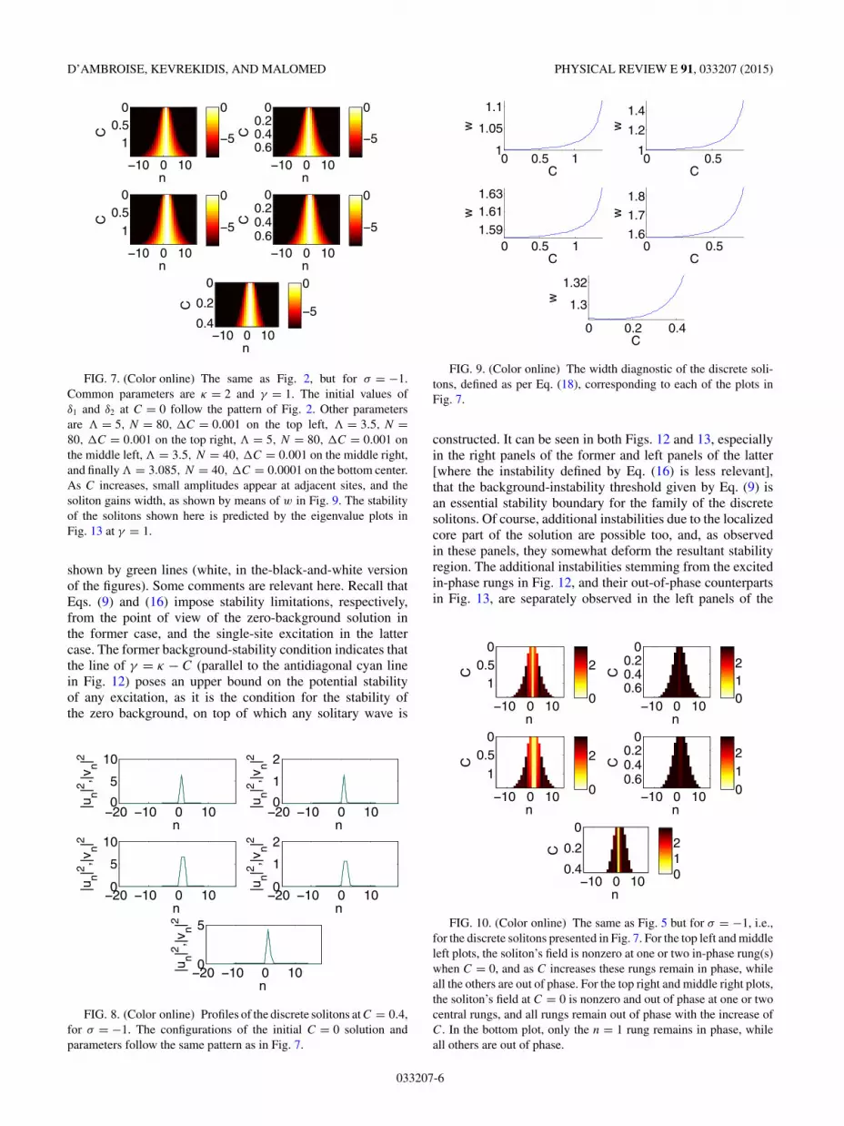
FIG. 7. (Color online) The same as Fig. 2, but for σ = −1.Common parameters are κ = 2 and γ = 1. The initial values ofδ1 and δ2 at C = 0 follow the pattern of Fig. 2. Other parametersare = 5, N = 80, �C = 0.001 on the top left, = 3.5, N =80, �C = 0.001 on the top right, = 5, N = 80, �C = 0.001 onthe middle left, = 3.5, N = 40, �C = 0.001 on the middle right,and finally = 3.085, N = 40, �C = 0.0001 on the bottom center.As C increases, small amplitudes appear at adjacent sites, and thesoliton gains width, as shown by means of w in Fig. 9. The stabilityof the solitons shown here is predicted by the eigenvalue plots inFig. 13 at γ = 1.

shown by green lines (white, in the-black-and-white versionof the figures). Some comments are relevant here. Recall thatEqs. (9) and (16) impose stability limitations, respectively,from the point of view of the zero-background solution inthe former case, and the single-site excitation in the lattercase. The former background-stability condition indicates thatthe line of γ = κ − C (parallel to the antidiagonal cyan linein Fig. 12) poses an upper bound on the potential stabilityof any excitation, as it is the condition for the stability ofthe zero background, on top of which any solitary wave is

20 10 0 100

5

10

n

|un|2 ,|v

n|2

20 10 0 100

1

2

n

|un|2 ,|v

n|2

20 10 0 100

5

10

n

|un|2 ,|v

n|2

20 10 0 100

1

2

n

|un|2 ,|v

n|2

20 10 0 100

5

n

|un|2 ,|v

n|2

FIG. 8. (Color online) Profiles of the discrete solitons at C = 0.4,for σ = −1. The configurations of the initial C = 0 solution andparameters follow the same pattern as in Fig. 7.

0 0.5 11

1.05

1.1

C

w

0 0.51

1.2

1.4

C

w

0 0.5 11.59

1.611.63

C

w

0 0.51.6

1.7

1.8

C

w

0 0.2 0.4

1.3

1.32

C

w

FIG. 9. (Color online) The width diagnostic of the discrete soli-tons, defined as per Eq. (18), corresponding to each of the plots inFig. 7.

constructed. It can be seen in both Figs. 12 and 13, especiallyin the right panels of the former and left panels of the latter[where the instability defined by Eq. (16) is less relevant],that the background-instability threshold given by Eq. (9) isan essential stability boundary for the family of the discretesolitons. Of course, additional instabilities due to the localizedcore part of the solution are possible too, and, as observedin these panels, they somewhat deform the resultant stabilityregion. The additional instabilities stemming from the excitedin-phase rungs in Fig. 12, and their out-of-phase counterpartsin Fig. 13, are separately observed in the left panels of the

n

C

10 0 10

00.5

10

2

n

C

10 0 10

00.20.40.6

012

n

C

10 0 10

00.5

10

2

n

C

10 0 10

00.20.40.6

012

n

C

10 0 10

0

0.2

0.4 012

FIG. 10. (Color online) The same as Fig. 5 but for σ = −1, i.e.,for the discrete solitons presented in Fig. 7. For the top left and middleleft plots, the soliton’s field is nonzero at one or two in-phase rung(s)when C = 0, and as C increases these rungs remain in phase, whileall the others are out of phase. For the top right and middle right plots,the soliton’s field at C = 0 is nonzero and out of phase at one or twocentral rungs, and all rungs remain out of phase with the increase ofC. In the bottom plot, only the n = 1 rung remains in phase, whileall others are out of phase.

033207-6

STAGGERED PARITY-TIME-SYMMETRIC LADDERS WITH . . . PHYSICAL REVIEW E 91, 033207 (2015)

20 10 0 10202

n

u, v

20 10 0 102101

n

u, v

20 10 0 10202

n

u, v

20 10 0 10

210

nu,

v

20 10 0 10202

n

u, v

FIG. 11. (Color online) The phase of each rung θu := arg(un)(blue lines) and θv := arg(vn) (green lines) in the interval (−π,π ],plotted as a function of the spatial variable n for the fixed parametervalues C = 0.4, γ = 1, and σ = −1. That is, the un,vn solutions arethe same as those whole modulus is plotted in Fig. 8.

former figure and right panels of the latter one. Given thatthis critical point was found in the framework of the ACL,it features no C dependence, but it clearly contributes todelimiting the stability boundaries of the discrete solitons;sometimes, this effect is fairly dramatic, as in the middle-rowleft and right panels of Figs. 12 and 13, respectively, i.e.,the two-site, same-phase excitations may be susceptible tothis instability mechanism. Although the precise stabilitythresholds may be fairly complex, arising from the interplay oflocalized and extended modes in the nonlinear ladder system,a general conclusion is that the above-mentioned instabilitiesplay a critical role for the stability of the localized states inthis system (see also the discussion below). Another essentialconclusion is that the higher the coupling (C), the less robustthe corresponding solutions are likely to be, the destabilizationcaused by the increase of C being sometimes fairly dramatic.

The values of iω whose maximum real part is represented inFigs. 12 and 13 were computed with the help of an appropriatenumerical eigenvalue solver. At C = 0, the eigenvalues agreewith Eqs. (14) and (15). As shown in Figs. 14 and 15, followingthe variation of C and γ , eigenvalues (14), associated withthe empty (zero-value) sites, vary in accordance with theprediction of Eq. (8), and eigenvalues (15), associated withexcited rungs, also shift in the complex plane upon variation ofC,γ . In the case of the mixed-phase solutions with asymmetricamplitude (seen in the bottom-most plot of Fig. 3), there is astable region for low values of the parameters C and γ . Forlarger values of γ , there are parametric intervals (across C > 0for fixed γ ) in which discrete solitons with phase profilesdifferent from those initialized in the ACL of C = 0 havebeen identified; see the bottom two plots in Fig. 6. Thesedistinct branches of the unstable solutions give rise to “streaks”observed in the bottom middle panel of Fig. 12. The amplitudeprofiles of such alternate solutions are similar to those shownin the bottom plot of Fig. 3, and the gain in width functiondefined in (18) as a function of C is similar to the examples

C

0 0.5 1 1.5

0

1

2

1

2

3

C

0 0.5 1 1.5

0

1

2 0

0.5

1

1.5

C

0 0.5 1 1.5

0

1

20.511.522.5

C

0 0.5 1 1.5

0

1

2 0

0.5

1

1.5

C0 0.5 1 1.5

0

0.5

1

C

0 0.5 1 1.5

0

1

200

1

2

3

C

0 0.5 1 1.5

0

1

200 0

0.5

1

1.5

C

0 0.5 1 1.5

0

1

200

0.511.522.5

C

0 0.5 1 1.5

0

1

200 0

0.5

1

1.5

C0 0.5 1 1.5

0

0.5

10.511.522.5

FIG. 12. (Color online) The largest instability growth ratemax[Re(iω)], determined by matrix M in Eq. (5), for parametervalues following the same pattern as in Fig. 2, except that here γ variesalong the horizontal axis. In the top two plots in the right column,the cyan line represents the analytically predicted critical valueγ (1)

cr (C) = κ − C; this line originates from the cyan dot in the cornerat γ (1)

cr (0) = κ [see Eq. (9)]. If an in-phase excited rung is present, thenthe second cyan dot is located at γ (2)

cr = √κ2 − 2/4, in accordance

with Eq. (16). Green lines indicate stability boundaries, between thedark region corresponding to stability {or very weak instability, withmax[Re(iω)] < 10−3}, and the bright region corresponding to theinstability.

shown in the bottom plots of Figs. 2 and 4. Mechanisms bywhich solutions become unstable for these alternate solutionsare outlined below.

The most obvious type of the instability is associated withinitializing a solution at C = 0 from a single unstable rung,i.e., at γ > γ (2)

cr (C = 0) in (16). Eigenvalues for this type of theinstability are shown in the top two panels of Fig. 15. There arethree other scenarios of destabilization of the discrete solitonswith the increase of C, each corresponding to a particulartype of a critical point (transition to the instability). Thesetransitions are demonstrated in Figs. 14 and 15. The firsttype occurs when eigenvalue ω associated with an excitedrung collides with one of the intervals in Eq. (10). Thisweak instability generates an eigenfrequency quartet and isrepresented in Figs. 12 and 13, where the green boundarydeviates (as C increases from 0) from the threshold given byEq. (16). Figures 14 and 15 illustrate this type of transition inmore detail by plotting the eigenvalues directly in the complexplane.

033207-7

D’AMBROISE, KEVREKIDIS, AND MALOMED PHYSICAL REVIEW E 91, 033207 (2015)C

0 0.5 1 1.5

0

0.5

1

0

0.5

1

1.5

C

0 0.5 1 1.5

0

0.2

0.4

0.60

1

2

C

0 0.5 1 1.5

0

0.5

1

0

0.5

1

1.5

C

0 0.5 1 1.5

0

0.2

0.4

0.6 0.511.522.5

C

0 0.5 1 1.5

0

0.2

0.40.511.52

FIG. 13. (Color online) The same as in Fig. 12, but for parametervalues from Fig. 7. Here, the cyan line is drawn on the top two plotsin the left column, and the second cyan dot on the C = 0 axis appearsonly in the case where the out-of-phase excited rung is present atC = 0.

The second type of the transition occurs when the intervalsin Eq. (10) come to overlap at γ = γ (1)

cr (C) [see Eq. (9)]. This isthe background instability at empty sites, as shown in Figs. 12and 13 by bright spots originating from the corners of thediagrams, where γ = κ = γ (1)

cr (C = 0). A more detailed plotof these eigenvalues and the corresponding collisions in thecomplex eigenvalue plane is displayed in Fig. 14.

The third type of the instability onset occurs for essentiallyall values of C in the case of two in-phase rungs at σ > 0,or two out-of-phase ones at σ < 0. It may be thought of as alocalized instability due to the simultaneous presence of twopotentially unstable elements, due to the instability determinedby Eq. (16). At C > 0, it is seen as the bright spots in Figs. 12and 13 originating from γ (2)

cr (C = 0) =√

κ2 − 2/4. Theeigenvalues emerge from the corresponding zero eigenvaluesat C = 0. That is, in the middle-row left plot of Fig. 12 atC = 0 for γ < γ (2)

cr (C = 0) there are four zero eigenvalues; asC increases, two of the four eigenvalues move from zero ontothe real axis in the complex plane. A similar effect is observedat γ < γ (2)

cr (C = 0) in the middle-row right plot of Fig. 13.Finally, it is worth making one more observation in

connection, e.g., to Fig. 15 and the associated jagged lines inthe top right panel of Fig. 13. Notice that, as C increases, initialstabilization of the mode unstable due to the criterion given byEq. (16) takes place, but then a collision with the continuousspectrum on the imaginary axis provides destabilization anew.It is this cascade of events that accounts for the jaggedness ofthe curve in the top right of Fig. 13 and in similar occurrences

0.1 0 0.15

0

5

Im(i

)

0.1 0 0.15

0

5

0.1 0 0.1

5

0

5

Re(i )

Im(i

)

0.2 0 0.2

5

0

5

Re(i )

FIG. 14. (Color online) Stability eigenvalues iω in the complexplane, for parameters chosen in accordance with the topmost leftpanel of Fig. 12 with γ = 0.5. For C = 0, in the top left plot we showthe agreement of the numerically found eigenvalues (blue circles)with results produced by Eqs. (14) (green filled circles) and (15)(red filled). For C = 0.3, in the top right panel we show that theeigenvalues associated with the zero solution indeed lie within thepredicted intervals (10), the boundaries of which are shown by dashedlines. Next, for C = 1, in the bottom left plot we observe that valuesof iω associated with the excited state have previously (at smaller C)merged with the dashed intervals, and now an unstable quartet hasemerged from the axis. For C = 1.5, in the bottom right panel thecritical point corresponding to Eq. (9) is represented, where unstableeigenvalues emerge from the axis at the values of ±( + C), asthe intervals in Eq. (10) merge. Comparing plots in the bottom row,we conclude that the critical point of the latter type gives rise, ingeneral, to a stronger instability than the former one.

2 0 25

0

5

Im(i

)

2 0 25

0

5

0.1 0 0.15

0

5

Re(i )

Im(i

)

0.5 0 0.55

0

5

Re(i )

FIG. 15. (Color online) The same as in Fig. 14, but for parameterschosen in accordance with the top right panel of Fig. 13, with γ =1.2. At C = 0, in the top left plot we show the agreement of thenumerically found eigenvalues (blue circles) with Eqs. (14) (greenfilled circles) and (15) (red filled). At C = 0.275, in the top rightwe see that eigenvalues associated to the red x’s have moved inwardtowards zero. Next, for C = 0.3, in the bottom left panel we observethat, after merging with zero, the eigenvalues now emerge from zeroon the imaginary axis. Finally, at C = 0.7 in the bottom right panel,we observe that, after the eigenvalues merge with the dashed-lineintervals, an unstable quartet emerges from the axis.

033207-8

STAGGERED PARITY-TIME-SYMMETRIC LADDERS WITH . . . PHYSICAL REVIEW E 91, 033207 (2015)

20 0 200

0.5

1|

n(0)|

2 , |n(0

)|2

n20 0 200

0.2

0.4

n

|an|2 ,|b

n|2 ,|cn|2 ,|d

n|2

20 0 200

2

4

n|n(1

22)|2 ,|

n(122

)|2

102

0

10

20

t

D1(t

), D

2(t)

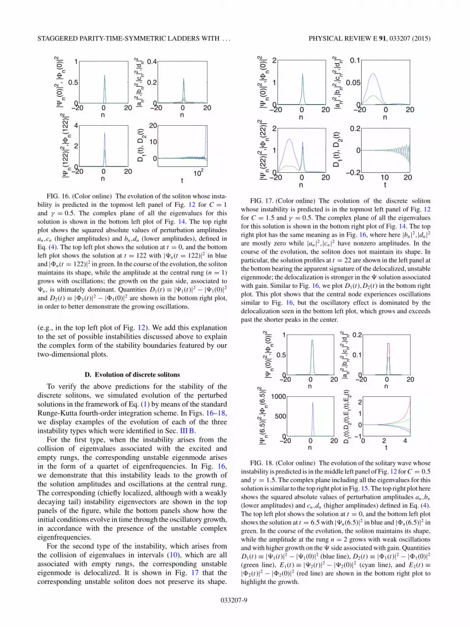
FIG. 16. (Color online) The evolution of the soliton whose insta-bility is predicted in the topmost left panel of Fig. 12 for C = 1and γ = 0.5. The complex plane of all the eigenvalues for thissolution is shown in the bottom left plot of Fig. 14. The top rightplot shows the squared absolute values of perturbation amplitudesan,cn (higher amplitudes) and bn,dn (lower amplitudes), defined inEq. (4). The top left plot shows the solution at t = 0, and the bottomleft plot shows the solution at t = 122 with |�n(t = 122)|2 in blueand |�n(t = 122)|2 in green. In the course of the evolution, the solitonmaintains its shape, while the amplitude at the central rung (n = 1)grows with oscillations; the growth on the gain side, associated to�n, is ultimately dominant. Quantities D1(t) ≡ |�1(t)|2 − |�1(0)|2and D2(t) ≡ |�1(t)|2 − |�1(0)|2 are shown in the bottom right plot,in order to better demonstrate the growing oscillations.

(e.g., in the top left plot of Fig. 12). We add this explanationto the set of possible instabilities discussed above to explainthe complex form of the stability boundaries featured by ourtwo-dimensional plots.

D. Evolution of discrete solitons

To verify the above predictions for the stability of thediscrete solitons, we simulated evolution of the perturbedsolutions in the framework of Eq. (1) by means of the standardRunge-Kutta fourth-order integration scheme. In Figs. 16–18,we display examples of the evolution of each of the threeinstability types which were identified in Sec. III B.

For the first type, when the instability arises from thecollision of eigenvalues associated with the excited andempty rungs, the corresponding unstable eigenmode arisesin the form of a quartet of eigenfrequencies. In Fig. 16,we demonstrate that this instability leads to the growth ofthe solution amplitudes and oscillations at the central rung.The corresponding (chiefly localized, although with a weaklydecaying tail) instability eigenvectors are shown in the toppanels of the figure, while the bottom panels show how theinitial conditions evolve in time through the oscillatory growth,in accordance with the presence of the unstable complexeigenfrequencies.

For the second type of the instability, which arises fromthe collision of eigenvalues in intervals (10), which are allassociated with empty rungs, the corresponding unstableeigenmode is delocalized. It is shown in Fig. 17 that thecorresponding unstable soliton does not preserve its shape.

20 0 200

1

2

|n(0

)|2 ,|

n(0)|

2

n20 0 200

0.05

0.1

n

|an|2 ,|b

n|2 ,|cn|2 ,|d

n|2

20 0 200

1

2

n

|n(2

2)|2 ,|

n(22)

|2

0 10 200.2

0

0.2

t

D1(t

), D

2(t)

FIG. 17. (Color online) The evolution of the discrete solitonwhose instability is predicted is in the topmost left panel of Fig. 12for C = 1.5 and γ = 0.5. The complex plane of all the eigenvaluesfor this solution is shown in the bottom right plot of Fig. 14. The topright plot has the same meaning as in Fig. 16, where here |bn|2,|dn|2are mostly zero while |an|2,|cn|2 have nonzero amplitudes. In thecourse of the evolution, the soliton does not maintain its shape. Inparticular, the solution profiles at t = 22 are shown in the left panel atthe bottom bearing the apparent signature of the delocalized, unstableeigenmode; the delocalization is stronger in the � solution associatedwith gain. Similar to Fig. 16, we plot D1(t),D2(t) in the bottom rightplot. This plot shows that the central node experiences oscillationssimilar to Fig. 16, but the oscillatory effect is dominated by thedelocalization seen in the bottom left plot, which grows and exceedspast the shorter peaks in the center.

20 0 200

0.5

1

|n(0

)|2 ,|

n(0)|

2

n20 0 200

0.1

0.2

n

|an|2 ,|b

n|2 ,|cn|2 ,|d

n|2

20 0 200

500

1000

n

|n(6

.5)|2 ,|

n(6.5

)|2

0 2 41

0

1

2

t

D1(t

),D

2(t),

E1(t

),E

2(t)

FIG. 18. (Color online) The evolution of the solitary wave whoseinstability is predicted is in the middle left panel of Fig. 12 for C = 0.5and γ = 1.5. The complex plane including all the eigenvalues for thissolution is similar to the top right plot in Fig. 15. The top right plot hereshows the squared absolute values of perturbation amplitudes an,bn

(lower amplitudes) and cn,dn (higher amplitudes) defined in Eq. (4).The top left plot shows the solution at t = 0, and the bottom left plotshows the solution at t = 6.5 with |�n(6.5)|2 in blue and |�n(6.5)|2 ingreen. In the course of the evolution, the soliton maintains its shape,while the amplitude at the rung n = 2 grows with weak oscillationsand with higher growth on the � side associated with gain. QuantitiesD1(t) ≡ |�1(t)|2 − |�1(0)|2 (blue line), D2(t) ≡ |�1(t)|2 − |�1(0)|2(green line), E1(t) ≡ |�2(t)|2 − |�2(0)|2 (cyan line), and E2(t) ≡|�2(t)|2 − |�2(0)|2 (red line) are shown in the bottom right plot tohighlight the growth.

033207-9

D’AMBROISE, KEVREKIDIS, AND MALOMED PHYSICAL REVIEW E 91, 033207 (2015)

Instead, the instability causes delocalization of the solution,which acquires a tail reminiscent of the spatial profile of thecorresponding unstable eigenvector.

Lastly, the third type of the instability is shown in Fig. 18.It displays the case of two excited in-phase rungs at σ = 1.Other examples of the same type are similar, e.g., withtwo out-of-phase excited rungs at σ = −1. The instabilityhas a localized manifestation with the amplitudes growingat the gain nodes of each rung and decaying at the lossones.

IV. CONCLUSIONS

We have introduced the lattice of the ladder type with stag-gered pairs of mutually compensated gain and loss elementsat each rung, and the usual onsite cubic nonlinearity, self-focusing or defocusing. This nearly-one-dimensional systemis the simplest one which features two-dimensional PTsymmetry. It may be realized in optics as a waveguide array.We have constructed families of discrete stationary solitonsseeded by a single excited rung, or a pair of adjacent ones,in the anticontinuum limit of uncoupled rungs. The seedexcitations may have the in-phase or out-of-phase structure

in the vertical direction (between the gain and loss poles). Thedouble seed with the in- and out-of-phase structures in thetwo rungs naturally features an asymmetric amplitude profile.We have identified the stability of the discrete solitons via thecalculation of eigenfrequencies for small perturbations, acrossthe system’s parameter space. A part of the soliton familiesare found to be dynamically stable, while unstable solitonsexhibit three distinct scenarios of the evolution. The differentscenarios stem, roughly, from interactions of localized modeswith extended ones, from extended modes alone, or fromlocalized modes alone.

A natural extension of the work may be the considerationof mobility of kicked discrete solitons in the present laddersystem. It may also be interesting to seek nonstationary solitonswith periodic intrinsic switching (cf. Ref. [25]). A challengingperspective is the development of a 2D extension of the system.Effectively, this would entail adding further alternating ladderpairs along the transverse direction and examining 2D discreteconfigurations. It may be relevant in such 2D extensionsto consider different lattice settings that support not onlysolutions in the form of discrete solitary waves, but also onesbuilt as discrete vortices, similarly to what has been earlierdone in the DNLS system [22], and recently in another 2DPT -symmetric system [18].

[1] D. N. Christodoulides, F. Lederer and Y. Silberberg, Discretizinglight behavior in linear and nonlinear waveguide lattices, Nature(London) 424, 817 (2003); F. Lederer, G. I. Stegeman, D.N. Christodoulides, G. Assanto, M. Segev and Y. Silberberg,Discrete solitons in optics, Phys. Rep. 463, 1 (2008); I. L.Garanovich, S. Longhi, A. A. Sukhorukov, and Y. S. Kivshar,Light propagation and localization in modulated photoniclattices and waveguides, ibid. 518, 1 (2012); Z. Chen, M. Segevand D. N. Christodoulides, Optical spatial solitons: Historicaloverview and recent advances, Rep. Prog. Phys. 75, 086401(2012).

[2] B. A. Malomed and P. G. Kevrekidis, Discrete vortex solitons,Phys. Rev. E 64, 026601 (2001); P. G. Kevrekidis, B. A.Malomed, and Yu. B. Gaididei, Solitons in triangular andhoneycomb dynamical lattices with the cubic nonlinearity, ibid.66, 016609 (2002); P. G. Kevrekidis, B. A. Malomed, Z.Chen, and D. J. Frantzeskakis, Stable higher-order vortices andquasivortices in the discrete nonlinear Schrodinger equation,ibid. 70, 056612 (2004); M. Oster and M. Johansson, Stablestationary and quasiperiodic discrete vortex breathers withtopological charge S=2, ibid. 73, 066608 (2006); Mejıa-Cortes,J. M. Soto-Crespo, M. I. Molina, and R. Vicencio, Dissipativevortex solitons in two-dimensional lattices, Phys. Rev. A 82,063818 (2010).

[3] D. Neshev, T. J. Alexander, E. A. Ostrovskaya, Y. S. Kivshar,H. Martin, I. Makasyuk, and Z. Chen, Observation of discretevortex solitons in optically induced photonic lattices, Phys. Rev.Lett. 92, 123903 (2004); J. W. Fleischer, G. Bartal, O. Cohen,O. Manela, M. Segev, J. Hudock, and D. N. Christodoulides,Observation of vortex-ring discrete solitons in 2D photoniclattices, ibid. 92, 123904 (2004); B. Terhalle, T. Richter, A.S. Desyatnikov, D. N. Neshev, W. Krolikowski, F. Kaiser, C.

Denz, and Y. S. Kivshar, Observation of multivortex solitons inphotonic lattices, ibid. 101, 013903 (2008).

[4] D. N. Christodoulides and E. D. Eugenieva, Blocking and rout-ing discrete solitons in two-dimensional networks of nonlinearwaveguide arrays, Phys. Rev. Lett. 87, 233901 (2001).

[5] N. K. Efremidis, S. Sears, D. N. Christodoulides, J. W. Fleischer,and M. Segev, Discrete solitons in photorefractive opticallyinduced photonic lattices, Phys. Rev. E 66, 046602 (2002); J. W.Fleischer, M. Segev, N. K. Efremidis, and D. N. Christodoulides,Observation of two-dimensional discrete solitons in opticallyinduced nonlinear photonic lattices, Nature (London) 422, 147(2003).

[6] A. A. Sukhorukov, Y. S. Kivshar, H. S. Eisenberg, and Y.Silberberg, Spatial optical solitons in waveguide arrays, IEEEJ. Quantum Electron. 39, 31 (2003); A. Szameit, J. Burghoff,T. Pertsch, S. Nolte, A. Tunnermann, and F. Lederer, Two-dimensional soliton in cubic fs laser written waveguide arraysin fused silica, Opt. Express 14, 6055 (2006); A. Szameit andS. Nolte, Discrete optics in femtosecond-laser-written photonicstructures, J. Phys. B: At., Mol. Opt. Phys. 43, 163001 (2010).

[7] T. Schwartz, G. Bartal, S. Fishman, and M. Segev, Transport andAnderson localization in disordered two-dimensional photoniclattices, Nature (London) 446, 52 (2007); Y. Lahini, A. Avidan,F. Pozzi, M. Sorel, R. Morandotti, D. N. Christodoulides, andY. Silberberg, Anderson localization and nonlinearity in one-dimensional disordered photonic lattices, Phys. Rev. Lett. 100,013906 (2008).

[8] A. Ruschhaupt, F. Delgado, and J. G. Muga, Physical realizationof PT -symmetric potential scattering in a planar slab waveg-uide, J. Phys. A: Math. Gen. 38, L171 (2005); K. G. Makris, R.El-Ganainy, D. N. Christodoulides, and Z. H. Musslimani, Beamdynamics in PT symmetric optical lattices, Phys. Rev. Lett.

033207-10

STAGGERED PARITY-TIME-SYMMETRIC LADDERS WITH . . . PHYSICAL REVIEW E 91, 033207 (2015)

100, 103904 (2008); S. Longhi, Spectral singularities and Braggscattering in complex crystals, Phys. Rev. A 81, 022102 (2010);C. E. Ruter, K. G. Makris, R. El-Ganainy, D. N. Christodoulides,M. Segev, and D. Kip, Observation of parity-time symmetry inoptics, Nat. Phys. 6, 192 (2010); K. G. Makris, R. El-Ganainy,D. N. Christodoulides, and Z. H. Musslimani, PT symmetricperiodic optical potentials, Int. J. Theor. Phys. 50, 1019 (2011).

[9] R. Driben and B. A. Malomed, Stability of solitons in parity-time-symmetric couplers, Opt. Lett. 36, 4323 (2011); N. V.Alexeeva, I. V. Barashenkov, A. A. Sukhorukov, and Y. S.Kivshar, Optical solitons in PT-symmetric nonlinear couplerswith gain and loss, Phys. Rev. A 85, 063837 (2012); Yu.V. Bludov, R. Driben, V. V. Konotop, and B. A. Malomed,Instabilities, solitons and rogue waves in PT -coupled nonlinearwaveguides, J. Opt. (Bristol, UK) 15, 064010 (2013).

[10] A. E. Miroshnichenko, B. A. Malomed, and Y. S. Kivshar,Nonlinearly PT -symmetric systems: Spontaneous symmetrybreaking and transmission resonances, Phys. Rev. A 84, 012123(2011); S. V. Dmitriev, S. V. Suchkov, A. A. Sukhorukov, andY. S. Kivshar, Scattering of linear and nonlinear waves in awaveguide array with a PT -symmetric defect, ibid. 84, 013833(2011); S. V. Suchkov, A. A. Sukhorukov, S. V. Dmitriev,and Y. S. Kivshar, Scattering of the discrete solitons on thePT -symmetric defects, Europhys. Lett. 100, 54003 (2012); A.Regensburger, M. A. Miri, C. Bersch, and J. Nager, Observationof defect states in PT -symmetric optical lattices, Phys. Rev.Lett. 110, 223902 (2013).

[11] J. D’Ambroise, P. G. Kevrekidis, and S. Lepri, Asym-metric wave propagation through nonlinear PT -symmetricoligomers, J. Phys. A: Math. Gen. 45, 444012 (2012);,Eigenstates and instabilities of chains with embedded defects,

Chaos 23, 023109 (2013).[12] W. H. Weber and G. W. Ford, Propagation of optical excitations

by dipolar interactions in metal nanoparticle chains, Phys.Rev. B 70, 125429 (2004); P. A. Belov and C. R. Simovski,Homogenization of electromagnetic crystals formed by uniaxialresonant scatterers, Phys Rev. E 72, 026615 (2005); I. V.Shadrivov, A. A. Zharov, N. A. Zharova, Yu. S. Kivshar, Non-linear magnetoinductive waves and domain walls in compositemetamaterials, Photon. Nanostruct. 4, 69 (2006); R. E. Noskov,P. A. Belov and Yu. S. Kivshar, Subwavelength modulationalinstability and plasmon oscillons in nanoparticle arrays, Phys.Rev. Lett. 108, 093901 (2012).

[13] X. Zhang, J. Chai, J. Huang, Z. Chen, Y. Li, and B. A. Malomed,Discrete solitons and scattering of lattice waves in guiding arrayswith a nonlinear PT -symmetric defect, Opt. Express 22, 13927(2014).

[14] K. Li and P. G. Kevrekidis, PT -symmetric oligomers: Ana-lytical solutions, linear stability and nonlinear dynamics, Phys.Rev. E 83, 066608 (2011); D. A. Zezyulin and V. V. Konotop,Nonlinear modes in finite-dimensional PT -symmetric systems,Phys. Rev. Lett. 108, 213906 (2012).

[15] Y. V. Kartashov, B. A. Malomed, and L. Torner, UnbreakablePT symmetry of solitons supported by inhomogeneous defo-cusing nonlinearity, Opt. Lett. 39, 5641 (2014).

[16] S. V. Suchkov, B. A. Malomed, S. V. Dmitriev, and Y. S. Kivshar,Solitons in a chain of PT -invariant dimers, Phys. Rev. E 84,046609 (2011).

[17] S. V. Suchkov, S. V. Dmitriev, B. A. Malomed, andY. S. Kivshar, Wave scattering on a domain wall in achain of PT -symmetric couplers, Phys. Rev. A 85, 033835(2012).

[18] Z. Chen, J. Liu, S. Fu, Y. Li, and B. A. Malomed, Discretesolitons and vortices on two-dimensional lattices of PT -symmetric couplers, Opt. Express 22, 29679 (2014).

[19] K. Li, P. G. Kevrekidis, B. A. Malomed, and U. Gunther,Nonlinear PT -symmetric plaquettes, J. Phys. A: Math. Gen.45, 444021 (2012).

[20] K. Li, P. G. Kevrekidis, and B. A. Malomed, Nonlinearmodes and symmetries in linearly-coupled pairs ofPT -invariantdimers, Stud. Appl. Math. 133, 281 (2014).

[21] I. Szelengowicz, M. A. Hasan, Y. Starosvetsky, A. Vakakis, andC. Daraio, Energy equipartition in two-dimensional granularcrystals with spherical intruders, Phys. Rev. E 87, 032204(2013).

[22] P. G. Kevrekidis, The Discrete Nonlinear Schrodinger Equation:Mathematical Analysis, Numerical Computations, and PhysicalPerspectives (Springer, Berlin, 2009).

[23] T. J. Alexander, A. A. Sukhorukov, Yu. S. Kivshar, Asymmetricvortex solitons in nonlinear periodic lattices, Phys. Rev. Lett.93, 063901 (2004).

[24] D. Leykam, V. V. Konotop, and A. S. Desyatnikov, Discretevortex solitons and parity time symmetry, Opt. Lett. 38, 371(2013).

[25] A. S. Desyatnikov, M. R. Dennis, and A. Ferrando, All-opticaldiscrete vortex switch, Phys. Rev. A 83, 063822 (2011).

033207-11