Form 836 (7/06)

LA-UR- Approved for public release;

distribution is unlimited.

Los Alamos National Laboratory, an affirmative action/equal opportunity employer, is operated by the Los Alamos National Security, LLC

for the National Nuclear Security Administration of the U.S. Department of Energy under contract DE-AC52-06NA25396. By acceptance

of this article, the publisher recognizes that the U.S. Government retains a nonexclusive, royalty-free license to publish or reproduce the

published form of this contribution, or to allow others to do so, for U.S. Government purposes. Los Alamos National Laboratory requests

that the publisher identify this article as work performed under the auspices of the U.S. Department of Energy. Los Alamos National

Laboratory strongly supports academic freedom and a researcher’s right to publish; as an institution, however, the Laboratory does not

endorse the viewpoint of a publication or guarantee its technical correctness.

Title:

Author(s):

Intended for:

09-02630

Reduced-Dissipation Remapping of Velocity in StaggeredArbitrary Lagrangian-Eulerian Methods

David Bailey, Markus Berndt, Milan Kucharik, MikhailShashkov

Submitted to Journal of Computational Physics

Reduced-Dissipation Remapping of Velocity

in Staggered Arbitrary Lagrangian-Eulerian

Methods

David Bailey a Markus Berndt b Milan Kucharik c

Mikhail Shashkov d

aLawrence Livermore National Laboratory, P.O. Box 808 L-016, Livermore, CA

94551, USA, dsb@llnl.gov

bTheoretical Division, T-5, Los Alamos National Laboratory MS-B284, Los

Alamos, NM. 87545, USA, berndt@lanl.gov

cTheoretical Division, T-5, Los Alamos National Laboratory MS-B284, Los

Alamos, NM. 87545, USA, kucharik@lanl.gov,

kucharik@karkulka.fjfi.cvut.cz

dTheoretical Division, T-5, Los Alamos National Laboratory MS-B284, Los

Alamos, NM. 87545, USA, shashkov@lanl.gov

Abstract

Remapping is an essential part of most Arbitrary Lagrangian-Eulerian (ALE) meth-ods. In this paper, we focus on the part of the remapping algorithm that performsthe interpolation of the fluid velocity field from the Lagrangian to the rezoned com-putational mesh in the context of a staggered discretization. Standard remappingalgorithms generate a discrepancy between the remapped kinetic energy, and thekinetic energy that is obtained from the remapped nodal velocities which conservesmomentum. In most ALE codes, this discrepancy is redistributed to the internalenergy of adjacent computational cells which allows for the conservation of totalenergy. This approach can introduce oscillations in the internal energy field, whichmay not be acceptable. We analyze the approach introduced in [1] which is not sup-posed to introduce dissipation. On a simple example, we demonstrate a situationin which this approach fails. A modification of this approach is described, whicheliminates (when it is possible) or reduces the energy discrepancy.

Key words:

Conservative Interpolations, Staggered Discretization, Flux-Based Remap,Velocity Remap.

Preprint submitted to Journal of Computational and Applied Mathematics16 April 2009

1 Introduction

Arbitrary Lagrangian-Eulerian (ALE) methods introduced in [6] appear tobe a reasonable compromise between Lagrangian and Eulerian approaches,allowing to solve a large variety of fluid problems. The standard ALE algorithmuses a Lagrangian solver to update fluid quantities and the computationalmesh in the next time step, which can eventually tangle the mesh. To avoidsuch problems, mesh regularization (untangling or smoothing) is applied in thecase of low mesh quality, followed by a remapping step that interpolates allfluid quantities from the Lagrangian to the smoothed mesh. Many authors havedescribed ALE strategies to optimize accuracy, robustness, or computationalefficiency, see for example [2,9,7,12].

It is possible to formulate the ALE scheme as a single algorithm [5] based onsolving the equations in a moving coordinate frame. For fluid flows, it is com-mon to separate the ALE scheme into three separate stages, 1) a Lagrangianstage in which the solution and computational mesh are updated; 2) a re-zoning stage in which the nodes of the computational mesh are moved to amore optimal position; and 3) a remapping stage in which the Lagrangiansolution is interpolated onto the rezoned mesh. Here, we focus on the last partof the ALE algorithm – remapping – in the case of a staggered discretization,where scalar quantities (density, pressure, specific internal energy) are definedinside mesh cells, and vector quantities (positions, velocities) are defined atmesh nodes [3]. A staggered discretization is used in most current ALE codes.Any proper remapping method must conserve mass, momentum, and totalenergy. Remapping of cell quantities in a flux form is described for examplein [10,11,8], here, we focus on the remap of the nodal momenta/velocities.Generally, remapped nodal kinetic energy is not equal to nodal kinetic energyobtained from remapped velocities (usually obtained from momentum conser-vation equation in a flux form). This discrepancy leads to energy conservationviolation and consequently to wrong shock speeds. Conservation of total en-ergy is usually restored by redistributing the kinetic energy discrepancy tothe internal energy of adjacent cells [2], which can violate smoothness of theinternal energy field.

In an alternative approach introduced in [1], the remapped nodal kinetic en-ergy is expressed in a flux form derived from the conservation of momentumand implies some constraints on momentum fluxes. Its conservation is thus en-forced, and dissipation in the remapping process is eliminated. This approachrequires the solution of a global system of coupled non-linear equations.

This paper has three main goals:

(1) illustrate that approach [1] does not always work;

2

(2) describe an alternative approach, which yields the same solution as [1]when it exists and reduces dissipation if it does not;

(3) highlight that this alternative approach can be used to get high-orderfluxes in the context of FCT-like (flux corrected transport) remapping toimprove accuracy but stay in bounds for velocity.

Only the 1D case and 1D examples are discussed in this paper. However, thisapproach is generalizable into multiple dimensions, and we implemented thisin our Research Multi-Material ALE (RMALE) code.

2 Flux Form of Nodal Mass Remapping

In this paper, we use integer enumeration for mesh nodes, and half-integersfor mesh cells, as shown in Figure 1. The nodal mass in node i is remapped

ii−1 i+1i+1/2i−1/2

Fig. 1. Enumeration of nodes (black) and cells (red) of the 1D computational mesh.Coordinates of cell centers (red circles) computed by averaging of involved nodalcoordinates.

in a standard flux form

mi = mi + F mi+1/2 − F m

i−1/2 . (1)

where F mi+1/2

represents an oriented mass flux from node i to a neighboringnode i + 1. The tilde denotes the remapped quantity (mass) in the new node.

The inter-nodal mass fluxes can be computed in several ways. The most nat-ural way is based on intersecting the Lagrangian and rezoned nodal controlvolumes, and integrating the reconstructed cell density profile here to obtainthe mass flux. This is simple in 1D but difficult to generalize to 2D, where itleads to intersections of similar, generally non-convex polygons. Another ap-proach is based on the interpolation of inter-nodal mass fluxes from inter-cellmass fluxes, as described in [13]. When inter-nodal mass fluxes are computed,all nodal quantities can then be remapped in an analogous flux form, where thefluxes of a particular quantity are constructed by multiplying the mass fluxesby the value of the reconstructed quantity per unit mass. This is demonstratedin the next section for nodal momentum. For the purpose of this paper, theparticular method for computation of inter-nodal mass flux F m is not impor-tant. Though, in real calculations, it can be complicated to compute the massfluxes correctly (better than first order accurate).

3

3 Flux Form of Momentum Remapping

The remap of momentum can be performed in the flux form

µi = mi ui = mi ui + F µi+1/2

− F µi−1/2

, (2)

defining the remapped nodal velocity u. This formula guarantees global con-servation of momentum.

In our approach, the momentum flux is obtained by multiplication of the massfluxes by the flux velocities,

F µi+1/2

= F mi+1/2 u∗

i+1/2 . (3)

The flux velocities u∗

i+1/2must be defined. The new nodal velocity is then

computed as ui = µi/mi.

It is straightforward that this approach satisfies the DeBar condition [4,2],which is usually understood as a condition for self-consistency of a velocityremapping method. Suppose that we have a constant velocity field un = u andan arbitrary density field. After an arbitrary mesh movement, the remappingprocess must reproduce the constant velocity field. Any velocity reconstructionmethod will yield u∗ = u for all flux velocities, so u can be factored from thewhole right hand side of (2). The rest of the right hand side correspondsexactly to the new nodal mass (1), which cancels with the denominator inthe expression of the new velocity formula. Thus, with the momentum flux inform (3), the remapping algorithm preserves the constant velocity field and isDeBar-consistent under the condition that the velocity reconstruction methodpreserves it also.

The only remaining question is how to define flux velocities u∗. Several meth-ods exist for the low- or high-order definition of u∗. We focus here on a high-order velocity reconstruction method potentially conserving global nodal ki-netic energy.

4 Kinetic Energy “Conserving” Remapping

In this section, we describe the high-order velocity definition algorithm thatconserves global nodal kinetic energy, introduced in [1]. We will describe thederivation of the system and show a simple 1D example, for which the solutionof this system does not exist. We will also suggest a modification of the system,which has the same solution as the solution of the original system if it exists.

4

This modification reduces the kinetic energy discrepancy, even in the casewhen the solution of the original system does not exist.

4.1 System Derivation

As the original paper [1] was published in a not easily accessible journal, werepeat the derivation of the system here. We substitute the old nodal massin the momentum update formula (2) by the nodal mass update formula (1),and we obtain

mi ui =(mi − F m

i+1/2 + F mi−1/2

)ui + F m

i+1/2 u∗

i+1/2 − F mi−1/2 u∗

i−1/2 , (4)

and after moving the first term to the left hand side, we can rewrite theexpression as

mi (ui − ui) = F mi+1/2

(u∗

i+1/2 − ui

)− F m

i−1/2

(u∗

i−1/2 − ui

). (5)

Now, we multiply this equation with

ui =ui + ui

2(6)

and we obtain

mi

(u2

i

2−

u2i

2

)= F m

i+1/2

(u∗

i+1/2 − ui

)ui − F m

i−1/2

(u∗

i−1/2 − ui

)ui . (7)

To obtain the difference between new and old nodal kinetic energy on the lefthand side, we add (mi − mi) u2

i /2 to the equation, and get

Ki − Ki =1

2mi u

2i −

1

2mi u

2i

=1

2(mi − mi) u2

i + F mi+1/2

(u∗

i+1/2 − ui

)ui

− F mi−1/2

(u∗

i−1/2 − ui

)ui .

(8)

After substituting for mi from (1), we can rewrite the expression as

Ki − Ki = F mi+1/2

((u∗

i+1/2 − ui

)ui +

u2i

2

)

− F mi−1/2

((u∗

i−1/2 − ui

)ui +

u2i

2

).

(9)

We require the nodal kinetic energy in the flux form

Ki = Ki + F Ki+1/2 − F K

i−1/2 . (10)

5

To guarantee global conservation of the nodal kinetic energy, a particular fluxviewed from both involved nodes must have the same value, which for examplefor flux F K

i+1/2means

(u∗

i+1/2 − ui

)ui +

u2i

2=(u∗

i+1/2 − ui+1

)ui+1 +

u2i+1

2, (11)

and, analogously for all other fluxes. After solving the equation for the fluxvelocity u∗

i+1/2, we obtain the final expression

u∗

i+1/2 =ui+1 ui+1 − ui ui −

(u2

i+1 − u2i

)/2

ui+1 − ui. (12)

Finally, we have a system of three types of equations (12), (6), and (2).Thissystem can be solved for the set of unknowns {u∗, u, u} and its solution definesthe flux velocities u∗.

A simple fixed point iteration process can be used as a solver. The initial guessfor u∗ can be computed as an average of adjacent nodal velocities, for example

u∗,κ=0

i+1/2=

1

2(ui + ui+1) , (13)

where κ represents the iteration index. The iterative process is then

uκi =

1

mi

(mi ui + F m

i+1/2 u∗,κ−1

i+1/2− F m

i−1/2 u∗,κ−1

i−1/2

), (14)

uκi =

uκi + ui

2, (15)

u∗,κi+1/2

=ui+1 uκ

i+1 − ui uκi −

(u2

i+1 − u2i

)/2

ui+1 − ui

. (16)

In the first step of the iterative process, we use this initial guess for the updateof nodal velocities using the momentum formula (14). In the second step, allu are updated as in (15). Finally, in the third step, the u∗,κ are updatedaccording to (16) (and similarly for other flux velocities), and we can startthe first step of the next iteration. Due to the construction of the system, itssolution must have the same kinetic energy as the old (Lagrangian) kineticenergy. This allows us to choose the stopping criteria in the form

∣∣∣∣Kκ − K

K

∣∣∣∣ < ǫ , (17)

where the tolerance for the kinetic energy discrepancy ǫ is chosen on the order

6

of 10−14 − 10−10, and the nodal kinetic energies are computed as

K =∑

∀n

1

2mn u2

n , (18)

Kκ =∑

∀n

1

2mn (uκ

n)2 . (19)

An alternative approach to solving this system is based on the construction ofa vector function by moving the left hand side of (11) to the right hand side,

~Fi+1/2 (u∗, u) =(u∗

i+1/2 − ui+1

)ui+1 +

u2i+1

2−(u∗

i+1/2 − ui

)ui +

u2i

2. (20)

After substituting for u from (6), and for u from (2), the function ~F onlydepends on u∗. In (20), only one component of the vector function is shown,but similar expressions are constructed for all other fluxes. Even though thisfunction has a local stencil, it is relatively large, especially in multiple dimen-sions. System (20) is basically system of coupled quadratic equations of thegeneral form

~F (~u∗) = ~0 (21)

which can be solved using a Newton solver. We omit the explicit computationof the Jacobian of F as required by the classic Newton’s method, and insteademploy the Jacobian Free Newton Krylov (JFNK) method. In practice, we usethe JFNK implementation in the NITSOL package [14].

4.2 Counter-Example – Non-Existent Solution

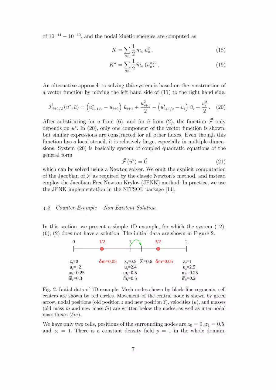
In this section, we present a simple 1D example, for which the system (12),(6), (2) does not have a solution. The initial data are shown in Figure 2.

m =0.250

m =0.3~0

m =0.51

m =0.5~1

m =0.252

m =0.2~2

~0 1 2

u =−2 u =2.4 u =2.50 1 2

1z =0 z =0.5 z =0.6 z =1

0 1/2 1 3/2 2

δ δm=0.05 m=0.05

Fig. 2. Initial data of 1D example. Mesh nodes shown by black line segments, cellcenters are shown by red circles. Movement of the central node is shown by greenarrow, nodal positions (old position z and new position z), velocities (u), and masses(old mass m and new mass m) are written below the nodes, as well as inter-nodalmass fluxes (δm).

We have only two cells, positions of the surrounding nodes are z0 = 0, z1 = 0.5,and z2 = 1. There is a constant density field ρ = 1 in the whole domain,

7

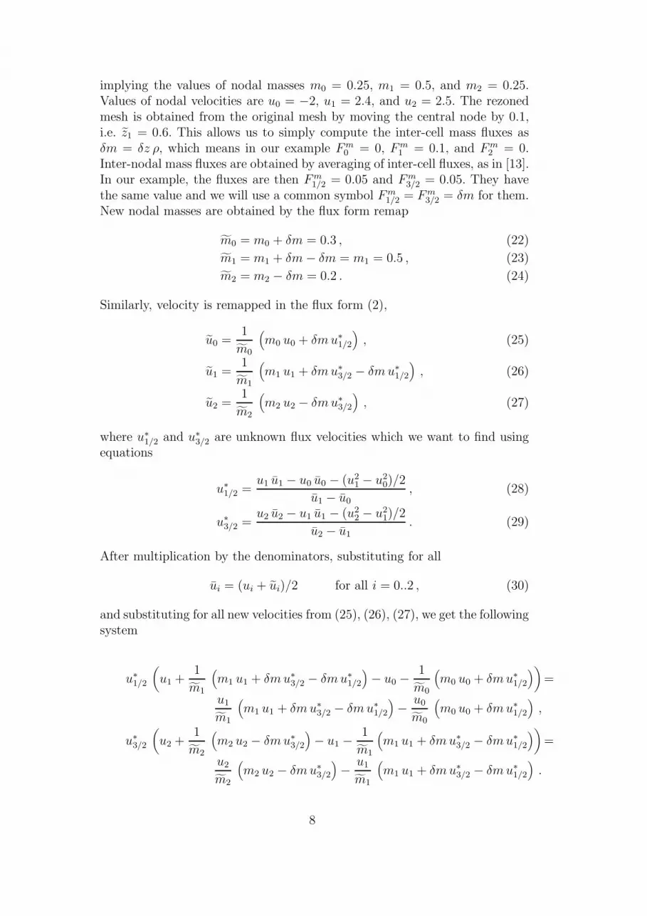
implying the values of nodal masses m0 = 0.25, m1 = 0.5, and m2 = 0.25.Values of nodal velocities are u0 = −2, u1 = 2.4, and u2 = 2.5. The rezonedmesh is obtained from the original mesh by moving the central node by 0.1,i.e. z1 = 0.6. This allows us to simply compute the inter-cell mass fluxes asδm = δz ρ, which means in our example F m

0 = 0, F m1 = 0.1, and F m

2 = 0.Inter-nodal mass fluxes are obtained by averaging of inter-cell fluxes, as in [13].In our example, the fluxes are then F m

1/2= 0.05 and F m

3/2= 0.05. They have

the same value and we will use a common symbol F m1/2

= F m3/2

= δm for them.New nodal masses are obtained by the flux form remap

m0 = m0 + δm = 0.3 , (22)

m1 = m1 + δm − δm = m1 = 0.5 , (23)

m2 = m2 − δm = 0.2 . (24)

Similarly, velocity is remapped in the flux form (2),

u0 =1

m0

(m0 u0 + δm u∗

1/2

), (25)

u1 =1

m1

(m1 u1 + δm u∗

3/2 − δm u∗

1/2

), (26)

u2 =1

m2

(m2 u2 − δm u∗

3/2

), (27)

where u∗

1/2and u∗

3/2are unknown flux velocities which we want to find using

equations

u∗

1/2 =u1 u1 − u0 u0 − (u2

1 − u20)/2

u1 − u0

, (28)

u∗

3/2 =u2 u2 − u1 u1 − (u2

2 − u21)/2

u2 − u1

. (29)

After multiplication by the denominators, substituting for all

ui = (ui + ui)/2 for all i = 0..2 , (30)

and substituting for all new velocities from (25), (26), (27), we get the followingsystem

u∗

1/2

(u1 +

1

m1

(m1 u1 + δm u∗

3/2 − δm u∗

1/2

)− u0 −

1

m0

(m0 u0 + δm u∗

1/2

))=

u1

m1

(m1 u1 + δm u∗

3/2 − δm u∗

1/2

)−

u0

m0

(m0 u0 + δm u∗

1/2

),

u∗

3/2

(u2 +

1

m2

(m2 u2 − δm u∗

3/2

)− u1 −

1

m1

(m1 u1 + δm u∗

3/2 − δm u∗

1/2

))=

u2

m2

(m2 u2 − δm u∗

3/2

)−

u1

m1

(m1 u1 + δm u∗

3/2 − δm u∗

1/2

).

8

We construct a vector of solutions ~x = [x1, x2] = [u∗

1/2, u∗

3/2]. By subtracting

the right hand side of the system, we can then rewrite the previous system inthe form

~F(~x) = ~0 , (31)

where

F1(x1, x2) = C11 x2

1 + C21 x1 x2 + C3

1 x1 + C41 x2 + C5

1 , (32)

F2(x1, x2) = C12 x2

2 + C22 x1 x2 + C3

2 x1 + C42 x2 + C5

2 , (33)

and where the constants are

C11 = −

δm

m1

−δm

m0

, (34)

C21 =

δm

m1

, (35)

C31 = u1

(1 +

m1

m1

+δm

m1

)− u0

(1 +

m0

m0

−δm

m0

), (36)

C41 = −

δm

m1

u1 , (37)

C51 = −

m1

m1

u21 +

m0

m0

u20 , (38)

and

C12 = −

δm

m2

−δm

m1

, (39)

C22 =

δm

m1

, (40)

C32 = −

δm

m1

u1 , (41)

C42 = u2

(1 +

m2

m2

+δm

m2

)− u1

(1 +

m1

m1

−δm

m1

), (42)

C52 = −

m2

m2

u22 +

m1

m1

u21 . (43)

First, we attempted to solve the original system (28), (29) using the fixed pointiteration but the iterative process did not converge. Next, we used NITSOL’sJFNK [14] to solve the equivalent system (31) but it fails also, after 1000iterations the solution jumps back and forth. We will show that the solutionindeed does not exist by locating the minimum of ‖ ~F(~x)‖2 and showing that~F 6= ~0 there (let us note that the solution of the original system can exist whenthe remapping process is performed in several steps, known as subcycling).

We note that, for other examples, the solution may exist. For example, afterchanging the sign of the left velocity u0 = +2, both mentioned approaches

9

(fixed point iterative process and JFNK solver) converge in several iterationsto the correct solution with a zero kinetic energy discrepancy.

4.3 Modification of the System

We construct a scalar function G,

G(~u∗) = ‖ ~F(~u∗)‖2 . (44)

Note, that both functions have the same solution G(~u∗) = 0 ⇔ ~F(~u∗) = ~0.

While the components of the original function ~F can change their sign, G isalways positive. This means that G is equal to zero in its minimum, coincidingwith the solution of ~F . Therefore, we are going to locate a minimum of G. Bothsolving ~F = ~0 and G = 0 requires the inversion of the respective Jacobians,JF and JG. Jacobian of G is better conditioned than JG, but JG is symmetricwhereas JF is not. Now we construct third function

~H(~u∗) = ∇G(~u∗) , (45)

which is equal to ~0 in the minimum of G. The system

~H(~u∗) = ~0 (46)

can again be solved by JFNK.

Particularly, for our 1D example, the scalar function G has the form

G(x1, x2) = F21 + F2

2 , (47)

and, consequently the vector function ~H is

~H(x1, x2) =

[∂G(x1, x2)

∂x1

,∂G(x1, x2)

∂x2

]. (48)

The solution of the system (46) is

~x solH = [0.354034363763449, 2.46508769340600] , (49)

where ‖ ~H(~x solH)‖ ∼ 10−15. So, we have found a minimum of G up to machineaccuracy, and thus the point closest to the solution of system (31). In this

point, the norm of F is still relatively large, ‖ ~F(~x solH)‖ ∼ 5.51 · 10−3. Theenergy discrepancy here is δK = K − K = −2.75 · 10−4 and it is not possibleto decrease it any more. For the initial guess ~x IG = [0.2, 2.45], the discrepancyis δK = −3.28 · 10−2. For comparison, we have tried to remap velocity usingthe donor approach (flux velocity is chosen from the nodal velocities according

10

to the mass flux sign, i.e. ~xdonor = [2.4, 2.5] in our example). In this case, theenergy discrepancy is δK = 0.404.

To clarify the situation, we demonstrate the situation in Figure 3. We havesampled ‖ ~F(~x)‖ for x1 ∈ 〈0.1, 0.7〉 and x2 ∈ 〈1.4, 4.5〉. The magenta curve is

0.1 0.2 0.3 0.4 0.5 0.6 0.7

1.5

2

2.5

3

3.5

4

4.5

← δK=0

IG u*H

FPI odd

FPI even

F odd

F even

0.05

0.1

0.15

0.2

0.25

0.3

0.35

0.4

0.35 0.352 0.354 0.356 0.358 0.36

2.3

2.35

2.4

2.45

2.5

2.55

2.6

u*H

F even

← δK=0

0

0.005

0.01

0.015

0.02

0.025

0.03

(a) (b)

Fig. 3. Colormap and several isolines of G(x1, x2) = ‖ ~F(x1, x2)‖2 sample over

x1 ∈ 〈0.1, 0.7〉 and x2 ∈ 〈1.4, 4.5〉 (a), and zoom to the center of the samplingregion. Horizontal axis represents x1 = u∗

1/2, vertical one represents x2 = u∗

3/2. Ma-

genta line represent isoline of zero kinetic energy discrepancy δK = 0, the solutionis expected to be located on this line. Points show initial guess (IG, average of ad-jacent nodal velocities), last odd and even iteration of fixed point iterative process(FPI odd and FPI even), last odd and even iteration of NITSOL’s JFNK solver for~F = ~0 (F odd and F even), and solution of ~H = ~0 (u∗

H).

the isoline of K−K = 0, so we expect the solution to be located on this curve.The initial guess (average of adjacent nodal velocities), and last odd and even

iterations of the fixed point iterative process and the JFNK solver for ~F = ~0are shown to demonstrate divergence of the iterative process. Shown is also thepoint representing the JFNK solution of the modified ~H = ~0 system (~x solH),located close, but not exactly on the zero discrepancy curve. Thus, we havereduced the value of the kinetic energy discrepancy, but have not eliminatedit completely.

To conclude our 1D example, we have demonstrated, that the system (28),(29) has no solution in this case. Therefore, instead of looking for a solution of~F (~x) = 0 we find the minimum of ‖~F (~x)‖2, which, if the solution of ~F (~x) = 0existed, would coincide with it. The minimum is found correctly, up to machineaccuracy, the kinetic energy discrepancy is dramatically decreased (by thefactor of 102 when compared to the initial guess), but does not equal to zero.

We note that in 2D, the situation is similar. We can construct the G and ~Hfunctionals the analogous to 1D, but there will be a significantly larger number

11

of functional components and unknown flux velocities. The evaluation of the~H is more complex in the 2D case. The method has the same properties as in1D – if the solution of the original system (31) exists, we find it by solving themodified system (46). If it does not exist, the solution of (46) decreases thekinetic energy discrepancy, but does not eliminate it completely.

5 Conclusion

In this paper, we have discussed a potentially kinetic-energy-conservative al-gorithm [1] for remapping nodal velocities in a staggered discretization. Wehave demonstrated that this approach is not bullet-proof – in some cases, theappropriate system might not have a solution. We have suggested a modifica-tion of this approach that is based on the minimization of ‖~F (~x)‖ instead of

solving the original system ~F (~x) = ~0. This modification has the same solutionas the original system, if it exists. If the solution of the original system does notexist, our modification decreases the kinetic energy discrepancy (dissipation)but does not generally eliminate it completely. This approach (as well as mostother high-order methods) can introduce oscillations in the remapped nodalvelocity field. Therefore, a combination of this approach with the low-orderdonor method by flux-corrected remap (FCR) is suggested.

Let us note that this (or a similar) approach is very promising as it elimi-nates problems with energy conservation in the remapping stage of the ALEalgorithm without introducing disturbances into the internal energy field. Thedescribed process can be incorporated to a multi-dimensional, multi-materialstaggered remapper. Currently, it is implemented in the framework of ourRMALE research code, and it will be described in a future paper.

Acknowledgments

This work was performed under the auspices of the National Nuclear Security Ad-

ministration of the US Department of Energy at Los Alamos National Laboratory

under Contract DE-AC52-06NA25396. The authors acknowledge the partial sup-

port of the DOE Advance Simulation and Computing (ASC) Program and the

DOE Office of Science ASCR Program, and the Laboratory Directed Research and

Development program (LDRD) at the Los Alamos National Laboratory.

12

References

[1] D. S. Bailey. Second-order monotonic advection in LASNEX. In Laser Program

Annual Report ’84, number UCRL-50021-84, pages 3–57–3–61, 1984.

[2] D. J. Benson. Computational methods in Lagrangian and Eulerian hydrocodes.Computer Methods in Applied Mechanics and Engineering, 99(2-3):235–394,1992.

[3] E. J. Caramana, D. E. Burton, M. J. Shashkov, and P. P. Whalen. Theconstruction of compatible hydrodynamics algorithms utilizing conservation oftotal energy. Journal of Computational Physics, 146(1):227–262, 1998.

[4] R. B. DeBar. Fundamentals of the KRAKEN code. Technical Report UCIR-760, Lawrence Livermore Laboratory, 1974.

[5] J. Donea, S. Guiliani, and J.P. Halleux. An arbitrary Lagrangian-Eulerian finiteelement method for transient fluid-structure interactions. Computer Methods

in Applied Mechanics and Engineering, 33(1-3):689–723, 1982.

[6] C. W. Hirt, A. A. Amsden, and J. L. Cook. An arbitrary Lagrangian-Euleriancomputing method for all flow speeds. Journal of Computational Physics,14(3):227–253, 1974.

[7] P. Kjellgren and J. Hyvarinen. An arbitrary Lagrangian-Eulerian finite elementmethod. Computational Mechanics, 21(1):81–90, 1998.

[8] M. Kucharik, M. Shashkov, and B. Wendroff. An efficient linearity-and-bound-preserving remapping method. Journal of Computational Physics, 188(2):462–471, 2003.

[9] L. G. Margolin. Introduction to ”An arbitrary Lagrangian-Eulerian computingmethod for all flow speeds”. Journal of Computational Physics, 135(2):198–202,1997.

[10] L. G. Margolin and M. Shashkov. Second-order sign-preserving conservativeinterpolation (remapping) on general grids. Journal of Computational Physics,184(1):266–298, 2003.

[11] L.G. Margolin and M. Shashkov. Remapping, recovery and repair on staggeredgrid. Computer Methods in Applied Mechanics and Engineering, 193(39-41):4139–4155, 2004.

[12] J. S. Peery and D. E. Carroll. Multi-material ALE methods in unstructuredgrids. Computer Methods in Applied Mechanics and Engineering, 187(3-4):591–619, 2000.

[13] R. B. Pember and R. W. Anderson. A comparison of staggered-mesh Lagrangeplus remap and cell-centered direct Eulerian Godunov schemes for Eulerianshock hydrodynamics. Technical report, LLNL, 2000. UCRL-JC-139820.

[14] M. Pernice and H. F. Walker. NITSOL: A Newton iterative solver for nonlinearsystems. SIAM Journal on Scientific Computing, 19(1):302–318, 1998.

13