vegetation index-based crop coefficients to estimate evapotranspiration by remote sensing in...

HYDROLOGICAL PROCESSESHydrol. Process. (2011)Published online in Wiley Online Library(wileyonlinelibrary.com) DOI: 10.1002/hyp.8392

Vegetation index-based crop coefficients to estimateevapotranspiration by remote sensing in agricultural and

natural ecosystems

Edward P. Glenn,1* Christopher M. U. Neale,2 Doug J. Hunsaker3 and Pamela L. Nagler41 Environmental Research Laboratory of the University of Arizona, 2601 East Airport Drive, Tucson, AZ, 86706, USA

2 Civil & Environmental Engineering, Utah State University, Logan, UT, USA, 84322-41103 USDA-ARS, Arid Land Agricultural Research Center, 21881 N. Cardon Lane, Maricopa, AZ, 85138, USA4 U.S. Geological Survey, Sonoran Desert Research Station, University of Arizona, Tucson, AZ, USA, 85721

*CLabTucE-m

Co

Abstract:

Crop coefficients were developed to determine crop water needs based on the evapotranspiration (ET) of a reference cropunder a given set of meteorological conditions. Starting in the 1980s, crop coefficients developed through lysimeter studiesor set by expert opinion began to be supplemented by remotely sensed vegetation indices (VI) that measured the actualstatus of the crop on a field-by-field basis. VIs measure the density of green foliage based on the reflectance of visible andnear infrared (NIR) light from the canopy, and are highly correlated with plant physiological processes that depend on lightabsorption by a canopy such as ET and photosynthesis. Reflectance-based crop coefficients have now been developed fornumerous individual crops, including corn, wheat, alfalfa, cotton, potato, sugar beet, vegetables, grapes and orchard crops.Other research has shown that VIs can be used to predict ET over fields of mixed crops, allowing them to be used tomonitor ET over entire irrigation districts. VI-based crop coefficients can help reduce agricultural water use by matchingirrigation rates to the actual water needs of a crop as it grows instead of to a modeled crop growing under optimalconditions. Recently, the concept has been applied to natural ecosystems at the local, regional and continental scales ofmeasurement, using time-series satellite data from the MODIS sensors on the Terra satellite. VIs or other visible-NIR bandalgorithms are combined with meteorological data to predict ET in numerous biome types, from deserts, to arctic tundra, totropical rainforests. These methods often closely match ET measured on the ground at the global FluxNet array of eddy covariancemoisture and carbon flux towers. The primary advantage of VI methods for estimating ET is that transpiration is closely related toradiation absorbed by the plant canopy, which is closely related to VIs. The primary disadvantage is that they cannot capture stresseffects or soil evaporation. Copyright © 2011 John Wiley & Sons, Ltd.

KEY WORDS MODIS; Landsat; reflectance-based crop coefficients; irrigation scheduling; hydrological cycle; climate changestudies

Received 18 July 2011; Accepted 17 October 2011

INTRODUCTION

Starting in the 1960s, operational methods for estimat-ing evapotranspiration (ET) from land surfaces beganto diverge (Shuttleworth, 2007). Meteorological ap-proaches emphasized modeling land-atmosphere bound-ary conditions, whereas the agricultural communitydeveloped a more empirical approach based on cropcoefficients (Kc) (Jensen, 1968; Jensen et al., 1971; Allenet al., 1998, 2005). A crop coefficient relates the actualET of a crop at a given stage of development to referenceET (ETo) calculated from meteorological data by one of anumber of different equations, depending upon dataavailability. If sufficient weather data are available, asfrom automated meteorological stations, the FAOPenman–Monteith formula for daily ETo can be used(Allen et al., 1998):

orrespondence to: Edward P. Glenn, Environmental Researchoratory of the University of Arizona, 2601 East Airport Drive,son, AZ 86706 USA.ail: [email protected]

pyright © 2011 John Wiley & Sons, Ltd.

ETo ¼ ½0:408Δ Rn � Gð Þþg900=ðTþ273Þu2 es�eað Þ�= Δþ g 1þ :34u2ð Þ½ � (1)

where:

ETo
reference evapotranspiration [mmday�1], Rn net radiation at the crop surface [MJm�2 day�1], G soil heat flux density [MJm�2 day�1], T mean daily air temperature at 2m height [�C], u2 wind speed at 2m height [m s�1], es saturation vapour pressure [kPa], ea actual vapour pressure [kPa], es-ea saturation vapour pressure deficit [kPa], D slope vapour pressure curve [kPa �C�1], g psychrometric constant [kPa �C�1].
Equation (1) is derived from the general form of thePenman–Monteith equation, as presented in the FAO-56manual on crop evapotranspiration (Allen et al., 1998).Numerical constants for surface and aerodynamic resis-tances and albedo are inserted into the formula based on a

E. P. GLENN ET AL.

hypothetical grass crop with an assumed height of 0.12m,an albedo of 0.23 and a fixed bulk canopy resistance of70 sm�1 (Allen et al., 1998). Numerous other formulasfor calculating ETo exist (Xu and Singh, 2002; Fisheret al., 2011). Alfalfa is used as the reference crop invarious areas of the United States (Wright, 1982; Allenet al., 2005), which is typically 1–1.25 times higherthan ETo as defined in FAO-56 (Allen et al., 1998). TheAmerican Society of Civil Engineers modified Equation (1)to include different crop heights (Walter et al., 2002).Once ETo is computed, actual ET (simply abbreviated

as ET in this paper) is then calculated as:

ET ¼ KcETo (2)

Crop coefficients are generally developed through fieldexperiments using lysimeters (e.g. Jensen, 1968), plantedwith the crop being studied and are typically at monthlyintervals to conform to the main growth stages of thecrop. These crop coefficients are usually developed forcrops grown under optimum agronomic conditions, andare therefore only useful approximations of the actual ETand water requirements for a given crop. However, theactual crop ET in the field can vary from estimatedKc-based ET for a number of reasons, including cropvariety differences, planting density, climatic factors,nutrient status, irrigation management, salinity and otherconditions. Often, these factors reduce actual waterdemand below that expected for a crop grown underoptimal conditions. Therefore, using crop coefficients forirrigation scheduling can lead to over-irrigation of crops,which can be a serious concern at the field level whenirrigation water is in short supply, as well as at the districtand regional level of water management, especially inwater-short arid and semi-arid areas of the world (Santoset al., 2007).Vegetation Index (VI) methods replace (or supplement)

crop coefficients with a VI that reflects the actual growthstage of the crop at the time of measurement. VI-based cropcoefficients (Kc-VI) have been developed for individual andmixed crops in agricultural regions starting nearly 30 yearsago (e.g. Neale, 1983). More recently, the concept has beenapplied to natural ecosystems at local, regional and globalscales of measurement (Glenn et al., 2010).The following sections review the different VIs

commonly used in ET studies; the theoretical justificationfor Kc-VI methods; their application to individual andmixed crops in agriculture; and their extension to naturalecosystems. A final section reviews the sources of errorand uncertainty inherent in these measurements. Theoverall goal is to describe the methods in sufficient detailthat they can be adapted to other applications by anincreasing number of resource managers and researcherswho need accurate estimates of ET at spatial and temporalscales that require remote sensing methods. This reviewbuilds on other recent reviews on the use of remotesensing to estimate ET, which include other approachessuch as the use of thermal bands and methods based onsolving the surface energy balance equation (Diak et al.,

Copyright © 2011 John Wiley & Sons, Ltd.

2004; Courault et al., 2005; Neale et al., 2005; Allenet al., 2007; Glenn et al., 2007; Gowda et al., 2008;Kalma et al., 2008; Kustas and Anderson, 2009; Tanget al., 2009; Glenn et al., 2010).

VEGETATION INDICES USED IN ET STUDIES

VIs were developed with the launch of the first satellitesused for vegetation monitoring in the early 1970s (Rouseet al., 1973; reviewed in Bausch and Neale, 1987; Bannariet al., 1995; Huete and Glenn, 2011). The NormalizedDifference VI (NDVI) is the most common VI, and it iscalculated as:

NDVI¼ rNIR-rRedÞ= rNIRþrRedÞðð (3)

where rNIR and rRed are the near infrared and red bandreflectance values received by a sensor over a vegetatedsurface, respectively. NDVI values fall between �1.0 and+1.0, with water having negative values, soil slightlypositive values, and vegetation having increasingly highvalues approaching 0.95 for very dense vegetation cover(Bannari et al., 1995). The NDVI captures the sharp contrastin reflection of light from green leaves between the Red andNIR wavelengths. Red light is strongly absorbed bychlorophyll a and b in leaves, interacting mostly with thetop layers of a dense canopy, but nearly all of the NIR istransmitted, reflected or scattered by the mesophyll structurein leaves, penetrating deep into the canopy and interactingwith multiple leaf layers. This light is received by adownward-looking sensor sensitive to the NIR band.Numerous studies have shown a high correlation betweenNDVI and biophysical characteristics of plants, includingfractional cover (fc), leaf area index (LAI); chlorophyllcontent; and wet and dry biomass (reviewed in Bausch andNeale, 1987; Glenn et al., 2008). NDVI is also stronglycorrelated with physiological processes that depend on lightabsorption by the canopy, including ET, yield, and net andgross primary productivity.Two other VIs used in the ET studies reported here are

the Soil Adjusted VI (SAVI) and the Enhanced VI (EVI)(Nagler et al., 2001; Huete et al., 2002; Huete and Glenn,2011). SAVI is calculated as:

SAVI¼ rNIR-rRedð Þ 1þ Lð Þ= rNIRþrRedþLð Þ (4)

where L is a correction factor usually set at 0.5 to accountfor soil background effects. EVI is calculated as:

EVI ¼ G rNIR-rRedð Þ=ðrNIRþC1 � rRed

þC2 � rBlueþ LÞ(5)

where C1 and C2 are coefficients designed to correct foraerosol resistance, which uses the blue band to correctfor aerosol influences in the red band. The coefficients,C1 and C2, are set at �6 and 7.5, respectively, G is a gainfactor (set at 2.5) and L for this model is a canopybackground adjustment (set to 1.0). These VIs aredescribed in detail in (Huete et al., 2002; Huete andGlenn, 2011). EVI and SAVI are non-linearly related to

Hydrol. Process. (2011)DOI: 10.1002/hyp

VEGETATION INDEX-BASED CROP COEFFICIENTS

NDVI and extend the range over which VIs respondto increases in foliage density beyond a LAI of about3 (Choudhury et al., 1994; Nagler et al., 2001; Hueteet al., 2002).The MODIS LAI product (Myneni et al., 2002) uses

visible and NIR data collected at several view angles andtabular data on land cover type to calculate LAI based ona radiation transfer model. There is a strong but non-linearrelation between MODIS LAI and NDVI and other VIs.

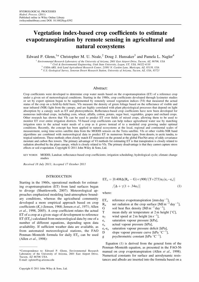
Figure 1. NDVI-determined crop coefficient (Kcr) (A); lysimeter-determined crop coefficient (Kcb) (B); and regression of lysimeter-determined (y-axis) and NDVI-determined crop coefficients (C) forcorn crops grown at Fruita, Colorado, 1984 (from Neale et al., 1989)

EXPERIMENTAL AND THEORETICALJUSTIFICATION FOR KC-VI METHODS

In early work on this topic, Neale (1983), Bausch andNeale (1987), Neale (1987), and Bausch and Neale (1989),Neale et al., (1989) and Bausch (1995) compared cropdevelopment characteristics with ET and NDVI values forirrigated corn crops at two experimental farm sites inColorado. Crops were grown in fields equipped withweighing lysimeters, and Kc was calculated with alfalfa asthe reference crop grown at each facility (i.e. Kc=ETcorn/ETalfalfa). NDVI was measured with down-looking radio-meters suspended 2m above the canopies. They found thatNDVI was highly correlated with LAI and fc, and thatKc-VI

derived from radiometric measurements closely trackedmeasured Kc over the crop cycle (Figure 1). The inflectionpoint for maximum ET, maximum LAI and maximumNDVI occurred at approximately the same points in thegrowing cycle (ca. DOY 210–220). They concluded(Bausch and Neale, 1987) that crop coefficients derivedfromNDVI were independent of time parameters and otherfactors affecting crop performance, and represented real-time coefficients that could be used to schedule irrigationson a field-by-field basis.Choudhury et al. (1994) used a modeling approach

to justify using VIs to replace Kc in Equation (2). Theyshowed that:

Tc ¼ VI�ð Þ� (6)

where Tc is a plant transpiration coefficient (by analogy abasal crop coefficient, Kcb) and VI* is a VI stretchedbetween 0 (representing bare soil) and 1.0 (representingfully transpiring, unstressed vegetation) calculated usingthe formula:

VI� ¼ 1� VImax � VIð Þ= VImax � VIminð Þ (7)

where VImax is the VI value when ET is maximal andVImin is the VI of bare soil. Then, ET (ignoring bare soilevaporation) is approximated as:

ET ¼ ETo VI�� Z

(8)

The exponent, �, is determined by the relationshipbetween transpiration and the VI used in Equation (7).Choudhury et al. (1994) pointed out that SAVI (and byextension EVI from which it is derived) extends the rangeof LAI values over which a VI is responsive, because it


does not ‘saturate’ as quickly as NDVI at high LAIs.They showed that SAVI was curvilinearly related to LAIup to LAI of 5, and since ET is also curvilinearly relatedto LAI, ET was near-linearly related to SAVI. Hence, forEVI and SAVI, the exponent � in Equation (8) is 1.0. Bycontrast, NDVI, which typically saturates at an LAI ofabout 3.0, was curvilinearly related to ET, and � wasless than 1.0. SAVI also had a higher r2 relationship tomeasured ET than NDVI.


E. P. GLENN ET AL.

Another advantage of using the SAVI or EVI for cropcoefficient relationships is that these indices are lesssensitive to soil background reflectance changes due tosurface moisture, a common occurrence in irrigated areas.Darkened, wet soils will artificially increase the NDVIduring the vegetative growth stages when incompletecanopy cover is prevalent, leading to an over predictionof ET when using a relationship developed with dry soilsurface data. This was observed by Neale (1987) in thedevelopment of NDVI – basal crop coefficient (Kcb)relationship and led to the use of the SAVI by Bausch(1993) for corn, Neale et al. (1996) for cotton; Jayanthiet al. (2000) and Jayanthi et al. (2007) for beans andpotato, respectively. The basal crop coefficient, proposedby Wright (1982) for several crops in southern Idaho, isdefined for a dry soil surface and no water limitation inthe root zone of the crop. Thus, the SAVI may be bettersuited to be related to the Kcb with the added advantagethat relationships developed with the SAVI using anL= 0.5 can be applied to different regions with dark orlight natural dry soil reflectance (Huete, 1988). However,a definitive experiment directly comparing the differentVIs with respect to fc, LAI or ET has not yet beenconducted, to our knowledge.

APPLICATION TO INDIVIDUAL CROPS

Following the early work on corn (Neale, 1983, 1987;Bausch andNeale, 1987; Neale et al., 1989), the reflectance-based crop coefficient methods (Kc-VI methods) have beenapplied to numerous other crops, as illustrated by thefollowing examples.

Vineyards and orchards

Vineyards and orchards are especially difficult tomodel with static crop coefficients due to differencesin plant spacing, varieties and plant heights amongfields, and the variable amount of bare soil or understoryvegetation between vines or trees. Furthermore, ETchanges during fruit filling. Campos et al. (2011) assessedsatellite-based Kc-VIs for irrigated grapes in Spain, usingan energy-balance moisture flux tower to independentlymeasure actual ET and ETo. Both NDVI and SAVI wereable to predict ET by simple linear regression equations,validating the use of remote sensing to estimate ET inwine grapes.Samani et al. (2009) used NDVI from Landsat imagery

to develop field-scale Kc-VI values for pecan orchards inthe lower Rio Grande Valley, New Mexico, USA. Pecanscover 11,000 ha and consume 40% of irrigation water inthe area, and there is a need to quantify actual water useby the trees to resolve issues of water rights allocation,water management and agronomic practices. Satellite-derived ET values were within 4% of ET measured at aneddy covariance tower site in a mature field. They foundthat ET over 279 fields varied from 498 to 1259mmyear�1, and that only 5% of fields were within the rangeof maximum ET and Kc set for the crop by expert


opinion, indicating the potential for significant watersavings. Although many of the fields were under chronicwater stress, ET was still closely related to NDVI becausethe trees adjusted LAI to reflect water availability.

Wheat

Wheat has been extensively studied due to itsimportance as an irrigated crop in water-short arid andsemi-arid regions El-Raki et al. (2007). Duchemin et al.(2006) used NDVI from two Landsat images to map LAIand transpiration in irrigated wheat fields in Morocco.The satellite-derived Kc-VI had an error of only 15%compared to ground measurements and the mapsdisplayed a high field-to-field variability in actual waterrequirements depending on the state of canopy develop-ment, opening up the possibility of improving irrigationefficiency through satellite monitoring of crop phenology.Gontia and Tiwari (2010) used NDVI and SAVI fromsatellite sensors to map wheat water use in an irrigationdistrict in West Bengal, India. They developed field-specific crop coefficients based on measured ETo andsatellite data, and were able to generate spatiallydistributed, monthly ET maps of the irrigation district.These maps could then be compared to water applicationrates to identify areas where water savings were possible.Extensive work has been conducted on wheat by the

USDA-ARS in a desert irrigation district in Maricopa,Arizona, USA (Hunsaker et al., 2005b; Hunsaker et al.,2007a, 2007b). In initial field experiments (Hunsakeret al., 2005b), a crop coefficient model for wheat ET wasdeveloped based on the dual crop coefficient approachof FAO-56, which includes a basal crop coefficient,Kcb, corresponding to crop transpiration, and a separatecoefficient, Ke, that accounts for soil evaporation (Allenet al., 2005):

ET ¼ KcbETo þ KeETo (9)

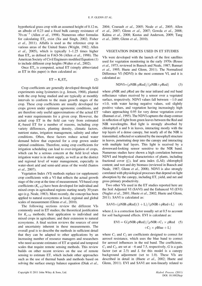
The experimental results showed that the contribu-tion of soil evaporation was approximately 10% of thetotal wheat ET in this irrigation district, as surfacesoils were normally dry and precipitation was low. TheNDVI-derived Kc-VI tracked within 5% of measured Kcb

(Figure 2). In subsequent experiments, wheat was grownin field plots for two seasons under six treatmentcombinations: typical, dense and sparse plant densities,with adequate and limited nitrogen. The FAO-56reference-crop method was used to calculate Kcb andET in Equation (9) on daily time steps to predict soilmoisture depletion and to schedule irrigations. Forcomparison, Kcb was estimated by the NDVI-derivedKc-VI derived from the earlier experiments (Hunsakeret al., 2007a). In these studies, NDVI was measured witha hand-held radiometer two to four times per week in alltreatment plots. Actual soil moisture depletion wasmeasured frequently with neutron hydroprobes in accesstubes ports installed in plots.


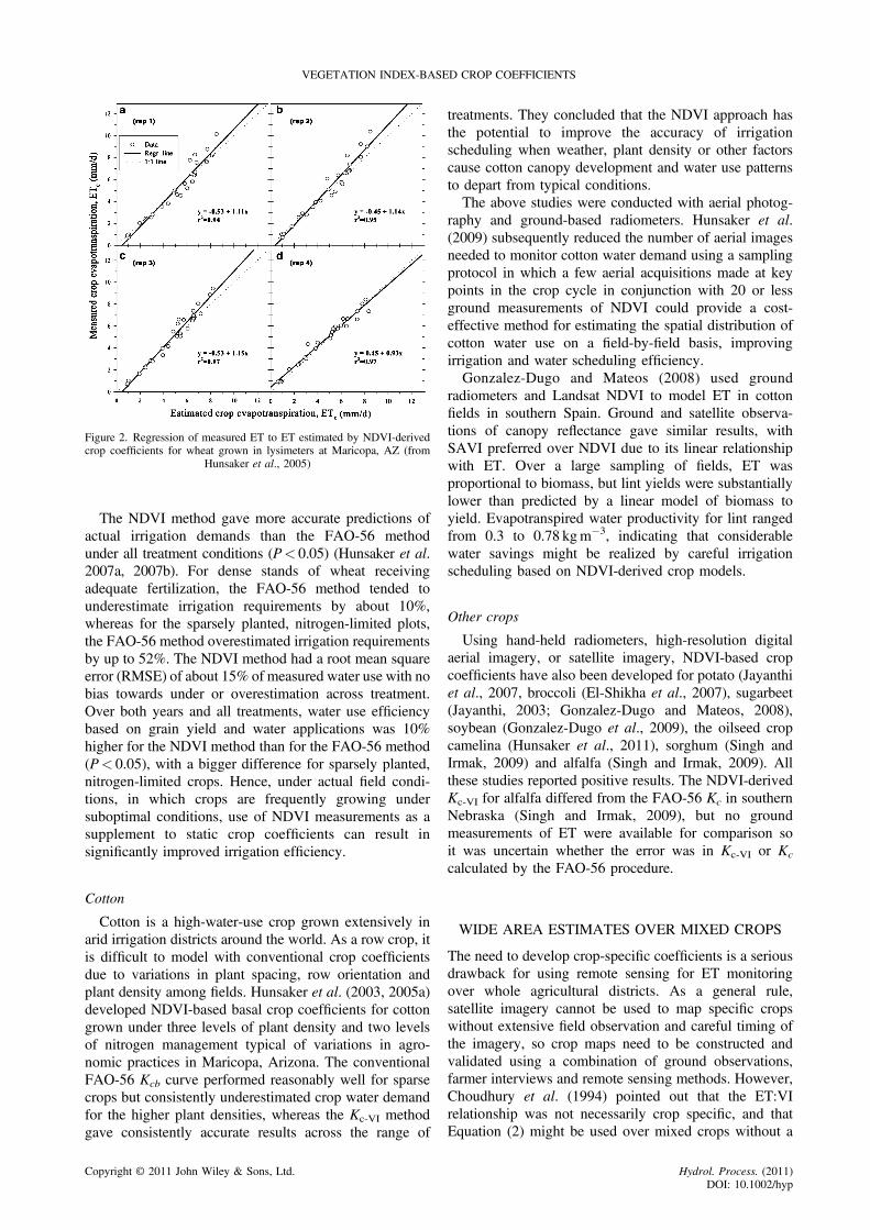
Figure 2. Regression of measured ET to ET estimated by NDVI-derivedcrop coefficients for wheat grown in lysimeters at Maricopa, AZ (from

Hunsaker et al., 2005)


The NDVI method gave more accurate predictions ofactual irrigation demands than the FAO-56 methodunder all treatment conditions (P< 0.05) (Hunsaker et al.2007a, 2007b). For dense stands of wheat receivingadequate fertilization, the FAO-56 method tended tounderestimate irrigation requirements by about 10%,whereas for the sparsely planted, nitrogen-limited plots,the FAO-56 method overestimated irrigation requirementsby up to 52%. The NDVI method had a root mean squareerror (RMSE) of about 15% of measured water use with nobias towards under or overestimation across treatment.Over both years and all treatments, water use efficiencybased on grain yield and water applications was 10%higher for the NDVI method than for the FAO-56 method(P< 0.05), with a bigger difference for sparsely planted,nitrogen-limited crops. Hence, under actual field condi-tions, in which crops are frequently growing undersuboptimal conditions, use of NDVI measurements as asupplement to static crop coefficients can result insignificantly improved irrigation efficiency.

Cotton

Cotton is a high-water-use crop grown extensively inarid irrigation districts around the world. As a row crop, itis difficult to model with conventional crop coefficientsdue to variations in plant spacing, row orientation andplant density among fields. Hunsaker et al. (2003, 2005a)developed NDVI-based basal crop coefficients for cottongrown under three levels of plant density and two levelsof nitrogen management typical of variations in agro-nomic practices in Maricopa, Arizona. The conventionalFAO-56 Kcb curve performed reasonably well for sparsecrops but consistently underestimated crop water demandfor the higher plant densities, whereas the Kc-VI methodgave consistently accurate results across the range of


treatments. They concluded that the NDVI approach hasthe potential to improve the accuracy of irrigationscheduling when weather, plant density or other factorscause cotton canopy development and water use patternsto depart from typical conditions.The above studies were conducted with aerial photog-

raphy and ground-based radiometers. Hunsaker et al.(2009) subsequently reduced the number of aerial imagesneeded to monitor cotton water demand using a samplingprotocol in which a few aerial acquisitions made at keypoints in the crop cycle in conjunction with 20 or lessground measurements of NDVI could provide a cost-effective method for estimating the spatial distribution ofcotton water use on a field-by-field basis, improvingirrigation and water scheduling efficiency.Gonzalez-Dugo and Mateos (2008) used ground

radiometers and Landsat NDVI to model ET in cottonfields in southern Spain. Ground and satellite observa-tions of canopy reflectance gave similar results, withSAVI preferred over NDVI due to its linear relationshipwith ET. Over a large sampling of fields, ET wasproportional to biomass, but lint yields were substantiallylower than predicted by a linear model of biomass toyield. Evapotranspired water productivity for lint rangedfrom 0.3 to 0.78 kgm�3, indicating that considerablewater savings might be realized by careful irrigationscheduling based on NDVI-derived crop models.

Other crops

Using hand-held radiometers, high-resolution digitalaerial imagery, or satellite imagery, NDVI-based cropcoefficients have also been developed for potato (Jayanthiet al., 2007, broccoli (El-Shikha et al., 2007), sugarbeet(Jayanthi, 2003; Gonzalez-Dugo and Mateos, 2008),soybean (Gonzalez-Dugo et al., 2009), the oilseed cropcamelina (Hunsaker et al., 2011), sorghum (Singh andIrmak, 2009) and alfalfa (Singh and Irmak, 2009). Allthese studies reported positive results. The NDVI-derivedKc-VI for alfalfa differed from the FAO-56 Kc in southernNebraska (Singh and Irmak, 2009), but no groundmeasurements of ET were available for comparison soit was uncertain whether the error was in Kc-VI or Kc

calculated by the FAO-56 procedure.

WIDE AREA ESTIMATES OVER MIXED CROPS

The need to develop crop-specific coefficients is a seriousdrawback for using remote sensing for ET monitoringover whole agricultural districts. As a general rule,satellite imagery cannot be used to map specific cropswithout extensive field observation and careful timing ofthe imagery, so crop maps need to be constructed andvalidated using a combination of ground observations,farmer interviews and remote sensing methods. However,Choudhury et al. (1994) pointed out that the ET:VIrelationship was not necessarily crop specific, and thatEquation (2) might be used over mixed crops without a


E. P. GLENN ET AL.

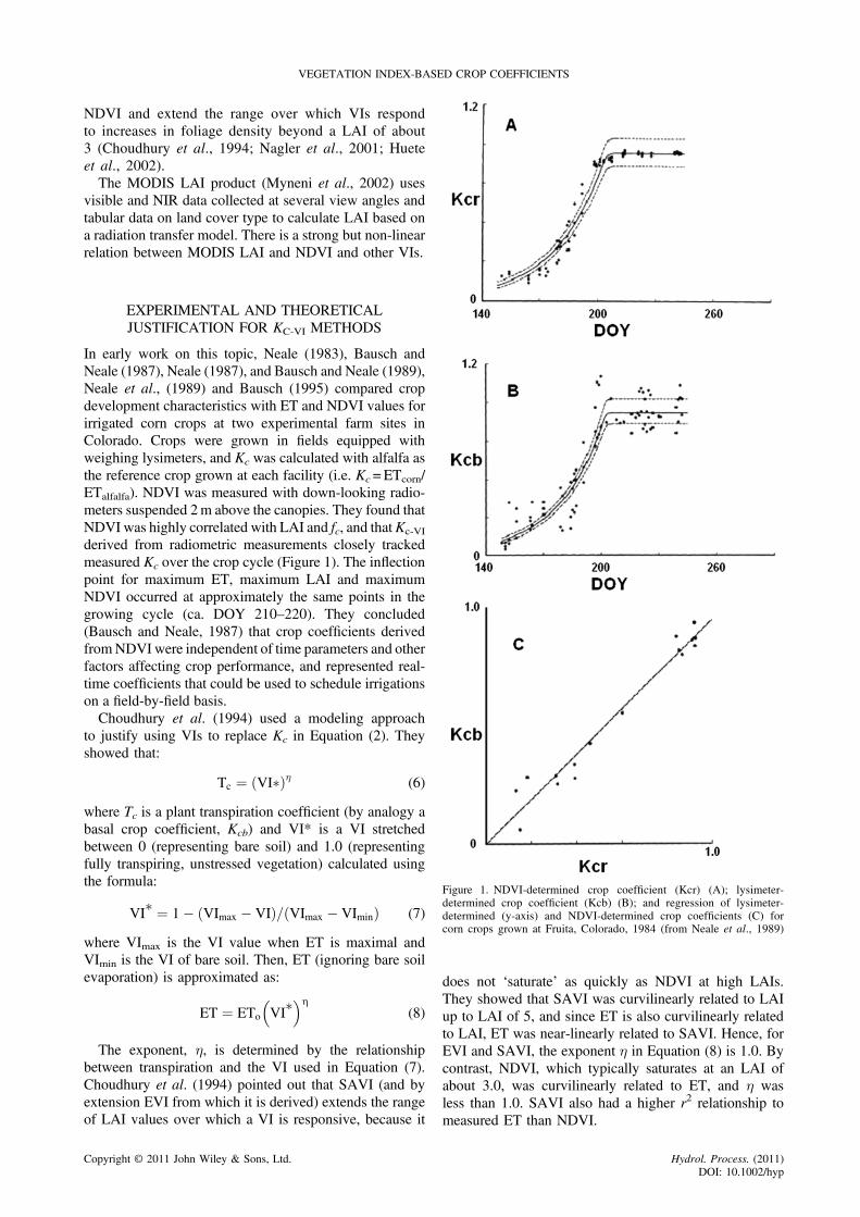
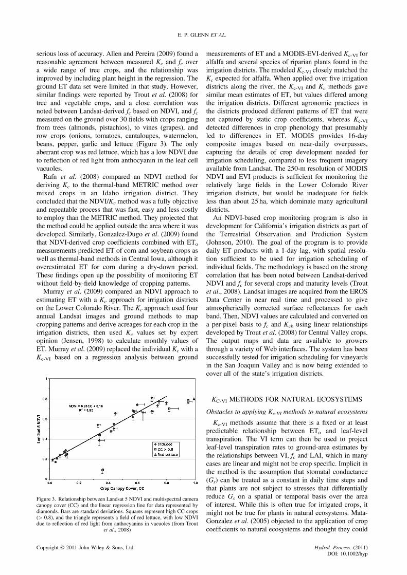
serious loss of accuracy. Allen and Pereira (2009) found areasonable agreement between measured Kc and fc overa wide range of tree crops, and the relationship wasimproved by including plant height in the regression. Theground ET data set were limited in that study. However,similar findings were reported by Trout et al. (2008) fortree and vegetable crops, and a close correlation wasnoted between Landsat-derived fc based on NDVI, and fcmeasured on the ground over 30 fields with crops rangingfrom trees (almonds, pistachios), to vines (grapes), androw crops (onions, tomatoes, cantaloupes, watermelon,beans, pepper, garlic and lettuce (Figure 3). The onlyaberrant crop was red lettuce, which has a low NDVI dueto reflection of red light from anthocyanin in the leaf cellvacuoles.Rafn et al. (2008) compared an NDVI method for

deriving Kc to the thermal-band METRIC method overmixed crops in an Idaho irrigation district. Theyconcluded that the NDVI/Kc method was a fully objectiveand repeatable process that was fast, easy and less costlyto employ than the METRIC method. They projected thatthe method could be applied outside the area where it wasdeveloped. Similarly, Gonzalez-Dugo et al. (2009) foundthat NDVI-derived crop coefficients combined with ETo

measurements predicted ET of corn and soybean crops aswell as thermal-band methods in Central Iowa, although itoverestimated ET for corn during a dry-down period.These findings open up the possibility of monitoring ETwithout field-by-field knowledge of cropping patterns.Murray et al. (2009) compared an NDVI approach to

estimating ET with a Kc approach for irrigation districtson the Lower Colorado River. The Kc approach used fourannual Landsat images and ground methods to mapcropping patterns and derive acreages for each crop in theirrigation districts, then used Kc values set by expertopinion (Jensen, 1998) to calculate monthly values ofET. Murray et al. (2009) replaced the individual Kc with aKc-VI based on a regression analysis between ground

Figure 3. Relationship between Landsat 5 NDVI and multispectral cameracanopy cover (CC) and the linear regression line for data represented bydiamonds. Bars are standard deviations. Squares represent high CC crops(> 0.8), and the triangle represents a field of red lettuce, with low NDVIdue to reflection of red light from anthocyanins in vacuoles (from Trout

et al., 2008)


measurements of ET and a MODIS-EVI-derived Kc-VI foralfalfa and several species of riparian plants found in theirrigation districts. The modeled Kc-VI closely matched theKc expected for alfalfa. When applied over five irrigationdistricts along the river, the Kc-VI and Kc methods gavesimilar mean estimates of ET, but values differed amongthe irrigation districts. Different agronomic practices inthe districts produced different patterns of ET that werenot captured by static crop coefficients, whereas Kc-VI

detected differences in crop phenology that presumablyled to differences in ET. MODIS provides 16-daycomposite images based on near-daily overpasses,capturing the details of crop development needed forirrigation scheduling, compared to less frequent imageryavailable from Landsat. The 250-m resolution of MODISNDVI and EVI products is sufficient for monitoring therelatively large fields in the Lower Colorado Riverirrigation districts, but would be inadequate for fieldsless than about 25 ha, which dominate many agriculturaldistricts.An NDVI-based crop monitoring program is also in

development for California’s irrigation districts as part ofthe Terrestrial Observation and Prediction System(Johnson, 2010). The goal of the program is to providedaily ET products with a 1-day lag, with spatial resolu-tion sufficient to be used for irrigation scheduling ofindividual fields. The methodology is based on the strongcorrelation that has been noted between Landsat-derivedNDVI and fc for several crops and maturity levels (Troutet al., 2008). Landsat images are acquired from the EROSData Center in near real time and processed to giveatmospherically corrected surface reflectances for eachband. Then, NDVI values are calculated and converted ona per-pixel basis to fc and Kcb using linear relationshipsdeveloped by Trout et al. (2008) for Central Valley crops.The output maps and data are available to growersthrough a variety of Web interfaces. The system has beensuccessfully tested for irrigation scheduling for vineyardsin the San Joaquin Valley and is now being extended tocover all of the state’s irrigation districts.

KC-VI METHODS FOR NATURAL ECOSYSTEMS

Obstacles to applying Kc-VI methods to natural ecosystems

Kc-VI methods assume that there is a fixed or at leastpredictable relationship between ETo and leaf-leveltranspiration. The VI term can then be used to projectleaf-level transpiration rates to ground-area estimates bythe relationships between VI, fc and LAI, which in manycases are linear and might not be crop specific. Implicit inthe method is the assumption that stomatal conductance(Gs) can be treated as a constant in daily time steps andthat plants are not subject to stresses that differentiallyreduce Gs on a spatial or temporal basis over the areaof interest. While this is often true for irrigated crops, itmight not be true for plants in natural ecosystems. Mata-Gonzalez et al. (2005) objected to the application of cropcoefficients to natural ecosystems and thought they could



overestimate plant water use by 50%–100% in aridregions where heat and moisture stress are common.On the other hand, optimization theory predicts that

plants will adjust LAI to match the environment’scapacity to support photosynthesis (Field, 1991; Fieldet al., 1995; Albrizio and Steduto, 2003. Seasonal leafproduction in an ecosystem is generally matched to thelimiting factors for photosynthesis at that location (e.g.nutrients, water and radiation). Even in sparse deserts,rainfall tends to be efficiently captured by vegetation, andacross agricultural and natural ecosystem, transpirationusually accounts for 70% to> 90% of ET (Huxman et al.,2004; Williams et al., 2004). As a result, measured ETrates (as from energy balance flux towers) are usuallystrongly correlated with satellite-derived VIs over a widerange of biomes. Therefore, estimating fc or LAI byremote sensing is a good first step in deriving ETestimates over mixed vegetation types in natural ecosys-tems (Glenn et al., 2010).

The example of saltcedar as a test of assumptions

Saltcedar (Tamarix ramosissima) is an introduced, salt-tolerant shrub that has spread widely on western U.S.rivers. Because it grows in dense stands, it has beenconsidered to have very high water use, and a number ofstudies have attempted to measure saltcedar ET. Based onLAI, Jensen (1998) set a crop coefficient for saltcedarequal to alfalfa on the Lower Colorado River. However,Westenburg et al. (2006), using Bowen ratio moistureflux towers in dense stands at Havasu National WildlifeRefuge on the Lower Colorado River, reported rates ofabout 800mmyear�1, less than half of ETo or alfalfa.Neale et al. (2001) reported midday rates equal to lessthan half of net radiation for a dense stand on the MiddleRio Grande as measured by moisture flux towers, and themeasured rates were only half as great as rates estimatedby aerial remote sensing methods.Groeneveld et al. (2007) and Groeneveld and Baugh

(2007) estimated saltcedar ET from NDVI based on asimple crop coefficient method, in which NDVI wasstretched between bare soil (0) and fully transpiring cropfields (1.0) on Landsat images. The scaled NDVI wasmultiplied by ETo to estimate ET on an annual basis fromsingle summer Landsat scenes, and the results wereclosely related to values measured at moisture flux towers(r2 = 0.95). Since they have access to a constant source ofwater, phreatophytes are considered to be non-stressedwith relatively constant rates of Gs on daily time stepsat a given location (e.g. Groeneveld and Baugh, 2007;Groeneveld et al., 2007).However, Nagler et al. (2009a, 2009b) found a wide

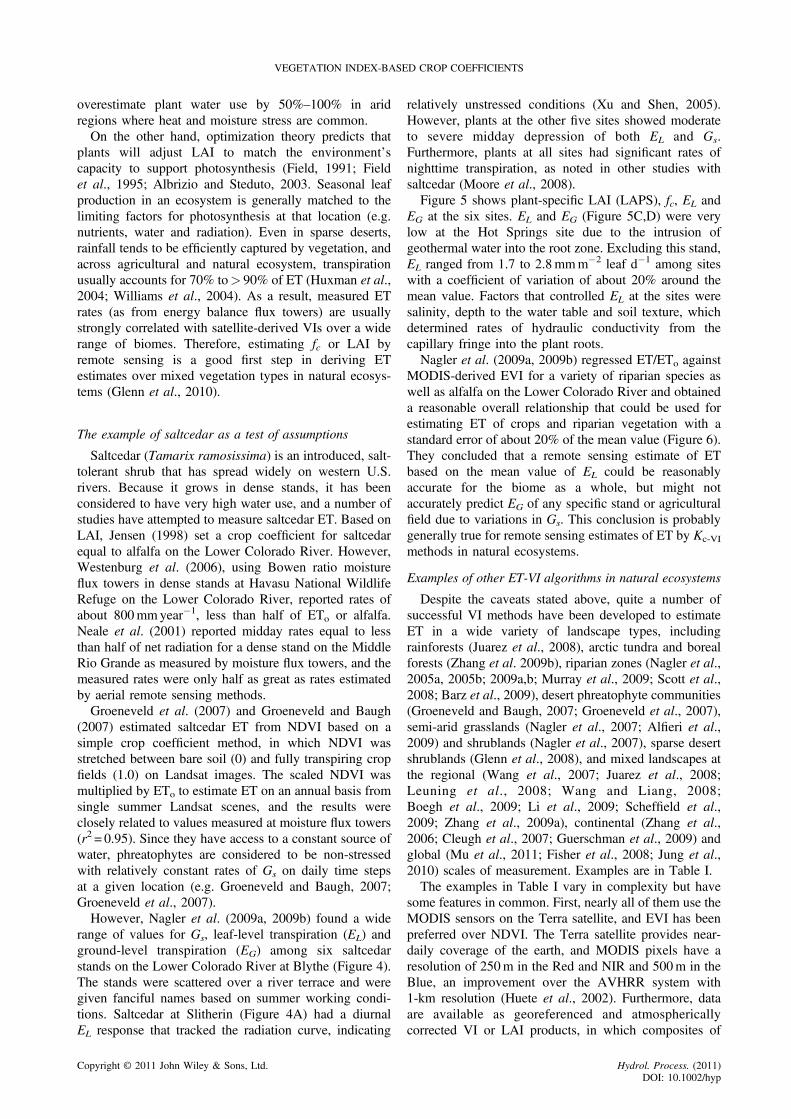
range of values for Gs, leaf-level transpiration (EL) andground-level transpiration (EG) among six saltcedarstands on the Lower Colorado River at Blythe (Figure 4).The stands were scattered over a river terrace and weregiven fanciful names based on summer working condi-tions. Saltcedar at Slitherin (Figure 4A) had a diurnalEL response that tracked the radiation curve, indicating


relatively unstressed conditions (Xu and Shen, 2005).However, plants at the other five sites showed moderateto severe midday depression of both EL and Gs.Furthermore, plants at all sites had significant rates ofnighttime transpiration, as noted in other studies withsaltcedar (Moore et al., 2008).Figure 5 shows plant-specific LAI (LAPS), fc, EL and

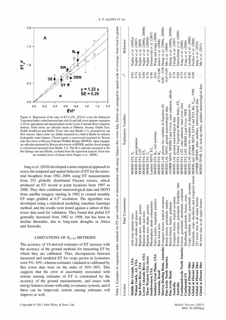
EG at the six sites. EL and EG (Figure 5C,D) were verylow at the Hot Springs site due to the intrusion ofgeothermal water into the root zone. Excluding this stand,EL ranged from 1.7 to 2.8mmm�2 leaf d�1 among siteswith a coefficient of variation of about 20% around themean value. Factors that controlled EL at the sites weresalinity, depth to the water table and soil texture, whichdetermined rates of hydraulic conductivity from thecapillary fringe into the plant roots.Nagler et al. (2009a, 2009b) regressed ET/ETo against

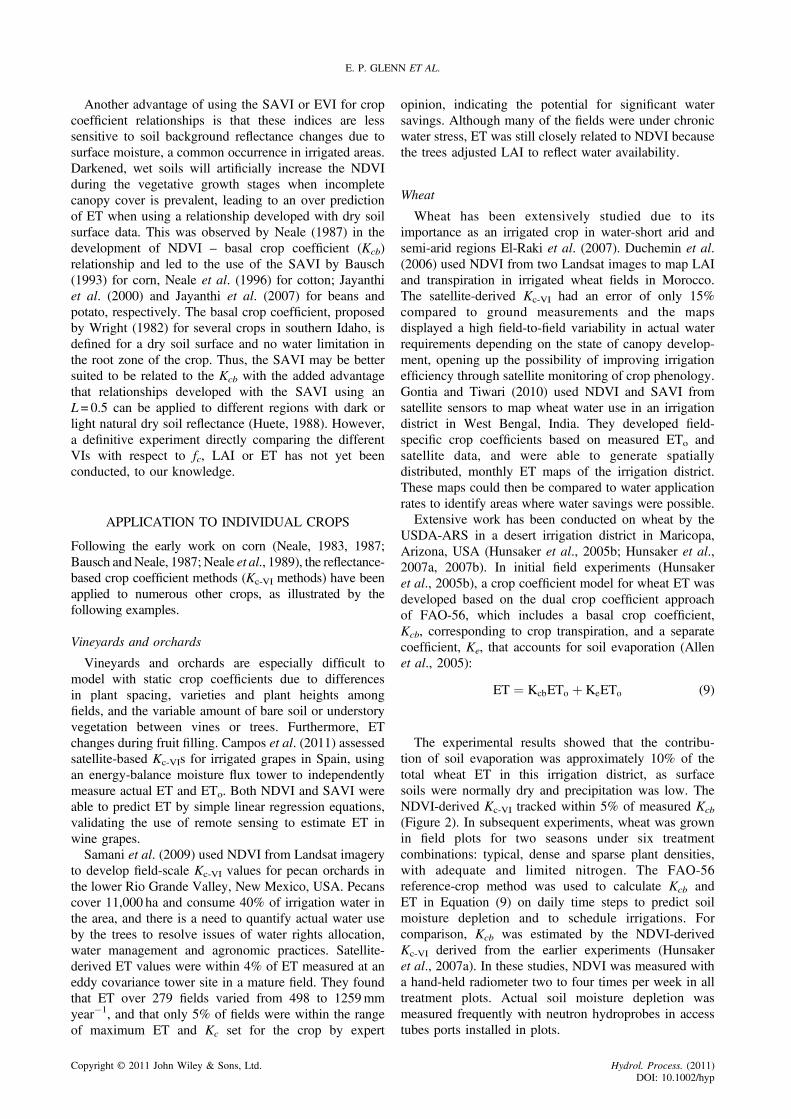
MODIS-derived EVI for a variety of riparian species aswell as alfalfa on the Lower Colorado River and obtaineda reasonable overall relationship that could be used forestimating ET of crops and riparian vegetation with astandard error of about 20% of the mean value (Figure 6).They concluded that a remote sensing estimate of ETbased on the mean value of EL could be reasonablyaccurate for the biome as a whole, but might notaccurately predict EG of any specific stand or agriculturalfield due to variations in Gs. This conclusion is probablygenerally true for remote sensing estimates of ET by Kc-VI

methods in natural ecosystems.

Examples of other ET-VI algorithms in natural ecosystems

Despite the caveats stated above, quite a number ofsuccessful VI methods have been developed to estimateET in a wide variety of landscape types, includingrainforests (Juarez et al., 2008), arctic tundra and borealforests (Zhang et al. 2009b), riparian zones (Nagler et al.,2005a, 2005b; 2009a,b; Murray et al., 2009; Scott et al.,2008; Barz et al., 2009), desert phreatophyte communities(Groeneveld and Baugh, 2007; Groeneveld et al., 2007),semi-arid grasslands (Nagler et al., 2007; Alfieri et al.,2009) and shrublands (Nagler et al., 2007), sparse desertshrublands (Glenn et al., 2008), and mixed landscapes atthe regional (Wang et al., 2007; Juarez et al., 2008;Leuning et al., 2008; Wang and Liang, 2008;Boegh et al., 2009; Li et al., 2009; Scheffield et al.,2009; Zhang et al., 2009a), continental (Zhang et al.,2006; Cleugh et al., 2007; Guerschman et al., 2009) andglobal (Mu et al., 2011; Fisher et al., 2008; Jung et al.,2010) scales of measurement. Examples are in Table I.The examples in Table I vary in complexity but have

some features in common. First, nearly all of them use theMODIS sensors on the Terra satellite, and EVI has beenpreferred over NDVI. The Terra satellite provides near-daily coverage of the earth, and MODIS pixels have aresolution of 250m in the Red and NIR and 500m in theBlue, an improvement over the AVHRR system with1-km resolution (Huete et al., 2002). Furthermore, dataare available as georeferenced and atmosphericallycorrected VI or LAI products, in which composites of


Figure 4. Diurnal traces of leaf-level transpiration (EL) and stomatal conductance (Gs) for saltcedar measured by sap flux sensors in six separate stands ona river terrace on the Lower Colorado River near Blythe, CA. Error bars are standard errors over 16–35 days of measurement at each site during summer.

White bar over the x-axis shows the daylight hours at each site

E. P. GLENN ET AL.

cloud-free images are prepared for 8-day or 16-dayintervals in near real time. Thus, MODIS lends itself totime-series analyses of ET and other physiologicalprocesses. Several studies (e.g. Nagler et al., 2005a,2007; Wang et al., 2007) showed that MODIS EVI wassignificantly better correlated with ground-based ETmeasurements than MODIS NDVI across a variety ofland cover types, as predicted also by Choudhury et al.(1994) in their comparison of NDVI versus SAVI.However, non-linear regressions of ET and NDVI werenot tested in these studies.Second, most of them use energy balance flux tower

data from the Fluxnet system of towers to calibrate orvalidate their algorithms (Baldocchi et al., 2001). Groundmeasurements of ET from flux towers set in naturalecosystems are used to develop best-fit equations betweenET, satellite-derived VIs, ancillary remote sensing dataand ground meteorological data. However, they vary in


approach from strictly empirical approaches (e.g.Nagler et al., 2009b), to physical models that attempt todetermine the parameters in the Penman–Monteithequation with a combination of ground and remotesensing data. For the studies in Table I, r2 values rangedfrom 0.45 to 0.95. RMSE of ET ranged from 10% to 25%of mean ET values over the studies.

Examples of Kc-VI approaches for mixed biome types

Australia has a national water-monitoring program,developed in part in response to the recent 10-yeardrought (Glenn et al., this volume). As part of this effort,they reviewed eight operational methods for estimatingET over the continent at a 1 km2 scale of measurement.The remote sensing method selected was based on theone developed by Guerschman et al. (2009). It usedbidirectional-distribution-function corrected MODIS


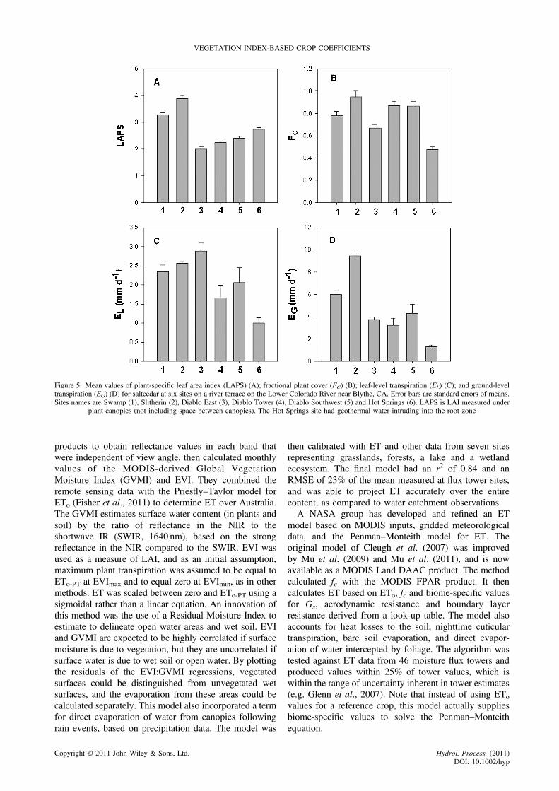
Figure 5. Mean values of plant-specific leaf area index (LAPS) (A); fractional plant cover (FC) (B); leaf-level transpiration (EL) (C); and ground-leveltranspiration (EG) (D) for saltcedar at six sites on a river terrace on the Lower Colorado River near Blythe, CA. Error bars are standard errors of means.Sites names are Swamp (1), Slitherin (2), Diablo East (3), Diablo Tower (4), Diablo Southwest (5) and Hot Springs (6). LAPS is LAI measured under

plant canopies (not including space between canopies). The Hot Springs site had geothermal water intruding into the root zone


products to obtain reflectance values in each band thatwere independent of view angle, then calculated monthlyvalues of the MODIS-derived Global VegetationMoisture Index (GVMI) and EVI. They combined theremote sensing data with the Priestly–Taylor model forETo (Fisher et al., 2011) to determine ET over Australia.The GVMI estimates surface water content (in plants andsoil) by the ratio of reflectance in the NIR to theshortwave IR (SWIR, 1640 nm), based on the strongreflectance in the NIR compared to the SWIR. EVI wasused as a measure of LAI, and as an initial assumption,maximum plant transpiration was assumed to be equal toETo-PT at EVImax and to equal zero at EVImin, as in othermethods. ET was scaled between zero and ETo-PT using asigmoidal rather than a linear equation. An innovation ofthis method was the use of a Residual Moisture Index toestimate to delineate open water areas and wet soil. EVIand GVMI are expected to be highly correlated if surfacemoisture is due to vegetation, but they are uncorrelated ifsurface water is due to wet soil or open water. By plottingthe residuals of the EVI:GVMI regressions, vegetatedsurfaces could be distinguished from unvegetated wetsurfaces, and the evaporation from these areas could becalculated separately. This model also incorporated a termfor direct evaporation of water from canopies followingrain events, based on precipitation data. The model was


then calibrated with ET and other data from seven sitesrepresenting grasslands, forests, a lake and a wetlandecosystem. The final model had an r2 of 0.84 and anRMSE of 23% of the mean measured at flux tower sites,and was able to project ET accurately over the entirecontent, as compared to water catchment observations.A NASA group has developed and refined an ET

model based on MODIS inputs, gridded meteorologicaldata, and the Penman–Monteith model for ET. Theoriginal model of Cleugh et al. (2007) was improvedby Mu et al. (2009) and Mu et al. (2011), and is nowavailable as a MODIS Land DAAC product. The methodcalculated fc with the MODIS FPAR product. It thencalculates ET based on ETo, fc and biome-specific valuesfor Gs, aerodynamic resistance and boundary layerresistance derived from a look-up table. The model alsoaccounts for heat losses to the soil, nighttime cuticulartranspiration, bare soil evaporation, and direct evapor-ation of water intercepted by foliage. The algorithm wastested against ET data from 46 moisture flux towers andproduced values within 25% of tower values, which iswithin the range of uncertainty inherent in tower estimates(e.g. Glenn et al., 2007). Note that instead of using ETo

values for a reference crop, this model actually suppliesbiome-specific values to solve the Penman–Monteithequation.


forETandcoefficientsof

determ

inationwith

energy

balanceflux

tower

data.E

ntries

arearranged

byspatialscaleof

coverage,from

localto

global

Plant

Com

munities

Explanatory

Variables

r2Reference

parian

trees

MODIS

EVI,Ta

0.82

Nagleret

al.(2005a)

sandgrasses

MODIS

EVI,precipitatio

n0.74

Nagleret

al.(2007)

s,shrubs,grasses

MODIS

EVI,LST

0.93

Nagleret

al.2005b

ubsandtrees

MODIS

EVI,ETo

0.80

Nagleret

al.(2009a,2009b)

s,shrubs,grasses

MODIS

EVI,Ta

0.76

Nagleret

al.(2005b)

shrubcommunities

Landsat

NDVI,ETo

0.96

Groeneveldet

al.(2007)

e,rangeland,

pastures

MODIS

EVI,Rn,soilmoisture

0.82

WangandLiang

(2008)

rees

MODIS

EVI,Rn

0.72–0

.86

Juarez

etal.(2008)

rests,tropical

savannas

MODIS

LAI,proxiesforvariablesin

Equation(6)

0.66

–0.90

Zhang

etal.(2009a,2009b)

ts,grasslands,tundra

MODIS

LAI,NDVI,ground

meteorologicaldata

0.45–0

.89

Muet

al.(2009)

ts,tund

ra,peatlands

AVHRRNDVI,MODIS

LandCover,solarradiation,

albedo

0.91

Zhang

etal.(2009a,2009b)

rests,tropical

savannas

MODIS

LAI,ground

meteorologicaldata

0.74

Cleughet

al.(2007)

nnas,grasslands,floodplain,lake

MODIS

EVI,GlobalVegetationMoistureIndex,

ETo

0.84

Guerschman

etal.(2009)

slands,shrublands,croplands

MODIS

EVI,LST,solarradiation,

land

coverclass

0.75

Yanget

al.(2006)

grasslands,forests,crops

MODIS

EVI,LST,MODIS

LandCover,SWR

0.75

Yanget

al.(2006)

nds,forests,grasslands,savannas

MODIS

LAI,proxiesforvariablesin

Equation(6)

0.80

Leuning

etal.(2008)

crops,deciduousandevergreenforestsMODIS

andAVHRRNDVI,SAVIandEVI,Rn,

Tmax,VPD

0.90

Fischer

etal.(2008)

tesin

allmajor

biom

esAVHRR,MODIS,othersatellites,meteorologicaldata

-Jung

etal.(2010)

sin

allmajor

biom

esMODIS

FPAR,LAI,look-uptables,griddedmeteorologicaldata

-Muet

al.(2011)

Figure 6. Regression of the ratio of ET to ETo (EToF) versus the EnhancedVegetation Index scaled between bare soil (0) and full cover riparian vegetation(1.0) for agricultural and riparian plants in the Lower Colorado River irrigationdistricts. Solid circles are saltcedar stands at Slitherin, Swamp, Diablo East,Diablo Southwest and Diablo Tower sites near Blythe, CA, measured by sapflow sensors. Open circles are alfalfa measured in a field at Blythe by neutronhydroprobe water balance. Closed square is arrowweed measured by Bowenratio flux tower at Havasu National Wildlife Refuge (HNWR). Open trianglesare saltcedarmeasured byBowen ratio towers atHNWR, and the closed triangleis cottonwood measured near Blythe, CA. The X is saltcedar measured at theHot Springs site near Blythe, excluded from the regression analysis. Error bars

are standard errors of means (from Nagler et al., 2009b)

E. P. GLENN ET AL.

Jung et al. (2010) developed amore empirical approach toassess the temporal and spatial behavior of ET for the terres-trial biosphere from 1982–2009, using ET measurementsfrom 253 globally distributed Fluxnet towers, whichproduced an ET record at point locations from 1997 to2006. They then combined meteorological data and NDVIfrom satellite imagery starting in 1982 to created monthlyET maps gridded at 0.5o resolution. The algorithm wasdeveloped using a statistical modeling (machine learning)method, and the results were tested against a subset of fluxtower data used for validation. They found that global ETgenerally increased from 1982 to 1998, but has been indecline thereafter, due to long-term droughts in Africaand Australia.

Table

I.Examples

ofvegetatio

nindexmethods

Location

MiddleRio

Grand

e,USA

Arid-zone

riWalnu

tGulch,AZ,USA

Desertshrub

SanPedro

River,USA

Ripariantree

Low

erColorad

oRiver,USA

Riparianshr

Three

Western

USA

rivers

Ripariantree

Southw

estern

USA

Phreatophyte

Southern

Great

Plains,USA

Nativeprairi

Amazon

ia,Brazil

Rainforestt

Murray-Darlin

gBasin,Australia

Evergreen

foPan

-ArcticNorth

America

Borealfores

Pan

-ArcticBasin

Borealfores

Australia

Evergreen

foAustralia

Forests,sava

Con

tinental-scale

North

AmericaForests,gras

Con

tinental

US

Shrublands,

Globa

lat

Fluxn

etSites

Crops,wetla

Globa

lat

Fluxn

etSites

Grasslands,

Globa

lat

Fluxn

etSites

253tower

siGloba

lat

Fluxn

etSites

46tower

site

LIMITATIONS OF KC-VI METHODS

The accuracy of VI-derived estimates of ET increase withthe accuracy of the ground methods for measuring ET bywhich they are calibrated. Thus, discrepancies betweenmeasured and modeled ET for crops grown in lysimeterswere 5%–10%, whereas estimates validated or calibrated byflux tower data were on the order of 10%–30%. Thissuggests that the error or uncertainty associated withremote sensing estimates of ET is constrained by theaccuracy of the ground measurements, and issues withenergy balance closure with eddy covariance systems, and ifthese can be improved, remote sensing estimates willimprove as well.

Copyright © 2011 John Wiley & Sons, Ltd. Hydrol. Process. (2011)DOI: 10.1002/hyp


The Kc-VI methods were most accurate for singleagricultural crops, and accuracy can be expected to be lessfor mixed crops, due to differences in Gs among crops(Allen and Pereira, 2009). Even greater uncertainty isexpected for estimates over mixed natural biomes. Nagleret al. (2009b) showed that saltcedar, at least, violatedsome of the major assumptions made in scaling groundestimates of ET by remote sensing. First, most models(e.g. Mu et al., 2011) assume that Gs is zero at night andwater loss is only from cuticular transpiration. To thecontrary, as much as 26% of total transpiration is throughstomata kept open during the night in saltcedar (Mooreet al., 2008), apparently as a mechanism for excretingexcess salts from leaves (Glenn et al., in press). Second,thermal-band remote sensing methods produce a snapshotof ET at the time of satellite overpass, and they project theresults over an entire day or over several days, assumingthat (Rn - G):ET is constant over the daylight hours andover different days on a daily time step. However, onlyone of the six saltcedar sites fulfilled this condition, andthe others exhibited midday depression of ET. A mid-morning satellite overpass would overestimate daily ETby different amounts at each site. Hence, an under-standing of the environmental constraints on ET for thevegetation of interest in a specific application is needed,along with spatially distributed, seasonal ground mea-surements of EL and EG, to produce a robust ET modelusing remote sensing. For example, it is still uncertain ifET is more closely related to fc or LAI, which arepredicted differently by VIs.Despite the limitations, Kc-VI methods are increasingly

used in tasks such as irrigation scheduling, constructingagricultural district budgets and estimating water useefficiency and opportunities for water conservation inagriculture. They are also used in constructing waterbudgets for natural or mixed ecosystems at the local,regional and continental scales of measurement, and inprojecting trends in global ET over time as affected byclimate and land use changes (e.g. Jung et al., 2011).Continuity missions are planned for the major satellitesensor systems used in ET studies, so a seamless trend-lineof global ET starting in 1982 can be continued into the futureas the hydrological cycle intensifies due to global warming.

REFERENCES

Albrizio R, Steduto P. 2003. Photosynthesis, respiration and conservativecarbon use efficiency of four field grown crops. Agricultural and ForestMeteorology 116: 19–36.

Alfieri JG, Xiao XM, Niyogi D, Pielke RA, Chen F, LeMone MA. 2009.Satellite-based modeling of transpiration from the grasslands in theSouthern Great Plains, USA. Global Planet Change 67: 78–86.

Allen RG, Pereira LS. 2009. Estimating crop coefficients from fraction ofground cover and height. Irrigation Science 28: 17–34.

Allen R, Pereira L, Rais D, Smith M. 1998. Crop evapotranspiration –guidelines for computing crop water requirements – FAO irrigationand drainage paper 56. Food and Agriculture Organization of theUnited Nations: Rome, Italy.

Allen RG, Pereira LS, Smith M, Raes D, Wright JL. 2005. FAO-56 dualcrop coefficient method for estimating evaporation from soil andapplication extensions. Journal of Irrigation and Drainage Engineer-ing-ASCE 131: 2–13.


Allen R, Tasumi M, Trezza R. 2007. Satellite-based energy balance formapping evapotranspiration with internalized calibration (METRIC) –Model. Journal of Irrigation and Drainage Engineering 133: 380–394.

Allen RG, Pereira LS, Howell TA, Jensen ME. 2011. Evapotranspirationinformation reporting: I. Factors governing measurement accuracy.Agricultural Water Management 98: 899–920.

Baldocchi D, Falge E, Gu L, Olson R, Hollinger D, Running S, AnthoneP, Berhofer C, Davis K, Evans R, Fuentes J, Goldstein A, Katul G, LawB, Lee X, Malhi Y, Meyers T, Munger W, Oechel W, Pilegaard K,Schmid H, Valentini R, Verma S, Vesala T, Wilson K, Wofsy S. 2001.Fluxnet: a new tool to study the temporal and spatial variability ofecosystem-scale carbon dioxide, water vapor, and energy flux densities.Bulletin of the American Meteorological Society 82: 2415–2434.

Bannari A, Morin D, Bonn F, Huete A. 1995. A review of vegetationindices. International Journal of Remote Sensing 13: 85–120.

Barz D, Watson RP, Kanneyh JF, Roberts JD, Groeneveld DP. 2009.Cost/benefit considerations for recent saltcedar control, Middle PecosRiver, New Mexico. Environmental Management 43: 282–298.

Bausch WC. 1993. Soil background effects on reflectance-based cropcoefficients for corn. Remote Sensing of Environment 46: 213–222.

Bausch WC. 1995. Remote sensing of crop coefficients for improving theirrigation scheduling of corn. Agricultural Water Management 27: 55–68.

Bausch WC, Neale CMU. 1987. Crop coefficients derived from reflectedcanopy radiation: a concept. Transactions of ASAE 30: 703–709.

BauschWC,Neale CMU. 1989. Spectral inputs improve corn crop coefficientsand irrigation scheduling. Transactions of ASAE 32: 1901–1908.

Boegh E, Pooulsen RN, Butts M, Abrahamsen P, Dellwik E, Hansen S,Hasager CB, Ibrom A, Loerup JK, Pilegaard K, Soegaard H. 2009.Remote sensing based evapotranspiration and runoff modeling ofagricultural, forest and urban flux sites in Denmark: From field tomacro-scale. Journal of Hydrology 377: 300–316.

Campos I, Neale CMU, Calera A. 2011. Assessing satellite-based basalcrop coefficients for irrigated grapes (Vitus vinifera L.) AgriculturalWater Management 98: 45–54.

Choudhury B, Ahmed N, Idso S, Reginato R, Daughtry C. 1994. Relationsbetween evaporation coefficients and vegetation indices studied bymodel simulations. Remote Sensing of Environment 50: 1–17.

Cleugh HA, Leuning R, Mu QZ, Running SW. 2007. Regionalevaporation estimates from flux tower and MODIS satellite data.Remote Sensing of Environment 106: 285–304.

Courault D, Sequin B, Olioso A. 2005. Review on estimation ofevapotranspiration from remote sensing data: From empirical tonumerical modeling approaches. Irrigation and Drainage Systems19: 223–249.

Diak G, Mecikalski J, Anderson M, Norman J, Kustas W, Torn R, DeWolfR. 2004. Estimating land surface energy budgets from space - review andcurrent efforts at the University of Madison - Wisconsin and USDA -ARS. Bulletin of the American Meteorological Society 85: 65–78.

Duchemin B, Hadria R, Erraki S, Boulet G, Maisongrande P, ChehbouniA, Escadafal R, Ezzahar J, Hoedies JCB, Kharrou MH, Khabba S,Mougenot B, Olioso A, Rodriquez JC, Simoneaux V. 2006. Monitoringwheat phenology and irrigation in Central Morocco: On the use ofrelationships between evapotranspiration, crop coefficients, leaf areaindex and remotely-sensed vegetation indices. Agricultural WaterManagement 79: 1–27.

El-Shikha DM, Waller P, Hunsaker D, Clarke T, Barnes E. 2007. Ground-based remote sensing for assessing water and nitrogen status ofbroccoli. Agricultural Water Management 92: 182–193.

Er-Raki S, Chehbouni A, Guemouria N, Duchemin B, Ezzahar J, HadriaR. 2007. Combining FAO-56 model and ground-based remote sensingto estimate water consumptions of wheat crops in a semi-arid region.Agricultural Water Management 87: 41–54.

Field C. 1991. Ecological scaling of carbon gain to stress and resourceavailability. In Response of plants to multiple stresses, Mooney H,Winner W, Pell E (eds). Academic Press: London; 35–66.

Field C, Randerson J, Malmstromk C. 1995. Global net primaryproduction: combining ecology and remote sensing. Remote Sensingof Environment 51: 74–88.

Fisher JB, Tu KP, Baldocchi DB. 2008. Global estimates of the land-atmosphere water flux based on monthly AVHRR and ISLSCP-II data,validated at 16 FLUXNET sites. Remote Sensing of Environment 112:901–919.

Fisher JB, Whittaker RJ, Malhi Y. 2011. ET come home: potentialevapotranspiration in geographical ecology. Global Ecology andBiogeography 20: 1–18.

Glenn EP, Huete AR, Nagler PL, Hirschboeck KK, Brown P. 2007.Integrating remote sensing and ground methods to estimate evapo-transpiration. Critical Reviews in Plant Sciences 26: 139–168.


E. P. GLENN ET AL.

Glenn EP, Morino K, Didan K, Jordan F, Carroll KC, Nagler PL, Hultine K,Sheader L, Waugh J. 2008. Scaling sap flux measurements of grazed andungrazed shrub communities with fine and coarse-resolution remotesensing. Ecohydrology 1: 316–329.

Glenn EP, Nagler PL, Huete AR. 2010. Vegetation index methods forestimating evapotranspiration by remote sensing. Surveys in Geophysics31: 531–555.

Glenn EP, Morino K, Nagler PL, Murray S, Pearlstein S, Hultine K. 2012.Role of saltcedar (Tamarix spp.) and capillary rise in salinizing a non-flooding terrace on a flow-regulated desert river. Journal of AridEnvironments (in press).

Gontia NK, Tiwari KN. 2010. Estimation of crop coefficient andevapotranspiration of wheat (Triticuum aerstivum) in a irrigationcommand using remote sensing and GIS.Water Resources Management24: 1399–1414.

Gonzalez-Dugo MP, Mateos L. 2008. Spectral vegetation indices forbenchmarking water productivity of irrigated cotton and sugarbeetcrops. Agricultural Water Management 95: 48–58.

Gonzalez-Dugo MP, Neale CMU, Mateos L, Kustas WP, Prueger JH,Anderson MC, Li F. 2009. A comparison of operational remotesensing-based models for estimating crop evapotranspiration. Agricul-tural and Forest Meteorology 149: 1843–1853.

Gowda PH, Chavez JL, Colaizzi PD, Evett SR, Howell TA, Tolk JA.2008. ET mapping for agricultural water management: present statusand challenges. Irrigation Science 26: 223–237.

GroeneveldDP, BaughWM. 2007. Correcting satellite data to detect vegetationsignal for eco-hydrologic analyses. Journal of Hydrology 344: 135–145.

Groeneveld DP, Baugh WM, Sanderson JS, Cooper DJ. 2007. Annualgroundwater evapotranspiration mapped from single satellite scenes.Journal of Hydrology 344: 146–156.

Guerschman JP, Van Dijk AIJM, Mattersdorf G, Beringer J, Hutley LB,Leuning R, Pipunic RC, Sherman BS. 2009. Scaling of potentialevapotranspiration with MODIS data reproduces flux observations andcatchment water balance observations across Australia. Journal ofHydrology 369: 107–119.

Huete AR. 1988. A soil adjusted vegetation index (SAVI). RemoteSensing of Environment 25: 295–309.

Huete AR, Glenn EP. 2011. Remote sensing of ecosystem structure andfunction. In Advances in Environmental Remote Sensing, Weng Q (ed).CRC Press: Boca Raton, Florida; 291–320.

Huete A, Didan K,Miura T, Rodriquez E, Gao X, Ferreira L. 2002. Overviewof the radiometric and biophysical performance of the MODIS vegetationindices. Remote Sensing of Environment 83: 195–213.

Hunsaker DJ, Pinter PJ, Barnes EM, Kimball BA. 2003. Estimating cottonevapotranspiration crop coefficients with a multispectral vegetationindex. Irrigation Science 22: 95–104.

Hunsaker DJ, Pinter PJ, Kimball BA. 2005a. Wheat basal crop coefficientsdetermined by normalized difference vegetation index. IrrigationScience 24: 1–14.

Hunsaker DJ, Barnes EM, Clarke TR, Fitzgerald GJ, Pinter PJ. 2005b.Cotton irrigation scheduling using remotely sensed and FAO-56 basalcrop coefficients. Transactions of ASAE 48: 1395–1407.

Hunsaker DJ, Fitzgerald GJ, French AN, Clarke TR, Ottman MJ, PinterPJ. 2007a. Wheat irrigation management using multispectral cropcoefficients. I. Crop evapotranspiration prediction. Transactions of theASABE 50: 2017–2033.

Hunsaker DJ, Fitzgerald GJ, French AN, Clarke TR, Ottman MJ, PinterPJ. 2007b. Wheat irrigation management using multispectral cropcoefficients. II. Irrigation scheduling performance, grain yield, andwater use efficiency. Transactions of the ASABE 50: 2035–2050.

Hunsaker DJ, El-Shikha DM, Clarke TR, French AN, Thorp KR. 2009.Using ESAP software for predicting the spatial distributions ofNDVI and transpiration of cotton. Agricultural Water Management96: 1293–1304.

Hunsaker DJ, French AN, Clarke TR, El-Shikha DM. 2011. Water use,crop coefficients and irrigation management criteria for camelinaproduction in arid regions. Irrigation Science 29: 27–43.

Huxman T, Smith M, Fay P, Knapp S, Shaw M, Loik M, Smith D, Tissue C,Zak J, Weltzin J, Pockman W, Sala O, Haddad B, Harte J, Koch G,Schwinning S, Small E, Williams D. 2004. Convergence across biomes toa common rain-use efficiency. Nature 429: 651–654.

Jayanthi H. 2003. Airborne and ground-based remote sensing for theestimation of evapotranspiration and yield of bean, potato and sugarbeet. PhD dissertation, Utah State University, Logan, Utah.

Jayanthi H, Neale CMU, Wright JL. 2000. Seasonal evapotranspirationestimation using canopy reflectance - A case study. IAHS Proceedingsof Remote Sensing and Hydrology, 2000, April 3–5, Sante Fe, NewMexico


Jayanthi H, Neale CMU, Wright JL. 2007. Development and validation ofcanopy reflectance-based crop coefficients for potato. AgriculturalWater Management 88: 235–246.

Jensen ME. 1968. Water consumption by agricultural plants. In Waterdeficits and plant growth, vol. 2, Chapter 1, Kozlowski TT (ed).Academic Press: Salt Lake City, Utah, 1–22 pp.

Jensen M. 1998. Coefficients for vegetative evapotranspiration and openwater evaporation for the Lower Colorado River Accounting System.United States Bureau of Reclamation, Boulder Canyon OperationsOffice: Boulder City, Nevada.

Jensen ME, Wright JL, Pratt BJ. 1971. Estimating soil moisture depletionfrom climate, crop and soils data. Transactions of ASAE 14: 954–959.

Johnson L. 2010. Information technology supports integration of satelliteimagery with irrigation management. 5th National Decennial IrrigationConference, Paper No. IRR10-9645, ASABE Publication 711P081cd.

Juarez RIN, Goulden ML, Myneni RB, Fu R, Bernardes S, Gao H. 2008.Estimating catchment evpotranspiration and runoff using MODIS leafarea index and the Penman-Monteith equation. International Journal ofRemote Sensing 29: 7045–7063.

Jung M, Reichstein M, Ciais P, Seneviratne SI, Shefield J, Goulden ML,Bonon G, Cescatti A, Chen JQ, de Jeu R, Dolman AJ, Eugster W,Gerten D, Gianelle D, Gobron N, Heinke J, Kimball J, Law BE,Montagnini L, Mu QZ, Mueller B, Oleson K, Papale D, RichardsonAD, Roupsard O, Running S, Tomelleri E, Viovy N, Weber U,Williams C, Wood E, Zaehle S, Shang K. 2010. Recent decline in theglobal land evapotranspiration trend due to limited moisture supply.Nature 467: 951–954.

Kalma JD, McVicar TR, McCabe MF. 2008. Estimating land surfaceevaporation: A review of methods using remotely sensed surfacetemperature data. Surveys in Geophysics 29: 421–469.

Kustas W, Anderson M. 2009. Advances in thermal infrared remotesensing for land surface modeling. Agricultural and Forest Meteor-ology 149: 2071–2081.

Leuning R, Zhang YQ, Rajaud A, Cleugh H, Tu K. 2008. A simplesurface conductance model to estimate regional evaporation usingMODIS leaf area index and the Penman-Monteith equation. WaterResoures Research 44: W10419.

Li R, Min QL, Lin B. 2009. Estimation of evapotranspiration in a mid-latitude forest using the Microwave Emissivity Difference VegetationIndex (EDVI). Remote Sensing of Environment 113: 2011–2018.

Mata-Gonzalez R, McLendon T, Martin DW. 2005. The inappropriateuse of crop transpiration coefficients (Kc) to estimate evapotranspi-ration in arid ecosystems. Arid Land Research and Management 19:285–295.

Moore GW, Cleverly JR, Owens MK. 2008. Nocturnal transpiration inriparian Tamarix thickets authenticated by sap flux, eddy covarianceand leaf gas exchange measurements. Tree Physiology 28: 521–528.

Mu QZ, Zhao M, Running SW. 2011. Improvements to a MODIS globalterrestrial evapotranspiration algorithm. Remote Sensing of Environment(in press). Available on-line as DOI: 10.10.16.res.2011.02.019

Murray RS, Nagler PL, Morino K, Glenn EP. 2009. An empiricalalgorithm for estimating agricultural and riparian evapotranspirationusing MODIS Enhanced Vegetation Index and ground measurements ofET. II. Application to the Lower Colorado River, U.S. Remote Sensing1: 1125–1138

Myneni RB, Hoffman S, Knyazikhim Y, Privette JL, Glassy J, Tian Y,Wang Y, Song X, Zhang Y, Smith GR, Lotsch A, Friedl M, MorisetteJT, Votava P, Nemani RR, Running SW. 2002. Global products ofvegetation leaf area index and fraction absorbed PAR from year one ofMODIS data. Remote Sensing of Environment 83: 214–231.

Nagler P, Glenn E, Huete A. 2001. Assessment of vegetation indices forriparian vegetation in the Colorado River delta, Mexico. Journal of AridEnvironments 49: 91–110.

Nagler P, Cleverly J, Lampkin D, Glenn E, Huete A, Wan, Z. 2005a.Predicting riparian evapotranspiration from MODIS vegetation indicesand meteorological data. Rem Sens Envir 94: 17–30.

Nagler P, Scott R, Westenberg C, Cleverly J, Glenn E, Huete A. 2005b.Evapotranspiration on western U.S. rivers estimated using the EnhancedVegetation Index from MODIS and data from eddy covariance andBowen ratio flux towers. Remote Sensing of Environment 97: 337–351.

Nagler P, Glenn E, Kim H, Emmerich W, Scott R, Huxman T, Huete, A.2007. Seasonal and interannual variation of ET for a semiarid watershedestimated by moisture flux towers and MODIS vegetation indices.Journal of Arid Environments 70: 443–463.

Nagler PL, Morino K, Didan K, Osterberg J, Hultine K, Glenn EP. 2009a.Wide-area estimates of saltcedar (Tamarix spp.) evapotranspiration onthe lower Colorado River measured by heat balance and remote sensingmethods. Ecohydrology 2: 18–33.



Nagler PL, Morino K, Murray R, Osterberg J, Glenn EP. 2009b. Anempirical algorithm for estimating agricultural and riparian evapotrans-piration using MODIS Enhanced Vegetation Index and ground groundmeasurements of ET. I. Descpription of method. Remote Sensing1: 1273–1297.

Neale CMU. 1983. Monitoring corn development using reflectedradiation. M.S. Thesis, Colorado State University, Fort Collins, 134 pp.

Neale CMU. 1987. Development of Reflectance-based crop coefficientsfor Corn. PhD Dissertation, Colorado State University, Fort Collins.

Neale CMU, BauschWC, Heermann DF. 1989. Development of reflectance-baed crop coefficients for corn. Transactions of ASAE 32: 1891–1899.

Neale CMU, Ahmed RH, Moran MS, Pinter, Jr. PJ, Qi J, Clarke TR. 1996.Estimating cotton seasonal evapotranspiration using canopy reflectance.Proceedings of the International Conference on Evapotranspirationand Irrigation Scheduling, 3–6 November, San Antonio, Texas.

Neale CMU, Hipps HP, Prueger JH, Kustas WP, Cooper DIEichinger WE.2001. Spatial mapping of evapotranspiration and energy balancecomponents over riparian vegetation using airborne remote sensing.Remote Sensing and Hydrology 2000, IAHS Publication no. 267.

Neale C, Jayanthi H, Wright JL. 2005. Irrigation water management usinghigh resolution airborne remote sensing. Irrigation and DrainageSystems 19: 321–336.

Rafn EB, Contor B, Ames DP. 2008. Evaluation of a method forestimating irrigated crop-evapotranspiration coefficients from remotelysensed data in Idaho. Journal of Irrigation and Drainage EngineeringASCE 134: 722–729.

Rouse JW, Hass RH, Schell JA, Deering DW. 1973. Monitoringvegetation systems in the Great Plains with ERTS. Third ERTSSymposium, NASA SP-351 1: 309–317.

Samani Z, Bawazir AS, Bleiweiss M, Skaggs R, Longworth J, Tran VD,Pinon A. 2009. Using remote sensing to evaluate the spatial variabilityof evapotranspiration and crop coefficient in the lower Rio GrandeValley, New Mexico. Irrigation Science 28: 93–100.

Santos C, Lorite IJ, Tasumi M, Allen RG, Fereres E. 2007. Integratingsatellite-based evapotranspiration with simulation models for irrigationmanagement at the scheme level. Irrigation Science 3: 277–288.

Scheffield J, Ferguson CR, Troy TJ, Wood EF, McCabe MF. 2009.Closing the terrestrial water budget from satellite remote sensing.Geophysical Research Letters 36: L07403.

Scott RL, Cable WL, Huxman TE, Nagler PL, Hernandez M, GoodrichDC. 2008. Multiyear riparian evapotranspiration and groundwater usefor a semiarid watershed. Journal of Arid Environments 72: 1232–1246.

Shuttleworth WJ. 2007. Putting the ‘vap’ into evapotranspiration.Hydrology and Earth System Sciences 11: 210–244.

Singh RK, Irmak A. 2009. Estimation of crop coefficients using satelliteremote sensing. Journal of Irrigation and Drainage Engineering ASCE135: 597–608.


Tang QH, Gao HL, Lu H, Lettenmaier DP. 2009. Remote sensing:hydrology. Progress in Physical Geography 33: 490–509.

Trout T, Johnson L, Gartun J. 2008. Remote sensing of canopy cover inhorticultural crops. HortScience 43: 333–337.

Walter IA, Allen RG, Elliott R, Itenfisu D, Brown P, Jensen ME, MechamB, Howell TA, Snyder RL, Eching S, Spofford T, Hattendorf M, MartinD, Cuenca RH, Wright JL. 2002. The ASCE standardized referenceevapotranspiration equation. American Society of Civil Engineering,Reston, VA. http://www.kimberly.uidaho.edu/water/asceewri/main.pdf

Wang KC, Liang SL. 2008. An improved method for estimating globalevapotranspiration based on satellite determination of surface netradiation, vegetation index, temperature and soil moisture. Journal ofHydrometeorology 9: 712–727.

Wang KC, Wang P, Li ZQ, Cribb M, Sparrow M. 2007. A simple methodto estimate actual evapotranspiration from a combination of netradiation, vegetation index, and temperature. Journal of GeophysicalResearch – Atmosphere 112: D151107.

Westenburg CL, Harper DP, DeMeo GA. 2006. Evapotranspiration byphreatophytes along the Lower Colorado River at Havasu NationalWildlife Refuge, Arizona. U.S. Geological Survey Scientific Investiga-tions Report 2006–5043 (http://pubs.usgs.gov/sir/2006/5043/).

Williams D, Cable W, Hultine K, Hoedjes H, Yepez E, Simonneaux V,Er-Raki S, Boulet G, de Bruin H, Chehbouni A, Hartogensis O, TimoukF. 2004. Evapotranspiration components determined by stable isotope,sap flow and eddy covariance techniques. Agricultural and ForestMeteorology 125: 241–258.

Wright JL. 1982. New evapotranspiration crop coefficients. Journal of theIrrigation and Drainage Division ASCE 108(IR2): 57–74.

Xu D, Shen Y. 2005. External and internal factors responsible formidday depression of photosynthesis. In Handbook of photosynthesis,2nd edn, Pessarakli M (ed). Taylor & Francis: Boca Raton, FL, USA;297–298.

Xu CY, Singh VP. 2002. Cross comparison of empirical equations forcalculating potential evapotranspiration with data from Switzerland.Water Resources Management 16: 197–219.

Zhang F, White M, Michaelis A, Ichii K, Hashimoto H, Votava P, Zhu S,Nemani R. 2006. Prediction of continental-scale evapotranspirationby combining MODIS and Ameriflux data through support vectormachine. IEEE Transactions in Geosciences and Remote Sensing 44:3452–3461.

Zhang K, Kimball JS, Mu QZ, Jones LA, Goetz SJ, Running SW. 2009a.Saltellite based analysis of northern ET trends and associated changes inthe regional water balance from 1983 to 2005. Journal of Hydrology379: 92–110.

Zhang YQ, Chew FHS, Zhong L, Li HX. 2009b. Use of remotely sensedactual evapotranspiration to improve rainfall-runoff modeling in SoutheastAustralia. Journal of Hydrology and Meteorology 10: 969–980.


http://pubs.usgs.gov/sir/2006/5043/

http://pubs.usgs.gov/sir/2006/5043/

vegetation index-based crop coefficients to estimate evapotranspiration by remote sensing in...

Documents