Higher order functions and Walsh coefficients

M.Teresa Iglesias∗ Vicente S. Penaranda Alain Verschoren

Abstract

In this note, we characterize the order of fitness functions in terms of their

Walsh coefficients.

Introduction

Genetic algorithms (GAs) are a mathematical tool inspired upon the mechanisms ofnatural evolution and are mainly applied in the framework of function optimization.If a GA is unable to find an optimum of a function in a reasonable time, one saysthat this function is “(GA) hard”. It remains an open problem to characterize these“difficult” functions.

In [9], Rawlins introduced the notion of epistasis (named after a related char-acteristic in genetics) as an estimator for function difficulty. In particular, Rawl-ins speaks of minimal epistasis when all genes are independent of the others andit appears that functions having this property are exactly what should be called“functions of order one”. It has been shown in [6] that these functions may alsobe described by the fact that their Walsh coefficients wt vanish for t 6∈ 0, 2i, aproperty which allows for efficient calculation of (normalized) epistasis, cf. loc. cit.The main purpose of this note is to show that a similar result holds for functions ofhigher order. En passant, we will show by some examples how order and difficultyare linked for several types of well-known functions.

1 Preliminaries

In order to apply a GA to the optimization of a function, one first has to codifythe data to which this function will be applied. Our data will always be assumed

∗Research partially supported by a grant of Xunta de Galicia, PGIDIT03PXIA10502PR

Received by the editors October 2004.

Communicated by A. Hoogewijs.

Bull. Belg. Math. Soc. 13 (2006), 633–643

634 M.Teresa Iglesias – V. S. Penaranda – A. Verschoren

to be encoded as vectors (or strings) of length ℓ. GAs essentially act by processingschemata, i.e., the algorithm acts on certain particular subsets of the search space,ignoring others. Formally, if one considers the alphabet of alleles Σ (in our caseΣ = 0, 1) and if one adds the symbol #, one obtains an extended alphabet Σ′. Aschema is an hyperplane H in the set Ωℓ of binary strings of length ℓ and may beviewed as an element H = hℓ−1 . . . h0 of (Σ′)ℓ, where each place where the symbol #occurs may be filled in by 0 or 1. Actually, one says that a string s ∈ Ωℓ “belongs”to H (and one writes s ∈ H), if it has the same structure as H , i.e., if si = hi

whenever hi 6= #. For example, 100111 belongs to H = 10##1#, but 001011 doesnot. The number of positions not filled in by # is the order of the schema. Theabove schema is of order 3.

In what follows, we will consider for every 1 ≤ p ≤ ℓ, every set of indicesJ = j1, . . . , jp ⊂ 0, . . . , ℓ− 1 and every 1 ≤ n ≤ p the set

PJ = (αn, βp−n); αn, βp−n is a partition of J ⊂ P(J) × P(J)

and the order p schema

Hβp−nαn

= t ∈ Ωℓ; ti = 0 if i ∈ αn, tj = 1 if j ∈ βp−n ∈ (Σ′)ℓ,

where (αn, βp−n) ∈ PJ . Occasionally, it may be convenient to make explicit the lociwhich are defined in the schema: we will write

Hj1...jp−n

i1...in = s ∈ Ωℓ; si1 = · · · = sin = 0, sj1 = · · · = sjp−n = 1.

On the other hand, we will denote the schema s ∈ Ωℓ; si1 = · · · = sip = 0, resp.s ∈ Ωℓ; sj1 = · · · = sjp = 1 by Hi1...ip, resp. Hj1...jp . One easily sees that the order0 schema Ωℓ may be written as the disjoint union of two schemata of order 1. Forexample, considering the schemata Hi = s ∈ Ωℓ; si = 0 and H i = s ∈ Ωℓ; si = 1for fixed i, clearly Hi, H

i defines a partition of Ωℓ. Moreover, if we denote forany fitness function f : Ωℓ → R by f(Ωℓ), f(Hi) and f(H i) the average of f onrespectively Ωℓ, Hi and H i, then

f(Ωℓ) =1

2ℓ

∑

s∈Ωℓ

f(s) =1

2ℓ

∑

s∈Hi

f(s) +∑

s∈Hi

f(s)

=

1

2

[f(Hi) + f(H i)

].

More generally, any order p schema may be written as the disjoint union of twoschemata of order p+ 1. In particular, it then follows that

f(Ωℓ) =1

4

[f(Hij) + f(Hj

i ) + f(H ij) + f(H ij)

],

for example. Iterating this process, we obtain the following result:

Higher order functions and Walsh coefficients 635

Lemma 1. The space Ωℓ may be decomposed into the disjoint union of 2p schemata

of order p.

Proof. Write Ep−nn (J) as the disjoint union

⋃PJ

Hβp−nαn

of(

pn

)schemata, then

Ωℓ =⋃

0≤n≤p

Ep−nn (J) =

⋃

0≤n≤p

⋃

PJ

Hβp−nαn

.

As an immediate corollary, note that the fitness f(Ωℓ) of the space Ωℓ is thearithmetic average of the fitness values of the above schemata. Indeed, f(Ep−n

n (J))is equal to

1

2ℓ−p(

pn

)∑

s∈⋃PJ

Hβp−nαn

f(s) =1

2ℓ−p(

pn

)∑

PJ

∑

s∈Hβp−nαn

f(s) =1(pn

)∑

PJ

f(Hβp−nαn

)

and hence

f (Ωℓ) =1

2ℓ

p∑

n=0

∑

s∈Ep−nn (J)

f(s) =1

2ℓ

p∑

n=0

2ℓ−p(

pn

)f(Ep−n

n (J))

=1

2p

p∑

n=0

∑

PJ

f(Hβp−n

αn

).

As pointed out in the introduction, functions of minimal epistasis in the senseof [9] are exactly those fitness functions f : Ωℓ → R, for which there exist gi :

0, 1 → R such that f(s) =ℓ−1∑i=0

gi(si), i.e., they are described by components which

individually only depend upon a single bit. These functions are usually referredto as being of order 1 and are “easy” to optimize with a genetic algorithm. Thisnotion may be generalized by defining a function to be of order k > 1, if f(s) maybe written in the form

∑

0≤i<ℓ

gi(si) +∑

0≤i1<i2<ℓ

gi1i2(si1 , si2) + · · · +∑

0≤i1<···<ik<ℓ

gi1···ik(si1, . . . , sik) (1)

where gi1···ir(si1 , . . . , sir) essentially describes the interaction between the r allelessituated at the locations i1, i2, · · · , ir.

2 Order and difficulty: some examples

In this section, we will give some examples of functions, for which there is goodcorrelation between GA hardness and the order of the function.

As a first, easy example, recall (from [10], e. g.) that a function f (defined onlength ℓ strings) is said to be a camel function if for some 0 ≤ i < 2ℓ we havefi = f2ℓ−1−i 6= 0 and fj = 0 elsewhere. (We denote by fk the k-th component of theassociated vector f of f.)

636 M.Teresa Iglesias – V. S. Penaranda – A. Verschoren

It is obvious that camel functions have order ℓ. Note that camel functions areextremely hard to optimize and are exactly those functions whose (normalized)epistasis is maximal, cf. [10] for details. This already gives a first indication thatthe order of a function is connected to its difficulty of being optimized.

As another example, let us consider the so-called Template functions, definedby assigning to any string s ∈ Ωℓ the number of times a certain substring t oflength n ≤ ℓ appears in it. For convenience’s sake, we will always assume thatt = 1n = 1...1. These Template functions thus clearly depend upon two parametersonly (ℓ and n) and will be denoted by T n

ℓ . For example, T 2ℓ (1ℓ) = T 2

ℓ (1...1) = ℓ− 1and T 3

ℓ (01110...011) = 1.Let us note:

Lemma 2. The function T nℓ has order n.

Proof. It suffices to note that T nℓ (s) =

ℓ−n∑j=0

τj(s), where, for every 0 ≤ j ≤ ℓ− n, we

have

τj(s) =

1 if sj = ... = sj+n−1 = 1

0 otherwise.

As a last example, let us consider the so-called generalized Royal Road functions,defined as follows. We consider binary strings of length ℓ = 2n and for every m ≤ nlet us define the schema σn,m

i = #2mi12m#2n−2m(i+1) of order 2m, where 0 ≤ i < 2n−m.

As in [7] and inspired by previous work by Forrest and Mitchell [2], we then definethe generalized Royal Road function ℜn

m by ℜnm(s) =

∑s∈σn,m

i

2m. Let us note:

Lemma 3. The function ℜnm has order 2m.

Proof. It suffices to note that ℜnm(s) =

2n−m−1∑j=0

ρj(s), where, for each 0 ≤ j < 2n−m,

we have

ρj(s) =

2m if sj·2m = · · · = s(j+1)·2m−1 = 1

0 otherwise.

With these definitions, one may verify the nice correlation between the orderof the previous functions and their GA hardness. Indeed, in the table below wetake a look at what happens over strings of length 64. We used ranking selection,one-point crossover with probability 0.7 and simple mutation with probability 0.001.We stop the GA when 50% of the population consists of the maximum and we usethe number of generations needed to attain this as a measure for the difficulty ofthe function.

ord 1 2 4 8 16

f ℜ60 T 1

64 ℜ61 T 2

64 ℜ62 T 4

64 ℜ63 T 8

64 ℜ64 T 16

64

NG 37 41 68 46 164 63 > 1200 99 > 1200 > 1200

Higher order functions and Walsh coefficients 637

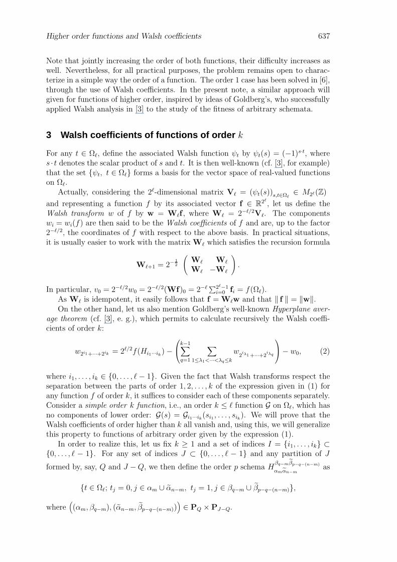
Note that jointly increasing the order of both functions, their difficulty increases aswell. Nevertheless, for all practical purposes, the problem remains open to charac-terize in a simple way the order of a function. The order 1 case has been solved in [6],through the use of Walsh coefficients. In the present note, a similar approach willgiven for functions of higher order, inspired by ideas of Goldberg’s, who successfullyapplied Walsh analysis in [3] to the study of the fitness of arbitrary schemata.

3 Walsh coefficients of functions of order k

For any t ∈ Ωℓ, define the associated Walsh function ψt by ψt(s) = (−1)s·t, wheres · t denotes the scalar product of s and t. It is then well-known (cf. [3], for example)that the set ψt, t ∈ Ωℓ forms a basis for the vector space of real-valued functionson Ωℓ.

Actually, considering the 2ℓ-dimensional matrix Vℓ = (ψt(s))s,t∈Ωℓ∈ M2ℓ(Z)

and representing a function f by its associated vector f ∈ R2ℓ

, let us define theWalsh transform w of f by w = Wℓf , where Wℓ = 2−ℓ/2Vℓ. The componentswi = wi(f) are then said to be the Walsh coefficients of f and are, up to the factor2−ℓ/2, the coordinates of f with respect to the above basis. In practical situations,it is usually easier to work with the matrix Wℓ which satisfies the recursion formula

Wℓ+1 = 2−12

(Wℓ Wℓ

Wℓ −Wℓ

).

In particular, v0 = 2−ℓ/2w0 = 2−ℓ/2(Wf)0 = 2−ℓ∑2ℓ−1i=0 fi = f(Ωℓ).

As Wℓ is idempotent, it easily follows that f = Wℓw and that ‖ f ‖ = ‖w‖.On the other hand, let us also mention Goldberg’s well-known Hyperplane aver-

age theorem (cf. [3], e. g.), which permits to calculate recursively the Walsh coeffi-cients of order k:

w2i1+···+2ik = 2ℓ/2f(Hi1···ik) −

k−1∑

q=1

∑

1≤λ1<···<λq≤k

w2

iλ1 +···+2iλq

− w0, (2)

where i1, . . . , ik ∈ 0, . . . , ℓ− 1. Given the fact that Walsh transforms respect theseparation between the parts of order 1, 2, . . . , k of the expression given in (1) forany function f of order k, it suffices to consider each of these components separately.Consider a simple order k function, i.e., an order k ≤ ℓ function G on Ωℓ, which hasno components of lower order: G(s) = Gi1···ik(si1 , . . . , sik). We will prove that theWalsh coefficients of order higher than k all vanish and, using this, we will generalizethis property to functions of arbitrary order given by the expression (1).

In order to realize this, let us fix k ≥ 1 and a set of indices I = i1, . . . , ik ⊂0, . . . , ℓ − 1. For any set of indices J ⊂ 0, . . . , ℓ − 1 and any partition of J

formed by, say, Q and J −Q, we then define the order p schema Hβq−mβp−q−(n−m)

αmαn−mas

t ∈ Ωℓ; tj = 0, j ∈ αm ∪ αn−m, tj = 1, j ∈ βq−m ∪ βp−q−(n−m),

where((αm, βq−m), (αn−m, βp−q−(n−m))

)∈ PQ ×PJ−Q.

638 M.Teresa Iglesias – V. S. Penaranda – A. Verschoren

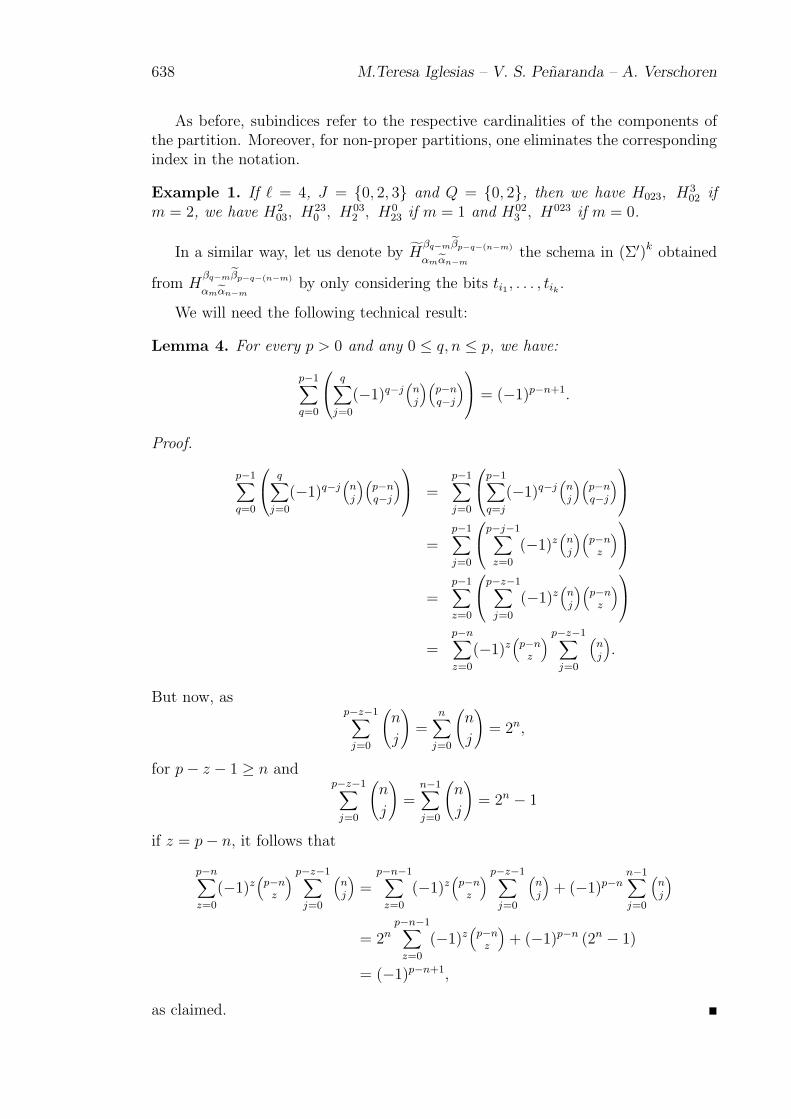
As before, subindices refer to the respective cardinalities of the components ofthe partition. Moreover, for non-proper partitions, one eliminates the correspondingindex in the notation.

Example 1. If ℓ = 4, J = 0, 2, 3 and Q = 0, 2, then we have H023, H302 if

m = 2, we have H203, H

230 , H

032 , H

023 if m = 1 and H02

3 , H023 if m = 0.

In a similar way, let us denote by Hβq−mβp−q−(n−m)

αmαn−mthe schema in (Σ′)k obtained

from Hβq−mβp−q−(n−m)

αmαn−mby only considering the bits ti1 , . . . , tik .

We will need the following technical result:

Lemma 4. For every p > 0 and any 0 ≤ q, n ≤ p, we have:

p−1∑

q=0

q∑

j=0

(−1)q−j(

nj

)(p−nq−j

) = (−1)p−n+1.

Proof.

p−1∑

q=0

q∑

j=0

(−1)q−j(

nj

)(p−nq−j

) =

p−1∑

j=0

p−1∑

q=j

(−1)q−j(

nj

)(p−nq−j

)

=p−1∑

j=0

p−j−1∑

z=0

(−1)z(

nj

)(p−n

z

)

=p−1∑

z=0

p−z−1∑

j=0

(−1)z(

nj

)(p−n

z

)

=p−n∑

z=0

(−1)z(

p−nz

) p−z−1∑

j=0

(nj

).

But now, asp−z−1∑

j=0

(n

j

)=

n∑

j=0

(n

j

)= 2n,

for p− z − 1 ≥ n andp−z−1∑

j=0

(n

j

)=

n−1∑

j=0

(n

j

)= 2n − 1

if z = p− n, it follows that

p−n∑

z=0

(−1)z(

p−nz

) p−z−1∑

j=0

(nj

)=

p−n−1∑

z=0

(−1)z(

p−nz

) p−z−1∑

j=0

(nj

)+ (−1)p−n

n−1∑

j=0

(nj

)

= 2np−n−1∑

z=0

(−1)z(

p−nz

)+ (−1)p−n (2n − 1)

= (−1)p−n+1,

as claimed.

Higher order functions and Walsh coefficients 639

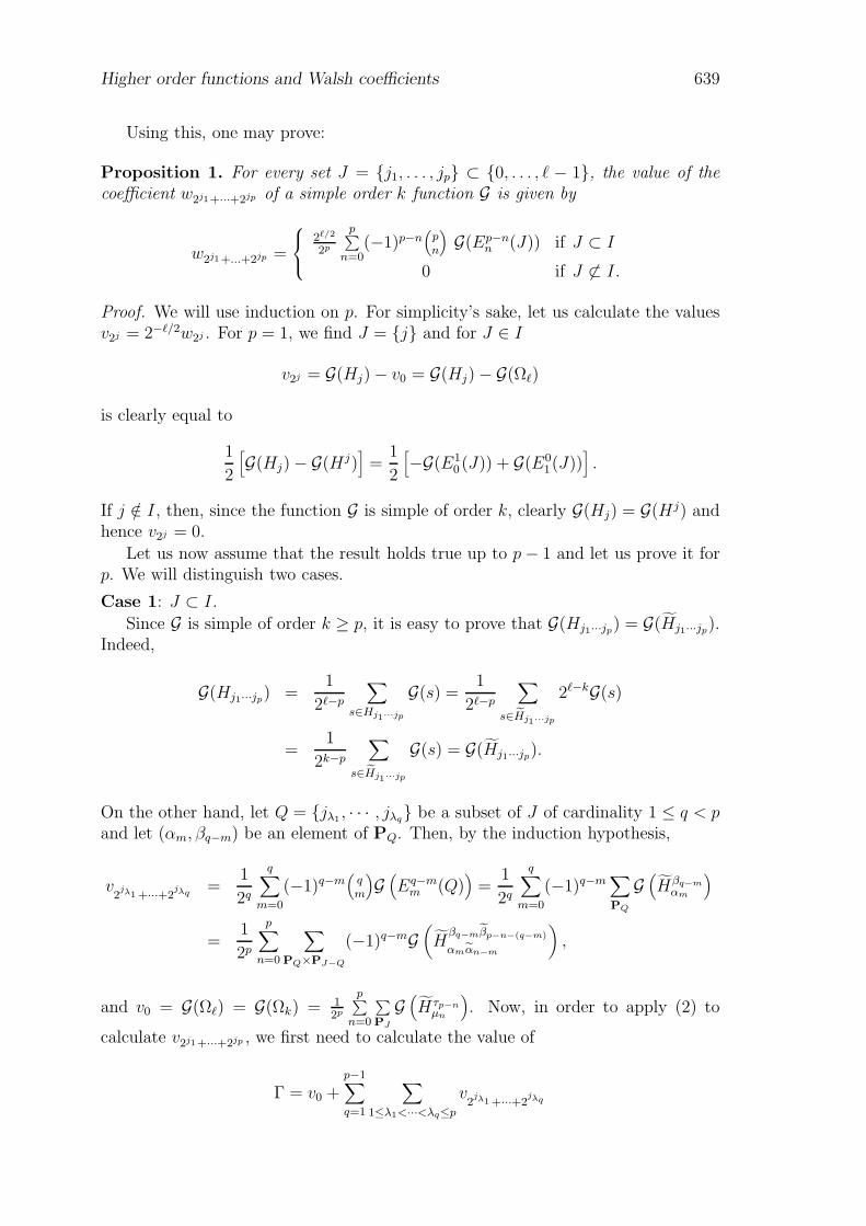
Using this, one may prove:

Proposition 1. For every set J = j1, . . . , jp ⊂ 0, . . . , ℓ − 1, the value of the

coefficient w2j1+···+2jp of a simple order k function G is given by

w2j1+...+2jp =

2ℓ/2

2p

p∑n=0

(−1)p−n(

pn

)G(Ep−n

n (J)) if J ⊂ I

0 if J 6⊂ I.

Proof. We will use induction on p. For simplicity’s sake, let us calculate the valuesv2j = 2−ℓ/2w2j . For p = 1, we find J = j and for J ∈ I

v2j = G(Hj) − v0 = G(Hj) − G(Ωℓ)

is clearly equal to

1

2

[G(Hj) − G(Hj)

]=

1

2

[−G(E1

0 (J)) + G(E01(J))

].

If j /∈ I, then, since the function G is simple of order k, clearly G(Hj) = G(Hj) andhence v2j = 0.

Let us now assume that the result holds true up to p− 1 and let us prove it forp. We will distinguish two cases.

Case 1: J ⊂ I.

Since G is simple of order k ≥ p, it is easy to prove that G(Hj1···jp) = G(Hj1···jp).Indeed,

G(Hj1···jp) =1

2ℓ−p

∑

s∈Hj1···jp

G(s) =1

2ℓ−p

∑

s∈Hj1···jp

2ℓ−kG(s)

=1

2k−p

∑

s∈Hj1···jp

G(s) = G(Hj1···jp).

On the other hand, let Q = jλ1 , · · · , jλq be a subset of J of cardinality 1 ≤ q < pand let (αm, βq−m) be an element of PQ. Then, by the induction hypothesis,

v2

jλ1 +···+2jλq =

1

2q

q∑

m=0

(−1)q−m(

qm

)G(Eq−m

m (Q))

=1

2q

q∑

m=0

(−1)q−m∑

PQ

G(Hβq−m

αm

)

=1

2p

p∑

n=0

∑

PQ×PJ−Q

(−1)q−mG(H

βq−mβp−n−(q−m)

αmαn−m

),

and v0 = G(Ωℓ) = G(Ωk) = 12p

p∑n=0

∑PJ

G(Hτp−n

µn

). Now, in order to apply (2) to

calculate v2j1+···+2jp , we first need to calculate the value of

Γ = v0 +p−1∑

q=1

∑

1≤λ1<···<λq≤p

v2

jλ1 +···+2jλq

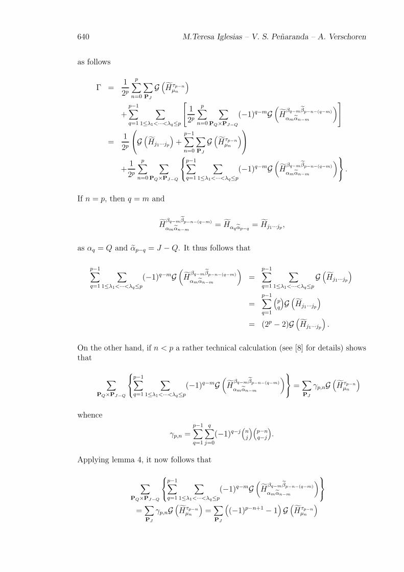
640 M.Teresa Iglesias – V. S. Penaranda – A. Verschoren

as follows

Γ =1

2p

p∑

n=0

∑

PJ

G(Hτp−n

µn

)

+p−1∑

q=1

∑

1≤λ1<···<λq≤p

1

2p

p∑

n=0

∑

PQ×PJ−Q

(−1)q−mG(H

βq−mβp−n−(q−m)

αmαn−m

)

=1

2p

G

(Hj1···jp

)+

p−1∑

n=0

∑

PJ

G(Hτp−n

µn

)

+1

2p

p∑

n=0

∑

PQ×PJ−Q

p−1∑

q=1

∑

1≤λ1<···<λq≤p

(−1)q−mG(H

βq−mβp−n−(q−m)

αmαn−m

) .

If n = p, then q = m and

Hβq−mβp−n−(q−m)

αmαn−m= Hαqαp−q

= Hj1···jp,

as αq = Q and αp−q = J −Q. It thus follows that

p−1∑

q=1

∑

1≤λ1<···<λq≤p

(−1)q−mG(H

βq−mβp−n−(q−m)

αmαn−m

)=

p−1∑

q=1

∑

1≤λ1<···<λq≤p

G(Hj1···jp

)

=p−1∑

q=1

(pq

)G(Hj1···jp

)

= (2p − 2)G(Hj1···jp

).

On the other hand, if n < p a rather technical calculation (see [8] for details) showsthat

∑

PQ×PJ−Q

p−1∑

q=1

∑

1≤λ1<···<λq≤p

(−1)q−mG(H

βq−mβp−n−(q−m)

αmαn−m

) =

∑

PJ

γp,nG(Hτp−n

µn

)

whence

γp,n =p−1∑

q=1

q∑

j=0

(−1)q−j(

nj

)(p−nq−j

).

Applying lemma 4, it now follows that

∑

PQ×PJ−Q

p−1∑

q=1

∑

1≤λ1<···<λq≤p

(−1)q−mG(H

βq−mβp−n−(q−m)

αmαn−m

)

=∑

PJ

γp,nG(Hτp−n

µn

)=∑

PJ

((−1)p−n+1 − 1

)G(Hτp−n

µn

)

Higher order functions and Walsh coefficients 641

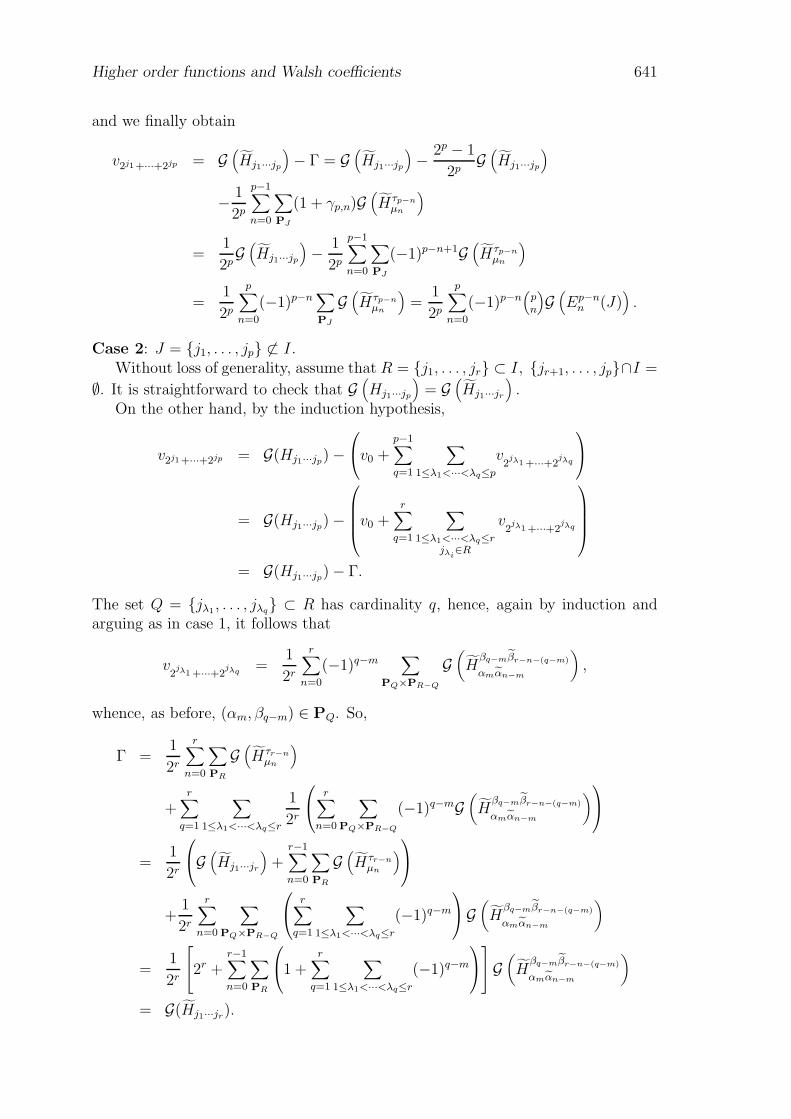
and we finally obtain

v2j1+···+2jp = G(Hj1···jp

)− Γ = G

(Hj1···jp

)−

2p − 1

2pG(Hj1···jp

)

−1

2p

p−1∑

n=0

∑

PJ

(1 + γp,n)G(Hτp−n

µn

)

=1

2pG(Hj1···jp

)−

1

2p

p−1∑

n=0

∑

PJ

(−1)p−n+1G(Hτp−n

µn

)

=1

2p

p∑

n=0

(−1)p−n∑

PJ

G(Hτp−n

µn

)=

1

2p

p∑

n=0

(−1)p−n(

pn

)G(Ep−n

n (J)).

Case 2: J = j1, . . . , jp 6⊂ I.Without loss of generality, assume that R = j1, . . . , jr ⊂ I, jr+1, . . . , jp∩I =

∅. It is straightforward to check that G(Hj1···jp

)= G

(Hj1···jr

).

On the other hand, by the induction hypothesis,

v2j1+···+2jp = G(Hj1···jp) −

v0 +

p−1∑

q=1

∑

1≤λ1<···<λq≤p

v2

jλ1 +···+2jλq

= G(Hj1···jp) −

v0 +

r∑

q=1

∑

1≤λ1<···<λq≤rjλi

∈R

v2

jλ1 +···+2jλq

= G(Hj1···jp) − Γ.

The set Q = jλ1 , . . . , jλq ⊂ R has cardinality q, hence, again by induction andarguing as in case 1, it follows that

v2

jλ1 +···+2jλq =

1

2r

r∑

n=0

(−1)q−m∑

PQ×PR−Q

G(H

βq−mβr−n−(q−m)

αmαn−m

),

whence, as before, (αm, βq−m) ∈ PQ. So,

Γ =1

2r

r∑

n=0

∑

PR

G(Hτr−n

µn

)

+r∑

q=1

∑

1≤λ1<···<λq≤r

1

2r

r∑

n=0

∑

PQ×PR−Q

(−1)q−mG(H

βq−mβr−n−(q−m)

αmαn−m

)

=1

2r

G

(Hj1···jr

)+

r−1∑

n=0

∑

PR

G(Hτr−n

µn

)

+1

2r

r∑

n=0

∑

PQ×PR−Q

r∑

q=1

∑

1≤λ1<···<λq≤r

(−1)q−m

G

(H

βq−mβr−n−(q−m)

αmαn−m

)

=1

2r

2r +

r−1∑

n=0

∑

PR

1 +

r∑

q=1

∑

1≤λ1<···<λq≤r

(−1)q−m

G

(H

βq−mβr−n−(q−m)

αmαn−m

)

= G(Hj1···jr).

642 M.Teresa Iglesias – V. S. Penaranda – A. Verschoren

Indeed, for n = r we have q = m and Hβq−mβr−n−(q−m)

αmαn−m= Hαqαr−q

= Hj1···jr (as

αq = Q and αr−q = R−Q) hence

r∑

q=1

∑

1≤λ1<···<λq≤r

(−1)q−mG(H

βq−mβr−n−(q−m)

αmαn−m

)=

r∑

q=1

∑

1≤λ1<···<λq≤r

G(Hj1···jr

)

= (2r − 1)G(Hj1···jr

).

On the other hand, if n < r, it has been proved in [8] that

∑

PQ×PR−Q

r∑

q=1

∑

1≤λ1<···<λq≤r

(−1)q−mG(H

βq−mβr−n−(q−m)

αmαn−m

)=∑

PR

ζr,nG(Hτr−n

µn

)

with

ζr,n =r∑

q=1

q∑

j=0

(−1)q−j(

nj

)(r−nq−j

)

equal to

γr,n +r∑

j=0

(−1)r−j(

nj

)(r−nr−j

)= [−1 + (−1)r−n+1] + (−1)r−n = −1.

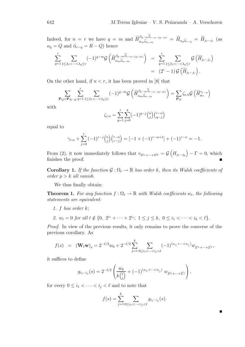
From (2), it now immediately follows that v2j1+···+2jp = G(Hj1···jp

)− Γ = 0, which

finishes the proof.

Corollary 1. If the function G : Ωℓ → R has order k, then its Walsh coefficients of

order p > k all vanish.

We thus finally obtain:

Theorem 1. For any function f : Ωℓ → R with Walsh coefficients wt, the following

statements are equivalent:

1. f has order k;

2. wt = 0 for all t /∈ 0, 2i1 + · · · + 2ij ; 1 ≤ j ≤ k, 0 ≤ i1 < · · · < ik < ℓ.

Proof. In view of the previous results, it only remains to prove the converse of theprevious corollary. As

f(s) = (Wℓw)s = 2−ℓ/2w0 + 2−ℓ/2k∑

j=1

∑

0≤i1<···<ij<ℓ

(−1)(si1+···+sij

)w2i1+···+2ij ,

it suffices to define

gi1···ij (s) = 2−ℓ/2

w0

k(

ℓj

) + (−1)(si1+···+sij

) w2i1+···+2ij

,

for every 0 ≤ i1 < · · · < ij < ℓ and to note that

f(s) =k∑

j=1

∑

0≤i1<···<ij<ℓ

gi1···ij (s).

Higher order functions and Walsh coefficients 643

References

[1] Davidor, Y.: Epistasis and Variance: A Viewpoint on GA-Hardness. In: Rawl-ins, G. J. E. (Ed.): Foundations of Genetic Algorithms 1, Morgan KaufmannPublishers, 1991, pp. 23–25.

[2] Forrest, S. and Mitchell, M.: Relative Building-Block Fitness and the Building-Block Hypotesis, Foundations of Genetic Algorithms 2. Ed. L.D. Whitley, Mor-gan Kaufmann Publishers, San Mateo, 1993.

[3] Goldberg, D. E.: Genetic Algorithms and Walsh functions: Part I, A GentleIntroduction. Complex Systems, Vol. 3, 1989, pp. 129–152.

[4] Iglesias, M. T., Naudts, B., Verschoren, A. and Vidal, C.: A CombinatorialApproach to Epistasis, Springer, Dordrecht, 1995.

[5] Iglesias, M. T., Verschoren, A. and Vidal, C.: Template Functions and theirEpistasis. In: Proceedings of MS’2000 International Conference on Modellingand Simulation, Las Palmas de Gran Canaria, 2000, pp. 539-546.

[6] Naudts, B., Suys, D. and Verschoren, A.: Epistasis, Deceptivity and WalshTransforms. In: Proceedings of the International ICSC Symposium on Engi-neering of Intelligent Systems (EIS’98), V1: Fuzzy Logic/Genetic Algorithms,ICSC Academic Press, 1998, pp. 210–216.

[7] Naudts, B., Suys, D. and Verschoren, A.: Generalized Royal Road functionsand their Epistasis, Artificial Intelligence, Vol. 19, 2000, pp. 317-334.

[8] Penaranda, V. S.: Epistasis superior, Ph.D. Thesis, Universidade da Coruna,in preparation.

[9] Rawlins, G. J. E.: Foundations of Genetic Algorithms, Morgan Kaufmann Pub-lishers, San Mateo, 1991.

[10] Suys, D. and Verschoren, A.: Extreme Epistasis. In: International Conferenceon Intelligent Technologies in Human-Relates Sciences (ITHURS 96), Vol. II,Leon, 1996, pp. 251–258.

[11] Van Hove, H.: Representational Issues in Genetic Algorithms, Ph.D. Thesis,University of Antwerp, 1995.

M.Teresa Iglesias, Vicente S. PenarandaDepartamento de MatematicasUniversidade da CorunaA Coruna, Spainemail : totero@udc.es, vesp@udc.es

Alain VerschorenDepartment of Mathematics and Computer ScienceUniversity of AntwerpAntwerp, Belgiumemail : alain.verschoren@ua.ac.be