1

29th Symposium on Naval Hydrodynamics Gothenburg, Sweden, 26-31 August 2012

URANS Study of Delft Catamaran Total/Added

Resistance, Motions and Slamming Loads in Head Sea Including Irregular Wave and Uncertainty Quantification

for Variable Regular Wave and Geometry

Wei He1,2, Matteo Diez1,3

, Daniele Peri3, Emilio Campana3

, Yusuke Tahara4

, and Frederick Stern1,†

(1IIHR–Hydroscience & Engineering, The University of Iowa, Iowa City, US, 2NAOCE, Shanghai Jiao Tong University, China,

3CNR–INSEAN, Natl. Research Council–Maritime Research Centre, Rome, Italy, 4NMRI, National Maritime Research Institute, Tokyo, Japan)

ABSTRACT1

A methodology is assessed for uncertainty quantification (UQ) of resistance, motions and slamming loads in variable regular wave representing a given sea state, and compared to irregular wave (benchmark) and deterministic regular wave studies. UQ is conducted over joint distribution of wave period and height; irregular wave inlet boundary condition is based on wave energy spectrum; deterministic study is conducted at most probable condition. Application to the high-speed Delft Catamaran at Fr=0.5 in sea state 6 is presented and discussed. Deterministic regular wave study shows average error for design optimization-related quantities (expected values of resistance, motions amplitude and slamming loads) equal to 25%. Variable regular wave UQ shows average error close to 6%, providing in addition empirical distribution functions. Extension to uncertain design through Karhunen-Loève expansion is presented and discussed; variable geometry studies show a potential reduction of 6.5% for calm water resistance and 3.9% for resistance in wave, with small variations in motions amplitudes; an increase of 6.4% of maximum slamming load is experienced by reduced-resistance geometry, revealing a trade-off between performances and loads. UQ with metamodels reveals Kriging and polyharmonic spline as the most effective metamodels overall.

†

Corresponding author. Email: frederick-stern@uiowa.edu

1 INTRODUCTION University of Iowa, CNR–INSEAN, NMRI collaboration has successfully developed and applied its Simulation Based Design (SBD) tool box for deterministic shape optimization (Campana et al., 2006, 2009). Capabilities include multiple optimization methods [sequential quadratic programming (SQP), genetic algorithms (GA), and particle swarm optimization (PSO)]; multifidelity solvers (CFDShip-Iowa, WARP, and FreDOM); multiple geometry modification methods [free-form deformation (FFD), B-splines, and morphing]; high performance computing (MPI based parallel processing taking advantage of advance reservation system in DoD HPC machines); and portability (modular components allow for easy plug and play). Demonstration applications include 5415 bow shape optimization for 70% wave slope reduction (Campana et al., 2006); HSSL A shape optimization for 9% reduction in resistance (Stern et al., 2008); HSSL B shape optimization for resistance and heave RAO reduction (Tahara et al., 2011a); high-speed ferry shape optimization for 10% reduction of far-field energy (Kandasamy et al., 2011a); JHSS bow and waterjet inlet/duct shape optimization for 14% powering reduction (Kandasamy et al., 2011b); Delft catamaran (DC) hull and waterjet inlet/duct shape optimization for 5% powering reduction (Kandasamy et al., 2011a); and DC hull shape optimization for resistance reduction over range of Froude number, Fr (Tahara et al. 2011b). Towing tank experiments at CNR-INSEAN validated most applications.

2

Recently, focus is on advancements for stochastic optimization [robust design optimization (RDO) and reliability based design optimization (RBDO)] with application to DC total/added resistance/powering - which is of timely importance due to recent IMO (International Maritime Organization) EEOI (Energy Efficiency Operational Indicator) requirements - and slamming loads. Developing RDO/RBDO capability requires research in uncertainty quantification (UQ) methods. Indeed, UQ studies are a prerequisite and a fundamental part of RDO/RBDO, since (a) provide preliminary sensitivity analysis for the uncertain parameters involved, (b) identify the most efficient UQ methods, and (c) give objectives and constraints in the design optimization process. Current UQ research is in collaboration with NATO-AVT 191 “Application of Sensitivity Analysis and UQ to Military Vehicle Design”.

Initial research developed and demonstrated the applicability of a framework for convergence and validation of stochastic UQ and relationship with deterministic verification and validation (V&V). The framework, with an example for a unit problem assessing a NACA 0012 hydrofoil with variable Reynolds number was presented in Mousaviraad et al. 2012. Convergence of Latin-hypercube sampling Monte Carlo method (MC-LHS, see, e.g., Helton and Davis, 2003) with deterministic URANS simulations was shown as well as convergence and validation of MC-LHS with metamodels and quadrature formulas. MC-LHS with deterministic simulations was used to get benchmark results and MC-LHS with metamodels and quadrature formulas were validated versus benchmark. The stochastic influence factor (defined as the difference between deterministic performance and its stochastic expectation) was assessed and found not significant for the unit problem. The approach was extended and applied towards application of interest, i.e., DC calm water resistance, sinkage and trim UQ for variable Fr (representing stochastic operation) and/or geometry (representing uncertain design), using URANS and potential flow (PF) solvers (Diez et al., 2012b). Geometric variability was intended as an epistemic design uncertainty and related to the optimization space of earlier deterministic DC optimization studies (Kandasamy et al., 2011b). This was assessed through Karhunen-Loève expansion (KLE; detailed methodology is presented in Diez et al. 2012a). MC-LHS and efficient UQ methods (MC-LHS with metamodels and quadrature formulas) were assessed and discussed. Among the metamodels used, linear interpolation, although very simple, and Hermite cubic interpolation performed well on average for the univariate problems (separate variable Fr and

geometry studies), whereas thin plate spline (polyharmonic spline of 2nd order) appeared to be the best for the multivariate problem (based on joint distribution of Fr and geometry). Among the quadrature formulas, Gauss-Legendre quadrature on CDF image domain was found the best for the univariate and multivariate problems. Geometric UQ was found consistent with earlier optimization work (Kandasamy et al. 2011b and Tahara et al. 2011b) and showed small differences between deterministic and stochastic optimal-geometries performances over Fr range; this suggested that the impact of variable Fr on designer choice (through RDO) was negligible in that context.

Currently, extensions are in progress for URANS UQ for DC total/added resistance, heave and pitch motions, and slamming loads for variable regular head waves and variable geometry, including comparison with irregular head wave studies. The paper provides formulations and methods for stochastic analysis of forces, motions and slamming loads in irregular and variable regular wave. Irregular wave studies are carried out using inlet boundary conditions based on wave energy spectrum and associated probability density function (PDF) of period and height for a given sea state (Longuet-Higgins, 1983); frequentist statistical analysis of the relevant outputs is taken as a benchmark for validating variable regular wave UQ studies. An optimal wave design approach for the boundary condition is given and discussed. Bayesian UQ for variable regular wave is based on the joint PDF of wave period and height associated to the given spectrum, and solved using the Markov-Chain Monte Carlo (MCMC) method. Comparison of irregular wave (benchmark) versus variable regular wave UQ studies is given and discussed. UQ for variable regular wave over joint PDF may be effectively coupled with efficient UQ methods such as MC with metamodels and/or quadrature formulas (as done in earlier calm water UQ work). Here, MCMC with metamodels (inverse distance weighting, radial basis functions network, polyharmonic splines, least-square support vector machine and Kriging) is shown and the results validated versus CFD-based MCMC. Prerequisite V&V for calm water and deterministic regular head wave is provided and discussed. The code CFDShip-Iowa is used for current analyses.

Geometry and conditions for present UQ studies are given. Extension to uncertain design (variable geometry) is presented, based on KLE. The results will be used to formulate appropriate RDO/RBDO for DC total/added resistance/powering, heave and pitch motions, and slamming loads; future optimization will include hull and waterjet inlet/duct design.

3

Supplemental material provides preliminary deterministic URANS simulations with V&V in calm water and regular wave. It also provides statistical convergence study for wave period and height items over joint PDF, and preliminary regular wave UQ study.

2 PROBLEM FORMULATION AND ANALYSIS METHODS 2.1 Geometry and conditions

The problem of interest is that of a high-speed catamaran operating in a real transit scenario. DC is selected and, since full-scale ship is not available, a length between perpendiculars equal to 100 m is chosen. Table 1 summarizes the relevant full-scale DC design parameters used herein. Natural frequencies for heave and pitch coupled motions are estimated following Castiglione et al. 2012, using CFD simulations in calm water at Fr=0; resulting fn is included in Table 1. Geometry is shown in Figure 1 for model scale (DC 372). Present study is conducted considering the bare hull only.

The routes from San Diego to Honolulu and from Guam to Okinawa (Japan) are selected as possible operating scenario. Honolulu is approximately 4200km from San Diego, bearing West/South-West (WSW); the route falls into areas 22 and 31 of Global Wave Statistics (Hogben et al. 1986). Okinawa is approximately 2300km from Guam, bearing North-West (NW) and the route falls into areas 41, 42 and 52. Sea state 6 is taken as a challenging test case to assess UQ methods and simulation tools capabilities. As shown in Table 2, sea state 6 has a probability of occurrence in North Pacific of nearly 16% with an exceedance of 10% (Bales 1982; Lee and Bales 1984). Only head waves are considered, being variable encounter angle beyond the scope of the present work. Current study is performed at the hump speed, Fr=0.5.

2.2 Calm water and regular wave deterministic simulations

Prerequisite calm water simulation for total resistance, sinkage and trim, is carried out at Fr=0.5. Verification and validation focus on: calm water total resistance coefficient, (where is the calm-water total resistance [N], the water density [kg/m3], U the ship speed [m/s] and S the static wetted area [m2]), non-dimensional sinkage,

, and trim, τ [rad]. Deterministic regular head wave simulation for

total/added resistance, heave and pitch motions, is studied at Fr=0.5 and (corresponding to

most probable condition in sea state 6) and 1/50, in the range from 0.5 to 2 (where is the wavelength). V&V is assessed for and

(corresponding to most probable conditions in sea state 6). Focus is on time histories of following variables: non-dimensional force,

, (where is the total resistance [N]), non-dimensional heave, , and pitch, [rad]. Verification variables are: added resistance coefficient

(where is the time mean of and b the beam of the demi hull); 0th and 1st harmonics amplitudes, 1st harmonics phase and RMS of total resistance coefficient ( ), non-dimensional heave ( ) and non-dimensional pitch ( ) respectively. is the wave amplitude and is the wave number. 0th and 1st harmonics amplitudes and 1st harmonic phase are identified through fast Fourier transform (FFT). A moving window consisting of 128 time steps (corresponding to one period) is used for FFT and running mean and RMS estimate.

2.3 Irregular wave simulation and statistical analysis of relevant outputs

Fully nonlinear URANS simulation in irregular wave (Figure 2) is carried out, in analogy with what is usually done for model testing. Inlet boundary conditions are given in terms of elemental wave (linear) superposition. Once entered the domain, the wave components can interact nonlinearly. Bretschneider spectrum (Bretschneider, 1959) is used, assuming open ocean, fully developed seas. Accordingly, the wave energy spectrum is expressed as a function of the wave angular frequency ( ) as:

(1)

where is the peak (modal) angular frequency and is the significant wave height (e.g., Michel

1999). is the period associated to the modal frequency. Table 2 shows and most probable for sea states from 1 to 8.

Assuming equally-spaced (in frequency) elemental (head) wave components, the inlet boundary condition is defined as

(2)

with . URANS provides the time histories of the output

variables, namely . FFT is applied to compute amplitudes in the encounter frequency ( ) domain, with

4

FFT amplitudes are used to get response amplitude operators (RAO) as:

where , is the ship displacement and is the wave number. In order to avoid

noisy responses, a Gaussian filter is applied to both input and output FFT.

For each mean-crossing period (both up and down crossing, see Figure 3), the associated mean ( ), root mean square of deviations from mean ( ), and amplitude ( ) are identified. Expected values (EV), standard deviations (SD) and empirical cumulative distribution functions (CDF) of relevant outputs are evaluated as:

(3)

(4)

(5)

where is the Heaviside step function of , and

(6)

with for resistance, heave and pitch motions, and for emerging and re-entering slamming loads, respectively. Approach for slamming loads identification is discussed later in Section 2.5.

EV and SD uncertainties, UEV and USD respectively, are estimated at 95% level of confidence as:

(7)

where tN-1;0.95 is the 95% percentile of Student’s t-distribution with degrees of freedom;

(8)

where χ2N-1;0.975 is the 97.5% percentile of the Chi-

square distribution with degrees of freedom. It may be noted that Equation 8 represents the upper band of the confidence interval for SD. This is greater than the lower band and converges to the lower band for large N.

CDF uncertainty is derived from Liang and Mahadevan 2011. Specifically, the error of empirical CDF values (Eq. 5) compared to unknown true values is modeled as a normal random variable, with zero mean and standard deviation given by

Assuming 95% confidence interval, the uncertainty of CDF(y) is approximately . CDF overall uncertainty may be defined as the root mean square of over y:

( )

where K is the number of bins, . Empirical CDFs are compared to theoretical

models (m) such as Normal, Gamma or Beta distributions through Cramer-Von Mises accuracy A, as shown in Forbes et al., 2011:

(10)

2.4 UQ for variable regular wave simulations, based on joint PDF of wave period and height

Theoretical joint and marginal PDFs for zero-crossing period and height may be derived from the given energy spectrum. Following Longuet-Higgins 1983, and defining the non-dimensional quantities and , with

and

it is

(11)

The non-dimensional coordinates of the mode

(most probable condition) are given by:

where is the spectrum parameter:

5

Marginal PDF for non-dimensional wave period

is given by

(12)

whereas marginal PDF of non-dimensional height is given by the Rayleigh distribution (under the condition , e.g. Ochi 1998):

(13)

UQ over joint PDF of Eq. 11 is performed for parameters of Eq. 6 (same outputs are assessed for regular and irregular wave). Specifically, when

, with , it is

(14)

(15)

(16)

Whereas, when , , it is

(17)

(18)

(19) Uncertainties for EV, SD, and CDF follow Eqs.

7-9. Results from Eqs. 14-19 are validated versus irregular wave values (Eqs. 3-5). Specifically, EVs and SDs are validated following Mousaviraad et al. 2012. Errors are defined as

(20)

whereas validation uncertainties are

(21)

(22)

where superscripts b indicate benchmark values from irregular wave studies.

CDFs are validated versus benchmark distributions following Diez et al. 2012b. Error is defined as the root mean square error (RMSE) over the bins:

(23)

whereas validation uncertainty is

(24)

Validation is achieved at level if . 2.5 Slamming loads studies Slamming loads studies are conducted according to the guidelines from the American Bureau of Shipping (ABS guide 2011). In rough seas, the vessel’s bow and stern may occasionally emerge from water and re-enter with a significant impact or slam. ABS defines three types of slams: bottom slamming, bow flare slamming and stern slamming. Slamming in the bow area is more severe in head wave, while slamming in the stern area is more critical in following sea; latest condition is known to be more critical at low speeds.

Herein, in order to detect the slamming loads, the time-history of pressure is studied at pressure probes. Figure 1 shows the location of bow (B1 – B21) and stern (S1) probes. Probes are located at the centerline of the demi-hull. Slamming loads are detected on time histories as pressure jumps [see Figure 4 (a)]; a threshold value is usually applied. Jumps may be negative or positive. In the former case, the pressure jump is defined as emerging slamming load ( ), whereas the latter condition identifies re-entering slamming loads ).

Figure 4 (b) shows the number of slamming events occurring at different probes for current problem (using URANS simulation in irregular wave in sea state 6). Figure 4 (c) shows the maximum loads detected, whereas Figure 4 (d) presents the influence of threshold value for loads detection on number of events (that is, statistical sample size). Probe B1 is chosen for current studies, since provides largest number of events and largest loads. A threshold value of 2 kPa is selected since allows for highest number of events. Accordingly, B1 with a threshold value of 2 kPa is used hereafter for irregular wave, deterministic and variable regular wave studies.

6

2.6 Geometric UQ through Karhunen-Loève Expansion (KLE) Design uncertainty is assessed by means of geometric UQ. The approach follows Diez et al. (2012a) and is briefly recalled here. Geometric uncertainty is related to a design optimization research space. Without loss of generality, in current study a free-form deformation (FFD) technique is applied to the original DC geometry. The research space is sampled randomly using S items (geometry realizations) and the mean geometry is defined as

The principal directions, zk ,of the research space expressed by:

are solution of the eigenproblem:

where

with

The eigenvalues of R represent the geometric variance associated to the corresponding eigenvector zk (principal direction). Geometric UQ is conducted herein along the direction which retains the largest geometric variance, as per

with

where represents the uncertain design parameter. 2.7 UQ using metamodels Metamodels are used to predict unseen wave periods

and heights H and/or geometry parameters . Specifically, if N is the MC sample size, a number M<N of CFD simulations is used to predict the required values in the sample. Five metamodels are applied: namely, inverse distance weighting (IDW, Shepard 1968), radial basis functions network with multiquadric kernel (RBF-MQ, Buhmann 2003),

polyharmonic splines (PHS, Harder and Desmarais 1972), least-square support vector machine (LS-SVM, Suykens et al. 2002) and Kriging using linear and exponential covariance functions (Peri 2009). Three different tuning parameters are used for each metamodel. Specifically: p, for p-th order inverse distance weighting; e, for radial basis functions network with multiquadric kernel of the form

; k, for polyharmonic spline of k-th order; g for LS-SVM (see Diez et al. 2012b, parameter γ in Eq. 21); e, for Kriging with linear [ and exponential

covariance functions. Convergence of prediction error versus

systematic increase of training set size , is studied. The prediction error is defined as

the normalized root mean square error (NRMSE) of predictions versus CFD values:

where superscript d indicates values obtained with deterministic CFD. The test set used for assessing NRMSE is defined as the difference between training set and MC sample. Available MC items are used for training the metamodels. NRMSE is required to be <5% and monotonically convergent versus M (oscillatory convergence is accepted if relative solution change is less than 1%).

Once M is found appropriate, stochastic and deterministic convergence of MC versus N is studied. Here, N=129 is chosen and the results obtained using metamodels are compared with MC based on CFD simulations. Errors are defined for EV and SD as per Eq. 20, substituting superscript b with d; the latter indicates values from CFD-based MC. Similarly, the CDF error is defined as per Eq. 23 where a number of

bins is used. Uncertainties for EV, SD and CDF are evaluated as per Eqs. 7-9 and validation uncertainties follow Eqs. 21, 22 and 24.

Metamodels are ranked based on associated MC results. Specifically, computational efficiency is taken into account by means of the ratio between the training set size required to achieve both convergence and validation, and the maximum size allowed: M/Mmax. Accuracy is assessed using the ratio between the average error on EV, SD and CDF, and its largest value among all the metamodels: E/Emax. Fulfillment of convergence and validation criteria is taken into account by means of the ratio Nfail/Nfunctions, where Nfail is the number of times the metamodel fails in achieving convergence and/or validation, and Nfunctions is the number of functions assessed for each problem.

7

3 DETERMINISTIC V&V The overall approach in Stern et al. (2006) along with detailed procedures in Coleman and Stern (1997) and Xing and Stern (2010) are followed. It is assumed that all input variables/models are deterministic and deterministic numerical and modeling errors and uncertainties are assessed. For solutions in the asymptotic range, the estimated numerical error and its estimated error are used to obtain a corrected solution (numerical benchmark) and its uncertainty. Verification procedures identify the most important numerical error sources (such as iterative, grid size, and time step errors) and provide error and uncertainty estimates. Validation methodology and procedures use experimental benchmark data and properly take into account both deterministic numerical and experimental uncertainties in estimating validation uncertainty.

Verification procedures estimate numerical uncertainties ( ) based on iterative ( ), grid ( ), and time step ( ) uncertainties:

. Grid and time step convergence studies are

carried out for three solutions ( ) with systematic refinement ratio , where 3, 2, and 1 represent the coarse, medium, and fine grids, respectively. Solution changes and the convergence ratio are defined as and . The convergence is evaluated as:

, monotonic convergence , oscillatory convergence

, monotonic divergence , oscillatory divergence

When monotonic convergence is achieved, factor of safety method (Xing and Stern, 2010) is used for estimations of , and , whereas is evaluated following Stern et al. (2001); when oscillatory convergence is achieved, is calculated by

. Validation procedure defines the comparison

error ( ) and the validation uncertainty ( ) using experimental benchmark data ( ) and its uncertainty ( ). If bounds , the combination of all the errors in and is smaller than and validation is achieved at the interval, with and

. 4 CFD METHOD

The code CFDShip-Iowa V4.5 is used for the CFD simulations. Using the code SUGGAR, the overset structured grid connectivity is obtained at running time to simulate large-amplitude motions. 6DOF

capabilities are implemented using Euler angles. The blended turbulence and single-phase level set free-surface modeling is used. The location of the free-surface is given by the “zero” value of the level-set function, positive in water and negative in air. Numerical methods include advanced iterative solvers, second and higher order finite difference schemes with conservative formulations, parallelization based on a domain decomposition approach using the message-passing interface (MPI). The fluid flow equations are solved in an earth-fixed inertial reference system, while the rigid body equations are solved in the ship system. Due to the symmetric condition of the simulation, the half domain is modeled, extending from

, in dimensionless coordinates, based on ship length. The ship axis is aligned with with the bow at and the stern at . The axis is positive to starboard with pointing upward. symmetric condition is employed at . The far field boundary conditions are imposed on the top and bottom of background. The no-slip condition is applied on the solid surfaces.

5 DESIGN AND STATISTICAL ANALYSYS OF INLET BOUNDARY CONDITION FOR IRREGULAR WAVE SIMULATION

In order to compare and validate variable regular wave UQ versus irregular wave benchmark, it is necessary that the inlet boundary condition for irregular wave simulation is coherent with the joint PDF used for variable regular wave UQ. That is, it is necessary that frequentist and Bayesian analyses have coherent simulation inputs. To this aim, the error of empirical distribution from irregular wave boundary condition (Eq. 2) versus theoretical marginal distributions (Eqs. 12 and 13) is assessed following Eq. 23. Uncertainty estimate follows Eqs. 9. Several boundary condition designs, varying and random phase sets (Eq. 2), are studied. For current studies in sea state 6, the wave angular frequency is taken within the range . For each {50, 100, 200, 400, 800, 1600}, a number of 1,000 random phase sets, with (uniform distribution), are generated and compared. The statistics for and is based on a 3,600 s run in full scale, which is found appropriate for convergence. This corresponds to 566 non- dimensional time and nearly 11 minutes at 3m-model scale. The number of bins used for error and uncertainty estimates equals , where is the sample size.

Best-set results for each are presented in Table 3 in terms of empirical CDF error vs. theory

8

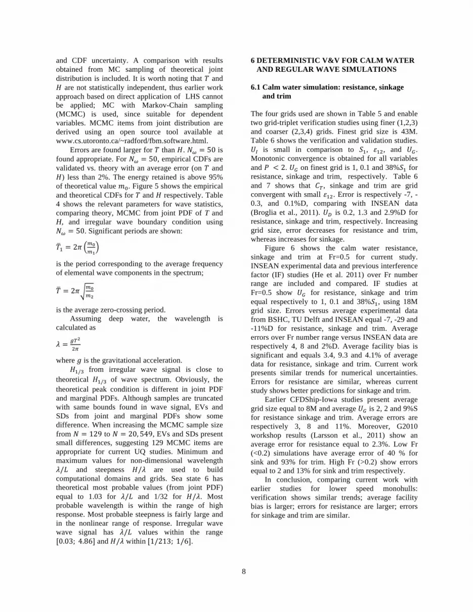
and CDF uncertainty. A comparison with results obtained from MC sampling of theoretical joint distribution is included. It is worth noting that and

are not statistically independent, thus earlier work approach based on direct application of LHS cannot be applied; MC with Markov-Chain sampling (MCMC) is used, since suitable for dependent variables. MCMC items from joint distribution are derived using an open source tool available at www.cs.utoronto.ca/~radford/fbm.software.html.

Errors are found larger for than . is found appropriate. For , empirical CDFs are validated vs. theory with an average error (on and

) less than 2%. The energy retained is above 95% of theoretical value . Figure 5 shows the empirical and theoretical CDFs for and respectively. Table 4 shows the relevant parameters for wave statistics, comparing theory, MCMC from joint PDF of T and H, and irregular wave boundary condition using

. Significant periods are shown:

is the period corresponding to the average frequency of elemental wave components in the spectrum;

is the average zero-crossing period. Assuming deep water, the wavelength is

calculated as

where is the gravitational acceleration. from irregular wave signal is close to

theoretical of wave spectrum. Obviously, the theoretical peak condition is different in joint PDF and marginal PDFs. Although samples are truncated with same bounds found in wave signal, EVs and SDs from joint and marginal PDFs show some difference. When increasing the MCMC sample size from to , EVs and SDs present small differences, suggesting 129 MCMC items are appropriate for current UQ studies. Minimum and maximum values for non-dimensional wavelength

and steepness are used to build computational domains and grids. Sea state 6 has theoretical most probable values (from joint PDF) equal to 1.03 for and 1/32 for . Most probable wavelength is within the range of high response. Most probable steepness is fairly large and in the nonlinear range of response. Irregular wave wave signal has values within the range

and within .

6 DETERMINISTIC V&V FOR CALM WATER AND REGULAR WAVE SIMULATIONS

6.1 Calm water simulation: resistance, sinkage and trim

The four grids used are shown in Table 5 and enable two grid-triplet verification studies using finer (1,2,3) and coarser (2,3,4) grids. Finest grid size is 43M. Table 6 shows the verification and validation studies.

is small in comparison to , , and . Monotonic convergence is obtained for all variables and . on finest grid is 1, 0.1 and 38% for resistance, sinkage and trim, respectively. Table 6 and 7 shows that , sinkage and trim are grid convergent with small . Error is respectively -7, -0.3, and 0.1%D, comparing with INSEAN data (Broglia et al., 2011). is 0.2, 1.3 and 2.9%D for resistance, sinkage and trim, respectively. Increasing grid size, error decreases for resistance and trim, whereas increases for sinkage.

Figure 6 shows the calm water resistance, sinkage and trim at Fr=0.5 for current study. INSEAN experimental data and previous interference factor (IF) studies (He et al. 2011) over Fr number range are included and compared. IF studies at Fr=0.5 show for resistance, sinkage and trim equal respectively to 1, 0.1 and 38% , using 18M grid size. Errors versus average experimental data from BSHC, TU Delft and INSEAN equal -7, -29 and -11%D for resistance, sinkage and trim. Average errors over Fr number range versus INSEAN data are respectively 4, 8 and 2%D. Average facility bias is significant and equals 3.4, 9.3 and 4.1% of average data for resistance, sinkage and trim. Current work presents similar trends for numerical uncertainties. Errors for resistance are similar, whereas current study shows better predictions for sinkage and trim.

Earlier CFDShip-Iowa studies present average grid size equal to 8M and average is 2, 2 and 9%S for resistance sinkage and trim. Average errors are respectively 3, 8 and 11%. Moreover, G2010 workshop results (Larsson et al., 2011) show an average error for resistance equal to 2.3%. Low Fr (<0.2) simulations have average error of 40 % for sink and 93% for trim. High Fr (>0.2) show errors equal to 2 and 13% for sink and trim respectively.

In conclusion, comparing current work with earlier studies for lower speed monohulls: verification shows similar trends; average facility bias is larger; errors for resistance are larger; errors for sinkage and trim are similar.

9

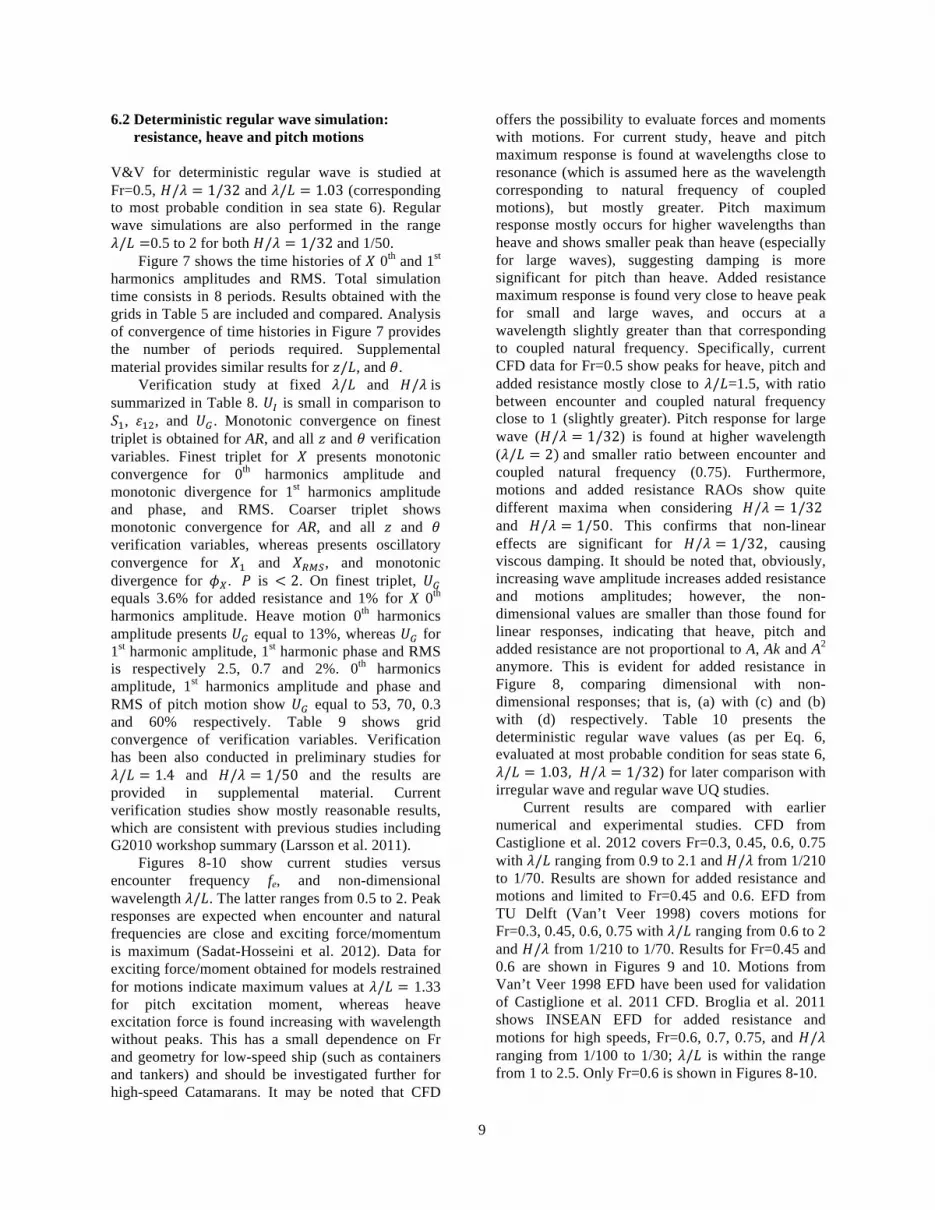
6.2 Deterministic regular wave simulation: resistance, heave and pitch motions

V&V for deterministic regular wave is studied at Fr=0.5, and (corresponding to most probable condition in sea state 6). Regular wave simulations are also performed in the range

0.5 to 2 for both and 1/50. Figure 7 shows the time histories of 0th and 1st

harmonics amplitudes and RMS. Total simulation time consists in 8 periods. Results obtained with the grids in Table 5 are included and compared. Analysis of convergence of time histories in Figure 7 provides the number of periods required. Supplemental material provides similar results for , and .

Verification study at fixed and is summarized in Table 8. is small in comparison to

, , and . Monotonic convergence on finest triplet is obtained for AR, and all and verification variables. Finest triplet for presents monotonic convergence for 0th harmonics amplitude and monotonic divergence for 1st harmonics amplitude and phase, and RMS. Coarser triplet shows monotonic convergence for AR, and all and verification variables, whereas presents oscillatory convergence for and , and monotonic divergence for . is . On finest triplet, equals 3.6% for added resistance and 1% for X 0th harmonics amplitude. Heave motion 0th harmonics amplitude presents equal to 13%, whereas for 1st harmonic amplitude, 1st harmonic phase and RMS is respectively 2.5, 0.7 and 2%. 0th harmonics amplitude, 1st harmonics amplitude and phase and RMS of pitch motion show equal to 53, 70, 0.3 and 60% respectively. Table 9 shows grid convergence of verification variables. Verification has been also conducted in preliminary studies for

and and the results are provided in supplemental material. Current verification studies show mostly reasonable results, which are consistent with previous studies including G2010 workshop summary (Larsson et al. 2011).

Figures 8-10 show current studies versus encounter frequency fe, and non-dimensional wavelength . The latter ranges from 0.5 to 2. Peak responses are expected when encounter and natural frequencies are close and exciting force/momentum is maximum (Sadat-Hosseini et al. 2012). Data for exciting force/moment obtained for models restrained for motions indicate maximum values at 1.33 for pitch excitation moment, whereas heave excitation force is found increasing with wavelength without peaks. This has a small dependence on Fr and geometry for low-speed ship (such as containers and tankers) and should be investigated further for high-speed Catamarans. It may be noted that CFD

offers the possibility to evaluate forces and moments with motions. For current study, heave and pitch maximum response is found at wavelengths close to resonance (which is assumed here as the wavelength corresponding to natural frequency of coupled motions), but mostly greater. Pitch maximum response mostly occurs for higher wavelengths than heave and shows smaller peak than heave (especially for large waves), suggesting damping is more significant for pitch than heave. Added resistance maximum response is found very close to heave peak for small and large waves, and occurs at a wavelength slightly greater than that corresponding to coupled natural frequency. Specifically, current CFD data for Fr=0.5 show peaks for heave, pitch and added resistance mostly close to =1.5, with ratio between encounter and coupled natural frequency close to 1 (slightly greater). Pitch response for large wave ( ) is found at higher wavelength ( and smaller ratio between encounter and coupled natural frequency (0.75). Furthermore, motions and added resistance RAOs show quite different maxima when considering and . This confirms that non-linear effects are significant for , causing viscous damping. It should be noted that, obviously, increasing wave amplitude increases added resistance and motions amplitudes; however, the non-dimensional values are smaller than those found for linear responses, indicating that heave, pitch and added resistance are not proportional to A, Ak and A2 anymore. This is evident for added resistance in Figure 8, comparing dimensional with non-dimensional responses; that is, (a) with (c) and (b) with (d) respectively. Table 10 presents the deterministic regular wave values (as per Eq. 6, evaluated at most probable condition for seas state 6,

) for later comparison with irregular wave and regular wave UQ studies.

Current results are compared with earlier numerical and experimental studies. CFD from Castiglione et al. 2012 covers Fr=0.3, 0.45, 0.6, 0.75 with ranging from 0.9 to 2.1 and from 1/210 to 1/70. Results are shown for added resistance and motions and limited to Fr=0.45 and 0.6. EFD from TU Delft (Van’t Veer 1998) covers motions for Fr=0.3, 0.45, 0.6, 0.75 with ranging from 0.6 to 2 and from 1/210 to 1/70. Results for Fr=0.45 and 0.6 are shown in Figures 9 and 10. Motions from Van’t Veer 1998 EFD have been used for validation of Castiglione et al. 2011 CFD. Broglia et al. 2011 shows INSEAN EFD for added resistance and motions for high speeds, Fr=0.6, 0.7, 0.75, and ranging from 1/100 to 1/30; is within the range from 1 to 2.5. Only Fr=0.6 is shown in Figures 8-10.

10

EFD for motions shows good agreement between the two facilities (TU Delft and INSEAN), while added resistance is only available from INSEAN EFD. The trends for motions and added resistance are consistent with the expectations, especially for short and long waves. For Fr=0.45, 0.5 and 0.6, heave and pitch natural frequencies from CFD (Table 1) correspond to wavelengths equal to 1.4, 1.5, 1.6, respectively. Heave EFD shows peak responses for Fr=0.45 and 0.6 close to =1.3 and 1.6 respectively. Pitch EFD peaks for Fr=0.45 and 0.6 occur at =1.5 and 1.8 respectively. Motions from Castiglione et al. 2011 CFD and Van’t Veer 1998 EFD are in good agreement for both Fr=0.45 and 0.6. Added resistance values from Castiglione et al. 2011 CFD and Broglia et al. (2011) EFD do not agree, likely due to different and different statistical convergence.

Current CFD studies at Fr=0.5 and and 1/50 show trends for motions and added

resistance consistent with EFD and earlier CFD data. Comparing all available data, it may be noted

how increasing Fr makes motions responses higher, with peaks at larger wavelengths. Combined effects of Fr and wave amplitude on responses deserves further investigation and will be addressed in future work. 7 IRREGULAR WAVE SIMULATION 7.1 Resistance, heave and pitch motions

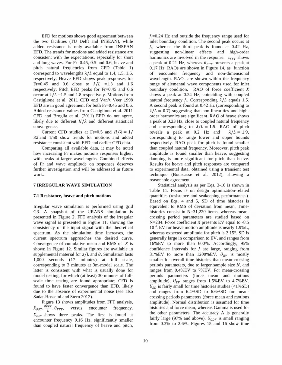
Irregular wave simulation is performed using grid G3. A snapshot of the URANS simulation is presented in Figure 2. FFT analysis of the irregular wave signal is presented in Figure 11, showing the consistency of the input signal with the theoretical spectrum. As the simulation time increases, the current spectrum approaches the desired curve. Convergence of cumulative mean and RMS of is shown in Figure 12. Similar figures are available in supplemental material for and . Simulation lasts 1,000 seconds (17 minutes) at full scale, corresponding to 3 minutes at 3m-model scale. The latter is consistent with what is usually done for model testing, for which (at least) 30 minutes of full-scale time testing are found appropriate; CFD is found to have faster convergence than EFD, likely due to the absence of experimental noise (see also Sadat-Hosseini and Stern 2012).

Figure 13 shows amplitudes from FFT analysis, , versus encounter frequency.

shows three peaks. The first is found at encounter frequency 0.16 Hz, significantly smaller than coupled natural frequency of heave and pitch,

fn=0.24 Hz and outside the frequency range used for inlet boundary condition. The second peak occurs at fn, whereas the third peak is found at 0.42 Hz, suggesting non-linear effects and high-order harmonics are involved in the response. shows a peak at 0.21 Hz, whereas presents a peak at 0.17 Hz. RAOs are shown in Figure 14, as function of encounter frequency and non-dimensional wavelength. RAOs are shown within the frequency range of elemental wave components used for inlet boundary condition. RAO of force coefficient X shows a peak at 0.24 Hz, coinciding with coupled natural frequency fn. Corresponding equals 1.5. A second peak is found at 0.42 Hz (corresponding to

) suggesting that non-linearities and high-order harmonics are significant. RAO of heave shows a peak at 0.23 Hz, close to coupled natural frequency and corresponding to . RAO of pitch reveals a peak at 0.2 Hz and , corresponding to range lower and upper bounds respectively. RAO peak for pitch is found smaller than coupled natural frequency. Moreover, pitch peak amplitude is found smaller than heave, suggesting damping is more significant for pitch than heave. Results for heave and pitch responses are compared to experimental data, obtained using a transient test technique (Bouscasse et al. 2012), showing a reasonable agreement.

Statistical analysis as per Eqs. 3-10 is shown in Table 11. Focus is on design optimization-related quantities (resistance and seakeeping performances). Based on Eqs. 4 and 5, SD of time histories is equivalent to RMS of deviation from mean. Time-histories consist in N=31,220 items, whereas mean-crossing period parameters are studied based on N=234. Force coefficient X presents EV equal to -8.5 10-3. EV for heave motion amplitude is nearly 1.9%L, whereas expected amplitude for pitch is 3.15°. SD is generally large in comparison to EV, and ranges from 16%EV to more than 600%. Accordingly, 95% confidence intervals for are large, ranging from 31%EV to more than 1200%EV. is mostly smaller for overall time histories than mean-crossing periods parameters, due to larger sample size N, and ranges from 0.4%EV to 7%EV. For mean-crossing periods parameters (force mean and motions amplitude), ranges from 1.5%EV to 4.7%EV.

is fairly small for time histories studies (<1%SD) and ranges from 6.4%SD to 6.6%SD for mean-crossing periods parameters (force mean and motions amplitude). Normal distribution is assumed for time histories and force mean, whereas Gamma is used for the other parameters. The accuracy A is generally fairly large (97% and above). is small ranging from 0.3% to 2.6%. Figures 15 and 16 show time

11

histories and mean-crossing period parameters distributions including empirical and analytical.

7.2 Slamming loads

Eqs. 3-10 are applied to and the results are shown in Table 12. EV is found larger in absolute value for re-entering than emerging slams and equal respectively to 27 and 53 kPa. SD is found significant compared to EV and equal to 13%EV for emerging slams and 20%EV for re-entering slams. Empirical distributions of emerging and re-entering slamming loads are shown in Figure 19. Comparison with Gamma distribution is included and found reasonable.

Statistical analysis of waves producing slams and incident waves is also included in Table 12. Average wave steepness is found the same and equal to 1/43. Slamming waves have a slightly larger height and period.

Figure 4 (e) and (f) shows a snapshot of the maximum emerging slam including pressure distribution on the demi-hull. Figure 4 (g) and (h) shows similar results for maximum re-entering slam.

8 UQ FOR VARIABLE REGULAR WAVE USING DETERMINISTIC SIMULATIONS 8.1 Resistance, heave and pitch motions with variable regular wave (2D UQ) Equations 14-19 are used to get EV, SD, CDF of relevant parameters as per Eq. 6. Eq. 11 gives the input distribution, whereas output variables are evaluated running deterministic regular wave simulations using grid G3. In order to focus on solution variability and avoid unfavorable bias towards calm water values, only simulations satisfying are taken into account. is the total RMS for variable V, which corresponds by definition to time-history standard deviation (Eq 4). Accordingly, simulations with variance below 5% of total are disregarded.

MCMC items are ordered with increasing , allowing for a systematic refinement on . Convergence studies for and (with related parameters and ) are available in supplemental material. Stochastic uncertainties are assessed as per Eqs. 7-9, varying the sample size N. Deterministic converge is studied following a similar procedure to that shown in Section 4, using systematic increase for the sample size: . Nmax=129 is the maximum sample size considered.

Table 13 presents a summary of UQ results. The focus is on force mean and motions amplitude. EV

for force coefficient X equals -8.67 10-3. EV for heave and pitch time histories equal respectively -0.2%L and 1.9°. Expected amplitudes are 2.2%L and 3.1°, for heave and pitch respectively. SD is generally large in comparison to EV and ranges from 21%EV to more than 800%. Accordingly 95% confidence intervals for are large, ranging from 32%EV to 1700%EV. is mostly smaller for time histories, due to larger sample size N, and ranges from 0.7%EV to 15%EV. For mean-crossing periods parameters (force mean and motions amplitude), ranges from 4.2%EV to 10.8%EV. is small for time histories (<1.3%SD) and about 12.1%SD for mean-crossing periods parameters. It may be noted that uncertainties on EV and SD are larger than irregular wave studies due to smaller sample size. Normal distribution is assumed for time histories and force means, whereas Gamma is used for motions amplitude. The accuracy A ranges from 88 to 99%.

is small ranging from 0.5% to 7%. Deterministic convergence studies reveal

monotonic convergence for EV of all variables and parameters. SD in found convergent except for force mean and heave motion amplitude. Accuracy is found convergent except for heave amplitude and pitch time history.

Figure 15 shows PDF for time history of and , obtained using variable regular wave.

The empirical distributions are compared to Normal, showing a good agreement. Figures 16 presents PDF for force mean and motions amplitude, respectively. Empirical distributions are compared to Normal (force mean) and Gamma (motions amplitude). Figure 17 shows force mean and motions amplitude, versus wave period and height, and encounter frequency and wave amplitude. Force mean response is included in Figure 8, whereas RAOs of first harmonics amplitudes for motions are included in Figures 9 and 14. Figure 10 shows motions phase. Figures 8-10 show UQ items colored by steepness values. Results for show significant non-linear effects for added resistance coefficient. Force mean (dimensional) presents largest response close to T=10 s, , and encounter frequency equal to 0.2 Hz. First and second harmonics RAO show peak at same values. Second harmonic values are included in Figure 12, at their own frequency (2 fe) for later comparison, and are found significant. First and second harmonics amplitudes for X are shown in Figure 18 as function of wave periods and height, and encounter frequency and wave amplitude. It may be noted that first harmonics response is large in correspondence to heave and pitch peaks, whereas second harmonics has large response in between motions peaks. RAOs for motions reveal viscous damping for . Heave amplitude

12

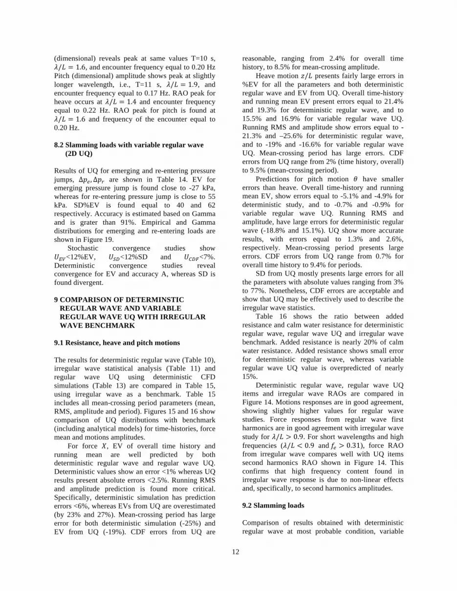
(dimensional) reveals peak at same values T=10 s, , and encounter frequency equal to 0.20 Hz

Pitch (dimensional) amplitude shows peak at slightly longer wavelength, i.e., T=11 s, , and encounter frequency equal to 0.17 Hz. RAO peak for heave occurs at and encounter frequency equal to 0.22 Hz. RAO peak for pitch is found at

and frequency of the encounter equal to 0.20 Hz. 8.2 Slamming loads with variable regular wave (2D UQ)

Results of UQ for emerging and re-entering pressure jumps, are shown in Table 14. EV for emerging pressure jump is found close to -27 kPa, whereas for re-entering pressure jump is close to 55 kPa. SD%EV is found equal to 40 and 62 respectively. Accuracy is estimated based on Gamma and is grater than 91%. Empirical and Gamma distributions for emerging and re-entering loads are shown in Figure 19.

Stochastic convergence studies show <12%EV, <12%SD and <7%.

Deterministic convergence studies reveal convergence for EV and accuracy A, whereas SD is found divergent. 9 COMPARISON OF DETERMINSTIC REGULAR WAVE AND VARIABLE REGULAR WAVE UQ WITH IRREGULAR WAVE BENCHMARK 9.1 Resistance, heave and pitch motions The results for deterministic regular wave (Table 10), irregular wave statistical analysis (Table 11) and regular wave UQ using deterministic CFD simulations (Table 13) are compared in Table 15, using irregular wave as a benchmark. Table 15 includes all mean-crossing period parameters (mean, RMS, amplitude and period). Figures 15 and 16 show comparison of UQ distributions with benchmark (including analytical models) for time-histories, force mean and motions amplitudes.

For force , EV of overall time history and running mean are well predicted by both deterministic regular wave and regular wave UQ. Deterministic values show an error <1% whereas UQ results present absolute errors <2.5%. Running RMS and amplitude prediction is found more critical. Specifically, deterministic simulation has prediction errors <6%, whereas EVs from UQ are overestimated (by 23% and 27%). Mean-crossing period has large error for both deterministic simulation (-25%) and EV from UQ (-19%). CDF errors from UQ are

reasonable, ranging from 2.4% for overall time history, to 8.5% for mean-crossing amplitude.

Heave motion presents fairly large errors in %EV for all the parameters and both deterministic regular wave and EV from UQ. Overall time-history and running mean EV present errors equal to 21.4% and 19.3% for deterministic regular wave, and to 15.5% and 16.9% for variable regular wave UQ. Running RMS and amplitude show errors equal to -21.3% and –25.6% for deterministic regular wave, and to -19% and -16.6% for variable regular wave UQ. Mean-crossing period has large errors. CDF errors from UQ range from 2% (time history, overall) to 9.5% (mean-crossing period).

Predictions for pitch motion have smaller errors than heave. Overall time-history and running mean EV, show errors equal to -5.1% and -4.9% for deterministic study, and to -0.7% and -0.9% for variable regular wave UQ. Running RMS and amplitude, have large errors for deterministic regular wave (-18.8% and 15.1%). UQ show more accurate results, with errors equal to 1.3% and 2.6%, respectively. Mean-crossing period presents large errors. CDF errors from UQ range from 0.7% for overall time history to 9.4% for periods.

SD from UQ mostly presents large errors for all the parameters with absolute values ranging from 3% to 77%. Nonetheless, CDF errors are acceptable and show that UQ may be effectively used to describe the irregular wave statistics.

Table 16 shows the ratio between added resistance and calm water resistance for deterministic regular wave, regular wave UQ and irregular wave benchmark. Added resistance is nearly 20% of calm water resistance. Added resistance shows small error for deterministic regular wave, whereas variable regular wave UQ value is overpredicted of nearly 15%.

Deterministic regular wave, regular wave UQ items and irregular wave RAOs are compared in Figure 14. Motions responses are in good agreement, showing slightly higher values for regular wave studies. Force responses from regular wave first harmonics are in good agreement with irregular wave study for . For short wavelengths and high frequencies ( and ), force RAO from irregular wave compares well with UQ items second harmonics RAO shown in Figure 14. This confirms that high frequency content found in irregular wave response is due to non-linear effects and, specifically, to second harmonics amplitudes. 9.2 Slamming loads Comparison of results obtained with deterministic regular wave at most probable condition, variable

13

regular wave (UQ) and irregular wave (benchmark) is shown in Table 17. Deterministic regular wave overpredicts the absolute value of slamming loads, specifically by 66% and 54% for emerging and re-entering slams. Regular wave UQ model shows small errors on EV (respectively 1.4% and 3% for emerging and re-entering slams). SD has larger errors of -17% and 70% for emerging and re-entering slams respectively. Comparison of empirical distributions obtained using variable regular wave with benchmark is shown is Figure 19. Comparison of analytical Gamma distribution obtained by matching moments is also shown and found quite reasonable. 10 UQ FOR VARIABLE REGULAR WAVE USING METAMODELS Table 18 shows a summary of MCMC studies with metamodels for resistance, heave and pitch motions. Functions shape is shown in Figure 17 using polyharmonic spline of 2nd order. The maximum size allowed for the training size, Mmax, is assumed equal to 65. Metamodels are ranked as per efficiency, accuracy and fulfillment of convergence and validation criteria. Kriging with exponential covariance function and e=1 is found the most effective. Radial basis functions network and Kriging with linear covariance function also perform well, showing small performance differences. 11 GEOMETRIC UQ USING DETERMINISTIC SIMULATIONS The methodology presented in Section 2.5 is applied to a set of S=10,000 random geometries obtained by a 20 design-variables FFD of the original DC. The eigenvector associated to the highest eigenvalue (first principal direction) is used for geometric UQ. This retains the 47% of the total geometric variance of the space. Extending the analysis to the first four directions of the space would allow for exploring the 95% of the total geometric variance. Complete exploration of geometric variability will be assessed in future work and is beyond the scope of the present work. Accordingly, based on sensitivity analysis, geometric UQ is conducted along the first principal direction, specifically from the original hull towards the most promising geometry. This coincides with the upper bound for geometry modifications, and is shown in Figure 20. Accordingly the geometric parameter is taken within the range and a uniform distribution is assumed.

11.1 Calm-water simulations for resistance, sinkage and trim with variable geometry (1D UQ) A 1D UQ in calm water at Fr=0.5 is conducted for variable geometry. Deterministic convergence using systematic refinement is studied up to N=33 for EV, SD, and A for calm water resistance, sinkage and trim, respectively. Systematic refinement is based on iterative LHS. The results are shown in Table 19.

EV for resistance coefficient equals 6.62 10-3, whereas EV for sinkage and trim equal respectively -0.4%L and 1.37°. SD%EV is found equal to 2, 0.3 and 7 for resistance sinkage and trim respectively. Empirical distributions are compared to Beta in Figure 21 and show accuracy A greater than 96%. Lower bound for resistance is found for α=1 and exhibits a 6.5% reduction with respect to the original geometry. Sinkage variations are noisy and very small (<1%EV). Trim variations are within 12%EV.

Stochastic convergence presents mostly small , due to small SD; <2.4%EV. is large

due to small N and close to 20%SD. is <14%. Deterministic converge studies reveal that monotonic convergence is achieved for all parameters. 11.2 Deterministic regular wave simulations for resistance, heave and pitch motions and slamming loads with variable geometry (1D UQ) A 1D UQ problem is solved for deterministic regular head wave at most probable condition (Tp, Hp) with variable geometry. Focus is on resistance, heave and pitch motions. Table 20 presents UQ results obtained using iterative LHS. Systematic refinement convergence is studied up to N=33 for EV, SD, A of force mean, heave and pitch motions amplitude. Non-dimensional force coefficient presents EV equal to -7.93 10-3, whereas heave and pitch motions amplitudes EV equals 1.5%L and 2.60°. SD%EV is found <1.21 for all parameters. Heave amplitude variations are small (about 1%EV). Pitch amplitude variations are also small and within 2.5%EV. Lower bound for resistance is found for α=1 and exhibits a 3.9% reduction with respect to the original geometry. Empirical distributions are compared to Beta and shown in Figure 22; comparison error equals 1.2%, 11.5% and 7% for force mean, heave and pitch amplitudes respectively. Stochastic convergence presents <0.4%EV, close to 20%SD, and

<14%. As shown in deterministic convergence studies, monotonic and oscillatory convergence is achieved for all parameters.

Slamming loads are studied using deterministic regular wave at most probable condition, varying the

14

uncertain geometry parameter. Iterative LHS is used and the results are shown in Table 21. Systematic refinement convergence is studied up to N=33 for EV, SD, A of emerging and re-entering slamming loads ( ). Absolute values of EV are found larger than those found for original geometry in deterministic regular wave. Expected value of emerging pressure jump equals -26 kPa, whereas expected value of re-entering pressure jump equals 102 kPa. The latter is 25% greater than that found for original DC. SD%EV equals 15 and 4 for emerging and re-entering loads respectively. Empirical distributions are compared to Beta and shown in Figure 23. Stochastic convergence presents

<5.2%EV, close to 20%SD, and <14%. Deterministic convergence studies show monotonic convergence for EV. SD of emerging slamming loads diverges monotonically, whereas SD of re-entering slamming loads converges monotonically. Accuracy A presents oscillatory convergence for emerging slamming loads and monotonic divergence for re-entering slamming loads. 11.3 Variable regular wave simulations for resistance, heave and pitch motions and slamming loads with variable geometry (3D UQ) Variable geometry is coupled with variable regular wave and a 3D UQ is solved. Systematic refinement convergence is studied up to N=129 for EV, SD, A of time histories, force mean, heave and pitch motions amplitude. Systematic refinement is done using a hybrid approach. MCMC samples are sorted as per increasing T; geometry is sampled following iterative LHS. Results are shown in Table 22. Absolute value of EV for force mean is found 6.2% smaller than that obtained using original hull, confirming the beneficial influence of geometry modifications on resistance. Heave amplitude EV is close to original, whereas pitch amplitude EV is 3.4% smaller. SD shows similar values to those found for the original hull. Empirical distributions are compared to Gamma and shown in Figure 24. Comparison errors for CDF are 12.7%, 1.5% and 3.5% for force mean, heave and pitch amplitudes respectively. Stochastic convergence presents quite large <14%EV,

<13%SD, and <13%. Deterministic convergence studies reveal monotonic convergence is always achieved for EV. SD converges monotonically for all time histories and pitch amplitude, whereas diverges for force mean and heave amplitude. CDF accuracy vs. analytical models converges for force and heave time histories, force mean and heave amplitudes; diverges for pitch time history and amplitude

Slamming loads using variable regular wave and geometry are studied and the results are presented in Table 23. Expected values of emerging and re-entering loads show greater absolute values than those found for original DC in variable regular wave. They equal respectively -40 and 62 kPa, revealing an increase with respect to the original hull of 48% and 13%. SD also increases by 42% and 8.7% for emerging and re-entering loads respectively. The upper bound for the re-entering pressure jump is found larger than original by 6.4%. Empirical CDFs are compared to Gamma and shown in Figure 25. Stochastic convergence studies show <11%EV,

<12%SD, and <7%. Systematic refinement reveals deterministic convergence (monotonic and oscillatory) for EV and SD of emerging and re-entering slamming loads. Accuracy A shows monotonic convergence for re-entering load, whereas diverges for emerging load. 12 GEOMETRIC UQ USING METAMODELS Table 24 summarizes the results for metamodels studies in calm water and variable geometry. Focus is on 1D UQ for resistance, sinkage and trim at Fr=0.5. The maximum size allowed for the training size, Mmax, is assumed equal to 17. Inverse distance weighting is found the most effective. Least square support vector machine also has good performance, close to IDW.

Results for metamodels studies for variable geometry in deterministic regular wave are summarized in Table 25. Focus in on 1D UQ for resistance, heave and pitch motions. Mmax is assumed equal to 17. Kriging with both linear and exponential covariance function is found the most effective. Polyharmonic spline with k=1 (membrane spline) also performs well, showing similar performance.

Three dimensional UQ results for variable regular wave and geometry using metamodels are summarized in Table 26. Focus is on resistance, heave and pitch motions. Mmax equals 65. Kriging with exponential covariance function is found the most effective. Radial basis functions network and polyharmonic spline (k=1) also shows good performance. 13 CONCLUSIONS AND FUTURE WORK A methodology has been presented for variable regular wave UQ and compared to irregular wave statistical studies (taken as a benchmark) and deterministic regular wave simulation. Variable regular wave UQ is based on items from joint PDF of wave period and height, whereas deterministic study is conducted at most probable condition (PDF peak).

15

Application to the high-speed Delft Catamaran advancing at Fr=0.5 in sea state 6 has been shown. Verification results for deterministic calm water and regular wave at most probable condition for sea state 6 has been presented, as well as regular wave studies for variable wavelength. Inlet boundary condition for irregular wave simulation in sea state 6 has been validated versus theory using an optimal wave design approach. Irregular wave studies have been presented and discussed. Variable regular wave UQ has been shown, based on MCMC and MCMC with metamodels; metamodels have been ranked taking into account computational efficiency, accuracy and fulfillment of convergence and validation criteria. Results from deterministic regular wave and variable regular wave UQ have been compared to irregular wave benchmark. Extension to uncertain design through KLE analysis of variable geometry has been presented and discussed.

Irregular wave signal has been studied running 3,600 s at full scale, corresponding to 566 non-dimensional time and 11 minutes at 3m-model scale. Using wave angular frequencies within the range

and limiting the number of random phase sets to 1,000 for each , a number of 50 components has been found adequate for current problem. Using a wider range of frequencies and comparing a number of random realizations greater than 1,000 and proportional to the number of components , are expected to give a more accurate representation of the sea state and will be part of future work. Joint PDF of wave period and height has been studied comparing theory with MCMC. A sample size equal to 129 items has been found adequate for current problem. Most probable condition from joint PDF presents and

showing that (a) most probable wave is large and (b) falls within high responses range.

Verification results for deterministic calm water and regular wave at most probable condition for sea state 6 have been found consistent with previous studies, although far from the asymptotic range. Future work will include finer grids for getting closer or achieving the asymptotic range; convergence will be applied to justify the use of coarser grids with finer grids uncertainties for UQ and optimization. Calm water resistance error still has to be reduced, whereas model testing for high-speed multihulls is still required in order to reduce the facility bias and confirm the validation intervals.

Deterministic regular wave studies within the range from 0.5 to 2 have been found reasonable in comparison with previous CFD and EFD studies. Peak response for added resistance, heave and pitch has been found at non-dimensional wavelength close to . Moreover, heave and pitch maximum

response is found at wavelength close to that corresponding to natural frequency of coupled motions, but slightly greater. Pitch maximum response mostly occurs for higher wavelengths than heave and shows smaller peak especially for large waves. Added resistance maximum response is found very close to heave peak for small and large waves, and occurs at wavelength slightly greater than that corresponding to coupled natural frequency.

Irregular wave CFD simulation has run 1000 full-scale time, corresponding to 17 minutes at full scale and 3 minutes at 3m-model scale. This is consistent with model testing procedures, for which (at least) 30 minutes full-scale runs are found appropriate. Response for force X presents the highest peak at equal to 1.5. A second peak is found at smaller non-dimensional wavelength, equal to 0.7, indicating non-linearities are significant. Heave and pitch responses present peaks at equal to 1.5 and 1.9 respectively. These are found consistent with EFD studies (from transient test technique). Statistical analysis reveals EV for force coefficient X (time-history) equal to -8.5 10-3, whereas heave and pitch amplitudes expectation is found equal to 1.9%L and 3.15° respectively. SD%EV values are found significant and >35%. Analytical models for distributions based on Normal (time-histories and force mean) and Gamma (heave and pitch amplitudes) give accuracy >98%. Slamming loads studies reveal absolute value for EV larger for re-entering than emerging slams and equal respectively to 27 and 53 kPa. Associated SD is found significant compared to EV and equal to 13%EV for emerging and 20%EV for re-entering slams. Comparison of empirical distributions with Gamma is found reasonable. Validation of irregular wave studies versus experiments is still needed.

For variable regular wave UQ, a number N=129 items have been selected from joint PDF of wave period and height using Markov-chain sampling. Variable regular wave UQ items show peak response for X first and second harmonics at exciting close to 1.6. Heave and pitch motions show peak responses at equal to 1.4 and 1.6 respectively. MCMC gives EV for force coefficient X time history equal to -8.7 10-3; heave and pitch amplitudes EV is found equal to 2.2%L and 3.1° respectively. SD%EV is found significant and >42%. Empirical distributions for time histories are compared to Normal, showing accuracy >98%. Force mean distribution is compared to Normal, revealing accuracy equal to 88%; comparing motions amplitude to Gamma gives accuracy >97%. Stochastic convergence reveals

<10.8%EV and <12.1%. Deterministic convergence studies show convergence for EV of all variables and parameters, and SD except for force

16

mean and heave motion amplitude. Accuracy is convergent except for heave amplitude and pitch time history. Slamming loads studies show EV for emerging pressure jump close to -27 kPa, and nearly 55 kPa for re-entering pressure jump. SD%EV is found equal to 40 and 62 respectively. Accuracy is estimated based on Gamma and found reasonable (>91%). Stochastic convergence studies show

<12%EV, <12%SD and <7%. Deterministic convergence studies reveal convergence for EV and accuracy A, whereas SD is found divergent. The possibility of increasing the sample size, in order to get better convergence, is currently under investigation.

Comparison of deterministic regular wave versus benchmark shows good results for added resistance, whereas motions amplitudes are overpredicted. Regular wave UQ generally exhibits greater variability and larger SD than benchmark. UQ shows reasonable results for resistance and pitch, whereas heave amplitude is overpredicted, but closer to benchmark than deterministic study. Distributions from UQ are reasonable comparing to benchmark, especially for time histories. RAOs obtained using irregular wave and variable regular wave UQ are in close agreement. Force RAOs from UQ items reveal that non-linear effects found in irregular wave studies are due to second harmonics. Deterministic studies for slamming loads reveal large comparison errors for EV, whereas variable regular wave UQ shows small errors. Errors on SD are large. Specifically, deterministic regular wave at most probable condition shows error for added resistance <1% (Table 16), and presents average comparison error for EV of outputs time histories (force and motions) equal to 8.8% (Table 15). Average error for running RMS is close to 15%, whereas average error for mean-crossing amplitudes is 15.5%. Average error considering only motions amplitude is >20%. Slamming loads present average error for EV close to 60% (Table 17). Variable regular wave UQ shows error for added resistance close to 15% (Table 16). Average errors for EV, SD and CDF of outputs time histories equal to 6.2%, 14.9% and 1.7%, respectively (Table 15). Average error for running RMS equals 14.5%, whereas average error for mean-crossing amplitudes is 15.5%. Average error for motions amplitude is 9.6%. Slamming loads EV reveals average error equal to 2.2%, whereas SD shows average error equal to 44% (Table 17). In summary, quantities related to design optimization (namely, force time-history EV, motions amplitude EV and slamming loads EV) present average error equal to 25% using deterministic regular wave and 6% using variable regular wave UQ. Overall, results reveal that deterministic study gives rough estimates

of optimization-related statistical quantities, whereas variable wave UQ gives much better predictions.

KLE studies were performed using random geometry realizations obtained by FFD of original hull, with 20 design variables. Geometric UQ was performed along the first principal direction of the space, specifically from original hull (lower bound for geometric UQ) to most promising geometry (upper bound for geometric UQ). Variable geometry studies conducted so far reveal that calm-water resistance can be reduced by 6.5%, and resistance in deterministic regular wave by 3.9%. Nevertheless, hull modifications towards low-resistance geometries produce an increase in slamming loads. Specifically, upper bound for re-entering load increases by 6.4%, revealing a trade-off between performances and loads. Conditional distributions for resistance, motions and slamming loads, given the geometry, will be assessed in future work for deeper analysis. A broader investigation of geometric variability, through the inclusion of additional principal directions will be part of future work. Specifically, four principal directions will be assessed in order to retain the 95% of total geometric variance associated to the research space.

For metamodels studies, Kriging with exponential covariance function and radial basis functions network have been found the most effective for 2D UQ of resistance and motions over joint PDF of wave period and height; inverse distance weighting and least-square support vector machine have been found the most effective for 1D UQ of calm water resistance, sinkage and trim for variable geometry; Kriging with exponential covariance function and 1st order polyharmonic spline have been found the most effective for 1D UQ of resistance and motions in deterministic regular wave with variable geometry, whereas 3D UQ studies for variable regular wave (from joint PDF of wave period and height) and geometry has shown Kriging (exponential covariance function) and radial basis functions network as most effective. Table 27 shows an overall ranking, based on average results of UQ problems for resistance and motions. Kriging with exponential covariance function is found the most effective. Kriging with linear covariance function and 1st order polyharmonic spline also reveal good performance overall. Future work includes implementation and/or application of metamodels based on dynamic sampling, such as dynamic Kriging (DK, Zhao et al. 2011 and Lee et al. 2011) or dynamic version of emulators (O’Hagan 2006) based on radial basis functions network.

Future stochastic design optimization will be formulated as a reliability-based robust design optimization (RBRDO) problem with EV of

17

resistance in wave as objective function (eventually coupled with calm water resistance) with motions amplitudes and slamming loads either as objectives or constraints. Air entrapment in waterjet inlet will be also included if required. According to Table 28 (showing a parametric analysis for added resistance in different sea states), optimization will focus on sea state 7, since more critical for added fuel consumption due to waves. In view of the computational effort required by URANS-based optimization, the possibility of including multi-fidelity studies based on potential flow using Aegir (Kring et al. 2004) is currently under investigation. ACKNOWLEDGMENTS

The present research is supported by the Office of Naval Research, Grant N000141110237 and NICOP Grant N629091117011, under the administration of Dr. Ki-Han Kim. Research for slamming loads has been partially supported under Grant N000141210881, administered by Dr. Robert Brizzolara. URANS computations were performed at the NAVY DoD Supercomputing Resource Center. Dr. Patrick Purtell provided support for the precursory research. The research was conducted in collaboration with NATO AVT-191: Application of Sensitivity Analysis and Uncertainty Quantification to Military Vehicle Design. REFERENCES American Bureau of Shipping, “Slamming Loads and Strength Assessment for Vessels,” ABS guide, March 2011. Bales S.L., “Designing ships to the natural environment,” Association of Scientists and Engineers of the Naval Sea System Command, 19th Annual Technical symposium, 1982. Bouscasse, B, Broglia, R., Stern, F., Experimental Investigation of a Fast Catamaran in Head Waves, in preparation, 2012. Broglia, R., Bouscasse, B., Jacob, B., Olivieri, A., Zaghi, S., and Stern, F., “Calm Water and Seakeeping Investigation for a Fast Catamaran,” Proc. 11th Intl. Conf. Fast Sea Transportation, Hawaii, USA, Sept. 2011. Bretschneider, C. L. 1959. “Wave Variability and Wave Spectra for Wind-Generated Gravity Waves," U.S. Army Corps of Engrs., Beach Erosion Board, Tech. Memo. No. 118 Buhmann, M.D., Radial Basis Functions: Theory and Implementations, Cambridge University, 2003, ISBN 0-521-63338-9.

Campana, E.F., Peri, D. Tahara, Y. and Stern, F., “Shape Optimization in Ship Hydrodynamics Using Computational Fluid Dynamics,” J. of Computer Methods in Applied Mechanics and Engineering, Vol. 196, Dec. 2006, pp. 634-651. Campana, E.F., Peri, D., Kandasamy, M., Tahara, Y., Stern F, “Numerical Optimization Methods for Ship Hydrodynamic Design,” SNAME annual meeting, Providence (Rhode Island, USA), 2009. Coleman, H. W. and Stern, F., “Uncertainties and CFD code validation,” J. Fluids Eng., 119(4):795-803, 1997. Castiglione, T., Stern, F., Bova, S., Kandasamy, M., “Numerical investigation of the seakeeping behavior of a catamaran advancing in regular head waves,” Ocean Engineering, Vol. 38(16), Nov. 2011, pp. 1806-1822. Diez, M., Campana, E.F., and Stern, F., “Karhunen-Loeve expansion for assessing stochastic subspaces in geometry optimization and geometric uncertainty quantification,” IIHR Technical Report No. 481, January 2012a. Diez, M., He, W., Campana, E.F., and Stern, F., “Deterministic and multivariate stochastic uncertainty quantification for the Delft catamaran with variable Froude number and/or geometry using URANS and potential flow solvers,” in preparation, 2012b. Forbes, C., Evans, M., Hastings, N., and Peacock, B., Statistical Distributions, Wiley, New Jersey, 2011. Goda, Y., Random seas and design of Maritime Structures, World Scientific, Singapore, 2010. Harder, R.L., and Desmarais, R.N., “Interpolation using surface splines,” Journal of Aircraft, Issue 2, pp. 189-191, 1972. He, W., Castiglione, T., Kandasamy, M., Stern, F., “URANS Simulation of Catamaran Interference,” Proc. 11th Intl. Conf. Fast Sea Transportation, Hawaii, USA, Sept. 2011. Helton, J.C., and Davis, F.J., “Latin hypercube sampling and the propagation of uncertainty in analyses of complex systems,” Reliability Engineering & System Safety, 81:23-69, 2003. Hogben, N., Dacunha, N.M.C., Olliver, G.F., Global Wave Statistics, BMT, London 1986. Kandasamy, M., Ooi, S.K., Carrica, P., Stern, F., Campana, E.F., Peri, D., Osborne, P., Cote, J., McDonald, N., de Waal, N., “Multi-fidelity Optimization of a High-speed Foil-assisted Semi-planing Catamaran for Low Wake,” J. of Marine Science and Technology, Vol. 16, No. 2, Jun. 2011a, pp. 143-156.

18

Kandasamy, M., He, W., Tahara, Y., Peri, D., Campana, E., Wilson, W., and Stern, F., “Optimization of waterjet propelled high speed ships JHSS and Delft catamaran,” Proc. 11th Intl. Conf. Fast Sea Transportation, Hawaii, USA, Sept. 2011b. Kring, D.C., Milewski, W.M., and Fine, N.E., “Validation of a NURBS-Based BEM for Multihull Ship Seakeeping”, Proc. 25th Symposium on Naval Hydrodynamics, St. John’s, Newfoundland and Labrador, Canada, 2004. Larsson, L., Stern, F., and M. Visonneau, “CFD in Ship Hydrodynamics – Results of the Gothenburg 2010 Workshop,” Proc. IV International Conference on Computational Methods in Marine Engineering, 28-30 September 2011, Lisbon, Portugal. Lee, W. T., Bales, S. L., “Environmental data for design of marine vehicles,” in Ship Structure Symposium '84, pp. 197-209. New York: The Society of Naval Architects and Marine Engineers (SNAME), 1984. Lee, I., Choi, K.K., and Zhao, L., “Sampling-Based RBDO Using the Stochastic Sensitivity Analysis and Dynamic Kriging Method,” Structural and Multidisciplinary Optimization, Vol. 44, 2011, pp. 299-317. Liang, B. and Mahadevan, S., “Error and uncertainty quantification and sensitivity analysis in mechanics computational models,” International Journal for Uncertainty Quantification, Vol. 1, 2011. pp. 147-161. Longuet-Higgins, M.S., “On the Joint Distribution of Wave Period and Amplitudes in a Random Wave Field,” Proc. Roy. Soc. London, Series A, Vol. 389, 1983, pp. 241-258. Michel, W.H., “Sea Spectra Revisited,” Marine Technology, vol. 36, no. 4, 1999, pp. 211-227. Mousaviraad, S.M., He, W., Diez, M., and Stern, F., “Framework for convergence and validation of stochastic UQ and relationship to deterministic V&Vwith example for a unit problem,” Intl. J. for Uncertainty Quantification, in press, 2012. Ochi, M.K., Ocean Waves: the Stochastic Approach, Cambridge University Press, 1998. O’Hagan, A., Bayesian analysis of computer code outputs: A tutorial, Reliability Engineering and System Safety 91, pp. 1290–1300, 2006. Peri, D., “Self-Learning Metamodels for Optimization, Ship Technology Research, Vol.56, 94-108, 2009. Sadat-Hosseini, H., and Stern, F., “5415M course keeping in irregular waves,” NATO AVT-216 Report, 25 May, 2012.

Sadat-Hosseini, H., Wu, P.C., Carrica, P.M., Kim, H., Toda, Y. and Stern, F., “CFD verification and validation of added resistance and motions of KVLCC2 with fixed and free surge in short and long head waves”, accepted for publication in Ocean Engineering, 2012. Shepard, D., “A two-dimensional interpolation function for irregularly- spaced data,” Proceedings of the 1968 ACM National Conference, pp. 517–524, 1968, doi:10.1145/800186.810616. Stern, F., Wilson, R.V., Coleman, H.W., and Paterson, E.G., “Comprehensive approach to verification and validation of CFD simulations Part 1: Methodology and Procedures,” ASME J. Fluids Eng., 123(4):793-802, 2001. Stern, F., Wilson, R., and Shao, J., “Quantitative approach to V&V of CFD simulations and certification of CFD codes,” Intl. J. for Numerical Methods in Fluids, 50:1335-1355, 2006. Stern, F., Carrica, P., Kandasamy, K., Oii, S., Gorski, J., O’Dea, J., Fu, T., Henrix, D., Kennel, C., Hughes, M., Miller, R., Marino., T., Hess, D., Kring, D., Milewski, W., Hoffman, R., Smith. S., Cary, C., Taylor, P., Peterson, B., Haris, D., Monaco, C., “Computational Hydrodynamic Tools for High-Speed Sealift: Phase II Final Report,” IIHR Report No. 465, June 2008, 113 pp. Strom-Tejsen, J., Hugh Y.H. Yeh and Moran D.D., “Added Resistance in Waves,” SNAME, Transactions, Vol. 81, 1973, pp. 109-143. Suykens, J. A. K., Gestel, T. V., Brabanter, J. D., Moor, B. D., and Vandewalle, J., Least Squares Support Vector Machines, World Scientific, 2002. Tahara, Y., Peri, D., Campana, E.F., and Stern, F., “Single and Multi Objective Design Optimization of a Fast Multihull Ship: numerical and experimental results,” J. of Marine Science and Technology, Vol. 16, No 4, December 2011a, pp. 412-433. Tahara, Y., Hino, T., Kandasamy, M., He, W., and Stern, F., “CFD-based multi-objective optimization of waterjet propelled high speed ships,” Proc. 11th International Conference Fast Sea Transportation, Hawaii, USA, Sept. 2011b. Van’t Veer, R., “Experimental Results of Motions, Hydrodynamic Coefficients and Wave Loads on the 372 Catamaran Model”, TU Delft Report, No.1129, 1998. Xing, T. and Stern, F., “Factors of safety for Richardson extrapolation,” J. of Fluids Engineering, 132(6), 2010. Zhao, L., Choi, K.K., and Lee, I., “Metamodeling Method Using Dynamic Kriging for Design Optimization,” AIAA Journal, Vol. 49, No. 9, 2011, pp. 2034-2046.

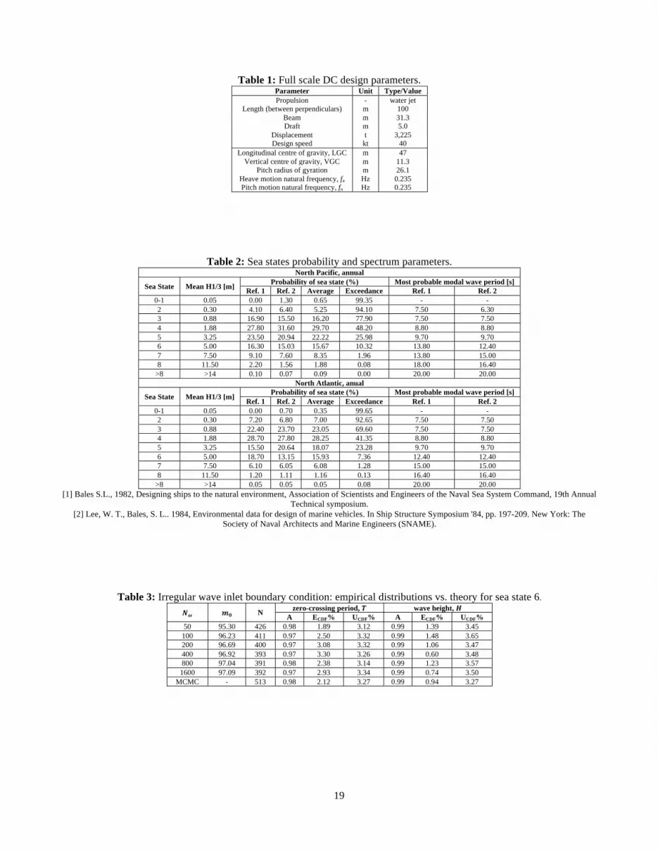
19

Table 1: Full scale DC design parameters.

Parameter Unit Type/Value Propulsion - water jet

Length (between perpendiculars) m 100 Beam m 31.3 Draft m 5.0

Displacement t 3,225 Design speed kt 40

Longitudinal centre of gravity, LGC m 47 Vertical centre of gravity, VGC m 11.3

Pitch radius of gyration m 26.1 Heave motion natural frequency, fn Hz 0.235 Pitch motion natural frequency, fn Hz 0.235

Table 2: Sea states probability and spectrum parameters. North Pacific, annual

Sea State Mean H1/3 [m] Probability of sea state (%) Most probable modal wave period [s] Ref. 1 Ref. 2 Average Exceedance Ref. 1 Ref. 2

0-1 0.05 0.00 1.30 0.65 99.35 - - 2 0.30 4.10 6.40 5.25 94.10 7.50 6.30 3 0.88 16.90 15.50 16.20 77.90 7.50 7.50 4 1.88 27.80 31.60 29.70 48.20 8.80 8.80 5 3.25 23.50 20.94 22.22 25.98 9.70 9.70 6 5.00 16.30 15.03 15.67 10.32 13.80 12.40 7 7.50 9.10 7.60 8.35 1.96 13.80 15.00 8 11.50 2.20 1.56 1.88 0.08 18.00 16.40

>8 >14 0.10 0.07 0.09 0.00 20.00 20.00 North Atlantic, anual

Sea State Mean H1/3 [m] Probability of sea state (%) Most probable modal wave period [s] Ref. 1 Ref. 2 Average Exceedance Ref. 1 Ref. 2

0-1 0.05 0.00 0.70 0.35 99.65 - - 2 0.30 7.20 6.80 7.00 92.65 7.50 7.50 3 0.88 22.40 23.70 23.05 69.60 7.50 7.50 4 1.88 28.70 27.80 28.25 41.35 8.80 8.80 5 3.25 15.50 20.64 18.07 23.28 9.70 9.70 6 5.00 18.70 13.15 15.93 7.36 12.40 12.40 7 7.50 6.10 6.05 6.08 1.28 15.00 15.00 8 11.50 1.20 1.11 1.16 0.13 16.40 16.40

>8 >14 0.05 0.05 0.05 0.08 20.00 20.00 [1] Bales S.L., 1982, Designing ships to the natural environment, Association of Scientists and Engineers of the Naval Sea System Command, 19th Annual

Technical symposium. [2] Lee, W. T., Bales, S. L.. 1984, Environmental data for design of marine vehicles. In Ship Structure Symposium '84, pp. 197-209. New York: The

Society of Naval Architects and Marine Engineers (SNAME).

Table 3: Irregular wave inlet boundary condition: empirical distributions vs. theory for sea state 6. N zero-crossing period, wave height,

A ECDF% UCDF% A ECDF% UCDF% 50 95.30 426 0.98 1.89 3.12 0.99 1.39 3.45

100 96.23 411 0.97 2.50 3.32 0.99 1.48 3.65 200 96.69 400 0.97 3.08 3.32 0.99 1.06 3.47 400 96.92 393 0.97 3.30 3.26 0.99 0.60 3.48 800 97.04 391 0.98 2.38 3.14 0.99 1.23 3.57

1600 97.09 392 0.97 2.93 3.34 0.99 0.74 3.50 MCMC - 513 0.98 2.12 3.27 0.99 0.94 3.27

20

Table 4: Comparison of theoretical and empirical values for Bretschneider spectrum in sea state 6.

Parameters Unit

S Joint PDF Marginal PDF

Bretschneider Spectrum

Wave signal

PDF f PDF f1 PDF f2

Theory MCMC Sampling*

Theory Sampling*

Theory Sampling*

(N=129) (N=21229) (N=513) (N=513)

H

H1/3

M

5.000 4.641 HP 3.254 2.500

EV(H) 3.003 3.284 3.107 3.133 3.037 SD(H) 1.445 1.504 1.413 1.638 1.506 Min 0.125 0.547 0.130 0.125 Max 6.932 6.352 6.931 6.932

T

Tm

S

12.40 9.585

Tp 8.121 8.593 EV(T) 9.442 10.005 10.001 9.371 SD(T) 2.824 3.321 3.282 2.945 Min 1.450 2.422 1.452 1.450 Max 17.64 17.64 17.64 17.64

λ

λp

M

103.0 115.4 EV(λ) 151.6 173.5 173.0 150.6 SD(λ) 90.26 110.0 108.6 93.5 Min 3.282 7.848 3.293 3.282 Max 485.9 485.6 485.8 485.6

λ/L λp/L 1.03 1.15 Min 0.03 0.08 0.03 0.03 Max 4.86 4.86 4.86 4.86

H/λ Hp/λp 1/32 Min 1/213 1/458 1/2196 Max 1/6 1/10 1/5

(*) Note: Samples are truncated using irregular wave bounds

Table 5: Grids used in current study. Grid Dimensions Total Y+ Study Hull in and out Background G1 331×108×121 457×153×493 43.1M 0.12 V&V G2 234×76×85 323×108×348 15.2M 0.16 V&V G3 166×54×61 229×77×247 5.4M 0.23 V&V, UQ G4 117×38×43 162×54×174 1.9M 0.32 V&V

Table 6: Verification and validation for calm water simulation at Fr=0.5; S1 is solution of G1 or G2 and D is INSEAN EFD.

Para. Triplet Verification Validation† (INSEAN EFD)

R P UI%S1 UI/ε12 UI% UG UG%S1 UD USN/UD UV E

CT 1,2,3 0.61 0.72 0.107 0.36 0.13 0.84 0.21 4.05 0.88 -7.41 2,3,4 0.38 1.38 0.203 0.41 0.03 2.40 11.48 2.42 -7.68

σ 1,2,3 0.55 0.86 0.100 1.17 1.21 0.08 1.31 0.10 1.32 0.26 2,3,4 0.28 1.83 0.057 0.53 0.09 0.64 0.49 1.46 0.20

τ 1,2,3 0.87 0.20 0.020 0.008 0.0005 37.82 2.91 13.00 37.93 0.11 2,3,4 0.54 0.88 0.064 0.02 0.011 5.91 2.03 6.59 -2.35

† Note: UD, UV and E are %D

Table 7: Calm water simulation of Delft catamaran, Fr=0.5, Re=7.14×106. Grid CT×103 σ×103 τ×102

S E%D ε12%S1 USN%S S E%D ε12%S1 USN%S S E%D ε12%S1 USN%S G1 7.130 -7.41 0.30 0.84 -3.909 0.26 0.06 0.08 3.055 0.11 2.46 37.82 G2 7.109 -7.68 0.49 2.40 -3.907 0.20 0.11 0.64 2.980 -2.35 2.89 5.91 G3 7.074 -8.14 1.29 -3.903 0.09 0.38 2.893 -5.17 5.47 G4 6.983 -9.32 -3.888 -0.29 2.735 -10.35

Note: EFD solutions are CT=7.701×10-3, σ=-3.899×10-3, and τ=3.051×10-2 ε12%S1=(S1-S2)%S1, where S1 is the result of finer grid and S2 is the coarse grid

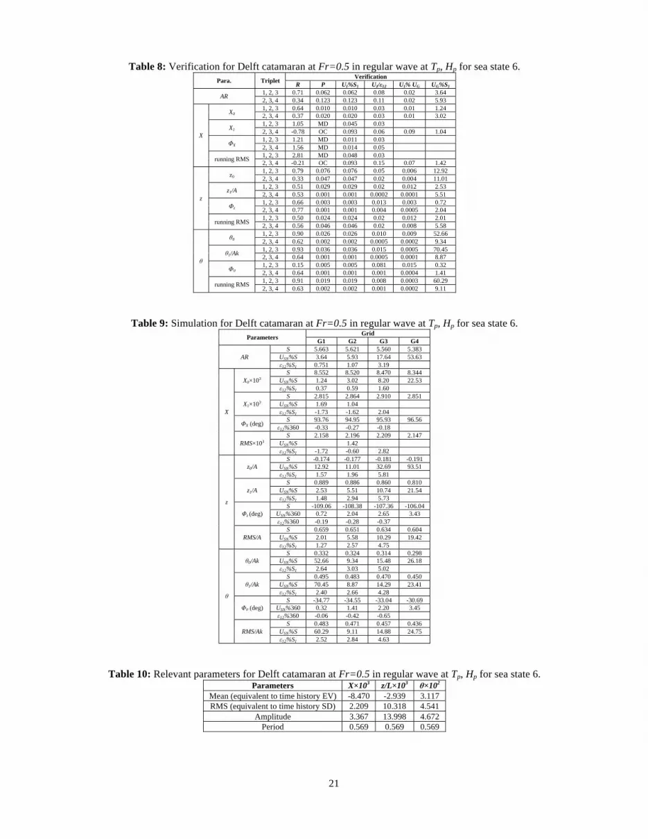
21

Table 8: Verification for Delft catamaran at Fr=0.5 in regular wave at Tp, Hp for sea state 6. Para. Triplet Verification

R P UI%S1 UI/ε12 UI% UG UG%S1

AR 1, 2, 3 0.71 0.062 0.062 0.08 0.02 3.64 2, 3, 4 0.34 0.123 0.123 0.11 0.02 5.93

X

X0 1, 2, 3 0.64 0.010 0.010 0.03 0.01 1.24 2, 3, 4 0.37 0.020 0.020 0.03 0.01 3.02

X1 1, 2, 3 1.05 MD 0.045 0.03 2, 3, 4 -0.78 OC 0.093 0.06 0.09 1.04

ΦX 1, 2, 3 1.21 MD 0.011 0.03 2, 3, 4 1.56 MD 0.014 0.05

running RMS 1, 2, 3 2.81 MD 0.048 0.03 2, 3, 4 -0.21 OC 0.093 0.15 0.07 1.42

z

z0 1, 2, 3 0.79 0.076 0.076 0.05 0.006 12.92 2, 3, 4 0.33 0.047 0.047 0.02 0.004 11.01

z1/A 1, 2, 3 0.51 0.029 0.029 0.02 0.012 2.53 2, 3, 4 0.53 0.001 0.001 0.0002 0.0001 5.51

Φz 1, 2, 3 0.66 0.003 0.003 0.013 0.003 0.72 2, 3, 4 0.77 0.001 0.001 0.004 0.0005 2.04

running RMS 1, 2, 3 0.50 0.024 0.024 0.02 0.012 2.01 2, 3, 4 0.56 0.046 0.046 0.02 0.008 5.58

θ

θ0 1, 2, 3 0.90 0.026 0.026 0.010 0.009 52.66 2, 3, 4 0.62 0.002 0.002 0.0005 0.0002 9.34

θ1/Ak 1, 2, 3 0.93 0.036 0.036 0.015 0.0005 70.45 2, 3, 4 0.64 0.001 0.001 0.0005 0.0001 8.87

Φθ 1, 2, 3 0.15 0.005 0.005 0.081 0.015 0.32 2, 3, 4 0.64 0.001 0.001 0.001 0.0004 1.41

running RMS 1, 2, 3 0.91 0.019 0.019 0.008 0.0003 60.29 2, 3, 4 0.63 0.002 0.002 0.001 0.0002 9.11

Table 9: Simulation for Delft catamaran at Fr=0.5 in regular wave at Tp, Hp for sea state 6. Parameters Grid

G1 G2 G3 G4

AR S 5.663 5.621 5.560 5.383

USN%S 3.64 5.93 17.64 53.63 ε12%S1 0.751 1.07 3.19

X

X0×103 S 8.552 8.520 8.470 8.344

USN%S 1.24 3.02 8.20 22.53 ε12%S1 0.37 0.59 1.60

X1×103 S 2.815 2.864 2.910 2.851

USN%S 1.69 1.04 ε12%S1 -1.73 -1.62 2.04

ΦX (deg) S 93.76 94.95 95.93 96.56 ε12%360 -0.33 -0.27 -0.18

RMS×103 S 2.158 2.196 2.209 2.147

USN%S 1.42 ε12%S1 -1.72 -0.60 2.82

z

z0/A S -0.174 -0.177 -0.181 -0.191

USN%S 12.92 11.01 32.69 93.51 ε12%S1 1.57 1.96 5.81

z1/A S 0.889 0.886 0.860 0.810

USN%S 2.53 5.51 10.74 21.54 ε12%S1 1.48 2.94 5.73

Φz (deg) S -109.06 -108.38 -107.36 -106.04

USN%360 0.72 2.04 2.65 3.43 ε12%360 -0.19 -0.28 -0.37

RMS/A S 0.659 0.651 0.634 0.604

USN%S 2.01 5.58 10.29 19.42 ε12%S1 1.27 2.57 4.75

θ

θ0/Ak S 0.332 0.324 0.314 0.298

USN%S 52.66 9.34 15.48 26.18 ε12%S1 2.64 3.03 5.02

θ1/Ak S 0.495 0.483 0.470 0.450

USN%S 70.45 8.87 14.29 23.41 ε12%S1 2.40 2.66 4.28

Φθ (deg) S -34.77 -34.55 -33.04 -30.69

USN%360 0.32 1.41 2.20 3.45 ε12%360 -0.06 -0.42 -0.65

RMS/Ak S 0.483 0.471 0.457 0.436

USN%S 60.29 9.11 14.88 24.75 ε12%S1 2.52 2.84 4.63

Table 10: Relevant parameters for Delft catamaran at Fr=0.5 in regular wave at Tp, Hp for sea state 6. Parameters X×103 z/L×103 θ×102

Mean (equivalent to time history EV) -8.470 -2.939 3.117 RMS (equivalent to time history SD) 2.209 10.318 4.541

Amplitude 3.367 13.998 4.672 Period 0.569 0.569 0.569

22

Table 11: Statistical analysis for irregular wave simulation in sea state 6 at Fr=0.5 (N=234). Parameters EV SD%|EV| UJ,l%|EV| UJ,u%|EV| A% UEV%|EV| USD%SD UCDF%

X ×103

Time history, overall -8.465 35.01 68.48 68.48 99.63 0.39 0.78 0.30 Running mean -8.508 16.05 31.39 31.39 97.09 1.55 6.39 2.33

z/L ×103

Time history, overall -2.421 626.32 1225.09 1225.09 99.55 6.93 0.78 0.30 Mean-crossing amplitude 18.820 46.43 69.29 109.44 97.74 4.67 6.65 2.59

θ ×102

Time history, overall 3.284 132.17 258.53 258.53 99.12 1.46 0.78 0.30 Mean-crossing amplitude 5.505 42.31 64.95 98.40 98.52 4.22 6.60 2.54

Table 12: Statistical analysis of slamming loads and waves from irregular wave benchmark (probe B1).

Parameter Slamming load ps (Kpa) Slamming wave Incident wave Emerging Re-entering Ts (s) Hs (m) λs/L* Hs/λs

T (s) H (m) λ/L* H/λ N 208 210 225 234

EV -26.86 52.98 9.008 2.943 1.267 1/43 8.864 2.863 1.226 1/43 SD 13.06 19.83 2.385 1.379 0.089 - 2.454 1.411 0.094 -

SD%|EV| 48.62 37.44 26.48 46.85 7.00 - 27.68 49.27 - * Note: EV and SD of are corresponding to EV(Ts) and SD(Ts)

Table 13: UQ for regular wave simulation: MCMC for joint distribution of H and T in sea state 6.

Variable Study N Values Stochastic convergence Deterministic convergence

EV SD CDF

EV SD %|EV|

UJ,l %|EV|

UJ,u %|EV| A% UEV

%|EV| USD

%SD UCDF% R ε21% R ε21% R ε21%

X 103

Time history 33 -8.91 44.42 86.89 86.89 97.77 1.51 2.35 0.97 65 -8.75 42.91 83.92 83.92 97.49 1.04 1.69 0.68 1.84 5.44 0.29 129 -8.67 42.49 83.11 83.11 97.56 0.73 1.21 0.48 0.47 0.88 0.34 1.86 -0.23 -0.07

Mean 33 -8.91 22.47 69.31 21.51 92.35 8.62 21.57 13.41 65 -8.75 22.31 72.42 20.07 87.26 6.11 16.33 9.23 1.84 2.56 5.84 129 -8.67 21.46 73.94 19.36 87.68 4.20 12.20 6.67 0.47 0.88 1.82 4.88 -0.08 -0.48

z/L 103

Time history 33 -1.73 1114.36 2179.69 2179.69 98.82 39.33 2.44 1.07 65 -1.93 945.31 1849.02 1849.02 98.85 23.59 1.74 0.73 -10.29 5.75 -0.03 129 -2.05 869.59 1700.92 1700.92 98.88 15.42 1.24 0.51 0.58 -5.63 0.44 2.59 0.91 -0.03

Amplitude 33 24.40 48.72 79.22 128.93 96.53 19.45 22.28 12.98 65 22.63 52.83 77.59 146.86 96.47 14.91 16.75 10.42 7.83 -0.56 0.06 129 21.95 53.87 78.01 154.50 98.83 10.81 12.48 7.07 0.38 3.10 -1.95 1.10 -41.70 -2.39

θ 102

Time history 33 3.38 134.82 263.71 263.71 99.12 4.57 2.35 1.01 65 3.33 127.98 250.34 250.34 99.25 3.10 1.69 0.70 1.23 6.64 -0.13 129 3.31 127.46 249.30 249.30 99.38 2.19 1.20 0.50 0.68 0.84 0.19 1.26 1.03 -0.13

Amplitude 33 5.80 47.97 76.82 92.09 92.17 18.40 21.57 15.02 65 5.45 47.28 75.30 104.72 94.89 12.95 16.33 10.74 6.58 8.12 -2.88 129 5.36 47.78 74.92 148.10 97.36 9.30 12.15 6.75 0.23 1.52 0.06 0.45 0.90 -2.53

Table 14: Variable regular wave (SS6): MC study for slamming loads.

Parameter N Values Stochastic convergence Deterministic convergence

EV SD CDF

EV SD %|EV|

UJ,l %|EV|

UJ,u %|EV| A% UEV

%|EV| USD

%SD UCDF% R ε21% R ε21% R ε21%

Emerging pressure jump [kPa] 33 -27.35 41.94 61.67 73.07 88.79 15.23 20.64 15.30 65 -26.64 42.81 82.64 87.86 92.67 11.00 15.46 9.81 2.66 0.00 0.58 -4.18 129 -27.24 39.82 78.60 88.13 91.88 7.36 11.60 6.89 -0.85 -2.21 8.45 5.13 -0.20 0.86

Re-entering pressure jump [kPa] 33 59.65 57.98 74.82 105.09 91.24 21.06 20.64 15.15 65 56.49 60.68 80.42 134.08 93.59 15.58 15.46 10.24 5.58 0.00 0.89 -2.51 129 54.56 61.85 96.05 142.40 95.72 11.23 11.42 6.96 0.61 3.55 1.75 1.59 0.91 -2.23

Table 15: Comparison of deterministic regular wave (Tp, Hp) and UQ versus irregular wave benchmark.

Parameters Deterministic regular wave

UQ EV SD CDF

E%|EVb| E%|EVb| UEVV%|EVb| E%SDb USD

V%SDb E% UCDFV%

X ×103

Time history, overall 0.06 -2.45 0.86 -24.34 1.69 2.39 0.59 Running mean -0.45 -1.93 4.55 -36.29 17.81 5.41 5.74 Running RMS -5.10 -23.20 14.20 22.91 11.37 6.52 4.87

Mean-crossing amplitude -5.64 -27.20 15.05 -15.04 15.42 8.47 5.83 Mean-crossing period -24.75 -19.16 9.18 -1.80 13.97 7.27 5.68

z/L

Time history, overall 21.40 15.46 13.02 -17.37 1.65 1.96 0.60 Running mean 19.31 16.92 23.98 44.03 9.64 5.64 4.68 Running RMS -21.28 -19.05 13.79 -37.20 18.37 6.40 6.35

Mean-crossing amplitude -25.62 -16.63 13.44 -35.32 18.15 5.62 6.32 Mean-crossing period -30.73 -17.08 8.46 -38.38 18.50 9.47 6.53

θ 102

Time history, overall -5.09 -0.69 2.66 2.90 1.40 0.74 0.55 Running mean -4.93 -0.86 4.24 42.53 9.61 9.21 4.08 Running RMS 18.18 1.29 10.08 -10.58 14.96 2.37 5.73

Mean-crossing amplitude -15.14 2.57 10.00 -10.04 14.91 2.56 5.76 Mean-crossing period -29.76 -10.84 7.98 -77.46 22.54 9.42 7.01

Average absolute errors for outputs time histories 8.85 6.20 5.51 14.87 1.58 1.70 0.58 Average absolute errors for running RMS 14.85 14.51 12.69 23.56 14.90 5.10 5.65

Average absolute errors for mean-crossing amplitudes 15.47 15.47 12.83 20.13 16.16 5.55 5.97 Average absolute errors for motions mean-crossing amplitudes 20.38 9.6 11.72 22.68 16.53 4.09 6.04

23

Table 16: Comparison of deterministic regular wave and UQ added resistance vs. irregular wave benchmark. Approach RAW%RC E% RAW

b Deterministic regular wave at at Tp, Hp 19.73 -0.37

Irregular wave (benchmark) 19.66 - Variable regular wave UQ over joint PDF 22.59 -14.92

Table 17: Comparison of slamming loads for deterministic regular wave (Tp, Hp) and regular wave UQ versus irregular wave benchmark.

Parameters Deterministic regular wave

UQ EV SD

E%|EVb| E%|EVb| UEVV%|EVb| E%SDb USD

V%SDb Emerging slam -65.71 1.42 7.43 -16.94 14.98

Re-entering slam 54.32 2.97 11.33 70.16 14.64 Average absolute errors (% benchmark) 60.01 2.20 9.38 43.55 14.81

Table 18: Metamodels ranking for variable regular wave and original geometry: 2D UQ for resistance,and motions.

Metamodel Computational

efficiency: M/Mmax

Accuracy: E/Emax

Convergence and validation criteria:

Nfail/Nfunctions Total

Kriging (exp., e=1) 0.67 0.39 0.00 1.06 RBF-MQ (e=1) 0.84 0.23 0.00 1.07

RBF-MQ (e=10) 0.84 0.29 0.00 1.12 Kriging (lin., e=0.25) 0.84 0.29 0.00 1.13 Kriging (lin., e=0.5) 0.84 0.29 0.00 1.13 Kriging (lin., e=1) 0.84 0.29 0.00 1.13

Kriging (exp., e=0.25) 0.84 0.30 0.00 1.13 RBF-MQ (e=100) 0.84 0.30 0.00 1.13

Kriging (exp., e=0.50) 0.84 0.30 0.00 1.13 PHS (k=1) 0.84 0.30 0.00 1.13 PHS (k=3) 0.67 0.26 0.33 1.26 PHS (k=2) 0.84 0.25 0.33 1.41

LS-SVM (g=1e8) 1.00 0.27 0.67 1.93 LS-SVM (g=1e4) 1.00 0.27 0.67 1.93

IDW (p=8) 1.00 0.28 1.00 2.28 IDW (p=16) 1.00 0.28 1.00 2.28 IDW (p=4) 1.00 0.29 1.00 2.29

LS-SVM (g=1e2) 1.00 0.72 1.00 2.72

Table 19: Variable geometry in calm water: MC study for resistance, sinkage and trim.

Parameter N Values Stochastic convergence Deterministic convergence

EV SD CDF

EV SD %|EV|

UJ,l %|EV|

UJ,u %|EV| A% UEV

%|EV| USD

%SD UCDF% R ε21% R ε21% R ε21%

CT 103

5 6.63 2.72 2.98 3.75 78.91 0.93 19.58 12.31 9 6.63 2.36 2.94 3.80 89.31 0.80 19.58 13.62 0.04 15.23 -11.65 17 6.62 2.20 2.92 3.82 94.48 0.75 19.58 13.80 0.51 0.02 0.45 7.31 0.50 -5.47 33 6.62 2.08 2.89 3.85 96.42 0.71 19.58 13.82 1.06 0.02 0.73 5.62 0.38 -2.01

σ/L 103

5 -3.99 0.33 0.31 0.52 74.43 0.11 19.58 10.30 9 -4.00 0.31 0.42 0.65 89.47 0.10 19.58 11.35 -0.13 8.24 -16.81 17 -4.00 0.28 0.37 0.70 93.64 0.09 19.58 11.43 0.43 -0.06 1.17 10.63 0.28 -4.46 33 -4.00 0.26 0.40 0.73 96.29 0.09 19.58 11.75 0.55 -0.03 0.57 6.45 0.63 -2.75

τ 102

5 2.39 9.32 11.56 11.93 84.95 3.17 19.58 12.31 9 2.39 8.09 11.46 12.05 93.69 2.75 19.58 13.76 0.11 15.36 -9.34 17 2.39 7.46 11.38 12.16 95.78 2.54 19.58 13.73 0.89 0.10 0.52 8.59 0.24 -2.18 33 2.39 7.13 11.32 12.24 97.79 2.43 19.58 13.92 0.72 0.07 0.51 4.60 0.97 -2.06

Table 20: Variable geometry in deterministic regular wave (Tp,Hp): MC study for resistance and motions.

Parameter N Values Stochastic convergence Deterministic convergence

EV SD CDF

EV SD %|EV|

UJ,l %|EV|

UJ,u %|EV| A% UEV

%|EV| USD

%SD UCDF% R ε21% R ε21% R ε21%

X, mean

5 -7.93 1.59 2.21 1.78 98.83 1.39 40.09 31.62 9 -7.93 1.38 2.23 1.76 95.40 0.90 32.45 25.00 0.02 15.47 3.59 17 -7.93 1.27 2.25 1.74 98.75 0.60 25.52 19.53 0.83 0.02 0.49 8.19 -0.98 -3.39 33 -7.93 1.21 2.26 1.73 98.84 0.41 19.58 14.01 0.60 0.01 0.56 4.79 0.03 -0.09

z/L 103, amplitude

5 14.57 0.59 0.98 0.44 84.21 0.51 40.09 27.39 9 14.58 0.50 1.05 0.37 86.19 0.33 32.45 22.57 -0.07 17.46 -2.29 17 14.58 0.44 1.08 0.35 87.87 0.21 25.52 17.08 0.37 -0.02 0.68 13.49 0.85 -1.92 33 14.58 0.42 1.09 0.35 88.45 0.14 19.58 12.18 0.42 -0.01 0.33 4.66 0.34 -0.65

θ 102, amplitude

5 4.53 1.53 2.42 1.22 83.96 1.34 40.09 27.39 9 4.53 1.31 2.49 1.15 95.68 0.86 32.45 25.46 -0.07 16.58 -12.25 17 4.53 1.20 2.52 1.14 91.51 0.57 25.52 17.94 0.46 -0.03 0.53 9.56 -0.36 4.55 33 4.53 1.14 2.53 1.13 92.97 0.39 19.58 13.54 0.32 -0.01 0.49 4.90 -0.35 -1.57

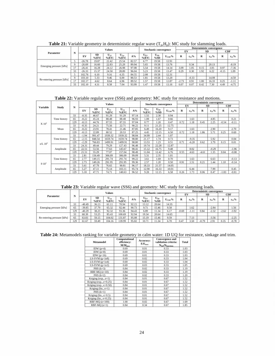
24

Table 21: Variable geometry in deterministic regular wave (Tp,Hp): MC study for slamming loads.

Parameter N Values Stochastic convergence Deterministic convergence

EV SD CDF

EV SD %|EV|

UJ,l %|EV|

UJ,u %|EV| A% UEV

%|EV| USD

%SD UCDF% R ε21% R ε21% R ε21%

Emerging pressure [kPa]

5 -26.78 19.87 22.42 25.54 82.57 6.77 19.58 12.91 9 -26.69 16.60 22.83 25.29 89.94 5.65 19.58 13.76 0.34 20.13 -8.19 17 -26.41 16.28 24.12 26.98 97.08 5.54 19.58 14.14 3.09 1.05 0.15 3.05 0.97 -7.36 33 -26.33 15.37 24.50 28.89 96.04 5.23 19.58 13.47 0.29 0.30 1.92 6.22 -0.15 1.09

Re-entering pressure [kPa]

5 102.76 6.10 9.16 6.35 84.55 2.08 19.58 12.31 9 103.10 5.33 9.46 6.00 88.53 1.81 19.58 13.20 -0.33 14.08 -4.50 17 102.17 4.62 8.64 6.96 89.52 1.57 19.58 12.87 -2.73 0.91 1.00 16.33 0.25 -1.11 33 102.10 4.31 8.58 7.04 93.99 1.47 19.58 13.16 0.07 0.07 0.42 7.30 4.49 -4.75

Table 22: Variable regular wave (SS6) and geometry: MC study for resistance and motions.

Variable Study N Values Stochastic convergence Deterministic convergence

EV SD CDF

EV SD %|EV|

UJ,l %|EV|

UJ,u %|EV| A% UEV

%|EV| USD

%SD UCDF% R ε21% R ε21% R ε21%

X 103

Time history 33 -8.35 46.67 91.29 91.29 97.14 1.55 2.30 0.94 65 -8.22 45.24 88.48 88.48 96.93 1.08 1.67 0.66 1.63 4.85 0.21 129 -8.13 44.76 87.55 87.55 97.04 0.77 1.20 0.47 0.72 1.18 0.45 2.25 -0.54 -0.11

Mean 33 -8.35 24.21 75.56 22.71 90.22 9.11 21.25 12.75 65 -8.22 23.91 78.41 21.46 87.85 6.49 16.20 9.17 1.63 2.90 2.70 129 -8.13 22.89 80.52 20.53 87.25 4.45 12.15 6.50 0.72 1.18 1.86 5.71 0.25 0.69

z/L 103

Time history 33 -1.94 991.47 1939.32 1939.32 98.84 34.99 2.44 1.07 65 -2.15 848.54 1659.74 1659.74 98.80 21.17 1.74 0.73 -9.35 5.92 0.04 129 -2.29 766.83 1499.91 1499.91 98.80 13.53 1.23 0.51 0.71 -6.20 0.62 3.79 0.15 0.01

Amplitude 33 24.31 49.44 79.29 127.43 96.48 19.74 22.28 12.87 65 22.51 53.56 77.63 145.67 98.41 15.12 16.75 9.48 8.02 -0.29 -1.96 129 21.51 55.29 77.07 157.04 98.49 11.04 12.42 6.76 0.55 4.63 -4.61 1.35 0.04 -0.08

θ 102

Time history 33 2.81 156.49 306.09 306.09 99.09 5.31 2.35 1.01 65 2.77 149.15 291.74 291.74 99.22 3.61 1.69 0.70 1.63 6.63 -0.13 129 2.73 149.26 291.95 291.95 99.36 2.57 1.20 0.50 0.91 1.51 0.21 1.44 1.10 -0.14

Amplitude 33 5.61 47.79 76.65 90.81 96.17 18.33 21.57 14.05 65 5.27 47.11 75.14 103.11 95.74 12.90 16.33 10.01 6.44 7.99 0.45 129 5.18 47.71 74.71 148.63 96.52 9.28 12.15 6.58 0.26 1.73 0.06 0.47 -1.83 -0.81

Table 23: Variable regular wave (SS6) and geometry: MC study for slamming loads.

Parameter N Values Stochastic convergence Deterministic convergence

EV SD CDF

EV SD %|EV|

UJ,u %|EV|

UJ,u %|EV| A% UEV

%|EV| USD

%SD UCDF% R ε21% R ε21% R ε21%

Emerging pressure [kPa] 33 -40.49 36.13 61.11 70.94 92.15 13.12 20.64 14.35 65 -39.85 37.79 65.32 92.44 90.73 9.71 15.46 9.58 1.62 -2.84 1.56 129 -40.29 38.25 92.32 93.36 94.43 6.89 11.34 6.17 -0.69 -1.11 0.84 -2.32 -2.62 -3.92

Re-entering pressure [kPa] 33 68.39 53.25 85.43 100.69 92.94 19.34 20.64 14.65 65 63.83 59.15 104.02 131.87 95.08 15.19 15.46 9.59 7.13 -3.56 -2.25 129 61.67 59.49 104.16 139.99 95.82 10.71 11.34 6.70 0.47 3.50 -0.79 2.91 0.35 -0.78

Table 24: Metamodels ranking for variable geometry in calm water: 1D UQ for resistance, sinkage and trim. Metamodel

Computational efficiency: M/Mmax

Accuracy: E/Emax

Convergence and validation criteria:

Nfail/Nfunctions Total

IDW (p=4) 0.69 0.01 0.33 1.03 IDW (p=8) 0.69 0.01 0.33 1.03 IDW (p=16) 0.69 0.01 0.33 1.03

LS-SVM (g=1e8) 0.69 0.02 0.33 1.04 LS-SVM (g=1e4) 0.69 0.02 0.33 1.04 LS-SVM (g=1e2) 0.69 0.03 0.33 1.05

PHS (k=3) 0.84 0.02 0.33 1.19 RBF-MQ (e=10) 0.84 0.02 0.33 1.19

PHS (k=2) 0.84 0.02 0.33 1.20 Kriging (exp., e=1) 0.84 0.01 0.67 1.52

Kriging (exp., e=0.25) 0.84 0.01 0.67 1.52 Kriging (exp., e=0.50) 0.84 0.01 0.67 1.52

Kriging (lin., e=1) 0.84 0.01 0.67 1.52 PHS (k=1) 0.84 0.01 0.67 1.52

Kriging (lin., e=0.5) 0.84 0.01 0.67 1.52 Kriging (lin., e=0.25) 0.84 0.01 0.67 1.52

RBF-MQ (e=100) 1.00 0.02 0.67 1.69 RBF-MQ (e=1) 0.84 0.34 0.67 1.85

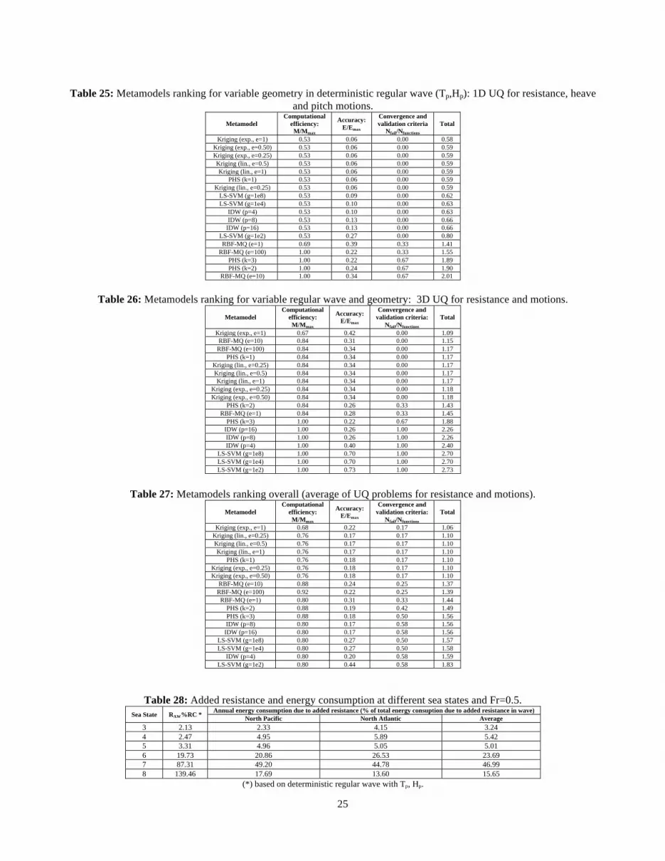
25

Table 25: Metamodels ranking for variable geometry in deterministic regular wave (Tp,Hp): 1D UQ for resistance, heave and pitch motions.

Metamodel Computational

efficiency: M/Mmax

Accuracy: E/Emax

Convergence and validation criteria

Nfail/Nfunctions Total

Kriging (exp., e=1) 0.53 0.06 0.00 0.58 Kriging (exp., e=0.50) 0.53 0.06 0.00 0.59 Kriging (exp., e=0.25) 0.53 0.06 0.00 0.59 Kriging (lin., e=0.5) 0.53 0.06 0.00 0.59 Kriging (lin., e=1) 0.53 0.06 0.00 0.59

PHS (k=1) 0.53 0.06 0.00 0.59 Kriging (lin., e=0.25) 0.53 0.06 0.00 0.59

LS-SVM (g=1e8) 0.53 0.09 0.00 0.62 LS-SVM (g=1e4) 0.53 0.10 0.00 0.63

IDW (p=4) 0.53 0.10 0.00 0.63 IDW (p=8) 0.53 0.13 0.00 0.66 IDW (p=16) 0.53 0.13 0.00 0.66

LS-SVM (g=1e2) 0.53 0.27 0.00 0.80 RBF-MQ (e=1) 0.69 0.39 0.33 1.41

RBF-MQ (e=100) 1.00 0.22 0.33 1.55 PHS (k=3) 1.00 0.22 0.67 1.89 PHS (k=2) 1.00 0.24 0.67 1.90

RBF-MQ (e=10) 1.00 0.34 0.67 2.01

Table 26: Metamodels ranking for variable regular wave and geometry: 3D UQ for resistance and motions.

Metamodel Computational

efficiency: M/Mmax

Accuracy: E/Emax

Convergence and validation criteria:

Nfail/Nfunctions Total

Kriging (exp., e=1) 0.67 0.42 0.00 1.09 RBF-MQ (e=10) 0.84 0.31 0.00 1.15 RBF-MQ (e=100) 0.84 0.34 0.00 1.17

PHS (k=1) 0.84 0.34 0.00 1.17 Kriging (lin., e=0.25) 0.84 0.34 0.00 1.17 Kriging (lin., e=0.5) 0.84 0.34 0.00 1.17 Kriging (lin., e=1) 0.84 0.34 0.00 1.17

Kriging (exp., e=0.25) 0.84 0.34 0.00 1.18 Kriging (exp., e=0.50) 0.84 0.34 0.00 1.18

PHS (k=2) 0.84 0.26 0.33 1.43 RBF-MQ (e=1) 0.84 0.28 0.33 1.45

PHS (k=3) 1.00 0.22 0.67 1.88 IDW (p=16) 1.00 0.26 1.00 2.26 IDW (p=8) 1.00 0.26 1.00 2.26 IDW (p=4) 1.00 0.40 1.00 2.40

LS-SVM (g=1e8) 1.00 0.70 1.00 2.70 LS-SVM (g=1e4) 1.00 0.70 1.00 2.70 LS-SVM (g=1e2) 1.00 0.73 1.00 2.73

Table 27: Metamodels ranking overall (average of UQ problems for resistance and motions).

Metamodel Computational

efficiency: M/Mmax

Accuracy: E/Emax

Convergence and validation criteria:

Nfail/Nfunctions Total

Kriging (exp., e=1) 0.68 0.22 0.17 1.06 Kriging (lin., e=0.25) 0.76 0.17 0.17 1.10 Kriging (lin., e=0.5) 0.76 0.17 0.17 1.10 Kriging (lin., e=1) 0.76 0.17 0.17 1.10

PHS (k=1) 0.76 0.18 0.17 1.10 Kriging (exp., e=0.25) 0.76 0.18 0.17 1.10 Kriging (exp., e=0.50) 0.76 0.18 0.17 1.10

RBF-MQ (e=10) 0.88 0.24 0.25 1.37 RBF-MQ (e=100) 0.92 0.22 0.25 1.39 RBF-MQ (e=1) 0.80 0.31 0.33 1.44

PHS (k=2) 0.88 0.19 0.42 1.49 PHS (k=3) 0.88 0.18 0.50 1.56 IDW (p=8) 0.80 0.17 0.58 1.56 IDW (p=16) 0.80 0.17 0.58 1.56

LS-SVM (g=1e8) 0.80 0.27 0.50 1.57 LS-SVM (g=1e4) 0.80 0.27 0.50 1.58

IDW (p=4) 0.80 0.20 0.58 1.59 LS-SVM (g=1e2) 0.80 0.44 0.58 1.83

Table 28: Added resistance and energy consumption at different sea states and Fr=0.5. Sea State RAW%RC * Annual energy consumption due to added resistance (% of total energy consuption due to added resistance in wave)

North Pacific North Atlantic Average 3 2.13 2.33 4.15 3.24 4 2.47 4.95 5.89 5.42 5 3.31 4.96 5.05 5.01 6 19.73 20.86 26.53 23.69 7 87.31 49.20 44.78 46.99 8 139.46 17.69 13.60 15.65

(*) based on deterministic regular wave with Tp, Hp.

26

Figure 1: Lines plan of the Delft cat. 372.

Figure 2: URANS simulation in

irregular wave (sea state 6).

Figure 3: Amplitudes and periods

for generic variable V(t).

(a) (b) (c) (d)

(e) (f) (g) (h)

Figure 4: Slamming loads; identification from pressure time-history (a); selection of pressure probe (b,c) and identification threshold (d) for current slamming studies. Max. emerging (e,f) and re-enetring (g,h) slams including pressure distribution.

(a) (b)

Figure 5: Empirical versus theoretical CDF for (a) wave period and (b) wave height H in sea state 6.

(a) (b) (c) Figure 6: Calm water simulation: CT (a), σ (b) and τ (c) vs. Fr.

0

0.2

0.4

0.6

0.8

1

0 5 10 15 20

CD

F(T

)

T

empiricaltheory

0

0.2

0.4

0.6

0.8

1

0 1 2 3 4 5 6 7 8

CD

F(H

)

H

empiricaltheory

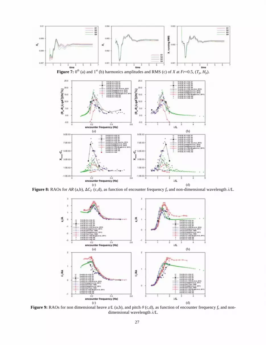
27

Figure 7: 0th (a) and 1st (b) harmonics amplitudes and RMS (c) of X at Fr=0.5, (Tp, Hp).

(a) (b)

(c) (d)

Figure 8: RAOs for AR (a,b), (c,d), as function of encounter frequency fe and non-dimensional wavelength λ/L.

(a) (b)

(c) (d)

Figure 9: RAOs for non dimensional heave z/L (a,b), and pitch θ (c,d), as function of encounter frequency fe and non-dimensional wavelength λ/L.

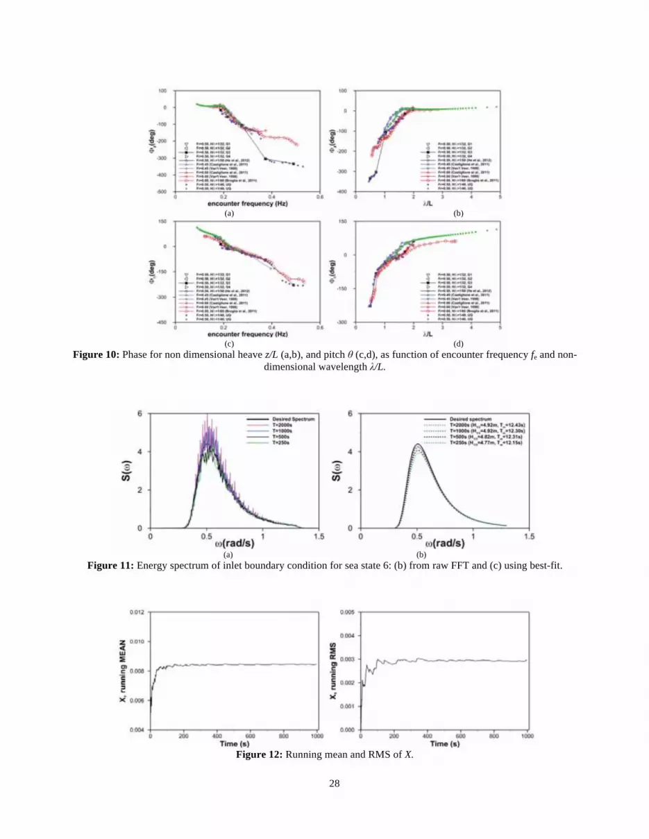
28

(a) (b)

(c) (d)

Figure 10: Phase for non dimensional heave z/L (a,b), and pitch θ (c,d), as function of encounter frequency fe and non-dimensional wavelength λ/L.

(a) (b)

Figure 11: Energy spectrum of inlet boundary condition for sea state 6: (b) from raw FFT and (c) using best-fit.

Figure 12: Running mean and RMS of X.

29

(a) (b) (c)

Figure 13: FFT of force X (a) non-dimensional pitch z/L (b) and pitch θ (c) in sea state 6, at Fr=0.5.

(a) (b)

(c) (d)

(e) (f)

Figure 14: RAOs for force X (a,b), non-dimensional heave z/L (c,d), and pitch θ (e,f), as function of encounter frequency fe and non-dimensional wavelength λ/L, at Fr=0.5.

0

0.05

0.1

0.15

0.2

0.25

0.3

0.35

0.4

0.45

0 0.1 0.2 0.3 0.4 0.5 0.6

XF

FT 1

03

encounter frequency, fe [Hz]

within wave comp. freq. range

outside wave comp. freq. range

0

0.005

0.01

0.015

0.02

0.025

0 0.1 0.2 0.3 0.4 0.5 0.6

z FF

T/L

103

frequency [Hz]

within wave comp. freq. range

outside wave comp. freq. range

0

0.1

0.2

0.3

0.4

0.5

0.6

0.7

0.8

0 0.1 0.2 0.3 0.4 0.5 0.6

θ FF

T 1

02

frequency [Hz]

within wave comp. freq. range

outside wave comp. freq. range

0

0.2

0.4

0.6

0.8

1

0 0.1 0.2 0.3 0.4 0.5 0.6

X#

Fr2 L

S /

2 Δ A

k

frequency [Hz]

irregular wave, XFFT(fe)

regular wave, H/λ=1/32, X1(fe)

reg.w. UQ, 1/458<H/λ<1/10, X1(fe)

reg.w. UQ, 1/458<H/λ<1/10, X2(2fe)

0

0.2

0.4

0.6

0.8

1

0 1 2 3 4 5 6

X#

Fr2 L

S /

2 Δ A

k

λ/L

irregular wave, XFFT[λ(fe)/L]

regular wave, H/λ=1/32, X1[λ(fe)/L]

reg.w. UQ, 1/458<H/λ<1/10, X1[λ(fe)/L]

reg.w. UQ, 1/458<H/λ<1/10, X2[λ(2fe)/L]

0

0.5

1

1.5

2

2.5

0 0.1 0.2 0.3 0.4 0.5 0.6

z #/A

frequency [Hz]

irregular wave, zFFT(fe)

regular wave, H/λ=1/32, z1(fe)

reg.w. UQ, 1/458<H/λ<1/10, z1(fe)

EFD (Bouscasse et al., 2012), zFFT(fe)

0

0.5

1

1.5

2

2.5

0 1 2 3 4 5 6

z #/A

λ/L

irregular wave, zFFT[λ(fe)/L]

regular wave, H/λ=1/32, z1[λ(fe)/L]

reg.w. UQ, 1/458<H/λ<1/10, z1[λ(fe)/L]

EFD (Bouscasse et al., 2012), z1[λ(fe)/L]

0

0.2

0.4

0.6

0.8

1

1.2

1.4

1.6

0 0.1 0.2 0.3 0.4 0.5 0.6

θ #/A

k

frequency [Hz]

irregular wave, θFFT(fe)

regular wave, H/λ=1/32, θ1(fe)

reg.w. UQ, 1/458<H/λ<1/10, θ1(fe)

EFD (Bouscasse et al., 2012), θFFT(fe)

0

0.2

0.4

0.6

0.8

1

1.2

1.4

1.6

0 1 2 3 4 5 6

θ #/A

k

λ/L

irregular wave, θFFT[λ(fe)/L]

regular wave, H/λ=1/32, θ1[λ(fe)/L]

reg.w. UQ, 1/458<H/λ<1/10, θ1[λ(fe)/L]

EFD (Bouscasse et al., 2012), θFFT[λ(fe)/L]

30

(a) (b) (c) Figure 15: Comparison of time history PDF for irregular wave benchmark and variable regular wave UQ. Empirical and

Normal density functions are shown: (a) force X, (b) heave z/L, (c) pitch θ.

(a) (b) (c)

Figure 16: 2D UQ for variable regular wave: PDF of (a) force mean, mean-crossing amplitude for heave (b) and pitch (c) motions. Empirical distributions are compared with Normal (time mean) and Gamma (amplitudes).

(a) (b) (c)

(d) (e) (f)

Figure 17: 2D UQ for variable regular wave: contours of (a,d) force mean, mean-crossing amplitude for heave (b,e) and pitch (c,f), as function of wave period and height and encounter frequency and wave amplitude. Polyharmonic spline (k=2)

is used to get contours. Black dots are MCMC items.

0

0.02

0.04

0.06

0.08

0.1

0.12

0.14

0.16

-25 -20 -15 -10 -5 0 5

PD

F

X 103

benchmark (empirical)UQ (empirical)

benchmark (Normal)UQ (Normal)

0

5

10

15

20

25

30

35

-0.08 -0.06 -0.04 -0.02 0 0.02 0.04 0.06

PD

F

z/L

benchmark (empirical)

UQ (empirical)benchmark (Normal)

UQ (Normal)

0

2

4

6

8

10

12

-0.15 -0.1 -0.05 0 0.05 0.1 0.15 0.2 0.25

PD

F

θ [rad]

benchmark (empirical)

UQ (empirical)benchmark (Normal)

UQ (Normal)

0

0.05

0.1

0.15

0.2

0.25

0.3

0.35

-16 -14 -12 -10 -8 -6 -4 -2 0 2

PD

F

X 103, running mean

benchmark (empirical)

UQ (empirical)benchmark (Gamma)

UQ (Gamma)

0

10

20

30

40

50

60

0 0.005 0.01 0.015 0.02 0.025 0.03 0.035 0.04 0.045 0.05

PD

F

z/L, mean-crossing amplitude

benchmark (empirical)

UQ (empirical)benchmark (Gamma)

UQ (Gamma)

0

2

4

6

8

10

12

14

16

18

20

0 0.02 0.04 0.06 0.08 0.1 0.12 0.14

PD

F

θ, mean-crossing amplitude [rad]

benchmark (empirical)

UQ (empirical)benchmark (Gamma)

UQ (Gamma)

1

2

3

4

5

6

2 4 6 8 10 12 14 16 18

H [m

]

T [s]

X 103, running mean

-16

-15

-14

-13

-12

-11

-10

-9

-8

-7

-6

1

2

3

4

5

6

2 4 6 8 10 12 14 16 18

H [m

]

T [s]

z/L, mean-crossing amplitude

0

0.01

0.02

0.03

0.04

0.05

0.06

1

2

3

4

5

6

2 4 6 8 10 12 14 16 18

H [m

]

T [s]

θ, mean-crossing amplitude [rad]

0

0.02

0.04

0.06

0.08

0.1

0.12

0.14

0.5

1

1.5

2

2.5

3

0.1 0.15 0.2 0.25 0.3 0.35 0.4

A [m

]

fe [Hz]

X 103, running mean

-15

-14

-13

-12

-11

-10

-9

-8

-7

0.5

1

1.5

2

2.5

3

0.1 0.15 0.2 0.25 0.3 0.35 0.4

A [m

]

fe [Hz]

z/L, mean-crossing amplitude

0

2

4

6

8

10

12

0.5

1

1.5

2

2.5

3

0.1 0.15 0.2 0.25 0.3 0.35 0.4

A [m

]

fe [Hz]

θ, mean-crossing amplitude

0

0.5

1

1.5

2

2.5

3

3.5

4

4.5

5

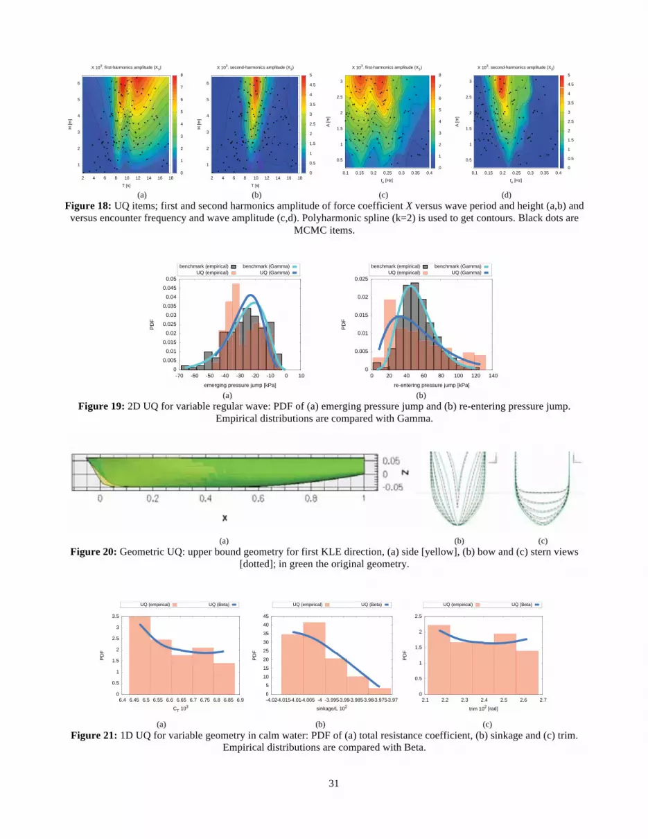
31

(a) (b) (c) (d)

Figure 18: UQ items; first and second harmonics amplitude of force coefficient X versus wave period and height (a,b) and versus encounter frequency and wave amplitude (c,d). Polyharmonic spline (k=2) is used to get contours. Black dots are

MCMC items.

(a) (b)

Figure 19: 2D UQ for variable regular wave: PDF of (a) emerging pressure jump and (b) re-entering pressure jump. Empirical distributions are compared with Gamma.

(a) (b) (c)

Figure 20: Geometric UQ: upper bound geometry for first KLE direction, (a) side [yellow], (b) bow and (c) stern views [dotted]; in green the original geometry.

(a) (b) (c)

Figure 21: 1D UQ for variable geometry in calm water: PDF of (a) total resistance coefficient, (b) sinkage and (c) trim. Empirical distributions are compared with Beta.

1

2

3

4

5

6

2 4 6 8 10 12 14 16 18

H [m

]

T [s]

X 103, first-harmonics amplitude (X1)

0

1

2

3

4

5

6

7

8

1

2

3

4

5

6

2 4 6 8 10 12 14 16 18

H [m

]

T [s]

X 103, second-harmonics amplitude (X2)

0

0.5

1

1.5

2

2.5

3

3.5

4

4.5

5

0.5

1

1.5

2

2.5

3

0.1 0.15 0.2 0.25 0.3 0.35 0.4

A [m

]

fe [Hz]

X 103, first-harmonics amplitude (X1)

0

1

2

3

4

5

6

7

8

0.5

1

1.5

2

2.5

3

0.1 0.15 0.2 0.25 0.3 0.35 0.4

A [m

]

fe [Hz]

X 103, second-harmonics amplitude (X2)

0

0.5

1

1.5

2

2.5

3

3.5

4

4.5

5

0

0.005

0.01

0.015

0.02

0.025

0.03

0.035

0.04

0.045

0.05

-70 -60 -50 -40 -30 -20 -10 0 10

PD

F

emerging pressure jump [kPa]

benchmark (empirical)

UQ (empirical)benchmark (Gamma)

UQ (Gamma)

0

0.005

0.01

0.015

0.02

0.025

0 20 40 60 80 100 120 140

PD

F

re-entering pressure jump [kPa]

benchmark (empirical)

UQ (empirical)benchmark (Gamma)

UQ (Gamma)

0

0.5

1

1.5

2

2.5

3

3.5

6.4 6.45 6.5 6.55 6.6 6.65 6.7 6.75 6.8 6.85 6.9

PD

F

CT 103

UQ (empirical) UQ (Beta)

0

5

10

15

20

25

30

35

40

45

-4.02-4.015-4.01-4.005 -4 -3.995-3.99-3.985-3.98-3.975-3.97

PD

F

sinkage/L 102

UQ (empirical) UQ (Beta)

0

0.5

1

1.5

2

2.5

2.1 2.2 2.3 2.4 2.5 2.6 2.7

PD

F

trim 102 [rad]

UQ (empirical) UQ (Beta)

32

(a) (b) (c)

Figure 22: 1D UQ for variable geometry in deterministic regular wave: PDF of (a) force mean, mean-crossing amplitude for heave (b) and pitch (c) motions. Empirical distributions are compared with Beta.

(a) (b)

Figure 23: 1D UQ for variable geometry in deterministic regular wave: PDF of (a) emerging pressure jump and (b) re-entering pressure jump. Empirical distributions are compared with Beta.

(a) (b) (c)

Figure 24: 3D UQ for variable regular wave and geometry: PDF of (a) force mean, mean-crossing amplitude for heave (b) and pitch (c) motions. Empirical distributions are compared with Normal (time mean) and Gamma (amplitudes).

(a) (b)

Figure 25: 3D UQ for variable regular wave and geometry: PDF of (a) emerging pressure jump and (b) re-entering pressure jump. Empirical distributions are compared with Gamma.

0

0.5

1

1.5

2

2.5

3

3.5

4

4.5

-8.15 -8.1 -8.05 -8 -7.95 -7.9 -7.85 -7.8 -7.75

PD

F

X 103, mean

UQ (empirical) UQ (Beta)

0

2

4

6

8

10

12

14

16

14.4 14.45 14.5 14.55 14.6 14.65

PD

F

z/L 103, amplitude

UQ (empirical) UQ (Beta)

0

2

4

6

8

10

12

14

16

4.4 4.42 4.44 4.46 4.48 4.5 4.52 4.54 4.56 4.58 4.6

PD

F

θ 102, amplitude

UQ (empirical) UQ (Beta)

0

0.01

0.02

0.03

0.04

0.05

0.06

0.07

0.08

0.09

-34 -32 -30 -28 -26 -24 -22 -20 -18

PD

F

emerging pressure jump [kPa]

UQ (empirical) UQ (Beta)

0

0.02

0.04

0.06

0.08

0.1

0.12

92 94 96 98 100 102 104 106 108 110P

DF

re-entering pressure jump [kPa]

UQ (empirical) UQ (Beta)

0

0.1

0.2

0.3

0.4

0.5

0.6

-15 -14 -13 -12 -11 -10 -9 -8 -7 -6

PD

F

X 103, mean

UQ (empirical) UQ (Normal)

0

0.005

0.01

0.015

0.02

0.025

0.03

0.035

0.04

0.045

0.05

0 10 20 30 40 50 60 70

PD

F

z/L 103, amplitude

UQ (empirical) UQ (Gamma)

0

0.05

0.1

0.15

0.2

0.25

0 2 4 6 8 10 12 14 16

PD

F

θ 102, amplitude

UQ (empirical) UQ (Gamma)

0

0.005

0.01

0.015

0.02

0.025

0.03

-80 -70 -60 -50 -40 -30 -20 -10 0

PD

F

emerging pressure jump [kPa]

UQ (empirical) UQ (Gamma)

0

0.002

0.004

0.006

0.008

0.01

0.012

0.014

0.016

0.018

0.02

-20 0 20 40 60 80 100 120 140 160

PD

F

re-entering pressure jump [kPa]

UQ (empirical) UQ (Gamma)