Forensic speaker recognitionBased on text analysis of transcribedspeech fragments

Nelleke Scheijen

Delft

Unive

rsity

ofTe

chno

logy

Forensic speaker recognitionBased on text analysis of transcribed

speech fragmentsby

Nelleke Scheijento obtain the degree of

Master of Science in Applied MathematicsSpecialisation Stochastics

at the Delft University of Technology,to be defended publicly on Wednesday June 24, 2020 at 14:00.

Student number: 4323874Project duration: Oktober 7, 2019 – June 24, 2020Thesis committee: Dr. J. Söhl, TU Delft, supervisor

Dr. ir. M. Keijzer, TU DelftProf. dr. ir. G. Jongbloed, TU DelftA. J. Leegwater, MSc. NFI, daily supervisor

An electronic version of this thesis is available at http://repository.tudelft.nl/.

Abstract

Speaker recognition is an important subject and a constantly developing field in forensic science. Currently,speaker recognition research is mainly based on phonetics and speech signal processing. This research ad-dresses speaker recognition from a new perspective, analysing the transcription of a fragment of speech withtext analysis methods. Since text analysis is based on the transcription text only, it can be assumed indepen-dent from current automatic speaker recognition software. Hence, it would contribute significantly to theoverall evidential value. The analysis is based on the frequencies of non-content, highly frequent words. Westudy whether information about the identity of the speaker is contained in the transcription of spoken text.

The value of evidence is quantified using a score-based likelihood ratio. The score-based approach ischosen because in most forensic cases, there is not enough data from the suspect or of the disputed speechfragment available to model a robust feature-based likelihood ratio. Different methods to model the systemfrom feature vector over score to likelihood ratio have been compared. As a baseline, a distance based methodis used, where the score is the distance between the feature vectors. To improve upon this baseline, machinelearning algorithms are implemented. The results from SVM and XGBoost are explored. As a third methoda feature-based likelihood ratio is calculated and used as a score instead of as a direct likelihood ratio. Withthis method, both similarity and typicality are taken into account.

The model is trained and tested on the FRIDA data set from the Netherlands Forensic Institute, consistingof Dutch conversations from a homogeneous group of 250 individuals. The performance of the likelihoodratio system is evaluated through computing the cost log-likelihood-ratio Cl l r , which is a measure for theaccuracy and quality of the likelihood ratios, and the accuracy A of the likelihood ratios solely. The perfor-mance is also evaluated by inspecting the Tippett, empirical cross-entropy and pool-adjacent-violators plots.Different values for parameters used in the calculation of the likelihood ratios are investigated: the length ofthe sample N , the number of frequent words (number of features) F# and the number of samples S# neededto train the model.

The distance method showed a strong baseline, with good performance for large sample lengths. The SVMmethod outperformed the distance method for all parameter settings, with a peak performance of A = 0.94and Cl l r = 0.24. The XGBoost method showed promising results for smaller samples lengths, but a too largeamount of data is needed to obtain good performance for larger sample lengths. The LR score method showedmoderate results, but no improvements due to the necessity to estimate high-dimensional distributions.

This thesis shows that information about the identity of the speaker is contained in transcriptions ofspeech. The complete process from data to likelihood ratio is constructed, where the likelihood ratio quanti-fies the evidential value of a transcribed speech fragment.

iii

Preface

With handing in this thesis, my life as a student comes to an end. This thesis is the final requirement to obtainmy Master’s degree in Applied Mathematics in the specialisation Stochastics. During the last 9 months, Iworked on the subject of forensic speaker recognition, based on text analysis of transcribed speech fragments.I am really glad to have studied this topic, as it perfectly fits my idea of an interesting mathematical problemwith a clear application in real life. I had no previous experience with forensic science and learned a lotabout quantifying evidence as well as machine learning and programming. It sparked my enthusiasm aboutforensic science and I appreciate the opportunity to have gained knowledge about this research area. Withoutmy supervisors, friends and family around me, this thesis would not have been as it is now. Therefore, I wouldlike to thank some people in particular.

First of all I would like to thank my supervisor Jakob Söhl from TU Delft. For helping me plan my thesis,always supportive advise and small chats about rowing during our two-weekly meetings. You helped mefinishing my thesis in time, during corona and a small stress moment in the last two weeks. I also would liketo thank Marleen Keijzer and Geurt Jongbloed, for taking place in my graduation committee.

Secondly, I would like to thank my daily supervisor Jeannette Leegwater from the NFI. Our weekly meet-ings were always a good mix between discussing research ideas, my progress and chatting about boulderingor something else. You helped me writing a clear thesis about the research I conducted. I am grateful for theopportunity to have carried out this research at the NFI. I had a great time with all my colleagues. They helpedme with interesting suggestions for my thesis, but we also planned fun activities as bouldering and runningbreaks. Thank you Wauter and David, for your guidance in the forensic speaker recognition research.

A special thanks goes to my family. My parents, Rob & Noor, Bibi & Thei, for always supporting me duringmy entire time as a student and in every decision I made. For celebrating great times and offering help whenI needed it. To my siblings Amy & Coen and my twin sister Guusje, for just always being there for me.

Lastly, I would like to thank all the people who made my student life as exciting as it was. My rowingteammates, with whom I spend almost all my time at the rowing association with, during my bachelor years.Thank you for all the sporty adventures and tea drinking sessions. My board members, with whom I took agap year and who turned into close friends. Thank you for supporting me in good, but also stressful times. Myflatmates, who were always caring and helpful when I needed a cheer-up. My study friends from the bachelor,but also new study friends from the master. You guys made studying till late hours that much more fun. Chris,for the sweet unconditional support during my thesis. And just to everyone I met on the way, thank you!

Nelleke ScheijenDelft, June 2020

v

Contents

1 Introduction 11.1 Thesis outline . . . . . . . . . . . . . . . . . . . . . . . . . . . . . . . . . . . . . . . . . . . 2

2 Identification of source framework 32.1 Common source . . . . . . . . . . . . . . . . . . . . . . . . . . . . . . . . . . . . . . . . . 42.2 Specific source . . . . . . . . . . . . . . . . . . . . . . . . . . . . . . . . . . . . . . . . . . 52.3 Comparison frameworks for the speaker recognition case study . . . . . . . . . . . . . . . . . 6

3 Likelihood ratio framework 93.1 Value of evidence . . . . . . . . . . . . . . . . . . . . . . . . . . . . . . . . . . . . . . . . . 93.2 Score-based approach . . . . . . . . . . . . . . . . . . . . . . . . . . . . . . . . . . . . . . 113.3 Verbal likelihood ratios . . . . . . . . . . . . . . . . . . . . . . . . . . . . . . . . . . . . . . 133.4 Combination of forensic evidence . . . . . . . . . . . . . . . . . . . . . . . . . . . . . . . . 14

4 Data set NFI 175 Text analysis 19

5.1 Features FRIDA data set. . . . . . . . . . . . . . . . . . . . . . . . . . . . . . . . . . . . . . 215.2 Frameworks in text analysis . . . . . . . . . . . . . . . . . . . . . . . . . . . . . . . . . . . . 22

6 Features to scores 236.1 Distance method . . . . . . . . . . . . . . . . . . . . . . . . . . . . . . . . . . . . . . . . . 236.2 Machine learning score algorithms . . . . . . . . . . . . . . . . . . . . . . . . . . . . . . . . 256.3 Feature-based likelihood ratio as score . . . . . . . . . . . . . . . . . . . . . . . . . . . . . . 29

6.3.1 Two-level normal-normal model. . . . . . . . . . . . . . . . . . . . . . . . . . . . . . 306.3.2 Common source score calculation . . . . . . . . . . . . . . . . . . . . . . . . . . . . . 316.3.3 Specific source score calculation . . . . . . . . . . . . . . . . . . . . . . . . . . . . . . 31

7 Calibration of scores to likelihood ratios 337.1 Kernel density estimation . . . . . . . . . . . . . . . . . . . . . . . . . . . . . . . . . . . . . 337.2 Score calibration to likelihood ratio . . . . . . . . . . . . . . . . . . . . . . . . . . . . . . . . 34

8 Likelihood ratio validation 378.1 Pool adjacent violators algorithm . . . . . . . . . . . . . . . . . . . . . . . . . . . . . . . . . 388.2 Log-likelihood-ratio cost . . . . . . . . . . . . . . . . . . . . . . . . . . . . . . . . . . . . . 398.3 Empirical cross entropy plot . . . . . . . . . . . . . . . . . . . . . . . . . . . . . . . . . . . 398.4 Tippett plot . . . . . . . . . . . . . . . . . . . . . . . . . . . . . . . . . . . . . . . . . . . . 40

9 Results 439.1 Performance distance method . . . . . . . . . . . . . . . . . . . . . . . . . . . . . . . . . . 449.2 Performance machine learning methods . . . . . . . . . . . . . . . . . . . . . . . . . . . . . 509.3 Performance LR score method . . . . . . . . . . . . . . . . . . . . . . . . . . . . . . . . . . 55

9.3.1 Common source LR score method . . . . . . . . . . . . . . . . . . . . . . . . . . . . . 559.3.2 Specific source LR score method . . . . . . . . . . . . . . . . . . . . . . . . . . . . . . 58

9.4 Comparison performance all methods . . . . . . . . . . . . . . . . . . . . . . . . . . . . . . 62

10 Conclusion and recommendations 6310.1 Conclusion and discussion . . . . . . . . . . . . . . . . . . . . . . . . . . . . . . . . . . . . 6310.2 Recommendations for future work . . . . . . . . . . . . . . . . . . . . . . . . . . . . . . . . 64

Bibliography 67A Data 71

A.1 Frequent words FRIDA data set . . . . . . . . . . . . . . . . . . . . . . . . . . . . . . . . . . 71A.2 Frequent words CGN data set . . . . . . . . . . . . . . . . . . . . . . . . . . . . . . . . . . . 72

vii

viii Contents

B Detailed calculations and settings 75B.1 Two-level normal-normal model . . . . . . . . . . . . . . . . . . . . . . . . . . . . . . . . . 75

B.1.1 Common source . . . . . . . . . . . . . . . . . . . . . . . . . . . . . . . . . . . . . . 75B.1.2 Specific source . . . . . . . . . . . . . . . . . . . . . . . . . . . . . . . . . . . . . . . 76

B.2 Machine learning algorithm settings . . . . . . . . . . . . . . . . . . . . . . . . . . . . . . . 77

C Additional results 79C.1 Distance method . . . . . . . . . . . . . . . . . . . . . . . . . . . . . . . . . . . . . . . . . 79

C.1.1 Different distance metrics . . . . . . . . . . . . . . . . . . . . . . . . . . . . . . . . . 79C.1.2 Tables additional Cllr results . . . . . . . . . . . . . . . . . . . . . . . . . . . . . . . . 79

C.2 Machine learning results . . . . . . . . . . . . . . . . . . . . . . . . . . . . . . . . . . . . . 81C.3 LR score results . . . . . . . . . . . . . . . . . . . . . . . . . . . . . . . . . . . . . . . . . . 82

1Introduction

Assume a person, suspected by the police of a criminal act. The police places a tap on their mobile phoneto investigate the matter. On one of the tapped recordings, the suspect speaks about a criminal act. Thetapped recordings can be used as evidence by the police. After this event the suspect is arrested. However,the person claims the phone was stolen and thus the person on the tap is not them. The police then tasks aforensic scientist to look at the value of evidence to research if the (unknown) speaker can be identified byinformation deduced from the telephone conversation. Can the telephone conversation be used as evidenceby comparing the suspect’s manner of speaking and the conversation on the phone? In forensic science,this type of research is called speaker recognition. Two approaches are possible for speaker recognition, thefirst one is to determine the speaker of a disputed fragment of speech by comparing the disputed fragmentwith speech from the suspect. The second approach is to compare two fragments of speech from unknownspeaker(s), to determine if they originate from one speaker or two different speakers [34, 35]. This approachcould be used to research whether two tapped recordings point to one or two suspects, even if the person isstill unknown.

Speaker recognition is an important subject and a constantly developing field in forensic science. At theNetherlands Forensic Institute (NFI), where this thesis is conducted, the speech department currently usestwo methods to identify the speaker of a speech fragment. These methods are the automatic voice recog-nition tools and the judgement of an expert [59]. Currently, a drawback of the automatic voice recognitionsystem is its dependency on the recording situation. For different background noises, e.g. a telephone tapand a car tap, the system does not provide consistent results [28]. The judgement of an expert is performedby an individual and is a human judgement. This is a valuable analysis, but also subjective as the measure-ment metric is a human [59]. This research attempts to address automatic speaker recognition from a newperspective, by analysing the transcription from a fragment of speech. A new method based on text analy-sis could contribute to the already existing methods named before. Text analysis for authorship analysis onwritten text has already been a research topic for over 50 years and has promising results for applicationslike plagiarism detection or authorship analysis of novels [3, 4, 32]. It has been shown that authors unknow-ingly use specific words or sentence structures distinctively in all types of written text [15, 21]. This raisesthe question if a transcription from speech also contains a certain amount of information about the speaker,contained in the choice of words while having a conversation.

In order to determine the value of evidence of a speech fragment, a forensic scientist has to quantify thisvalue. For this a universal framework to evaluate evidence is needed. The value is determined by compar-ing the evidence conditional on two competing hypotheses. The hypotheses are mutually exclusive and arecommonly denoted as the prosecutor’s hypothesis Hp and the defence hypothesis Hd . The ratio of the prob-abilities of the evidence conditional on these hypotheses results in the likelihood ratio quantifying the valueof evidence. The choice of hypotheses is an important part of forensic evidence evaluation. To use speakerrecognition based on text analysis in a forensic context, the result has to be stated in the form of a likelihoodratio, rather than just as a correct classification of the speaker. In a legal case a judge is interested in a quan-titative judgement about the evidence: to what extent does the evidence support one of the hypotheses withrespect to the other hypothesis? The framework to quantify the evidence is further outlined in Chapter 2.We research a problem where one is interested in the source of a trace, the so-called identification of source

1

2 1. Introduction

problem [34, 35]. In our case the forensic scientist is interested in the speaker of the fragment of speech, i.e.the source of the speech fragment.

At the moment of writing this thesis, to the best of the author’s knowledge, no publications are availableon authorship analysis on the transcriptions of spontaneous spoken text. Therefore, this thesis explores a newapplication. Text analysis can be assumed independent from current automatic speaker recognition software,which is mainly based on phonetics and speech signal processing. It thus would contribute significantlyto the overall evidential value of speaker recognition. Especially for comparing fragments of speech withdifferent background noise, text analysis of the transcription can be a suitable option to explore.

To summarise, the scope of this research is to quantify the evidential value in the transcription of spo-ken text in a forensic context. The theoretical statistical forensic framework is explained, taking into accountthe limitations present in a real forensic case as in the example stated above. The text analysis methods forauthorship analysis are implemented and tested for automatic speaker recognition. The forensic frameworkand the text analysis methods are combined to cover the complete process and validation from the transcrip-tion of a fragment of speech to a value of evidence in terms of a likelihood ratio. The research is conductedon a data set of transcriptions of speech fragments, provided by the NFI.

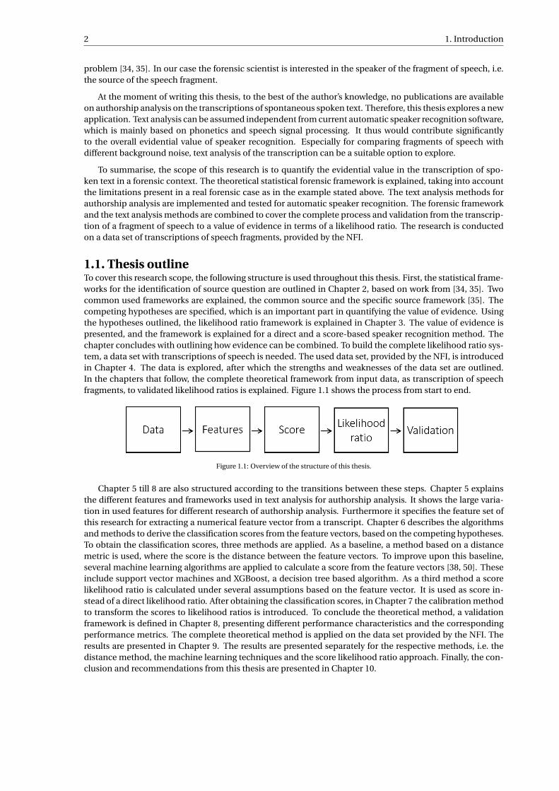
1.1. Thesis outlineTo cover this research scope, the following structure is used throughout this thesis. First, the statistical frame-works for the identification of source question are outlined in Chapter 2, based on work from [34, 35]. Twocommon used frameworks are explained, the common source and the specific source framework [35]. Thecompeting hypotheses are specified, which is an important part in quantifying the value of evidence. Usingthe hypotheses outlined, the likelihood ratio framework is explained in Chapter 3. The value of evidence ispresented, and the framework is explained for a direct and a score-based speaker recognition method. Thechapter concludes with outlining how evidence can be combined. To build the complete likelihood ratio sys-tem, a data set with transcriptions of speech is needed. The used data set, provided by the NFI, is introducedin Chapter 4. The data is explored, after which the strengths and weaknesses of the data set are outlined.In the chapters that follow, the complete theoretical framework from input data, as transcription of speechfragments, to validated likelihood ratios is explained. Figure 1.1 shows the process from start to end.

Figure 1.1: Overview of the structure of this thesis.

Chapter 5 till 8 are also structured according to the transitions between these steps. Chapter 5 explainsthe different features and frameworks used in text analysis for authorship analysis. It shows the large varia-tion in used features for different research of authorship analysis. Furthermore it specifies the feature set ofthis research for extracting a numerical feature vector from a transcript. Chapter 6 describes the algorithmsand methods to derive the classification scores from the feature vectors, based on the competing hypotheses.To obtain the classification scores, three methods are applied. As a baseline, a method based on a distancemetric is used, where the score is the distance between the feature vectors. To improve upon this baseline,several machine learning algorithms are applied to calculate a score from the feature vectors [38, 50]. Theseinclude support vector machines and XGBoost, a decision tree based algorithm. As a third method a scorelikelihood ratio is calculated under several assumptions based on the feature vector. It is used as score in-stead of a direct likelihood ratio. After obtaining the classification scores, in Chapter 7 the calibration methodto transform the scores to likelihood ratios is introduced. To conclude the theoretical method, a validationframework is defined in Chapter 8, presenting different performance characteristics and the correspondingperformance metrics. The complete theoretical method is applied on the data set provided by the NFI. Theresults are presented in Chapter 9. The results are presented separately for the respective methods, i.e. thedistance method, the machine learning techniques and the score likelihood ratio approach. Finally, the con-clusion and recommendations from this thesis are presented in Chapter 10.

2Identification of source framework

In this chapter a literature study is presented, mainly based on [34–36]. The purpose of this literature study is topresent the framework and theory which is needed to understand the remainder of this thesis.

As outlined in the introduction, a forensic scientist is tasked to quantify the value of evidence. The valueof evidence is often defined as a ratio between two competing hypotheses, which is called the likelihoodratio, first introduced by [13]. Typically, a hypothesis of the prosecution, denoted Hp , and a hypothesis of thedefence, denoted Hd , are stated. The ratio between the probabilities of the evidence given the hypotheses iscalled the likelihood ratio. The exact formulation of the hypotheses depends on the type of identification ofsource model. Two identification of source approaches will be considered, the common source model andthe specific source model, as specified by [34, 35]. The specific source model tries to answer the questionwhether a speech fragment originates from a specific known source, where the common source problem isfocused on determining if two texts originate from the same unknown source. The two frameworks look quitesimilar and can be interpreted in the same context, but the method to approach both problems could leadto different results [34, 35]. Both models give rise to different pairs of competing hypotheses, these will bediscussed below.

In forensic science, scientists are interested in the way the evidence is generated, instead of only classicalhypotheses testing of the parameters [34, 35]. Thus, the hypotheses include the choice for a sampling model.In classical testing, the sampling model is specified beforehand, in forensic science the sampling model dif-fers for the specific source and common source model. Therefore, to do hypothesis testing in forensic science,the following components are needed, as specified by [34, 35]. First, the sampling models corresponding tothe competing hypotheses have to be stated. Secondly, the corresponding parametric distribution used in thesampling models has to be estimated. Theoretically a non-parametric distribution is also possible, but infea-sible because of the high dimensional feature vector. The number of samples needed to fit a non-parametricdistribution accurately, increases exponentially with number of dimensions [24]. It has to be noted here, thatit has to be assumed the data follows a parametric distribution [11]. In many cases, as also in speaker recog-nition, picking a correct parametric distribution can be quite hard or even impossible due to the unknowndistribution and high-dimensional data. This is further outlined in Section 3.2. Lastly, to use the parametricdistribution, the parameters have to be estimated. In this section only the sampling models are presented,the parametric distribution with corresponding parameters is outlined in Chapter 6.

In the remainder of this chapter three sets of evidence are used. Evidence from a specific known sourcees , evidence from a unknown source eu and evidence from a large set of known sources often referred to asthe background population of alternative sources ea , following the notation of [34, 35]. This background setshould be relevant for the hypotheses that are tested. With relevant we mean the sources should be compara-ble with respect to the background information a forensic scientist has about the sources under investigation.Which evidence sets are used per framework will be further outlined below. It is important to note that thechoice of background material can have a large impact on the results, it has to represent the total alternativepopulation of speakers.

The common source and specific source sampling models are briefly discussed, to explain the frameworksfor the application in this thesis. The models are introduced and detailed outlined in [34, 35].

3

4 2. Identification of source framework

2.1. Common sourceThe classical common source problem starts with two traces. Suppose two traces of unknown origin are foundat two different crime scenes. It is interesting whether the crimes can be linked together. One is interestedif the traces come from the same unknown source. The two different traces lead to two pieces of evidencewith unknown source: eu1 and eu2 . One is not researching who is the unknown source, but only if bothtraces originate from the same unknown source [34, 35]. In terms of speaker recognition, assume havingtwo different speech fragments from unknown speakers (eu1 ,eu2 ). The question of interest is, whether bothfragments originate from the same speaker. The evidence set is completed with material from the backgroundpopulation (ea), the background population of alternative sources, and defined as e =

eu1 ,eu2 ,ea. For the

common source problem, the hypotheses in the context of speaker recognition are stated as [34, 35]:

Hp: The two speech fragments (eu1 , eu2 ) from unknown speakers originate from the same unknown speaker.

Hd: The two speech fragments (eu1 , eu2 ) from unknown speakers originate from two different unknownspeakers.

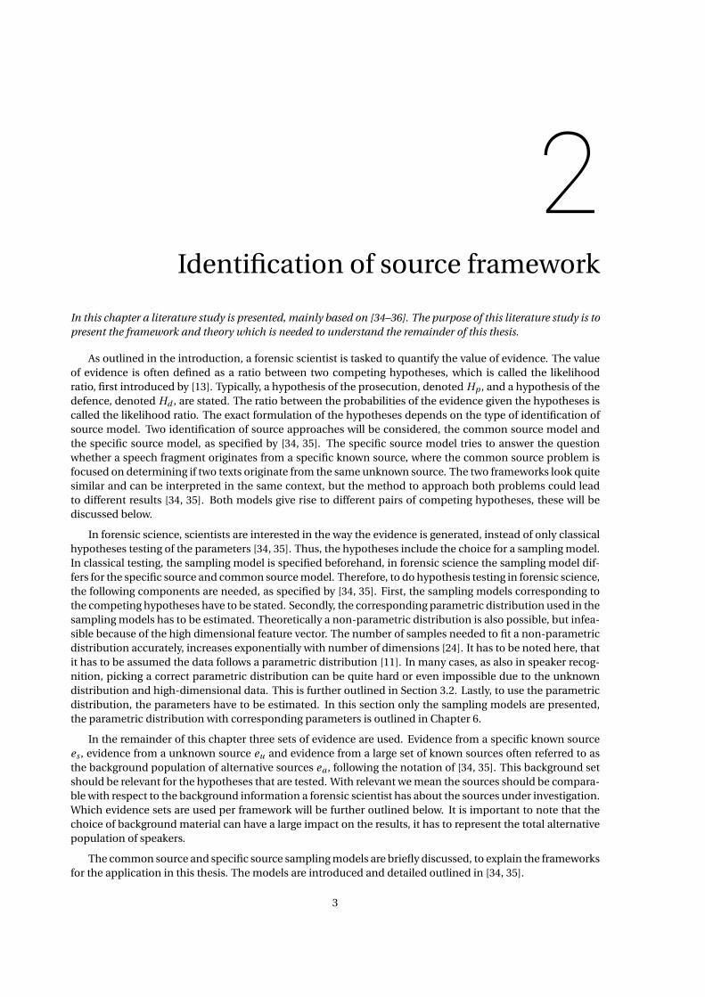
To evaluate the transcription in the statistical framework, first a numerical feature vector has to be deducedfrom the transcription. This can be achieved by using relevant features, which will be described in Chapter 5.Assume we have l features, define n as the number of different speakers in the background population andm the number of samples per speaker. The number of samples m can vary because some speakers will havea large speech fragment, which can be divided, resulting in several speech fragments. Using the backgroundpopulation data set containing a relevant subset of known speakers, samples of fragments of speech can beextracted. Assuming the background population has a sufficient amount of data, per speaker several samplesm, with l features can be extracted. Assuming the feature vectors obtained from the data follow a certainparametric distribution, two distributions can be specified. First the between-source distribution as

G (·|θa) , (2.1)

where θa is the l -dimensional parameter that indexes the l-dimensional between-source distribution. definePi as the sources in the background population of alternative sources, the sources are sampled according tothe between-source distribution. Secondly, the within-source distribution given a specific source Pi = pi

from the background population, is defined as

Fi(·|θa ,pi

), (2.2)

where θa is the l-dimensional parameter that indexes the l-dimensional within-source distribution. Fig-ure 2.1 shows the hierarchical structure of the within-source and in between-source distribution, the ob-tained samples are denoted as x. In the speaker recognition context, these distributions are referred to as thebetween-speaker and within-speaker distributions.

Figure 2.1: Schematic view of the between-source distribution and the within-source distribution, based on [31] (Fig 2, p. 48).

Define mu1 and mu2 as the number of samples obtained from the unknown speaker(s). The hypothesesfor the common source framework give rise to two different competing sampling models, the prosecutionsampling model Mp and the defence sampling model Md [34, 35]:

2.2. Specific source 5

Ma: The background evidence from all alternative known speakers ea is generated by sampling n speakersfrom the background population and sampling m samples from every speaker.

Mp: The evidence from the two speech fragments from the unknown speakers, eu1 and eu2 , is generated byfirst randomly sampling one speaker from the background population and then sampling mu1 +mu2

samples from the same speaker.

Md: The evidence from the two speech fragments from the unknown speakers, eu1 and eu2 , is generated byfirst randomly sampling two sources from the background population and then sampling mu1 samplesfrom one source and sampling mu2 samples from the other source.

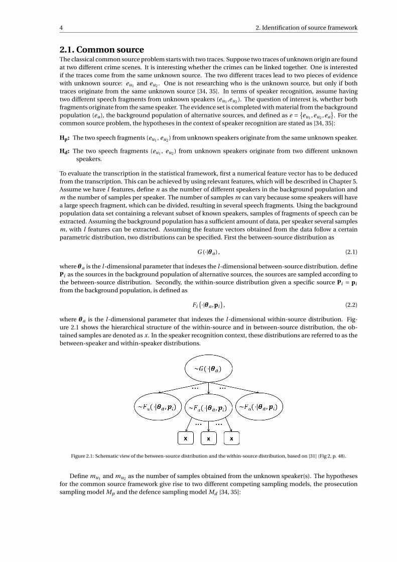
The schematic sampling model is illustrated in Figure 2.2, a sample is denoted as xp,j, which correspondsto the j th sample of speaker p. Note that the two hypotheses agree on the background sampling modelMa . The blue and orange box, top left and top right respectively, represent the competing sampling modelsMp and Md about the evidence [36]. The prosecution argues the evidence from the two unknown speechfragments, eu1 and eu2 , is generated by one speaker, but the defence argues the evidence is generated by twodifferent speakers from the background population.

Figure 2.2: Overview of the sampling model for the common source model. The orange and blue box represent the two competingsampling models Mp and Md , top left and top right respectively. The schematic overview is based on [36] (Fig. 1, p. 4).

2.2. Specific sourceThe classical specific source problem is stated the following way: a trace is found at a crime scene and thequestion is whether a specific suspected source can be linked to this trace [34, 35]. In other research thismodel is applied to the question of source problem for glass fragments, fingermarks and DNA [37]. From thetrace, several measurements are taken and this results in the unknown source evidence eu . From the sus-pected source measurements are taken and this results in the specific source evidence es . In terms of speakerverification, assume having one speech fragment from an unknown speaker (eu) and some speech fragmentsfrom a known specific speaker (es ). The question of interest is, whether the unknown speech fragment origi-nates from the known specific speaker. To complete the evidence set for the specific source model, materialfrom the background population is needed (ea). The complete set of evidence is defined as e = eu ,es ,ea.The competing hypotheses for the specific source problem, applied to speaker verification, are specified thefollowing way [34, 35]:

Hp: The speech fragment from an unknown speaker (eu) and speech fragment from a known specific speaker(es ) originate from the same known specific speaker.

6 2. Identification of source framework

Hd: The speech fragment from an unknown speaker (eu) does not originate from the known specific speaker,but from an alternative speaker.

Again the speech fragments are transformed to numerical feature vectors with l features. Define n as thenumber of different speakers in the background population and m the number of samples per speaker. As-sume the specific speaker data gives rise to ms l-dimensional samples. The unknown speech fragment resultsin mu l -dimensional feature vectors. For the specific source model, an additional sampling model is added,the specific source sampling model Ms , followed by the background population sampling model and the twocompeting sampling models Mp and Md [34, 35]:

Ms: The evidence es from the known specific speaker is generated by sampling ms samples from the specificspeaker.

Ma: The background evidence ea from all alternative known speakers is generated by sampling n speakersfrom the background population and sampling m samples from every speaker.

Mp: The evidence eu from the speech fragment from unknown speaker is generated by sampling mu samplesfrom the specific speaker.

Md: The evidence eu from the speech fragment from unknown speaker is generated by sampling one sourcefrom the background population and sampling mu samples from the source.

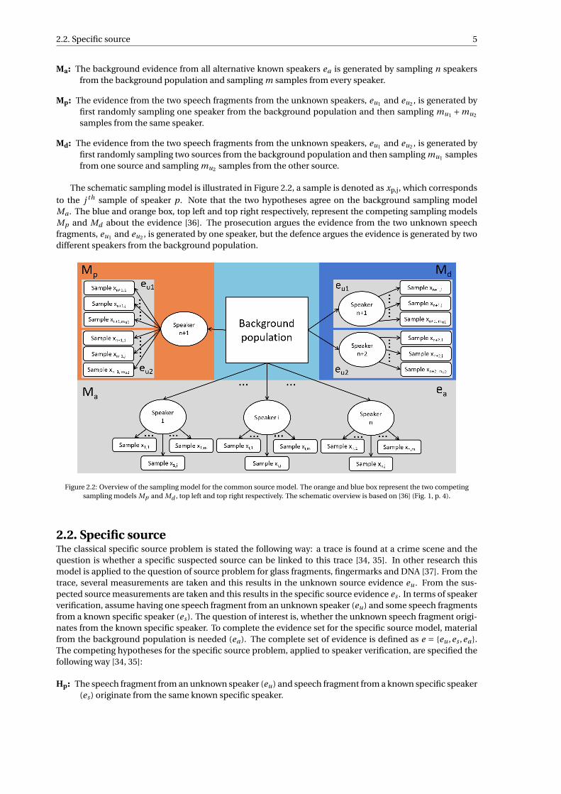
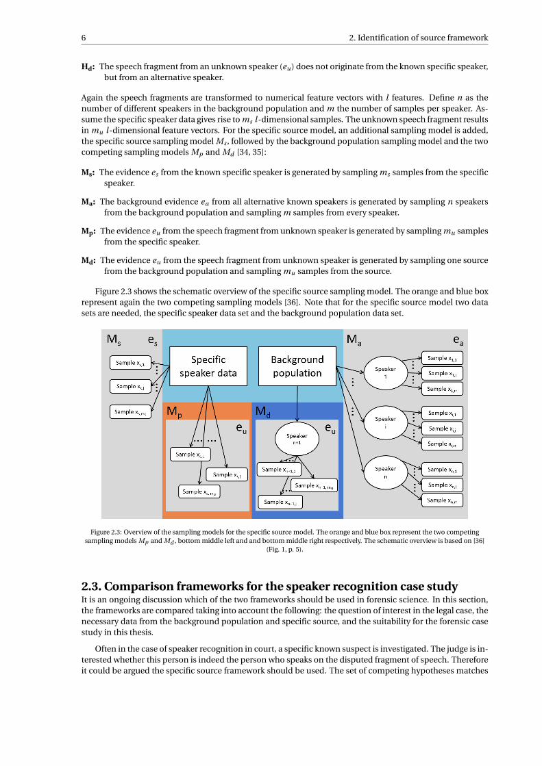
Figure 2.3 shows the schematic overview of the specific source sampling model. The orange and blue boxrepresent again the two competing sampling models [36]. Note that for the specific source model two datasets are needed, the specific speaker data set and the background population data set.

Figure 2.3: Overview of the sampling models for the specific source model. The orange and blue box represent the two competingsampling models Mp and Md , bottom middle left and and bottom middle right respectively. The schematic overview is based on [36]

(Fig. 1, p. 5).

2.3. Comparison frameworks for the speaker recognition case studyIt is an ongoing discussion which of the two frameworks should be used in forensic science. In this section,the frameworks are compared taking into account the following: the question of interest in the legal case, thenecessary data from the background population and specific source, and the suitability for the forensic casestudy in this thesis.

Often in the case of speaker recognition in court, a specific known suspect is investigated. The judge is in-terested whether this person is indeed the person who speaks on the disputed fragment of speech. Thereforeit could be argued the specific source framework should be used. The set of competing hypotheses matches

2.3. Comparison frameworks for the speaker recognition case study 7

better with the question of interest. It can be argued the common source model is better suitable for an on-going investigation, for example whether two speech fragments from different crimes can be linked together.

However, for specific source modelling, sufficient data from the specific source has to be available to traina model for the specific speaker according to the sampling model. The difference between the commonsource model and specific source model is sometimes referred to as the difference between using one or twobackground populations data sets, respectively. For the common source model one background populationdata set is needed. For the specific source model a background population data set and a specific source dataset is needed [35]. For some applications in forensic science, for example glass, it is possible to take moresamples from the disputed glass fragment, from which the specific source model can be constructed. Forspeaker recognition, the data of the specific speaker in question can be limited and it can be hard to collectmore data. The suspect in an investigation, the specific speaker, is probable to not talk in a natural way duringthe interrogation or can be not cooperative. Often there is not enough transcribed speech available to modela specific source model from the suspect speaker. In some cases only one speech fragment from the specificspeaker and one disputed fragment of speech is available. This suggests the common source model is moreapplicable to use in a real forensic case, where data is limited [34]. Common source modelling tends to bemore conservative, because it contains an extra uncertainty.

The speech department at the NFI is interested what evidential value can be calculated in the case wherethe disputed speech fragment(s) and the speech fragments from a suspect or unknown person are compared.Often the disputed speech fragment(s) is used as one sample, as this is the limiting factor in the research.The background population can be divided according to the size of the disputed fragment. This sets the pa-rameters mu1 ,mu2 ,mu = 1. The parameter ms , the number of specific speaker samples, is in most speechcomparison cases small. This is important in the remainder of this thesis. The question is whether an eviden-tial value can be obtained with small amounts of data from the specific source and how much backgroundsources are needed.

For both frameworks several advantages and disadvantages have been mentioned. In the application thisthesis is used for, the critical factor is the lack of a sufficient large data set from the specific speaker in a realforensic case. Therefore first the common source method is explored, to look whether results can be obtainedfrom using only a background population data set. The specific source model is implemented in one method,the score likelihood ratio, to research whether it is possible to model with a small specific speaker data set.

3Likelihood ratio framework

This chapter contains an introduction to the likelihood ratio framework. First, the definition of the value ofevidence is introduced. After this, the score-based approach is outlined and the advantages and disadvan-tages are stated. The chapter concludes with the verbal equivalent of the calculated likelihood ratios andtheory about the combination of evidence.

3.1. Value of evidenceForensic scientists are tasked to quantify the value of evidence. Given two hypotheses as defined in the pre-vious section, the question is to what extent the evidence supports one hypothesis over the other hypothesis.It is important to quantify the value of evidence objectively – a clear, universal framework is needed. Thelikelihood ratio framework to quantify the value of evidence is internationally accepted by forensic scientistsand was first introduced in 1970 [13, 60]. The likelihood ratio is based on applying the Bayes theorem. TheBayes theorem describes how to update the probability of an event given new information.

In almost every legal case, scientific and non-scientific evidence is present [24]. Examples of non-scientificevidence are the testimony of a witness, a motive or an alibi. Scientific evidence includes, for example, DNA,patterns in traces and also the fragments of speech used in this thesis. Scientific evidence is based on empiri-cal data. In a legal process, first the legal experts (e.g. a judge) have to determine the probability of hypothesisHp against hypothesis Hd given the non-scientific evidence and background information I , this is specifiedas the prior. The prior is defined as

P(Hp |I

)P (Hd |I )

, (3.1)

and is also called the prior belief or prior odds. When scientific evidence is present, one is interested whichhypothesis is more likely given all evidence, including all scientific evidence e. The value of interest is theratio

P(Hp |e, I )

P(Hd |e, I ), (3.2)

this is called the posterior odds. It is an update of the prior odds with information provided by the scientificevidence e. It gives legal experts a numerical value to support a decision between the two competing hy-potheses. It is not possible to calculate the posterior odds immediately. To calculate the posterior odds, theprior odds have to be updated. First, the theorem of Bayes is introduced [45]. Let A and B be events whereP(A) > 0 and P(B) > 0, then the conditional probability of A given B can be expressed through

P(A|B) = P(B |A)P(A)

P(B). (3.3)

The posterior odds in Equation (3.2) can be rewritten using the Bayes theorem and the definition of condi-tional probabilities as

P(Hp |e, I

)P (Hd |e, I )

= P(e, I |Hp )P(Hp )

P(e, I )· P(e, I )

P(e, I |Hd )P(Hd )

= P(e|Hp , I )

P(e|Hd , I )· P(I |Hp )

P(I |Hd )· P(Hp )

P(Hd ).

(3.4)

9

10 3. Likelihood ratio framework

Often the non-scientific background information I is omitted, because of readability. Equation (3.4) leads tothe standard form of the likelihood ratio framework

P(Hp |e

)P (Hd |e)︸ ︷︷ ︸

posterior odds

= P(e|Hp

)P (e|Hd )︸ ︷︷ ︸

likelihood ratio

· P(Hp

)P (Hd )︸ ︷︷ ︸

prior odds

. (3.5)

The likelihood ratio is used as the value of evidence. Equation (3.5) is called the odds form of the theoremof Bayes. The prior belief is updated by the likelihood ratio (LR), to find the posterior odds [23]. A LR > 1favours the prosecutor’s hypothesis Hp , an LR < 1 favours the defence hypothesis Hd . An advantage of thelikelihood ratio framework is the division between the task of the legal experts and the forensic experts. Theforensic scientist provides an objective likelihood ratio, while the legal expert can determine an appropriateprior belief, before seeing the scientific evidence. The legal expert can afterwards update this belief to theposterior odds with the likelihood ratio provided by the forensic scientist.

To calculate the ratio between the two probabilities of the evidence given the hypotheses, the two likeli-hood functions for the total evidence e conditional on the hypotheses need to be determined. The likelihoodratio is given by

LR(θ,e) = f (e|Hp ,θ)

f (e|Hd ,θ). (3.6)

Here, θ is the multi-dimensional parameter indexing the likelihood function. The true parameter θ is un-known and an estimate of the true parameter has to be substituted. To determine an estimate for this param-eter, two approaches are possible, the frequentist and Bayesian approach. The parameter can be estimatedusing the background material, the estimated parameter can be plugged into the equation, this approach isthe frequentist approach. The Bayesian approach proposes an appropriate prior for parameter θ, this priorneeds to be chosen carefully, as it effects the inference process. In this thesis only the frequentist approachis researched, as this approach is analytical tractable and no priors have to be specified. The likelihood func-tions are defined per identification of source framework, the common source model and the specific sourcemodel. A complete and detailed version of the derivation of the likelihood functions can be found in [34].

For the common source model, the unknown source evidence consists of two speech fragments of un-known speakers, e = eu1 ,eu2 [34], applying this to Equation (3.6) gives

LR(θa ,eu1 ,eu2 ) = f (eu1 ,eu2 |Hp ,θa)

f (eu1 ,eu2 |Hd ,θa). (3.7)

Here, θa is the estimated l-dimensional parameter using the background population of alternative sources.The numerator is conditioned on hypothesis Hp . The sampling model specified in Chapter 2 shows that eu1

and eu2 are generated by drawing a random speaker p from the background population and drawing twosamples from this speaker. The two samples are independent conditionally on the drawn speaker. Assumey u1

and y u2are the resulting feature vectors from eu1 and eu2 , respectively. To draw a random speaker, the

between-source and within-source distribution from Equations (2.1) and (2.2) are used. fa is the probabilitydensity function of the within-source distribution and g is the probability density function of the between-source distribution. This results in

f (eu1 ,eu2|Hp ,θa) = fa(y u1, y u2

|Hp ,θa) =∫

fa(

y u1, y u2

|p,θa , Hp)

g(p|θa

)dp

=∫

fa(

y u1|p,θa

)fa

(y u2

|p,θa)

g(p|θa

)dp.

(3.8)

The denominator is conditioned on hypothesis Hd . The sampling model specified in Chapter 2 shows thatthe evidence is generated by randomly drawing two speakers p1 and p2 from the background populationand drawing one sample from each speaker. The evidence is from two different randomly drawn speakers,thus evidence eu1 and eu2 are unconditionally independent. Then the denominator in Equation (3.7) can bewritten as

f (eu1 ,eu2 |Hd ,θa) = f (eu1 |θa) f (eu2 |θa) = fa(y u1|θa) fa(y u2

|θa)

=∫

fa(

y u1|p1,θa

)g

(p1|θa

)dp1 ·

∫fa

(y u2

|p2,θa)

g(p2|θa

)dp2.

(3.9)

3.2. Score-based approach 11

For the specific source model, the unknown source evidence consists of one fragment of speech of un-known speaker e = eu [34]. The numerator is conditioned on hypothesis Hp , the sampling model specifiedin Chapter 2 shows that eu is generated by the specific known speaker. Therefore, no between-source dis-tribution is present here. Let y u be the resulting feature vector from eu . The numerator can be rewrittenas

f (e|Hp ,θ) = f (eu |Hp ,θs ) = fs (y u |θs ). (3.10)

Here, θs is the estimated parameter using the specific speaker data set and fs the probability density func-tion of the specific speaker. The denominator is conditioned on hypothesis Hd . The sampling model fromChapter 2 shows that eu is generated by drawing a random speaker p from the background population anddrawing one sample from this speaker. In the same manner as the common source denominator, this resultsin

f (e|Hd ,θ) = f (eu |Hd ,θa) = fa(y u |θa)

=∫

fa(

y u |p,θa)

g(p|θa

)dp.

(3.11)

Here, θa is again the estimated parameter using the background population of alternative sources.

To calculate the specified likelihood functions, the corresponding parametric distribution and the index-ing parameter for fa and g have to be estimated, this is further outlined in Chapter 6. However, as alreadymentioned in the introduction, specifying an appropriate parametric distribution and fitting it correctly for ahigh-dimensional space is challenging. Therefore, in the next section the score-based approach is outlined.

3.2. Score-based approachIn the previous section the value of evidence is expressed as a likelihood ratio. The direct method to calculatea likelihood ratio uses Equation (3.6) directly with the specified likelihood functions. This is called a feature-based approach, it assumes a distribution of the original features. However, to calculate the feature-basedlikelihood functions, several problems arise. First, due to the high dimensional feature space in text analysis(further outlined in Chapter 5), the number of samples has to be substantially large to fit a parametric dis-tribution accurately. Due to limited available data this is not always feasible. Also, high-dimensional modelsrequire a large computational power. Second, by directly calculating the likelihood ratio using the high di-mensional feature space, maybe unsupported assumptions are made regarding the underlying process thatgenerated the evidence [19]. No literature is available which proposes distributions for the used featuresbased on words.

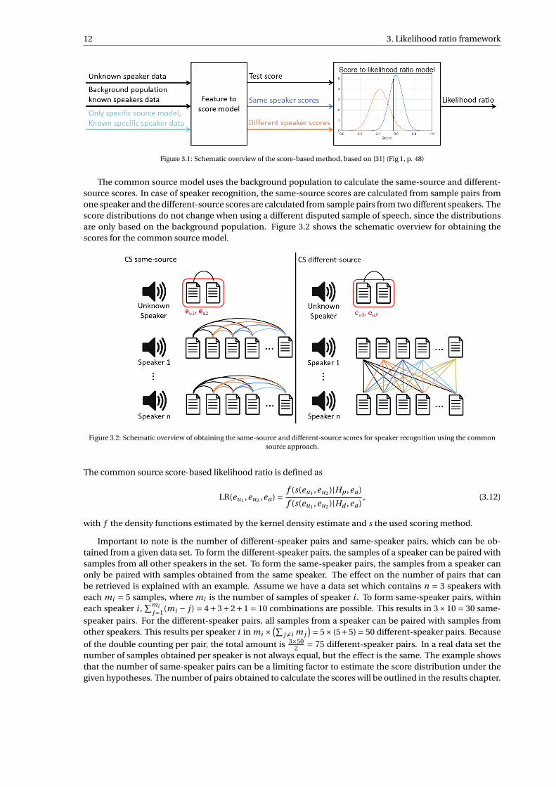
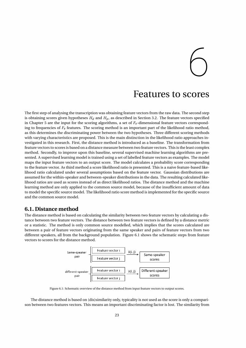
To avoid the difficulties arising from a high dimensional feature-based approach, the score-based ap-proach is introduced. Instead of having a multi-dimensional feature vector per sample, a one-dimensionalscore is calculated between two samples, under the given competing hypotheses [6, 19, 36]. This score iscalculated by using a scoring method. As a baseline a distance based method is used, where the score is thedistance between two feature vectors. To improve upon this baseline, several machine learning algorithmsare applied to calculate a score from the feature vectors. As a third method a feature-based likelihood ratiois calculated under several assumptions and used as a score. The used score methods are further explainedin Chapter 6. All scoring methods have the same kind of input and output. Assume two samples with l -dimensional feature vectors xi and x j , this is the input of the method. The output is a one-dimensional scorelabelled as same-source or different-source score. The same-source scores are obtained by comparing same-source pairs of feature vectors and the different-source scores are obtained comparing different-source pairsof feature vectors. The likelihood ratio is calculated dividing the probability density function of the same-source score distribution by the probability density function of the different-source score distribution. Theneeded data sets for the score-based approach agree with the sampling models specified in Chapter 2. Theinput is respectively the fragment(s) of speech from an unknown speaker, the background population of al-ternative speakers data set and in case of specific source modelling, a specific known speaker data set. Fromthe background population (and the specific speaker data set) the same-source and different-source scoresare calculated. The probability distribution of both of sets of scores is estimated using a non-parametrickernel density estimate, this is further outlined in Chapter 7. The score likelihood ratio is calculated by theratio between the two distribution of the scores, given the competing hypotheses [14]. Figure 3.1 shows theschematic figure for obtaining the likelihood ratio with the score-based approach [31].

12 3. Likelihood ratio framework

Figure 3.1: Schematic overview of the score-based method, based on [31] (Fig 1, p. 48)

The common source model uses the background population to calculate the same-source and different-source scores. In case of speaker recognition, the same-source scores are calculated from sample pairs fromone speaker and the different-source scores are calculated from sample pairs from two different speakers. Thescore distributions do not change when using a different disputed sample of speech, since the distributionsare only based on the background population. Figure 3.2 shows the schematic overview for obtaining thescores for the common source model.

Figure 3.2: Schematic overview of obtaining the same-source and different-source scores for speaker recognition using the commonsource approach.

The common source score-based likelihood ratio is defined as

LR(eu1 ,eu2 ,ea) = f (s(eu1 ,eu2 )|Hp ,ea)

f (s(eu1 ,eu2 )|Hd ,ea), (3.12)

with f the density functions estimated by the kernel density estimate and s the used scoring method.

Important to note is the number of different-speaker pairs and same-speaker pairs, which can be ob-tained from a given data set. To form the different-speaker pairs, the samples of a speaker can be paired withsamples from all other speakers in the set. To form the same-speaker pairs, the samples from a speaker canonly be paired with samples obtained from the same speaker. The effect on the number of pairs that canbe retrieved is explained with an example. Assume we have a data set which contains n = 3 speakers witheach mi = 5 samples, where mi is the number of samples of speaker i . To form same-speaker pairs, withineach speaker i ,

∑mij=1(mi − j ) = 4+3+2+1 = 10 combinations are possible. This results in 3×10 = 30 same-

speaker pairs. For the different-speaker pairs, all samples from a speaker can be paired with samples fromother speakers. This results per speaker i in mi ×

(∑j 6=i m j

)= 5× (5+5) = 50 different-speaker pairs. Because

of the double counting per pair, the total amount is 3×502 = 75 different-speaker pairs. In a real data set the

number of samples obtained per speaker is not always equal, but the effect is the same. The example showsthat the number of same-speaker pairs can be a limiting factor to estimate the score distribution under thegiven hypotheses. The number of pairs obtained to calculate the scores will be outlined in the results chapter.

3.3. Verbal likelihood ratios 13

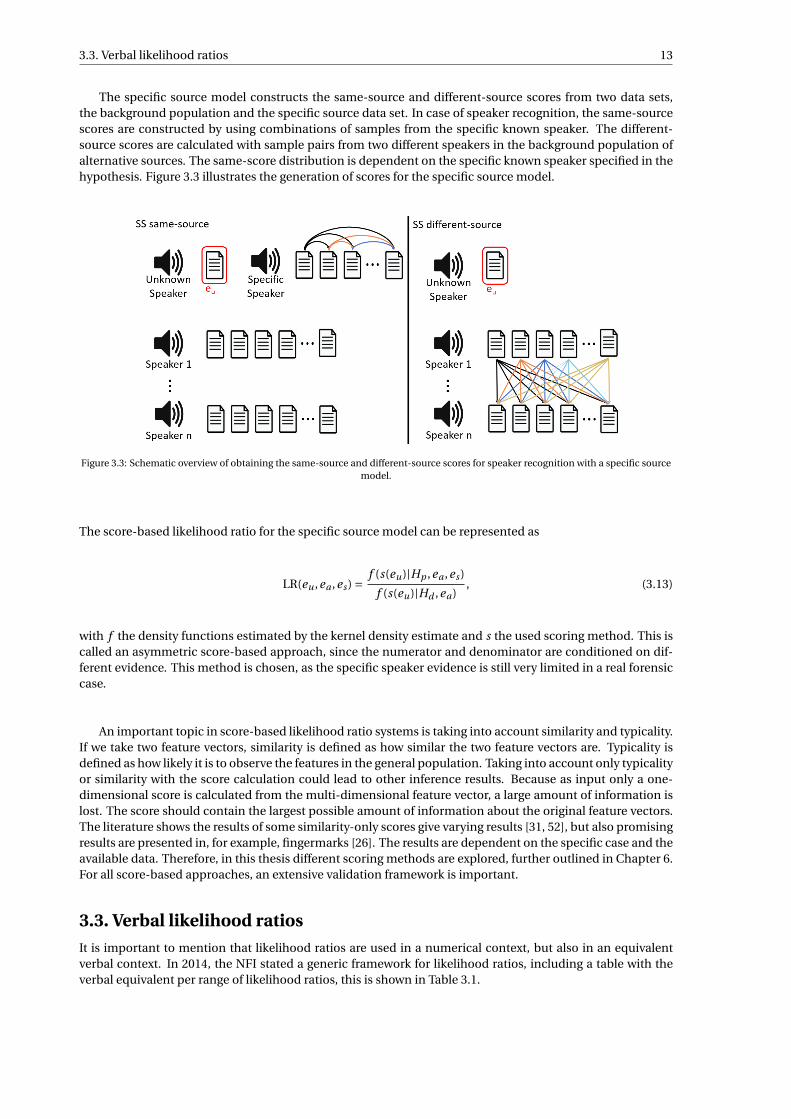
The specific source model constructs the same-source and different-source scores from two data sets,the background population and the specific source data set. In case of speaker recognition, the same-sourcescores are constructed by using combinations of samples from the specific known speaker. The different-source scores are calculated with sample pairs from two different speakers in the background population ofalternative sources. The same-score distribution is dependent on the specific known speaker specified in thehypothesis. Figure 3.3 illustrates the generation of scores for the specific source model.

Figure 3.3: Schematic overview of obtaining the same-source and different-source scores for speaker recognition with a specific sourcemodel.

The score-based likelihood ratio for the specific source model can be represented as

LR(eu ,ea ,es ) = f (s(eu)|Hp ,ea ,es )

f (s(eu)|Hd ,ea), (3.13)

with f the density functions estimated by the kernel density estimate and s the used scoring method. This iscalled an asymmetric score-based approach, since the numerator and denominator are conditioned on dif-ferent evidence. This method is chosen, as the specific speaker evidence is still very limited in a real forensiccase.

An important topic in score-based likelihood ratio systems is taking into account similarity and typicality.If we take two feature vectors, similarity is defined as how similar the two feature vectors are. Typicality isdefined as how likely it is to observe the features in the general population. Taking into account only typicalityor similarity with the score calculation could lead to other inference results. Because as input only a one-dimensional score is calculated from the multi-dimensional feature vector, a large amount of information islost. The score should contain the largest possible amount of information about the original feature vectors.The literature shows the results of some similarity-only scores give varying results [31, 52], but also promisingresults are presented in, for example, fingermarks [26]. The results are dependent on the specific case and theavailable data. Therefore, in this thesis different scoring methods are explored, further outlined in Chapter 6.For all score-based approaches, an extensive validation framework is important.

3.3. Verbal likelihood ratiosIt is important to mention that likelihood ratios are used in a numerical context, but also in an equivalentverbal context. In 2014, the NFI stated a generic framework for likelihood ratios, including a table with theverbal equivalent per range of likelihood ratios, this is shown in Table 3.1.

14 3. Likelihood ratio framework

Table 3.1: Table of the verbal expressions of numerical likelihood ratio values [33].

Values of likelihood ratio Verbal equivalent

1-2 As probable, no assistance2-10 Slightly more probable10-100 More probable100-10.000 Much more probable10.000-1.000.000 Far more probable>1.000.000 Exceedingly more probable

Especially when a likelihood ratio has to be reported in court, it is useful to have a verbal equivalent. Thenumerical statement of an forensic expert in a speaker recognition case would be:

‘The information found by comparing the two speech fragments is 160 times more probable if they come fromthe same speaker than if they come from different speakers.’

Which can be translated, according to Table 3.1, to the verbal counterpart:

‘The information found by comparing the two speech fragments is much more probable if they come from thesame speaker than if they come from different speakers.’

3.4. Combination of forensic evidenceAnalysing the transcribed speech fragment for speaker recognition is assumed to be independent from cur-rent automatic voice recognition. As an additional mean of evidence, text analysis can contribute signifi-cantly to the overall evidential information about the speaker. To specify this possibility more precisely, inthis chapter the theory and constraints of combining evidence are further outlined.

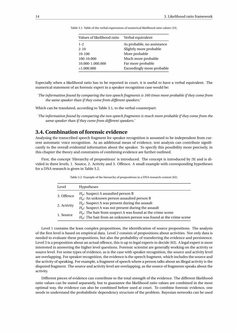
First, the concept ‘Hierarchy of propositions’ is introduced. The concept is introduced by [9] and is di-vided in three levels, 1. Source, 2. Activity and 3. Offence. A small example with corresponding hypothesesfor a DNA research is given in Table 3.2.

Table 3.2: Example of the hierarchy of propositions in a DNA research context [63].

Level Hypotheses

3. OffenceHp : Suspect A assaulted person BHd : An unknown person assaulted person B

2. ActivityHp : Suspect A was present during the assaultHd : Suspect A was not present during the assault

1. SourceHp : The hair from suspect A was found at the crime sceneHd : The hair from an unknown person was found at the crime scene

Level 1 contains the least complex propositions, the identification of source propositions. The analysisof the first level is based on empirical data. Level 2 consists of propositions about activities. Not only data isneeded to evaluate these propositions, but also the probability of transferring the evidence and persistence.Level 3 is a proposition about an actual offence, this is up to legal experts to decide [63]. A legal expert is mostinterested in answering the higher level questions. Forensic scientist are generally working on the activity orsource level. For some types of evidence, as is the case with speaker recognition, the source and activity levelare overlapping. For speaker recognition, the evidence is the speech fragment, which includes the source andthe activity of speaking. For example, a fragment of speech where a person talks about an illegal activity is thedisputed fragment. The source and activity level are overlapping, as the source of fragments speaks about theactivity.

Different pieces of evidence can contribute to the total strength of the evidence. The different likelihoodratio values can be stated separately, but to guarantee the likelihood ratio values are combined in the mostoptimal way, the evidence can also be combined before used at court. To combine forensic evidence, oneneeds to understand the probabilistic dependency structure of the problem. Bayesian networks can be used

3.4. Combination of forensic evidence 15

to represent the dependency structure [63]. A Bayesian network is a directed graph that illustrates the depen-dencies between random variables. The variables are the nodes, the dependencies are illustrated by directededges.

For speaker recognition three parts of evidence can be combined. First, the information obtained fromthe automatic speaker recognition easr , based on phonetics and speech signal processing. Second, the infor-mation from the text analysis et a , only based on the transcription of the speech fragment. Third, the evidenceresulting from the judgement of an expert e j e . For the first two pieces of evidence easr and et a , a numericallikelihood ratio can be computed. The two pieces of evidence are based on different parts of the speech frag-ment, transcription and phonetics, and thus can be assumed conditionally independent. This assumptionmust be taken cautiously and has to be validated precisely in further research. This means the prior beliefregarding the hypotheses can be updated in the same way as introduced in Section 3.1. An addition to thelikelihood ratio defined in Equation (3.6) results in

LR(easr ,et a) = f (easr |Hp )

f (easr |Hd )· f (et a |Hp )

f (et a |Hd ). (3.14)

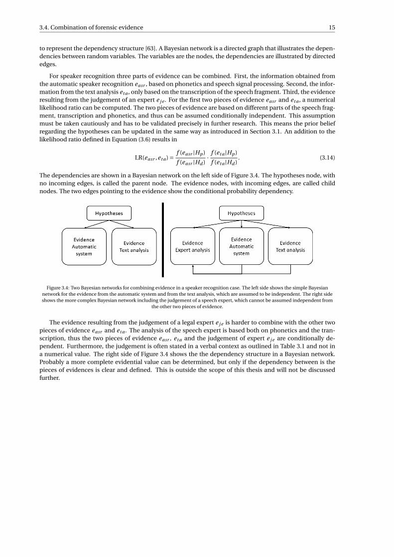
The dependencies are shown in a Bayesian network on the left side of Figure 3.4. The hypotheses node, withno incoming edges, is called the parent node. The evidence nodes, with incoming edges, are called childnodes. The two edges pointing to the evidence show the conditional probability dependency.

Figure 3.4: Two Bayesian networks for combining evidence in a speaker recognition case. The left side shows the simple Bayesiannetwork for the evidence from the automatic system and from the text analysis, which are assumed to be independent. The right sideshows the more complex Bayesian network including the judgement of a speech expert, which cannot be assumed independent from

the other two pieces of evidence.

The evidence resulting from the judgement of a legal expert e j e is harder to combine with the other twopieces of evidence easr and et a . The analysis of the speech expert is based both on phonetics and the tran-scription, thus the two pieces of evidence easr , et a and the judgement of expert e j e are conditionally de-pendent. Furthermore, the judgement is often stated in a verbal context as outlined in Table 3.1 and not ina numerical value. The right side of Figure 3.4 shows the the dependency structure in a Bayesian network.Probably a more complete evidential value can be determined, but only if the dependency between is thepieces of evidences is clear and defined. This is outside the scope of this thesis and will not be discussedfurther.

4Data set NFI

The speech department at the NFI recently acquired a data set specifically designed for research in foren-sic science, the Forensically Realistic Inter-Device Audio Database (FRIDA). This data set is constructed ofconversations of 250 different people, each having 16 conversations of approximately 5 minutes. In total thisresulted in 333 hours of speech [56]. The speakers are all from a similar target group; male, dutch speaking(50% native, 50% immigrant background), of lower education level and 80% younger than 35 years of age[54]. The data set is designed for automatic speaker comparison (based on phonetics) research and to serveas a background population in forensic case studies. Half of the conversations of all speakers have been tran-scribed and thus this data set is also very suitable for the research in this thesis. In this research only thetranscriptions of the data set are used, not the audio files or further information about recording devices.Each person is recorded during conversations with another person from the group, with 4 recording sessionsper day. Half of the conversations per person were held inside and half outside, divided in noisy areas andquiet areas. All transcripts contain the timestamp followed by the spoken text. The conversations are ortho-graphic transcribed by three native Dutch speakers. Orthographic means according to the standard spellingof a language, in this case Dutch. Per conversation, the fragment is transcribed by one and checked by theother two, to avoid personal influences in transcribing. A small example of the transcribed data can be foundin Figure 4.1.

Figure 4.1: An example of a part of a transcript.

An interesting feature for this research is the notation of words in informal language. The transcriptionmakes special notations for words from a different language, new non-existing words, street words, not com-pleted words and distortion of words, with *v, *n, *s, *a and *u respectively. An example, also included inFigure 4.1, is the word ‘wollah’ which is transcribed as ‘wollah*s’. This ensures the data set is readable andresistant against different spellings, this is important for text analysis.

The strength of this data set is the size, with 250 different speakers and 8 transcribed fragments perspeaker, the homogeneous target group and the available transcription. However, some remarks are im-portant to note, to keep in mind in the remainder of this thesis. For speaker verification, it is important to

17

18 4. Data set NFI

have a data set that contains conversations about different topics. The goal is to classify a transcription bythe speaker, not by topic. The speakers are asked to talk normal and not focus on specific topics. However,some speakers talk about the same topic in all eight conversations. If this is the case, it is difficult to de-termine which features are effective non-topic instead of topic based. In a real forensic case, topics couldcompletely differ between the two fragments of speech from unknown speakers, thus it is necessary to usenon-topic features. It is noted that in some conversations the person did not know what to talk about, buthad to finish up the required 5 minutes. This results in sentences which would probably not have been usedin a spontaneous conversation. Consequently this could lead to less informative samples for a speaker. Fur-thermore, because the data set is used as training and test set to validate the method, it can be assumed thatthe background population is certainly relevant. For a real forensic case, this background population has tobe specified according to the knowledge the forensic scientist has about the speaker from the forensic case.Thus the agreement of the background population with the disputed data in an actual forensic case could bedifferent, which could give other results.

The FRIDA data set showed an inconsistent number of transcribed recordings per speaker. For somespeakers, a smaller number than 8 transcriptions of recording sessions were available. To obtain a stableamount of data per speaker, the speakers with less than 8 transcribed speech fragments are not used in thetest case. After the data selection, the data set contains 217 speakers.

Besides the FRIDA data set, another data set containing transcribed Dutch speech is the ‘Corpus Gespro-ken Nederlands’ (CGN) data set. The CGN data set is acquired from 1998 to 2004 with the goal to have adatabase of contemporary Dutch as spoken by adult speakers in the Netherlands and Flanders [1]. The setcontains transcribed fragments from various speech fragments, for example telephone conversations, inter-views, speeches etc. The speech fragments are transcribed according to the same guidelines as the FRIDAdata set. A subset of the CGN data set, containing spontaneous telephone conversations, is used to deter-mine a set of frequent words independent from the FRIDA data set.

5Text analysis

The first step in the process of analysing the transcriptions, is the transformation from raw transcriptionsto features vectors. A feature is a measurable characteristic from a transcription. A feature should help todistinguish between different speakers of speech fragments. All different features from a speech fragmentcombined form a feature vector. The numerical feature vector is used to train a model or measure similaritybetween different transcriptions.

Author analysis, based on written text, has already been applied to different data sets, for example email,literary books and presidential written speeches. From the authorship analysis research, the promising, oftenused effective features are selected. Besides using features from authorship analysis research, it is also inter-esting to explore if transcribed spoken text has data specific features. An example of a data specific featureis a title or greeting for email data. A feature set could work well for classifying literary books, but this setcould fail for online messages. In the case of transcribed speech, it is interesting to look at features whichare normally not used in written text. In the upcoming part of this section, different types of features arediscussed, including their applicability in the speaker recognition case. At the end, the final selected featuresare presented.

While establishing the selected features, it is important to keep the goal of the research in mind. Forspeaker recognition, the features have to be discriminating for different speakers, not for different topics ina conversation. For example, a speaker will speak about completely different topics during a police conver-sation, than during a phone conversation with a friend. The ideal features do not discriminate for topics orcontent, but only on variables which are unconsciously used in speech. The features discriminate betweenstyle and not topic.

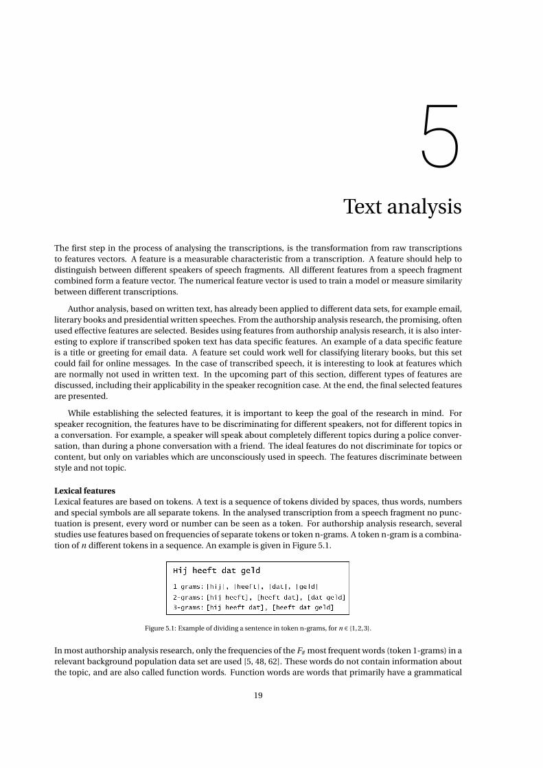
Lexical featuresLexical features are based on tokens. A text is a sequence of tokens divided by spaces, thus words, numbersand special symbols are all separate tokens. In the analysed transcription from a speech fragment no punc-tuation is present, every word or number can be seen as a token. For authorship analysis research, severalstudies use features based on frequencies of separate tokens or token n-grams. A token n-gram is a combina-tion of n different tokens in a sequence. An example is given in Figure 5.1.

Figure 5.1: Example of dividing a sentence in token n-grams, for n ∈ 1,2,3.

In most authorship analysis research, only the frequencies of the F# most frequent words (token 1-grams) in arelevant background population data set are used [5, 48, 62]. These words do not contain information aboutthe topic, and are also called function words. Function words are words that primarily have a grammatical

19

20 5. Text analysis

function within a sentence and no substantive meaning. Examples of Dutch function words are ‘want’, ‘naar’and ‘voor’, translated in English to ‘as’, ‘to’ and ‘for’. It is interesting to note that for topic-based text classifying,the most frequent words are often not used, as they do not contribute to topic classifying. The parameter F#,the number of frequent words used as features, varies a lot in different studies [50].

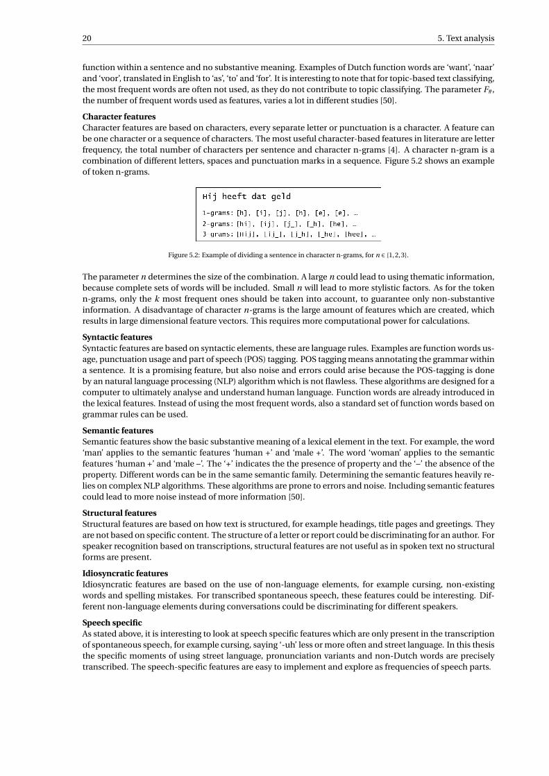
Character featuresCharacter features are based on characters, every separate letter or punctuation is a character. A feature canbe one character or a sequence of characters. The most useful character-based features in literature are letterfrequency, the total number of characters per sentence and character n-grams [4]. A character n-gram is acombination of different letters, spaces and punctuation marks in a sequence. Figure 5.2 shows an exampleof token n-grams.

Figure 5.2: Example of dividing a sentence in character n-grams, for n ∈ 1,2,3.

The parameter n determines the size of the combination. A large n could lead to using thematic information,because complete sets of words will be included. Small n will lead to more stylistic factors. As for the tokenn-grams, only the k most frequent ones should be taken into account, to guarantee only non-substantiveinformation. A disadvantage of character n-grams is the large amount of features which are created, whichresults in large dimensional feature vectors. This requires more computational power for calculations.

Syntactic featuresSyntactic features are based on syntactic elements, these are language rules. Examples are function words us-age, punctuation usage and part of speech (POS) tagging. POS tagging means annotating the grammar withina sentence. It is a promising feature, but also noise and errors could arise because the POS-tagging is doneby an natural language processing (NLP) algorithm which is not flawless. These algorithms are designed for acomputer to ultimately analyse and understand human language. Function words are already introduced inthe lexical features. Instead of using the most frequent words, also a standard set of function words based ongrammar rules can be used.

Semantic featuresSemantic features show the basic substantive meaning of a lexical element in the text. For example, the word‘man’ applies to the semantic features ‘human +’ and ‘male +’. The word ‘woman’ applies to the semanticfeatures ‘human +’ and ‘male –’. The ‘+’ indicates the the presence of property and the ‘–’ the absence of theproperty. Different words can be in the same semantic family. Determining the semantic features heavily re-lies on complex NLP algorithms. These algorithms are prone to errors and noise. Including semantic featurescould lead to more noise instead of more information [50].

Structural featuresStructural features are based on how text is structured, for example headings, title pages and greetings. Theyare not based on specific content. The structure of a letter or report could be discriminating for an author. Forspeaker recognition based on transcriptions, structural features are not useful as in spoken text no structuralforms are present.

Idiosyncratic featuresIdiosyncratic features are based on the use of non-language elements, for example cursing, non-existingwords and spelling mistakes. For transcribed spontaneous speech, these features could be interesting. Dif-ferent non-language elements during conversations could be discriminating for different speakers.

Speech specificAs stated above, it is interesting to look at speech specific features which are only present in the transcriptionof spontaneous speech, for example cursing, saying ‘-uh’ less or more often and street language. In this thesisthe specific moments of using street language, pronunciation variants and non-Dutch words are preciselytranscribed. The speech-specific features are easy to implement and explore as frequencies of speech parts.

5.1. Features FRIDA data set 21

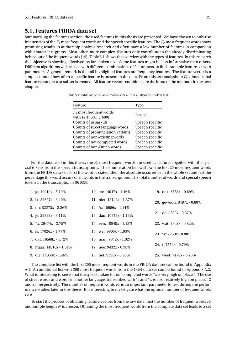
5.1. Features FRIDA data setSummarising the features section, the used features in this thesis are presented. We have chosen to only usefrequencies of the F# most frequent words and the speech specific features. The F# most frequent words showpromising results in authorship analysis research and often have a low number of features in comparisonwith character n-grams. Most other, more complex, features only contribute to the already discriminatingbehaviour of the frequent words [15]. Table 5.1 shows the overview with the types of features. In this researchthe objective is showing effectiveness for spoken text. Some features might be less informative than others.Different algorithms will be used with different combinations of feature sets, to find a suitable feature set withparameters. A general remark is that all highlighted features are frequency features. The feature vector is asimple count of how often a specific feature is present in the data. From this text analysis an F#-dimensionalfeature vector per text subset is created. All feature vectors combined are the input of the methods in the nextchapter.

Table 5.1: Table of the possible features for author analysis on spoken text.

Feature Type

F# most frequent wordswith F# ∈ (50, . . . ,600)

Lexical

Counts of using -uh Speech specificCounts of street language words Speech specificCounts of pronunciation variants Speech specificCounts of non-existing words Speech specificCounts of not completed words Speech specificCounts of non-Dutch words Speech specific

For the data used in this thesis, the F# most frequent words are used as features together with the spe-cial tokens from the speech transcriptions. The enumeration below shows the first 25 most frequent wordsfrom the FRIDA data set. First the word is stated, then the absolute occurrence in the whole set and last thepercentage this word occurs of all words in the transcriptions. The total number of words and special speechtokens in the transcription is 961698.

1. ja: 49919x - 5.19%

2. ik: 32697x - 3.40%

3. uh: 32273x - 3.36%

4. je: 29893x - 3.11%

5. *a: 26474x - 2.75%

6. is: 17026x - 1.77%

7. dat: 16568x - 1.72%

8. maar: 14816x - 1.54%

9. die: 14059x - 1.46%

10. en: 14047x - 1.46%

11. niet: 13142x - 1.37%

12. *s: 10986x - 1.14%

13. dan: 10873x - 1.13%

14. een: 10849x - 1.13%

15. wel: 9905x - 1.03%

16. man: 9842x - 1.02%

17. nee: 9432x - 0.98%

18. het: 9398x - 0.98%

19. ook: 8553x - 0.89%

20. gewoon: 8487x - 0.88%

21. de: 8399x - 0.87%

22. wat: 7862x - 0.82%

23. *v: 7739x - 0.80%

24. t: 7554x - 0.79%

25. weet: 7470x - 0.78%

The complete list with the first 200 most frequent words in the FRIDA data set can be found in AppendixA.1. An additional list with 200 most frequent words from the CGN data set can be found in Appendix A.2.What is interesting to see is that the speech token for not completed words *a is very high on place 5. The useof street words and words in another language, transcribed with *s and *v, is also relatively high on places 12and 23, respectively. The number of frequent words F# is an important parameter to test during the perfor-mance studies later in this thesis. It is interesting to investigate what the optimal number of frequent wordsF# is.

To start the process of obtaining feature vectors from the raw data, first the number of frequent words F#

and sample length N is chosen. Obtaining the most frequent words from the complete data set leads to a set

22 5. Text analysis

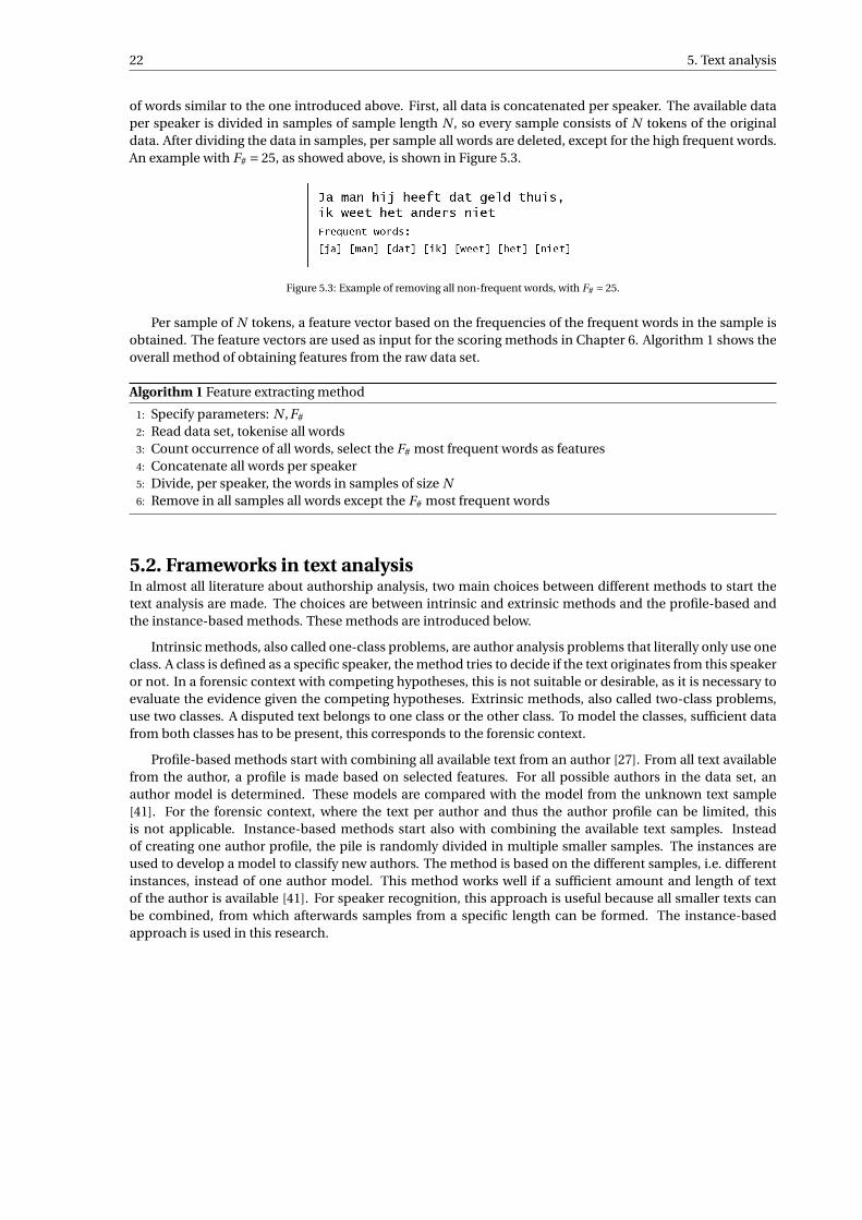
of words similar to the one introduced above. First, all data is concatenated per speaker. The available dataper speaker is divided in samples of sample length N , so every sample consists of N tokens of the originaldata. After dividing the data in samples, per sample all words are deleted, except for the high frequent words.An example with F# = 25, as showed above, is shown in Figure 5.3.

Figure 5.3: Example of removing all non-frequent words, with F# = 25.

Per sample of N tokens, a feature vector based on the frequencies of the frequent words in the sample isobtained. The feature vectors are used as input for the scoring methods in Chapter 6. Algorithm 1 shows theoverall method of obtaining features from the raw data set.

Algorithm 1 Feature extracting method

1: Specify parameters: N ,F#

2: Read data set, tokenise all words3: Count occurrence of all words, select the F# most frequent words as features4: Concatenate all words per speaker5: Divide, per speaker, the words in samples of size N6: Remove in all samples all words except the F# most frequent words

5.2. Frameworks in text analysisIn almost all literature about authorship analysis, two main choices between different methods to start thetext analysis are made. The choices are between intrinsic and extrinsic methods and the profile-based andthe instance-based methods. These methods are introduced below.

Intrinsic methods, also called one-class problems, are author analysis problems that literally only use oneclass. A class is defined as a specific speaker, the method tries to decide if the text originates from this speakeror not. In a forensic context with competing hypotheses, this is not suitable or desirable, as it is necessary toevaluate the evidence given the competing hypotheses. Extrinsic methods, also called two-class problems,use two classes. A disputed text belongs to one class or the other class. To model the classes, sufficient datafrom both classes has to be present, this corresponds to the forensic context.

Profile-based methods start with combining all available text from an author [27]. From all text availablefrom the author, a profile is made based on selected features. For all possible authors in the data set, anauthor model is determined. These models are compared with the model from the unknown text sample[41]. For the forensic context, where the text per author and thus the author profile can be limited, thisis not applicable. Instance-based methods start also with combining the available text samples. Insteadof creating one author profile, the pile is randomly divided in multiple smaller samples. The instances areused to develop a model to classify new authors. The method is based on the different samples, i.e. differentinstances, instead of one author model. This method works well if a sufficient amount and length of textof the author is available [41]. For speaker recognition, this approach is useful because all smaller texts canbe combined, from which afterwards samples from a specific length can be formed. The instance-basedapproach is used in this research.

6Features to scores

The first step of analysing the transcription was obtaining feature vectors from the raw data. The second stepis obtaining scores given hypotheses Hd and Hp , as described in Section 3.2. The feature vectors specifiedin Chapter 5 are the input for the scoring algorithms, a set of F#-dimensional feature vectors correspond-ing to frequencies of F# features. The scoring method is an important part of the likelihood ratio method,as this determines the discriminating power between the two hypotheses. Three different scoring methodswith varying characteristics are proposed. This is the main distinction in the likelihood ratio approaches in-vestigated in this research. First, the distance method is introduced as a baseline. The transformation fromfeature vectors to scores is based on a distance measure between two feature vectors. This is the least complexmethod. Secondly, to improve upon this baseline, several supervised machine learning algorithms are pre-sented. A supervised learning model is trained using a set of labelled feature vectors as examples. The modelmaps the input feature vectors to an output score. The model calculates a probability score correspondingto the feature vector. As third method a score likelihood ratio is presented. This is a naive feature-based like-lihood ratio calculated under several assumptions based on the feature vector. Gaussian distributions areassumed for the within-speaker and between-speaker distributions in the data. The resulting calculated like-lihood ratios are used as scores instead of as direct likelihood ratios. The distance method and the machinelearning method are only applied to the common source model, because of the insufficient amount of datato model the specific source model. The likelihood ratio score method is implemented for the specific sourceand the common source model.

6.1. Distance methodThe distance method is based on calculating the similarity between two feature vectors by calculating a dis-tance between two feature vectors. The distance between two feature vectors is defined by a distance metricor a statistic. The method is only common source modelled, which implies that the scores calculated arebetween a pair of feature vectors originating from the same speaker and pairs of feature vectors from twodifferent speakers, all from the background population. Figure 6.1 shows the schematic steps from featurevectors to scores for the distance method.

Figure 6.1: Schematic overview of the distance method from input feature vectors to output scores.

The distance method is based on (dis)similarity only, typicality is not used as the score is only a compari-son between two features vectors. This means an important discriminating factor is lost. The similarity from

23

24 6. Features to scores

a high dimensional space is compressed in a one-dimensional score, which also implies loss of information.The distance method is a simple way to obtain scores, instead of having a more ‘black box’ approach withmachine learning. The distance method can be used as a baseline, more complex techniques are expected tohave a better performance.

The most important step is choosing an effective distance measure δ. This measure should contain asmuch information as possible about the original feature vectors. The method is named distance measure asit does not need to possess the mathematical metric properties. A distance metric is a function which obeysthe identity, symmetry and triangle inequality axioms. Although the first axioms are desirable, the third oneis not needed. Some statistics, also called similarity measures, do not obey these axioms, but show promisingbehaviour for defining a similarity measure between two feature vectors. Both similarity measures and dis-tance metrics are explored for the distance method. In the literature, many different distance measures havebeen proposed and tested for authorship analysis. Examples of used distance measures for author analysis onwritten text are the Manhattan distance by [15] and the Kullback—Leibler divergence by [48]. In the literatureabout different identification of source questions (drugs, shoe soles, etc.), the distance method is also appliedwith different distance metrics, for example the Kullback–Leibler divergence for fingermarks [19]. Below, thebest performing distances are presented. For every measure outlined below, x and y are the feature vectorswhere we want to determine the distance between and xi and yi a single feature i from these feature vec-tors, with i ∈ (1, . . . , l ). Below several often used metrics are introduced, the performance of all the distancemeasures is assessed in the complete likelihood ratio model.

An often used metric for text analysis is the cosine similarity, defined as

δcos (x,y) = x ·y

‖x‖‖y‖ =∑l

i=1 xi yi√∑li=1 x2

i

√∑li=1 y2

i

. (6.1)

The cosine similarity is used distance measure for the authorship detection research in [21].

The Minkowski distance is a generalised distance metric. The Minkowski distance of order p is defined as

δmi n(x,y) =(

l∑i=1

∣∣xi − yi∣∣p

)1/p

, (6.2)

with integer p ≥ 1. Three well-known distance metrics are the Manhattan, Euclidean and Chebyshev distance,for p = 1, p = 2 and p = 3, respectively. The Manhattan distance is used in the author verification researchin [15], for written text in different languages and genres. The Manhattan distance is also used within otherapplications for score-based likelihood ratios, for example comparing the source of drug tablets [6].

The Bray–Curtis distance is often used in biology and defined as

δbc (x,y) =∑l

i=1

∣∣xi − yi∣∣∑l

i=1

∣∣xi + yi∣∣ . (6.3)

The metric is commonly used in ecology, quantifying the similarity between two areas based on counts ofspecies on the two sites [46]. Instead of counting species per site, in text analysis, frequent words per sampleare counted.

The Jensen–Shannon distance is based on the Kullback–Leibler divergence and is defined as

δS J (x,y) =√

D(x‖m)+D(y‖m)

2, (6.4)

with D the Kullback–Leibler divergence and m the element-wise mean of the two feature vectors x and y. TheKullback–Leibler divergence is defined as

D(x‖y) =l∑

i=1

xi log(xi /yi ) xi > 0, yi > 00 xi = 0, yi ≥ 0∞ otherwise

. (6.5)

The Jensen–Shannon distance is the square root from the Jensen–Shannon divergence. This metric is de-scribed by [12], together with the proof of the metric properties. The advantage of the Jensen–Shannon dis-tance over the Kullback–Leibler divergence is that it is a metric and thus symmetric. The calculation of scoresbetween feature vectors should be symmetric, as the feature vectors are exchangeable.

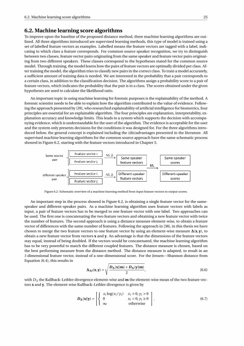
6.2. Machine learning score algorithms 25

6.2. Machine learning score algorithmsTo improve upon the baseline of the proposed distance method, three machine learning algorithms are out-lined. All three algorithms introduced are supervised learning methods, this type of model is trained using aset of labelled feature vectors as examples. Labelled means the feature vectors are tagged with a label, indi-cating to which class a feature corresponds. For common source speaker recognition, we try to distinguishbetween two classes, feature vector pairs originating from the same speaker and feature vector pairs originat-ing from two different speakers. These classes correspond to the hypotheses stated for the common sourcemodel. Through training, the model learns how the pairs of feature vectors are optimally divided per class. Af-ter training the model, the algorithm tries to classify new pairs in the correct class. To train a model accurately,a sufficient amount of training data is needed. We are interested in the probability that a pair corresponds toa certain class, in addition to the classification decision. The algorithms assign a probability score to a pair offeature vectors, which indicates the probability that the pair is in a class. The scores obtained under the givenhypotheses are used to calculate the likelihood ratio.

An important topic in using machine learning for forensic purposes is the explainability of the method. Aforensic scientist needs to be able to explain how the algorithm contributed to the value of evidence. Follow-ing the approach presented by [39], who researched explainability of artificial intelligence for biometrics, fourprinciples are essential for an explainable algorithm. The four principles are explanation, interpretability, ex-planation accuracy and knowledge limits. This leads to a system which supports the decision with accompa-nying evidence, which is understandable for the user of the algorithm. The evidence is acceptable for the userand the system only presents decisions for the conditions it was designed for. For the three algorithms intro-duced below, the general concept is explained including the (dis)advantages presented in the literature. Allsupervised machine learning algorithms for the common source approach have the same schematic processshowed in Figure 6.2, starting with the feature vectors introduced in Chapter 5.

Figure 6.2: Schematic overview of a machine learning method from input feature vectors to output scores.

An important step in the process showed in Figure 6.2, is obtaining a single feature vector for the same-speaker and different-speaker pairs. As a machine learning algorithm uses feature vectors with labels asinput, a pair of feature vectors has to be merged to one feature vector with one label. Two approaches canbe used. The first one is concatenating the two feature vectors and obtaining a new feature vector with twicethe number of features. The second approach is using a distance measure element-wise, to obtain a featurevector of differences with the same number of features. Following the approach in [38], in this thesis we havechosen to merge the two feature vectors to one feature vector by using an element-wise measure ∆(x,y), toobtain a new feature vector from vectors x and y. An advantage is that the dimensions of the feature vectorsstay equal, instead of being doubled. If the vectors would be concatenated, the machine learning algorithmhas to be very powerful to match the different coupled features. The distance measure is chosen, based onthe best performing measure from the distance method. The distance measure is adapted, to result in anl -dimensional feature vector, instead of a one-dimensional score. For the Jensen—Shannon distance fromEquation (6.4), this results in

∆S J (x,y) =√

D∆(x‖m)+D∆(y‖m)

2, (6.6)

with D∆ the Kullback–Leibler divergence element-wise and m the element-wise mean of the two feature vec-tors x and y. The element-wise Kullback–Leibler divergence is given by

D∆(x‖y) =

xi log(xi /yi ) xi > 0, yi > 00 xi = 0, yi ≥ 0∞ otherwise

. (6.7)

26 6. Features to scores

The obtained single feature vectors for each same-speaker or different-speaker pair are the input for the ma-chine learning algorithms.

Additional characteristics of machine learning algorithms to take into account include:

• Within machine learning an algorithm can be used for multi-class or binary problems. This means thealgorithm has to learn to classify between multiple classes or between two classes. In this research, weare interested in the distinction between two classes, corresponding to the prosecutor’s hypothesis Hp

and the defence hypothesis Hd . Thus the described algorithms are always used for a binary problem.

• An important property of machine learning algorithms is the bias-variance trade-off. Bias is definedas wrongly making simplifying assumptions in the learning algorithm. High bias in an algorithm cancause missing the important relations and not being sufficiently flexible to model the problem, alsoknown as underfitting. The variance is defined as the sensitivity to small fluctuations in the input. Amodel with high variance models the noise in the problem, instead of the important relations, alsocalled overfitting [18].

• A critical note is the sensitivity of machine learning algorithms to class imbalance. Class imbalancemeans that the distribution of classes in the training set is not equally divided. As explained in Section3.2, the number of same-speaker pairs and different-speaker pairs can vary largely. The user of thealgorithm has to be aware when this is the case for a certain training set. Training the algorithm ondata with a large class imbalance can lead to poor predictions. This can be regulated using differentparameters for the machine learning algorithms and balancing the data set.

Naive BayesNaive Bayes is a machine learning algorithm, included in the probabilistic classifier family. It is used in severalauthorship analysis studies with promising results [4, 20]. The output of the algorithm is a probability of thefeature vector being in a class, denoted as c.

Assume input features xi with corresponding class labels ci . The possible classes are the same-speakerand different-speaker class, css and cd s , respectively. For a feature vector xi = ( f1, . . . , fl ), the probability ofclass c given the feature vector P (c|xi ) is calculated. This probability can be calculated using the Bayes for-mula (defined in Equation (3.3)), written as

P (c|xi ) = P (xi |c) ·P(c)

P (xi ). (6.8)

To calculate this equation explicitly, the ‘naive’ part of the classifier is used, assuming all features in xi =( f1, . . . , fl ) are independent and uniformly distributed, thus P (xi|c) = ∏l

i=1P(

fi |c). In many realistic cases,

this assumption is too strict, but naive Bayes still shows promising results. Noting that the denominator is aconstant value, Equation (6.8) can be written as

P (c|xi ) ∝P(c) ·l∏

i=1P

(fi |c

). (6.9)

The labelled training data is used to estimate the probabilities P(c) and P(

fi |c). P(c) is the prior probability,

the relative frequency of class c in the training set. The probability P(

fi |c)

is calculated by assuming a para-metric distribution. The main distinction between different naive Bayes algorithms is the assumption usedto calculate this probability. An often used naive Bayes algorithm for text classification is multinomial naiveBayes [61]. P

(fi |c

)is calculated using a multinomial distribution, the probability that the feature fi appears

in class c is calculated as

P(

fi |c)= N fi +α

N f +αl, (6.10)

where N fi is the count of feature fi in a sample of class c and N f the count of all features in class c. Thesmoothing parameter α is added to avoid dividing by zero.

The largest disadvantage of the naive Bayes method is the assumption of independent and uniform dis-tributed features. This assumption is too strict for the features used in this research. An advantage is thesimplicity, the algorithm is clearly explainable and has fast computation times. For all calculations the multi-nomial naive Bayes implementation in the Scikit-learn Python library is used. The default and custom set-tings are outlined in Appendix B.2.

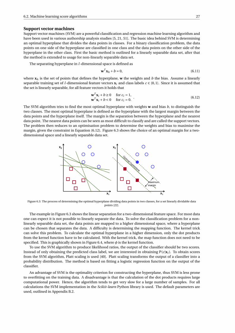
6.2. Machine learning score algorithms 27

Support vector machinesSupport vector machines (SVM) are a powerful classification and regression machine learning algorithm andhave been used in various authorship analysis studies [5, 21, 51]. The basic idea behind SVM is determiningan optimal hyperplane that divides the data points in classes. For a binary classification problem, the datapoints on one side of the hyperplane are classified in one class and the data points on the other side of thehyperplane in the other class. First the basic method is outlined for a linearly separable data set, after thatthe method is extended to usage for non-linearly separable data set.

The separating hyperplane in l -dimensional space is defined as

wT xh +b = 0, (6.11)

where xh is the set of points that defines the hyperplane, w the weights and b the bias. Assume a linearlyseparable training set of l-dimensional feature vectors xi and class labels c ∈ 0,1. Since it is assumed thatthe set is linearly separable, for all feature vectors it holds that

wT xi +b ≥ 0 for ci = 1,wT xi +b < 0 for ci = 0.

. (6.12)

The SVM algorithm tries to find the most optimal hyperplane with weights w and bias b, to distinguish thetwo classes. The most optimal hyperplane is defined as the hyperplane with the largest margin between thedata points and the hyperplane itself. The margin is the separation between the hyperplane and the nearestdata point. The nearest data points can be seen as most difficult to classify and are called the support vectors.The problem then reduces to an optimisation problem to determine the weights and bias to maximise themargin, given the constraint in Equation (6.12). Figure 6.3 shows the choice of an optimal margin for a two-dimensional space and a linearly separable data set.

Figure 6.3: The process of determining the optimal hyperplane dividing data points in two classes, for a set linearly dividable datapoints [22].

The example in Figure 6.3 shows the linear separation for a two-dimensional feature space. For most dataone can expect it is not possible to linearly separate the data. To solve the classification problem for a non-linearly separable data set, the data points are mapped to a higher dimensional space, where a hyperplanecan be chosen that separates the data. A difficulty is determining the mapping function. The kernel trickcan solve this problem. To calculate the optimal hyperplane in a higher dimension, only the dot productsfrom the kernel function have to be calculated. With the kernel trick, the map function does not need to bespecified. This is graphically shown in Figure 6.4, where φ is the kernel function.

To use the SVM algorithm to produce likelihood ratios, the output of the classifier should be two scores.Instead of only obtaining the predicted class label, we are interested in obtaining P(c|xi ). To obtain scoresfrom the SVM algorithm, Platt scaling is used [40]. Platt scaling transforms the output of a classifier into aprobability distribution. The method is based on fitting a logistic regression function on the output of theclassifier.

An advantage of SVM is the optimality criterion for constructing the hyperplane, thus SVM is less proneto overfitting on the training data. A disadvantage is that the calculation of the dot products requires largecomputational power. Hence, the algorithm tends to get very slow for a large number of samples. For allcalculations the SVM implementation in the Scikit-learn Python library is used. The default parameters areused, outlined in Appendix B.2.

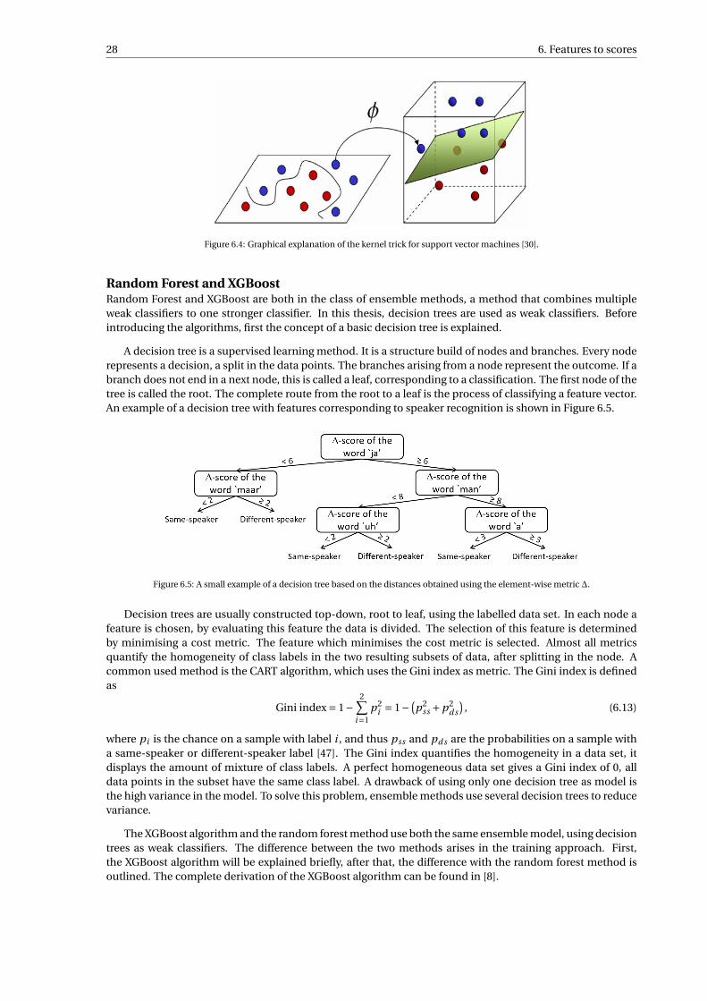
28 6. Features to scores

Figure 6.4: Graphical explanation of the kernel trick for support vector machines [30].

Random Forest and XGBoostRandom Forest and XGBoost are both in the class of ensemble methods, a method that combines multipleweak classifiers to one stronger classifier. In this thesis, decision trees are used as weak classifiers. Beforeintroducing the algorithms, first the concept of a basic decision tree is explained.

A decision tree is a supervised learning method. It is a structure build of nodes and branches. Every noderepresents a decision, a split in the data points. The branches arising from a node represent the outcome. If abranch does not end in a next node, this is called a leaf, corresponding to a classification. The first node of thetree is called the root. The complete route from the root to a leaf is the process of classifying a feature vector.An example of a decision tree with features corresponding to speaker recognition is shown in Figure 6.5.

Figure 6.5: A small example of a decision tree based on the distances obtained using the element-wise metric ∆.

Decision trees are usually constructed top-down, root to leaf, using the labelled data set. In each node afeature is chosen, by evaluating this feature the data is divided. The selection of this feature is determinedby minimising a cost metric. The feature which minimises the cost metric is selected. Almost all metricsquantify the homogeneity of class labels in the two resulting subsets of data, after splitting in the node. Acommon used method is the CART algorithm, which uses the Gini index as metric. The Gini index is definedas

Gini index = 1−2∑

i=1p2

i = 1− (p2

ss +p2d s

), (6.13)

where pi is the chance on a sample with label i , and thus pss and pd s are the probabilities on a sample witha same-speaker or different-speaker label [47]. The Gini index quantifies the homogeneity in a data set, itdisplays the amount of mixture of class labels. A perfect homogeneous data set gives a Gini index of 0, alldata points in the subset have the same class label. A drawback of using only one decision tree as model isthe high variance in the model. To solve this problem, ensemble methods use several decision trees to reducevariance.

The XGBoost algorithm and the random forest method use both the same ensemble model, using decisiontrees as weak classifiers. The difference between the two methods arises in the training approach. First,the XGBoost algorithm will be explained briefly, after that, the difference with the random forest method isoutlined. The complete derivation of the XGBoost algorithm can be found in [8].

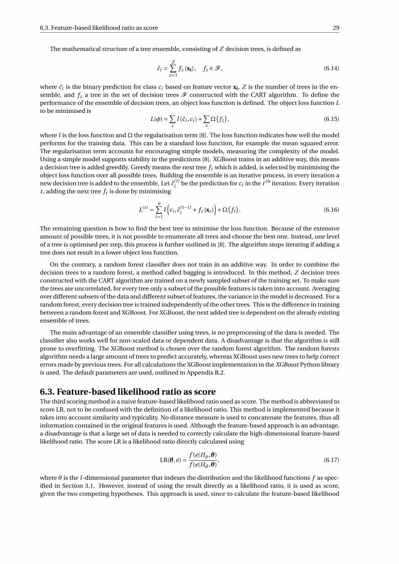
6.3. Feature-based likelihood ratio as score 29

The mathematical structure of a tree ensemble, consisting of Z decision trees, is defined as

ci =Z∑

z=1fz (xi) , fz ∈F , (6.14)

where ci is the binary prediction for class ci based on feature vector xi, Z is the number of trees in the en-semble, and fz a tree in the set of decision trees F constructed with the CART algorithm. To define theperformance of the ensemble of decision trees, an object loss function is defined. The object loss function Lto be minimised is

L(φ) =∑i

l (ci ,ci )+∑

zΩ

(fz

), (6.15)

where l is the loss function andΩ the regularisation term [8]. The loss function indicates how well the modelperforms for the training data. This can be a standard loss function, for example the mean squared error.The regularisation term accounts for encouraging simple models, measuring the complexity of the model.Using a simple model supports stability in the predictions [8]. XGBoost trains in an additive way, this meansa decision tree is added greedily. Greedy means the next tree ft which is added, is selected by minimising theobject loss function over all possible trees. Building the ensemble is an iterative process, in every iteration anew decision tree is added to the ensemble. Let c(t )

i be the prediction for ci in the t th iteration. Every iterationt , adding the next tree ft is done by minimising

L(t ) =n∑

i=1l(ci , c(t−1)

i + ft (xi ))+Ω(

ft)

. (6.16)

The remaining question is how to find the best tree to minimise the loss function. Because of the extensiveamount of possible trees, it is not possible to enumerate all trees and choose the best one. Instead, one levelof a tree is optimised per step, this process is further outlined in [8]. The algorithm stops iterating if adding atree does not result in a lower object loss function.

On the contrary, a random forest classifier does not train in an additive way. In order to combine thedecision trees to a random forest, a method called bagging is introduced. In this method, Z decision treesconstructed with the CART algorithm are trained on a newly sampled subset of the training set. To make surethe trees are uncorrelated, for every tree only a subset of the possible features is taken into account. Averagingover different subsets of the data and different subset of features, the variance in the model is decreased. For arandom forest, every decision tree is trained independently of the other trees. This is the difference in trainingbetween a random forest and XGBoost. For XGBoost, the next added tree is dependent on the already existingensemble of trees.

The main advantage of an ensemble classifier using trees, is no preprocessing of the data is needed. Theclassifier also works well for non-scaled data or dependent data. A disadvantage is that the algorithm is stillprone to overfitting. The XGBoost method is chosen over the random forest algorithm. The random forestsalgorithm needs a large amount of trees to predict accurately, whereas XGBoost uses new trees to help correcterrors made by previous trees. For all calculations the XGBoost implementation in the XGBoost Python libraryis used. The default parameters are used, outlined in Appendix B.2.

6.3. Feature-based likelihood ratio as scoreThe third scoring method is a naive feature-based likelihood ratio used as score. The method is abbreviated toscore LR, not to be confused with the definition of a likelihood ratio. This method is implemented because ittakes into account similarity and typicality. No distance measure is used to concatenate the features, thus allinformation contained in the original features is used. Although the feature-based approach is an advantage,a disadvantage is that a large set of data is needed to correctly calculate the high-dimensional feature-basedlikelihood ratio. The score LR is a likelihood ratio directly calculated using

LR(θ,e) = f (e|Hp ,θ)

f (e|Hd ,θ), (6.17)

where θ is the l -dimensional parameter that indexes the distribution and the likelihood functions f as spec-ified in Section 3.1. However, instead of using the result directly as a likelihood ratio, it is used as score,given the two competing hypotheses. This approach is used, since to calculate the feature-based likelihood

30 6. Features to scores

ratio, several assumptions are needed. This suggests the directly calculated likelihood ratios are probablyill-calibrated. The assumptions are specified later in this section. The scores are calibrated to obtain a like-lihood ratio and hence this method is again a score-based approach. Two distributions are needed: thewithin-speaker and between-speaker distribution. Because no underlying distribution is known, a two-levelnormal-normal model is proposed. This model is often used in forensic sciences, for example for modellingsubstances in drugs tablets or composition analysis of glass fragments [2, 11]. First the two-level normal-normal model is explained generally, afterwards the implementation for speaker recognition is outlined.

6.3.1. Two-level normal-normal modelA two-level model is a statistical model which is appropriate to use when data has a hierarchical structurewith more than one level. In our case the speech fragments are nested in different speakers. The distributionof speech fragments from the same speaker is defined as the within-speaker distribution and the distribu-tion of speech fragments from two different speakers is defined as the between-speaker distribution. Thetwo-level normal-normal model assumes the within-speaker and between-speaker distributions follow mul-tivariate normal distributions. To make this more precise, assuming a normal distribution for the within- andbetween-speaker distribution, results in the hierarchy shown in Figure 6.6.

Figure 6.6: Structure of the two-level normal-normal distribution assumed in the background population of alternative speakers, thefeature samples are denoted as x, based on [31] (Fig 2, p. 48).

Here µb is the l -dimensional vector with the overall mean values per feature and Σb is the covariancematrix from the between-speaker distribution. µw is the l -dimensional vector with mean values per featureper speaker, the within-speaker mean, and Σw the covariance matrix from the within-speaker distribution.The within-speaker mean is inherited from the overall mean, thus the parameters µb , Σb and Σw have to beestimated. With yi , j defined as a sample j of speaker i and Pi the speakers in the background population, thetwo-level normal-normal model is defined as

Pi ∼ N (µb ,Σb)

yi , j |Pi = pi ∼ N (pi ,Σw ),(6.18)

where pi is the realisation of Pi . For the common source model all data is assumed to follow a two-levelmodel. For the specific source model, instead of sampling from an unknown speaker, the sample is obtainedfrom a known specific speaker. This indicates the model is a one-level model, with ys, j defined as sample j ofthe specific speaker s, represented as

ys, j ∼ N (µs ,Σs ), (6.19)

whereµs is the specific speaker mean vector andΣs the covariance matrix of the specific speaker distribution.The background data set of alternative speakers is used to estimate the parameters indexing the distri-

butions. It is challenging to estimate the high dimensional parameters µb , Σb , Σw , µs and Σs correctly. Thefollowing assumptions are used to implement the two-level normal-normal model for the speaker recogni-tion case and estimate the parameters.

• The frequentist approach is used, the parametersµb ,Σb ,Σw ,µs andΣs are estimated and plugged intothe equation.

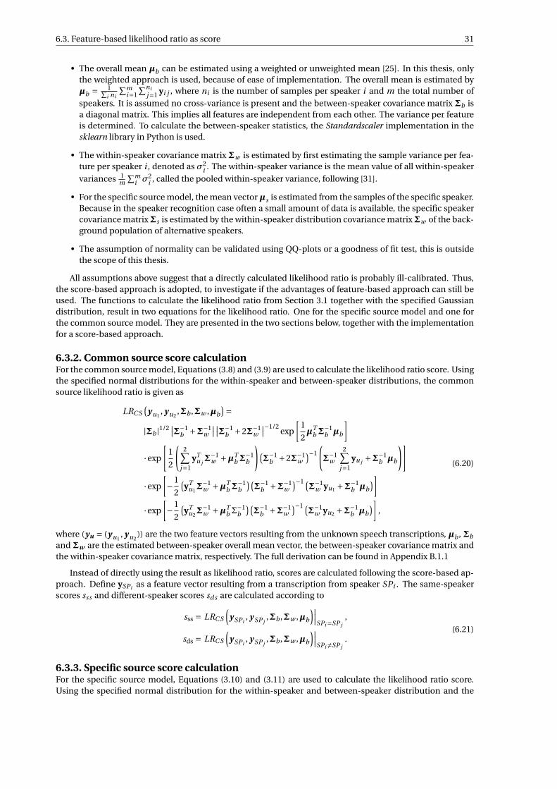
6.3. Feature-based likelihood ratio as score 31

• The overall mean µb can be estimated using a weighted or unweighted mean [25]. In this thesis, onlythe weighted approach is used, because of ease of implementation. The overall mean is estimated byµb = 1∑

i ni

∑mi=1

∑nij=1 yi j , where ni is the number of samples per speaker i and m the total number of

speakers. It is assumed no cross-variance is present and the between-speaker covariance matrix Σb isa diagonal matrix. This implies all features are independent from each other. The variance per featureis determined. To calculate the between-speaker statistics, the Standardscaler implementation in thesklearn library in Python is used.

• The within-speaker covariance matrix Σw is estimated by first estimating the sample variance per fea-ture per speaker i , denoted as σ2

i . The within-speaker variance is the mean value of all within-speaker

variances 1m

∑mi σ2

i , called the pooled within-speaker variance, following [31].

• For the specific source model, the mean vectorµs is estimated from the samples of the specific speaker.Because in the speaker recognition case often a small amount of data is available, the specific speakercovariance matrixΣs is estimated by the within-speaker distribution covariance matrixΣw of the back-ground population of alternative speakers.

• The assumption of normality can be validated using QQ-plots or a goodness of fit test, this is outsidethe scope of this thesis.

All assumptions above suggest that a directly calculated likelihood ratio is probably ill-calibrated. Thus,the score-based approach is adopted, to investigate if the advantages of feature-based approach can still beused. The functions to calculate the likelihood ratio from Section 3.1 together with the specified Gaussiandistribution, result in two equations for the likelihood ratio. One for the specific source model and one forthe common source model. They are presented in the two sections below, together with the implementationfor a score-based approach.

6.3.2. Common source score calculationFor the common source model, Equations (3.8) and (3.9) are used to calculate the likelihood ratio score. Usingthe specified normal distributions for the within-speaker and between-speaker distributions, the commonsource likelihood ratio is given as

LRC S(

y u1, y u2

,Σb ,Σw ,µb

)=|Σb |1/2 ∣∣Σ−1

b +Σ−1w

∣∣ ∣∣Σ−1b +2Σ−1

w

∣∣−1/2exp

[1

2µT

bΣ−1b µb

]·exp

[1

2

(2∑

j=1yT

u jΣ−1

w +µTbΣ

−1b

)(Σ−1

b +2Σ−1w

)−1

(Σ−1

w

2∑j=1

yu j +Σ−1b µb

)]

·exp

[−1

2

(yT

u1Σ−1

w +µTbΣ

−1b

)(Σ−1

b +Σ−1w

)−1 (Σ−1

w yu1 +Σ−1b µb

)]·exp

[−1

2

(yT

u2Σ−1

w +µTb Σ

−1b

)(Σ−1

b +Σ−1w

)−1 (Σ−1

w yu2 +Σ−1b µb

)],

(6.20)

where (yu = (y u1, y u2

)) are the two feature vectors resulting from the unknown speech transcriptions, µb , Σb

and Σw are the estimated between-speaker overall mean vector, the between-speaker covariance matrix andthe within-speaker covariance matrix, respectively. The full derivation can be found in Appendix B.1.1

Instead of directly using the result as likelihood ratio, scores are calculated following the score-based ap-proach. Define ySPi as a feature vector resulting from a transcription from speaker SPi . The same-speakerscores sss and different-speaker scores sd s are calculated according to

sss = LRC S

(y SPi

, y SP j,Σb ,Σw ,µb

)∣∣∣SPi=SP j

,

sds = LRC S

(y SPi

, y SP j,Σb ,Σw ,µb

)∣∣∣SPi 6=SP j

.(6.21)

6.3.3. Specific source score calculationFor the specific source model, Equations (3.10) and (3.11) are used to calculate the likelihood ratio score.Using the specified normal distribution for the within-speaker and between-speaker distribution and the

32 6. Features to scores

estimated specific speaker statistics, the specific source likelihood ratio is given as

LRSS(

yu ,Σb ,Σw ,µb ,Σs ,µs)=

|Σs |−1/2 |Σw |1/2 |Σb |1/2 ∣∣Σ−1b +Σ−1

w

∣∣1/2

·exp

[−1

2(yu −µs)TΣ−1

s (yu −µs)

]·exp

[1

2

(yT

uΣ−1w yu

)+ 1

2µT

bΣ−1b µb

]·exp

[−1

2

(yT

uΣ−1w +µT

bΣ−1b

)(Σ−1

b +Σ−1w

)−1 (Σ−1

w yu +Σ−1b µb

)],

(6.22)

where µs is the specific speaker mean vector, Σs the covariance matrix of the specific speaker distributionand the remainder of the indexing parameters are equal to the ones defined in Equation (6.20). The extensivederivation can be found in Appendix B.1.2

The scores are calculated following the score-based approach. Define ySPi as a feature vector resultingfrom a transcription from speaker SPi . The same-speaker scores sss and different-speaker scores sd s arecalculated using the labelled training set as

sss = LRSS

(y SPi

,Σb ,Σw ,µb ,ΣSP j ,µSP j

)∣∣∣SPi=SP j

,

sds = LRSS

(y SPi

,Σb ,Σw ,µb ,ΣSP j ,µSP j

)∣∣∣SPi 6=SP j

,(6.23)

where ΣSP j is the specific speaker SP j covariance matrix and µSP jthe specific speaker SP j mean vector.

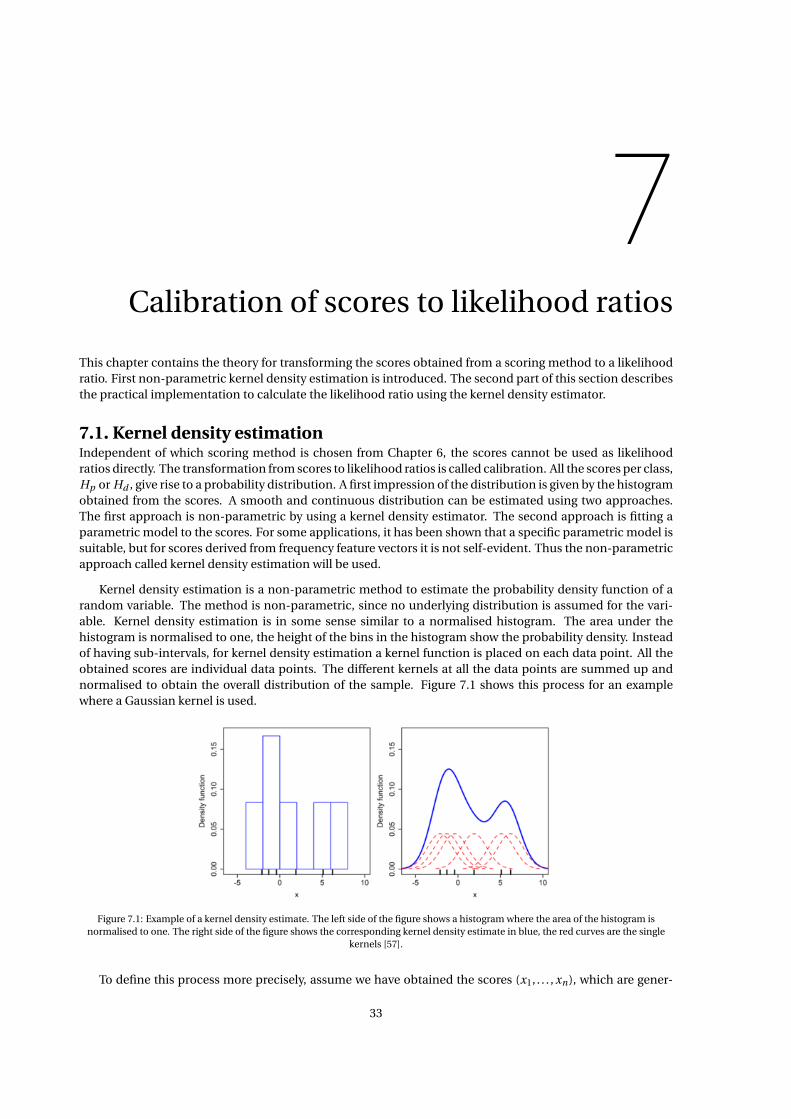
7Calibration of scores to likelihood ratios

This chapter contains the theory for transforming the scores obtained from a scoring method to a likelihoodratio. First non-parametric kernel density estimation is introduced. The second part of this section describesthe practical implementation to calculate the likelihood ratio using the kernel density estimator.

7.1. Kernel density estimationIndependent of which scoring method is chosen from Chapter 6, the scores cannot be used as likelihoodratios directly. The transformation from scores to likelihood ratios is called calibration. All the scores per class,Hp or Hd , give rise to a probability distribution. A first impression of the distribution is given by the histogramobtained from the scores. A smooth and continuous distribution can be estimated using two approaches.The first approach is non-parametric by using a kernel density estimator. The second approach is fitting aparametric model to the scores. For some applications, it has been shown that a specific parametric model issuitable, but for scores derived from frequency feature vectors it is not self-evident. Thus the non-parametricapproach called kernel density estimation will be used.

Kernel density estimation is a non-parametric method to estimate the probability density function of arandom variable. The method is non-parametric, since no underlying distribution is assumed for the vari-able. Kernel density estimation is in some sense similar to a normalised histogram. The area under thehistogram is normalised to one, the height of the bins in the histogram show the probability density. Insteadof having sub-intervals, for kernel density estimation a kernel function is placed on each data point. All theobtained scores are individual data points. The different kernels at all the data points are summed up andnormalised to obtain the overall distribution of the sample. Figure 7.1 shows this process for an examplewhere a Gaussian kernel is used.

Figure 7.1: Example of a kernel density estimate. The left side of the figure shows a histogram where the area of the histogram isnormalised to one. The right side of the figure shows the corresponding kernel density estimate in blue, the red curves are the single

kernels [57].

To define this process more precisely, assume we have obtained the scores (x1, . . . , xn), which are gener-

33

34 7. Calibration of scores to likelihood ratios

ated by an unknown density function F . Then the estimator of F , denoted as Fh , is defined as

Fh(x) = 1

n

n∑i=1

Kh (x −xi ) = 1

nh

n∑i=1

K( x −xi

h

), (7.1)

with h the bandwidth of the kernel and K the kernel function [57]. A kernel function can be any function thatintegrates to one

∫K (x)d x = 1. (7.2)

Often used kernels are a Gaussian function or a uniform function. In this thesis, we use a Gaussian kernelfunction with zero mean and standard deviation one, defined as

K (x) = 1p2π

exp

(−1

2x2

). (7.3)

The standard Gaussian kernel is widely used for kernel density estimates.

The bandwidth of the kernel distribution determines the scale of the kernel function and has a strongeffect on the estimated distribution. For a large bandwidth, the mass of the kernel function is widely spreadaround the data points. This could result in a density estimate which is over smoothed. For a small band-width, the mass is concentrated closely around the data points. This could lead to a result which is undersmoothed. To choose the parameter h in an optimal way, different criteria are used to estimate an appropri-ate bandwidth. The most common criterion is choosing h in such a way that the mean integrated squarederror (MISE) is minimised. The MISE is defined as

MISE(h) = E

[∫ (fh(x)− f (x)

)2d x

]. (7.4)

Here fh is the estimated density function and f the unknown, real density function [57]. Because the un-known density function is used in the function, this criterion cannot be used directly. Hence, several empiri-cal approaches are defined to practically estimate the parameter h. In this thesis Silverman’s rule of thumb isused to determine the bandwidth, defined as

h =(

4σ5

3n

) 15

, (7.5)

with σ the standard deviation of the sample and n the number of samples [17]. The rule of thumb per-forms well for estimating distributions which approach a Gaussian distribution, but can become inaccuratefor distributions not similar to a Gaussian distribution. This is a point which has to be kept in mind, whencalculating the results and inspecting the density estimation.

7.2. Score calibration to likelihood ratioWith kernel density estimation the distribution of scores under Hp and Hd is estimated. It is important tolook at the goodness of the fit, a poor fit does not represent the underlying data. Furthermore, an inaccu-rate fit can lead to instability of the likelihood ratio method, as the density estimation does not follow theunderlying data. Looking back at Equations (6.23) and (6.21), calculating the likelihood ratio for the disputedtranscription follows directly and is illustrated in Figure 7.2a.

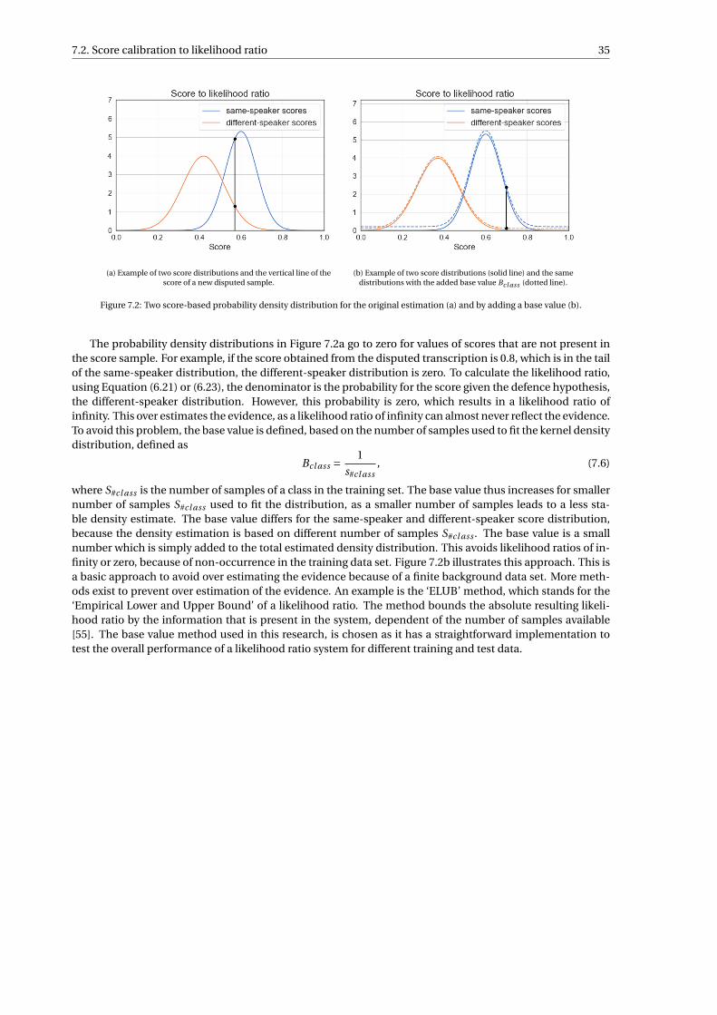
7.2. Score calibration to likelihood ratio 35

(a) Example of two score distributions and the vertical line of thescore of a new disputed sample.

(b) Example of two score distributions (solid line) and the samedistributions with the added base value Bcl ass (dotted line).

Figure 7.2: Two score-based probability density distribution for the original estimation (a) and by adding a base value (b).

The probability density distributions in Figure 7.2a go to zero for values of scores that are not present inthe score sample. For example, if the score obtained from the disputed transcription is 0.8, which is in the tailof the same-speaker distribution, the different-speaker distribution is zero. To calculate the likelihood ratio,using Equation (6.21) or (6.23), the denominator is the probability for the score given the defence hypothesis,the different-speaker distribution. However, this probability is zero, which results in a likelihood ratio ofinfinity. This over estimates the evidence, as a likelihood ratio of infinity can almost never reflect the evidence.To avoid this problem, the base value is defined, based on the number of samples used to fit the kernel densitydistribution, defined as

Bcl ass =1

s#cl ass, (7.6)

where S#cl ass is the number of samples of a class in the training set. The base value thus increases for smallernumber of samples S#cl ass used to fit the distribution, as a smaller number of samples leads to a less sta-ble density estimate. The base value differs for the same-speaker and different-speaker score distribution,because the density estimation is based on different number of samples S#cl ass . The base value is a smallnumber which is simply added to the total estimated density distribution. This avoids likelihood ratios of in-finity or zero, because of non-occurrence in the training data set. Figure 7.2b illustrates this approach. This isa basic approach to avoid over estimating the evidence because of a finite background data set. More meth-ods exist to prevent over estimation of the evidence. An example is the ‘ELUB’ method, which stands for the‘Empirical Lower and Upper Bound’ of a likelihood ratio. The method bounds the absolute resulting likeli-hood ratio by the information that is present in the system, dependent of the number of samples available[55]. The base value method used in this research, is chosen as it has a straightforward implementation totest the overall performance of a likelihood ratio system for different training and test data.

8Likelihood ratio validation

Validation is an important part of the likelihood ratio method. In order for the likelihood ratio method to beeligible for use in court, the method has to be validated and the results need accompanying documentation.For validation of the results obtained in this thesis, the framework defined by [29] is used. The framework isbased on three important concepts: performance characteristics, performance metrics and validation crite-ria.

Performance characteristics are quantities that are important for the validation of the likelihood ratiomethod. An important aspect of a likelihood ratio is the discriminating power between the two competing hy-potheses. Discriminating power is a performance characteristic of the likelihood ratio system. Performancemetrics quantify the performance characteristic. It is essential to have a suitable metric for the characteristic.A validation criterion is a threshold which is set on the characteristic metric. Whether the result is below orabove the threshold, determines if a likelihood ratio system can be assumed to be valid.

The use of a standard validation process is not common practice, this is a critical note on the likelihoodratio validation process [43]. A guideline has been presented in [29], but not all likelihood ratio systemsconstructed are validated according to this guideline. Different approaches and metrics are used to presentthe validation and assessment of a likelihood ratio system.

In Table 8.1 the three most important performance characteristics are outlined: accuracy, discriminatingpower and calibration [42]. Accuracy means the agreement between the determined likelihood ratio and theground truth. The ground truth is the label that corresponds to the sample, Hp or Hd . A likelihood ratio ismore accurate if the value supports the correct hypothesis. Discriminating power is defined as the capabilityof the method to distinguish between two competing hypotheses. Calibration is a property of the likelihoodratios. A good calibration refers to a set of likelihood ratios that can be interpreted as the strength of theevidence for the given competing hypotheses [16]. More performance characteristics exist, the characteristicsused in this thesis are selected as they show a good indication of the performance of a likelihood ratio system.The corresponding performance metrics and the corresponding graphical representation are stated in Table8.1.

Table 8.1: Table with performance characteristics, performance metrics and graphical representations [29].

Performance characteristic Performance metric Graphical representation

Accuracy Cl l r , accuracy ECE plotDiscriminating power C mi n

ll r ECE plotCalibration C cal

l l r PAV plot, ECE plot, Tippett plot

Note that accuracy is defined as a performance characteristic, but also a performance metric. We havechosen to add accuracy to the performance metrics proposed in the validation framework in [29]. This choiceis made as it shows an intuitive measure and can be used to compare the results with other authorship anal-ysis papers, where only the classification accuracy is presented instead of forensic likelihood ratios. Further-more, it is interesting to look at the interaction between the accuracy and the Cl l r . To give a clear view, the

37

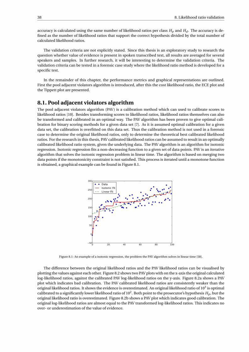
38 8. Likelihood ratio validation

accuracy is calculated using the same number of likelihood ratios per class Hp and Hd . The accuracy is de-fined as the number of likelihood ratios that support the correct hypothesis divided by the total number ofcalculated likelihood ratios.

The validation criteria are not explicitly stated. Since this thesis is an exploratory study to research thequestion whether value of evidence is present in spoken transcribed text, all results are averaged for severalspeakers and samples. In further research, it will be interesting to determine the validation criteria. Thevalidation criteria can be tested in a forensic case study where the likelihood ratio method is developed for aspecific test.

In the remainder of this chapter, the performance metrics and graphical representations are outlined.First the pool adjacent violators algorithm is introduced, after this the cost likelihood ratio, the ECE plot andthe Tippett plot are presented.

8.1. Pool adjacent violators algorithmThe pool adjacent violators algorithm (PAV) is a calibration method which can used to calibrate scores tolikelihood ratios [10]. Besides transforming scores to likelihood ratios, likelihood ratios themselves can alsobe transformed and calibrated in an optimal way. The PAV algorithm has been proven to give optimal cali-bration for binary scoring methods for a given data set [7]. As it is assumed optimal calibration for a givendata set, the calibration is overfitted on this data set. Thus the calibration method is not used in a forensiccase to determine the original likelihood ratios, only to determine the theoretical best calibrated likelihoodratios. For the research in this thesis, PAV calibrated likelihood ratios can be assumed to result in an optimallycalibrated likelihood ratio system, given the underlying data. The PAV algorithm is an algorithm for isotonicregression. Isotonic regression fits a non-decreasing function to a given set of data points. PAV is an iterativealgorithm that solves the isotonic regression problem in linear time. The algorithm is based on merging twodata points if the monotonicity constraint is not satisfied. This process is iterated until a monotone functionis obtained, a graphical example can be found in Figure 8.1.

Figure 8.1: An example of a isotonic regression, the problem the PAV algorithm solves in linear time [58].

The difference between the original likelihood ratios and the PAV likelihood ratios can be visualised byplotting the values against each other. Figure 8.2 shows two PAV plots with on the x-axis the original calculatedlog-likelihood ratios, against the calibrated PAV log-likelihood ratios on the y-axis. Figure 8.2a shows a PAVplot which indicates bad calibration. The PAV calibrated likelihood ratios are consistently weaker than theoriginal likelihood ratios. It shows the evidence is overestimated. An original likelihood ratio of 103 is optimalcalibrated to a significantly lower likelihood ratio of 102. Both point to the prosecutor’s hypothesis Hp , but theoriginal likelihood ratio is overestimated. Figure 8.2b shows a PAV plot which indicates good calibration. Theoriginal log-likelihood ratios are almost equal to the PAV transformed log-likelihood ratios. This indicates noover- or underestimation of the value of evidence.

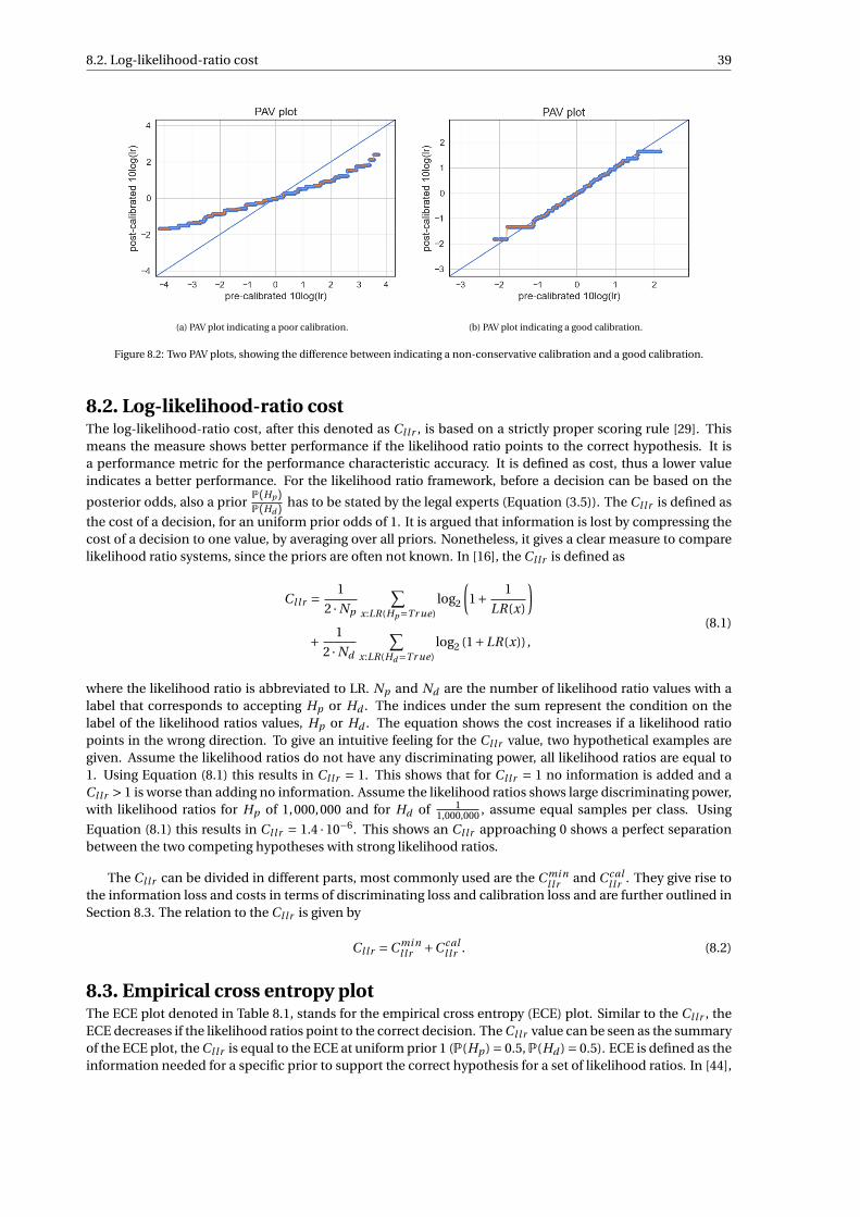
8.2. Log-likelihood-ratio cost 39

(a) PAV plot indicating a poor calibration. (b) PAV plot indicating a good calibration.

Figure 8.2: Two PAV plots, showing the difference between indicating a non-conservative calibration and a good calibration.

8.2. Log-likelihood-ratio costThe log-likelihood-ratio cost, after this denoted as Cl l r , is based on a strictly proper scoring rule [29]. Thismeans the measure shows better performance if the likelihood ratio points to the correct hypothesis. It isa performance metric for the performance characteristic accuracy. It is defined as cost, thus a lower valueindicates a better performance. For the likelihood ratio framework, before a decision can be based on the

posterior odds, also a priorP(Hp )P(Hd ) has to be stated by the legal experts (Equation (3.5)). The Cl l r is defined as

the cost of a decision, for an uniform prior odds of 1. It is argued that information is lost by compressing thecost of a decision to one value, by averaging over all priors. Nonetheless, it gives a clear measure to comparelikelihood ratio systems, since the priors are often not known. In [16], the Cl l r is defined as

Cl l r =1

2 ·Np

∑x:LR(Hp=Tr ue)

log2

(1+ 1

LR(x)

)

+ 1

2 ·Nd

∑x:LR(Hd=Tr ue)

log2 (1+LR(x)) ,

(8.1)

where the likelihood ratio is abbreviated to LR. Np and Nd are the number of likelihood ratio values with alabel that corresponds to accepting Hp or Hd . The indices under the sum represent the condition on thelabel of the likelihood ratios values, Hp or Hd . The equation shows the cost increases if a likelihood ratiopoints in the wrong direction. To give an intuitive feeling for the Cl l r value, two hypothetical examples aregiven. Assume the likelihood ratios do not have any discriminating power, all likelihood ratios are equal to1. Using Equation (8.1) this results in Cl l r = 1. This shows that for Cl l r = 1 no information is added and aCl l r > 1 is worse than adding no information. Assume the likelihood ratios shows large discriminating power,with likelihood ratios for Hp of 1,000,000 and for Hd of 1

1,000,000 , assume equal samples per class. Using

Equation (8.1) this results in Cl l r = 1.4 ·10−6. This shows an Cl l r approaching 0 shows a perfect separationbetween the two competing hypotheses with strong likelihood ratios.

The Cl l r can be divided in different parts, most commonly used are the C mi nll r and C cal

l l r . They give rise tothe information loss and costs in terms of discriminating loss and calibration loss and are further outlined inSection 8.3. The relation to the Cl l r is given by

Cl l r =C mi nl lr +C cal

l l r . (8.2)

8.3. Empirical cross entropy plotThe ECE plot denoted in Table 8.1, stands for the empirical cross entropy (ECE) plot. Similar to the Cl l r , theECE decreases if the likelihood ratios point to the correct decision. The Cl l r value can be seen as the summaryof the ECE plot, the Cl l r is equal to the ECE at uniform prior 1 (P(Hp ) = 0.5,P(Hd ) = 0.5). ECE is defined as theinformation needed for a specific prior to support the correct hypothesis for a set of likelihood ratios. In [44],

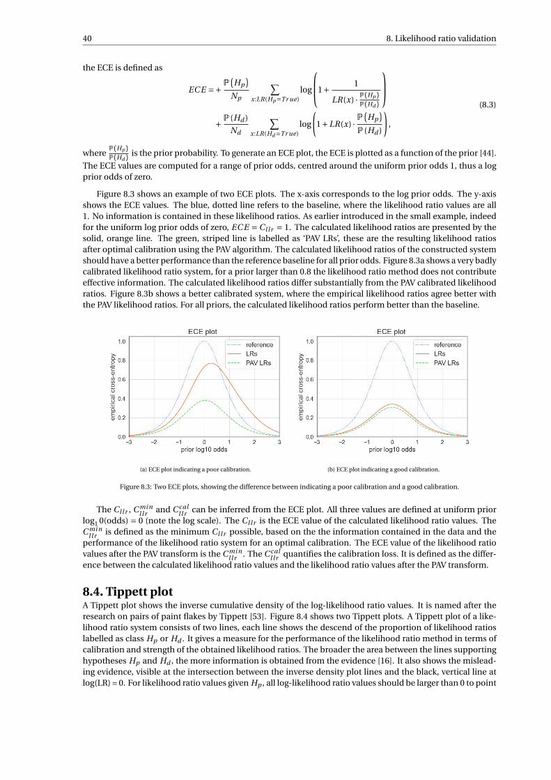
40 8. Likelihood ratio validation

the ECE is defined as

EC E =+ P(Hp

)Np

∑x:LR(Hp=Tr ue)

log

1+ 1

LR(x) · P(Hp )P(Hd )

+ P (Hd )

Nd

∑x:LR(Hd=Tr ue)

log

(1+LR(x) · P

(Hp

)P (Hd )

),

(8.3)

whereP(Hp )P(Hd ) is the prior probability. To generate an ECE plot, the ECE is plotted as a function of the prior [44].

The ECE values are computed for a range of prior odds, centred around the uniform prior odds 1, thus a logprior odds of zero.

Figure 8.3 shows an example of two ECE plots. The x-axis corresponds to the log prior odds. The y-axisshows the ECE values. The blue, dotted line refers to the baseline, where the likelihood ratio values are all1. No information is contained in these likelihood ratios. As earlier introduced in the small example, indeedfor the uniform log prior odds of zero, EC E = Cl l r = 1. The calculated likelihood ratios are presented by thesolid, orange line. The green, striped line is labelled as ‘PAV LRs’, these are the resulting likelihood ratiosafter optimal calibration using the PAV algorithm. The calculated likelihood ratios of the constructed systemshould have a better performance than the reference baseline for all prior odds. Figure 8.3a shows a very badlycalibrated likelihood ratio system, for a prior larger than 0.8 the likelihood ratio method does not contributeeffective information. The calculated likelihood ratios differ substantially from the PAV calibrated likelihoodratios. Figure 8.3b shows a better calibrated system, where the empirical likelihood ratios agree better withthe PAV likelihood ratios. For all priors, the calculated likelihood ratios perform better than the baseline.

(a) ECE plot indicating a poor calibration. (b) ECE plot indicating a good calibration.

Figure 8.3: Two ECE plots, showing the difference between indicating a poor calibration and a good calibration.

The Cl l r , C mi nll r and C cal

l l r can be inferred from the ECE plot. All three values are defined at uniform priorlog1 0(odds) = 0 (note the log scale). The Cl l r is the ECE value of the calculated likelihood ratio values. TheC mi n

ll r is defined as the minimum Cl l r possible, based on the the information contained in the data and theperformance of the likelihood ratio system for an optimal calibration. The ECE value of the likelihood ratiovalues after the PAV transform is the C mi n

ll r . The C call l r quantifies the calibration loss. It is defined as the differ-

ence between the calculated likelihood ratio values and the likelihood ratio values after the PAV transform.

8.4. Tippett plotA Tippett plot shows the inverse cumulative density of the log-likelihood ratio values. It is named after theresearch on pairs of paint flakes by Tippett [53]. Figure 8.4 shows two Tippett plots. A Tippett plot of a like-lihood ratio system consists of two lines, each line shows the descend of the proportion of likelihood ratioslabelled as class Hp or Hd . It gives a measure for the performance of the likelihood ratio method in terms ofcalibration and strength of the obtained likelihood ratios. The broader the area between the lines supportinghypotheses Hp and Hd , the more information is obtained from the evidence [16]. It also shows the mislead-ing evidence, visible at the intersection between the inverse density plot lines and the black, vertical line atlog(LR) = 0. For likelihood ratio values given Hp , all log-likelihood ratio values should be larger than 0 to point

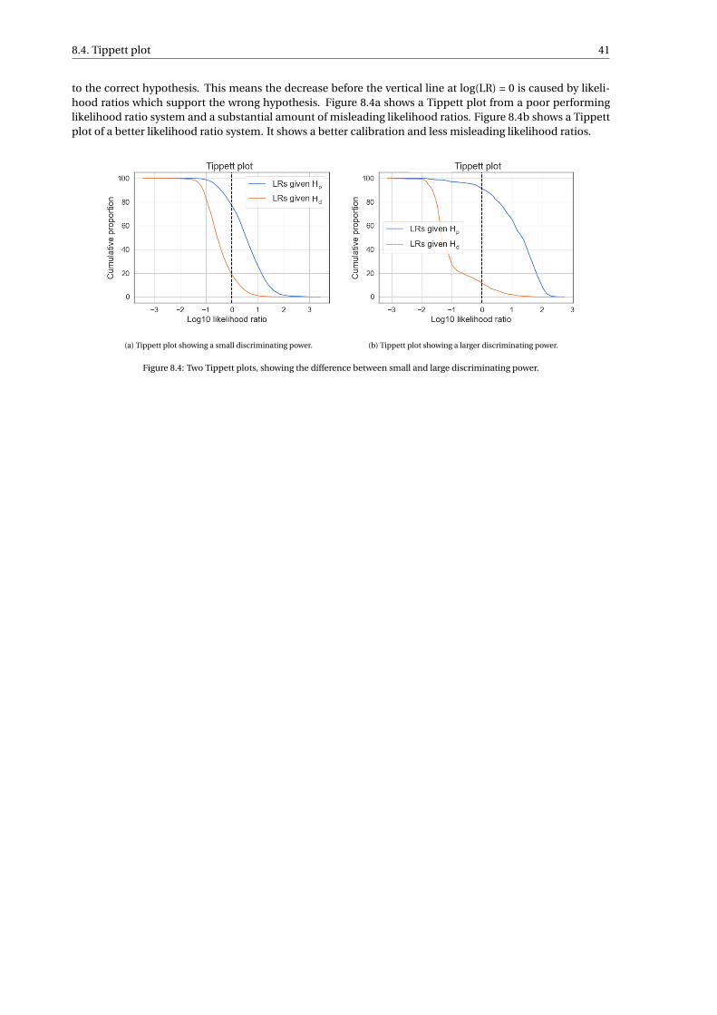
8.4. Tippett plot 41

to the correct hypothesis. This means the decrease before the vertical line at log(LR) = 0 is caused by likeli-hood ratios which support the wrong hypothesis. Figure 8.4a shows a Tippett plot from a poor performinglikelihood ratio system and a substantial amount of misleading likelihood ratios. Figure 8.4b shows a Tippettplot of a better likelihood ratio system. It shows a better calibration and less misleading likelihood ratios.

(a) Tippett plot showing a small discriminating power. (b) Tippett plot showing a larger discriminating power.

Figure 8.4: Two Tippett plots, showing the difference between small and large discriminating power.

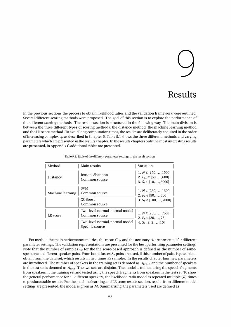
9Results

In the previous sections the process to obtain likelihood ratios and the validation framework were outlined.Several different scoring methods were proposed. The goal of this section is to explore the performance ofthe different scoring methods. The results section is structured in the following way. The main division isbetween the three different types of scoring methods, the distance method, the machine learning methodand the LR score method. To avoid long computation times, the results are deliberately acquired in the orderof increasing complexity, as described in Chapter 6. Table 9.1 shows the three different methods and varyingparameters which are presented in the results chapter. In the results chapters only the most interesting resultsare presented, in Appendix C additional tables are presented.

Table 9.1: Table of the different parameter settings in the result section

Method Main results Variations

DistanceJensen–ShannonCommon source

1. N ∈ [250, . . . ,1500]2. F#S ∈ [50, . . . ,600]3. S# ∈ [10, . . . ,5000]

Machine learningSVMCommon source

1. N ∈ [250, . . . ,1500]2. F# ∈ [50, . . . ,600]3. S# ∈ [100, . . . ,7000]XGBoost

Common source

LR scoreTwo-level normal-normal modelCommon source

1. N ∈ [250, . . . ,750]2. F# ∈ [20, . . . ,75]4. S#s ∈ [2, . . . ,10]Two-level normal-normal model

Specific source

Per method the main performance metrics, the mean Cl l r and the accuracy A, are presented for differentparameter settings. The validation representations are presented for the best performing parameter settings.Note that the number of samples S# for the the score-based approach is defined as the number of same-speaker and different-speaker pairs. From both classes S# pairs are used, if this number of pairs is possible toobtain from the data set, which results in two times S# samples. In the results chapter four new parametersare introduced. The number of speakers in the training set is denoted as Atr ai n and the number of speakersin the test set is denoted as Atest . The two sets are disjoint. The model is trained using the speech fragmentsfrom speakers in the training set and tested using the speech fragments from speakers in the test set. To showthe general performance for all different speakers, the likelihood ratio model is repeated multiple (R) timesto produce stable results. For the machine learning and LR score results section, results from different modelsettings are presented, the model is given as M . Summarising, the parameters used are defined as

43

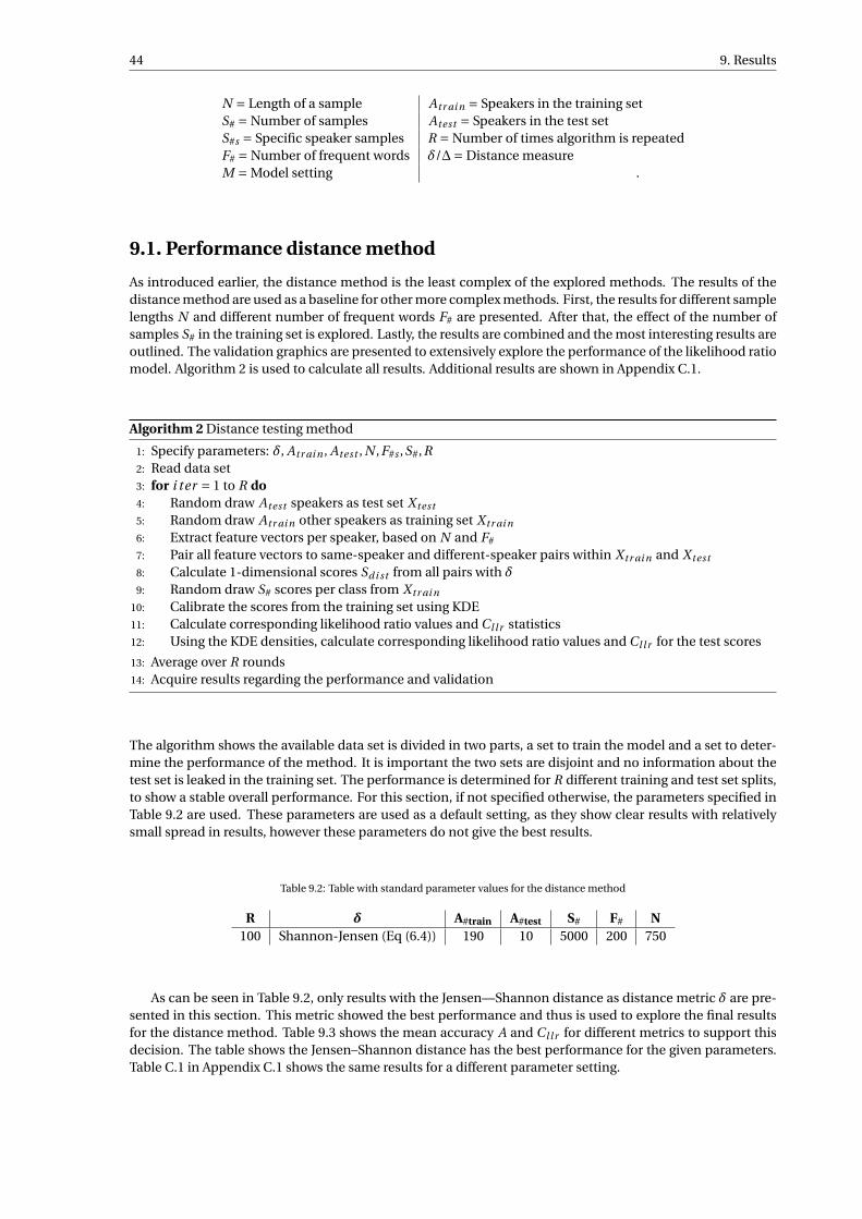
44 9. Results

N = Length of a sample Atr ai n = Speakers in the training setS# = Number of samples Atest = Speakers in the test setS#s = Specific speaker samples R = Number of times algorithm is repeatedF# = Number of frequent words δ/∆= Distance measureM = Model setting .

9.1. Performance distance method

As introduced earlier, the distance method is the least complex of the explored methods. The results of thedistance method are used as a baseline for other more complex methods. First, the results for different samplelengths N and different number of frequent words F# are presented. After that, the effect of the number ofsamples S# in the training set is explored. Lastly, the results are combined and the most interesting results areoutlined. The validation graphics are presented to extensively explore the performance of the likelihood ratiomodel. Algorithm 2 is used to calculate all results. Additional results are shown in Appendix C.1.

Algorithm 2 Distance testing method

1: Specify parameters: δ, Atr ai n , Atest , N ,F#s ,S#,R2: Read data set3: for i ter = 1 to R do4: Random draw Atest speakers as test set X test

5: Random draw Atr ai n other speakers as training set X tr ai n

6: Extract feature vectors per speaker, based on N and F#

7: Pair all feature vectors to same-speaker and different-speaker pairs within X tr ai n and X test

8: Calculate 1-dimensional scores Sdi st from all pairs with δ

9: Random draw S# scores per class from X tr ai n

10: Calibrate the scores from the training set using KDE11: Calculate corresponding likelihood ratio values and Cl l r statistics12: Using the KDE densities, calculate corresponding likelihood ratio values and Cl l r for the test scores

13: Average over R rounds14: Acquire results regarding the performance and validation

The algorithm shows the available data set is divided in two parts, a set to train the model and a set to deter-mine the performance of the method. It is important the two sets are disjoint and no information about thetest set is leaked in the training set. The performance is determined for R different training and test set splits,to show a stable overall performance. For this section, if not specified otherwise, the parameters specified inTable 9.2 are used. These parameters are used as a default setting, as they show clear results with relativelysmall spread in results, however these parameters do not give the best results.

Table 9.2: Table with standard parameter values for the distance method

R δ A#train A#test S# F# N100 Shannon-Jensen (Eq (6.4)) 190 10 5000 200 750

As can be seen in Table 9.2, only results with the Jensen—Shannon distance as distance metric δ are pre-sented in this section. This metric showed the best performance and thus is used to explore the final resultsfor the distance method. Table 9.3 shows the mean accuracy A and Cl l r for different metrics to support thisdecision. The table shows the Jensen–Shannon distance has the best performance for the given parameters.Table C.1 in Appendix C.1 shows the same results for a different parameter setting.

9.1. Performance distance method 45

Table 9.3: Results in terms of mean Cl l r and accuracy A for the distance method for different distance metrics, with N = 500, F# = 200and S# = 5000.

Distance metric δ Cl l r Accuracy

Jensen-Shannon 0.61 0.81Bray-Curtis 0.62 0.81Manhattan 0.69 0.77Euclidean 0.71 0.77

Cosine 0.71 0.77

First, the effect of varying number of frequents words F# and sample length N on the performance isshown in Figure 9.1. For different numbers of frequent words F#, the mean Cl l r and accuracy A are plottedagainst sample length N . It shows the clear trend that for a higher sample length, the performance in termsof mean accuracy A and mean Cl l r improves. The accuracy A increases and the Cl l r decreases. The figuresshow that for smaller number of frequent words in the range between 50 ≤ F# ≤ 100, the performance is lowerthan for higher number of frequent words in the range 200 ≤ F# ≤ 600. For the range 200 ≤ F# ≤ 600, theperformance does not differ largely for varying number of frequent words.

(a) Mean Accuracy A. (b) Mean Cl l r .

Figure 9.1: Plots of mean accuracy A and Cl l r per sample length N for different values of number of frequent words F# and S# = 5000.

To give a more extensive view of the two parameters N and F#, the boxplots of the sample obtained byrepeating the algorithm are presented. The boxplots show the degree of spread in R repetitions. First thenumber of frequent words is fixed on F# = 200. This number has been chosen as this shows a good perfor-mance in the first exploratory plot. An important trade-off in these results is the number of samples S# andthe sample length N . A larger sample length leads to a smaller number of samples which can be obtainedwith Atr ai n = 190 and Atest = 10. Table 9.4 shows the decrease in the number of different-speaker and same-speaker pairs for varying sample lengths. It shows the limiting factor is the number of same-speaker pairs.The number of different-speaker and same-speaker pairs used to train the method is determined in the de-fault parameters as S#, however the numbers in the table show this amount of samples is not obtained for allsample lengths. We have chosen not to keep the number of samples static for the test of the influence of thesample length, as this is a natural effect of a limiting data set, which cannot be omitted. The parameter S#

is defined as a cap for the maximum number of used sample pairs. When the parameter S# is varied to testthe sensitivity of the method for this parameter, the sample length N is chosen such that both classes have atleast S# pairs.

46 9. Results

Table 9.4: The data statistics corresponding to Atr ai n = 190 and Atest = 10

Sample length Samples from data Same-speaker pairs Different-speaker pairs

250 3276 28733 5338343

500 1591 6415 1259341

750 1029 2513 526788

1000 745 1234 276165

1250 573 672 163399

1500 472 416 110883

1750 386 246 74420

Figure 9.2 shows again that the mean accuracy A increases and the Cl l r decreases for the a larger samplelength. However, the graph also shows an increasing spread for an increasing sample length N . Looking at theaccuracy at sample length N = 1500, the best result is 1, but the worst result is 0.77. This large spread couldhave multiple reasons. Some speakers have more distinctive speech than others. Within an automatic testcase where different speakers are used, some will give better results than other speakers. Therefore, a naturalspread in the results is present, resulting from the available data quality and not from the method. The largerspread could also be attributed to the fewer number of samples available. As is shown in Table 9.4, for alarge sample length the data set is not sufficient to keep using S# number of same-speaker and S# number ofdifferent-speaker pairs. To increase the sample length more and to test adequately, more data is needed. Ifwe look at the mean Cl l r value, it also shows a large deviation between 0.07 and 0.7 for sample length 1500.This shows again the method is working, but has a natural spread due to the different speakers in the data set,but also due to the other reasons mentioned.

(a) Cl l r per sample length N . (b) Accuracy A per sample length N .

Figure 9.2: Boxplots of accuracy A and Cl l r per sample length N for the distance method, including the mean values, with F# = 200 andS# = 5000.

To show the trend and degree of spread in the mean Cl l r and accuracy A for different number of frequentwords F#, in Figure 9.3 the mean Cl l r and accuracy A are plotted against the number of frequent words F#

with corresponding boxplots. Note that the x-axis of the figure is not linear and thus the slope of the graphis out of proportion. The plot shows the method reaches a stable performance for F# ≥ 200. The boxplotsshow that the spread is again relatively large, but no trend is shown relative to the number of frequent wordsF#. In determining the optimal number of frequent words F#, it is important to keep in mind that a modelshould not be more complex than needed. Thus, in our case it is best to take F# = 200 as optimal number offrequent words, as this shows almost an equal performance as a higher number of frequent words F#. It isalso important to note that although the performance in terms of accuracy A and Cl l r is lower for F# = 50,still a discriminating performance is obtained.

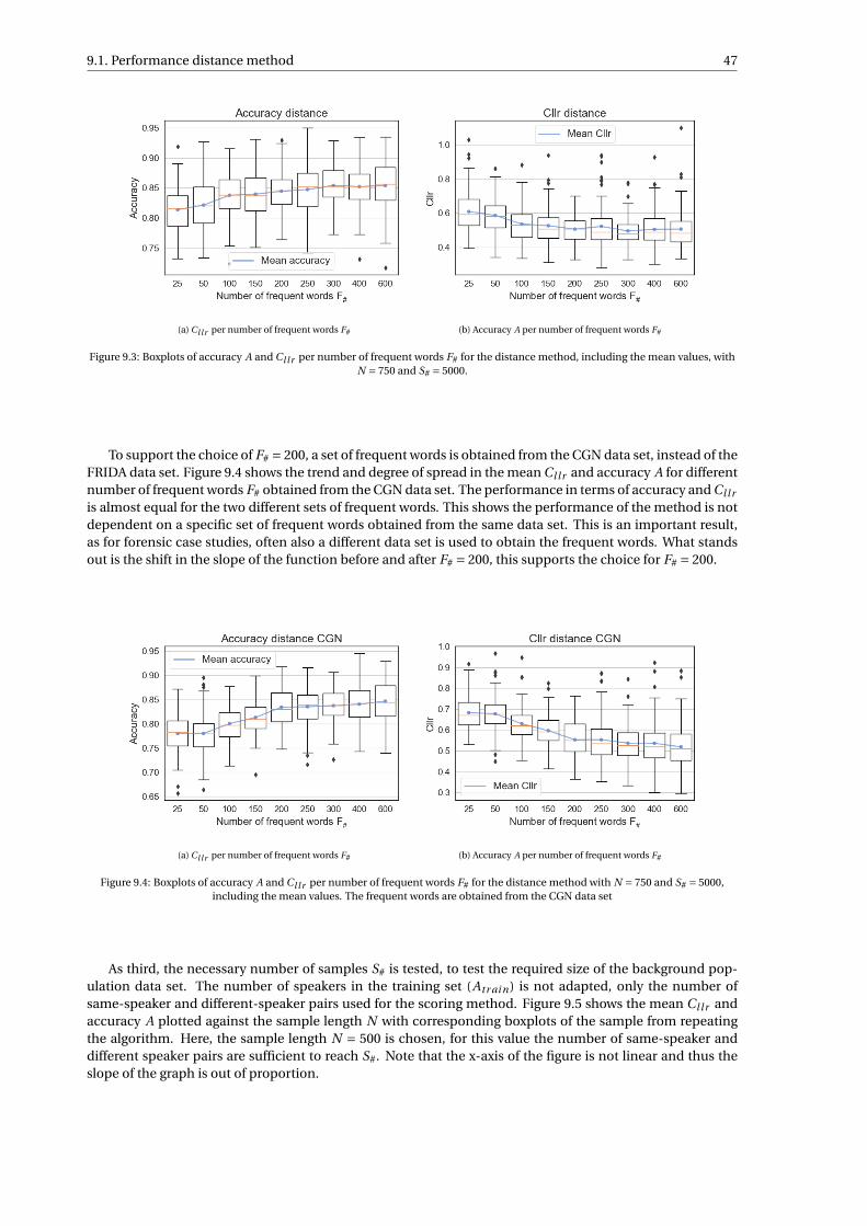
9.1. Performance distance method 47

(a) Cl l r per number of frequent words F# (b) Accuracy A per number of frequent words F#

Figure 9.3: Boxplots of accuracy A and Cl l r per number of frequent words F# for the distance method, including the mean values, withN = 750 and S# = 5000.

To support the choice of F# = 200, a set of frequent words is obtained from the CGN data set, instead of theFRIDA data set. Figure 9.4 shows the trend and degree of spread in the mean Cl l r and accuracy A for differentnumber of frequent words F# obtained from the CGN data set. The performance in terms of accuracy and Cl l r

is almost equal for the two different sets of frequent words. This shows the performance of the method is notdependent on a specific set of frequent words obtained from the same data set. This is an important result,as for forensic case studies, often also a different data set is used to obtain the frequent words. What standsout is the shift in the slope of the function before and after F# = 200, this supports the choice for F# = 200.

(a) Cl l r per number of frequent words F# (b) Accuracy A per number of frequent words F#

Figure 9.4: Boxplots of accuracy A and Cl l r per number of frequent words F# for the distance method with N = 750 and S# = 5000,including the mean values. The frequent words are obtained from the CGN data set

As third, the necessary number of samples S# is tested, to test the required size of the background pop-ulation data set. The number of speakers in the training set (Atr ai n) is not adapted, only the number ofsame-speaker and different-speaker pairs used for the scoring method. Figure 9.5 shows the mean Cl l r andaccuracy A plotted against the sample length N with corresponding boxplots of the sample from repeatingthe algorithm. Here, the sample length N = 500 is chosen, for this value the number of same-speaker anddifferent speaker pairs are sufficient to reach S#. Note that the x-axis of the figure is not linear and thus theslope of the graph is out of proportion.

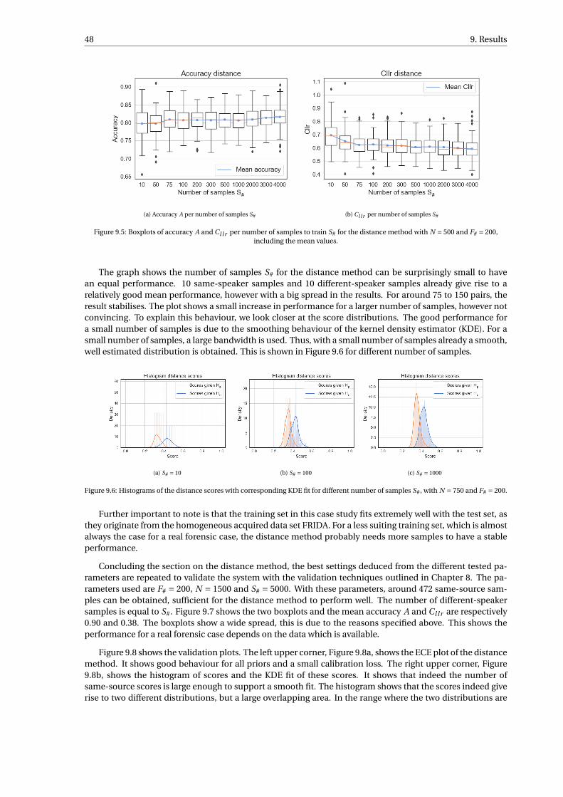
48 9. Results

(a) Accuracy A per number of samples S# (b) Cl l r per number of samples S#

Figure 9.5: Boxplots of accuracy A and Cl l r per number of samples to train S# for the distance method with N = 500 and F# = 200,including the mean values.

The graph shows the number of samples S# for the distance method can be surprisingly small to havean equal performance. 10 same-speaker samples and 10 different-speaker samples already give rise to arelatively good mean performance, however with a big spread in the results. For around 75 to 150 pairs, theresult stabilises. The plot shows a small increase in performance for a larger number of samples, however notconvincing. To explain this behaviour, we look closer at the score distributions. The good performance fora small number of samples is due to the smoothing behaviour of the kernel density estimator (KDE). For asmall number of samples, a large bandwidth is used. Thus, with a small number of samples already a smooth,well estimated distribution is obtained. This is shown in Figure 9.6 for different number of samples.

(a) S# = 10 (b) S# = 100 (c) S# = 1000

Figure 9.6: Histograms of the distance scores with corresponding KDE fit for different number of samples S#, with N = 750 and F# = 200.

Further important to note is that the training set in this case study fits extremely well with the test set, asthey originate from the homogeneous acquired data set FRIDA. For a less suiting training set, which is almostalways the case for a real forensic case, the distance method probably needs more samples to have a stableperformance.

Concluding the section on the distance method, the best settings deduced from the different tested pa-rameters are repeated to validate the system with the validation techniques outlined in Chapter 8. The pa-rameters used are F# = 200, N = 1500 and S# = 5000. With these parameters, around 472 same-source sam-ples can be obtained, sufficient for the distance method to perform well. The number of different-speakersamples is equal to S#. Figure 9.7 shows the two boxplots and the mean accuracy A and Cl l r are respectively0.90 and 0.38. The boxplots show a wide spread, this is due to the reasons specified above. This shows theperformance for a real forensic case depends on the data which is available.

Figure 9.8 shows the validation plots. The left upper corner, Figure 9.8a, shows the ECE plot of the distancemethod. It shows good behaviour for all priors and a small calibration loss. The right upper corner, Figure9.8b, shows the histogram of scores and the KDE fit of these scores. It shows that indeed the number ofsame-source scores is large enough to support a smooth fit. The histogram shows that the scores indeed giverise to two different distributions, but a large overlapping area. In the range where the two distributions are

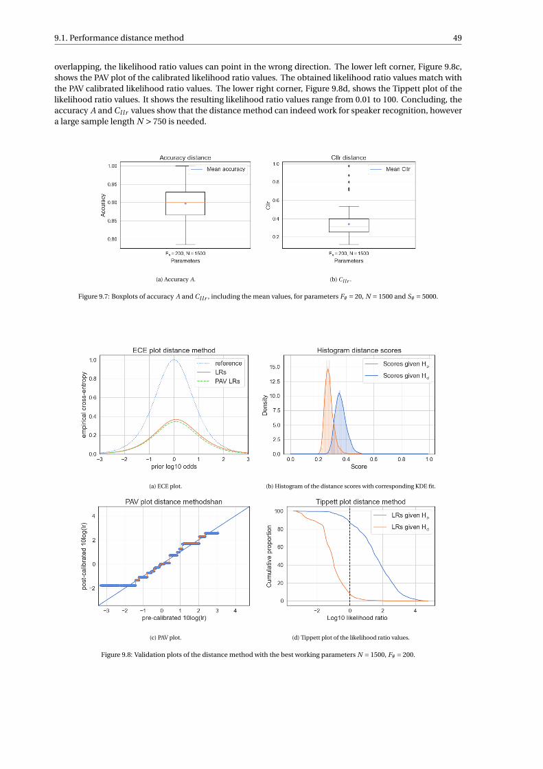
9.1. Performance distance method 49

overlapping, the likelihood ratio values can point in the wrong direction. The lower left corner, Figure 9.8c,shows the PAV plot of the calibrated likelihood ratio values. The obtained likelihood ratio values match withthe PAV calibrated likelihood ratio values. The lower right corner, Figure 9.8d, shows the Tippett plot of thelikelihood ratio values. It shows the resulting likelihood ratio values range from 0.01 to 100. Concluding, theaccuracy A and Cl l r values show that the distance method can indeed work for speaker recognition, howevera large sample length N > 750 is needed.

(a) Accuracy A. (b) Cl l r .

Figure 9.7: Boxplots of accuracy A and Cl l r , including the mean values, for parameters F# = 20, N = 1500 and S# = 5000.

(a) ECE plot. (b) Histogram of the distance scores with corresponding KDE fit.

(c) PAV plot. (d) Tippett plot of the likelihood ratio values.

Figure 9.8: Validation plots of the distance method with the best working parameters N = 1500, F# = 200.

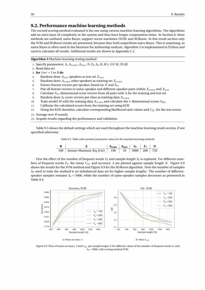
50 9. Results

9.2. Performance machine learning methodsThe second scoring method evaluated is the one using various machine learning algorithms. The algorithmsadd an extra layer of complexity to the system and thus have longer computation times. In Section 6, threemethods are outlined, naive Bayes, support vector machines (SVM) and XGBoost. In this result section onlythe SVM and XGBoost results are presented, because they both outperform naive Bayes. This is surprising, asnaive Bayes is often used in the literature for authorship analysis. Algorithm 3 is implemented in Python andused to calculate all results. Additional results are shown in Appendix C.2.

Algorithm 3 Machine learning testing method

1: Specify parameters: ∆, Atr ai n , Atest , N ,F#,S#,R, M ∈ SV M , XGB 2: Read data set3: for i ter = 1 to R do4: Random draw Atest speakers as test set X test

5: Random draw Atr ai n other speakers as training set X tr ai n

6: Extract feature vectors per speaker, based on N and F#s

7: Pair all feature vectors to same-speaker and different-speaker pairs within X tr ai n and X test

8: Calculate F#s -dimensional score vectors from all pairs with ∆ for the training and test set9: Random draw S# score vectors per class as training data X tr ai n

10: Train model M with the training data X tr ai n and calculate the 1-dimensional scores SML

11: Calibrate the calculated scores from the training set using KDE12: Using the KDE densities, calculate corresponding likelihood ratio values and Cl l r for the test scores

13: Average over R rounds14: Acquire results regarding the performance and validation

Table 9.5 shows the default settings which are used throughout the machine learning result section, if notspecified otherwise.

Table 9.5: Table with standard parameter values for the machine learning methods

R ∆ Atrain Atest S# F# N100 Jensen-Shannon (Eq (6.6)) 190 10 5000 200 750

First the effect of the number of frequent words F# and sample length S# is explored. For different num-bers of frequent words F#, the mean Cl l r and accuracy A are plotted against sample length N . Figure 9.9shows the results for the SVM method and Figure 9.9 for the XGBoost algorithm. Note the number of samplesS# used to train the method is an imbalanced data set for higher sample lengths. The number of different-speaker samples remains S# = 5000, while the number of same-speaker samples decreases as presented inTable 9.4.

(a) Mean accuracy A. (b) Mean Cl l r .

Figure 9.9: Plots of mean accuracy A and Cl l r per sample length N for different values of the number of frequent words F# andS# = 5000, with scoring method SVM.

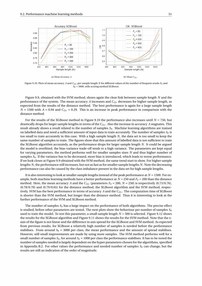
9.2. Performance machine learning methods 51

(a) Mean Accuracy A. (b) Mean Cl l r .

Figure 9.10: Plots of mean accuracy A and Cl l r per sample length N for different values of the number of frequent words F# andS# = 5000, with scoring method XGBoost.

Figure 9.9, obtained with the SVM method, shows again the clear link between sample length N and theperformance of the system. The mean accuracy A increases and Cl l r decreases for higher sample length, asexpected from the results of the distance method. The best performance is again for a large sample lengthN = 1500 with A = 0.94 and Cl l r = 0.29. This is an increase in peak performance in comparison with thedistance method.

For the results of the XGBoost method in Figure 9.10 the performance also increases until N = 750, butdrastically drops for larger sample lengths in terms of the Cl l r . Also the increase in accuracy A stagnates. Thisresult already shows a result related to the number of samples S#. Machine learning algorithms are trainedon labelled data and need a sufficient amount of input data to train accurately. The number of samples S# istoo small to train accurately in this case. With a high sample length N , the data set is too small to keep thesame number of samples to train. The figures show that this amount of labelled data is not sufficient to trainthe XGBoost algorithm accurately, as the performance drops for larger sample length N . It could be arguedthe model is overfitted, the bias-variance trade-off tends to a high variance. The parameters are kept equalfor varying parameters, the method performs well for smaller samples sizes N and thus higher number ofsamples S#. If the variance has to be decreased, more bias is introduced, which leads to worse performance.If we look closer at Figure 9.9 obtained with the SVM method, the same trend start to show. For higher samplelengths N , the performance still increases, but not as fast as for smaller sample lengths N . Note the decreasingperformance can also be caused by the class imbalance present in the data set for high sample lengths.

It is also interesting to look at smaller sample lengths instead of the peak performance at N = 1500. For ex-ample, both machine learning methods have a better performance at N = 250 and F# = 200 than the distancemethod. Here, the mean accuracy A and the Cl l r (parameters F# = 200, N = 250) is respectively (0.73/0.76),(0.78/0.70) and (0.79/0.65) for the distance method, the XGBoost algorithm and the SVM method, respec-tively. SVM has the best performance in terms of accuracy A and the Cl l r . The computation time of XGBoostis shorter than the SVM method, but longer than the distance method. Thus it is interesting to look at thefurther performance of the SVM and XGBoost method.

The number of samples S# has a large impact on the performance of both algorithms. The precise effectis studied, before other parameters are tested. The next plots show the behaviour per number of samples S#

used to train the model. To test this parameter, a small sample length N = 500 is selected. Figure 9.12 showsthe results for the XGBoost algorithm and Figure 9.11 shows the results for the SVM method. Note that the x-axis of the figure is not linear and the difference in axis spread for the XGBoost and SVM method. As expectedfrom previous results, for XGBoost a relatively high number of samples is needed before the performancestabilises. From around S# = 3000 per class, the mean performance and the amount of spread stabilises.However, still small improvements are made by using more samples. The SVM method performs well for asmall number of samples S#, for around S# = 1000 per class the performance stabilises. It has to be noted thenumber of samples needed is largely dependent on the hyper parameters chosen for the algorithms, specifiedin Appendix B.2. For other values the performance and needed number of samples S# can change, but theresults are still an indication of the order of magnitude.

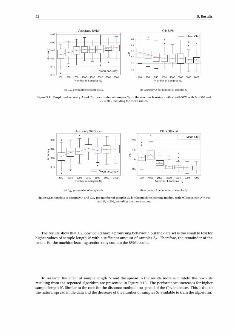
52 9. Results

(a) Cl l r per number of samples S#. (b) Accuracy A per number of samples S#.

Figure 9.11: Boxplots of accuracy A and Cl l r per number of samples S# for the machine learning method with SVM with N = 500 andF# = 200, including the mean values.

(a) Cl l r per number of samples S#. (b) Accuracy A per number of samples S#.

Figure 9.12: Boxplots of accuracy A and Cl l r per number of samples S# for the machine learning method with XGBoost with N = 500and F# = 200, including the mean values.

The results show that XGBoost could have a promising behaviour, but the data set is too small to test forhigher values of sample length N with a sufficient amount of samples S#. Therefore, the remainder of theresults for the machine learning section only contain the SVM results.

To research the effect of sample length N and the spread in the results more accurately, the boxplotsresulting from the repeated algorithm are presented in Figure 9.13. The performance increases for highersample length N . Similar to the case for the distance method, the spread of the Cl l r increases. This is due tothe natural spread in the data and the decrease of the number of samples S# available to train the algorithm.

9.2. Performance machine learning methods 53

(a) Cl l r per sample length N . (b) Accuracy A per sample length N .

Figure 9.13: Boxplots of accuracy A and Cl l r per sample length N for the machine learning method with SVM, including the meanvalues, with F# = 200 and S# = 5000.

Finally, the effect of the number of frequent words F# is studied. The results are obtained for sample lengthN = 750, to ensure a consistent number of samples S#. Figure 9.14 shows the boxplots and mean line for theSVM method. The mean accuracy A and Cl l r stabilises around F# = 200. Since using more features increasesthe possibility of overfitting and a simple model supports more stable predictions, F# = 200 is the optimalchoice. Again it is noted although for smaller values of the number of frequent words F# the performancedecreases, it still shows a discriminating ability.

(a) Cl l r per number of frequent words F#. (b) Accuracy A per number of frequent words F#.

Figure 9.14: Boxplots of accuracy A and Cl l r per number of frequent words F# for the machine learning method with the SVM method,including the mean values, with N = 750 and S# = 5000.

Concluding the section about the results of the machine learning method, the best settings deduced fromthe sensitivity analysis are repeated to validate the system with the validation techniques outlined in Chap-ter 8. For the current data set used, SVM shows the most promising behaviour. The optimal parameters usedfor the SVM method are F# = 200, N = 1500 and all samples (maximal S#) that are possible to obtain from thetotal background population. Figure 9.15 shows the two boxplots, the mean Cl l r and the accuracy A are 0.28and 0.94, respectively. The boxplots show a wide spread, this is due to the same reasons as specified above.This shows that the performance for a real forensic case depends on the available data and the speakerspresent in the data set.

Figure 9.16 shows the validation plots. The left upper corner, Figure 9.16a, shows the ECE plot. The rightupper corner, Figure 9.16b, shows the histogram of scores and the KDE fit of the scores. The fit is inaccurate,because the bandwidth is quite large for the sudden peak in the distribution of scores. Also, the bandwidth isnot well estimated, since the score distributions is not close to a Gaussian. It does show a large discriminatingpower between same-speaker and different-speaker feature pairs. The left lower corner, Figure 9.16c, showsthe PAV plot of the calibrated likelihood ratio values. The plot shows that for lower likelihood ratio values

54 9. Results

10log(LR) ≤−1, the likelihood ratios are overestimated in comparison with the optimal calibrated likelihoodratios. The right lower corner, Figure 9.16d, shows the Tippett plot of the likelihood ratio values. The valuesof the resulting likelihood ratios range from 0.05 to 100. This is slightly more conservative than the likelihoodratios obtained from the distance method. The Cl l r values are, however, lower than for the distance method.Concluding, the accuracy A and Cl l r values show that the SVM method performs better than the distancemethod for the best performing parameters. An interesting area for further research is for lower samples sizesN , where the machine learning algorithms both outperform the distance method. This area is interesting tostudy for a specific real forensic case, where it could lead to promising results.

(a) Accuracy A. (b) Cl l r .

Figure 9.15: Boxplots of accuracy A and Cl l r , including the mean values, for parameters F# = 200, N = 1500 and scoring method SVM.

(a) ECE plot. (b) Histogram of the distance scores with corresponding KDE fit.

(c) PAV plot. (d) Tippett plot of the likelihood ratio values.

Figure 9.16: Validation plots of the SVM method with the best performing parameters N = 1500, F# = 200.

9.3. Performance LR score method 55

9.3. Performance LR score methodThis chapter presents the LR score results. The chapter is divided in two sections, the common source modelresults and the specific source model results. First the common source model results are analysed. After-wards, it is explored if specific source modelling with a small amount of specific speaker data leads to betterperformance. All results for the LR score method are obtained using Algorithm 4. Additional results are shownin Appendix C.3.

Algorithm 4 LR score

1: Specify parameters: Atr ai n , Atest , N ,F#,S#,S#s ,R, M ∈ common,specific2: Read data set3: for i ter = 1 to R do4: Random draw Atest speakers as test set X test

5: Random draw Atr ai n other speakers as training set X tr ai n

6: Extract feature vectors per speaker, based on N and F#s

7: Estimate the between-source and within-source distribution parameters µb , Σb and Σw from thetraining set

8: if M = common then9: Pair all feature vectors to same-speaker and different-speaker pairs according to Figure 3.2

10: Calculate 1-dimensional scores SLR from all pairs in the training set X tr ai n and test set X test usingEquation (6.21)

11: if M = specific then12: Random draw S#s samples per speaker from the specific speaker samples13: Estimate the specific speaker distribution parameters µs from the training set14: Calculate 1-dimensional scores SLR from all feature vectors in the training set X tr ai n and test set

X test using Equation (6.23)

15: Calibrate the calculated scores SLR using KDE16: Using the KDE densities, calculate corresponding likelihood ratio values and Cl l r for the test scores

17: Average over R rounds18: Acquire results regarding the performance and validation

Table 9.6 shows the default parameters which are used throughout the LR score results section, if notspecified otherwise. Note that the number of speakers used in the training set Atr ai n is lower than for theprevious used methods. Some speakers in the data set have a relatively small set of speech fragments. Forthe specific source model a long fragment of speech is needed, as the data has to be divided in a trainingand test set for the specific speaker. Speakers with small speech fragments are not suitable for this method.As the F#-dimensional parameters indexing the distributions have to be estimated, a large amount of datais needed. Exploratory results showed that even when using all feature vectors obtained from Atr ai n , themethod can be unstable. The estimated parameters result in numerical instabilities, leading to a singularcovariance matrix or under- or overflow errors. These errors occur when a calculated number is smaller thana computer can store. Therefore, all data available in the training set is used to estimate the parameters forall results presented in this chapter. Hence, the number of samples S# is not specified in Table 9.6. All datacorresponds to approximately 40 minutes of speech per speaker from 170 speakers.

Table 9.6: Table with default parameter values for LR score results.

R Atrain Atest S# F# N S#s

100 170 10 - 50 500 5

9.3.1. Common source LR score methodThe common source results start with presenting the performance per sample length N for different values ofthe number of frequent words F#. Figure 9.17 shows the mean Cl l r and the accuracy A for the common sourceLR score method. As expected from previous results, the performance increases for higher sample lengths N .The method is only tested for N ∈ [250,750], because the method is unstable for higher sample lengths N . Themethod implemented in Python shows numerical underflow problems. The best performance is reached for

56 9. Results

N = 750 and F# = 35, with A = 0.84 and Cl l r = 0.54. The results are similar to the results from the distancemethod. The results are worse than the result obtained with the SVM method.

(a) Accuracy A. (b) Cl l r .

Figure 9.17: Plots of mean accuracy A and Cl l r per sample length N for different values of number of frequent words F# for thecommon source LR score method.

To further investigate the results, the spread of the results for varying sample lengths is analysed. Figure9.18 shows the boxplots and mean line for varying sample lengths N . It shows the increasing performance forlarger sample length, but also the increase in the spread of the Cl l r values for larger sample lengths N . Thisresult suggests the estimated distributions do not define the underlying process correctly for larger samplessizes. This can be explained by the decrease of the number of samples for larger sample lengths N . As alreadyearlier denoted, the data set is limited, so increasing the sample length results in a smaller number of samples.

(a) Accuracy A. (b) Cl l r .

Figure 9.18: Boxplots of accuracy A and Cl l r per sample length N for the common source LR score method with F# = 50, including themean values.

The effect of varying the number of frequent words is shown in Figure 9.19. The plot shows a surprising re-sult, the performance is almost stable for varying number of frequent words F#. The method is only tested forF# ∈ [20,60], because the method is unstable for higher number of frequent words. A possible explanation forthe instability for higher number of frequent words F#, is the higher dimensional distribution that has to beestimated. The plots show the best performance at F# = 40, but this trend is not convincing given the spreadin the results and the small improvement in performance. This result differs from results obtained with thedistance method and the machine learning methods. This can be explained since the LR score method esti-mates the parameters of a feature-based F#-dimensional distribution. The results suggest trying to estimatea higher dimensional distribution adds more uncertainty and does not lead to a better performance.

9.3. Performance LR score method 57

(a) Accuracy A. (b) Cl l r .

Figure 9.19: Boxplots of accuracy A and Cl l r per number of frequent words F# for the common source LR score method with N = 500,including the mean values.

The two results for varying sample lengths N and number of frequent words F# show that the commonsource LR score method does not perform better than the baseline method. It supports the choice of completescore-based approaches, as estimating the feature-based likelihood ratio with the specified assumptions doesnot show better results. To complete the section on the results of the common source score LR, the best resultsare shown in Figure 9.20, with parameters F# = 40 and N = 750. The two boxplots and the mean accuracy Aand Cl l r are 0.84 and 0.53, respectively.

(a) Accuracy A. (b) Cl l r .

Figure 9.20: Boxplots of accuracy A and Cl l r , including the mean values, for parameters F# = 40, N = 750 and scoring method commonsource LR score.

The validation plots for the best performing parameters are shown in Figure 9.21. The upper left corner,Figure 9.21a, shows the ECE plot. The plot shows the method is calibrated very well with almost no calibrationloss. This is confirmed by the PAV plot shown in Figure 9.21c. The upper right corner, Figure 9.21b, shows thehistogram of scores and the KDE fit of the scores. The fit of the two distributions is accurate. The histogramshows the scores give rise to two overlapping distributions. This shows the discriminating power between thetwo hypotheses is not sufficient. The lower right corner, Figure 9.21d, shows the Tippett plot of the likelihoodratio values. The main part of the resulting likelihood ratios range from 0.1 to 10. These values indicate thatthe common source score LR method does not show great discriminating power between the two hypotheses.

58 9. Results

(a) ECE plot. (b) Histogram of the distance scores with corresponding KDE fit.

(c) PAV plot. (d) Tippett plot of the likelihood ratio values.

Figure 9.21: Validation plots of the distance method with the best working parameters N = 750, F# = 40.

9.3.2. Specific source LR score methodAll results so far are obtained using the common source model. In addition to these results, the LR scoremodel is also implemented applied to the specific source model. This gives rise to a different, more spe-cific set competing hypotheses, more interesting for a judge. Since the scores are calculated using a specificspeaker data set, this could lead to better or other results. The specific source model is possible for the LRscore method only under strong assumptions. For the specific source model besides a background popu-lation of alternative speakers, a specific speaker data set is needed. The specific speaker data set is oftenlimited, so an important question is whether it is possible to use the specific source model with limited data.The score LR assumes a parametric normal distribution for the specific speaker distribution. The parametersare estimated using the background data set and the samples of the specific speaker.

To first test the amount of specific speaker data that is needed to model the specific source LR method,the results for varying number of specific speaker samples S#s are presented in Figure 9.22. The x-axis showsthe total number of samples used to estimate µs . Note the small number of specific speaker samples to es-timate the specific speaker distribution. The amount of samples is very small to estimate an F#-dimensionalindexing parameter.

The figure shows the performance increases for a higher number of specific speaker samples S#s . This re-sult is expected, as this means more samples are available to fit the specific speaker distribution. The methodis only stable for a relatively low number of frequent words F#, as the co-variance matrix is singular for highervalues. Furthermore, the available amount of data per speaker is too small to test for a larger number of spe-cific speaker samples S#s . Keeping the practical implementation in mind, probably not more specific speakersamples will be present in a real forensic case. Therefore, for the next section the number of specific speakersamples is fixed at S#s = 5. The performance for different sample lengths N including the spread is interesting,as the estimated distribution is based on a small number of samples. What is interesting is that the perfor-mance for the relatively small sample length N = 250 is A = 0.78 and Cl l r = 0.68. This is slightly better than

9.3. Performance LR score method 59

the distance method for this sample length, the distance method had an accuracy of A = 0.77 and Cl l r = 0.74with F# = 200. Note that the competing hypotheses are different as the distance method is only applied to thecommon source model. A comparison of the performance of the methods using different hypotheses shouldbe made carefully. Figure 9.23 shows the spread in the results for varying number of specific speaker samples.It shows a relative large spread in the results is present for all values of S#s , but no difference in the amount ofspread for increasing or decreasing number of specific speaker samples.

(a) Accuracy A. (b) Cl l r .

Figure 9.22: Plots of mean accuracy A and Cl l r per number of samples of the specific source S#s for different values of number offrequent words F# and sample length N = 250. The scoring method used is the specific source LR score.

(a) Accuracy A. (b) Cl l r .

Figure 9.23: Boxplots of accuracy A and Cl l r per sample length number of specific speaker samples S#s for the specific source LR scoremethod with F# = 20 and N = 250, including the mean values.

Figure 9.24 shows the performance of the specific source LR score method for varying sample lengths N .The method is only tested in the range N ∈ [200,600], as the data per speaker is too small to test for highersample lengths N . The figure shows an increase in performance and in spread for larger sample lengths N .This can again be explained by the decrease of the number of samples available at higher sample lengths.

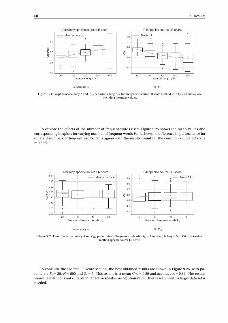
60 9. Results

(a) Accuracy A. (b) Cl l r .

Figure 9.24: Boxplots of accuracy A and Cl l r per sample length N for the specific source LR score method with F# = 20 and S# = 5,including the mean values.

To explore the effects of the number of frequent words used, Figure 9.25 shows the mean values andcorresponding boxplots for varying number of frequent words F#. It shows no difference in performance fordifferent numbers of frequent words. This agrees with the results found for the common source LR scoremethod.

(a) Accuracy A. (b) Cl l r .

Figure 9.25: Plots of mean accuracy A and Cl l r per number of frequent words with S#s = 5 and sample length N = 500 with scoringmethod specific source LR score.

To conclude the specific LR score section, the best obtained results are shown in Figure 9.26, with pa-rameters F# = 20, N = 500 and S# = 5. This results in a mean Cl l r = 0.59 and accuracy A = 0.84. The resultsshow the method is not suitable for effective speaker recognition yet, further research with a larger data set isneeded.

9.3. Performance LR score method 61

(a) Accuracy A. (b) Cl l r .

Figure 9.26: Boxplots of accuracy A and Cl l r , including the mean values, for parameters N = 500, F# = 20 and S#s = 5, and scoringmethod specific source LR score.

Figure 9.27 shows the validation plots for the the specific source LR score method with parameters N =500, F# = 20 and S#s = 5. The upper left corner, Figure 9.27a, shows the ECE plot. The plot shows the methodis calibrated well with almost no calibration loss. The lower left corner, Figure 9.27c, shows the PAV plot.The plot shows the calibration for the lower likelihood ratios is conservative. For higher likelihood ratios themethod is well-calibrated. The upper right corner, Figure 9.27b, shows the histogram of scores and the KDEfit of the scores. The fit of the two distributions is accurate. The histogram shows that the scores give rise totwo overlapping distributions. The lower right corner, Figure 9.27d, shows the Tippett plot of the likelihoodratio values. The main part of the resulting likelihood ratios range from 0.1 to 10. These values show that thespecific source score LR method does not show great discriminating power between the two hypotheses.

(a) ECE plot. (b) Histogram of the distance scores with corresponding KDE fit.

(c) PAV plot. (d) Tippett plot of the likelihood ratio values.

Figure 9.27: Validation plots of specific source LR score with the best performing parameters N = 500, F# = 20 and S#s = 5.

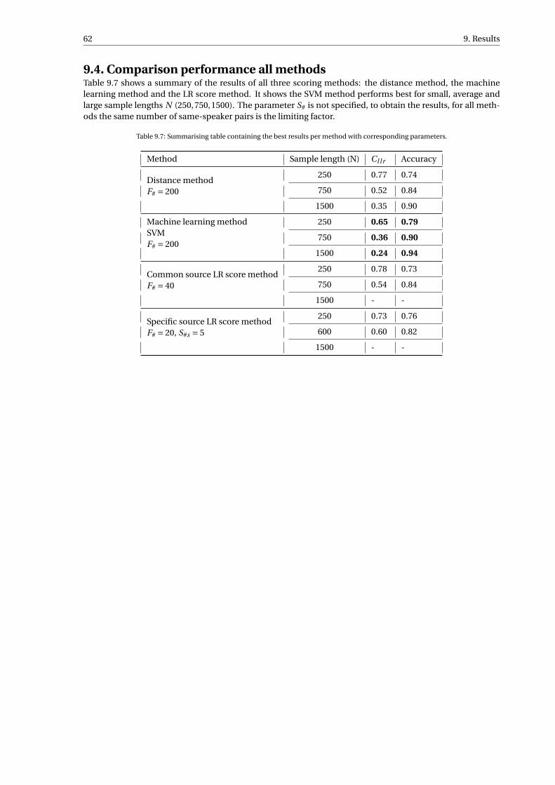
62 9. Results

9.4. Comparison performance all methodsTable 9.7 shows a summary of the results of all three scoring methods: the distance method, the machinelearning method and the LR score method. It shows the SVM method performs best for small, average andlarge sample lengths N (250,750,1500). The parameter S# is not specified, to obtain the results, for all meth-ods the same number of same-speaker pairs is the limiting factor.

Table 9.7: Summarising table containing the best results per method with corresponding parameters.

Method Sample length (N) Cl l r Accuracy

Distance methodF# = 200

250 0.77 0.74

750 0.52 0.84

1500 0.35 0.90

Machine learning methodSVMF# = 200

250 0.65 0.79

750 0.36 0.90

1500 0.24 0.94

Common source LR score methodF# = 40

250 0.78 0.73

750 0.54 0.84

1500 - -

Specific source LR score methodF# = 20, S#s = 5

250 0.73 0.76

600 0.60 0.82

1500 - -

10Conclusion and recommendations

In this chapter, first the conclusions and discussion are presented. Afterwards, the recommendations forfuture research based on the conclusions from this research are presented.

10.1. Conclusion and discussionThe objective of this research was to quantify the evidential value in the transcription of a speech fragment.The value of evidence is quantified by the likelihood ratio. The common source and specific source model forthe identification of source question are outlined and discussed for application to speaker recognition. Theprocess from input data to validated likelihood ratio is explored and constructed. Since the method basedon text analysis of the transcription is independent from current automatic speaker recognition, it wouldcontribute significantly to the overall evidential value.

The data used is the FRIDA data set consisting of transcriptions of 250 speakers. To transform the rawdata to numerical feature vectors, a relevant set of features is needed. Features used in authorship analysis ofwritten text are analysed for implementation in speaker recognition. The most promising category of featuresare the frequencies of occurrence of frequent words, also called function words.

The feature vectors are transformed to scores, according to the common source model. The commonsource model is the most suitable approach for modelling the forensic case study, given the available data.However, the common source model is more conservative than the specific source model. Three differentscoring methods are proposed in this research. This is the main distinction in the likelihood ratio approachesinvestigated in this research. As a baseline, a method based on a distance metric is used, where the scoreis the distance between two feature vectors. To improve upon this baseline, several machine learning algo-rithms are applied to calculate a score from the feature vectors. The best results are obtained for supportvector machines and XGBoost, a decision tree based algorithm. As a third method a score likelihood ratio iscalculated under several assumptions based on the feature vector. It is used as score instead of a direct likeli-hood ratio. The likelihood ratio score method is also applied following the specific source framework, to testif better performance can be achieved. The score likelihood ratio approach is tested as it includes similarityand typicality.

The scores obtained from the scoring algorithms give rise to two probability distributions, the same-speaker and different-speaker score distribution, which are estimated with KDE. Using the estimated distri-bution, the test scores are transformed to a likelihood ratio. The resulting likelihood ratio values are validatedby inspecting several performance characteristics. The main characteristics are discriminating power, accu-racy and calibration. The most important corresponding metrics are the cost log-likelihood ratio Cl l r and theaccuracy A. Furthermore, the results are presented in the form of an ECE plot, a PAV plot and a Tippett plot.The Tippett plot shows the distribution of the resulting likelihood ratios given the hypotheses.

The resulting likelihood ratios show that information about the speaker is contained in the transcriptionof a speech fragment, which is a promising performance. To further test the applicability, a sensitivity analysisis performed for the sample length N , the number of frequent words F# and the number of samples to trainS#. The parameters tested in this thesis can be used as a guideline to explore the possibilities in a real forensiccase.

63

64 10. Conclusion and recommendations

Three main outcomes can be concluded from the results of all methods. First, the sample length N hasa large effect on the performance of the likelihood ratio method. In general, higher sample lengths give bet-ter performance. It can be concluded for a common source framework, that samples with sample lengthN < 750 do not contain enough information to distinguish effectively between same-speaker and different-speaker pairs. A critical point is that a large sample length implies a smaller number of samples available.Secondly, in the range of number of frequent words F# ≤ 200, an increase of frequent words F# results in abetter performance. The performance stabilises for values larger than F# = 200. It shows most of the informa-tion is contained in the 200 most frequent words. The performance only decreases slowly for smaller valuesof frequent words F#, although small values still show discriminating power. For frequent words obtainedfrom the FRIDA data set, as with frequent words obtained from the CGN data set, the same effect is present.Thirdly, all results show a substantial spread in terms of accuracy and the Cl l r , this is due to differences be-tween distinctive speech per speaker and thus differences in the results. The results are further discussed perscoring method.

The distance method shows best performance with the Jensen–Shannon distance measure. A solid base-line is established with A = 0.9 and Cl l r = 0.35 for N = 1500 and F# = 200. The results suggest only a smallnumber of samples S# = 100 is needed to train the model accurately. However, it is important to note that if abackground data set is used which is less similar to the test set, maybe more samples are needed.

The machine learning methods SVM and XGBoost both show better performance than the other methodsfor smaller sample lengths N and thus a large amount of samples S#. However, XGBoost needs a too largetraining set to gain a good performance for large sample lengths N . For both machine learning methods, arelatively high number of samples is needed to train the model. Around S# = 3000 and S# = 1000 samples forthe XGBoost algorithm and SVM method, respectively. SVM shows the best performance of all methods, witha peak performance of A = 0.94 and Cl l r = 0.24 for N = 1500 and F# = 200. Also for smaller samples sizes inthe range between 250 ≤ N ≤ 1500, SVM outperforms the baseline established by the distance method.

The score likelihood ratio methods are used to find out whether a feature-based method which includedtypicality could lead to better performance. The results for the specific and common source approach weresimilar to the baseline set by the distance method for small sample lengths N ≤ 700. The method is numer-ically unstable to test for larger sample lengths. As the feature space is large and the method is unstable, thenumber of sample parameter S# is not tested. For this method a larger data set and further research is needed.

In summary, in this thesis it has been shown that information about the speaker is contained in tran-scriptions of speech fragments. This is shown for the case where a limited amount of data is available froma suspect, as often appears in a real forensic case. The complete process from data to likelihood ratio is con-structed and the likelihood ratio system using SVM has shown the best results. A sensitivity analysis has beenperformed to determine a guideline for the used parameters. This research brings us one step closer to thegoal of using the method in a real forensic case. For the next steps, a set of recommendations is provided inthe next section.

This research is the first step in the goal of using text analysis of transcribed speech fragments to quantifythe evidential value of a speech fragment. To use the method in a real forensic case, more research is needed.A set of recommendations is outlined in the next section.

10.2. Recommendations for future workThis thesis shows support that evidential information is contained in transcriptions of spoken text.

• In this thesis the common source framework is used because of the limited available data in most foren-sic cases. This is the most suitable model regarding the data, but less suitable regarding the questionof interest of a judge. Furthermore, no specific suspect is used as known background information. It isinteresting to investigate the performance when the specific source model is implemented. The largesample length needed for a good performance in the common source model, could lead to more sam-ples of smaller sample length. The samples can be used to model a specific source approach. Especiallyfor the distance method, where only a small number of samples is needed for a stable performance, itis interesting to further investigate this option.

10.2. Recommendations for future work 65

• The method is developed and tested using only speakers present in the FRIDA data set. For furthervalidation, a study with the speakers present in the CGN data set or in real forensic case data is rec-ommended. It is interesting to investigate whether the guidelines for the constraints on parametersresulting from this thesis, will also apply in a real forensic case. During further testing, also validationcriteria need to be determined. Furthermore, the data from the FRIDA data set is immediately usedas input for the method. Only a small data selection is performed, based on the amount of data avail-able per speaker. For further research, performance can possibly be improved by more extensive dataexploring.

• The feature set selected in this research consists only of frequencies of frequent words. Although thisis a feature set often used, it is interesting to investigate if other features can improve the performance.New features can be extracted automatically from the transcriptions, but can also be determined incombination with speech experts. The speech expert can point out important distinguishing featuresused in a conversation, which are not found by using automated extracted features. It is interesting totest the combination of automatic extracted features and features from a speech expert.

• The research in this thesis was focused on the overall performance of a likelihood ratio system forspeaker recognition. A large spread in the performance of the system is shown in the results section.Since the test set contains different speakers for every iteration, no conclusion can be made regardingthe stability of the method for one speaker. We recommend to test the stability of the method by testingthe method for a single speaker.

• It is recommended to research the assumed independency between the automatic speaker methodand the text analysis method. To combine the evidential value obtained from both methods, the de-pendency structure has to be precisely validated. Using the assumed independency, the text analysismethod contributes largely to the overall evidential value.

• The scoring methods used in this thesis are all statistical models or basic machine learning models. Itis interesting to investigate whether a convolutional neural network model can achieve a better perfor-mance. Several authorship analysis studies already used a form of a convolutional neural network withfrequency based features and showed promising results [49]. However, it has to be noted that the ex-plainability of the method becomes more challenging. This is a trade-off important for forensic analysisused in court.

Bibliography

[1] Project Corpus Gesproken Nederlands. Technical report. URL http://lands.let.ru.nl/cgn/.

[2] Colin G. G. Aitken, Grzegorz Zadora, and David Lucy. A Two-Level Model for Evidence Evaluation. Jour-nal of Forensic Sciences, 52(2):412–419, 3 2007. doi: 10.1111/j.1556-4029.2006.00358.x.

[3] Muna AlSallal, Rahat Iqbal, Vasile Palade, Saad Amin, and Victor Chang. An integrated approach forintrinsic plagiarism detection. Future Generation Computer Systems, 96:700–712, 2019. ISSN 0167739X.doi: 10.1016/j.future.2017.11.023.

[4] Alaa Saleh Altheneyan and Mohamed El Bachir Menai. Naïve Bayes classifiers for authorship attributionof Arabic texts. Journal of King Saud University - Computer and Information Sciences, 26(4):473–484,2014. ISSN 22131248. doi: 10.1016/j.jksuci.2014.06.006.

[5] Shlomo Argamon. Measuring the Usefulness of Function Words for Authorship Attribution. In ACH/ALLCConference, 2005.

[6] Annabel Bolck, Haifang Ni, and Martin Lopatka. Evaluating score- and feature-based likelihood ratiomodels for multivariate continuous data: applied to forensic MDMA comparison. Law, Probability andRisk, 14(3):243–266, 9 2015. ISSN 1470-8396. doi: 10.1093/lpr/mgv009.

[7] Niko Brummer and Johan Du Preez. The PAV algorithm optimizes binary proper scoring rules. Universityof Stellenbosch, 2013.

[8] Tianqi Chen. Introduction to Boosted Trees. University Lecture, University of Washington, 2014.

[9] R. Cook, I. W. Evett, G. Jackson, P. J. Jones, and J. A. Lambert. A hierarchy of propositions: Deciding whichlevel to address in casework. Science and Justice - Journal of the Forensic Science Society, 38(4):231–239,1998. ISSN 13550306. doi: 10.1016/S1355-0306(98)72117-3.

[10] Jan De Leeuw, Kurt Hornik, and Patrick Mair. Isotone Optimization in R: Pool-Adjacent-Violators Algo-rithm (PAVA) and Active Set Methods. Journal of Statistical Software, 32(5), 2009.

[11] I N Van Dorp. Statistical modelling of forensic evidence. Delft University of Technology, 2018. MScthesis.

[12] M. Dominik Endres and E. Johannes Schindelin. A New Metric for Probability Distributions. IEEE Trans-actions on Information Forensics and Security, 49(7):1858–1860, 2003. doi: 10.1109/TIT.2003.813506.

[13] Michael O. Finkelstein and William B. Fairley. A Bayesian Approach to Identification Evidence. HarvardLaw Review, 83(3):489, 1 1970. ISSN 0017811X. doi: 10.2307/1339656.

[14] Nathaniel Garton, Danica Ommen, Jarad Niemi, and Alicia Carriquiry. Score-based likelihood ratios toevaluate forensic pattern evidence. 2 2020.

[15] Oren Halvani, Christian Winter, and Anika Pflug. Authorship verification for different languages, genresand topics. Digital Investigation, 16:S33–S43, 2016. ISSN 17422876. doi: 10.1016/j.diin.2016.01.006.

[16] Rudolf Haraksim. Validation of likelihood ratio methods used for forensic evidence evaluation: Applica-tion in forensic fingerprints. PhD thesis, University of Twente, Enschede, The Netherlands, 6 2014.

[17] Wolfgang Härdle, Axel Werwatz, Marlene Müller, and Stefan Sperlich. Nonparametric and Semipara-metric Models. Springer-Verlag Berlin Heidelberg, 1 edition, 2004. ISBN 978-3-540-20722-1. doi:10.1007/978-3-642-17146-8.

67

68 Bibliography

[18] Simon Haykin, New York, Boston San, Francisco London, Toronto Sydney, Tokyo Singapore, MadridMexico, City Munich, Paris Cape, Town Hong, and Kong Montreal. Neural Networks and Learning Ma-chines Third Edition. Pearson Education, 3 edition, 2009. ISBN 9780131471399.

[19] Amanda B. Hepler, Christopher P. Saunders, Linda J. Davis, and Jo Ann Buscaglia. Score-based likelihoodratios for handwriting evidence. Forensic Science International, 219(1-3):129–140, 2012. ISSN 03790738.doi: 10.1016/j.forsciint.2011.12.009.

[20] Fatma Howedi and Masnizah Mohd. Text Classification for Authorship Attribution Using Naive BayesClassifier with Limited Training Data. Computer Engineering and Intelligent Systems, 5(4), 2014. ISSN2222-1719.

[21] Manuela Hürlimann, Benno Weck, Esther Van Den Berg, Simon Šuster, and Malvina Nissim. GLAD:Groningen lightweight authorship detection. In CEUR Workshop Proceedings, volume 1391, 2015.

[22] P. P. Ippolito. SVM: Feature Selection and Kernels, 2019. URL https://towardsdatascience.com/svm-feature-selection-and-kernels-840781cc1a6c.

[23] Shunichi Ishihara. A likelihood ratio-based evaluation of strength of authorship attribution evidencein SMS messages using N-grams. International Journal of Speech, Language and the Law, 21(1):23–49,2014. ISSN 17488893. doi: 10.1558/ijsll.v21i1.23.

[24] F S Kool. Feature-based models for forensic likelihood ratio calculation, Supporting research for theENFSI-LR project. Delft University of Technology, 2016. MSc thesis.

[25] Fréderique Suzanne Kool, Inoni Nadine van Dorp, Annabel Bolck, Anna Jeannette Leegwater, and GeurtJongbloed. Overall mean estimation of trace evidence in a two-level normal–normal model. ForensicScience International, 297:342–349, 4 2019. ISSN 18726283. doi: 10.1016/j.forsciint.2019.01.047.

[26] Anna Jeannette Leegwater, Didier Meuwly, Marjan Sjerps, Peter Vergeer, and Ivo Alberink. PerformanceStudy of a Score-based Likelihood Ratio System for Forensic Fingermark Comparison. Journal of ForensicSciences, 62(3):626–640, 5 2017. ISSN 00221198. doi: 10.1111/1556-4029.13339. URL http://doi.wiley.com/10.1111/1556-4029.13339.

[27] Zhenshi Li. An Exploratory Study on Authorship Verification Models for Forensic Purpose. Delft Univer-sity of Technology, 2013. MSc thesis.

[28] Miranti Indar Mandasari, Mitchell McLaren, and David A. Van Leeuwen. The effect of noise on modernautomatic speaker recognition systems. In ICASSP, IEEE International Conference on Acoustics, Speechand Signal Processing - Proceedings, pages 4249–4252, 2012. ISBN 9781467300469. doi: 10.1109/ICASSP.2012.6288857.

[29] Didier Meuwly, Daniel Ramos, and Rudolf Haraksim. A guideline for the validation of likelihood ratiomethods used for forensic evidence evaluation. Forensic Science International, 276:142–153, 2017. ISSN18726283. doi: 10.1016/j.forsciint.2016.03.048.

[30] Catarina Moreira. Learning To Rank Academic Experts. Instituto Superior Tecnico, 2011. MSc thesis.

[31] Geoffrey Stewart Morrison and Ewald Enzinger. Score based procedures for the calculation of forensiclikelihood ratios – Scores should take account of both similarity and typicality. Science and Justice, 58(1):47–58, 1 2018. ISSN 18764452. doi: 10.1016/j.scijus.2017.06.005.

[32] Frederick Mosteller and David L. Wallace. Inference in an Authorship Problem. Journal of the AmericanStatistical Association, 58(302):275–309, 1963. ISSN 1537274X. doi: 10.1080/01621459.1963.10500849.

[33] NFI. Vakbijlage, De reeks waarschijnlijkheidstermen van het NFI en het Bayesiaanse model van inter-pretatie van bewijs. Technical report, 2017.

[34] Danica Ommen. Approximate Statistical Solutions to the Forensic Identification of Source Problem. PhDthesis, South Dakota State University, 2017.

[35] Danica Ommen and Christopher Saunders. Building a Unified Statistical Framework for the ForensicIdentification of Source Problems. Law Probability and Risk, 17:179–197, 2018. doi: 10.1093/lpr/mgy008.

Bibliography 69

[36] Danica M Ommen and Christopher P Saunders. Reconciling the Bayes Factor and Likelihood Ratio forTwo Non-Nested Model Selection Problems. 2019.

[37] Danica M. Ommen, Christopher P. Saunders, and Cedric Neumann. A Note on the Specific Source Iden-tification Problem in Forensic Science in the Presence of Uncertainty about the Background Population.2015.

[38] Soyoung Park and Alicia Carriquiry. Learning algorithms to evaluate forensic glass evidence. Annals ofApplied Statistics, 13(2):1068–1102, 2019. ISSN 19417330. doi: 10.1214/18-AOAS1211.

[39] P. Jonathon Phillips and Mark Przybocki. Four Principles of Explainable AI as Applied to Biometrics andFacial Forensic Algorithms. 2 2020.

[40] John C. Platt. Probabilistic Outputs for Support Vector Machines and Comparisons to Regularized Like-lihood Methods. Advances in large margin classifiers, pages 61–74, 1999. doi: 10.1.1.41.1639.

[41] Nektaria Potha and Efstathios Stamatatos. A profile-based method for authorship verification. InLecture Notes in Computer Science (including subseries Lecture Notes in Artificial Intelligence and Lec-ture Notes in Bioinformatics), volume 8445 LNCS, pages 313–326, 2014. ISBN 9783319070636. doi:10.1007/978-3-319-07064-3\_25.

[42] Daniel Ramos, Rudolf Haraksim, and Didier Meuwly. Likelihood ratio data to report the validation of aforensic fingerprint evaluation method. Data in Brief, 10:75–92, 2 2017. ISSN 23523409. doi: 10.1016/j.dib.2016.11.008.

[43] Daniel Ramos, Ram P. Krish, Julian Fierrez, and Didier Meuwly. From Biometric Scores to Forensic Likeli-hood Ratios. In Massimo Tistarelli and Christophe Champod, editors, Handbook of Biometrics for Foren-sic Science, chapter 14, pages 305–327. Springer International Publishing, 2017. ISBN 978-3-319-50671-5.doi: 10.1007/978-3-319-50673-9. URL http://link.springer.com/10.1007/978-3-319-50673-9.

[44] Daniel Ramos, Javier Franco-Pedroso, Alicia Lozano-Diez, and Joaquin Gonzalez-Rodriguez. Decon-structing cross-entropy for probabilistic binary classifiers. Entropy, 20(3):208, 2018. ISSN 10994300. doi:10.3390/e20030208.

[45] John A. Rice. Mathematical Statistics and Data Analysis. Nelson Education, 2006. ISBN 978-8131519547.

[46] C. Ricotta and J. Podani. On some properties of the Bray-Curtis dissimilarity and their ecological mean-ing. Ecological Complexity, 31:201–205, 9 2017. ISSN 1476945X. doi: 10.1016/j.ecocom.2017.07.003.

[47] Leszek Rutkowski, Maciej Jaworski, Lena Pietruczuk, and Piotr Duda. The CART Decision Tree for MiningData Streams. In Information Science. Czestochowa University of Technology, 2013.

[48] Jacques Savoy. Estimating the Probability of an Authorship Attribution Jacques. Journal of the Associa-tion for Information Science and Technology, 67(June), 2015. doi: 10.1002/asi.23455.

[49] Prasha Shrestha, Sebastian Sierra, Fabio González, Manuel Montes, Paolo Rosso, and Thamar Solorio.Convolutional Neural Networks for Authorship Attribution of Short Texts. In European Chapter of theAssociation for Computational Linguistics, pages 669–674. Association for Computational Linguistics,2017. doi: 10.18653/v1/E17-2106.

[50] Efstathios Stamatatos. A survey of modern authorship attribution methods. Journal of the AmericanSociety for Information Science and Technology, 60(3):538–556, 2009. ISSN 15322882. doi: 10.1002/asi.21001.

[51] Efstathios Stamatatos. Authorship Attribution Using Text Distortion. In the Association for Computa-tional Linguistics, volume 1, pages 1138–1149, 2017.

[52] Yi Tang and Sargur N. Srihari. Likelihood ratio estimation in forensic identification using similarity andrarity. Pattern Recognition, 47(3):945–958, 3 2014. ISSN 00313203. doi: 10.1016/j.patcog.2013.07.014.

[53] C. F. Tippett, V. J. Emerson, M. J. Fereday, F. Lawton, A. Richardson, L. T. Jones, and Miss S.M. Lampert.The Evidential Value of the Comparison of Paint Flakes from Sources other than Vehicles. Journal of theForensic Science Society, 8(2-3):61–65, 1968. ISSN 00157368. doi: 10.1016/S0015-7368(68)70442-4.

70 Bibliography

[54] David Van Der Vloed, Jos Bouten, Finnian Kelly, and Anil Alexander. NFI-FRIDA-Forensically RealisticInter-Device Audio database and initial experiments. In ISCA Speaker and Language Characterization,2014. URL http://www.praat.org/.

[55] Peter Vergeer, Andrew van Es, Arent de Jongh, Ivo Alberink, and Reinoud Stoel. Numerical likelihoodratios outputted by LR systems are often based on extrapolation: When to stop extrapolating? Scienceand Justice, 56(6):482–491, 12 2016. ISSN 18764452. doi: 10.1016/j.scijus.2016.06.003.

[56] David Van Der Vloed, Finnian Kelly, and Anil Alexander. Exploring The Effects Of Device Variability OnForensic Speaker Comparison Using VOCALISE And NFI-FRIDA, A Forensically Realistic Database. InODYSSEY, 2020.

[57] Wikipedia. Kernel density estimation, 2020. URL https://en.wikipedia.org/wiki/Kernel_density_estimation.

[58] Wikipedia. Isotonic regression, 2020. URL https://en.wikipedia.org/wiki/Isotonic_regression.

[59] Meike Willebrands and Menno Groenewegen. Over DNA in auto’s, vingersporenonderzoek en automa-tische sprekervergelijking Jaargang 6. @NFI, 2019. URL magazines.forensischinstituut.nl/.

[60] SM Willis, L McKenna, S McDermott, G O’Donell, A Barrett, B Rasmusson, A Nordgaard, CEH Berger,MJ Sjerps, and J Lucena-Molina. ENFSI guideline for evaluative reporting in forensic science. Technicalreport, European Network of Forensis Science Institutes, 2015.

[61] Shuo Xu, Yan Li, and Zheng Wang. Bayesian multinomial naïve bayes classifier to text classification.In Lecture Notes in Electrical Engineering, volume 448, pages 347–352. Springer Verlag, 2017. ISBN9789811050404. doi: 10.1007/978-981-10-5041-1\_57.

[62] Ying Zhao and Justin Zobel. Effective and Scalable Authorship Attribution Using Func-tion Words. In AIRS 2005, pages 174–189, 2005. URL papers2://publication/uuid/97C99154-6116-4BBD-85CC-3BE690928DF5.

[63] Jacob Coenraad De Zoete. Combining Forensic Evidence. PhD thesis, University of Amsterdam, 2016.

AData

A.1. Frequent words FRIDA data setThe 200 most frequent words obtained from the FRIDA data set. First the word is stated, then the absolutenumber of occurrences and the relative occurrence in percentage.

1. ja: 49919x - 5.19%

2. ik: 32697x - 3.40%

3. uh: 32273x - 3.36%

4. je: 29893x - 3.11%

5. a: 26474x - 2.75%

6. is: 17026x - 1.77%

7. dat: 16568x - 1.72%

8. maar: 14816x - 1.54%

9. die: 14059x - 1.46%

10. en: 14047x - 1.46%

11. niet: 13142x - 1.37%

12. s: 10986x - 1.14%

13. dan: 10873x - 1.13%

14. een: 10849x - 1.13%

15. wel: 9905x - 1.03%

16. man: 9842x - 1.02%

17. nee: 9432x - 0.98%

18. het: 9398x - 0.98%

19. ook: 8553x - 0.89%

20. gewoon: 8487x - 0.88%

21. de: 8399x - 0.87%

22. wat: 7862x - 0.82%

23. v: 7739x - 0.80%

24. t: 7554x - 0.79%

25. weet: 7470x - 0.78%

26. ze: 7148x - 0.74%

27. van: 7139x - 0.74%

28. heb: 6754x - 0.70%

29. hij: 6164x - 0.64%

30. in: 6104x - 0.63%

31. met: 5986x - 0.62%

32. we: 5903x - 0.61%

33. oo: 5604x - 0.58%

34. dus: 5341x - 0.56%

35. echt: 5183x - 0.54%

36. nog: 5048x - 0.52%

37. toch: 4987x - 0.52%

38. okee: 4940x - 0.51%

39. op: 4750x - 0.49%

40. was: 4736x - 0.49%

41. als: 4545x - 0.47%

42. moet: 4514x - 0.47%

43. ga: 4457x - 0.46%

44. of: 4333x - 0.45%

45. he: 4332x - 0.45%

46. me: 3966x - 0.41%

47. zo: 3948x - 0.41%

48. kan: 3806x - 0.40%

49. jij: 3780x - 0.39%

50. er: 3758x - 0.39%

51. daar: 3706x - 0.39%

52. goed: 3665x - 0.38%

53. voor: 3650x - 0.38%

54. naar: 3562x - 0.37%

55. gaat: 3363x - 0.35%

56. ben: 3347x - 0.35%

57. hoe: 3309x - 0.34%

58. gaan: 3297x - 0.34%

59. x: 3265x - 0.34%

60. zijn: 3191x - 0.33%

61. nu: 3191x - 0.33%

62. te: 3017x - 0.31%

63. nou: 2986x - 0.31%

64. ee: 2957x - 0.31%

65. had: 2802x - 0.29%

66. mij: 2784x - 0.29%

67. ie: 2769x - 0.29%

68. bij: 2731x - 0.28%

69. zeg: 2473x - 0.26%

70. u: 2471x - 0.26%

71. want: 2453x - 0.26%

72. aan: 2417x - 0.25%

73. m: 2411x - 0.25%

74. doen: 2402x - 0.25%

75. toen: 2249x - 0.23%

76. effe: 2231x - 0.23%

77. al: 2207x - 0.23%

78. weer: 2187x - 0.23%

79. heel: 2169x - 0.23%

80. aa: 2081x - 0.22%

81. ofzo: 2050x - 0.21%

82. heeft: 1950x - 0.20%

83. geen: 1909x - 0.20%

84. over: 1895x - 0.20%

85. precies: 1886x - 0.20%

86. denk: 1883x - 0.20%

87. k: 1860x - 0.19%

88. twee: 1832x - 0.19%

89. hebben: 1823x - 0.19%

90. zei: 1817x - 0.19%

91. hoor: 1808x - 0.19%

92. waar: 1767x - 0.18%

93. beetje: 1762x - 0.18%

94. om: 1680x - 0.17%

95. veel: 1653x - 0.17%

96. eigenlijk: 1620x - 0.17%

97. klopt: 1614x - 0.17%

98. meer: 1614x - 0.17%

99. één: 1606x - 0.17%

100. uhm: 1604x - 0.17%

101. mm: 1570x - 0.16%

102. keer: 1551x - 0.16%

103. helemaal: 1545x - 0.16%

104. wil: 1540x - 0.16%

105. d: 1465x - 0.15%

106. i: 1403x - 0.15%

107. zou: 1375x - 0.14%

108. w: 1343x - 0.14%

109. alleen: 1340x - 0.14%

110. lekker: 1328x - 0.14%

111. dit: 1308x - 0.14%

112. jou: 1291x - 0.13%

113. volgens: 1273x - 0.13%

114. vvv: 1264x - 0.13%

115. tegen: 1214x - 0.13%

116. j: 1198x - 0.12%

117. kijk: 1193x - 0.12%

118. wie: 1190x - 0.12%

119. mensen: 1184x - 0.12%

120. zit: 1173x - 0.12%

121. niks: 1156x - 0.12%

122. uit: 1146x - 0.12%

123. hier: 1125x - 0.12%

71

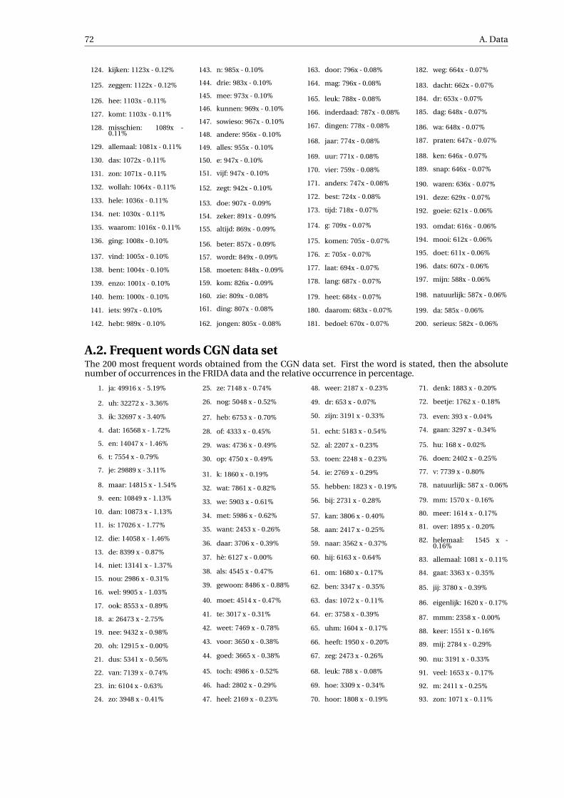
72 A. Data

124. kijken: 1123x - 0.12%

125. zeggen: 1122x - 0.12%

126. hee: 1103x - 0.11%

127. komt: 1103x - 0.11%

128. misschien: 1089x -0.11%

129. allemaal: 1081x - 0.11%

130. das: 1072x - 0.11%

131. zon: 1071x - 0.11%

132. wollah: 1064x - 0.11%

133. hele: 1036x - 0.11%

134. net: 1030x - 0.11%

135. waarom: 1016x - 0.11%

136. ging: 1008x - 0.10%

137. vind: 1005x - 0.10%

138. bent: 1004x - 0.10%

139. enzo: 1001x - 0.10%

140. hem: 1000x - 0.10%

141. iets: 997x - 0.10%

142. hebt: 989x - 0.10%

143. n: 985x - 0.10%

144. drie: 983x - 0.10%

145. mee: 973x - 0.10%

146. kunnen: 969x - 0.10%

147. sowieso: 967x - 0.10%

148. andere: 956x - 0.10%

149. alles: 955x - 0.10%

150. e: 947x - 0.10%

151. vijf: 947x - 0.10%

152. zegt: 942x - 0.10%

153. doe: 907x - 0.09%

154. zeker: 891x - 0.09%

155. altijd: 869x - 0.09%

156. beter: 857x - 0.09%

157. wordt: 849x - 0.09%

158. moeten: 848x - 0.09%

159. kom: 826x - 0.09%

160. zie: 809x - 0.08%

161. ding: 807x - 0.08%

162. jongen: 805x - 0.08%

163. door: 796x - 0.08%

164. mag: 796x - 0.08%

165. leuk: 788x - 0.08%

166. inderdaad: 787x - 0.08%

167. dingen: 778x - 0.08%

168. jaar: 774x - 0.08%

169. uur: 771x - 0.08%

170. vier: 759x - 0.08%

171. anders: 747x - 0.08%

172. best: 724x - 0.08%

173. tijd: 718x - 0.07%

174. g: 709x - 0.07%

175. komen: 705x - 0.07%

176. z: 705x - 0.07%

177. laat: 694x - 0.07%

178. lang: 687x - 0.07%

179. heet: 684x - 0.07%

180. daarom: 683x - 0.07%

181. bedoel: 670x - 0.07%

182. weg: 664x - 0.07%

183. dacht: 662x - 0.07%

184. dr: 653x - 0.07%

185. dag: 648x - 0.07%

186. wa: 648x - 0.07%

187. praten: 647x - 0.07%

188. ken: 646x - 0.07%

189. snap: 646x - 0.07%

190. waren: 636x - 0.07%

191. deze: 629x - 0.07%

192. goeie: 621x - 0.06%

193. omdat: 616x - 0.06%

194. mooi: 612x - 0.06%

195. doet: 611x - 0.06%

196. dats: 607x - 0.06%

197. mijn: 588x - 0.06%

198. natuurlijk: 587x - 0.06%

199. da: 585x - 0.06%

200. serieus: 582x - 0.06%

A.2. Frequent words CGN data setThe 200 most frequent words obtained from the CGN data set. First the word is stated, then the absolutenumber of occurrences in the FRIDA data and the relative occurrence in percentage.

1. ja: 49916 x - 5.19%

2. uh: 32272 x - 3.36%

3. ik: 32697 x - 3.40%

4. dat: 16568 x - 1.72%

5. en: 14047 x - 1.46%

6. t: 7554 x - 0.79%

7. je: 29889 x - 3.11%

8. maar: 14815 x - 1.54%

9. een: 10849 x - 1.13%

10. dan: 10873 x - 1.13%

11. is: 17026 x - 1.77%

12. die: 14058 x - 1.46%

13. de: 8399 x - 0.87%

14. niet: 13141 x - 1.37%

15. nou: 2986 x - 0.31%

16. wel: 9905 x - 1.03%

17. ook: 8553 x - 0.89%

18. a: 26473 x - 2.75%

19. nee: 9432 x - 0.98%

20. oh: 12915 x - 0.00%

21. dus: 5341 x - 0.56%

22. van: 7139 x - 0.74%

23. in: 6104 x - 0.63%

24. zo: 3948 x - 0.41%

25. ze: 7148 x - 0.74%

26. nog: 5048 x - 0.52%

27. heb: 6753 x - 0.70%

28. of: 4333 x - 0.45%

29. was: 4736 x - 0.49%

30. op: 4750 x - 0.49%

31. k: 1860 x - 0.19%

32. wat: 7861 x - 0.82%

33. we: 5903 x - 0.61%

34. met: 5986 x - 0.62%

35. want: 2453 x - 0.26%

36. daar: 3706 x - 0.39%

37. hè: 6127 x - 0.00%

38. als: 4545 x - 0.47%

39. gewoon: 8486 x - 0.88%

40. moet: 4514 x - 0.47%

41. te: 3017 x - 0.31%

42. weet: 7469 x - 0.78%

43. voor: 3650 x - 0.38%

44. goed: 3665 x - 0.38%

45. toch: 4986 x - 0.52%

46. had: 2802 x - 0.29%

47. heel: 2169 x - 0.23%

48. weer: 2187 x - 0.23%

49. dr: 653 x - 0.07%

50. zijn: 3191 x - 0.33%

51. echt: 5183 x - 0.54%

52. al: 2207 x - 0.23%

53. toen: 2248 x - 0.23%

54. ie: 2769 x - 0.29%

55. hebben: 1823 x - 0.19%

56. bij: 2731 x - 0.28%

57. kan: 3806 x - 0.40%

58. aan: 2417 x - 0.25%

59. naar: 3562 x - 0.37%

60. hij: 6163 x - 0.64%

61. om: 1680 x - 0.17%

62. ben: 3347 x - 0.35%

63. das: 1072 x - 0.11%

64. er: 3758 x - 0.39%

65. uhm: 1604 x - 0.17%

66. heeft: 1950 x - 0.20%

67. zeg: 2473 x - 0.26%

68. leuk: 788 x - 0.08%

69. hoe: 3309 x - 0.34%

70. hoor: 1808 x - 0.19%

71. denk: 1883 x - 0.20%

72. beetje: 1762 x - 0.18%

73. even: 393 x - 0.04%

74. gaan: 3297 x - 0.34%

75. hu: 168 x - 0.02%

76. doen: 2402 x - 0.25%

77. v: 7739 x - 0.80%

78. natuurlijk: 587 x - 0.06%

79. mm: 1570 x - 0.16%

80. meer: 1614 x - 0.17%

81. over: 1895 x - 0.20%

82. helemaal: 1545 x -0.16%

83. allemaal: 1081 x - 0.11%

84. gaat: 3363 x - 0.35%

85. jij: 3780 x - 0.39%

86. eigenlijk: 1620 x - 0.17%

87. mmm: 2358 x - 0.00%

88. keer: 1551 x - 0.16%

89. mij: 2784 x - 0.29%

90. nu: 3191 x - 0.33%

91. veel: 1653 x - 0.17%

92. m: 2411 x - 0.25%

93. zon: 1071 x - 0.11%

A.2. Frequent words CGN data set 73

94. x: 3265 x - 0.34%

95. ga: 4457 x - 0.46%

96. vind: 1005 x - 0.10%

97. geen: 1909 x - 0.20%

98. waar: 1767 x - 0.18%

99. zit: 1173 x - 0.12%

100. zei: 1816 x - 0.19%

101. uit: 1146 x - 0.12%

102. oké: 1917 x - 0.00%

103. één: 1898 x - 0.00%

104. zou: 1375 x - 0.14%

105. het: 9398 x - 0.98%

106. mee: 973 x - 0.10%

107. iets: 997 x - 0.10%

108. twee: 1832 x - 0.19%

109. me: 3965 x - 0.41%

110. u: 2471 x - 0.26%

111. mn: 390 x - 0.04%

112. ns: 240 x - 0.02%

113. wij: 454 x - 0.05%

114. wil: 1540 x - 0.16%

115. z: 705 x - 0.07%

116. hele: 1036 x - 0.11%

117. niks: 1156 x - 0.12%

118. kunnen: 969 x - 0.10%

119. precies: 1886 x - 0.20%

120. hier: 1125 x - 0.12%

121. misschien: 1089 x -0.11%

122. altijd: 869 x - 0.09%

123. geweest: 332 x - 0.03%

124. zeggen: 1122 x - 0.12%

125. net: 1030 x - 0.11%

126. komt: 1103 x - 0.11%

127. hebt: 989 x - 0.10%

128. d: 1465 x - 0.15%

129. erg: 415 x - 0.04%

130. hadden: 511 x - 0.05%

131. dit: 1308 x - 0.14%

132. uur: 771 x - 0.08%

133. effe: 2231 x - 0.23%

134. alleen: 1340 x - 0.14%

135. zal: 295 x - 0.03%

136. kijken: 1123 x - 0.12%

137. wordt: 849 x - 0.09%

138. lekker: 1328 x - 0.14%

139. mensen: 1184 x - 0.12%

140. andere: 956 x - 0.10%

141. moeten: 848 x - 0.09%

142. anders: 747 x - 0.08%

143. week: 450 x - 0.05%

144. zn: 482 x - 0.05%

145. inderdaad: 787 x -0.08%

146. mooi: 612 x - 0.06%

147. dacht: 661 x - 0.07%

148. waren: 636 x - 0.07%

149. zitten: 543 x - 0.06%

150. bedoel: 670 x - 0.07%

151. zegt: 942 x - 0.10%

152. door: 796 x - 0.08%

153. komen: 705 x - 0.07%

154. drie: 983 x - 0.10%

155. ging: 1008 x - 0.10%

156. jullie: 541 x - 0.06%

157. jaar: 774 x - 0.08%

158. jou: 1291 x - 0.13%

159. vond: 302 x - 0.03%

160. gedaan: 491 x - 0.05%

161. dingen: 778 x - 0.08%

162. tijd: 718 x - 0.07%

163. hé: 963 x - 0.00%

164. dag: 648 x - 0.07%

165. doe: 907 x - 0.09%

166. volgens: 1273 x - 0.13%

167. zoiets: 316 x - 0.03%

168. moest: 487 x - 0.05%

169. weg: 664 x - 0.07%

170. zelf: 528 x - 0.05%

171. omdat: 616 x - 0.06%

172. s: 10986 x - 1.14%

173. tegen: 1213 x - 0.13%

174. mijn: 588 x - 0.06%

175. alles: 955 x - 0.10%

176. gehad: 213 x - 0.02%

177. zich: 295 x - 0.03%

178. verder: 381 x - 0.04%

179. ah: 15 x - 0.00%

180. kijk: 1193 x - 0.12%

181. af: 458 x - 0.05%

182. zij: 556 x - 0.06%

183. best: 724 x - 0.08%

184. tot: 466 x - 0.05%

185. nooit: 544 x - 0.06%

186. zeker: 891 x - 0.09%

187. ons: 427 x - 0.04%

188. eerst: 432 x - 0.04%

189. staat: 407 x - 0.04%

190. morgen: 370 x - 0.04%

191. zat: 437 x - 0.05%

192. geloof: 204 x - 0.02%

193. laat: 694 x - 0.07%

194. zien: 552 x - 0.06%

195. geval: 224 x - 0.02%

196. worden: 466 x - 0.05%

197. doet: 611 x - 0.06%

198. kom: 826 x - 0.09%

199. kun: 140 x - 0.01%

200. tien: 484 x - 0.05%

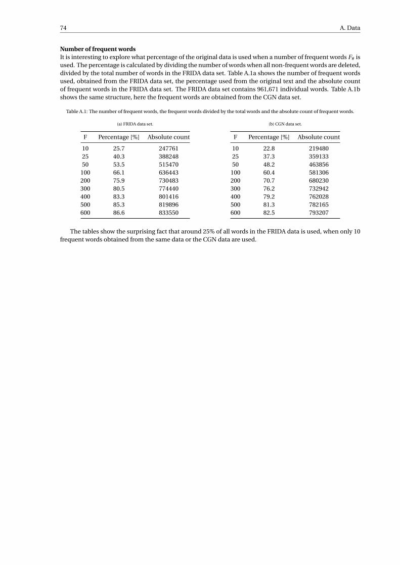
74 A. Data

Number of frequent wordsIt is interesting to explore what percentage of the original data is used when a number of frequent words F# isused. The percentage is calculated by dividing the number of words when all non-frequent words are deleted,divided by the total number of words in the FRIDA data set. Table A.1a shows the number of frequent wordsused, obtained from the FRIDA data set, the percentage used from the original text and the absolute countof frequent words in the FRIDA data set. The FRIDA data set contains 961,671 individual words. Table A.1bshows the same structure, here the frequent words are obtained from the CGN data set.

Table A.1: The number of frequent words, the frequent words divided by the total words and the absolute count of frequent words.

(a) FRIDA data set.

F Percentage [%] Absolute count

10 25.7 24776125 40.3 38824850 53.5 515470

100 66.1 636443200 75.9 730483300 80.5 774440400 83.3 801416500 85.3 819896600 86.6 833550

(b) CGN data set.

F Percentage [%] Absolute count

10 22.8 21948025 37.3 35913350 48.2 463856

100 60.4 581306200 70.7 680230300 76.2 732942400 79.2 762028500 81.3 782165600 82.5 793207

The tables show the surprising fact that around 25% of all words in the FRIDA data is used, when only 10frequent words obtained from the same data or the CGN data are used.

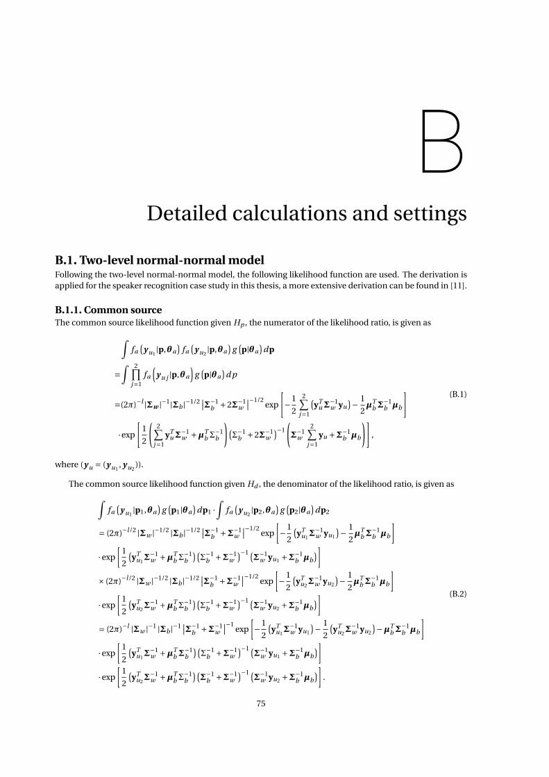
BDetailed calculations and settings

B.1. Two-level normal-normal modelFollowing the two-level normal-normal model, the following likelihood function are used. The derivation isapplied for the speaker recognition case study in this thesis, a more extensive derivation can be found in [11].

B.1.1. Common sourceThe common source likelihood function given Hp , the numerator of the likelihood ratio, is given as∫

fa(

y u1|p,θa

)fa

(y u2

|p,θa)

g(p|θa

)dp

=∫ 2∏

j=1fa

(y u j |p,θa

)g

(p|θa

)d p

=(2π)−l |Σw |−1|Σb |−1/2 ∣∣Σ−1b +2Σ−1

w

∣∣−1/2exp

[−1

2

2∑j=1

(yT

uΣ−1w yu

)− 1

2µT

bΣ−1b µb

]

·exp

[1

2

(2∑

j=1yT

uΣ−1w +µT

b Σ−1b

)(Σ−1

b +2Σ−1w

)−1

(Σ−1

w

2∑j=1

yu +Σ−1b µb

)],

(B.1)

where (y u = (y u1, y u2

)).

The common source likelihood function given Hd , the denominator of the likelihood ratio, is given as∫fa

(y u1

|p1,θa)

g(p1|θa

)dp1 ·

∫fa

(y u2

|p2,θa)

g(p2|θa

)dp2

= (2π)−l/2 |Σw |−1/2 |Σb |−1/2 ∣∣Σ−1b +Σ−1

w

∣∣−1/2exp

[−1

2

(yT

u1Σ−1

w yu1

)− 1

2µT

bΣ−1b µb

]·exp

[1

2

(yT

u1Σ−1

w +µTb Σ

−1b

)(Σ−1

b +Σ−1w

)−1 (Σ−1

w yu1 +Σ−1b µb

)]× (2π)−l/2 |Σw |−1/2 |Σb |−1/2 ∣∣Σ−1

b +Σ−1w

∣∣−1/2exp

[−1

2

(yT

u2Σ−1

w yu2

)− 1

2µT

bΣ−1b µb

]·exp

[1

2

(yT

u2Σ−1

w +µTb Σ

−1b

)(Σ−1

b +Σ−1w

)−1 (Σ−1

w yu2 +Σ−1b µb

)]= (2π)−l |Σw |−1 |Σb |−1 ∣∣Σ−1

b +Σ−1w

∣∣−1exp

[−1

2

(yT

u1Σ−1

w yu1

)− 1

2

(yT

u2Σ−1

w yu2

)−µTbΣ

−1b µb

]·exp

[1

2

(yT

u1Σ−1

w +µTbΣ

−1b

)(Σ−1

b +Σ−1w

)−1 (Σ−1

w yu1 +Σ−1b µb

)]·exp

[1

2

(yT

u2Σ−1

w +µTb Σ

−1b

)(Σ−1

b +Σ−1w

)−1 (Σ−1

w yu2 +Σ−1b µb

)].

(B.2)

75

76 B. Detailed calculations and settings

It then follows the common source likelihood ratio is given as

LRC S =|Σb |1/2 ∣∣Σ−1b +Σ−1

w

∣∣ ∣∣Σ−1b +2Σ−1

w

∣∣−1/2exp

[1

2µT

bΣ−1b µb

]·exp

[1

2

(2∑

j=1yT

uΣ−1w +µT

bΣ−1b

)(Σ−1

b +2Σ−1w

)−1

(Σ−1

w

2∑j=1

yu +Σ−1b µb

)]

·exp

[−1

2

(yT

u1Σ−1

w +µTbΣ

−1b

)(Σ−1

b +Σ−1w

)−1 (Σ−1

w yu1 +Σ−1b µb

)]·exp

[−1

2

(yT

u2Σ−1

w +µTb Σ

−1b

)(Σ−1

b +Σ−1w

)−1 (Σ−1

w yu2 +Σ−1b µb

)].

(B.3)

B.1.2. Specific sourceThe specific source likelihood function given Hp , the numerator of the likelihood ratio, is given as

fs (yu |θs ) = (2π)−l/2 |Σs |−1/2 exp

[−1

2(yu −µs )TΣ−1

s (yu −µs )

]. (B.4)

The specific source likelihood function given Hd , the denominator of the likelihood ratio, is given as∫fa

(yu |p,θa

)g

(p|θa

)dp

=∫

(2π)−l/2 |Σw |−1/2 exp

[−1

2(yu −p)TΣ−1

w (yu −p)

](2π)−l/2 |Σb |−1/2 exp

[−1

2(p−µb)TΣ−1

b (p−µb)

]dp

=(2π)−l/2 |Σw |−1/2 |Σb |−1/2 ∣∣Σ−1b +Σ−1

w

∣∣−1/2exp

[−1

2

(yT

uΣ−1w yu

)− 1

2µT

bΣ−1b µb

]·exp

[1

2

(yT

uΣ−1w +µT

bΣ−1b

)(Σ−1

b +Σ−1w

)−1 (Σ−1

w yu +Σ−1b µb

)].

(B.5)

It then follows the specific source likelihood ratio is given as

LRSS =|Σs |−1/2 |Σw |1/2 |Σb |1/2 ∣∣Σ−1b +Σ−1

w

∣∣1/2

·exp

[−1

2(yu −µs )TΣ−1

s (yu −µs )

]·exp

[1

2

(yT

uΣ−1w yu

)+ 1

2µT

bΣ−1b µb

]·exp

[−1

2

(yT

uΣ−1w +µT

bΣ−1b

)(Σ−1

b +Σ−1w

)−1 (Σ−1

w yu +Σ−1b µb

)].

(B.6)

B.2. Machine learning algorithm settings 77

B.2. Machine learning algorithm settingsThe used machine learning algorithms are readily implemented in Python, with hyper parameters that can bevaried for optimal performance per case. For exactness and reproducibility the parameters which are tunedare outlined below.

Naive BayesFor all calculations the sklearn.naive_bayes.MultinomialNB Python class is used. The default parameters areused, outlined in the sklearn documentation.

Support vector machinesFor all calculations the sklearn.svm.SVC Python class is used. The default parameters are used, outlined inthe sklearn documentation. The following hyper parameters are tuned:

• kernel = linear

• probability = True

• class_weight = ‘balanced’

XGBoostFor all calculations the xgboost.XGBclassifier Python class is used. The default parameters are used, outlinedin the xgboost documentation. The following hyper parameters are tuned:

• learning_rate = 0.2

• max_depth = 3

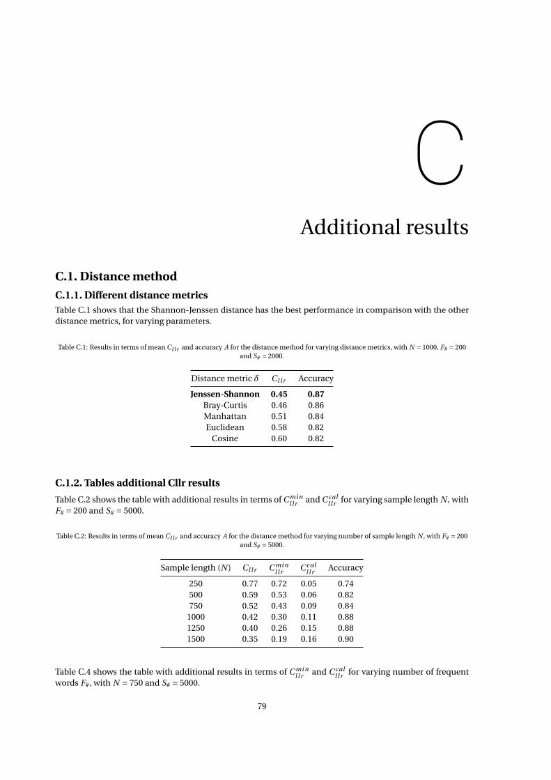
CAdditional results

C.1. Distance method

C.1.1. Different distance metricsTable C.1 shows that the Shannon-Jenssen distance has the best performance in comparison with the otherdistance metrics, for varying parameters.

Table C.1: Results in terms of mean Cl l r and accuracy A for the distance method for varying distance metrics, with N = 1000, F# = 200and S# = 2000.

Distance metric δ Cl l r Accuracy

Jenssen-Shannon 0.45 0.87Bray-Curtis 0.46 0.86Manhattan 0.51 0.84Euclidean 0.58 0.82

Cosine 0.60 0.82

C.1.2. Tables additional Cllr results

Table C.2 shows the table with additional results in terms of C mi nl lr and C cal

l l r for varying sample length N , withF# = 200 and S# = 5000.

Table C.2: Results in terms of mean Cl l r and accuracy A for the distance method for varying number of sample length N , with F# = 200and S# = 5000.

Sample length (N ) Cl l r C mi nll r C cal

l l r Accuracy

250 0.77 0.72 0.05 0.74500 0.59 0.53 0.06 0.82750 0.52 0.43 0.09 0.84

1000 0.42 0.30 0.11 0.881250 0.40 0.26 0.15 0.881500 0.35 0.19 0.16 0.90

Table C.4 shows the table with additional results in terms of C mi nl lr and C cal

l l r for varying number of frequentwords F#, with N = 750 and S# = 5000.

79

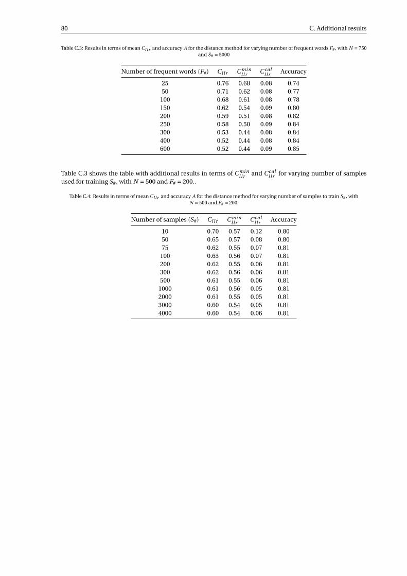
80 C. Additional results

Table C.3: Results in terms of mean Cl l r and accuracy A for the distance method for varying number of frequent words F#, with N = 750and S# = 5000

Number of frequent words (F#) Cl l r C mi nll r C cal

l l r Accuracy

25 0.76 0.68 0.08 0.7450 0.71 0.62 0.08 0.77

100 0.68 0.61 0.08 0.78150 0.62 0.54 0.09 0.80200 0.59 0.51 0.08 0.82250 0.58 0.50 0.09 0.84300 0.53 0.44 0.08 0.84400 0.52 0.44 0.08 0.84600 0.52 0.44 0.09 0.85

Table C.3 shows the table with additional results in terms of C mi nll r and C cal

l l r for varying number of samplesused for training S#, with N = 500 and F# = 200..

Table C.4: Results in terms of mean Cl l r and accuracy A for the distance method for varying number of samples to train S#, withN = 500 and F# = 200.

Number of samples (S#) Cl l r C mi nll r C cal

l l r Accuracy

10 0.70 0.57 0.12 0.8050 0.65 0.57 0.08 0.8075 0.62 0.55 0.07 0.81

100 0.63 0.56 0.07 0.81200 0.62 0.55 0.06 0.81300 0.62 0.56 0.06 0.81500 0.61 0.55 0.06 0.81

1000 0.61 0.56 0.05 0.812000 0.61 0.55 0.05 0.813000 0.60 0.54 0.05 0.814000 0.60 0.54 0.06 0.81

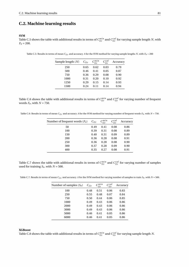
C.2. Machine learning results 81

C.2. Machine learning results

SVMTable C.5 shows the table with additional results in terms of C mi n

l lr and C call l r for varying sample length N , with

F# = 200.

Table C.5: Results in terms of mean Cl l r and accuracy A for the SVM method for varying sample lengths N , with F# = 200

Sample length (N ) Cl l r C mi nll r C cal

l l r Accuracy

250 0.65 0.62 0.03 0.79500 0.46 0.41 0.05 0.87750 0.36 0.29 0.08 0.90

1000 0.31 0.20 0.10 0.921250 0.29 0.15 0.14 0.931500 0.24 0.11 0.14 0.94

Table C.6 shows the table with additional results in terms of C mi nl lr and C cal

l l r for varying number of frequentwords F#, with N = 750.

Table C.6: Results in terms of mean Cl l r and accuracy A for the SVM method for varying number of frequent words F#, with N = 750.

Number of frequent words (F#) Cl l r C mi nl lr C cal

l l r Accuracy

50 0.49 0.41 0.08 0.86100 0.39 0.31 0.08 0.89150 0.40 0.31 0.09 0.89200 0.36 0.28 0.08 0.91250 0.36 0.28 0.08 0.90300 0.37 0.28 0.09 0.90400 0.35 0.27 0.08 0.91

Table C.7 shows the table with additional results in terms of C mi nl lr and C cal

l l r for varying number of samplesused for training S#, with N = 500.

Table C.7: Results in terms of mean Cl l r and accuracy A for the SVM method for varying number of samples to train S#, with N = 500.

Number of samples (S#) Cl l r C mi nl lr C cal

l l r Accuracy

100 0.48 0.51 0.06 0.83250 0.55 0.48 0.07 0.84750 0.50 0.44 0.06 0.85

1000 0.49 0.43 0.06 0.862000 0.49 0.43 0.06 0.863000 0.49 0.43 0.06 0.865000 0.46 0.41 0.05 0.866000 0.46 0.41 0.05 0.86

XGBoostTable C.8 shows the table with additional results in terms of C mi n

ll r and C call l r for varying sample length N .

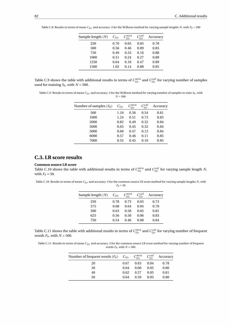
82 C. Additional results

Table C.8: Results in terms of mean Cl l r and accuracy A for the XGBoost method for varying sample lengths N , with F# = 200

Sample length (N ) Cl l r C mi nll r C cal

l l r Accuracy

250 0.70 0.65 0.05 0.78500 0.56 0.46 0.09 0.85750 0.49 0.33 0.16 0.88

1000 0.51 0.24 0.27 0.891250 0.64 0.18 0.47 0.891500 1.02 0.14 0.88 0.85

Table C.9 shows the table with additional results in terms of C mi nll r and C cal

l l r for varying number of samplesused for training S#, with N = 500.

Table C.9: Results in terms of mean Cl l r and accuracy A for the XGBoost method for varying number of samples to train S#, withN = 500.

Number of samples (S#) Cl l r C mi nll r C cal

l l r Accuracy

500 1.10 0.56 0.54 0.811000 1.24 0.51 0.73 0.832000 0.82 0.49 0.32 0.843000 0.63 0.45 0.32 0.845000 0.60 0.47 0.13 0.846000 0.57 0.46 0.11 0.857000 0.55 0.45 0.10 0.85

C.3. LR score resultsCommon source LR scoreTable C.10 shows the table with additional results in terms of C mi n

ll r and C call l r for varying sample length N ,

with F# = 50.

Table C.10: Results in terms of mean Cl l r and accuracy A for the common source LR score method for varying sample lengths N , withF# = 50

Sample length (N ) Cl l r C mi nll r C cal

l l r Accuracy

250 0.78 0.75 0.03 0.73375 0.68 0.64 0.04 0.78500 0.63 0.58 0.05 0.81625 0.56 0.50 0.06 0.83750 0.54 0.46 0.08 0.84

Table C.11 shows the table with additional results in terms of C mi nll r and C cal

l l r for varying number of frequentwords F#, with N = 500.

Table C.11: Results in terms of mean Cl l r and accuracy A for the common source LR score method for varying number of frequentwords F#, with N = 500.

Number of frequent words (F#) Cl l r C mi nll r C cal

l l r Accuracy

20 0.67 0.63 0.04 0.7830 0.64 0.60 0.05 0.8040 0.62 0.57 0.05 0.8150 0.64 0.59 0.05 0.80

C.3. LR score results 83

Specific source LR scoreTable C.12 shows the table with additional results in terms of C mi n

ll r and C call l r for varying number of specific

speaker samples S#s , with F# = 20 and N = 250.

Table C.12: Results in terms of mean Cl l r and accuracy A for the specific source LR score method for varying number of specificspeaker samples S#s , with F# = 20 and N = 250.

Sample length (N ) Cl l r C mi nll r C cal

l l r Accuracy

2 0.79 0.73 0.07 0.724 0.74 0.67 0.08 0.756 0.69 0.61 0.08 0.788 0.68 0.60 0.08 0.78

10 0.69 0.60 0.10 0.78

Table C.13 shows the table with additional results in terms of C mi nll r and C cal

l l r for varying sample length N ,with F# = 20.

Table C.13: Results in terms of mean Cl l r and accuracy A for the specific source LR score method for varying sample lengths N , withF# = 20.

Sample length (N ) Cl l r C mi nll r C cal

l l r Accuracy

200 0.75 0.69 0.06 0.74300 0.68 0.60 0.09 0.78400 0.64 0.53 0.11 0.80500 0.60 0.46 0.14 0.82600 0.59 0.40 0.19 0.83

Table C.11 shows the table with additional results in terms of C mi nll r and C cal

l l r for varying number of frequentwords F#, with N = 500.

Table C.14: Results in terms of mean Cl l r and accuracy A for the specific source LR score method for varying number of frequent wordsF#, with N = 500.

Number of frequent words (F#) Cl l r C mi nl lr C cal

l l r Accuracy

20 0.57 0.41 0.15 0.8430 0.58 0.44 0.15 0.8340 0.59 0.44 0.14 0.8350 0.58 0.44 0.15 0.83