MEng Individual Project

Imperial College London

Department of Computing

Universal Lesion Detector: Deep Learningfor Analysing Medical Scans

Author:Martin Zlocha

Supervisor:Dr Ben Glocker

Second Marker:Dr Jonathan Passerat-Palmbach

June 17, 2019

Abstract

Accurate, automated lesion detection is an important yet challenging task due to the largevariation of lesion types, sizes, locations and appearances. Most of the recent work onlyfocuses on lesion detection in a constrained setting - detecting lesions in a specific organ.We tackle the general problem of detecting lesions across the whole body and proposeapproaches which are not limited to a particular dataset. This is done by redesigning Reti-naNet to be more applicable to medical imaging, using a general approach for optimisinganchor configurations and by generating additional weak labels from the provided groundtruth. We evaluate our approach on two different datasets - a large public Computed To-mography (CT) dataset called DeepLesion, consisting of 32,735 lesions, and a much smallerwhole-body Magnetic Resonance Imaging (MRI) dataset made up of only 213 scans. Weshow that our approach achieves state-of-the-art results, significantly outperforming thebest reported methods by over 5% on the DeepLesion benchmark, while being generalisableenough to achieve excellent results on the much smaller whole-body MRI dataset.

Acknowledgements

I would like to thank my supervisor Dr Ben Glocker, for his consistent guidance andsupport. I would also like to thank my collaborator, Dr Qi Dou, for her invaluable advice.

Further, I would like to thank Jan Matas, Inara Ramji and Jayati Sarkar for proof-readingkey chapters of the report.

Lastly, I would like to thank my friends and family for giving me advice throughout theproject and always supporting me.

Contents

1 Introduction 11.1 Objectives . . . . . . . . . . . . . . . . . . . . . . . . . . . . . . . . . . . . . 11.2 Challenges . . . . . . . . . . . . . . . . . . . . . . . . . . . . . . . . . . . . . 21.3 Contribution . . . . . . . . . . . . . . . . . . . . . . . . . . . . . . . . . . . 21.4 Publication . . . . . . . . . . . . . . . . . . . . . . . . . . . . . . . . . . . . 31.5 Report Layout . . . . . . . . . . . . . . . . . . . . . . . . . . . . . . . . . . 3

2 Background 42.1 Approaches . . . . . . . . . . . . . . . . . . . . . . . . . . . . . . . . . . . . 42.2 Object Detection Networks . . . . . . . . . . . . . . . . . . . . . . . . . . . 4

2.2.1 Region-based Convolutional Network . . . . . . . . . . . . . . . . . . 42.2.2 You Only Look Once . . . . . . . . . . . . . . . . . . . . . . . . . . . 82.2.3 Focal Loss for Dense Object Detection . . . . . . . . . . . . . . . . . 92.2.4 Comparison . . . . . . . . . . . . . . . . . . . . . . . . . . . . . . . . 10

2.3 Backbones . . . . . . . . . . . . . . . . . . . . . . . . . . . . . . . . . . . . . 102.3.1 VGG . . . . . . . . . . . . . . . . . . . . . . . . . . . . . . . . . . . . 102.3.2 Inception/GoogLeNet . . . . . . . . . . . . . . . . . . . . . . . . . . 112.3.3 ResNet . . . . . . . . . . . . . . . . . . . . . . . . . . . . . . . . . . 122.3.4 Comparison . . . . . . . . . . . . . . . . . . . . . . . . . . . . . . . . 12

2.4 U-Net based Object Detectors in Medical Imaging . . . . . . . . . . . . . . 132.4.1 U-Net . . . . . . . . . . . . . . . . . . . . . . . . . . . . . . . . . . . 132.4.2 Retina U-Net . . . . . . . . . . . . . . . . . . . . . . . . . . . . . . . 142.4.3 Attention U-Net . . . . . . . . . . . . . . . . . . . . . . . . . . . . . 14

3 Universal Lesion Detector 163.1 Key Tools and Libraries . . . . . . . . . . . . . . . . . . . . . . . . . . . . . 163.2 Model Design . . . . . . . . . . . . . . . . . . . . . . . . . . . . . . . . . . . 173.3 Optimized Anchor Configuration . . . . . . . . . . . . . . . . . . . . . . . . 173.4 Generating Dense Masks from Weak RECIST Labels . . . . . . . . . . . . . 183.5 Dense Mask Supervision . . . . . . . . . . . . . . . . . . . . . . . . . . . . . 193.6 Attention Mechanism for Gated Feature Fusion . . . . . . . . . . . . . . . . 21

4 Validation on the DeepLesion dataset 234.1 DeepLesion . . . . . . . . . . . . . . . . . . . . . . . . . . . . . . . . . . . . 23

4.1.1 Annotations . . . . . . . . . . . . . . . . . . . . . . . . . . . . . . . . 234.1.2 Limitations . . . . . . . . . . . . . . . . . . . . . . . . . . . . . . . . 25

4.2 Data Augmentation . . . . . . . . . . . . . . . . . . . . . . . . . . . . . . . 264.3 Training . . . . . . . . . . . . . . . . . . . . . . . . . . . . . . . . . . . . . . 274.4 Evaluation . . . . . . . . . . . . . . . . . . . . . . . . . . . . . . . . . . . . . 28

4.4.1 Current state-of-the-art results . . . . . . . . . . . . . . . . . . . . . 284.4.2 Visual evaluation of the attention mechanism . . . . . . . . . . . . . 28

i

4.4.3 Visual results of lesion detection . . . . . . . . . . . . . . . . . . . . 294.4.4 Ablation study . . . . . . . . . . . . . . . . . . . . . . . . . . . . . . 30

5 Validation on the whole-body MRI dataset 345.1 Whole-body MRI dataset . . . . . . . . . . . . . . . . . . . . . . . . . . . . 34

5.1.1 Annotations . . . . . . . . . . . . . . . . . . . . . . . . . . . . . . . . 345.1.2 Limitations . . . . . . . . . . . . . . . . . . . . . . . . . . . . . . . . 35

5.2 Data Augmentation . . . . . . . . . . . . . . . . . . . . . . . . . . . . . . . 365.3 Training Data Generation . . . . . . . . . . . . . . . . . . . . . . . . . . . . 385.4 Training . . . . . . . . . . . . . . . . . . . . . . . . . . . . . . . . . . . . . . 385.5 Stabilizing loss when negative samples are used . . . . . . . . . . . . . . . . 385.6 Merging 2D predictions . . . . . . . . . . . . . . . . . . . . . . . . . . . . . 395.7 Evaluation . . . . . . . . . . . . . . . . . . . . . . . . . . . . . . . . . . . . . 40

5.7.1 Visual results . . . . . . . . . . . . . . . . . . . . . . . . . . . . . . . 405.7.2 Transfer Learning . . . . . . . . . . . . . . . . . . . . . . . . . . . . . 415.7.3 Ablation study . . . . . . . . . . . . . . . . . . . . . . . . . . . . . . 41

6 Spot-the-Lesion Game 45

7 Conclusion and Future Work 477.1 Future Work . . . . . . . . . . . . . . . . . . . . . . . . . . . . . . . . . . . 47

7.1.1 Dataset cleaning and augmentation . . . . . . . . . . . . . . . . . . . 477.1.2 Model Design . . . . . . . . . . . . . . . . . . . . . . . . . . . . . . . 487.1.3 Extensive evaluation . . . . . . . . . . . . . . . . . . . . . . . . . . . 48

A Visual results for CT lesion detection 49

B Visual results for MRI lesion detection 51

ii

List of Figures

2.1 Structure of R-CNN [13]. . . . . . . . . . . . . . . . . . . . . . . . . . . . . 52.2 Structure of Fast R-CNN [14]. . . . . . . . . . . . . . . . . . . . . . . . . . . 62.3 Structure of Faster R-CNN [40]. . . . . . . . . . . . . . . . . . . . . . . . . . 72.4 Anchor generation in Faster R-CNN [40]. . . . . . . . . . . . . . . . . . . . . 72.5 Structure of R-FCN [5]. . . . . . . . . . . . . . . . . . . . . . . . . . . . . . 82.6 Structure of YOLO [39]. . . . . . . . . . . . . . . . . . . . . . . . . . . . . . 82.7 Loss calculated by using Focal Loss vs Cross Entropy [30]. . . . . . . . . . . 92.8 Structure of RetinaNet [30]. . . . . . . . . . . . . . . . . . . . . . . . . . . . 102.9 Comparison of object detectors [30]. . . . . . . . . . . . . . . . . . . . . . . 102.10 Structure of VGG [43]. . . . . . . . . . . . . . . . . . . . . . . . . . . . . . . 112.11 Structure of Inception v1 [46]. . . . . . . . . . . . . . . . . . . . . . . . . . . 122.12 Design of the residual learning block in ResNet [17]. . . . . . . . . . . . . . 122.13 Structure of U-NET [41]. . . . . . . . . . . . . . . . . . . . . . . . . . . . . . 132.14 Structure of Retina U-Net [21]. . . . . . . . . . . . . . . . . . . . . . . . . . 142.15 Schematic of the Attention Gate [36] . . . . . . . . . . . . . . . . . . . . . . 152.16 Structure of Attention U-Net [36]. . . . . . . . . . . . . . . . . . . . . . . . 15

3.1 Network architecture of RetinaNet without any modifications. . . . . . . . . 173.2 An example of a mask generated from RECIST labels. . . . . . . . . . . . . 193.3 Network architecture of RetinaNet with Dense Mask Supervision. . . . . . . 203.4 Network architecture of RetinaNet with Attention Mechanism for Gated

Feature Fusion. . . . . . . . . . . . . . . . . . . . . . . . . . . . . . . . . . . 223.5 Schematic of the Attention Gate [36] . . . . . . . . . . . . . . . . . . . . . . 22

4.1 Visualization of a subset of the DeepLesion dataset [52]. . . . . . . . . . . . 244.2 Example labeled CT scan [52]. . . . . . . . . . . . . . . . . . . . . . . . . . 254.3 Numbers of lesions which are visible at different HU windows. . . . . . . . . 264.4 Example attention map overlaid on the input image. . . . . . . . . . . . . . 294.5 Visual results for lesion detection at 0.5 FP rate using our improved RetinaNet. 304.6 FROC curves for our improved RetinaNet variants and baselines on DeepLe-

sion dataset. . . . . . . . . . . . . . . . . . . . . . . . . . . . . . . . . . . . . 32

5.1 Example of an ADC, DW and T2W scan. . . . . . . . . . . . . . . . . . . . 355.2 Multiple T2W scans taken with different protocols [25] . . . . . . . . . . . . 365.3 Example of the data quality challenges (artefacts) we encountered in the

dataset. . . . . . . . . . . . . . . . . . . . . . . . . . . . . . . . . . . . . . . 375.4 The ground truth segmentation overlaid on a DW scan. . . . . . . . . . . . 405.5 The predicted segmentation overlaid on a DW scan. . . . . . . . . . . . . . 415.6 The predicted heatmap overlaid on a DW scan. . . . . . . . . . . . . . . . . 425.7 Plot of the mean Average Precision (mAP) achieved during training. . . . . 435.8 Sensitivity (TPR), Precision (PPV) and F1 score of our model for different

ground truth-detection distances. . . . . . . . . . . . . . . . . . . . . . . . . 44

iii

6.1 The main view of the website. . . . . . . . . . . . . . . . . . . . . . . . . . . 466.2 The view of the website after time runs out. . . . . . . . . . . . . . . . . . . 46

A.2 Visual results for lesion detection at 0.5 FP rate using our improved RetinaNet. 50

B.1 The ground truth segmentation overlaid on a DW scan. . . . . . . . . . . . 51B.2 Very accurate predicted segmentation overlaid on a DW scan. . . . . . . . . 52B.3 A falsely predicted segmentation overlaid on a DW scan. . . . . . . . . . . . 52B.4 The grorund truth segmentation overlaid on a DW scan. . . . . . . . . . . . 53B.5 The predicted segmentation overlaid on a DW scan. . . . . . . . . . . . . . 53

iv

List of Tables

4.1 Detection performance of different methods and our ablation study at mul-tiple false positive (FPs) rates. . . . . . . . . . . . . . . . . . . . . . . . . . 31

4.2 Detection performance of the modified anchor configuration compared tothe original configuration. . . . . . . . . . . . . . . . . . . . . . . . . . . . . 31

4.3 Detection performance of different lesion types at 4 false positives (FP) perimage. . . . . . . . . . . . . . . . . . . . . . . . . . . . . . . . . . . . . . . . 33

5.1 Detection performance of different scan preprocessing methods. . . . . . . . 425.2 Detection performance of elastic deformation with different values of sigma

and different transformation of individual training samples. . . . . . . . . . 435.3 Detection performance split by lesion type. . . . . . . . . . . . . . . . . . . 44

v

Chapter 1

Introduction

Cancer is one of the most common causes of death in the UK [15] and deaths from neo-plasms (cancers and other non-cancerous tissue growths) are one of the leading causes ofavoidable deaths in the UK [1]. However, the high workload and fatigue of clinicians meansthat they might miss a significant number of lesions. 30% of the false-negative errors areconsidered as scanning errors where the doctor missed the lesion even though it was visiblein the scan [24]. To make the task harder, clinicians routinely only spend 4.6 minutes [12]before they have to make a diagnosis. The lack of time, pressure, limited resources andcomplexity of making a diagnosis introduces errors which may have fatal consequences.

Computer-aided detection/diagnosis (CADe/CADx) systems can be used to reduce thenumber of human errors during diagnosis. Research shows that these systems detected upto 70% of lung cancers that were not detected by the radiologist but failed to detect about20% of the lung cancers when they were identified by the radiologist, which suggests thatCAD may be useful in the role of second reader [29]. Automated detection systems couldalso be used to passively look for lesions in patients who initially received a ComputedTomography (CT) or Magnetic Resonance Imaging (MRI) scan for a different reason. Upto 39% of patients with lung cancer are asymptomatic at the time of diagnosis [18], however,it is too costly to look for lesions in every scan if the patient does not display the symptoms.

The main drawback of these systems is that they aren’t general enough to be applied tolesions in CT and MRI scans from everywhere in the body, which limits their applicabilityin industry.

1.1 Objectives

The objective of this project is to develop a deep learning model for detection of lesions.Most of the current research focuses on detecting lesions in a single organ or of a singlelesion type. This project aims to produce a universal architecture which can be applied toboth CT and MRI scans from anywhere in the body and will reliably be able to detect thelesions.

We will use two datasets. Firstly, the DeepLesion [53] dataset will be used, as itconsists of 32,735 lesions in 32,120 CT slices from 10,594 studies of 4,427 unique patients.Most other datasets only focus on collecting only one type of lesion or on only one organ,however, DeepLesion contains lesions from 8 different locations with significantly varyingsizes and appearances. To verify that our approach is general enough and can be appliedto datasets with other modalities, we will use a whole-body MRI dataset which consists of213 MRI scans and contains both colorectal and lung lesions. This tests the generalisabilityof our model, as well as the ability to learn on smaller sample size.

After this goal has been completed, we have also added a stretch goal to make theproject demonstrable to the wider public. This makes our research more approachable,tangible and easier to understand.

1

To achieve this goal, the task is split into several sub-tasks:

1. Consider several standard object detectors and decide which is the most suitable forthis task.

2. Preprocess the data so that it can be fed into the object detector and achieves goodresults.

3. Modify the model so that it achieves state-of-the-art results on the DeepLesiondataset.

4. Verify that our model can generalise and achieves good results on the whole-bodyMRI dataset.

5. Create a website for non-technical people which gamifies lesion detection and demon-strates the accuracy of our model.

1.2 Challenges

During the project, we found the following to be the biggest challenges:

1. New datasets - The DeepLesion dataset has been released recently, and there is alack of research based on it so far. It is also very diverse with many different lesiontypes. These two factors make it harder to achieve good results. The whole-bodyMRI dataset is only used in-house and is much smaller, so we were not sure if it willbe feasible to train a model on it without overfitting.

2. Lack of domain knowledge - Medical imaging and lesion detection in CT andMRI scans requires a lot of domain knowledge when done manually. Even thoughthis domain knowledge is not required when training object detectors, this deficiencymay be a drawback compared to other research and might hinder the performanceof our model.

3. Training times - The size of the DeepLesion dataset and complexity of the modelsrestrict the iteration times. Currently, it takes a day to train a model which uses2D convolutions from start to finish, and this may increase to the order of days orweeks if we use 3D convolutions. This requires good time management and planningto avoid wasting time while waiting for training to complete.

4. Access to sufficient hardware - This project involves training deep neural net-works which require high memory machines to train. As many students are alsodoing machine learning based projects, the number of available resources providedby the department was limited which, required us to make compromises and limitedall of the experimentation which we could do.

1.3 Contribution

1. Optimize the feature pyramid scheme and anchor configuration - We havemodified the architecture of the network to be more suitable for medical imaging anddemonstrated how a differential evolution search algorithm could be used to optimisethe anchor configuration, which greatly improves the performance without needingextensive domain knowledge. This approach to optimising the anchor configurationcan be applied to any dataset, which makes it suitable for a universal lesion detectorand wider use.

2

2. Generate Dense Mask from Weak RECIST Labels - We utilise the responseevaluation criteria in solid lesions (RECIST) [8] diameters, which are widely used forannotations of lesions and generate high-quality, dense masks. This is done usingthe GrabCut [42] algorithm which reduces the workload on doctors as pixel-wiseannotations are tedious and expensive to obtain. Using these masks as an additionalsupervision signal shows great benefit for training the detector.

3. Employ multiple strategies for boosting the detection performance - Weuse the lesion mask predictions and compare them to the bounding box predictions toevaluate the coherence and adjust the prediction score. We also integrate an attentionmechanism into our feature pyramids, which further improves the performance.

4. Demonstrate how the architecture can be applied to different datasets - Awhole-body MRI dataset is utilised to demonstrate that the modified architecture isapplicable to other datasets without major modifications. We further demonstratethe improvement in results when transfer learning is used to initialise the modelweights when training on the whole-body MRI dataset.

5. Website - We built a website which demonstrates our work in an accessible andgamified format. The aim was to make it engaging to non-technical people whilepreserving the educational value about the difficulties of detecting lesions.1

1.4 Publication

The work which focuses on the DeepLesion dataset was submitted and accepted to MedicalImage Computing and Computer Assisted Intervention (MICCAI2) 2019 conference underthe title "Improving RetinaNet for CT Lesion Detection with Dense Masks from WeakRECIST Labels" [54]. After the submission to MICCAI 2019, our work was focused ondemonstrating how the architecture can be applied to different datasets such as the whole-body MRI dataset.

1.5 Report Layout

Chapter 2 focuses on research in object detection which is commonly used in industry andalso briefly introduces research in object detection specific to medical imaging. A briefcomparison of different approaches and motivation for the usage of RetinaNet can also befound in this chapter.

The work done is split into four chapters. Chapter 3 focuses on the work required toredesign RetinaNet to be more applicable to medical imaging. Chapter 4 first introducesthe DeepLesion dataset and evaluates the performance showing that our approach achievesstate-of-the-art results, significantly outperforming the best reported methods by over 5%.Afterwards, chapter 5 introduces a whole-body MRI dataset in order to demonstrate howour design can be applied to other datasets and achieves excellent results without significantmodifications. Chapter 6 briefly introduces a website which was made to demonstrate ourwork and gamify the task of detecting lesions in CT scans while educating people.

Chapter 7 concludes this report by summarising the work which was done and suggestsseveral areas of future work.

1https://www.doc.ic.ac.uk/~mz4315/deeplesion/2https://www.miccai2019.org/

3

Chapter 2

Background

Recent advances in object detection neural networks and availability of new medical imag-ing datasets enabled automated segmentation of CT and MRI scans both for commercialand research purposes.

This chapter surveys current state-of-art approaches to object detection and localisationboth in the medical and non-medical field, how these approaches have evolved.

2.1 Approaches

In the past this was done using traditional machine learning approaches where it wasfirst necessary to define features and then to perform classification using Haar-FeatureClassifiers [50] or Histogram of oriented gradients (HOG) [6].

Recently deep learning techniques have gained in popularity because they are able to doend-to-end object detection without having to define custom features [9]. These use con-volutional neural networks where each neuron processes data only for its region of space.Examples of this approach include Region-based Convolutional Network (R-CNN [13],Fast R-CNN [14], Faster R-CNN [40], R-FCN [5]), You Only Look Once (YOLO) [39],Single Shot MultiBox Detector (SSD) [32] or Focal Loss for Dense Object Detection (Reti-naNet) [30].

These object detection networks usually also work with multiple different backbonessuch as VGG [43], Inception/GoogLeNet [46] and ResNet [17].

This section will focus on the deep learning techniques as those have shown to achievebetter results and are more commonly used in medical imaging.

2.2 Object Detection Networks

When deciding on which object detection network should be used, the key metric wasmAP (Mean Average Precision), which is the most used metric to compare object detectionnetworks. Another metric which is widely used is the inference time. For this project, thisis not as important because the network would never be used in real-time systems wherehigh throughput is required.

2.2.1 Region-based Convolutional Network

R-CNN

Image classification has been most commonly approached by using HOG [6] or CNN’s.Unlike image classification, detection requires finding (many) objects within an image.One approach is to treat this as a regression problem which works well for finding the

4

bounding box of a single object but does not scale to an arbitrary number of objects. Analternative approach is to use a sliding window approach and feed that region into a CNN.The problem of this approach is that it requires all objects to share a common size andaspect ratio.

To tackle these problems, R-CNN [13] is split into three modules:

1. Region proposals - Instead of using regions of fixed size generated by sliding awindow across the whole image, selective search [49] is used which reduces the numberof regions that have to be considered.

2. Feature extraction - This step uses a CNN with an S*S RBG image input whichproduces a fixed-size feature vector which can be used by the next module. Beforedoing this the region has to be re-sized so that it is compatible with the CNN, thisis done by warping the image.

3. Class-specific linear SVM - This module scores the feature vectors for each ofthe regions. After all of the regions are scored, a region is rejected if it has an IoU(intersection over union) overlap with a higher scoring region larger than a learnedthreshold.

Figure 2.1: Structure of R-CNN [13].

This design was further extended by adding a bounding-box regression stage. Afterscoring each output from the CNN with a class-specific linear SVM, a new bounding boxis predicted using the bounding-box regressor to achieve better IoU. This new boundingbox is scored again to obtain the final score. This process can be iterated; however, theresults didn’t improve noticeably.

Problems with R-CNN

• This process is very slow because you have to classify 2000 regions per image. Thisis very inefficient as many of the regions overlap so a lot of work is duplicated.

• Selective search is a fixed algorithm that cannot learn, which can lead to bad pro-posals.

• Training is a multi-stage process because first, the CNN has to be trained, then theSVM has to be fit to the CNN features and in the last stage, the bounding-boxregressor is trained.

Fast R-CNN

Fast R-CNN [14] builds on the work of the original R-CNN and resolves the problems ofvery slow training and testing times and allows training in a single stage.

5

In Fast R-CNN, the network takes the whole image as an input, applies several con-volutional and max-pooling layers and produces a feature map. For each region proposal(which can be generated using selective search), we need to extract a fixed size feature vec-tor, to do this a Region of Interest (RoI) pooling layer is used. Region of Interest poolinguses max-pooling layer to produce a HxW feature (e.g. 7× 7).

Each feature map is fed into a sequence of fully connected (dense) layers that finallysplit into two output layers.

• Layer that produces softmax probability estimates for all of the K object classes plusa "background" class.

• Layer that generates four numbers for each of the K object classes. These fournumbers represent the refined bounding-box position for each of the classes.

Each of the parts of Fast R-CNN can be seen in figure 2.2.

Figure 2.2: Structure of Fast R-CNN [14].

These changes result in training times 9x faster than R-CNN and test times 213x fasterwhile achieving higher mAP. However, not all problems are eliminated such as having touse a fixed algorithm to generate region proposals which cannot learn.

Faster R-CNN

Fast R-CNN has been able to achieve very fast inference times, but the region proposalshave become a bottleneck consuming as much running time as the detection network. Totackle this problem, Faster R-CNN is made up of two modules:

1. Region Proposal Network (RPN) - Takes an image (of any size) as input andproduces a feature map similarly to Fast R-CNN. A small network slides across thefeature map. At each of the sliding-window locations, multiple region proposals aregenerated with a score which defines the likelihood of the region being a foregroundvs a background object. These regions are called anchors; this will be explained in asection below.

2. Fast R-CNN - This module takes as input the different region proposals and thefeature map from the RPN and applies the Region of Interest (RoI) pooling layer andall subsequent layers as in Fast R-CNN. The convolutional and max-pooling layersare shared between the RPN and the Fast R-CNN.

These two modules of the Faster R-CNN can be seen in figure 2.3. This shows theshared convolutional layers and the produced feature map, the RPN and the Fast R-CNN,which works on the two inputs.

6

Figure 2.3: Structure of Faster R-CNN [40].

AnchorsAt each sliding-window location, multiple region proposals are generated. The regres-

sion layer defines the bounding box, and the classification layer scores the probability ofthe bounding box being foreground vs background. All of the bounding boxes are definedrelative to the reference sliding window, which we call anchors. Each anchors position isdefined to be at the centre of the sliding window and its dimensions. This can be seen infigure 2.4.

Figure 2.4: Anchor generation in Faster R-CNN [40].

R-FCN (Region-based Fully Convolutional Networks)

The drawback of Fast/Faster R-CNN [14, 40] is that it applies a costly per-region sub-network which produces the probability estimates and refines the bounding-box. In con-trast, R-FCN [5] is fully convolutional with almost all of the computation done on theentire image only once. This is done by generating position-sensitive score maps for eachcategory which address the dilemma between translation-invariance in image classificationand translation-variance in object detection. These score maps can be seen in figure 2.5

7

as layers of different colours (these colours represent all of the categories which are beingclassified).

Figure 2.5: Structure of R-FCN [5].

A Region Proposal Network (RPN) is used to generate candidate regions, this is alsoa fully convolutional network which is shared with the R-FCN.

R-FCN ends with a position-sensitive RoI pooling layer. This layer aggregates theoutputs of the position-sensitive score maps and generates scores for each class in the RoI.However, this part uses no convolutional of dense layers. Instead, it averages the valuesfrom the score maps.

2.2.2 You Only Look Once

Compared to all of the other object detection methods, YOLO [39] focuses on simplicityand inference time instead of accuracy. It uses a one-step convolutional network whichframes object detection as a regression problem. In a single step, it predicts the boundingboxes and the class probabilities. Compared to other methods it makes more localisationerrors but its less likely to predict false positives on background, this is because othermethods use sliding window or region-proposal based techniques which lack the spatialcontext during classification.

Figure 2.6: Structure of YOLO [39].

However, YOLO is inferior compared to other state-of-art object detection methodsinaccuracy. This is because YOLO divides the input image into an S × S grid. If the

8

centre of an object falls into a grid cell, that grid cell is responsible for detecting thatobject. This means that if there are multiple objects within a grid cell, YOLO might notbe able to detect all of them. This can be seen in figure 2.6, which shows that each gridsquare is assigned a single class.

2.2.3 Focal Loss for Dense Object Detection

The highest accuracy object detectors which are most commonly used are based on atwo-stage approach of R-CNN [13]. In this case, the classifier is applied to a sparse setof candidate object locations and most commonly does not take into account the spatialcontext which is included in one-stage object detectors such as YOLO [39]. However,one-stage detectors are applied over a regular, dense sampling of possible locations. Thiscan result in a faster and simpler approach with less false positives, but up till now, thesedetectors achieved lower accuracy than their two-stage counterpart.

The cause for the inferior accuracy of one-stage detectors is the extreme foreground vsbackground class imbalance encountered during training. To tackle this problem standardcross-entropy is replaced by Focal Loss, which down-weights the loss assigned to exampleswith high predicted probability. This prevents a large number of easy negatives fromoverwhelming the detector during training. Focal Loss adds a (1 − pt)

γ term to cross-entropy where γ is a parameter. The difference between cross-entropy and Focal Loss canbe seen in figure 2.7.

Figure 2.7: Loss calculated by using Focal Loss vs Cross Entropy [30].

The paper also proposes a new network called RetinaNet. This is a single-stage networkmade up of a backbone and two task-specific subnetworks:

• Backbone - A Feature Pyramid Network (FPN) is used as the backbone. FPNaugments the standard backbone with a top-down pathway and lateral connections,so the network constructs a multi-scale feature pyramid from a single resolution inputimage. This allows for better detection of objects at different scales. By default,RetinaNet uses ResNet as the backbone; however, others can be used. Differentbackbones will be discussed in the next sub-section.

• Subnetworks - Similar to Faster R-CNN [40], in RetinaNet there are two sub-networks, one for classifying the region and the second one is used to refine thebounding boxes. Both of these subnetworks have the same design (4 hidden convolu-tional layers, only the output layer is different) and are applied to the whole featuremap produced by the FPN which helps to preserve the spatial context.

This can be seen in the figure 2.8 where (a) and (b) is the backbone with the FPN and(c) and (d) are the two subnetworks used for classification and regression.

9

Figure 2.8: Structure of RetinaNet [30].

2.2.4 Comparison

The three main object detectors which were considered for this project were Faster R-CNN,YOLO and RetinaNet. Although YOLO was quickly eliminated as it focuses on inferencetime instead of accuracy.

The Focal Loss for Dense Object Detection paper contained a very good chart whichcompares the accuracy of different object detectors, including Faster R-CNN with differentbackbones. This can be seen in figure 2.9. Based on this RetinaNet was selected as theobject detector, which will be used as a basis for the project.

Figure 2.9: Comparison of object detectors [30].

2.3 Backbones

Most of the object detection networks mentioned before rely on a very deep network whichgenerates a feature map that can then be used for region classification and regression.Originally the networks mentioned below have been used for classification of ImageNetimages, but if the last fully connected (dense) layers are removed, they can be reused forobject detection.

2.3.1 VGG

This is one of the first very deep convolutional models which are still used today and achievevery good results. VGG [43] only uses convolutional and max-pooling layers followed bymultiple fully connected (dense) layers; however, these are not used for object detection.

The biggest difference between VGG and previous networks is that it only uses more3x3 convolutional layers instead of having larger filters (e.g. 7 × 7). Having three con-volutional layers instead of a single 7 × 7 captures the same amount of area and makesthe decision function more discriminative. This also reduces the number of parametersrequired. Assuming that three 3x3 convolutional layers are used instead of a single 7 × 7

10

convolutional layer, we require 3× 32 × C2 = 27× C2 weights (where C is the number ofchannels) however for a 7× 7 convolutional layer we require 72 × C2 = 49× C2 weights.

There are many different configurations in which VGG has been tested and used; how-ever, most commonly the 16 and 19 weight configuration is used. These can be seen infigure 2.10.

Figure 2.10: Structure of VGG [43].

2.3.2 Inception/GoogLeNet

The most common way to increase the accuracy of a model is to either increase its depth(number of layers that it uses) or the width (the number of neurons in each layer). Thisapproach, however, comes with its drawbacks:

• Increasing the size of the network will increase the number of parameters which needto be trained. This requires more training data which might not always be availableand make it more prone to overfitting.

• Increasing the number of parameters and the size of the network will increase thetraining times; however, it might not result in better accuracy.

The way of solving these issues would be to use sparsely connected architectures insteadof fully connected ones. However, the current compute resources are not optimised fornumerical calculations on sparse matrices.

To solve this, dense layers are used to approximate the sparse local structure in aconvolutional network. A combination of 1 × 1, 3 × 3 and 5 × 5 convolutions are used.Having a high number of 5 × 5 convolutions is too prohibitive, to tackle this, dimensionreductions and projections are used which reduce the computational requirements. Theseblocks of layers are called the Inception modules, which then make up GoogLeNet. Thenaive and improved Inception modules can be seen in figure 2.4.

There have been many improvements to the design of the Inception block and theGoogLeNet model [47, 45] however those won’t be discussed here because they build onthe principles mentioned above and aren’t used further in the project.

11

Figure 2.11: Structure of Inception v1 [46].

2.3.3 ResNet

Previous work has shown that deeper networks have been able to achieve better accuracy.This has been shown with the introduction of VGG-16 and VGG-19, which was deeper thanthe previous networks. However improving the accuracy is not as simple as adding morelayers because the network will suffer from the problem of vanishing/exploding gradients,which impedes the convergence from the beginning. Another problem of increasing thedepth of a neural network its the degradation, which leads to lower accuracy and highertraining error.

To tackle this problem ResNet [17] introduces residual learning blocks as shown infigure 2.12. Lets say that the layer should learn a function F (x), in the residual block weinstead learn H(x) where F (x) = H(x)+x. The hypothesis is that it is easier to optimizeF (x) than the original H(x).

Figure 2.12: Design of the residual learning block in ResNet [17].

This residual learning blocks allow building much deeper networks, the deepest having152 layers (ResNet-152) while having lower complexity than VGG and achieving betteraccuracy.

2.3.4 Comparison

When deciding which backbone to use with RetinaNet, VGG and ResNet have been con-sidered. This was because they were both implemented in the RetinaNet library, which wasused as a starting point for this project. When testing both implementations, ResNet al-ways performed poorer than VGG. This result is also supported by other research [52, 51]which uses the DeepLesion dataset and achieves better mAP with VGG; however, thatresearch uses R-CNN or other object detectors, so it is not directly comparable.

12

2.4 U-Net based Object Detectors in Medical Imaging

In many cases, medical imaging requires specialised networks as it comes with a differentset of challenges. The first difference is the vastly different input data format. Traditionalobject detection and segmentation uses RGB images, but in medical imaging, we mostlydeal with 3D monochrome volumes and in some cases with multiple volumes with differentmodalities. The data itself also has different characteristics, in traditional imaging thereis a large range of object sizes and the objects are usually locationally invariant and inde-pendent. This is not the case in medical imaging as we usually know the voxel sizes, andmost objects are usually a similar size across different data points. Another common issuein medical imaging is a lack of large clean datasets. Medical images can only be annotatedby experts, which reduces the dataset sizes and in general, they contain more noise thantraditional images. Below are a few networks that were built for medical datasets and wereused within the project.

2.4.1 U-Net

All of the previously discussed networks rely on large datasets such as ImageNet [7] toachieve good results and usually only produce bounding boxes. U-Net [41] consists of acontracting path to capture context and a symmetric expanding path that enables preciselocalisation and generates a semantic segmentation mask. The contracting path of thenetwork has a very similar design to VGG however the convolutions are not padded whichreduces the output feature map size after each convolution, this can be seen in figure 2.13.To compensate for this, the input image has to be extended by applying "mirroring" atthe border.

Figure 2.13: Structure of U-NET [41].

The paper also presents a training strategy that relies on a strong use of data augmenta-tion, which allows the network to be trained end-to-end from a few images and outperformsthe prior best methods. The key to better results was to apply random elastic deformationsusing random displacement vectors on a coarse 3 by 3 grid. The displacements are sampledfrom a Gaussian distribution with 10 pixels standard deviation.

13

2.4.2 Retina U-Net

In medical imaging, the most common task is semantic segmentation, where each pixel islabelled. This, however, relies on ad-hoc heuristics when attempting to calculate object-level scores. On the other hand, it is possible to generate bounding boxes from the groundtruth masks and treat it as an object detection problem. However, in this case, we lose theability to exploit the full pixel-wise supervision signal. Retina U-Net [21] paper proposeshow the RetinaNet [30] architecture can be fused with U-Net [41] which allows the archi-tecture to use both pixel-level and object-level annotations without introducing additionalcomplexity.

To do this, the sub-networks which normally operate on P3-P7 are shifted by onelevel and use P2-P6. This makes it possible to detect small objects, but it comes at acomputational price as there are more anchors produced. Then additional pyramid levelsP0 and P1 are added to the top-down pathway and skip connections are added whichconnect them to the respective levels in the bottom-up path; these changes can be seen infigure 2.14.

Figure 2.14: Structure of Retina U-Net [21].

The segmentation loss is a combination of pixel-wise cross-entropy and a soft Dice losswhich is introduced to stabilise training on highly imbalanced data sets.

The network was tested on a lung nodule dataset and compared with multiple differentnetworks, including RetinaNet. It generally performs better in both 2D and 3D scenariosdemonstrating the importance of utilising the additional training signals.

2.4.3 Attention U-Net

Attention has traditionally been used in machine translation or generation where the lengthof both the input and output is unbounded. Attention allows the model to focus andremember long term dependencies between relevant inputs. However recently it has alsobeen used in imaging to focus the network on a specific part of the image.

Oktay et al. [36] demonstrated how an attention module can be used in a U-Net [41]to automatically learn to focus on target structures, in their case the goal was to focus onthe pancreas.

The Attention Gate (AG), which can be seen in figure 2.15, produces attention coef-ficients (α) and then using element-wise multiplication the attention coefficients are usedto prune feature responses in the input feature-maps. In the default case with only onesemantic class, a single scalar attention value is computed for each pixel vector x, whichmakes the attention module very lightweight. In the case of multiple semantic classes, thepaper proposes the use of multi-dimensional attention coefficients so that each coefficientcan focus on a subset of the target structures. Traditionally for image captioning and clas-sification softmax is used as the activation function to normalise the attention coefficients,

14

Figure 2.15: Schematic of the Attention Gate (AG), x is the feature response propagatedthrough the skip connection and g is the gating signal, in our case those are the featuresupsampled from coarser scale [36].

but the paper notes that it produces sparser output so sigmoid activation function is usedinstead.

Figure 2.16: Structure of Attention U-Net [36].

The AG described above is incorporated into the standard U-Net model by inserting itbefore the concatenation operation which merges the features from the skip connection andthe up-sampled features from a coarser scale, this can be seen in figure 2.16. The featuresfrom a coarser scale are used as the gating signal to prune the feature map propagated bythe skip connection.

The Attention U-Net model was evaluated on two different CT abdominal datasets,one with 150 scans and the second with 82 scans. In both cases, small improvement tothe results has been achieved, demonstrating that Attention U-Net achieves better resultseven when trained on smaller datasets compared to the DeepLesion [53] dataset.

15

Chapter 3

Universal Lesion Detector

This chapter focuses on the work required to redesign RetinaNet to be more applicable tomedical imaging. First, we introduce the tools and libraries used throughout the projectin section 3.1 and 3.2. Using these tools, in section 3.3, we show how the detectionperformance can be significantly improved without modifying the architecture of the modeljust by optimising the anchor configuration. In section 3.4 and 3.5, where we demonstratehow RECIST labels which are provided in many datasets can be used to generate additionalweak labels and used during training to improve the performance of the model. Lastly, insection 3.6, where we show how attention can be introduced to RetinaNet to improve theresults without the sizeable computational overhead.

3.1 Key Tools and Libraries

Before we can dive into the implementation of our model, we first had to decide on whichtools and programming languages will be used. Python was used as the programminglanguage as it is the industry standard for machine learning and offers a massive ecosystemof libraries and a large user community. The next important decision was which machinelearning library to use, the decision came down to two main contenders:

• Keras [4] is a high-level neural network API capable of running on top of TensorFlow,CNTK and Theano. It has gained popularity as it is easier to use compared to theother libraries and allows fast prototyping. Only using the high-level API can howeverhave its drawbacks and be limiting. To overcome this problem, Keras has an excellentintegration with TensorFlow, which allows building of custom layers directly usingthe TensorFlow API. This can be useful when using non-standard loss functions suchas Focal Loss.

• PyTorch [37] on the other hand, is a lower-level API focused on direct work with ar-ray expressions. It has gained a lot of interest recently becoming a prevalent solutionfor academic research and applications of machine learning, which require customlayers and expressions. Another advantage of PyTorch compared to TensorFlow isthe relative ease of debugging; however, this will change with TensorFlow v2, whichshould make debugging much easier.

A decision was made to use Keras as fast prototyping and a gradual learning curve isvital during a busy university schedule and slightly longer training duration won’t be anissue if time is managed well.

Other libraries which were used extensively include OpenCV [2] and SciPy [22] whichare useful when dealing with images. When dealing with MRI scans, we mainly usedSimpleITK [33] - an Insight Segmentation and Registration Toolkit (ITK) which facilitatesrapid prototyping and simple preprocessing of MRI scans.

16

3.2 Model Design

Figure 3.1: Network architecture of RetinaNet without any modifications. C1 to C5 are the5 convolutional blocks of the backbone. P3 to P7 are the convolutional layers introducedby RetinaNet.

RetinaNet implemented in the keras-retinanet1 library is used as a basis of theproject. It has over 2500 stars on GitHub and a very active community of users who an-swer GitHub Issues and their Slack channel has over 600 users. The library is also verywell maintained with continuous integration (CI), good documentation and easy extensi-bility. The library supports several backbones; the default is ResNet-50 yet ResNet-101and ResNet-152 [17] have also been implemented. There are also several community-contributed backbones such as VGG [43], MobileNet [19] and DenseNet [20], which makethis library an ideal starting point as it allows quick experimentation.

We use VGG-19 as the backbone for RetinaNet as it achieved the best performanceon the DeepLesion [53] dataset. The usage of multiple variations of ResNet and DenseNetwere also explored, but its performance was worse on the DeepLesion dataset. This resultis in line with results reported in [52]. We find that the default implementation worksrelatively well without any modification, use of focal loss addresses the problem of classimbalance; however, the sensitivity on small lesions was low. This is caused by the factthat RetinaNet requires intersection over union (IoU) of 0.5 and we find the default anchorsizes (32, 64, 128, 256 and 512), aspect ratios (1:2, 1:1 and 2:1), scales (2

03 , 2

13 and 2

23 ) and

strides (8, 16, 32, 64 and 128) are ineffective for small lesions or lesions with large ratios.

3.3 Optimized Anchor Configuration

To achieve good results using RetinaNet on any dataset it is important that the boundingboxes of our objects have similar dimensions as the anchor boxes of the RetinaNet model.In general, the default anchor configuration works well on images; however, tumours areusually much smaller.

Initially, we attempt to manually find a better anchor configuration using trial anderror however this is a very slow method because each change is tested by training a newmodel on the whole dataset which can take one or two days if trained till convergence.

Instead of using trial and error, we frame the anchor optimisation problem as a max-imisation of the average IoU between the "best" anchor and the lesion bounding box. Foreach position, there are s× r anchors where s is the number of scales which are used and

1https://github.com/fizyr/keras-retinanet

17

r is the number of ratios. The "best" anchor is one of the anchors taken from the set ofs× r anchors which has the highest IoU with the lesion bounding box.

The bounding boxes are defined by a set of 4 parameters, these are the anchor scales(s), aspect ratios (r), strides and sizes. The aim is to optimise the anchor scales and aspectratios as anchor sizes and strides are fixed and defined by the architecture of the model.In the default implementation of RetinaNet only 3 scales and 3 strides are used, but wefind that 5 scales achieve a much better IoU as some of the lesions have large ratios. Thiscomes at a computational cost as the number of anchors per anchor centroid is increasedfrom 9 to 15. Another disadvantage of increasing the number of anchors is that the numberof positive samples per anchor is decreased so this trade-off might produce better fittingbounding boxes but might result in lower confidence of the model. When the version with 9anchors was tested compared to the version with 15 anchors we indeed saw an improvementin the results, the main gain came from lesions with large ratios and there was no loss inprecision in the other cases. This indicates that the dataset is large enough to supportmore anchors.

To reduce the search space when optimising the anchor configuration we fix one ratioas 1 : 1, and define other ratios as reciprocal pairs (i.e., if one ratio is 1 : γ then another isγ : 1). Thus, we need to optimise only five variables, i.e., two ratio pairs and three scalesinstead of five ratio pairs and three scales.

To find the best set of variables we employ a differential evolution search algorithm [44],implemented in the scipy [22] library, which is a global optimisation algorithm. This algo-rithm works by randomly initialising a population of candidate solutions, then iterativelyimproves the population by combining the solutions to produce new ones. This optimi-sation method is known as metaheuristic as it does not make any assumption about theproblem which it is trying to solve and can search a large solution space. A local optimisa-tion algorithm is not used as some combination of variables might generate anchors whichdo not match any lesions and a slight modification to these variables might not produceany changes which could get the value stuck in a local minimum.

Running this algorithm only takes several hours compared to the original method, whichrequired training the model for each anchor configuration. It also removes the guess-workand finds the anchor configuration, which achieves the best overlap with our dataset. Thewhole approach can also be applied to new datasets as it makes no assumptions about thesamples.

3.4 Generating Dense Masks from Weak RECIST Labels

The standard RetinaNet architecture only requires bounding boxes for training. However"weak" labels such as RECIST diameters which are routinely generated in clinical practiceand have been provided in the DeepLesion dataset as well. To leverage this additionalinformation, we automatically generate dense lesion masks from the RECIST diametersusing GrabCut [42].

The algorithm works by labelling the pixels in the image as background (TB), fore-ground (TF ) and unclear (TU ). This initialisation is used to generate a Markov randomfield over the pixel labels. The unclear pixels are iteratively set to (TB) and (TF ) by solvingthe min-cut of this graph.

Cai et al. [3] demonstrated how GrabCut can be used to generate lesion masks fromthe RECIST diameters for weakly-supervised lesion segmentation in 2D. They then furtheruse a CNN for mask propagation to generate a 3D mask from the mask generated usingGrabCut.

Their TB is set as pixels outside the bounding box defined by RECIST axes, and TF isobtained by dilation of the diameters so that the new diameters takes up 10% of the area

18

in the bounding box.Such initialisation may be sub-optimal because a large portion of the image is not

labelled as TF or TB, specifically, for large lesions, where a considerable number of lesionpixels, which are quite sure to belong to the foreground, are not covered by the dilateddiameters and omitted in TF . For small lesions, the dilation has the risk of hard-labellingbackground pixels into TF , which cannot be corrected in the optimisation.

Yi [28] argued that lesions are often elliptical objects, so instead of detecting boundingboxes, it is possible to detect lesion bounding ellipses by representing them as 2D Gaussiandistributions on the image plane.

Foreground (TF)

Background (TB)

Unclear (TU)

Raw image Generated mask

RECIST diameter

Lesion bbx

Dense mask from weak label

Figure 3.2: An example of a mask generated from RECIST labels. The top images showthe original image and the resulting mask. Below we can see the different labels which areused to initialize the GrabCut algorithm to produce the mask.

To achieve higher-quality masks using GrabCut we propose a different strategy whichuses the assumption that lesions generally have a convex and elliptical outline. Instead ofdilating the RECIST axes we consecutively connect the four vertices of the axes to build aquadrilateral. If a pixel falls inside that quadrilateral it is labelled as TF , if it falls outsideof the bounding box provided with the DeepLesion dataset it is labelled as TB and allother pixels are labelled as TU as seen in figure 3.2. This approach dramatically reducesthe number of unknown pixels, which improves the results when GrabCut is applied whilekeeping the simplicity of the strategy.

Some images contain multiple lesions; in those cases, the masks are merged into one.This might result in lesion boundaries being merged; however, for our use-case, this is notan issue as our model also generated bounding boxes and only having a single mask pertraining sample reduces the model complexity.

3.5 Dense Mask Supervision

To use the generated masks from the previous section, the architecture has to be modifiedfirst as RetinaNet only outputs regressed bounding boxes. The design has been modifiedin the following steps, which can also be seen in figure 3.3:

19

1. The sub-networks which classify and regress the bounding boxes are shifted fromP3-P7 to P2-P6. This retains a higher resolution of the feature maps and reducesthe sizes of the anchors (16, 32, 64, 128, 256) and strides (4, 8, 16, 32, 64) by a half.Due to this we also have to multiply the scales by two. This improves the precisionfor smaller lesions; however, it comes at a cost as the overall number of boundingboxes is higher because the input feature maps have a higher resolution.

2. Two more upsampling layers and multiple convolutional layers are added (called P1and P2) as well as a segmentation prediction layer (P0) where the P0 to P2 layersfollow the same structure of P3-P6. Skip connections are employed by fusing featuresobtained from C1 and C2 (via a 1 × 1 convolution which is the same as the otherskip connections) and input (via two 3× 3 convolutions). We used two convolutionsbetween the input and the segmentation mask to increase the receptive field whilekeeping a large feature map. These modifications are similar to what Jaeger etal. [21] described in Retina U-Net except for the skip connection from the input tothe segmentation mask.

Figure 3.3: Network architecture of RetinaNet with Dense Mask Supervision. C1 to C5are the 5 convolutional blocks of the backbone. P1 to P6 are the convolutional layersintroduced by RetinaNet. Compared to 3.1 Segmentation, P1 and P3 blocks have beenadded and P7 has been removed. The classification and regression blocks have been shiftedby one.

As we have added another output to the network, we have to decide on the loss functionwhich should be used. We have experimented with three different loss functions for themask output:

• Cross Entropy is often used in semantic segmentation but does not work well forour use-case where we have a large imbalance of classes. The output is 512 × 512pixels and in most cases, the lesion is smaller than 40× 40 pixels, which is less than1% of the output. If cross entropy was used, then the network would achieve verygood loss and accuracy just by classifying everything as negative, but the precisionwould be very low.

• DICE Loss is more suitable when there is a significant class imbalance as it onlytakes positive samples into account. DICE loss is also very intuitive and aligns withour objective, which is to get the best overlap between the prediction and groundtruth; however, it does come with its drawbacks. The Dice Coefficient (D) can bewritten as

D =2∑N

i piti∑Ni pi +

∑Ni ti

20

∂D

∂p=

2∑N

i t2i

(∑N

i pi +∑N

i ti)2

where the sum is computed over N voxels, with the prediction labelled as p andground truth as t. The formula for calculating its derivative has squared terms inthe denominator, which could cause training instability when the values are small.In addition during testing we found that the predicted values would usually be veryclose to the extremes (either close to 0 or 1) and in many cases all of the values wouldbe 0 which wasn’t suitable for our use-case as we wanted to see the most probableareas with lesions instead of finding a very accurate segmentation.

• Focal Loss was chosen as the loss function for the mask output as it works wellfor classes with a large imbalance and the derivative doesn’t suffer from the sameinstability as the DICE loss. During testing, we found that the results were muchbetter than when DICE loss was utilised, the mask had a better distribution ofpredicted probabilities and generated a heatmap instead of a binary output. Wefound that in some cases, the mask scores for a lesion might be very high eventhough the classification score for the bounding boxes is very low. For this reason,we rely on the classification score and only if it is high, we display the mask for thebounding box.

This makes it is possible to use this mask prediction as another supervision signal andimprove the sensitivity of the model. Compared to networks such as Mask R-CNN [16],our modified model generates a single mask per detection instead of generating a mask perobject. This approach does not apply well to other domains where you have many objectswhich are nearby but works well for lesion detection as in most cases the number of lesionsis low and it is more important to find the approximate position and not a perfect outline.

Although the masks and predicted bounding boxes are not always the same becausethey don’t share the entire network we would expect them to correlate. To capture thiscorrelation and use it to achieve better results, we do the following:

1. Normalise the mask to the range of [0, 1] and round all values so that they are either0 or 1.

2. Generate bounding box for each object in the mask.

3. For each bounding box generated by the classification and regression sub-networkswe find a bounding box from the mask with the highest IoU between the pair.

4. The prediction probability of a lesion is updated using p̃ = p × (1 + IoU) where pwas the probability predicted by the classification sub-network.

Higher IoU indicates high confidence in the lesion prediction and hence, the predictionprobability is increased. This mainly benefits sensitivity at low FP rates.

3.6 Attention Mechanism for Gated Feature Fusion

We are using the attention gate (AG) model proposed by Oktay et al. [36] which implicitlylearns to suppress irrelevant regions in an input image while highlighting useful featuresby producing an attention map. In their research, it focuses on finding the pancreas andeliminates the necessity of using explicit external tissue/organ localisation modules. In ourcase, the hope is that the AGs will highlight areas in the body where it is likely to findlesions.

21

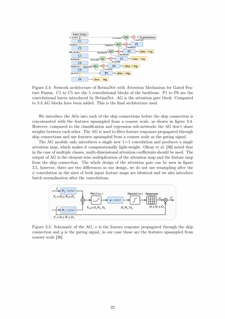
Figure 3.4: Network architecture of RetinaNet with Attention Mechanism for Gated Fea-ture Fusion. C1 to C5 are the 5 convolutional blocks of the backbone. P1 to P6 are theconvolutional layers introduced by RetinaNet. AG is the attention gate block. Comparedto 3.3 AG blocks have been added. This is the final architecture used.

We introduce the AGs into each of the skip connections before the skip connection isconcatenated with the features upsampled from a coarser scale, as shown in figure 3.4.However, compared to the classification and regression sub-networks the AG don’t shareweights between each other. The AG is used to filter feature responses propagated throughskip connections and use features upsampled from a coarser scale as the gating signal.

The AG module only introduces a single new 1×1 convolution and produces a singleattention map, which makes it computationally light-weight. Oktay et al. [36] noted thatin the case of multiple classes, multi-dimensional attention coefficients should be used. Theoutput of AG is the element-wise multiplication of the attention map and the feature mapfrom the skip connection. The whole design of the attention gate can be seen in figure3.5, however, there are two differences in our design, we do not use resampling after theψ convolution as the sizes of both input feature maps are identical and we also introducebatch normalisation after the convolutions.

Figure 3.5: Schematic of the AG, x is the feature response propagated through the skipconnection and g is the gating signal, in our case those are the features upsampled fromcoarser scale [36].

22

Chapter 4

Validation on the DeepLesion dataset

Following all of the modifications made to RetinaNet in chapter 3 we first introduce theDeepLesion [53] dataset in section 4.1. Section 4.2 focuses on the data augmentation doneto improve our results and section 4.3 discusses the details of training our model and theimprovements made to achieve faster and more stable results. Finally, in section 4.4, weevaluate the model; first, we visually inspect the output of the attention blocks and thefinal output of the model to ensure that the results are reasonable. Next, we perform anablation study to measure the effectiveness of our three contributions and compare theresults to other literature, which also uses the DeepLesion dataset.

4.1 DeepLesion

DeepLesion is a very recently released dataset and the largest CT scan dataset. Most otherdatasets contain less than a thousand lesions; this dataset consists of 32,120 CT slices from10,594 studies of 4,427 unique patients. There are 1∼3 lesions in each slice, adding up to32,735 lesions in total. Most other datasets only focus on collecting only one type of lesionor on only one organ. However, DeepLesion contains lesions from 8 different locations:bone, abdomen, mediastinum (mainly lymph nodes), liver, lung, kidney, soft tissue andpelvis with significantly varying diameters ranging from 0.21 to 342.5mm. Figure 4.1 showsa sample of the lesions.

Most of the current research has focused on developing Computer-aided detection/diagnosis(CADe/CADx) systems that focus on a specific lesion type. For example, the Brain TumorSegmentation (BraTS) [35] challenge focuses on brain lesion segmentation, and the LungNodule Analysis (LUNA) [34] challenge focuses on automatic nodule detection. However,this dataset allows development of CAD systems which focus on multiple lesion typeswhich can be found throughout the body. The size and multiplicity of the dataset will alsoimprove the ability to train deep neural networks which require large amounts of images.

The size of the dataset also makes it easier to train networks without initializing themodel with ImageNet [7] or COCO [31] weights. This is particularly helpful for trainingnetworks which have more than 3 input channels.

4.1.1 Annotations

The lesions are annotated using response evaluation criteria in solid lesions (RECIST)diameters which consist of two lines: one measuring the longest diameter of the lesionand the second measuring its longest perpendicular diameter in the plane of measurement,however, we found that the two lines are not always perfectly perpendicular. Bound-ing boxes are also provided, these have been generated from the RECIST diameters byadding/subtracting 5 pixels from maximum/minimum x and y coordinates of the vertices

23

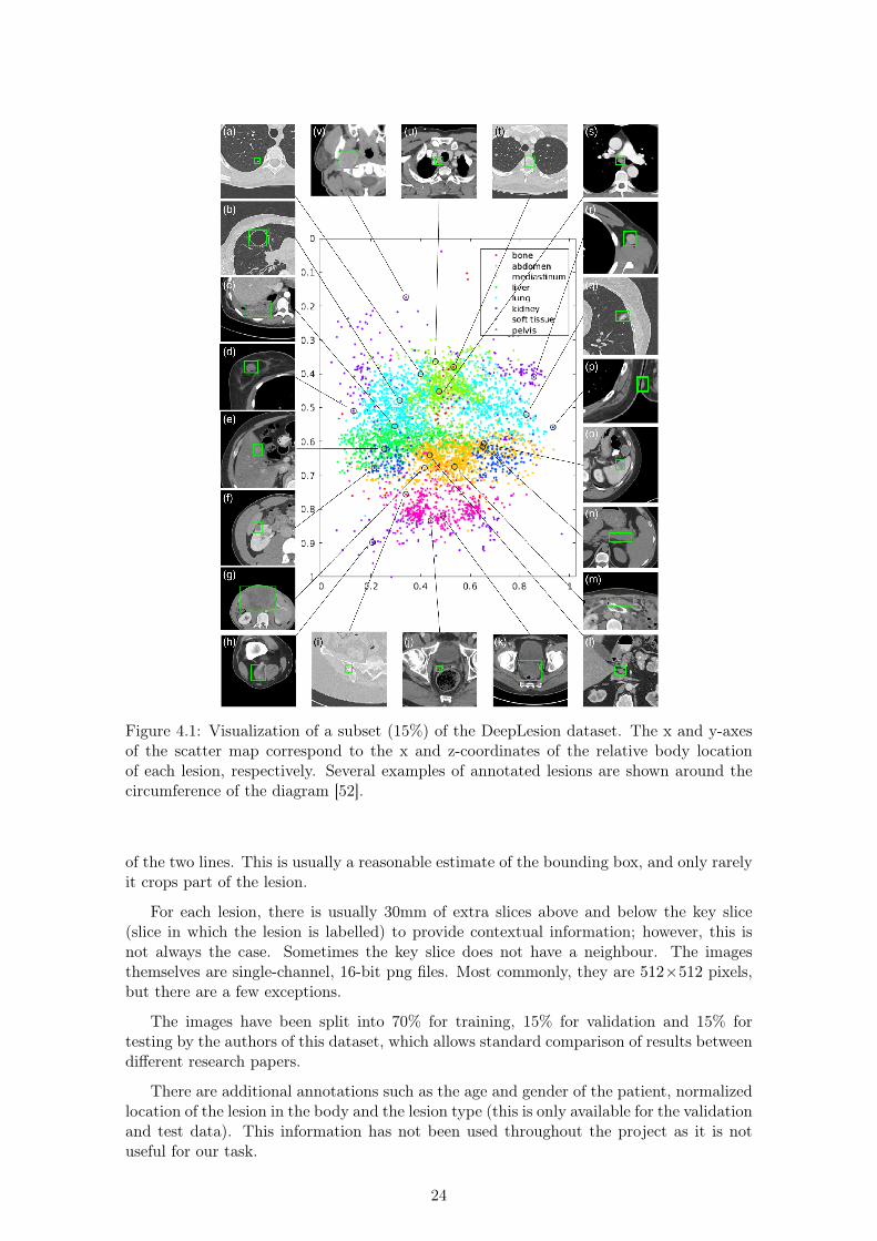
Figure 4.1: Visualization of a subset (15%) of the DeepLesion dataset. The x and y-axesof the scatter map correspond to the x and z-coordinates of the relative body locationof each lesion, respectively. Several examples of annotated lesions are shown around thecircumference of the diagram [52].

of the two lines. This is usually a reasonable estimate of the bounding box, and only rarelyit crops part of the lesion.

For each lesion, there is usually 30mm of extra slices above and below the key slice(slice in which the lesion is labelled) to provide contextual information; however, this isnot always the case. Sometimes the key slice does not have a neighbour. The imagesthemselves are single-channel, 16-bit png files. Most commonly, they are 512×512 pixels,but there are a few exceptions.

The images have been split into 70% for training, 15% for validation and 15% fortesting by the authors of this dataset, which allows standard comparison of results betweendifferent research papers.

There are additional annotations such as the age and gender of the patient, normalizedlocation of the lesion in the body and the lesion type (this is only available for the validationand test data). This information has not been used throughout the project as it is notuseful for our task.

24

Figure 4.2: Example labeled CT scan [52].

4.1.2 Limitations

The DeepLesion dataset is very useful, but it also comes with a few limitations:

• Only 2D RECIST diameter measurements and bounding-boxes of lesions are avail-able. It has no semantic segmentation masks or 3D bounding-boxes. This makes asegmentation task much harder compared to object detection.

• Lesion type is only specified for the validation and test sets. This makes it very hardto train an object detection network which also classifies the lesion based on its type.

• Not all lesions were annotated in the images, radiologists typically only annotatelesions of interest to facilitate follow-up studies of lesion matching and growth track-ing [52]. This means that the object detector might correctly detect some lesionswhen being trained, but it will get penalized as they aren’t annotated and reducethe accuracy of the object detector.

• The dataset contains some noisy bookmarks or bookmarks which measure normalstructures such as lymph nodes. The authors note which images are noisy, so it ispossible to skip them; however, the list of noisy scans is not exhaustive.

• The spacing between CT slices is not always the same, most frequently the CT slicesare 1 or 5 mm apart; however, there are cases of different separation (e.g. 0.625 mmor 2 mm). Interpolation is required to be able to achieve good results when training.One advantage of the difference in spacing is that the trained models will be morerobust and should achieve better results when used in practice.

• There aren’t always 30 mm of extra slices above and below the key slice, and in somerare cases, the key slice has no extra slices above or below. This makes it harderto use many slices at once with a 2D convolutional network as the number of inputchannels has to be the same.

25

4.2 Data Augmentation

Before we can start training the model, we have to preprocess the CT scans so that theycan be fed into the model. The scans are made up of axial slices which in the case ofDeepLesion are stored as 16-bit single-channel png files where each pixel is an integer inHounsfield units (HU) [10] (after a fixed offset has been removed). The CT scans first haveto be changed to a format which is accepted by RetinaNet.

As most object detectors use traditional 8-bit 3-channel images we have to modify theCT scan to this format. To reduce the number of bits which represent each pixel, we clipthe HU window, which is considered. If we want to capture a broad HU range this can berestricted to -1000 to 4000 HU and then normalized to the range of -1 and 1. However,in most cases, even the -1000 to 4000 HU window is too large. In the case of DeepLesion,all of the lesions are within -1024 to 1050 HU, so these values were used to clip the HUwindow. This can be seen in figure 4.3.

Figure 4.3: Numbers of lesions which are visible at different HU windows. The numberson the y-axis should be divided by 10 to find the number of lesions which have at least onepixel of a specific HU. This is because each of the histogram buckets covers a range of 10HU.

All of the images were also resized into 512×512 pixels, resulting in a voxel-spacingbetween 0.175 and 0.977 mm with a mean of 0.802 mm.

We also experimented with resizing all images so that the voxel-spacing is 0.8 mm.When images are not the same size, padding has to be used during training to ensurethat each batch is the same size, although this allows the model to be trained, it mightintroduce strange artefacts. Another disadvantage of resizing is that it introduces blurring;this is caused by the fact that the newly sampled pixels might be interpolated. When wetested both fixed-sized images and compared them to results achieved when the voxel-sizewas fixed to 0.8 mm, we found that it was better to use fixed-sized images.

A naive approach to generate 3-channel images is to duplicate the single-channel imagetwo more times. A better approach is to use the neighbouring CT slices, but this is notstraightforward as different CT scans are taken with different distance between the slices(most commonly 1 mm and 5 mm). There are two approaches to tackle this problem:

• Take the neighbouring slice without considering the distance between slices. This

26

is very simple to implement, but the irregularities in the input data will make itharder to train an accurate object detector. When this method was tested, it slightlyimproved the performance compared to simply duplicating the image; however, theresult was not satisfactory.

• Resample the images at a fixed distance. This generally produces better results. Inour experiments, we resample the images to a 2 mm separation. We chose 2 mmbecause half of the samples in the dataset already have another slice 2 mm away,so fewer images have to be resampled. We also tried using 5 mm as the resamplingdistance; however, the results were worse, this might be because many lesions areless than 10 mm so they might not be visible across all input channels.

In rare cases where neighbouring slices of the key slice are not provided, we duplicatethe key slice to fill the missing input channels.

Data augmentation is used where images are flipped in both horizontal and verticaldirections with a 50% chance. We also use affine transformations with rotation/shearingof up to 0.1 radians, and scaling/translation of up to 10% of the image size. We find thatthis augmentation improves performance and reduces the overfitting of the model.

4.3 Training

Due to the size of the RetinaNet architecture and the size of the DeepLesion dataset, it wasnot feasible to train locally on a personal laptop. Instead, the hardware provided by thedepartmental Computing Support Group (CSG). To store data, we used the "bitbucket"network storage device. To train the model we initially used the "graphic" machines whichare equipped with a range of NVidia GPUs with the weakest being Nvidia GTX 780 andNVidia GTX Titan X. Most of the time we utilized the machines with NVidia GTX 1080,this was because all of the machines operate on the first come first serve basis and theNVidia GTX Titan X was always utilized. Later into the project, we discovered thatthe "ray" machines also had NVidia GTX 1080, which were mostly unutilized as not manypeople knew that they contained GPUs. This greatly improved the rate of experimentationas at some points, we had 4 experiments running concurrently on different machines.

To train the network most of the original parameters were used. We also used Adam [23]optimizer but found that the network converged faster with a learning rate of 10−4 insteadof 10−5. The batch size was set to 4 as this was the highest we could achieve on the hardwareavailable. Also ReduceLROnPlateau1 was used which reduced the learning rate by a factorof 10 when the mean average precision (mAP) has not improved for 2 consecutive epochs,after this reduction a cooldown period of 3 epochs as used to avoid too many consecutivelearning rate reductions. To reduce overfitting, EarlyStopping2 is used if the mAP hasnot improved for 4 consecutive epochs on the validation set.

Our proposed anchor optimisation described in section 3.3 was used to generate newanchors scales and ratios. We obtain optimal scales of 0.85, 1.08 and 1.36, and ratios of3.27:1, 1.78:1, 1:1, 1:1.78, 1:3.27, which fits objects of small size and large ratios.

Traditionally RetinaNet is trained by initializing the backbone weights to the weightsreceived by training the backbone on the ImageNet dataset or initializing the whole modelto weights received by training RetinaNet on the COCO dataset. However, we found thatthe final results were very similar when trained both with weights or when the weights wererandomly initialized. Both of these datasets always only use 3 channels (RGB) howeverin medical imaging we are not limited to only 3 channels, so we decided to use random

1https://keras.io/callbacks/#reducelronplateau2https://keras.io/callbacks/#earlystopping

27

weights as it will make it easier to compare the results when more channels are added. Thetraining usually takes 20 to 30 epochs with around 2 hours per epoch.

4.4 Evaluation

The key metric when evaluating the project is sensitivity of the object detector on thetest set of the DeepLesion dataset. The dataset has been split by the authors into 70%for training, 15% for validation and 15% for testing. A lesion is considered detected ifthe intersection over union (IoU) is more than 0.5. This allows our results to be directlycompared with other literature, which uses the DeepLesion dataset. The sensitivity isevaluated at 0.5, 1, 2, 4, 8 and 16 average false positives (FPs) per image.

Another important metric is the sensitivity for different lesion sizes; the sizes are splitinto three categories based on the length of the shorter RECIST diameter. The firstcategory contains lesions smaller than 10mm, the second contains lesions between 10mmand 30mm and the third contains lesions larger than 30mm.

A secondary metric which we also report is the average inference time; this is notdirectly comparable to other research due to the hardware differences however it can beused to indicate the added complexity of our modifications to RetinaNet.

4.4.1 Current state-of-the-art results

Given that the DeepLesion dataset had only been published in July 2018 there are only3 relevant publications which can be directly compared to this work. Alongside releasingthe DeepLesion dataset, Yan et al. [52] also demonstrated how it can be used for lesiondetection and provided baseline results. They used Faster R-CNN and adopted VGG-16 as the backbone of the network. Tang et al. [48] demonstrated results using MaskR-CNN, used pseudo mask construction and hard negative example mining to proposea new universal lesion detection method which they named ULDor. Currently, the bestresults have been achieved by Yan et al. [51] when they adopted the R-FCN network andincorporated 3D context into the design.

4.4.2 Visual evaluation of the attention mechanism

When Oktay et al. [36] used an attention gate (AG) module for suppressing irrelevantregions during segmentation of the pancreas, they were able to achieve excellent visualresults. We want to see if the same is the case when the AG module is applied to ourmodified RetinaNet which does both segmentation and object detection and when trainedon a more varied dataset which contains 8 different lesion types across a broad HU range.

We inspect the output of the ψ convolution after the sigmoid activation function hasbeen applied, as seen in figure 3.5. These values are then transformed between 0 and 1and overlaid on the original image, red indicates probability closer to 1 and blue indicatesprobability close to 0. If the attention map is smaller than the input image it is resizedwithout using interpolation. There is a green box in each image which displays the groundtruth annotation for reference.

In total we use 5 AG modules, first is connected in the skip connection between theinput image and the segmentation output, the others are connected in the skip connectionsbetween C1-C4 and P1-P4, this can be seen in figure 3.4. In figure 4.4 we display 3 CTsamples and for each sample 5 attention maps.

We find the results to be very intriguing as each attention map is very different andseems to be focusing on different structures with a different purpose. Looking at thetwo finest attention maps (left), we can see that they highlight regions with high lesionprobability, the second column, however, is much more discriminate compared to the first

28

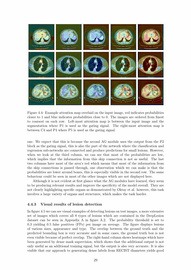
Figure 4.4: Example attention map overlaid on the input image, red indicates probabilitiescloser to 1 and blue indicates probabilities close to 0. The images are ordered from finestto coarsest on each row. Left-most attention map is between the input image and thesegmentation where P1 is used as the gating signal. The right-most attention map isbetween C4 and P4 where P5 is used as the gating signal.

one. We expect that this is because the second AG module uses the output from the P2block as the gating signal, this is also the part of the network where the classification andregression sub-networks are connected and produce predictions for small lesions. However,when we look at the third column, we can see that most of the probabilities are low,which implies that the information from this skip connection is not as useful. The lasttwo columns have most of the area’s red which means that most of the information fromthe skip connections is passed through, one observation which we can make is that theprobabilities are lower around bones, this is especially visible in the second row. The samebehaviour could be seen in most of the other images which are not displayed here.

Although it is not evident at first glance what the AG modules have learned, they seemto be producing relevant results and improve the specificity of the model overall. They arenot clearly highlighting specific organs as demonstrated by Oktay et al. however, this taskinvolves a large variety of organs and structures, which makes the task harder.

4.4.3 Visual results of lesion detection

In figure 4.5 we can see visual examples of detecting lesions on test images, a more extensiveset of images which covers all 8 types of lesions which are contained in the DeepLesiondataset can be seen in Appendix A in figure A.2. The probability threshold is set to0.3 yielding 0.5 false positives (FPs) per image on average. The figure displays lesionsof various sizes, appearance and type. The overlap between the ground truth and thepredicted bounding box is very accurate and in some cases, the ground truth box is noteven visible because of perfect overlap. The right-hand column shows heatmaps which havebeen generated by dense mask supervision, which shows that the additional output is notonly useful as an additional training signal, but the output is also very accurate. It is alsovisible that our approach to generating dense labels from RECIST diameters yields good

29

Figure 4.5: Visual results for lesion detection at 0.5 FP rate using our improved RetinaNet.The first three columns show different sizes from small to large. The right column showsheatmaps from the segmentation layer overlaid on detections. Yellow boxes are groundtruth, green are true positives, red are false positives. Last row shows intriguing failurecases with possibly incorrect ground truth.

results which are sufficient for training and it is not necessary to generate them manually.In the last row, we can see several results where the network fails to detect the lesioncorrectly. The detections look plausible and might be negative because some of the lesionswere not labelled as they weren’t relevant to the clinicians who annotated the dataset.

4.4.4 Ablation study

In Table 4.1, we present the lesion detection sensitivities with different FPs per image.As a baseline we quote the results provided by Yan et al. using Faster R-CNN (reportedin [51] as they do not report results for 4 FPs in the original paper) and a result providedby Tang et al. [48] using Mask R-CNN. The current best results achieved by Yan et al. [51]using a modified Faster R-CNN called 3DCE and results achieved by Tang et al. [48] usinga modified Mask R-CNN called ULDor are also reported. In an ablation study, the resultsmentioned above are first compared to the original RetinaNet without any modificationsand then our improvements are incrementally added with the final improvement showingthe results for our final model.

The results show that the default anchor configuration performs poorly, even worsethan Faster R-CNN and Mask R-CNN, which indicates that out-of-the-box approaches aresub-optimal for medical imaging. This is because datasets such as COCO, which are usedto design better object detection models, generally contain larger objects of many classesand medical imaging datasets contain smaller objects which are usually classified into fewerclasses.

After the automatic anchor optimization was used to optimize the scales and ratios

30

Table 4.1: Detection performance of different methods and our ablation study at multiplefalse positive (FPs) rates.

Methods 0.5 1 2 4 8 16 runtime

Faster R-CNN [40] 56.90 67.26 75.57 81.62 85.83 88.74 32 msMask R-CNN [16] 39.82 52.66 65.58 77.73 85.54 91.80 -

ULDor (Tang et al. [48]) 52.86 64.80 74.84 84.38 87.17 91.80 -3DCE (Yan et al. [51]) 62.48 73.37 80.70 85.65 89.09 91.06 114 ms

original RetinaNet [30] 45.80 54.17 62.50 69.80 75.34 79.48 28 ms+ anchor optimization 64.82 74.98 82.29 87.87 92.20 94.90 31 ms+ dense supervision 70.24 78.28 85.10 90.39 93.81 96.01 39 ms+ attention gate 72.15 80.07 86.40 90.77 94.09 96.32 41 ms

Table 4.2: Detection performance of the modified anchor configuration compared to theoriginal configuration.

Methods 0.5 1 2 4 8 16

Original config.<10mm 13.99 20.49 27.98 35.77 43.19 49.4410-30mm 58.32 68.26 77.28 85.25 90.22 93.47>30mm 75.03 81.17 89.30 92.71 95.81 98.14

Modified config.<10mm 61.90 71.90 78.77 84.85 89.50 92.7010-30mm 65.60 75.61 83.24 88.93 92.83 95.71>30mm 69.77 80.62 87.90 91.16 94.41 96.90

of anchor boxes, RetinaNet already outperforms previous state-of-art models. This is arelatively inexpensive step as it does not require any modification to the model or the inputdata; neither does it require extensive hyperparameter optimization and a lot of hours oftraining. This whole step can be done automatically, which makes it an ideal first stepbefore investing a lot of time and resources into modifying the network architecture. Thesensitivity at 0.5 FP is 2.34% higher than 3DCE and this improvement can be seen acrossall FP rates. The increase in runtime can be attributed to the fact that the model producesmore positive predictions which require non-maximum suppression to be applied to moreobjects; however, the number of weights has not changed at all.

The optimised anchor configuration results in an average IoU of 0.7046 compared to theoriginal 0.5808 IoU. Another key metric is the number of lesions which are not matchedby any bounding box as unmatched lesions effectively reduce the training set size; thenew configuration successfully matches all of the lesions in the training set, the originalconfiguration fails to match 5573 samples which is 26.10% of the training set.

In table 4.2, we can see a more in-depth evaluation of the sensitivity achieved onthe DeepLesion dataset at different FP rates when both original and modified anchorconfiguration is used. From this, we can see that the model which was trained with theoriginal configuration struggles to find small (< 10mm) lesions reliably or even mid-size(10-30mm) lesions. This is greatly improved by the modified configuration; however, itis still harder to find smaller and mid-sized lesions compared to the large lesions. Theoriginal configuration is better at finding lesions which are larger than 30 mm; we suspectthis is because the smaller lesions were not matched and were ignored during training,so the training set was skewed to larger lesions which wasn’t the case with the originalconfiguration.

Adding dense supervision with segmentation masks generated from RECIST diame-

31

Figure 4.6: Left: FROC curves for our improved RetinaNet variants and baselines onDeepLesion dataset. Right: Per lesion size results at 4 FPs compared to 3DCE [51].

ters significantly boosts detection sensitivity across all FP rates, with 5.42% improvementat 0.5 FP. The pixel-wise supervision adds an important training signal, providing moreprecise localization information in addition to bounding-boxes. This step adds additionalcomplexity as it requires multiple convolutions and upsampling blocks to be added, whichincreases the runtime by 25% however, it still runs faster than 3DCE. Using the consis-tency between bounding-box regression and dense classification also helps to reduce falsepositives, although this hasn’t been added as a separate entry in the table the main im-provement was seen at 0.5 and 1 FP per image. Finally, adding an attention mechanismfurther improves the performance; however, this is not as significant at higher FP rates.Overall our combined architecture achieves a sensitivity of 72.15% at 0.5 FPs and 90.77%at 4 FPs, with an improvement of almost 10% at 0.5 FP over the best-reported results.

In figure 4.6, we display the free-response receiver operating characteristics (FROC)curves of different methods. For Faster R-CNN, Mask R-CNN, ULDor and 3DCE we use6 points to plot the lines as we could only get data for 0.5, 1, 2, 4, 8 and 16 FPs which isthe same as displayed in table 4.1. On the right in figure 4.6, we can see the performanceof our model compared to 3DCE for different lesion sizes. The lesions are divided intothree groups based on the length of the shorter RECIST diameter. A significant differencebetween our model and 3DCE can be seen for lesions smaller than 10 mm, in this case, oursensitivity is 88.35% compared to 80% for 3DCE however model still outperforms 3DCEat different sizes as well. We achieve sensitivity of 91.73% compared to 87% achievedby 3DCE with lesions between 10mm and 30mm, and for lesions larger than 30 mm thesensitivity of our model is 93.02% compared to 84% of 3DCE. Although 3DCE performswell compared to other approaches, it seems that the additional 3D context is not as helpfulfor small lesions compared to medium and larger ones. The feature pyramid successfullyretains responses from small lesions and together with dense supervision it can achievevery good results mainly on small lesions, this is critical as it is easier to miss a smallerlesion in a large scan when it is analyzed by clinicians.

Each lesion in the test and validation datasets also is assigned one of the 8 lesion types.In table 4.3, we can see the sensitivity at 4 FPs per image on the test set of DeepLesion.We report the accuracy of Faster R-CNN and 3DCE (reported in [51]) as well as our resultswith anchor optimization, dense supervision and attention gate improvements.

From the results, we can see that our model achieves better results for almost all lesiontypes except for the soft tissue type, which contains lesions in muscles, skin, and fat. Thismight be because there aren’t a lot of samples of soft tissue lesions in the dataset andthey are more spread across the body compared to kidney or bone lesions. Compared tothe results achieved by Faster R-CNN and 3DCE we achieve a lower spread of sensitivities

32

Table 4.3: Detection performance of different lesion types at 4 false positives (FP) perimage. The last row contains the number of samples of each lesion type in the test set.The lesion types have been sorted based on the size of the test. The abbreviations of lesiontypes stand for abdomen (AB), lung (LU), mediastinum (ME), liver (LV), pelvis (PV),soft tissue (ST), kidney (KD), and bone (BN), respectively. The mediastinum type mainlyconsists of lymph nodes in the chest. Abdomen lesions are miscellaneous lesions that arenot in the liver or kidneys. The soft tissue lesion type contains lesions in muscles, skin,and fat [51].

Lesion typeAB LU ME LV PV ST KD BN

Faster R-CNN 75 88 84 80 76 76 72 553DCE 80 91 88 84 81 82 76 63Ours 89 93 93 94 90 80 87 83

Number of samples 1171 1100 864 700 409 327 233 108

among the different lesion types, the highest sensitivity is 94% for liver lesion type and thelowest is 80% for soft tissue lesion type which results in a spread of 14%. 3DCE achieves91% for lung lesion type and 63% for bone resulting in 28% spread. We can see the greatestimprovement with bone lesions where the sensitivity improved by 20% from 63% achievedby 3DCE to 83% achieved by our model.

33

Chapter 5

Validation on the whole-body MRIdataset

We were able to achieve a sensitivity of 90.77% at 4 false positives per image on the DeepLe-sion dataset which significantly outperforms all other research on the same dataset. In thischapter we will demonstrate that our model can be applied to another medical datasetwithout any modifications to the architecture and is truly a universal lesion detector.

To do this we will use a whole-body Magnetic Resonance Imaging (MRI) dataset andattempt to correctly detect primary colorectal and lung lesions. Most of this chapter focuseson describing the work required to preprocess and augment the data, how we overcameseveral difficulties such as finding lesions in a 3D volume with a network which uses 2Dslices. Finally we will evaluate our performance on the dataset and discuss which changeswere the most beneficial.

5.1 Whole-body MRI dataset

The second dataset used is an in-house whole-body MRI dataset which contains Apparentdiffusion coefficient (ADC), Diffusion-weighted (DW) and T2-Weighted (T2W) imagingprotocols as well as semantic annotation of a primary colorectal and lung lesion in eachscan. The dataset is much smaller than the DeepLesion dataset with only 213 MRI scans,however we found 3 of these scans to contain artefacts preventing us from using them soonly 210 scans will be used.

Figure 5.1 displays 9 slices (3 slices per imaging protocol) from 3 different MRI scans.The figure is a good example of the modality and richness of the data but also it demon-strates that the challenges which we will face such as noise, missing slices and misalignment.

5.1.1 Annotations

The dataset was provided with semantic segmentation’s of lesions. In each scan only theprimary lesion should be annotated however in some cases the annotations were noisy whichresulted in multiple disjoint partial segmentation of the lesion or it contains multiple smallervolumes which were probably introduced accidentally during the annotation process. Toremedy these issues we applied 1 iteration of binary dilation to connect the semanticsegmentation’s which are disconnected but are close to each other. Afterwards 1 iterationof binary erosion was applied to counteract the dilation while keeping the volume connected.Finally all holes in the mask were filled in, the assumption was that if a voxel is entirelysurrounded by a lesion then it should be considered to be a part of the lesion. If thesegmentation volume still contains multiple volumes the largest one is retained and therest are removed.

34

Figure 5.1: Example of an ADC, DW and T2W scan (from left to right). For each of theimaging protocols three different slices are shown. They are taken along the axial, coronaland sagittal plane (from top to bottom).

5.1.2 Limitations

Comparatively to the DeepLesion dataset the whole-body MRI dataset is much smaller.It contains only 210 usable scans whereas the DeepLesion dataset consisted of 32,120 CTslices from 10,594 studies of 4,427 unique patients. Although the 210 scans can generatemore 2D samples which contain a lesions, the slices are highly correlated so they add lessvalue than having more scans from unique patients. This means that it will be harder to getgood results and more care is required during training to stop the model from overfitting.

A major drawback of the dataset is that it has been collected from multiple sources ondifferent MRI systems which have different field strengths and coil characteristics. Anotherdrawback compared to CT scans is that image intensities in MRI do not have a fixedinterpretation so if the same patient is scanned using a different protocol the intensitiesmight be different. Although this might not be a problem if a human reader is inspectingthe scan it will pose a problem for our model if correct preprocessing is not used. Anexample of this can be seen in figure 5.2.

The last limitation which reduces the dataset size usable for training is the occurrenceof artefacts and noise in the scan. An example of few artefacts can be seen in figure 5.3.

35

Figure 5.2: Multiple T2W scans taken with different protocols [25]

5.2 Data Augmentation

As the dataset is made up of 3 different scans, namely ADC, DW and T2W, it is firstrequired to prepossess them individually before they are merged and fed into the model.

First all of the scans are resized so that they have the same size and spacing. In ourcase the spacing is (1.5, 1.5, 5.5) and the size is 320x320x232. Although fully convolutionalnetworks don’t require all input images to be the same size, if multiple images are fed in asingle batch then the input size has to be the same for the batch so it was easier to resizethe entire scan instead of ensuring a whole batch has the same size at runtime.

To achieve the best results it is important to rescale the voxel intensities such thatmost of them are between -1 and 1. We experiment with two different approaches to dothis.

This first approach uses clipping of intensities which removes all outliars. The ADCvalues are clipped between [0, 3800], DW values are clipped between [0, 1050] and T2Ware clipped between [0, 8200]. After the values are clipped they are normalized between -1and 1. This approach worked well on the DeepLesion dataset because the values ended upcentered around 0 however in this case the distribution of intensities is positively skewedand most of the intensities after normalization end up centered around -1.

To tackle the skewness of the data we use a StandardScaler implemented in sklearn [38].This rescales all of the values so that the mean is 0 and the standard deviation is 1. Giventhat a large part of the scan is background all zero intensities are ignored when calculatinghow the values should be transformed. This approach produces much better results thanusing clipping.

During experimentation we noticed that the ADC and T2W scans are not perfectlyaligned so we experiment with registration to transform the T2W scan. Initially the centresof mass for both scans are aligned, then Mutual Information is used for Rigid Transforma-tion and consecutively for Affine Transformation. Both of these transformations are doneat 3 different resolution settings. The lowest resolution is 4 times smaller than the originalimage and Gaussian blurring with sigma of 3 is applied, at this level the algorithm waslimited to 10000 iterations. The next resolution is 2 times smaller than the original one

36

Figure 5.3: Example of the data quality challenges (artefacts) we encountered in the datasetsuch as missing slices, interference and motion artefacts [25]

with sigma of 1 and 1000 iterations and then the last round of optimization is applied atthe original resolution without any blurring for 100 iterations. To reduce the time taken forregistration the Mutual Information is calculated by only sampling 10% of the pixels and32 bins are used for computing the histogram intensity. During evaluation we found thatin some cases the scans were better aligned but in others it resulted in a lot of unnaturalelastic deformation and did not make a meaningful impact on the results. We did not useregistration in the final model.

We have also experimented with several forms of denoising in an attempt to improvethe results however we were not able to do so. The following methods were attempted:

• Gaussian denoising was applied on the ADC scans with multiple different sigmavalues ranging from 1 to 5. The best results were for sigma of 1 however the accuracywas still lower than without denoising.

• Noise2noise [26] was used because it has been previously successfully applied to otherMRI data. The results when using this were better than when Gaussian denoising wasused however there was no improvement. However for this experiment an unofficialKeras implementation was used instead of the official one with a slightly differentmodel so that could have been one of the causes.

• Non-local means denoising implemented by the dipy [11] library was used with bothRician and Gaussian noise. It provides a function to estimate the amount of noisefrom local patches which avoids having to use hard-coded values. This was tested onboth ADC and DW scans.

To further reduce overfitting we apply elastic deformation to the entire scan. Thisallows us to augment the data in all 3 axes. The deformation grid has three points with asigma of 25. For each scan which is in the training set we generate 4 additional elasticallydeformed scans.

Our model requires both semantic segmentation and bounding boxes for training, gen-erating bounding boxes is however easier than generating semantic segmentation masksfrom bounding boxes as we have done previously. The bounding box is generated sepa-rately for each axial slice of the MRI by finding the minimum and maximum x and y valuesfor the segmentation in that slice and adding or subtracting 5 pixels. This is done so that

37

the smallest bounding boxes are not ignored during training. The expansion of boundingboxes might introduce a slight amount of noise during training however it ensures thatevery slice which has a partial semantic segmentation will also have an associated bound-ing box which is big enough so that it isn’t ignored by the classification and regressionsub-models. Another advantage of slightly increasing the bounding box size is that morebounding boxes are detected by the coarser levels in the feature pyramid which shouldtheoretically improve the results as there are more convolution layers between the inputand output.

5.3 Training Data Generation

Our model only uses 2D convolutions and produces 2D bounding boxes and heatmap. Thismakes it impossible to feed in all of the slices at the same time into the model. Insteadwe only input 9 axial slices at a time for each of the 3 scans, this results in a total of 27channels. To reduce the number of false positive predictions we also randomly sample 8negative slices (slices which don’t contain a lesion) from each scan so that there is a roughlyequal number of slices with and without a lesion. For a slice to be selected it must containat least one pixel with intensity greater than 0 in the ADC scan. It also cannot be within5 slices of another slice which contains the lesion. This is done to avoid selecting sliceswhich might still contain a small part of the lesion even though they have not be labelled.

We split the dataset into training, validation and test such that there are 150 (71.4%)scans in the training set, 30 (14.3%) scans in the validation set and 30 (14.3%) scans inthe test set. The dataset contains 136 scans with colorectal lesions and 74 lung lesions. Toensure that the test and validation sets are roughly representative of the dataset there are10 lung lesions and 20 colorectal lesions in both the validation and test sets.

5.4 Training

One of our goals when training on the whole-body MRI dataset was to make minimalmodifications to the model design to demonstrate that the same model can be applied toother datasets so no modification was made to the architecture itself. The only modificationwas to the configuration parameters which define the dimensions of the anchors and thebatch size. The same scales were used for this dataset as for DeepLesion however insteadof using ratios of 3.27:1, 1.78:1, 1:1, 1:1.78, 1:3.27 we used ratios of 2:1, 1.5:1, 1:1, 1:1.5,1:2.

We were able to increase the batch size from 4 to 8 samples given that the input sizeto the 2D convolution is 320×320 instead of 512×512 (number of channels is omitted asincreasing the number of input channels in a 2D convolution does not increase the numberof weights in further convolutions).

The model was trained using the same method as when trained on DeepLesion datasethowever we found that training from randomly initialized weights was very unstable. In-stead we used the weights trained on the DeepLesion dataset.

5.5 Stabilizing loss when negative samples are used

When we used negative samples during training we noticed that the loss was very unstable,this however was not the case when only positive samples were used. The problem gotworse as the ratio between positive and negative samples increased. Initially the thoughtbehind this was that the network is trained to produce a lot of positive predictions and ispenalized more when there are no positive samples in the training batch. However upon

38

further inspection of the implementation of Focal Loss which was used during trainingwe noticed that the loss is divided by the number of positive targets in the batch. Inthe classification sub-network the number of positive targets is the same as the numberof anchors which have more than 0.5 IoU with the ground truth which is usually at least5 per sample. In the semantic segmentation output there is usually at least 100 positivetargets per sample. However if all samples in a batch are negative we would divide by 1.

Given that the batch size used was 8 and there was the same number of positive andnegative samples in the dataset there was a 0.58 = 0.0039 (0.39%) probability that a batchwas completely negative. In this case the loss was not divided and could be 10 to a 100times higher than usual.

To remove these loss spikes we first tried to use the mean loss instead of dividing bythe number of positive targets. This greatly reduced the loss as most samples are classifiedcorrectly as negative and removed spikes in the loss. The drawback of this approach is thatit puts more weight on larger lesions as the output of the semantic classification has morepositive pixels and the loss is higher in this case. This is contradictory to our goal as largerlesions are easier to classify. Another issue with this approach was that RetinaNet also usesL1 loss for the output of the regression subnetwork, because the Focal Loss got reduced,the overall weight of the L1 loss was higher which indicated to the network that it is moreimportant to have a good overlap between the predicted bounding box and the groundtruth but it is not as important to correctly classify the lesion. Again this is contradictoryto our goal as detecting the lesion is more important.

To overcome the problems with the method above we instead keep a running averageof the number of positive ground truth outputs in a batch and in the case that the wholebatch has only negative samples we divide by the loss by the average instead of dividingit by 1. This way the ratio between L1 and Focal Loss remains the same and we take intoaccount the size of the lesion. There is still an issue that we don’t take into account howmany positive and negative samples there are in a batch, we only address the case with 0positive samples however there might be 1 positive and 7 negative samples. Although inthis case the loss might still be divided by a low number introducing a small spike, duringtraining we found that our solution above greatly improved the stability and there was noneed for further optimization.

5.6 Merging 2D predictions

To train and validate the model we feed in 2D slices of the MRI scans and the modeloutputs 2D masks and bounding boxes. Our goal is to produce 3D segmentation so weneed to devise a suitable method of combining our results into a single prediction.

The initial approach was to merge the bounding boxes on adjacent slices if they hadan IoU more than 0.5 into a single 3D prediction. However this approach has severalshortcomings:

• It is possible that two bounding boxes on the same slice have an overlap of more than0.5 with another bounding box on the adjacent slice. If we add both bounding boxesinto our prediction we effectively create a fork in the lesion which most probablydoesn’t represent its structure, we could either merge the 2 boxes or we can pickthe box with the highest probability. This seems like a reasonable approach howevergreedily picking the best anchor can lead to a sub-optimal final result.

• Using 0.5 as an IoU between slices is very arbitrary and introduces another hyper-parameter which needs to be optimized.

• It is not clear how to calculate the final prediction score for the lesion based on thescores from the individual bounding boxes.

39

Instead of relying on the bounding box we used the mask output and concatenated theoutputs for all slices into a single volume. Then to generate a binary mask we normalizethe prediction volume so that all values are between 0 and 1 and then round the values togive us either 0 or 1. There are usually some very small predictions which are too small tobe lesions so all predictions which are only on a single slices are ignored. Bounding boxesare then used to define the score of a prediction, the bounding box with the highest scoreand with IoU of 0.5 with the prediction is used.

5.7 Evaluation

In this section we will evaluate how differences in preprocessing, training and evaluationaffect the sensitivity of our model. We cannot compare it to other research as the whole-body MRI dataset is completely new and no one else has trained models on it for the sametask and to the same extent as we have. The task of colorectal and lung lesion detectionin whole body MRI using machine learning has not been extensively studied so it is notpossible to compare to other models even if they have been trained on other datasets.

5.7.1 Visual results

In figure 5.4 we can see a visual example of a DW scan and a ground truth segmentationof the lesion. In figure 5.5 we can see the segmentation mask generated by our model. Theprediction shows two volumes which might be colorectal lesions, there are also two lunglesions predicted (not shown in the image). There are also several very small predictedvolumes next to the main predictions. As these are separate they might increase thenumber of false positive predictions in our evaluation even though they are very close toeach other. To improve the results there needs to be another post-processing step whichremoves small noisy predictions however it is not possible to just do this based on the sizeof the prediction as lung lesions are also very small.

Figure 5.4: The ground truth segmentation overlaid on a DW scan. Bottom left viewshows a 3D render of the lesion and the other show 2D slices of the MRI.

Instead of displaying the binary mask segmentation it might be more useful to displaya heatmap. An example can be seen in figure 5.6. This focuses the clinicians focus at the

40

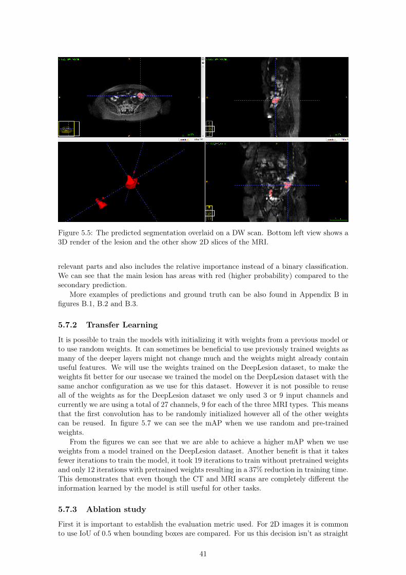
Figure 5.5: The predicted segmentation overlaid on a DW scan. Bottom left view shows a3D render of the lesion and the other show 2D slices of the MRI.

relevant parts and also includes the relative importance instead of a binary classification.We can see that the main lesion has areas with red (higher probability) compared to thesecondary prediction.

More examples of predictions and ground truth can be also found in Appendix B infigures B.1, B.2 and B.3.

5.7.2 Transfer Learning

It is possible to train the models with initializing it with weights from a previous model orto use random weights. It can sometimes be beneficial to use previously trained weights asmany of the deeper layers might not change much and the weights might already containuseful features. We will use the weights trained on the DeepLesion dataset, to make theweights fit better for our usecase we trained the model on the DeepLesion dataset with thesame anchor configuration as we use for this dataset. However it is not possible to reuseall of the weights as for the DeepLesion dataset we only used 3 or 9 input channels andcurrently we are using a total of 27 channels, 9 for each of the three MRI types. This meansthat the first convolution has to be randomly initialized however all of the other weightscan be reused. In figure 5.7 we can see the mAP when we use random and pre-trainedweights.

From the figures we can see that we are able to achieve a higher mAP when we useweights from a model trained on the DeepLesion dataset. Another benefit is that it takesfewer iterations to train the model, it took 19 iterations to train without pretrained weightsand only 12 iterations with pretrained weights resulting in a 37% reduction in training time.This demonstrates that even though the CT and MRI scans are completely different theinformation learned by the model is still useful for other tasks.

5.7.3 Ablation study

First it is important to establish the evaluation metric used. For 2D images it is commonto use IoU of 0.5 when bounding boxes are compared. For us this decision isn’t as straight

41

Figure 5.6: The predicted heatmap overlaid on a DW scan. Areas with red are areas witha high probability of a lesion and blue areas have low probability.

Table 5.1: Detection performance of different scan preprocessing methods.

Methods 0.5 1 2 4

Value clipping 46 63 70 70StandardScaler 66 70 73 73

forward because we generate both segmentation masks and bounding boxes. In addition tothis we find it more important to get an approximate location with high confidence insteadof getting a perfect segmentation. We will consider a lesion as detected if it has a DICEscore of 0.2 with our prediction.

The first modification which we evaluate is how we preprocess the intensities in thescans. Initially we used value clipping and then rescaled the clipped values between -1 and1. The second method uses StandardScaler1 implemented in sklearn. It rescales theintensities so that they have a mean of 0 and standard deviation of 1. Both of these havebeen explained in further detail in section 5.2. The results of this experiment can be seenin table 5.1. From the results it is visible that it is much better to use the StandardScaleras it achieves better results, mainly with a low number of FPs.

To make the dataset more diverse we experiment with elastic deformation applied to theoriginal MRI scans before we create 2D slices. The aim of this is to reduces overfitting and

1https://scikit-learn.org/stable/modules/generated/sklearn.preprocessing.StandardScaler.html

42

Figure 5.7: Plot of the mean Average Precision (mAP) achieved during training. The topimage shows the mAP during training when no weights are used. The bottom image showsthe mAP during training when pre-trained weights are used.

Table 5.2: Detection performance of elastic deformation with different values of sigma anddifferent transformation of individual training samples.

Methods 0.5 1 2 4

Sigma of 10 + No 2D transformation 43 56 66 73Sigma of 10 + 2D transformation 66 70 80 80

Sigma of 25 + No 2D transformation 60 73 76 80Sigma of 25 + 2D transformation 66 70 83 83

to add 3D transformation in addition to the 2D transformations which are done duringtraining. Ronneberger et al. [41] used elastic deformation with sigma of 10 to improvethe results when they introduced the U-Net model. We experimented with both sigmaof 10 and 25. After we generate the 2D slices we also investigate whether further 2Daugmentation such as rotation and translation (the augmentation is the same as describedin section 4.2) is still useful. The results of this experiment can be seen in table 5.2.

It is very hard to directly judge how the change in sigma affects the performancehowever we can see that using 2D transformation improves the results and that the resultswith elastic deformation are better than the results in table 5.1.

In table 5.3 we can see the detection performance for each of the lesion types in thedataset. It is however hard to judge the performance as there are only 10 lung lesionsand 20 colorectal lesions in the test set. It would be beneficial if cross-validation was usedhowever this would greatly increase the amount of time required to train and validate ourresults.

In practice is more important to find the approximate location of the lesion instead of aperfect overlap between the ground truth and the semantic segmentation. We experimentwith another evaluation metric which instead measures the distance between the centroidof the prediction and the ground truth. If the centroid is within the ground truth thenthe distance is considered as 0, otherwise its the distance to the closest voxel which is partof the lesion. The sensitivity (TPR), precision (PPV) and F1 scores can be seen in figure5.8. From the figure we can see that even at 2 predictions per image on average we canfind more than 80% of the lesions within 4cm from our prediction and with 4 predictions

43

Table 5.3: Detection performance split by lesion type.

lesion type 0.5 1 2 4

Colorectal 60 60 80 80Lung 80 90 90 90

per image we can find all of the lesions.

Figure 5.8: Sensitivity (TPR), Precision (PPV) and F1 score of our model for differentground truth-detection distances. In the left image there are 2 predictions per image onaverage, in the right image there are 4 predictions per image on average.

44

Chapter 6

Spot-the-Lesion Game

To demonstrate our results and introduce people to medical imaging, we have built a smallbrowser game where the user has to locate a lesion in a CT scan. This tool is not aimedat doctors as it is relatively simplistic, it only allows the users to click on a single imagewithout viewing neighbouring slices, seeing the CT scan along all axes and modifying theHU window. The website has been designed for both PC and larger touch screens withresponsive design and simple controls.

In the game, the user is shown a slice from a CT scan which contains only one lesion.The user has 10 seconds to find and click on the lesion. This task is difficult so to help theuser a circle will appear after 5 seconds indicating a smaller area where the lesion can befound. After the player runs out of time, the ground truth, as well as the prediction fromour model, appears. To make the game fair, we only use the most probable prediction fromour model, even if there might be multiple. In figure 6.1 we can see the game screen whichthe user can see. In figure 6.2 we can see the red circle which narrows down the searcharea, the ground truth and the prediction from our model.

We use our model as an opponent. Initially, the aim was to deploy the model andsend requests to it live. However, continuously running it a server with a GPU would becostly and just running inference on a CPU would be slow as our model is very large.Instead, we attempted to deploy it on a serverless platform called Algorithmia1 which isbuilt purposefully for deploying machine learning models and allows us to run them on aGPU. During testing we saw that it takes between 60 and 120 seconds to complete therequests and even subsequent requests are equally slow so it seems that the container whichruns the model does not stay warm between runs so it would not be possible to warm itup when a user visits the website.

To avoid having to wait so long for a prediction, we pre-compute the results for allsamples and then request the result with the image which will be shown to the user. Tokeep the game exciting and to avoid repetition of the same images we use all of the testslices which contain a single lesion, this gives us a total of 4817 samples.

The CT images which are shown to the user are chosen randomly; however, during usertesting we found this to be a disadvantage because some of the samples were noisy or thelesion was too hard to find. To avoid this, we give the user the ability to provide a randomseed so that a predictable sequence of samples is generated. This change makes it easierto demonstrate the website and allows multiple people to compete with each other whilebeing shown the same examples.

1https://algorithmia.com/

45

Figure 6.1: The main view of the website. There are instructions on how to play the game,on the right you can see how well you do compare to our trained model and in the center,you can see the current CT slice.

Figure 6.2: The view of the website after time runs out. The red circle indicates a smallerarea where the lesion can be found. The yellow rectangle is the ground truth and the greenrectangle is the prediction from our model.

46

Chapter 7

Conclusion and Future Work

We have successfully redesigned RetinaNet to be used for medical imaging and achievedstate-of-the-art results on two datasets showing that our approach is generalisable.

This was done by first designing an approach which can be used to automaticallyoptimise RetinaNet anchor configuration without having to use many resources on trainingthe network. This greatly improves iteration speed and reduces the number of variableswhich have to be manually optimised. To make better use of the annotated data, wegenerated dense masks from weak RECIST labels which are routinely produced in clinicalpractice. This allows full use of the available data and improves the accuracy withouthaving a large impact on training or inference times. Further, we have also integrated anattention mechanism into the network, which has improved the sensitivity mainly at lownumber of false positives.

To validate our results we have used two datasets. The first one being the DeepLesiondataset, where we achieve a sensitivity of 90.77% at 4 false positives per image, significantlyoutperforming the best reported methods by over 5%. We also used a much smaller whole-body MRI dataset to demonstrate that the model can be applied to 3D datasets withdifferent modalities and still achieve excellent results.

Overall, the results show that we have indeed built a universal lesion detector. Althoughthe results significantly outperform the best reported methods, there is still a lot of areafor further research before this work can be used in the industry.

7.1 Future Work

Although we have been able to achieve excellent results and evaluated our model on twodifferent datasets, there is still a lot of room for future work. The primary focus would beon improving the datasets which are used for training. The second opportunity for futurework is to improve the model design itself, because to achieve state-of-the-art results,medical imaging requires modification to existing models, as we have shown. The finalarea for extension is to do a more in-depth evaluation which would involve clinicians, inorder to achieve a better understanding of how well our approach works when used inindustry.

7.1.1 Dataset cleaning and augmentation

When we used the DeepLesion dataset, we saw that it contained noisy CT scans. Some ofthese were labelled as noisy and could be ignored during training, validation and testing.However, due to the complexity and expertise required when labelling the training data,there may still be incorrectly labelled scans. When we used the whole-body MRI dataset,we could see random noise in the ground truth labels or two annotations which were disjoint

47

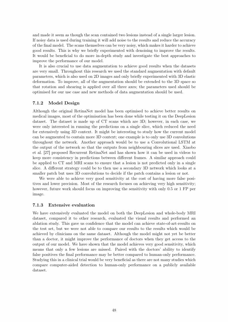
and made it seem as though the scan contained two lesions instead of a single larger lesion.If noisy data is used during training it will add noise to the results and reduce the accuracyof the final model. The scans themselves can be very noisy, which makes it harder to achievegood results. This is why we briefly experimented with denoising to improve the results.It would be beneficial to do more in-depth study and investigate the best approaches toimprove the performance of our model.

It is also crucial to use data augmentation to achieve good results when the datasetsare very small. Throughout this research we used the standard augmentation with defaultparameters, which is also used on 2D images and only briefly experimented with 3D elasticdeformation. To improve, all of the augmentation should be extended to the 3D space sothat rotation and shearing is applied over all three axes; the parameters used should beoptimised for our use case and new methods of data augmentation should be used.

7.1.2 Model Design

Although the original RetinaNet model has been optimised to achieve better results onmedical images, most of the optimisation has been done while testing it on the DeepLesiondataset. The dataset is made up of CT scans which are 3D; however, in each case, wewere only interested in running the predictions on a single slice, which reduced the needfor extensively using 3D context. It might be interesting to study how the current modelcan be augmented to contain more 3D context; one example is to only use 3D convolutionsthroughout the network. Another approach would be to use a Convolutional LSTM atthe output of the network so that the outputs from neighbouring slices are used. Xiaoboet al. [27] proposed Recurrent RetinaNet and has shown how it can be used in videos tokeep more consistency in predictions between different frames. A similar approach couldbe applied to CT and MRI scans to ensure that a lesion is not predicted only in a singleslice. A different strategy could be to then use a secondary 3D network which looks at asmaller patch but uses 3D convolutions to decide if the patch contains a lesion or not.

We were able to achieve very good sensitivity at the cost of having more false posi-tives and lower precision. Most of the research focuses on achieving very high sensitivity;however, future work should focus on improving the sensitivity with only 0.5 or 1 FP perimage.

7.1.3 Extensive evaluation

We have extensively evaluated the model on both the DeepLesion and whole-body MRIdataset, compared it to other research, evaluated the visual results and performed anablation study. This gave us confidence that the model can achieve state-of-art-results onthe test set, but we were not able to compare our results to the results which would beachieved by clinicians on the same dataset. Although the model might not yet be betterthan a doctor, it might improve the performance of doctors when they get access to theoutput of our model. We have shown that the model achieves very good sensitivity, whichmeans that only a few lesions are missed. Paired with the doctors’ ability to identifyfalse positives the final performance may be better compared to human-only performance.Studying this in a clinical trial would be very beneficial as there are not many studies whichcompare computer-aided detection to human-only performance on a publicly availabledataset.

48

Appendix A

Visual results for CT lesion detection

49

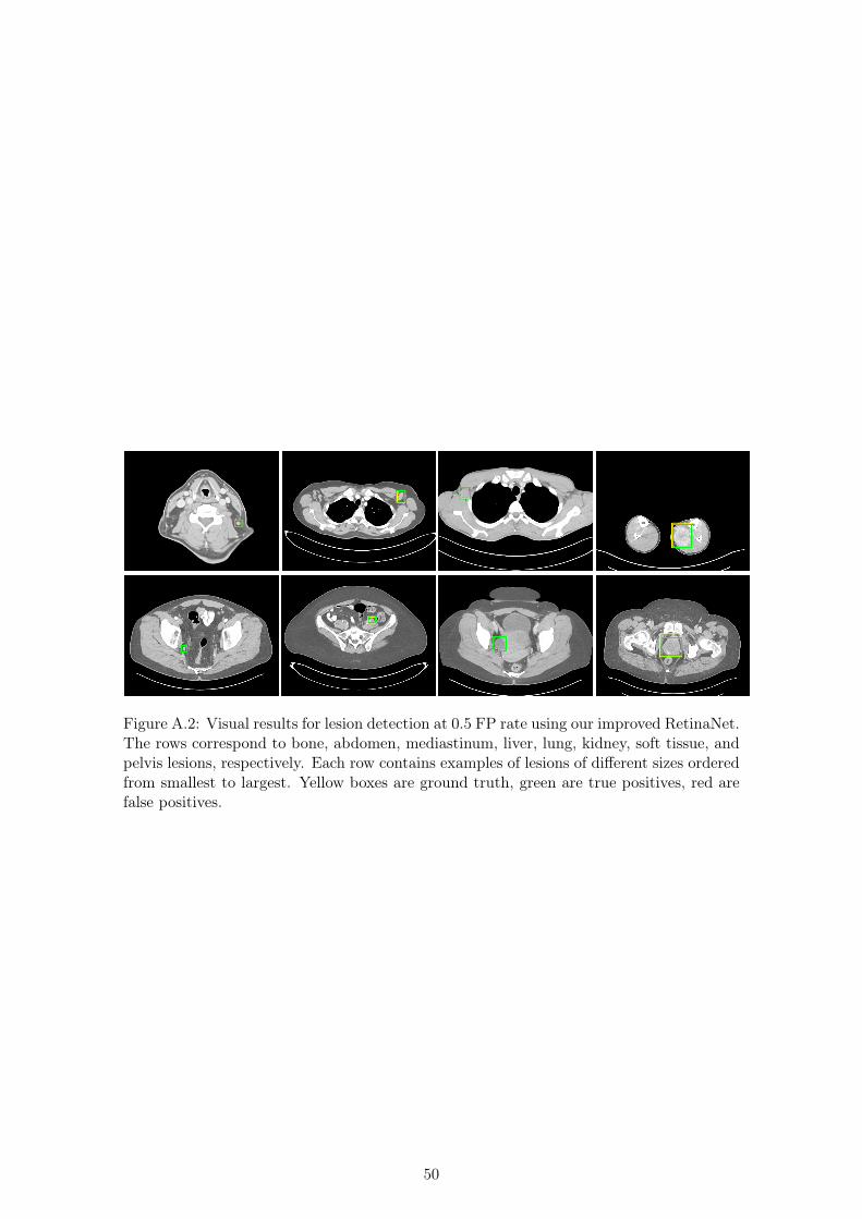
Figure A.2: Visual results for lesion detection at 0.5 FP rate using our improved RetinaNet.The rows correspond to bone, abdomen, mediastinum, liver, lung, kidney, soft tissue, andpelvis lesions, respectively. Each row contains examples of lesions of different sizes orderedfrom smallest to largest. Yellow boxes are ground truth, green are true positives, red arefalse positives.

50

Appendix B

Visual results for MRI lesiondetection

Figures B.1, B.2 and B.3 show the ground truth, a correct and very accurate prediction andthen one false positive prediction of a lung tumour however the model is not constrainedto only the lungs and the false positive prediction is a colorectal prediction.

Figure B.1: The ground truth segmentation overlaid on a DW scan. Bottom left viewshows a 3D render of the tumour and the other show 2D slices of the MRI.

Figures B.4 and B.5 show the ground truth and a correct prediction of a colorectaltumour. We can see that although there are bits of the tumour not covered in our predictioncompared to the ground truth the centroid of the prediction is correct.

51

Figure B.2: Very accurate predicted segmentation overlaid on a DW scan. Bottom leftview shows a 3D render of the tumour and the other show 2D slices of the MRI.

Figure B.3: A falsely predicted segmentation overlaid on a DW scan. The shape of theprediction is very strange as one of the slices has much larger surface area than the others,these large discrepancies could help a second network to further remove false positives.Bottom left view shows a 3D render of the tumour and the other show 2D slices of theMRI.

52

Figure B.4: The grorund truth segmentation overlaid on a DW scan. Bottom left viewshows a 3D render of the tumour and the other show 2D slices of the MRI.

Figure B.5: The predicted segmentation overlaid on a DW scan. Bottom left view showsa 3D render of the tumour and the other show 2D slices of the MRI.

53

Bibliography

[1] M. Bennett, “Avoidable mortality in the UK: 2016,” Apr 2018. [Online]. Avail-able: https://www.ons.gov.uk/peoplepopulationandcommunity/healthandsocialcare/causesofdeath/bulletins/avoidablemortalityinenglandandwales/2016

[2] G. Bradski, “The OpenCV Library,” Dr. Dobb’s Journal of Software Tools, 2000.

[3] J. Cai, Y. Tang, L. Lu, L. Yang, R. M. Summers, and et al., “Accurate weakly-supervised deep lesion segmentation using large-scale clinical annotations: Slice-propagated 3d mask generation from 2d recist,” in MICCAI, 2018, pp. 396–404.

[4] F. Chollet et al., “Keras,” https://keras.io, 2015.

[5] J. Dai, Y. Li, K. He, and J. Sun, “R-FCN: object detection via region-basedfully convolutional networks,” CoRR, vol. abs/1605.06409, 2016. [Online]. Available:http://arxiv.org/abs/1605.06409

[6] N. Dalal and B. Triggs, “Histograms of oriented gradients for human detection,” in2005 IEEE Computer Society Conference on Computer Vision and Pattern Recogni-tion (CVPR’05), vol. 1, June 2005, pp. 886–893 vol. 1.

[7] J. Deng, W. Dong, R. Socher, L.-J. Li, K. Li, and L. Fei-Fei, “ImageNet: A Large-ScaleHierarchical Image Database,” in CVPR09, 2009.

[8] E. A. Eisenhauer, P. Therasse, J. Bogaerts, L. H. Schwartz, D. Sargent, R. Ford,J. Dancey, S. Arbuck, S. Gwyther, M. Mooney et al., “New response evaluation criteriain solid tumours: revised RECIST guideline (version 1.1),” European journal of cancer,vol. 45, no. 2, pp. 228–247, 2009.

[9] W. Foundation, “Object detection,” Nov 2018. [Online]. Available: https://en.wikipedia.org/wiki/Object_detection

[10] ——, “Hounsfield scale,” Jan 2019. [Online]. Available: https://en.wikipedia.org/wiki/Hounsfield_scale

[11] E. Garyfallidis, M. Brett, B. Amirbekian, A. Rokem, S. Van Der Walt, M. Descoteaux,and I. Nimmo-Smith, “Dipy, a library for the analysis of diffusion MRI data,” Frontiersin neuroinformatics, vol. 8, p. 8, 2014.

[12] S. Gaur, N. Lay, S. A. Harmon, S. Doddakashi, S. Mehralivand, B. Argun, T. Barrett,S. Bednarova, R. Girometti, E. Karaarslan et al., “Can computer-aided diagnosis assistin the identification of prostate cancer on prostate MRI? a multi-center, multi-readerinvestigation,” Oncotarget, vol. 9, no. 73, p. 33804, 2018.

[13] R. Girshick, J. Donahue, T. Darrell, and J. Malik, “Region-Based Convolutional Net-works for Accurate Object Detection and Segmentation,” IEEE Transactions on Pat-tern Analysis and Machine Intelligence, vol. 38, no. 1, pp. 142–158, Jan 2016.

54

[14] R. B. Girshick, “Fast R-CNN,” CoRR, vol. abs/1504.08083, 2015. [Online]. Available:http://arxiv.org/abs/1504.08083

[15] GOV.UK, “Chapter 2: trends in mortality,” Sept2018. [Online]. Available: https://www.gov.uk/government/publications/health-profile-for-england-2018/chapter-2-trends-in-mortality

[16] K. He, G. Gkioxari, P. Dollár, and R. B. Girshick, “Mask R-CNN,” CoRR, vol.abs/1703.06870, 2017. [Online]. Available: http://arxiv.org/abs/1703.06870

[17] K. He, X. Zhang, S. Ren, and J. Sun, “Deep Residual Learning forImage Recognition,” CoRR, vol. abs/1512.03385, 2015. [Online]. Available:http://arxiv.org/abs/1512.03385

[18] R. Hossain, C. C. Wu, P. M. de Groot, B. W. Carter, M. D. Gilman, and G. F. Abbott,“Missed Lung Cancer,” Radiologic Clinics of North America, vol. 56, no. 3, pp. 365– 375, 2018, imaging of Lung Cancer: Update on Staging and Therapy. [Online].Available: http://www.sciencedirect.com/science/article/pii/S0033838918300046

[19] A. G. Howard, M. Zhu, B. Chen, D. Kalenichenko, W. Wang, T. Weyand,M. Andreetto, and H. Adam, “Mobilenets: Efficient convolutional neural networksfor mobile vision applications,” CoRR, vol. abs/1704.04861, 2017. [Online]. Available:http://arxiv.org/abs/1704.04861

[20] G. Huang, Z. Liu, and K. Q. Weinberger, “Densely connected convolutionalnetworks,” CoRR, vol. abs/1608.06993, 2016. [Online]. Available: http://arxiv.org/abs/1608.06993

[21] P. F. Jaeger, S. A. A. Kohl, S. Bickelhaupt, F. Isensee, T. A. Kuder, H. Schlemmer,and K. H. Maier-Hein, “Retina U-Net: Embarrassingly Simple Exploitation ofSegmentation Supervision for Medical Object Detection,” CoRR, vol. abs/1811.08661,2018. [Online]. Available: http://arxiv.org/abs/1811.08661

[22] E. Jones, T. Oliphant, P. Peterson et al., “SciPy: Open source scientific tools forPython,” 2001–. [Online]. Available: http://www.scipy.org/

[23] D. P. Kingma and J. Ba, “Adam: A method for stochastic optimization,” arXivpreprint arXiv:1412.6980, 2014.

[24] H. Kundel, C. Nodine, and D. Carmody, “Visual scanning, pattern recognition anddecision-making in pulmonary nodule detection,” Investigative radiology, vol. 13, no. 3,p. 175—181, 1978. [Online]. Available: http://europepmc.org/abstract/MED/711391

[25] I. Lavdas, B. Glocker, D. Rueckert, S. Taylor, E. Aboagye, and A. Rockall, “Machinelearning in whole-body MRI: experiences and challenges from an applied study usingmulticentre data,” Clinical Radiology, vol. 74, no. 5, pp. 346 – 356, 2019. [Online].Available: http://www.sciencedirect.com/science/article/pii/S0009926019300741

[26] J. Lehtinen, J. Munkberg, J. Hasselgren, S. Laine, T. Karras, M. Aittala, andT. Aila, “Noise2Noise: Learning Image Restoration without Clean Data,” CoRR, vol.abs/1803.04189, 2018. [Online]. Available: http://arxiv.org/abs/1803.04189

[27] X. Li, H. Zhao, and L. Zhang, “Recurrent retinanet: A video object detection modelbased on focal loss,” in Neural Information Processing, L. Cheng, A. C. S. Leung, andS. Ozawa, Eds. Cham: Springer International Publishing, 2018, pp. 499–508.

55

[28] Y. Li, “Detecting Lesion Bounding Ellipses With Gaussian Proposal Networks,”CoRR, vol. abs/1902.09658, 2019. [Online]. Available: http://arxiv.org/abs/1902.09658

[29] M. Liang, W. Tang, D. M. Xu, A. C. Jirapatnakul, A. P. Reeves, C. I. Henschke, andD. Yankelevitz, “Low-dose CT screening for lung cancer: computer-aided detection ofmissed lung cancers,” Radiology, vol. 281, no. 1, pp. 279–288, 2016.

[30] Lin, Goyal, Girshick, Ross, and Piotr, “Focal Loss for Dense Object Detection,” Feb2018. [Online]. Available: https://arxiv.org/abs/1708.02002

[31] T.-Y. Lin, M. Maire, S. Belongie, J. Hays, P. Perona, D. Ramanan, P. Dollár, andC. L. Zitnick, “Microsoft coco: Common objects in context,” in European conferenceon computer vision. Springer, 2014, pp. 740–755.

[32] Liu, Wei, Anguelov, Dragomir, Erhan, Dumitru, Scott, Cheng-Yang, Berg, A. C.,and et al., “SSD: Single Shot MultiBox Detector,” Dec 2016. [Online]. Available:https://arxiv.org/abs/1512.02325

[33] I. L. Lowekamp BC, Chen DT and B. D. (2013), “SimpleITK,” 2013. [Online].Available: http://www.simpleitk.org/

[34] LUNA16, “LUNA16 - Lung Nodule Analysis 2016.” [Online]. Available: https://luna16.grand-challenge.org/

[35] B. H. Menze, A. Jakab, S. Bauer, J. Kalpathy-Cramer, K. Farahani, J. Kirby, Y. Bur-ren, N. Porz, J. Slotboom, R. Wiest et al., “The multimodal brain tumor imagesegmentation benchmark (BRATS),” IEEE transactions on medical imaging, vol. 34,no. 10, pp. 1993–2024, 2014.

[36] O. Oktay, J. Schlemper, L. L. Folgoc, M. C. H. Lee, M. P. Heinrich, K. Misawa,K. Mori, S. G. McDonagh, N. Y. Hammerla, B. Kainz, B. Glocker, and D. Rueckert,“Attention U-Net: Learning Where to Look for the Pancreas,” CoRR, vol.abs/1804.03999, 2018. [Online]. Available: http://arxiv.org/abs/1804.03999

[37] A. Paszke, S. Gross, S. Chintala, G. Chanan, E. Yang, Z. DeVito, Z. Lin, A. Des-maison, L. Antiga, and A. Lerer, “Automatic differentiation in PyTorch,” in NIPS-W,2017.

[38] F. Pedregosa, G. Varoquaux, A. Gramfort, V. Michel, B. Thirion, O. Grisel, M. Blon-del, P. Prettenhofer, R. Weiss, V. Dubourg, J. Vanderplas, A. Passos, D. Cournapeau,M. Brucher, M. Perrot, and E. Duchesnay, “Scikit-learn: Machine learning in Python,”Journal of Machine Learning Research, vol. 12, pp. 2825–2830, 2011.

[39] Redmon, Joseph, Divvala, Santosh, Girshick, Ross, Farhadi, and Ali, “You OnlyLook Once: Unified, Real-Time Object Detection,” May 2016. [Online]. Available:https://arxiv.org/abs/1506.02640

[40] S. Ren, K. He, R. B. Girshick, and J. Sun, “Faster R-CNN: towards real-time objectdetection with region proposal networks,” CoRR, vol. abs/1506.01497, 2015. [Online].Available: http://arxiv.org/abs/1506.01497

[41] O. Ronneberger, P. Fischer, and T. Brox, “U-Net: Convolutional Networksfor Biomedical Image Segmentation,” CoRR, vol. abs/1505.04597, 2015. [Online].Available: http://arxiv.org/abs/1505.04597

56

[42] C. Rother, V. Kolmogorov, and A. Blake, “Grabcut: Interactive foreground extractionusing iterated graph cuts,” in ACM transactions on graphics, 2004, pp. 309–314.

[43] K. Simonyan and A. Zisserman, “Very Deep Convolutional Networks for Large-ScaleImage Recognition,” in International Conference on Learning Representations, 2015.

[44] R. Storn and K. Price, “Differential evolution–a simple and efficient heuristic for globaloptimization over continuous spaces,” Journal of global optimization, vol. 11, no. 4,pp. 341–359, 1997.

[45] C. Szegedy, S. Ioffe, and V. Vanhoucke, “Inception-v4, Inception-ResNet and theImpact of Residual Connections on Learning,” CoRR, vol. abs/1602.07261, 2016.[Online]. Available: http://arxiv.org/abs/1602.07261

[46] C. Szegedy, W. Liu, Y. Jia, P. Sermanet, S. E. Reed, D. Anguelov, D. Erhan,V. Vanhoucke, and A. Rabinovich, “Going Deeper with Convolutions,” CoRR, vol.abs/1409.4842, 2014. [Online]. Available: http://arxiv.org/abs/1409.4842

[47] C. Szegedy, V. Vanhoucke, S. Ioffe, J. Shlens, and Z. Wojna, “Rethinking theInception Architecture for Computer Vision,” CoRR, vol. abs/1512.00567, 2015.[Online]. Available: http://arxiv.org/abs/1512.00567

[48] Y. Tang, K. Yan, Y. Tang, J. Liu, J. Xiao, and R. M. Summers, “ULDor: A universallesion detector for ct scans with pseudo masks and hard negative example mining,”arXiv preprint arXiv:1901.06359, 2019.

[49] J. Uijlings, K. van de Sande, T. Gevers, and A. Smeulders, “Selective Searchfor Object Recognition,” International Journal of Computer Vision, 2013. [Online].Available: http://www.huppelen.nl/publications/selectiveSearchDraft.pdf

[50] P. Viola and M. Jones, “Rapid object detection using a boosted cascade of simplefeatures,” in Proceedings of the 2001 IEEE Computer Society Conference on ComputerVision and Pattern Recognition. CVPR 2001, vol. 1, Dec 2001, pp. I–I.

[51] K. Yan, M. Bagheri, and R. M. Summers, “3D Context Enhanced Region-BasedConvolutional Neural Network for End-to-End Lesion Detection,” in Medical ImageComputing and Computer Assisted Intervention – MICCAI 2018, A. F. Frangi, J. A.Schnabel, C. Davatzikos, C. Alberola-López, and G. Fichtinger, Eds. Cham: SpringerInternational Publishing, 2018, pp. 511–519.

[52] K. Yan, X. Wang, L. Lu, and R. M. Summers, “DeepLesion: automated miningof large-scale lesion annotations and universal lesion detection with deep learning,”Journal of Medical Imaging, vol. 5, pp. 5 – 5 – 11, 2018. [Online]. Available:https://doi.org/10.1117/1.JMI.5.3.036501

[53] K. Yan, X. Wang, L. Lu, L. Zhang, A. P. Harrison, M. Bagheri, and R. M. Summers,“Deep lesion graphs in the wild: relationship learning and organization of significantradiology image findings in a diverse large-scale lesion database,” in CVPR, 2018.

[54] M. Zlocha, Q. Dou, and B. Glocker, “Improving RetinaNet for CT Lesion Detectionwith Dense Masks from Weak RECIST Labels,” arXiv preprint arXiv:1906.02283,2019.

57