Example Based Lesion Segmentation

Snehashis Roy*, Qing He*, Aaron Carass�, Amod Jog�, Jennifer L. Cuzzocreo§,Daniel S. Reich� Jerry Prince�, Dzung Pham*

*Center for Neuroscience and Regenerative Medicine,Henry M. Jackson Foundation for the Advancement of Military Medicine, USA

�Department of Electrical and Computer Engineering, The Johns Hopkins University, USA§Department of Radiology, The Johns Hopkins School of Medicine, USA

�Translational Neuroradiology Unit, Neuroimmunology BranchNational Institute of Neurological Disorders and Stroke, USA

ABSTRACT

Automatic and accurate detection of white matter lesions is a significant step toward understanding the pro-gression of many diseases, like Alzheimer’s disease or multiple sclerosis. Multi-modal MR images are often usedto segment T2 white matter lesions that can represent regions of demyelination or ischemia. Some automatedlesion segmentation methods describe the lesion intensities using generative models, and then classify the lesionswith some combination of heuristics and cost minimization. In contrast, we propose a patch-based method, inwhich lesions are found using examples from an atlas containing multi-modal MR images and correspondingmanual delineations of lesions. Patches from subject MR images are matched to patches from the atlas andlesion memberships are found based on patch similarity weights. We experiment on 43 subjects with MS, whosescans show various levels of lesion-load. We demonstrate significant improvement in Dice coefficient and totallesion volume compared to a state of the art model-based lesion segmentation method, indicating more accuratedelineation of lesions.

Keywords: magnetic resonance imaging, MRI, lesion segmentation, MS, patches

1. INTRODUCTION

With Alzheimer’s disease, multiple sclerosis (MS) and cerebral small vessel ischemic diseases, lesions often occurin cerebral white matter (WM). These lesions are usually hypointense in 3D gradient-echo T1-weighted imagesand hyperintense in T2-weighted images. Lesion volume has been shown to be correlated with the state andprogression of MS.1 Although manual segmentation of lesions are considered to be the “gold standard”, fast andaccurate automatic segmentations are essential to quantitatively assess the lesion load more robustly, as manualsegmentations are time-consuming and are subject to both inter-rater and intra-rater variations, especially whenmore than one image modality is used to guide manual delineation.

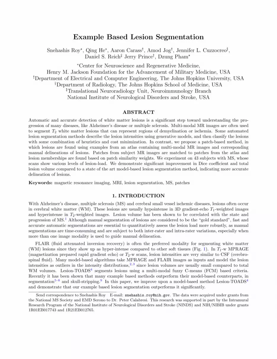
FLAIR (fluid attenuated inversion recovery) is often the preferred modality for segmenting white matter(WM) lesions since they show up as hyper-intense compared to other soft tissues (Fig. 1). In T1-w MPRAGE(magnetization prepared rapid gradient echo) or T2-w scans, lesion intensities are very similar to CSF (cerebro-spinal fluid). Many model-based algorithms take MPRAGE and FLAIR images as inputs and model the lesionintensities as outliers in the intensity distributions,2,3 since lesion volumes are usually small compared to totalWM volumes. Lesion-TOADS4 segments lesions using a multi-modal fuzzy C-means (FCM) based criteria.Recently it has been shown that many example based methods outperform their model-based counterparts, insegmentation5–8 and skull-stripping.9 In this paper, we improve upon a model-based method Lesion-TOADS4

and demonstrate that our example based lesion segmentation outperforms it significantly.

Send correspondence to Snehashis Roy E-mail: snehashis.roy@nih.gov. The data were acquired under grants fromthe National MS Society and EMD Serono to Dr. Peter Calabresi. This research was supported in part by the IntramuralResearch Program of the National Institute of Neurological Disorders and Stroke (NINDS) and NIH/NIBIB under grants1R01EB017743 and 1R21EB012765.

T1-w MPRAGE FLAIR Manual Segmentation

Figure 1. A T1-w MPRAGE, FLAIR, and manual lesion segmentation are shown. Lesions are usually hypo-intense inMPRAGE, resembling CSF. They are hyper-intense in FLAIR, which is the preferred modality for WM lesion segmenta-tion.

We use T1-w MPRAGE and FLAIR scans to find lesions using examples from atlases. Patches from a subjectMPRAGE and FLAIR scans are matched to similar patches from atlas T1-w and FLAIR scans. The correspondinghard segmentation labels (Fig. 1) of the atlas are weighted by the similarity criteria accordingly,10 therebycreating a fuzzy lesion membership. The lesion memberships are thresholded to obtain a hard segmentation.Although this idea of patch matching has been explored previously for the purpose of image synthesis,10–13

atrophy detection,14,15 and tissue segmentation,6 the novelty of our method lies in fuzzy lesion segmentationusing a sparse dictionary of WM lesions.

2. METHOD

We define the “atlas” as a triplet of co-registered T1-w MPRAGE, FLAIR, and the manual binary lesion seg-mentation images (e.g., Fig. 1). The “subject” is a co-registered pair of T1-w MPRAGE and FLAIR images. Theatlas MPRAGE and FLAIR (both skull-stripped), having the same resolution as the subject, are generally notregistered to the subject. Both subject and atlas MPRAGE and FLAIRs are normalized such that their modes

Subject

Atlases

MPRAGE

· · ·

FLAIR · · ·

Segmentation

· · ·

Lesion Memberships Average

· · ·

Segmentations

Lesion-TOADS Example Manual

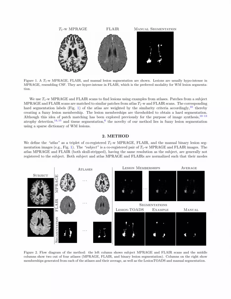
Figure 2. Flow diagram of the method: the left column shows subject MPRAGE and FLAIR scans and the middlecolumns show two out of four atlases (MPRAGE, FLAIR, and binary lesion segmentation). Columns on the right showmemberships generated from each of the atlases and their average, as well as the LesionTOADS and manual segmentation.

of WM intensities are at unity. The modes are automatically obtained from the corresponding image histogramsusing kernel density estimator.16

At each voxel of an image, 3D p × q × r patches are stacked into 1D vectors of size d × 1, d = pqr. Sinceatlas images are co-registered, the pair of patches centered at the same voxel of the atlas MPRAGE and FLAIRare concatenated to form a 2d × 1 vector, denoted a1(i) ∈ R2d×1, i = 1, . . . ,M . For simplicity of notation, wewill interchangeably denote “patch” to identify 2d × 1 vectors also. The subject MPRAGE and FLAIR arealso similarly decomposed into patches, denoted b1(j) ∈ R2d×1, j = 1, . . . , N . M and N denote the number ofnon-zero voxels in the atlas and the subject, respectively. For typical 1mm3 images, M,N ∼ 107. For the ith

atlas patch, the corresponding patch in the lesion segmentation image is denoted by a2(i) ∈ Rd×1. The elementsof a2(i) are {0, 1}.

We assume that for the jth subject patch b1(j), a small number of similar atlas patches can always be foundfrom a rich collection of atlas patches, whose convex combination is b1(j). It is unlikely that a single atlas patcha1(i) will match b1(j) exactly, but a convex combination of a few atlas patches from a large dictionary of atlaspatches is more likely to approximate b1(j) closely. The idea can be succinctly written as

b1(j) ≈ A1(j)xj , for some xj ∈ RL×1, ||xj ||0 � L,xj ≥ 0. (1)

A1(j) is a dictionary containing atlas patches (a1(i)s) similar to b1(j). Instead of using all M atlas patches forevery subject patch, we use a kd-tree to choose L similar atlas patches (from the larger set of M patches) forevery single subject patch,17 such that A1(j) ∈ R2d×L. L is empirically chosen to be 100 based on speed andmemory limitation. The variable xj is a L× 1 sparse weight vector indicating that only a few patches out of theL patches in A1(j) are used to reconstruct b1(j). The non-negativity constraint on the weights xj enforces the“texture” of the chosen atlas patches to match with that of the subject patch b1(j). This idea of sparse weightreconstruction has been explored earlier in relation to atlas based super-resolution18 and image synthesis.10,11

Because of speed limitations, it has been suggested that similar patches should be chosen from a windowedneighborhood of the voxel in the atlas,6 after the atlas is registered to the subject. However, we choose atlaspatches irrespective of their spatial location, since the anatomy might vary widely between the subject and atlas.For example, if the subject has large ventricles and the atlas does not, the size of the search window should varyaccording to the size of the structure,6,9 and the accuracy of the registration used. We avoid this problem at thecost of a nearest-neighbor search using a kd-tree irrespective of the spatial locations of the atlas patches.

Every atlas patch a1(i) has a corresponding lesion label patch a2(i). Thus, once the sparse weights xj arefound, the lesion labels are combined accordingly to form the lesion membership for the jth subject patch as

b2(j) = A2(j)xj

||xj ||1, (2)

where A2(j) ∈ Rd×L is a wide matrix that includes lesion segmentation patches as columns corresponding to

A1(j). The lesion membership b2(j) is normalized by ||xj ||1 so that it ranges between [0, 1]. It is advantageousto generate a continuous valued variable (instead of a hard segmentation) that could have a probabilistic inter-pretation to allow tuning the threshold. Also, because the boundaries of lesions are often vague, this provides ameasure of confidence.

To solve the `0 problem in Eqn. 1 efficiently, it can be reformulated as a `1 minimization, which gives thesame optimal solution as the `0 problem, if ||xj ||0 is sufficiently small.20 Eqn. 1 is rewritten as

xj = arg minx≥0

[||b1(j)−A1x||22 + λ ||x||1

], (3)

where λ is a weight penalizing the sparsity of xj . Here we note that for uniqueness of the solution of Eqn. 3, bothb1(j) and each column of A1 are to be normalized so that their `2 norm is unity.18 All patches are normalized bythe maximum of their `2 norms.10 We solve for xj using SparseLab.20 In all our experiments, we use overlapping3× 3× 3 patches (d = 27) and empirically set λ = 0.02. Once xj is found from Eqn. 3, the corresponding lesion

membership b2(j) is obtained from Eqn. 2 and only the value at the center voxel is used.

(a) (b) (c)

(d) (e) (f)

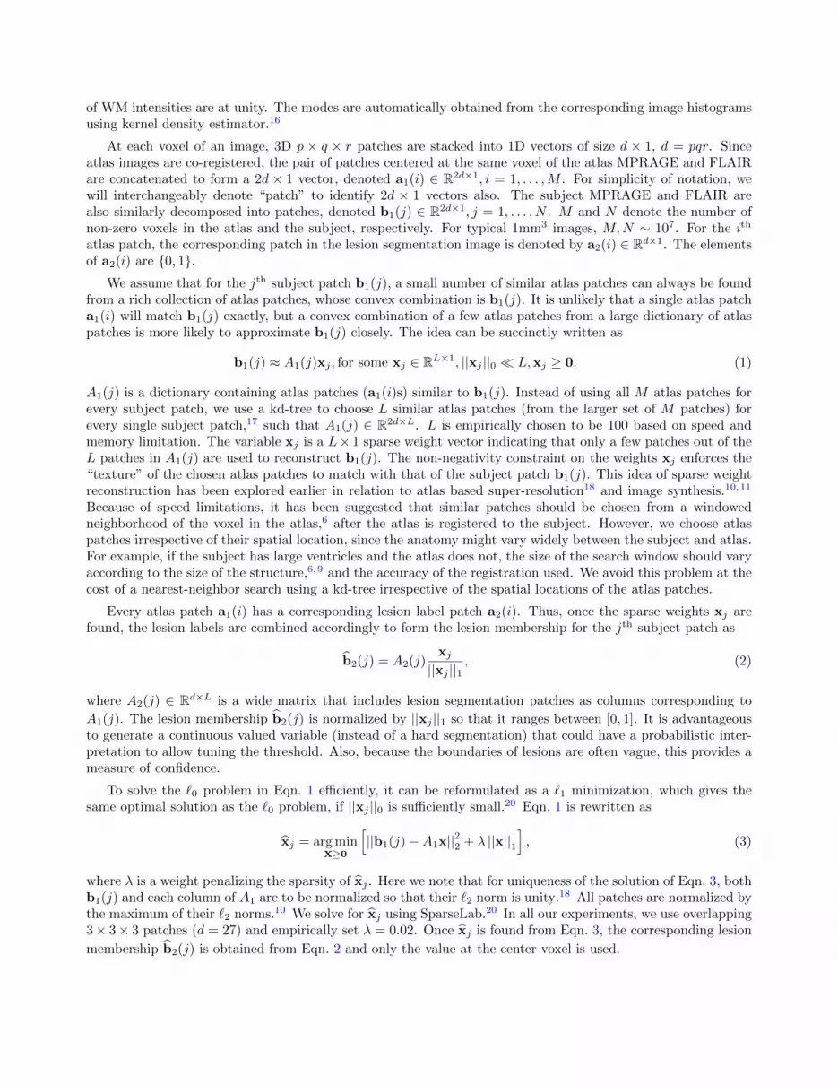
Figure 3. Top row shows a subject MPRAGE, FLAIR, and manual segmentation images. Bottom row shows the cor-responding WM mask (obtained from TOADS19), an uncorrected membership, and a hard segmentation corrected bymasking the membership.

3. RESULTS

We use a pool of 47 MS subjects, all having lesions. Manual segmentations are available on all of them. Imagingprotocols and manual segmentation details can be found in.4 To quantitatively evaluate the segmentationaccuracy with Lesion-TOADS, we used the following measures: Dice coefficient, total lesion volume, sensitivity(true positive rate) and specificity (false negative rate). Four randomly chosen subjects are used as atlases,and the remaining 43 are used as subjects. For every subject, we generate four lesion memberships (one foreach of the atlases) and average them for robustness. Fig. 2 shows a diagram of the methodology having asubject, two out of four atlases, corresponding fuzzy lesion memberships and the average membership basedon four atlases. The average membership is then thresholded to obtain a hard segmentation. Estimation ofthe threshold is explained later. Since there is no spatial information while choosing patches from the atlas,there are false positives occurring mostly in the anterior part of the brain, cortex and cerebellum, where theFLAIR scans contain some hyper-intensities as image artifacts. As we are interested only in white matter lesions,the memberships are corrected by masking with WM masks obtained from TOADS.19 An example is shown inFig. 3, where a subject MPRAGE and FLAIR are shown in the top row. The corresponding lesion membership(Fig. 3(e)) is corrected by the WM mask (Fig. 3(d)) to obtain the hard segmentation (Fig. 3(f)). The manualsegmentation is also shown in Fig. 3(c).

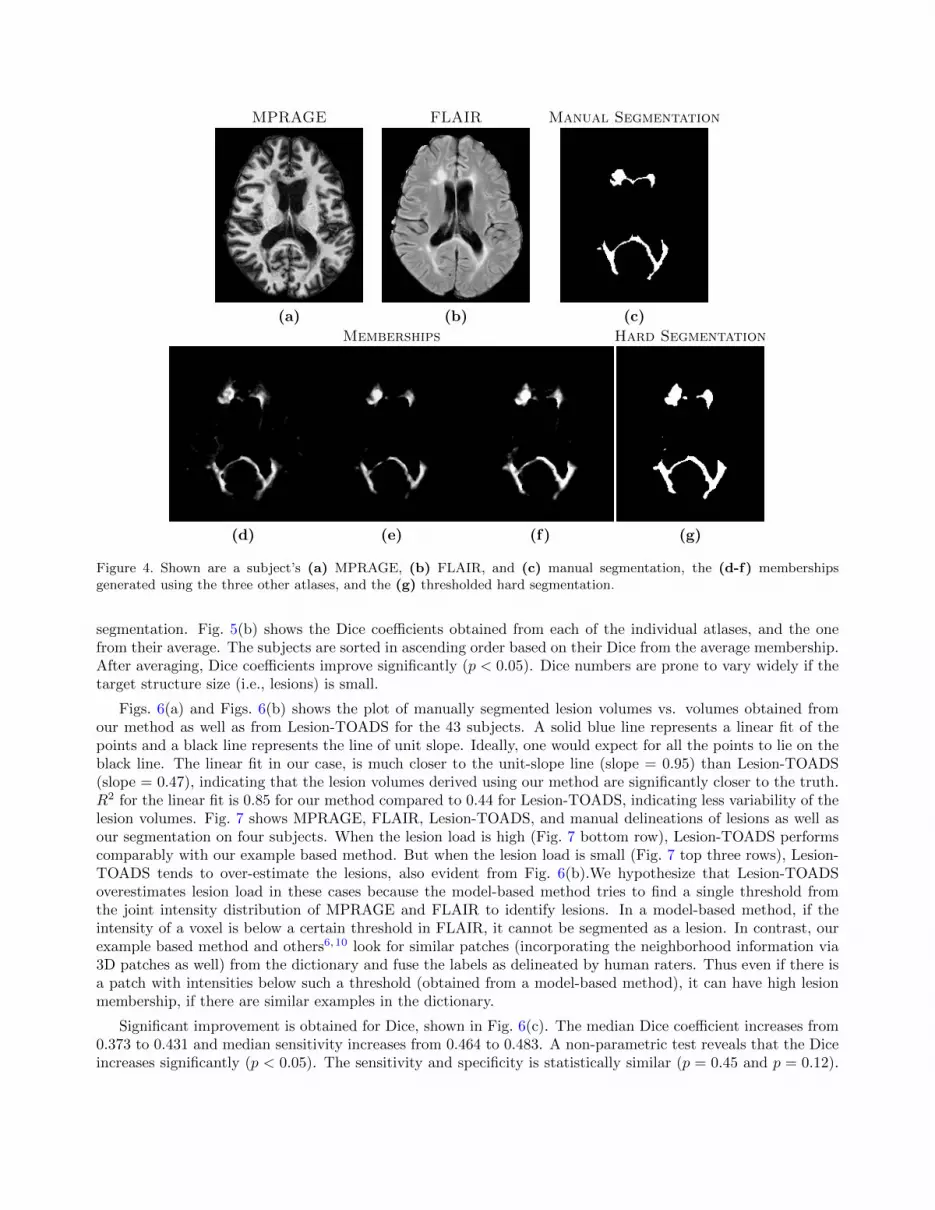
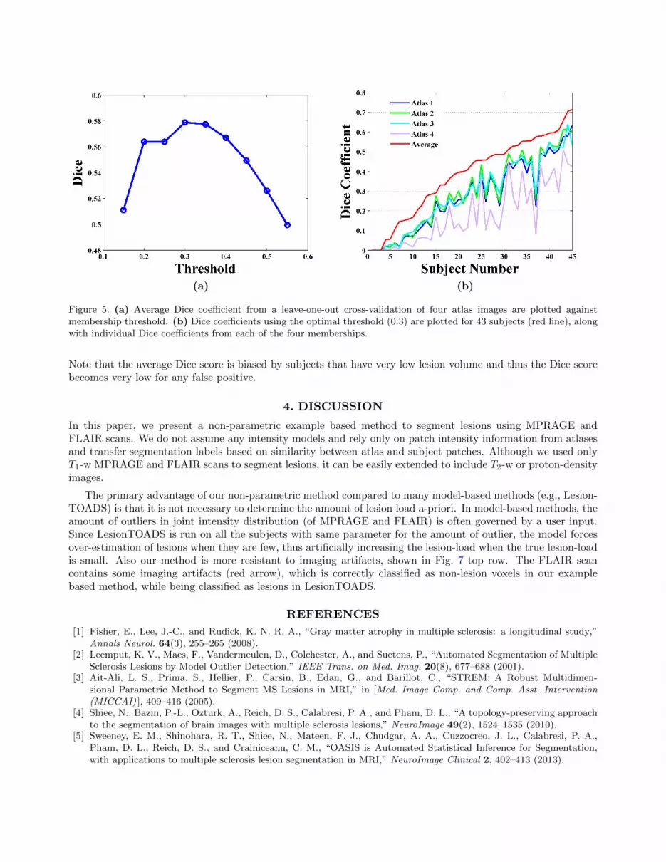
The hard segmentation threshold is chosen based on a leave-one-out cross-validation on the four atlases.For every atlas image, the same methodology is applied to generate three memberships, using the remainingthree atlas images. Figs. 4(a) and Figs. 4(b) show MPRAGE and FLAIR scans from an atlas, with its threememberships obtained using three other atlas images. The corresponding manual segmentation is also shownin Fig. 4(c). Average Dice coefficient (averaged over four atlases, each having three memberships) between themanual segmentation (e.g., Fig. 4(c)) and the hard segmentation (e.g., Fig. 4(g)) are plotted against the thresholdin Fig. 5(a), which shows a threshold of 0.3 to be optimal. We used this threshold on the remaining 43 subjects.

Instead of using one atlas, memberships are averaged over four atlases to improve robustness in the final

MPRAGE FLAIR Manual Segmentation

(a) (b) (c)

Memberships Hard Segmentation

(d) (e) (f) (g)

Figure 4. Shown are a subject’s (a) MPRAGE, (b) FLAIR, and (c) manual segmentation, the (d-f) membershipsgenerated using the three other atlases, and the (g) thresholded hard segmentation.

segmentation. Fig. 5(b) shows the Dice coefficients obtained from each of the individual atlases, and the onefrom their average. The subjects are sorted in ascending order based on their Dice from the average membership.After averaging, Dice coefficients improve significantly (p < 0.05). Dice numbers are prone to vary widely if thetarget structure size (i.e., lesions) is small.

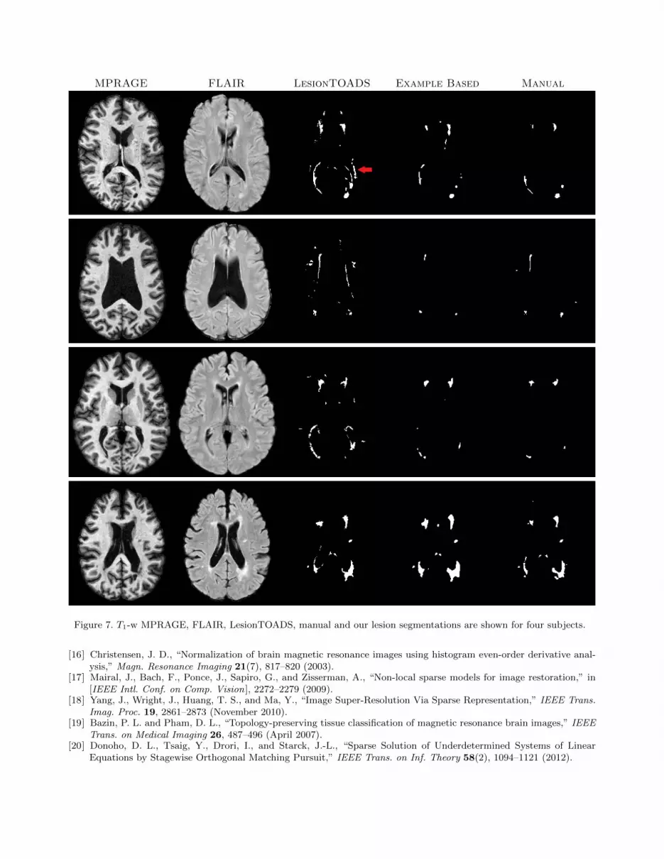
Figs. 6(a) and Figs. 6(b) shows the plot of manually segmented lesion volumes vs. volumes obtained fromour method as well as from Lesion-TOADS for the 43 subjects. A solid blue line represents a linear fit of thepoints and a black line represents the line of unit slope. Ideally, one would expect for all the points to lie on theblack line. The linear fit in our case, is much closer to the unit-slope line (slope = 0.95) than Lesion-TOADS(slope = 0.47), indicating that the lesion volumes derived using our method are significantly closer to the truth.R2 for the linear fit is 0.85 for our method compared to 0.44 for Lesion-TOADS, indicating less variability of thelesion volumes. Fig. 7 shows MPRAGE, FLAIR, Lesion-TOADS, and manual delineations of lesions as well asour segmentation on four subjects. When the lesion load is high (Fig. 7 bottom row), Lesion-TOADS performscomparably with our example based method. But when the lesion load is small (Fig. 7 top three rows), Lesion-TOADS tends to over-estimate the lesions, also evident from Fig. 6(b).We hypothesize that Lesion-TOADSoverestimates lesion load in these cases because the model-based method tries to find a single threshold fromthe joint intensity distribution of MPRAGE and FLAIR to identify lesions. In a model-based method, if theintensity of a voxel is below a certain threshold in FLAIR, it cannot be segmented as a lesion. In contrast, ourexample based method and others6,10 look for similar patches (incorporating the neighborhood information via3D patches as well) from the dictionary and fuse the labels as delineated by human raters. Thus even if there isa patch with intensities below such a threshold (obtained from a model-based method), it can have high lesionmembership, if there are similar examples in the dictionary.

Significant improvement is obtained for Dice, shown in Fig. 6(c). The median Dice coefficient increases from0.373 to 0.431 and median sensitivity increases from 0.464 to 0.483. A non-parametric test reveals that the Diceincreases significantly (p < 0.05). The sensitivity and specificity is statistically similar (p = 0.45 and p = 0.12).

(a) (b)

Figure 5. (a) Average Dice coefficient from a leave-one-out cross-validation of four atlas images are plotted againstmembership threshold. (b) Dice coefficients using the optimal threshold (0.3) are plotted for 43 subjects (red line), alongwith individual Dice coefficients from each of the four memberships.

Note that the average Dice score is biased by subjects that have very low lesion volume and thus the Dice scorebecomes very low for any false positive.

4. DISCUSSION

In this paper, we present a non-parametric example based method to segment lesions using MPRAGE andFLAIR scans. We do not assume any intensity models and rely only on patch intensity information from atlasesand transfer segmentation labels based on similarity between atlas and subject patches. Although we used onlyT1-w MPRAGE and FLAIR scans to segment lesions, it can be easily extended to include T2-w or proton-densityimages.

The primary advantage of our non-parametric method compared to many model-based methods (e.g., Lesion-TOADS) is that it is not necessary to determine the amount of lesion load a-priori. In model-based methods, theamount of outliers in joint intensity distribution (of MPRAGE and FLAIR) is often governed by a user input.Since LesionTOADS is run on all the subjects with same parameter for the amount of outlier, the model forcesover-estimation of lesions when they are few, thus artificially increasing the lesion-load when the true lesion-loadis small. Also our method is more resistant to imaging artifacts, shown in Fig. 7 top row. The FLAIR scancontains some imaging artifacts (red arrow), which is correctly classified as non-lesion voxels in our examplebased method, while being classified as lesions in LesionTOADS.

REFERENCES

[1] Fisher, E., Lee, J.-C., and Rudick, K. N. R. A., “Gray matter atrophy in multiple sclerosis: a longitudinal study,”Annals Neurol. 64(3), 255–265 (2008).

[2] Leemput, K. V., Maes, F., Vandermeulen, D., Colchester, A., and Suetens, P., “Automated Segmentation of MultipleSclerosis Lesions by Model Outlier Detection,” IEEE Trans. on Med. Imag. 20(8), 677–688 (2001).

[3] Ait-Ali, L. S., Prima, S., Hellier, P., Carsin, B., Edan, G., and Barillot, C., “STREM: A Robust Multidimen-sional Parametric Method to Segment MS Lesions in MRI,” in [Med. Image Comp. and Comp. Asst. Intervention(MICCAI) ], 409–416 (2005).

[4] Shiee, N., Bazin, P.-L., Ozturk, A., Reich, D. S., Calabresi, P. A., and Pham, D. L., “A topology-preserving approachto the segmentation of brain images with multiple sclerosis lesions,” NeuroImage 49(2), 1524–1535 (2010).

[5] Sweeney, E. M., Shinohara, R. T., Shiee, N., Mateen, F. J., Chudgar, A. A., Cuzzocreo, J. L., Calabresi, P. A.,Pham, D. L., Reich, D. S., and Crainiceanu, C. M., “OASIS is Automated Statistical Inference for Segmentation,with applications to multiple sclerosis lesion segmentation in MRI,” NeuroImage Clinical 2, 402–413 (2013).

(a) (b)

(c) (d) (e)

Figure 6. A plot of manually segmented lesion volumes vs. (a) the volumes obtained from our example based methodand (b) Lesion-TOADS are shown for 43 subjects. Dice coefficient, sensitivity and specificity compared with manualsegmentations are shown in (c)-(e).

[6] Coupe, P., Manjon, J. V., Pruessner, J., Robles, M., Fonov, V., and Collins, D. L., “Patch-based segmentation usingexpert priors: Application to hippocampus and ventricle segmentation,” NeuroImage 54(2), 940–954 (2011).

[7] Jog, A., Roy, S., Prince, J. L., and Carass, A., “MR Brain Segmentation using Decision Trees,” in [MICCAI GrandChallenge on MR Brain Image Segmentation ], (2013).

[8] Lao, Z., Shen, D., Liu, D., Jawad, A. F., Melhem, E. R., Launer, L. J., Bryan, R. N., and Davatzikos, C., “Computer-Assisted Segmentation of White Matter Lesions in 3D MR Images Using Support Vector Machine,” Academic Radi-ology 15(3), 300–313 (2008).

[9] Eskildsen, S. F., Coupe, P., Fonov, V., Manjon, J. V., Leung, K. K., Guizard, N., Wassef, S. N., Ostergaard, L. R.,Collins, D. L., and The Alzheimer’s Disease Neuroimaging Initiative, “BEaST: Brain extraction based on nonlocalsegmentation technique,” NeuroImage 59(3), 2362–2373 (2012).

[10] Roy, S., Carass, A., and Prince, J. L., “Magnetic Resonance Image Example-Based Contrast Synthesis,” IEEE Trans.on Med. Imag. 32(12), 2348–2363 (2013).

[11] Roy, S., Carass, A., and Prince, J. L., “A Compressed Sensing Approach For MR Tissue Contrast Synthesis,” in[Inf. Proc. in Med. Imaging (IPMI) ], 371–383 (2011).

[12] Hertzmann, A., Jacobs, C. E., Oliver, N., Curless, B., and Salesin, D. H., “Image analogies,” in [Proc. of 28th Ann.Conf. on Comp. Graphics and Interactive Techniques ], SIGGRAPH ’01, 327–340 (2001).

[13] Roy, S., Carass, A., Shiee, N., Pham, D. L., and Prince, J. L., “MR contrast synthesis for lesion segmentation,” in[IEEE Intl. Symp. on Biomed. Imaging ], 932–935 (2010).

[14] Ye, D. H., Zikic, D., Glocker, B., Criminisi, A., and Konukoglu, E., “Modality Propagation: Coherent Synthesisof Subject-Specific Scans with Data-Driven Regularization,” in [Med. Image Comp. and Comp. Asst. Intervention(MICCAI) ], 606–613 (2013).

[15] Wang, H. and Yushkevich, P. A., “Multi-atlas Segmentation without Registration: A Supervoxel-Based Approach,”in [Med. Image Comp. and Comp. Asst. Intervention (MICCAI) ], 8151, 535–542 (2013).

MPRAGE FLAIR LesionTOADS Example Based Manual

Figure 7. T1-w MPRAGE, FLAIR, LesionTOADS, manual and our lesion segmentations are shown for four subjects.

[16] Christensen, J. D., “Normalization of brain magnetic resonance images using histogram even-order derivative anal-ysis,” Magn. Resonance Imaging 21(7), 817–820 (2003).

[17] Mairal, J., Bach, F., Ponce, J., Sapiro, G., and Zisserman, A., “Non-local sparse models for image restoration,” in[IEEE Intl. Conf. on Comp. Vision ], 2272–2279 (2009).

[18] Yang, J., Wright, J., Huang, T. S., and Ma, Y., “Image Super-Resolution Via Sparse Representation,” IEEE Trans.Imag. Proc. 19, 2861–2873 (November 2010).

[19] Bazin, P. L. and Pham, D. L., “Topology-preserving tissue classification of magnetic resonance brain images,” IEEETrans. on Medical Imaging 26, 487–496 (April 2007).

[20] Donoho, D. L., Tsaig, Y., Drori, I., and Starck, J.-L., “Sparse Solution of Underdetermined Systems of LinearEquations by Stagewise Orthogonal Matching Pursuit,” IEEE Trans. on Inf. Theory 58(2), 1094–1121 (2012).