statistical analysis and data display at the geochemical prospecting research centre and applied...

doi:10.1144/1467-7873/09-238 2010; v. 10; p. 289-315 Geochemistry: Exploration, Environment, Analysis

Richard J. Howarth and Robert G. Garrett

Centre and Applied Geochemistry Research Group, Imperial College, LondonStatistical analysis and data display at the Geochemical Prospecting Research

Geochemistry: Exploration, Environment, Analysis

serviceEmail alerting to receive free email alerts when new articles cite this article click here

requestPermission to seek permission to re-use all or part of this article click here

SubscribeCollection

to subscribe to Geochemistry: Exploration, Environment, Analysis or the Lyellclick here

Notes

Downloaded by on 8 September 2010

© 2010 Geological Society of London

http://geea.lyellcollection.org/cgi/alerts

http://www.geolsoc.org.uk/gsl/publications/page417.html

http://geea.lyellcollection.org/subscriptions

Statistical analysis and data display at the Geochemical ProspectingResearch Centre and Applied Geochemistry Research Group,

Imperial College, London

Richard J. Howarth1,* & Robert G. Garrett2

1Dept. of Earth Sciences, University College London, Gower Street, London WC1E 6BT, United Kingdom2Emeritus Scientist, Geological Survey of Canada, 601 Booth St., Ottawa, Ontario, K1A 0E8, Canada

*Corresponding author: (e-mail: [email protected])

ABSTRACT: The Imperial College of Science and Technology, a constituent collegeof the University of London in the 1960s, had the good fortune to be one of the firstcolleges in the United Kingdom to have access to digital computing facilities. Thisreview traces the history of the application of computing in the GeochemicalProspecting Research Centre and its successor, the Applied Geochemistry ResearchGroup, as computing moved from being a frontier research area to becoming acommonplace tool. The three principal areas in which it was involved comprised: thequality control, and thereby assurance, of analytical data; the production ofpioneering atlases of regional geochemical variation in Northern Ireland (1973) andEngland and Wales (1978); and the application of methods introduced by workersin pattern-recognition and statistics to the interpretation of land-based and marineregional geochemical data.

KEYWORDS: computers, computing, applied geochemistry, history of geochemistry, history ofstatistics, history of cartography, regional mapping, spatial filters, geochemical atlas, SC4020,LGP2703, multi-element maps, data transformation, factor analysis, cluster analysis, discriminantanalysis, ridge regression, Kleiner-Hartigan trees, robust statistics, quality assurance

The Geochemical Prospecting Research Centre (GPRC) wasestablished in 1954, under the direction of Professor JohnStuart Webb (1920–2007), in the Mining Geology section ofthe Royal School of Mines (RSM), Imperial College of Scienceand Technology (ICST), London. Initial studies were con-cerned with mineral prospecting using soil and drainage sam-pling in Northern Rhodesia (Zambia), Uganda, Sierra Leone,Bechuanaland (Botswana), Tanganyika (Tanzania), BritishNorth Borneo (Sabah, East Malaysia), Burma (Myanmar) andthe Federation of Malaya (West Malaysia), and extended in the1960s to Southern Rhodesia (Zimbabwe), the PhilippineRepublic, Borneo (now divided between Malaysia andIndonesia), Fiji, East Africa, Australia, and the UnitedKingdom. By 1960, its studies had broadened into regionalgeochemistry, based on the analysis of stream sediments. In1963, Webb initiated the first of a series of investigationsconcerning the relationship between regional geochemistry andagricultural problems in livestock in Eire (Webb 1964; Webb &Atkinson 1965). The application of geochemistry to marinemineral exploration began in 1964 (Tooms 1967). Conse-quently, by 1963, the Centre’s name was changed to theApplied Geochemistry Research Group (AGRG) to reflect theincreasing breadth of its applications.

The work of the GPRC and AGRG was underpinned bydevelopments in two complementary spheres: methods andinstrumentation for chemical analysis (discussed in the paper byMichael Thompson (2010) and computing (Fig. 1). The latterfacilitated: (i) statistical quality-assurance in the analytical lab-

oratory; (ii) the display of large, multi-element, data sets in mapform; and (iii) the interpretation of such multi-element datasets.

First steps

Many of the early studies undertaken by research students inthe GPRC included simple, manually-based, statistical analyses.

Fig. 1. Annual numbers of GPRC/AGRG publications (total n=76)and theses (n=24) with a substantial computing and/or statisticalcontent over the years 1954–88.

Geochemistry: Exploration, Environment, Analysis, Vol. 10 2010, pp. 289–315 1467-7873/10/$15.00 � 2010 AAG/Geological Society of LondonDOI 10.1144/1467-7873/09-238

The situation in the early 1960s is summarized in Hawkes &Webb (1962). The use of histograms to display the frequencydistributions of element concentrations was commonplace,while probability plots of cumulative frequency distributionswere less frequently prepared. In both cases, the data for therequisite plots were compiled by hand through the preparationof ‘tally tables’. At that time, analytical quality assurance wasbased on the use of ‘statistical series’ samples. These were aseries of synthetic samples (each of which was composed ofknown proportions of two natural end-members, one having alow concentration of the element of interest, the other a highconcentration) which were included in analytical batches fol-lowing the procedure developed by the ex-RSM geologist andchemical engineer, Charles Alex Urton Craven (1918–93), withadvice from Professor George Alfred Bernard (1915–2002) ofthe Mathematics Department, ICST (Craven 1954), in order toestimate analytical accuracy and precision. For the largeamounts of photographic-plate spectrographic data generatedat the GPRC, bins for data concentration-ranges were selected(because of a tendency of operators to unconsciously interpo-late values which were biased towards those of the analyticalstandards used), using a logarithmic concentration scale, andbin boundaries were placed mid-way between the knownconcentrations of the geochemical standards. A tick (the ‘tally’)was placed in the appropriate bin for each analysis falling in thatrange, every fifth count being drawn as a horizontal linethrough the previous four ticks. This facilitated counting thetotal numbers of analytical results falling into each bin. A book,widely used by students at the time, was Moroney’s (1960)‘Facts from Figures’, which gave formulae for the calculation ofmeans and standard deviations from such grouped data, asaccumulated in the ‘tally tables’.

For those more interested in statistical analysis, Dixon &Massey (1957) was the text of choice. However, in the early-and mid-1960s, textbooks written by geologist and statisticianco-authors started to be published on the topics of statisticaldata analysis and modelling, e.g. Miller & Kahn (1962) andKrumbein & Graybill (1965), and these, together with agrowing number of research papers, did much to exposestudents to the possibilities of the application of mathematicsand statistics to applied geochemical problems. In the early1960s such computations were carried out by means of tablesof logarithms and a ‘six-inch’ (15 cm) slide-rule, with whichstudents were as adept as today’s are with pocket calculators.

To assist in the calculations (based on a linear regressionmodel) required by Craven’s (1954) method of estimation ofanalytical accuracy and precision, preprinted work-sheets wereused; one simply followed the steps and the results were arrivedat – very much a ‘black box’ approach. In order to meet therequirements of normality of residual errors in the regressionmodelling, and homogeneity of variance when the concen-tration levels in the ‘statistical series’ samples spanned over anorder-of-magnitude, it was desirable to carry out these calcula-tions following a logarithmic transformation. This was thesubject of an MSc thesis by Stern (1959), but the routineapplication of his method was computationally complex, andessentially impractical for routine application, even using theMonroe electro-mechanical calculator available in the GPRC.Stern’s supervisor in the Department of Mathematics, Dr. G.M. Jenkins (1933–82), who later became an expert in time-series analysis and systems engineering, appears to have begunwork on improving the deficiencies he recognised in Stern’sapproach, in an unpublished manuscript ‘A statistical problemin geochemical prospecting’ (1959?, recently found in oldAGRG files). In 1970, an ex-member of the GPRC staff,Clifford (‘Cliff’) Henry James (1931–2003), published a version

of Craven’s method still adapted to hand-calculation, on thegrounds that “one of the difficulties of the method as originallydescribed is that the calculations involved require a computeror an electronic calculator with a memory unit . . . manylaboratories do not possess these facilities” (James 1970, B88).

REGIONAL MAPPING

Following extensive fieldwork over several thousand squaremiles of Africa in the mid-1950s by Webb, Tooms and theirstudents, it became apparent that there was considerable scopefor regional geochemical surveys based on drainage reconnais-sance surveys. By 1960, this hypothesis was confirmed throughfurther studies in what was then Northern Rhodesia, elsewherein Africa, and in S.E. Asia. In 1960, a suite of drainage samplescollected for a base metal drainage reconnaissance survey over3000 mi2 (7770 km2) of the Livingstone–Namwala Concessionarea, Zambia, were made available to the GPRC by NamwalaConcessions Ltd. These were analysed spectrographically andchemically for 17 elements in 1961–62. Following a study of theassociation between trace element concentrations in the drainagematerials and the geology (Harden 1962), it was apparent thatthe <80-mesh (<177 µm) size fraction of the sediment would besufficiently representative. Regional maps for 10 elements (Webbet al. 1964a), accompanied by a geochemical interpretation(Webb et al. 1964b), were subsequently published (Fig. 2) and, atthe time, were the most comprehensive of their kind.

Computing arrives

In early 1964, an IBM 7090/1401 installation arrived atImperial College and was set up in the Electrical Engineeringbuilding, just behind the Royal School of Mines. The story wasthat these machines, at that time considered to be at the leadingedge, had been in one of Britain’s Atomic Weapons ResearchEstablishments (AWREs), and for tax purposes IBM donatedthem to Imperial College rather than remove them from thecountry. The ‘number cruncher’ was the transistorised IBM7090, one of the fastest machines of its day and now regardedas the classic ‘mainframe’ computer because of its architecture,performance and financial success (Ceruzzi 1998). It had 32Kwords of core memory (equivalent to c. 150 Kbytes today); a36-bit word-length, which suited it to the accuracy required inscientific computation; and a large memory-swapping magneticdrum. The small IBM 1401 computer that accompanied it wasfor input of programs or data from decks of 80-columnHollerith punched cards, copying the input stream to a reel ofmagnetic tape for transfer to the ‘mainframe’ and output to132-character wide lineprinters. The facility became availablefor general use in the summer of 1964. Intending users had toundertake a brief training course in the FORTRAN IV pro-gramming language and the IBSYS ‘operating system’, and hadalso to become familiar with the keypunch machine used toprepare the punched cards. Special ‘control cards’, containingspecific operating system codes punched into particular col-umns of the cards, were inserted into the card deck for a joband informed the computer that what followed was theFORTRAN program, data, or the start or end of the job, etc.

For his Ph.D. project, Garrett was having to deal with13-element regional geochemical data from three schist belts inSierra Leone, each with up to 1300 sample sites and, by 1964,he had become totally frustrated with ‘tally sheets’. So, courseswere taken, cards were punched, and software to plot histo-grams was written and punched onto cards. That first GPRCprogram (Garrett 1966, 181–190) drew histograms using thelineprinter’s output characters, computed summary statistics

R. J. Howarth & R. G. Garrett290

Fig

.2.

Port

ion

ofa

poin

t-sy

mbo

lmap

ofth

eco

ncen

trat

ion

ofco

ld-e

xtra

ctab

leco

pper

(ppm

)in

the

<80

-mes

hst

ream

sedi

men

tfra

ctio

nov

erth

eN

amw

ala

conc

essi

onar

ea,Z

ambi

a.C

once

ntra

tion

isol

ines

(red

)w

ere

inte

rpol

ated

byey

ean

dha

nd-d

raw

n.(f

rom

Web

bet

al.1

964a

,Map

I;or

igin

alis

30�

91cm

insi

ze).

Statistical analysis and data display at GPRC and AGRG 291

(with or without a logarithmic transform), calculated theinter-element correlation coefficients for the data and theirstatistical significance using ‘Student’s’ [W.S. Gosset (1836–1937)] t-test (Student 1908), all as described in Moroney’s‘Facts from Figures’. The availability of this program was wellworth the investment in time as, finally, the ‘tally sheets’ werebanished from the GPRC (together with the frustration ofnever appearing to have exactly the same number of analysesfor each element!).

The histograms were redrafted for incorporation into theregional geochemical maps, which at that time were still plottedby hand, using a standard set of circular symbols of graduallyincreasing size and visual density to represent the geochemicalconcentration levels (Fig. 2). Sheets of such symbols were laterproduced commercially (Letraset Sheet S3589) and werewidely used within AGRG.

Trend-surfaces and rolling means

The advent of computing power was truly a mind-expandingevent, finally mathematical and statistical approaches, hithertocomputationally intractable, were made possible. Encouragedby statistical advice from Colin James Dixon (1933–2006) ofthe Mining Geology section of the Department and Dr. DennisJ.G. Farlie of the Mathematics Department, software waswritten to provide Stern’s (1959) solution to Craven’s (1954)statistical series calculations (Garrett 1966, 176–180), and thework of Miller (1956), Krumbein (1959), Allen & Krumbein(1962), and Whitten (1959, 1963) on ‘trend-surface’ analysis (amethod of fitting linear, quadratic, cubic or higher polynomialsurfaces by regression analysis to spatially-distributed data) wasinvestigated and applied to the ultra-low density basementsurvey of Sierra Leone undertaken in 1964 (Garrett, 1966,121–125, 127–132; Garrett & Nichol 1967). Whitten’s (1963)trend-surface program was adapted to undertake the surface-fitting on the basis of log-transformed concentration values,reconverting to natural numbers for output of the lineprintercontour maps. The boundaries between the bands of symbolswere subsequently redrawn by hand to produce the final maps(Fig. 3). The same approach was used by Hazelhoff-Roelfzema(1968) in his study of detrital cassiterite distribution in Mount’sBay, Cornwall.

It is easy to forget that at this time, although computer-contouring packages (such as those of McCue (1963) and McCue& DuPrie (1965), based on values falling at the intersections of asquare grid; and of Shepard (1968) for irregularly-spaced data),were being written for the IBM 7094, suitable plotters, other thanthe Stromberg-Carlson (SC) 4020 Microfilm Recorder used byMcCue at North American Aviation Inc., were not yet widelyavailable and lineprinter output was more commonly used(Shepard 1968). Even so, fast, computationally-efficient, solu-tions for the contouring of irregularly-spaced data sets of morethan a few hundred points did not come into use until the late1970s (e.g. Akima 1978a, b; 1979).

In 1965 Garrett wrote a FORTRAN IV program (Garrett1966, 191–198) to compute ‘rolling means’ (Berthorsson &Doos 1955), a term then used for moving-averages applied in a2-dimensional spatial context, and the results were found tocompare favourably with the polynomial surface-fittingapproach (Garrett 1966, 136–139; Nichol et al. 1969) (Fig. 3).Residuals from the computed surfaces were used as an indica-tion of potentially anomalous element concentrations. Garrett(1966) also plotted moving standard deviation surfaces, andKhaleelee (1969, 484–504) extended the program to map theratio of within-cell variance to total variance, both as indicatorsof the spatial geochemical variability.

The first computer-plotted regional maps

Experiments were also made by Garrett with directly plottingthe point-source geochemical map data onto 35-mm film usingthe SC 4020 plotter at AWRE Aldermaston, Berkshire. Tapeswere first written on the ICST computer for each element, witheasting- and northing-coordinates and a symbol number corre-sponding to the element concentration level at each samplelocation. These were then taken to the computer center atAldermaston, where a FORTRAN IV program had beenwritten by Dr. J.G.T. Jones to plot the data using the standardAGRG set of graded circular symbols to represent increasingconcentration classes (Fig. 4; Nichol et al. 1966a, b). The SC4020 took high-resolution photographs of plots displayed on aspecial cathode-ray tube, the Charactron Tube (developed byConvair in 1948), in which the cathode-ray beam first passesthrough a mask within the tube, taking on the appearance of adesignated character or symbol, before plotting on the tubescreen (which had a 1024 � 1024 raster resolution) at thecorrect spatial location. This enabled complete plot symbols tobe instantaneously displayed at high speed, rather than requiringthem to be drawn individually. A glass plate carrying additionalartwork could be placed between the tube face and the camera,so that standard backgrounds (e.g. a drainage network andother geographic information) could be added at no additionalcost in computer time. The final image could be permanentlyrecorded on 16-mm film, 35 mm film, or as 8 � 8 in (20 � 20cm) square images on a roll of sensitised vellum paper exposedin a 9.5 in (24 cm) camera and wet-developed.

In 1963, Webb had initiated the first of a series of studiesinvestigating the relationship between regional geochemistryand agricultural problems in livestock in Eire (Webb 1964;Webb & Atkinson 1965) and, in 1965, the counties of Devon-shire, Denbighshire and Derbyshire in England, based onstream sediment surveys. The latter three studies comprised thefirst regional-scale geochemical surveys to be undertaken inBritain. Atlases with 1:0.25M scale maps in colour wereproduced, based on data sets of c. 1200 samples in each case(Nichol et al. 1970a, b; 1971).

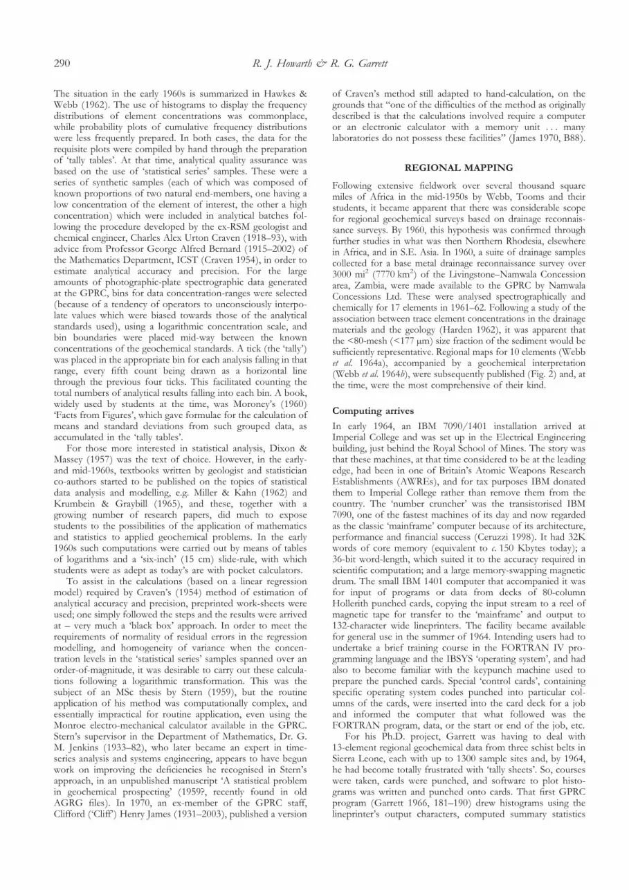
Khaleelee, for his PhD project, was working on the Devon-shire, Denbighshire and Derbyshire data sets to produce theatlases, and interpret the data. He investigated (Khaleelee 1969,104–122) the feasibility of posting sample values using anoffline California Computer Products Inc. CALCOMP 563plotter which plots using a pen onto a continuous roll of paper31 in (79 cm) wide; both chart drum and the pen are capable ofbi-directional movement. In practice, the limiting factor whenplotting large numbers of points was the number of plottinginstructions that could be written to a single magnetic tape. Asa reminder of how far things have come since these early days,Figure 5 shows the time required to compute the plottinginstructions, and to actually draw the map, for a set of 25 � 25in (64 � 64 cm) maps requiring 4 or 5 numerical characters forthe posted value at each sample location for a set of 100–900data points with their spatial coordinates drawn from a uniformrandom distribution. It was clear that for regional map produc-tion, use of the AWRE SC 4020 plotter would again beessential. In addition to the production of working maps usingthe AGRG symbols, as before (Fig. 6; Nichol & Webb 1967),for the atlas maps, the plotting program was modified byKhaleelee (1969) to produce separate solid point-symbolimages for each concentration-class level. These were thencombined, using offset-lithography printing, to make maps withcoloured point symbols overprinted on a map showing thegeology and drainage network (Fig. 7). Khaleelee (1969, 113–125) describes the difficulties he encountered in practice in


Fig. 3. Comparison of (left) cubic trend-surface and (right) ‘rolling mean’ (moving-average) maps for nickel concentrations (ppm) in bedrock,soil, and the <80-mesh stream sediment fraction over eastern Sierra Leone. Percentage values in each map are a measure of ‘goodness of fit’.Nichol & Webb (1967, fig. 4; redrawn from Garrett 1966).


making these maps, caused by the non-uniform stretch of theSC 4020 vellum prints: shrinkage across the width of the paperplus a slight shrinkage (or stretch) along the length of thepaper, caused by slight variations in the tension maintained bythe rollers which wound the vellum through the camera; inaddition, there was insufficient contrast between the darker plotsymbols and the white vellum for subsequent photographicreproduction, and sometimes uneven development of some ofthe vellum plates as a result of variations in the distribution ofthe developer fluid. Two of the map areas (Denbighshire andDevonshire) were rectangular and these required two vellumplates each for coverage; the variable stretch frequently pro-duced slight differences where they abutted. Consequently,although the entire data processing was accomplished in 15 minof IBM 7094 time on the AWRE installation to produce 236vellum plates, a further 100 man-hours were required to

produce the final camera-ready copy for the offset-litho plates(Khaleelee 1969, 121).

For the production of synoptic regional maps, moving-average smoothing became the standard approach, as it effectivelyreduced the inevitable variability (‘noise’) introduced as a result offield sampling and subsequent chemical analysis (Armour-Brown& Nichol 1970; Howarth & Lowenstein 1971, 1972). The successof the Devonshire, Denbighshire and Derbyshire pilot studies ledon to the production of the pioneering regional atlases of thestream sediment geochemistry.

Geochemical atlases of Northern Ireland and Englandand Wales

Whereas earlier data sets had been of the order of a fewhundred to c. 1200 samples in size, the Northern Ireland (Webb

Fig. 4. Prototype (1965)SC4020-plotted geochemical map(Nichol et al. 1966, fig. 1).


et al. 1973) and England and Wales (Webb et al. 1978)geochemical atlases involved the production and interpretationof data sets comprising 18 elements and c. 4 800 samples, and22 elements and c. 50 000 samples, respectively. This increase inscope necessitated the development of new approaches to bothanalytical quality assurance (discussed below) and map display.In both cases, the majority of elements in the <80-meshfraction of the oven-dried sediment samples were determinedusing an ARL 29000B Quantometer (a 40-channel automaticoptical emission spectrometer) linked to an automatic type-writer and an IBM 545 card punch via a Solartron analoguecomputer. Arsenic and molybdenum were determined usingrapid chemical procedures and these data were transcribed,together with the field data records, to punched cards by hand.As a result of the necessity to produce many large-scale workingmaps, and smoothed synoptic maps at 1:1M and 1:2M scales,rapidly and cheaply, it was decided to use lineprinter maps withmultiple-character overprints to produce a grey-scale imagewith up to 10 classes (Howarth 1971a).

In 1968, the Imperial College IBM 7094/1401 installationhad been replaced by a Control Data Corporation (CDC) 6400,and a CDC 6600 ‘supercomputer’ formed the nucleus of theLondon University Computer Centre (a courier service trans-mitted card decks, tapes and lineprinter output between the twoestablishments). These machines were extremely fast and,despite precautions taken by the more careful programmers toprevent numerical truncation and round-off errors in programswritten for the earlier generation of computers, the 60-bitword-length of the CDC machine brought about greatimprovement in numerical accuracy of calculations, because itenabled much larger exponents for a numerical value to beheld. (This was strikingly illustrated when, as a class demon-stration in 1968, a colleague in the ICST Geology Department,John Ferguson, happened to run a widely-used trend-surfacefitting program on the CDC 6400 using the same data set withwhich he had run it on the IBM machine the previous year: thetopography of the contours of the newly-fitted 3rd degreesurface was surprisingly different from its predecessor! Relatedcomputation problems were recognized by Mancey (1980, 155)as being present in the results of early factor analysis studies inthe literature.)

The program for production of the AGRG lineprintergeochemical maps, PLTLP1 (Howarth 1971a), was first writtenin 1969. Its objective was to be able to process a data set ofunlimited size by proceeding in a line-by-line manner from thetop to bottom of the map area, but only retaining in memorythe data required for calculation of the current strip ofmap-cells (each corresponding to the 1/8 in by 1/10 in(0.32 � 0.25 cm) printer character-size) and its immediateneighbours:

i averaging any data points falling into the individual map cells;ii computing the local moving-average smoothing;iii ‘gap-filling’, i.e. filling-in small holes in the smoothed image

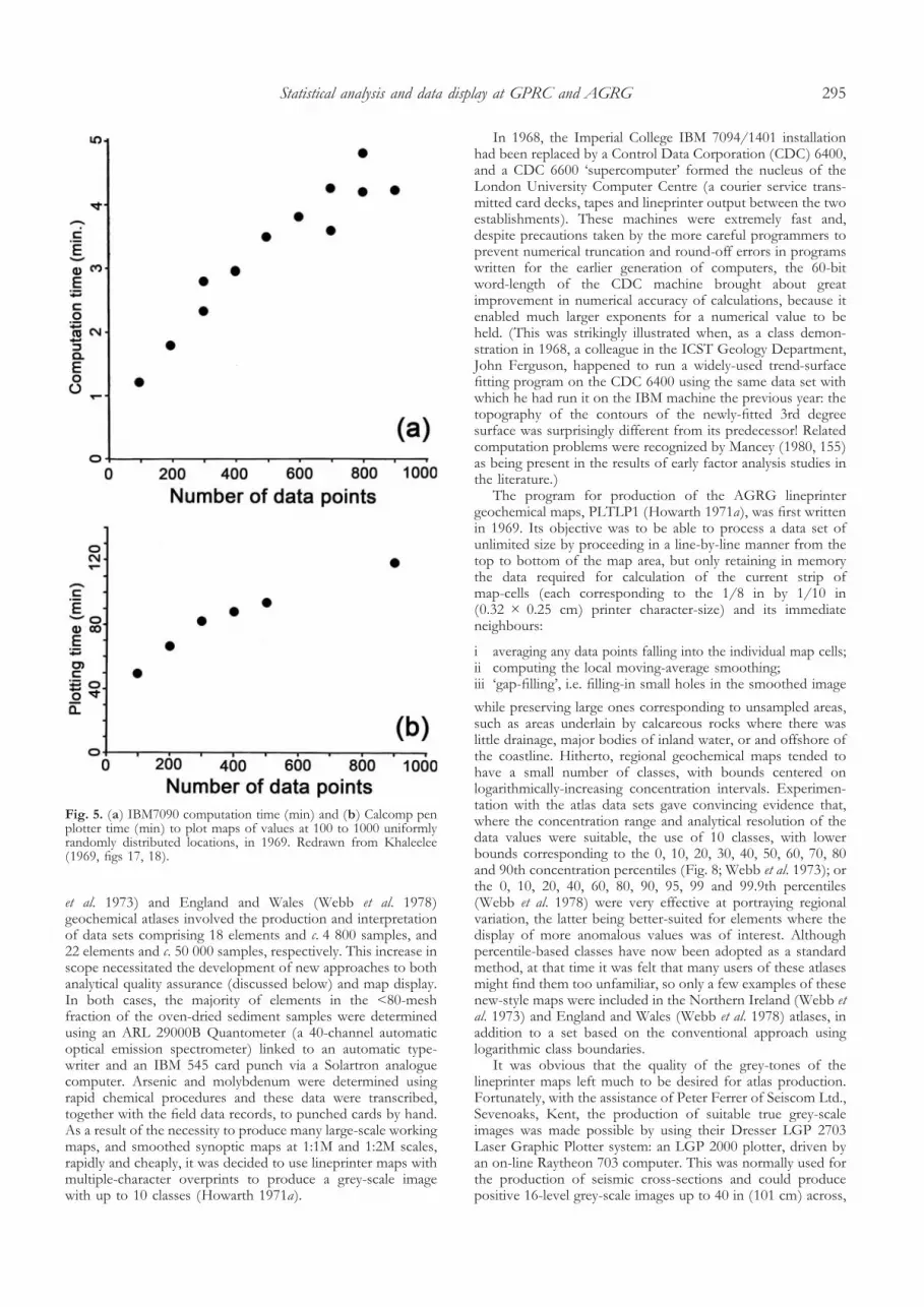
while preserving large ones corresponding to unsampled areas,such as areas underlain by calcareous rocks where there waslittle drainage, major bodies of inland water, or and offshore ofthe coastline. Hitherto, regional geochemical maps tended tohave a small number of classes, with bounds centered onlogarithmically-increasing concentration intervals. Experimen-tation with the atlas data sets gave convincing evidence that,where the concentration range and analytical resolution of thedata values were suitable, the use of 10 classes, with lowerbounds corresponding to the 0, 10, 20, 30, 40, 50, 60, 70, 80and 90th concentration percentiles (Fig. 8; Webb et al. 1973); orthe 0, 10, 20, 40, 60, 80, 90, 95, 99 and 99.9th percentiles(Webb et al. 1978) were very effective at portraying regionalvariation, the latter being better-suited for elements where thedisplay of more anomalous values was of interest. Althoughpercentile-based classes have now been adopted as a standardmethod, at that time it was felt that many users of these atlasesmight find them too unfamiliar, so only a few examples of thesenew-style maps were included in the Northern Ireland (Webb etal. 1973) and England and Wales (Webb et al. 1978) atlases, inaddition to a set based on the conventional approach usinglogarithmic class boundaries.

It was obvious that the quality of the grey-tones of thelineprinter maps left much to be desired for atlas production.Fortunately, with the assistance of Peter Ferrer of Seiscom Ltd.,Sevenoaks, Kent, the production of suitable true grey-scaleimages was made possible by using their Dresser LGP 2703Laser Graphic Plotter system: an LGP 2000 plotter, driven byan on-line Raytheon 703 computer. This was normally used forthe production of seismic cross-sections and could producepositive 16-level grey-scale images up to 40 in (101 cm) across,

Fig. 5. (a) IBM7090 computation time (min) and (b) Calcomp penplotter time (min) to plot maps of values at 100 to 1000 uniformlyrandomly distributed locations, in 1969. Redrawn from Khaleelee(1969, figs 17, 18).


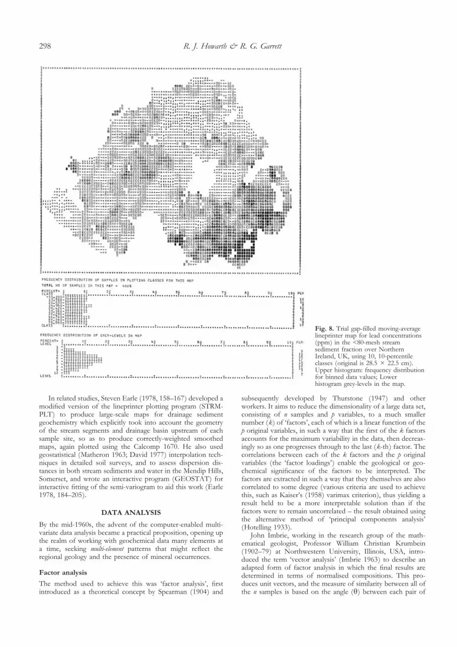
on dimensionally-stable Kodak 2496 RAR film. The plottinginstructions for the LGP 2703 were generated by an off-line IBM360 computer from tapes produced at the ICST, using a modifiedversion of the AGRG plotting program. The rectangularlineprinter-size cells were retained for the Northern Ireland atlas(Fig. 9; Webb et al. 1973), but for the England and Wales atlas(Webb et al. 1978) the program was modified to produce plotswith square cells at the appropriate map-scale. The laser-plottedmap images were then contact-printed, using a suitable half-tonescreen, onto dimensionally-stable ammonia-developed Ozalidsepia diazo pro-film for production of the final offset-lithographyplates for the atlases (Howarth & Lowenstein 1974). Figure 10shows the 1976 Chromalin proofs of the unsmoothed andsmoothed gap-filled percentile-based maps for zinc from theEngland and Wales atlas (Webb et al. 1978).

Multi-element maps

Experimentation into methods of map production had alsobeen undertaken by the AGRG in collaboration with theNatural Environment Research Council’s (NERC) Experimen-tal Cartography Unit (ECU) at the Royal College of Art,London, under the direction of the cartographer David PelhamBickmore (1917–1993). These arrived at multivariateproportional-length symbols of the multi-arm windrose typesuperimposed over a variety of ingenious monochrome geo-logical maps (Rhind et al. 1973). Although various trial mapsbased on a portion of the Northern Ireland data set wereproduced (Fig. 11), they were deemed, by both AGRG staffand others in industry to whom they were shown, to be onlysuited to large-scale maps, and were thought too expensive toproduce for routine use. An exhaustive series of tests on theefficacy of their use carried out by the ECU also suggested that“the low level of accuracy in the use of the symbols maysuggest that graduated, rather than proportional symbols are

more suitable for use” (Rhind et al. 1973, 118). Nevertheless,the method was subsequently taken up by the British Geologi-cal Survey for production of some of their early large-scalegeochemical atlases (e.g. Institute of Geological Sciences 1978)and proved successful with their users.

However, colour-combined 3-component multispectralimages were at this time beginning to be used in remote-sensing, and it was decided to investigate the applicability ofsuch methods to regional geochemical maps. In order toconvince somewhat skeptical colleagues, using the NorthernIreland atlas data, Howarth initially wrote a program to displaya map of three elements using only three concentrationintervals (‘background’, ‘near-anomalous’, ‘anomalous’) each,i.e. a total of 27 possible combinations, as the lineprintercharacters A–Z, plus an asterisk where all three fell into theanomalous class. A translucent overlay was then hand-colouredto produce the final map. Having established the utility of themethod, once the laser-plotter images became available, thesewere used to produce subtractive colour-combined maps withup to 10 levels per component (Webb et al. 1973, 1978). Acolour-combined map for potassium, strontium and chromiumwas first shown at the ‘Geochemical Exploration 1972’ meetingin London (Lowenstein & Howarth 1973) and formed thecover of the Northern Ireland atlas (Fig. 12; Webb et al. 1973).An ‘economy’ version was also developed, which simply used aseries of lineprinter-produced black masks and diazo contactprinting, to produce 3-level, 3-component maps (Howarth &Lowenstein 1976). The England and Wales atlas (Webb et al.1978) included examples of both two-component (Fig. 13) andthree component (Fig. 14) colour-combined maps.

Anomaly enhancement

In order to assist the recognition of areas of ‘anomalously’ highelement concentrations in regional maps, the PLTLP1 program

Fig. 6. Prototype SC4020-plotted map(Dec. 1965) for zinc concentrations(ppm) in the <80-mesh streamsediment fraction over Denbighshire,UK (original is 29.5 � 22 cm in size).


was extended in 1972–73 to include a variety of image-processingoperators: the moving-average smoothing already being used wasa low-pass filter; now the option was added to apply:

i a high-pass filter (HPF), contrasting a central map-cell withthe mean of a square block of surrounding cells;

ii a picture-frame filter (PFF; Holmes 1966), contrasting thecentral cell with the mean of a surrounding square annulusof cells at some distance away;

iii a probabilistic Kolmogorov-Smirnov filter (KSF; Muerle &Allen 1968)

which computed if the cumulative frequency distribution of thevalues in a square central block of cells was statistically greaterthan that of the cumulative distribution of those in a surround-ing square annulus at some distance away, based on theKolmogorov–Smirnov test (Kolmogorov 1933; Smirnov 1939).These were initially investigated using data from the NorthernIreland atlas, operating on the image grey-levels (Fig. 15),essentially the equivalent of using a ranked statistics approach(Howarth 1983).

The PLTLP1 program was subsequently applied in jointwork, directed by Professor George Koch Jr. at the Universityof Georgia, USA, under contract to the United States Depart-ment of Energy National Uranium Resource Evaluation

(NURE) Program, to data sets from the Hydrogeochemical andStream Sediment Reconnaissance (HSSR) phase of the pro-gramme for North Carolina, Virginia, and Tennessee (Kochet al. 1979, 1981a, b; Howarth et al. 1980). For this project,Howarth’s original program was converted in 1977/78 by C.Y.(‘Sam’) Chork, a post-doctoral researcher in AGRG, who hadobtained his PhD at the University of New Brunswick, Canada,under Professor Gerald (‘Gerry’) Govett (who had obtained hisown PhD at AGRG; 2010), to use the actual concentrationvalues and automatic selection of percentile class intervals; andby Steven Mancey, an AGRG doctoral student, to use interac-tive user-selection of classes. Mancey (1980, 255–271) appliedthese techniques to the entire England and Wales atlas data set,with output onto 35-mm microfilm, using the recently-installedoff-line Calcomp 1670 microfilm plotter at the University ofLondon Computer Centre, with a mapping program (MIC-MAP) he had written (Mancey 1980, 57–61) utilising theirPICPAC microfilm plotting software (Colvill & Kitchingman1976). The results from all these studies showed the PFF wasmore effective at identifying regional geochemical anomaliesthan a comparable HPF, and that the KSF produced no betterresults than the PFF, while it was computationally much moretime-consuming, owing to its greater complexity of calculationsrequired.

Fig. 7. Prototype SC4020-plotted map(May 1967) for lead concentrations(ppm) in the <80-mesh streamsediment fraction over Derbyshire, UK(original is 20.5 � 25 cm).


In related studies, Steven Earle (1978, 158–167) developed amodified version of the lineprinter plotting program (STRM-PLT) to produce large-scale maps for drainage sedimentgeochemistry which explicitly took into account the geometryof the stream segments and drainage basin upstream of eachsample site, so as to produce correctly-weighted smoothedmaps, again plotted using the Calcomp 1670. He also usedgeostatistical (Matheron 1963; David 1977) interpolation tech-niques in detailed soil surveys, and to assess dispersion dis-tances in both stream sediments and water in the Mendip Hills,Somerset, and wrote an interactive program (GEOSTAT) forinteractive fitting of the semi-variogram to aid this work (Earle1978, 184–205).

DATA ANALYSIS

By the mid-1960s, the advent of the computer-enabled multi-variate data analysis became a practical proposition, opening upthe realm of working with geochemical data many elements ata time, seeking multi-element patterns that might reflect theregional geology and the presence of mineral occurrences.

Factor analysis

The method used to achieve this was ‘factor analysis’, firstintroduced as a theoretical concept by Spearman (1904) and

subsequently developed by Thurstone (1947) and otherworkers. It aims to reduce the dimensionality of a large data set,consisting of n samples and p variables, to a much smallernumber (k) of ‘factors’, each of which is a linear function of thep original variables, in such a way that the first of the k factorsaccounts for the maximum variability in the data, then decreas-ingly so as one progresses through to the last (k-th) factor. Thecorrelations between each of the k factors and the p originalvariables (the ‘factor loadings’) enable the geological or geo-chemical significance of the factors to be interpreted. Thefactors are extracted in such a way that they themselves are alsocorrelated to some degree (various criteria are used to achievethis, such as Kaiser’s (1958) varimax criterion), thus yielding aresult held to be a more interpretable solution than if thefactors were to remain uncorrelated – the result obtained usingthe alternative method of ‘principal components analysis’(Hotelling 1933).

John Imbrie, working in the research group of the math-ematical geologist, Professor William Christian Krumbein(1902–79) at Northwestern University, Illinois, USA, intro-duced the term ‘vector analysis’ (Imbrie 1963) to describe anadapted form of factor analysis in which the final results aredetermined in terms of normalised compositions. This pro-duces unit vectors, and the measure of similarity between all ofthe n samples is based on the angle (�) between each pair of

Fig. 8. Trial gap-filled moving-averagelineprinter map for lead concentrations(ppm) in the <80-mesh streamsediment fraction over NorthernIreland, UK, using 10, 10-percentileclasses (original is 28.5 � 22.5 cm).Upper histogram: frequency distributionfor binned data values; Lowerhistogram grey-levels in the map.


vectors, the ‘cos � coefficient’ (Imbrie 1963; for which signifi-cance levels were given by Howarth 1977). Imbrie (1963) calledthis approach ‘Q-mode analysis’, in contrast to calculation ofthe more familiar correlation coefficient matrix between the pvariables (which he called ‘R-mode analysis’). In a conventionalR-mode factor analysis, the first step is to compute the kuncorrelated principal components, then to retain the first p ofthese and rotate them (e.g. using the ‘varimax’ criterion) toobtain the final solution. In the Q-mode approach, each of thek factors corresponds to an actual sample of ‘extreme’ com-position. These are end-members, and the entire data set is thusrepresented in terms of the relative contributions of theseend-members, the factor ‘scores’ increasing from zero to unityas a sample’s composition approaches more exactly that of oneof the end-member reference vectors. This approach was firstapplied at Northwestern to compositional analysis of variationsin carbonate sediments (Imbrie & Purdy 1962) and to lithos-tratigraphy (Krumbein & Imbrie 1963). The availability of acomputer program for the IBM 7094/1401 computer system(Manson & Imbrie 1964) enabled Q-mode factor analysis to betaken up by Garrett (1967), who was able to successfully applyit to interpretation of the geochemistry of his regional streamsediment data from Sierra Leone (Garrett 1966, 142–148;Nichol & Webb 1967; Nichol et al. 1969) (Fig. 16). However,because of memory-size limitations, Q-mode analysis was atthis time subject to the serious restriction of handling amaximum of 100 samples.

The relatively small number of samples capable of beinganalysed by Q-mode factor analysis program proved a powerfullimitation where the large data sets involved in regional geo-chemistry were concerned. On completion of his thesis, Garrettvisited Northwestern University on a post-doctoral research

fellowship, where he investigated the utility of R-mode factoranalysis as an alternative to the Q-mode approach, based on astudy of stream sediment samples from the Nimini Hills schistbelt of Sierra Leone (Garrett & Nichol 1969). The computerprograms developed by Garrett (1966, 1967) were modified byKhaleelee in 1969 for use within the AGRG.

In an extensive study of the regional drainage sedimentgeochemistry of parts of SW England, Wales, and the EnglishPeak District, Khaleelee (1969, 204–445) used both the R- andQ-mode approaches. He concluded that, quite apart from thesevere limitation on the number of samples to which theQ-mode method could be applied, the fact that compositionsof Q-mode end-members differed markedly between differentsubsets of the same regional data set made the R-modeapproach far better suited to analysis of large regional data sets.He verified this by means of a detailed comparison of theresults of R-mode analysis applied to the geochemistry ofbedrock, soil, and stream sediment samples (n = 104, 287 and198, respectively) from the Onecote district of NE Stafford-shire, analysed for 15 elements (Khaleelee 1969, 326–445).Tragically, Khaleelee lost his life in a helicopter accident, shortlyafter taking up a new post in Australia in 1970.

The R-mode approach was subsequently used: by AshlynArmour-Brown (1971; Armour-Brown & Nichol 1970) withregional geochemical data from Zambia; by Colin Summer-hayes (1971, 1972) to interpret the geochemistry of phosphaticcontinental margin sediments from NW Africa; and byGeoffrey Glasby (Glasby et al. 1974) in a study of thegeochemistry of manganese concretions from the Indian ocean.This approach thereafter became an established tool in AGRGwork. Mancey & Howarth (1978) used varimax-rotated factorsof the Box–Cox (1964) transformed (see below) England and

Fig. 9. Trial LGP2703 laser-plottedmap for zinc concentrations (ppm) inthe <80-mesh stream sediment fractionover Northern Ireland, UK, using‘empirical’ (logarithmic) class intervals(original is 30 � 27.5 cm).


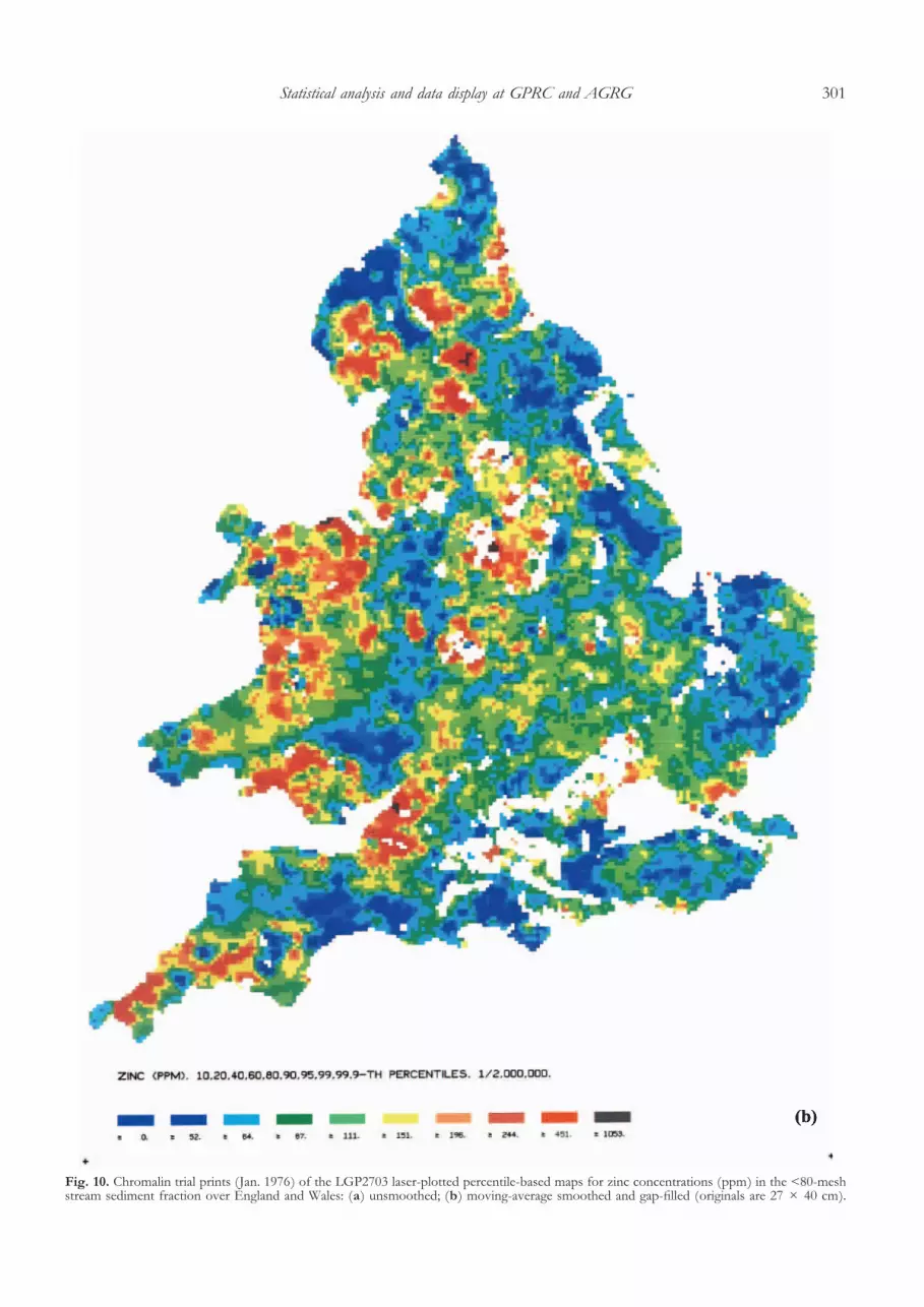
Fig. 10. Chromalin trial prints (Jan. 1976) of the LGP2703 laser-plotted percentile-based maps for zinc concentrations (ppm) in the <80-meshstream sediment fraction over England and Wales: (a) unsmoothed; (b) moving-average smoothed and gap-filled (originals are 27 � 40 cm).


Fig. 11. Detail of 1972 trial ‘windrose’map for copper (left), zinc (vertical)and lead (right) concentrations (ppm)in the <80-mesh stream sedimentfraction over a part of NorthernIreland. Geological boundaries (grey);faults (gold). AGRG-NERC ECU trialmap 5a (original is 40 � 26 cm).

Fig. 12. Cover of the Northern Irelandgeochemical atlas (Webb et al. 1973)showing subtractive colour-combinedmap for potassium (increasingconcentrations (ppm), magenta),chromium (increasing, yellow) andstrontium (increasing, cyan) in the<80-mesh stream sediment fraction(original is 35 � 27 cm).


Wales atlas data set to produce a pair of colour-combined mapswhich together embodied 68% of its total variance; see Mancey(1980, 182–196) for detailed interpretation. These were printedfrom enlargements of grey-scale images generated on 35-mmmicrofilm using Mancey’s MICMAP program (Fig. 17).

‘Empirical’ (potential function) discriminant analysis

Nevertheless, the increasingly large size of the geochemical datasets being produced within AGRG made it imperative thatadditional multivariate methods capable of giving furtherinsight into relationships between sample compositions weremade available for AGRG workers. Two approaches wereinitially investigated: discriminant analysis, which allocatessamples into pre-defined compositional groups based on atraining set of samples for each group; and cluster analysis,which seeks to allocate samples to ‘natural’ groups of similarcomposition. Although the classical techniques for accomplish-ing these objectives had become available to geologists sincethe mid-1960s, largely through the computer programs dissemi-nated by the Kansas Geological Survey ‘Computer Bulletin andSpecial Distribution Publication’ series, and textbooks, such asDavis & Sampson (1973), new methods were being developedby workers in pattern recognition and electrical engineering. The

first of these to be implemented in AGRG, in 1969, was the‘empirical discriminant function’ (EDF; Specht 1967), whichcombined the use of gaussian potential (kernel) functions with aBayesian classifier. This proved a very effective classificationmethod and had the added advantage that samples sufficientlyunlike any of the training sets were classified as ‘unknown’,rather than being forced into one of the pre-defined groups, aswas the case with the classical linear discriminant functionapproach. In the AGRG implementation (Howarth 1973a) forthe CDC 6600, sequential backwards selection (BAKWRDprogram) proved the best method to find both the optimumcombination of elements (Howarth 1973c, 1974) and the bestvalue of the smoothing parameter for the potential function, onwhich to base the subsequent classification process. The resultsof the classification itself (PRSYS1 program, written by Howarthin 1969) were plotted as a map using an off-line Calcomp penplotter. The practicality of the method was initially establishedusing a lithogeochemical data set (Howarth 1971b), then theDevon atlas data (Howarth 1971c, 1972), and in a moreexhaustive study by Rolando Castillo-Muñoz (1973; Castillo-Muñoz & Howarth 1976) (Fig. 18). Fong Tai Loon, an MScstudent in the Department of Computing and Control, super-vised by Howarth and Dr. Francis N. Parr, examined the utility

Fig. 13. Subtractive colour-combinedmap of molybdenum (increasingconcentrations (ppm), magenta) andcopper (decreasing concentrations(ppm), cyan) in the <80-mesh streamsediment fraction over England andWales. (Webb et al. 1978, fig. 67;original is 30 � 39 cm). Bovinehypocupraemia is particularly associatedwith areas of black shale in which thecopper:molybdenum ratios are low(Leech 1984; see Thornton (2010) fordiscussion).


of the Divergence (Bhattacharyya 1943) and Bhattacharyyadistance (Jeffreys 1946; Kailath 1967) criteria as measures ofclass separability in a lithogeochemical context, finding diver-gence to be a useful separability criterion, but it required fairlylarge training set sizes (Fong 1975). Although the EDF methodwas found to be very effective (particularly in attracting attentionto data unlike anything present in the training sets), it becameevident that there was not much demand from AGRG users forthis approach in analysis of the regional atlas data and this workwas not pursued.

Cluster analysis

Hitherto, virtually all the cluster analysis methods used ingeological studies were based on agglomerative hierarchicalclustering methods (Imbrie & Purdy 1962; Parks 1970). Thesewere commonly used with relatively small data sets andproduced a hierarchical ‘tree’ structure, with the mostcompositionally-similar samples grouped at the tips of the‘branches’ (Fig. 19). John Sammon Jr. at the Rome AirDevelopment Centre (RADC), New York, developed an alter-native ‘non-linear mapping (NLM) algorithm’ (Sammon 1969).This projected the positions of points in high-dimensional (i.e.multivariate) space onto a plane, adjusting the locations of the

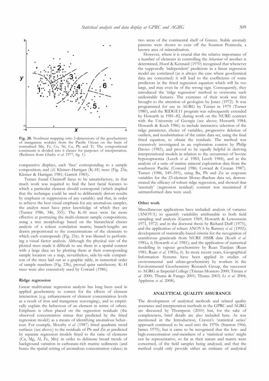
points in the plane until the matrix of their inter-point distanceswas as close as possible to that for the equivalent points in theoriginal high-dimensional space. Howarth (1973b) comparedthe results of the NLM method with those obtained in anumber of geological studies that had previously used hierarchi-cal cluster analysis, and found it to be extremely effective.Application to a variety of applied geochemical data sets(Howarth 1973b, c; Castillo-Muñoz 1973; Howarth et al. 1977;Howarth & Johnson 1977) showed it could successfully delin-eate ‘natural’, i.e. separated, clusters or reveal a compositionalcontinuum, where such existed, as well as identify outliers. In aset of marine manganese nodule data classified by hierarchicalclustering into a number of discrete groups (Fig. 19; Glasby et al.1974), NLM shows that there is actually a complete lack ofdiscrete ‘natural’ clusters (Fig. 20) although division of the cloudof points in the NLM plot produces viable groupings in a spatialcontext (Fig. 21). The success of the NLM method was such that,with the permission of the RADC, AGRG (via the ICSTComputer Centre) distributed the program for many years.

In order to cope with cluster analysis of large data sets onecould use a non-hierarchical method, such as NLM, or theISODATA clustering algorithm (Ball & Hall 1965), which hadfirst been evaluated in AGRG with data from the Denbighshire

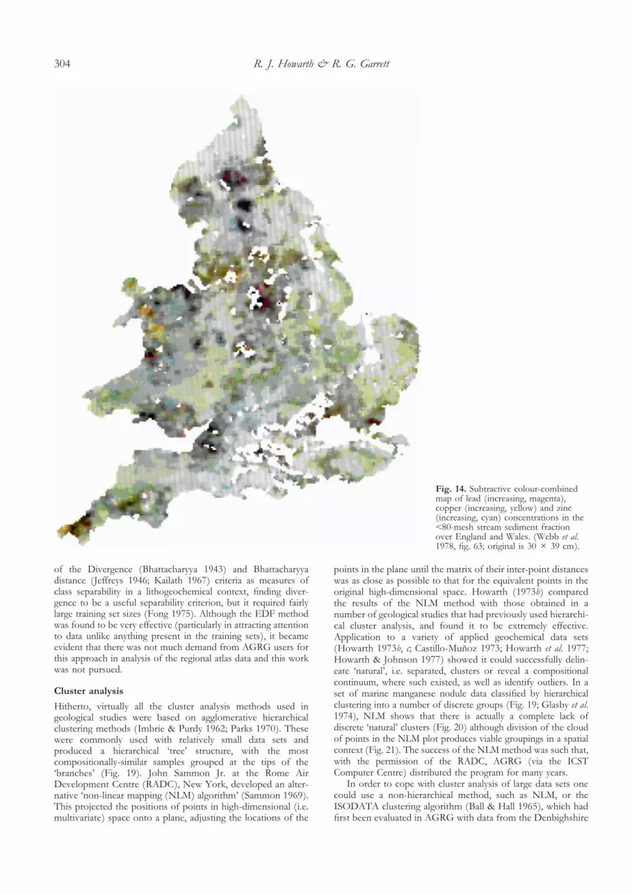
Fig. 14. Subtractive colour-combinedmap of lead (increasing, magenta),copper (increasing, yellow) and zinc(increasing, cyan) concentrations in the<80-mesh stream sediment fractionover England and Wales. (Webb et al.1978, fig. 63; original is 30 � 39 cm).


atlas by David Crisp (1974), using a subset of data (subsampledat a broadly even spatial density) to identify a number ofgeochemical groups, which were then used as training sets forsubsequent EDF classification of the entire data set. In this way,Mancey (1980, 207–254) was able to achieve a regional classifi-cation of the entire England and Wales atlas data into ninespatially-coherent and geochemically-meaningful categories, plusa small number of outlying (anomalous) data points.

Data transformation

It has been known for many years that many geochemicalelements have concentrations that tend to have a skewed(asymmetrical) frequency distribution, usually with the distri-bution extended towards higher concentration values. From theearliest days of geochemistry (Ahrens 1954; Hawkes & Webb1962), it was assumed that logarithmic transformation of suchdata provided an adequate transformation to symmetry, therebyadequately approximating a normal frequency distribution.However, as ever-larger regional data sets were investigated inAGRG, it became apparent that distributions existed withpositive (or occasionally negative) skewness which could not besymmetrised by simple log-transformation. Howarth & Earle(1979) wrote a program (MINSK) that implemented the powertransform to normality of Box & Cox (1964).

y =Hsx � � 1d ⁄ �, � fi 0

lnsxd, � = 0 Jx . 0,

where x is the set of original observations; � is the powercoefficient; and y is the transformed data set, by minimising anobjective function of skewness and kurtosis (Fig. 22). While inmany cases the transformed distribution (y) is still not a perfectnormal distribution, it is generally symmetrical, which is themost important thing. Mancy (1980, 157–182) and Mancey &Howarth (1978, 1980) illustrated its efficacy with principalcomponents analysis of the England and Wales atlas data.Turner (1986, 181–253) found data transformation, and the

Box–Cox transform in particular, to be equally useful with a503-sample, 24-element British Geological Survey stream sedi-ment data set from the Dalradian of the Moray–Buchan area ofNE Scotland (British Geological Survey 1991), as did NeilCoward (1986) with a suite of marine geochemical data fromthe SW Pacific.

The problem of induced correlation in percentaged (constant-sum) data has been recognised for many years. The first attemptto address this in the geosciences was made by the petrographerFelix Chayes (1971; Howarth 2004). In 1982, the statistician,John Aitchison, proposed a solution based on application ofthe ‘logratio transform’ (Aitchison 1982, 1986), which trans-forms a set of percentaged variables, x1, . . . xk (with theprovisio that all xi > 0 and �xi,i=1,k =100) to a new set ofvariables y1, . . ., y(k�1) where yj = loge[xi/x(k�1)]; j=1, k�1.In recent years, this transform has been widely promoted foruse in the earth sciences (most recently by Buccianti et al. 2006).Howarth tried on several occasions to apply the logratiotransform as a precursor to multivariate analysis of variousAGRG geochemical data sets but found that, in practice, theresults were often geochemically uninterpretable, and thatwhenever xi �0, the transform resulted in serious outlierproblems. More research, with a wide variety of data sets, isrequired on this subject.

In recent years, Dennis Helsel (Helsel & Hirsch 1992,357–376; Helsel 2005), of the US Geological Survey WaterResources Division, has provided new approaches to theproblem of dealing with censored, i.e. below analytical detec-tion limit (dl), data. In the days of GPRC/AGRG, any suchvalues in a data set were routinely set to the appropriate dl/2for the purposes of statistical analysis and, in practice, it isdoubtful whether it brought any geologically significant biasinto the geochemical interpretations arrived at.

Robust methods

The deleterious effect of outliers present in a data set, leading tobias in calculation of the mean, inflated variances, spurious

Fig. 15. Trial Kolomogorov–Smirnovfiltered map for zinc concentrations(ppm) in the <80-mesh streamsediment fraction over NorthernIreland. (%) Unsampled areas; (*)anomalous map-cells; (m) associatedwith manganese scavenging; (z)associated with mineralization. (Originalis 28.5 � 23 cm).


correlation coefficients, and so on, has long been recognised.However, it was only in the mid-1970s that methods whichcould automatically down-weight the effects of outliers to

obtain ‘robust’ estimates of both univariate statistics (such asthe mean and standard deviation) and the covariance matrixor correlation matrix (which underpin principal components,

Fig. 16. Q-mode factor analysis maps for the geochemistry of the <80-mesh stream sediment fraction, Nimini Hills, eastern Sierra Leone: (upperleft) vector 1, (upper right) vector 2, (lower left) vector 3, end-members shown by solid dot in each case; (lower right) communality. Garrett(1966, fig. 52; original is 18 � 23 cm).


factor and classical linear discriminant analysis) began to bedeveloped (Andrews et al. 1972; Huber 1981), but it was awhile before their potential utility in applied geochemistry waspointed out (Campbell 1982; Garrett 1983; Howarth 1984).Robust correlation matrices were calculated by Leech (1984),using software developed by the statistician Norman Camp-bell of the Commonwealth Scientific and Industrial ResearchOrganisation, Australia (Campbell 1980), who had taken hisdoctorate in the Statistics Department at Imperial College.Turner (1986) implemented robust versions of both principalcomponents analysis and ridge regression software, whichproved immensely useful to AGRG research subsequently(e.g. Coward & Cronan 1987).

The extensive study of the application of robust principalcomponents and factor analysis by Turner (1986, 434–548)concluded that factor analysis is preferable to principal compo-nents analysis because the use of a small number of factorsforces a grouping of the variables, reducing the dimensionalityof the problem and increasing interpretability. The greatestanomaly contrast is obtained using untransformed data; priorBox–Cox transformation of the data is best if backgroundassociations and relationships are to be revealed.

Data displays

The arrival of the interactive statistical package MINITAB(Ryner et al. 1976) on the College’s distributed terminal systemenabled routine data analysis to be used by both staff andstudents in AGRG and, because it embodied much of therecent thinking on graphics-based Exploratory Data Analysis(Tukey 1977), box-plots, quantile-quantile plots and othergraphical displays were soon taken up in AGRG work (Earle1982; Howarth 1984; Turner 1986). Earle (1982, 168–183)developed a program (GIRAF) for the interactive dissection ofprobability plots into constituent sub-populations. Turner(1986, 166–179) showed the utility of multivariate probabilityplots, based on the cube-root of the Mahalanobis distance(Healy 1968; Campbell 1979) for detection of multivariateoutliers.

Use of two new multivariate graphics to portray multi-element sample compositions for the purpose of comparisonwere extensively investigated by Turner (1986), using theMoray–Buchan data set: (i) Chernoff faces (Chernoff 1973),which assigns features of the human face (e.g. position/style ofeyes, eyebrows, nose, mouth) to different variables to make

Fig. 17. Subtractive colour-combinedmap of the first three varimax rotatedfactors of the Box–Cox transformedgeochemistry of the <80-mesh streamsediment fraction over England andWales. This map accounts for 64% ofthe variation of the entire data set(Mancey & Howarth 1978, sheet 1;original is 14 � 18.5 cm).


Fig. 18. Empirical discriminant classification map of the geochemistry of Pb, Ga, V, Mo, Cu, Zn, Ti, Ni, Co, Mn, Cr and Fe2O3 in the <80-meshstream sediment fraction over Denbighshire, UK. Training areas are for five lithologies are boxed in; samples assigned to ‘unknown’ group areshown solid, of these samples 62% were related to known mineralized areas. (Castillo-Muñoz & Howarth 1976, fig. 6).

Fig. 19. (right) Q-mode weighted pairgroup dendrogram based on agglomerativecluster analysis of the normalized Mn, Fe,SiO2, Ti, V, Cr, Co, Ni, Cu, Zn, Zr, Moand Pb concentrations of 180 manganesenodules and crusts from the westernflanks of the Carlsberg Ridge, IndianOcean; rectangle length is proportional tonumber of samples/group; (left)proportion of massive or granular crusts,or nodules in each cluster-analysis group;(centre) proportion of collection sites inmassif or ridge settings (Glasby et al.1974, fig. 4).


comparative displays, each ‘face’ corresponding to a samplecomposition; and (ii) Kleiner–Hartigan (K–H) trees (Fig. 23a;Kleiner & Hartigan 1981; Garrett 1983).

Turner found Chernoff faces to be unsatisfactory, in thatmuch work was required to find the best facial features towhich a particular element should correspond (which impliedthat the technique could be used to deliberately distort resultsby emphasis or suppression of any variable) and that, in orderto achieve the best visual emphasis for any anomalous samples,the analyst must have prior knowledge of which they are(Turner 1986, 346, 355). The K–H trees were far moreeffective at portraying the multi-element sample compositions,using a tree morphology based on the hierarchical clusteranalysis of a robust correlation matrix; branch-lengths aredrawn proportional to the concentrations of the elements towhich each corresponds (Fig. 23a). It was likened to perform-ing a visual factor analysis. Although the physical size of theplotted trees made it difficult to use them in a spatial contextwith a large data set by plotting them at their correspondingsample location on a map, nevertheless, side-by-side compari-son of the trees laid out as a graphic table, in numerical orderof sample numbers (Fig. 23b), proved quite satisfactory. K–Htrees were also extensively used by Coward (1986).

Ridge regression

Linear multivariate regression analysis has long been used inapplied geochemisty to correct for the effects of elementinteraction (e.g. enhancement of element concentration levelsas a result of iron and manganese scavenging), and to empiri-cally explain the behaviour of an element in terms of others.Emphasis is often placed on the regression residuals (theobserved concentration minus that predicted by the fittedregression model) as a means of identifying anomalous behav-iour. For example, Moorby et al. (1987) fitted quadratic trendsurfaces (see above) to the residuals of Pb and Zn as predictedby separate regression models fitted to the suite of elements{Ca, Mg, Al, Fe, Mn} in order to delineate broad trends ofbackground variation in carbonate-rich marine sediments (andhence the spatial setting of anomalous concentration values) in

two areas of the continental shelf of Greece. Stable anomalypatterns were shown to exist off the Sounion Peninsula, aknown area of mineralisation.

However, where it is crucial that the relative importance ofa number of elements in controlling the behaviour of another isdetermined, Hoerl & Kennard (1970) recognised that wheneverthe supposedly ‘independent’ predictors in a linear regressionmodel are correlated (as is always the case where geochemicaldata are concerned) it will lead to the coefficients of somepredictors in the fitted regression equation which will be toolarge, and may even be of the wrong sign. Consequently, theyintroduced the ‘ridge regression’ method to overcome suchundesirable features. The existence of their work was firstbrought to the attention of geologists by Jones (1972). It wasprogrammed for use in AGRG by Turner in 1979 (Turner1980), and the RIDGE11 program was subsequently extendedby Howarth in 1981–82, during work on the NURE contractwith the University of Georgia (see above; Howarth 1984;Howarth & Koch 1986) to include interactive selection of theridge parameter, choice of variables, progressive deletion ofoutliers, and resubstitution of the entire data set, using the finalfitted equation, to obtain the residuals. The method wasextensively investigated in an exploration context by PhilipDavies (1983), and proved to be equally helpful in derivinginterpretational models in relation to the occurrence of bovinehypocupraemia (Leech et al. 1983; Leech 1984), and in theanalysis of a suite of marine mineral exploration data from thesouthwest Pacific (Coward 1986; Coward & Cronan 1987).Turner (1986, 549–593), using Ba, Pb and Zn as responsevariables for the 23-element Moray–Buchan data set, demon-strated the efficacy of robust ridge regression, and showed that‘anomaly’ (regression residual) contrast was maximised ifuntransformed data were used.

Other work

Miscellaneous applications have included: analysis of variance(ANOVA) to quantify variability attributable to both fieldsampling and analysis (Garrett 1969; Howarth & Lowenstein1971, 1972) and in the doctoral thesis by Richard Duff (1975),and the application of robust ANOVA by Ramsey et al. (1992);development of statistically-based criteria for the recognition ofuraniferous granitoids from NURE HSSR data (Koch et al.1981a, b; Howarth et al. 1981); and the application of numericalmodelling in vapour geochemistry by Ruan Tianjian (Ruan1981; Ruan et al. 1985a, b). In more recent years, GeographicalInformation Systems have been applied in studies ofenvironmental- and urban-geochemistry by workers in theEnvironmental Geochemistry Research Group, the successorto AGRG at Imperial College (Tristan-Montero 2000; Tristan etal. 2000; Thums & Farago 2001; Thums 2003; Li et al. 2004;Appleton et al. 2008).

ANALYTICAL QUALITY ASSURANCE

The development of analytical methods and related qualityassurance and interpretation methods in the GPRC and AGRGare discussed by Thompson (2010) but, for the sake ofcompleteness, brief details are also included here. As wasmentioned in the Introduction, Craven’s ‘statistical series’approach continued to be used into the 1970s (Stanton 1966;James 1970), but it came to be recognized that the low- andhigh-concentration end-members of a ‘statistical series’ mightnot be representative, so far as their nature and matrix wereconcerned, of the field samples being analysed, and that themethod could only provide either an estimate of analytical

Fig. 20. Nonlinear mapping onto 2-dimensions of the geochemistryof manganese nodules from the Pacific Ocean on the basis ofnormalised Mn, Fe, Co, Ni, Cu, Pb and Ti. The compositionalcontinuum is divided into 6 classes for purposes of interpretation.(Redrawn from Glasby et al. 1977, fig. 1).


precision (repeatability) at a particular concentration, or anaverage precision value over the concentration range.Thompson & Howarth (1973, 1976, 1978), Howarth &

Thompson (1976), and Thompson (1978, 1981, 1983), devel-oped an alternative approach, based on duplicate analysis ofrandomised splits of routine field samples in which it was

Fig. 21. Spatial disposition in thePacific Ocean (Lambert equal-areaprojection) of the 6 classes from thenonlinear mapping of Fig. 20. (Redrawnfrom Glasby et al. 1977, fig. 3).

Fig. 22. Comparison of the Box–Coxtransform in reducing skewness (s) andkurtosis (k; shown as √k) for a data setwith the same parameters for theuntransformed and log-transformed datavalues (Howarth & Earle 1979, fig. 8).


assumed: (i) that analytical error could generally be wellmodelled by the normal distribution (Thompson & Howarth1980); and (ii) that analytical precision varied as a linearfunction of concentration in the analytical system (Thompson1988) which, it turns out, was also assumed by Jenkins in hisunpublished (1959?) manuscript mentioned p. 290. The ‘dupli-

cate analysis’ method rapidly became established within AGRG,alongside the use of classical Shewhart (1931) control charts tocontrol analytical batch performance through the monitoring ofanalyte concentration levels in splits of long-term house refer-ence materials (Thompson 1981, 1983). The ‘Thompson–Howarth chart’, as it became named, was subsequently adopted

Fig. 23. (a) Kleiner–Hartigan (K–H)tree morphology for theMoray–Buchan, Scotland, streamsediment data set based on Ward’s(1963) agglomerative clusteringalgorithm applied to a robustcorrelation matrix of Box–Coxtransformed data (redrawn from Turner1986, fig. 7.76); (b) Examples of K–Htrees for actual samples from theMoray–Buchan data set (portion ofTurner 1986, fig. 7.102).


by the wider geochemical and chemical community (e.g. Ana-lytical Methods Committee 2002) and their approach continuesto be extended in scope (e.g. Stanley 2006; Stanley & Lawie2008).

In other applications, simulation and regression techniqueshave been applied to evaluation of matrix correction andinterference effects (Howarth 1973d; Thompson et al. 1979)and to the comparison of analytical accuracy between analyticalmethods (Thompson 1982). More recently, robust ANOVAhas been used to determine the magnitude of analytical variancein relation to other sources of variance in geochemical data(Ramsey et al. 1992).

When John Webb initiated the pioneering series of multi-element multi-purpose geochemical atlases in the mid-1960s,there was inevitable trade-off between the analytical methodused, expected analytical precision, and rapidity of turn-round;this was not what traditional geochemists were used to, and thematter proved controversial. AGRG staff had to justify thisnew approach (Howarth & Lowenstein 1971, 1972; Webb &Thompson 1977; Webb et al. 1978). Even today, despiteconsiderable advances in analytical methods, such a ‘fitness-for-purpose’ approach to analysis requires explanation (Thompson& Fearn 1996; Fearn et al. 2002).

Looking back now, it is probably impossible for youngergeochemists to realise just how difficult it was, not only toimplement many of the statistical techniques, where we werebreaking new ground in applied geochemistry, but to convincepotential users of the utility of the results. In a broaderperspective, Garrett et al. (2008) reviewed the development ofinternational geochemical mapping to date; it is pleasing tothink that AGRG pioneered many of the methods that subse-quently became adopted.

The development and implementation of the computer-basedmethods over the years described here was enabled by many bodies.We principally have to thank the Department of Scientific andIndustrial Research and its successor, the Natural EnvironmentResearch Council in Britain for their support to AGRG over manyyears; other contributions have come from the Anglo AmericanCorporation (South Africa) Ltd.; the Institute of GeologicalSciences/British Geological Survey; Roan Selection Trust TechnicalServices; Sierra Leone Geological Survey; Ministerio de Economia,Industria y Comercio de Costa Rica; Wolfson Foundation; and theU.S. Department of Energy, National Aeronautics and SpaceAdministration, and Rome Air Development Center (New York).We are grateful to them all for their assistance, whether throughresearch contracts, support for studentships, or other help. Theauthors are most grateful to the Editor, Gwendy Hall, and theAssociation of Applied Geochemists for their assistance with thefunding of the colour illustrations in this paper.

REFERENCES

A, L.H. 1954. The log-normal distribution of the elements (A funda-mental law of geochemistry and its subsidiary). Geochemica et CosmochimicaActa, 5, 49–73; 6, 121–131.

A, J. 1982. The statistical analysis of compositional data. Journal of theRoyal Statistical Society, B44, 139–177.

A, J. 1986. The Statistical Analysis of Compositional Data. Chapman andHall. London and New York.

A, H. 1978a. A method of bivariate interpolation and smooth surfacefitting for irregularly distributed data points. ACM Transactions on MathematicalSoftware, 4, 148–159.

A, H. 1978b. Algorithm 526. Bivariate interpolation and smooth surfacefitting for irregularly distributed data points. ACM Transactions on MathematicalSoftware, 4, 160–164.

A, H. 1979. Remark on Algorithm 526. ACM Transactions on MathematicalSoftware, 5, 242–243.

A, P. & K, W.C. 1962. Secondary trend components in the TopAshdown Pebble Bed: A case history. Journal of Geology, 70, 507–538.

ANALYTICAL METHODS COMMITTEE 2002. A simple fitness-for-purpose control chart based on duplicate results obtained from routine testmaterials. Analytical Methods Committee Technical Brief no. 9, at the website:www.rsc.org/Membership/Networking/InterestGroups/Analytical/AMC/TechnicalBriefs.asp

A, D.F., B, P.J., H, F.R., H, P.J., R, W.H. &T, J.W. 1972. Robust estimates of location. Survey and advances. PrincetonUniversity Press, Princeton, NJ.

A, J.D., R, B.G. & T, I. 2008. National scaleestimation of potentially harmful elements background concentrations intopsoil using parent material classified soil:stream sediment relationships.Applied Geochemistry, 23, 2596–2611.

A-B, A. 1971. Provincial and regional geochemical studies in Zambia.Unpublished PhD thesis, University of London, UK.

A-B, A. & N, I. 1970. Regional geochemical reconnais-sance and the location of metallogenic provinces. Economic Geology, 65,312–330.

B, G.H. & H, D.J. 1965. ISODATA, a novel method of data analysisand pattern classification. Stanford Research Institute, Menlo Park, CA.Research Report, AD-699616, April 1965.

B, P. & D, B.R. 1955. Numerical weather map analysis. Tellus,7, 16–60.

B, A. 1943. On a measure of divergence between twostatistical populations defined by their probability distributions. Bulletin of

the Calcutta Mathematical Society, 35, 99–109.B, G.E.P. & C, D.R. 1964. An analysis of transformations. Journal of the

Royal Statistical Society, B26, 211–252.B G S. 1991. Regional geochemistry of the East Grampians

area. British Geological Survey, Keyworth, Nottingham.B, A., M-F, G. & P-G, V. (eds) 2006.

Compositional Data Analysis in the Geosciences. From Theory to Practice. Geologi-cal Society, London, Special Publication, 264.

C, N.A. 1979. Canonical variate analysis: Some practical aspects. Unpub-lished PhD thesis, University of London, UK.

C, N.A. 1980. Robust procedures in multivariate analysis. I. Robustcovariance estimation. Applied Statistics, 29, 231–237.

C, N.A. 1982. Statistical treatment of geochemical data. In: S,R.E. (ed.) Geochemical Exploration in Deeply Weathered Terrain. CSIROInstitute of Energy and Earth Resources, Floreat Park, WA, 141–144.

C-M̃, R. 1973. Application of discriminant and cluster analysis to regional

geochemical surveys. Unpublished PhD thesis, University of London, UK.C-M̃, R. & H, R.J. 1976. Application of the empirical

discriminant function to regional geochemical data from the UnitedKingdom. Bulletin of the Geological Society of America, 87, 1567–1581.

C, P.E. 1998. A history of modern computing. MIT Press, Cambridge, MS.C, F. 1971. Ratio Correlation. A Manual for Students of Petrology and

Geochemistry. The University of Chicago Press, Chicago and London.C, H. 1973. The use of faces to represent points in K-dimensional

space graphically. Journal of the American Statistical Association. 68, 361–368.C, R. & K, P.G. 1976. Digital image processing on a microfilm

plotter. Unpublished report, University of London Computer Centre,London.

C, R.N. 1986. A statistical appraisal of regional geochemical data from the

south-west Pacific for mineral exploration. Unpublished PhD thesis, University ofLondon, UK.

C, R.N. & C, D.S. 1987. A statistical evaluation of geochemicaldata in regard to bedrock and placer mineral exploration in the S.W.Pacific. Marine Mining, 6, 205–221.

C, C.A.U. 1954. Statistical estimation of the accuracy of assaying.Transactions of the Institution of Mining & Metallurgy, London, 63, 551–563.

C, D.A. 1974. Application of multivariate methods to regional geochemistry: the

evaluation of a new technique. Unpublished MSc thesis, University of London,UK.

D, M. 1977. Geostatistical ore reserve estimation. Elsevier, Amsterdam.D, P.R. 1983. Geochemical applications of ridge regression for tin–mineralised

granitoids. Unpublished MSc thesis, University of London, UK.D, J.C. & S, R.J. 1973. Statistics and data analysis in geology. John

Wiley & Sons, New York.D, W.J. & M, F.J. 1957. Introduction to Statistical Analysis. 2nd edition.

McGraw-Hill Book Co, New York.D, J.R.V. 1975. Variability in some stream sediment geochemical data from

Australia. Unpublished PhD thesis, University of London, UK.E, S.A.M. 1982. Geological interpretation of the geochemistry of stream sediments,

waters and soils in the Bristol district, with particular reference to the Mendip Hills,

Somerset. Unpublished PhD thesis, University of London, UK.


E, S.A.M. 1978. Spatial presentation of data from regional geochemicalstream surveys. Transactions of the Institution of Mining and Metallurgy, London,B87, 61–65.

F, T., F, S.A., T, M. & E, S.L. 2002. A decisiontheory approach to fitness for purpose in analytical measurement. TheAnalyst, 127, 818–824.

F, T.L. 1975. Feature selection in multiclass pattern recognition. UnpublishedMSc thesis, University of London, UK.

G, R.G. 1966. Regional Geochemical Reconnaissance of Eastern Sierra Leone.Unpublished PhD thesis, University of London, UK.

G, R.G. 1967. Two programs for the factor analysis of geologic and remotesensing data. National Aeronautics and Space Administration, NorthwesternUniversity Report, 12.

G, R.G. 1969. The determination of sampling and analytical errors inexploration geochemistry. Economic Geology, 64, 568–569.

G, R.G. 1983. Opportunities for the 80s. Mathematical Geology, 15,385–398.

G, R.G. & N, I. 1967. Regional geochemical reconnaissance ineastern Sierra Leone. Transactions of the Institution of Mining & Metallurgy,London, B76, 97–B112.

G, R.G. & N, I. 1969. Factor analysis as an aid in theinterpretation of regional geochemical stream sediment data. In: C,F.C. (ed.) Proceedings of the International Geochemical Exploration Symposium(April 17–20, 1968, Colorado School of Mines, Golden, Colorado).Quarterly of the Colorado School of Mines, 64, 245–264.

G, R.G., R, C., S, D.B. & X, X. 2008. From geochemi-cal prospecting to international geochemical mapping: a historical over-view. Geochemistry: Exploration, Environment, Analysis, 8, 205–217.

G, G.P., T, J.S. & H, R.J. 1974. Geochemistry of manga-nese concretions from the northwest Indian Ocean. New Zealand Journal ofScience, 17, 387–407.

G, J.G.S. 2010. Early years in the Geochemical Prospecting ResearchCenter, Imperial College of Science and Technology, London: explorationgeochemistry in Zambia in the late 1950s; a personal recollection.Geochemistry: Exploration, Environment, Analysis, 10, 237–249.

H, G. 1962. Geochemical dispersion patterns and their relation to bedrock geologyin the Nyawa area, N. Rhodesia. Unpublished PhD thesis, University ofLondon, UK.

H, H.E. & W, J.S. 1962. Geochemistry in Mineral Exploration. Harper &Row, New York.

H-R, B.H. 1968. Geochemical dispersion of tin in marinesediments. Mount’s Bay, Cornwall. Unpublished PhD thesis, University ofLondon, UK.

H, M.J.R. 1968. Multivariate normal plotting. Applied Statistics. 17,157–161.

H, D.R. 2005. Nondetects And Data Analysis. Statistics for Censored Environ-mental Data. Wiley-Interscience, John Wiley, Hoboken, NJ.

H, D.R. & H, R.M. 1992. Statistical Methods in Water Resources.Studies in Environmental Science, 49. Elsevier, Amsterdam, London andNew York.

H, A.E. & K, E.W. 1970. Ridge regression: biased estimation fornonorthogonal problems. Technometrics, 12, 55–67, 69–82.

H, W.S. 1966. Automatic photointerpretation and target location.Proceedings of the IEEE, 54, 1679–1686.

H, H. 1933. Analysis of a complex of statistical variables intoprincipal components. Journal of Educational Psychology, 24, 417–441,498–520.

H, R.J. 1971a. FORTRAN IV program for grey-level mapping ofspatial data. Mathematical Geology, 3, 95–121.

H, R.J. 1971b. An empirical discriminant method applied to sedimen-tary rock classification from major-element geochemistry. MathematicalGeology, 3, 51–60.

H, R.J. 1971c. Empirical discriminant classification of regionalstream-sediment geochemistry in Devon and east Cornwall. Transactions ofthe Institution of Mining and Metallurgy, London, B80, 142–149.

H, R.J. 1972. Empirical discriminant classification of regionalstream-sediment geochemistry in Devon and east Cornwall. Discussion.Transactions of the Institution of Mining and Metallurgy, London, B81,115–119.

H, R.J. 1973a. FORTRAN IV programs for empirical discriminantclassification of spatial data. Geocom Bulletin, 6, 1–31.

H, R.J. 1973b. Preliminary assessment of a nonlinear mappingalgorithm in a geological context. Mathematical Geology, 5, 39–57.

H, R.J. 1973c. The pattern recognition problem in applied geochem-istry. In: J, M.J. (ed.) Geochemical Exploration 1972. Institution of Miningand Metallurgy, London, 259–273.

H, R.J. 1973d. Monte Carlo simulation of matrix correlation effects.The Analyst, 98, 777–781.

H, R.J. 1974. The impact of pattern recognition methodology ingeochemistry [Abstract]. Proceedings of the Second Joint Conference on PatternRecognition. Copenhagen, August 1974, 411–412.

H, R.J. 1977. Approximate levels of significance for the cos thetacoefficient. Computers & Geosciences, 3, 25–30.

H, R.J. 1983. Mapping. In: H, R.J. (ed.), Statistics and dataanalysis in geochemical prospecting. Elsevier, Amsterdam, 111–205.

H, R.J. 1984. Statistical applications in geochemical prospecting: Asurvey of recent developments. Journal of Geochemical Exploration, 21, 41–61.

H, R.J. 2004. Not “just a petrographer”: The life and work of FelixChayes (1916–1993). Earth Sciences History, 23, 343–364.

H, R.J., C, D.S. & G, G.P. 1977. Non-linear mapping ofregional geochemical variability of manganese nodules in the PacificOcean. Transactions of the Institution of Mining and Metallurgy, London, B86, 4–8.

H, R.J. & E, S.A.M. 1979. Application of a generalised powertransform to geochemical data. Mathematical Geology, 11, 45–58.

H, R.J. & J, R.W. 1977. Multi-element trends of variation ofthe South Bismark Sea rocks as shown by the nonlinear mappingalgorithm. In: J, R.W. (ed.) Distribution and major-element chemistry oflate Cainozoic volcanoes at the southern margin of the Bismark Sea, Papua NewGuinea. Australian Bureau of Mineral Resources, Canberra. 162–170.

H, R.J. & K, G.S. jr 1986. Problems of using rock-volume data inpredictive resource studies. Economic Geology, 81, 617–626.

H, R.J., K, G.S., C, C.Y., C, R.H. &S, J.H. 1980. Statistical map analysis techniques applied toregional distribution of uranium in stream sediment samples from thesoutheastern United States for the National Uranium Resource Evaluationprogram. Mathematical Geology, 12, 339–366.

H, R.J., K, G.S. jr, P, J.A. & L, R.K. 1981. Identifi-cation of uraniferous granitoids in the USA using stream sedimentgeochemical data. Mineralogical Magazine, 44, 455–470.

H, R.J. & L, P.L. 1971. Sampling variability of stream-sediments in broad-scale geochemical reconnaissance. Transactions of theInstitution of Mining and Metallurgy, London, B80, 363–372.

H, R.J. & L, P.L. 1972. Sampling variability of stream-sediments in broad-scale geochemical reconnaissance. Discussion. Transac-tions of the Institution of Mining and Metallurgy, London, B81, 122–124.

H, R.J. & L, P.L. 1974. Data Processing for the ProvisionalGeochemical Atlas of Northern Ireland. Applied Geochemistry Research Group,Imperial College of Science and Technology, London. Technical Com-munication, 61.

H, R.J. & L, P.L. 1976. Three-component colour mapsfrom lineprinter output. Transactions of the Institution of Mining and Metallurgy,London, B85, 234–237.

H, R.J. & T, M. 1976. Duplicate analysis in geochemicalpractice. II. Examination of the proposed method and examples of its use.The Analyst, 101, 699–709.

H, P.J. 1981. Robust statistics. John Wiley, New York.I, J. 1963. Factor and vector analysis programs for analysing geologic data. Office

of Naval Research, Geography Branch. Northwestern University, Evanston,Illinois. Technical Report no. 6. ONR Task no. 389–135.

I, J. & P, E.G. 1962. Classification of modern Bahamian carbonatesediments. In: H, W.E. (ed.) Classification of carbonate rocks: a symposium.Memoir 1, American Association of Petroleum Geologists, Tulsa, OK.253–272.

INSTITUTE OF GEOLOGICAL SCIENCES 1978. Geochemical atlas of GreatBritain: Shetland Islands. Institute of Geological Sciences [British GeologicalSurvey], London.

J, C.H. 1970. A rapid method for calculating the statistical precision ofgeochemical prospecting analyses. Transactions of the Institution of Mining andMetallurgy, London, B79, 88–89.

J, H. 1946. An invariant form for the prior probability in estimationsproblems. Proceedings of the Royal Society, London, A186, 453–461.

J, T.A. 1972. Multiple regression with correlated independent variables.Mathematical Geology, 4, 203–218.

K, T. 1967. The Divergence and Bhattacharyya distance measures insignal selection. IEEE Transactions on Communication Technology, 15, 52–60.

K, H.F. 1958. The varimax criterion for analytic rotation in factoranalysis. Psychometrika, 23, 187–200.

K, J. 1969. The application of some data processing techniques to theinterpretation of geochemical data. Unpublished PhD thesis, University ofLondon, UK.

K, B. & H, J.A. 1981. Representing points in many dimensionsby trees and castles. Journal of the American Statistical Association, 76, 260–269.


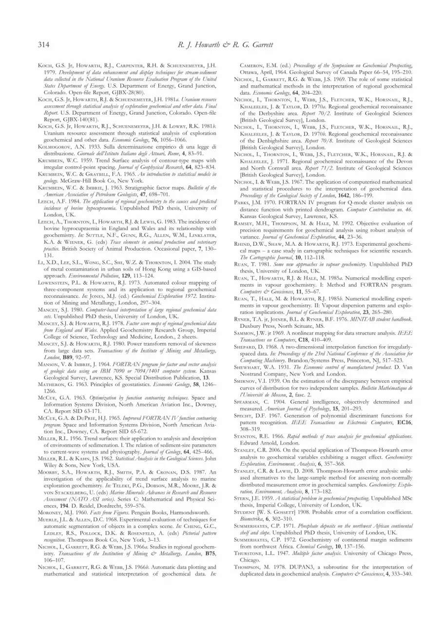
K, G.S. Jr, H, R.J., C, R.H. & S, J.H.1979. Development of data enhancement and display techniques for stream-sedimentdata collected in the National Uranium Resource Evaluation Program of the UnitedStates Department of Energy. U.S. Department of Energy, Grand Junction,Colorado. Open-file Report, GJBX-28(80).

K, G.S. Jr, H, R.J. & S, J.H. 1981a. Uranium resourceassessment through statistical analysis of exploration geochemical and other data. FinalReport. U.S. Department of Energy, Grand Junction, Colorado. Open-fileReport, GJBX-140(81).

K, G.S. Jr, H, R.J., S, J.H. & L, R.K. 1981b.Uranium resource assessment through statistical analysis of explorationgeochemical and other data. Economic Geology, 76, 1056–1066.

K, A.N. 1933. Sulla determinazione empirico di una legge didistribuzione. Giornale dell’Istituto Italiano degli Attuari, Rome, 4, 83–91.

K, W.C. 1959. Trend Surface analysis of contour-type maps withirregular control-point spacing. Journal of Geophysical Research, 64, 823–834.

K, W.C. & G, F.A. 1965. An introduction to statistical models ingeology. McGraw-Hill Book Co, New York.

K, W.C. & I, J. 1963. Stratigraphic factor maps. Bulletin of theAmerican Association of Petroleum Geologists, 47, 698–701.

L, A.F. 1984. The application of regional geochemistry to the causes and predictedincidence of bovine hypocupraemia. Unpublished PhD thesis, University ofLondon, UK.

L, A., T, I., H, R.J. & L, G. 1983. The incidence ofbovine hyprocupraemia in England and Wales and its relationship withgeochemistry. In: S, N.F., G, R.G., A, W.M., L,K.A. & W, G. (eds) Trace elements in animal production and veterinarypractice. British Society of Animal Production. Occasional paper, 7, 130–131.

L, X.D., L, S.L., W, S.C., S, W.Z. & T, I. 2004. The studyof metal contamination in urban soils of Hong Kong using a GIS-basedapproach. Environmental Pollution, 129, 113–124.

L, P.L. & H, R.J. 1973. Automated colour mapping ofthree-component systems and its application to regional geochemicalreconnaissance. In: J, M.J. (ed.) Geochemical Exploration 1972. Institu-tion of Mining and Metallurgy, London, 297–304.

M, S.J. 1980. Computer-based interpretation of large regional geochemical datasets. Unpublished PhD thesis, University of London, UK.

M, S.J. & H, R.J. 1978. Factor score maps of regional geochemical datafrom England and Wales. Applied Geochemistry Research Group, ImperialCollege of Science, Technology and Medicine, London., 2 sheets.

M, S.J. & H, R.J. 1980. Power transform removal of skewnessfrom large data sets. Transactions of the Institute of Mining and Metallurgy,London, B89, 92–97.

M, V. & I, J. 1964. FORTRAN program for factor and vector analysisof geologic data using an IBM 7090 or 7094/1401 computer system. KansasGeological Survey, Lawrence, KS. Special Distribution Publication, 13.

M, G. 1963. Principles of geostatistics. Economic Geology, 58, 1246–1266.

MC, G.A. 1963. Optimization by function contouring techniques. Space andInformation Systems Division, North American Aviation Inc., Downey,CA. Report SID 63-171.

MC, G.A. & DP, H.J. 1965. Improved FORTRAN IV function contouringprogram. Space and Information Systems Division, North American Avia-tion Inc., Downey, CA. Report SID 65-672.

M, R.L. 1956. Trend surfaces: their application to analysis and descriptionof environments of sedimenation. I. The relation of sediment-size parametersto current-wave systems and physiography. Journal of Geology, 64, 425–466.

M, R.L. & K, J.S. 1962. Statistical Analysis in the Geological Sciences. JohnWiley & Sons, New York, USA.

M, S.A., H, R.J., S, P.A. & C, D.S. 1987. Aninvestigation of the applicability of trend surface analysis to marineexploration geochemistry. In: T, P.G., D, M.R., M, J.R. & S, U. (eds) Marine Minerals: Advances in Research and ResourceAssessment (NATO ASI series). Series C: Mathematical and Physical Sci-ences, 194. D. Reidel, Dordrecht, 559–576.

M, M.J. 1960. Facts from Figures. Penguin Books, Harmondsworth.M, J.L. & A, D.C. 1968. Experimental evaluation of techniques for

automatic segmentation of objects in a complex scene. In: C, G.C.,L, R.S., P, D.K. & R, A. (eds) Pictorial patternrecognition. Thompson Book Co, New York, 3–13.

N, I., G, R.G. & W, J.S. 1966a. Studies in regional geochem-istry. Transactions of the Institution of Mining & Metallurgy, London, B75,106–107.

N, I., G, R.G. & W, J.S. 1966b. Automatic data plotting andmathematical and statistical interpretation of geochemical data. In:

C, E.M. (ed.) Proceedings of the Symposium on Geochemical Prospecting,Ottawa, April, 1964. Geological Survey of Canada Paper 66–54, 195–210.

N, I., G, R.G. & W, J.S. 1969. The role of some statisticaland mathematical methods in the interpretation of regional geochemicaldata. Economic Geology, 64, 204–220.

N, I., T, I., W, J.S., F, W.K., H, R.J.,K, J. & T, D. 1970a. Regional geochemical reconaissanceof the Derbyshire area. Report 70/2. Institute of Geological Sciences[British Geological Survey], London.

N, I., T, I., W, J.S., F, W.K., H, R.J.,K, J. & T, D. 1970b. Regional geochemical reconaissanceof the Denbighshire area. Report 70/8. Institute of Geological Sciences[British Geological Survey], London.

N, I., T, I., W, J.S., F, W.K., H, R.J. &K, J. 1971. Regional geochemical reconaissance of the Devonand North Cornwall area. Report 71/2. Institute of Geological Sciences[British Geological Survey], London.

N, I. & W, J.S. 1967. The application of computerised mathematicaland statistical procedures to the interpretation of geochemical data.Proceedings of the Geological Society of London, 1642, 186–199.

P, J.M. 1970. FORTRAN IV program for Q-mode cluster analysis ondistance function with printed dendrogram. Computer Contribution no. 46.Kansas Geological Survey, Lawrence, KS.

R, M.H., T, M. & H, M. 1992. Objective evaluation ofprecision requirements for geochemical analysis using robust analysis ofvariance. Journal of Geochemical Exploration, 44, 23–36.

R, D.W., S, M.A. & H, R.J. 1973. Experimental geochemi-cal maps – a case study in cartographic techniques for scientific research.The Cartographic Journal, 10, 112–118.

R, T. 1981. Some new approaches in vapour geochemistry. Unpublished PhDthesis, University of London, UK.

R, T., H, R.J. & H, M. 1985a. Numerical modelling experi-ments in vapour geochemistry. I: Method and FORTRAN program.Computers & Geosciences, 11, 55–67.

R, T., H, M. & H, R.J. 1985b. Numerical modelling experi-ments in vapour geochemistry. II: Vapour dispersion patterns and explo-ration implications. Journal of Geochemical Exploration, 23, 265–280.

R, T.A. jr, J, B.L. & R, B.F. 1976. MINITAB student handbook.Duxbury Press, North Scituate, MS.

S, J.W. jr 1969. A nonlinear mapping for data structure analysis. IEEE

Transactions on Computers, C18, 410–409.S, D. 1968. A two-dimensional interpolation function for irregularly-

spaced data. In: Proceedings of the 23rd National Conference of the Association for

Computing Machinery. Brandon/Systems Press, Princeton, NJ, 517–523.S, W.A. 1931. The Economic control of manufactured product. D. Van

Nostrand Company, New York and London.S, V.I. 1939. On the estimation of the discrepancy between empirical

curves of distribution for two independent samples. Bulletin Mathématique de

l’Université de Moscou, 2, fasc. 2.S, C. 1904. General intelligence, objectively determined and

measured. American Journal of Psychology, 15, 201–293.S, D.F. 1967. Generation of polynomial discriminant functions for

pattern recognition. IEEE Transactions on Electronic Computers, EC16,308–319.

S, R.E. 1966. Rapid methods of trace analysis for geochemical applications.Edward Arnold, London.

S, C.R. 2006. On the special application of Thompson-Howarth erroranalysis to geochemical variables exhibiting a nugget effect. Geochemistry:

Exploration, Environment, Analysis, 6, 357–368.S, C.R. & L, D. 2008. Thompson-Howarth error analysis: unbi-

ased alternatives to the large-sample method for assessing non-normallydistributed measurement error in geochemical samples. Geochemistry: Explo-

ration, Environment, Analysis, 8, 173–182.S, J.E. 1959. A statistical problem in geochemical prospecting. Unpublished MSc

thesis, Imperial College, University of London, UK.S [W. S. G] 1908. Probable error of a correlation coefficient.

Biometrika, 6, 302–310.S, C.P. 1971. Phosphate deposits on the northwest African continental

shelf and slope. Unpublished PhD thesis, University of London, UK.S, C.P. 1972. Geochemistry of continental margin sediments

from northwest Africa. Chemical Geology, 10, 137–156.T, L.L. 1947. Multiple factor analysis. University of Chicago Press,

Chicago.T, M. 1978. DUPAN3, a subroutine for the interpretation of

duplicated data in geochemical analysis. Computers & Geosciences, 4, 333–340.


T, M. 1981. Quality control in the laboratory. In: F, W.K.(ed.) Analytical methods in geochemical prospecting. Handbook of ExplorationGeochemistry, 1, 25–46.

T, M. 1982. Regression methods in the comparison of accuracy. TheAnalyst, 107, 1169–1180.

T, M. 1983. Control procedures in geochemical analysis. In:H, R.J. (ed.) Statistics and data analysis in geochemical prospecting.Handbook of Exploration Geochemistry, 2, 39–58.

T, M. 1988. Variation of precision with concentration in ananalytical system. The Analyst, 113, 1579–1587.

T, M. 2010. Analytical methodology in the Applied GeochemistryResearch Group (1950–1988) at the Imperial College of Science andTechnology, London. Geochemistry: Exploration, Environment, Analysis, 10,251–259.

T, M. & F, T. 1996. What exactly is fitness for purpose inanalytical measurement. The Analyst, 121, 275–278.

T, M. & H, R.J. 1973. The rapid estimation and control ofprecision by duplicate determinations. The Analyst, 98, 153–160.

T, M. & H, R.J. 1976. Duplicate analysis in geochemicalpractice. I. Theoretical approach and estimation of analytical reproducibil-ity. The Analyst, 101, 690–698.

T, M. & H, R.J. 1978. A new approach to the estimation ofanalytical precision. Journal of Geochemical Exploration, 9, 23–30.

T, M. & H, R.J. 1980. The frequency distribution ofanalytical error. The Analyst, 105, 1188–1195.

T, M., W, S.J. & W, S.J. 1979. Statistical appraisal ofinterference effects in the determination of trace elements by atomic-absorption spectrophotometry in applied geochemistry. The Analyst, 104,299–312.

T, I. 2010. Research in Applied Environmental Geochemistry, withparticular reference to Geochemistry and Health. Geochemistry: Exploration,Environment, Analysis, 10–3, 000–000.

T, C.R. 2003. Geochemical associations and the spatial distribution of metals inurban soils. Unpublished PhD thesis, University of London, UK.

T, C. & F, M.E. 2001. Investigating urban geochemistry usinggeocgaphical information systems. Science Progress, 84, 183–204.

T, J.S. 1967. The inorganic mineral potential of the sea-floor andproblems in its exploration. In: Proceedings of the British National Conference onthe Technology of the Sea and Seabed held at the Atomic Energy ResearchEstablishment, Harwell, April 5th, 6th and 7th, 1967; sponsored by the Ministry ofTechnology. United Kingdom Atomic Energy Authority (Research Group),Harwell, Didcot, Berks. Report AERE-R 5500. Her Majesty’s StationeryOffice, London. Paper SB16, 1–20.

T, E., D, A., R, M.H., R, M.S.,S, P., T, I., V, E. & V, K. 2000.

Spatially resolved hazard and exposure assessments: an example of lead insoil at Laviron, Greece. Environmental Research, A82, 33–45.

T-M, E.E. 2000. Human health risk assessment for contaminated land

in historical mining areas. Unpublished PhD thesis, University of London,UK.

T, J.W. 1977. Exploratory data analysis. Addison-Wesley, Reading, MS[preliminary edition printed for private circulation, 1970].

T, M.St.J. 1980. A comparative study of multiple regression techniques in

geochemistry. Unpublished MSc thesis, University of London, UK.T, M.St.J. 1986. Statistical analysis of geochemical data illustrated by reference to

the Dalradian of N.E. Scotland. Unpublished PhD. Thesis, University ofLondon, UK.

W, J.H. 1963. Hierarchical grouping to optimize an objective function.Journal of the American Statistical Association. 58, 236–244.

W, J.S. 1964. Geochemistry and life. New Scientist. 23, 504–507.W, J.S. & A, W.J. 1965. Regional geochemical reconnaissance

applied to some agricultural problems in Co. Limerick, Eire. Nature, 208,1056–1059.

W, J.S. & T, M. 1977. Analytical requirements in explorationgeochemistry. Pure and Applied Chemistry, 49, 1507–1518.

W, J.S., F, J., N, I. & T, J.S. 1964a. Regional geochemical

reconnaissance in the Namwala Concession area Zambia. To accompany theGeochemical Maps of the Namwala Concession Area published by theGeological Survey of Zambia in. 1964. Applied Geochemistry ResearchGroup, Imperial College of Science and Technology, London. TechnicalCommunication no. 47.

W, J.S., F, J. et al. 1964b. Regional geochemical maps of the Namwala

Concession area, Zambia based on a Reconnaissance Stream Sediment Survey.Geological Survey of Zambia, Zambia.

W, J.S., N, I., F, R., L, P.L. & H, R.J. 1973.Provisional Geochemical Atlas of Northern Ireland. Applied GeochemistryResearch Group, Imperial College of Science and Technology, London.Technical Communication, 60.

W, J.S., T, I., T, M., H, R.J. & L,P.L. 1978. The Wolfson Geochemical Atlas of England and Wales. ClarendonPress, Oxford and London.

W, E.H.T. 1959. Composition trends in granite: Modal variations andghost stratigraphy in part of the Donegal Granite, Eire. Journal of Geophysical

Research, 64, 835–848.W, E.H.T. 1963. A surface-fitting program suitable for testing geological models

which involve areally-distributed data. Office of Naval Research, GeographyBranch. Northwestern University, Evanston, Illinois. Technical Report No.2, ONR Task No. 389–135, Contract No. 1228(26).

Received 29 July 2008; revised typescript accepted 8 April 2009.


statistical analysis and data display at the geochemical prospecting research centre and applied...

Documents