Technical Article

Uncertainty Quantification in Computational Electromagnetics: The stochastic approach Abstract — Models in electromagnetism are more and more accurate. In some applications, the gap between the experience and the model comes from the deviation on input data of the model which are not perfectly known. The stochastic approach can be used to quantify the effect of these input data uncertainties on the outputs of the model. In this article, the application of such approach in computational electromagnetics is presented. The four steps development of the model, characterization and modeling of the input data variability, uncertainty quantification, postprocessing (sensitivity analysis) are described and illustrated by an example of electrical machine with uncertain dimensions.

I. INTRODUCTION

Applying a numerical method (FEM, FIT…) to solve the Maxwell equations leads to valuable tools for understanding and predicting the features of electromagnetic devices. With the progress in the fields of numerical analysis, CAD and postprocessor tools, it is now possible to represent and to mesh very complex geometries and also to take into account more realistic material behavior laws with non linearities, hysteresis….. Besides, computers have nowadays such capabilities that it is customary to solve problems with millions of unknowns. The modeling error due to the assumptions made to build the mathematical model (the set of equations) and the numerical errors due especially to the discretisation (by a Finite Element method for example) can be negligible. Consequently, in some applications, if a gap exists between the measurements, assuming them perfect, and the results given by the numerical model, it comes from deviations on input parameters which are not in the “real world” equal to their prescribed values. The origins of these deviations are numerous and are related to either a lack of knowledge (epistemic uncertainties) or uncontrolled variations (aleatoric uncertainties). For example, mechanical parts are manufactured with dimensional tolerances whereas some dimensions, such as air gaps in electric machines, are critical as they strongly influence performance. Besides uncertainties in material composition, the material characteristics which change with uncontrolled environmental factors (humidity, pressure, etc.) are also often unknown. Even if the environmental factors are perfectly known, in some situations, the behavior law parameters can’t be identified because measurements are not possible under the right experimental conditions. In practice, if the uncertainties on some parameters can’t be neglected, the normal process of increasing the precision of the deterministic model becomes futile. Models taking into account the uncertainties on the input parameters become then essential. Applications of such kind of models are numerous. For example, it can be very helpful to improve the accuracy of a model by orienting the measurement campaign. Indeed, the input parameters which have the most influence on the output variability can be identified [37]. Then, with new measurements, these most influential input parameters can be better characterized, and so less uncertain, improving the

accuracy the model. Reversely, it can avoid measurements campaign on input parameters which variability has almost no effect on the outputs. These models can be also useful to evaluate the impact of the variability introduced by a manufacturing process of an electrical machine on its performances [53]. The influence of the different stages such as assembling, punching, welding… can be compared. The most influential stages can be segregated and, then, can be modified or better controlled in order to reduce their impact on the performance variability of electrical machines [4]. From these models, tools can be derived to increase the robustness during the process of design. Since we are able to evaluate the effect of the variability of the input parameters on the output, the design can be oriented to meet the product specifications and also to be almost insensitive to the input parameter variabilities [51]. These models can be applied for example to determine the tolerances on the dimensions [49,50]. To take into account the uncertainties, several approaches are proposed in the literature. The first one is based on the worst case scenario (the uncertain input data are supposed to be bounded in intervals). The second one is based on the fuzzy logic. The last one is the stochastic approach where the uncertain input parameters are modeled by random variables or fields. This last approach is richer than the two previous ones in terms of information embedded by the stochastic model. However, this approach can require more data to represent the variability of the input parameters and also more numerical resources. Since the early 90’s, numerous researches in the field of engineering have addressed the development of stochastic models, mainly in mechanical and civil engineering [42,43][46]. In the field of computational electromagnetics, the development and the application of such models have started in the early 2000’s and know a growing interest in the community [1-3][6,7][22]. This technical article aims at giving an overview about the stochastic approach in computational electromagnetics It is mainly dedicated to static and quasi-static problems. In the first part, the four different steps to implement a stochastic model are briefly presented. Then, these four steps are described in detail and especially their numerical implementation. The example of an electrical machine with uncertain dimensions (introduced by the process of fabrication) is proposed to illustrate the stochastic approach.

II. STOCHASTIC APPROACH

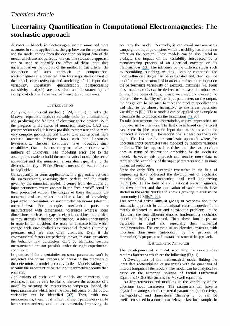
The development of a model accounting for uncertainties requires four steps which are the following (Fig. 1):

A-Development of the mathematical model linking the input data (deterministic or uncertain) with the quantities of interest (outputs of the model). The model can be analytical or based on the numerical solution of Partial Differential Equations (PDE) like such as the Maxwell equations.

B-Characterization and modeling of the variability of the uncertain input parameters. The parameters can have a physical meaning such that material parameters (conductivity, permeability..) and dimensions (diameter,…) or can be coefficients used in a non-linear behavior law for example. In

the stochastic approach, based on expertise and measurements, each uncertain parameter is modeled by a random variable.

C-Propagation of the variability of the input parameters through the model developed in the step A. This step enables to quantify the variability of the quantities of interest (outputs of the model).

D-Characterization of the uncertain outputs from the results obtained at the end of the step C. The statistics (mean, standard deviation, correlation between the outputs…) can be calculated. Global sensitivity of the outputs versus the inputs can be also analyzed. This sensitivity analysis enables to determine the most influential input parameters that influence the most the variability of the output parameters.

Geometry (θθθθ)

Behaviors law of materials (permeability,

conductivity….) (θθθθ)

Sources (voltages, flux…) (θθθθ)

Actual device

Quantities of interest(flux, magnetomotiveforce, electromotive

force…) (θθθθ)

Step A : construction of mathematical model of the physical process

Maxwell’s Equations+

Boundary conditions+

Behaviour laws

Step B : modelling of uncertaininput data with random fields or variables

Step C : propagating the uncertainties through the mathematical model

Step D : postprocessing

Fig. 1. Description of the four steps required to develop a model accounting

for uncertainties (Stochastic approach)

In the following, we will present in more details the steps A, B, C and D. To illustrate our approach, we will consider a model based on the solution of the magnetostatic equations using the Finite Element Method. However, most of the methods present in the following can be applied in Quasi Statics or Wave Propagation problems solved numerically by various methods (FIT, FD…).

III STEP A : DEVELOPMENT OF THE MODEL

We will consider an electromagnetic device which can be modeled by the magnetostatic equations on a domain D. The equations to be solved are:

curl H(x) = J(x) (1)

div B(x) = 0 (2)

with H the magnetic field, B the magnetic flux density and J the current density that is assumed to be known. In addition, boundary conditions on H and B are added. To solve the problem, the vector potential formulation can be used:

curl [ν(x) curlA (x)] = J(x) (3)

with A(x) the vector potential and ν(x) the reluctivity. To find an approximate solution of this equation, the Finite Element method can be used. We seek for an approximation A(x) of the vector potential in the edge element space such that:

( ) ∑=

=N

iii )x(ax

1

wA (4)

with N the number of Degrees of Freedom (DoF’s), wi(x) the edge shape functions and ai unknown real coefficients. By applying the Galerkin method to a weak form of (3):

[ ]NidxxxdxxxxD

iD

i ,)(w)(J)(curlw)(curlA)( 1∈∀=⋅ν ∫∫ , (5)

the coefficients ai can be obtained by solving the linear system of equations:

S A = F (6)

with S the stiffness matrix (NxN), F the source vector (Nx1) and A the vector of the coefficients ai. The coefficients sij of S and fi of F satisfy:

∫

∫

=

⋅ν=

Dii

Djiij

dx)x()x(f

dx)x()x()x(s

curlwJ

curlwcurlw

(7)

The model of the electromagnetic device is now available. From the solution (6), quantities of interest such as torque or flux can be determined in a postprocessing step. The solution (6) depends on the input parameters which are the shape of the boundary of D, the shapes of inner interfaces between different materials and the reluctivity. If the inputs of the model are subject to variability, the solution (4) will be also subject to variability. The stochastic approach enables to quantify this variability of the output.

STEP B: CHARACTERIZATION AND MODELING OF THE INPUT

DATA VARIABILITY

In the stochastic approach, the input data are modeled with random fields or random variables which pdf are identified from measurements and expertise. In this section, we will present first a general approach proposed in the literature to determine the pdf. We will illustrate this approach with an example related to the modeling of uncertainty on the geometry.

A. General consideration

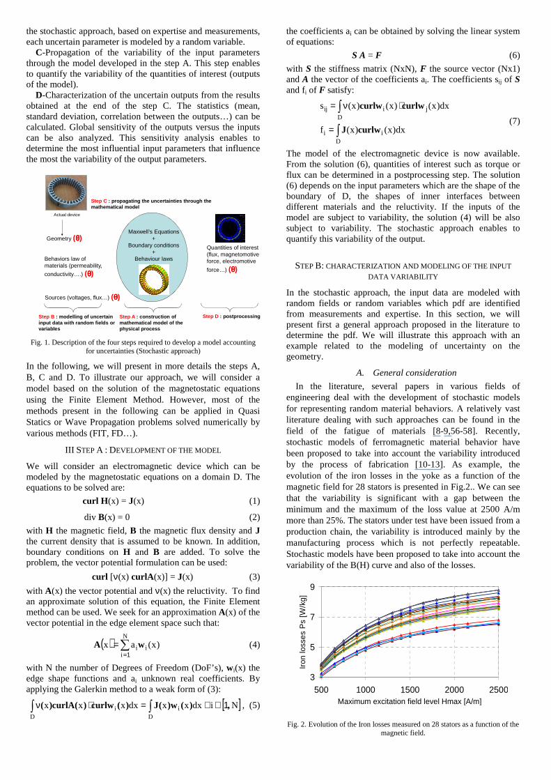
In the literature, several papers in various fields of engineering deal with the development of stochastic models for representing random material behaviors. A relatively vast literature dealing with such approaches can be found in the field of the fatigue of materials [8-9,56-58]. Recently, stochastic models of ferromagnetic material behavior have been proposed to take into account the variability introduced by the process of fabrication [10-13]. As example, the evolution of the iron losses in the yoke as a function of the magnetic field for 28 stators is presented in Fig.2.. We can see that the variability is significant with a gap between the minimum and the maximum of the loss value at 2500 A/m more than 25%. The stators under test have been issued from a production chain, the variability is introduced mainly by the manufacturing process which is not perfectly repeatable. Stochastic models have been proposed to take into account the variability of the B(H) curve and also of the losses.

3

5

7

9

500 1000 1500 2000 2500Maximum excitation field level Hmax [A/m]

Iron

loss

es P

s [W

/kg]

Fig. 2. Evolution of the Iron losses measured on 28 stators as a function of the magnetic field.

In all these works, the approach is almost the same and is

decomposed in 4 main steps which are the following:

• Model selection: the first step consists in comparing existing deterministic models which are suitable to describe correctly the phenomenon (behavior law, dimension)[11][14]. This can be done based on available experimental data. The parameters of the different models are identified and the model which fits the better the experimental data is chosen. For example, to represent a B(H) curve, several mathematical expressions are proposed in the literature. Let consider different expressions B=fi(H,pi) with pi a vector of real parameters and a collection of experimental points (Hexp

k,Bexp

k)1≤k≤L measured on a sample. The parameters pi are identified using the least square method:

( )[ ]∑=

−=L

ki

expki

expki ,HfBR

1

2p (8)

The “best” model will be the one which yields the lowest criterion Ri.

• Stochastic modeling of input parameters: with the selected model, the next step consists in splitting the data into two subsets (chosen randomly): a Modeling Subset (MS) that is used to develop the probabilistic model, and a Test Subset (TS) to test the prediction of the model. Let consider a MS of R experimental B(H) curves, by minimizing (8) using the chosen model B=f(H,p), we determine R realizations of the parameter vector p. This sample of size R is then used to determine the probability distribution functions (pdf) of the random vector p(θ). This can be achieved in the context of a parametric approach for which a classical pdf (uniform, Gaussian, lognormal…) can be tested according to the Kolmogorov Smirnov (KS) statistical test. The test enables to select the most suitable marginal distribution for each parameter of p(θ).

• Correlation analysis: once the marginal distribution of each parameter of the model is identified, the next step deals with the analysis of the inter-dependence of the input parameters. If they are all distributed according to a Gaussian distribution, and only in this case, one can quantify the intensity of the dependency using the Pearson coefficient calculated from the experimental data (MS). If it is not the case, it may be useful to identify the intensity of this dependence using the rank correlation method [3]. At the end of these three steps, a stochastic model is then available. Considering our previous example, the stochastic model can be written in the form B(θ)=f(H,p(θ)).

• Validation of the model: the validation of the model consists in implementing Monte Carlo Simulation Method (MCSM) and applying the two samples KS test to check whether our stochastic model represents “correctly” the phenomenon. The sample generated by the MCSM is compared either with the MS data (to check the adequacy of the model with the data used for the identification) or with the TS data (to analyze the capability of prediction of the model). The correlation structure between the parameters has also to be taken into account in the MCSM. When all the parameters are Gaussian distributed, one can define a Multivariate Gaussian Distribution (MGD) to account for the marginal distribution and the correlation between the parameters. If it is not the case, the Iman and Conover method may

be implemented, and aims at approximating the desired rank correlation between the input parameters, when each marginal distribution remains intact [3].

An example of application of the previous methodology is given in [11] to develop stochastic models to describe the random behavior of soft magnetic electrical steels. To apply this methodology, experimental data sample should be of large size. In practice, experimental data are not so numerous because engineers don’t need a large sample of experimental data to deal with deterministic models. To compensate this lack of information, expertise and additional assumptions (on the dependency between the random parameters) are required to develop the stochastic model. Moreover, models are not necessarily available to describe the random phenomenon and need to be developed. In the following section, we will give an example to illustrate this case.

B. Example

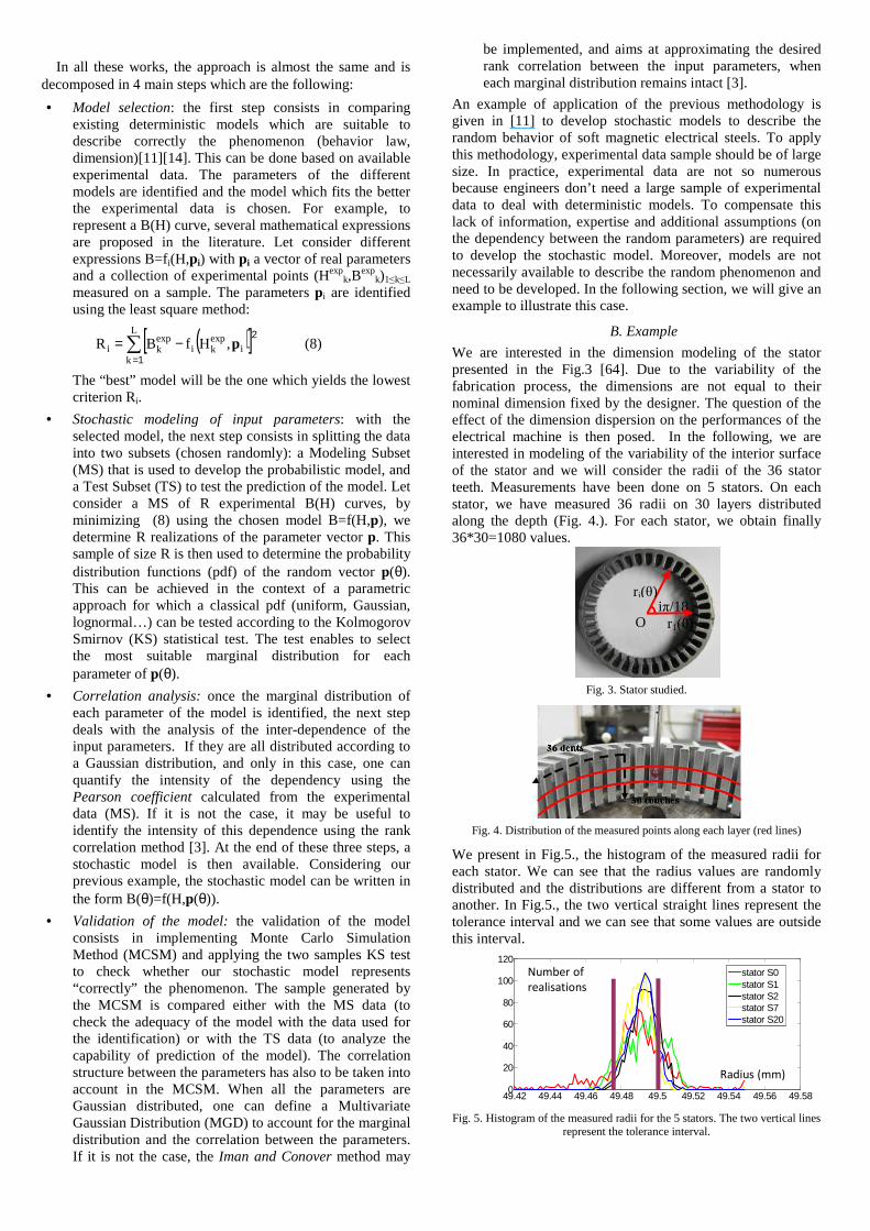
We are interested in the dimension modeling of the stator presented in the Fig.3 [64]. Due to the variability of the fabrication process, the dimensions are not equal to their nominal dimension fixed by the designer. The question of the effect of the dimension dispersion on the performances of the electrical machine is then posed. In the following, we are interested in modeling of the variability of the interior surface of the stator and we will consider the radii of the 36 stator teeth. Measurements have been done on 5 stators. On each stator, we have measured 36 radii on 30 layers distributed along the depth (Fig. 4.). For each stator, we obtain finally 36*30=1080 values.

Fig. 3. Stator studied.

Fig. 4. Distribution of the measured points along each layer (red lines)

We present in Fig.5., the histogram of the measured radii for each stator. We can see that the radius values are randomly distributed and the distributions are different from a stator to another. In Fig.5., the two vertical straight lines represent the tolerance interval and we can see that some values are outside this interval.

49.42 49.44 49.46 49.48 49.5 49.52 49.54 49.56 49.580

20

40

60

80

100

120stator S0stator S1stator S2stator S7stator S20

Radius (mm)

Number of

realisations

Fig. 5. Histogram of the measured radii for the 5 stators. The two vertical lines

represent the tolerance interval.

r1(θ)

ri(θ)

O iπ/18

The interior surface of the stator is represented by 1080 radius values. A model with 1080 random variables is suited to represent the variability of the interior surface of the stator. However, this probabilistic model, with a very high number of random variables, may cause excessive computation time during the step C of propagation of uncertainties. We seek for a model with a reduced number of random variables. The idea is then to express the 1080 random radii with a limited number of random variables. A model reduction approach based on a Principal Component Analysis (PCA) [45] can be used to approximate these 1080 random variables in terms of N mutually uncorrelated random variables (N can be fixed arbitrarily but lower than 1080). This method is optimal in the L2 sense. However, with this approach, it can be difficult to link the N random variables obtained with PCA to the actual measured dimensions. This link with the actual dimensions is necessary since it enables to establish a relationship with the steps of the fabrication process which are the sources of uncertainty. A more "physical" representation for the 30 layers using a Discrete Fourier Transform (DFT) has been chosen and the radius of the tooth i (1≤i≤36) on the layer j (1≤j≤30) can be written under the form:

( ) ( ) ( ) ( )∑=

θϕ+πθτ+θτ+=θn

kkjkjjij

ikcosRr

101 18

(9)

With R1 the nominal radius of the teeth, τ0j(θ), αkj(θ) and βkj(θ) random coefficients to determine and n the total number of harmonics equal in our case to 17. To reduce the number of random variables, we select the random variables τkj(θ) and ϕkj(θ) corresponding to the harmonic ranks k which contribute the most to the variability. To select these harmonics, we consider rij

m(θ) the truncated expression of rij(θ) up to the order m (1≤m≤n) and the random variable y(m,θ):

( )( ) ( )[ ]

( )[ ]∑∑

∑∑

= =

= =

−θ

θ−θ−=θ

30

1

36

1

21

30

1

36

1

2

1

j iij

j i

mijij

Rr

rr

,my (10)

The random variable y(m,θ) lies in the interval [0,1]. For a given realization θ (a stator), the closer to 1 y(m,θ) is, the better the approximation rij

m(θ) of rij(θ). From the measurements made on the five stators, we have five realizations of each random variables rij(θ) which enables to determine five realizations rij

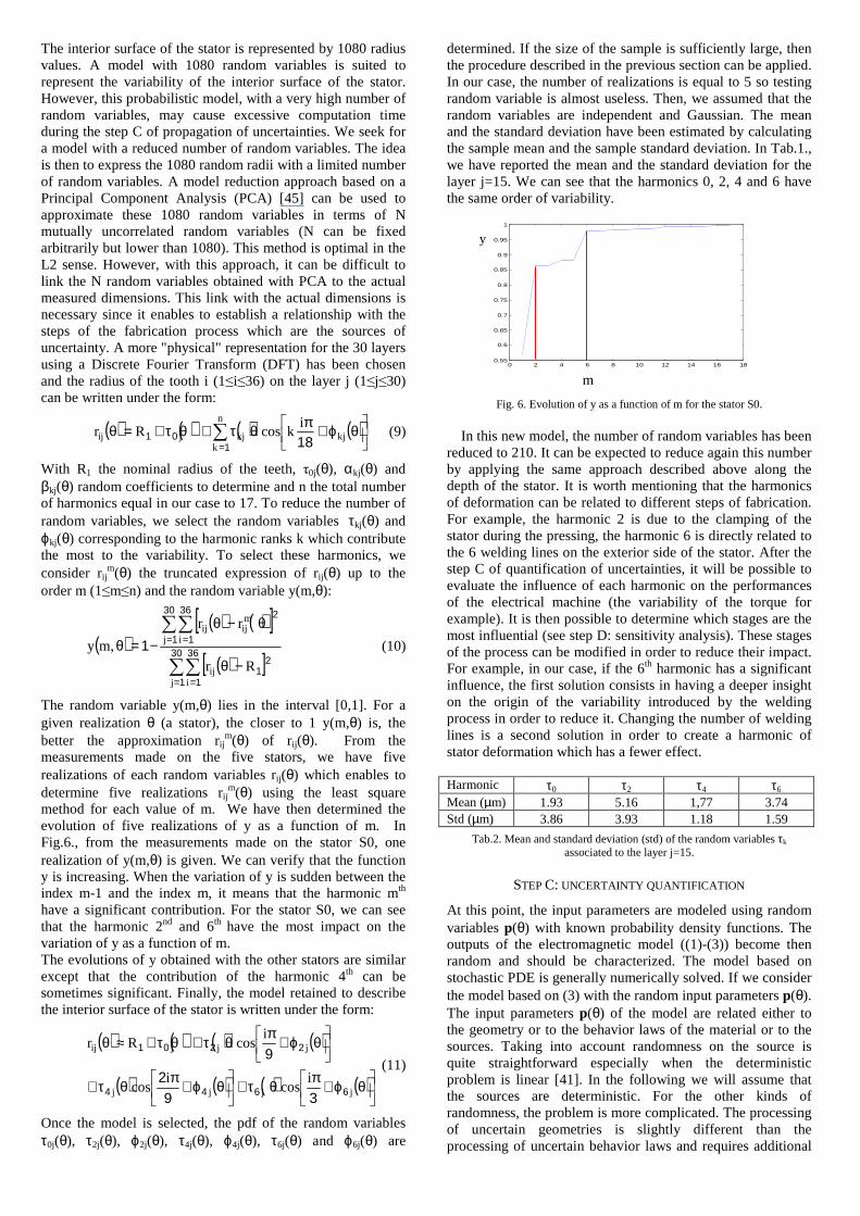
m(θ) using the least square method for each value of m. We have then determined the evolution of five realizations of y as a function of m. In Fig.6., from the measurements made on the stator S0, one realization of y(m,θ) is given. We can verify that the function y is increasing. When the variation of y is sudden between the index m-1 and the index m, it means that the harmonic mth have a significant contribution. For the stator S0, we can see that the harmonic 2nd and 6th have the most impact on the variation of y as a function of m. The evolutions of y obtained with the other stators are similar except that the contribution of the harmonic 4th can be sometimes significant. Finally, the model retained to describe the interior surface of the stator is written under the form:

( ) ( ) ( ) ( )

( ) ( ) ( ) ( )

θϕ+πθτ+

θϕ+πθτ+

θϕ+πθτ+θτ+≈θ

jjjj

jjjij

icos

icos

icosRr

6644

2201

392

9 (11)

Once the model is selected, the pdf of the random variables τ0j(θ), τ2j(θ), ϕ2j(θ), τ4j(θ), ϕ4j(θ), τ6j(θ) and ϕ6j(θ) are

determined. If the size of the sample is sufficiently large, then the procedure described in the previous section can be applied. In our case, the number of realizations is equal to 5 so testing random variable is almost useless. Then, we assumed that the random variables are independent and Gaussian. The mean and the standard deviation have been estimated by calculating the sample mean and the sample standard deviation. In Tab.1., we have reported the mean and the standard deviation for the layer j=15. We can see that the harmonics 0, 2, 4 and 6 have the same order of variability.

Fig. 6. Evolution of y as a function of m for the stator S0.

In this new model, the number of random variables has been reduced to 210. It can be expected to reduce again this number by applying the same approach described above along the depth of the stator. It is worth mentioning that the harmonics of deformation can be related to different steps of fabrication. For example, the harmonic 2 is due to the clamping of the stator during the pressing, the harmonic 6 is directly related to the 6 welding lines on the exterior side of the stator. After the step C of quantification of uncertainties, it will be possible to evaluate the influence of each harmonic on the performances of the electrical machine (the variability of the torque for example). It is then possible to determine which stages are the most influential (see step D: sensitivity analysis). These stages of the process can be modified in order to reduce their impact. For example, in our case, if the 6th harmonic has a significant influence, the first solution consists in having a deeper insight on the origin of the variability introduced by the welding process in order to reduce it. Changing the number of welding lines is a second solution in order to create a harmonic of stator deformation which has a fewer effect. Harmonic τ0 τ2 τ4 τ6 Mean (µm) 1.93 5.16 1,77 3.74 Std (µm) 3.86 3.93 1.18 1.59

Tab.2. Mean and standard deviation (std) of the random variables τk associated to the layer j=15.

STEP C: UNCERTAINTY QUANTIFICATION

At this point, the input parameters are modeled using random variables p(θ) with known probability density functions. The outputs of the electromagnetic model ((1)-(3)) become then random and should be characterized. The model based on stochastic PDE is generally numerically solved. If we consider the model based on (3) with the random input parameters p(θ). The input parameters p(θ) of the model are related either to the geometry or to the behavior laws of the material or to the sources. Taking into account randomness on the source is quite straightforward especially when the deterministic problem is linear [41]. In the following we will assume that the sources are deterministic. For the other kinds of randomness, the problem is more complicated. The processing of uncertain geometries is slightly different than the processing of uncertain behavior laws and requires additional

0 2 4 6 8 10 12 14 16 180.55

0.6

0.65

0.7

0.75

0.8

0.85

0.9

0.95

1

x=order of fourier series

y=co

varia

nce

fact

or

covraince factor of S01

y=1-Reisudal2/Error2

m

y

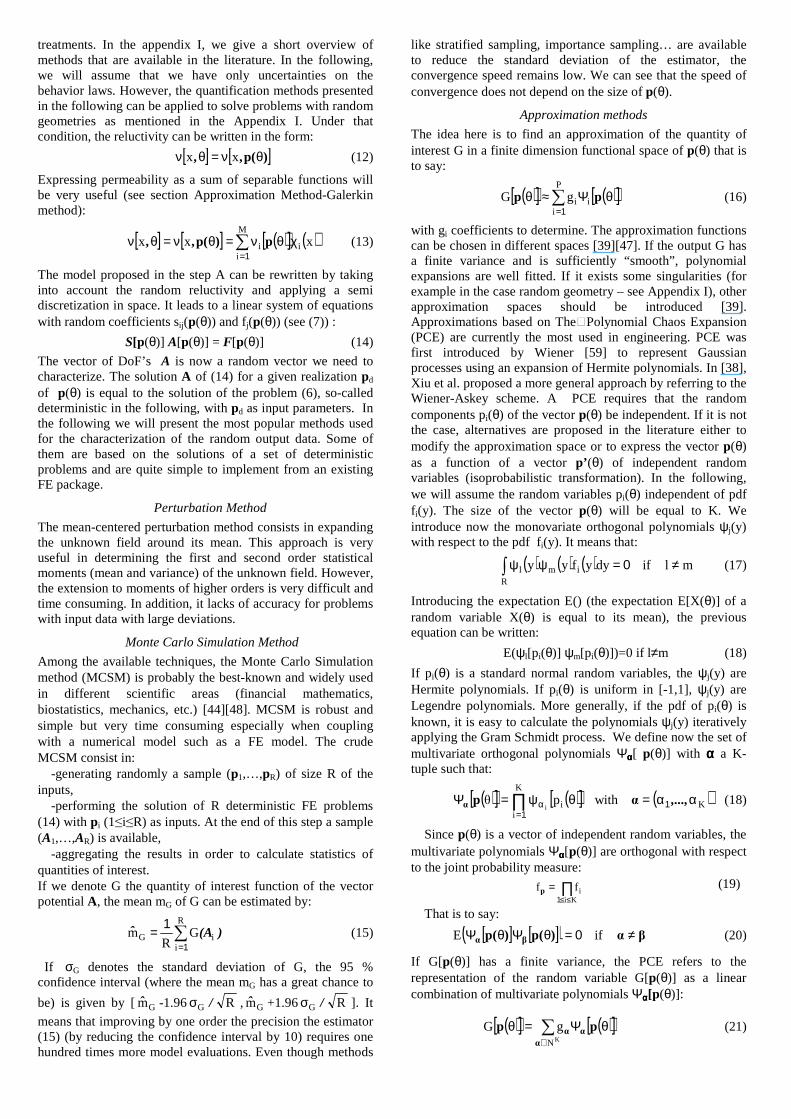
treatments. In the appendix I, we give a short overview of methods that are available in the literature. In the following, we will assume that we have only uncertainties on the behavior laws. However, the quantification methods presented in the following can be applied to solve problems with random geometries as mentioned in the Appendix I. Under that condition, the reluctivity can be written in the form:

[ ] [ ])(p,, θν=θν xx (12)

Expressing permeability as a sum of separable functions will be very useful (see section Approximation Method-Galerkin method):

[ ] [ ] ( )[ ] ( )∑=

χθν=θν=θνM

iii xxx

1

p)(p,, (13)

The model proposed in the step A can be rewritten by taking into account the random reluctivity and applying a semi discretization in space. It leads to a linear system of equations with random coefficients sij(p(θ)) and fj(p(θ)) (see (7)) :

S[p(θ)] A[p(θ)] = F[p(θ)] (14)

The vector of DoF’s A is now a random vector we need to characterize. The solution A of (14) for a given realization pd of p(θ) is equal to the solution of the problem (6), so-called deterministic in the following, with pd as input parameters. In the following we will present the most popular methods used for the characterization of the random output data. Some of them are based on the solutions of a set of deterministic problems and are quite simple to implement from an existing FE package.

Perturbation Method

The mean-centered perturbation method consists in expanding the unknown field around its mean. This approach is very useful in determining the first and second order statistical moments (mean and variance) of the unknown field. However, the extension to moments of higher orders is very difficult and time consuming. In addition, it lacks of accuracy for problems with input data with large deviations.

Monte Carlo Simulation Method

Among the available techniques, the Monte Carlo Simulation method (MCSM) is probably the best-known and widely used in different scientific areas (financial mathematics, biostatistics, mechanics, etc.) [44][48]. MCSM is robust and simple but very time consuming especially when coupling with a numerical model such as a FE model. The crude MCSM consist in:

-generating randomly a sample (p1,…,pR) of size R of the inputs,

-performing the solution of R deterministic FE problems (14) with pi (1≤i≤R) as inputs. At the end of this step a sample (A1,…,AR) is available,

-aggregating the results in order to calculate statistics of quantities of interest. If we denote G the quantity of interest function of the vector potential A, the mean mG of G can be estimated by:

∑=

=R

iiG G

Rm

1

1)(Aˆ (15)

If σG denotes the standard deviation of G, the 95 % confidence interval (where the mean mG has a great chance to

be) is given by [ Gm̂ -1.96 RG /σ , Gm̂ +1.96 RG /σ ]. It

means that improving by one order the precision the estimator (15) (by reducing the confidence interval by 10) requires one hundred times more model evaluations. Even though methods

like stratified sampling, importance sampling… are available to reduce the standard deviation of the estimator, the convergence speed remains low. We can see that the speed of convergence does not depend on the size of p(θ).

Approximation methods

The idea here is to find an approximation of the quantity of interest G in a finite dimension functional space of p(θ) that is to say:

( )[ ] ( )[ ]∑=

θΨ≈θP

iiigG

1

pp (16)

with gi coefficients to determine. The approximation functions can be chosen in different spaces [39][47]. If the output G has a finite variance and is sufficiently “smooth”, polynomial expansions are well fitted. If it exists some singularities (for example in the case random geometry – see Appendix I), other approximation spaces should be introduced [39]. Approximations based on ThePolynomial Chaos Expansion (PCE) are currently the most used in engineering. PCE was first introduced by Wiener [59] to represent Gaussian processes using an expansion of Hermite polynomials. In [38], Xiu et al. proposed a more general approach by referring to the Wiener-Askey scheme. A PCE requires that the random components pi(θ) of the vector p(θ) be independent. If it is not the case, alternatives are proposed in the literature either to modify the approximation space or to express the vector p(θ) as a function of a vector p’ (θ) of independent random variables (isoprobabilistic transformation). In the following, we will assume the random variables pi(θ) independent of pdf f i(y). The size of the vector p(θ) will be equal to K. We introduce now the monovariate orthogonal polynomials ψj(y) with respect to the pdf f i(y). It means that:

( ) ( ) ( )∫ ≠=ψψR

iml mlifdyyfyy 0 (17)

Introducing the expectation E() (the expectation E[X(θ)] of a random variable X(θ) is equal to its mean), the previous equation can be written:

E(ψl[pi(θ)] ψm[pi(θ)])=0 if l≠m (18)

If pi(θ) is a standard normal random variables, the ψj(y) are Hermite polynomials. If pi(θ) is uniform in [-1,1], ψj(y) are Legendre polynomials. More generally, if the pdf of pi(θ) is known, it is easy to calculate the polynomials ψj(y) iteratively applying the Gram Schmidt process. We define now the set of multivariate orthogonal polynomials Ψαααα[ p(θ)] with αααα a K-tuple such that:

( )[ ] ( )[ ] ( )K

K

ii withpθ

iαα=θψ=Ψ ∏

=α ,...,1

1

αpα (18)

Since p(θ) is a vector of independent random variables, the multivariate polynomials Ψαααα[p(θ)] are orthogonal with respect to the joint probability measure:

∏≤≤

=Ki

iff1

p (19)

That is to say:

[ ] [ ]( ) βα)(p)(p βα ≠=θΨθΨ ifE 0 (20)

If G[p(θ)] has a finite variance, the PCE refers to the representation of the random variable G[p(θ)] as a linear combination of multivariate polynomials Ψαααα[p(θ)]:

( )[ ] ( )[ ]∑∈

θΨ=θKN

gGα

αα pp (21)

In practice, the expansion (21) is truncated up to the polynomials of order p. If we denote by ZP

K the space of the K-tuples αααα which satisfy:

pi

K

i

≤α∑=1

(22)

The total number of polynomials in the truncated PCE is equal to:

K!p!

p)!(KP

+= (23)

Later, we denote by CPK the space of multivariate polynomials

Ψαααα[p(θ)] such that αααα∈ZPK. In Tab.3, we have reported the

dimension P of the space of approximation CPK as a function

of the polynomial order p and the number of input random variables K. We can see that P increases exponentially with the dimension which is usually so-called the “curse of dimensionality”. p=1 p=2 p=3 p=4 K=2 3 6 10 15 K=5 6 21 56 126 K=10 11 66 286 1001

Tab.3. Example of the dimension P of the approximation space CPK as a function of the polynomial order p and the number of random inputs K.

In the following, to simplify the notation, the multivariate polynomials Ψαααα[p(θ)] will be indexed by an integer i (1≤i≤P) instead of the K-tuple αααα. The function G[p(θ)] is approximated by a truncated expansion given by (16) of orthogonal multivariate polynomials defined by (18). After applying the semi discretisation in space, the coefficients ai(θ) of the vector A(θ) are random (see (14)). Each ai(θ) is approximated using a truncated PCE (16). Finally, the vector potential A[x,p(θ)] is approximated by the expression:

( )[ ] ( )[ ]∑∑= =

θΨ=θN

i

P

jijij (x)ax

1 1

wppA , (24)

The number of coefficients aij is equal to NxP. In a postprocessing step, quantities of interest (energy, flux,…) can be also expressed using (16). Several methods are available in the literature to determine these coefficients like the collocation method, the regression method, the projection method, the Galerkin method….. Approximation methods have been already applied in computational electromagnetics to study EEG Source Analysis [55], Eddy Current in human body [54], Eddy Current Non Destructive Testing [15,16], Accelerator Cavities [1], Dosimetry [7]….In the following we will present the projection method and the Galerkin method.

Projection method

Since the polynomials Ψj[p(θ)] are orthogonal (see (20), the coefficients aij satisfy:

( )[ ] ( )[ ]( )( )[ ]( )

( ) ( ) ( )( ) ( )

( ) ( ) ( ) ( )( ) ( ) ( )∫

∫

∫

∫

Ψ

Ψ=

Ψ

Ψ=

θΨ

θΨθ=

K

K

K

K

R KKKKj

R KKKKjKi

R j

R ji

j

jiij

dpdppfpfpp

dpdppfpfppppa

df

dfa

E

aEa

.......,...,

.......,...,,...,

1112

1

11111

22 ppp

pppp

p

pp

p

p

(24)

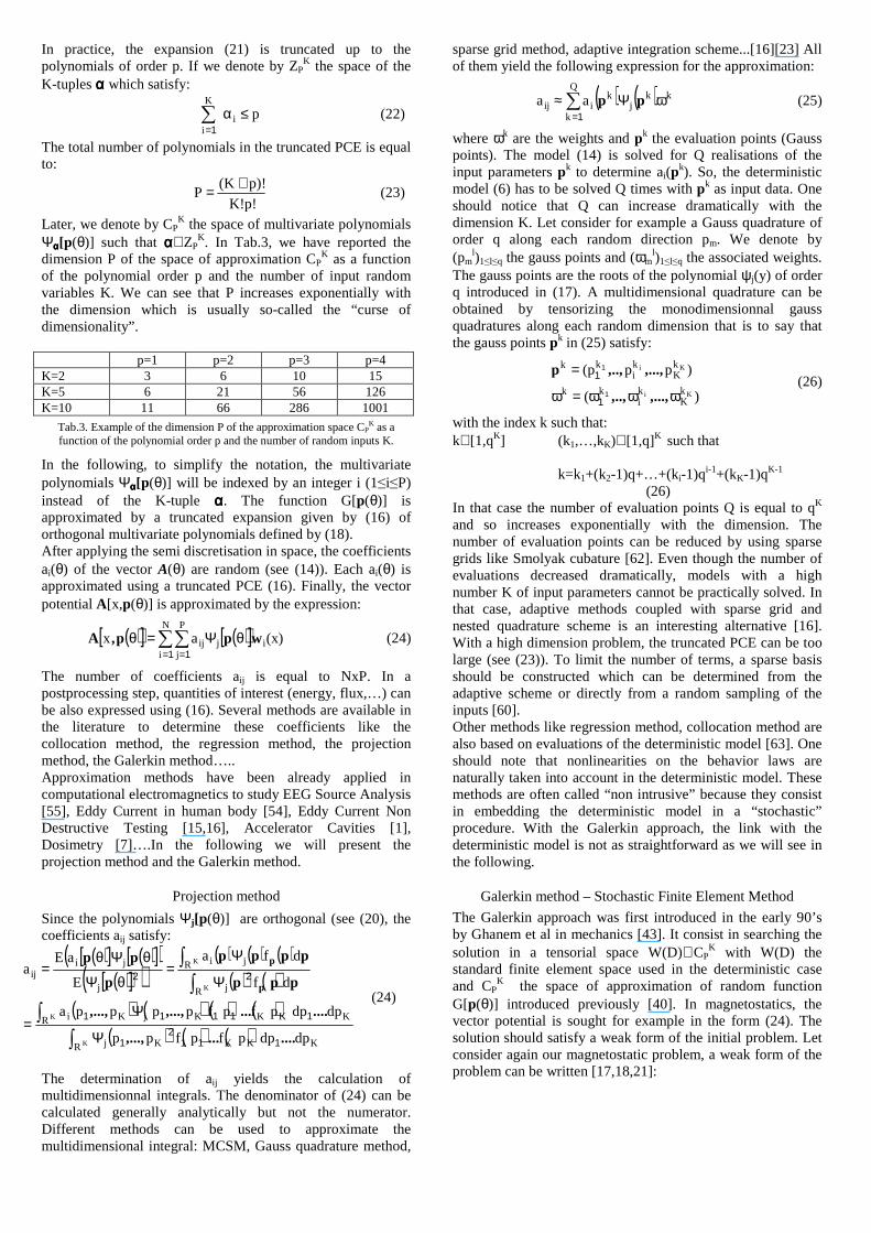
The determination of aij yields the calculation of multidimensionnal integrals. The denominator of (24) can be calculated generally analytically but not the numerator. Different methods can be used to approximate the multidimensional integral: MCSM, Gauss quadrature method,

sparse grid method, adaptive integration scheme...[16][23] All of them yield the following expression for the approximation:

( ) ( )∑=

ωΨ≈Q

k

kkj

kiij aa

1

pp (25)

where ωk are the weights and pk the evaluation points (Gauss points). The model (14) is solved for Q realisations of the input parameters pk to determine ai(p

k). So, the deterministic model (6) has to be solved Q times with pk as input data. One should notice that Q can increase dramatically with the dimension K. Let consider for example a Gauss quadrature of order q along each random direction pm. We denote by (pm

l)1≤l≤q the gauss points and (ωml)1≤l≤q the associated weights.

The gauss points are the roots of the polynomial ψj(y) of order q introduced in (17). A multidimensional quadrature can be obtained by tensorizing the monodimensionnal gauss quadratures along each random dimension that is to say that the gauss points pk in (25) satisfy:

)(

)pp(p

Ki

Ki

kK

ki

kk

kK

ki

kk

ωωω=ω

=

,...,,..,

,...,,..,

1

1

1

1p (26)

with the index k such that: k∈[1,qK] (k1,…,kK)∈[1,q]K such that

k=k1+(k2-1)q+…+(ki-1)qi-1+(kK-1)qK-1 (26)

In that case the number of evaluation points Q is equal to qK and so increases exponentially with the dimension. The number of evaluation points can be reduced by using sparse grids like Smolyak cubature [62]. Even though the number of evaluations decreased dramatically, models with a high number K of input parameters cannot be practically solved. In that case, adaptive methods coupled with sparse grid and nested quadrature scheme is an interesting alternative [16]. With a high dimension problem, the truncated PCE can be too large (see (23)). To limit the number of terms, a sparse basis should be constructed which can be determined from the adaptive scheme or directly from a random sampling of the inputs [60]. Other methods like regression method, collocation method are also based on evaluations of the deterministic model [63]. One should note that nonlinearities on the behavior laws are naturally taken into account in the deterministic model. These methods are often called “non intrusive” because they consist in embedding the deterministic model in a “stochastic” procedure. With the Galerkin approach, the link with the deterministic model is not as straightforward as we will see in the following.

Galerkin method – Stochastic Finite Element Method

The Galerkin approach was first introduced in the early 90’s by Ghanem et al in mechanics [43]. It consist in searching the solution in a tensorial space W(D)⊗CP

K with W(D) the standard finite element space used in the deterministic case and CP

K the space of approximation of random function G[p(θ)] introduced previously [40]. In magnetostatics, the vector potential is sought for example in the form (24). The solution should satisfy a weak form of the initial problem. Let consider again our magnetostatic problem, a weak form of the problem can be written [17,18,21]:

( )[ ] ( )[ ] ( ) ( )[ ]

( )[ ] ( ) ( )[ ] ( ) [ ] [ ]PxNjidxxxE

dxxxxE

Dji

Dji

,,,,

,,

11∈∀

θΨθ

=

θΨθνθ

∫

∫

pwpJ

pcurlwppcurlA

(27)

The NxP test functions wi(x)Ψj[p(θ)] belong to the space of approximation W(D)⊗CP

K. Replacing A[x,p(θ)] by its expression (24), we get the following system to solve:

Ss As = Fs (28)

With As the 1x (NxP) vector of (ask)1≤k≤NP with: as

k=aij with k=i+(j-1)N with (i,j)∈[1,N]x[1,P], Fs the 1x(NxP) vector with the coefficients (fs

k)1≤k≤NP such that:

( ) [ ] [ ]

( )[ ] ( ) ( )[ ]

θΨθ=

∈−+=∀

∫D

jisk dxxxEf

PxNji)N(jikk

pwpJ ,

,,, 111

and AS the matrix with the coefficients (alm)1≤l≤NP, 1≤m≤NP such that:

( ) [ ] [ ]( ) [ ] [ ]

( )[ ] ( )[ ] ( ) ( )[ ] ( )

θνθΨθΨ=

∈−+=∀∈−+=∀

∫D

iijjskl dxxxxEa

PxNji1)N(jill

PxNji1)N(jikk

curlwpcurlwpp ,

,,','''

,,,

''

11

11

The size of the product NP can be extremely large preventing the storage of the matrix As and so the resolution of the problem. If the reluctivity can be written as a sum of separable functions (13), the system can be rewritten taking advantage of the kronecker product. This representation of the reluctivity as a sum of separable functions can be obtained either during the process of modeling of the input data (step B) by imposing this representation or by applying a model reduction technique (Karuhnen-Loeve expansion for example). Considering the expression (13) for the reluctivity, the matrix As can be written in the form [19]:

( )[ ] ( )[ ] ( )[ ]( ) [ ]( ) ( ) ( ) [ ]∫

∑

∈χ=

∈θνθΨθΨ=

⊗==

D

2lim

ilm

2iml

ilm

M

i

N1,m)(l,withdxxxxd

P1,m)(l,withEc

curlwcurlw

ppp

1iis DCA

(29)

The memory space requires can be significantly reduces by storing only the 2M matrices Ci and Di. One can also notice that the matrices Di can be easily extracted from a standard magnetostatic finite element code. Indeed, these matrices are equal to the stiffness matrices of deterministic problems where the reluctivity is equal to χi(x). The matrices Ci can be determined by a standalone external procedure. Indeed, if it is not possible to calculate analytically, the terms ci

lm can be estimated by a MCSM or approximated by a quadrature method (see (25)). It should be mentioned that the calculation can be highly sped up by splitting νi[p(θ)] in the PCE because the coefficient cilm can be expressed as a linear combination of the terms djlm=[E(Ψj[p(θ)]Ψl[p(θ)]Ψm[p(θ)])] with 1≤j≤Pin (Pin is the polynomial number of the truncated PCE of νi[p(θ)]). The terms djlm can be calculated exactly either analytically or using a Gauss quadrature. The matrices Dk of the coefficients dk

lm are generally sparse. To save memory, the matrices Cj can be expressed in function of the matrices Dk which are the only one stored. The determination of the matrix As does not require a high modification of the deterministic code and so

the “intrusivity” of the Galerkin approach can be highly reduced using expression based on separable functions for the reluctivity. This approach can be extended in the quasistatic case [13]. Dedicated solvers can be employed to solve the equation (28) by taking advantage the expression (29) based on Kronecker products. Non linearities can be taken into account in the Galerkin approach [5], it requires some additional developments and it is not so straightforward as it is with the projection method or the sampling method. We should mention that the Galerkin method, for given approximation spaces, minimizes the error of approximation in the “L2” sense which is not the case with other approximation method based on the evaluations of the deterministic model (projection method, collocation method…). However, when double orthogonal polynomial expansion is used, the collocation and the Galerkin methods are equivalent [18].

Error estimation

At the end of the step C, an approximate of the exact solution is available. The error of approximation depends on the choice of the approximation basis. In our magnetostatic example, the error is function of:

-the mesh of the domain D, -the order p of truncation of the PCE, -the method (Galerkin, Projection…).

The error should be estimated to evaluate the quality of the solution and if desired to improve it by adaption of the approximation spaces by remeshing the domain D or by increasing the order of the truncated PCE. A-priori and a-posteriori error estimators have been proposed in the literature [30-33][47][52].

STEP D : POSTPROCESSING

General context

At the end of the step C, the available results depend on the method used to solve the problem:

-the perturbation method will give information on the mean and the standard deviation of the quantities of interest,

-the MCSM enables to estimate any statistical moment, pdf, probability of failure…

-the approximation methods yield a surrogate model of the quantity of interest that is expressed in a finite dimension space (see (16)) [20]. From this expression, it is possible to approximate either analytically or numerically any statistical moments, pdf… if the latter don’t have an analytical expression, a numerical determination is very fast because only a polynomial expressions have to be handled. Besides statistical information related to the quantities of interest, it is also often interesting to evaluate the influence of the input parameters p on the output G(p). In the deterministic case, the sensitivity is usually determined “locally” by calculating the partial derivatives ∂G/∂pi

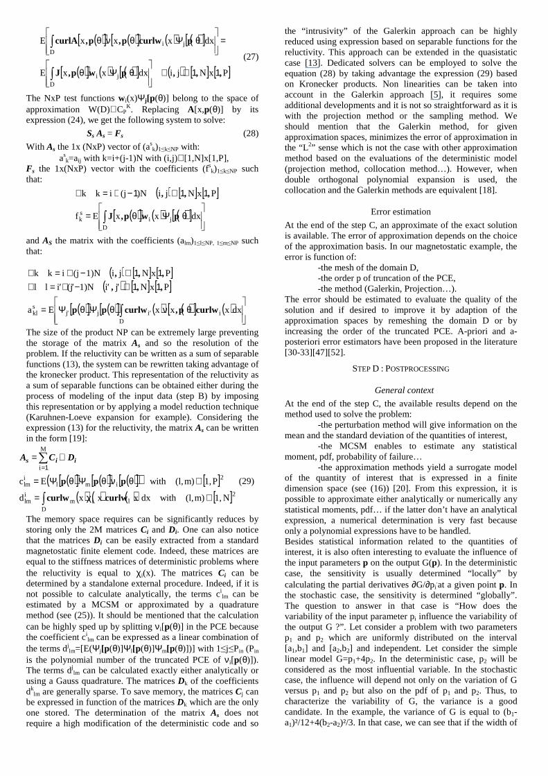
.at a given point p. In the stochastic case, the sensitivity is determined “globally”. The question to answer in that case is “How does the variability of the input parameter pi influence the variability of the output G ?”. Let consider a problem with two parameters p1 and p2 which are uniformly distributed on the interval [a1,b1] and [a2,b2] and independent. Let consider the simple linear model G=p1+4p2. In the deterministic case, p2 will be considered as the most influential variable. In the stochastic case, the influence will depend not only on the variation of G versus p1 and p2 but also on the pdf of p1 and p2. Thus, to characterize the variability of G, the variance is a good candidate. In the example, the variance of G is equal to (b1-a1)²/12+4(b2-a2)²/3. In that case, we can see that if the width of

the intervals of definition of p1 and p2 is of the same size, p2 remains the most influential but if the interval width of p2 is of two orders lower than the parameter p1 will be the most influential. Sobol has proposed a method to undertake a global sensitivity analysis based on an Analysis Of Variance (ANOVA) [34]. The idea is to decompose the variance of the quantity of interest G[p(θ)] as:

( )[ ][ ] M

K

i

K

ijj

ij

K

ii DDDGVar ......... 12

1 21

+++=θ ∑∑∑=

>==

p (30)

The terms Du (u=(u1,..uk) a k-tuple, 1≤k≤K, with u1<u2<..<uk and ui∈[1,K]) are positive and are the fraction of variance of G explained by the inputs pu1,..,puk. The Sobol indices are defined such that:

Su = Du/Var(G[p(θ)]) (31)

The Sobol indices are positive and their sum is equal to 1. A significant value of a Sobol index Su versus the others means that the interaction between the parameters pu1,..,puk contributes significantly to the variability of G[p(θ)]. The number of Sobol indices is very large 2K-1. In practice, only the K Sobol indices of first order (u is a singleton) and the K total Sobol indices defined by STi= Σi∈uSu are calculated. From, these both sets of indices, we can conclude that if Si is significant, the influence of pi is also significant. If STi is small, pi has no significant influence. The calculation of the Sobol indices can be easily estimated using a MSCM by using two distinct samples for the inputs. If an approximation method is used, from the truncated PCE, it is straightforward to approximate the Sobol indices from the coefficients gi (see (16)) [35-37].

Example

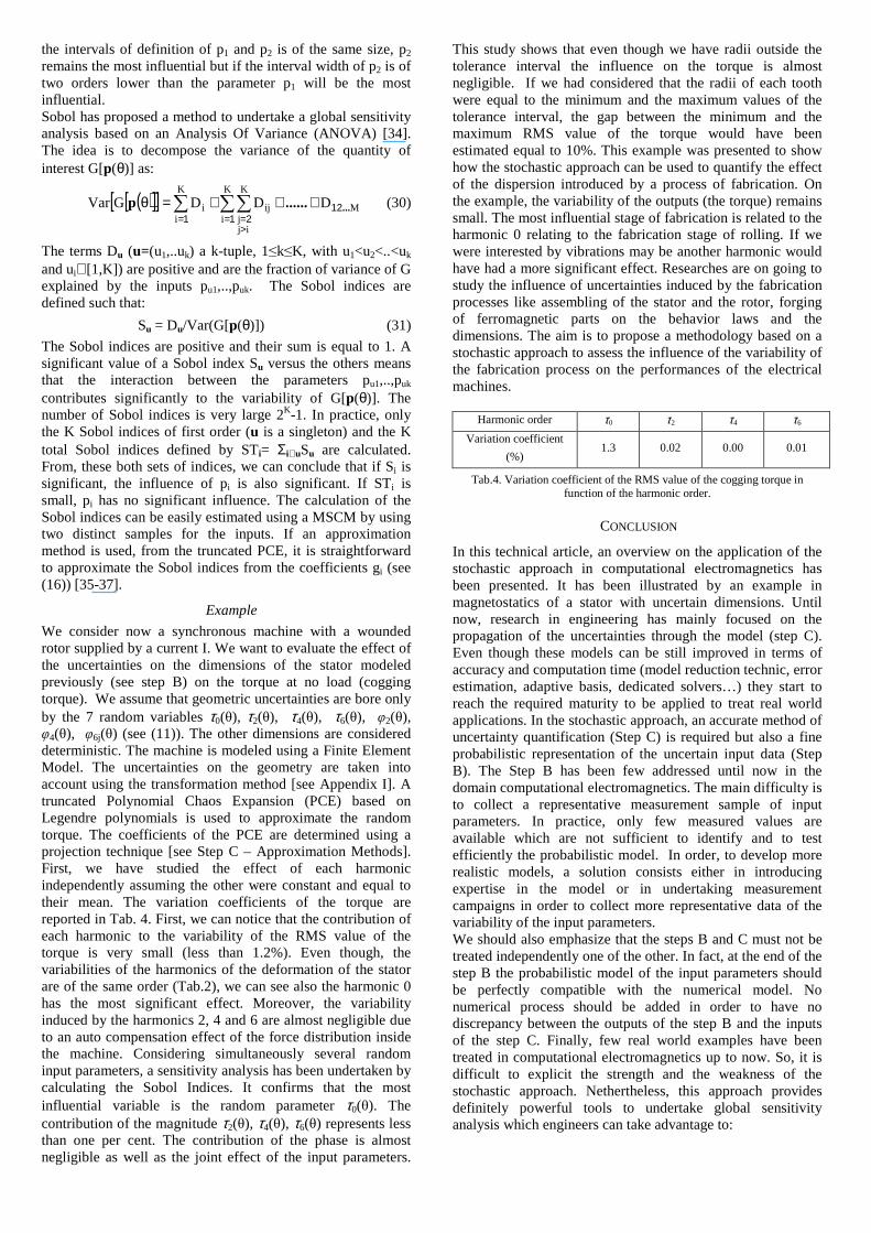
We consider now a synchronous machine with a wounded rotor supplied by a current I. We want to evaluate the effect of the uncertainties on the dimensions of the stator modeled previously (see step B) on the torque at no load (cogging torque). We assume that geometric uncertainties are bore only by the 7 random variables τ0(θ), τ2(θ), τ4(θ), τ6(θ), φ2(θ), φ4(θ), φ6j(θ) (see (11)). The other dimensions are considered deterministic. The machine is modeled using a Finite Element Model. The uncertainties on the geometry are taken into account using the transformation method [see Appendix I]. A truncated Polynomial Chaos Expansion (PCE) based on Legendre polynomials is used to approximate the random torque. The coefficients of the PCE are determined using a projection technique [see Step C – Approximation Methods]. First, we have studied the effect of each harmonic independently assuming the other were constant and equal to their mean. The variation coefficients of the torque are reported in Tab. 4. First, we can notice that the contribution of each harmonic to the variability of the RMS value of the torque is very small (less than 1.2%). Even though, the variabilities of the harmonics of the deformation of the stator are of the same order (Tab.2), we can see also the harmonic 0 has the most significant effect. Moreover, the variability induced by the harmonics 2, 4 and 6 are almost negligible due to an auto compensation effect of the force distribution inside the machine. Considering simultaneously several random input parameters, a sensitivity analysis has been undertaken by calculating the Sobol Indices. It confirms that the most influential variable is the random parameter τ0(θ). The contribution of the magnitude τ2(θ), τ4(θ), τ6(θ) represents less than one per cent. The contribution of the phase is almost negligible as well as the joint effect of the input parameters.

This study shows that even though we have radii outside the tolerance interval the influence on the torque is almost negligible. If we had considered that the radii of each tooth were equal to the minimum and the maximum values of the tolerance interval, the gap between the minimum and the maximum RMS value of the torque would have been estimated equal to 10%. This example was presented to show how the stochastic approach can be used to quantify the effect of the dispersion introduced by a process of fabrication. On the example, the variability of the outputs (the torque) remains small. The most influential stage of fabrication is related to the harmonic 0 relating to the fabrication stage of rolling. If we were interested by vibrations may be another harmonic would have had a more significant effect. Researches are on going to study the influence of uncertainties induced by the fabrication processes like assembling of the stator and the rotor, forging of ferromagnetic parts on the behavior laws and the dimensions. The aim is to propose a methodology based on a stochastic approach to assess the influence of the variability of the fabrication process on the performances of the electrical machines.

Harmonic order τ0 τ2 τ4 τ6

Variation coefficient

(%) 1.3 0.02 0.00 0.01

Tab.4. Variation coefficient of the RMS value of the cogging torque in function of the harmonic order.

CONCLUSION

In this technical article, an overview on the application of the stochastic approach in computational electromagnetics has been presented. It has been illustrated by an example in magnetostatics of a stator with uncertain dimensions. Until now, research in engineering has mainly focused on the propagation of the uncertainties through the model (step C). Even though these models can be still improved in terms of accuracy and computation time (model reduction technic, error estimation, adaptive basis, dedicated solvers…) they start to reach the required maturity to be applied to treat real world applications. In the stochastic approach, an accurate method of uncertainty quantification (Step C) is required but also a fine probabilistic representation of the uncertain input data (Step B). The Step B has been few addressed until now in the domain computational electromagnetics. The main difficulty is to collect a representative measurement sample of input parameters. In practice, only few measured values are available which are not sufficient to identify and to test efficiently the probabilistic model. In order, to develop more realistic models, a solution consists either in introducing expertise in the model or in undertaking measurement campaigns in order to collect more representative data of the variability of the input parameters. We should also emphasize that the steps B and C must not be treated independently one of the other. In fact, at the end of the step B the probabilistic model of the input parameters should be perfectly compatible with the numerical model. No numerical process should be added in order to have no discrepancy between the outputs of the step B and the inputs of the step C. Finally, few real world examples have been treated in computational electromagnetics up to now. So, it is difficult to explicit the strength and the weakness of the stochastic approach. Nethertheless, this approach provides definitely powerful tools to undertake global sensitivity analysis which engineers can take advantage to:

-determine the most influential input parameters on quantities of interest enabling to focus the measurement campaign on those parameters, -evaluate the impacts of the dependency between the inputs, -identify the inter dependency between the output parameters, -to increase the robustness in an optimization procedure…

VI. REFERENCES

[1]Deryckere, J.; Masschaele, B.; De Gersem, H.; Steyaert, D.; Stochastic Response Surface Method for Dimensioning Accelerator Cavities, OIPE 2012, Gent (Belgium), Sept 2012 [2]Ferber, M.; Vollaire, C.; Krahenbuhl, L.;Vasconcelos, J.; Adaptive Unscented Transform for Uncertainty Quantification in EMC Large-Scale Systems, OIPE 2012, Gent (Belgium), Sept 2012 [3]Hulsmann T.,Bartel A.,Shops S., De Gersem H., Simulation of Inrush Currents, CEFC 2012, Oita (Japan), Nov 2012 [4]So, S.G.; Jang, J.; Lee, S.-J.; Kim, K.-S.; Hong, J.-P.; Jang W.-K., Lee T. H., Reliability analysis of back electromotive force considering manufacturing tolerances of permanent magnet in PMSM, CEFC 2012, Oita (Japan), 2012 [5]Rosseel, E.; De Gersem, H.; Vandewalle, S. ; Spectral Stochastic Simulation of a Ferromagnetic Cylinder Rotating at High Speed IEEE Transactions on Magnetics, Vol. 47, N.5, pp 1182–1185, 2011 [6]Drissaoui, A.; Lanteri, S.;Lévêque, P.; Musy, P.; Nicolas, L.; Perrussel, R.;Voyer, D., A Stochastic Collocation Method Combined With a Reduced Basis Method to Compute Uncertainties in Numerical Dosimetry, IEEE Transactions on Magnetics, Vol. 48, N. 2, 2012, pp 563-566 [7]Voyer, D.; Musy, F.;Nicolas, L.; Perrussel, R.,Probabilistic methods applied to 2D electromagnetic numerical dosimetry, The International Journal for Computation and Mathematics in Electrical and Electronic Engineering, Vol. 27, N. 3, 2008, pp. 651-667 [8]Wu, W.F.; Ni, C.C., A study of stochastic fatigue crack growth modeling through experimental data, Probabilistic Engineering Mechanics 18, pp 107-118, 2003. [9]Soize, C.; Capiez-Lernout, E.; Durand, J.-F. ; Fernandez, C.; Gagliardini L., Probabilistic model identification of uncertainties in computational models for dynamical systems and experimental validation, Comput. Methods Appl. Mech. Engrg. 198, 2008, pp 150–163. [10]Ramarotafika, R.; Benabou, A.; Clénet, S.; Stochastic Modelling of Anhysteretic Magnetic Curve using Random Inter-dependant Coefficients, OIPE 2012, Gent (Belgium), Sept 2012 [11]Ramarotafika, R.; Benabou, A.; Clénet, S.; Stochastic Modeling of Soft Magnetic Properties of Electrical Steels: Application to Stators of Electrical Machines, IEEE Transactions on Magnetics, Vol. 48, N. 10, 2012, pp. 2573 – 2584 [12]Ramarotafika, R.; Benabou, A.; Clénet, S.; Mipo, J.C.; Experimental characterization of the iron losses variability in stators of electrical machines, IEEE Transactions on Magnetics, Vol. 48, N°4, 2012, pp 1629-1632 [13] Jarrah, A.; Clénet, S.; Benabou, A.; Ramarotafika, R., Statistical modeling of the behavior of a randomly stacked anisotropic laminations, CEFC 2010, Chicago (USA), 2010 [14]Offerman, P; Hameyer, K; Comparison of Physical and Non-Physical Stochastic Magnetisation Fault Approaches, OIPE 2012, Gent (Belgium), Sept 2012 [15]Beddek, K.; Clénet, S.; Moreau, O.; Le Menach, Y., Solution of Large Stochastic Finite Element Problems – Application to ECT-NDT, CEFC 2012, Oita (Japan), Nov 2012

[16]Beddek, K.; Clenet, S.; Moreau, O.; Costan, V.; Le Menach, Y.; Benabou, A.; Adaptive method for non-intrusive spectral projection application on a stochastic eddy current NDT problem, IEEE Transactions on Magnetics, Vol. 48, N°2, 2012, pp 759-762 [17]Beddek, K.; Le Menach, Y.; Clenet, S.; Moreau, O.; Stochastic Spectral Finite Element Method in static electromagnetism using vector potential formulation, IEEE Transactions on Magnetics, Vol. 47, N°5, 2011, pp 1250-1253 [18]Clénet, S.; Ida, N.; Gaignaire, R.; Moreau, O.; Solution of dual stochastic static formulations using double orthogonal polynomials of Static Field, IEEE Transactions on Magnetics, Vol. 46, N°8, 2010, pp 3543-3546 [19]Gaignaire, R. ;Clénet S.; Moreau, O; Guyomarch, F.; Sudret, B; Speeding up in SSFEM Computation using Kronecker Tensor Products, IEEE Transactions on Magnetics, Vol. 45, N°3, 2009, pp 1432-1435 [20]Gaignaire, R. ;Clénet S.; Moreau, O; Sudret, B; Current Calculation in Electrokinetics using a Spectral Stochastic Finite Element Method, IEEE Transactions on Magnetics, Vol. 44, N°.6 2008, ,pp.754-757 [21]Gaignaire, R. ;Clénet S.; Moreau, O; Sudret, B; 3D Spectral Stochastic Finite Element Method in Electromagnetism, IEEE Transactions on Magnetics, vol. 43 ,N°4, 2007, pp 1209 – 1212 [22]Chauviere, C.; Hesthaven J.S.; Lurati, L., Computational modeling of uncertainty in time domain electromagnetism, SIAM J. Sci. Comput., Vol. 28, No. 2, pp. 751-775. [23]Liu M.; Gao, Z. ; Hesthaven J.S., Adaptive sparse grid algorithms with applications to electromagnetic scattering under uncertainty;Applied Numerical Mathematics, Vol. 61, N. 1, 2011, pp. 24-37 [24]Xiu, D.; Tartakovsky, D.M., Numerical methods for differential equations in random domains. SIAM J.SCI COMPUT. No 3, 2006, pp.1167-1185 [25]Mac, H.; Clénet, S.; Mipo, J.C.; Comparison of two approaches to compute magnetic field in problems with random domains, IET Science, Measurement & Technology, doi: 10.1049/iet-smt.2011.0123, (2012) [26]Mac, H.; Clénet, S.; Mipo, J.C.; Transformation method for static field problem with Random Domains, IEEE Transactions on Magnetics, Vol. 47, N°5,2011, pp 1446-1449 [27]Mac, H.; Clénet, S.; Mipo, J.C.; Moreau, O.; Solution of Static Field Problems with Random Domains, IEEE Transactions on Magnetics, Vol. 46, N°8, 2010, pp 3385-3388 [28]Nouy, A.; Clément, A.; eXtended Stochastic Finite Element Method for the numerical simulation of heterogeneous materials with random material interfaces, Int. Jour. For Num, Meth. In Eng., Vol. 83, N. 10, 2010,pp1312-1344 [29]Nouy, A.; Clement, A.; Schoefs, F.; et al. ; An extended stochastic finite element method for solving stochastic partial differential equations on random domains, Comp. Meth. in Applied Mech. and Eng., Vol. 197, N. 51-52, 2008, pp 4663-4682. [30]Mac, H.; Clénet, S.; Mipo, J.C; Tsukerman I., A priori error estimator in the transformation method taking into account the geometric Uncertainties, CEFC 2012, Oita (Japan), Nov 2012 [31]Prager, W.; Synge, J.L., Approximation in elasticity based on the concept of functions space, Quart. Appl. Math. 5, 1947, pp 261-269 [32]Clénet, S.; Ida N.; Error estimation in a stochastic finite element method in electrokinetics, International Journal for Numerical Methods in Engineering, Vol. 81, N°11, 2010, pp 1417-1438

[33]Chamoin, L.;Florentin, E.; Pavot, S. ;Visseq, V ; Robust goal-oriented error estimation based on the constitutive relation error for stochastic problems, Computers & Structures, Volumes 106–107, September 2012, Pages 189-195 [34]Sobol, I.M., Sensitivity estimates for non linear mathematical models and their Monte Carlo Estimates, Mathematics and Computers in Simulation, Vol. 55, 2001, pp. 271–280 [35]Crestaux, T.; Le Maître, O.; Martinez, J.M. Polynomial Chaos Expansion for Sensitivity Analysis, Reliability Engineering and System Safety, Vol. 94:7, 2009, pp.1161-1172 [36]Sudret, B., Global sensitivity analysis using polynomial chaos expansions. Reliab. Eng. Sys. Safety, 93, 2008, pp. 964–979. [37]Beddek, K.; Clenet, S.; Moreau, O.; Le Menach, Y., Stochastic Non Destructive Testing simulation: sensitivity analysis applied to material properties in clogging of nuclear power plant steam generators, CEFC 2012, Oita (Japan), Nov 2012 [38]Xiu, D.; Karniadakis, G, The Wiener Askey polynomial chaos for stochastic differential equations, SIAM J. Sci. Comput., Vol. 24, No. 2, pp. 619-644. [39]Le Maitre O. P.; Knio O.M.; Najm H.N.; Ghanem R.G., Uncertainty propagation using Wiener-Haar expansions, Journal of computational Physics, N. 197, 2004, pp 28-57 [40]Babuska, I.; Tempone R.; Zouraris G. E., Solving elliptic boundary value problem with uncertain coefficients by the finite element method: the stochastic formulation, Comput. Methods Appl. Mech. Engrg., Vol. 194, 2005, pp 1251-1294 [41]Matthies, H.G.; Keese, A., Galerkin method for linear and non linear elliptic stochastic partial differential equations, Comput. Methods Appl. Mech. Engrg., Vol. 194, 2005, pp 1295-1331 [42]B. Sudret, and Der Kiureghian, Stochastic Finite Elements and reliability: A state-of-the-art report, University of California, Berkeley, Report UCB/SEMM-2000-08, 2000 [43]Ghanem, R.; Spanos, P.D, Stochastic Finite Elements: A spectral approach, Dover, New York, 2003 [44]Hammersley, J. M.; Handscomb, D. C. , Monte Carlo Methods, Chapman and Hall, London & New York, 1964. [45]Hotelling, H., Analysis of a complex of statistical variables into principal components. Journal of Educational Psychology, Vol 24(7), pp. 498-520, 1933. [46]Le Maitre, O.; Knio, O.M., Spectral Methods for Uncertainty Quantification with Applications to Computational Fluid Dynamics, Springer Series Scientific Computation [47] Babuska, I; Tempone, R; Zouraris, E, Galerkin Finite Element Approximation of Stochastic Elliptic Partial Differential Equations, SIAM J. Numer. Anal., Vol. 42, No. 2, pp. 800–825, 2004 [48] Metropolis, N; Rosenbluth, A.W., Rosenbluth, M.N.; Teller, H.A.; Teller, E, Equation of state calculations by fast computing machines, J. Chemical Physics, Vol. 21, No. 6, pp 1087-1092, 1953 [49] Kim, Y.; Hong, J.; Hur, J., Torque Characteristic analysis Considering the Manufacturing Tolerance for Electric Machine by Stochastic Response Surface Method, IEEE Transaction On Industry Applications, vol. 39, No. 3, pp. 713-719, 2003 [50] Ombach, G.; Junak, J. Design of PM brushless motor taking into account tolerances of mass production - six sigma design method, 42nd IAS Annual Meeting. Conference Record 2007

[51]Coenen, I.; Herranz Gracia, M.; Hameyer, K., Influence and evaluation of non-ideal manufacturing process on the cogging torque of a permanent magnet excited synchronous machine, XXIth Symposium on Electromagnetic Phenomena in Nonlinear Circuits (EPNC), Essen, Germany, June 2009 [52] Wan, X.; Karniadakis, G.E., Error Control in Multi-Element Generalized Polynomial Chaos Method for Elliptic Problems with Random Coefficients. CICP, Vol. 5, No. 2-4, pp. 793-820, 2009 [53]Libert, F.; Soulard, J., Manufacturing Methods of Stator Cores with Concentrated Windings”, Proceedings of IET International Conference on Power Electronics, Machines and Drives PEMD, pp. 676-680, 2006. [54] Gaignaire, R.; Scorretti, R.; Sabariego, R.V.; Geuzaine, C Stochastic Uncertainty Quantification of Eddy Currents in the Human Body by Polynomial Chaos Decomposition,IEEE Transaction on Magnetics, Vol .48, N. 2,2012, pp 451 – 454 [55] Gaignaire, R.; Crevecoeur, G.; Dupré, L.; Sabariego,

R.V.; Dular, P.; Geuzaine, C. Stochastic Uncertainty Quantification of the Conductivity in EEG Source Analysis by Using Polynomial Chaos Decomposition IEEE Transaction on Magnetics, Vol. 46 ,N. 8, 2010 , pp 3457 – 3460 [56] Paris, P.; Erdogan, P., A critical analysis of crack propagation laws, Journal of Basic Engineering, Vol.85, Issue 4, pp 528–534, 1963 [57]Virkler, A.; Hillberry, B. M.; Goel, P. K., The statistical nature of fatigue crack propagation, Journal of Engineering Materials and Technology, Vol.101, Issue 2, pp148-153, 1979 [58] Ditlevsen, O.; Olesen, R., Statistical analysis of the Virkler data on fatigue crack growth", Engineering Fracture Mechanics, Vol. 25. No. 2, pp. 177-195, 1986 [59] Weiner, N., The homogeneous chaos, American Journal of Mathemetics, Vol. 60, N.4, pp 897-936, 1938 [60]Doostan, A; Owhadi, H, A non-adapted sparse approximation of PDEs with stochastic inputs, Journal of Computational Physics, Vol. 230, 2011, pp. 3015–3034 [61]Nouy, A., A generalized spectral decomposition technique to solve a class of linear stochastic partial differential equations, Comput. Methods Appl.Mech. Eng. Vol. 196, N 37–40, 2007, pp 4521–4537 [62]Smolyak, S., ,Quadrature and Interpolation Formulas for Tensor Products of Certain Classes of Functions,, Doklady Akademii Nauk SSSR, Vol. 4, 1963, pp 240-243 [63] Berveiller, M. ; Sudret, B. ; Lemaire, M., Stochastic finite elements: a non intrusive approach by regression. Eur. J. Comput. Mech., Vol. 15(1-3), 2006, pp. 81–92 [64] Mac, D.H.; Clénet, S; Zheng, S; Coorevits, T; Mipo, J.C., on the geometric uncertainties of an electrical machine : stochastic modeling and impact on the performances, submitted to COMPUMAG’13, Budapest (Hungary), 2013

APPENDIX I : UNCERTAINTIES ON THE GEOMETRY

The uncertainties on the geometry can be modelled by random interfaces Γk between two sub-domains Di and Dj. In each sub-domain, the reluctivity νi is assumed to be constant in each subdomain Di. We suppose also that these interfaces can be parameterized by known random variables p(θ) and a parameter c, we have:

x=gk[p(θ),c] with c∈∆k⊂R2 (A.1)

where x are the coordinates of the points located on this interface. The parameter c belongs to ∆k a subset of R2 (R in the 2D case). For each realization of p(θ), there is a bijective map between ∆k and Γk. Even though the reluctivity is assumed to be constant on each subdomain, it depends on the position x and also on the realization of the random interfaces.

Indeed, for a point x located close to a random interface Γk, the value of the permeability depends on which side of Γk the point x is located. Thus, in a point x of D which can be located on both sides of a random boundary Γk (between the subdomains Di and Dj) the permeability switches from the values νi to νj. If we denote IDi(x,), the function associated to the domain Di (IDi[x,p(θ)]=1 if x∈Di and 0 elsewhere), the reluctivity on the domain D can be written in the form:

[ ] [ ] ( )[ ]∑=

θν=θν=θνM

iii I

1

pxpxx ,)(,, (A.2)

where M is the number of subdomains. Since the reluctivity is a random field, the magnetic field H and the magnetic flux density B are also random fields. The quantity of interest G[p(θ)] is calculated in a postprocessing step after solving numerically the stochastic vector potential formulation. To deal with problems with random domains, an easy way consist in remeshing each geometry corresponding to a new evaluation point pk (see step C – MCSM and approximation methods). However, this approach has some drawbacks. First, since we have to remesh, the stiffness matrix and the source vector have to be recalculated for each evaluation pk point which is time consuming. Remeshing the domain D adds a numerical noise on the output data because the mesh (the connectivities between elements, the number of elements…) changes from an evaluation point to another. Moreover, the expression of the shape functions changes as well. Consequently, it is not obvious to obtain an explicit expression of the vector potential as (24) so the distribution of the fields H and B. Finally, as we will see in the following part, the magnetic field at certain fixed points could have some discontinuities along the stochastic dimension. Therefore, the approximation of magnetic field at this point using a polynomial chaos expansion is no longer appropriate. To avoid the former drawback, one possibility is to introduce additional functions (enrichment basis method) that can account for these discontinuities. This technique has been proposed for the stochastic finite element method in [28-29]. Another possibility consists in using the transformation method proposed in [25].

Enrichment basis method

We suppose that the discontinuity point p=p0 is a priori known. The main idea consists in adding P’ enrichment functions to the space of approximation defined by the truncated PCE (16) in the stochastic dimension [28,29]. The approximation of G becomes:

[ ] ( )[ ] ( )[ ]∑∑==

θΗ+θΨ≈θ'P

iii

P

iii hg)(G

11

ppp (A.3)

where Ψi orthogonal polynomials defined in (18) and Ηi is a discontinuous function at the point p=p0 and gi and hi real coefficients. Since the discontinuities of G[p(θ)] can then be taken into account by the functions Ηi, the accuracy of the approximation is better. We can use of the following form:

( )[ ] ( )[ ] ( )[ ] Ktoiii 1=θΨθτ=θΗ ppp (A.4)

where ( )[ ] ( )

−≤θ=θτ

else

if

1

1 0ppp

The coefficients gi and hi of the expansion can be calculated using either a Galerkin approach or a projection method (see Step C)

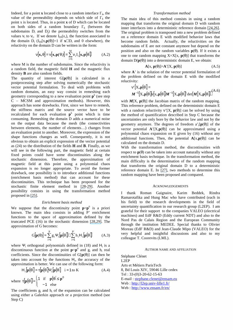
Transformation method

The main idea of this method consists in using a random mapping that transforms the original domain D with random inner interfaces into a deterministic reference domain [24,26]. The original problem is transposed into a new problem defined on a reference domain E with modified behavior laws that become random fields. Actually, the reluctivities on the subdomains of E are not constant anymore but depend on the position and also on the random variables p(θ). If it exists a one to one random mapping X=X[x, p(θ)] that transforms the domain D(p(θ)) into a deterministic domain E, we obtain:

A[x, p(θ)]=A’[X, p(θ)] (A.5)

where A ’ is the solution of the vector potential formulation of the problem defined on the domain E with the modified reluctivity:

( )[ ]

( )[ ] ( )[ ] ( )[ ] ( )[ ]( )θθθνθ

=θν−− pppp

p

,M,M,,M

,'

XdetXxX

Xt11

(A.6)

with M[X, p(θ)] the Jacobian matrix of the random mapping. This reference problem, defined on the deterministic domain E with a random reluctivity ν’[X, p(θ)] can be solved by using the method of quantification described in Step C because the uncertainties are only bore by the behavior law and not by the geometry anymore. The degrees of freedom a’i[p(θ)] of the vector potential A’[X, p(θ)] can be approximated using a polynomial chaos expansion on E given by (16) without any additional functions. Then, the potential A[x,p(θ)] can be calculated on the domain D. With the transformation method, the discontinuities with respect to p(θ) can be taken into account naturally without any enrichment basis technique. In the transformation method, the main difficulty is the determination of the random mapping that transforms the original domain D to a deterministic reference domain E. In [27], two methods to determine this random mapping have been proposed and compared.

ACKNOWLEDGEMENTS

I thank Roman Gaignaire, Karim Beddek, Rindra Ramarotafika and Hung Mac who have contributed (each in his field) to the research developments in the field of uncertainty quantification in our research group (L2EP). I am grateful for their support to the companies VALEO (electrical machines) and EdF R&D (Eddy current NDT) and also to the Nord Pas de Calais Region and the European Community through the institution MEDEE. Special thanks to Olivier Moreau (EdF R&D) and Jean-Claude Mipo (VALEO) for the very helpful and insightful discussions and also to my colleague T. Coorevits (LML).

AUTHOR NAME AND AFFILIATION

Stéphane Clénet L2EP Arts et Métiers ParisTech 8, Bd Louis XIV, 59046 Lille cedex Tel : 33-(0)3-20-62-15-63 E-mail : stephane.clenet@ensam.eu Web : http://l2ep.univ-lille1.fr/ Web : http://www.ensam.fr/en/