Uncertainty and Climate Change

Geoffrey Heal∗

Columbia Business School, New York, NY 10027.

Bengt KriströmSLU-Umeå, 901 83 Umeå, Sweden.

November 2001, revised February 2002.

Abstract

Uncertainty is pervasive in analysis of climate change. How should economistsallow for this? And how have they allowed for it? This paper reviews both ofthese questions.Key Words: Climate change, uncertainty, risk.JEL ClassiÞcation: D 80, Q 00

1 Overview

The extent to which the earth�s climate will change as a result of human activity isstill unclear. Although the basic science is well-understood and now seems conÞrmedby the data available, the precise magnitudes of the various effects that contributeto the climate regime are not yet known. The most recent assessment by the UNIntergovernmental Panel on Climate Change (IPCC), the Third Assessment Report(TAR), has for the Þrst time made an explicit attempt to give an indication of thedegrees of uncertainty associated with its various predictions.1 The TAR gives anindication of the degree of conÞdence that the leading authorities in the Þeld ofclimate change have in their forecasts. In some cases it is clear that, while the sign ofan impact is clearly known, there remains massive uncertainty about the size, withthe range of possible magnitudes involving differences of several hundred percent.This is illustrated by the IPCC�s widely-quoted range for the possible change in

∗Contact author - Heal at gmh1@columbia.edu, www.gsb.columbia.edu/faculty/gheal.1An earlier review of the extent and nature of uncertainty in climate forecasting can be found in

Roughgarden and Schneider (1999).

1

global mean temperature, which goes from 1.5 to 6 degrees centigrade.2 In the TARthe IPCC classiÞes its Þndings according to the degree of conÞdence in them. Itrecognizes Þve different conÞdence levels, ranging from �very high (>95%)� through�high (67<X<95%)� and �medium (33<X<67%)� to �very low (<5%)�. Most ofits major Þndings are assigned one of these probability rankings, which in generalare assumed to correspond to Bayesian subjective probabilities. In cases in whicha Bayesian characterization is considered inappropriate, largely because the state ofknowledge is too primitive, the IPCC TAR uses a four-way classiÞcation:

Level of agreement

Amount of evidence (observations, model output, theory, etc.)Low High

High Established but incomplete Well-establishedLow Speculative Competing explanations

Table 1. IPCC TAR classiÞcations.

This classiÞcation shows four cases: the most certain is a high level of agreementbetween scientists and a substantial amount of evidence on the issue, but not enoughto distinguish between the competing theories: the opposite case is low agreementabout the alternative theories and little evidence to distinguish between them. Theycharacterize this as a situation where the analysis has to be �speculative�.As economists, it is not only uncertainty about the underlying climate science

that should be of concern to us. Ultimately we are interested in the impact of climatechange on human societies, and this involves knowing not only how the climate mayalter but also how changes in the climate regime translate into impacts that matter forhumans. How do climate changes translate into changes in agricultural production,into changes in the ranges of disease vectors, into changes in patterns of tourist travel,even into feelings of well-being directly associated with the state of the climate? So weare concerned here about the outcome of a process with at least two stages: stage oneis a change in the climate regime and stage two is the translation of this into changesin things that matter directly to us. Even if we knew exactly what the climate wouldbe in 2050, we still would face major economic uncertainties because we currently donot know how altered climate states map into human welfare.In assessing the economics of climate change there are therefore at least two

sources of uncertainty - what the climate will be, and what any given changed climatewill mean in economic terms. We can think of these as the scientiÞc uncertainties

2To be fair to the climate science community we should probably think of the change in temper-ature as a variation in the earth�s absolute temperature, which is about 280 degrees Kelvin, so thatwe are looking at uncertainty that is only a couple of percentage points of the absolute temperature.Mason (1995) provides a perspective on the development of climate modelling. Note that anthro-pogenic emissions are only a fraction of what is added each year in terms of carbon. This does notsimplify the task of predicting the consequences for the climate of human-made carbon reductionsthat are likely to be some fraction of current emissions.

2

analyzed by the IPCC�s TAR, and the uncertainties about climate impacts. In factthere is a third stage, uncertainty about the policies that we will choose to controlemissions over the coming decades. So in trying to forecast what the climate will beat a future date such as 2050 we have not only to forecast how the climate systemwill respond to human inßuence but also what that inßuence will be: what policieswill be chosen in the interim.In total, we seem to have to take account of scientiÞc uncertainty, impact uncer-

tainty and policy uncertainty. Possible policy responses to climate change take twoforms: mitigation, i.e., actions that reduce the ßow of greenhouse gases into the at-mosphere and, thereby, change the probability distribution over future climate states;and adaptation � actions that reduce the damages associated with a given climatestate.3 Both provide sources of uncertainty. In the domain of mitigation, perhaps themost prominent source of uncertainty is institutional: will the international commu-nity adopt aggressive mandates to restrict emissions of greenhouse gases? Will theinstitutions that implement these mandates be efficient, i.e., will the marginal costof net reductions in emissions be roughly equal across all sources and sinks? Whattechnical changes will appear to reduce the costs of mitigation? Adaptation likewiseinvolves uncertainty about the different options that will become available, and theircosts.The IPCC TAR goes further and recognizes no less than Þve stages of uncertainty,

as a result of breaking down the scientiÞc uncertainty into sub categories. Its Þvecategories are uncertainty about emission scenarios (i.e. about anthropogenic emis-sions of greenhouse gases), about the responses of the carbon cycle to these emissions,about the sensitivity of the climate to changes in the carbon cycle, about the regionalimplications of a global climate scenario, and Þnally uncertainty about the possibleimpacts on human societies. We have noted the Þrst of these - uncertainty aboutemissions scenarios. And we aggregate the next three (concerning the response of thecarbon cycle, the sensitivity of the climate system and the regional implications ofglobal scenarios) as these are all �scientiÞc uncertainty� from the perspective of aneconomist. This leaves the Þnal category of uncertainty as impacts.The TAR has adiagram that shows the degree of uncertainty rising as we move through these Þvestages, with the error bars growing from stage to stage.

3Interestingly, the Þrst two IPCC Assessment Reports did not discuss adaptation. This omissionhas been attributed to political pressure from the environmental lobby. As the Columbia sociologistSteve Rayner has quipped, �Environmentalists don�t want to talk about adaptation for the samereason Southern Baptists don�t want to talk about birth control,� i.e., out of concern that the act oftalking about these measures might be construed as an acceptance of the sinful behavior leading totheir necessity. See Kane and Shogren (2000) for a summary on adaption and mitigation arguments.They make the important point that adaption and mitigation are linked. Indeed, the Kyoto-protocolposits world-wide (but not global) mitigation efforts. Combining mitigation and adaption, however,would seem to afford the same climate improvement at lesser cost. They also note that attemptsto �assess risk levels solely in terms of natural science may be misleading and costly; adaption andmitigation are endogenous to the integrated system...�

3

Uncertainty can of course be reduced through learning. This consideration leads toa second-order, or meta- form of uncertainty: what new information will be revealedto resolve the present uncertainties? To what extent can and will research acceleratethe pace of learning? Given the possibility of future learning, issues of irreversibilityand quasi-option value may become salient. This discussion suggests clearly that anyeconomic analysis of climate change should include uncertainty as a central feature.Yet a review of the literature shows that the bulk of the work to date has beendeterministic, though there are exceptions and the trend is changing. If uncertaintyis central then attitudes towards risk and the degree of risk aversion will presumablybe central parameters. Institutions for risk-shifting will also be important, and thepossibility that some changes are irreversible and that we may learn more aboutthem with the passage of time suggests that real option values may also matter inthe analysis of policy measures. Another analytically interesting feature of climatechange is that the risks are not exogenous, as in many models of uncertainty ineconomics, but are generated by our own activities. This endogeneity of the risksraises questions about the use of markets and insurance for hedging some of the risksassociated with possible climate change: there is the macro-level equivalent of moralhazard here. Finally, as many authors have remarked, the time horizon implicit inclimate change is very long indeed, measured in centuries, far longer than economistsare used to. Uncertainties are almost inevitably large when decisions involve suchlong time horizons. In sum: in analyzing climate change policies, attitudes towardsrisk will be important, as may be the values of maintaining certain options open.Endogeneity of risks may pose some problems for the use of certain types of

Þnancial institutions, and the length of the time horizon will pose a challenge toour normal ideas about discounting.4 As the preceding discussion indicates, theeconomic problem of climate management cleaves (usefully, if imperfectly) into fourparts. Section 2 summarizes what climate scientists can tell us about the main sourcesof uncertainty in the relationship between greenhouse gas emissions and future climatestates. Section 3 addresses the relationship between future climate states and impactson human welfare. Section 4 sets out the basic economic issues, and summarizessome calculations indicative of the possible importance of key economic parameters.In section 4 we set out a very general model that seems to incorporate most of thecentral issues. This model is too complex to be solved analytically, and we thenreview the models that have actually been solved to date, most of which can beseen as special cases of this framework. In subsequent sections we look at a rangeof issues relating to the management of climate risks by economic institutions suchas Þnancial markets, and the impact of uncertainty and the endogeneity of risks onthese institutions.

4For a recent summary of the environmental economics literature on endogenous risk, see Crockerand Shogren (2003).

4

2 Uncertainty in the TAR

To set the stage, we begin by surveying the area where economics has the least di-rect relevance: understanding the relationship between greenhouse gas buildup andpossible future climate states. What can the scientiÞc community tell us about theserelationships, and with what degree of certainty? The basic physics of climate changeis well-understood and not controversial, and has been known for over a century. Un-certainties arise when applying the physical principles via complex computer modelswith many parameters that have to be estimated or calibrated from inadequate datasets. These are issues to which economists can surely relate!So most of the central numerical estimates are subject to considerable error, as

indicated by the ßagship prediction of the IPCC that global mean temperature willchange by between 1.5 and 6 degrees centigrade by 2100 relative to 1990 - a differenceof a factor of four between the top and bottom of the range. To be fair we have torecall that this is a 100 year forecast - how many economists would want to put theirnames to forecasts for 2100? Probably we would Þnd that the range of social andeconomic uncertainties is even greater if we were to think about it. Many of theuncertainties that appear in the forecasts arise naturally from the length of the timehorizon considered combined with the uncertainties in the model parameters. SpeciÞcissues that make an additional contribution to uncertainty include the impacts ofaerosols - Þne particles in the air often caused by pollution - on the condensationof water vapor and the formation of clouds, and more generally the formation ofclouds. Clouds reßect sunlight back into space and so control warming to somedegree, and little is understood numerically about their formation, though it is knownthat Þne particles in the air provide nuclei on which water droplets can form andstart the process of cloud formation. A rather different source of uncertainty is thepossible failure of the thermohaline circulation system in the north Atlantic: thisis the technical name for the Gulf Stream that brings hot water from the tropicalregions to northern Europe. This massive heat transfer is largely responsible for thecomparatively benign climate of northern Europe relative to those of other regionsat the same latitude, and there is evidence that during past climate ßuctuations thissystem has stopped, leading to massive cooling in Europe. Computer models doindicate that atmospheric warming by greenhouse gases could switch off this massiveheat transfer system, with dramatic results for the climates of many densely populatedregions.5

5A numerical analysis of the economics of a potential collapse of the thermohaline circulationsystem, using a modiÞed cversion of DICE (Nordhaus (1994)), is in Keller, Tan, Morel, and Bradford(2000). An expanded version of this work that also include e.g. learning effects, arrives at the sameconclusion, namely that signiÞcant reductions of carbon emissions may be worthwhile. See Keller,K. , Bolker, B.M. and D.F. Bradford, �Uncertain Thresholds and Economic Optimal Growth�.www.princeton.edu/~bradford/kellerbolker.pdf. This is to be compared with several well-knownempirical models, DICE is an example, that predict rather modest costs of climate change. Moreon this later in the paper.

5

However, the IPCC assigns a �low� probability to this. The fact that something isa low probability event does not of course mean that it does not matter economically -if the consequences are sufficiently dramatic then this may more than compensate forthe low likelihood and mean that the expected loss is still signiÞcant. So the IPCC�scomment that something is �low probability� does not mean that as social scientistswe should neglect it; this depends on the consequences. Other issues that are stillnot resolved at the scientiÞc level concern the behavior of terrestrial carbon sinksat higher temperatures and carbon dioxide concentrations, and also the behavior ofthe oceans both as heat sinks and as carbon sinks. As the oceans sequester morecarbon than the terrestrial biosphere and are a major element in the planet�s heattransfer system, this lack of detailed understanding translates into a signiÞcant sourceof uncertainty.

3 Climate change and human welfare

Changes in climate have effects on human welfare through many pathways. To datemost studies have considered the impact of climate change on agricultural produc-tivity and on sea level and indeed have more or less equated the overall impact ofclimate change with these impacts. We are beginning to see that this is probablya very restricted and limited view of climate change and its human impacts. Thereare suggestions emerging that climate has an impact on economic development andon the pattern of economic growth. There are also suggestions that climate affectshuman welfare directly, not via agricultural output or economic development but asan argument of the utility function. Climate changes will also affect the occurrenceof extreme events and the geographical range of many disease vectors such as themalarial pathogens.David Landes (1998) includes climate as one of the key factors in his widely read

(and controversial) �The Wealth and Poverty of Nations�. Tropical diseases, accessto water, the propensity to natural disasters, etc. present regions like Africa witha handicap, according to Landes. He also presents an account of geographers andothers who marshalled climate as the key variable to explain economic differences. Ina similar vein is a recent study by Horowitz (2001) . He carried out a regression thataddresses the relationship across countries between average annual temperature andGDP per head, looking at the income-temperature relationship for a cross-sectionof 156 countries in 1999. As is well known, hotter countries are poorer on average.The widespread belief is that this relationship is mostly historical; that is, due to apast effect of climate. Acemoglu, Johnson, and Robinson (2001) have recently madegreat gains in identifying a speciÞc historical path for this relationship. They positthat mortality rates of early colonizing settlers had a profound effect on the insti-tutions that were set up in those colonies. These institutional differences persist tothis day, they argue, and have strong effects on current incomes. Because colonialmortality and average temperature are highly correlated, the mortality-income rela-

6

tionship also manifests itself as an income-temperature relationship. Horowitz arguesthat there is, however, sufficient evidence to warrant continued examination of theincome-temperature relationship. He Þnds a strong income-temperature relationshipwithin OECD countries, a result that does not appear to be predicted by the colonialmortality model. He also Þnds that the income-temperature relationship is essentiallythe same within the OECD and non-OECD countries, a striking yet unremarked andas-yet unexplained result. Finally he Þnds a strong income-temperature relationshipwithin the Þfteen countries of the former Soviet Union, where colonial institutionswould seem to have been wiped out. His best measure of the effect of temperature onincome, after accounting for the inßuence of colonial mortality, is that a one percentincrease in temperature leads to a -0.9 percent decrease in per capita income. Thus,a temperature increase of 3 degrees Fahrenheit would result in a 4.6 percent decreasein world GNP. The result is striking. While the result is only suggestive � there is nocausal mechanism offered � it suggests that there is a relationship between temper-ature and economic production, and that changes in temperature may, then, createÞrst-order changes in economic output and welfare.Similar conclusions are emerging from other related studies. Gallup, Sachs and

Mellinger (1998) have suggested that tropical climates make economic developmentmore difficult, via reduced agricultural productivity and added disease burden. Theydo not speciÞcally comment on the economic consequences of climate change butan implication of their Þndings is surely that as �tropical� climates become morewidespread then so will their economic disadvantages. Similar conclusions are sug-gested by Gavin and Hausman (1998). All of the results that tie climate to economicdevelopment are tentative and are too preliminary to form the basis for quantitativeestimates of welfare impacts. They represent a mechanism through which climatechange can have economic consequences which has been little explored to date, andconsequently is a source of uncertainty in any estimates of climate change impacts.

3.1 Direct effects on human well-being

There is a clear connection between weather, climate, and how well people feel. Wedislike very cold climates and very hot ones, and possibly also very humid ones.There are probably good reasons for these likes and dislikes, founded in evolutionarybiology. In this context, Maddison and Bigano (2000) Þnd that the most populartourist destinations are those offering temperatures of around 88◦F (31◦ C): thisappears to be an �ideal temperature�, at least for the inhabitants of western Europe.Lise and Tol (2001) Þnd similar results. They carry out a cross-section analysison destinations of OECD tourists and a factor and regression analysis on holidayactivities of Dutch tourists, to Þnd optimal temperatures at travel destination fordifferent tourists and different tourist activities. Globally, OECD tourists prefer atemperature of 21◦C (= 70 F) (average of the hottest month of the year) at theirchoice of holiday destination. This Þnding and Maddison�s results indicate that,

7

under a scenario of gradual warming, tourists would spend their holidays in differentplaces than they currently do. It also suggests that as temperatures change as aresult of global warming there could be a loss of welfare in some regions just becauseof the climate change itself and quite independently of any consequences for economicactivity.It seems a very safe assumption that human preferences about temperature are

biologically determined and are likely, therefore, to be stable over time. This is not todeny that temperature preferences may well exhibit cross-sectional variation acrosscultures and ethnic groups. Insofar as people are biologically or culturally adapted toparticular climes, change may be bad per se. In some sense this is just an extension ofthe argument that plants and animals that are adapted to certain climate conditionswill suffer from climate change. Humans are just one of many species of animals,albeit an unusually disruptive one, and so in principle are subject to the same effects.The direct effects of climate on human welfare are probably the least explored of alleffects so far, and could be some of the more important, especially for populationsin areas where agriculture will not be greatly affected by a changed climate regime.They are therefore a major source of uncertainty.

4 The economic framework

That discount rates and attitudes to the far future matter in assessing climate changehas always been clear. Now it should also be clear that risk aversion will matter aswell. An important implication of this is that even though an event is very unlikely, ifit is costly and we are risk averse we may invest signiÞcantly in avoiding it or insuringagainst it. By way of illustration, our houses rarely burn down, yet most of us insurethem against this event on terms that are actuarially unfair.In the context of climate change there is a real potential for learning over time.

Global circulation models have been greatly reÞned and enhanced since their Þrst usein analyzing climate change, and this has improved our understanding of what mighthappen. There are many other ways in which our understanding might improve inthe future. We might learn about cleaner energy production technologies, or aboutnovel methods of carbon sequestration. Over several decades the changes in ourunderstanding of these possibilities could be far-reaching. SigniÞcant changes in ourunderstanding of these possibilities could alter the relative merits of different economicpolicies. As an illustration, Lackner et al. (1999) have proposed the sequestration ofcarbon dioxide by using calcium hydroxide, and the scrubbing of emission gases fromfossil fuel plants using the same chemical (spraying tropical waters with iron Þlings isanother geoengineering suggestion, see Keith (2000) for a review). The possibility ofimplementing this on a large scale is still speculative and will remain so for some years,but this discussion offers a tantalizing glimpse of the kind of qualitative technologicalchange that might occur within the next few decades.

8

4.1 Irreversibility

It is also likely that many of the changes in climate, and changes in the naturalenvironment driven by climate change, will be irreversible. The consequences of thispossible irreversibility have been discussed at great length, if rather inconclusively,so it is important to understand the underlying issues. Changes in the climate mayin themselves be irreversible: once the climate regime in an area has changed, it maynot be possible to restore the original. The most notable case of this arises from thepossible change in the path of the Gulf Stream, a possibility that we mentioned asone of the biggest sources of uncertainty in forecasting climate regimes. The issuehere is that the climate system is a complex nonlinear dynamical system and likemost such systems has several possible equilibrium states or attractors. Each hasa basin of attraction - a set of initial conditions within which it is stable, in thesense that if the initial conditions are within the basin then the system moves to thatequilibrium. Stresses on the system, such as human changes to the mix of gases inthe atmosphere, could possibly move the climate system from one basin of attractionto another. Moving from one conÞguration of the Gulf Stream to another would bean example of this. Once the system is in a new basin of attraction it is not obviousthat we could move it back to the original, so such a change may be irreversible.Possible irreversibilities may also arise because the climate is determined by inter-

actions between the atmosphere, the oceans and the biosphere. Changes in the climatemight lead to changes in oceans or the biosphere that would make the restoration ofthe original conÞguration impossible. For example, the climate of the Amazonian re-gion is created in part by the forests there; trees in the forest transpire vast quantitiesof moisture into the air and contribute to the humidity of the region. Were the regionto become hotter and drier, these trees would die and consequently the soils wouldchange. Reducing the concentration of greenhouse gases in the atmosphere wouldthen probably not restore the original climate to the Amazonian region because theforest would have died and could not be restarted, and was a key element of theoriginal climate system. Another irreversible aspect of climate change would be themelting of the west antarctic ice sheet, which would lead to a signiÞcant and rapidincrease in sea levels globally.Issues of how far climate changes could be reversed by reducing greenhouse gas

concentrations have not been extensively studied, although in most economic modelsprocesses are modelled as if the changes in climate can eventually be reversed, even ifslowly. Even if changes in the climate were to be reversible, there are other associatedchanges that might not be. For example, climate changes might drive certain speciesextinct if their habitats are destroyed: indeed increased extinction rates are a widely-forecast consequence of climate change. Extinction is self-evidently not a reversibleprocess. At a more mundane level, climate change will alter plant and animal com-munities in ways that may make it impossible to reestablish the original communityeven if the components are not extinct. In this vein, an expected consequence ofclimate change is the death of some coral reefs. This will lead to changes in marine

9

communities that will not be reversible on human timescales. This combination ofpotential for learning together with irreversibilities is the classical breeding groundfor real option values. If climate change or its consequences are indeed irreversibleand there is a chance of learning more over time, then there may be a real optionvalue associated with preserving the present climate regime, i.e. with freezing allactions that are likely to contribute to climate change. This real option value couldreinforce the widely-cited but seldom analyzed �precautionary principle,� a nostrumto the effect that we should avoid making possible environmental changes until weare sure of their consequences. However, confusingly, there is another possible realoption value at work here. Suppose that substantial sunk costs must be incurredto begin the process of abating greenhouse gas emission and avoiding or minimizingclimate change. The return to this investment is the avoidance of climate change andif we learn about the value of this over time then there is also a real option valueassociated with postponing investment in greenhouse gas abatement. So there couldalso be an �inverse precautionary principle� at work here suggesting that we avoidcostly policies requiring irreversible investments until we are really sure that they areneeded.Striking a balance here is made more complex by the fact that it is not only the

time horizons that are long, but also the time lags in many parts of the system.Both climate and economic systems are likely to respond very slowly to policiesimplemented to change greenhouse gas emissions. So even if a forceful greenhousegas abatement policy were implemented tomorrow, its impact might not be felt onemission levels until 2010 or later, and the consequences for the climate of a reductionin GHG ßows beginning in 2010 or later would be slight prior to 2020 at the veryearliest. There would be further lags between changes in climate trends and thetrends in the factors that affect humans - agriculture, diseases, etc. Consequentlythere is an argument that as there is a real risk that the climate will be seriouslyperturbed by human action by say 2040, and as the lags in the systems that linkour policies to the outcomes that matter are so long, then we have a responsibilityto start taking actions now, as actions taken later will be too late to avoid harm tothose living in 2040.By now it is clear that setting out a convincing analytical framework for climate

policy choices is a challenge: the intrinsic uncertainties enter in many different ways.Next we take a look at how these issues could in principle be captured, and how theyhave actually been captured, in the literature to date.

4.2 Preliminary calculations: the value of avoiding climatechange

Before developing a general framework and reviewing the literature, which is themain purpose of this paper, we review some simple yet suggestive calculations thatindicate the importance of allowing for uncertainty in the economics of climate change.

10

These calculations were addressed to the question: what costs is it worth incurringto avoid the risk of climate change? Within a simple framework we can carry outcalculations that illustrate the issues involved, and how discount rates, risk aversionand probabilities interact. The answer depends on the following four parameters, ofwhich two are clearly economic:(1) the probability distribution of the effects of climate change,(2) the degree to which we are risk averse,(3) the date at which the climate change will occur, and(4) the rate at which we discount future beneÞts and costs relative to those in the

present.How exactly might we compute what it might be rational to pay to avoid the risks

of climate change?6 Denote society�s income in the absence of climate change by Iand the beneÞts derived from this income by utility u (I). Utility is taken to be afunction of I that increases at a decreasing rate. The expected utility after climatechange is

Pj pju (Ij) .

7 Climate change occurs, if it occurs at all, in year C. Denoteby δ ≤ 1 the weight given to costs or beneÞts at date t+ 1 relative to those at t, sothat δt−1 is the weight given to those at t relative to those at 1. Then (1− δ)× 100is the discount rate as a percent.Suppose that it possible by incurring a cost from now to the date C at which

climate change might occur, to rule out this occurrence. What cost x is it worth ourwhile incurring, from now to C, in order to ensure that the climate does not changeat C? The number x that we seek is the solution to the equation

CXt=1

δt−1 [u (I)− u (I − x)] =TX

t=C+1

δt−1

"u (I)−

Xj

pju (Ij)

#(1)

The left hand side is the loss of utility in incurring the cost x from now to the timeC of climate change, with future losses discounted back to the present: the loss eachyear is [u (I)− u (I − x)] , and we sum this, discounted, over all years up to C. Theright hand side is what we would lose each year, in expected value terms, if climatechange were to occur, summed from its occurrence at C to a distant date T , andagain discounted to the present. The expected annual loss is

hu (I)−P

j pju (Ij)i.

This sum on the right is therefore also the beneÞt of avoiding climate change. Themaximum we should be willing to pay is the value of x at which these two are equal:hence the equation. The date T is the maximum time horizon that we considerrelevant to these calculations.

6The calculations that follow are taken from work in progress by Geoffrey Heal and Yun Lin,Columbia University.

7If there is climate change, then income drops from I to Ij with probability pj , where clearlyIj ≤ I and

Pj pj ≤ 1. This can be weakened to allow an income drop on the average, in order to

include a possibility for income increases. With risk aversion, people would still be willing to pay toavoid the change. Thanks to Mark Machina for pointing this out.

11

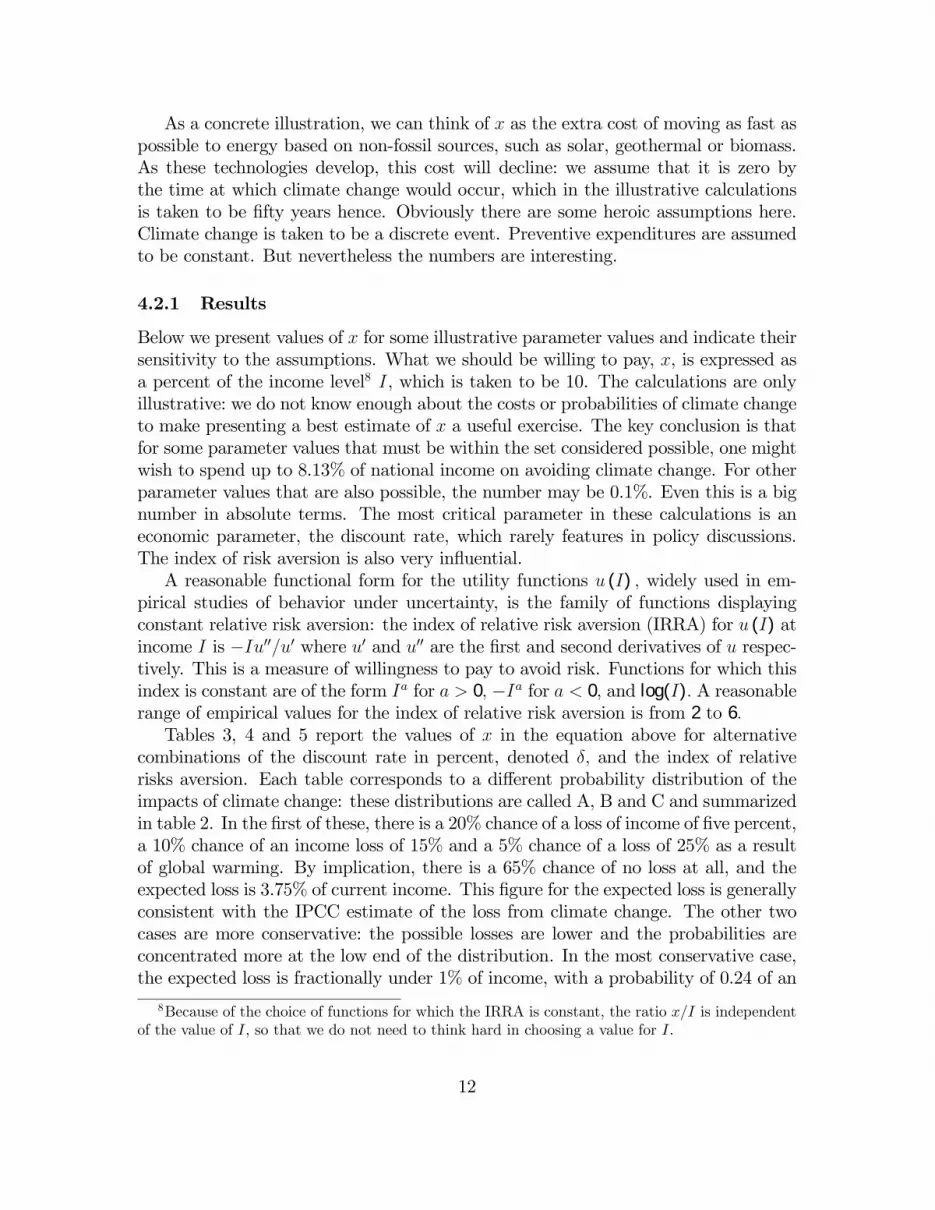
As a concrete illustration, we can think of x as the extra cost of moving as fast aspossible to energy based on non-fossil sources, such as solar, geothermal or biomass.As these technologies develop, this cost will decline: we assume that it is zero bythe time at which climate change would occur, which in the illustrative calculationsis taken to be Þfty years hence. Obviously there are some heroic assumptions here.Climate change is taken to be a discrete event. Preventive expenditures are assumedto be constant. But nevertheless the numbers are interesting.

4.2.1 Results

Below we present values of x for some illustrative parameter values and indicate theirsensitivity to the assumptions. What we should be willing to pay, x, is expressed asa percent of the income level8 I, which is taken to be 10. The calculations are onlyillustrative: we do not know enough about the costs or probabilities of climate changeto make presenting a best estimate of x a useful exercise. The key conclusion is thatfor some parameter values that must be within the set considered possible, one mightwish to spend up to 8.13% of national income on avoiding climate change. For otherparameter values that are also possible, the number may be 0.1%. Even this is a bignumber in absolute terms. The most critical parameter in these calculations is aneconomic parameter, the discount rate, which rarely features in policy discussions.The index of risk aversion is also very inßuential.A reasonable functional form for the utility functions u (I) , widely used in em-

pirical studies of behavior under uncertainty, is the family of functions displayingconstant relative risk aversion: the index of relative risk aversion (IRRA) for u (I) atincome I is −Iu00/u0 where u0 and u00 are the Þrst and second derivatives of u respec-tively. This is a measure of willingness to pay to avoid risk. Functions for which thisindex is constant are of the form Ia for a > 0, −Ia for a < 0, and log(I). A reasonablerange of empirical values for the index of relative risk aversion is from 2 to 6.Tables 3, 4 and 5 report the values of x in the equation above for alternative

combinations of the discount rate in percent, denoted δ, and the index of relativerisks aversion. Each table corresponds to a different probability distribution of theimpacts of climate change: these distributions are called A, B and C and summarizedin table 2. In the Þrst of these, there is a 20% chance of a loss of income of Þve percent,a 10% chance of an income loss of 15% and a 5% chance of a loss of 25% as a resultof global warming. By implication, there is a 65% chance of no loss at all, and theexpected loss is 3.75% of current income. This Þgure for the expected loss is generallyconsistent with the IPCC estimate of the loss from climate change. The other twocases are more conservative: the possible losses are lower and the probabilities areconcentrated more at the low end of the distribution. In the most conservative case,the expected loss is fractionally under 1% of income, with a probability of 0.24 of an

8Because of the choice of functions for which the IRRA is constant, the ratio x/I is independentof the value of I, so that we do not need to think hard in choosing a value for I.

12

income loss of 2%, a probability of 0.10 of a loss of 5% and a probability of 0.01 of aloss of 10%.9

ProbabilityLoss A B C2% 0.245% 0.2 0.24 0.110% 0.0115% 0.1 0.1020% 0.0125% 0.050 0.65 0.65 0.65

E. Loss 3.75% 2.99% 0.99%Table 2: alternative probability distributions.

As mentioned, the date for climate change C is assumed to be Þfty years, and wetake the upper limit of the sum of beneÞts T to be 1000.The following tables reports the results of solving the equation for x for these

probability distributions and a range values for the discount rate (from 1% to 5%)and for the IRRA (from 0 to 6).

IRRA 0 1 2 3 4 5 6δ1 5.74 6.07 6.42 6.81 7.22 7.66 8.132 2.15 2.32 2.50 2.72 2.96 3.23 3.543 1.05 1.13 1.23 1.35 1.48 1.64 1.824 0.56 0.61 0.66 0.73 0.81 0.89 1.005 0.31 0.34 0.37 0.41 0.45 0.50 0.56Table 3: willingness-to-pay for distribution A.

IRRA 0 1 2 3 4 5 6δ1 4.44 4.61 4.78 4.96 5.15 5.35 5.562 1.66 1.75 1.84 1.95 2.06 2.18 2.313 0.81 0.86 0.91 0.96 1.02 1.09 1.164 0.43 0.46 0.49 0.51 0.55 0.59 0.635 0.24 0.26 0.27 0.29 0.31 0.33 0.36Table 4: willingness-to-pay for distribution B.

9For an interesting review of the available evidence on the probabilities of loss from climate changesee Roughgarden and Schneider (1999), who take a range of expert opinions and Þt a systematicprobability density function to these. Geoffrey Heal is in the process of recomputing this model withthe probability-of-loss function given in Roughgarden and Schneider (1999).

13

IRRA 0 1 2 3 4 5 6δ1 1.65 1.68 1.70 1.72 1.74 1.77 1.792 0.62 0.63 0.64 0.65 0.67 0.68 0.693 0.30 0.30 0.31 0.32 0.33 0.33 0.344 0.16 0.16 0.17 0.17 0.18 0.18 0.185 0.09 0.09 0.09 0.10 0.10 0.10 0.10Table 5: willingness-to-pay for distribution C.

Can we pin down more precisely the most appropriate parameter ranges? Thequestion of risk aversion has not been studied in the context of climate change. How-ever there are many empirical studies of risk aversion in Þnance, and the range ofvalues for the IRRA considered to be appropriate there runs from 2 to 6. The issueof the right discount rate is a controversial one: one of the founders of dynamics eco-nomics, Frank Ramsey (1928) declared in a paper that is still in many ways deÞnitivethat �discounting of future utilities is unethical, and arises purely from a weaknessof the imagination.�10 This implies a discount rate of zero, which in turn implies awillingness to spend from 15% to 30% of income to prevent global warming. Mostcontemporary commentators have implicitly disagreed with Ramsey, in many caseswithout clearly stating their reasons, and for the very long time horizons involvedin climate change have worked with discount rates of 1% or 2%.11 The table makesit clear that the choice of a discount rate is critical: a general sensitivity analysisconÞrms that within the range of reasonable parameters and functional forms, this isthe central parameter. It is clear that for Þfty to one hundred years ahead, discountrates of 5%, 4% and 3% give almost no present value. At these rates, climate changesimply does not matter: it occurs on a time frame which such discount rates value atless than ten cents in the dollar. Hence the general presumption that lower discountrates are appropriate. Weitzman (1998) reports an interesting survey of the opinionsof 1,720 economists on this issue: their median response for the appropriate discountrate to be used in problems relating to global warming is 2% and the mean 4%±3%.1210As Arrow (1995, p. 16) points out, however: �When Ramsey was in a less moral mode he in fact

agreed [that the pure rate of time preference is positive]�. Arrow refers to Ramsey (1931, p. 291).11For a general discussion of these issues, see Heal (1998). Cline (1992) is an empirical study that

indicates the sensitivity of a choice to the discount rate.12Weitzman asks for a constant discount rate, although as Heal (1998) points out, the consumption

discount rate is not necessarily constant over the time spans considered (several centuries). Thisfollows from the Euler equation of a standard Ramsey problem. A slowing down of economic growthentails, for example, a lower consumption discount rate, if the utility discount rate is taken to beconstant (in a steady-state the consumption discount rate and the utility discount rate are equal).In this view, it becomes difficult to state the discount rate for long-run, large, projects.

14

0123456789

1

1.25 1.

5

1.75 2

2.25 2.

5

2.75 3

E x p e c t e d l o s s

Willi

ngne

ss to

pay

Figure 1:

Another interesting possibility, not investigated here, is the use of a non-constantdiscount rate, through logarithmic or hyperbolic discounting (see Heal (1998, chapter5) and references therein). These approaches apply discount rates that are lower, thefurther into the future the costs and beneÞts are. There is now a signiÞcant amountof evidence that this is the way in which people behave when making intertemporaldecisions. Applying this approach leads to a very signiÞcant increase in the amountthat society should be willing to pay to avoid climate change.Intuitively, one would expect sensitivity to the magnitude of the expected loss to

be important. The three probability distributions, A, B and C give some indication ofthis, which is summarized in Þgure 1, which shows willingness-to-pay in % of incomeversus expected loss in % of income for three different combinations of discount rateand IRRA. In each case the discount rate is 1% and the IRRA values used are 0, 3and 6. Willingness to pay increases more than linearly with expected loss, with thenon-linearity increasing with the IRRA13. Both willingness-to-pay and expected lossare expressed as a fraction of income, and in general the willingness-to-pay exceedsthe expected loss, a natural result of risk aversion.Figure 1. Willingness-to-pay in % of income versus expected loss in % of income

for three different combinations of discount rate and IRRA

4.3 Risk and climate change

Note that discount rates and attitudes towards risk are to some degree culture spe-ciÞc: different cultures exhibit quite different degrees of future-orientation and of risk

13Note that only three points on each curve are �real�, those corresponding to expected losses of1%, 3% and 3.75%: the rest are interpolations.

15

tolerance. The US, for example, is often characterized as a society with a high levelof impatience (a high discount rate) and a high level of risk tolerance (a low IRRA).Europe and Japan are placed by the same observers at the other end of the spectrum.If this is correct, and different countries really value avoiding climate change differ-ently, then there is scope for trade between them (see Chichilnisky and Heal (1993)for details).What are the implications of this model? Certainly one would not want to take

the numerical conclusions at face value. The point is that uncertainty, risk and ourattitudes towards risk really do matter in making policy decisions. They should betaken quite explicitly into account in formulating policy on climate change. Our Þnalpolicy analysis may be as sensitive to attitudes towards risk as to some aspects of thescientiÞc data which we work so hard to generate. Yet to date we have done little tointroduce these issues into the policy debate.In fact the role of risk and uncertainty in an analysis of policy towards climate

change goes much further. There are several dimensions of this role that merit par-ticular comment: these are the endogeneity of the risks that we face, and the factthat the risks are substantially unknown. Endogeneity of the risks is clear from thefact that they are anthropogenic: we create them as a result of our social and eco-nomic activity. It is human activity that drives biodiversity loss, climate change andozone depletion. That the associated risks are substantially unknown is also clearfrom the brief discussions above. Another difficult characteristic of climate risks isthat a large number of people face the same risks - the risks are correlated acrosslarge communities. This means that standard insurance models, relying as they doon independent risks, are probably not appropriate as mechanisms for managing therisks. It also means that we cannot argue, as for many risks (following Arrow andLind (1970)), that at the social level risks can be neglected as they affect individualsand are independent and so in the aggregate cancel out.

5 A general model

Clearly we have to work with a stochastic dynamic model in which the chance ofclimate change is affected by, and affects, economic activity and welfare. The mostnatural and widely-used model seems to be an extension of the standard optimalgrowth model along the following lines. Output is produced from capital stocks andother inputs, primarily labor. The capital stocks should include both physical capitaland natural capital, as some of the most important possible impacts of climate changeare on the productivity of natural capital, for example on the productivity of landor of Þsheries or the value that can be generated from ski resorts. Climate changecould affect land values by changing rainfall patterns, changing access to river ßow,or changing the range of agricultural pathogens.The output can as usual be consumed or invested: production also leads to a

ßow of greenhouse gases that cumulate into a stock. The size of this stock drives

16

the probability of climate change, and so can affect output. The state of the climatecan also affect welfare directly, as we may derive well-being from the climate - wemay prefer mild dry climates to hot wet ones, for example. And it can affect humanhealth via factors like the range of disease vectors. There is evidence that the rangeof malaria has increased in parts of the world in response to changes in climate andduring El Nino events the ranges of diseases such as Dengue fever appear to vary inresponse to changed climate conditions. Mathematically we are looking at a systemlike the following:

c+�K +

�A+

�S = f (K,G) (2)

u = u (c,G) (3)�G = e (K,A)− σ (S) (4)

where K is a vector of manufactured and natural capital stocks, c is consumption,G is the stock of greenhouse gases, S is the capital invested in carbon sequestration,A is investment in minimizing greenhouse gas emissions and a dot over a variabledenotes a time derivative. Some key functional relationships here, f (K,G) , e (K,A)and u (c,G) are known only with some degree of uncertainty, at least as far as theroles of the greenhouse gas stock G and of the abatement capital A are concerned.The dynamics of the greenhouse gas are shown by the third equation and this in-dicates that accumulations of certain types of capital - manufactured capital K -can affect the output of greenhouse gases. For example, the stock of coal-poweredelectricity generating plants affects the output of carbon dioxide. This relationshipmay be moderated by investment in capital A designed to minimize the output ofgreenhouse gases - for example by investment in plants designed to use fossil fuelsmore efficiently or to capture greenhouse gases rather than allowing them to escapeinto the atmosphere. It is also possible to invest in sequestering greenhouse gases, forexample by growing forests: the rate of sequestration depends on the capital invested

in this activity. For a constant climate regime we clearly need·G = 0 which implies

that e (K,A) = σ (S), the rates of emission and sequestration are equal.These considerations lead to a model that in a deterministic context is relatively

tractable. Without the complications of uncertainty we would seek to solve the prob-lem:

max

Z ∞

0

u (ct, Gt) e−rtdt subject to (5)

�Gt = e (Kt, At)− σ (S) and

�Kt = f (Kt, Gt)− ct − a− s

where s =�S ( the rate of sequestration of greenhouse gases) and a =

�A. The discount

rate is r. The presence of four state variables - greenhouse gases G, productive

17

capital K, sequestration capital S and GHG mitigation capital A - makes this acomplex problem but one that is nevertheless tractable to some degree. We can solveit by writing out the Hamiltonian and then deriving the Þrst order conditions in acompletely standard way:

H = u (ct, Gt) e−rt + λe−rt [e (Kt, At)− σ (S)] + (6)

µe−rt [f (Kt, Gt)− ct − a− s] + νe−rt [s] + ξe−rt [a]

From the choice of control variables we have

∂u

∂c= µ = ν = ξ (7)

and then the adjoint variables follow the differential equations:

�λ− rλ = − ∂u

∂G− µ ∂f

∂G(8)

�µ− rµ = −λ ∂e

∂K− µ ∂k

∂K(9)

�ν − rν = λ

∂σ

∂S(10)

�ξ − rξ = −λ ∂e

∂A(11)

We can Þnd a stationary solution to this system and then analyze how it behavesnear that solution, establishing at least the local properties of a stationary solution.However, to introduce uncertainty about some of the key functional relationshipshere - those involving the impact of greenhouse gases on welfare and production,and perhaps the effects of mitigation capital on emissions - would make the overallproblem quite intractable.In model like that just outlined, what is the role of irreversibility? The stock

of greenhouse gases G builds up as a result of economic activity. If accumulation

were truly irreversible, then we would have the constraint�Gt ≥ 0. In fact

�Gt =

e (Kt, At)− σ (S) : the Þrst term here is non-negative and the second positive. So inprinciple the stock of greenhouse gases in this model could be reduced. Most modelsin the literature also have a term like −δG in the GHG accumulation equation,representing the natural oxidation of carbon dioxide to other compounds with a halflife of about 60 years. So with sequestration and natural decay the accumulationof GHGs is certainly not irreversible, although the timescale of reduction may belong relative to that of accumulation. Nor is anything else in this framework trulyirreversible: for example, utility and production both decrease with increases inG butdecrease as G falls: there is no irrevocable change in welfare or production becauseof GHG accumulation. And the abatement capital stock A can be decumulated as

18

there is no non-negativity constraint on its rate of change. This suggests that thismodel is not ideally suited to capturing all aspects of the problem at hand. We needa framework where there is at least a possibility of a change that cannot be reversed.Some of the models discussed below have this property.

6 Modelling climate change: some Þndings

Next we review the literature on modelling climate change and the optimal level ofinvestment in the abatement of greenhouse gases. Because of the complexity of thefull problem, all the models to date have focussed on one or other of these sourcesof uncertainty to the exclusion of other aspects of the model, or have simpliÞed theframework to a discrete time two period context.

6.1 Heal

One of the earliest formal models was that of Heal (1984)14, which looked entirely atthe impact of climate change on the economy�s productivity and modelled the uncer-tainty about this in terms of a very simple stochastic process. Heal assumed that theatmosphere has a Þxed but unknown capacity to absorb greenhouse gases withoutchange and then changes discretely when this capacity is exceeded. At this pointthere is a discrete and completely irreversible change in the productivity of the econ-omy�s capital stock and in the well-being of its citizens, so this model does capturethe irreversibility of climate change. The uncertainty about the future stems fromour lack of knowledge of the level of cumulative emissions at which there will be a dis-crete change in the economic system as a result of changing atmospheric composition.This model is essentially a model of the optimal depletion of an exhaustible resource,such as fossil fuel, augmented by a relationship between cumulative fuel use and thestock of greenhouse gases. This stock triggered a change in economic productivitywhen it crossed an unknown threshold, a threshold over which we had a probabilitydistribution. This framework retains the key aspects of an optimal depletion modeland transforms the problem of managing climate change into one similar to optimaldepletion. In view of what we know almost twenty years later about the possibleresponses of the natural environment and the economy to changing atmospheric com-position this framework seems limited but it did provide a rationale for introducing aprecautionary motive for reducing the emissions of greenhouse gases and cutting backon the emissions of fossil fuels. The optimal rate of fossil fuel use was seen to declinemore rapidly relative to the situation with no climate change by an amount thatdepended on the index of risk aversion and on the characteristics of the probabilitydistribution over possible thresholds at which the stock of greenhouse gases tips theeconomy into a less productive mode. SpeciÞcally the conditional probability that

14Early related work appears in Cropper (1976) and Dasgupta and Heal (1974).

19

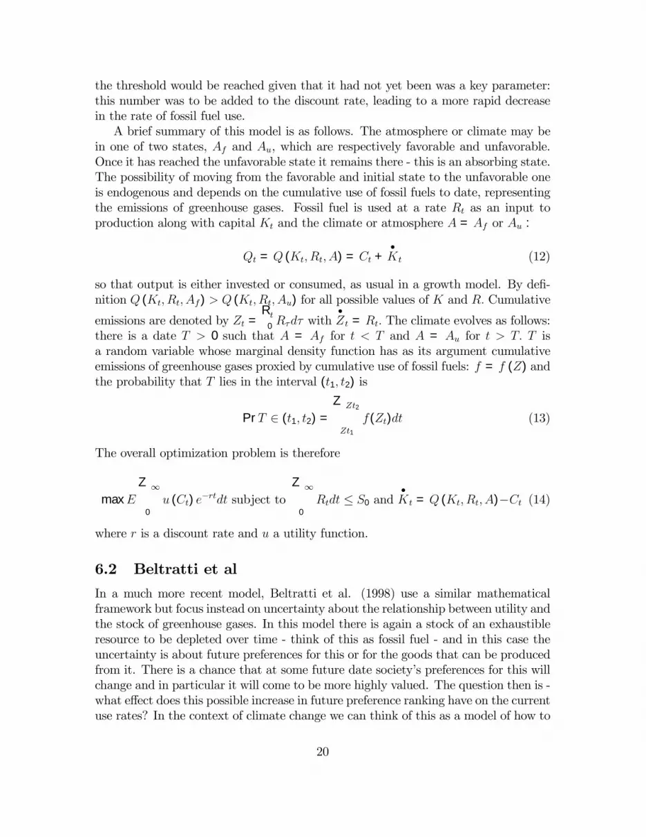
the threshold would be reached given that it had not yet been was a key parameter:this number was to be added to the discount rate, leading to a more rapid decreasein the rate of fossil fuel use.A brief summary of this model is as follows. The atmosphere or climate may be

in one of two states, Af and Au, which are respectively favorable and unfavorable.Once it has reached the unfavorable state it remains there - this is an absorbing state.The possibility of moving from the favorable and initial state to the unfavorable oneis endogenous and depends on the cumulative use of fossil fuels to date, representingthe emissions of greenhouse gases. Fossil fuel is used at a rate Rt as an input toproduction along with capital Kt and the climate or atmosphere A = Af or Au :

Qt = Q (Kt, Rt, A) = Ct +�Kt (12)

so that output is either invested or consumed, as usual in a growth model. By deÞ-nition Q (Kt, Rt, Af) > Q (Kt, Rt, Au) for all possible values of K and R. Cumulative

emissions are denoted by Zt =R t

0Rτdτ with

�Zt = Rt. The climate evolves as follows:

there is a date T > 0 such that A = Af for t < T and A = Au for t > T. T isa random variable whose marginal density function has as its argument cumulativeemissions of greenhouse gases proxied by cumulative use of fossil fuels: f = f (Z) andthe probability that T lies in the interval (t1, t2) is

PrT ∈ (t1, t2) =

Z Zt2

Zt1

f(Zt)dt (13)

The overall optimization problem is therefore

maxE

Z ∞

0

u (Ct) e−rtdt subject to

Z ∞

0

Rtdt ≤ S0 and�Kt = Q (Kt, Rt, A)−Ct (14)

where r is a discount rate and u a utility function.

6.2 Beltratti et al

In a much more recent model, Beltratti et al. (1998) use a similar mathematicalframework but focus instead on uncertainty about the relationship between utility andthe stock of greenhouse gases. In this model there is again a stock of an exhaustibleresource to be depleted over time - think of this as fossil fuel - and in this case theuncertainty is about future preferences for this or for the goods that can be producedfrom it. There is a chance that at some future date society�s preferences for this willchange and in particular it will come to be more highly valued. The question then is -what effect does this possible increase in future preference ranking have on the currentuse rates? In the context of climate change we can think of this as a model of how to

20

conserve current assets, such as natural environments or biodiversity, given that wemay value them more in the future than we do now but we are not sure when if everthis change will take place. The analytical connection with the Heal (1984) paperlies in the fact that the basic model is once again an optimal depletion model anduncertainty is again modeled by the possibility of a one time change at an unknowndate. The use of an optimal depletion model coupled with this discrete representationof uncertainty as about a one-time occurrence leads to great simpliÞcations relativeto alternatives and makes analytical solutions possible The authors incorporate adirect impact of the stock of greenhouse gases on welfare. Beltratti et al. study theemergence of option values in this framework and show that as in the Heal model theconditional probability of change given that it has not yet occurred is a key variable.This model has recently been extended by Brasão and Cunha-e-Sá (1998) and byAyong Le Kama and Schubert (2001).

6.3 Kelly and Kolstad

Kelly and Kolstad (2001) use a growth model that is a special case of the generalframework set out above to investigate two parameters claimed to be of signiÞcantimportance for climate change predictions: population and productivity growth. Theresults produced by current integrated assessment models seem to crucially dependon the assumption that both productivity and population growth are slowing downover the next century. Indeed, Kelly and Kolstad claim that integrated assessmentmodels rely on a signiÞcant slowdown in population and productivity to solve theclimate change problem. An important and apparently robust Þnding of Kelly andKolstad is that there is almost a one-to-one correspondence between population andproductivity growth assumptions, the degree of climate change, and hence the optimalresponse to climate change. Uncertainty arises here at a rather fundamental level, aspopulation and productivity are notoriously hard to predict, at least over the timespans of interest.Kelly and Kolstad use a standard Ramsey-type growth model that includes a cli-

mate component. In the calibrated version of the model, they Þnd that climate changehas little impact on the steady-state capital stock, using standard assumptions aboutthe values of the key parameters, i.e. a tapering off of population and productivitygrowth. The reason why the impact of climate change on the steady-state capitalstock is �small� is rather intuitive. If labor growth is decreasing, so will be capitalgrowth and subsequently output. This slowdown is �quick enough� according to thecalculations; the engine of growth is turned off before the climate change apparatusswitches into high gear.Clearly, what is �too fast� or �too slow� in this context depends critically on the

parametrization and the parameter values used. But the authors claim that if thereis no growth in (adjusted) labor, temperature increases are virtually zero (only drivenby current inertia) and that this is a robust result. On the other hand, if current

21

trends are to be continued, so that the two key parameters are roughly constant, thenthere are signiÞcant impacts on steady-state capital stocks.Kelly and Kolstad propose that we add a �baby tax� to a carbon-tax, because

exogenous population growth is another way of inducing climate change. Given thatpopulation growth is exogenous, the �baby tax� should be interpreted as the socialnet value of one additional person. Moving down the family tree, we see that thebirth of one person literally induces carbon emissions indeÞnitely. Hence the claimthat the �baby tax� should be set such that it incorporate damages from emissionsin the future. The welfare economics of population growth raises profound questions,not the least empirical ones (how is one to go about placing a value on those yetunborn?). Furthermore, population growth cannot be positive forever, if only forspace considerations. Yet the point Kelly and Kolstad make is an important one inunderstanding the output from the many integrated assessment models in currentuse.A policy conclusion that does seem to follow is that laxer climate controls may be

defended by pointing to forthcoming demographic problems (the �graying Europe� isa case in point) Bringing uncertainty proper into a model with similar characteristicsmay turn the Kelly and Kolstad argument on its head, at least according to Pizer(1998), to which we now turn.

6.4 Pizer

Pizer�s (1998) model allows for many different states of nature, includes econometricestimates of key technology and preference parameters (rather than �best guesses�)and has consistent welfare aggregation of uncertain utilities15. A representative con-sumer maximizes a Von Neumann-Morgenstern utility function within a stochasticgrowth model that has a climate component (from the DICE-model). The utility func-tion has constant relative risk aversion and a Þxed utility discount rate is assumed.Production (Cobb-Douglas technology) is a function of capital and augmented labor.Net labor productivity is related to the costs of controlling damages; essentially aquadratic damage cost function is used (for temperature changes less than about 10degrees Celsius). Exogenous labor productivity is a random walk (in logarithms).This formulation implies that exogenous productivity growth slows down over time(and begins at about 1.3%, according to Pizer�s estimates). Population growth, whichis exogenous, is modelled in a similar manner. Emissions are proportional to BAU-output and endogenous emission reductions. A simple climate module completes themodel.The empirical model encompasses a rich set of different uncertainties, including

15Well-known models in this literature include the DICE-model (Nordhaus (1994)) and the Global2100 model (Manne and Richels (1992)). For a survey, see e.g. the special issue of Energy Journal,1999. Nordhaus and Boyer (2000) compares several integrated models, including RICE-99 andDICE-99.

22

uncertainty utility, cost and technology parameters, as well as parameters describ-ing the development of carbon dioxide in the atmosphere. The econometric modelcombines data with a prior distribution over the parameters, i.e. Bayesian analysisis used. Data from the national accounts covering the US over the period 1952-1992are used to estimate structural parameters, such as time preference, productivitygrowth and capital share. In this way, the marginal distribution of each parameter isobtained, which then provides a coherent way of describing parameter uncertainty.According to Pizer (1998), the impact of general parameter uncertainty shows

most clearly in the long-run; short-run responses are rather similar, whether or notuncertainty is included. He Þnds that productivity slowdown encourages stricter op-timal regulation, thus reversing the Kelly and Kolstad conclusion. The explanationis, according to Pizer, related to how damages are discounted. Slower productivitygrowth tends to depress interest rates (this follows from the Euler equation). Con-sequently, if damages are discounted with a lower discount rate, the present valueof those damages is higher. Thus, from the point of view of �today� the value ofavoiding climate damages in the future gets a relatively higher value.A puzzling result is that if best-guessed parameter values are imposed, this pro-

duces a path with lower welfare, compared to the case when uncertainty is explicitlyhandled. It appears as if the stricter policy associated with uncertainty case winsmore often than it loses, because the gains from avoiding large losses in a bad stateof the world, outweigh the cost of overcompliance in the good states. This is re-lated to Weitzman�s (1974) price versus quantity result. In Pizer�s (1998) model, themarginal beneÞt curve is relatively ßat compared to the marginal cost curve. If fol-lows from Weitzman (1974) that taxes tend to give lower efficiency losses, comparedto a quantity instrument, in such settings (see Dasgupta (1982) for a useful discussionof instrument choice under uncertainty)). The proposition that tax instruments areto be preferred in climate policy has some general support, see e.g. Toman (2001).Finally, we note that the model appears to be rather sensitive to climate parame-

ters. This seems, at least, to be true for the original DICE-model and there are goodreasons to believe that this conclusion carries over. An important parameter is theclimate sensitivity, which is set to 2.9 degrees Celsius in the standard DICE model.It is allowed to vary in Pizer�s model according to a uniform 5-point distribution onthe interval (1.5-4.5). Keller et al (2000) illustrate the key role played by this param-eter in their analysis of potential thermohaline collapse, within a slightly modiÞedDICE-model.

6.5 Irreversibility, option values and precaution.

There is a group of papers that focus on the modeling of irreversibility and thepossibility of an option value, as discussed above. These include Fisher and Narain(2002), Gollier et al. (2000), Kolstad (1996 a,b), Pindyck (2000), Ulph and Ulph

23

(1997), and several others.16 We group them together because they have many pointsin common. In an interesting and provocative paper, Ulph and Ulph focus directlyon the question of whether there are option values associated with the preservationof the existing climate system. As already noted, the preconditions necessary for theexistence of an option value seem to be satisÞed in the context of climate change.We expect to learn about the costs of climate change and about the costs of avoidingit over the next decades. And we expect that some of the decisions that we couldtake will have consequences that are irreversible. These are the hallmarks of decisionsthat give rise to option values associated with conservation - the pioneering studiesby Arrow and Fisher (1974) and by Henry (1974a,b) have exactly these properties.But although these conditions are necessary for the existence of option values theyare not sufficient. Kolstad uses a similar framework and asks a similar question: itis to his paper that we owe the observation that there is another possible real optionvalue at work here. If substantial sunk costs must be incurred to begin the processof abating greenhouse gas emission and avoiding or minimizing climate change, ifthe return to this investment is the avoidance of climate change, and if we learnabout the value of this over time, then there is also a real option value associatedwith postponing investment in greenhouse gas abatement. So in Kolstad�s model,which like the general model above has both GHG accumulation and investment inabatement capital, there are two option values acting in opposition in this framework.Both Ulph and Ulph and Kolstad use a result of Epstein�s (1980) which can be appliedto the analysis of learning and option values: this is in some sense a generalizationof the famous papers by Henry and Arrow and Fisher and gives conditions that arenecessary and sufficient for the existence of option values. Ulph and Ulph and Kolstadgive conditions under which there are option values associated with the preservationof the existing climate regime, and it is clear that these conditions are quite restrictive- although there is no suggestion that they are necessary. Ulph and Ulph, Kolstadand Fisher and Narain specialize to discrete time two or three period models in orderto Þnd solutions. An unattractive feature of the Epstein result, and of some othersbased on it, is that the third derivative of the utility function is a key variable: aninequality involving this third derivative determines whether or not there is an optionvalue. From a decision-making perspective this is unappealing: we clearly have littleor no idea about the sign, let alone the value, of the third derivative, although it hasto be recognized that in other problems involving choice under uncertainty the thirdderivative of the utility function has been a key variable. Fisher and Narain have amore encouraging outcome: in their formulation the index of relative risk aversion isthe important parameter. Their paper has a good summary of earlier results in itsintroduction, and makes an interesting observation about irreversibility of investmentin abatement capital: they note that there are two possible interpretations here. One

16See also the early and inßuential papers by Malinvaud (1969) and Freixas and Laffont (1984),the results of which are incorporated in many of the papers that we review. Another recent paperthat we do not review in detail for reasons of space is Torvanger (1997).

24

is to measure irreversibility by the durability of the capital, as in the Kolstad paper:the other is to deÞne investment in abatement capital as irreversible if that capitalis �non-shiftable� in the terminology of optimal growth theorists (Arrow and Kurz(1970)) - i.e. if it cannot be consumed or used in some other sector. Fisher andNarain note that the consequences of irreversibility of abatement investment dependon which of these deÞnitions one uses, and that they are somewhat more intuitiveif one uses the conventional optimal growth interpretation of irreversibility. Fisherand Narain also compare results with exogenous and endogenous climate risks - i.e.in the cases where the probability distribution of damages due to greenhouse gasaccumulation is affected by the stock of greenhouse gases. The other papers take thisdistribution to be exogenous.Pindyck works with the most general of the models in this category, using a multi-

period stochastic optimal growth model. Not surprisingly he gives only numericalsolutions, and offers a very appropriate summary of the issues and of why it provesdifficult to reach Þrm conclusions about the nature and direction of option values.He comments that �I have focused largely on a one-time policy adoption to reduceemissions of a pollutant. If the policy imposes sunk costs on society, and if it can bedelayed, there is an opportunity cost of adopting the policy now rather than waitingfor more information. This is analogous to the incentive to wait that arises withirreversible investment decisions. In the case of environmental policy, however, thisopportunity cost must be balanced against the opportunity �beneÞt� of early action- a reduced stock of pollutant that might decay only slowly, imposing irreversiblecosts on society.� He goes on to make comments that are speciÞc to his particularmodel structure, but are nevertheless enlightening on how things work in this context.�In the simple models presented in this paper, an increase in uncertainty, whetherover future costs and beneÞts of reduced emissions, or over the evolution of thestock of pollutant, leads to a higher threshold for policy adoption. This is becausepolicy adoption involves a sunk cost associated with a discrete reduction in the entiretrajectory of future emissions, whereas inaction over any small time interval onlyinvolves continued emissions over that interval...... The validity of this result dependson the extent to which environmental policy is indeed irreversible, in the sense ofinvolving commitments to future ßows of sunk costs.� An interpretation of this seemsto be that if policies are ßexible and do not necessarily involve commitments to theircontinuation over long periods, then the asymmetry that he Þnds would vanish andthere would no longer be a tendency of greater uncertainty to favor a more cautiousadoption of policies. This in turn suggests that we need to spend more time thanwe have thinking about the design of policies in this area, and in particular ensuringthat they are ßexible and permit changes in response to new information.Gollier et al. (2000) tackle a similar set of questions but from a slightly different

perspective. They use the idea of the �precautionary principle� as the organizingtheme of their work. They quote the 1992 Rio Declaration (Article 15) as a state-ment of this: �where there are threats of serious and irreversible damage, lack of full

25

scientiÞc certainty shall not be used as a reason for postponing cost-effective mea-sures to prevent environmental degradation.� The reference to scientiÞc uncertaintyhere implies, for the authors, the possible resolution of this uncertainty by researchand learning. Most economists, if asked to think of a justiÞcation for this principle,would probably couch it in terms of learning, irreversibilities and option values, sointuitively we think we two are related. Gollier et al note that in fact the precau-tionary principle can be given a formal justiÞcation without invoking irreversibilities,just assuming a stock damage effect and possible learning over time. They considertwo economies that are identical except in the way the information structure evolvesover time. They then say that the precautionary principle holds if in the economy inwhich more information becomes available over time we do not invest less in damageprevention: for them the essence of the precautionary principle is a positive relation-ship between information acquisition and precaution. They note, as in most of themodels already discussed, that there are two contradictory effects. One is that we in-vest less in prevention in the economy which may learn more because this investmentmay be inefficient: when we know more we may be able to choose better investments.They describe this as the �learn then act� strategy. The opposing tendency is gen-erated by the fact that if we follow this strategy then the risk that society faces inthe future will be greater. The principle result of the Gollier et al paper is that thebalance between these two effects depends on the shape of the utility function andin particular on whether or not society shows �prudence�. Prudence is equivalentto a positive third derivative of the utility function: a prudent person increases hersavings in the face of an increase in the risk associated with future revenues (Kimball(1990)). For a class of utility functions Gollier et al. give necessary and sufficientconditions for the precautionary principle to hold, but note that outside of this classthere are no general results. They then go on to consider the relationship betweenthe precautionary principle and irreversibility.In a very interesting paper, Carpenter, Ludwig and Brock (1999) set out a rad-

ically different approach. Their paper is not in fact about climate change: the ti-tle is �Management of Eutrophication for Lakes Subject to Potentially IrreversibleChange.� The problem addressed can be summarized as follows. In a farming region,such as the mid West of the USA, phosphorous P is applied as a fertilizer to the landaround a lake and some of it runs from there into the lake. In sufficient concentrationin the lake, it can cause a change in the biological state of the lake, to a potentiallystable state of eutrophication in which the lake is unproductive for most human uses.So eutrophication is irreversible. The response to P concentration is highly non-linearand the concentration of P depends not only on the runoff but also on temperatureand rainfall, which are random. How should we manage the runoff of P over time tomaximize the expected discounted value of beneÞts net of the costs of P mitigation?This problem has all the structure of the climate problem: indeed as we said in theÞrst discussion of irreversibilities, the climate system is a complex nonlinear dynami-cal system that may change regime under human perturbation. This is exactly what

26

Carpenter, Ludwig and Brock model treats, though for a more Þnite problem. Theytalk about the concept of resilience, �the capacity of a non-linear system to remainwithin a stability domain....� This concept has been widely used in mathematicalecology. They model the dynamics of the interacting lake and agricultural systemsas a nonlinear dynamical system with several different locally stable states, one ofwhich is highly unattractive. Avoiding this state is costly, so that there are trade-offsto be made. And the stochasticity of the weather means that the problem has tobe seen in probabilistic terms. An interesting conclusion that these authors reach isthe following: �An important lesson from this analysis is a precautionary principle.If P inputs are stochastic, lags occur in implementing P input policy, or decisionmakers are uncertain about lake response to altered P inputs, then P input targetsshould be reduced. In reality, all of these factors - stochasticity, lags, uncertainty -occur to some degree. Therefore, if maximum economic beneÞt is the goal of lakemanagement, P input levels should be reduced below levels derived from traditionallimnological models. The reduction in P input targets represents the cost a decisionmaker should be willing to pay as insurance against the risk that the lake will recoverslowly or not at all from eutrophication. This general result resembles those derivedin the case of harvest policies for living resources subject to catastrophic collapse.�They go on to say that �We believe that the precautionary principle that emergesfrom our model applies to a wide range of scenarios in which maximum beneÞt issought from an ecosystem subject to hysteretic or irreversible changes.�The model of Carpenter and coauthors seems very readily applicable to climate

change: as we have noted above, the climate system may in some respects be irre-versible and in some aspects it can be modelled as a dynamical nonlinear system withseveral basins of attraction - this is the way in which climate modelers represent thealternative states of thermohaline circulation and the Gulf Stream. And even if weare dealing with aspects of the climate system that do not have this characteristic,the changes in ecosystems driven by the climate are very likely to have exactly thecharacteristics considered by Carpenter, Ludwig and Brock (1999). So consideringthe climate system and its ecological consequences, which is what is relevant from thesocial and economic perspective, this seems like a productive framework. In this con-text the precautionary principle enunciated by Carpenter, Ludwig and Brock (1999)is thought-provoking. Little as clear as this has emerged from the other models citedhere. Their result is suggestive of the certainties of the early papers of Arrow-Fisherand Henry. In part this probably reßects the advantages of modelling the system�sdynamics explicitly, and perhaps also reßects the fact that the Carpenter et al. omits- quite legitimately in their context - one issue that is central to the work of Kolstad,Ulph and Ulph and others cited above. This is the need to make a durable investmentin greenhouse gas abatement. In controlling the runoff of P there is no equivalent: theapplication of P can be controlled on a day-to-day basis and can be decreased withoutprior investments in capital equipment. It would be of great interest to know whetherthe Carpenter, Ludwig and Brock results would survive the need for investment to

27

control P runoff.

7 Climate change and risk management

Next we discuss the institutional framework with which we could manage the risksarising from climate change. Economists have two standard models of risk-allocationin a market economy. The more general is that of Arrow and Debreu, in whichagents trade �contingent commodities�. The alternative is the model of insurancevia risk-pooling in large populations. Neither can address fully all the particularcharacteristics of global environmental risks. In particular, both assume the risks tobe known in some sense, and to be exogenous.In the Arrow-Debreu framework there is a set of �states of nature.� The proba-

bilities of these being realized are exogenous and these states represent the sources ofuncertainty. Classically one thinks of events such as earthquakes and meteor strikes.Their occurrences are assumed to be exogenous to the economic system, and notaffected by economic activity. Agents in the economy are allowed to trade com-modities contingent on the values of these exogenous variables. These are called�state-contingent commodities�. With a complete set of markets for state-contingentcommodities, the Þrst theorem of welfare economics holds for economies under un-certainty: an ex-ante Pareto efficient allocation of resources can be attained by acompetitive economy with uncertainty about exogenous variables.Arrow showed that efficiency can in fact be attained by using a mixture of securi-

ties markets and markets for non-contingent commodities, so that a complete set ofcontingent commodity markets is not required. This observation provides a naturaland important role for securities markets in the allocation of risk-bearing. The se-curities used are contracts that pay one unit if and only if a particular state occurs.While the contingent contract approach is in principle all-inclusive and covers mostconceivable cases of uncertainty, in practical terms there are cases where it can be im-possible to implement. It can be very demanding in terms of the number of marketsrequired. For example, if agents face individual risks (i.e., risks whose probabilitiesvary from individual to individual), then in a population of 100 similar agents eachof whom faces two possible states, the number of markets required would be 2100 (seeChichilnisky and Heal (1998)). The number of markets required is so large as to makethe contingent contract approach unrealistic.The use of insurance markets for pooling risks is a less general but more practical

alternative. This requires that populations be large and that the risks be small,similar and statistically independent. The law of large numbers then operates and thefrequency of occurrence of an insured event in a large sample of agents approximatesits frequency in the population as a whole. To be precise, assume that each ofN people faces a loss of L with probability π, and an insurance company insuresthem against this loss. Assume the losses are independent. The loss rate for thepopulation is the expected claims divided by the total insurance offered. A 95%

28

conÞdence interval for this is just π ±√π[1−π]√N

so that the loss rate converges to theactuarial probability as the population increases. There is thus a role for insurancecompanies to act as intermediaries and pool large numbers of similar but statisticallyindependent risks. In so doing they are able via aggregation and the use of the lawof large numbers to neutralize the risks faced by many similar agents. The mainreferences on this are Arrow and Lind (1970) and Malinvaud (1972, 1973).The insurance approach is at a disadvantage when risks are correlated. When large

numbers are likely to be affected at once, risk-pooling will not work. However it doeshave the advantage relative to the contingent market approach of economizing dra-matically on the number of markets needed. In the above example, only two mutualinsurance contracts and 2809 securities would be needed instead of 2100 contingentcontracts.

7.1 Unknown risks

When risks are allocated by trading state-contingent commodities securities, or byrisk-pooling and insurance, it is very important that agents know, or believe that theyknow, the relative frequencies of the states of nature, at least approximately. Thisis obvious when trading insurance contracts. The actuarial calculations needed toset insurance premia can only be performed if the parties believe that the relativefrequencies of the insured events are approximately known.In the Arrow-Debreu approach, it suffices to think of agents maximizing expected

utility to appreciate the need for them to know, or at least behave as if they know, therelative frequencies of exogenous states. These frequencies are the weights placed ontheir utilities from state-dependent consumption. The point is simple: if agents cannot assign relative frequencies then their preferences are not well-deÞned and theycannot act to maximize expected utility.As we have noted above, in the context of such risks as climate change, ozone

depletion and in particular biodiversity loss this is probably much too demanding.Agents, even experts, do not know the frequencies of different states, and recognizethat they do not know them. The reviews by Roughgarden and Schneider (1999) andthe IPCC TAR of expert judgements on the impact of climate changes emphasizesthis. They recognize that there are several different opinions about what these are,but feel unable to choose deÞnitively between these alternatives. In such a case, it isnatural to think of the frequency distribution over environmental changes as a stateof the world, a risk, in the Savage sense: we do not know what value it will assume,and whatever value this is, it affects economic activity. Ignorance then assumes therole of a collective risk, and can be treated by the use of state-contingent markets.Chichilnisky and Heal (1993, 1998) formalize this type of situation in a simple

general equilibrium model. Each agent faces the risk of being in one of several states(e.g. healthy or sick, productive or unproductive, environmentally impoverished ornot, etc.). No-one knows what will be the true frequency distribution of affected

29

agents. A probability is assigned to each of several frequency distributions thoughtto be possible. A typical probability distribution of this type might state for examplethat there is a 10% chance that 90% of the population will be harmed by global warm-ing, a 25% chance that 50% of the population will be harmed, etc. The probabilitydistribution over alternative frequency distributions may be different from individualto individual. Again this is consistent with the expert opinions on climate changesummarized by Roughgarden and Schneider.In this framework, we have two levels of uncertainty. The Þrst level of uncertainty

is collective: what is the distribution of agents who are harmed in the economy? Will90% be harmed, or only 30%? This is a question about the aggregate incidence ofthe phenomenon over the population as a whole. This risk represents or arises fromour lack of knowledge of the phenomena at stake.The second level of uncertainty is individual: it is uncertainty about whether a

given agent is harmed or not by climate change. It devolves about questions such as:given that 90% of the population will be harmed or environmentally impoverished,will a particular agent be harmed or not? The issue here is: contingent on a particularoverall incidence of the phenomenon, who are the agents who will be affected?Chichilnisky and Heal (1998) suggests an institutional structure which uses two

types of Þnancial instruments which are tailored to these two aspects of the problem.These can lead to efficient allocation in the face of such risks. One instrument isa mutual insurance contract to deal with the risks faced by agents or communitiescontingent on each possible distribution of harmful effects worldwide. A mutual in-surance contract is an agreement between parties subject to similar risks that thosewho are harmed will be compensated by the others. Examples are agricultural coop-eratives of the type recorded in Europe at least since the Þfteenth century, and thenineteenth century U.K. workers� associations and friendly societies. These involvedagreements between a group of workers that if one were sick and unable to work, heor she would be compensated by the others. In the present context, one could thinkof groups of communities subject to the possible impact of climate change, with thoseunharmed compensating the others. Making the terms of such a mutual insurancecontract contingent on the distribution of harmful effects worldwide means that thereis a different compensation agreement between the parties for each possible aggregatedistribution of harmful effects. To know what compensation is due in any particularcase, the parties have Þrst to assess the distribution of harmful effects globally, andon the basis of this decide which mutual insurance contract to apply.Having dealt with individual risks by mutual insurance, we still face collective

risks. We need statistical securities to deal with these collective risk induced byuncertainty about the overall distribution of adverse effects. Arrow securities aredeÞned as securities that pay one dollar if and only if a particular state of the worldoccurs. Statistical securities pay one dollar if and only if there is a particular frequencyof affected parties in the population, i.e., if and only if there is a particular statisticalstate, a state of the economy with speciÞed statistical characteristics. As already

30

noted, the incidence of impacts on the population as a whole is being treated as a�state of the world� in the Arrow-Debreu sense. We treat each possible distributionof adverse affects as a distinct collective state (called a statistical state), and usesecurities markets to enable parties to transfer wealth between these states. Onestatistical security is needed for each possible distribution of adverse effects worldwide,because to attain Pareto efficiency each separate state must be covered by a security.The core of the results in Chichilnisky and Heal is that with unknown risks we cantrade securities contingent on statistical states and this can allow the uncertaintyintroduced by alternative probability distributions to be fully hedged.There are two features of the results which are of general interest. One is the

development of a framework for achieving efficient allocations in the face of uncertainindividual risks. Given rapid changes in technology with potentially far-reaching en-vironmental impacts and health effects, the problem of providing insurance againstsuch risks is particularly important. It is a matter of very active concern in the insur-ance industry. The second interesting feature is the way a combination of securitiesmarkets and insurance markets can be used to provide a relatively simple institutionalstructure for dealing with unknowable risks. Current trends in the securitization ofcertain risks are consistent with this analysis. In Chichilnisky and Heal (1998) itis shown that under certain simplifying assumptions this framework will lead to anefficient allocation of risks in a competitive general equilibrium model. SubsequentlyKlimpel and Requate (2000) generalized these results.Another radically different approach to the fact that risks are unknown has been

explored by Henry and Henry (2000). A central feature of their analysis is an explicitrecognition that we do not have a complete probability distribution over possibleclimate change events and consequences. There may be changes and consequencesthat we have not yet envisaged. In such a case the probabilities that we assign tothe events about which we do have information must sum to less than one, to leaveroom for the unknown events. So what we have to work with is a measure on theset of known possible events, whose integral is less than one. And even on the eventsabout which we know something, it is possible that our beliefs can not be describedby a measure that satisÞes the conditions that are needed for it to be a part of aprobability distribution: they may be too imprecise for this. Implementing theseobservations, which seem quite compelling in the climate change context, requiresthat we work within the framework of non-additive probabilities on the state space.The prerequisites for following such arguments in detail are more demanding thanthose for most of the literature that we have reviewed, so we will merely mentionthis approach, which to us looks particularly promising, and note that it providesanother context in which one can formalize a precautionary principle. Precautionarybehavior is now motivated in part by the possibility of events and outcomes that wecannot characterize. One is reminded of Hamlet�s thoughts on death:

The dread of something after deathThat undiscovered country from whose bourn

31

No traveller returns, puzzles the willAnd makes us rather bear those ills we haveThan ßy to others that we know not of.

Shakespeare seems to have anticipated the precautionary principle here.

7.2 Endogenous risks

The risks we face in environmental change are not only not well known: they are alsonot exogenous. Almost by deÞnition, they are endogenous and are determined byour behavior. In effect we both create states of nature and determine the probabilitydistributions over these. By creating the states of nature we mean that human actionsmake possible states of the planetary systems that would not otherwise occur. Forexample, human actions are leading to patterns of land use and of species diversitythat certainly would not have occurred without our actions: intensive agricultureis a form of land use that would not have arisen without human activity, and thetransportation of exotic species, a major threat to biodiversity, is also uniquely aproduct of the patterns of human activity.In all of the classical models of risk management discussed above, it is assumed

that the risks faced are exogenous: that is, they are not affected by human actions.At the microeconomic level, the fact that human actors can affect the probabilitiesof the risks that they face has long been recognized as a serious problem for theoperation of insurance markets, under the title of moral hazard. The focus in thisliterature has been on the fact that offering insurance to a person may lead her tobehave in a way that alters the risk that she faces. Deductibles and co-insurance havebeen the recommended solutions to the problems that this creates for attaining anefficient allocation of the risks - although they do not lead to a Þrst best outcome.More recently there has been a literature on endogenous uncertainty in a general

equilibrium context.17 This literature has addressed the issues that arise when agentsare uncertain about the values of endogenous variables. A good example is providedby uncertainty about the values of stock prices or of exchange rates. The naturalquestion is whether we can use the device of trading state-contingent contracts tohandle this uncertainty. In this case the contracts would have to be contingent onthe prices about which agents are uncertain. These have been termed price contingentcontracts, or PCSs. It is possible to construct an institutional framework within whichtrading price-contingent contracts will lead to a fully efficient insurance of the risksassociated with uncertainty about prices, and this leads quite naturally to a generalequilibrium theory of the role and pricing of derivative securities. The frameworkinvolves trading securities contingent on the prices that are realized at equilibriumin a market for PCSs that operates before the market for goods and services opens.

17For dynamic general equilibrium models that includes endogenous probability for climatic catas-trophes, including cost-beneÞt rules, see e.g. Backlund et al (2000).

32

Heal (1995) considers an exchange economy augmented by the possibility of tradingprice contingent securities which pay a speciÞed sum if and only if the equilibriumprice vector assumes a speciÞed value. Prices play the role played by �states ofnature� in the Savage framework, so the determination of the state is endogenous.Agents have expectations about possible prices, and trade price contingent securitiesto insure price risks. They use these securities to exchange income in price states inwhich they are well off for income in states in which they are badly off. Before anequilibrium price emerges agents trade these securities, shifting income across pricestates. This changes their endowments in the exchange economy, which now becomeprice contingent.How does this relate to the endogeneity of environmental uncertainty? The simi-

larity is that the possible environmental states and their probabilities are determinedby human actions, indeed in part by the equilibrium of our economic system and theenvironmental impacts of the selected activities. The analogy with endogenous priceuncertainty suggests an approach based on trading securities contingent on the envi-ronmental states before these are realized. This would involve markets on which wetrade securities that pay dependent on the amount of climate change and its locationand timing, or on the state of the ozone layer in a given year, or on the state of biodi-versity. So we would have markets for climate bonds, or ozone bonds or biodiversitybonds. In case this sounds exotic, note that Wall Street already trades hurricanebonds, earthquake bonds, catastrophe futures, Act-of-God bonds and a few others.All of these exist for the purpose of shifting the risks associated with environmentalphenomena.How would such instruments work and what would they contribute? The payoffs

from these bonds would shift endowments around in a way that depended on thestate of the environment, making the distribution of endowments in the rest of theeconomic system contingent on the state of the environment, just as PCSs makethe distribution of endowments contingent on the vector of equilibrium prices in ageneral equilibrium model with price uncertainty. Given a state of the environmentand a distribution of endowments resulting from environment-contingent bonds, tradewould then occur as normal and would lead under the right conditions to an efficientallocation of resources.By following the arguments in Heal (1995), we can show that this system has

a competitive equilibrium at which all agents are insured to precisely the degreethat they want against the risks associated with not knowing what the states ofthe environment and economy will be. The markets for securities contingent onthe state of the environment and the economy will provide an efficient allocationof the risks arising from environmental uncertainty. The kinds of markets we havein mind here are exempliÞed by markets in which one can insure against a certainlevel of climate change and its economic consequences, captured in the model bythe environmental state e and the price vector p. Such markets do not currentlyexist, but markets for securities continent on the state of the environment do exist,

33

in the form of hurricane bonds and weather swaps. There is currently a proposal tointroduce a tradable index of the state of the ENSO (El Nino-Southern Oscillator)cycle, which would be a move closer to a general security whose payoff depends onthe state of the climate system. Note that although these markets would allocateefficiently the risks of environmental change, they would not lead to a Pareto efficientallocation, as the externalities associated with behavior that affects the climate arenot corrected. That would require a separate set of policy instruments, such as theclassical corrective taxes and subsidies or the use of tradable permits. In the formalmodel presented above, there is no explicit connection between the acts of any oneagent and the probabilities of the states e ∈ E, so that these externalities are notaddressed. However, if corrective taxes or equivalents (such as permit markets) werein place, then the outcome of these markets would be a Pareto efficient allocation.

8 Conclusion

Climate change involves uncertainties in a breathtaking number of dimensions, includ-ing, but not limited to, the Þelds of natural science and economics. This paper triesto show why economic analysis that explicitly incorporates uncertainty gives somevaluable insights into the policy issues raised by the possibility of climate change.True, even if the underlying problems were deterministic, then the economics of thisissue would pose many interesting challenges, but formal analysis of decision makingunder uncertainty must certainly play a dominant role in any economic discussionabout climate change policy.A Þrst point that we make may seem self-serving to non-economists, yet its im-

portance is often overlooked in a discussion that gravitates too much towards thescientiÞc uncertainties. Both empirical and theoretical studies show that we shouldworry not only about disentangling nature�s true blueprint but also about uncertain-ties that are intrinsic to the economic system, such as discount rates, growth rates andthe rate of technological advance. After all, the engine of growth is a driver of climatechange and understanding the relevant parts of the economic system should help usmake better predictions. Our survey of some of the relevant empirical evidence doesbring this point home rather forcefully.There is a signiÞcant economic literature on irreversibilities, option values and the

value of ßexibility, and this literature plays a dominant role in our discussions. Akey insight from this literature is that option values have two dimensions: there is avalue of waiting for more information in order not to destroy irreversibly some naturalprocess, but there is also a value of waiting to invest scarce resources in abatementtechnology. While the relevant empirical evidence on option values is scarce, to saythe least, economic theory gives some useful leads on where to look further and whyone needs to strike a balance between countervailing forces.To this we must add the sobering fact that there are future unknown risks that

will require scarce economic resources. Somehow we need to Þnd a balance between

34

allocating resources to risks that are known today and to future unknown risks. AsWildawsky (1988, p. 217) eloquently put it �Insofar as we today should consider thewelfare of future generations, our duty lies not in leaving them exactly the social andenvironmental life we think they ought to have, but rather in making it possible forthem to inherit a climate of open choices. That is, in leaving behind a larger level ofgeneral ßuid resources to be redirected as they, not we, see Þt.� Climate policy thatproperly takes into account the value of ßexibility and adaptation seems to be themost promising way of satisfying this recommendation.

9 Acknowledgments

We are grateful to Max Auffhammer, Claude Henry, Mark Machina and Art Smallfor valuable comments and suggestions on this paper.

10 References

Acemoglu, D., Johnson, S. and J.A. Robinson (2001) �The Colonial Origins of Com-parative Development: An Empirical Investigation�, American Economic Review ,91, 5, 1369-1401.Arrow, K.J. (1995) �Intergenerational Equity and the Rate of Discount in Long-

Term Social Investment�, IEA World Congress, December 1995. Stanford, Depart-ment of Economics, Working Paper 97-005.http://www-econ.stanford.edu/faculty/workp/swp97005.html.Arrow, K.J. and A.C. Fisher. (1974) �Environmental Preservation, Uncertainty

and Irreversibility�. Quarterly Journal of Economics, 88, 2, 312-319.Arrow, K.J. and M. Kurz (1970). Public Investment, the Rate of Return, and

Optimal Fiscal Policy. Published by the Johns Hopkins Press for Resources for theFuture Inc.Ayong Le Kama, A.D. and K Schubert. "Growth, Environment and Uncertain

Future Preferences." Working Paper, EUREQua, Université de Paris I.Arrow, K.J. and R.C. Lind. (1970) �Uncertainty and the Evaluation of Public

Investment Decisions�. American Economic Review, 60, 3, 364-378.Backlund, K. , Kriström, B., Löfgren, K.-G. and E. Samakovlis (2000) �Global

Warming and Dynamic Cost-BeneÞt Analysis Under Uncertainty�: An EconomicAnalysis of Forest sequestration Options�, Working Paper, Department of ForestEconomics, SLU-Umeå.Beltratti, A., Chichilnisky, G. and G.M. Heal. (1998) �Uncertain Future Prefer-

ences and Conservation�. in Sustainability: Dynamics and Uncertainty. Chichilnisky,G., Heal, G.M. and A. Vercelli (eds), Kluwer, Dordrecht.Brasão A. and M. Cunha-e-Sá. (1998) �Optimal Growth, Uncertain Future Pref-

erences and Preservation.� Universidade Nova de Lisboa, Faculdada de Economia.

35

Paper Presented at the First World Congress, EARE/EAERE, Venice, June 25-27.Carpenter, S.R., Ludwig, D. and W.A. Brock. (1999) �Management of Eutrophi-

cation for Lakes subject to Potentially Irreversible Change�. Ecological Applications,9, 3, 751-771.Chichilnisky, G. and G.M. Heal (1998) �Catastrophe Futures: Financial Markets

for Unknown Risks�. In Chichilnisky, G., Heal, G.M. and A. Vercelli (eds.) Sustain-ability: Dynamics and Uncertainty, Kluwer, Dordrecht.Chichilnisky, G. and G.M. Heal (1993) �Global Environmental Risks� Journal of

Economic Perspectives, 7, 4, 65-86.Cline, W. (1992) The Economics of Global Warming. The Institute for Interna-

tional Economics (www.iie.com).Crocker, T.D. and J.F. Shogren �Choosing Environmental Risk�, forthcoming,

The International Yearbook of Environmental and Resource Economics, Folmer, H.and T. Tietenberg, Edgar Elgar, Cheltenham, UK.Cropper, M.L. (1976) �Regulating Activities with Catastrophic Environmental

Effects�, Journal of Environmental Economics & Management, 4, 1, 1-15.Daily, G. (1997) Nature�s Services: Societal Dependence on Natural Ecosystems.

Island Press, Washington, D.C.Dasgupta, P. (1982) The Control of Resources, Basil Blackwell, Oxford.Dasgupta, P. and G.M. Heal (1974) �The Optimal Depletion of Exhaustible Re-

sources�, Symposium, Review of Economic Studies, 3-28.Epstein, L.G. (1980) �Decision Making and the Temporal Resolution of Uncer-

tainty�. International Economic Review, 21, 2, 269-283.Fisher, A.C. and U. Narain. (2002) �Global Warming, Endogenous Risk and Ir-

reversibility.� Working Paper, Department of Agricultural and Resource Economics,UC Berkeley.Freixas, X. and J.J. Laffont (1984). �On the Irreversibility Effect�. In: Boyer,

M., Kihlstrom R. (Eds.) Bayesian Models in Economic Theory, Elsevier, Dordrecht.Gavin M. and R. Hausman (1998) �Nature, Development and Distribution in

Latin America: Evidence on the Role of Geography, Climate and Natural Resources�.IADB, Inter-American Development Bank. August, IADB, Research DepartmentWorking Paper No. 378.Gallup J.L., J.D. Sachs, and A.D. Mellinger (1998), NBER Working Paper No.

W6849.Gollier, C., B. Jullien and N. Treich. (2000) �ScientiÞc Progress and Irreversibil-

ity: an Economic Interpretation of the �Precautionary Principle��.Journal of PublicEconomics 75, 229-253.Heal G. M. (1984) �Interaction Between Economy and Climate: A Framework

for Policy Design Uncertainty� in Advances in Applied Microeconomics, Vol 2, V. K.Smith and A Dryden White (eds), JAI Press.Heal G.M. (1995) �Equilibrium with Derivatives: Price Contingent Securities and

Resource Allocation.� Columbia Business School Working Paper

36

Heal G.M. (1998)Valuing the Future: Economic Theory and Sustainability. ColumbiaUniversity Press, New York.Henry, C. (1974a) �Option Values in the Economics of Irreplaceable Assets.�

Review of Economic Studies, Symposium on the Economics of Exhaustible Resources,89-104.Henry, C. (1974b) �Investment Decisions under Uncertainty: the Irreversibility

Effect�, American Economic Review, 64, 6, 1005-1012.Henry C. and M. Henry (2000). �Formalization and Applications of the Precau-

tionary Principle�. Working Paper, Laboratoire d�Econometrie, Ecole Polytechnique,France.Horowitz J.K. (2001) �The Income-Temperature Relationship in a Cross-Section

of Countries and its Implications for Global Warming� University of Maryland, Febru-ary 14, U of Maryland Working Paper No. 01-02.Intergovernmental Panel on Climate Change (IPCC),http://www.ipcc.ch/pub/wg1TARtechsum.pdf.Kane, S. and J. Shogren (2000) �Linking Adaption and Mitigation in Climate

Change Policy�, Climate Change, 45, 1, 75-101.Keith, W.D. �Geoengineering the Climate: History and Prospect�, Annual Re-

views of Energy and the Environment, 25, 1, 245-84.Keller, K., K. Tan, M.M.FMorel and D.F. Bradford (2000) �Preserving the Ocean

Circulation: Implications for Climate Policy�, Climatic Change, 47, 1-2, 17-42.Kelly, D. and C.D.Kolstad (2001) �Malthus and Climate Change: Betting on

a Stable Population� Journal of Environmental Economics & Management, 41, 1,135-161.Kimball, M.S. (1990). �Precautionary Saving in the Small and in the Large.�

Econometrica 58, 1, 53-73.Klimpel, S. and T. Requate. (2000) �Financial Markets for Unknown Risks if

Beliefs Differ�, Geneva Papers of Risk and Insurance Theory, 25, 1, 29-49.Kolstad, C.D. (1996a) �Fundamental Irreversibilities in Stock Externalities.� Jour-

nal of Public Economics, 60, 2, 221-233.Kolstad, C.D. (1996b) �Learning and Stock effects in Environmental Regulation:

the Case of Greenhouse Gas Emissions�. Journal of Environmental Economics andManagement, 31, 1, 1-18.Lackner, K. P. Grimes and H.-J. Ziock. (1999) �Carbon Dioxide Extraction from

the Air?� Working Paper, Los Alamos National Laboratory.Landes, D. (1998) The Wealth and Poverty of Nations. W.W. Norton, New York.Lise, W. and R.S.J. Toll (2001) �Impact of Climate on Tourist Demand� Vrije

Universiteit Amsterdam (Free University), FEEM Working Paper, No. 48.Maddison, D. and A. Bigano (2000). �The Amenity Value of the Italian Climate.�

Working Paper, Centre for Social and Economic Research on the Global Environment,University College London and University of East Anglia,http://www.cserge.ucl.ac.uk/publications.html.

37

Malinvaud, E. (1969). �First Order Certainty Equivalence.� Econometrica, 37, 4,706-718.Malinvaud, E. (1972) �The Allocation of Individual Risks in Large Markets� Jour-

nal of Economic Theory, 4, 2, 312-328.Malinvaud, E. (1973) �Markets for an Exchange Economy with Individual Risks�

Econometrica, 41, 3, 383-409.Manne, A.S. and R.G. Richels (1993) Buying Greenhouse Insurance: The Eco-

nomic Costs of CO2 Emission Limits, MIT Press, Cambridge.Mason B.J. (1995) �Predictions of Climate Changes Caused by Man-Made Emis-

sions of Greenhouse Gases�. Contemporary Physics, 36, 5, 299-319.Nordhaus, W.D. (1994) Managing the Global Commons: The Economics of Cli-

mate Change, MIT Press, Cambridge, Mass.Nordhaus, W.D. and Boyer, J. (2000) Warming the World: Economic Models of

Global Warming, MIT Press, Cambridge, MA.Oi, W. (1995) �Safety at What Price?�, American Economic Review, 85, 2, 67-71.Pindyck R.S. (2000) �Irreversibilities and the Timing of Environmental Policy.�

Resource and Energy Economics, 22, 3, 233-260.Pizer, W. A. (1998) �Optimal choice of Policy Instrument and Stringency under

Uncertainty: The Case of Climate Change�, Discussion Paper, RFF, August 1998.Roughgarden, T. and S.H. Schneider (1999) �Climate Change Policy: Quantifying

Uncertainties for Damages and Optimal Carbon Taxes�. Energy Policy, 27, 415-429.Ramsey, F. P. (1928)�A Mathematical Theory of Saving�. Economic Journal, 38,

152, 543-559.Ramsey, F. P. (1931) �Epilogue� in Ramsey, F.P. The Foundations of Mathematics

and Other Logical Essay, R.B. Braithwaite (ed.), Routledge and Kegan Paul, London.As quoted by Arrow (1995).Toman, M. A. (2001) �Economic Analysis and the Formulation of US Climate

Policy�, Resources for the Future Discussion Paper.Torvanger, A. (1997) �Uncertain Climate Change in an Intergenerational Model.�

Environmental and Resource Economics 9, 1, 103-124.Ulph, A. and D. Ulph. (1997) �Global Warming, Irreversibility and Learning.�,

Economic Journal 107, 442, 636-650.Weitzman, M.L (1974) �Prices vs. Quantities� Review of Economic Studies, 41,

4, 477�91.Weitzman, M.L. (1998) �Gamma Discounting.� Paper presented at the 1998 Sum-

mer Environmental Meetings of the NBER. See also Weitzman, M.L. (1998) �Dis-counting the Far Distant Future,� Journal of Environmental Economics and Man-agement, 36, 3, November 201-208.Wildavsky A. (1988) �Searching for Safety,� Transaction Publishers, NewBrunswick,

NJ. As quoted by Oi (1995).

38