Uncertainty and Learning in Climate Change

Erin Baker∗

University of Massachusetts, Amherst

December 19, 2005

Abstract

Global climate change presents a classic problem of decision making under uncertainty

with learning. We provide stochastic dominance theorems that provide new insights into

when abatement and investment into low carbon technology should increase in risk. We

show that R&D into low-carbon technologies and near-term abatement are in some sense

opposites in terms of risk. Abatement provides insurance against the possibility of major

catastrophes; R&D provides insurance against the possibility that climate change is mar-

ginally worse than average. We extend our results to the comparative statics of learning.

JEL classification: D81;O32; Q54; Q55; Q58

Keywords: Climate change; Information and uncertainty; Environmental policy; R&D

∗Correspondence Address: Erin Baker, 220 ELab, University of Massachusetts, Amherst, MA 01002;edbaker@ecs.umass.edu

1

1 Introduction

While scientists largely agree that humans are changing the climate, there is a great deal of

uncertainty about the degree to which emissions of the greenhouse gasses that cause global

warming will cause damages in the future. This is part of what is causing a very large debate

about how best to proceed in the fight against global climate change. Possible near term policy

responses include both restrictions on emissions (through emissions limits or taxes) as well as

investment in environmentally friendly technologies. In this paper, we consider how the optimal

emissions path and the optimal technology investment are simultaneously impacted by increases

in uncertainty about climate damages. We show that in many cases abatement and R&D act as

"risk-substitutes": changes in risk that induce an increase in one, induce a decrease in the other.

Our approach to this problem is as follows. We develop an optimization model with two

decision variables — abatement (i.e. a reduction of emissions) and investment in improving low-

emissions technologies. We investigate how the optimal levels of the two variables change with

changes in risk and with changes in the amount expected to be learned in the future. It is

well known that in models of climate change, the impact of risk (defined as a mean-preserving

spread (Rothschild and Stiglitz, 1970)) on the decision variables is ambiguous. Thus, we define

and interpret subsets of increases in risk that lead to unambiguous changes in the vector of

decision variables; and relate these subsets of increases in risk to the shape of the marginal

benefit functions. By focussing on the shape of the marginals, we provide a unifying approach

to analyzing the comparative statics of climate policy under uncertainty and learning.

We provide a brief background on the state of the literature on the comparative statics of

uncertainty and learning in the rest of this section. In Section 2 we introduce our model of climate

2

change policy. In Section 3 we discuss what is known about the shape of the marginal benefits

to abatement and to R&D, and re-interpret the current literature in this context. We introduce

the key assumptions that lead to unambiguous results, and discuss their interpretations and

relevance. In Section 4 we present some new stochastic dominance theorems that are necessary for

comparative statics results in the climate change problem. In Section 5, we apply these theorems

to get insights on how the optimal emission policy and the optimal technology investment policy

are impacted by the uncertainty around climate change. In Section 6 we extend the results to a

partial learning problem. We conclude in Section 7.

1.1 Comparative statics of risk and uncertainty

Our approach is related to the stochastic dominance literature. Papers in this literature consider

different subsets of utility functions, and characterize the changes in probability distributions

that cause expected utility to increase or decrease (see e.g. Hadar and Russel, 1969). The classic

literature considers increasing concave utility functions. There is also some recent work, inspired

by prospect theory, considering increasing S-shaped and reverse S-shaped functions (Levy and

Wiener, 1998). We develop stochastic dominance theorems for less standard sets of functions,

guided by the shapes of the marginal benefits to abatement and to R&D, and apply them to

two-period decision problems to get at the comparative statics of risk and learning.

We start this section by defining an increase in risk, and discussing why we focus on subsets of

mean-preserving-spreads. In Subsection 1.1.2, we introduce a generic decision problem to discuss

the comparative statics of risk, and discuss how our approach compares to other approaches in

the literature.

3

1.1.1 Definition of Risk

In this paper we focus on increasing risk or mean-preserving-spreads (MPS), as defined by Roth-

schild & Stiglitz (1970). Let Z represent a random variable.

Definition 1 Z is riskier (or more uncertain or more variable or an MPS) than Z 0 iff

EZ U (Z) ≤ EZ0 U (Z 0) for all concave U.

By definition, this is exactly what risk-averters don’t like. This definition differs from what

is often called Second Order Stochastic Dominance, in that SOSD is defined only for increasing,

concave U . The result of this different definition is that "increasing risk" only orders random

variables with equal means; SOSD orders a larger set. In general, the more restrictions that are

put on the set of functions U , the larger is the set of probability functions that can be ordered;

and vice-versa.1 We focus on MPS because they do not conflate the impact of an increase in

mean with an increase in risk; and they are relatively easy to characterize and interpret. Finally,

there is an added benefit to considering MPS — there is a strong parallel between MPS and an

increase in informativeness, in the Blackwell sense. Thus, through studying what kinds of MPS

increase the optimal value of a decision variable, we can infer what kinds of signals increase the

optimal value of a decision variable.

1.1.2 Generic Decision Problem

Consider a generic decision problem, where the costs are known but the benefits are uncertain:

maxxEz [b (x;Z)]− c (x) (1)

4

where x is a decision variable, Z is a random variable; b (·; ·) and c (·) are the costs and benefits

of the action. We assume that the problem is well-behaved: b0, c0, c00 ≥ 0 and b00 ≤ 0. The first

order condition for this problem is

c0 (x) = Ez [Mb (x;Z)] (2)

whereMb = ∂b∂xrepresents the marginal benefits to x. Any change in the probability distribution

of Z that increases (decreases) the expected marginal benefits will cause the optimal value of

the decision variable to increase (decrease).2 Expected marginal benefits will increase (decrease)

for all increases in risk if and only if the marginal benefits are convex (concave) in Z.3 This is a

direct result of the definition of increasing risk.

Stochastic Dominance theory has been applied to decision theory for about 50 years (See Levy

1992 for a review). This problem, however, was prominently analyzed in the economics literature

by Rothschild and Stiglitz (1971).4 They focused on finding the conditions under which various

decision problems had Mb either everywhere convex or everywhere concave. Unfortunately, in

more cases than not, marginal benefits are neither convex nor concave. This is especially the

case in two period decision problems with learning, such as follows:

maxx1Ez

·maxx2

b (x1, x2;Z)− c2 (x2)

¸− c1 (x1) (3)

Unless the benefits are temporally separable, the second period decision, x2 will generally be

a function of the first period decision, x1. Thus, even with extremely simple and well-behaved

primitives, it is rare to find Mb that are everywhere convex or concave. When Mb are neither

5

convex nor concave it implies ambiguity: the optimal action will increase for some increases in

risk and decrease for other increases in risk. This problem — the lack of convexity/concavity of

the Mb — has been noted in an extensive literature, and has been approached in two ways. The

first approach creates new definitions of increasing risk such that Mb will decrease for all risk

averters. For example Meyer and Ormiston (1985) define a notion of "strong increases in risk"

under which all risk averters will choose less of an action in a specific decision problem.5 Gollier

(1995) generalizes this result, giving necessary and sufficient conditions for all risk averters to

choose a lower action. The second approach puts restrictions on the set of payoff functions (or

more specifically the utility functions of the decision makers) so that Mb will always decrease.

The seminal paper in this literature is Kimball (1990), who shows that "prudent" decision makers

will increase precautionary savings as risk increases.

In this paper we first characterize the Mb in the climate change problem. These Mb don’t

conform to the general decision problem set up in the literature, which tends to focus on the

impact of risk aversion on decisions (e.g. Jewitt, 1989; Eeckhoudt and Gollier, 1995; Hadar and

Seo, 1998). Based on the characteristics of Mb, we find the subsets of MPS under which the

expected Mb will always decrease. Thus, we take clues from each of the two approaches.

1.1.3 Learning

The generic problem was further generalized by Epstein (1980), who considered a two-period

problem with partial learning before the second period, as follows:

maxx1EY

·maxx2EZ|Y b (x1, x2;Z)− c2 (x2)

¸− c1 (x1) (4)

6

where Y is a "signal", a random variable defined on the same sample space as Z, thus possibly

providing information about Z. Using Blackwell’s (1951) definition of a more informative signal,

he shows that the first period action x1 increases (decreases) with a more informative signal

if and only if the Mb are convex (concave) in the conditional probability distribution FZ|Y .

Baker (Forthcoming) exploits the parallel between increasing risk and increasing informativeness,

showing that, if the benefit is separable in a function of Z, then the action in (4) increases with

an increasingly informative signal if and only if the action in (3) increases in risk. Thus, once we

describe the subset of MPS that causes an action to increase or decrease, we can immediately

describe the subset of informative signals that will cause an action to increase or decrease.

2 Climate change model

In this section we present a simple climate change decision model. We represent uncertainty in

climate change through a single random variable Z that impacts the damage curve.

minµ≤1,α

c1 (µ) + g (α) + Ez

·minµ2≤1

c2 (µ2;α) +D (S − µ− µ2;Z)

¸(5)

where µ, µ2 are first and second period abatement (measured as the fraction of emissions reduced

below the business-as-usual level of emissions); α is the impact on the abatement cost curve from

technological change; S is the current stock of emissions; Z is the random variable( with range

R+) that impacts damages; c1, c2 are the abatement cost functions in the first and second period;

g is the cost of achieving technical change equal to α, and D is the damage from global climate

change. We make the standard assumptions that g, c1, c2 are increasing and convex; and that

7

D is increasing and convex in the stock s = S − µ − µ2. Furthermore, the random variable Z

is defined so that D is increasing and (weakly) convex in z; and that D (sH , z) − D (sL, z) is

increasing and (weakly) convex in z for all sH > sL. These assumptions imply that uncertainty

is something to be concerned with: it increases both the expected damages and the expected

marginal damages. In Section 6 we will consider a special case of this last assumption where D

is multiplicatively separable in s and z: D (s, z) = h (z) D (s) with h, D increasing and convex.

A further, important special case is when h (z) = z.

Finally, throughout the paper we assume that technical change takes a specific form, namely

that it will decrease the cost of abatement proportionally: c2(µ2;α) = (1 − α)c2(µ2). Baker,

Clarke, andWeyant (2005) have argued that this assumption is a good representation of technical

change aimed at reducing the cost of low-carbon alternatives, and that this kind of technical

change can be a hedge against some increases in uncertainty. We note here that other assumptions

on how technical change impacts the cost curve can have fundamentally different results6. We

do not mean to imply that all technical change is the same.

Abatement in the second stage is assumed to be optimal, and to depend on climate damages.

Formally, the optimal interior value of µ∗2 (z) (where lower-case z represents a realization of the

random variable Z) satisfies the first order condition

∂c2∂µ2

=∂D

∂s(6)

We may, however, have a corner point solution, where µ∗2 (z) = 1 and∂c2∂µ2≤ ∂D

∂s. We define z as

the "full abatement point", the level of damage that induces the corner point solution: µ∗2 (z) = 1

for all z ≥ z. This point is central to many of the results following. Figure 1 illustrates optimal

8

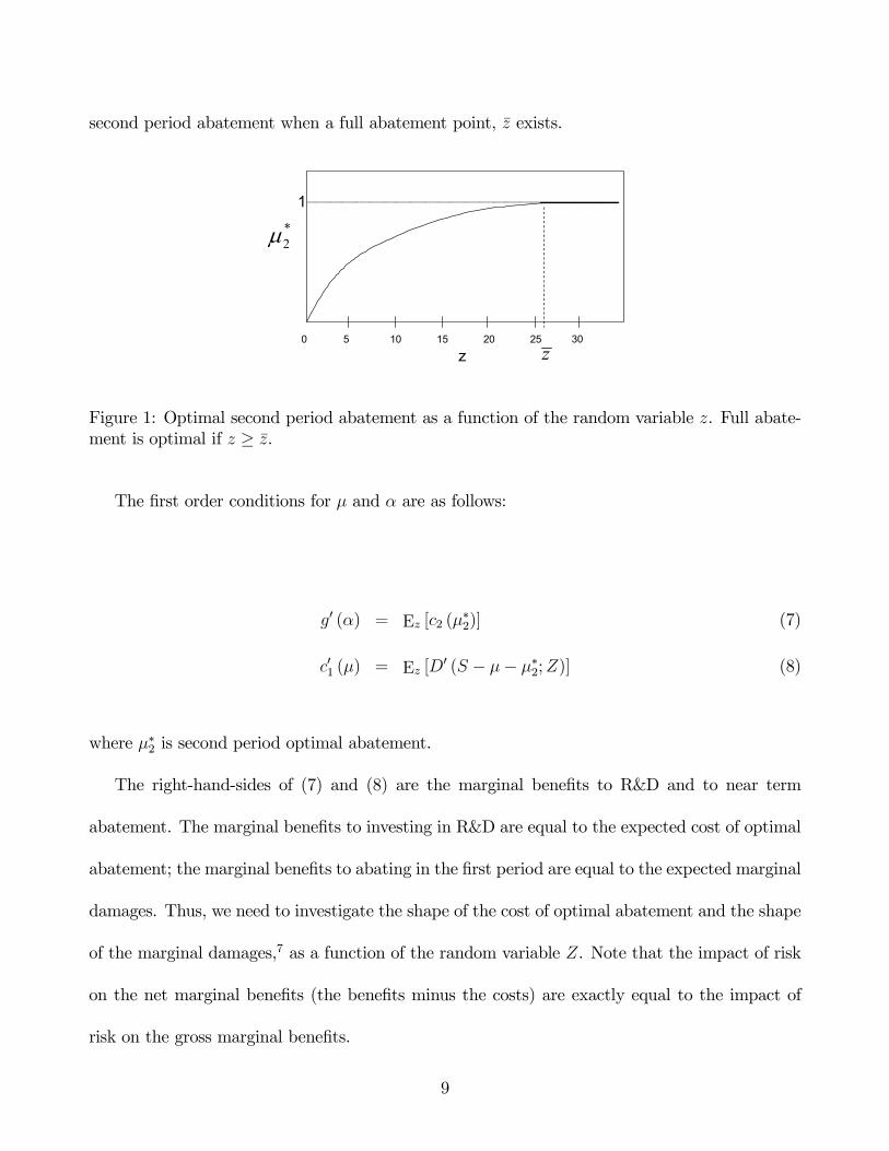
second period abatement when a full abatement point, z exists.

z z0 5 10 15 20 25 30

1*2µ

Figure 1: Optimal second period abatement as a function of the random variable z. Full abate-ment is optimal if z ≥ z.

The first order conditions for µ and α are as follows:

g0 (α) = Ez [c2 (µ∗2)] (7)

c01 (µ) = Ez [D0 (S − µ− µ∗2;Z)] (8)

where µ∗2 is second period optimal abatement.

The right-hand-sides of (7) and (8) are the marginal benefits to R&D and to near term

abatement. The marginal benefits to investing in R&D are equal to the expected cost of optimal

abatement; the marginal benefits to abating in the first period are equal to the expected marginal

damages. Thus, we need to investigate the shape of the cost of optimal abatement and the shape

of the marginal damages,7 as a function of the random variable Z. Note that the impact of risk

on the net marginal benefits (the benefits minus the costs) are exactly equal to the impact of

risk on the gross marginal benefits.

9

3 The shape of the marginals

At the heart of this paper (and, we argue, driving all previous results) are the shapes of the mar-

ginal functions. We illustrate the concepts using the shapes induced from quadratic assumptions.

We then use this context as a unifying to device to interpret the state of the current literature.

We go on to discuss how different sets of assumptions lead to implications about the shapes of

the marginals, which then lead to comparative statics results.

3.1 An illustration

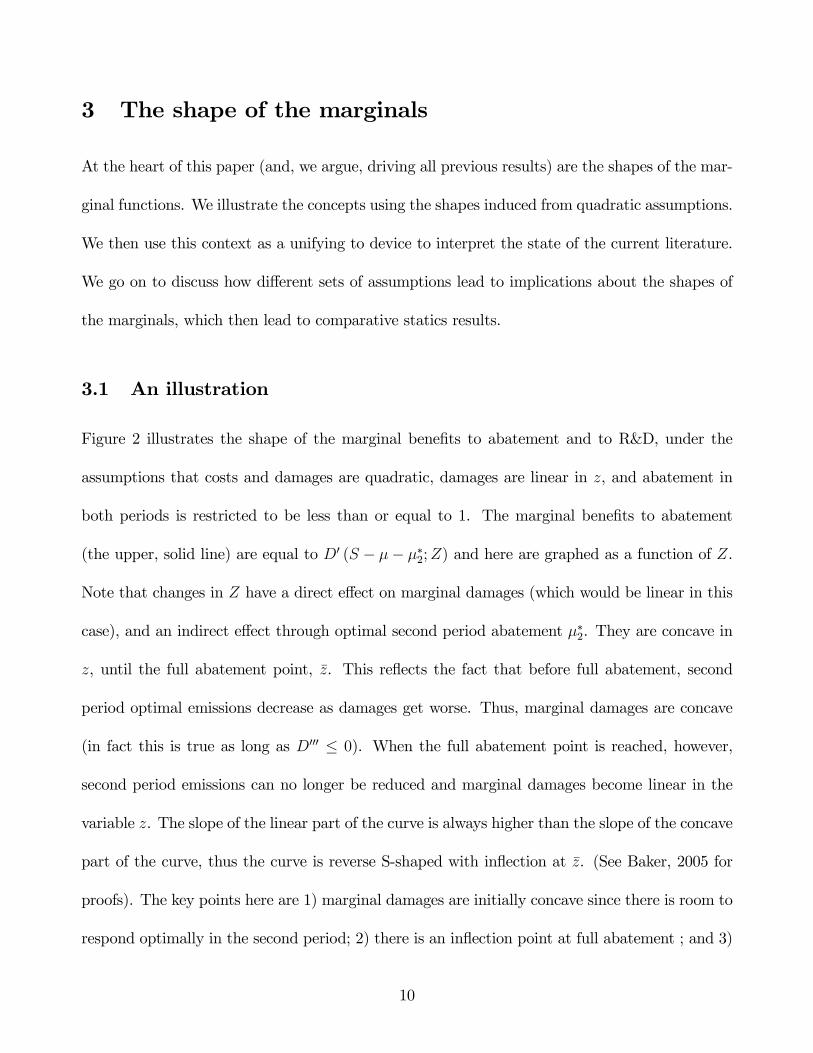
Figure 2 illustrates the shape of the marginal benefits to abatement and to R&D, under the

assumptions that costs and damages are quadratic, damages are linear in z, and abatement in

both periods is restricted to be less than or equal to 1. The marginal benefits to abatement

(the upper, solid line) are equal to D0 (S − µ− µ∗2;Z) and here are graphed as a function of Z.

Note that changes in Z have a direct effect on marginal damages (which would be linear in this

case), and an indirect effect through optimal second period abatement µ∗2. They are concave in

z, until the full abatement point, z. This reflects the fact that before full abatement, second

period optimal emissions decrease as damages get worse. Thus, marginal damages are concave

(in fact this is true as long as D000 ≤ 0). When the full abatement point is reached, however,

second period emissions can no longer be reduced and marginal damages become linear in the

variable z. The slope of the linear part of the curve is always higher than the slope of the concave

part of the curve, thus the curve is reverse S-shaped with inflection at z. (See Baker, 2005 for

proofs). The key points here are 1) marginal damages are initially concave since there is room to

respond optimally in the second period; 2) there is an inflection point at full abatement ; and 3)

10

the shape of the marginal benefits to abatement after the inflection point depends only on the

direct effect of the random variable on the marginal damages.

0 5 10 15 20 25 30 35

z

Marginal Benefits

z

Cost of abatement(marginal benefits of R&D)

Marginal Damages (marginal benefits to abatement)

Figure 2: The marginal benefits of abatement and R&D as a function of multiplicative uncertaintyon damages, Z. The marginal benefits to abatement are equal toD0 (S − µ− µ∗2;Z); the marginalbenefits to R&D are equal to c (µ∗2) .The dashed line represents the marginal benefits to abate-ment, holding second period abatement constant at full abatement µ2 = 1: D

0 (S − µ− 1;Z).

The marginal benefits to R&D are equal to c2 (µ∗2). This is impacted indirectly by Z, since Z

impacts optimal emissions, µ∗2. This marginal has a shape that is in some sense opposite to the

marginal for abatement. The cost of optimal abatement is convex at z = 0, since c2 (·) is convex

and µ is increasing in z. However, optimal abatement is concave in z — it becomes increasingly

expensive to reduce the next unit of emissions, therefore the marginal reduction in emissions

slows down. This leads to an inflection point z ≤ z after which the cost of optimal abatement

is concave8. Finally, the cost of optimal abatement is constant for z ≥ z since abatement is

constant for that range. This leads the marginal benefits of R&D to be S-shaped. The key

points here are 1) optimal cost is initially convex if cost is convex and abatement is increasing

rapidly near the origin; 2) optimal cost will generally become concave in high damages, since

optimal abatement will be strongly concave (as it approaches a maximum level); and 3) if a full

11

abatement point exists, then optimal cost will be constant after this point.

The figure shows that for both control variables the marginal benefits are neither convex nor

concave under even these extremely simple assumptions, and thus both optimal abatement and

optimal R&D will increase with some increases in risk and decrease with other increases in risk.

3.2 Prior Results and the shape of the marginals

There has been a substantial amount of work analyzing the impact of uncertainty and learning

on optimal abatement. The most common result has been that the impact of uncertainty and

learning on abatement is ambiguous. This result is driven by two conflicting irreversibilities. On

the one hand, the ability to react in the second period (increasing abatement if damages are high)

puts a downward pressure on first period abatement. This is because the resources allocated to

abatement in the first period cannot be recouped in the second period. On the other hand, if

the damages from climate change turn out to be very high, then the ability to react is limited:

second period abatement is restricted to full abatement. Thus, the irreversibility of emissions

will bite in this case. This puts an upward pressure on abatement, but only in proportion to

the probability that damages are high enough to induce full abatement. The first irreversibility

induces the concavity in marginal damages seen near the origin; the second irreversibility induces

the convexity at the full abatement point.

A prominent example of these kind of results on optimal abatement is found in Ulph and Ulph

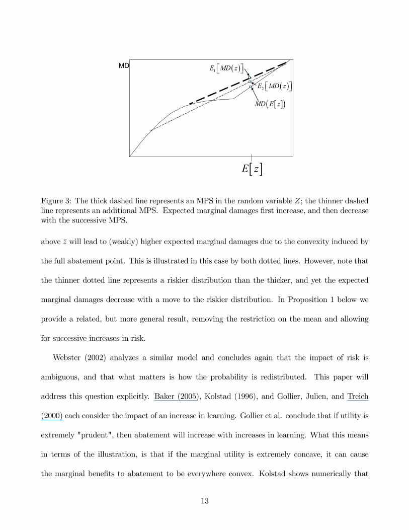
(1997). They go on to show in Lemma 3iii that if the mean damages are high, E [z] > z, then

abatement will be higher under risk than under no risk.9 To understand how this result is related

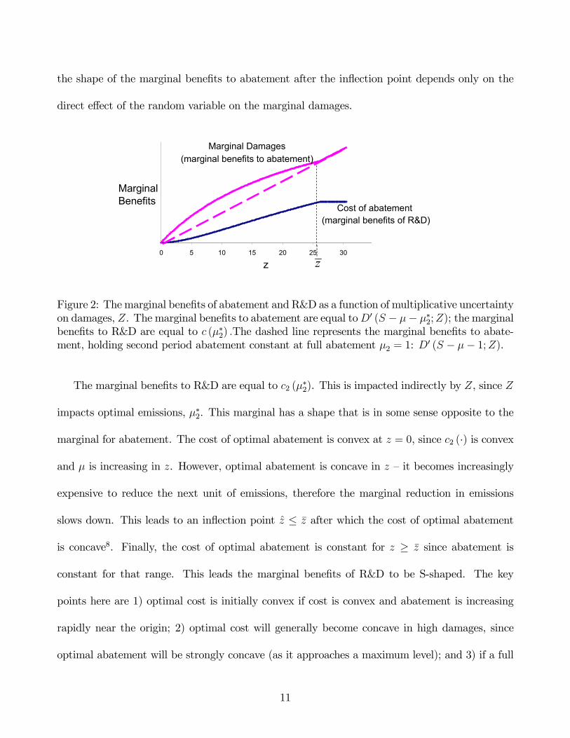
to the shape of the marginal damages see Figure 3. Note that any simple MPS around any point

12

[ ]E z

[ ]( )MD E z

( )2E MD z

( )1E MD z MD

Figure 3: The thick dashed line represents an MPS in the random variable Z; the thinner dashedline represents an additional MPS. Expected marginal damages first increase, and then decreasewith the successive MPS.

above z will lead to (weakly) higher expected marginal damages due to the convexity induced by

the full abatement point. This is illustrated in this case by both dotted lines. However, note that

the thinner dotted line represents a riskier distribution than the thicker, and yet the expected

marginal damages decrease with a move to the riskier distribution. In Proposition 1 below we

provide a related, but more general result, removing the restriction on the mean and allowing

for successive increases in risk.

Webster (2002) analyzes a similar model and concludes again that the impact of risk is

ambiguous, and that what matters is how the probability is redistributed. This paper will

address this question explicitly. Baker (2005), Kolstad (1996), and Gollier, Julien, and Treich

(2000) each consider the impact of an increase in learning. Gollier et al. conclude that if utility is

extremely "prudent", then abatement will increase with increases in learning. What this means

in terms of the illustration, is that if the marginal utility is extremely concave, it can cause

the marginal benefits to abatement to be everywhere convex. Kolstad shows numerically that

13

if the mean is low (E [z] << z) then increases in learning, represented as a star-shaped spread,

lead to a small increase in optimal emissions. A star-shaped spread in learning is equivalent

to a symmetric MPS. It can be seen from the illustration that a symmetric MPS around a

small z will lead to lower expected marginal damages, since marginal damages are concave at

that point. The work in this paper indicates that asymmetric increases in risk and in learning

can induce different results. Baker extends the above model to a non-cooperative game, showing

that if damages are perfectly negatively correlated across players, then strategic behavior induces

convexity in the marginal damages, and equilibrium emissions decrease in risk and in learning.

We note that numerical explorations have shown that the impact of uncertainty and learning on

optimal emissions tends to be quite small (Kolstad 1996, Ulph and Ulph 1997).

We know of very little work considering how optimal R&D is impacted by uncertainty and

learning other than (Baker et al., 2005) mentioned above.

3.3 What can be inferred about the shape of the marginals?

In the first subsection below we discuss how very weak assumptions about the costs and damages

of climate change, coupled with the assumption that a full abatement point exists, lead to

something we call generalized convexity/concavity in the marginals. In the following subsection

we discuss, both qualitatively and mathematically, what kinds of assumptions lead to marginals

that are convex/concave near the origin. Finally, in the last subsection we discuss the special

case of S-shaped marginals.

14

3.3.1 Generalized convexity/concavity

In this section we assume that a full abatement point exists. Formally, it is defined as z (µ, α)

such that µ∗2 (z, µ, α) = 1 for all z ≥ z (µ, α), i.e. it is the level of damage that induces a corner

point solution in the second period.

Marginal damages We assume that marginal damages are increasing in z. If this were not

true, then optimal abatement would decrease with an increase in damages — theoretically possi-

ble, but not likely. The standard assumption that damages are convex in the stock of emissions

implies that marginal damages are decreasing in abatement; therefore, we can conclude that

∂D(S−µ∗2(z);z)∂S

≥ ∂D(S−µ∗2(z);z)∂S

: marginal damages when abatement is optimal are (weakly) greater

than marginal damages when abatement is full. Furthermore, under the assumption that mar-

ginal damages are convex in z (holding abatement constant), we can say that marginal damages

are convex in z after full abatement, that is for z ≥ z. Thus, the marginal benefits to abatement

belong to the set of what we call "Generalized rightward convex" functions. Formally, we define

the set ∆z : all increasing functions d : R → R, such that there exists a continuous, convex

function κ (z) with the following properties

1. d (z) ≥ κ (z) for all z ≤ z.

2. d (z) = κ (z) for z ≥ z;

The left hand panel in Figure 4 illustrates 4 representative functions in this set, each with

the same underlying convex function κ (z). These functions are convex around all points to the

right of the inflection point (that is for any points x, x0such that γx + (1− γ)x0 ≥ z, it is true

that γd (x) + (1− γ) d (x0) ≥ d (γx+ (1− γ)x0)). Note that all convex functions as well as all

15

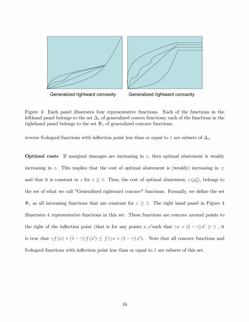
Generalized rightward convexity Generalized rightward concavity

Figure 4: Each panel illustrates four representative functions. Each of the functions in thelefthand panel belongs to the set ∆z of generalized convex functions; each of the functions in therighthand panel belongs to the set Ψz of generalized concave functions.

reverse S-shaped functions with inflection point less than or equal to z are subsets of ∆z.

Optimal costs If marginal damages are increasing in z, then optimal abatement is weakly

increasing in z. This implies that the cost of optimal abatement is (weakly) increasing in z;

and that it is constant in z for z ≥ z. Thus, the cost of optimal abatement, c (µ∗2), belongs to

the set of what we call "Generalized rightward concave" functions. Formally, we define the set

Ψz as all increasing functions that are constant for z ≥ z. The right hand panel in Figure 4

illustrates 4 representative functions in this set. These functions are concave around points to

the right of the inflection point (that is for any points x, x0such that γx + (1− γ)x0 ≥ z , it

is true that γf (x) + (1− γ) f (x0) ≤ f (γx+ (1− γ)x0). Note that all concave functions and

S-shaped functions with inflection point less than or equal to z are subsets of this set.

16

3.3.2 Concavity/Convexity near the origin

Marginal damages As we have seen, under quadratic assumptions, and in most of the lit-

erature, marginal damages are concave in the random variable as long as damages are not too

high. This is driven largely by the ability to respond to damages in the second period. When

might this not be true? First, if costs were extremely convex at low levels of abatement, then

abatement could be extremely concave, possibly inducing marginal damages that were convex.

However, we know of no experts who are claiming that even a small amount of abatement will

be extremely expensive; to the contrary many argue that initial abatement will come at a very

low price, through increases in efficiency for example.10 Second, if marginal damages are very

convex in the random variable itself (holding abatement constant), this may induce a convexity

in optimal marginal damages. This second issue is relevant if we are concerned about a partic-

ular random variable, say climate sensitivity, and marginal damages are quite convex in climate

sensitivity (holding abatement constant). In general we can conclude that marginal damages will

be concave at low levels of damage as long as neither costs nor damages are too convex.

Mathematically, assuming that damages are linear in the random variable Z, Baker (2005)

shows that marginal damages are always concave at z = 0; and that a sufficient condition for

marginal damages to be concave for all z ≤ z is that D000 ≤ 0 and c0002 ≤ 0.

Optimal costs Again, the quadratic assumptions show optimal costs to be convex near the

origin. This will hold as long as the cost of control is convex in the abatement level; and optimal

abatement is not too concave in damages. As argued above, under assumptions of the existence

of "low-hanging fruit", the cost of abatement itself is not likely to induce extremely concave

abatement at low damage levels.

17

Mathematically, in the on-line Appendix we show that the cost of optimal abatement is

convex at z = 0 if D is linear in z and costs are more convex than damages, c002c02≥ 2D00

D0 . This

inequality is likely to hold in the case of climate change, since damages are a function of the

stock of emissions, whereas costs are a function of the flow of emissions, and the flow is very

small compared to the stock. Thus marginal damages tend to be nearly linear in the flow.

Concavity/Convexity everywhere to the left of the inflection point Here we provide

sufficient conditions for marginal damages to be reverse S-shaped and optimal abatement cost

to be S-shaped. This is true when uncertainty is linear as long as c0002 , D000 ≤ 0, c002

c02≥ 2D00

D0 and

c2 (1) <∞. In particular, if D000 = 0, then both marginals have their inflection point at z.

4 Stochastic Dominance Theorems

In this section we present new stochastic dominance theorems based on the shapes we determined

for the marginals above. Table 1 summarizes the sets of functions (related to the shapes of the

marginals) used in the stochastic dominance theorems. We focus on two subsets of MPS. In the

first section we focus on MPS that stretch the tail of the distribution to the right; in the second

we consider MPS where the risk is mainly increased to the left of an extreme point.

4.1 Generalized Convexity/Concavity

In this section we present stochastic dominance theorems for the sets of generalized convex and

concave functions. Since each of these sets are convex/concave around points to the right of the

inflection point, we consider an MPS that stretches or skews the distribution to the right, while

18

leaving the relative probabilities to the left of the inflection point unchanged. Let F and G be

cumulative probability distributions. First we define the probability distribution to the left and

the right of the inflection point. These are the original probability distributions normalized.

FL ≡F (x)F (z)

x ≤ z

1 x ≥ z(9)

FR ≡ 0 x ≤ zF (x)−F (z)1−F (z) x ≥ z

(10)

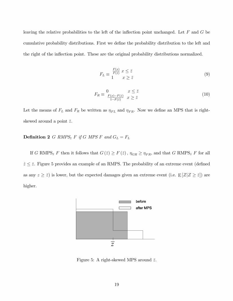
Let the means of FL and FR be written as ηFL and ηFR. Now we define an MPS that is right-

skewed around a point z.

Definition 2 G RMPSz F if G MPS F and GL = FL

If G RMPSz F then it follows that G (z) ≥ F (z) , ηGR ≥ ηFR, and that G RMPSz F for all

z ≤ z. Figure 5 provides an example of an RMPS. The probability of an extreme event (defined

as any z ≥ z) is lower, but the expected damages given an extreme event (i.e. E [Z|Z ≥ z]) are

higher.

before

after MPS

before

after MPS

z

Figure 5: A right-skewed MPS around z.

19

Following the stochastic dominance literature, we say that G dominates F on the set Υ if

Zu (x) dG ≥

Zu (x) dF ∀u ∈ Υ (11)

Now we present our stochastic dominance theorems for generalized rightward convexity and

concavity, respectively. See the Appendix for proofs.

Theorem 1 If G RMPSz F then G dominates F on ∆z, the set of generalized rightward convex

functions.

Theorem 2 If G RMPSz F then F dominates G on Ψz, the set of generalized rightward concave

functions.

4.2 Concave/Convex near the origin

In this section we present stochastic dominance theorems for functions that are convex or concave

to the left of the inflection point, and linear or constant to the right. Thus, we consider an MPS

near the origin, leaving the tail of the distribution unchanged.

Define the set δz as all increasing functions that are concave for z ≤ z and linear for z ≥ z.

Theorem 3 if G MPS F and F (z) = G (z) and ηFR = ηGR then F dominates G on the set δz

Define the set Ωz as all increasing functions that are convex for z ≤ z and constant for z ≥ z.

Theorem 4 If G MPS F and F (z) ≥ G (z) and GL MPS FL then G dominates F on the set

Ωz

20

4.3 S-shaped functions

Define the set Υpz as the set of increasing payoff functions that are convex for x < z and concave

for x > z; and the set Υmz as the set of increasing payoff functions that are concave for x < z

and convex for x > z. These are the sets of S-shaped and reverse S-shaped functions. See the

on-line Appendix for proof of the following theorem.

Theorem 5 If G is an MPS of F, then the following three statements are equivalent:

1. F = G for x > z (x < z)

2. G dominates F on the set Υpz (Υmz) ;

3. F dominates G on the set Υmz (Υpz) .

Set Notation Set Definition

∆z

½f |f : R→ R,∃κ (z) continuous, convex s.t.f (z) ≥ κ (z)∀z ≤ z; f (z) = κ (z)∀z ≥ z

¾Ψz f |f : R→ R, non-decreasing, constant ∀z ≥ zδz f |f : R→ R,non-decreasing, concave ∀z ≤ z, linear ∀z ≥ zΩz f |f : R→ R, non-decreasing, convex ∀z ≤ z, constant ∀z ≥ zΥpz f |f : R→ R, non-decreasing, convex ∀z ≤ z, concave ∀z ≥ zΥmz f |f : R→ R, non-decreasing, concave ∀z ≤ z, convex ∀z ≥ z

Table 1: Summary of Set Definitions

5 Application of Theorems to climate change

In this section we combine the discussions in Section 3 on the shape of the marginals with

the Theorems from Section 4 to get comparative statics results for climate change. The first

proposition says that if we believe that a full abatement point exists, and that uncertainty is

21

something to be concerned about (in the sense that expected damages increase in uncertainty)

then increases in risk that stretch the tail of the probability distribution lead to optimally higher

abatement and lower R&D investments.

Proposition 1 Assume full abatement is optimal at z and marginal damages D0 (s;Z) increase

in Z. Then optimal R&D will decrease with RMPSz. If marginal damages are (weakly) convex

in the random variable Z (holding second period abatement constant) then optimal first period

abatement will increase with RMPSz. Precisely, let α (F ) , µ (F ) , be the optimal values of the

decision variables given distribution of damages F , and z (F ) the full abatement point given

α (F ) , µ (F ). If G RMPSz F for any z ≥ z (F ) then α (G) ≤ α (F ) and µ (G) ≥ µ (F ).

Proof. If marginal damages increase in Z, then optimal abatement increases in Z. If, addition-

ally, z is the full abatement point, then c (µ∗2) ∈ Ψz, the set of generalized rightward concave

functions. Theorem 1 implies that the RHS of (8), E [c (µ∗2)], is higher under G, and therefore the

optimal µ is higher. If marginal damages (holding 2nd period abatement constant) are increas-

ing and (weakly) convex then D0 (S − µ− µ∗2;Z) ∈ ∆z, the set of rightward convex functions.

Theorem 2 implies that the RHS of (7), E [D0 (S − µ− µ∗2;Z)], is lower under G, and therefore

optimal α is lower.

An RMPS means that there is a higher likelihood of being in the lower part of the distribution

(where the lower part is defined by the inflection point, z ≤ z); but given that damages are in

the higher part of the distribution, expected damages are now worse. In terms of R&D this

means that the overall probability of full abatement is lower, thus the expected benefits from

R&D decrease with the RMPS. For abatement, this means that if the irreversibility constraint

does bite, it bites harder. Thus, it provides an incentive for leaving a little more flexibility to

22

reduce emissions.

The next proposition makes stronger assumptions that lead to marginal damages being con-

cave and optimal cost being convex everywhere before full abatement. Under these assumptions,

a change in the distribution of damages that is riskier in the left-hand side of the distribution, but

keeps the probability of extreme events the same, will decrease abatement and increase optimal

R&D.

Proposition 2 Let damages be linear in the random variable Z, D000 = 0, c0002 ≤ 0, c002c02≥ 2D00

D0 and

let z (F ) be the full abatement point given F . Then abatement is decreasing (µ (G) ≤ µ (F )) and

R&D is increasing (α (G) ≥ α (F )) whenever G MPS F, F (z) = G (z), and GL MPS FL.

Proof. Given that damages are linear in Z, D000 = 0, and c0002 ≤ 0, D0 (S − µ− µ∗2;Z) ∈ δz.

Theorem 3 then implies that marginal damages are decreasing in the MPS described in the

proposition. Under the additional assumption that c002c02≥ 2D

00D0 , then c (µ∗2) ∈ Ωz. Theorem 4

implies that optimal cost is increasing in the MPS described in the proposition. Thus, optimal

abatement is decreasing and optimal R&D is increasing.

The next proposition is similar to the previous one. It has weaker assumptions on the mar-

ginals (they are only required to be concave/convex near the origin), but a more restrictive set

of MPS.

Definition 3 z (F ) ≡

sup [z : D0 (S − µ− µ∗2; z) concave in z and c (µ∗2) convex in z for z ≤ z| α (F ) , µ (F )]

Proposition 3 For any F for which z (F ) exists, optimal abatement is decreasing (µ (G) ≤

µ (F )) and optimal R&D is increasing (α (G) ≥ α (F )) whenever G MPS F and F = G for ∀z >

z (F ).

23

Proof. The assumption that z (F ) exists implies that optimal marginal damages are concave

and optimal cost is convex for all z ≤ z (F ). Thus, Theorem 5 implies that expected marginal

damages are decreasing and expected optimal cost is increasing for an MPS to the left of z;

implying that optimal first period abatement will decrease and optimal R&D spending will

increase.

0

0.10.20.30.40.50.60.7

0.10.20.30.40.50.60.7

0 5 10 15 20 25 30

Percentage GDP loss with 2.5°C warming

0

0.10.20.30.40.50.60.7

0.10.20.30.40.50.60.7

0 5 10 15 20 25 30

Before MPS to left After MPS to left

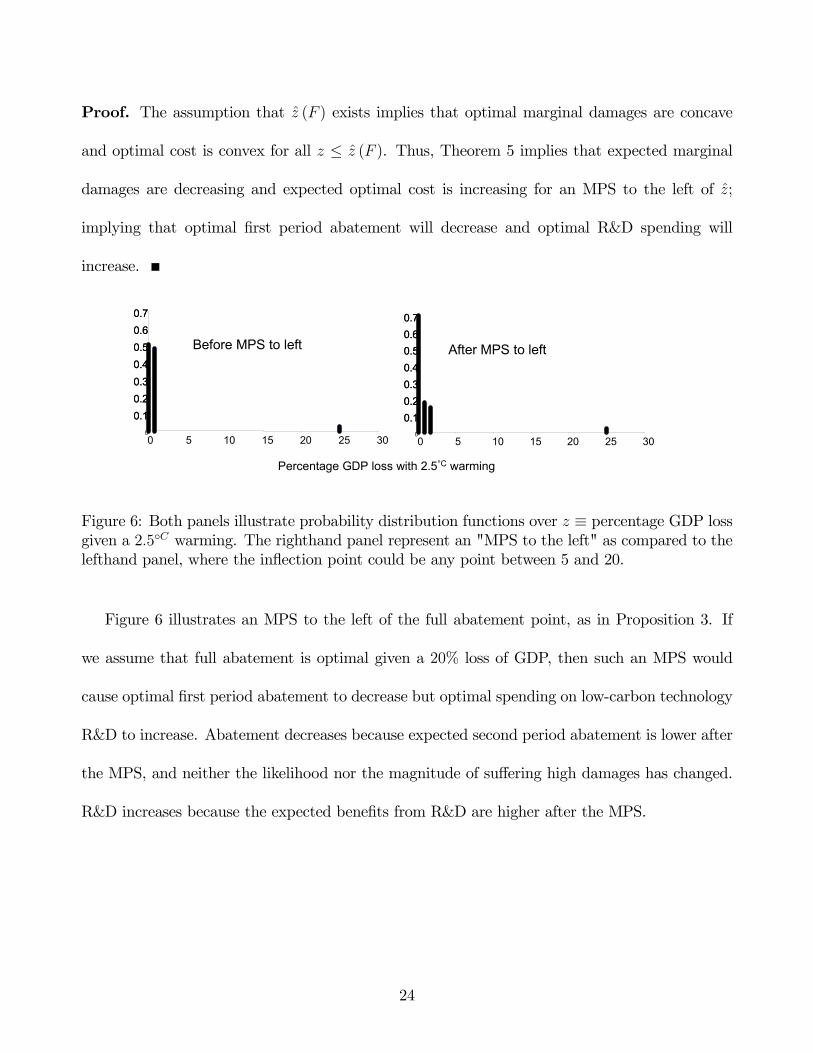
Figure 6: Both panels illustrate probability distribution functions over z ≡ percentage GDP lossgiven a 2.5C warming. The righthand panel represent an "MPS to the left" as compared to thelefthand panel, where the inflection point could be any point between 5 and 20.

Figure 6 illustrates an MPS to the left of the full abatement point, as in Proposition 3. If

we assume that full abatement is optimal given a 20% loss of GDP, then such an MPS would

cause optimal first period abatement to decrease but optimal spending on low-carbon technology

R&D to increase. Abatement decreases because expected second period abatement is lower after

the MPS, and neither the likelihood nor the magnitude of suffering high damages has changed.

R&D increases because the expected benefits from R&D are higher after the MPS.

24

5.1 Role of assumptions

5.1.1 Costs and Damages Not separable

The decision problem in (5) implies that the decision maker is risk-neutral, has perfect elasticity

of substitution across time, and that costs of abatement are separable from damages. All of

these assumptions are reversed if we put a utility function around second period costs and

damages.11 Theoretically, this can change the shape the marginal benefits to abatement and to

R&D. Specifically, the right-hand sides of the first order conditions (7) and (8) will be multiplied

by the marginal (dis)utility. If utility reflects extreme prudence, then the marginal benefits to

both abatement and R&D could be everywhere convex. For example, Gollier, Julien, and Treich

(2000) have shown, in a slightly different model, that marginal damages can become everywhere

convex. The level of curvature required, however, was very large, and thus may not be very

relevant. Moreover, the results presented here are consistent with Baker, Clarke, and Weyant

(2005), who used the DICE model, which has a log utility function, to test how optimal R&D

responds to increases in risk.

5.1.2 Full Abatement

In the above propositions we assume that full abatement is achievable, but that abatement is

capped at 1. It may be argued, on the one hand, that full abatement is not possible, that the

cost of abatement goes to infinity as abatement approaches one. It may be argued, on the other

hand, that there is no strict limit on abatement, that it is physically possible to remove carbon

emissions from the atmosphere. Sufficient conditions for a full abatement point to exist are that

the cost of abatement is finite at full abatement, it is impossible to reduce the flow of emissions

25

below zero, and damages increase indefinitely as z increases. Even if a full abatement point does

not exist, however, the results for optimal abatement will hold as long as 1) there exists some

value k such that µ∗2 (z) ≤ k ∀z and 2) z is such that µ∗2 (z) ≥ k− ε ∀z ≥ z where ε is sufficiently

small. This is because the key to the abatement results is that the second period ability to react

must become severely limited at some point.

On the other hand, in the absence of a full abatement point, it is theoretically possible that

the optimal cost of abatement is everywhere convex, in particular, if marginal damages are very

convex in the stock and full abatement is not achievable. In this case, the optimal investment

in alternative R&D would unambiguously increase in risk. It would be interesting to see if any

technologically-detailed integrated assessment models could induce such a result, and what kinds

of assumptions it would require.

A second question is whether the full abatement point, if it exists, is relevant. To answer that

requires more in-depth expert assessments on the possible damages from climate change than

have been done to this point. We note that some models indicate that full abatement may be

optimal if our goal is to stabilize the stock of emissions at 350ppmv (Wigley et al., 1996), and

that this stabilization goal may be optimal if damages turn out to be severe. Thus, it would

appear that there is a positive probability that climate change could induce full abatement.

26

6 Learning

These results can be extended to partial learning. We can re-write the climate change decision

problem as a problem of sequential decision making under partial learning, as follows:

minµ,α

c1 (µ) + g (α) + EY

·minµ2EZ|Y c2 (µ2;α) +D (S − µ− µ2;Z)

¸(12)

where Y is a random variable defined on the same space as Z, thus it may give some information

about Z. We define a more informative signal in the Blackwell sense: Y is more informative than

Y 0 if every decision maker is (weakly) better off under signal Y than Y 0. Baker (Forthcoming)

shows that if the damages D are linearly separable in a function of Z, then the impact of learning

more is the same as the impact of increasing risk. To illustrate the intuition behind this, assume

that D is linear in Z. Then (12) simplifies to

minµ,α

c1 (µ) + g (α) + EY minµ2[c2 (µ2;α) + E [Z|Y ]D (S − µ− µ2)] (13)

As Y increases in informativeness, the random variable E [Z|Y ] increases in risk. For intuition

consider the two extreme cases. If Y is independent from Z then E [Z|Y ] = E [Z] for all possible

realizations of Y : the random variable E [Z|Y ] is constant. On the other hand, if Y provides

perfect information about Z, that implies that E [Z|Y ] = Z, i.e. the variability of E [Z|Y ] will

be exactly equal to the variability of Z. Thus, an increase in the informativeness of the signal

has the same qualitative impact as an increase in the risk of the random variable.

The broad intuition of this result is as follows: if in problem (13) we expect to have more

information before we choose 2nd period abatement µ2 then we will want to choose 1st period

27

abatement and R&D in such a way to leave ourselves more flexibility to react to what is learned.

Similarly, the more prior risk we face in problem (5), the more flexibility we would like when

choosing µ2. Hence, an increase in informativeness and an increase in risk have similar effects

on first period decisions.

Just as current decisions in (5) depend on the probability distribution of Z; in the learning

model (13) current decisions depend on the distribution of E [Z|Y ]. Thus, a more informative

signal that induces an RMPS in E [Z|Y ] will have the same impact as an RMPS in Z. Here we

present a proposition that generalizes Proposition 1. The proofs of Propositions 4 and 5 follow

from an application of Theorem 1 of Baker (Forthcoming).12

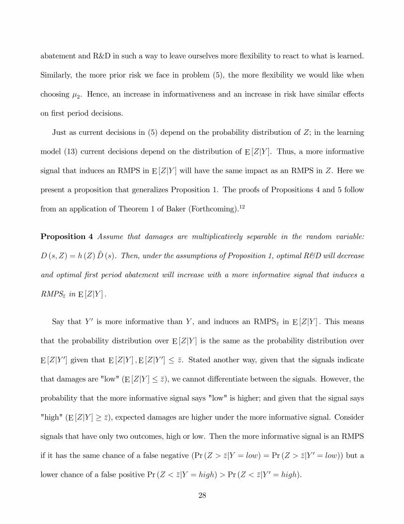
Proposition 4 Assume that damages are multiplicatively separable in the random variable:

D (s, Z) = h (Z) D (s). Then, under the assumptions of Proposition 1, optimal R&D will decrease

and optimal first period abatement will increase with a more informative signal that induces a

RMPSz in E [Z|Y ] .

Say that Y 0 is more informative than Y , and induces an RMPSz in E [Z|Y ] . This means

that the probability distribution over E [Z|Y ] is the same as the probability distribution over

E [Z|Y 0] given that E [Z|Y ] ,E [Z|Y 0] ≤ z. Stated another way, given that the signals indicate

that damages are "low" (E [Z|Y ] ≤ z), we cannot differentiate between the signals. However, the

probability that the more informative signal says "low" is higher; and given that the signal says

"high" (E [Z|Y ] ≥ z), expected damages are higher under the more informative signal. Consider

signals that have only two outcomes, high or low. Then the more informative signal is an RMPS

if it has the same chance of a false negative (Pr (Z > z|Y = low) = Pr (Z > z|Y 0 = low)) but a

lower chance of a false positive Pr (Z < z|Y = high) > Pr (Z < z|Y 0 = high).

28

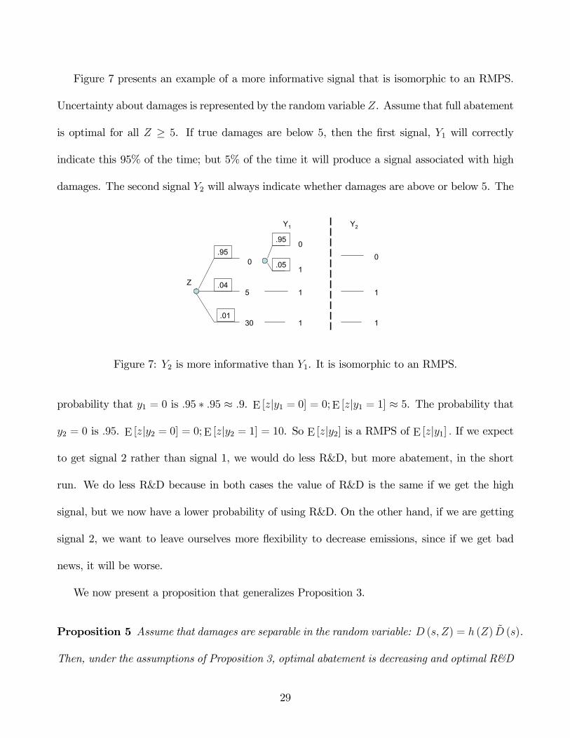
Figure 7 presents an example of a more informative signal that is isomorphic to an RMPS.

Uncertainty about damages is represented by the random variable Z. Assume that full abatement

is optimal for all Z ≥ 5. If true damages are below 5, then the first signal, Y1 will correctly

indicate this 95% of the time; but 5% of the time it will produce a signal associated with high

damages. The second signal Y2 will always indicate whether damages are above or below 5. The

Z

0

5

30

.95

.04

.01

Y1 Y2

1

1

1

0.95

.05

1

1

0

Figure 7: Y2 is more informative than Y1. It is isomorphic to an RMPS.

probability that y1 = 0 is .95 ∗ .95 ≈ .9. E [z|y1 = 0] = 0;E [z|y1 = 1] ≈ 5. The probability that

y2 = 0 is .95. E [z|y2 = 0] = 0; E [z|y2 = 1] = 10. So E [z|y2] is a RMPS of E [z|y1] . If we expect

to get signal 2 rather than signal 1, we would do less R&D, but more abatement, in the short

run. We do less R&D because in both cases the value of R&D is the same if we get the high

signal, but we now have a lower probability of using R&D. On the other hand, if we are getting

signal 2, we want to leave ourselves more flexibility to decrease emissions, since if we get bad

news, it will be worse.

We now present a proposition that generalizes Proposition 3.

Proposition 5 Assume that damages are separable in the random variable: D (s, Z) = h (Z) D (s).

Then, under the assumptions of Proposition 3, optimal abatement is decreasing and optimal R&D

29

is increasing with a more informative signal, when the signal is only more informative about out-

comes to the left of z.

This implies that if we expect (in the future) to get a better handle on damages near the

mean of the distribution, while leaving the tail unexplored, then we should optimally spend more

on R&D and less on abatement. Given better information around the mean, we expect to get

more value, on average, from R&D. This is because, near mean damages, the cost of abatement

is increasing rapidly; thus if we learn that damages are a bit higher than the mean, we get a

fair amount of value from R&D. On the other hand, given better information around the mean

means that we can more accurately respond in the second period in terms of abatement; when

damages are near the mean, we know that we will not hit a constraint, so first period abatement

has relatively less value since we will have flexibility to respond in the 2nd period; thus there is

an option value to waiting to implementing higher abatement.

Thus, to the degree that climate change research is aimed at analyzing the impact of a given

mean temperature change, and mean damages resulting from the temperature change, more

should be spent on R&D and less on short term abatement. On the other hand, to the degree

that climate change research is aimed at increasing our understanding of the probability of a

high damage event, less should be spent on R&D and more should be spent on abatement.

7 Conclusions

In this paper we provide a new perspective for analyzing the comparative statics of uncertainty

and learning in the climate change problem. By focussing on the shape of the marginals we

were able to provide new, unambiguous results on how optimal policy changes with changes in

30

risk and changes in what we expect to learn. We have shown that abatement and investment in

alternative energy R&D may be risk-substitutes in many cases: changes in risk that optimally

increase one, decrease the other. In particular, we have shown that if a "full abatement point"

exists, then an MPS that stretches the probability distribution over damages to the right of that

point (or analogously, an expectation of learning more about the tail of the damage distribution

than about the mean) will increase optimal abatement and decrease optimal alternative energy

R&D spending. On the other hand, if we consider multiplicative damage uncertainty, and assume

that neither damages nor costs are too convex in abatement, then an MPS near the mean (or

analogously, an expectation of learning more around the mean than around the tail) will result

in a decrease in optimal abatement and an increase in optimal alternative energy R&D spending.

Moreover, the focus on the shapes of the marginals presents a unifying framework for in-

terpreting the prior work on the comparative statics of uncertainty and learning in the climate

change problem. For example, we show how an assumption that mean damages are very high

leads to higher optimal abatement under risk than under no risk. Additionally, we point out

that the essential role played by the assumption of "prudence" is to induce concavity in a reverse

S-shaped marginal.

In order to provide comparative statics results, we have presented and proved new stochastic

dominance theorems, in particular for the sets of "generalized" convex/concave functions. These

theorems may be applicable in other problems in which an irreversibility constraint induces a

bend in the marginals that prevents the application of standard stochastic dominance theorems.

There is much room for future work expanding the results in this paper. First, more work

can be done describing the shape of the marginals under different assumptions. In particular,

31

a more thorough analysis in the presence of risk aversion would be useful. Second, this paper

suggests the importance of more empirical results on the shapes of optimal costs and damages.

Along this vein, a multi-model approach, where a number of different climate change integrated

assessment models generate optimal cost and damage curves for some of the most important

uncertainties, such as the economic impacts of mean temperature change or climate sensitivity,

may lead to valuable insights.

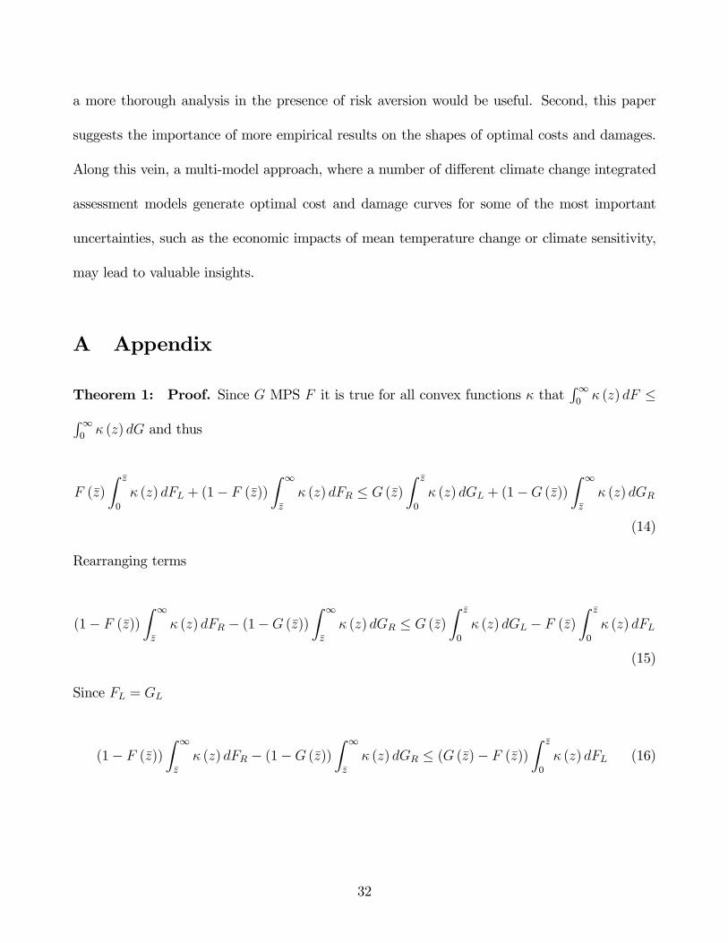
A Appendix

Theorem 1: Proof. Since G MPS F it is true for all convex functions κ thatR∞0

κ (z) dF ≤R∞0

κ (z) dG and thus

F (z)

Z z

0

κ (z) dFL + (1− F (z))

Z ∞

z

κ (z) dFR ≤ G (z)

Z z

0

κ (z) dGL + (1−G (z))

Z ∞

z

κ (z) dGR

(14)

Rearranging terms

(1− F (z))

Z ∞

z

κ (z) dFR − (1−G (z))

Z ∞

z

κ (z) dGR ≤ G (z)

Z z

0

κ (z) dGL − F (z)

Z z

0

κ (z) dFL

(15)

Since FL = GL

(1− F (z))

Z ∞

z

κ (z) dFR − (1−G (z))

Z ∞

z

κ (z) dGR ≤ (G (z)− F (z))

Z z

0

κ (z) dFL (16)

32

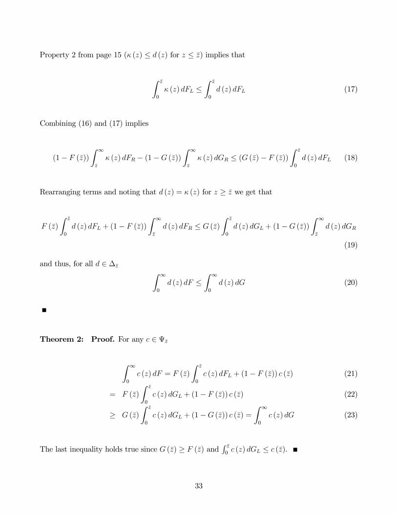
Property 2 from page 15 (κ (z) ≤ d (z) for z ≤ z) implies that

Z z

0

κ (z) dFL ≤Z z

0

d (z) dFL (17)

Combining (16) and (17) implies

(1− F (z))

Z ∞

z

κ (z) dFR − (1−G (z))

Z ∞

z

κ (z) dGR ≤ (G (z)− F (z))

Z z

0

d (z) dFL (18)

Rearranging terms and noting that d (z) = κ (z) for z ≥ z we get that

F (z)

Z z

0

d (z) dFL + (1− F (z))

Z ∞

z

d (z) dFR ≤ G (z)

Z z

0

d (z) dGL + (1−G (z))

Z ∞

z

d (z) dGR

(19)

and thus, for all d ∈ ∆z Z ∞

0

d (z) dF ≤Z ∞

0

d (z) dG (20)

Theorem 2: Proof. For any c ∈ Ψz

Z ∞

0

c (z) dF = F (z)

Z z

0

c (z) dFL + (1− F (z)) c (z) (21)

= F (z)

Z z

0

c (z) dGL + (1− F (z)) c (z) (22)

≥ G (z)

Z z

0

c (z) dGL + (1−G (z)) c (z) =

Z ∞

0

c (z) dG (23)

The last inequality holds true since G (z) ≥ F (z) andR z0c (z) dGL ≤ c (z).

33

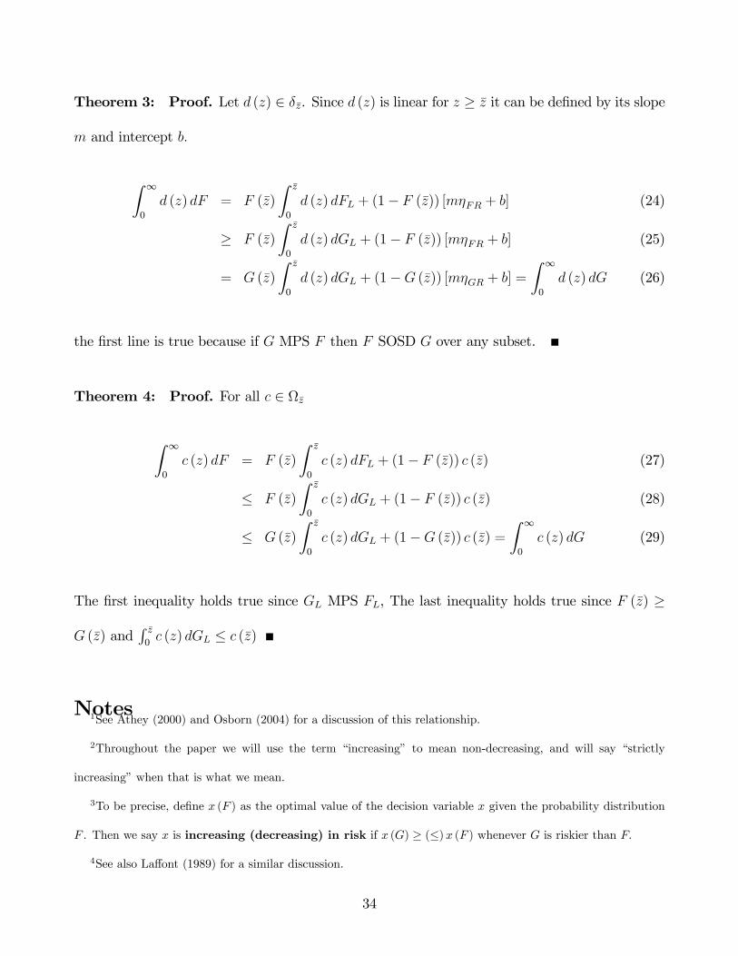
Theorem 3: Proof. Let d (z) ∈ δz. Since d (z) is linear for z ≥ z it can be defined by its slope

m and intercept b.

Z ∞

0

d (z) dF = F (z)

Z z

0

d (z) dFL + (1− F (z)) [mηFR + b] (24)

≥ F (z)

Z z

0

d (z) dGL + (1− F (z)) [mηFR + b] (25)

= G (z)

Z z

0

d (z) dGL + (1−G (z)) [mηGR + b] =

Z ∞

0

d (z) dG (26)

the first line is true because if G MPS F then F SOSD G over any subset.

Theorem 4: Proof. For all c ∈ Ωz

Z ∞

0

c (z) dF = F (z)

Z z

0

c (z) dFL + (1− F (z)) c (z) (27)

≤ F (z)

Z z

0

c (z) dGL + (1− F (z)) c (z) (28)

≤ G (z)

Z z

0

c (z) dGL + (1−G (z)) c (z) =

Z ∞

0

c (z) dG (29)

The first inequality holds true since GL MPS FL, The last inequality holds true since F (z) ≥

G (z) andR z0c (z) dGL ≤ c (z)

Notes1See Athey (2000) and Osborn (2004) for a discussion of this relationship.

2Throughout the paper we will use the term “increasing” to mean non-decreasing, and will say “strictly

increasing” when that is what we mean.

3To be precise, define x (F ) as the optimal value of the decision variable x given the probability distribution

F . Then we say x is increasing (decreasing) in risk if x (G) ≥ (≤)x (F ) whenever G is riskier than F.

4See also Laffont (1989) for a similar discussion.

34

5The marginal of the underlying payoff, however, is still required to be concave.

6For example, technical change into efficiency of fossil-fuels is not typically a hedge against risk (See Baker,

Clarke, and Weyant (Forthcoming), Baker And Shittu (Forthcoming), Baker and Adu-Bonnah (2005)) ,

7We have assumed above that marginal damages holding the stock constant ∂D(s,z)∂s are convex in z. When we

refer to marginal damages here we refer to ∂D(S−µ−µ∗2,z)∂S . This may not be convex in z since µ∗2 is a function of z.

8Specifically, if c2 (µ) = aµ2 + bµ and D (S − µ) = (S − µ)2 then z =a+ b

2

S−1 and z = min

·a(aS− b

2)2+ab

2aS+b , z

¸9Their result is stated in terms of learning versus no learning. Given their linear model, their result is true

if and only if abatement is higher under risk than under no risk. See Baker (Forthcoming) for details of the

equivalence between increases in risk and increases in learning.

10For example, a comparison of 11 integrated assessment models shows them all to have nearly linear marginal

costs of abatement in the U.S. up to 15-20% abatement. (Weyant and Hill, 1999).

11First period utility does not impact the comparative statics of risk or learning, so it is ignored.

12See http://www.ecs.umass.edu/mie/faculty/baker/BakerOR.pdf for a copy of the paper.

References

Athey, S. (2000). Characterizing properties of stochastic objective function. Manuscript, De-

partment of Economics, Stanford University, Palo Alto.

Baker, E. (2005). Uncertainty and learning in a strategic environment: Global climate change.

Resource and Energy Economics, 27:19—40.

Baker, E. (Forthcoming). Increasing risk and increasing informativeness: Equivalence theorems.

Operations Research.

Baker, E. and Adu-Bonnah, K. (2005). Investment in risky R&D programs in the face of climate

uncertainty. The Energy Journal, Under Review.

35

Baker, E., Clarke, L., and Weyant, J. (2005). Optimal technology R&D in the face of climate

uncertainty. Climatic Change, Forthcoming.

Baker, E. and Shittu, E. (2005). Profit-maximizing R&D in response to a random carbon tax.

Resource and Energy Economics, Forthcoming.

Blackwell, D. (1951). Comparison of experiments. In Proceedings of the Second Berkeley Sym-

posium on Mathematical Statistics and Probability, pages 93—102. University of California

Press.

Eeckhoudt, L. and Gollier, C. (1995). Demand for risky assets and the monotone probability

ratio order. Journal of Risk and Uncertainty, 11:113—122.

Epstein, L. G. (1980). Decision making and the temporal resolution of uncertainty. International

Economic Review, 21(2):269—283.

Gollier, C. (1995). The comparative statics of changes in risk revisited. Journal of Economic

Theory, 66:522—535.

Gollier, C., Jullien, B., and Treich, N. (2000). Scientific progress and irreversibility: An economic

interpretation of the ’precautionary pricipal’. Journal of Public Economics, 75:229—253.

Hadar, J. and Russell, W. (1969). Rules for ordering uncertain prospects. American Economic

Review, 59:25—34.

Hadar, J. and Seo, T. K. (1988). Asset proportions in optimal portfolios. Review of Economic

Studies, 55:459—468.

Jewitt, I. (1989). Choosing between risky prospects: The characterization of comparative statics

results and location independant risk. Management Science, 35:60—70.

Kimball, M. S. (1990). Precautionary savings in the small and in the large. Econometrica,

36

58:53—73.

Kolstad, C. D. (1996). Learning and stock effects in environmental regulation: The case of

greenhouse gas emissions. Journal of Environmental Economics and Management, 31:1—18.

Laffont, J.-J. (1989). The Economics of Uncertainty and Information. MIT Press, Cambridge,

Massachusetts.

Levy, H. (1992). Stochastic dominance and expected utility: Survey and analysis. Managment

Science, 38:555—593.

Levy, H. and Wiener, Z. (1998). Stoachastic dominance and prospect dominance with subjetive

weitghting functions. The Journal of Risk and Uncertainty, 16:147—63.

Meyer, J. and Ormiston, M. B. (1985). Strong increases in risk and their comparative statics.

International Economic Review, 26:425—437.

Osborn, D. (2004). Fractional Stochastic Dominance on Normed Linear Spaces. PhD thesis,

Stanford University.

Rothschild, M. and Stiglitz, J. (1970). Increasing risk I: A definition. Journal of Economic

Theory, 2:225—243.

Rothschild, M. and Stiglitz, J. (1971). Increasing risk II: Its economic consequences. Journal of

Economic Theory, 3:66—84.

Ulph, A. and Ulph, D. (1997). Global warming, irreversibility and learning. The Economic

Journal, 107:636—650.

Webster, M. (2002). The curious role of "learning" in climate policy: Should we wait for more

data? The Energy Journal, 23:97—119.

Weyant, J. P. and Hill, J. (1999). Introduction and overview. The Costs of the Kyoto Protocol:

37

A Multi-Model Evaluation. Special Issue of The Energy Journal., pages vii—xliv.

Wigley, T., Richels, R., and Edmonds, J. (1996). Economic and environmental choices in the

stabilization of atmospheric CO2 concentrations. Nature, 379:240—243.

38