uncertainty assessments of climate change projections over south america

After online publication, subscribers (personal/institutional) to this journal will haveaccess to the complete article via the DOI using the URL:

If you would like to know when your article has been published online, take advantageof our free alert service. For registration and further information, go to:http://www.springerlink.com.

Due to the electronic nature of the procedure, the manuscript and the original figureswill only be returned to you on special request. When you return your corrections,please inform us, if you would like to have these documents returned.

Dear Author

Here are the proofs of your article.

• You can submit your corrections online, via e-mail or by fax.

• For online submission please insert your corrections in the online correction form.

Always indicate the line number to which the correction refers.

• You can also insert your corrections in the proof PDF and email the annotated PDF.

• For fax submission, please ensure that your corrections are clearly legible. Use a fine

black pen and write the correction in the margin, not too close to the edge of the page.

• Remember to note the journal title, article number, and your name when sending your

response via e-mail or fax.

• Check the metadata sheet to make sure that the header information, especially author

names and the corresponding affiliations are correctly shown.

• Check the questions that may have arisen during copy editing and insert your

answers/corrections.

• Check that the text is complete and that all figures, tables and their legends are included.

Also check the accuracy of special characters, equations, and electronic supplementary

material if applicable. If necessary refer to the Edited manuscript.

• The publication of inaccurate data such as dosages and units can have serious

consequences. Please take particular care that all such details are correct.

• Please do not make changes that involve only matters of style. We have generally

introduced forms that follow the journal’s style.

• Substantial changes in content, e.g., new results, corrected values, title and authorship are

not allowed without the approval of the responsible editor. In such a case, please contact

the Editorial Office and return his/her consent together with the proof.

• If we do not receive your corrections within 48 hours, we will send you a reminder.

• Your article will be published Online First approximately one week after receipt of your

corrected proofs. This is the official first publication citable with the DOI. Further

changes are, therefore, not possible.

• The printed version will follow in a forthcoming issue.

Please note

http://dx.doi.org/10.1007/s00704-012-0718-7

http://dx.doi.org/10.1007/s00704-012-0718-7

AUTHOR'S PROOF!

Metadata of the article that will be visualized in OnlineFirst

1 Article Title Uncertainty assessments of climate change projections ov er

South America

2 Article Sub- Title

3 Article Copyright -Year

Springer-Verlag 2012(This will be the copyright line in the final PDF)

4 Journal Name Theoretical and Applied Climatology

5

Corresponding

Author

Family Name Torres

6 Particle

7 Given Name Roger Rodrigues

8 Suffix

9 Organization Center for Weather Forecast and Climate Studies,National Institute for Space Research(CPTEC/INPE)

10 Division

11 Address Rodovia Presidente Dutra km 40, CachoeiraPaulista 12630-000, São Paulo, Brazil

12 Organization Federal University of Itajubá (IRN/UNIFEI)

13 Division Natural Resources Institute

14 Address Av. BPS, 1303, Itajubá 37500-903, Minas Gerais,Brazil

15 e-mail [email protected]

16

Author

Family Name Marengo

17 Particle

18 Given Name Jose Antonio

19 Suffix

20 Organization Earth System Science Center, National Institutefor Space Research (CCST/INPE)

21 Division

22 Address Rodovia Presidente Dutra km 40, CachoeiraPaulista 12630-000, São Paulo, Brazil

23 e-mail

24

Schedule

Received 14 December 2011

25 Revised

26 Accepted 5 July 2012

_____________________________________________________________________________________

Please note: Images will appear in color online but will be printed in black and white._____________________________________________________________________________________

_____________________________________________________________________________________


_____________________________________________________________________________________


_____________________________________________________________________________________


AUTHOR'S PROOF!

27 Abstract This paper assesses the uncertainties involved in the projections ofseasonal temperature and precipitation changes over SouthAmerica in the twenty-first century. Climate simulations generatedby 24 general circulation models are weighted according to thereliabil ity ensemble averaging (REA) approach. The results showthat the REA mean temperature change is slightly smaller overSouth America compared to the simple ensemble mean. Higherreliabil ity in the temperature projections is found over the La Platabasin, and a larger uncertainty range is located in the Amazon. Atemperature increase exceeding 2 °C is found to have a very l ikely(>90 %) probability of occurrence for the entire South Americancontinent in all seasons, and a more likely than not (>50 %)probability of exceeding 4 °C by the end of this century is foundover northwest South America, the Amazon Basin, and NortheastBrazil. For precipitation, the projected changes have the samemagnitude as the uncertainty range and are comparable to naturalvariabil ity.

28 Keywordsseparated by ' - '

29 Foot noteinformation

This manuscript is prepared for submission to Theoretical andApplied Climatology, June 2012.

AUTHOR'S PROOF!

UNCORRECTEDPROOF

1

23 ORIGINAL PAPER

4 Uncertainty assessments of climate change projections5 over South America

6 Roger Rodrigues Torres & Jose Antonio Marengo

7 Received: 14 December 2011 /Accepted: 5 July 20128 # Springer-Verlag 2012

9

10 Abstract This paper assesses the uncertainties involved in11 the projections of seasonal temperature and precipitation12 changes over South America in the twenty-first century.13 Climate simulations generated by 24 general circulation14 models are weighted according to the reliability ensemble15 averaging (REA) approach. The results show that the REA16 mean temperature change is slightly smaller over South17 America compared to the simple ensemble mean. Higher18 reliability in the temperature projections is found over the19 La Plata basin, and a larger uncertainty range is located in20 the Amazon. A temperature increase exceeding 2 °C is21 found to have a very likely (>90 %) probability of occur-22 rence for the entire South American continent in all seasons,23 and a more likely than not (>50 %) probability of exceeding24 4 °C by the end of this century is found over northwest25 South America, the Amazon Basin, and Northeast Brazil.26 For precipitation, the projected changes have the same mag-27 nitude as the uncertainty range and are comparable to natural28 variability.29

301 Introduction

31Although the great scientific and computational advances32over the last few decades have enabled a better understand-33ing of the dynamics of the global climate system and greatly34contributed to the analysis of the possible causes and the35future impacts of climate change, the uncertainties in these36climate projections based on numerical models continue to37be high, with higher uncertainties on a regional scale. The38uncertainties in the future projections of climate change39arise from different sources and are introduced in the se-40quence of steps in the modeling process, thereby producing41a cascade of uncertainties (Knutti et al. 2010; Giorgi 2005).42Several factors contribute to uncertainties in climate simu-43lations or projections: stochastic and nonlinear behavior of44the climate system processes (that includes the natural var-45iations in climate or internal variability), random aspects of46the natural and anthropogenic forcings (e.g., volcanic erup-47tions and man-made greenhouse and aerosol emissions),48feedback of the climate system to the external forcings,49and insufficient knowledge of the initial and boundary con-50ditions of the complete system and the model uncertainty,51commonly subdivided into parameter uncertainty (uncer-52tainty in the parameters that control the parameterized phys-53ical processes in climate models) and structural uncertainty54(uncertainties in choices made when coding the resolved55processes, Giorgi 2005; Collins 2007; Tebaldi and Knutti562007; Knutti et al. 2010).57To attempt to cover the range of uncertainties mentioned58above, two approaches are usually employed: the use of59multimodel ensembles with different initial and boundary60conditions (Collins 2007; Tebaldi and Knutti 2007) and61perturbed physics ensembles (Murphy et al. 2007).62Additionally, those ensembles can also use several green-63house gases (GHG) and aerosol emissions scenarios, such as64those developed in the Intergovernmental Panel on Climate65Change (IPCC) Special Report on Emissions Scenarios

Q4 This manuscript is prepared for submission to Theoretical and AppliedClimatology, June 2012.

R. R. Torres (*)Center for Weather Forecast and Climate Studies,National Institute for Space Research (CPTEC/INPE),Rodovia Presidente Dutra km 40,12630-000 Cachoeira Paulista, São Paulo, BrazilQ2Q3=e-mail: [email protected]

R. R. TorresNatural Resources Institute,Federal University of Itajubá (IRN/UNIFEI),Av. BPS, 1303,37500-903 Itajubá, Minas Gerais, Brazil

J. A. MarengoEarth System Science Center,National Institute for Space Research (CCST/INPE),Rodovia Presidente Dutra km 40,12630-000 Cachoeira Paulista, São Paulo, Brazil

Theor Appl ClimatolDOI 10.1007/s00704-012-0718-7

JrnlID 704_ArtID 718_Proof# 1 - 14/07/2012

AUTHOR'S PROOF!

UNCORRECTEDPROOF

66 (SRES), baed on four storylines, which essentially attempt to67 cover the range of the possible future emissions under differ-68 ent nonintervention scenarios (Nakicenovic et al. 2000).69 Because climate change projections possess an intrinsic70 level of uncertainty (Giorgi 2005), probabilistic considera-71 tions should be taken into account when analyzing future72 climate outcomes. However, the degree of uncertainty73 depends on the variables and spatial/temporal scales inves-74 tigated. Many components of the climate system are chaotic75 but are believed to be predictable on large spatial scales and76 on decadal or longer time scales (Knutti 2008).77 South America is one of the regions of the planet that is78 currently affected by extreme climate events and can be79 most affected by the projected future climate change80 (IPCC 2007; Meehl 2007a; Baettig et al. 2007; Torres et81 al. 2012). The region is vulnerable to current climate vari-82 ability and extremes, mainly in the form of intense rain and83 floods or dry spells, and may be affected by more frequent84 extremes in a warmer climate (Marengo et al. 2010a, b;85 Rusticucci et al. 2010 and references therein). With an86 economy that is strongly based on agricultural production,87 highly dependent on hydroelectric generation and subject to88 the numerous social and environmental problems associated89 with development patterns and urbanization, this continent90 constantly suffers from temperature and precipitation91 extremes that cause enormous economic damage and92 casualties.93 In recent years, several studies analyzed climate change94 projections over South America, which were mainly based95 on the general circulation models (GCMs) from the Coupled96 Model Intercomparison Project Phase 3 (CMIP3, Meehl97 2007b; Boulanger et al. 2006, 2007; Vera et al. 2006; Vera98 and Silvestri 2009; Bombardi and Carvalho 2009; Marengo99 et al. 2010a; Rusticucci et al. 2010; Seth et al. 2010).100 Various studies also analyzed the climate projections in this101 region using downscaling methods (Nuñez et al. 2008;102 Urrutia and Vuille 2009; Boulanger et al. 2010; Marengo103 et al. 2009, 2010b, 2012 and references therein; Chou et al.104 2012). Among these studies, none of the models have a105 superior performance in representing the current climate.106 The performance of the models varies according to the107 region, time scale, and variables analyzed. Furthermore,108 few of these studies analyzed the uncertainties in the109 climate change projections over the region in a system-110 atic and probabilistic way, and sometimes, they used111 only a small subset of all the GCMs available in the112 CMIP3.113 A common method to synthesize the results of an ensem-114 ble prediction (or projection) is to produce a simple average115 of its members, where each member is assigned an equal116 probability of occurrence. This approach has been shown to117 be useful in producing results closer to the actual observa-118 tions that are better than any single member of the ensemble

119model (Ebert 2001). Other techniques proposed to cope with120different climate projections are to subselect the models with121the best performance over a region (and consequently122throwing out the models with the worst performance), mod-123el weighting of the entire ensemble (e.g., assigning different124weights to models according to its performance in simulat-125ing the present climate), and the use of a probabilistic126approach, in which the results of several models are127employed to produce a probability or cumulative density128function (PDF or CDF, respectively, Giorgi 2005; Collins1292007). Several methodologies have been proposed to gen-130erate these functions based on the statistical processing of131large- or medium-sized ensemble simulations performed132with models of varying complexity (Wigley and Raper1332001; Giorgi and Mearns 2002, 2003; Greene et al. 2006;134Murphy et al. 2007; Tebaldi et al. 2005; Q5Tebaldi and Knutti1352007; Xu et al. 2010; and citations quoted therein).136Giorgi and Mearns (2002) proposed a method, based on a137weighted mean of the different GCMs that account for the138“reliability” of each model, which is called reliability en-139semble averaging (REA). In the REA approach, this reli-140ability is determined by taking into account the ability of a141particular model to simulate the observed climate (by mea-142suring the bias) and the degree of convergence of its pro-143jected climate change with respect to the other models in the144ensemble. This method allows an assessment of the credi-145bility of the ensemble mean climate change, the calculation146of an uncertainty range, and the production of probabilistic147outcomes (Giorgi and Mearns 2002, 2003). The REA meth-148od is considered to be a flexible tool that can be applied on149both global and regional scales, and has been applied in150several studies (Giorgi and Mearns 2003; Moise and151Hudson 2008; Xu et al. 2010; Kim and Lee 2010; Tao et152al. 2012). Because of the various types of information153generated and the simplicity of its implementation, this154method was chosen for this study as a first assessment of155the uncertainties in the climate change projections for South156America.157Therefore, based on the complexity of the problems out-158lined above and the remaining need for detailed information159on the climate change uncertainties in the model pro-160jections for South America, this paper performs an161assessment of the uncertainties in climate change pro-162jections for this part of the world using the REA ap-163proach to analyze 24 GCMs from the CMIP3 dataset in164three different nonintervention emissions scenarios. This pa-165per focuses on the uncertainties due to intermodel variability166and, to some extent, due to uncertainties in the future GHG167and aerosol emissions. Furthermore, this study aims to pro-168duce mean and probabilistic projections for the changes in the169mean surface air temperature and precipitation over the entire170South American continent while coping with the involved171uncertainties.

R.R. Torres, J.A. Marengo


AUTHOR'S PROOF!

UNCORRECTEDPROOF

172 2 Data and methods

173 2.1 Data

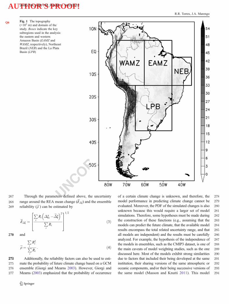
174 This study uses simulations and projections of the mean175 precipitation and surface air temperature generated by 24176 GCMs from the CMIP3 dataset used in the IPCC Fourth177 Assessment Report (IPCC AR4, Solomon et al. 2007). More178 details about the models and simulations can be found in179 Randall et al. (2007, Table 8.1) and Meehl et al. (2007a, b)180 and on the Program for Climate Models Diagnosis and181 Intercomparison website (http://www-pcmdi.llnl.gov/ipcc/182 about_ipcc.php).183 Climate simulations for the twentieth century (20C3M)184 and projections for the twenty-first century for three dif-185 ferent GHG and aerosol emissions scenarios, SRES B1,186 A1B, and A2 (Nakicenovic et al. 2000), are used in the187 seasonal averages for the periods 1961–1990 (present188 time), 2041–2070, and 2071–2100 (future time slices).189 These scenarios correspond to an equivalent CO2 concen-190 tration in 2100 of approximately 550 (B1), 700 (A1B),191 and 850 ppm (A2). Throughout this work, the changes are192 referenced to the averaged 1961–1990 period. When more193 than one model run per experiment is available, the mean194 of all the analyzed model runs is used. This is possible195 because the averages over time slices of more than196 10 years do not differ substantially between different runs197 of the same model experiment, and because these differ-198 ences are much smaller than the comparison between199 different models (Giorgi and Francisco 2000; Knutti200 2008). All of the model simulations for the twentieth201 century are compared against the observed surface air202 temperature and precipitation from the CRU TS 3.0 data-203 set (Mitchell and Jones 2005) produced by the University204 of East Anglia Climate Research Unit.205 The spatial resolution of the GCMs varies from ap-206 proximately 1° to 5° (Randall et al. 2007, Table 8.1), and207 for intercomparison purposes, the model runs and the208 observed data are interpolated to a common 2.5°×2.5°209 grid. REA calculations are performed using all of the210 simulations and projections for each South American211 land grid point, but some area averages of the results212 are taken into account in four key subregions: the eastern213 and western Amazon Basin (EAMZ and WAMZ, respec-214 tively), Northeast Brazil (NEB), and the La Plata Basin215 (LPB, Fig. 1). These regions were chosen because they216 represent different climatic conditions during El Niño and217 La Niña events, as well as sea surface temperature218 anomalies in the tropical Atlantic (Ambrizzi et al. 2004;219 Nobre et al. 2006). Moreover, these regions have pre-220 sented different signals of precipitation change among the221 climate models projected by the end of the twenty-first222 century (Meehl et al. 2007a; Marengo et al. 2010b).

2232.2 Reliability ensemble averaging

224In Q7the REA approach (Giorgi and Mearns 2002), the mean

225change for a climate variable ξ (~Δx) projected by a set of

226models is given by the weighted average of each ensemble227member projected change (Δxi) as Q8:

~Δx ¼

PiRiΔxiPiRi

; ð1Þ

228229where Ri is the reliability factor of the model defined by

Ri ¼ RB;i

� �m � RD;i

� �n� � 1= m�nð Þ½ �

¼ "x

abs Bx;i� �

" #m"x

abs Dx;i� �

" #n( ) 1= m�nð Þ½ �: ð2Þ

230231232RB, i is a factor that measures the model reliability as a233function of its bias (Bξ, i) when simulating the variable ξ234in the current climate, that is, the higher the bias, the235lower the model reliability. RD, i evaluates the model236reliability in terms of the distance (Dξ, i) between its237projected change and the ensemble REA mean, that is,238an outlier model result is downweighted. In other words,239RB, i and RD, i represents the model’s performance and240convergence criteria, respectively. Equations (1) and (2)241establish that a given model projection is said to be more242reliable when its bias and distance to the REA mean are243within the natural variability of the analyzed variable244(εξ), such that RB ¼ RD ¼ 1. Parameters m and n were245introduced by Giorgi and Mearns to balance both criteria246differently, but for simplicity, in this work, it was as-247sumed that m0n01.248The convergence criteria are based on the hypothesis that,249for a given emission scenario, if the climate change signals250produced by the different climate models are not very sen-251sitive to the differences among the models, these signals are252said to be more reliable, and the ensemble model average253could converge to the future climate conditions. However,254as emphasized by Giorgi and Mearns (2002), the distance to255the REA mean is only an estimate of the convergence256criteria because the future conditions are not known.257Moreover, the REA mean is not intended to be the true258climate response to a given forcing scenario, but rather a259better estimate of it. In this study, just as in Giorgi and260Mearns (2002), the natural variability of the surface air261temperature and precipitation are estimated for each grid262point by taking the difference between the highest and263minimum values of the observed time series (1901–2000),264after removing the linear tendency of the data and applying a265running mean filter to average-over fluctuations shorter than26630 years.

Uncertainty assessments of climate change projectionsQ1


AUTHOR'S PROOF!

UNCORRECTEDPROOF

267 Through the parameters defined above, the uncertainty

268 range around the REA mean change (~dΔx) and the ensemble

269 reliability ( ~ρ ) can be estimated by

~dΔx ¼

PiRi Δxi �

~Δx

� �2

PiRi

2664

37751=2

ð3Þ

270271 and

~ρ ¼PiR2iP

iRi

: ð4Þ

272273274 Additionally, the reliability factors can also be used to esti-275 mate the probability of future climate change based on a GCM276 ensemble (Giorgi and Mearns 2003). However, Giorgi and277 Mearns (2003) emphasized that the probability of occurrence

278of a certain climate change is unknown, and therefore, the279model performance in predicting climate change cannot be280evaluated. Moreover, the PDF of the simulated changes is also281unknown because this would require a larger set of model282simulations. Therefore, some hypotheses must be made during283the construction of these functions (e.g., assuming that the284models can predict the future climate, that the available model285results encompass the total related uncertainty range, and that286all models are independent) and the results must be carefully287analyzed. For example, the hypothesis of the independence of288the models in ensembles, such as the CMIP3 dataset, is one of289the main caveats of model weighting studies, such as the one290discussed here. Most of the models exhibit strong similarities291due to factors that included their being developed at the same292institution, their sharing versions of the same atmospheric or293oceanic components, and/or their being successive versions of294the same model (Masson and Knutti 2011). This model

Fig. 1 TheQ6 topography(×102 m) and domain of thestudy. Boxes indicate the keysubregions used in the analysis:the eastern and westernAmazon Basin (EAMZ andWAMZ, respectively), NortheastBrazil (NEB) and the La PlataBasin (LPB)



AUTHOR'S PROOF!

UNCORRECTEDPROOF

295 dependency reduces the effective sample size in the ensemble296 averaging process.297 According to Giorgi and Mearns (2003), the probability298 of occurrence of a climate change projection simulated by a299 model i (Pmi ) can be considered to be proportional to the300 normalized reliability parameter defined in Eq. (2), i.e.,

Pmi ¼RiPNj¼1 Rj

; ð5Þ

301302 where N represents the number of different GCMs. In other303 words, it is assumed that a climate change simulated by a304 model with a higher reliability parameter value is more305 likely to occur.306 The construction and validation of a PDF (or CDF) are307 far from being a trivial task. First, to evaluate the PDFs308 generated from model ensembles, an observed and well-309 representative distribution of the present climate variability310 must be created, which is not easy to accomplish because of311 the geographically sparse data and the lack of extended and312 continuous observational climate data information, especial-313 ly for South America. Due to this basic restriction, the314 validation of any model-based PDF is compromised, when315 a real PDF distribution of the current climate is not known.316 Second, a good model-based PDF should be constructed317 (ideally) from a very large sample of hundreds of simula-318 tions of the same model at a high spatial resolution, and this319 large number of simulations should be performed for each of320 several different models, a task that is very computationally321 expensive and not feasible. Because of this, it is difficult to322 establish one methodology to construct the PDFs or to deter-323 mine the PDF results as being more suitable or reliable. All of324 the studies (including the present study) are limited to a325 relatively small sample size of simulations and observations.326 However, although REA is a very simple methodology, the327 PDFs generated by this method are in agreement with and are328 quite comparable to more sophisticated methodologies pre-329 sented in the literature (Tebaldi et al. 2005; Tebaldi and Knutti330 2007; Greene et al. 2006; Furrer et al. 2007).

331 3 Results

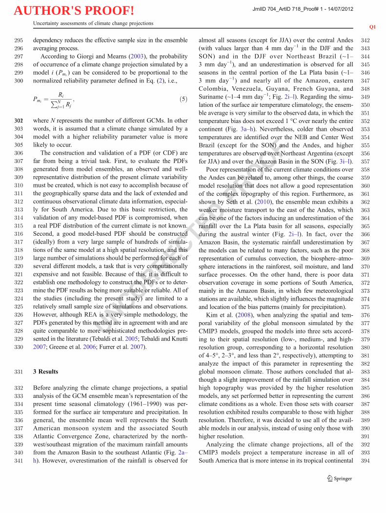
332 Before analyzing the climate change projections, a spatial333 analysis of the GCM ensemble mean’s representation of the334 present time seasonal climatology (1961–1990) was per-335 formed for the surface air temperature and precipitation. In336 general, the ensemble mean well represents the South337 American monsoon system and the associated South338 Atlantic Convergence Zone, characterized by the north-339 west/southeast migration of the maximum rainfall amounts340 from the Amazon Basin to the southeast Atlantic (Fig. 2a–341 h). However, overestimation of the rainfall is observed for

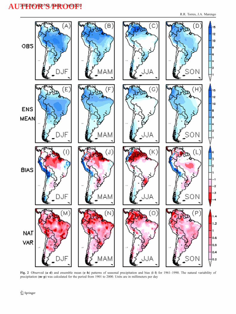
342almost all seasons (except for JJA) over the central Andes343(with values larger than 4 mm day−1 in the DJF and the344SON) and in the DJF over Northeast Brazil (~1–3453 mm day−1), and an underestimation is observed for all346seasons in the central portion of the La Plata basin (~1–3473 mm day−1) and nearly all of the Amazon, eastern348Colombia, Venezuela, Guyana, French Guyana, and349Suriname (~1–4 mm day−1; Fig. 2i–l). Regarding the simu-350lation of the surface air temperature climatology, the ensem-351ble average is very similar to the observed data, in which the352temperature bias does not exceed 1 °C over nearly the entire353continent (Fig. 3a–h). Nevertheless, colder than observed354temperatures are identified over the NEB and Center West355Brazil (except for the SON) and the Andes, and higher356temperatures are observed over Northeast Argentina (except357for JJA) and over the Amazon Basin in the SON (Fig. 3i–l).358Poor representation of the current climate conditions over359the Andes can be related to, among other things, the coarse360model resolution that does not allow a good representation361of the complex topography of this region. Furthermore, as362shown by Seth et al. (2010), the ensemble mean exhibits a363weaker moisture transport to the east of the Andes, which364can be one of the factors inducing an underestimation of the365rainfall over the La Plata basin for all seasons, especially366during the austral winter (Fig. 2i–l). In fact, over the367Amazon Basin, the systematic rainfall underestimation by368the models can be related to many factors, such as the poor369representation of cumulus convection, the biosphere–atmo-370sphere interactions in the rainforest, soil moisture, and land371surface processes. On the other hand, there is poor data372observation coverage in some portions of South America,373mainly in the Amazon Basin, in which few meteorological374stations are available, which slightly influences the magnitude375and location of the bias patterns (mainly for precipitation).376Kim et al. (2008), when analyzing the spatial and tem-377poral variability of the global monsoon simulated by the378CMIP3 models, grouped the models into three sets accord-379ing to their spatial resolution (low-, medium-, and high-380resolution group, corresponding to a horizontal resolution381of 4–5°, 2–3°, and less than 2°, respectively), attempting to382analyze the impact of this parameter in representing the383global monsoon climate. Those authors concluded that al-384though a slight improvement of the rainfall simulation over385high topography was provided by the higher resolution386models, any set performed better in representing the current387climate conditions as a whole. Even those sets with coarser388resolution exhibited results comparable to those with higher389resolution. Therefore, it was decided to use all of the avail-390able models in our analysis, instead of using only those with391higher resolution.392Analyzing the climate change projections, all of the393CMIP3 models project a temperature increase in all of394South America that is more intense in its tropical continental



AUTHOR'S PROOF!

UNCORRECTEDPROOF

Fig. 2 Observed (a–d) and ensemble mean (e–h) patterns of seasonal precipitation and bias (i–l) for 1961–1990. The natural variability ofprecipitation (m–p) was calculated for the period from 1901 to 2000. Units are in millimeters per day



AUTHOR'S PROOF!

UNCORRECTEDPROOF

Fig. 3 a–p The same as in Fig. 2, but for seasonal surface air temperature (in degrees Celsius)



AUTHOR'S PROOF!

UNCORRECTEDPROOF

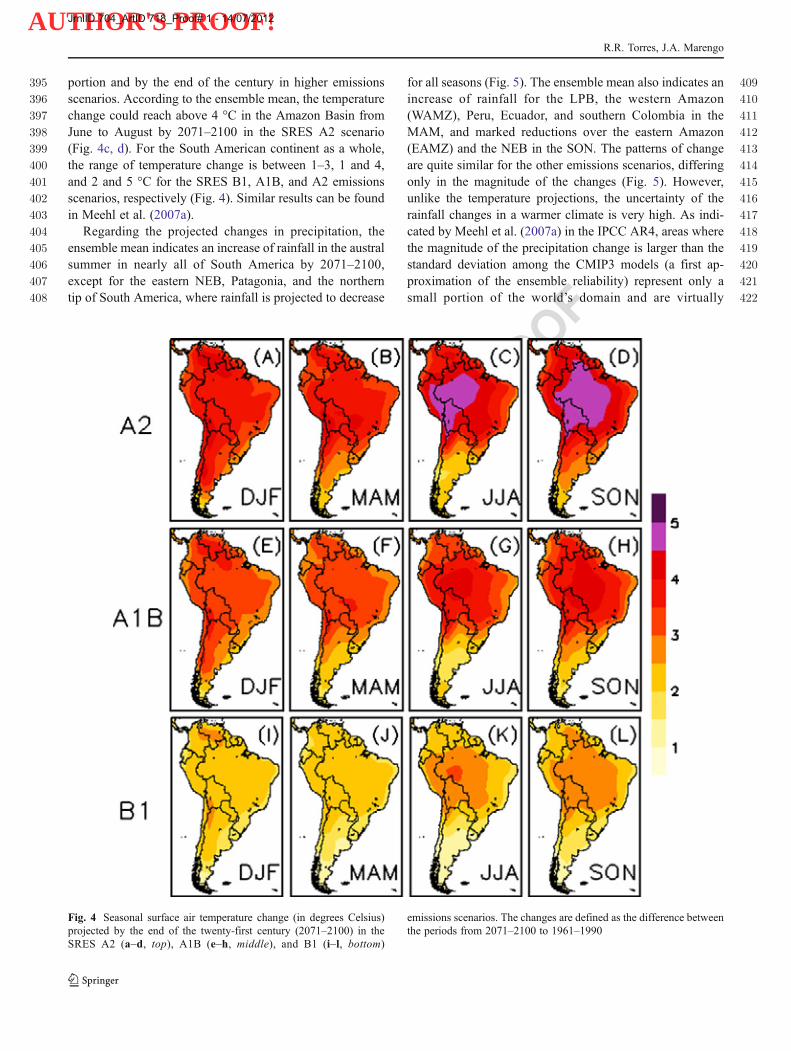
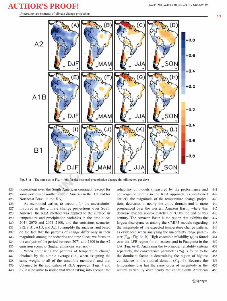
395 portion and by the end of the century in higher emissions396 scenarios. According to the ensemble mean, the temperature397 change could reach above 4 °C in the Amazon Basin from398 June to August by 2071–2100 in the SRES A2 scenario399 (Fig. 4c, d). For the South American continent as a whole,400 the range of temperature change is between 1–3, 1 and 4,401 and 2 and 5 °C for the SRES B1, A1B, and A2 emissions402 scenarios, respectively (Fig. 4). Similar results can be found403 in Meehl et al. (2007a).404 Regarding the projected changes in precipitation, the405 ensemble mean indicates an increase of rainfall in the austral406 summer in nearly all of South America by 2071–2100,407 except for the eastern NEB, Patagonia, and the northern408 tip of South America, where rainfall is projected to decrease

409for all seasons (Fig. 5). The ensemble mean also indicates an410increase of rainfall for the LPB, the western Amazon411(WAMZ), Peru, Ecuador, and southern Colombia in the412MAM, and marked reductions over the eastern Amazon413(EAMZ) and the NEB in the SON. The patterns of change414are quite similar for the other emissions scenarios, differing415only in the magnitude of the changes (Fig. 5). However,416unlike the temperature projections, the uncertainty of the417rainfall changes in a warmer climate is very high. As indi-418cated by Meehl et al. (2007a) in the IPCC AR4, areas where419the magnitude of the precipitation change is larger than the420standard deviation among the CMIP3 models (a first ap-421proximation of the ensemble reliability) represent only a422small portion of the world’s domain and are virtually

Fig. 4 Seasonal surface air temperature change (in degrees Celsius)projected by the end of the twenty-first century (2071–2100) in theSRES A2 (a–d, top), A1B (e–h, middle), and B1 (i–l, bottom)

emissions scenarios. The changes are defined as the difference betweenthe periods from 2071–2100 to 1961–1990



AUTHOR'S PROOF!

UNCORRECTEDPROOF

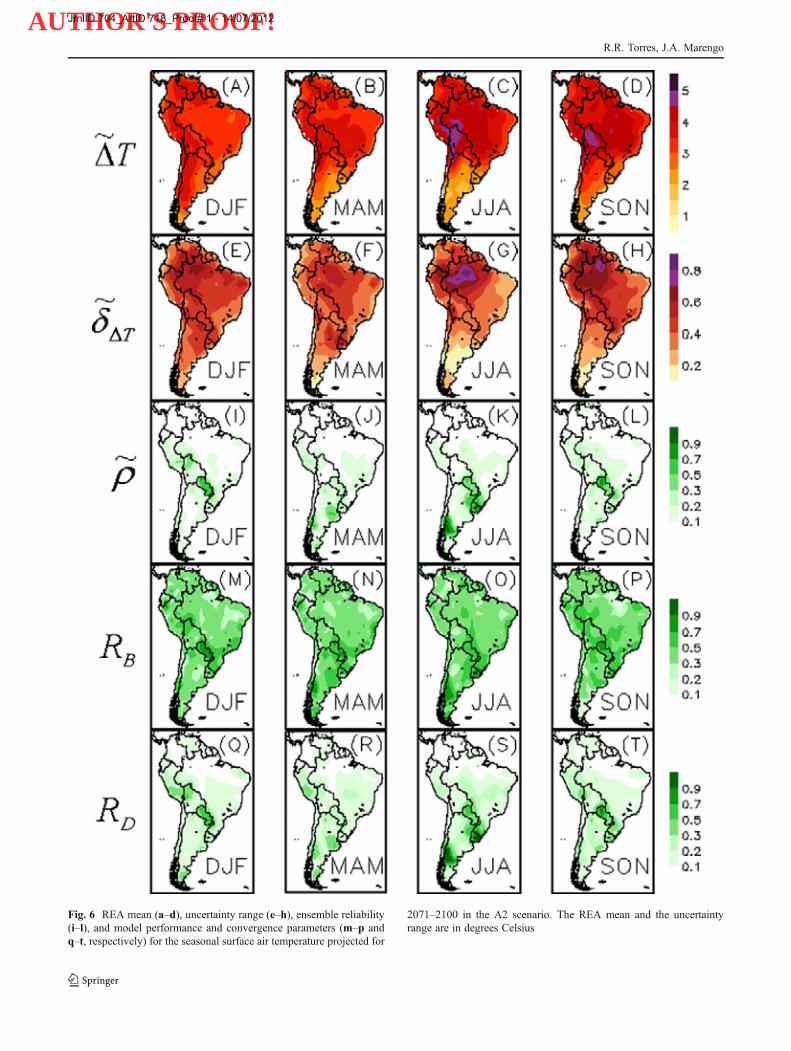
423 nonexistent over the South American continent (except for424 some portions of southern South America in the DJF and for425 Northeast Brazil in the JJA).426 As mentioned earlier, to account for the uncertainties427 involved in the climate change projections over South428 America, the REA method was applied to the surface air429 temperature and precipitation variables in the time slices430 2041–2070 and 2071–2100, and the emissions scenarios431 SRES B1, A1B, and A2. To simplify the analysis, and based432 on the fact that the patterns of change differ only in their433 magnitude among the scenarios and time slices, we focus on434 the analysis of the period between 2071 and 2100 in the A2435 emission scenario (higher emissions scenario).436 When comparing the patterns of temperature change437 obtained by the simple average (i.e., when assigning the438 same weight to all of the ensemble members) and that439 obtained by the application of REA approach (Figs. 4 and440 6), it is possible to notice that when taking into account the

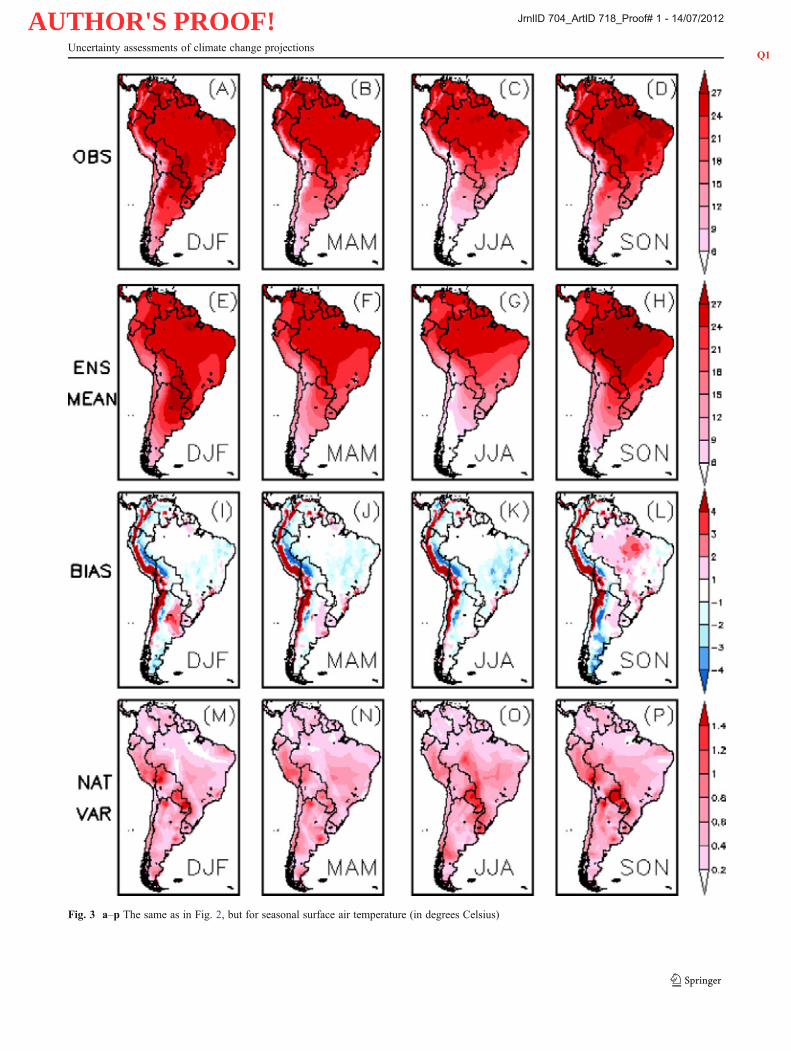
441reliability of models (measured by the performance and442convergence criteria in the REA approach, as mentioned443earlier), the magnitude of the temperature change projec-444tions decreases in nearly the entire domain and is more445pronounced over the western Amazon Basin, where this446decrease reaches approximately 0.5 °C by the end of this447century. The Amazon Basin is the region that exhibits the448largest discrepancies among the CMIP3 models regarding449the magnitude of the expected temperature change pattern,450as evidenced when analyzing the uncertainty range param-451eter (~dΔT , Fig. 6e–h). High ensemble reliability (~ρ) is found452over the LPB region for all seasons and in Patagonia in the453JJA (Fig. 6i–l). Analyzing the two model reliability criteria454separately, the convergence parameter (RD) is found to be455the dominant factor in determining the region of highest456confidence in the studied domain (Fig. 6). Because the457temperature bias has the same order of magnitude as the458natural variability over nearly the entire South American

Fig. 5 a–l The same as in Fig. 4, but for the seasonal precipitation change (in millimeters per day)



AUTHOR'S PROOF!

UNCORRECTEDPROOF

Fig. 6 REA mean (a–d), uncertainty range (e–h), ensemble reliability(i–l), and model performance and convergence parameters (m–p andq–t, respectively) for the seasonal surface air temperature projected for

2071–2100 in the A2 scenario. The REA mean and the uncertaintyrange are in degrees Celsius



AUTHOR'S PROOF!

UNCORRECTEDPROOF

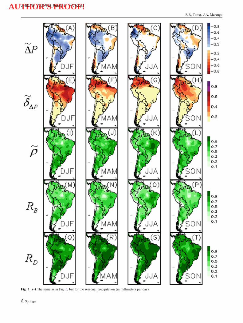
459 region (Fig. 3i–p and m–p, respectively), high RB values are460 found throughout the studied domain. As the range of the461 projected temperature change is large among the models and462 the natural variability is small (Fig. 3m–p), RD is small, except463 in some seasons over Paraguay, Northwest Bolivia/southern464 Peru, southern Brazil, Uruguay, and southern Argentina,465 which possess high natural variability, as shown in Fig. 3m–p.466 The REA average changes for precipitation (Fig. 7a–d)467 show no marked difference when compared with the simple468 ensemble mean (Fig. 5), except in northern Peru/southern469 Colombia in the DJF and eastern Amazonia in the SON, in470 which the magnitude of the projected precipitation change is471 reduced (approximately 0.4 and 0.2 mm day−1, respectively).472 Large uncertainty ranges are noticeable over northern South473 America in all seasons, and over the Amazon Basin, NEB, and474 Center West Brazil in the DJF and the SON. The convergence475 parameter is greater than the performance parameter (RDRB)476 because the model bias is larger than the magnitude of the477 projected rainfall changes, and the magnitude of the changes478 is small and comparable to the natural variability (Fig. 2m–p).479 The ensemble reliability is above 0.5 in nearly the entire South480 American continent, which may indicate that there is high481 reliability in a projection of no significant change. Similar482 results were found by Giorgi and Mearns (2002), when ap-483 plying the REA method to a set of 18 different GCMs aver-484 aged over 22 continental regions covering the entire globe.485 Tables 1 and 2 show the REA results for the rainfall and486 surface air temperature averaged in the key regions indicat-487 ed in Fig. 1 for the periods 2041–2070 and 2071–2100, and488 in the SRES B1, A1B, and A2 scenarios, for the austral489 summer and winter. The REA approach, when applied to the490 temperature variable, in all regions, time slices, and scenar-491 ios, reduces the magnitude of change (by approximately492 8 %) when compared with the simple ensemble mean.493 Furthermore, all REA mean temperature changes are larger494 than its associated uncertainty range and, as expected, the495 ensemble reliability decreases when analyzing higher emis-496 sions scenarios and more distant periods. Therefore, for497 2071–2100 (2041–2070) in the A2 scenario, higher reliabil-498 ity is found over the LPB, as previously analyzed, where499 temperature increases can reach 3.1±0.8 °C (1.9±0.5 °C) in500 the austral summer and 3.3±0.6 °C (1.9±0.4 °C) in the501 austral winter. On the other hand, a higher uncertainty range502 is found in the Amazon Basin, where the results show a503 temperature increase of 3.3±0.9 °C (3.9±0.9 °C) in the504 austral summer (winter) over the eastern Amazon, and 3.5505 ±1.1 °C (4.2±1.1 °C) in the austral summer (winter) for the506 western Amazon, for 2071–2100 (2041–2070) in the A2507 scenario. For projections of the precipitation change, the508 uncertainty range, as derived by the REA approach, has509 the same order of magnitude as the projected change in all510 of the analyzed regions, scenarios, and time slices, indicat-511 ing no significant change.

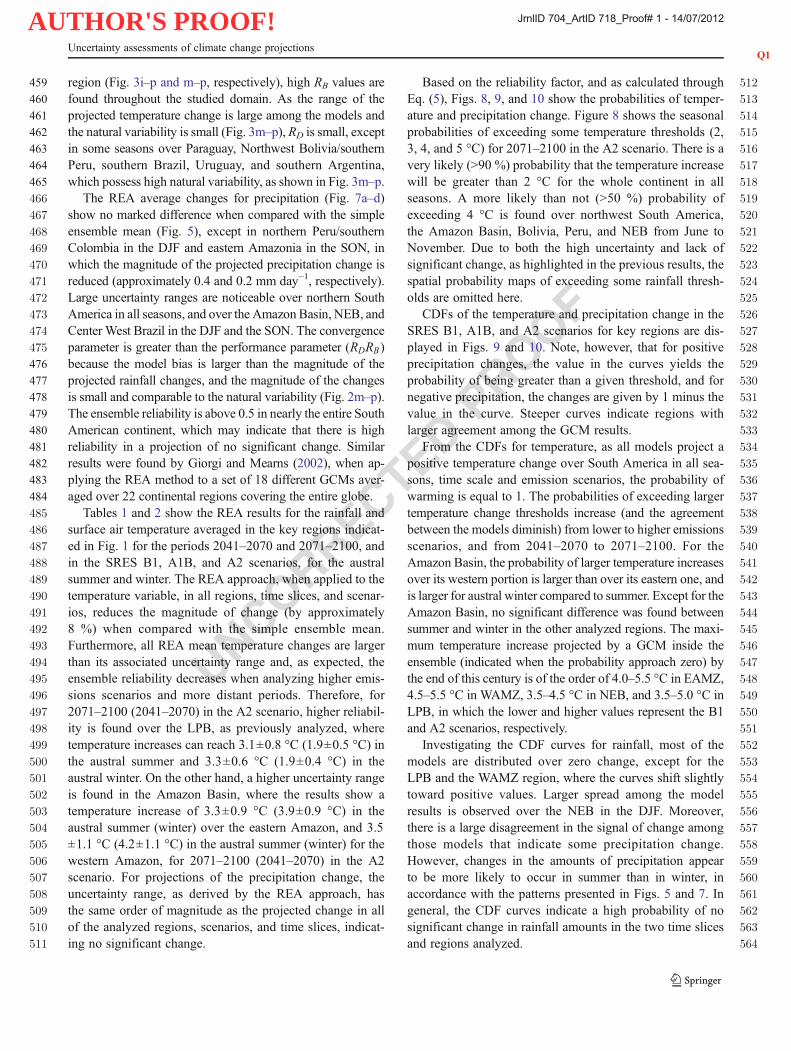
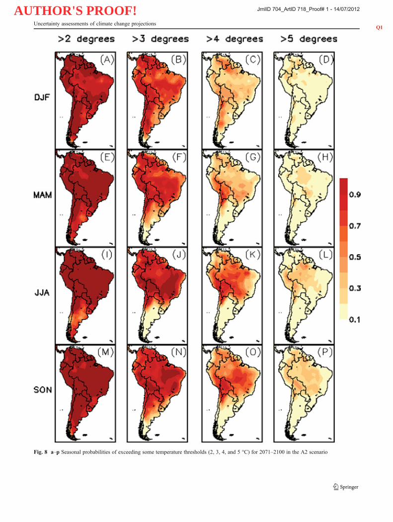
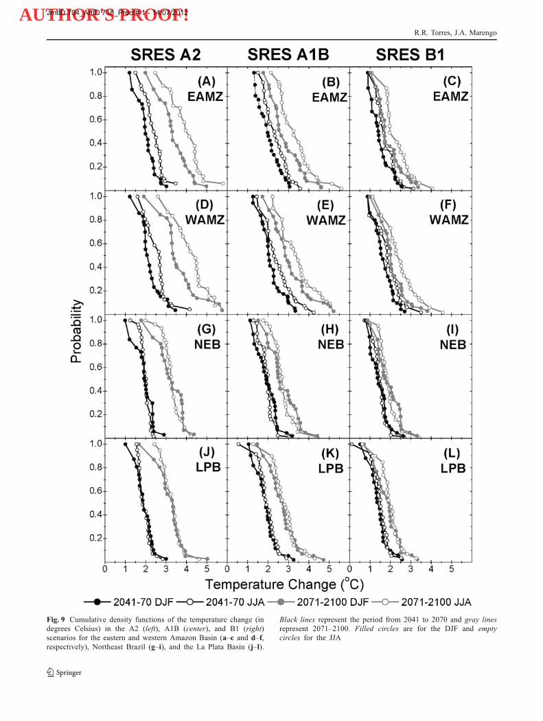
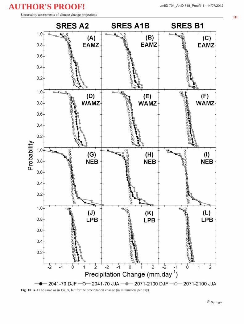
512Based on the reliability factor, and as calculated through513Eq. (5), Figs. 8, 9, and 10 show the probabilities of temper-514ature and precipitation change. Figure 8 shows the seasonal515probabilities of exceeding some temperature thresholds (2,5163, 4, and 5 °C) for 2071–2100 in the A2 scenario. There is a517very likely (>90 %) probability that the temperature increase518will be greater than 2 °C for the whole continent in all519seasons. A more likely than not (>50 %) probability of520exceeding 4 °C is found over northwest South America,521the Amazon Basin, Bolivia, Peru, and NEB from June to522November. Due to both the high uncertainty and lack of523significant change, as highlighted in the previous results, the524spatial probability maps of exceeding some rainfall thresh-525olds are omitted here.526CDFs of the temperature and precipitation change in the527SRES B1, A1B, and A2 scenarios for key regions are dis-528played in Figs. 9 and 10. Note, however, that for positive529precipitation changes, the value in the curves yields the530probability of being greater than a given threshold, and for531negative precipitation, the changes are given by 1 minus the532value in the curve. Steeper curves indicate regions with533larger agreement among the GCM results.534From the CDFs for temperature, as all models project a535positive temperature change over South America in all sea-536sons, time scale and emission scenarios, the probability of537warming is equal to 1. The probabilities of exceeding larger538temperature change thresholds increase (and the agreement539between the models diminish) from lower to higher emissions540scenarios, and from 2041–2070 to 2071–2100. For the541Amazon Basin, the probability of larger temperature increases542over its western portion is larger than over its eastern one, and543is larger for austral winter compared to summer. Except for the544Amazon Basin, no significant difference was found between545summer and winter in the other analyzed regions. The maxi-546mum temperature increase projected by a GCM inside the547ensemble (indicated when the probability approach zero) by548the end of this century is of the order of 4.0–5.5 °C in EAMZ,5494.5–5.5 °C in WAMZ, 3.5–4.5 °C in NEB, and 3.5–5.0 °C in550LPB, in which the lower and higher values represent the B1551and A2 scenarios, respectively.552Investigating the CDF curves for rainfall, most of the553models are distributed over zero change, except for the554LPB and the WAMZ region, where the curves shift slightly555toward positive values. Larger spread among the model556results is observed over the NEB in the DJF. Moreover,557there is a large disagreement in the signal of change among558those models that indicate some precipitation change.559However, changes in the amounts of precipitation appear560to be more likely to occur in summer than in winter, in561accordance with the patterns presented in Figs. 5 and 7. In562general, the CDF curves indicate a high probability of no563significant change in rainfall amounts in the two time slices564and regions analyzed.



AUTHOR'S PROOF!

UNCORRECTEDPROOF

Fig. 7 a–t The same as in Fig. 6, but for the seasonal precipitation (in millimeters per day)



AUTHOR'S PROOF!

UNCORRECTEDPROOF

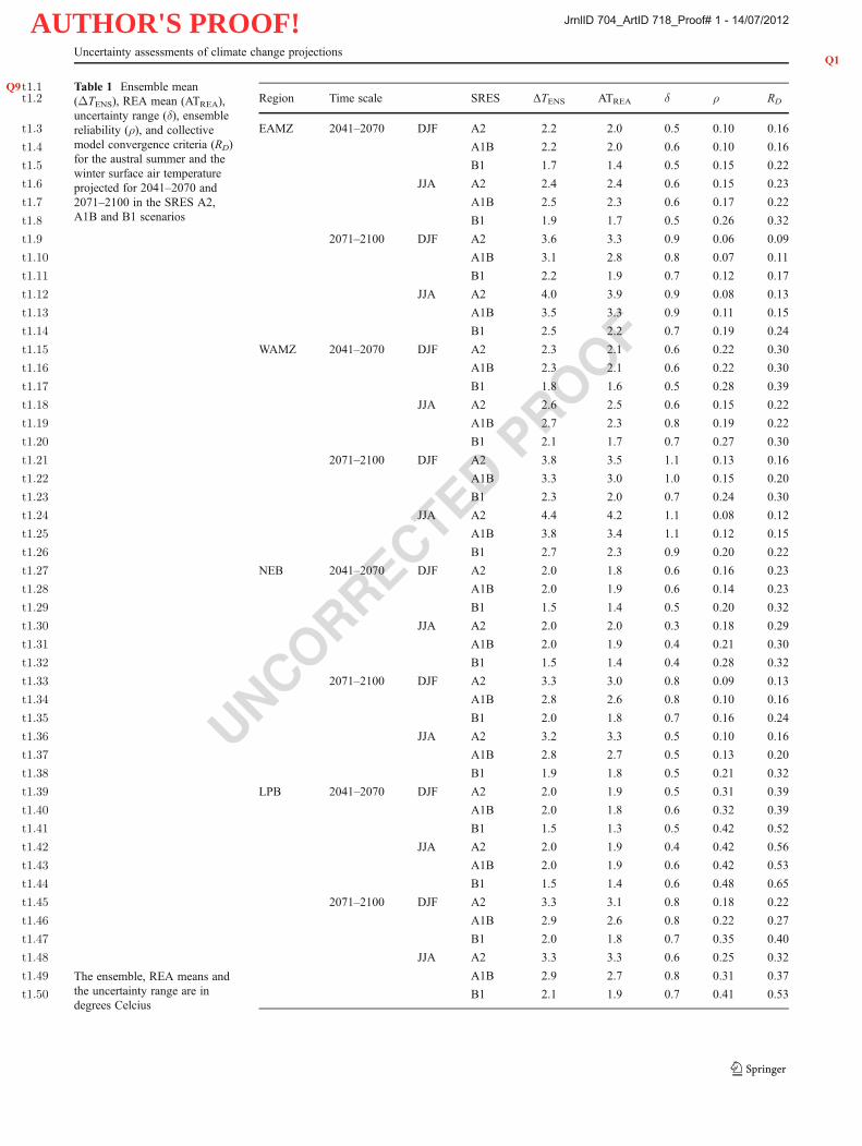
t1:1 Table 1 EnsembleQ9 mean(ΔTENS), REA mean (ATREA),uncertainty range (δ), ensemblereliability (ρ), and collectivemodel convergence criteria (RD)for the austral summer and thewinter surface air temperatureprojected for 2041–2070 and2071–2100 in the SRES A2,A1B and B1 scenarios

The ensemble, REA means andthe uncertainty range are indegrees Celcius

t1:2 Region Time scale SRES ΔTENS ATREA δ ρ RD

t1:3 EAMZ 2041–2070 DJF A2 2.2 2.0 0.5 0.10 0.16

t1:4 A1B 2.2 2.0 0.6 0.10 0.16

t1:5 B1 1.7 1.4 0.5 0.15 0.22

t1:6 JJA A2 2.4 2.4 0.6 0.15 0.23

t1:7 A1B 2.5 2.3 0.6 0.17 0.22

t1:8 B1 1.9 1.7 0.5 0.26 0.32

t1:9 2071–2100 DJF A2 3.6 3.3 0.9 0.06 0.09

t1:10 A1B 3.1 2.8 0.8 0.07 0.11

t1:11 B1 2.2 1.9 0.7 0.12 0.17

t1:12 JJA A2 4.0 3.9 0.9 0.08 0.13

t1:13 A1B 3.5 3.3 0.9 0.11 0.15

t1:14 B1 2.5 2.2 0.7 0.19 0.24

t1:15 WAMZ 2041–2070 DJF A2 2.3 2.1 0.6 0.22 0.30

t1:16 A1B 2.3 2.1 0.6 0.22 0.30

t1:17 B1 1.8 1.6 0.5 0.28 0.39

t1:18 JJA A2 2.6 2.5 0.6 0.15 0.22

t1:19 A1B 2.7 2.3 0.8 0.19 0.22

t1:20 B1 2.1 1.7 0.7 0.27 0.30

t1:21 2071–2100 DJF A2 3.8 3.5 1.1 0.13 0.16

t1:22 A1B 3.3 3.0 1.0 0.15 0.20

t1:23 B1 2.3 2.0 0.7 0.24 0.30

t1:24 JJA A2 4.4 4.2 1.1 0.08 0.12

t1:25 A1B 3.8 3.4 1.1 0.12 0.15

t1:26 B1 2.7 2.3 0.9 0.20 0.22

t1:27 NEB 2041–2070 DJF A2 2.0 1.8 0.6 0.16 0.23

t1:28 A1B 2.0 1.9 0.6 0.14 0.23

t1:29 B1 1.5 1.4 0.5 0.20 0.32

t1:30 JJA A2 2.0 2.0 0.3 0.18 0.29

t1:31 A1B 2.0 1.9 0.4 0.21 0.30

t1:32 B1 1.5 1.4 0.4 0.28 0.32

t1:33 2071–2100 DJF A2 3.3 3.0 0.8 0.09 0.13

t1:34 A1B 2.8 2.6 0.8 0.10 0.16

t1:35 B1 2.0 1.8 0.7 0.16 0.24

t1:36 JJA A2 3.2 3.3 0.5 0.10 0.16

t1:37 A1B 2.8 2.7 0.5 0.13 0.20

t1:38 B1 1.9 1.8 0.5 0.21 0.32

t1:39 LPB 2041–2070 DJF A2 2.0 1.9 0.5 0.31 0.39

t1:40 A1B 2.0 1.8 0.6 0.32 0.39

t1:41 B1 1.5 1.3 0.5 0.42 0.52

t1:42 JJA A2 2.0 1.9 0.4 0.42 0.56

t1:43 A1B 2.0 1.9 0.6 0.42 0.53

t1:44 B1 1.5 1.4 0.6 0.48 0.65

t1:45 2071–2100 DJF A2 3.3 3.1 0.8 0.18 0.22

t1:46 A1B 2.9 2.6 0.8 0.22 0.27

t1:47 B1 2.0 1.8 0.7 0.35 0.40

t1:48 JJA A2 3.3 3.3 0.6 0.25 0.32

t1:49 A1B 2.9 2.7 0.8 0.31 0.37

t1:50 B1 2.1 1.9 0.7 0.41 0.53



AUTHOR'S PROOF!

UNCORRECTEDPROOF

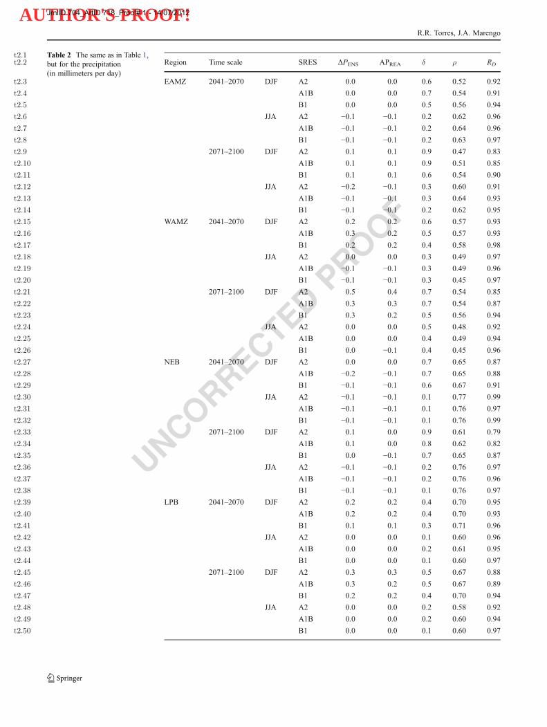
t2:1 Table 2 The same as in Table 1,but for the precipitation(in millimeters per day)

t2:2 Region Time scale SRES ΔPENS APREA δ ρ RD

t2:3 EAMZ 2041–2070 DJF A2 0.0 0.0 0.6 0.52 0.92

t2:4 A1B 0.0 0.0 0.7 0.54 0.91

t2:5 B1 0.0 0.0 0.5 0.56 0.94

t2:6 JJA A2 −0.1 −0.1 0.2 0.62 0.96

t2:7 A1B −0.1 −0.1 0.2 0.64 0.96

t2:8 B1 −0.1 −0.1 0.2 0.63 0.97

t2:9 2071–2100 DJF A2 0.1 0.1 0.9 0.47 0.83

t2:10 A1B 0.1 0.1 0.9 0.51 0.85

t2:11 B1 0.1 0.1 0.6 0.54 0.90

t2:12 JJA A2 −0.2 −0.1 0.3 0.60 0.91

t2:13 A1B −0.1 −0.1 0.3 0.64 0.93

t2:14 B1 −0.1 −0.1 0.2 0.62 0.95

t2:15 WAMZ 2041–2070 DJF A2 0.2 0.2 0.6 0.57 0.93

t2:16 A1B 0.3 0.2 0.5 0.57 0.93

t2:17 B1 0.2 0.2 0.4 0.58 0.98

t2:18 JJA A2 0.0 0.0 0.3 0.49 0.97

t2:19 A1B −0.1 −0.1 0.3 0.49 0.96

t2:20 B1 −0.1 −0.1 0.3 0.45 0.97

t2:21 2071–2100 DJF A2 0.5 0.4 0.7 0.54 0.85

t2:22 A1B 0.3 0.3 0.7 0.54 0.87

t2:23 B1 0.3 0.2 0.5 0.56 0.94

t2:24 JJA A2 0.0 0.0 0.5 0.48 0.92

t2:25 A1B 0.0 0.0 0.4 0.49 0.94

t2:26 B1 0.0 −0.1 0.4 0.45 0.96

t2:27 NEB 2041–2070 DJF A2 0.0 0.0 0.7 0.65 0.87

t2:28 A1B −0.2 −0.1 0.7 0.65 0.88

t2:29 B1 −0.1 −0.1 0.6 0.67 0.91

t2:30 JJA A2 −0.1 −0.1 0.1 0.77 0.99

t2:31 A1B −0.1 −0.1 0.1 0.76 0.97

t2:32 B1 −0.1 −0.1 0.1 0.76 0.99

t2:33 2071–2100 DJF A2 0.1 0.0 0.9 0.61 0.79

t2:34 A1B 0.1 0.0 0.8 0.62 0.82

t2:35 B1 0.0 −0.1 0.7 0.65 0.87

t2:36 JJA A2 −0.1 −0.1 0.2 0.76 0.97

t2:37 A1B −0.1 −0.1 0.2 0.76 0.96

t2:38 B1 −0.1 −0.1 0.1 0.76 0.97

t2:39 LPB 2041–2070 DJF A2 0.2 0.2 0.4 0.70 0.95

t2:40 A1B 0.2 0.2 0.4 0.70 0.93

t2:41 B1 0.1 0.1 0.3 0.71 0.96

t2:42 JJA A2 0.0 0.0 0.1 0.60 0.96

t2:43 A1B 0.0 0.0 0.2 0.61 0.95

t2:44 B1 0.0 0.0 0.1 0.60 0.97

t2:45 2071–2100 DJF A2 0.3 0.3 0.5 0.67 0.88

t2:46 A1B 0.3 0.2 0.5 0.67 0.89

t2:47 B1 0.2 0.2 0.4 0.70 0.94

t2:48 JJA A2 0.0 0.0 0.2 0.58 0.92

t2:49 A1B 0.0 0.0 0.2 0.60 0.94

t2:50 B1 0.0 0.0 0.1 0.60 0.97



AUTHOR'S PROOF!

UNCORRECTEDPROOF

Fig. 8 a–p Seasonal probabilities of exceeding some temperature thresholds (2, 3, 4, and 5 °C) for 2071–2100 in the A2 scenario



AUTHOR'S PROOF!

UNCORRECTEDPROOF

Fig. 9 Cumulative density functions of the temperature change (indegrees Celsius) in the A2 (left), A1B (center), and B1 (right)scenarios for the eastern and western Amazon Basin (a–c and d–f,respectively), Northeast Brazil (g–i), and the La Plata Basin (j–l).

Black lines represent the period from 2041 to 2070 and gray linesrepresent 2071–2100. Filled circles are for the DJF and emptycircles for the JJA



AUTHOR'S PROOF!

UNCORRECTEDPROOF

Fig. 10 a–l The same as in Fig. 9, but for the precipitation change (in millimeters per day)



AUTHOR'S PROOF!

UNCORRECTEDPROOF

565 4 Summary and conclusion

566 Due to the increasing need for a detailed and probabilistic567 analysis of the uncertainties in climate change projections568 over South America, this study analyzes the projected tem-569 perature and precipitation changes from all the GCMs avail-570 able in the CMIP3 dataset over different time slices (2041–571 2070 and 2071–2100) and emissions scenarios (SRES B1,572 A1B, and A2), relative to the present climate (1961–1990).573 The REA approach is applied to the seasonal mean surface574 air temperature and the precipitation changes for both time575 slices and for all the analyzed emissions scenarios.576 When taking into account the performance of each model577 in representing the current climate and the convergence of578 its projection to the ensemble mean in the ensemble aver-579 aging, as proposed by the REA method, it is noted that the580 REA mean temperature change projection is slightly smaller581 (approximately 8 %) over the entire continent when com-582 pared with the simple ensemble mean. This indicates that583 outlier results are downweighted in the ensemble mean. The584 temperature change is larger than the corresponding uncer-585 tainty range for the entire South American domain and for586 the investigated time slices, showing a high reliability of the587 projected REA mean change for this variable. Higher reli-588 ability is found over the La Plata Basin, where the REA589 mean temperature change is 3.1±0.8 °C in the austral sum-590 mer and 3.3±0.6 °C in the austral winter by 2071–2100 for591 the A2 scenario. On the other hand, higher uncertainty592 ranges are found in the Amazon Basin, where the results593 show a temperature increase of 3.3±0.9 °C (3.9±0.9 °C) in594 the austral summer (winter) over the eastern Amazon and595 3.5±1.1 °C (4.2±1.1 °C) in the austral summer (winter) for596 its western portion, for the same period and scenario.597 The probability of a temperature increase exceeding the598 2 °C threshold is found to be very likely (>90 %) for all599 seasons in the entire South America region and a more likely600 than not (>50 %) probability of exceeding 4 °C is found601 over northwest South America, the Amazon Basin, Bolivia,602 Peru, and NEB from June to November by the end of the603 twenty-first century in the A2 scenario. These are the same604 areas indicated by Fung et al. (2011) that could experience605 an increase in water stress with a global temperature that is606 +2 or +4 °C warmer than the 1961–1990 average for the607 2060s. Betts et al. (2011) explains that the IPCC AR4608 projections clearly suggest that much greater levels of609 warming are possible by the end of the twenty-first century610 in the absence of mitigation. The central value of the range611 of AR4-projected global warming is approximately 4 °C.612 The higher end of the projected warming is associated with613 the higher emissions scenarios and models which included614 stronger carbon cycle feedbacks.615 When applied to precipitation, the REA mean shows no616 marked differences when compared with the simple

617ensemble mean. In general, the uncertainty range has the618same order of magnitude as the projected change. Therefore,619based on this set of global climate models and on the620applied methodology, there is high reliability in a pro-621jection of no significant rainfall change (in magnitude)622in the two future time slices analyzed over the entire623South American region. However, these results do not624apply to the projections of climate extremes. South625America had experienced an increase of extreme temperature626and precipitation events in the last half of the twentieth century627(Marengo et al. 2010a; Rusticucci et al. 2010), and many628climate models project an even further increase of such events629by the end of twenty-first century (Tebaldi et al. 2006;630Marengo et al. 2009).631In the literature, there are several proposed methods for632combining projections from ensembles of climate models633and estimating an uncertainty range, but none of them have634been shown to be the most suitable or reliable. Moreover,635this subject is far from being trivial, as indicated by Knutti et636al. (2010).637Model weighting, as in the case of the REA approach,638imposes a strong assumption in the climate change analysis639when explicitly assuming that performance in the past cli-640mate is a certain guarantee for performance into the future641climate projections. This issue is widely debated in the642scientific community, and no consensus has been reached.643Additionally, the impact of model dependency into the644ensemble mean reliability imposes some restrictions on the645interpretation of our results, so that the results must be646carefully analyzed. The REA method was chosen for its647simplicity and the various types of information that it can648provide. Other methodologies must be applied to compare649these results. In addition, regional climate model ensembles650and the next generation of global climate models that have651been prepared for the IPCC AR5 may be used to652increase the reliability in future climate change projec-653tions. Finally, the two main contributions of this study654are as follows: (1) being the first spatially explicit and655deep assessment of the climate change projections uncertain-656ties in South America and (2) producing summarized and657probabilistic information on the possible climate change out-658comes, which is more suitable for impact, adaptation, and659vulnerabilities studies.660

661Acknowledgments We thank the modeling groups, the Program for662Climate Model Diagnosis and Intercomparison and the WCRP’s Work-663ing Group on Coupled Modeling, for their roles in making the WCRP664CMIP3 multimodel dataset available. The first author was supported665by the Coordination for Improvement of Higher Education Personnel666(CAPES) and by the Brazilian National Council for Scientific and667Technological Development (CNPq). Additional funding was provided668by Rede-CLIMA, the National Institute of Science and Technology for669Climate Change (INCT-CC), and the FAPESP-Assessment of Impacts670and Vulnerability to Climate Change in Brazil and strategies for Ad-671aptation options project (Ref. 2008/58161-1).



AUTHOR'S PROOF!

UNCORRECTEDPROOF

672 References673

674 Ambrizzi T, Souza EB, Pulwarty RS (2004). The Hadley and Walker675 regional circulations and associated ENSO impacts on the South676 American seasonal rainfall. In: Diaz HF, Bradley RS (eds). The677 Hadley circulation: present, past and future. Kluwer, Dordrecht,678 21, pp 203–235679 Baettig MB, Wild M, Imboden DM (2007) A climate change index:680 where climate change may be most prominent in the 21st century.681 Geophys Res Lett 34:L01705. doi:10.1029/2006GL028159682 Betts RA, Collins M, Hemming D, Jones CD, Lowe JA, Snderson MG683 (2011) When could global warming reach 4 °C? Phil Trans R Soc684 A 369:67–84. doi:10.1098/rsta.2010.0292685 Bombardi RJ, Carvalho LMV (2009) IPCC Global coupled climate686 model simulations of the South America Monsoon System. Clim687 Dyn 33:893–916. doi:10.1007/s00382-008-0488-1688 Boulanger JP, Martinez F, Segura EC (2006) Projection of future689 climate change conditions using IPCC simulations, neural net-690 works and Bayesian statistics. Part 1: temperature mean state and691 seasonal cycle in South America. Clim Dyn 27:233–259.692 doi:10.1007/s00382-006-0134-8693 Boulanger JP, Martinez F, Segura EC (2007) Projection of future694 climate change conditions using IPCC simulations, neural net-695 works and Bayesian statistics. Part 2: precipitation mean state and696 seasonal cycle in South America. Clim Dyn 28:255–271.697 doi:10.1007/s00382-006-0182-0698 Boulanger JP, Brasseur G, Carril AF, Castro M, Degallier N, Ereño C,699 Treut HL, Marengo JA, Menendez G, Nuñez MN, Penalba OC,700 Rolla AL, Rusticucci M, Terra RA (2010) Europe-South America701 network for climate change assessment and impact studies. Clim702 Chang 98:307–329. doi:10.1007/s10584-009-9734-8703 Chou SC, Marengo JA, Lyra A, Sueiro G, Pesquero J, Alves LM, Kay G,704 Betts R, Chagas D, Gomes J, Bustamante J (2012) Downscaling of705 South America present climate driven by 4-member HadCM3 runs.706 Clim Dyn 38(3–4):635–653. doi:10.1007/s00382-011-1002-8707 Collins M (2007) Ensembles and probabilities: a new era in the708 prediction of climate change. Phil Trans R Soc A 365:1957–709 1970. doi:10.1098/rsta.2007.2068710 Ebert EE (2001) Ability of a poor man’s ensemble to predict the711 probability and distribution of precipitation. Mon Wea Rev712 129:2461–2480. doi:10.1175/1520-0493(2001)129<2461:713 AOAPMS>2.0.CO;2714 Fung F, Lopez A, New M (2011) Water availability in +2 °C and +4 °C715 worlds. Phil Trans R Soc A 369:99–116. doi:10.1098/rsta.2010.0293716 Furrer R, Sain SR, Nychka D, Meehl GA (2007) Multivariate Bayesian717 analysis of atmosphere–ocean general circulation models.718 Environ Ecol Stat 14:249–266. doi:10.1007/s10651-007-0018-z719 Giorgi F (2005) Climate change prediction. Clim Change 73:239–265.720 doi:10.1007/s10584-005-6857-4721 Giorgi F, Francisco R (2000) Uncertainties in regional climate change722 prediction: a regional analysis of ensemble simulations with the723 HadCM2 coupled AOGCM. Clim Dyn 16:169–182. doi:10.1007/724 PL00013733725 Giorgi F, Mearns LO (2002) Calculation of average, uncertainty range726 and reliability of regional climate changes from AOGCM simu-727 lations via the “Reliability Ensemble Averaging (REA)” method.728 J Clim 15:1141–1158729 Giorgi F, Mearns LO (2003) Probability of regional climate change730 calculated using the Reliability Ensemble Averaging (REA) meth-731 od. Geophys Res Lett 30:1629. doi:10.1029/2003GL017130732 Greene AM, Goddard L, Upmanu L (2006) Probabilistic multi-model733 regional temperature change projections. J Clim 19:4326–4343.734 doi:10.1175/JCLI3864.1735 IPCC (2007) Summary for policymakers. In Solomon S, Qin D,736 Mamming M, Chen Z, Marquis M, Averyt KB, Tignor M,

737Miller HL (eds.) Climate change 2007: the physical science basis.738Contribution of Working Group I to the Fourth Assessment739Report of the Intergovernmental Panel on Climate Change.740Cambridge University Press, Cambridge741Kim Y-O, Lee J-K (2010) Addressing heterogeneities in climate change742studies for water resources in Korea. Curr Sci 98:1077–1083743Kim H-J, Wang B, Ding Q (2008) The global monsoon variability744simulated by CMIP3 coupled climate models. J Clim 20:4497–7454525. doi:10.1175/2008JCLI2041.1746Knutti R (2008) Should we believe model predictions of future climate747change? Phil Trans R Soc 366:4647–4664. doi:10.1098/748rsta.2008.0169749Knutti R, Furrer R, Tebaldi C, Cermak J, Meehl GA (2010) Challenges750in combining projections from multiple climate models. J Clim75123:2739–2758. doi:10.1175/2009JCLI3361.1752Marengo JA, Jones R, Alves LM, Valverde M (2009) Future change of753temperature and precipitation extremes in South America as de-754rived from the PRECIS regional climate modeling system. Int J755Climatol 30:1–15. doi:10.1002/joc.1863756Marengo JA, Rusticucci M, Penalba O, Renom M (2010a) An inter-757comparison of observed and simulated extreme rainfall and tem-758perature events during the last half of the twentieth century. Part 2:759historical trends. Clim Chang 98:509–529. doi:10.1007/s10584-760009-9743-7761Marengo JA, Ambrizzi T, Rocha RP, Alves LM, Cuadra SV, Valverde762M, Ferraz SET, Torres RR, Santos DC (2010b) Future change of763climate in South America in the late XXI century: intercompari-764son of scenarios from three regional climate models. Clim Dyn76535:1073–1097. doi:10.1007/s00382-009-0721-6766Marengo JA, Chou SC, Kay G, Alves LM, Pesquero JF, Soares WR,767Santos DC, Lyra AA, Sueiro G, Betts R, Chagas DJ, Gomes JL,768Bustamante JF, Tavares P (2012) Development of regional future769climate change scenarios in South America using the Eta CPTEC/770HadCM3 climate change projections: climatology and regional anal-771yses for the Amazon. São Francisco and the Parana River Basins.772Clim Dyn 38(9–10):1829–1848. doi:10.1007/s00382-011-1155-5773Masson D, Knutti R (2011) Climate model genealogy. Geophys Res774Lett 38:L08703. doi:10.1029/2011GL046864775Meehl GA, Stocker TF, Collins WD, Friedlingstein P, Gaye AT,776Gregory JM, Kitoh A, Knutti R, Murphy JM, Noda A, Raper777SCB, Watterson IG, Weaver AJ, Zhao Z-C (2007a) Global climate778projections. In Solomon S, Qin D, Mamming M, Chen Z, Marquis779M, Averyt KB, Tignor M, Miller HL (eds.) Climate change 2007:780the physical science basis. Contribution of Working Group I to the781Fourth Assessment Report of the Intergovernmental Panel on782Climate Change. Cambridge University Press, Cambridge783Meehl GA, Covey C, Delworth T, Mojib L, McAvaney B, Mitchell784JFB, Stouffer RJ, Taylor KE (2007b) The WCRP CMIP3 multi-785model dataset: a new era in climate change research. Bull Am786Meteorol Soc 88:1383–1394. doi:10.1175/BAMS-88-9-1383787Mitchell TD, Jones PD (2005) An improved method of constructing a788database of monthly climate observations and associated high-789resolution grids. Int J Climatol 25:693–712. doi:10.1002/joc.1181790Moise AF, Hudson DA (2008) Probabilistic predictions of climate791change for Australia and southern Africa using the reliability792ensemble average of IPCC CMIP3 model simulations. J793Geophys Res 113:D15113. doi:10.1029/2007JD009250794Murphy JM, Booth BBB, Collins M, Harris GR, Sexton DMH, Webb795MJ (2007) A methodology for probabilistic predictions of region-796al climate change from perturbed physics ensembles. Phil Trans R797Soc A 365:1993–2028. doi:10.1098/rsta.2007.2077798Nakicenovic N, Alcamo J, Davis G, De Vries B, Fenhann J, Gaffin S,799Gregory K, Grubler A, Jung TY, Kram T, La Rovere EL,800Michaelis L, Mori S, Morita T, Pepper W, Pitcher H, Price L,801Riahi K, Roehrl A, Rogner HH, Sankovski A, Schlesinger M,802Shukla P, Smith S, Swart R, Van Rooijen S, Victor N, Dadi Z



AUTHOR'S PROOF!

UNCORRECTEDPROOF

803 (2000) Special report on emissions scenarios. Cambridge804 University Press, Cambridge805Q10 New M, Liverman D, Schroder H, Anderson K (2011) Four degrees806 and beyond: the potential for a global temperature increase of four807 degrees and its implications. Phil Trans R Soc A 369:6–19.808 doi:10.1098/rsta.2010.0303809 Nobre P, Marengo JA, Cavalcanti IFA, Obregon G (2006) Seasonal-to-810 decadal predictability and prediction of South American climate. J811 Clim 19:5988–6004. doi:10.1175/JCLI3946.1812 Nuñez MN, Solman SA, Cabré MF (2008) Regional climate change813 experiments over southern South America. II: climate change814 scenarios in the late twenty-first century. Clim Dyn 32:1081–815 1095. doi:10.1007/s00382-008-0449-8816 Randall DA, Wood RA, Bony S, Colman R, Fichefet T, Fyfe J, Kattsov817 V, Pitman A, Shukla J, Srinivasan J, Stouffer RJ, Sumi A, Taylor818 KE (2007) Climate models and their evaluation. In Solomon S,819 Qin D, Manning M, Chen Z, Marquis M, Averyt KB, Tignor M,820 Miller HL (eds.) Climate change 2007: the physical science basis.821 Contribution of Working Group I to the Fourth Assessment822 Report of the Intergovernmental Panel on Climate Change.823 Cambridge University Press, Cambridge824 Rusticucci M, Marengo JA, Penalba O, Renom M (2010) An inter-825 comparison of observed and simulated extreme rainfall and tem-826 perature events during the last half of the twentieth century: part827 1: mean values and variability. Clim Chang 98:493–508.828 doi:10.1007/s10584-009-9742-8829 Seth A, Rojas M, Rauscher SA (2010) CMIP3 projected changes in the830 annual cycle of the South American monsoon. Clim Change831 98:331–357. doi:10.1007/s10584-009-9736-6832 Solomon S, Qin D, Mamming M, Chen Z, Marquis M, Averyt KB,833 Tignor M, Miller HL (2007) Climate change 2007: the physical834 science basis. Contribution of Working Group I to the Fourth835 Assessment Report of the Intergovernmental Panel on Climate836 Change. Cambridge University Press, Cambridge837 Tao H, Gemmer M, Jiang J, Lai X, Zhang Z (2012) Assessment of838 CMIP3 climate models and projected changes of precipitation and

839temperature in the Yangtze River Basin. China Clim Change 111840(3–4):737–751. doi:10.1007/s10584-011-0144-3841Tebaldi C, Knutti R (2007) The use of the multi-model ensemble in842probabilistic climate projections. Phil Trans R Soc A 365:2053–8432075. doi:10.1098/rsta.2007.2076844Tebaldi C, Smith RL, Nychka D, Mearns LO (2005) Quantifying845uncertainty in projections of regional climate change: a846Bayesian approach to the analysis of multimodel ensembles. J847Clim 18:1524–1540848Tebaldi C, Hayhoe K, Arblaster JM, Meehl G (2006) Going to the849extremes. An intercomparison of model-simulated historical and850future changes in extremes events. Clim Change 79:185–211.851doi:10.1007/s10584-006-9051-4852Q11Torres RR, Lapola DM, Marengo JA, Lombardo MA (2012) Socio-853climatic hotspots in Brazil. Clim Change. doi:10.1007/s10584-854012-0461-1855Urrutia R, Vuille M (2009) Climate change projections for the tropical856Andes using a regional climate model: temperature and precipita-857tion simulations for the end of the 21st century. J Geophys Res858114:D02108. doi:10.1029/2008JD011021859Vera C, Silvestri G (2009) Precipitation interannual variability in South860America from the WCRP-CMIP3 multi-model dataset. Clim Dyn86132:1003–1014. doi:10.1007/s00382-009-0534-7862Vera C, Silvestri G, Liebmann B, González P (2006) Climate change863scenarios for seasonal precipitation in South America from IPCC-864AR4 models. Geophys Res Lett 33:L13707. doi:10.1029/8652006GL025759866Wigley TM, Raper SC (2001) Interpretation of high projections for867global-mean warming. Science 293:451–454. doi:10.1126/868science.1061604869Q12Xu Y, Xuejie G, Giorgi F (2009) Regional variability of climate change870hot-spots in East Asia. Adv Atmos Sci 26:783–792. doi:10.1007/871s00376-009-9034-2872Xu Y, Xuejie G, Giorgi F (2010) Upgrades to the reliability ensemble873averaging method for producing probabilistic climate change874projections. Clim Res 41:61–81. doi:10.3354/cr00835

875



AUTHOR'S PROOF!

UNCORRECTEDPROOF

AUTHOR QUERIES

AUTHOR PLEASE ANSWER ALL QUERIES.

Q1. Please check the suggested running page title if appropriate. Otherwise, please provide shortrunning title with maximum of 65 characters including spaces.

Q2. Affiliation 1 has been set as the corresponding affiliation. Please check if correct.Q3. Please check all affiliations and addresses if captured and presented correctly.Q4. Please check if the article note is presented correctly.Q5. The citation “2007” (original) has been changed to “Tebaldi and Knutti 2007”. Please check if

appropriate.Q6. Please check all figure captions if presented correctly.Q7. As per Springer style guide, if a symbol/single character denotes a value, it should be set in

italic. If the symbol is a label or attached to a variable giving information about that variable,then it should be set upright. Please check all occurrences of symbols or single characters ifpresented correctly.

Q8. Please check all equations if presented correctly.Q9. Please check all tables and table captions if presented correctly.Q10. New et al. (2011) was not cited anywhere in the text. Please provide a citation. Alternatively,

delete the item from the list.Q11. Please check if this reference is correctly presented.Q12. Xu et al. (2009) was not cited anywhere in the text. Please provide a citation. Alternatively,

delete the item from the list.

uncertainty assessments of climate change projections over south america

Documents