AVERTISSEMENT

Ce document est le fruit d'un long travail approuvé par le jury de soutenance et mis à disposition de l'ensemble de la communauté universitaire élargie. Il est soumis à la propriété intellectuelle de l'auteur. Ceci implique une obligation de citation et de référencement lors de l’utilisation de ce document. D'autre part, toute contrefaçon, plagiat, reproduction illicite encourt une poursuite pénale. Contact : ddoc-theses-contact@univ-lorraine.fr

LIENS Code de la Propriété Intellectuelle. articles L 122. 4 Code de la Propriété Intellectuelle. articles L 335.2- L 335.10 http://www.cfcopies.com/V2/leg/leg_droi.php http://www.culture.gouv.fr/culture/infos-pratiques/droits/protection.htm

U.F.R. Sciences & Techniques de la Matière et des Procédés Ecole Doctorale EMMA Département de Formation Doctorale POEM

Thèse

présentée pour l'obtention du titre de

Docteur de l'Université Henri Poincaré, Nancy-I

en Physique des plasmas

par Martin KOČAN

Ion temperature measurements in the scrape-off layer of

the Tore Supra tokamak

Soutenance publique prévue l’Octobre 6, 2009

Membres du jury : Président : M. Michel VERGNAT Professeur, U.H.P., Nancy I Rapporteurs : M. Jan STÖCKEL Chercheur (HDR) IPP, Prague

M. Volker ROHDE Chercheur (HDR) IPP, Garching Examinateurs : M. Gerard BONHOMME Professeur, U.H.P., Nancy I

(Directeur de thèse) M. James Paul GUNN Chercheur CEA, Cadarache (Directeur de thèse CEA) M. André GROSMAN Chercheur CEA, Cadarache M. Guido Van OOST Professeur, Gent University

----------------------------------------------------------------------------------------------------------------------------------------------------------------------------------

Laboratoire de Physique des Milieux Ionisés et Applications Faculté des Sciences & Techniques - 54500 Vandoeuvre-lès-Nancy

2

Abstract

The thesis describes measurements of the scrape-off layer (SOL) ion temperature Ti with a retarding field analyzer (RFA) in the limiter tokamak Tore Supra. In the first chapter, some well known facts about nuclear fusion, limiter SOL, Langmuir probes, etc. are briefly recalled. Various diagnostics for SOL Ti measurements developed in the past are addressed as well. The second chapter is dedicated to the RFA. The principle of the RFA, technical details and operation of the Tore Supra RFA, and the influence of instrumental effects on RFA measurements are addressed. In the third chapter, the experimental results are presented in the form of papers published (or submitted for publication) during the thesis. Three ongoing projects to validate RFA Ti measurements in Tore Supra are summarized in the last chapter.

Considerable emphasis is placed on study of the instrumental effects of RFAs and their influence on Ti measurements. In general, the influence of instrumental effects on Ti measurements is found to be relatively small. Selective ion transmission through the RFA slit is found to be responsible for an overestimation of Ti by less than 14% even for relatively thick slit plates. The effect of positive space charge inside the analyzer, the influence of the electron repelling grid, the misalignment of the probe head with respect to the magnetic field, and the attenuation of the incident ion current by some of the probe components on Ti measurements is negligible.

The instrumental study is followed by systematic measurements of Ti (as well as other parameters) in the Tore Supra SOL. This includes the scaling of SOL temperatures and electron density with the main plasma parameters (such as the plasma density, toroidal magnetic field, working gas, and the radiated power fraction). Except at very high densities or in detached plasmas, SOL Ti is found to be higher than Te by up to a factor of 7. While SOL Ti is found to vary by almost two orders of magnitude, following the variation of the core temperatures, SOL Te changes only little and seems to be decoupled from the core plasma. The first continuous Ti / Te profile from the edge of the confined plasma into the SOL is constructed using data from different tokamaks. It is shown that 1/ >ei TT in the SOL but also in the confined plasma, and increases with

radius. Measurements of edge ei TT / in JET L-mode are analyzed. The first evidence of poloidal asymmetry of the radial ion and electron energy

transport in the SOL is reported. Implications for ITER start-up phase are discussed. Correlation of the asymmetries of SOL Ti and Te measured from both directions along the magnetic field lines with changes of the parallel Mach number is studied.

SOL Ti was measured for the first time in Tore Supra by charge exchange recombination spectroscopy (CXRS) and compared to RFA data. A factor of 4 higher Ti measured by CXRS is a subject of further analysis.

The segmented tunnel probe (STP) for fast measurements of SOL Ti and Te has been designed, built, calibrated by particle simulations, and used for the first time in a large tokamak. Preliminary results from the STP measurements in Tore Supra are presented. The disagreement between the currents to the probe electrodes predicted by simulations and the measurements is addressed. Large floating potentials measured by the side of the probe connected to the ICRH antenna are reported.

3

Acknowledgement I owe my thanks to many people who made this thesis possible. Foremost I thank my thesis supervisor Jamie Gunn. His foresight and physical intuition has been a constant guide throughout this entire work. Although my name appears alone on this thesis, he certainly deserves to be a co-author. I also thank my wife Hana for being so tolerant the past few months and my daughter Judita for relatively calm nights. Thanks are also due to Professor Gerard Bonhomme for his support as a thesis director. I am greatly indebted to Jean Yves Pascal for his excellent technical expertise. I thank the members of the jury for reading this thesis and for constructive comments. I also record my appreciation for enlightening discussions with Vincent Basiuk, Sophie Carpentier, Frederic Clairet, Yann Corre, Nicolas Fedorczak, Christel Fenzi, Xavier Garbet, Thomas Gerbaud, Remy Guirlet, Philippe Ghendrih, Tuong Hoang, Frederic Imbeaux, Philippe Lotte, Yannick Marandet, Philippe Moreau, Pascale Monier-Garbet, Bernard Pegourie, Jean-Luc Segui, Jean-Claude Vallet and other members of the IRFM. I would like to thank Michael Komm for running SPICE simulations, Patrick Tamain for helping me with a simple edge power balance model and Richard Pitts for useful comments. I thank IRFM for supporting this work as well as my participations at the conferences, workshops, summer schools and stays on MAST and JET. The leaders of the Tore Supra task-force AP3 (Patrick Maget, Remy Guirlet and Pascale Hannequin) are gratefully acknowledged for the experimental time offered for the measurements reported in this thesis. I also thank CEA for financing my thesis. I thank Yasmin Andrew for her help and many useful discussions during my stay on JET. Finally, I would like to thank the members of the IPP Prague mechanical workshop for the high quality work with which they manufactured the segmented tunnel probe for Tore Supra.

4

Contents

Chapter 1 – Introduction 6 Basic principle of magnetic confinement fusion 6 Why fusion 6 The principle of the nuclear fusion 8 Ignition 9 Magnetic confinement fusion 11 Tokamak 12 Progress in the tokamak research 14 ITER 15 Fusion power plant 17 Plasma boundary in tokamaks 18 Impurities 19 Limiter SOL 20 Radial drop of density and temperature in the SOL 21 The Debye sheath 22 The heat flux density and the heat transmission coefficient 23 Parallel density and potential gradients in the pre-sheath 24 Langmuir probes 25 Mach probe 27 Disturbance of the plasma by probe insertion 28 Tore Supra 30 Ion temperature measurements in the tokamak plasma boundary 33 The importance of SOL Ti measurements 33 Techniques for SOL Ti measurements 36 Ratynskaia probe 37 Katsumata probe 38 Rotating double probe 38 E×B probe 39 Plasma ion mass spectrometer (PIMS) 39 Langmuir probe with a thermocouple 40 Thermal desorption probe 40 Carbon resistance probe 40 Surface collection probe 41 Charge exchange recombination spectroscopy 42 Chapter 2 – Retarding field analyzer 43 RFA in the tokamak plasma boundary 43 RFA principle 45 Tore Supra RFA 49 Probe design, electronics, operation and data analysis 50 Probe design 50 Electronics 53 Operation and data analysis 55 Instrumental study of the Tore Supra RFA 63

5

Attenuation of the ion flux on the CFC protective housing 65 Background of the ion current attenuation 67 Tunnel probe 69 Particle-in-cell simulations 70 Comparison of experimental data, theory and PIC simulations 72 Attenuation of the ion flux on the protective plate 74 Ion transmission through the entrance slit 79 Theoretical model of ion transmission through the slit 79 PIC simulations of the ion transmission through the slit 83 Deformation of I-V characteristics 86 The relative slit transmission factor 87 Space charge effects 89 Influence of the negatively biased grid 93 Some remarks on the error on Vs and Ti due to the fit to the measured I-V characteristics

98

Introduction 98 Analysis of the artificial I-V characteristics 101 Annex 105 Chapter 3 – Experimental results 115 M. Kočan et al 2008 Plasma Phys. Control. Fusion 50 125009 117 M. Kočan et al 2008 Proc. 35th EPS Conference on Plasma Physics (Hersonissos, June 9 – 13) ECA Vol. 32D, P-1.006

127

M. Kočan et al 2009 J. Nucl. Mater. 390-391 1074 131 M. Kočan et al 2009 submitted to Plasma Phys. Control. Fusion 135 M. Kočan and J. P. Gunn 2009 to be published in the Proc. 36th EPS Conference on Plasma Physics (Sofia, June 29 – July 3)

167

Chapter 4 – Three projects to validate Ti measurements in Tore Supra 171 Edge ion-to-electron temperature ration in the L-mode plasma in JET 173 Introduction 173 JET L-mode database of edge Ti and Te 173 Preliminary results 176 Comparison of the SOL Ti measured by the RFA and by the CXRS in Tore Supra

179

The segmented tunnel probe for Tore Supra plasma boundary 183 Introduction 183 STP principle 184 A prototype STP tested in the tokamak CASTOR 186 Tore Supra STP 188 Probe design 188 Probe calibration 191 Experimental data 196 Measurements of the large floating potentials in the ICRH power scan

205

Conclusions 208 References 213

6

Chapter 1

Introduction

1.1. Basic principle of magnetic confinement fusion 1.1.1. Why fusion?

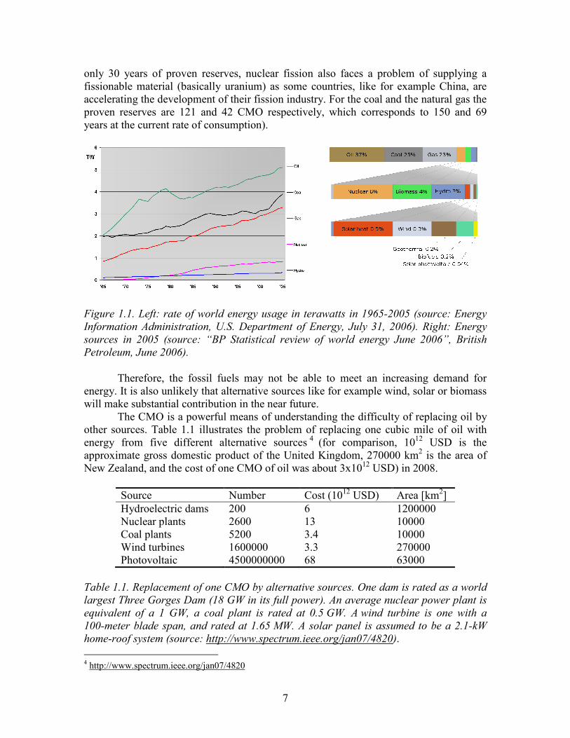
In 2005, the total worldwide energy consumption was about 5 x 1020 J, which corresponds to an energy consumption rate of 15 TW (figure 1.1, left). This is equivalent to three cubic miles of oil (CMO), an energy unit (1.6×1020 J) introduced by American engineer H. Crane in order to provide an illustrative concept of the world’s energy consumption and resources. About 85% of the consumption was provided by combustion of fossil fuels such as oil, coal and gas (figure 1.1, right).

Global proven oil reserves are estimated at approximately 43 CMO1 and, at the current rate of use, they would last for about 40 years. However, the annual consumption of oil is needed to increase by 50% in the next 25 years, mostly due to the economical development of India and China2. However, discoveries of new oil fields have been declining since the 1960’s, and in fact the difference between annual discoveries and annual consumption became negative in 1980. The current rate of oil consumption cannot be maintained and some expert analysis shows that it might already be declining3. With 1 “World Proved Reserves of Oil and Natural Gas, Most Recent Estimates”, Energy Information Administration, 2008, http://www.eia.doe.gov/emeu/international/reserves.html. 2 “World Energy Outlook 2005”, International Energy Agency, 2005, http://www.iea.org/textbase/nppdf/free/2005/weo2005.pdf. 3 http://www.peakoil.net/

7

only 30 years of proven reserves, nuclear fission also faces a problem of supplying a fissionable material (basically uranium) as some countries, like for example China, are accelerating the development of their fission industry. For the coal and the natural gas the proven reserves are 121 and 42 CMO respectively, which corresponds to 150 and 69 years at the current rate of consumption).

Figure 1.1. Left: rate of world energy usage in terawatts in 1965-2005 (source: Energy Information Administration, U.S. Department of Energy, July 31, 2006). Right: Energy sources in 2005 (source: “BP Statistical review of world energy June 2006”, British Petroleum, June 2006).

Therefore, the fossil fuels may not be able to meet an increasing demand for energy. It is also unlikely that alternative sources like for example wind, solar or biomass will make substantial contribution in the near future.

The CMO is a powerful means of understanding the difficulty of replacing oil by other sources. Table 1.1 illustrates the problem of replacing one cubic mile of oil with energy from five different alternative sources 4 (for comparison, 1012 USD is the approximate gross domestic product of the United Kingdom, 270000 km2 is the area of New Zealand, and the cost of one CMO of oil was about 3x1012 USD) in 2008.

Source Number Cost (1012 USD) Area [km2] Hydroelectric dams 200 6 1200000 Nuclear plants 2600 13 10000 Coal plants 5200 3.4 10000 Wind turbines 1600000 3.3 270000 Photovoltaic 4500000000 68 63000

Table 1.1. Replacement of one CMO by alternative sources. One dam is rated as a world largest Three Gorges Dam (18 GW in its full power). An average nuclear power plant is equivalent of a 1 GW, a coal plant is rated at 0.5 GW. A wind turbine is one with a 100-meter blade span, and rated at 1.65 MW. A solar panel is assumed to be a 2.1-kW home-roof system (source: http://www.spectrum.ieee.org/jan07/4820). 4 http://www.spectrum.ieee.org/jan07/4820

8

The environmental, social, and financial costs of such replacement are, however, immense and require flooding large areas and displacing millions of people (hydro energy), produces radioactive waste (nuclear plants), contribute to acid rain, global warming, and air pollution, and may obtain its fuel via controversial methods such as mountaintop removal (coal plants). An alternative source like wind turbines, photovoltaic, or biomass requires a location with an abundance of steady wind or sun, may be visually obtrusive, requires large areas or are relatively expensive. An inexhaustible, safe, and clean energy source is currently not available.

Large quantities of energy can be generated by fusing the nuclei of light isotopes (section 1.1.2). Nuclear fusion promises to be a safe, inexhaustible and relatively little polluting method of energy production and to become the best compromise between nature and the energy needs of mankind. However tantalizing the potential of fusion energy, it should be also noted that controlled fusion is a very difficult process to master and after fifty years of active research an economically viable fusion power plant is still many years away.

1.1.2. The principle of nuclear fusion

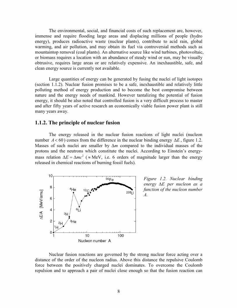
The energy released in the nuclear fusion reactions of light nuclei (nucleon number 60<A ) comes from the difference in the nuclear binding energy E∆ , figure 1.2. Masses of such nuclei are smaller by m∆ compared to the individual masses of the protons and the neutrons which constitute the nuclei. According to Einstein’s energy-mass relation 2mcE ∆=∆ ( ≈MeV, i.e. 6 orders of magnitude larger than the energy released in chemical reactions of burning fossil fuels).

Figure 1.2. Nuclear binding energy E∆ per nucleon as a function of the nucleon number A.

Nuclear fusion reactions are governed by the strong nuclear force acting over a

distance of the order of the nucleon radius. Above this distance the repulsive Coulomb force between the positively charged nuclei dominates. To overcome the Coulomb repulsion and to approach a pair of nuclei close enough so that the fusion reaction can

9

occur requires the kinetic energies of the fusing nuclei to be of the order of several hundreds of keV,

−∝∝

hveZZ

PE tunnelingcrit

221exp (1.1)

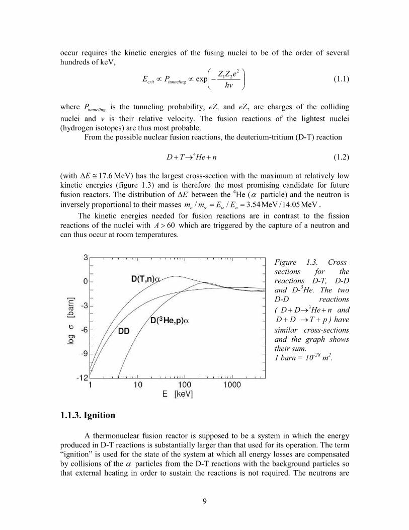
where tunnelingP is the tunneling probability, 1eZ and 2eZ are charges of the colliding nuclei and v is their relative velocity. The fusion reactions of the lightest nuclei (hydrogen isotopes) are thus most probable. From the possible nuclear fusion reactions, the deuterium-tritium (D-T) reaction

nHeTD +→+ 4 (1.2) (with 6.17≅∆E MeV) has the largest cross-section with the maximum at relatively low kinetic energies (figure 1.3) and is therefore the most promising candidate for future fusion reactors. The distribution of E∆ between the 4He (α particle) and the neutron is inversely proportional to their masses MeV05.14/MeV54.3// == nn EEmm αα . The kinetic energies needed for fusion reactions are in contrast to the fission reactions of the nuclei with 60>A which are triggered by the capture of a neutron and can thus occur at room temperatures.

Figure 1.3. Cross-sections for the reactions D-T, D-D and D-3He. The two D-D reactions ( nHeDD +→+ 3 and

DD + pT +→ ) have similar cross-sections and the graph shows their sum. 1 barn = 10-28 m2.

1.1.3. Ignition

A thermonuclear fusion reactor is supposed to be a system in which the energy produced in D-T reactions is substantially larger than that used for its operation. The term “ignition” is used for the state of the system at which all energy losses are compensated by collisions of the α particles from the D-T reactions with the background particles so that external heating in order to sustain the reactions is not required. The neutrons are

10

supposed to leave the plasma without interaction so that in the reactor their kinetic energy can be transferred into utilizable heat.

The ignition criterion [Lawson 1957] can be derived from a simple energy balance in the fusion reactor:

( )QEvkT

Tn E /5112 2

+>

αστ (1.3)

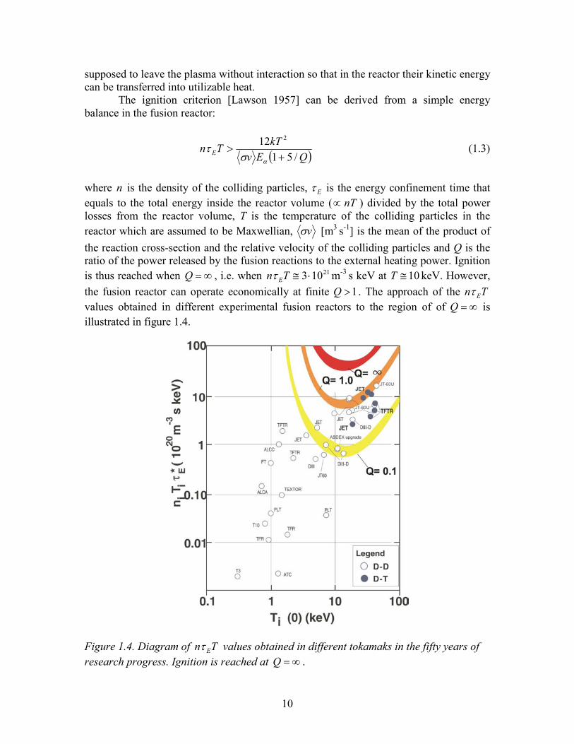
where n is the density of the colliding particles, Eτ is the energy confinement time that equals to the total energy inside the reactor volume ( nT∝ ) divided by the total power losses from the reactor volume, T is the temperature of the colliding particles in the reactor which are assumed to be Maxwellian, vσ [m3 s-1] is the mean of the product of the reaction cross-section and the relative velocity of the colliding particles and Q is the ratio of the power released by the fusion reactions to the external heating power. Ignition is thus reached when ∞=Q , i.e. when 21103 ⋅≅Tn Eτ m-3 s keV at 10≅T keV. However, the fusion reactor can operate economically at finite 1>Q . The approach of the Tn Eτ values obtained in different experimental fusion reactors to the region of of ∞=Q is illustrated in figure 1.4.

Figure 1.4. Diagram of Tn Eτ values obtained in different tokamaks in the fifty years of research progress. Ignition is reached at ∞=Q .

11

1.1.4. Magnetic Confinement Fusion

In the core of the sun the nuclei are confined by the gravitation force which provides sufficient pressure for igniting proton-proton nuclear fusion reactions (or 12C-based catalytic reactions in heavier stars). The simplest approach to achieving controlled fusion on earth would be to accelerate beams of light nuclei to sufficient kinetic energies and bring them into collision. However, for single collision events, Coulomb scattering would dominate over fusion reactions due to its much larger cross-section, leading to negative energy balance. This problem can be overcome by confining a population of thermalized particles at temperatures of several tens of keV for a sufficiently long time that a large fraction of the particles would have kinetic energies high enough to fuse. At such energies light particles are completely ionized and form a plasma consisting of ions and electrons.

A charged particle in a magnetic field experiences the Lorentz force and its orbit describes a helical motion along the magnetic field lines. The radius of the gyro-motion is referred to as Larmor radius

)/( BqmvrL ⊥= (1.4)

where m, q and ⊥v are the mass, charge and velocity component of a charged particle perpendicular to the magnetic field vector B. For B of several Tesla the Larmor radius of hydrogen isotopes with the temperature of 10 – 100 eV is typically a few hundreds of µm.

Charged particles can be, therefore, confined by a magnetic field generated by a system of coils. Reactor concepts based on this approach are referred to as “magnetic confinement fusion” (MCF) reactors. (Another concept, the “inertial confinement fusion” (ICF), uses lasers or particle beams to heat frozen D-T pellets, either directly or indirectly via conversion into X-rays, in order to reach the temperatures necessary for fusion reaction. ICF is not a subject of this thesis.)

In order to avoid the end losses of the early linear configurations (i.e. devices with zero curvature of the magnetic field on the axis and thus open field lines), the confining field line structure is given a toroidal shape. In a simple toroidal magnetic field system the magnetic field curvature and gradient, together with the different sign of the ion and electron charge, would result in a vertical electric field E, leading to particle losses due to the outward BE× drift. Such losses can be suppressed by twisting the magnetic field lines by means of an additional poloidal magnetic field component created by the toroidal electric current in the plasma (the plasma current pI ) or by twisting the external magnetic coils (either toroidally continuous or modular) around the confined region. The first principle is used in tokamaks (section 1.1.5), the latter is the used in stellarators. Because of the absence of the plasma current, stellarators provide more stable (eventually steady-state) operation. These advantages are, however, outnumbered by the complexity of the magnetic coils structure, smaller plasma volume (thus reactor efficiency) and worse plasma accessibility due to smaller diagnostic ports. Stellarators are not discussed further in this thesis.

A single-particle description of the tokamak plasma is not possible due to a large number of charges in the confined volume ( 2319 1010 → ). Magnetically confined plasma

12

can be, however, described by a magnetic fluid model known as magnetohydrodynamics (MHD). The MHD equations of the steady state the equilibrium configuration are

00

=⋅∇

=×∇∇=×

B

JBBJ

µp

(1.5)

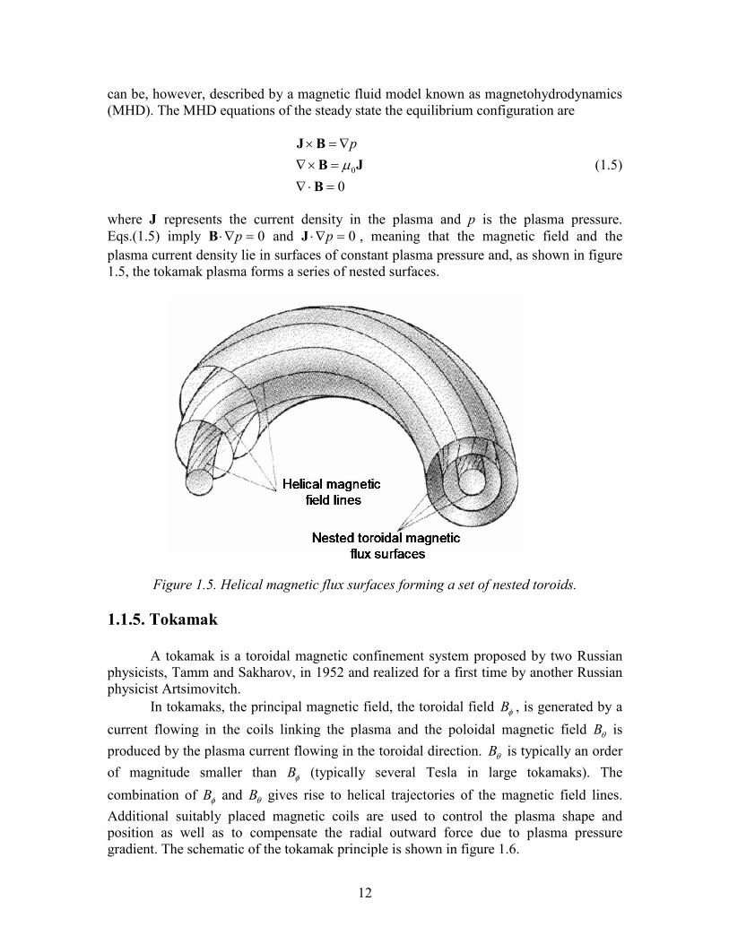
where J represents the current density in the plasma and p is the plasma pressure. Eqs.(1.5) imply 0=∇⋅ pB and 0=∇⋅ pJ , meaning that the magnetic field and the plasma current density lie in surfaces of constant plasma pressure and, as shown in figure 1.5, the tokamak plasma forms a series of nested surfaces.

Figure 1.5. Helical magnetic flux surfaces forming a set of nested toroids.

1.1.5. Tokamak

A tokamak is a toroidal magnetic confinement system proposed by two Russian physicists, Tamm and Sakharov, in 1952 and realized for a first time by another Russian physicist Artsimovitch.

In tokamaks, the principal magnetic field, the toroidal field φB , is generated by a

current flowing in the coils linking the plasma and the poloidal magnetic field θB is

produced by the plasma current flowing in the toroidal direction. θB is typically an order

of magnitude smaller than φB (typically several Tesla in large tokamaks). The

combination of φB and θB gives rise to helical trajectories of the magnetic field lines. Additional suitably placed magnetic coils are used to control the plasma shape and position as well as to compensate the radial outward force due to plasma pressure gradient. The schematic of the tokamak principle is shown in figure 1.6.

13

Figure 1.6. Schematic description of the tokamak principle. Twisted magnetic field lines in tokamaks are produced by the combination of toroidal and poloidal magnetic fields. The principal toroidal magnetic field is produced by current in external toroidal field coils. The poloidal magnetic field is produced by the plasma current which is driven by the change of the flux through the torus produced by primary winding of the transformer.

The helical magnetic field line goes around the torus on its magnetic flux surface

and returns to the same poloidal location after a change of toroidal angle φ∆ , corresponding to πφ 2/∆=q toroidal circumferences. q is called the safety factor (because of the role it plays in determining the stability of tokamak plasma). When the plasma small radius a (the minor radius) is substantially smaller compared to the plasma major radius R (this is referred to as large aspect ratio), θφ RBrBq /≅ where r is the horizontal distance from the plasma centre.

The current in the plasma serves also for plasma build-up and ohmic heating and is usually driven by a toroidal electric field induced by transformer action. In present large tokamaks, plasma current of several MA is produced. As long as the plasma current is generated by induction (alternative current drive methods have been developed), the tokamak is a pulsed system. Another disadvantage of the plasma current is a potential danger of a sudden termination of the discharge, known as disruption, which can give rise to large mechanical forces on the machine.

14

Since the plasma resistivity decreases with the plasma temperature ( 2/3−∝T ), pI can heat the tokamak plasma only to temperatures of a few keV. The temperatures >10 keV, needed to reach a reasonable probability for fusion reactions to occur, can be achieved by additional heating by neutral particle beams or by electromagnetic waves. The first is based on charge-exchange reactions between thermal fuel ions and fast injected neutrals with energies of 100≈ keV and total current up to 100 A. The latter is based on the absorption of the RF wave at a cyclotron resonance with plasma ions or electrons.

Tokamak plasma is contained in a vacuum vessel. Since the impurities in the plasma can give rise to radiation losses and dilute the fuel, the restriction of their entry into the plasma is critical for successful reactor operation. Therefore, the plasma must be separated as much as possible from the walls of the vacuum vessel either by defining the outer boundary of the confined plasma with a material limiter or by modifying the magnetic field by means of additional coils to produce a magnetic divertor, section 1.2. 1.1.6. Progress in tokamak research

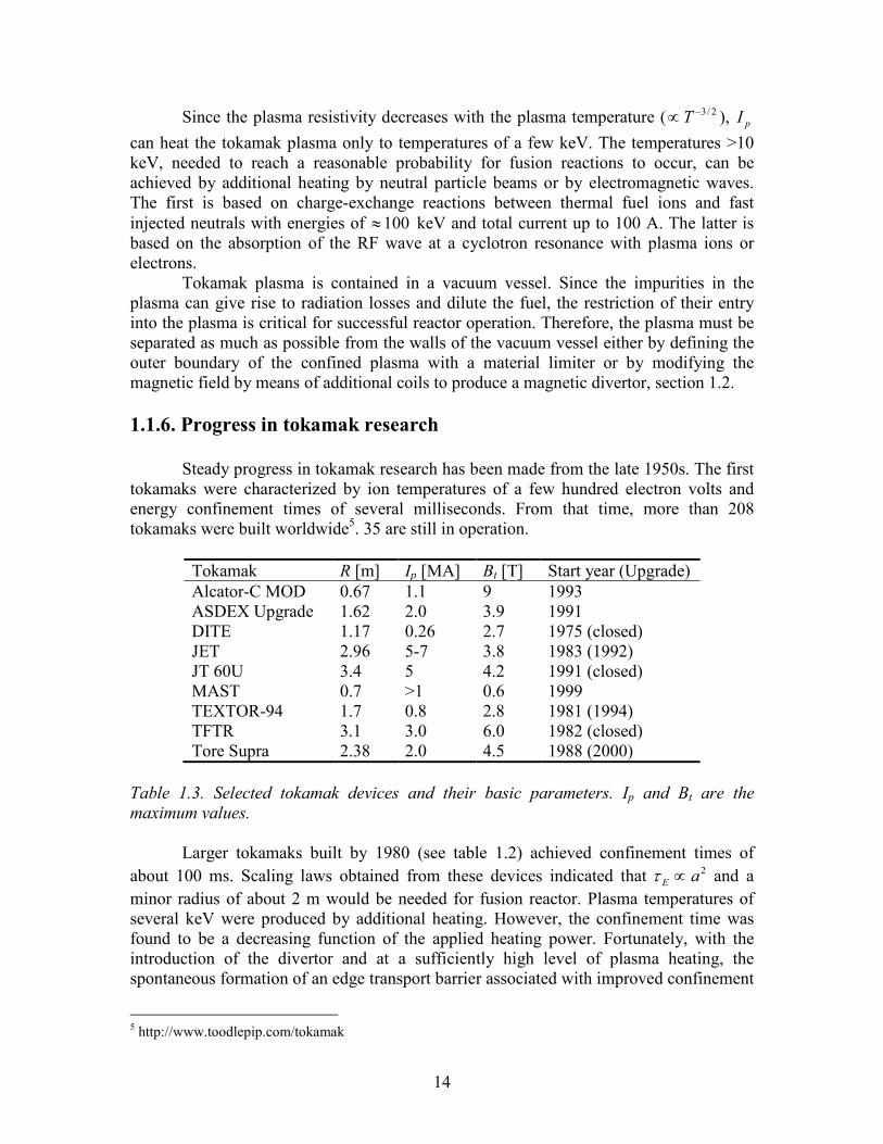
Steady progress in tokamak research has been made from the late 1950s. The first tokamaks were characterized by ion temperatures of a few hundred electron volts and energy confinement times of several milliseconds. From that time, more than 208 tokamaks were built worldwide5. 35 are still in operation.

Tokamak R [m] Ip [MA] Bt [T] Start year (Upgrade) Alcator-C MOD 0.67 1.1 9 1993 ASDEX Upgrade 1.62 2.0 3.9 1991 DITE 1.17 0.26 2.7 1975 (closed) JET 2.96 5-7 3.8 1983 (1992) JT 60U 3.4 5 4.2 1991 (closed) MAST 0.7 >1 0.6 1999 TEXTOR-94 1.7 0.8 2.8 1981 (1994) TFTR 3.1 3.0 6.0 1982 (closed) Tore Supra 2.38 2.0 4.5 1988 (2000)

Table 1.3. Selected tokamak devices and their basic parameters. Ip and Bt are the maximum values.

Larger tokamaks built by 1980 (see table 1.2) achieved confinement times of

about 100 ms. Scaling laws obtained from these devices indicated that 2aE ∝τ and a minor radius of about 2 m would be needed for fusion reactor. Plasma temperatures of several keV were produced by additional heating. However, the confinement time was found to be a decreasing function of the applied heating power. Fortunately, with the introduction of the divertor and at a sufficiently high level of plasma heating, the spontaneous formation of an edge transport barrier associated with improved confinement

5 http://www.toodlepip.com/tokamak

15

(so-called H-mode) was found in ASDEX tokamak [Wagner 1982]. On the other hand, the occurrence of various types of instabilities was found to seriously restrict the operating regimes of the tokamaks. For example, a new kind of instability, termed the ELM (Edge Localized Modes), appeared in the H-mode [ASDEX Team 1989], and is associated with a periodic expulsion of the outermost layers of hot, dense, confined plasma onto the wall.

In largest tokamak JET several important milestones were passed. Confinement times greater than 1 s, ion temperatures more than 30 keV and pulse lengths of up to one minute were achieved, although not simultaneously. Another large tokamak TFTR produced a fusion power of almost 11 MW using a 50-50 D-T mixture. After the closure of TFTR, JET became the only tokamak able to operate with a D-T mixture. In JET, a maximum transient fusion power output of 16.1 MW was obtained in an ELM-free H-mode with 62.0=Q . A quasi steady-state ELMy H-mode discharge produced 4 MW of fusion power for about 4 seconds [Jaquinot 1999].

1.1.7. ITER

ITER is a joint international research and development project that aims to demonstrate the scientific and technical feasibility of fusion power. ITER is a device based on divertor tokamak concept. It is believed that ITER is the final step before a prototype of a commercial fusion reactor is built.

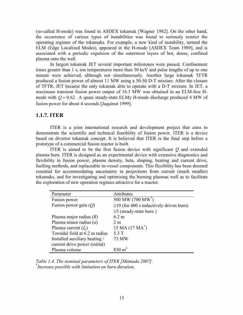
ITER is aimed to be the first fusion device with significant Q and extended plasma burn. ITER is designed as an experimental device with extensive diagnostics and flexibility in fusion power, plasma density, beta, shaping, heating and current drive, fuelling methods, and replaceable in-vessel components. This flexibility has been deemed essential for accommodating uncertainty in projections from current (much smaller) tokamaks, and for investigating and optimising the burning plasmas well as to facilitate the exploration of new operation regimes attractive for a reactor.

Parameter Attributes Fusion power 500 MW (700 MW*) Fusion power gain (Q) ≥10 (for 400 s inductively driven burn)

≥5 (steady-state burn ) Plasma major radius (R) 6.2 m Plasma minor radius (a) 2 m Plasma current (Ip) 15 MA (17 MA*) Toroidal field at 6.2 m radius 5.3 T Installed auxiliary heating / current drive power (initial)

73 MW

Plasma volume 830 m3

Table 1.4. The nominal parameters of ITER [Shimada 2007]. *Increase possible with limitation on burn duration.

16

The ITER physics basis was addressed in the special issue of Nuclear Fusion6. The performance specifications require ITER 7 : (i) to achieve extended burn in inductively driven D-T plasma operation with 10≥Q , not precluding ignition, with a burn duration of between 300 and 500 s, (ii) to aim at demonstrating steady-state operation using non-inductive current drive with 5≥Q . The reference plasma operating scenario for ITER inductive operation is the ELMy H-mode. The nominal parameters of ITER using inductive current drive are stated in table 1.4 [Shimada 2007].

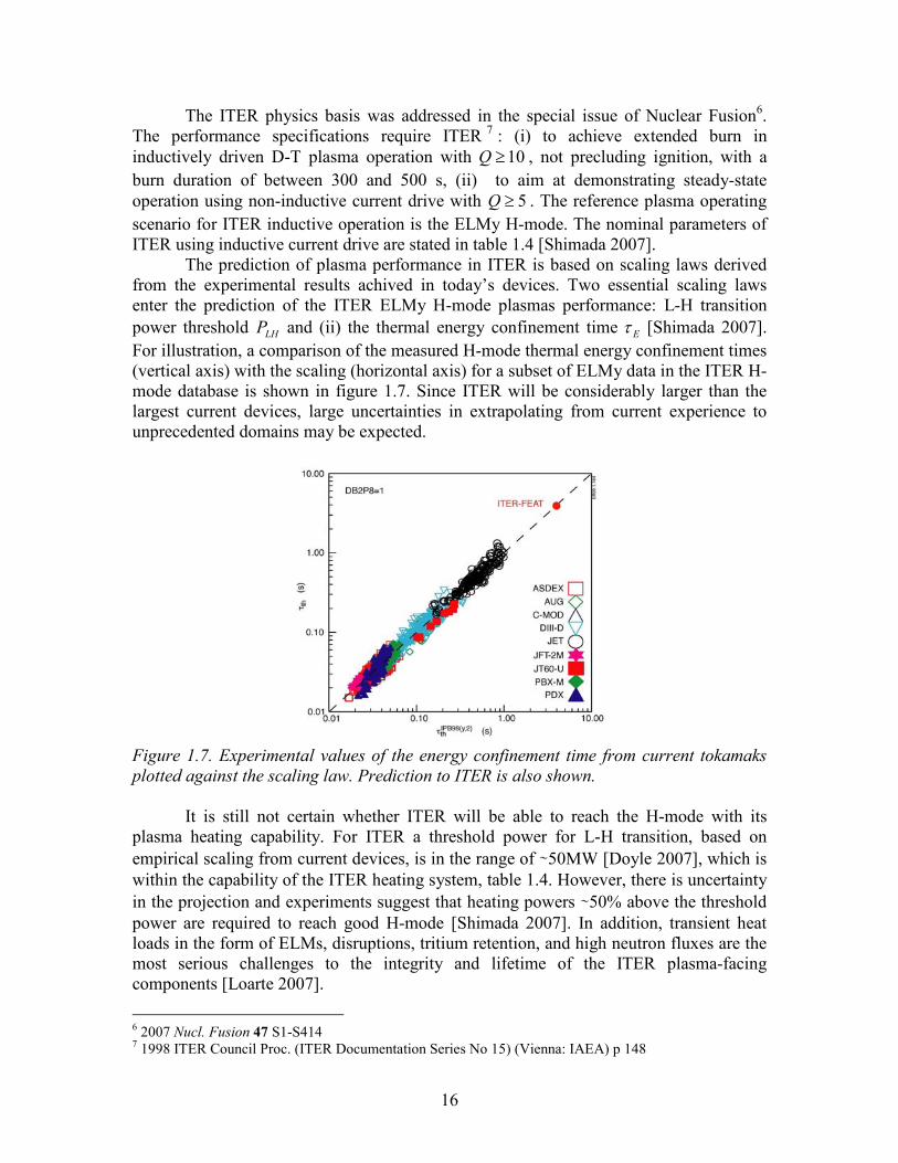
The prediction of plasma performance in ITER is based on scaling laws derived from the experimental results achived in today’s devices. Two essential scaling laws enter the prediction of the ITER ELMy H-mode plasmas performance: L-H transition power threshold LHP and (ii) the thermal energy confinement time Eτ [Shimada 2007]. For illustration, a comparison of the measured H-mode thermal energy confinement times (vertical axis) with the scaling (horizontal axis) for a subset of ELMy data in the ITER H-mode database is shown in figure 1.7. Since ITER will be considerably larger than the largest current devices, large uncertainties in extrapolating from current experience to unprecedented domains may be expected.

Figure 1.7. Experimental values of the energy confinement time from current tokamaks plotted against the scaling law. Prediction to ITER is also shown.

It is still not certain whether ITER will be able to reach the H-mode with its plasma heating capability. For ITER a threshold power for L-H transition, based on empirical scaling from current devices, is in the range of 50MW [Doyle 2007], which is within the capability of the ITER heating system, table 1.4. However, there is uncertainty in the projection and experiments suggest that heating powers 50% above the threshold power are required to reach good H-mode [Shimada 2007]. In addition, transient heat loads in the form of ELMs, disruptions, tritium retention, and high neutron fluxes are the most serious challenges to the integrity and lifetime of the ITER plasma-facing components [Loarte 2007].

6 2007 Nucl. Fusion 47 S1-S414 7 1998 ITER Council Proc. (ITER Documentation Series No 15) (Vienna: IAEA) p 148

17

1.1.8. Fusion power plant The tokamak reactor can be used for production of energy in two ways: as a “pure” fusion power plant or as a part of a hybrid fission-fusion power plant. While the first is currently the mainstream of the fusion research because of its attractiveness with regards to environmental and safety issues, the latter might be easier to put into practice in the not too distant future.

Compared to the current experimental devices, a “pure” fusion power plant with tokamak reactor will require additional elements in order to convert the fusion power into electricity. The vacuum vessel will be surrounded by a blanket that will (i) absorb the energy of the neutrons from the fusion reactions and transform it to heat carried away by a coolant, (ii) protect the outer components of the reactor from the neutron flux and (iii) allow for breeding of tritium to fuel the reactions. This may be accomplished by composing the blanket of Li2O. Additional elements like e.g. the blanket coolant, heat exchanger, turbine and the generator will be needed. Since the tokamak transformer action can drive the electric field only for limited period, the reactor will work in pulsed operation. Alternatively, continuous current drive could be provided by combining the bootstrap current produced by plasma itself with that produced by injection of the neutral particle beams or electromagnetic waves.

The idea of the hybrid fission-fusion reactor is to surround the fusion reactor with a blanket of abundant “fertile” materials such as uranium-238 or thorium-232. Fast neutrons produced in D-T reactions in the tokamak plasma will convert these materials into fissile isotopes (uranium-233 or plutonium-239). The fissile material will then be used as a fuel for ordinary fission reactors. The fission-fusion power plant should consist of a relatively small ( 52 −=Q ) pulsed tokamak (i.e. current drive might not be necessary) that could breed enough fuel for several satellite fission reactors. The feasibility of the hybrid fission-fusion systems has been addressed e.g. in [Bethe 1979, Nifnecker 1999, Gohar 2001, Hoffman 2002, Stacey 2002]. The fusion-fission hybrid system has potential attractiveness because of the large amount of produced energy and the abundance of fuel available compared to the fission reactor. Hybrid reactors are expected to be able to provide energy for more than 10000 years, giving a comfortable fuel assurance. The conditions for making such reactors economical may be considerably less stringent than those for fusion reactors producing electric power alone. Hybrids seem to be a practical path to the early application of fusion for energy production and would provide enough time to continue the progress towards pure fusion reactor, which is now many years away. However, apart of the political and public objections that the hybrid concept will probably provoke (because of the risk of proliferation as well as the fact that hybrid reactors involve nuclear fission), a number of technical issues needs to be solved. This includes e.g. the increase of the neutron fluence, the problems related to the first wall materials, and the design of the fissile fuel breeding blanket.

18

1.2. Plasma boundary in tokamaks

In tokamaks all four states of matter (solid walls of the vessel, liquid melting layer, gas consisting of neutral atoms, as well as plasma consisting of ionized atoms, molecules, and electrons) interact in a very small space. The transition between the plasma and the outer world is the biggest challenge of controlled fusion. The interaction of plasma with first-wall surfaces will have a considerable impact on the performance of fusion plasmas, the lifetime of plasma facing components and the retention of tritium in the next step experiment ITER.

In addition to the motion along B, magnetically confined charged particles diffuse across magnetic field lines from the confining region towards the inner wall of the vacuum vessel. The interaction of the charged particles with the material wall leads to the production of impurities and subsequent dilution of the plasma. In addition, large concentrated heat fluxes from the plasma can damage (i.e. by melting, sputtering, or brittle destruction) the plasma facing components. If the first wall were parallel with B at every point, the total radial heat flux from the plasma would be dissipated over large area, leading to very low heat flux densities. However, such a configuration could not be built in reality because of the finite edges of the wall tiles, diagnostic ports, screws, etc. that must inevitably appear. Another reason why the uniform distribution of the incident heat flux density could not be achieved is that the particle and energy fluxes from the plasma are poloidally non-uniform (e.g. [Asakura 2007, Kočan 2009] because of the curvature of the magnetic field lines. In addition, fast particles can be detrapped from the magnetic ripple wells due to the finite number of the toroidal magnetic field coils [Basiuk 2001], leading to a localized damage of the inner vessel components. Therefore, instead of bringing the whole plasma surface in contact with the material surface, tokamak plasmas are separated as much as possible from the vessel wall.

The simplest and oldest method to separate the tokamak plasma from the vessel wall is to insert an annulus of solid material called a “limiter”. Limiters can be either discrete or continuous in the toroidal or poloidal direction. Curved inner walls of the vessel covered by protective tiles are used as a wall-limiter. Additional limiters are used to protect the RF heating antennas . In fact, any object that is inserted into the plasma and is large enough (see section 1.2.4.2) acts as a limiter. Obviously, the price paid for the separation of the first wall from the plasma by means of a limiter is in the high flux densities to the limiter surface.

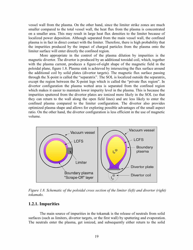
The poloidal cross-section of a limiter tokamak is shown in figure 1.8. The magnetic field lines which lie on flux surfaces that are not in contact with the limiter are termed “closed”. Those which intersect a solid surface are termed “open”. The outermost flux surface with closed magnetic field lines is termed “last closed flux surface” (LCFS). LCFS separates the “confined” region (being the region inside the LCFS) from the scrape-off layer (SOL) which is localized outside the LCFS (more accurate definition of the SOL is given in section 1.2.2.1).

Once inside the SOL, the particles move along the field lines towards the limiter strike zones. Because the parallel movement of particles (which in this thesis coincides with the movement along B) is much faster compared to the perpendicular movement, the particles only have time to diffuse a short distance beyond the LCFS – typically a few centimetres in large tokamaks, section 1.2.2.1. The limiter thus effectively separates the

19

vessel wall from the plasma. On the other hand, since the limiter strike zones are much smaller compared to the total vessel wall, the heat flux from the plasma is concentrated on a smaller area. This may result in large heat flux densities to the limiter because of localized power deposition. Although separated from the main vessel wall, the confined plasma is in fact in direct contact with the limiter. Therefore, there is high probability that the impurities produced by the impact of charged particles from the plasma onto the limiter surface will enter directly the confined region.

More appropriate in the control of the plasma dilution by impurities is the magnetic divertor. The divertor is produced by an additional toroidal coil, which, together with the plasma current, produces a figure-of-eight shape of the magnetic field in the poloidal plane, figure 1.8. Plasma sink is achieved by intersecting the flux surface around the additional coil by solid plates (divertor targets). The magnetic flux surface passing through the X-point is called the “separatrix”. The SOL is localized outside the separatrix, except the region between the X-point legs which is called the “private flux region”. In divertor configuration the plasma wetted area is separated from the confined region which makes it easier to maintain lower impurity level in the plasma. This is because the impurities sputtered from the divertor plates are ionized more likely in the SOL (so that they can return to the wall along the open field lines) and are less likely to enter the confined plasma compared to the limiter configuration. The divertor also provides optimized plasma shape and allows for exploring possible advantages of the small aspect ratio. On the other hand, the divertor configuration is less efficient in the use of magnetic volume.

Figure 1.8. Schematic of the poloidal cross section of the limiter (left) and divertor (right) tokamaks. 1.2.1. Impurities

The main source of impurities in the tokamak is the release of neutrals from solid surfaces (such as limiters, divertor targets, or the first wall) by sputtering and evaporation. The neutrals enter the plasma, get ionized, and subsequently either return to the solid

20

surface or are transported further into the plasma. The most important consequence of impurities in tokamaks is the cooling of the plasma by radiation. Impurities can have both harmful as well as beneficial effects on tokamak performance. First negative effect of the impurities is the radiation power loss that could account of a large fraction of the heating power at relatively low impurity concentrations. Much more preferable in this sense are low Z materials: while high-Z elements retain some orbital electrons also at the core plasma temperatures and act as “effective” radiators, low-Z atoms become completely stripped of the orbital electrons at low temperatures and therefore radiate only in the plasma edge. This has in fact a beneficial effect since up to 100% of the input power can be radiated over the whole reactor surface rather than deposited by particle impact on much smaller limiter or divertor targets, leading to a localized power deposition. Strong peripheral radiation by impurities, referred to as “detachment” or “cold plasma mantle”, has been observed in many tokamaks (e.g. [Strachan 1985, O’Rourke 1985, Allen 1986, McCracken 1987, Bush 1990, Samm 1993]). In addition to the radiative losses, impurities can dilute the fuel and thus cause the degradation of the reactor performance. Since the total number of the ion and electron charges in the quasi-neutral plasma is approximately equal, already a small number of high-Z impurities can replace a large fraction of fuel ions and significantly reduce the fusion power output.

Two quantities have important role in the quantification of the impurity content in the tokamak plasma: the effective ion charge effZ and the radiated power radP . An

empirical relation between effZ and radP was found by Behringer [Behringer 1986] on JET data and confirmed later on by Matthews [Matthews 1997] on the multi-machine database. Although this relation is not fully understood, its robustness allows for relatively reliable extrapolation to ITER.

Large progress in impurity control has been achieved since the first magnetic fusion devices. This includes e.g. the ultra-high vacuum technology, refractory (tungsten, molybdenum) or low-Z materials (carbon) for the limiters, oxygen gettering with boron, beryllium or lithium [Winter 1990]. In parallel, Monte Carlo neutral codes like EIRENE [Reiter 1991, Reiter 1991b], DEGAS [Heifetz 1982] or NIMBUS [Radford 1996], coupled with the fluid codes, improved the understanding of the transport of impurity atoms and molecules in the edge plasma.

Ideal material for a fusion reactor does not exist and the price for e.g. low radiative losses (C, Be compared to W) is paid in the higher retention of the hydrogen isotopes (C) or lower limits for the peak heat loads (Be). 1.2.2. Limiter SOL

Since the experiments described in this thesis were performed in the limiter tokamak Tore Supra, in this section we focus on the limiter SOL and address some of its well known basic properties. We also define some basic quantities such as the e-folding length, sheath potential drop and the heat transmission coefficient. We do not attempt to make a comprehensive survey of the limiter SOL which is provided in the references stated below.

21

1.2.2.1 Radial drop of density and temperatures in the SOL

In the simplest case with no particle sources and sinks (such as ionization or recombination) in the SOL, the particle flow perpendicular to the magnetic field lines into the SOL is balanced by the parallel particle losses at the limiter targets, i.e.

//Γ≈Γ⊥drd

Lc (1.6)

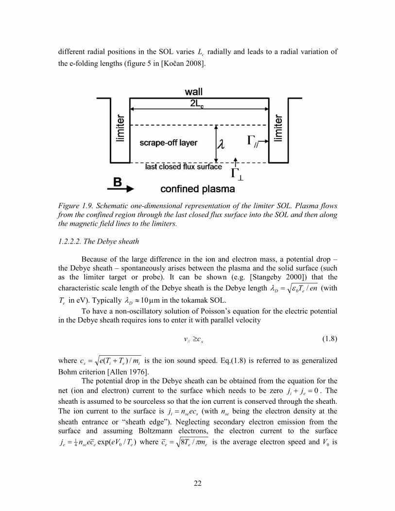
with drdnD /⊥⊥ −=Γ and //// nv∝Γ , figure 1.9. Here ⊥D is the cross-field particle diffusion coefficient and Lc is the magnetic connection length defined in figure 1.9. A large fraction of the perpendicular transport is believed to originate by the intermittent expulsion of plasma filaments, or “blobs”, from the last closed flux surface (LCFS) (e.g. [Hidalgo 1995, Naulin 2007]). Turbulent transport makes ⊥D “anomalously” high compared to what is expected from the neoclassical (collisional) theory.

Assuming for simplicity that cL , //v and ⊥D are independent of radius in the

SOL and ⊥D is poloidally uniform, Eq.(1.6) gives

[ ]nLCFS arnrn λ/)(exp)( −−≈ (1.7a) with LCFSn and /// vLD cn ⊥≈λ being the plasma density at the LCFS and the density e-folding length, respectively. Analogous consideration for the electron and ion energy balance (neglecting all heat sources and sinks in the SOL) gives

[ ]TiLCFSii arTrT λ/)(exp)( −−≈ (1.7b)

[ ]TeLCFSee arTrT λ/)(exp)( −−≈ (1.7c) with Tiλ and Teλ being respectively the ion and electron temperature e-folding lengths.

Within the accuracy inherent to the model used here the measurements of the SOL e-folding lengths give gives approximate values of the particle and heat transport coefficients (e.g. cn LvD ///

2λ=⊥ ). The e-folding lengths also define the approximate width

of the SOL. As demonstrated experimentally in most divertor and limiter tokamak [Asakura 2007], the poloidal asymmetry in the particle transport through the LCFS makes the e-folding lengths strongly dependent on the position of the plasma contact point. Similar asymmetry was recently measured also for the ion and electron energy transport [Kočan 2009]. It is also worth noticing that the SOL temperatures and density profiles are often not characterized by a single e-folding length as cL , //v and particle and

heat diffusivities may vary radially and the particle and heat sources and sinks in the SOL, neglected in Eqs.(1.7a-c), may play a role. For example, insertion of various limiters at

22

different radial positions in the SOL varies cL radially and leads to a radial variation of

the e-folding lengths (figure 5 in [Kočan 2008].

Figure 1.9. Schematic one-dimensional representation of the limiter SOL. Plasma flows from the confined region through the last closed flux surface into the SOL and then along the magnetic field lines to the limiters. 1.2.2.2. The Debye sheath

Because of the large difference in the ion and electron mass, a potential drop –

the Debye sheath – spontaneously arises between the plasma and the solid surface (such as the limiter target or probe). It can be shown (e.g. [Stangeby 2000]) that the characteristic scale length of the Debye sheath is the Debye length enTeD /0ελ = (with

eT in eV). Typically 10≈Dλ µm in the tokamak SOL. To have a non-oscillatory solution of Poisson’s equation for the electric potential

in the Debye sheath requires ions to enter it with parallel velocity

scv ≥// (1.8) where ieis mTTec /)( += is the ion sound speed. Eq.(1.8) is referred to as generalized Bohm criterion [Allen 1976].

The potential drop in the Debye sheath can be obtained from the equation for the net (ion and electron) current to the surface which needs to be zero 0=+ ei jj . The sheath is assumed to be sourceless so that the ion current is conserved through the sheath. The ion current to the surface is ssei ecnj = (with sen being the electron density at the sheath entrance or “sheath edge”). Neglecting secondary electron emission from the surface and assuming Boltzmann electrons, the electron current to the surface

)/exp( 041

eesee TeVcenj = where eee mTc π/8= is the average electron speed and 0V is

23

the potential of the surface (with 0=seV ). Hence the potential drop between the sheath edge and the electrically floating surface

+=

e

i

i

eesf T

Tmm

eT

V 12ln5.0 π . (1.9)

Again, Eq.(1.9) is derived assuming zero secondary electron emission from the surface. Allowing for secondary electron emission, additional factor of 2)1( −−δ (with δ being the secondary electron emission coefficient) will appear inside the logarithm. sfV

decreases with the increase of ei TT / and δ , and with the decrease of ion mass. esf TV 3≅

for ei TT = , 0=δ and Di mm = (where Dm is the deuteron mass). The existence of the sheath has an important consequence for plasma-wall interactions: in the sheath the kinetic energy of ions is increased by sfiVeZ and can thus exceed the threshold for the physical sputtering, increasing the impurity production rate. 1.2.2.3. The heat flux density and the heat transmission coefficient

The parallel heat flux density //q in the SOL plays a key role in the determination

of the power loads on the plasma-facing components in tokamaks.

//// Γ= eTq γ , (1.10)

where γ is the total (ion and electron) heath transmission coefficient. γ eT is thus the

amount of heat [W] removed from plasma per each ion-electron pair. //Γ is equivalent to

ejsat / , the parallel ion current density which, together with eT , is directly accessible by Langmuir probes, section 1.2.4. The details of the derivation of the heat transmission coefficient can be found e.g. in [Stangeby 2000b]. We state here only the final relation which is derived for electrically floating surface and assuming that the floating potential is negligible compared to sfV :

( )δ

δπγ−

+

−

+−≅ −

12

112ln5.05.2 2

e

i

i

e

e

i

TT

mm

TT

. (1.11)

δ is again the secondary electron emission coefficient which includes true secondary as well as reflected electrons. First term on the RHS of Eq.(1.11) accounts for the kinetic energy of ions increased by the sheath acceleration. eT in the denominator of the first

term is due to the fact that //q in Eq.(1.11) is scaled in eT . The remaining two terms account for the kinetic energy of electrons. δ−1 in the denominator of the third term appears because of the secondary electrons re-injected into the plasma (either true secondary electrons or reflected ones). The heat flux density of the Maxwellian electrons to the wall sec)2( jVjVTq sfesfee +−= with ej being the electron current density to the

24

wall and secj being the current density of the secondary electrons re-injected into the

plasma. sfV (with 0<sfV , Eq. (1.9)) accounts for the deceleration (acceleration) of the incident (secondary) electrons in the Debye sheath. Since the net ion and electron current densities to the walls are equal (section 1.2.2.2), netsat jj = with )1( δ−= enet jj so that

the electron component of the heat flux density to the wall can be written as neteee jTq γ=

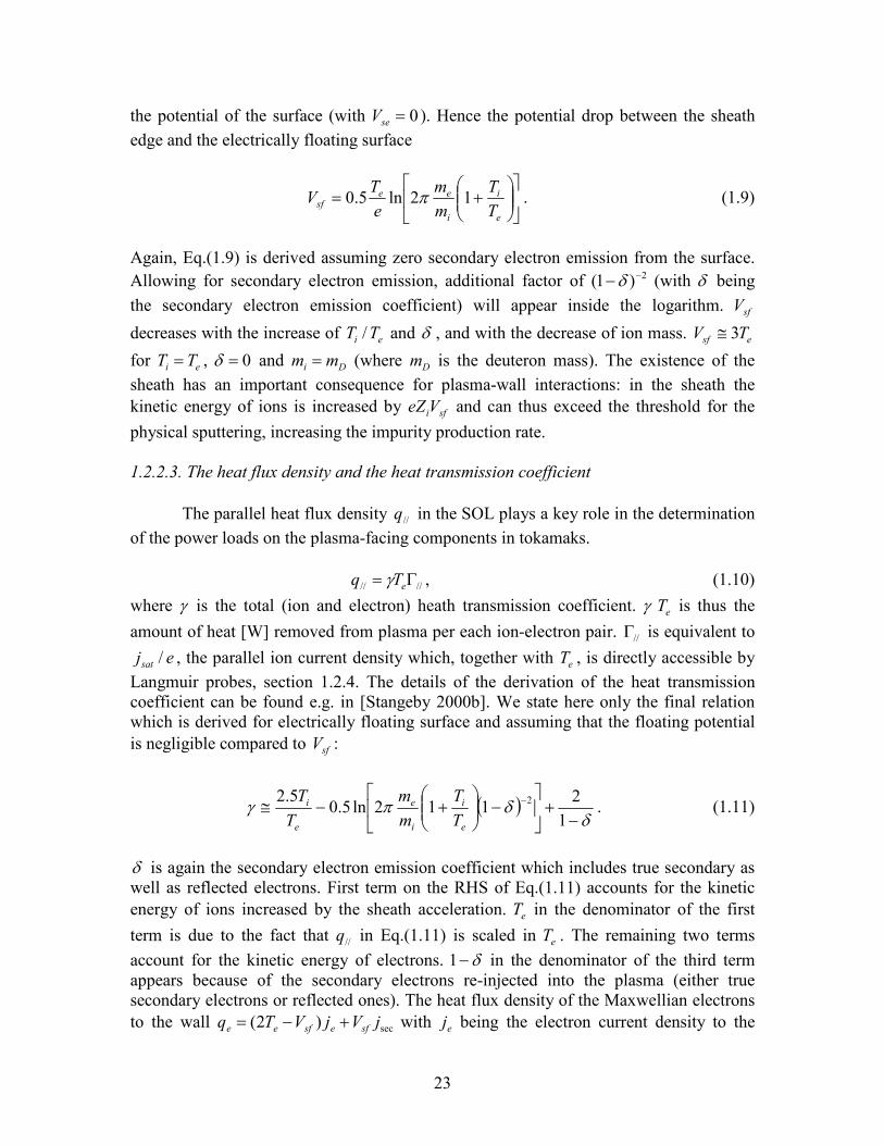
with ese TV /)1/(2 −−= δγ . At fixed satj , higher δ coincides with higher ej (i.e. higher electron heat flux density to the wall). This is why δ−1 appears in the denominator of Eq.(1.11) and why γ (Eq.(1.11)) increases with δ . In figure 1.10, γ is plotted against

ei TT / . For example, within the typical range of SOL //Γ and eT in most tokamaks (1022 -

1024 m-2, 10-100 eV) 7007.0// →≅q MW m-2 for ei TT = and 14014.0// →≅q MW m-2

for ei TT 4= .

0 2 4 6 8 105

10

15

20

25

30

Ti / Te

γ

Figure 1.10. Total, ion and electron, heat transmission coefficient γ from Eq.(1.11) plotted against the ion-to-electron temperature ratio. γ is calculated for zero secondary electron emission. 1.2.2.4. Parallel density and potential gradients in the pre-sheath

Assuming steady-state, isothermal 1D flow along the magnetic field lines in the

SOL, the conservation of particles and momentum gives

( ) 02// =+ nmvp

dxd

, (1.12)

(with )( ei TTnp += ) so that

25

2//

0// 11

)(M

nMn+

= , (1.13)

where 0n is the density at the stagnation point ( 0// =v ) and scvM ///// = is the parallel Mach number. Eq.(1.13) predicts a factor of ~2 drop of density along the magnetic field lines between the stagnation point and the sheath edge ( 1// =M ) [Stangeby 1984]. Allowing ions to diffuse not only into but also out of the collecting region defined by the radial extension of the collecting object (such as the probe or limiter) gives a numerical factor 0// 35.0)1( nMn == [Hutchinson 1987] instead of 0.5 given by Stangeby. Assuming that the electron density is given by Boltzmann relation, Eq.(1.13) gives

)1ln()( 2//// M

eT

M e +−=ϕ (1.14)

for the potential drop along the field lines. The potential drop between the stagnation point and the sheath edge (referred to as pre-sheath) is thus eTeps /7.0−≅ϕ . Compared

to the Debye sheath with the thickness of the order of 01.0=Dλ m, the quasineutral pre-sheath extends over the total connection length (10 – 100 m). 1.2.4. Langmuir probes

Langmuir probes (LP) are one of the most important and widely used diagnostics in the tokamak plasma boundary. They are relatively easy to build, can be operated in the SOL plasma, and provide information about the SOL parameters with relatively good spatial and temporal resolution. It is also worth notice that the interpretation of the LP measurements is often a subject of discussions.

The simplest LP consists of an electrode inserted into the plasma. A swept voltage is applied to the electrode with respect to the vacuum vessel ground (often termed torus ground) and the current to the probe is measured. The analysis of the LP current-voltage (I-V) characteristics can yield measurements of the electron temperature and density. From the Eqs.(2.61)-(2.71) in [Stangeby 2000c] for the current to an electrically biased surface inserted into the plasma it follows that

( )ef TVV

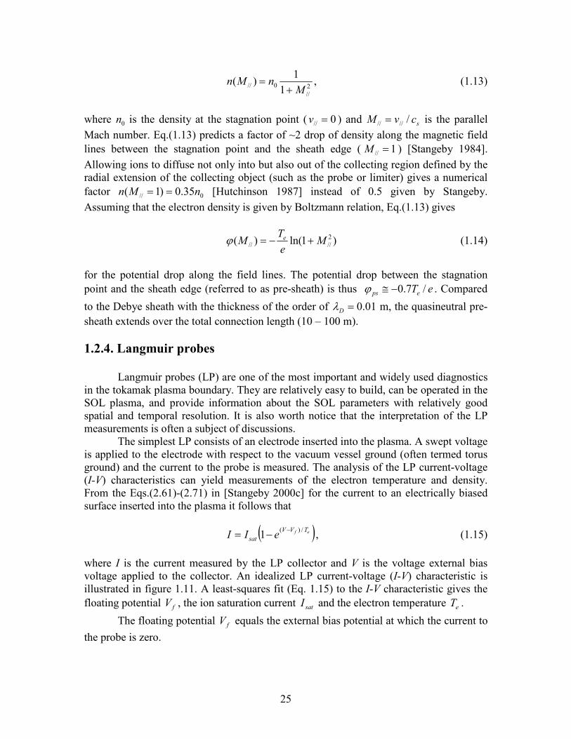
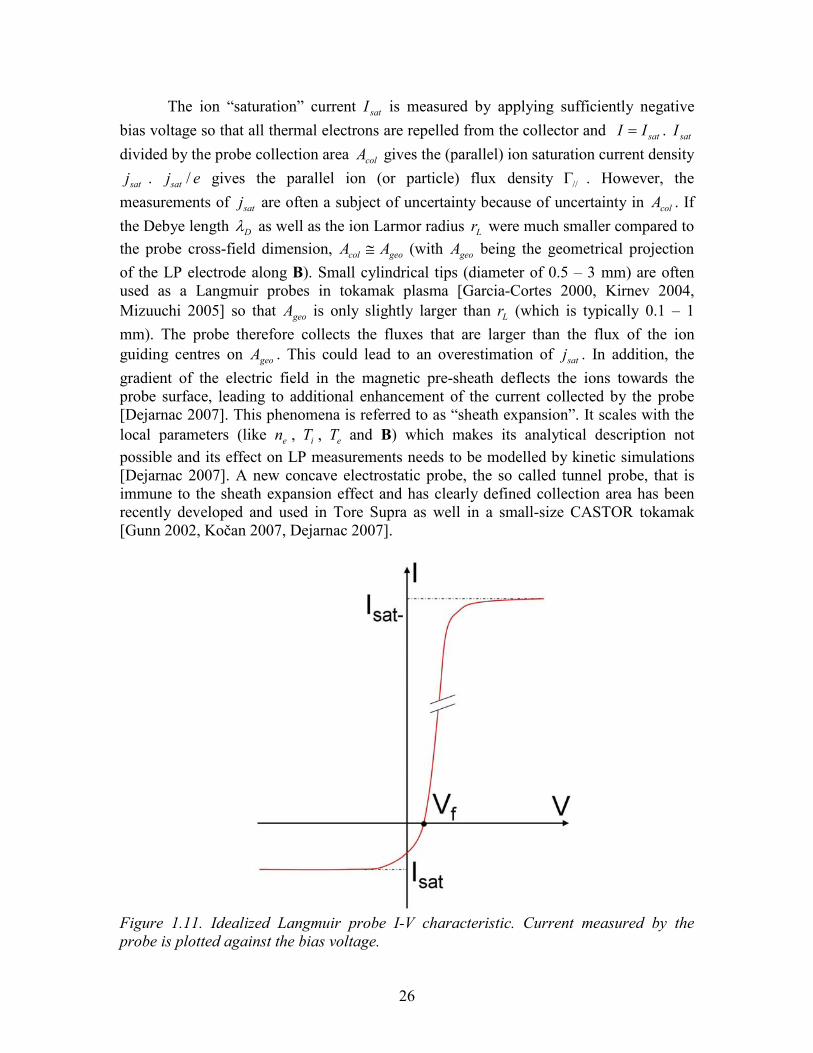
sat eII /)(1 −−= , (1.15) where I is the current measured by the LP collector and V is the voltage external bias voltage applied to the collector. An idealized LP current-voltage (I-V) characteristic is illustrated in figure 1.11. A least-squares fit (Eq. 1.15) to the I-V characteristic gives the floating potential fV , the ion saturation current satI and the electron temperature eT .

The floating potential fV equals the external bias potential at which the current to the probe is zero.

26

The ion “saturation” current satI is measured by applying sufficiently negative

bias voltage so that all thermal electrons are repelled from the collector and satII = . satI

divided by the probe collection area colA gives the (parallel) ion saturation current density

satj . ejsat / gives the parallel ion (or particle) flux density //Γ . However, the

measurements of satj are often a subject of uncertainty because of uncertainty in colA . If

the Debye length Dλ as well as the ion Larmor radius Lr were much smaller compared to the probe cross-field dimension, geocol AA ≅ (with geoA being the geometrical projection of the LP electrode along B). Small cylindrical tips (diameter of 0.5 – 3 mm) are often used as a Langmuir probes in tokamak plasma [Garcia-Cortes 2000, Kirnev 2004, Mizuuchi 2005] so that geoA is only slightly larger than Lr (which is typically 0.1 – 1 mm). The probe therefore collects the fluxes that are larger than the flux of the ion guiding centres on geoA . This could lead to an overestimation of satj . In addition, the gradient of the electric field in the magnetic pre-sheath deflects the ions towards the probe surface, leading to additional enhancement of the current collected by the probe [Dejarnac 2007]. This phenomena is referred to as “sheath expansion”. It scales with the local parameters (like en , iT , eT and B) which makes its analytical description not possible and its effect on LP measurements needs to be modelled by kinetic simulations [Dejarnac 2007]. A new concave electrostatic probe, the so called tunnel probe, that is immune to the sheath expansion effect and has clearly defined collection area has been recently developed and used in Tore Supra as well in a small-size CASTOR tokamak [Gunn 2002, Kočan 2007, Dejarnac 2007].

Figure 1.11. Idealized Langmuir probe I-V characteristic. Current measured by the probe is plotted against the bias voltage.

27

eT can be measured by the LP from the slope of the I-V characteristic, Eq. (1.15). Sheath theory predicts the electron current to rise exponentially for bias voltages above

fV (often called the electron branch of the I-V characteristic) until the probe potential equals to the plasma potential. At this point the electron current to the probe

satieeisatcolesesat ITmTmIAcenI >>==− )/(41 . Ideally, the fit to the decaying part of the

characteristics between satI and −satI would give eT . However, much lower satsat II /− ratios are observed experimentally in tokamaks [Gunther 1990]. In addition, as shown in [Tagle 1987], eT inferred from the electron side of the I-V characteristics raises a factor of 2 as more points from the electron side of the characteristic are included in the fit (Eq. (1.15)) to the measured I-V characteristic. In [Stangeby 1982] the non-ideal behaviour of the net electron collection was explained by electron momentum loss to the ions that can be neglected for probe voltages below fV . Therefore, the experimental data on the I-V

characteristic measured above fV are often ignored in the calculation of eT . As a consequence, the fit comprises only a small fraction of the electron distribution, restricted to the high-energy tail.

Since sseisat cenjj == and 0nnse ≅ , section 1.2.2.4, the measurements of satj and

eT give an estimate of the SOL electron density )35.0/(0 ssate ecjnn ≅= , with

ieis mTTec /)( += . Since the LP does not measure the ion temperature, ei TT > leads to

an overestimation of the electron density by a factor 2/)/1( ei TT+ (i.e. 1.2 for ei TT 2=

and 2 for ei TT 7= ). 1.2.4.1. Mach probe

The simplest Mach probe consists of two electrically insulated Langmuir probes mounted back-to-back and aligned with the magnetic field lines, measuring the ion saturation current density separately from both directions along B. The difference in satj measured by each side of the Mach probe is interpreted as a flow of the unperturbed plasma. The Mach probe theory, either fluid [Hutchinson 1987] or kinetic [Chung 1988], provides the calibration between the ion saturation current ratio and the parallel flow velocity //// Mcu s= where

≅ B

sat

Asat

jj

M ln4.0// (1.16)

A or B indicates the side of the probe. One of the basic assumption of the fluid Mach probe theory is that the parallel electron velocity distribution is Maxwellian, in which case the same electron temperature would be measured by each side of the Mach probe. However, strong asymmetries of eT on each side of the Mach probes are often observed in experiment [LaBombard 2004, Kočan 2009]. A theory that could explain the asymmetries on eT is not available.

28

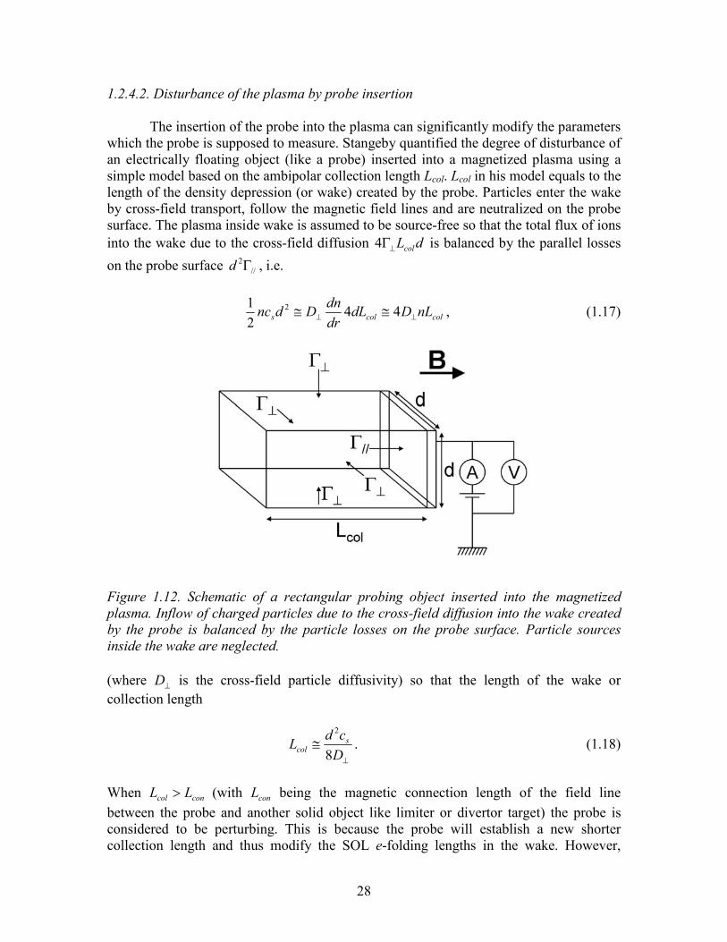
1.2.4.2. Disturbance of the plasma by probe insertion

The insertion of the probe into the plasma can significantly modify the parameters which the probe is supposed to measure. Stangeby quantified the degree of disturbance of an electrically floating object (like a probe) inserted into a magnetized plasma using a simple model based on the ambipolar collection length Lcol. Lcol in his model equals to the length of the density depression (or wake) created by the probe. Particles enter the wake by cross-field transport, follow the magnetic field lines and are neutralized on the probe surface. The plasma inside wake is assumed to be source-free so that the total flux of ions into the wake due to the cross-field diffusion dLcol⊥Γ4 is balanced by the parallel losses

on the probe surface //2Γd , i.e.

colcols nLDdLdrdn

Ddnc ⊥⊥ ≅≅ 4421 2 , (1.17)

Figure 1.12. Schematic of a rectangular probing object inserted into the magnetized plasma. Inflow of charged particles due to the cross-field diffusion into the wake created by the probe is balanced by the particle losses on the probe surface. Particle sources inside the wake are neglected. (where ⊥D is the cross-field particle diffusivity) so that the length of the wake or collection length

⊥

≅Dcd

L scol 8

2

. (1.18)

When concol LL > (with conL being the magnetic connection length of the field line between the probe and another solid object like limiter or divertor target) the probe is considered to be perturbing. This is because the probe will establish a new shorter collection length and thus modify the SOL e-folding lengths in the wake. However,

29

although the probe can be considered as non-perturbing for concol LL < it can only measure the quantities spatially averaged along the wake it creates.

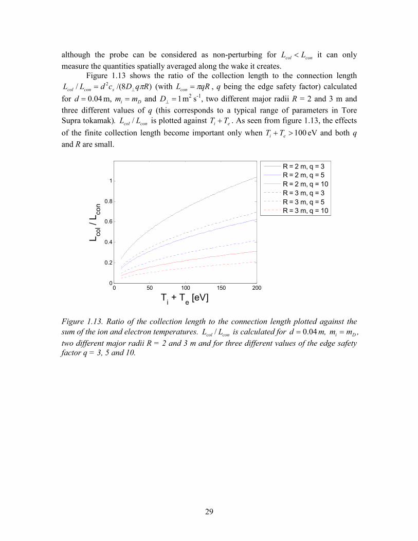
Figure 1.13 shows the ratio of the collection length to the connection length )8/(/ 2 RqDcdLL sconcol π⊥= (with qRLcon π= , q being the edge safety factor) calculated

for 04.0=d m, Di mm = and 1=⊥D m2 s-1, two different major radii R = 2 and 3 m and three different values of q (this corresponds to a typical range of parameters in Tore Supra tokamak). concol LL / is plotted against ei TT + . As seen from figure 1.13, the effects

of the finite collection length become important only when 100>+ ei TT eV and both q and R are small.

0 50 100 150 2000

0.2

0.4

0.6

0.8

1

Ti + T

e [eV]

L col / L c

on

R = 2 m, q = 3R = 2 m, q = 5R = 2 m, q = 10R = 3 m, q = 3R = 3 m, q = 5R = 3 m, q = 10

Figure 1.13. Ratio of the collection length to the connection length plotted against the sum of the ion and electron temperatures. concol LL / is calculated for 04.0=d m, Di mm = , two different major radii R = 2 and 3 m and for three different values of the edge safety factor q = 3, 5 and 10.

30

1.3. Tore Supra

Tore Supra (TS) is a tokamak operated by the “commissariat a l’énergie atomique” (CEA) in Cadarache, France. The construction of Tore Supra started in 1982 and the first plasma was achieved in April 1988. Tore Supra is a limiter tokamak with a circular cross plasma section ( 39.2=R m, 72.0=a m) whose LCFS is typically defined by the intersection of the plasma with the bottom toroidal pump limiter. The maximum plasma current and the toroidal magnetic field are 2<pI MA, 4<tB T, respectively, both oriented in the negative toroidal direction, i.e. clockwise viewed from above.

The primary mission of Tore Supra is the investigation of physics and technology issues of steady state tokamak operation [Giruzzi 2009].

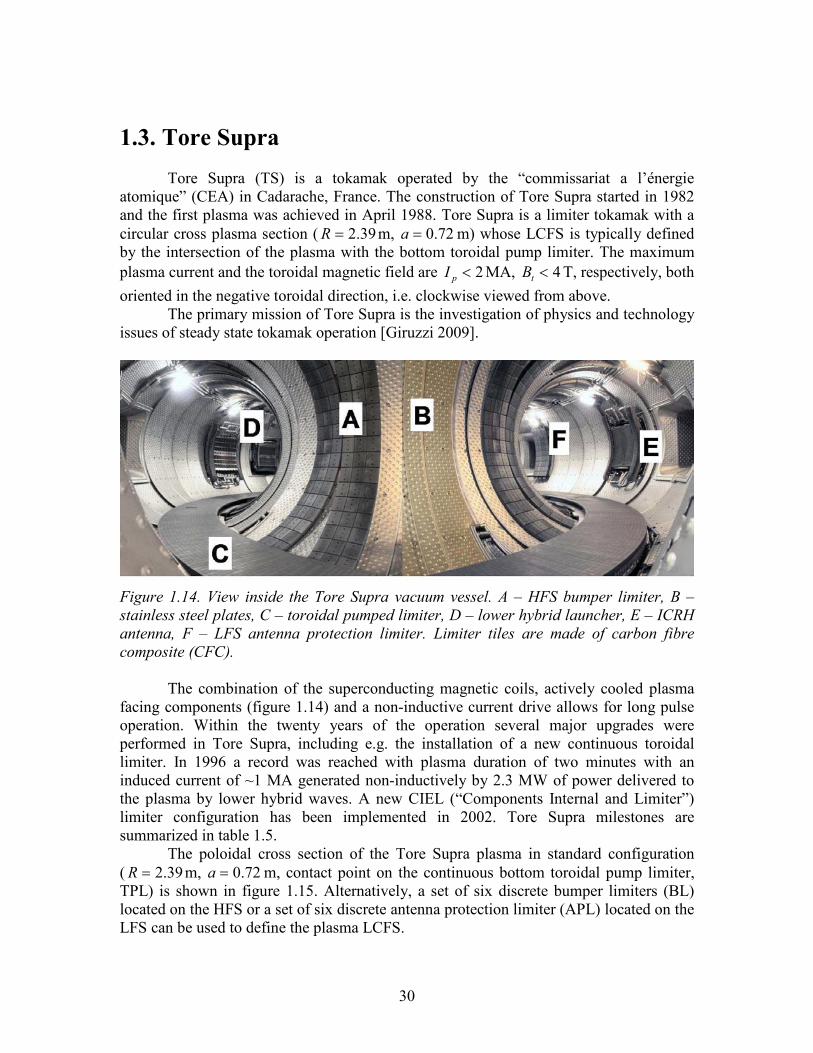
Figure 1.14. View inside the Tore Supra vacuum vessel. A – HFS bumper limiter, B – stainless steel plates, C – toroidal pumped limiter, D – lower hybrid launcher, E – ICRH antenna, F – LFS antenna protection limiter. Limiter tiles are made of carbon fibre composite (CFC).

The combination of the superconducting magnetic coils, actively cooled plasma

facing components (figure 1.14) and a non-inductive current drive allows for long pulse operation. Within the twenty years of the operation several major upgrades were performed in Tore Supra, including e.g. the installation of a new continuous toroidal limiter. In 1996 a record was reached with plasma duration of two minutes with an induced current of ~1 MA generated non-inductively by 2.3 MW of power delivered to the plasma by lower hybrid waves. A new CIEL (“Components Internal and Limiter”) limiter configuration has been implemented in 2002. Tore Supra milestones are summarized in table 1.5.

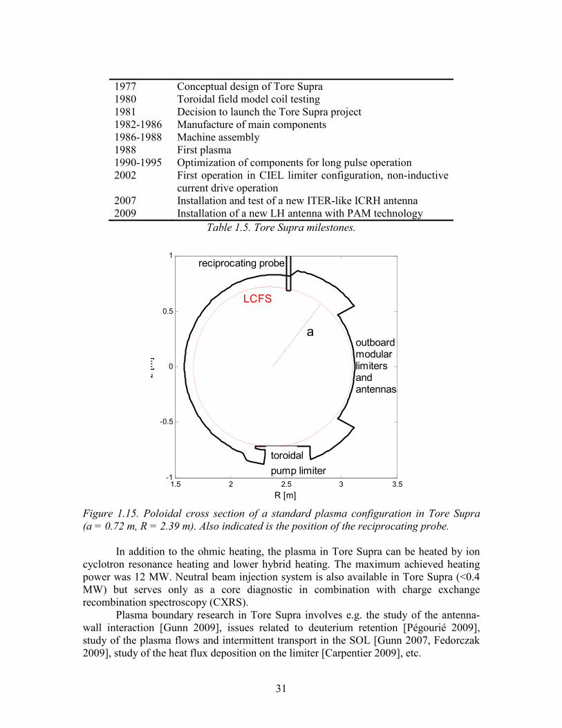
The poloidal cross section of the Tore Supra plasma in standard configuration ( 39.2=R m, 72.0=a m, contact point on the continuous bottom toroidal pump limiter, TPL) is shown in figure 1.15. Alternatively, a set of six discrete bumper limiters (BL) located on the HFS or a set of six discrete antenna protection limiter (APL) located on the LFS can be used to define the plasma LCFS.

31

1977 Conceptual design of Tore Supra 1980 Toroidal field model coil testing 1981 Decision to launch the Tore Supra project 1982-1986 Manufacture of main components 1986-1988 Machine assembly 1988 First plasma 1990-1995 Optimization of components for long pulse operation 2002 First operation in CIEL limiter configuration, non-inductive

current drive operation 2007 Installation and test of a new ITER-like ICRH antenna 2009 Installation of a new LH antenna with PAM technology

Table 1.5. Tore Supra milestones.

1.5 2 2.5 3 3.5-1

-0.5

0

0.5

1

R [m]

z [m

]

pump limitertoroidal

aoutboardmodularlimitersandantennas

LCFS

reciprocating probe

Figure 1.15. Poloidal cross section of a standard plasma configuration in Tore Supra (a = 0.72 m, R = 2.39 m). Also indicated is the position of the reciprocating probe.

In addition to the ohmic heating, the plasma in Tore Supra can be heated by ion

cyclotron resonance heating and lower hybrid heating. The maximum achieved heating power was 12 MW. Neutral beam injection system is also available in Tore Supra (<0.4 MW) but serves only as a core diagnostic in combination with charge exchange recombination spectroscopy (CXRS).

Plasma boundary research in Tore Supra involves e.g. the study of the antenna-wall interaction [Gunn 2009], issues related to deuterium retention [Pégourié 2009], study of the plasma flows and intermittent transport in the SOL [Gunn 2007, Fedorczak 2009], study of the heat flux deposition on the limiter [Carpentier 2009], etc.

32

The main components of the Langmuir probe system in Tore Supra are two vertical reciprocating drives located at 526.2=R m (figure 1.16). Some general details about the reciprocating probe system are stated in section 2.3.1. In this thesis, only the data measured by the reciprocating probes are analyzed. A toroidal array of four fixed Langmuir probes is located at the entrance of pumping throats under the TPL [Dionne 2005].

Typical values of the SOL ion and electron temperatures, plasma density, Debye length, and ion Larmor radius are 2005→=iT eV, 1005→=eT eV, 3020 →=Dλ µm,

and 800150 →=Lr µm, respectively. More details about Tore Supra performance as well as the main results achieved

in the past can be found e.g. in [Jacquinot 2004, Giruzzi 2009]

Figure 1.16. Left: Schematic view on the Tore Supra vacuum vessel with two reciprocating probes drives. Right: a detail view on the reciprocating probe system.

33

1.4. Ion temperature measurements in the tokamak plasma boundary 1.4.1. The importance of SOL Ti measurements

The ion temperature iT in the tokamak SOL is of key importance for modelling plasma surface interaction processes such as physical sputtering, reflection and impurity release, estimation of the amount of the heat flux deposited on the divertor tiles and main chamber walls, calculation of the importance of the classical drift flows compared to turbulence driven flows, etc. These are critical parameters for designing tokamak plasma facing components. In addition, the ion temperature at the LCFS is, in addition to eT , an important boundary condition for core modelling.

It is often argued that SOL iT is very difficult to measure compared to the SOL

eT (which is accessible by a simple Langmuir probes) and the measurements of SOL iT are therefore not available. In the models, the lack of iT measurements is often followed by the assumption ei TT = (e.g. [Federici 2007]). In some cases, experimentally measured edge temperature profiles are arbitrarily shifted radially to make the two temperatures agree [Saarelma 2005] and to make the model consistent with this assumption.

Most models are relatively sensitive to the exact value of the ion-to-electron temperature ratio and a significant error can be therefore anticipated if, in reality, iT and

eT are not equal. One example is the calculation of the parallel heat flux density in the

SOL //q , Eq.(1.10). As shown in section 1.2.2.3., //q is proportional to the heat

transmission coefficient which increases with ei /TT , Eq.(1.11). For example, ei 4TT =

would imply two times higher //q compared to ei TT = . Another example is the calculation of the electron density which is inversely proportional to the ion sound speed

sc so that 2/1eie )( −+∝ TTn . iT plays a role in the estimation of the pressure driven

(Pfirsch-Schlüter) flows (e.g. [Asakura 2000, Pitts 2007]) which are proportional to the ion pressure, in the estimation of the physical sputtering rates, etc.

It is true that SOL iT cannot be measured like eT by a simple electrode swept with respect to the plasma potential. However, several techniques have been developed for SOL iT measurements and successfully applied in many tokamaks (see references below and in section 1.4.2). Also true is that the database of SOL iT measurements is very limited, but sporadic measurements of SOL iT were already reported from most tokamaks like e.g.

• Alcator C [Wan 1986], • ASDEX (Upgrade) [Staib 1980, Staib 1982, Reich 2004, Reich 2004b], • CASTOR [Kočan 2005, Kočan 2006, Kočan 2007, Adamek 2008], • DITE [Erents 1982, Stangeby 1983, Pitts 1989, Matthews 1991, Pitts 1991, Pitts 1996], • JET [Guo 1996, Pitts 2003], • JFT-2M [Uehara 1998],

34

• JT-60U [Asakura 1997], • Petula [El Shaer 1981], • PLT and PDX [Wampler 1983], • TEXTOR [Höthker 1990, Bogen 1995, Huber 2000, Kreter 2001], • TFR 600 [Staudenmaier 1980], • Tore Supra [Kočan 2008, Kočan 2009, Kočan 2009b, Kočan 2009c].

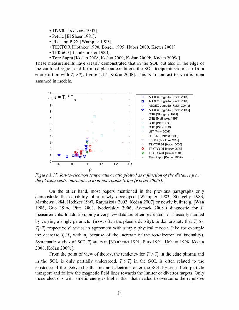
These measurements have clearly demonstrated that in the SOL but also in the edge of the confined region and for most plasma conditions the SOL temperatures are far from equipartition with ei TT > , figure 1.17 [Kočan 2008]. This is in contrast to what is often assumed in models.

0.8 0.9 1 1.1 1.2 1.30

1

2

3

4

5

6

7

8

9

10

11

ρ

ASDEX Upgrade [Reich 2004]ASDEX Upgrade [Reich 2004]ASDEX Upgrade [Reich 2004b]ASDEX Upgrade [Reich 2004b]DITE [Stangeby 1983]DITE [Matthews 1991]DITE [Pitts 1991]DITE [Pitts 1996]JET [Pitts 2003]JFT-2M [Uehara 1998]JT-60U [Asakura 1997]TEXTOR-94 [Huber 2000]TEXTOR-94 [Huber 2000]TEXTOR-94 [Kreter 2001]Tore Supra [Kocan 2009b]

τ = Ti / Te

Figure 1.17. Ion-to-electron temperature ratio plotted as a function of the distance from the plasma centre normalized to minor radius (from [Kočan 2008]).

On the other hand, most papers mentioned in the previous paragraphs only demonstrate the capability of a newly developed [Wampler 1983, Stangeby 1983, Matthews 1984, Höthker 1990, Ratynskaia 2002, Kočan 2007] or newly built (e.g. [Wan 1986, Guo 1996, Pitts 2003, Nedzelskiy 2006, Adamek 2008]) diagnostic for iT measurements. In addition, only a very few data are often presented. iT is usually studied by varying a single parameter (most often the plasma density), to demonstrate that iT (or

ei /TT respectively) varies in agreement with simple physical models (like for example

the decrease ei /TT with en because of the increase of the ion-electron collisionality). Systematic studies of SOL iT are rare [Matthews 1991, Pitts 1991, Uehara 1998, Kočan 2008, Kočan 2009c].

From the point of view of theory, the tendency for ei TT > in the edge plasma and

in the SOL is only partially understood. ei TT > in the SOL is often related to the existence of the Debye sheath. Ions and electrons enter the SOL by cross-field particle transport and follow the magnetic field lines towards the limiter or divertor targets. Only those electrons with kinetic energies higher than that needed to overcome the repulsive

35

force of the Debye sheath (Eq.(1.9)) can reach the targets, meaning that most of the thermal electrons are reflected back into the plasma. The removal of the fastest electrons from the distribution has a cooling effect on the electron population and decreases the effective electron temperature of the distribution. In the radial sense, the cooling effect of the sheath on electrons can be considered as a volumetric loss term so that eT in the SOL

becomes lower than iT and ei /TT increases with radius [Stangeby 2000d]. The ions simply follow the magnetic field lines towards the targets and are absorbed. The Debye sheath only shifts the ion distribution towards higher energies but the characteristic temperature of the distribution is unaffected. Both SOL temperatures become equal only when the ion-electron collisionality is strong enough to restore equipartition, i.e. when the ion-electron equipartition time ee

ieth nT /2/3∝τ becomes substantially smaller than the

ion parallel transit time through the SOL eiconi TTL +∝ ///τ (i.e. at high plasma density,

low electron temperature or long connection length). The variation of SOL ei /TT with the plasma density measured experimentally agrees with this model.

As seen from figure 1.17 ei /TT >1 is also measured at the LCFS as well as in the edge of the confined plasma [Uehara 1998, Kreter 2001, Reich 2004, Reich 2004b, Kočan 2008] i.e. in the region where the field lines are not terminated by the Debye sheath. It is not yet clear whether the faster drop of Te just inside the LCFS is due to the cooling of the edge electrons by the propagation of the cold electrons from the SOL or by the difference in the ion and electron transport (i.e. different heat diffusivities or volumetric loss terms like e.g. charge-exchange reactions, interaction of electrons with impurity ions and neutrals, etc.) in the edge plasma. In addition, sheath cooling effect on electrons is governed by parallel transport, so it certainly cannot explain e.g. the strong variation of ei /TT with tB reported recently in [Kočan 2009b].

Moreover, as mentioned above, the simple model for the radial dependence of SOL temperatures predicts infinite ion temperature e-folding lengths Tiλ [Stangeby 2000d]. Tiλ measured experimentally is, however, comparable to or, in some cases, even smaller than Teλ [Uehara 1998, Kočan 2009, Kočan 2009c]. This suggests that other processes (like for example the power conducted by ions, volumetric power losses in the SOL), neglected in a simple model, need to be taken into account.

The poloidal asymmetry in the radial ion energy transport is also studied very poorly. Recent result from Tore Supra [Kočan 2009] demonstrated for a first time that the ion energy transport is poloidally enhanced on the low-field-side, similar to the particle transport [Asakura 2007, Gunn 2007]. However, the database of iT measurements shown in [Kočan 2009] is very small, yet such measurements could help to evaluate an appropriate plasma start-up scenario for ITER [Gribov 2004]. Only a very few results are available on the measurements of the energies of ELM ions in the far SOL. In [Pitts 2006] it was demonstrated experimentally that during ELMs the ions arrive to the non-divertor components with the impact energies that would provide non-negligible physical sputtering in ITER where higher pedestal temperatures and hence more energetic ELMs are expected. More systematic measurements could help to validate the model of radial ELM filament energy evolution in the SOL [Fundamenski 2006, Fundamenski 2007] and enhance its predictive capability to ITER.

36

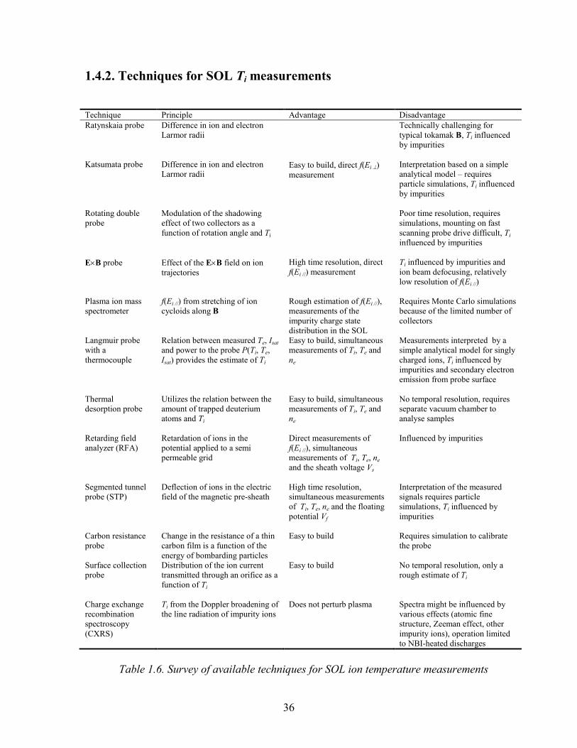
1.4.2. Techniques for SOL Ti measurements

Table 1.6. Survey of available techniques for SOL ion temperature measurements

Technique Principle Advantage Disadvantage

Ratynskaia probe Difference in ion and electron Larmor radii

Technically challenging for typical tokamak B, Ti influenced by impurities

Katsumata probe Difference in ion and electron Larmor radii

Easy to build, direct f(Ei ⊥) measurement

Interpretation based on a simple analytical model – requires particle simulations, Ti influenced by impurities

Rotating double probe

Modulation of the shadowing effect of two collectors as a function of rotation angle and Ti

Poor time resolution, requires simulations, mounting on fast scanning probe drive difficult, Ti influenced by impurities

E×B probe Effect of the E×B field on ion trajectories

High time resolution, direct f(Ei //) measurement

Ti influenced by impurities and ion beam defocusing, relatively low resolution of f(Ei //)

Plasma ion mass spectrometer

f(Ei //) from stretching of ion cycloids along B

Rough estimation of f(Ei //), measurements of the impurity charge state distribution in the SOL

Requires Monte Carlo simulations because of the limited number of collectors

Langmuir probe with a thermocouple

Relation between measured Te, Isat and power to the probe P(Ti, Te, Isat) provides the estimate of Ti

Easy to build, simultaneous measurements of Ti, Te and ne

Measurements interpreted by a simple analytical model for singly charged ions, Ti influenced by impurities and secondary electron emission from probe surface

Thermal desorption probe

Utilizes the relation between the amount of trapped deuterium atoms and Ti

Easy to build, simultaneous measurements of Ti, Te and ne

No temporal resolution, requires separate vacuum chamber to analyse samples

Retarding field analyzer (RFA)

Retardation of ions in the potential applied to a semi permeable grid

Direct measurements of f(Ei //), simultaneous measurements of Ti, Te, ne and the sheath voltage Vs

Influenced by impurities

Segmented tunnel probe (STP)

Deflection of ions in the electric field of the magnetic pre-sheath

High time resolution, simultaneous measurements of Ti, Te, ne and the floating potential Vf

Interpretation of the measured signals requires particle simulations, Ti influenced by impurities

Carbon resistance probe

Change in the resistance of a thin carbon film is a function of the energy of bombarding particles

Easy to build Requires simulation to calibrate the probe

Surface collection probe

Distribution of the ion current transmitted through an orifice as a function of Ti

Easy to build No temporal resolution, only a rough estimate of Ti

Charge exchange recombination spectroscopy (CXRS)

Ti from the Doppler broadening of the line radiation of impurity ions

Does not perturb plasma Spectra might be influenced by various effects (atomic fine structure, Zeeman effect, other impurity ions), operation limited to NBI-heated discharges

37

Simple Langmuir probe can tell us nothing about the SOL ion temperature. This is because the measurements of the ion energy distribution )( iEf would require to sweep the probe from zero to high positive voltage with respect to the torus ground and to measure the I-V characteristics of only the ion current. However, in experiment the probe measures the total (ion and electron) current which, at high positive bias, will be dominated by electron current because of their much lower mass compared to ions.

A dozen techniques for iT measurements in the SOL have been developed in the past and most of them have been successfully tested in tokamaks. Table 1.6 provides the survey of available techniques for SOL iT measurements. The table briefly defines their principle as well as the most significant advantages and disadvantages of individual diagnostics. More details are given in sections 1.4.2.1-1.4.2.10. The retarding field analyzer (RFA) and the segmented tunnel probe (STP) are described in dedicated Chapters 2 and 4, respectively. 1.4.2.1. Ratynskaia probe

A probe for the measurement of the ion energy distribution in the magnetized plasma, based on the method suggested in [Demidov 1999], was built by Ratynskaia [Ratynskaia 2002]. The probe described therein consists of a molybdenum wire, 0.25 mm in diameter and 0.35 mm length, closed at both ends by electrically insulating ceramic plugs with a diameter of 0.4 mm. The wire was oriented parallel to the magnetic field, preventing the electrons to reach the wire.

The probe utilizes the Druyvesteyn formula for cylindrical probe in magnetized plasma and for singly charged ions [Druyvesteyn 1930]:

2

2

3

2

2)(

dVjd

em

Ef ii π= (1.19)

to obtain the ion energy distribution )( iEf from the measured probe current density j and bias voltages V. Eq.(1.19) is valid only for

Lr eiL >>, (1.20) where eBmvr eiL /, ⊥= are the ion and electron Larmor radii, respectively and L is the wire length. The probe was tested in toroidal plasma device Blaamann [Demidov 1999b] which has a magnetic field of only 4 – 40 mT.

However, the application of the probe in tokamak plasma is practically impossible since the central wire will need to be much shorter than 0.1 – 1 mm (which is the typical values of the ion Larmor radius in the SOL). Moreover, since the currents measured in the SOL are subject to noise, second derivative of the measured current could hardly give any information about Ti.

38

1.4.2.2. Katsumata probe

Katsumata probe [Katsumata 1967] is also based on differentiating between ion and electron Larmor radii. The probe is basically a Langmuir probe slightly inserted into an electrically insulated tube with the tube axis perpendicular to B. The electrons are assumed to be not able to reach the probe because of much smaller Larmor radii compared to ions. It is therefore assumed that the probe collects only the ion current. It is argued that the ion current to the collector scales as )/exp( ikTeV− . This expression is obtained from the model which assumes Maxwellian ion beam and neglects the cross-field diffusion as well as the effects on the ion energy distribution arising from the presence of electrons (that are neglected in the model).

In Petula tokamak iT measured by the Katsumata probe was found to be a factor

of 2 lower compared to iT from the RFA [El Shaer 1981]. More recently, a Katsumata probe has been used in small-size CASTOR tokamak [Adamek 2008]. Good agreement has been found between the SOL iT measured by Katsumata probe and by the segmented tunnel probe. 1.4.2.3. Rotating double probe

A rotating double probe for SOL iT measurements was proposed by Höthker and used in TEXTOR tokamak [Höthker 1990]. The probe consists of two symmetric cylindrical pins, 5 mm in diameter and length, separated by 10 mm. During the discharge the system rotates around its axis which is perpendicular to B with a frequency of 2 Hz.

The ion saturation current collected by probe pins showed a dependence on the angle of rotation, reaching a minimum value when the pins magnetically shadow each other. In [Höthker 1990] the observed ion current modulation with the rotation angle was associated with finite ion Larmor radius effects and studied by Monte Carlo simulations.

iT was determined by fitting a calculated profile of the collected particle flux to the measured ion saturation current profiles. The accuracy of iT measurements could be, however, affected by simplifications used in the Monte Carlo simulations. For example, the model assumes a simple Maxwellian distribution (i.e. it neglects the pre-sheath effects on the parallel ion velocity distribution) and neglects the space charge effects [Höthker 1990]. Some other effects that can influence iT measurements are discussed in [Höthker 1990] and the authors

claim the error on iT is around 30%. Obviously, measurement of the radial profile of

SOL iT by the rotating probe mounted on a fast reciprocating drive will be technically challenging since much higher rotation frequencies will be required. A similar double probe with asymmetric electrodes [Amemiya 1989, Maeda 1997, Amemiya 1994] as well as the rotating double probe with symmetric and asymmetric electrodes [Uehara 1998] were used to measure iT in the JFT-2 tokamak.

39

1.4.2.4. E×B probe

The probe consists of a series of collectors (each being thinner than the ion Larmor radius) located at the end of a gap created by two electrodes parallel to B. The electrodes are used to create an electric field E perpendicular to B. The second end of the gap is terminated by a plate with a thin aperture (width of Dλ ). The ions enter the probe cavity through the aperture while the electrons are repelled by the aperture plate. The collector currents provide measurements of the parallel ion velocity distribution. The energy resolution of the probe is limited by number of collectors. The advantage of the E×B probe is that it can be operated in DC mode with high time resolution.

E×B probe was used for a first time by Staib in ASDEX [Staib 1980, Staib 1982] and later on by Matthews in DITE [Matthews 1984].

Since the ion current distribution on collectors corresponds to the distribution of parallel ion velocities ii meEv /2 //// = and not energies //iE , it can be influenced by

impurities. Defocusing of ions inside the probe cavity may also contribute to the blurring of the image measured on probe collectors. These two effects were observed in [Staib 1982] and [Matthews 1984] and studied in [Matthews 1994]. 1.4.2.5. Plasma ion mass spectrometers (PIMS)

Three types of mass spectrometers, used in the tokamak plasma boundary to measure the charge state distribution of impurities, are usually referred to as “180°” [Kojima 1984], “omegatron” [Nachtrieb 2000, Nachtrieb 2000b], and “cycloidal focusing” [Matthews 1989, Matthews 1990] spectrometers. Only two of them, omegatron used in Alcator-C MOD and cycloidal focusing PIMS used in DITE, can also measure the ion temperature. Omegtron PIMS utilizes the RFA principle (Chapter 2) to measure iT and is therefore irrelevant to this section.

DITE PIMS is based on the principle of cycloidal focusing [Matthews 1989, Matthews 1990] which is produced by perpendicular magnetic and electric fields inside the probe cavity. The electric field is produced by two parallel plates. The ions enter the probe through a thin aperture (width of Dλ ) and are focused onto an array of three electrically insulated collectors that are parallel to B. The principal application of the DITE PIMS is the measurement of the charge state distribution of SOL ions, which is inferred from the mass spectra obtained by ramping the electric field in time to sweep the various foci across the collector array.

The measurements of iT by PIMS are similar to that of the E×B probe. Since the ions have different parallel energies, their cycloids are stretched along the collectors. The collector currents can be used to measure )( //iEf . The ion temperature is obtained from the least squares fit of the distributions calculated by Monte Carlo simulations to the experimental collector current ratios. In Monte Carlo simulations it is assumed that the different charge state distributions are isothermal, isotropic and Maxwellian with a velocity shift associated with the Debye sheath acceleration [Matthews 1991]. Since the ion energy distribution at the sheath edge in front of the probe is known to be perturbed

40

by the presence of the probe combined with the plasma flow [Chung 1988] such assumptions could provide only very approximate values of iT . 1.4.2.6. Langmuir probe with a thermocouple

The probe consists of a thermocouple that works simultaneously as a Langmuir probe. The analysis of the measured data is carried as follows:

(i) The Langmuir probe provides the measurements of eT and satI . (ii) The thermocouple measures the incident power P . (iii) Assuming that ),( eisat TTEAIP = (with A being the thermocouple area and

),( ei TTE the energy transferred to the thermocouple per one ion-electron

pair) iT , the only unknown, can be obtained by an iterative process. The probe was successfully used in the SOL of DITE [Stangeby 1983] and PLT

[Manos 1982]. The advantage of this probe is in its relative simplicity and robustness. In addition,

the measurements of iT , eT and satI provide also the information about the SOL electron

density, ),(/ eissate TTcIn ∝ .

On the other hand, ),( ei TTE is calculated using a simple sheath theory for Maxwellian electrons and singly charged ions [Stangeby 1983] and is a function of other parameters that are not measured (e.g. the coefficient of the secondary electron emission from the thermocouple surface). Moreover, the statistical error on iT includes the errors

on eT , satI and P and can be, therefore, relatively large. 1.4.2.7. Thermal desorption probe

In the thermal desorption probe the population of trapped ions in a sample is associated to the ion impact energies. The carbon thermal desorption probe was operated in DITE [Erents 1982]. The probe bias voltage was changed on shot-to-shot basis. After each discharge the probe was withdrawn into a separate vacuum chamber, thermally desorbed, and the amount of trapped deuterium was measured. iT , averaged over the set of discharges, was obtained from the slope of the fluence versus the probe bias voltage [Cohen 1979, Wampler 1981]. The advantage of the thermal desorption probe is that it can measure the electron density and temperature using the sample as a Langmuir probe [Erents 1982]. On the other hand, since the probe requires exposure to cumulative discharges, it has virtually no spatial and temporal resolution. 1.4.2.8. Carbon resistance probe

Carbon resistance probe was used in the edge plasma in the PLT and PDX tokamaks to measure the incident ion energies [Wampler 1983]. The technique is based on measurements of the change in resistance of a thin carbon film due to bombardment of energetic particles (the change in the resistance is due to the damage of the lattice [Wampler 1982]). The probe was calibrated by measuring the resistance change caused

41

by the implantation of ions at different incident energies. Compared to other collecting probes, a carbon resistance probe does not require the analysis of an exposed sample in a separate facility so that the results are known during the exposure sequence. The probe described in [Wampler 1983] was calibrated by Monte Carlo simulations performed for a broad range of energies of the bombarding ions and two different ion energy distributions (Maxwellian and monoenergetic). Samples were exposed to plasma at different positions outside the LCFS in a series of successive discharges in PLT and PDX tokamaks. The mean ion energy was estimated by fitting the measured change in the sample resistance to the calculated curves. The ion energies obtained using the calibration curves calculated for Maxwellian and monoenergetic ions were different by a factor of ~2. Another disadvantage is that the scatter of the experimentally measured change in the sample resistance does not allow resolving the variation of the ion energies less than several tens of eV. 1.4.2.9. Surface collection probe

This method utilizes the fact that in the presence of a magnetic field the transmission of ions through a thick aperture aligned with B is a function of the perpendicular ion energy. The probe consists of two plates. The first plate, the shield, is exposed to the plasma and has an aperture with a radius comparable to the ion Larmor radius. The shield is made sufficiently thick so that most ions make at least one revolution inside the aperture, meaning that the ion transmission is only a function of the perpendicular ion energy. The second plate, the collector, is placed behind the aperture. The ion current distribution on the collector is a function of iT .

Such probe was used e.g. in TFR 600 tokamak [Staudenmaier 1980]. After exposure, the ion current distribution on the collector was determined by four different surface analysis techniques. Experimental results were juxtaposed by a set of the ion current distribution profiles after transmission, calculated theoretically for different ion temperatures and ion species, assuming isotropic Maxwellian ion energy distribution and neglecting the electric field (i.e. only the geometrical effects are taken into account which makes the model similar to the Larmor radius skimming model described in [Gunn 2001]). The ion temperature was given by iT of the theoretical profile that was closest to

the experimental ion deposition profile. The experimental error on iT which includes the statistical errors on measured fluences as well as the uncertainty of the effective aperture diameter was estimated to be about 25%.

Several effects neglected in the model (e.g. the electric field at the aperture edges, the defocusing of the transmitted ion beam, the misalignment of the aperture axis from B, the effects of the finite aperture thickness, etc.) can modify the ion deposition profile on collector and increase further the error on iT [Staudenmaier 1980].

More sophisticated diagnostic, combining the surface collection technique with a simple RFA arrangement was used in DITE to determine the charge state distribution of impurity ions [Pitts 1989].

42

1.4.2.10. Charge exchange recombination spectroscopy (CXRS)

This method, based on the measurements of the Doppler broadening of the spectral lines of impurity ions (mainly C5+ ions), has been applied for the SOL measurements of iT in several tokamaks (e.g. [Kimura 1979, Bogen 1995, Reich 2004, Reich 2004b]). Ion temperature, toroidal rotation velocity and the concentration of impurities can be obtained from the Doppler width, Doppler shift and the intensity of the radiation, respectively. C5+ ions are formed in excited state mainly by charge-exchange recombination of C6+ ions with fuel atoms. The atoms are provided by means of the neutral beam injector.

In the SOL, the spectroscopic measurements of iT are subject of several difficulties [Bogen 1995]. Because of relatively low densities the energy equipartition time between the impurity ions might be longer than the life time (ionization time) of impurity ions so that )()( ionsfuelTimpuritiesT ii ≠ [Spitzer 1962, Hey 1994]. For

example, at 30=eT eV, 60=iT eV and 18105 ⋅=en m-3, the lifetime (ionization time) of a C+ ion is only 15 µs, whereas the energy equipartition time between C+ and D+ ions is about 500 µs, i.e. thermal equilibrium cannot normally be established between these ions. For C6+ ions the lifetime is mainly determined by recombination on the wall or limiter and is rather long, whereas energy equipartition times of C6+ ions are a factor 36/12 =−

iZ shorter than those of C+ ions. Moreover, possible overlapping of the C VI line with hydrogen-like lines of other ions (e.g. O5+, figure 1 in [Bogen 1995]) may occur. Finally, atomic fine structure and Zeeman effect may appear in the Doppler-broadened profile and confuse the spectral analysis. Also important factor is that the measurements usually require a neutral beam and cannot be therefore performed in all discharges.

In [Kimura 1979], SOL iT measured from the Doppler broadening of impurity

lines was found to be consistent with iT from Katsumata probe. Similar measurements

were performed recently in Tore Supra and revealed a large discrepancy between iT measured by RFA and CXRS, Chapter 4.

43

Chapter 2

Retarding field analyzer

2.1. RFA in the tokamak plasma boundary

The retarding field analyzer (RFA) was one of the earliest devices used for the

measurement of the energy distribution of charged particles [Simpson 1961]. In theory, an energy analyzer for charged particles could hardly be simpler than the planar RFA – an equipotential plane (established by a biased semi permeable grid placed between the sample and a detector) that discriminates particles entering the analyzer. The RFA is one of the only widely accepted diagnostics for SOL iT measurements in tokamaks.

Kimura [Kimura 1978, Kimura 1979] was the first who used the RFA for measurements of the ion energy distribution in the tokamak scrape-off layer. Later on, Molvik used a RFA to measure the energy distribution of ions escaping along the magnetic field lines in the 2XIIB magnetic mirror (and later on in the Tandem Mirror Experiment, TMX) [Molvik 1981]. Kimura and Molvik also addressed some instrumental effects such as the appropriate aperture width, secondary electron suppression, the space charge limits inside the analyzer, appropriate bias voltage sweep rates, etc. Molvik also provided an excellent review on the principles of the design of a RFA for tokamak plasma.

A RFA combined with an E×B probe, mounted on a reciprocating probe drive, was used by Matthews [Matthews 1984] to measure the ion energy distribution in the SOL of DITE tokamak. Several important results were achieved using the RFA in plasma boundary of DITE, including e.g. the simultaneous measurements of SOL iT and Te for wide range of the plasma parameters [Pitts 1991, Matthews 1991], in-situ measurements of the secondary electron emission [Pitts 1991], the influence of impurities with a

44

different charge-to-mass ratio on the measured energy distribution [Pitts 1991, Pitts 1996], the comparison of the experimentally measured ion energy distribution with theory [Pitts 1991, Pitts 1991b, Pitts 1996], etc.

A multiple-function bi-directional probe whose components included RFA, Langmuir probe and calorimeter was used by Wan in the boundary plasma of the Alcator C [Wan 1986] tokamak. The RFA was used to measure both the ion and electron energy distribution. Wan also addressed several RFA design considerations such as the appropriate aperture width and the space charge effect inside the analyzer.

A bi-directional RFA mounted on a reciprocating drive was used in the JET tokamak to measure simultaneously the SOL ion and electron temperatures in NBI-heated L-mode discharges [Guo 1996]. The design of the JET RFA was similar to the DITE RFA. Later on, a new RFA [Pitts 2003, Pitts 2003b] characterized by a more compact design was used in JET to measure the SOL Ti as well as the ion energies in the far SOL during ELMs [Pitts 2006].

The ion energy distribution in rf-sustained argon discharges was measured by a RFA in H-1 heliac [Shats 1997]. The design of this RFA was similar to that used in Alcator C and DITE.

A RFA was used in Indian tokamak SINP [Raychaudhuri 1999]. However, the relatively good performance of the RFA used in SINP is quite surprising as the analyzer worked without the protective slit plate, with the ion repelling grid being directly exposed to plasma.

A small unidirectional RFA with a circular aperture has been also used for the measurements of ion temperature in plasma boundary of ISTTOK tokamak [Nedzelskiy 2006].

An omegatron E×B ion mass spectrometer combined with a retarding field analyzer equipped with three grids has been used in the plasma boundary of Alcator C-Mod [Nachtrieb 2000, Nachtrieb 2000b].

It is appropriate to mention that the RFA is used more widely (and was used much earlier) in, for example, high-energy colliders, plasma etching and the plasma-assisted deposition devices, where the energy distribution of the charge particles is a subject of technological and research interest. Several different types of RFA’s have been used for such applications, including planar, cylindrical and spherical RFAs [Simpson 1961] with a number of grids varying from one [Zou 2000, Stenzel 1982] up to eight [Enloe 1992], grid-less analyzers [Johnson 2003], simple compact analyzers [Simpson 1961], [Charles 2000, Bohm 1993], sophisticated commercial ones [Olthoff 1994, Cebulla 1998], the analyzers combined with the mass spectrometer [Jiang 2005], etc. A large number of studies focus on the instrumental effects of such devices like e.g. the divergence of the charged particle beam inside the analyzer [Zou 2002], the improvement of the energy resolution [Goto 1972, Staib 1972], the ionization of the neutral gas inside the analyzer [Bohm 1993], problems associated with a non-ideal retarding field due to the finite number of the grid wires [Enloe 1992], etc. A vast number of further references related to the RFA in low temperature plasmas or high-energy particle beams can be found in the studies referred to above. However, in most cases, the design of these analyzers is adjusted for the measurements of energies above 1 keV without the confining magnetic field and under relatively low heat fluxes, which makes them different compared to the RFAs used in tokamak plasma boundary.

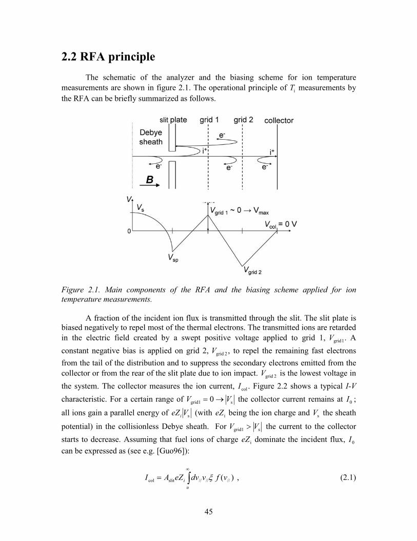
45

2.2 RFA principle The schematic of the analyzer and the biasing scheme for ion temperature

measurements are shown in figure 2.1. The operational principle of iT measurements by the RFA can be briefly summarized as follows.

Figure 2.1. Main components of the RFA and the biasing scheme applied for ion temperature measurements.

A fraction of the incident ion flux is transmitted through the slit. The slit plate is

biased negatively to repel most of the thermal electrons. The transmitted ions are retarded in the electric field created by a swept positive voltage applied to grid 1, .1 gridV A

constant negative bias is applied on grid 2, ,2 gridV to repel the remaining fast electrons from the tail of the distribution and to suppress the secondary electrons emitted from the collector or from the rear of the slit plate due to ion impact. 2 gridV is the lowest voltage in

the system. The collector measures the ion current, .colI Figure 2.2 shows a typical I-V

characteristic. For a certain range of sgrid1 0 VV →= the collector current remains at 0I ;

all ions gain a parallel energy of sVeZi (with ieZ being the ion charge and sV the sheath

potential) in the collisionless Debye sheath. For sgrid1 VV > the current to the collector

starts to decrease. Assuming that fuel ions of charge ieZ dominate the incident flux, 0I can be expressed as (see e.g. [Guo96]):

∫∞

=u

i vfvdveZAI )( //////slitcol ξ , (2.1)

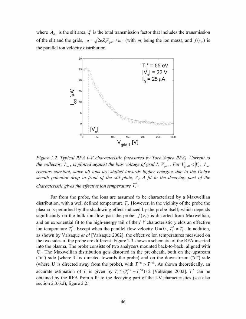
46

where slitA is the slit area, ξ is the total transmission factor that includes the transmission

of the slit and the grids, igrid1i /2 mVeZu = (with im being the ion mass), and )( //vf is

the parallel ion velocity distribution.

0 50 100 150 200 250 300-5

0

5

10

15

20

25

30

Vgrid 1 [V]

I col [µA]

Ti* = 55 eV|Vs| = 22 VI0 = 25 µA

|Vs|

Figure 2.2. Typical RFA I–V characteristic (measured by Tore Supra RFA). Current to the collector, ,colI is plotted against the bias voltage of grid 1, .grid1V For ,sgrid1 VV < colI remains constant, since all ions are shifted towards higher energies due to the Debye sheath potential drop in front of the slit plate, .sV A fit to the decaying part of the

characteristic gives the effective ion temperature .*iT

Far from the probe, the ions are assumed to be characterized by a Maxwellian

distribution, with a well defined temperature .iT However, in the vicinity of the probe the plasma is perturbed by the shadowing effect induced by the probe itself, which depends significantly on the bulk ion flow past the probe. )( //vf is distorted from Maxwellian, and an exponential fit to the high-energy tail of the I-V characteristic yields an effective ion temperature .*

iT Except when the parallel flow velocity 0=U , .i*

i TT ≠ In addition, as shown by Valsaque et al [Valsaque 2002], the effective ion temperatures measured on the two sides of the probe are different. Figure 2.3 shows a schematic of the RFA inserted into the plasma. The probe consists of two analyzers mounted back-to-back, aligned with U . The Maxwellian distribution gets distorted in the pre-sheath, both on the upstream (“u”) side (where U is directed towards the probe) and on the downstream (“d”) side (where U is directed away from the probe), with d *

iu *

i TT > . As shown theoretically, an

accurate estimation of iT is given by 2/)( d *i

u *ii TTT +≅ [Valsaque 2002]. *

iT can be obtained by the RFA from a fit to the decaying part of the I-V characteristics (see also section 2.3.6.2), figure 2.2:

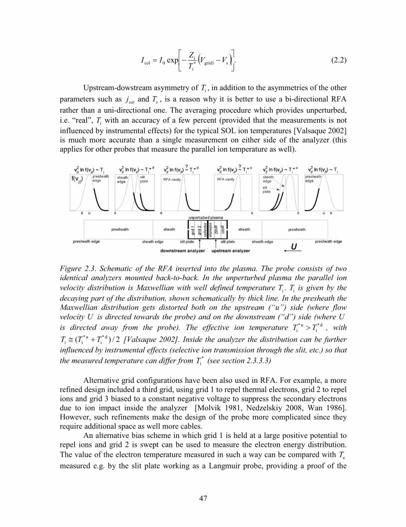
47

( ) .exp sgrid1*i

i0col

−−= VV

TZ

II (2.2)

Upstream-dowstream asymmetry of iT , in addition to the asymmetries of the other

parameters such as satj and eT , is a reason why it is better to use a bi-directional RFA rather than a uni-directional one. The averaging procedure which provides unperturbed, i.e. “real”, iT with an accuracy of a few percent (provided that the measurements is not influenced by instrumental effects) for the typical SOL ion temperatures [Valsaque 2002] is much more accurate than a single measurement on either side of the analyzer (this applies for other probes that measure the parallel ion temperature as well).

Figure 2.3. Schematic of the RFA inserted into the plasma. The probe consists of two identical analyzers mounted back-to-back. In the unperturbed plasma the parallel ion velocity distribution is Maxwellian with well defined temperature iT . iT is given by the decaying part of the distribution, shown schematically by thick line. In the presheath the Maxwellian distribution gets distorted both on the upstream (“u”) side (where flow velocity U is directed towards the probe) and on the downstream (“d”) side (where U is directed away from the probe). The effective ion temperature d *

iu *

i TT > , with

2/)( d *i

u *ii TTT +≅ [Valsaque 2002]. Inside the analyzer the distribution can be further

influenced by instrumental effects (selective ion transmission through the slit, etc.) so that the measured temperature can differ from *

iT (see section 2.3.3.3) Alternative grid configurations have been also used in RFA. For example, a more

refined design included a third grid, using grid 1 to repel thermal electrons, grid 2 to repel ions and grid 3 biased to a constant negative voltage to suppress the secondary electrons due to ion impact inside the analyzer [Molvik 1981, Nedzelskiy 2008, Wan 1986]. However, such refinements make the design of the probe more complicated since they require additional space as well more cables.

An alternative bias scheme in which grid 1 is held at a large positive potential to repel ions and grid 2 is swept can be used to measure the electron energy distribution. The value of the electron temperature measured in such a way can be compared with eT measured e.g. by the slit plate working as a Langmuir probe, providing a proof of the

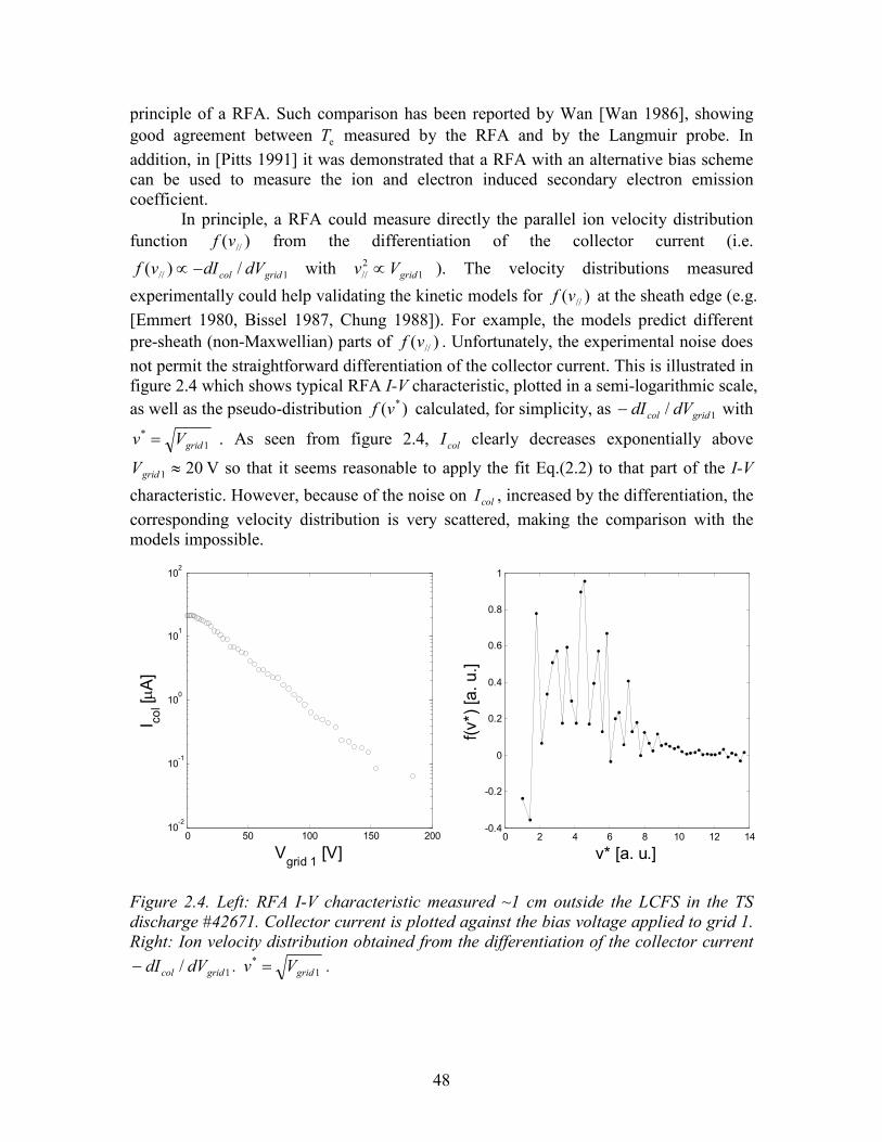
48

principle of a RFA. Such comparison has been reported by Wan [Wan 1986], showing good agreement between eT measured by the RFA and by the Langmuir probe. In addition, in [Pitts 1991] it was demonstrated that a RFA with an alternative bias scheme can be used to measure the ion and electron induced secondary electron emission coefficient.

In principle, a RFA could measure directly the parallel ion velocity distribution function )( //vf from the differentiation of the collector current (i.e.

1// /)( gridcol dVdIvf −∝ with 12// gridVv ∝ ). The velocity distributions measured

experimentally could help validating the kinetic models for )( //vf at the sheath edge (e.g. [Emmert 1980, Bissel 1987, Chung 1988]). For example, the models predict different pre-sheath (non-Maxwellian) parts of )( //vf . Unfortunately, the experimental noise does not permit the straightforward differentiation of the collector current. This is illustrated in figure 2.4 which shows typical RFA I-V characteristic, plotted in a semi-logarithmic scale, as well as the pseudo-distribution )( *vf calculated, for simplicity, as 1/ gridcol dVdI− with

1*

gridVv = . As seen from figure 2.4, colI clearly decreases exponentially above

201 ≈gridV V so that it seems reasonable to apply the fit Eq.(2.2) to that part of the I-V

characteristic. However, because of the noise on colI , increased by the differentiation, the corresponding velocity distribution is very scattered, making the comparison with the models impossible.

0 50 100 150 20010

-2

10-1

100

101

102

Vgrid 1

[V]

I col [µA]

0 2 4 6 8 10 12 14-0.4

-0.2

0

0.2

0.4

0.6

0.8

1

v* [a. u.]

f(v*) [a. u.]

Figure 2.4. Left: RFA I-V characteristic measured ~1 cm outside the LCFS in the TS discharge #42671. Collector current is plotted against the bias voltage applied to grid 1. Right: Ion velocity distribution obtained from the differentiation of the collector current

1/ gridcol dVdI− . 1*

gridVv = .

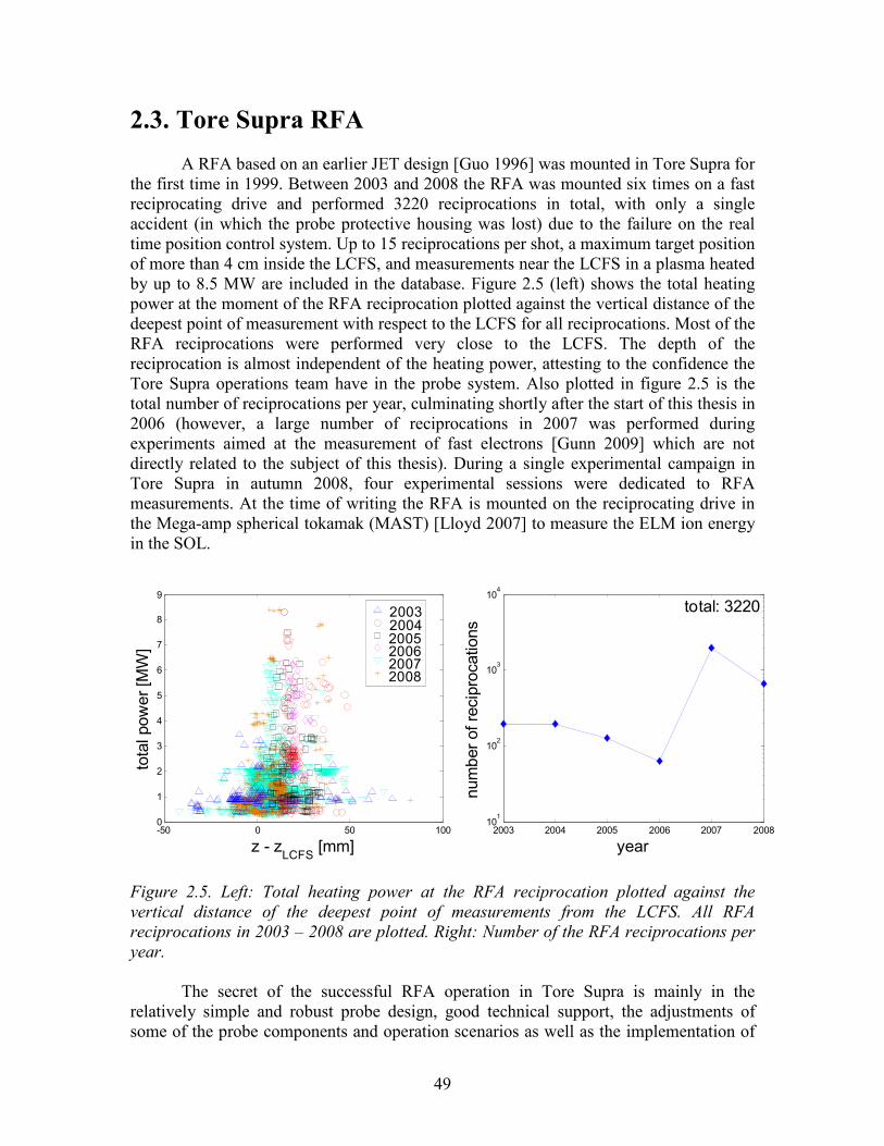
49

2.3. Tore Supra RFA

A RFA based on an earlier JET design [Guo 1996] was mounted in Tore Supra for the first time in 1999. Between 2003 and 2008 the RFA was mounted six times on a fast reciprocating drive and performed 3220 reciprocations in total, with only a single accident (in which the probe protective housing was lost) due to the failure on the real time position control system. Up to 15 reciprocations per shot, a maximum target position of more than 4 cm inside the LCFS, and measurements near the LCFS in a plasma heated by up to 8.5 MW are included in the database. Figure 2.5 (left) shows the total heating power at the moment of the RFA reciprocation plotted against the vertical distance of the deepest point of measurement with respect to the LCFS for all reciprocations. Most of the RFA reciprocations were performed very close to the LCFS. The depth of the reciprocation is almost independent of the heating power, attesting to the confidence the Tore Supra operations team have in the probe system. Also plotted in figure 2.5 is the total number of reciprocations per year, culminating shortly after the start of this thesis in 2006 (however, a large number of reciprocations in 2007 was performed during experiments aimed at the measurement of fast electrons [Gunn 2009] which are not directly related to the subject of this thesis). During a single experimental campaign in Tore Supra in autumn 2008, four experimental sessions were dedicated to RFA measurements. At the time of writing the RFA is mounted on the reciprocating drive in the Mega-amp spherical tokamak (MAST) [Lloyd 2007] to measure the ELM ion energy in the SOL.

-50 0 50 1000

1

2

3

4

5

6

7

8

9

z - zLCFS

[mm]

total pow

er [M

W]

2003 2004 2005 2006 2007 200810

1

102

103

104

year

number o

f reciprocations

200320042005200620072008

total: 3220

Figure 2.5. Left: Total heating power at the RFA reciprocation plotted against the vertical distance of the deepest point of measurements from the LCFS. All RFA reciprocations in 2003 – 2008 are plotted. Right: Number of the RFA reciprocations per year.

The secret of the successful RFA operation in Tore Supra is mainly in the relatively simple and robust probe design, good technical support, the adjustments of some of the probe components and operation scenarios as well as the implementation of

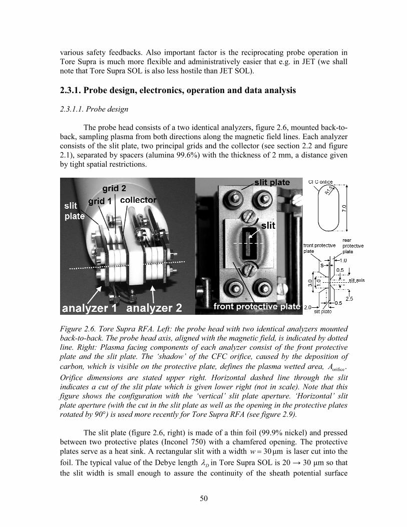
50

various safety feedbacks. Also important factor is the reciprocating probe operation in Tore Supra is much more flexible and administratively easier that e.g. in JET (we shall note that Tore Supra SOL is also less hostile than JET SOL). 2.3.1. Probe design, electronics, operation and data analysis 2.3.1.1. Probe design

The probe head consists of a two identical analyzers, figure 2.6, mounted back-to-back, sampling plasma from both directions along the magnetic field lines. Each analyzer consists of the slit plate, two principal grids and the collector (see section 2.2 and figure 2.1), separated by spacers (alumina 99.6%) with the thickness of 2 mm, a distance given by tight spatial restrictions.

Figure 2.6. Tore Supra RFA. Left: the probe head with two identical analyzers mounted back-to-back. The probe head axis, aligned with the magnetic field, is indicated by dotted line. Right: Plasma facing components of each analyzer consist of the front protective plate and the slit plate. The ‘shadow’ of the CFC orifice, caused by the deposition of carbon, which is visible on the protective plate, defines the plasma wetted area, .orificeA Orifice dimensions are stated upper right. Horizontal dashed line through the slit indicates a cut of the slit plate which is given lower right (not in scale). Note that this figure shows the configuration with the ‘vertical’ slit plate aperture. ‘Horizontal’ slit plate aperture (with the cut in the slit plate as well as the opening in the protective plates rotated by 90°) is used more recently for Tore Supra RFA (see figure 2.9).

The slit plate (figure 2.6, right) is made of a thin foil (99.9% nickel) and pressed

between two protective plates (Inconel 750) with a chamfered opening. The protective plates serve as a heat sink. A rectangular slit with a width µm30=w is laser cut into the foil. The typical value of the Debye length Dλ in Tore Supra SOL is 20 → 30 µm so that the slit width is small enough to assure the continuity of the sheath potential surface

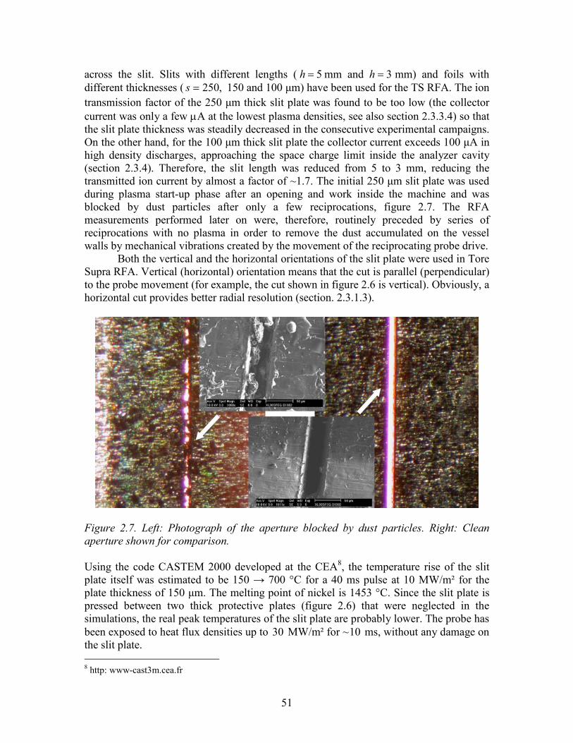
51

across the slit. Slits with different lengths ( 5=h mm and 3=h mm) and foils with different thicknesses ( ,250=s 150 and 100 µm) have been used for the TS RFA. The ion transmission factor of the 250 µm thick slit plate was found to be too low (the collector current was only a few µA at the lowest plasma densities, see also section 2.3.3.4) so that the slit plate thickness was steadily decreased in the consecutive experimental campaigns. On the other hand, for the 100 µm thick slit plate the collector current exceeds 100 µA in high density discharges, approaching the space charge limit inside the analyzer cavity (section 2.3.4). Therefore, the slit length was reduced from 5 to 3 mm, reducing the transmitted ion current by almost a factor of ~1.7. The initial 250 µm slit plate was used during plasma start-up phase after an opening and work inside the machine and was blocked by dust particles after only a few reciprocations, figure 2.7. The RFA measurements performed later on were, therefore, routinely preceded by series of reciprocations with no plasma in order to remove the dust accumulated on the vessel walls by mechanical vibrations created by the movement of the reciprocating probe drive.

Both the vertical and the horizontal orientations of the slit plate were used in Tore Supra RFA. Vertical (horizontal) orientation means that the cut is parallel (perpendicular) to the probe movement (for example, the cut shown in figure 2.6 is vertical). Obviously, a horizontal cut provides better radial resolution (section. 2.3.1.3).

Figure 2.7. Left: Photograph of the aperture blocked by dust particles. Right: Clean aperture shown for comparison. Using the code CASTEM 2000 developed at the CEA8, the temperature rise of the slit plate itself was estimated to be 150 → 700 °C for a 40 ms pulse at 10 MW/m² for the plate thickness of 150 µm. The melting point of nickel is 1453 °C. Since the slit plate is pressed between two thick protective plates (figure 2.6) that were neglected in the simulations, the real peak temperatures of the slit plate are probably lower. The probe has been exposed to heat flux densities up to 30 MW/m² for ~10 ms, without any damage on the slit plate. 8 http: www-cast3m.cea.fr

52

Figure 2.8. Photograph of the grid area.

The grids are laser-cut in a 99.9% nickel plates. The plate thickness is 30 µm. Grid wires with width of =∆ 63 µm are separated by =D 0.4 mm, giving an optical transmission factor of the grid ( ) .71.0/ 22

opt ≅∆−= DDξ The grid area is 8 × 8 mm, figure 2.8, meaning that the length of the grid area exceeds the 5 mm long slit plate aperture by 1.5 mm on each end of the aperture. This distance is larger than ion Larmor radius ( 800150 −≅Lr µm in the Tore Supra SOL), meaning that the grid transmission factor is not affected by the collection of ions outside the grid area even for relatively large probe head misalignment with respect to B. The grid wires are diagonal to the slit plate aperture to ensure that no single wire will block the trajectories of the particles transmitted through the aperture. In addition to the principal grids 1 and 2, another grid, referred to as “grid 0” (not shown in the schematic figure 2.1), is attached to the rear Inconel protective plate of the slit plate in order to render the electric field behind the chamfered opening of the protective plate as planar as possible.

The collector is made of oxygen-free high conductivity (OFHC) copper. Taking the absorption of ions on the grid wires into account, the relative

transmission factor of the slit plate calculated from the experimentally measured quantities approximately equals to:

3optsat

0expr ξξ

hwjI

+

≅ . (2.3)

For all three grids, the transmission factor is assumed to be equal to optξ . The total grid

transmission factor 3optξ is only approximate as the attenuation by subsequent grids could

be a function of the alignment of grids relative to one other. Additional uncertainty in exprξ can be due to e.g. ion induced secondary electron emission from the slit plate, which,

if non-zero, would cause sat+j to be overestimated (and thus underestimate )exprξ . The

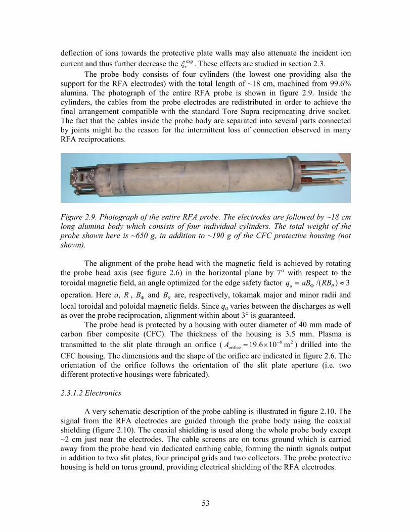
53

deflection of ions towards the protective plate walls may also attenuate the incident ion current and thus further decrease the exp

rξ . These effects are studied in section 2.3. The probe body consists of four cylinders (the lowest one providing also the

support for the RFA electrodes) with the total length of ~18 cm, machined from 99.6% alumina. The photograph of the entire RFA probe is shown in figure 2.9. Inside the cylinders, the cables from the probe electrodes are redistributed in order to achieve the final arrangement compatible with the standard Tore Supra reciprocating drive socket. The fact that the cables inside the probe body are separated into several parts connected by joints might be the reason for the intermittent loss of connection observed in many RFA reciprocations.

Figure 2.9. Photograph of the entire RFA probe. The electrodes are followed by ~18 cm long alumina body which consists of four individual cylinders. The total weight of the probe shown here is ~650 g, in addition to ~190 g of the CFC protective housing (not shown).

The alignment of the probe head with the magnetic field is achieved by rotating the probe head axis (see figure 2.6) in the horizontal plane by 7° with respect to the toroidal magnetic field, an angle optimized for the edge safety factor 3)/( ≈= Φ θRBaBqa

operation. Here a, R , ΦB and θB are, respectively, tokamak major and minor radii and local toroidal and poloidal magnetic fields. Since qa varies between the discharges as well as over the probe reciprocation, alignment within about 3° is guaranteed.

The probe head is protected by a housing with outer diameter of 40 mm made of carbon fiber composite (CFC). The thickness of the housing is 3.5 mm. Plasma is transmitted to the slit plate through an orifice ( 26

orifice m106.19 −×=A ) drilled into the CFC housing. The dimensions and the shape of the orifice are indicated in figure 2.6. The orientation of the orifice follows the orientation of the slit plate aperture (i.e. two different protective housings were fabricated).

2.3.1.2 Electronics

A very schematic description of the probe cabling is illustrated in figure 2.10. The signal from the RFA electrodes are guided through the probe body using the coaxial shielding (figure 2.10). The coaxial shielding is used along the whole probe body except ~2 cm just near the electrodes. The cable screens are on torus ground which is carried away from the probe head via dedicated earthing cable, forming the ninth signals output in addition to two slit plates, four principal grids and two collectors. The probe protective housing is held on torus ground, providing electrical shielding of the RFA electrodes.

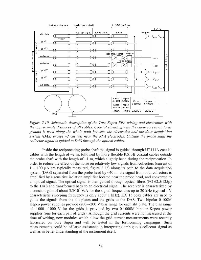
54

Figure 2.10. Schematic description of the Tore Supra RFA wiring and electronics with the approximate distances of all cables. Coaxial shielding with the cable screen on torus ground is used along the whole path between the electrodes and the data acquisition system (DAS) except ~2 cm just near the RFA electrodes. Outside the probe shaft the collector signal is guided to DAS through the optical cables.

Inside the reciprocating probe shaft the signal is guided through UT141A coaxial

cables with the length of ~2 m, followed by more flexible KX 3B coaxial cables outside the probe shaft with the length of ~1 m, which slightly bend during the reciprocation. In order to reduce the effect of the noise on relatively low signals from collectors (current of 1 – 100 µA are typically measured, figure 2.12) along its path to the data acquisition system (DAS) separated from the probe head by ~40 m, the signal from both collectors is amplified by a sensitive isolation amplifier located near the probe head, and converted to an optical signal. The optical signal is then guided through optical fibres (FO 62.5/125µ) to the DAS and transformed back to an electrical signal. The receiver is characterized by a constant gain of about 3.3·103 V/A for the signal frequencies up to 20 kHz (typical I-V characteristic sweeping frequency is only about 1 kHz). KX 15 coax cables are used to guide the signals from the slit plates and the grids to the DAS. Two bipolar 0-100M Kepco power supplies provide -200→200 V bias range for each slit plate. The bias range of -1000→1000 V for the grids is provided by two 0-1000M bipolar Kepco power supplies (one for each pair of grids). Although the grid currents were not measured at the time of writing, new modules which allow the grid current measurements were recently fabricated on Tore Supra and will be tested in the forthcoming campaigns. Such measurements could be of large assistance in interpreting ambiguous collector signal as well as in better understanding of the instrument itself.

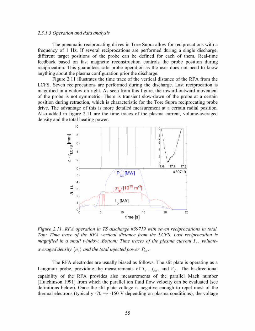
55

2.3.1.3 Operation and data analysis

The pneumatic reciprocating drives in Tore Supra allow for reciprocations with a frequency of 1 Hz. If several reciprocations are performed during a single discharge, different target positions of the probe can be defined for each of them. Real-time feedback based on fast magnetic reconstruction controls the probe position during reciprocation. This guarantees safe probe operation as the user does not need to know anything about the plasma configuration prior the discharge.

Figure 2.11 illustrates the time trace of the vertical distance of the RFA from the LCFS. Seven reciprocations are performed during the discharge. Last reciprocation is magnified in a widow on right. As seen from this figure, the inward-outward movement of the probe is not symmetric. There is transient slow-down of the probe at a certain position during retraction, which is characteristic for the Tore Supra reciprocating probe drive. The advantage of this is more detailed measurement at a certain radial position. Also added in figure 2.11 are the time traces of the plasma current, volume-averaged density and the total heating power.

2 4 6 8 0

2

4

6

8

10

z - z

LCFS [m

m]

0 5 10 15 20 250

1

2

3

4

5

time [s]

a. u.

17.6 17.7 17.80

2

4

6

8

10

Ptot [MW]

⟨ne⟩ [1019 m-3]

Ip [MA]

#39719

Figure 2.11. RFA operation in TS discharge #39719 with seven reciprocations in total. Top: Time trace of the RFA vertical distance from the LCFS. Last reciprocation is magnified in a small window. Bottom: Time traces of the plasma current pI , volume-

averaged density en and the total injected power totP .

The RFA electrodes are usually biased as follows. The slit plate is operating as a Langmuir probe, providing the measurements of eT , satj , and fV . The bi-directional capability of the RFA provides also measurements of the parallel Mach number [Hutchinson 1991] from which the parallel ion fluid flow velocity can be evaluated (see definitions below). Once the slit plate voltage is negative enough to repel most of the thermal electrons (typically -70 → -150 V depending on plasma conditions), the voltage

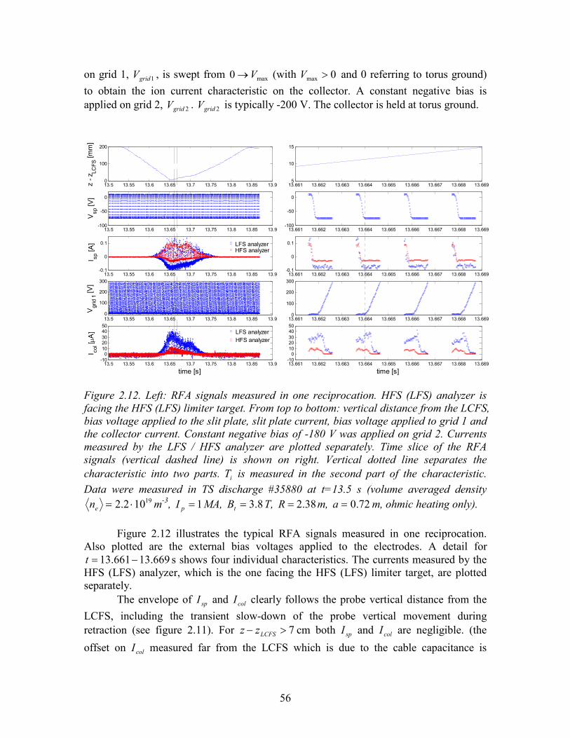
56

on grid 1, 1gridV , is swept from max0 V→ (with 0max >V and 0 referring to torus ground) to obtain the ion current characteristic on the collector. A constant negative bias is applied on grid 2, 2gridV . 2gridV is typically -200 V. The collector is held at torus ground.

13.5 13.55 13.6 13.65 13.7 13.75 13.8 13.85 13.90

100

200

z - z

LCFS [m

m]

13.661 13.662 13.663 13.664 13.665 13.666 13.667 13.668 13.6695

10

15

13.5 13.55 13.6 13.65 13.7 13.75 13.8 13.85 13.9-100

-50

0

Vsp [V

]

13.661 13.662 13.663 13.664 13.665 13.666 13.667 13.668 13.669-100

-50

0

13.5 13.55 13.6 13.65 13.7 13.75 13.8 13.85 13.9-0.1

0

0.1

I sp [A]

13.661 13.662 13.663 13.664 13.665 13.666 13.667 13.668 13.669-0.1

0

0.1

13.5 13.55 13.6 13.65 13.7 13.75 13.8 13.85 13.90

100

200

300

Vgrid 1 [V

]

13.661 13.662 13.663 13.664 13.665 13.666 13.667 13.668 13.6690

100

200

300

13.5 13.55 13.6 13.65 13.7 13.75 13.8 13.85 13.9-1001020304050

I col [ µA]

time [s]13.661 13.662 13.663 13.664 13.665 13.666 13.667 13.668 13.669-1001020304050

time [s]

LFS analyzerHFS analyzer

LFS analyzerHFS analyzer

Figure 2.12. Left: RFA signals measured in one reciprocation. HFS (LFS) analyzer is facing the HFS (LFS) limiter target. From top to bottom: vertical distance from the LCFS, bias voltage applied to the slit plate, slit plate current, bias voltage applied to grid 1 and the collector current. Constant negative bias of -180 V was applied on grid 2. Currents measured by the LFS / HFS analyzer are plotted separately. Time slice of the RFA signals (vertical dashed line) is shown on right. Vertical dotted line separates the characteristic into two parts. iT is measured in the second part of the characteristic. Data were measured in TS discharge #35880 at t=13.5 s (volume averaged density

19102.2 ⋅=en m-3, 1=pI MA, 8.3=tB T, 38.2=R m, 72.0=a m, ohmic heating only).

Figure 2.12 illustrates the typical RFA signals measured in one reciprocation. Also plotted are the external bias voltages applied to the electrodes. A detail for

669.13661.13 −=t s shows four individual characteristics. The currents measured by the HFS (LFS) analyzer, which is the one facing the HFS (LFS) limiter target, are plotted separately.

The envelope of spI and colI clearly follows the probe vertical distance from the LCFS, including the transient slow-down of the probe vertical movement during retraction (see figure 2.11). For 7>− LCFSzz cm both spI and colI are negligible. (the

offset on colI measured far from the LCFS which is due to the cable capacitance is

57

subtracted during the data analysis.) The envelope of the RFA signals compared to the probe distance from the LCFS gives rough idea about the SOL width.

The detail of spI signal shows that the current to the slit plate saturates around

20−=spV V, meaning that the maximum bias voltage applied to the slit plate (-75 V) is sufficient to repel all thermal electrons.

The asymmetry of the HFS / LFS currents is believed to be due to the parallel flow in the SOL which is directed towards the LFS analyzer for the standard plasma configuration in Tore Supra (i.e. 39.2=R m, 72.0=a m, plasma contact point at the TPL, figure 1.15). The LFS analyzer thus receives larger ion currents. In addition, colI

measured by the HFS analyzer drops faster with 1gridV that colI measured by the LFS

analyzer, meaning that the effective ion temperature *iT at the HFS analyzer is lower

compared to the LFS analyzer. The asymmetry in *iT roughly follows the ion current

asymmetry, which is consistent with the kinetic model of Valsaque [Valsaque 2002] (section 2.2).

Because of the asymmetry in *iT it would be preferential to bias grid 1 of each

analyzer separately with different maximum 1gridV , maxV . As seen in figure 2.12 the collector current measured by the HFS-analyzer drops to zero already at about

1501 ≈gridV V, so that the points on the I-V characteristics measured for higher 1gridV are sampled just at noise level and does not contribute to the fit Eq.(2.2). In turn, the LFS analyzer (which is here characterized by higher *

iT ) would require even larger maxV than that used in #35880 to repel all ions. Separate biasing of grid 1 for each analyzer is not possible because of the hardware restrictions.

Each characteristic is sampled for about 1 ms. Individual characteristics are separated by a window of about 1 ms during which the RFA signals are not measured (in addition, no data are collected between individual reciprocations), providing the time resolution of about 2 ms. The separation of the individual characteristics is used in order to reduce the volume of the data measured in one discharge. For the reciprocation shown in figure 2.12 (as well as for most RFA reciprocations) the number of data points per single characteristic is 64. The integration time between the individual data points is 16 µs, meaning that the RFA cannot measure any events characterized by smaller timescale.

The spatial resolution of the RFA is defined by the radial extension of the probe collection area increased by the radial displacement of the probe during the measurement of a single I-V characteristic. The vertical displacement of the RFA during the measurement of a single I-V characteristic is about 1 mm, except at the target position where the probe velocity is zero. Since the RFA is located close to the top of the plasma, the vertical displacement is nearly perpendicular to the magnetic flux surface. For the slit plate measurements (i.e. eT , satj , and fV ) the collection area is defined by orificeS (figure

2.6). For the collector measurements (i.e. iT , sV and 0I ) the collection area is defined by

the area of the slit plate aperture, hwSaperture = , (section 2.3.1.1). The orifice and the aperture dimensions are respectively 7 mm × 3 mm and 5 × 30 µm. As mentioned in section 2.3.1.1, both the vertical and the horizontal orientation of the orifice and the aperture was used for TS RFA. For the vertical orientation the radial resolution of the

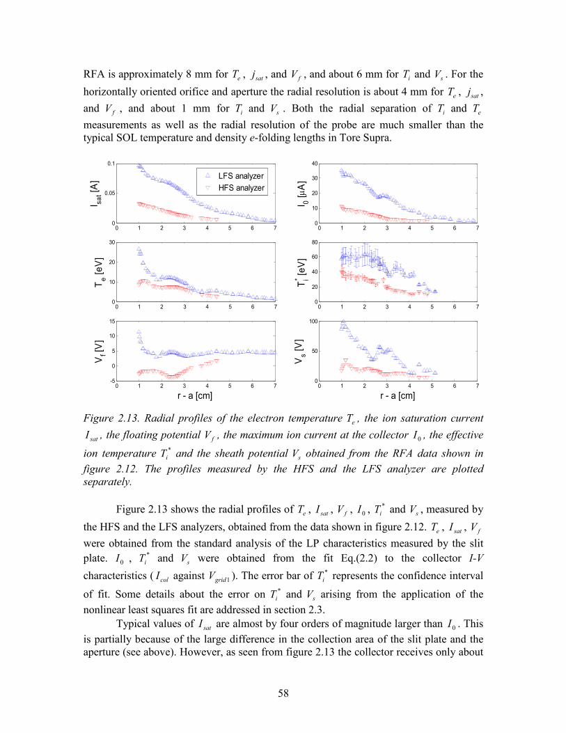
58

RFA is approximately 8 mm for eT , satj , and fV , and about 6 mm for iT and sV . For the

horizontally oriented orifice and aperture the radial resolution is about 4 mm for eT , satj ,

and fV , and about 1 mm for iT and sV . Both the radial separation of iT and eT measurements as well as the radial resolution of the probe are much smaller than the typical SOL temperature and density e-folding lengths in Tore Supra.

0 1 2 3 4 5 6 70

0.05

0.1

I sat [A

]

0 1 2 3 4 5 6 70

10

20

30

Te [eV]

0 1 2 3 4 5 6 7-5

0

5

10

15

Vf [V]

r - a [cm]

0 1 2 3 4 5 6 70

10

20

30

40

I 0 [µ

A]

0 1 2 3 4 5 6 70

20

40

60

80

Ti* [eV

]

0 1 2 3 4 5 6 70

50

100

Vs [V]

r - a [cm]

LFS analyzerHFS analyzer

Figure 2.13. Radial profiles of the electron temperature eT , the ion saturation current

satI , the floating potential fV , the maximum ion current at the collector 0I , the effective

ion temperature *iT and the sheath potential sV obtained from the RFA data shown in

figure 2.12. The profiles measured by the HFS and the LFS analyzer are plotted separately.

Figure 2.13 shows the radial profiles of eT , satI , fV , 0I , *

iT and sV , measured by

the HFS and the LFS analyzers, obtained from the data shown in figure 2.12. eT , satI , fV were obtained from the standard analysis of the LP characteristics measured by the slit plate. 0I , *

iT and sV were obtained from the fit Eq.(2.2) to the collector I-V

characteristics ( colI against 1gridV ). The error bar of *iT represents the confidence interval

of fit. Some details about the error on *iT and sV arising from the application of the

nonlinear least squares fit are addressed in section 2.3. Typical values of satI are almost by four orders of magnitude larger than 0I . This

is partially because of the large difference in the collection area of the slit plate and the aperture (see above). However, as seen from figure 2.13 the collector receives only about

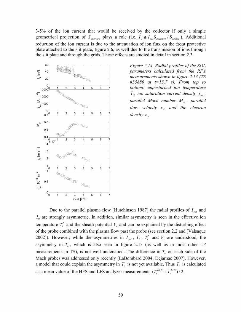
59

3-5% of the ion current that would be received by the collector if only a simple geometrical projection of apertureS plays a role (i.e. orificeaperturesat SSII /0 ≅ ). Additional reduction of the ion current is due to the attenuation of ion flux on the front protective plate attached to the slit plate, figure 2.6, as well due to the transmission of ions through the slit plate and through the grids. These effects are studied in detail in section 2.3.

0 1 2 3 4 5 6 70

20

40

60

T i [eV]

0 1 2 3 4 5 6 70

1000

2000

3000

j sat [A m

-2]

0 1 2 3 4 5 6 70.4

0.5

0.6

0.7

M//

0 1 2 3 4 5 6 71

2

3

4x 10

4

v // [m s-1]

0 1 2 3 4 5 6 70

0.5

1

r - a [cm]

n e [101

8 m-3]

Figure 2.14. Radial profiles of the SOL parameters calculated from the RFA measurements shown in figure 2.13 (TS #35880 at t=13.7 s). From top to bottom: unperturbed ion temperature

iT , ion saturation current density satj ,

parallel Mach number //M , parallel

flow velocity //v and the electron

density en .

Due to the parallel plasma flow [Hutchinson 1987] the radial profiles of satI and

0I are strongly asymmetric. In addition, similar asymmetry is seen in the effective ion

temperature *iT and the sheath potential sV and can be explained by the disturbing effect

of the probe combined with the plasma flow past the probe (see section 2.2 and [Valsaque 2002]). However, while the asymmetries in satI , 0I , *

iT and sV are understood, the

asymmetry in eT , which is also seen in figure 2.13 (as well as in most other LP

measurements in TS), is not well understood. The difference in eT on each side of the Mach probes was addressed only recently [LaBombard 2004, Dejarnac 2007]. However, a model that could explain the asymmetry in eT is not yet available. Thus eT is calculated

as a mean value of the HFS and LFS analyzer measurements 2/)( LFSe

HFSe TT + .

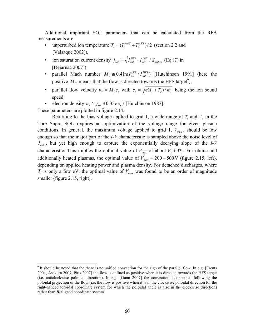
60

Additional important SOL parameters that can be calculated from the RFA measurements are:

• unperturbed ion temperature 2/)( LFSi

HFSii TTT += (section 2.2 and

[Valsaque 2002]),

• ion saturation current density orificeLFSsat

HFSsatsat SIIj /⋅= (Eq.(7) in

[Dejarnac 2007]) • parallel Mach number )/ln(4.0//

HFSsat

LFSsat IIM ≅ [Hutchinson 1991] (here the

positive //M means that the flow is directed towards the HFS target9),

• parallel flow velocity scMv //// = with ieis mTTec /)( += being the ion sound speed,

• electron density ( )ssate cejn 35.0/≅ [Hutchinson 1987]. These parameters are plotted in figure 2.14.

Returning to the bias voltage applied to grid 1, a wide range of iT and sV in the Tore Supra SOL requires an optimization of the voltage range for given plasma conditions. In general, the maximum voltage applied to grid 1, maxV , should be low enough so that the major part of the I-V characteristic is sampled above the noise level of

colI , but yet high enough to capture the exponentially decaying slope of the I-V

characteristic. This implies the optimal value of maxV of about is TV 3+ . For ohmic and

additionally heated plasmas, the optimal value of 500200max −=V V (figure 2.15, left), depending on applied heating power and plasma density. For detached discharges, where

iT is only a few eV, the optimal value of maxV was found to be an order of magnitude smaller (figure 2.15, right).

9 It should be noted that the there is no unified convection for the sign of the parallel flow. In e.g. [Erents 2004, Asakura 2007, Pitts 2007] the flow is defined as positive when it is directed towards the HFS target (i.e. anticlockwise poloidal direction). In e.g. [Gunn 2007] the convection is opposite, following the poloidal projection of the flow (i.e. the flow is positive when it is in the clockwise poloidal direction for the right-handed toroidal coordinate system for which the poloidal angle is also in the clockwise direction) rather than B-aligned coordinate system.

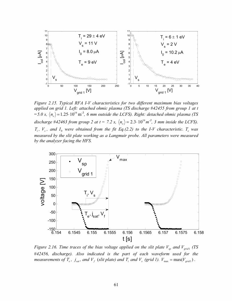
61

0 5 10 15 20 25 30 35 40-1

0

1

2

3

4

5

6

7

8

9

10

11

Vgrid 1

[V]

I col [µA]

Vgrid 1 [V]

I col [µA]

0 50 100 150 200 250-1

0

1

2

3

4

5

6

7

8

9

10

11

Vs

Ti = 6 ± 1 eV

Vs = 2 V

I0 = 10.2 µA

Vs

Ti = 29 ± 4 eV

Vs = 11 V

I0 = 8.0 µA

Te = 9 eV T

e = 4 eV

Figure 2.15. Typical RFA I-V characteristics for two different maximum bias voltages applied on grid 1. Left: attached ohmic plasma (TS discharge #42455 from group 1 at t =5.0 s, 191025.1 ⋅=en m-3, 6 mm outside the LCFS). Right: detached ohmic plasma (TS

discharge #42463 from group 2 at t = 7.2 s, 19103.2 ⋅=en m-3, 3 mm inside the LCFS).

iT , sV , and 0I were obtained from the fit Eq.(2.2) to the I-V characteristic. eT was measured by the slit plate working as a Langmuir probe. All parameters were measured by the analyzer facing the HFS.

6.154 6.1545 6.155 6.1555 6.156 6.1565 6.157 6.1575 6.158-150

-100

-50

0

50

100

150

200

250

300

t [s]

voltage

[V]

Vsp

Vgrid 1

Te, jsat, V

f

Ti, V

s

Vmax

Figure 2.16. Time traces of the bias voltage applied on the slit plate spV and 1gridV (TS #42456, discharge). Also indicated is the part of each waveform used for the measurements of eT , satj , and fV (slit plate) and iT and sV (grid 1). )max( 1max gridVV = .

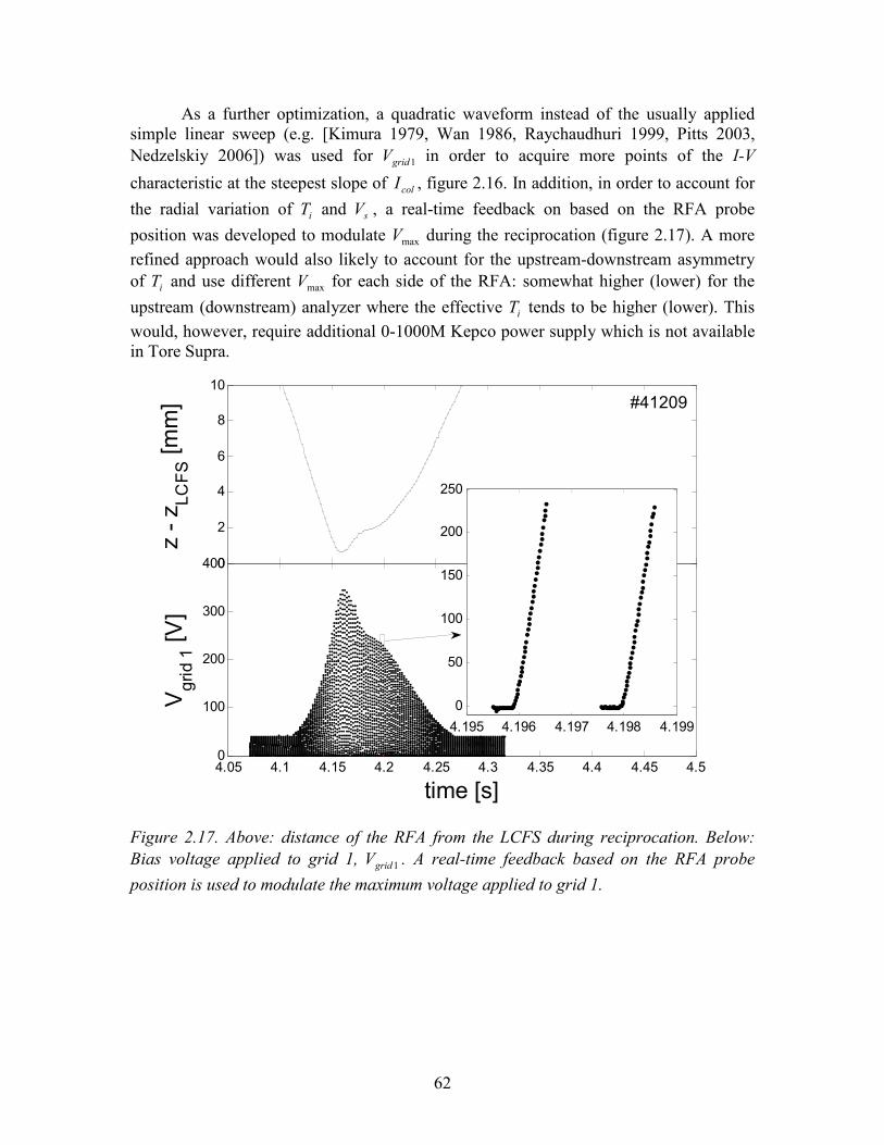
62

As a further optimization, a quadratic waveform instead of the usually applied simple linear sweep (e.g. [Kimura 1979, Wan 1986, Raychaudhuri 1999, Pitts 2003, Nedzelskiy 2006]) was used for 1gridV in order to acquire more points of the I-V

characteristic at the steepest slope of colI , figure 2.16. In addition, in order to account for

the radial variation of iT and sV , a real-time feedback on based on the RFA probe

position was developed to modulate maxV during the reciprocation (figure 2.17). A more refined approach would also likely to account for the upstream-downstream asymmetry of iT and use different maxV for each side of the RFA: somewhat higher (lower) for the

upstream (downstream) analyzer where the effective iT tends to be higher (lower). This would, however, require additional 0-1000M Kepco power supply which is not available in Tore Supra.

4,1 4,15 4,2 4,25 4,3 4,35 4,4 4,450

2

4

6

8

10

z - z

LCFS [m

m]

4.05 4.1 4.15 4.2 4.25 4.3 4.35 4.4 4.45 4.50

100

200

300

400

time [s]

Vgrid 1 [V

]

4.195 4.196 4.197 4.198 4.199

0

50

100

150

200

250

#41209

Figure 2.17. Above: distance of the RFA from the LCFS during reciprocation. Below: Bias voltage applied to grid 1, 1gridV . A real-time feedback based on the RFA probe position is used to modulate the maximum voltage applied to grid 1.

63

2.4. Instrumental study of the Tore Supra RFA

The theory of the RFA operation is so straightforward that it is tempting to assume that the response of the real RFA is the same as that of an idea device. However, since an independent experimental validation of RFA iT measurements on a large fusion reactor is not yet available due to a lack of simultaneous measurements with other relevant diagnostics, in this section, the instrumental effects and their influence on RFA measurements ( iT in particular) are studied. Some results from the following sections are compiled in the paper published in the Review of Scientific Instruments [Kocan 2008c] (see annex to chapter 2).

Following the ion path from the entrance of the CFC protective housing to the collector, we study separately the following processes:

(i) Attenuation of the ion flux on the CFC protective housing and its influence on

satj measurements (section 2.4.1). (ii) Attenuation of the ion flux on front protective plate of the slit plate and its

influence on iT measurements (section 2.4.2). (iii) Ion transmission through the entrance slit and its influence on iT measurements

(section 2.4.3). (iv) Effect of the positive space charge inside the RFA cavity and its influence on iT

measurements (section 2.4.4). (v) Influence of the negatively biased grid on iT measurements (section 2.4.5).

Experimental and theoretical investigations of the instrumental effects in RFA were already reported elsewhere. Some of the topics mentioned above were addressed e.g. in [Pánek 2004] (i), [Nachtrieb 2000, Matthews 1984, Wan 1986, Pitts 1991, Pitts 1996] (iii), [Molvik 1981, Wan 1986, Matthews 1985] (iv) and [Matthews 1985] (v). In this section we introduce several improvements and arrive at some new conclusions with respect to the earlier studies.

In (i) we take into account specific geometry of the orifice of the Tore Supra RFA protective housing. Moreover, compared to [Pánek 2004] where the attenuation was studied only by particle simulations, we combine the experimental data, particle simulations and a simple theoretical model based on the scaling of the magnetic pre-sheath thickness to quantify the attenuation effect. We conclude that the attenuation of the ion flux on the CFC protective housing is responsible for an underestimation of satj measured by the Tore Supra RFA by up to a factor of ~2.

(ii) is similar to (i). The attenuation of the ion current on the protective plate is studied by means of PIC simulations. We conclude that the actual protective plate geometry of Tore Supra RFA attenuates strongly the incident ion current (factor of 1.7 – 3 for the range of parameters studied here). We propose an alternative protective plate geometry to reduce this effect. However, even for the actual protective plate geometry the effect of the attenuation on iT measurements is negligible for the typical external slit plate bias voltages.

64

In (iii) we partially follow some ideas originally proposed by Nachtrieb [Nachtrieb 2000]. What is new is the quantitative evaluation of the effect of the slit transmission on iT as a function of the slit plate thickness, ion-to-electron temperature ratio and the angle of the slit plate misalignment with respect to the magnetic field vector B. We show that the selective ion transmission through the RFA slit plate is responsible for an overestimation of iT by less than 14%, even for a relatively thick slit plate. We therefore conclude that, providing that the signal level is sufficient, thicker slit plates are preferable since they reduce, e.g., the risk of melting during off-normal events, and the effect of the positive space charge inside the RFA cavity. In addition, improving upon [Nachtrieb 2000], we apply more general approach in the evaluation of the relative slit transmission factor and compare the theoretical calculation with the particle simulations and experimental data for different slit plate thicknesses and slit lengths. We demonstrate that the relative slit transmission factor is almost independent of the misalignment of the slit with respect to B. Therefore, taken that the electrons are transmitted into the analyzer by optical transmission because of much smaller Larmor radii compared to ions, a slightly tilted slit plate (by an angle defined by the slit width-to-thickness ratio) could be used as effective method for preventing the electrons to enter the analyzer independently of the bias voltage applied to the slit plate.

In (iv) the formula derived in [Nachtrieb 2000] was used to calculate the modification by positive space charge of the vacuum potential between the slit plate and grid 1. We conclude that for the typical ion currents measured by Tore Supra RFA the potential between the slit plate and grid 1 is dominated by the vacuum potential and space charge effects are therefore negligible.

In (v) we show that (in contrast to what was suggested in [Pitts 2003]) the transmission of the negatively biased grid is close to optical and its influence on iT measurements is negligible.

Finally, the error on sV and iT arising from the application of the standard fitting procedure (Eq.(2.2)) to the RFA I-V characteristics is studied for the first time. We show that the application of the standard fitting procedure leads to an overestimation of iT by

up to ~10% and to the overestimation of sV by up to eT3.0 . Because the measurements of the collector current are necessarily subject to noise and the parallel ion velocity distributions are not exponential for a certain range of velocities, these errors are largely unavoidable. It is concluded that in order to reduce the error on iT the upper limit of the range of the collector currents included in the fit (Eq.(2.2)) should be as small as possible (within the limits given by the collector current signal-to-noise ratio).

Some issues concerning the reliability of iT measurements are not addressed in this section, the most important of them being the influence of impurity ions in the SOL. As the analysis of the RFA current-voltage (I-V) characteristics assumes Maxwellian singly charged ions, impurities with higher charge states can affect the measurement of

iT . Separation of the components of the analyzed ion flux by charge state and temperature has been proposed in [Pitts 1991]. However, the model needs to specify the fractions of the total flux carried by ions with a given charge state as well as their temperatures. Such measurements are not available.

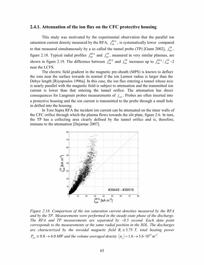
65

2.4.1. Attenuation of the ion flux on the CFC protective housing

This study was motivated by the experimental observation that the parallel ion saturation current density measured by the RFA, ,RFA

satj is systematically lower compared

to that measured simultaneously by a so called the tunnel probe (TP) [Gunn 2002], ,TPsatj

figure 2.18. Typical radial profiles RFAsatj and TP

satj , measured in very similar plasmas, are

shown in figure 2.19. The difference between RFAsatj and TP

satj increases up to RFAsatj / TP

satj ~2 near the LCFS.

The electric field gradient in the magnetic pre-sheath (MPS) is known to deflect the ions near the surface towards its normal if the ion Larmor radius is larger than the Debye length [Riyopoulos 1996a]. In this case, the ion flux entering a tunnel whose axis is nearly parallel with the magnetic field is subject to attenuation and the transmitted ion current is lower than that entering the tunnel orifice. The attenuation has direct consequences for Langmuir probes measurements of satj . Probes are often inserted into a protective housing and the ion current is transmitted to the probe through a small hole in drilled into the housing.

In Tore Supra RFA the incident ion current can be attenuated on the inner walls of the CFC orifice through which the plasma flows towards the slit plate, figure 2.6. In turn, the TP has a collecting area clearly defined by the tunnel orifice and is, therefore, immune to the attenuation [Dejarnac 2007].

0 10 20 30 40 50 60 70 800

10

20

30

40

50

60

70

80

jsatRFA [kA m-2]

j sat

TP [kA m

-2]

#39445 - #39519

Figure 2.18. Comparison of the ion saturation current densities measured by the RFA and by the TP. Measurements were performed in the steady-state phase of the discharge. The RFA and TP measurements are separated by ~0.5 second. Each data point corresponds to the measurements at the same radial position in the SOL. The discharges are characterized by the toroidal magnetic field 75.3≅tB T, total heating power

0.68.0 →≅totP MW and the volume averaged density 19106.36.1 ⋅→=en m-3.

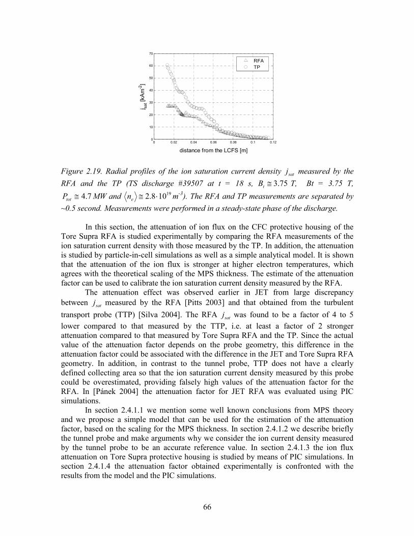
66

0 0.02 0.04 0.06 0.08 0.1 0.120

10

20

30

40

50

60

70

distance from the LCFS [m]j sa

t [kA

m-2]

RFATP

Figure 2.19. Radial profiles of the ion saturation current density satj measured by the

RFA and the TP (TS discharge #39507 at t = 18 s, 75.3≅tB T, Bt = 3.75 T,

7.4≅totP MW and 19108.2 ⋅≅en m-3). The RFA and TP measurements are separated by ~0.5 second. Measurements were performed in a steady-state phase of the discharge. In this section, the attenuation of ion flux on the CFC protective housing of the Tore Supra RFA is studied experimentally by comparing the RFA measurements of the ion saturation current density with those measured by the TP. In addition, the attenuation is studied by particle-in-cell simulations as well as a simple analytical model. It is shown that the attenuation of the ion flux is stronger at higher electron temperatures, which agrees with the theoretical scaling of the MPS thickness. The estimate of the attenuation factor can be used to calibrate the ion saturation current density measured by the RFA.

The attenuation effect was observed earlier in JET from large discrepancy between satj measured by the RFA [Pitts 2003] and that obtained from the turbulent

transport probe (TTP) [Silva 2004]. The RFA satj was found to be a factor of 4 to 5 lower compared to that measured by the TTP, i.e. at least a factor of 2 stronger attenuation compared to that measured by Tore Supra RFA and the TP. Since the actual value of the attenuation factor depends on the probe geometry, this difference in the attenuation factor could be associated with the difference in the JET and Tore Supra RFA geometry. In addition, in contrast to the tunnel probe, TTP does not have a clearly defined collecting area so that the ion saturation current density measured by this probe could be overestimated, providing falsely high values of the attenuation factor for the RFA. In [Pánek 2004] the attenuation factor for JET RFA was evaluated using PIC simulations.

In section 2.4.1.1 we mention some well known conclusions from MPS theory and we propose a simple model that can be used for the estimation of the attenuation factor, based on the scaling for the MPS thickness. In section 2.4.1.2 we describe briefly the tunnel probe and make arguments why we consider the ion current density measured by the tunnel probe to be an accurate reference value. In section 2.4.1.3 the ion flux attenuation on Tore Supra protective housing is studied by means of PIC simulations. In section 2.4.1.4 the attenuation factor obtained experimentally is confronted with the results from the model and the PIC simulations.

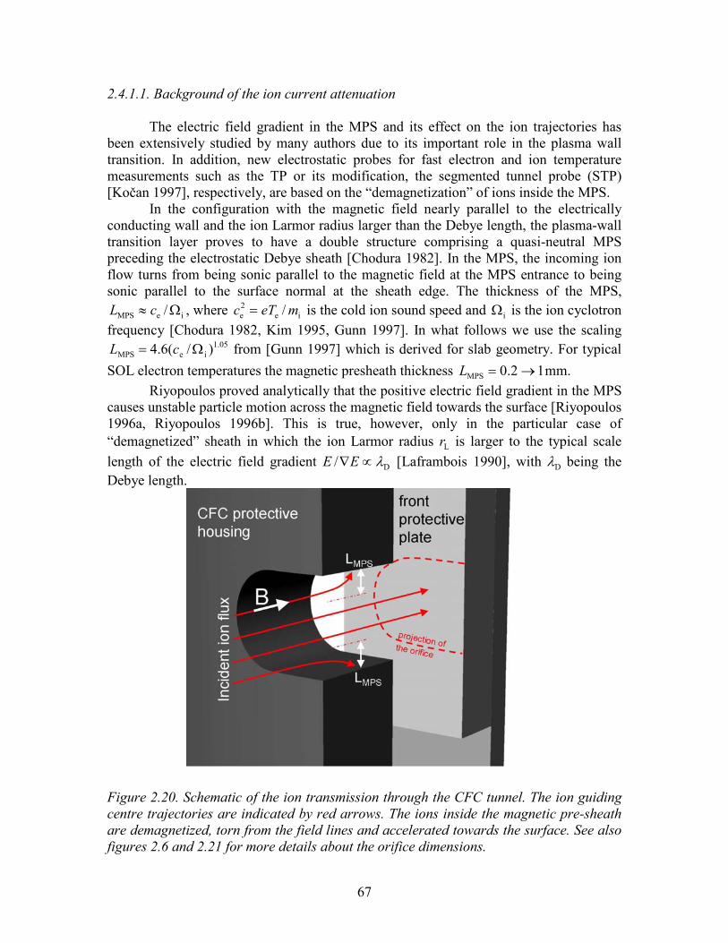
67

2.4.1.1. Background of the ion current attenuation

The electric field gradient in the MPS and its effect on the ion trajectories has been extensively studied by many authors due to its important role in the plasma wall transition. In addition, new electrostatic probes for fast electron and ion temperature measurements such as the TP or its modification, the segmented tunnel probe (STP) [Kočan 1997], respectively, are based on the “demagnetization” of ions inside the MPS.

In the configuration with the magnetic field nearly parallel to the electrically conducting wall and the ion Larmor radius larger than the Debye length, the plasma-wall transition layer proves to have a double structure comprising a quasi-neutral MPS preceding the electrostatic Debye sheath [Chodura 1982]. In the MPS, the incoming ion flow turns from being sonic parallel to the magnetic field at the MPS entrance to being sonic parallel to the surface normal at the sheath edge. The thickness of the MPS,

ieMPS /Ω≈ cL , where ie2e / meTc = is the cold ion sound speed and iΩ is the ion cyclotron

frequency [Chodura 1982, Kim 1995, Gunn 1997]. In what follows we use the scaling 05.1

ieMPS )/(6.4 Ω= cL from [Gunn 1997] which is derived for slab geometry. For typical

SOL electron temperatures the magnetic presheath thickness 12.0MPS →=L mm. Riyopoulos proved analytically that the positive electric field gradient in the MPS

causes unstable particle motion across the magnetic field towards the surface [Riyopoulos 1996a, Riyopoulos 1996b]. This is true, however, only in the particular case of “demagnetized” sheath in which the ion Larmor radius Lr is larger to the typical scale length of the electric field gradient D/ λ∝∇EE [Laframbois 1990], with Dλ being the Debye length.

Figure 2.20. Schematic of the ion transmission through the CFC tunnel. The ion guiding centre trajectories are indicated by red arrows. The ions inside the magnetic pre-sheath are demagnetized, torn from the field lines and accelerated towards the surface. See also figures 2.6 and 2.21 for more details about the orifice dimensions.

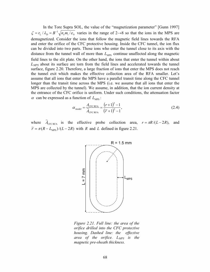
68

In the Tore Supra SOL, the value of the “magnetization parameter” [Gunn 1997]

0ie1

DL // ελζ mnBr −== varies in the range of 2→8 so that the ions in the MPS are demagnetized. Consider the ions that follow the magnetic field lines towards the RFA and enter the orifice of the CFC protective housing. Inside the CFC tunnel, the ion flux can be divided into two parts. Those ions who enter the tunnel close to its axis with the distance from the tunnel wall of more than MPSL continue unaffected along the magnetic field lines to the slit plate. On the other hand, the ions that enter the tunnel within about LMPS about its surface are torn from the field lines and accelerated towards the tunnel surface, figure 2.20. Therefore, a large fraction of ions that enter the MPS does not reach the tunnel exit which makes the effective collection area of the RFA smaller. Let’s assume that all ions that enter the MPS have a parallel transit time along the CFC tunnel longer than the transit time across the MPS (i.e. we assume that all ions that enter the MPS are collected by the tunnel). We assume, in addition, that the ion current density at the entrance of the CFC orifice is uniform. Under such conditions, the attenuation factor α can be expressed as a function of MPSL :

( )( )

,11~11

~ 2

2

RFA CFC

RFA CFCmodel −+

−+==

rr

AA

α (2.4)

where RFA CFC

~A is the effective probe collection area, ),2/( RLRr −= π and

)2/()(~MPS RLLRr −−= π with R and L defined in figure 2.21.

Figure 2.21. Full line: the area of the orifice drilled into the CFC protective housing. Dashed line: the effective area of the orifice. LMPS is the magnetic pre-sheath thickness.

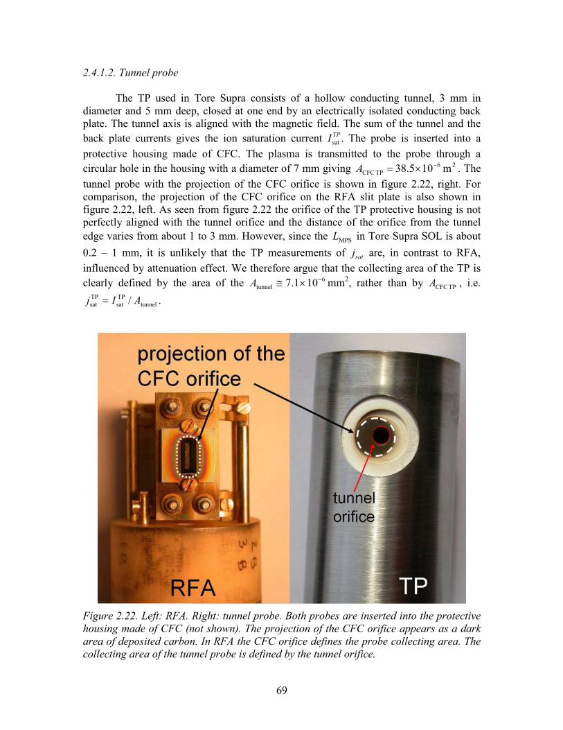
69

2.4.1.2. Tunnel probe The TP used in Tore Supra consists of a hollow conducting tunnel, 3 mm in

diameter and 5 mm deep, closed at one end by an electrically isolated conducting back plate. The tunnel axis is aligned with the magnetic field. The sum of the tunnel and the back plate currents gives the ion saturation current .sat

TPI The probe is inserted into a protective housing made of CFC. The plasma is transmitted to the probe through a circular hole in the housing with a diameter of 7 mm giving 26

TP CFC m105.38 −×=A . The tunnel probe with the projection of the CFC orifice is shown in figure 2.22, right. For comparison, the projection of the CFC orifice on the RFA slit plate is also shown in figure 2.22, left. As seen from figure 2.22 the orifice of the TP protective housing is not perfectly aligned with the tunnel orifice and the distance of the orifice from the tunnel edge varies from about 1 to 3 mm. However, since the MPSL in Tore Supra SOL is about

0.2 – 1 mm, it is unlikely that the TP measurements of satj are, in contrast to RFA, influenced by attenuation effect. We therefore argue that the collecting area of the TP is clearly defined by the area of the 6

tunnel 101.7 −×≅A mm2, rather than by TP CFCA , i.e.

tunnelTPsat

TPsat / AIj = .

Figure 2.22. Left: RFA. Right: tunnel probe. Both probes are inserted into the protective housing made of CFC (not shown). The projection of the CFC orifice appears as a dark area of deposited carbon. In RFA the CFC orifice defines the probe collecting area. The collecting area of the tunnel probe is defined by the tunnel orifice.

70

2.4.1.3. Particle-in-cell simulations

In this section, the attenuation of ion flux in the tunnel of the RFA protective housing is studied by particle-in-cell (PIC) simulations. In contrast to the model proposed in section 2.3.1.2 which was based on a simple geometrical assumptions and does not account for the finite tunnel length (assuming that all ions entering the MPS inside the tunnel are absorbed), in the PIC simulations the magnetic pre-sheath inside the tunnel is solved self-consistently and the trajectories of individual particles are tracked.

The attenuation is studied by means of the PIC code XOOPIC [Verboncoeur 1995]. The cross-section of the tunnel is oval (figure 2.21) which implies three-dimensional geometry of the problem to solve. The XOOPIC code allows for simulations with only two spatial dimensions so that the geometry of the problem requires simplifications. We utilize the fact that in the Tore Supra SOL the typical 12.0MPS →=L mm which is substantially smaller compared to the both orifice dimensions (figure 2.21). Therefore, the attenuation acts only in a thin layer above the inner walls of the tunnel and is not significantly influenced by the actual curvature of the tunnel walls. The attenuation factor will be, therefore, similar for a tunnel with a circular cross-section but with the circumference identical to that of the real oval orifice. Such circular orifice is axially symmetric and can be therefore modelled by XOOPIC code in a cylindrical geometry. The simulations were performed as follows. Ions and electrons were injected towards a tunnel with the length of 5.3=s mm and the radius of 8.2CFC =r mm. The injection plane was positioned 1 mm in front of the tunnel orifice. The system was terminated by a slit plate, positioned 1 mm behind the tunnel exit, i.e. the real distance of the RFA slit plate from the CFC housing (about 4 mm) was reduced in order to make the simulations faster. This should have no influence on the particle trajectories inside the tunnel, as the Debye sheath potential drop in front of the slit plate was found to be substantially smaller than 1 mm so that it does not influence the electric field inside the tunnel. The potential difference between the injection plane and the tunnel was set to

,12ln2 e

i

i

eeph

+=

TT

mmT

πφ (2.5)

assuming that the protective housing is biased to the floating sheath potential with respect to plasma. The potential difference between the injection plane and the slit plate was set to

,12ln2 e

i

i

eespsp

++=

TT

mmT

V πφ (2.6)

where 80sp −=V V is the slit plate external bias voltage (similar bias voltage for the RFA

slit plate was used for the measurements of the experimental data addressed here). iT and

eT are respectively the ion and electron temperatures at injection. Secondary electron emission from the protective housing and from the slit plate was neglected. The ions and

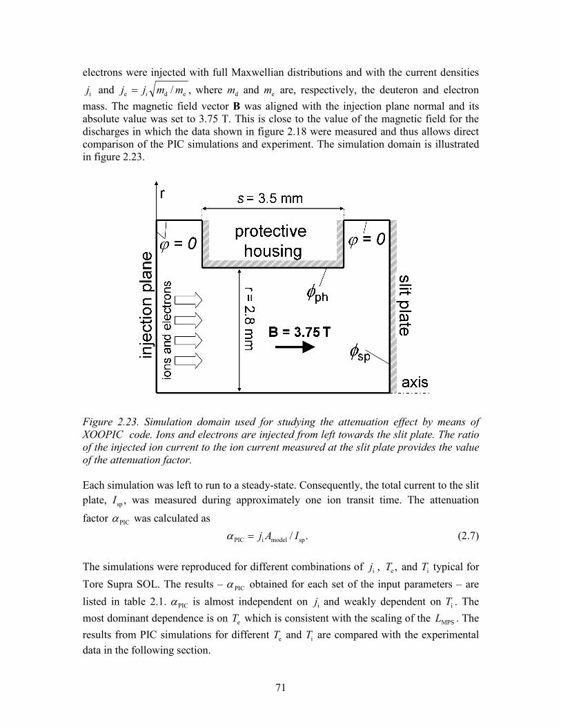
71

electrons were injected with full Maxwellian distributions and with the current densities

ij and ,/ ede mmjj i= where dm and em are, respectively, the deuteron and electron mass. The magnetic field vector B was aligned with the injection plane normal and its absolute value was set to 3.75 T. This is close to the value of the magnetic field for the discharges in which the data shown in figure 2.18 were measured and thus allows direct comparison of the PIC simulations and experiment. The simulation domain is illustrated in figure 2.23.

Figure 2.23. Simulation domain used for studying the attenuation effect by means of XOOPIC code. Ions and electrons are injected from left towards the slit plate. The ratio of the injected ion current to the ion current measured at the slit plate provides the value of the attenuation factor.

Each simulation was left to run to a steady-state. Consequently, the total current to the slit plate, ,spI was measured during approximately one ion transit time. The attenuation

factor PICα was calculated as

./ spmodeliPIC IAj=α (2.7)

The simulations were reproduced for different combinations of ,ij ,eT and iT typical for

Tore Supra SOL. The results – PICα obtained for each set of the input parameters – are

listed in table 2.1. PICα is almost independent on ij and weakly dependent on iT . The

most dominant dependence is on eT which is consistent with the scaling of the MPSL . The

results from PIC simulations for different eT and iT are compared with the experimental data in the following section.

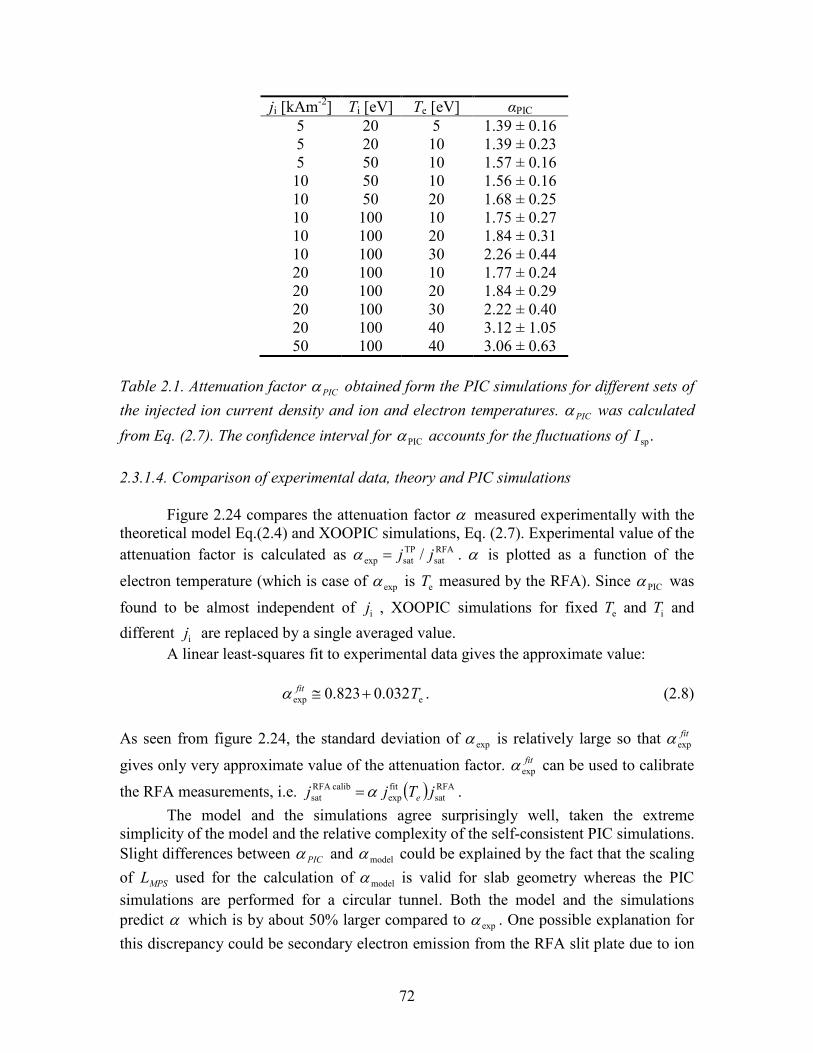
72

ji [kAm-2] Ti [eV] Te [eV] αPIC

5 20 5 1.39 ± 0.16 5 20 10 1.39 ± 0.23 5 50 10 1.57 ± 0.16 10 50 10 1.56 ± 0.16 10 50 20 1.68 ± 0.25 10 100 10 1.75 ± 0.27 10 100 20 1.84 ± 0.31 10 100 30 2.26 ± 0.44 20 100 10 1.77 ± 0.24 20 100 20 1.84 ± 0.29 20 100 30 2.22 ± 0.40 20 100 40 3.12 ± 1.05 50 100 40 3.06 ± 0.63

Table 2.1. Attenuation factor PICα obtained form the PIC simulations for different sets of

the injected ion current density and ion and electron temperatures. PICα was calculated

from Eq. (2.7). The confidence interval for PICα accounts for the fluctuations of .spI 2.3.1.4. Comparison of experimental data, theory and PIC simulations

Figure 2.24 compares the attenuation factor α measured experimentally with the theoretical model Eq.(2.4) and XOOPIC simulations, Eq. (2.7). Experimental value of the attenuation factor is calculated as RFA

satTPsatexp / jj=α . α is plotted as a function of the

electron temperature (which is case of expα is eT measured by the RFA). Since PICα was

found to be almost independent of ij , XOOPIC simulations for fixed eT and iT and

different ij are replaced by a single averaged value. A linear least-squares fit to experimental data gives the approximate value:

eexp 032.0823.0 Tfit +≅α . (2.8)

As seen from figure 2.24, the standard deviation of expα is relatively large so that fitexpα

gives only very approximate value of the attenuation factor. fitexpα can be used to calibrate

the RFA measurements, i.e. ( ) RFAsat

fitexp

calibRFA sat jTjj eα= .

The model and the simulations agree surprisingly well, taken the extreme simplicity of the model and the relative complexity of the self-consistent PIC simulations. Slight differences between PICα and modelα could be explained by the fact that the scaling

of MPSL used for the calculation of modelα is valid for slab geometry whereas the PIC simulations are performed for a circular tunnel. Both the model and the simulations predict α which is by about 50% larger compared to expα . One possible explanation for this discrepancy could be secondary electron emission from the RFA slit plate due to ion

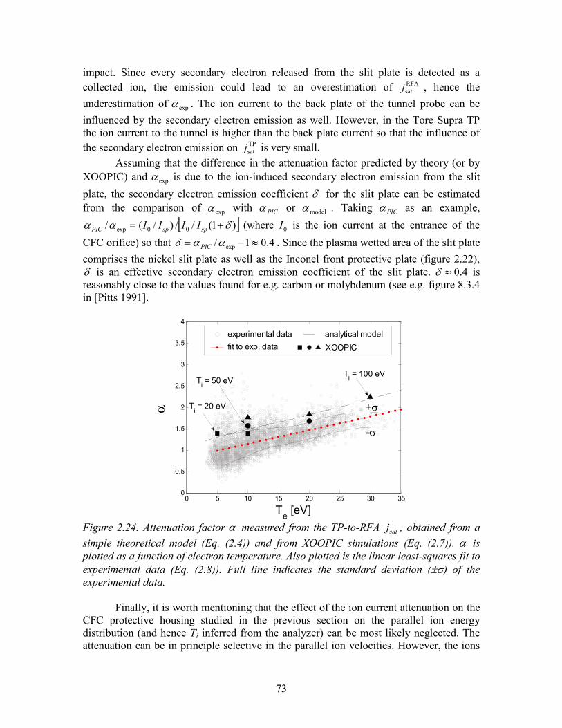
73

impact. Since every secondary electron released from the slit plate is detected as a collected ion, the emission could lead to an overestimation of RFA

satj , hence the

underestimation of expα . The ion current to the back plate of the tunnel probe can be influenced by the secondary electron emission as well. However, in the Tore Supra TP the ion current to the tunnel is higher than the back plate current so that the influence of the secondary electron emission on TP

satj is very small. Assuming that the difference in the attenuation factor predicted by theory (or by

XOOPIC) and expα is due to the ion-induced secondary electron emission from the slit

plate, the secondary electron emission coefficient δ for the slit plate can be estimated from the comparison of expα with PICα or modelα . Taking PICα as an example,

[ ])1(//)/(/ 00exp δαα += spspPIC IIII (where 0I is the ion current at the entrance of the

CFC orifice) so that 4.01/ exp ≈−= ααδ PIC . Since the plasma wetted area of the slit plate comprises the nickel slit plate as well as the Inconel front protective plate (figure 2.22), δ is an effective secondary electron emission coefficient of the slit plate. 4.0≈δ is reasonably close to the values found for e.g. carbon or molybdenum (see e.g. figure 8.3.4 in [Pitts 1991].

0 5 10 15 20 25 30 350

0.5

1

1.5

2

2.5

3

3.5

4

α

Te [eV]

+σ

-σ

experimental data

fit to exp. data

analytical model

XOOPIC

Ti = 100 eV

Ti = 50 eV

Ti = 20 eV

Figure 2.24. Attenuation factor α measured from the TP-to-RFA satj , obtained from a simple theoretical model (Eq. (2.4)) and from XOOPIC simulations (Eq. (2.7)). α is plotted as a function of electron temperature. Also plotted is the linear least-squares fit to experimental data (Eq. (2.8)). Full line indicates the standard deviation (±σ) of the experimental data.

Finally, it is worth mentioning that the effect of the ion current attenuation on the CFC protective housing studied in the previous section on the parallel ion energy distribution (and hence Ti inferred from the analyzer) can be most likely neglected. The attenuation can be in principle selective in the parallel ion velocities. However, the ions

74

flowing towards the slit plate aperture (i.e. the ones whose parallel energy distribution is measured by the analyzer) are about 1.5 mm far from the tunnel walls which is a distance larger than the LMPS. Therefore, the ions flowing through the tunnel towards the aperture are most likely unaffected by the attenuation and its effect on Ti measurements can be neglected. Simulations should be carried out in order to verify this hypothesis.

2.4.2. Attenuation of the ion flux on the protective plate

As shown in figure 2.6, the aperture of the TS RFA is preceded by the front protective plate which serves as a heat sink. The ions flow towards the aperture through the rectangular window in the protective plate. Since the aperture is only 0.5 mm from the walls (which is a distance comparable to the magnetic pre-sheath thickness in TS SOL, see section 2.4.1.1), the ion flux to the aperture can be subject to attenuation similar to the one addressed in the previous section. Since the protective plate is in electrical contact with the slit plate, the attenuation caused by the protective plate does not affect the measurements of satj . However, because of selective parallel ion loss, it could affect

iT measurements as well as the transmission factor of the slit plate evaluated from experimental data, Eq. 2.3. The latter could be affected because the ion current actually received by the aperture can be smaller than satj multiplied by the aperture area which is one of the assumptions in Eq. 2.3.

The attenuation of ion flux on the protective plate is studied by means of the PIC code SPICE (Sheath Particle In CEll) [Dejarnac 2007]. Originally, the SPICE code was developed for studying the flow of plasma into gaps between the limiter and divertor tiles. SPICE allows for 2d3v simulations in Cartesian coordinates. The code implements a standard leapfrog method for particle advancing, and uses first order (cloud-in-cell) weighting [Birdsall 1985].

Two different protective plate geometries are assumed in the simulations: • actual geometry of the TS RFA protective plate referred to as “A”, • alternative knife edge geometry referred to as “B”. The simulation domains for both A and B are shown in figure 2.25, right. The

Cartesian coordinate system is used. The simulation domain is aligned with the x-z plane (with x being the direction aligned with B). y-direction is ignored in the simulations. The absorbing walls of the protective plate as well as the slit plate are set at the potential defined by Eq.(2.6), which includes the external slit plate bias voltage spV as well as the natural sheath potential drop. The “plasma” boundaries (i.e. the injection plane and the boundaries attached to it) are set to 0=ϕ . The boundaries attached to the injection plane are periodic. The length of the system in the z-direction as well as the distance of the injection plane from the protective plate are set large enough to avoid perturbations generated by the chamfered edges as well as to allow for a Debye sheath potential drop in front of the wall, respectively. The magnetic field B = 3.5 T is uniform and directed towards the slit plate. The ions ( Di mm = ) are injected with a parallel velocity distribution calculated from the kinetic model of Chung and Hutchinson [Chung 1988] for zero drift

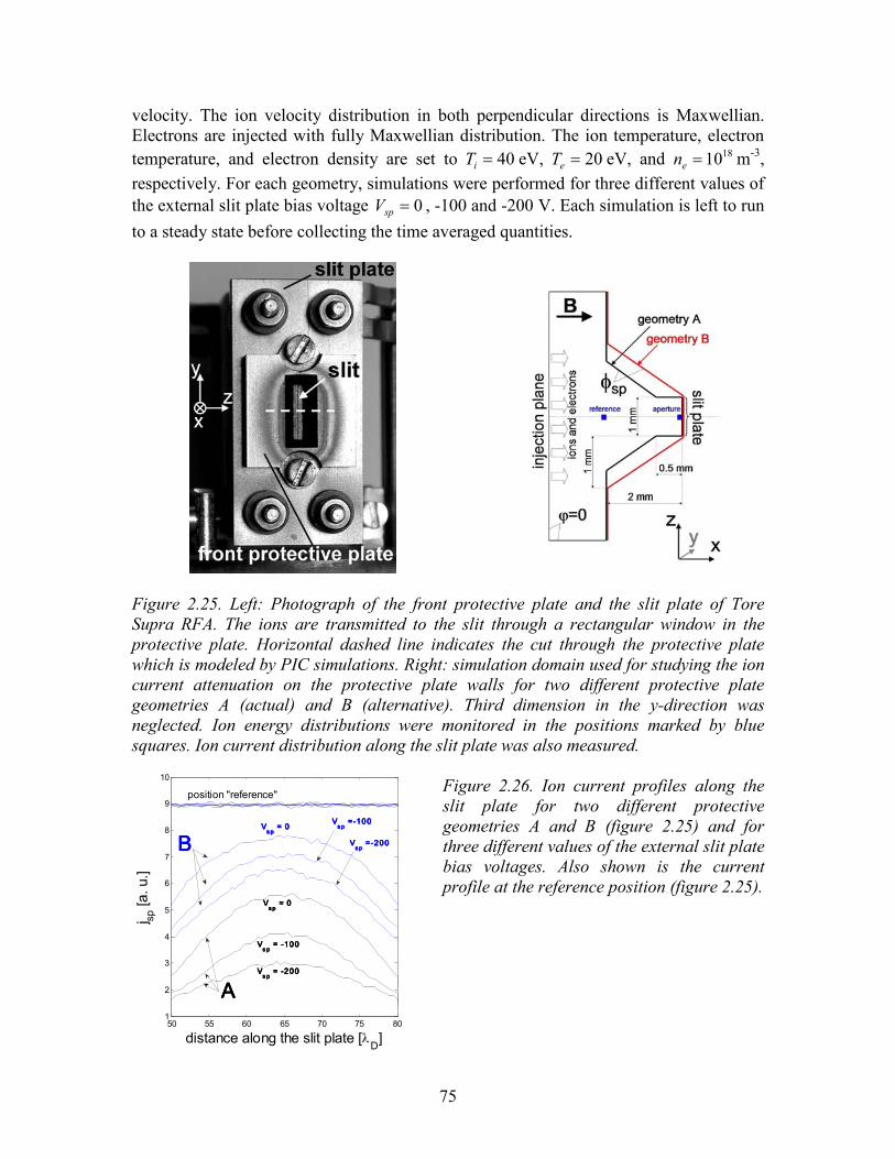
75

velocity. The ion velocity distribution in both perpendicular directions is Maxwellian. Electrons are injected with fully Maxwellian distribution. The ion temperature, electron temperature, and electron density are set to 40=iT eV, 20=eT eV, and 1810=en m-3, respectively. For each geometry, simulations were performed for three different values of the external slit plate bias voltage 0=spV , -100 and -200 V. Each simulation is left to run to a steady state before collecting the time averaged quantities.

Figure 2.25. Left: Photograph of the front protective plate and the slit plate of Tore Supra RFA. The ions are transmitted to the slit through a rectangular window in the protective plate. Horizontal dashed line indicates the cut through the protective plate which is modeled by PIC simulations. Right: simulation domain used for studying the ion current attenuation on the protective plate walls for two different protective plate geometries A (actual) and B (alternative). Third dimension in the y-direction was neglected. Ion energy distributions were monitored in the positions marked by blue squares. Ion current distribution along the slit plate was also measured.

50 55 60 65 70 75 801

2

3

4

5

6

7

8

9

10

distance along the slit plate [λD]

j sp [a. u.]

VVVVspspspsp =-100 =-100 =-100 =-100

VVVVs ps ps ps p = -200 = -200 = -200 = -200

VVVVspspspsp = 0 = 0 = 0 = 0

VVVVspspspsp = 0 = 0 = 0 = 0

VVVVspspspsp =-200 =-200 =-200 =-200BBBB

AAAA

position "reference"

VVVVs ps ps ps p = -100 = -100 = -100 = -100

Figure 2.26. Ion current profiles along the slit plate for two different protective geometries A and B (figure 2.25) and for three different values of the external slit plate bias voltages. Also shown is the current profile at the reference position (figure 2.25).

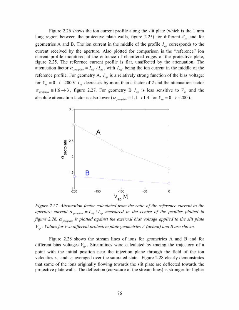
76

Figure 2.26 shows the ion current profile along the slit plate (which is the 1 mm long region between the protective plate walls, figure 2.25) for different spV and for

geometries A and B. The ion current in the middle of the profile apI corresponds to the current received by the aperture. Also plotted for comparison is the “reference” ion current profile monitored at the entrance of chamfered edges of the protective plate, figure 2.25. The reference current profile is flat, unaffected by the attenuation. The attenuation factor aprefprotplate II /=α , with refI being the ion current in the middle of the

reference profile. For geometry A, apI is a relatively strong function of the bias voltage:

for 2000 −→=spV V apI decreases by more than a factor of 2 and the attenuation factor

36.1 →≅protplateα , figure 2.27. For geometry B apI is less sensitive to spV and the

absolute attenuation factor is also lower ( 4.11.1 →≅protplateα for 2000 −→=spV ).

-200 -150 -100 -50 01

1.5

2

2.5

3

3.5

Vsp [V]

αprotplate

A

B

Figure 2.27. Attenuation factor calculated from the ratio of the reference current to the aperture current aprefprotplate II /=α measured in the centre of the profiles plotted in

figure 2.26. protplateα is plotted against the external bias voltage applied to the slit plate

spV . Values for two different protective plate geometries A (actual) and B are shown. Figure 2.28 shows the stream lines of ions for geometries A and B and for

different bias voltages spV . Streamlines were calculated by tracing the trajectory of a point with the initial position near the injection plane through the field of the ion velocities xv and zv averaged over the saturated state. Figure 2.28 clearly demonstrates that some of the ions originally flowing towards the slit plate are deflected towards the protective plate walls. The deflection (curvature of the stream lines) is stronger for higher

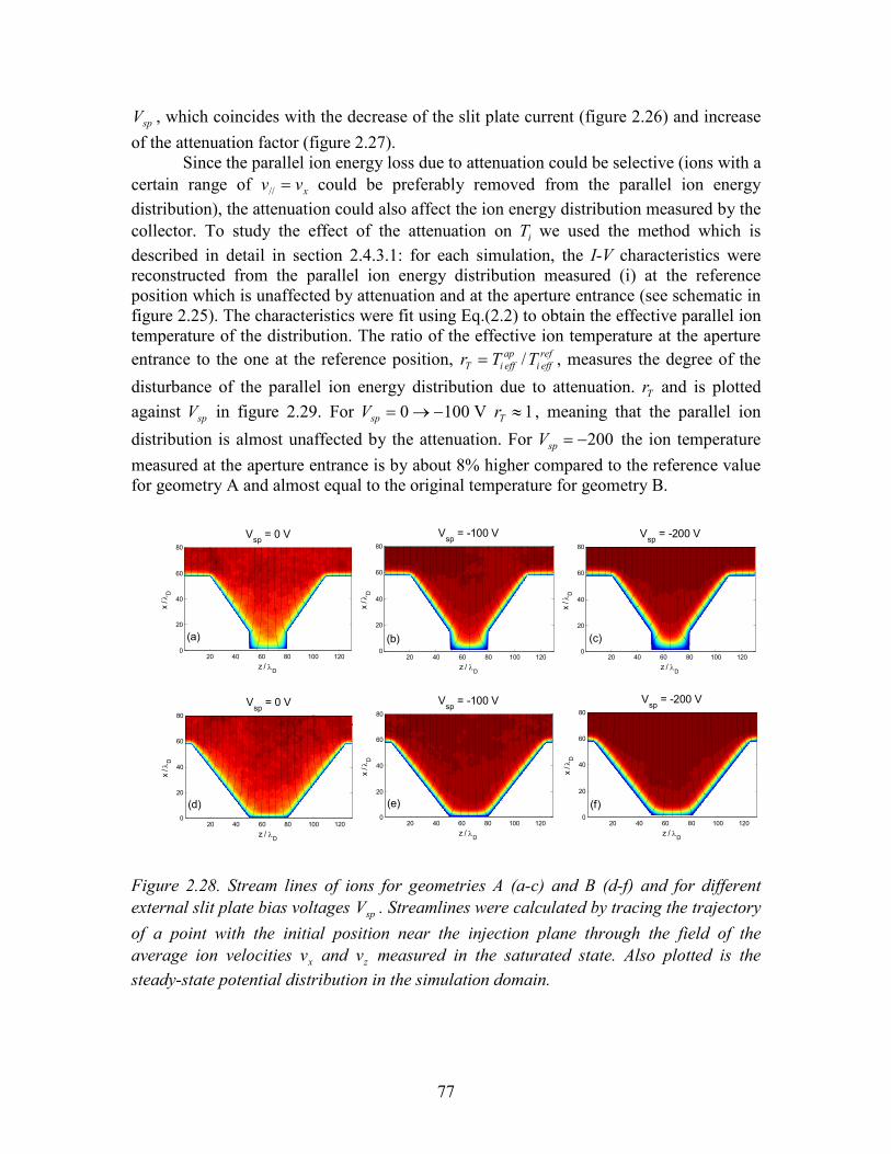
77

spV , which coincides with the decrease of the slit plate current (figure 2.26) and increase of the attenuation factor (figure 2.27).

Since the parallel ion energy loss due to attenuation could be selective (ions with a certain range of xvv =// could be preferably removed from the parallel ion energy distribution), the attenuation could also affect the ion energy distribution measured by the collector. To study the effect of the attenuation on iT we used the method which is described in detail in section 2.4.3.1: for each simulation, the I-V characteristics were reconstructed from the parallel ion energy distribution measured (i) at the reference position which is unaffected by attenuation and at the aperture entrance (see schematic in figure 2.25). The characteristics were fit using Eq.(2.2) to obtain the effective parallel ion temperature of the distribution. The ratio of the effective ion temperature at the aperture entrance to the one at the reference position, ref

effiapeffiT TTr /= , measures the degree of the

disturbance of the parallel ion energy distribution due to attenuation. Tr and is plotted against spV in figure 2.29. For 1000 −→=spV V 1≈Tr , meaning that the parallel ion

distribution is almost unaffected by the attenuation. For 200−=spV the ion temperature measured at the aperture entrance is by about 8% higher compared to the reference value for geometry A and almost equal to the original temperature for geometry B.

z / λD

x / λ

D

Vsp = 0 V

20 40 60 80 100 1200

20

40

60

80

z / λD

x / λ

D

Vsp = -100 V

20 40 60 80 100 1200

20

40

60

80

z / λD

x / λ

D

Vsp = -200 V

20 40 60 80 100 1200

20

40

60

80

z / λD

x / λ

D

Vsp = 0 V

20 40 60 80 100 1200

20

40

60

80

z / λD

x / λ

D

Vsp = -100 V

20 40 60 80 100 1200

20

40

60

80

z / λD

x / λ

D

Vsp = -200 V

20 40 60 80 100 1200

20

40

60

80

(a) (b) (c)

(f)(e)(d)

Figure 2.28. Stream lines of ions for geometries A (a-c) and B (d-f) and for different external slit plate bias voltages spV . Streamlines were calculated by tracing the trajectory of a point with the initial position near the injection plane through the field of the average ion velocities xv and zv measured in the saturated state. Also plotted is the steady-state potential distribution in the simulation domain.

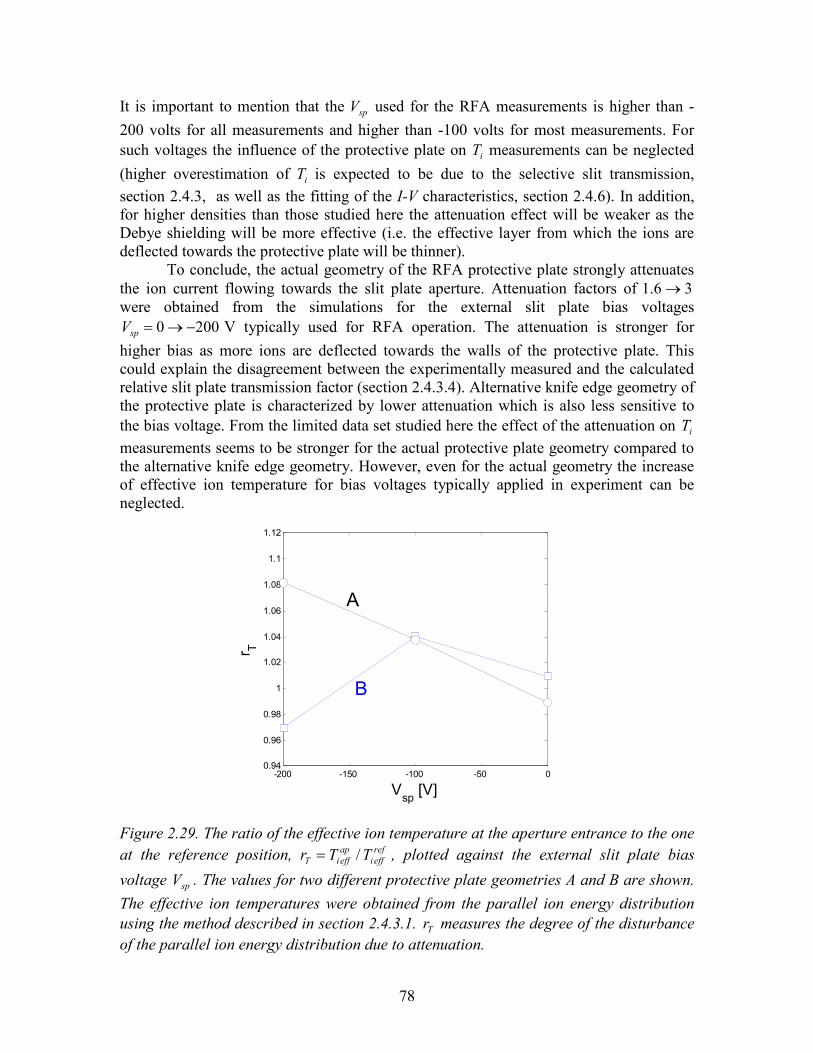
78

It is important to mention that the spV used for the RFA measurements is higher than -200 volts for all measurements and higher than -100 volts for most measurements. For such voltages the influence of the protective plate on iT measurements can be neglected

(higher overestimation of iT is expected to be due to the selective slit transmission, section 2.4.3, as well as the fitting of the I-V characteristics, section 2.4.6). In addition, for higher densities than those studied here the attenuation effect will be weaker as the Debye shielding will be more effective (i.e. the effective layer from which the ions are deflected towards the protective plate will be thinner).

To conclude, the actual geometry of the RFA protective plate strongly attenuates the ion current flowing towards the slit plate aperture. Attenuation factors of 36.1 → were obtained from the simulations for the external slit plate bias voltages

2000 −→=spV V typically used for RFA operation. The attenuation is stronger for higher bias as more ions are deflected towards the walls of the protective plate. This could explain the disagreement between the experimentally measured and the calculated relative slit plate transmission factor (section 2.4.3.4). Alternative knife edge geometry of the protective plate is characterized by lower attenuation which is also less sensitive to the bias voltage. From the limited data set studied here the effect of the attenuation on iT measurements seems to be stronger for the actual protective plate geometry compared to the alternative knife edge geometry. However, even for the actual geometry the increase of effective ion temperature for bias voltages typically applied in experiment can be neglected.

-200 -150 -100 -50 00.94

0.96

0.98

1

1.02

1.04

1.06

1.08

1.1

1.12

Vsp [V]

r T

A

B

Figure 2.29. The ratio of the effective ion temperature at the aperture entrance to the one at the reference position, ref

effiapeffiT TTr /= , plotted against the external slit plate bias

voltage spV . The values for two different protective plate geometries A and B are shown. The effective ion temperatures were obtained from the parallel ion energy distribution using the method described in section 2.4.3.1. Tr measures the degree of the disturbance of the parallel ion energy distribution due to attenuation.

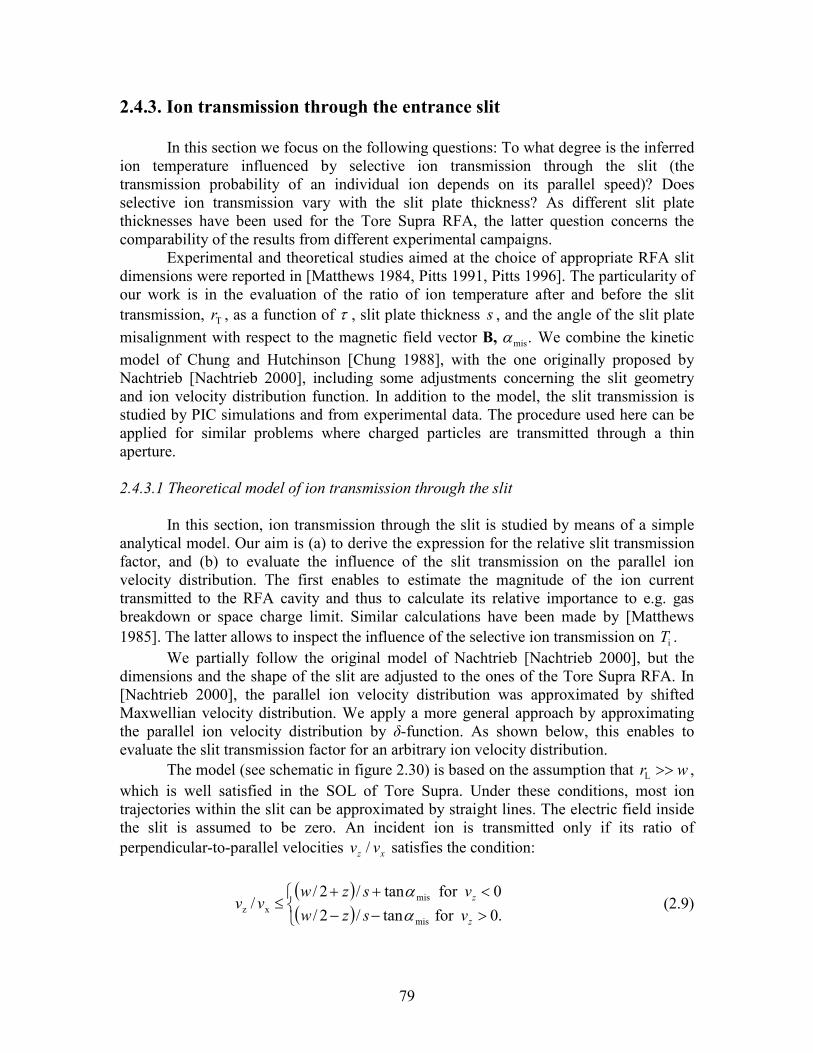
79

2.4.3. Ion transmission through the entrance slit

In this section we focus on the following questions: To what degree is the inferred ion temperature influenced by selective ion transmission through the slit (the transmission probability of an individual ion depends on its parallel speed)? Does selective ion transmission vary with the slit plate thickness? As different slit plate thicknesses have been used for the Tore Supra RFA, the latter question concerns the comparability of the results from different experimental campaigns.

Experimental and theoretical studies aimed at the choice of appropriate RFA slit dimensions were reported in [Matthews 1984, Pitts 1991, Pitts 1996]. The particularity of our work is in the evaluation of the ratio of ion temperature after and before the slit transmission, Tr , as a function of τ , slit plate thickness s , and the angle of the slit plate misalignment with respect to the magnetic field vector B, .misα We combine the kinetic model of Chung and Hutchinson [Chung 1988], with the one originally proposed by Nachtrieb [Nachtrieb 2000], including some adjustments concerning the slit geometry and ion velocity distribution function. In addition to the model, the slit transmission is studied by PIC simulations and from experimental data. The procedure used here can be applied for similar problems where charged particles are transmitted through a thin aperture. 2.4.3.1 Theoretical model of ion transmission through the slit

In this section, ion transmission through the slit is studied by means of a simple analytical model. Our aim is (a) to derive the expression for the relative slit transmission factor, and (b) to evaluate the influence of the slit transmission on the parallel ion velocity distribution. The first enables to estimate the magnitude of the ion current transmitted to the RFA cavity and thus to calculate its relative importance to e.g. gas breakdown or space charge limit. Similar calculations have been made by [Matthews 1985]. The latter allows to inspect the influence of the selective ion transmission on iT .

We partially follow the original model of Nachtrieb [Nachtrieb 2000], but the dimensions and the shape of the slit are adjusted to the ones of the Tore Supra RFA. In [Nachtrieb 2000], the parallel ion velocity distribution was approximated by shifted Maxwellian velocity distribution. We apply a more general approach by approximating the parallel ion velocity distribution by δ-function. As shown below, this enables to evaluate the slit transmission factor for an arbitrary ion velocity distribution.

The model (see schematic in figure 2.30) is based on the assumption that wr >>L , which is well satisfied in the SOL of Tore Supra. Under these conditions, most ion trajectories within the slit can be approximated by straight lines. The electric field inside the slit is assumed to be zero. An incident ion is transmitted only if its ratio of perpendicular-to-parallel velocities xz vv / satisfies the condition:

( )( )

>−−

<++≤

.0fortan/2/

0fortan/2//

mis

misxz

z

z

vszw

vszwvv

αα

(2.9)

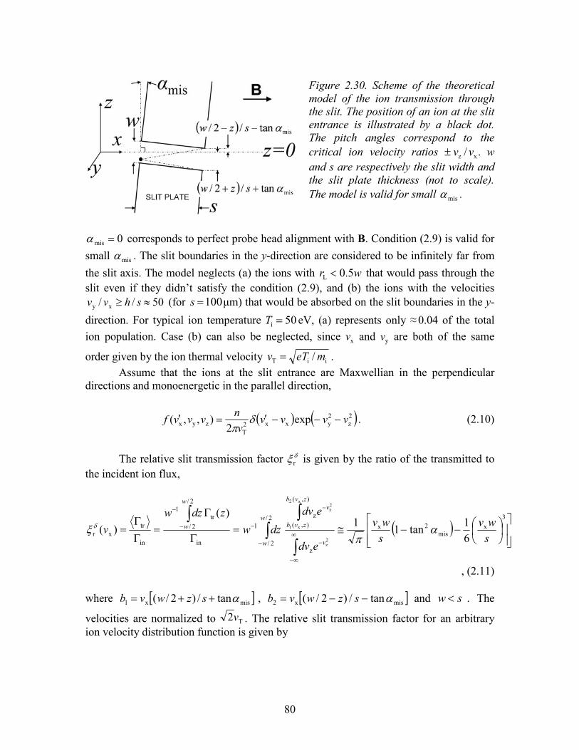
80

0mis =α corresponds to perfect probe head alignment with B. Condition (2.9) is valid for

small misα . The slit boundaries in the y-direction are considered to be infinitely far from

the slit axis. The model neglects (a) the ions with wr 5.0L < that would pass through the slit even if they didn’t satisfy the condition (2.9), and (b) the ions with the velocities

50// xy ≈≥ shvv (for 100=s µm) that would be absorbed on the slit boundaries in the y-

direction. For typical ion temperature 50i =T eV, (a) represents only ≈ 0.04 of the total ion population. Case (b) can also be neglected, since xv and yv are both of the same

order given by the ion thermal velocity iiT / meTv = . Assume that the ions at the slit entrance are Maxwellian in the perpendicular

directions and monoenergetic in the parallel direction,

( ) ( )2z

2yxx2

Tzyx exp

2),,( vvvv

vn

vvvf −−−′=′ δπ

. (2.10)

The relative slit transmission factor δξr is given by the ratio of the transmitted to

the incident ion flux,

( )

−−≅=Γ

Γ=

Γ

Γ=

−∞

∞−

−

−

−−

−

∫

∫∫

∫ 3x

mis2x

z

),(

),(z2/

2/

1

in

2/

2/tr

1

in

trxr 6

1tan1

1)(

)(2z

x2

x1

2z

swv

swv

edv

edv

dzwzdzw

vv

zvb

zvb

v

w

w

w

w απ

ξ δ

, (2.11)

where [ ]misx1 tan/)2/( α++= szwvb , [ ]misx2 tan/)2/( α−−= szwvb and sw < . The

velocities are normalized to T2v . The relative slit transmission factor for an arbitrary ion velocity distribution function is given by

Figure 2.30. Scheme of the theoretical model of the ion transmission through the slit. The position of an ion at the slit entrance is illustrated by a black dot. The pitch angles correspond to the critical ion velocity ratios ./ xz vv± w and s are respectively the slit width and the slit plate thickness (not to scale). The model is valid for small misα .

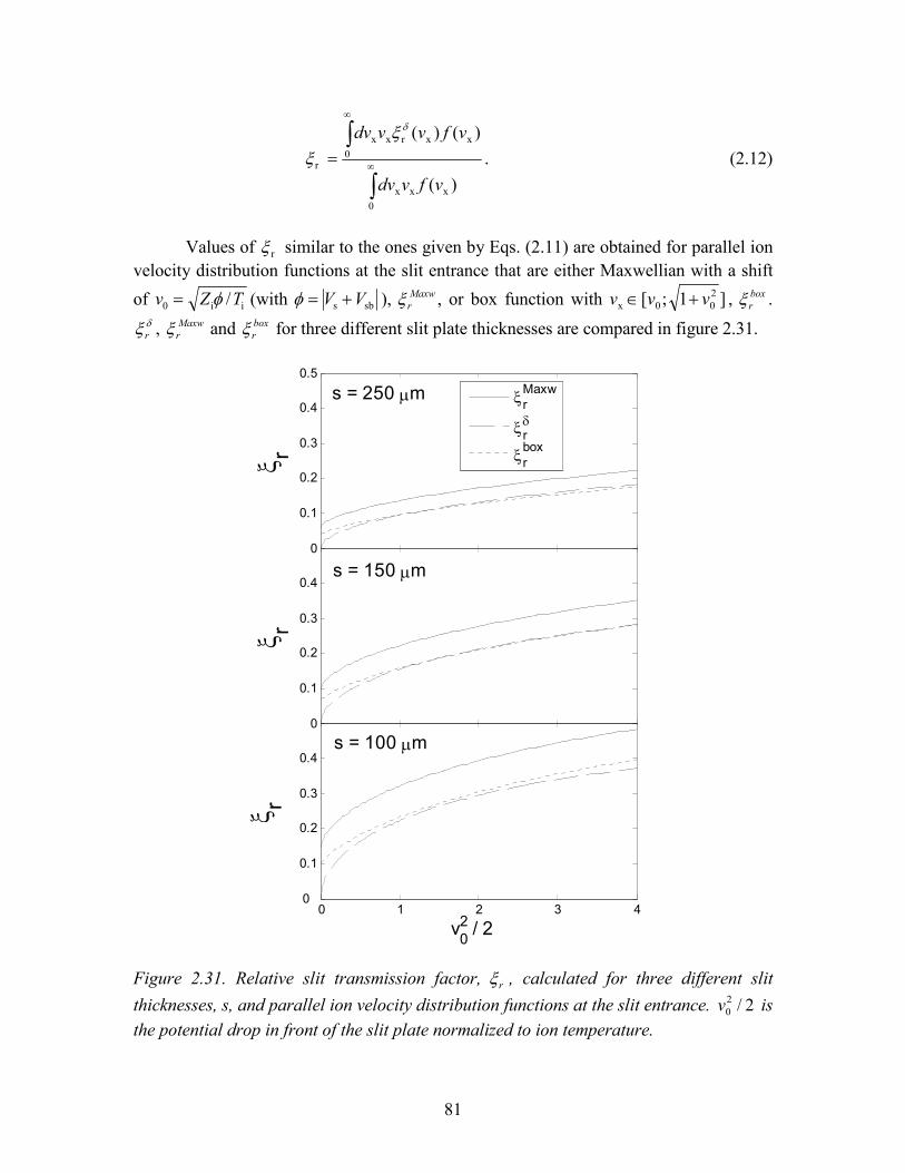
81

)(

)()(

x0

xx

0xxrxx

r

vfvdv

vfvvdv

∫

∫∞

∞

=

δξξ . (2.12)

Values of rξ similar to the ones given by Eqs. (2.11) are obtained for parallel ion

velocity distribution functions at the slit entrance that are either Maxwellian with a shift

of ii0 /TZv φ= (with sbs VV +=φ ), Maxwrξ , or box function with ]1;[ 2

00x vvv +∈ , boxrξ .

δξr , Maxwrξ and box

rξ for three different slit plate thicknesses are compared in figure 2.31.

0.5 1 1.5 2 0

0.1

0.2

0.3

0.4

0.5

ξ r

0.5 1 1.5 2 0

0.1

0.2

0.3

0.4

ξ r

0 1 2 3 40

0.1

0.2

0.3

0.4

v02 / 2

ξ r

ξrMaxw

ξrδ

ξrbox

s = 250 µm

s = 150 µm

s = 100 µm

Figure 2.31. Relative slit transmission factor, rξ , calculated for three different slit thicknesses, s, and parallel ion velocity distribution functions at the slit entrance. 2/2

0v is the potential drop in front of the slit plate normalized to ion temperature.

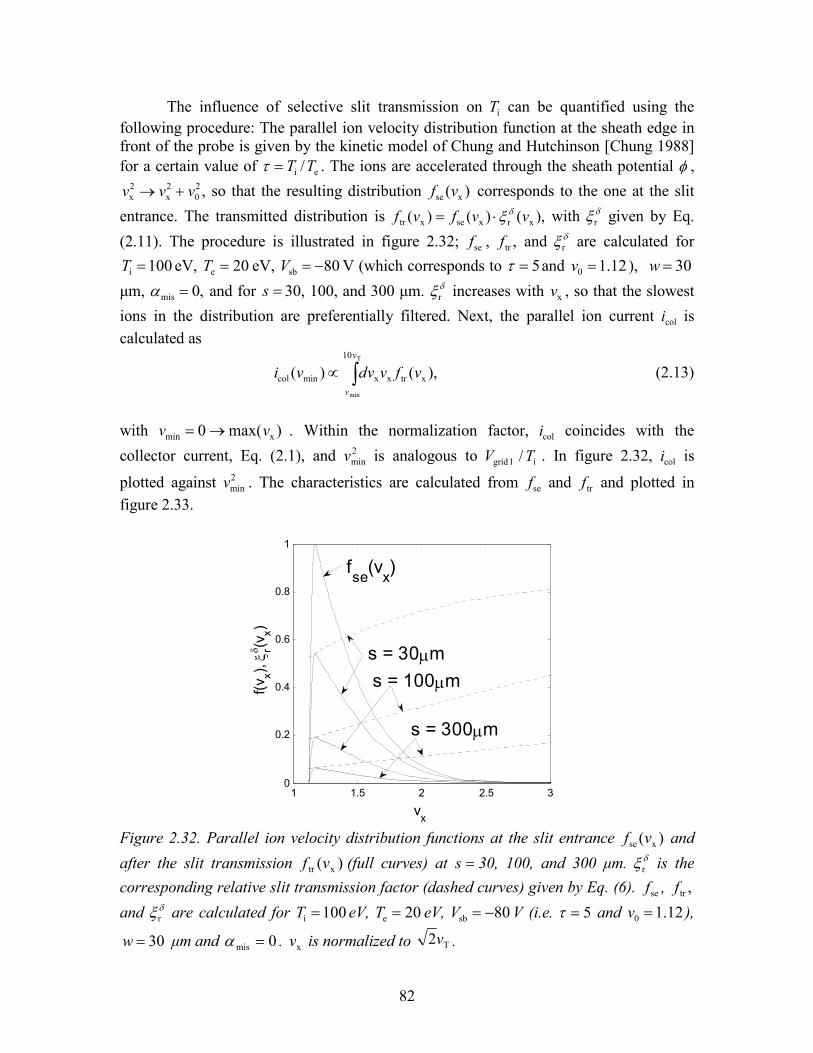
82

The influence of selective slit transmission on iT can be quantified using the following procedure: The parallel ion velocity distribution function at the sheath edge in front of the probe is given by the kinetic model of Chung and Hutchinson [Chung 1988] for a certain value of ei /TT=τ . The ions are accelerated through the sheath potential φ ,

,20

2x

2x vvv +→ so that the resulting distribution )( xse vf corresponds to the one at the slit

entrance. The transmitted distribution is ),()()( xrxsextr vvfvf δξ⋅= with δξr given by Eq.

(2.11). The procedure is illustrated in figure 2.32; sef , ,trf and δξr are calculated for

100i =T eV, 20e =T eV, 80sb −=V V (which corresponds to 5=τ and 12.10 =v ), 30=w

µm, ,0mis =α and for =s 30, 100, and 300 µm. δξr increases with xv , so that the slowest

ions in the distribution are preferentially filtered. Next, the parallel ion current coli is calculated as

),()( xtrxx

10

mincol

T

min

vfvvdviv

v∫∝ (2.13)

with )max(0 xmin vv →= . Within the normalization factor, coli coincides with the

collector current, Eq. (2.1), and 2minv is analogous to i1 grid / TV . In figure 2.32, coli is

plotted against 2minv . The characteristics are calculated from sef and trf and plotted in

figure 2.33.

1 1.5 2 2.5 30

0.2

0.4

0.6

0.8

1

vx

f(v x), ξrδ (v x)

fse(vx)

s = 30µms = 100µm

s = 300µm

Figure 2.32. Parallel ion velocity distribution functions at the slit entrance )( xse vf and

after the slit transmission )( xtr vf (full curves) at =s 30, 100, and 300 µm. δξr is the

corresponding relative slit transmission factor (dashed curves) given by Eq. (6). sef , ,trf

and δξr are calculated for 100i =T eV, 20e =T eV, 80sb −=V V (i.e. 5=τ and 12.10 =v ),

30=w µm and 0mis =α . xv is normalized to T2v .

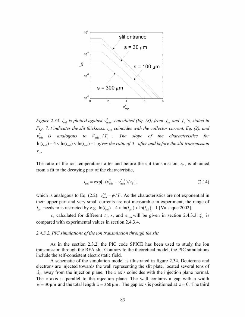
83

0 2 4 6 810

-3

10-2

10-1

100

vmin2

i col

slit entrance

s = 30 µm

s = 300 µm

s = 100 µm

Figure 2.33. coli is plotted against 2minv , calculated (Eq. (8)) from sef and trf ’s, stated in

Fig. 7. t indicates the slit thickness. coli coincides with the collector current, Eq. (2), and 2minv is analogous to i1 grid / TV . The slope of the characteristics for

1)ln()ln(4)ln( colcolcol −<<− iii gives the ratio of iT after and before the slit transmission

Tr .

The ratio of the ion temperatures after and before the slit transmission, Tr , is obtained from a fit to the decaying part of the characteristic,

]/)(exp[ T2 *

min2mincol rvvi −−= , (2.14)

which is analogous to Eq. (2.2). ./ i

2 *min Tv φ= As the characteristics are not exponential in

their upper part and very small currents are not measurable in experiment, the range of coli needs to is restricted by e.g. 1)ln()ln(4)ln( colcolcol −<<− iii [Valsaque 2002].

Tr calculated for different τ , s, and misα will be given in section 2.4.3.3. rξ is compared with experimental values in section 2.4.3.4. 2.4.3.2. PIC simulations of the ion transmission through the slit

As in the section 2.3.2, the PIC code SPICE has been used to study the ion transmission through the RFA slit. Contrary to the theoretical model, the PIC simulations include the self-consistent electrostatic field.

A schematic of the simulation model is illustrated in figure 2.34. Deuterons and electrons are injected towards the wall representing the slit plate, located several tens of

Dλ away from the injection plane. The x axis coincides with the injection plane normal. The z axis is parallel to the injection plane. The wall contains a gap with a width

µm30=w and the total length µm360=s . The gap axis is positioned at .0=z The third

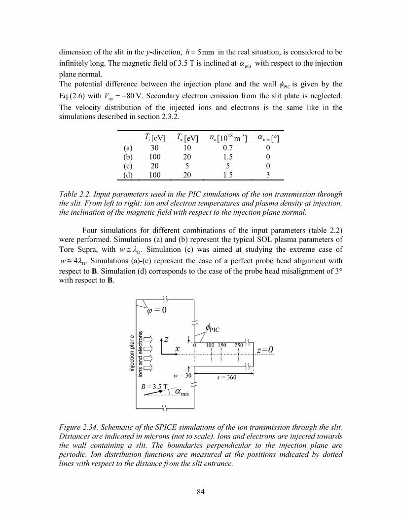
84

dimension of the slit in the y-direction, mm5=h in the real situation, is considered to be infinitely long. The magnetic field of 3.5 T is inclined at misα with respect to the injection plane normal. The potential difference between the injection plane and the wall PICφ is given by the Eq.(2.6) with 80sp −=V V. Secondary electron emission from the slit plate is neglected. The velocity distribution of the injected ions and electrons is the same like in the simulations described in section 2.3.2.

iT [eV] eT [eV] en [1018 m-3] misα [°] (a) 30 10 0.7 0 (b) 100 20 1.5 0 (c) 20 5 5 0 (d) 100 20 1.5 3

Table 2.2. Input parameters used in the PIC simulations of the ion transmission through the slit. From left to right: ion and electron temperatures and plasma density at injection, the inclination of the magnetic field with respect to the injection plane normal.

Four simulations for different combinations of the input parameters (table 2.2) were performed. Simulations (a) and (b) represent the typical SOL plasma parameters of Tore Supra, with .Dλ≅w Simulation (c) was aimed at studying the extreme case of

.4 Dλ≅w Simulations (a)-(c) represent the case of a perfect probe head alignment with respect to B. Simulation (d) corresponds to the case of the probe head misalignment of 3° with respect to B.

Figure 2.34. Schematic of the SPICE simulations of the ion transmission through the slit. Distances are indicated in microns (not to scale). Ions and electrons are injected towards the wall containing a slit. The boundaries perpendicular to the injection plane are periodic. Ion distribution functions are measured at the positions indicated by dotted lines with respect to the distance from the slit entrance.

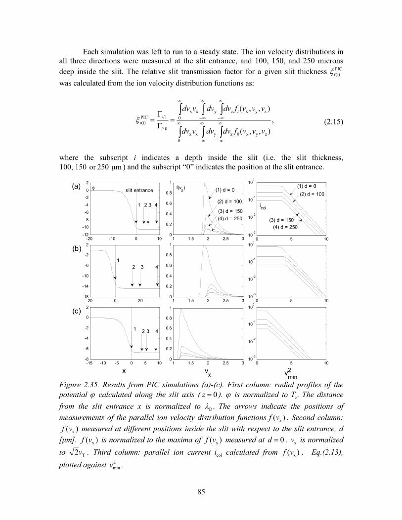
85

Each simulation was left to run to a steady state. The ion velocity distributions in all three directions were measured at the slit entrance, and 100, 150, and 250 microns deep inside the slit. The relative slit transmission factor for a given slit thickness PIC

r(i)ξ was calculated from the ion velocity distribution functions as:

,),,(

),,(

0zyx0zyxx

0zyxzyxx

0//

i//PICr(i)

∫ ∫ ∫

∫ ∫ ∫∞ ∞

∞−

∞

∞−

∞ ∞

∞−

∞

∞−=Γ

Γ=

vvvfdvdvvdv

vvvfdvdvvdv i

ξ (2.15)

where the subscript i indicates a depth inside the slit (i.e. the slit thickness,

µm250or150,100 ) and the subscript “0” indicates the position at the slit entrance.

-20 -10 0 10-12

-10

-8

-6

-4

-2

0

2

-20 0 20-18

-14

-10

-6

-2

2

-15 -10 -5 0 5 10-8

-6

-4

-2

0

2

x

1 1.5 2 2.5 30

0.2

0.4

0.6

0.8

1

1 1.5 2 2.5 30

0.2

0.4

0.6

0.8

1

1 1.5 2 2.5 30

0.2

0.4

0.6

0.8

1

vx

0 5 1010

-3

10-2

10-1

1000 5 10

10-3

10-2

10-1

100

0 5 1010

-3

10-2

10-1

100

v2min

(a)

(b)

(c)

slit entranceφ f(vx)

icol4

(1) d = 0

(2) d = 100

(3) d = 150(4) d = 250

321

(1) d = 0

(2) d = 100

(3) d = 150(4) d = 250

12 3 4

1 2 3 4

Figure 2.35. Results from PIC simulations (a)-(c). First column: radial profiles of the potential ϕ calculated along the slit axis ( 0=z ). ϕ is normalized to .eT The distance from the slit entrance x is normalized to .Dλ The arrows indicate the positions of measurements of the parallel ion velocity distribution functions )( xvf . Second column:

)( xvf measured at different positions inside the slit with respect to the slit entrance, d [µm]. )( xvf is normalized to the maxima of )( xvf measured at 0=d . xv is normalized

to T2v . Third column: parallel ion current coli calculated from )( xvf , Eq.(2.13),

plotted against 2minv .

86

Figure 2.35 compiles the results from the SPICE simulations for perfect probe head alignment with respect to B. Each row corresponds to one simulation, (a)-(c), characterized by the parameters stated in table 2.2. The first column in figure 2.35 shows the radial profiles of the electrostatic potential )0,( =zxϕ . ϕ is normalized to .eT The

distance from the right boundary of the simulation system, ,x is normalized to Dλ . The slit entrance is indicated by a vertical line. The arrows indicate the positions of measurements of )( xvf . For simulations (a) and (c) (where Dλ≅w ) ϕ reaches its minimum value within approximately ~ Dλ inside the slit. For simulation (b) ( D4λ≅w ) the equipotential surface corresponding to PICφ is not perfectly parallel to the front face of

the slit plate but penetrates ~ D4λ inside the slit. ϕ does not reach its minimum at the slit entrance. This gives rise to a perpendicular electric field wdeV /)(2 res≈ .

PICres )0,()( φϕ −== zddV is the residual voltage and d is the position inside the slit with respect to the slit entrance. The influence of a perpendicular electric field on ion transmission is discussed in the next section. The second column in figure 2.35 shows

)( xvf , scanned at different d (in µm). The )( xvf are normalized to the maxima of )( xvf

measured at .0=d Parallel ion velocity xv is normalized to .2 Tv Due to ,resV the

)( xvf measured at 0>d are somewhat narrower and shifted to higher velocities, compared to the ones measured at the slit entrance. The third column of figure 2.35 shows the characteristics ( coli versus 2

minv ) calculated from )( xvf , Eq. (2.13). A fit, Eq.

(2.14), to the decaying part of the characteristics gives Tr . In the next section, Tr from the PIC simulations is compared with the one obtained from the theoretical model. 2.4.3.3. Deformation of I-V characteristics

Figure 2.36 shows the ratio Tr , calculated from the theoretical model (section 2.3.3.1) for 30=w µm. Tr is plotted as a function of s for 30030→=s µm. Tr is evaluated for 51→=τ and for two different values of 0mis =α and 10°. The results from the model are juxtaposed to the ones obtained from PIC simulations (a)-(c).

Tr obtained from the model increases with s and .τ The increase of Tr with s is most significant for 100<s µm. For 100>s µm, Tr increases only by ~2%. τ∂∂ /Tr is a decreasing function of τ . For 250100 ≤≤ s µm, ).83.2ln( 05.0

T τ≅r PIC simulations and the model predict very similar values of Tr . This indicates that the influence of the perpendicular electric field inside the slit weV /2 res on selective ion transmission does not

play an important role, even at D4λ≅w . For 250=s µm the agreement between the model and PIC simulations is somewhat worse. In this case, the particle statistics in the PIC simulation are less reliable due to relatively low number of ions deep inside the slit. Within the range of Tr plotted in figure 2.36, the overestimation of iT is less than 14%.

The slit plate misalignment has only a small influence on ion transmission. The values of Tr for 0mis =α and °=10misα are very similar. In addition, simulation (d) for

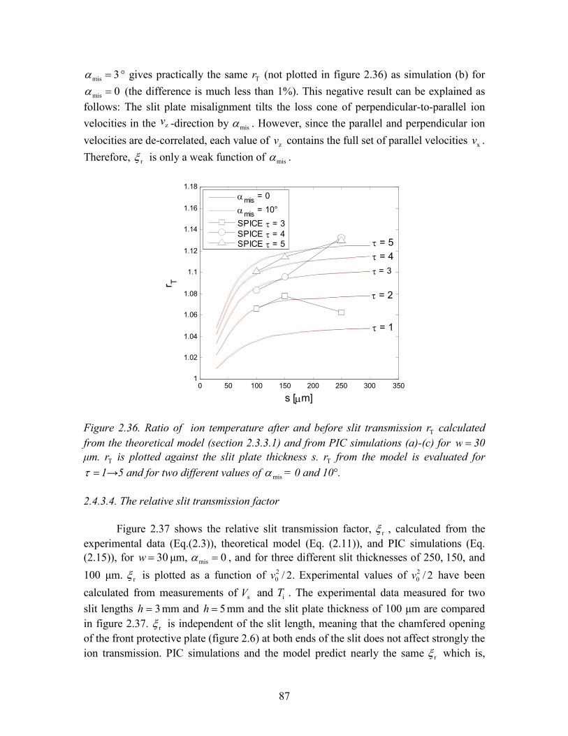
87

3mis =α ° gives practically the same Tr (not plotted in figure 2.36) as simulation (b) for 0mis =α (the difference is much less than 1%). This negative result can be explained as

follows: The slit plate misalignment tilts the loss cone of perpendicular-to-parallel ion velocities in the zv -direction by misα . However, since the parallel and perpendicular ion

velocities are de-correlated, each value of zv contains the full set of parallel velocities xv . Therefore, rξ is only a weak function of misα .

0 50 100 150 200 250 300 3501

1.02

1.04

1.06

1.08

1.1

1.12

1.14

1.16

1.18

s [µm]

r T

αmis = 0

αmis = 10°

SPICE τ = 3SPICE τ = 4SPICE τ = 5

τ = 1

τ = 2

τ = 3τ = 4τ = 5

Figure 2.36. Ratio of ion temperature after and before slit transmission Tr calculated from the theoretical model (section 2.3.3.1) and from PIC simulations (a)-(c) for =w 30 µm. Tr is plotted against the slit plate thickness s. Tr from the model is evaluated for =τ 1→5 and for two different values of misα = 0 and 10°.

2.4.3.4. The relative slit transmission factor

Figure 2.37 shows the relative slit transmission factor, rξ , calculated from the experimental data (Eq.(2.3)), theoretical model (Eq. (2.11)), and PIC simulations (Eq. (2.15)), for 30=w µm, 0mis =α , and for three different slit thicknesses of 250, 150, and

100 µm. rξ is plotted as a function of .2/20v Experimental values of 2/2

0v have been

calculated from measurements of sV and .iT The experimental data measured for two slit lengths 3=h mm and 5=h mm and the slit plate thickness of 100 µm are compared in figure 2.37. rξ is independent of the slit length, meaning that the chamfered opening of the front protective plate (figure 2.6) at both ends of the slit does not affect strongly the ion transmission. PIC simulations and the model predict nearly the same rξ which is,

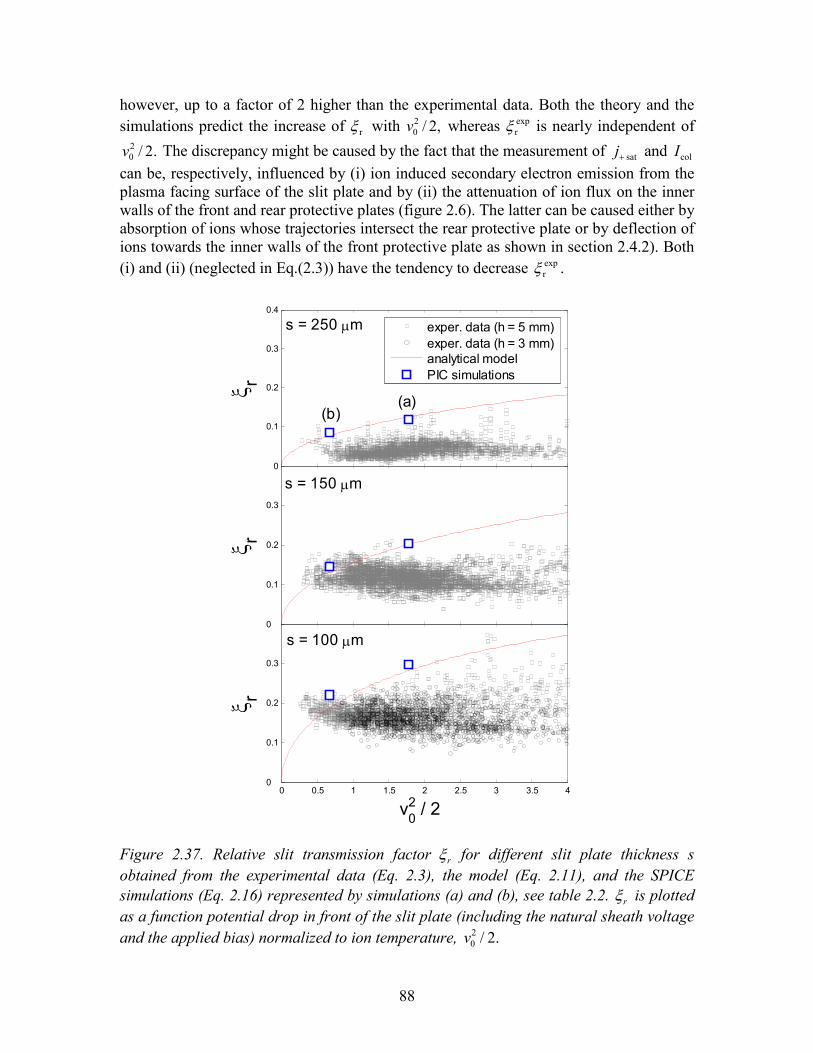
88

however, up to a factor of 2 higher than the experimental data. Both the theory and the simulations predict the increase of rξ with ,2/2

0v whereas exprξ is nearly independent of

.2/20v The discrepancy might be caused by the fact that the measurement of sat +j and colI

can be, respectively, influenced by (i) ion induced secondary electron emission from the plasma facing surface of the slit plate and by (ii) the attenuation of ion flux on the inner walls of the front and rear protective plates (figure 2.6). The latter can be caused either by absorption of ions whose trajectories intersect the rear protective plate or by deflection of ions towards the inner walls of the front protective plate as shown in section 2.4.2). Both (i) and (ii) (neglected in Eq.(2.3)) have the tendency to decrease exp

rξ .

0.5 1 1.5 2 2.5 3 3.50

0.1

0.2

0.3

0.4

ξ r

0.5 1 1.5 2 2.5 3 3.50

0.1

0.2

0.3

ξ r

0 0.5 1 1.5 2 2.5 3 3.5 40

0.1

0.2

0.3

v02 / 2

ξ r

exper. data (h = 5 mm)exper. data (h = 3 mm)analytical modelPIC simulations

s = 250 µm

s = 100 µm

(b)(a)

s = 150 µm

Figure 2.37. Relative slit transmission factor rξ for different slit plate thickness s obtained from the experimental data (Eq. 2.3), the model (Eq. 2.11), and the SPICE simulations (Eq. 2.16) represented by simulations (a) and (b), see table 2.2. rξ is plotted as a function potential drop in front of the slit plate (including the natural sheath voltage and the applied bias) normalized to ion temperature, .2/2

0v

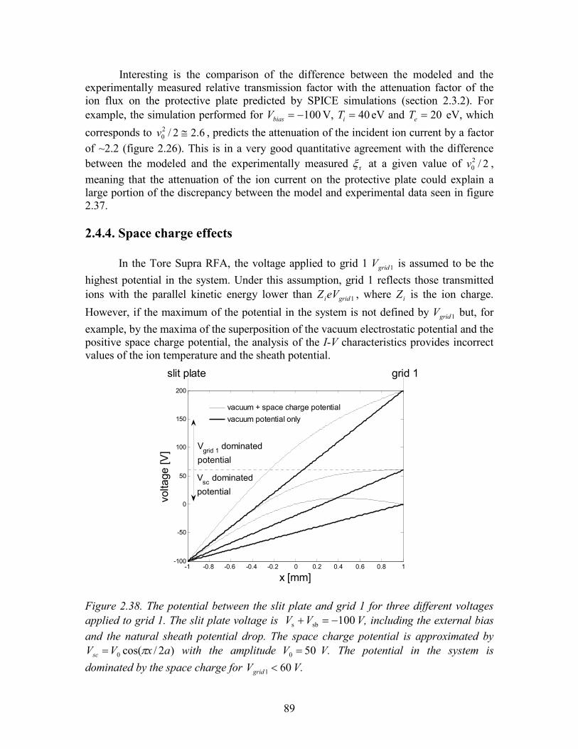
89

Interesting is the comparison of the difference between the modeled and the experimentally measured relative transmission factor with the attenuation factor of the ion flux on the protective plate predicted by SPICE simulations (section 2.3.2). For example, the simulation performed for 100−=biasV V, 40=iT eV and 20=eT eV, which

corresponds to 6.22/20 ≅v , predicts the attenuation of the incident ion current by a factor

of ~2.2 (figure 2.26). This is in a very good quantitative agreement with the difference between the modeled and the experimentally measured rξ at a given value of 2/2

0v , meaning that the attenuation of the ion current on the protective plate could explain a large portion of the discrepancy between the model and experimental data seen in figure 2.37. 2.4.4. Space charge effects

In the Tore Supra RFA, the voltage applied to grid 1 1gridV is assumed to be the highest potential in the system. Under this assumption, grid 1 reflects those transmitted ions with the parallel kinetic energy lower than 1gridieVZ , where iZ is the ion charge.

However, if the maximum of the potential in the system is not defined by 1gridV but, for example, by the maxima of the superposition of the vacuum electrostatic potential and the positive space charge potential, the analysis of the I-V characteristics provides incorrect values of the ion temperature and the sheath potential.

-1 -0.8 -0.6 -0.4 -0.2 0 0.2 0.4 0.6 0.8 1-100

-50

0

50

100

150

200

x [mm]

voltage [V

]

slit plate grid 1

Vgrid 1 dominated

potential

Vsc dominated

potential

vacuum + space charge potential

vacuum potential only

Figure 2.38. The potential between the slit plate and grid 1 for three different voltages applied to grid 1. The slit plate voltage is 100sbs −=+VV V, including the external bias and the natural sheath potential drop. The space charge potential is approximated by

)2/cos(0 axVVsc π= with the amplitude 500 =V V. The potential in the system is dominated by the space charge for 601 <gridV V.

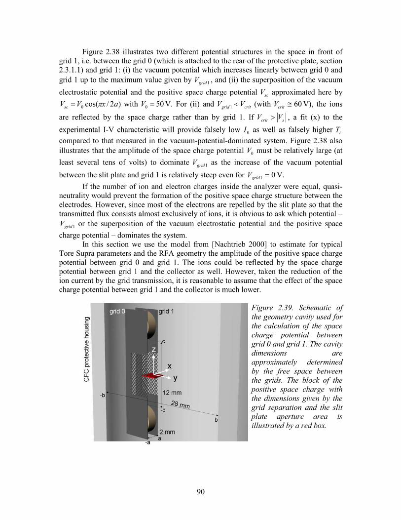
90

Figure 2.38 illustrates two different potential structures in the space in front of grid 1, i.e. between the grid 0 (which is attached to the rear of the protective plate, section 2.3.1.1) and grid 1: (i) the vacuum potential which increases linearly between grid 0 and grid 1 up to the maximum value given by 1gridV , and (ii) the superposition of the vacuum

electrostatic potential and the positive space charge potential scV approximated here by )2/cos(0 axVVsc π= with 500 =V V. For (ii) and critgrid VV <1 (with 60≅critV V), the ions

are reflected by the space charge rather than by grid 1. If scrit VV > , a fit (x) to the

experimental I-V characteristic will provide falsely low 0I as well as falsely higher iT compared to that measured in the vacuum-potential-dominated system. Figure 2.38 also illustrates that the amplitude of the space charge potential 0V must be relatively large (at least several tens of volts) to dominate 1gridV as the increase of the vacuum potential

between the slit plate and grid 1 is relatively steep even for 01 =gridV V. If the number of ion and electron charges inside the analyzer were equal, quasi-

neutrality would prevent the formation of the positive space charge structure between the electrodes. However, since most of the electrons are repelled by the slit plate so that the transmitted flux consists almost exclusively of ions, it is obvious to ask which potential –

1gridV or the superposition of the vacuum electrostatic potential and the positive space charge potential – dominates the system.

In this section we use the model from [Nachtrieb 2000] to estimate for typical Tore Supra parameters and the RFA geometry the amplitude of the positive space charge potential between grid 0 and grid 1. The ions could be reflected by the space charge potential between grid 1 and the collector as well. However, taken the reduction of the ion current by the grid transmission, it is reasonable to assume that the effect of the space charge potential between grid 1 and the collector is much lower.

Figure 2.39. Schematic of the geometry cavity used for the calculation of the space charge potential between grid 0 and grid 1. The cavity dimensions are approximately determined by the free space between the grids. The block of the positive space charge with the dimensions given by the grid separation and the slit plate aperture area is illustrated by a red box.

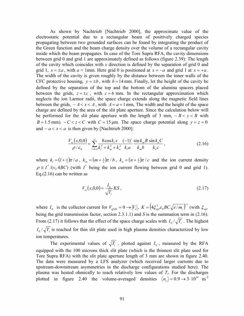
91

As shown by Nachtrieb [Nachtrieb 2000], the approximate value of the electrostatic potential due to a rectangular beam of positively charged species propagating between two grounded surfaces can be found by integrating the product of the Green function and the beam charge density over the volume of a rectangular cavity inside which the beam propagates. In case of the Tore Supra RFA, the cavity dimensions between grid 0 and grid 1 are approximately defined as follows (figure 2.39): The length of the cavity which coincides with x direction is defined by the separation of grid 0 and grid 1, ax ±= , with a = 1mm. Here grid 0 is positioned at ax −= and grid 1 at ax += . The width of the cavity is given roughly by the distance between the inner walls of the CFC protective housing, by ±= , with 14=b mm. Finally, let the height of the cavity be defined by the separation of the top and the bottom of the alumina spacers placed between the grids, cz ±= , with 6=c mm. In the rectangular approximation which neglects the ion Larmor radii, the space charge extends along the magnetic field lines between the grids, AxA <<− , with 1== aA mm, The width and the height of the space charge are defined by the area of the slit plate aperture. Since the calculation below will be performed for the slit plate aperture with the length of 3 mm, ByB <<− with

5.1=B mm). CzC <<− with 15=C µm. The space charge potential along 0== zy and axa <<− is then given by [Nachtrieb 2000]:

( )

ckCk

bkBk

akkkkxkxV

n

n

m

m

nml l

l

nml

lsc sinsin)1(cos8/

0,0,

,,222

0∑∞ −

++=

ερ, (2.16)

where ( ) alkl /2

1 π+= , ( ) bmkm /21 π+= , ( ) cnkn /2

1 π+= and the ion current density

)4/(* BCvI T≅ρ (with *I being the ion current flowing between grid 0 and grid 1). Eq.(2.16) can be written as

( ) KSTI

xVi

sc00,0, = , (2.17)

where 0I is the collector current for sgrid1 0 VV →= , ( ) 1

02 /4

−= iopt meBCK εξ (with optξ

being the grid transmission factor, section 2.3.1.1) and S is the summation term in (2.16). From (2.17) it follows that the effect of the space charge scales with iTI /0 . The highest

iTI /0 is reached for thin slit plate used in high plasma densities characterized by low ion temperatures.

The experimental values of iT , plotted against 0I , measured by the RFA equipped with the 100 microns thick slit plate (which is the thinnest slit plate used for Tore Supra RFA) with the slit plate aperture length of 3 mm are shown in figure 2.40. The data were measured by a LFS analyzer (which received larger currents due to upstream-downstream asymmetries in the discharge configurations studied here). The plasma was heated ohmically to reach relatively low values of Ti. For the discharges plotted in figure 2.40 the volume-averaged densities 191039.0 ⋅→=en m-3

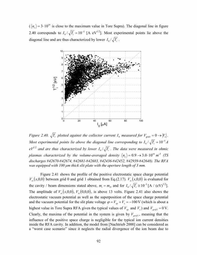
92

( 19103 ⋅=en is close to the maximum value in Tore Supra). The diagonal line in figure

2.40 corresponds to 50 10/ −=iTI [A eV1/2]. Most experimental points lie above the

diagonal line and are thus characterized by lower iTI /0 .

0 20 40 60 80 1000

1

2

3

4

5

6

7

8

9

10

I0 [µA]

Ti1/2 [eV]

Figure 2.40. iT plotted against the collector current 0I measured for sgrid1 0 VV →= .

Most experimental points lie above the diagonal line corresponding to 50 10/ −=iTI A

eV1/2 and are thus characterized by lower iTI /0 . The data were measured in ohmic

plasmas characterized by the volume-averaged density 19100.39.0 ⋅→=en m-3 (TS discharges #42670-#42674, #42681-#42683, #42436-#42452, #42939-#42648). The RFA was equipped with 100 µm thick slit plate with the aperture length of 3 mm.

Figure 2.41 shows the profile of the positive electrostatic space charge potential

( )0,0,xVsc between grid 0 and grid 1 obtained from Eq.(2.17). ( )0,0,xVsc is evaluated for

the cavity / beam dimensions stated above, Di mm = and for 50 10/ −≅iTI [A / (eV)1/2].

The amplitude of ( )0,0,xVsc , ( )0,0,0scV , is above 13 volts. Figure 2.41 also shows the electrostatic vacuum potential as well as the superposition of the space charge potential and the vacuum potential for the slit plate voltage 100−=+= ssp VVϕ V (which is about a

highest value in Tore Supra RFA given the typical values of spV and sV ) and 01 =gridV V.

Clearly, the maxima of the potential in the system is given by 1gridV , meaning that the influence of the positive space charge is negligible for the typical ion current densities inside the RFA cavity. In addition, the model from [Nachtrieb 2000] can be considered as a “worst case scenario” since it neglects the radial divergence of the ion beam due to

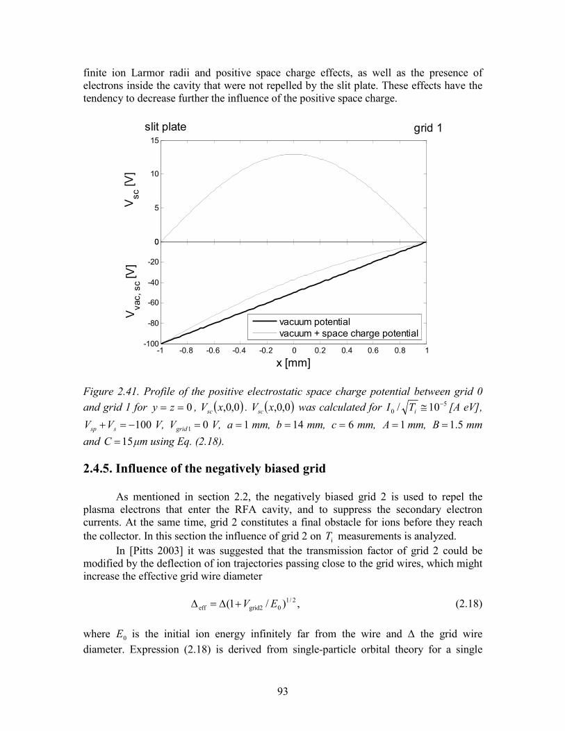
93

finite ion Larmor radii and positive space charge effects, as well as the presence of electrons inside the cavity that were not repelled by the slit plate. These effects have the tendency to decrease further the influence of the positive space charge.

-0.5 0 0.5 -0.5 0 0.5 0

5

10

15Vsc [V

]

-1 -0.8 -0.6 -0.4 -0.2 0 0.2 0.4 0.6 0.8 1-100

-80

-60

-40

-20

0

x [mm]

Vvac, sc [V]

vacuum potentialvacuum + space charge potential

slit plate grid 1

Figure 2.41. Profile of the positive electrostatic space charge potential between grid 0 and grid 1 for 0== zy , ( )0,0,xVsc . ( )0,0,xVsc was calculated for 5

0 10/ −≅iTI [A eV],

100−=+ ssp VV V, 01 =gridV V, 1=a mm, 14=b mm, 6=c mm, 1=A mm, 5.1=B mm

and 15=C µm using Eq. (2.18). 2.4.5. Influence of the negatively biased grid

As mentioned in section 2.2, the negatively biased grid 2 is used to repel the plasma electrons that enter the RFA cavity, and to suppress the secondary electron currents. At the same time, grid 2 constitutes a final obstacle for ions before they reach the collector. In this section the influence of grid 2 on iT measurements is analyzed.

In [Pitts 2003] it was suggested that the transmission factor of grid 2 could be modified by the deflection of ion trajectories passing close to the grid wires, which might increase the effective grid wire diameter

,)/1( 2/1

0grid2eff EV+∆=∆ (2.18)

where 0E is the initial ion energy infinitely far from the wire and ∆ the grid wire diameter. Expression (2.18) is derived from single-particle orbital theory for a single

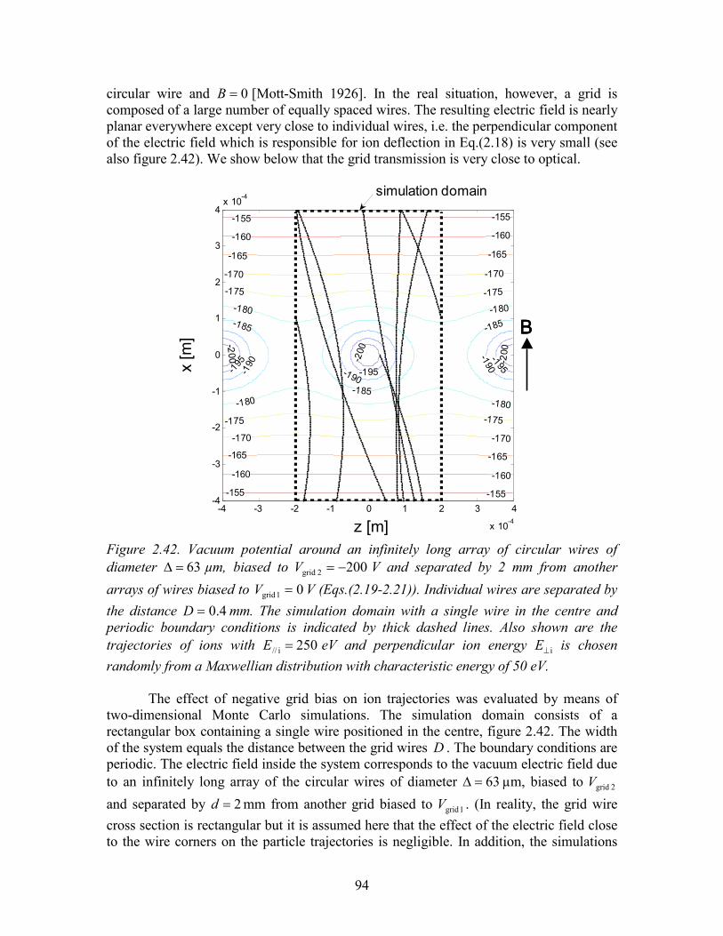
94

circular wire and 0=B [Mott-Smith 1926]. In the real situation, however, a grid is composed of a large number of equally spaced wires. The resulting electric field is nearly planar everywhere except very close to individual wires, i.e. the perpendicular component of the electric field which is responsible for ion deflection in Eq.(2.18) is very small (see also figure 2.42). We show below that the grid transmission is very close to optical.

-200 -2

00

-200

-195

-195-195-190

-190-190

-185 -185

-185

-180 -180

-180 -180

-175 -175

-175 -175

-170 -170

-170 -170

-165 -165

-165 -165

-160 -160

-160 -160

-155 -155

-155 -155

z [m]

x [m]

-4 -3 -2 -1 0 1 2 3 4

x 10-4

-4

-3

-2

-1

0

1

2

3

4x 10

-4

BBBB

simulation domain

Figure 2.42. Vacuum potential around an infinitely long array of circular wires of diameter 63=∆ µm, biased to 2002 grid −=V V and separated by 2 mm from another

arrays of wires biased to 01 grid =V V (Eqs.(2.19-2.21)). Individual wires are separated by

the distance 4.0=D mm. The simulation domain with a single wire in the centre and periodic boundary conditions is indicated by thick dashed lines. Also shown are the trajectories of ions with 250i// =E eV and perpendicular ion energy i⊥E is chosen randomly from a Maxwellian distribution with characteristic energy of 50 eV.

The effect of negative grid bias on ion trajectories was evaluated by means of two-dimensional Monte Carlo simulations. The simulation domain consists of a rectangular box containing a single wire positioned in the centre, figure 2.42. The width of the system equals the distance between the grid wires D . The boundary conditions are periodic. The electric field inside the system corresponds to the vacuum electric field due to an infinitely long array of the circular wires of diameter 63=∆ µm, biased to 2 gridV

and separated by 2=d mm from another grid biased to 1 gridV . (In reality, the grid wire cross section is rectangular but it is assumed here that the effect of the electric field close to the wire corners on the particle trajectories is negligible. In addition, the simulations

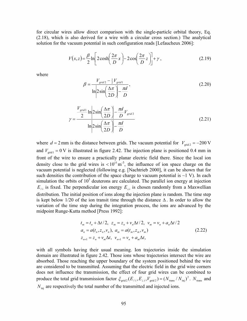
95

for circular wires allow direct comparison with the single-particle orbital theory, Eq. (2.18), which is also derived for a wire with a circular cross section.) The analytical solution for the vacuum potential in such configuration reads [Lefaucheux 2006]:

( ) γππβ+

−

= z

Dx

DzxV

2cos2

2cosh2ln

2, , (2.19)

where

Dd

D

VV gridgrid

ππβ

−

∆

−=

2sin2ln

121

2 , (2.20)

Dd

D

VDd

D

Vgrid

grid

ππ

ππ

γ−

∆

−

∆

=

2sin2ln

2sin2ln

2 21

(2.21)

where 2=d mm is the distance between grids. The vacuum potential for 2002 grid −=V V

and 01 grid =V V is illustrated in figure 2.42. The injection plane is positioned 0.4 mm in front of the wire to ensure a practically planar electric field there. Since the local ion density close to the grid wires is 1510< m-3, the influence of ion space charge on the vacuum potential is neglected (following e.g. [Nachtrieb 2000], it can be shown that for such densities the contribution of the space charge to vacuum potential is ~1 V). In each simulation the orbits of 105 deuterons are calculated. The parallel ion energy at injection

i//E is fixed. The perpendicular ion energy i⊥E is chosen randomly from a Maxwellian distribution. The initial position of ions along the injection plane is random. The time step is kept below 1/20 of the ion transit time through the distance ∆ . In order to allow the variation of the time step during the integration process, the ions are advanced by the midpoint Runge-Kutta method [Press 1992]:

,,

),,(),,,(

2/,2/,2/

11 tavvtvzz

vztaavztaa

tavvtvzzttt

mnnmnn

mmmmnnnn

nnmnnmnm

∆+=∆+=

==

∆+=∆+=∆+=

++

(2.22)

with all symbols having their usual meaning. Ion trajectories inside the simulation domain are illustrated in figure 2.42. Those ions whose trajectories intersect the wire are absorbed. Those reaching the upper boundary of the system positioned behind the wire are considered to be transmitted. Assuming that the electric field in the grid wire corners does not influence the transmission, the effect of four grid wires can be combined to produce the total grid transmission factor 2

injtrans2 gridi i// 2grid )/(),,( NNVEE =⊥ξ . transN and

injN are respectively the total number of the transmitted and injected ions.

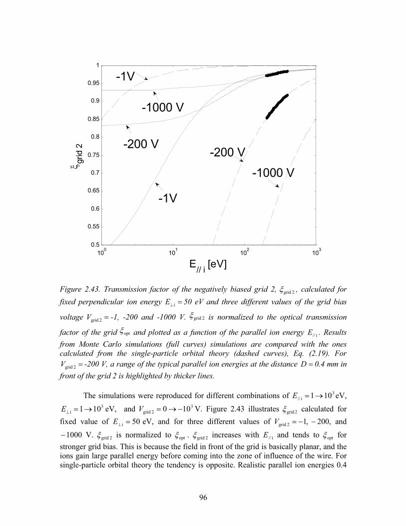
96

Figure 2.43. Transmission factor of the negatively biased grid 2, 2 gridξ , calculated for

fixed perpendicular ion energy =⊥ iE 50 eV and three different values of the grid bias

voltage =2 gridV -1, -200 and -1000 V. 2 gridξ is normalized to the optical transmission

factor of the grid optξ and plotted as a function of the parallel ion energy i//E . Results from Monte Carlo simulations (full curves) simulations are compared with the ones calculated from the single-particle orbital theory (dashed curves), Eq. (2.19). For

=2 gridV -200 V, a range of the typical parallel ion energies at the distance =D 0.4 mm in front of the grid 2 is highlighted by thicker lines.

The simulations were reproduced for different combinations of 3i// 101→=E eV,

3i 101→=⊥E eV, and 3

2 grid 100 −→=V V. Figure 2.43 illustrates 2gridξ calculated for

fixed value of 50i =⊥E eV, and for three different values of ,12 grid −=V ,200− and

1000− V. 2 gridξ is normalized to optξ . 2 gridξ increases with i//E and tends to optξ for stronger grid bias. This is because the field in front of the grid is basically planar, and the ions gain large parallel energy before coming into the zone of influence of the wire. For single-particle orbital theory the tendency is opposite. Realistic parallel ion energies 0.4

100

101

102

103

0.5

0.55

0.6

0.65

0.7

0.75

0.8

0.85

0.9

0.95

1

E// i [eV]

ξ grid 2

-1000 V

-200 V

-1V

-1000 V

-200 V

-1V

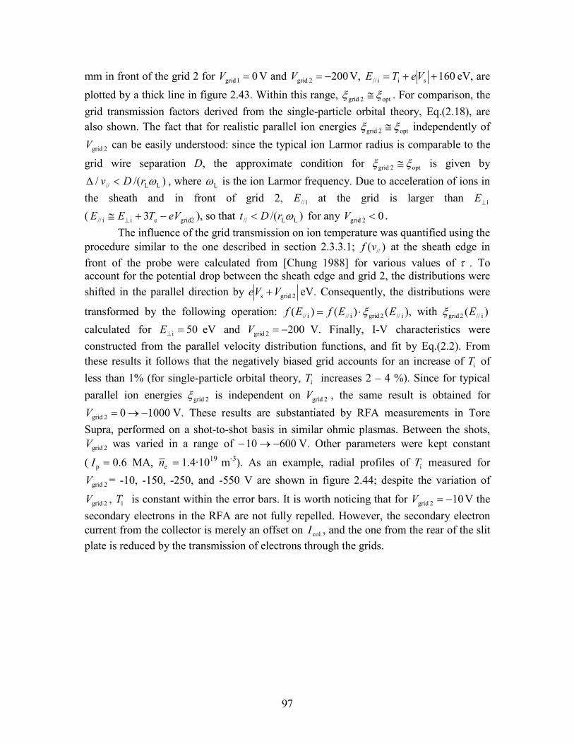
97

mm in front of the grid 2 for 01 grid =V V and 2002 grid −=V V, 160sii// ++= VeTE eV, are

plotted by a thick line in figure 2.43. Within this range, opt2 grid ξξ ≅ . For comparison, the grid transmission factors derived from the single-particle orbital theory, Eq.(2.18), are also shown. The fact that for realistic parallel ion energies opt2 grid ξξ ≅ independently of

2 gridV can be easily understood: since the typical ion Larmor radius is comparable to the

grid wire separation D, the approximate condition for opt2 grid ξξ ≅ is given by

)/(/ LL// ωrDv <∆ , where Lω is the ion Larmor frequency. Due to acceleration of ions in the sheath and in front of grid 2, i//E at the grid is larger than i⊥E

( grid2eii// 3 eVTEE −+≅ ⊥ ), so that )/( LL// ωrDt < for any 02 grid <V . The influence of the grid transmission on ion temperature was quantified using the

procedure similar to the one described in section 2.3.3.1; )( //vf at the sheath edge in front of the probe were calculated from [Chung 1988] for various values of τ . To account for the potential drop between the sheath edge and grid 2, the distributions were shifted in the parallel direction by 2 grids VVe + eV. Consequently, the distributions were

transformed by the following operation: ),()()( i// 2gridi//i// EEfEf ξ⋅= with )( i// 2grid Eξ

calculated for 50i =⊥E eV and 2002 grid −=V V. Finally, I-V characteristics were constructed from the parallel velocity distribution functions, and fit by Eq.(2.2). From these results it follows that the negatively biased grid accounts for an increase of iT of less than 1% (for single-particle orbital theory, iT increases 2 – 4 %). Since for typical

parallel ion energies 2 gridξ is independent on 2 gridV , the same result is obtained for

100002 grid −→=V V. These results are substantiated by RFA measurements in Tore Supra, performed on a shot-to-shot basis in similar ohmic plasmas. Between the shots,

2 gridV was varied in a range of 60010 −→− V. Other parameters were kept constant

( =pI 0.6 MA, =en 1.4·1019 m-3). As an example, radial profiles of iT measured for

2 gridV = -10, -150, -250, and -550 V are shown in figure 2.44; despite the variation of

2 gridV , iT is constant within the error bars. It is worth noticing that for 102 grid −=V V the secondary electrons in the RFA are not fully repelled. However, the secondary electron current from the collector is merely an offset on colI , and the one from the rear of the slit plate is reduced by the transmission of electrons through the grids.

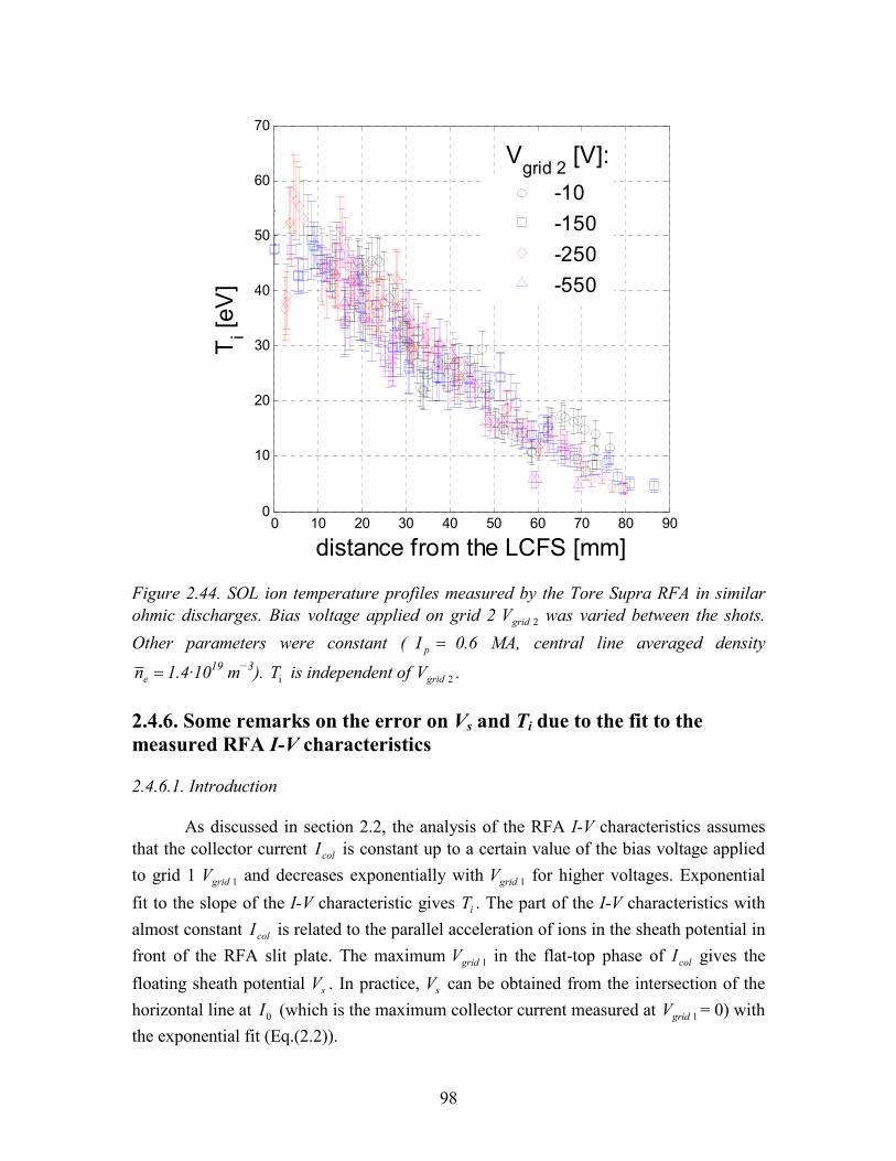
98

0 10 20 30 40 50 60 70 80 900

10

20

30

40

50

60

70

distance from the LCFS [mm]

Ti [eV

]-10-150-250-550

Vgrid 2

[V]:

Figure 2.44. SOL ion temperature profiles measured by the Tore Supra RFA in similar ohmic discharges. Bias voltage applied on grid 2 2grid V was varied between the shots.

Other parameters were constant ( =pI 0.6 MA, central line averaged density

=en 1.4·1019 m−3). iT is independent of 2grid V . 2.4.6. Some remarks on the error on Vs and Ti due to the fit to the measured RFA I-V characteristics 2.4.6.1. Introduction

As discussed in section 2.2, the analysis of the RFA I-V characteristics assumes that the collector current colI is constant up to a certain value of the bias voltage applied to grid 1 1gridV and decreases exponentially with 1gridV for higher voltages. Exponential

fit to the slope of the I-V characteristic gives iT . The part of the I-V characteristics with almost constant colI is related to the parallel acceleration of ions in the sheath potential in front of the RFA slit plate. The maximum 1gridV in the flat-top phase of colI gives the

floating sheath potential sV . In practice, sV can be obtained from the intersection of the horizontal line at 0I (which is the maximum collector current measured at 1gridV = 0) with the exponential fit (Eq.(2.2)).

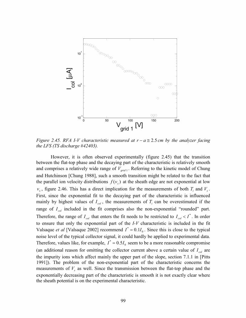
99

0 50 100 150 20010

-1

100

101

Vgrid 1

[V]

I col [ µ

A]

Figure 2.45. RFA I-V characteristic measured at 5.2≅− ar cm by the analyzer facing the LFS (TS discharge #42403).

However, it is often observed experimentally (figure 2.45) that the transition

between the flat-top phase and the decaying part of the characteristic is relatively smooth and comprises a relatively wide range of 1gridV . Referring to the kinetic model of Chung and Hutchinson [Chung 1988], such a smooth transition might be related to the fact that the parallel ion velocity distributions )( xvf at the sheath edge are not exponential at low

xv , figure 2.46. This has a direct implication for the measurements of both iT and sV . First, since the exponential fit to the decaying part of the characteristic is influenced mainly by highest values of colI , the measurements of iT can be overestimated if the range of colI included in the fit comprises also the non-exponential “rounded” part.

Therefore, the range of colI that enters the fit needs to be restricted to *II col < . In order to ensure that only the exponential part of the I-V characteristic is included in the fit Valsaque et al [Valsaque 2002] recommend 0

* 1.0 II = . Since this is close to the typical noise level of the typical collector signal, it could hardly be applied to experimental data. Therefore, values like, for example, 0

* 5.0 II = seem to be a more reasonable compromise (an additional reason for omitting the collector current above a certain value of colI are the impurity ions which affect mainly the upper part of the slope, section 7.1.1 in [Pitts 1991]). The problem of the non-exponential part of the characteristic concerns the measurements of sV as well. Since the transmission between the flat-top phase and the exponentially decreasing part of the characteristic is smooth it is not exactly clear where the sheath potential is on the experimental characteristic.

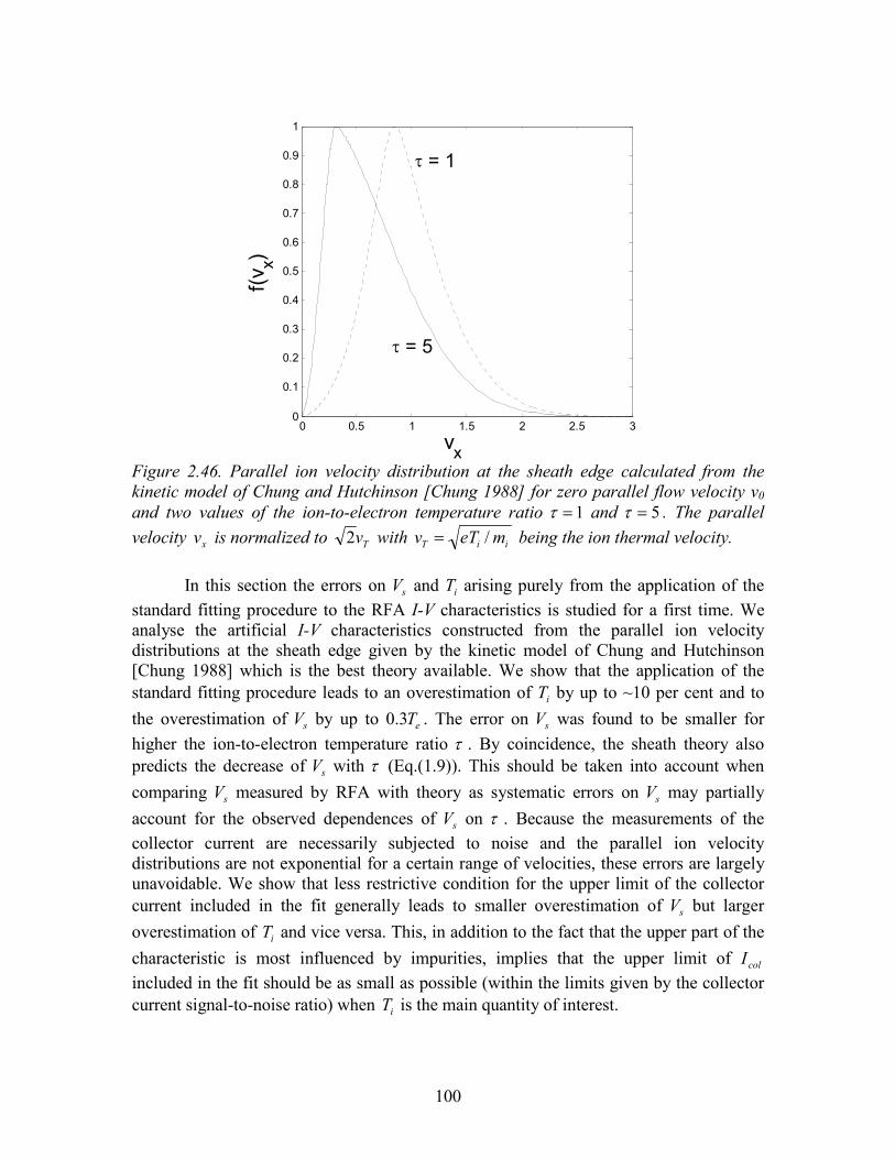
100

0 0.5 1 1.5 2 2.5 30

0.1

0.2

0.3

0.4

0.5

0.6

0.7

0.8

0.9

1

vx

f(v x)

τ = 5

τ = 1

Figure 2.46. Parallel ion velocity distribution at the sheath edge calculated from the kinetic model of Chung and Hutchinson [Chung 1988] for zero parallel flow velocity v0 and two values of the ion-to-electron temperature ratio 1=τ and 5=τ . The parallel velocity xv is normalized to Tv2 with iiT meTv /= being the ion thermal velocity.

In this section the errors on sV and iT arising purely from the application of the standard fitting procedure to the RFA I-V characteristics is studied for a first time. We analyse the artificial I-V characteristics constructed from the parallel ion velocity distributions at the sheath edge given by the kinetic model of Chung and Hutchinson [Chung 1988] which is the best theory available. We show that the application of the standard fitting procedure leads to an overestimation of iT by up to ~10 per cent and to the overestimation of sV by up to eT3.0 . The error on sV was found to be smaller for higher the ion-to-electron temperature ratio τ . By coincidence, the sheath theory also predicts the decrease of sV with τ (Eq.(1.9)). This should be taken into account when comparing sV measured by RFA with theory as systematic errors on sV may partially account for the observed dependences of sV on τ . Because the measurements of the collector current are necessarily subjected to noise and the parallel ion velocity distributions are not exponential for a certain range of velocities, these errors are largely unavoidable. We show that less restrictive condition for the upper limit of the collector current included in the fit generally leads to smaller overestimation of sV but larger overestimation of iT and vice versa. This, in addition to the fact that the upper part of the characteristic is most influenced by impurities, implies that the upper limit of colI included in the fit should be as small as possible (within the limits given by the collector current signal-to-noise ratio) when iT is the main quantity of interest.

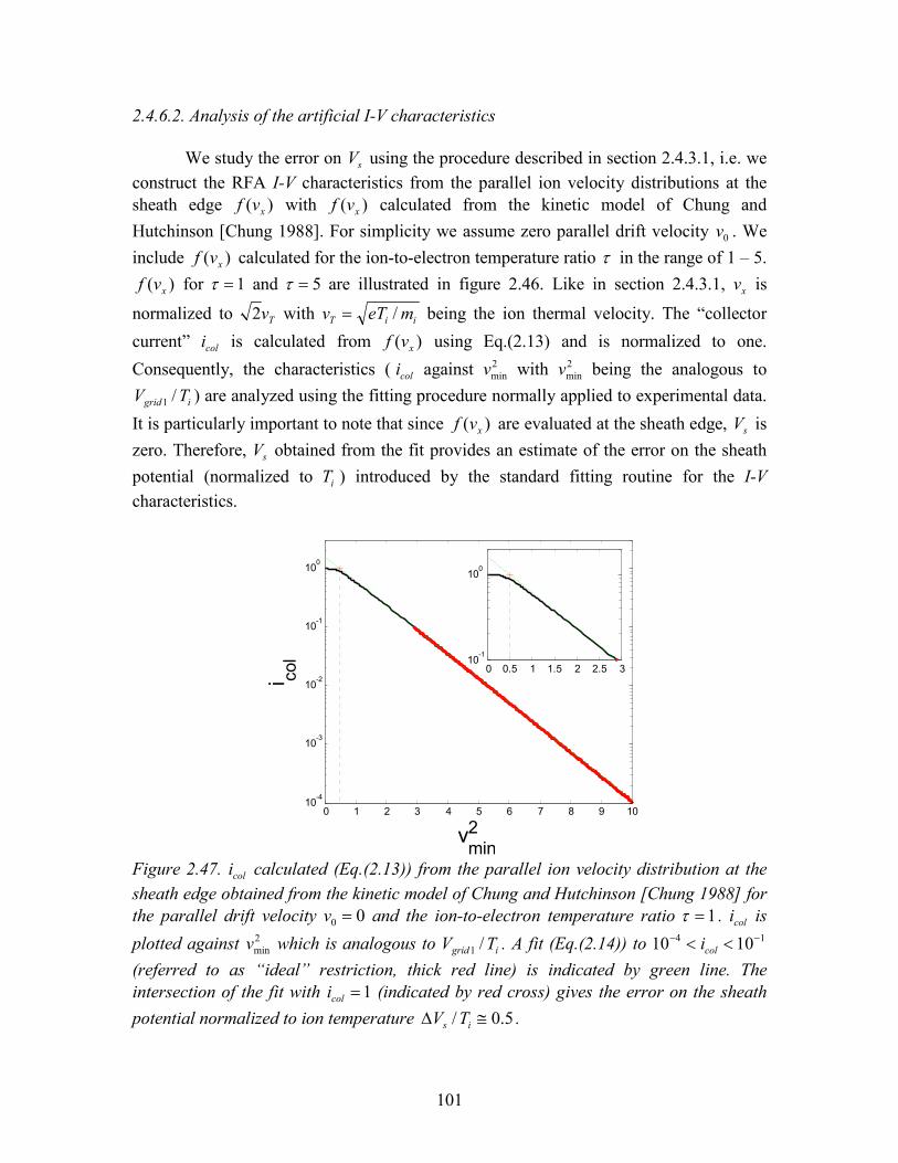
101

2.4.6.2. Analysis of the artificial I-V characteristics

We study the error on sV using the procedure described in section 2.4.3.1, i.e. we construct the RFA I-V characteristics from the parallel ion velocity distributions at the sheath edge )( xvf with )( xvf calculated from the kinetic model of Chung and Hutchinson [Chung 1988]. For simplicity we assume zero parallel drift velocity 0v . We include )( xvf calculated for the ion-to-electron temperature ratio τ in the range of 1 – 5.

)( xvf for 1=τ and 5=τ are illustrated in figure 2.46. Like in section 2.4.3.1, xv is

normalized to Tv2 with iiT meTv /= being the ion thermal velocity. The “collector

current” coli is calculated from )( xvf using Eq.(2.13) and is normalized to one.

Consequently, the characteristics ( coli against 2minv with 2

minv being the analogous to

igrid TV /1 ) are analyzed using the fitting procedure normally applied to experimental data.

It is particularly important to note that since )( xvf are evaluated at the sheath edge, sV is zero. Therefore, sV obtained from the fit provides an estimate of the error on the sheath potential (normalized to iT ) introduced by the standard fitting routine for the I-V characteristics.

0 1 2 3 4 5 6 7 8 9 1010

-4

10-3

10-2

10-1

100

v2min

i col 0 0.5 1 1.5 2 2.5 3

10-1

100

Figure 2.47. coli calculated (Eq.(2.13)) from the parallel ion velocity distribution at the sheath edge obtained from the kinetic model of Chung and Hutchinson [Chung 1988] for the parallel drift velocity 00 =v and the ion-to-electron temperature ratio 1=τ . coli is

plotted against 2minv which is analogous to igrid TV /1 . A fit (Eq.(2.14)) to 14 1010 −− << coli

(referred to as “ideal” restriction, thick red line) is indicated by green line. The intersection of the fit with 1=coli (indicated by red cross) gives the error on the sheath potential normalized to ion temperature 5.0/ ≅∆ is TV .

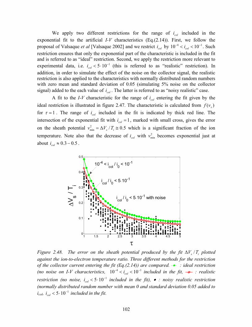
102

We apply two different restrictions for the range of coli included in the exponential fit to the artificial I-V characteristics (Eq.(2.14)). First, we follow the proposal of Valsaque et al [Valsaque 2002] and we restrict coli by 14 1010 −− << coli . Such restriction ensures that only the exponential part of the characteristic is included in the fit and is referred to as “ideal” restriction. Second, we apply the restriction more relevant to experimental data, i.e. 1105 −⋅<coli (this is referred to as “realistic” restriction). In addition, in order to simulate the effect of the noise on the collector signal, the realistic restriction is also applied to the characteristics with normally distributed random numbers with zero mean and standard deviation of 0.05 (simulating 5% noise on the collector signal) added to the each value of coli . The latter is referred to as “noisy realistic” case.

A fit to the I-V characteristic for the range of coli entering the fit given by the ideal restriction is illustrated in figure 2.47. The characteristic is calculated from )( xvf for 1=τ . The range of coli included in the fit is indicated by thick red line. The intersection of the exponential fit with 1=coli , marked with small cross, gives the error

on the sheath potential 5.0/2min ≅∆= is TVv which is a significant fraction of the ion

temperature. Note also that the decrease of coli with 2minv becomes exponential just at

about 5.03.0 −≈coli .

1 1.5 2 2.5 3 3.5 4 4.5 50

0.1

0.2

0.3

0.4

0.5

τ

∆Vs / T

i

10-4 < icol / i

0 < 10-1

icol / i

0 < 5⋅10-1

icol / i

0 < 5⋅10-1 with noise

Figure 2.48. The error on the sheath potential produced by the fit is TV /∆ plotted against the ion-to-electron temperature ratio. Three different methods for the restriction of the collector current entering the fit (Eq.(2.14)) are compared. • : ideal restriction (no noise on I-V characteristics, 14 1010 −− << coli included in the fit, o : realistic

restriction (no noise, 1105 −⋅<coli included in the fit), • : noisy realistic restriction (normally distributed random number with mean 0 and standard deviation 0.05 added to icol, 1105 −⋅<coli included in the fit.

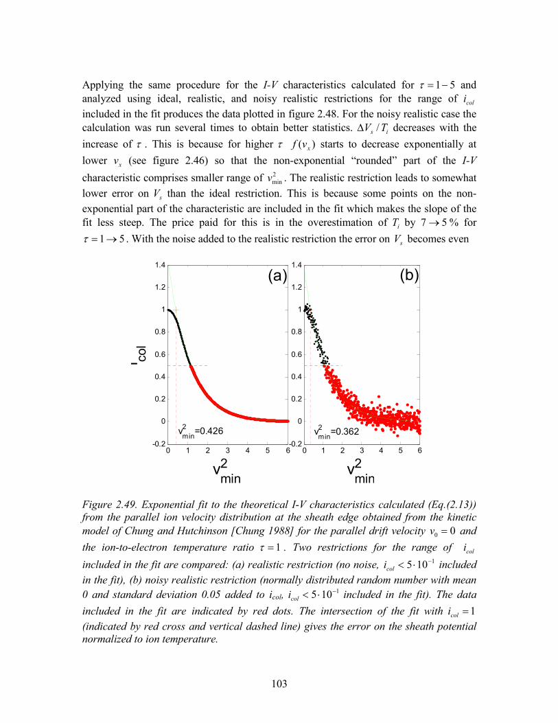
103

Applying the same procedure for the I-V characteristics calculated for 51−=τ and analyzed using ideal, realistic, and noisy realistic restrictions for the range of coli included in the fit produces the data plotted in figure 2.48. For the noisy realistic case the calculation was run several times to obtain better statistics. is TV /∆ decreases with the increase of τ . This is because for higher τ )( xvf starts to decrease exponentially at lower xv (see figure 2.46) so that the non-exponential “rounded” part of the I-V

characteristic comprises smaller range of 2minv . The realistic restriction leads to somewhat

lower error on sV than the ideal restriction. This is because some points on the non-exponential part of the characteristic are included in the fit which makes the slope of the fit less steep. The price paid for this is in the overestimation of iT by 57 → % for

51→=τ . With the noise added to the realistic restriction the error on sV becomes even

0 1 2 3 4 5 6-0.2

0

0.2

0.4

0.6

0.8

1

1.2

1.4

v2min

0 1 2 3 4 5 6-0.2

0

0.2

0.4

0.6

0.8

1

1.2

1.4

v2min

i col

(a) (b)

v2min

=0.426 v2min

=0.362

Figure 2.49. Exponential fit to the theoretical I-V characteristics calculated (Eq.(2.13)) from the parallel ion velocity distribution at the sheath edge obtained from the kinetic model of Chung and Hutchinson [Chung 1988] for the parallel drift velocity 00 =v and the ion-to-electron temperature ratio 1=τ . Two restrictions for the range of coli

included in the fit are compared: (a) realistic restriction (no noise, 1105 −⋅<coli included in the fit), (b) noisy realistic restriction (normally distributed random number with mean 0 and standard deviation 0.05 added to icol, 1105 −⋅<coli included in the fit). The data

included in the fit are indicated by red dots. The intersection of the fit with 1=coli (indicated by red cross and vertical dashed line) gives the error on the sheath potential normalized to ion temperature.

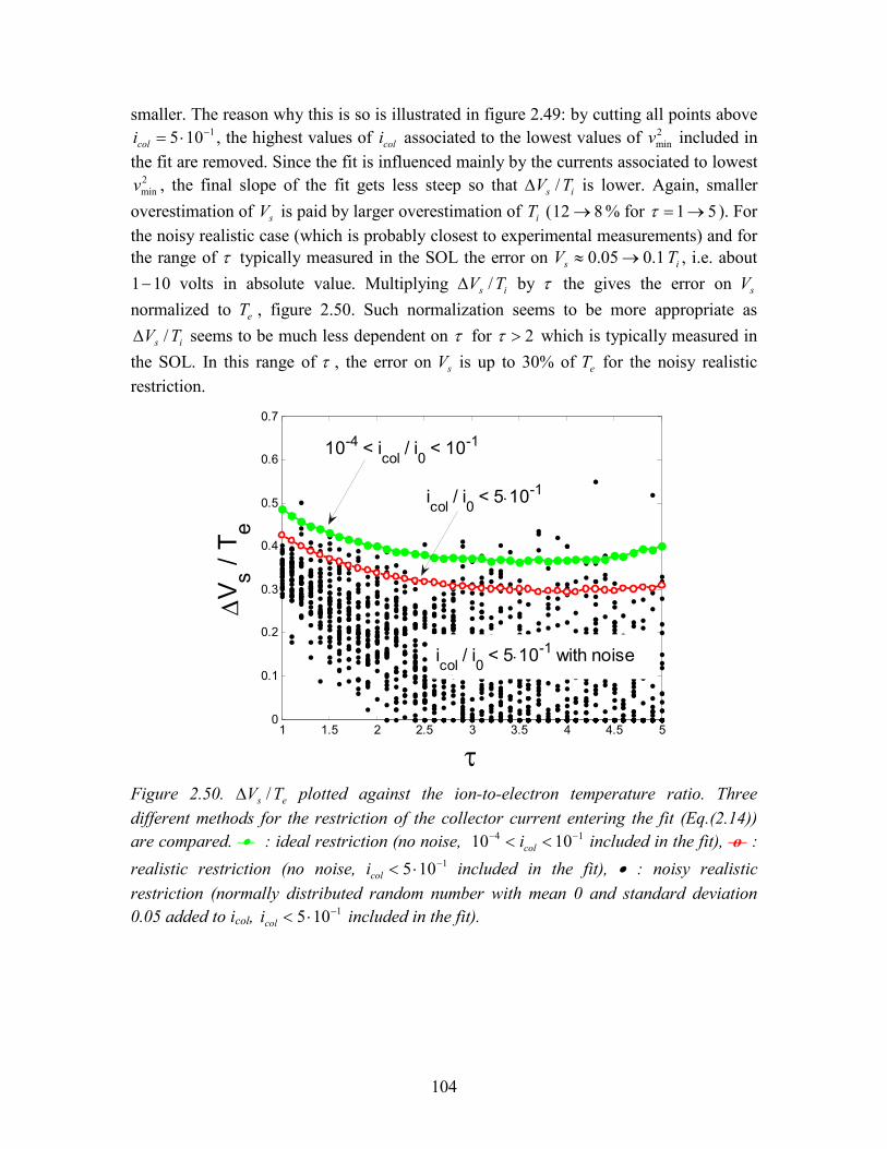
104

smaller. The reason why this is so is illustrated in figure 2.49: by cutting all points above 1105 −⋅=coli , the highest values of coli associated to the lowest values of 2

minv included in the fit are removed. Since the fit is influenced mainly by the currents associated to lowest

2minv , the final slope of the fit gets less steep so that is TV /∆ is lower. Again, smaller

overestimation of sV is paid by larger overestimation of iT ( 812 → % for 51→=τ ). For the noisy realistic case (which is probably closest to experimental measurements) and for the range of τ typically measured in the SOL the error on 1.005.0 →≈sV iT , i.e. about

101− volts in absolute value. Multiplying is TV /∆ by τ the gives the error on sV normalized to eT , figure 2.50. Such normalization seems to be more appropriate as

is TV /∆ seems to be much less dependent on τ for 2>τ which is typically measured in the SOL. In this range of τ , the error on sV is up to 30% of eT for the noisy realistic restriction.

1 1.5 2 2.5 3 3.5 4 4.5 50

0.1

0.2

0.3

0.4

0.5

0.6

0.7

τ

∆Vs / T e

10-4 < icol / i

0 < 10-1

icol / i

0 < 5⋅10-1

icol / i

0 < 5⋅10-1 with noise

Figure 2.50. es TV /∆ plotted against the ion-to-electron temperature ratio. Three different methods for the restriction of the collector current entering the fit (Eq.(2.14)) are compared. • : ideal restriction (no noise, 14 1010 −− << coli included in the fit), o :

realistic restriction (no noise, 1105 −⋅<coli included in the fit), • : noisy realistic restriction (normally distributed random number with mean 0 and standard deviation 0.05 added to icol, 1105 −⋅<coli included in the fit).

105

Annex

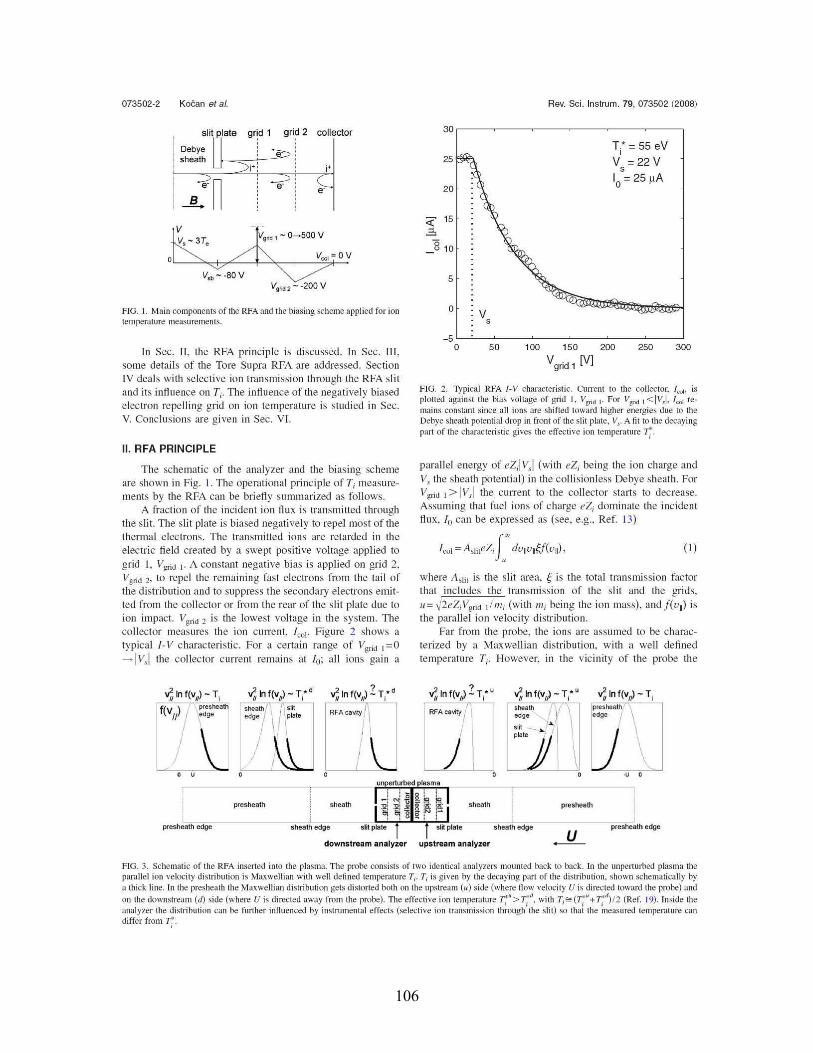
106

073502-2 Koéan et al. Rev. Sei. Instrum. 79, 073502 (2008)

FIG. 1. Main components of the RFA :md the biasing scheme applied for iontemperature llleaSlirements.

V~2--200V

Ti· = 55 eVV =22V,10

= 25 ~A

V,

30 r--------------------,

"e-e-

collector

Vgrld 1 - 0-500 V

Vsll --80V

slltplate

Debyeshealh

vV~ - 3T.

300250100 150 200

Vg 'ld1 [VI

50-5 '---~~-~--~-~-~-------'

o

FIG. 2. Typical RFA l-V characteristic. CUrrent to the collector. '001, isplottoo against the bias voltage of grid 1. Vp-id l' For Vp-id 1<lvJ /ool re­mains constant since all ions are shifted toward higher energies due to theDebye sheath potential drop in front of the slit plate. V,. A titto the decayingpart of the characteristic gives the effective ion telllperalUre r;.

ln Sec. IL the RFA principle is discussed. In Sec. Ill.some details of the Tore Supra RFA are addressed. SectionIV deals with selective ion transmission through the RFA slitand its influence on Ti' TIle influence of the negatively biasedelectron repelling grid on ion temperature is studied in Sec.V. Conclusions are given in Sec. VI.

II. RFA PRINCIPLE

(I)

The schematic of the analyzer and the biasing schemeare shown in Fig. 1. The opemtional principle of Ti measure­ments by the RFA can be briefty summarized as follows.

A fraction of the incident ion flux is transmitted throughthe slit. The slit plate is biased negatively to repel most of thethermal electrons. The transmitted ions are retarded in theelectric field created by a swept positive voltage applied tagrid L Vgrid [_ A constant negative bias is applied on grid 2.Vgrid 2. ta repel the remaining fast electrons frol11 the tail ofthe distribution and ta suppress the secondary electrons emit­ted frol11 the collector or from the rear of the slit plate due taion impact. Vgrid :2 is the lowest voltage in the system. TIlecollector measures the ion cUITent, 100[, Figure 2 shows atypical 1-\1 characteristic. For a certain range of Vgrid [=0-IVsl the collector current remains at 10 : all ions gain a

parallel energy of eZAVsl (with eZi being the ion charge andVs the sheath potential) in the collisionless Debye sheath. ForVgrid J>IVsl the CUITent to the collector starts to decrease.Assuming that fuel ions of charge eZ; dOlllinate the incidentflux. 10 can be expressed as (see. e.g.. Ref. 13)

1001 = AsliteZ;J.'''' dViVI~f(vl)'

where A slit is the slit area. g is the total transmission factorthat includes the transmission of the slit and the grids.11= ,12eZYgrid 1/1Il; (with mi being the ion 111ass), andf(vl) isthe parallel ion velocity distribution.

Far frol11 the probe. the ions are assumed ta be charac­terized by a Maxwellian distribution. with a well definedtemperature T;. However. in the vicinity of the probe the

r--­1 preshealh sheath shealh presheeth

preshe.".<hC'''d'''';--------.:;..=,:;,t"~".,=,------;=b!-t-'-''-''--',---J,;;;!;;;;;-;:---.:;"=":;,."~,,.,=,-------~p:;'"'..""a'th edge

downstream analyzer upstream analyzer ---.Y......FIG. 3. Schematic of the RFA inscrted into the plasma. The probe consists of two identical analyzers mounled back to b.1ck. In the uilpenurbed plasma theparallel ion velocity distribution is Maxwe11ian with weIl defined temperature Ti' Ti is given by the decaying pan of the distribution. shown schematical1y bya thick line. ln the presheath the Maxwellian distribution gets distorted both on the upstrealll (II) side (where flow velocity U is directed toward the probe) andon the downstream (d) side (where U is directed away from the probe). The effective ion temperalUre 17"> r;J. with Ti 9! (r;~+ r;J)f2 (Ref. 19). Inside theanaly;o:er the distribution can be further influenced by instrumental effccts (selective ion transmission throllgh the slit) so that the measllred temperalUre candiffer from 17.

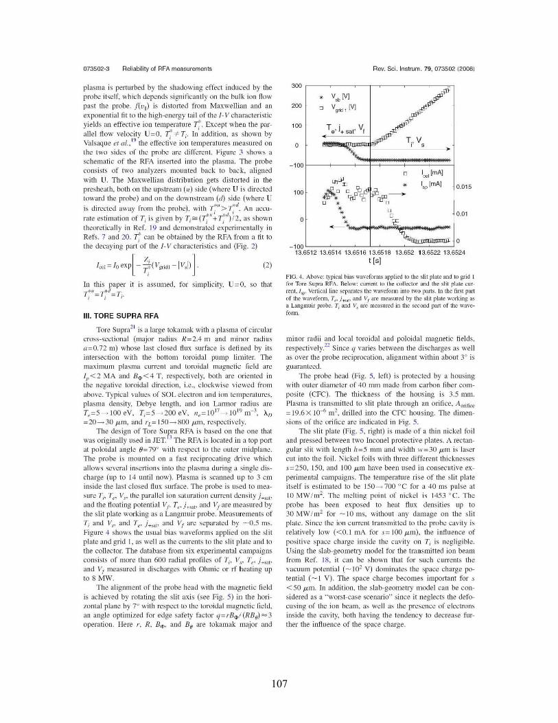
107

073502-3 Reliabilily of RFA measuremenls Rev. Sei. Inslrum. 79, 073502 (2008)

plasma is perturbed by the shadowing effect induced by theprobe itself. which depends significantly on the bull ion flowpast the probe. f(v,) is distOlted from Maxwelli<m and anexponential fit to the high-energy tail of the /- Vcharacteristicyields an effective ion temperature -r. Except when the par­aUel flow velocity U=O. -r *- Ti' ln' addition. as shown byValsaque et al.. 19 the effecti~e ion temperatures rneasured onthe two sides of the probe are different. Figure 3 shows aschematic of the RFA inserted into the plasma. The probeconsists of two analyzers mounted back to back. ahgnedwith U. The Maxwellian distribution gets distorted in thepresheath. both on the upstream (II) side (where U is directedtoward the probe) and on the downstream (d) side (where Uis directed away from the probe). with -r" > -rd. An accu-

. . f . . (...."' ....")'rate estImatIOn 0 Ti IS glven by Ti= /. + /. /2_ as showntheoreticaUy in Ref. 19 and dernonstrated e~perirnental1y inRefs. 7 and 20. r can be obtained by the RFA From a fit tothe decaying part'of the /-V characteristics and (Fig. 2)

lool=loeXP[-~(V"'idl-IV,Dl (2)

ln this yaper it is assumed. for simplicity, U=O. so that

t;"=t; = Ti'

III. TORE SUPRA RFA

Tore Supra21 is a large tokamak with a plasma of circularcross-sectional (major radius R=2.4 m and rninor radiusa=O.72 rn) whose last closed flux surface is defined by itsintersection with the bottorn toroidal pump limiter. TIlemaximum plasma current and toroidal rnagnetic field areIp <2 MA and 8'l,<4 T. respectively. bath are oriented inthe negative toroidal direction, i.e.. c10ckwise viewed fromabove. Typical values of SOL electron and ion temperatures,plasma density. Debye length. and ion Lanllor radius areTe=S----;.IOO eV. Ti=5----' 200 eV, " e =10 17 ----;.1019 rn~3. ÀD=20----;.30 Itm. and rL= 150----;.800 1t111. respectively.

The design of Tore Suwa RFA is based on the one thatwas original1y used in JET. J The RFA is located in a top portat poloidal angle ()=79° with respect to the outer rnidplane.The probe is mounted on a fast reciprocating drive whichaUows several insertions into the plasma during a single dis­charge (up ta 14 until now). Plasma is scanned up ta 3 cminside the last c10sed flux surface. The probe is used to mea­sure Ti' Te. Vs. the paral1el ion saturation current density lt-Sm.and the floating potential Vf' Te· lmt, and Vfare rneasured bythe sht plate working as a Langmuir probe. Measurements ofTi and V5 • and Te' l+sat. and Vf are separated by -0.5 ms.Figure 4 shows the usual bias wavefonns apphed on the slitplate and grid 1. as well as the currents to the sht plate and tothe col1ector. The database from six experimental campaignsconsists of more than 600 radial profiles of Ti' V5 , Te· J+sm.and Vf measured in discharges with Ohmic or rf heating upto 8 MW.

The alignment of the probe head with the magnetic fieldis achieved by rotating the sht axis (see Fig. 5) in the hori­zontal plane by r with respect to the toroidal magnetic field.an angle optimized for edge safety factor q=r8q,I(R80) =3operation. Here r. R. 8<I>. and 8 0 are tokamak major and

300

• V", [VI200 D Vgrld1 M

100Te' i+ saI' Vf

0 Ti' Vs

-100D Icol[mA)

",@ • 1sp[mAJCID 0.015

$~D en100C@DDD 01"'-

D • D

• D• 0.010 • D

• '15'~

1 ~~~~~o-100~13.6512 13.6514 13.6516 13.6518 13.652 13.6522 13.6524

t[s]

FIG. 4. Above: lypicaJ bias waveforms applied 10 Ihe sHt plaie and to grid J

for Tore Supra RFA. Below: current to the coI1ector and the siil ptate cur­rent. l>p. Vertical line separales the waveform into two parts. In the first partof the wavefoml. T,. j ....... and VI are measllred by the slil plate working asa Langmuir probe. Ti and V, are measured in the second part of the wave­fonn.

minor radii and local toroidal and poloidal magnetic fields.respectively.22 Since q varies between the discharges as wellas over the probe reciprocation. alignlllent within about 3° isguaranteed.

The probe head (Fig. 5, left) is protected by a housing\Vith outer diameter of 40 mm made From carbon fiber com­posite (CFe). The thickness of the hOllsing is 3.5 mm.Plasma is transmitted to sHt plate through an orifice. Aorifice

=19.6x 1O~61ll2. drilled into the CFC housing. The dimen­sions of the orifice are indicated in Fig. 5.

The sht plate (Fig. 5, right) is made of a thin nickel foiland pressed between two Inconel protective plates. A rectan­gular slit with length 11=5 mm and width 11'=30 tLJ11 is lasereut into the foil. Nickel foils with three different thicknessess=2S0. 150. and 100 1tJ11 have been used in consecutive ex­perimental campaigns. The temperature rise of the sht plateitself is estimated to be 150----;.700 oC for a 40 ms pulse at10 MW/m2. The melting point of nickel is 1453 oc. Theprobe has been exposed to heat flux densities up to30 MW/m2 for -10 ms. without any damage on the shtplate. Since the ion current transmitted to the probe cavity isrelatively low «0.1 mA for s= 100 Itlll), tlle influence ofpositive space charge inside the cavity on Ti is negligible.Using the slab-geometry model for the transmitted ion beamfrom Ref. 18. it can be shown that for such currents thevacuum potential (_102 V) dominates the space charge po­tential (-1 V). The space charge becomes imp01tant for s

<50 1t11l. In addition. the slab-geol1letry model can be con­sidered as a "worst-case scenario" since it neglects the defa­cusing of the ion beam. as well as the presence of electronsinside the cavity, both having the tendency to decrease fur­ther the influence of the space charge.

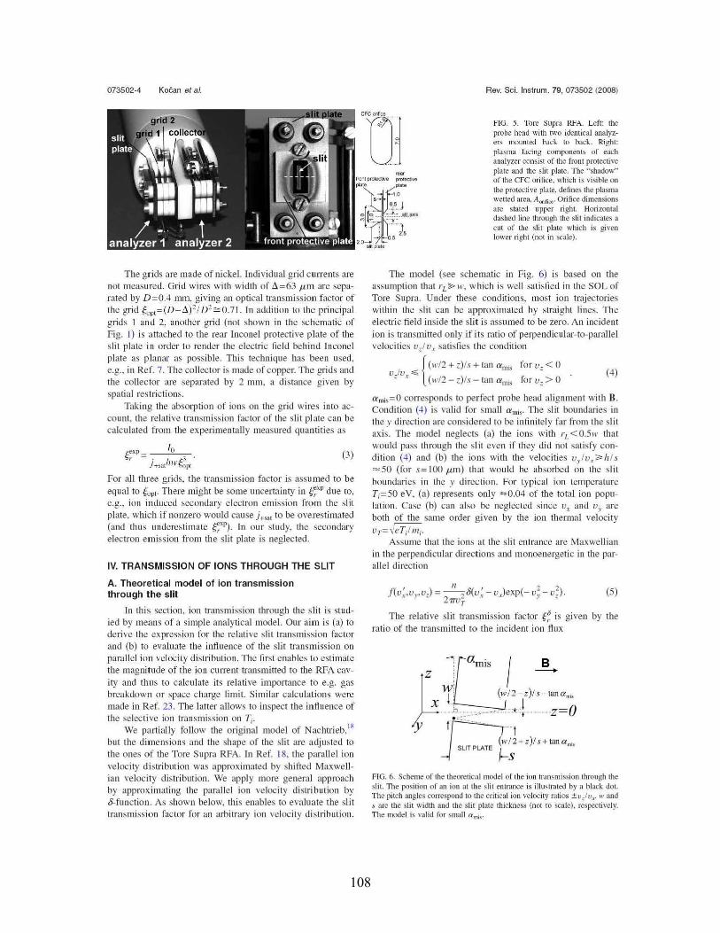
108

073502-4 Koéan et al.

TJ1...­",.,.

Rev. Sei. Instrum. 79, 073502 (2008)

FIG. 5. Tore Suprn RFA. Left: theprobe hend with two idenlical analYl­ers mounled bnck 10 back. Right:plasma facing componenls of eachnnnlyzer consisl of lhe front proleclivepinte and the sHI plate. The "shadow"of lhe CFC orifice. which is visible onthe proteclive plate, defines the plasmawel1ed aren. A"il",,' Orifice dimensionsnre slnled upper right. Horiwnlaldashed line through the sHI indicates acut of the slit plate which is givcnlower right (not in seale).

(4)

The grids are made of nickel. Individual grid currents arenot measured. Grid wires with width of ~=63 ttlTl are sepa­rated by D=O.4 mm. giving an optical transmission factor ofthe grid çoPt=(D-~)2/D2:0.71. In addition to the principalgrids 1 and 2. another grid (not shown in the schernatic ofFig. 1) is attached to the rear [nconel protective plate of thesht plate in order ta render the electric field hehind Inconelplate as planar as possible. This technique has been used,e.g.. in Ref. 7. The collector is made of copper. The grids andthe collector are separated by 2 mm. a distance given byspatial restrictions.

Taking the absorption of ions on the grid wires into ac­count. the relative transrnission factor of the sht pl ate can beca1culated from the experirnentally rneasured quantities as

<:,p_ 'a (3)r - J+s31hll'ç~pI'

For ail three grids. the transmission factor is assumed ta beequal ta çopt. There might be sorne ullcertainty in f,:xp due to.e.g., ion induced secondary electron emission from the slitplate, which if nonzero would cause J+S3t ta be overestimated(and thus underestimate ç::xP). In our study. the secondaryelectron emission from the sht plate is neglected.

IV. TRANSMISSION OF IONS THROUGH THE SUT

The model (see schernalic in Fig. 6) is based on Iheass1l111plion Ihal rL'P Il'. which is well satisfied in Ihe SOL ofTore Supra. Under these conditions. most ion Imjeclorieswilhin Ihe sht can he approxirnated by straight hnes. TIleelectric field inside Ihe sht is asslirned to be zero. An incidention is lransmitted only if its ratio of perpendicular-to-paral1elvelocities v/vx satisfies tJle condition

<(I1'I2+:J!s+tanamis forv~<OV~K- .~. (wl2-z)/.~-tanall1is torv~>O

amis=O corresponds ta perfect probe head ahgnment with B.Condition (4) is vahd for sma11 amis' TIle slit boundaries inthe y direction are considered to be infinitely far from the slitaxis. The model neglects (a) the ions with rL <0.5ll' thatwould pass throllgh the slit even if they did not satisfy con­dition (4) and (b) the ions \Vith the velocities vJv.,<3h!s=50 (for s= 100 Itm) that would he absorbed on the slitboundaries in the y direction. For typical ion ternperatureTi=50 eV, (a) represents only =0.04 of the total ion popu­lation. Case (b) can also be neglected since Vx and v y areboth of the same arder given by the ion thermal velocity

vT= \feT;llIIi'Assurne that the ions at the sht entmnce are Maxwellian

in the perpendiclilar directions and monoenergetic in the par­allel direction

FIG. 6. Scheme of lhe theorelical model of the ion transmission through theslil. The position of an ion at the slil entmnce is illuslraled by a black dol.The pilch nngles correspond to lhe crilical ion velocity ratios ±u/ur li' ands are the sHt width and the slit plnle thickncss (not 10 seale). respectively.The model is valid for small ami•.

A. Theoretical model of ion transmissionthrough the slit

ln this section. ion transmission through the sht is stud­ied by menns of a simple analytical mode!. Our aim is (a) taderive the expression for the relative sht transmission factorand (b) ta evaluate the influence of the sht transmission onparallel ion velocity distribution. TIle first enables ta estimatethe magnitude of the ion current transmitted ta the RFA cav­ity and thus ta ca1culate its relative importance ta e.g. gasbreakdown or space charge hmit. Similar ca1culations weremade in Ref. 23. The latter aUows ta inspect the influence ofthe selective ion transmission on Ti'

We pm1ially foUow the original model of Nachtrieb,18but the dimensions and the shape of the sht are adjllsted tathe alles of the Tore Supra RFA. ln Ref. 18. the parallel ionvelocity distribution was approxirnated by shifted Maxwell­ian velocity distribution. We apply more general approachby approximating the parallel ion velocity distribution byS-function. As shawn helow. this enables ta evaluate the slittransmission factor for an arbitrary ion velocity distribution.

( ' """)(22)f VX,vy.V) = ~u,Vx - Vx exp - v)' - v~ .27TV T

The relative slit transmission factor e is givenratio of the transrnitted to the incident ion flux

(5)

by the

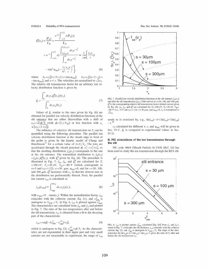
109

073502-5 Reliabilityof RFA measurements Rev. Sei. Instrum. 79, 073502 (2008)

where b l =uJ(1I'/2+.:)/s+tan a nùs]. b2=v.J(IV/2-z)/s

-tan amis]. and \1.< ..... The velocities are nonnalized to livT'The relative slit transmission factor for an arbitrary ion ve­locity distribution function is given by

with vnùn=O-Hnax(ux )' Within the normalization factor. icoJcoincides with the collecto~ curr~nt,. Eq. (1). an~ v~ÜIJ, isanalogous to Vgrid liT;. [n FIg. 8. 1001 JS plotted agamst v;;"in'The characteristics are calculated from fse and flr and plottedin Fig. 7. The ratio of the ion temperatures after and beforethe slit transmission. l'T' is obtained frOIll a fit to the decayingpart of the characteristic

86

s = 30 ~m

2

\s = 30~ms = 100~m

\ ....

S = 300~m

10-3 L ~ ~__-'-~--"-''''-J

o

>XO.6

~ "~ 0.5-x.:: 0.4

0.3

0.1

0.2

0.7

si il enlrance

B. PIC simulations of the ion transmission throughthe slit

PIC code SPICE (Sheath Partic1e ln CEI1) (Ret. 24) hasbeen used to study the ion transmission through the RFA slit.

s = 300 ~m

oLC::~~~_-.J1 1.5 2 2.5 3

V,

10'

0.8

0.9

FIG. 7. Parullel ion velocity distribution funclions at the slit entrance!..(v,)and af1er the slil transmissionf,iv,) (full curves) al 5=30. Joo. and 300 JLm.eis the corresponding relative slit transmission factor (dotted CUfl/CS) givcnby Eq. (6). f ... f". and e are ca1culaled for Tj =100 eV, T,=20 eV. V.,=-80 V (i.e.. T=5 and vo= J .12). 1<'=30 JLm. and u ....,=O. v, is nomlalized to\!2vr.

needs to is restricted by. e.g.. 1nCicoJ)-4 < 1nCicoJ) < InCicoJ)_1. 19

TT calculated for different 7. s. and amis will be given inSec. IV C. gr is compared to experirnental values in Sec.IV D.

(8)

(6)

(7)

, 1(",,,,)3]- tan- amiJ -"6 ----;- .

fa" dv,v~~(v,)f(v,)

Jooo

dvpJ(v x)

Values of Çr similar to the ones given by Eq. (6) areobtained for parallel ion velocity distribution functions at theslit entrance that are either Maxwellian with a shift of

VO=\/ZitTi~(With 4>=IVs+VsbDor box function with Vx

E [vo: \ 1+vii].The influence of selective slit transmission on Ti can he

quantified using the fol1owing procedure. The paral1el ionvelocity distribution function at the sheath edge in front ofthe probe is given by the kinetic model of Chung andHutchinson l7 for a certain value of 7=TJTr The ions areaccelerated through the sheath potential r/J. v~_v;+v~. sothat the resulting distribution fse(v x) corresponds to the oneat the slit entrance. The transmitted distribution is flrCV)=fse(v)ç~(vx)' with ç~ given by Eq. (6). The procedure isillllstrated in Fig. 7: fse. flr' and e are calculated for Ti= 100 eV. Te =20 eV. Vsb =-80 V (which corresponds to7=5 and Vo= 1.12).11'=30 /tin. amis=O. and for s=30. 100.and 300 /ttll. eincreases with Vx so that the slowest ions inthe distribution are preferentially filtered. Next. the parallelion current icol is calclllated as

(9)

which is analogous to Eq. (2). v*2 =cjJITi• As the character-111111

istics are not exponential in their upper part and very smallcurrents are not ll1easurable in experiment. the range of icoJ

FIG. 8. iool is plotted against v~". calculatcd [Eq. (8)] from f .. and f,,·s.s1ated in Fig. 7. s indicates the slit thickncss. irol coincides with the collectorCUITent. Eq. (2). and V~D is analogolls to Vpid 1fT,. The slope of the chH­:JCteristics for In(icol)-4<ln(iool)<ln(iool)-J gives the ratio of T, after andbefore the slit transmission rr.

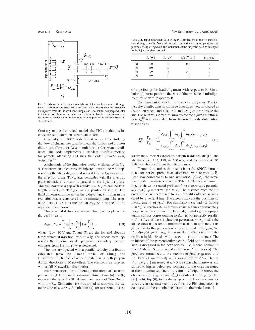
110

073502-6 Koéan et al. Rev. Sei. Instrum. 79, 073502 (2008)

(10)

FIG. 9. Schematic of the SPICE simulations of the ion transmission throughthe sHI. Distances are indicated in microns (not to scale). Ions and electronsare injectèd towards the wall containing a slit. The bollndaries perpendicularto the injection plane are periodic. [on distribution functions are measured atthe positions indicatcd by dotted lines with respect to the distance from theslit entrance.

Conlrary la Ihe Iheorelical modeL the PIC simulations in­clude the self-consistent electrostatic field.

Originally. the SPICE code was developed for studyingthe flow of plasma into gaps between the limiter and divertortiles. SPICE allows for 2d3v simulations in Cartesian coordi­nates. The code implements a standard leapfrog methodfor particle advancing and uses first arder (cloud-in-cell)weighting?5

A schernatic of the simulation model is illustrated in Fig.9. Deuterons and electrons are injected toward the wall rep­resenting the sht plate. located several tens of ÀD away fromthe injection plane. The x axis coincides with the injectionplane normal. The.: axis is parallel to the injection plane.The wall contains a gap with a width 11'=30 tLrn and the totallength 5=360 tLll1. The gap axis is positioned at z=O. Thethird dimension of the slit in the y direction. 11=5 mm in thereal sintation. is considered ta be infinitely long. The mag­netic field of 3.5 T is inclined at amis with respect ta theinjection plane normal.

The potential difference between the injection plane andthe wall is set to

T< [ m« T;)]ePr>IC=Vsb+-In 27T- 1+- .2 III; Te

where Vsb=-SO V and Ti and Te are the ion and electrontemperatures at injection. respectively. The second term rep­resents the floating sheath potential. Secondary electronemission from the sUt plate is neglected.

The ions are injected with a parallel velocity distributioncalculated from the kinetic model of Chung andHutchinson. 17 The ion velocity distribution in both perpen­dicular directions is Maxwellian. The electrons are injectedwith a full Maxwellian distribution.

Four simulations for different cOl11binations of the inputparameters (Table 1) were perfonned. Simulations (a) and (b)represent the typical SOL plasma parameters of Tore Supra.with 11'= ÀD. Simulation (c) was aimed at studying the ex­treme case of w= 4ÀD. Simulations (a)-(c) represent the case

TABLE 1. Input paramelers used in the PIC simulalions of the ion transmis­sion throllgh the slit. From left 10 right: ion and electron lemperatllres andplasma densily al injeclion, the inclination of the magnetic field wilh respeclto the injeclion plane normal.

Ti (eV) T, (eV) il/lOIS m-3) ami. (deg)

(a) 30 10 0.7 0

(b) 100 20 1.5 0

(c) 20 5 5 0

(d) 100 20 1.5 3

of a perfect probe head ahgnment with respect to B. Simu­lation (d) corresponds ta the case of the probe head misahgn­ment of 3° with respect to B.

Each simulation was left to run ta a steady state. 111e ionvelocity distributions in ail three directions were measured atthe sht entrance. and \00. 150. and 250 tLl11 deep inside theshI. The relative slit transmission factor for a given sht thick­ness f;(;~ was calculated from the ion velocity distributionfunctions as

where the subscript i indicates a depth inside the sht (i.e.. thesht thickness. 100. 150. or 250 ~m) and the subscript "0"indicates the position at the slit entrance.

Figure 10 compiles the results from the SPICE simula­tions for perfect probe head alignment with respect ta B.Each row corresponds to one simulation, (a)-(c), character­ized by the parameters stated in Table 1. The first column inFig. la shows the radial profiles of the electrostatic potentialrp(x .z=O). 'P is nonnahzed ta Te' The distance from the slitentrance, x. is nonnalized ta ÀD. The sht entrance is indi­cated by a vertical hne. The arrows indicate the positions ofmeasurernents of f(v x)' For simulations (a) and (c) (wherelI'=ÀD) rp reaches its minimum value within approximately-ÀDinside the slit. For simulation (b) (1I'=4ÀD) the equipo­tential surface corresponding ta ePr>IC is not perfectly parallelta front face of the slit plate but penetrates -4ÀD inside theshI. 'P does not reach its minimum at the sht entrance. Thisgives rise ta the perpendicular electric field =2eV",s(d)iI\'.Vres(d) =rp(d ,.:=0) - ePr>IC is the residual voltage and d is theposition inside the slit with respect to the sht entrance. Theinfluence of the perpendicular electric field on ion transmis­sion is discussed in the next section. The second column inFig. la showsf(vx)' scanned at different d (in microns).l1lef(vx) are nonnalized to the maxima of f(vx) measured at d

=0. Parallel ion velocity Vx is nonnahzed ta "lVT' Due taVres ' the f(v x ) llleasured at d>O are sOl11ewhat narrower andshifted ta higher velocities. compared to the ones measuredat the sht entrance. The third column of Fig. 10 shows thecharacteristics (icol versus U~in) calculated from f(v x) [Eq.(8)]. A fit. Eq. (9). to tlle decaying pmt of the characteristicsgives TT' ln the next section. TT from the PIC simulations iscompared to the one obtained from the theoretical model.

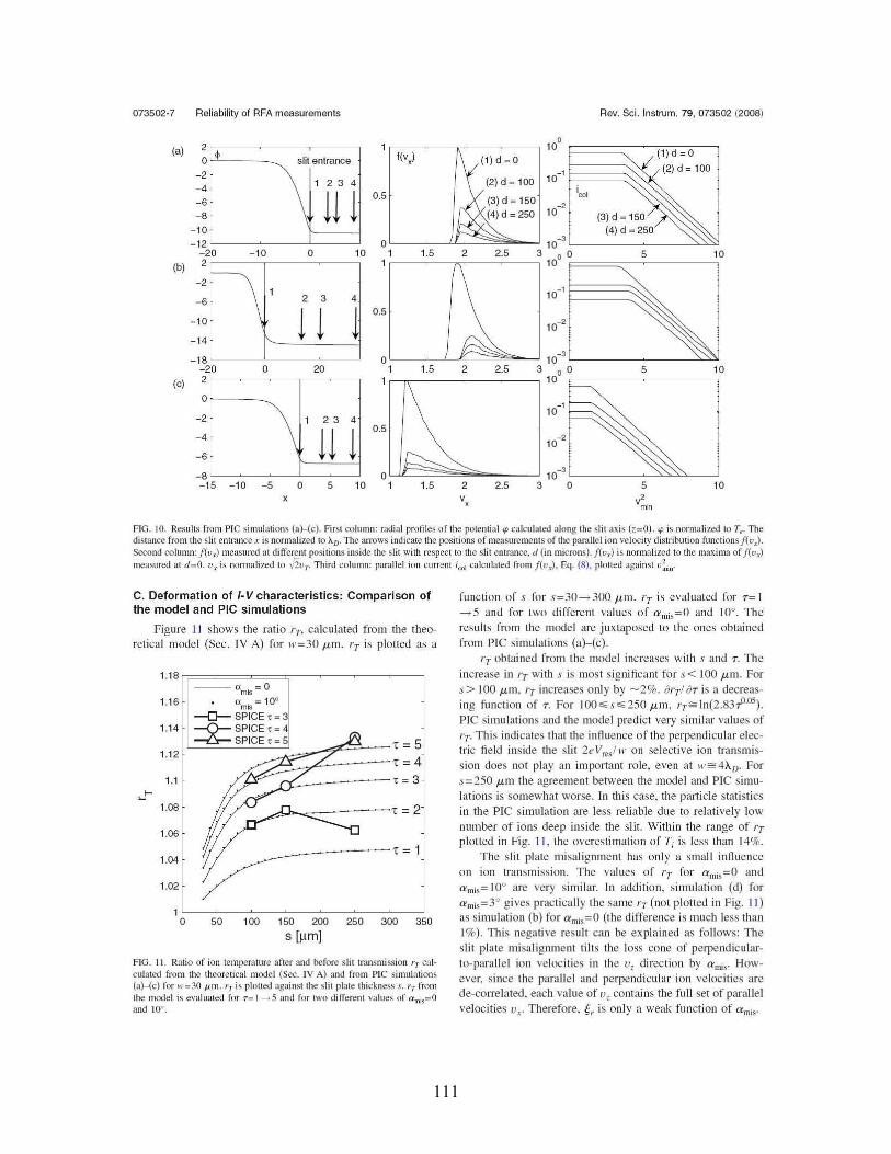
111

073502-7 Reliabilily 01 RFA measuremenls Rev. Sei. Inslrum. 79, 073502 (2008)

2 10'(a) • I(v) (1)d =0

0\" ","aoc"-2 10~1

(2)d=100

-, 1 2 3 4 (2)d=1ooiCOI

Hl 0.5 (3)d=1S0-610-2-8 (4)d=2S0 (3)d=1S0

-10 (4) d = 250-12 0 10-3

-20 -10 0 10 1 1.5 2 2.5 3100 0 5 10

(b) 2 1

-2

~'-6 2 3 , 10-1

l l l 0.5-10 10~2

-1'

10-3-18 0-20 0 20 1 1.5 2 2.5 3 , 0 5 10

(0) 2 1 10

0

-2 \'10~1

23 ,

11 l0.5-, 10-2

-6

-8 0 10~3

-15 -10 -5 0 5 10 1 1.5 2 2.5 3 0 5 10v, v;,,,

FIG. [o. Resulls from PIC simulntions (n)-(c). First column: rndinl profiles of the potentinl '" ca1culated nlong the slit axis (z=O). If! is normalized to T,. Thedistnnce from the slit entr:tl1cc x is normalizcd to AD' The :t/TOWS indicnte the positions of measurements of the parnllel ion velocity distribution functions f(v~).

Second column: f(v~) measured at dilferent positions inside the slit with respect to the slit entrance. d (in microns). f(v~) is nonnnlizcd to the maxima off(v~)measured at d=O. v~ is normalized to \i2vT. Third column: parallel ion CUITent i rol ca1culated from f(v~). Eq. (8). plollcd against v~n'

FIG. 11. Ratio of ion tempernture after:tl1d before slit transmission rT cal­culatcd from the theoretical mooel (Sec. IV A) and from PIC simulations(a)--c) for ",=30 J.l.m. rTis plolled againstthe slit pInte thickness s. rT fromthe model is evaluated for T= [-5 and for two different values of 0"00,=0and 10°.

C. Deformation of /- V characteristics: Comparison ofthe model and PIC simulations

Figure 11 shows the ratio rT' ca1culated fram the theo­retical model (Sec. IV A) for 11'=30 /Lm. rT is plotted as a

function of s for ...·=30_300 /Lm. rT is evaluated for 7= 1_5 and for two different values of amis=O and 10°. Theresults fram the model are juxtaposed to the olles obtainedfrom PIC simulations (a)-(c).

rT obtained fram the model increases with sand 7.111eincrease in rT with s is most significant for s< 100 /Lill. Fors> 100 /Lm. rT increases only by -2%. JrT/JT is a decreas­ing function of 7. For 100.:0;;:: s.:o;;:: 250 /Lm. rr=ln(2.83.fl·05

).

PIC simulations and the model predict very similar values ofrT' This indicates that the influence of the perpendicular elec­tric field inside the sht 2eVres /1I' on selective ion transmis­sion does not play an important raie. even at 1I"=4ÀD • Fors=250!Lm the agreement between the model and PIC simu­lations is somewhat worse. In this case. the particle statisticsin the PIC simulation are less rehable due to relatively lownumber of ions deep inside the slit. Within the range of rT

plotted in Fig. 11. the overesti mation of Tj is less than 14%.The sht plate misalignment has only a slllall influence

on ion transmission. The values of rT for amis=O andamis= 100 are very similar. In addition. simulation (d) fora mis=3° gives practically the same rr (not plotted in Fig. 11)as simulation (b) for umis=O (the difference is much less than1%). This negative result can he explained as follows: TIlesht plate misaligmnent tilts the loss cone of perpendicular­to-parallel ion velocities in the u;: direction by a nùs. How­ever. since the parallel and perpendicular ion velocities arede-correlated, each value of u;: contains the full set of parallelvelocities Ur Therefore. ~r is only a weak function of amis'

50 100 150 200 250 300 350

S [~m]

1.16

1.14

1.12

1.18 rc=====c==;--------,--- ctmls=O

ct = 10°m"--0-- SPICE 1: =3--- SPICE 1: =4

L_-b--='----'S~P:'C~E~,~=~5~;:2~~=='t = 51=4.J:Je:-----, = 31.1

,!-1.08

1.06

1.04

1.02

10

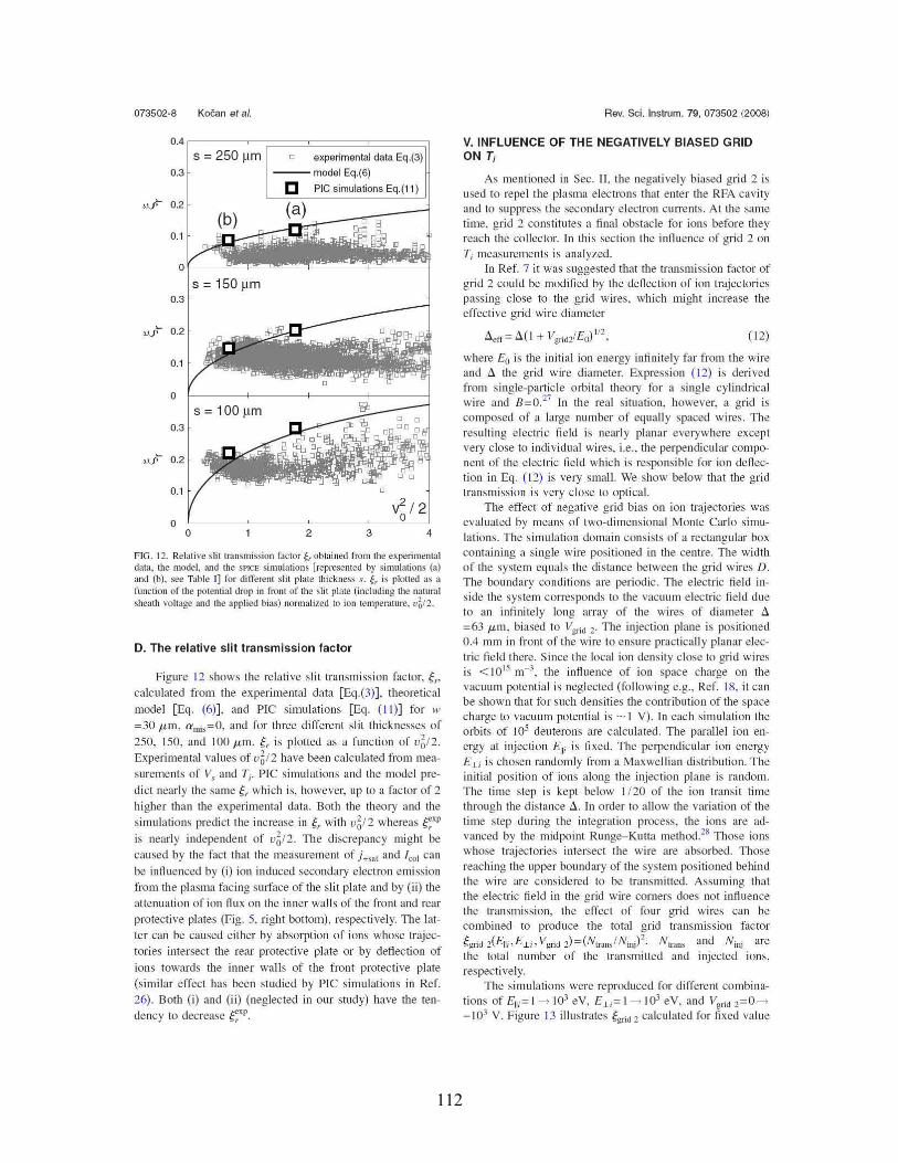
112

FIG. 12. Relative slit tmnsmission factor Çr obtained frorn the experirnentaldata. the mode!. :Uld the SPICE simulations [represented by simulations (a)and (h). see Table l] for different slit plate thickness s. Çr is plotted as afUllction of the potential drop in front of the slit plate (inc1uding the natumlsheath voilage and the applied bias) normalized to ion temperature. v~!2.

D. The relative slit transmission factor

Figure 12 shows the relative slit transmission factor, gr'cakulated from the experirnental data [Eg.(3)]. theoretical

model [Eg. (6)]. and PIC simulations [Eq. (11)] for II'

=30 IttlL Qlmis=O. and for t1lfee different slit thicknesses of

250. 150. and 100 ttm. gr is plotted as a function of v6/2.Experimental values of v~/2 have been calculated from mea­surernents of Vs and Ti' PIC simulations and the rnodel pre­

dict nearly the same gr which is, however. up to a factor of 2higher than the experimental data. Both the theory and thesimulations predict the increase in gr with v6/2 whereas f,:xpis nearly independent of v6/2. The discrepancy might becaused by the fact that the measurement of )+S3t and lrol can

be influenced by (i) ion induced secondary electron emissionfrom the plasma facing surface of the slit plate and by (ii) theattenuation of ion flux on the inner walls of the front and rear

protective plates (Fig. 5, right bottom). respectively. The lat­ter can be caused either by absorption of ions whose trajec­tories intersect the rear protective plate or by deflection ofions towards the inner walls of the front protective plate

(similar effect has been studied by PIC simulations in Ref.26). Both (i) and (ii) (neglected in our study) have the ten­dency to decrease ~xP.

Rev. Sei. Instrum. 79, 073502 (2008)

V. INFLUENCE OF THE NEGATIVELY BIASED GRIDON Ti

As mentioned in Sec. IL the negatively biased grid 2 isused to repel the plasma electrons that enter Ole RFA cavityand to suppress the secondary electron CUlTents. At the sailletime. grid 2 constitutes a final obstacle for ions before theyreach the collector. ln this section the influence of grid 2 onT j measurements is analyzed.

ln Ref. 7 it was sllggested that the transmission factor ofgrid 2 cOllld be modified by the deflection of ion tmjectoriespassing close to the grid wires. which rnight increase theeffective grid wire diameter

aerr=â(l +Vgrid2IEo)tl2. (12)

where Eo is the initial ion energy infinitely far from the wireand a the grid wire diameter. Expression (12) is derivedfrom single-particle orbital theory for a single cylindricalwire and 8=0.27 ln the real situation. however. a grid iscomposed of a large number of equally spaced wires. TIleresulting electric field is nearly planar everywhere exceptvery close ta itldividual wires. i.e.. the perpendicular compo­tient of the electric field which is responsible for ion deflec­tion in Eq. (12) is very smal\. We show below that the gridtransmission is very close to optica1.

The effect of negative grid bias on ion trajectories wasevaluated by means of two-dimensional Monte Carlo simu­lations. The simulation domain consists of a rectangular boxcontaining a single wire positioned in the centre. The widthof the system equals the distance between the grid wires D.The boundary conditions are periodic. The electric field in­side the system corresponds to the vacuum electric field dueta an infinitely long array of the wires of diameter â=63 Itm. biased to Vgrid 2' The injection plane is positioned0.4 mm in front of the wire ta ensure practically planar elec­tric field there. Since the local ion density close to grid wiresis <10 t5 m-3• the influence of ion space charge on tllevacuum potential is neglected (following e.g.. Ref. 18. it canbe shawn that for such densities the contribution of the spacecharge to vacuum potential is ~ 1 V). In each simulation theorbits of 105 deuterons are calculated. The parai lei ion en­ergy at injection E11; is fixed. The perpendicular ion energyE.Li is chosen randomly from a Maxwellian distribution. Theinitial position of ions along the injection plane is random.The time step is kept below [/20 of the ion transit timethrough the distance â. In order to allow the variation of thetime step during the integration process. the ions are ad­vanced by the midpoint Runge-Kutta method.28 TIlOse ionswhose tmjectories intersect the wire are absorbed. TIlOsereaching the upper boundary of the system positioned behindthe wire are considered to be transmitted. Assurning thatthe electric field in the grid wire corners does not influencethe transmission, the effect of four grid wires can becornbined to produce the total grid transmission factorÇgrid 2(E11 ;.E.Li' Vgrid 2) = (NtransINinl· Nuans and Ninj arethe total nurnber of tlle transrnitted and injected ions.respectively.

The simulations were reproduced for different combina­tions of En;= 1-----t 103 eV. Eu = 1_ J 03 eV. and Vgrill 2=0­_103 V. Figure 13 illustrates Çgrid 2 calculated for fixed value

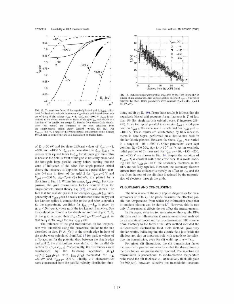
113

073502-9 Reliabilityof RFA measurements Rev. Sei. Instrum. 79, 073502 (2008)

Vgrid2

[VI:

a -10

o -150

o -250t::. -550

FIG. 14. SOL ion temperature profiles measured by the Tore Supr:t RFA insimilar ohmic discharges. Bias voltage applied on grid 2 Vpid 2 was variedbetween the ShOIS. Other jXlmmelc.rs were constant (lp=0.6 MA. Ii,= J.4X 1019 m-3).

>--

10

20

o0'-----=2:-0---,4:-0---,6::0---,8::0~distance from the LCfS [mm]

10'

1

10'

"­-1V

11

0.9

0.6

0.81 1

1 1-200V 1 1

'", -1000 V /, ,,', ,1 1

1 1

1 1

1 11 1

Elfi[eVj0.5 UC---~~~_~---L_~_L----"~~

10'

0.55

0.85~ ~

- 1V 'v - -0.95 f----7"""~/-.----_:::~'/"

0.65

N

~~ 0.75

0.7

FIG. 13. Transmission factor of the negmively biased gJid 2. Çpid 2. calcu­lated fOf fixed perpendicular ion energy E jj=50 eV and thrce difTerent val­ues of the grid bias voltage Vl!Jid 2=-1. -200. and -10CXl V. çgid 2 is nOf­maliled to the optical transmission factof of the grid çOl" and plOlled as afunction of the parallel ion energy El;' Results from Monte Carlo simula·tions (full cUf\'es) are compared to the ones calculated fromthe single-particle orbital theory (dashed curves). Eq. (11). ForVpid 2=-200 V. a range of the typical Ximllel ion energies m the distanceD=O.4 mm in front of the grid 2 is highlighted by thicker lines.

of E u =50 eV and for three different values of Vgrid 2=-!.-200. and -1000 V. ggrid 2 is nonnalized to gapt· ggrid 2 in­creases with E'i and tends to goP! for stronger grid bias. nlisis because the field in front of the grid is basically planar andthe ions gain large parallel energy before coming into thezone of influence of the wire. For single-partic1e orbitaltheory the tendency is opposite. Realistic parallel ion ener­gies 004 Illm in front of the grid 2 for Vgrid 1=0 V andVgrid2=-200 V. E1i=Ti+eIVsl+160eV. are plotted by a

thick line in Fig. 13. Within this range. ~grid 2::= ~OPI' For com­parison. the grid transmission factors derived from thesingle-partie le orbital theory. Eq. (12). are also shown.l1lefact that for reahstic parallel ion energies ggrid 2=gopl inde­pendently of Vgrid 2 can be easily understood since the typicalion Larmor radius is comparable to the grid wire separationD. the approximate condition for ggrid 2=gopl is given by!lI VI < DI(rLwL)' where WL is the ion Larmor frequency. Dueto acceleration of ions in the sheath and in front of grid 2. E'iat the grid is larger than E.l i (E'i=E.li+3T~-eVgrid 2)' sothat !llv~<DI(rLwJ for any Vgrid 2<0.

The influence of the grid transmission on ion tempera­lure was quantified using the procedure similar to the onedescribed in Sec. IV A; !(v.) at the sheath edge in front ofthe probe were calculated from ReL 17 for various values ofT. To account for the potential drop between the sheath edgeand grid 2. the distributions were shifted in the parallel di­rection by elVs+ Vgrid 21. Consequently. the distributions weretransformed by the fol1owing operation: !(EII;)=!(Elli)·ggrid 2(ER;). with ggrid 2(E~j) calculated for E.l i

=50 eV and Vgrid 2=-200 V. Finally. I-V characteristicswere constructed from the parullel velocity distribution func-

tions. and fit by Bq. (9). From these results it follows that theneg<ltively biased grid accounts for an increase in Tj of lessthan 1% (for single-particle orbital theory. Tj increases 2%­4%). Since for typical parallel ion energies Çgrid 2 is indepen­dent on Vgrid 2. the same result is obtained for Vgrid 2=0­-1000 V. These results are substantiated by RFA Illeasure­Illents in Tore Supra. petfoflned 011 a shot-to-shot basis insilllilar Olunic plasmas. Between the shots. V grid 2 was variedin a range of -10_-600 V. Other pararneters were keptconstant (/,,=0.6 MA, il~= lA X JOI9 m-3). As an example.radial profiles of Ti measured for Vgrid 2=-10. -150. -250.and -550 V are shown in Fig. 14; despite the variation ofVgrid 2. Tj is constant within the error bars. Il is worth notic­ing that for Vgrid 2=-10 V the secondary electrons in theRFA are not fully repelled. However, the secondary electronCUITent from the collector is merely an offset on IcoJ and theone frolll the rear of tlle sht plate is reduced by the transmis­sion of electrons through the grids.

VI. SUMMARY AND CONCLUSIONS

The RFA is one of the only apphed diagnostics for Illea­surernents of SOL Tj • The probe measures the effective par­allel ion temperature. from which the information about thatin ambient plasma can he derived. t9 However. this is trueonly if instrumental effects do not affect the Illeasurements.

ln this paper. selective ion transmission through the RFAslit plate and its influence on Tj Illeasurements was analyzedby an an31ytical model and by two-dimensional PIC simula­tions. Contmry to the fonner. the latter met/lOd included theself-consistent electrostatic field. Both Illethods gave verysimilar results. indicating that the electric field just inside theslit does not play an important role with regards to the selec­tive ion transmission. even for slit width up to 1I'=4ÀD •

For given sht dimensions. the slit transmission factorincreases with parallel ion velocity so that the slowest ions inthe distribution are preferenti<llly removed. The selective iontransmission is proportional to ion-to-electron tel1lperatureratio T and the slit thickness s. For relatively thick sht plate(s=300 Itm). however, selective ion transmission accounts

114

115

Chapter 3

Experimental results

In this chapter, selected experimental results are presented in the form of papers published (or submitted for publication) during the thesis. The main diagnostic in all experiments is the RFA.

In order to motivate the reader for this chapter we refer to section 1.4.1, in which the importance of SOL iT measurements, the experimental results related to SOL iT reported from different tokamaks, and some ideas for further work were discussed.

In the first two papers [Kočan 2008, Kočan 2008b] measurements of both iT and

eT in an ohmic helium density scan in the Tore Supra SOL are reported. It is shown that the usual assumption of equal SOL temperatures due to equipartition is not satisfied in the Tore Supra SOL, confirming the results obtained in other tokamaks, but demonstrated on a smaller dataset (see references in section 1.4.1). The link between iT and eT measured in the SOL and the temperatures measured inside the LCFS by charge exchange recombination spectroscopy, Thomson scattering, and electron cyclotron emission diagnostics, is discussed. The first continuous ei TT / profile from the edge of the confined plasma into the SOL is constructed using data from several tokamaks. It is shown that ei TT / increases with radius, with 1/ >ei TT already in the edge of the confined plasma.

In the third paper [Kočan 2009b] a previously unobserved strong increase of SOL iT with the intensity of the toroidal magnetic field tB is reported. The only other

parameter which is found to be also correlated with the tB is the core electron

116

temperature (core ion temperature is not available for the discharges analyzed in this paper). SOL eT is found to be practically decoupled from core electron temperature.

The fourth paper [Kočan 2009c] is aimed at the study of the dependence of SOL parameters (such as iT , eT , satj and en ) on the plasma density and the radiated power fraction, including detached plasmas. SOL ion temperature is measured for the first time in a detached plasma. The influence of the radiated power fraction on SOL iT and eT measured experimentally is compared with the results obtained from a simple power balance model.

Finally, in the last paper [Kočan 2009], the first evidence of a poloidal asymmetry of the radial ion and electron energy transport is reported. Implications for ITER start-up phase are discussed. Correlation of the asymmetries of SOL iT and eT measured on each side of the RFA with changes of the parallel Mach number //M , important for validating kinetic Mach probe theory, are briefly addressed.

117

Edge ion-to-electron temperature ratio in theTore Supra tokamak

M Kocan l , J P Gunni, J-Y Pascal 1,G Bonhomme2, C Fenzi 1,

E Gauthier' and J-L Segui'

1 CEA. IRFM, F-1310S Saint-Paul-lez-Durance. France2 Nancy-Université. BP 239. 54506 Vandœuvre-lès-Nancy Cedex. France

E-mail: ll1aI1in.kocan@cea.fr

Received 29 July 2008, in final l'orm 2 Oetober 2008Published 6 November 2008Online at staeks.iop.org/PPCF/50/l25009

Abstract80th ion and electron temperatures in the scrape-off layer (SOL) of the ToreSupra tokamak were measurec! by a retarding field analyzer during an ohmic

density scan. SOL Ji was round to be higher than Te by a factor of 4-7. Theion-to-electron temperatllre ratio r c1ecreases with increasing density. Core Tiand Tc measurements in Tore Supra combinee! \Vith a mu1ti-machine databaseof T measurements show that r > 1 also in the edge of the confined plasmaand increases with radius.

(Some figures in this article are in colour only in the electronic version)

1. Introduction

The ion temperalUre T; in the tokamak serape-off layer (SOL) is of key importance formodelling plasma-surface interaction processes such as physical sputtering, reflection andimpurity release [1] and estimation of the amount of the heat flux deposited on the divertortiles and main chamber walls. These are critical paramelers for designing tokamak plasmafacing components.

While the SOL electron temperature Te is easily accessible by simple Langmuir probes,~ can be measured only by complex particle analyzers or, indirectly, by, for example,charge-exchange recombination spectroscopy (CXRS) or From the post-mortem analysis ofion deposition pronles on collector probes. Measurements of Ti were obtained in tokamakssuch as Alcator C-mod [2], ASDEX Upgrade [3,4], CASTOR [5], DITE [6-1 1], JET [12, 13],JFf-2M [14]. JT-60U [15], TEXTOR [16-18], TFR 600 [19] and recently in Tore Supra [20]showing that ~ > Te in the SOL but also in Ihe edge of the conflned region. This is in contrastto what is onen assllmed in models (~ = Te). For example, in orcier to be consistent withIhis assumption, experimentally measured eclge temperatllre profiles in [21] were arbitrarilyshiftecl radially ta make the (wo temperatures agree.

0741-3335/08/125009+10$30.00 © 2008 JOP Publishillg Ltcl Prillted in the UK

118

Plasma Phys. Control. Fusion 50 (2008) 125009 M Koeall el a/

Both SOL ~ and Te were measured by a retarding field analyzer (RFA) during an ohmicdensity scan in the Tore Supra tokamak [22]. We show that the assumption of equal SOLtemperaI-ures due to equipartition is notjustified in Tore Supra, confirming results ofa similarstudy performed in the DITE [9, la]. T; and T, measured in the SOL are compared with theones measured inside the last c10sed flux surface (LCFS) by CXRS, Thomson scattering (TS)and electron cyclotron emission (ECE) diagnostics. In addition, our resu1ts are compared witha multi-machine database of the measurements of the ion-to-electron temperaI-ure ratio. To

our knowledge this is the first time that a global study using data from several machines hasattempted to conslruct a continuous ~/Tc profile from the edge into the SOL

The paper is organized as follm.vs. The experiment is described in section 2. Theoperalional principle of the RFA is addressed in section 3. Experimental results are shown anddiscussed in section 4. Conclusions are given in section 5.

2. Experimental set up

Tore Supra is a large tokamak with a plasma of circulaI' cross-section whose LCFS is definedby its intersection with the bottom toroidal pump limiter.

SOL ~ and Te were measured by a RFA ([23] and references t-herein). For comparison,T, was measured simultaneously by a tunnel probe (TP) [24]. RFA and TP were separatedloroidally by 1200

• Both probes were mounted on a fast reciprocating drive located in topports at a poloidal angle 9 = 79 0 with respect 10 the outer midplane. The fast reciprocatingdrive allows several insertions of the probe ciuring a single discharge (up lu 15 until now) upta 3 cm inside the LCFS.

The discharges were characterized by plasma current I p = 0.5 MA and toroidal magnelicfield Bt = 3.8 T. Major and minor radii were R = 2.38m and a = 0.72 m, respectively,giving a safety factor at the LCFS Cfa = 10. The centralline-averaged density '-"ic ~ 0.7 ---*

4.2 x 1019 m-3 (corresponding to a Greenwald densily fraction '-ic/iï~w = 0.23 ---'l> 1.37,where l'~W = i,,/(Ha') [1020 m-3 , MA, m]) was varied on shot-to-shot basis. Feedbackcontrol on gas puffing was used to keep the density constant during probe reciprocation. Adatabase consisting of90 reciprocations (corresponding to 14 discharges performed in a singleexperimental session) was assembled. Helium was used as the working gas, since il providesa higher densily limit than deuterium. Ali discharges were ohmically heated.

3. Tore Supra RFA

The design of the Tore Supra RFA is based on the one that was originally used in JET [12].Technical details of the probe were addressed in [23]. The probe is usee! to measure~, Te, thesheath potential Vs, the pm'allel ion saturation current densily j+sal and Ihe f10alÎng potentialVI'. Te. Ùsat and VI' are measured by the sLit plate working as a Langmuir probe (see [23]).Measurements of Ti and Vs and Tc, j+Sal and VI' are separated by "'-'0.5 ms. The database Fromsix experimental campaigns consists of more than 3000 probe reciprocations in dischargeswith ohmic or RF heating up 10 8 MW.

The schematic of the analyzer and the biasing scheme are shown in figure 1. Theoperational principle of ~ measurements by the RFA can be brieily summarized as follows.

The probe head is aligned with the magnetic field. A fraction of the incident ion ilux istransmittee! through the slil. The slit plate is biased negatively to repel most of the thermalelectrons. The transmitted ions are retarded in the electric field created by a swept positivevoltage applied to grid l, Vgrid 1. A constant negative bias is applied on grid 2, Vgrid 2, to repel Ille

2

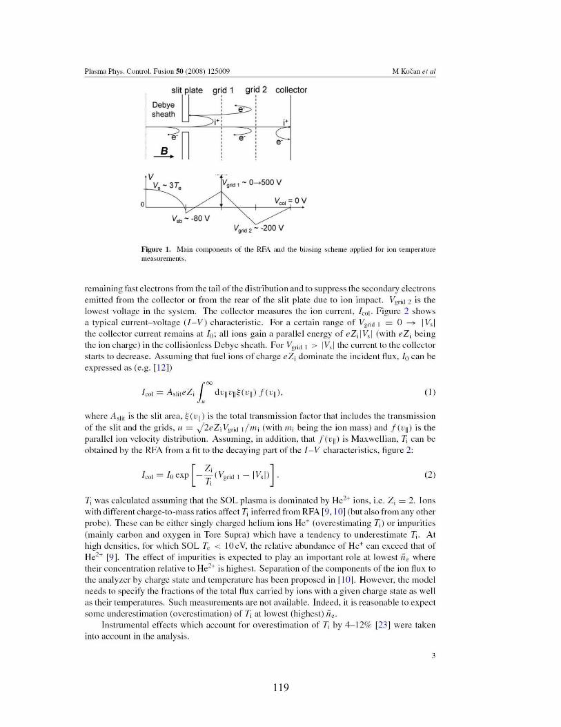
119

Plasma Phys. Control. Fusion 50 (2008) 125009 M Kocan et a/

slit plate

Debyeshealh

gr!d 1,,,

grd 2 collector

(1 )

V'rid 1 - 0~500 V

oL-----"t-;r"'----+-----".,----+-----'V"':O;",;/------OV

V'b - -80 VV'rid 2 - -200 V

Figure 1. Main components of the RFA and the biasing scheme applied for ion temperaturellleaSllrements.

remaining fast electrons fromlhe tail of the distribution and to suppress the secondary electronsemilled frol11 the collector or from the rear of the slit plate due to ion impact. Vgrid 2 is thelowest voltage in the system. The colleclor measures the ion currem, Icol . Figure 2 showsa typical cUITent-voltage (I-V) characteristic. For a certain range of Vgrid 1 = 0 ---+ 1 Vslthe collector current remains at la; ail ions gain a parallel energy of eZilVsl (with eZi beingthe ion charge) in the collisionless Debye sheath. For Vgrid 1 > IVsl the current to the collectorstarts to decrease. Assuming that fuel ions of charge e2i dominate the incident flux. la can beexpressecl as (e.g. [12])

l,a] = A,];,e2; 1"" ciVil VII~(UII) 1(vlI)·u

where As1it is the slit area. ~(vu) is the total transmission factor that includes the transmissionof the slit and the grids, U =J2eZi Vgrid 1/mi (with mi being the ion mass) and !(vu) is theparallel ion velocity distribution. Assuming, in addition, that !(vu) is Maxwellian, li can beobtained by the RFA from a fit to the decaying part of the I-V characteristics, figure 2:

(2)

7j was calcuJated assuming that the SOL plasma is dominated by He2+ ions, i.e. Zi = 2. Ionswith different charge-to-mass ratios affect Ti inferred from RFA [9, 10] (but also from any otherprobe). These can be either singly charged helium ions He+ (overestimating 7j) or impurities

(mainly carbon and oxygen in Tore Supra) which have a tendency to unclerestil11ate li. Athigh densities, for which SOL Te < 10eV, the relative abundance of He+ can exceed that ofHe2+ [9]. The effect of impurities is expected to play an important role at lowest iï e wheretheir concentration relative 10 He2+ is highest. Separation of the components of the ion flux tothe analyzer by charge slate and temperature has been proposed in [10]. However, the modeJneeds to specify the fractions of the total flux carried by ions with a given charge state as weilas their lemperatures. Such measurements are not available. Indeed, it is reasonabJe to expectsome unclerestil11ation (overestimation) of ~ at lowest (highest) "e.

Instrumental effects which account for overestimation of li by 4-12% [23] were takeninto account in the analysis.

3

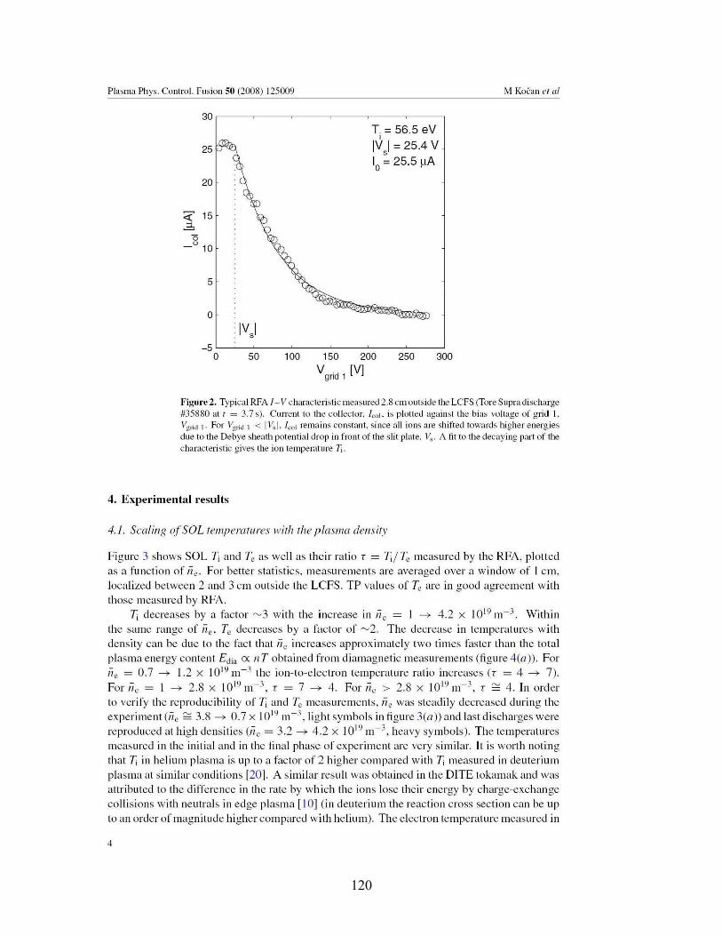
120

Plasma Phys. ControL FlIsion50 (2008) 125009 M Kocan el a/

30,----~--~-~--~-~-____,

T = 56.5 eV1

IV 1 = 25.4 Vs10

= 25.5 ,uA

5

0

IV 1s

-50 50 100 150 200 250 300

V. [V]gnd 1

25

20

Figure 2. Typîcal RFA /-V characteristic measured 2.8 cm outside the LCfS (Tore Supra discharge#35880 at f = 3.7s). Current to tlle col1ector. /col. is plottec! against the bias voltage of grid 1.Vgrid 1· For Vgrid 1 < 1Vsl, /coJ remains constant. since ail ions are shifted towards higher energiesdue ta the Debye sheath potential drop in front of the sht plate. Vs' A fit ta the decaying part of thecharacteristic gives the ion tempemture Ti.

4. Experimental results

4. J. Scalil/g ofSOL remperarures wirh rhe plasma del/sir."

Figure 3 shows SOL Ji and Te as weIl as lheir ratio r = Iii Tc measured by the RFA, plolledas a function of " c. For belter statistics, measurements are averaged over a window of 1cm,localized between 2 and 3 cm outside the LCFS. TP values of Tc are in good agreement withIhose measured by RFA.

~ decreases by a faclor "-'3 with the increase in "e = 1 ----+ 4.2 X 1019 m-3 . Wiùlinthe same range of " c , Tc decreases by a factor of "-'2. The decrease in temperatures withdensily can be due to the faclthat " c increases approximately two times faster than the totalplasma ellergy content Edia <X liT obtained from diamagnetic measurements (figure4(a». For" c = 0.7 ----+ 1.2 x 1019 m-3 the ion-to-electron temperature ratio increases (r = 4 ----+ 7).For " c = 1 ----+ 2.8 X 1019 m-3 , r = 7 ----;.. 4. For "e> 2.8 x 1019 m-3, r 2:: 4. In orderto verify the reproducibility of Ti and Te measurements, " c was steadily decreased during theexperiment ('/c 2:: 3.8 ----+ 0.7 x 1019

111-3

, light symbols in figure 3(a» and lastdischarges werereproduced at high densities (" c = 3.2 ----+ 4.2 X 1019 m-3. heavy symbols). The temperaturesmeasurecl in the initial and in the final phase of experiment are very similar. Il is worth notingthat Ii in helium plasma is up to a factor of 2 higher compared with Ti measured in deuteriLimplasma at similar conditions [20]. A similar result was obtained in the DITE tokamak and wasattribllted to the difference in the rate by which the ions lose their energy by charge-exchangecollisions with nelltrals in edge plasma [10] (in deuterillm the reaction cross section can be upto an order of magnitude higher comparecl with helium). The electron temperature measured in

4

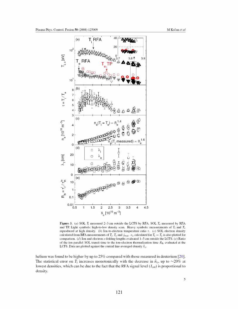
121

Plasma Phys. ControL Fusion 50 (2008) J25OO9 M Kocan et a/

10'

10'

.~._~- 10­._~:::::"

2

4

8 (b)

7

6

5

4

3f------j---+---+---+--+---+---+------1

o

10

•c

f­

"

4.543.51.50.01 L-~_~_~_~_~_~_~-----"

0.5

Figure 3. (a) SOL Ti measured 2-3 cm olltside the LCFS by RFA. SOL Tc measured by RFAand TP. Light symbols: high-to-low density SCllJl. Heavy symbols: measurernents of Ti and Tereprodllced at high density. (b) Ion-to-eJectron temperatllre ratio r. (c) SOL electron densityca1culated from RFA measurements of Ti. Tc and 1+sal. Ile calclllated for Ti = Te is also plotted forcomparison. (d) Ion and electron e-folding lengths evaluated 1-5 cm outside the LCFS. (e) Ratioof the ion parallel SOL transit time to the ion---electron thermalization time R1h evaluated at theLCFS. Datu are plotted against the central line-averaged density Il c .

heliulll was found 10 be higher by up to 25% compared with those llleasured in deuteriulll [20].The statistical erraI' on ~ increases lllonolonically with the decrease in Ile, up to .......,20% allowest densities, which can be due 10 the facl that the RFA signallevel (lcol) is proportional todensity.

5

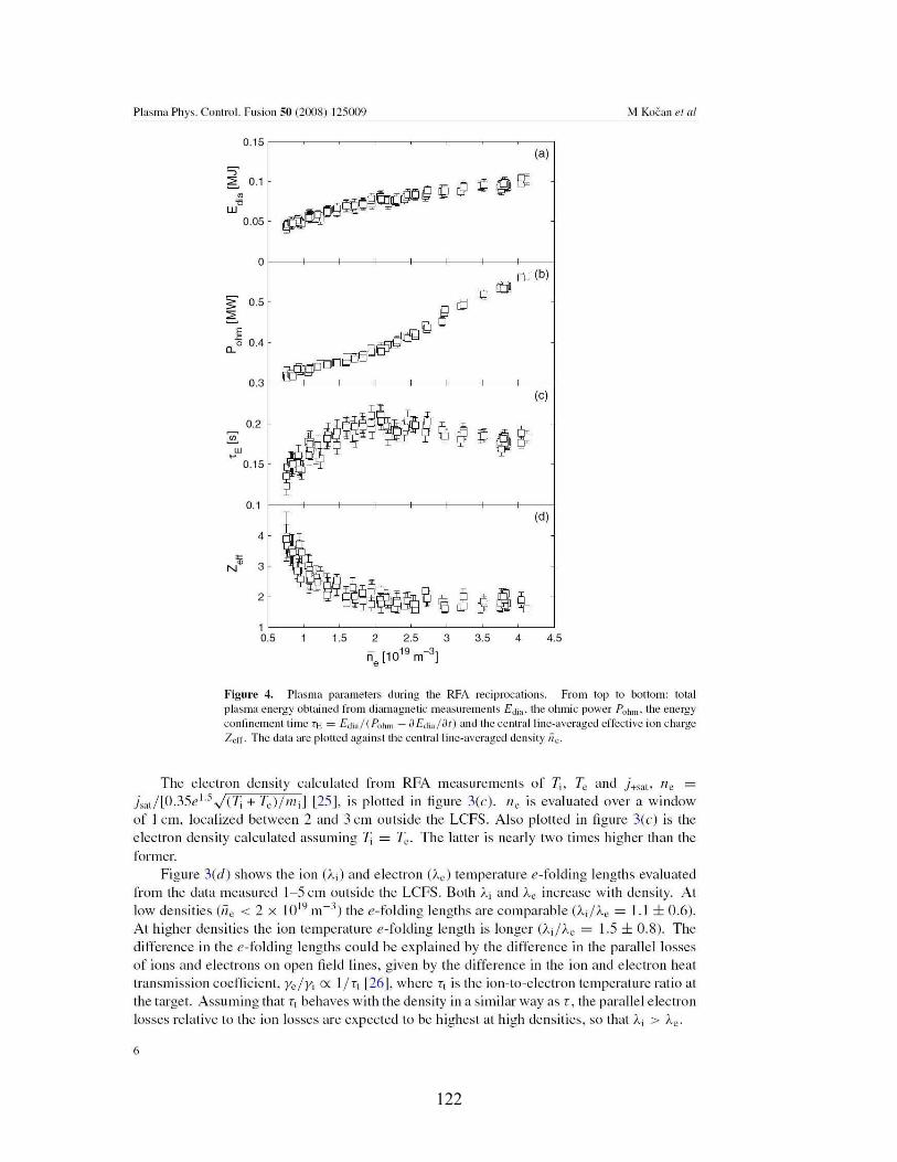
122

Plasma Phys. ControL Fusion 50 (2008) 125009 M Kocan ef a/

4.543.51.5 2 2.5 3

n [1019 m-31e

(a)

oo'3~I,Hj ~ ~ @ EP

~

[jJ (b)

§IÔ!QG

~Q

~~(c)

~~~~~~~ é ~ @~p

~(d)

~aOOS~ç ~ 8 è ~~2

10.5

4

0.1

0.2

0.3

0.4

0.5

o

0.15

0.05

Nll 3

'"~ 0.1

•'"w

Figure 4. Plasma parameters during the RFA reciprocations. From top ta bottom: totalplasma energy obtained from diamagnetic measurements Edia . the ohmic power Pohm , the energyconfinement ti me rr: = Edia/ (Pohm - J Edia/Jr) and the central line-averagecl effective ion chargeZeff. The c1ata are plottecl against the central line-averagecl c1ensily Ile.

The electron density calculatecl From RFA measurements of ~, Tc and j+SUI, I/ è =j'"t/[0.35eI.5~(T; + T,)/III;] [25], is ploned in figure 3(c). Il, is evaluated over a windowof 1cm. localized between 2 and 3 cm outside the LCFS. Also ploUed in figure 3(c) is theelectron density calculated assllming ~ = Tè • The latter is nearly Iwo times higher than theformer.

Figure 3(d) shows the ion (Ài) and electron O'c) temperature e-folding lengths evaluatedfrom the data measured 1-5 cm outside the LCFS. Both Ài and Àe increase with clensity. Atlow densities (II, < 2 x 10'9 m-') the e-l'alding lengths are comparable (À;/À, = 1.1 ± 0.6).At higher densities the ion temperatllre e-folding length is longer (Ài/Àc = 1.5 ± 0.8). Thedifference in the e-folding lengths cou Id be explained by the difference in the parallellossesof ions and electrons on open field lines, given by the difference in the ion and electron heattransmission coefficient, Ye/Yi oc 1/ Tt [26], where Tl is the ion-to-electron temperature ratio atthe targe!. Assllllling that Tl behaves with the density in a similar way as T, the parallel electronlosses relative to the ion losses are expected to be highest al. high densities, so that À j > Àc.

6

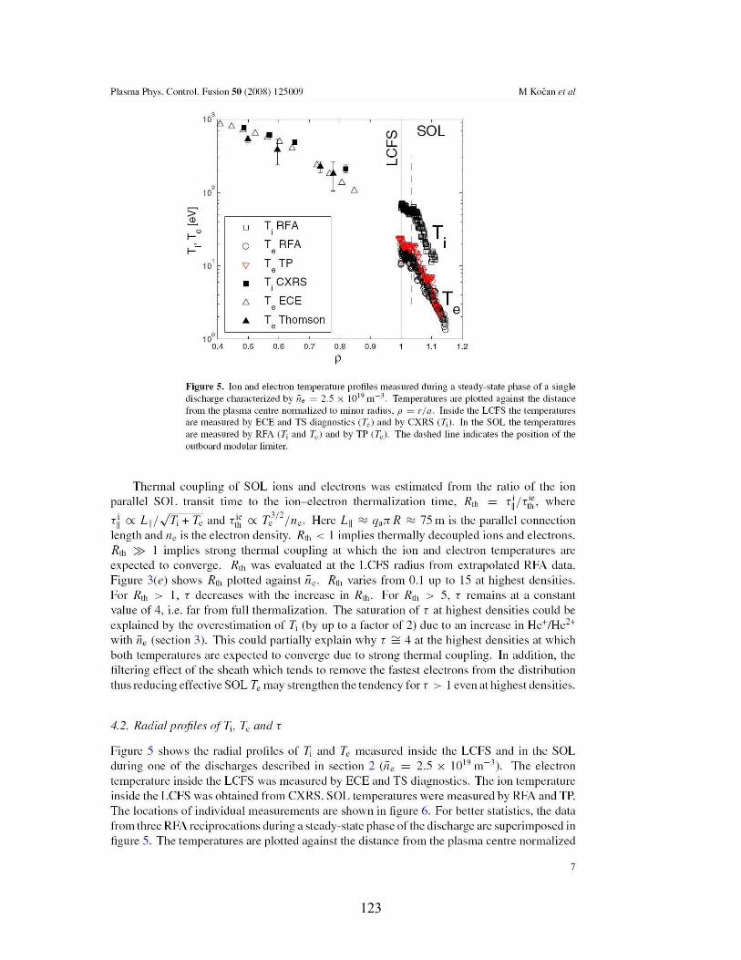
123

Plasma Phys. ControL Fusion 50 (2008) J 25009 M Kocan et a/

10'".!l SOL," ~ (fJ

f ~ LLÜ

"!1"Ii "

--l

10'

:>~

0 T RFAf-w ,

f- a T RFAe

10' 'V T TPe

• TCXRS,

" T ECEe

• T Thomsone

10'DA 0.5 0.6 0.7 0.8 0.9 1.1 1.2

P

Figure 5. Ion and electron temperature profiles measured during a steady-state phase of a singledischarge characterized by Ile = 2.5 X 1019 rn-3 . Temperatures are plotted against the distancefrom the plasma centre nonnalized to rninor radius. p = ria. Inside the LCFS the ternperaturesare measured by ECE and TS diagnostics (Te) and by CXRS (7;). ln the SOL the ternperaturesare ll1easured by RFA (Ti and Te) and by TP (Te). The dashed line indicates the position of theoutboard modular limiter.

Thermal coupling of SOL ions and electrons was eSlimated from the ratio of the ionparallel SOL transit lime to the ion-electron thermalization time, Rlh = rl\/rti~, where

rl\ ex: Lui-J~ + Te and rit~ ex: T~1/2 Ille. Here LU ~ qaJr R ~ 75 m is the parallel connectionlength and IIc is the electron density. Rlh < 1 implies thermally decoupled ions and electrons.Rlh » 1 implies strong thermal coupling at which the ion and eleclron temperatures areexpected to converge. Rlh was evaluated at the LCFS radius from extrapolated RFA data.Figure 3(e) shows Rlh ploued against Tic. Rlh varies from 0.1 up 1.0 15 at highest c1ensities.For Rlh > l, r decreases with the increase in Ru1 . For Rlh > 5, r remains al a constantvalue of 4, i.e. far from full thermalization. The saturation of r at highest densities could beexplained by the overestimation of ~ (by up to a factor of 2) due to an increase in He+/He2+with Tic (section 3). This could partially explain why r 2:: 4 at the highest densities at whichboth temperatures are expected to converge due to strong thermal coupling. In addition, theli1tering effect of the sheath which tends 1.0 remove the fastest electrons from the distributionthus reducing effective SOL Tc may strengthen the tendency for r > 1even at highest densities.

4.2. Radial profiles ofT;, Te al/d r

Figure 5 shows the radial proliles of ~ and Te measured inside the LCFS and in the SOLduring one of the discharges described in section 2 (ii e = 2.5 x 1019 111-3). The electrontemperat-ure insicle the LCFS was measured by ECE and TS diagnostics. The ion temperatureinside the LCFS was obtained from CXRS. SOL temperatures were measured by RFA and TP.The locations of individualmeasurements are shown in ligure 6. For better statistics, the datafrom Ihree RFA reciprocations during a steady-state phase of the discharge are superimposed infigure 5. The temperal1lres are plotted against the distance fromlhe plasma centre normalized

7

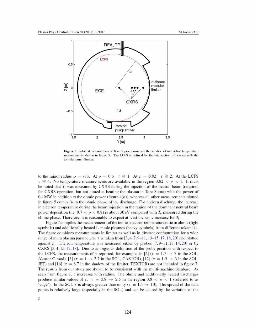
124

Plasma Phys. ControL Fusion 50 (2008) 125009

RFA, TP

M Kocan et a/

0.5

E oN

-0.5

outboardmodularlimiter

-1 L- ~ __".L ~ ___J

1.5 2 2.5 3 3.5

R[m]

Figure 6. Poloidal cross-section of Tore Supra plasma and the location of individual temperaturerneasurements shown in figure 5. The LCFS is defined by tlle intersection of plasma with thetoroidal pump limiter.

ta dle minar radius p = ria. Ar p = 0.6 r ~ 1. At P = 0.82 r ~ 2. At the LCFSr ~ 4. No lemperature measurements are available in the region 0.82 < p < 1. Il mustbe noled lhat Ti was measured by CXRS during the injection of the neulral beiJt11 (requiredfor CXRS operation, bul nol aimed at heating the plasma in Tore Supra) with the power ofOA MW in addition to the ohmic power (figure 4(b)), whereas ail other measuremenls plonedin figure 5 comes From the ohmic phase of the discharge. For a given discharge the increasein electron temperalure during the beam injection in the region of the dominant: neutral beampower deposilion (i.e. 0.7 < p < 0.8) is about 30eV compared with Te measured during theohmic phase. Therefore, it is reasonable 10 expecl alleasl the same increase for~.

Figure 7 compiles the measurements ofthe ion-to-electron temperature ratio in ohmic (lightsymbols) and aclditionally heated L-l11ode plasmas (heavy symbols) from differenl tokamaks.The figure combines measurements in limiter as weIl as in divertor configuration for a widerange of main plasma paramelers. r is taken from [3,4,7,9-1 1, 13-15, 17, 18,20] and platted

against p. The ion remperature was measured eirher by probes [7,9-11, 13, 14,20] or byCXRS [3,4,15.17,18]. Due ta ambiguaus definitian of the probe position with respect tathe LCFS, the measurements of r reparted, for example, in [2] (r = 1.7 ---> 7 in the SOL,Alcatar C-mad), [5] (r = 1 ---> 2.7 in the SOL, CASTOR), [12] Cr = 1.5 ---> 3 in the SOL,JET) and [16] Cr = 8.7 in the shadaw of the limiter, TEXTOR) are nat included in figure 7.The results from our stuc!y are shown to be consistenl with lhe mulli-machine dalabiJse. Asseen From figure 7, r increases with radius. The ohmic and addilionally heated dischargesproduce similar values of r. r = 0.8 ~ 2.5 in the region 0.8 < p < 1 (referred to as'edge'). In the SOL r is always greater than unily (r = 1.5 ~ 10). The spread of the datapoints is relatively large (especially in the SOL) and can be causee! by lhe variation of the

8

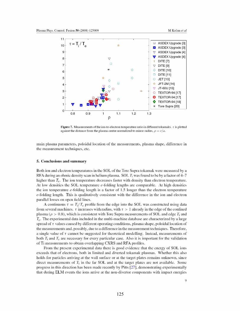
125

Plasma Phys. ControL Fusion 50 (2008) J25009 M Kocan et a/

T=TIT1 e

V 1:1

'V

D

*

D

o

<)

<)

+

D ASDEX UP9rade [3]

1:1 ASDEX UP9rade [3]

'V ASDEX UP9rade [4]

V ASDEX UP9rade [4]

+ DITE [7]

'V DITE [9]

<) DITE [10]

D DITE [11]

o JET[13]

"" JFT-2M [14]

'V JT-GOU [15]

o TEXTOR-94 [17]

o TEXTOR-94 [17]

~ TEXTOR-94 [18]

* Tore Supra [20]OL-~--~--~--~--~-_---l

0.8 0.9p

1.1 1.2 1.3

Figure 7. Measurements of the ion-to-eJectron temperature ratio in c1ifferent tokamaks. ris plotteclagainst the distance frolll the plasma centre Ilonlmlized to rninor radius, p = rja.

main plasma parameters, poloidal location of the measurements, plasma shape, c1ifference inthe measuremenl techniques, etc.

5. Conclusions and summary

80th ion and e1ectron lemperatures in the SOL oflhe Tore Supra tokamak were measurecl by aRFA during an ohmic density scan in helium plasma. SOL Ii was found to be by a factor of4-7higher than Te. The ion temperalure decreases faster with clensity than electron temperature.At low densities the SOL temperaI-ure e-folding lengths are comparable. At high densitiesthe ion temperaI-ure e-folding length is a factor of 1.5 longer than the electron temperaturee-folding length. This is qualitatively consistent with the c1ifference in the ion and electronparallel losses on open field lines.

A continuolls r = Iii Tc profi le from the edge into the SOL was constrllcted using dataFrom severalmachines. r increases with radius, with r > 1 already in the edge of the confinedplasma (p > 0.8), which is consistent with Tore Supra measurements of SOL and edge Ii andTe. The experimental data included in the multi-machine database are characterized by a largespread of r values caused by different operating conditions, plasma shape, poloidallocation ofthe measurements and. possibly, due to a difference in the measurement techniques. Therefore,a single value of r cannot be suggested for theoretical modelling. Instead, meaSllrements ofboth Ti and Te are necessary for every parliClllar case. Aiso it is important for the validationof Ti measurements to obtain overlapping CXRS and RFA profiles.

From the present experimental data there is good evidellce that the energy of SOL ionsexceeds that of electrons, both in limited and diverted tokamak plasmas. Whether this alsoholds for particies arriving at the wall surface or at the target plates remains unknown, sincedirect measuremenls of 7i in the far SOL and at the target plates are not available. Someprogress in this direction has been made recelltly by Pius [27], demonstrating experimelltallythat during ELM events the ions arrive at the non-divenor components with impact energies

9

126

Plasma Phys. ControL Fusion 50 (2008) 125009 M Koean et al

Ihat would provide non-negligible erosion rates in future tllngsten-wall machines. Therefore,high priority should be given to the development ofdiagnostics for measurementof ion energiesin the far SOL and al the target plates.

Acknowledgments

The authors wish to lhank Ors X Garbet, T Hoang and P Lotte for useflll comments.This work, supported by the European Communities under the contract of Associationbelween EURATOM and CEA, was carried our within the framework of the European FusionOevelopment Agreement. The views and opinions expressed herein do not necessarily re/leclthose of the European Commission.

References

[1] Kirschner A, Philipps V, Winter J and Kogler U 2000 NI/cl. Fusiol/ 40 989[2] Wan A S. Yang T F. Lipschultz Band LaBombard B 1986 Rel'. Sei. fnsTrw/I. 57 1542[3] Reich M. Wolfrum E. Schweinzer J. Ehrnler H, Horton L D, Neuhauser J and ASDEX Upgrade Team 2(X)4

Plasma Pllys. CollTrol. FI/sion 46 797[4] Reich M, Wolfrum E, HOlton L D. Schweinzer J, Neuhauser J and ASDEX UpgradeTeam 2(X)4 31sr EPSCol/f.

01/ Plasma Physics (Londol/, 28 June-2 July 2(04)[5] Kocall M, Panek R. StOckel J. Hron M. Gunn J P and Dejarnac R 2007 1. Nile/. Mara 363-365 1436[6] Erents S K and Stangeby PC 1982 J. NllcI. Mara 111-112 165[7] Stangeby PC. McCracken G M, Erents S K. Vi nce J E and Wiklen R 19831. Vae. Sei. Tee/Illol. A J 1302[8] Pitts R A. McCracken G M and Matthews G F 19891. NlicI. Motel: 162-164 568[9] Matthews G F. Pitts R A, McCracken G M and Stangeby PC 1991 NllcI. FI/sion 31 1495

[10] Pitts R A 1991 PhD Thesis University of London[1 1] Pitts R A 1996 Com,.ih. Plasma Phys. 36 87[12] Guo H Y. Matthews G F. Davies S J. Erents S K, Horton L D. Mond R D. Stangeby PC 1996 Cont,.ib. Plasllla

Phys. 3681[13] Pitts R A. Chavan R. Davies S J. Erents S K. Kaveney G. Matthews G F, Neill G, Vince JE and Duran 12003

Rel'. Sei. fl1srrl/lll. 744644-57

[14] Uehara K. Tawakami T. Amemiya H. Hothker K. Cosler A and BiegerW 1998 NI/cl. Fusiol/ 381665[15] Asakura N. Koide Y, Itami K. Shimizu K. Tsuji-Iio S, Sakurai Sand Sakasai A 19971. NI/cl. Maret: 241-243 559[16] Hothker K, Belitz H-J. Bieger W ancl Amellliya H 1990 Rel'. Sei. fl/stmm. 61 114[17] Hllber A. Pospieszczyk A. Unterberg B. Brix M. Meltens Ph. Philipps V and Schweer B 2000 Plasma Phys.

COlITrol. Fusion 42 569[18] Kreter A 2001 PIID Thesis Düsse1clorf University

[19] Staudenmaier G. Staib P ancl Poschenrieder W 19801. NI/cl. Mare!: 121-126 121[20] Kocan M eT al 2008 Measurement.s of scrape-off layer ion-t.o-electron temperature ratio in Tore Supra ohmic

plasmas 1. NI/cl. Mater. submitted[21] Saarelma S et 012005 Plasma Pllyx. COl/trol. FI/siol/ 47 713[22] Jacqui not J and Hoang G T 2004 Plasma Sei. Tecllllol. 6 2101[23] Kocall M. GUl1n J P. Kornm M. Pasc~d J- Y. Gauthier E and Bonhomme G 2008 Rel'. Sei. fl/Sll"llllT. 79073502[24] Gunn J P er 012002 C:.ecll. 1. PItYJ. 52 1107[25] Hutchinson [ H 1987 Pitys. FII/id.\ 30 3777[26] Stangeby PC 2000 Tite Plasma BOI/l/da,.y in Magneric FI/siol/ Del'iees (Bristol: Inslitute of Physics Pllblishing)

p 649[27] Pitts R A, Fundamenski W. Erents S K. Andrew Y. Lomte A. Silva C ancl JET-EFDA contributors 2006 Nlle/.

FI/sion 46 S2

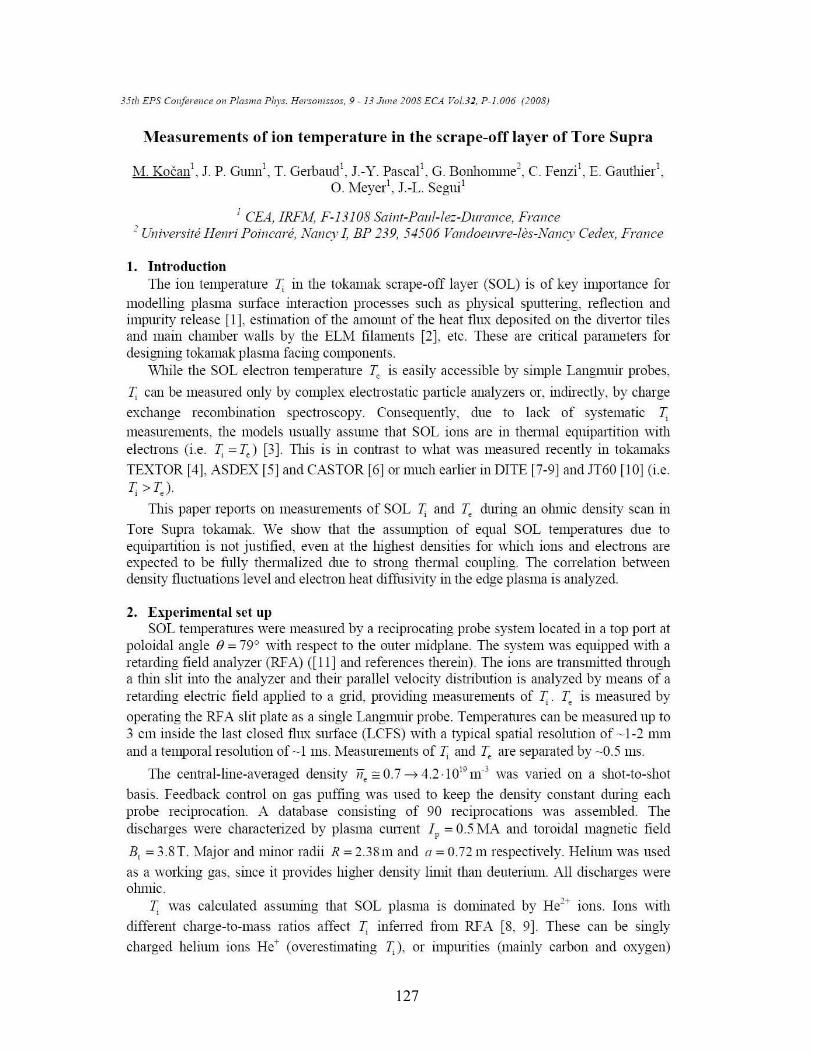
127

351h EPS Conference 0/1 Plasma Pilys. Hersollissos, 9 - 13 JUlie 1008 ECA Vol.3l, P-1.006 (lOOS)

Measurements of ion temperature in the scrape-off layer of Tore Supra

M. Kocan l, .T. P. Gunni, T. Gerbaud!, .T.-Y. Pascal l

, G. BOlùlonllne2, C. Fenzi l

, E. Gauthier!,O. Meyer', .T.-L. Segui'

1 CEA, fRFlvi, F-1310S Sah/t-Palll-Ie:-Dllmllce, Frai/cel UlI;";ers;té Henri Poi1lcaré, .Nancy 1, BP 239, 54506 Valldoeuvre-Iès-Nancy Cedex, Fm1lce

1. IntroductionThe ion temperature 1; in the tokamak scrape-off layer (SOL) is of key importance for

modeIling plasma surface interaction processes such as physical sputtering, reflection andimpurity release [1], estimation of the mnouIlt of the heat flux deposited on the divertor tilesand main chamber walls by the ELM filaments [2], etc. These are critical parmneters fordesigning tokamak plasma facing components.

While the SOL electron temperahlre T~ is easily accessible by simple Langmuir probes,

1; can be measured only by complex electrostatic particle mmlyzers or, indirectly, by charge

exchange recombination spectroscopy. Consequently, due to Jack of systematie T,measurements, the models usually assume that SOL ions are in thermal equipal1ition \Vithelectrons (i.e. 1; = T.) [3]. This is in contrast to \Vhat \Vas measured recently in tokamaks

TEXTOR [4], ASDEX [5] and CASTOR [6] or llluch earlier in DITE [7-9] and JT60 [10] (i.e.r; > T.).

This paper reports on measurements of SOL T, and T~ during an olunie density scan in

Tore Supra tokamak. \Ve show that the assumption of equal SOL temperahlres due toequipmtition is not justified, even at the highest densities for which ions and electrons areexpected to be fully thennalized due to strong thermal coupling. The cOlTelation betweendensity fluctuations level and electron heat diffusivity in the edge plasma is analyzed.

2. Expel'iment.lI set upSOL temperatures were measured by a reciprocating probe system located in a top pOlt at

poloidal angle B = 79° with respect to the outer midplane. The system was equipped \Vith aretarding field analyzer (RFA) ([11] ancl references therein). The ions are transmitted througha thin slit into the analyzer and thei..r parallel velocity distribution is mmlyzed by means of aretarding electric field applied to a grid, providing measurements of T,. T~ is measured by

operating the RFA slit plate as a single Langmuir probe. Temperahlres can be measured up to3 cm inside the last closed flux surface (LeFS) with a typical spatial resolution of -1-2 nUlland a temporal resolution of -1 ms. Measurements of 1; and T~ are separated by -0.5 ms.

The central-line-averaged density li. == 0.7 ----t 4.2, 1O!9 m-3 was varied on a shot-to-shot

basis. Feedback control on gas pufting \Vas used to keep the density constant during eachprobe reciprocation. A database consisting of 90 reciproeations \Vas assembled. Thedisclmrges were characterized by plasma CUITent f p = 0.5 MA and toroidal nmgnetic field

Br = 3.8T. rvlajor anc1minor radii R = 2.38m and a = O.72m respectively. Helium was used

as a \Vorking gas, since it provides higher density limit than deuterium. AIl diseharges wereolunie.

1; was ealculated assuming that SOL plasma is dominated by He1- ions. Ions \Vith

different charge-to-mass ratios affect T, infelTed from RFA [K 9]. These ean be singly

charged helium ions He+ (overestimating 1;), or impurities (nminly c.mbon and oxygen)

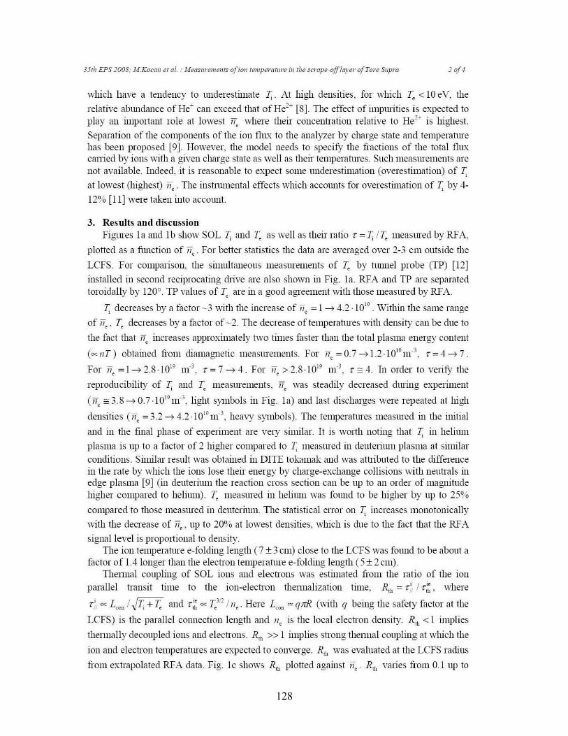
128

351h EPS 2008: M.Koml! cIal. : MeasliremelJls ofio/l remperalllre in The scrape-ojJlaya ofTO/·e Supra 20f4

which have a tendeney ta underestinmte T;. At high densities, for which Te < 10 eV, the

relative ablUldanee of He- can exceed that of He2- [8]. The effect of impurities is expected ta

play an imp0l1ant role at lowest lie where their concentration relative ta He2- is highest.

Separation of the components of the ion flux ta the analyzer by charge state and temperaturehas been proposed [9]. However. the model needs ta specify the fractions of the total fluxcalTied by ions \vith a given charge state as \vell as their temperahlres. Such me<Jsurements arenot available. Illdeed, it is reasonable ta expect some underestimation (overestinmtion) of T,.<Il lowest (highest) li•. The instnunental effects which aceounts for overestilllation of T, by 4­

12% [Il] were taken into account.

3. Results and discussionFigures la and 1b show SOL T, and T.: as weil as their ratio T = T, /r. measured by RFA,

plotted as a function of lie. For better statistics the data are averaged over 2-3 cm outside the

LCFS. For eomparison, the simultaneous measurements of r. by hUlnei probe (TP) [12J

installed in second reciprocating drive are <1lso shO\vn in Fig. la. RFA and TP are separatedtoroidally by 120°. TP values of Te are in a good agreement with those measured by RFA.

T, decreases by a factor ~3 with the increase of li. = 1~ 4.2 .1019. Within the same range

of li., T. decreases by a factor of ~2. The clecrease oftemperahlres with density can be due ta

the fact that lie inereases approximately two times faster than the total plasma energy content

(oc liT) obtained fiom dialllagnetic measurements. For lie = O. 7~ 1.2 .1019 m-3, T = 4~ 7 .

For li. =1~ 2.8.1019 nf', T= 7 ~ 4. For li. >2.8.1019 m-3, T == 4. In order ta verify the

reproducibility of T, and T. measurements. lie was steadily decreased during experiment

(lie == 3.8 --?o 0.7 ·1 019 nf', light symbols in Fig. la) and last clischarges were repe<Jtec1 at high

densities (lie = 3.2~ 4.2 .1019 nf', heavy symbols). The temperahlres measured in the initial

and in the final phase of experiment are very simil<Jr. Il is worth noting that T, in helium

plasm<J is up ta a factor of 2 higher compared ta T, measured in deuterium plaSIl1<J at similarconditions. Similar result was obtained in DITE tokamak and was attributed ta the differencein the rate by which the ions lose their energy by charge-exchange collisions with neutrals inedge plasma [9] (in deuteriulll the reaction cross section can be up ta an arder of magnitudehigher compared ta helium). Te measured in helium was found ta be higller by up ta 25%

compared ta those measured in deuterium. The statistical erTor on T, increases monotonically

\vith the decrease of li., up ta 20% at lowest densities, which is due ta the fact that the RFA

signallevel is prop0l1ional ta density.The ion temperahlre e-folding length (7 ± 3cm) close ta the LCFS was found ta be about a

factor of 1.4 longer than the electron temperahlre e-folding length (5 ± 2cm).Thennal coupling of SOL ions and eleetrons was estimated from the ratio of the ion

parallel transit time ta the ion-electron thennalization lime, Rlh = r;, / T:~, where

T;, oc Leon l ,IT, + r. and T;~ 0<: T.:3!2/ lie . Here Lcon '" qJrR (with q being the safety factor at the

LCFS) is the parallel connection length and Il. is the local electron density. Rth < l implies

thennally decoupled ions and electrons. Rrn »1 implies strong thermal coupling at which the

ion and eleetron temperatures are expected ta converge. Rrh was evaluated at the LCFS radius

from extrapolated RFA clata. Fig. le shows Rth plotted against lie. Rlh varies from 0.1 up ta

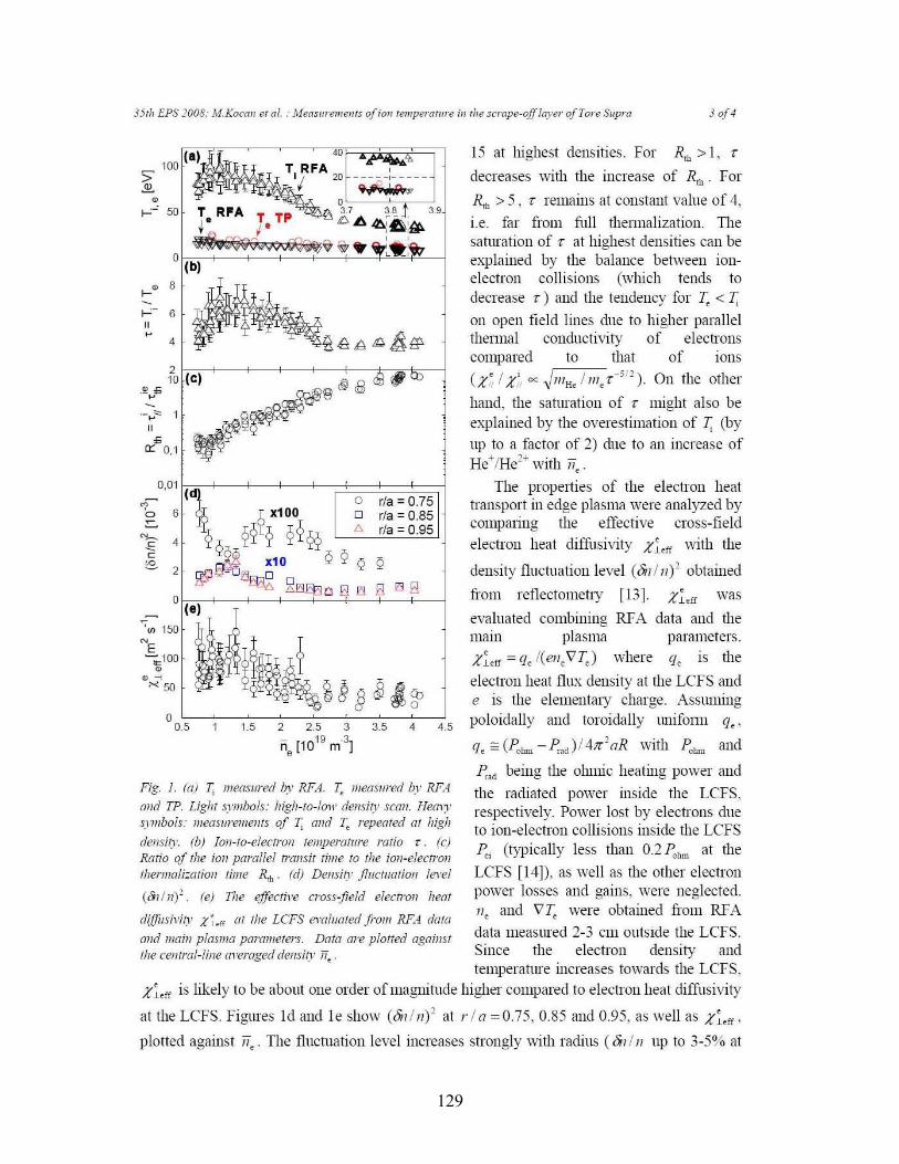
129

35111 EPS 1008: M.KoCGI! elal. . Mea5f1remen75 0li011 femperarure in The 5crape-ofJ/ayer olTore SI/pm 3014

Fig. 1. (aj T, measllred b.l' RFA. T, lIIeasl/red by RFA

alld TP. Lighr symbols. high-ro-101l' del/siry Scall. Hem')'symbols: lIIeaSl/remCIlfS of T, alld T, repeared ar high

dClISit)·, (b) fOIl-ro-e/ecrroll remperarure l'ario r. (c)Rario of the iOIl paralfef rramir time ro tlie iOIl-efectl'ollrhcl'ma;=afioll rime Reh • (dj DellSit)' fll/ctllarioll fel-e/

((ji/IIi. (ej The ejfecrire cross-jie/d electl'OII hem

diifllsil'iry l'~..ff ar thc LCFS e1'0111ared 11'011I RFA dara

alld lIIaill plasma paralllelers. Data are ploned againsrthe cellnnl-lille al'eraged demi!)' /i•.

rIa = 0.75rIa = 0.85rIa = 0.95

oo

'"

6>­

"

15 at highest densities. For RIb> L 1"

decreases \Vith the increase of RIb' For

Rlh > 5, T remains at constant value of 4,

I.e. far from full thennalization. Thesaturation of r at highest densities can beexplained by the balance between ion­electron collisions (which tends todecrease r) and the tendency for T~ < T..on open field hnes due ta higller pm'allelthermal conductivity of electronscompared to that of Ions

(X~ / X;, lX JIIIH./I1I~ [-512). On the other

hand, the sahlration of 1" nlight also beexplained by the overestimation of T.. (by

up ta a factor of 2) due to an increase ofHe+/He1+ with li•.

The propelties of the electron heattransport in edge plasma \Vere analyzed bycompanng the effective cross-field

electron heat diffusivity X1.ff with the

density fluctuation level (01//11)" obtained

from retlectometry [13]. X1~ff was

evaluated combining RFA data and thenmm plasma parameters.

X1.ff = q~ /(el/~ VT~) where q~ îs the

electron heat flux density at the LCFS ande is the elementmy charge. Assunling

a O.L5---C--~1.'=5--c2:---c'2."C5--:3--3".cc5--;4---J4_5 poloic1ally ancl toroidally unifonn q.,

ile [t019 m-3

] q~=(~hm-PraJ)/4ff"/R \Vith ~hm and

P"ad being the olunic heatillg po\Ver and

the mcliated power inside the LCFS,respectively. Power lost by electrons dueto ion-electron collisions inside the LCFSP.:i (typically less than 0.2 Pohm at the

LCFS [14]), as well as the other electronpower losses and gains. were neglected./~ and VT~ \Vere obtaillecl from RFA

data measured 2-3 cm outside the LCFS.Since the electron dellsity andtemperature increases towards the LCFS,

X1.ff is likely to be about one order of magnitude higher compared ta electron heat diffusivity

at the LCFS. Figures Id and le show (ali/II)" at 1'/ a =0.75, 0.85 and 0.95, as weIl as X1~ff'

plotted against li•. The fluctuation level increases strongly \Vith radius ((jn/II up ta 3-5% at

130

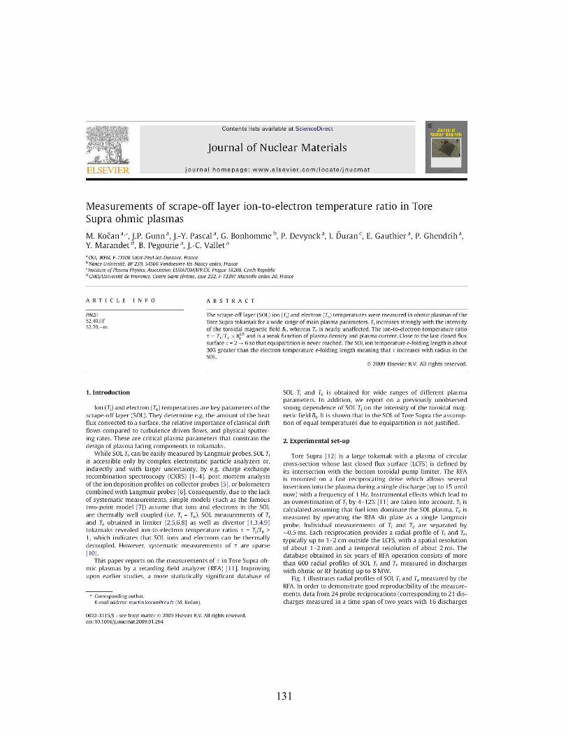
131

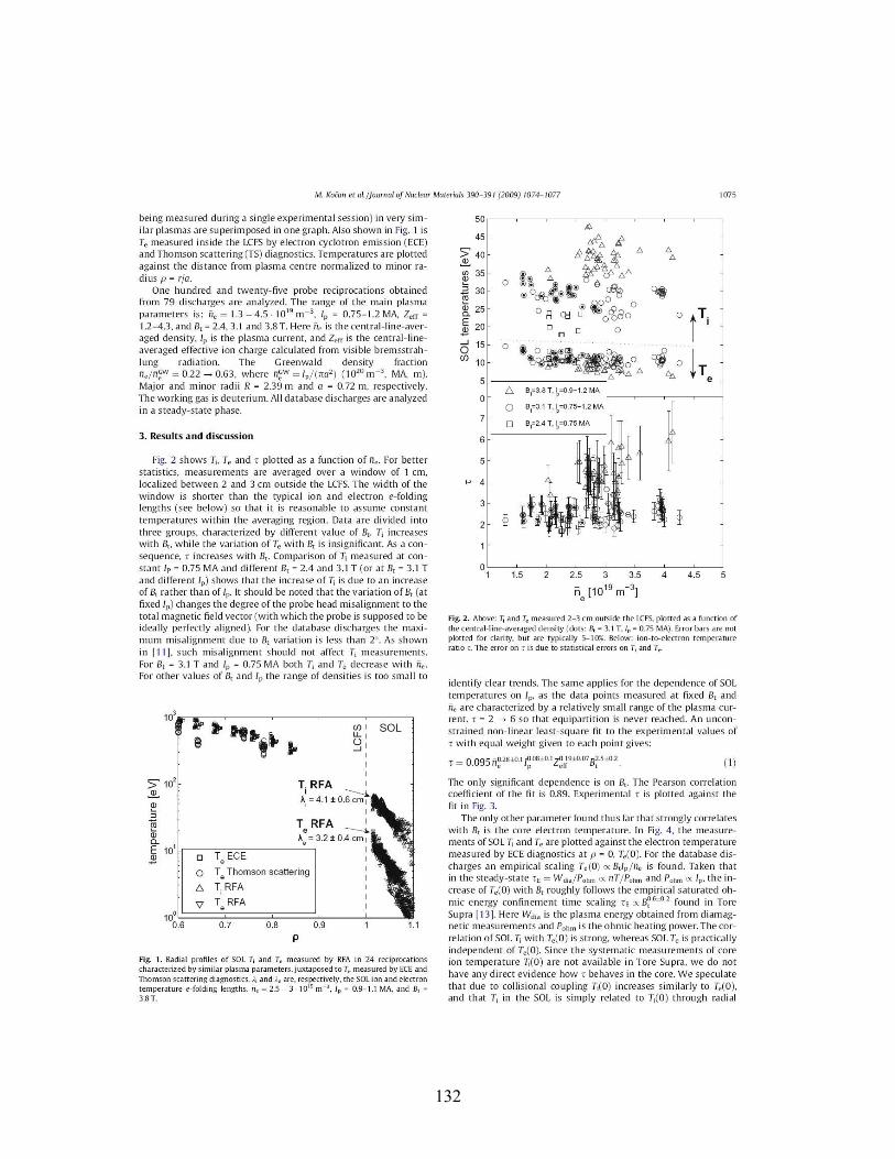
132

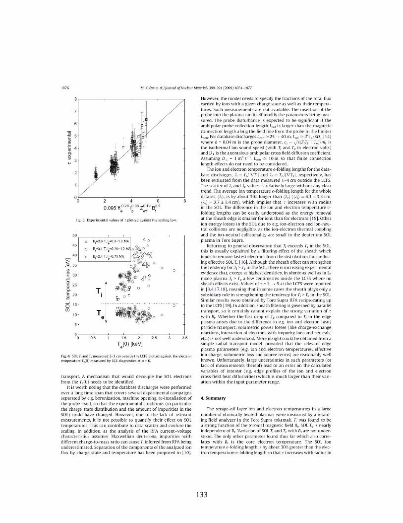
133

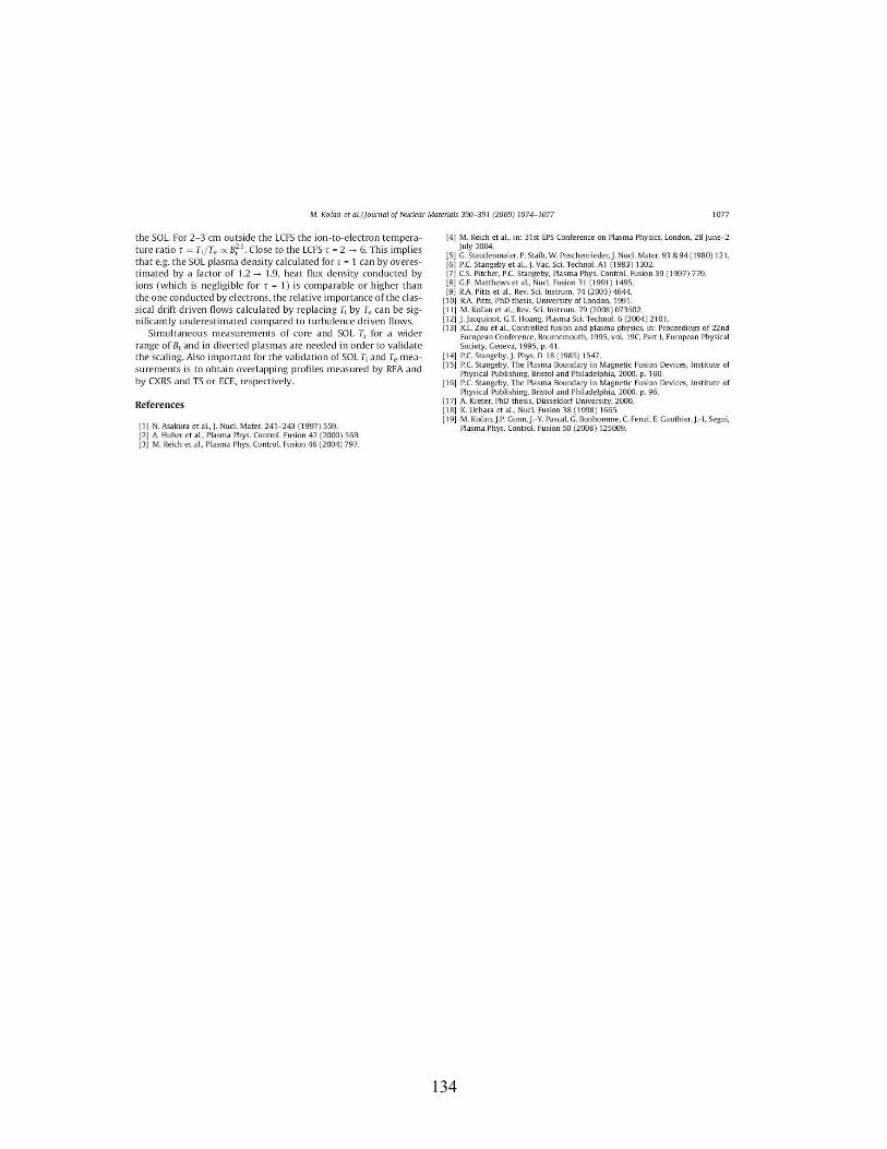
134

135

Influence of the plasma density and the radiated power

fraction on the Tore Supra scrape-off layer

M Kočan, J P Gunn, P Tamain 1, O Meyer, J-Y Pascal, J-L Segui and

J-C Vallet

CEA, IRFM, F-13108 Saint-Paul-lez-Durance, France. 1 EURATOM/UKAEA Fusion Association, Culham Science Centre,

Oxfordshire OX14 3DB, UK

E-mail: martin.kocan@cea.fr

Abstract. The scrape-off layer (SOL) ion and electron temperatures, iT and eT ,

electron density en , and the ion saturation current density satj are studied in

Tore Supra deuterium plasma for a wide range of densities en and radiated

power fractions radf , including detached plasma. In ohmic plasma for low en

and radf , 43/ −≅ei TT and 50≅iT eV at the last closed flux surface. At

highest en and radf as well as in detached plasma, ei TT ≅ , both only a few

electron volts. Detachment is also associated with the drop of both satj and en

as well as the flattening of the radial profiles from the SOL to the edge of the

confined plasma, which is consistent with earlier Langmuir probe measurements

[McCracken G M et al 1987 J. Nucl. Mater. 145-147 181]. At constant en an

increase of radf by about ~30% coincides with a decrease of SOL iT by almost a

factor of 2, whereas SOL eT is much less affected. A strong drop of iT but also

a substantial decrease of eT with the increase of radf is obtained from a simple

power balance model of the temperatures in the edge of the confined plasma.

PACS 52.25.Fi, 52.25.Xz, 52.55.Fa, 52.70.-m, 52.70.Ds

136

1. Introduction

One of the options for the ohmic plasma start-up phase in the current ITER design

consists of two limiter modules located at the low-field side. The limiters will define the plasma

last closed flux surface (LCFS) for about 30 seconds before the X-point divertor configuration is

established [1]. The start-up plasma will be, therefore, characterized by the configuration close to

that of the large circular tokamaks. Because of their small plasma-wetted area, the limiters will

receive relatively large heat loads. Modelling activities have been recently focused on the

estimation of the power crossing the LCFS as well as the resulting power load distribution on

ITER limiters (e.g. [2, 3]). Taking into account the usual uncertainties in code predictions, the

difference between the predicted heat flux densities to the ITER start-up limiters (<6 MW m-2 [2])

and their engineering limit (8 MW m-2 [4]) appears to be considerably small. Therefore, the

modellers ask for further SOL measurements that could help to validate the codes [3].

In this work we study the scrape-off layer (SOL) ion and electron temperatures, electron

density and the ion saturation current density for a broad range of core plasma density and

radiated power fraction, including detached plasmas, in the large circular limiter tokamak Tore

Supra [5]. The SOL parameters are measured by a retarding field analyzer (RFA) [6]. We focus

mainly on ohmic discharges which are characterized by relatively low SOL heat fluxes and thus

allow for probe measurements up to the LCFS.

Improving upon earlier studies (e.g. [7-11]), we show more systematic measurements of

the SOL iT which is an essential parameter for interpretation of the Langmuir probe

measurements and modelling. Only a very limited database of SOL iT is available (see [11] and

references therein). In addition, the paper reports on first measurements of SOL iT in detached

plasma as well as previously unreported variation of SOL iT with the radiated power. The paper

also addresses some improvements of the RFA probe operation.

In order to avoid confusion, the “detachment” refers here to a steady state with poloidally

symmetric radiation shifted inside the LCFS by about 30 cm, or 60% of the minor radius. The

‘attached’ plasma, in turn, refers to the state with poloidally asymmetric radiation localized just

above the plasma contact point.

In this paper the temperatures are stated in electron volts and the indication “parallel”

relates to the magnetic field vector B.

The paper is organized as follows. The main plasma parameters of the discharges studied

in this paper are stated in section 2. The principle of the RFA probe is briefly described in section

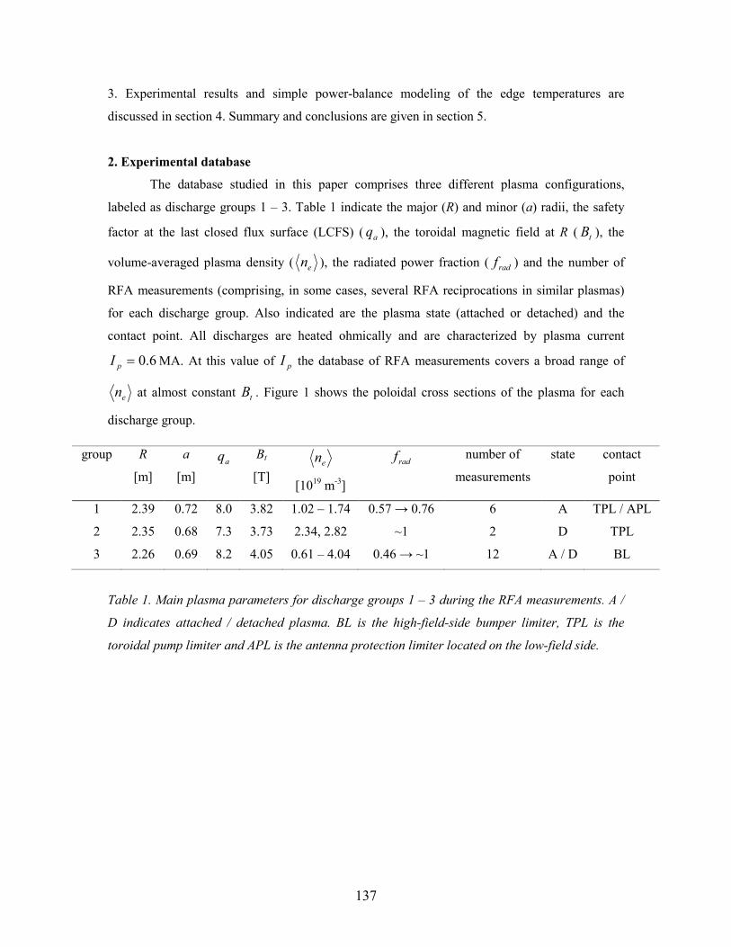
137

3. Experimental results and simple power-balance modeling of the edge temperatures are

discussed in section 4. Summary and conclusions are given in section 5.

2. Experimental database

The database studied in this paper comprises three different plasma configurations,

labeled as discharge groups 1 – 3. Table 1 indicate the major (R) and minor (a) radii, the safety

factor at the last closed flux surface (LCFS) ( aq ), the toroidal magnetic field at R ( tB ), the

volume-averaged plasma density ( en ), the radiated power fraction ( radf ) and the number of

RFA measurements (comprising, in some cases, several RFA reciprocations in similar plasmas)

for each discharge group. Also indicated are the plasma state (attached or detached) and the

contact point. All discharges are heated ohmically and are characterized by plasma current

6.0=pI MA. At this value of pI the database of RFA measurements covers a broad range of

en at almost constant tB . Figure 1 shows the poloidal cross sections of the plasma for each

discharge group.

Table 1. Main plasma parameters for discharge groups 1 – 3 during the RFA measurements. A /

D indicates attached / detached plasma. BL is the high-field-side bumper limiter, TPL is the

toroidal pump limiter and APL is the antenna protection limiter located on the low-field side.

group R

[m]

a

[m] aq Bt

[T] en

[1019 m-3]

radf number of

measurements

state contact

point

1 2.39 0.72 8.0 3.82 1.02 – 1.74 0.57 → 0.76 6 A TPL / APL

2 2.35 0.68 7.3 3.73 2.34, 2.82 ~1 2 D TPL

3 2.26 0.69 8.2 4.05 0.61 – 4.04 0.46 → ~1 12 A / D BL

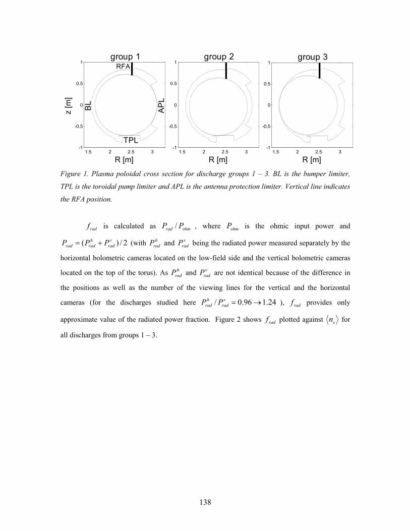
138

1.5 2 2.5 3-1

-0.5

0

0.5

1

R [m]

z [m]

BL

APL

1.5 2 2.5 3-1

-0.5

0

0.5

1

R [m]1.5 2 2.5 3

-1

-0.5

0

0.5

1

R [m]

group 1 group 2 group 3

TPL

RFA

Figure 1. Plasma poloidal cross section for discharge groups 1 – 3. BL is the bumper limiter,

TPL is the toroidal pump limiter and APL is the antenna protection limiter. Vertical line indicates

the RFA position.

radf is calculated as ohmrad PP / , where ohmP is the ohmic input power and

2/)( vrad

hradrad PPP += (with h

radP and vradP being the radiated power measured separately by the

horizontal bolometric cameras located on the low-field side and the vertical bolometric cameras

located on the top of the torus). As hradP and v

radP are not identical because of the difference in

the positions as well as the number of the viewing lines for the vertical and the horizontal

cameras (for the discharges studied here 24.196.0/ →=vrad

hrad PP ), radf provides only

approximate value of the radiated power fraction. Figure 2 shows radf plotted against en for

all discharges from groups 1 – 3.

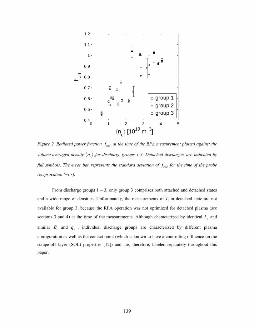
139

0 1 2 3 4 50.4

0.5

0.6

0.7

0.8

0.9

1

1.1

1.2

⟨ne⟩ [1019 m−3]

f rad

group 1group 2group 3

Figure 2. Radiated power fraction radf at the time of the RFA measurement plotted against the

volume-averaged density en for discharge groups 1-3. Detached discharges are indicated by

full symbols. The error bar represents the standard deviation of radf for the time of the probe

reciprocation (~1 s).

From discharge groups 1 – 3, only group 3 comprises both attached and detached states

and a wide range of densities. Unfortunately, the measurements of iT in detached state are not

available for group 3, because the RFA operation was not optimized for detached plasma (see

sections 3 and 4) at the time of the measurements. Although characterized by identical pI and

similar tB and aq , individual discharge groups are characterized by different plasma

configuration as well as the contact point (which is known to have a controlling influence on the

scrape-off layer (SOL) properties [12]) and are, therefore, labeled separately throughout this

paper.

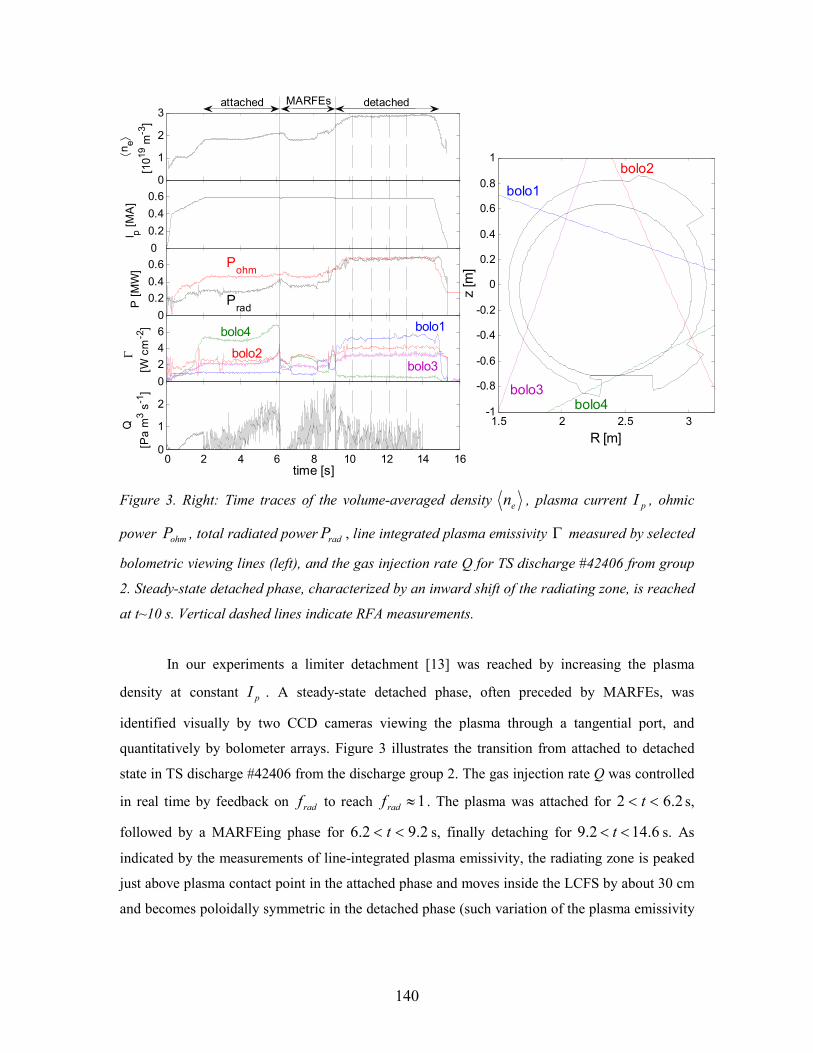
140

1.5 2 2.5 3-1

-0.8

-0.6

-0.4

-0.2

0

0.2

0.4

0.6

0.8

1

R [m]

z [m]

2 4 6 8 10 12 140

0.2

0.4

0.6

I p [MA]

2 4 6 8 10 12 140

0.20.4

0.6

P [MW]

0

1

2

3⟨ne⟩

[101

9 m-3]

2 4 6 8 10 12 140

246

time [s]

Γ

[W cm-2]

0 2 4 6 8 10 12 14 160

1

2

Q

[Pa m3 s-1 ]

time [s]

Pohm

Prad

bolo4

bolo2bolo3

bolo1

bolo4

attached detached

bolo1

MARFEs

bolo2

bolo3

Figure 3. Right: Time traces of the volume-averaged density en , plasma current pI , ohmic

power ohmP , total radiated power radP , line integrated plasma emissivity Γ measured by selected

bolometric viewing lines (left), and the gas injection rate Q for TS discharge #42406 from group

2. Steady-state detached phase, characterized by an inward shift of the radiating zone, is reached

at t~10 s. Vertical dashed lines indicate RFA measurements.

In our experiments a limiter detachment [13] was reached by increasing the plasma

density at constant pI . A steady-state detached phase, often preceded by MARFEs, was

identified visually by two CCD cameras viewing the plasma through a tangential port, and

quantitatively by bolometer arrays. Figure 3 illustrates the transition from attached to detached

state in TS discharge #42406 from the discharge group 2. The gas injection rate Q was controlled

in real time by feedback on radf to reach 1≈radf . The plasma was attached for 2.62 << t s,

followed by a MARFEing phase for 2.92.6 << t s, finally detaching for 6.142.9 << t s. As

indicated by the measurements of line-integrated plasma emissivity, the radiating zone is peaked

just above plasma contact point in the attached phase and moves inside the LCFS by about 30 cm

and becomes poloidally symmetric in the detached phase (such variation of the plasma emissivity

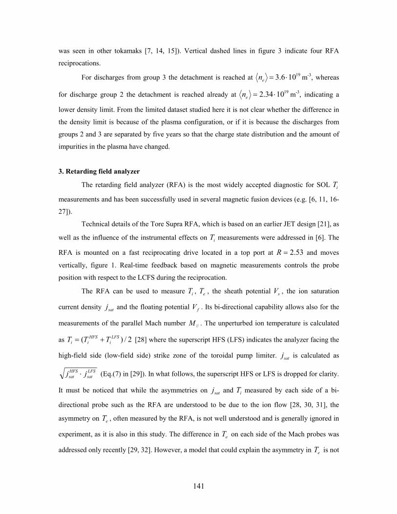
141

was seen in other tokamaks [7, 14, 15]). Vertical dashed lines in figure 3 indicate four RFA

reciprocations.

For discharges from group 3 the detachment is reached at 19106.3 ⋅=en m-3, whereas

for discharge group 2 the detachment is reached already at 191034.2 ⋅=en m-3, indicating a

lower density limit. From the limited dataset studied here it is not clear whether the difference in

the density limit is because of the plasma configuration, or if it is because the discharges from

groups 2 and 3 are separated by five years so that the charge state distribution and the amount of

impurities in the plasma have changed.

3. Retarding field analyzer

The retarding field analyzer (RFA) is the most widely accepted diagnostic for SOL iT

measurements and has been successfully used in several magnetic fusion devices (e.g. [6, 11, 16-

27]).

Technical details of the Tore Supra RFA, which is based on an earlier JET design [21], as

well as the influence of the instrumental effects on iT measurements were addressed in [6]. The

RFA is mounted on a fast reciprocating drive located in a top port at 53.2=R and moves

vertically, figure 1. Real-time feedback based on magnetic measurements controls the probe

position with respect to the LCFS during the reciprocation.

The RFA can be used to measure iT , eT , the sheath potential sV , the ion saturation

current density satj and the floating potential fV . Its bi-directional capability allows also for the

measurements of the parallel Mach number //M . The unperturbed ion temperature is calculated

as 2/)( LFSi

HFSii TTT += [28] where the superscript HFS (LFS) indicates the analyzer facing the

high-field side (low-field side) strike zone of the toroidal pump limiter. satj is calculated as

LFSsat

HFSsat jj ⋅ (Eq.(7) in [29]). In what follows, the superscript HFS or LFS is dropped for clarity.

It must be noticed that while the asymmetries on satj and iT measured by each side of a bi-

directional probe such as the RFA are understood to be due to the ion flow [28, 30, 31], the

asymmetry on eT , often measured by the RFA, is not well understood and is generally ignored in

experiment, as it is also in this study. The difference in eT on each side of the Mach probes was

addressed only recently [29, 32]. However, a model that could explain the asymmetry in eT is not

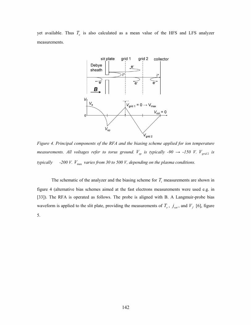
142

yet available. Thus eT is also calculated as a mean value of the HFS and LFS analyzer

measurements.

Figure 4. Principal components of the RFA and the biasing scheme applied for ion temperature

measurements. All voltages refer to torus ground. spV is typically -90 → -150 V. 2gridV is

typically -200 V. maxV varies from 30 to 500 V, depending on the plasma conditions.

The schematic of the analyzer and the biasing scheme for iT measurements are shown in

figure 4 (alternative bias schemes aimed at the fast electrons measurements were used e.g. in

[33]). The RFA is operated as follows. The probe is aligned with B. A Langmuir-probe bias

waveform is applied to the slit plate, providing the measurements of eT , satj , and fV [6], figure

5.

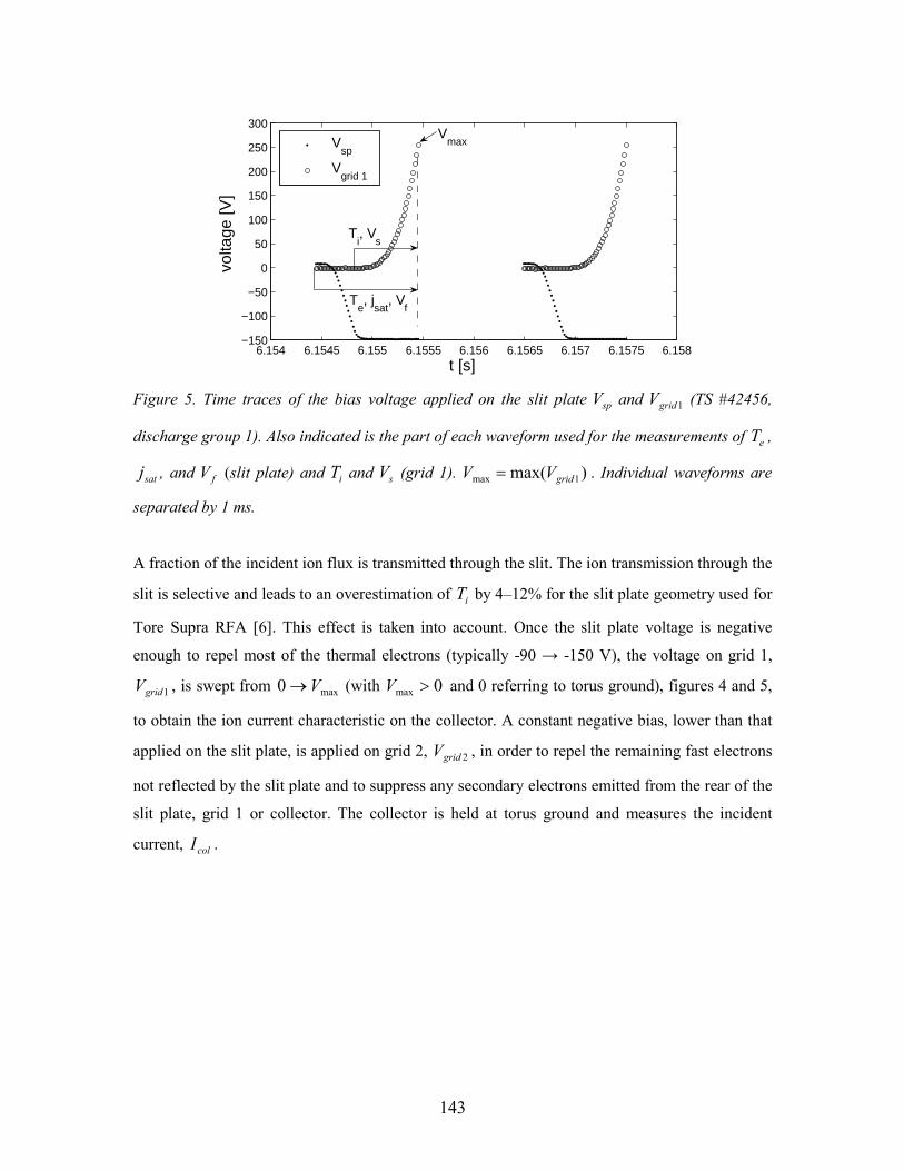
143

6.154 6.1545 6.155 6.1555 6.156 6.1565 6.157 6.1575 6.158−150

−100

−50

0

50

100

150

200

250

300

t [s]

volta

ge [V

]

Vsp

Vgrid 1

Te, j

sat, V

f

Ti, V

s

Vmax

Figure 5. Time traces of the bias voltage applied on the slit plate spV and 1gridV (TS #42456,

discharge group 1). Also indicated is the part of each waveform used for the measurements of eT ,

satj , and fV (slit plate) and iT and sV (grid 1). )max( 1max gridVV = . Individual waveforms are

separated by 1 ms.

A fraction of the incident ion flux is transmitted through the slit. The ion transmission through the

slit is selective and leads to an overestimation of iT by 4–12% for the slit plate geometry used for

Tore Supra RFA [6]. This effect is taken into account. Once the slit plate voltage is negative

enough to repel most of the thermal electrons (typically -90 → -150 V), the voltage on grid 1,

1gridV , is swept from max0 V→ (with 0max >V and 0 referring to torus ground), figures 4 and 5,

to obtain the ion current characteristic on the collector. A constant negative bias, lower than that

applied on the slit plate, is applied on grid 2, 2gridV , in order to repel the remaining fast electrons

not reflected by the slit plate and to suppress any secondary electrons emitted from the rear of the

slit plate, grid 1 or collector. The collector is held at torus ground and measures the incident

current, colI .

144

0 10 20 30 40-101234567891011

Vgrid 1

[V]

I col [ µA]

Vgrid 1

[V]

I col [ µA]

0 50 100 150 200 250-101234567891011

Vs

Ti = 6 ± 1 eV

Vs = 2 V

I0 = 10.2 µA

Vs

Ti = 29 ± 4 eV

Vs = 11 V

I0 = 8.0 µA

Te = 9 eV T

e = 4 eV

Figure 6. Typical RFA I-V characteristics for two different maximum bias voltages applied on

grid 1. Left: attached plasma (TS discharge #42455 from group 1 at t =5.0 s, 191025.1 ⋅=en m-

3, 6 mm outside the LCFS). Right: detached plasma (TS discharge #42463 from group 2 at t = 7.2

s, 19103.2 ⋅=en m-3, 3 mm inside the LCFS). iT , sV , and 0I were obtained from the fit Eq.(2)

to the I-V characteristic. eT was measured by the slit plate working as a Langmuir probe. All

parameters were measured by the analyzer facing the HFS.

Figure 6 shows typical current-voltage (I-V) characteristics ( colI against 1gridV ) measured

by the RFA. For certain range of sgrid VV →= 01 the collector current is approximately constant

since all ions gain a parallel energy of siVeZ (with ieZ being ion charge) in the collisionless

Debye sheath in front of the slit plate. For sgrid VV >1 the collector current decreases as the

retarding potential begins to repel the slowest ions of the distribution. Assuming that fuel ions

dominate the incident flux, colI can be expressed as [21]:

∫∞

=u

i vfvvdveZAI )()( ////////slitcol ξ (1)

where slitA is the slit area, )( //vξ is the total transmission factor that includes the transmission of

the slit and the grids, igrid1i /2 mVeZu = (with im being the ion mass) is the minimum ion

145

velocity needed to overcome the repulsive force of grid 1 biased to 1gridV , and )( //vf is the

parallel ion velocity distribution. Assuming, in addition, that )( //vf is Maxwellian, iT can be

obtained from a fit to the decaying part of the I-V characteristic:

( ) .exp grid1i

i0col

−−= sVV

TZ

II (2)

Since spV and 1gridV are not swept simultaneously, figure 5, the measurements of eT and

iT by Tore Supra RFA are separated by ~0.5 ms (during which the probe moves radially by less

than 1 mm). In principle, one could sweep both electrodes simultaneously and use only grid 2 to

repel the electrons from the collector. However, repelling most of the thermal electrons by the slit

plate may prevent the ionization of the neutral gas inside the RFA cavity that could affect iT

measurements (see e.g. figure 4(b) in [34]).

The spatial resolution of the RFA is defined by the radial extension of the probe

collection area increased by the radial displacement of the probe during the measurement of a

single I-V characteristic. For eT , satj , and fV the collection area is defined by the orifice drilled

into the CFC protective housing, through which the plasma flows towards the slit plate. For iT

and sV the collection area is defined by the slit plate aperture. The orifice and the aperture

dimensions are respectively 7 mm × 3 mm and 5 mm × 30 µm. For discharge groups 1 and 2 both

the orifice and the aperture were oriented horizontally and for group 3 vertically. The vertical

displacement of the RFA during the measurement of a single I-V characteristic is about 1 mm,

except at the target position where the probe velocity is zero. Since the RFA is located close to

the top of the plasma, the vertical and the radial displacement are almost identical. Therefore, for

discharge groups 1 and 2 the radial resolution is about 4 mm for eT , satj , and fV , and about 1

mm for iT and sV . For discharge group 3 the radial resolution of the RFA is approximately 8 mm

for eT , satj , and fV , and about 6 mm for iT and sV . As shown in Sec. 4, both the radial

separation of iT and eT measurements as well as the radial resolution of the probe are much

smaller than the typical SOL temperature and density e-folding lengths.

Returning to the bias voltage applied to grid 1, a wide range of iT reported in our study

required an optimization of the voltage range for given plasma conditions. In general, the

146

maximum voltage applied to grid 1, maxV , should be low enough so that the major part of the I-V

characteristic is sampled above the noise level of colI , but yet high enough to capture the

exponentially decaying slope of the I-V characteristic. This implies the optimal value of maxV of

about is TV 3+ . Since iT and sV are a priori unknown, maxV can only be adjusted for a given

plasma conditions by repetitive measurements. For attached discharges, the optimal value of

500200max −=V V (figure 6, left), depending on applied heating power and plasma density. For

detached discharges the optimal value of maxV was found to be an order of magnitude smaller

(figure 6, right). Further optimization implemented for 1gridV in Tore Supra RFA include a real-

time feedback on maxV based on the probe position with respect to the LCFS which accounts for

the radial variation of iT and sV and a quadratic waveform instead of the usually applied simple

linear sweep (e.g. [17, 20, 23-25]) in order to acquire more points of the I-V characteristic at the

steepest slope of colI (figure 5).

Finally, it is worth mentioning that satj from the RFA slit plate is found to be

systematically lower than that measured simultaneously by a tunnel probe (TP) [35] in Tore

Supra SOL (figure 7). A similar discrepancy was observed earlier in JET between satj measured

by the RFA [24] and the turbulent transport probe [36]. In [37] this discrepancy was attributed to

the attenuation of ion flux due to the deflection of ions in the magnetic pre-sheath above the RFA

protective walls attached to the slit plate, and quantified using particle-in-cell (PIC) simulations.

The attenuation decreases the effective probe collecting area, so that satj inferred from the ion

saturation current measurements is smaller by a factor attγ (referred to as attenuation factor). In

the Tore Supra RFA the incident ion current can be attenuated in a similar way on the inner walls

of the CFC orifice through which the plasma flows towards the slit plate (see [6]). The ratio of

satj measured by the TP and the RFA provides an approximate value

2103.082.0 →≅+≅ eatt Tγ (the TP has a collecting area clearly defined by the tunnel orifice

[35] and is therefore immune to the attenuation [29]). The dependence of attγ on eT is consistent

with the scaling of the magnetic pre-sheath thickness [38, 39]. Similar values of attγ were found

in unpublished PIC simulation study which reproduces [37] for Tore Supra RFA geometry. In this

paper, the experimental values of satj are multiplied by attγ .

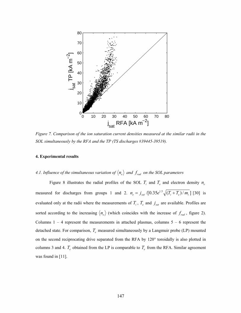
147

0 10 20 30 40 50 60 70 800

10

20

30

40

50

60

70

80

jsat

RFA [kA m−2]

j sat T

P [k

A m

−2]

Figure 7. Comparison of the ion saturation current densities measured at the similar radii in the

SOL simultaneously by the RFA and the TP (TS discharges #39445-39519).

4. Experimental results

4.1. Influence of the simultaneous variation of en and radf on the SOL parameters

Figure 8 illustrates the radial profiles of the SOL iT and eT and electron density en

measured for discharges from groups 1 and 2. ]/)(35.0/[ 5.1ieisate mTTejn += [30] is

evaluated only at the radii where the measurements of iT , eT and satj are available. Profiles are

sorted according to the increasing en (which coincides with the increase of radf , figure 2).

Columns 1 – 4 represent the measurements in attached plasmas, columns 5 – 6 represent the

detached state. For comparison, eT measured simultaneously by a Langmuir probe (LP) mounted

on the second reciprocating drive separated from the RFA by 120° toroidally is also plotted in

columns 3 and 4. eT obtained from the LP is comparable to eT from the RFA. Similar agreement

was found in [11].

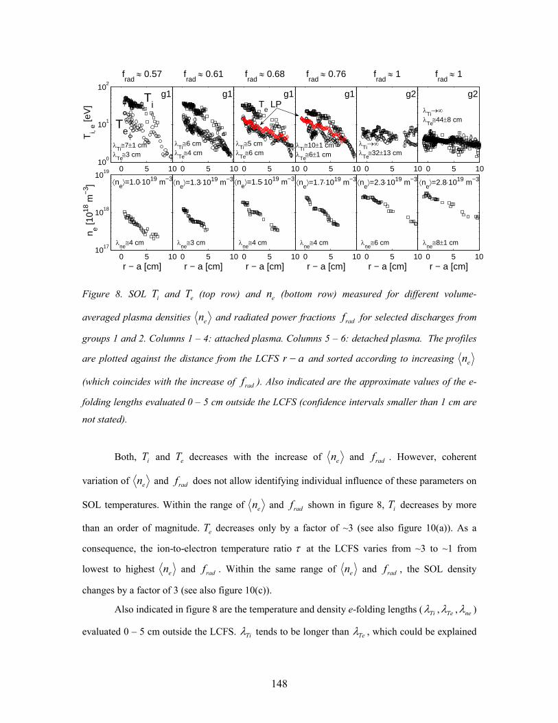
148

0 5 1010

0

101

102

frad

≈ 0.57T

i, e [e

V]

0 5 1010

17

1018

1019

r − a [cm]

n e [1018

m−3

]

0 5 10

frad

≈ 0.61

0 5 10r − a [cm]

0 5 10

frad

≈ 0.68

0 5 10r − a [cm]

0 5 10

frad

≈ 0.76

0 5 10r − a [cm]

0 5 10

frad

≈ 1

0 5 10r − a [cm]

0 5 10

frad

≈ 1

0 5 10r − a [cm]

Ti

Te

Te LP

g1 g1 g1 g1 g2 g2

⟨ne⟩=1.0⋅1019 m−3 ⟨n

e⟩=1.3⋅1019 m−3 ⟨n

e⟩=1.5⋅1019 m−3 ⟨n

e⟩=1.7⋅1019 m−3 ⟨n

e⟩=2.3⋅1019 m−3 ⟨n

e⟩=2.8⋅1019 m−3

λTi≅7±1 cm

λTe≅3 cm

λTi≅6 cm

λTe≅4 cm

λTi≅5 cm

λTe≅6 cm

λTi≅10±1 cm

λTe≅6±1 cm

λTi→∞

λTe≅32±13 cm

λTi→∞

λTe≅44±8 cm

λne≅4 cm λ

ne≅3 cm λ

ne≅4 cm λ

ne≅4 cm λ

ne≅6 cm λ

ne≅8±1 cm

Figure 8. SOL iT and eT (top row) and en (bottom row) measured for different volume-

averaged plasma densities en and radiated power fractions radf for selected discharges from

groups 1 and 2. Columns 1 – 4: attached plasma. Columns 5 – 6: detached plasma. The profiles

are plotted against the distance from the LCFS ar − and sorted according to increasing en

(which coincides with the increase of radf ). Also indicated are the approximate values of the e-

folding lengths evaluated 0 – 5 cm outside the LCFS (confidence intervals smaller than 1 cm are

not stated).

Both, iT and eT decreases with the increase of en and radf . However, coherent

variation of en and radf does not allow identifying individual influence of these parameters on

SOL temperatures. Within the range of en and radf shown in figure 8, iT decreases by more

than an order of magnitude. eT decreases only by a factor of ~3 (see also figure 10(a)). As a

consequence, the ion-to-electron temperature ratio τ at the LCFS varies from ~3 to ~1 from

lowest to highest en and radf . Within the same range of en and radf , the SOL density

changes by a factor of 3 (see also figure 10(c)).

Also indicated in figure 8 are the temperature and density e-folding lengths ( Tiλ , Teλ , neλ )

evaluated 0 – 5 cm outside the LCFS. Tiλ tends to be longer than Teλ , which could be explained

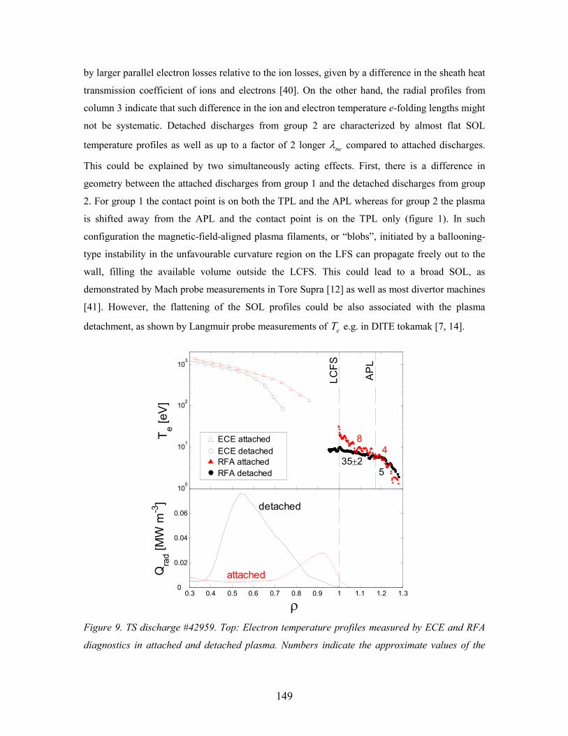
149

by larger parallel electron losses relative to the ion losses, given by a difference in the sheath heat

transmission coefficient of ions and electrons [40]. On the other hand, the radial profiles from

column 3 indicate that such difference in the ion and electron temperature e-folding lengths might

not be systematic. Detached discharges from group 2 are characterized by almost flat SOL

temperature profiles as well as up to a factor of 2 longer neλ compared to attached discharges.

This could be explained by two simultaneously acting effects. First, there is a difference in

geometry between the attached discharges from group 1 and the detached discharges from group

2. For group 1 the contact point is on both the TPL and the APL whereas for group 2 the plasma

is shifted away from the APL and the contact point is on the TPL only (figure 1). In such

configuration the magnetic-field-aligned plasma filaments, or “blobs”, initiated by a ballooning-

type instability in the unfavourable curvature region on the LFS can propagate freely out to the

wall, filling the available volume outside the LCFS. This could lead to a broad SOL, as

demonstrated by Mach probe measurements in Tore Supra [12] as well as most divertor machines

[41]. However, the flattening of the SOL profiles could be also associated with the plasma

detachment, as shown by Langmuir probe measurements of eT e.g. in DITE tokamak [7, 14].

0.4 0.5 0.6 0.7 0.8 0.9 1 1.1 1.210

0

101

102

103

ρ

Te [eV]

LCFS

APL

0.3 0.4 0.5 0.6 0.7 0.8 0.9 1 1.1 1.2 1.30

0.02

0.04

0.06

ρ

Qrad [MW m

-3]

ECE attachedECE detachedRFA attachedRFA detached

8

35±24

5

attached

detached

Figure 9. TS discharge #42959. Top: Electron temperature profiles measured by ECE and RFA

diagnostics in attached and detached plasma. Numbers indicate the approximate values of the

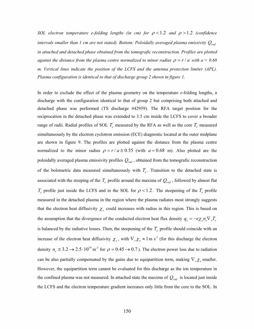
150

SOL electron temperature e-folding lengths (in cm) for 2.1<ρ and 2.1>ρ (confidence

intervals smaller than 1 cm are not stated). Bottom: Poloidally averaged plasma emissivity radQ

in attached and detached phase obtained from the tomografic reconstruction. Profiles are plotted

against the distance from the plasma centre normalized to minor radius ar /=ρ with a = 0.68

m. Vertical lines indicate the position of the LCFS and the antenna protection limiter (APL).

Plasma configuration is identical to that of discharge group 2 shown in figure 1.

In order to exclude the effect of the plasma geometry on the temperature e-folding lengths, a

discharge with the configuration identical to that of group 2 but comprising both attached and

detached phase was performed (TS discharge #42959). The RFA target position for the

reciprocation in the detached phase was extended to 3.5 cm inside the LCFS to cover a broader

range of radii. Radial profiles of SOL eT measured by the RFA as well as the core eT measured

simultaneously by the electron cyclotron emission (ECE) diagnostic located at the outer midplane

are shown in figure 9. The profiles are plotted against the distance from the plasma centre

normalized to the minor radius 55.0/ ≅= arρ (with 68.0=a m). Also plotted are the

poloidally averaged plasma emissivity profiles radQ , obtained from the tomografic reconstruction

of the bolometric data measured simultaneously with eT . Transition to the detached state is

associated with the steeping of the eT profile around the maxima of radQ , followed by almost flat

eT profile just inside the LCFS and in the SOL for 2.1<ρ . The steepening of the eT profile

measured in the detached plasma in the region where the plasma radiates most strongly suggests

that the electron heat diffusivity eχ could increases with radius in this region. This is based on

the assumption that the divergence of the conducted electron heat flux density ereee Tneq ∇−= χ

is balanced by the radiative losses. Then, the steepening of the eT profile should coincide with an

increase of the electron heat diffusivity eχ , with 1≈∇ erχ m s-1 (for this discharge the electron

density 19105.22.3 ⋅→≅en m-3 for 7.045.0 →=ρ ). The electron power loss due to radiation

can be also partially compensated by the gains due to equipartition term, making erχ∇ smaller.

However, the equipartition term cannot be evaluated for this discharge as the ion temperature in

the confined plasma was not measured. In attached state the maxima of radQ is located just inside

the LCFS and the electron temperature gradient increases only little from the core to the SOL. In

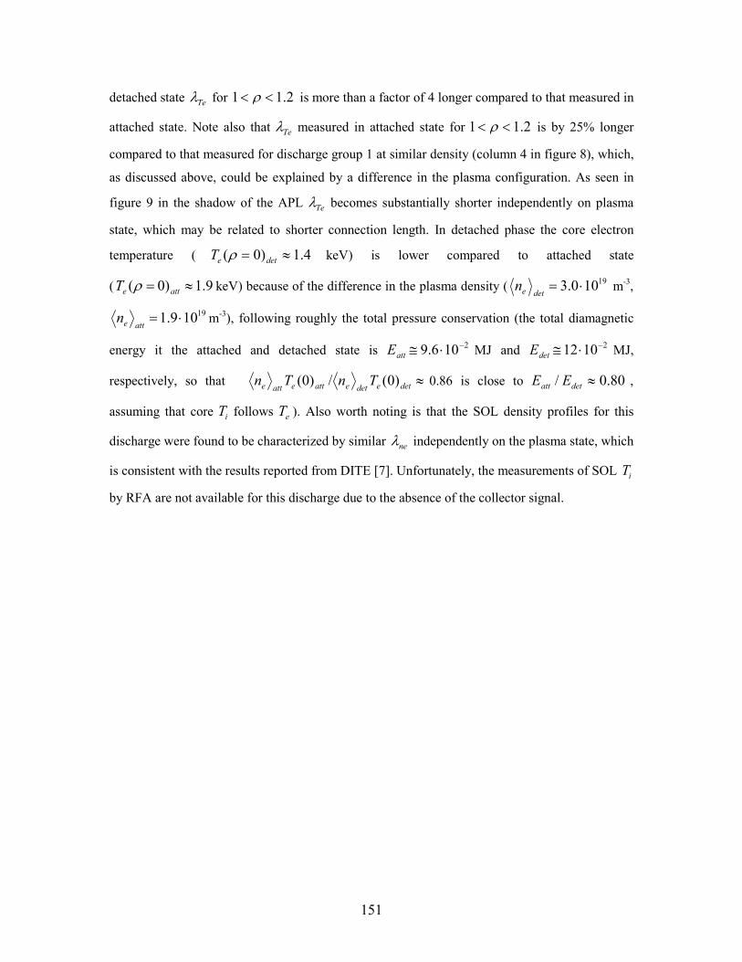
151

detached state Teλ for 2.11 << ρ is more than a factor of 4 longer compared to that measured in

attached state. Note also that Teλ measured in attached state for 2.11 << ρ is by 25% longer

compared to that measured for discharge group 1 at similar density (column 4 in figure 8), which,

as discussed above, could be explained by a difference in the plasma configuration. As seen in

figure 9 in the shadow of the APL Teλ becomes substantially shorter independently on plasma

state, which may be related to shorter connection length. In detached phase the core electron

temperature ( 4.1)0( ≈= deteT ρ keV) is lower compared to attached state

( 9.1)0( ≈= atteT ρ keV) because of the difference in the plasma density ( 19100.3 ⋅=deten m-3,

19109.1 ⋅=atten m-3), following roughly the total pressure conservation (the total diamagnetic

energy it the attached and detached state is 2106.9 −⋅≅attE MJ and 21012 −⋅≅detE MJ,

respectively, so that ≈detedeteatteatte TnTn )0(/)0( 0.86 is close to 80.0/ ≈detatt EE ,

assuming that core iT follows eT ). Also worth noting is that the SOL density profiles for this

discharge were found to be characterized by similar neλ independently on the plasma state, which

is consistent with the results reported from DITE [7]. Unfortunately, the measurements of SOL iT

by RFA are not available for this discharge due to the absence of the collector signal.

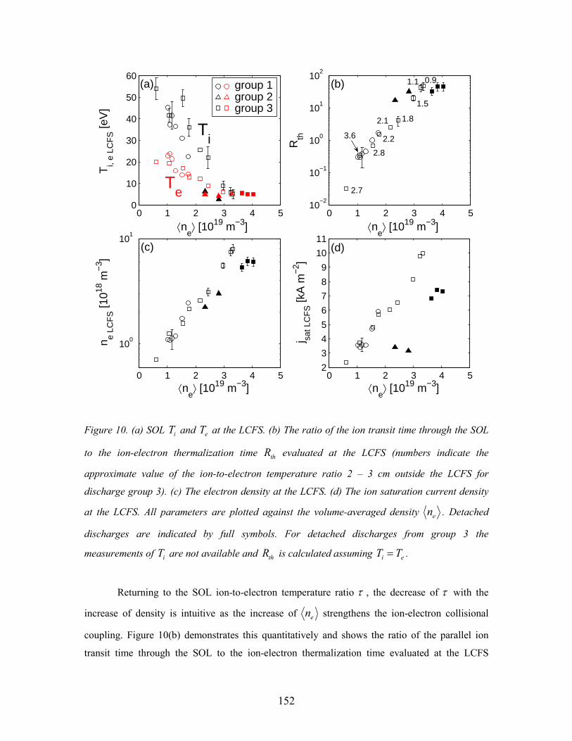
152

0 1 2 3 4 50

10

20

30

40

50

60

⟨ne⟩ [1019 m−3]

Ti,

e LC

FS [e

V]

0 1 2 3 4 510

−2

10−1

100

101

102

⟨ne⟩ [1019 m−3]

Rth

0 1 2 3 4 5

100

101

⟨ne⟩ [1019 m−3]

n e LC

FS [1

018 m

−3]

0 1 2 3 4 52

3

4

5

6

7

8

9

10

11

⟨ne⟩ [1019 m−3]

j sat L

CF

S [k

A m

−2]

Ti

Te

group 1group 2group 3

2.7

2.8

2.2

2.1 1.8

1.5

1.1 0.9

3.6

(a) (b)

(c) (d)

Figure 10. (a) SOL iT and eT at the LCFS. (b) The ratio of the ion transit time through the SOL

to the ion-electron thermalization time thR evaluated at the LCFS (numbers indicate the

approximate value of the ion-to-electron temperature ratio 2 – 3 cm outside the LCFS for

discharge group 3). (c) The electron density at the LCFS. (d) The ion saturation current density

at the LCFS. All parameters are plotted against the volume-averaged density en . Detached

discharges are indicated by full symbols. For detached discharges from group 3 the

measurements of iT are not available and thR is calculated assuming ei TT = .

Returning to the SOL ion-to-electron temperature ratio τ , the decrease of τ with the

increase of density is intuitive as the increase of en strengthens the ion-electron collisional

coupling. Figure 10(b) demonstrates this quantitatively and shows the ratio of the parallel ion

transit time through the SOL to the ion-electron thermalization time evaluated at the LCFS

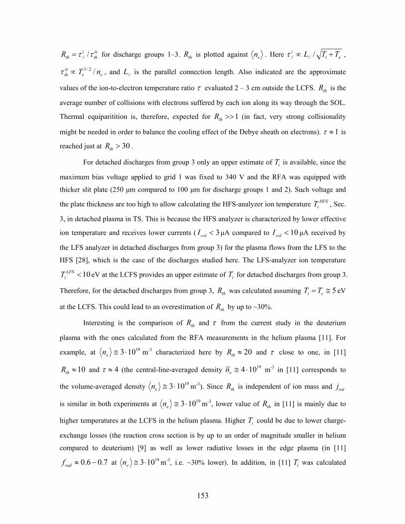
153

ieth

ithR ττ ///= for discharge groups 1–3. thR is plotted against en . Here ei

i TTL +∝ /////τ ,

eeieth nT /2/3∝τ , and //L is the parallel connection length. Also indicated are the approximate

values of the ion-to-electron temperature ratio τ evaluated 2 – 3 cm outside the LCFS. thR is the

average number of collisions with electrons suffered by each ion along its way through the SOL.

Thermal equiparitition is, therefore, expected for 1>>thR (in fact, very strong collisionality

might be needed in order to balance the cooling effect of the Debye sheath on electrons). 1≈τ is

reached just at 30>thR .

For detached discharges from group 3 only an upper estimate of iT is available, since the

maximum bias voltage applied to grid 1 was fixed to 340 V and the RFA was equipped with

thicker slit plate (250 µm compared to 100 µm for discharge groups 1 and 2). Such voltage and

the plate thickness are too high to allow calculating the HFS-analyzer ion temperature HFSiT , Sec.

3, in detached plasma in TS. This is because the HFS analyzer is characterized by lower effective

ion temperature and receives lower currents ( 3<colI µA compared to 10<colI µA received by

the LFS analyzer in detached discharges from group 3) for the plasma flows from the LFS to the

HFS [28], which is the case of the discharges studied here. The LFS-analyzer ion temperature

10<LFSiT eV at the LCFS provides an upper estimate of iT for detached discharges from group 3.

Therefore, for the detached discharges from group 3, thR was calculated assuming 5≅= ei TT eV

at the LCFS. This could lead to an overestimation of thR by up to ~30%.

Interesting is the comparison of thR and τ from the current study in the deuterium

plasma with the ones calculated from the RFA measurements in the helium plasma [11]. For

example, at 19103 ⋅≅en m-3 characterized here by 20≈thR and τ close to one, in [11]

10≈thR and 4≈τ (the central-line-averaged density 19104 ⋅≅en m-3 in [11] corresponds to

the volume-averaged density 19103 ⋅≅en m-3). Since thR is independent of ion mass and satj

is similar in both experiments at 19103 ⋅≅en m-3, lower value of thR in [11] is mainly due to

higher temperatures at the LCFS in the helium plasma. Higher iT could be due to lower charge-

exchange losses (the reaction cross section is by up to an order of magnitude smaller in helium

compared to deuterium) [9] as well as lower radiative losses in the edge plasma (in [11]

7.06.0 −≈radf at 19103 ⋅≅en m-3, i.e. ~30% lower). In addition, in [11] iT was calculated

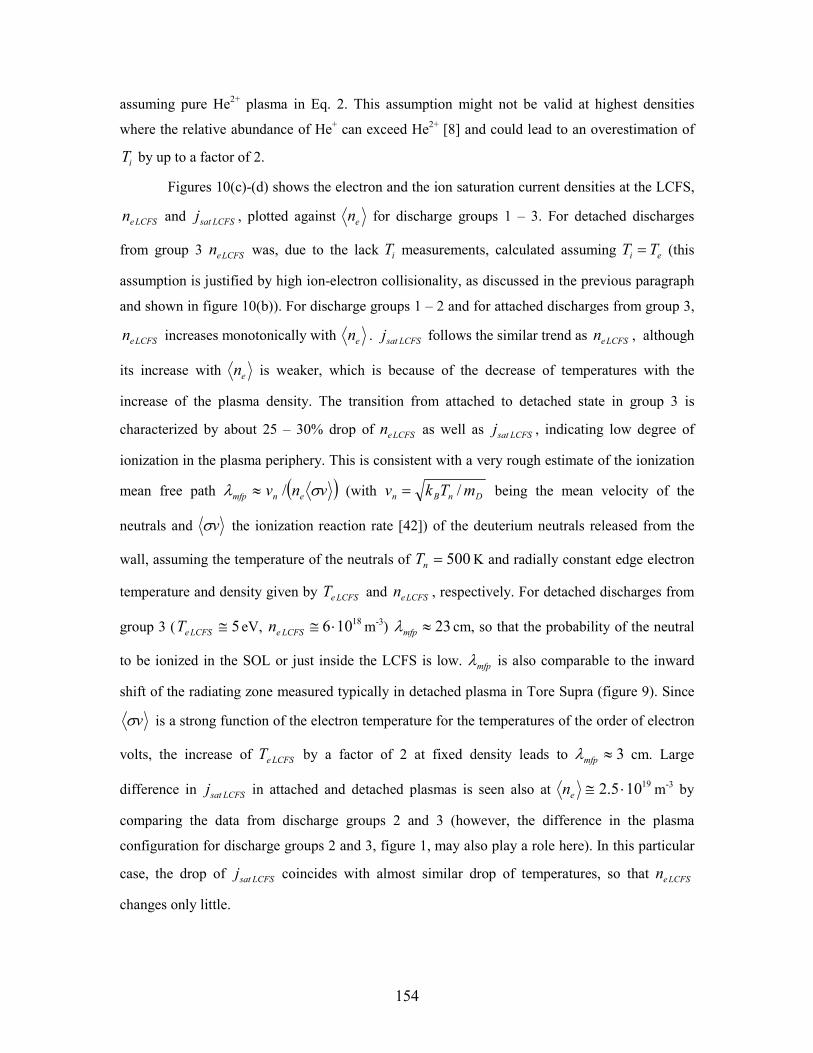
154

assuming pure He2+ plasma in Eq. 2. This assumption might not be valid at highest densities

where the relative abundance of He+ can exceed He2+ [8] and could lead to an overestimation of

iT by up to a factor of 2.

Figures 10(c)-(d) shows the electron and the ion saturation current densities at the LCFS,

LCFSen and LCFSsatj , plotted against en for discharge groups 1 – 3. For detached discharges

from group 3 LCFSen was, due to the lack iT measurements, calculated assuming ei TT = (this

assumption is justified by high ion-electron collisionality, as discussed in the previous paragraph

and shown in figure 10(b)). For discharge groups 1 – 2 and for attached discharges from group 3,

LCFSen increases monotonically with en . LCFSsatj follows the similar trend as LCFSen , although

its increase with en is weaker, which is because of the decrease of temperatures with the

increase of the plasma density. The transition from attached to detached state in group 3 is

characterized by about 25 – 30% drop of LCFSen as well as LCFSsatj , indicating low degree of

ionization in the plasma periphery. This is consistent with a very rough estimate of the ionization

mean free path ( )vnv enmfp σλ /≈ (with DnBn mTkv /= being the mean velocity of the

neutrals and vσ the ionization reaction rate [42]) of the deuterium neutrals released from the

wall, assuming the temperature of the neutrals of 500=nT K and radially constant edge electron

temperature and density given by LCFSeT and LCFSen , respectively. For detached discharges from

group 3 ( 5≅LCFSeT eV, 18106 ⋅≅LCFSen m-3) 23≈mfpλ cm, so that the probability of the neutral

to be ionized in the SOL or just inside the LCFS is low. mfpλ is also comparable to the inward

shift of the radiating zone measured typically in detached plasma in Tore Supra (figure 9). Since

vσ is a strong function of the electron temperature for the temperatures of the order of electron

volts, the increase of LCFSeT by a factor of 2 at fixed density leads to 3≈mfpλ cm. Large

difference in LCFSsatj in attached and detached plasmas is seen also at 19105.2 ⋅≅en m-3 by

comparing the data from discharge groups 2 and 3 (however, the difference in the plasma

configuration for discharge groups 2 and 3, figure 1, may also play a role here). In this particular

case, the drop of LCFSsatj coincides with almost similar drop of temperatures, so that LCFSen

changes only little.

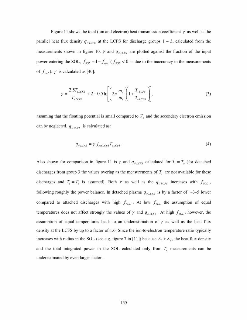
155

Figure 11 shows the total (ion and electron) heat transmission coefficient γ as well as the

parallel heat flux density LCFSq// at the LCFS for discharge groups 1 – 3, calculated from the

measurements shown in figure 10. γ and LCFSq// are plotted against the fraction of the input

power entering the SOL, radSOL ff −=1 ( 0<SOLf is due to the inaccuracy in the measurements

of radf ). γ is calculated as [40]:

+

−+=

LCFSe

LCFSi

i

e

LCFSe

LCFSi

T

T

mm

T

T12ln5.02

5.2πγ , (3)

assuming that the floating potential is small compared to sV and the secondary electron emission

can be neglected. LCFSq// is calculated as:

LCFSeLCFSsatLCFS Tjq γ=// . (4)

Also shown for comparison in figure 11 is γ and LCFSq// calculated for ei TT = (for detached

discharges from group 3 the values overlap as the measurements of iT are not available for these

discharges and ei TT = is assumed). Both γ as well as the LCFSq// increases with SOLf ,

following roughly the power balance. In detached plasma LCFSq// is by a factor of ~3–5 lower

compared to attached discharges with high SOLf . At low SOLf the assumption of equal

temperatures does not affect strongly the values of γ and LCFSq// . At high SOLf , however, the

assumption of equal temperatures leads to an underestimation of γ as well as the heat flux

density at the LCFS by up to a factor of 1.6. Since the ion-to-electron temperature ratio typically

increases with radius in the SOL (see e.g. figure 7 in [11]) because ei λλ > , the heat flux density

and the total integrated power in the SOL calculated only from eT measurements can be

underestimated by even larger factor.

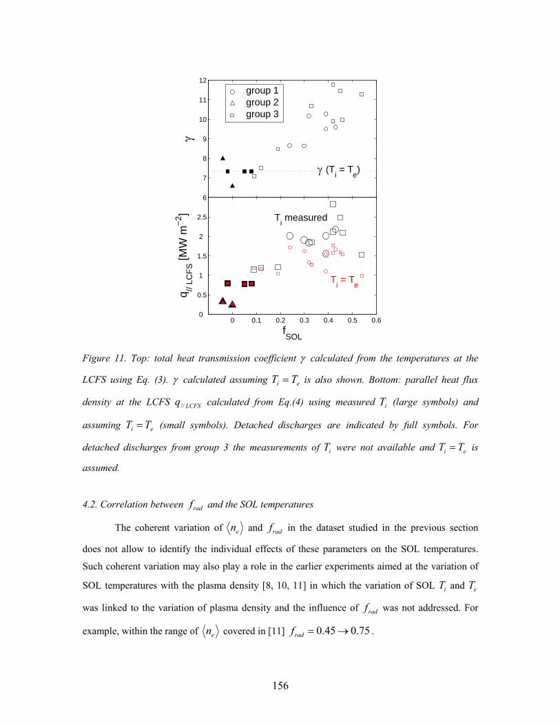
156

0 0.1 0.2 0.3 0.4 0.5 0.60

0.5

1

1.5

2

2.5

fSOL

q // LC

FS [M

W m

−2]

6

7

8

9

10

11

12

γ

group 1group 2group 3

(Ti = T

e)γ

Ti measured

Ti = T

e

Figure 11. Top: total heat transmission coefficient γ calculated from the temperatures at the

LCFS using Eq. (3). γ calculated assuming ei TT = is also shown. Bottom: parallel heat flux

density at the LCFS LCFSq// calculated from Eq.(4) using measured iT (large symbols) and

assuming ei TT = (small symbols). Detached discharges are indicated by full symbols. For

detached discharges from group 3 the measurements of iT were not available and ei TT = is

assumed.

4.2. Correlation between radf and the SOL temperatures

The coherent variation of en and radf in the dataset studied in the previous section

does not allow to identify the individual effects of these parameters on the SOL temperatures.

Such coherent variation may also play a role in the earlier experiments aimed at the variation of

SOL temperatures with the plasma density [8, 10, 11] in which the variation of SOL iT and eT

was linked to the variation of plasma density and the influence of radf was not addressed. For

example, within the range of en covered in [11] 75.045.0 →=radf .

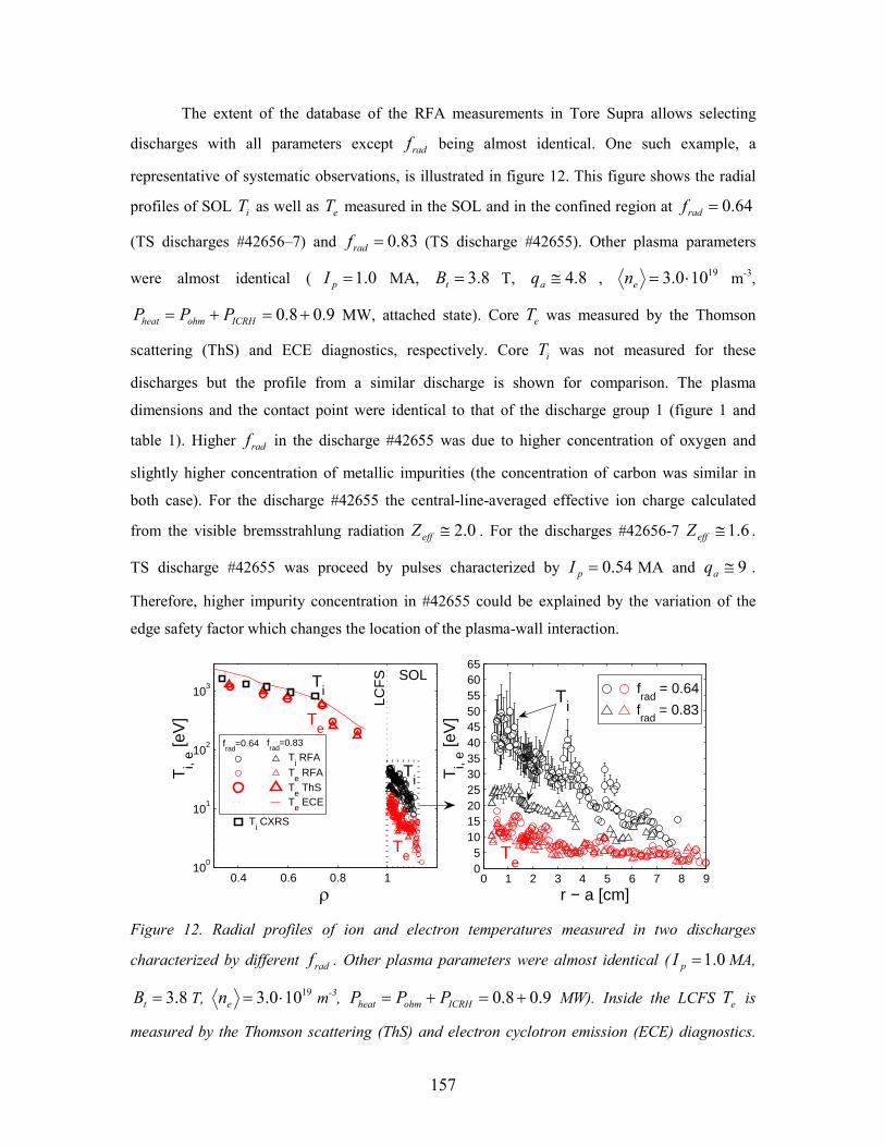
157

The extent of the database of the RFA measurements in Tore Supra allows selecting

discharges with all parameters except radf being almost identical. One such example, a

representative of systematic observations, is illustrated in figure 12. This figure shows the radial

profiles of SOL iT as well as eT measured in the SOL and in the confined region at 64.0=radf

(TS discharges #42656–7) and 83.0=radf (TS discharge #42655). Other plasma parameters

were almost identical ( 0.1=pI MA, 8.3=tB T, 8.4≅aq , 19100.3 ⋅=en m-3,

9.08.0 +=+= ICRHohmheat PPP MW, attached state). Core eT was measured by the Thomson

scattering (ThS) and ECE diagnostics, respectively. Core iT was not measured for these

discharges but the profile from a similar discharge is shown for comparison. The plasma

dimensions and the contact point were identical to that of the discharge group 1 (figure 1 and

table 1). Higher radf in the discharge #42655 was due to higher concentration of oxygen and

slightly higher concentration of metallic impurities (the concentration of carbon was similar in

both case). For the discharge #42655 the central-line-averaged effective ion charge calculated

from the visible bremsstrahlung radiation 0.2≅effZ . For the discharges #42656-7 6.1≅effZ .

TS discharge #42655 was proceed by pulses characterized by 54.0=pI MA and 9≅aq .

Therefore, higher impurity concentration in #42655 could be explained by the variation of the

edge safety factor which changes the location of the plasma-wall interaction.

0 1 2 3 4 5 6 7 8 905

101520253035404550556065

r − a [cm]

Ti,

e [eV

]

0.4 0.6 0.8 110

0

101

102

103

ρ

Ti,

e [eV

]

LCF

S

Ti

Te

frad

= 0.64

frad

= 0.83

Ti

Ti

Te

Te

Ti RFA

Te RFA

Te ThS

Te ECE

frad

=0.64 frad

=0.83

Ti CXRS

SOL

Figure 12. Radial profiles of ion and electron temperatures measured in two discharges

characterized by different radf . Other plasma parameters were almost identical ( 0.1=pI MA,

8.3=tB T, 19100.3 ⋅=en m-3, 9.08.0 +=+= ICRHohmheat PPP MW). Inside the LCFS eT is

measured by the Thomson scattering (ThS) and electron cyclotron emission (ECE) diagnostics.

158

Left: Temperatures plotted against the distance from the plasma centre normalized to minor

radius, ar /=ρ with 72.0=a m. Core iT was not measured for these discharges but the profile

from a similar discharge #39598 is shown ( 2.1=pI MA, 8.3=tB T, 19108.2 ⋅=en m-3,

8.00.1 +=+= ICRHohmheat PPP MW). Right: SOL iT and eT measured by the RFA plotted

against the distance from the LCFS.

As seen from figure 12, the increase of radf coincides with the decrease of SOL iT by

almost a factor of 2, whereas SOL eT is much less affected. In addition, core electron temperature

changes only little with the increase of radf (the variation in much smaller than the difference in

eT measured by ThS and ECE). No temperature measurements are available just inside the LCFS.

However, in order to connect the SOL profiles, both temperature gradients have to increase in this

region.

The large variation of SOL iT with radf and almost constant SOL eT may be surprising

as the variation of the radiated power is intuitively linked with the variation of SOL electron

rather than ion temperature. Since radP comes mainly from line radiation due to the interaction of

electrons with impurity ions and neutrals in the edge of the confined region, the increase of radP

should lead to a lower edge eT . SOL eT is expected to simply follow the variation of edge eT by

radial transport. However, we argue that the drop of eT in the edge of the confined region due to

radiation strengthens the energy transfer from ions to electrons via collisional coupling

( 2/32)( −−∝ eeeiie TnTTQ ). This may lead to the decrease the edge ion temperature. When eT

becomes very low relative to iT , so that the cross-field heat flux in the electron channel becomes

small, the radiative losses on electrons are, through equipartition term, compensated from the ion

channel. Note that the decrease of SOL iT by a factor of 2 coincides with a similar decrease of

SOLf (0.36 → 0.17), indicating that the power lost due to radiation comes really from the ion

channel. The edge eT is sustained at a low value, balanced between the radiative losses and gains

due to equipartition. Other volumetric loss terms such as charge-exchange collisions of ions with

neutrals, recombination and ionization could also play a role in the ion and electron power

balance, but are typically much smaller compared to the radiative losses on electrons.

These qualitative arguments were verified by modelling the ion and electron temperature

profiles in the edge of the confined plasma using power balance equations. Radiation and

159

equipartition were the only source terms taken into account in the model. Further approximations,

forced by a lack of relevant measurements, were following. The cross-field heat transport, iT , eT ,

en and the radiated power density radQ were assumed to be poloidally and toroidally uniform,

reducing the model to one dimension in the radial direction. Ion and electron heat diffusivities,

iχ and eχ , were assumed to be constant. ei nn = i.e. the effective ion charge in the plasma edge

1=effZ . Convective heat fluxes were neglected as the cross-field particle diffusivities are not

measured in the edge plasma. radQ is known to be poloidally localized above the plasma contact

point in the attached plasma. However, the assumption of the uniform radQ is justified by the fact

that the electron transit time through the edge region (which is of the similar order as the energy

confinement time, 1.0≈ s) is at least by a factor of 104 longer compared to the time of one

electron poloidal circumference ( ee meTRq //π≅ ). On the other hand, we apply additional

simplifying assumption that the radial profile of radQ is given, i.e. independent of local eT and

en .

Under these assumptions the ion and electron power balance equations in the cylindrical

geometry read:

iei

ei QdrdT

rndrd

re −=

1χ , (5)

and

radiee

ee QQdrdT

rndrd

re −=

1χ . (6)

The equations were solved numerically inside the region 17.0/ →== arρ , where the

radiated power density is highest in TS attached plasma. The unknowns of the system were the

temperature profiles. All the other fields were set as parameters. Incoming energy fluxes were

imposed at the inner boundary ( 7.0=ρ ) by imposing the temperature gradients eirT ,∇ . The

proportionality between the temperature gradients and the local temperatures, eieieir TT ,,, λ−=∇

(where ei,λ is the experimental decay length), was imposed at the outer boundary ( 1=ρ ) to

160

insure the continuity with the exponentially decaying profiles in the SOL. The non-linear system

(5)-(6) was solved iteratively starting from an initial guess of the temperature profiles. For each

iteration, the diffusion operators were inverted and the non-linear energy equipartition term ieQ

was computed as an explicit right-hand side from eT and iT obtained from the previous iteration.

The iterative process was terminated when ( ) 61,

1,, 10−−− <− n

ienie

nie TTT where n is the number of

iterations.

The calculation was performed for discharges shown in figure 12. )(rne was taken from

reflectometry measurements. 5, ≈TeTiλ cm was determined from RFA measurements.

37.0, −=∇

=ρeirT keV m-1 was provided from ECE and charge exchange recombination

spectroscopy (CXRS) measurements, respectively (CXRS measurements were not available for

the discharges studied here and 7.0, =

∇ρeirT was taken from a similar discharge #39598, assuming

that 7.0, =

∇ρeirT is independent of radf ). == ei χχ 2.8 m2 s-1, leading to realistic temperatures at

the LCFS, and [ ]radrad QQ λρ /)1(exp0 −= (with 14.0=radλ m), approximately equal to the

poloidally averaged plasma emissivity measured by bolometry, were assumed.

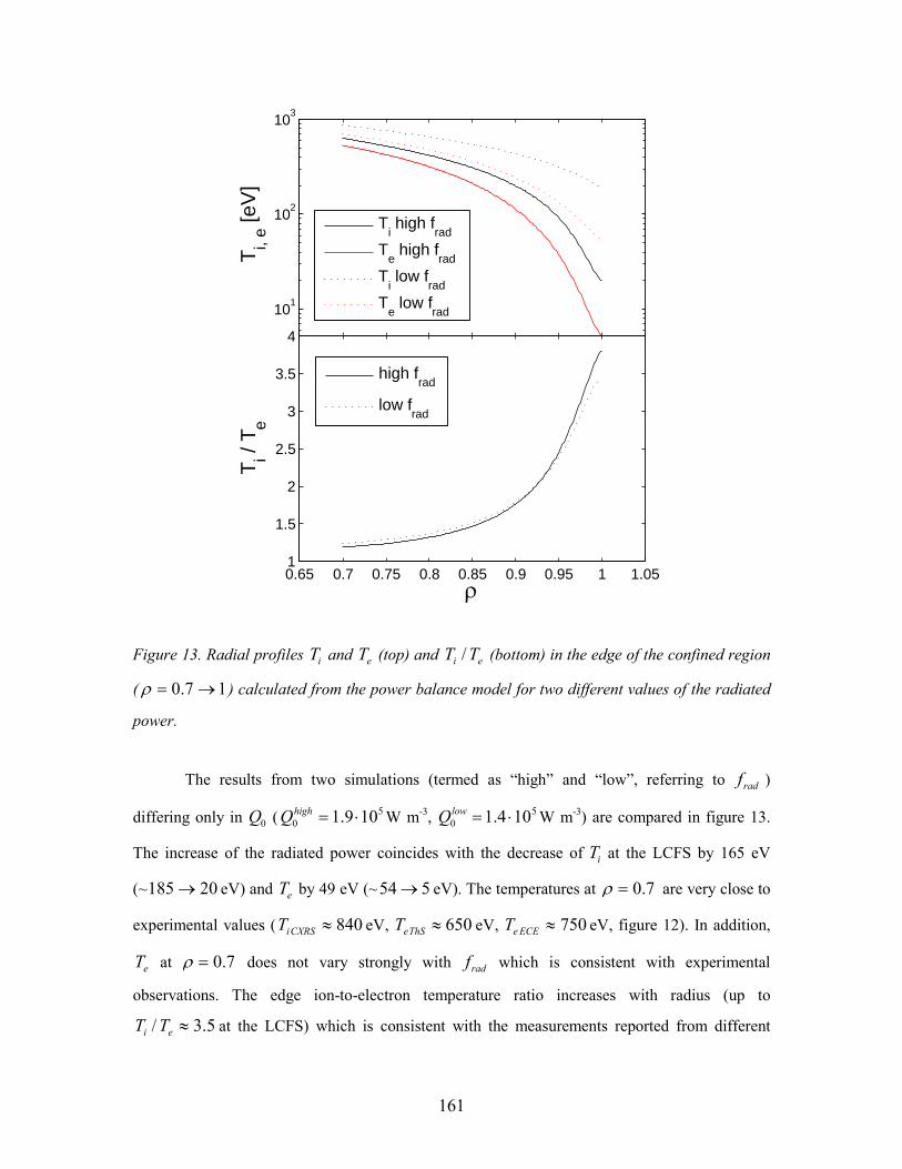
161

0.7 0.75 0.8 0.85 0.9 0.95 1

101

102

103

ρ

Ti,

e [eV

]

0.65 0.7 0.75 0.8 0.85 0.9 0.95 1 1.051

1.5

2

2.5

3

3.5

4

ρ

Ti /

T e

high frad

low frad

Ti high f

rad

Te high f

rad

Ti low f

rad

Te low f

rad

Figure 13. Radial profiles iT and eT (top) and ei TT / (bottom) in the edge of the confined region

( 17.0 →=ρ ) calculated from the power balance model for two different values of the radiated

power.

The results from two simulations (termed as “high” and “low”, referring to radf )

differing only in 0Q ( 50 109.1 ⋅=highQ W m-3, 5

0 104.1 ⋅=lowQ W m-3) are compared in figure 13.

The increase of the radiated power coincides with the decrease of iT at the LCFS by 165 eV

(~ 20185 → eV) and eT by 49 eV (~ 554→ eV). The temperatures at 7.0=ρ are very close to

experimental values ( 840≈CXRSiT eV, 650≈ThSeT eV, 750≈ECEeT eV, figure 12). In addition,

eT at 7.0=ρ does not vary strongly with radf which is consistent with experimental

observations. The edge ion-to-electron temperature ratio increases with radius (up to

5.3/ ≈ei TT at the LCFS) which is consistent with the measurements reported from different

162

tokamaks (see figure 7 in [11]). As mentioned above, the values of iχ and eχ were adjusted in

order to obtain realistic LCFS temperatures. However, similar variation of the LCFS temperatures

with radf was obtained from the simulations with different values iχ and eχ . Moreover,

favorable values of edge iχ and eχ used in our calculation does not differ significantly from the

ones suggested from more complex fluid models elsewhere. The model reproduces well the

experimentally observed strong variation of iT with radf and suggests that the drop of edge eT

due to radiation could significantly influence edge iT due to ion-electron collisional coupling. On

the other hand, the model also predicts relatively strong variation of the LCFS eT with radf

which is not seen in experiment (although the decrease of eT with the increase of radf is much

smaller in absolute values compared to iT ). This discrepancy indicates that some processes in the

edge plasma and eventually in the SOL that could have a controlling influence on the electron

temperature are not accounted in the model. In addition, radQ which is pre-defined in our model

is in reality coupled with the local electron temperature and density and should be, therefore,

modelled in a self-consistent way. The same arguments may apply for the heat diffusivities. In

addition, it is known that the convective turbulent heat flux, neglected in our model, may be

comparable to or larger than the conductive component [43].

5. Summary

Experimental studies of the SOL parameters in large circular limiter plasmas are needed

to validate the models aimed e.g. at the estimation of the heat loads on the ITER start-up-phase

limiters.

In this paper we studied in a large circular limiter tokamak Tore Supra the SOL ion and

electron temperatures, iT and eT , electron density en and the ion saturation current density satj

for a broad range of the plasma density en and the radiated power fractions radf , including

detached plasmas.

In ohmic plasma for low en and radf , 43/ −≅ei TT and 50≅iT eV at the LCFS. At

highest en and radf as well as in detached plasma, ei TT ≅ , both only a few electron volts. The

decrease of ei TT / with en roughly follows the increase of the ion-electron collisionality in the

SOL. In attached plasma, the LCFS satj and en increases monotonically with en except the

163

transition from attached to detached state which was found to be associated with 25 – 30% drop

of the LCFS satj and en .

Tiλ was found to be generally higher than Teλ which is consistent with larger parallel

electron losses relative to the ion losses in the SOL. The transition to detached state was found to

be related with a strong flattening of the SOL temperature profiles and less than a factor of 2

increase of neλ .

The parallel heat flux density at the LCFS LCFSq// calculated from RFA measurements

was found to be consistent with the power balance. In detached plasma LCFSq// was found to be a

factor of ~3-5 lower compared to attached discharges characterized by

5.03.01 −≈−= radSOL ff . In detached plasma ( ei TT ≅ ) the lack of iT measurements does not

affect the calculation of the heat flux densities in the SOL. However, in attached plasma, the heat

flux density as well as the total integrated power in the SOL, calculated assuming ei TT = , can be

significantly underestimated because ei TT > and TeTi λλ > in the SOL.

SOL temperatures were also studied in the discharges with all parameters except the

radiated power being fixed. The increase of radf by about ~30% was found to be associated with

a decrease of SOL iT by almost a factor of 2 but almost unaffected eT in the SOL as well as in

the core plasma. The decrease of SOL iT coincides with a similar decrease of SOLf , indicating

that the power lost due to radiation comes mainly from the ion channel. A simple power balance

model, with the radiation and equipartition being the only volumetric loss terms included, was

employed to study the dependence of iT and eT on radf in the edge of the confined region. The

model reproduces well a strong decrease of the LCFS iT with the increase of the radiated power

and shows that the power loss on electrons in the edge plasma can be, through ion-electron

collisional coupling, compensated from the ion channel and strongly influence the edge iT . The

model also reproduces small variation of the core electron temperature with radf as well as the

steepening of the temperature profiles just inside the LCFS suggested from the comparison of the

core and the SOL measurements. However, the model fails in reproducing almost constant LCFS

eT independently of the radiated power. Although the modeled LCFS eT varies much less than

iT in the absolute values with the increase of the radiated power, it decreases by a similar factor.

We do not have any other explanation for this discrepancy except that the processes that would

164

decouple the edge and the SOL electrons are not accounted in our simple model. In the next step,

2D code which comprises both the edge plasma and the SOL, resolves the processes such as the

radiation in a self-consistent way and includes additional volumetric loss terms such as the

charge-exchange losses, recombination and ionization, needs to be employed to study the edge

temperatures.

In general, we have demonstrated that the reciprocating probes in Tore Supra access the

SOL parameters, in particular the ion temperature, for a broad range of the plasma conditions.

This allows e.g. characterizing the heat flux densities in the SOL without using simplifying (and

often underestimating) assumptions on SOL iT . These results suggest that it could be interesting

to further investigate detached plasma operation, and the significant increase in SOL spreading

with the contact point on the HFS, to develop alternative start-up scenarios for ITER.

Acknowledgements

The authors would like to thank Drs. F. Clairet and C. Fenzi for providing the

reflectometry and the CXRS measurements, respectively. The authors are grateful to Dr. P.

Ghendrih for the fruitful discussions. This work, supported by the European Communities under

the contract of Association between EURATOM and CEA, was carried out within the framework

of the European Fusion Development Agreement. The views and opinions expressed herein do

not necessarily reflect those of the European Commission.

References

[1] Gribov Y Control System Design and Assessment (CSD), Appendix B: Magnetic

configuration and poloidal field scenarios, ITER document N 19 RI 14 R0.1, August 2004.

[2] Kobayashi M et al 2007 Nucl. Fusion 47 61

[3] Federici G et al 2007 J. Nucl. Mater. 363-365 346

[4] Cardella A, Skladnov K, Ioki K, Pacher H, Strebkov Y and Daenner W 2002 Fus. Eng.

Des. 61-62 111

[5] Jacquinot J and Hoang G T 2004 Plasma Sci. Technol. 6 2101

[6] Kočan M, Gunn J P, Komm M, Pascal J-Y, Gauthier E and Bonhomme G 2008 Rev. Sci.

Instrum. 79 073502

[7] McCracken G M et al 1987 J. Nucl. Mater. 145-147 181

[8] Matthews G F, Pitts R A, McCracken G M, Stangeby P C 1991 Nucl. Fusion 31 1495

[9] Pitts R A 1991 PhD Thesis University of London

165

[10] Kočan M, Pánek R, Stöckel J, Hron M, Gunn J P and Dejarnac R 2007 J. Nucl. Mater.

363-365 1436

[11] Kočan M, Gunn J P, Pascal J-Y, Bonhomme G, Fenzi C, Gauthier E and Segui J-L 2008

Plasma Phys. Control. Fusion 50 125009

[12] Gunn J P et al 2007 J. Nucl. Mater. 363-365 484

[13] Matthews G F 1995 J. Nucl. Mater. 220-222 104

[14] Allen J et al 1986 Plasma Phys. Control. Fusion 28 101

[15] Strachan J D et al 1985 12th Eur. Conf. on Controlled Fusion and Plasma Physics

(Budapest, Hungary) part 1, p. 263

[16] Kimura H et al 1987 Nucl. Fusion 18 1195

[17] Kimura H, Odajima K, Sugie T, Maeda H 1979 Japan. J. Appl. Phys. 18 2275

[18] Molvik A W 1981 Rev. Sci. Instrum. 52 704

[19] Matthews G F 1984 J. Phys. D: Appl. Phys. 17 2243

[20] Wan A S, Yang T F, Lipschultz B and LaBombard B 1986 Rev. Sci. Instrum. 57 1542

[21] Guo H Y, Matthews G F, Davies S J, Erents S K, Horton L D, Mond R D, Stangeby P C

1996 Contrib. Plasma Phys. 36 81

[22] Shats M G, Rudakov D L, Boswell R W and Borg G G 1997 Phys. Plasmas 4 3629

[23] Raychaudhuri S 1999 Contrib. Plasma Phys. 39 4, 359

[24] Pitts R A, Chavan R, Davies S J, Erents S K, Kaveney G, Matthews G F, Neill G, Vince J

E and Ďuran I 2003 Rev. Sci. Instrum. 74 4644

[25] Nedzelskiy I S, Silva C, Figueiredo H, Fernandes H and Varandes C A F 2006 Rev. Sci.

Instrum. 77 10E729

[26] Pitts R A, Fundamenski W, Erents S K, Andrew Y, Loarte A, Silva C and JET-EFDA

contributors 2006 Nucl. Fusion 46 82

[27] Kočan M and Gunn J P, “First evidence for poloidal asymmetries of radial ion energy

transport by ion temperature measurements in the scrape-off layer of Tore Supra” abstract

submitted to 36th EPS Conference on Contr. Fusion and Plasma Physics (Sofia, June 29 –

July 3)

[28] Valsaque F, Manfredi G, Gunn J P and Gauthier E 2002 Phys. Plasmas 9 1806

[29] Dejarnac R, Gunn J P, Stöckel J, Adámek J, Brotánková J and Ionita C 2007 Plasma Phys.

Control. Fusion 49 1791

[30] Hutchinson I H 1987 Phys. Fluids 30 3777

[31] Chung K S and Hutchinson I H 1988 Phys. Rev. A 38 4721

[32] LaBombard B et al 2004 Nucl. Fusion 44 1047

166

[33] Gunn J P et al 2009 “Measurements of lower hybrid hot spots using a retarding field

analyzer in Tore Supra” J. Nucl. Mater. (in press), doi:10.1016/j.jnucmat.2009.01.232

[34] Böhm C and Perrin J 1993 Rev. Sci. Instrum. 64 31

[35] Gunn J P et al 2002 Czech. J. Phys. 52 1107

[36] Silva C, Gonçalves B, Hidalgo C, Pedrosa M A, Erents S K, Matthews G F and Pitts R A

2004 Rev. Sci. Instrum. 75 4314

[37] Pánek R, Pitts R A, Gunn J P and Erents S K 2004 Czech. J. Phys. 54 150

[38] Chodura R 1982 Phys. Fluids 25 1628

[39] Gunn J P 1997 Phys. Plasmas 4 4435

[40] Stangeby P C The Plasma Boundary of Magnetic Fusion Devices 2000 (Bristol: Institute

of Physics Publishing) p 649

[41] Asakura N 2007 J. Nucl. Mater. 363-365 41

[42] Jones E M 1997 Atomic Collision Processes in Plasma Experiments: Analytic

Expressions for Selected Cross-Sections and Maxwellian Coefficients II, Rep. CLM-R

175, Culham Laboratory, Abingdon, Oxfordshire

[43] Pigarov A Y et al 2003 J. Nucl. Mater. 313-316 1076

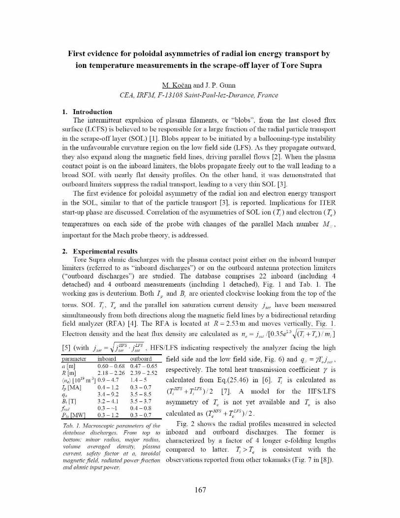
167

First evidence for poloidal asymmetries of radial ion energy transport by

ion temperatnre measnrements in the scrape-off layer of Tore Snpra

M. Kocan and J. P. GUll11

CEA, IRFA1, F-1310S Saint-Paul-/e:-DlIrance, France

1. IntroductionThe intenuittent expulsion of plasma filaments, or "blobs", from the last closed flux

surface CLefS) is believed to he responsible for Cl large fraction of the radial particle transpOll

in the scrape-off layer (SOL) [1]. Blobs appear to be illitiated by a ballooning-type illstabilityin the llllf~1vourable Cl1rvature region on the law field sicle (LFS). As they propagate outward,

they also expancl along the magnetic field hues, driving parallel flows [2]. When the plasmacontact point is on the illboard limiters, the blobs propagate freely ont to the wall leadillg to abroad SOL \vith nearIy flat density profiles. On the other hand, it was demonstrated that

outboard limiters suppress the radial trallsp011, leadillg to a very thin SOL [3].The first evidenee for poloidal asynllnetry of the radial ion and electron energy transport

in the SOL, similar to that of the particle transport [3], is reported. Implications for 11ER

stml-up phase are discussed. Conelation of the asynuuetries of SOL ion (I;) and eleetron (TJ

temperatures on each side of the probe with changes of the parallel Mach number l.\tIfI,

important for the Mach probe theory, is addressed.

2. Experimental resultsTore Supra olunie discharges with the plasma contact point either on the inboard bumper

limiters (refelTed to as "inboard discharges") or on the outboard antenna protection limiters("outboard discllarges") are shtdied. Ihe database comprises 22 inboard (including 4detached) and 4 outboard measurements (including 1 detached), Fig. 1 and Tab. 1. Theworking gas is deuterium. Both 1p and BI are oriented clockwise lookillg from the top of the

tonts. SOL 1;, Te and the parallel ion saturation ClUTent density isar have been measured

simultaneously from both directions along the magnetic field lines by a bidirectional retardingfield analyzer (RFA) [4]. The RFA is located at R = 2.53m and moves vertically, Fig.!.

Electron density and the heat flux density are calculated as ne = isOl l[ü.35e15 ~(T; + TJ 11/1;]

[5] (with isOl = ,/i::::s'l::s , HFS/LFS indieating respectively the analyzer facing the high

parallleter inboard outboard field side and the low field side, Fig. 6) and qi/ = yT"isOl'n[m] 060-068 0.47-0.65 . 1 TI II .. ffi· .R[lll] 2:18-2:26 2.39-2.52 respectlve y. le tota leat transnllsslOn coe lCIent y 1S(11.,)[ 1019 111-3] 0.9 - 4.7 1.4 - 5 calculated from Eq.(25.46) in [6]. I; is ealculated as

Ip [MA] 0.4 - 1.2 0.3 - 0.7 (T,HFS + T,LFS) /2 [7]. A mode! for the HFS/LFSja 3.4 - 9.2 3.5 - 8.5B,[T] 3.2-4.1 3.5-3.7 asymmetry of T., is not yet available and Te is alsofrad 0.3 - -1 0.4 - 0.8Pi" [MW] 0.3 - 1.2 0.3 _ 0.7 calculated as (T.,HFS + Tc

LFs) 12.

Tab. J. Macroscopic parameters ofrhe Fig. 2 shov·,rs the radial profiles measured in selecteddmabase discharges. From top ro inboard and outboard discharges. The fonner isbo([om: millor radil/s, II/ajor radius, characterized by a factor of 4 longer e-folding lengths'·O!IIII/e ayeraged dellSi!)', plasma d! TT· . . 1 1compare to alter. ; > c IS consIstent Wlt 1 t leCI/l'relit, safety factor (If a, tOl'oidallIIagl/etic field, radimed powerfi'acrioll observations reported from other tokamaks (Fig. 7 in [8]).and o1lmic il/pm power.

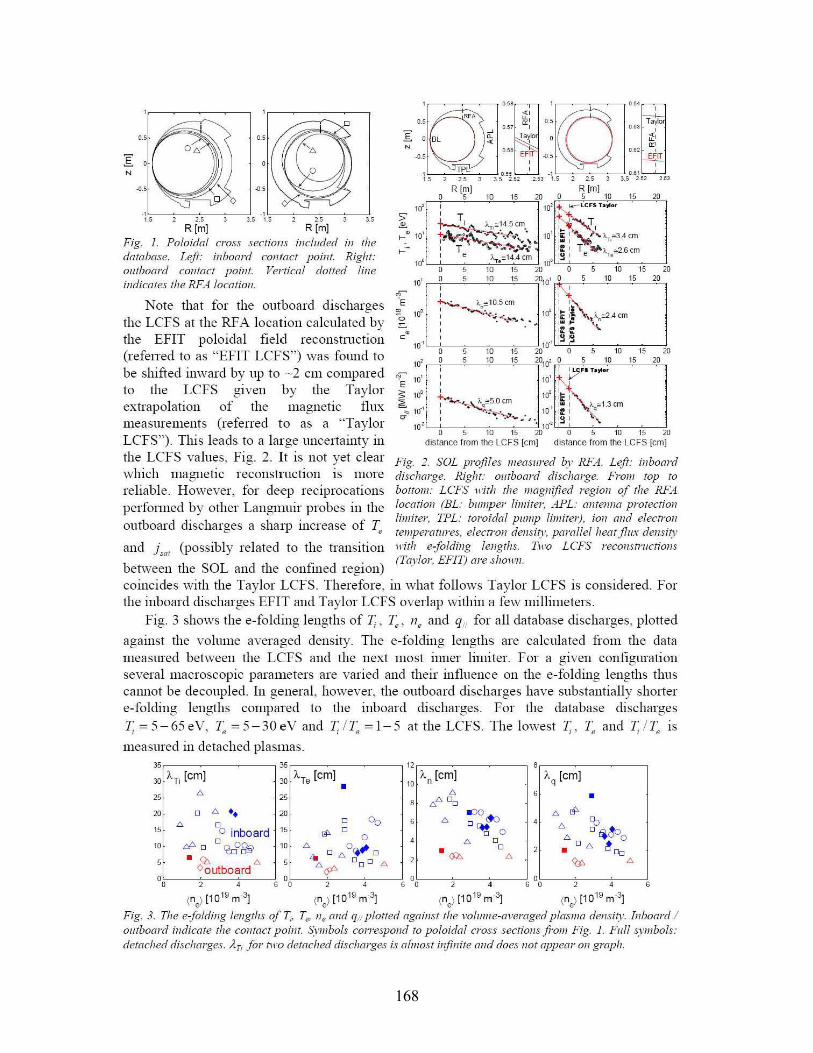
168

'"'"

'-.,,1.3 cm

Rlm]5101520

'u'" ,"' "~, 1

o ~I.',.,-0: "~1 E~rr

,."' 1.5 2 2.5 3 '.5 ,." 2."'

R(m]5101520

,

a:" ~wc ,,

",

",

"

H'

Fig. 2. SOL profiles lIIeasured by RFA. Lefr: illboarddisclwrge. Right: ol/rboard discharge. From rop roboffoll/: LCFS lI'irli rhe magnified regioll of rhe RFAlocarioll (BL: bl/ll/per lill/iter, APL: allfelllla prorecrioll!illliter, TPL: roroidal pllmp limirel), iOIl and elecrrollrempemfllres, electron del/si,:,', pmoa!!el hear flux densiryHith e-foldillg lengtlls. Iwo LCFS loeCOl/srrucrions(Taylor, EFIT) are shoH'll

"'

o.,

,

2.5 3.5 25 l.5 5' 1- _TIR [ml R (ml .!!. '-:---!..,"" 1,-,,,14.5 cm.

1-'" 10' +,," -.;i!- - ....~r. ,Fig. 1. P%idal cross sectio/Js illCbuled ill the ,....:_ l 'V;"f"w-~~ v<database. Left: il/board contact paim. Rigil': lOo~~'_,e~~,"--;;,-c;outbom'cf conract poim. Vertical dorted fille la 15

inniwfes fhe RFA location. la' ,~,_-,-_~w~--,,"~~

"lE 'Note that for the outboard discharges "" ~),. ,,10.5cm- tif: -~~~.

the LCfS al the RFA location calculated by -0 1 . " ....... ~.,

the EFIT poloidal field reconstruction cO> 10''--.;-'-",,---;;,-e; w'U"';'----,---:cc--;c----c!

(referred to as "EFIT LCf S") was found to 10' "'--2_-,:,,:_'.'i~"----'i~lO' ~"'-ccc+.="w,-'-"-,,,;-"--,,,,,'-,'"he shifted inward by up to -2 cm compared ~ 1 ~"T."'r

":'E 10' : 10' 1

to the LCfS glven by the Taylor s: 10' 1 la' :~ 1

extrapolation of the magnetic t1ux ;;t"" 10' :".a-..~~_: . 10·':;:measurements (refened to as a "Taylor ~ 10'L--te'-,-m'-"-,,'-'-'l° 10·' I~ 1

o 5 10 15 20 0 5 10 15 20LCfS"). This leads to a large uncertainty in distance from the LCFS lem] distance from the LCFS lem]

the LCfS values, fig. 2. Ir is not yet clearwhich magnetic reconstruction lS morereliable. However, for deep reciprocationsperfonned by other Langmuir probes in theoutboard discharges a shalV increase of T"

and fiat (possibly related to the transition

between the SOL and the confined region)coincides with the Taylor LCfS. Therefore, in what follows Taylor LCFS is considered. Forthe inboard discharges EfIT and Taylor LCfS overlap within Cl few millimeters.

Fig. 3 shows the e-folding lengths of 1;, T", Il,, and qI/ for aIl database discharges, plotted

against the volume averaged density. The e-folding lengths are calculated from the datameasured between the LCFS and the next most inner limiter. fora given configurationseveral macroscopic parameters are varied and their influence on the e-folding lengths thuscannot be decoupled. In general, however, the outboard discharges have substantially shortere-folding lengths compared to the inboard discharges. For the database discharges1; =5-65eV, Te =5-30eV and 1;IT" =1-5 at the LCFS. The lowest 1;, T" and 1;17., is

measnred in detached plasmas.,

")~n[cmj ).q [cm]" ~ , •" é'%

o:xJ~ " ci', " , 'b0,* "o a D. 0 ti~oo,~ 0

0" ~• <lb ° ,

" . "", 'IF "" "

o J:::, ••

o 0 ~a inboard 15 @. 0 0

cl'-D DWO~ 10 D. 0,41DJ:::,~D

-Cl> D. D. DDDJ:::,°outboard <Jf."

"~"__~,,.::-=c::..:::':::_--!, "".!----''-----c~---!6 0 6 0 2 4(n \ [10 19 m-3] (n )[1019 m-3) (n )[1019 m-l (n )[10 19 m-l

et e e eFig. 3. The e-foldillg lellgrhs of Tb Tf1> Il,, and (j//ploffed agai/lst rhe l"OlllllTe-m·emged plasma densit)!. II/board /outboard i/ldicare the contact poillf. SYII/bols correspond ro poloidal cross sections fi'OIII Fig. J. Fu!! ~:VII/bols:

derached discharges. Ân for nro derached dischm-ges is allllost infinite and does /lor appem- 0/1 gmph

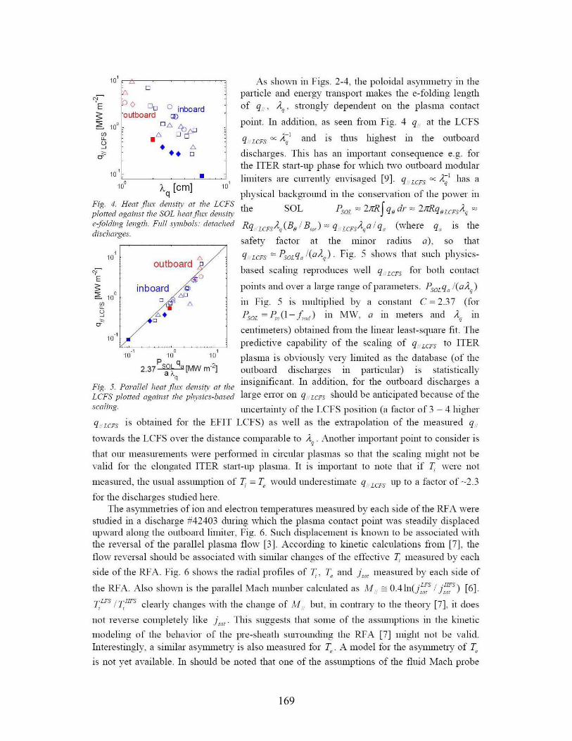
169

As shawn in Figs. 2-4, the poloidal asyulllletly in theparticle and energy transp0l1 makes the e-foldillg lengthof qj/, Âq , strongly dependent on the plasma contact

point. In addition, as seen [rom Fig. 4 q/l at the LCfS

q,ILCFS ex ,..Çl and is thU5 highest in the outboard

discharges. This has an important consequence e.g. forthe 11ER staIl-Up phase for which two outboard modularlimiters are clllTently envisaged [9]. qllLCFS ex À;l has a

physical background in the conservation of the power in

the SOL PSOL "" 2ffRfq( dl' "" 2/[RQOLCFSÀq ""

RqIILCFSÂq(B(/ Bror) <:=; q/ILCFSÀqalqa (where qa lS the

safety factor at the nllnor radius a), so that

ql/LCFS <:=; PSOLqa l(aÀq ). Fig. 5 shows that sucb physics­

based scaling reproduces weIl ql/LCFS for both contact

o

o"outboard

".o

o

inboard

,10

10'

N- "'

'E 00 DO 0 inboards: outboard CD,)

6 10° D~ èo"' '" 0 ~i'; •~ . '"&- •• 0

points and over a large range ofparameters. PSOLqa l(aÀq )

in Fig. 5 is muitiplied by a constant C = 2.37 (forPSOL = P;,,(l- fmd) in MW, a in meters and À-q m

centimeters) obtained from the linear least-square fit. Thepredictive capability of the scaling of ql/LCFS to lIER

10 101

p q plasma is obviously very limited as the clatabase (of the2.37~[MW rn-2

] outboarcl discharges m pat1icular) lS statisticallyq insignificant. In addition, for the ontboard discharges a

Fig. 5. Farallel hem flux dellsiry m tl,eLCFS plotted ngnillst the physics-bnsed large enor on q/f LCFS should be anticipated because of the

scnlillg. uncertainty of the LCFS position (a factor of 3 - 4 higherql/LCFS is obtained for the EFIT LCFS) as weIl as the extrapolation of the measured qi/

towarcls the LCfS over the distance comparable to À-q . Another important point to consicler is

that our measurements were perfonned in circular plasmas so that the scaling might not bevalicl for the elongatecl ITER stat1-UP plasma. It is important to note that if 1; \vere not

measured, the usual assumption of T; = Te would unclerestimate q//LCFS up to a factor of -2.3

for the discharges studied here.The asymmetries of ion and electron temperatures measured by each side of the RFA were

stucliecl in a discharge #42403 during which the plasma contact point was steadily displacedupward along the ontboard limiter, Fig. 6. Snch displacement is known to be associated withthe reversai of the parallel plasma flow [3]. Accorcling to kinetic calculations from [7], theflow reversaI should be associated with similar changes of the effective 1; measurecl by each

sicle of the RFA. Fig. 6 shows the radial profiles of r;, Te and Joar measured by each sicle of

the RFA. Also shown is the parallel Mach number calculated as M fl == OAln(j;:s 1/:'~s) [6].

r;LFS I1;HFS clearly changes with the change of AI Il but, in contrary to the theory [7], it does

not reverse completely like Joar. This suggests that some of the assumptions in the kinetic

modeling of the behavior of the pre-sheath surrounding the RFA [7] might not be valid.Interestingly, a similar asynllnetly is also measured for Te. A model for the asymllletry of Te

is not yet available. In shollld be noted that one of the assulllptions of the fluid Mach probe

•), [cm]

qFig. 4. Hem flux del/sir)' ar fhe LCFSplarrca agaillSt fhe SOL hem filiX densitye-foldillg lei/gril. Full symbols: derncheddisclwrges.

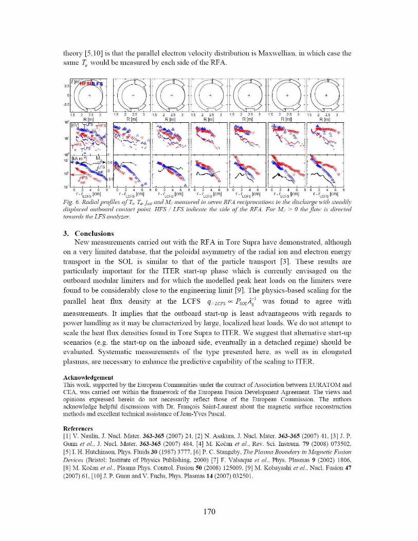
170

theOlY [5,10] is that the paraBet electron velocity distribution is Maxwellian, in which case thesame Te would be measnred by each side of the RFA.

w'

1.5 2 2.5 3

11)' R[m]

le~T~F

10' \~Hfs".:·· ;:k\... ,

Te TlFS .....10' e

W'

~~~~10·'~"--c,~,;-~"--! L";-~,~,;-~"=-C"!'-;"~~,--e,~"~t..B 0 2 4 6 8 0 2 4 6 8 0 2 4 6 8 0 2 4 6

f fLCFS[cm] f rLCFS[cmj f flCFS[cm] f fLCFS[cm] f flcFslcm] f flCFS[cm] f-fLCFS[cmj

Fig. 6. Radial profiles of Ti, Tb i;ar and 1\1// lIIeasllred ill .5'~WI RFA reciprocatioJ/s ill The discJwrge wiTh sTeadi~y

displaced ol/Tboard COli tacT poillf. HFS / LFS illdicate The side of The RFA. For _M// > 0 The flo1\" is direcTedt01mrds The LFS mw~y=er.

3. ConclusionsNew measurements canied out with the RFA in Tore Supra have demonstrated, although

on a very limited database, that the poloidal asynulletry of the radial ion and electron energytransport in the SOL is similar to that of the panicle transport [3]. These resnlts arepm1icularly imp0l1ant for the ITER start-up phase which is cunently envisaged on theoutboard modular limiters and for which the modeBed peak heat loads on the limiters werefound to be considerably close to the engineering limit [9]. The physîcs-based scaling for the

par·allel heat flux density at the LCfS qllLCFS oc PSOLÀ~l was fOlmd to agree with

measnrements. It implies that the outboard star1-up is least advantageous with regards topower handling as it may be characterized by large, localized heat loads. We do not attempt toscale the heat flux densities fOlmd in Tore Supra ta ITER. We suggest that alternative start-upscenarios (e.g. the stan-up on the inboard side, evennmlly in a detachecl regime) should beevaluated. Systematic measnrements of the type presented here, as weIl as in elongatedplasmas, are necessary to enhance the predictive capability of the scaling to ITER.

ArknowledgementThis \Vork. supp0l1ed by the European Communities under the commcr of Association between EURATOM andCEA. \Vas cmTied out within the framework of the European Fusion Development Agreement. The views andopinions expressed herein do nOT necessarily reflect those of the European Commission. The aurhorsacknowledge helpful discussions \Vith Dr. François Saint-Laurent abour the magnetic surface reconstl1lctionmethods and excellent technical assistance of Jean-Yves Pasca!.

References[1] V. Naulin. J. Nud. Mater. 363-365 (2007) 24. [2] N. Asakura. J. Nuc!. Mater. 363-365 (2007) 41. [3] J. P.Gunn er al.. J. Nuc!. Mater. 363-365 (2007) 484. [4] J'vI. Koèan et al.. Rev. Sci. Instrum. 79 (2008) 073502.[5] 1. H. Hutchinsoll. Phys. Fluids 30 (1987) 3777. [6] P. C. Stangeby. The Plasl/la BOlllldmy ill Maglletic FI/sionDe\"ices (Bristol: Instimre of Physics Publishing. 2000) [7] F. Valsaque et al.. Phys. Plasmas 9 (2002) 1806.[8] M. Koèan et al.. Plasma Phys. COllU"O!. Fusion 50 (2008) 125009. [9] M. Kobayashi eT al.. Nud. Fusion 47(2007) 61. [10] J. P. GlUlil and V. Fuchs. Phys. Plasmas 14 (2007) 032501.

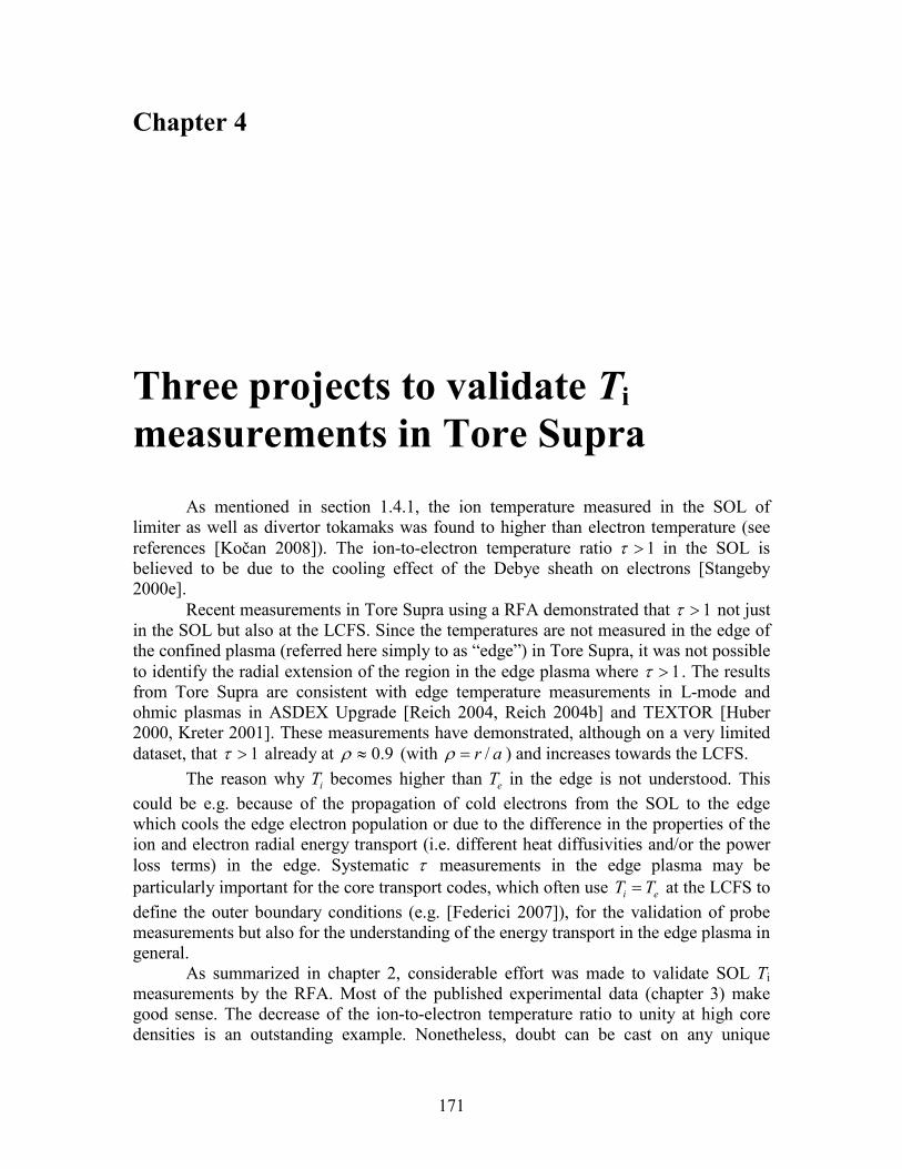
171

Chapter 4

Three projects to validate Ti measurements in Tore Supra

As mentioned in section 1.4.1, the ion temperature measured in the SOL of limiter as well as divertor tokamaks was found to higher than electron temperature (see references [Kočan 2008]). The ion-to-electron temperature ratio 1>τ in the SOL is believed to be due to the cooling effect of the Debye sheath on electrons [Stangeby 2000e].

Recent measurements in Tore Supra using a RFA demonstrated that 1>τ not just in the SOL but also at the LCFS. Since the temperatures are not measured in the edge of the confined plasma (referred here simply to as “edge”) in Tore Supra, it was not possible to identify the radial extension of the region in the edge plasma where 1>τ . The results from Tore Supra are consistent with edge temperature measurements in L-mode and ohmic plasmas in ASDEX Upgrade [Reich 2004, Reich 2004b] and TEXTOR [Huber 2000, Kreter 2001]. These measurements have demonstrated, although on a very limited dataset, that 1>τ already at 9.0≈ρ (with ar /=ρ ) and increases towards the LCFS.

The reason why iT becomes higher than eT in the edge is not understood. This could be e.g. because of the propagation of cold electrons from the SOL to the edge which cools the edge electron population or due to the difference in the properties of the ion and electron radial energy transport (i.e. different heat diffusivities and/or the power loss terms) in the edge. Systematic τ measurements in the edge plasma may be particularly important for the core transport codes, which often use ei TT = at the LCFS to define the outer boundary conditions (e.g. [Federici 2007]), for the validation of probe measurements but also for the understanding of the energy transport in the edge plasma in general. As summarized in chapter 2, considerable effort was made to validate SOL Ti measurements by the RFA. Most of the published experimental data (chapter 3) make good sense. The decrease of the ion-to-electron temperature ratio to unity at high core densities is an outstanding example. Nonetheless, doubt can be cast on any unique

172

diagnostic method as long as simultaneous and independent measurements by another diagnostic are unavailable. In this chapter, three well advanced, ongoing projects to obtain independent validation of the RFA results from Tore Supra are described. Firstly, it was decided that it would be useful to visit the JET tokamak to make a systematic study of ion-to-electron temperature ratio in the edge region using multiple diagnostics. The results indicate that, in agreement with the multi-machine database (Fig. 7 in [Kočan 2008]), that the ratio is greater than unity over a significant radial distance in the JET edge plasma. These results provoked a strong reaction amongst our JET colleagues, and they have undertaken a study to see if this result could be due to a shift in the electron temperature profile caused by uncertainties of the magnetic reconstruction. The completed analysis and present status of this project are presented in section 4.1. In Tore Supra CXRS provides measurements of Ti in the core plasma, but in the standard magnetic configuration, the outermost chord is too far from the LCFS to be compared with RFA measurements in the SOL. A dedicated experiment was proposed and executed in order to overlay the two measurements. This was done by making a small plasma leaning on the high field side bumper limiter, whose minor radius was chosen such some the outermost CXRS measurements lay in the SOL. Strong disagreement was found between the two methods. The preliminary analysis can be found in section 4.2. Finally, in section 4.3, a project to develop a new, independent probe method to measure ion temperature is described. The probe is known as the “segmented tunnel probe”, and was developed in collaboration between the CEA and IPP-Prague. The author of this thesis took charge of the design of the probe, had it built by IPP-Prague in a collaborative effort, and installed it on Tore Supra in 2008. The probe worked perfectly from a technical point of view. Kinetic simulations of the probe were performed in order to calibrate it. Initial comparison with the measurements is presented here.

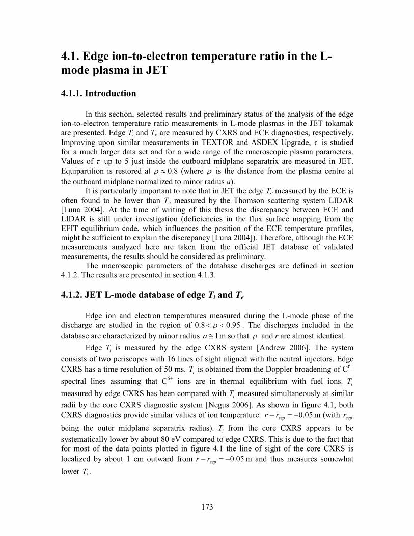
173

4.1. Edge ion-to-electron temperature ratio in the L-mode plasma in JET 4.1.1. Introduction

In this section, selected results and preliminary status of the analysis of the edge ion-to-electron temperature ratio measurements in L-mode plasmas in the JET tokamak are presented. Edge Ti and Te are measured by CXRS and ECE diagnostics, respectively. Improving upon similar measurements in TEXTOR and ASDEX Upgrade, τ is studied for a much larger data set and for a wide range of the macroscopic plasma parameters. Values of τ up to 5 just inside the outboard midplane separatrix are measured in JET. Equipartition is restored at 8.0≈ρ (where ρ is the distance from the plasma centre at the outboard midplane normalized to minor radius a).

It is particularly important to note that in JET the edge Te measured by the ECE is often found to be lower than Te measured by the Thomson scattering system LIDAR [Luna 2004]. At the time of writing of this thesis the discrepancy between ECE and LIDAR is still under investigation (deficiencies in the flux surface mapping from the EFIT equilibrium code, which influences the position of the ECE temperature profiles, might be sufficient to explain the discrepancy [Luna 2004]). Therefore, although the ECE measurements analyzed here are taken from the official JET database of validated measurements, the results should be considered as preliminary.

The macroscopic parameters of the database discharges are defined in section 4.1.2. The results are presented in section 4.1.3. 4.1.2. JET L-mode database of edge Ti and Te

Edge ion and electron temperatures measured during the L-mode phase of the discharge are studied in the region of 95.08.0 << ρ . The discharges included in the database are characterized by minor radius 1≅a m so that ρ and r are almost identical.

Edge iT is measured by the edge CXRS system [Andrew 2006]. The system consists of two periscopes with 16 lines of sight aligned with the neutral injectors. Edge CXRS has a time resolution of 50 ms. iT is obtained from the Doppler broadening of C6+ spectral lines assuming that C6+ ions are in thermal equilibrium with fuel ions. iT measured by edge CXRS has been compared with iT measured simultaneously at similar radii by the core CXRS diagnostic system [Negus 2006]. As shown in figure 4.1, both CXRS diagnostics provide similar values of ion temperature 05.0−=− seprr m (with sepr

being the outer midplane separatrix radius). iT from the core CXRS appears to be systematically lower by about 80 eV compared to edge CXRS. This is due to the fact that for most of the data points plotted in figure 4.1 the line of sight of the core CXRS is localized by about 1 cm outward from 05.0−=− seprr m and thus measures somewhat

lower iT .

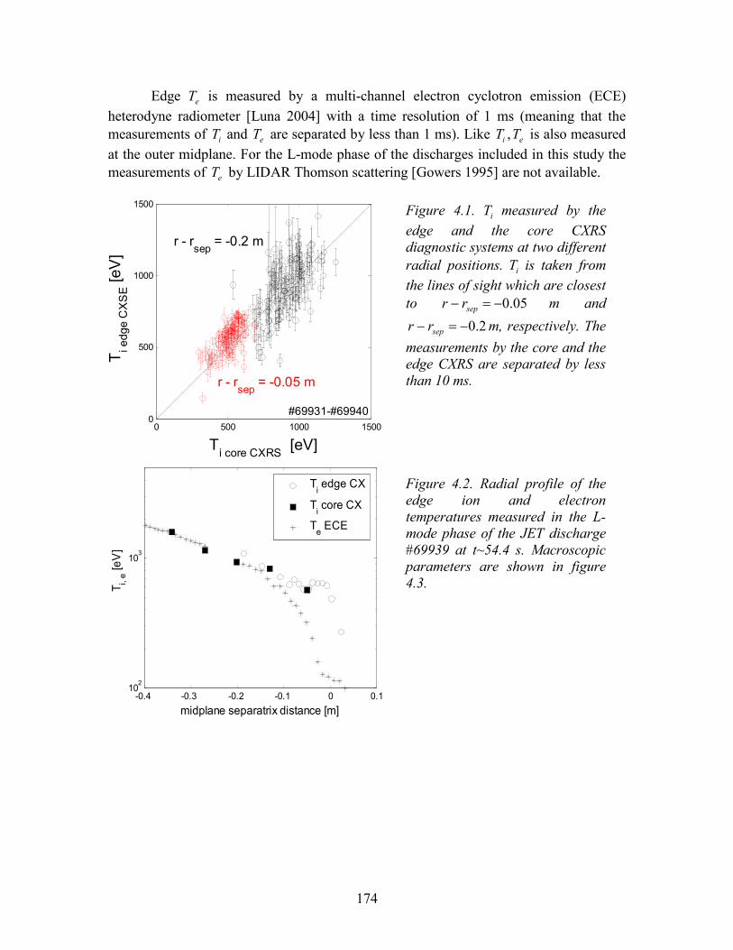
174

Edge eT is measured by a multi-channel electron cyclotron emission (ECE) heterodyne radiometer [Luna 2004] with a time resolution of 1 ms (meaning that the measurements of iT and eT are separated by less than 1 ms). Like iT , eT is also measured at the outer midplane. For the L-mode phase of the discharges included in this study the measurements of eT by LIDAR Thomson scattering [Gowers 1995] are not available.

0 500 1000 15000

500

1000

1500

Ti core CXRS

[eV]

Ti edg

e CXSE [eV]

r - rsep

= -0.2 m

r - rsep

= -0.05 m

#69931-#69940

Figure 4.1. iT measured by the edge and the core CXRS diagnostic systems at two different radial positions. iT is taken from the lines of sight which are closest to 05.0−=− seprr m and

2.0−=− seprr m, respectively. The measurements by the core and the edge CXRS are separated by less than 10 ms.

-0.4 -0.3 -0.2 -0.1 0 0.110

2

103

midplane separatrix distance [m]

T i, e [eV]

Ti edge CX

Ti core CX

Te ECE

Figure 4.2. Radial profile of the edge ion and electron temperatures measured in the L-mode phase of the JET discharge #69939 at t~54.4 s. Macroscopic parameters are shown in figure 4.3.

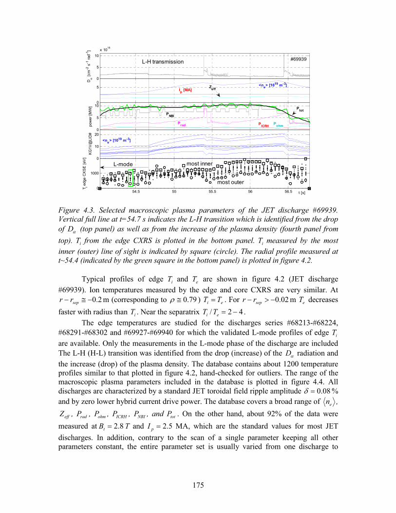
175

54.5 55 55.5 56 56.50

5

10

x 1015

Dα [cm

-2 s-1 rad

-1]

54.5 55 55.5 56 56.50

5

time [s]

54.5 55 55.5 56 56.50

5

10

power [MW]

54.5 55 55.5 56 56.50

10

20

KG1V

@LID#

54.5 55 55.5 56 56.50

1000

T i edge CXSE [eV

]ZeffIp [MA]

t [s]

#69939

PtotPNBI

Prad PICRH

Pohm

L-mode

<ne> [1019 m-3]

<ne> [1019 m-3]

most outer

most inner

L-H transmission

Figure 4.3. Selected macroscopic plasma parameters of the JET discharge #69939. Vertical full line at t=54.7 s indicates the L-H transition which is identified from the drop of αD (top panel) as well as from the increase of the plasma density (fourth panel from top). iT from the edge CXRS is plotted in the bottom panel. iT measured by the most inner (outer) line of sight is indicated by square (circle). The radial profile measured at t~54.4 (indicated by the green square in the bottom panel) is plotted in figure 4.2.

Typical profiles of edge iT and eT are shown in figure 4.2 (JET discharge #69939). Ion temperatures measured by the edge and core CXRS are very similar. At

2.0−≅− seprr m (corresponding to 79.0≅ρ ) ei TT = . For 02.0−>− seprr m eT decreases

faster with radius than iT . Near the separatrix 42/ −=ei TT . The edge temperatures are studied for the discharges series #68213-#68224,

#68291-#68302 and #69927-#69940 for which the validated L-mode profiles of edge iT are available. Only the measurements in the L-mode phase of the discharge are included The L-H (H-L) transition was identified from the drop (increase) of the αD radiation and the increase (drop) of the plasma density. The database contains about 1200 temperature profiles similar to that plotted in figure 4.2, hand-checked for outliers. The range of the macroscopic plasma parameters included in the database is plotted in figure 4.4. All discharges are characterized by a standard JET toroidal field ripple amplitude 08.0=δ % and by zero lower hybrid current drive power. The database covers a broad range of en ,

effZ , radP , ohmP , ICRHP , NBIP , and totP . On the other hand, about 92% of the data were

measured at 8.2=tB T and 5.2=pI MA, which are the standard values for most JET discharges. In addition, contrary to the scan of a single parameter keeping all other parameters constant, the entire parameter set is usually varied from one discharge to

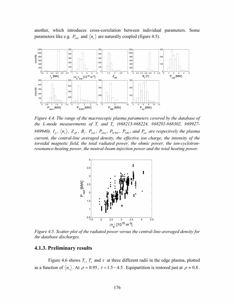
176

another, which introduces cross-correlation between individual parameters. Some parameters like e.g. radP and en are naturally coupled (figure 4.5).

1.8 2 2.2 2.4 2.6 2.80

200

400

600

800

1000

1200

Ip [MA]

1 2 3 4 5 60

100

200

300

400

500

<ne>line

[1019 m-3]

1 1.5 2 2.5 30

100

200

300

400

500

Zeff

2 2.2 2.4 2.6 2.8 3 3.20

200

400

600

800

1000

1200

Bt [T]

0 1 2 3 4 50

100

200

300

Prad

[MW]

0 0.5 1 1.5 2 2.50

100

200

300

400

500

coun

ts

Pohm

[MW]

coun

ts

0 1 2 3 40

200

400

600

800

PICRH

[MW]0 5 10

0

200

400

600

PNBI

[MW]2 4 6 8 10 12

0

100

200

300

Ptot [MW]

Figure 4.4. The range of the macroscopic plasma parameters covered by the database of the L-mode measurements of iT and eT (#68213-#68224, #68291-#68302, #69927-

#69940). pI , en , effZ , tB , radP , ohmP , ICRHP , NBIP , and totP are respectively the plasma current, the central-line averaged density, the effective ion charge, the intensity of the toroidal magnetic field, the total radiated power, the ohmic power, the ion-cyclotron-resonance-heating power, the neutral-beam-injection power and the total heating power.

1.5 2 2.5 3 3.5 4 4.50.5

1

1.5

2

2.5

3

3.5

4

⟨ne⟩ [1019 m-3]

Prad [MW]

Figure 4.5. Scatter plot of the radiated power versus the central-line-averaged density for the database discharges.

4.1.3. Preliminary results

Figure 4.6 shows iT , eT and τ at three different radii in the edge plasma, plotted

as a function of en . At 95.0=ρ , 5.45.1 −=τ . Equipartition is restored just at 8.0≈ρ .

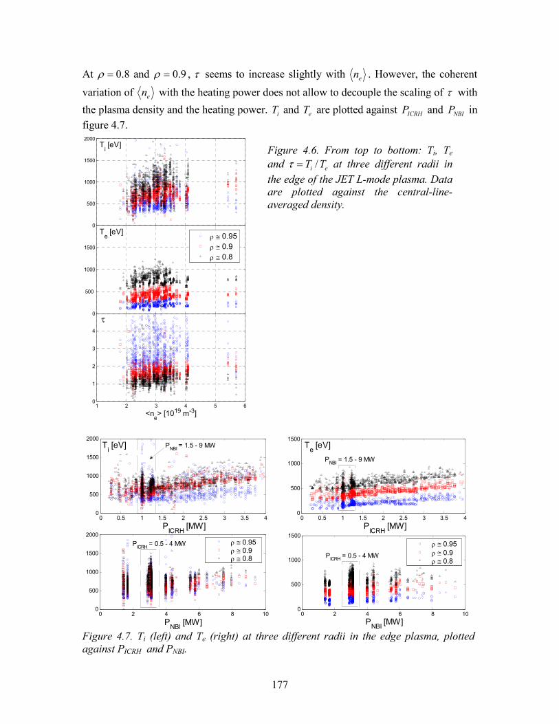
177

At 8.0=ρ and 9.0=ρ , τ seems to increase slightly with en . However, the coherent

variation of en with the heating power does not allow to decouple the scaling of τ with

the plasma density and the heating power. iT and eT are plotted against ICRHP and NBIP in figure 4.7.

2 3 4 50

500

1000

1500

2000

<ne>lin [1019 m-3]

2 3 4 5

500

1000

1500

1 2 3 4 5 60

1

2

3

4

0

<ne> [1019 m-3]

ρ ≅ 0.95ρ ≅ 0.9ρ ≅ 0.8

Ti [eV]

τ

Te [eV]

Figure 4.6. From top to bottom: Ti, Te and ei TT /=τ at three different radii in the edge of the JET L-mode plasma. Data are plotted against the central-line-averaged density.

0 0.5 1 1.5 2 2.5 3 3.5 40

500

1000

1500

2000

0 2 4 6 8 100

500

1000

1500

2000ρ ≅ 0.95ρ ≅ 0.9ρ ≅ 0.8

Ti [eV]

PICRH

[MW]

PNBI

[MW]

PNBI = 1.5 - 9 MW

PICRH = 0.5 - 4 MW

0 0.5 1 1.5 2 2.5 3 3.5 40

500

1000

1500

PICRH

[MW]

0 2 4 6 8 100

500

1000

1500

PNBI

[MW]

ρ ≅ 0.95ρ ≅ 0.9ρ ≅ 0.8

Te [eV]

PNBI = 1.5 - 9 MW

PICRH = 0.5 - 4 MW

Figure 4.7. Ti (left) and Te (right) at three different radii in the edge plasma, plotted against PICRH and PNBI.

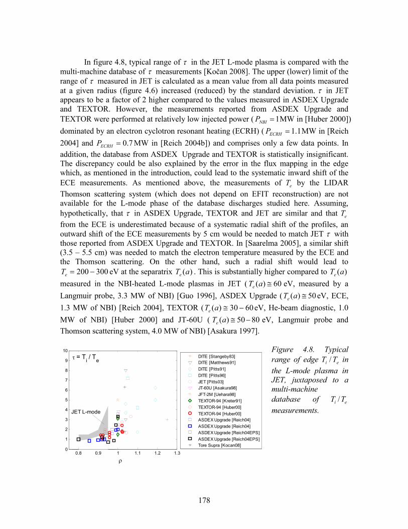
178

In figure 4.8, typical range of τ in the JET L-mode plasma is compared with the

multi-machine database of τ measurements [Kočan 2008]. The upper (lower) limit of the range of τ measured in JET is calculated as a mean value from all data points measured at a given radius (figure 4.6) increased (reduced) by the standard deviation. τ in JET appears to be a factor of 2 higher compared to the values measured in ASDEX Upgrade and TEXTOR. However, the measurements reported from ASDEX Upgrade and TEXTOR were performed at relatively low injected power ( 1=NBIP MW in [Huber 2000]) dominated by an electron cyclotron resonant heating (ECRH) ( 1.1=ECRHP MW in [Reich 2004] and 7.0=ECRHP MW in [Reich 2004b]) and comprises only a few data points. In addition, the database from ASDEX Upgrade and TEXTOR is statistically insignificant. The discrepancy could be also explained by the error in the flux mapping in the edge which, as mentioned in the introduction, could lead to the systematic inward shift of the ECE measurements. As mentioned above, the measurements of eT by the LIDAR Thomson scattering system (which does not depend on EFIT reconstruction) are not available for the L-mode phase of the database discharges studied here. Assuming, hypothetically, that τ in ASDEX Upgrade, TEXTOR and JET are similar and that eT from the ECE is underestimated because of a systematic radial shift of the profiles, an outward shift of the ECE measurements by 5 cm would be needed to match JET τ with those reported from ASDEX Upgrade and TEXTOR. In [Saarelma 2005], a similar shift (3.5 – 5.5 cm) was needed to match the electron temperature measured by the ECE and the Thomson scattering. On the other hand, such a radial shift would lead to

300200 −=eT eV at the separatrix )(aTe . This is substantially higher compared to )(aTe measured in the NBI-heated L-mode plasmas in JET ( 60)( ≅aTe eV, measured by a Langmuir probe, 3.3 MW of NBI) [Guo 1996], ASDEX Upgrade ( 50)( ≅aTe eV, ECE, 1.3 MW of NBI) [Reich 2004], TEXTOR ( 6030)( −≅aTe eV, He-beam diagnostic, 1.0 MW of NBI) [Huber 2000] and JT-60U ( 8050)( −≅aTe eV, Langmuir probe and Thomson scattering system, 4.0 MW of NBI) [Asakura 1997].

0.8 0.9 1 1.1 1.2 1.30

1

2

3

4

5

6

7

8

9

10

ρ

DITE [Stangeby83]DITE [Matthews91]DITE [Pitts91]DITE [Pitts96]JET [Pitts03]JT-60U [Asakura98]JFT-2M [Uehara98]TEXTOR-94 [Kreter91]TEXTOR-94 [Huber00]TEXTOR-94 [Huber00]ASDEX Upgrade [Reich04]ASDEX Upgrade [Reich04]ASDEX Upgrade [Reich04EPS]ASDEX Upgrade [Reich04EPS]Tore Supra [Kocan08]

τ = Ti / Te

JET L-mode

Figure 4.8. Typical range of edge ei TT / in the L-mode plasma in JET, juxtaposed to a multi-machine database of ei TT / measurements.

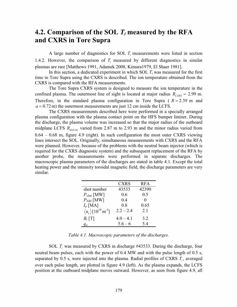
179

4.2. Comparison of the SOL Ti measured by the RFA and CXRS in Tore Supra

A large number of diagnostics for SOL iT measurements were listed in section 1.4.2. However, the comparison of iT measured by different diagnostics in similar plasmas are rare [Matthews 1991, Adamek 2008, Kimura1979, El Shaer 1981].

In this section, a dedicated experiment in which SOL Ti was measured for the first time in Tore Supra using the CXRS is described. The ion temperature obtained from the CXRS is compared with the RFA measurements.

The Tore Supra CXRS system is designed to measure the ion temperature in the confined plasma. The outermost line of sight is located at major radius =CXRSR 2.99 m. Therefore, in the standard plasma configuration in Tore Supra ( 39.2=R m and

72.0=a m) the outermost measurements are just 12 cm inside the LCFS. The CXRS measurements described here were performed in a specially arranged

plasma configuration with the plasma contact point on the HFS bumper limiter. During the discharge, the plasma volume was increased so that the major radius of the outboard midplane LCFS outmidR varied from 2.87 m to 2.93 m and the minor radius varied from 0.64 – 0.68 m, figure 4.9 (right). In such configuration the most outer CXRS viewing lines intersect the SOL. Originally, simultaneous measurements with CXRS and the RFA were planned. However, because of the problems with the neutral beam injector (which is required for the CXRS diagnostic system) and the subsequent replacement of the RFA by another probe, the measurements were performed in separate discharges. The macroscopic plasma parameters of the discharges are stated in table 4.1. Except the total heating power and the intensity toroidal magnetic field, the discharge parameters are very similar.

CXRS RFA shot number 43533 42390 Pohm [MW] 0.6 0.5 PNBI [MW] 0.4 0 Ip [MA] 0.8 0.65

en [1019 m-3] 2.2 – 2.4 2.1

Bt [T] 4.0 – 4.1 3.2 qa 5.6 – 6 5.4

Table 4.1. Macroscopic parameters of the discharges.

SOL iT was measured by CXRS in discharge #43533. During the discharge, four

neutral beam pulses, each with the power of 0.4 MW and with the pulse length of 0.5 s, separated by 0.5 s, were injected into the plasma. Radial profiles of CXRS iT , averaged over each pulse length, are plotted in figure 4.9 (left). As the plasma expands, the LCFS position at the outboard midplane moves outward. However, as seen from figure 4.9, all

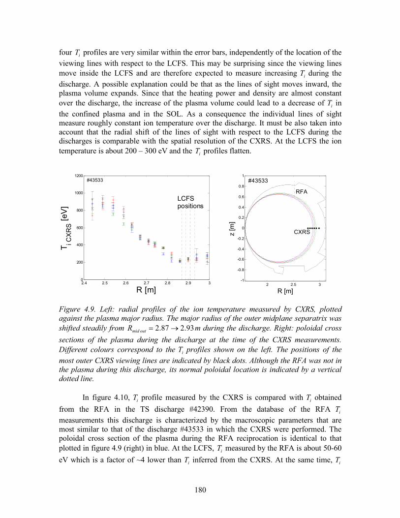
180

four iT profiles are very similar within the error bars, independently of the location of the viewing lines with respect to the LCFS. This may be surprising since the viewing lines move inside the LCFS and are therefore expected to measure increasing iT during the discharge. A possible explanation could be that as the lines of sight moves inward, the plasma volume expands. Since that the heating power and density are almost constant over the discharge, the increase of the plasma volume could lead to a decrease of iT in the confined plasma and in the SOL. As a consequence the individual lines of sight measure roughly constant ion temperature over the discharge. It must be also taken into account that the radial shift of the lines of sight with respect to the LCFS during the discharges is comparable with the spatial resolution of the CXRS. At the LCFS the ion temperature is about 200 – 300 eV and the iT profiles flatten.

2.4 2.5 2.6 2.7 2.8 2.9 30

200

400

600

800

1000

1200

R [m]

T i CXRS [e

V]

#43533

LCFSpositions

2 2.5 3

-1

-0.8

-0.6

-0.4

-0.2

0

0.2

0.4

0.6

0.8

1

R [m]

z [m]

#43533

RFA

CXRS

Figure 4.9. Left: radial profiles of the ion temperature measured by CXRS, plotted against the plasma major radius. The major radius of the outer midplane separatrix was shifted steadily from 93.287.2 →=outmidR m during the discharge. Right: poloidal cross sections of the plasma during the discharge at the time of the CXRS measurements. Different colours correspond to the iT profiles shown on the left. The positions of the most outer CXRS viewing lines are indicated by black dots. Although the RFA was not in the plasma during this discharge, its normal poloidal location is indicated by a vertical dotted line.

In figure 4.10, iT profile measured by the CXRS is compared with iT obtained from the RFA in the TS discharge #42390. From the database of the RFA iT measurements this discharge is characterized by the macroscopic parameters that are most similar to that of the discharge #43533 in which the CXRS were performed. The poloidal cross section of the plasma during the RFA reciprocation is identical to that plotted in figure 4.9 (right) in blue. At the LCFS, iT measured by the RFA is about 50-60 eV which is a factor of ~4 lower than iT inferred from the CXRS. At the same time, iT

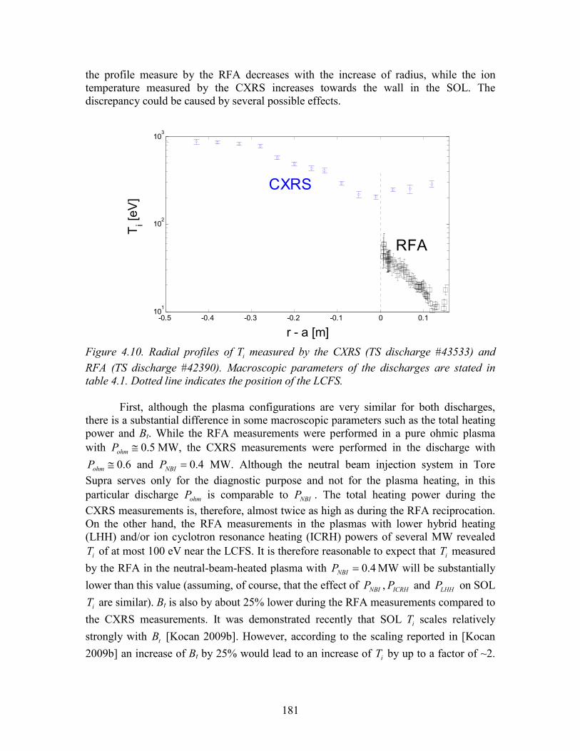
181

the profile measure by the RFA decreases with the increase of radius, while the ion temperature measured by the CXRS increases towards the wall in the SOL. The discrepancy could be caused by several possible effects.

-0.5 -0.4 -0.3 -0.2 -0.1 0 0.110

1

102

103

Ti [eV

]

r - a [m]

RFA

CXRS

Figure 4.10. Radial profiles of iT measured by the CXRS (TS discharge #43533) and RFA (TS discharge #42390). Macroscopic parameters of the discharges are stated in table 4.1. Dotted line indicates the position of the LCFS.

First, although the plasma configurations are very similar for both discharges,

there is a substantial difference in some macroscopic parameters such as the total heating power and Bt. While the RFA measurements were performed in a pure ohmic plasma with 5.0≅ohmP MW, the CXRS measurements were performed in the discharge with

6.0≅ohmP and 4.0=NBIP MW. Although the neutral beam injection system in Tore Supra serves only for the diagnostic purpose and not for the plasma heating, in this particular discharge ohmP is comparable to NBIP . The total heating power during the CXRS measurements is, therefore, almost twice as high as during the RFA reciprocation. On the other hand, the RFA measurements in the plasmas with lower hybrid heating (LHH) and/or ion cyclotron resonance heating (ICRH) powers of several MW revealed

iT of at most 100 eV near the LCFS. It is therefore reasonable to expect that iT measured by the RFA in the neutral-beam-heated plasma with 4.0=NBIP MW will be substantially lower than this value (assuming, of course, that the effect of NBIP , ICRHP and LHHP on SOL

iT are similar). Bt is also by about 25% lower during the RFA measurements compared to the CXRS measurements. It was demonstrated recently that SOL iT scales relatively strongly with tB [Kocan 2009b]. However, according to the scaling reported in [Kocan 2009b] an increase of Bt by 25% would lead to an increase of iT by up to a factor of ~2.

182

Therefore, the difference in the heating power or in tB cannot fully explain the difference in the CXRS and the RFA iT .

Another source of the discrepancy might be due to the influence of impurities on the RFA measurements. Since the analysis of the RFA I-V characteristics assumes Maxwellian singly charged ions SOL, iT inferred from the RFA measurements may be influenced by impurities [Pitts 1991]. As mentioned in section 2.3, separation of the components of the analyzed ion flux by charge state and temperature has been proposed in [Pitts 1991]. However, the model needs to specify the fractions of the total flux carried by ions with a given charge state as well as their temperatures. Such quantities are not available. In general, in a plasma with singly charged fuel ions the impurities lead to an underestimation of the measured ion temperature. However, if the impurity fluxes were important, the decaying part of the RFA I-V characteristic plotted on a semi-logarithmic scale would be characterized by a curvature instead of a linear decay (see e.g. figure 7.1.4 in [Pitts 1991]). Although these effects may be partially masked by the experimental noise, such curvature is not seen on the I-V characteristics, indicating perhaps that the effect of impurities on RFA iT measurements is insignificant.

Several questions concerning the CXRS measurements in the edge plasma and in the SOL, already mentioned in section 1.4.2.10 and discussed in more detail in [Bogen 1995]), need to be addressed. Are the impurity ions in thermal equilibrium with fuel ions at the SOL densities and electron temperatures 18105.2 ⋅<en m-3 and 20<eT eV, respectively? How does the overlapping of the Doppler-broadened C VI lines by other hydrogen-like lines (or other effects like e.g. atomic fine structure or Zeeman effect) in the SOL influence the spectral analysis? If not in the SOL, at what radial position in the edge plasma can we already believe the CXRS measurements? A large number of uncertainties mentioned above make a direct comparison of SOL iT measured by the RFA and the CXRS difficult. It is possible that the discrepancy could be fully explained by combining the individual uncertainties. It is also important to mention that iT measured by RFA is close to that measured in the similar plasmas in other tokamaks using different probe diagnostics (see references in section 1.4.1). In addition, the flattening or even small increase of SOL iT measured by the CXRS is also inconsistent with experimental observations reported elsewhere. Moreover, if the CXRS measurements were correct and SOL iT was 4 times higher compared to what is typically measured by the RFA, then ii TT / in the SOL would also be four times higher. This would imply 4/ =ii TT in detached plasmas and ii TT / up to 30 in heated plasmas. Such high values of the ion-to-electron temperature ratio would be inconsistent with the degree of the ion-electron collisisonality in the SOL (see chapter 3).

183

4.3. The segmented tunnel probe for Tore Supra plasma boundary

As a part of this thesis, a segmented tunnel probe (STP) for fast measurements of temperature and density measurements in the SOL of Tore Supra was designed, built, calibrated by particle simulations, and used for the first time in a large tokamak. This work is summarized in the following sections. 4.3.1. Introduction

It is generally accepted that anomalous transport – one of the key issues in the magnetic fusion research – is due to plasma turbulence (e.g. [Callen 1990, Connor 1993, Hidalgo 1995, Conway 2008]). A better understanding of turbulence in the plasma boundary region requires measurements of the fluctuation-induced conducted ( ET

~~)

and convected fluxes ( Tn~~ ) [Wootton 1990]. This requires new experimental

techniques for the simultaneous measurements of the fluctuations of the ion and electron temperatures, the electron density and the electric field. While the fluctuations of the electron temperature eT

~ can be measured using Langmuir probes (e.g. [Rudakov 2002]),

the measurements of the fluctuations of the ion temperature iT~

are extremely rare [Kočan 2006, Stöckel 2006]. In recent simulations of the MAST L-mode plasma using the 3D turbulence code BOUT, the amplitude of the fluctuations of the ion temperature was found to be approximately twice that of the electron temperature, both inside and outside the LCFS [Dudson 2008]. Simultaneous measurements of iT

~ and eT

~ on turbulence time-

scales (~µs) would thus be very useful for the validation of the codes. From the experimental techniques described in section 1.4.2, only the E×B

analyzer (section 1.4.2.4 and [Staib 1980, Staib 1982, Matthews 1984]) can be used for the fast iT measurements. However, because of the limited number of collectors, the ion velocity distribution is not measured directly. Instead, the ion currents received by the probe collectors are fit to the distributions obtained from a set of particle simulations. The reliability of the measurements thus depends on how realistic are the simulations (i.e. the velocity distribution of the injected ions, modelled geometry, secondary electron emission from the collectors, etc.). In addition, an E×B probe cannot measure iT

~, eT

~ and

en~ simultaneously.

A new probe, the STP, for fast measurements of iT~

, eT~

, en~ and fV~

(with fV~

being the fluctuations of the floating potential) has been recently tested in the CASTOR tokamak [Stöckel 2006, Kočan 2007, Adamek 2008]. During the evaluation of the thesis, a new segmented tunnel probe was designed, calibrated, and used in the Tore Supra SOL. Two STPs are placed back to back in a Mach probe arrangement to provide measurements of the parallel flow velocity. All quantities can be measured simultaneously, which, together with some other important advantages (such as the

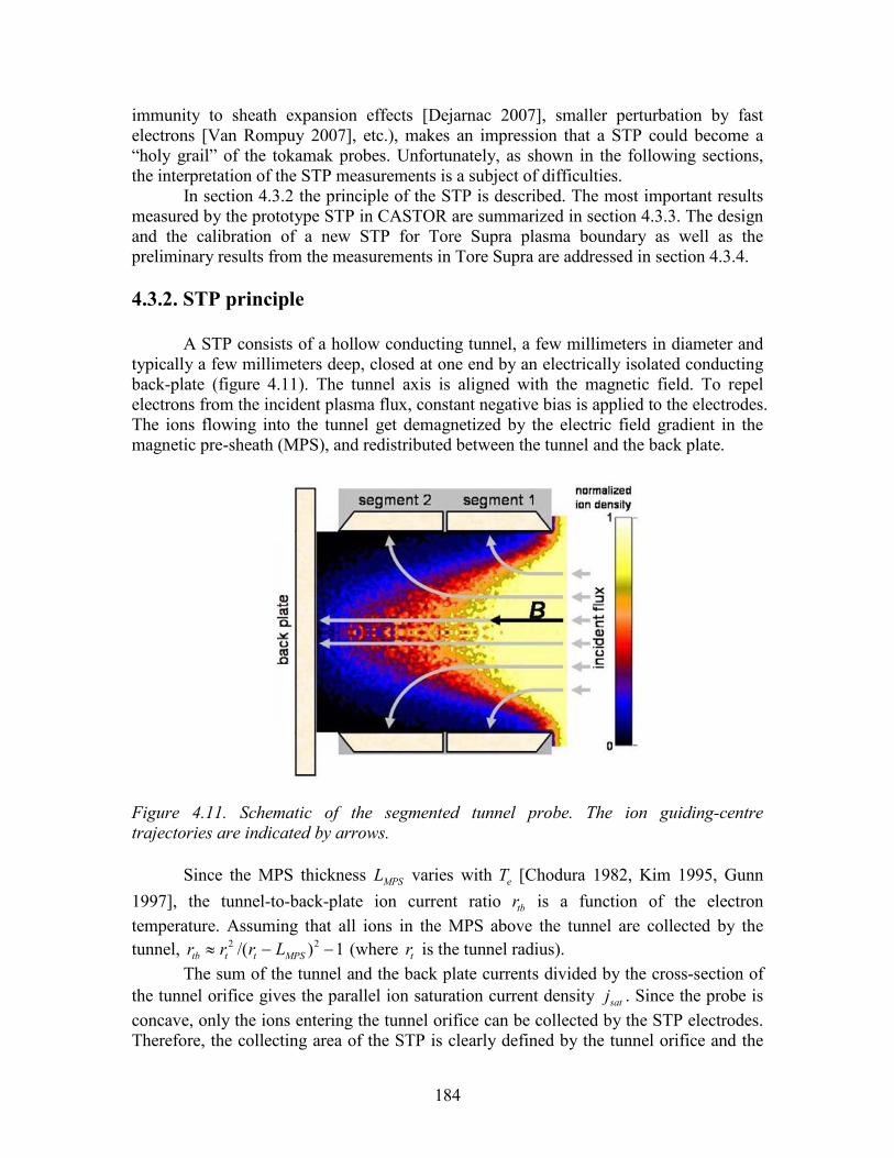
184

immunity to sheath expansion effects [Dejarnac 2007], smaller perturbation by fast electrons [Van Rompuy 2007], etc.), makes an impression that a STP could become a “holy grail” of the tokamak probes. Unfortunately, as shown in the following sections, the interpretation of the STP measurements is a subject of difficulties.

In section 4.3.2 the principle of the STP is described. The most important results measured by the prototype STP in CASTOR are summarized in section 4.3.3. The design and the calibration of a new STP for Tore Supra plasma boundary as well as the preliminary results from the measurements in Tore Supra are addressed in section 4.3.4. 4.3.2. STP principle

A STP consists of a hollow conducting tunnel, a few millimeters in diameter and typically a few millimeters deep, closed at one end by an electrically isolated conducting back-plate (figure 4.11). The tunnel axis is aligned with the magnetic field. To repel electrons from the incident plasma flux, constant negative bias is applied to the electrodes. The ions flowing into the tunnel get demagnetized by the electric field gradient in the magnetic pre-sheath (MPS), and redistributed between the tunnel and the back plate.

Figure 4.11. Schematic of the segmented tunnel probe. The ion guiding-centre trajectories are indicated by arrows.

Since the MPS thickness MPSL varies with eT [Chodura 1982, Kim 1995, Gunn 1997], the tunnel-to-back-plate ion current ratio tbr is a function of the electron temperature. Assuming that all ions in the MPS above the tunnel are collected by the tunnel, 1)/( 22 −−≈ MPStttb Lrrr (where tr is the tunnel radius).

The sum of the tunnel and the back plate currents divided by the cross-section of the tunnel orifice gives the parallel ion saturation current density satj . Since the probe is concave, only the ions entering the tunnel orifice can be collected by the STP electrodes. Therefore, the collecting area of the STP is clearly defined by the tunnel orifice and the

185

measurements of satj are immune to the sheath expansion [Dejarnac 2007] (this is in contrast to a convex Langmuir probes which, due to the deflection of ions in the MPS, collect the ion fluxes that are larger than that the flux of the ion guiding centres on the geometrical projection of the probe electrode along B). In addition, the measurements of

satj are only weakly influenced by secondary electron emission due to ion impact as a large fraction of the incident ion current is collected by the tunnel (The current to the tunnel is not affected by the secondary electron emission. This is because the tunnel surface is aligned with B and any secondary electrons emitted from the tunnel surface return back within less than one electron Larmor period so that the net secondary electron current from the tunnel surface is zero).

The axial distribution of ion flux along the tunnel is determined by the relative strength of the radial acceleration of ions with respect to their incident parallel velocity. Therefore, if the tunnel is divided into two segments the ion temperature iT could be obtained from the ratio of the ion currents to the tunnel segments segr .

The spatial resolution of the STP is defined by the tunnel diameter. To resolve the turbulent structures in the SOL, the tunnel diameter must be smaller than the typical radial size of the intermittent plasma filaments, or “blobs”, (~1 cm). On the other hand, in order to measure comparable tunnel and back plate currents, the tunnel diameter should be about 4 MPSL . MPSL is typically 0.2 – 1 mm in Tore Supra. This implies a tunnel diameter of a few millimeters.

A STP has several advantages compared to simple Langmuir probes. In addition to the simultaneous measurements of satj , eT and iT , its most important advantage is its temporal resolution. Since the measurements are performed at constant negative bias (dc mode), the temporal resolution a STP is limited only by the sampling frequency of the probe electronics. Moreover, as shown in [Gunn 2002b] the tunnel-to-back-plate ion current ratio tbr is relatively insensitive to the angular misalignment between the tunnel axis and B as long as the misalignment is less than 5°. Such tolerances can be easily achieved in experiment, leaving for wide margin of the variation of the edge safety factor. In addition, a recent theoretical study [Van Rompuy 2007] shows that in many conditions a STP may be less affected by hot electrons than a simple Langmuir probe.

On the other hand, the main handicap of the STP is in the difficulty of the interpretation of the temperature measurements. Since the electrostatic potential inside the tunnel is influenced by the local temperatures and densities, the measurements can only be interpreted by calibrating the probe using particle simulations. Typically, a set of PIC simulations (section 4.3.4.2) for given probe dimensions and the various combinations of iT , eT , satj and diffV (with diffV being the potential difference between the unperturbed plasma and the probe electrodes) is performed to produce the calibration curves, i.e. the scaling between the measured tbr and segr and unknown eT and iT ,

respectively [Kočan 2007]. fsfbiasdiff VVVV ++= where biasV is the external bias voltage

applied to the electrode, sfV is the floating sheath potential (Eq.(1.9)) and fV is the

floating potential). Since fV varies in time and space and in some cases it becomes

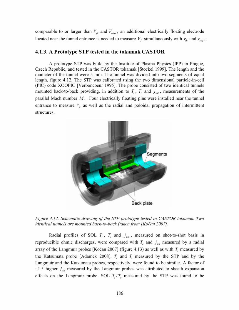
186

comparable to or larger than sfV and biasV , an additional electrically floating electrode

located near the tunnel entrance is needed to measure fV simultaneously with tbr and segr . 4.1.3. A Prototype STP tested in the tokamak CASTOR

A prototype STP was build by the Institute of Plasma Physics (IPP) in Prague, Czech Republic, and tested in the CASTOR tokamak [Stöckel 1999]. The length and the diameter of the tunnel were 5 mm. The tunnel was divided into two segments of equal length, figure 4.12. The STP was calibrated using the two dimensional particle-in-cell (PIC) code XOOPIC [Verboncoeur 1995]. The probe consisted of two identical tunnels mounted back-to-back providing, in addition to iT , eT and satj , measurements of the parallel Mach number //M . Four electrically floating pins were installed near the tunnel entrance to measure fV as well as the radial and poloidal propagation of intermittent structures.

Figure 4.12. Schematic drawing of the STP prototype tested in CASTOR tokamak. Two identical tunnels are mounted back-to-back (taken from [Kočan 2007].

Radial profiles of SOL iT , eT and satj , measured on shot-to-shot basis in

reproducible ohmic discharges, were compared with eT and satj measured by a radial array of the Langmuir probes [Kočan 2007] (figure 4.13) as well as with iT measured by the Katsumata probe [Adamek 2008]. eT and iT measured by the STP and by the Langmuir and the Katsumata probes, respectively, were found to be similar. A factor of ~1.5 higher satj measured by the Langmuir probes was attributed to sheath expansion effects on the Langmuir probe. SOL ei TT / measured by the STP was found to be

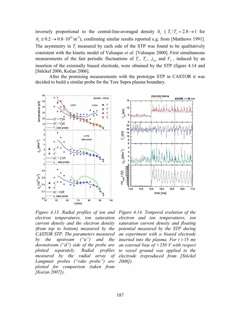
187

inversely proportional to the central-line-averaged density en ( 18.2/ →=ei TT for 18108.02.0 ⋅→≅en m-3), confirming similar results reported e.g. from [Matthews 1991].

The asymmetry in iT measured by each side of the STP was found to be qualitatively consistent with the kinetic model of Valsaque et al. [Valsaque 2000]. First simultaneous measurements of the fast periodic fluctuations of iT , eT , satj and fV , induced by an insertion of the externally biased electrode, were obtained by the STP (figure 4.14 and [Stöckel 2006, Kočan 2006].

After the promising measurements with the prototype STP in CASTOR it was decided to build a similar probe for the Tore Supra plasma boundary.

Figure 4.13. Radial profiles of ion and electron temperatures, ion saturation current density and the electron density (from top to bottom) measured by the CASTOR STP. The parameters measured by the upstream (“u”) and the downstream (“d”) side of the probe are plotted separately. Radial profiles measured by the radial array of Langmuir probes (“rake probe”) are plotted for comparison (taken from [Kočan 2007]).

Figure 4.14. Temporal evolution of the electron and ion temperatures, ion saturation current density and floating potential measured by the STP during an experiment with a biased electrode inserted into the plasma. For 15>t ms an external bias of +250 V with respect to vessel ground was applied to the electrode (reproduced from [Stöckel 2006]).

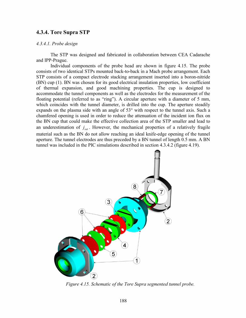
188

4.3.4. Tore Supra STP 4.3.4.1. Probe design

The STP was designed and fabricated in collaboration between CEA Cadarache

and IPP-Prague. Individual components of the probe head are shown in figure 4.15. The probe

consists of two identical STPs mounted back-to-back in a Mach probe arrangement. Each STP consists of a compact electrode stacking arrangement inserted into a boron-nitride (BN) cup (1). BN was chosen for its good electrical insulation properties, low coefficient of thermal expansion, and good machining properties. The cup is designed to accommodate the tunnel components as well as the electrodes for the measurement of the floating potential (referred to as “ring”). A circular aperture with a diameter of 5 mm, which coincides with the tunnel diameter, is drilled into the cup. The aperture steadily expands on the plasma side with an angle of 53° with respect to the tunnel axis. Such a chamfered opening is used in order to reduce the attenuation of the incident ion flux on the BN cup that could make the effective collection area of the STP smaller and lead to an underestimation of satj . However, the mechanical properties of a relatively fragile material such as the BN do not allow reaching an ideal knife-edge opening of the tunnel aperture. The tunnel electrodes are thus preceded by a BN tunnel of length 0.5 mm. A BN tunnel was included in the PIC simulations described in section 4.3.4.2 (figure 4.19).

Figure 4.15. Schematic of the Tore Supra segmented tunnel probe.

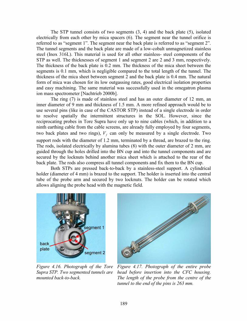
189

The STP tunnel consists of two segments (3, 4) and the back plate (5), isolated electrically from each other by mica spacers (6). The segment near the tunnel orifice is referred to as “segment 1”. The segment near the back plate is referred to as “segment 2”. The tunnel segments and the back plate are made of a low-cobalt unmagnetized stainless steel (Inox 316L). This material is used for all other stainless- steel components of the STP as well. The thicknesses of segment 1 and segment 2 are 2 and 3 mm, respectively. The thickness of the back plate is 0.2 mm. The thickness of the mica sheet between the segments is 0.1 mm, which is negligible compared to the total length of the tunnel. The thickness of the mica sheet between segment 2 and the back plate is 0.4 mm. The natural form of mica was chosen for its low outgassing rates, good electrical isolation properties and easy machining. The same material was successfully used in the omegatron plasma ion mass spectrometer [Nachtrieb 2000b].

The ring (7) is made of stainless steel and has an outer diameter of 12 mm, an inner diameter of 9 mm and thickness of 1.5 mm. A more refined approach would be to use several pins (like in case of the CASTOR STP) instead of a single electrode in order to resolve spatially the intermittent structures in the SOL. However, since the reciprocating probes in Tore Supra have only up to nine cables (which, in addition to a ninth earthing cable from the cable screens, are already fully employed by four segments, two back plates and two rings), fV can only be measured by a single electrode. Two support rods with the diameter of 1.2 mm, terminated by a thread, are brazed to the ring. The rods, isolated electrically by alumina tubes (8) with the outer diameter of 2 mm, are guided through the holes drilled into the BN cup and into the tunnel components and are secured by the locknuts behind another mica sheet which is attached to the rear of the back plate. The rods also compress all tunnel components and fix them to the BN cup.

Both STPs are pressed back-to-back by a stainless-steel support. A cylindrical holder (diameter of 4 mm) is brazed to the support. The holder is inserted into the central tube of the probe arm and secured by two locknuts. The holder can be rotated which allows aligning the probe head with the magnetic field.

Figure 4.16. Photograph of the Tore Supra STP. Two segmented tunnels are mounted back-to-back.

Figure 4.17. Photograph of the entire probe head before insertion into the CFC housing. The length of the probe from the centre of the tunnel to the end of the pins is 263 mm.

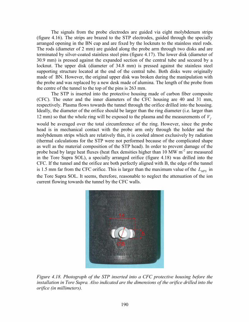
190

The signals from the probe electrodes are guided via eight molybdenum strips (figure 4.16). The strips are brazed to the STP electrodes, guided through the specially arranged opening in the BN cup and are fixed by the locknuts to the stainless steel rods. The rods (diameter of 2 mm) are guided along the probe arm through two disks and are terminated by silver-coated stainless steel pins (figure 4.17). The lower disk (diameter of 30.9 mm) is pressed against the expanded section of the central tube and secured by a locknut. The upper disk (diameter of 34.8 mm) is pressed against the stainless steel supporting structure located at the end of the central tube. Both disks were originally made of BN. However, the original upper disk was broken during the manipulation with the probe and was replaced by a new desk made of alumina. The length of the probe from the centre of the tunnel to the top of the pins is 263 mm.

The STP is inserted into the protective housing made of carbon fiber composite (CFC). The outer and the inner diameters of the CFC housing are 40 and 31 mm, respectively. Plasma flows towards the tunnel through the orifice drilled into the housing. Ideally, the diameter of the orifice should be larger than the ring diameter (i.e. larger than 12 mm) so that the whole ring will be exposed to the plasma and the measurements of fV would be averaged over the total circumference of the ring. However, since the probe head is in mechanical contact with the probe arm only through the holder and the molybdenum strips which are relatively thin, it is cooled almost exclusively by radiation (thermal calculations for the STP were not performed because of the complicated shape as well as the material composition of the STP head). In order to prevent damage of the probe head by large heat fluxes (heat flux densities higher than 10 MW m-2 are measured in the Tore Supra SOL), a specially arranged orifice (figure 4.18) was drilled into the CFC. If the tunnel and the orifice are both perfectly aligned with B, the edge of the tunnel is 1.5 mm far from the CFC orifice. This is larger than the maximum value of the MPSL in the Tore Supra SOL. It seems, therefore, reasonable to neglect the attenuation of the ion current flowing towards the tunnel by the CFC walls.

Figure 4.18. Photograph of the STP inserted into a CFC protective housing before the installation in Tore Supra. Also indicated are the dimensions of the orifice drilled into the orifice (in millimeters).

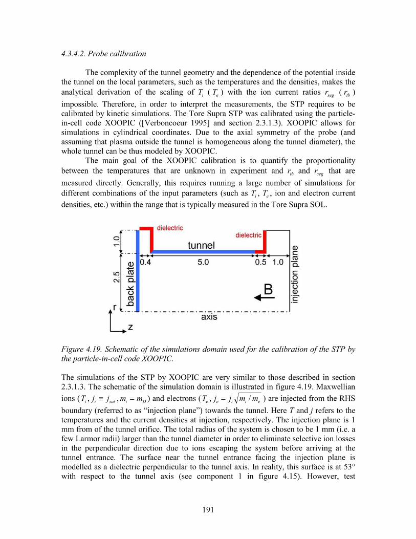
191

4.3.4.2. Probe calibration

The complexity of the tunnel geometry and the dependence of the potential inside the tunnel on the local parameters, such as the temperatures and the densities, makes the analytical derivation of the scaling of iT ( eT ) with the ion current ratios segr ( tbr ) impossible. Therefore, in order to interpret the measurements, the STP requires to be calibrated by kinetic simulations. The Tore Supra STP was calibrated using the particle-in-cell code XOOPIC ([Verboncoeur 1995] and section 2.3.1.3). XOOPIC allows for simulations in cylindrical coordinates. Due to the axial symmetry of the probe (and assuming that plasma outside the tunnel is homogeneous along the tunnel diameter), the whole tunnel can be thus modeled by XOOPIC.

The main goal of the XOOPIC calibration is to quantify the proportionality between the temperatures that are unknown in experiment and tbr and segr that are measured directly. Generally, this requires running a large number of simulations for different combinations of the input parameters (such as iT , eT , ion and electron current densities, etc.) within the range that is typically measured in the Tore Supra SOL.

Figure 4.19. Schematic of the simulations domain used for the calibration of the STP by the particle-in-cell code XOOPIC. The simulations of the STP by XOOPIC are very similar to those described in section 2.3.1.3. The schematic of the simulation domain is illustrated in figure 4.19. Maxwellian ions ( iT , sati jj ≡ , Di mm = ) and electrons ( eT , eiie mmjj /= ) are injected from the RHS boundary (referred to as “injection plane”) towards the tunnel. Here T and j refers to the temperatures and the current densities at injection, respectively. The injection plane is 1 mm from of the tunnel orifice. The total radius of the system is chosen to be 1 mm (i.e. a few Larmor radii) larger than the tunnel diameter in order to eliminate selective ion losses in the perpendicular direction due to ions escaping the system before arriving at the tunnel entrance. The surface near the tunnel entrance facing the injection plane is modelled as a dielectric perpendicular to the tunnel axis. In reality, this surface is at 53° with respect to the tunnel axis (see component 1 in figure 4.15). However, test

192

simulations revealed that the chamfering does not influence the ion current ratios tbr and

segr . While the chamfered edges near the tunnel orifice are neglected in the simulations, a 0.5 mm long dielectric tunnel attached to segment 1 is taken into account. This is because the dielectric tunnel collects all ions with the Larmor radius larger than their distance from the tunnel surface if the ion parallel transit time along the dielectric tunnel is longer than the Larmor period. For 5.3=B T, Di mm = , and 20=iT eV, the Larmor period

8107.3)/(2 −⋅≅= qBmT iL π s, which is only by a factor of ~3 longer than the parallel

transit time //// / vLt = (with L being the length of the dielectric tunnel and //v - defined

here as Tv2 - the parallel ion velocity). In the test simulations without the dielectric the ion current to segment 1 was by about 25% higher compared to the simulations with the dielectric tunnel, indicating that a non-negligible fraction of ions in the MPS above the tunnel surface can be collected by the dielectric tunnel. The dielectric which separates the tunnel segment (i.e. a mica plate with the thickness of 0.1 mm) is neglected in the simulations. The ion currents to segment 1 and segment 2, 1segi and 2segi , are calculated by integrating the ion current distribution along the tunnel collected in the steady state over the distance corresponding to the length of a given segment.

The injection plane and the boundary attached to it are held at 0 V. The tunnel and the back plate are at phbiasV φ+ (with phφ defined by Eq.(2.5)) with respect to the injection

plane. Most of the simulations were performed for 100−=biasV V. However, the simulations for different values of biasV are also discussed below (figure 4.21).

The magnetic field 5.3=B T (which is the value of the toroidal magnetic field at the magnetic axis used in most Tore Supra discharges) is aligned with the tunnel axis. PIC simulations for 5.2=B T were also performed for comparison (see figure 4.22).

The calibration was performed for the following range of ion and electron temperatures and ion current densities: 1605−=iT eV, 805−=eT eV and 81−=satj kA m-2. While the range if Ti and Te, typically measured in the Tore Supra SOL, is well covered by the simulations, the ion current densities in the Tore Supra SOL can reach up to 100 kA m-2. The reason why we did not perform the simulations for higher values of jsat is because of the long time needed for single XOOPIC run. The simulation for

8=satj kA m-2 and 10=eT eV already takes several days to run on a Pentium 4 CPU 3GHz PC, meaning that the simulation for higher satj would require up to several weeks.

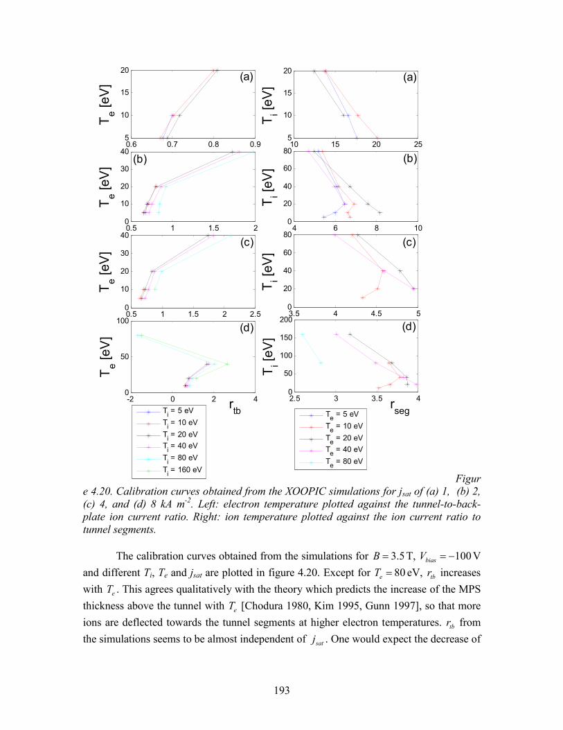
193

0.6 0.7 0.8 0.95

10

15

20

Te [eV]

0.5 1 1.5 20

10

20

30

40

Te [eV]

0.5 1 1.5 2 2.50

10

20

30

40

Te [eV]

-2 0 2 40

50

100

Te [eV]

Ti = 5 eV

Ti = 10 eV

Ti = 20 eVTi = 40 eV

Ti = 80 eV

Ti = 160 eV

10 15 20 255

10

15

20

Ti [eV

]

4 6 8 100

20

40

60

80

Ti [eV

]

3.5 4 4.5 50

20

40

60

80

Ti [eV

]

2.5 3 3.5 40

50

100

150

200

Ti [eV

]

Te = 5 eV

Te = 10 eV

Te = 20 eVTe = 40 eV

Te = 80 eV

rtb

rseg

(a) (a)

(b) (b)

(c)(c)

(d) (d)

Figure 4.20. Calibration curves obtained from the XOOPIC simulations for jsat of (a) 1, (b) 2, (c) 4, and (d) 8 kA m-2. Left: electron temperature plotted against the tunnel-to-back-plate ion current ratio. Right: ion temperature plotted against the ion current ratio to tunnel segments.

The calibration curves obtained from the simulations for 5.3=B T, 100−=biasV V

and different Ti, Te and jsat are plotted in figure 4.20. Except for 80=eT eV, tbr increases with eT . This agrees qualitatively with the theory which predicts the increase of the MPS thickness above the tunnel with eT [Chodura 1980, Kim 1995, Gunn 1997], so that more ions are deflected towards the tunnel segments at higher electron temperatures. tbr from the simulations seems to be almost independent of satj . One would expect the decrease of

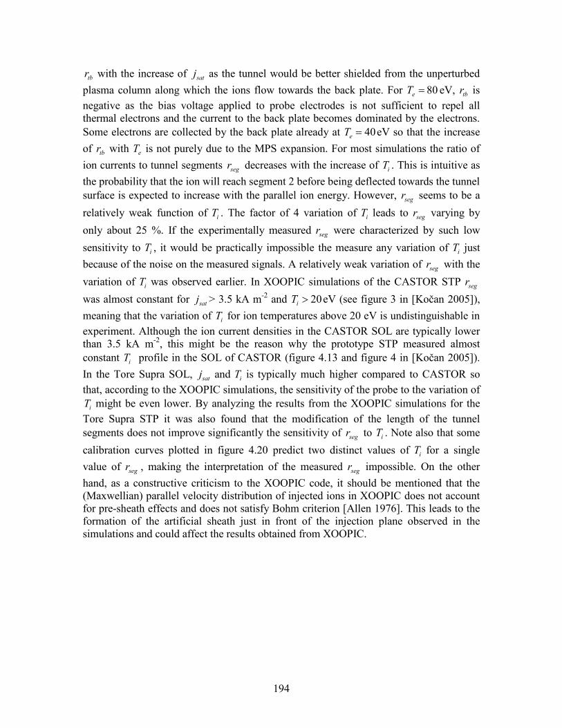
194

tbr with the increase of satj as the tunnel would be better shielded from the unperturbed plasma column along which the ions flow towards the back plate. For 80=eT eV, tbr is negative as the bias voltage applied to probe electrodes is not sufficient to repel all thermal electrons and the current to the back plate becomes dominated by the electrons. Some electrons are collected by the back plate already at 40=eT eV so that the increase of tbr with eT is not purely due to the MPS expansion. For most simulations the ratio of ion currents to tunnel segments segr decreases with the increase of iT . This is intuitive as the probability that the ion will reach segment 2 before being deflected towards the tunnel surface is expected to increase with the parallel ion energy. However, segr seems to be a

relatively weak function of iT . The factor of 4 variation of iT leads to segr varying by

only about 25 %. If the experimentally measured segr were characterized by such low

sensitivity to iT , it would be practically impossible the measure any variation of iT just because of the noise on the measured signals. A relatively weak variation of segr with the

variation of iT was observed earlier. In XOOPIC simulations of the CASTOR STP segr

was almost constant for satj > 3.5 kA m-2 and 20>iT eV (see figure 3 in [Kočan 2005]), meaning that the variation of iT for ion temperatures above 20 eV is undistinguishable in experiment. Although the ion current densities in the CASTOR SOL are typically lower than 3.5 kA m-2, this might be the reason why the prototype STP measured almost constant iT profile in the SOL of CASTOR (figure 4.13 and figure 4 in [Kočan 2005]). In the Tore Supra SOL, satj and iT is typically much higher compared to CASTOR so that, according to the XOOPIC simulations, the sensitivity of the probe to the variation of

iT might be even lower. By analyzing the results from the XOOPIC simulations for the Tore Supra STP it was also found that the modification of the length of the tunnel segments does not improve significantly the sensitivity of segr to iT . Note also that some

calibration curves plotted in figure 4.20 predict two distinct values of iT for a single value of segr , making the interpretation of the measured segr impossible. On the other hand, as a constructive criticism to the XOOPIC code, it should be mentioned that the (Maxwellian) parallel velocity distribution of injected ions in XOOPIC does not account for pre-sheath effects and does not satisfy Bohm criterion [Allen 1976]. This leads to the formation of the artificial sheath just in front of the injection plane observed in the simulations and could affect the results obtained from XOOPIC.

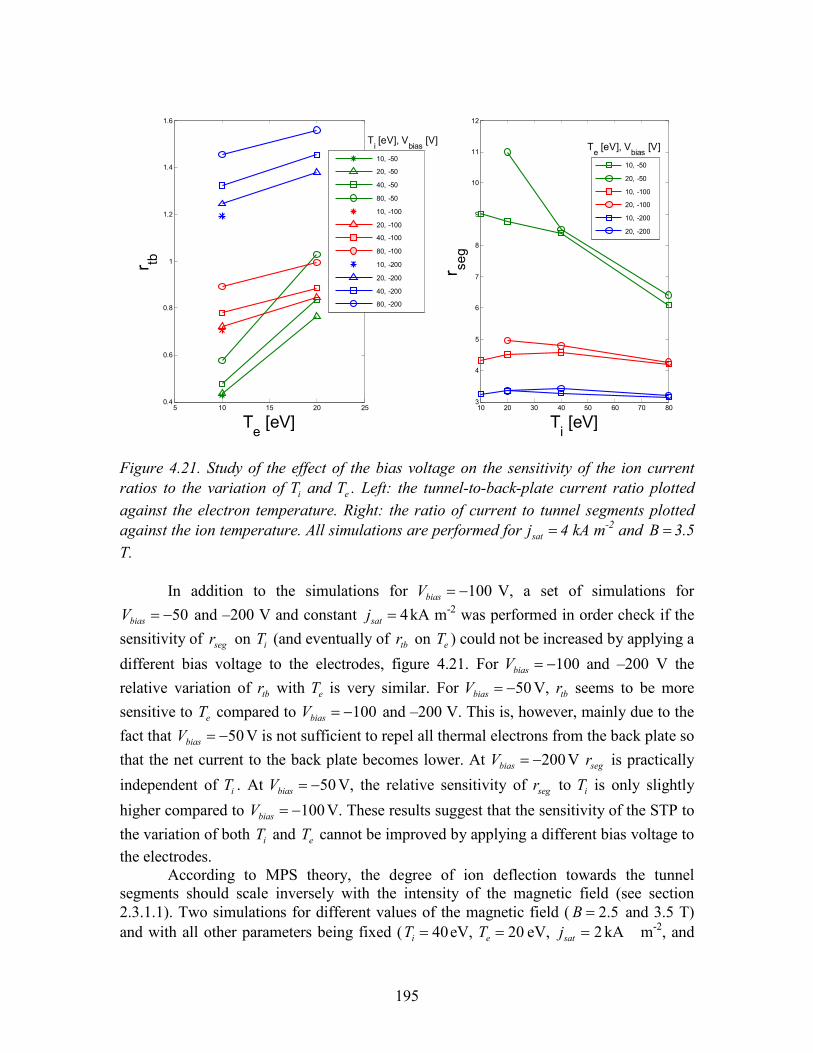
195

5 10 15 20 250.4

0.6

0.8

1

1.2

1.4

1.6

r tb

Te [eV]

10 20 30 40 50 60 70 803

4

5

6

7

8

9

10

11

12

r seg

Ti [eV]

10, -50

20, -50

40, -50

80, -50

10, -100

20, -100

40, -100

80, -100

10, -200

20, -200

40, -200

80, -200

10, -50

20, -50

10, -100

20, -100

10, -200

20, -200

Ti [eV], V

bias [V]

Te [eV], V

bias [V]

Figure 4.21. Study of the effect of the bias voltage on the sensitivity of the ion current ratios to the variation of iT and eT . Left: the tunnel-to-back-plate current ratio plotted against the electron temperature. Right: the ratio of current to tunnel segments plotted against the ion temperature. All simulations are performed for =satj 4 kA m-2 and =B 3.5 T.

In addition to the simulations for 100−=biasV V, a set of simulations for 50−=biasV and –200 V and constant 4=satj kA m-2 was performed in order check if the

sensitivity of segr on iT (and eventually of tbr on eT ) could not be increased by applying a

different bias voltage to the electrodes, figure 4.21. For 100−=biasV and –200 V the relative variation of tbr with eT is very similar. For 50−=biasV V, tbr seems to be more sensitive to eT compared to 100−=biasV and –200 V. This is, however, mainly due to the fact that 50−=biasV V is not sufficient to repel all thermal electrons from the back plate so that the net current to the back plate becomes lower. At 200−=biasV V segr is practically

independent of iT . At 50−=biasV V, the relative sensitivity of segr to iT is only slightly

higher compared to 100−=biasV V. These results suggest that the sensitivity of the STP to the variation of both iT and eT cannot be improved by applying a different bias voltage to the electrodes.

According to MPS theory, the degree of ion deflection towards the tunnel segments should scale inversely with the intensity of the magnetic field (see section 2.3.1.1). Two simulations for different values of the magnetic field ( 5.2=B and 3.5 T) and with all other parameters being fixed ( 40=iT eV, 20=eT eV, 2=satj kA m-2, and

196

100−=biasV V) are compared in figure 4.22. The dependence of segr and tbr on B agrees qualitative agreement with the theory. The ion current to both tunnel segments decreases with the increase of B whereas the back plate current increases with B. This is because the number of ions that are torn from the magnetic field lines and deflected towards the tunnel segments is lower at higher B. As a consequence, tbr decreases with the increase of B. Since the ion currents to segment 1 and 2 decrease by the same amount with the increase of B but the current to segment 2 is lower in the absolute value compared to the current to segment 1, segr increases with B.

2.5 3 3.50

0.005

0.01

0.015

0.02

i [a.u.]

ibpiseg 1iseg 2

2.5 3 3.50.8

1

1.2

1.4

1.6

r tb

2 2.5 3 3.5 43

4

5

6

B [T]

r seg

Figure 4.22. Top: ion currents to the tunnel segments ( 1segi , 2segi ) and to the

back plate ( bpi ). Middle: tunnel-to-back-plate ion current ratio. Bottom: ratio of ion currents to tunnel segments. Results from the XOOPIC simulations for =iT 40 eV, =eT 20 eV, =satj 2 kA m-2, =biasV –100 V and for two values of the magnetic field B = 2.5 and 3.5 T.

4.3.4.3. Experimental data

The STP was installed in Tore Supra in September 2008. In the period between

16th September and 2nd October, 177 reciprocations were performed with the STP. The probe target position was steadily shifted towards the LCFS in consecutive discharges (figure 4.23, right). For most of the reciprocations the measurements were acquired up to 5 mm outside the LCFS. All STP signals kept their normal behavior even at the maximum target position 4 cm inside the LCFS in an ohmic discharge as well as 2.5 cm outside the LCFS in a plasma heated to 8 MW (figure 4.23, left). The range of the macroscopic plasma parameters covered by the STP is plotted in figure 4.24. Most measurements were performed at the value of Bt close to that used in the PIC simulations (3.5 T).

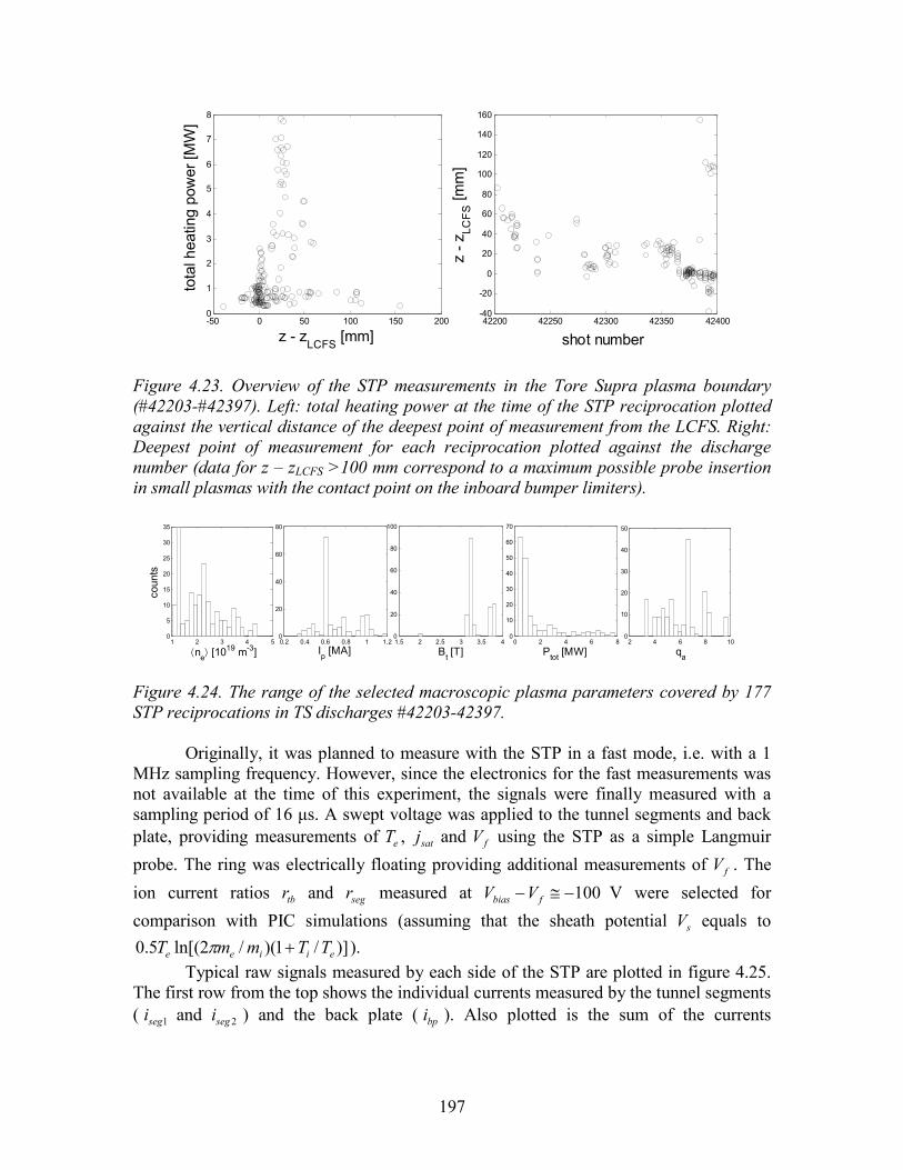
197

-50 0 50 100 150 2000

1

2

3

4

5

6

7

8

z - zLCFS

[mm]

total heating power [M

W]

42200 42250 42300 42350 42400-40

-20

0

20

40

60

80

100

120

140

160

shot number

z - z

LCFS [m

m]

Figure 4.23. Overview of the STP measurements in the Tore Supra plasma boundary (#42203-#42397). Left: total heating power at the time of the STP reciprocation plotted against the vertical distance of the deepest point of measurement from the LCFS. Right: Deepest point of measurement for each reciprocation plotted against the discharge number (data for z – zLCFS >100 mm correspond to a maximum possible probe insertion in small plasmas with the contact point on the inboard bumper limiters).

1 2 3 4 50

5

10

15

20

25

30

35

counts

⟨ne⟩ [1019 m-3]

0.2 0.4 0.6 0.8 1 1.20

20

40

60

80

Ip [MA]

1.5 2 2.5 3 3.5 40

20

40

60

80

100

Bt [T]2 4 6 8 10

0

10

20

30

40

50

qa 0 2 4 6 8

0

10

20

30

40

50

60

70

Ptot [MW] Figure 4.24. The range of the selected macroscopic plasma parameters covered by 177 STP reciprocations in TS discharges #42203-42397.

Originally, it was planned to measure with the STP in a fast mode, i.e. with a 1 MHz sampling frequency. However, since the electronics for the fast measurements was not available at the time of this experiment, the signals were finally measured with a sampling period of 16 µs. A swept voltage was applied to the tunnel segments and back plate, providing measurements of eT , satj and fV using the STP as a simple Langmuir

probe. The ring was electrically floating providing additional measurements of fV . The

ion current ratios tbr and segr measured at 100−≅− fbias VV V were selected for

comparison with PIC simulations (assuming that the sheath potential sV equals to )]/1)(/2ln[(5.0 eiiee TTmmT +π ).

Typical raw signals measured by each side of the STP are plotted in figure 4.25. The first row from the top shows the individual currents measured by the tunnel segments ( 1segi and 2segi ) and the back plate ( bpi ). Also plotted is the sum of the currents

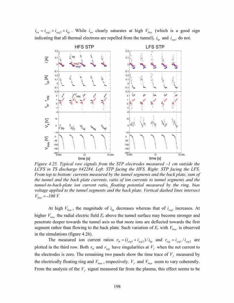
198

bpsegsegtot iiii ++= 21 . While toti clearly saturates at high biasV (which is a good sign

indicating that all thermal electrons are repelled from the tunnel), bpi and 1segi do not.

10 -0.1

0

0.1

0.2HFS STP

i [A]

10 -0.1

0

0.1

0.2LFS STP

10 -0.2

-0.1

0

0.1

0.2

i tot [A]

10 -0.2

-0.1

0

0.1

0.2

10 -2

-1

0

1

2

r tb, r seg

10 -2

-1

0

1

2

10 -10

0

10

Vfl [V]

10 -10

0

10

9.995 10 10.005-200

-150

-100

-50

0

time [s]

Vbias [V

]

9.995 10 10.005-200

-150

-100

-50

0

time [s]

bp

seg1seg2

rseg

rtb

Figure 4.25. Typical raw signals from the STP electrodes measured ~1 cm outside the LCFS in TS discharge #42284. Left: STP facing the HFS. Right: STP facing the LFS. From top to bottom: currents measured by the tunnel segments and the back plate, sum of the tunnel and the back plate currents, ratio of ion currents to tunnel segments and the tunnel-to-back-plate ion current ratio, floating potential measured by the ring, bias voltage applied to the tunnel segments and the back plate. Vertical dashed lines intersect

=biasV -100 V. At high biasV , the magnitude of bpi decreases whereas that of 1segi increases. At

higher biasV the radial electric field Er above the tunnel surface may become stronger and penetrate deeper towards the tunnel axis so that more ions are deflected towards the first segment rather than flowing to the back plate. Such variation of Er with biasV is observed in the simulations (figure 4.26).

The measured ion current ratios bpsegsegtb iiir /)( 21 += and 21 / segsegseg iir = are

plotted in the third row. Both tbr and segr have singularities at fV when the net current to

the electrodes is zero. The remaining two panels show the time trace of fV measured by

the electrically floating ring and biasV , respectively. fV and biasV seem to vary coherently.

From the analysis of the fV signal measured far from the plasma, this effect seems to be

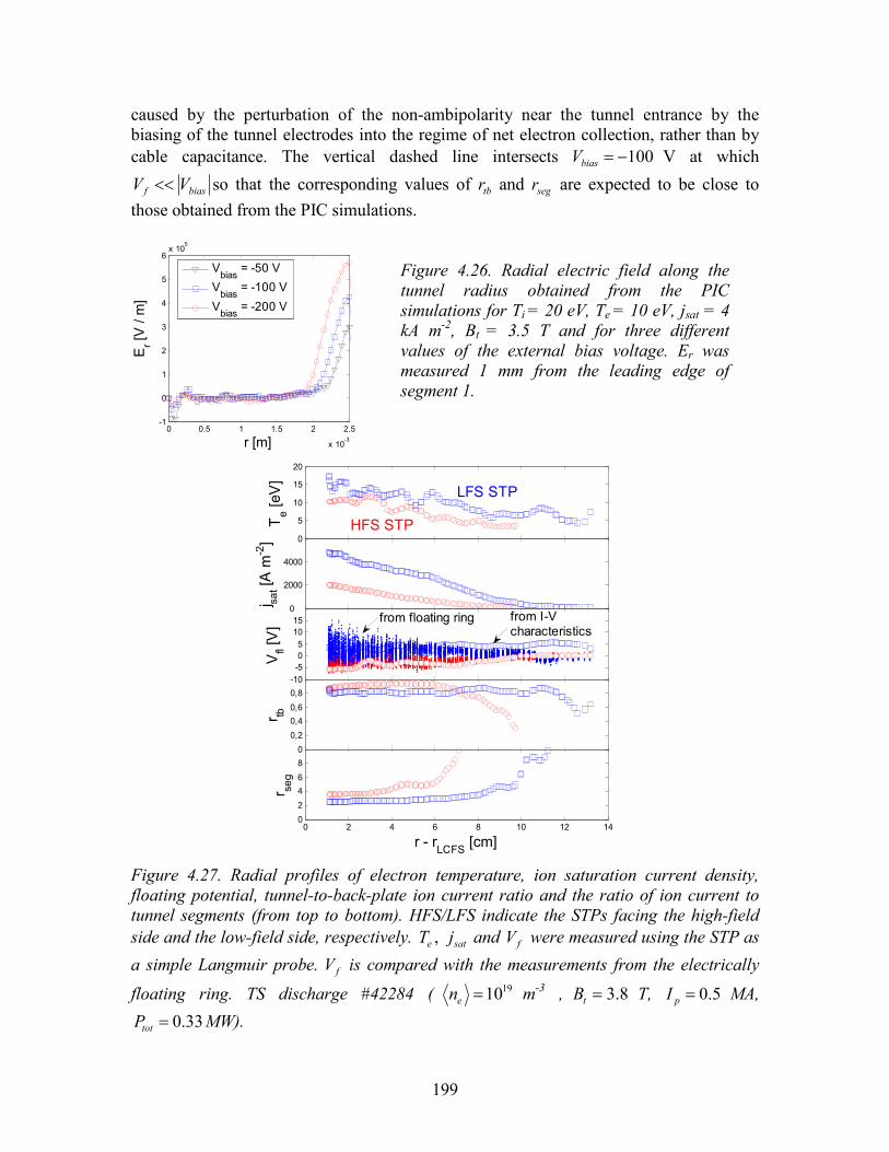
199

caused by the perturbation of the non-ambipolarity near the tunnel entrance by the biasing of the tunnel electrodes into the regime of net electron collection, rather than by cable capacitance. The vertical dashed line intersects 100−=biasV V at which

biasf VV << so that the corresponding values of tbr and segr are expected to be close to those obtained from the PIC simulations.

0 0.5 1 1.5 2 2.5

x 10-3

-1

0

1

2

3

4

5

6x 10

5

r [m]

Er [V / m]

Vbias

= -50 V

Vbias

= -100 V

Vbias

= -200 V

Figure 4.26. Radial electric field along the tunnel radius obtained from the PIC simulations for Ti = 20 eV, Te = 10 eV, jsat = 4 kA m-2, Bt = 3.5 T and for three different values of the external bias voltage. Er was measured 1 mm from the leading edge of segment 1.

2 4 6 8 10 120

5

10

15

20

Te [eV]

2 4 6 8 10 120

2000

4000

j sat [A m

-2]

2 4 6 8 10 12-10-5051015

Vfl [V]

2 4 6 8 10 120

0,2

0,4

0,6

0,8

r tb

0 2 4 6 8 10 12 140

2

4

6

8

r - rLCFS [cm]

r seg

LFS STP

HFS STP

from floating ring from I-Vcharacteristics

Figure 4.27. Radial profiles of electron temperature, ion saturation current density, floating potential, tunnel-to-back-plate ion current ratio and the ratio of ion current to tunnel segments (from top to bottom). HFS/LFS indicate the STPs facing the high-field side and the low-field side, respectively. eT , satj and fV were measured using the STP as

a simple Langmuir probe. fV is compared with the measurements from the electrically

floating ring. TS discharge #42284 ( 1910=en m-3 , 8.3=tB T, 5.0=pI MA,

33.0=totP MW).

200

The analysis of the rough data yields the radial profiles plotted in figure 4.27. As mentioned above, eT , satj and fV are obtained from standard Langmuir-probe analysis of

toti versus biasV (Eq. 1.15). The radial profiles of eT and satj measured by each side of the STP are clearly asymmetric. Similar asymmetries are measured by other reciprocating probes in Tore Sure (see section 2.3.1.3 and [Gunn 2007, Kočan 2009]).

The floating potential obtained from Langmuir-probe analysis of the I-V characteristics is juxtaposed to fV measured by the electrically floating ring located near

the tunnel entrance. Both values of fV are very similar.

Also plotted in figure 4.27 are the radial profiles of tbr and segr measured at

100−≅− fbias VV V. For a certain range of LCFSrr − ( 11< cm for the LFS STP and 6< cm

for the HFS STP) tbr is almost independent of radius and decreases with radius for larger radii. This could be explained by two competing effects. While the MPS thickness above the tunnel scales with eT (so that tbr is expected to increase with eT ), at higher satj , tbr tends to decrease because of stronger Debye shielding. Since both eT and satj increases towards the LCFS, the actual radial dependence of tbr could depend on which parameter,

eT or satj , has a dominant influence at given radii. This could also explain the variation of the HFS/LFS asymmetry of tbr with radius (if tbr was controlled by eT only, one would expect to measure higher tbr by the LFS STP for all radii). For 155−≅eT eV and

41−≅satj k Am-2, tbr varies between 0.8 and 1. The experimental tbr is close to that predicted by simulations (more systematic comparison is made below). It should be mentioned that the current measured by the back plate can be influenced by secondary electron emission due to ion impact as each secondary electron counts as a collected ion. In order to account for the secondary electron emission from the back plate, tbr from the PIC simulations (in which the secondary electron emission is neglected) should divided by a factor δ+1 . Here δ is the secondary electron emission coefficient due to ion impact, averaged over the incident ion energies and impact angles. For stainless steel and for relevant ion impact energies, δ measured by Thomas [Thomas 1991] varies from 0.4 to 1.

The bottom row in figure 4.27 shows the radial profile of segr measured for

100−≅− fbias VV V. segr decreases with radius up to 3 cm outside the LCFS for the HFS

STP and up to 6 cm outside the LCFS for the LFS STP. For smaller radii segr is almost

independent of radius. The decrease of segr towards the LCFS is intuitive. The probability that the ion will reach a distant part of the tunnel (i.e. segment 2) increases with the parallel ion velocity. The increase of iT towards the LCFS (which is measured by RFA) should be, therefore, associated with a decrease of segr . In addition, the HFS STP

measures higher segr than the LFS STP, indicating that the effective ion temperature on that side of the probe could be lower than on the LFS STP. Since the parallel flow is directed towards the LFS STP, such asymmetry in iT is consistent with the kinetic model of Valsaque et al. [Valsaque 2000] as well as with the RFA measurements (section

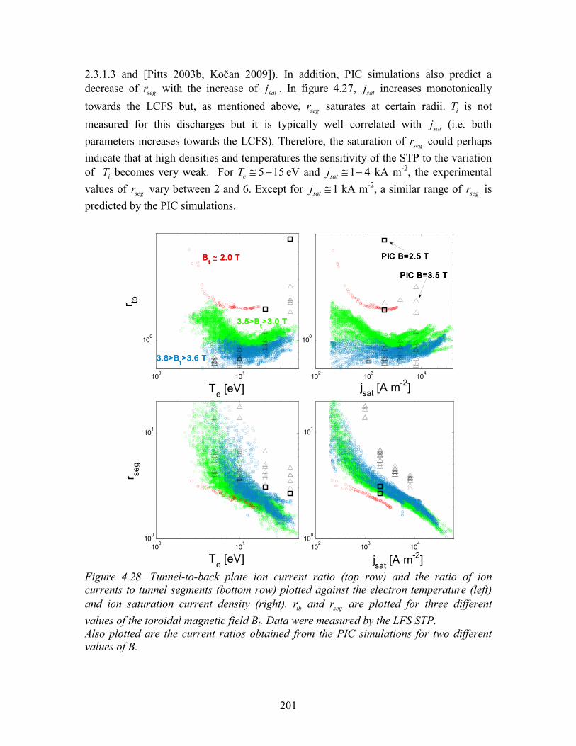
201

2.3.1.3 and [Pitts 2003b, Kočan 2009]). In addition, PIC simulations also predict a decrease of segr with the increase of satj . In figure 4.27, satj increases monotonically

towards the LCFS but, as mentioned above, segr saturates at certain radii. iT is not

measured for this discharges but it is typically well correlated with satj (i.e. both parameters increases towards the LCFS). Therefore, the saturation of segr could perhaps indicate that at high densities and temperatures the sensitivity of the STP to the variation of iT becomes very weak. For 155−≅eT eV and 41−≅satj kA m-2, the experimental values of segr vary between 2 and 6. Except for 1≅satj kA m-2, a similar range of segr is predicted by the PIC simulations.

100

101

100

Te [eV]

r tb

102

103

104

100

jsat [A m-2]

100

101

100

101

Te [eV]

r seg

102

103

104

100

101

jsat [A m-2]

3.8>B3.8>B3.8>B3.8>Btttt>3.6 T>3.6 T>3.6 T>3.6 T

3.5>B3.5>B3.5>B3.5>Btttt>3.0 T>3.0 T>3.0 T>3.0 T

BBBBtttt ≅≅≅≅ 2.0 T 2.0 T 2.0 T 2.0 T

PIC B=3.5 TPIC B=3.5 TPIC B=3.5 TPIC B=3.5 T

PIC B=2.5 TPIC B=2.5 TPIC B=2.5 TPIC B=2.5 T

Figure 4.28. Tunnel-to-back plate ion current ratio (top row) and the ratio of ion currents to tunnel segments (bottom row) plotted against the electron temperature (left) and ion saturation current density (right). tbr and segr are plotted for three different values of the toroidal magnetic field Bt. Data were measured by the LFS STP. Also plotted are the current ratios obtained from the PIC simulations for two different values of B.

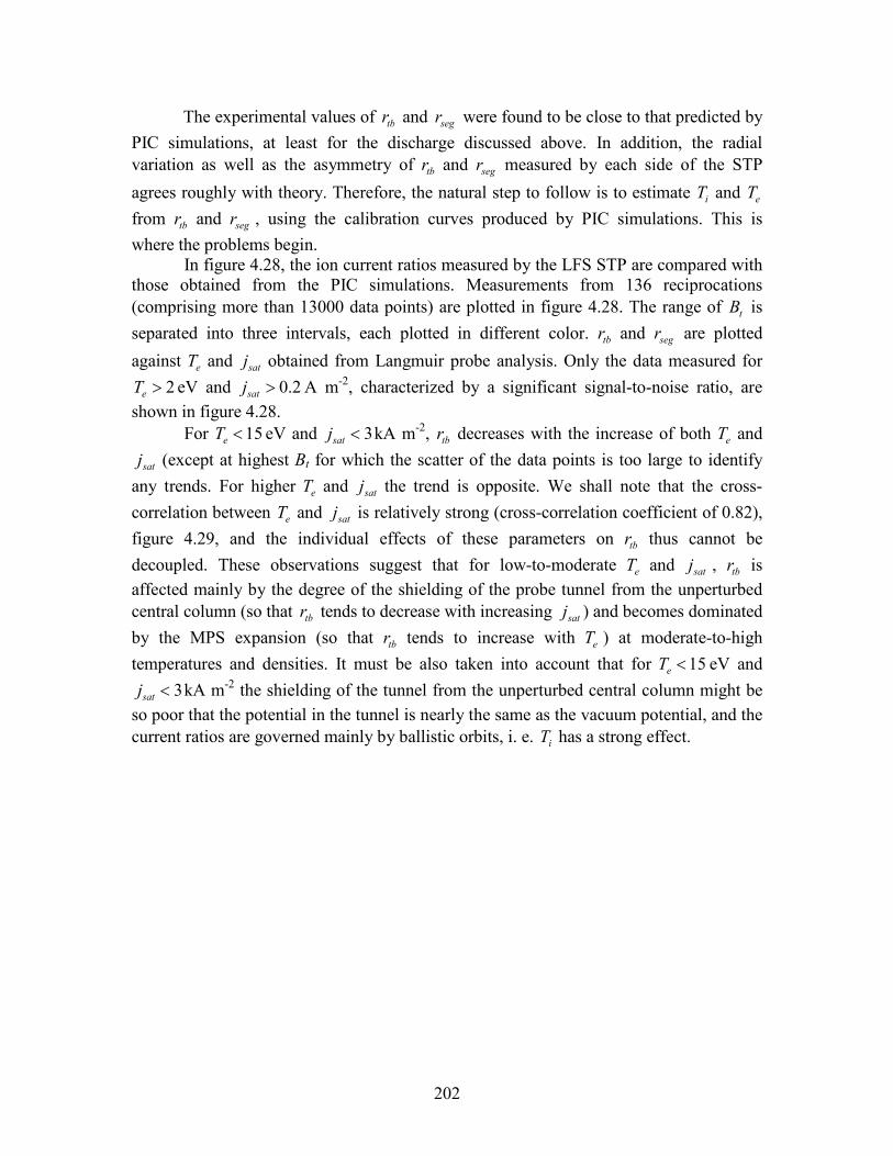
202

The experimental values of tbr and segr were found to be close to that predicted by PIC simulations, at least for the discharge discussed above. In addition, the radial variation as well as the asymmetry of tbr and segr measured by each side of the STP

agrees roughly with theory. Therefore, the natural step to follow is to estimate iT and eT from tbr and segr , using the calibration curves produced by PIC simulations. This is where the problems begin. In figure 4.28, the ion current ratios measured by the LFS STP are compared with those obtained from the PIC simulations. Measurements from 136 reciprocations (comprising more than 13000 data points) are plotted in figure 4.28. The range of tB is separated into three intervals, each plotted in different color. tbr and segr are plotted

against eT and satj obtained from Langmuir probe analysis. Only the data measured for 2>eT eV and 2.0>satj A m-2, characterized by a significant signal-to-noise ratio, are

shown in figure 4.28. For 15<eT eV and 3<satj kA m-2, tbr decreases with the increase of both eT and

satj (except at highest Bt for which the scatter of the data points is too large to identify any trends. For higher eT and satj the trend is opposite. We shall note that the cross-correlation between eT and satj is relatively strong (cross-correlation coefficient of 0.82), figure 4.29, and the individual effects of these parameters on tbr thus cannot be decoupled. These observations suggest that for low-to-moderate eT and satj , tbr is affected mainly by the degree of the shielding of the probe tunnel from the unperturbed central column (so that tbr tends to decrease with increasing satj ) and becomes dominated by the MPS expansion (so that tbr tends to increase with eT ) at moderate-to-high temperatures and densities. It must be also taken into account that for 15<eT eV and

3<satj kA m-2 the shielding of the tunnel from the unperturbed central column might be so poor that the potential in the tunnel is nearly the same as the vacuum potential, and the current ratios are governed mainly by ballistic orbits, i. e. iT has a strong effect.

203

102

103

104

105

100

101

102

jsat [A m-2]

T e [e

V]

102

103

104

105

10-1

100

jsat [A m-2]

r tb

Te=5 eVTe=10 eV

Te=20 eV

Te=40 eV

XOOPIC

experimental data

Te=5 eV

Te=10 eV

Te=20 eV

Te=40 eV

Figure 4.29. Left: Experimental data measured for Bt = 3 – 3.5 T (dots) compared with the database of all XOOPIC simulations for Vbias = -100 V (squares). Right: Tunnel-to-back-plate ion current ratio plotted against jsat. The experimental data measured for Bt = 3 – 3.5 T and four discrete values of Te (small symbols) are compared with PIC simulations for Ti = 2 Te (large symbols) and with the results from a simple model (horizontal lines).

tbr scales inversely with B which is consistent with theory; for low B the ions are less magnetized and are more easily deflected towards the tunnel wall. PIC simulations predict a similar dependence of tbr on B. On the other hand, the measured dependences of

tbr on eT and satj are not reproduced by PIC simulations. While the absolute values of tbr measured at moderate eT are similar for both simulations and experiment, tbr from the PIC simulations increases monotonically with eT and is practically independent of satj .

Figure 4.29 (left) shows all experimental data measured for 5.33−=tB T as well as the PIC simulations performed for different combinations of eT and satj and for

100−=biasV V. The experimental range of eT and satj is well covered by the PIC simulations except at highest as well as lowest values of eT and satj . In the PIC simulations for 40=eT eV, the values of satj are lower than those measured experimentally at similar electron temperatures (as mentioned in section 4.1.4.2 the simulations for 8>satj kA m-2 were not performed because of a unrealistically long time required for a single run). On the other hand, the simulations for 5=eT eV were performed for the values of satj that are up to a factor of 2 higher compared to those measured by the STP. Since the combination of high eT and low satj (and vice versa) is

204

practically never measured in experiment, one can anticipate that the corresponding current ratios obtained from the PIC simulations will be outside the range of the experimental values. Such mismatch in tbr between the PIC simulations and the experimental data for 5=eT eV and 40 eV is seen in figure 4.28.

More details about the dependence of tbr on eT are given in figure 4.29 (right). tbr is plotted against satj . Only the experimental values measured at 5.33−=tB T and for four discrete values of 5=eT , 10, 20 and 40 eV (within ±1 eV) are shown. Also plotted are the values of tbr obtained from the PIC simulations for the same set of eT values (with

ei TT 2= ). Horizontal lines are the values of tbr calculated from a simple geometrical assumptions addressed in section 4.1.2 (with the scaling of the LMPS taken from [Gunn 1997], section 2.3.1.1). For both the PIC simulations and the experimental data, tbr is almost independent of eT for 105−=eT eV and increases strongly with eT for higher electron temperatures. This is in contrast to the model which predicts roughly linear increase of tbr with eT . In addition, except at highest eT , tbr given by the model is generally lower compared to the PIC simulations and the experimental data. This could be explained by the fact that in the cylindrical geometry LMPS could be larger than that given by the slab geometry model [Gunn 1997], leading to higher values of tbr .

segr measured experimentally (figure 4.28) decreases with both eT and satj (however, we recall the strong correlation between these two parameters). The coherent variation of segr with B is, again, qualitatively consistent with the PIC simulations (see

figure 4.22). However, as for the tbr , the simulations and the experimental data are not matched. For example, for segr plotted against satj both the measurements and the

simulations produce similar trends, but the PIC simulations predict segr which is a factor of 2-3 higher compared to the experimental values. To summarize, the results discussed so far, the ion current ratios measured by the STP and obtained from the PIC simulations are characterized by some similar trends which agree qualitatively with theory. The disagreement between the simulations and the measurements as well as some ambiguous trends on the simulated segr does not allow

interpreting the STP measurements for both iT and eT . The discrepancy between the simulations and the measurements could be e.g. due to the difference in the real dimensions of the STP electrodes and the idealized system assumed in the simulations. Since the ion current distribution along the tunnel decreases strongly with the distance from the tunnel entrance, segr is sensitive to the precise length of segment 1. If segment 1 was shorter compared to what is assumed in the PIC simulations (or the real attenuation of the incident ion flux by the dielectric at the tunnel orifice was stronger than that predicted by the PIC simulations), segr obtained from the PIC simulations would be overestimated. Such effects could partially explain the discrepancy seen in figure 4.28. Dissembling of the STP would be required in order to measure the precise length of the segments. Secondary electron emission from the back plate could explain the disagreement between the PIC simulations and the experimental data for tbr at high eT (at

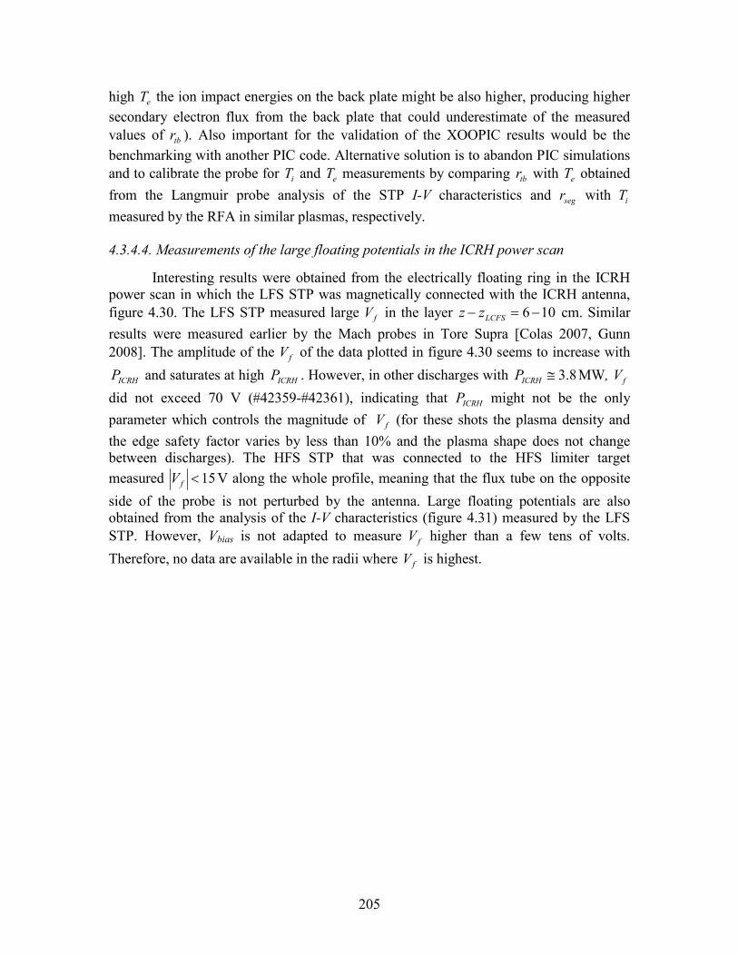
205

high eT the ion impact energies on the back plate might be also higher, producing higher secondary electron flux from the back plate that could underestimate of the measured values of tbr ). Also important for the validation of the XOOPIC results would be the benchmarking with another PIC code. Alternative solution is to abandon PIC simulations and to calibrate the probe for iT and eT measurements by comparing tbr with eT obtained from the Langmuir probe analysis of the STP I-V characteristics and segr with iT measured by the RFA in similar plasmas, respectively. 4.3.4.4. Measurements of the large floating potentials in the ICRH power scan

Interesting results were obtained from the electrically floating ring in the ICRH power scan in which the LFS STP was magnetically connected with the ICRH antenna, figure 4.30. The LFS STP measured large fV in the layer 106−=− LCFSzz cm. Similar results were measured earlier by the Mach probes in Tore Supra [Colas 2007, Gunn 2008]. The amplitude of the fV of the data plotted in figure 4.30 seems to increase with

ICRHP and saturates at high ICRHP . However, in other discharges with 8.3≅ICRHP MW, fV

did not exceed 70 V (#42359-#42361), indicating that ICRHP might not be the only parameter which controls the magnitude of fV (for these shots the plasma density and the edge safety factor varies by less than 10% and the plasma shape does not change between discharges). The HFS STP that was connected to the HFS limiter target measured 15<fV V along the whole profile, meaning that the flux tube on the opposite

side of the probe is not perturbed by the antenna. Large floating potentials are also obtained from the analysis of the I-V characteristics (figure 4.31) measured by the LFS STP. However, Vbias is not adapted to measure fV higher than a few tens of volts.

Therefore, no data are available in the radii where fV is highest.

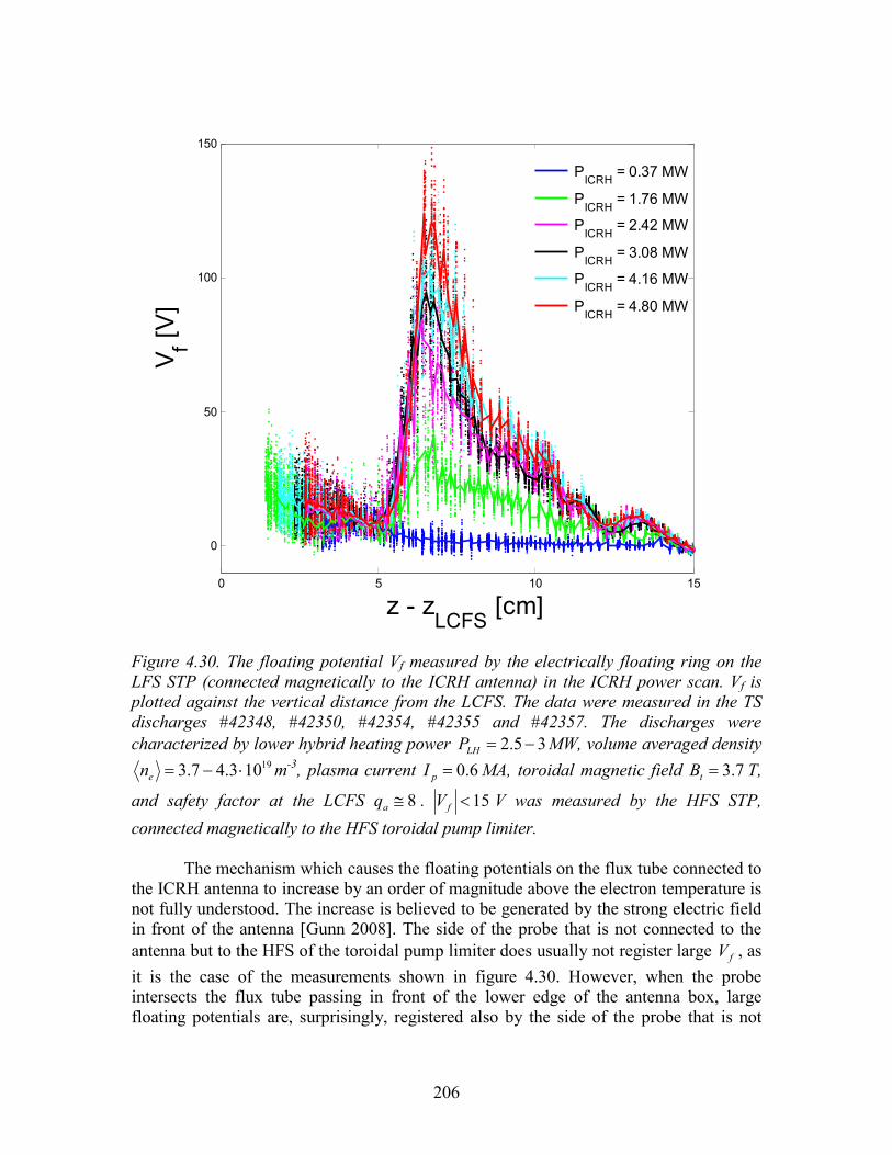
206

0 5 10 15

0

50

100

150

z - zLCFS

[cm]

Vf [V]

PICRH

= 0.37 MW

PICRH

= 1.76 MW

PICRH

= 2.42 MW

PICRH

= 3.08 MW

PICRH

= 4.16 MW

PICRH

= 4.80 MW

Figure 4.30. The floating potential Vf measured by the electrically floating ring on the LFS STP (connected magnetically to the ICRH antenna) in the ICRH power scan. Vf is plotted against the vertical distance from the LCFS. The data were measured in the TS discharges #42348, #42350, #42354, #42355 and #42357. The discharges were characterized by lower hybrid heating power 35.2 −=LHP MW, volume averaged density

19103.47.3 ⋅−=en m-3, plasma current 6.0=pI MA, toroidal magnetic field 7.3=tB T,

and safety factor at the LCFS 8≅aq . 15<fV V was measured by the HFS STP,

connected magnetically to the HFS toroidal pump limiter. The mechanism which causes the floating potentials on the flux tube connected to

the ICRH antenna to increase by an order of magnitude above the electron temperature is not fully understood. The increase is believed to be generated by the strong electric field in front of the antenna [Gunn 2008]. The side of the probe that is not connected to the antenna but to the HFS of the toroidal pump limiter does usually not register large fV , as it is the case of the measurements shown in figure 4.30. However, when the probe intersects the flux tube passing in front of the lower edge of the antenna box, large floating potentials are, surprisingly, registered also by the side of the probe that is not

207

connected to the antenna but to the HFS of the toroidal pump limiter (figure 5 in [Gunn 2008]).

2 4 6 8 10 12 140

5

10

15

20

25

30

r - rLCFS

[cm]

Vf [V]

Figure 4.31. Radial profile of the floating potential obtained from the analysis of the I-V characteristics measured by the LFS STP connected to the ICRH antenna (TS discharge #42355, 8.4=ICRHP MW, see captions to figure 4.30 for other macroscopic plasma parameters). Because of inappropriate bias voltages, no measurements of Vf are available for 116 −=− LCFSrr cm.

208

Conclusions

The tokamak plasma boundary plays a critical role in controlling the confined region. An important step towards improving our understanding of the plasma surface interaction in tokamaks is the experimental study of the scrape-off layer plasma. This thesis addressed the measurement of ion temperature – an important but yet rarely measured quantity – in the SOL of the Tore Supra tokamak using a retarding field analyzer.

An independent validation of the RFA Ti measurements is not yet available due to

a lack of simultaneous measurements with other relevant diagnostics. Therefore, a large part of the thesis focused on a study of the instrumental effects of RFAs and their influence on Ti measurements.

The attenuation of the ion current on the protective plate of the RFA was studied by means of self-consistent particle simulations. While the effect of the attenuation on Ti measurements was found to be negligible for the range of the plasma parameters and the bias voltages typically applied to the RFA slit plate, the attenuation of the incident ion current was found to be significant (factor of 1.7 – 3) and could lead to an underestimation of the collector current and the slit transmission factor. A less perturbing knife-edge geometry was proposed for the RFA protective plate.

Selective ion transmission through the RFA slit plate was analyzed by an analytical model and by self-consistent particle simulations. Even for relatively thick slit plates selective ion transmission accounts for an overestimation of Ti by less than 14% percent. Thick slit plates can be therefore used to advantage since they reduce the risk of melting during off-normal events, the neutral pressure inside the RFA cavity that can lead to electrical breakdown, and the positive space charge. The influence of slit plate misalignment with respect to the magnetic field as well as the influence of the electron repelling grid was proved to be negligible. Since the ion current transmission is almost independent of the misalignment angle, a tilted slit plate could be used as an effective method for preventing electrons from the plasma from entering the analyzer, independently of their kinetic energy. This could be of a large assistance e.g. in the experiments aimed at measurements of the energies of fast ions generated by the RF antennas.

The effect of positive space charge inside the RFA cavity and its influence on Ti measurements was studied. It was demonstrated that even for relatively strong ion currents, the potential inside the RFA cavity is dominated by the vacuum potential and the effect of space charge on Ti measurements can be neglected. In addition, the defocusing of the ion beam because of the positive space charge as well as large ion Larmor radii compared to the slit width (both neglected in the model) reduces further the influence of the positive space charge.

It is often observed experimentally that the upper region of the decaying part of the RFA I-V characteristics is rounded instead of being exponential. This is attributed to the non-Maxwellian (pre-sheath) part of the parallel ion velocity distribution. By analyzing the artificial I-V characteristics constructed from the ion velocity distribution at the sheath edge obtained from the kinetic Mach probe model [Chung 1988], it was

209

demonstrated that Ti calculated from the standard fit to the I-V characteristics can be overestimated by up to 12% if the non-exponential part of the characteristic is included in the fit. This error can be partially reduced by decreasing the upper limit of the collector current included in the fit.

In general, the influence of instrumental effects of RFAs addressed in this thesis was found to relatively low, increasing confidence in Ti measured by the RFA. On the other hand, perhaps one of the most important factors – the effect of impurities on Ti measurements – has not been addressed here. The model [Pitts 1991] that includes the effect of impurities needs to specify the fractions of the total flux carried by ions with a given charge state as well as their temperatures. Such measurements are not available in Tore Supra. Simultaneous measurements by a RFA and a plasma ion mass spectrometer (which measures the fluxes carried by different impurity ions) would be of large assistance in characterizing the effect of impurities.

The measurements of Ti (as well as other parameters like e.g. the electron

temperature and density, the ion saturation current density, the heat flux density and the SOL e-folding lengths) in the Tore Supra SOL were compiled in Chapter 3.

In general, SOL Ti was systematically found to be higher that Te by up to a factor of 7 which is consistent with earlier similar measurements reported from other tokamaks. Equal temperatures were measured only in detached plasma or at the highest plasma densities. The first continuous ei TT / profile from the edge of the confined region into the SOL was constructed using data from several tokamaks. It was demonstrated that ei TT / increases with radius and 1/ >ei TT already in the edge of the confined plasma. Relatively high ion-to-electron temperature ratios measured in the SOL of Tore Supra are, therefore, inconsistent with the assumption of the thermal equipartition, usually applied in the models.

iT , eT and ei TT / were found to be inversely proportional to the plasma density. The decrease of iT and eT with the plasma density could be explained by the conservation of the pressure in the SOL. The decrease of ei TT / with plasma density was found to be consistent with the increase of SOL ion-electron collisionality.

In helium plasma iT was found to be higher by a factor of ~2 compared to iT measured in deuterium plasma at similar plasma densities. This could be due to lower charge-exchange losses of ions in helium compared to deuterium as well as the presence of singly-charged helium ions in the helium discharges that could lead to an overestimation of iT by up to a factor of 2 at highest plasma densities.

An increase of the radiated power fraction by about 30% (with all other parameters being fixed) was found to be associated with a decrease of SOL iT by a factor of 2 but eT was almost unaffected. The drop of iT is also associated with the decrease of the power in the SOL by a similar factor, indicating that the power lost due to radiation comes mainly from the ion channel. A simple power balance model for the temperatures in the edge of the confined plasma, with radiation and equipartition being the only volumetric loss terms included, was employed. The model reproduces well a strong decrease of iT with the increase of the radiated power and shows that the power loss on

210

electrons in the edge of the confined region can be, through ion-electron collisional coupling, compensated from the ion channel. Almost constant eT independently of the radiated power is not reproduced by the model; the ratio iT / eT in the model remains roughly constant. A two dimensional model which comprises both the edge of the confined plasma as well as SOL needs to be employed to study further the edge temperatures.

A previously unobserved strong dependence of SOL iT on the intensity of the toroidal magnetic field tB was reported. While SOL iT increases with tB , SOL eT was found to be almost independent of tB . The only other parameter found thus far that strongly correlates with tB is the core electron temperature. Measurements of the core ion temperature were not available. We speculate that, due to collisional coupling, core

iT increases with tB similarly to core eT and that SOL iT is simply related to core iT through radial transport. A mechanism that would decouple the SOL electrons from the core plasma needs to be identified. At the same time, data from the recent CXRS measurements in a magnetic field scan need to be analyzed in order to verify if iT in the core and in the SOL changes in a similar way with tB .

Dedicated experiments with the plasma contact point either on the inboard bumper limiters or on the outboard modular limiters have demonstrated that the poloidal asymmetry of the radial ion and electron energy transport in the SOL is similar to that of the particle transport. When the plasma contact point is on the inboard side, the temperature and density e-folding lengths are up to a factor of 5 longer compared to the outboard side plasma. These results are particularly important for the ITER start-up phase which is currently envisaged on the outboard modular limiters and for which the modelled peak heat loads on the limiters were found to be considerably close to the engineering limit. The parallel heat flux density at the LCFS was found to be proportional to the power in the SOL and inversely proportional to the parallel heat flux density e-folding length. These results imply that the outboard start-up is least advantageous with regards to power handling as it may be characterized by large, localized heat loads. Alternative start-up scenarios like, for example, the start-up on the inboard side, eventually in a detached regime should be evaluated.

The asymmetries of ion and electron temperatures measured by each side of the RFA were studied in a discharge during which the plasma contact point was steadily displaced upward along the outboard limiter, leading to the reversal of the parallel plasma flow. The asymmetry of iT was found to be correlated with a change of the parallel Mach

number M// but, in contrary to the theory [Valsaque 2002], iT it does not reverse

completely like M//. This suggests that some of the assumptions in the kinetic modeling of the behavior of the pre-sheath surrounding the RFA [Valsaque 2002] might not be valid or the poloidal temperature gradient may play a role. Interestingly, a similar asymmetry is also measured for eT . A model for the asymmetry of eT is not yet available.

In should be noted that one of the assumptions of the fluid Mach probe theory

211

[Hutchinson 1987, Gunn 2007b] is that the parallel electron velocity distribution is Maxwellian, in which case the same eT would be measured by each side of the RFA.

Three ongoing projects aimed at the validation of RFA Ti measurements in Tore

Supra were summarized in Chapter 4. The selected results and the preliminary status of the analysis of the edge ion-to-

electron temperature ratio measurements in the JET L-mode plasma were presented. Values of ei TT / up to 5 just inside the outboard midplane separatrix were obtained. Equal temperatures were measured just at 8.0≈ρ . However, it is important to note that because of the uncertainly in the radial position of the eT measurements by ECE due to the flux surface mapping (which was not resolved at the time of writing) these results are only preliminary.

SOL iT was measured for a first in Tore Supra by charge exchange recombination spectroscopy. SOL iT measured by the CXRS was found to be a factor of 4 higher compared to iT measured by the RFA in a similar discharge. Further study is needed to track down the causes of this discrepancy. Some possible candidates (like e.g. the difference in the main plasma parameters during the CXRS and the RFA measurements, the effect of impurities on Ti measured by the RFA, etc.) were outlined.

A segmented tunnel probe for fast SOL iT measurements has been designed, built, calibrated by particle simulations, and used for the first time in a large tokamak, Tore Supra. In some aspects the results obtained from the PIC simulations and in experiment are similar and consistent with simple theoretical assumptions. However, a significant quantitative disagreement was found between the PIC simulations and the experimental data, making the calculation of the SOL temperatures from the experimental data impossible. Further analysis of the geometrical effects as well as the benchmarking with other PIC codes is needed. Large positive floating potentials ( fV up to 150 V), possibly generated by a strong electric field in front of the ICRH antenna, were measured in the ICRH power scan by the side of the segmented tunnel probe that was magnetically connected with the ICRH antenna.

From the experimental data presented in this thesis as well as reported from other

tokamaks there is a clear evidence that in most plasmas ei TT > in the SOL, at the LCFS, and in the edge of the confined plasma. While the tendency for ei TT > in the SOL can be explained by the cooling of the electrons in the Debye sheath (alternative explanation could be the heating of ions in the SOL due to strong turbulent fluctuations of plasma potential [Bellan 1993]), ei TT > in the edge of the confined plasma is not understood. It is not yet clear whether the faster drop of eT just inside the LCFS is due to the cooling of the edge electrons by the propagation of the cold electrons from the SOL into the edge or by the difference in the ion and electron energy transport in the edge plasma. A two-dimensional model which comprises both the edge plasma as well as the SOL needs to be employed to study further the edge temperatures. At the same time, an effort should be

212

devoted to the experimental study of ion temperature for different plasma geometry (circular and X-point plasma) or at different poloidal locations. Overlapping probe/CXRS

iT profiles and the comparison of iT measured by different probes are important for the validation of iT measurements.

The optimization of the ITER start-up phase and the design the ITER first wall requires understanding the correlation between the plasma contact point and the SOL e-folding lengths. Now that it appears we are reaching this point, it is necessary to study systematically the SOL parameters in the discharges with the HFS and LFS contact in order to increase the confidence of the recent results demonstrated on a limited dataset [Kočan 2009]. Detached HFS/LFS start-up, the scaling of the e-folding lengths with the main plasma parameters, measurements in elongated plasmas are certainly worthy of further investigation.

The ELM ion energies in the SOL have been measured only recently using a RFA [Pitts 2006]. These results, although obtained for a single set of the discharge parameters and a single value of the bias voltage, combined with the transient model for the propagation of an ELM filament in the SOL, demonstrated that in ITER the ELM ions can arrive at the non-divertor components with the energies above the sputtering threshold for all candidate materials for the ITER first wall. A more systematic investigation of the ELM ion energies in the SOL is clearly called for. We can study several important questions: What is the ELM ion energy as a function of the distance from the separatrix, SOL density, SOL/pedestal temperatures, ELM type, etc.?

During the thesis a collaborative project with the UKAEA (U.K.) aimed at the measurements of the far SOL ELM ion energies in the MAST tokamak using the Tore Supra RFA was established. The experiments in MAST were performed shortly before the submission of the thesis. Strong peaks of RFA collector current correlated with the peaks on Dα signal were measured during type I and type III ELMs up to 20 cm outside the separatrix. These results are being analyzed and are not included in this thesis. However, they suggest that ELMs can transport radially over a large distance a significant fraction of their pedestal energies, confirming the results from JET. At the same time, during the evaluation of this thesis a new RFA was designed for the ASDEX Upgrade tokamak within the framework of the collaboration between the CEA and the Max Planck Institut für Plasmaphysik in Garching, Germany. The probe is now under construction and is planned to be used to for studying the ELM ion energies as well as ion temperature in the ASDEX Upgrade plasma boundary.

213

References [Adamek 2008] Adamek J, Kočan M, Panek R, Gunn J P, Martines E, Stöckel J,

Ionita C, Popa G, Costin C, Brotankova J, Schrittwieser R and Van Oost G 2008 Contrib. Plasma Phys. 48 1

[Allen 1976] Allen J E 1976 J. Phys D: Appl. Phys. 9 2331 [Allen 1986] Allen J et al 1986 Plasma Phys. Control. Fusion 28 101 [Amemiya 1989] Amemiya H 1989 Jpn. J. Appl. Phys. 28 1109 [Amemiya 1994] Amemiya H and Uehara K 1994 Rev. Sci. Instrum. 65 2607 [Andrew 2006] Andrew Y et al 2006 Rev. Sci. Instrum. 77 10E913-1 [Asakura 1997] Asakura N, Koide Y, Itami K, Shimizu K, Tsuji-Iio S, Sakurai S

and Sakasai A 1997 J. Nucl. Mater. 241-243 559 [Asakura 2000] Asakura N, Sakurai S, Shimada M, Koide Y, Hosogane N, Itami K

2000 Phys. Rev. Lett. 84 3093 [Asakura 2007] Asakura N 2007 J. Nucl. Mater. 363-365 41 [ASDEX Team] ASDEX Team 1989 Nucl. Fusion 29 1959 [Basiuk 2001] Basiuk V et al 2001 Nucl. Fusion 41 477 [Behringer 1986] Behringer K et al 1986 Proc 11th Int. Conf. on Plasma Phys. and

Controlled Nuclear Fusion Research (Kyoto 1986) IAEA-CN-47/A-IV-1

[Bellan 1993] Bellan P M 1993 Plasma Phys. Control. Fusion 35 169 [Bethe 1979] Bethe H A 1979 Physics Today (May 1979) [Bogen 1995] Bogen P, Hey J D, Hintz E, Lie Y T, Rusbüldt D and Samm U

1995 J. Nucl. Mater. 220-222 472 [Bohm 1993] Bohm C and Perrin J 1993 Rev. Sci. Instrum. 64 31 [Bush 1990] Bush C E et al 1990 J. Nucl. Mater. 176-177 786 [Callen 1990] Callen J D 1990 Phys Fluids B 2 2869 [Carpentier 2009] Carpentier S et al 2009 J. Nucl. Mater. 390-391 955 [Cebulla 1998] Cebulla R et al 1998 J. Appl. Phys. 83 1087 [Charles 2000] Charles C et al 2000 Phys. Plasma 7 5232 [Chodura 1982] Chodura R 1982 Phys. Fluids 25 1628 [Chung 1988] Chung K S and Hutchinson I H 1988 Phys. Rev. A 38 4721 [Cohen 1979] Cohen S A and McCracken G M 1979 J. Nucl. Mater. 84 157 [Colas 2007] Colas L et al 2007 J. Nucl. Mater. 363-365 555 [Connor 1993] Connor J W 1993 Plasma Phys. Control. Fusion 35 B293 [Conway 2008] Conway G B 2008 Plasma Phys. Control. Fusion 50 124026 [Dejarnac 2007] Dejarnac R, Gunn J P, Stöckel J, Adámek J, Brotánková J and

Ionita C 2007 Plasma Phys. Control. Fusion 49 1791 [Demidov 1999] Demidov V I, Ratynskaia S V and Rypdal K 1999 Rev. Sci.

Instrum. 70 4266 [Demidov 1999b] Demidov V I, Ratynskaia S V, Armstrong R J and Rypdal K 1999

Phys. Plasmas 6 35 [Dionne 2005] Dionne M 2005 Master Thesis, Université du Québec, INRS

Energie, Matériaux, et Télécommunications [Doyle 2007] Doyle E J et al 2007 Nucl. Fusion 47 S18

214

[Druyvesteyn 1930] Druyvesteyn M J 1930 J. Phys. 64 781 [Dudson 2008] Dudson B D et al 2008 Plasma Phys. Control. Fusion 50 124012 [El Shaer 1981] El Shaer M 1981 PhD thesis Scientific and Medical University of

Grenoble [Enloe 1992] Enloe C L and Shell J R 1992 Rev. Sci. Instrum. 63 1788 [Erents 1982] Erents S K and Stangeby P C 1982 J. Nucl. Mater. 111-112 165 [Erents 2004] Erents S K, Pitts R A, Fundamenski W, Gunn J P and Matthews G

F 2004 Plasma Phys. Control. Fusion 46 1757 [Federici 2007] Federici G et al 2007 J. Nucl. Mater. 363-365 346 [Fedorczak 2009] Fedorczak N, Gunn J P, Ghendrih Ph, Monier-Garbet P and

Pocheau A 2009 J. Nucl. Mater. 390-391 368 [Fundamenski 2006] Fundamenski W, Pitts R A and JET EFDA contributors 2006

Plasma Phys. Control. Fusion 48 109 [Fundamenski 2007] Fundamenski W, Pitts R A and JET EFDA contributors 2007 J.

Nucl. Mater. 363-365 319 [Garcia-Cortes 2000] Garcia-Cortes I et al 2000 Plasma Phys. Control. Fusion 42 389 [Giruzzi 2009] Giruzzi G on behalf of the Tore Supra team 2009 Tore Supra

special issue, Fus. Sci. Tech. (to be published) [Gohar 2001] Gohar Y 2001 Fusion Engineering and Design 58-59 1097 [Goto 1972] Goto K and Ishikawa K 1972 Rev. Sci. Instrum. 43 427 [Gowers 1995] Gowers C et al 1995 Rev. Sci. Instrum. 66 471 [Gribov 2004] Gribov Y Control System Design and Assessment (CSD), Appendix

B: Magnetic configuration and poloidal field scenarios, ITER document N 19 RI 14 R0.1 (August 2004)

[Gunn 1997] Gunn J P 1997 Phys. Plasmas 4 4435 [Gunn 2001] Gunn J P 2001 Phys Plasmas 8 1040 [Gunn 2002] Gunn J P et al 2002 Czech J. Phys. 52 1107 [Gunn 2002b] Gunn J P et al 2002 Proc. 29th EPS Conference on Plasma Physics

and Contr. Fusion Montreux, 17-21 June 2002 ECA Vol. 26 B, P-5.093

[Gunn 2007] Gunn J P et al 2007 J. Nucl. Mater. 363-365 484 [Gunn 2007b] Gunn J P and Fuchs V 2007 Phys. Plasmas 14 032501 [Gunn 2008] Gunn J P et al 2008 Proc. 22nd IAEA Int. Conference on Fusion

Energy (Geneva 2008) [Gunn 2009] Gunn J P, Petrzilka V, Ekedahl A, Fuchs V, Gauthier E, Goniche

M, Kočan M and Saint-Laurent F 2009 J. Nucl. Mater. 390-391 90 [Gunther 1990] Gunther K, Herrmann A, Laux M, Pech P and Reiner H-D 1990 J.

Nucl. Mater. 176-177 236 [Guo 1996] Guo H Y, Matthews G F, Davies S J, Erents S K, Horton L D,

Mond R D and Stangeby P C 1996 Contrib. Plasma Phys. 36 81 [Heifetz 1982] Heifetz D et al 1982 J. Comput. Phys. 46 309 [Hey 1994] Hey J D, Lie Y T, Rusbüldt D and Hintz E 1994 Contrib. Plasma

Phys. 34 725 [Hoffman 2002] Hoffman E A and Stacey W M 2002 Fusion Engineering and

Design 63-64 87

215

[Höthker 1990] Höthker K, Belitz H-J, Bieger W and Amemiya H 1990 Rev. Sci. Instrum. 61 114

[Huber 2000] Huber A, Pospieszczyk A, Unterberg B, Brix M, Mertens Ph, Philipps V and Schweer B 2000 Plasma Phys Control. Fusion 42 569

[Hutchinson 1987] Hutchinson I H 1987 Phys. Fluids 30 3777 [Hutchinson 1991] Hutchinson I 1991 Phys. Fluids B 3 847 [Jaquinot 1999] Jaquinot J and the JET Team 1999 Plasma. Phys. Control. Fusion

41 A13 [Jacquinot 2004] Jacquinot J and Hoang G T 2004 Plasma Sci. and Technol. 6 2101 [Jiang 2005] Jiang N et al 2005 Nucl. Instr. and Meth. In Phys. Res. B 229 508 [Johnson 2003] Johnson S D, El-Gomati M M and Enloe L 2003 J. Vac. Sci.

Technol. B 21 350 [Katsumata 1967] Katsumata I and Okazaki M 1967 Jpn. J. Appl. Phys. 6 123 [Kim 1995] Kim G-H, Hershkowitz N, Diebold N A and Cho M-H 1995 Phys.

Plasmas 2 3222 [Kimura 1978] Kimura H et al 1987 Nucl. Fusion 18 1195 [Kimura 1979] Kimura H, Odajima K, Sugie T and Maeda H 1979 Jpn. J. Appl.

Phys. 18 2275 [Kirnev 2004] Kirnev G S et al 2004 Plasma Phys. Control. Fusion 46 621 [Kočan 2005] Kočan M, Pánek R, Gunn J P, Stöckel J and Skalný J D 2009 Proc.

32nd EPS Conference on Contr. Fusion and Plasma Physics (Tarragona, June 27 – July 1) ECA Vol. 29C, P-2.082

[Kočan 2006] Kočan M 2006 Master thesis, Comenius University [Kočan 2007] Kočan M, Pánek R, Stöckel J, Hron M, Gunn J P and Dejarnac R

2007 J. Nucl. Mater. 363-365 1436 [Kočan 2008] Kočan M, Gunn J P, Pascal J-Y, Bonhomme G, Fenzi C, Gauthier

E and Segui J-L 2008 Plasma Phys. Control. Fusion 50 125009 [Kočan 2008b] Kočan M et al 2008 Proc. 35th EPS Conference on Plasma Physics

(Hersonissos, June 9 – 13) ECA Vol. 32D, P-1.006 [Kočan 2008c] Kočan M, Gunn J P, Komm M, Pascal J-Y, Gauthier E and

Bonhomme G 2008 Rev. Sci Instrum. 79 073502 [Kočan 2009] Kočan M and Gunn J P 2009 “First evidence for poloidal

asymmetries of radial ion energy transport by ion temperature measurements in the scrape-off layer of Tore Supra” submitted to 36th EPS Conference on Plasma Physics (Sofia, June 29 – July 3)

[Kočan 2009b] Kočan M et al 2009 J. Nucl. Mater. 390-391 1074 [Kočan 2009c] Kočan M et al 2009 “Influence of the plasma density and the

radiated power fraction on the Tore Supra scrape-off layer”, submitted to Plasma Phys. Control. Fusion (2009)

[Kojima 1984] Kojima H, Sugari H, Mori T, Toyada H and Okuda T 1984 J. Nucl. Mater. 128-129 965

[Kreter 2001] Kreter A 2001 PhD thesis, Düsseldorf University [LaBombard 2004] LaBombard B et al 2004 Nucl. Fusion 44 1047 [Laframbois 1990] Laframbois G J and Rubinstein J 1990 Phys. Fluids 19 1976 [Lawson 1957] Lawson J D 1957 Proc. Phys. Soc. B 70 6

216

[Lefaucheux 2006] Lefaucheux P 2006 Proc. Atelier analyse de plasmas par sondes électrostatiques 8/17, 14 – 16 June, Saracenas, France

[Lloyd 2007] Lloyd et al 2007 Nucl. Fusion 47 S658-S667 [Loarte 2007] Loarte A et al 2007 Nucl. Fusion 47 S203 [Luna 2004] Luna E de la et al 2004 Rev. Sci. Instrum. 75 3831 [Manos 1982] Manos D M, Budny R, Satake T and Cohen S A 1982 J. Nucl.

Mater. 111-112 81 [Maeda 1997] Maeda M, Uehara K and Amemiya H 1997 Jpn. J. Appl. Phys. 36

6992 [Matthews 1984] Matthews G F 1984 J. Phys. D: Appl. Phys. 17 2243 [Matthews 1985] Matthews G F 1985 PhD thesis University of Oxford [Matthews 1989] Matthews G F 1989 Plasma Phys. Control. Fusion 31 841 [Matthews 1990] Matthews G F, Pedgely J M, Pitts R A and Stangeby P C 1990 J.

Nucl. Mater. 176-177 1032 [Matthews 1991] Matthews G F, Pitts R A, McCracken G M and Stangeby P C 1991

Nucl. Fusion 31 1495 [Matthews 1994] Matthews G F 1994 Plasma. Phys. Control. Fusion 36 1595 [Matthews 1997] Matthews G F 1997 J. Nucl. Mater. 241-243 450 [McCracken 1987] McCracken G M et al 1987 J. Nucl. Mater. 145-147 181 [Mizuuchi 2005] Mizuuchi T et al 2005 J. Nucl. Mater. 337–339 332 [Molvik 1981] Molvik A W 1981 Rev. Sci. Instrum. 52 704 [Mott-Smith 1926] Mott-Smith H M and Langmuir I 1926 Phys. Review 28 727 [Nachtrieb 2000] Nachtrieb R 2000 PhD thesis, Massachusetts Institute of

Technology [Nachtrieb 2000b] Nachtrieb R, LaBombard B and Thomas E 2000 Rev Sci. Instrum.

71 4107 [Naulin 2007] Naulin V 2007 J. Nucl. Mater. 363-365 24 [Nedzelskiy 2006] Nedzelskiy I S, Silva C, Figueiredo H, Fernandes H and Varandas

C A F 2006 Rev. Sci. Instrum. 77 10E729-1 [Negus 2006] Negus C R et al 2006 Rev. Sci. Instrum. 77 10F102-1 [Nifnecker 1999] Nifenecker H, David S, Loiseaux J M and Giorni A 1999 Progress

in Particle and Nuclear Physics 43 683-827 [Olthoff 1994] Olthoff J K et al 1994 J. Appl. Phys. 75 116 [O’Rourke 1985] O’Rourke J et al 1985 Proc. 12th EPS Conf. (Budapest 1985 vol 1

155) [Pánek 2004] Pánek R, Pitts R A, Gunn J P and Erents S K 2004 Czech J. Phys.

54 150 [Pégourié 2009] Pégourié B et al 2009 J. Nucl. Mater. 390-391 550 [Pitts 1989] Pitts R A, McCracken G M and Matthews G F 1989 J. Nucl.

Mater. 162-164 568 [Pitts 1991] Pitts R A 1991 PhD thesis, University of London [Pitts 1991b] Pitts R A 1991 Phys. Fluids B 3 2871 [Pitts 1996] Pitts R A 1996 Contrib. Plasma Phys. 36 87 [Pitts 2003] Pitts R A, Chavan R, Davies S J, Erents S K, Kaveney G,

Matthews G F, Neill G, Vince J E and Ďuran I 2003 Rev. Sci. Instrum. 74 4644

217

[Pitts 2003b] Pitts R A et al 2003 30th EPS Conference on Contr. Fusion and Plasma Phys. St. Petersburg, 7-11 July 2003 ECA Vol. 27A, P-2.84

[Pitts 2006] Pitts R A, Fundamenski W, Erents S K, Andrew Y, Loarte A, Silva C and JET-EFDA contributors 2006 Nucl. Fusion 46 82

[Pitts 2007] Pitts R A et al 2007 J. Nucl. Mater. 363-365 505 [Press 1992] Press W H, Teukolsky S A, Vetterling W T and Flannery B P 1992

Numerical Recipes in Fortran 77, Cambridge University Press, Cambridge, Chap. 16

[Radford 1996] Radford G, Chankin A, Corrigan G, Simonini R and Spence J et al 1996 Contrib. Plasma Phys. 26 187

[Ratynskaia 2002] Ratynskaia S V, Demidov V I and Rypdal K 2002 Rev. Sci. Instrum 73 4232

[Raychaudhuri 1999] Raychaudhuri S 1999 Contrib. Plasma Phys. 39 359 [Reich 2004] Reich M, Wolfrum E, Schweinzer J, Ehmler H, Horton L D,

Neuhauser J and ASDEX Upgrade Team 2004 Plasma Phys. Control. Fusion 46 797

[Reich 2004b] Reich M, Wolfrum E, Horton L D, Schweinzer J, Neuhauser J and ASDEX Upgrade Team 2004 31st EPS Conf. on Plasma Physics (London, 28 June – 2 July 2004)

[Reiter 1991] Reiter D, Börner P, Küppers B, Baelmans M, and Maddison G 1991 Final report on KFA-NET contract 428/90-8/FU-D

[Reiter 1991b] Reiter D et al 1991 Plasma Phys. Control. Fusion 33 1579 [Riyopoulos 1996a] Riyopoulos S 1996 Phys. Plasmas 3 2511 [Riyopoulos 1996b] Riyopoulos S 1996 Phys. Plasmas 3 4355 [Rudakov 2002] Rudakov D L et al 2002 Plasma Phys. Control. Fusion 44 717 [Saarelma 2005] Saarelma S et al 2005 Plasma Phys. Control. Fusion 47 713 [Samm 1993] Samm U et al 1993 Plasma Phys. Control. Fusion 35 167 [Shats 1997] Shats M G, Rudakov D L, Boswell R W and Borg G G 1997 Phys.

Plasmas 4 3629 [Shimada 2007] Shimada M et al 2007 Nucl. Fusion 47 S1 [Simpson 1961] Simpson J A 1961 Rev. Sci. Instrum. 32 1283 [Spitzer 1962] Spitzer L1962 Physics of Fully Ionized Gases, 2nd ed. (Interscience,

New York, 1962) [Stacey 2002] Stacey W M et al 2002 Fusion Engineering and Design 63-64 81 [Staib 1972] Staib P 1972 Vacuum 22 481 [Staib 1977] Staib P and Dinklage U 1977 J. Phys. E: Sci. Instrum. 10 914 [Staib 1980] Staib P 1980 J. Nucl. Mater. 93-94 351 [Staib 1982] Staib P 1982 J. Nucl. Mater. 111-112 109 [Stangeby 1982] Stangeby P C 1982 J. Phys. D: Appl. Phys. 15 1007 [Stangeby 1983] Stangeby P C, McCracken G M, Erents S K, Vince J E and Wilden

R 1983 J. Vac. Sci. Technol. A 1 1302 [Stangeby 1984] Stangeby P C 1984 Phys. Fluids 27 2699 [Stangeby 2000] Stangeby P C 2000 The Plasma Boundary of Magnetic Fusion

Devices (Institute of Physics Publishing 2000) p 73

218

[Stangeby 2000b] Stangeby P C 2000 The Plasma Boundary of Magnetic Fusion Devices (Institute of Physics Publishing 2000) p 649

[Stangeby 2000c] Stangeby P C 2000 The Plasma Boundary of Magnetic Fusion Devices (Institute of Physics Publishing 2000) p 81-82

[Stangeby 2000d] Stangeby P C 2000 The Plasma Boundary of Magnetic Fusion Devices (Institute of Physics Publishing 2000) p 160

[Stangeby 2000e] Stangeby P C 2000 The Plasma Boundary of Magnetic Fusion Devices (Institute of Physics Publishing 2000) p 95

[Staudenmaier 1980] Staudenmaier G, Staib P, Poschenrieder W 1980 J. Nucl. Mater. 121-126 121

[Stenzel 1982] Stenzel R L et al 1982 Rev. Sci. Instrum. 57 1027 [Stöckel 1999] Stöckel J et al 1999 Plasma Phys. Control. Fusion 41 A577 [Stöckel 2006] Stöckel J et al 2006 Problems of Atomic Science and Technology

No.6 Series: Plasma Physics (12) 19-23 [Strachan 1985] Strachan J D et al 1985 12th Eur. Conf. on Controlled Fusion and

Plasma Physics (Budapest, Hungary) part 1, p. 263 [Tagle 1987] Tagle J A, Stangeby P C and Erents S K 1987 Plasma Phys.

Control. Fusion 29 297 [Thomas 1991] Thomas E W 1991 Suppl. Nucl. Fusion 1 79 [Uehara 1998] Uehara K, Tawakami T, Amemiya H, Höthker K, Cosler A and

Bieger W 1998 Nucl. Fusion 38 1665 [Valsaque 2002] Valsaque F, Manfredi G, Gunn J P and Gauthier E 2002 Phys.

Plasmas 9 1806 [Van Rompuy 2007] Van Rompuy T, Gunn J P, Dejarnac R, Stöckel J and Van Oost G

2007 Plasma Phys. Control. Fusion 49 619 [Verboncoeur 1995] Verboncoeur J P, Langdon A B and Gladd N T 1995 Comp. Phys.

Comm. 87 199-211 [Wagner 1982] Wagner F et al 1982 Phys. Rev. Lett. 49 1408 [Wampler 1981] Wampler W R et al 1981 J. Nucl. Mater. 102 304 [Wampler 1982] Wampler W R 1982 Appl. Phys. Lett. 41 335 [Wampler 1983] Wampler W R and Manos D M 1982 J. Vac. Sci. Technol. A 1 (2)

827 [Wan 1986] Wan A S, Yang T F, Lipschultz B and LaBombard B 1986 Rev.

Sci. Instrum. 57 1542 [Winter 1990] Winter J 1990 J. Nucl. Mater. 176-177 14 [Wootton 1990] Wootton A J et al 1990 Phys Fluids B 12 2879 [Zou 2000] Zou Y 2000 PhD Thesis, University of Maryland [Zou 2002] Zou Y et al 2002 Phys. Rev. Spec. Topics - Accelerators and

beams 5 072801