Abstract Structure

Jeffrey Ketland∗

January 10, 2015

Abstract

Structured mathematical objects—orderings, graphs, rings, groups,fields, topological spaces, etc.—typically have the form “carrier set +distinguished relations (structure)”. When A and B are isomorphicobjects, we say A and B “have the same abstract structure”. Butwhat is abstract structure? Intuitively, it is what all isomorphic copiesof structured objects have in common. With this in mind, one aimsto identify for each structure A, a corresponding object, the “abstractstructure” A, satisfying the condition: A = B ⇔ A ∼= B (we call thisLeibniz Abstraction). The proposal given here is that, for each (set-sized) structure A, we identify A with the propositional function 〈ΦA〉expressed by a certain categorical second-order “diagram formula” ΦA,which defines the isomorphism type of A. The propositional function〈ΦA〉 encodes all “structural information” given by any representativestructure, while “abstracting away” from the particular domain/carrierset.

Contents

1 The Problem of Abstract Structure 2

2 What Abstract Structures Could Not Be: A PermutationArgument 4

3 Leibniz Abstraction 8

4 A Sketch of the Diagram View 11

5 Diagram Axiomatization 13

6 Examples 20

7 Labellings, Automorphisms and Skolemization 22

∗Pembroke College (Oxford) & Munich Center for Mathematical Philosophy (LMU).

1

8 The Diagram Conception of Abstract Structure 26

9 Applications 32

10 Summary 39

1 The Problem of Abstract Structure

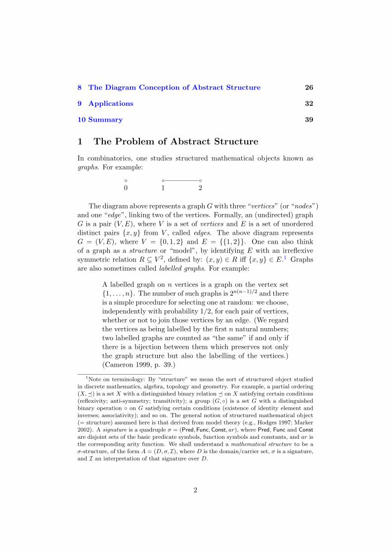
In combinatorics, one studies structured mathematical objects known asgraphs. For example:b b b

0 1 2

The diagram above represents a graphG with three “vertices” (or “nodes”)and one “edge”, linking two of the vertices. Formally, an (undirected) graphG is a pair (V,E), where V is a set of vertices and E is a set of unordereddistinct pairs {x, y} from V , called edges. The above diagram representsG = (V,E), where V = {0, 1, 2} and E = {{1, 2}}. One can also thinkof a graph as a structure or “model”, by identifying E with an irreflexivesymmetric relation R ⊆ V 2, defined by: (x, y) ∈ R iff {x, y} ∈ E.1 Graphsare also sometimes called labelled graphs. For example:

A labelled graph on n vertices is a graph on the vertex set{1, . . . , n}. The number of such graphs is 2n(n−1)/2 and thereis a simple procedure for selecting one at random: we choose,independently with probability 1/2, for each pair of vertices,whether or not to join those vertices by an edge. (We regardthe vertices as being labelled by the first n natural numbers;two labelled graphs are counted as “the same” if and only ifthere is a bijection between them which preserves not onlythe graph structure but also the labelling of the vertices.)(Cameron 1999, p. 39.)

1Note on terminology: By “structure” we mean the sort of structured object studiedin discrete mathematics, algebra, topology and geometry. For example, a partial ordering(X,�) is a set X with a distinguished binary relation � on X satisfying certain conditions(reflexivity; anti-symmetry; transitivity); a group (G, ◦) is a set G with a distinguishedbinary operation ◦ on G satisfying certain conditions (existence of identity element andinverses; associativity); and so on. The general notion of structured mathematical object(= structure) assumed here is that derived from model theory (e.g., Hodges 1997; Marker2002). A signature is a quadruple σ = (Pred,Func,Const, ar), where Pred, Func and Constare disjoint sets of the basic predicate symbols, function symbols and constants, and ar isthe corresponding arity function. We shall understand a mathematical structure to be aσ-structure, of the form A = (D,σ, I), where D is the domain/carrier set, σ is a signature,and I an interpretation of that signature over D.

2

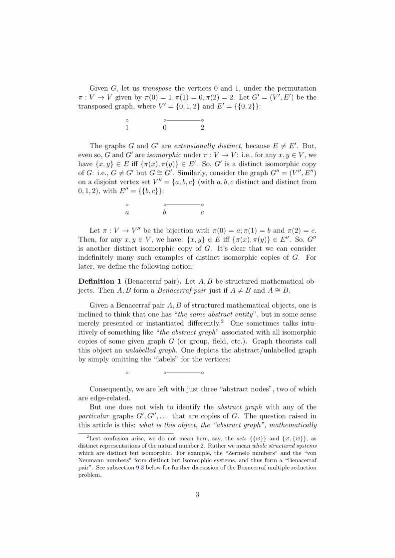
Given G, let us transpose the vertices 0 and 1, under the permutationπ : V → V given by π(0) = 1, π(1) = 0, π(2) = 2. Let G′ = (V ′, E′) be thetransposed graph, where V ′ = {0, 1, 2} and E′ = {{0, 2}}:b b b

1 0 2

The graphs G and G′ are extensionally distinct, because E 6= E′. But,even so, G and G′ are isomorphic under π : V → V : i.e., for any x, y ∈ V , wehave {x, y} ∈ E iff {π(x), π(y)} ∈ E′. So, G′ is a distinct isomorphic copyof G: i.e., G 6= G′ but G ∼= G′. Similarly, consider the graph G′′ = (V ′′, E′′)on a disjoint vertex set V ′′ = {a, b, c} (with a, b, c distinct and distinct from0, 1, 2), with E′′ = {{b, c}}:b b b

a b c

Let π : V → V ′′ be the bijection with π(0) = a;π(1) = b and π(2) = c.Then, for any x, y ∈ V , we have: {x, y} ∈ E iff {π(x), π(y)} ∈ E′′. So, G′′

is another distinct isomorphic copy of G. It’s clear that we can considerindefinitely many such examples of distinct isomorphic copies of G. Forlater, we define the following notion:

Definition 1 (Benacerraf pair). Let A,B be structured mathematical ob-jects. Then A,B form a Benacerraf pair just if A 6= B and A ∼= B.

Given a Benacerraf pair A,B of structured mathematical objects, one isinclined to think that one has “the same abstract entity”, but in some sensemerely presented or instantiated differently.2 One sometimes talks intu-itively of something like “the abstract graph” associated with all isomorphiccopies of some given graph G (or group, field, etc.). Graph theorists callthis object an unlabelled graph. One depicts the abstract/unlabelled graphby simply omitting the “labels” for the vertices:b b b

Consequently, we are left with just three “abstract nodes”, two of whichare edge-related.

But one does not wish to identify the abstract graph with any of theparticular graphs G′, G′′, . . . that are copies of G. The question raised inthis article is this: what is this object, the “abstract graph”, mathematically

2Lest confusion arise, we do not mean here, say, the sets {{∅}} and {∅, {∅}}, asdistinct representations of the natural number 2. Rather we mean whole structured systemswhich are distinct but isomorphic. For example, the “Zermelo numbers” and the “vonNeumann numbers” form distinct but isomorphic systems, and thus form a “Benacerrafpair”. See subsection 9.3 below for further discussion of the Benacerraf multiple reductionproblem.

3

speaking? Let’s not be sneaky by trying to pretend that this is a faconde parler. We make the central assumption explicit: there are such enti-ties: there is such a thing as the unique “abstract structure” of G (i.e., thecorresponding unlabelled graph) and let us baptise it G.

There seems little difficulty understanding the intuitive idea here. Gis what is pictured above. But, pictures aside, it remains terribly unclearwhat it is. What are these “abstract nodes” in an unlabelled graph? Thesmall circular token inscriptions in a token of such a picture are not thenodes! And neither are the circle types in a picture-type. Somehow, thecircles “represent” the nodes.3 Saying that one obtains the abstract graphby merely omitting the labels is an example of a use/mention confusion. Thelinguistic labels ‘0’, ‘1’ and ‘2’ are indeed omitted from the picture of thegraph; but it is just not the linguistic labels ‘0’, ‘1’ and ‘2’ (of the domainelements 0, 1 and 2) that are omitted; rather, the objects 0, 1 and 2 in thevertex set V itself are somehow forgotten or abstracted away, leaving an(alleged) abstract graph which somehow has no specific domain of vertices,but still, mysteriously, has a domain of “abstract nodes”. The problem isthat the graph G = (V,E) is built up from the vertex set V itself. So, if wesomehow “get rid” of the vertex set V , then we get rid of the edge relationE too—for E is simply a set of pairs of elements of V . So, omitting theelements of the vertex set in fact literally removes the graph itself!

The aim of this article is to try and give an account of what these mys-terious entities, such as G, are. More generally, if A is a structured object,we aim to make sense of what its abstract structure, A, is. In a nutshell,the answer will be that the abstract structure A is a categorical second-orderpropositional function expressed by a (possibily infinitary) formula ΦA re-lated to what logicians call the diagram of the structure A.

2 What Abstract Structures Could Not Be: APermutation Argument

Given our example graph G in section 1, we postulated an entity G, theabstract structure of G, depicted:b b b

The first question we ask is this: is G itself a graph?4 More generally,for any specific structure A, is A itself a structured set (of the same signa-ture), isomorphic to A, but somehow more abstract? If so, the abstraction

3The tokens of the picture are the physical inscriptions of it, including physical patternson a screen; whereas the picture itself is a type, of which all the tokens are instances. Formore on this important topic see Wetzel 2011.

4This question is reminiscent of Aristotle’s Third Man Argument, whose conclusion isthat the abstract form/essence Man, what all men have in common, cannot be a man.

4

somehow consists in eliminating the “identity” of the elements of the do-main of any specific copy of A, leaving behind a structure, let us denote thisMA, isomorphic to A but whose domain dom(MA) contains only “abstractnodes”. An example of such a view of abstract structure is that advocatedby Shapiro (1997), which he has called ante rem structuralism: the abstractstructure MA of A has its own domain of nodes. On this view, the abstractstructure is isomorphic to its instantiations:

MA∼= A.

But this is somewhat mysterious. We shall shortly argue that the assump-tion that an abstract structure has a domain of nodes faces a permutationobjection.

First, we define a useful notion:

Definition 2 (Pushforward). If X and Y are sets, a mapping f : X → Yinduces mappings that apply to higher-types on X (e.g., sequences, subsets,relations, etc.). Let x = (x0, . . . ) be a sequence of elements of X and let R ⊆Xn be a relation on X. Then we define the corresponding “pushforward”map f∗ induced by f :5

f∗x := (f(x0), . . . )

f∗R := {f∗x | x ∈ R}.

Then, for x from X, we obtain:

f∗x ∈ f∗R⇔ x ∈ R.

Next let σ be a signature, and let A = (D,σ, I) be a σ-structure. Given afunction f : D → X, there is an obvious way of applying f∗ to the wholestructure A.

Definition 3 (Pushforward of a Structure). Let A = (D,σ, I) be a σ-structure, and let f : D → X be a function. The pushforward of I underf , written f∗I, is the interpretation function defined, for any constant c,predicate symbol P or function symbol F , by: (f∗I)(c) = f(cI); (f∗I)(P ) =f∗P

I ; and (f∗I)(F ) = f∗FI . And the pushforward of A under f , written

f∗A, is the σ-structure:

f∗A := (f∗D,σ, f∗I).

Definition 4 (Embedding; isomorphism; automorphism). Suppose A,B areσ-structures with domains DA, DB, and f : DA → DB a function. Thenf : A → B is an embedding iff f is an injection and f∗A ⊆ B; and f is an

5The notation “f∗” is borrowed from geometry, where it means a “pushforward” oper-ation, determined by f , on some object. If U ⊆ X, then f∗U is simply the f -image of U ,often written f [U ] or f(U).

5

isomorphism iff f is a bijection and f∗A = B; and f is an automorphism iffB = A, f is a permutation and f∗A = A. If f : A → B is an isomorphismbetween A and B, we write:

Af∼= B

Or, if we merely wish to assert the existence of some isomorphism,

A ∼= B.

With these definitions, there follows a simple lemma:

Lemma 1 (Pushforward Lemma). Let A be a σ-structure and let f : DA →X be any bijection. Then:

Af∼= f∗A.

This is, to be sure, quite trivial. It is analogous to saying that, given anybijection f : X → Y , then X is equinumerous with its image f [X]. Even so,it provides a means of “copying” the abstract structure of any given structureA onto any set X whose cardinality is the same as A’s cardinality.6

Next, to explain the permutation objection, let us assume, for the sakeof argument, that the postulated abstract structure G is itself a graph. Itfollows that

G = (V , E),

for some 3-element set V (of abstract nodes) and edge relation E on V , suchthat:

(V , E) ∼= (V,E).

Though we know not what these three elements are, we can still parametri-cally label them, as n1, n2, n3 say.7 So,

V = {n1, n2, n3}.

And then E is an edge relation on V isomorphic to E. For example, wemight define E as follows:

E = {{n2, n3}}.6The significance of this simple result is that it lies at the heart of several important

“permutation arguments” in modern analytic philosophy. For example, the famous objec-tion to Russell’s structuralism (e.g., Russell 1919 and Russell 1927) given in Newman 1928,an objection revitalized in Demopoulous & Friedman 1985 and Ketland 2004, 2009. Theunderlying mathematical point amounts to Lemma 1. Other examples of “permutationarguments” appear in the work of Quine and Putnam connected to metasemantics. Ein-stein’s “hole argument” is, if analysed carefully, a permutation argument (see subsection9.5).

7This is an example of skolemization of an existential statement. We return to thistopic below in subsections 7.2 and 9.1.

6

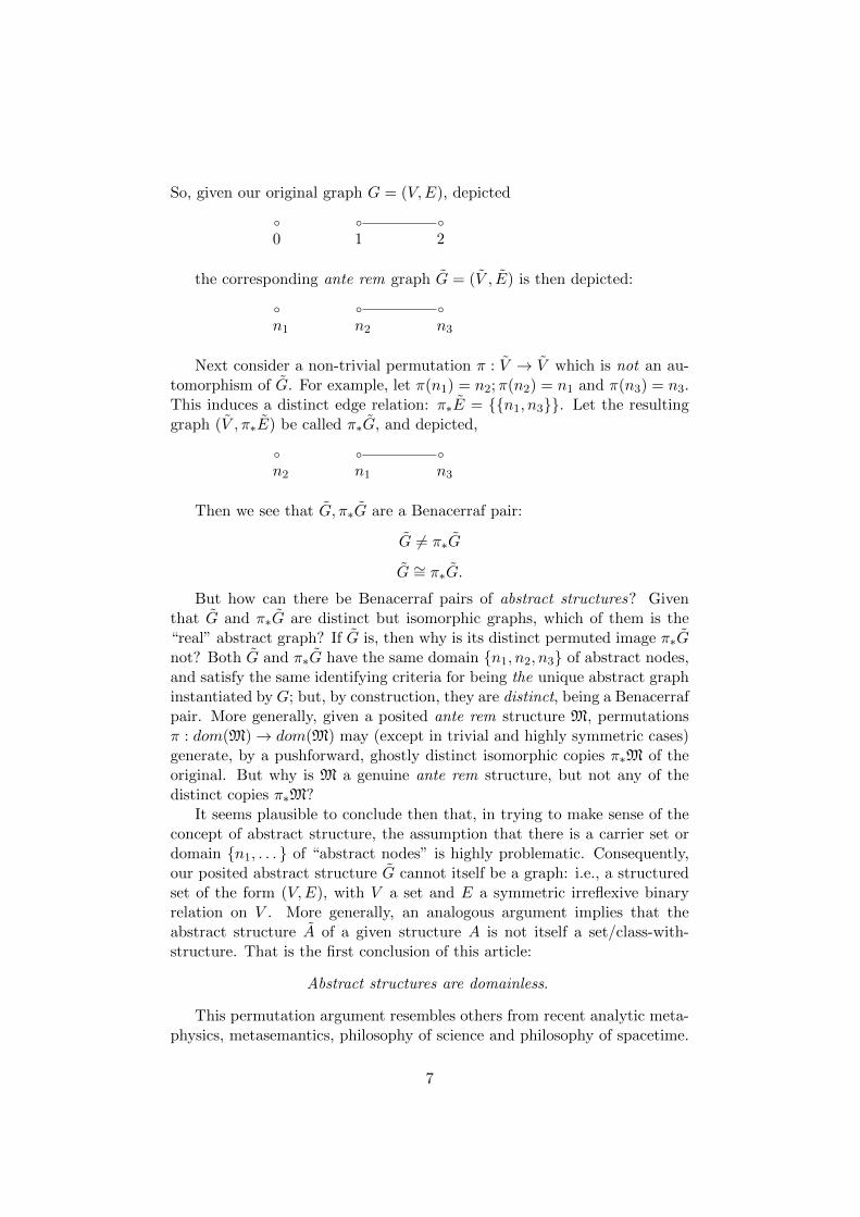
So, given our original graph G = (V,E), depictedb b b0 1 2

the corresponding ante rem graph G = (V , E) is then depicted:b b bn1 n2 n3

Next consider a non-trivial permutation π : V → V which is not an au-tomorphism of G. For example, let π(n1) = n2;π(n2) = n1 and π(n3) = n3.This induces a distinct edge relation: π∗E = {{n1, n3}}. Let the resultinggraph (V , π∗E) be called π∗G, and depicted,b b b

n2 n1 n3

Then we see that G, π∗G are a Benacerraf pair:

G 6= π∗G

G ∼= π∗G.

But how can there be Benacerraf pairs of abstract structures? Giventhat G and π∗G are distinct but isomorphic graphs, which of them is the“real” abstract graph? If G is, then why is its distinct permuted image π∗Gnot? Both G and π∗G have the same domain {n1, n2, n3} of abstract nodes,and satisfy the same identifying criteria for being the unique abstract graphinstantiated by G; but, by construction, they are distinct, being a Benacerrafpair. More generally, given a posited ante rem structure M, permutationsπ : dom(M)→ dom(M) may (except in trivial and highly symmetric cases)generate, by a pushforward, ghostly distinct isomorphic copies π∗M of theoriginal. But why is M a genuine ante rem structure, but not any of thedistinct copies π∗M?

It seems plausible to conclude then that, in trying to make sense of theconcept of abstract structure, the assumption that there is a carrier set ordomain {n1, . . . } of “abstract nodes” is highly problematic. Consequently,our posited abstract structure G cannot itself be a graph: i.e., a structuredset of the form (V,E), with V a set and E a symmetric irreflexive binaryrelation on V . More generally, an analogous argument implies that theabstract structure A of a given structure A is not itself a set/class-with-structure. That is the first conclusion of this article:

Abstract structures are domainless.

This permutation argument resembles others from recent analytic meta-physics, metasemantics, philosophy of science and philosophy of spacetime.

7

The argument here has previously been given by Geoffrey Hellman.8 Criti-cizing Shapiro’s ante rem structuralism (Shapiro 1997), Hellman puts it likethis:

In fact, [ante rem structuralism] seems ultimately subject tothe very objection of Benacerraf [1965] that helped inspirerecent structuralist approaches to number systems in thefirst place. Suppose we had the ante rem structure for thenatural numbers, call it 〈N,ϕ, 1〉, where ϕ is the privilegedsuccessor function, and 1 the initial place. Obviously, thereare indefinitely many other progressions, explicitly definablein terms of this one, which qualify equally well as referentsfor our numerals and are just as “free from irrelevant fea-tures”; simply permute any (for simplicity, say finite) num-ber of places, obtaining a system 〈N,ϕ′, 1′〉, made up of thesame items but set in order by an adjusted transformation,′. Why should this not have been called “the archetypicalante rem progression”, or “the result of Dedekind abstrac-tion”? We cannot say, e.g., “because 1 is really first”, sincethe very notion “first” is relative to an ordering; relative to′, 1′, not 1, is “first”. (Hellman, 2007, pp. 11-12.)

And concludes:

Indeed, Benacerraf, in his original paper, generalized his ar-gument that numbers cannot really be sets to the conclu-sion that they cannot really be objects at all, and here, withpurported ante rem structures, we can see again why not,as multiple, equally valid identifications compete with oneanother as “uniquely correct”. Hyperplatonist abstraction,far from transcending the problem, leads straight back to it.(Hellman, 2007, pp. 11-12.)

If this permutation argument is correct, the abstract structure A of Adoes not have a domain or carrier set at all. What might A be?

3 Leibniz Abstraction

Taking the initial example from section 1 again, let G be the abstract graphdepicted: b b b

8Many thanks to Robert Black for alerting me to Hellman’s article. What we call Gabove corresponds to Hellman’s 〈N,ϕ, 1〉 and what we call π∗G corresponds to Hellman’s〈N,ϕ′, 1′〉.

8

Our working supposition is that there is such an abstract entity. Andmore generally, for each given structure A, there is an entity A—the abstractstructure of A—which somehow “corresponds to”, or is “instantiated” by, allisomorphic copies of A. There is an intuitively clear and central constrainton what A might be. If B is an isomorphic copy of A, then we expect A = Bto hold; and, conversely, if A = B, then we expect A ∼= B to hold.9

Consequently, the problem of abstract structure can be defined as fol-lows: one should like to find some kind of mapping

A 7→ A

which implements the following abstraction principle:10

Leibniz Abstraction: A = B if and only if A ∼= B.

How might we implement this? In section 2, a permutation argumentwas given against ante rem structuralism. For, given a proposed ante remstructure M, this proposal generates ghostly distinct-but-isomorphic (per-muted) copies π∗M—that is, unwanted Benacerraf pairs. But still, there areseveral remaining options.11

One option is to identify A with the equivalence class of all isomorphiccopies of A, the isomorphism type of A. A variation on this theme is toidentify A with the property of being isomorphic to A.12 In graph theory and

9There is an interesting caveat. One might draw a weaker conclusion, namely thatA and B are definitionally equivalent structures under some isomorphism. This can beimplemented by saying that A and B have isomorphic atomizations. The atomization ofA is obtained by considering all definable relations in A and extending the signature of Aby a new primitive predicate PR for each such relation R. The atomization Aat is thenthe corresponding expanded structure.

10The neologism “Leibniz Abstraction” may seem anachronistic, but seems appropriate,as Leibniz was the first to suggest an identification of “indiscernibles”; for structures, theidentification criterion is isomorphism.

11Throughout, we are considering the abstract structure of what are, in effect, “models”in the logician’s terminology. But is it correct to regard the crucial “same-abstract-structure” relation between A and B as being isomorphism? For example, for the categorytheorist, the abstract structure of a category C is usually understood in terms of therelation of category equivalence rather than the relation of category isomorphism. Thismay suggest that the notion of isomorphism does not yield the right way of abstractingto obtain the relevant notion of abstract structure. In footnotes 9 and 30, it is brieflysuggested that the equivalence relation over which the abstraction occurs may be weakenedto definitional equivalence, understood in terms of the atomization Aat of a structureA. One might argue that category theory yields the insight that, as a referee noted,“the abstract structure of an object is not something determined solely by the object’sinternal constitution, but also by the kind of structure-preserving mappings the class ofthese objects allow”. This is an interesting point and certainly deserves fuller and carefuldiscussion. But, at this point, the discussion must be postponed somewhat, in order thatthe current proposal for explicating the notion of abstract structure can be worked outfirst.

12I am grateful to Peter Fritz and Mike Shulman for emphasizing this point.

9

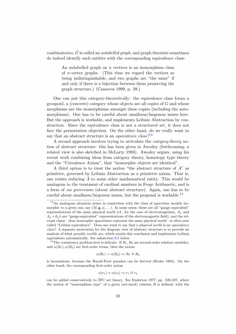
combinatorics, G is called an unlabelled graph, and graph theorists sometimesdo indeed identify such entities with the corresponding equivalence class:

An unlabelled graph on n vertices is an isomorphism classof n-vertex graphs. (This time we regard the vertices asbeing indistinguishable, and two graphs are “the same” ifand only if there is a bijection between them preserving thegraph structure.) (Cameron 1999, p. 39.)

One can put this category-theoretically: the equivalence class forms agroupoid, a (concrete) category whose objects are all copies of G and whosemorphisms are the isomorphisms amongst these copies (including the auto-morphisms). One has to be careful about smallness/largeness issues here.But the approach is workable, and implements Leibniz Abstraction by con-struction. Since the equivalence class is not a structured set, it does notface the permutation objection. On the other hand, do we really want tosay that an abstract structure is an equivalence class?13

A second approach involves trying to articulate the category-theory no-tion of abstract structure: this has been given in Awodey (forthcoming; arelated view is also sketched in McLarty 1993). Awodey argues, using hisrecent work combining ideas from category theory, homotopy type theoryand the “Univalence Axiom”, that “isomorphic objects are identical”.

A third option is to treat the notion “the abstract structure of A” asprimitive, governed by Leibniz Abstraction as a primitive axiom. That is,one resists reducing A to some other mathematical entity. This would beanalogous to the treatment of cardinal numbers in Frege Arithmetic, and isa form of sui generisism (about abstract structure). Again, one has to becareful about smallness/largeness issues, but the proposal is workable.14

13An analogous situation arises in connection with the class of spacetime models iso-morphic to a given one, say (M,g, φ, . . . ). In some sense, these are all “gauge equivalent”representations of the same physical world (cf., for the case of electromagetism, Aµ andAµ+∂µλ are “gauge-equivalent” representations of the electromagnetic field), and the rel-evant claim—that isomorphic spacetimes represent the same physical world—is often nowcalled “Leibniz equivalence”. Does one want to say that a physical world is an equivalenceclass? A separate motivation for the diagram view of abstract structure is to provide ananalysis of what possible worlds are, which avoids this conclusion and implements Leibnizequivalence automatically. See subsection 9.5 below.

14The consistency problem here is delicate. If R1, R2 are second-order relation variables,and α(R1), α(R2) are first-order terms, then the axiom

α(R1) = α(R2)↔ R1∼= R2

is inconsistent, because the Burali-Forti paradox can be derived (Hodes 1984). On theother hand, the corresponding first-order axiom

α(r1) = α(r2)↔ r1 ∼= r2

can be added conservatively to ZFC set theory. See Enderton 1977, pp. 220-227, wherethe notion of “isomorphism type” of a given (set-sized) relation R is defined, with the

10

A fourth option is the proposal we develop here, which we shall call thediagram conception of abstract structure.15

4 A Sketch of the Diagram View

On the approach we shall develop here, given a structure A (which doeshave a carrier set), the abstract structure A is not a structured set (orclass), set/class-with-structure, etc. In particular, A does not have a do-main/carrier set of “abstract nodes”. The central idea or motivation here isto eliminate the carrier set of objects/nodes. But how can we make senseof the notion of an abstract structure which lacks a domain—a domainlessstructure?

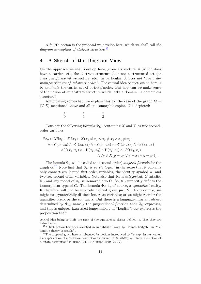
Anticipating somewhat, we explain this for the case of the graph G =(V,E) mentioned above and all its isomorphic copies. G is depicted:b b b

0 1 2

Consider the following formula ΦG, containing X and Y as free second-order variables:

∃x0 ∈ X∃x1 ∈ X∃x2 ∈ X(x0 6= x1 ∧ x0 6= x2 ∧ x1 6= x2

∧ ¬Y (x0, x0) ∧ ¬Y (x0, x1) ∧ ¬Y (x0, x2) ∧ ¬Y (x1, x0) ∧ ¬Y (x1, x1)

∧ Y (x1, x2) ∧ ¬Y (x2, x0) ∧ Y (x2, x1) ∧ ¬Y (x2, x2)

∧ ∀y ∈ X(y = x0 ∨ y = x1 ∨ y = x2)).

The formula ΦG will be called the (second-order) diagram formula for thegraph G.16 Note first that ΦG is purely logical in the sense that it containsonly connectives, bound first-order variables, the identity symbol =, andtwo free second-order variables. Note also that ΦG is categorical : G satisfiesΦG and any model of ΦG is isomorphic to G. So, ΦG implicitly defines theisomorphism type of G. The formula ΦG is, of course, a syntactical entity.It therefore will not be uniquely defined given just G. For example, wemight use syntactically distinct letters as variables; or we might reorder thequantifier prefix or the conjuncts. But there is a language-invariant objectdetermined by ΦG, namely the propositional function that ΦG expresses,and this is unique. Expressed longwindedly in “Loglish”, ΦG expresses theproposition that:

central idea being to limit the rank of the equivalence classes defined, so that they areindeed sets.

15A fifth option has been sketched in unpublished work by Hannes Leitgeb: an “ax-iomatic theory of graphs”.

16The proposal given here is influenced by notions introduced by Carnap. In particular,Carnap’s notion of a “relation description” (Carnap 1928: 20-23), and later the notion ofa “state description” (Carnap 1947: 9; Carnap 1950: 70-72).

11

There are three distinct things in X, and everything in X isone of them, and the first bears Y to nothing and nothingbears Y to it, the second bears Y only to the third, and thethird bears Y only to the second.

So, assuming the legitimacy of positing such propositional content, we define

〈ΦG〉 := the propositional function expressed by ΦG.

Being an “unsaturated” propositional function 〈ΦG〉 may be applied to tworelations-in-intension R1, R2 (one unary and one binary) to give a satu-rated proposition, that we denote 〈ΦG〉[R1, R2]. For example, consider theproperty Person and the binary relation Likes. Applying 〈ΦG〉 to theserelations, we obtain:

〈ΦG〉[Person, Likes] = the proposition that there are ex-actly three persons, and the first likes no one and is liked byno one, the second likes only the third, and the third likesonly the second.

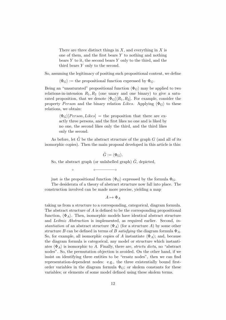
As before, let G be the abstract structure of the graph G (and all of itsisomorphic copies). Then the main proposal developed in this article is this:

G := 〈ΦG〉.So, the abstract graph (or unlabelled graph) G, depicted,b b bjust is the propositional function 〈ΦG〉 expressed by the formula ΦG.The desiderata of a theory of abstract structure now fall into place. The

construction involved can be made more precise, yielding a map

A 7→ ΦA

taking us from a structure to a corresponding, categorical, diagram formula.The abstract structure of A is defined to be the corresponding propositionalfunction, 〈ΦA〉. Then, isomorphic models have identical abstract structureand Leibniz Abstraction is implemented, as required earlier. Second, in-stantiation of an abstract structure 〈ΦA〉 (for a structure A) by some otherstructure B can be defined in terms of B satisfying the diagram formula ΦA.So, for example, all isomorphic copies of A instantiate 〈ΦA〉; and, becausethe diagram formula is categorical, any model or structure which instanti-ates 〈ΦA〉 is isomorphic to A. Finally, there are, strictu dictu, no “abstractnodes”. So, the permutation objection is avoided. On the other hand, if weinsist on identifying three entities to be “ersatz nodes”, then we can findrepresentation-dependent nodes: e.g., the three existentially bound first-order variables in the diagram formula ΦG; or skolem constants for thesevariables; or elements of some model defined using these skolem terms.

12

5 Diagram Axiomatization

The basic idea from section 4 is to associate with a given structure A adiagram formula ΦA in some language L, and then identify the abstractstructure A with the corresponding propositional function 〈ΦA〉. In thissection we shall give a slightly more rigorous presentation of this basic idea.The main issue that arises is how to deal with infinite structures. In orderto define the diagram formula, we must invoke the resources of infinitarylanguages.

First, we recap the diagram lemma from first-order model theory.

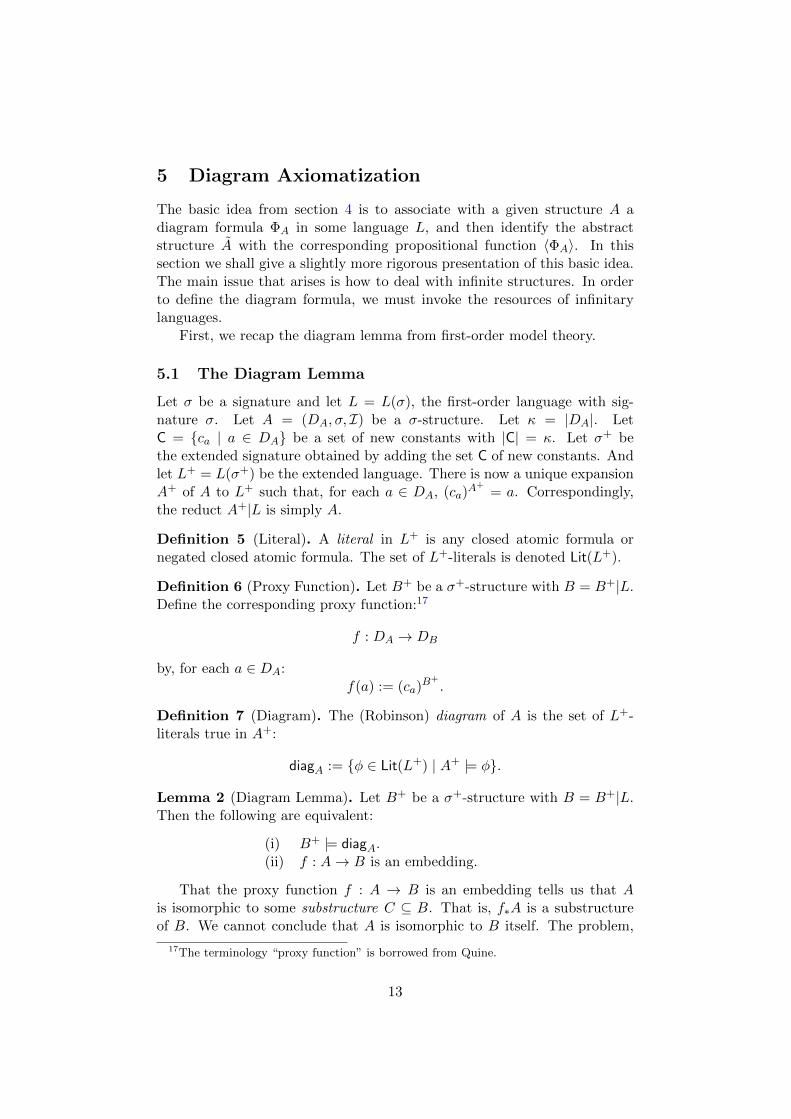
5.1 The Diagram Lemma

Let σ be a signature and let L = L(σ), the first-order language with sig-nature σ. Let A = (DA, σ, I) be a σ-structure. Let κ = |DA|. LetC = {ca | a ∈ DA} be a set of new constants with |C| = κ. Let σ+ bethe extended signature obtained by adding the set C of new constants. Andlet L+ = L(σ+) be the extended language. There is now a unique expansionA+ of A to L+ such that, for each a ∈ DA, (ca)

A+= a. Correspondingly,

the reduct A+|L is simply A.

Definition 5 (Literal). A literal in L+ is any closed atomic formula ornegated closed atomic formula. The set of L+-literals is denoted Lit(L+).

Definition 6 (Proxy Function). Let B+ be a σ+-structure with B = B+|L.Define the corresponding proxy function:17

f : DA → DB

by, for each a ∈ DA:f(a) := (ca)

B+.

Definition 7 (Diagram). The (Robinson) diagram of A is the set of L+-literals true in A+:

diagA := {φ ∈ Lit(L+) | A+ |= φ}.

Lemma 2 (Diagram Lemma). Let B+ be a σ+-structure with B = B+|L.Then the following are equivalent:

(i) B+ |= diagA.(ii) f : A→ B is an embedding.

That the proxy function f : A → B is an embedding tells us that Ais isomorphic to some substructure C ⊆ B. That is, f∗A is a substructureof B. We cannot conclude that A is isomorphic to B itself. The problem,

17The terminology “proxy function” is borrowed from Quine.

13

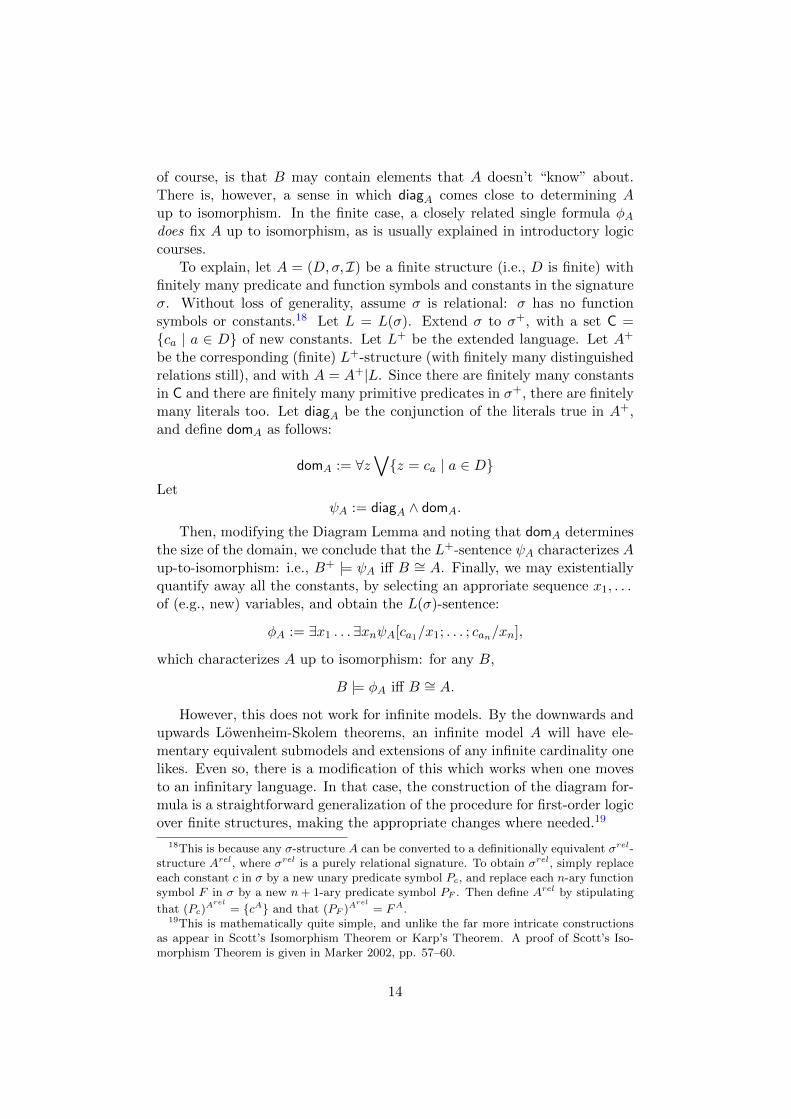
of course, is that B may contain elements that A doesn’t “know” about.There is, however, a sense in which diagA comes close to determining Aup to isomorphism. In the finite case, a closely related single formula φAdoes fix A up to isomorphism, as is usually explained in introductory logiccourses.

To explain, let A = (D,σ, I) be a finite structure (i.e., D is finite) withfinitely many predicate and function symbols and constants in the signatureσ. Without loss of generality, assume σ is relational: σ has no functionsymbols or constants.18 Let L = L(σ). Extend σ to σ+, with a set C ={ca | a ∈ D} of new constants. Let L+ be the extended language. Let A+

be the corresponding (finite) L+-structure (with finitely many distinguishedrelations still), and with A = A+|L. Since there are finitely many constantsin C and there are finitely many primitive predicates in σ+, there are finitelymany literals too. Let diagA be the conjunction of the literals true in A+,and define domA as follows:

domA := ∀z∨{z = ca | a ∈ D}

LetψA := diagA ∧ domA.

Then, modifying the Diagram Lemma and noting that domA determinesthe size of the domain, we conclude that the L+-sentence ψA characterizes Aup-to-isomorphism: i.e., B+ |= ψA iff B ∼= A. Finally, we may existentiallyquantify away all the constants, by selecting an approriate sequence x1, . . .of (e.g., new) variables, and obtain the L(σ)-sentence:

φA := ∃x1 . . . ∃xnψA[ca1/x1; . . . ; can/xn],

which characterizes A up to isomorphism: for any B,

B |= φA iff B ∼= A.

However, this does not work for infinite models. By the downwards andupwards Lowenheim-Skolem theorems, an infinite model A will have ele-mentary equivalent submodels and extensions of any infinite cardinality onelikes. Even so, there is a modification of this which works when one movesto an infinitary language. In that case, the construction of the diagram for-mula is a straightforward generalization of the procedure for first-order logicover finite structures, making the appropriate changes where needed.19

18This is because any σ-structure A can be converted to a definitionally equivalent σrel-structure Arel, where σrel is a purely relational signature. To obtain σrel, simply replaceeach constant c in σ by a new unary predicate symbol Pc, and replace each n-ary functionsymbol F in σ by a new n+ 1-ary predicate symbol PF . Then define Arel by stipulating

that (Pc)Arel

= {cA} and that (PF )Arel

= FA.19This is mathematically quite simple, and unlike the far more intricate constructions

as appear in Scott’s Isomorphism Theorem or Karp’s Theorem. A proof of Scott’s Iso-morphism Theorem is given in Marker 2002, pp. 57–60.

14

5.2 Infinitary Logic

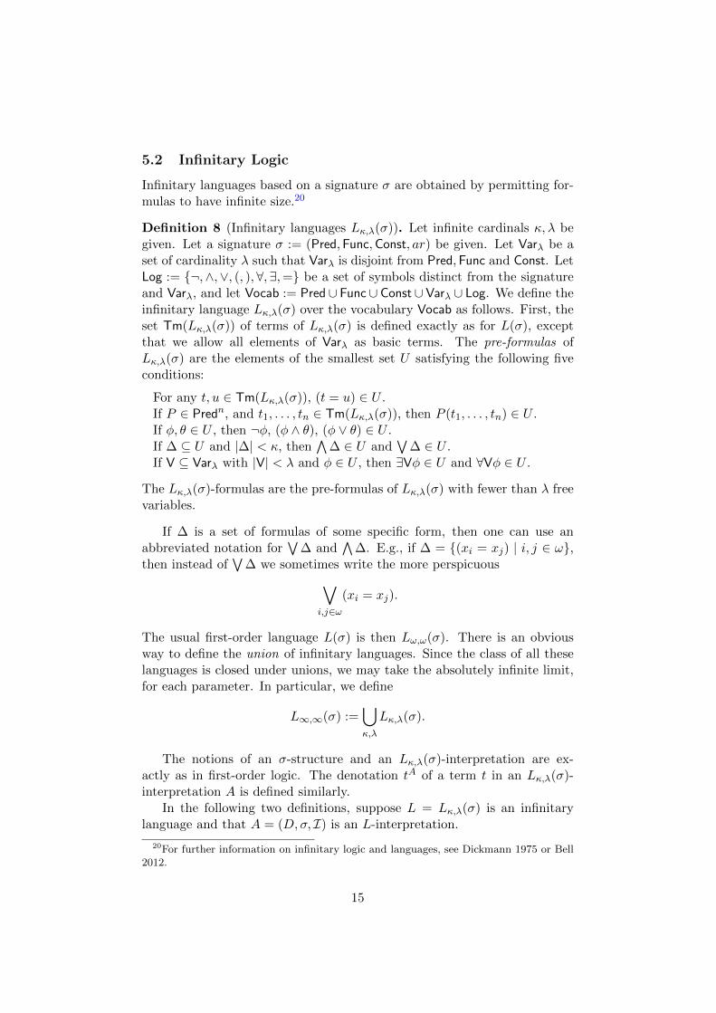
Infinitary languages based on a signature σ are obtained by permitting for-mulas to have infinite size.20

Definition 8 (Infinitary languages Lκ,λ(σ)). Let infinite cardinals κ, λ begiven. Let a signature σ := (Pred,Func,Const, ar) be given. Let Varλ be aset of cardinality λ such that Varλ is disjoint from Pred,Func and Const. LetLog := {¬,∧,∨, (, ),∀, ∃,=} be a set of symbols distinct from the signatureand Varλ, and let Vocab := Pred∪ Func∪ Const∪Varλ ∪ Log. We define theinfinitary language Lκ,λ(σ) over the vocabulary Vocab as follows. First, theset Tm(Lκ,λ(σ)) of terms of Lκ,λ(σ) is defined exactly as for L(σ), exceptthat we allow all elements of Varλ as basic terms. The pre-formulas ofLκ,λ(σ) are the elements of the smallest set U satisfying the following fiveconditions:

For any t, u ∈ Tm(Lκ,λ(σ)), (t = u) ∈ U .If P ∈ Predn, and t1, . . . , tn ∈ Tm(Lκ,λ(σ)), then P (t1, . . . , tn) ∈ U .If φ, θ ∈ U , then ¬φ, (φ ∧ θ), (φ ∨ θ) ∈ U .If ∆ ⊆ U and |∆| < κ, then

∧∆ ∈ U and

∨∆ ∈ U .

If V ⊆ Varλ with |V| < λ and φ ∈ U , then ∃Vφ ∈ U and ∀Vφ ∈ U .

The Lκ,λ(σ)-formulas are the pre-formulas of Lκ,λ(σ) with fewer than λ freevariables.

If ∆ is a set of formulas of some specific form, then one can use anabbreviated notation for

∨∆ and

∧∆. E.g., if ∆ = {(xi = xj) | i, j ∈ ω},

then instead of∨

∆ we sometimes write the more perspicuous∨i,j∈ω

(xi = xj).

The usual first-order language L(σ) is then Lω,ω(σ). There is an obviousway to define the union of infinitary languages. Since the class of all theselanguages is closed under unions, we may take the absolutely infinite limit,for each parameter. In particular, we define

L∞,∞(σ) :=⋃κ,λ

Lκ,λ(σ).

The notions of an σ-structure and an Lκ,λ(σ)-interpretation are ex-actly as in first-order logic. The denotation tA of a term t in an Lκ,λ(σ)-interpretation A is defined similarly.

In the following two definitions, suppose L = Lκ,λ(σ) is an infinitarylanguage and that A = (D,σ, I) is an L-interpretation.

20For further information on infinitary logic and languages, see Dickmann 1975 or Bell2012.

15

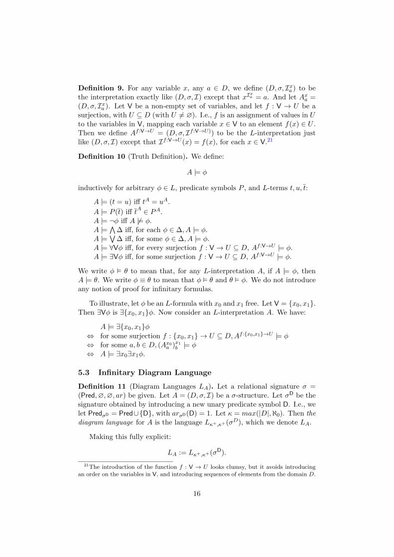
Definition 9. For any variable x, any a ∈ D, we define (D,σ, Ixa ) to bethe interpretation exactly like (D,σ, I) except that xI

xa = a. And let Axa =

(D,σ, Ixa ). Let V be a non-empty set of variables, and let f : V → U be asurjection, with U ⊆ D (with U 6= ∅). I.e., f is an assignment of values in Uto the variables in V, mapping each variable x ∈ V to an element f(x) ∈ U .Then we define Af :V→U = (D,σ, If :V→U)) to be the L-interpretation justlike (D,σ, I) except that If :V→U (x) = f(x), for each x ∈ V.21

Definition 10 (Truth Definition). We define:

A |= φ

inductively for arbitrary φ ∈ L, predicate symbols P , and L-terms t, u, t:

A |= (t = u) iff tA = uA.

A |= P (t) iff tA ∈ PA.

A |= ¬φ iff A 6|= φ.A |=

∧∆ iff, for each φ ∈ ∆, A |= φ.

A |=∨

∆ iff, for some φ ∈ ∆, A |= φ.A |= ∀Vφ iff, for every surjection f : V→ U ⊆ D, Af :V→U |= φ.A |= ∃Vφ iff, for some surjection f : V→ U ⊆ D, Af :V→U |= φ.

We write φ � θ to mean that, for any L-interpretation A, if A |= φ, thenA |= θ. We write φ ≡ θ to mean that φ � θ and θ � φ. We do not introduceany notion of proof for infinitary formulas.

To illustrate, let φ be an L-formula with x0 and x1 free. Let V = {x0, x1}.Then ∃Vφ is ∃{x0, x1}φ. Now consider an L-interpretation A. We have:

A |= ∃{x0, x1}φ⇔ for some surjection f : {x0, x1} → U ⊆ D,Af :{x0,x1}→U |= φ⇔ for some a, b ∈ D, (Ax0a )x1b |= φ⇔ A |= ∃x0∃x1φ.

5.3 Infinitary Diagram Language

Definition 11 (Diagram Languages LA). Let a relational signature σ =(Pred,∅,∅, ar) be given. Let A = (D,σ, I) be a σ-structure. Let σD be thesignature obtained by introducing a new unary predicate symbol D. I.e., welet PredσD = Pred∪{D}, with arσD(D) = 1. Let κ = max(|D|,ℵ0). Then thediagram language for A is the language Lκ+,κ+(σD), which we denote LA.

Making this fully explicit:

LA := Lκ+,κ+(σD).

21The introduction of the function f : V → U looks clumsy, but it avoids introducingan order on the variables in V, and introducing sequences of elements from the domain D.

16

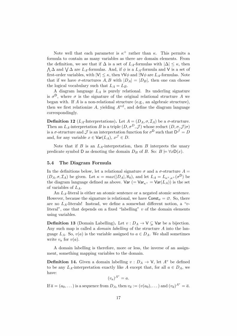
Note well that each parameter is κ+ rather than κ. This permits aformula to contain as many variables as there are domain elements. Fromthe definition, we see that if ∆ is a set of LA-formulas with |∆| ≤ κ, then∧

∆ and∨

∆ are LA-formulas. And, if φ is a LA-formula and V is a set offirst-order variables, with |V| ≤ κ, then ∀Vφ and ∃Vφ are LA-formulas. Notethat if we have σ-structures A,B with |DA| = |DB|, then one can choosethe logical vocabulary such that LA = LB.

A diagram language LA is purely relational. Its underling signatureis σD, where σ is the signature of the original relational structure A webegan with. If A is a non-relational structure (e.g., an algebraic structure),then we first relationize A, yielding Arel, and define the diagram languagecorrespondingly.

Definition 12 (LA-Interpretations). Let A = (DA, σ, IA) be a σ-structure.Then an LA-interpretation B is a triple (D,σD,J ) whose reduct (D,σ,J |σ)is a σ-structure and J is an interpretation function for σD such that DJ = Dand, for any variable x ∈ Var(LA), xJ ∈ D.

Note that if B is an LA-interpretation, then B interprets the unarypredicate symbol D as denoting the domain DB of B. So: B |= ∀xD(x).

5.4 The Diagram Formula

In the definitions below, let a relational signature σ and a σ-structure A =(DA, σ, IA) be given. Let κ = max(|DA|,ℵ0), and let LA = Lκ+,κ+(σD) bethe diagram language defined as above. Var (= Varκ+ = Var(LA)) is the setof variables of LA.

An LA-literal is either an atomic sentence or a negated atomic sentence.However, because the signature is relational, we have Constσ = ∅. So, thereare no LA-literals! Instead, we define a somewhat different notion, a “v-literal”, one that depends on a fixed “labelling” v of the domain elementsusing variables.

Definition 13 (Domain Labelling). Let v : DA → V ( Var be a bijection.Any such map is called a domain labelling of the structure A into the lan-guage LA. So, v(a) is the variable assigned to a ∈ DA. We shall sometimeswrite va for v(a).

A domain labelling is therefore, more or less, the inverse of an assign-ment, something mapping variables to the domain.

Definition 14. Given a domain labelling v : DA → V, let Av be definedto be any LA-interpretation exactly like A except that, for all a ∈ DA, wehave:

(va)Av = a.

If a = (a0, . . . ) is a sequence fromDA, then va := (v(a0), . . . ) and (va)Av = a.

17

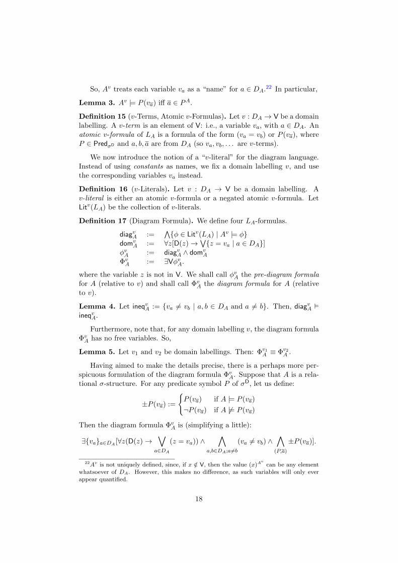
So, Av treats each variable va as a “name” for a ∈ DA.22 In particular,

Lemma 3. Av |= P (va) iff a ∈ PA.

Definition 15 (v-Terms, Atomic v-Formulas). Let v : DA → V be a domainlabelling. A v-term is an element of V: i.e., a variable va, with a ∈ DA. Anatomic v-formula of LA is a formula of the form (va = vb) or P (va), whereP ∈ PredσD and a, b, a are from DA (so va, vb, . . . are v-terms).

We now introduce the notion of a “v-literal” for the diagram language.Instead of using constants as names, we fix a domain labelling v, and usethe corresponding variables va instead.

Definition 16 (v-Literals). Let v : DA → V be a domain labelling. Av-literal is either an atomic v-formula or a negated atomic v-formula. LetLitv(LA) be the collection of v-literals.

Definition 17 (Diagram Formula). We define four LA-formulas.

diagvA :=∧{φ ∈ Litv(LA) | Av |= φ}

domvA := ∀z[D(z)→

∨{z = va | a ∈ DA}]

φvA := diagvA ∧ domvA

ΦvA := ∃VφvA.

where the variable z is not in V. We shall call φvA the pre-diagram formulafor A (relative to v) and shall call Φv

A the diagram formula for A (relativeto v).

Lemma 4. Let ineqvA := {va 6= vb | a, b ∈ DA and a 6= b}. Then, diagvA �ineqvA.

Furthermore, note that, for any domain labelling v, the diagram formulaΦvA has no free variables. So,

Lemma 5. Let v1 and v2 be domain labellings. Then: Φv1A ≡ Φv2

A .

Having aimed to make the details precise, there is a perhaps more per-spicuous formulation of the diagram formula Φv

A. Suppose that A is a rela-tional σ-structure. For any predicate symbol P of σD, let us define:

±P (va) :=

{P (va) if A |= P (va)

¬P (va) if A 6|= P (va)

Then the diagram formula ΦvA is (simplifying a little):

∃{va}a∈DA [∀z(D(z)→∨a∈DA

(z = va)) ∧∧

a,b∈DA;a6=b(va 6= vb) ∧

∧(P,a)

±P (va)].

22Av is not uniquely defined, since, if x /∈ V, then the value (x)Av

can be any elementwhatsoever of DA. However, this makes no difference, as such variables will only everappear quantified.

18

The first notable property of the diagram formula ΦvA is more or less imme-

diate from the definitions:

Lemma 6. Let v be any domain labelling. Then: A |= ΦvA.

5.5 Categoricity and Equivalence

In the lemmas below, we suppose that a relational signature σ and a σ-structure A = (DA, σ, IA) are given and that LA is defined as above. Weassume a fixed labelling v : DA → V ( Var is given and that Av, φvA and Φv

A

are defined as above.

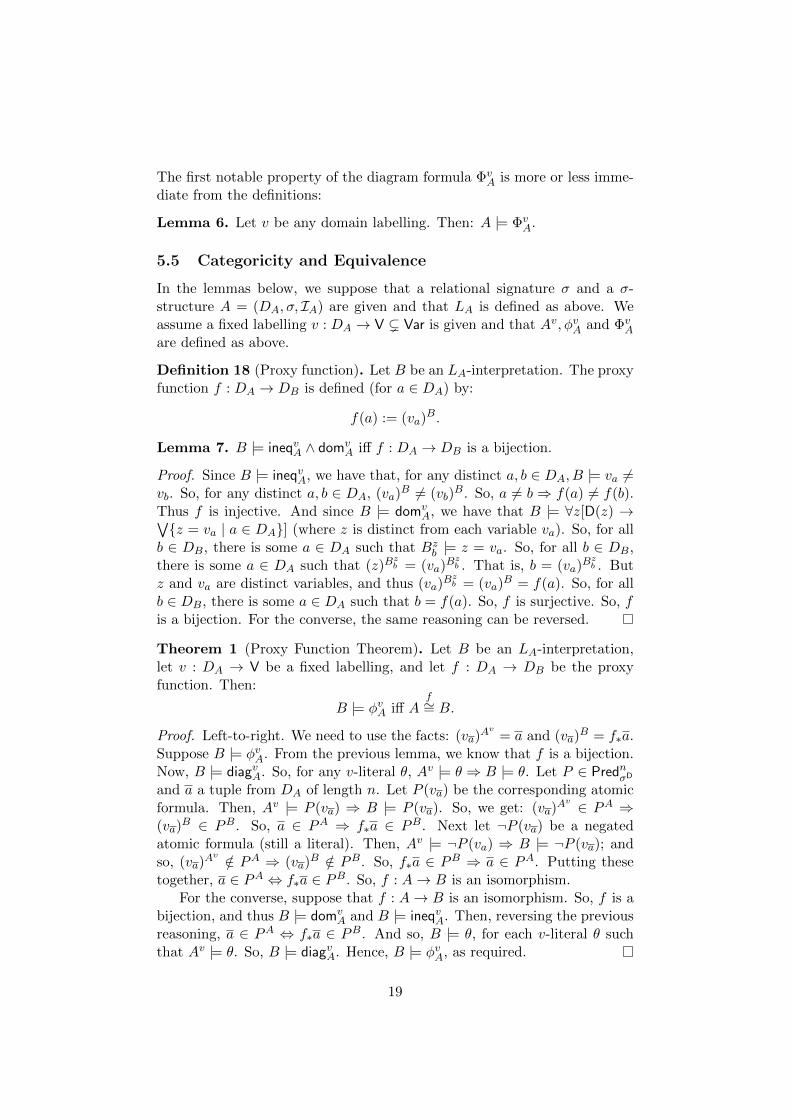
Definition 18 (Proxy function). Let B be an LA-interpretation. The proxyfunction f : DA → DB is defined (for a ∈ DA) by:

f(a) := (va)B.

Lemma 7. B |= ineqvA ∧ domvA iff f : DA → DB is a bijection.

Proof. Since B |= ineqvA, we have that, for any distinct a, b ∈ DA, B |= va 6=vb. So, for any distinct a, b ∈ DA, (va)

B 6= (vb)B. So, a 6= b⇒ f(a) 6= f(b).

Thus f is injective. And since B |= domvA, we have that B |= ∀z[D(z) →∨

{z = va | a ∈ DA}] (where z is distinct from each variable va). So, for allb ∈ DB, there is some a ∈ DA such that Bz

b |= z = va. So, for all b ∈ DB,there is some a ∈ DA such that (z)B

zb = (va)

Bzb . That is, b = (va)Bzb . But

z and va are distinct variables, and thus (va)Bzb = (va)

B = f(a). So, for allb ∈ DB, there is some a ∈ DA such that b = f(a). So, f is surjective. So, fis a bijection. For the converse, the same reasoning can be reversed.

Theorem 1 (Proxy Function Theorem). Let B be an LA-interpretation,let v : DA → V be a fixed labelling, and let f : DA → DB be the proxyfunction. Then:

B |= φvA iff Af∼= B.

Proof. Left-to-right. We need to use the facts: (va)Av = a and (va)

B = f∗a.Suppose B |= φvA. From the previous lemma, we know that f is a bijection.Now, B |= diagvA. So, for any v-literal θ, Av |= θ ⇒ B |= θ. Let P ∈ PrednσD

and a a tuple from DA of length n. Let P (va) be the corresponding atomicformula. Then, Av |= P (va) ⇒ B |= P (va). So, we get: (va)

Av ∈ PA ⇒(va)

B ∈ PB. So, a ∈ PA ⇒ f∗a ∈ PB. Next let ¬P (va) be a negatedatomic formula (still a literal). Then, Av |= ¬P (va) ⇒ B |= ¬P (va); andso, (va)

Av /∈ PA ⇒ (va)B /∈ PB. So, f∗a ∈ PB ⇒ a ∈ PA. Putting these

together, a ∈ PA ⇔ f∗a ∈ PB. So, f : A→ B is an isomorphism.For the converse, suppose that f : A→ B is an isomorphism. So, f is a

bijection, and thus B |= domvA and B |= ineqvA. Then, reversing the previous

reasoning, a ∈ PA ⇔ f∗a ∈ PB. And so, B |= θ, for each v-literal θ suchthat Av |= θ. So, B |= diagvA. Hence, B |= φvA, as required.

19

From the previous results, it follows that the diagram formula ΦvA cate-

gorically axiomatizes A in the following sense:23

Theorem 2 (Categoricity Theorem). Let B be an LA-interpretation. Letv : DA → V be a fixed labelling. Then

B |= ΦvA ⇔ A ∼= B.

Proof. (⇐) Let A ∼= B. Now Av |= ΦvA. Since A ∼= B, we have B |= Φv

A.(⇒) Suppose B |= φvA and let f : DA → DB be the proxy function. We

have, by the Proxy Function Theorem, B |= φvA ⇔ Af∼= B. So, A

f∼= B, asrequired.

Theorem 3 (Equivalence Theorem). Let A and B be σ-structures and letv1 : DA → V and v2 : DB → V′ be labellings. Then

A ∼= B ⇔ Φv1A ≡ Φv2

B .

Proof. This follows from the Categoricity Theorem.

The Equivalence Theorem states that the diagram formulas for isomor-phic structures are logically equivalent, and that logically equivalent diagramformulas correspond to isomorphic structures.

This completes the description of how to define the diagram formula ΦvA

for a given structure A. The formula ΦvA tells you “everything you need to

know, up to isomorphism” about the structure A.

6 Examples

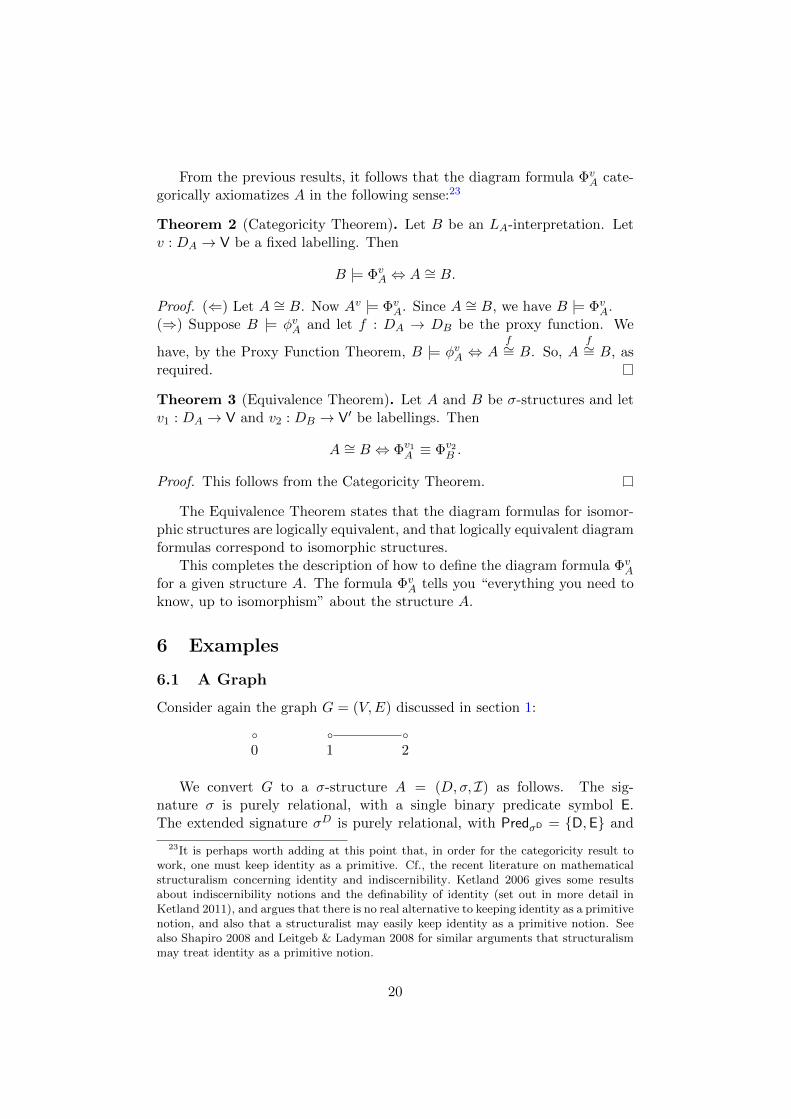
6.1 A Graph

Consider again the graph G = (V,E) discussed in section 1:b b b0 1 2

We convert G to a σ-structure A = (D,σ, I) as follows. The sig-nature σ is purely relational, with a single binary predicate symbol E.The extended signature σD is purely relational, with PredσD = {D,E} and

23It is perhaps worth adding at this point that, in order for the categoricity result towork, one must keep identity as a primitive. Cf., the recent literature on mathematicalstructuralism concerning identity and indiscernibility. Ketland 2006 gives some resultsabout indiscernibility notions and the definability of identity (set out in more detail inKetland 2011), and argues that there is no real alternative to keeping identity as a primitivenotion, and also that a structuralist may easily keep identity as a primitive notion. Seealso Shapiro 2008 and Leitgeb & Ladyman 2008 for similar arguments that structuralismmay treat identity as a primitive notion.

20

arσD(D) = 1. The carrier set D is {0, 1} and the edge relation EA ⊆ D2 isnow {(1, 2), (2, 1)} (a symmetric irreflexive binary relation on D). Fix a la-belling v : D → V by: v(0) = x0; v(1) = x1; v(2) = x2. So, the set of v-termsis V = {x0, x1, x2}. The corresponding diagram formula Φv

G is equivalent to(simplifying a little):24

∃x0 ∈ D∃x1 ∈ D∃x2 ∈ D(x0 6= x1 ∧ x0 6= x2 ∧ x1 6= x2

∧ ¬E(x0, x0) ∧ ¬E(x0, x1) ∧ ¬E(x0, x2) ∧ ¬E(x1, x0) ∧ ¬E(x1, x1)

∧ E(x1, x2) ∧ ¬E(x2, x0) ∧ E(x2, x1) ∧ ¬E(x2, x2)

∧ ∀z ∈ D(z = x0 ∨ z = x1 ∨ z = x2)).

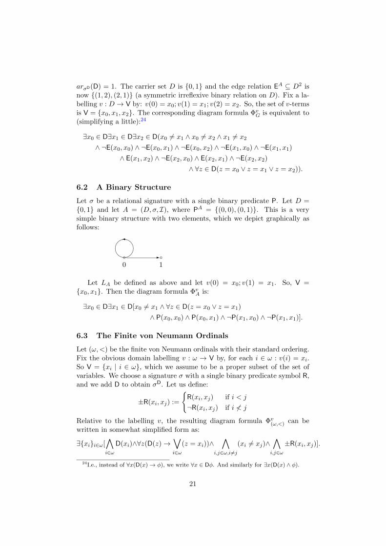
6.2 A Binary Structure

Let σ be a relational signature with a single binary predicate P. Let D ={0, 1} and let A = (D,σ, I), where PA = {(0, 0), (0, 1)}. This is a verysimple binary structure with two elements, which we depict graphically asfollows:

b b����

-

�

0 1

Let LA be defined as above and let v(0) = x0; v(1) = x1. So, V ={x0, x1}. Then the diagram formula Φv

A is:

∃x0 ∈ D∃x1 ∈ D[x0 6= x1 ∧ ∀z ∈ D(z = x0 ∨ z = x1)

∧ P(x0, x0) ∧ P(x0, x1) ∧ ¬P(x1, x0) ∧ ¬P(x1, x1)].

6.3 The Finite von Neumann Ordinals

Let (ω,<) be the finite von Neumann ordinals with their standard ordering.Fix the obvious domain labelling v : ω → V by, for each i ∈ ω : v(i) = xi.So V = {xi | i ∈ ω}, which we assume to be a proper subset of the set ofvariables. We choose a signature σ with a single binary predicate symbol R,and we add D to obtain σD. Let us define:

±R(xi, xj) :=

{R(xi, xj) if i < j

¬R(xi, xj) if i 6< j

Relative to the labelling v, the resulting diagram formula Φv(ω,<) can be

written in somewhat simplified form as:

∃{xi}i∈ω[∧i∈ω

D(xi)∧∀z(D(z)→∨i∈ω

(z = xi))∧∧

i,j∈ω,i6=j(xi 6= xj)∧

∧i,j∈ω

±R(xi, xj)].

24I.e., instead of ∀x(D(x)→ φ), we write ∀x ∈ Dφ. And similarly for ∃x(D(x) ∧ φ).

21

This formula categorically axiomatizes (ω,<). I.e., for any L(ω,<)-interpretationB, we have:

B |= Φv(ω,<) ⇔ B ∼= (ω,<).

7 Labellings, Automorphisms and Skolemization

7.1 Automorphism Theorems

The choice of domain labelling function v : DA → V ( Var is innocuous inconnection with the equivalence of diagram formulas, because the variablesva labelling the domain elements a ∈ DA are bound by the initial existentialquantifier prefix in the diagram formula ∃VφvA. But we can explore labellingsmore carefully by considering the pre-diagram formula φvA, given by:

φvA := diagvA ∧ domvA.

Let

v1, v2 : DA → V

be two domain labellings with the same range. Since they are both bijectionsDA → V, it follows that

(v2)−1 ◦ v1 : DA → DA

v2 ◦ (v1)−1 : V→ V

are both bijections. We might think of v2 ◦ (v1)−1 as a relabelling of the

domain DA. In a sense, it is a bit like a co-ordinate transformation betweencharts in differential geometry. We might then think of (v2)

−1 ◦ v1 as thecorresponding “active” transformation on the domain.25

We now show that “logically equivalent” relabellings are intimately re-lated to automorphisms of the structure A. In the two lemmas and twotheorems below, let π : DA → DA be a bijection and let vπ := v ◦ π.

Lemma 8. Let g : DA → DA be defined by: g(a) := (vπ(a))A. Then g = π.

Proof. Recall that (v(a))Av

= a. Now g(a) = (vπ(a))Av

= (v(π(a)))Av

=π(a). I.e., g = π.

Theorem 4 (First Automorphism Theorem). Av |= φvπ

A iff π ∈ Aut(A).

25For example, let (φ,U), (ψ, V ) be n-charts on a manifold M with overlap U ∩ V . Forsimplicity, suppose U = V . The images O1 = φ[U ] and O2 = ψ[U ] are open subsets of Rn.Then ψ◦φ−1 : O1 → O2 is a “co-ordinate transformation”, and the map ψ−1◦φ : U → U isthe corresponding active transformation. Readers curious about the differential geometryused here might consult, e.g., Robbin & Salamon 2011.

22

Proof. Let B be an LA-interpretation and apply the Proxy Function The-orem to φv

π

A . Define the proxy function g : DA → DB by g(a) = (vπ(a))B.

By the Proxy Function Theorem, B |= φvπ

A iff Ag∼= B. Now suppose B is

Av. By the previous lemma, g = π. So, Av |= φvπ

A iff Aπ∼= A.

Lemma 9. Let the proxy functions f, g : DA → DB be defined by:

f(a) := (v(a))B

g(a) := (vπ(a)))B

Then g = f ◦ π.

Proof. For vπ(a) = (v ◦π)(a) = v(π(a)). So, g(a) = (v(π(a)))B = f(π(a)) =(f ◦ π)(a), as required.

Theorem 5 (Second Automorphism Theorem). π ∈ Aut(A) iff φvA ≡ φvπ

A .

Proof. Let π ∈ Aut(A) and suppose B |= φvA. By the Proxy FunctionTheorem,

B |= φvA iff Af∼= B.

B |= φvπ

A iff Ag∼= B.

So, f : A → B is an isomorphism. By the previous lemma, g = f ◦ π. Andsince π ∈ Aut(A), it follows that g : A → B is an isomorphism. Hence, bythe Proxy Function Theorem again, B |= φv

π

A . Similar reasoning shows thatif B |= φv

π

A , then B |= φvA. Since B was arbitrary, φvA ≡ φvπ

A , as required.Conversely, suppose that φvA ≡ φv

π

A . Now Av |= φvA. So, Av |= φvπ

A . So,by the First Automorphism Theorem, π : A → A is an isomorphism. I.e.,π ∈ Aut(A), as required.

In the left-to-right direction, this says that given a labelling v : DA → V,of the domain elements to variables, the pre-diagram formula φvA is “logi-cally invariant” under any automorphism π ∈ Aut(A). And the right-to-leftdirection says that when two such formulas given by labellings v1 and v2 arelogically equivalent, then the map (v2)

−1◦v1 : DA → DA is an automorphismof the structure A.

7.2 Skolemization Theorem

Consider again the example 3-vertex graph G discussed several times above:b b b0 1 2

23

Consider the pre-diagram formula φvG:

D(x0) ∧ D(x1) ∧ D(x2) ∧ x0 6= x1 ∧ x0 6= x2 ∧ x1 6= x2

∧ ¬E(x0, x0) ∧ ¬E(x0, x1) ∧ ¬E(x0, x2) ∧ ¬E(x1, x0) ∧ ¬E(x1, x1)

∧ E(x1, x2) ∧ ¬E(x2, x0) ∧ E(x2, x1) ∧ ¬E(x2, x2)

∧ ∀z(D(z)→ (z = x0 ∨ z = x1 ∨ z = x2)).

This is a conjunction of four formulas:

(i) D(x0) ∧ D(x1) ∧ D(x2)(ii) x0 6= x1 ∧ x0 6= x2 ∧ x1 6= x2(iii) ∀z(D(z)→ (z = x0 ∨ z = x1 ∨ z = x2)).(iv) ¬E(x0, x0)∧¬E(x0, x1)∧¬E(x0, x2)∧¬E(x1, x0)∧¬E(x1, x1)

∧E(x1, x2) ∧ ¬E(x2, x0) ∧ E(x2, x1) ∧ ¬E(x2, x2)

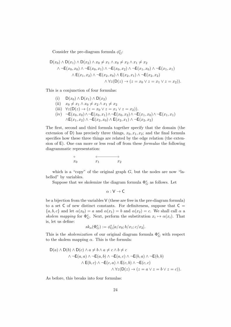
The first, second and third formula together specify that the domain (theextension of D) has precisely three things, x0, x1, x2; and the final formulaspecifies how these three things are related by the edge relation (the exten-sion of E). One can more or less read off from these formulas the followingdiagrammatic representation:b b b

x0 x1 x2

which is a “copy” of the original graph G, but the nodes are now “la-belled” by variables.

Suppose that we skolemize the diagram formula ΦvG as follows. Let

α : V→ C

be a bijection from the variables V (these are free in the pre-diagram formula)to a set C of new distinct constants. For definiteness, suppose that C ={a, b, c} and let α(x0) = a and α(x1) = b and α(x2) = c. We shall call α askolem mapping for Φv

G. Next, perform the substitution xi 7→ α(xi). Thatis, let us define:

skα(ΦvG) := φvG[a/x0; b/x1; c/x2].

This is the skolemization of our original diagram formula ΦvG with respect

to the skolem mapping α. This is the formula:

D(a) ∧ D(b) ∧ D(c) ∧ a 6= b ∧ a 6= c ∧ b 6= c

∧ ¬E(a, a) ∧ ¬E(a, b) ∧ ¬E(a, c) ∧ ¬E(b, a) ∧ ¬E(b, b)

∧ E(b, c) ∧ ¬E(c, a) ∧ E(c, b) ∧ ¬E(c, c)

∧ ∀z(D(z)→ (z = a ∨ z = b ∨ z = c)).

As before, this breaks into four formulas:

24

(i) D(a) ∧ D(b) ∧ D(c)(ii) a 6= b ∧ a 6= c ∧ b 6= c(iii) ∀z(D(z)→ (z = a ∨ z = b ∨ z = c)).(iv) ¬E(a, a) ∧ ¬E(a, b) ∧ ¬E(a, c) ∧ ¬E(b, a) ∧ ¬E(b, b)

∧E(b, c) ∧ ¬E(c, a) ∧ E(c, b) ∧ ¬E(c, c)

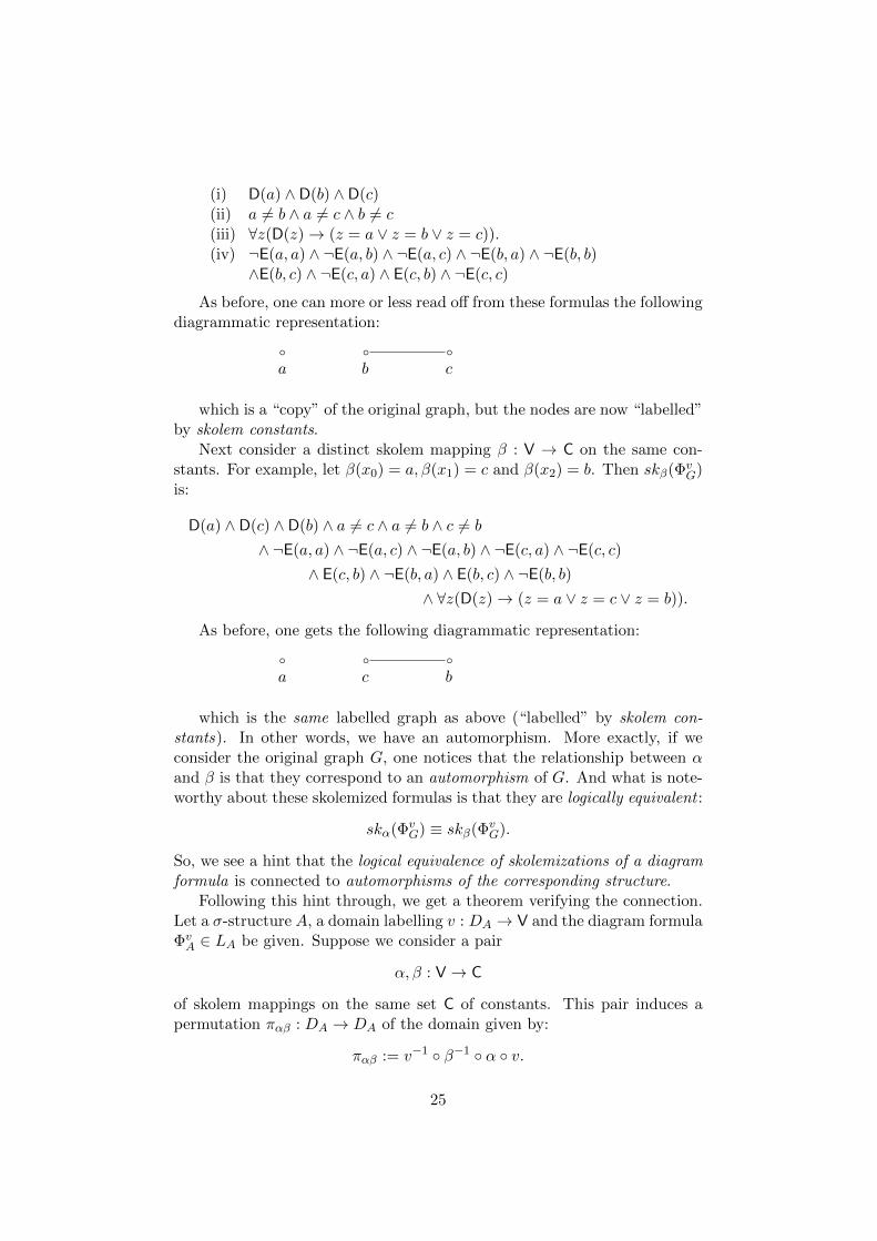
As before, one can more or less read off from these formulas the followingdiagrammatic representation:b b b

a b c

which is a “copy” of the original graph, but the nodes are now “labelled”by skolem constants.

Next consider a distinct skolem mapping β : V → C on the same con-stants. For example, let β(x0) = a, β(x1) = c and β(x2) = b. Then skβ(Φv

G)is:

D(a) ∧ D(c) ∧ D(b) ∧ a 6= c ∧ a 6= b ∧ c 6= b

∧ ¬E(a, a) ∧ ¬E(a, c) ∧ ¬E(a, b) ∧ ¬E(c, a) ∧ ¬E(c, c)

∧ E(c, b) ∧ ¬E(b, a) ∧ E(b, c) ∧ ¬E(b, b)

∧ ∀z(D(z)→ (z = a ∨ z = c ∨ z = b)).

As before, one gets the following diagrammatic representation:b b ba c b

which is the same labelled graph as above (“labelled” by skolem con-stants). In other words, we have an automorphism. More exactly, if weconsider the original graph G, one notices that the relationship between αand β is that they correspond to an automorphism of G. And what is note-worthy about these skolemized formulas is that they are logically equivalent :

skα(ΦvG) ≡ skβ(Φv

G).

So, we see a hint that the logical equivalence of skolemizations of a diagramformula is connected to automorphisms of the corresponding structure.

Following this hint through, we get a theorem verifying the connection.Let a σ-structure A, a domain labelling v : DA → V and the diagram formulaΦvA ∈ LA be given. Suppose we consider a pair

α, β : V→ C

of skolem mappings on the same set C of constants. This pair induces apermutation παβ : DA → DA of the domain given by:

παβ := v−1 ◦ β−1 ◦ α ◦ v.

25

One can then show:

Theorem 6 (Skolemization Theorem). παβ ∈ Aut(A) iff skα(ΦvA) ≡ skβ(Φv

A).

The proof is a modification of the proof of the Second AutomorphismTheorem.

8 The Diagram Conception of Abstract Structure

8.1 Second-Order Languages L(2)κ,λ

Definition 19 (Relational pure second-order infinitary languages L(2)κ,λ). Let

Var(2) = {Xni | i, n ∈ ω} be a set of second-order relation variables of all

finite arities, where the arity of Xni is n. Let κ, λ be infinite cardinals, and

let L(2)κ,λ be the corresponding second-order infinitary language based on the

empty signature. Let L(2)∞,∞ be the limit language.

The languages L(2)κ,λ have no primitive predicate symbols and no quan-

tifiers for the second-order variables. In a sense, any formula φ ∈ L(2)κ,λ is

“purely logical”.26

Definition 20 (Relational pure second-order infinitary language L(2)A ). Let

A = (D,σ, I) where σ = (Pred,∅,∅, ar) is a relational signature. Letκ = max(|D|,ℵ0). As before, let D be the new predicate symbol. Let

◦ : Pred ∪ {D} → Var(2)

be a function mapping each predicate symbol P from Pred∪{D} to a second-

order variable P ◦, preserving arity. Then we let L(2)A be the pure second-

order language L(2)κ+,κ+

.

Definition 21 (Translation into L(2)A ). Given any φ ∈ LA, we next define a

translation◦ : LA → L

(2)A

by letting φ◦ be the result of substituting P ◦ for each occurrence of P in φ,for each predicate symbol P .

Definition 22 (Second-order diagram formula). Let ΦvA ∈ LA be the dia-

gram formula for A, relative to v. The second-order diagram formula for A

is the L(2)A -formula (Φv

A)◦.

26The languages L(2)κ,λ are infinitary in two dimensions as it were—the cardinality of

Boolean compounds and the cardinality of the set of first-order variables. However, theyare restricted to countably many second-order variables (i.e., |Var(2)| = ℵ0). And they aresecond-order, rather than higher-order. Each restriction could in principle be lifted.

26

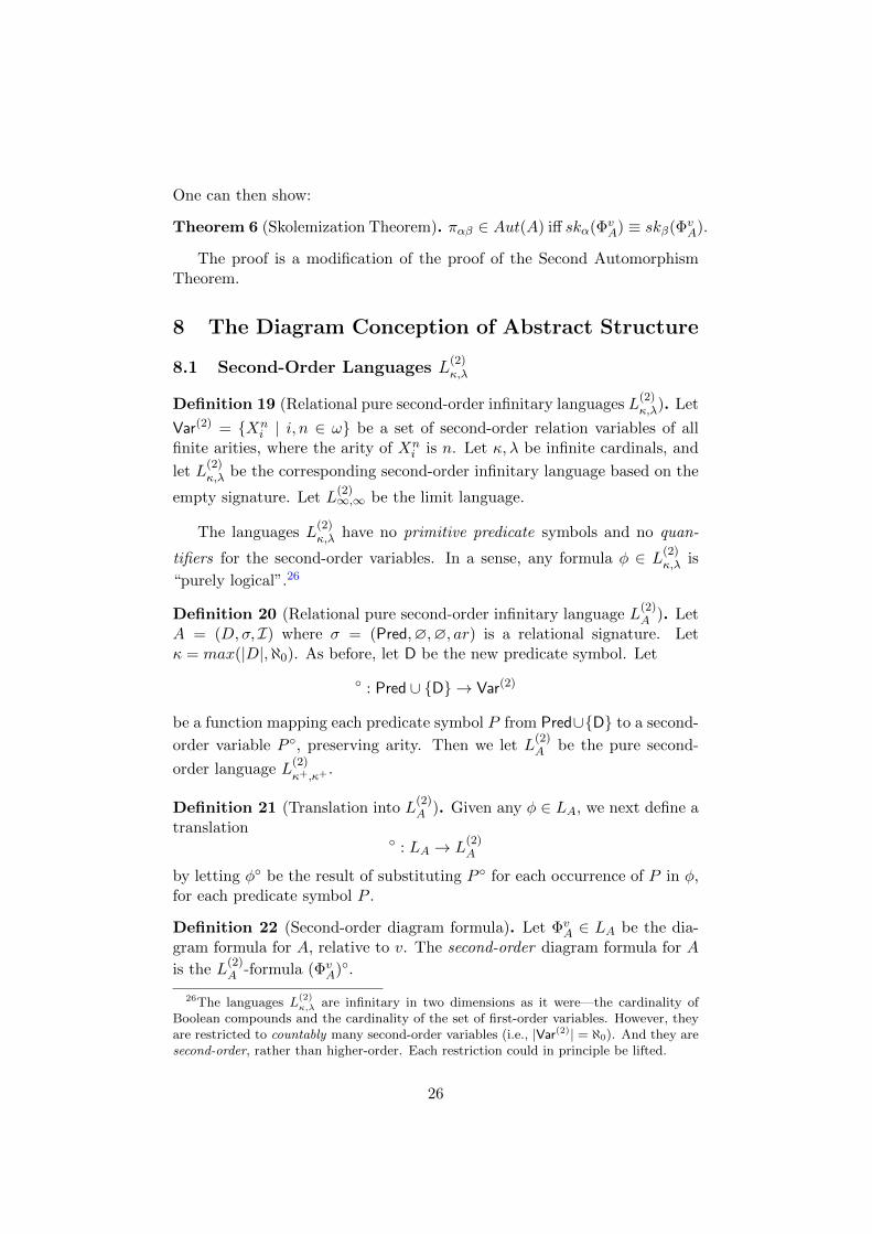
This sounds more complicated that it really is. For example, considerthe earlier example of a simple structure with a single binary relation,

b b����

-

�

0 1

whose diagram formula ΦvA was:

∃x0 ∈ D∃x1 ∈ D(x0 6= x1 ∧ ∀z ∈ D(z = x0 ∨ z = x1)

∧ ¬P(x1, x0) ∧ ¬P(x1, x1) ∧ P(x0, x0) ∧ P(x0, x1).

We convert this to the second-order diagram formula by replacing thepredicate symbols D,P by second-order variables, X,Y of correspondingarities. So, let the translation ◦ be such that D◦ = X and P◦ = Y . Theformula (Φv

A)◦(X,Y ) is,

∃x0 ∈ X∃x1 ∈ X(x0 6= x1 ∧ ∀z ∈ X(z = x0 ∨ z = x1)

∧ ¬Y (x1, x0) ∧ ¬Y (x1, x1) ∧ Y (x0, x0) ∧ Y (x0, x1)).

Similarly for the example of the finite von Neumann ordinals (ω,<). Thesecond-order diagram formula (Φv

(ω,<))◦(X,Y ) is, in abbreviated notation:

∃{xi}i∈ω[∧i∈ω

X(xi)∧∀z ∈ X∨i∈ω

(z = xi)∧∧

i,j∈ω;i 6=j(xi 6= xj)∧

∧i,j∈ω

±Y (xi, xj)].

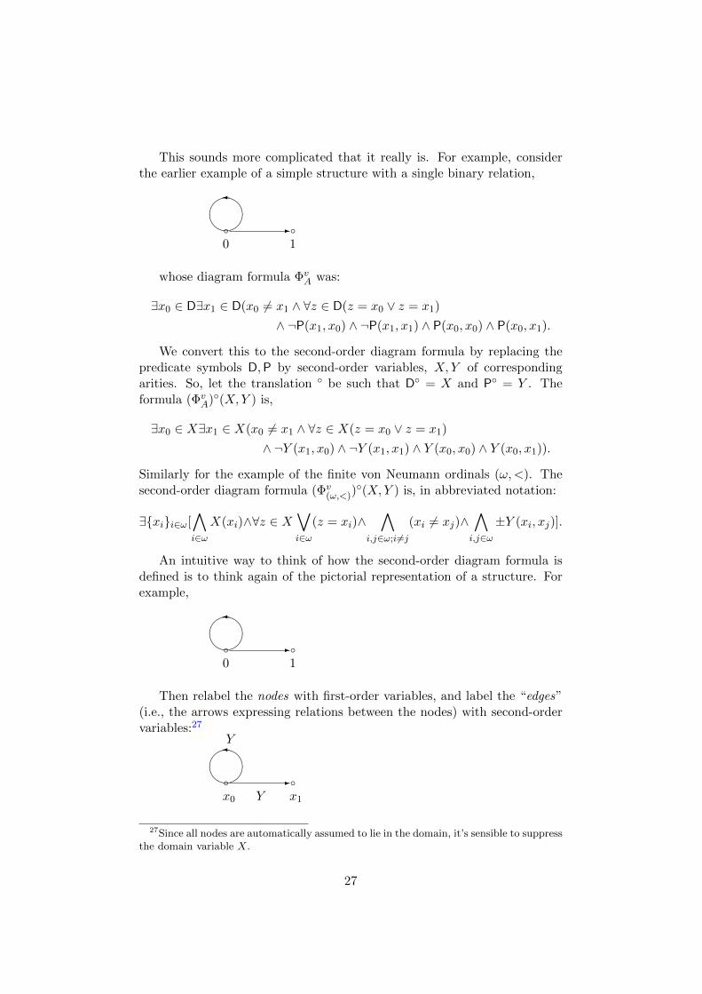
An intuitive way to think of how the second-order diagram formula isdefined is to think again of the pictorial representation of a structure. Forexample,

b b����

-

�

0 1

Then relabel the nodes with first-order variables, and label the “edges”(i.e., the arrows expressing relations between the nodes) with second-ordervariables:27

b b����

-

�

x0 x1Y

Y

27Since all nodes are automatically assumed to lie in the domain, it’s sensible to suppressthe domain variable X.

27

It is then intuitively clear how to “read-off” the second-order diagramformula from this.

8.2 Propositional Content

Given a signature σ, and a σ-structure A = (D,σ, I), we have still not quitereached a point where we can identify a unique something as the abstractstructure A for A. As we’ve seen, the diagram formula Φv

A implicitly definesthe isomorphism type of all structures isomorphic to A. But the diagramformula Φv

A is a syntactical entity—built out of symbols. Therefore, it willnot be invariant under various different choices of syntax. So, one has notfound a unique entity to be the abstract structure for A.

One might initially consider the equivalence class

[ΦvA] := {ψ ∈ LA | ψ ≡ Φv

A}

of sentences in LA. As we have seen, this eliminates v-dependence. But wehave only fixed the diagram formula Φv

A relative to the language LA. If oneuses a syntactically different language one gets a different equivalence class.In a sense, there are a number of “syntactic gauge choices” which must be“quotiented out”.

Our intuitive idea is that the abstract structure of A is somehow ex-pressed by the diagram formula Φv

A, although it’s clear that the diagramformula is itself not uniquely defined—distinct choices of syntax lead to dis-tinct formulas. What links these distinct syntactic representations is theirpropositional content, sometimes called intensional content.28 If we acceptthese notions, it suggests a way of construing abstract structures as second-order propositional functions.

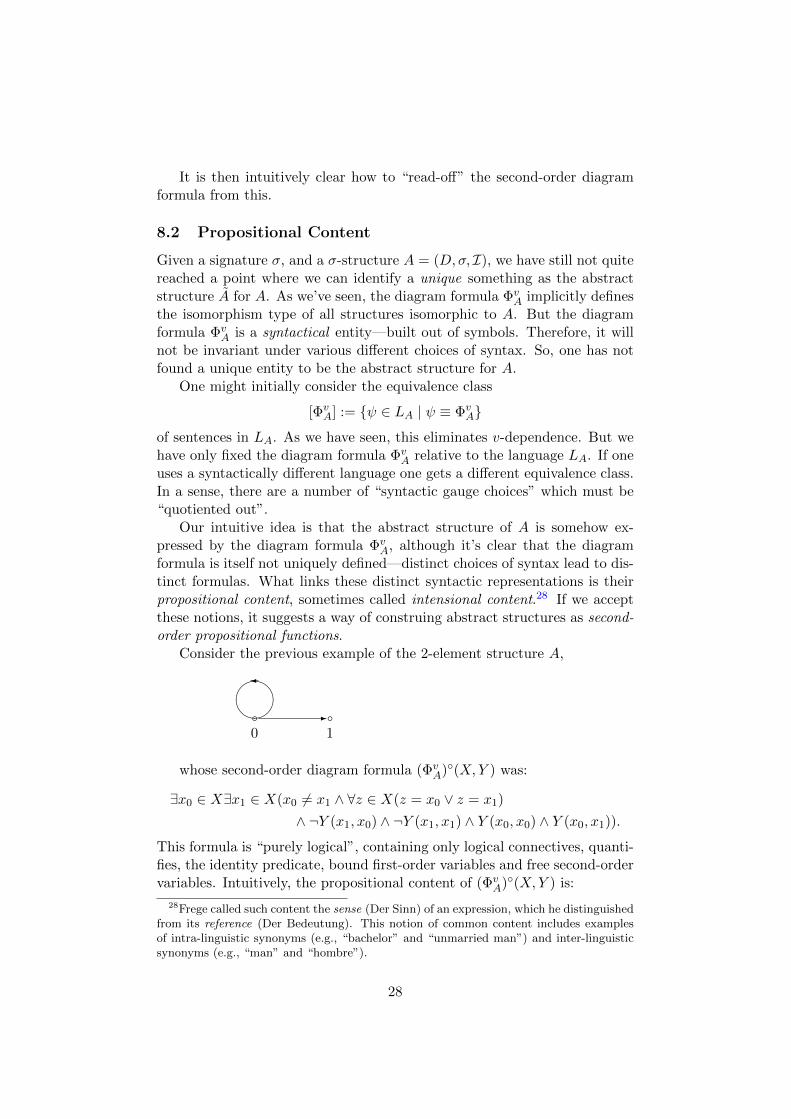
Consider the previous example of the 2-element structure A,

b b����

-

�

0 1

whose second-order diagram formula (ΦvA)◦(X,Y ) was:

∃x0 ∈ X∃x1 ∈ X(x0 6= x1 ∧ ∀z ∈ X(z = x0 ∨ z = x1)

∧ ¬Y (x1, x0) ∧ ¬Y (x1, x1) ∧ Y (x0, x0) ∧ Y (x0, x1)).

This formula is “purely logical”, containing only logical connectives, quanti-fies, the identity predicate, bound first-order variables and free second-ordervariables. Intuitively, the propositional content of (Φv

A)◦(X,Y ) is:

28Frege called such content the sense (Der Sinn) of an expression, which he distinguishedfrom its reference (Der Bedeutung). This notion of common content includes examplesof intra-linguistic synonyms (e.g., “bachelor” and “unmarried man”) and inter-linguisticsynonyms (e.g., “man” and “hombre”).

28

The proposition that there are exactly two things in X andthese are such that one of them bears Y to itself and to theother, but the other does not bear Y to itself or the other.

More generally, the assumption we make is that an L(2)A -formula Φ(X1, . . . , Xn)

expresses a propositional function taking an ordered n-tuple (R1, . . . , Rn) ofrelations-in-intension to a proposition, saying that R1, . . . , Rn are relatedin a certain way. So, proceeding in this way, let A = (D,σ, I) be a rela-tional structure. Let Φv

A be the diagram formula in LA. Let (ΦvA)◦ be the

second-order diagram formula, the result of replacing predicate symbols bysecond-order variables under ◦.

Definition 23. Let 〈ΦA〉 be the propositional function expressed by (ΦvA)◦.29

8.3 Abstract Structure

We have seen how to define, given a structure A, the second-order diagramformula (Φv

A)◦, which is now a formula with free second-order variables cor-responding to the domain of A and to its distinguished predicate symbols. Itis a purely logical formula. In general, we may think of (Φv

A)◦ as expressinga constraint on the relations denoted by these variables: (Φv

A)◦ expresses a“logical relation amongst relations”. And, as we have seen, (Φv

A)◦ is trueof A, and is categorical in the required sense: any structure B it is true ofmust be isomorphic to A.

While (ΦvA)◦ is a syntactic entity, we can consider 〈ΦA〉, the propositional

function expressed by (ΦvA)◦. We shall argue that this has all the properties

we expect of the requisite abstract structure, and so we may propose thefollowing definition of “abstract structure”:

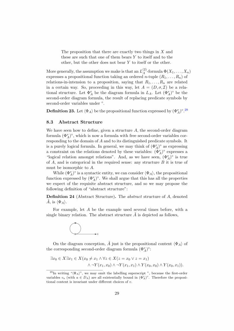
Definition 24 (Abstract Structure). The abstract structure of A, denotedA, is 〈ΦA〉.

For example, let A be the example used several times before, with asingle binary relation. The abstract structure A is depicted as follows,

b b����

-

�

On the diagram conception, A just is the propositional content 〈ΦA〉 ofthe corresponding second-order diagram formula (Φv

A)◦:

∃x0 ∈ X∃x1 ∈ X(x0 6= x1 ∧ ∀z ∈ X(z = x0 ∨ z = x1)

∧ ¬Y (x1, x0) ∧ ¬Y (x1, x1) ∧ Y (x0, x0) ∧ Y (x0, x1)).

29In writing “〈ΦA〉”, we may omit the labelling superscript v, because the first-ordervariables va (with a ∈ DA) are all existentially bound in (ΦvA)◦. Therefore the proposi-tional content is invariant under different choices of v.

29

On this conception, the abstract structure of A is a categorical second-order propositional function, expressed by a “diagram formula” of puresecond-order logic, which defines the isomorphism type of A. Modulo anassumption to be discussed in a moment, this conception of abstract struc-ture then yields the required abstraction principle:

Leibniz Abstraction: A = B iff A ∼= B.

To provide some kind of justification (if not quite a proof) of this, weneed two assumptions governing propositional identity, for pure second-orderformulas of the kind (Φv

A)◦ we have defined for a given A. Let Φ,Ψ be

formulas of L(2)∞,∞. Suppose that Φ expresses propositional function f and

Ψ expresses propositional function g. Then:

(a) f = g ⇒ Φ ≡ Ψ.(b) Φ ≡ Ψ⇒ f = g.

We these in hand, we then give an informal proof for Leibniz Abstraction.Let A = B. So, 〈ΦA〉 = 〈ΦB〉. Then, by (a), ΦA ≡ ΦB and so, by the Equiv-alence Theorem, A ∼= B. Conversely, let A ∼= B. Then, by the EquivalenceTheorem, ΦA ≡ ΦB. So, by (b) above, 〈ΦA〉 = 〈ΦB〉. So, A = B.

The word “seems” is appropriate here. No genuine proof has been given,because the crucial theoretical notion

“propositional function expressed by the formula (ΦvA)◦”

has not really been given a sufficiently clear explication and the assumptions(a) and (b) might be questioned.

Of these two assumptions, the first seems quite unproblematic: if Φ andΨ express the same proposition, they must be logically equivalent. Thesecond (b) seems more questionable: it says that logically equivalent (pure)formulas express the same propositional functions. This is plausible, ofcourse.

Having noted these potential sticking points, what has been done isconditional: assuming that we accept the notion of “propositional functionexpressed by a pure second-order formula” governed by principles (a) and(b) above, then Leibniz Abstraction can be implemented as above.30

On the current approach, we may define instantiation as follows:

30 At this point, we note that there is an even broader sense of abstract structure, inwhich definitionally equivalent copies of a structure A are counted as having the sameabstract structure. Let A ∼=df B mean that A and B are definitionally equivalent undersome isomorphism. One can incorporate this into the present approach by atomizing thegiven structure A to obtain Aat. If we define A 7→ A† by letting A† be 〈ΦAat〉, then weobtain a generalization of Leibniz Abstraction: A† = B† ⇔ A ∼=df B.

30

Definition 25 (Instantiation). Let A = (DA, σA, IA) and B = (DB, σB, IB)be structures with σA = σB. Let Φv

A be the diagram formula for A and letA = 〈ΦA〉 be the abstract structure of A. Then B instantiates 〈ΦA〉 just ifB |= Φv

A.

This delivers what one expects. For example:

Lemma 10. A instantiates A. And A instantiates B iff A ∼= B.

8.4 Fixing a Gauge

Suppose that G = (V,E) is a graph but that we are only interested in itsabstract structure G, the corresponding “unlabelled graph”. On the diagramconception, G is not itself a graph, with peculiar “abstract nodes”. Rather,G is a propositional function; or, if you like, a bundle of structural propertieswhich uniquely picks out the isomorphism type of G via its diagram. Still,to do mathematics, we actually do need to fix a “representative”—despiteknowing that, ontologically speaking, “any instantiation is as good as anyother”.

An instantiation may, in fact, have further properties specific to it whichmake it more “useful” to reason about; but we must be careful not to importthese specificities back to G itself. An example of this occurs when we areinterested in the abstract structure of (ω,<). The abstract structure simplyencodes its various abstract properties: for example, it has a least element;it is discrete and unbounded above; every non-empty subset has a leastelement. However, the instantiation (ω,<) in fact has a number of furthernon-structural properties which are very useful, because the elements x ∈ ωare well-ordered sets.31

To return to the more general point, we suggest that selecting a rep-resentative instantiation is, in some respects, analogous to what physicistscall “fixing a gauge”. For example, consider again the abstract/unlabelledgraph G, b b b

Suppose we are interested in its automorphisms. Well, in some sense,this object has two automorphisms: the trivial one (the identity) and thepermutation swapping the two edge-related vertices. But on the diagramconception, the abstract structure G actually has no vertices. Only a rep-resentative or instantiation G = (V,E) has a domain V of vertices. So,to actually do the mathematical work, one chooses a representative, say

31The two useful properties of the elements of ω are that: a < b ⇔ a ∈ b and a < b ⇔a ⊆ b. However, the membership relation ∈ and subset relation ⊆ on ω are “invisible” tothe abstract structure of (ω,<). They are specific features of the representation (ω,<),but they are not features of the abstract structure of (ω,<).

31

V = {0, 1, 2} and E = {{1, 2}}, and then one notes that the two auto-morpisms are the identity I : V → V , and the permutation π : V → Vtransposing 1 and 2. So, the group of automorphisms is {I, π} (where thegroup operation is understood to be composition of permutations; clearlyπ ◦ π = I). Having identified the automorphism group—upon abstraction,the abstract permutation group S2—we can now forget all about the “gaugechoice” of V and E.

9 Applications

We next look at several applications of the diagram conception of abstractstructure.

9.1 Abstract Groups

In the previous section, we considered the abstract “graph” G,b b bOn our analysis, G is itself not a graph, but rather a categorical proposi-

tional function 〈ΦG〉: consequently, only a representative, G = (V,E) has au-tomorphisms. Fixing a representative, with V = {0, 1, 2} and E = {{1, 2}},we conclude that the set of automorphisms (of G) is {I, π} Let

G := ({I, π}, ◦)

be the group with domain {I, π} and ◦ the group operation. Then, abstract-ing away, we see that

G = S2,

the abstract “permutation group” on 2 elements. However, S2 is an abstractstructure; on the diagram conception, it is not itself a group! Rather, it isthe propositional function 〈ΦG〉 expressed by the diagram formula ΦG forany of its representations, namely:32

∃x0 ∈ X∃x1 ∈ X(x0 6= x1 ∧ ∀z ∈ X(z = x0 ∨ z = x1)

∧ Y (x0, x0, x0) ∧ ¬Y (x0, x0, x1) ∧ ¬Y (x0, x1, x0) ∧ Y (x0, x1, x1)

∧ ¬Y (x1, x0, x0) ∧ Y (x1, x0, x1) ∧ Y (x1, x1, x0) ∧ ¬Y (x1, x1, x1)).

To see how to recover the more familiar way that S2 is described, supposewe skolemize ΦG , with constants a, e, obtaining,

X(e) ∧X(a) ∧ e 6= a ∧ ∀z ∈ X(z = e ∨ z = a))

∧ Y (e, e, e) ∧ ¬Y (e, e, a) ∧ ¬Y (e, a, e) ∧ Y (e, a, a)

∧ ¬Y (a, e, e) ∧ Y (a, e, a) ∧ Y (a, a, e) ∧ ¬Y (a, a, a)

32The ternary relation variable Y is expressing the binary group operation.

32

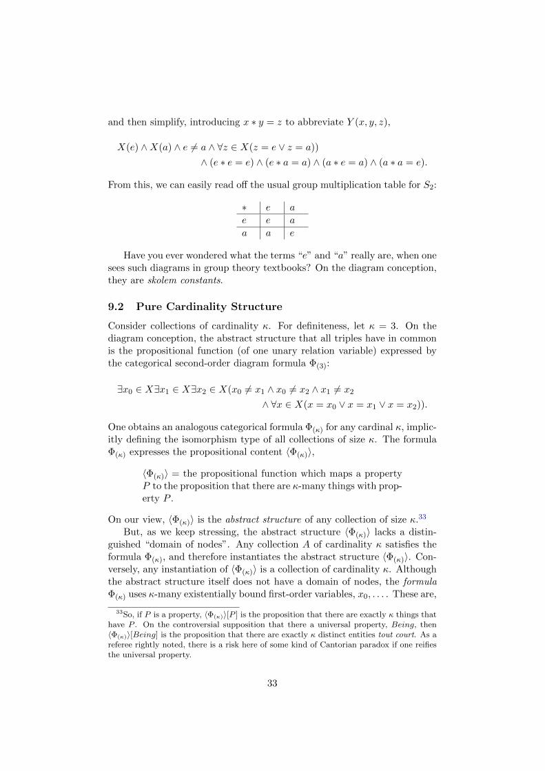
and then simplify, introducing x ∗ y = z to abbreviate Y (x, y, z),

X(e) ∧X(a) ∧ e 6= a ∧ ∀z ∈ X(z = e ∨ z = a))

∧ (e ∗ e = e) ∧ (e ∗ a = a) ∧ (a ∗ e = a) ∧ (a ∗ a = e).

From this, we can easily read off the usual group multiplication table for S2:

∗ e a

e e a

a a e

Have you ever wondered what the terms “e” and “a” really are, when onesees such diagrams in group theory textbooks? On the diagram conception,they are skolem constants.

9.2 Pure Cardinality Structure

Consider collections of cardinality κ. For definiteness, let κ = 3. On thediagram conception, the abstract structure that all triples have in commonis the propositional function (of one unary relation variable) expressed bythe categorical second-order diagram formula Φ(3):

∃x0 ∈ X∃x1 ∈ X∃x2 ∈ X(x0 6= x1 ∧ x0 6= x2 ∧ x1 6= x2

∧ ∀x ∈ X(x = x0 ∨ x = x1 ∨ x = x2)).

One obtains an analogous categorical formula Φ(κ) for any cardinal κ, implic-itly defining the isomorphism type of all collections of size κ. The formulaΦ(κ) expresses the propositional content 〈Φ(κ)〉,

〈Φ(κ)〉 = the propositional function which maps a propertyP to the proposition that there are κ-many things with prop-erty P .

On our view, 〈Φ(κ)〉 is the abstract structure of any collection of size κ.33

But, as we keep stressing, the abstract structure 〈Φ(κ)〉 lacks a distin-guished “domain of nodes”. Any collection A of cardinality κ satisfies theformula Φ(κ), and therefore instantiates the abstract structure 〈Φ(κ)〉. Con-versely, any instantiation of 〈Φ(κ)〉 is a collection of cardinality κ. Althoughthe abstract structure itself does not have a domain of nodes, the formulaΦ(κ) uses κ-many existentially bound first-order variables, x0, . . . . These are,

33So, if P is a property, 〈Φ(κ)〉[P ] is the proposition that there are exactly κ things thathave P . On the controversial supposition that there a universal property, Being, then〈Φ(κ)〉[Being] is the proposition that there are exactly κ distinct entities tout court. As areferee rightly noted, there is a risk here of some kind of Cantorian paradox if one reifiesthe universal property.

33

at best, “ersatz nodes”, for there is no distinguished way of saying whichvariable xi is identified with which entity a ∈ A in any given A. Any suchidentification would amount to a domain labelling v : A→ V, or a skolemiza-tion of Φ(κ). Again, as we know, these are unique only up-to-automorphism(here, such automorphisms are simply permutations of A).

9.3 The Benacerraf Multiple Reduction Problem

We turn next to the problem of multiple reductions raised in Benacerraf(1965). Let V be the cumulative hierarchy of pure well-founded sets. Thenatural numbers, the integers, the rationals, the reals, etc., can all be repre-sented as sets in V , in various different ways. The natural numbers can berepresented as finite von Neumann ordinals or as “Zermelo” numbers. Thereals can be represented as cuts in the rationals or as equivalence classes ofconvergent sequences of rationals. But it doesn’t follow that natural num-bers, reals, etc., must be reduced to sets in V , or that they “are” suchsets. For, as Benacerraf (1965) pointed out, this demand leads to pseudo-problems of the form, “which set is the natural number 2 really?”, “whichset is the real number π, really?”

To this conundrum, there are several responses. For example, the set-theoretic reductionist (e.g., Quine 1969) may claim that mathematical realityis, in fact, V (U): the cumulative hierarchy of well-founded sets built up overa collection U of urelements. Reductions are merely matters of convenience.The structuralist (e.g., Shapiro 1997, Resnik 1997) may respond that math-ematical reality consists in self-contained, “ante rem” structures. And thisresponse is one that Benacerraf hinted at himself. A somewhat unexploredresponse, nonetheless attractive, is sui generisism: certain mathematical en-tities are sui generis, requiring no further reduction to some set or anythingelse, for that matter. One can make this case for ordered pairs, naturalnumbers, integers, rationals, etc.34

Suppose, however, that we wish to pursue the idea of there being anabstract structure that all copies of the von Neumann ordinals, etc., “havein common”. Let the algebraic signature of first-order arithmetic,

σ = {Pred,Func,Const, ar},

be given by Pred = ∅,Func = {succ, plus, times} and Const = {0}, withar(succ) = 1, ar(plus) = 2 and ar(times) = 2. Axioms of Peano arithmetic

34For example, the ordered pair (a, b) is usually reduced to some set, such as{{a}, {a, b}}. Instead of reduction, however, ordered pairs may be treated as sui generisobjects, governed by the ordered-pair abstraction axiom,

OP : (a, b) = (c, d) iff a = c and b = d.

The set-theoretic reduction assures us of consistency and indeed ontological economy. Butthe reduction doesn’t have to be assumed.

34

in this signature would then include, for example,

∀x∀y(succ(x) = succ(y)→ x = y)∀x(plus(x, 0) = x)etc.

Consider the σ-structure

M (vN) = (ω, σ, I)

with succI = Sω, plusI = +ω, and timesI = ×ω, where ω is the set of finite

von Neumann ordinals, Sω(x) = x ∪ {x}, and +ω and ×ω are the usualaddition and multiplication operations on the finite von Neumann ordinals.Write this more suggestively as

M (vN) := (ω,∅, Sω,+ω,×ω).

We shall call this structure M (vN) the “von Neumann gauge” for arithmetic.Similarly, consider the structure

M (Zerm) := (Cl{}({∅}),∅, SZerm,+Zerm,×Zerm),

where Cl{}({∅}) is the closure of {∅} under the unit set operation x 7→ {x},and SZerm(x) = {x}, and +Zerm and ×Zerm are the corresponding additionand multiplication operations on Cl{}({∅}). We shall call this structure

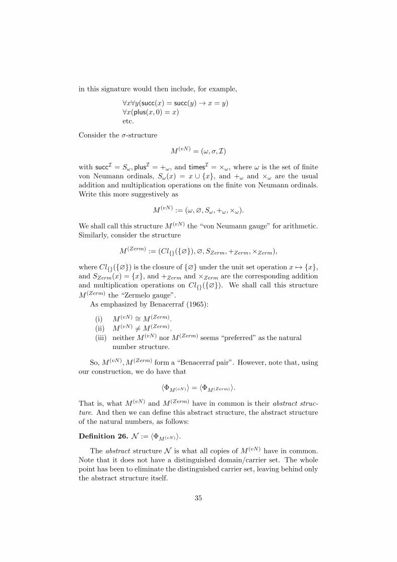
M (Zerm) the “Zermelo gauge”.As emphasized by Benacerraf (1965):

(i) M (vN) ∼= M (Zerm).

(ii) M (vN) 6= M (Zerm).

(iii) neither M (vN) nor M (Zerm) seems “preferred” as the naturalnumber structure.

So, M (vN),M (Zerm) form a “Benacerraf pair”. However, note that, usingour construction, we do have that

〈ΦM(vN)〉 = 〈ΦM(Zerm)〉.

That is, what M (vN) and M (Zerm) have in common is their abstract struc-ture. And then we can define this abstract structure, the abstract structureof the natural numbers, as follows:

Definition 26. N := 〈ΦM(vN)〉.

The abstract structure N is what all copies of M (vN) have in common.Note that it does not have a distinguished domain/carrier set. The wholepoint has been to eliminate the distinguished carrier set, leaving behind onlythe abstract structure itself.

35

But surely—one wishes to respond—in addition to the abstract structureN , there is also the usual set N of natural numbers. How then do we obtaina set of natural numbers? It seems to me that there is a distinguished setN of natural numbers, and the elements of this set should be understood assui generis entities in the manner given by Frege long ago, via:

Hume’s Principle: |X| = |Y | if and only if X ∼= Y .

where |.| is a primitive cardinality operation mapping sets to objects.As is well-known, in the context of second-order logic equippped with |.|,Hume’s Principle allows one to prove the axioms of second-order Peanoarithmetic: what is nowadays called Frege’s Theorem.35 One may thereforedefine N as follows:

Definition 27. x ∈ N iff, for some finite X, x = |X|.

Assembling this, together with 0, S, + and × (restricted to N), yields acanonical natural number structure M (Frege):

Definition 28. M (Frege) := (N, 0, S,+,×).

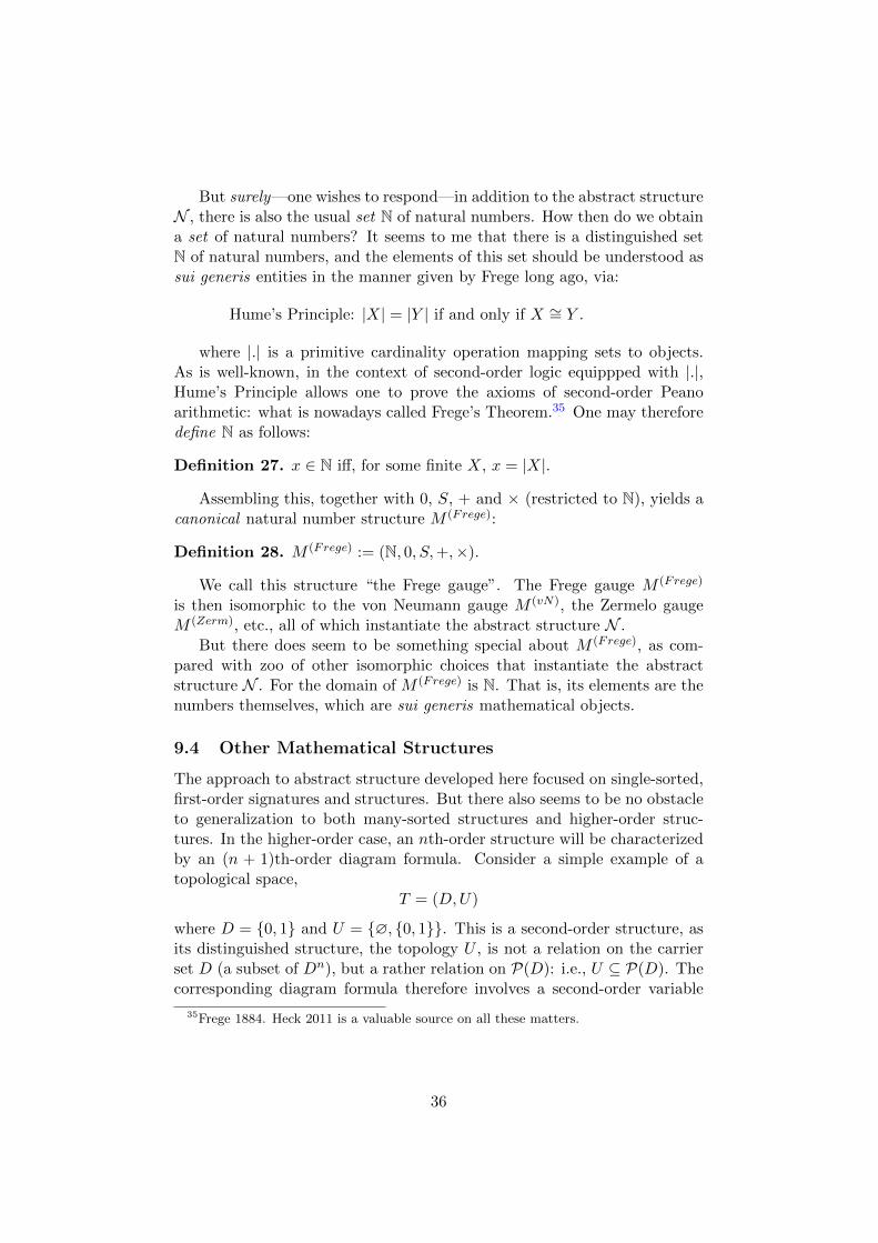
We call this structure “the Frege gauge”. The Frege gauge M (Frege)

is then isomorphic to the von Neumann gauge M (vN), the Zermelo gaugeM (Zerm), etc., all of which instantiate the abstract structure N .

But there does seem to be something special about M (Frege), as com-pared with zoo of other isomorphic choices that instantiate the abstractstructure N . For the domain of M (Frege) is N. That is, its elements are thenumbers themselves, which are sui generis mathematical objects.

9.4 Other Mathematical Structures

The approach to abstract structure developed here focused on single-sorted,first-order signatures and structures. But there also seems to be no obstacleto generalization to both many-sorted structures and higher-order struc-tures. In the higher-order case, an nth-order structure will be characterizedby an (n + 1)th-order diagram formula. Consider a simple example of atopological space,

T = (D,U)

where D = {0, 1} and U = {∅, {0, 1}}. This is a second-order structure, asits distinguished structure, the topology U , is not a relation on the carrierset D (a subset of Dn), but a rather relation on P(D): i.e., U ⊆ P(D). Thecorresponding diagram formula therefore involves a second-order variable

35Frege 1884. Heck 2011 is a valuable source on all these matters.

36

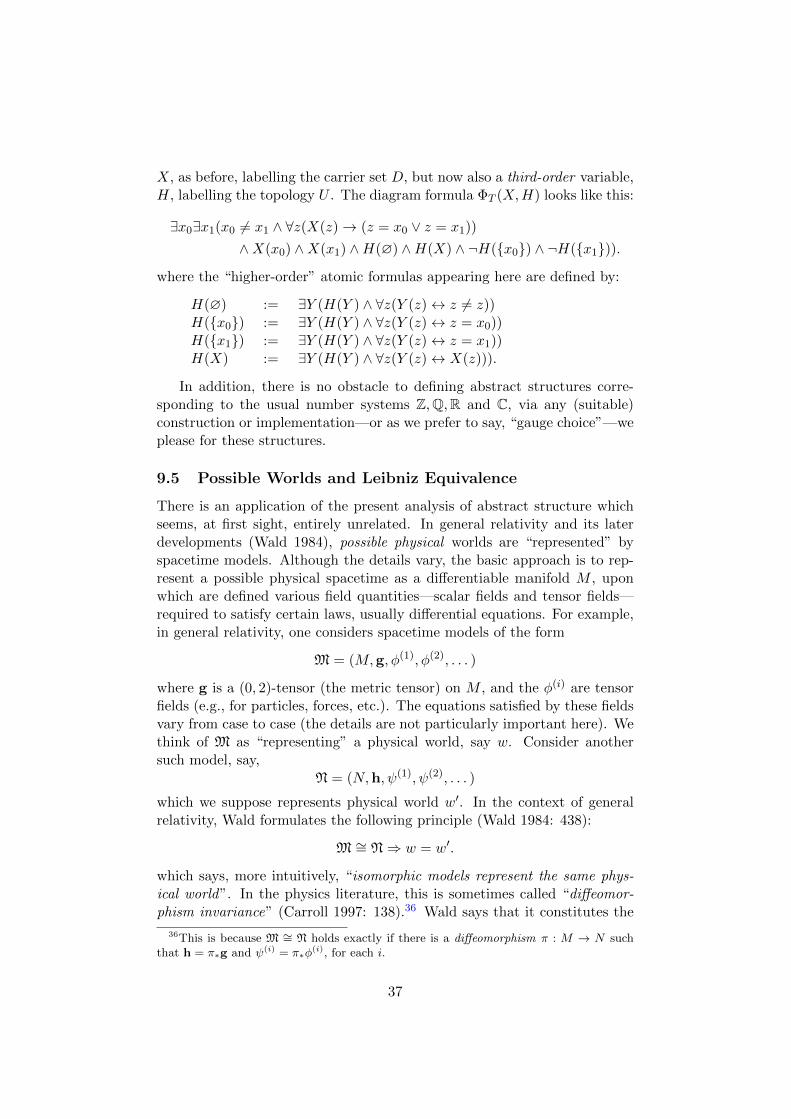
X, as before, labelling the carrier set D, but now also a third-order variable,H, labelling the topology U . The diagram formula ΦT (X,H) looks like this:

∃x0∃x1(x0 6= x1 ∧ ∀z(X(z)→ (z = x0 ∨ z = x1))

∧X(x0) ∧X(x1) ∧H(∅) ∧H(X) ∧ ¬H({x0}) ∧ ¬H({x1})).

where the “higher-order” atomic formulas appearing here are defined by:

H(∅) := ∃Y (H(Y ) ∧ ∀z(Y (z)↔ z 6= z))H({x0}) := ∃Y (H(Y ) ∧ ∀z(Y (z)↔ z = x0))H({x1}) := ∃Y (H(Y ) ∧ ∀z(Y (z)↔ z = x1))H(X) := ∃Y (H(Y ) ∧ ∀z(Y (z)↔ X(z))).

In addition, there is no obstacle to defining abstract structures corre-sponding to the usual number systems Z,Q,R and C, via any (suitable)construction or implementation—or as we prefer to say, “gauge choice”—weplease for these structures.

9.5 Possible Worlds and Leibniz Equivalence

There is an application of the present analysis of abstract structure whichseems, at first sight, entirely unrelated. In general relativity and its laterdevelopments (Wald 1984), possible physical worlds are “represented” byspacetime models. Although the details vary, the basic approach is to rep-resent a possible physical spacetime as a differentiable manifold M , uponwhich are defined various field quantities—scalar fields and tensor fields—required to satisfy certain laws, usually differential equations. For example,in general relativity, one considers spacetime models of the form

M = (M,g, φ(1), φ(2), . . . )

where g is a (0, 2)-tensor (the metric tensor) on M , and the φ(i) are tensorfields (e.g., for particles, forces, etc.). The equations satisfied by these fieldsvary from case to case (the details are not particularly important here). Wethink of M as “representing” a physical world, say w. Consider anothersuch model, say,

N = (N,h, ψ(1), ψ(2), . . . )

which we suppose represents physical world w′. In the context of generalrelativity, Wald formulates the following principle (Wald 1984: 438):

M ∼= N⇒ w = w′.

which says, more intuitively, “isomorphic models represent the same phys-ical world”. In the physics literature, this is sometimes called “diffeomor-phism invariance” (Carroll 1997: 138).36 Wald says that it constitutes the

36This is because M ∼= N holds exactly if there is a diffeomorphism π : M → N suchthat h = π∗g and ψ(i) = π∗φ

(i), for each i.

37

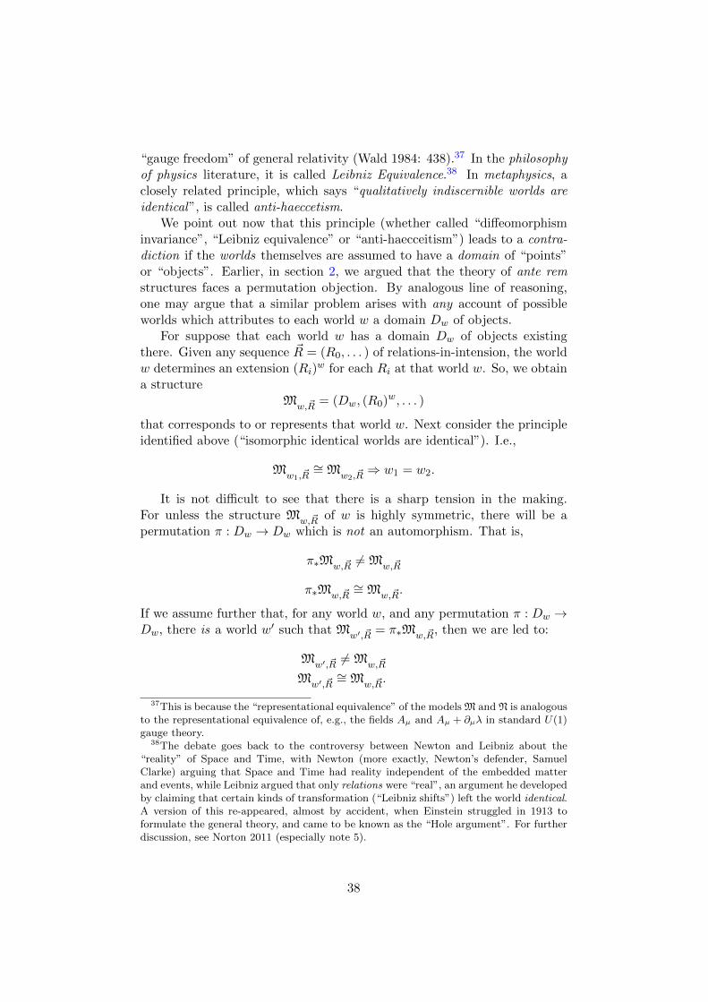
“gauge freedom” of general relativity (Wald 1984: 438).37 In the philosophyof physics literature, it is called Leibniz Equivalence.38 In metaphysics, aclosely related principle, which says “qualitatively indiscernible worlds areidentical”, is called anti-haeccetism.

We point out now that this principle (whether called “diffeomorphisminvariance”, “Leibniz equivalence” or “anti-haecceitism”) leads to a contra-diction if the worlds themselves are assumed to have a domain of “points”or “objects”. Earlier, in section 2, we argued that the theory of ante remstructures faces a permutation objection. By analogous line of reasoning,one may argue that a similar problem arises with any account of possibleworlds which attributes to each world w a domain Dw of objects.

For suppose that each world w has a domain Dw of objects existingthere. Given any sequence ~R = (R0, . . . ) of relations-in-intension, the worldw determines an extension (Ri)

w for each Ri at that world w. So, we obtaina structure

Mw,~R = (Dw, (R0)w, . . . )

that corresponds to or represents that world w. Next consider the principleidentified above (“isomorphic identical worlds are identical”). I.e.,

Mw1, ~R∼= Mw2, ~R

⇒ w1 = w2.

It is not difficult to see that there is a sharp tension in the making.For unless the structure Mw,~R of w is highly symmetric, there will be apermutation π : Dw → Dw which is not an automorphism. That is,

π∗Mw,~R 6= Mw,~R

π∗Mw,~R∼= Mw,~R.

If we assume further that, for any world w, and any permutation π : Dw →Dw, there is a world w′ such that Mw′, ~R = π∗Mw,~R, then we are led to:

Mw′, ~R 6= Mw,~R

Mw′, ~R∼= Mw,~R.

37This is because the “representational equivalence” of the models M and N is analogousto the representational equivalence of, e.g., the fields Aµ and Aµ + ∂µλ in standard U(1)gauge theory.

38The debate goes back to the controversy between Newton and Leibniz about the“reality” of Space and Time, with Newton (more exactly, Newton’s defender, SamuelClarke) arguing that Space and Time had reality independent of the embedded matterand events, while Leibniz argued that only relations were “real”, an argument he developedby claiming that certain kinds of transformation (“Leibniz shifts”) left the world identical.A version of this re-appeared, almost by accident, when Einstein struggled in 1913 toformulate the general theory, and came to be known as the “Hole argument”. For furtherdiscussion, see Norton 2011 (especially note 5).

38

The first of these implies w′ 6= w. But, the second, along with anti-haecceitism (i.e., Leibniz equivalence) implies w′ = w. Contradiction.

A way out of this conundrum is to apply the current theory of abstractstructure to possible worlds as follows: we drop the assumption that eachworld w has a specific domain Dw (or underlying set) of objects. Instead,worlds can be understood as saturated abstract structure. Our accountstates that abstract structures are (categorical) second-order propositionalfunctions. The abstract structure of a given structure A is a certain propo-sitional function 〈ΦA〉. Now, we can “saturate” this propositional contentwith non-mathematical properties and relations. That is, 〈ΦA〉 is a functionwhich when applied to a sequence ~R = (R0, R1, . . . ) of properties and rela-tions yields a single, “saturated”, proposition which says that the relationsare related as the formula ΦA requires them to be.

Roughly, the proposal is that each possible world w has the form

w = 〈ΦA〉[~R],

where ~R is a sequence of relations-in-intension. As well as resolving thecontradiction sketched above, this account of worlds automatically satisfiesLeibniz Equivalence. More exactly,

Theorem 7 (Leibniz equivalence). Suppose we have worlds w1, w2 withw1 = 〈ΦA〉[~R] and w2 = 〈ΦB〉[~R]. Then: A ∼= B ⇒ w1 = w2.

Proof. Suppose A ∼= B. Then, by Leibniz abstraction, 〈ΦA〉 = 〈ΦB〉. So,〈ΦA〉[~R] = 〈ΦB〉[~R]. So, w1 = w2.

10 Summary

We hope to have presented a coherent explication of the notion of abstractstructure A, for any given structure A = (D,σ, I), under the mild constraintthat A be small (set-sized).39 To summarize the approach, given a structureA:

39This constraint can almost certainly be relaxed to permit a treatment of large struc-tures A = (D,σ, I), with D a proper class. Indeed, for the cumulative hierarchy (V,∈) ofpure sets. However, the detailed theory would probably require careful assumptions aboutclass existence—for example, the diagram formula Φ(V,∈) for (V,∈) is itself a proper classsized—which we have tried to sweep under the carpet here.

39

1. Assume that A is relational (if it isnt, apply the procedureto its relationization Arel).

2. Introduce the (possibly infinitary) diagram language LA =Lκ+,κ+(σD).

3. Introduce the diagram formula ΦvA, relative to a domain

labelling v : D → V ⊆ Var(LA).4. Convert Φv

A to a pure second-order diagram formula (ΦvA)◦

under a translation ◦ taking predicates to second-order vari-ables.

5. The abstract structure A of A is then defined to be thepropositional function 〈ΦA〉 expressed by (Φv

A)◦.6. Then, modulo two assumptions concerning the notion “ex-

pressing a propositional function”, this construction imple-ments Leibniz Abstraction: A = B ⇔ A ∼= B.

The aim here has not been to defend any kind of structuralism (the on-tological view that mathematics is “about” structures). Indeed, the permu-tation argument given at section 2 was directed against ante rem structural-ism. The aim here has been to explicate the concept of “abstract structure”on the basis of an anti-reductionist understanding of mathematical objectsas sui generis abstract objects—sets, pairs, relations, numbers, functions,syntactical entities, structures, propositional functions, etc. Within thiszoo of sui generis mathematical objects, there are also abstract structures,satisfying Leibniz Abstraction, which we have identified with the class ofcategorical second-order propositional functions expressed by what we havecalled “diagram formulas”.40

References

[1] Awodey, S. forthcoming: “Structuralism, Invariance and Univalence”.

[2] Bell, J.S. 2012: “Infinitary Logic”. Stanford Encyclopedia of Philosophy(20 July 2014).

[3] Benacerraf, P. 1965: “What Numbers Could Not Be”. PhilosophicalReview 74: 47–73.

[4] Bourbaki, N. 1968: Theory of Sets. Berlin: Springer.

[5] Cameron, P.J. 1999: Permutation Groups. London Mathematical Soci-ety Student Texts 45. Cambridge: CUP.

[6] Carnap, R. 1928: Der logische Aufbau der Welt. References to Englishtranslation, The Logical Structure of the World: Pseudoproblems in

40Acknowledgements: I’m grateful for comments from ...

40

Philosophy, by Rolf. A, George (1967 London: Routledge and KeganPaul).

[7] —. 1947. Meaning and Necessity. Chicago: University of Chicago Press.

[8] —. 1950. Logical Foundations of Probability. Second edition, 1962.Chicago: University of Chicago Press.

[9] Carroll, S. 1997: Lecture Notes on General Relativity.http://arxiv.org/abs/gr-qc/9712019.

[10] Demopoulos, W. & Friedman, M. 1985: “Bertrand Russell’s The Anal-ysis of Matter : Its historical context and contemporary interest”. Phi-losophy of Science 52: 621–639.

[11] Dickmann, M. A. 1975: Large Infinitary Languages: Model Theory.Studies in Logic and the Foundations of Mathematics 83. Amsterdam:North-Holland Pub. Co.

[12] Enderton, H. 1977. Elements of Set Theory. London: Academic Press.

[13] Frege, G. 1884. Die Grundlagen der Arithmetik. Breslau. Translated byJ. L. Austin, The Foundations of Arithmetic, Oxford: Blackwell, secondrevised edition, 1974.

[14] Heck, R. 2011. Frege’s Theorem. Oxford: Oxford University Press.

[15] Hellman, G. 2007: “Structuralism”, in S. Shapiro (ed.) 2007, OxfordHandbook of the Philosophy of Mathematics and Logic. Oxford: OxfordUniversity Press.

[16] Hodes, H. 1984: “Logicism and the ontological commitments of arith-metic”. Journal of Philosophy 81: 123–149.

[17] Hodges, W. 1997: A Shorter Model Theory. Cambridge: CambridgeUniversity Press.

[18] Ketland, J. 2004: “Empirical Adequacy and Ramsification”. BritishJournal for the Philosophy of Science 55: 287300.

[19] —. 2006: “Structuralism and the Identity of Indiscernibles”. Analysis66: 303–315.

[20] —. 2009: “Empirical Adequacy and Ramsification, II”. In A. Hieke &H. Leitgeb (eds), Reduction, abstraction, analysis: Proceedings of the31st International Ludwig Wittgenstein symposium in Kirchberg, 2008.Gazelle books, Lancaster, pp. 29-46.

[21] —. 2011. “Identity and Indiscerniblity”. Review of Symbolic Logic 4:171–185.

41

[22] Leitgeb, H. & Ladyman, J. 2008: “Criteria of Identity and StructuralistOntology”. Philosophia Mathematica 16: 388–396.

[23] Marker. D. 2002. Model Theory: An Introduction. Graduate Texts inMathematics 217. New York: Springer-Verlag.

[24] McLarty, C. 1993: “Numbers Can Be Just What They Have To”. Nous27: 487–498.

[25] Newman, M.H.A. 1928: “Mr. Russell’s ‘Causal Theory of Perception’”. Mind 37: 137–148.

[26] Norton, J. 2011: “The Hole Argument”. Online Stanford Encyclopediaof Philosophy.

[27] Quine, W.V. 1969: Set Theory and its Logic. Cambridge, Ma.: HarvardUniversity Press.

[28] Resnik, M.D. 1997: Mathematics as a Science of Patterns. Oxford:Oxford University Press.

[29] Robbin, J.W. & Salamon, D.A. 2011: Introduction to Differential Ge-ometry. ETH, Lecture Notes.

[30] Russell, B.A.W. 1919: An Introduction to Mathematical Philosophy.London: George Allen and Unwin.

[31] —. 1927: Analysis of Matter. London: Routledge and Kegan Paul.

[32] Shapiro, S. 1997: Philosophy of Mathematics: Structure and Ontology.Oxford: Oxford University Press.

[33] —. 2008: “Identity, indiscernibility, and ante rem structuralism: thetale of i and −i”. Philosophia Mathematica 16: 285–309.

[34] Wald, R.M. 1984: General Relativity. Chicago: University of ChicagoPress.

[35] Wetzel, L. 2011. Types and Tokens. Boston, Ma.: MIT Press.

42