ABSTRACT

ZERO DISTRIBUTION OF BINOMIAL COMBINATIONS OFCHEBYSHEV POLYNOMIALS OF THE SECOND KIND

For α ∈ R such that 0 < α ≤ 1, we can construct a sequence of real

polynomials {Pm(z)}∞m=0 that is generated by

1

(1− t)α(1− 2zt+ t2)=

∞∑m=0

Pm(z)tm.

The sequence {Pm(z)}∞m=0 is a binomial combination of the well-known

Chebyshev polynomials of the second kind, which have all real zeros on the

interval (−1, 1). We prove that there exists a constant C (independent of m)

such that the number of zeros of Pm(z) outside of the interval (−1, 1) is at

most C for all m ∈ N.

Summer Al HamdaniMay 2021

ZERO DISTRIBUTION OF BINOMIAL COMBINATIONS OF

CHEBYSHEV POLYNOMIALS OF THE SECOND KIND

by

Summer F. Al Hamdani

A thesis

submitted in partial

fulfillment of the requirements for the degree of

Master of Science in Mathematics

in the College of Science and Mathematics

California State University, Fresno

May 2021

APPROVED

For the Department of Mathematics:

We, the undersigned, certify that the thesis of the followingstudent meets the required standards of scholarship, format, andstyle of the university and the student’s graduate degree programfor the awarding of the master’s degree.

Summer F. Al Hamdani

Thesis Author

Khang Tran (Chair) Mathematics

Michael Bishop Mathematics

Stefaan Delcroix Mathematics

For the University Graduate Committee:

Dean, Division of Graduate Studies

AUTHORIZATION FOR REPRODUCTION

OF MASTER’S THESIS

I grant permission for the reproduction of this thesis in part orin its entirety without further authorization from me, on thecondition that the person or agency requesting reproductionabsorbs the cost and provides proper acknowledgment ofauthorship.

X Permission to reproduce this thesis in part or in its entiretymust be obtained from me.

Signature of thesis author:

ACKNOWLEDGMENTS

I would like to thank my advisor, Dr. Khang Tran, for his guidance,

knowledge, and immense patience throughout this project as well as in the

undergraduate and graduate courses that I took with him. I would like to also

express my gratitude to Dr. Doreen DeLeon, who first encouraged me to

apply to summer math programs for undergraduates many moons ago; I most

likely would not have seriously considered pursuing graduate school in the

first place had I not participated in the PUMP program all those years ago. I

am also grateful to Dr. Tamas Forgacs, who supervised my undergraduate

research project and helped me learn what research in mathematics was about

despite my optimistic pessimism throughout most of the process; had I not

known about all of the cool math I could be doing in graduate school, I

definitely would not have gotten this far. Lastly, I would like to thank Drs.

Stefaan Delcroix and Michael Bishop for not only agreeing to be on my thesis

committee, but also for teaching me how to approach my mathematics

education.

I finally would like to thank my partner, Adam, for his unwavering

support and words of encouragement throughout the process, as well as my

parents for their uncountably infinite sacrifices made in order for me to obtain

a college education.

TABLE OF CONTENTS

Page

LIST OF FIGURES . . . . . . . . . . . . . . . . . . . . . . . . . . . . . vi

INTRODUCTION . . . . . . . . . . . . . . . . . . . . . . . . . . . . . . 1

Necessary Results from Real and Complex Analysis . . . . . . . . . . 5

Asymptotic Analysis and Special Functions . . . . . . . . . . . . . . 17

CHEBYSHEV POLYNOMIALS OF THE SECOND KIND . . . . . . . . 24

Chebyshev Polynomials’ Zero Distribution . . . . . . . . . . . . . . . 25

Finite Summation of Chebyshev Polynomials’ Zero Distribution . . . 34

BINOMIAL COMBINATION OF CHEBYSHEV POLYNOMIALS . . . 48

An ‘Explicit’ Formula . . . . . . . . . . . . . . . . . . . . . . . . . . 51

Inequality Involving Trigonometric Integrals . . . . . . . . . . . . . . 59

Zero Distribution . . . . . . . . . . . . . . . . . . . . . . . . . . . . . 65

CONCLUSIONS . . . . . . . . . . . . . . . . . . . . . . . . . . . . . . . 70

REFERENCES . . . . . . . . . . . . . . . . . . . . . . . . . . . . . . . . 74

LIST OF FIGURES

Page

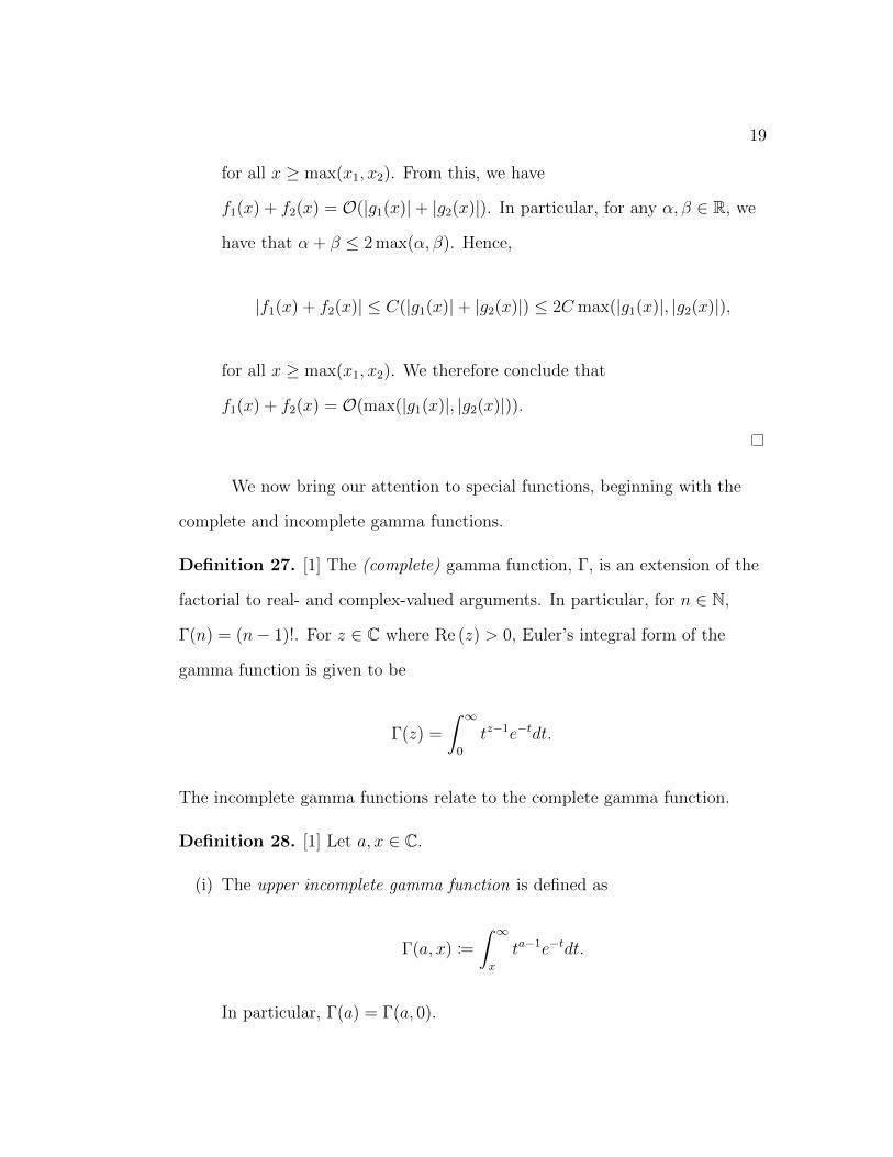
Figure 1. The zeros of U6(z) and U7(z) plotted. Notice that betweenevery two consecutive zeros of U7(z), there is a zero of U6(z). . . . 31

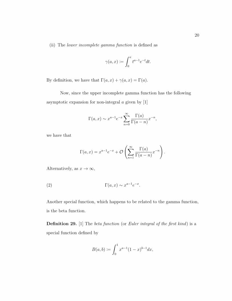
Figure 2. The zeros of U15(z) and U16(z) plotted. We observe thatthere will be a zero of U15(z) between every two consecutive zerosof U16(z). . . . . . . . . . . . . . . . . . . . . . . . . . . . . . . . 31

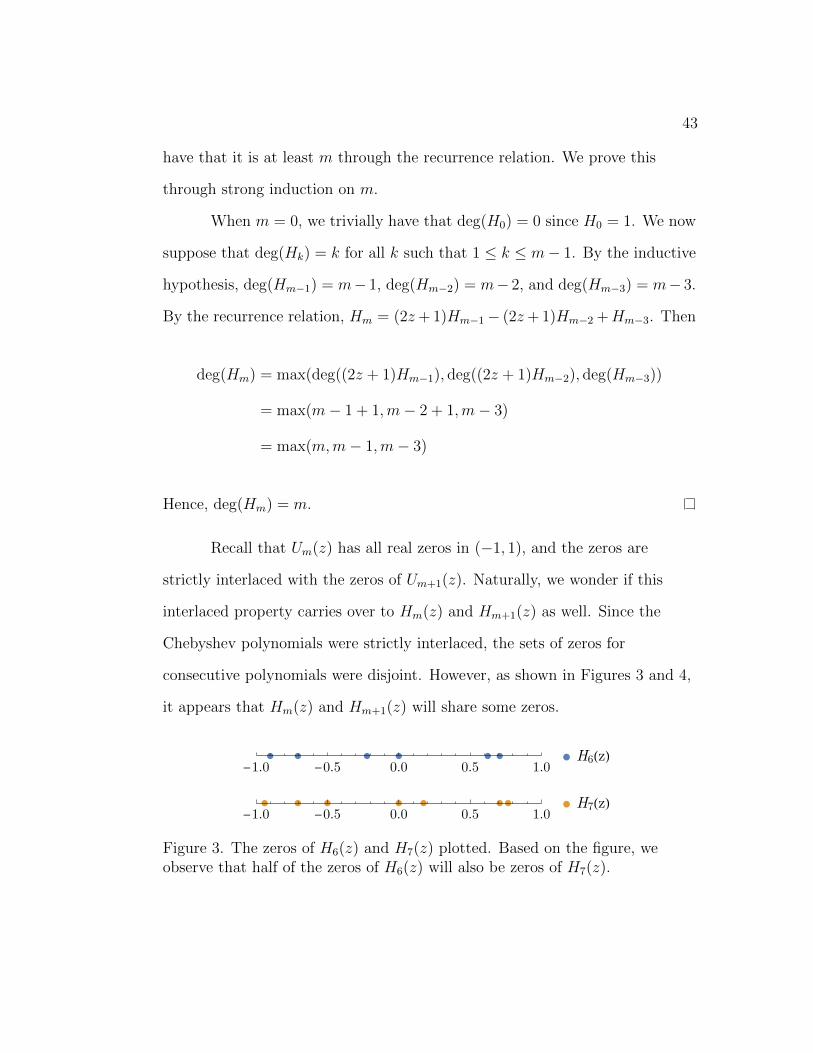
Figure 3. The zeros of H6(z) and H7(z) plotted. Based on the figure,we observe that half of the zeros of H6(z) will also be zeros of H7(z). 43

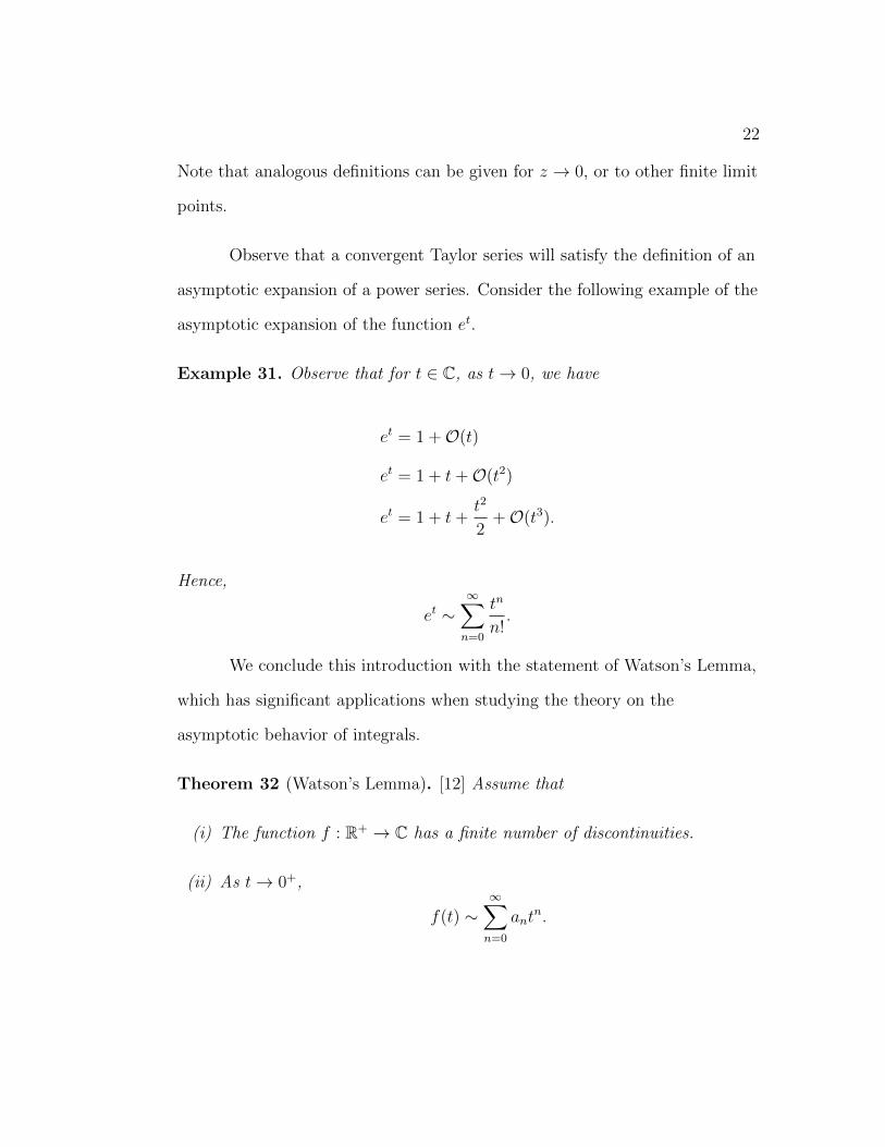
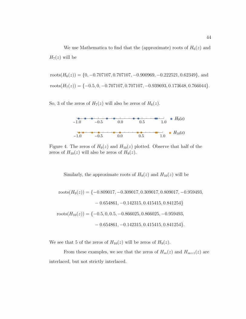
Figure 4. The zeros of H9(z) and H10(z) plotted. Observe that halfof the zeros of H10(z) will also be zeros of H9(z). . . . . . . . . . . 44

Figure 5. The zero distribution of P20(z) with α = 0.5. . . . . . . . . 50

Figure 6. The zero distribution of P20(z) with α = 2. . . . . . . . . . 50

Figure 7. The contour region γ = CR ∪ Cε ∪ `1 ∪ `2. . . . . . . . . . 53

Figure 8. The region of the singularities from the function generatedby {Pm(z)}∞m=0. . . . . . . . . . . . . . . . . . . . . . . . . . . . . 59

Figure 9. The zeros of P6(z) and P7(z) plotted for α = 3/8. Noticethat between every two consecutive zeros of P7(z), there is a zeroof P6(z). . . . . . . . . . . . . . . . . . . . . . . . . . . . . . . . . 68

Figure 10. The zeros of P8(z) and P9(z) plotted for α = 4/11. Ob-serve that the interval between two consecutive zeros of P9(z) willcontain a zero of P8(z). . . . . . . . . . . . . . . . . . . . . . . . . 69

Figure 11. The zero distributions of Cm(α, z) for some given m andα ∈ C such that |α| ≤ 1. . . . . . . . . . . . . . . . . . . . . . . . 72

Figure 12. The zero distributions of Pm(z) for some given m withα = 73/10. . . . . . . . . . . . . . . . . . . . . . . . . . . . . . . . 73

Figure 13. The zero distributions of Pm(z) for some given m withα = 13/9. . . . . . . . . . . . . . . . . . . . . . . . . . . . . . . . 73

INTRODUCTION

Studying the distribution of zeros of polynomials has proven to be a

long-term endeavor for mathematicians. Despite being introduced early on in

the American mathematics curriculum for low degree polynomials,

determining the explicit location of zeros for a given polynomial is often not

trivial. Although the Fundamental Theorem of Algebra states a polynomial of

degree m will have exactly m zeros over the field of the complex numbers,

including multiplicity [4], determining what exactly those zeros are is quite

difficult and can often be impossible to do using algebraic operations. Indeed,

just finding the subset of C that the zeros reside in can be daunting.

One can define sequences of polynomials through either a recursion or

generating function. Furthermore, the latter can be determined if the

recursion formula is known. In particular, we work with the Chebyshev

polynomials of the second kind, which are generated by [1]

∞∑m=0

Um(z)tm =1

1− 2zt+ t2.

The sequence {Um(z)}∞m=0 is a well-known sequence of orthogonal polynomials

in mathematics. Orthogonality of these polynomials implies that the zeros of

all polynomials in this sequence lie on the support of the weight function,

which is the real interval (−1, 1) [9]. Another approach for proving that these

zeros are real, as presented in this thesis, is to apply Cauchy’s Differentiation

Formula to the formal power series associated with the generating function of

these polynomials. With this technique, we can explicitly determine what the

zeros of each polynomial will be and prove that the zeros are interlaced. If we

2

make the substitution z = cos θ for θ ∈ (0, π), we show that the polynomials

satisfy

Um(z) =sin((m+ 1)θ)

sin θ,

which relates to the famous Dirichlet kernel, Dm(θ), since one can show

Dm(θ) =sin((2m+ 1) θ

2)

sin θ2

= U2m

(cos

θ

2

).

The result above can be obtained by looking at the summation of the first m

Chebyshev polynomials Hm(z) =∑m

k=0 Uk(z), which is also known to have all

real zeros in (−1, 1) and the sequence is generated by

∞∑m=0

Hm(z)tm =1

(1− t)(1− 2zt+ t2).

For this thesis, we look at the zero distribution of a linear combination

of these polynomials, which is generated by

∞∑m=0

Pm(z)tm =1

(1− t)α(1− 2zt+ t2),

where 0 < α < 1. The polynomials by this sequence Pm(z) are a linear

combination of the first m Chebyshev polynomials, with binomial-type

coefficients that are dependent on α.

Several studies of the zero distribution of linear combinations of

Chebyshev polynomials have been published and connected to various areas of

mathematics. In [11], the zero distribution of linear combinations Chebyshev

polynomials with a fixed real coefficients is discussed and applied to the

3

theory of Pisot and Salem numbers. In a spring-mass system where all springs

have equal stiffness and all masses are equal (except the first and last), the

natural frequencies of this four-parameter system can be expressed as the

zeros of certain linear combinations of Chebyshev polynomials whose

coefficients are obtained from these parameters; furthermore, imposing extra

conditions on the parameters show that the zeros will all be in the interval

(−1, 1) (see [2]). In [7], the zeros of linear combinations of the Chebyshev

polynomials with absolutely constant coefficients are discussed and connected

with other known orthogonal sequences of polynomials.

We consider the open upper-half of the complex plane, which is given

by H = {z ∈ C : Im (z) > 0}. A polynomial f ∈ C[z] is called stable if either

f ≡ 0 identically or for any z ∈ H, f(z) 6= 0. If we let G[z] be the set of all

stable polynomials in C[z], then the set of all real stable polynomials is given

by GR[z] = G[z] ∩ R[z] [13]. Since a complex number is a zero of a real

polynomial if and only if its complex conjugate is a zero of the polynomial, we

conclude that a real polynomial is real stable is the same as the polynomial

having all real zeros. We prove that for any m, Um(z), Hm(z) ∈ GR[z].

Furthermore, we show that at most a constant number of zeros of Pm(z) are

non-real for large values of m and provide suggestions on possible ways to

show that Pm(z) ∈ GR[z] for all m.

Another important property of the Chebyshev polynomials is that for

each polynomial, the zeros will interlace with the zeros of the next polynomial

in the sequence. This property is often explored for various sequences of

polynomials and is associated with the sequence being orthogonal. The

Hermite-Kakeya-Obreschkoff Theorem states that for real polynomials f and

4

g, their zeros interlace and f, g ∈ GR[z] if and only if any af + bg ∈ GR[z] for

all a, b ∈ R [13]. A similar result is the Hermite-Biehler Theorem, which states

that real polynomials f and g have all real zeros that interlace if and only if

g + if ∈ G[z] [13].

Lastly, a significant property of the Chebyshev polynomials Um(z) is

that the zeros are dense in (−1, 1) as m→∞. By dense, we mean that for

every open subset of (−1, 1), there will be a zero of Um(z) for all large m. A

similar result can be shown for Hm(z) and Pm(z) in (−1, 1). The significance

of this property is that the interval (−1, 1) is optimal in the sense that for any

ε > 0, the interval (−1 + ε, 1− ε) will not contain all the zeros of Um(z) for all

large m.

We now consider a sequence λ : N→ R and let Tλ : R[x]→ R[x] be the

linear transformation given by Tλ(xn) = λ(n)xn and linear extension. We call

λ a multiplier sequence (of the first kind) if Tλ(f) ∈ GR[x] whenever

f ∈ GR[x] [13]. A famous result known as the Polya-Schur Theorem

characterized multiplier sequences in several ways: in particular, one of these

characterizations is that a binomial transformation of λ given by Tλ((1 + x)n)

for all n ∈ N is real stable (with all zeros having the same sign) if and only if

λ is a multiplier sequence [13]. Intuitively, these multiplier sequences generate

linear operators that preserve the reality of zeros for a given real stable

polynomial. Stability-preserving linear operators were characterized further

for arbitrary circular domains by Borcea and Branden in [3]. The significance

of this in relation to the work presented in this thesis is due to the fact that

we study the transformation of Chebyshev polynomials by a binomial factor;

5

the connection between this and the result by Polya-Schur has yet to be

investigated, but seems promising.

Necessary Results from Real and Complex Analysis

We commence by presenting well-known definitions and results of

significance from analysis that are used throughout this thesis. For further

details, we refer the reader to [4], [6], and [10]. First, we illuminate a variation

of what many math enthusiasts deem as the ‘most beautiful’ equation in

mathematics.

Theorem 1 (Euler’s and de Moivre’s Formulas). For α ∈ C,

eiαx = cos(αx) + i sin(αx).

We next list definitions relating to the topology of C.

Definition 2. [4], [6] Let D ⊆ C. Then

1. D is open if it has an empty intersection with its boundary, ∂D;

2. D is connected if any two points of D can be joined by a polygonal

curve contained within D; and

3. D is a domain (or region) if D is open and connected.

Many properties of analysis over R do not change when studying such

properties over the larger field C. However, we do make the crucial note that

a function being analytic over C differs from being analytic over R.

6

Definition 3. [4] A function f defined for t in a domain D ⊆ C is

differentiable at a point t0 ∈ D if

limt→t0

f(t)− f(t0)

t− t0= lim

h→0

f(t0 + h)− f(t0)

h

exists. If this limit exists, then it is denoted by f ′(t0). Furthermore, if f is

differentiable at every point in D, then f is (complex) analytic in D.

Recall that over R, a function f is (real) analytic in E ⊆ R when it is

not only infinitely differentiable at every point in E, but if for any x0 ∈ E, the

Taylor series of f centered at x0 converges to f(x) for some x within a

neighborhood of x0.

Definition 4. [4, p. 135] An analytic function f has an isolated singularity at

a point t0 if f is analytic in the punctured disc 0 < |t− t0| < r, for some r > 0.

In general, for R > 0, a function analytic in the disc |t− t0| < R can be

expanded on the disc in a power series. Similarly, if a function has a power

series valid on the disc |t− t0| < R, then it is analytic in this disc. However,

what about functions that are analytic in the punctured disc 0 < |t− t0| < R

or in the annulus 0 ≤ r < |t− t0| < R? For this reason, we now define the

Laurent series.

Definition 5. [4, p. 142] Let R > r ≥ 0. For a function f analytic on

r < |t− t0| < R, we can decompose f as

f(t) = f1(t) + f2(t), r < |t− t0| < R,

7

where f1 is analytic on |t− t0| < R and f2 is analytic on r < |t− t0|, including

at infinity. Thus, f1 has a power series in t− t0 which is valid for |t− t0| < R,

and f2 has a power series in (t− t0)−1 which is valid for r < |t− t0|. Thus,

f(t) =∞∑k=0

ak(t− t0)k +∞∑k=1

bk(t− t0)−k,

or, equivalently,

f(t) =∞∑

k=−∞

ak(t− t0)k, a−k = bk, k ∈ N, r < |t− t0| < R.

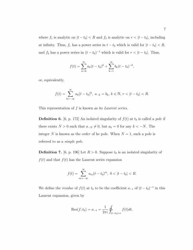
This representation of f is known as its Laurent series.

Definition 6. [6, p. 172] An isolated singularity of f(t) at t0 is called a pole if

there exists N > 0 such that a−N 6= 0, but ak = 0 for any k < −N . The

integer N is known as the order of he pole. When N = 1, such a pole is

referred to as a simple pole.

Definition 7. [6, p. 196] Let R > 0. Suppose t0 is an isolated singularity of

f(t) and that f(t) has the Laurent series expansion

f(t) =∞∑

m=−∞

am(t− t0)m, 0 < |t− t0| < R.

We define the residue of f(t) at t0 to be the coefficient a−1 of (t− t0)−1 in this

Laurent expansion, given by

Res(f ; t0) = a−1 =1

2πi

‰|t−t0|=r

f(t)dt,

8

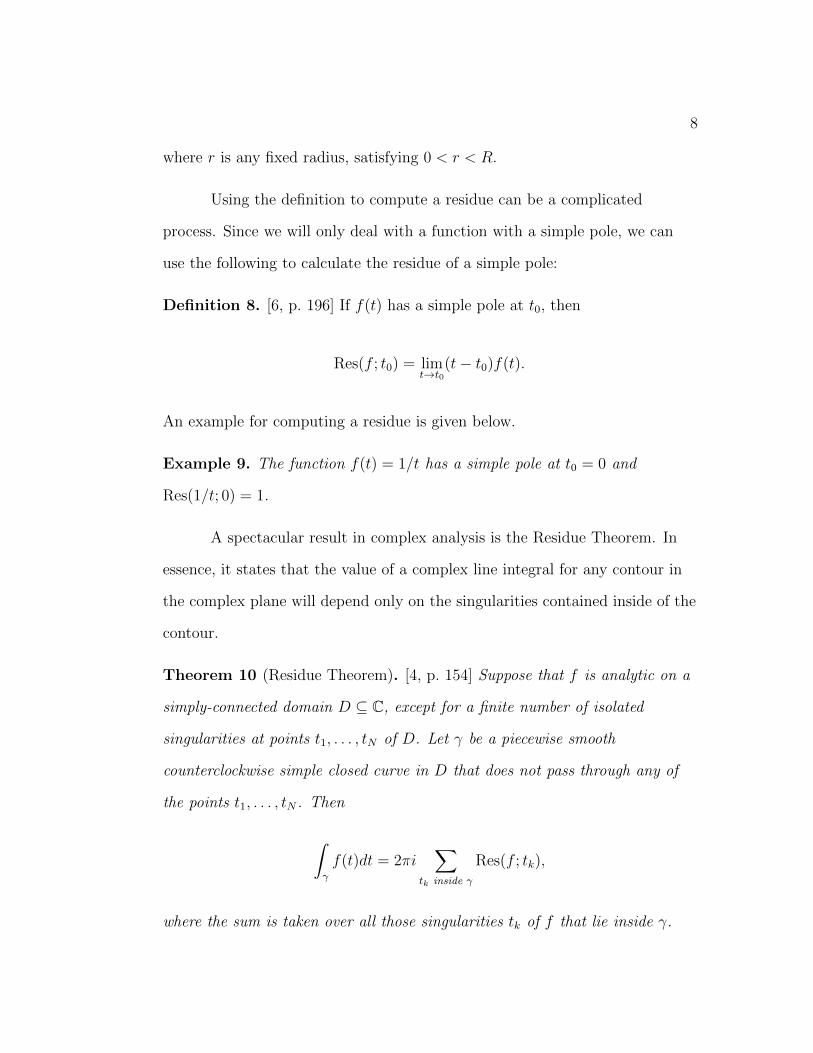
where r is any fixed radius, satisfying 0 < r < R.

Using the definition to compute a residue can be a complicated

process. Since we will only deal with a function with a simple pole, we can

use the following to calculate the residue of a simple pole:

Definition 8. [6, p. 196] If f(t) has a simple pole at t0, then

Res(f ; t0) = limt→t0

(t− t0)f(t).

An example for computing a residue is given below.

Example 9. The function f(t) = 1/t has a simple pole at t0 = 0 and

Res(1/t; 0) = 1.

A spectacular result in complex analysis is the Residue Theorem. In

essence, it states that the value of a complex line integral for any contour in

the complex plane will depend only on the singularities contained inside of the

contour.

Theorem 10 (Residue Theorem). [4, p. 154] Suppose that f is analytic on a

simply-connected domain D ⊆ C, except for a finite number of isolated

singularities at points t1, . . . , tN of D. Let γ be a piecewise smooth

counterclockwise simple closed curve in D that does not pass through any of

the points t1, . . . , tN . Then

ˆγ

f(t)dt = 2πi∑

tk inside γ

Res(f ; tk),

where the sum is taken over all those singularities tk of f that lie inside γ.

9

One may recall the definition of a power series in R or C and its radius

of convergence from real and complex analysis, respectively. We present a

generalization of polynomials over any field F where we permit an infinite

number of terms through an infinite series and we do not concern ourselves

with convergence of this series.

Definition 11. [8] A formal power series over a field F is an infinite sequence

{am}∞m=0 of elements of F. An equivalent interpretation is that it is a function

mapping from the set of non-negative integers to F, i.e., {0, 1, 2, . . .} → F.

For practicality, the formal power series is written in the form

a0 + a1t+ a2t2 + · · ·+ amt

m + · · ·

or, equivalently,∞∑m=0

amtm,

where we do not assign any value to the symbol t and, instead, allow it to

serve as a placeholder.

This placeholder role in conjunction with the + are introduced because

they correspond with algebraic operations that we omit from this thesis, but

refer the reader to [8] for further information. Regarding the symbol t, we

note that since there is no norm defined on our field F, we cannot discuss

convergence of the formal power series even if t were replaced with an element

of F. Moreover, even if a norm was defined, this does not guarantee

convergence of the formal power series. Consequentially, we do not consider

10

convergence when discussing formal power series as we ordinarily would for

power series.

Note that for our purposes, the field F will be C. We next define the

product of two formal power series over the field C.

Definition 12. [8] Consider the formal power series given by

A(t) =∞∑m=0

amtm and B(t) =

∞∑m=0

bmtm,

where {am}∞m=0 and {bm}∞m=0 are infinite complex sequences. Then the

product of these formal power series, known as the Cauchy product, is given by

A(t)B(t) =

(∞∑m=0

amtm

)(∞∑m=0

bmtm

)=

∞∑m=0

cmtm,

with

cm =m∑k=0

akbm−k.

This definition for cm follows naturally from expanding the product

A(t)B(t), applying the distributive laws, and collecting coefficients of equal

powers (in this case, the mth power) of t. Next, we discuss generating

functions.

Definition 13. [8] Given a sequence of numbers {am}∞m=0, where am ∈ C for

all m ∈ N ∪ {0}, the ordinary generating function, f(t), associated with this

sequence encodes the sequence as the coefficients of a formal power series in t:

f(t) =∞∑m=0

amtm.

11

Since we disregard convergence for formal power series and thus assign

no value to t, we instead use each tm to serve as a placeholder for the

coefficients of interest [8, p. 9]. Other types of generating functions exist, such

as exponential, Dirichlet, etc. However, for the purposes of this thesis, we are

not concerned with these. Henceforth, “generating function” will refer to the

ordinary generating function. Presented below are two examples of generating

functions.

Example 14. The function generating the sequence {1}∞m=0 is

1

1− t=

∞∑m=0

tm.

This series, known as the geometric series, converges only when |t| < 1.

Example 15. For a function generating {am}∞m=0 given by

A(t) =∑∞

m=0 amtm, then the sequence {(m+ 1)am+1}∞m=0 is generated by

A′(t) =∞∑m=0

(m+ 1)am+1tm.

We now present a theorem that relates a generating function to a

corresponding recurrence relation.

Theorem 16. Let A(z), B(z), C(z) ∈ C[z]. Suppose for small t that the

following holds:

1

1 + A(z)t+B(z)t2 + C(z)t3=

∞∑m=0

Sm(z)tm.

12

Then for all m ≥ 3,

Sm(z) + A(z)Sm−1(z) +B(z)Sm−2(z) + C(z)Sm−3(z) = 0,

with S0(z) = 1, S1(z) = −A(z), and S2(z) = A2(z)−B(z).

Proof. We expand the right side of the identity

1 = (1 + A(z)t+B(z)t2 + C(z)t3)(S0(z) + S1(z)t+ S2t2 + . . .) and put

Sm := Sm(z) to obtain

(1 + A(z)t+B(z)t2 + C(z)t3)

(∞∑m=0

Smtm

)

=∞∑m=0

Smtm +

∞∑m=0

A(z)Smtm+1 +

∞∑m=0

B(z)Smtm+2 +

∞∑m=0

C(z)Smtm+3

=∞∑m=0

Smtm +

∞∑m=1

A(z)Sm−1tm +

∞∑m=2

B(z)Sm−2tm +

∞∑m=3

C(z)Sm−3tm

= S0 + (S1 + A(z)S0)t+ (S2(z) + A(z)S1 +B(z)S0)t2

+∞∑m=3

(Sm + A(z)Sm−1 +B(z)Sm−2 + C(z)Sm−3)tm.

Equating coefficients and simplifying yields the following system of equations:

S0 = 1,

S1 = −A(z),

S2 = A2(z)−B(z),

Sm = −A(z)Sm−1 −B(z)Sm−2 − C(z)Sm−3, m ≥ 3.

Thus, we obtain the desired result.

13

We now provide some definitions regarding the roots/zeros of

polynomials.

Definition 17. [5] If f is a polynomial of degree m with all real roots, then

we define

roots(f) = {a1, . . . , an},

where ai ≤ ai+1 and f(ai) = 0 for each 1 ≤ i ≤ n. This notation assumes that

f has all real roots.

Definition 18. [5], [13] Given two real polynomials f, g with

roots(f) = {a1, . . . , an} and roots(g) = {b1, . . . , bm} with m ≥ n, then f and g

are said to interlace if these roots alternate, i.e., either

a1 ≤ b1 ≤ a2 ≤ b2 ≤ · · · ≤ an ≤ bn

or

b1 ≤ a1 ≤ b2 ≤ a2 ≤ · · · ≤ bn

If all of the inequalities are strict (so we replace ≤ with <), then we say that

f and g strictly interlace.

Next, we discuss a crucial result from complex analysis: Cauchy’s

Differentiation Formula. However, before that, we first briefly recall partial

fraction decomposition, where, for real polynomials p(x), q(x) such that

q(x) 6= 0 and deg((p(x)) < deg(q(x)), then

p(x)

q(x)=∑i

pi(x)

qi(x),

14

where each qi(x) is a power of an irreducible polynomial dividing q(x) and

pi(x) is a polynomial such that deg(pi(x)) < deg(qi(x)). We present an

example of partial fraction decomposition below.

Example 19. Consider the rational functionx+ 4

x2 + x− 2. The denominator

can be written as the product of its irreducible factors in the following way:

x2 + x− 2 = (x+ 2)(x− 1). By partial fraction decomposition, there exists

A,B ∈ R such that

x+ 4

x2 + x− 2=

A

x+ 2+

B

x− 1.

We multiply both sides of the equality by x2 + x− 2, which yields

x+ 4 = A(x− 1) +B(x+ 2) = (A+B)x+ (2B − A). Then, we equate

coefficients to obtain the following system of equations:

A+B = 1

2B − A = 4.

Thus, A = −2/3 and B = 5/3. Therefore, the partial fraction decomposition

becomes

x+ 4

x2 + x− 2=−2/3

x+ 2+

5/3

x− 1.

The method of partial fraction decomposition is convenient for

separating rational functions. However, for functions that have several

‘factors’ in their denominator or functions that are not rational, the method

becomes either cumbersome or ineffective. A more general (and oftentimes

less complicated) approach known as Cauchy’s Differentiation Formula can,

instead, be used for analytic functions in a neighborhood around the origin.

15

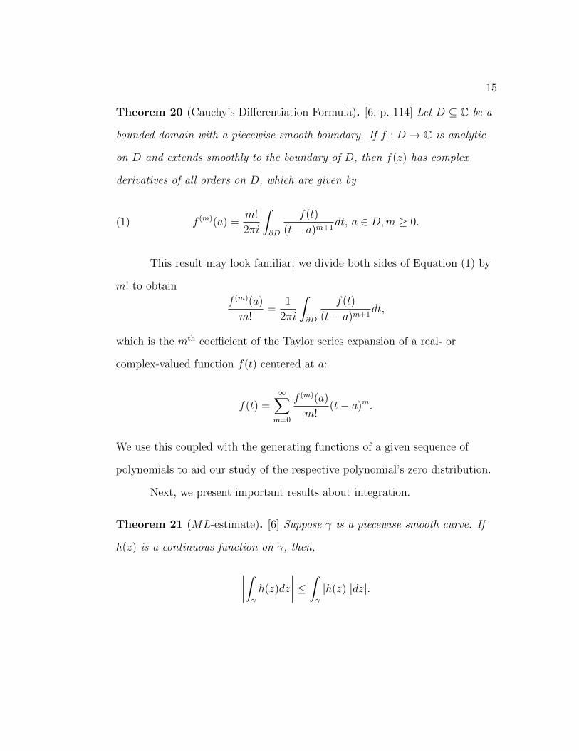
Theorem 20 (Cauchy’s Differentiation Formula). [6, p. 114] Let D ⊆ C be a

bounded domain with a piecewise smooth boundary. If f : D → C is analytic

on D and extends smoothly to the boundary of D, then f(z) has complex

derivatives of all orders on D, which are given by

(1) f (m)(a) =m!

2πi

ˆ∂D

f(t)

(t− a)m+1dt, a ∈ D,m ≥ 0.

This result may look familiar; we divide both sides of Equation (1) by

m! to obtain

f (m)(a)

m!=

1

2πi

ˆ∂D

f(t)

(t− a)m+1dt,

which is the mth coefficient of the Taylor series expansion of a real- or

complex-valued function f(t) centered at a:

f(t) =∞∑m=0

f (m)(a)

m!(t− a)m.

We use this coupled with the generating functions of a given sequence of

polynomials to aid our study of the respective polynomial’s zero distribution.

Next, we present important results about integration.

Theorem 21 (ML-estimate). [6] Suppose γ is a piecewise smooth curve. If

h(z) is a continuous function on γ, then,

∣∣∣∣ˆγ

h(z)dz

∣∣∣∣ ≤ ˆγ

|h(z)||dz|.

16

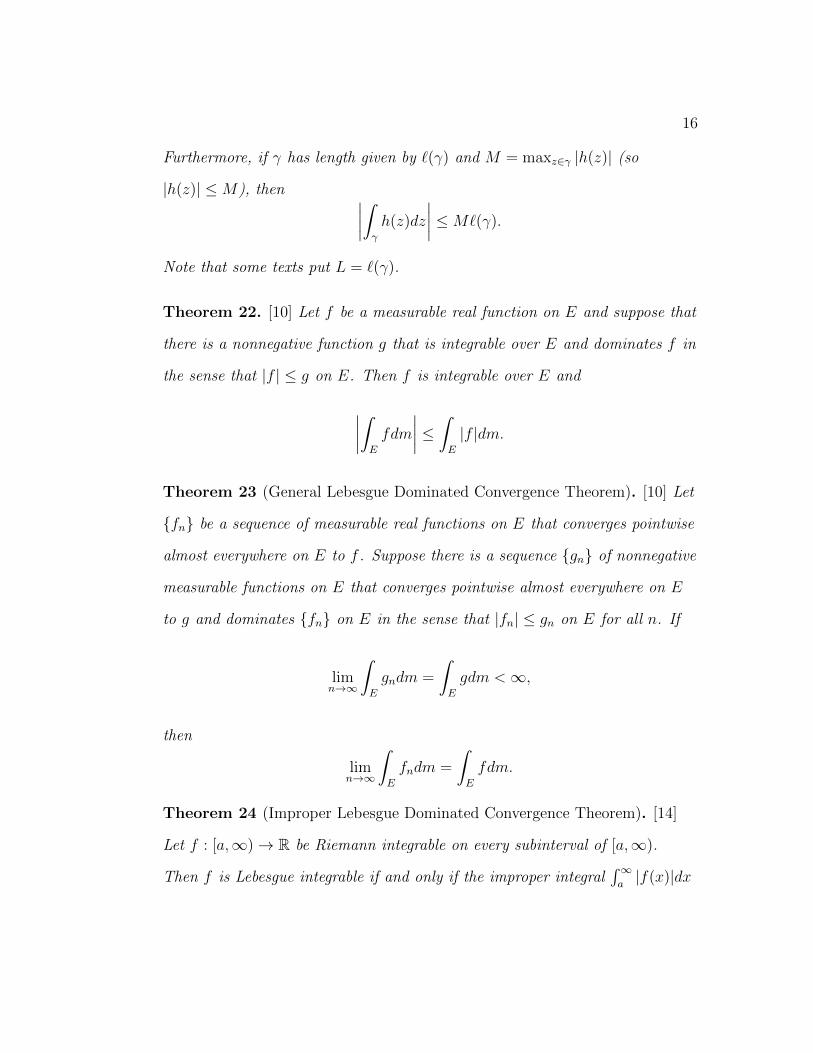
Furthermore, if γ has length given by `(γ) and M = maxz∈γ |h(z)| (so

|h(z)| ≤M), then ∣∣∣∣ˆγ

h(z)dz

∣∣∣∣ ≤M`(γ).

Note that some texts put L = `(γ).

Theorem 22. [10] Let f be a measurable real function on E and suppose that

there is a nonnegative function g that is integrable over E and dominates f in

the sense that |f | ≤ g on E. Then f is integrable over E and

∣∣∣∣ˆE

fdm

∣∣∣∣ ≤ ˆE

|f |dm.

Theorem 23 (General Lebesgue Dominated Convergence Theorem). [10] Let

{fn} be a sequence of measurable real functions on E that converges pointwise

almost everywhere on E to f . Suppose there is a sequence {gn} of nonnegative

measurable functions on E that converges pointwise almost everywhere on E

to g and dominates {fn} on E in the sense that |fn| ≤ gn on E for all n. If

limn→∞

ˆE

gndm =

ˆE

gdm <∞,

then

limn→∞

ˆE

fndm =

ˆE

fdm.

Theorem 24 (Improper Lebesgue Dominated Convergence Theorem). [14]

Let f : [a,∞)→ R be Riemann integrable on every subinterval of [a,∞).

Then f is Lebesgue integrable if and only if the improper integral´∞a|f(x)|dx

17

exists. Moreover, in this case,

ˆ[a,∞)

fdm =

ˆ ∞a

f(x)dx.

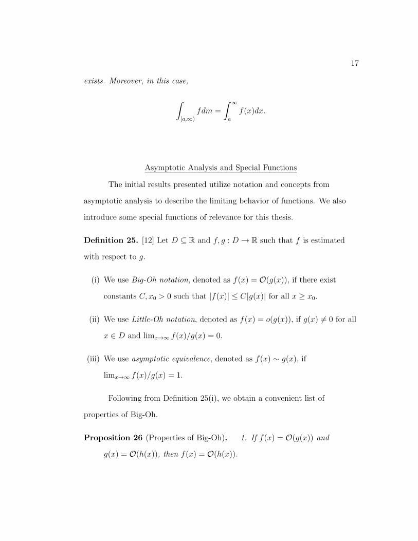
Asymptotic Analysis and Special Functions

The initial results presented utilize notation and concepts from

asymptotic analysis to describe the limiting behavior of functions. We also

introduce some special functions of relevance for this thesis.

Definition 25. [12] Let D ⊆ R and f, g : D → R such that f is estimated

with respect to g.

(i) We use Big-Oh notation, denoted as f(x) = O(g(x)), if there exist

constants C, x0 > 0 such that |f(x)| ≤ C|g(x)| for all x ≥ x0.

(ii) We use Little-Oh notation, denoted as f(x) = o(g(x)), if g(x) 6= 0 for all

x ∈ D and limx→∞ f(x)/g(x) = 0.

(iii) We use asymptotic equivalence, denoted as f(x) ∼ g(x), if

limx→∞ f(x)/g(x) = 1.

Following from Definition 25(i), we obtain a convenient list of

properties of Big-Oh.

Proposition 26 (Properties of Big-Oh). 1. If f(x) = O(g(x)) and

g(x) = O(h(x)), then f(x) = O(h(x)).

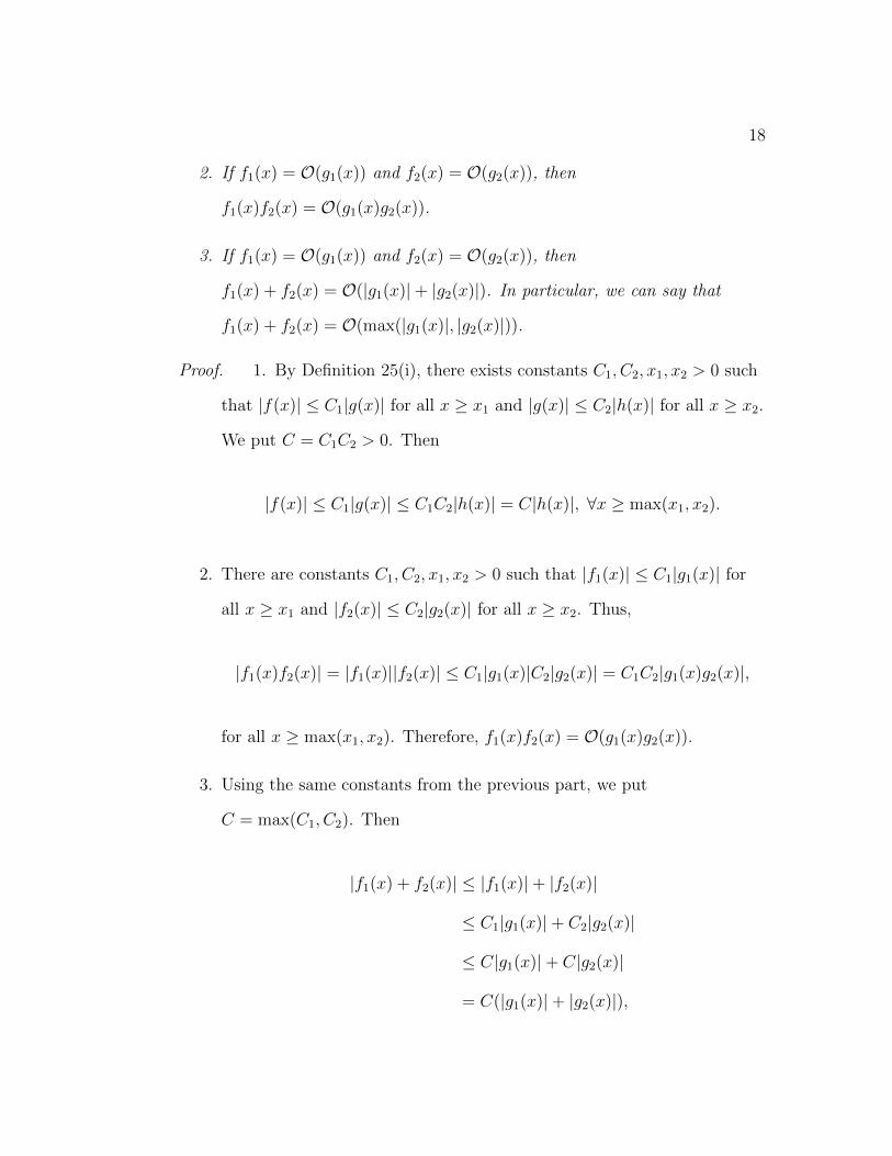
18

2. If f1(x) = O(g1(x)) and f2(x) = O(g2(x)), then

f1(x)f2(x) = O(g1(x)g2(x)).

3. If f1(x) = O(g1(x)) and f2(x) = O(g2(x)), then

f1(x) + f2(x) = O(|g1(x)|+ |g2(x)|). In particular, we can say that

f1(x) + f2(x) = O(max(|g1(x)|, |g2(x)|)).

Proof. 1. By Definition 25(i), there exists constants C1, C2, x1, x2 > 0 such

that |f(x)| ≤ C1|g(x)| for all x ≥ x1 and |g(x)| ≤ C2|h(x)| for all x ≥ x2.

We put C = C1C2 > 0. Then

|f(x)| ≤ C1|g(x)| ≤ C1C2|h(x)| = C|h(x)|, ∀x ≥ max(x1, x2).

2. There are constants C1, C2, x1, x2 > 0 such that |f1(x)| ≤ C1|g1(x)| for

all x ≥ x1 and |f2(x)| ≤ C2|g2(x)| for all x ≥ x2. Thus,

|f1(x)f2(x)| = |f1(x)||f2(x)| ≤ C1|g1(x)|C2|g2(x)| = C1C2|g1(x)g2(x)|,

for all x ≥ max(x1, x2). Therefore, f1(x)f2(x) = O(g1(x)g2(x)).

3. Using the same constants from the previous part, we put

C = max(C1, C2). Then

|f1(x) + f2(x)| ≤ |f1(x)|+ |f2(x)|

≤ C1|g1(x)|+ C2|g2(x)|

≤ C|g1(x)|+ C|g2(x)|

= C(|g1(x)|+ |g2(x)|),

19

for all x ≥ max(x1, x2). From this, we have

f1(x) + f2(x) = O(|g1(x)|+ |g2(x)|). In particular, for any α, β ∈ R, we

have that α + β ≤ 2 max(α, β). Hence,

|f1(x) + f2(x)| ≤ C(|g1(x)|+ |g2(x)|) ≤ 2C max(|g1(x)|, |g2(x)|),

for all x ≥ max(x1, x2). We therefore conclude that

f1(x) + f2(x) = O(max(|g1(x)|, |g2(x)|)).

We now bring our attention to special functions, beginning with the

complete and incomplete gamma functions.

Definition 27. [1] The (complete) gamma function, Γ, is an extension of the

factorial to real- and complex-valued arguments. In particular, for n ∈ N,

Γ(n) = (n− 1)!. For z ∈ C where Re (z) > 0, Euler’s integral form of the

gamma function is given to be

Γ(z) =

ˆ ∞0

tz−1e−tdt.

The incomplete gamma functions relate to the complete gamma function.

Definition 28. [1] Let a, x ∈ C.

(i) The upper incomplete gamma function is defined as

Γ(a, x) :=

ˆ ∞x

ta−1e−tdt.

In particular, Γ(a) = Γ(a, 0).

20

(ii) The lower incomplete gamma function is defined as

γ(a, x) :=

ˆ x

0

ta−1e−tdt.

By definition, we have that Γ(a, x) + γ(a, x) = Γ(a).

Now, since the upper incomplete gamma function has the following

asymptotic expansion for non-integral a given by [1]

Γ(a, x) ∼ xa−1e−x∞∑n=0

Γ(a)

Γ(a− n)x−n,

we have that

Γ(a, x) = xa−1e−x +O

(∞∑n=1

Γ(a)

Γ(a− n)x−n

).

Alternatively, as x→∞,

(2) Γ(a, x) ∼ xa−1e−x.

Another special function, which happens to be related to the gamma function,

is the beta function.

Definition 29. [1] The beta function (or Euler integral of the first kind) is a

special function defined by

B(a, b) :=

ˆ 1

0

xa−1(1− x)b−1dx,

21

where Re (a) ,Re (b) > 0. If we make the substitution x 7→ 1/(1 + x), then the

integral becomes

B(a, b) =

ˆ ∞0

xb−1

(1 + x)a+bdx.

In particular,

B(a, b) =Γ(a)Γ(b)

Γ(a+ b).

Definition 30. [12] Let F be a function of a real or complex variable z and

let∑∞

n=0 anz−n denote a formal power series for which the sum of the first n

terms is denoted by Sn(z). Let

Rn(z) = F (z)− Sn(z), n = 0, 1, 2, . . . .

That is,

F (z) = a0 +a1z

+a2z2

+ · · ·+ an−1zn−1

+Rn(z), n = 0, 1, 2, . . . ,

where we assume that when n = 0, F (z) = R0(z). Next, assume that for each

n ∈ N ∪ {0}, the following relation holds

Rn(z) = O(z−n), z →∞,

in some unbounded domain D. Then∑∞

n=0 anz−n is called an asymptotic

expansion of the function F (z) and we denote this by

F (z) ∼∞∑n=0

anz−n, z →∞, z ∈ D.

22

Note that analogous definitions can be given for z → 0, or to other finite limit

points.

Observe that a convergent Taylor series will satisfy the definition of an

asymptotic expansion of a power series. Consider the following example of the

asymptotic expansion of the function et.

Example 31. Observe that for t ∈ C, as t→ 0, we have

et = 1 +O(t)

et = 1 + t+O(t2)

et = 1 + t+t2

2+O(t3).

Hence,

et ∼∞∑n=0

tn

n!.

We conclude this introduction with the statement of Watson’s Lemma,

which has significant applications when studying the theory on the

asymptotic behavior of integrals.

Theorem 32 (Watson’s Lemma). [12] Assume that

(i) The function f : R+ → C has a finite number of discontinuities.

(ii) As t→ 0+,

f(t) ∼∞∑n=0

antn.

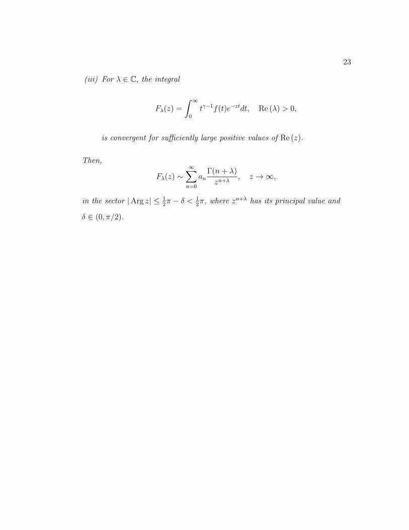
23

(iii) For λ ∈ C, the integral

Fλ(z) =

ˆ ∞0

tγ−1f(t)e−ztdt, Re (λ) > 0,

is convergent for sufficiently large positive values of Re (z).

Then,

Fλ(z) ∼∞∑n=0

anΓ(n+ λ)

zn+λ, z →∞,

in the sector |Arg z| ≤ 12π − δ < 1

2π, where zn+λ has its principal value and

δ ∈ (0, π/2).

CHEBYSHEV POLYNOMIALS OF THE SECOND KIND

The main sequences of interest for this thesis are those related to the

Chebyshev polynomials of the second kind.

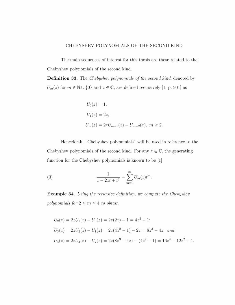
Definition 33. The Chebyshev polynomials of the second kind, denoted by

Um(z) for m ∈ N ∪ {0} and z ∈ C, are defined recursively [1, p. 901] as

U0(z) = 1,

U1(z) = 2z,

Um(z) = 2zUm−1(z)− Um−2(z), m ≥ 2.

Henceforth, “Chebyshev polynomials” will be used in reference to the

Chebyshev polynomials of the second kind. For any z ∈ C, the generating

function for the Chebyshev polynomials is known to be [1]

(3)1

1− 2zt+ t2=

∞∑m=0

Um(z)tm.

Example 34. Using the recursive definition, we compute the Chebyshev

polynomials for 2 ≤ m ≤ 4 to obtain

U2(z) = 2zU1(z)− U0(z) = 2z(2z)− 1 = 4z2 − 1;

U3(z) = 2zU2(z)− U1(z) = 2z(4z2 − 1)− 2z = 8z3 − 4z; and

U4(z) = 2zU3(z)− U2(z) = 2z(8z3 − 4z)− (4z2 − 1) = 16z4 − 12z2 + 1.

25

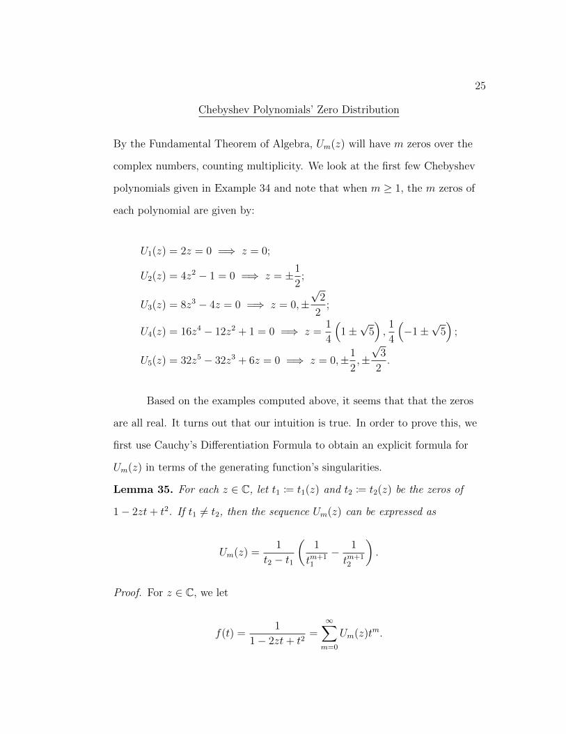
Chebyshev Polynomials’ Zero Distribution

By the Fundamental Theorem of Algebra, Um(z) will have m zeros over the

complex numbers, counting multiplicity. We look at the first few Chebyshev

polynomials given in Example 34 and note that when m ≥ 1, the m zeros of

each polynomial are given by:

U1(z) = 2z = 0 =⇒ z = 0;

U2(z) = 4z2 − 1 = 0 =⇒ z = ±1

2;

U3(z) = 8z3 − 4z = 0 =⇒ z = 0,±√

2

2;

U4(z) = 16z4 − 12z2 + 1 = 0 =⇒ z =1

4

(1±√

5),1

4

(−1±

√5)

;

U5(z) = 32z5 − 32z3 + 6z = 0 =⇒ z = 0,±1

2,±√

3

2.

Based on the examples computed above, it seems that that the zeros

are all real. It turns out that our intuition is true. In order to prove this, we

first use Cauchy’s Differentiation Formula to obtain an explicit formula for

Um(z) in terms of the generating function’s singularities.

Lemma 35. For each z ∈ C, let t1 := t1(z) and t2 := t2(z) be the zeros of

1− 2zt+ t2. If t1 6= t2, then the sequence Um(z) can be expressed as

Um(z) =1

t2 − t1

(1

tm+11

− 1

tm+12

).

Proof. For z ∈ C, we let

f(t) =1

1− 2zt+ t2=

∞∑m=0

Um(z)tm.

26

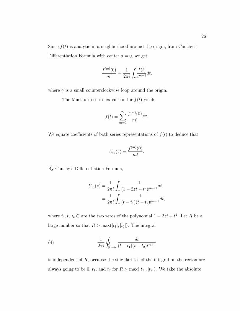
Since f(t) is analytic in a neighborhood around the origin, from Cauchy’s

Differentiation Formula with center a = 0, we get

f (m)(0)

m!=

1

2πi

ˆγ

f(t)

tm+1dt,

where γ is a small counterclockwise loop around the origin.

The Maclaurin series expansion for f(t) yields

f(t) =∞∑m=0

f (m)(0)

m!tm.

We equate coefficients of both series representations of f(t) to deduce that

Um(z) =f (m)(0)

m!.

By Cauchy’s Differentiation Formula,

Um(z) =1

2πi

ˆγ

1

(1− 2zt+ t2)tm+1dt

=1

2πi

ˆγ

1

(t− t1)(t− t2)tm+1dt,

where t1, t2 ∈ C are the two zeros of the polynomial 1− 2zt+ t2. Let R be a

large number so that R > max(|t1|, |t2|). The integral

(4)1

2πi

‰|t|=R

dt

(t− t1)(t− t2)tm+1

is independent of R, because the singularities of the integral on the region are

always going to be 0, t1, and t2 for R > max(|t1|, |t2|). We take the absolute

27

value of the expression in (4) and note that for any m ∈ N,

∣∣∣∣ 1

2πi

‰|t|=R

dt

(t− t1)(t− t2)tm+1

∣∣∣∣ ≤ 1

2π

‰|t|=R

|dt||t− t1||t− t2||t|m+1

≤ 1

2π

‰|t|=R

|dt|(|t| − |t1|)(|t| − |t2|)|t|m+1

≤ 1

2π(R− |t1|)(R− |t2|)Rm+1

‰|t|=R|dt|

=2πR

2π(R− |t1|)(R− |t2|)Rm+1

=1

(R− |t1|)(R− |t2|)Rm.(5)

If we fix m ∈ N and take the limit of the expression in (5) as R goes to

infinity, then the expression converges to 0. Therefore, the expression in (4)

will also converge to 0 as R goes to infinity. Since the singularities inside the

region |t| < R are 0, t1, and t2, we conclude that the expression in (4) is equal

to the sum of three integrals:

1. the integral over a small loop around the origin, which is Um(z);

2. the integral over a small loop around t1; and

3. the integral over a small loop around t2.

By the Residue Theorem, the sum of the integrals around the small

loops around t1 and t2 is

1

(t1 − t2)tm+11

+1

(t2 − t1)tm+12

=1

t1 − t2

(1

tm+11

− 1

tm+12

).

28

Therefore,

Um(z) +1

t1 − t2

(1

tm+11

− 1

tm+12

)= 0,

or, equivalently,

Um(z) =1

t2 − t1

(1

tm+11

− 1

tm+12

).

Note that the same result can be achieved through the partial fraction

decomposition of

1

1− 2zt+ t2=

1

(t− t1)(t− t2).

Although partial fractions is a relatively easy (and perfectly valid) approach

for when the generation function is rational, our generating function of interest

1

(1− t)α(1− 2zt+ t2)=

∞∑m=0

Pm(z)

for 0 < α < 1 is not rational and thus we need to rely on Cauchy’s

Differentiation Formula.

In Lemma 35, we obtain an expression for the mth degree Chebyshev

polynomial in terms of its generating function’s singularities. We can use this

to determine the number of real zeros of the Chebyshev polynomials.

Theorem 36. All zeros of the Chebyshev polynomials of the second kind,

Um(z), generated by∞∑m=0

Um(z)tm =1

1− 2zt+ t2,

lie on the real interval (−1, 1).

29

Proof. For θ ∈ (0, π), we define

z(θ) := cos θ,

t1(θ) := eiθ, and

t2(θ) := e−iθ.

We will first prove that t1 := t1(θ) and t2 := t2(θ) are the zeros of

1− 2z(θ)t+ t2. We note that (t− t1)(t− t2) = t2 − (t2 + t2) + t1t2 and

t1t2 = eiθe−iθ = e0 = 1. Furthermore, by Euler and de Moivre,

einθ = cos(nθ) + i sin(nθ) for all n ∈ Z, which implies that

t1 + t2 = eiθ + e−iθ = cos θ + i sin θ + cos θ − i sin θ = 2 cos θ = 2z.

Since t1 and t2 satisfy the above equalities, they must be the zeros of

1− 2zt+ t2. By construction, t1 and t2 are distinct and nonzero for θ ∈ (0, π).

As proven in Lemma 35,

(6) Um(z(θ)) =1

t2 − t1

(1

tm+11

− 1

tm+12

).

30

Hence, we can substitute t1 = eiθ and t2 = e−iθ into Equation (6) to obtain

Um(z) =1

e−iθ − eiθ

(1

(eiθ)m+1− 1

(e−iθ)m+1

)=

1

−2i sin θ

(e−(m+1)iθ − e(m+1)iθ

)=

1

−2i sin θ(−2i sin((m+ 1)θ))

=sin((m+ 1)θ)

sin θ.

We define

(7) gm(θ) :=sin((m+ 1)θ)

sin θ,

with gm := gm(θ). We set Equation (7) equal to 0 and find that the zeros of

gm are given by

θ =kπ

m+ 1, k ∈ Z.

However, θ ∈ (0, π), so 1 ≤ k ≤ m. Thus, there are m zeros of gm, which

occur whenever

z = cos θ = cos

(kπ

m+ 1

)∈ (−1, 1), 1 ≤ k ≤ m.

Note that z′(θ) = − sin θ < 0 for all θ ∈ (0, π). Thus, z(θ) is monotone on

(0, π). The monotonicity of z(θ) implies that each distinct solution of gm = 0

corresponds to a distinct solution of Um = 0. Clearly, deg(Um(z)) = m for

every m ∈ N. Since we have found m zeros of gm on (0, π), by the

31

Fundamental Theorem of Algebra, we conclude that all of the zeros of Um(z)

are real and lie on the interval (−1, 1).

Note that we can prove that gm(θ) above is indeed equal to Um(z) by

verifying the initial conditions: since Um(z) = gm(θ) for z = cos θ with

g0 =sin θ

sin θ= 1 = U0

and

g1 =sin(2θ)

sin θ=

sin θ cos θ + cos θ sin θ

sin θ= 2 cos θ = 2z = U1,

we use the recurrence relation Um = 2zUm−1 − Um−2 for m ≥ 2 and Equation

(7) to conclude that for z = cos θ, gm = 2zgm−1 − gm−2, for any m ≥ 2. The

two sequences Um(z) and gm(z) satisfy the same initial conditions and

recurrence relation, so they must be the same sequence. However, as we will

see later on, gm will not be as easily obtained for our sequence of interest, so

this method will not work.

-0.5 0.0 0.5

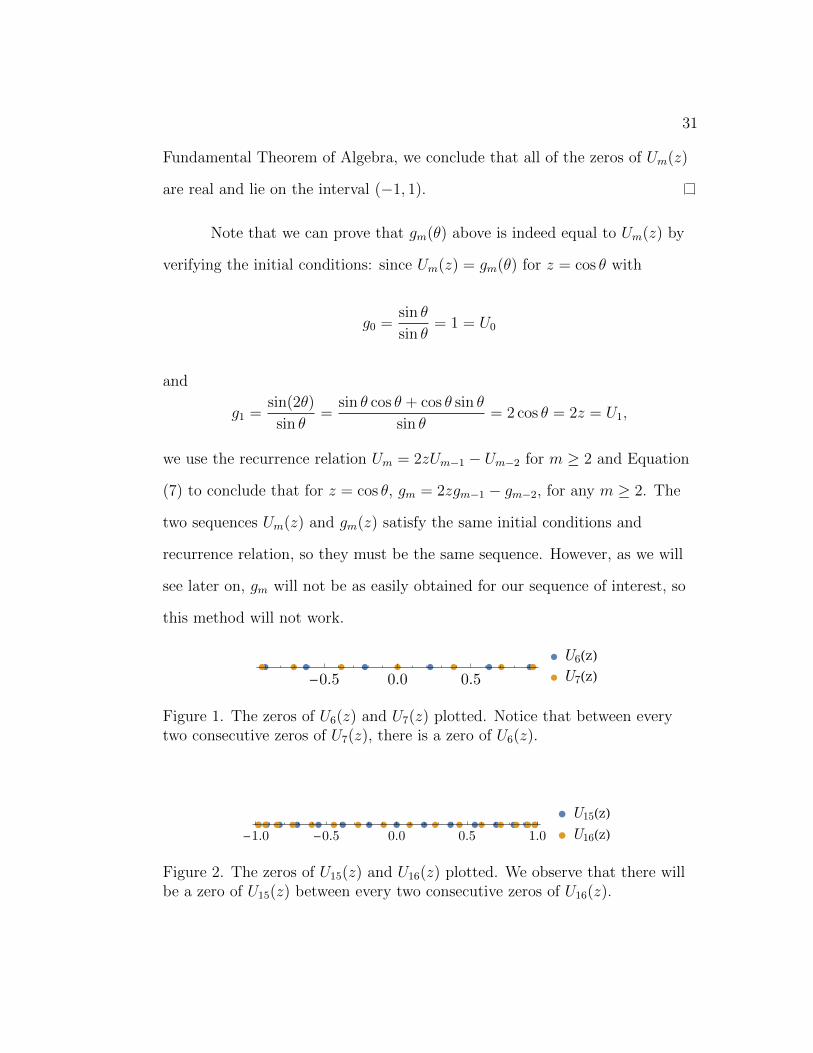
U6(z)U7(z)

Figure 1. The zeros of U6(z) and U7(z) plotted. Notice that between everytwo consecutive zeros of U7(z), there is a zero of U6(z).

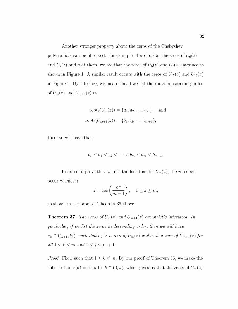
-1.0 -0.5 0.0 0.5 1.0

U15(z)U16(z)

Figure 2. The zeros of U15(z) and U16(z) plotted. We observe that there willbe a zero of U15(z) between every two consecutive zeros of U16(z).

32

Another stronger property about the zeros of the Chebyshev

polynomials can be observed. For example, if we look at the zeros of U6(z)

and U7(z) and plot them, we see that the zeros of U6(z) and U7(z) interlace as

shown in Figure 1. A similar result occurs with the zeros of U15(z) and U16(z)

in Figure 2. By interlace, we mean that if we list the roots in ascending order

of Um(z) and Um+1(z) as

roots(Um(z)) = {a1, a2, . . . , am}, and

roots(Um+1(z)) = {b1, b2, . . . , bm+1},

then we will have that

b1 < a1 < b2 < · · · < bm < am < bm+1.

In order to prove this, we use the fact that for Um(z), the zeros will

occur whenever

z = cos

(kπ

m+ 1

), 1 ≤ k ≤ m,

as shown in the proof of Theorem 36 above.

Theorem 37. The zeros of Um(z) and Um+1(z) are strictly interlaced. In

particular, if we list the zeros in descending order, then we will have

ak ∈ (bk+1, bk), such that ak is a zero of Um(z) and bj is a zero of Um+1(z) for

all 1 ≤ k ≤ m and 1 ≤ j ≤ m+ 1.

Proof. Fix k such that 1 ≤ k ≤ m. By our proof of Theorem 36, we make the

substitution z(θ) = cos θ for θ ∈ (0, π), which gives us that the zeros of Um(z)

33

are given by

ak := cos

(kπ

m+ 1

), 1 ≤ k ≤ m

and the zeros of Um+1(z) are given by

bj := cos

(jπ

m+ 2

), 1 ≤ j ≤ m+ 1.

Since m+ 1 < m+ 2, we clearly have that kπm+2

< kπm+1

. We know cos θ

is strictly decreasing on (0, π), which implies

ak = cos

(kπ

m+ 1

)< cos

(kπ

m+ 2

)= bk.

Observe that since 1 ≤ k ≤ m, we have

(k+1)(m+1) = km+k+m+1 = k(m+1)+m+1 > k(m+1)+k = k(m+2).

Thus, (k + 1)π(m+ 1) > kπ(m+ 2), or equivalently (k+1)πm+2

> kπm+1

. Once

again, since cos θ is strictly decreasing on (0, π),

bk+1 = cos

((k + 1)π

m+ 2

)< cos

(kπ

m+ 1

)= ak.

Hence, ak ∈ (bk+1, bk) for every 1 ≤ k ≤ m. Therefore,

bm+1 < am < bm < · · · < b2 < a1 < b1.

Thus, the zeros of consecutive Chebyshev polynomials strictly interlace.

34

Based on the how the zeros of Um(z) are defined in Theorem 36, we

observe that the zeros are dense in (−1, 1) as m→∞. Recall that by dense in

(−1, 1), we mean that every open subset of (−1, 1) will contain a zero of

Um(z) for all large m.

Theorem 38. The zeros of Um(z) are dense in (−1, 1) as m→∞.

Proof. From Theorem 36, the zeros of Um(z) occur whenever

z(θ) = cos θ = coskπ

m+ 1, 1 ≤ k ≤ m.

Since θ ∈ (0, π), we see that the interval (0, π) is partitioned into m+ 1

subintervals whose lengths go to 0 as m→∞ such that each interval endpoint

(except for 0 and π) is a solution to Um(z(θ)) = 0. As m→∞, any

subinterval (α, β) ⊆ (0, π) will therefore contain a zero of Um(z(θ)) for all

large m. If we put a = cos−1 β and b = cos−1 α, we see that as m→∞, the

subinterval (a, b) ⊆ (−1, 1) will contain a zero of Um(z). Therefore, the zeros

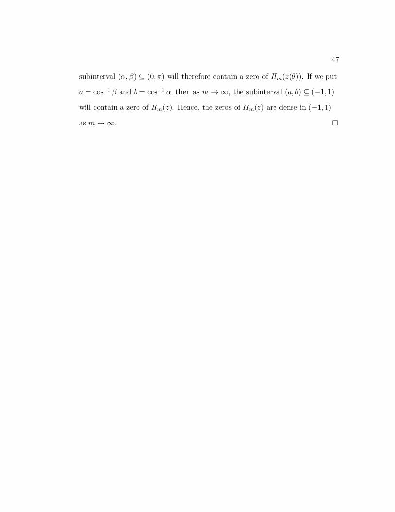
of Um(z) are dense in (−1, 1) as m→∞.

Finite Summation of Chebyshev Polynomials’ Zero Distribution

Recall that the generating function for the geometric series is given by

(8)1

1− t=

∞∑m=0

tm.

We redirect our attention to the finite summation of Chebyshev

polynomials. We consider {Hm(z)}∞m=0, where Hm(z) :=∑m

k=0 Uk(z). Then

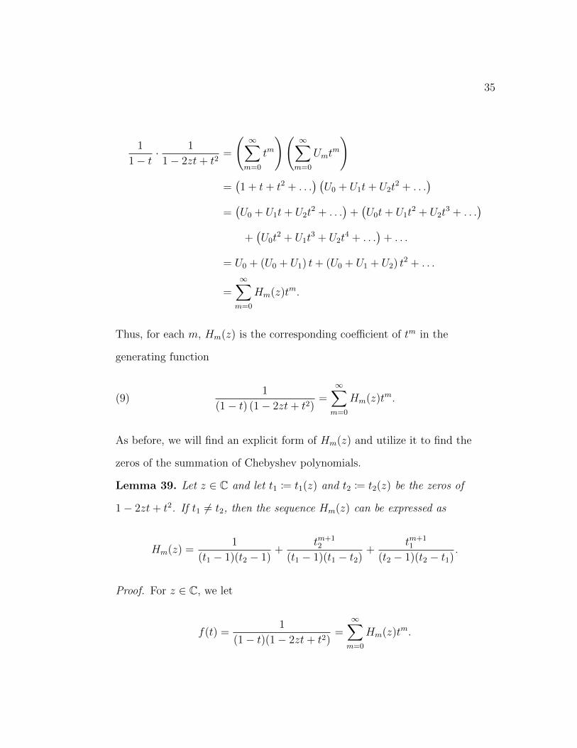
35

1

1− t· 1

1− 2zt+ t2=

(∞∑m=0

tm

)(∞∑m=0

Umtm

)

=(1 + t+ t2 + . . .

) (U0 + U1t+ U2t

2 + . . .)

=(U0 + U1t+ U2t

2 + . . .)

+(U0t+ U1t

2 + U2t3 + . . .

)+(U0t

2 + U1t3 + U2t

4 + . . .)

+ . . .

= U0 + (U0 + U1) t+ (U0 + U1 + U2) t2 + . . .

=∞∑m=0

Hm(z)tm.

Thus, for each m, Hm(z) is the corresponding coefficient of tm in the

generating function

(9)1

(1− t) (1− 2zt+ t2)=

∞∑m=0

Hm(z)tm.

As before, we will find an explicit form of Hm(z) and utilize it to find the

zeros of the summation of Chebyshev polynomials.

Lemma 39. Let z ∈ C and let t1 := t1(z) and t2 := t2(z) be the zeros of

1− 2zt+ t2. If t1 6= t2, then the sequence Hm(z) can be expressed as

Hm(z) =1

(t1 − 1)(t2 − 1)+

tm+12

(t1 − 1)(t1 − t2)+

tm+11

(t2 − 1)(t2 − t1).

Proof. For z ∈ C, we let

f(t) =1

(1− t)(1− 2zt+ t2)=

∞∑m=0

Hm(z)tm.

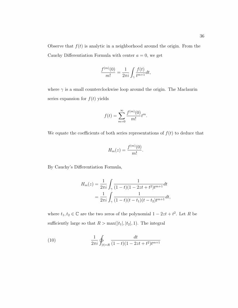
36

Observe that f(t) is analytic in a neighborhood around the origin. From the

Cauchy Differentiation Formula with center a = 0, we get

f (m)(0)

m!=

1

2πi

ˆγ

f(t)

tm+1dt,

where γ is a small counterclockwise loop around the origin. The Maclaurin

series expansion for f(t) yields

f(t) =∞∑m=0

f (m)(0)

m!tm.

We equate the coefficients of both series representations of f(t) to deduce that

Hm(z) =f (m)(0)

m!.

By Cauchy’s Differentiation Formula,

Hm(z) =1

2πi

ˆγ

1

(1− t)(1− 2zt+ t2)tm+1dt

=1

2πi

ˆγ

1

(1− t)(t− t1)(t− t2)tm+1dt,

where t1, t2 ∈ C are the two zeros of the polynomial 1− 2zt+ t2. Let R be

sufficiently large so that R > max(|t1|, |t2|, 1). The integral

(10)1

2πi

‰|t|=R

dt

(1− t)(1− 2zt+ t2)tm+1

37

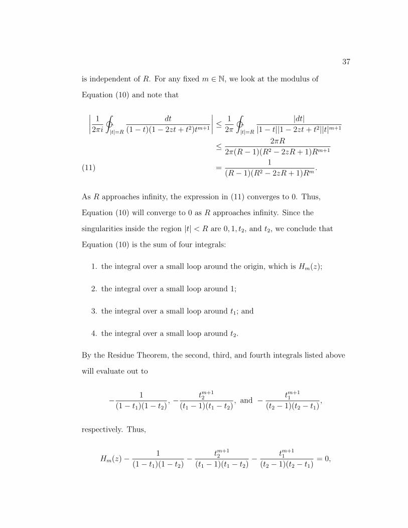
is independent of R. For any fixed m ∈ N, we look at the modulus of

Equation (10) and note that

∣∣∣∣ 1

2πi

‰|t|=R

dt

(1− t)(1− 2zt+ t2)tm+1

∣∣∣∣ ≤ 1

2π

‰|t|=R

|dt||1− t||1− 2zt+ t2||t|m+1

≤ 2πR

2π(R− 1)(R2 − 2zR + 1)Rm+1

=1

(R− 1)(R2 − 2zR + 1)Rm.(11)

As R approaches infinity, the expression in (11) converges to 0. Thus,

Equation (10) will converge to 0 as R approaches infinity. Since the

singularities inside the region |t| < R are 0, 1, t2, and t2, we conclude that

Equation (10) is the sum of four integrals:

1. the integral over a small loop around the origin, which is Hm(z);

2. the integral over a small loop around 1;

3. the integral over a small loop around t1; and

4. the integral over a small loop around t2.

By the Residue Theorem, the second, third, and fourth integrals listed above

will evaluate out to

− 1

(1− t1)(1− t2), − tm+1

2

(t1 − 1)(t1 − t2), and − tm+1

1

(t2 − 1)(t2 − t1),

respectively. Thus,

Hm(z)− 1

(1− t1)(1− t2)− tm+1

2

(t1 − 1)(t1 − t2)− tm+1

1

(t2 − 1)(t2 − t1)= 0,

38

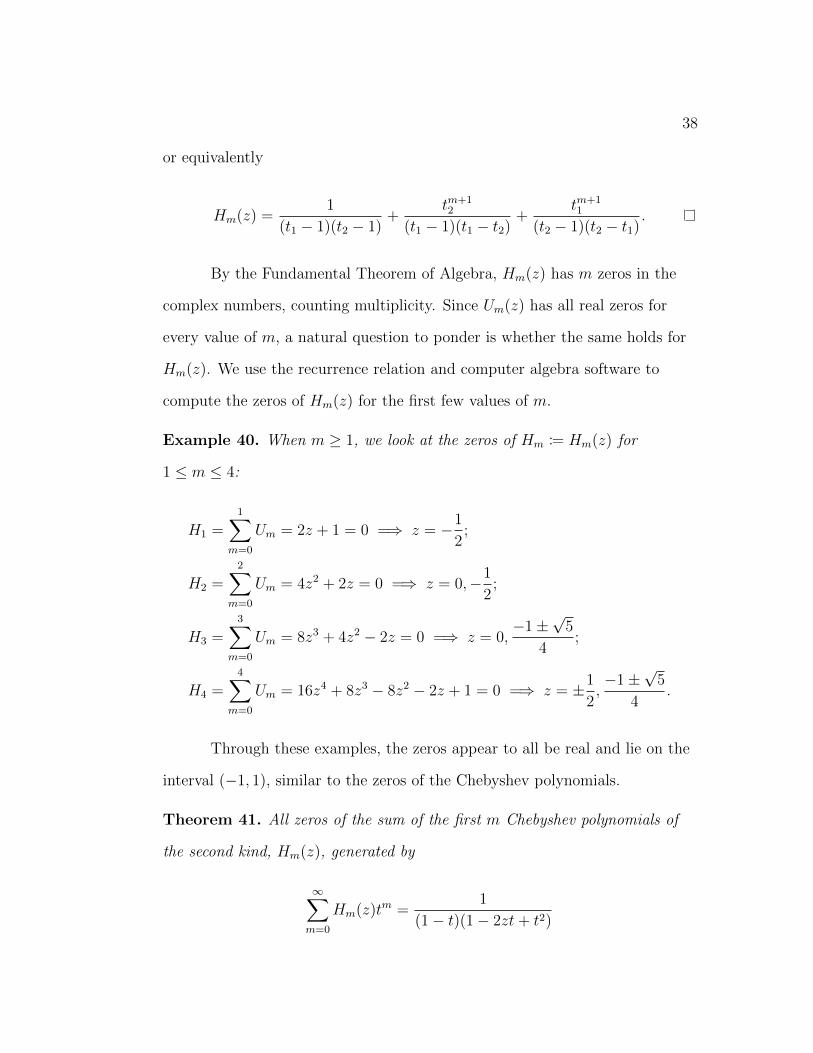
or equivalently

Hm(z) =1

(t1 − 1)(t2 − 1)+

tm+12

(t1 − 1)(t1 − t2)+

tm+11

(t2 − 1)(t2 − t1).

By the Fundamental Theorem of Algebra, Hm(z) has m zeros in the

complex numbers, counting multiplicity. Since Um(z) has all real zeros for

every value of m, a natural question to ponder is whether the same holds for

Hm(z). We use the recurrence relation and computer algebra software to

compute the zeros of Hm(z) for the first few values of m.

Example 40. When m ≥ 1, we look at the zeros of Hm := Hm(z) for

1 ≤ m ≤ 4:

H1 =1∑

m=0

Um = 2z + 1 = 0 =⇒ z = −1

2;

H2 =2∑

m=0

Um = 4z2 + 2z = 0 =⇒ z = 0,−1

2;

H3 =3∑

m=0

Um = 8z3 + 4z2 − 2z = 0 =⇒ z = 0,−1±

√5

4;

H4 =4∑

m=0

Um = 16z4 + 8z3 − 8z2 − 2z + 1 = 0 =⇒ z = ±1

2,−1±

√5

4.

Through these examples, the zeros appear to all be real and lie on the

interval (−1, 1), similar to the zeros of the Chebyshev polynomials.

Theorem 41. All zeros of the sum of the first m Chebyshev polynomials of

the second kind, Hm(z), generated by

∞∑m=0

Hm(z)tm =1

(1− t)(1− 2zt+ t2)

39

are real and lie on the interval (−1, 1).

Proof. For θ ∈ (0, π), we define

z(θ) = cos θ,

t1(θ) = eiθ, and

t2(θ) = e−iθ.

By Lemma 39,

Hm(z) =1

(t1 − 1)(t2 − 1)+

tm+12

(t1 − 1)(t1 − t2)+

tm+11

(t2 − 1)(t2 − t1)

=1

(t1 − 1)(t2 − 1)

(1 +

tm+12 (t2 − 1)

t1 − t2− tm+1

1 (t1 − 1)

t1 − t2

)

We note that t1 − t2 = 2i sin θ and (t1 − 1)(t2 − 1) = 2− 2 cos θ. Moreover,

since t1,2 = e±iθ,

tm+12 (t2 − 1)

t1 − t2− tm+1

1 (t1 − 1)

t1 − t2=tm+22 − tm+1

2 − tm+21 + tm+1

1

2i sin θ

=2i(sin((m+ 1)θ)− sin((m+ 2)θ))

2i sin θ

=sin((m+ 1)θ)− sin((m+ 2)θ)

sin θ.

Recall from trigonometry that for any α, β ∈ R, the following identities hold:

sinα− sin β = 2 cos α+β2

sin α−β2

, cosα− cos β = −2 sin α+β2

sin α−β2

, and

sinα = 2 sin α2

cos α2. Equivalently, if sin(α/2) 6= 0,

cosα

2=

sinα

2 sin(α/2).

40

We observe that

1 +sin((m+ 1)θ)− sin((m+ 2)θ)

sin θ= 1 +

2 cos (2m+3)θ2

sin −θ2

sin θ

= 1−2 cos (2m+3)θ

2sin θ

2

sin θ

=cos θ

2− cos

((m+ 3

2

)θ)

cos θ2

=−2 sin (m+2)θ

2sin (−m−1)θ

2

cos θ2

=2 sin (m+2)θ

2sin (m+1)θ

2

cos θ2

.

Therefore,

Hm(z) =2 sin (m+2)θ

2sin (m+1)θ

2

cos θ2(2− 2 cos θ)

=sin (m+2)θ

2sin (m+1)θ

2

cos θ2(1− cos θ)

.

Note that cos θ2

and 1− cos θ do not effect the zeros of Hm(z). Thus, we define

gm(θ) := sin(m+ 2)θ

2sin

(m+ 1)θ

2.

Then gm(θ) = 0 whenever

(m+ 2)θ

2= kπ or

(m+ 1)θ

2= kπ,

where k ∈ Z. Therefore,

θ =2kπ

m+ 2or θ =

2kπ

m+ 1.

41

Recall that θ ∈ (0, π). When m = 2n for some n ∈ N, we have that

2kπ

m+ 2=

2kπ

2n+ 2=

kπ

n+ 1∈ (0, π)

and

2kπ

m+ 1=

2kπ

2n+ 1∈ (0, π)

if and only if 1 ≤ k ≤ n = m/2. We note that when m = 2n,

b(m+ 1)/2c = n = bm/2c. On the other hand, if m = 2n+ 1, then

2kπ

m+ 2=

2kπ

2n+ 3∈ (0, π)

if and only if 1 ≤ k ≤ n+ 1 = b(m+ 1)/2c, and

2kπ

m+ 1=

2kπ

2n+ 2=

kπ

n+ 1∈ (0, π)

if and only if 1 ≤ k ≤ n = bm/2c.

Therefore, there are m zeros of gm(θ). Each zero of gm(θ) gives a real

zero of Hm(z) on (−1, 1) via

z(θ) = cos2kπ

m+ 2∈ (−1, 1), 1 ≤ k ≤

⌊m+ 1

2

⌋

or

z(θ) = cos2kπ

m+ 1∈ (−1, 1), 1 ≤ k ≤

⌊m2

⌋.

42

We note that

1

(1− t)(1− 2zt+ t2)=

1

1 + (−2z − 1)t+ (2z + 1)t2 + (−1)t3.

By Theorem 16, the corresponding recurrence relation for Hm(z) is

Hm(z) + (−2z − 1)Hm−1(z) + (2z + 1)Hm−2(z)−Hm−3(z) = 0,

or equivalently

(12) Hm(z) = (2z + 1)Hm−1(z)− (2z + 1)Hm−2(z) +Hm−3(z).

By definition of our generating function, Hm := Hm(z) is the summation of

Chebyshev polynomials from k = 0 to k = m. Thus, H−m = 0, and from

Example 40, we found that H0 = U0 = 1, H1 = 1 + 2z, H2 = 2z + 4z2, and

H3 = −2z + 4z2 + 8z3. We use the recurrence relation in Equation (12) to

calculate H3 and find that

H3 = (2z + 1)H2 − (2z + 1)H1 +H0

= (2z + 1)(4z2 + 2z)− (2z + 1)(2z + 1) + 1

= 8z3 + 4z2 + 4z2 + 2z − (4z2 + 4z + 1) + 1

= 8z3 + 4z2 − 2z.

Therefore, we have the correct recurrence relation. Now, we want to use this

recurrence relation to prove the degree of Hm(z) is equal to m since we clearly

43

have that it is at least m through the recurrence relation. We prove this

through strong induction on m.

When m = 0, we trivially have that deg(H0) = 0 since H0 = 1. We now

suppose that deg(Hk) = k for all k such that 1 ≤ k ≤ m− 1. By the inductive

hypothesis, deg(Hm−1) = m− 1, deg(Hm−2) = m− 2, and deg(Hm−3) = m− 3.

By the recurrence relation, Hm = (2z+ 1)Hm−1− (2z+ 1)Hm−2 +Hm−3. Then

deg(Hm) = max(deg((2z + 1)Hm−1), deg((2z + 1)Hm−2), deg(Hm−3))

= max(m− 1 + 1,m− 2 + 1,m− 3)

= max(m,m− 1,m− 3)

Hence, deg(Hm) = m.

Recall that Um(z) has all real zeros in (−1, 1), and the zeros are

strictly interlaced with the zeros of Um+1(z). Naturally, we wonder if this

interlaced property carries over to Hm(z) and Hm+1(z) as well. Since the

Chebyshev polynomials were strictly interlaced, the sets of zeros for

consecutive polynomials were disjoint. However, as shown in Figures 3 and 4,

it appears that Hm(z) and Hm+1(z) will share some zeros.

-1.0 -0.5 0.0 0.5 1.0H6(z)

-1.0 -0.5 0.0 0.5 1.0H7(z)

Figure 3. The zeros of H6(z) and H7(z) plotted. Based on the figure, weobserve that half of the zeros of H6(z) will also be zeros of H7(z).

44

We use Mathematica to find that the (approximate) roots of H6(z) and

H7(z) will be

roots(H6(z)) = {0,−0.707107, 0.707107,−0.900969,−0.222521, 0.62349}, and

roots(H7(z)) = {−0.5, 0,−0.707107, 0.707107,−0.939693, 0.173648, 0.766044}.

So, 3 of the zeros of H7(z) will also be zeros of H6(z).

-1.0 -0.5 0.0 0.5 1.0H9(z)

-1.0 -0.5 0.0 0.5 1.0H10(z)

Figure 4. The zeros of H9(z) and H10(z) plotted. Observe that half of thezeros of H10(z) will also be zeros of H9(z).

Similarly, the approximate roots of H9(z) and H10(z) will be

roots(H9(z)) = {−0.809017,−0.309017, 0.309017, 0.809017,−0.959493,

− 0.654861,−0.142315, 0.415415, 0.841254}

roots(H10(z)) = {−0.5, 0, 0.5,−0.866025, 0.866025,−0.959493,

− 0.654861,−0.142315, 0.415415, 0.841254}.

We see that 5 of the zeros of H10(z) will be zeros of H9(z).

From these examples, we see that the zeros of Hm(z) and Hm+1(z) are

interlaced, but not strictly interlaced.

45

Theorem 42. The zeros of Hm(z) and Hm+1(z) are interlaced. In particular,

if we list the zeros in descending order, we will have that ak ∈ [bk+1, bk) for

1 ≤ k ≤ m, where each ak is a zero of Hm(z) and each bk is a zero of Hm+1(z).

Proof. By our proof of Theorem 41, if we make the substitution z(θ) = cos θ

with θ ∈ (0, π), then the m zeros of Hm(z) are given by

a2`−1 = cos2`π

m+ 2, 1 ≤ ` ≤

⌊m+ 1

2

⌋

and

a2` = cos2`π

m+ 1, 1 ≤ ` ≤

⌊m2

⌋.

Similarly, the m+ 1 zeros of Hm+1(z) are given by

b2j = cos2jπ

m+ 2, 1 ≤ j ≤

⌊m+ 1

2

⌋

and

b2j−1 = cos2jπ

m+ 3, 1 ≤ j ≤

⌊m+ 2

2

⌋.

Fix 1 ≤ k ≤ b(m+ 1)/2c. By definition, we have that a2k−1 = b2k.

Furthermore, since 2kπm+2

> 2kπm+3

and cosine is decreasing on (0, π), we get that

a2k−1 = b2k = cos2kπ

m+ 2< cos

2kπ

m+ 3= b2k−1.

Hence, a2k−1 ∈ [b2k, b2k−1).

On the other hand, 2kπm+1

> 2kπm+2

, so

a2k = cos2kπ

m+ 1< cos

2kπ

m+ 2= b2k.

46

Moreover,

b2k+1 = b2(k+1)−1 = cos2(k + 1)π

m+ 3.

We note that since m ≥ 0,

(k + 1)(m+ 3) = km+ 3k +m+ 3 > km+ 3k = k(m+ 3),

which implies that 2(k+1)πm+3

> 2kπm+1

. Thus,

b2k+1 = cos2(k + 1)π

m+ 3< cos

2kπ

m+ 1= a2k.

We conclude that a2k ∈ (b2k+1, b2k). Hence, for any 1 ≤ k ≤ m, we have that

ak ∈ [bk+1, bk).

Similar to Um(z), we also have that the zeros of Hm(z) are dense as

m→∞.

Theorem 43. The zeros of Hm(z) are dense in (−1, 1) as m→∞.

Proof. By our proof of Theorem 41, the m zeros of Hm(z) are given by

z(θ) = cos2kπ

m+ 2, 1 ≤ k ≤

⌊m+ 1

2

⌋

and

z(θ) = cos2kπ

m+ 1, 1 ≤ k ≤

⌊m2

⌋.

Since θ ∈ (0, π), we observe that the interval (0, π) is partitioned into m+ 2

subintervals whose lengths go to 0 as m→∞ such that each interval endpoint

(except for 0 and π) is a solution to Hm(z(θ)) = 0. As m→∞, any

47

subinterval (α, β) ⊆ (0, π) will therefore contain a zero of Hm(z(θ)). If we put

a = cos−1 β and b = cos−1 α, then as m→∞, the subinterval (a, b) ⊆ (−1, 1)

will contain a zero of Hm(z). Hence, the zeros of Hm(z) are dense in (−1, 1)

as m→∞.

BINOMIAL COMBINATION OF CHEBYSHEV POLYNOMIALS

In this section, we consider the zeros of a binomial combination of Chebyshev

polynomials generated by

1

(1− t)α(1− 2zt+ t2)=

∞∑m=0

Pm(z)tm,

where α ∈ R such that α > 0. In the generating function above and

throughout this paper, we use the principal branch cut. Observe that in the

previous section, we considered the cases when α = 0 and α = 1. Recall the

binomial series for β ∈ C given by

(1 + t)β =∞∑m=0

(β

m

)tm,

with

(β

m

)being the generalized binomial coefficient defined by

(β

0

)= 1 and

(β

m

):=

β(β − 1)(β − 2) · · · (β −m+ 1)

m!, if m = 1, 2, 3, . . . .

In particular, if α is a positive real number, then

1

(1− t)α=

∞∑m=0

(α +m− 1

m

)tm.

49

We compute the Cauchy product of the formal power series generated by the

reciprocal of (1− t)α(1− 2zt+ t2) to obtain

1

(1− t)α(1− 2zt+ t2)=

(∞∑m=0

(α +m− 1

m

)tm

)(∞∑m=0

Um(z)tm

)

=∞∑m=0

(m∑k=0

(α + k − 1

k

)Um−k(z)

)tm.

We equate coefficients for the two formal power series representations to

deduce

Pm(z) =m∑k=0

(α + k − 1

k

)Um−k(z).

Notice that our definition of Pm(z) is a generalization of Um(z) and

Hm(z). If α = 0, then

(α + k − 1

k

)=

(k − 1

k

)=

0 if k ≥ 1

1 if k = 0,

since by definition of the binomial coefficient,(βk

)= 0 if β = 0, 1, 2, . . . , k − 1

and(β0

)= 1 for any β ∈ R. Hence, if α = 0, then Pm(z) = Um(z).

Furthermore, if α = 1, then

(α + k − 1

k

)=

(k

k

)= 1,

which implies that Pm(z) =∑m

k=0 Um−k(z) =∑m

k=0 Uk(z) = Hm(z).

As implied by our explorations in the previous section, our interest is

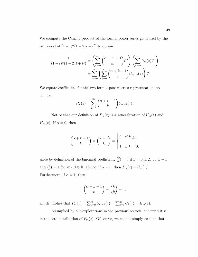
in the zero distribution of Pm(z). Of course, we cannot simply assume that

50

the zeros of Pm(z) will reside in the interval (−1, 1) because such was true for

Um(z) and Hm(z). However, one can easily use computer software such as

Mathematica to plot the zero distribution of Pm(z) on the complex plane for

different values of m and α.

-1.0 -0.5 0.5 1.0

-1.0

-0.5

0.5

1.0

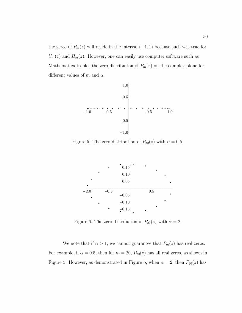
Figure 5. The zero distribution of P20(z) with α = 0.5.

-1.0 -0.5 0.5

-0.15

-0.10

-0.05

0.05

0.10

0.15

Figure 6. The zero distribution of P20(z) with α = 2.

We note that if α > 1, we cannot guarantee that Pm(z) has real zeros.

For example, if α = 0.5, then for m = 20, P20(z) has all real zeros, as shown in

Figure 5. However, as demonstrated in Figure 6, when α = 2, then P20(z) has

51

no real zeros. We observe that for |α| > 1, the real and complex zeros appear

to be within the unit circle in the complex plane.

As was the case when we studied the zero distributions of Um(z) and

Hm(z), our goal is to count the number of real zeros of Pm(z) in the real

interval (−1, 1) and compare that with the degree of the polynomial, m. With

use of the Cauchy Differentiation Formula, we can obtain an expression for

Pm(z) in terms of its singularities given by the proposition stated in the

following section as long as we impose the restriction that 0 < α ≤ 1.

An ‘Explicit’ Formula

In this section, we shall prove a proposition (c.f. Proposition 45) that

provides a more explicit formula for Pm(z). We first prove the following

lemma, which is used in the proof of the proposition.

Lemma 44. For any α, θ ∈ R,

(1− eiθ

)α= eiα(θ−π)/2

(2 sin

θ

2

)α

and (1− e−iθ

)α= e−iα(θ−π)/2

(2 sin

θ

2

)α.

Proof. We use the fact that i = eiπ/2 and −i = e−iπ/2 to obtain

(1− eiθ

)α=(eiθ/2

(e−iθ/2 − eiθ/2

))α= eiαθ/2

(−2i sin

θ

2

)α= eiα(θ−π)/2

(2 sin

θ

2

)α.

52

Similarly,(1− e−iθ

)α= e−iα(θ−π)/2

(2 sin θ

2

)α.

Observe that this lemma is true regardless of what value θ, α ∈ R take.

Thus, using the assumptions of the proposition below, we may apply the

results of this lemma.

Proposition 45. Let 0 < α < 1. Consider the sequence of polynomials

{Pm(z)}∞m=0 generated by

1

(1− t)α(1− 2zt+ t2)=

∞∑m=0

Pm(z)tm.

Then, with z(θ) = cos θ and t1,2(θ) = e±iθ for θ ∈ (0, π),

Pm(z) =1

πIm

(ˆ ∞0

dx

xαe−iαπ(1 + x− t1)(1 + x− t2)(1 + x)m+1

)+

(2 sin θ

2

)αsin θ(2− 2 cos θ)α

sin

((m+ 1)θ +

α(θ − π)

2

).

Proof. As shown in Theorem 36, the two zeros in t of 1 + 2z(θ)t+ t2 are given

by t1 := t1(θ) and t2 := t2(θ). Let R� 1 and 1 > ε > 0. By the Cauchy

Differentiation Formula, we have for some small δ > 0,

Pm(z(θ)) =1

2πi

‰|t|=δ

dt

(1− t)α(1− 2z(θ)t+ t2)tm+1

=1

2πi

‰|t|=δ

dt

(1− t)α(t− t1)(t− t2)tm+1.(13)

We define γ to be the region with counterclockwise orientation such

that γ is the union of part of the circle of radius R centered at the origin CR,

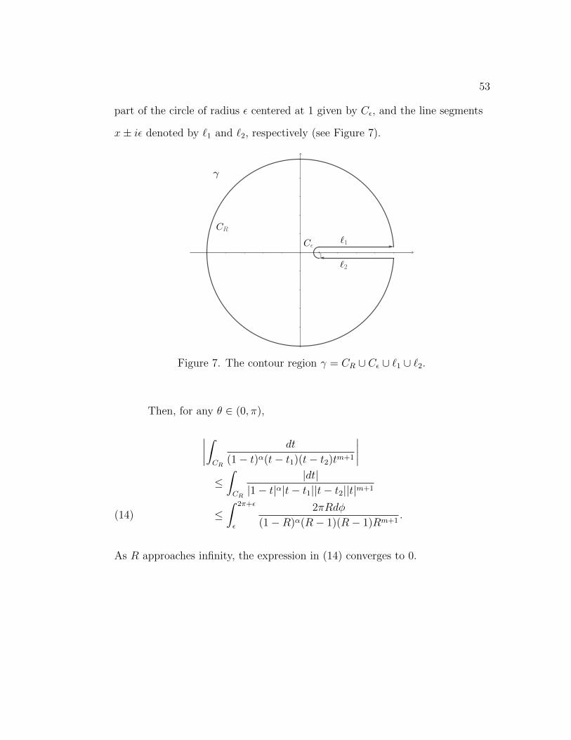
53

part of the circle of radius ε centered at 1 given by Cε, and the line segments

x± iε denoted by `1 and `2, respectively (see Figure 7).

Figure 7. The contour region γ = CR ∪ Cε ∪ `1 ∪ `2.

Then, for any θ ∈ (0, π),

∣∣∣∣ˆCR

dt

(1− t)α(t− t1)(t− t2)tm+1

∣∣∣∣≤ˆCR

|dt||1− t|α|t− t1||t− t2||t|m+1

≤ˆ 2π+ε

ε

2πRdφ

(1−R)α(R− 1)(R− 1)Rm+1.(14)

As R approaches infinity, the expression in (14) converges to 0.

54

We parameterize the circle Cε as Cε : t = 1 + εeiφ, π/2 ≤ φ ≤ 3π/2.

Hence,

∣∣∣∣ˆCε

dt

(1− t)α(t− t1)(t− t2)tm+1

∣∣∣∣≤ˆCε

|dt||1− t|α|t− t1||t− t2||t|m+1

≤ˆ 3π/2

π/2

ε|eiφ|dφεα|eiφ|α|1 + εeiφ − t1||1 + εeiϕ − t2||1 + εeiϕ|m+1

≤ˆ 3π/2

π/2

εdφ

εα|1 + εeiφ − t1||1 + εeiϕ − t2||1 + εeiϕ|m+1.(15)

As ε→ 0+, the expression in (15) converges to 0 because 0 < α < 1.

We parameterize the curves `1 and `2 as `1 : t = 1 + x+ iε and

`2 : t = 1 + x− iε for x ∈ [0, R− 1]. For every m and θ, the function in x

(16)1

(1− t)α(t− t1)(t− t2)tm+1

converges pointwise to

1

xαe−iπα(1 + x− t1)(1 + x− t2)(1 + x)m+1

for x ∈ (0,∞) as R→∞ and ε→ 0+. Since x ∈ (0,∞), we have

|1 + x− t1||1 + x− t2| = (1 + x)2 − 2 cos θ(1 + x) + 1 ≥ 2− 2 cos θ.

Thus, we can dominate the absolute value of (16) by

1

|1− t|α|t− t1||t− t1||t|m+1≤ 1

xα(2− 2 cos θ)(1 + x)m+1,

55

where the right-hand side is integrable with respect to x on (0,∞) since

integrating yields the beta function. By Theorem 23, as R→∞ and ε→ 0+,

ˆ`1

dt

(1− t)α(t− t1)(t− t2)tm+1

=

ˆ R−1

0

dx

(−x− iε)α(1 + x+ iε− t1)(1 + x+ iε− t2)(1 + x+ iε)m+1

→ˆ ∞0

dx

xαe−iαπ(1 + x− t1)(1 + x− t2)(1 + x)m+1.(17)

Similarly, for the region `2, we have that as R→∞ and ε→ 0+,

ˆ`2

dt

(1− t)α(t− t1)(t− t2)tm+1

=

ˆ R−1

0

−dx(−x+ iε)α(1 + x− iε− t1)(1 + x− iε− t2)(1 + x− iε)m+1

→ −ˆ ∞0

dx

xαeiαπ(1 + x− t1)(1 + x− t2)(1 + x)m+1.(18)

We put h(t, θ) equal to the integrand in (13), i.e.,

h(t, θ) =1

(1− t)α(t− t1)(t− t2)tm+1.

By the Residue Theorem, we obtain the equation

1

2πi

ˆCR

h(t, θ)dt+1

2πi

ˆCε

h(t, θ)dt+1

2πi

ˆ`1

h(t, θ)dt+1

2πi

ˆ`2

h(t, θ)dt

= Pm(z(θ)) +

‰|t−t1|=δ

h(t, θ)dt+

‰|t−t2|=δ

h(t, θ)dt.

56

Thus, as R approaches ∞ and ε approaches 0,

Pm(z(θ)) =1

2πi

ˆ`1

h(t, θ)dt+1

2πi

ˆ`2

h(t, θ)dt

− 1

2πi

ˆ|t−t1|=δ

h(t, θ)dt− 1

2πi

ˆ|t−t2|=δ

h(t, θ)dt.(19)

The integrals over the curves `1 and `2 are complex conjugates that are

opposite in sign. Thus, when we parameterize and take the limits as R

approaches infinity and ε approaches 0 from the right, we can take the sum of

the integrals in (17) and (18) to obtain

1

2πi

ˆ`1

h(t, θ)dt+1

2πi

ˆ`2

h(t, θ)dt

→ 1

2πi

ˆ ∞0

cos(απ) + i sin(απ)− cos(απ) + i sin(απ)dx

xα(1 + x− t1)(1 + x− t2)(1 + x)m+1

=1

π

ˆ ∞0

sin(απ)dx

xα(1 + x− t1)(1 + x− t2)(1 + x)m+1

=1

πIm

(ˆ ∞0

dx

xαe−iαπ(1 + x− t1)(1 + x− t2)(1 + x)m+1

).(20)

We note that since t1,2 = e±iθ, we can simplify (1− t1)α(1− t2)α to get

(1− t1)α(1− t2)α = (1− t1 − t2 + 1)α = (2− 2 cos θ)α.

57

By Cauchy’s Differentiation Formula and Lemma 44,

− 1

2πi

ˆ|t−t1|=δ

h(t, θ)dt− 1

2πi

ˆ|t−t2|=δ

h(t, θ)dt

=−1

(1− t1)α(t1 − t2)tm+11

+−1

(1− t2)α(t2 − t1)tm+12

=tm+11

(1− t2)α(t1 − t2)− tm+1

2

(1− t1)α(t1 − t2)

=1

(t1 − t2)(2− 2 cos θ)α((1− t1)αtm+1

1 − (1− t2)αtm+12 )

=1

2i sin θ(2− 2 cos θ)α((

1− eiθ)αei(m+1)θ −

(1− e−iθ

)αe−i(m+1)θ

)=

(2 sin θ

2

)α2i sin θ(2− 2 cos θ)α

(2i sin

((m+ 1)θ +

α(θ − π)

2

))=

(sin θ

2

)αsin θ(1− cos θ)α

sin

((m+ 1)θ +

α(θ − π)

2

).(21)

We plug the expressions found in (20) and (21) into (19) to obtain

Pm(z) =1

πIm

(ˆ ∞0

dx

xαe−iαπ(1 + x− t1)(1 + x− t2)(1 + x)m+1

)(22)

+

(sin θ

2

)αsin θ(1− cos θ)α

sin

((m+ 1)θ +

α(θ − π)

2

).

Note that we must have that 0 < α ≤ 1 for the result of the lemma

above to hold true. If α > 1, then (15) will diverge to infinity as ε→ 0+.

Since we already considered when α = 1 in the previous section, we

therefore proceed with the assumption that 0 < α < 1. With a more explicit

expression for Pm(z) given in (22), we observe that the oscillation of the

trigonometric expression for θ ∈ (0, π) can be used to our advantage. In order

58

to do this, we compare

∣∣∣∣ 1π Im

(ˆ ∞0

dx

xαe−iαπ(1 + x− t1)(1 + x− t2)(1 + x)m+1

)∣∣∣∣with ∣∣∣∣∣

(sin θ

2

)αsin θ(1− cos θ)α

sin

((m+ 1)θ +

α(θ − π)

2

)∣∣∣∣∣ .For x ≥ 0 and θ ∈ (0, π), we have that

|1 + x− t1||1 + x− t2| = (1 + x)2 − 2 cos θ(1 + x) + 1 ≥ 2− 2 cos θ > 0.

One method of counting the number of real zeros of Pm(z) would be to

apply the Intermediate Value Theorem on the intervals that Pm(z) switches

signs. In order to do that, we would need to consider the values of θ for which∣∣∣sin((m+ 1)θ + α(θ−π)2

)∣∣∣ = 1 and then, for such values of θ, prove that

(23)1

π

ˆ ∞0

dx

xα(1 + x)m+1((1 + x)2 − 2 cos θ(1 + x) + 1)<

(sin θ

2

)αsin θ(1− cos θ)α

.

Note that in the integral, there are two simple poles at t = t1,2 = e±iθ and a

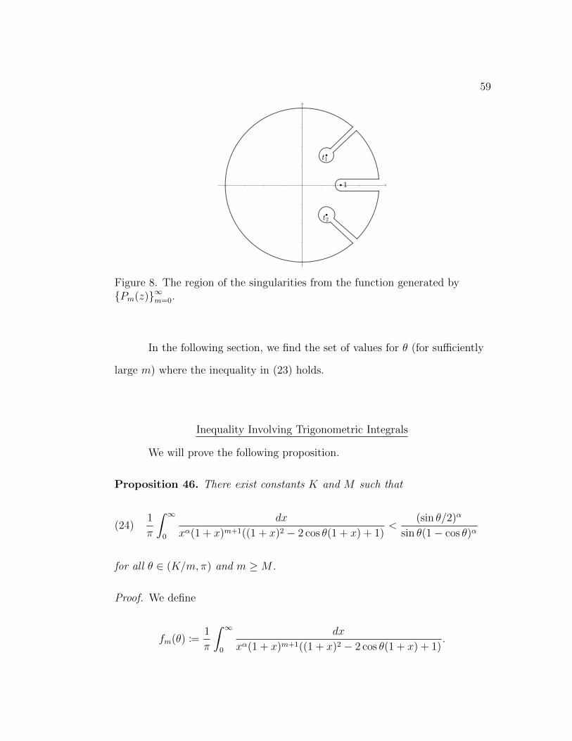
branch cut at t = 1. The primary value of θ of concern is when θ approaches

0. As θ → 0, then t1, t2 → 1, which is where we have a branch cut on the

contour region. When looking at the region shown in Figure 8, we note that

as θ → 0, then Pm(z(θ)) will diverge to infinity.

59

Figure 8. The region of the singularities from the function generated by{Pm(z)}∞m=0.

In the following section, we find the set of values for θ (for sufficiently

large m) where the inequality in (23) holds.

Inequality Involving Trigonometric Integrals

We will prove the following proposition.

Proposition 46. There exist constants K and M such that

(24)1

π

ˆ ∞0

dx

xα(1 + x)m+1((1 + x)2 − 2 cos θ(1 + x) + 1)<

(sin θ/2)α

sin θ(1− cos θ)α

for all θ ∈ (K/m, π) and m ≥M .

Proof. We define

fm(θ) :=1

π

ˆ ∞0

dx

xα(1 + x)m+1((1 + x)2 − 2 cos θ(1 + x) + 1).

60

Then we substitute 1 + x = eu to obtain

fm(θ) =1

π

ˆ ∞0

e−mudu

(eu − 1)α(e2u − 2eu cos θ + 1)

=1

π

ˆ ∞0

e−(m+α)udu

(1− e−u)α(e2u − 2eu cos θ + 1)

=1

π

ˆ ∞0

e−(m+α)uu−αg(u)du,(25)

where

f(u) :=

(u

1− e−u

)αand g(u) :=

f(u)

e2u − 2eu cos θ + 1.

Note that if θ is fixed, then one can apply Watson’s Lemma to obtain an

asymptotic formula that is nonuniform in θ for the integral in (25); however,

all of the asymptotic identities in the remainder of this paper are uniform in θ

in the sense that all of the Big-Oh constants are independent of θ. Since the

range of θ depends on m by the supposition, we cannot directly apply

Watson’s Lemma. Instead, we apply an elementary approach based on the

proof of Watson’s Lemma. For further details regarding uniform asymptotic

formulas for other important integrals, we refer the reader to [12].

Observe that f(u) = O(uα) as u→∞. We split the integral in (25) as

(26)

ˆ 1/√m

0

e−(m+α)uu−αg(u)du+

ˆ ∞1/√m

e−(m+α)u−αg(u)du.

61

We note that eu + e−u ≥ 2 for all u ∈ R since it reaches its global minimum of

2 at u = 0. Thus, for all u ∈ (0,∞), we have

e2u − 2eu cos θ + 1 = eu(eu + e−u − 2 cos θ)

≥ eu(2− 2 cos θ)

≥ 2− 2 cos θ.

Then, since 1− cos θ = O(θ2), we have that 2− 2 cos θ = O(θ2), so

1

2− 2 cos θ= O

(1

θ2

).

We can therefore bound the second integral in the expression in (26) as

∣∣∣∣ˆ ∞1/√m

e−(m+α)uu−αg(u)du

∣∣∣∣ = O(

1

θ2

ˆ ∞1/√m

e−(m+α)uu−αuαdu

)= O

(1

θ2

ˆ ∞1/√m

e−(m+α)udu

)= O

(e−√m

mθ2

).(27)

Since limu→0 f(u) = 1, we define g(0) := limu→0 g(u) = 1/(2− 2 cos θ). Then

by Mean Value Theorem, g(u) = g(0) + ug′(v) for some v ∈ (0, u), where

g′(v) =(e2v − 2ev cos θ + 1)f ′(v)− f(v)(2e2v − 2ev cos θ)

(e2v − 2ev cos θ + 1)2

≤ (e2v − 2ev cos θ + 1)f ′(u)

(e2v − 2ev cos θ + 1)2

=f ′(v)

e2v − 2ev cos θ + 1.

62

By the product and quotient rules for differentiation, we have that

f ′(v) = α

(v

1− e−v

)α−11− e−v(1 + v)

(1− e−v)2.

Then, since

limv→0

f ′(v) =α

2and lim

v→∞f ′(v) = 0,

we conclude that f ′(v) is bounded on (0,∞). Thus,

g′(v) = O(

f ′(v)

e2v − 2ev cos θ + 1

)= O

(1

θ2

).

We can now bound the first integral in (26) by using the substitution

g(u) = g(0) + ug′(v) coupled with the triangle and ML-inequalities to obtain

(28)

ˆ 1/√m

0

e−(m+α)uu−α|g(0)|du+

ˆ 1/√m

0

e−(m+α)uu1−α|g′(v)|du.

We apply Proposition 26 and the asymptotic relation for the upper

incomplete gamma function in (2) to the first integral in (28), which gives us

ˆ 1/√m

0

e−(m+α)uu−α|g(0)|du = O

(1

θ2

ˆ 1/√m

0

e−(m+α)uu−αdu

)

= O(

Γ(1− α)− Γ(1− α, (m+ α)/√m)

θ2m1−α

)= O

(1

θ2m1−α +(m+ α)−αe−(m+α)/

√m

θ2m1−3α/2

)= O

(1

θ2m1−α

).(29)

63

Similarly, the second integral in (28) gives us

ˆ 1/√m

0

e−(m+α)uu1−α|g′(v)|du = O

(1

θ2

ˆ 1/√m

0

e−(m+α)uu1−αdu

)

= O(

Γ(2− α)− Γ(2− α, (m+ α)/√m)

θ2m2−α

)= O

(1

θ2m2−α +(m+ α)1−αe−(m+α)/

√m

m(3−α)/2

)= O

(1

θ2m2−α

).(30)

Then, by Proposition 26, the sum of (29) and (30) yields

O(

1

θ2m1−α

)+O

(1

θ2m2−α

)= O

(1

θ2m1−α

).

Hence, ˆ 1/√m

0

e−(m+α)uu−αg(u)du = O(

1

θ2m1−α

).

Thus far, we have obtained the following upper bound

(31) fm(θ) = O(

1

θ2m1−α

).

We now put

h(θ) :=sin θ(1− cos θ)α

(sin(θ/2))α· 1

θ1+α,

and note that limθ→0 h(θ) = 1 and limθ→π h(θ) = 0, which implies that h(θ) is

bounded on the interval (0, π). Therefore,

(32)(sin(θ/2))α

sin θ(1− cos θ)α= O

(1

θ1+α

).

64

for θ ∈ (0, π). From this, we divide both sides of (31) by the respective sides

of (32) to obtain

sin θ(1− cos θ)α

(sin(θ/2))α· fm(θ) = O

(θ1+α

θ2m1−α

)= O

(1

(θm)1−α

).

Hence,

(33)sin θ(1− cos θ)α

(sin(θ/2))α· 1

π

ˆ ∞0

dx

xα((1 + x)2 − 2(1 + x) cos θ + 1)(1 + x)m+1

is at most a constant multiple of

1

(mθ)1−α.

Therefore, there exist constants K and M such that the expression in (33) is

less than 1 for all θ ∈ (K/m, π) and m ≥M .

Recall that we wanted to use the Intermediate Value Theorem to count

the number of zeros of Pm(z). Through Proposition 46 and the inequality in

(22), we obtain a useful corollary.

Corollary 47. With the constants K and M in Proposition 46, for all

θ ∈ (K/m, π) such that

∣∣∣∣sin((m+ 1)θ +α(θ − π)

2

)∣∣∣∣ = 1

the sign of Pm(z(θ)) is the same as the sign of sin

((m+ 1)θ +

α(θ − π)

2

)for

all m ≥M .

65

Thus, if we consider values of θ ∈ (K/m, π) where

∣∣∣∣sin((m+ 1)θ +α(θ − π)

2

)∣∣∣∣ = 1,

and if we can show that the sign of Pm(z(θ)) does indeed oscillate a countable

number of times on this interval, then we can apply the Intermediate Value

Theorem to prove that there is a constant C such that the number of zeros of

Pm(z) existing outside of (−1, 1) is at most C. We proceed to prove this in

the following theorem.

Zero Distribution

The goal of this section is to prove the following theorem.

Theorem 48. Let α ∈ R such that 0 < α < 1 and let {Pm(z)}∞m=0 be the

sequence of polynomials generated by

1

(1− t)α(1− 2zt+ t2)=

∞∑m=0

Pm(z)tm.

Then there exists a constant C (independent of m) such that the number of

zeros of Pm(z) outside (−1, 1) is at most C for all m ∈ N.

Proof. We may assume that Propositions 45 and 46 hold. Let n ∈ N ∪ {0}.

We consider the values of θn ∈ (K/m, π) such that

(34) sin

((m+ 1)θn +

α(θn − π)

2

)= ±1.

66

Thus, we must have that

(m+ 1)θn +α(θn − π)

2=

(2n+ 1)π

2=

(n+

1

2

)π.

This implies that

θn

(m+ 1 +

α

2

)=

(n+

1

2+α

2

)π,

and thus we have an expression for θn given by

θn =

(n+ 1

2+ α

2

)π

m+ 1 + α2

.

Since θn ∈ (K/m, π), we have

K

m<

(n+ 1

2+ α

2

)π

m+ 1 + α2

< π

⇔K(m+ 1 + α

2

)mπ

< n+1

2+α

2< m+ 1 +

α

2

⇔K(m+ 1 + α

2

)mπ

− 1 + α

2< n < m+

1

2.(35)

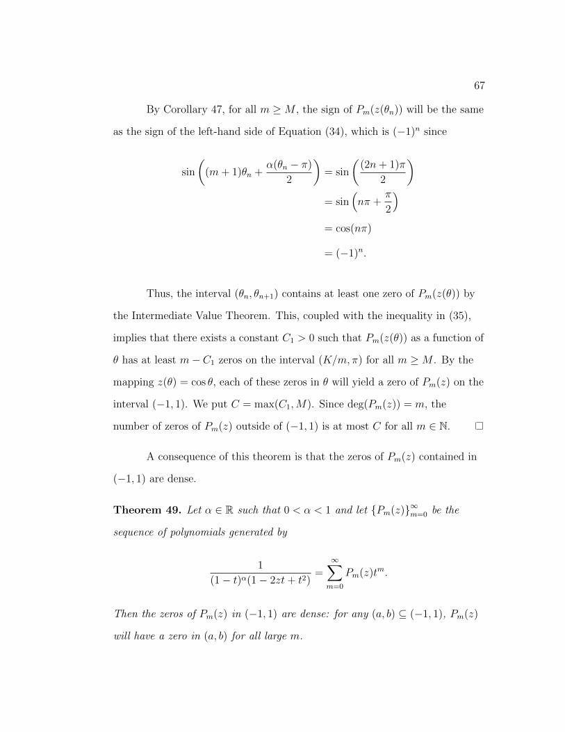
67

By Corollary 47, for all m ≥M , the sign of Pm(z(θn)) will be the same

as the sign of the left-hand side of Equation (34), which is (−1)n since

sin

((m+ 1)θn +

α(θn − π)

2

)= sin

((2n+ 1)π

2

)= sin

(nπ +

π

2

)= cos(nπ)

= (−1)n.

Thus, the interval (θn, θn+1) contains at least one zero of Pm(z(θ)) by

the Intermediate Value Theorem. This, coupled with the inequality in (35),

implies that there exists a constant C1 > 0 such that Pm(z(θ)) as a function of

θ has at least m− C1 zeros on the interval (K/m, π) for all m ≥M . By the

mapping z(θ) = cos θ, each of these zeros in θ will yield a zero of Pm(z) on the

interval (−1, 1). We put C = max(C1,M). Since deg(Pm(z)) = m, the

number of zeros of Pm(z) outside of (−1, 1) is at most C for all m ∈ N.

A consequence of this theorem is that the zeros of Pm(z) contained in

(−1, 1) are dense.

Theorem 49. Let α ∈ R such that 0 < α < 1 and let {Pm(z)}∞m=0 be the

sequence of polynomials generated by

1

(1− t)α(1− 2zt+ t2)=

∞∑m=0

Pm(z)tm.

Then the zeros of Pm(z) in (−1, 1) are dense: for any (a, b) ⊆ (−1, 1), Pm(z)

will have a zero in (a, b) for all large m.

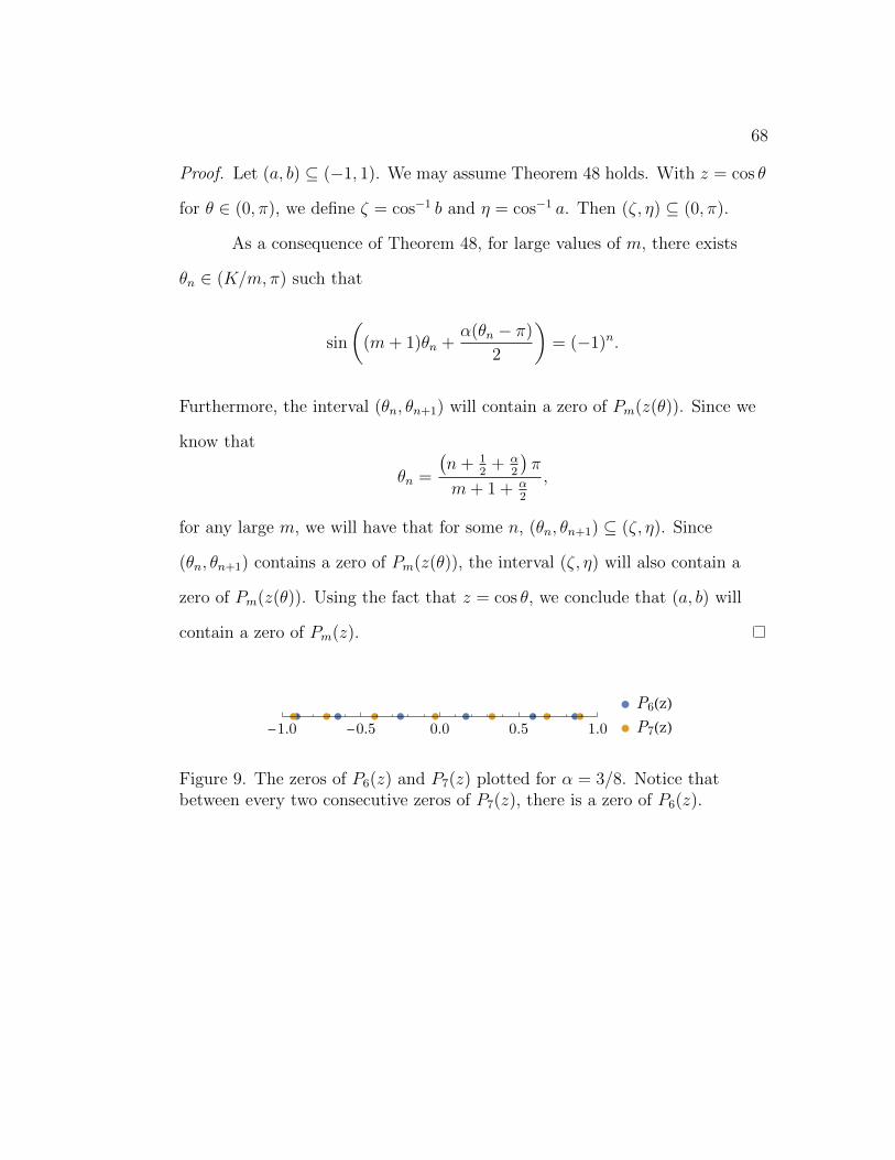
68

Proof. Let (a, b) ⊆ (−1, 1). We may assume Theorem 48 holds. With z = cos θ

for θ ∈ (0, π), we define ζ = cos−1 b and η = cos−1 a. Then (ζ, η) ⊆ (0, π).

As a consequence of Theorem 48, for large values of m, there exists

θn ∈ (K/m, π) such that

sin

((m+ 1)θn +

α(θn − π)

2

)= (−1)n.

Furthermore, the interval (θn, θn+1) will contain a zero of Pm(z(θ)). Since we

know that

θn =

(n+ 1

2+ α

2

)π

m+ 1 + α2

,

for any large m, we will have that for some n, (θn, θn+1) ⊆ (ζ, η). Since

(θn, θn+1) contains a zero of Pm(z(θ)), the interval (ζ, η) will also contain a

zero of Pm(z(θ)). Using the fact that z = cos θ, we conclude that (a, b) will

contain a zero of Pm(z).

-1.0 -0.5 0.0 0.5 1.0

P6(z)P7(z)

Figure 9. The zeros of P6(z) and P7(z) plotted for α = 3/8. Notice thatbetween every two consecutive zeros of P7(z), there is a zero of P6(z).

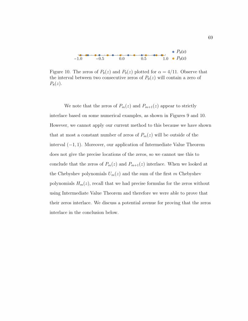
69

-1.0 -0.5 0.0 0.5 1.0

P8(z)P9(z)

Figure 10. The zeros of P8(z) and P9(z) plotted for α = 4/11. Observe thatthe interval between two consecutive zeros of P9(z) will contain a zero ofP8(z).

We note that the zeros of Pm(z) and Pm+1(z) appear to strictly

interlace based on some numerical examples, as shown in Figures 9 and 10.

However, we cannot apply our current method to this because we have shown

that at most a constant number of zeros of Pm(z) will be outside of the

interval (−1, 1). Moreover, our application of Intermediate Value Theorem

does not give the precise locations of the zeros, so we cannot use this to

conclude that the zeros of Pm(z) and Pm+1(z) interlace. When we looked at

the Chebyshev polynomials Um(z) and the sum of the first m Chebyshev

polynomials Hm(z), recall that we had precise formulas for the zeros without

using Intermediate Value Theorem and therefore we were able to prove that

their zeros interlace. We discuss a potential avenue for proving that the zeros

interlace in the conclusion below.

CONCLUSIONS

We began by exploring the famous sequence of orthogonal polynomials

known as the Chebyshev polynomials (of the second kind), denoted by

{Um(z)}∞m=0. Each polynomial has all real zeros on (−1, 1), which interlace

with the zeros of the next consecutive polynomial in the sequence.

Furthermore, the finite summation of these polynomials, {Hm(z)}∞m=0 where

Hm(z) =∑m

k=0 Uk(z), also have all real zeros on (−1, 1) that interlace with

the zeros of Hm+1(z). We modified the generating function of {Hm(z)}∞m=0 by

replacing the exponent of 1 on the term 1− t with α, where 0 < α < 1, to

obtain a new sequence of polynomials denoted by {Pm(z)}∞m=0. By applying

Cauchy’s product rule for multiplying power series, we found that these

polynomials took the form of being binomial combinations of the first m

Chebyshev polynomials. We used Cauchy’s Differentiation Formula and the

Residue Theorem to obtain an expression for Pm(z(θ)), where θ ∈ (0, π) and

z(θ) = cos θ, based on the singularities of the generating function. This

expression contained an indefinite (trigonometric) integral added to a

trigonometric ratio. We used the asymptotic behavior of both to prove the

existence of a constant K such that the integral will be smaller in magnitude

than the trigonometric ratio for all θ ∈ (K/m, π) for sufficiently large m.

These results were then applied to the main theorem, where we proved that

there is at most a constant (independent of m) number of zeros of Pm(z) that

lie outside of (−1, 1) for all m ∈ N.

A method of proving that for 0 < α < 1, the zeros of Pm(z) and

Pm+1(z) interlace is to apply the Hermite-Kakeya-Obreschkoff (HKO)

71

Theorem by fixing a, b ∈ R and looking at Qm := aPm(z) + bPm+1(z). We let

g = (1− t)−α(1− 2zt+ t2)−1. Then, we will have that

∞∑m=0

Qm(z)tm =∞∑m=0

(aPm(z) + bPm+1(z))tm

= ag +1

t

∞∑m=0

bPm+1tm+1

= ag +1

t

∞∑m=1

bPmtm

= ag +b

t(g − 1),

since P0(z) = 1. One could try applying the methods utilized in this paper to

the generating function ag + bt(g − 1) to prove that Qm(z) has all real zeros.

Then, as a consequence of the HKO Theorem, Pm(z) and Pm+1(z) will have

all real zeros and their zeros interlace.

We can extend our study to complex values of α to obtain a new

sequence of polynomials. If we momentarily assume that α is not fixed, we

obtain a sequence of bivariate polynomials given by

1

(1− t)α(1− 2zt+ t2)=

∞∑m=0

Cm(α, z)tm.

For every m, the coefficients of the polynomial will be real and have the form

m∑k=0

(α +m− k − 1

m− k

)Uk(z),

which is a polynomial in α and z. Based on initial numerical results from

Mathematica (see Figure 11), we propose the following open problem.

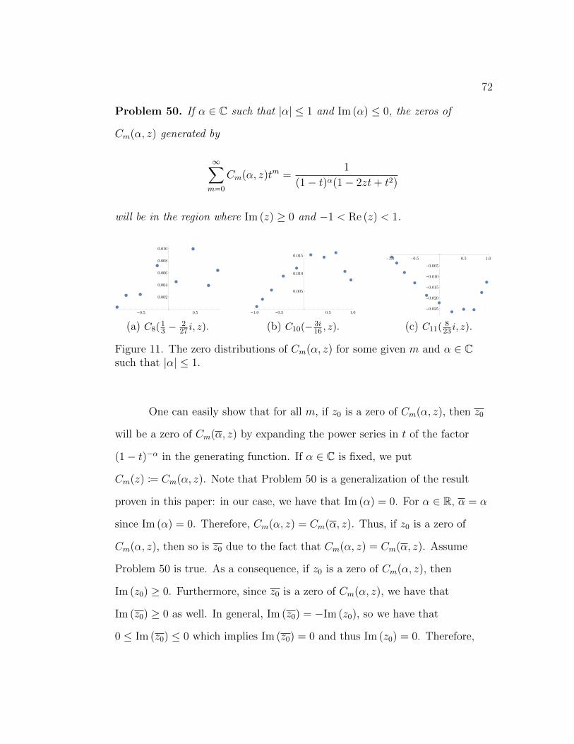
72

Problem 50. If α ∈ C such that |α| ≤ 1 and Im (α) ≤ 0, the zeros of

Cm(α, z) generated by

∞∑m=0

Cm(α, z)tm =1

(1− t)α(1− 2zt+ t2)

will be in the region where Im (z) ≥ 0 and −1 < Re (z) < 1.

-0.5 0.5

0.002

0.004

0.006

0.008

0.010

(a) C8(13 −

227 i, z).

-1.0 -0.5 0.5 1.0

0.005

0.010

0.015

(b) C10(− 3i16 , z).

-1.0 -0.5 0.5 1.0

-0.025

-0.020

-0.015

-0.010

-0.005

(c) C11(823 i, z).

Figure 11. The zero distributions of Cm(α, z) for some given m and α ∈ Csuch that |α| ≤ 1.

One can easily show that for all m, if z0 is a zero of Cm(α, z), then z0

will be a zero of Cm(α, z) by expanding the power series in t of the factor

(1− t)−α in the generating function. If α ∈ C is fixed, we put

Cm(z) := Cm(α, z). Note that Problem 50 is a generalization of the result

proven in this paper: in our case, we have that Im (α) = 0. For α ∈ R, α = α

since Im (α) = 0. Therefore, Cm(α, z) = Cm(α, z). Thus, if z0 is a zero of

Cm(α, z), then so is z0 due to the fact that Cm(α, z) = Cm(α, z). Assume

Problem 50 is true. As a consequence, if z0 is a zero of Cm(α, z), then

Im (z0) ≥ 0. Furthermore, since z0 is a zero of Cm(α, z), we have that

Im (z0) ≥ 0 as well. In general, Im (z0) = −Im (z0), so we have that

0 ≤ Im (z0) ≤ 0 which implies Im (z0) = 0 and thus Im (z0) = 0. Therefore,

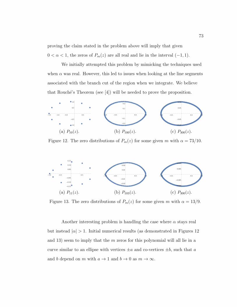
73

proving the claim stated in the problem above will imply that given

0 < α < 1, the zeros of Pm(z) are all real and lie in the interval (−1, 1).

We initially attempted this problem by mimicking the techniques used

when α was real. However, this led to issues when looking at the line segments

associated with the branch cut of the region when we integrate. We believe

that Rouche’s Theorem (see [4]) will be needed to prove the proposition.

-1.5 -1.0 -0.5 0.5

-1.0

-0.5

0.5

1.0

(a) P10(z).

-1.0 -0.5 0.5 1.0

-0.2

-0.1

0.1

0.2

(b) P100(z).

-1.0 -0.5 0.5 1.0

-0.10

-0.05

0.05

0.10

(c) P300(z).

Figure 12. The zero distributions of Pm(z) for some given m with α = 73/10.

-1.0 -0.5 0.5

-0.15

-0.10

-0.05

0.05

0.10

0.15

(a) P11(z).

-1.0 -0.5 0.5 1.0

-0.02

-0.01

0.01

0.02

(b) P103(z).

-1.0 -0.5 0.5 1.0

-0.010

-0.005

0.005

0.010

(c) P300(z).

Figure 13. The zero distributions of Pm(z) for some given m with α = 13/9.

Another interesting problem is handling the case where α stays real

but instead |α| > 1. Initial numerical results (as demonstrated in Figures 12

and 13) seem to imply that the m zeros for this polynomial will all lie in a

curve similar to an ellipse with vertices ±a and co-vertices ±b, such that a

and b depend on m with a→ 1 and b→ 0 as m→∞.

REFERENCES

[1] George B. Arfken and Hans J. Weber, Mathematical methods forphysicists, 5th ed., Harcourt/Academic Press, Burlington, MA, 2001.

[2] Herman Bavinck, On the zeros of certain linear combinations ofChebyshev polynomials, Proceedings of the International Conference onOrthogonality, Moment Problems and Continued Fractions (Delft, 1994),1995, pp. 19–26, DOI 10.1016/0377-0427(95)00098-4.

[3] Julius Borcea and Petter Branden, Polya-Schur master theorems forcircular domains and their boundaries, Ann. of Math. (2) 170 (2009),no. 1, 465–492, DOI 10.4007/annals.2009.170.465.

[4] Stephen D. Fisher, Complex variables, Dover Publications, Inc., Mineola,NY, 1999. Corrected reprint of the second (1990) edition.

[5] Steve Fisk, Polynomials, roots, and interlacing (2008).arXiv:math/0612833v2 [math.CA].

[6] Theodore W. Gamelin, Complex analysis, Undergraduate Texts inMathematics, Springer-Verlag, New York, 2001.

[7] Zinoviy Grinshpun, Special linear combinations of orthogonalpolynomials, J. Math. Anal. Appl. 299 (2004), no. 1, 1–18, DOI10.1016/j.jmaa.2004.04.062.

[8] Peter Henrici, Applied and computational complex analysis. Vol. 1, WileyClassics Library, John Wiley & Sons, Inc., New York, 1988. Powerseries—integration—conformal mapping—location of zeros; Reprint ofthe 1974 original; A Wiley-Interscience Publication.

[9] Earl D. Rainville, Special functions, The Macmillan Co., New York, 1960.

[10] H. L. Royden, Real analysis, 3rd ed., Macmillan Publishing Company,New York, 1988.

[11] Dragan Stankov, On linear combinations of Chebyshev polynomials, Publ.Inst. Math. (Beograd) (N.S.) 97(111) (2015), 57–67, DOI10.2298/PIM150220001S.

[12] Nico M. Temme, Asymptotic methods for integrals, Series in Analysis,vol. 6, World Scientific Publishing Co. Pte. Ltd., Hackensack, NJ, 2015.

75

[13] David G. Wagner, Multivariate stable polynomials: theory andapplications, Bull. Amer. Math. Soc. (N.S.) 48 (2011), no. 1, 53–84, DOI10.1090/S0273-0979-2010-01321-5.

[14] William P. Ziemer, Modern real analysis, 2nd ed., Graduate Texts inMathematics, vol. 278, Springer, Cham, 2017. With contributions byMonica Torres.

Fresno State Non-exclusive Distribution License (Keep for your records) (to archive your thesis/dissertation electronically via the Fresno State Digital Repository)

By submitting this license, you (the author or copyright holder) grant to the Fresno State Digital Repository

the non-exclusive right to reproduce, translate (as defined in the next paragraph), and/or distribute your

submission (including the abstract) worldwide in print and electronic format and in any medium, including

but not limited to audio or video.

You agree that Fresno State may, without changing the content, translate the submission to any medium or format for the purpose of preservation.

You also agree that the submission is your original work, and that you have the right to grant the rights

contained in this license. You also represent that your submission does not, to the best of your knowledge,

infringe upon anyone’s copyright.

If the submission reproduces material for which you do not hold copyright and that would not be

considered fair use outside the copyright law, you represent that you have obtained the unrestricted

permission of the copyright owner to grant Fresno State the rights required by this license, and that such

third-party material is clearly identified and acknowledged within the text or content of the submission.

If the submission is based upon work that has been sponsored or supported by an agency or organization

other than Fresno State, you represent that you have fulfilled any right of review or other obligations

required by such contract or agreement.

Fresno State will clearly identify your name as the author or owner of the submission and will not make

any alteration, other than as allowed by this license, to your submission. By typing your name and date

in the fields below, you indicate your agreement to the terms of this use. Publish/embargo options (type X in one of the boxes).

Make my thesis or dissertation available to the Fresno State Digital Repository

immediately upon submission.

Embargo my thesis or dissertation for a period of 2 years from date of graduation. After 2 years, I understand that my work will automatically become part of the university’s public institutional repository unless I choose to renew this embargo here:

fsdr-discuss@csufresno.edu

Embargo my thesis or dissertation for a period of 5 years from date of graduation. After 5 years, I understand that my work will automatically become part of the university’s public

institutional repository unless I choose to renew this embargo here:

fsdr-discuss@csufresno.edu

Type full name as it appears on submission

Date

Summer F. Al Hamdani

April 19, 2021

X