,;

'

S 1-D~

Thermo-fluid analysis in the built environment: expectations and limitations

F ALAMDARI, BSc, MSc, PhD, CEng, MCIBSE Thermo-Fluid Energy Ltd, North Crawley, Buckinghamshire UK.

SYNOPSIS - Since the late 1970's, advanced computer models have been developed for the prediction of air flow, field temperature and pressure distributions, smoke (or other contaminate) dispersion, in the con­text of the built environment. These models are based on the established numerical techniques known as computational fluid dynamics (CFD). The complex nature of CFD models has made them far more difficult to use than the CAD and HV AC software tools currently used by architects and building services engineers.

The need for building and environmental rnicroclimate analysis (using CFD calculation methods) is out­lined, together with the capabilities, limitations, costs and userfriendliness of computational fluid dynamics software.

NOTATION

a c D k

Siii

SP1S'P

uj

xj

~

coefficients in discretization equations convective term in discretization equations diffusion term in discretization equations turbulence kinetic energy (m2s-2)

sources or sinks of variable ~

coefficients in linearised sources or sinks in discretization equations time (s) time-averaged velocity components in the

coordinate direction xj (m s-1)

coordinate directions (m)

any dependent variable

r 41 effective diffusion coefficients for each ~

p fluid density (Kg m-3)

a (IPenl) weighting function p and n indices, denoting respectively, central and

neighbouring nodes in domain discretization grid

INTRODUCTION

In recent yenrs, advances in computer-aided engineering de­sign have been accompanied by a proliferation of applica­tions in the built enl•ironment. notably in architectural design and structural analysis. Si.nee the rnid-l970's a num­ber of sophisticated dynamic building energy simulation programs have been developed, which are now being taken up by the building industry. Those for computational fluid dynamics (CFD), however, have moved relatively more slowly. The reason for this is that the mathematicaJ repr~ sentation of the physics of fluid flow, and the numerical so­lution procedures used in CFD models are far from simple.

The author and his co-workers developed a range of thermo­fluid calculation methods for determining air flow and convective heat transfer in and around buildings over the period 1980-1986. The emphasis was placed on meeting the needs of thermal simulation programs for accurate input data in convective heat exchange in and around buildings. The calculation methods ranged from 'lower-level' ap­proaches, including analytical solutions and elaborate data correlations for limiting cases (see, for example, (1)), to the development of a 'higher-level' flow model, using CPD techniques to the solution of the governing partial differen­tial equations for microclimate analysis of building enclo­sures (2). This program, known as the ESCEA T <E.lliptic Equation .S.olver for .Convection and H-'it .D:ansfer) code. Both the lower and higher-level models have been used to develop and verify 'intermedfate-level' computer codes, which formed the basis for generating input convective heat transfer data for dynamic building models (3) and (4).

In the present contribution, the environmental and building services requirements for predicting airflow and related phe­nomena, such as convective heat transfer and smoke move­ment, in the context of the building environment are out­lined, together, with the capabilities, limitations, costs and userfriendliness of the current CFD software for microcli­mate design of buildings.

2 BUILDING AND ENVIRONMENTAL PERFORMANCE ANALYSIS

Industry and commerce have evolved stringent needs for environmental control which demands ever more sophisticated design methodologies. Design issues, such as energy consciousness, thermal comfort. environmental qual­ity and hazard have produced demands for change of building design in order to reduce their negative impact on energy consumption, human comfort, safety and the "green" environment. These are largely influenced by the thennal behaviour of the buildings structure and air movement in and around buildings.

5

Predicting the actual energy consumed by a building is a complex function of prevailing climate influences, environmental requirements, building fabric, plant and control systems. In the last decade it has become increasingly recognised lhat in order to deve.lop realistic methods for energy-conscious design of buildings it is necessary to model the dynamic energy perfonnance of the system (5). These dynamic models require a computational solution, in contrast to the manual-calculation methods used with the traditional steady-state procedures. Thermal models are capable of providing the detailed infonnation necessary to configure effective solutions for thennal design and management of buildings. However. a weakness in these models is that the emphasis has been placed on dynamic thennal performance of the fabric, while airflow and con­vective heal exchange in and around the building are modelled using only rough approximation (4). In addition, they provide only an averaged space air velocity and tem­perature, rather than the field values of these variables, which are required for thermal comfort and safety assessment of the environment

Jn recent years, the need for environmental quality and hazard analysis within building spaces has taken a high profile in the design and maintenance of controlled and acceptable environments. This need has been particularly amplified by the adoption of features such as atria in building complexes, passive solar buildings and complex shopping centres which create further dilemma in the pre­diction of airflow and temperature distribution. Until recently, the only methods for obtaining a realistic prediction of the air/smoke movement, temperature and pressure distribution in and around buildings were to perform field measurements or to use models in wind­tunnels. Both of these traditional approaches are costly nnd time-consuming. In addition, the data and infonnation obtained by these methods is rather limited and does not always yield all the designers' requirements.

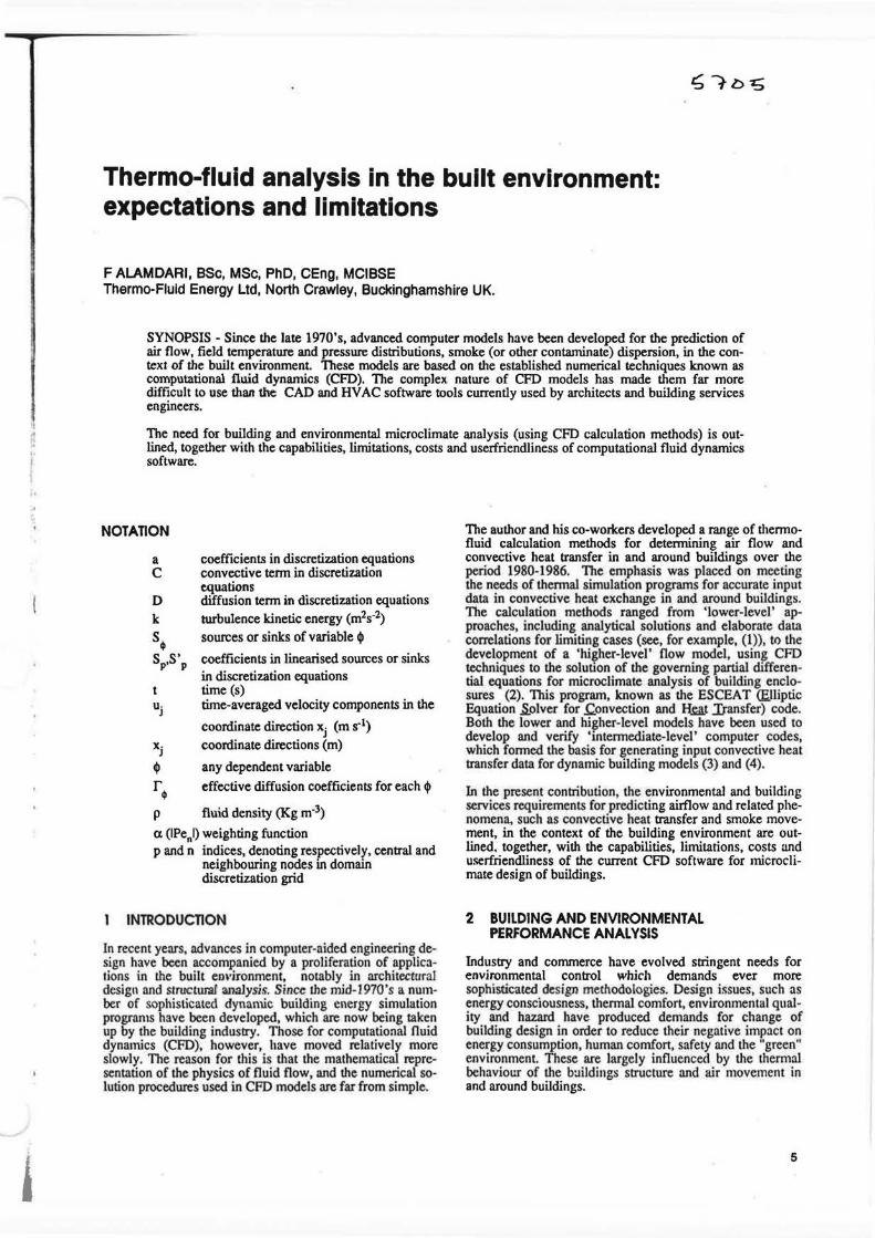
In grinciple, CFO models are capable of providing, both heat transfer data required by thennal models and the de­tailed infonnation necessary to assess environmental performance. The interrelationship between the dynamic lhennal models and microclimate models is illustrated by the schematic diagram shown in Figure 1. The link between the two models is shown by shaded arrows and the iterative process of updating convective heat transfer data in thennal model and boundary conditions in CFO model is represent­ed in Figure 1 by dashed Jines.

In Jl.11KlkL CFD models have a number of limitations (see section 3), and are very costly in tenns of computing resources. The author and his co-workers have argued (see. for example, (4)) that 'intermediate-level' models offer the best prospect of meeting the needs of dynamics thermal models, in terms of economy and userfriendJiness for providing convective heat transfer data. 1l1erefore, CFO models should be used as an independent tool for environ­ment thermal comfort and safety assessment, rnth~r than being integrated into the thermal models.

3 COMPUTATIONAL FLUID DYNAMICS MODELS

3. 1 Background

6

All therm.o-fluid problems are governed by the principles of conservation of mass, momentum, themial energy and chemical species. These 'conservation laws' may each be expressed in tenns of partial differential equations, the solu­tion of which provides the basis for the computational fluid dynamics (CFO) model. CFO models solve, numerically, the governing conservation equations in order to generate field values for the velocity components, the static pressure, the temperature and concentration of chemical species. The

Building Design Conditions

r······················-~" ;.J·; I ~enn~ Energy Model I 's, '('-·· . . ! 1: s i a I $ ·1 ~ : ..... ~-····-········ t1 J ~: : 1 f g ! Building Energy Performance i i5 i ! ~ j AnaljlSJ•·s ___ _.

j ~ f j aj j .~ ! i i ! Space Design Conditions ! fl i I x ! i ~ i t' iii } ....... ~ ....... ~,. • o ••• 1 I j U ! Microclimate Model (CFO) ......... 1 .. ~

~"~-············---·-···· Environmental Perfonnance

Analvsis

TIIE BUILT ENVIRONMENT

·I ~ .~ ~ ....

~ !XI

.g

! f

Fig 1 Interrelationship between the thermal energy and the microclimate models

governing equations for air flow, thermal field and concen­tration species may be represented by a common fonn, using tensor notation (6):

a (p</JJ 1 iJt +a (pui <PJ 1 axi = a f I'; (o</JliJx} J 1 axi +s; (1)

where uj are the time-averaged velocity components in the

coordinate direction xj• q, are any of the dependent variables,

r; are the effective diffusion coefficients, S; are the sources

or sinks, p is the fluid density, and t is time.

These governing flow equations are strongly inter-linked with no obvious equation available for the static pressure that appears in the momentum equations. Therefore, it is necessary to use numerical solution techniques for their solution. The numerical solution of the governing .flow equations requires some discretization of the flow domain into a finite set of elemental or control volumes, formed by computational grid (2) and (6). The differential equntions may then be integrated over each el~mental volume of the computational grid. This leads to a set of algebraic equa­tions in the following finite-volume form:

(ap - S'p) </Jp = 1:, a,,4',, +Sp (2)

a,,= D,, a(/Pej) + [{ 0, ±C,,/]

aP =I,, a,.

where, indices p and 11 denote the central computational grid point nnd its neighbouring points respectively, C and D in­dicate the strength of the convection and diffusion respec-

tively, a (/Pe,/) is a weighting function, and the symbol {{a,b]], denotes the greater of a and b. The source tenn Sil>

in Equation I is evaluated using a linearised expression

(SP +S' p</Jp) in order to enhance numerical stability.

I

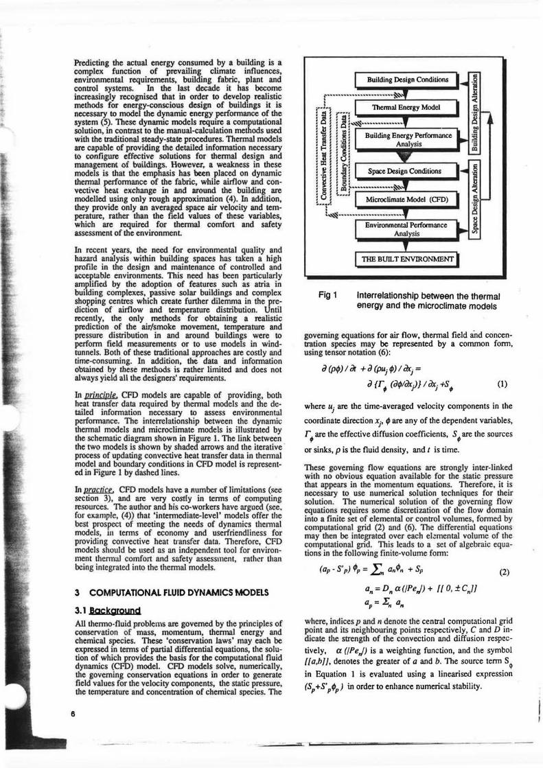
These algebraic equations are then solved in a finite-volume CFD model by an iterative manner (sec Figure 2). The itera­tive solution continues until the imbalance or error in the equations is sufficiently small to be considered negligible.

Inpnt data & inillal values for all +

Repeat for inner iteration

1.-1 Repeat for outer iteration

End of solution

Fig 2 Iterative solution sequence

3.2 Cgogbl!lfles Today, CFD codes have grown much in complexity, taking advantage of the speed and power of new computers, and can offer a powerful and versatile computer-aided-engineer­ing design tool. In the most general form these codes are potentially capable of handling time-dependent, turbulent, chemically reacting, compressible, non-Newtonian, multi­phase flows in complex geometries. Heat exchange by means of convection, conduction and radiation in both fluid and solid and the effect of thermal buoyancy and gravita­tional forces can be studied.

The commonality of the thermo-fluid processes in applica­tion area.'!, and the form of the governing equations, allow the same CPD code to be used in a number of engineering practical situations, for example:

(] External aerodynamics of aircraft, motor cars, ships

(] Heat transfer and combustion processes within internal-combustion or gas-turbine engines

(] Thermal-hydraulics of nuclear reactors, steam generators, condensers, etc.

In the context of the built environment, CFD models may be used as an efficient and powerful tool for:

(] Air movement and thermal comfort assessment This is an important aspect of air conditioning per­formance analysis and preventing problems, such as 'sick building syndrome', which arc mainly as­sociated with poor air movement and temperature distribution within the space.

(] Smoke and other pollutants movement analysis The effectiveness and performance of the ventila­tion system in removing the smoke as a result of fire or other contaminants is important in the safe design of buildings.

(] Convective heat exchange calculation The accuracy in the thermal energy performance analysis of buildings is limited by uncertainties in data, particularly for convective heat transfer rates (sec Section 2).

In addition to the above, CFD may be used to predict thermo-fluid phenomena in the natural environment, such as:

(] Pollution analysis The spread of smoke and other pollutants dis­charged from chimney or chemical plant into the atmosphere, the dispersion of sewage in the ocean, etc.

(] Climatic analysis The prediction of atmospheric gravity-influenced turbulent flows, analysis of microclimate effects on humans, etc.

Those CFD codes that could be used in all of the above application areas and more arc categorised as 'general purpose' CFO programs. Most of U1~se codes are notoriously difficult to use. However, in the last few yenrs, the advances in computer graphics have enhanced the userfriendliness of most of these codes. Furthermore, a range of 'special-purpose' CFO codes have been developed and optimized for particular application areas.

3.3 Aoollcatlons In the Bultt Eny!ronment Computational fluid dynamics models, have a wide range of ·application areas in buildings, some of which are given below:

(] Atria Atria with large glazing have gained popularity within the new architectural design of office com­plexes. CFO can be used to analyse the environ­mental pcrfonnance under various summer and winter climatic conditions for over-heating and cold down-draughts respectively.

(] Art galleries and museums Poor air movement. temperature and humidity dis­tribution in art galleries and museums may dam­age paintings and other expensive displays. There­fon; CFD simulation has a high potential in de­sign and maintenance of these environments.

(] Shopping centres, Tunnels, Airport terminals, etc. In addition to analysis of heating, cooling and ven­tilation of these spaces. CFO simDlation can be used as aJ'owerful tool to predict the smoke move­ment an spread of fire. Jn recent years, this exercise has taken a high profile in the design and control of safe public building enclosures.

7

;-

i

• · ~

0 Air conditioned offices. CFO is a useful tool in predicting the flow pattern and temperature distribution within mechanically­or naturally-ventilated rooms. The performance and position of the air supply and exhaust diffusers, or radiators, etc. can be optimized.

0 Clean rooms and Operating thea.tres. In the design of tightly controlled environments, CFO simulation may be used to predict the flow pattern and contaminant movement.

0 /11dustria/ buildings. . CFO sUllulation may be used to predict the perfor­mance of the ventilation and air distribution system within industrial buildings. The simulation could include the heat distributed from machinery, the movement of flying dust, etc.

3.4 Modelllng Regy!rements & Limitations

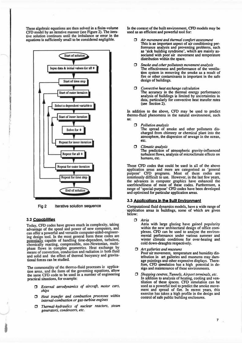
Geometrical aspects The first step in the solution of Equations (2) is the discreti­zation of the flow domain, and the definition of the points at which variables are located. Discretization of the flow domain must conform to the boundaries in such a way that boundary conditions can be accurately represented and allow the computational cells to be small in regions with steep property gradients, such as near the walls, around ob­stacles, regions with high curvature, etc. Domain discretization is provided by a computational grid, generat­ed using an appropriate coordinate system. Most building spaces may be discretized by using rectangular cells (or elemental-volwnes) and adopting simple Cartesian coordi­nate system. However, some difficulties may arise in specifying angled or curved surfaces, which have to be rep­resented by 'besr stt.p-wise' fit to a grid and blocking off ceJJs (see, for ex.ample, Figure 3). The CFD models using this approach are very efficient in running time, but the ac­curacy of the solution may be affected.

8

Blocked off cells

Fig 3 Non-uniform Cartesian grid

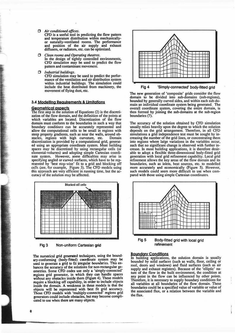
The numerical grid generared techniques, using the bound­ary-confonning (body-fitted) coordinate system may be used to generate a grid to fit irregular boundaries. This en­hances the accuracy of the solutions for non-rectangular ge­ometries. Some CFO codes use only a 'simply-connected' regions grid generator, in which they can handle spaces without any obstacles inside them (Figure 4). These models require a blocking off capability, in order to include objects inside the domain. A weakness in these models is that the objects will be represented with best fit grid accuracy. Those CFO models with 'multiply-connected' regions grid generators could include obstacles, but may become compli­cated to use when there are many objects.

' ~ ~~ : .//~

""v "'.:::: "'v r--"- ......_ i,..- i--.._

- -

Fig 4 'Simply-connected' body-fitted grid

The new generation of 'composite' grids consider the flow domain to be divided into sub-domains (sub-regions), bounded by generally curved sides, and within each sub-do­main an inclividuaJ coordinate system being generated. The ove.ra.ll coordinate system, covering the entire domain, is then formed by joining the sub-domains at the sub-region boundaries (7).

The accuracy of the solution obtained by CFO simulation usually relies heavily upon the degree to which the solution depends on the grid arrangement. Therefore, in all CFO simulations a grid independence test must be sought by in­creasing the number of the grid lines, or concentrating them into regions where large variations in the variables occur, such that no significant change is observed with further in­crease. In most building applic-ations, it is therefore desir­able to adopt a flexible three-dimensional body-fitted grid generation with local grid refinement capability. Local grid refinement allows the key areas of the flow domain and its boundaries, such as inlets, heat sources, etc. to modeUed more accurately and economically (Figure 5). However, such models could seem more difficult to use when com­pared with those using simple Cartesian coordinates.

Fig5

N-1 I I I I I 11

Body-fitted grid with local grid refinement

·eoyndgry Conditions In building applications, the solution domain is usually bounded by solid surfaces (such as walls, floor, ceiling or roof, doors and windows) and fluid surfaces (such as air supply and exhaust registers). Because of the 'elliptic' na­ture of the flow in the built environment, the condition at any point in the flow can be influenced by other points. Therefore, it is necessary to supply boundary conditions for all variables at all boundaries of the flow domain. These boundaries could be a specified value of variable or value of the associated flux, or a relation between the variable and the flux.

-- . -·-------

j ' " : • f t

f

The time-dependent interaction between the external condi­tions, building structure fabric and internal conditions, means that the domain boundary conditions vary with time. Therefore, it is desirable to linlc a CFO model with a dy­namic thermal model (see Figure 1). However, since CFO models require a sophisticated iterative solution procedure (see Figure 2) on very small time scale (ie. seconds rather than the hours that are usually used by thermal models), this link could increase the computer execution time dramatically (8). Some compromises may made on th~ scale of interaction, for example, performing steady-state CFD simulation for every few hours of thermal model simulation and using the results of previous CFD simulation for the initialization of the domain.

Time-dependent flow simula1ions usually require substan1ial computing resources, therefore, in practice, boundary conditions may be assumed to be steady-state, based on Chi! analytical or experimental results, except when CPD is used to predict the dispersion time of gases or smoke; for example, in evacuation time analysis.

In turbulent flows, viscous and turbulent stresses are of the same order of magnitude near the wall. This forces the val­ues of turbulent transport properties to fall to their laminar values and the resuh is a steep, non-linear varfation with distance from the wall in dependent variables and their gra­dients. Most CPD models use the so-called 'wall-functions' in order to bridge the steep property gradients close to the solid surfaces (9). These are based 6n the bilogarithmic be­haviour of the mean velocity and temperature near solid walls. The present gener.nion of wall-functions are not ap­propriate for recirculating flows and will give rise to error in, for example, heat transfer calculations (10).

flow Type The transient radiation, conduction and convection heat transfer processes in and a.round buildings gives rise to very complex fluid flow problems. The airflow around buildings are usuaJJy turbulent flows, while the Reynolds numbers (the ratio of inertia to viscous forces) for most flows within the built environment are in the transition range. Even in the turbulent regime, there is currently no universal turbu­lent model available that can reflect the behaviour of the full r:inge of complex turbulent flows obseived in buildings (11).

In turbulent flows, the closure of the governing equations (Equation 1), may be achieved by using a 'turbulence model'. The most commonly used turbulence model is the k·e model, which involves the solution of two additional paniaJ differential equations for the turbulence kinetic ener­gy (k) and its dissipation rate (e). Other models such as Reynolds stress and large-eddy simulation models (12-14) may be used to achieve greater accuracy (depending on the application), but they increase complexity and require more computing resources.

Buoyancy effects are common in the built environment, and should be incorporated into discretization equations. In most building applications, air density can be assumed constant throughout the flow domain. Therefore, buoyancy effects may be introduced into the solution by the adoption of the so-called Boussinesq approximation (see for example (2)). However, this usually reduces the rate of convergence.

Solution and Controls The solution method shown in Figure 2, is aimed at solving a set of nonlinear, interlinked equations in an iterative, 'point-by-point' or 'line-by-line' manner. In this method, it is necessary to examine how the current solution approxi­mates to the exact solution of Equation 2 at the end of each iteration, for each variable. Therefore, convergence criteria may be defined, for example, to be based on the imbalance source for Equation 2.

TI1e iterative solution should, in principle, handle any non­linear and interlinked equations. However, th.e use of some form of under-relaxation is found to be very useful, with 'cell-by-cell' or 'line-by-line' iterative solution methods. It reduces the magnitude of current error level in the field, while preventing the divergence in the iterative solution of the equations. There are several ways of introducing under­relaxation, for example, 'linear' approaches via relaxation factors and 'inertia' methods, by introducing inertia tenns into the discretized equations. However, there are no gener­al rules for describing the optimum values of relaxation fac­tor and inertia term. Suitable under-relaxation factors or 1erms can be found by experience and from exploratory computations for given problems.

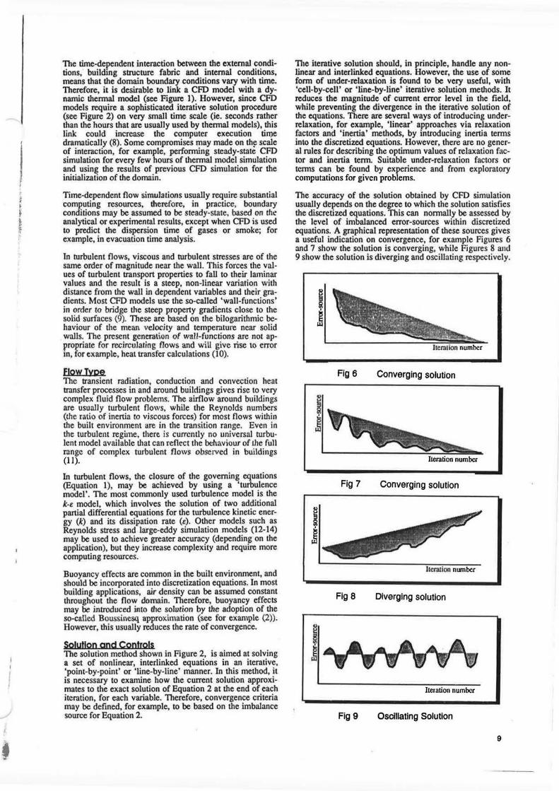
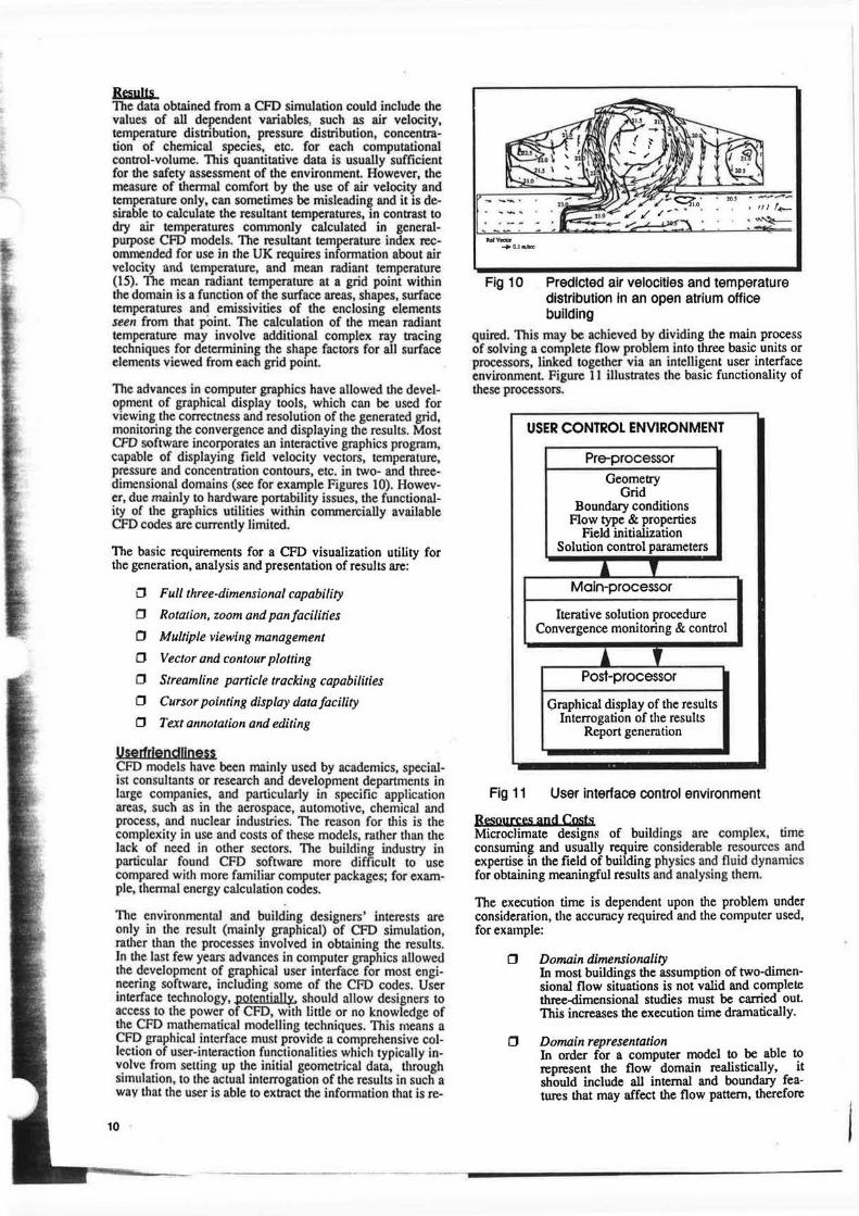
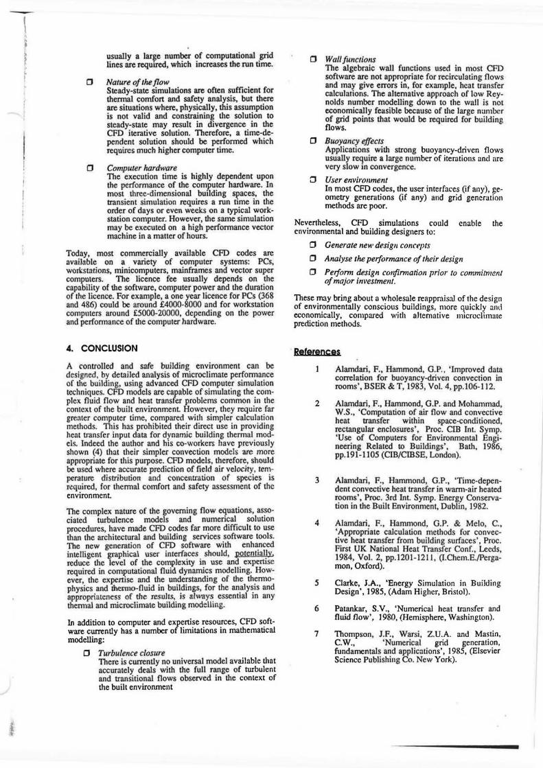
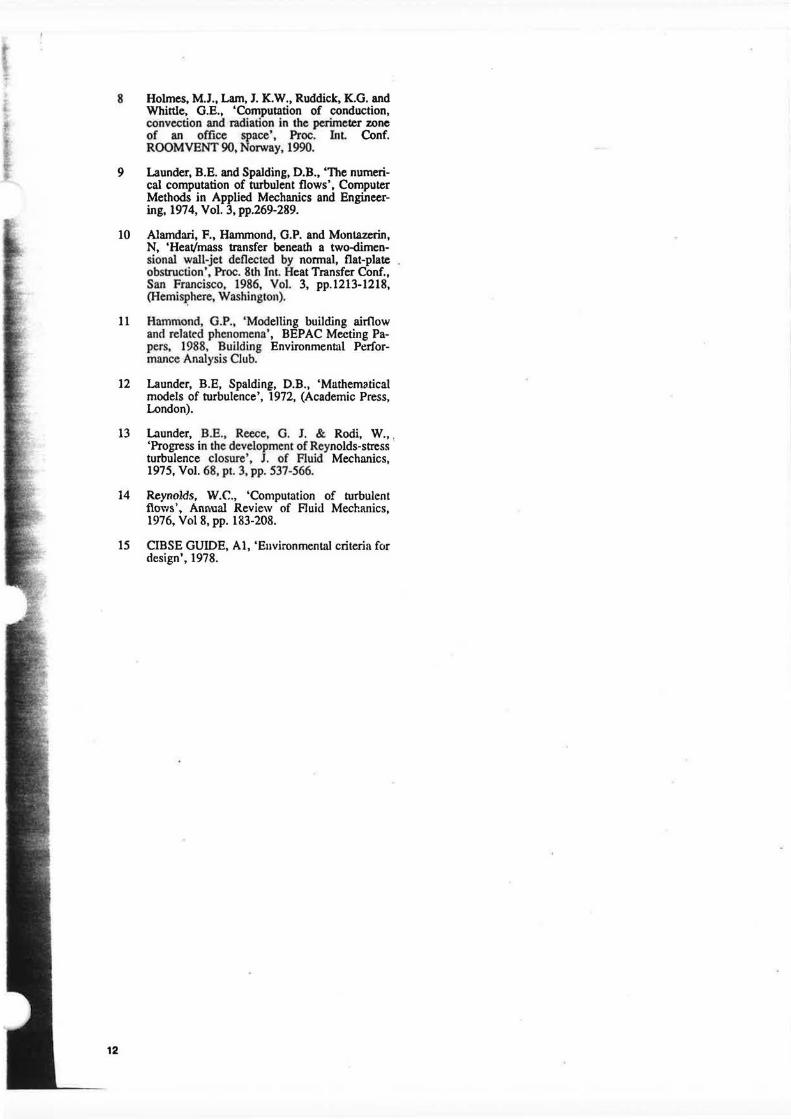
The accuracy of the solution obtained by CFD simulation usually depends on the degree to which the solution satisfies the discretized equations. This can normally be assessed by the level of imbalanced error-sources within discretized equations. A graphical representation of these sources gives a useful indication on convergence, for example Figures 6 and 7 show ·the solution is converging, while Figures 8 and 9 show the solution is diverging and oscillating respectively.

1 l1cra1ion number

Fig 6 Converging solution

Iteration number

Fig 7 Converging solution

l!eration nwnber

Fig 8 Diverging solution

Iteration number

Fig 9 Oscillating Solution

9

Rw&Ia The data obtained from a CFD simulation could include the values of all dependent variables, such as air velocity, temperature distribution, pressure distribution, concentra­tion of chemical species, etc. for each computational control-volume. This quantitative data is usually sufficient for the safety assessment of the environment. However, the measure of thermal comfort by the use of air velocity and temperature only, can sometimes be misleading and it is de­sirable to calculate the resultant temperatures, in contrast to dry air temperatures commonly calculated in general­pwpose CFO models. The resultant temperature index rec­ommended for use in the UK requires information about air velocity and temperature, and mean radiant temperature (15). The mean radiant temperature at a grid point within the domain is a func.tion of the surface areas, shapes, surface temperatures and emissivities of the enclosing elements seen from that point The calculation of the mean radiant temperature may involve additional complex ray tracing techniques for determining the shape factors for all surface elements viewed from each grid point.

The advances in computer graphics have allowe.d the devel­opment of graphical display tools, whkh can be used for viewing the correctness and resolution of the generated grid, monitoring the convergence and displaying the results. Most CFO software incorporates an interactive graphics program, capable of displaying field velocity vectors, temperature, pressure and concentration contours, etc. in two- and three­dimens.ional domains (see for example Figures 10). Howev­er, due mainly to hardware portability issues, the functional­ity of the graphics utilities within corrunercially available CFO codes are currently limited.

The basic requirements for a CFO visualization utility for the generation, analysis and presentation ofresults are:

CJ Full three-dimensional capability

D Rotation, zoom and pan facilities

D Multiple viewing management

D Vector and contour plotting

D Streamline particle tracki11g capabilities

D Cursor pointing display data facility

D Text annotation and editing

Userfrlendllness CPD models have been mainly used by academics, special­ist consultants or research and development departments in large companies, and particularly in specific application areas, such as in the aerospace, automotive, chemical and process, and nuclear industries. The reason for this is the complexity in use and costs of these models, rather than the lack of need in other sectors. TI1e building industry in particular found CFO software more difficult to use compared with more familiar computer packages; for exam­ple, thennal energy calculation codes.

TI1e environmental and building designers' interests are only in the result (mainly graphical) of CFO simulation, rather than the processes involved in obtaining the results. In the last few years advances in computer graphics allowed the development of graphical user interface for most engi­neering software, including some of the CFD codes. User interface technology, potentially, should allow designers to access to the power of CFO, with little or no knowledge of the CFO mathematical modelling techniques. This means a CFO graphical interface must provide a comprehensive col­lection of user-interaction functionalities which typically in­volve from selling up the initial geometrical data, through simulation, to the actual interrogation of the results in such a way that the user is able to extract the infonnation thnt is re-

10

-------------· -- --

w v­-+O.lm/aee

Fig 10 Predicted air velocities and temperature distribution in an open atrium office building

quired. This may be achieved by dividing the main process of solving a complete flow problem into three basic units or processors, linked together via an intelligent user interface environment Figure 11 illustrates the basic functionality of these processors.

USER CONTROL ENVIRONMENT

Pre-processor

Geometry Grid

Boundary conditions Flow type & properties

Field initialization Solution control parameters

' y Main-processor

Iterative solution procedure Convergence monitoring & control

' ' Post-processor

Graphical display of the results Interrogation of the results

Report generation

Fig 11 User interface control environment

Resources apd Costs Microclimate designs of buildings are complex, time consuming and usually require considerable resources and expertise in the field of building physics and fluid dynamics for obtaining meaningful results and analysing them.

The execution time is dependent upon the problem under consideration, the accuracy required and the computer used, for example:

D Domain dimensionality In most buildings the assumption of two-dimen­sional flow situations is not valid and complete three-dimensional studies must be carried out. This increases the execution time dramatically.

D Domain representation In order for a computer model to be able to represent the flow domain realistically, it should include all internal and boundary fea­tures that may affect the flow pattern, therefore

-

i t

' ~ ~ ;. J. f a

a

usually a large number of computational grid lines are required, which increases the run time.

Nature of the flow . Steady-state simulations are often sufficient for thermal comfon and safety analysis, but lhere are situations where, physically, this assumption is not valid and constraining lhe solution to steady-state may result in divergence in the CPD iterative solution. Therefore, a time-de­pendent solution should be performed which requires much higher computer time.

Computer hardware The execution time is highly dependent upon the performance of the computer hardware. In mosL three-dimensional building spaces, lhe transient simulation requires a run time in the order of days or even weeks on a typical work­station computer. However, the same simulation may be execut.ed on a high performance vector machine in a matter of hours.

Today, most commercially available CPD codes are available on a variety of computer systems: PCs, worl:stations, minicomputers, mainframes and vector super computers. The licence fee usually depends on the capability of the software, computer power and the duration of rhe licence. For example, a one year licence for PCs (368 and 486) could be around £4000-8000 and for workstation computers around £5000-20000, depending on the power and perfonnance of the computer hardware.

4. CONCLUSION

A controlled and safe building environment can be designed, by detailed analysis of microclimate performance of the building, using advanced CFO computer simulation techniques. CFO models are capable of simulating the com­plex fluid flow and heat transfer problems common in the context of the built environment. However, they require far greater computer time, compared with simpler calculation methods. TI1is has prohibited their direct use in providing heat transfer input data for dynamjc building thermal mod­els. Indeed the author and his co-workers have previously shown (4) that their simpler convection mod.e.Js are more appropriate for this purpose. CPD models, therefore, should be used where accurate prediction of field air velocity , tern~ perature dislribution and concentration of species is required, for thermal comfort and safety assessment of the environment.

The complex nature of the governing flow equations, asso­ciated turbulence models and numerical solution procedures, have made CFO codes far more difficult to use than the architectural and building services software tools. The new generation of CFD software with enhanced intelligent graphical use!' interfaces should, potentially. reduce the level of the complexity in use and expertise required in computational fluid dynamics modelling. How­ever, the expertise and the understanding of the thenno­physics and thermo-fluid in buildings, for the analysis and appropriateness of the re,~ullS, is always essential in any thermal and microclimate building modelling.

In addition to computer and expenise resources, CFO soft­ware currently has a number of limitations in mathematical modelling:

a Turbulence closure There is currently no universal model available chat accurate.ly deaJs with lhe full range of turbulent and transitional flows observed in the context of the built environment

a Wall functions The algebraic wall functions used in most CFD software are not appropriate for recirculating flows and may give e.rrors in, for example, heat transfer calculations. The alternative approach of low Rey­nolds number modelling down to the wall is not economically feasible because of the large number of grid points that would be required for building flows.

a Buoyancy ejfecls Applications with strong buoyancy-driven flows usually require a large number of iterations and are very slow in convergence.

:::J User environment In most CFO codes, the user interfaces (if any), ge­ometry generations (if any) a11d grid generation methods are poor.

Nevertheless, CPD simulations could enable the environmental and building designers to:

a Generate new design concepts

a Analyse the performance of their design

a Perform design co11fim1ation prior to commitment of major investment.

These may bring about a wholesale reappraisal of the design of environmentally conscious buildings, more quickly and economically, comp:u·ed with alternative microclimate prediction methods.

References

1 Alamdari, F., Hammond, G.P., ' Improved data correlation for buoyancy-driven convection in rooms', BSE~ & T, 1983, Vol 4, pp.106-112.

2 Alamdari, F., Hammond, G.P. and Mohammad, W.S., 'Computation of air flow and convective heat transfer within space-conditioned, rectangular enclosures', Proc. CIB Int. Symp. 'Use of Computers for Environmental Engi­neering Related to Buildings', Bath. 1986, pp.191-1105 (CIB/CIBSE, London).

3 Alamdari, F., Hammond, G.P., 'Time-depen­dent convective heat transfer in wann-air heated rooms', Proc. 3rd Int. Symp. Energy Conserva­tion in the Built Environment, Dublin, 1982.

4 AJamdari, P., Hammond, G.P. & Melo, C., 'Appropriate calculation methods for convec­tive heat transfer from building surfaces' . Proc. First UK National Heat Transfer Conf., Leeds, 1984, Vol. 2, pp.1201-1211, (l.Chem.E./Perga­mon, Oxford).

5 Clarke, J.A., 'Energy Simulation in Building Design', 1985, (Adam Higher, Bristol).

6 Patankar, S.V., 'Numerical heat transfer and fluid flow', 1980, (Hemisphere, Washington).

7 Thompson, J.P., Warsi, Z.U.A. and Mastin, C.W., 'Numerical grid generation, fundamentals and applications', 1985, (Elsevier Science Publishing Co. New York).

8 Holmes, M.J., Lam, J. K.W., Ruddick, K.G. and Whittle, G.E., 'Computation of conduction, convection and radiation in the perimeter zone of an office space', Proc. Int Conf. ROOMVENT 90, Norway, 1990.

9 Launder, B.E. and Spalding, D.B., 'The numeri­cal computation of turbulent flows', Computer Methods in Applied Mechanics and Engineer­ing, 1974, Vol. 3, pp.269-289.

10 Alamdllri, F., Hammond, G.P. and Montazerin, N, 'Heat/mass transfer beneath a two-dimen­sional wall-jet deflected by normal, flat-plate obstruction', Proc. 8th Int. Heat Transfer Conf., San Franc.isco, 1986, Vol. 3, pp.1213-1218, (Hemi~here, Washington).

11 Hammond, G.P., 'Modelling building airflow and related phenomena', BEPAC Meeting Pa­pers, 1988, Building Environmental Perfor­mance Analysis Club.

12 Launder, B.E, Spalding, D.B., 'Muthem11tical models of turbulence', 1972, (Academic Press, London).

12

13 Launder, B.E., Reece, G. J. & Rodi, W., . 'Progress in the development of Reynolds-stress · turbulence closure', J. of Fluid Mechanics, 1975, Vol. 68, pt. 3, pp. 537-566.

14 Reynolds, W.C., 'Computation of turbulent flows'. Annual Review of Fluid Mechanics, 1976, Vol 8, pp. 183-208.

15 CIBSE GUIDE, Al, 'Environmental criteria for design', 1978.