pdf viewing archiving 300 dpi - aivc
TRANSCRIPT

CONTENTS
Session 1 : Papers - Ventilation & Energy
Ventilation Rates and Air Tightness Levels in the Swedish Housing Stock. J Kronvall, C-A Boman (SWE)
Potential Energy Savings from Modified Ventilation of Dwellings. N. Bergsae (DEN)
Ventilation-Energy Liabilities in US Dwellings. M. Sherman, N, Matson (USA)
The Energy Impact of Ventilation & Air Infiltration in an Atrium. A Blomsterberg, M Wall (SWE)
The Energy Impact of Ventilation on Industrial Buildings. P.J. Jones, D K Alexander, G. Powell, (UK)
Theoretical Basis for Assessment of Air Quality & Heat Losses for Domestic Ventilation Systems in France. J-G Vilenave, J-R Millet, J. Rib6ron (FRA)
Session 2: Posters -Ventilation Systems
Ventilation Efficiency Measurements in a Test Chamber with Different Ventilation & Cooling Systems. C-A Roulet, P. Cretton, P Kofoed (SWITZ)
Efficient "Horizontal Flow" Ventilation: Influence of Supply lnlet Designs, Y-Q Tang, S Holmberg (SWE)
Natural Ventilation without Draught. (Abstract only) M Egedorf (DEN)
Mechanical Ventilation System with Heat Exchanger in One Room - Low Cost Mechanical Ventilation System. (Abstract only) M Egedorf (DEN)
Some Aspects of Using Jets for Cooling. (Abstract only) T Karimipanah, M. Sandberg (SWE)
The Effect of Various lnlet Conditions on the Flow Pattern in Ventilated Rooms - Measurements and Computations. G Morgenstern, E. Richter, M. RUsler, P. Vogel (GER)
Theoretical & Experimental Simulation of Exhaust Hoods. N. Cardinale, R.M. D i Tommaso, G. Fracastom, E, Nino, M. Perino (ITA)
Demand Controlled Ventilation in an Auditorium. (Abstract only) S.Svennberg, L-G Mdnsson (SWE)
Development & Investigation of a Combined Ventilation & Floor-Heating System. F Steimle, B. Mengede (GER)
Simulation of Displacement Ventilation and Radiative Cooling. M Koschenz (S WITZ)
Energy Implications of Domestic Ventilation Strategy. S. L. Palin, R. Winstanley, D. A. Mclntyre, R. E. Edwards (UK)
Cooling Ceiling Systems & Displacement Flow. G Me& (GER)
Stack Effect Ventilation of An Infants School. J Palmer, M. Trollope, R. Watkins (UK)
Benefits and Limits of Free Cooling in Non-Residential Buildings. A Bbllinger, H Roth (GER)
A New Method for Assessing Room Air Distribution Strategies. H B Awbi (UK)
Session 3: Papers - Ventilation & lndoor Air Quality
Moisture Admittance Model: Measurement in a Furnished Dwelling. L Serive-Mattei. R Jones, M. Kolokotmni, J. Littler (UK)
The Influence of the Humidity on Thermal Comfort, Heat Load Calculation & Cooling Capacity. F Sfeimle (GER)
The Pleiade Dwelling: An IEA Task Xlll Low Energy Dwelling with Emphasis on IAQ & Thermal Comfort. P Woufers, D, LIHeureux, A. De Herde, E. Gratia (BELG)
The lnfluence of Purpose-Provided Openings on Natural Ventilation of Buildings Equipped with Gas-Fired Appliances. R Borchiellini, M. Cali, M. Girard, M. Masoero (ITA)
Natural Ventilation via Courtyards: Theory & Measurements. R. R. Walker, L Shao, M. Woolliscrofi (UK)
Energy Impact of Ventilation and Dynamic Insulation. L Jensen (SWE)
A New Development of Total Heat Recovery Wheels. F Dehli (GER), T. Kuma, N. Shirahama (JAPAN)
Modeling Adjustable Speed Drive Fans to Predict Energy Savings in VAV Systems. D Lorenzetti, (USA)
Session 4: Posters - Ventilation Energy & I A Q
High Comfort to Reasonable Cost. B. Barath (GER)
Clean Room Technology. J Pedersen (DEN)
Programme for Energy Efficient & Healthy Apartment Buildings in Stockholm. L Fyrhake, P-A Hedkvist, M Hult (SWE)
Long-Term Performance of Residential Ventilation Systems. M-L Pallari, M. Luoma (FIN)
Ventilation of Public Swimming Pools. D Dickson (UK)
The lnfluence of lndoor Tobacco Smoking on Energy Demand for Ventilation. L-G Mdnsson, S.Svennberg (SWE)
The Variation of Heat Loss Through Suspended Floors With Ventilation Rate. D J Harris, S. Dudek (UK)
Natural Ventilation Characteristics & lndoor Air Quality of Buildings. G Beccali, G. Cannistraro, G. Giaconia, G. Rizzo (ITA)
Indoor Air Quality Index. D Creuzevault (FRA)
Correlations Between C02 and Steam Concentrations Measured in 60 Occupied Housing Units (Abstract only) P Dalicieux (FRA)
Natural Ventilation in 18 Belgian Apartments: Final Results of Longterm Monitoring. P Wouters, D. LIHeureux, B. Geerinckx (BELG)
Practical Aspects of Energy Rating within the UK. (Abstract only) C Irwin, R. Edwards (UK)
A PMV Controlled Ventilation Strategy. (Abstract only) P Simmonds (NETH)
Assessment of Energy Impact of Ventilation & Infiltration in the French Regulations for Residential Buildings. J Riberon, J-R Millet, J-G Villenave (FRA)
Natural Ventilation Via Courtyards: The Application of CFD. L. Shao, R.R. Walker, M, Woolismfl (UK)
Session 5: Posters - Measurement Techniques
Development of a New Tracer-gas Sampling System For Measuring Airflow in Ducts. S. B. Riffat, K S Kohal, K W Cheong (UK)
Computer Modelling and Measurement of Aimow in an Environmental Chamber. J.S. Kohal, S.B. Riffat (UK)
Flow of Aerosol Particles Through Large Openings. N M Adam, S. 6. Riffat (UK)
Mixing vs. Displacement Ventilation in Terms of Air Diffusion Effectiveness. N 0 Breum, E. 0rhede (DEN)
Influence of Air Infiltration on Heat Losses in a Multifamily Dwelling House. A Baranowski (POL)
Tests and Simulation of Air Flows in Multizone Dwelling Houses: The Alternative Method of Airflows Prediction. M B Nantka (POL)
Flow Paths in a Swedish Single Family House - A Case Study. B. Hedin (SWE)
Distributions of Expected Air Infiltration & Related Energy Use in Buildings Based on Statistical Methods with Independent or Correlated Parameters. A Nielsen (NOR)
A Four Zone Ventilation Test Facility. C E Brouns, J R Waters (UK)
The Evaluation of Ventilation Effectiveness Measurements in a Four Zone Laboratory Test Facility. (Abstract only) J. Waters, C. Brouns (UK)
Application of a New Method for Improved Multizone Model Predictions. A Schaelin, V. Dorer, J. Van Der Maas, A. Moser (SWITZ)
Balancing Ventilation Systems Using Thermography. I C Ward (UK)
Thermography: Its Applications for Building Air Leakage Measurements. J W Roberts, I, Ward (UK)
Visualization of Measured Three-Dimensional Well-Mixed Zones of Temperature & Humidity in a Ventilated Space. M De Moor, D Berckmans (BEL) 543
Session 6: Papers -Ventilation Modelling & Simulation 553
Neutral Pressure Levels in a Two-Storey Wood Frame House. (Abstract only) J. T. Reardon, C-Y Shaw (CAN) 555
Measurements of Air Change & Energy Loss with Large Open Outer Doors. A Nielsen, E. Olsen (NOR) 557
Multi-zone Cooling Model for Calculating the Potential of Night Time Ventilation. J Van der Maas, C-A Roulet (SWITZ) 567
Comparison of Multizone Air Flow Measurements & Simulations of the LESO Building Including Sensitivity Analysis. V Dorer, J-M Forbringer (SWI R) 587
Proximity Effects: Air Infiltration & Ventilation Heat Loss of a Low-Rise Office Block Near a Tall Slab Building. M D A E S Perera, R. Kaleem, A.D. Penwarden, R.G. Tull (UK) 597

Session 1 : Papers - Ventilation and Energy

Energy Impact of Ventilation and Air Infiltration 14th AlVC Conference, Copenhagen, Denmark
21 -23 September 1993
J Kronvall*, C-A Bornan*"
*Technergo AB, IDEON Research Park, Sd23 70 LUND, Sweden **Swedish Institute for Building Research, P O Box 785, 5-801 29 GAVLE, Sweden

1 SYNOPSIS
This paper reports results from the ventilation and air tightness measurements in Swedish dwellings as part of the 1992 Swedish Energy and Indoor Climate Survey (the ELIB- study). The indoor climate in a random sample of 1200 single- and multi-family houses from the Swedish housing stock were investigated. Among different parameters the ventilation and the air-tightness of the houses were measured. The ventilation measurements were performed dwing one month in each house/flat by means of the so called PFT-method and the air tightness of a sub-sample of 90 buildings were measured by means of pressurisation technique. Main results are that the ventilation rate is lower than 0.35 l/(s,m2) or 0.5 ACH in more than 80 % of all the single-family houses and more than 50 % of all the multi-family houses. Expressed in V(s,inhabitant) around 50 % of all, both single- and multi-family houses, have a ventilation rate higher than 10 V(s,inhabitant). The influence of age, construction year, ventilation system, renovation staatus and geographical region can be traced by means of a scheme of relative- differences correction factors. The investigation of the air tightness of the houses showed mainly that newer houses are less leaky than older ones and that the prescribed maximum n50-leakage value, as stated in the Swedish Building Code, is reached only by the newest multi-family houses.
2 BACKGROUND
A nation-wide energy and indoor climate survey, the ELIB-study (Norlen and Andersson (1993) and (1993b)), has been carried out in Sweden. A number of indoor air quality parameters, among them ventilation rate, were measured in a random sample of 1200 single- and multi-family houses from the Swedish housing stock. A sub-sample of 90 single- and multi-family houses were investigated more in detail, Boman and Sundberg (1993). In these houses the air tightness levels were measured by means of pressurisation technique.
3 VENTILATION RATES
3.1 Measurement technique
Measurements by means of a "passive" constant emission tracer gas technique were used, the so called PFT-method (perfluorcarbon tracers). The fkther development of the method for this investigation, which was performed at the Swedish Institute for Building Research, is described in Stymne and Boman (1993). In this investigation the method has been applied as a single- or (mainly in two-storey houses) two zone model.
3.2 Results
The results of the long-term PFT-measurements are summarized in figures 1 and 2. The method used for estimation of the distribution functions is described in Waller and Hogberg (1 993). For each dwelling the measurement was performed during approximately one month in the period November 199 1 to April 1992.
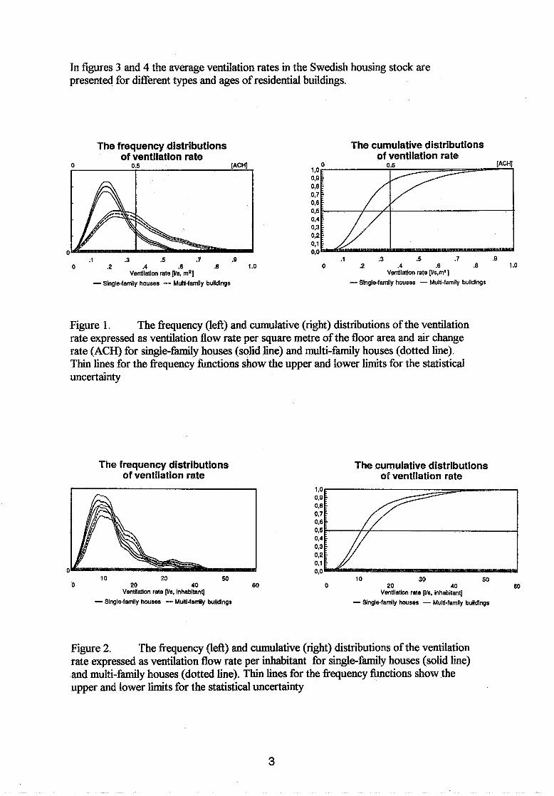
In figures 3 and 4 the average ventilation rates in the Swedish housing stock are presented for different types and ages of residential buildings.
The frequency distributions of ventilation rate
.I .3 .5 .7 .9 0 .2 .4 .6 .8 1 .O
Ventilation rate vs, mX] - Single-family houses .-- Multi-family buildings
The cumulative distributions of ventilation rate
V.V
.I .3 .5 .7 .9 0 2 .4 .6 .8 1 .O
Ventilation rate [Vs,ma] - Single-famlly houses - Multi-family buildings
Figure 1. The fi-equency (left) and cumulative (right) distributions of the ventilation rate expressed as ventilation flow rate per square metre of the floor area and air change rate (ACH) for single-family houses (solid line) and multi-family houses (dotted line). Thin lines for the fi-equency functions show the upper and lower l i i t s for the statistical uncertainty
The frequency distributions of ventilation rate
0 20 40 60 Ventilation rate v. Inhabitant] - Single-family houses -- Mu&-family bulldings
The cumulative distributions of ventilation rate
10 30 50 0 20 40 60
Ventilation rate PIS, inhabitant] - Slngle-family houses - MUM-family buildings
Figure 2. The frequency (lea) and cumulative (right) distributions of the ventilation rate expressed as ventilation flow rate per inhabitant for single-family houses (solid line) and multi-family houses (dotted line). Thin lines for the fi-equency hctions show the upper and lower limits for the statistical uncertainty

E3 Mulit-family buildings gBSl Single-family houses Ventilation rate I / s , m2
0,s
Year of construction
Figure 3. Average ventilation rate (I/(s,m2)) in the Swedish housing stock by type of building and year of construction. 95%-confidence intervals of the averages are indicated.
Year of construction
Figure 4. Average ventilation rate (I/(s,inhabitant)) in the Swedish housing stock by type of building and year of construction. 95%-confidence intervals of the averages are indicated.

Based on these diagrams, some obvious observations are:
- The variation in average ventilation rates (expressed in I/(s,m2) is very large. It ranges fiom an average value of 0.20 for single-family houses built in 1961 - 1975 up to a value close to twice as large (0.38) for multi-family houses built up to 1940.
- Compared to prescribed ventilation rate for dwellings of 0.35 I/(s,mZ), as stated in the Swedish Building Regulations from 1975 and onwards, the average for all single-family houses of all ages fall below. This is the case for most multi-family houses too, except for the group with the oldest houses and the group built in 1961-1975.
- Generally the average ventilation rates in multi-family houses are higher than in single-family houses. There is no exception in any age-group.
- When the average ventilation rate based on number of inhabitants, (V(s,inhabitant)), is considered, the variation is small, both between different age- groups of the same type of house and between different types of houses.
In order to analyse the extent to which specific factors, such as age, ventilation system, renovation status and geographical region influence the average ventilation rate of dwellings , loglinear regression analyses were performed. The results are summarized in figures 5 and 6, quoted fi-om Norlen and Andersson (1993 b).
Here we assume that the average ventilation in a group of residential buildings can be written as a product of a reference value and factors of age, renovat* ventilation and geographical region.
'\ /'
Thus, the average ventilation in a g r b i r p o f 8 U e roughly estimated by multiplying the reference value by the actual relative differences. Consider for example the group comprising all naturally ventilated, not renovated single-family houses built in or before 1960 in central Sweden: Figure 5 can supply the following estimate of its average ventilation in litres per second and person: 12 * 1.10 * 1.02 * 1.04 = 14.

VENTILATION SINGLE- Y HOUSES
a) Ventilation in litres per second and square metre
Average relative difference (reference valu~0.22) according to:
Construction Ventilation Renovation hgraphical year system status region
- 1960 1.04 (Natural vent 1.00) Not 1.05 Southern 1.01 renovated Sweden
Natural vent 0.78 Central 1.07 1961- 0.96 Exhaust vent 0.99 Renovated 0.95 Sweden
Supply-and- 1,23 exhaust vent Northern 0.91
Sweden
b) Ventilation in litres per second andperson
Average relative difference (referenee value=12) according to:
Construction Ventilation Renovation Geographical Year system status region
- 1960 1.10 (Natural vent 1.00) Not 1.02 Southern 1.04 renovated Sweden
Natural vent 0.92 Central 1.04 1961- 0.90 Exhaust vent 0.98 Renovated 0.98 Sweden
Supply-and- 1.1 1 exhaust vent Northern 0.92
Sweden
Figure 5. Ventilation in single-family houses by construction year, renovation status, ventilation system and geographical region. Relative differences for significant factors are given in semi-bold. Single-family houses from or before 1960 with mechanical ventilation are not included in the analysis because of too few observations made.

VEN TION MULTI-FAMILY HOUSES l
a) Ventilation in litres per second and square nzetre
Average relative difference (reference value=0.30) according to:
Construction Ventilation Renovation Geographical Year system status region
- 1960 1.04 Natural vent 0.95 Not 1.06 Southern 1.09 Exhaust vent 1.05 renovated Sweden
Naturalvent 0.86 Central 1.05 1961- 0.96 Exhaust vent 1.01 Renovated 0.94 Sweden
Supply-and- 1.13 exhaust vent Northern 0.86
Sweden
b) Ventilation in second and person
Average relative value=13) according to:
Construction intilation Renovation Geographical Year , /system status region
,
4 ' 1.07 Natural vent 0.95 Not 1.03 Southern 1.07 Exhaust vent 1.05 renovated Sweden
Natural vent 0.86 Central 1.06 1961- 0.93 Exhaust vent 0.99 Renovated 0.97 Sweden
Supply-and- 1.15 exhaust vent Northern 0.87
Sweden
Figure 6. Ventilation in multi-family houses by construction year, renovation status, ventilation system and geographical region. Relative differences for significant factors are given in semi-bold. Multi-family hbuses from or before 1960 with supply-and-exhaust ventilation are not included in the analysis because of too few observations made.
4 AIR TIGHTNESS
4.1 Sample and measurement technique
The sub-sample of 90 single- and multifamily houses was drawn from the main random sample of 1200 houses, used for the main investigation. The sub-sample is identical to the sample chosen for the Institute's quality control performance regarding the sub- contractors that were hired by the Swedish Institute for Building Research for performing the inspections of the houses in the main investigation. Practical aspects, such as availabilty, travel optimisation etc may have influenced the choise of houses for the sub-sample, which means that the sub-sample is not a correct random sample. Anyhow, the houses in the sample represents a wide variety of bulidings in different geographical regions.
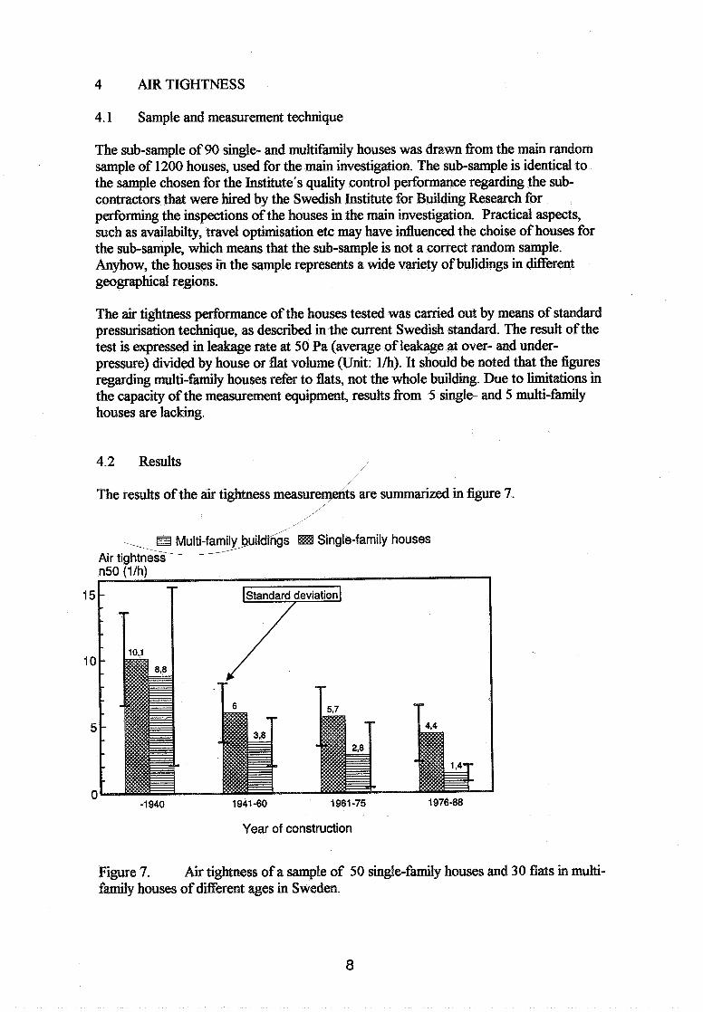
The air tightness performance of the houses tested was carried out by means of standard pressurisation technique, as described in the current Swedish standard. The result of the test is expressed in leakage rate at 50 Pa (average of leakage at over- and under- pressure) divided by house or flat volume (Unit: llh). It should be noted that the figures regarding multi-family houses refer to flats, not the whole building. Due to limitations in the capacity of the measurement equipment, results from 5 single- and 5 multi-family houses are lacking.
4.2 Results / //
The results of the air tightness m e a s u r e ~ t s are summarized in figure 7.
,' /_j FB'l Single-family houses
Year of construction
Figure 7. Air tightness of a sample of 50 single-family houses and 30 flats in multi- family houses of different ages in Sweden.

It could be seen from figure 7 that:
- The standard deviations are rather large, due to the relatively small number of houses in each age-group.
- There is a clear tendency that newer houses are less leaky than older ones.
- Multi-family houses have lower 1150-values than single-family houses; this is due to higher volume-to-leaking area relationship.
- Compared to the prescribed maximum values of n5O as stated in the Swedish Building Code of 1980 (3.0 for single-family houses and 1.0 - 2.0 for multi-family houses), only the newest multi-family houses (on average) seem to meet the prescribed level.
5 ACKNOWLEDGEMENTS
The research was supported by the Swedish Council for Building Research, the Ministry of Industry and Commerce and the Swedish Board for Industrial and Technical Development. Thanks for good assistance in this work go to Anita Eliasson, Britt-Marie
Stig Skogberg and Ragnvald Pelttari at the Swedish Institute for
J3csf6&, CA. & Sundberg, J., Fallstudier av inneklimatet i 90 bostadshus. EEIB-rapport /'nr 5. (Case Studies of the Indoor Climate in 90 Dwellings. ELIB-report nr S.), In
Swedish, Swedish Institute for Building Research, Givle, Sweden, 1993. In preparation.
Norlen, U. & Andersson, K., An Indoor Climate Survey of the Swedish Housing Stock (Die ELIB-stud)), Proc. of Indoor Air '93, Vol. 1, Helsinki, 1993.
Norlen, U. & Andersson, K., (eds.), (1993b), me Indoor Climate in the Swedish Housing Stock, Swedish Institute for Building Research, GZivle, Sweden, 1993.
Stymne, H. & Bornan, CA., Measwring Ventilation Rates on a Large Scale, Proc. of Indoor Air '93, Vol. 5, Helsinki, 1993.
Waller, T. & Hogberg, H., Probability Density Estimation of the Levels of Indoor Air Quality Variables, Proc. of Indoor Air '93, Vol. 1, Helsinki, 1993.

Energy impact of Ventilation and Air Infiltration 14th AlVC Conference, Copenhagen, Denmark
21 -23 September 1993
Potential Energy Savings from Modified Ventilation of Dwellings
N C Bergsse
Danish Building Research Institute, Postboks 119, DK-2970 Hsrsholm, Denmark
Synopsis A total of 177 measurements have been performed in apartments in multi-story buildings without mechanical ventilation. The buildings comprised renovated and non-renovated buildings built between 1930 and 1960. Measurements of air change rate and relative hu- midity have been performed using passive measurement techniques including a passive multiple tracer gas technique, the so-called PFT-technique. In each apartment the main bedroom has been investigated separately. In addition, the occupants completed a ques- tionnaire concerning their use of the dwelling.
The objects of the measurements have been to determine the level of the average ven- tilation in naturally ventilated apartments in existing buildings and to evaluate whether the ventilation is adequate.
The measurements were performed during two heating periods and statistical tests have shown that in addition to dividing the measurement results into two groups, being reno- vated and non-renovated buildings respectively, each group had to be divided additionally according to the time of year the measurements were performed.
Results have shown that in a winter period with typical outdoor temperatures there is no statistical difference in the average air change rate in apartments in renovated and non- renovated buildings, respectively. The average air change rate was about 0.4 h-l. During a winter period with extraordinary mild outdoor conditions the average air change rate was somewhat higher, about 0.5 h-l, in apartments in renovated buildings and more than 0.6 h-l, in apartments in non-renovated buildings.
The results of the measurements of relative humidity show that on average the relative n acceptable level. However, indications are given that some apartments
of having condensation problems.
1982 the Danish building code has provided the use of mechanical exhaust ventila- in multi-story buildings. The code also provides that a dwelling must be
/ventilated corresponding to an air change rate of 0.5 h-I and specific provisions are stated -- ' regarding ventilation of kitchens and bathrooms. Previous large scale field investigations
of ventilation in residential buildings built after 1982 (1) have shown an average air change rate of just under 0.6 h-' in apartments in multi-story buildings equipped with mechanical exhaust ventilation.
The energy consumption for ventilation of dwellings will become increasingly important, as the energy consumption for coverage of transmission heat loss is reduced, due to overall improvements of the standard of insulation of buildings. Prospects for further reduction of the energy consumption will depend increasingly on the possibilities of reducing the energy consumption in the field of ventilation. It is of vital importance to the valuation to establish whether ventilation is adequate in existing buildings.
Renovation of multi-story buildings usually comprises replacement of the windows with new double-glazed sealed windows and improvement of the joints. This will enhance the overall air tightness of the building envelope resulting in a reduction in the uncontrolled part of air infiltration in dwellings. This in turn may have a negative effect on the indoor climate and increase the risk of causing damage to building components due to elevated humidity levels in the apartments.
This investigation concerns naturally ventilated apartments in existing buildings. An important issue is the influence from the occupants' use of their apartment on the average air change rate and the relative humidity. The matter includes the occupants' use of out- door air inlets and window openings. This has been examined through this investigation as long-term passive sampling techniques has been used in connection with a questionnaire.
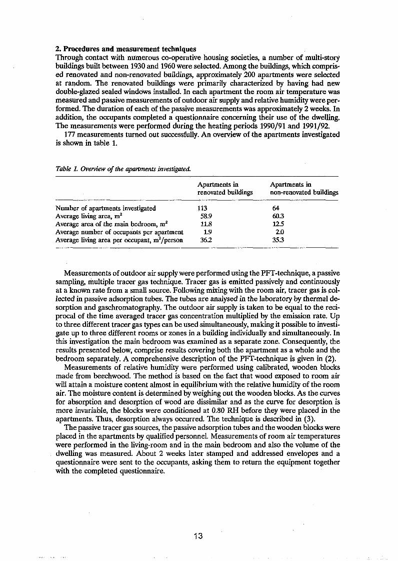
2. Procedures and measurement techniques Through contact with numerous co-operative housing societies, a number of multi-story buildings built between 1930 and 1960 were selected. Among the buildings, which compris- ed renovated and non-renovated buildings, approximately 200 apartments were selected at random. The renovated buildings were primarily characterized by having had new double-glazed sealed windows installed. In each apartment the room air temperature was measured and passive measurements of outdoor air supply and relative humidity were per- formed. The duration of each of the passive measurements was approximately 2 weeks. In addition, the occupants completed a questionnaire concerning their use of the dwelling. The measurements were performed during the heating periods 1990/91 and 1991/92.
177 measurements turned out successfully. An overview of the apartments investigated is shown in table 1.
Table 1. Overview of the apartments investigated.
Apartments in Apartments in renovated buildings non-renovated buildings
Number of apartments investigated 113 64 Average living area, m2 58.9 60.3 Average area of the main bedroom, m2 11.8 12.5 Average number of occupants per apartment 1.9 2.0 Average living area per occupant, m2/person 36.2 35.3
Measurements of outdoor air supply were performed using the PFT-technique, a passive sampling, multiple tracer gas technique. Tracer gas is emitted passively and continuously at a known rate from a small source. Following mixing with the room air, tracer gas is col- lected in passive adsorption tubes. The tubes are analysed in the laboratory by thermal de- sorption and gaschromatography. The outdoor air supply is taken to be equal to the reci- procal of the time averaged tracer gas concentration multiplied by the emission rate. Up to three different tracer gas types can be used simultaneously, making it possible to investi- gate up to three different rooms or zones in a building individually and simultaneously. In this investigation the main bedroom was examined as a separate zone. Consequently, the results presented below, comprise results covering both the apartment as a whole and the bedroom separately. A comprehensive description of the PFT-technique is given in (2).
Measurements of relative humidity were performed using calibrated, wooden blocks made from beechwood. The method is based on the fact that wood exposed to room air will attain a moisture content almost in equilibrium with the relative humidity of the room air. The moisture content is determined by weighing out the wooden blocks. As the curves for absorption and desorption of wood are dissimilar and as the curve for desorption is more invariable, the blocks were conditioned at 0.80 R H before they were placed in the apartments. Thus, desorption always occurred. The technique is described in (3).
The passive tracer gas sources, the passive adsorption tubes and the wooden blocks were placed in the apartments by qualified personnel. Measurements of room air temperatures were performed in the living-room and in the main bedroom and also the volume of the dwelling was measured. About 2 weeks later stamped and addressed envelopes and a questionnaire were sent to the occupants, asking them to return the equipment together with the completed questionnaire.

3. Results Measurements have been performed in 177 apartments. Each apartment was investigated once, however, a complete set of results for each apartment does not exist. Individual erro- neous results have been excluded. In the following result tables, the number of results be- ing used as the basis for the average given, are shown. From statistical tests it is recognized that the results obtained are influenced by the time the measurements were performed. Therefore, in addition to dividing the results into two groups comprising results from mea- surements in renovated and non-renovated buildings respectively, each group were divided according to the heating period in which the measurements were performed.
Results of the measured quantities are shown in table 2. Table 3 is showing the climatic conditions during the measurement periods.
Table 2. Summary of results of measurements, mean + standard error.
Apartments in Apartments in renovated buildings non-renovated buildings
Number of results, living-room 60 - 63 43 - 47 24 - 26 30 - 37 Number of results, bedroom 45 - 63 31 - 46 20 - 26 24 - 36
Temperature, living-room, "C 20.0 + 0.1 21.2 + 0.2 20.2 + 0.2 21.2 r 0.2 Temperature, bedroom, "C 19.7 + 0.2 20.1 + 0.3 19.5 + 0.4 20.4 + 0.3
Outdoor air supply, 11s 15.4 r 0.8 19.2 + 1.0 14.3 + 1.5 255 + 1.3 Outdoor air supply, 11s per m2 0.27 + 0.01 0.32 + 0.02 0.24 + 0.02 0.42 r 0.02 Outdoor air supply, I/s per person 8.5 + 0.6 13.2 + 1.3 8.3 + 1.0 16.5 + 1.5 Average air change rate, h-' 0.42 + 0.02 0.49 + 0.03 0.36 + 0.03 0.65 + 0.03
Outdoor air supply, bedr., 11s 4.4 + 0.5 5.0 + 0.6 4.1 + 0.8 6.1 r 0.7 Outdoor air supply, bedr., 11s pr. m2 0.44 + 0.04 0.39 + 0.05 0.38 + 0.07 0.49 + 0.06
Relative humidity, living-room 0.35 + 0.01 0.44 +. 0.01 0.39 + 0.01 0.39 + 0.01 Relative humidity, bedroom 0.38 + 0.01 0.46 f 0.01 0.42 + 0.01 0.43 + 0.01
Table 3. Outdoor air temperature and average water content in the outdoor air, mean + standard error.
Heating period Heating period 1990/91 1991/92
Average outdoor air temperature, "C -0.1 + 0.3 6.8 + 0.3 Average water content in the outdoor air, g H20/kg 3.2 + 0.1 4.6 + 0.1
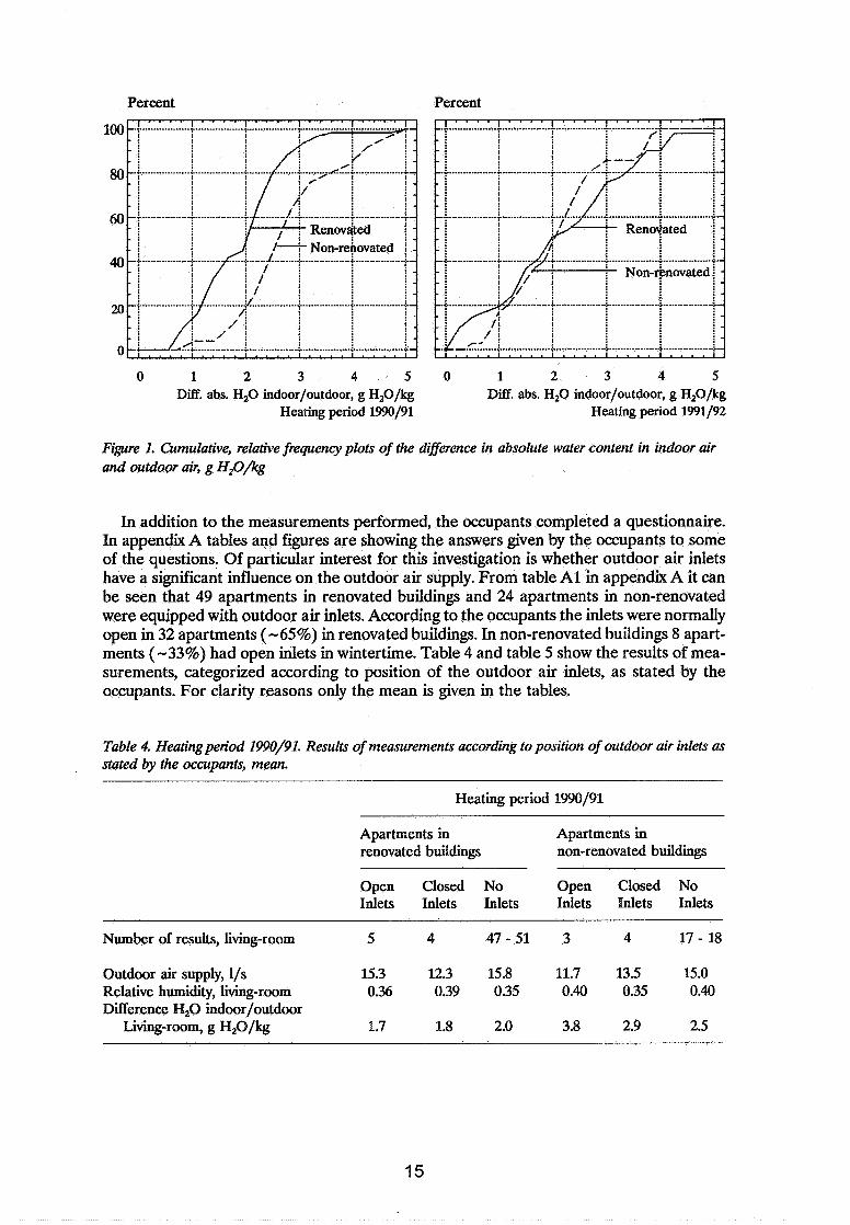
From measurements of temperatures and relative humidities in the indoor air and in the outdoor air, the difference in the absolute water content in the indoor air and outdoor air is calculated. Cumulative, relative frequency plots are shown in figure 1.
Percent Percent
0 1 2 3 4 5 Diff. abs. H20 indoor/outdoor, g H20/kg
Heating period 1990/91
I . . . . l . . . . l . . . . I . . . . I . . . . I
0 1 2 3 4 5 Diff. abs. H,O indoor/outdoor, g H20/kg
Heating period 1991/92
Figure 1. Cumulative, relative frequency plots of the difference in absolute water content in indoor air and outdoor air, g H,O/kg
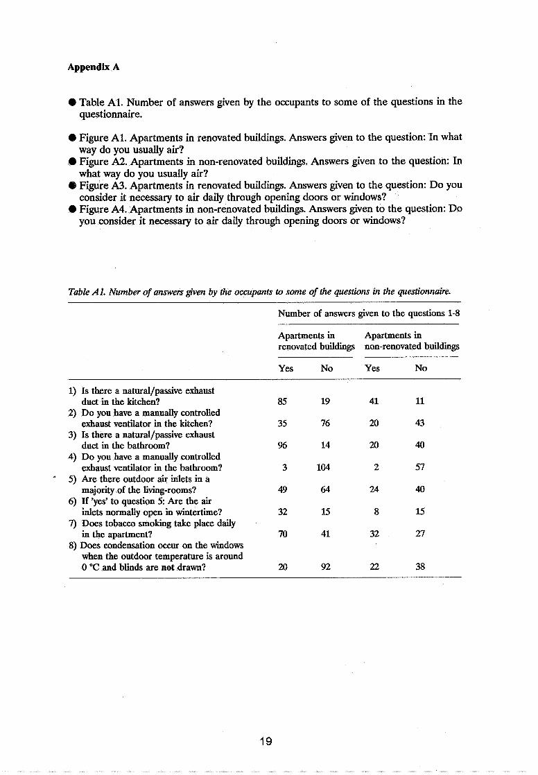
In addition to the measurements performed, the occupants completed a questionnaire. In appendix A tables and figures are showing the answers given by the occupants to some of the questions. Of particular interest for this investigation is whether outdoor air inlets have a significant influence on the outdoor air supply. From table A1 in appendix A it can be seen that 49 apartments in renovated buildings and 24 apartments in non-renovated were equipped with outdoor air inlets. According to the occupants the inlets were normally open in 32 apartments (-65%) in renovated buildings. In non-renovated buildings 8 apart- ments (-33%) had open inlets in wintertime. Table 4 and table 5 show the results of mea- surements, categorized according to position of the outdoor air inlets, as stated by the occupants. For clarity reasons only the mean is given in the tables.
Table 4. Heatingperiod 1990/91. Results of measurements according to position of outdoor air inlets as stated by the occupants, mean.
Heating period 1990/91
Apartments in Apartments in renovated buildings non-renovated buildings
Open Closed No Open Closed No Inlets Inlets Inlets Inlets Inlets Inlets
Number of results, living-room 5 4 47 - 51 3 4 17 - 18
Outdoor air supply, l/s 15.3 12.3 15.8 11.7 13.5 15.0 Relative humidity, living-room 0.36 0.39 0.35 0.40 0.35 0.40 Difference H20 indoor/outdoor
Living-room, g H20/kg 1.7 1.8 2.0 3.8 2.9 2.5

Table 5. Heating period 1991/92. Results of measurements according to position of outdoor air inlets as stated by the occupants, mean.
Heating period 1991/92
Apartments in Apartments in renovated buildings non-renovated buildings
Open Closed No Open Closed No Inlets Inlets Inlets Inlets Inlets Inlets
Number of results, living-room 20-25 7 -10 9 - 1 2 5 11 13 - 19
Outdoor air supply, l/s 21.3 14.0 19.7 29.5 20.4 29.0 Relative humidity, living-room 0.44 0.47 0.45 0.38 0.43 0.36 Difference H20 indoor/outdoor
Living-room, g H,O/kg 2.0 3.4 1.5 1.8 2.7 1.7
Also, questions were asked concerning the reason why the occupants considered airing required in various rooms and the way in which the airing was performed. Figure A1 and figure A2 in appendix A are showing the answers given by occupants in renovated and non-renovated buildings, respectively, regarding their airing habits.
From the figures it can be seen that the principal procedure for airing the main bed- room is through constantly keeping a window ajar. Table 6 and table 7 show results catego- rized according to the way airing was performed. For clarity reasons only the mean is given in the tables.
Table 6. Heating period 1990/91. Main bedroom. Measurement results according to way of airing.
Heating period 1990/91
Apartments in Apartments in renovated buildings non-renovated buildings
Constantly a Periodic Constantly a Periodic window ajar airing window ajar airing
Number of results, bedroom 16 - 22 27 - 38 7 - 8 12 - 17
Outdoor air supply, bedroom, 11s 6.1 3.4 4.9 3.7 Relative humidity, bedroom 0.39 0.38 0.42 0.42 Difference H20 indoor/outdoor
bedroom, g H20/kg 2.0 2.3 3.2 2.8

Table 7. Heatingperiod 1991/92. Main bedroom. Measurement results according to way of airing.
Heating period 1991/92
Apartments in Apartments in renovated buildings nin-renovated buildings
Constantly a Periodic Constantly a Periodic window ajar a i r i i window ajar airiig
Number of results, bedroom 13 - 25 8 - 21 9 - 10 15 - 24
Outdoor air supply, bedroom, l/s 6.5 3.0 8.0 5.0 Relative humidity, bedroom 0.45 0.48 0.45 0.43 Difference H20 indoor/outdoor
bedroom, g H2O/kg 1.8 2.4 2.6 2.4
4. Discussion Statistical analyses and tests have been conducted to determine whether statistically signifi- cant trends occurred in the material. The correlation coefficients in the regression analyses were generally low, however, looking at both heating periods as a whole, the following find- ings are significant: In apartments in both renovated and non-renovated buildings the ave- rage air change rate is positively correlated to the outdoor temperature. In apartments in renovated buildings the relative humidity in both living-room and bedroom is positively correlated to the outdoor temperature and negatively correlated to the outdoor relative humidity. In apartments in non-renovated buildings the relative humidity in the bedroom is positively correlated to the outdoor temperature. No significant correlation was found for the living-room in apartments in non-renovated buildings.
For both renovated and non-renovated buildings, statistical tests have shown, that the measurement results of the average air change rate, obtained through measurements performed in heating period 1990/91, are significantly different from the results obtained through measurements performed in heating period 1991/92. In addition, tests have shown, that the average air change rate, measured in apartments in non-renovated buildings, is significantly higher in heating period 1991/92 than in heating period 1990/91. These find- ings are unanticipated as the outdoor temperature on average was higher in heating period 1991/92. In naturally ventilated buildings the ventilation rate is expected to be negatively correlated to the outdoor temperature. Further analysis of the results is necessary in order to explain the matter. For apartments in renovated buildings the average air change rate is found to be 0.42 h-' in heating period 1990/91 and 0.49 h-I in heating period 1991/92. For apartments in non-renovated buildings the results are 0.36 h-I and 0.65 h-l, respecti- vely. Compared to the present Danish building code it can be seen that these provisions are met in non-renovated buildings in heating period 1991/92 and almost also in renovated buildings. However, in both renovated and non-renovated buildings the provisions are not met in heating period 1990/91. If the outdoor air supply is expressed in liters per second, l/s, the results obtained through measurements in renovated buildings show 15 l/s in heat- ing period 1990/91 and 19 11s in heating period 1991/92. The results from measurements in apartments in non-renovated buildings show 14 11s (1990/91) and 26 11s (1991/92). Specific provisions are in the Danish building code regarding extraction of air from kit- chens and bathrooms. For the type and size of apartments investigated here the passive
exhaust ducts must provide extraction of 20 11s from kitchens and 15 11s from bathrooms, equalling a total of 35 11s for the apartment. These provisions are definitely not met.
The results of the measurements of the relative humidity show that in both building types the humidity is higher in the bedroom than in the living-room. In non-renovated buildings there is no statistical difference between the periods 1990/91 and 1991/92.
Interesting results are seen from the calculations of the difference in absolute water content in the indoor air and outdoor air. In heating period 1990/91 the difference is higher in the non-renovated than in the renovated buildings.
Recommendations for maximum acceptable humidity in the indoor air can be given on two different viewpoints. One is that in winter condensation on the windows must be pre- vented. A difference in absolute water content in the indoor air and the outdoor air of 2.5 g H20/kg is normally considered sufficient to avoid condensation. Differences of 3 - 4 g H20/kg may cause problems in dwellings with double glazing when room temperature is lowered and curtains are drawn. If 3.5 g H20/kg is taken as the limit it can be seen from figure 1 that in heating period 1990/91 approximately 20 percent of the apartments in the non-renovated buildings may be suspected of having condensation problems. In heating period 1991/92 10-20 percent of the apartments, both in renovated and non-renovated buildings, may be suspected of having problems with condensation, however the heating period was not typical. The other viewpoint is that the number of house dust mites per gram house dust must be kept low. This means a maximum acceptable humidity in the in- door air of 7.0 g H20/kg corresponding to a relative humidity of about 0.45 at 20-22 "C, in typical climatic winter conditions in Denmark. Focusing on heating period 1990/91 - heating period 1991/92 was extraordinary warm - it can be seen from table 2 that some of the apartments investigated, particularly the bedrooms, may be suspected of having an increased number of house dust mites.
5. References (1) Bergsoe, Niels C.
"Investigations on Air Change and Air Quality in Dwellings" International CIB W67 Symposium on Energy, Moisture and Climate in Buildings. 3-6 September 1990. Rotterdam. The Netherlands.
(2) Sateri, Jorma 0. (Ed.) "The Development of the PFT-Method in the Nordic Countries" D9:1991. Swedish Council for Building Research, Stockholm, Sweden.
(3) Nielsen, Ove Luftfugtighed i renoverede hpljhuse med tre ventilationslplsninger (The humidity con- ditions in renovated high-rise buildings with three ventilation solutions. In Danish). Danish Building Research Institute. SBI-report 198. Hplrsholm, 1989.
Appendix A
Table Al . Number of answers given by the occupants to some of the questions in the questionnaire.
Figure Al . Apartments in renovated buildings. Answers given to the question: In what way do you usually air? Figure A2. Apartments in non-renovated buildings. Answers given to the question: In what way do you usually air?
@ Figure A3. Apartments in renovated buildings. Answers given to the question: D o you consider it necessary to air daily through opening doors or windows?
@ Figure A4. Apartments in non-renovated buildings. Answers given to the question: Do you consider it necessary to air daily through opening doors or windows?
Table AI. Number of answers given by the occupants to some of the questions in the questionnaire.
Number of answers given to the questions 1-8
Apartments in renovated buildings
Yes No
1) Is there a natural/passive exhaust duct in the kitchen? 85 19
2) Do you have a manually controlled exhaust ventilator in the kitchen? 35 76
3) Is there a natural/passive exhaust duct in the bathroom? % 14
4) Do you have a manually controlled exhaust ventilator in the bathroom? 3 104 - 5) Are there outdoor air inlets in a majority of the living-rooms? 49 64
6) If 'yes' to question 5: Are the air inlets normally open in wintertime? 32 15
7) Does tobacco smoking take place daily in the apartment? 70 41
8) Does condensation occur on the windows when the outdoor temperature is around 0 "C and blinds are not drawn? 20 92
Apartments in non-renovated buildings
Yes No

Percent
100
Short-term airing (5-10 minutes) several times per day Long-term airing (10-60 minutes) a few times per day Long-term airing (10-60 minutes) several times per day A window is always ajar
Living-room Bedroom Kitchen Bathroom Way of airing
Apartments in renovated buildings
Figure A l . Apartments in renovated buildings. Answets given to the question: In what way do you usually air?
Percent
100
Living-room Bedroom Kitchen Bathroom Way of airing
Apartments in non-renovated buildings
- - - Airing seldom or never - - Short-term airing (5-10 minutes) a few times per day
7
- Short-term airing (5-10 minutes) several times per day -
- - Long-term airing (10-60 minutes) a few times per day -
- Long-term airing (10-60 minutes) several times per day -
- - A window is always ajar - -
- - - - - - - - - - - - -
- - - - - - - - - - - -
Figure A2. Apartments in non-renovated buildings. Answers given to the question: In what way do you usually air?

Percent
Bedroom Kitchen Bathroom Reason for airing
Apartments in renovated buildings
Figure A3. Apartments in renovated buildings. Answers given to the question: Do you consider it necessary to air daily through opening doors or windows?
Percent
Living-room Bedroom Kitchen Bathroom Reason for airing
Apartments in non-renovated buildins
Figure A4. Apartments in non-renovated buildings. Answers given to the question: Do you consider it necessaiy to air daily through opening doors or windows?

Energy lm pact of Ventilation and Air Infiltration 14th AlVC Conference, Copenhagen, Denmark
21 -23 Septem ber 1993
Ventilation-Energy Liabilities in US Dwellings
M Sherman, N Matson
Energy Performance of Buildings Group, Energy and Environment Division, Lawrence Berkeley Laboratory, University of California, Berkeley, California
VENTILATION-ENERGY LI LITIES IN U.S. D LLINGS
Max Sherman Nance Matson
Energy Performance of Buildings Group
Energy and Environment Division
Lawrence Berkeley Laboratory University of California
Berkeley, California
The role of ventilation in the housing stack is to provide fresh air and to di- lute internally-generated pollutants in order to assure adequate indoor air quality. Providing this ventilation service requires energy either directly for moving the air or indirectly for conditioning the outdoor air for thermal comfort. Different kinds of ventilation systems have different energy re- quirements. Existing dwellings in the United States are ventilated primatiy through leaks in the building shell (i.e., hfibation) rather than by mechan- ical ventilation systems. The purpose of this report is to ascertain, ftom best available data, the energy liability assoGiated with providing the current levels of ventilation and to estimate the energy savings or penalties associ- ated with tightening or loosening the building envelope. Various ASHRAE Standards (e.g., 62,119, and 136) are used to determine acceptable venti- lation levels and energy req-ents. Building characteristics, energy use, and building tightness data are combined to estimate both the energy liabil- ities of ventilation and its dependance on building stock dwacteristics. The average annual ventilation energy use for a typical dwelling is about 46 GJ (roughly 50% of total energy usage); the cost-effective savings po- tential is about 28 GJ. The associated total annual ventilation energy use for the residential stock is about 3 ET (ExaToules).
1. This work was supported by the Assistant Secretary for Conse~ation and Renewable Energy, Office of Building Technology of the U.S. Depamnent of Energy under contact no. DE-AC03-76SF00098.
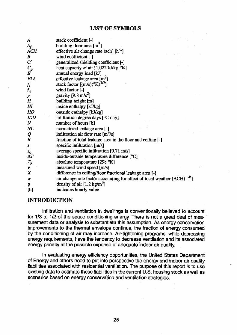
LIST OF SYMBOLS
A
Af ACH B C'
stack coefficient [-I building floor area [m2] effective air change rate (ach) [h-'1 wind coefficient [-I generalized shielding coefficient [-I heat capacity of air 11.022 kJ/kg-OK] annual energy load &ll effective leakage area [m2] stack factor [(m/s)(O~)~'~] wind factor [-I gravity [9.8 m/s2] building height [m] inside enthalpy w k g ] outside enthalpy w k g ] infiltration degree days [OC-day] number of hours [h] normalized leakage area [- 4 infiltration air flow rate [m Is] fraction of total leakage area in the floor and ceiling [-I specific infiltration [ d s ] average specific infiltration [0.7 1 m/s] inside-outside temperature difference [OC] absolute temperature [298 OK] measured wind speed [mls] difference in ceiling/floor fractional leakage area [-I air change rate factor accounting for effect of local weather (ACH) rh] density of air [1.2 kglm3] indicates hourly value
INTRODUCTION
infiltration and ventilation in dwellings is conventionally believed to account for 113 to 112 of the space conditioning energy. There is not a great deal of mea- surement data or analysis to substantiate this assumption. As energy conservation improvements to the thermal envelope continue, the fraction of energy consumed by the conditioning of air may increase. Air-tightening programs, while decreasing energy requirements, have the tendency to decrease ventilation and its associated energy penalty at the possible expense of adequate indoor air quality.
In evaluating energy efficiency opportunities, the United States Department of Energy and others need to put into perspective the energy and indoor air quality liabilities associated with residential ventilation. The purpose of this report is to use existing data to estimate these liabilities in the current U.S. housing stock as well as scenarios based on energy conservation and ventilation strategies.
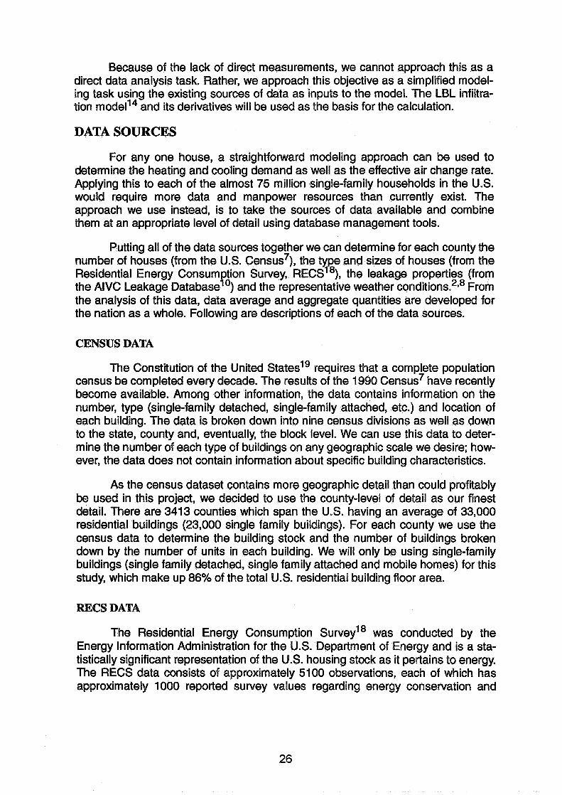
Because of the lack of direct measurements, we cannot approach this as a direct data analysis task. Rather, we approach this objective as a simplified model- ing task using the existing sources of data as inputs to the model. The LBL infiltra- tion model'4 and its derivatives will be used as the basis for the calculation.
DATA SOURCES
For any one house, a straightforward modeling approach can be used to determine the heating and cooling demand as well as the effective air change rate. Applying this to each of the almost 75 million single-family households in the U.S. would require more data and manpower resources than currently exist. The approach we use instead, is to take the sources of data available and combine them at an appropriate level of detail using database management tools.
Putting all of the data sources together we can determine for each county the number of houses (from the U.S. census7), the type and sizes of houses (from the Residential Energy Consum tion Survey, RECS' 8), the leakage properties (from
Po the AlVC Leakage Database ) and the representative weather condition^.'^^ From the analysis of this data, data average and aggregate quantities are developed for the nation as a whole. Following are descriptions of each of the data sources.
CENSUS DATA
The Constitution of the United statesqg requires that a complete population census be completed every decade. The results of the 1990 census7 have recently become available. Among other information, the data contains information on the number, type (single-family detached, single-family attached, etc.) and location of each building. The data is broken down into nine census divisions as well as down to the state, county and, eventually, the block level. We can use this data to deter- mine the number of each type of buildings on any geographic scale we desire; how- ever, the data does not contain information about specific building characteristics.
As the census dataset contains more geographic detail than could profitably be used in this project, we decided to use the county-level of detail as our finest detail. There are 3413 counties which span the U.S. having an average of 33,000 residential buildings (23,000 single family buildings). For each county we use the census data to determine the building stock and the number of buildings broken down by the number of units in each building. We will only be using single-family buildings (single family detached, single family attached and mobile homes) for this study, which make up 86% of the total U.S. residential building floor area.
RECS DATA
The Residential Energy Consumption was conducted by the Energy Information Administration for the U.S. Department of Energy and is a sta- tistically significant representation of the U.S. housing stock as it pertains to energy. The RECS data consists of approximately 5100 observations, each of which has approximately 1000 reported survey values regarding energy conservation and
building characteristics. The survey contains information on building size and shape, the type, details, and use of heating and cooling systems, indications of the level of air tightness, as well as age and geographic location of each representative building.
We have broken the dataset up into 32 different types of houses: old vs. new (using 1970 as a dividing point); single-story vs. multistory; poor condition vs. good condition; duct systems vs. none; and floor leakage vs. no floor leakage. The RECS data is used to determine, for each census division, the floor area and percentage of air conditioning use for each of the 32 house types. The smallest, statistically sig- nificant geographical breakdown in the RECS data is the census division. Therefore the properties of the housing stock are separately determined for each of the nine census divisions. Every county within a given division is assumed to have the same relative distribution of housetypes, where the number of houses in each county is determined from the Census data.
LEAKAGE DATA
While the RECS data contains some indications of air tightness, it does not contain quantitative values which could be used as part of this modeling effort. Sev- eral years ago LBL compiled a database on measured air tightness for the u.s.'~ which has since been included in the AlVC numerical databaseq0. The dataset con- tains the measured air tightness, NL, as well as a general description of the building which allows estimates of leakage distribution, R & X, and condition.
In contrast to the census data, the leakage data is very sparse. The current database consists of approximately 500 measured U.S. single-family houses. This sample was a sample of convenience and therefore cannot be said to be statisti- cally representative. Although more measurements have been made, this data set represents the best available compilation. Of the complete dataset, 242 houses meet the criteria of the 32 house types and are used to estimate national average leakage characteristics for each house type.
'WEATHER DATA
Representative weather data is necessary to run any infiltration model. LBL has a library of approximately 240 representative weather sites across the country. These weather files have been selected to be representative of typical years for each site and are derived from the WYEC (Weather Year for Ener y Calculations), B TMY (Typical Meteorological Year), TRY (Typical Reference Year) and CTZ (Cali- fornia Climate ones)^ weather tapes. For each county, the most representative weather site was chosen, based primarily on geography. Each weather file contain outside temperature and humidity, wind speed and direction and barometric pres- sure.
MODELING TOOLS
In order to use this information we must have a way of predicting instanta- neous ventilation rates and deriving the corresponding seasonal and annual air change rates and ventilation energy requirements. The fundamental relationship between the infiltration and the house and climate properties is expressed by the LBL infiltration rnode~'~, which is incorporated into the ASHRAE Handbook of Fun- damentals'. The LBL infiltration model is used to generate, on an hourly basis, spe- cific infiltration and air flow rates. From these hourly results, seasonal average air change rates and corresponding energy consumption, as well as overall measures of tightness (ASHRAE Standard 11 Q ) ~ and rates for adequate ventilation (ASHRAE Standard 6214 are determined.
LBL INFllLTRATION MODEL
The LBL infiltration model'5 calculates specific infiltration rate, s[h], as:
(EQ 1)
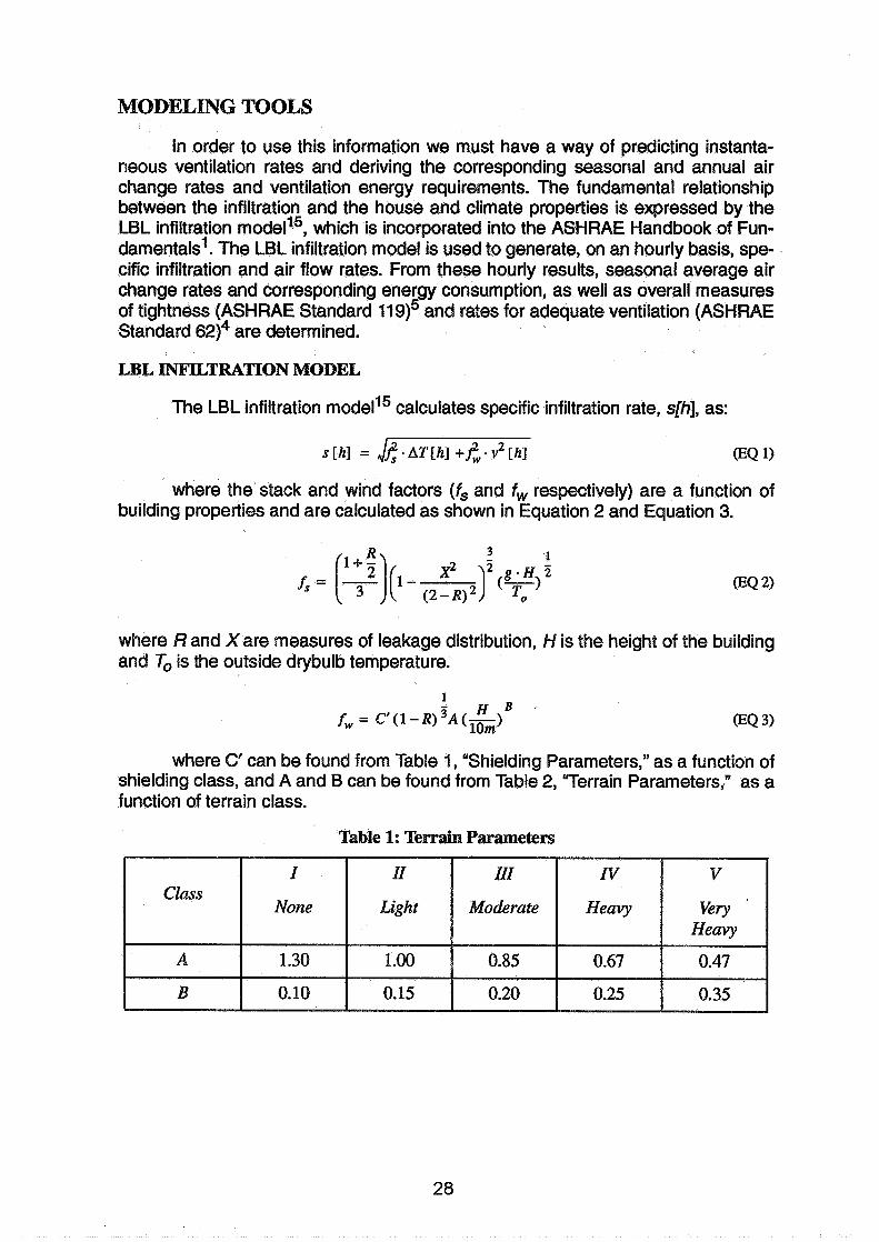
where the stack and wind factors ( f , and f, respectively) are a function of building properties and are calculated as shown in Equation 2 and Equation 3.
where R and X are measures of leakage distribution, H is the height of the building and 7, is the outside drybulb temperature.
(EQ 3)
where C' can be found from Table 1, "Shielding Parameters," as a function of shielding class, and A and B can be found from Table 2, "Terrain Parameters,." as a function of terrain class.
Table 1: Terrain Parameters
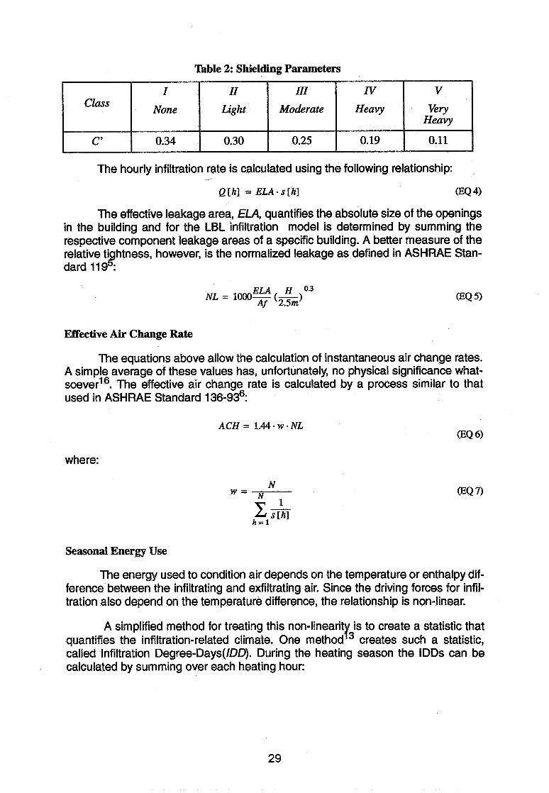
Table 2: Shielding Parameters
The hourly infiltration rate is calculated using the following relationship: J
Q [h] = ELA s [h] (EQ 4)
The effective leakage area, E U , quantifies the absolute size of the openings in the building and for the LBL infiltration model is determined by summing the respective component leakage areas of a specific building. A better measure of the relative ti htness, however, is the normalized leakage as defined in ASHRAE Stan- 51 dard 119 .
ELA H 0.3 NL = 1000- (-) Af 2.5m
Effective Air Change Rate
The equations above allow the calculation of instantaneous air change rates. A simple average of these values has, unfortunately, no physical significance what- s~ever '~. The effective air change rate is calculated by a process similar to that used in ASHRAE Standard 1 36-93?
ACH = 1.44. W - N L
where:
Seasonal Energy Use
The energy used to condition air depends on the temperature or enthalpy dif- ference between the infiltrating and exfiltrating air. Since the driving forces for infil- tration also depend on the temperature difference, the relationship is non-linear.
A simplified method for treating this non-linearit is to create a statistic that quantifies the infiltration-related climate. One methodY3 creates such a statistic, called Infiltration Degree-Days(1DD). During the heating season the lDDs can be
1 calculated by summing over each heating hour: I I I i
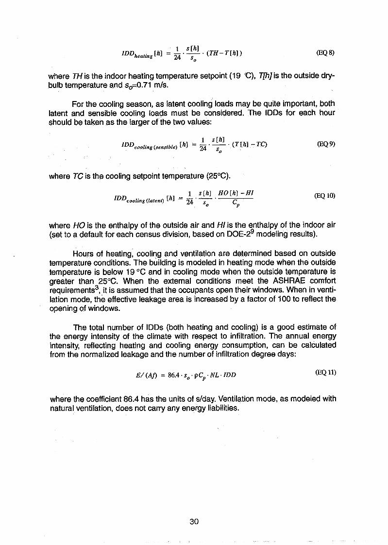
s[hl ( T H - T [ h ] ) ]LIDheating [h] = - - . 24 so
(EQ 8)
where TH is the indoor heating temperature setpoint (19 @), T[h]is the outside dry- bulb temperature and se0.71 mls.
For the cooling season, as latent cooling loads may be quite important, both latent and sensible cooling loads must be considered. The IDDs for each hour should be taken as the larger of the two values:
1 s [hl zDDcooling (sensible) ihl = . 7 ' (TEh] - TC) (EQ 9)
where TC is the cooling setpoint temperature (25°C).
1 s [h] HO [h] - H I IDDcooling (latent) [hl = - * - .
24 so cP (EQ 10)
where HO is the enthalpy of the outside air and HI is the enthalpy of the indoor air (set to a default for each census division, based on DOE-^' modeling results).
Hours of heating, cooling and ventilation are determined based on outside temperature conditions. The building is modeled in heating mode when the outside temperature is below 19 OC and in cooling mode when the outside temperature is greater than 25°C. When the external conditions meet the ASHRAE comfort requirements3, it is assumed that the occupants open their windows. When in venti- lation mode, the effective leakage area is increased by a factor of 100 to reflect the opening of windows.
The total number of lDDs (both heating and cooling) is a good estimate of the energy intensity of the climate with respect to infiltration. The annual energy intensity, reflecting heating and cooling energy consumption, can be calculated from the normalized leakage and the number of infiltration degree days:
E / ( A f i = 8 6 . 4 . ~ ; PC,. NL. IDD (EQ 11)
where the coefficient 86.4 has the units of slday. Ventilation mode, as modeled with natural ventilation, does not carry any energy liabilities.
Compliance with ASHRAE Standards
Compliance is checked with two ASHRAE standards: Standard 11g5, the tightness standard, and Standard 624, the ventilation standard.
ASHRAE Standard 119 relates normalized leakage to infiltration degree- days. The standard can be expressedI2 in the following form:
2000 NLI -
ZDD (EQ 12)
where the denominator is the total number of lDDs for heating and cooling. A build- ing is considered to be in compliance with the tightness standard when the above relationship is true.
The effective air change rate, as calculated using Equation 6, is the value of the air change rate that should be used in determining compliance with minimum ventilation requirements. ASHRAE Standard 62 sets minimum air change rate requirements, for residences, of 0.35 air changes per hour. If we use Equation 6 to represent the effective minimum air change rate then the requirement becomes:
A building is considered to be in compliance with the ventilation standard when the above relationship is true. It should be noted, for smaller residences, that the addi- tional requirement of a minimum of 7.5 11s per occupant must also be met in order to meet compliance.
RESULTS
The houses used in this analysis are selected to reflect the current U.S. sin- gle family housing stock, including almost 75 million households (86% of the total U.S. residential housing floor area). Thirty-two housetypes are developed based on the RECS data for each of the nine census divisions. House floor areas range from 92 to 335 m2 with a national average of 193 m2. The percentage of houses having air conditioning varies from housetype to housetype and from division to division. By division, average percentage of houses with air conditioning ranges from 22% to 72%. Nationally, the average percentage of houses with air conditioning is 50%. Normalized leakage factors (NL) range from 0.24 to 1.70 for the 32 housetypes. Shielding and terrain classes of Ill are assumed for all locations.
The scenario described above can be considered as the base case in that it represents our best estimate of the housing stock. The same approach can be used to consider alternative scenarios to consider either policy options or the impact of various technologies on indoor air quality and energy consumption.
In developing a national infiltration energy picture, we have explored two additional scenarios: the "119 Case" and the "62 Case". For the "119 Case," any houses that do not meet the tightness standard are tightened to meet the standard.

Conversely, for the "62 Case," any houses that do not meet the ventilation standard are loosened unit they meet the standard.
Using the characteristics of the housing stock described above, for each of the three scenarios, we have derived corresponding infiltration energy consump- tion, ventilation rates and percent of houses complying with ASHRAE standards 11 9 and 62. The results from our three scenarios follow:
Base Case: Current U.S. Single Family Housing Stock
Our results would indicate that the national average effective annual air change rate is 0.83 ACH with a 19% standard deviation, based on county-averaged air change rates. Of real importance, however, is the compliance with the tightness and ventilation standards, Standards 11 9 and 62 respectively. Table 3, "Percent of U.S. Houses Meeting ASHRAE Standards," shows the percentages of houses which comply with these Standards.
} 88houses% Meet 62
} 50% Meet 119
TABLE 3. Percent of U.S. Houses Meeting AS Standards
t
Neither Standard I 0.1 I
Standard
Due to the looseness of the U.S. housing stock, 88% of the base case houses meet Standard 62, the standard for adequate ventilation. Conversely, 50% of the houses meet Standard 11 9, the tightness standard. Of interest is the 38% of houses which meet both standards, implying that some balance between lower energy consumption and increased indoor air quality has been achieved for certain climates. Only a small portion of houses meet neither standard, being too loose to meet the tightness standard but not loose enough to meet the ventilation standard.
% of Houses
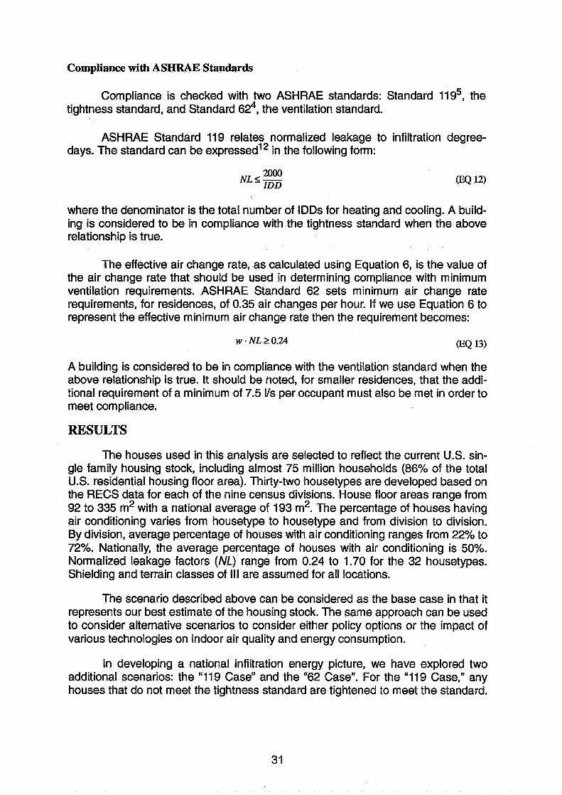
The map in Figure 1, shows the geographic distribution of the percentages of houses which meet Standard 11 9, based on county-wide averages. In colder cli- mates, less than 20 percent of the houses meet the tightness standard, driven by the higher number of infiltration degree days in the cooler climates. In the warmer climates over 80 percent of the houses meet the tightness standard, reflecting the milder climate and hence lower infiltration degree days.
There is very little variation in the geographic distribution of the percent of houses meeting Standard 62 is relatively flat and, thus, shows no obvious trends.
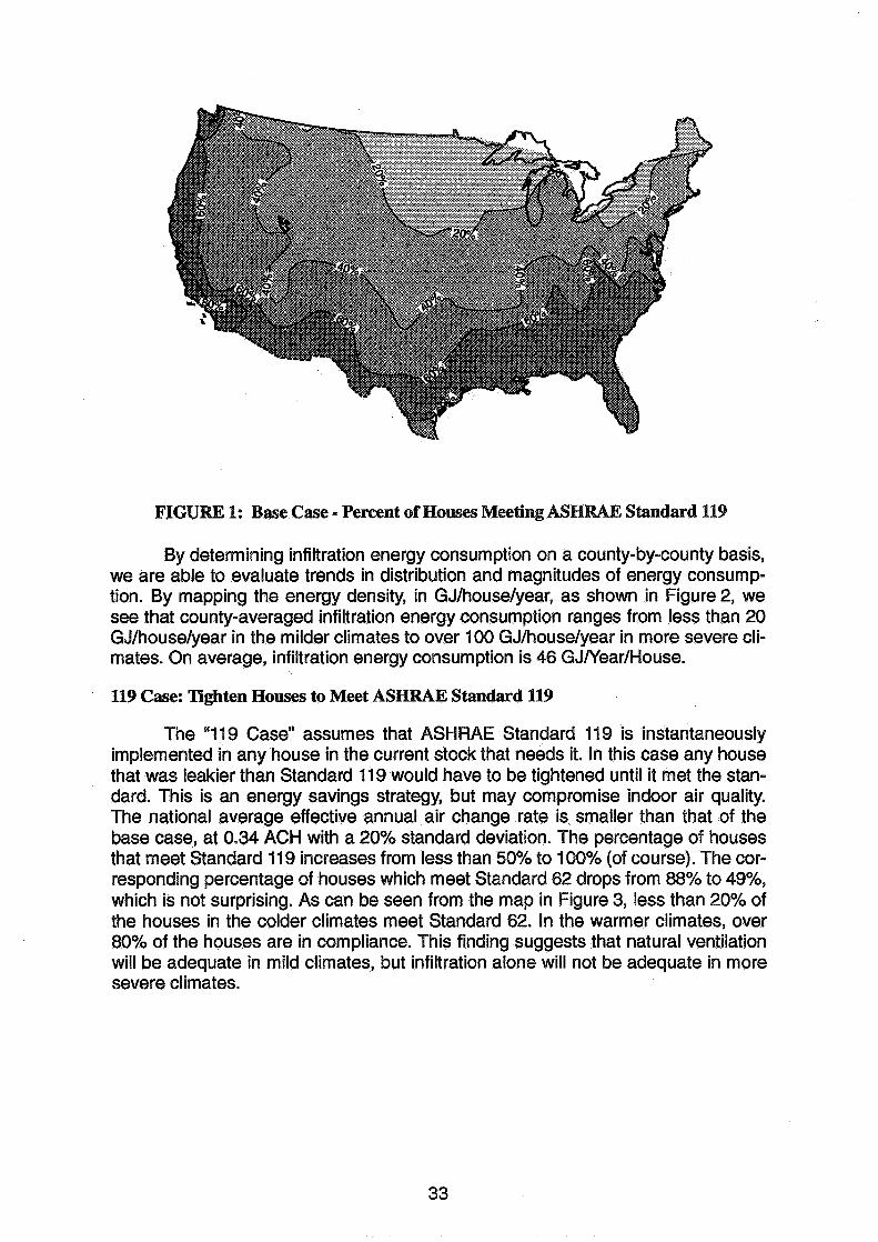
FIGURE 1: Base Case - Percent of Houses Meeting ASHRAE SItandard 119
By determining infiltration energy consumption on a county-by-county basis, we are able to evaluate trends in distribution and magnitudes of energy consump- tion. By mapping the energy density, in GJ/house/year, as shown in Figure 2, we see that county-averaged infiltration energy consumption ranges from less than 20 GJIhouselyear in the milder climates to over 100 GJhouseIyear in more severe cli- mates. On average, infiltration energy consumption is 46 GJPlearlHouse.
119 Case: Tighten Houses to Meet ASHRAE Standard 119
The "119 Case" assumes that ASHRAE Standard 119 is instantaneously implemented in any house in the current stock that needs it. In this case any house that was leakier than Standard 119 would have to be tightened until it met the stan- dard. This is an energy savings strategy, but may compromise indoor air quality. The national average effective annual air change rate is smaller than that of the base case, at 0.34 ACH with a 20% standard deviation. The percentage of houses that meet Standard 11 9 increases from less than 50% to 100% (of course). The cor- responding percentage of houses which meet Standard 62 drops from 88% to 49%, which is not surprising. As can be seen from the map in Figure 3, less than 20% of the houses in the colder climates meet Standard 62. In the warmer climates, over 80% of the houses are in compliance. This finding suggests that natural ventilation will be adequate in mild climates, but infiltration alone will not be adequate in more severe climates.

FIGURE 2: Base Case - Infiteation Energy Consumption (GJhouseIyear)
FIGURE 3: 119 Case - Percent of Houses Meeting ASHRAE Standard 62
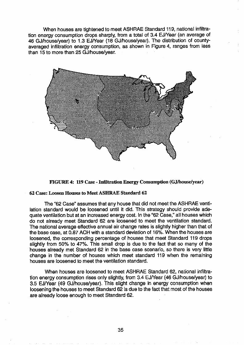
When houses are tightened to meet ASHRAE Standard 11 9, national infiltra- tion energy consumption drops sharply, from a total of 3.4 EJNear (an average of 46 GJhouselyear) to 1.3 EJNear (18 GJhouselyear). The distribution of county- averaged infiltration energy consumption, as shown in Figure 4, ranges from less than 15 to more than 25 GJ/house/year.
FIGURE 4: 119 Case - tration Energy Consumption (GJ/house/year)
62 Case: Loosen Houses to Meet ASHRAE Standard 62
The '"2 Case" assumes that any house that did not meet the ASHRAE venti- lation standard would be loosened until it did. This strategy should provide ade- quate ventilation but at an increased energy cost. In the "62 Case," all houses which do not already meet Standard 62 are loosened to meet the ventilation standard. The national average effective annual air change rates is slightly higher than that of the base case, at 0.87 ACH with a standard deviation of 16%. When the houses are loosened, the corresponding percentage of houses that meet Standard 11 9 drops slightly from 50% to 47%. This small drop is due to the fact that so many of the houses already met Standard 62 in the base case scenario, so there is very little change in the number of houses which meet standard 119 when the remaining houses are loosened to meet the ventilation standard.
When houses are loosened to meet ASHRAE Standard 62, national infiltra- tion energy consumption rises only slightly, from 3.4 EJNear (46 GJhouselyear) to 3.5 EJIYear (49 GJ/house/year). This slight change in energy consumption when loosening the houses to meet Standard 62 is due to the fact that most of the houses are already loose enough to meet Standard 62.

Analysis of Errors
Data from four sources (U.S. Census, RECS, AIVC leakage database and weather files) is used to determine the effective infiltration rates and related energy consumption and compliance with ASHRAE tightness and ventilation standards. Inherent in these data sources is a certain level of uncertainty, the largest of which is related to the leakage database.
As the U.S. Census tries to sample each and every household in the United States, the related sampling errors are very low. Our interpretation of the RECS data has an estimated maximum error of less than five percent for individual aver- ages. The weather data approximates a typical or an average weather year for a specific weather site, with some level of error as to its accuracy in modeling any specific year. While the weather data may have biases in it for various purposes, it can be considered as representative to some degree.
The estimated error in the use of the data from the AIVC leakage database is of more importance due to the potentially large sampling bias. Of the 243 houses, there is a limited range of construction styles, age of buildings, and a large geo- graphic bias (most of the houses in the database are located in the Pacific and Northwest regions of the country). The results also do not include houses built in the last decade. Our Bayesian estimate for the error in the mean is 40%. Clearly, the leakage data is the largest driving force in the level of uncertainty of these results.
The relatively poor data quality of the leakage data implies uncertainty in the base case results, but the difference between the "119 Case" and the "62 Case" is not materially affected by this uncertainty. Thus, if we assume that U.S. homeown- ers will be motivated to meet ventilation requirements by infiltration, there exists 2 EJ potential savings in infiltration load reduction by meeting Standard 11 9.
Our analysis is based on housing and leakage data available on hand at the time of our analysis. This analysis provides a preliminary view of the distribution and magnitude of infiltration-related energy consumption in the U.S. single- family build- ing sector. We have found that, based on our analysis, the current U.S. housing stock is relatively loose, signifying that most of the houses (88%) meet the ASHRAE ventilation standard. Of equal interest, however, is the potential for further energy conservation as reflected by the large number of houses not meeting ASHRAE Standard 119. While 88% of the total base case houses meet or exceed the ventila- tion requirements of Standard 62, 50% of the total houses meet the tightness requirements of Standard 119, with an overlap of 38% meeting both standards.
Table 4 summarizes, on a national basis, annual heating, cooling and total infiltration energy consumption for the base case and each of the two scenarios. By tightening up the housing stock to meet Standard 11 9, the potential national energy savings are projected to be up to 2.1 EJEear (28 GJhouseIyear). However, at the same time, the number of houses which meet the ventilation standard drop from
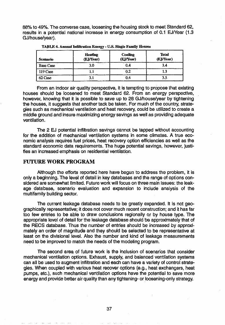
88% to 49%. The converse case, loosening the housing stock to meet Standard 62, results in a potential national increase in energy consumption of 0.1 EJNear (1.3 GJhouseIyear).
TABLE 4. Annual Mtration Energy - U.S. Single Family Houses
From an indoor air quality perspective, it is tempting to propose that existing houses should be loosened to meet Standard 62. From an energy perspective, however, knowing that it is possible to save up to 28 GJhouseIyear by tightening the houses, it suggests that another tack be taken. For much of the country, strate- gies such as mechanical ventilation and heat recovery, could be utilized to create a middle ground and insure maximizing energy savings as well as providing adequate ventilation.
The 2 EJ potential infiltration savings cannot be tapped without accounting for the addition of mechanical ventilation systems in some climates. A true eco- nomic analysis requires fuel prices, heat recovery option efficiencies as well as the standard economic data requirements. The huge potential savings, however, justi- fies an increased emphasis on residential ventilation.
F'UTURE WORK PROG
Although the efforts reported here have begun to address the problem, it is only a beginning. The level of detail in key databases and the range of options con- sidered are somewhat limited. Future work will focus on three main issues: the leak- age database, scenario evaluation and expansion to include analysis of the multifamily building sector.
The current leakage database needs to be greatly expanded. It is not geo- graphically representative; it does not cover much recent construction; and it has far too few entries to be able to draw conclusions regionally or by house type. The appropriate level of detail for the leakage database should be approximately that of the RECS database. Thus the number of entries should be increased by approxi- mately an order of magnitude and they should be selected to be representative at least on the divisional level. Also the number and kind of leakage measurements need to be improved to match the needs of the modeling program.
The second area of future work is the inclusion of scenarios that consider mechanical ventilation options. Exhaust, supply, and balanced ventilation systems can all be used to augment infiltration and each can have a variety of control strate- gies. When coupled with various heat recover options (e.g., heat exchangers, heat pumps, etc.), such mechanical ventilation options have the potential to save more energy and provide better air quality than any tightening- or loosening-only strategy.

This report has dealt exclusively with thermal loads. To convert thermal loads to resource energy or life-cycle costs it is necessary to have appropriate information on system efficiencies and appropriate economic factors. Proper evaluation of mechanical options requires that this data be incorporated into the analysis proce- dure.
This analysis covers only single-family buildings. It is tempting to say that we would use the same energy intensity for multifamily buildings, which represent only 14% of the U.S. residential floor area, and scale up our values. Future work will attempt to ascertain the accuracy of such an assumption.
REFERENCES
1 ASHRAE Handbook of Fundamentals, Chapter 23, American Society of Heating, Refrigerating and Air conditioning Engineers, 1989.
2 ASHRAE Handbook of Fundamentals, Chapter 24, American Society of Heating, Refrigerating and Air conditioning Engineers, 1989
ASHRAE Standard 55, Thermal Environmental Conditions for Human Oc- cupancy. American Society of Heating, Refrigerating and Air conditioning Engineers, 198 1.
ASHRAE Standard 62, Air Leakage Performance for Detached Single-Family Residential Buildings, American Society of Heating, Refkigerating and Air conditioning Engineers, 1989.
ASHRAE Standard 1 19, Air Leakage Performance for Detached Single-Fam- ily Residential Buildings, American Society of Heating, Refrigerating and Air conditioning Engineers, 1988.
ASHRAE Standard 136, A Method of Determining Air Change Rates in De- tached Dwellings, American Society of Heating, Refrigerating and Air conditioning Engineers, 1993.
Bureau of the Census, U.S. Department of Commerce, "21st Decennial Cen- sus," 1990.
California Energy Commission, "Climate Zone Weather Data Analysis and Revision Project," April 199 1.
Lawrence Berkeley Laboratory, "DOE-2 Reference Manual, Version 2. ID," LBd8706, Rev. 2, June 1989.
M. Limb, "AIRGUIDE: Guide to the fWCs Bibliographic Database," Air Infil- tration and Ventilation Centre, ATG-TN-38- 1992, 1992.
M.H. Sherman, "ASHRAE's Air Tightness Standard for Single-Family Hous- es." Lawrence Berkeley Laboratory Report LBd2543 1, LBL- 17585, March 1986.
M.H. Sherman, "EXEGESIS OF PROPOSED ASHRAE STANDARD 119: Air Leakage Performance for Detached Single-Family Residential Buildings." Roc. BTECC/DOE Symposium on Guidelines for Air Infiltration, Venti- lation, and Moisture Transfer, Fort Worth, TX, December 2-4, 1986.
Lawrence Berkeley Laboratory Report No. LBL2 1040, July 1986.
13 M.H. Sherman, "Infiltration Degree-Days: A Statistic for Infiltration-Related Climate," ASHRAE Trans. 92(II), 1986. Lawrence Berkeley Laboratory Report, LBL- 19237, April 1986.
14 M.H. Sherman, D.T. Grimsrud, me Measurement of Infiltration using Fan Pressurization and Weather Data" Proceedings, First International Air In- filtration Centre Conference, London, England. Lawrence Berkeley Labo- ratory Report, LBL 10852, October 1980.
15 M.H. Sherman, M.P. Modera, "Infiltration Using the LBL Infiltration Model." Special Technical Publication No. 904, Measured Air Leakage Perfor- mance of Buildings, pp. 325 - 347. ASTM, Philadelphia, PA, 1984; Lawrence Berkeley Laboratory
16 M.H. Sherman and D.J. Wilson, "Relating Actual and Effective Ventilation in Determining Indoor Air Quality." Building and Environment, 2 1 (3/4), pp. 135- 144, 1986. Lawrence Berkeley Report No. 20424.
17 M.H. Sherman, D.J. Wilson, D. Kiel, "Variability in Residential Air Leakage." Special Technical Publication No. 904 Measured Air Leakage Perfor- mance of Buildings, pp. 348 364, ASTM, Philadelphia, PA, 1984. Lawrence Berkeley Laboratory Report, LBL- 17587,
18 U.S.D.O.E., Energy Information Administration, "Housing Characteristics: Residential Energy Consumption Survey, 1990." DOE/EIA-0314(90), May, 1992.
19 United States Government, "U.S. Constitution, Article 1, Section 2," 1776.

Energy lm pact of Ventilation and Air Infiltration 14th AlVC Conference, Copenhagen, Denmark
21 -23 September 1 993
The Energy Impact of Ventilation and Air Infiltration in an Atrium
* Swedish National Testing & Research Institute, Box 857, S-50115 Borh ** Lund University, Department of Building Science, Box 118, S-22100 Lund

Synopsis
Many modem office and residential buildings in Sweden include an atrium. The atria are often mechanically ventilated and sometimes they are heated. Very little is known about the ventilation and air in built atria. These issues were examined in an apartment building with a non-heated and mechanically ventilated atrium, built in 1986 in Sweden. The ventilation of the atrium is coupled to the apartments.
The paper examines the ventilation, air infiltration, airtightness and the energy impact of an atrium. Fan pressurization was employed to characterize the air leakage of the atrium and the apartments. The energy use and temperatures in the atrium and in the apartments were monitored continuously for a year. A multi-zone network model was used to further evaluate the ventilation and the air infiltration. The energy balance was estimated using a dynamic simulation model.
The roof of the tested atrium is very leaky and therefore the exf~ltration is large. The energy use for space heating of the tested apartments can be reduced if the atrium and the apartments are made airtighter. The knowledge concerning the real airtightness and ventilation of atria and surrounding buildings is insufficient. There are also many ideas as to how to ventilate an atrium.
1. INTRODUCTION
The research and the measurements carried out by the Department of Building Science at Lund University concerning different atria have resulted in valuable knowledge concerning the technical problems that arise for different running conditions in buildings with atria (Lange 1986, Wall 1992). This experience has been used when determining the general principles for an apartment building with atrium in Malma. Requirements on climate and energy conservation have influenced the design of the atrium and the heating and ventilation system.
The building was designed during 1985 and built during 1986. Performance monitoring and evaulation were carried out during 1987 - 1991. A detailed description of the building and the results from the performance monitoring and evaluation is given in a final report (Blomsterberg 1993).
2. THE ATRIUM TESTED
The building includes an atrium with a floor area of 240 m2. The atrium is surrounded on three sides by a building with 3.5 floors. The building contains 28 apartments with a total floor area of 2034 m*. The entrance to each aparment is from the atrium. The atrium has two glazed areas, the singe1 glazed roof and the double glazed south facade. The atrium together with the modestly insulated wall facing the atrium has a U-value corresponding to a well insulated exterior wall. The building including the atrium has the same calculated conduction losses as the same building excluding the atrium, but with the wall facing the courtyard insulated according to the Swedish Building Code of 1980. The atrium has a distribution of conduction and ventilation loss coefficients, between the wall area facing the atrium and the glazed area facing the outside, of 1 : 1. This means that the temperature in

the atrium should always at least be equal to the average of the temperature in the apartments and outside. Solar radiation will raise the temperature above this average. There is no heating system in the atrium. The sun will heat the atrium and reduce the-eonduction losses from the apartments to the atrium and preheat the supply air to the apartments.
The building is equipped with a balanced ventilation system including an air-to-air heat exchanger. The outdoor air preheated by the heat exchanger first ventilates the atrium and then the apartments. The apartments are equipped with exhaust ventilation, where the exhaust air is passed through the heat exchanger.
3. MONITORING PROGRAM
The overall aim has been to monitor and evaluate the energy use and the indoor climate. This has been done by examining: the energy balance of the apartments, the energy balance of the atrium, the air temperatures in the apartments, and the air temperatures in the atrium.
The monitoring period was started with one-time tests: depressurization of five apartments, air leakage detection using themography in three apartments, depressurization tpressurization of the atrium, and measurements of the air flows in the ventilation system,
The test of the airtightness of the atrium was carried out using a specially developed fan (Lundin 1986), with a maximum capacity of 85000 m3/h at 50 Pa. The air flow through the fan was measured using tracer gas technique. A constant tracer gas flow was supplied upstream the fan and the concentration was measured downstream. The fan is attached to the main entrance of the atrium by means of a specially developed door.
After the one-time tests, continuous measurements were started. They were focused on energy use, indoor climate and outdoor climate. The building was occupied.
4. RESULTS
4.1 Energy use A comparison between measured and predicted use of energy for space heating during the heating season shows that the measured value, 57 kWh/m2, is 116 higher than the design value, 48 kWh/m2 (January - March and October - December). The predictions were made using the BKL-method (Kiblad 1984). The boundary conditions were almost the same but not quite the same during the measurements as for the calculations which complicates a comparison (see table 4.1).
Table 4.1 Boundary conditions during measurements and design calculations. . Mechanical ventilation, apartments Infiltration from outside, apartments Indoor temperature, apartments Mean yearly outdoor temperature Mean outdoor temperature, Oct - March
, Internal gains excl. solar ium curtains, winter
Measured, 1988 Design 0.6 air changes/h 0.7 air change& 0.1 3 air change& 0.10 air changes/h + 21 OC + 20 O C
+ 8.6 O C + 8.6 O C + 4.2 OC + 3.7 OC 21 7 kWh/day 200 kWh/day none double and airtight

The yearly use electricity for household purposes is reasonable, appr 2000 kwapartment. The use of electricity for running the building (shared laundry, shared lights, elevator, fans etc) is fairly large, 2600 kwapartrnent. The main part of this is the use of electricty for running the fans.
4.2 Airtightness of the apartments The results from the tests of the airtightness are presented as airchanges per hour at a pressure difference between inside and outside of 50 Pa (see table 4.2). The results can be compared with the requirements in the Swedish Building Code of 1980,l air change per hour i.e. no apartment fullfjdls the requirement.
Table 4.2. Airtightness at 50 Pa, air changes/h f 10 %. The values are an average of negative pressure and positive pressure. For the case with counter-pressure only negative pressure (depressurization) is given. Apartment nr Swedish Entrance to Open supply Counter-
standard neighboor open ducts pressure in atrium
11 1.81 1.82 1.83 0.7 12 1.69 - 1.80 0.58 23 1.47 - 1.96 0.73 28 1.85
The measurements in apartment no 11 according to the Swedish standard resp. with main entrance to neighboor open indicates that the air leakage between the apartments is small. This makes sense as the partition walls and the intermediate floors are made of concrete.
In order to illustrate the distribution of the leakage paths the effective leakage area was determined from the measurements (see table 4.3) (Sherman 1980). The effective leakage area was determined for a pressure difference of 4 Pa, which is a value which is more representative for the conditions in the real building when the fans are running. As the apartments are ventilated by an exhaust fan the leakage area was determined for a negative pressure. There are reasons for assuming that more air enters the apartments from the atrium than directly from outside, as the walls facing outside are airtighter than the ones facing the the atrium.
Table 4.3. Effective leakage area at a pressure difference of 4 Pa for the apartments,
partment no All walls Walls facing Supply duct Walls facing atrium from atrium outside
4.3 Airtightness of the atrium The entire atrium was depressurized and pressurized. All fans in the ventilation system were closed and the air terminal devices taped over during the measurements. The atrium was shown to be very leaky, according to a curve fit to the measurements, 12.5 air changes per
hour (average of depressurization and pressurization) at 50 Pa. The main part of the air leakage is located in the roof of the atrium. In the roof there are four longitudinal 1 cm wide cracks, which according to an estimate could account for all air leakage.
Using the results from the tests of airtightness, the air leakage through the apartments was calculated to account for 7 % of the air leakage of the atrium. The inaccuracy in this determination is of little importance as the dominating air lekage is through the glazed roof. If the glazed south facade of the atrium is assumed to leak 3 m3/m2h at 50 Pa, then the roof will leak 64 m3/m2h, which can be compared to the requirement of the new Swedish Building Code of 1988,3 m3/m2h for dwellings.
5. ANALYSIS
5.1 Ventilation of the atrium The real total ventilation of the atrium is unknown. The air flow rates which can be measured are the supply to the atrium and the exhaust from the apartments. The unknown air flows are the air flow between the atrium and the apartments, the air flow between the atrium and the outside, and the air flow between the apartments and the outside.
In order to estimate these unknown air flows, predictions have been performed using a multi-cell air flow program (MOVECOMP) (Herrlin 1987, Bring 1988, Blomsterberg 1990). The measured inputs used were: the airtightness of the atrium, the airtightness of the apartments, the air flows in the ventilation system, the air temperatures in the ventilation ducts, the air temperatures in the atrium, the air temperatures in the apartments, and the outdoor temperatures.
The simulations show that the exfiltration through the roof of the atrium varies with the outdoor temperature. When there is no wind the exfiltration is appr 1100 m3/h or 30 % of the supply air at an outdoor temperature of - 10 OC and appr 800 m3/h or 25 % of the supply air at an outdoor temperature of + 10 OC (see case 1 in table 5.1). If the average wind speed of the heating season prevails, then the exfiltration will increase by 20 %. The result is that during the heating season appr. 30 % of the preheated supply air vanishes out through the roof of the atrium.
All outdoor air to the apartments does not come from the atrium, but a not negligible part enters directly from the outside. The infiltration from the outside varies from 630 m3/h or 20 % of the supply air at - 10 OC to 530 m3/h or 17 % of the supply air at + 10 OC (see case 1 in table 5.1). This occurs when there is no wind. If the average wind of the heating season prevails, then the infiltration will increase by 30 %. There is no exfiltration from the apartments.
Next step was to repeat the simulations assuming that the roof of the atrium is very airtight e g fullfills the requirement of the new Swedish Building Code of 1988 for dwellings, 3 m3/m2h at 50 Pa. When there is no wind the exfiltration through the roof is reduced from 1100 m3/h (or 30 % of the supply air) to 500 m3/h (or appr. 15 % of the supply air) at an outdoor temperature of - 10 OC and reduced from appr 800 m3/h (or 25 % of the supply air) to 350 m3/h (or appr. 10 % of the supply air) at an outdoor temperature of + 10 "C (see case 2 in table 5.1). If the average wind speed of the heating season prevails, then the

exfiltration will increase by 20 %. The result is that during the heating season appr. 15 % of the preheated supply air vanishes out through the roof of the atrium.
The infiitration from the outside is in this case reduced from 630 m3/h (or 20 % of the supply air) to 130 m3/h (or appr. 5 % of the supply) at - 10 OC and from 530 m3/h (or 17 % of the supply air) to 180 m3/h (or appr. 6 % of the supply air) at + 10 OC (see case 2 in table 5.1). This occurs when there is no wind. If the average wind of the heating season prevails, then the infiltration will increase by 60 %. Exfiltration will occur from the apartments at the top floor.
Next step was to repeat the simulations assuming that the roof of the atrium has the measured airtightness, but the supply air flow to the atrium is almost the same as the exhaust air flow from the apartments. When there is no wind the exfiltration through the roof is increased from the earlier 500 m3/h to 600 m3/h at an outdoor temperature of - 10 OC and reduced from 350 m3/h to appr. 250 m3/h at an outdoor temperature of + 10 OC (see case 3 in table 5.1). If the average wind speed of the heating season prevails, then the exfiltration will increase by 50 %. The result is that during the heating season appr. 35 % of the preheated supply air disappears out through the roof of the atrium.
The infiltration from the outside will in this case increase somewhat from the original 630 m3/h (or 20 % of the supply air) to appr. 675 m3/h at - 10 OC and from the original 530 m3/h (or 17 % of the supply air) to appr 550 m3/h at + 10 OC (see case 3 in table 5.1). This occurs when there is no wind. If the average wind of the heating season prevails, then the infiltration will increase by 30 %.
Table 5.1 Calculated air flows, m3/h. The exfiltration through the roof of the atrium and the infiltration to the apartments from the outside is calculated for an outdoor temperature of - 10 OC and + 10 "C. The exhaust air flow of 3050 m3/h for the apartments
Case 1 2 4 Airtightness As measured New Code As measured No leakage Supply air 3350 3350 2800 3350 Exhaust air 3050 3050 3050 3050 Atrium exfiltration -Om/s(wind) 780-1100 360 - 480 260 - 600 300 -5rn/s(wind) 980-1330 450 - 570 450 - 830 300 Apartment infiltration
The last step, which does not require any calculations, is the case probably assumed by the designer i.e. all air to the apartments enters from the atrium (see case 4 in table 5.1).
5.2 Energy use In order to evaluate the influence on the energy use for space heating of the apartments by the airtightness and ventilation of the atrium, simulations were performed using DEROB- LTH (Arurni-No6 1979, Fredlund 1989). The first step was to see how accurately DEROB can predict the energy use for different measuring periods. Four different test period were chosen. Two-week periods with cold and mild weather, almost no sun and a lot of sun, small and large diurnal variations are represented. The agreement was shown to be good concerning the variation over time in space heating and the average temperature in the atrium.
The predictions underestimate the absolute level of space heating. For sunny periods the simulations tend to underestimate the space heating demand. This is most likely caused by the fact that DEROB-LTH assumes a perfect control system without any time delay for the heating system, which does not correspond to what actually happened. The predictions do no take into account that there are curtains in each apartment i e more useful solar energy in the calculations. If the sunny periods are corrected, then the agreement is reasonable.
The second step was to predict the energy use for space heating for a reference year, Malrno 1971. The third step was a prediction, based on previously calculated air flows assuming the atrium to fullfill the airtightness requirements of the new Swedish Building Code of 1988 (see case 2 in table 5.1). The fourth step was a prediction, where the supply air flow to the atrium is balanced with the exhaust air flow from the apartments (see case 3 in table 5.1). The last step was a prediction for the theoretical case with no infitration (see case 4 in table 5.1). In all predictions the indoor temperature of the apartments was + 20 "C.
If the atrium had fullfilled the airtightness requirements of the new Building Code of 1988, then the energy use for space heating would have been reduced by 8 % (see table 5.4). This is due to the fact that if the atrium is made airtighter, then the exfiltration from the atrium and the infiltration directly from the outside to the apartments are reduced i. e. the air flow from the atrium to the apartments is increased. Balanced air flows do not mean any improvement compared with the base case. Neither the temperature in the atrium or the infiltration directly from the outside to the apartments are influenced. The theoretical case, where no Sitration to the apartments directly from the outside occurs, means of course the lowest energy use.
All predictions with DEROB-LTH show that the objective that the air temperature of the atrium always should be at least equal to the average value of the outdoor temperature and the temperature in the apartments is achieved for monthly averages. The measurements do however for 1988 show that during almost 100 days, when the daily mean outdoor temperature was below + 7 "C, the daily mean temperature in the atrium was 1 - 2 "C too low.

1 Measured airtightness and air flows, real 72 occupancy
2 New Code airtightness, measured air flows, 66 real occupancy
3 Measured airtightness, balanced air flows, real 73 occupancy
4 Measured airtightness and air flows, real 63
6. CONCLUSIONS
The performance monitoring and evaluation show that it is possible to build a well functioning apartment building including an atrium. Apart from short periods with high temperatures the system has created reasonable temperatures in the atrium and the apartments.
The aim for the building was to always maintain a temperature in the atrium, which is at least the average value of the air temperature in the apartments and outside. This was met apart from 100 days during a year when the temperature in the atrium is somewhat too low. One reason was that the roof of the atrium never was equipped with double and airtight curtains. The curtains were also never used during the nights as was planned.
The energy use for space heating of the apartments was somewhat higher than predicted, probably due to lower solar gains than in theory.
The exfiltration through the roof of the atrium is large due to a very leaky roof. The infiltration from outside to the apartments is also large. The idea was that most of the air to the apartments was to enter from the atrium. The apartments were too leaky.
If the atrium had fullfilled the airtightness requirements of the new Swedish Building code of 1988, then the energy use for space heating of the apartments would have been reduced by 10 %. The airtightness of the atrium would have been even more important if the atrium had been heated to normal indoor temperature e g + 20 "C.
A study of several atria shows that many ideas exist as to how to ventilate an atrium and how to couple its ventilation with the surrounding building. Different requirements are made on what level of temperature is to be maintained in an atrium. The knowledge concerning the real airtightness and ventilation of atria and surrounding buildings is insufficient. The size of the total ventilation is of importance to the indoor air quality and the energy use.
7. REFERENCES
Arumi-NoC, F., 1979, The DEROB System Volume II - Explanatory Notes and Theory. Numerical Simulation Laboratory, School of Architecture, University of Texas, Austin, Texas, USA.

Blomsterberg, A., 1990, Ventilation and airtightness in low-rise residential buildings - Analyses and full-scale measurements. Ph. D. thesis, Swedish Council for Building Research, D10: 1990, Stockholm, Sweden.
Blomsterberg, A., 1993, Apartment building with atrium - Technical description and evaluation of a project in Malmo. Department of Building Science, Lund University, TABK 9313013, Sweden (in Swedish).
Bring, A., Herrlin, M., 1988, User's Manual - MOVECOMP-PC(R) - An Air Infiltration and Ventilation System Simulation Program. Bris Data AB , Saltsjobaden, Sweden.
Fredlund, B., 1989, Blocks of flats with glazed verandas, Taberg - Analysis of energy and internal climate. Swedish Council for Building Research, D3: 1989, Stockholm, Sweden.
Herrlin, M., 1987, Air flows in buildings - a calculation modell. Royal Institute of Technolgy, Department of Building Services, Stockholm, Sweden (in Swedish).
Kiblad, K., Adamson, B., 1984, The BKL-method: A simplified method to predict energy consumption in buildings. Swedish Council for Building Research, D8: 1984, Stockholm, Sweden.
Lange, E.,1986, Glazed areas - Climate and energy - Experience from performance monitoring and evaluation of two projects. Swedish Council for Building Research R35: 1986, Stockholm, Sweden (in Swedish).
Lundin, L., 1986, Air Leakage in Industrial Buildings - Description of Equipment. Measured Air Leakage in Buildings, ASTM STP 904, pp 101 - 105, Philadelphia, USA.
Wall, M.,1992, Glazed courtyard at T h a n - Thermal performance of the courtyard and surrounding residential buildings - Measurements and calculations. Swedish Council for Building Research, D7: 1992, Stockholm, Sweden.
Sherman, M., 1980, Air Infiltration in Buildings. Lawrence Berkeley Laboratory, Ph.D. thesis, LBL-10712, Berkeley, California, USA.

Energy Impact of Ventilation and Air Infiltration 14th AlVC Conference, Copenhagen, Denmark
21 -23 Septem ber 1993
The Energy Impact of Ventilation on Industrial Buildings
P J Jones, G Powell, D K Alexander
Welsh School of Architecture, University of Wales College of Cardiff, King Edward VII Avenue, Cardiff, CF1 3AP, UK
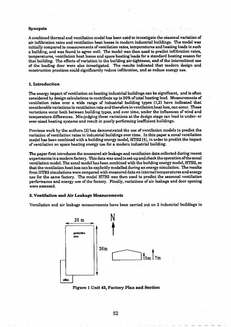
Synopsis
A combined thermal and ventilation model has been used to investigate the seasonal variation of air infiltration rates and ventilation heat losses in modern industrial buildings. The model was initially compared to measurements of ventilation rates, temperatures and heating loads in such a building, and was found to agree well. The model was then used to predict infiltration rates, temperatures, ventilation heat losses and space heating loads for a standard heating season for that building. The effects of variation in the building air-tightness, and of the intermittent use of the loading door were also investigated. The results indicated that modern design and construction practices could significantly reduce infiltration, and so reduce energy use.
1. Introduction
The energy impact of ventilation on heating industrial buildings can be significant, and is often considered by design calculations to contribute up to 50% of total heating load. Measurements of ventilation rates over a wide range of industrial building types [1,21 have indicated that considerable variations in ventilation rate and therefore in ventilation heat loss, can occur. These variations occur both between building types, and over time, under the influences of wind and temperature differences. Mis-judging these variations at the design stage can lead to under- or over-sized heating systems and result in poorly performing inefficient buildings,
Previous work by the authors C31 has demonstrated the use of ventilation models to predict the variation of ventilation rates in industrial buildings over time. In this paper a zonal ventilation model has been combined with a building energy model, HTB2 [41, in order to predict the impact of ventilation on space heating energy use for a modern industrial building.
The paper first introduces the measured air leakage and ventilation data collected during recent experiments in a modern factory. This data was used to set-up and check the operation of the zonal ventilation model. The zonal model has been combined with the building energy model, HTB2, so that the ventilation heat loss can be explicitly modelled during an energy simulation. The results from HTB2 simulations were compared with measured data on internal temperatures and energy use for the same factory. The model HTB2 was then used to predict the seasonal ventilation performance and energy use of the factory. Finally, variations of air leakage and door opening were assessed.
2. Ventilation and Air Lealrage Masurenaents
Ventilation and air leakage measurements have been carried out on 3 industrial buildings in
I o&e I 1 Unit 42, Factory Plan and Section

Aberaman, South Wales, as part of a project to investigate the design and construction of modern low energy' factories [ll. The factories involved were designed within the current building regulation requirements, with a design U-value of 0.45 W/m2/OC. They were also specifically designed to achieve a low air infiltration rate. Attention was given to the detailing of the building to ensure that the thermal insulation was properly installed and that air leakage was minimised. The design and construction processes were monitored to determine and correct any problems.
The factory monitored (Figure 1) was of 720m2 production floor area, with a composite cladding construction. The heating system comprised of two wall-mounted warm air heaters, with destratification fans in operation. The factory had an insulated loading door and 2 roof ventilators.
Air leakage and ventilation measurements were carried out in February and August 1992, respectively. The air leakage measurements were carried out by pressurisation fans installed in the fire doors. InternaVextemal pressure differences of up to 60 Pa were achieved for air flow rates of 7 ma/s. Ventilation measurements were carried out using constant concentration and tracer decay methods with N20 as the tracer gas. Continuous constant concentration measurements were carried out over a 14 day period. Tracer decay tests were also performed to assess the ventilation rates occurring during the use of the loading door. The results are summarised in Table 1.
Average ventilation rate 0.16 a& Typical ventilation rate with
loading door open 1.5 a&
Average temperature during ventilation measurements; Internal 21.5 OC
External 16.2 "C
of air leakage and ventilation mea
3. Prepmtion of Zonal Ventilation Model
The data required for the zonal ventilation model was derived as follows, using the same procedures as developed in an earlier investigation 131 :
i) the measured air leakage curves, as shown in Figure 2, for background (doors and roof ventilators sealed) and total (doors and roof ventilators unsealed - but not open) situations were used to estimate the equivalent crack opening parameters for the envelope. The resultant open areas are summarised below :
background leakage area - 1.21m2 loading door (closed) leakage area - negligible roof vents (closed) leakage area - 0.1m2
ii) throughvisual inspection, and application of the simple rule developed in the earlier work, these open areas were located on the envelope. Apart from the location of the ventilators and door, there were no obvious sites for anomalous background leakage. Accordingly, the background was apportioned equally (by wall length) to locations where there were changes in comtruction or junction of major components, i.e. a t eaves level, or at rooflights. This

Leakage Rate m31s 8 measured background
m measured total *
model background - m ode1 total P
" 0 10 20 3 0 4 0 5 0 60
Pressure Pa.
Figure 2 Measured and Best Fit Leakage Data
provided the following simple background opening distribution; facade height open area a t each height south wall l m & 5m 0.0755m2 west wall 1m & 5m 0.1510m2 north wall l m & 5m 0.0755m2 east wall l m & 5m 0.15 10m2 west roof 6m 0. 1510m2 east roof 6m 0.1510m2
This initial distribution of background areas was not altered further. It is worth noting that thermographic experiments with and without building pressurisation indicated considerable leakage a t the eaves levels, a s assumed in the above.
iii) surface average wind pressure coefficients were calculated using standard algorithms, a s previously used [31.
The zonal ventilation model was applied to this data to predict the variation of air infiltration rate over time for a two week period in JulyIAugust 1992, for which measured ventilation data was available for comparison. These ventilation measurements were obtained from constant concentration experiments Ell. Internal and external air temperature data was collected on site and wind velocity data was obtainedfrom a nearby meteorological station. The predictions for this comparison were made using the recorded internal temperatures.
The predicted and measured infiltration rates are plotted for the 10 day period in Figure 3. Hourly values for predicted and measured infiltration rates are compared in Figure 4. There was a reasonable agreement between the two data sets. A mi$or contribution to the differences was considered to be due to the use of off-site wind velocity data. It was not possible to permanently monitor wind velocity directly on-site, due to a high risk of vandalism.
4. Test Simulation Using
As part of on-going developmental work within the WSA research group, the building thermal model HTB2 has been modified to include the zonal ventilation model within its' dynamic calculation procedure. The modular nature of HTB2 [41 enables such additional sub-models to be incorporated with relative ease.
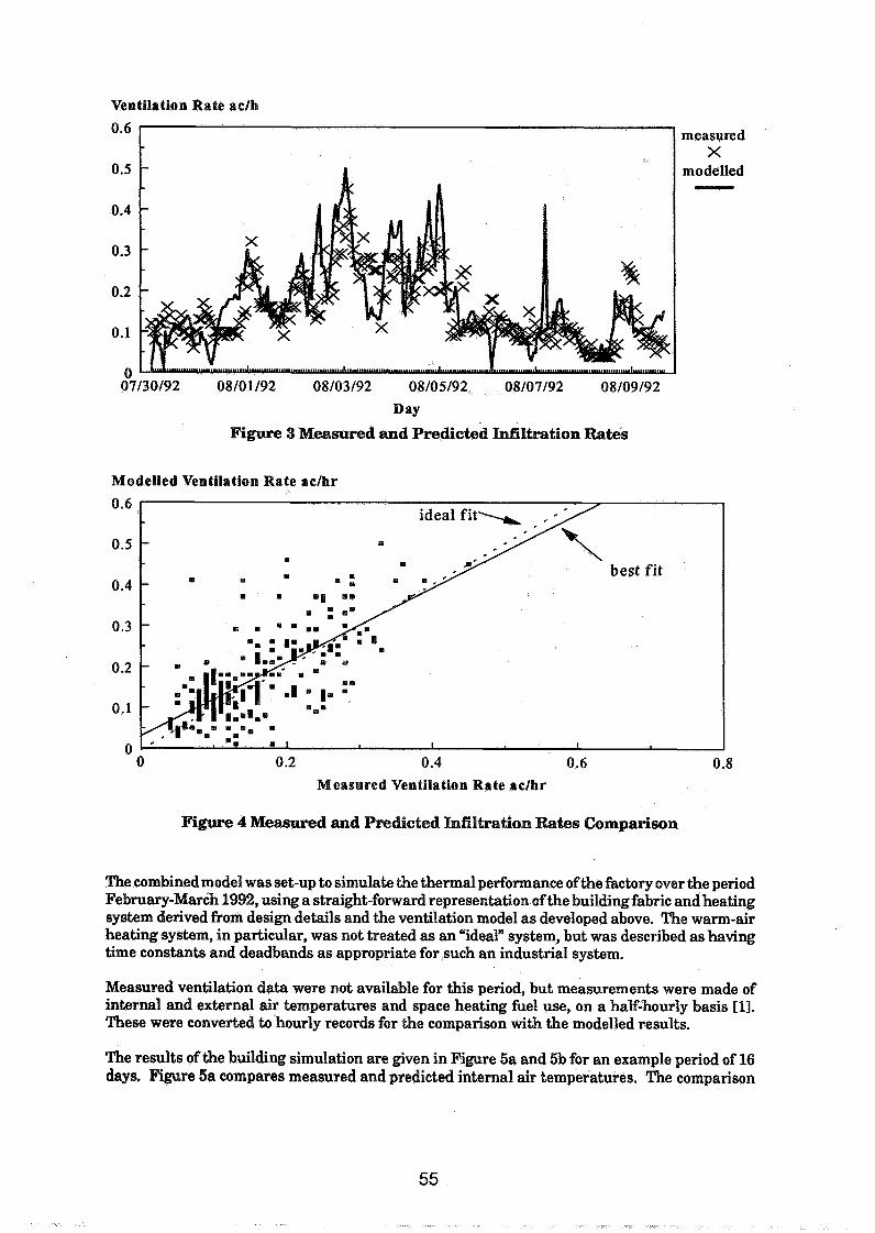
Ventilation Rate aclh 0.6
0 07/30/92 08/01 192 08/03/92 08/05/92 08/07/92 08/09/92
Day Figure 3 Measured and Predicted Infiltration Rates
Modelled Ventilation Rate a c h r
measured X
modelled
0.2 0.4 0.6
Measured Ventilation Rate aclhr
Fi d and Predicted Infiltration Rates amparison
The combinedmodel was set-up to simulate the thermal performance of the factory over the period February-March 1992, using a straight-forward representation of the building fabric and heating system derived from design details and the ventilation model as developed above. The warm-air heating system, in particular, was not treated as an "ideal" system, but was described a s having time constants and deadbands as appropriate for such a n industrial system.
Measured ventilation data were not available for this period, but measurements were made of internal and external air temperatures and space heating he1 use, on a half-hourly basis [I]. These were converted to hourly records for the comparison with the modelled results.
The results of the building simulation are given in Figure 5a and 5b for an example period of 16 days. Figure 5a compares measured and predicted internal air temperatures. The comparison
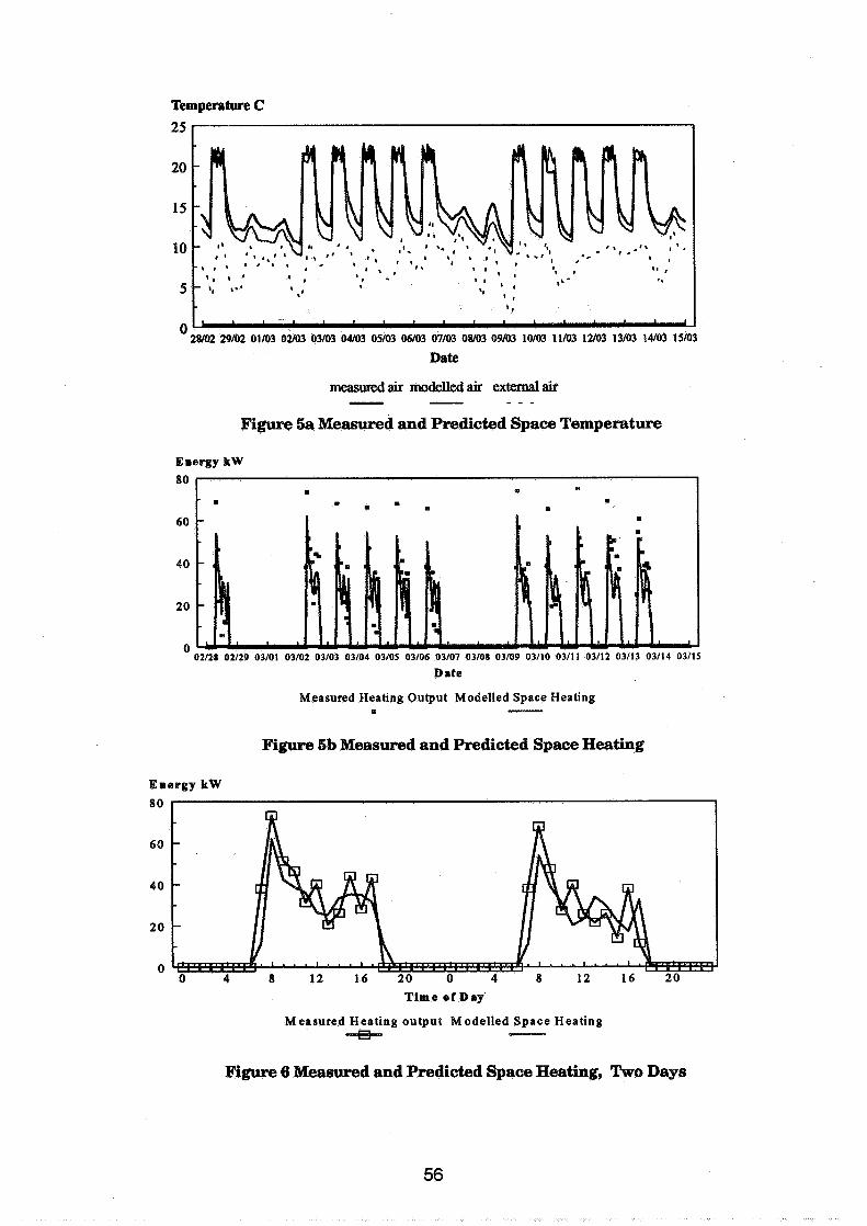
Temperature C
25 1
O 28/02 29/02 01/03 02103 03/03 04/03 05/03 06/03 07/03 08/03 09/03 10103 1 1/03 12103 13/03 14/03 15/03
Date
measured air modelled air external air P - - - -
Figure Sa Measured and Predicted Space Temperature
Emergy k W 80
rn
m m I
m I
Date
Measured Heating Output Modelled Space Heating m -
Figure Sb Measured and Predicted Space Heating
Emergy k W 80
60
40
2 0
0 0 4 8 12 16 20 0 4 8 12 16 20
Time of Day'
Measured Heating output Modelled Space Heating --Et- -
Fi d and Predicted Space Heating, Two Days
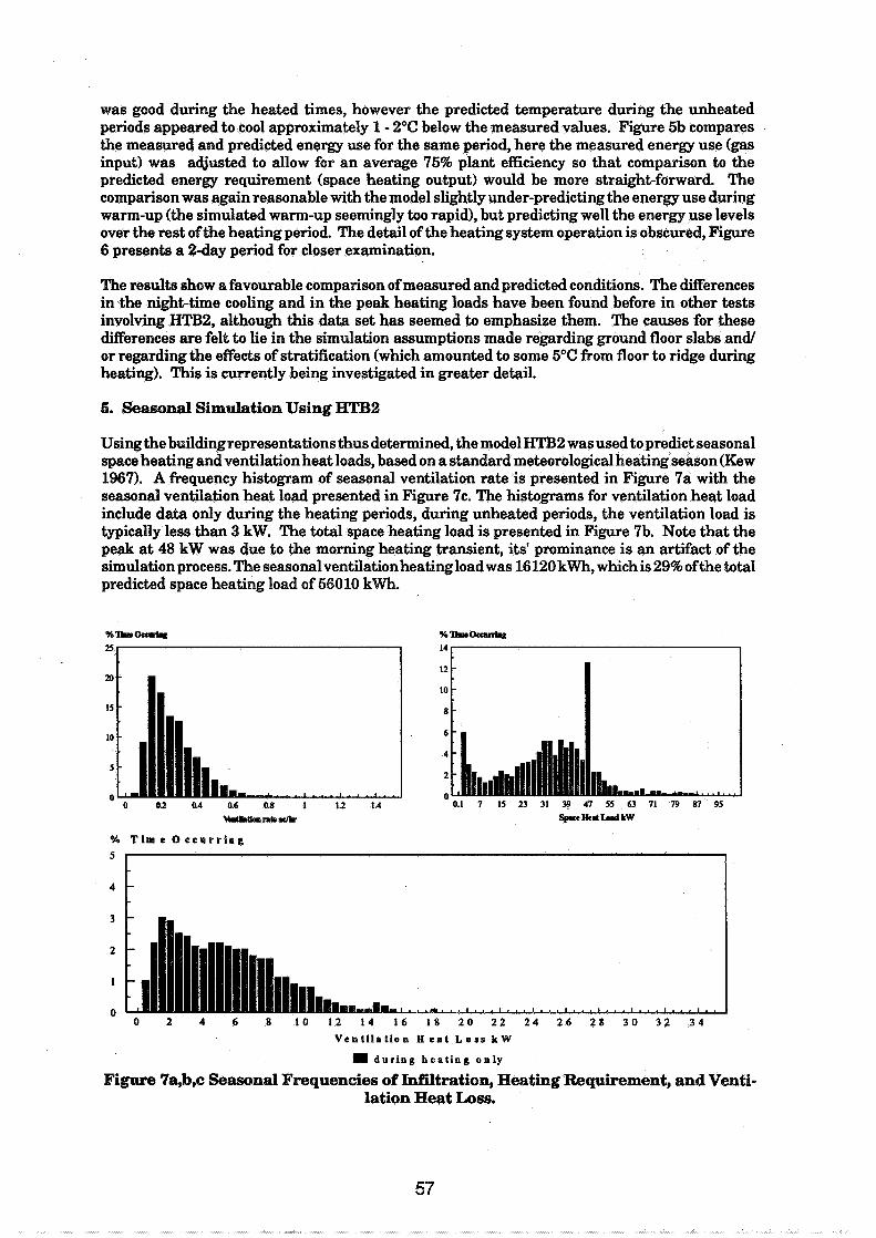
was good during the heated times, however the predicted temperature during the unheated periods appeared to cool approximately 1 - 2OC below the measured values. Figure 5b compares the measured and predicted energy use for the same period, here the measured energy use (gas input) was adjusted to allow for an average 75% plant efficiency so that comparison to the predicted energy requirement (space heating output) would be more straight-forward. The comparison was again reasonable with the model slightly under-predicting the energy use during warm-up (the simulated warm-up seemingly too rapid), but predicting well the energy use levels over the rest of the heating period. The detail of the heating system operation is obscured, Figure 6 presents a 2-day period for closer examination.
The results show a favourable comparison of measured and predicted conditions. The differences in the night-time cooling and in the peak heating loads have been found before in other tests involving HTB2, although this data set has seemed to emphasize them. The causes for these differences are felt to lie in the simulation assumptions made regarding ground floor slabs and1 or regarding the effects of stratification (which amounted to some 5OC from floor to ridge during heating). This is currently being investigated in greater detail.
5. Seasonal Simulation Using IETS2
Using the buildingrepresentations thus determined, the model HTB2 was used to predict seasonal space heating and ventilation heat loads, based on a standard meteorological heating season (Kew 1967). A frequency histogram of seasonal ventilation rate is presented in Figure 7a with the seasonal ventilation heat load presented in Figure 7c. The histograms for ventilation heat load include data only during the heating periods, during unheated periods, the ventilation load is typically less than 3 kW. The total space heating load is presented in Figure 7b. Note that the peak at 48 kW was due to the morning heating transient, its' prominance is an artifact of the simulation process. The seasonal ventilation heating load was 16120 kWh, which is 29% of the total predicted space heating load of 56010 kWh.
V e n t i l a t i o n H e a t L o r n k W
during h e a t i n g only
7a,b,c Seasonal Frequencies of Infiltration, Heating Requirement, and Venti- lation Heat Loss.
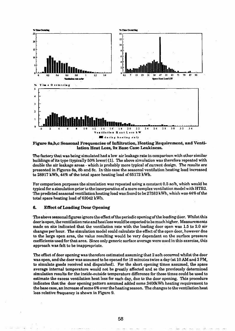
V s m t l l a t l e m H e a t L e s s k W
d u r i n g h e a t i n g o n l y
Figure 8a,b,c Seasonal Frequencies of Infiltration, Heating Requirement, and Venti- lation Heat Loss, 2x Base Case Leakiness.
The factory that was being simulated had a low air leakage rate in comparison with other similar buildings of its type (typically 50% lower) Cll. The above simulation was therefore repeated with double the air leakage areas - which is probably more typical of current design. The results are presented in Figures 8a, 8b and 8c. In this case the seasonal ventilation heating load increased to 28917 kWh, 44% of the total space heating load of 65172 kWh.
For comparison purposes the simulation was repeated using a constant 0.5 a h , which would be typical for a simulation prior to the incorporation of a more complex ventilation model with HTB2. The predicted seasonal ventilation heating load was found to be 27583 kwh, which was 44% of the total space heating load of 62042 kWh.
6. Effect of Loading Door Opening
The above seasonal figures ignore the effect of the periodic opening of the loading door. Whilst this door is open, theventilation rate and heatloss would be expected to be muchhigher. Measurements made on site indicated.that the ventilation rate with the loading door open was 1.5 to 2.0 air changes per hour. The simulation model could calculate the effect of the open door, however due to the large open area, the value resulting would be very dependant on the surface pressure coefficients used for that area. Since only generic surface average were used in this exercise, this approach was felt to be inappropriate.
The effect of door opening was therefore estimated assuming that 2 a h occurred whilst the door was open, and the door was assumed to be opened for 15 minutes twice a day (at 10 AM and 3 PM, to simulate goods received and dispatched). For the short opening times assumed, the space average internal temperature would not be greatly affected and so the previously determined simulation results for the inside-outside temperature difference for those times could be used to estimate the excess ventilation heat loss for each day, due to the door opening. This procedure indicates that the door opening pattern assumed added some 3400kWh heating requirement to the base case, an increase of some 6% over the heating season. The changes to the ventilation heat loss relative frequency is shown in Figure 9.
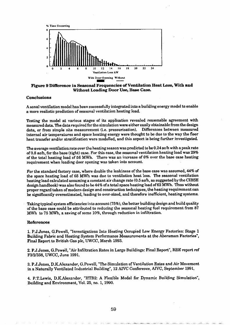
% Time Occurring 8 I
Ventilation Loss kW
With Door Opening Without I -
Figure 9 Difference in Seasonal Frequencies of Ventilation Heat Loss, With and Without Loading Door Use, Base Case.
Conclusions
A zonal ventilation model has been successfully integrated into a building energy model to enable a more realistic prediction of seasonal ventilation heating load.
Testing the model at various stages of its application revealed reasonable agreement with measured data. The data required for the simulation were either easily obtainable from the design data, or from simple site measurement (i.e. pressurisation). Differences between measured internal air temperatures and space heating energy were thought to be due to the way the floor heat transfer andlor stratification were modelled, and this aspect is being further investigated.
The average ventilation rate over the heating season was predicted to be 0.24 a& with a peak rate of 0.8 a&, for the base (tight) case. For this case, the seasonal ventilation heating load was 29% of the total heating load of 56 MWh. There was an increase of 6% over the base case heating requirement when loading door opening was taken into account.
For the standard factory case, where double the leakiness of the base case was assumed, 44% of the space heating load of 65 MWh was due to ventilation heat loss. The seasonal ventilation heating load calculated assuming a constant air change rate (0.5 a&, as suggested by the CIBSE design handbook) was also found to be 44% of a total space heating load of 62 MWh. Thus without proper regard taken of modern design and construction techniques, the heatingrequirement can be significantly overestimated, leading to over-sized, and therefore inefficient, heating systems.
Taking typical system efficiencies into account (75%), the better building design and build quality of the base case could be attributed to reducing the seasonal heating fuel requirement from 87 MWh to 75 MWh, a saving of some lo%, through reduction in infiltration.
References
1. P.J.Jones, G.Powell, "Investigations Into Heating Occupied Low Energy Factories: Stage 1 Building Fabric and Heating System Performance Measurements a t the Aberaman Factories", Final Report to British Gas plc, UWCC, March 1993.
2. P.J.Jones, G.Powel1, "Air Infiltration Rates in Large Buildings: Final Report", BRE report ref F3121338, UWCC, June 1991.
3. P.J.Jones, D.KAlexander, G.Powel1, "The Simulation of Ventilation Rates and Air Movement in a Naturally Ventilated Industrial Building", 12 ATVC Conference, AIVC, September 1991.
4. P.T.Lewis, D.KAlexander, "HTB2: A Flexible Model for Dynamic Building Simulation", Building and Environment, Vol. 25, no. 1, 1990.


Energy lrn pact of Ventilation and Air Infiltration 14th AlVC Conference, Copenhagen, Denmark
21 -23 Septern ber 1993
Theoretical Basis for Assessment of Air Quality and Heat Losses for Domestic Ventilation Systems in France
J G Villenave, J-R Millet, J Riberon
Centre Scientifique et Technique du Biltiment, Marne la Vallee, France
ABSTRACT.
Ventilation of buildmgs is necessary, both to insure adequate indoor air quality and to protect the building itself against condensation and mould growth. On the other hand, ventilation rates must not lead to excessive energy consumption.
French regulation doesn't appreciate directly the indoor air quality but fixes requirements for the value of exhaust stale air in service rooms ; furthermore heat losses related to cross ventilation due to wind effects are also taken into account. For assessment of Demand Control Ventilation systems both air quality and heat losses have to be compared to a mechanical exhaust only system.
In this paper, we describe the methodology and the CSTB computer models, and how they have been used to design the French rules related to the energy demand of ventilation systems and the air quality level obtained with DCV systems by reference to a conventional mechanical ventilation system.
1 - INTRODUCTION.
Ventilation of buildings is necessary, both to insure adequate indoor air quality and to protect the building itself against condensation and mould growth. On the other hand, ventilation rates must not lead to excessive energy loads. Mechanical ventilation systems, which have been in common use in France since the sixties, comply this requirement.
Mechanical systems have been improved for ten years : new systems with variable flow rate according to the prevailing indoor climatic conditions, enable energy conservation and indoor air quality to be further improved.
Evidence from a variety of investigations and systematic studies (in France but also in other countries) suggests that the use of these systems can improve indoor air quality while the energy consumption be reduced [l, 2 and 31.
2 - BASIS OF FRENCH REGULATION.
2.1 - Historical. For more than 20 years French Regulations for dwelling have been the mover of the building insulation and ventilation technological progress.
In 1969 ventilation had to supply fresh air to the habitable rooms and to exhaust stale air from the service rooms (this point of the French regulation has been continuously used since then) with an air change rate about 1 volume/hour. The French authorities decided to include the energy loss due to the ventilation in the total energy loss of the buildings. This point of the French regulation, which has been continuously used since then is very specific and important : it makes it possible to compare the design alternative and parametrics studies.
After the energy crisis (1974) research on occupied dwellings came to the conclusion that almost 50 % of dwellings were over ventilated; with the 1982183 regulation the flow rate depends on the number of habitable rooms with a possibility of reducing the ventilation rate during under occupancy. One of the technological consequence is the development of humidity controlled ventilation systems. Air leakage's through a building envelope can disrupt the intended operation of heating and ventilation. In view of high stakes, research works were conducted at the C.S .T.B. into air infiltration in buildings [4]. They involved improvement in heat losses calculation due to cross ventilation and development of air leakage measurement methods.
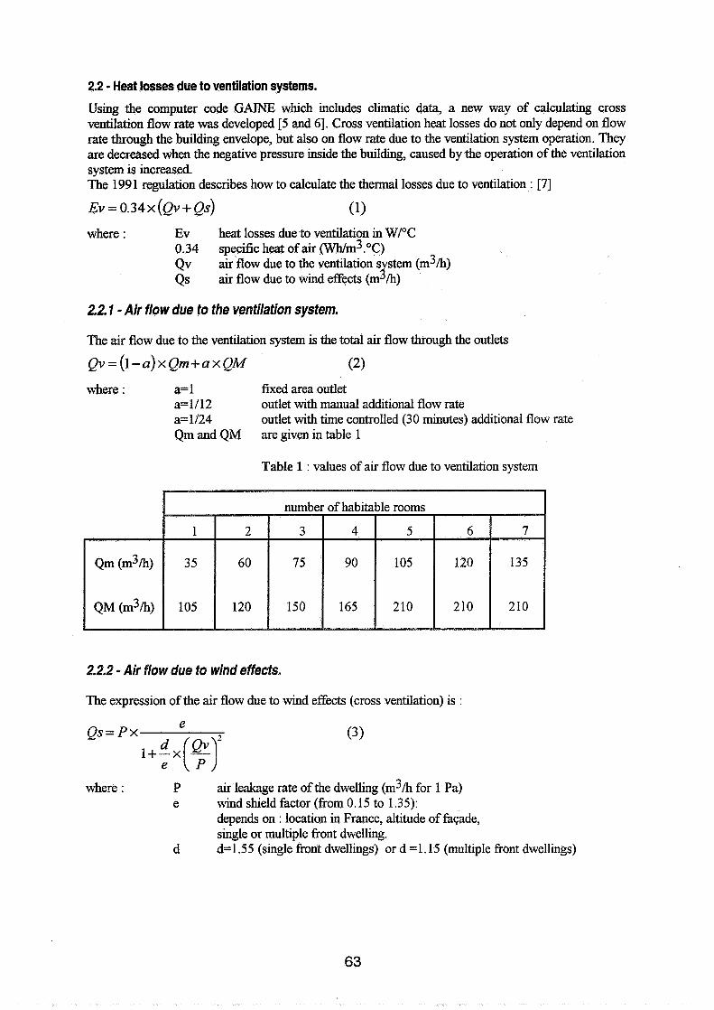
2.2 - Heat losses due to ventilation systems.
Using the computer code GAINE which includes climatic data, a new way of calculating cross ventilation flow rate was developed [5 and 61. Cross ventilation heat losses do not only depend on flow rate through the buildmg envelope, but also on flow rate due to the ventilation system operation. They are decreased when the negative pressure inside the building, caused by the operation of the ventilation system is increased. The 1991 regulation describes how to calculate the thermal losses due to ventilation : [7]
where : Ev heat losses due to ventilation in WI0C 0.34 specific heat of air ( w ~ ~ . ~ c ) Qv air flow due to the ventilation s stem (m3/h) 1 Qs air flow due to wind effects (m /h)
2.2.1 - Air flow due to the ventilation system.
The air flow due to the ventilation system is the total air flow through the outlets
where : a= 1 fixed area outlet a=1/12 outlet with manual additional flow rate a=1/24 outlet with time controlled (30 minutes) additional flow rate Qm and QM are given in table 1
Table 1 : values of air flow due to ventilation system
2.2.2 - Air flow due to wind effects.
The expression of the air flow due to wind effects (cross ventilation) is :
where : P air leakage rate of the dwelling (m3/h for 1 Pa) e wind shield factor (from 0.15 to 1.35):
depends on : location in France, altitude of faqade, single or multiple front dwelling.
d d= 1.55 (single front dwellings) or d = 1.15 (multiple front dwellings)
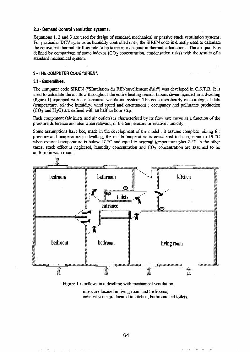
2.3 - Demand Control Ventilation systems.
Equations 1,2 and 3 are used for design of standard mechanical or passive stack ventilation systems. For particular DCV systems as humidity controlled ones, the SIREN code is directly used to calculate the equivalent thermal air flow rate to be taken into account in thermal calculations. The air quality is defined by comparison of some indexes (GO2 concentration, condensation risks) with the results of a standard mechanical system.
3 -THE COMPUTER CODE "SIREN".
3.1 - Generalities.
The computer code SIREN ("Simulation du RENouvellement d'air") was developed in C .S .T.B. It is used to calculate the air flow throughout the entire heating season (about seven months) in a dwelling (figure 1) equipped with a mechanical ventilation system. The code uses hourly meteorological data (temperature, relative humidity, wind speed and orientation) ; occupancy and pollutants production (C02 and H20) are defined with an half an hour step.
Each component (air inlets and air outlets) is characterised by its flow rate curve as a function of the pressure difference and also when relevant, of the temperature or relative humidity.
Some assumptions have bee, made in the development of the model : it assume complete mixing for pressure and temperature in dwelling, the inside temperature is considered to be constant to 19 OC when external temperature is below 17 "C and equal to external temperature plus 2 "C in the other cases, stack effect is neglected, humidity concentration and C02 concentration are assumed to be uniform in each room.
Figure 1 : airflows in a dwelling with mechanical ventilation.
inlets are located in living room and bedrooms, exhaust vents are located in kitchen, bathroom and toilets.
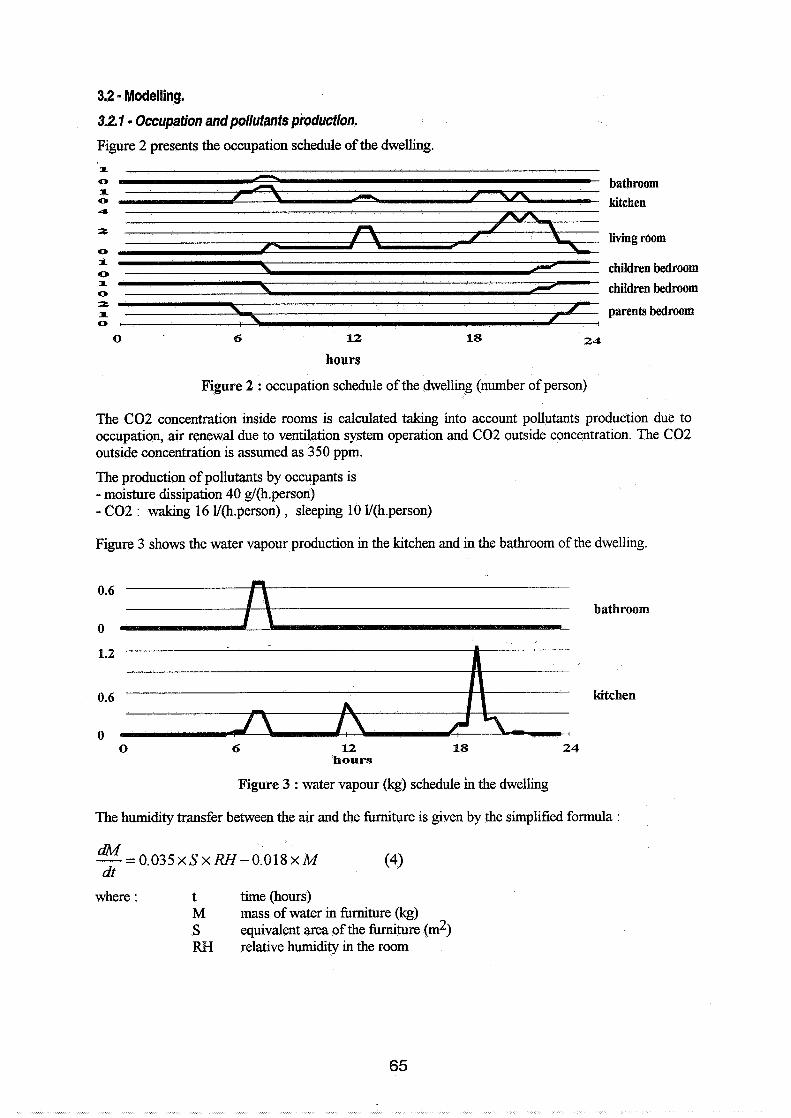
3.2 - Modelling.
3.2.1 - Occupation and pollutants production.
Figure 2 presents the occupation schedule of the dwelling.
i
0 n 1
bathroom 0 4
kitchen
2 living room
0 a. 0 \ children bedroom 1 0 \ children bedroom 2 1 parents bedroom 0
hours
Figure 2 : occupation schedule of the dwelling (number of person)
The C02 concentration inside rooms is calculated taking into account pollutants production due to occupation, air renewal due to ventilation system operation and C02 outside concentration. The C02 outside concentration is assumed as 350 ppm.
The production of pollutants by occupants is - moisture dissipation 40 g/(h.person) - C02 : waking 16 V(h.person) , sleeping 10 V(h.person)
Figure 3 shows the water vapour production in the kitchen and in the bathroom of the dwelling
bathroom
1.2
0.6 kitchen
0 12 18
hours
Figure 3 : water vapour (kg) schedule in the dwelling
The humidity transfer between the air and the furniture is given by the simplified formula :
where : t time (hours) M mass of water in furniture (kg) S equivalent area of the fimiture (m2) RH relative humidity in the room

3.2.2 - Wind effects.
The pressure (Pascal) in the front of the dwelling is :
where : Cp wind pressure coefficient (table 2) P volukic mass of air (kg/m3) V wind speed (mls)
Table 2 : Cp versus wind direction
3.2.3 Heat losses due to ventilation system.
The DCV and the standard mechanical ventilation systems are compared with an averaged flowrate which give the same heat losses on the heating season (seven month) :
where : Q(t) instantaneous ventilation flow rate (m3/h) Ti internal temperature (OC) Te external temperature ("C) 0.34 specific heat of air (%Vh/m3 ."c)
3.3 - Description of the studied systems.
3.3.1 - Reference system 181.
The curve of the components of the reference system are shown in figure 5 :
Figure 5 : simulated curves of components (flow versus pressure)
Self-regulated inlets
- one self regulated inlet in each habitable room,
Self-regulated outlets
- one self regulated outlet in each service room ; in the kitchen an additional flow rate of 135 m3/h is available
0 2 50 100 150
Pressure difference (Pa)
0 50 100 150 200
Pressure difference (Pa)

3.3.2 - Humidity controlled system 1.
The curve of the components of the system 1 are given in figure 6 :
Humidity controlled inlet I I Humidity controlled outlet I
I I 1
Figure 6 : simulated curves of humidity controlled components (flow versus humidity)
45
6 40 35 30
s ii 8 1s % 10
5 0
0 20 40 60 80 100
Relatlve humldity
- one humidity controlled inlet in each habitable room
50 45 40
$ 35 m 30 25
8 f z % 10 b: 5
0 0 20 40 60 80 100
Relatlve humidity
- one humidity controlled outlet in the kitchen and the bathroom; in the kitchen an additional flow rate of 150 m3k is available
- one two flows outlet (5 m3k with additional flow of 30 m3k) in the toilets.
3.3.3 - Humidify controlled system 2.
Humidity controlled system 2 as the same inlets than reference system and the same outlets than humidity controlled system 1.
4 - RESULTS
We present results of the two humidity control ventilation systems compared with the reference system.
4.2 - Air renewal.
The averaged air renewals calculated with formula 6, and the heat losses due to air renewal (in the Parisian area) are given here after :
Heat losses due to air renewal depend on location in France : humidity control system 1 can save between 700 (Mediterranean area) and 1400 (east of Frame) kwh per year
4.3 - Air quality
It is necessary to distinguish the pollution due to human activities and the pollution sources due to materials in the building. Even when these second pollution sources are as low as possible, the ventilation system has to exhaust human bioeffluents. C02 concentration reflects the human bioeffluents concentration [9 and 101.

To compare the-systems we calculate the C02 ppm.hours cumulated basis X in the parents' bedroom which pennit a better comparison between the systems than the simple frequencies. To meet requirements the ppm.hours cumulated basis 2000 have to be lower than 500000.
vr 140 '-no loo = all 60 40 20 n
5 - CONCLUSION
A computer model is used to assess the performances of different mechanical ventilation systems, includmg DCV systems, in dwellings.
Heat losses by air renewal are calculated with reference to a standard ventilation system. The flow rates of DCV systems should be dimensioned in order to achieve a similar air quality level for each system. On this basis the load reduction, using advanced systems, which have been released since ten years on the French market, is found to be appreciable.
The two humidity controlled system described in this paper save energy. Although the air quality of the two DCV systems is slightly lower than the air quality of reference system, the energy savings are more important with the system 1 which has a better air quality level than the system 2.
The calculated values of this reduction are somewhat depending on the air quality indicator chosen, which therefore should be carelidly selected.
Further work with a model taking in account phenomena which, so far, have been neglected (windows opening, stack effect, . . .) is needed in order to confirm the results presented in this paper.
ACKNOWLEDGEMENTS
The authors wish to thank the ML (French Ministry of Building) for the research support.
REFERENCES
[l] Kilberger M., "Lt&ration hygroregulk : suivi de trois logements", CETE Lyon, avril 1987
[2] Riberon J., Simeon R., "Suivis d'installations de ventilation hygroreglable : operation pilote de Chanteloup-les-Vignes", CSTB, decembre 1989
[3] Hiq&gat F., Donnini G., "IAQ and energy management by demand control ventilation" Environment Technology, vol 13, n04, pp 35 1-360
[4] Ribkron J. "Guide methodologique pour la mesure de la permeabilite a l'air des enveloppes de bfitiments" Cahier du CSTB no 2493, Paris, May 1991
[5] Ribkron J, Millet JR, Villenave JG. "Assesment of energy impact of ventilation and infiltration in the French regulations for residential buildings". 14th AIVC conference on Energy Impact of Ventilation and Air Infiltration, Copenhagen, September 1993.
[6] Riberon J., Bienfait D., Chandelier J., "Revision des Regles Th-G, partie ventilation" CSTB GECDAC 90-18D, Marne la Vallk, February 1990
[7] "Regles Th-G : regles de calcul du coefficient GV des biitiments d'habitation et du coefficient G1 des bfitiments autres que d'habitation" Cahier du CSTB no 2486, Paris, April 199 1
[8] Villenave JG, Riberon J, Millet JR, French ventilation in dwellings. International conference on "Building design technology and occupant well-being in temperate climates", Brussels, February 1993
[9] Millet JR, Riberon J. Deux composants de l'air a l'interieur des locaux : le gaz carbonique, la vapeur d'eau. Cahier du CSTB, livraison 323, octobre 1991
[lo] Millet JR, Villenave JG Assesment of the overall comfort in the indoor environment, Indoor Air 93 conference, Helsinski.


Session 2: Posters - Ventilation Systems

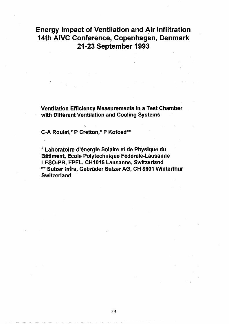
Energy impact of Ventilation and Air Infiltration 14th AlVC Conference, Copenhagen, Denmark
21 -23 Septem ber 1993
Ventilation Efficiency Measurements in a Test Chamber with Different Ventilation and Cooling Systems
C-A Roulet," P Cretton," P Kofoed"
* Laboratoire d'energie Solaire et de Physique du Biitiment, Ecole Polytechnique Federale-Lausanne LESO-PB, EPFL, CHI01 5 Lausanne, Switzerland ** Sulzer Infra, Gebriider Sulzer AG, CH 8601 Winterthur Switzerland

VENTILATION EFFICIENCY MEASUREMENTS IN A TEST CHAMBER WITH DIFFERENT VENTILATION AND COOLING SYSTEMS
Synopsis Cooling ceilings are more and more proposed, in order to eliminate excess heat in office buildings without consuming much energy in air transport. On the other hand, piston ventilation is proposed to efficiently eliminate contaminants. These two systems may however interact and experiments were planned to look at these interactions.
Measurements of the age of air and air change efficiency were performed, together with more classical temperature and air velocity measurements, on various ventilation systems installed in the test chamber of Sulzer Infra, in Winterthur. The test chamber was arranged to simulate an office room, with heat generated from computers and occupants. Moreover, the contaminants from one occupant were simulated with a tracer gas and the contaminant removal effectiveness was measured at various locations in the room.
Six different series of measurements were performed with displacement ventilation, with two types of cooling ceilings. Two more tests were performed with mixing ventilation, using two different inlet grilles.
As expected, both mixing system, measured with the continuous cooling ceiling "on", reach nearly complete mixing, hence an air change efficiency close to 50 % and a uniform contaminant removal effectiveness close to 1.
Displacement ventilation systems showed a larger air change efficiency in most cases. However, the cooling ceiling counteracts the displacement and important mixing is observed when it is on, mainly if the air flow rate is lower than 5 volumes per hour. A test without cooling showed a strong displacement effect, the local mean age at every occupant location being lower than the room mean age. Except in this particular test, the contaminant removal effectiveness is generally about 1. It should be noted that, for these latter measurements, the contaminant source was not far from the inlet grilles, which represents the worst possible case.
It is also shown that systems with a high air change efficiency do not necessarily provide fresh air to the occupants.
1 Planning of the Experiment
1.1. Purpose of the experiment
The scope of the experiment is to evaluate various ventilation systems, that is to answer the following questions: 1. how does that ventilation system performs to bring fresh air to the occupants? 2. how does that ventilation system performs to evacuate contaminants from a room?
To answer question 1, the age of air was measured at various locations within the room. To evaluate question 2, a contaminant source is placed within the room, and the contaminant concentration is measured at various locations in the room.
However, within a limited budget, it was obviously not possible to perform extensive expensive experiments. The conditions in which the few possible experiments should be performed were hence carefully studied, using the theory of experimental planning , but also taking account of some comercial requirements.
1.2. Variables
Numerous parameters may have some influence on the internal air flow pattern, on the temperature distribution and on the indoor air quality. We can enumerate the following ones, without claiming to be exhaustive: 0 parameters linked to the room: dimensions, furniture and occupancy, location and strength of the heat and
contaminant sources, distribution and magnitude of infiltration paths, location of the occupants; 0 parameters linked to the ventilation system: ventilation type, type and location of inlets and outlets, air
flow rate, air temperature;
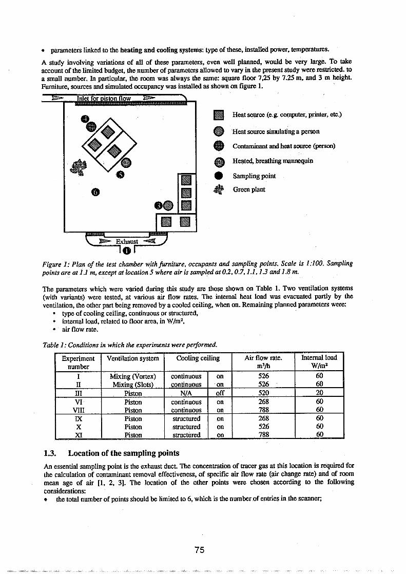
parameters linked to the heating and cooling systems: type of these, installed power, temperatures.
A study involving variations of all of these parameters, even well planned, would be very large. To take account of the limited budget, the number of parameters allowed to vary in the present study were restricted. to a small number. In particular, the room was always the same: square floor 7,25 by 7.25 m, and 3 m height. Furniture, sources and simulated occupancy was installed as shown on figure 1.
Heat source (e.g computer, printer, etc.)
@ Heat source simulating a pemn
@ Con-t and heat source (person)
@ Heated, breathing mannequin
@ Sampling point
.$ Greenplant
Figure 1: Plan of the test chamber with furniture, occupants and sampling points. Scale is 1:lOO. Sampling points are at 1 .I m, except at location 5 where air is sampled at 0.2.0.7,l .I, 1.3 and 1.8 m.
The parameters which were varied during this study are those shown on Table 1. Two ventilation systems (with variants) were tested, at various air flow rates. The internal heat load was evacuated partly by the ventilation, the other part being removed by a cooled ceiling, when on. Remaining planned parameters were:
type of cooling ceiling, continuous or structured, * internal load, related to floor area, in W/m2, * air flow rate.
Table 1: Conditions in which the experiments were performed.
1.3. Location of the sampling points
An essential sampling point is the exhaust duct. The concentration of tracer gas at this location is required for the calculation of contaminant removal effectiveness, of specific air flow rate (air change rate) and of room mean age of air [l, 2, 31. The location of the other points were chosen according to the following considerations: a the total number of points should be limited to 6, which is the number of entries in the scanner;
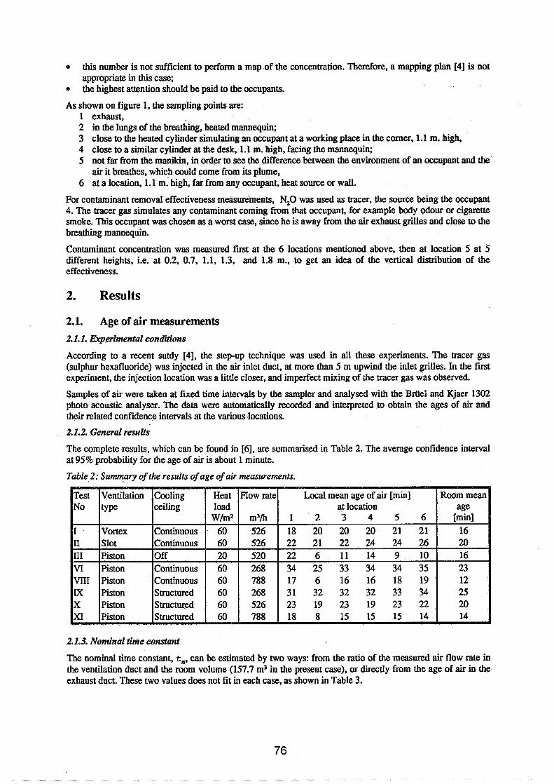
this number is not sufficient to perform a map of the concentration. Therefore, a mapping plan [4] is not appropriate in this case; the highest attention should be paid to the occupants.
As shown on figure 1, the sampling points are: 1 exhaust, 2 in the lungs of the breathing, heated mannequin; 3 close to the heated cylinder simulating an occupant at a working place in the comer, 1.1 m. high, 4 close to a similar cylinder at the desk, 1.1 m. high, facing the mannequin; 5 not far from the manikin, in order to see the difference between the environment of an occupant and the
air it breathes, which could come from its plume, 6 at a location. 1.1 m. high, far from any occupant, heat source or wall.
For contaminant removal effectiveness measurements, N,O was used as tracer, the source being the occupant 4. The tracer gas simulates any contaminant coming from that occupant, for example body odour or cigarette smoke. This occupant was chosen as a worst case, since he is away from the air exhaust grilles and close to the breathing mannequin.
Contaminant concentration was measured fmt at the 6 locations mentioned above, then at location 5 at 5 different heights, i.e. at 0.2, 0.7, 1.1, 1.3, and 1.8 m., to get an idea of the vertical distribution of the effectiveness.
2. Results
2.1. Age of air measurements 2.1.1. Experimental conditions
According to a recent sutdy [4], the step-up technique was used in all these experiments. The tracer gas (sulphur hexafluoride) was injected in the air inlet duct, at more than 5 m upwind the inlet grilles. In the fmt experiment, the injection location was a little closer, and imperfect mixing of the tracer gas was observed.
Samples of air were taken at fixed time intervals by the sampler and analysed with the Briiel and Kjaer 1302 photo acoustic analyser. The data were automatically recorded and interpreted to obtain the ages of air and their related confidence intervals at the various locations.
2.1.2. General results
The complete results, which can be found in [6], are summarised in Table 2. The average confidence interval at 95% probability for the age of air is about 1 minute.
Table 2: Summary of the results of age of air measurements.
2.1.3. Nominal time constant
The nominal time constant, t,, can be estimated by two ways: from the ratio of the measured air flow rate in the ventilation duct and the room volume (157.7 m3 in the present case), or directly from the age of air in the exhaust duct. These two values does not fit in each case, as shown in Table 3.
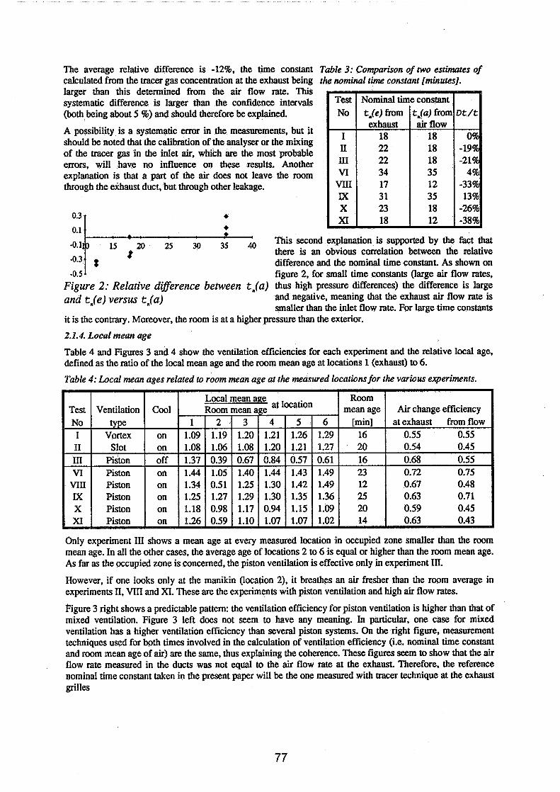
The average relative difference is -12%. the time constant Table 3: Comparison of two estimates of calculated from the tracer gas concentration at the exhaust being the nominal time constant [minutes]. larger than this determined from the air flow rate. This systematic difference is larger than the confidence intervals (both being about 5 %) and should therefore be explained.
A possibility is a systematic error in the measurements, but it should be noted that the calibration of the analyser or the mixing of the tracer gas in the inlet air, which are the most probable errors, will have no influence on these results. Another explanation is that a part of the air does not leave the room through the exhaust duct, but through other leakage.
0.3
-0.1 0.1-i This there second is an obvious explanation correlation is supported between by the the fact relative that -0.3 difference and the nominal time constant. As shown on -0.5 figure 2, for small time constants (large air flow rates,
Figure 2: Relative diflerence between t,(a) thus high pressure differences) the difference is large and tm(e) versus tll(a) and negative, meaning that the exhaust air flow rate is
smaller than the inlet flow rate. For large time constants it is the contrary. Moreover, the room is at a higher pressure than the exterior.
2.1.4. Local mean age
Table 4 and Figures 3 and 4 show the ventilation efficiencies for each experiment and the relative local age, &fined as the ratio of the local mean age and the room mean age at locations 1 (exhaust) to 6.
Table 4: Local mean ages related to room mean age at the measured locations for the various experiments.
Only experiment I11 shows a mean age at every measured location in occupied zone smaller than the room mean age. In all the other cases, the average age of locations 2 to 6 is equal or higher than the room mean age. As far as the occupied zone is concerned, the piston ventilation is effective only in experiment 111.
However, if one looks only at the manikin (location 2), it breathes an air fresher than the room average in experiments 11, VIII and XI. These are the experiments with piston ventilation and high air flow rates.
pigure 3 right shows a predictable pattern: the ventilation efficiency for piston ventilation is higher than that of mixed ventilation. Figure 3 left does not seem to have any meaning. In particular, one case for mixed ventilation has a higher ventilation efficiency than several piston systems. On the right figure, measurement techniques used for both times involved in the calculation of ventilation efficiency (i.e. nominal time constant and room mean age of air) are the same, thus explaining the coherence. These figures seem to show that the air flow rate measured in the ducts was not equal to the air flow rate at the exhaust. Therefore, the reference nominal time constant taken in the present paper will be the one measured with tracer technique at the exhaust grilles

Figure 3: Ventilation eficiencies for the various experiments. At the lefi, the nominal time constant is calculated from the air flow rate. At the right, the nominal time constant is taken as the age of air at the exhaust.
Figure 4 shows clear differences between the various systems. It should be noted, that the measurement accuracy shall be taken into account when comparing the various figures. To be significant, any difference should be larger than the confidence interval. The error in the age of air is about 1 minute, that is 3 to 5 %. The error in the room mean age is similar. Therefore, errors in relative age or in ventilation efficiency is 5 to 10%.
Figure 4: Local relative ages (compared to the room mean age) at the measured locations for the various experiments.
I II 111 VI VIII IX X XI
When compared to all the other measured systems, system I11 gives the youngest air to the occupants. This is a piston ventilation system, and the only one without cooling ceiling. Nevertheless, its global efficiency is not better than systems VI and VIII, which are similar but with cooling ceiling on. A global, room averaged parameter provides an average information, but does not show local differences, which could be dramatic, as, for example, those observed on figure 4 between case I11 and cases VI and VIII. See also the system IX, with an air change efficiency of 0.63 and a relative age of air higher than the room average for every occupant. This shows that, as far as the occupants are concerned, global parameters, like the ventilation efficiency, should be used with care.
The exhaust presents in all cases, as it should be, a relative age equal or higher than the other places. The youngest air reaches first the mannequin (location 2), then the cylinder 4. That is a surprise, since cylinder 4 is closer to the inlet grilles. Maybe the air takes some time to climb at 1.1 m, where the sampling tubes are. In general, relative differences in the relative age of air in all systems with cooling ceiling are larger when the air flow rate is high (systems VII, and XI)
As it could be expected, the mixed ventilation systems (experiments I and 11) present a ventilation efficiency close to 0.5 and an homogeneous age of air. However, some piston systems (e.g. IX or X) do not perform much better. In the systems studied, the cooling ceiling seems to maintain the air at a low level or to mix the air within the room.
2.2. Contarninant removal effectiveness
This effectiveness was measured at the same locations as the age of air, the contaminant source being cylinder 4. This location for a contaminanting person (e.g. a smoker) is the worst one. The complete results from these measurements are given in reference [6], and summarised on Table 5 and Figures 5 and 6.

Basically these measurements were planned to be taken at steady state, after constant injection of tracer gas around cylinder 4. Assuming zero background concentration, the contaminant removal effectiveness is obtained by dividing the tracer gas concentration measured at the exhaust by the concentration at the places of interest.
Table 5: Contaminant removal efictiveness at various locations, when contaminant is coming from cylinder 4, at 1 .l m high. Results in italics are dubious.
The contaminant removal effectiveness equals 1 for complete mixing, can be lower if the concentration at location is higher than at the exhaust (bad removal), and higher if the concentration is small.
Here again, system 111, without cooling, presents the largest differences. With a few exceptions, all the other systems have a contaminant removal effectiveness close to 1. The exceptions are as well for piston ventilation (in the mannequin, for experiments VIII and XI and for mixed ventilation (system I1 at location 4).
As it should be, location 4, which is at the contaminant source, presents generally the worse effectiveness. The mannequin, located downwind and not far from cylinder 4, also presents in some case a poor effectiveness. The best place, with regard to that source of contaminant, is at location 3, in the opposite comer of the mom.
Figure 5: Contaminant removal effectiveness at various locations, when contaminant is coming from cylinder 4, at 1 .I m high. Value at locations 6 and 3 for experiment 111 are out of scale (effective values: 5 and 14)
3.0 m
V)
2.0 8 P
'51
1.0 4 W
0.0 6 5 4 3 2
Location
The differences between piston ventilation systems and mixed systems are more obvious on Figure 6, which shows the vertical distribution of the contaminant removal effectiveness at location 5, that is in the vicinity of the mannequin. All the mixed systems have an effectiveness close to one, from floor to ceiling, while most piston ventilation systems show differences. The exception is system IX, with structured cooling ceiling and low air flow rate, which is homogeneous.
The best figures are obtained in system 111, at 1.3 m, and for systems VI and VIII, close to the floor. The worst case, at location 5, is for systems X and XI, close to the floor. However, this level does not need to be well ventilated, since only small pets may breath at that height.
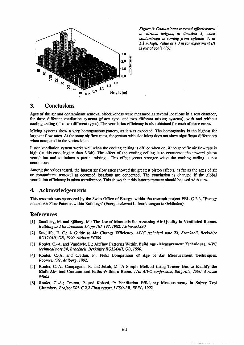
Figure 6: Contaminant removal effectiveness at various heights, at location 5 , when contaminant is coming from cylinder 4, at 1 .I m high. Value at 1.3 m for experiment ZZZ is out of scale (15).
3.0
2.0 8 S 1 .o 3 0.0
z
Height [m]
3. Conclusions Ages of the air and contaminant removal effectiveness were measured at several locations in a test chamber, for three different ventilation systems (piston type, and two different mixing systems), with and without cooling ceiling (also two different types). The ventilation efficiency is also obtained for each of these cases.
Mixing systems show a very homogeneous pattern, as it was expected. The homogeneity is the highest for large air flow rates. At the same air flow rates, the system with slot inlets does not show significant differences when compared to the vortex inlets.
Piston ventilation system works well when the cooling ceiling is off, or when on, if the specific air flow rate is high (in this case, higher than 3.3h). The effect of the cooling ceiling is to counteract the upward piston ventilation and to induce a partial mixing. This effect seems stronger when the cooling ceiling is not continuous.
Among the values tested, the largest air flow rates showed the greatest piston effects, as far as the ages of air or contaminant removal at occupied locations are concerned. The conclusion is changed if the global ventilation efficiency is taken as reference. This shows that this latter parameter should be used with care.
4. Acknowledgements This research was sponsored by the Swiss Office of Energy, within the research project ERL C 2.2, "Energy related Air Flow Patterns within Buildings" (Energierelevant LuftstrGmungen in Geblluden).
References [I] Sandberg, M. and Sjbberg, M.: The Use of Moments for Assessing Air Quality in Ventilated Rooms.
Building and Environment 18, pp 181-197,1982. Airbase#1320
[2] Sutcliffe, H. C.: A Guide to Air Change Efficiency. AIVC technical note 28, Bracknell, Berkshire RG124AH. GB, 1990. Airbase #4000
[3] Roulet, C.-A. and Vandaele, L.: Airflow Patterns Within Buildings - Measurement Techniques. AIVC technical note 34, Bracknell, Berkshire RG124AH, GB, 1990.
[4] Roulet, C.-A. and Cretton, P.: Field Comparison of Age of Air Measurement Techniques. Roomvent'92, Aalborg. 1992.
[5] Roulet, C.-A., Compagnon, R, and Jakob, M.: A Simple Method Using Tracer Gas to Identify the Main Air- and Contaminant Paths Within a Room. 11th AIVC conference, Belgirate, 1990. Airbase #4865.
[6] Roulet, C.-A.; Cretton, P. and Kofoed, P: Ventilation Efficiency Measurements in Sulzer Test Chamber. Project ERL C 2 2 Final report, LESO-PB, EPFL, 1992.
Energy Impact of Ventilation and Air Infiltration 14th AlVC Conference, Copenhagen, Denmark
21 -23 Septem ber 1993
Efficient "Horizontal Flow" Ventilation: Influence of Supply Inlet Designs
Y-Q Tang, S Holmberg
Ventilation Division, National Institute of Occupational Health, S-I71 84 Solna, Sweden
Efficient "Horizontal Flow" Ventilation: Influence of Supply Inlet Designs
Yan-Qiu Tang and Sture Holmberg Ventilation Division, National Institute of Occupational Health S-171 84 Solna, Sweden
Abstract
An even distribution of room air can improve indoor air quality, lower energy costs, and create thermally comfortable environments. This paper investigates the influence of the design of plaque diffusers on the efficiency of supply air.
For better comfort and more accurate observations, the isothermal flow investigation was made in a small scale chamber with the air supply and exhaust on opposite walls. The supply air was spread radially and symmetrically over the vertical inlet wall. Plaques of different sizes, both solid and perforated were tested. The diameter of the plaques and the distance to the inlet wall were important parameters. They both influenced the general flow pattern in the room and the flow pattern close to the inlet region. Promising results regarding air change efficiency were reached by perforated plaques. The experimental results are compared to the results from numerical simulations on a fine grid where the plaque perforation degree has also been taken into consideration. An acceptable agreement was reached between experimental and numerical results.
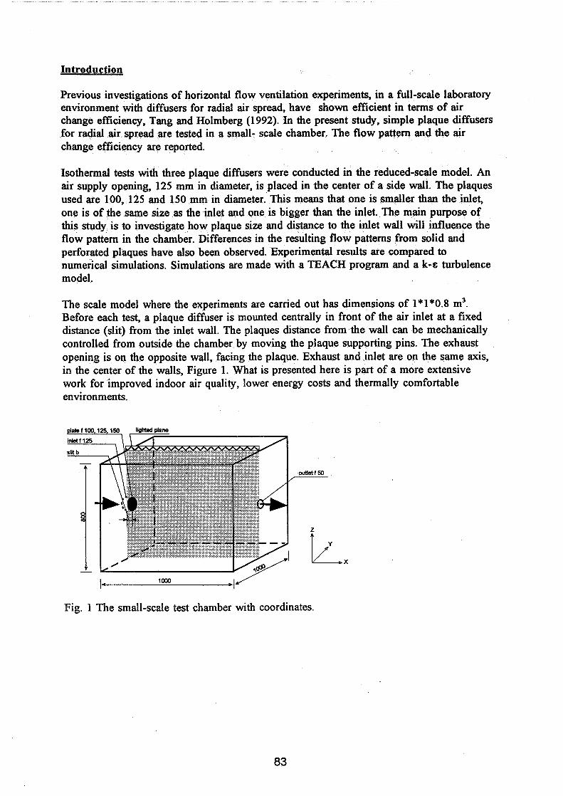
Introduction
Previous investigations of horizontal flow ventilation experiments, in a full-scale laboratory environment with diffusers for radial air spread, have shown efficient in terms of air change efficiency, Tang and Holmberg (1992). In the present study, simple plaque diffusers for radial air spread are tested in a small- scale chamber. The flow pattern and the air change efficiency are reported.
Isothermal tests with three plaque diffusers were conducted in the reduced-scale model. An air supply opening, 125 mm in diameter, is placed in the center of a side wall. The plaques used are 100, 125 and 150 mm in diameter. This means that one is smaller than the inlet, one is of the same size as the inlet and one is bigger than the inlet. The main purpose of this study is to investigate how plaque size and distance to the inlet wall will influence the flow pattern in the chamber. Differences in the resulting flow patterns from solid and perforated plaques have also been observed. Experimental results are compared to numerical simulations. Simulations are made with a TEACH program and a k-e turbulence model.
The scale model where the experiments are carried out has dimensions of 1*1*0.8 m3. Before each test, a plaque diffuser is mounted centrally in front of the air inlet at a fixed distance (slit) from the inlet wall. The plaques distance from the wall can be mechanically controlled from outside the chamber by moving the plaque supporting pins. The exhaust opening is on the opposite wall, facing the plaque. Exhaust and inlet are on the same axis, in the center of the walls, Figure 1. What is presented here is part of a more extensive work for improved indoor air quality, lower energy costs and thermally comfortable environments.
plate f lM),125,150 liiMed plane
A inlet f 125 , \Ldi
Fig. 1 The small-scale test chamber with coordinates.
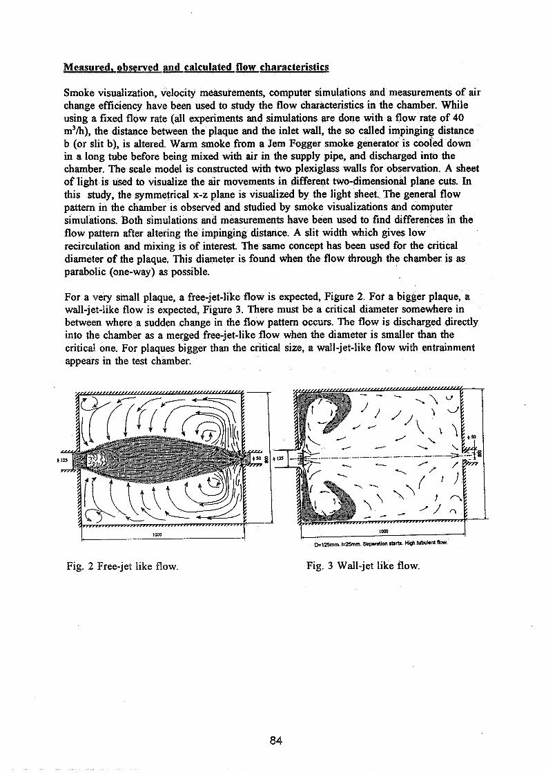
Measured. observed &calculated flow characteristics
Smoke visualization, velocity measurements, computer simulations and measurements of air change efficiency have been used to study the flow characteristics in the chamber. While using a fixed flow rate (all experiments and simulations are done with a flow rate of 40 m3/h), the distance between the plaque and the inlet wall, the so called impinging distance b (or slit b), is altered. Warm smoke from a Jem Fogger smoke generator is cooled down in a long tube before being mixed with air in the supply pipe, and discharged into the chamber. The scale model is constructed with two plexiglass walls for observation. A sheet of light is used to visualize the air movements in different two-dimensional plane cuts. In this study, the symmetrical x-z plane is visualized by the light sheet, The general flow pattern in the chamber is observed and studied by smoke visualizations and computer simulations. Both simulations and measurements have been used to find differences in the flow pattern after altering the impinging distance. A slit width which gives low recirculation and mixing is of interest. The same concept has been used for the critical diameter of the plaque. This diameter is found when the flow through the chamber is as parabolic (one-way) as possible.
For a very small plaque, a free-jet-like flow is expected, Figure 2. For a bigger plaque, a wall-jet-like flow is expected, Figure 3. There must be a critical diameter somewhere in between where a sudden change in the flow pattern occurs. The flow is discharged directly into the chamber as a merged free-jet-like flow when the diameter is smaller than the critical one. For plaques bigger than the critical size, a wall-jet-like flow with entrainment appears in the test chamber.
Fig. 2 Free-jet like flow. Fig. 3 Wall-jet like flow.
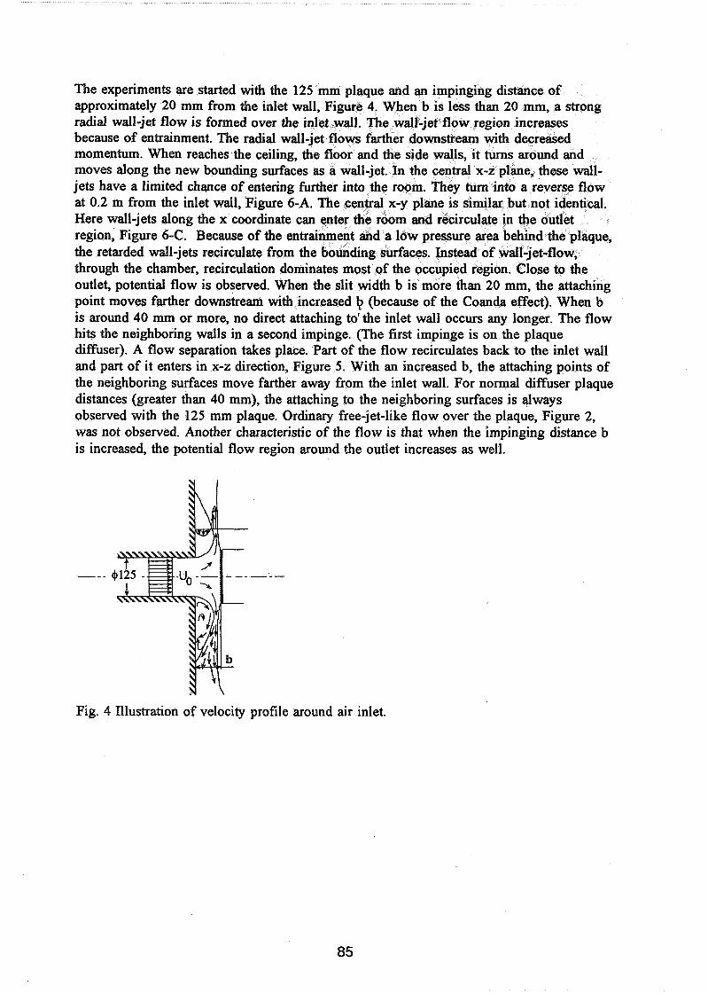
The experiments are started with the 125 mm plaque and an impinging distance of approximately 20 mm from the inlet wall, Figure 4. When b is less than 20 mm, a strong radial wall-jet flow is formed over the inlet wall. The wall-jet flow region increases because of entrainment. The radial wall-jet flows farther downstream with decreased momentum. When reaches the ceiling, the floor and the side walls, it turns around and moves along the new bounding surfaces as a wall-jet. In the central x-z plane, these wall- jets have a limited chance of entering further into the room. They turn into a reverse flow at 0.2 m from the inlet wall, Figure 6-A. The central x-y plane is similar but not identical. Here wall-jets along the x coordinate can enter the room and recirculate in the outlet region, Figure 6-C. Because of the entrainment and a low pressure area behind the plaque, the retarded wall-jets recirculate from the bounding surfaces. Instead of wall-jet-flow, through the chamber, recirculation dominates most of the occupied region. Close to the outlet, potential flow is observed. When the slit width b is more than 20 mm, the attaching point moves farther downstream with increased \ (because of the Coanda effect). When b is around 40 mm or more, no direct attaching to' the inlet wall occurs any longer. The flow hits the neighboring walls in a second impinge. (The first impinge is on the plaque diffuser). A flow separation takes place. Part of the flow recirculates back to the inlet wall and part of it enters in x-z direction, Figure 5. With an increased b, the attaching points of the neighboring surfaces move farther away from the inlet wall. For normal diffuser plaque distances (greater than 40 mm), the attaching to the neighboring surfaces is always observed with the 125 mm plaque. Ordinary free-jet-like flow over the plaque, Figure 2, was not observed. Another characteristic of the flow is that when the impinging distance b is increased, the potential flow region around the outlet increases as well.
Fig. 4 Illustration of velocity profile around air inlet.

Fig. 5 Experimental flow pattern from a 125 mm plaque diffuser, x-z plane at y = 0.5 rn, slit width b = 40 mm. I
Fig. 6 Simulated three-dimensional flow pattern from a 125 mm plaque diffuser, A) x-z cut at y = 0.5 m, slit width b = 4 3 m m B) x-z cut at y = 0.5 rn, slit width b = 8 1 m m C) x-y cut at z = 0.4 m, slit width b = 43 mm.

Fig. 7 Experimental flow pattern from a 150 mm plaque diffuser, x-z plane at y = 0.5 m, dit width b = 60 mm.
Fig. 8 Simulated three-dimensional flow pattern from a 150 mm plaque diffuser, x-z cut at y = 0.5 m, slit width b = 68 mm.
With the 150 mm plaque, the critical experimental separation distance is about 45 mm. When b is about 60 mm, the attachment to the ceiling appears. Recirculation and wall-jet, however, still dominate the general flow pattern, Figure 6. Figure 7 shows the calculated velocity flow field at slit width b = 68 mm. The direct attaching to the ceiling has not yet occurred here in the simulation.
When comparing the observed and the simulated flow patterns, one can see that there are similarities, but also differences between them. Generally speaking, the simulated critical slit values are larger than the observed ones. For the 125 mm plaque, the experimental attaching to the ceiling starts from a slit width b around 40 mm, which is smaller than the simulated vaIue around 70 mm.
If the plaque diameter is 100 mm, the flow pattern will be totally different from what has been observed in Figures 4-8. With the 100 mm plaques, the flow-spread capacity is lost

and the flow is similar to a free jet. The main flow goes through the chamber, and part of it directly to the exhaust. The rest recirculates along the bounding surfaces, Figures 9 and 10
Fig. 9 Experimental flow pattern from a 100 mm plaque diffuser, x-z plane at y = 0.5 m, slit width b = 40 mm.
Fig. 10 Simulated three-dimensional flow pattern from a 100 mm plaque diffuser, x-z cut at y = 0.5 m, slit width b = 68 mm.
Thcritical diameter
The tests have shown that the impinging distance has less influence on the flow pattern than the plaque size. The 125 mm plaque creates a wall-jet-flow within the practical design impinging distances of b. The 100 mm plaque always creates a free jet like flow.
When the plaque diameter is 114 mm, the flow pattern is very sensitive to small changes of the plaque diameter. The flow changes from wall-jet-like to a much more forward flow when the plaque diameter is slightly changed, e.g. 1 mm smaller. Again, when the plaque
diameter is 1 mm bigger, the flow pattern is characterized by wall-jet-like flow. The impinge distance has more influence on wall-jet-like flows than on free-jet-like flows.
Air chan~e efficiencv
Air change efficiency is measured by a step-down tracer gas technique. Perforated plaque diffusers are used in comparison with solid ones. Perforated plaques are used to eliminate the characteristic back-flow behind plaques, in order to diminish recirculation and improve forward directed flow movements. The age-of-air concept is employed, which means the age of air <y> is calculated from measured tracer-gas concentrations:
C cJt) at id)
where t,, = cut-off point, s. ci = instantaneous concentration of tracer gas in the exhaust opening, ppm.
The following relation is applied to calculated the air change efficiency:
where e =air change efficiency z, = nominal time constant, s.
Results from air change efficiency tests with a perforated plaque give an air change efficiency around 52%. The flow in the chamber is turbulent and thus mixed. The nominal time constant in our tests here is 25 times less than previous full-scale tests, Tang and Holmberg (1992).
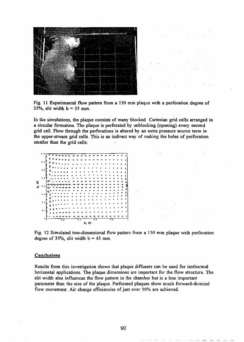
Fig. 11 Experimental flow pattern from a 150 mm plaque with a perforation degree of 33%, slit width b = 35 mm.
In the simulations, the plaque consists of many blocked Cartesian grid cells arranged in a circular formation. The plaque is perforated by unblocking (opening) every second grid cell. Flow through the perforations is altered by an extra pressure source term in the upper-stream grid cells. This is an indirect way of making the holes of perforation smaller than the grid cells.
Fig. 12 Simulated two-dimensional flow pattern from a 150 mm plaque with perforation degree of 35%, slit width b = 43 mm.
Conclusions
Results from this investigation shows that plaque diffusers can be used for isothermal horizontal applications. The plaque dimensions are important for the flow structure. The slit width also influences the flow pattern in the chamber but is a less important parameter than the size of the plaque. Perforated plaques show much forward-directed flow movement. Air change efficiencies of just over 50% are achieved.
Acknowledeements
The authors are greatful to Bjorn Nilsson, Andrzej Paprocki, Sten Lundstrorn and Tyrrell Burt for their help with this paper. The work was financially supported by The Swedish Work Environment Fund.
References
1. Waschke, G. " a e r die L.iiEhmg mittels isothermer, turbulenter, radialer Deckenstrahlenw Ki Klima+Kalte-Ingenieur 7-8/76, 1976, pp277-284.
2. Pattie, D. R. and Milne, W. R. "Ventilation air-flow patterns by use of models", ASAE Trans. 9(5), 1966, pp646- 649.
3. Timmons, M. B. "Use of physical models to predict the fluid motion in slot-ventilated livestock structure", ASAE Trans. 27(5), 1984, pp15 14- 1 5 17.
4. Zhang, J. S. "A fundamental study of two dimensional room ventilation flows under isothermal and non-isothermal conditions", Ph. D. thesis, University of Illinois, Urbana, Illinois, 1991.
5. Reinartz, A. and Renz, U. "Calculations of the temperature and flow field in a room ventilated by a radial air distributor", International J. of Refrigeration, Vol. 7, No. 5, 1984, pp308-312.
6. Tang, Y.Q. and Holmberg, S. "An experimental investigation of a horizontal displacement ventilation system"', Undersiikningsrapport 1992:2, National Institute of Occupational Health, 5-171 84 Solna, Sweden.


Energy Impact of Ventilation and Air Infiltration 14th AlVC Conference, Copenhagen, Denmark
21 -23 September 1993
Natural Ventilation Without Draught
M Egedorf
Institute of Building Technology, Gregersensveg, DK-2630 Taastrup, Denmark
NATURAL VENTILATION WITHOUT DRAUGHT
- Development of storm safety valve
Draught from fresh-air vents during windy weather or periods with frost can be avoided by means of a newly developed flow valve. The valve has been developed by the Institute of Buil- ding Technology in collaboration with Fresh Danmark A/S in a project under the Research Program of the Ministry of Energy.
Valves with almost similar function were already available in Europe, when we began the development. But those valves lacked some of the features we found important. We wanted a storm safety valve that did not inflect the air flow under normal weather conditions and a valve that would function in arctic climate, enabling natural ventilation without draught in Greenland, too.
The storm safety valve is designed to be installed in fresh- air vents. It reduces the air flow through the fresh-air vents, when the wind is exceptionally strong, but it does not affect the air flow under normal weather conditions. It func- tions without electricity.
In practice, the storm safety valve limits considerably the inconvenience of draught from fresh-air vents. When there is no risk of draught from the fresh-air vent, the inhabitants are less inclined to shut off the fresh-air vent thereby re- ducing the risk of damages caused by humidity.
A dwelling equipped with fresh-air vents with storm safety valves will have the same air infiltration rate in calm weather as with fresh-air vents without storm safety valves. The storm safety valve does not impede the normal air flow, the difference is felt only in periods with strong winds, because the storm safety valve reduces the air flow, for instance to 30 m3/h per fresh-air vent.
In principle, the storm safety valve can be installed in all fresh air vents of a certain dimension. The storm safety valve has been tested in fresh-air vents with dimensions from 075 rnm to 150 mm x 150 mm. The storm safety valve is manufactured in Denmark.
The paper will describe the development of the storm safety valve, experience from use and suggestions for use in other connections.
BYGGETEKNISK INSTITUT Morten Egedorf
Energy Impact of Ventilation and Air Infiltration 14th AlVC Conference, Copenhagen, Denmark
21 -23 September 1993
Mechanical Ventilation System with Heat Exchanger in One Room - Low Cost Mechanical Ventilation System
M Egedorf
institute of Building Technology, Gregersensveg, DK-2630 Taastrup, Denmark
MECHANICAL VENTILATION SYSTEM WITH HEAT EXCHANGER IN ONE ROOM - Low cost mechanical ventilation system
A new miniature mechanical ventilation system with both supply and extract air and an air-to-air heat exchanger has been developed in Great Britain and Denmark. The system which is intented t~ ventilate a single room has the dimensions of a shoe box and can be placed/installed on the inside wall in an existing air vent.
The system can operate with two air flows, 40 or 70 mvh. At the low speed the noise is insignificant, intended to be "not disturbingN in sleeping rooms. Switching between the two speeds can be done either manually or automatically controlled by the relative humidity of the extracted air. The system is also provided with filters.
This spring we will perform different measurements in the laboraty to check the system performances, for instance volume flow rate, draught, short circuiting of air, efficiency of the heat exchanger and noise.
In the paper we will report the results of the tests. Maybe this system is the long desired cheap and no-problems solution of mould-problems in sleeping rooms or tobacco smoke in off ices?
BYGGETEKNISK INSTITUT Morten Egedorf
Energy Impact of Ventilation and Air Infiltration 14th AlVC Conference, Copenhagen, Denmark
21 -23 September 1993
Some Aspects of Using Jets for Cooling
T Karimipanah, M Sandberg
The National Swedish lnstitut for Building Research, P 0 Box 785, S-80129 Gavle, Sweden
ABSTRACT
Some Aspects of Using Jets for Cooling
The efficiency of removing excess heat by employing mixing ventilation is based on the properties of jets. Therefore the behaviour of jets in enclosures is important. A correct supply design is essential otherwise the jet will separate from the ceiling and drop into the occupied zone. This will give rise to unacceptable high velocities. the basic properties of jets in ideal situations like an infinite space are well known. However, in a room the jet interacts with the room air and the room surfaces. Therefore a research program on the basic properties of jets in rooms has been started at the institute. This paper reports the findings from both an experimental study comprising both model studies and full scale studies supplemented by numerical simulations of room flow.
Energy Impact of Ventilation and Air Infiltration 14th AlVC Conference, Copenhagen, Denmark
21 -23 Septern ber 1993
The Effect of Various Inlet Conditions on the Flow Pattern in Ventilated Rooms - Measurements and Computations
P Vogel, E Richter, M R6sler
Technische Universitat Dresden, lnstitut fur Stromungsmechanik, Lehrstuhl fur Thermofluiddynamik, Mommsenstr. 13, D-01062 Dresden, Germany
1. Introduction
A test room (figure 1, [I]) which was built at a scale 1:5 to the original one has
been used to investigate air-conditioned rooms. The original room was specified
by the international project IEA ANNEX 20 ([2],[3]). A lot of experiments were
made on different inlet geometries (figures 2, 3) and air change rates. Velocities
and turbulent quantities were measured not only in the inlet plane but also in the
room itself by means of hot wire anemometry. The ammonia absorption method according to Kriickels [4] has been applied to determine the heat transfer coefficients at the walls. Qualitative results were obtained by laser light sheets.
The experimental results serving as boundary conditions and relative values for
numerical studies are used to progress the computer code ResCUE developed in
Dresden. Further on, the experimental data provide statements on conditions in
the occupied zone.
The laser light sheet technique used to represent the flow field also visualizes
domains which are not appropriate for hot wire measurements.Whereas a 4 Watt
Argon-Ion-Laser provides the light, a smoke generator evaporates an alcoholic
liquid in order to induce the necessary tracer gas for visualizing the flow. The
diameter of the droplets is approximately lpm. A CCD-camera records the
pictures of the flow field to the memory of the computer or to video.
Both flow velocities and turbulence quantities are obtained by hot wire
measurements. The voltage given by the DANTEC-55M-system is digitized by
an a/d-converter into a 16-bit information and stored in the access memory of a
PC. On average, 15 x 60 measuring points were chosen in a plane (x,z-
plane=500mm x 600rnm) and 10000 values are taken at each point in order to
determine the mean velocities and turbulent quantities locally. This equals 3
seconds integration time at each measuring point. The hot wire probes have been
locally adjusted with a positioning device of modular-design principle made by
ISEL AUTOMATION. This device is computer-controlled and owing to an
incremental pitch of 0.0125mm7 it makes a rather precizely positioning possible.
As mentioned above heat transfer coefficients are determined by means of the
ammonia transfer method [6] using the analogy between heat and mass transfer
and a computer aided image processing system [5]. Small quantities of ammonia

are added to the supplied air. That causes a chemical reaction at foils moistened
with a reaction substance. The colouring of this foils indicates the intensity of the mass transfer. Using the analogy between heat and mass transfer, the heat
transfer coefficients can be calculated by
3. Ex~erimental and numerical Investi~ations
Experiments were carried out for an air change rate of 373 h-' and 150 h-'
using as well inlet geometry 1 as 2 (figures 2, 3). In all cases the same positions
of the probes were chosen. Experimental data have been averaged in time and
space. That is
Thus the velocities are given as absolute values. Therefore the velocities close to
the outlet device have the same direction like the inlet device velocities.
In correspondence with the experiments numerical investigations were carried
out using the code ResCUE, which has been developed at the Dresden
University of Technology.
It is based on a finite volume discretization of the Reynolds averaged Navier-
Stokes equations. A k-E model is used for turbulence modelling. The Poisson
equation for the pressure is solved by a multigrid method in every time step of
the velocity pressure iteration, for details see [7].
The boundary conditions for modelling the various inlets were formulated within
the inlet opening. Following a proposal of [8], the HESCO diffuser was
modelled by 7 x 4 rectangular slots.
Computations were carried out on a HP workstation 90001730 and grids of 283
and 403 discrete cells were used.
The evaluation and intepretation of the experimental data show a clearly
different behavior of the flow in all investigated cases. The main reason for that
is the very different momentum at the inlet. Figure 7 shows the velocity profiles

in the symmetry plane for the inlet geometry 1 and the high air change rate. For
this case measured and simulated values are in a good agreement. But it is seen
from figure 10 that even for this simulation the numerical prediction does not
meet the typical behaviour of the jet (compare figure 9 and 10). This tendency is considerably amplified for the low air change rate. In case of inlet geometry 2 (HESCO diiser), the modelling by a lot of rectangular slots
can only be regarded as a trial. Because of the very fine grid, the computer capacity of a workstation is quickly reached. In addition, turbulence modelling
by a k-E model is probably not suitable in the region near the inlet opening.
Although the calculated heat transfer coefficients ( figure 6 ) show a similar
pattern as the measured ones (figure 5 ) the results are not satisfying and should
be improved in further investigations.
5. Conclusions
Experiments in a scaled test room are very helpful to study the behaviour of the
flow under various inlet conditions. It makes the application of some interesting
methods, like the arnonnia transfer method possible.
Computations show the global situation within the test room, but do not meet
the typical behaviour of the flow especially for a low air change rate and
complicated inlet devices. Improvement is necessary above all in modelling of
turbulence for such situations.
The authors are grateful to Oliver Hack and Guido Lehmann for carring out
numerous measurements and computations.
The research was supported by the Bundesministerium f i r Forschung und
Technologic under the contract 03290 16D.
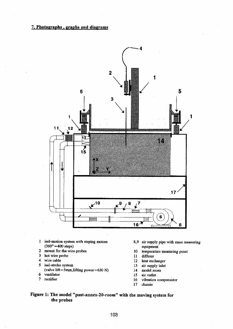
7. Photo~ra~hs , ~ r a ~ h s and dia~rams
1 isel-motion system with steping motors (360° =400 steps)
2 mount for the wire probes 3 hot wire probe 4 wire cable 5 isel-stroke system
(valve lift = 5mm,liftiig power=630 N) 6 ventilator 7 rectifier
8,9 air supply pipe with mass measuring equipment
10 temperature measuring point 11 diffuser 12 heat exchanger 13 air supply inlet 14 model room 15 air outlet 16 vibration compensator 17 chassis
Figure 1: The model "post-annex-20-room" with the moving system for the probes
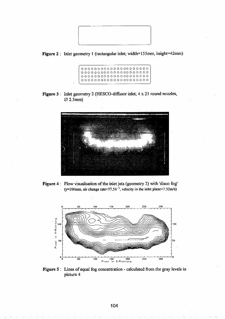
Figure 2 : Inlet geometry 1 (rectangular inlet; width=155mm, height=42mm)
Figure 3 : Inlet geometry 2 (HESCO-diffuser inlet; 4 x 21 round nozzles, 0 2.3mm)
Figure 4 : Flow visualisation of the inlet jets (geometry 2) with 'disco fog' @=100mm, air change rate=37,5h-', velocity in the inlet plane=7.52m/s)
Figure 5 : Lines of equal fog concentration - calculated from the gray levels in picture 4
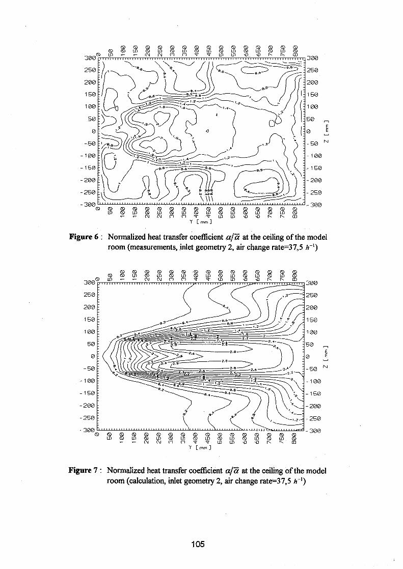
Y C m m l
Figure 6 : Normalized heat transfer coefficient a/E at the ceiling of the model room (measurements, inlet geometry 2, air change rate=3 7,5 h-')
Figure 7 : Normalized heat transfer coefficient a/Zi at the ceiling of the model room (calculation, inlet geometry 2, air change rate=37,5 h-I)
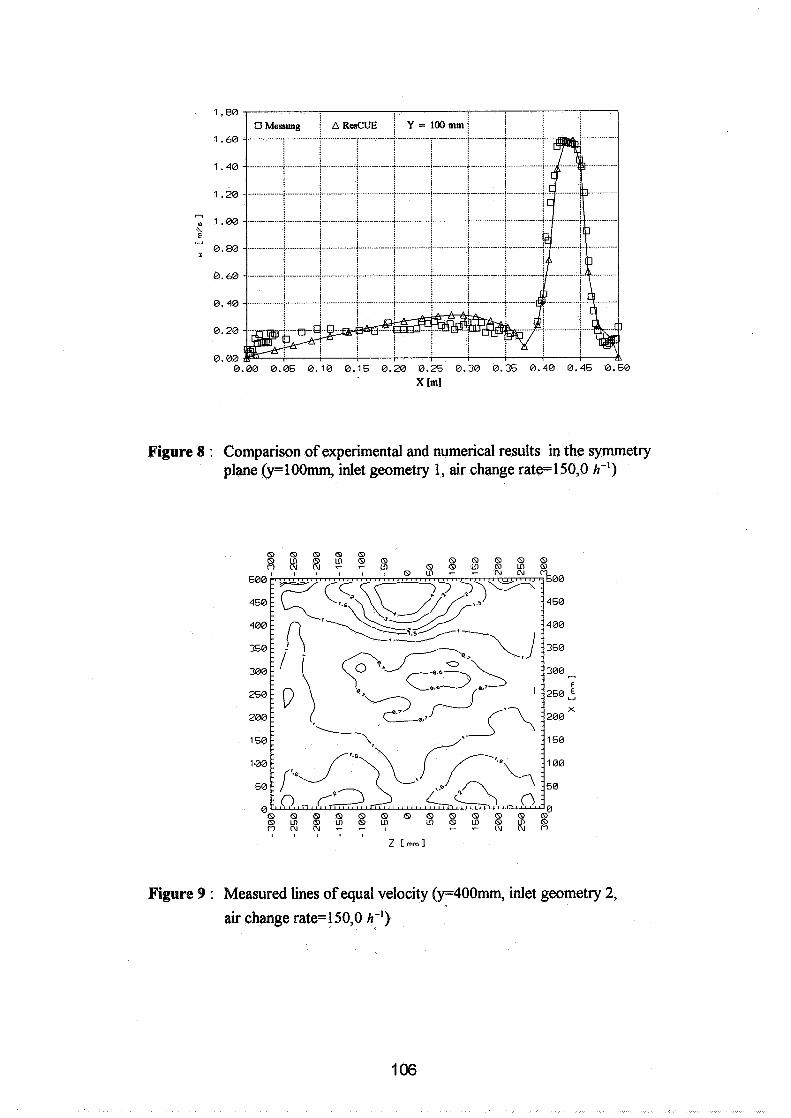
Figure 8 : Comparison of experimental and numerical results in the symmetry plane (y=lOOmm, inlet geometry 1, air change rate=150,0 h-')
Figure 9 : Measured lines of equal velocity (y=400mm, inlet geometry 2,
air change rate= 150,O h-')
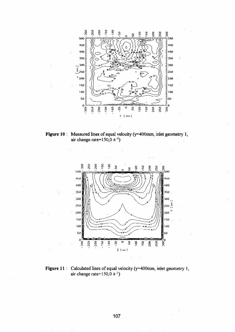
Figure 10 : Measured lines of equal velocity (y=400mm, inlet geometry 1, air change rate=150,0 h-')
Figure 11 : Calculated lines of equal velocity (y=400mm, inlet geometry 1, air change rate=150,0 h-')
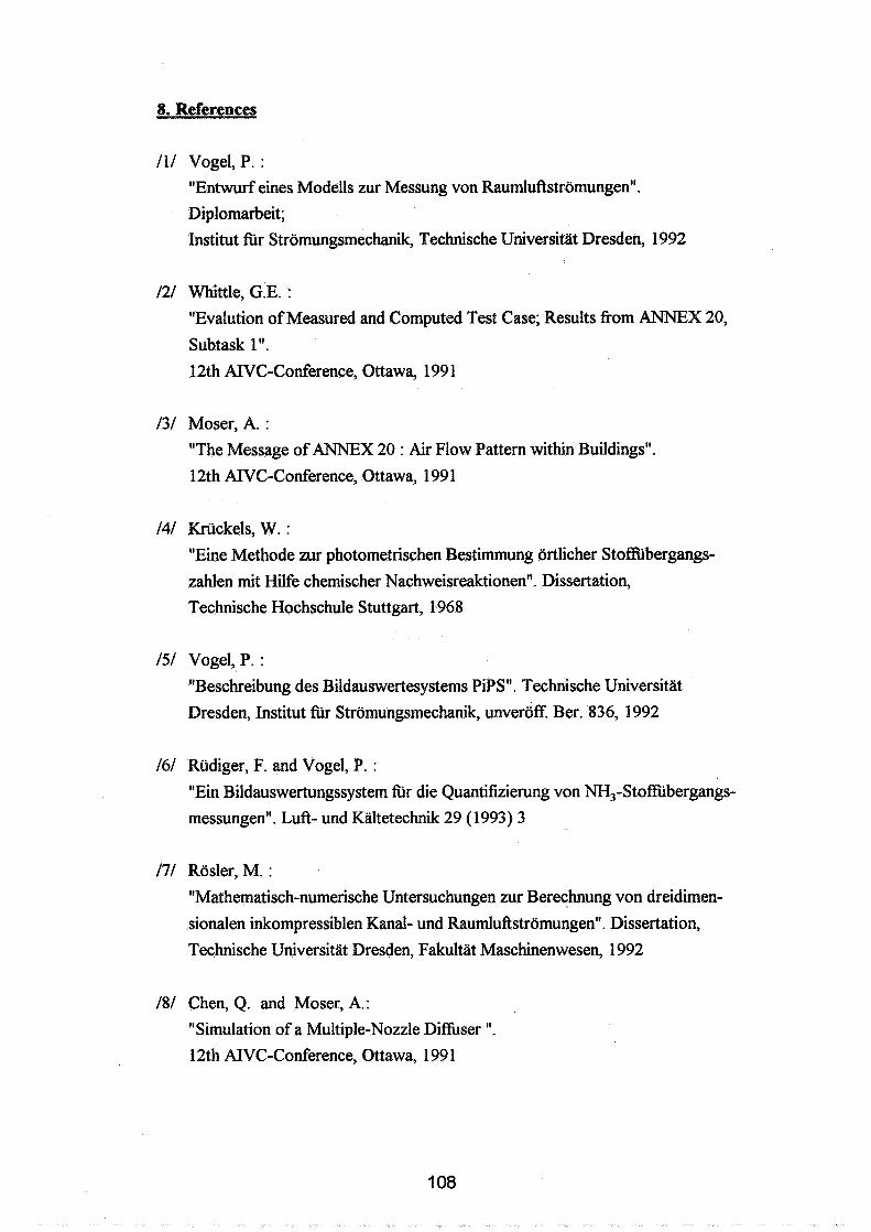
8. References
111 Vogel, P. : "Entwurf eines Modells zur Messung von Raumluftstromungen".
Diplomarbeit;
Institut fiir Stromungsmechanik, Technische Universitat Dresden, 1992
121 Whittle, G.E. :
"Evalution of Measured and Computed Test Case; Results from ANNEX 20,
Subtask 1 ". 12th AIVC-Conference, Ottawa, 199 1
I31 Moser, A. : "The Message of ANNEX 20 : Air Flow Pattern within Buildings".
12th AIVC-Conference, Ottawa, 199 1
I41 Kriickels, W. : "Eine Methode zur photometrischen Bestimmung ortlicher Stoffiibergangs-
zahlen mit Hilfe chemischer Nachweisreaktionen". Dissertation,
Technische Hochschule Stuttgart, 1968
151 Vogel, P. :
"Beschreibung des Bildauswertesystems PiPS". Technische Universitat
Dresden, Institut fiir Stromungsmechanik, unveroff Ber. 836, 1992
I61 Riidiger, F. and Vogel, P. :
"Ein Bildauswertungssystem fir die Quantifizierung von NH,-Stoffbbergangs-
messungen". Luft- und Kaltetechnik 29 (1993) 3
I71 Rosler, M. :
"Mathematisch-numerische Untersuchungen zur Berechnung von dreidimen-
sionalen inkompressiblen Kanal- und Raumluftstromungen". Dissertation,
Technische Universitat Dresden, Fakultat Maschinenwesen, 1992
I81 Chen, Q. and Moser, A.: "Simulation of a Multiple-Nozzle Diffuser ".
12th AIVC-Conference, Ottawa, 199 1

Energy Impact of Ventilation and Air Infiltration 14th AlVC Conference, Copenhagen, Denmark
21 -23 September 1993
Theoretical and Experimental Simulation of Exhaust Hoods
N Cardinale," R M Di Tommaso,* G V Fracastoro,"" E Nino," M Perino*"
* Dipartimento di lngegneria e Fisica del19Atmosfera, Universita' della Basilicata, Via Nazario Sauro 85, 851 00 Potenza, Italy ** Dipartimento di Energetics, Politecnico di Torino Corso Duca degli Abruzzi 24, 10129 Torino, Italy

Synopsis
The paper presents a criterion to assess the performance of mechanical exhaust hoods for dome stic kitchens and a procedure to experimentally test them; an analysis of the relevant parameters which affect their performance is made, the test results are shown, and finally these are compa- red with the results of a numerical fluid dynamic code. Experiments were performed using the tracer gas technique, and attention has been drawn rather on the hood efficiency in the removal of pollutants than on the IAQ in the test room. It was first shown that the choice of the tracer gas has no influence on the results of the experiments. Then, the influence of the following parameters has been investigated: distance from hood to pollution source, thermal power dissipated under the source itself, extracted air flow rate, and hood-to- walls geometry. The repeatibility of the experimental apparatus was less than 10 9%. A simplified empirical expression based on nondimensional parameters has been derived, which provides a precise estimate of hood efficiency. Furthemre, a number of tests have been simulated by means of a CFD model. The results pro- vide an interesting insight on the hood fluidynamic behaviour, yet the calculated efficiency is underestimated by 20 - 30 % respect to the measured values.
List of symbols
C = concentration D = diameter E = efficiency of the hood g = gravity acceleration h = height of the hot plate H = distance between hot plate and base of the hood q = tracer gas volume flow rate Q = air volume flow rate S = area V = room volume W = electrical power released by the hot plate 8 = volume coefficient of expansion v = kinematic viscosity
1. Introduction
Kitchen hoods are used to remove and extract, directly from the source, pollutants of different kinds, usually while a certain amount of heat is released underneath.
Different indices have been adopted to describe their performance. For example, the French and Swedish standards NF E 51-704 and 88433 05 01 have adopted the so-called "collec- tion efficiency", defined as:
where C is the concentration in the room. A similar indicator, called "pollution index", more oriented to the definition of indoor
air quality in the room, has been introduced by Wouters (1992). On the other side, a "device-oriented" performance indicator could be simply defined as
the ratio between the contaminant concentration at the exhaust of the hood and the maximum at- tainable contaminant concentration, i e, the value that would be reached if all the contaminant emitted by the source would be "captured" by the hood. This hood eflciency as a local extraction device is therefore given by:

where C is the concentration in the exhaust. With this definition, one assumes that
(a) the size of the room has no influence whatever on the efficiency of the hood, and (b) the phenomenon takes place in steady-state regime.
2. Description of the experimental apparatus
The experimental apparatus is located at the University of Basilicata (Poteoza), where other ventilation facilities, as the Controlled Ventilation Chamber described by Fracastoro et a1 (1991), are located.
The hood under test is mounted on a steel frame and is placed above a table on which a circular electric hot plate @ = 0.17 m, h = 0.15 m) rests.
The dimensions and shape of the hood used in this first set of experiments are shown in Fig. 1. The hood is suspended to a metal framework; the exhaust duct is flexible and is connected to an iron plate duct @ = 80 mm, L = 1.20 m), sized (L = 15 x D) in order to ensure a sufficien- tly uniform distribution of air streams.
Three quantities have to be measured to derive the efficiency of the hood (see Eqn. 2): Q, q, and C. Furthermore, the parameters, as the released electrical power (W) and the distance (H) from the hot plate to the base of the hood, are to be known.
Airflow rate measurement and control The air flow measurement and control system (Fig. 2) are mounted on the first arm of a
union tee, whose second arm is connected to a centrifugal fan having a nominal flow rate of 50 m3/h, while the third arm is connected to the ambient air through a gate valve serving as a by- pass for the control of flow rate through the hood.
The air flow rate was measured by a mass flow meter (error less than 2 % on the rea- ding) based on a venturi and a hot wire anemometer, provided by a digital display. The flow rate is expressed in normal litres per minute, and to obtain the correct volume flow rate a correction coefficient, function of air temperature and ambient pressure; has to be applied.
Tracer gas flow rate measurement and control The tracer gas source is placed above the electric hot plate. The gas flows out of a glass
tube (D = 6 mm, L = 0.15 m) connected to a rotameter by means of a plastic Rilsan tube. The ro- tameter has a range of 2.5 to 8.5 nllh, with an error of 3 % full-scale. The flow rate is referred to air in standard conditions, therefore, in order to use it with gases different from air, a correction coefficient equal to the square root of the ratio between the molecular mass of the air and the gas has to be applied. In practice, since the value indicated by the rotameter was not considered too reliable, it was only used to check the stability of the flow during the test; the measurement of tracer gas flow rate was actually performed using "inversely" the procedure outlined by Svensson (1983) to measure the air flow rate in a duct. This procedure provides the volume flow rate in a duct (Q) as a function of the volume flow rate (q) of a tracer gas injected in the duct and of the concentration (C) which establishes downstream, where the tracer gas is assumed to be perfectly mixed, that is
The preceding Eqn. 3 was solved for q, being Q known from above, and the concentration mea- sured as follows.
Tracer gas concentration measurement The measurement of gas concentration in the exhaust of the hood is performed using
two double-cell infrared gas analyzers for CH4, SF6, and N20, all three in the range 0-200 ppm, and an error of 2 % full scale. The analyzers are connected to a Data Acquisition and Control U- nit, in its turn connected to a PC 286 through a GPIB interface.

Hot plate power measurements The power released by the electric hot plate was measured indirectly through the eletri-
cal resistance of the hot plate and the input voltage. The relative error was 0.5 96 for the resistan- ce and 1 96 for the voltage.
The resulting probable and maximum relative errors are reported in Table 1.
Table 1 - Relative error of measured quantities.
Measured quantity Probable error Maximum error
Air flow rate 2.0 96 2.0 55 Tracer gas flow rate 2.8 96 4.0 96 Tracer gas concentration 2.0 96 2.0 96 Hot plate electrical power 1.4 96 2.5 96 Hood efficiency 2.8 96 6.8 96
3. Testing methodology and experimental results
Preliminary campaign: influence of the tracer gas type At first, the question of the influence of the different tracer gas on the test results was
faced. Experiments have shown that, when no heat is released from the hot plate, the influence of the tracer gas becomes very large. In fact, since there is no sufficient energy to break the link between molecules, heavy tracer gases tend to sink down and do not follow the air across the hood. Measurements turn out to be scarcely repeatible, and in practice the tracer gas technique cannot be applied. On the other hand, when a sufficient convective drag is present, experiments have shown that the type of gas does not influence the results of the tests.
Therefore, the experiments were always performed with non-zero values of the hot plate power. Experiments were performed varying the height of the hood above the hot plate and the exhaust air flow rate. The values assumed during the experiments by the variable parameters are shown in Table 2. The tracer gas volume flow rate and the hot plate power were kept constant re- spectively at 4 l/h and 1040 W.
Table 2 - Parameter values in the preliminary measurement campaign.
Case Tracer gas Height (a) Air flow rate (b)
1 N2° 0.50 m 500 llmin 2 0.75 m 750 llmin 3 cH4 1.00 m
The results of the 18 tests performed combining the different parameters are summari- zed in Table 3. The influence of tracer gas is inversely proportional to the efficiency of the hood, as could be expected from the considerations above. In any case, the difference from gas to gas is always below f 5.5 % of the average - that is, close to the measurement error itself - and does not show any systematic variation. It may then be concluded that in these conditions the influen- ce of the tracer gas is negligible.
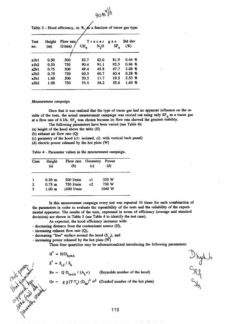
Table 3 - Hood efficiency, in 96, A" a function of tracer gas type.
Test Height Flow T r a c e r g a s Stddev no. (m) (11min) *2O SF6 (96)
albl 0.50 500 82.7 82.0 81.9 0.44 % alb2 0.50 750 90.4 91.1 92.5 0.96 96 a2bl 0.75 500 49.4 45.8 47.7 3.08 96 a2b2 0.75 750 60.3 60.7 60.4 0.28 96 a3bl 1.00 500 20.2 17.7 19.5 5.53 5% a3b2 1.00 750 53.5 54.2 55.6 1.60 %
Measurement campaign
Once that it was realized that the type of tracer gas had no apparent influence on the re- sults of the tests, the actual measurement campaign was camed out using only SF6 as a tracer gas at a flow rate of 4 llh. SF, was chosen because its flow rate. showed the greatest stability.
The following parameters have been varied (see Table 4): (a) height of the hood above the table (H) (b) exhaust air flow rate (Q) (c) geometry of the hood (cl: isolated, c2: with vertical back panel) (d) electric power released by the hot plate (W)
Table 4 - Parameter values in the measurement campaign.
Case Height Flow rate Geometry Power (a) (b) ( 4 (dl
1 0.50 m 500 llmin cl 320 W 2 0.75 m 750 llmin c2 730 W 3 1.00m 1OOOllmin 1040 W
In this measurement campaign every test was repeated 10 times for each combination of the parameters in order to evaluate the repeatibility of the tests and the reliability of the experi- mental apparatus. The results of the tests, expressed in terms of efficiency (average and standard deviation) are shown in Table 5 (see Table 4 to identify the test case).
As expected, the hood efficiency increases with: - decreasing distance from the contaminant source (H), - increasing exhaust flow rate (Q), - decreasing "free" surface around the hood (S, f), and - increasing power released by the hot plate @)
These four quantities may be adimensionalized introducing the following parameters:
(Reynolds number of the hood)
(Grashof number of the hot plate)

Table 5. Hood efficiency for different values of the parameters.
Case cldl cld2 cld3 c2dl c2d2 c2d3
a lbl 81.5f 2.7 8 3 . 6 ~ 2.5 84.8f 2.2 83.2f 2.2 84.7f 1.9 85.9f 1.7 alb2 89.2f 3.8 91.8f3.4 92.5f2.8 91.6f 3.4 92.9f2.8 93.0f2.5 alb3 94.5f 4.6 95.2f 3.9 95.7f 3.2 96.1f 3.1 96.4f2.7 96.452.5
Due to the limited number of parameters actually varied in the tests performed, the last two parameters may be replaced, without any loss of accuracy, simply by the following:
Q* = QIQ, with, for example, Qo = 100 m31h
W* = WMIo with, for example, Wo = 1000 W
A regression analysis has shown that the hood efficiency may be expressed as a function of the nondimensional parameters above:
with A = - 2.527 a = - 1.544 b = - 0.346 c = 1.165 d = 0.160
A comparison between the values calculated by means of Eqn 4 and the experimental data is shown in Fig. 3. A correlation coefficient r2 = 0.96 was found.
4. Theoretical approach and simulation results
The theoretical simulations were carried on at Turin Polytechnic using the Creare Inc. FLUENT package, chosen after several recently performed validations. A description of this mo- del may be found in Cafaro et al. (1992), to which the interested reader is sent back.
For this specific problem the boundary conditions at the inlet cells were assumed at the tracer gas immission and air extraction duct in terms of distribution of air velocity and turbulent intensity value, and at the ideal lateral surface from the table to the hood base, in terms of fixed pressure conditions. At the hood walls the gradient of the main variable and the heat flux are as- sumed zero. At the hot plate surface a specific thermal flux was imposed.
To the domain of calculation a non-uniform threedimensional cartesian grid made of 30x25~33 cells has been superposed. Power Law discretization scheme has been adopted. Simula- tions have been performed on a workstation HP 720 Apollo. A good convergence was achieved with about 3,000 iterations. The running time was about 24 hours.
At the moment only cases a2blcld2, a2b2cld2, and a2b3cld2 (see Table 5) were simula-
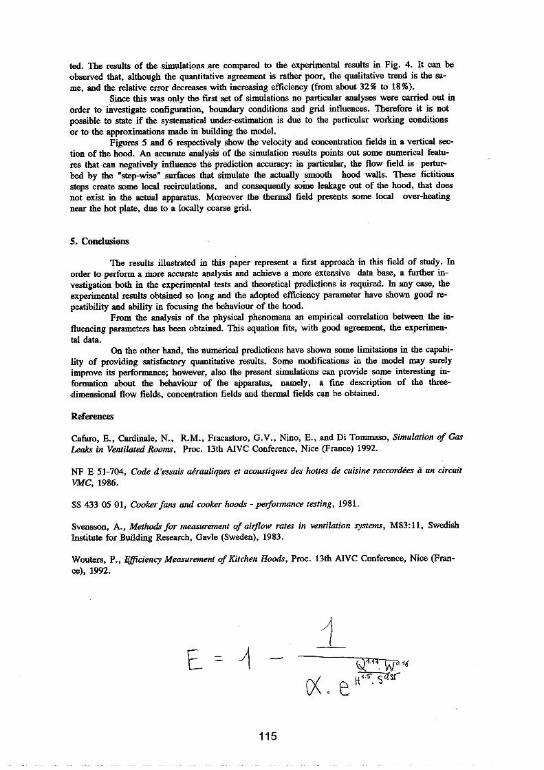
ted. The results of the simulations are compared to the experimental results in Fig. 4. It can be observed that, although the quantitative agreement is rather poor, the qualitative trend is the sa- me, and the relative error decreases with increasing efficiency (from about 32% to 18%).
Since this was only the first set of simulations no particular analyses were camed out in order to investigate configuration, boundary conditions and grid influences. Therefore it is not possible to state if the systematical under-estimation is due to the particular working conditions or to the approximations made in building the model.
Figures 5 and 6 respectively show the velocity and concentration fields in a vertical sec- tion of the hood. An accurate analysis of the simulation results points out some numerical featu- res that can negatively influence the prediction accuracy: in particular, the flow field is pertur- bed by the "step-wise" surfaces that simulate the actually smooth hood walls. These fictitious steps create some local recirculations, and consequently some leakage out of the hood, that does not exist in the actual apparatus. Moreover the thermal field presents some local over-heating near the hot plate, due to a locally coarse grid.
5. Conclusions
The results illustrated in this paper represent a first approach in this field of study. In order to perform a more accurate analysis and achieve a more extensive data base, a further in- vestigation both in the experimental tests and theoretical predictions is required. In any case, the experimental results obtained so long and the adopted efficiency parameter have shown good re- peatibility and ability in focusing the behaviour of the hood.
From the analysis of the physical phenomena an empirical correlation between the in- fluencing parameters has been obtained. This equation fits, with good agreement, the experimen- tal data.
On the other hand, the numerical predictions have shown some limitations in the capabi- lity of providing satisfactory quantitative results. Some modifications in the model may surely improve its performance; however, also the present simulations can provide some interesting in- formation about the behaviour of the apparatus, namely, a fine description of the three- dimensional flow fields, concentration fields and thermal fields can be obtained.
References
Cafaro, E., Cardinale, N., R.M., Fracastoro, G.V., Nino, E., and Di Tommaso, Simulation of Gas Le& in Ventilated Rooms, Proc. 13th AIVC Conference, Nice (France) 1992.
NF E 51-704, Code d'essais drauliques et acoustiques des hotfes de cuisine raccordLes h un circuit MMC, 1986.
SS 433 05 01, Cooker fans and cooker hoods - peg5omance testing, 1981.
Svensson, A., Methods for measurement of ai@ow rates in ventilation systems, M83:ll, Swedish Institute for Building Research, Gavle (Sweden), 1983.
Wouters, P., Eflciency Measurement of Kitchen Hoods, Proc. 13th AIVC Conference, Nice (Fran- ce), 1992.

bottle
Fig. 1 - Layout of the experimental apparatus.
Gate valves
+ Hood
I / Digital display g
'Flexible duct
~ana'
Fig. 2 - Layout of the air flow rate measurement and control.
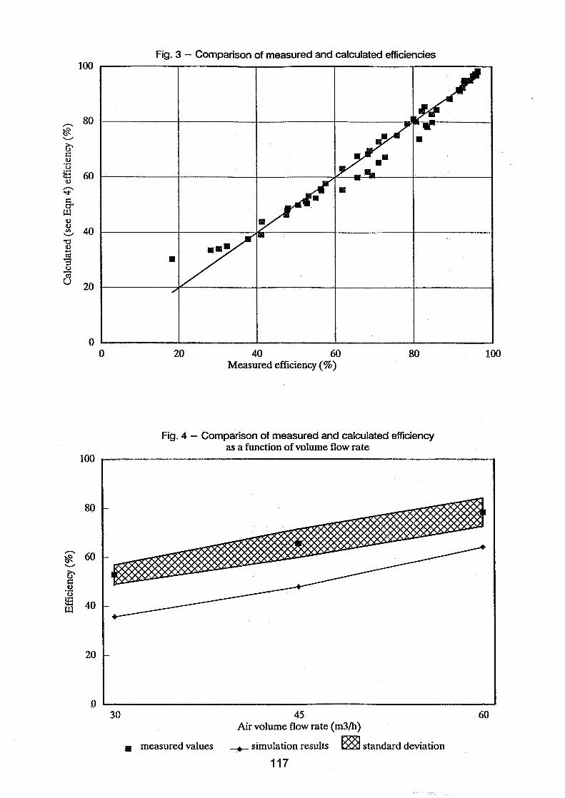
Fig. 3 - Comparison of measured and calculated efficiencies
" 0 20 40 60 80 100
Measured efficiency (%)
Fig. 4 - Comparison of measured and calculated efficiency as a function of volume flow rate
30 45 60 Air volume flow rate (m31h)
measured values + simulation results standard deviation
117
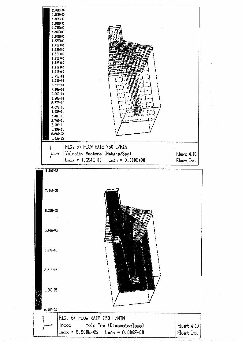
Energy Impact of Ventilation and Air Infiltration 14th AlVC Conference, Copenhagen, Denmark
21 -23 Septern ber 1993
Demand Controlled Ventilation in an Auditorium
S A Svennberg*, L-G Miinsson**
*RAMAS Teknik AB, Solkraftsvagen, S-135 70 Stockholm, Sweden **LGM Consult AB, Adler Salvius vag 87, S-146 53 Tullinge, Sweden
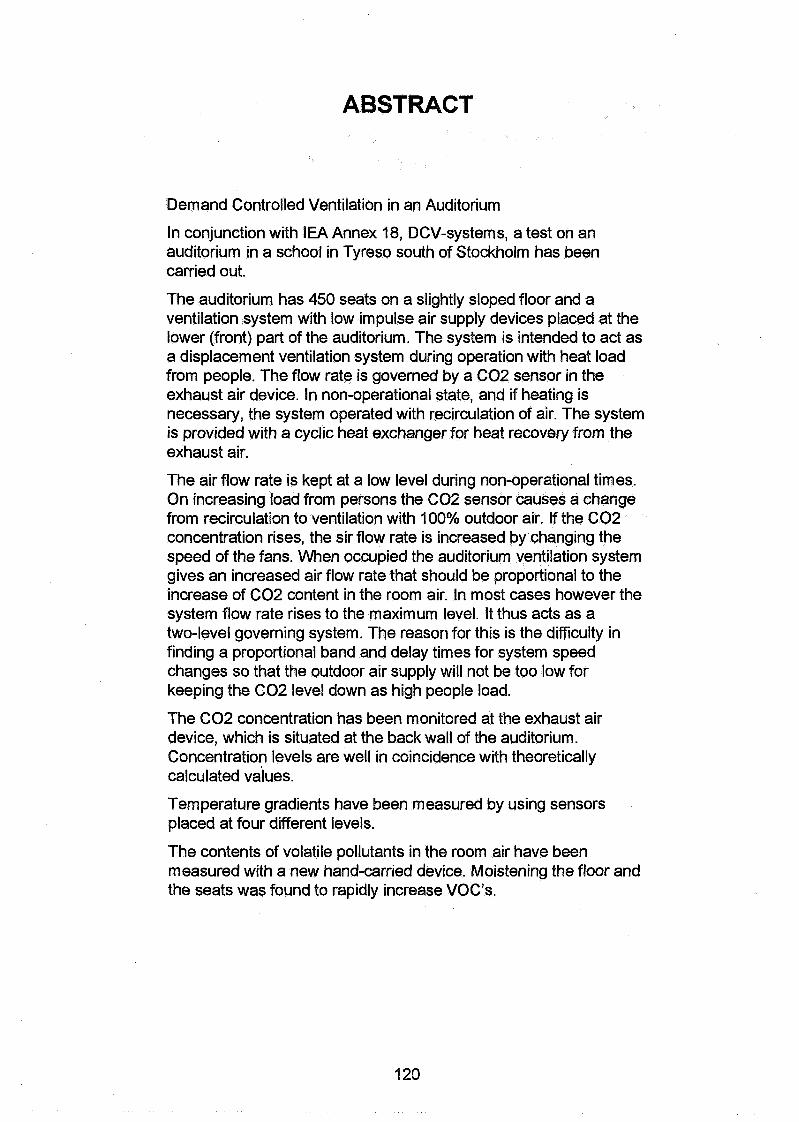
ABSTRACT
Demand Controlled Ventilation in an Auditorium
In conjunction with IEA Annex 18, DCV-systems, a test on an auditorium in a school in Tyreso south of Stockholm has been carried out.
The auditorium has 450 seats on a slightly sloped floor and a ventilation system with low impulse air supply devices placed at the lower (front) part of the auditorium. The system is intended to act as a displacement ventilation system during operation with heat load from people. The flow rate is governed by a C02 sensor in the exhaust air device. In non-operational state, and if heating is necessary, the system operated with recirculation of air. The system is provided with a cyclic heat exchanger for heat recovery from the exhaust air.
The air flow rate is kept at a low level during non-operational times. On increasing load from persons the C02 sensor causes a change from recirculation to ventilation with 100% outdoor air. If the C02 concentration rises, the sir flow rate is increased by changing the speed of the fans. When occupied the auditorium ventilation system gives an increased air flow rate that should be proportional to the increase of C02 content in the room air. In most cases however the system flow rate rises to the maximum level. It thus acts as a two-level governing system. The reason for this is the difficulty in finding a proportional band and delay times for system speed changes so that the outdoor air supply will not be too low for keeping the C02 level down as high people load.
The C02 concentration has been monitored at the exhaust air device, which is situated at the back wall of the auditorium. Concentration levels are well in coincidence with theoretically calculated values.
Temperature gradients have been measured by using sensors placed at four different levels.
The contents of volatile pollutants in the room air have been measured with a new hand-carried device. Moistening the floor and the seats was found to rapidly increase VOC's.

Energy Impact of Ventilation and Air Infiltration 14th AlVC Conference, Copenhagen, Denmark
21 -23 Septem ber 1993
Development and Investigation of a Combined Ventilation and Floor-Heating System
F Steimle, B Mengede
Universitiit Essen, Angewandte Thermodynamik und Klimatechnik, Universit~tsstr.l5,45117 Essen, Germany
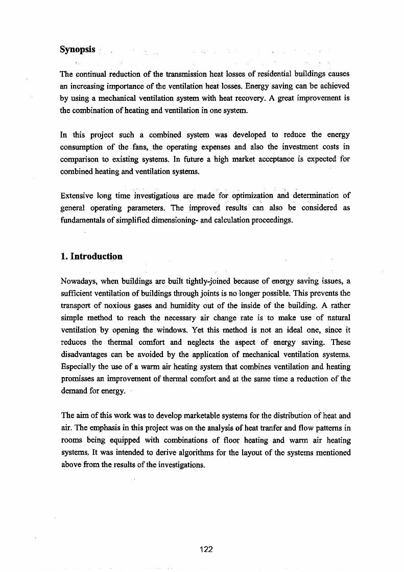
Synopsis
The continual reduction of the transmission heat losses of residential buildings causes an increasing importance of the ventilation heat losses. Energy saving can be achieved by using a mechanical ventilation system with heat recovery. A great improvement is the combination of heating and ventilation in one system.
In this project such a combined system was developed to reduce the energy consumption of the fans, the operating expenses and also the investment costs in comparison to existing systems. In fume a high market acceptance is expected for combined heating and ventilation systems.
Extensive long time investigations are made for optimization and determination of general operating parameters. The improved results can also be considered as fundamentals of simplified dimensioning- and calculation proceedings.
1. Introduction
Nowadays, when buildings are built tightly-joined because of energy saving issues, a sufficient ventilation of buildings through joints is no longer possible. This prevents the transport of noxious gases and humidity out of the inside of the building. A rather simple method to reach the necessary air change rate is to make use of natural ventilation by opening the windows. Yet this method is not an ideal one, since it reduces the thermal comfort and neglects the aspect of energy saving. These disadvantages can be avoided by the application of mechanical ventilation systems. Especially the use of a warm air heating system that combines ventilation and heating promisses an improvement of thermal comfort and at the same time a reduction of the demand for energy. .
The aim of this work was to develop marketable systems for the distribution of heat and air. The emphasis in this project was on the analysis of heat tranfer and flow patterns in rooms being equipped with combinations of floor heating and warm air heating systems. It was intended to derive algorithms for the layout of the systems mentioned above from the results of the investigations.

2. Description of the systems
The developed systems are based on the warm air heating that is characterized by its
ease of control, its quick adjustment of heating power and the low level of temperature being necessary to provide the heating energy. Moreover, a warm air heating system
allows the application of heat recovery systems which enlarge the energy saving
potential especially in highly insulated buildings where a great part of the heat
requirement is caused by the ventilation heat losses.
The air conducting components of the developed systems are integrated in the floor
construction. Thus part of the heat transfer takes place through the surface of the floor.
The amount of the heat transmitted through the floor depends on the construction of the
floor and the air conducting components.
The three developed heating systems are all chracterized by a central treatment of the
air (filtering, heat recovery, preheating), whereas they differ in the further treatment and
conduction of the air.
1st variant: The supply air is heated up to 50 "C by a waterlair heat exchanger in the
central boiler plant. It is distributed in the building by a system of
insulated air ducts. The entrance of the air into the floor is near the
internal wall of the room. In the hollow floor the air flows through ducts
in the direction of the external roomwall. The ducts are ending in a
cavity of one meter length, built with cones, that equalizes gradients in
air velocity and temperature. The air flows into the room through outlet
grilles that are installed in front of the external wall. In this variant the
part of heat transmitted through the floor is quite small. If this heating
system is installed in highly insulated buildings, the air change rate
necessary due to hygienic reasons is sufficient for the transport of the
demanded heat. In buildings that are insulated according to present
standards the recirculation of additional air is necessary to reach the
required heating capacity.
2nd variant: Depending on the required heating capacity the supply air is heated up to
a temperature of 20 "C - 40 "6. Starting on the side of the internal

roomwall the air flows through a cavity built with cones, that is situated between the two layers of the floor (fig. 1).
after-heater
attenuation / them4
While the air is streaming through the cavity, the heat is transmitted into the room through the upper layer of the floor (the finish floor). So the air is cooled down until it reaches almost the temperature of the room near the air inlet into the room on the side of the outer roomwall. Shortly before it reaches the outlet grilles the air is tempered by an after-heater so that it enters the room with a supply air temperature that is significantly higher than the room temperature so that a draught can be prevented. The 2nd variant represents a warm air heating system that uses the floor as a low temperature heating surface. Because of the floor- integrated after-heater the second variant, in contrast to the first variant, is able to supply the necessary heating capacity for a building with an average standard of insulation without additional costs for the transport of air.
3rd varianc Above the cavity that is built with cones and through which the supply air is streaming a conventional floor-heating with hot water used as heat carrier is installed (fig. 2). The floor-heating works like a heat exchanger with a large surface. The heat is on the one hand transferred from the water through the floor finish to the room and on the other hand it is
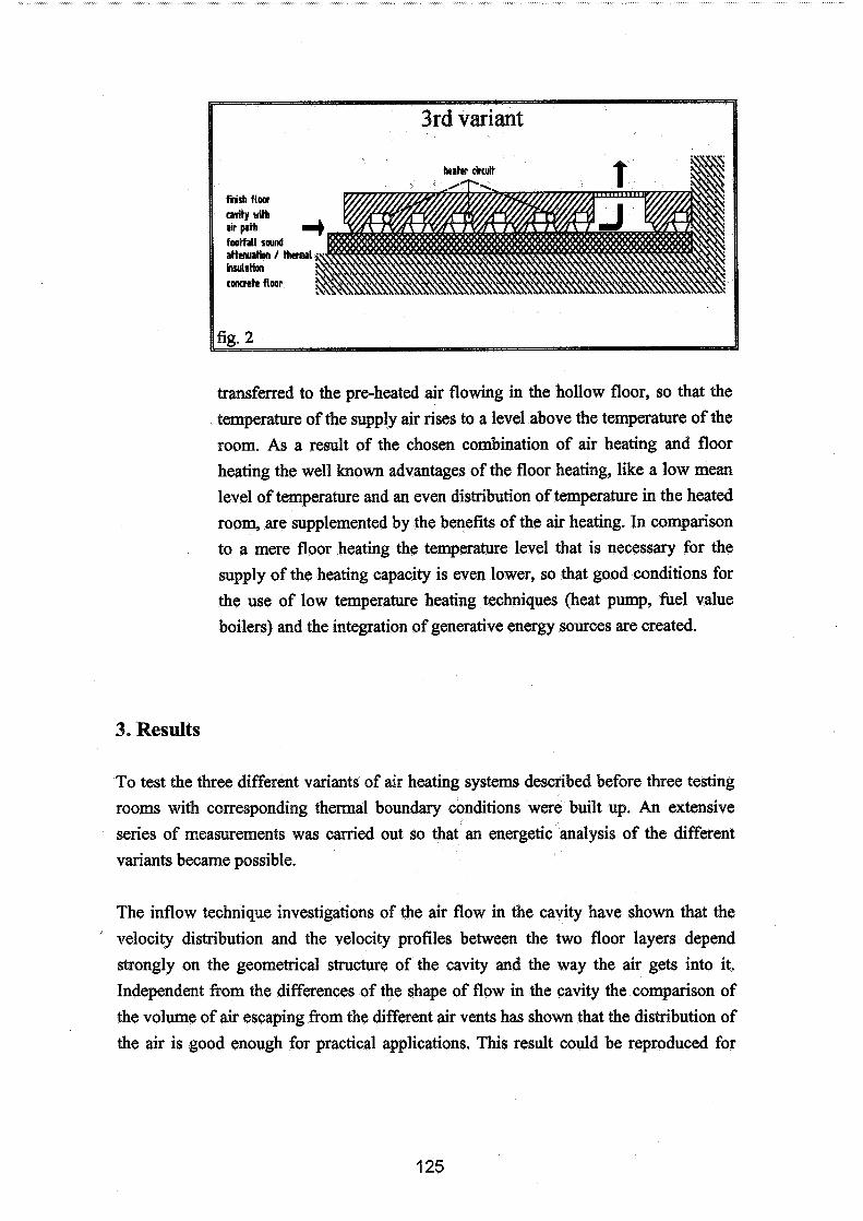
hate circuit
attenurtan / thcmrl
transferred to the pre-heated air flowing in the hollow floor, so that the temperature of the supply air rises to a level above the temperature of the room. As a result of the chosen combination of air heating and floor heating the well known advantages of the floor heating, like a low mean level of temperature and an even distribution of temperature in the heated room, are supplemented by the benefits of the air heating. In comparison to a mere floor heating the temperature level that is necessary for the supply of the heating capacity is even lower, so that good conditions for the use of low temperature heating techniques (heat pump, fuel value , . . \ , . . . I- A - - - _ _ _ _ _ - --- ---- A - 1 nnlterel ann m e inrea~rinn nr opnprnTlve merw cniircec are crearnn
3. Results
To test the three different variants of air heating systems described before three testing rooms with corresponding thermal boundary conditions were built up. An extensive series of measurements was carried out so that an energetic analysis of the different variants became possible.
The inflow technique investigations of the air flow in the cavity have shown that the ' velocity distribution and the velocity profiles between the two floor layers depend
strongly on the geometrical structure of the cavity and the way the air gets into it. Independent from the differences of the shape of flow in the cavity the comparison of the volume of air escaping from the different air vents has shown that the distribution of the air is good enough for practical applications. This result could be reproduced for
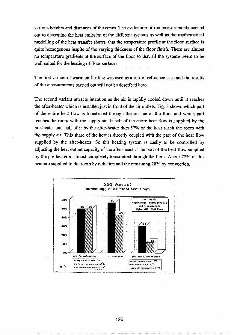
various heights and distances of the cones. The evaluation of the measurements carried
out to determine the heat emission of the different systems as well as the mathematical
modelling of the heat transfer shows, that the temperature profile at the floor surface is
quite homogenous inspite of the varying thickness of the floor finish. There are almost
no temperature gradients at the surface of the floor so that all the systems seem to be
well suited for the heating of floor surfaces.
The first variant of wann air heating was used as a sort of reference case and the results
of the measurements carried out will not be described here.
The second variant attracts intention as the air is rapidly cooled down until it reaches
the after-heater which is installed just in front of the air outlets. Fig. 3 shows which part
of the entire heat flow is transferred through the surface of the floor and which part
reaches the room with the supply air. If half of the entire heat flow is supplied by the
pre-heater and half of it by the after-heater then 57% of the heat reach the room with
the supply air. This share of the heat is directly coupled with the part of the heat flow
supplied by the after-heater. So this heating system is easily to be controlled by
adjusting the heat output capacity of the after-heater. The part of the heat flow supplied
by the pre-heater is almost completely transmitted through the floor. About 72% of this
heat are supplied to the room by radiation and the remaining 28% by convection.
percentage of different heat flows
pre-/afterheating radiation/~~evectlon

In contrast to the first and second variant, in the third variant the air is heated up while
flowi11g through the cavity, so that when it reaches the outlet, the supply air is
significantly warmer than the room. Fig. 4 shows that the heating up of the air in the
cavity advances rapidly inspite of the low excess temperature of the heating water. The
warming up of the air in the cavity guarantees that besides the part of the heat
transmitted through the floor part of the heat is supplied to the room by the supply air.
3rd variant temperature gradient in flow direction
temperature ('c) 23
22
21
20
19
18
-ii of the indoor alr 17
entrance 1000 2000 3000 exit
length of flow (mm)
Inltlsl rater temperature 24.3%
fig. 4
Fig. 5 shows that the temperature-distribution in the floor finish is homogene even if
the distance between the tubes with the heating water is big. Because of the excess
temperature at the floor surface the part of the heat transferred to the room through the
floor is considerably bigger than in the second variant. As shown in fig. 6, 90% of the
entire heat flow are supplied to the room by the floor surface. 75% of the heat transfer
from the floor to the room are radiation, 25% are convection.
If the air change rate amounts to 1 per hour 10% of the entire heat flow are transmitted
to the room by the supply air. As the investigations have shown, the temperature of the
supply air remains almost constant if the quantity of supply air is risen. The heat flow
through the floor staying almost constant, the part of the heat supplied to the room by
the air is increased. So a quick adaptation of the heating capacity is possible.
3rd variant distribution of surface temperature
temperature (OC)
finish floor surface
-1500-1000 -500 0 500 1000 1500 distance to axis of the room (mm)
fig. 5
percentage of different heat flows
Measurements of temperature and air velocity in the room have shown that both art;
distributed in a homogene way. This has a positive influence on the thermal comfort as
well as on the economic efficiency and on hygienical aspects.
4. Summary
The measurements carried out under operating conditions are obviously in accordance with the mathematical modelling carried out before. Both, the measurements and the modelling, show that the developed heating systems meet the demands concerning thermal comfort and energy efficiency.
Since special demands arised for the components of the installation and for the control equipment due to operating characteristics of the analyzed systems, these components had to be developed or improved in the course of the project.
5. Acknowledgement
The research was supported by the Bundesministerium fiir Forschung und Technologic
under the contract number 03350 13A.

Energy 14th Al
Impact of Ventilation and Air Infiltration VC Conference, Copenhagen, Denmark
21 -23 September 1993
Simulation of Displacement Ventilation and Radiative Cooling
M Koschenz
EMPA, Section Building Equipment, Duebendorf, Switzerland
ABSTRACT
For thermal comfort and energy conservation reasons, displacement ventilation and radiative cooling systems are increasingly used. Simulation programs are general not able to correctly simulate such systems because of their one node approach for the air temperature. A procedure for creating DOE-2 inputs to simulate both system types each alone or in combination - without program code change - was developed, based on a more detailed new TRNSYS-Type, and validated against existing experimental data sets. The used approaches in DOE-2 are a two zone model for the displacement ventilation and a 'dummy' zone for the radiative cooling. A sufficiently good agreement shows that this is possible. The new TRNSYS-Type is a one zone model similar to the existing Type 19, but it simulates the temperature gradient in the room with 3 air nodes.
LIST OF SYMBOLS
TaC Air temperature in the centre of gain PC]
TCe Temperature of the ceiling
Te Exhaust air temperature
T, Air temperature near the floor ["cl T, Supply air temperature ["cl q Heat power in the lower zone [W/m2]
UP Heat power in the upper zone [W/m2]
qh Heat source power [W/m2]
q Heat flow from zone 1 to zone 2 [W/m2]
q21 Heat flow from zone 2 to zone 1 [W/m2] Q, Load split [-I oac Temperature efficiency in the centre of gain [-I o, Temperature efficiency near the floor [-I
For reasons of thermal comfort, low-turbulence air supplies are becoming increasingly important. Because their capacity for heat removal is limited, the two tasks of cooling and air renewal must be split into two different systems. The cooling task is advantageously done by a radiant element, which also leads to an energy efficient solution due to low air transport energy. For air renewal, vertical di- rected ventilation (displacement ventilation) is adequate.
The simulation program DOE-2 [6] lacks both of these systems, which is one of the most fre- quently heard arguments against it. The goal was to find a way to create a practicable simulation model for radiant ceiling and displacement ventilation within this program, without changing the pro- gram code, by clever geometric input and, if necessary, by using the "functional inpur' feature of the program.
The parameters necessary for the DOE-2 model are calculated by a more detailed TRNSYS model [7]. This leads to the question why a more or less exact DOE-2 model is needed as the more detailed TRNSYS model is available. At first the concepts of the two programs are different. In DOE-2 the components and HVAC systems are predefined. By definition of parameters some components can be defined or suppressed. The TRNSYS components are defined by the user in FORTRAN routines and linked to each other by in- and outputs. But the so achieved individual applicability results in much more complex problems with the modelling. Numerical problems cannot be excluded. This requires

exact knowledge of the user about the algorithms. DOE-2 on the other hand is a complete program which does not have instability problems. Input errors are documented by numerous and pmprehen- sive error messages. Furthermore the computation times are much shorter with DOE-2 than with TRNSYS. Therefore the transfer of the parameters into a simplified model is sensible for some appli- cations.
DISPLACEMENT VENTILATION
Most simulation programs are not able to simulate a temperature gradient over the room height because of there one node approach for the air temperature. For the simulation of a temperature gra- dient at least two air nodes are necessary.
The TRNSYS model room is a geometric one zone model with walls, windows and doors. It calcu- lates the air temperature in three nodes and the temperatures of all surrounding surfaces. The heat transfer through the walls is calculated with the response factor technique. Taking into consideration the view factors of the different surface areas, of the heat source, and of the lighting system, the ra- diative balance is solved. At each surface and heat source, a convective heat transfer is applied. In every time step, the equation system is solved simultaneously.
Figure 1 : TRNSY S model room
Mathisen [2] shows in his measurements that the shape of the air temperature in a room varies with different loads. However, if one plots the air temperature as a dimensionless temperature difference in the centre of heat gains
a dependency from the specific air flowrate can be shown. The same result was found by Mathisen in his study. The temperature efficiency in the centre of heat gains for a typical room with various spec. heat gains in a stationary case is calculated with the model and shown in Figure 3. In the same way it is possible to calculate the temperature efficiency near the floor (Figure 2).
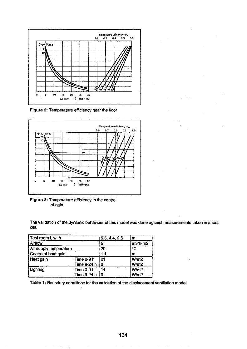
Temperature efliciency o, 0.2 0.3 0.4 0.5 0.6
0 5 10 15 20 25 30
Air flow 6 Im31h-m21
Figure 2: Temperature efficiency near the floor
Temperature efficiency a, 0.6 0.7 0.8 0.9 1.0
0 5 10 15 20 25 30 ~ i r riow Im3h-m21
Figure 3: Temperature efficiency in the centre of gain
The validation of the dynamic behaviour of this model was done against measurements taken in a test cell.
Table 1 : Boundary conditions for the validation of the displacement ventilation model.
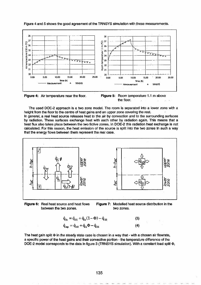
Figure 4 and 5 shows the good agreement of the TRNSYS simulation with these measurements.
28 28
-27 - 27 2 2 E 26 E 26 'n - 4 25 o ' 25 C $ 24 $ 24 Q 8 23 23 E 2 2 22 L 5 22 a 2, 2 21
20 20 0.00 5.00 10.00 15.00 20.00 25.00 0.00 5.00 10,133 15.00 20.00 25.00
nme [h) ame (h) Measurement A TRNSYS - Measurement A TRNSYS
Figure 4: Air temperature near the floor. Figure 5: Room temperature 1.1 m above the floor.
The used DOE-2 approach is a two zone model. The room is separated into a lower zone with a height from the floor to the centre of heat gains and an upper zone covering the rest. In general, a real heat source releases heat to the air by convection and to the surrounding surfaces by radiation. These surfaces exchange heat with each other by radiation again. This means that a heat flux also takes place between the two fictive zones. In DOE-2 this radiation heat exchange is not calculated. For this reason, the heat emission of the source is split into the two zones in such a way that the energy flows between them represent the real case.
Figure 6: Real heat source and heat flows Figure 7: Modelled heat source distribution in the between the two zones. two zones.
The heat gain split (Z, in the steady state case is chosen in a way that - with a chosen air flowrate, a specific power of the heat gains and their convective portion - the temperature difference of the DOE-2 model corresponds to the data in figure 3 (TRNSYS simulation). With a constant load split @,

the DOE-2 model also shows the dependence of the temperature difference on the specific air flowrate (Figure 8).
1
0.9
0.8 - + 0.7'
2 0.6 - 2 0.5 F
8 0.4 0 5 0.3
0.2
0 "' I 0 5 10 15 20 25 30
Alr flow (m3h-m2) A WE-2 - TRNSYS
Figure 8: Temperature efficiency as a function of the airflow rate
For the evaluation of the DOE-2 approach in the dynamic case, also boundary conditions according to table 1 were used. The room temperatures on a height of 1.1 m obtained from the measurements cannot be compared directly with the DOE-2 data, because this program does not show the surface temperatures due to the weighting factor technique. For this reason the two models in DOE-2 and TRNSYS are compared.
29 30
- 28 - 29
2 2 7 2 28 E , 26 2 27 - 9 25 g 26
a 2 g 24
E 25 2 5 24 8 23 323
!.! 22 3 g 22
21 U J 21
20 20 0 5 10 15 20 25 0 5 10 15 20 25
Tlme 0) lime (h) - WE-2 - TRNSYS -DOE-2 -TRNSYS
Figure 9: Co,mparison o f ' ~ O ~ - 2 and TRNSYS Figure 10: Exhaust air temperature Air temperature 1.1 m above the floor
RADIANT CEILING
As shown in Figure 1, it is possible to have a radiant ceiling on the top of the TRNSYS room. The radiant ceiling can be either a quick metal or a concrete type. The validation was done against measurements in a test cell with a quick metal radiant ceiling. For the begin of the measurement the room was in steady state conditions at a temperature of 32 "6. The radiant ceiling was off and only the displacement ventilation system was on operation. At the begin of the measurements the opera- tion of the radiant ceiling was also started.
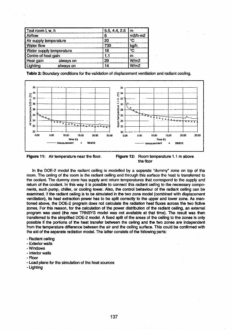
Table 2: Boundary conditions for the validation of displacement ventilation and radiant cooling.
36 36
-34 E" k? E 32 E 32 - $30 ' 30
8 f 28 $ 28
I= P $26
2 24 5 24
a 22 A! 22
20 20 0.00 5.00 10.00 15.00 20.00 25.00 0.00 5.00 10.00 15.00 20.00 25.00
rime m1 nme (h) -- Measurement A TRNSYS - Measurement A TRNSYS
Figure 11 : Air temperature near the floor. Figure 12: Room temperature 1.1 m above the floor
In the DOE-2 model the radiant ceiling is modelled by a separate "dummyu zone on top of the room. The ceiling of the room is the radiant ceiling and through this surface the heat is transferred to the coolant. The dummy zone has supply and return temperatures that correspond to the supply and return of the coolant. In this way it is possible to connect this radiant ceiling to the necessary compo- nents, such pump, chiller, or cooling tower. Also, the control behaviour of the radiant ceiling can be examined. If the radiant ceiling is to be simulated in the two zone model (combined with displacement ventilation), its heat extraction power has to be split correctly to the upper and lower zone. As men- tioned above, the DOE-2 program does not calculate the radiation heat fluxes across the two fictive zones. For this reason, for the calculation of the power distribution of the radiant ceiling, an external program was used (the new TRNSYS model was not available at that time). The result was then transferred to the simplified DOE-2 model. A fixed split of the areas of the ceiling to the zones is only possible if the portions of the heat transfer between the ceiling and the two zones are independent from the temperature difference between the air and the ceiling surface. This could be confirmed with the aid of the separate radiation model. The latter consists of the following parts:
- Radiant ceiling - Exterior walls - Windows - Interior walls - Floor - Load plane for the simulation of the heat sources - Lighting

Figure 13: Geometry and temperatures of the radiation model
Based on the geometry, the program calculates the view factors between the radiation ceiling and the different surfaces. By choice of the temperature of the different surfaces, the radiative balance of the ceiling can be found. If the heat exchanges of all surfaces of the upper or lower zone are added up, the requested split of the radiative power is obtained. To make sure that a wide range of possible variations for the surface temperatures is considered with the simulation, these were varied by a random number generator within an admissible range according to the indications in Figure 13. 140 temperature variations were calculated for each parameter.
80 1
70 0.9
0.8
E" 0.7 S5O .$ 0.6
-& 40 .u
6 2 0.5
430 .$0.4
= 20 0.3
0.2 10
0.1 0 0
0 2 4 6 8 10 12 14 0 2 4 6 8 1 0 1 2 1 4
Temperature difference (tair -Ice) [l<l Temperature difference (lair - tce) [K] - Radiation model irlol - Radiation model jlrup
Figure 1 4 Total radiation power and portion Figure 15: Relation between the radiative power in the upper zone. in the upper zone and the total
radiative power.
From the large number of resulting points, the radiation of the ceiling is derived as a function of the difference between the air and the ceiling surface temperatures. If the relation between the radiation in the upper zone and the total radiation is plotted, it can be shown that this relation is nearly constant over a wide temperature range. The convective heat fluxes of the involved surfaces in the zones can be considered only roughly. The convectively generated airflow cannot be simulated sufficiently. Therefore, it is assumed in the DOE-2 model that the split of the convective heat flows to the two zones is equal to the radiative one. For the validation the experiments No 12 and 15 in the thesis of Kuelpmann [I] were used. They have the following characteristic data:
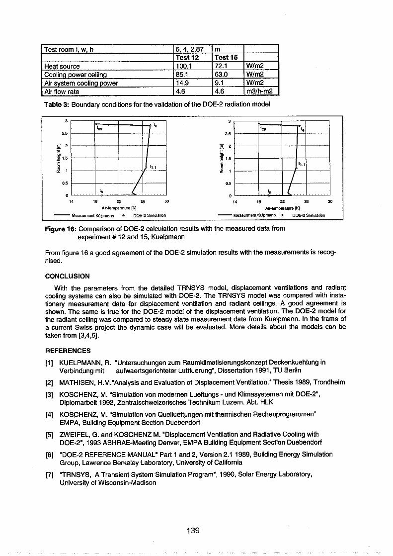
Table 3: Boundary conditions for the validation of the DOE-2 radiation model
Figure 16: Comparison of DOE-2 calculation results with the measured data from experiment # 12 and 15, Kuelpmann
From figure 16 a good agreement of the DOE-2 simulation results with the measurements is recog- nised.
CONCLUSION
With the parameters from the detailed TRNSYS model, displacement ventilations and radiant cooling systems can also be simulated with DOE-2. The TRNSYS model was compared with insta- tionary measurement data for displacement ventilation and radiant ceilings. A good agreement is shown. The same is true for the DOE-2 model of the displacement ventilation. The DOE-2 model for the radiant ceiling was compared to steady state measurement data from Kuelpmann. In the frame of a current Swiss project the dynamic case will be evaluated. More details about the models can be taken from [3,4,5].
REFERENCES
[ I ] KUELPMANN, R. "Untersuchungen zum Raumklimatisierungskonzept Deckenkuehlung in Verbindung mit aufwaertsgerichteter Luftfuerung", Dissertation 1991, TU Berlin
[2] MATHISEN, H.M."Analysis and Evaluation of Displacement Ventilation." Thesis 1989, Trondheim
[3] KOSCHENZ, M. "Simulation von modernen Lueftungs - und Klimasystemen mit DOE-2", Diplomarbeit 1992, Zentralschweizerisches Technikum Luzern. Abt. HLK
[4] KOSCHENZ, M. "Simulation von Quellueftungen mit thermischen Rechenprogrammen" EMPA, Building Equipment Section Duebendorf
[5] ZWEIFEL, G. and KOSCHENZ M. "Displacement Ventilation and Radiative Cooling with DOE-2", 1993 ASHRAE-Meeting Denver, EMPA Building Equipment Section Duebendorf
[6] "DOE-2 REFERENCE MANUAL" Part 1 and 2, Version 2.1 1989, Building Energy Simulation Group, Lawrence Berkeley Laboratory, University of California
[7] "TRNSYS, A Transient System Simulation Program", 1990, Solar Energy Laboratory, University of Wisconsin-Madison

Energy lm pact of Ventilation and Air Infiltration 14th AlVC Conference, Copenhagen, Denmark
21 -23 September 1993
Energy Implications of Domestic Ventilation Strategy
S L Palin: R Win~tanley,~ D A Mclntyre,** R E Edwards*"
* UMISTIEA Technology Post-Graduate Training Partnership ** EA Technology, Capenhurst, Chester CHI 6ES, UK *H UMIST, P 0 Box 88, Sackville Street, Manchester M6O IQD, UK
Synopsis
Mechanical ventilation with heat recovery (MVHR) and passive stack ventilation (PSV) systems are both proposed as methods of ensuring satisfactory ventilation rates in UK housing. MVHR provides controlled ventilation in all rooms together with heat recovery, while the cheaper PSV system offers lower running costs, but without heat recovery and without a controlled air supply to all rooms. The relative energy consumption of the two systems depends on a number of factors that are difficult to predict.
To provide a direct comparison, a test house at EA Technology was fitted with both MVHR and PSV systems. In a pilot study, the systems were operated alternately during the winter of 1993, with controlled internal air temperature and humidity. Both systems provided satisfactory humidity control; the use of humidity sensitive extract with PSV was found to be effective. Overall energy consumption of the PSV system was similar to MVHR.
1 Introduction
In older houses, especially in the UK, there has usually been adequate ventilation provision due to natural through leaks in the building envelope. However, in recent years there has been a trend towards more airtight buildings, due to improved building practices and concerns about energy efficiency. In such cases, it is necessary to introduce some form of purpose-provided ventilation system. However, it is important to ensure that a balance is achieved between energy efficiency and acceptable indoor air quality.
In some countries, such as Sweden and Canada, where the level of air-tightness in houses is very high in comparison to the UK, the law requires that mechanical ventilation with heat recovery (MVHR) be installed in new premises [1,2]. This ensures sufficient ventilation and also warms the incoming cold fresh air with heat from the exhaust stale air. In such countries, where the climate is severe, this system provides considerable energy savings.
Other countries make use of purpose-provided natural ventilation, an example of which is passive stack ventilation (PSV). This system consists of stacks, usually one each from the kitchen and bathroom to the roof, relying on the chimney principle and wind speed to extract the stale air. Passive stack systems have a low unit cost, and have been demonstrated to give satisfactory condensation control [3-51; however, the extraction rates are not controlled, and there is a risk that over ventilation may take place, thus resulting in the wasting of energy [6]. If current proposals are accepted, PSV will be specifically sanctioned within the Building Regulations, subject to restrictions on system design.
2 The Test House
The test house [7] is one of a row of six semi-detached three-bedroom houses (No. 16) near the EA Technology site at Capenhmt, on a flat, moderately exposed site. The house has suspended floors, a pitched roof and timber and plasterboard internal partitions. Double glazing has been installed and the exterior walls are well insulated to give a calculated design day heat loss of 4.2 kW. The gable and party walls are of brick and block construction, whilst the front and rear walls are timber framed with tile cladding.
Prior to the monitoring program the airtightness of the test house was measured using the fan pressurisation procedure described in [8]. Initially, the fan pressurisation technique was carried out before any sealing work was done. The result was approximately 13 air changes per hour (aclh): that
is not unusual for a British house of this type, but not good enough for the installation of a ventilation system. It was therefore necessary to seal leak paths prior to the installation of the ventilation systems. This gave a result of approximately 7 ac/h, which is acceptable.
However, several weeks later after the installation of the systems and the house being fully heated, the fan pressurisation test gave a result of over 9 ac/h. All detectable leaks were sealed but it was impossible to achieve the desired result, the final result being over 7 ac/h. This appears to be due to the fact that heating the house has dried it out considerably, increasing the infiltration. It was therefore necessary to measure airtightness at periodic intervals. The final fan pressurisation test, on 20 April 1993, gave a result of 8.55 ac/h.
3 Ventilation Equipment
3.1 PSV Description and Installation
Each stack comprises a ceiling extract connected to 150 mm diameter ducting to the loft where it was connected to flexible ducting that was connected via an adapter to a ridge terminal. Initially the extract terminals used were the standard circular type. These were used with the centre-piece removed. Also used were humidity sensitive terminals that are designed to give a high rate of ventilation when the humidity in the room is high then close down when humidity is low; also a constant volume flow terminal, which provides a flow of 30 m3/h when the pressure difference across the terminal is 50-150 Pa. Fresh air is brought into the house by a combination of natural and trickle ventilators that are fitted to all the windows except in the kitchen and bathroom.
3.2 MVHR Description and Installation
The MVHR unit was a commercially available unit with fans and heat exchanger mounted over a cooker hood. Stale air was extracted from the kitchen and bathroom and fresh air was supplied to the other rooms by 100 mm ducting. In a new house, ductwork is normally concealed in the ceiling space, with the diffusers flush to the ceiling. In the experimental house, the ducts and diffusers have been installed as close to the ceiling as possible.
The supply terminals used were the standard circular type. The cooker hood has three user- controlled levels of operation (level two was used) and also a pullout section that doubles the surface area whilst halving the resistance to flow caused by the filters, hence greatly increasing the extract rate in the kitchen. This section was kept closed during measurement in order to increase the extraction from the bathroom.
4 Experimental Procedure
The systems were operated alternately from February to April 1993, several variables being monitored using a programmable data logger. Individual room heater controls were each set to maintain 20°C over twenty-four hours. Reasonable uniformity was achieved but a tendency for upstairs rooms to overheat slightly was evident. Downstairs room temperatures settled within a band of 20°C+1.5"C while upstairs the range was 22"C+1.5"C. Water vapour was produced by humidifiers in the kitchen and bathroom in order to simulate occupancy and enable comparison of the systems in terms of moisture control. Therefore the humidity and air temperature in each room, and at three points in the stairwell were monitored. Other variables monitored include the wet and dry bulb temperatures outside the house (enabling the outside humidity to be calculated), wind velocity and the energy consumption of the eight heaters in the house. The insolation on a horizontal solarimeter was also measured by another logger. The velocity of air exhausted via the
stacks was measured using hot wire anemometers, which were calibrated against an orifice plate using [9].
5 Results
5.1 Ventilation Rates
Several tracer gas decay measurements were carried out. The kitchen and bathroom were tested simultaneously using different tracer gases and hence ventilation in both rooms can be compared under identical conditions. One result shown by tracer gas decay measurements was that, with PSV, air change rate in the bathroom was usually higher than in the kitchen. 'Values between 1 and 4 ac/h were recorded in the bathroom (equivalent to 10-38 m3/h) and 0.25 to 2.15 ac/h in the kitchen (equivalent to 4-32 m3/h). Figure 2 gives an example of some stack flows and their correlation with the weather conditions, where Ps is pressure difference due to the stack effect (proportional to the interior/exterior temperature difference) and Pw pressure difference due to wind (proportional to the square of wind speed); this is based on an expression derived in [lo]. The values used are within the range 3.8-15.8K temperature difference and 0.1-3.1 m/s wind speed. Measurements carried out with MVHR running on fan setting 2 gave results of 3.1 to 3.6 ac/h for the kitchen (45-53 m3/h) and 4.5 to 5.2 ac/h for the bathroom (42-49 m3/h), which is in good agreement with extract flows of 42 m3/h and 47 m3/h measured during commissioning.
5.2 Humidity Control
The performance of both systems (MVHR and PSV with circular terminals) was similar with regard to moisture extraction in the kitchen and bathroom, the only significant difference W i g that the MVHR gave a lower mean background humidity level in the moisture producing rooms (30% as opposed to 50% for PSV). Both systems allowed some spread of moisture to other moms; however this was not excessive. The humidity sensitive terminal also performed well, giving an enhanced rate of extraction at times of high moisture production coupled with a low background rate at other times. The constant volume flow terminal under-ventilated due to the low driving forces of PSV; it is therefore unsuitable for this application.
5.3 Energy Efficiency
Over a period when there is no change in the heat stored in the house, the energy input over that period must equal the energy loss: electric heating + solar heating + fan heating (from MVHR) = transmission and ventilation heat losses. The electric heating and fan heating were measured directly and solar gain estimated from the measured insolation using [ l l ] . Dividing each side by the mean internflexternal temperature difference gives an estimate of the heat loss coefficient in W/K, enabling comparison of the two systems independent of variations in temperature difference. Values of the left-hand side were plotted for a typical period of operation for each system, see figure 1 (PSV with circular terminals). This shows that the heat loss coefficients for the two systems are very similar. The ventilation heat loss for both systems was estimated from the discharge flow rate and the discharge air temperature; this does not include heat loss due to background infiltration. The heat recovery of the MVHR led to a lower discharge air temperature than for PSV. However this was compensated by the rather higher discharge flow rate, and led to a similar ventilation heat loss of around 35 W/K for both systems.
5.4 Back-flow in PSV system
Reverse flow in stacks has been known as a potential problem [12] therefore this possibility was monitored. It was found that this did not occur, however it is more likely where the dwelling is sheltered by tall buildings.
6 Discussion
Various problems were encountered in the work, the most significant being the level of airtightness of the test house, which, despite much draught-sealing, did not match up to the electricity industry's "Medallion 2MKY' specification [13], which requires a result of 7 aclh from the fan pressurisation test before installation of MVHR. The concept of "build tight - ventilate right" as advocated by the Building Research Establishment [14] is most important. Problems were also encountered with the operation of the MVHR with regard to heat recovery and the balance of supply and extract flows. These results show that MVHR has similar performance to PSV in this type of dwelling, although it is more suitable than PSV in other types of dwellings such as flats, dwellings that are sheltered by tall buildings, or where the outdoor air quality is poor. PSV, although dependent on weather conditions, is likely to provide adequate ventilation for this type of dwelling during the winter season and will not over-ventilate in a reasonably airtight UK house.
7 Conclusions
This is a pilot study that has shown that PSV is a viable alternative to MVHR in this type of dwelling in terms of energy efficiency. PSV with humidity sensitive extract offers increased potential for energy saving but should only be used where humidity is the main pollutant.
Further work is necessary, and will be carried out over the next heating season in a refurbished, more airtight test house, with the elimination of the problems mentioned above. In particular, the ventilation rates in individual rooms need to be considered.
References
[I] Nybyggnadsregler (Swedish Building Code), 1988. Swedish Board of Planning and Building, BFS 1988: 18, Karlskrona, Sweden.
[2] National Building Code of Canada 1985. Issued by the Associate Committee on the National Building Code, National Research Council of Canada, Ottawa.
[3] K. A. Johnson, A. I. Gaze, D. M. Brown. A Passive Ventilation System Under Trial in UK Homes. 6th AIC Conference "Ventilation Strategies and Measurement Techniques", Netherlands, 1985.
[4] Northern Consortium of Housing Authorities. Passive ventilation to dwellings with condensation. Durham, Chester-le-Street, NCHA, 1986.
[S] A. I. Gaze. Passive ventilation: a method of controllable natural ventilation of housing. TRADA Research Report 12/86, December 1986.
[6] D. J. Wilson, I. S. Walker. Passive Ventilation to Maintain Indoor Air Quality. Extended summary of departmental report no. 8 1, March 199 1, Alberta, Canada.
[7] J. B. Siviour. Construction, instrumentation and heat loss data of the ECRC experimental houses, Job No. 461. ECRClN839.1975.
[8] R. K Stephen. Determining the airtightness of buildings by the fan-pressurisation method: BRE recommended procedure. Building Research Establishment. 1988.
[9] BS 1042. Methods of measurement of fluid flow in closed conduits. Part 1. Pressure differential devices. Section 1.1. Orifice plates, nozzles and venturi tubes inserted in circular cross-section conduits d n g full. British Standards Institution, 1981.
[lo] R. Winstanley, S. L. Palin. Mechanical and Passive Stack Ventilation - A Comparative Experimental Study. EA Technology report R2930R, Job No. P5136. June 1993.
[ l l ] J. B. Siviour. Theoretical and experimental heat losses of a well-insulated house. ECRClN1537, Job No. 01 16. August 1982.
[12] W. F. de Gids, H. P. L. den Ouden. Three Investigations of the Behaviour of Ducts for Natural Ventilation, in which an examination is made of the influence of location and height of the outlet, of the built up nature of the surroundings and of the form of the outlet. Klirnaat Ventilatie Venvarming in Woninggen en Gebouwen, (in Dutch) 1974.
[13] Medallion 2000 Award Homes - Builders Guide. Electricity Council publication EC5 13814.89, 1989.
[14] E. Perera, L. Parkins. Build tight - ventilate right. Building Services, JU& 1992, pp. 37-38.

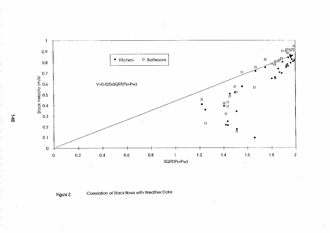
Energy Impact of Ventilation and Air Infiltration 14th AIVC Conference, Copenhagen, Denmark
21 -23 Septem ber 1993
Cooling Ceiling Systems and Displacement Flow
G Mertz
Fachinstitut Gebaude-Kilma e.V., Danziger Strasse 20 D-74321 Bietighelm-Bissingen, Germany
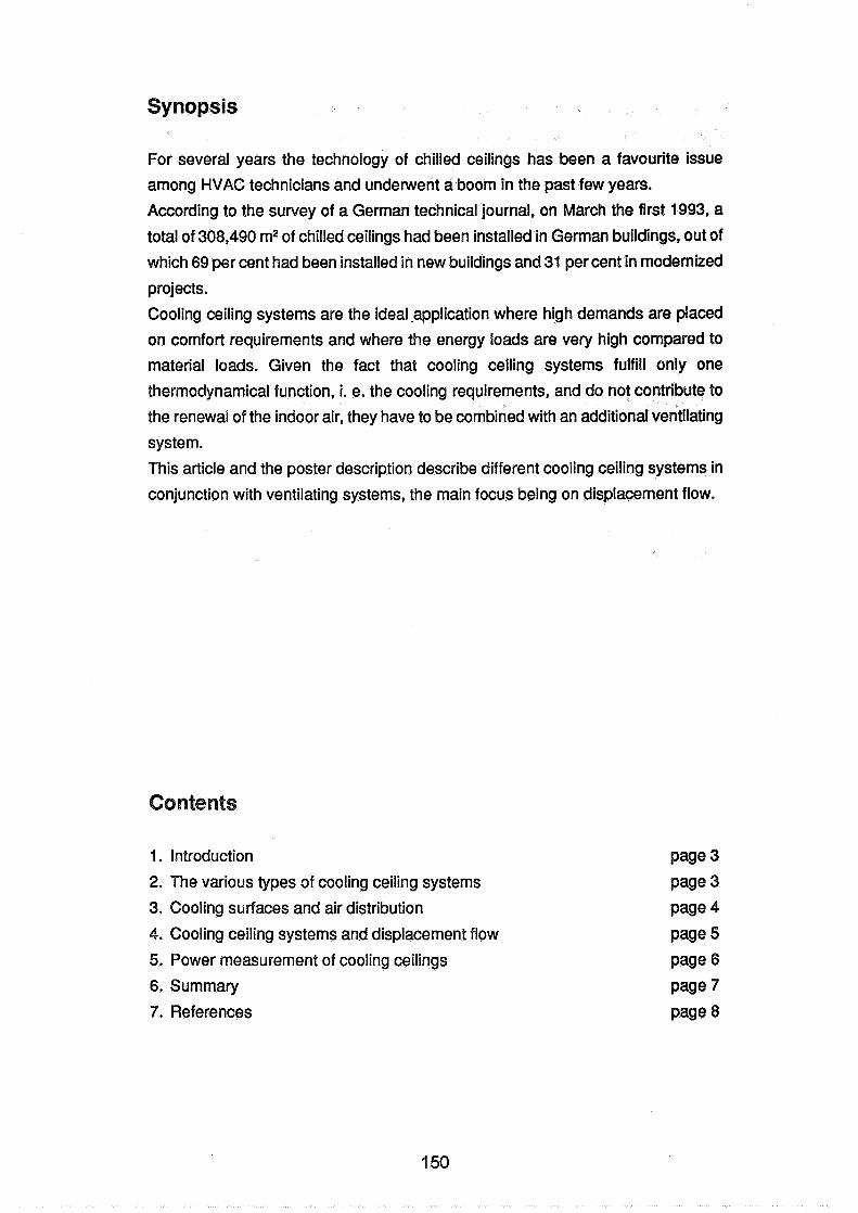
Synopsis
For several years the technology of chilled ceilings has been a favourite issue
among HVAC technicians and underwent a boom in the past few years.
According to the survey of a German technical journal, on March the first 1993, a
total of 308,490 m2 of chilled ceilings had been installed in German buildings, out of
which 69 per cent had been installed in new buildings and 31 per cent in modernized
projects.
Cooling ceiling systems are the ideal.application where high demands are placed
on comfort requirements and where the energy loads are very high compared to
material loads. Given the fact that cooling ceiling systems fulfill only one
thermodynamical function, i. e. the cooling requirements, and do not contribute to
the renewal of the indoor air, they have to be combined with an additional ventilating
system.
This article and the poster description describe different cooling ceiling systems in
conjunction with ventilating systems, the main focus being on displacement flow.
Contents
1. Introduction
2. The various types of cooling ceiling systems
3. Cooling surfaces and air distribution
4. Cooling ceiling systems and displacement flow
5. Power measurement of cooling ceilings
6. Summary
7. References

Introduction
The task of air-conditioning plants, for example in offices and administrative
buildings, in meeting and conference rooms, warehouses and concert halls, hotels
and restaurants, in hospitals and numerous other buildings, is to ensure comfortable
and healthy indoor air conditions as well as the rational use of energy. In order to
obtain pleasant indoor air conditions the cooling loads created in the room have to
be removed, in other words the room has to be cooled.
Rising room cooling loads on the one hand, e. g. through EDP equipment, and
increasing demands on comfort on the other hand have set air-conditioning
technology a difficult task. And this is precisely where cooling ceiling systems can
help in a number of cases.
The various types of cooling ceiling systems
In the meantime, a large number of different cooling ceiling systems has become
available on the market. Thanks to the large number of designs, cooling ceiling
systems are suitable both for new buildings and the modernisation of older buildings
(see also the results of the survey mentioned in the synopsis).
In principle, cooling ceiling systems can be divided into radiation ceilings and
convection ceilings. Radiation ceilings have a closed surface. The heat transfer
takes place primarily through radiation. They can be constructed as plastered
ceilings or also precast ceilings. Generally they require no more space than the
construction of a normal ceiling without cooling system (see figure 1).
Cooling ceiling systems
/ \ Radiation ceiling Convection ceiling
/ \ Plaster Installed Smooth Fins
/ \
= Bare ceiling = Cooling element
Figure 1 : Classification of types of cooling ceiling systems

Cooling surfaces and air distribution
Since cooling surfaces make no contribution to air renewal they should always be operated in conjunction with a ventilating or air-conditioning plant, which also ensures the necessary dehumidification. If appropriately combined the cooling
surface can relieve the air-conditioning system, i, e. the air flow rate is decoupled from the energy load. This leads to smaller air flow rates, which in the ideal case correspond with the supply air flow rate. The minimal outdoor air flow rate meets with an air flow rate of about 7 to 9 m3 (h x m2). This is only a small share of the air
I Turbulent mixing air flow Laminar air flow
Cooling ceiling / \
with ceiling twist outlet with floor twist outlet
with slot outlet with air supply through carpets
I with wall outlet with displacement outlet
Figure 2: Cooling ceiling systems and alr dlstrlbutlon systems
flow rate required to cover the room cooling load in the case of conventional air-
conditioning plants. In general, cooling ceiling systems can be combined with any
existing ventilating system (see figure 2).
Cooling ceiling systems and displacement flow
The air volume is supplied into the room by means of large-surface air outlets near
the floor. It enters the room at low air-velocities of about 0.2 to 0.3 mls and with a
temperature of about 1 to 1.5 K below the temperature of the room air. As a result
-caused by these conditions -the cooler supply air will uniformly spread over the
entire floor space where it forms a "lake of fresh air" and will then flow evenly
distributed over the entire room from that area to the ceiling. The flow velocities
then existing in the room are very low (below 0.1 rnls), unstable, and can only be
proved by smoke tests. A heat source in the Row just described - for example a
person or a heat-emissing office machine - will modify this flow pattern. Due to
thermal convection, produced by the temperature difference between the warm
surface of the heat source and the cooler supply air from the lake of fresh air, the
person or machine transports a continuous airflow towards the ceiling.
Using this system only the immediate surroundings of the heat sources are
supplied with fresh air - the ventilation effectiveness of the loading zone is also
excellent. On the other hand, draft annoyance still existing in many systems with
the conventional "mixing flow pattern" does not exist here. As each heat source in the room covers its own air demands from the lake of fresh air on the floor
(conditioned outside air), air quality and ventilation effectiveness as well are
significantly better than with a system of mixing ventilation. However, this flow
pattern largely excludes a horizontal flow. That means that there will be no
overflow of smoke or odourous substances from one area to another.
On the other hand, air velocities in the room -caused by this air flow pattern -are
mostly very low (below 0,1 rnls) and have also very low turbulences, which have an
important effect on draughts.
This displacement flow system is often limited, nevertheless, due to the temperature
stratification in the room and low temperatures at floor level. However, in conjunction
with chilled ceilings this typical disadvantage can be avoided, as the only task of
the supply air remains the renewal of the room air. The cooling is done by the
ceiling. As a result of the human capacity of compensating radiation, the slightly
lower temperature of the ceiling leads to a perceived temperature being 2 K lower
than the actual room temperature -even at higher indoor air temperatures such as
26 to 28 'C. This effect increases comfort and helps to save energy as well as to
reduce the size of the plant.
Power measurement of cooling ceilings
The standardized power control of cooling ceilings has always been an important
matter of concern of the "Heating and cooling surfaces" working group of the
Fachinstitut Gebilude-Klima e.V. (FGK) in which the leading German manufacturing
firms and suppliers of cooling ceiling systems are represented. The purpose of
uniform measurement techniques is to render the power indications comparable
so that performance variations within +/- 20 per cent, possibly distorting competition,
will become impossible.
At the end of 1992, the members of the FGK working group mentioned before
presented their "thermic measurement of cooling ceiling elements". The power
measurements are based on a so-called "box measurement" with a box of the
following dimensions: 2.40 m x 1.20 m x 1.50 m (lenght x width x height). The
advantages of this technique are obvious: it is neither time consuming nor too
expensive and comparison measurements by manufacturers have shown
furthermore that deviations between room and box measurements are about 3 per
cent, i. e. they do not exceed normal measuring inaccuracy. According to the FGK
guidelines for box measurements, the cooling ceiling elements are tested under
clearly defined boundary conditions and the results are recorded in a test certificate.
In view of the design and the relevant boundary conditions the testing box must
meet explicit requirements.
The guidelines contain inter alia sketches of the testing box indicating the
corresponding metering points. At least three series of measurements are required
and the flow temperature is to be fixed at 12, 14 and 16 'C with a maximum
deviation of +/- 0.5 K from the set value. The cooling performance as well as the
steady state characteristic of both the cooling ceiling and the room must be
indicated for evaluation and representation puposes. According to the FGK guide-
lines, both smooth and open (grid) cooling ceiling systems can be tested.
In the meantime, the German standard organisation (DIN) has outlined standards
for the performance measurement of cooling ceilings. The difference between the
applied measurement techniques is almost neglectable, the measurements being
performed in a room (4 m length x 4 m width x 3 m height) and not in a "box".
Summary
"The ventilation and air conditioning industry should carefully avoid calling the cold
ceiling - without concurrent ventilation - an acceptable air-conditioning system
and offer it to customers: it is nothing but an integral component of an aggregate
system, which -without controlled ventilation to eliminate humiditiy and odourous
substances - is doomed to failure".
This was the r6sum6 of the FGK symposium on cooling ceilings and room ventilation
in which 200 air-conditioning experts took part in September 1990 in Stuttgart,
Germany. The experts agreed that the cold ceiling is not the solution to all air
conditioning problems, but that - if correctly applied and operated - it is capable of
contributing greatly to an increase in thermal comfort in a room. With that, the
supply air volume can be reduced to the flow necessary to eliminate odourous
substances or humidity. Compared to conventional air-conditioning systems where
the cooling load must be eliminated only by convection, this means a reduction of
the supply air volume by approximately 60 to 80 per cent. On the one hand, this
leads to considerable savings in fan energy and to a reduction of the peak power
load. On the other hand, the low airflow velocities of displacement flow ventilation
prevent draughts. Summing up the figures for the two air-conditioning components,
one gets an overall capacity of about 100 W/m2. Normally, this capacity suffices to
ensure a removal of the load even in modern office rooms with high internal heat
sources. Should the internal thermal loads exceed 100 W/m2, the responsible
people will have to rethink the overall planning of the room andlor building. In those
cases either the architectural planning is wrong or someone forgot to provide the
windows with effective sun protection devices. Given the fact that this system
which in Germany has been installed for more than 300,000 m2 in office buildings
in the last two years, also has advantages as for the costs for installation and
operating compared to conventional systems in case of room loads of approximately
50 W/m2 onwards, it should only be a matter of time until this system prevails not
only in the West European countries but also internationally.

References:
Air Conditioning and Ventilation Engineering - Cooling Ceiling Systems. An information brochure, published by the Fachinstitut Gebiiude-Klima e.V., Bietigheim-Bissingen, Germany, 1992
DIN, Deutsches lnstitut fur Normung (NormenausschuB Heiz- und Raum- lufttechnik, NH RS) : Raumkuhlfliichen - Leistungsmessung bei freier Strii- mung, Normentwurf/Gelbdruck, Berlin 1993
Mertz, Gunther: Chilled Ceilings and Ventilation Systems - Thermal Comfort and Energy Saving, in: Air Infiltration Review, Vol. 13, No. 3. June 1992
Mertz, Gunther: Kuhldecke und Raumlijftung, in: ISH-Jahrbuch fur Gebiiu- detechnik, Gutersloh 1993, Bertelsrnann Verlag
Recknagel, Sprenger, Honmann: Taschenburg fur Heizung und Klimatech- nik, Munchen 1990, Oldenbourg Verlag
Stahl, Manfred; Keller, Gunther: "Cold Ceiling and System of Ventilation by Heat Sources - A New Development in Air Conditioning. Lecture notes, ASHRAE-Conference, 1992
Energy Impact of Ventilation and Air Infiltration
14th AlVC Conference, Copenhagen, Denmark 21 -23 September 1993
(Title) STACK EFFECT VENTILATION OF AN INFANT'S SCHOOL
(Author(s)) J.PALMER, P SHAW"
(Affiliation) "DATABUILD LTD, 4, VENTURE WAY, ASTON SCIENCE PARK
tCONSULTANT

SYNOPSIS
This paper presents the results of monitoring the ventilation in Netley Infants School in Hampshire. The study was carried out on behalf of the Department of Trade and Industry as part of the Energy Performance Assessment Project, as managed by the Energy Technology Support Unit.
The school was designed so that during the summer the solar heating of a south facing conservatory would enhance the stack effect and induce ventilation in the adjacent classrooms. It was expected that ventilation rates would be adequate to maintain comfort conditions and air quality.
The monitoring was carried out over a period of two months in 1991 and incorporated one- off measures of ventilation rates, short term tests of the ventilation strategy and long term monitoring of carbon dioxide to assess air quality. The measurements were carried out using an automated NDIR analyser sampling from points throughout the school, and a weather station erected in the school grounds.
The results show a general background infiltration rate of 0.4 ach with ventilation rates of about 1.5 ach when the building was operated as designed. The more normal operation, which involved opening the doors between the classrooms and conservatory, raised the ventilation rate to approximately 2 to 4 ach. This still fell short of the recommended fresh air rate of 30m3/person/h. Over periods of high ambient temperatures and solar radiation the external fire doors of the classrooms were opened to augment the vents: satisfactory ventilation was then achieved.
1, INTRODUCTION
Netley Abbey Infants School is a single storey building with a gross floor area of 1035m2 - including the conservatory. The primary aim of the design was to use as conservatory to provide solar heated air for the classrooms in the heating season. In doing this it was recognised that the solar gain in summer could be used to drive stack effect ventilation to the classrooms'. The client for the school was the Hampshire County Council, and the design was developed by the Martin Centre of Cambridge University2.
The school was studied as part of the Energy Performance Assessment Project of the Department of Trade and industry3. The solar ventilation pre-heating strategy was very successful and is reported elsewhere4. This paper reports on the detailed study of the air movement and ventilation.
The school is sited in Hampshire, England, on the edge of a residential area. Figure 1 shows the orientation and the floor plan.
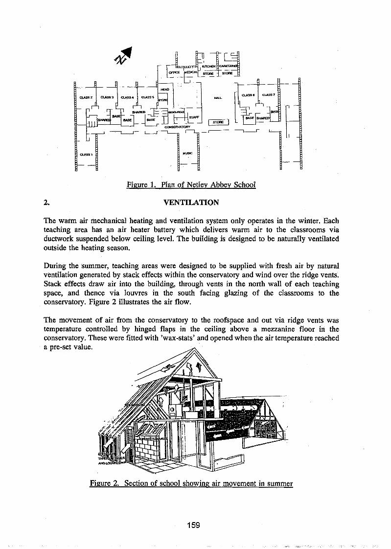
Figure 1. Plan of Netlev Abbey School
VENTILATION
The warm air mechanical heating and ventilation system only operates in the winter. Each teaching area has an air heater battery which delivers warm air to the classrooms via ductwork suspended below ceiling level. The building is designed to be naturally ventilated outside the heating season.
During the summer, teaching areas were designed to be supplied with fresh air by natural ventilation generated by stack effects within the conservatory and wind over the ridge vents. Stack effects draw air into the building, through vents in the north wall of each teaching space, and thence via louvres in the south facing glazing of the classrooms to the conservatory. Figure 2 illustrates the air flow.
The movement of air from the conservatory to the roofspace and out via ridge vents was temperature controlled by hinged flaps in the ceiling above a mezzanine floor in the conservatory. These were fitted with 'wax-stats' and opened when the air temperature reached a pre-set value.
Figure 2. Section of school showing air movement in summer

2.1 Monitoring Objective
The objective of this evaluation was to test the design intent of providing adequate natural ventilation to the classrooms as described above. This was done by undertaking short and long term tests. Classrooms 2,3,4 and 5 where taken as representative.
The short term tests were concerned with attempting to measure the ventilation rates in the classrooms undir known conditions. The tests were carried out by tracer gas tests using carbon dioxide introduced into the classrooms and recording its decay through time.
Long term tests were concerned with attempting to quantify ventilation rates under different weather conditions and looking at amenity issues such as air quality and overheating. For the long term tests it was decided to use occupant generated carbon dioxide as the tracer gas. There are disadvantages to this in that a detailed knowledge of occupancy and metabolic rates are needed for accurate computation of ventilation rates for occupied periods. Also there is a fairly high, and variable, background concentration which needs to be taken into account.
Other researchers have used this method for assessing ventilation rates, notably Penmans, and it had a number of practical advantages. It did not have to be introduced into the spaces, there would be no objections from the school, and the analyser and other equipment had been used previously for long term monitoring and had been found to be very reliable. The level of carbon dioxide also gives an indication of air quality. It was therefore considered that this method would provide reasonable estimates of the ventilation rates.
A weather station was set up adjacent to the school. This measured external temperature, horizontal global and diffuse solar radiation, wind speed and wind direction.
MEASUREMENTS AND FINDINGS
3.1 Short Term Tests
The short term tests were conducted on one day, over which period the external temperature varied between 19°C and 22"C, the measured wind speed varied between 1.3 m/s and 1.8 m/s and the wind direction varied between SSE and SW. The temperature of classrooms 2 & 3 varied from 23°C to 24"C, that of classrooms 4 & 5 varied between 24°C to 2S°C, the conservatory temperature ranged from 24°C to 26°C and the mezzanine level temperature was 36°C at the start of the tests (12.30pm) and had dropped to 25°C by the end of the tests (5.30pm).
Four tests were undertaken in each pair of classrooms. For each test the vents in the mezzanine ceiling were checked and found to be fully open. The test conditions were as follows:
3.1.1. Design conditions, i.e. the sliding shutters over the north gable grilles were open, in classrooms 4 and 5 the louvres to the conservatory were opened and the rooflight was opened in classrooms 2 and 3. Doors were closed.
3.1.2. All grilles, louvres, windows and doors closed to get an indication of the background leakage.

3.1.3. 'Normally used' conditions, i.e. as test one, but including the entrance door to each pair of classrooms open.
3.1.4. To simulate the reported operation during very hot weather. This was as in the previous test but with the fire door in the north gable also opened.
At the end of each decay test, smoke tests were carried out to assess the direction of air flow through the vents, louvres, windows and floors. This was done in conjunction with a hot wire anemometer to get an indication of the air speed.
Table 1 below gives the ventilation rates found from the decay tests. These are only really applicable to the weather and internal conditions occurring at the time of the test.
Table 1. CO, Decay Test Ventilation Rates
* Based on 30 children/classroom with volume of classrooms 2 and 3 being 339m3 and classrooms 4 and 5 being 303m3. To provide the recommended rate of 30m3/h/person6 approximately 6 ach are required.
As can be seen the ventilation rates for the design conditions were very similar in each pair of classrooms at about 1.5 to 1.6 ach. When these figures are related to fresh air supply per person they are equivalent to about 8m3/h/person.
Background leakage rates of each pair of classrooms were again similar with ventilation rates of just over 0.4 ach. This is a little higher than the background ventilation rate of 0.32 ach measured at Walmley Schools7.
The results for test 3, showed that for classrooms 2 and 3 the ventilation rate more than doubled to 3.2 ach when the classroom entrance door was opened. For classrooms 4 and 5 the effect was less dramatic with a small rise in ventilation rate to 2.2 ach. The fresh air supply rates were equivalent to 18m3/h and llm3/h respectively. Figure 2 below shows the air flows.

-
Figure 2. Air movement in Classrooms 2 and 3 - Test 3.
Ventilation rates in excess of 12 ach were found in both pairs of classrooms when the fire door was opened for test 4. This is equivalent to about 70 m3/h/person.
Throughout the tests the air flowed out of the classrooms through the vents on the north of the building and not through the conservatory ridge. Clearly the wind dominated the flow under the prevailing conditions.
3.2 Long Term Tests
The long term tests were extended over a period of 33 days, in June and July, of which 18 were occupied. The weather was normal with reasonable levels of solar radiation and external temperature, apart from two very warm days in early July. With the exception of those two days average classroom temperatures were below 25°C. The mezzanine temperature, as would be expected, is very sensitive to levels of solar radiation. Although there are a number of days where the average temperature difference between the mezzanine level and outside is about 10°C, with a ridge hieght of approximately 4 metres the pressure differences generated by the stack effect will be low.
The average carbon dioxide levels in the classrooms, conservatory, the mezzanine level and externally for occupied days between 8am and 4pm are shown in Figure 3.
Figure 3 indicates that some fairly high average concentrations of carbon dioxide were found in the classrooms, particularly during mid July. What is also noticeable about this figure is the fall in CO, levels at lunchtime. It was confirmed by the teachers that the children were normally out of the classrdoms between 12.30 and 1.30 pm. Therefore the ventilation rate for this period was computed using the standard decay equation for each of the occupied days for each pair of classrooms. The results for classrooms 4 and 5 are given in Figure 4.
Calculations using CIBSE A4*, with typical measurements, show that the areas available at low and high levels would provide approximately 4 ach. The measured areas for the air inlet grilles in the northern gable wall were about 0.5m2, which served two classroom areas: if this were to be increased to lm2 then the recommended rate is predicted.
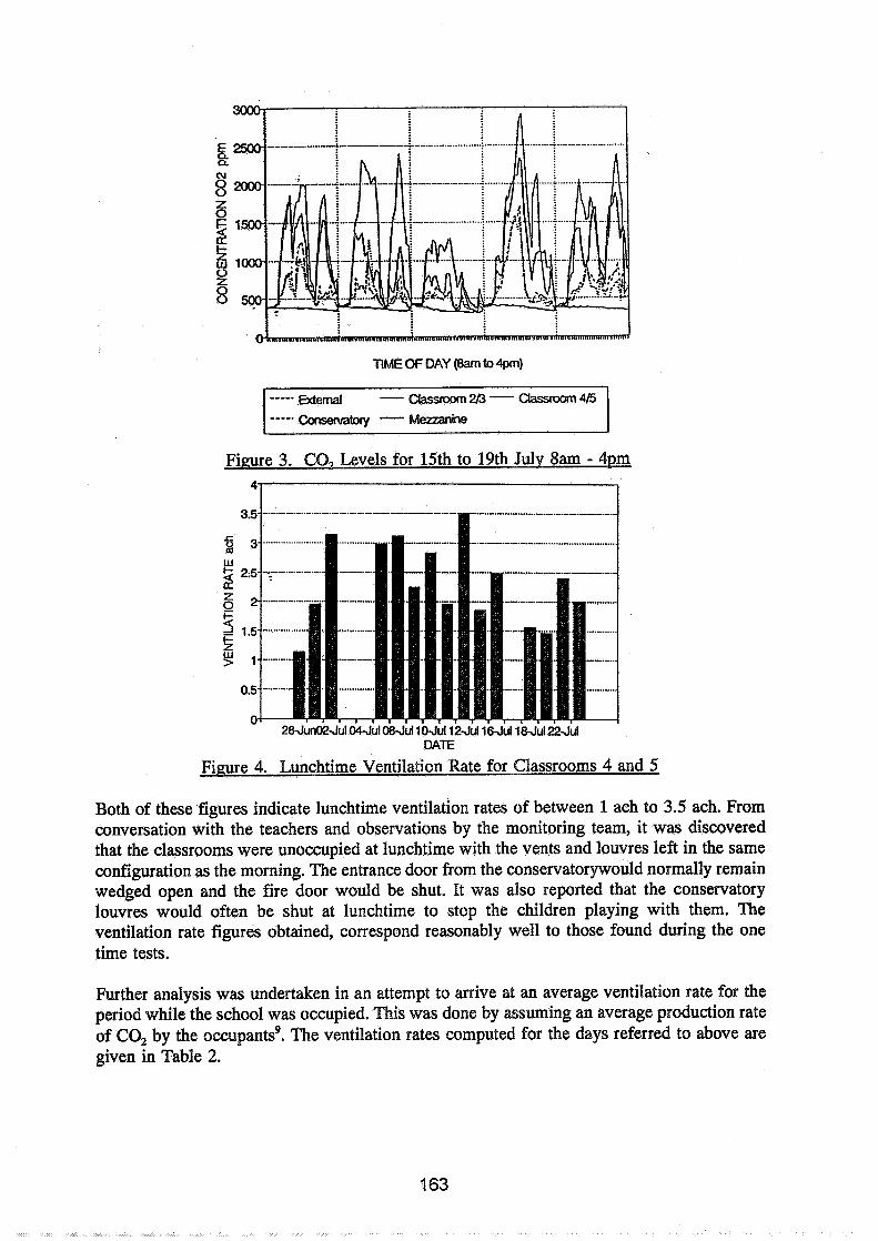
TIME OF DAY (8am to 4pm)
----- Conservatory - f V k 2 a - h I Figure 3. CO, Levels for 15th to 19th July 8am - 4pm
28Jun02Jul 04Jul08Jul1OJul12Ju116-Jul 18Ju122Jul DATE
Figure 4. Lunchtime Ventilation Rate for Classrooms 4 and 5
Both of these figures indicate lunchtime ventilation rates of between 1 ach to 3.5 ach. From conversation with the teachers and observations by the monitoring team, it was discovered that the classrooms were unoccupied at lunchtime with the vents and louvres left in the same configuration as the morning. The entrance door from the conservatorywould normally remain wedged open and the fire door would be shut. It was also reported that the conservatory louvres would often be shut at lunchtime to stop the children playing with them. The ventilation rate figures obtained, correspond reasonably well to those found during the one time tests.
Further analysis was undertaken in an attempt to arrive at an average ventilation rate for the period while the school was occupied. This was done by assuming an average production rate of CO, by the occupantsg. The ventilation rates computed for the days referred to above are given in Table 2.

Table 3.6. Average Ventilation Rates for 1st to 5th July
4. CONCLUSIONS
The short term tests indicated that, ventilation to the classrooms was dominated by wind effects, the design mechanism having little or no effect on air movement. As the test day was less than averagely windy it is to be assumed that the wind would normally be the dominant driving force for the ventilation.
The tests also indicated that under the designed operating conditions, ventilation rates were only one quarter of those recommended by Design Note 17. Under the normal operating conditions, in which doors from the classroom to the conservatory were propped open, ventilation rates were between 1 and 3 ach, still below the recommended rate. This indicates the limited opportunity for air to pass into the conservatory with the doors closed. The only way of achieving the recommended level was to open the emergency exit. door in the north gable wall.
The long term tests suggested that this strategy was used by the occupants, particularly on sunny afternoons, and that it proved effective in providing sufficient ventilation to keep internal temperatures close to ambient. However, it suggests that the ventilation openings in the north gable are insufficient.
Although the average temperature difference between the mezzanine level of the conservatory and ambient was frequently in the region of 10"C, the pressure difference due to the stack effect would be low due to the limited height and restricted free area available. It is likely that the wind effects would often dominate as found in the short term tests.
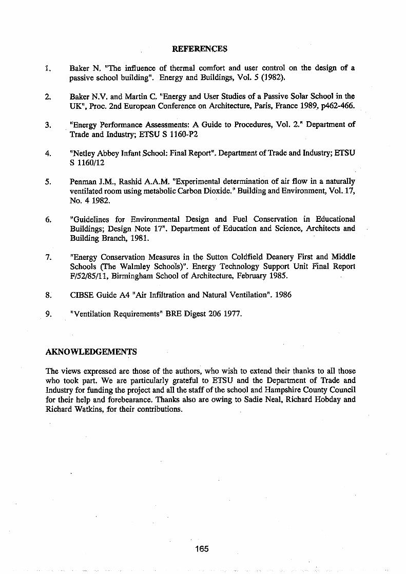
REFERENCES
1. Baker N. "The influence of thermal comfort and user control on the design of a passive school building". Energy and Buildings, Vol. 5 (1982).
2. Baker N.V. and Martin C. "Energy and User Studies of a Passive Solar School in the UK", Proc. 2nd European Conference on Architecture, Paris, France 1989, p462-466.
3. "Energy Performance Assessments: A Guide to Procedures, Vol. 2." Department of Trade and Industry; ETSU S 1160-P2
4. "Netley Abbey Infant School: Final Report". Department of Trade and Industry; ETSU S 1160112
5. Penman J.M., Rashid A.A.M. "Experimental determination of air flow in a naturally ventilated room using metabolic Carbon Dioxide." Building and Environment, Vol. 17, No. 4 1982.
6. "Guidelines for Environmental Design and Fuel Conservation in Educational Buildings; Design Note 17". Department of Education and Science, Architects and Building Branch, 198 1.
7. "Energy Conservation Measures in the Sutton Goldfield Deanery First and Middle Schools (The Walmley Schools)". Energy Technology Support Unit Final Report F/52/85/11, Birmingham School of Architecture, February 1985.
8. CIBSE Guide A4 "Air Infiltration and Natural Ventilation". 1986
9. "Ventilation Requirements" BRE Digest 206 1977.
0 WLEDGEMENTS
The views expressed are those of the authors, who wish to extend their thanks to all those who took part. We are particularly grateful to ETSU and the Department of Trade and Industry for funding the project and all the staff of the school and Hampshire County Council for their help and forebearance. Thanks also are owing to Sadie Neal, Richard Hobday and Richard Watkins, for their contributions.

Energy Impact of Ventilation and Air Infiltration 14th AlVC Conference, Copenhagen, Denmark
21 -23 September 1993
Benefits and Limits of Free Cooling in Non-Residential Buildings
A Bollinger, H W Roth
R & D Department for Air Conditioning Systems and Components, LTG Lufttechnische GmbH, Postfach 40 05 49,70405 Stuttgart (Zuffenhausen) Germany
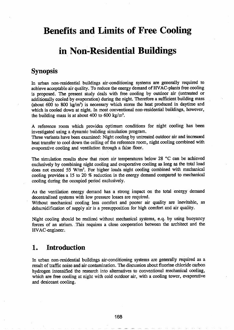
Benefits and Limits of Free Cooling
in Non-Residential Buildings
Synopsis
In urban non-residential buildings air-conditioning systems are generally required to achieve acceptable air quality. To reduce the energy demand of HVAC-plants free cooling is proposed. The present study deals with free cooling by outdoor air (untreated or additionally cooled by evaporation) during the night. Therefore a sufficient building mass (about 600 to 800 kg/m2) is necessary which stores the heat produced in daytime and which is cooled down at night. In most conventional non-residential buildings, however, the building mass is at about 400 to 600 kg/m2.
A reference room which provides optimum conditions for night cooling has been investigated using a dynamic building simulation program. Three variants have been examined: Night cooling by untreated outdoor air and increased heat transfer to cool down the ceiling of the reference room, night cooling combined with evaporative cooling and ventilation through a false floor.
The simulation results show that room air temperatures below 28 "C can be achieved exclusively by combining night cooling and evaporative cooling as long as the total load does not exceed 55 W/m2. For higher loads night cooling combined with mechanical cooling provides a 15 to 20 % reduction in the energy demand compared to mechanical cooling during the occupied period exclusively.
As the ventilation energy demand has a strong impact on the total energy demand decentralized systems with low pressure losses are required. Without mechanical cooling less comfort and poorer air quality are inevitable, as dehumidification of supply air is a presupposition for high comfort and air quality.
Night cooling should be realized without mechanical systems, e.q. by using buoyancy forces of an atrium. .This requires a close cooperation between the architect and the HVAC-engineer .
1 Introduction
In urban non-residential buildings air-conditioning systems are generally required as a result of traffic noise and air contamination. The discussion about fluorine chloride carbon hydrogen intensified the research into alternatives to conventional mechanical cooling, which are free cooling at night with cold outdoor air, with a cooling tower, evaporative and desiccant cooling.
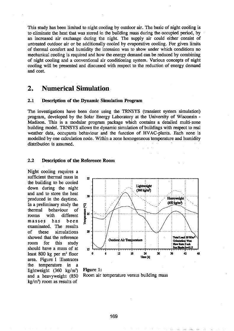
This study has been limited to night cooling by outdoor air. The basic of night cooling is to eliminate the heat that was stored in the building mass during the occupied period, by an increased air exchange during the night. The supply air could either consist of untreated outdoor air or be additionally cooled by evaporative cooling. For given limits of thermal comfort and humidity the intension was to show under which conditions no mechanical cooling is required and how the energy demand can be reduced by combining of night cooling and a conventional air conditioning system. Various concepts of night cooling will be presented and discussed with respect to the reduction of energy demand and cost.
2. Numerical Simulation
2.1 Description of the Dynamic Sinmulation Program
The investigations have been done using the TRNSYS (transient system simulation) program, developed by the Solar Energy Laboratory at the University of Wisconsin - Madison. This is a modular program package which contains a detailed multi-zone building model. TRNSYS allows the dynamic simulation of buildings with respect to real weather data, occupants behaviour and the function of HVAC-plants. Each zone is modelled by one calculation node. Within a zone homogeneous temperature and humidity distribution is assumed.
2.2 Description of the Reference Room
Night cooling requires a sufficient thermal mass in the building to be cooled down during the night and and to store the heat produced in the daytime. In a preliminary study the thermal behaviour of rooms with different masses has been exarninated. The results of these simulations
showed that the reference room for this study should have a mass of at IS least 800 kg per m2 floor o 6 12 18 2~ 30 36 42 48
area. Figure 1 illustrates -PI
the temperature in a lightweight (360 kg/m")~re 1: and a heavyweight (850 Room air temperature versus building mass kg/m2) room as results of

a simulated two-day period.
Another requirement for energy efficient buildings is an effective sun shade. In Figure 2 temperatures are plotted for the reference room without sun shade (b = 1.0) , with blinds partially closed (b = 0.35) and totally closed (b = 0.15).
With good sun shade the impact of beam radiation Figure 2:
Room air temperature versus sun shade and outside air conditions can be neglected if the building is well-insulated
and air-tight. Therefore the orientation of the reference room is of less importance.
Referring to these issues a reference room has been defined. The calculations have been performed for a room of the following dimensions: 4.5 m x 5.2 m = 23.4 m2 with a height of 2.7 m. The main structure is made of concrete. The external wall is insulated to a U-value of 0.5 W/m2 K, the windows have a U-value of 2.9 W/m2 K. Details are shown in Figure 3.
It is supposed that the test room is located in the west facade of the building and surrounded by identical rooms.
Figure 3: Geometry of the reference room

2.3 Boundary conditions
The simulation was carried out using hourly weather data (outdoor temperature, diffuse and beam radiation on a horizontal plane and humidity) from the Test Reference Year for FrankfurtIMain. For the analysis of the maximum room temperature a two-day period was used which has been repeated until stationary conditions have been achieved. The outdoor air temperature for this period is shown in Figure 1. The diurnal variation of the hot day's temperature corresponds to a design day according to VDI 2078 121.
The varying occupancy patterns have been considered by switching the internal load as shown in Figure 4 and by closing the sun shade 0, =O. 15) when the beam radiation on the window plane exceeds 250 W/m2. The maximum total load (external plus internal load) has been varied from 30 W/m2 to 60 W/m2. The air exchange rate was chosen depending upon the temperature difference between inside and - outdoor air. During the 3 occupied period (from g3,, 7.00 a.m. to 7.00 p.m.) l the ventilation rate was set to 3 ach if the room f air temperature was ,a higher than the outdoor temperature. Otherwise the ventilation rate was reduced to 1.5 ach. o 6 12 18 24 30 36 42 48
During the night an Time [h]
infiltration of 0.15 ach Figure 4:
was presumed. Night External, internal and total load during the two-day was activated lf simulation period (example)
the difference between inside and outside temperature was greater than 3 K. The ventilation rate for night cooling was varied in the simulation (3 or 6 ach).
To ensure thermal comfort the room air temperature should not exceed 27 "C. Without mechanical cooling 28 "C are supposed to be acceptable for 1 to 2 hours. For calculations based upon combined mechanical and night cooling, room temperature was allowed to vary from 22 "C to 27 "C during the occupied period. To compare the cooling energy demand a three-month period from June to August (Test Reference Year Frankfurt) has been used in simulation. In all calculations with air blown into the room by a fan, a rise in the supply air temperature of 1.5 K has been considered.

Variants of night cooling
The easiest way to realize night cooling is to open the window. The air flow rate @at could be achieved, depends on the area and the location of the open window as well as on wind velocity and direction. Therefore it is not possible to provide a defined air exchange. Furthermore, aspects of security and outdoor climate should be considered. Another disadvantage of ventilation through the window is that heat recovery is impossible in winter time. With respect to these reasons mechanical ventilation systems are presupposed in the present study. Mechanical ventilation systems should increase the storage effect of the building mass. This is to improve the heat transfer to walls, floor or ceiling. To realize higher heat transfer coefficients, outdoor air should be blown out against the wall or the ceiling. Another possibility is to blow the air through a false floor or ceiling. The latter is a very ambitious solution if the building makes use of the stack effect of a central atrium to draw the air through the storage mass.
The advantage of mechanical systems is the possibility of combining night cooling and evaporative cooling.
In the present study the following variants have been examined: 1. mechanical ventilation with increased heat tranfer by blowing out untreated
outdoor air against the storage mass (ceiling) 2. mechanical ventilation corresponding to I., combined with evaporative
cooling up to a maximum humidity of 11 glkg dry air. 3. mechanical ventilation through a false floor with untreated outdoor air.
At first, the variants described above have been tested in view of the maximum total load still allowing comfortable room air temperatures without mechanical cooling. Therefore the two-day sequence of weather data has been used.
For higher loads three-month simulations have been carried out combining mechanical and night cooling. To quantify the benefit of the different variants of night cooling a reference simulation has been conducted with mechanical cooling only. In this case the air flow rate was fixed to 3 ach. Internal load and sun shade control were modelled as described above.
The scale of evaluation are the cost for mechanical cooling (0.066 DMIkWh) and for ventilation (0.05 DM11000 m3). For ventilation a decentralized system with extremly low pressure losses is supposed to be installed. With conventional systems ventilation cost are about 0.15 DM11000 m3. Differences in capital cost, space requirement for the HVAC- plant and heating energy demand have not been taken into account. It should be noted that all energy data only refer to the three-month summer period.
3.1 Mechanical ventilation with increased heat transfer
The relation between total load, air exchange rate at night and maximum air temperature in the reference room without mechanical cooling is shown in Figure 5. With three air

exchanges per hour the temperature threshold (28 OC) is reached at a specific load of about 35 W/m2. An air exchange rate of six per hour permits a load of about 41 W/mZ. Highe r a i r exchange rates allow only slightly higher loads. Therefore it can be stated that in this case mechanical cooling is necessary if the total 20 30 40 50 60 m
specifie load exceeds 40 Total Specific Load [WW]
W/mZ. Figure 5: But the combination of Night cooling by increased heat transfer at the ceiling -
g 0o ' ng and relation between maximum room temperature, total specific mechanical cooling results load and air exchange in a reduction of the cooling energy demand as shown in Figure 6. For a total specific load of about 50 W/m2 the energy demand during the three-month summer period could be reduced by up to 18 %. For higher loads, however, the energy saving potential is negligable. Furthermore the difference between 3 and 6 ach is quite small. Therefore this variant of night cooling can only be recommended with three air exchanges per hour during the night.
Another aspect of night - cooling is illustrated in Figure 7. Night cooling ................................ reduces the required cooling capacity of the HVAC-plant. Even for high specific loads, where the reduction of energy .EI demand is low, the cooling capacity can be reduced significantly.
Total Specific h a d [W/mZ]
Figure 6: Reduction in energy demand (night cooling combined with mechanical cooling, no evaporative cooling) compared to the reference room with mechanical cooling only.
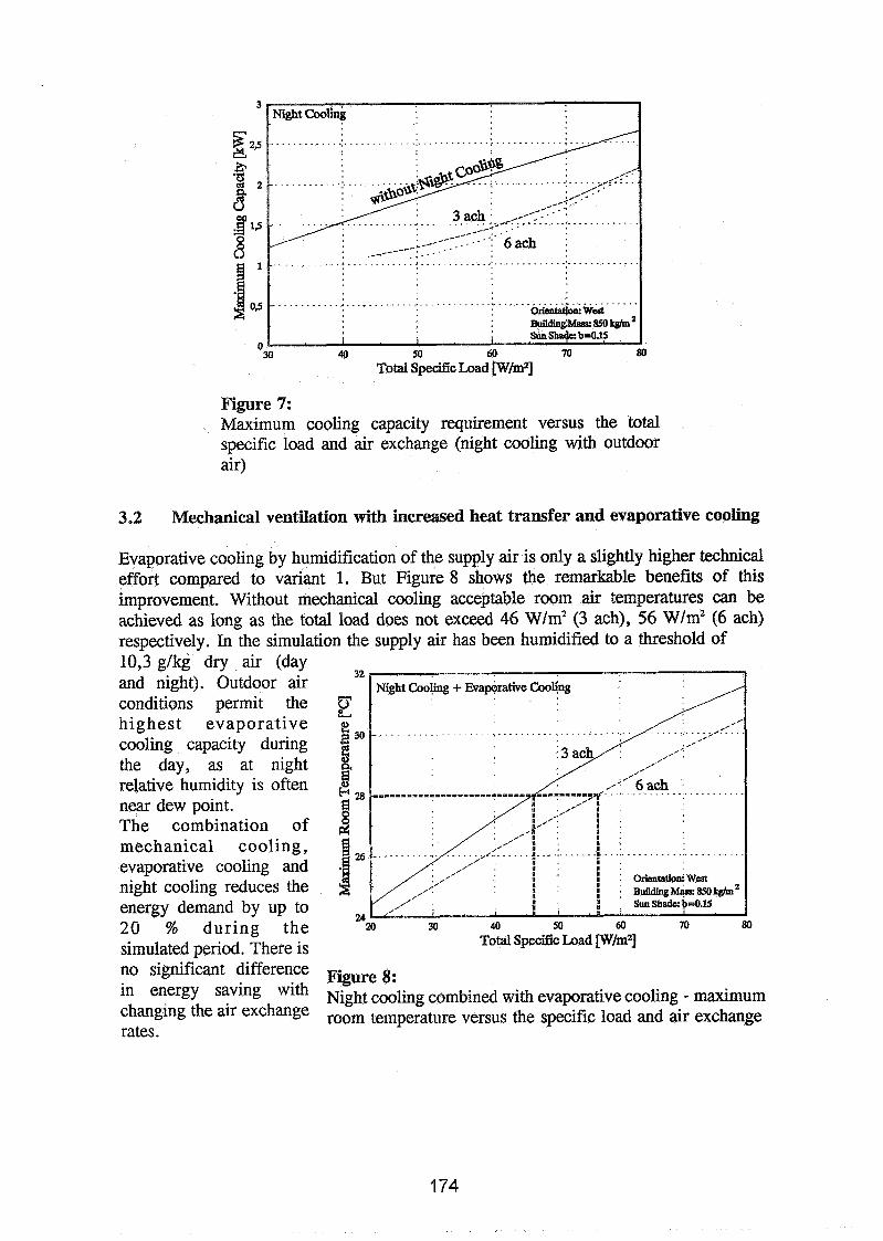
Figure 7: Maximum cooling capacity requirement versus the total specific load and air exchange (night cooling with outdoor air)
3.2 Mechanical ventilation with increased heat transfer and evaporative cooling
Evaporative cooling by humidification of the supply air is only a slightly higher technical effort compared to variant 1. But Figure 8 shows the remarkable benefits of this improvement. Without mechanical cooling acceptable room air temperatures can be achieved as long as the total load does not exceed 46 W/mZ (3 ach), 56 W/mz (6 ach) respectively. In the simulation the supply air has been humidified to a threshold of 10,3 glkg dry air (day and night). Outdoor air conditions permit the highest evaporat ive cooling capacity during the day, as at night relative humidity is often near dew point. The combination of mechanical cooling, evaporative cooling and night cooling reduces the energy demand by up to 20 % during the m 40 50 60 70 80
simulated period. There is Total S p d c Load [Wlmz]
no significant difference Figure S:
in energy saving with Night cooling combined with evaporative cooling - maximum changing the air exchange room temperature versus the specific load and air exchange rates.
3.3 Night cooling by mechanical ventilation through a false floor
The results in this case are similar to the first variant. The maximum room load is about 35 W/m2 with an air flow corresponding to 3 air exchanges per hour in the room, 42 W/m2 with 6 ach respectively. There are no significant differences in energy consumption, too. The advantage of this system however is that room ventilation and night cooling are seperate. Remarkable reductions in energy consumption can be achieved by using the stack effect of an atrium to draw the air through the false floor or if room ventilation during the occupied period is realized through the windows. As the windows are closed at night, this system does not cause security problems. But it should be noted that it might be difficult to close the false floor tightly against outdoor climate in winter to prevent heat loss at low outside temperature.
Conclusions
The variants of night ~ooling with outdoor air discussed above permit a 15 to 20 % reduction in the energy demand if they are combined with mechanical cooling. Without mechanical cooling acceptable room air temperatures can be achieved at total specific loads of up to 55 W/m2 if evaporative cooling is used additionally. With untreated outdoor air the room load should not exceed 40 W/m2. The basic requirement for night cooling is however, that there is a sufficient storage mass which can be cooled down during the night. Simulations have shown that the specific building mass should exceed 800 kg per m2 floor area. In practice this value can only be achieved with a reinforced concrete floor and heavyweight walls. These surfaces however must not be insulated for thermal or acoustic purposes.
As the ventilation energy demand has a strong impact on the total energy demand and the operation cost decentralized systems with low pressure losses are required. With conventional systems significant energy savings cannot be achieved.
Comfortable indoor air conditions are hard to realize without mechanical ventilation. During a longer heat period increased room temperatures might occur if the outdoor temperature does not cool down at night and the storage mass is completely loaded. Dehumidification of supply air is a presupposition for high comfort and air quality. Therefore night cooling cannot replace mechanical cooling, but can reduce energy cost and refrigeration capacity.
In most conventional non-residential buildings, however, the building mass is about 400 to 600 kg/m2. Floors are insulated by carpets and false ceilings are common installations. In this case the benefits of night cooling using the conventional HVAC-system is rather small.
Night cooling should be realized without mechanical systems, e.q. by using buoyancy forces of an atrium. This requires close cooperation between the architect and HVAC- engineer.
Acknowledgement
This paper is based on the thesis of mchael Fehrmann 111 which he prepared at LTG Lufttechnische GmbH, Stuttgart, in cooperation with the Pachhochschule Erfurt, Fachbereich Versorgungstechnik. The study has been attended by the authors (LTG) and Dipl. Ing. W. Fienhold (FH Erfurt).
References
/ 11 Michael Fehrmann "Grenzen und Einsatzbereiche der freien Kiihlung bei Biirogebauden" Diplomarbeit FH Erfurt, 1993
121 VDI 2078 (Entwurf November 1990) "Berechnung der Kiihllast klimatisierter Raume (VDI-Kiihllastregeln)", 1990
Energy Impact of Ventilation and Air Infiltration 14th AIVC Conference, Copenhagen, Denmark
21 -23 September 1993
Numerical Assessment of Room Air Distribution Strategies
H B Awbi
Department of Construction Management & Engineering, University of Reading, Whiteknights, Reading, UK

SYNOPSIS
The air distribution in a room is investigated using computational fluid dynamics. Four common methods of supplying air to a room are compared. The effect of air change rate on the ventilation effectiveness for contamination is small, however the effect of room heating or cooling load can be very significant. It was found that air turbulence has a major influence on the air movement, air velocity and dispersion of contaminants in the room.
1. INTRODUCTION
Numerous studies have been carried out during the last few years to determine what effect the method of supplying air to a room has on the air quality in the occupied zone. The traditional method of supplying the air at high level, representing mixing or dilution ventilation, is generally considered less effective in reducing the contaminant concentration in the occupied zone in comparison with a floor displacement system, eg Kim and Homma 2 . Nielsen (3) has also shown that mixing ventilation has a lower effectiveness than displacement ventilation because this method produces large contaminant concentration in the occupied zone. However, there are many other parameters that can influence the air movement in a room: such as the position and strength of the heat sources/sinks; the physical properties of air supply, eg temperature, velocity and turbulence; the position of the air extract, obstructions, etc. Because all these factors can influence room air movement, it is almost impossible to establish 'rules of thumb' in designing air distribution systems . In the investigation of the performance of different ventilation methods the emphasis has invariably been on the effectiveness of the system in removing contaminants, ie to maximise the ventilation effectiveness for contaminant removal, E,. However, there are other factors which must be included in evaluating the overall performance of the air distribution system such as the thermal comfort level and the effectiveness of heat removal, E,. Using computational fluid dynamics (CFD) for predicting the room air movement, Awbi et a1 ( 4 , 5 ) have shown that some methods of air distribution may produce a large value of E, but may have a low value of E, and vice versa. Whereas a high E, can mean a reduction in fresh air supply, thus saving energy, a low E, could cancel any energy saving accrued. An efficient air distribution system is one that is capable of producing the highest values of E, and E, under all operating conditions.
In this paper a CFD code called VORTEX has been applied to assess four methods of supplying air to a room containing a CO, source under isothermal and non-isothermal conditions. The effectiveness of each method is investigated for different air change rates.

2. METHOD
2.1 Ventilation Effectiveness
The overall effectiveness for contaminant removal (2,) and heat removal (zt) from the occupied zone represent the ability of the air distribution system to maintain average values of concentration and temperature in the occupied zone as a whole. These are defined as follows:
where cOz and to, are the occupied zone average of the contaminant concentration (ppm) and temperature respectively; c and t with subscripts i and e refer to the values at the inlet and exit positions respectively.
Similarly, a local effectiveness for contamination removal (E,) and heat removal (E,) can be defined to evaluate the performance of the air distribution system at specified positions in the room such as the breathing zone of an occupant. These are then defined as follows:
where c, and tp represent the concentration and temperature at the required point in the room.
2.2 CFD Code
The CFD code VORTEX (Ventilation Of Rooms with Turbulence and Energy exchange) has been used to simulate the air£ low, heat transfer and contaminant diffusion in a room. Although there are two and three dimensional versions of this code the two- dimensional program has been used in this study to enable better assessment be made of the large amount of data that is generated. The Navier-Stokes equation, the continuity equation, the thermal energy equation, the concentration of species equation and the two equations for the kinetic energy of turbulence (k) and its dissipation rate ( E ) are solved using a finite volume method and a structured cartesian grid. Further details of VORTEX are found in references (5) and ( 6 ) .

2.3 Numerical Test Room
Measurements in environmental chambers are often tedious, time consuming and the results can be influenced by scaling. A validated CFD code should be able to produce accurate prediction of the flow providing that a suitable grid is used with realistic boundary conditions. However, experience in this area has shown that there are certain limitations to the application of the k-& turbulence model in room air flow because this is an isotropic model which can predict fully turbulent flows more accurately than flows where there may be non-isotropy of turbulence. The latter occurs in a room where the flow may not be fully developed or where the flow experiences separation or reattachment such as the flow over obstructions. In the absence of these situations a CFD simulation should produce reliable results (6).
The numerical test room selected for this study is a two- dimensional box of length 6m and height 3m with a contaminant source producing 5 ~ 1 0 - ~ l/s of CO, (rate produced by a sedentary person) at a height of lm above the centre of the floor. Simulations where carried out for the cases shown in Fig 1 (a to d), ie a single air supply over the ceiling representing mixing ventilation, a single air supply over the floor representing floor displacement ventilation, four air supplies from the floor representing upward displacement ventilation, and four air supplies from the ceiling representing downward displacement ventilation.
Simulations have been carried out for isothermal flow, cooling and heating. In the cooling mode a heat gain of 60 W m-2 has been assumed over a curtain (east) wall and 20 W m-2 over the floor giving a total cooling load for the room of 300 W, ie 50 W per m2 of floor area. In the heating mode the heat loss from the curtain wall was -60 W m-2 giving a room heating. load of -180 W or -30 W per m2 of floor area. Four air change rates were used for the room, ie 2, 4, 6 and 8 h-I.
3. RESULTS DISCUSSION
A total of 24 simulations were carried out, 16 for isothermal conditions covering an air change rate from 2 to 8 h-I, 4 cooling simulations for an air change rate 8 h-l and 4 heating simulations for an air change rate of 8 h-I also. Other simulations have also been carried out which will be described later. The key input data and the main results are given in Table 1.
3.1 Effect of Air Change Rate
Figure 2 shows the effect of increasing'the air change rate on the average concentration of CO, in the occupied zone for the four methods of air supply which have been studied. These results are for isothermal flows. As would be expected there is a reduction in the concentration with increasing the flow rate but this reduction is lower at higher change rates than it is at
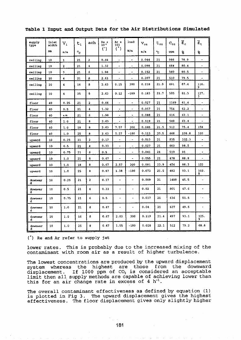
Table 1 Input and Output Data for the Air Distributions Simulated
( * ) Re and A r refer to supply jet
lower rates. This is probably due to the increased mixing of the contaminant with room air as a result of higher turbulence.
The lowest concentrations are produced by the upward displacement system whereas the highest are those from the downward displacement. If 1000 ppm of CO, is considered an acceptable limit then all supply methods are capable of achieving lower than this for an air change rate in excess of 4 h-l.
The overall contaminant effectiveness as defined by equation (1) is plotted in Fig 3. The upward displacement gives the highest effectiveness. The floor displacement gives only slightly higher
effectiveness than the downward displacement. This is because such a system is most effective in the presence of thermal loads in the room. There is only a small influence of air change rate on the effectiveness.
3.2 Effect of Room Load
Simulations have been carried for 8 air changes per hour to examine the effect of room load on the contamination effectiveness. The results of the overall effectiveness are shown in Fig 4. The same heating or cooling load is used in each air distribution method, however the ceiling supply and the upward displacement show only a small room load effect on E, . Velocity vector plots show that in the case of the ceiling supply the room air movement under cooling, heating and isothermal flows is similar and is primarily influenced by the air jet. This is also confirmed by the vertical distribution of the mean concentration in a horizontal plane which shown in Fig 5(a). A slightly higher value of E, is achieved in the cooling mode, Table 1.
In the case of upward ventilation vector plots show that the air movement in the cooling mode is largely influenced by an anti- clockwise circulation due to natural convection from the east wall causing a purge of the contaminant. An opposite circulation but a similar effect is produced in the heating mode, Fig 5(c). These profiles show large gradients in the lower part of the room for both cooling and heating but almost a uniform gradient for the isothermal flow. However, the overall contamination effectiveness for the three cases is almost the same. The value of E, for cooling is higher than that for heating, Table 1.
The overall contamination effectiveness for the downward displacement air supply is much higher for the cooling and heating modes than it is for isothermal flow, Fig 4. The isothermal flow shows almost uniform distribution of E, with marginally higher values in the upper part of the room as would be expected, see Fig 5 (d) . However, the heating mode produces a large stratification of the contaminant with much higher concentrations (low E,) in the lower part of the room and lower concentrations (high E,) in the upper part. This is caused by the buoyancy force counteracting the effect of supply jet momentum. The cooling mode produces similar effect but it is caused by the considerable air movement due to the convection from the heated east wall. Furthermore, the value of E, for cooling is almost double that for heating which makes the downward displacement method more effective for cooling than it is for heating.
The floor supply method produces a larger contamination effectiveness for the cooling mode than that for the isothermal flow because of the greater - mixing caused by convection from the east wall. However, E, is much higher for the heating mode than for the two other cases, Fig 4. This is a result of the supply jet separation from the floor just below the contamination source causing it to disperse throughout the room, hence more uniform
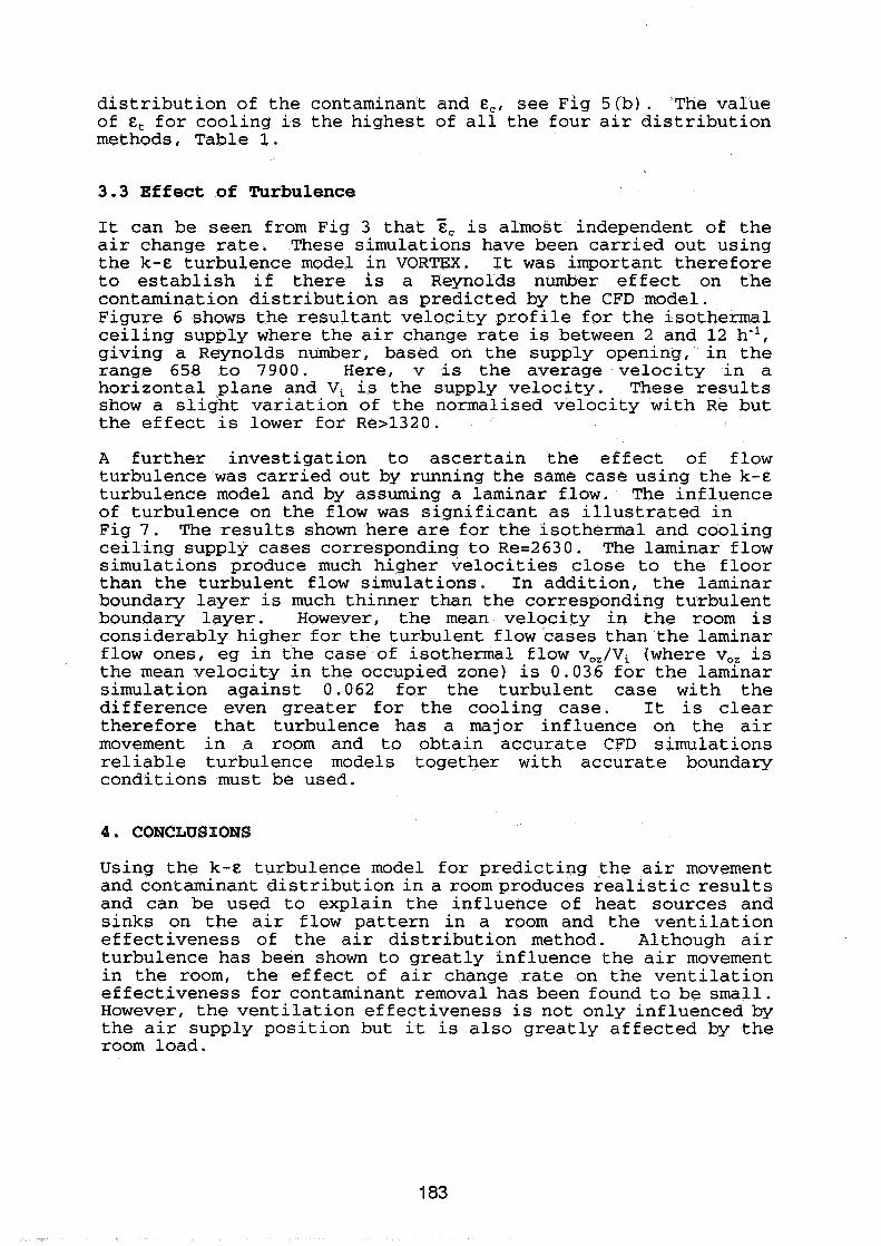
distribution of the contaminant and &,, see Fig 5 (b) . The value of E, for cooling is the highest of all the four air distribution methods, Table 1.
3.3 Effect of Turbulence
It can be seen from Fig 3 that z, is almost independent of the air change rate. These simulations have been carried out using the k-& turbulence model in VORTEX. It was important therefore to establish if there is a Reynolds number effect on the contamination distribution as predicted by the CFD model. Figure 6 shows the resultant velocity profile for the isothermal ceiling supply where the air change rate is between 2 and 12 h-l, giving a Reynolds number, based on the supply opening, in the range 658 to 7900. Here, v is the average velocity in a horizontal plane and Vi is the supply velocity. These results show a slight variation of the normalised velocity with Re but the effect is lower for Re>1320.
A further investigation to ascertain the effect of flow turbulence was carried out by running the same case using the k-& turbulence model and by assuming a laminar flow. The influence of turbulence on the flow was significant as illustrated in Fig 7. The results shown here are for the isothermal and cooling ceiling supply cases corresponding to Re=2630. The laminar flow simulations produce much higher velocities close to the floor than the turbulent flow simulations. In addition, the laminar boundary layer is much thinner than the corresponding turbulent boundary layer. However, the mean velocity in the room is considerably higher for the turbulent flow cases than the laminar flow ones, eg in the case of isothermal flow vo,/Vi (where v,, is the mean velocity in the occupied zone) is 0.036 for the laminar simulation against 0.062 for the turbulent case with the difference even greater for the cooling case. It is clear therefore that turbulence has a major influence on the air movement in a room and to obtain accurate CFD simulations reliable turbulence models together with accurate boundary conditions must be used.
4. CONCLUSIONS
Using the k-& turbulence model for predicting the air movement and contaminant distribution in a roomproduces realistic results and can be used to explain the influence of heat sources and sinks on the air flow pattern in a room and the ventilation effectiveness of the air distribution method. Although air turbulence has been shown to greatly influence the air movement in the room, the effect of air change rate on the ventilation effectiveness for contaminant removal has been found to be small. However, the ventilation effectiveness is not only influenced by the air supply position but it is also greatly affected by the room load.
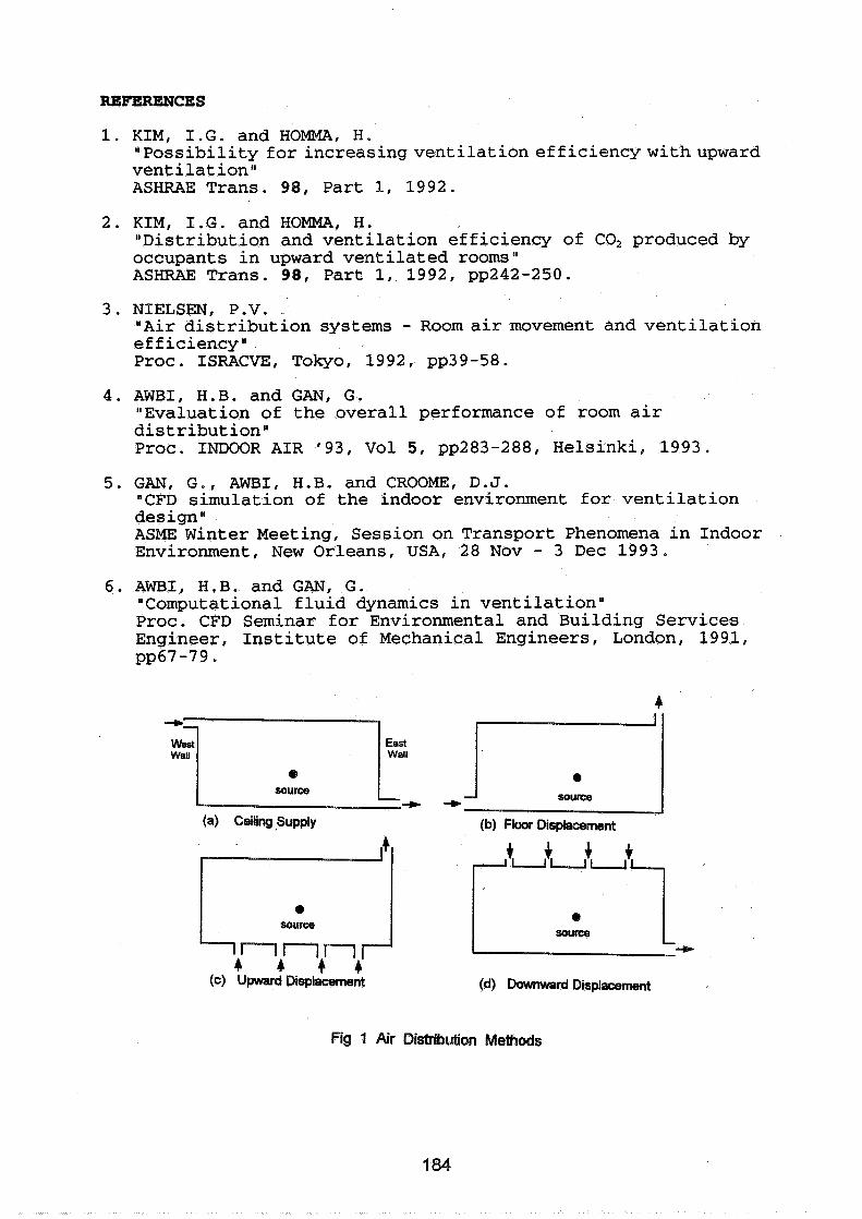
REFERENCES
1. KIM, I.G. and H O W , H. "Possibility for increasing ventilation efficiency with upward ventilationu ASHRAE Trans. 98, Part 1, 1992.
2. KIM, I.G. and H O W , H. "Distribution and ventilation efficiency of CO, produced by occupants in upward ventilated rooms" ASHRAE Trans. 98, Part 1, 1992, pp242-250.
3. NIELSEN, P.V. "Air distribution systems - Room air movement and ventilation efficiency" Proc. ISRACVE, Tokyo, 1992, pp39-58.
4. AWBI, H.B. and GAN, G. "Evaluation of the overall performance of room air distribution" Proc. INDOOR AIR '93, Vol 5 , pp283-288, Helsinki, 1993.
5. GAN, G., AWBI, H.B. and CROOME, D.J. "CFD simulation of the indoor environment for ventilation design" ASME Winter Meeting, Session on Transport Phenomena in Indoor Environment, New Orleans, USA, 28 Nov - 3 Dec 1993.
6. AWBI, H.B. and GAN, G. "Computational fluid dynamics in ventilation" Proc. CFD Seminar for Environmental and Building Services Engineer, Institute of Mechanical Engineers, London, 1991, pp67-79.
4
(a) Ceiling ,Supply (b) Floor Displacement
rl hnnn 4 4 4 4
(c) Upward Displacement (d) Downward Displacement
Fig 1 Air Distribution Methods

- downward dis.
Air Change Rate (llh)
Fig 2 CO2 Concentration in Occupied Zone with Air Change Rate
0 1 2 3 4 5 6 7 8 9 1 0
Air Change Rate (llh)
Fig 3 Overall Concentration Effectiveness with Air Change Rate
- downward dis. -i-- upward dis. --4--- over floor
-
- r I J I j . ! 0
-40-30-20-10 0 10 20 30 40 50 60 Load (Wlm "2 )
Fig 4 Overall Concentration Effectiveness with Room Load
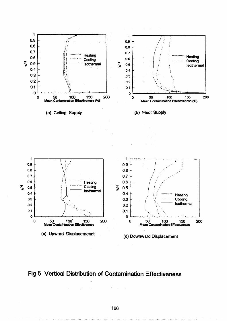
0.3 0.3
0.2 0.2
0.1 0.1
0 0 0 50 100 150 200 0 50 100 150 2W
Mean Contamination Effectiveness (%) Mean Contamination Effectiveness (%)
(a) Ceiling Supply (b) Floor Supply
0 50 100' 150 200 0 50 100 150 200 Mean Contamination ERectiveness Mean Contamination Effectiveness
(6) Upward Displacemennt (d) Downward Displacement
Fig 5 Vertical Distribution of Contamination Effectiveness

0 0 0.05 0.1 0.15 0.2 0.25
Mean Velocity Ratio (vNi)
Fig 6 Effect of Reynolds Number on the Mean Velocity Distribution (Ceiling Supply)
- - - - - - -. - -
Turb. Isothermal
0 0.05 0.1 0.15 0.2 0.25 Mean Velocity Ratio (vNi)
Fig 7 Mean Velocity Distribution for Laminar and Turbulent Flows (Ceiling Supply)


Session 3: Papers - Ventilation and Indoor Air Quality

Energy Impact of Ventilation and Air Infiltration 14th AlVC Conference, Copenhagen, Denmark
21 -23 September 1993
Moisture Admittance Model: Measurements in a Furnished Dwelling
L Serive-Mattei," R Jones," M Kolokotroni,* J Littler*
* Research in Building Group, University of Westminster, 35 Marylebone Road, London NW15LS, UK ** Building Research Establishment, Bucknalls Lane, Garston, Watford WD2 7JR, UK
1 SYNOPSIS The BRE method of predicting water vapour conditions in houses is based on two generalised moisture admittance parameters a and p. Previous laboratory experiments suggested that it is possible to determine these coefficients for an unfurnished room with wooden panels, using measurement periods of six hours under dynamic equilibrium conditions. The present study explores the possibility of using such conditions to determine a and P in-situ for the living-room and bedroom of a furnished flat of conventional construction. Dynamic equilibrium conditions were measured and used to calculate the moisture coefficients of both rooms. These were included in a simulation program based on the moisture admittance model developed by BRE, and compared with measurements for different scenarios: constant heat input, constant humidity input, both constant heat and humidity input.
Results show that a and P can be measured in real situations with an accuracy as good as in the laboratory, despite the widely differing materials involved in the process of absorption- /desorption. The mean deviation between measurements and predictions for the admittance model is about 30% lower than for the Loudon model. In addition some guidelines concerning the experiments in-situ are derived from the mathematical theory.
2 LIST OF SYMBOLS v(in)=vapour content of the inside air, kg/kg v(out)=vapour content of the outside air, kg/kg v(svp)=vapour content of the air at saturation vapour pressure, kg/kg G = rate of moisture in ut k p=density of air, kg/m 8 ghr
v=volume of the rooms m3 n=ventilation rate, air changes per hour a=absorption coefficient P=desorption coefficient
3 INTRODUCTION BS5250 [I] and IEA Annex 14 [2] include simplified equations for the calculation of the internal moisture load, taking into account ventilation rates, moisture production rate and vapour pressure difference between indoors and outdoors. The IEA Annex 14 equation also includes the effect of temperature variations. In conformity with the Loudon model, neither equation accounts for any adsorption by the internal surfaces. However, absorption during periods of water vapour production would reduce the moisture load, while desorption at later times would increase the internal air humidity. Therefore, the predictions of the Loudon model would differ from reality both during and after the period of water production.
Many models have been developed which include absorption and condensation in the calculations. An overview of available models until 1988 mainly in Europe can be found in ref [3] and a calculation method is decribed in [4]. Many models have been also proposed from researchers in Canada and the US [5-81. However, most of the models require the input of hygric properties of materials which are not readily available, especially in combinations usually found in the interior of the buildings. There are experimental results on the hygroscopic capacity of walls, floors, ceiling and furnishing [9-111 and published catalogues [12], but the data are not specific enough for the requirements of most moisture models.
An empirical equation has been developed by BRE [13] which takes into account absorption and desorption of internal surfaces. The equation uses two coefficients a and P to determine the overall rate of absorption and desorption in a room with some general characteristics. Work in a laboratory cell has produced a set of coefficients and a method of determining them for buildings, [13].

This project was initiated with the aim of measuring the coefficients a and P in an unoccupied furnished dwelling as a first step between laboratory and occupied building experiments. The study was intended to show whether the experimental procedure of dynamic equilibrium conditions, described by R. Jones [13], works in a typical furnished house, and whether it can be used to establish coefficients for a range of situations.
4 THE TEST HOUSE The ground floor flat of a converted early century house in south London was selected as the test house for the following reasons:
- stable conditions need to be maintained for a relatively long time in the rooms of the home - thick masonry walls have a larger hygric inertia in absorbingldesorbing moisture.
The flat consists of a living room, bedroom, dining area, kjtchen and WC in an almost linear arrangement with a total floor area of approximately 55m . The construction of the external walls is brick, plastered on the inside, without any insulation, with a total thickness of 0.22m. The sash timber framed windows are single glazed. Heating is provided with a gas fired boiler and conventional radiators in every room. Ventilation is through operable windows and background infiltration. Measurements were taken in the middle of the living room and bedroom. In addition the external conditions were measured. Table 1 summarizes the various characteristics of the two rooms.
Table I : Characteristics o f the test house
5 THE MEASUREMENTS
5.1 Conditioning period A two weeks conditioning period was set up for both the living-room and the bedroom. During the first week, conditions were maintained as follows (all doors closed):
- living-room: constant temperature of about 17°C from 9am to 6pm, and - bedroom: constant humidity of about 80%.
The conditions were changed during the second week as follows:
- bedroom: constant temperature of about 17°C from 9am to 6pm, and - living-room: constant humidity of about 80%.

In addition to the two weeks of conditioning, moisture and heat inputs were performed in both rooms in order to collect data on their humidity performance under various scenarios. These monitored periods are discussed further in section 7. Tracer gas tests were also carried out to measure the air change rate during each dynamic equilibrium experiment.
5.2 Dynamic equilibrium
Throughout the project, a total of twenty four dynamic equilibrium experiments have been performed (twelve in each room) in order to calculate the coefficients a and P using the following equation from [I 33 :
dy(in)/dt = Glpv - n(v(in) - out)) - av(in) + Pv(svp) (1) These experiments consisted of periods of 4 to 6 hours during which stable conditions of vapour pressure were achieved inside, using fan heaters, and outside weather permitting. Most of them were carried out around mid-day as the outside humidity conditions proved to be more stable at that time. Experiments were generally taking place in both rooms at the same time to optimize the site utilisation.
6 RESULTS AND ANALYSIS
6.1 Presentation of the results Which conditions are suitable for coupling with the others would depend on the coefficients of the dynamic equilibrium equation. Two equations are needed to solve for a and P as follows:
v(in>la - v(svp),P = -(n(v(in) - v(out))), and (2) v(in),a - v(svp),P = -(n(v(in) - v(out))), (3) We can solve for a and p provided that the determinant of the system is not zero, which implies:
Therefore one experiment would be suitable for coupling with another if the ratio of internal vapour pressure to internal saturation vapour pressure is different from another experiment. One way of achieving that is to heat the room to high temperatures.
On the other hand, the rooms could not be heated to very high temperatures because this would increase condensation risks on the windows because of desorbed moisture. For this reason, a compromise had to be reached between desirable and practical experimental conditions.
6.2 The coefficients selected Following the previous remarks, it was decided to divide the experiments into three groups. Group 1: experiments with a high vapour pressure ratio (about 0.65-0.70), Group 2: experiments with a medium ratio (0.50-0.60), and Group 3: experiments with a low ratio (about 0.40). Each experiment of one gioup can be coupled with any experiment of another group to produce a set of coefficients.
One set of coefficients was calculated for each coupling of two groups by averaging the coefficients obtained by cross calculation for these two groups: groups 1&2, groups 1&3, groups 2&3. Finally, an average value was calculated from the three averages. The values obtained are presented in Table 2.
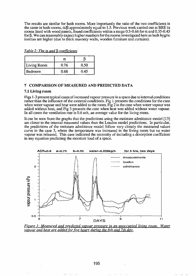
The results are similar for both rooms. More importantly the ratio of the two coefficients is the same in both rooms, a lp approximately equal to 1.5. Previous work carried out at BRE in rooms lined with wood panels, found coefficients within a range 0.5-0.66 for a and 0.35-0.45 for p. We can reasonably expect higher numbers for the rooms investigated here as both hygric inertias are higher (due to thick masonry walls, wooden furniture and curtains).
Table 2: The a and P coemcients
7 COMPARISON OF MEASURED AND PREDICTED DATA 7.1 Living room Figs 1-3 present typical cases of increased vapour pressure in a space due to internal conditions rather than the influence of the external conditions. Fig 1 presents the conditions for the case when water vapour and heat were added to the room. Fig 2 is the case when water vapour was added without heat, and Fig 3 presents the case when heat was added without water vapour. In all cases the ventilation rate is 0.6 ach, an average value for the living room.
It can be seen from the graphs that the predictions using the moisture admittance model [13] are closer to the internal measured values than the Loudon model predictions. In particular, the predictions of the moisture admittance model follow very closely the measured values curve in the case 3, where the temperature was increased in the living room but no water vapour was released. This case indicated the necessity of including a desorption coefficient in any equation predicting the moisture load of a space.
ACR=0.6 a=0.75 bz0.50 water=0.258kg/h for 5 hrs, two days
2 - - - - - - admittance
m 2z a, L 3 V ) V )
2 Q L
1 a- m >
0.5 5 7
DAYS 9
Fiaure 1: Measured and predicted vapour pressure in an unoccupied Eivina room. Water vapour and heat are added for five hours during the 6th and 7th dav.

0.3 1 I I I I I I I I I
0 1 2 3 4 5 DAYS
ACH=0.6 a=0.75 bz0.50 water=0.117kg/h Shrs day 2, 21 hrs day 3
Fiaure 2: Measured and predicted vapour pressure in an unoccupied livina room. Water vapour is added for 5 hours durin~ the 2nd dav and 21 hours during the 3rd dav,
1
0.9 -
0.8 - m a Y 0.7 - ?? ZJ V)
cn 0.6 - g L
a 0.5 - 8- >
0.4 -
ACH=O.6 a=0.75 bz0.50 no water vapour input 1.3
measurements
--- loudon
- - - - - admittance
0.5 ! I I I I I I I I I I I I I I
12 13 14 15 DAYS
Figure 3: Measured and predicted vapour vressure in an unoccupied living room. Heat is pdded for 10 hours durinn the 12th. 13th and 14th davs,
A further statistical analysis was carried out to compare the predictions of both the Loudon model and the moisture admittance model to the measured values. This analysis used the same data as those used for cases 1 to 3, in order to treat different situations. In table 3, the mean deviation represents the average absolute difference between either Loudon or admittance predictions and measured values. This gives a figure representative of both overlunder esti- mations of the measurements. The percentage of error is the ratio of this mean deviation to the average of measured values.

Table 3: Mean deviation and percentage o f error ofpredicted values compared to measure- ments for the livinn-room
Table 3 highlights the accuracy gained by the use of the admittance model for which the percentage of error is between half and two third of the one achieved with Loudon model. But it should be noted that the statistical analysis was carried out on all the data used for the various figures and not only on the specific periods of production of water vapour or heat. Figures 1 to 3 suggest that the difference of accuracy is much higher for these particular periods.
7.2 Bedroom Similar results were obtained for the case of the bedroom and are presented in Figure 4.
ACH=0.6 a=0.68 b=0.45 waterx0.33kgIh for 8hrs day 1 , 0.26kglh 5hrs day 2 I I
I I I I I I 1 I I I 1 I I I I I I
34.4 35 DAYS 35.8
- - -
Figure 4: Measured and predicted vavourpressure in an unoccupied bedroom. Water vavour pnd heat added for eight hours in the-first dav and five hours during the second day,
,/--I
// I \
measurements
The difference between the admittance model predictions and measured values is bigger in the bedroom than in the living room. This is mainly due to condensation occurring more frequently in the bedroom because of the smaller volume and the colder weather during monitoring. It is observed that the moisture admittance model predictions become flat at a certain point in Fig 4. This is the saturation vapour pressure point for the internal conditions. Therefore, the moisture admittance model predicts realistic values unlike the Loudon model. It is suggested that the remaining difference from the measured values is due to condensation on the cold window surfaces.
I I I
loudon - I I
I I - - - - - - admittance
As expected, the mean deviations are higher for the bedroom than for the living-room. The reason, as explained, might be the condensation which occured on the window. But the per- centage of error for the admittance model is still between half and two thirds of the Loudon one. A similar ratio was found for the percentage of error betwen the two models for the living-room, which might suggest that the admittance model reduces the inaccuracy of the Loudon model by 30 to 50%.
Table 4: Mean deviation and Dercentaae o f error of predicted values com~ared to measure- ments for the bedroom
8 CONCLUSIONS AND SUGGESTIONS FOR FURTHER WORK This study showed that it is possible to determine the coefficients for the moisture admittance model by performing equilibrium condition experiments in unoccupied rooms. The experi- ments suggested that for thecases of masonry construction with soft furnishing, the coefficients are similar to the wood lined test cell.
The mathematical theory to solve the dynamic equilibrium equations and the accuracy of the equipment, impose different ratios forv(in)/W(svp). This can generally be achieved by heating the room to higher temperatures during one experiment. However, too much heating could increase the risks of condensation on windows and cold bridges and ruin the results as con- densation is not taken into account by the moisture admittance model from which a and P are derived.
Therefore it is recommended that one experiment be carried out with no heating at all, and one with as much heating as possible provided that there is no condensation in the room. This should provide a satisfactorily large difference between the two ratios. Our results suggest that a difference of 0.1 is enough to achieve a relatively good accuracy. Outside conditions were also very important in establishing the dynamic equilibriums. Most of the experiments were conducted around mid-day as outside conditions proved to be more stable at that time. This should be taken into consideration for further work.
The moisture admittance model, being an empirical equation, relies on the availability of a range of coefficients which can be used for various building constructions, operation, heating regimes and moisture production. Monitored data gathered in the unoccupied furnished test dwelling of the present study have shown that the model can be successful in predicting the internal moisture conditions. The results obtained were in all cases a significant improvement on the "Loudon" prediction method. However in some cases the predicted values of vapour pressure were not as close to the measured values as had been hoped for. For this model to be useful as a prediction tool better agreement is required. As an alternative to deriving the coefficients by the dynamic equilibrium technique a method using optimised curve fitting is underway.
Moisture data from various spaces with different adsorption characteristics and different constructions need to be gathered and compared with the predictions of the moisture admittance model so that a complete set of coefficients is created. In addition, it is expected that seasonal variations might affect the adsorption capacity of the surfaces. Work is under way to gather humidity data in various situations. It is anticipated that these will help in the development

of a curve fitting model which will assist in determining coefficients for a wide range of available data from many sources. This will help in compiling a complete set of coefficients applicable to situations faced by designers. This approach agrees with the conclusions of similar studies undertaken by EDF [14].
Other spaces apart from the main living spaces of dwellings could be investigated such as crawl spaces, attics, under-stairs storages and garages. The prediction of humidity variations in such rooms could be helpful in determining the required ventilation rates to avoid a build-up of moisture which could lead to structural damage.
The development of more advanced humidity measuring techniques would be beneficial in detecting any problematic areas in large spaces, such as cathedral roofs and attics, or zones which are difficult to reach, such as crawl spaces. Such techniques could consist of equipment to survey wide sweeps and volumes of humidity instead of point measurements.
Finally, work should be carried out to investigate whether the "flywheel" hygric effect of wall surfaces (analogous to the flywheel thermal effect wall-mass), may be used to reduce humi- dification/dehumidification loads in commercial buildings.
9 REFERENCES 1 BS5250:1989, British Standard Code of Practice for "Control of Condensation in
Buildings", BSI, 1989. 2 International Energy Agency, Annex XIV, "Condensation and Energy", Volume 2,
Guidelines and Practice, Energy Conservation in Buildings and Community Systems Programme, 1990.
3 Castenmiller C J J and deGids W F, "Inventory of models for the distribution of water vapour in buildings", TNO Institute for Building Materials and Strucutres, Report B1-88-1376, 1988.
4 Hens H, Modelling: Hygric Aspects, Chapter 4 in "Condensation and Energy", Volume 1, Sourcebook, International Energy Agency, Annex XIV, Energy Conservation in Buildings and Community Systems Programme, 1991.
5 Kusuda T, "Indoor Humidity Calculations", ASHRAE Trans, 89(2), 728-740, 1983. 6 Barringer C G and McGugan C A, "Development of a Dynamic Model for Simulating
Indoor Air Temperature and Humidity", ASHRAE Trans, 95,229-460,1989. 7 El Diasty R, Fazio P and Budaiwai I, "Modelling of indoor air humidity: the dynamic
behaviour within an enclosure", Energy and Buildings, 19,61-73, 1992. 8 Kerestecioglu A, Swami M and Kame1 A, "Theoretical and Computational Investigation
of Simulataneous Heat and Moisture Transfer in Buildings: Effective Penetration Depth Theory", Technical paper presented at the ASHRAE 1990 Winter Meeting, Atlanta Georgia, 1990.
9 Boot J L C L and Plomp A N J, "The hygroscopic buffer capacities of fixtures and furniture", NOVEM Report 5018-1, Netherlands, 1989.
10 West M K and Hansen E C, "Determination of Material Hygroscopic Properties the Affect Indoor Air Quality", in "Human equation: health and comfort" Proc. IAQ 89, pp60-63, 1989.
11 Martin P C and Verschoor J D, "Cyclical Moisture DesorptionIAbsorption by Building Construction and Furnishing Materials", Symposium on air infiltration, ventilation and moisture transfer, Fort Worth, Texas, USA Building Thermal Envelope Coordinating Council, p59-70, 1988.
12 International Energy Agency, Annex XIV, "Condensation and Energy", Volume 3, Catalogue of Matertial Properties, Energy Conservation in Buildings and Community Systems Programme, 199 1.
13 Jones R, "Modelling Water Vapour Conditions in Buildings", BRE, PD 176191, 1991. 14 Dalicieux P and Fauconnier R, "L'HumiditC Relative a 1'IntCrieur d'un Logement", HE
12 W 2979, ElecricitC de France, Direction des Etudes et Recherches, 1990.

Energy lm pact of Ventilation and Air Infiltration 14th AlVC Conference, Copenhagen, Denmark
21 -23 September 1993
The Influence of the Humidity on Thermal Comfort, Heat Load Calculation and Cooling Capacity
F Steirnle
Universitat Essen, Universitatsstrasse 15, Essen 1, Germany
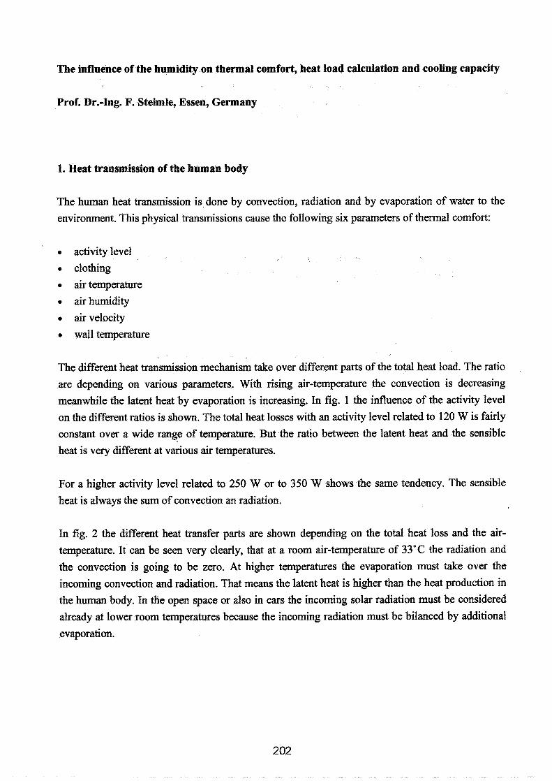
The influence of the humidity on thermal comfort, heat load calculation and cooling capacity
Prof. Dr.-Ing. F. Steimle, Essen, Germany
1. Heat transmission of the human body
The human heat transmission is done by convection, radiation and by evaporation of water to the
environment. This physical transmissions cause the following six parameters of thermal comfort:
o activity level 0 clothing
o air temperature
air humidity
o air velocity
e wall temperature
The different heat transmission mechanism take over different parts of the total heat load. The ratio
are depending on various parameters. With rising air-temperature the convection is decreasing
meanwhile the latent heat by evaporation is increasing. In fig. 1 the influence of the activity level
on the different ratios is shown. The total heat losses with an activity level related to 120 W is fairly
constant over a wide range of temperature. But the ratio between the latent heat and the sensible
heat is very different at various air temperatures.
For a higher activity level related to 250 W or to 350 W shows the same tendency. The sensible
heat is always the sum of convection an radiation.
In fig. 2 the different heat transfer parts are shown depending on the total heat loss and the air-
temperature. It can be seen very clearly, that at a room air-temperature of 33°C the radiation and
the convection is going to be zero. At higher temperatures the evaporation must take over the
incoming convection and radiation. That means the latent heat is higher than the heat production in
the human body. In the open space or also in cars the incoming solar radiation must be considered
already at lower room temperatures because the incoming radiation must be bilanced by additional
evaporation.
Because the parameters of the heat convection are very stable because of the constant body
temperature and a fixed clothing the control mechanism of the temperature by changing the heat
losses can only be done in the latent heat ratio. The rise of the temperature of the body surface can
only be shifted in very small limits and the room air temperature and the air-velocity can not be
ajusted individually. A change in the radiation is also not possible at a fixed wall temperature and
given room configuration. This shows clearly that whole control must be done by variable
evaporation.
Out of this considerations we see that the only possible ajustrnent of different activity levels f o ~ the
occupants in a room can only be done by variation of the evaporating water. This means that a
fairly low relativ humidity is necessary that the different bodies can find their own thermal comfort.
2. Humidity and comfort
The first investigations about the influence of the humidity of thermal comfort have been carried
out by Samuel Lewis (3). His diagram is shown in figure 3.
As a result of the work by Lewis a diagram of humidity vs. temperature was established. Figure 4
shows the comfort zone which was used in the sixties and seventies.
The investigations of 0. Fanger (5) about the thermal comfort in office buildings shows a much
smaller influence of the humidity. The reason of this results is the very small change of activity
level, a very simular clothing and a fairly stable air temperature. As shown in figure 1 and 2 the activity level is of great influence. It is not possible, therefore, to use the values for office buildings
in a much broader scale. In figure 5 the optimal conditions as shown in figure 3 are compared with
the comfort zone of DIN 1946 part 2. This results can also be shown by experiment where we
found that all test persons believe 26"C, 40% as definetly cooler than 24"C, 60%. This shows that
the influence of temperature can not be discussed without humidity.
3. Calcdation of cooling load
The correct equation for this calculation is
By using the enthalpy h the humidity is automatically included. Very often the equations only use
the temperature differences which is not correct.
Another very important mistake is done by using the exhaust air temperature as mean room
temperature. An optimal design of an air conditioning plant use a higher exhaust temperature. (See
figure 6) A ratio of enthalpie differences shows the effectivness of an air conditioning plant (2).
This ratio is as higher as more heat is going to the air flow after leaving the direct environment of
the occupants. Out of this consideration it is clear that the calculation of the cooling load must also
consider the design of the air flow.
4. Calculation of the refrigeration capacity
The cooling load is not enough to discribe the refrigeration capacity because it is also necessary to
consider the air changes. The air change rate cause especially in summertime a different
dehumidification load which effects the refrigeration capacity. The minimum air changes are
influenced strongly by the material which is used in the interial design. This can be shown in figure
7 (7). This example shows how great the influence of the material can be to the total energy
consumption offer building. This influence is somewhat higher than the influence of the insulation.
In summer everybody is speaking about cooling in air conditioning plants when he is going to
degreese the air temperature. For the dehumidification we have to calculate in central europe an
enthalpie difference of about 25 kJkg dry air. It is very important to see that the highest enthalpie
is not in the area of the highest temperature. Figure 8 shows the areas where temperature degreese
is important (zone A) and where the dehumidification is necessary (zone B). In this figure 8 the
area 1 shows 90% of all outdoor air conditions in Germany and area 2 shows 99% of the outdoor air conditions. The refrigeration capacity is therefore influence by the outdoor air humidity more
evidently than by the outdoor air temperature.
5. Conclnsion
This paper shows the great influence of the humidity on comfort, cooling load and refrigeration
capacity. A lot of knowledge is available since a long time. Very often simple calculation methods
do not use this knowledge. The computer programs of nowadays allow the consideration of
humidity without any problems.

Literature
Il l Schweizer Kiihllastregeln, 1969, Schweizer Verein fiir Heizung und LiiRung
I21 Steimle, F., Klimakursus, C.F. Miiller-Verlag Karlsruhe, 1969
131 Lewis, S .R., Air conditioning for Comfort Engineering Publications, Inc, Chicago 1932
141 Steimle, F., Spegele, H., Die Behaglichkeit in klimatisierten Mumen, Kiiltetechnik-Klimakursus 22 (1970) S. 81/82
151 Fanger, O., On thermal comfort, McGraw Hill, 1972 I61 Steimle, F., Spegele, H., Klima und Behaglichkeit, Klima-Ktiltetechnik, 1973, H 415
171 Steimle, F., Internationale Konferenz der IEA uber neue Energietechniken, April 1992, Dortmund

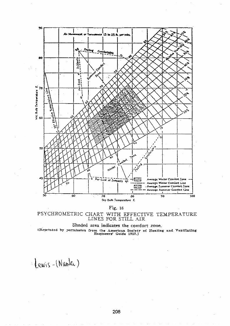
Fig. 16
PS\-CHROblETRIC CX-ART WITE EFFECTIVE TZlrlllER_-TER.E LINES FOR STILL ,AIR
Shaded area indicates the comfort zone. ( ~ c p r t n t e d by 3ermisslon from the hmericm S o c ! e t ~ oC Eeatlng snd Ventllatlng
Enqjneers' Gulde 1932.)

X +
Comfort-Zone in the summer A....in America E....in Europe
Comfort-Zone Angew. Thermodyn.
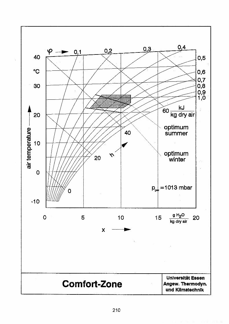
X +
Comfort-Zone

X -----)c
RA.....room air SA ..... supply air EA.....exhaust air


Energy Impact of Ventilation and Air Infiltration AlVC Conference, Copenhagen, Denmark
21 -23 Septern ber 1993
The PLEIADE Dwelling: an IEA Task Xlll Low Energy Dwelling with Emphasis on IAQ and Thermal Comfort
P Wouters," D L9Heureux,* A De Herde," E Gratia"
* Belgian Building Research Institute (WCBICSTC) Violetstraat 21 -23,1000 Brussels, Belgium ** Architecture et Climat, Place du Levant 1, 1348 Louvain-La-Neuve, Belgium
The major objective of the IEA task XI11 project is to design and construct low energy dwellings which should be technically and economically realistic in the period 2000-2010.
The design criteria for the Belgian dwelling are the following: - low energy demand for heating purposes; - good thermal comfort conditions, as well in winter as in summer with attention to the problem of
overheating; - very good aittightness (nb0 5 1 h-I); - good indoor air quality conditions; - attractive design for majority of potential clients; - only use of realistic technical solutions.
This paper includes a description of the overall design of this rowhouse, special attention being given to the conception of the envelope wit respect to the airtightness.
A detailed description of the philosophy of the balanced ventilation system with heat recovery and of the air heating system is given.
Results about the seasonal heating demand with special attention for the heating demand related to the ventilation are included. Also an estimation of the air change rates during periods of night ventilation is given (simulations with VENCON) and the impact of night ventilation on the thermal comfort conditions (simulations with MBDS).
Finally, an indication of the monitoring plans is given.
1. Introduction
The major objective of IEA Task Xlll 'Advanced Low Energy Dwellings' of the Solar Heating and Cooling programme is to think about the concept of low energy dwellings to be built in the period 2000- 2010. This Advanced Low Energy Dwelling should not only be a 'high tech' product but also be conform with national standards and local requirements. Also the concept of the dwelling should be attractive for future builders. Therefore, the construction of such an Advanced Low Energy Dwelling is a challenge for the involved teams with respect to the severe objectives and requirements.
2. The obiectives of the IEA Task Xlll proiec?
IEA Task Xlll started in 1990. In total, some 14 countries participate in the project : Austria, Belgium, Canada, Denmark, Finland, Germany, Italy, Japan, the Netherlands, Norway, Sweden, Switzerland, United Kingdom and United States. Operating Agent is Prof. A.G. Hestness from the University of Trondheim (Norway). The aim is to built in all participating countries a dwelling which should be for the period 2000-2010 a realistic low energy solar dwelling. An important boundary condition is that the techniques to be used should be cost effective within 10 ... 15 years. It is clear that such criteria cannot be evaluated in absolute terms in 1993 but one should at least try to exclude as much as possible techniques which don't give any reasonable perspective for a costeffective application.
At present, the construction in several countries is already finished or under way: Belgium, Canada, Germany, Netherlands, Norway.
The project at IEA level is assumed to finish in 1995. The results should include also information regarding the monitoring activities in these dwellings.

3. The Belaian context for the IEA participation
For Belgium, the Belgian Building Research Institute together with Architecture et Climat of the University of Louvain-La-Neuve take part in IEA Task XIII. The Belgian participation is financed by the Walloon Region.
Besides these 2 teams, a large number of other organizations are involved in the project : - Electrabel :
It is the Belgian electricity and gas company. Electrabel acts as owner of the dwelling. Moreover, its 2 laboratories, Laborelec (for all electrical applications) and A.R.G.B. (for all gas applications) are fully involved in the project and are responsible for the heating systems to be used in the dwelling. A gas system as well as an electrical heating system will be installed in order to allow a comparison between different systems;
- Laborelec : see above; - A.R.G.B. : see above; - a professional archiiectural office, leaded by Ph. Jaspard; - COMlTA : COMlTA is the association of all Belgian thermal insulation associations. The major
role of COMlTA is related to the choice and installation related aspects of the thermal insulation and glazing systems;
- Belgian Centre for Dornotics (B.C.D.), which is the Belgian association of organizations involved in domotics;
- a whole range of sponsors.
Given the facts that : - the last low energy demonstration dwelling was constructed in Belgium some 10 years ago; - many demonstration dwellings often suffer from problems as overheating, durability problems,
and are therefore not really a propaganda for building low energy dwellings;
it was a clear objective from the beginning of the project to construct a dwelling which by most of the potential builders will be appreciated.
In practice the following list of requirements was set up : - a very good thermal insulation level (there are requirements regarding the insulation level in the
Flemish and Walloon Regions); - good thermal comfort conditions, as well in winter time as in summer time but with a particular
interest for avoiding overheating problems in summer; - a potential for good indoor air quality conditions, by means of combining a good building
airtightness with a well designed balanced ventilation system; - good daylighting conditions; - nice architecture; - attention for durability aspects; - use of domotics for optimization of thermal comfort, energy use, general comfort and security.
The PLEIADE (Passive and Low Energy innovative Architecture DEsign) dwelling should fulfil all these requirements.
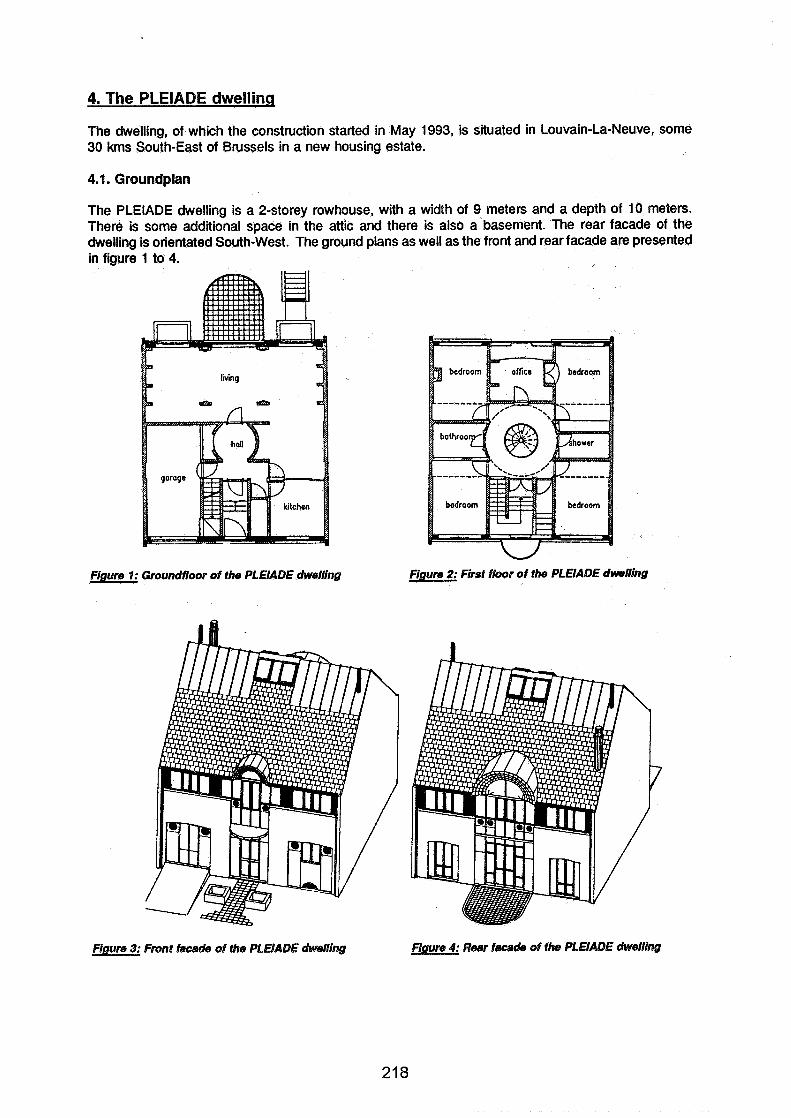
4. The PLEIADE dwelling
The dwelling, of which the construction started in May 1993, is situated in Louvain-La-Neuve, some 30 kms South-East of Brussels in a new housing estate.
4.1. Groundplan
The PLEIADE dwelling is a 2-storey rowhouse, with a width of 9 meters and a depth of 10 meters. There is some additional space in the attic and there is also a basement. The rear facade of the dwelling is orientated South-West. The ground plans as well as the front and rear facade are presented in figure 1 to 4.
Smng
Figure 1: Groundfloor of the PLEIADE dwelling
Figure 3: Fmnt facade of the PLEIADE dwelling Rear facade of the PLEIADE h l l i n g

4.2. Some important features
Walls, roofs and floors are, according to Belgian standards, extremely well insulated. The U-values are given in table 1.
Inclined Roof
The U-value of the walls of 0.14 ... 0.20 W/m2K corresponds with about 250 mm of thermal insulation. In Belgium, cavity walls consisting of an inner and outer leave in brickwork are normally used with some 40 ... 80 mm insulation in the cavity. Such technology cannot be used for a very large insulation thickness. Outside insulation could be an alternative. However, the urbanistic requirements in Louvain- La-Neuve are very severe and require brickwork. In order to obtain a very good U-value, the facade walls have no mechanical function and are not supporting the floor. This allows to have a cross section as shown in figure 5. This concept has also some advantages with respect to the airtightness as is described in $5. Another important feature concerns the various systems for providing the energy to the building. Briefly summarized, they are the following : - an air heating system selected by A.R.G.B., with a gas heated boiler. A 4 zone control system
is foreseen allowing different heating regimes for the different zones; - in parallel with the air heating system on gas, there are also electrical radiators (direct or with
accumulation) selected by Laborelec; - for the production of the domestic hot water, solar water collectors are planned in combination
with a gas boiler (no accumulation) - an advanced domotics system able to control the heating and ventilation system, lighting and
security aspects. B.C.D. is in charge of the choice and installation of the system. - 4 - .-'. - - - +
4+e+2L,3+
. r-.nI.,. i.. =I n M l
_t-"
-.*I.-
Figure 5: Some cross sections of the facade walls of the PLEIADE dwelling

5. Aspects reqardina buildinq airtiqhtness, ventilation and indoor air aualitv
From the beginning of the project, the achievement of good indoor air quality conditions is a top priority. However, the need to have a low energy consumption requires specific attention to the building airtightness and the efficiency of the ventilation system.
5.1. Building airtightness
The objective is to achieve an overall airtightness of n50 s 1 h-'. This is for the Belgian situation a very severe requirement. In principle, the airtightness of the facade walls can be very good since a continuous vapour barrier consisting of a PE-foil is foreseen (see figure 5) and should be continuous over the whole facade surface. The PE-foil shall be fixed on the window frames. Given the fact that no previous experience exists in Belgium, the installation of the PE-foil will require specific attention. The measurement of the airtightness is planned and, if necessary, improvements will be made. BBRl disposes of a large experience in airtightness testing.
5.2. The ventilation system
5.2.1. Basic ventilation
The first requirement of the ventilation system is that it should comply with the requirements of the Belgian standard NBN 050-001 [I]. Table 2 gives the nominal air flow rates for the various rooms as specified in NBN 050-001. The system consists of mechanical supply and mechanical extraction with a static heat recovery system. According to the standard, fresh air supply is required in the bedrooms whereas recirculation air is allowed for the living room. Transfer openings are foreseen in the inner doors corresponding with an air flow rate of 25 m31h for a pressure difference of 2 Pa.
Outside air
Outside air
Recirculated air '
Air extraction Air extraction
Table 2: The nominal air flow rates for the various rooms as given in NBN 050401
Some specific features of the system : - given the fact there is also an air heating system, an integration of the 2 systems is required.
However, the achievement of good thermal comfort and good indoor air quality conditions are given the same importance. Therefore, separate fresh air ducts and preheated air ducts are foreseen for the bedrooms and office. This clearly complicates the system but it was considered as a must in a low energy building with good IAQ conditions;
- there is a static heat exchanger with an efficiency of some 60 ... 65 %. Nevertheless, it is expected to have within 10 years better heat exchangers giving efficiencies in the order of 65 ... 75 % at competitive costs;
- there is a by-pass over the heat exchanger avoiding pre-heating in summertime mode.
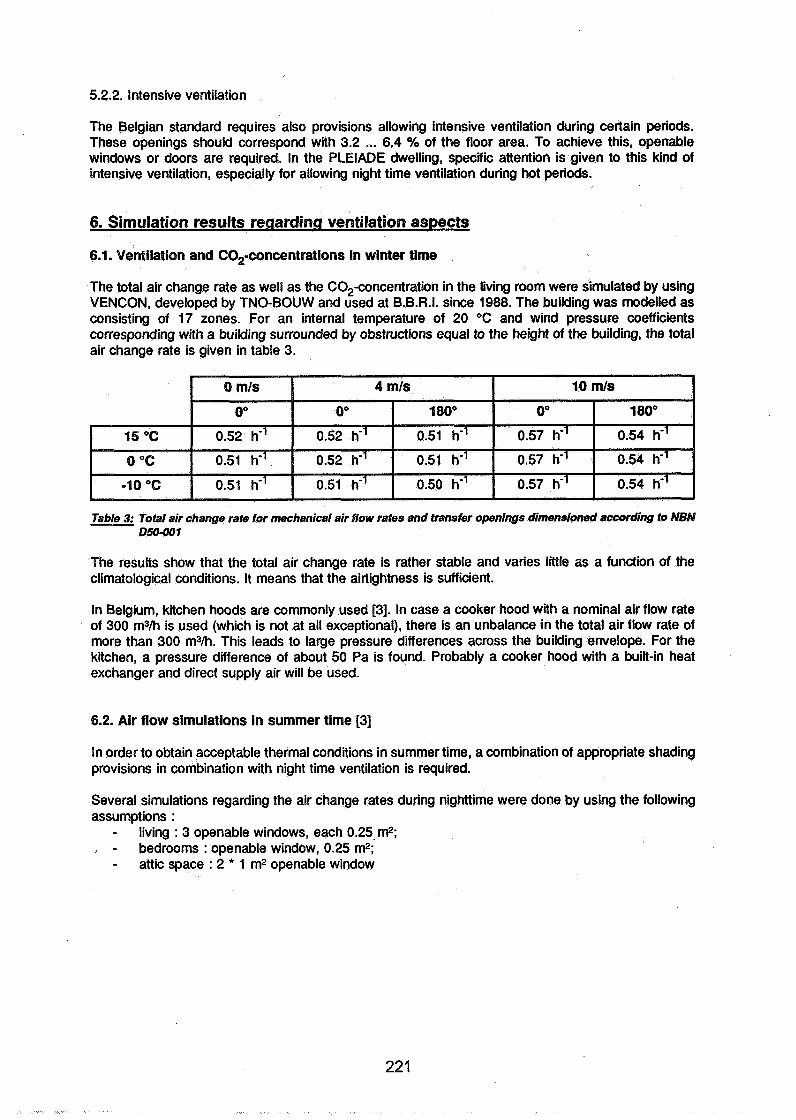
5.2.2. Intensive ventilation
The Belgian standard requires also provisions allowing intensive ventilation during certain periods. These openings should correspond with 3.2 ... 6.4 % of the floor area. To achieve this, open-able windows or doors are required. In the PLEIADE dwelling, specific attention is given to this kind of intensive ventilation, especially for allowing night time ventilation during hot periods.
6. Simulation results reclardina ventilation aspects
6.1. Ventilation and 60,-concentrations in winter time
The total air change rate as well as the C02-concentration in the living room were simulated by using VENCON, developed by TNO-BOUW and used at B.B.R.I. since 1988. The building was modelled as consisting of 17 zones. For an internal temperature of 20 OC and wind pressure coefficients corresponding with a building surrounded by obstructions equal to the height of the building, the total air change rate is given in table 3.
Table 3: Total air change rate for mechanical air flow rates and transfer openings dimensioned according to NBN 050-001
The results show that the total air change rate is rather stable and vanes little as a function of the climatological conditions. It means that the airtightness is sufficient.
In Belgium, kitchen hoods are commonly used 131. In case a cooker hood with a nominal air flow rate of 300 m3Ih is used (which is not at all exceptional), there is an unbalance in the total air flow rate of more than 300 mYh. This leads to large pressure differences across the building envelope. For the kitchen, a pressure difference of about 50 Pa is found. Probably a cooker hood with a built-in heat exchanger and direct supply air will be used.
6.2. Air flow simulations in summer time [3]
In order to obtain acceptable thermal conditions in summer time, a combination of appropriate shading provisions in combination with night time ventilation is required.
Several simulations regarding the air change rates during nighttime were done by using the following assumptions :
- living : 3 openable windows, each 0.25.rn2; , - bedrooms : openable window, 0.25 m2; - attic space : 2 * 1 m2 openable window
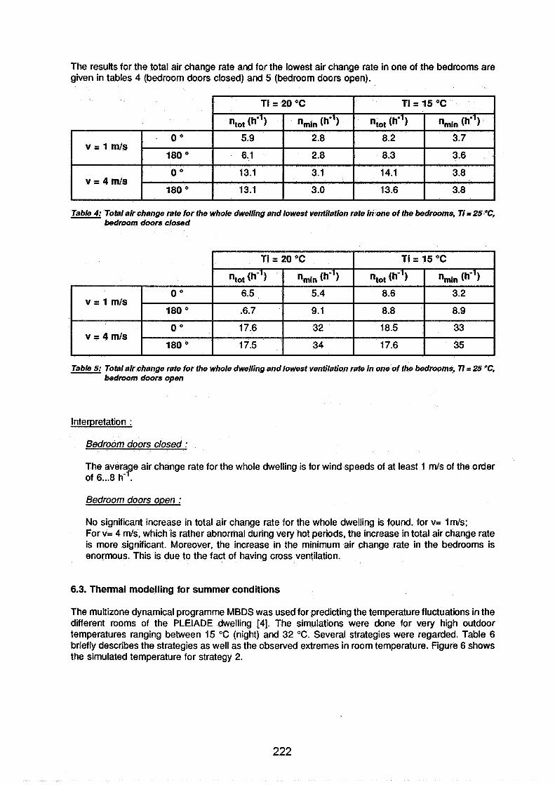
The results for the total air change rate and for the lowest air change rate in one of the bedrooms are given in tables 4 (bedroom doors closed) and 5 (bedroom doors open).
Table 4: Total air change rate for the whole dwelling and lowest ventilation rate in one of the bedrooms, Ti= 25 "C, bedroom doors closed
Table 5: Total air change rate for the whole dwelling and lowest ventilation rate in one of the bedrooms, Ti = 25 "C, bedroom doors open
Interpretation :
Bedroom doors closed :
The avera e air change rate for the whole dwelling is for wind speeds of at least 1 m/s of the order B of 6...8 h- .
Bedroom doors open :
No significant increase in total air change rate for the whole dwelling is found. for v= I d s ; For v= 4 m/s, which is rather abnormal during very hot periods, the increase in total air change rate is more significant. Moreover, the increase in the minimum air change rate in the bedrooms is enormous. This is due to the fact of having cross ventilation.
6.3. Thermal modelling for summer conditions
The multizone dynamical programme MBDS was used for predicting the temperature fluctuations in the different rooms of the PLEIADE dwelling [4]. The simulations were done for very high outdoor temperatures ranging between 15 O C (night) and 32 O C . Several strategies were regarded. Table 6 briefly describes the strategies as well as the observed extremes in room temperature. Figure 6 shows the simulated temperature for strategy 2.
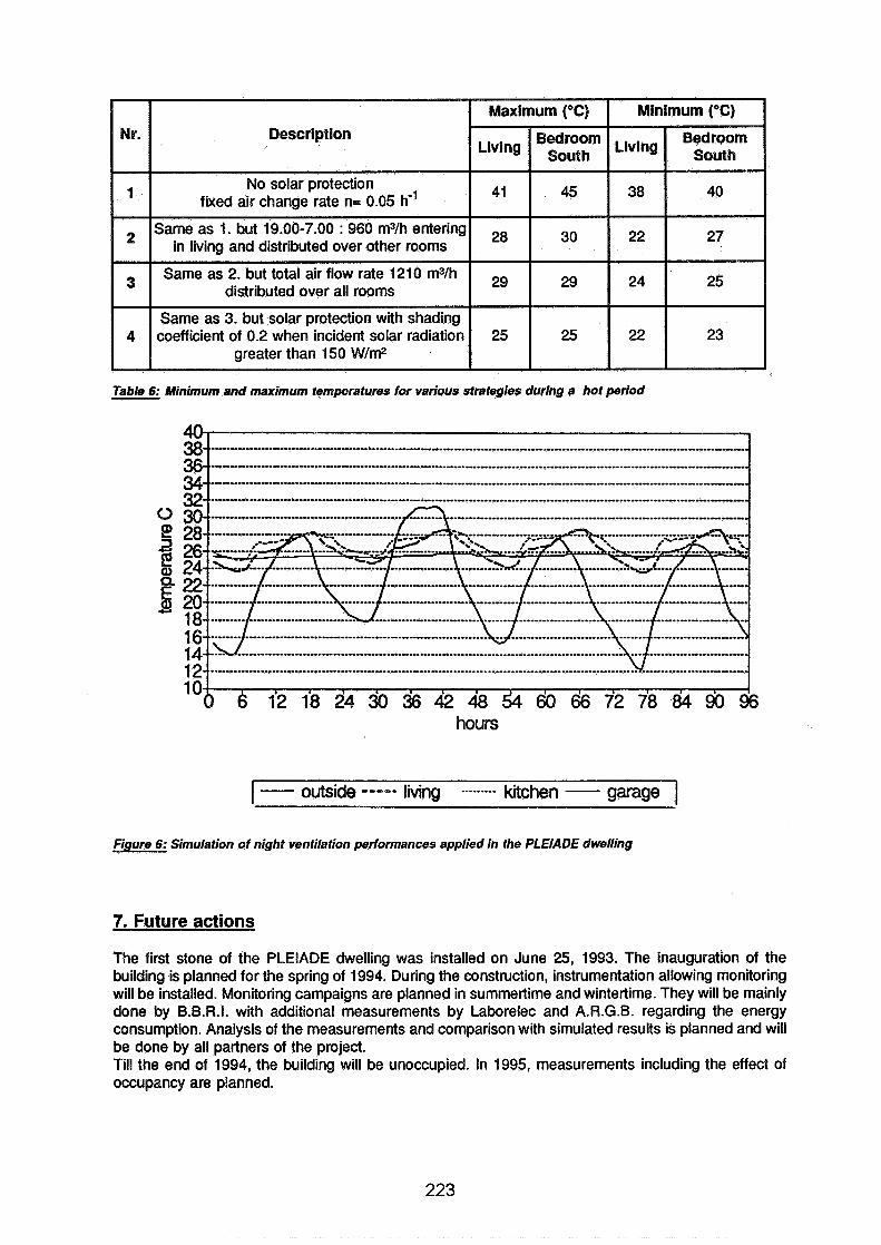
Table 6: Minimum and maximum temperatures for various strategies during a hot period
hours
- ......... outside ----- living kitchen - garage I
Figure 6: Simulation of night ventilation performances applied in the PLElADE dwelling
7. Future actions
The first stone of the PLElADE dwelling was installed on June 25, 1993. The inauguration of the building is planned for the spring of 1994. During the construction, instrumentation allowing monitoring will be installed. Monitoring campaigns are planned in summertime and wintertime. They will be mainly done by B.B.R.I. with additional measurements by Laborelec and A.R.G.B. regarding the energy consumption. Analysis of the measurements and comparison with simulated results is planned and will be done by all partners of the project. Till the end of 1994, the building will be unoccupied. In 1995, measurements including the effect of occupancy are planned.
8. Conclusions
Wih the design and the construction of the PLEIADE dwelling, the partners of the project aim to achieve a dwelling which is not only very attractive from the energy point of view but which also is very attractive from an architectural point of view and which has excellent qualities regarding thermal comfort and indoor air quality. All these features should be realised within realistic and modest budgetary limitations.
First practical results are expected in the summer of 1994 and will be probably reported at the 1994 A.I.V.C. conference.
9. Acknowledgments
The authors wishes first of all to thank the Walloon Region for the financial and moral support which is given to the project. Moreover, they like to thank Electrabel and its laboratories Laborelec and A.R.G.B., COMITA, B.C.D. as well as all the sponsors to the project.
10. References
[I] INSTITUT BELGE DE NORMALISATION "NBN D50-001, Dispositifs de ventilation dans les batiments d'habitiation" BIN, l e version, octobre 1991
[2] DE HERDE, A., GRATIA, E., WOUTERS P., L'HEUREUX D., " PLElADE dwelling" CIB W67 conference, Stuttgart, March 1993
[3] COHlLlS P., L'HEUREUX D., WOUTERS P. "The ventilation of the PLEIADE dwelling, Reporting of first simulation results" B.B.R.I., June 1992
[4] GRATIA E. "Maison PLEIADE : simulations" draft, April 1993
Energy Impact of Ventilation and Air Infiltration 14th AlVC Conference, Copenhagen, Denmark
21 -23 September 1993
The Influence of Purpose-Provided Openings on Natural Ventilation of Buildings Equipped with Gas Fired Appliances
R Borchiellini,* M Cali,* M Girard,** M Masoero*
* Dipartimento di Energetica, Politecnico di Torino, Corso Duca degli Abruui 24, Torino, Italy ** ITALGAS s.p.a., Largo Regio Partc, Torino, Italy
1. SYNOPSIS The growing diffision of small power, gas-fired individual units for space heating and service hot water production, as well as concern about operational safety issues, has promoted greater attention to the understanding of ventilation mechanisms in the dwellings equipped with such units. Within a joint research project between Politecnico di Torino and Italgas, an experimental campaign has been conducted in order to investigate the influence of purpose-provided ventilation openings (sized according to the national UNI-CIG 7129-72 standard) on air changes and IAQ. Measurements were conducted in one of the instrumented single-family buildings of the Italgas experimental facility in Venaria (Torino). Air permeability has been characterised with blower door tests, while tracer gas measurements were made in the building during boiler operation. In each test, the size of the ventilation openings and the cross section of the chimney were varied, in order to understand the influence of such factors on the overall system performance. The paper describes the experimental approach that was followed; results are analysed in view of verifling the applicability of such approach to more general cases.
2. INTRODUCTION Gas-fired domestic appliances for service hot water ( S H W ) production and space heating have experienced a growing diffision in Italy in recent years. It is likely that such trend will continue in the future, and that new fields of applications of domestic gas appliances will be developed. The thermal and fluid dynamic interaction between the appliance and the building has a clear influence on energy consumption, indoor air quality, and operational safety. Although gas appliances are equipped with reliable safety devices, accidents due to an incorrect installation are not unfiequent. The causes of such accidents must be ascribed both to insufficient information among builders and users, and to the practical difficulty in checking the respect of safety installation codes. Most of the accidents are due to either inadequate supply of combustion air, or to incorrect chimney sizing, or both. Experimental work on gas appliances can be conducted in different settings, i.e., in the laboratory [I] - a situation which is mostly suitable for characterising the performance of in- dividual systems or components under strictly controllable and repeatable conditions - or in the field, when real installations are examined. Based on past and present experience, acquired both in field and laboratory research, a third intermediate approach has been followed by the italian gas utility "Italgas": an experimental facility has been built in Venaria (Torino) and put into operation in 1990, which consists of two identical single-family buildings. The buildings - which are realistic examples of current building practice in the residential sector in Italy - are very flexible in terms of thermal sys- tems installation, and are fully instrumented for monitoring of relevant parameters such as ambient temperatures, meteorological conditions, combustion analyses, etc. In order to investigate the interaction between energy performance, indoor air quality, and operational safety, a research program has been jointly developed since 1990 by Italgas and Politecnico di Torino. In the first part of the program, the thermal and fluid dynamic properties of the buildings have been investigated through a set of experimental campaigns. The energy signature of the buildings have been determined by monitoring the heating

consumption over two consecutive years. The integrity and airtightness of the building envelope has been checked with I.R. thermography and blower door measurements. Tracer gas measurements have been performed in order to determine actual airchange rates under normal climatic and operating conditions [2]. This paper presents and discusses the results of a measurement campaign, which was conducted in the Fall of 1992, aimed at characterising the interaction between a gas-fired SHW production unit and the building, under varying conditions of combustion air supply and combustion gases exhaust. To this end, airchange rates, combustion parameters, and in- door pollutants concentrations have been monitored using the experimental setup described in the following chapter.
3. EXPERIMENTAL SETUP The building in which the experiment was conducted consists of two stories. The lower floor hosts the centralised service equipment and the data acquisition I processing system. The ground floor (in which the tests were performed) has a floor area of 114 m2, and includes two bedrooms, a living room, bathroom and kitchen. If necessary, the attic space above the ground floor can be heated, so that the test story may also reproduce the thermal condition of an apartment in a high-rise building. A plan view of the test area is shown in Figure 1.
M gas inlet P personal computer F gas dryer A gas analyser V voltmeter
C motor driven damper control T tracer gas apparatus ------ damper control line . . . . . .. . . airlgas sampling line
Figure 1 - Plan view of the test area
A 20 kW gas boiler for service hot water production was installed in the kitchen and connected to an existing vertical chimney of 18 x 20 cm cross section and 2.5 m high. Combustion air was supplied by natural ventilation through a purpose-provided opening, located in the lower part of the north facing external wall (under the window), sized accord- ing to the italian standard UNI-CIG 7129-72; such standard prescribes that combustion air
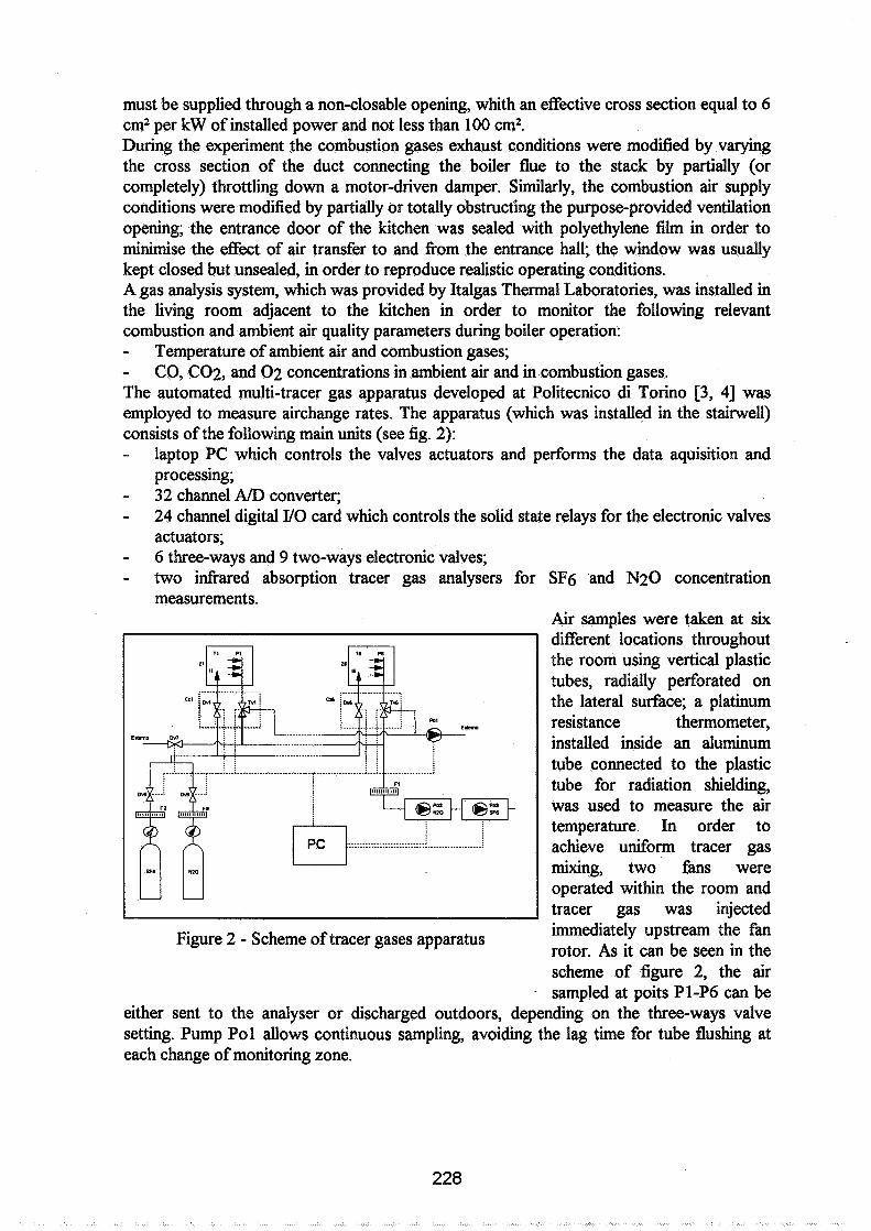
must be supplied through a non-closable opening, whith an effective cross section equal to 6 cm2 per kW of installed power and not less than 100 cm2. ~ u i n ~ the experiment the combustion gases exhaust conditions were modified by varying the cross section of the duct connecting the boiler flue to the stack by partially (or completely) throttling down a motor-driven damper. Similarly, the combustion air supply conditions were modified by partially or totally obstructing the purpose-provided ventilation opening; the entrance door of the kitchen was sealed with polyethylene film in order to rninimise the effect of air transfer to and from the entrance hall; the window was usually kept closed but unsealed, in order to reproduce realistic operating conditions. A gas analysis system, which was provided by Italgas Thermal Laboratories, was installed in the living room adjacent to the kitchen in order to monitor the following relevant combustion and ambient air quality parameters during boiler operation: - Temperature of ambient air and combustion gases; - CO, CO2, and 0 2 concentrations in ambient air and in combustion gases. The automated multi-tracer gas apparatus developed at Politecnico di Trorino [3, 41 was employed to measure airchange rates. The apparatus (which was installed in the stairwell) consists of the following main units (see fig. 2): - laptop PC which controls the valves actuators and performs the data aquisition and
processing; - 32 channel AID converter; - 24 channel digital VO card which controls the solid state relays for the electronic valves
actuators; - 6 three-ways and 9 two-ways electronic valves; - two infrared absorption tracer gas analysers for SF6 and N20 concentration
measurements. Air samples were taken at six different locations throughout the room using vertical plastic tubes, radially perforated on the lateral surface; a platinum resistance thermometer, installed inside an aluminum tube connected to the plastic tube for radiation shielding, was used to measure the air temperature. In order to achieve uniform tracer gas mixing, two fans were operated within the room and tracer gas was injected
Figure 2 - Scheme of tracer gases apparatus immediately upstream the fan rotor. As it can be seen in the scheme of figure 2, the air
- sampled at poits PI-P6 can be either sent to the analyser or discharged outdoors, depending on the three-ways valve setting. Pump Pol allows continuous sampling, avoiding the lag time for tube flushing at each change of monitoring zone.
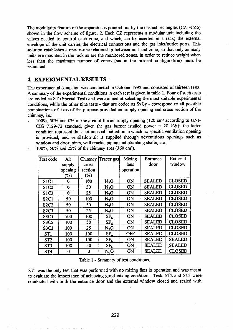
The modularity feature of the apparatus is pointed out by the dashed rectangles (CZl-CZ6) shown in the flow scheme of figure. 2. Each CZ represents a modular unit including the valves needed to control each zone, and which can be inserted in a rack; the external envelope of the unit carries the electrical connections and the gas inlet/outlet ports. This solution establishes a one-to-one relationship between unit and zone, so that only as many units are mounted in the rack as are the monitored zones, in order to reduce weight when less than the maximum number of zones (six in the present configuration) must be examined.
4. EXPERIMENTAL RESULTS The experimental campaign was conducted in October 1992 and consisted of thirteen tests. A summary of the experimental conditions in each test is given in table 1. Four of such tests are coded as ST (Special Test) and were aimed at selecting the most suitable experimental conditions, while the other nine tests - that are coded as SxCy - correspond to all possible combinations of sizes of the purpose-provided air supply opening and cross section of the chimney, i. e. : - loo%, 50% and 0% of the area of the air supply opening (120 cm2 according to UNI-
CIG 7129-72 standard, given the gas burner istalled power = 20 kW); the latter condition represent the - not unusual - situation in which no specific ventilation opening is provided, and ventilation air is supplied through adventitious openings such as window and door joints, wall cracks, piping and plumbing shafts, etc.;
- loo%, 50% and 25% of the chimney area (360 cm2).
Table 1 - Summary of test conditions.
ST1 was the only test that was performed with no mixing fans in operation and was meant to evaluate the importance of achieving good mixing conditions. Tests ST2 and ST3 were conducted with both the entrance door and the external window closed and sealed with

polyethylene film - a condition that appeared to be unrealistic for the purposes of the ex- periment, but that helped understanding the relative importance of the various adventitious ventilation sites within the room. ST4 represents the worst condition that can occur in a room that hosts a combustion unit, i.e. the case when both the chimney and the air supply opening are completely obstructed. Table 1 also indicates the type of tracer gas (SF6 or N20) that was used in each tracer decay test. Ambient air and flue gas analyses were also performed in parallel to the tracer gas measurements, but results of such measurements are not presented in this paper for lack of space. A comparison of average values and standard deviations of airchange measured in each test is given in table 2. Airchanges were calculated in two different ways, i.e.: 1) firstly, by assuming that the estimated parameters (i.e., flow rates) are constant in time; 2) secondly, by calculating the parameters at each time step, and then taking the average
of such time-dependent values.
* In test SIC1 the sensitivity of results to increasing r was investigated; since error decreases for increasing values of r, the results of the following tests were analysed with r = 48 only.
** Since test S2C3 was over 112 hour longer than the others, three different times were considered in the analysis:
@ time about equal 1800 seconds as in other tests time equal 3774 seconds which corresponds to the maximum number of steps that can be processed by the time constant parameters algorithm. actual test time
Table 2 - Measured airchange values N ~ , and standard deviation o
Time dependent parameters were calculated with the Sequential Function Specification

Procedure [5, 61, using a polynomial finction in which the parameters are the coefficients. The estimated average values and standard deviation obviously depend on the number of time steps, r, over which the function parameters are assumed to be constant. A reasonably good estimate was obtained taking r = 48 time steps; hence, the time step being equal to 5 seconds, the flow rates may be assumed constant over a 5 x 48 = 240 seconds interval. For the sake of comparison, table 2 also gives the values for r = r' = N - 1, where N is the total number of steps. The effect on airchanges of obstructing the air supply opening and throttling down the chimney cross section is shown in table 3. The results clearly indicate that the overall airchange of the test room is markedly influenced by variation in air supply andor gas exhaust conditions, since an almost 2:l variation of airchanges occur between the extreme cases: from roughly 1.9 ACH in the 100% - 100% case (supply - chimney), down to 1.0 ACH in the 0% - 25% condition, with a variation trend that consistently reflects the opening / closing sequence. Other observations can be made regarding the Special Tests results. ST1 corresponds to test S3C1, except for the absence of mixing fans; the time variations of airchanges are very irregular and clearly depending on poor mixing, rather than on variations in test conditions. Tests ST2 and ST3 (window closed and sealed) correspond to tests S3C1 and S3C2 (window closed but unsealed) respectively; by comparing the results of the corresponding tests, it appears that sealing the window does not influence significantly the results, since the variation in airchanges is only approximately equal to 0.07 ACHY i.e. is of the same order of sigma. Test ST4 (total obstruction) shows that the test room is not perfectly airtight, since an airchange of about 0.6 ACH still occurs. This fact means that airchanges cannot be attributed to the air supply - gas exhaust system only. The presence of a filly open air supply causes an increase in airchanges ranging between 14 and 22 m3lh (depending on the area of the chimney), which corresponds to a 23% to 62% variation with respect to the complete obstruction case. It is however clear that a significant part of the air flow does not occur through the purpose-provided opening, but rather through adventitious openings, and that the latter cannot be attributed to windows, since the window sealed vs. window unsealed data virtually coincide. It appears therefore that the test was influenced by the presence of adventitious openings other than the windows, which have an airflow capacity more than twice that of the purpose-provided air supply opening. Such evidence was hrther confirmed by blower door tests that were performed a few days after the experiment, which identified the presence of an air path connecting the test room and the adjacent living room. Consequently the results of the parametric test do not permit to characterise the performance of the purpose-provided opening only, and should therefore be interpreted in relative, rather than in absolute, terms. The combustion analysis data do also permit to estimate the gas flow rate in the chimney. By taking the measured concentrations of oxygen and carbon dioxide at the stack, and by estimating the natural gas flow rate entering the burner from the nominal power of the boiler (which was always operated at full load), the flow rate of combustion products can be easily calculated from well known stoichiometric equations. Unfortunately, since the natural gas flow rate was estimated rather than measured, it is not possible to attribute a standard deviation to the chimney flow rate, as it has been done for the measured airchange values. Throttling of the chimney damper does significantly affect the flow rate, which almost
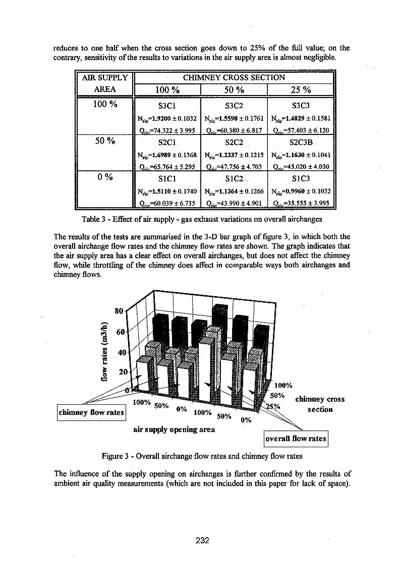
reduces to one half when the cross section goes down to 25% of the full value; on the contrary, sensitivity of the results to variations in the air supply area is almost negligible.
Table 3 - Effect of air supply - gas exhaust variations on overall airchanges
The results of the tests are summarised in the 3-D bar graph of figure 3, in which both the overall airchange flow rates and the chimney flow rates are shown. The graph indicates that the air supply area has a clear effect on overall airchanges, but does not affect the chimney flow, while throttling of the chimney does affect in comparable ways both airchanges and chimney flows.
chimney cross section
air supply opening area overall flow rates ezl
Figure 3 - Overall airchange flow rates and chimney flow rates
The influence of the supply opening on airchanges is further confirmed by the results of ambient air quality measurements (which are not included in this paper for lack of space).
The C02 concentration increases from 800 to 900 ppm when the supply area is reduced to 50%, and increasingly higher values are attained with global obstruction. The measured trends of CO concentration in ambient air are, on the contrary, not significant: No meaningfkl correlation was identified between test conditions and C 0 concentrations, which remained, even in the worse conditions, at quite acceptable levels.
5. CONCLUSIONS The results of the experiments have confirmed the reliability of applying tracer gas techniques and pollutant concentration measurements to the performance assessment of gas burning appliances, which are installed in a living space and draw combustion air from the space itself, while exhausting combustion gases outdoors through a chimney. Such configuration is very usual in Italy, particularly in older buildings, and installation of the system does not always comply with safety codes. The experiment did also confirm a belief, which arises from the examination of several CO poisoning accidents, and is fUrther confirmed by previous laboratory work performed by Italgas, i.e. that correct sizing of the chimney (cross section, height and shape) is the most crucial factor in achieving safe operation, more so than correctly sizing the purpose-provided ventilation opening as prescribed by the codes. The latter may be extremely important in airtight buildings (e.g., post-energy crisis constructions, buildings in mountain areas, etc.), while older dwellings are normally sufficiently permeable to guarantee an adequate supply of combustion air.
6. REFERENCES
[l] Guiducci M. "Dispositivi atti a prevenire I'inquinamento degli ambienti domestici dai prodotti della combustione di apparecchi a gas" Proc. of 3" ATIG National Congress, Genova 26-28 November 1990
[2] Girard M. and Masoero M. "Caratterhzazione termica e fluidodinamica di due edifici "'ad hoe" per la sperimentazione di apparecchi a gas" CH4 Energia Metano, Anno X, n. 2, marzo-aprile 1993.
[3] Borchiellini R. and Cali M. "An Automated Apparatus for Air Infiltration Measurement with Tracer Gases", Proc. of the 11th AIVC Conference, Belgirate, Italy, Vol. 1, pp 157-169, 1990.
[4] Borchiellini R, and Cali M., "Experimental and Numerical Analysis of Transient Air Changes in Buildings: A Case Study" Proc. of the 3rd International Conference "Air Distribution in Rooms" Roomvent '92, Aalborg Denmark, 2-4 September 1992, pp.417-433.
[5] Borchiellini R. "Tracer Gas Data Analysis Using Inverse Problem Theory" Pubblicazione interna Dipartimento di Energetica Politecnico di Torino, PT DE FT 282, Torino, Aprile 1992.
[6] Borchiellini R. and Cali M., "The Inverse Problem Theory Applied to Air Flow Estimations and Experiments Design in the Multizone Case" Proc. of the International Symposium "Air Flow in Multizone Structures" Budapest Unghery, 9 September 1992.


Energy Impact of Ventilation and Air Infiltration 14th AlVC Conference, Copen hagen, Denmark
21 -23 September 1993
Natural Ventilation via Courtyards: Theory & Measurements
R R WalkePL Shao** , M Woolliscroft*
** Building Research Establishment, Garston, Watford, WD2 7JR * University of Sheffield, School of Architectural Studies, Sheffield, S10 2UJ, UK (Now at Nottingham University)
Crown Copyright 1993 - Building Research Establishment
SUMMARY Existing regulations concerning the design and construction of residential buildings which are naturally ventilated via courtyards and lightwells have origins in daylighting rather than in aerodynamics. The design of narrow, high-sided courtyards which achieve healthy . conditions for occupants, has long been a problem and a subject of various guidance and research, although many doubts and gaps in knowledge still remained. The work described below resolves these problems, and the coherent theory developed may lead to clearer guidance on the design of courtyards for natural ventilation.
A fresh approach was adopted using computational fluid dynamics (CFD) software as an integrated technique in combination with measurements at both model and full scale. The adequacy of infiltration and ventilation rates in rooms opening onto the courtyard was also assessed. The salient results were used to develop a coherent descriptive model which explains the apparent discrepancies in earlier work and enabled revised design guidelines to be presented.
1, INTRODUCTION Existing regulation^'^ concerning the design and construction of residential buildings which are naturally ventilated via courtyards and lightwells have origins in daylighting rather than in aerodynamics. Their design to achieve healthy conditions for occupants has long been a problem and a subject of various guidance and research. Current guidance limits the height to width ratio of such courts, which effectively precludes narrow, high- sided courtyards as proposed elsewhere (eg Japan) for residential developments. By default, existing knowledge could be used as the basis of proposed new guidance on non- domestic buildings. Previous research left many doubts and gaps in knowledge which, if resolved, could lead to clearer guidance on the design of courtyards for natural ventilation. This is consistent with the increasing emphasis on natural ventilation as the primary design option, reflecting current concerns over indoor air quality, energy use and environmental issues.
This report addresses these needs by reviewing the salient findings of past research and identifying key issues. Work is then described in which computational fluid dynamics (CFD) software was used (in association with the University of Sheffield) as part of an integrated approach in combination with measurements at both model and full scale. The adequacy of infiltration and ventilation rates in rooms opening onto the courtyard was also assessed using a multizone prediction model. The salient results were used to develop a coherent descriptive model, which explains the apparent discrepancies in earlier work, and to present revised design guidelines. The CFD approach is described in more detail in a related pape? (Part 11).
2. HISTORIC BASIS OF CURRENT REGULATIONS Local and national building regulations and Acts from the 19th and 20th centuries contain requirements about the location of windows andlor ventilators which open onto external air spaces (eg courtyards and lightwells) closed on three or four sides. The origins of the restrictions on ventilation to a partly enclosed external air space strongly suggest that an emphasis on daylighting played a part. The essential core of the Regulations in the UK can be summarised, for a closed court, as stipulating that the height of the wall above an opening shall be less than twice (or, in Scotland three times ) the distance to the facing wall. The aerodynamical basis of this restriction is not clear.
3. KEY ISSUES AND CURRENT KNOWLEDGE There are two key issues concerned with any revision to guidelines on ventilation of buildings arranged around courtyards or lightwells:
* adequacy of courtyard ventilation, including contaminant dispersal; adequacy of ventilation in rooms opening onto the courtyard
The wind environment in the court itself may also be an important design consideration, but is outside the scope of this paper. The relevant findings of past studies are summarised below.
3.1 Full and model scale studies of courtyard ventilation The court should be well ventilated to provide a reservoir of 'fresh' outside air to habitable rooms with ventilation openings in the court. In addition, contaminants released into the court should adequately disperse to avoid possible re-ingestion at ventilation openings.
A literature survey of wind tunnel studies" -I4) revealed some instances of conditions where stable vortices may occur. In this case it may be that air remains trapped within the court, with only poor exchange with the free airstream above. In some cases a stable circulation has been observed to be confined to the upper portion of deep courts, leaving a zone of stagnant air below. These studies left some doubt as to whether air flowing above the courtyard effectively exchanged with air within it or, instead, 'skimmed over'.
There are very few published studies at full s ~ a l e ~ ~ ' ~ ~ ' ~ ~ ' ~ , and these mostly record air speeds and turbulence in the courtyard. Cockroft and RobertsonB used a tracer gas technique to measure air change rates of between 13 and 40 ach; unfortunately, experimental details and meteorological conditions were not given. ~urakami' used smoke dispersal to measure air change rates and proposed a relationship between air change rate and wind speed.
3.2 Ventilation within the building It is possible that the presence of the court (compared to a completely open area) may adversely affect wind-induced ventilation within rooms, particularly those which have openings in the courtyard. Two relevant past s tud ie~~* '~ concerned with hospital buildings predicted that ventilation rates would be less than 3 air changes per hour for as much as 50% of the winter period. However, minimum ventilation rates lower than 3 ach are recommended for health and safety of occupants office buildings and dwellings. Even so, the second study also predicted ventilation rates of less than 0.5 ach for significant periods of time. Recent measurements of leakage in office buildings l6 suggest that leakage may have been underestimated by as much as 50% in the above studies. To address these unresolved problems, the predicted ventilation performance of a building with lightwell is assessed below.
4. CFD MODELLING OF COURTYARD VENTILATION /Whilst previous research represents significant progress, clearly many doubts and gaps in knowledge still remained to be resolved to enable a consistent and general understanding of the problem to be developed. In general, field measurements provide data such as air flow and ventilation rate only at a particular location and time. Tests at model scale using a wind tunnel enable air flow in a range of situations and conditions to be considered, but do not provide sufficient information alone, and may not truly represent the flow regime at
full scale.
A fresh approach was therefore adopted using computational fluid dynamics (CFD) software, which is now capable of simulating and predicting air flow over a wide range of situations with sufficient resolution in three dimensions, due to advances in computer memory and speed. The CFD studies described below can be divided into three parts,
(a) studies of the mechanism of ventilation of courtyards (b) parametric study of key features of flow, building and surroundings which may impact on courtyard ventilation (c) model study of a real eight-storey building with lightwell
4.1 Mechanism of Ventilation of Courtyards Details of the CFD modelling used to study the mechanism by which air flows through a courtyard are described in a linked paper 3. The main findings of this study are that there are two distinct air flow patterns involved in the exchange of air within deep plan courtyards. One pattern comprises a circulation at the top of the court ('top vortex'), with stagnant air below, and in the other a vortex occupies the full width and depth of the courtyard ('full vortex'). A full vortex was shown to be created when the separated flow at the top upwind edge of the building re-attaches upstream or in the vicinity of the court opening at roof level.
Time-dependant solutions for contaminant removal were also used to trace flow paths through the court and, together with the concept of 'mean age of air', to calculate local ventilation rates. These showed that a top vortex would not provide an efficient air exchange throughout the court. A full vortex, on the other hand, was found to bring outside air deep into the court and give an efficient air exchange over nearly the whole of the space.
4.2 Parametric Studies of Courtyard Ventilation Using CFD, a parametric study was carried out to assess the possible influence of various factors (parameters) on reattachment at or near the courtyard as a criterion for achieving a full vortex. The basic calculation configuration consisted of a simple rectangular building 16 m x 16 m x 24 m high with a lightwell. An urban velocity profile" was defined upstream with a velocity of 5 rn/s at the top of the domain (at twice the building height) and, initially, with no surrounding buildings or other local effects. Upwards of 20,000 nodes were used. By varying each in turn, the following key parameters and their effects were identified:
Building width - there is a tendency to form a top vortex as building width is increased (Figure 1). This is because flow over the top of the wider buildings is greater, increasing the separation at the upwind edge of the roof.
Building heiqht - the taller the building the greater the tendency to form a top vortex (Figure 2), caused by a greater vertical component of velocity and consequent greater separation at the upwind edge of the roof.
Courtyard location - a full vortex is more likely as the distance of the courtyard from the upwind face'? increases.
height of surroundinq buildings - surrounding buildings of similar height assist
formation of full vortex (Figure 3). This would appear to explain why a top vortex has frequently been observed in wind tunnel tests using isolated buildings, but not in full scale tests, particularly those in towns and cities.
wind direction - a full vortex is more likely when the wind is not blowing normal to the facade.
Also varied but found to make no significant impact were absolute height of building and surroundings (varied together), terrain and wind profile (ie changing the inlet profile from an urban to a city profile) and wind velocity.
These results constitute a consistent and coherent model which explains the apparent discrepancies observed in earlier work. As such, they provide the basis for design guidance, although the detailed results should be interpreted only qualitatively, since many indeterminate factors could influence the air flow in a real situation.
4.3 Eight-storey lightwell The above predictions were tested further, with a view to subsequent full scale measurements, by carrying out calculations of air Row over a real eight-storey building which incorporated two lightwells to its full height (Figure 4). Investigations focused on the smaller of the two lightwells measuring approximately 16 m x 7 m x 27 m deep. Simulations were carried out initially for only the half of the building including this lightwell, although insignificant differences were found when these were repeated for the full building (but ignoring the larger lightwell to keep within computer memory limits).
A full vortex was predicted for conditions were the wind was blowing broadly parallel to the long side of the lightwell, without considering local shelter. When the wind speed was set to zero below roof level, to simulate the local shelter of surrounding tall buildings, the predicted depth of vortex was slightly increased. As expected, a top vortex was predicted when the air flow was parallel to the short side of the lightwell, but a full vortex was predicted when shelter was included (Figure 5).
Two further cases were simulated for the full building with shelter, for comparison with field measurements at full scale. In both cases a full vortex was predicted, and the air change rate was crudely estimated by summing all inflow and outflow for all grid cells across the opening in the lightwell at roof level, and then halving to give an estimate of the total in- or outflow. 43 ach was calculated for a wind of approximately 2.0 m/s from the south, and 35 ach for a similar windspeed from 30 north of west. Figure 6 shows the latter case, which used 148,000 nodes. These two results are broadly consistent with full scale field measurements described below.
5. MEASUREMENTS AT FULL AND MODEL SCALE Guided by the features of the air flow predicted above, and to test their validity, a series of measurements were carried out in the eight-storey building both in the field at full scale and in a wind tunnel at model scale.
5.1 Field Measurements in an eight-storey lightwell Tracer gas and smoke tests were carried out to assess the air movement and ventilation rate in the smaller of two lightwells in the real eight-storey building in its city-centre site. The lightwell was temporarily covered at roof level with a tarpaulin and the enclosed

space was filled with tracer gas. Air samples were taken at two locations, one at second- storey height and the other at sixth-storey height, and initial conditions were arranged to give approximately equal tracer concentrations at these points. The tarpaulin was then quickly removed and the falling concentration of tracer, recorded as it was diluted by incoming fresh air, was used to calculate the ventilation rate.
These were elaborate and labour intensive tests and consequently only two have been carried out. In the first test the wind speed observed at roof level was between 2 and 3 mfs, blowing from approximately northwest. The measured ventilation rate at both locations was approximately 50 air changes per hour, and tracer concentrations remained reasonably well-mixed. For the second test the average wind speed recorded at roof level was approximately 3.3 mls, blowing from approximately south-southwest. An air change rate of approximately 45 ach was calculated. Within broad limits of accuracy, these results compare quite well with CFD predictions of 43 and 35 ach, respectively.
Each of the above two tests were immediately followed by tests using smoke released at various points to visualise air movement in the courtyard. In both cases, we observed smoke descending at the downwind face of the court, traversing the base, then rising up on the upwind face. These results are consistent with the ventilation tests in indicating that there was an adequate flow of fresh air deep into the courtyard.
5.2 Measurements at model scale A boundary layer wind tunnel at BRE was used to carry out a series of smoke visualisation tests using a 11200 scale model of the eight-storey building (Figure 1) using an urban wind profile. With air flowing parallel to its long side at roof level, smoke was introduced into the small lightwell and, as expected, a full vortex was clearly observed. Consistent with this, when the smoke release was stopped (using a slow wind speed of approximately 1.3 Ws) smoke was observed to clear initially from the downwind side and subsequently away over the full depth.
However, when the wind was blowing parallel to the short side of the court, smoke was observed to remain circulating in the upper portion. This was contrary to expectations from the CFD modelling where sheltering was included. CFD was therefore used to simulate the airflow over the building at the model scale. A top vortex was predicted, as observed in the wind tunnel, but contrary to the predictions for the full scale. However, the vortex progressively extended over the full court depth as the simulated wind speed was increased by more than a factor of four. This result would appear to suggest that the Reynolds number may be too low at model scale, specifically where air speeds may be much lower than in the free airstream, eg in the lightwell.
6. PREDICTED VENTILATION PERFORMANCE WITHIN BUILDING The adequacy of ventilation within rooms with openings into the courtyard was identified (above) as a key issue. This raised some concerns that ventilation may be inadequate for significant periods of time in courtyard buildings. We have therefore used a commercially available multizone ventilation prediction procedure (BREEZE) to assess the wintertime ventilation performance of an eight-storey office building based on the design described above.
Infiltration flow through the fabric is calculated in the model using the empirical power-law relationship,

Q = k . (AP)" (2)
were k is a constant coefficient, AP is the inside-outside pressure difference due to wind and temperature differences and the exponent n was taken " as 0.6.
It was assumed that trickle ventilators were installed at window-head height, with an open area of 400 mm2 per 10 m2 of floor area la. Air flow through these vents was represented as flow through a sharp-edged circular orifice of the same open area and a discharge coefficient of 0.62. Ventilation requirements were calculated on the basis of an estimated design occupancy of 80 people per storey, a recommended rate of 8 litredsec per person and a minimum of 5 litreslsec per person. This gave 0.57 and 0.35 ach respectively. This would reduce to 0.43 and 0.26 ach in a domestic building of the same size, based on typical occupancy of 1 person 20 d of floor area.
6.1. Building in urban terrain Surface pressure data were obtainedf9 for a generalised rectangular building 30 m tall with a single courtyard, set in an urban terrain (or on the edge of a city). Local effects of possible surrounding tall buildings were not included in these measurements. Typical background air leakage of 10 m3/hr per m2 of permeable envelope area was assumed, based on recent dataq6 for office buildings.
The whole building air change rates were calculated for a wind speed of 4 rn/s for each of twelve wind directions at 30 degree intervals, with typical design air temperatures2' of 7°C outside and 20°C inside. Internal doors were assumed to be open. Due to the symmetry of the building from which the pressure data were derived, air change rates varied very little with wind direction, with a minimum of 0.49 ach for winds blowing from the north and a maximum of 0.54 ach for winds blowing from the west.
The results from these two wind directions were then taken to define the extremes of an envelope containing all other possible air change rates. For these two wind directions the whole building air change rates were then calculated for the range of wind speeds and outside air temperatures expected to occur during the hours between 9.00 am and 6 pm in the winter months September to March inclusive. These results were then combined with a weather data set for an urban site (Garston) consisting of hours of co-occurrence of intervals of wind speeds with outside air temperatures, for an average winter period as above. Results for all possible wind directions were assumed to be represented by either the 'maximum' or the 'minimum' condition and a cumulative frequency of occurrence of small intervals of air change rate was constructed.
The predicted mean (50% value) was approximately 0.46 ach, with a very narrow spread (approximately 0.5 ach) between the two extreme assumptions. The minimum requirements of 0.34 ach (office) and 0.26 ach (domestic) were easily met, and in fact exceeded more than 90% of the time.
Effects of reduced air leakaqe, closed internal doors and zonal air chanae rates The effect of assuming a very tight envelope (half typical leakage)16 was considered. The mean (50% of time) ventilation rate was determined to be 0.35 ach, and greater than 0.26 ach for 90% of time.
The effect of closing all internal doors was represented by typical leakage through joints
given by1 Q (Vs)=1 -~(AP)O.' per metre crack length of total 5.6 m each door. This had the effect of reducing the whole building air change rate by approximately 40% (calculated at a wind speed of 4 ds) . This is an extreme condition, and it may be more appropriate to assume half of all doors are open in practice.
Air change in selected zones with doors closed were calculated and found to be lowest in areas between the two lightwells. This is consistent with the expectation that wind pressure differences across these areas should be lowest. Nevertheless, they were broadly similar to whole building air change rate.
6.2. Effect of shelter by tall buildings Surface pressures were measured on the surface of the 11200 scale replica of the eight- storey building located amongst other tall buildings of similar height, set within an urban terrain. Although not fully representative of the actual surrounding city terrain of the real site, ventilation rates predicted using these data could be directly compared with predictions (above) using data collected with the same terrain but with no shelter.
The procedure for predicting whole building air change rates was repeated as above. For 4 m/s wind speed, air change rates varied by less than 2% from a mean of 0.45 ach. These are only approximately 13% less than the corresponding results predicted for the generalised building with no shelter.
It is noted, however, that this work highlights a general issue concerning the common practice of using pressure data which take no account of possible local shelter effects. However, when local shelter is included, there may be the difficulty of significant Reynolds number effects where air speeds are low between the tall buildings, as discussed above. This could cause errors in measurements of surface pressures on the sides of the building. However, this issue is a subject for further research in itself.
7. PROPOSED BASIS FOR REVISED DESIGN GUIDANCE ON COURTYARD DESIGN It has been shown (above) that adequate ventilation can achieved within the building, which addresses one of the two key issues raised earlier. The other concerned the requirement for adequate ventilation of the courtyard. In the light of the coherent theory of flow into the courtyard developed above, the salient facts can now be drawn together to formulate a basis for a revised design guideline.
If we take a criterion that wind driven ventilation in the courtyard should be adequate down to 1 m/s, then it can be concluded from Murakami's workq0 at model scale, and in the light of full scale measurements described above, that we might expect 10 ach as a conservative estimate. In the small lightwell in the eight-storey building considered, this is equivalent to 300 m3/h per m2 of courtyard area, or an effective purging velocity component of 0.08 m/s. The ratio of this velocity to the stated wind speed of 1 m/s is 0.08, which is less than 0.1 5 measured by Murakami, thus reinforcing the belief that we have taken a conservative estimate of the flow in the court.
Assuming an occupancy density of one person per 20 m2 of dwelling floor area, then the ventilation requirement (based on 8 litreslsec per person) is 300 m3/h per 200 m2 of floor area. We calculated above that this flow rate will be supplied by 1 m2 of courtyard area. If we also ailow for the additional burden of diluting kitchen extract flow rates, rated at approximately 30 litres/sec (per dwelling). Assuming three people per dwelling, and that only half of all extracts operate at any one time (ie a diversity factor of 50%), this amounts to an additional
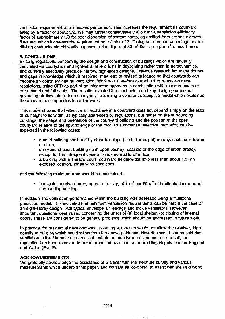
ventilation requirement of 5 litreslsec per person. This increases the requirement (ie courtyard area) by a factor of about 312. We may further conservatively allow for a ventilation efficiency factor of approximately 113 for poor dispersion of contaminants, eg emitted from kitchen extracts, flues etc, which increases the requirement by a factor of 3. Taking both requirements together for diluting contaminants efficiently suggests a final figure of 50 m2 floor area per m2 of court area.
8. CONCLUSIONS Existing regulations concerning the design and construction of buildings which are naturally ventilated via courtyards and lightwells have origins in daylighting rather than in aerodynamics, and currently effectively preclude narrow, high-sided designs. Previous research left many doubts and gaps in knowledge which, if resolved, may lead to revised guidance so that courtyards can become an option for natural ventilation. Work was therefore carried out to re-assess these restrictions, using CFD as part of an integrated approach in combination with measurements at both model and full scale. The results revealed the mechanism and key design parameters governing air flow into a deep courtyard, so forming a coherent descriptive model which explained the apparent discrepancies in earlier work.
This model showed that effective air exchange in a courtyard does not depend simply on the ratio of its height to its width, as typically addressed by regulations, but rather on the surrounding buildings, the shape and orientation of the courtyard building and the position of the open courtyard relative to the upwind edge of the roof. To summarise, effective ventilation can be expected in the following cases:
a court building sheltered by other buildings (of similar height) nearby, such as in towns or cities, an exposed court building (ie in open country, seaside or the edge of urban areas), except for the infrequent case of winds normal to one face a building with a shallow court (courtyard heighwwidth ratio less than about 1.5) an exposed location, for all wind conditions,
and the following minimum area should be maintained :
horizontal courtyard area, open to the sky, of 1 m2 per 50 m2 of habitable floor area of surrounding building.
In addition, the ventilation performance within the building was assessed using a multizone prediction model. This indicated that minimum ventilation requirements can be met in the case of an eight-storey design with typical envelope air leakage and trickle ventilators. However, important questions were raised concerning the effect of (a) local shelter, (b) closing of internal doors. These are considered to be general problems which should be addressed in future work.
In practice, for residential developments, planning authorities would not allow the relatively high density of building which could follow from the above guidance. Nevertheless, it can be said that ventilation in itself imposes no practical restraint on courtyard design and, as a result, the regulation has been removed from the proposed revisions to the Building Regulations for England and Wales (Part F).
ACKNOWLEDGEMENTS We gratefully acknowledge the assistance of S Baker with the literature survey and various measurements which underpin this paper, and colleagues 'co-opted' to assist with the field work;
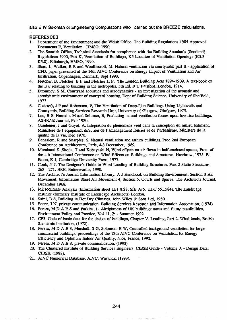
also E W Soloman of Engineering Computations who carried out the BREEZE calculations.
REFERENCES 1. Department of the Environment and the Welsh Office, The Building Regulations 1985 Approved
Documents F, Ventilation. HMSO, 1990. 2. The Scottish Office, Technical Standards for compliance with the Building Standards (Scotland)
Regulations 1990, Part K, Ventilation of Buildings, K5 Location of Ventilation Openings (K5.3 - K5.8), Edinburgh, HMSO, 1990.
3. Shao, L, Walker, R R and Woolliscroft, M, Natural ventilation via courtyards: part II - application of CFD, paper presented at the 14th AIVC Conference on Energy Impact of Ventilation and Air Miltration, Copenhagen, Denmark, Sept 1993.
4. Fletcher, B, Fletcher, B F and Fletcher H P, The London Building Acts 1894-1909. A text-book on the law relating to building in the metropolis. 5th Ed. B T Batsford, London, 1914.
5. Ettourney, S M, Courtyard acoustics and aerodynamics - an investigation of the acoustic and aerodynamic environment of courtyard housing, Dept of Building Science, University of Sheffield, 1973
6. Cockroft, J P and Robertson, P, The Ventilation of Deep-Plan Buildings Using Lightwells and Courtyards, Building Services Research Unit, University of Glasgow, Glasgow, 1975.
7. Lee, B E, Hussain, M and Soliman, B, Predicting natural ventilation forces upon low-rise buildings, ASNRAE Journal, Feb 1980.
8. Gandemer, J and Guyot, A, Integration du phenomene vent dans la conception du milieu batiment, Mimistere de l'equipment direction de l'amenagement foncier et de l'urbanisme, Ministere de la qualite de la vie, Dec 1976.
9. Bensalem, R and Sharpies, S, Natural ventilation and atrium buildings, Proc 2nd European Conference on Architecture, Paris, 4-8 December, 1989.
10. Murakami S, Shoda, T and Kobayashi N, Wind effects on air flows in half-enclosed spaces, Proc. of the 4th International Conference on Wind Effects on Buildings and Structures, Heathrow, 1975, Ed Eaton, K J, Cambridge University Press, 1977.
11. Cook, N J, The Designer's Guide to Wind Loading of Building Structures. Part 2 Static Structures, 268 - 271. BRE, Buttemorths, 1990.
12. The Architect's Journal Information Library, A J Handbook on Building Environment, Section 3 Air Movement, Information Sheet Air Movement 4, Section 5. Courts and Spaces. The Architects Journal, December 1968.
13. Microclimate Analysis (Infomtion sheet LF1 8.28, SfE3 Ac5, UDC 551.584). The Landscape Institute (formerly Institute of Landscape Architects) London.
14. Saini, B S, Building in Hot Dry Climates. John Wiley & Sons Ltd, 1980. 15. Potter, I N, private communication, Building Services Research and Information Association, (1974) 16. Perera, M D A E S and Parkins, L, Airtightness of UK buildings:status and future possibilities,
Environment Policy and Practice, Vol 1 1 , g - Summer 1992. 17. CP3, Code of basic data for the design of buildings, Chapter V. Loading, Part 2. Wind loads, British
Standards Institution, (1972). 18. Perera, M D A E S, Marshall, S 6 , Solomon, E W, Controlled background ventilation for large
commercial buildings, proceedings of the 13th AIVC Conference on Ventilation for Energy Efficiency and O p h m Indoor Air Quality, Nice, France, 1992.
19. Perera, M D A E S, private communication, (1993) 20. The Chartered Institute of Building Services Engineers, CIBSE Guide - Volume A - Design Data,
CIBSE, (1988). Nmerical Database, AIVC, Warwick, (1993). .
4 ---, A A&.-. - .I I.. . . . . . . . I
d -L 4 4 - - - 1
d A A d - , 1 : : 1 / I d - 4 - .,,
Figure I. Building width perpendicular to flow increased by faclors (a) 1.0 (b) 1.5 (c) 2.0
Figure 2. Building height increased by factors of (a) 1.0 (b) 1.5 (c) 2.5
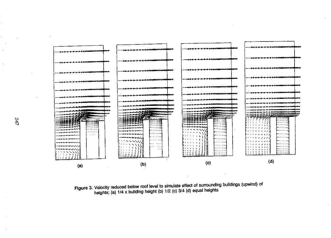
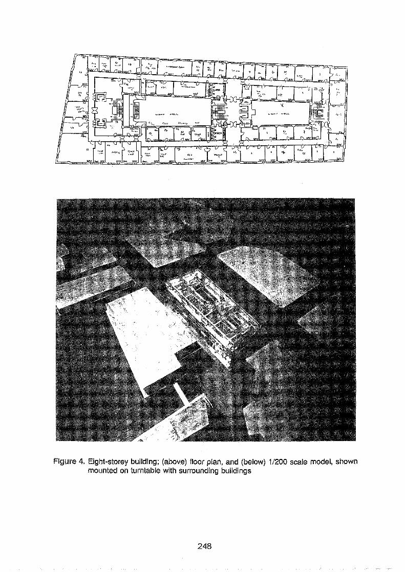
Figure 4. Eight-st~rey building; (above) floor plan, and (below) 11200 scale model, shown mounted an turntable with surrounding buildings
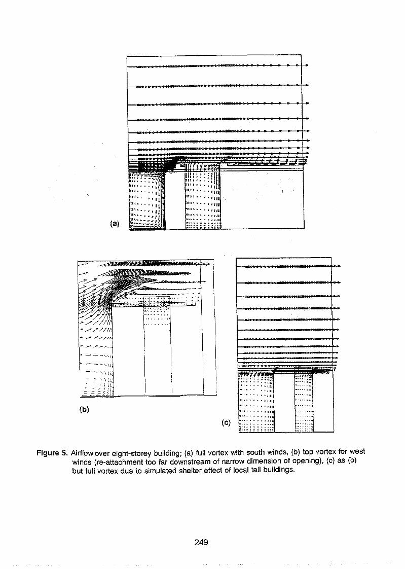
Figure 5. Airflow over eight-storey building; (a) full vortex with south winds, (b) top vortex for west winds (re-attachment too far downstream of narrow dimension of opening), {c) as (b) but full vortex due to simulated shelter effect of local tall buildings.
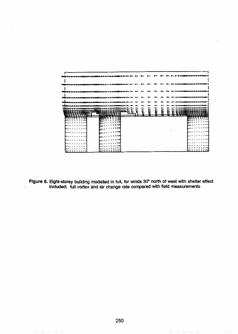
C C C C C C
C C C C C a-
......... ........... ......... ........... ......... ............ .......... ............ ............ ............ ............ ............ ............ .......... ........I ............ .......... .......... . . . . . . . . a ...........
Figure 6. Eight-storey building modelled in full, for winds 30" north of west with shelter effect included; full.vortex and air change rate compared with field measurements
Energy Impact of Ventilation and Air Infiltration 14th AlVC Conference, Copenhagen, Denmark
21 -23 September 1993
Energy Impact of Ventilation and Dynamic Insulation
L Jensen
Lund Institute of Technology Department of Building SciencelBuilding Services, P 0 Box 118, S-221 00 Lund, Sweden
Synopsis
Dynamic insulation stands for an insulation through which an air flow flows. The air flow is usually the normal ventilation flow. The air can flow in the same or in the opposite direction of the normal heat flow. The dynamic insulation can be arranged as single where only inlet or exhaust air passes the insulation, or as combined where inlet and exhaust air pass one half of the insulation each. Dynamic insulation using exhaust air might result in conden- sation problems in cold climates.
The normal insulation heat loss is reduced when using dynamic insulation and can be eliminated more or less only if the ventilation heat loss is several times larger than the normal insulation heat loss. The reduction of normal insulation and ventilation heat losses when using dynamic insulation is limited to 0.23 for single and 0.35 for combined dynamic insulation.
Dynamic insulation can be regarded as a ventilation heat recovery system. The equivalent ventilation heat recovery efficiency is limited to 0.5 for single dynamic insulation and to 1 for combined dynamic insulation, and decreases with increasing ventilation flow. An alternative to dynamic insulation in order to obtain the same saving is standard ventilation heat recovery system.
1. Introduction
Dynamic insulation is a notation which is often used. It is however not very descriptive and is far from dynamic in any sense. The notation is used to describe insulation with a constant flow through the insulation in the same or opposite direction of the normal heat flow. The word dynamic is also used for the so called dynamic U value which shows how the normal insulation U value decreases to zero with increasing flow through the insulation. Better notations that sometimes are used are co-flow insulation and counter-flow insulation.
The flow through the insulation is assumed to be the normal ventilation flow of a room or a building. The flow velocity is only in the range of a few m/h or even less than a s.
The benefit with flow insulation is that the total heat loss for the insulation and the ventilation flow is less than the heat loss for the same normal insulation and the ventilation flow added. The decrease is however limited to the normal insulation heat loss and this occurs only if the ventilation flow heat loss is several times the normal insulation heat loss. The decrease is also limited to the ventilation flow heat loss when the ventilation flow heat loss is small compared with the normal insulation heat loss and when both co-flow
and comter-flow insdation are used. Only half the decrease carn be obtained when using only co-flow or coaer-flow insula~on.
The flow insulation can be regarded as normal insulation with ventilation heat recovery. The equivalent ventilation heat recovery eB&ency decreases with increasing flow from I for combined co-flow and counter-flow insulation and from 0.5 for only co-flow or counter-flow insulation.
The ventilation heat loss can however be eliminated completely even for large flows if periodic s ~ t c b i n g between two parts of flow insulation is used. One part is in the co-flow mode and the other is in the counter-flow mode. The two parts of flow insulation can be regarded as two halves of a robry heat exchanger wheel which is rotated half a revolution each time. The large heat capacity of the insulation material makes this heat exchanger incredibly oversized and that is why the eEciency becomes dose to 1.
The aims of this paper, desc~bed in the following sections, are
@ t o derive simple expressions for total beat loss for single and combined co-flow and comter-flow insdations
@ to conapare total heat loss for single and combined co-now and couder-fiow insulations as a function of the cguotient between ventilation heat loss and normal insulation heat loss or as a function of insulation t&ckness for a given ventilation need
@ to show that the nomal insulation heat loss is only saved when using flow insulation and when the nomal insulation heat loss is m c h smaller than the ventilation heat loss
to show that the possible seduction in total heat loss for diEerent flow insu- lations compared ~ t h the sum of no 1 insulation heat loss zssad ventila- tion heat loss is limited
@ to show that the heat loss reduction for flow insulation can be regarded as a ventilation heat recovery and that the equivalent ventilation heat recovery efficiency decreases from I for combined flow insulation and from 0.5 for single flow insulation ~ t h increasing flow
to show that the heat savings when using flow insulation can easily be obtained f i t h stmdmd ventilation heat arecovesy techiqlues
2 A simple flow insulation model
An insulation with an area of 1 m2, a thickness of d (m) and a conductivity of h (WImK) is studied. The temperature of the air flow and the insulation material is assumed to be the same, given by T(x) (K) where x is the normalized and dimensionless position in the insulation block. The air flow is assumed to move in the x direction with the properties velocity v (mls), density p (kg/m3) and specific heat capacity c (JkgK).
The boundary conditions are given by the inlet and outlet temperatures as
The surface heat transfer coefficients are assumed to be infinite at both ending surfaces.
The sum of the heat transferred in the x direction by conduction and by flow must be constant for all x which gives
--- dT (x) + pcv T(x) = constant d dx
The differential equation (2.3) can be solved and the solution is given by
where the parameter a is the quotient between the ventilation heat loss and the normal (non-flow) insulation heat loss
Q.QY/O. IQ = b.9 1
a = pcv/(h/d) (-) (2.5) 4.X &\KO Q.u'\ = 42
The two parameters A and B are given by the boundary conditions (2.1) and (2.2). Simple calculations give
A = (To - Ti) /(ea - 1) B = T i - A
Note that the indices i and o stand for inlet and outlet and not indoor and outdoor or inside and outside.
The temperature profile T(x) in the flow insulation is shown in Figure 2.1 for a = 0,1 ,2 ,5 and 10, and boundary temperatures T(0) = 0 and T(1) = 1. The case a = 0 corresponds to the normal insulation case.
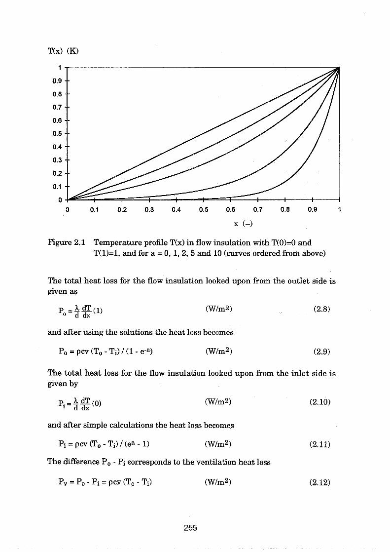
Figure 2.1 Temperature profile T(x) in flow insulation with T(O)=O and T(l)=l, and for a = 0,1,2,5 and 10 (curves ordered from above)
The total heat loss for the flow insulation looked upon from the outlet side is given as
and after using the solutions the heat loss becomes
Po = PCV (To - Ti) 1 ( 1 - e-a) (WIm2) (2.9)
The total heat loss for the flow insulation looked upon from the inlet side is given by
and after simple calculations the heat loss becomes
Pi = ~ C V (To - Ti) 1 (ea - 1) (WIm2) (2.11)
The difference Po - Pi corresponds to the ventilation heat loss
PV = PO - Pi = PCV (To - Ti) (WI1112)
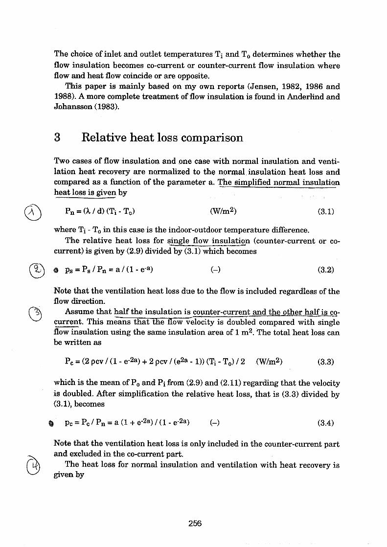
The choice of inlet and outlet temperatures Ti and To determines whether the flow insulation becomes co-current or counter-current flow insulation where flow and heat flow coincide or are opposite.
This paper is mainly based on my own reports (Jensen, 1982, 1986 and 1988). A more complete treatment of flow insulation is found in Anderlind and Johansson (1983).
3 Relative heat loss comparison
Two cases of flow insulation and one case with normal insulation and venti- lation heat recovery are normalized to the normal insulation heat loss and compared as a function of the parameter a. The -..-. simplified normal insulation heat loss is given by
where Ti - To in this case is the indoor-outdoor temperature difference. The relative heat loss for single flow insulation (counter-current or co-
current) is given by (2.9) divided by (3.1) which becomes
Note that the ventilation heat loss due to the flow is included regardless of the flow direction.
Assume that half the insulation is counter-current and the other half is cq- O current. This m with single flow insulation using the same insulation area of 1 m2. The total heat loss can be written as
PC = (2 pcv 1 (1 - e-2a) + 2 pcv 1 (e2a - 1)) (Ti - To) I 2 (WlmfL) (3.3)
which is the mean of Po and Pi from (2.9) and (2.11) regarding that the velocity is doubled. After simplification the relative heat loss, that is (3.3) divided by (3.11, becomes
Note that the ventilation heat loss is only included in the counter-current part and excluded in the co-current part.
The heat loss for normal insulation and ventilation with heat recovery is given by
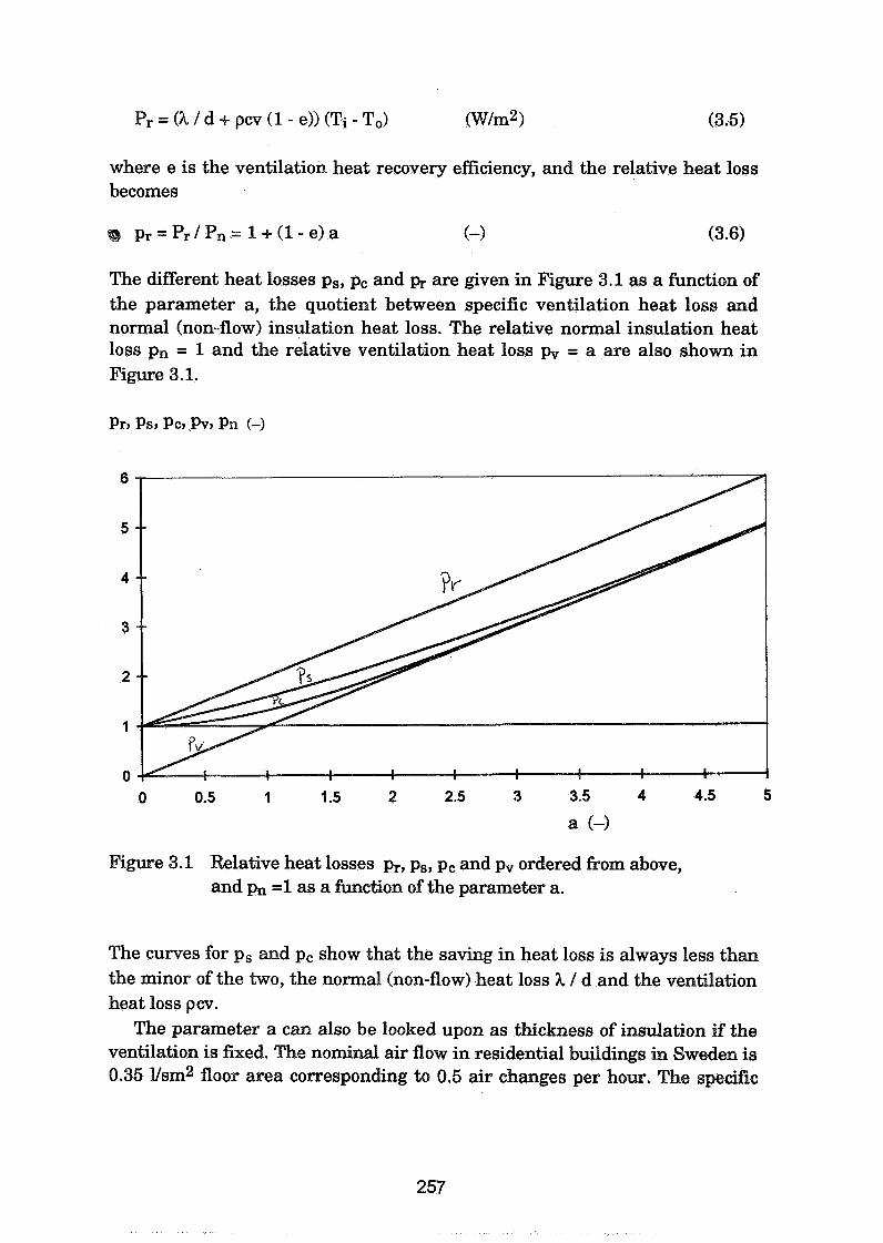
Pr = (h / d + ~ C V (1 - el) (Ti - To) (W/m2) (3.5)
where e is the ventilation heat recovery efficiency, and the relative heat loss becomes
The different heat losses ps9 pc and are given in Figure 3.1 as a function of the parameter a, the quotient between specific ventilation heat loss and normal (non-flow) insulation heat loss. The relative normal insulation heat loss p, = 1 and the relative ventilation heat loss p, = a are also shown in Figure 3.1.
Figure 3.1 Relative heat losses pr, p,, pc and pv ordered from above, and pn =1 as a function of the parameter a.
The curves for p, and pc show that the saving in heat loss is always less than the minor of the two, the normal (non-flow) heat loss h / d and the ventilation heat loss pcv.
The parameter a can also be looked upon as thickness of insulation if the ventilation is fxed. The nominal air flow in residential buildings in Sweden is 0.35 l/sm2 floor area corresponding to 0.5 air changes per hour. The specific
ventilation need is given by pcv and with PC = 1200 J-3 and v = 0.00035 d s it becomes 0.42 WIKm2. If the insulation material conductivity is set to suit- able figures 0.042 WImK then the relation between a and d becomes very simple a = 10 d. The parameter a can also be looked upon as thickness given in units of dm (0.1 m).
4 Relative heat loss reduction
The relative heat loss reduction is calculated relative to normal insulation and ventilation without heat recovery given by (3.6) with e = 0 for both single and combined flow insulation as
rs = ( ~ r - ~ s ) / ~ r and
rC=(pr-pc)/pr
The two quantities rs and r, are shown in Figure 4.1 as a function of the parameter a.
Figure 4.1 Relative heat loss reduction rs (below) and r, (above) as a function of the parameter a.

Both curves in Figure 4.1 show that the reduction has got a maximum for a specific value of the parameter a as follows
case a r single 1.79 0.23 combined 1.15 0.35
Note however that the absolute reduction increases up to the normal (non- flow) insulation heat loss with increasing parameter a. Note also that the total reduction for a given building will be even less because of heat losses from other building parts.
5 Equivalent ventilation heat recovery eficiency
The reduced heat loss for both single and combined flow insulation can be described as ventilation heat recovery. The equivalent ventilation heat recovery efficiency can be found by putting p, = p, and solving for e which gives
The efficiency e can be simplified to 1 / a for large values of the parameter a. The efficiency e is decreasing with increasing parameter a. Small relative ventilation needs or small parameter a values close to zero give e = 0.5. This means that only counter-current or only co-current insulation never can reduce the total heat losses more than a case with normal insulation and ventilation system with a heat recovery efficiency of 0.5.
The case with combined co-current and counter-current insulation gives an equivalent ventilation heat recovery efficiency e by putting pc = p, and solving for e gives
This efficiency e is also decreasing with increasing parameter a and is equal to 1 for a = 0, and is close to 1 / a for large values of the parameter a. This means that combined flow insulation can correspond to a ventilation heat recovery efficiency close to 1. The two efficiency functions e, and ec are given in Figure 5.1 as a function of the parameter a together with the simplified function 1 / a for a > 1.
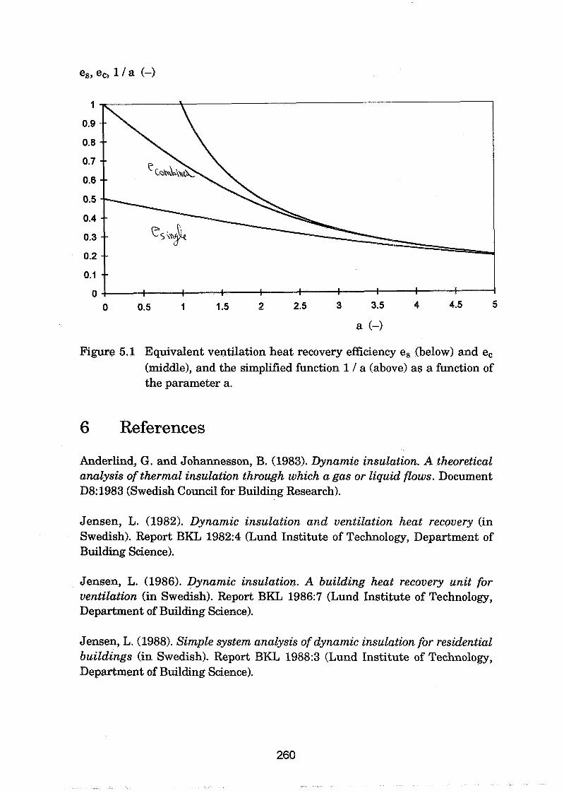
Figure 5.1 Equivalent ventilation heat recovery efficiency e, (below) and e, (middle), and the simplified function 1 1 a (above) as a function of the parameter a.
6 References
Anderlind, G. and Johannesson, B. (1983). Dynamic insulation. A theoretical analysis of thermal insulation through which a gas or liquid flows. Document D8: 1983 (Swedish Council for Building Research).
Jensen, L. (1982). Dynamic insulation and ventilation heat recovery (in Swedish). Report BKL 1982:4 (Lund Institute of Technology, Department of Building Science).
Jensen, L. (1986). Dynamic insulation. A building heat recovery unit for ventilation (in Swedish). Report BKL 1986:7 (Lund Institute of Technology, Department of Building Science).
Jensen, L. (1988). Simple system analysis of dynamic insulation for residential buildings (in Swedish). Report BKL 1988:3 (Lund Institute of Technology, Department of Building Science).
Energy Impact of Ventilation and Air Infiltration 14th AlVC Conference, Copenhagen, Denmark
21 -23 September 1993
A New Development for Total Heat Recovery Wheels
F Dehli*, T Kuma", N Shirahama"
* IBBTE, Universitat Stuttgart,Germany ** Seibu Giken Co. Ltd, Fukuoka, Japan
A NEW DEVELOPMENT FOR TOTAL HEAT RECOVERY WHEELS
1. Synopsis -
Total energy exchangers with a rotating heat storing matrix have been applied to airconditioning systems for more than 25 years with very good results for saving both heatlng and cooling energy. The efficien- cy of the hygroscopic coating of the rotors is very hprtant to re- cover the latent energy, butthere is the risk of cross contamination. To prevent odor transfer, the mechanism of the sorption and desorption process has to be investigated in detail. Selecting the adsorbant ac- cordingly, the rotating heat exchangers can meet the new ventilation requirements in buildings for a high indoor air quality.
2. Indoor Air Quality
For more than a hundred years ventilation standards for buildings have been bas& on Pettenkofer's theory that the CD2-concentration in roans is an acceptable scale for the indoor air quallty. It was assumed, that the human being is the main polluter, and therefore the required out- door air rate was specified per room occupant only. Unfortunately, these existing standards do not prevent serious complaints on air qua- lity-in many buildings, referring to odors and the perception of stale and stuffy air. During the past years, these dissatisfactions have been investigated systematically in detail in all types of buildings in Europe, North America and Japan.
Ir? 1988, Fanger started tc~ publish results of those studies, which had been carried out to identify the various pollution sources in buildings. This marked the beginning of a new philosophy in ventilation (1). Fanger related the pollutions, such as human bioeffluences, tobacco smoke, odor emissions frcm building materials, furniture, carpets, papers, office machines and the ventilating system, to the strength of the pollution source by the unit "olf", and defined the perceived air quality by the unit "decipl". These studies started in Copenhagen, randomly selecting 15 existing office buildings (2). As a surprising result, it had been found, that a non-neglectable contribution of the pollutions carne from the ventilation system itself. Therefore, further expsrimerIts had been carried out to evaluate the contribution of each ccmpnent of the ven- tilation system to the total pollution of the air passing the venti- lating system by measuring the air quality before and after each can- pnent. A typical value of the perceived air quality as incrmt, caused by each compnent, is shown in Fig.1 for one of the 15 investigated ven- tilation systems in Copenhagen. The overall increment shown is 1,O deci- pol and mainly caused by filter, heat exchanger coils andsound absorber.
Fanger's philosophy of ventilation stated that the total pollution strength in a space can be calculated by addition of the.strength of each single source. This brings a new method to calculate the required air volume of outdoor air for a ventilating system ( 3 ) ( 4 ) . This new method will cause a significant increase of2the outdoor air rate for so-called "low olf kuildings" with 0,2 olflrn with a high indoor air quality. According to

the present standards this incease can lead to a five times higher out- door air rate. Follwing this statement energy recovery systems will be- come much more important than in the past. But at the same time, when follwing Fanger's philosophy, it is also very important to know in de- tail the pollution emission of every type of the energy recovery systems as a main component of ventilating systems.
3. Energy Recovery Systems
In accordance with Eurovent 1 011 standards ( 5) energy recovery systems are devided into 3 categories (Fig.2):
- Recuperators with plates or tubes, preferably for small systems and with sensible energy recovery only,
- Closed circuit systems with finned heat exchangers connected by pipes, used primarily for modification and retrofit of existing buildings with sensible energy recovery only,
- fiegenerators with rotary heat storing matrix and combined transfer of heat and humidity for all fields of application with total energy re- covery. The matrix of the rotor is fabricated in a honeycarb structure of corrugated aluminum or ceramic fiber material with hygroscopic sur- f ace.
Fiq.2: Types of Energy Recovery S y s t e r s
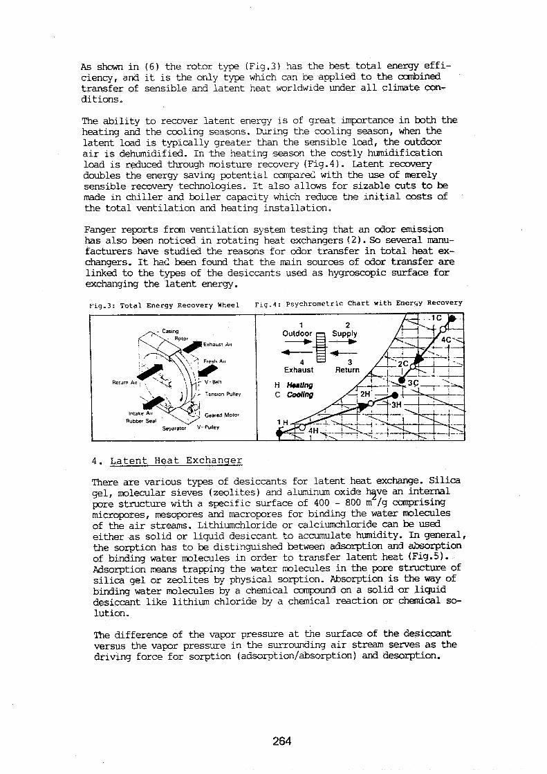
As sham in (6) the rotor type (Fig.3) has the best total energy effi- ciency, and it is the only type which can be applied to the d i n e d transfer of sensible and latent heat worldwide under all climate con- ditions.
The ability to recover latent energy is of great importance in both the heating and the cooling seasons. During the cooling season, when the latent load is typically greater than the senslble load, the outdoor air is dehumidified. In the heating season the costly humidification load is reduced through moisture recovery IFig.4). Latent recovery doubles the energy saving potential comprd with the use of merely sensible recovery technologies. It also allows for sizable cuts to be made in chiller and boiler capacity which reduce tne initial costs of the total ventilation and heating installation.
Fanger reports from ventilation system testing that an odor emission has also been noticed in rotating heat exchangers ! 2 ) . So several manu- facturers have studied the reasons for odor transfer in total heat ex- changers. It h C been found that the min sources of odor transfer are linked to the types of the desiccants used as hygroscopic surface for exchanging the latent energy.
F19.3: Total Energy Recovery Wheel ~ 1 9 . 4 : Psychrometric Chart with E n e r ~ y Recovery
4. Latent Heat Exchanger
There are various types of desiccants for latent heat exchange. Silica gel, molecular sieves (zeolites) and aluminum oxide 3ve an internal pore structure with a specific surface of 400 - 800 m /g carprising micropores, mesopores and macropores for binding the water molecules of the air streams. Lithiurnchloride or calciumchloride can be used either as solid or liquid desiccant to accumulate humidity. In general, the sorption has to be distinguished between adsorption and -rption of binding water molecules in order to transfer latent het (Fig.5). Adsorption means trapping the water molecules in the pore structure of silica gel or zeolites by physical sorption. Absorption is the way of binding water molecules by a chemical compound cn a solid or liquid desiccant like lithium chloride by a chemical reaction or chemical so- lution.
The difference of the vapor pressure at the surface of the desiccant versus the vapor pressure in the surrounding air stream serves as the driving force for sorption (adsorption/absorption) and desorption.
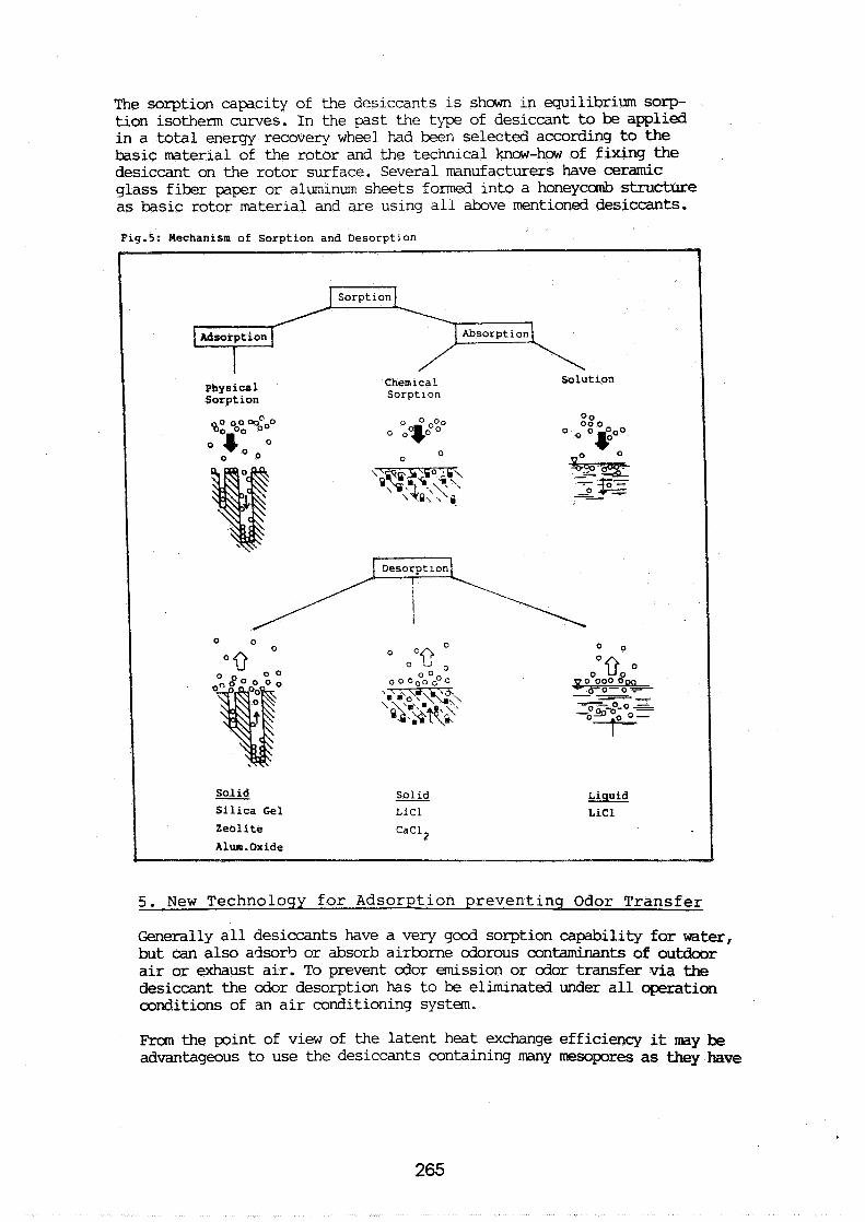
The sorption capacity of the desiccants is sham in equilibrium sorp- tion isotherm curves. In the past the type of desiccant to be applied in a total energy recovery wheel had been selected according to the basic material of the rotor and the technical knm-how of fixing the desiccant on the rotor surface. Several manufacturers have ceramic glass fiber paper or aluminum sheets formed into a honeycomb structure as basic rotor material and are using all above mentioned desiccants.
Fig.5: Mechanism of Sorption and Desorptlon
Chemical Solution Sorption
Sol ld - Silica Gel LiCl
5. New Technology for Adsorption preventing Odor Transfer
Generally all desiccants have a very good sorption capability for water, but can also adsorb or absorb airborne odorous contaminants of outdoor air or exhaust air. To prevent odor emission or odor transfer via the desiccant the odor desorption has to be eliminated under all operation conditions of an air conditioning system.
kcm the point of view of the latent heat exchange efficiency it may be advar,.tageous to use the desiccants containing many mesopores as they have
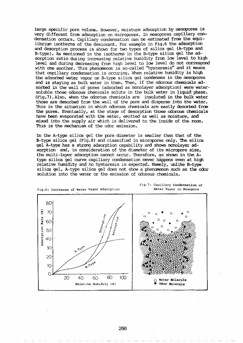
large specific pore volume. However, moisture adsorption by mesopo~s is very different from adsorption on micropores. In mesopores capillary con- densation occurs. Capillary condensation can be estimated fmm the &- librium isotherms of the desiccant. For example in Fig.6 the adsorption and desorption process is shown for two types of silica gel (A-type and B-tw). As mentioned in the isotherms in the B-type silica gel the ad- sorption ratio during increasing relative humidity from l m level to high level and during decreasing from high level to 1 m level do not comspod with one another. This phenawnon is so-called "hysteresis" and it means that capillary condensation is occuring. When relative humidity is high the adsorbed water vapor on B-type silica gel ~~~~es in the mesopores and is staying as bulk water in them. Then, if the odorous chemicals ad- sorbed in the wall of pores (adsorbed as monolayer adsorption) were water- soluble those odorous chemicals solute in the bulk water in liquid phase. (Fig.7).AlsoI when the odorous chemicals are insoluted in the bulk water those are desorbed fran the wall of the pore and disperse into the water. This is the situation in which odorous chemicals are easily desorbed from the pores. Ever.tually, at the stwe of desorption those odorous chemicals have been evaporated with the water, emitted as well as moisture, and mixed into the supply air which is delivered to the inside of the roan. This is the mechanism of the odor emission.
In the A-type silica gel the pore diameter is srnaller than that of the B-type silica gel (Fig.8) and classified in micropores only. 'I'he silica gel A-type has a strong adsorption capability and shaws monolayer ad- sorption and, in consideration of the diameter of its miampore size, the multi-layer adsorption cannot occur. Therefore, as shown in the A- type silica gel c m e capillary condensation never kppens wen at high relative humidity and no hysteresis is expected. Namely, unlike %type silica gel, A-typo, silica gel does not show a phenanenon such as the odor solution into the water or the emission of odorous chemicals.
F1g.7: Capillary Condensation of
F1g.6: Isotherms of Water Vapor Adsorption Water Vapor in Mesopore
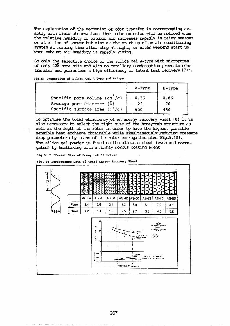
The =planation of the mechanism of odor transfer is corresponding ex- actly w i t h field observations that odor emission will be noticed when the relative humidity of outdoor air increases rapidly in rainy seasons or at a time of showex but also at the start up of an air conditioning system at morning time after stop at night, or after weekend start up
'when exhaust air humidity is rapidly rising.
So only thz selective choice of the silica gel A-type with micropores of only 22A pore size and with no capillary condensation prevents odor transfer and guarantees a high efficiency of latent heat recovery (7)*.
Fig.8: Properties of Silica Gel A-Type and B-Type
To optimise the total efficiency of an energy recovery theel (8) it is also necessary to select the right size of the honeycomb structure as well as the depth of the rotor in order to have the highest possible sensible heat exchange obtainable while simultaneously reducing pressure drop parameters by means of the rotor corrugation size (Fig. 9,10 ) . The silica gel powder is fixed on the aluminum sheet (even and corru- gated) by heatbaking with a highly porous coating agmt
Pig.9: Different Size of Honeycomb Structure
Pig.10: Performance Data of Total Energy Recovery Wheel
6. Summary
Enerqy recovery tcday is routinely incorporated into the ventilation systems of office I=uildings, hospitals, schools, hotels and industrial buildings. Because of the high efficiency for both sensible and latent enenergy recovery the rotating energy exchangers are superior to other types of heat exchangers. The risk of odor transfer in rotating systems had bee.rl investigated theoretically and experimentally. A new desiccant had been developped to prevent cross contamination without decreasing the latent en=ergy recovery efficiency. The new rotors had been introduced successfully in Japan.
7. References
(1) Fanger, P.O.:"A new Philosophy of Ventllatlon". XXII. International Congress for Bulldlng Services Englneerlng, Berlln 1011988
(2' Pejtersen, J., Bluyssen, P., Kondo, H., Clausen, G., Fanger, P.O. (1989): "Air Pollution Sources in Ventl- lation Systems". Proceedings of CLIMA 2000, Sarajevo 811989
(3) Guntermann, K.: "RaumluftqualltZt-Bewertung und MaR- nahmen zur Verbesserung". ISH-Jahrbuch fiir Gebaude- tech~ik, Bertelsmann Verlag 311993
(4) "Guidelines for Ventilation Requirements in Bulldlngs". Report No.11, European Concerted Action Indoor Alr Quality and lts Impact on Man, Commission of the European Communities, 1992
(5) Eurovent 1011 "Heat Recovery Standards", 1985 (6) Dehli, F. (7992): "Energy Recovery in Ventilation
Systems - A Worldwide Energy Saving and Environ- mental Protection Technology". Proceedings of the 13th AIVC-Conference "ventilation for Enerqy Efficiency and Optlmum Indoor Alr Quality", Nice 9 I1 997 - , - - -
* ( 7 ) Kuma, T., Shirahama, N. (Seibu Giken): New Total Heat Recovery Wheel Shuttlng out Odor Transfer". 58th General Meetlng of the Society of Chemlcal Engineering of Japan, Kagoshima 311993
(8) Kuma,T., Hirose, T. (Selbu Giken): "Honeycomb-shaped Heat Exchanger". 69th Meeting of the Soclety of Mechanical Engineers of Japan, Nagoya 1 011 991
* The "No-Odor Transfer Rotor" 1s a development of the company
Se5u Giken Co.,Lkd. 1033-5 Wada, Sasagarl-machl Kasuya-gun, Fukuoka-keniJapan
Patents pendlng: ;span, Korea, USA, Germany, Sweden, UK.
Energy Impact of Ventilation and Air Infiltration 14th AlVC Conference, Copenhagen, Denmark
21 -23 September 1993
Modelling Adjustable Speed Drive Fans to Predict Energy Savings in VAV Systems
D Lorenzetti
Building Technology Group, M.I.T. Department of Architecture, Room 4-209, 77 Massachusetts Avenue, Cambridge, MA 02139, USA
Modeling Adjustable Speed Drive Fans to Predict Energy Savings in VAV Systems
David M. Lorenzem Department of Architecture
Massachusetts Institute of Technology Cambridge, Massachusetts
SYNOPSIS
The momentum balance on a centrifugal fan, supplemented by a complete energy balance for rigorous interpretation of power-pressure interactions, relates these variables to flow rate and fan speed. Nonideal behavior is modeled by direct mechanical interpretation and by engineering correlation, leading to more general expressions than provided by the fan laws. First attempts to fit these expressions to measured data show promise but reveal limitations of current practice in the data collection and reporting process.
LIST OF SYMBOLS
Variables a Arbitrary pressure coefficient A Effective flow area b Arbitrary power coefficient c Absolute velocity of air [=I m/s d Characteristic fan size [=I m e Reynolds variation exponent [=I 1 f Moody friction factor [=I 1 rh Mass flow rate [=I kg/s n Fan speed [=] rpm p Pressure [=I kg/m.s2 P Power [=] kg-m2/s3 r Radial distance [=I m Re Reynolds number [=I 1 T Torque [=I kg.m2/s2
Operators, subscripts, and overscripts { ] Functional relationship [=] Has the units of
1 Of fan, at entrance to impeller 2 Of fan, at exit from impeller exit At fan exit eye At fan entrance fan Through or across fan fan Of power, delivered by fan to air
Impeller linear velocity [=I m/s Specific internal energy [=I m2/s2 Air velocity relative to impeller [=I m/s
Kinetic energy factor [=I 1 Velocity diagram angle Absolute surface roughness [=] m Flow coefficient [=] 1 Efficiency [=I 1 Dynamic viscosity [=I kg/m.s Density [=I kg/m3 Angular velocity [=I s-l Head coefficient [=I 1
id1 Ideal result for lossless case imp Through or across impeller 9 Tangential component r Radial component shft Of power, required at drive shaft z Axial component
- Vector quantity * At zero slip
1. INTRODUCTION
In a Variable Air Volume (VAV) ventilation system, a central fan supplies a variable flow rate of air to the conditioned spaces. Flow is regulated by dampers, inlet vanes, or by speed modulation of the fan, to meet the temperature and fresh air requirements of the local zones served by the fan. A return fan, similarly regulated, exhausts air from the zones.
Dampers and inlet vanes govern flow by increasing losses of mechanical energy along the flow path, thus decreasing the flow rate through the duct. If the same, lower, flow rate is established by decreasing fan speed, mechanical energy losses are reduced in the fan, rather
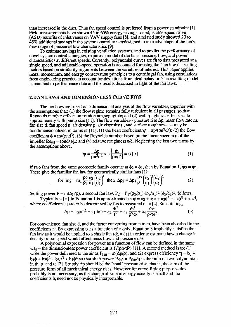
than increased in the duct. Thus fan speed control is p r e f e d from a power standpoint [I]. Field measurements have shown 45 to 65% energy savings for adjustable-speed drive (ASD) retrofits of inlet vanes on VAV supply fans [8], and a related study showed 20 to 45% additional savings if the system controller is redesigned to take advantage of the fan's new range of pressure-flow characteristics [9].
To estimate savings in existing ventilation systems, and to predict the performance of novel system control strategies, requires a model of the fan's pressure, flow, and power characteristics at different speeds. Currently, polynomial curves are fit to data measured at a single speed, and adjustable-speed operation is accounted for using the "fan lawsn-- scaling factors based on similarity arguments between the variables of interest. This paper applies mass, momentum, and energy conservation principles to a centrifugal fan, using correlations from engineering practice to account for deviations from ideal behavior. The resulting model is matched to performance data and the results discussed in light of the fan laws.
2. FAN LAWS AND DIMENSIONLESS CURVE FITS
The fan laws are based on a dimensional analysis of the flow variables, together with the assumptions that: (1) the flow regime remains fully turbulent in all passages, so that Reynolds number effects on friction are negligible; and (2) wall roughness effects scale approximately with pump size [ll]. The flow variables-- pressure rise Ap, mass flow rate m, fan size d, fan speed n, air density p, air viscosity p, and surface roughness E-- may be nondimensionalized in terms of [1 11: (1) the head coefficient y = ApI(pn2d2); (2) the flow coefficient @ = W(pnd3); (3) the Reynolds number based on the linear speed n-d of the impeller Rend = (pnd2)/p; and (4) relative roughness dd. Neglecting the last two terms by the assumptions above,
If two fans from the same geometric family operate at = $1, then by Equation 1, 1y2 = 1y1. These give the familiar fan-law for geome&cdly similar fans [I]:
Setting power P = m(Ap/p), a second fan law, P;! = ~~-(p2/p~).(n~/n~)3.(d~/d1)5, follows. Typically y ( @ ) in Equation 1 is approximated as y = ag + al@ + a2@ + a3@3 +
where coefficients ai are to be determined by fits to measured - data [2]. Substituting,
For convenience, fan size d, and the factor converting from n to o , have been absorbed in the coefficients ai. By expressing y as a function of @ only, Equation 3 implicitly satisfies the fan law as it would be applied to a single fan (d2 = dl) in order to estimate how a change in density or fan speed would affect mass flow and pressure rise.
A polynomial expression for power as a function of flow can be defined in the same way-- the dimensionless power coefficient is pl(pn3d5) [l 11. A second method is to: (1) write the power delivered to the air as Pf, = m(Ap/p); and (2) express efficiency q = bo + bl@ + b2@2 + b3@3 + b4@4 so that shaft power Pshft = P f d q is the ratio of two polynomials in m, p, and o [2]. Strictly Ap should be the "total" pressure rise, that is, the sum of the pressure form of all mechanical energy rises. However for curve-fitting purposes this probably is not necessary, as the change of kinetic energy usually is small and the coefficients bi need not be physically interpretable.
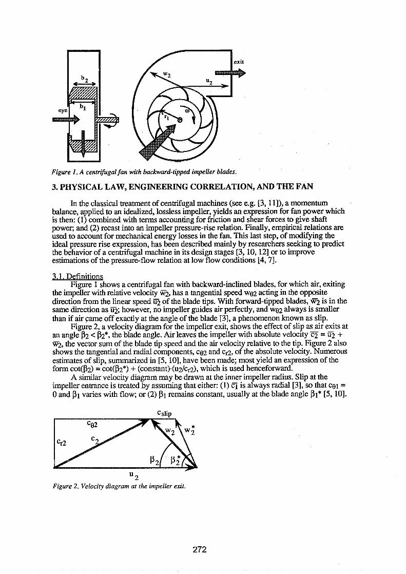
Figure 1. A centrifugal fan with backward-tipped impeller blades.
3. PHYSICAL LAW, ENGINEERING CORRELATION, AND THE FAN
In the classical treatment of centrifugal machines (see e.g. [3, 1 I]), a momentum balance, applied to an idealized, lossless impeller, yields an expression for fan power which is then: (1) combined with terms accounting for friction and shear forces to give shaft power; and (2) recast into an impeller pressure-rise relation. Finally, empirical relations are used to account for mechanical energy losses in the fan. This last step, of modifying the ideal pressure rise expression, has been described mainly by researchers seeking to predict the behavior of a centrifugal machine in its design stages [3,10,12] or to improve estimations of the pressure-flow relation at low flow conditions [4,7].
3.1. Definitions Figure 1 shows a centrifugal fan with backward-inclined blades, for which air, exiting
the impeller with relative velocity F2, has a tangential speed we2 acting in the opposite direction from the linear speed T2 of the blade tips. With forward-tipped blades, W2 is in the same direction as T2; however, no impeller guides air perfectly, and we2 always is smaller than if air came off exactly at the angle of the blade [3], a phenomenon known as slip.
Figure 2, a velocity diagram for the impeller exit, shows the effect of slip as air exits at an angle P2 < w, the blade angle. Air leaves the impeller with absolute velocity = iQ + F2, the vector sum of the blade tip speed and the air velocity relative to the tip. Figure 2 also shows the tangential and radial components, ce2 and cd, of the absolute velocity. Numerous estimates of slip, summarized in [5,10], have been made; most yield an expression of the form cot(P2) = cot@*) + (constant).(u~c~), which is used henceforward.
A similar velocity diagram may be drawn at the inner impeller radius. Slip at the impeller entrance is treated by assuming that either: (1) Cj is always radial [3], so that eel = 0 and pl varies with flow; or (2) pl remains constant, usually at the blade angle PI* [5, 101.
u 2 Figure 2 . Velocity diagram at the impeller exit.
3.2 Momentum Conservation in the Lossless Impeller The application of momentum conservation to a lossless centrifugal impeller is treated
in detail in e.g. [3,11]; the following overview highlights the idealizations made. At steady- state, conservation of angular momentum requires the sum of applied moments to balance the net rate of outflow of angular momentum from the control volume [I 11. For the annular region between the impeller entrance and exit, the moments include the torque T transmitted through the shaft, and those due to bearing friction and shear forces from the flow of air along the blades. These last two are neglected for the idealized, lossless, process, but are included later. Since pressure forces act radially they produce no moment. Taking o positive as shown in Figure 1, torque acts in the positive axial direction and therefore only the axial component of angular momentum leaving the control volume need be considered.
Only the tangential component of the fluid velocity produces an axial moment, so the outward angular momentum flux is J(r2ce2)drh at the impeller exit and k - r l c g l ) ~ at its inlet, where the flow is into the control volume. Combining, the momentum balance gives torque T = mimp(r2ce2 - rlcel) for the lossless impeller.
Fan power is P = COT, and using u = m, Pidl = mimp(u2ce2 - ~ 1 ~ 0 1 ) (4)
From the velocity diagram, c~cot(P2) = u2 - ce2. The slip expression described above gives cot@), and for incompressible flow the radial velocity is given by mimp = pA2c~. Estimates of the reduction of flow area A2 from its maximum of 2m2b2, taking into account blade thickness and recirculation effects at the periphery of the impeller [3,10], show no dependence on mass flow or angular velocity. Therefore A2 is treated as constant, although separation effects, which influence A2, play a role in impeller efficiency [12]. Since A2 already incorporates scaling factors, it is not necessary to assume c d is uniform over the flow area; only that the velocity profile across each blade passage remains similar, regardless of flow rate.
The inlet geometry is similar, although slip is treated differently, as mentioned above. The question of slip at the impeller inlet can be rendered moot by extending the control volume into the impeller core so that air crosses the control surface in the axial, rather than the radial, direction. In this case the momentum flux at the inlet becomes k-~c&y~)&, integrated from r = 0 to rl. The tangential velocity at the inlet, ceeye, sometimes known as "swirl" [12], accounts for the power benefit associated with inlet vanes over dampers [I]: while both regulate flow through dissipation, inlet vanes impart a prerotation to the air.
However slip is treated at the impeller entrance, the ideal power relation reduces to mlP20
Pidl = b lmimpd + b2 P (5)
where constants bl and b;! incorporate the physical and experimental parameters.
3.3 Nonideal processes affectin? fan Dower The ideal power expression must be modified to include the nonideal processes
affecting fan power. These are: (1) bearing loss due to friction in the shaft bearings, for which power is proportional to o [3,10]; and (2) disc loss, the power needed to overcome friction torque on the impeller surfaces [3,5, 101. From P = COT, disc power is proportional to o times a shear force; note that this treatment of disc power departs from that of [3,5, 101, which use P = Ap.A.v rather than P = oT.
The shear forces influencing disc loss, derived by analogy with turbulent duct flow, are proportional to pv2 [l 11. The characteristic velocity is o in the core and on external surfaces, and w2 in the blade passages. The disc friction power terms are: (1) p d in the core; and (2) mimpG, mimp2w/p, and p d in the flow passages, after w22 = cr22(1 + cot2P2) is substituted from the velocity diagram. Then shaft power becomes
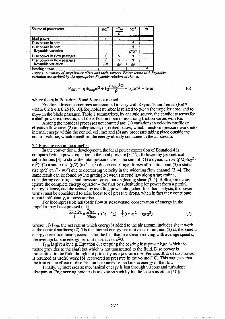
Table 1. Summary of shaft power terms and their sources. Power terms with Reynolds variation are divided by the appropriate Reynolds relation as shown.
where the bi in Equations 5 and 6 are not related. Frictional losses sometimes are assumed to vary with Reynolds number as (Re)"
where 0.2 1 e 10.25 [5, 101. Reynolds number is related to p o in the impeller core, and to mimp in the blade passages. Table 1 sumrnarizes, by analytic source, the candidate terms for a shaft power expression, and the effect on them of assuming friction varies with Re.
Among the nonideal processes not counted are: (1) variations in velocity profile or effective flow area; (2) impeller losses, described below, which transform pressure work into internal energy within the control volume; and (3) any processes taking place outside the control volume, which transform the energy already contained in the air stream.
3.4 Pressure rise in the impeller In the conventional development, the ideal power expression of Equation 4 is
compared with a power equation in the total pressure 13, 111, followed by geometrical substitutions [3] to show the total pressure rise is the sum of: (1) a dynamic rise (p12)-(c2~ - c12); (2) a static rise (p/2)-(u22 - u12) due to centrifugal forces of rotation; and (3) a static rise (~12)-(w12 - due to decreasing velocity in the widening flow channel [3,4]. The same result can be found by integrating Newton's second law along a streamline, considering centrifugal and pressure forces but neglecting shear [3,4]. Both approaches ignore the complete energy equation-- the first by substituting for power from a partial energy balance, and the second by avoiding power altogether. In either analysis, the power terms must be considered to arise because of pressure drops, when in fact they contribute, albeit inefficiently, to pressure rise.
For incompressible adiabatic flow at steady-state, conservation of energy in the impeller may be expressed [I 11
where: (1) Pf,, the net rate at which energy is added to the air stream, includes shear work at the control surfaces; (2) B is the internal energy per unit mass of air; and (3) a , the kinetic energy correction factor, accounts for the fact that in a stream moving with average speed c, the average kinetic energy per unit mass is not ~212.
Pf, is given by e.g. Equation 6, excepting the bearing loss power b4o, which the motor provides to the shaft but which is not transmitted to the fluid. Disc power is transmitted to the fluid though not primarily as a pressure rise. Perhaps 30% of disc power is returned as useful work [5], recovered as pressure in the volute [lo]. This suggests that the immediate effect of disc friction is to increase the kinetic energy of the flow.
Finally, fi2 increases as mechanical energy is lost through viscous and turbulent dissipation. Engineering practice is to express such hydraulic losses as either [lo]:

(1) dynamic (mixing and shock) losses of the form Ap = pv2; or (2) friction losses of the form Ap = f pv2, where friction factor f may vary with Reynolds number.
Impeller dynamic losses include: (1) entry shock due to the equivalent of slip at the impeller inlet, modeled as a mismatch velocity akin to cslip in Figure 2 [3,5, 101; (2) profile drag on the impeller blades, modeled as a relative speed w [lo]; and (3) wake shedding from the blades at the impeller exit, modeled as a sudden expansion loss in c n [lo].
Impeller friction losses are attributed to a representative relative velocity w [3,5,10]. Where disc power treats friction as a force producing a torque, impeller friction treats friction as a mechanism transforming the input power from pressure work to internal energy. Therefore the terms generated by these hydraulic losses are not quite the same as those due to disc friction. Table 2 demonstrates the differences between the terms.
3.5 Nonideal processes in the fan entrance and volute Energy balances similar to Equation 7 may be written from the eye to the impeller
inlet, and from the impeller outlet to the fan exit. Summing the three equations yields an expression for the fan pressure rise. Replacing changes in internal energy by the engineering approximations - of the hydraulic loss terms,
Pfan 1 Pexit - Peye = P + 3 ~(%yeceye~ - %xitcexit2) + pg(Gye - Gxid - Uploss (8)
where the pressures and kinetic energies internal to the fan have canceled, and the possibility of changes in gravitational potential energy has been admitted.
Due to leakage between the high- and low-pressure sides of the fan, the mass flow through the impeller will be higher than that through the fan. Leakage flow (mirn - rhfan) =
1/=[10]; unfortunately this expression leads to an implicit equation in (pi - pl). Thus this nonideality is ignored, and henceforward, mim d = Velocities ceye and cexit are related to mass ow by the density and the inlet and exit areas; the contribution of these terms, with a taken as constant, is given in Table 2. Note that at low flows the assumption %,it constant is especially problematic due to recirculation in the discharge duct [I, 71. Hydraulic losses in the eye and volute are summarized in [3,5,10] and produce the same functional terms as in the impeller; see Table 2.
Table 2. Summary of pressure terms and their sources.
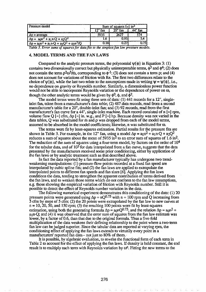
I I I I
Table 3. Error sums of squares for data fits to the simplest fan law pressure models.
4. MODEL TERMS AND THE FAN LAWS
Compared to the analytic pressure terms, the polynomial y($) in Equation 3: (1) contains two dimensionally carrect but physically uninterpretable terms, and @; (2) does not contain the term p2dIri-1, corresponding to $-I; (3) does not contab a term p; and (4) does not account for variations of friction with Re. The fmt two differences relate to the choice of y{$), while the last two relate to the assumptions made in writing y = y($), i.e., no dependence on gravity or Reynolds number. Similarly, a dimensionless power function would not be able to incorporate Reynolds variation or the dependence of power on a , though the other analytic k s would be given by $0, $, and $2.
-
The model terms were fit using three sets of data: (1) 441 records for a 12", single- inlet fan, taken from a manufacturer's data table; (2) 487 data records, read from a second manufacturer's table for a 20", double-inlet fan; and (3) 92 records, read from the first manufacturer's fan curve for a 44", single-inlet machine. Each record consisted of n [=I rpm, volume flow Q [=I cfm, Ap [=] in. w.g., and P [=I hp. Because density was not varied in the data tables, Q was substituted for m and p was dropped from each of the mode1 terms, assumed to be absorbed in the model coefficients; likewise, n was substituted for a.
The terms were fit by least-squares estimation. Partial results for the pressure fits are shown in Table 3. For example, in the 12" fan, using a model Ap = aon2 + aln-Q + a 2 ~ 2 reduces a sum of squares about the mean of 5935 in2 to an error sum of squares of 1.6 in2. The reduction of the sum of squares using a four-term model, by factors on the order of lo4 for the tabular data, and of 103 for data interpolated from a fan curve, suggests that the data presented by the manufacturers received some prior conditioning, either by application of the fan laws or by analytic treatment such as that described above.
In fact the data reported by a fan manufacturer typically has undergone two trend- weakening manipulations: (1) pressure-flow points recorded at a futed fan speed are interpolated by cubic spline fits; and (2) the fan laws are applied to extrapolate the interpolated points to different fan speeds and fan sizes [6]. Applying the fan laws conditions the data, tending to strengthen the apparent contribution of terms derived from the fan laws, and to weaken those terms which do not conform to the fan law assumptions, e.g. those showing the empirical variation of friction with Reynolds number. Still it is possible to detect the effect of Reynolds number variation in the data.
The following numerical experiment demonstrates this conditioning of the data: (1) 20 pressure points were generated using Ap = n~0.75 with n = 100 rpm and Q increasing from 5 cfm by steps of 5 cfm; (2) the 20 points were extrapolated by the fan law to new curves at n = 10,20,50, and 150 rpm; (3) the resulting 100 points were fit by least-squares estimation, using both the generating formula Ap = son@-75, and the relation Ap = aOn2 + aln-Q; and (4) it was observed that the error sum of squares from the fan law estimate was lower, by a factor of 0.6, than that due to the original formula. Thus a five-fold multiplication of the data weakens their defining relationship to the point where a two-term fan law can be judged superior. Since the tabular data are reported at varying rpm, the conditioning effect of applying the fan laws extends to virtually every point in a manufacturers' reported fan data-- not just to 80% of them. -
It is possible, by algebraic evaluation, to rewrite the functional form of each term in Table 2 to account for the effect of applying the fan laws. If density is held constant, the end result is to multiply each term with Reynolds variation by OF. Fitting the new terms to the

data gives an order of magnitude improvement in the error sums of squares, an effect which would not be expected if there was in fact no variation of friction with Reynolds number. However, it is impossible using this method to distinguish Reynolds effects due to changes in co, since the original data were measured at a single speed.
5. CONCLUSION
Analytic expressions have been developed for power and pressure in a centrifugal fan. These may be expected to represent fan behavior more accurately than do the fan laws, and preliminary data fits show evidence of the nonideal behavior modeled. However if the data to be fit are extrapolated from single-speed measurements using the fan laws, there is little incentive to seek more general or rigorous formulations. In any fan model, the choice of terms can be guided by physical law as well as by functional convenience.
ACKNOWLEDGEMENTS
This work is the outgrowth of a research project financially supported by EUA Cogenex, Northeast Utilities, and the Empire State Energy Research Corporation. The author also wishes to acknowledge the contributions and continued support of J.W. Axley and L.K. Norford, both of the Massachusetts Institute of Technology.
REFERENCES
1. ASHRAE, 1988.1988 ASNRAE Handbook, Equipment, SI Edition. American Society of Heating, Refrigerating and Air-Conditioning Engineers, Inc., Atlanta.
2. Brandemuehl, M.J. et al, 1992. "A Toolkit for Secondary HVAC System Energy Calculations." American Society of Heating, Refrigerating and Air Conditioning Engineers, Inc., Atlanta.
3. Eck, B.E., 1973. Fans; the design and operation of centrifugal, axial-flow, and cross-flow fans. Translated by Azad, R.S. and Scott, D.R. Pergamon Press, Oxford.
4. Engeda, A. and Rautenberg, M., 1989. "On the Flow in a Centrifugal Pump Near Shut-Off Head with Positive and Negative Flows," Eleventh International Conference of the British Pump Manufacturer's Association, April 1989, pp. 1-7. Springer-Verlag, Berlin.
5. Dick, E. and Belkacemi, M., 1992. "Optimum Design of Centrifugal Fans and Pumps," European Journal of Mechanical Engineering, v. 37, no. 1, March 1992, pp. 9-18.
6. Franklin, M. Personal communication. Twin City Fan and Blower, Minneapolis. 7. Frost, T.H. and Nilsen, E., 1991. "Shut-off Head of Centrifugal Pumps and Fans,"
Proceedings of the Institution of Mechanical Engineers, Part A: Journal of Power and Energy, v. 205, no. A3, pp. 217-23.
8. Lorenzetti, D.M. and L.K. Norford, 1992. "Measured Energy Consumption of Variable-Air-Volume Fans Under Inlet Vane and Variable-Speed-Drive Control," ASHRAE Transactions, Vol. 98, Part 2, 1992, pp. 37 1-79.
9. Lorenzetti, D.M. and L.K. Norford, 1993. "Pressure Reset Control of Variable Air Volume Ventilation Systems," Proceedings of the ASME International Solar Energy Conference, April 1993, pp. 445-53. American Society of Mechanical Engineers, New York.
10. Neumann, B., 1991. The Interaction Between Geometry and Pevormance of a Centrifugal Pump. Mechanical Engineering Publications Ltd., London.
1 1. White, F.M., 1979. Fluid Mechanics. McGraw-Hill Inc., New York. 12. Wilson, D.G., 1989. The Design of High-Eflciency Turbomachinery and Gas
Turbines, 4th printing. The MIT Press, Cambridge, Massachusetts.


Session 4: Posters - Ventilation Energy and IAQ


Energy Impact of Ventilation and Air Infiltration 14th AlVC Conference, Copenhagen, Denmark
21 -23 Septem ber 1993
High Comfort to Reasonable Cost
B Barath
lngenieiirburo Barath & Wagner GmbH, Wleerbusch, Germany
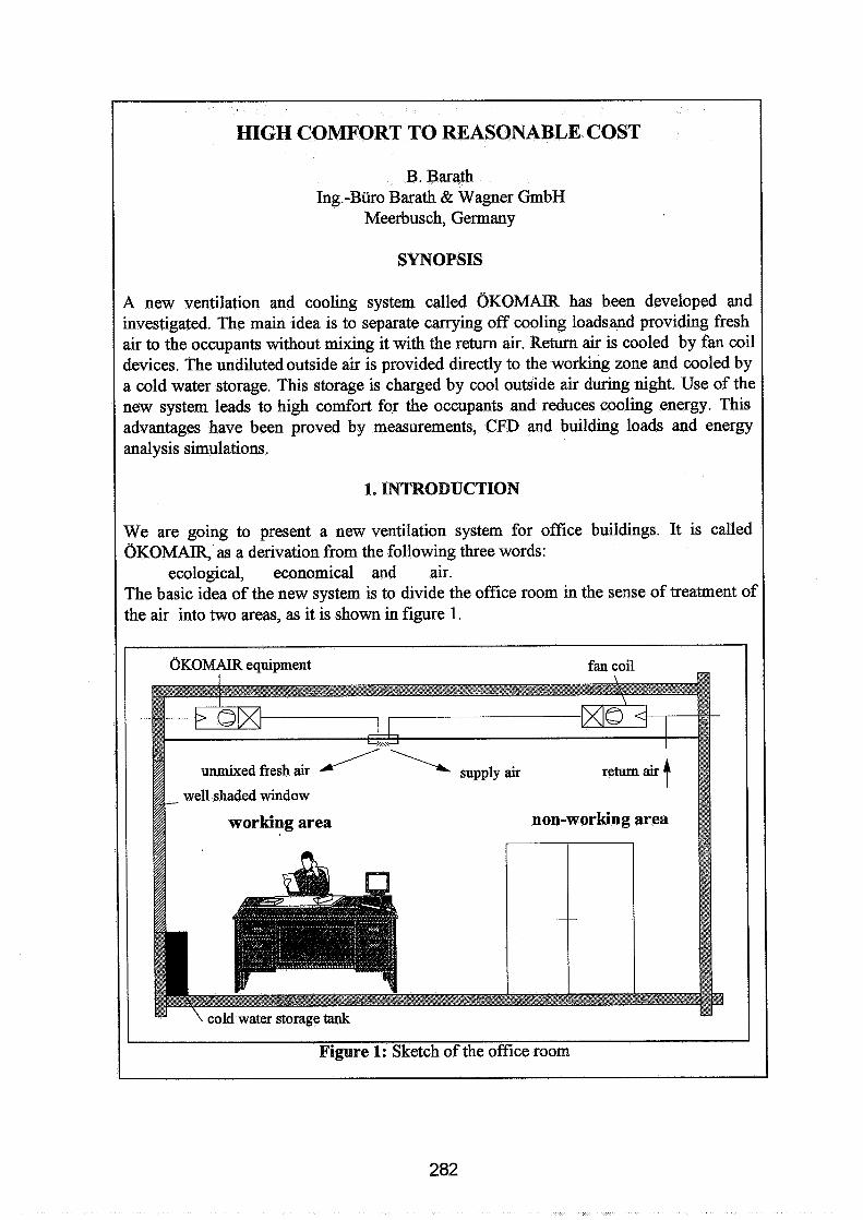
HIGH COMFORT TO REASONABLE COST
B. Barath 1ng.-Biiro Barath & Wagner GmbH
Meerbusch, Germany
SYNOPSIS
A new ventilation and cooling system called OKOMADR has been developed and investigated. The main idea is to separate carrying off cooling loadsand providing fresh air to the occupants without mixing it with the return air. Return air is cooled by fan coil devices. The undiluted outside air is provided directly to the working zone and cooled by a cold water storage. This storage is charged by cool outside air during night. Use of the new system leads to high comfort for the occupants and reduces cooling energy. This advantages have been proved by measurements, CFD and building loads and energy analysis simulations.
We are going to present a new ventilation system for office buildings. It is called OISOMAIR, as a derivation from the following three words:
ecological, economical and air. The basic idea of the new system is to divide the office room in the sense of treatment of the air into two areas, as it is shown in figure 1.
~KOMAIR equipment fan coil
unmixed fresh air
well shaded window
non-working area
Figure 1: Sketch of the office room ' I
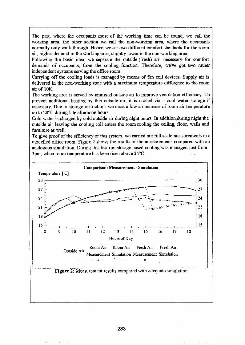
The part, where the occupants most of the working time can be found, we call the working area, the other section we call the non-working area, where the occupants normally only walk through. Hence, we set two different comfort standards for the room air, higher demand in the working area, slightly lower in the non-working area. Following the basic idea, we separate the outside (fresh) air, necessary for comfort demands of occupants, from the cooling function. Therefore, we've got two rather independent systems serving the office room. Carrying off the cooling loads is managed by means of fan coil devices. Supply air is delivered in the non-working zone with a maximum temperature difference to the room air of 10K. The working area is served by unmixed outside air to improve ventilation efficiency. To prevent additional heating by this outside air, it is cooled via a cold water storage if necessary. Due to storage restrictions we must allow an increase of room air temperature up to 28°C during late afternoon hours. Cold water is charged by cold outside air during night hours. In addition,during night the outside air leaving the cooling coil enters the roomcooling the ceiling, floor, walls and furniture as well. To give proof of the efficiency of this system, we carried out full scale measurements in a modelled office room. Figure 2 shows the results of the measurements compared with an analogous simulation. During this test run storage based cooling was managed just from 3pm, when room temperature has been risen above 24°C.
Comparison: Measurement - Simulation Temperature [ C] 3 0 3 0
27 27
24 24
21 21
18 18
15 15 8 9 10 11 12 13 14 15 16 17 18
Hours of Day
Room Air Room Air Fresh Air Fresh Air Outside Air
Measurement Simulation Measurement Simulation - - - - * - - - - -
Figure 2: Measurement results compared with adequate simulation
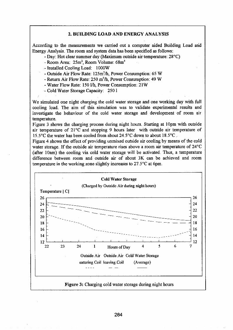
2. BUILDING LOAD AND ENERGY ANALYSIS
According to the measurements we carried out a computer aided Building Load atid Energy Analysis. The room and system data has been specified as follows:
- Day: Hot clear summer day (Maximum outside air temperature: 28°C) - Room Area: 25m2, Room Volume: 68m3 - Installed Cooling Load: 1000W - Outside Air Flow Rate: 125m3/h, Power Consumption: 65 W - Return Air Flow Rate: 250 m3/h, Power Consumption: 49 W - Water Flow Rate: 150 l/h, Power Consumption: 21W - Cold Water Storage Capacity: 250 1
We simulated one night charging the cold water storage and one working day with full cooling load. The aim of this simulation was to validate experimental results and investigate the behaviour of the cold water storage and development of room air temperature. Figure 3 shows the charging process during night hours. Starting at 10pm with outside air temperature of 21°C and stopping 9 hours later with outside air temperature of 15.5"C the water has been cooled from about 24.5"C down to about 18.5'C . Figure 4 shows the effect of providing unmixed outside air cooling by means of the cold water storage. If the outside air temperature rises above a room air temperature of 24°C (after loam) the cooling via cold water storage will be activated. Thus, a temperature difference between room and outside air of about 3K can be achieved and room temperature in the working zone slightly increases to 27.5'6 at 6pm.
Cold Water Storage
(Charged by Outside Air during night hours) Temperature [ C]
26
24
22
20
18
26
24
22
20
18
: . . - - - \ . . . -
1- .- . - - - - - - -
- - - _ _ ------ . . . . 16
14
12
- ..-------__-__ C C - 16 - - _ _ - * -
- - - - - - - _ _ _ _ _ _ _ _ _ - _ _ - - - - 14 I I I I I I I I 12
22 23 24 1 Hours of Day 4 5 6 7
Outside Air Outside Air Cold Water Storage
entering Coil leaving Coil (Average) - - - - - -
Figure 3: Charging cold water storage during night hours

Temperatures in the working zone Temperature [ C]
3 0 - 27 -
- _ _ _ - - - _ _ _ _ - - - - _ _ - - - - -
_ - - - _ _ - - - -
_ - - - , _ - - -
-
-
15 - - I 1 l I I I I I I I I I I I I ~ I I I
3 0
27
24
21
18
15
8 9 10 11 12 13 14 15 16 17 18
Hours of Day
Room Air Supply Air Outside Air - - - -
Figure 4: Development of room air temperature in the working zone
3. COMPARISON OF DIFFERENT HVAC-SYSTEMS
The major advantage of the new system is saving cooling energy. To give proof of this statement we carried out comparative investigations of different, widely used HVAC-systems. Besides our systems we simulated a variable air volume system and a two-pipe fan coil system, both serving the same office room, as specified above. These common systems need much more cooling energy for cooling necessary outside air. A minimum supply air temperature for all systems of 15°C has been defined. Figure 5 shows hourly room cooling loads and cooling rates of all systems. As it is seen, a small portion of cooling is also achieved by serving the working zone with unmixed outside air in the OKOMAIR-system. From high noon to end of working time cooling rates of common systems exceeds room cooling loads due to additional cooling of warm outside air. During f ~ s t 3 working hours the variable air volume system can serve with outside air only, but it must cooled down to 15OC, what seems to be an disadvantage. Finally, figure 6 shows the summary of-energy consumed by all systems, cooling and electrical energy, respectively. Using OKOMAIR-system we must pay saving cooling energy with consuming additional electrical energy due to night storage charging. Taking into account the advantages in improving room air comfort for occupants a major saving of energy costs can be achieved. Figure 7 shows the investment costs for all system in comparison.
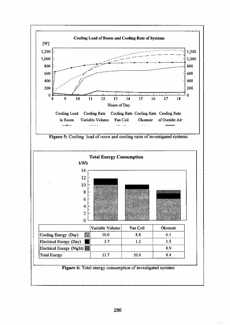
Cooling Load of Room and Cooling Rate of Systems [wl
_---- 1,200
1,000
800
600
400
200
0 10 11 12 13 14 15 16 17 18
Hours of Day
Cooling Load Cooling Rate Cooling Rate Cooling Rate Cooling Rate
in Room Variable Volume Fan Coil dkomair of Outside Air -.- - - - - - - -
Figure 5: Cooling load of room and cooling rates of investigated systems
Total Energy Consumption kwh
14
12
10
8
6
4
2
0
Figure 6: Total energy consumption of investigated systems
Okomair
6.1
1.5
0.9
8.4
Cooling Energy (Day)
Electrical Energy (Day)
Electrical Energy (Night)
Total Energy
Variable Volume
10.0
1.7
11.7
Fan Coil
8.8
1.2
10.0
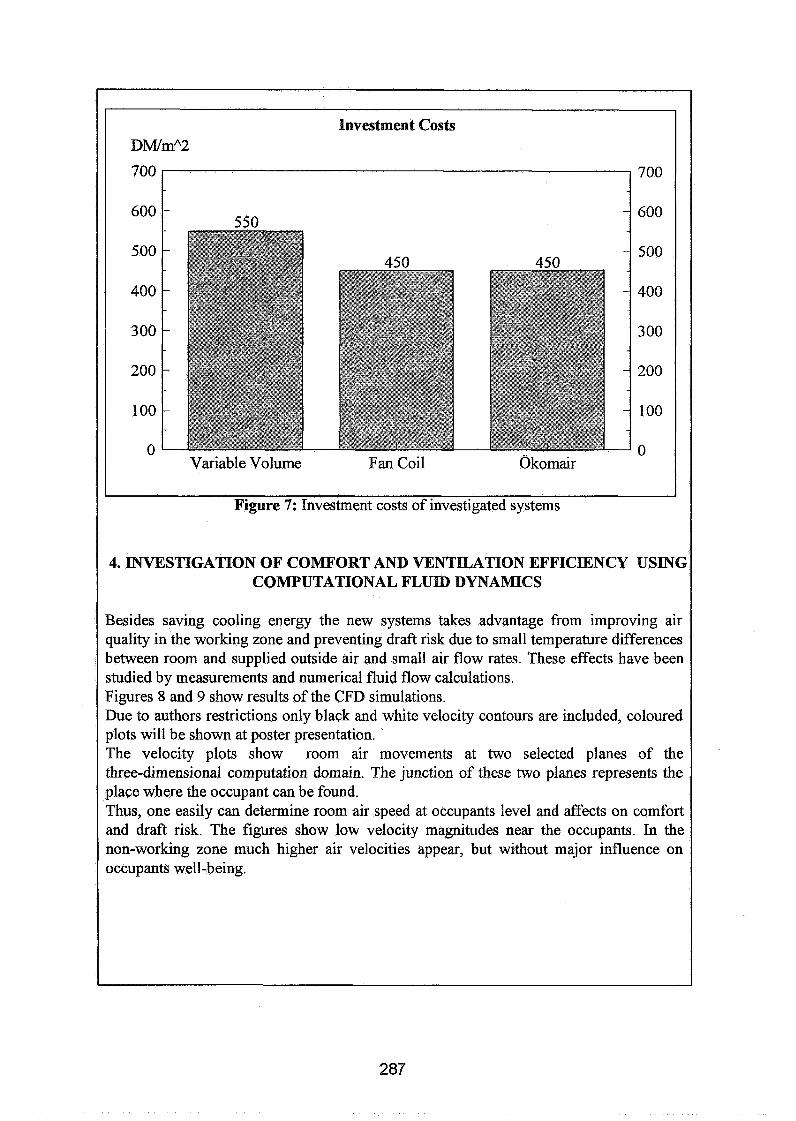
Investment Costs DM/mA2
700 700
600 600
500 500
400 400
3 00 3 00
200 200
100 100
0 0 Variable Volume Fan Coil Okomair
Figure 7: Investment costs of investigated systems
4. INVESTIGATION OF COMFORT AND VENTILATION EFFICIENCY USING COMPUTATIONAL FLUID DYNAMICS
Besides saving cooling energy the new systems takes advantage from improving air quality in the working zone and preventing draft risk due to small temperature differences between room and supplied outside air and small air flow rates. These effects have been studied by measurements and numerical fluid flow calculations. Figures 8 and 9 show results of the CFD simulations. Due to authors restrictions only black and white velocity contours are included, coloured plots will be shown at poster presentation. The velocity plots show room air movements at two selected planes of the three-dimensional computation domain. The junction of these two planes represents the place where the occupant can be found. Thus, one easily can determine room air speed at occupants level and affects on comfort and draft risk. The figures show low velocity magnitudes near the occupants. In the non-working zone much higher air velocities appear, but without major influence on occupants well-being.

I I Figure 8: Contours of velocity magnitudes from 0 to 0.2mIs (front view)
I I Figure 9: Contours of velocity magnitudes from 0 to 0.2mIs (side view)
The author gratefully expresses his thanks to Prof. Grdf (Institute of Energy and Air Conditioning, GieRen) for experiments, Prof. Boiting (Technical College, Miinster) for CFD-simulations using FLUENT V.4.11 and Mr. Morgenstern (1ng.-Biiro Barath & Wagner, Meerbusch) for building simulations using MICRO-DOE2.
Energy lrn pact of Ventilation and Air Infiltration 14th AlVC Conference, Copenhagen, Denmark
21 -23 Septem ber 1993
Clean Room Technology
J Pedersen
Birch & Krogboe, Consultants and Planners, Teknikerbyen 34, DK-2830 Virum, Denmark
Clean Room Technology
High quality is a prerequisite for industry to sell its products. To secure an op- timized production and at the same time assure a minimum of wastage, it is often required that the production takes place in an environment where control is exerted on the particle concentration in the air and also on thermal conditions.
Medical production is subjected to requirements from the authorities to comply with definite requirements of purity, according to the pharmaceutical in question.
Micro-electronic or mechanical industries indispensably require clean room technol- ogy, if rejections of finished products are to be avoided.
Experience shows that the quality of many food products gets an improved durability and less risk of bacterial contamination, when clean room technology is applied in the sections of production where the food products are most vulnerable to con- tamination from raw materials, air, water and human beings.
Background
Clean room technology has its origin in the military exploitation of nuclear energy. However in the 1950 and the 1960 the more peaceful utilization accelerated.
The micro-biologically controlled room - the clean room - was accepted and prevailed in the industries where dust and microorganisms were real "poison" to the products - i.a. in the pharmaceutical and the electronics industries. For these industries it was necessary to operate in clean rooms or with elements from the clean room technology to be able to deliver goods of the quality wanted by the market. Within the food industry, the producers started later to implement complete solutions corresponding to those known in the phar- maceutical industry.
Clean room technology is not a universal solution, solving all problems by killing all micro- organisms. The clean room technology is a tool which - by its many elements - succeeds in getting control of both particle concentration, as well as the microbiological contamination of the room.
For pharmaceutical production and food processing, it is primarily a question of avoiding live micro-organisms, while for the electronics industry it is a question of avoiding all types of particles. As dead particles however often act as "carriers" of live (bacteria, spores, fungi) the problem to a certain extent remains the same: full control of the particle content in the rooms.
The purpose of applying clean room technology is the wish to:

- exclude the surroundings affecting the production - prevent spreading of contamination to the production - prevent dangerous substances affecting the personnel - prevent cross-contamination from one product to another
Figure 1 shows which factors that essentially influence the product, for which "protection" is wanted by means of a clean room technology.
Definitions
The expression clean room leaves many thinking of ultra-clean surroundings, where the personnel work in space suits. In reality the word covers a wide range of cleanliness levels.
There are very many different definitions of a clean room. The most precise - and probably also the most frequently used - is the following from FED-STD-209E:
"A room in which the concentration of airborne particles are controlled and which contains one or more clean zones."
In the definition there is thus not any distinction between live and dead particles.
3. Standards
The standardization work within clean room technology has a tendency both in national and international work to be harmonized.
Thanks to the international standardization work, a uniform language and basis have been established for everybody working with clean room technology - users, designers and producers.
The standards define: - Production requirements for application of clean room facilities - Fundamental concepts and structural requirements - Measuring methods for control of compliance with the requirements - Requirements for the correct use of the clean rooms.
The word "standard" is used as a general term and covers actually a wide spectrum of: - Standards - Technical orders - Recommended papers - Recommendations
In this paper the word "standard" covers all areas.
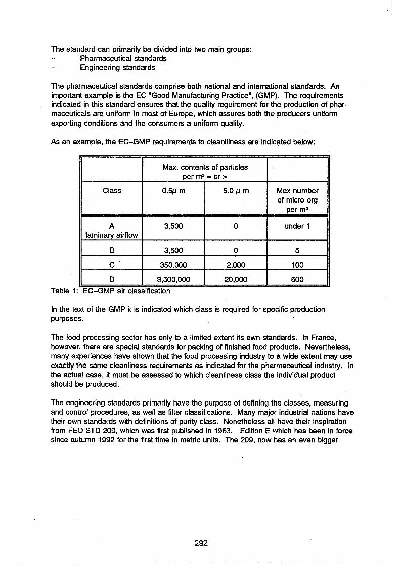
The standard can primarily be divided into two main groups: - Pharmaceutical standards - Engineering standards
The pharmaceutical standards comprise both national and international standards. An important example is the EC "Good Manufacturing Practice", (GMP). The requirements indicated in this standard ensures that the quality requirement for the production of phar- maceuticals are uniform in most of Europe, which assures both the producers uniform exporting conditions and the consumers a uniform quality.
As an example, the EC-GMP requirements to cleaniliness are indicated below:
Table 1 : EC-GMP air classification
In the text of the GMP it is indicated which class is required for specific production purposes.
The food processing sector has only to a limited extent its own standards. In France, however, there are special standards for packing of finished food products. Nevertheless, many experiences have shown that the food processing industry to a wide extent may use exactly the same cleanliness requirements as indicated for the pharmaceutical industry. In the actual case, it must be assessed to which cleanliness class the individual product should be produced.
The engineering standards primarily have the purpose of defining the classes, measuring and control procedures, as well as filter classifications. Many major industrial nations have their own standards with definitions of purity class. Nonetheless all have their inspiration from FED STD 209, which was first published in 1963. Edition E which has been in force since autumn 1992 for the first time in metric units. The 209, now has an even bigger
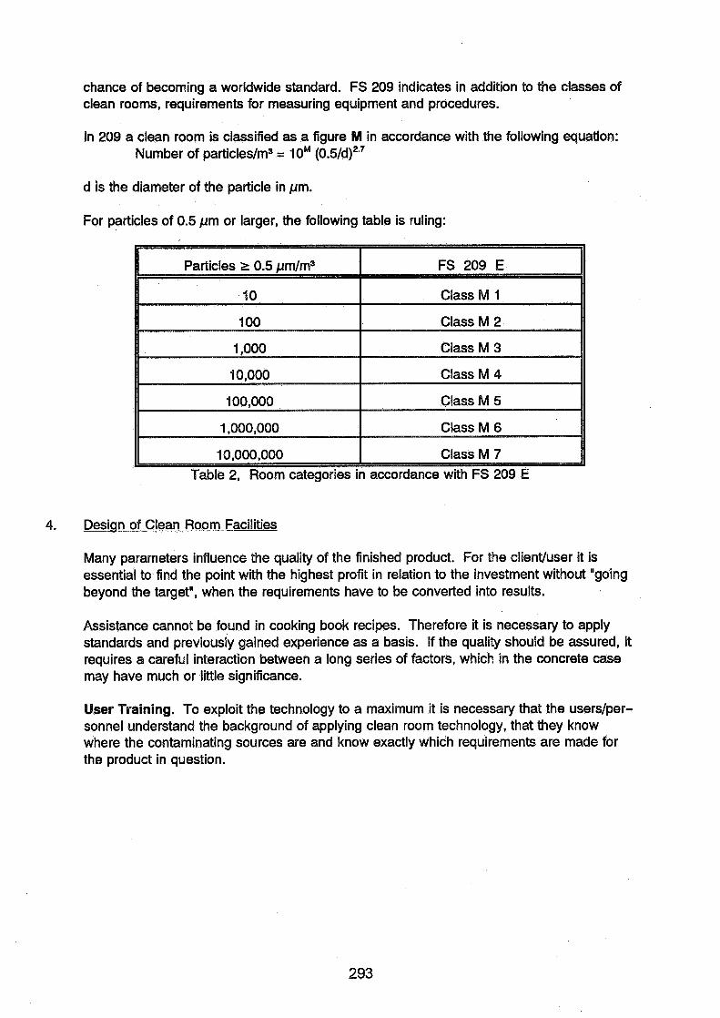
chance of becoming a worldwide standard. FS 209 indicates in addition to the classes of clean rooms, requirements for measuring equipment and procedures.
In 209 a clean room is classified as a figure M in accordance with the following equation: Number of particies/m3 = 1 oM (0.5/d)~.'
d is the diameter of the particle in pm.
For particles of 0.5 pm or larger, the following table is ruling:
I Class M 1
II IO.OOO.OOO I Class M 7 I' ~, I
Table 2, Room categories in accordance with FS 209 E
4. Design of Clean Room Facilities
Many parameters influence the quality of the finished product. For the clientluser it is essential to find the point with the highest profit in relation to the investment without "going beyond the target", when the requirements have to be converted into results.
Assistance cannot be found in cooking book recipes. Therefore it is necessary to apply standards and previously gained experience as a basis. If the quality should be assured, it requires a careful interaction between a long series of factors, which in the concrete case may have much or little significance.
User Training. To exploit the technology to a maximum it is necessary that the userslper- sonnel understand the background of applying clean room technology, that they know where the contaminating sources are and know exactly which requirements are made for the product in question.
Unambiguous output requirement. The users must be involved right from the beginning of the planning of the facilities: room classification, compressed air purity, water quality, etc. The requirements must be determined in collaboration with the consultants and if neces- sary be adjusted in the process. It is decisive that the requirements are well argumented. Do not require class M2, if class M4 is sufficient.
Building Layout. It is important that the processing and person flow of the building is designed in a rational way. An inventory must be established of raw materials, finished goods, package materials, and personnel. Avoid crossings of raw materials and finished goods. Cross-contamination from one product to another must be prevented. The personnel's communication lines must also be established.
Ventilation. The ventilation is one of the instruments, we may use to prevent infiltration of contamination and remove a possible contamination in the room. The ventilation must be adapted to the requirements put forward, it shall be designed with the filtration required and shall be carried out with the correct airflow pattern. Ventilation is dealt with later on in this paper. Can clean zones be designed as a limited area in order to reduce the ventilation need for the area outside of the clean zone?
Utilities. It is important to be aware of the requirements to the supply media, for example, sterile vapour for humidification, sterile compressed air for processing purposes and sterile water for injection. Which requirements will be made to the piping, supply reliability and control?
Equipment. Production equipment, machinery, etc must comply with the requirements. Has the machinery been designed in such a way that it can be serviced from a non-clean area - or shall the whole production be put to a standstill for servicing? It is also essential that the machinery is accessible for cleaning.
Measuring and control equipment. It must be emphasized that for continual assurance of compliance with the output requirements, it is necessary to establish consistent measur- ing procedures for cleanliness. The measuring equipment must be constantly available. The operators must be completely confident with the usage of the apparatuses.
Cleaning technique. Right from the first design phase it is necessary to plan meticulously the cleaning methods and needs.
Both quantifiable as well as non-quantifiable parameters should be applied for the evaluation of the success of a clean room. Whether the cleanliness requirement has been fulfilled or not is easily observed. But whether the processing flow could be optimised or not, is rather more difficult to verify. However the fulfilment of the expectations of the user to the non-quantifiable parameters is of imperative importance to the economic result.
Ventilation A reasonably designed ventilation system is one of the most important accessories to keep out contamination and remove contamination, which anyway will find its way to the clean area. The selection of the ventilation principle must be decided on a careful evaluation of requirements and needs.
In figure 2 the most common ventilation principles for clean room facilities are indicated. Traditional ventilation - mixed or by displacement - is applied, where the requirements are not very high. Laminary flow - horizontal or vertical - is applied combined with recir- culation in rooms, where the requirement to purity is very high.
In clean rooms of today it has become quite common that the traditional ventilation is combined with the laminary flow, in such a way that a clean room will be designed with a "controlled backgroundWith mixed ventilation combined with one or more "clean zones" with a laminary flow. Consequently a considerable reduction in the ventilation need is achieved - less investment and less operation costs.
Under all circumstances it is essential that both the inlet and the exhaust fittings are placed so that the physical laws are appraised - movements of air as a consequence of the thermal effect and sedimentation of "heavy" particles. Dead "angles" not being ventilated should be avoided, as the contamination might pile up in such places.
Within the biotechnology, it might be necessary to protect the processing, at the same time as which it is necessary to protect the operator against a contamination risk from the processing. Here the isolator module could be a solution. It is possible to find small glove boxes or large boxes accommodating a person (via access from the bottom through a completely covering protection suit on the upper part of the body) that enables the person to carry out his activities.
As mentioned, the choice of ventilation principle is based on the actual requirements. It is important that already at an early stage of the design phase, it is realized which ventilation principle to apply, as the space required for positioning is very different.
Many factors are controlled by means of the ventilation:
The purity of the room. The change of air is primarily calculated according to the requirement of purity and infiltration of contamination into the room. Air movement patterns. It should be clarified whether the need is for laminary, non- laminary flow or a combination of them. In general, it should be noted that requirements for a class M4 or better, normally would be carried out as a laminary flow. By sensible positioning of the inlet and exhaust fittings it is secured that the contamination is removed "at source" to the extent possible. Pressure conditions. To maintain the purity in the room, clean room facilities normally are designed as "a room in the room" with a lower pressure than in the purest area. A

variation pressure of 15 Pa from area to area is normal. If spreading of hazardous substances from the clean room should be prevented, the opposite solution could be considered, that is, the clean room has the negative pressure in relation to the adjacent rooms. Under the circumstances it is important to establish airlocks securing that the variations in pressure are not equalized by opening of doors. If the inletlexhaust volume flows vary, it is important to implement regulation equipment currently securing that the pressure conditions are correct. The regulation equipment should in addition be prepared for soiled filters and fittings. Temperature and humidity. The production often specifies exact requirements to temperature and humidity, determining the design of the ventilation systems. If no special requirements, it is the personnel's comfort requirement that determines the ventilation. A very important factor in the ventilation system is the filtration. The main part of the particles damaging the products within the food processing and pharmaceutical industries are larger than 0.3 pm. High-efficient filters (HEPA-filters) have a very high degree of separation of these particles. Therefore it is important that the correct filters are installed and that the ventilation system be prepared making it possible to gain full control of the room condition with regard to the particle content.
In figure 3 a principle is shown of the ventilation of a clean room with laminary flow for all the room. Due to energy cost-efficiency as much air as possible is recirculated through local ventilation units with ventilators and HEPA-filters. A certain amount of fresh air is added through the central ventilation system, in which a portion of the room air is recirculated. This system conditions/adapts the air in order to comply with the requirements to temperature and humidity.
The development is moving rapidly withln industry. A clean room system has typically a life time of about 10 years. Therefore it Is nwessary to secure that the requirements of "today" and "tomorrow" have been fulfilled. On the other hand, there Is no need to make more costly or complicated systems by guessing what will be the requirements of "the day after tomorrowu.
References 1. W. Whyte, Clean Room Design 2. Fed. Std. 209 E 3. EC and PIC-GMP (Pharmaceutical inspection Convention-Good Manufacturing
Practice) 4. h e Moller, Hur man bygger renrum, Renlighetsteknik nr. 4, 1992. 5. Raymond Schneider, How much clean room do you really need?, Clean Room
Europe Proceedings, 1991 6. H. Gebhardt, KontaminationskontroIle in die Nahrungsmittelindustrie, Swiss
Contamination Control, Nr. 2, 1992

Personnel Surroundings
Cleaning Process media
Fig. 1 Clean room production
Laminary flow
Clean Filling Room
Fig. 3 Room for aseptic filling

Laminary flow
background with clean zone
Fig.2 Ventilation principles

Energy Impact of Ventilation and Air Infiltration 14th AlVC Conference, Copenhagen, Denmark
21 -23 Septem ber 1993
Programme for Energy-Efficient and Healthy Apartment Buildings in Stockholm
L Fyrhake,* P-A HedkvistF* M Hult*
* The City of Stockholm, Stockholm Konsult, Energy & Environment, Box 8381, S-104 20 Stockholm, Sweden ** The City of Stockholm, The Stockholm City Dep of Building Control, Box 831 1, S-104 20 Stockholm, Sweden
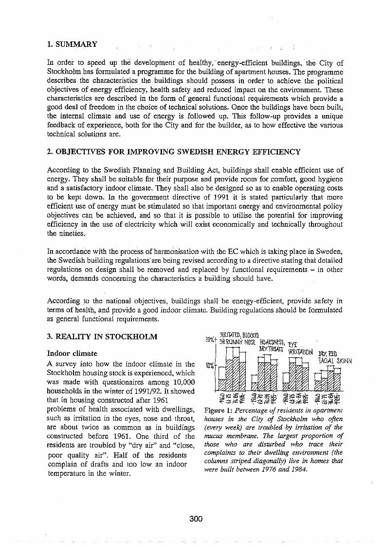
1. SUMMARY
In order to speed up the development of healthy, energy-efficient buildings, the City of Stockholm has formulated a programme for the building of apartment houses. The programme describes the characteristics the buildings should possess in order to achieve the political objectives of energy efficiency, health safety and reduced impact on the environment. These characteristics are described in the form of general functional requirements which provide a good deal of freedom in the choice of technical solutions. Once the buildings have been built, the internal climate and use of energy is followed up. This follow-up provides a unique feedback of experience, both for the City and for the builder, as to how effective the various technical solutions are.
2. OBJECTIVES FOR IMPROVING SWEDISH ENERGY EFFICIENCY
According to the Swedish Planning and Building Act, buildings shall enable efficient use of energy. They shall be suitable for their purpose and provide room for comfort, good hygiene and a satisfactory indoor climate. They shall also be designed so as to enable operating costs to be kept down. In the government directive of 1991 it is stated particularly that more efficient use of energy must be stimulated so that important energy and environmental policy objectives can be achieved, and so that it is possible to utilise the potential for improving efficiency in the use of electricity which will exist economically and technically throughout the nineties.
In accordance with the process of harmonisation with the EC which is taking place in Sweden, the Swedish building regulations are being revised according to a directive stating that detailed regulations on design shall be removed and replaced by functional requirements - in other words, demands concerning the characteristics a building should have.
According to the national objectives, buildings shall be energy-efficient, provide safety in terms of health, and provide a good indoor climate. Building regulations should be formulated as general functional requirements.
3. REALITY IN STOCKHOLM
Indoor climate A survey into how the indoor climate in the Stockholm housing stock is experienced, which was made with questionaires among 10,000 households in the winter of 1991/92. It showed that in housing constructed after 1961 problems of health associated with dwellings, such as irritation in the eyes, nose and throat, are about twice as common as in buildings constructed before 1961. One third of the residents are troubled by "dry air" and "close, poor quality air". Half of the residents complain of drafts and too low an indoor temperature in the winter.
SF^$ gF@$ %icS$ F ~ I T - - ? T-ZI#? ?==*g Sf&$%
Figure 1: Percentage of residents in apartment houses in the City of Stockholm who often (every week) are troubled by irritation of the mucus membrane. The largest proportion of those who are disturbed who trace their complaints to their dwelling environment (the columns striped diagonally) live in homes that were built between 1976 and 1984.
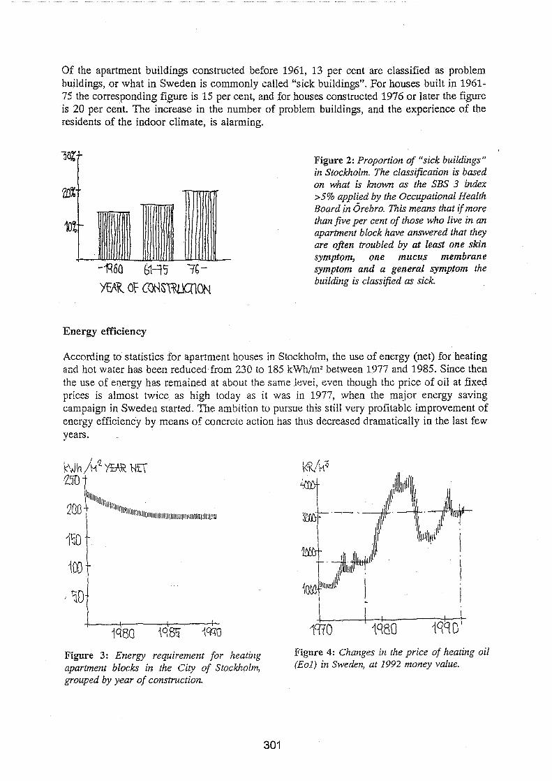
Of the apartment buildings constructed before 1961, 13 per cent are classified as problem buildings, or what in Sweden is commonly called "sick buildings". For houses built in 1961- 75 the corresponding figure is 15 per cent, and for houses constructed 1976 or later the figure is 20 per cent. The increase in the number of problem buildings, and the experience of the residents of the indoor climate, is alarming.
Figure 2: Proportion of "sick buildings" in Stockholm. The classification is based on what is h o w n as the SBS 3 index >5% applied by the Occupational Health Board in 0rebro. This means that if more than five per cent of those who live in an apartment block have answered that they are often troubled by at least one skin symptom, one mucus membrane symptom and a general symptom the building is classified as sick.
Energy eff~ccieny
According to statistics for apartment houses in Stockholm, the use of energy (net) for heating and hot water has been reduced from 230 to 185 kWh/rn2 between 1977 and 1985. Since then the use of energy has remained at about the same ievei, even though the price of oil at fixed prices is almost twice as high today as it was in 1977, when the majcr energy saving campaign in Sweden started. The ambition to pursue this still very profitable improvement of energy effieiencjr by means of concrete action has thus decreased dramatically in the iast few years.
Figure 3: Energy req~irement for heati~g Figure 4: Changes in the price of heating oil
ccpartment blocb in the Ciry of Stockholm, (Eol) in Sweden, at 1992 money value.
grouped by year of construction.
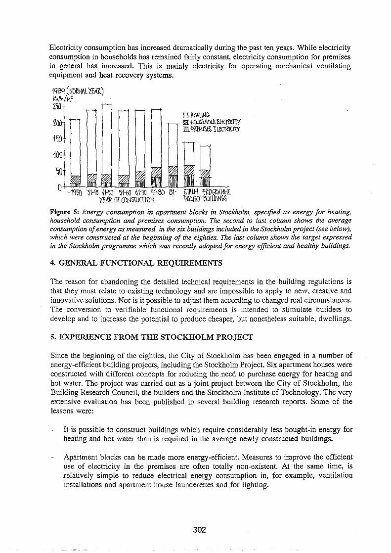
Electricity consumption has increased dramatically during the past ten years. While electricity consumption in households has remained fairly constant, electricity consumption for premises in general has increased. This is mainly electricity for operating mechanical ventilating equipment and heat recovery systems.
Figure 5: Energy consumption in apartment blocks in Stockholm, specified as energy for heating, household consumption and premises consumption. The second to last column shows the average consumption of energy as measured in the six buildings included in the Stockholm project (see below), which were constructed at the beginning of the eighties. The last column shows the target expressed in the Stockholm programme which was recently adopted for energy efficient and healthy buildings.
4. GENERAL FUNCTIONAL REQUIREMENTS
The reason for abandoning the detailed technical requirements in the building regulations is that they must relate to existing technology and are impossible to apply to new, creative and innovative solutions. Nor is it possible to adjust them according to changed real circumstances. The conversion to verifiable functional requirements is intended to stimulate builders to develop and to increase the potential to produce cheaper, but nonetheless suitable, dwellings.
5. EXPERIENCE FROM THE STOCKHOLM PROJECT
Since the beginning of the eighties, the City of Stockholm has been engaged in a number of energy-efficient building projects, including the Stockholm Project. Six apartment houses were constructed with different concepts for reducing the need to purchase energy for heating and hot water. The project was carried out as a joint project between the City of Stockholm, the Building Research Council, the builders and the Stockholm Institute of Technology. The very extensive evaluation has been published in several building research reports. Some of the lessons were:
- It is possible to construct buildings which require considerably less bought-in energy for heating and hot water than is required in the average newly constructed buildings.
- Apartment blocks can be made more energy-efficient. Measures to improve the efficient use of electricity in the premises are often totally non-existent. At the same time, is relatively simple to reduce electrical energy consumption in, for example, ventilation installations and apartment house launderettes and for lighting.

- Low energy consumption can be combined with a sound indoor climate if this is given greater emphasis in connection with planning, building and management.
- If a finished building is to satisfy functional and quality requirements, awareness must be increased, and quality control improved, throughout the entire building process and in the management phase.
- Details are important - thermal bridges, poor input air ducts, etc., can spoil energy efficiency in what is otherwise a sound building.
- The existing forms for the handing over, responsibility and commissioning do not guarantee efficient operating.
6. STOCKHOLM PROGRAMME FOR HEALTRY ENERGY EFFICIENT BUILDINGS
In the City of Stockholm's energy plan a spontaneous development of the use of energy is compared with a development where economically motivated measures are taken to improve efficiency. The analysis shows that considerable benefits are achieved with measures to improve the use of energy. Environmental disturbances from energy production installations can be halved, energy costs lowered, and the need for new energy production installations reduced. Stockholm's environmental plan emphasises the importaxe of concentrating on sound indoor environment, particularly against the background of the problems associated with the concept of "sick buildings".
The "Programme for energy-efficient and healthy apartment buildings - new buildings" is one stage in the project of implementing the intentions of the energy and environmental plans. These will be followed by programmes for other premises and for re-building activities.
Functional requirements for indoor climate
The objects of the programme regarding the indoor climate is that dwellings shall be healthy, have a high quality of air and satisfactory heating comforts. The functional requirements are:
- Health complaints stated by the residents in a survey with questionaire should not exceed the reference values for Stockholm.
- The air quality shall be evaluated as good or acceptable by at least 80 per cent of the residents.
- Heating comfort shall be regarded as good or acceptable by at least 80 per cent of the residents.
- The radon compound content in completed apartments shall not exceed 70 Bq/m3 in inspection measurements.
As a result of the above mentioned survey of 10,000 households in Stockholm a large body of reference material has been built up. This, together with other material, provides the basis

for creating those references which are needed in order to assess the normal quota of health complaints in apartment blocks. It also supports the assumption that the target - that at least 80 per cent of the residents should consider the indoor climate to be good or acceptable - is set at a reasonable level.
Functional requirements for energy efficiency
The functional requirements for energy efficiency are:
- The total use of energy in the building in question shall not be higher than the estimated use of energy for a corresponding programme building.
A programme building is a fictitious building which is based on the conditions of the building in question. It is thus exactly the same as the building which is to be constructed, but based on the reference building for in the new building regulations in terms of energy for heating. The production cost, therefore, is not affected in relation to the new building regulations in this respect.
The electricity efficiency of the programme building represents a considerable improvement compared with standards of the eighties. It is already profitable to further improve electricity efficiency in ventilation installations. The assumed electricity efficiency for ventilation installations involves a higher investment in the building phase but provides sound economy in the operating phase. Pay-off time is 3-5 years.
Weighting up of electrical energy
In calculating the total use of energy, the use of electricity shall be weighted up by a factor of 2.4. This means that the importance of effective use of electricity will increase. Exhaust air system buildings without heat recovery can thus satisfy the requirements for a building permission from the energy point of view, provided that the building as a whole is designed for efficient use of electricity and with a good climatic shell. The factor 2.4, which has been arrived at in co-operation with Stockholm Energy, is based partly on an appraisal of future changes in electricity prices compared with other energy carriers, and partly on the actual sacrifice of energy raw-materials and the environment which production of electricity gives rise to.
Upper level for total use of energy
The method of establishing a total level for the use of energy with the aid of a programme building gives the builder freedom to decide what building or installation technique s h e will use, in the way s h e considers best suits the individual case. The demand for a total level for energy use also means that the builder can rank a variety of measures to improve energy efficiency within the various areas of use - heating, hot water, premises electricity and household electricity.
The more effective use of energy leads to lower costs for the residents. Compared with a normal building from the eighties with 100 apartments, the cost of energy would be reduced by 320,000 kronor per year if the programme targets were satisfied.
Well functioning operations
The programme's targets for a well functioning operation are:
- Functional requirements for indoor climate and energy efficiency shall be maintained in the operating phase.
The builder shall demonstrate, in a quality plan, how the functional requirements are taken into account during planning and building, and how they are to be maintained in the operating phase.
Reporting in connection with building permission
The formulation of the energy programme, with functional requirements and follow-up of the completed building, are intended in the long run to generate a situation where the City's scrutiny can be limited to a follow-up to ensure that the characteristics have been achieved in the completed building. Initially, however, it is proposed that the builder should demonstrate in a report in connection with application for building permission how the energy programme had been achieved. This will enable a dialogue between the City and the builder as to how the functional requirements in the programme can be achieved. The reporting requirements in connection with building permission applications include:
- Quality plan;
- General system sketches for building method, heating and ventilation systems, air flows and air ducts, as well as total area specification;
- Calculation of the use of energy.
In the report the builder shall demonstrate that it is likely that the building in question can achieve the targets of the programme. The system sketches shall indicate in a general way the principles of the selected technical solutions for heating and ventilation systems - selections which can sometimes directly influence the part of the building design which is determined in connection with the building permission. The selection of the ventilation installation, for example, will influence the design of the building and must reasonably be used as a basis for the building design which is selected and established in the building permission.
.
The calculation of energy consumption is based either on the established design or on functional requirements for the continued planning and for implementation. The reporting requirements mean that the builder will have to make a choice as to what standard he is aiming for as regards indoor climate and energy efficiency. Thus, detailed planning is not required to satisfy the reporting requirements. The work input for calculation and system sketches is estimated to correspond to two working days.

Figure 6: Three systems sketches, a total estimate of energy consumption and aprogramme for quality assurance are submitted in connection with the application for building permission.
Follow-up of completed building
After the second heating season the builder should follow up the use of energy and the indoor climate in order to check that programme targets are satisfied in the finished building. The use of energy for heating, electricity for the premises and household electricity are measured and compared against the estimate of the energy requirements stated in the building permission application. The experience of the indoor climate and health is checked by a questionaire to the residents. After a time the overall facts about the indoor climate, energy consumption and the various technical solutions which are described in the form of systems sketches will provide a unique and valuable base of information for selecting and developing new technical solutions.
Incentives
In order to promote the programme's intentions a sum of 250,000 kronor (10,000 kronor per apartment) will be awarded during the first three years to builders which best satisfied the functional requirements in the programme. The award is financed by NUTEK (Swedish Business and Technical Development Agency).
7. EVALUATION AFTER TWO YEARS
Compared with new buildings in the eighties, the programme represents a reduction in the consumption of energy of some 35 per cent and thus a corresponding reduction in environmentally hazardous effluent.
The overall functional requirements for health, air quality and heating comfort, focusing on the experiences of the residents, probably means that the trend of an increasing number of sick buildings can be turned. Where they occur they should be discovered in connection with a follow-up and can thus be remedied at an early stage. However, if we can substantially reduce the cost of remedying some 20 per cent of new buildings which are today classified as problem buildings, a good deal has already been won.
The programme has been adopted by the Stockholm Property Board and Building Board. It

will be applied immediately and will be appraised after two years. The appraisal will be made in co-operation with the National Board of Housing, Building and Planning (Boverket), NUTEK and the Building Research Council, with a view to reporting experiences prior to future reviews of the building regulations.
Figure 7: Summary of programme requirements.
r.
Follow-up
Questionnaires to the residents. The builder is responsible for conducting surveys and for measuring the radon content in a sample of apartments.
Questionnaires to residents, see above
Questionnaires to residents, see above
The builder is responsible for ensuring that the energy consumption for the whole of the year covering the second heating season is measured and reported to the City. The measurements shall include the following items: bought-in energy for heating, hot tap water, premises electricity, household electricity and electricity for common rooms, if any.
Follow-up of programme requirements after the second heating season.
Targets and requirements
1. Indoor climate and comfort
1.1 Dwellings shall be healthy, reference values in Stockholm survey should not be exceeded. The radon compound content should not exceed 70Bq/m3 air.
1.2 Houses shall have a good quality of air, at least 80 per cent of the residents should consider that the air is good or acceptable.
1.3 Dwellings shall have a good heating comfort, at least 80 per cent of the residents should consider that they can achieve good or acceptable heating comfort.
2. Low need for purchased energy and electricity-eficient solutions.
2.1 The total use of energy for the building in question shall be lower than for the corresponding programme building. In calculations all use of electricity is weighted up by a factor of 2.4. In the case of heating and hot tap water the programme building corresponds to NR's reference building. Electricity consumption is calculated on the basis on an electricity efficient FTX system.
3. Well functioning operations
3.1 Functional requirements as regards indoor climate, comfort and heating needs and electricity comfort shall be maintained in the operating phase.
Reporting requirements
System sketches of building method, air £low, air diffusion and heat and ventilation systems. Investigation of ground radon content.
System sketches, see above
System sketches, see above
An estimate of energy consumption for the building in question and the corresponding programme building shall be stated. The energy requirement for heating and hot water is calculated on the basis of Nya Enorm or the equivalent. Electricity consumption is calculated separately in accordance with the model in the energy programme.
State in the quality plan measures for commissioning and operating, in order to maintain the programme requirements at the operating stage.


Energy lm pact of Ventilation and Air Infiltration 14th AlVC Conference, Copenhagen, Denmark
21 -23 September 1993
Long-Term Performance of Residential Ventilation Systems
M-L Pallari, M Luoma
Technical Research Centre of Finland, VTT Laboratoty of Heating and Ventilation, P O Box 206 (LBmp~miehen kuja 3), FIN-021 51 ESPOO, Finland

LONG-TERM PERFORMANCE OF RESIDENTIAL VENTILATION SYSTEMS
ABSTRACT
Several demonstration buildings were constructed in order to find technical solutions to energy saving and better indoor air quality in the 1980's in Fiand. Warm air heating systems were installed in two multi-storey residential buildings and in several single family homes. Heat recovery units were installed in many buildings. During renovation, mechanical supply air and heat recovery units were installed in two multi-storey residential buildings.
Studies on energy consumption and performance of air conditioning systems were carried out in the demonstration buildings. The opinions of occupants were asked. Some of the systems had problems already during the installation and commissioning phase.
A follow-up study was carried out in 1992-1993 on nine of the buildings studied in the 1980's. The aim of the follow-up study was to find out the long term performance of the residential air conditioning and heating systems. The maintenance staff was asked about the malfunctioning of the devices and the need for reparation The regular maintenance work was discussed, too. The regular maintenance included changing filters every third to sixth month, vacuum cleaning of the heat recovery units every twelfth month (only in the single family homes) and cleaning of ducts and air terminal devices when necessary. Exhaust air flows and pressure conditions were measured during the visits to the buildings.
The main observation was that the normal maintenance work was not sufficient in order to keep the ventilation and air heating systems in planned condition in the long-term. Air flows and pressure conditions of the buildings tend to change in the long term because of e.g. the occupants interaction. The energy consumption of heating and ventilation rose (2 - 39 9%) after the follow-up study except in the air heated multi-storey building where energy consumption fell 7 9%. However, the heating energy consumption was lower in every demonstration building than in the corresponding residential buildings, due to energy-saving devices.
INTRODUCTION
Several air conditioning systems with new technical solutions were developed in the 1970 - 1980's in Finland. The target was to save heating and ventilation energy. The systems were expected to ensure better indoor air, too. Several demonstration buildings were constructed by public funding and studies were carried out on functioning of devices, energy economy and indoor air. The reported experiences pointed out that the heating and ventilation systems in the demonstration buildings had both advantages and disadvantages. On the other hand the different technical solutions increased the possibilities of occupants to influence on the thermal comfort and ventilation in buildings. On the other hand the sensitivity of the systems to malfunction and the need for maintenance increased. Merely for the realization of the energy economy certain technical devices were necessary. As a rule, the follow-up studies in the demonstration buildings lasted for two heating periods. According to the follow-up studies, it was difficult to estimate the success of the systems in the long-term.
A follow-up study was carried out in 1992-1993 on nine of the buildings studied in the 1980's. The main target of the research was to chart the present ventilation'systems and to make conclusions of the changes in the function of systems. The maintenance staff was asked about the malfunctioning of the devices and the need for reparation. Also the regular maintenance work was discussed. The energy and ventilation systems were checked, exhaust air flows and pressure conditions were
measured during the visits to the buildings. The changes in the long-term energy consumption were estimated.
The heating and ventilation systems in the study were: - two air heating systems in multi-storey residential buildings - two mechanical supply and exhaust air systems in multi-storey residential buildings - one solar and earth-heath pump system in a single family house - one solar heating system in a terraced house - one air heating system in a terraced house - two heat recovery systems in multi-storey residential buildings installed during renovation
The energy and ventilation systems were more complicated than the usual ones (Figure 1) and contained the newest technology. All of the examined systems were still in use, i.e. none of the systems were altered from the original use. In some dwellings of the air heated terraced building electric heaters were installed, but the supply and circulating air devices were functioning normally. The solar heat unit in the solar and earth-heath pump system had not been in use since the 1984.
ENERGY CONSUMPTION
Generally, the total energy (heating of buildings, hot water and domestic electricity) consumption in Finland rose approximately 12 % from the period 1982 - 1985 to the period 1989 -1990 111. The heating energy of the demonstration buildings rose 2 % - 39 % after the follow-up studies except for the air heated multi-storey building where the energy consumption fell 7 %. The heating energy consumption (30 kwh/m3a -57 kWh/m3a) of the demonstration buildings of this study was, however, lower than that of the corresponding Finnish residential buildings (63 kWh/m3a), due to the energy saving devices.
The changes in the behavior of the occupants 111 and the falling energy prices effected the energy consumption in the demonstration buildings. During the follow-up study the occupants were aware of the fact that the energy consumption is studied. For this reason they directed their attention e.g. to the consumption of hot water and to the window opening. After the follow-up study, their interest to energy saving most probably fell. The increase in the energy consumption was biggest in the fuel oil heated terraced house, where the the energy consumption in 1990 was 39 % bigger than in 1979. The real price of fuel oil has fallen most compared to the prices of the other energy sources.
The aging of the heating and ventilation systems in the long-term could also affect to the growth of the energy consumption. For example the control valves did not function as designed. The energy meters had not been calibrated after the installation either.
VENTILATION RATE AND INDOOR AIR QUALITY
In this study the measured ventilation rates were low, 0,02 - 0,71 l/h. Only two dwellings (21 dwellings measured) fulfilled the minimum ventilation rate, 0 3 l/h. In comparison, in study of 25 1 Finnish dwellings 52 % of the dwellings did not fulfill the minimum ventilation rate (measured with PFT-method ) /2/.
Almost in every measured demonstration building the exhaust air flows had fallen with 15 % - 94 %. In one multi-storey building the exhaust air flows had grown with 9 % in the flats on the ground floor. In the same building the exhaust air flow had fallen in the upper floors.
Although the measured ventilation rates were low, the supply air distribution could be considered good in seven demonstration buildings where the supply air was distributed to the bedrooms and
livingrooms. In one of the buildings the supply air was distributed to the halls, in one of the buildings to the stairways.
Five demonstration buildings had warm air heating with air circulation. In three of these buildings the occupants were inquired about the content of dust in indoor air during the studies in the 1980's. From the interviewed occupants 33 %, 52 % and 72 % had considered the content of dust in their home bigger than usually. Circulating air tend to make the supply air devices dirty if the room air is dirty and the f i l t e ~ g is unsufficient.
Air flows and pressure conditions of the demonstration buildings tend to change in the long-term e.g. because of the occupants interaction and dirty ventilation components.
OCCUPANTS' POSSIBILITIES TO CONTROL THE SYSTEMS
Most of the systems had a control panel but that was not available to occupants. On the other hand, the occupants did not even know the normal position of the ventilation devices. The reason was that the use and maintenance instructions had disappeared when the occupants had moved out and new occupants moved in. In order to ensure the proper use of ventilation devices the instructions should be installed on the devices.
In six demonstration buildings the control panels of the ventilation and air circulating devices were located in the dwellings but only in three of them the occupants had the possibility to increase the air flow. On the other hand, the increase of circulating air did not always increase the heating capasity because the outdoor air flow increased, too. In one demonstration building the control system of the circulating air and the supply air temperature was broken.
In two of the air heated buildings the heating and ventilation systems were such that the occupants could not control the air flows or the supply air temperatures. In one of these buildings the occupants had complained of draught. For example the large window in the living room can cause so-called cool radiation in winter time if the supply air is not warm enough. It is important especially in the air heated systems that the occupants could control the supply air temperature.
MATNTENANCE
The heating and ventilating systems were maintained by the service staff or by the occupants. In one demonstration building where the heating and ventilation system was maintained by the service staff the gasgets of the engine doors were worn-out and partly totally missing. The exhaust air filter was not fastened properly. A great proportion of the exhaust air flew to the heat exchanger without filtering. The measured exhaust air flow had fallen 39 % since 1980' and the supply air flow had correspondingly fallen 13 %. In an air heated building the devices were maintained by the service staff. The fans and the filters were dirty. The quality of work done by service staff could be due to the fact that not enough time had been reserved to maintenance work.
In the air heated terraced building maintanance of the devices located in the dwellings should be done by the occupants. The devices were located in the ceiling, which made the maintenance difficult. Part of the devices were very dirty. The reason for the dirtyness could be the lack of knowledge about the importance of cleaning of devices or the difficulties in the cleaning and maintenance.
The cleaning and maintenance work should not be left to the occupants' responsibility. Usually the occupants have no tools to clean e.g. the fans. Even the cleaning of vents can be troublesome. As a rule, the cleaning of air terminal devices requires their loosening. Often the air terminal devices
in the bathrooms are located in the ceiling above the bathtubs. The cleaning of them can be difficult, even dangerous.
In order to keep the condition of the ventilation systems unchanged in the long-term regular maintenance work is needed and broken parts should be repared as soon as possible.
CONCLUSIONS
In the developing phase of the heating and ventilation systems in 1980's very complicated systems were designed. It was not possible to forecast the difficulties which could apRear in the installation and commissioning phase of the systems. Among other things Finland's first warm air heated multi- storey building had the biggest problems with the air locks in the heating water pipes. This problem could have been avoided with careful design atld careful installation of the system. The components of the ventilation systems were prototypes, which for example resulted problems in the control1 of the installed systems.
In Finland the type aproval of the components of ventilation systems was taken in use in 1983. The type approved products are quality controlled. This procedure has extremely improved the quality and performance of the ventilation equipment. On the other hand the systems are no more designed as complicated as during the developing phase of the ventilation systems in the beginning of the 1980's.
The long-term performance of the heating and ventilation systems requires regular maintenance work and reparing of broken parts as soon as possible. The regular inspections guarantee that the air flow rates do not change too much and the energy consumption does not rise due to malfunction of the heating devices in the long-term.
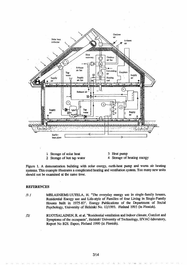
Earth- heat pipes
1 Storage of solar heat 3 Heat pump 2 Storage of hot tap water 4 Storage of heating energy
Figure 1. A demonstration building with solar energy, earth-heat pump and warm air heating systems. This example illustrates a complicated heating and ventilation system. Too many new units should not be examined at the same time.
REFERENCES
11 / MELASNIEM-UUTELA, H. "The everyday energy use in single-family houses, Residential Energy use and Life-style of Families of four Living in Single-Family Houses built in 1975-82". Energy Publications of the Department of Social Psychology, University of Helsinki No. 1211993. Finland 1993 (in Finnish).
121 RUOTSALAINEN, R. et al. "Residential ventilation and indoor climate, Comfort and Symptoms of the occupants", Helsinki University of Technology, HVAC-laboratory, Report No B28. Espoo, Finland 1990 (in Finnish).
Energy Impact of Ventilation and Air Infiltration 14th AlVC Conference, Copenhagen, Denmark
21 -23 Septem ber 1 993
Ventilation of Public Swimming Pools
D Dickson
E A Technology, Capenhurst, Chester, CHI 6ES, UK
Synopsis
Ventilation codes for swimming pools are based on preventing condensation. To save energy, air recycle with dehumidification is common. This successfully controls moisttke, but does not remove airborne contaminants arising from evaporation of chemically treated pool water. This contamination may cause discomfort, irritation or even harm.
Environmental conditions and energy consumption were monitored at two public swimming pools over one year to identify the critical factors affecting bather comfort, to relate these to proportions of recycled air, and to show how to achieve acceptable bather comfort while minimising energy costs.
Questionnaire surveys showed that even under the most comfortable conditions, 20 to 30% of pool users suffered irritation, mainly of the eyes, attributed both to the air and to the pool water. Over the range of fresh air conditions available using the existing plant, discomfort experienced by pool users was not found to relate to the ventilation conditions, but rather to the level of chlorine compounds ("combined chlorine") in the water. High combined chlorine levels in the water are expected to result in high levels of contamination in the air, but this proved difficult to measure. However, increasing the fresh air ventilation rate when the combined chlorine level in the water is high is desirable in order to dilute airborne contaminants, and it is proposed that the combined chlorine level in the water should be used as a fresh air ventilation control parameter, along with humidity and carbon dioxide, to minimise energy use and maintain acceptable air quality.
I Background
Ventilation rates for swimming pool halls have traditionally been determined by the need to limit condensation on the building structure. Comfort requirements of bathers and staff are then satisfied by choosing acceptable air and water temperatures.
The need to reduce energy consumption has encouraged the installation of heat recovery systems which dehumidify and recirculate a large proportion of pool hall return air'. These systems are economically attractive and the humidity can be controlled without the need for any fresh air at all. Consequently, there now exists the possibility of progressive build up of airborne contaminants in the pool hall atmosphere which may be corrosive, uncomfortable or even unhealthy.
The possible consequences of recirculating a high proportion of the air were discussed in The ~ance? in 1979 and by penny3 in 1983. They suggested that respiratory and eye irritation caused by chlorine compounds in the air may be more severe when an air recycle system is installed.
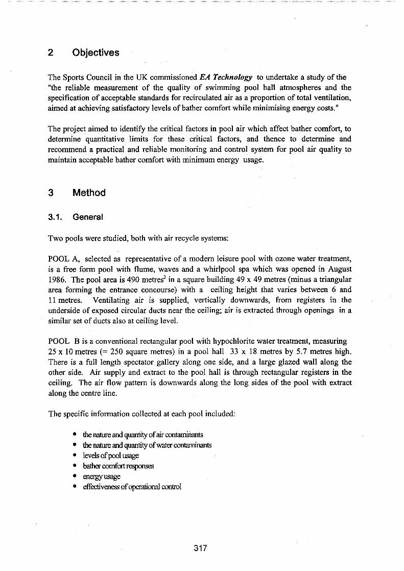
2 Objectives
The Sports Council in the UK commissioned EA Technology to undertake a study of the "the reliable measurement of the quality of swimming pool hall atmospheres and the specification of acceptable standards for recirculated air as a proportion of total ventilation, aimed at achieving satisfactory levels of bather comfort while minimising energy costs."
The project aimed to identify the critical factors in pool air which affect bather comfort, to determine quantitative limits for these critical factors, and thence to determine and recommend a practical and reliable monitoring and control system for pool air quality to maintain acceptable bather comfort with minimum energy usage.
3 Method
3.1. General
Two pools were studied, both with air recycle systems:
POOL A, selected as representative of a modern leisure pool with ozone water treatment, is a free form pool with flume, waves and a whirlpool spa which was opened in August 1986. The pool area is 490 metres2 in a square building 49 x 49 metres (minus a triangular area forming the entrance concourse) with a ceiling height that varies between 6 and 11 metres. Ventilating air is supplied, vertically downwards, from registers in the underside of exposed circular ducts near the ceiling; air is extracted through openings in a similar set of ducts also at ceiling level.
POOL B is a conventional rectangular pool with hypochlorite water treatment, measuring 25 x 10 metres (= 250 square metres) in a pool hall 33 x 18 metres by 5.7 metres high. There is a full length spectator gallery along one side, and a large glazed wall along the other side. Air supply and extract to the pool hall is through rectangular registers in the ceiling. The air flow pattern is downwards along the long sides of the pool with extract along the centre line.
The specific information collected at each pool included:
@ the nature and quantity of air contaminants @ the nature and quantity of water contaminants 0 levels of pool usage
bather comfort xrspnses
@ energyusage @ effectiveness of operational control
Following initial interviews with pool staff to find out how the pools were operated and the degree of cooperation and access to records which would be forthcoming, procedures for measurement and collection of physical and subjective data from pool users and staff were set up.
3.2. Physical conditions
Continuous logging of indoor and outdoor environmental conditions was carried out at 10 minute intervals comprising:
poolhallaird~ybulbteqxntm @ pool hall air wet bulb temperature @ retumairctrybulbteqxntm @ retumairwetbulbteqxntm
@ supplyair- retum air carbon dioxide concentmtion airflowratein~airduct air flow rate in recycle air duct.
Questionnaire surveys of pool users were carried out at appropriate intervals.
Relative humidity was measured by wet and dry bulb thermistors because commercially available capacitative thin film humidity sensors were rapidly poisoned (within days) in a swimming pool hall atmosphere.
Air flow rates in ventilation ducts were monitored by permanent vane anemometers in both the air supply duct and in the fresh-air-from-outside duct, calibrated by anemometer traverses. Carbon dioxide concentration in the return air duct was recorded continuously as an index of the fresh air ventilation rate and occupancy.
3.3. Ventilation conditions
The fresh air entering the swimming pool hall and diluting the contaminants is a combination of the fresh air delivered through the ventilation system plus weather dependent air leakage into the building by infiltration, augmented also, when the building is in use, by air interchange through external doors.
The total effective fresh air ventilation rate was measured by a tracer decay technique, using sulphur hexafluoride injected into the supply air dust. The rate of tracer decay was then measured in the return air duct to give an average fresh air ventilation rate for the pool hall.

3.4. Water chemistry
The water chemistry analysis for the substances present in swimming pool water is reasonably straightforward and well documented. Chlorine (introduced as solutions of sodium or calcium hypochlorite) reacts with water to form hydrochloric acid (HCl) and hypochlorous acid (HOCI) which reacts with organic and nitrogenous compounds (mainly ammonia NH,) in the water to form "combined chlorine" - chloro-organics, chloramines (NH,CI, NHCI,, NCl,) - and a residue of hypochlorous acid ("free chlorine"). Typical concentrations of 'free chlorine residual' are between 1 and 3 mg/litre (=ppm); free and total chlorine are checked routinely by the pool staff using DPD (diphenyldiamine) colorimetric tests, giving combined chlorine by difference. pH is controlled within the recommended range of 7.4 to 7.6, normally by adding acid.
3.5. Air chemistry
The air chemistry represents an altogether different problem. The main odorous and irritant contaminants in the air originate in the water where they are present at concentrations of a few parts per million. The concentrations of these substances in the pool atmosphere are likely to be one or two orders of magnitude less than in the water - perhaps 0.001 ppm4 . These low airborne concentrations cannot be measured directly; and established sensitive methods of chemical analysis of gases such as infra-red gas analysers cannot measure chlorine or chloramines at all.
Concentration of the sample by passing the air over a suitable absorbent for a long time (e.g. 30 minutes pumped or several hours passive) followed by rapid desorption in the laboratory and measurement using a gas chromatograph + mass spectrometer was used, but unfortunately the nature of the desorption precludes detection of chlorine and chloramines, although chloroform is readily detected.
An alternative procedure based on absorbing the airborne chlorine compounds into pure water in a bubbler and then analysing the water by the usual DPD chemistry was moderately successful.
3.6. Subjective surveys
The survey form presented to pool users was self-completion on both sides of an A5 card and designed to resolve the subjective factors likely to influence feelings of comfort in a swimming pool environment. Questions were asked about:
0 time spent in water * time spent in different areas of the building
feelings about the wata: temperature, discomfo~t feelings about the air: tempemku-e, discomfoit irritation of eyes, nose, throat, skin
A pilot survey was carried out first at both pools by intercepting pool users as they left the building, asking them the questions on the survey forms, and writing down the answers.
Subjective surveys of the perceived conditions were thereafter carried out by intercepting pool users as they left the building, and asking if they would complete a questionnaire. Cooperation was good when the card distribution was supervised in this way. When pool users were approached in the cafeteria, as well as at the exit, a much better response rate was achieved. The response rate was usually 30 to 40%.
4 Results
4.1. Physical conditions
The pool return air temperature, taken as representing the mean pool hall air temperature was generally in the range 28°C to 30"C, but at both pools there were days when the temperature reached 32°C to 34°C. Relative humidity was generally 60% to 70%.
Total air flow rates were 19m3/s (=4 air changeshour) equivalent to 0.02 m3/s per m2 of wet area at Pool A, and 3.7 m3/s (= 4.4 air changeshour) equivalent to 0.008 m3/s per m2 of wet area at Pool B. The current CIBSE and Sports Council recommendations are for a mechanical ventilation rate of 0.01m3/s per m2 of wet area. The proportion of fresh air was varied by resetting the dampers in the air-handling units. Including infiltration, the proportion of fresh to total air flow was varied in the range of 39% to 61% of total flow at Pool A, and 33% to 53% at Pool B.
4.2. Chemical conditions
At Pool A the free chlorine recordings showed a very regular cyclic variation of between 0.5 and 1.0 mgh, at a frequency of about 2 hours peak to peak. At Pool B the free chlorine charts showed a low value in the morning (0.5-1.0 mgh at loam) rising to a maximum soon after midday (about 2.0 mg/l at lpm) and then falling off again towards evening (1 .O- 1.5 mgll at 6pm).
The air chemistry tests proved difficult and inconclusive. The GC/MS technique detected chloroform concentrations which were 20 to 50 times higher at the lowest fresh air rates compared with the higher fresh air rates. The water bubbler technique indicated that the chlorine compounds in the air are at concentrations of the order or less than 1/10,000 of the concentrations in the water i.e. 0.1 ~gllitre or less.

4.3. lrritation experienced
An aim of the survey was to measure the amount of irritation and discomfort experienced by bathers, staff and spectators using and working at the pool, in particular that caused by the indoor air quality in the pool hall.
Questions of the type "What did you think of the pool water today?" and "How comfortable did you find the air at the pool today?" with reference to eyes, nose and throat, were designed to differentiate between water- and air-induced symptoms. Four surveys were carried out at each pool and the results are shown in Figure 1. Correlation between symptoms attributed to air and water respectively was good at both pools for the same part of the body, suggesting either that people could not differentiate the cause (air or water?) or that highly contaminated water results in highly contaminated air.
What did you think of the pool water today?
airleyee
airlnose How comfortable did you find the air at the pool today?
airjthroat
sore throat Since you entered the building, haw you experienced
sneeze any of the following symptoms?
runny now
block nose B maximum
cough 61 Intermediate
wheeze f) maximum
skin rash
no symptoms I 0 1 0 2 0 3 0 4 0 s o 6 0 Pool A %suffering imtation
waterfnow What dM you think of the pool water today?
waterlthroat
How comfortabb did you find
airjthroat k the air at the pool today
son throat Since you entered the building, haw you experienced
sneeze m y of the following symptoms?
runny nose
block now O maximum
cough L3 Intermediate
wheeze 0 mlnimum
skin rash I o maximum / I no symptoms
0 10 20 30 40 50 60 Pool B % aufiering Irritation
Figure 1 Questionnaire responses at the pools showing incidence of symptoms with different fresh air ventilation rates.
A general question, "Since you entered the building, have you experienced any of the following symptoms?", was also included followed by a list of possible symptoms. Sore eyes were by far the most common complaint and affected about 30% of pool users. About 10% suffered runny noses. About 50% of people reported no symptoms at all. A higher proportion of younger users reported symptoms. Susceptible individuals tended to suffer frequently.
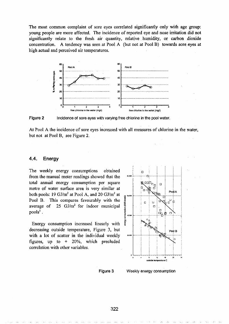
The most common complaint of sore eyes correlated significantly only with age group: young people are more affected. The incidence of reported eye and nose irritation did not significantly relate to the fresh air quantity, relative humidity, or carbon dioxide concentration. A tendency was seen at Pool A (but not at Pool B) towards sore eyes at high actual and perceived air temperatures.
1 2 3 4 01, 1 2 3 4 free chlonne in the water (mgn) free chlonne m the water (mgd)
Figure 2 Incidence of sore eyes with varying free chlorine in the pool water.
At Pool A the incidence of sore eyes increased with all measures of chlorine in the water, but not at Pool B, see Figure 2.
4.4. Energy
Figure 3 Weekly energy consumption
The weekly energy consumptions obtained from the manual meter readings showed that the *""
total annual energy consumption per square metre of water surface area is very similar at both pools: 19 GJ/m2 at Pool A, and 20 GJ/m2 at , f ,, Pool B. This compares favourably with the 2 g average of 25 GJlm2 for indoor municipal pools' . H
$ r o w
5 m
Energy consumption increased linearly with decreasing outside temperature, Figure 3, but with a lot of scatter in the individual weekly w m
figures, up to + 20%, which precluded correlation with other variables.
0
- - Ef- A
- . \ 9 n. n o
- .Rap O .
- -
. . . . . . . . . . . . . . . . . . . . . . . . 0 4 8 2 46 W 24
w t s d e temperature C

5 Conclusions
Under conditions which would be considered to be 'comfortable', 20% to 30% of bathers at swimming pools suffer discomfort, most commonly associated with the eyes.
Under the range of conditions experienced i.e. fresh air rates per m2 of wetted area of 0.003 to 0.005 and 0.008 to 0.013 m3/s, at total ventilating air flows of 0.008 and 0.02 m3/s per m2 respectively. The discomfort suffered by bathers was not related to fresh air ventilation rates. The most significant factor appears to be the amount of chlorine in the water.
6 Recommendation
Ventilation control should be based on the most demanding of the three factors: relative humidity, carbon dioxide concentration, "free" chlorine concentration in the pool water.
In this way, the ventilation rate and heat loss can be minimised while maintaining satisfactory indoor air quality.
Acknowledgements The cooperation of the staff at the two pools, and the support of The Sports Council, in particular David Bosher, are gratefully acknowledged. Sarah Kelly assisted with the questionnaire surveys and Roy Marchant with the measurements.
References
1. ETSU: "Energy efficiency technologies for swimming pools" Energy Technology Series 3. 1985.
2. Editorial: "Wheezing at the swimming pool" The Lancet, page 1342-1343, Dec 22-29, 1979.
3. Penny, P.T. "Swimming pool wheezing" British Medical Journal. 287, page 461-462, 1983.
4. Jessen, H. J., "Chloraminkonzentration in der Raumluft von Hallenbadern" Z. gesamte Hyg. 32, part 3, page 180-1 81, 1986.


Energy Impact of Ventilation and Air Infiltration 14th AlVC Conference, Copenhagen, Denmark
21 -23 September 1993
The Influence of Indoor Tobacco Smoking on Energy Demand for Ventilation
L-G Miinsson,* S A Svennberg**
* LGM Consult AB, Adler Salvius vag 87, S-146 53 Tullinge, Sweden ** RAMAS Teknick AB, Solkraftsvagen 25, S-135 70 Stockholm, Sweden
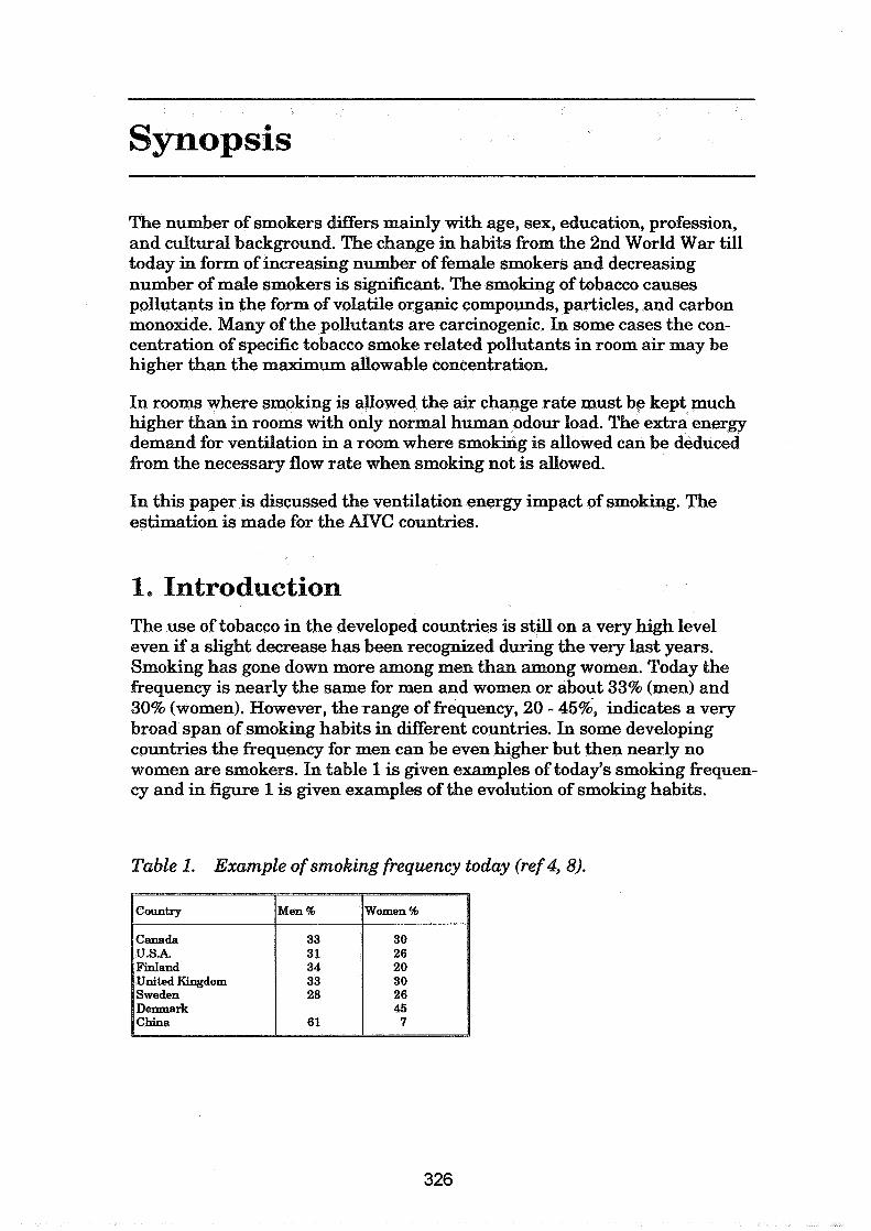
Synopsis
The number of smokers differs mainly with age, sex, education, profession, and cultural background. The change in habits from the 2nd World War till today in form of increasing number of female smokers and decreasing number of male smokers is significant. The smoking of tobacco causes pollutants in the form of volatile organic compounds, particles, and carbon monoxide. Many of the pollutants are carcinogenic. In some cases the con- centration of specific tobacco smoke related pollutants in room air may be higher than the maximum allowable concentration.
In rooms where smoking is allowed the air change rate must be kept much higher than in rooms with only normal human odour load. The extra energy demand for ventilation in a room where smoking is allowed can be deduced from the necessary flow rate when smoking not is allowed.
In this paper is discussed the ventilation energy impact of smoking. The estimation is made for the AlVC countries.
1, Introduction The use of tobacco in the developed countries is still on a very high level even if a slight decrease has been recognized during the very last years. Smoking has gone down more among men than among women. Today the frequency is nearly the same for men and women or about 33% (men) and 30% (women). However, the range of frequency, 20 - 45%, indicates a very broad span of smoking habits in different countries. In some developing countries the fiequency for men can be even higher but then nearly no women are smokers. In table 1 is given examples of today's smoking frequen- cy and in figure 1 is given examples of the evolution of smoking habits.
Table 1. Example of smoking fiequency today (ref 4 8 ) .
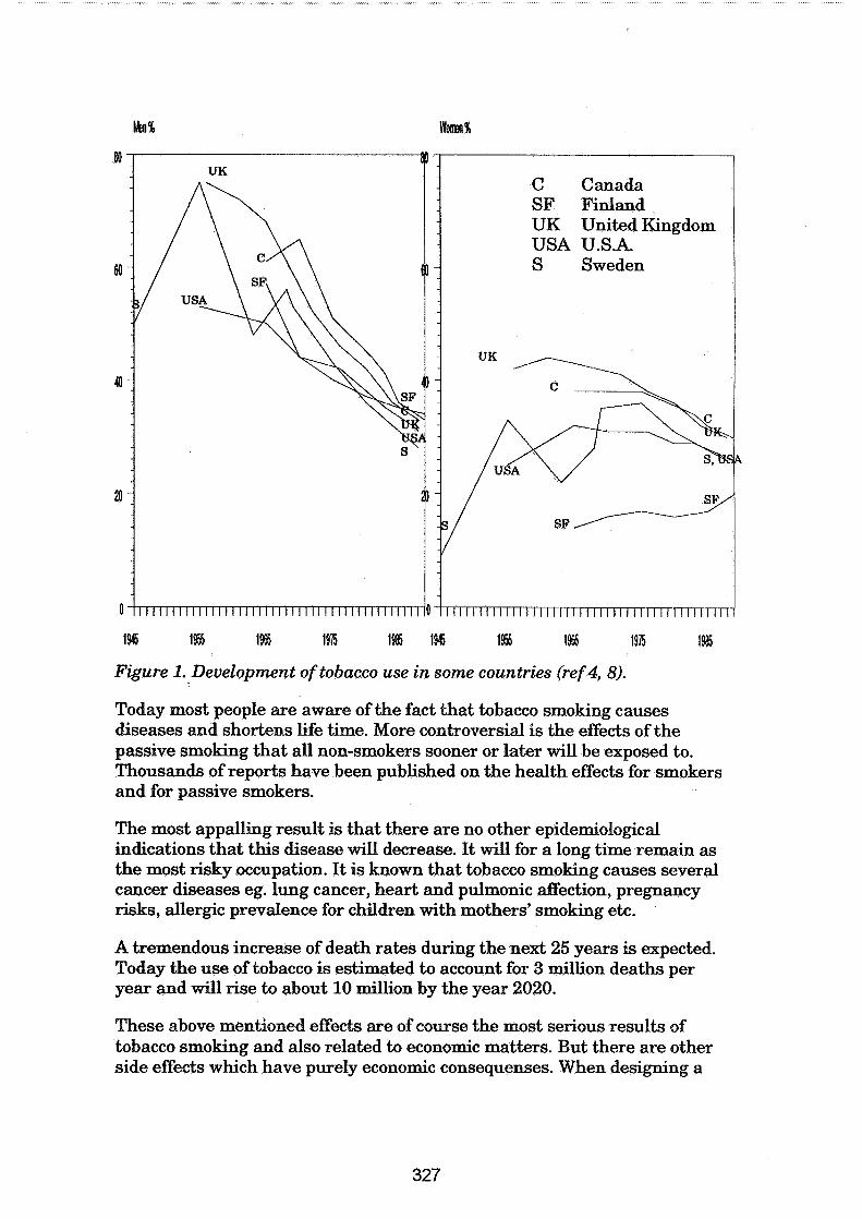
hn% Women%
80
SF Finland UK United Kingdom USA U.S.A.
60 S Sweden
Q
20
0
194 1456 1965 1975 1985 1945 1956 1966 1975 1985
Figure 1. Development of tobacco use in some countries (ref 4, 8).
Today most people are aware of the fact that tobacco smoking causes diseases and shortens life time. More controversial is the effects of the passive smoking that all non-smokers sooner or later will be exposed to. Thousands of reports have been published on the health effects for smokers and for passive smokers.
The most appalling result is that there are no other epidemiological indications that this disease will decrease. It will for a long time remain as the most risky occupation. It is known that tobacco smoking causes several cancer diseases eg. lung cancer, heart and pulmonic affection, pregnancy risks, allergic prevalence for children with mothers' smoking etc.
A tremendous increase of death rates during the next 25 years is expected. Today the use of tobacco is estimated to account for 3 million deaths per year and will rise to about 10 million by the year 2020.
These above mentioned effects are of course the most serious results of tobacco smoking and also related to economic matters. But there are other side effects which have purely economic consequenses. When designing a

ventilation system in eg. an office building, it has to be considered that tobacco smoking increases the necessary outdoor air supply rate. Higher investment for the air handling system follows. We also know that smokers are more sensitive to low temperature than non-smokers because of the reduced pulmonic function. If this has significantly called for a higher indoor temperature is still to be investigated.
2. Objective The objective of this study is to estimate the magnitude of extra energy use for heating the outdoor air required when tobacco smoking is allowed or could be expected somewhere in a building.
3. Method As there are very few data easily available the calculation has been based on both very detailed data and rough estimations by comparisons with the situation in a few other countries. Also data that can be compared give reasons to be quite critical because of the great variation. However, as the data still give the order of magnitude, the calculation is justified.
The calculation is made for non-industrial, non-domestic buildings in which it can be expected that smoking will be allowed. Thus the following building types are not included:
- Dwellings. The outdoor air flow rate does not take into account smoking habits. The occupants in a dwelling decide wether to smoke or not.
- Schools. Smoking is not allowed in the classrooms nor in most of the other areas
- Hospitals. Only a very small area is set aside for smokers.
The volume of the buildings must be estimated. The method used here is to use data for dwellings. Most of the A N C countries have the same living conditions, are industrialised at the same level, have the same area for each person in the non-domestic buildings, and the same proportions of area use in the building types where smoking is allowed. The proportions between dwellings and other non-domestic buildings in Sweden and France have been compared. Both countries have the same proportion between dwellings and non-domestic buildings and the same distribution between the various building types. The same has been asssumed for all the other AIVC countries.
The estimation of the climate has been made by using a simplified degree- day method. A mean value for individual countries has been chosen, where

the population density in the various climate zones has been taken into account.
The outdoor air supply for allowing smoking in the premises has been estimated to be increased, in comparison to what could have been necessary for having an acceptable indoor air quality in buildings for non-smokers. The choice of the flow rate is delicate because standards and codes give no background for the increased flow rate.
4. Assumptions and data used In this section will be given the data on which the estimationfcalculation are based. A discussion on the results and the degree of uncertanty will also be given.
Volume of the buildings The relation between the heated area of domestic buildings and other non- industrial buildings is assumed to be the same in all countries. In Sweden and France the dwelling area is 3 times larger than that of the actually studied buildings. The distribution of the various building types for Sweden has been used as an assumption for the other countries, see table 2. The relation between some of the building types has been compared to the situation in France. The definitions used have not been the same and no to- tal figure has been given for France. As can be seen from table 2 about 113 of the area can be assumed to be smoking area, which is the same as 1/10 of the dwelling area.
Table 2. The distribution of the use of non-domestic buildings and the proportion of area where smoking is allowed (ref 17).
From table 3 the dwelling area can be estimated. It must be noted that the areas are not always quite comparable. Generally the dwelling area given is excluding staircases, basements, sometimes also halls and small kitchens within the dwelling. For single family homes, however, these areas are included. For Sweden both the total heated area and the main dwelling area have been collected, and it is thereby found that the heated area is about
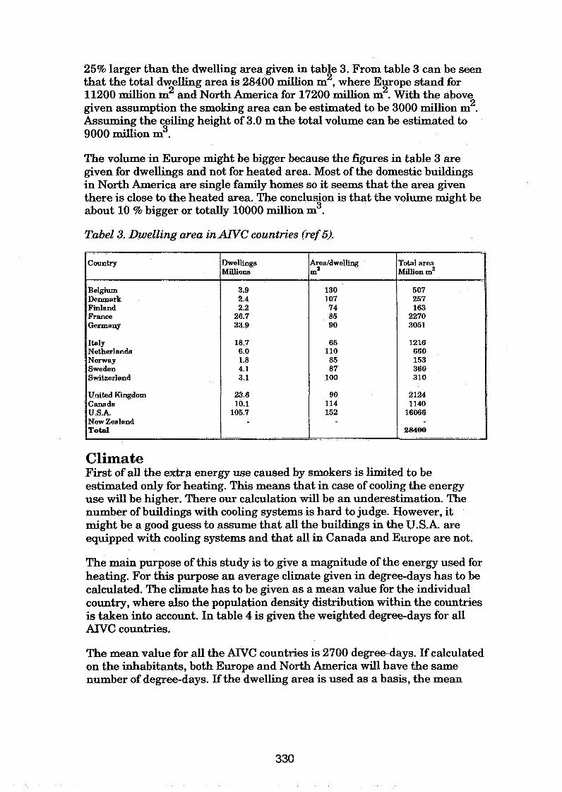
25% larger than the dwelling area given in table 3. From table 3 can be seen that the total dwelling area is 28400 million m2, where Europe stand for 11200 million m2 and North America for 17200 million m2. With the above given assumption the smoking area can be estimated to be 3000 million m2. Assuming the ceiling height of 3.0 m the total volume can be estimated to
3 9000 million m . The volume in Europe might be bigger because the figures in table 3 are given for dwellings and not for heated area. Most of the domestic buildings in North America are single family homes so it seems that the area given there is close to the heated area. The conclusion is that the volume might be about 10 % bigger or totally 10000 million m3.
Tabel 3. Dwelling area in A N C countries (ref 5).
Climate First of all the extra energy use caused by smokers is limited to be estimated only for heating. This means that in case of cooling the energy use will be higher. There our calculation will be an underestimation. The number of buildings with cooling systems is hard to judge. However, it might be a good guess to assume that all the buildings in the U.S.A. are equipped with cooling systems and that all in Canada and Europe are not.
The main purpose of this study is to give a magnitude of the energy used for heating. For this purpose an average climate given in degree-days has to be calculated. The climate has to be given as a mean value for the individual country, where also the population density distribution within the countries is taken into account. In table 4 is given the weighted degree-days for all AIVC countries.
The mean value for all the AlVC countries is 2700 degree-days. If calculated on the inhabitants, both Europe and North America will have the same number of degree-days. If the dwelling area is used as a basis, the mean
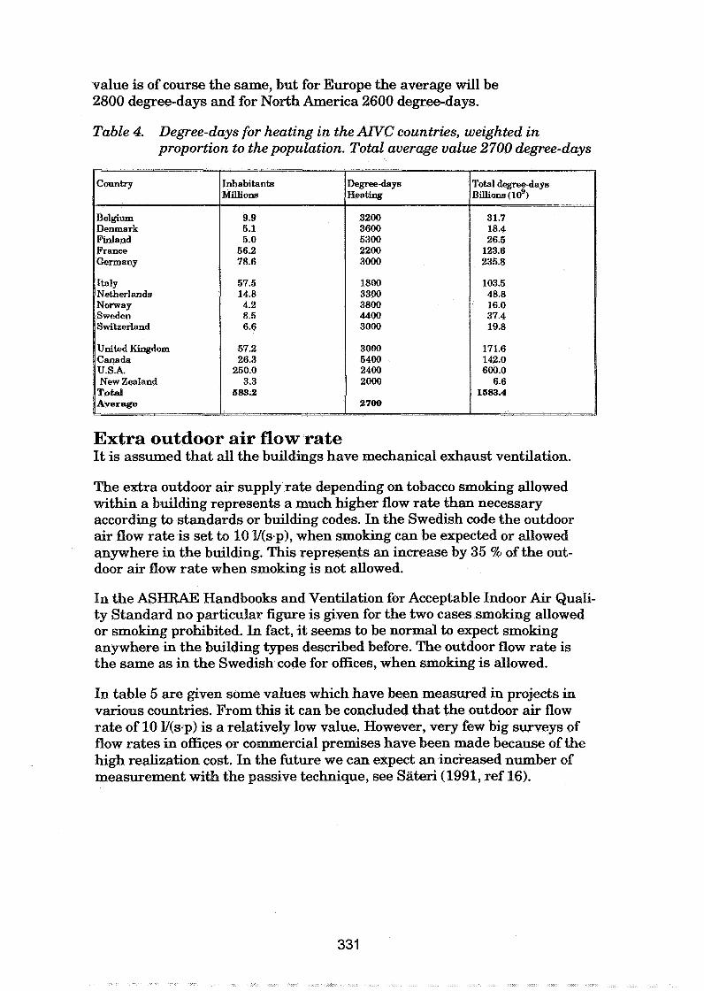
value is of course the same, but for Europe the average will be 2800 degree-days and for North America 2600 degree-days.
Table 4. Degree-days for heating in the A N C countries, weighted in proportion to the population. Total average value 2700 degree-days
Extra outdoor air flow rate It is assumed that all the buildings have mechanical exhaust ventilation.
The extra outdoor air supply rate depending on tobacco smoking allowed within a building represents a much higher flow rate than necessary according to standards or building codes. In the Swedish code the outdoor air flow rate is set to 10 l/(s.p), when smoking can be expected or allowed anywhere in the building. This represents an increase by 35 9% of the out- door air flow rate when smoking is not allowed.
In the ASHRAE Handbooks and Ventilation for Acceptable Indoor Air Quali- ty Standard no particular figure is given for the two cases smoking allowed or smoking prohibited. In fact, it seems to be normal to expect smoking anywhere in the building types described before. The outdoor flow rate is the same as in the Swedish code for offices, when smoking is allowed.
In table 5 are given some values which have been measured in projects in various countries. From this it can be concluded that the outdoor air flow rate of 10 l/(s.p) is a relatively low value. However, very few big surveys of flow rates in offices or commercial premises have been made because of the high realization cost. In the future we can expect an inckeased number of measurement with the passive technique, see Sateri (1991, ref 16).

Table 5. Measured outdoor air flow rates in projects reported at the Indoor Air 1990 in Toronto.
5. Summarized Estimation In section 4 has been discussed the parameters to be taken into consideration, when estimating the extra heat energy use for ventilation of non-domestic areas where tobacco smoking is allowed. One fhrther factor is
3 the heated volume per person.Here a volume of about 40 m per person is assumed. Then the outdoor air flow rate of 10l/(s.p) gives an air change rate of 0.9 per hour (hml).
For the energy calculation has been used the following formula:
Where
V = Total volume of premises where smoking is allowed m 3
n = Air change rate in the smoking case h-l f = Part of air change rate depending on smoking - p = Density of air (1.2) kg/m3 cp = Heat capacity of air (1.0) k J/(kgK) D = Degree-hours (24 times degree-days) K ~ / Y
Putting the deduced values into formula (1) gives:
Thus the extra energy demand is about 70 W y
With the price for energy of 0.055 y U / k W h (0.063 US$/kWh) the total extra cost is calculated to be 3.7-10 ECU/y (4.3.10~ US$/y)
6. Discussion Domestic building ventilation. In this paper the scope has been to discuss the influence of energy use and cost caused by indoor smoking in non-domestic buildings. It is, however,
interesting to notice that extra ventilation need in domestic buildings caused by smoking habits is of the same magnitude as that in non-domestic areas. The extra ventilation can be achieved by more frequently opened windows or by increasing speed of fans.
In the U.S.A. and some other countries where mechanical ventilation is widely used the amount of treated outdoor air often has been chosen so as to allow smoking generally. In Europe where natural ventilation is the most frequent system it is assumed that the needed extra outdoor air is povided by window-airing. It is reasonable to assume that this extra ventilation is in the order of 0.1 to 0.2 air changes per hour during the heating season.
Non-domestic building size. The estimation on non-domestic building volume is based on the relations- hip between domestic and non-domestic buildings in two countries (Sweden and France) may have underestimated the area of non-domestic buildings. One reason is that figures available only present usehl living floor area while heated area can be assumed to be about 30 % larger. The total volume of non-domestic buildings should be corrected accordingly.
Climate, additional heating Possible error in the estimated degree-days calculated is most probably towards the negative side. Thus an additional energy use caused by under- estimation in the order of 20 % is reasonable for both Europe and North America.
Climate, additional cooling Additional cooling of extra ventilation air is unavailable if the control of recirculation is inadequate or if necessary filtration of return air is not installed. A minimum of 10 % of heating energy is probable. The maximum level is hard to judge, but might be up to 40 %.
Air change rate The air change rate is sometimes lower but very offen also higher than that prescribed by standards or codes. Most probably the air change rate in buildings, where smoking is allowed, is a t the higher values, see table 5. Choosing a moderate value of 15 l/(s.p) from that table would double the air change rate cost shown in section 5.
Summarization The discussion above leads to a possibility of summarizing to minimum, maximum, and average levels of cost for indoor smoking. Figures are presen- ted in table 6.

Table 6. Summarization of discussed heating costs for ventilation caused by indoor tobacco smoking in ANC countries
For Sweden only, representing about 1,3 % of the ANC energy turnover found in this paper, the extra cost of energy used because of indoor tobacco smoking is in the order of 100-300 million ECUIyear. That amount is equal to the yearly profit (ref 18) after taxes shown by the Swedish Tobacco Company!
7. Conclusion Even if the number of smokers seems to be stable in the developed countries still many young people start smoking. The main aim must be to reduce the smoking habit to increase the quality of both the outdoor and the indoor environment. By quitting smoking we can reduce the energy use and hence the pollutants from energy production plants.
We can see that tobacco companies try to increase the smoking habit in the developing countries and specially amongst the younger women. If this trend can be stopped we can also save energy that would else be used for cooling or heating the indoor environment.
The ambivalence shown by the politicians is, however, of a great magnitude. Many governments have not dared to tackle the multidiciplinary problems with tobacco smoking with the implications on tax revenue, employment, export income, health and welfare expenditure, energy cost etc.
The bill has to be paid by both smokers and non-smokers. Extra energy use caused by indoor smoking in non-domestic buildings outside industry production is a t least about 3700 million ECU (4000 million US$) annually in the 14 AlVC countries.
1. ASH Handbook 1989, Fundamentals. ISBN 0-9101 10-57-3.
2. CENPTCl56/WG6. Working documents on indoor air quality.

3. A. Elmroth, P. Levin. Air Infiltration Control in Housing. Swedish Council for Building Research D2:1983. ISBN 91-540-3853-7
4. C. Chollat-Traquet. Women and Tobacco. WHO, Geneva 1992. ISBN 92-4-156147-5.
5. E. Hedman (ed). Swedish Housing Market in an International Perspective (in Swedish). National Board of Housing, Building, and Planning, Report 1993:2. ISBN 91-38-12860-8.
6. The Swedish Building Code 1980 and 1988:18. National Board of Housing, Building, and Planning. ISBN 91-38-05209-1 and 91-38-09758-3.
7. L-G Miinsson, S.A. Svennberg. Demand Controlled Ventilating Systems, Source Book IEA Annex 18. Swedish Council for Building Research D2:1993. ISBN 91-540-5513-X.
8. The use of tobacco products in Sweden (in Swedish). The Swedish Board for Public Health. Report 1986:9. ISBN 91-38-09131-3.
9. ASHRAE Standard ANSUASHRBE 62- 1989 Ventilation for Acceptable Indoor Air Quality. ISSN 1041-2336.
10. J. Sundell, 6. G ~ b e r g , S. Wall, B. Stenberg, P.A. Zingmark. The Office Illness Project in Northern Sweden. Indoor Air 1990 Toronto vol4.
11. M.E. Baldwin, J-P. Farant. Study of Selected VOCs in Office Buildings a t Different Stage of Occupancy. Indoor Air 1990 Toronto vol2.
12. P. Skov, 0. Valbjorn. The Danish Town Hall Study. Indoor Air 1990 Toronto vol 1.
13. J. J.K. Jaakkola, O.S. Miettinen, K. Komulainen, P. Tuomaala, 0. Seppiinen. The Effect of Air Recirculation on Symptoms and Environmental Complaints in Office Workers. Indoor Air 1990 Toronto vol 1.
14. V.L. Putnam, J.E. Woods, D.R. Rask. A Comparison of C02 Concentrations and Indoor Env. Acceptability in Commercial Buildings. Indoor Air 1990 Toronto vol3.
15. R.A. Grot, A.T. Hodgson, A. Persily. U Q Evaluation of a New Office Building. Indoor Air 1990 Toronto vol3.

16. J.O. Sateri. The Development of the PFT-Method in the Nordic Countries. Swedish Council for Building Research D9:1991. ISBN 91-540-53 17-X
17. L-G. Carlsson. Energy use in non-industrial buildings (in Swedish). Swedish Council for Building Research R30:1992. ISBN 91-540-5476-1.
18. Tobacco Act. Committee for Tobacco Control. Allmanna forlaget Report SOU 1990:29. ISBN 91-38-10545-4.
Energy Impact of Ventilation and Air Infiltration 14th AlVC Conference, Copenhagen, Denmark
21 -23 September 1993
The Variation of Heat Loss Through Suspended Floors with Ventilation Rate
D J Harris, S J-M Dudek
Department of Architecture, University of Newcastle upon Tyne, Newcastle upon Tyne NEI 7RU, UK
D.J.Hanis, S. J-M Dudek. Dept of Architecture. University of Newcastle upon Tyne. NEl. 7RU. Synopsis Increases in the levels of thermal insulation required in the walls and roofs of houses in the
U.K. in recent years have meant that heat losses through floors now assume greater
significance, as a proportion of the total heat loss from a dwelling. To effect further
reductions in the energy consumption of houses, the thermal performance of floors needs to
be examined to assess the most cost effective insulation strategy. Suspended floors present a
more difficult problem than solid floors because they require under-floor ventilation to
prevent build-up of moisture, and variations in wind speed lead to changes in the ventilation rate and consequent heat loss'. To assess the thermal performance of a suspended floor, a
full-size experimental room- was built and tested in an environmental chamber. The
magnitude and direction of the airflow under the floor were found to vary substantially over
its area, and there were corresponding variations in the effective U-value of the floor, related
to the overall ventilation rate- and the relative position of the air inlet and outlet vents.
Introduction
The ground floors of new houses are often constructed of solid concrete, but where ground
conditions are unfavourable or the site slopes heavily, a suspended floor may be required.
The floor itself and the beams on which it rests may be timber or concrete, and although the
minimum height of the under-floor space in new houses is fixed by regulations 111, in older
houses it may vary from a few centimetres to over half a metre. Suspended timber floors are
typical of a large number of local authority houses built in the twenties and thirties, many of
which are in need of refurbishment and require improved floor insulation to meet the
standards currently expected by householders. Ventilation is required under such floors to
prevent mould growth and rotting caused by condensation, and is normally provided by
natural means, using air bricks. The regulations require a minimum size of ventilation
opening (ie. the number of air bricks per metre run of wall), but do not specify their position.
Since a high rate of under-floor ventilation leads to large heat losses, it is important to ensure
that it is sufficient to prevent rot, but is not so high as to give rise to large energy bills. In
this paper, the way in which the heat losses vary with ventilation rate is investigated.
Theoretical Background
For many years the basis of the CIBSE [2] method for the assessment of U-values of solid
floors has been the work of Macey [3] and Billington [4] who assumed that the greater part
of the heat loss from a floor takes place through the perimeter. Thus, it was supposed that
insulating the perimeter alone would be more cost effective than insulating the whole floor.
However, doubts were cast on this theory when measurements by Spooner [5] showed that
vertical perimeter insulation to a depth of 500mm produced no measurable reduction in heat loss from the floor. The CIBSE method enables a steady-state U-value to be calculated,
based on the indoor-outdoor air temperature difference. This is not altogether realistic, since
the ambient and ground temperatures are constantly changing, but a steady-state U-value at
least gives an indication of the long-term thermal behaviour. In addition, timber suspended
floors may be assumed to have little inherent heat storage capacity. Since that early work,
many analytical studies have been carried out on heat flows through solid ground floors, using such methods as Fourier transforms, [6] finite-difference methods [7] and others, but little additional measured data is available, Anderson 181 developed the CIBSE formula to
give a simplified graphical method of estimating the U-value, based on perimeterlarea
values. The performance of'suspended floors has received considerably less attention than
solid floors. Anderson extended his calculations to include suspended floors, but of necessity
a fixed ventilation rate had to be assumed. The main causes of uncertainty in these predictions are:
i) Uncertainties concerning the thermal conductivity of the ground and the below-
ground temperature, both of which vary with soil constitution and moisture content.
Some data are available [9], but they are specific to soil type and location. Spooner [41
deduced that in general, variations in the below-ground temperature lagged behind
those of the air temperature by about 30 days, but with a much smaller amplitude.
ii) Random variations in the wind speed and direction.
iii) Doubts concerning the relationship between the wind speed and the ventilation rate.
The principal heat loss routes from such a floor are those shown in figure 1. They comprise:
i) Heat losses from the edge of the floor through the walls by conduction, which may
be 1,2 or 3 dimensional and which is mainly horizontal.
ii) Heat losses from the underside of the floor to the air in the cavity by convection and
radiation.
iii) Ventilation heat loss, dependent on the rate of air change in the cavity, and the
difference between the ambient and the cavity temperature.
iv) Conduction through the ground as for solid floors. The relative conmbution of each
mechanism to the overall heat loss has not been estimated.
Experimental Work
A test room was built and is shown in figure 2. The inside dimensions of the floor were
3.14m by 2.91m, the room was 2.8m high and the under-floor space was 0.5m from floor to
bottom of joists. The floor itself was of 18mm chipboard laid on 150mm by 50mm joists at
600mm centres, and between the joists and floor was a layer of damp-proofing membrane to
prevent leakage of air from the underfloor space to the room above. The walls and ceiling
were constructed of plywood panels on timber frames with lOOmm rockwool insulation, and
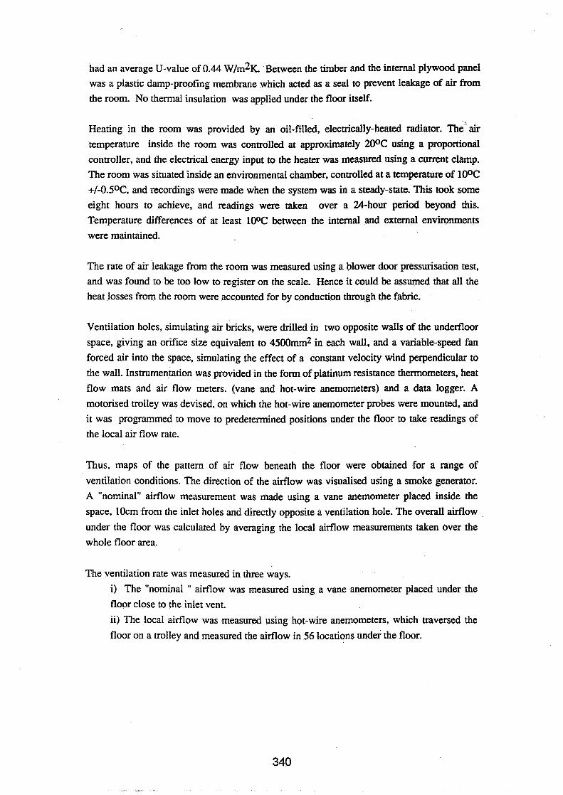
had an average U-value of 0.44 ~ / m 2 ~ . Between the timber and the internal plywood panel
was a plastic damp-proofing membrane which acted as a seal to prevent leakage of air from the room. No thermal insulation was applied under the floor itself.
Heating in the room was provided by an oil-filled, electrically-heated radiator. The air temperature inside the room was controlled at approximately 200C using a proportional
controller, and the electrical energy input to the heater was measured using a current clamp.
The room was situated inside an environmental chamber, controlled at a temperature of lOOC +/-OS°C, and recordings were made when the system was in a steady-state. This took some eight hours to achieve, and readings were taken over a 24-hour period beyond this.
Temperature differences of at least lOOC between the internal and external environments were maintained.
The rate of air leakage from the room was measured using a blower door pressurisation test,
and was found to be too low to register on the scale. Hence it could be assumed that all the
heat losses from the room were accounted for by conduction through the fabric.
Ventilation holes, simulating air bricks, were drilled in two opposite walls of the underfloor
space, giving an orifice size equivalent to 4500mm2 in each wall, and a variable-speed fan
forced air into the space, simulating the effect of a constant velocity wind perpendicular to
the wall. Instrumentation was provided in the form of platinum resistance thermometers, heat
flow mats and air flow meters. (vane and hot-wire anemometers) and a data logger. A motorised trolley was devised, on which the hot-wire anemometer probes were mounted, and
it was programmed to move to predetermined positions under the floor to take readings of
the local air flow rate.
Thus, maps of the pattern of air flow beneath the floor were obtained for a range of
ventilation conditions. The direction of the airflow was visualised using a smoke generator.
A "nominal" airflow measurement was made using a vane anemometer placed inside the
space, lOcm from the inlet holes and directly opposite a ventilation hole. The overall airflow
under the floor was calculated by averaging the local airflow measurements taken over the
whole floor area.
The ventilation rate was measured in three ways.
i) The "nominal " airflow was measured using a vane anemometer placed under the floor close to the inlet vent.
ii) The local airflow was measured using hot-wire anemometers, which traversed the
floor on a trolley and measured the airflow in 56 locations under the floor.
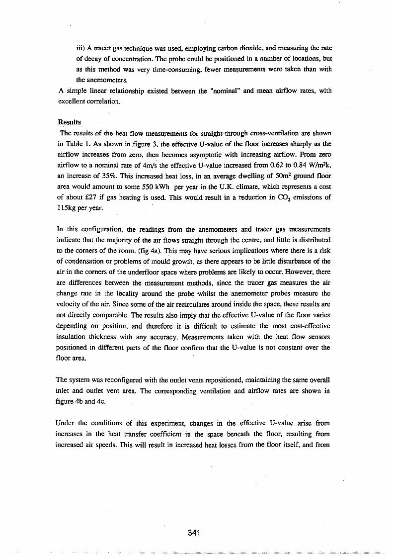
iii) A tracer gas technique was used, employing carbon dioxide, and measuring the rate of decay of concentration. The probe could be positioned in a number of locations, but as this method was very time-consuming, fewer measurements were taken than with
the anemometers.
A simple linear relationship existed between the "nominal" and mean airflow rates, with
excellent correlation.
Results The results of the heat flow measurements for straight-through cross-ventilation are shown in Table 1. As shown in figure 3, the effective U-value of the floor increases sharply as the
airflow increases from zero, then becomes asymptotic with increasing airflow. From zero
airflow to a nominal rate of 4& the effective U-value increased from 0.62 to 0.84 W/m2k,
an increase of 358. This increased heat loss, in an average dwelling.of 50m2 ground floor
area would amount to some 550 kWh per year in the U.K. climate, which represents a cost
of about £27 if gas heating is used. This would result in a reduction in C02 emissions of 1 15kg per year.
In this configuration, the readings from the anemometers and tracer gas measurements
indicate that the majority of the air flows straight through the centre, and little is dismbuted
to the comers of the room. (fig 4a). This may have serious implications where there is a risk
of condensation or problems of mould growth, as there appears to be little disturbance of the
air in the comers of the undemoor space where problems are likely to occur. However, there
are differences between the measurement methods, since the tracer gas measures the air change rate in the locality around the probe whilst the anemometer probes measure the
velocity of the air. Since some of the air recirculates around inside the space, these results are
not directly comparable. The results also imply that the effective U-value of the floor varies
depending on position, and therefore it is difficult to estimate the most cost-effective
insulation thickness with any accuracy. Measurements taken with the heat flow sensors
positioned in different parts of the floor confirm that the U-value is not constant over the floor area.
The system was reconfigured with the outlet vents repositioned, maintaining the same overall
inlet and outlet vent area. The corresponding ventilation and airflow rates are shown in
figure 4b and 4c.
Under the conditions of this experiment, changes in the effective U-value arise from
increases in the heat transfer coefficient in the space beneath the floor, resulting from
increased air speeds. This will result in increased heat losses from the floor itself, and from

the vertical walls beneath the floor, which will also experience an increase in heat transfer coefficient. The airflows measured close to the vertical walls are small, and the presence of
the joists (perpendicular to the main airfiow direction) means that the airflow pattern close to them fairly complex.
Changes in heat flow rates from the room to the space beneath are solely the result of increases in airflow beneath the floor. Since the upper surface thermal resistance and the
thermal resistance of the solid floor remain the same, these changes must therefore represent
increases in the lower surface resistance governing the transfer of heat between the bottom of
the floor and the air in the under-floor space. The values of this heat transfer coefficient have been calculated. (Table 1 and Figure 3.)
Conclusions
The relationship between heat .loss and ventilation rate under a suspended floor was
measured under a range of controlled conditions in a full-size test room. The airflow rate was
found to vary substantially over the area of the floor, depending on the location of the inlet
and outlet vents, and the average ventilation rate. Simultaneous measurements of the heat
losses from the lower surface of the floor indicate corresponding spatial fluctuations in the
effective U-value of the floor. Parts of the under-floor space experience significantly lower
air change rates than others, and where there is a risk of condensation and damp rot this will have implications for a minimum safe ventilation rate.
Acknowledgements The authors wish to acknowledge the financial support of the Science and Engineering Council of the U.K. for this work.
References
1. National House Building Council Standards. "Suspended Ground Floors." NHBC. 1992.
2. CIBSE Guide. Chartered Institute of Building Services Engineers. 1985.
3. Macey, H.H. "Heat Loss Through a Solid Floor." J.Inst. Fuel. 22. pp369-371. 1949. 4. Billington, N.S. "Heat Loss Through Solid Ground Floors." J. Inst Heating Ventil. Eng. 19. ~~351-372. 1951.
5. Spooner, D.C. "Heat Loss Measurements Through an Insulated Domestic Ground Floor."
Building Services Engineering Research and Technology. Vol. 3. No 4. pp147-151. 1982. 6. Delsante, A.E. "A Comparison Between Measured and Calculated Heat Losses Through a Slab on Ground Floor." Building & Env. Vol25, No. 1. pp25-3 1. 1990.
7. Ambrose, C.W. "Modelling Losses From Solid Floors." Building & Environment. Vol. 16.
NO. 4. pp25 1-258. 198 1. 8. Anderson, B.R. "U-values of Uninsulated Ground Floors: Relationship with Floor Dimensions." BSERT 12(3) 103-105 (1991). 9. Lacey, R.E. Climate and Building in Britain. HMSO, London. 1977.
Condunion
nducuon through ground to air
Figure 1. The Principal Heat Loss Routes From a Suspended Floor.
Figure 2. Section Through The Test Room.

Table 1. Effective Overall U-value of the floor at different under-floor air flow rates.
Figure 3. Thermal Resistance and Mean Air Speed
Themtal Resistance O.l m2kN
Lower Thermal
Resistance m 2 W
0.256 .
0.185
0.13
0.115
0.11
0.11
Nominal Air
Speed 4 s
0
1
2
3
3.5
4
Mean Measured Alr Speed mls
Effective U-value
W/m2K
0.62
0.76
0.78
0.83
0.84
0.84
Mean Airspeed
m/s
0
0.17
0.35
0.56
0.72
0.89
Equivalent Air
Change Ratekr
0
0.6
1.2
1.9
2.5
3.1

a. Centre cross-flow.
b. Comer cross-flow.
c. Inlet and outlet at right angles.
Figure 4. Airflow patterns beneath the floor at a nominal wind speed of I d s .


Energy Impact of Ventilation and Air Infiltration 14th AlVC Conference, Copenhagen, Denmark
21 -23 Septern ber 1993
Natural Ventilation Characteristics and Indoor Air Qualtity of Buildings
* Dipartimento di Energetica ed Applicazioni di Fisica, Universita di Palermo, Viale delle Scienze, 901 28 Palermo, ltaly ** lstituto di lngegneria Civile ed Energetica, Facolta di Ingegneria, Universita di Reggio Calabria, 89100 Reggio Calabria, ltaly
NATURAL VENTILATION CHARACTERISTICS AND INDOOR AIR QUALITY OF BUILDINGS
G. Beccali ', G. Cannistraro l, C. Giaconia l, G. Rizzo
Dipartimento di Energetica ed Applicazioni di Fisica, Universitii di Palermo, Viale delle Scienze, 90128 Palermo, Italia. Istituto di Ingegneria Civile ed Energetica, Facoltii di Ingegneria, Universitii di Reggio Calabria, 89100 Reggio Calabria, Italia.
1.0 Synopsis
The importance of natural ventilation, typically restricted to residential buildings application, is rapidly increasing also within the commercial buildings. This is mainly due to the energy savings expected from a reduction of the use of the forced ventilation. Moreover, the remote control of the indoors, provided by means of the intelligent buildings features, allows an easier management of the environmental quality. Furthermore, the indoor air quality is also directly affected by the air exchanges obtained by natural ventilation. Flow rates are strongly influenced by the design characteristics of the openings and by the location of the building with respect to the external winds. On the other hand, the indoor ventilation rates are modified by people who properly operate the window sashes. Using a computer code developed by some of the authors and validated by comparison with experimental data provided by Ispra Joint Research Centre, a comprehensive set of graphs is introduced, in order to check the suitability of the natural ventilation in bringing well conditions of life to the occupants. Fanger's theory based on "olf' and "decipol" methodology has been used for the definition of the indoor air quality levels. Graphs, for assigned geometries of the building and layout of the openings, and for given pollutant sources, give both the proper amount of the flow rate necessary for attaining an assigned percentage of dissatisfied and the flow rates provided by the natural ventilation. By facing these values, it is possible to establish whether the natural ventilation is sufficient or not to ensure the requested air cleanliness.
Following a recent methodology proposed by P.O. Fanger and coauthors (1) it is possible to determine the ventilation rates to be provided inside a building in order to bring well being conditions to the occupants. Unlike current standards, Fanger's procedure takes into account the quality of the external air and allows a measure of the internal pollution sources. The quality of the air and the pollution produced by a given source are checked by the computation of the quantities "olf' and

"decipol". The olf measures the emission rate of bioeffluents from a standard person, while any other source is considered as it was that number of standard people who would cause the same effects of the present pollutant source. The decipol is the pollution produced by one olf under a ventilation rate of 10 l/s of clean air. By relating the olfs subjected to different levels of ventilation with the dissatisfaction of judges that find the air quality unacceptable (2), it is possible to establish a link between the percentage of dissatisfied judges and the ventilation rate. Thus the flow rate Q, required for obtaining the desired quality of the indoor air is (3):
where G = the global pollutant sources [olfl; Ci= the perceived indoor air quality [decipol]; C,= the perceived outdoor air quality [decipol]; E,= the efficiency of the ventilation system. The parameter Ci is related to the percentage of dissatisfied PD by means of the equation:
A computer program for evaluating the air flow rates in a cross- ventilated room has been recently proposed (4). NATVE model provides the ventilation rates under some simplified conditions and it is based on the most consolidated developments in the field (5) and it has been validated using experimental data provided by ISPRA Joint Research Centre (6,7). The air flow rate Qv is computed by means of the following equation:
where A = the inlet free opening area; v = the wind speed; K,= the discharge coefficient; K, = the wind presure coefficient; K, = the inlet- outlet area coefficient; K, = the inlet-outlet distance coefficient; K, = the internal partition coefficient; I&= the fly-screen coefficient. Typical values of the coefficients can be found in (5) NATVE candidates itself as a very simplified procedure to compute the air flow rates in a room where all the windows are open, for this it takes into account only the effects related to the wind pressure and only requires as input data the geometrical parameters of the building and of the openings, the wind speed and direction. Being only a simplified model, NATVE does not take into account the temperature effects or infiltractions or the presence of other near buildings; however, it can

take into account the presence of centre-pivot-hung sashes, fly-screens and internal partitions. Using more complex models, we will surely obtain more accuracy in the results, but the philosophy of the method here presented remains unchanged.
3.0 Method of analisys
In an earlier paper, some of the authors, presented some pictures that translate in a graphical form the results obtained through the application of the NATVE model to some rooms having different geometries, purposes, number of occupants, internal pollution sources and external air quality. Three cross-ventilated rooms have been selected here, whose characteristics are reported in Tab.1 and in figs. la, 2a, 3a.
Tab. 1
The graphs of Figs. lb, 2b, 3b show the response of the rooms depicted above, in terms of air flow rate, to the wind speed and direction. Indeed, it is very hard to find on these graphs flow rates related to the angles of incidence different from that for which the calculation was made; this is why the relation is very complex between flow rates and wind direction. This relation that costitutes a specific characteristic of a room with its openings, and that we will name here "ventilability", is represented in figs lc, 2c, 3c. Ventilabilty graphs was built using the angle of incidence of the wind and the values of the flow rates calculated by NATVE, divided by the flow rate related to a fixed reference angle. In Figs 2a and 2c the reference angle is 0°, in fig. 2b the reference angle is 90". Adopting the linear relation between flow rate and wind velocity shown in figs lb, 2b, 3b we can use in a very simple way the "ventilability" graphs for any value of wind velocity from 0 to 0.5 m/sec. Therefore, knowing the values of the wind velocity v and

of the wind direction 8, it is possible to determine the value of the flow rate Q,:
where Q,/Qo.(@) is the ventilability function calculated once and for all for a given room and referred to a specified window or opening (called here "active"), K(@) relates, in the above hypotheses, the values of the flow rate with the velocity of the wind blowing perpendicularly through the active window. By comparing the value of Q, with the flow rate Q, referred to a standard pecentage of dissatisfied (viz. 20%) (8) it is possible to verify whether the natural ventilation is sufficient to ensure the desired IAQ or it is necessary to have resort to mechanical aids. In some instances a flow rate Q, can be found that largely exceeds the ventilation requirements, so the indoor air velocity could become annoying. In this case it would be advisable to reduce the air flow rate properly operating the centre-pivot-hung sashes of the active window. Fig.4, referred to the active window of fig. la, shows the effect of position of the openable sashes on the air flow; in this picture air flow rates are divided by the value of the flow rate passing through the window when the sashes are fully open. We have to rewrite eq.4 in the following form:
The knowledge of the function Q,/Qoo(a) makes it possible the automatic regulation of indoor air flow rate by a remote-controlled servomechanism acting on the angle a of the sashes of the active window. It will be observed that this kind of control shows a real effectiveness only for the rooms of figs l a and 3a. In these cases, in fact, there are only two windows, so the inlet or outlet air flow must pass through the active window, and the shape of the ventilability curves lb and 3b does not change, The room of Fig.2a has three openings and there are some instances in which the wind does not blow through the active window (90"). Fig.5 shows the variation of the shape of the ventilability curve for the room 2a as a function of the sash angle a. It will be noticed that in such a case the effectiveness of the control system is largely reduced. By combining together Eqs (1) and (2) and taking into account the influence of the sash angle a, it is possible to draw the graphs of figs.ld, 2d and 3d. The graphs show the relationship between the percentage of dissatisfieds and the sash angle a for some values of the velocity of the wind blowing perpendicularly through the active window.
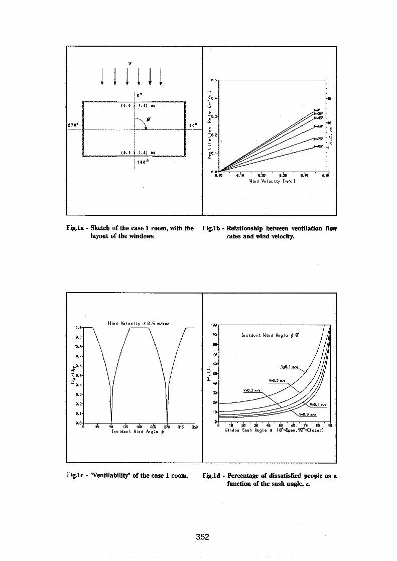
Fig.1a - Sketch of the case 1 room, with the Fig.lb - Relationship between ventilation flow layout of the windows rates and wind velocity.
Wlnd Velocity 6 0.5 m/sac
I n c l d e n t Wlnd Anglo (
Fig& - 'Yentilabiliw of the case 1 room. Fig.1d - Percentage of dissatisfied people as a function of the sash angle, a.
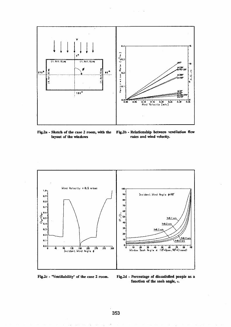
Fig2a - Sketch of the case 2 room, with the Fig.2b - Relationship between ventilation flow layout of the windows rates and wind velocity.
Wlnd V e l o c l t y 2 6.5 d s e c
Ur.dou Sash Anglo a ( O O = O p o n . ~ = C l o c o d )
Fig& - 'Ventilabiliw of the case 2 room. Fig2d - Percentage of dissatisfied people as a function of the sash angle, a.

F i 3 a - Sketch of the case 3 room, with the Fig3b - Relationship between ventilation flow layout of the windows rates and wind velocity.
Wind Velocity S 0.5 m/coo
Fig3c - 'Ventilability" of the case 3 room. Fig3d - Percentage of dissatisfied people as a function of the sash angle, a.

FigAa - Flow rates as a function of the angle Fig.4b - Sketch of the window equipped with a of the openable sash. sash.
u - 0.4-
0.3-
0.2-
0.1-
0.0-. * . . . . * . . 0 i b z h & 4 b & & 7 b w n
Windou %oh Angle a (@=Open .w=Closed)
Fig.§ - Variation of the ventilation shade as a function of the incident wind angles.
- d - C-
V C-
C-
C-

4.0 Conclusion remarks
Through this paper we have introduced the '"ventilability" curves as a simple but comprehensive way to represent the ventilation characteristics of a given room. The relationship between flow rates and wind direction has been obtained using the NATVE model. As far as the intelligent building features are concerned, simple and fast-running programs like NATVE can be used on-line by the control system and could be easily modified whenever we have to change a relevant parameter of the room. Results obtained using more accurate and complex models could be transferred once and for all in a ROM or in a look-up table which are indeed fast to read but hard to modify. Generally speaking the simplified methodology here outlined makes itself an useful tool for the identification of appropriate choices at the early stages of the design process regarding naturally ventilated buildings.
References
FANGER, P.O. "Introduction of the olf and decipol units to quantify air pollution perceived by humans indoors and outdoors" Energy and Buildings 12, 1988, ppl-6 FANGER, P.O. and BERG-MUNCH, B. "Ventilation and body odor" Proc. of An Engineering Foundation Conference on Management of Atmospheres in Tightly Enclosed Spaces ASHRAE, Atlanta, GA, 1983. FANGER, P.O. "The new Comfort Equation for Indoor Air Quality. ASHRAE Journal U, 1988, pp33-38 BUTERA, F. CANNISTRARO, G. YAGHOUBI, MA. and LAURITANO, A. "Natural Cooling of Buildings: a Design Tool for Predicting Comfort Conditions" ISES Solar World Congress, Hamburg, 1987. BUTERA, F. CANNISTRARO, G. YAGHOUBI, MA. and LAURITANO, A. "Benessere termico e ventilazione naturale negli edifici" Energie Alternative HTE 3, 1989, ppl83-189 BUTERA, F. CANNISTRARO, G. RIZZO, G. and YAGHOUBI "Simplified Thermal Analysis of Naturally Ventilated Dwellings" Renewable Energy u, 1991, pp749-756 CANNISTRARO, G. LA PICA, A. VAN HA'ITEM, YAGHOUBI, MA. "Validazione sperirnentale del model10 di ventilazione naturale NATVE" Proc. of 44" Congreso Nazionale AV, Cosenza, Italy, 1989 ANSIIASHRAE Standard 55 -1981 "Thermal Environment conditions for human occupancy" Atlanta, GA, 1981
Energy Impact of Ventilation and Air Infiltration 14th AlVC Conference, Copen hagen, Denmark
21 -23 Septem ber 1993
Indoor Air Quality Index
D Creuzevault
Gaz De France, DETN, 361 Ave du President Wilson, 9321 1 La Plaine Saint-Denis, France
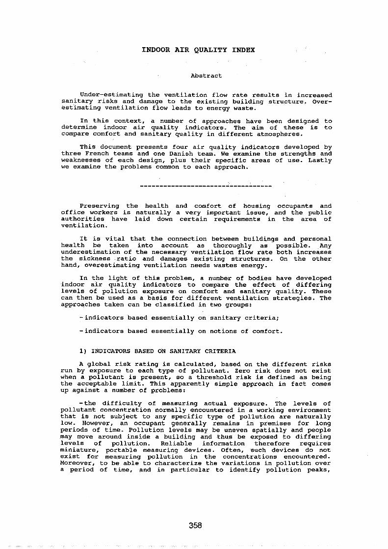
INDOOR A I R QUALITY INDEX
Abstract
Under-estimating the ventilation flow rate results in increased sanitary risks and damage to the existing building structure. Over- estimating ventilation flow leads to energy waste.
In this context, a number of approaches have been designed to determine indoor air quality indicators. The aim of these is to compare comfort and sanitary quality in different atmospheres.
This document presents four air quality indicators developed by three French teams and one Danish team. We examine the strengths and weaknesses of each design, plus their specific areas of use. Lastly we examine the problems common to each approach.
Preserving the health and comfort of housing occupants and office workers is naturally a very important issue, and the public authorities have laid down certain requirements in the area of ventilation.
It is vital that the connection between buildings and personal health be taken into account as thoroughly as possible. Any underestimation of the necessary ventilation flow rate both increases the sickness ratio and damages existing structures. On the other hand, overestimating ventilation needs wastes energy.
In the light of this problem, a number of bodies have developed indoor air quality indicators to compare the effect of differing levels of pollution exposure on comfort and sanitary quality. These can then be used as a basis for different ventilation strategies. The approaches taken can be classified in two groups:
-indicators based essentially on sanitary criteria;
-indicators based essentially on notions of comfort.
1) INDICATORS BASED ON SANITARY CRITERIA
A global risk rating is calculated, based on the different risks run by exposure to each type of pollutant. Zero risk does not exist when a pollutant is present, so a threshold risk is defined as being the acceptable limit. This apparently simple approach in fact comes up against a number of problems:
-the difficulty of measuring actual exposure. The levels of pollutant concentration normally encountered in a working environment that is not subject to any specific type of pollution are naturally low. However, an occupant generally remains in premises for long periods of time. Pollution levels may be uneven spatially and people may move around inside a building and thus be exposed to differing levels of pollution. Reliable information therefore requires miniature, portable measuring devices. Often, such devices do not exist for measuring pollution in the concentrations encountered. Moreover, to be able to characterize the variations in pollution over a period of time, and in particular to identify pollution peaks,
passive sampling is insufficient. The actual exposure is therefore difficult to quantify. Measurement devices and methods need to be improved. These constraints directly affect the relevance of the measurements made.
-the difficulty of evaluating sanitary risk. There are few reliable data concerning the risks run by extended exposure to a given pollutant in low concentrations. We note that:
*it is impossible (for reasons of cost, space, technology, etc.) to measure pollution in a sufficient number of premises to establish significant relations between pollution and sickness;
*sensitivity to a pollutant varies from person to person (the limit values of the risk must therefore take into account the requirements of subacute sectors of the population, e. g. asthma sufferers);
*there are a large number of components present in enclosed premises and potentially at risk. It is therefore impossible to carry out a detailed study for each pollutant;
*the relative risk is very low and therefore difficult to evaluate. Moreover, each illness results from the combination of a number of different factors, formation mechanisms and a sometimes long period of latency. Even for illnesses about which much is known, such as cancer, it is not always possible to precisely quantify the various formation risks. Current knowledge is basically qualitative in nature;
*for two equivalent exposures representing the same levels of pollutant inhaled, the effects will vary depending on the development of the concentration curve in time. Thus one hour's exposure to a pollutant in a concentration of 240 ppm will not have the same effect as 24-hours' exposure to 10 ppm of the same pollutant. Exposure limits cannot therefore be expressed using a concentration value for a given moment, but instead should use an average level that must not be exceeded over a given period, or a maximum value for a given time percentile. Unfortunately, for most pollutants with the exception of carbon monoxide, we only have a very limited amount of data for threshold-exposure levels as a function of time.
The difficulty of setting a recommended limit value is illustrated by the fact that the different authors' recommendations for dioxin vary _by a ratio of 1,000 (these deviations result largely from the different perceptions of what is "acceptable risk"). Another example is the doubling, from 1982 to 1983, of the WHO'S recommended limit value for 24 hours' exposure to C02.
-the difficulty of assessing any possible effects of synergy and neutralization between pollutants. To date, very few studies have been carried out into the effects of pollutant synergy or neutralization on human beings. In some cases, the effect of combining two pollutants is much greater than the simple sum of their effects. This is the case for NO2 and C02, for example. Similarly, the varying degree with which the combination of N02, water steam and nitric acid (HONO) was taken into account by laboratories studying the effects of NO2 on health probably lies at the root of their contradictory conclusions. To take account of this synergy for certain cases, limit values are proposed according to the combination of two pollutants.
Moreover, the simultaneous presence of a number of pollutants implies the permanent interaction of co-factors. To use a radio metaphor, this interaction generates a kind of background noise that
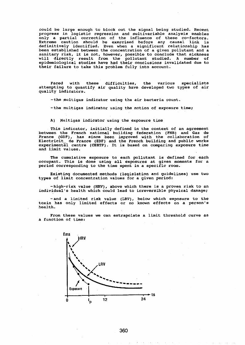
could be large enough to block out the signal being studied. Recent progress in logistic regression and multivariable analysis enables only a partial correction of the influence of these co-factors. Extreme caution should be exercised before any causal link is definitively identified. Even when a significant relationship has been established between the concentration of a given pollutant and a sanitary risk, it is not, however, possible to conclude that sickness will directly result from the pollutant studied. A number of epidemiological studies have had their conclusions invalidated due to their failure to take this problem fully into account.
Faced with these difficulties, the various specialists attempting to quantify air quality have developed two types of air quality indicators.
-the multigas indicator using the air bacteria count.
-the multigas indicator using the notion of exposure time;
A) Multigas indicator using the exposure time
This indicator, initially defined in the context of an agreement between the French national building federation (FNB) and Gaz de France (GDF), has since been improved with the collaboration of Electricit- de France (EDF) and the French building and public works experimental centre (CEBTP). It is based on comparing exposure time and limit values.
The cumulative exposure to each pollutant is defined for each occupant. This is done using all exposures at given moments for a period corresponding to the time spent in a specific room.
Existing documented methods (legislation and guidelines) use two types of limit concentration values for a given period:
-high-risk value (HRV), above which there is a proven risk to an individual's health which could lead to irreversible physical damage;
-and a limited risk value (LRV), below which exposure to the toxin has only limited effects or no known effects on a person's health.
From these values we can extrapolate a limit threshold curve as a function of time:
Ems
The HRVs and a period
indoor a i r q u a l i t y ind ica to r I A Q is ca lcu la ted using t h e LRVs f o r a function defined i n two pa r t s . For a p o l l u t a n t p, t and premises i, w e thus obtain:
I f t h e i n t e g r a t e d exposure =< LRV, I A Q ( p , t , i ) = ( in teg ra ted exposure - LRV) / LRV
I f t h e i n t e g r a t e d exposure >= LRV, IAQ ( p , t , i ) = ( in teg ra ted exposure - LRV) / (HRV - LRV)
IAQ = max IAQ ( p , t , i )
I f IAQ = -1, po l lu t ion concentrat ion is zero I f IAQ =< 0, t h e ind ica to r lets us compare l e v e l s of comfort I f IAQ = 0, t h e r i s k i n t h e premises s tudied is i n s i g n i f i c a n t I f 0 < I A Q < 1, t h e s a n i t a r y r i s k is limited I f I A Q >= 1, t h e r i s k i n t h e premises i s unacceptable
This kind of ind ica to r i s w e l l s u i t e d t o f inding an optimal s o l u t i o n by s imula t ion ( f o r v e n t i l a t i o n and a i r source) . The r i s k caused by humidity is taken i n t o account i n t h e ca lcu la t ion of t h e number of hours of annual p rec ip i t a t ion .
The main l i m i t a t i o n s of t h i s ind ica to r are:
- r i s k is not i d e n t i f i e d f o r aerosols and bacter ia ; - t h e i n d i c a t o r relies on poorly-defined l i m i t thresholds; -synergy e f f e c t s a r e not taken i n t o account; -it is necessary t o induce l e v e l s f o r a number of p o l l u t a n t s
during on-s i te tests (instrumentat ion d i f f i c u l t i e s ) ; - r igorous c a l c u l a t i o n leads t o an i n f i n i t e number of exposure
c a l c u l a t i o n s (over v a r i a b l e per iods with a va r i ab le t i m e o r i g i n ) . A s i m p l i f i c a t i o n f a c t o r is the re fo re genera l ly introduced ( c a l c u l a t i o n s f o r per iods of 1 t o 24 hours only) .
B ) Multigas i n d i c a t o r using t h e a i r b a c t e r i a count
This i n d i c a t o r ( Q I ) was developed by t h e P a r i s hygiene labora tory (LHVP). I t is t h e r e s u l t of over 20 years experience of analys ing a i r q u a l i t y i n d i f f e r e n t types of premises. Indoor a i r q u a l i t y is evaluated using t h e following t h r e e markers:
-carbon monoxide (CO) . The se lec ted threshold value is 5 ppm. This value was used because it is t h e threshold f o r t h e perception of tobacco smoke;
-carbon dioxide (CO2). The se lec ted threshold value is 1,000 ppm. This is t h e room confinement threshold;
- t h e t o t a l b a c t e r i a count (TBC). The se lec ted threshold value is 1,000 p a r t s which rep resen t s a colony per cubic metre. This corresponds t o a 95 p e r c e n t i l e of t h e r e s u l t s obtained f o r outdoor a i r . The bac te r io log ica l sampling c a r r i e d out aims t o d e t e c t s taphylococci (mucus and s k i n ) ; s t reptococci (d iges t ive t r a c t ) and en te robac te r i a ( d i g e s t i v e t r a c t , recent contamination).
The values used could be a l t e r e d t o t a k e i n t o account t h e s p e c i f i c requirements of t h e s i te being studied.
QI = CO / 5 + C02 / 1,000 + TBC / 1,000
An a i r q u a l i t y ind ica to r less than 3 i n d i c a t e s t h a t t h e mechanisms f o r e x t r a c t i n g po l lu t ion from t h e room a r e functioning
c o r r e c t l y and a r e well-sui ted t o t h e type of po l lu t ion source. On t h e o t h e r hand, a q u a l i t y ind ica to r g r e a t e r than 3 shows t h a t t h e a i r q u a l i t y i n t h e room should be improved and t h a t t h e systems f o r e x t r a c t i n g p o l l u t i o n need t o be re-examined.
This approach t akes i n t o account t h e r e l a t i v e importance of t h e main f a c t o r s of po l lu t ion r e s u l t i n g from t h e human metabolism and human a c t i v i t y p lus animal and vegetable pollut ion. The f a c t t h a t p r e c i p i t a t i o n is not taken i n t o account is compensated by t h e b a c t e r i a l parameter.
This i n d i c a t o r has s ince been put i n t o operat ion by a number of major French companies including t h e P a r i s metro (RATP).
This type of ind ica to r requi r ing on-si te measurements is w e l l s u i t e d t o t h e absolute cha rac te r i za t ion of a s p e c i f i c atmosphere.
The main l i m i t a t i o n s of t h i s ind ica to r are:
* t h e f a c t t h a t it takes i n t o account a only l imi ted number of po l lu tan t s . To ensure t h e ind ica to r remains va l id , its use is s t r i c t l y reserved f o r premises where t h e r e is normally no p a r t i c u l a r pol lu t ion;
* i t does not t a k e i n t o account t h e dura t ion of exposure. A number of measurements taken f o r a given moment (notably f o r b a c t e r i a ) can be used, however, t o r e f i n e t h e ana lys i s by br inging i n some element of t i m e ;
* a non-standard method is used t o sample b a c t e r i a l eve l s ;
* i t impossible t o model a type of atmosphere.
I t should be noted t h a t a combined sanitary-comfort approach has been developed by t h e Scandinavian federa t ion of c l ima t i c engineering assoc ia t ions (SCANVAC).
2 ) INDICATORS BASED ON COMFORT CRITERIA
For t h e s e approaches, a i r q u a l i t y is based on o l f a c t o r y perception.
A) S ing le marker ind ica to r
This i n d i c a t o r is t h e simplest of a l l . I t is based on t h e assumption t h a t a concentrat ion of a given po l lu tan t i n d i c a t e s t h e l e v e l of r i s k generated by a l l indoor pol lu t ion . I n general , i n t h e r e s i d e n t i a l and t e r t i a r y sec to r s , two p o l l u t a n t s a r e taken a s t h e p o l l u t i o n t r a c e : carbon dioxide o r r e l a t i v e humidity. Ven t i l a t ion systems regula ted by> changes i n one of t h e s e two p o l l u t a n t s a r e a l ready on t h e market.
This is t h e type of approach used by t h e French na t iona l bui ld ing s c i e n t i f i c and t echn ica l c e n t r e (CSTB) i n its comparative s t u d i e s modelling v e n t i l a t i o n systems (notably, humidity r egu la t ion) .
Where water vapour i s concerned, only t h e r i s k s of condensation ( leading t o s t r u c t u r a l damage) a r e taken i n t o account. A d i s t i n c t i o n is made between t h e t o t a l condensation t i m e and condensation t i m e s g r e a t e r than 30 minutes.
ded over a given period, or a maximum value for a given time concentration is related to the discomfort linked with body odour. It therefore falls into the category of the perceived quality of indoor air rather than any sanitary quality of this air. The limit values used (1,300 ppm and 2,500 ppm) are well below harmful concentration levels.
This approach is quite well suited to comparative studies of two ventilation systems.
In return for its simplicity, this approach has a number of limitations:
*the relative importance that has to be accorded to the risk related to hygrometry compared with that related to the C02 concentration cannot be quantified;
*exposure to various other pollutants is not taken into account;
* insufficient account is taken of the effect of concentrations varying in time. The indicator is soon to be modified to partially overcome this problem.
With this indicator, therefore, it is difficult to characterize a specific type of atmosphere to any absolute degree.
B) Olf and Decipol
This is a sensory approach developed by Professor Fanger (Denmark) in association with professor Bluyssen. It is based solely on the smell nuisance to the operator in certain configurations. The resulting indicator is an evaluation of passive air quality.
A unit termed the olf has been introduced to quantify the intensity of a pollution source. One olf is the level of air pollution produced by the average adult working in the tertiary sector, seated and in a stable temperature and with a hygiene level equivalent to 0.7 baths a day. All odours can be quantified in relation to this reference level. Current olf values for main polluting sources (occupants, smokers, materials, etc.) are listed in tables.
A similar unit, termed the decipol, quantifies perceived air pollution. One decipol is the perceived air pollution in a space having a polluting source of one olf, ventilated by e 10 11s flow of non-polluted air in stable conditions and in a uniform mixture (ventilation efficiency of 1). This gives us: 1 decipol = 0.1 olf/s.
A curve drawn using a panel of 168 judges in the presence of the bioeffluent of 1,000 subjects shows how air is perceived as a function of ventilation in a given room. It traces the percentage of dissatisfied judges, i.e. the percentage judging the air to be unacceptable just after having entered the room. From these data the curve was drawn for the percentage of dissatisfied judges on the panel as a function of the decipol number.
Based on the proportion of dissatisfied judges for the given room and the intensity of the different smells, we can then deduce the flow rate of air required to dilute this pollution.
These units can also be used to qualify outdoor air.
This approach to premises where people are the main source of pollution (much of the tertiary sector) is mirrored in the

ventilation standards expressed as an air flow rate per occupant. It is used in EC recommendations on ventilation requirements for buildings (the COST 613 project entitled "indoor air quality and impaot on individuals"), and in European Commission work in standardization, CEN/TC 156 (standard proposal). The advantage of this approach is that it brings a concrete solution and meets one of the main requirements expressed by occupants.
This approach is particularly well suited to studying premises where pollutant concentrations are too low to be measured by ordinary chemical analyses. Moreover, it makes it possible to select materials or equipment that emit low olf levels and assists in resolving the problem of so-called sick buildings.
This approach is the only one to date that has received a consensus of agreement by several countries for the specification and design of ventilation installations using air quality criteria.
The main limits of this concept are:
-it only slightly takes into account the health risks of pollution. Human sensory perception plays an important role in warning us of environmental dangers, but some types of pollution are odourless. Measurements taken in existing buildings have shown that C02 and particle concentrations are imperfectly correlated with olf measurements. However, it is also true that when the air quality is perceived as being "poor", there is also an increased risk of toxicity. By increasing ventilation flow rates to dilute odours, sanitary risks are also reduced;
-the intensity of all pollution sources is not always known. In this case it is necessary to call on a panel of experimenters to define the rate of dissatisfaction in the reference conditions;
-it is difficult to simulate conditions. This is a relatively recent concept and the models so far developed have only partially been validated.
Energy Impact of Ventilation and Air Infiltration 14th AlVC Conference, Copenhagen, Denmark
21 -23 Septern ber 1993
Correlations between CO2 and Steam concentrations Measured in 60 Occupied Housing Units
P Dalcieux
EDF Centre des Renardieres, Dept ADE Batiments, 77250 Moret Sur Loing, France
Within the fi-amework of demonstration and industrial pilot projects in the energy sector supported by the Commission of the European Economic Communities, an important experiment has been dedicated to the HYGRO-ADJOTSTABLE NATURAZ, VENTILATION (Contrat EE/166/87/FR).
The experiment took place on three sites :
Les ULIS (France), NAMUR (Belgium) and SCHIEDAM (the Netherlands).
A comparison has been made for each site between the ventilation flow rates and the quality of air in ten housing units fitted with hygro-adjustable natural ventilation equipment and ten equivalent housing units fitted with passive ventilation systems.
The flow rate o? air discharged and the rise in CO2 and steam concentrations internally emitted are known for each service room of a housing unit, namely the kitchen, bathroom or the lavatory. We deduct the amount of C02 and steam generated internally which are discharged through the ventilation ducts of service rooms.
The housing urrits involved being equiped with air intakes in the living rooms and air exits on the ventilation ducts in the service rooms, it is possible to deduce from information collected in service room, ir. :cresting information regarding the changes in COa and steam flow rates in :he living rocms.
Thus, when the wind is very low and the air change mainly ensured by the thermal draft ducts, the correlation's between the rise in CO2 and steam contents at night in "blind" lavatories are a fairly good representation of the correlations in rooms occupied where the pollutants are generated;
Under the same conditio;;~, the overall CO2 flow rate internally generated and discharged from the service rooms enable the overall amounts of CO2 generated in the living rooms to be assessed.
A comparison between ti:e cverzge correlations existing between the rise CO2 and steam concentration in the three categories of service rooms, namely kitchens, bathrooms and lavatories enables the particular nature of their respective needs to be best known. We can note in particular that the growth in the 6 0 2 rate in the lavatories which only depends on that existing in the living rooms always comes concurrently with a proportional growth in the steam concentration whereas, in bathrooms and kitchens, though this relation exists during current periods of time, it becomes entirely different when particular activities (cooking, bath, clothes drying and so on) take place.
Lastly, comparative analyses of variations in C02 and steam rates enable the effects of water absorption by the materials to be assessed and best taken into account to evaluate the efficiently of Hygro-adjustable Natural Ventilation processes.
The correlations made between variations in C 0 2 and steam rates for hygro-adjustable natural ventilation or passive ventilation systems are comparable ; they do not seem to be contingent upon the ventilation mode and can certainly be used in mechanical processes.

Energy Impact of Ventilation and Air Infiltration 14th AlVC Conference, Copenhagen, Denmark
21 -23 September 1993
Natural Ventilation in 18 Belgian Apartments: Final Results of Longterm Monitoring
P Wouters, B Geerinckx, D L'Heureux
Belgian Building Research Institute (WTCBICSTC) Violetstraat, 21 -23, 1000 Brussels, Belgium

In the framework of a CEC demonstration project on humidity controlled ventilation, detailed measurements are carried out in 18 aparfments in Namur, Belgium.
The paper gives a brief description of the building, of the airtightness of the apartments and of the ventilation provisions.
The largest part of the paper deals with the major outcomes of the study. This includes the following issues:
- air flow rates: on the average, dependency of wind and temperature difference; - indoor air quality indicators: C02 and water vapour; - behaviour of the humidity controlled system; - energy losses due to the ventilation.
Finally, some conclusions about the ventilation performances and of the monitoring programme are given.
The demonstration project showed very well the influence of the building characteristics on the performances of the ventilation system.
1. Introduction
As part of a CEC demonstration project of DG XVII, the performances of a humidity controlled natural ventilation system, developed by the French firm Aereco, was studied in 3 buildings. These buildings were situated in Les Ulis (France), Schiedam (Netherlands) and Namur (Belgium). The following organizations participated in the project : Aereco, Electricit6 de France, CETIAT, TNO-BOUW and BBRI. General information as well as first results were reported in [I] , [2]. The final report of this project will be published in the autumn of 1993 [3]. This paper gives only information on the results found in the Namur building and with emphasis on the performances of the natural ventilation in general. More information can be found in [3].
2. The buildinq
The building in Namur is situated in a suburban area of Namur. The test building makes part of a group of 4 similar buildings. Figure 1 shows the east facade. The construction is done between 1978 and 1982. The overall heat transmission coefficient of the facades is estimated to be 2.5 W/(m2K). The building is divided into 2 piles consisting each of 9 apartments (level 0 ti11 8). 9 apartments are equipped with a natural humidity controlled ventilamsystem, the dther 9 apartments are equipped with a standard natural ventilation system, called reference system. qigure 2 shows the floor plan of the apartments. The Shunt duct system has a single main duct for the levels 0 to 7. Level 8 has separate ducts. Figure 3 shows a cross section of the ducts. The heating system is a central warm water radiator heating system. A gas fired boiler is in the basement. The annual energy consumption per dwelling for heating is 45x103 MJ/year (1400 m3 gas per annum) based on the consumption of 1985. One apartment, the reference apartment at street level, was unoccupied during the whole duration of the measurement campaign.
To assure a good airtightness of the building, a rather detailed pressurization measurement campaign was carried out. The requirement was to achieve an airtightness of 3-h at apartment level at 50 Pa pressure difference over the envelope. The measured results are summarized in table 1. The results are expressed with respect to the gross volume (external dimensions), which is 192 m3.
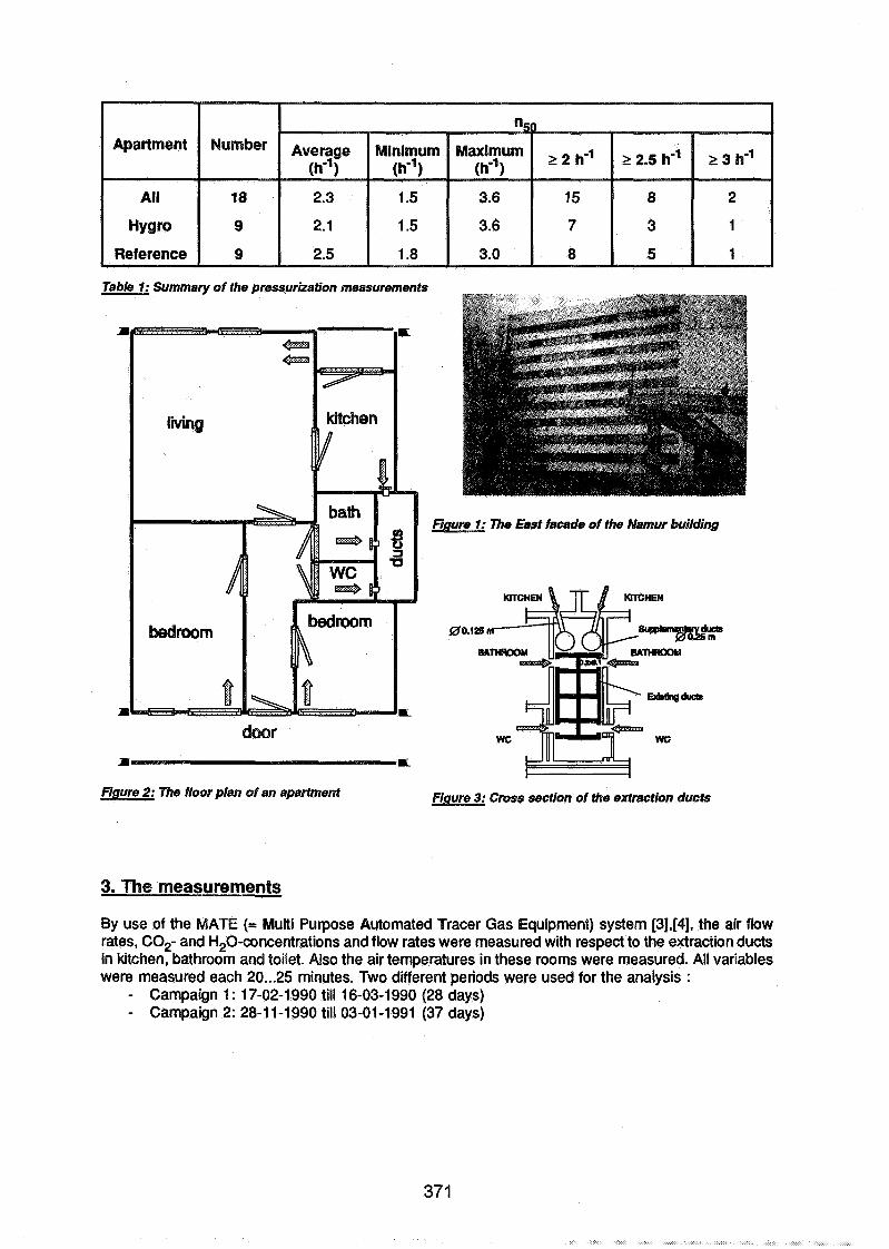
Table 1: Summary of the pressurization measurements
Figure I: Ths East facade of the Namur building
Figure 2: The floor plan of an apartment Figure 3: Cross section of the extraction ducts
3. The measurements
By use of the MATE (= Multi Purpose Automated Tracer Gas Equipment) system [3],[4], the air flow rates, C02- and H20-concentrations and flow rates were measured with respect to the extraction ducts in kitchen, bathroom and toilet. Also the air temperatures in these rooms were measured. All variables were measured each 20 ... 25 minutes. Two different periods were used for the analysis :
- Campaign 1 : 17-02-1 990 till 16-03-1 990 (28 days) - Campaign 2: 28-1 1-1990 till 03-01-1991 (37 days)

4. Results
4.1. Air flow rates
The average air flow rates for the total duration of both measurement campaigns are given in table 2 as function of the level and the type of ventilation system. The average air flow rate for the occupied apartments is 83 m31h. The distribution of the total extracted air flow rates for all reference and humidiiy controlled apartments is presented in figure 4. From these results, the classification of the air change rates as given in table 3 can be made. As given in table 3, the air flow rate is almost never below 0.25 h-'-
Total air flow rates (mYh)
Table 2: Average air flow rates for the whole dwelling, mference and humidity controlled apartments, Namur
Figure 4: Histogram of air flow rates for total dwelling in the Namur building
Table 3: Distribution of the total air change rates for apartments in Namur
The effect of wind speed and temperature on the total air change rate is illustrated for 2 apartments: one unoccupied apartment at street level in which the natural supply and extraction openings were the whole time open (figure 5) and an occupied apartment at the 7th floor (figure 6). For the unoccupied reference apartment at street level, a clear dependency of wind speed and temperature difference can be observed. The strange trend for large temperature differences may be misleading given the small amount of measurements. For the occupied apartment, the wind effect is significant but not as strong. The temperature effect is marginal. This can be explained by the small stack effect.

T a u a18 nou lare bm)
Figure 5: Variation of the total air flow in the unoccupied apartment
Figure 6: Variation of the total air flow rate in the reference apartment at level 7
4.2. C02-concentrations and C02-rates
The average C02-concentrations are given in table 4. The distribution of the C02-concentration is given in figure 7. The average concentrations in kitchen, bathroom and toilet are not so high. Unfortunately, no information is available for the living room and the bedrooms.
Table 4:. Average CQ~concentrations (ppm) for the whole dwelling, mference and humidity controlled apartments, Namur
nearly outside concentration, the average measured increase was I ppm
The extracted C02-flow rates as well as the distribution over the different ventilation ducts are presented in figure 8. The average value for the occupied apartments is about 43 Vhour. It must be stressed that only the extraction through the ducts is taken into account. In figure 9, the extracted C02- rates are expressed as function of the temperature difference for wind speeds between 0 and 2 mls. There is some increase as function of the temperature difference. Two explanations can be given :
- for small temperatures, there are probably open windows and cross ventilation;
Figure 7: Histogram of CQ2-concentrations (with _ gas cooking will increase the temperature in refemnce to outside)
the kitchen and can also explain the higher C02-rates for larger temperature differences.
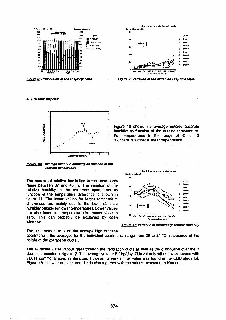
Figure 8: Distribution of the COzflow rates
4.3. Water vapour
FIgure 9: Variation of the ertracted COrflow rates
Humidity controlled apartments EmauedCeaateE &AIl
Figure 10: Average absolute humidityas function of the external femperature
250 -
2W.
150.
100.
Figure 10 shows the average outside absolute humidity as function of the outside temperature. For temperatures in the range of -5 to 10 OC, there is almost a linear dependency.
Learn X w o
pi-I . lwul + w 2
X Wo13
0 w 4
The measured relative humidities in the apartments range between 37 and 48 %. The variation of the relative humidity in the reference apartments as function of the temperature difference is shown in figure 11. The lower values for larger temperature differences are mainly due to the lower absolute humidity outside for lower temperatures. Lower values are also found for temperature differences close to zero. This can probably be explained by open windows.
Humidity controlled apartments Waave humimy pl)
Learn
Figure 11: Variation of the average relative humidity
The air temperature is on the average high in these apartments : the averages for the individual apartments range from 20 to 24 OC. (measured at the height of the extraction ducts).
The extracted water vapour rates through the ventilation ducts as well as the distribution over the 3 ducts is presented in figure 12. The average value is 5.0 kglday. This value is rather low compared with values commonly used in literature. However, a very similar value was found in the ELlB study [5]. Figure 13 shows the measured distribution together with the values measured in Namur.
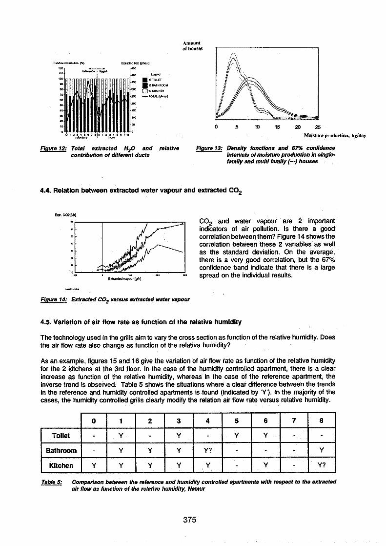
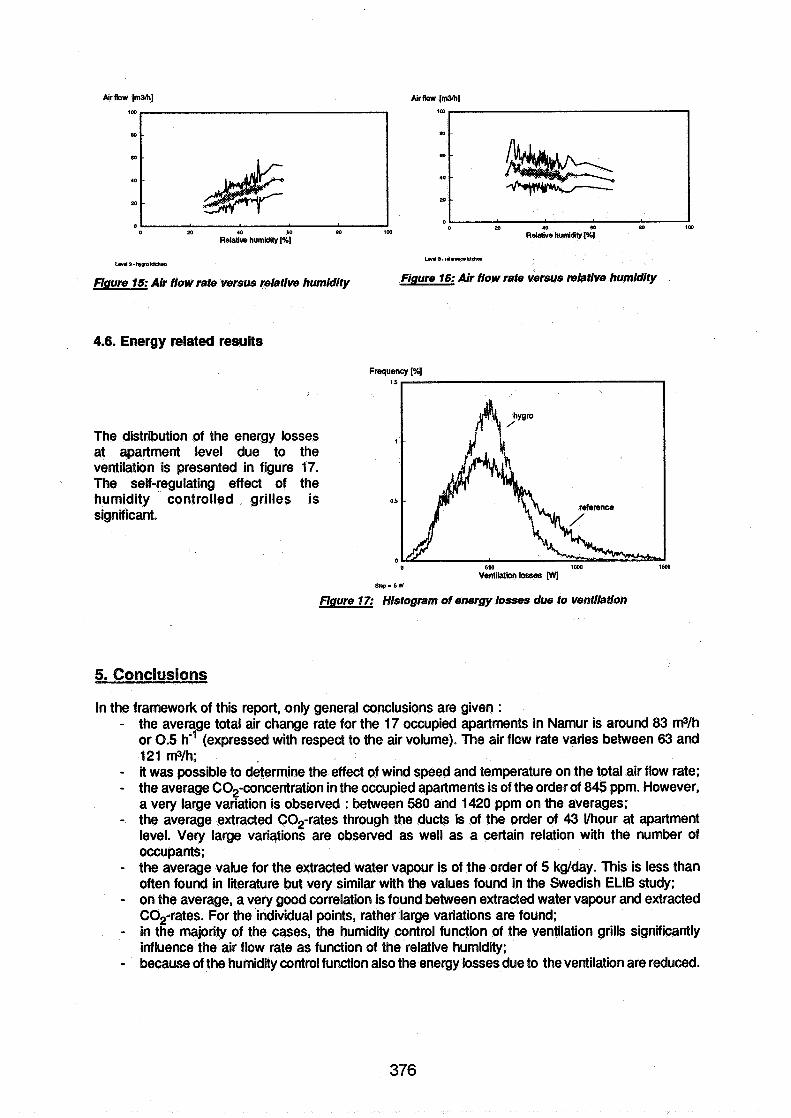
Air tbw [m%] Air fiow [m3m]
lm 1
0 0 w 40 60 60 1m
Relativo humidity [%j
L.nl3-rnU~chn W 3 - d e n a O h n
Figure 15: Air flow rate versus relative humidity Figure 16: Air flow rate versus nelative humidity
4.6. Energy related results
The distribution of the energy losses at apartment level due to the ventilation is presented in figure 17. The self-regulating effect of the humidity controlled grilles is significant.
Stq- 5 W
Figure 17: Histogram of energy losses due to ventilation
5. Conclusions
In the framework of this report, only general conclusions are given : - the average total air change rate for the 17 occupied apartments in Namur is around 83 m3/h
or 0.5 h" (expressed with respect to the air volume). The air flow rate varies between 63 and 121 Wlh;
- it was possible to determine the effect of wind speed and temperature on the total air flow rate; - the average Cog-concentration in the occupied apartments is of the order of 845 ppm. However,
a very large vanation is observed : between 580 and 1420 ppm on the averages; - the average extracted C02-rates through the ducts is of the order of 43 Vhour at apartment
level. Very large variations are observed as well as a certain relation with the number of occupants;
- the average value for the extracted water vapour is of the order of 5 kg/day. This is less than often found in literature but very similar with the values found in the Swedish ELlB study;
- on the average, a very good correlation is found between extracted water vapour and extracted C02-rates. For the individual points, rather large variations are found;
- in the majority of the cases, the humidity control function of the ventilation grills significantly influence the air flow rate as function of the relative humidity;
- because of the humidity control function also the energy losses due to the ventilation are reduced.

With respect to the influence of the humidity controlled ventilation grills, much more information can be found in the final report of this project [3]. As indicated in this report, the building characteristics in combination with the duct characteristics have a major impact on the performances of the system. Due to this, rather poor results are found for the Schiedam building, moderate results for the Namur building and good results for the Les Ulis building.
As a general conclusion, this study has on the one hand resulted in very interesting information with respect to the performances of natural ventilation systems in apartments. On the other hand, it has clearly highlights the relation between building characteristics and ventilation performances.
6. Acknowledqments
The authors wish to thank DG XVll of the Commission of the European Community for supporting this project. We are also very greatfull to the occupants of the dwellings involved in the study as well as the social housing society responsible for the building. Finally but not at least, we would like to thank the other participants in the project.
7. References
1. JARDlNlER P. and SIMONNOT J. "Principle and aim of a natural humidity controlled ventilation system" Netherlands, International CIB W67 Symposium, "Energy, Moisture and Climate in Buildings", 3-6 September 1990, Rotterdam, p.119
2. WOUTERS P., L'HEUREUX D., GEERINCKX B., VANDAELE L. "Performance evaluation of humidity controlled natural ventilation in apartments" AIVC, proceedings 12th AlVC Conference, Volume 1, p. 191 -1 92, September 1991
3. "Passive humidity controlled ventilation for existing dwellings'' CEC, final report of CEC demonstration project, 1993
4. ROULET C.-A. and VANDAELE L. "Airflow Patterns Within Buildings Measurement Techniques" AIVC, Technical Note 34, 1991
5. TOLSTOY N. " Humidity levels in the Swedish housing stock" Proceedings of Indoor Air '93, Helsinki, Finland, Vol. 6, p. 91- 96, 1993


Energy Impact of Ventilation and Air Infiltration 14th AlVC Conference, Copenhagen, Denmark
21 -23 Septern ber 1993
Practical Aspects of Energy Rating Within the UK
C Irwin, R Edwards
Department of Building Engineering, UMIST, P 0 Box 88, Sackville Street, Manchester, M60 IQD
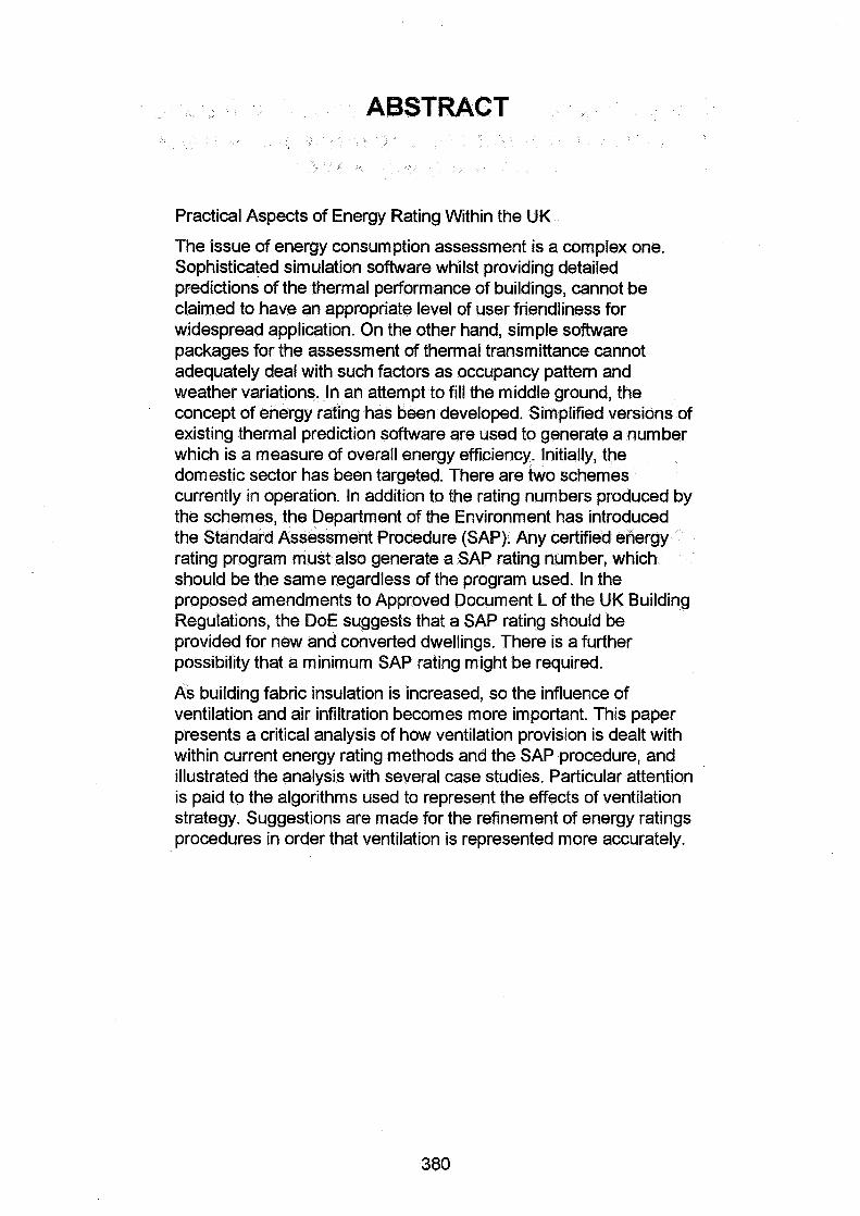
ABSTRACT
Practical Aspects of Energy Rating Within the UK
The issue of energy consumption assessment is a complex one. Sophisticated simulation software whilst providing detailed predictions of the thermal performance of buildings, cannot be claimed to have an appropriate level of user friendliness for widespread application. On the other hand, simple software packages for the assessment of thermal transmittance cannot adequately deal with such factors as occupancy pattern and weather variations. In an attempt to fill the middle ground, the concept of energy rating has been developed. Simplified versions of existing thermal prediction software are used to generate a number which is a measure of overall energy efficiency. Initially, the domestic sector has been targeted. There are two schemes currently in operation. In addition to the rating numbers produced by the schemes, the Department of the Environment has introduced the Standard Assessment Procedure (SAP). Any certified energy rating program must also generate a SAP rating number, which should be the same regardless of the program used. In the proposed amendments to Approved Document L of the UK Building Regulations, the DOE suggests that a SAP rating should be provided for new and converted dwellings. There is a further possibility that a minimum SAP rating might be required.
As building fabric insulation is increased, so the influence of ventilation and air infiltration becomes more important. This paper presents a critical analysis of how ventilation provision is dealt with within current energy rating methods and the SAP procedure, and illustrated the analysis with several case studies. Particular attention is paid to the algorithms used to represent the effects of ventilation strategy. Suggestions are made for the refinement of energy ratings procedures in order that ventilation is represented more accurately.
Energy Impact of Ventilation and Air Infiltration 14th AlVC Conference, Copen hagen, Denmark
21 -23 September 1993
A PMV Controlled Ventilation Strategy
P Simmonds
RTB van Heughten b.v., P 0 Box 8128,9702 KC Groningen, The Netherlands

ABSTRACT
A PMV Controlled Ventilation Strategy
Designing a comfortable inside climate for office buildings to operate within comfort limits (PMV +I- 0.5) requires a flexible operating strategy. Two systems a VAV and a VHV are identified and compared to each other. Dynamic simulation techniques are used to obtain an optimal design, based upon comfort conditions not temperatures. The control strategies are optim ised to minimize energy consumption while controlling the HVAC system to remain within comfort limits in the occupied zone.
Energy Impact of Ventilation and Air Infiltration 14th AlVC Conference, Copenhagen, Denmark
21 -23 September 1993
Assessment of Energy Impact of Ventilation and Infiltration of the French Regulations for Residential Buildings
J Riberon, J-R Millet, J G Villenave
Centre Scientifique et Technique du Bdtiment, BP 02-77421 Marne la Vallee, France
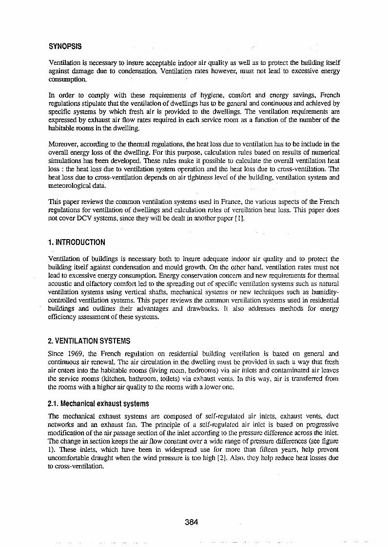
SYNOPSIS
Ventilation is necessary to insure acceptable indoor air quality as well as to protect the building itself against damage due to condensation Ventilation rates however, must not lead to excessive energy consumption
In order to comply with these requirements of hygiene, comfort and energy savings, French regulations stipulate that the ventilation of dwellings has to be general and continuous and achieved by specific systems by which fresh air is provided to the dwellings. The ventilation requirements are expressed by exhaust air flow rates required in each service room as a function of the number of the habitable rooms in the dwelling.
Moreover, according to the thermal regulations, the heat loss due to ventilation has to be include in the overall energy loss of the dwelling. For this purpose, calculation rules based on results of numerical simulations has been developed. These rules make it possible to calculate the overall ventilation heat loss : the heat loss due to ventilation system operation and the heat loss due to cross-ventilation. The heat loss due to cross-ventilation depends on air tightness level of the building, ventilation system and meteorological data.
This paper reviews the common ventilation systems uscd in France, the various aspects of the French regulations for ventilation of dwellings and calculation rules of vcntilation heat loss. This paper does not cover DCV systems, since they will be dealt in another paper I].
1. INTRODUCTION
Ventilation of buildings is necessary both to insure adequate indoor air quality and to protect the building itself against condensation and mould growth. On thc othcr hand, ventilation rates must not lead to excessive energy consumption. Energy conservation concern and ncw requirements for thermal acoustic and olfactory comfort led to the spreading out of speciiic vcntilation systems such as natural ventilation systems using vertical shafts, mechanical systems or ncw techniques such as humidity- controlled ventilation systems. This paper reviews the comnlon ventilation systems used in residential buildings and outlines their advantages and drawbacks. It dso actdresses methods for energy efficiency assessment of these systems.
2. VENTILATION SYSTEMS Since 1969, the French regulation on residential builrting ventilaliori is based on general and continuous air renewal. The air circulation in the dwelling must Ix providcd in such a way that fresh air enters into the habitable rooms (living room, bedrooms) via air inlels and contaminated air leaves the service rooms (kitchen, bathroom, toilets) via exhaust vents. In this way, air is transferred from the rooms with a higher air quality to the rooms with a lower one.
2.1. Mechanical exhaust systems The mechanical exhaust systems are composed of self-rcgulatcd air inlets, exhaust vents, duct networks and an exhaust fan. The principle of a self-regulated air inlet is based on progressive modification of the air passage section of the inlet according 10 thc pressure difference across the inlet. The change in section keeps the air flow constant over a wide rangc of pressure differences (see figure 1). These inlets, which have been in widespread use for morc than fifteen years, help prevent uncomfortable draught when the wind pressure is too high [2]. Also, thcy help rcduce heat losses due to cross-ventilation.
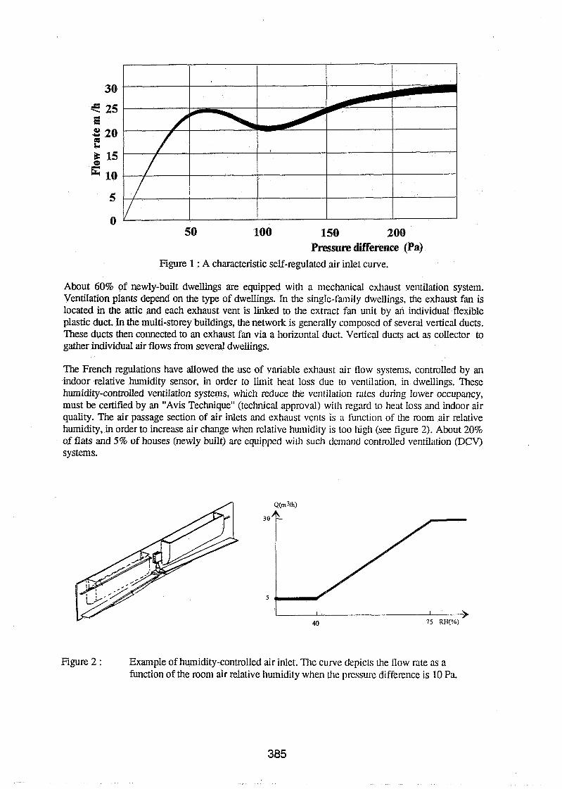
0 50 100 150 200
Pressure difference (Pa) Figure 1 : A characteristic self-regulated air inlet curve.
About 60% of newly-built dwellings are equipped with a mechanical exhaust ventilation system. Ventilation plants depend on the type of dwellings. In the single-l'amily dwellings, the exhaust fan is located in the attic and each exhaust vent is linked to the extract fan unit by an individual flexible plastic duct. In the multi-storey buildings, the network is generally composed of several vertical ducts. These ducts then connected to an exhaust fan via a horizontal duct. Vertical ducts act as collector to gather individual air flows from several dwellings.
The French regulations have allowed the use of variable exhaust air flow systems, controlled by an indoor relative humidity sensor, in order to limit heat loss due to ventilalion, in dwellings. These humidity-controlled ventilation systems, which reduce the verltilation rates during lower occupancy, must be certified by an "Avis Technique" (technical approval) wit11 regard to heat loss and indoor air quality. The air passage section of air inlets and exhaust vents: is a Sunclion of the room air relative humidity, in order to increase air change when relative humidity is too high (see figure 2). About 20% of flats and 5% of houses (newly built) are equipped wilh such demand controlled ventilation (DCV) systems.
Figure 2 : Example of humidity-controlled air inlet. Tllc curvc depicts h e flow rate as a function of the room air relative humidity when thc pressure difference is 10 Pa.

2.2. Balanced systems
In France, the balanced system is less common than the mechanical exhaust system; only 6% of the new single-family dwellings is equipped with it. Neverheless, the balanced system has numerous advantages. In comparison with the exhaust only systems, the balanced systems control air flow rate in each mom of the dwelling and therefore provide a better ventilation efficiency, prevent discomfort due to cold draught, acoustic annoyance due to noise, and prevent pollutants migration (e.g. dust, radon, ...) fmm outside. Additionally, the balanced ventilation systems make it possible to adjust ventilation rate according to needs, by transferring air flow f m ~ n a mom to another one, and to save energy using heat recovery system. However, the dwelling equipped with such a ventilation system must be sufficiently airtight in order to limit the heat losses due to cross-ventilation. Particular attention must be paid to the installation and maintenance to insure the energy saving potential.
2.3. Natural exhaust systems
In natural exhaust systems, the air flow rate is generated by buoyancy and wind effects. Therefore, flow rates are varying continuously. In single-family clwellings, every service room is provided with an exhaust vent linked to an air duct operating by passive stack cffcct (see figure 3). At the top of the duct, a cowl is installed in order to transform wind vclocily to pressure head. In multi-family dwellings, the vent ducts are either individual ones or shunt ducts : a shunt duct is a double duct composed of a small duct used for individual air exhaust of each Bat and a larger one used to collect individual air flows up to the top. The air inlets, located in every habitable rooms, are like the ones of mechanical exhaust systems (i.e. self-regdated air inlet), exccpt that the dimensioning must be higher. In order to prevent acoustic annoyance due to larger aperture arcs of air inlets, especially in noisy environment, air inlets with acoustic insulation are frequently uscd. Fipre 4 depicts the acoustic attenuation versus the frequency domain related to an air inlet equipped with or without different silencers; results show that the acoustic attenuation is increascci from 10 dBA up to 20 dBA when using a silencer.
cowl
air inlet 4-
Figure 3 : Passive stack ventilation in a singlc-family dwelling
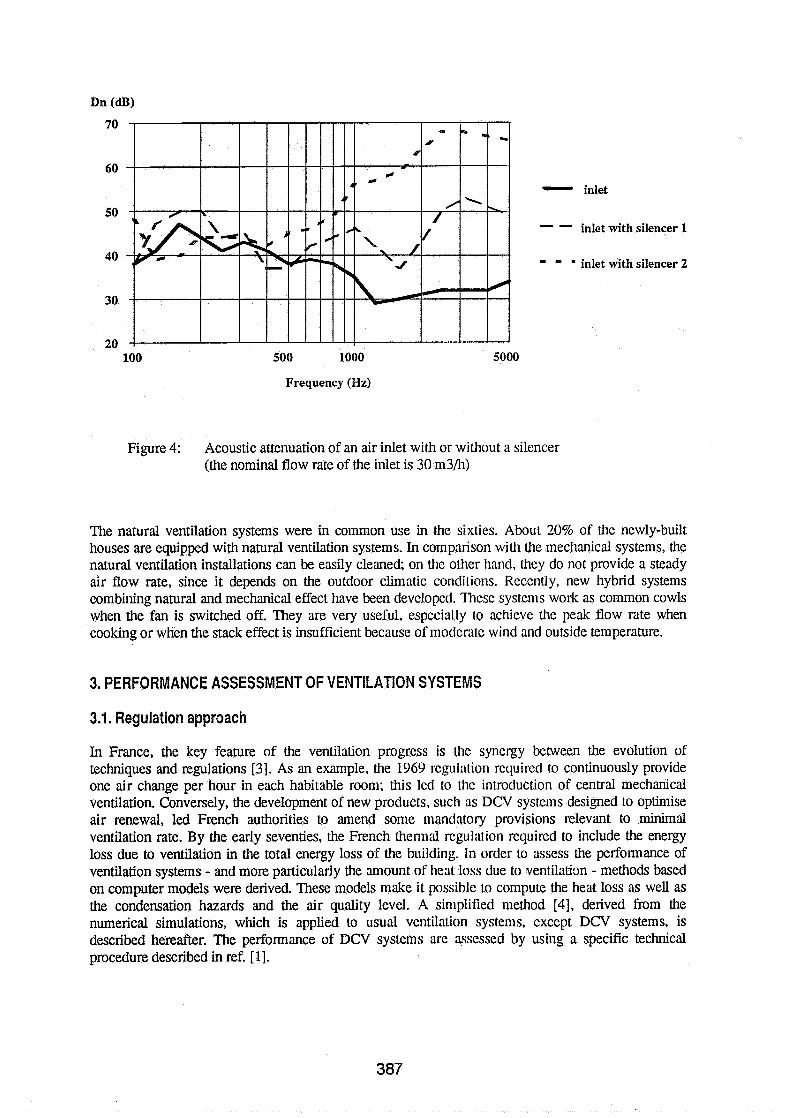
Dn (dB)
- inlet
-- inlet with silencer 1
- 1 inlet with silencer 2
Frequency (Hz)
Figure 4: Acoustic attenuation of an air inlet with or without a silencer (the nominal flow rate of the inlet is 30 m3/h)
The natural ventilation systems were in common use in the sixties. About 20% of the newly-built houses are equipped with natural ventilation systems. In comparison with the mechanical systems, the natural ventilation installations can be easily cleaned; on thc other hand, they do not provide a steady air flow rate, since it depends on the outdoor climatic conditions. Recently, new hybrid systems combining natural and mechanical effect have been devciopcd. These systems work as common cowls when the fan is switched off. They are very useful, especially to achieve the peak flow rate when cooking or when the stack effect is insufficient because of moderate wind and outside temperature.
3. PERFORMANCE ASSESSMENT OF VENTILATION SYSTEMS
3.1. Regulation approach
In France, the key feature of the ventilation progress is the syncrgy between the evolution of techniques and regulations [3]. As an example. the 1969 rcbqillrtion required to continuously provide one air change per hour in each habitable room; this led to the introduction of central mechanical ventilation. Conversely, the development of new products, such as DCV systems designed to optimise air renewal, led French authorities to amend some mandatory provisions relevant to minimal ventilation rate. By the early seventies, the French thennal regulation rcquircd to include the energy loss due to ventilation in the total energy loss of the building. in ordcr to assess Ihe performance of ventilation systems - and more particularly the amount of lie;~t loss due to vcntilation - methods based on computer models were derived. These models make it possible to compute the heat loss as well as the condensation hazards and the air quality level. A simplified method [4], derived from the numerical simulations, which is applied to usual ventilation systems, except DCV systems, is described hereafter. The performance of DCV systems are assessed by using a specific technical procedure described in ref. [I].
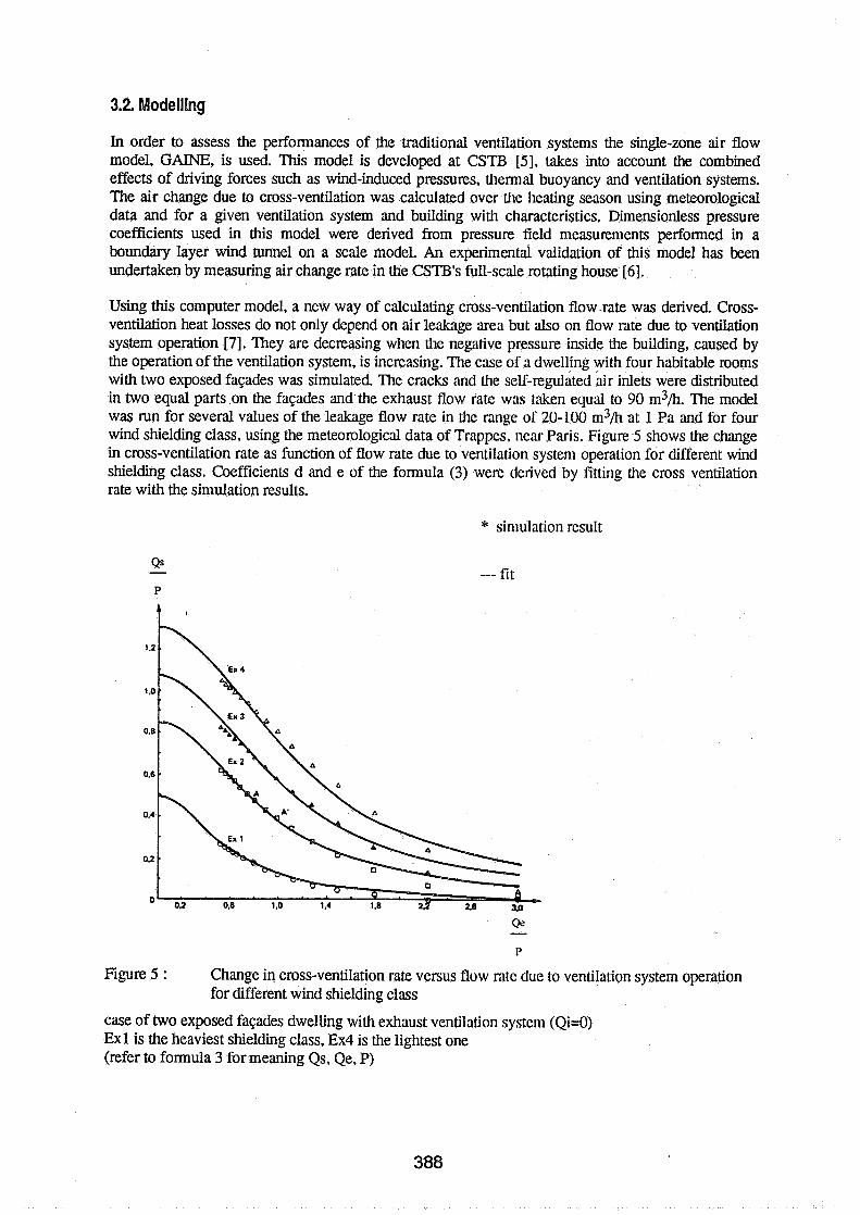
3.2. Modelling
In order to assess the performances of the traditional ventilation systems the single-zone air flow model, GAINE, is used. This model is developed at CSTB [ S ] , takes into account the combined effects of driving forces such as wind-induced pressures, thermal buoyancy and ventilation systems. The air change due to cross-ventilation was calculated over the heating season using meteorological data and for a given ventilation system and building with characteristics. Dimensionless pressure coefficients used in this model were derived from pressure field measurements performed in a boundary layer wind tunnel on a scale model. An experimental validalion of this model has been undertaken by measuring air change rate in the CSTB's full-scale rotating house 161.
Using this computer model, a new way of calculating cross-ventilation flow-rate was derived. Cross- ventilation heat losses do not only depend on air leakage area but also on flow rate due to ventilation system operation [7]. They are decreasing when the negative pressure inside the building, caused by the operation of the ventilation system, is increasing. The case of a dwelling with four habitable rooms with two exposed faqades was simulated. The cracks and Lhe sclf-regulated air inlets were distributed in two equal parts on the faqades and the exhaust flow rate WAS taken equal to 90 m3/h. The model was run for several values of the leakage flow rate in the range of 20-100 m3/h at 1 Pa and for four wind shielding class, using the meteorological data of Trappes, near Paris. Fi gure 5 shows the change in cross-ventilation rate as function of flow rate due to ventilation system operation for different wind shielding class. Coefficients d and e of the formula (3) werc derived by fitting the cross ventilation rate with the simulation results.
* simulation result
--- f i t
Figure 5 : Change in cross-ventilation rate versus Ilow ratc due to ventilation system operation for different wind shielding class
case of two exposed faqades dwelling with exhaust ventilation systcrn (Qi=O) Ex1 is the heaviest shielding class, Ex4 is the lightest one (refer to formula 3 for meaning Qs, Qe, P)

3.3. Method
The calculation rules, so-called "R8gles Th-G 141, describe how to calculate heat loss due to ventilation They apply to all traditional ventilation systems i.e. systems which are not innovative. Heat loss due to air renewal can be expressed by:
Where : DR is the heat loss due to air renewal (WI0C),
0.34 is the value of the specific heat capacity of air ( ~ h l n l ~ " ~ ) ,
Qv is the air flow rate due to ventilation systcm operation (1n3/h),
Q is the air flow rate due to cross-ventilation (n13/h).
For the dwellings having an exhaust ventilation system, the air flow rate Qv is the sum of the flow rates of each exhaust vent. The flow rate exhausted by a vcnt qv depends on its minimum and maximum values and variation during the vent operation :
qv=( 1-a)sm+a*sp (2)
Where: q,, is the specific flow rate of the exhaust vent (m3/11),
% is the minimum flow rate (m3/h),
qp is the maximum flow rate (m3/h),
a is the modulation factor.
a =1 when the aperture area of the vent is fixed
a =I112 when the modification of the area is operated by manu;il control
a =I124 when the vent is time controlled (peak time of 30 minutes).
The minimum and maximum flow rates have to be at least as great as the values allowed by the building regulation, these last ones being dependent on the number of habitable rooms.
In case of balanced ventilation systems, the supply and exhaust flow rates of Ule whole dwelling are calculated in the same way from formula (2); then, Ule spccitic air Ilow rate of the dwelling Qv is the greatest value of both.
It is obvious that cross-ventilation induced by wind effccl depends on numerous factors such as air tightness level of the building envelope, shielding of the surroundings and pressure inside the building due particularly to the operation of the ventilation system. Using computer model GAINE which uses meteorological data as input, a new way of calculating cross-ventilation flow rate was derived :
Where : Qs is the flow rate due to cross-ventilation (m3/h),
P is the flow rate through cmks and purpose provided openings in the building envelope when the pressure difference is 1 Pa (m3/h at 1 Pa),
Qi is the total supply flow rate (m3/h),
Qe is the total exhaust flow rate (m3/h),
d =1.55 for dwellings with only one exposed fapde and 1.15 for dwellings with more than one exposed facade,
e is the shielding coefficient which depends on shielding class and building exposure type.
In the case of exhaust only ventilation systems, the supply flow rate Qi is equal to zero and the exhaust flow rate Qe is equal to the specific rate Qv.
This formulation of the cross-ventilation rate has been accepled as 'an informative annex in the European standard on the simplified method of calculation of'building thcnnal perfomlance [8].
4. CONCLUSIONS
In France, dwelling regulation has enabled the development of efficient ventilation systems. They have to be assessed with regard to heat loss. Performance assessmcnt is an important issue as it may ease the development of new systems with a better efficiency. Thc encrgy loss duc to ventilation depends on the ventilation system operation and the infiltration. Thc flow rdtc due to air leakage of the building envelope are calculated taking into account the cracks of doors, windows and other components of the envelope.
Applying this computer model which uses meteorological data as input, a new procedure of calculating cross-ventilation flow rate was derived. This procedure is more representative of the physical phenomena and describes efficiently the shield eflect due to the negative pressure in the building.

ACKNOWLEDGEMENTS
The authors wish to thank Mr Redwan MOUNAJED for his assistance in the development of the computer model. The participation of ADEME (Agcnce dc llEnvironnement et de la Maitrise de l'Energie) and ML (Minisere du Logement) is gnlefully acknowlcdged for their financial support.
REFERENCES
1. VILLENAVE, J.G., MILLET, J.R. and RIBERON, J. "Theoretical basis for assessment of air quality and heat losses for don~estic ventilation systems in France" Fourteenth AIVC conference on Energy Impact of Ventilation and Air Infiltration, Copenhagen, Denmark, 21-23 September 1993.
2. RIBERON, J., and MILLET, J.R. "Draughts due to air inlets: an experimental approach" Thirteenth AIVC conference on Ventilation for Encrgy Eflicicncy and Optimum Indoor Air Quality, Nice, France, 15-18 September 1992, pp369-380.
3. VILLENAVE, J.G., RIBERON, J., and MILLET, J.R. "French ventilation in dwellings" International Conference on "Building design, technology and occupant well-being in temperate climates", B russels, 17- 19 February 1993.
4. "R2gles Th-G. R2gles de calcul du coefficicnt GV cles britiments d'habitation et du coefficient G1 des biitiments autres que d'habitation. AFNOR DTU P50-704. Cahiers du CSTB 2486, livraison 3 18. Avril 199 1.
5. MOUNAJED, R. "La mod6lisation des transferts d'air dans les b9tirncnts. Application 2 1'Ctude de la ventilation" Thbe de doctorat, ENPC, Noisy-le-Grand, France, Octobrc 1989.
6. MOUNAJED, R., RIBERON, J., and BARNAUD, G. "Wind turbulence and ventilation" INDOOR Ani' 90. Fifth international conferencc on indoor air quality and climate, Toronto, 29 July - 3 August 1990, V01.4, PP. 201-206.
7. RIBERON, J. "Revision des r2gles ThG et ThD. Evaluation dcs dCpcrditions par rcnouvellement d'air" CSTl3 report GEC 89-4792b, Champs-sur-mame, Frrlncc. June 1989.
8. "Thermal performance of buildings - Calculation or encrgy use for heating: Residential buildings" European Standard (draft) EN 832, CENtTC 89, Brussels. August 1992.


Energy Impact of Ventilation and Air Infiltration 14th AlVC Conference, Copen hagen, Denmark
21 -23 September 1993
Natural Ventilation via Courtyards: The Application of CFD
L Shao*, R R Walker", M Woolliscroft"K
** Building Research Establishment, Garston, Watford, WD2 7JR * University of Sheffield, School of Architectural Studies, Sheffield, SIO 2UJ, UK (Now at Nottingham University)
Crown Copyright 1993 - Building Research Establishment
Natural Ventilation via Courtyards: Part 11 - the application of CFD
by L Shao, R R Walker and M Woolliscroft.
SYNOPSIS Computational fluid Dynamics (CFD) is a powerfizl tool for analysing problems of air movement and has been increasingly widely used in applications in buildings. The emphasis has often been on its development as a replacement for the experimental approach, however, further work is needed to develop confidence in applying CFD to problems of air flow in buildings. It is suggested that CFD can be effectively used in an integrated manner together with experimental methods and that the interaction and integration of the two should be promoted in a variety of forms, and on a variety of levels within a research project. In this way the effectiveness of both the CFD and the experimental methods are enhanced. This approach has been applied to a study of the effectiveness of natural ventilation via courtyards, as part of a wider programme of work carried out at the Building Research Establishment. The CFD technique has been used to help formulate experiments, to assist in the interpretation of test results, and to perform parametric studies as well as exploring theoretical ideas. One of the important outcomes of the application of the CFD method has ben the foxmulation and verification of criterion for ensuring good courtyard ventilation.
1 Introduction
The related paper', Part I, describes how current understanding of natural ventilation in building courtyards was incomplete, with measurements at model scale in some cases contradicting observations at full scale. As a result of advances in computing power, CFD is now capable of modelling these air flows at sufficient resolution. This paper describes the application of CFD to this problem, as part of a wider programme of work which also involves site tests and wind tunnel experiments and described in Part I.
It is generally accepted amongst researchers that, for application to problems of air flow in buildings, CFD is not yet M y mature and results could be misleading if it is improperly used. On the other hand it is a promising technique and should not be ignored. The authors believe that by integrating the CFD approach with experimental methods and by promoting the interaction and interweaving of the two in a variety of forms and at different levels, the effectiveness of both the CFD and the experimental approach can be optimised.
This integrated approach for CFD application was adopted in this investigation which also utilised site and wind tunnel tests. The CFD technique normally assumed a supporting role. For example, it was used to estimate the air flow rates and patterns so experiments (e.g. tracer decay tests) could be better planned and set-up. Where test results were not as expected, the CFD program was run with the detailed description of the actual experimental conditions to help in judging whether the unexpected results were due to equipment/operator errors or were actual phenomena. In the latter case, the computed highly detailed flow field sometimes even allowed the causes of the unexpected results to be traced. In particular, CFD was used to explore new ideas on the causes of good or poor ventilation in courtyards. In addition, it proved effective in
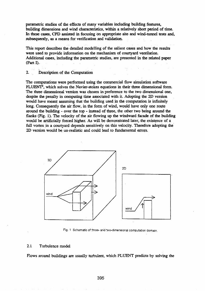
parametric studies of the effects of many variables including building features, building dimensions and wind characteristics, within a relatively short period of time. In these cases, CF'D assisted in focusing on appropriate site and wind-tunnel tests and, subsequently, as a means for verification and validation.
This report describes the detailed modelling of the salient cases and how the results were used to provide information on the mechanism of courtyard ventilation. Additional cases, including the parametric studies, are presented in the related paper Part I).
2. Description of the Computation
The computations were performed using the commercial flow simulation software FLUEDll?, which solves the Navier-stokes equations in their three dimensional form. The three dimensional version was chosen in preference to the two dimensional one, despite the penalty in computing time associated with it. Adopting the 2D version would have meant assuming that the building used in the computation is int"mite1y long. Consequently the air flow, in the form of wind, would have only one route around the building - over the top - instead of three, the other two being around the flanks (Fig. 1). The velocity of the air flowing up the windward facade of the building would be artificially forced higher. As will be demonstrated later, the existence of a full vortex in a courtyard depends sensitively on this velocity. Therefore adopting the 2D version would be un-realistic and could lead to fundamental errors.
Fig. 1 Schematic of three and ?No-dimensional computation doma~n
2.1 Turbulence model
mows around buildings are usually turbulent, which FLUENT predicts by solving the
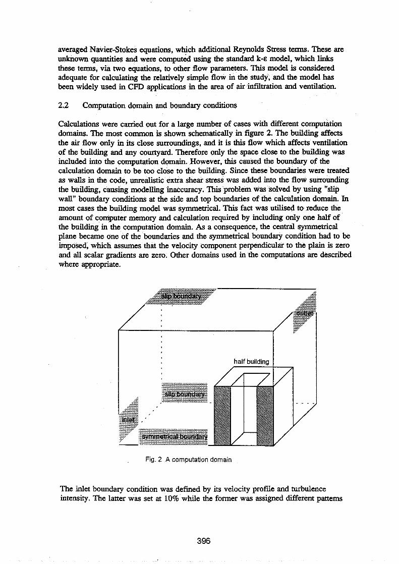
averaged Navier-Stokes equations, which additional Reynolds Stress terms. These are unknown quantities and were computed using the standard k-E model, which links these terms, via two equations, to other flow parameters. This model is considered adequate for calculating the relatively simple flow in the study, and the model has been widely used in CFD applications in the area of air infiltration and ventilation.
2.2 Computation domain and boundary conditions
Calculations were carried out for a large number of cases with different computation domains. The most common is shown schematically in figure 2. The building affects the air flow only in its close surroundings, and it is this flow which affects ventilation of the building and any courtyard. Therefore only the space close to the building was included into the computation domain. However, this caused the boundary of the calculation domain to be too close to the building. Since these boundaries were treated as walls in the code, unrealistic extra shear stress was added into the flow surrounding the building, causing modelling inaccuracy. This problem was solved by using "slip wall" boundary conditions at the side and top boundaries of the calculation domain. In most cases the building model was symmetrical. This fact was utilised to reduce the amount of computer memory and calculation required by including only one half of the building in the computation domain. As a consequence, the central symmetrical plane became one of the boundaries and the symmetrical boundary condition had to be imposed, which assumes that the velocity component perpendicular to the plain is zero and all scalar gradients are zero. Other domains used in the computations are described where appropriate.
h a l f building ) A I
Fig. 2 A computation domain
The inlet boundary condition was defined by its velocity profile and turbulence intensity. The latter was set at 10% while the former was assigned different patterns

including a unifonn profile, a urban wind profie and a city wind profile. The urban wind profile typically assumes the wind velocity (u) at a point in the atmospheric boundary layer to be.
where y is the vertical distance between the point and the ground. The city wind profile, as specified in the British Standard BS-5925, assumes that
It was also assumed, for this study, that the whole computations domain was submerged in the atmospheric boundary layer.
2.3 Numerical scheme
The NavierStokes equations were discretised into finite difference equations based on a 3-D Cartesian grid. Two considerations have to be made in deciding the grid density.0n the one hand the grid has to be dense enough so that gradients of flow field parameters can be accurately presented in the finite difference equations and the calculated flow is accurate and detailed. On the other hand, the grid has to be loose enough so that the number of cells is within the range that the memory capacity of a given computer can cope with and the solution converges at reasonable speed. To satisfy the two opposing requirements, denser grids were used near the walls and comers where the gradients were likely to be large and coarser grids away from walls and comers to minimise the total number of cells. The transition from the denser grids to the coarser grids was effected by means of gradual cell expansion. To promote numerical stability, the ratio of expansion from one cell to the next was limited to below 1.2 or 1.4 depending on the likely complexity of the local flow. The number of nodes for the cases computed vaiied from under 20,000 to over 148,000.
The finite difference equation resulting from the discretization process described above were solved using the SIMPLE3 algorithm. The solutions convergence was accelerated by increasing the under-relaxation coefficients, up to 1, after a certain number of iterations, during which the solution had shown steady convergence.
3. Results and Discussion
The cases computed can be classified into three groups. Cases in Group one were computed to examine a proposed criterion for good or poor courtyard ventilation. The following discussion will be focused on these cases. The second group was used for
' parametric studies, i.e. examining the effects on full vortex existence of building dimensions, building features, wind strength and wind directions, etc. The third group involves computing the courtyard flow pattems for a real building. The latter two group of cases are discussed in Part I.
There are two air flow patterns concerning the natural ventilation of courtyards. one of the patterns, referred to in the following as a top vortex, involves an air flow vortex suspended at the opening of the courtyard in the building roof. The second

pattern, referred to as a full vortex, is associated with a vortex occupying the full depth of the courtyard. These pattern are illustrated schematically in figure 3. A top vortex isolates the courtyard from the outside environment, resulting in poor ventilation and air quality and therefore is undesirable. A full vortex, on the other hand, ensures good ventilation by bringing fresh air into the courtyard and carrying away the stale air. Obviously, the question of "Under what conditions will the courtyard ventilation be satisfactory?" can now be transformed into a fluid dynamics question, i.e.: "Under what conditions will there be a full vortex?"
wind ---+ top vortex full vortex
Fig. 3 Schematic of the two types of vortices
Refer to Fig 4a which shows air flow in the form of wind passing by a rectangular building. It is known that the part of the wind flowing over the top of the building will without exception, separate from the roof, resulting in a region of recirculating air - a vortex - below it. The separated flow, provided that the building is long enough, will eventually reattach to the roof. If there is a courtyard in the building and the point of reattachments is either 'within' or nearby downstream of the courtyard opening in the roof, as shown in Fig. 4b, the vortex (Fig. 4a) will "drop" into the courtyard and form a full vortex. In the situation that the courtyard building is not long enough and the reattachment does not happen, as shown in Fig. 4, the vortex will remain largely on the roof, spanning the courtyard, although part of it does sink slightly into the opening. A further case is where reattachment occurs upstream of the courtyard opening, in which case a full vortex is caused by the flow shear stress.

rectangular bullding u
Fig. 4 Formation of either a full or top vortex
Based on the above discussion, it is proposed that a full vortex will form if reattachment occurs either upstream, within, or nearby downstream of the courtyard opening. In the cases examined, separation seems to occur when the width of the building downstream of the courtyard is less than about half the width of the courtyard. This is not a general criterion because the width downstream at which reattachment occurs is likely to be affected by several factors, wind velocity, height of building etc. and further work is necessary to attempt to produce a general criterion. It may be that a separate CFD calculation is necessary in each case. To examine the possibility for a specific criterion, six cases were computed:
- Case 1 (Fig. 5a) involved building without a courtyard, measuring 16m X 16m X 24m and with its windward facade perpendicular to the wind direction;
- Case 2 (Fig. 5b) differed from Case 1 in that the building was longer (24m instead of 16m) and
- Case 3 (Fig. 5c) was identical to Case 1 except that the building was partially sheltered and that the velocity at domain inlet was 0.5mIs up to half of the building height as shown by the first column of arrows in Fig. 6c.
The results from the cases are presented in graphic form in Fig. 5a, b, c, which show the velocity fields in the corresponding central symmetrical cross sections (also termed symmetrical boundary, as defined in Fig. 2) The arrow length and direction indicate air flow velocity and direction, respectively. Roof top velocity can be identified by the velocity arrows with opposite directions along the neighbouring horizontal grid lines close to the roofs. In all three cases, a vortex existed on top of the roof, close to its leading edge. The length of the vortex is marked by the length over which the arrows along the first horizontal grid line next to the roof remain in the direction opposite to

that of the wind. Obviously, the vortex for case 1 covers the whole length of the building and probably beyond and, in consequence, reattachment does not occur. For case 2, the vortex covers only part of the roof, due to the extra length of the building. Reattachment occurs and is characterised by the reversal of arrows along the rear part of the above described grid line to the wind direction. The point of reattachment is marked by the first reversed arrow. Reattachment also occurs in Case 3, but for a different reason. In this case the shelter reduces the air flow velocity up the building windward facade, principally by reducing the total flow of air over the building. This reduces the angle between the wind and the roof where flow separates at the leading edge, and the severity of separation is less, thereby causing earlier reattachment.
Suppose that a courtyard is built into each of the buildings at the location indicated by the dotted lines in Fig. 5 a, b, c; according to the above criterion, reattachment should occur in cases 2 and 3 and cause a full vortex to form. However, in case 1, a top vortex should occur. These situations were modelled as three further cases, 4, 5 and 6, and the results are shown in figure 6. The interpretation is similar to that for Fig 5. As expected, figures 6b and Fig. 6c show a full vortex in the courtyard, with air movement reaching all places while, in contrast, the courtyard shown in Fig. 6a is dominated by a top vortex with a region of stagnant air below it.
To sum up, the above discussions show that good courtyard ventilation depends on the existence of the full vortex and that the latter is formed when the separated flow over the building roof top reattaches on the roof and the point of the reattachment is either upstream, within, or nearby downstream of the courtyard top opening. As was mentioned earlier in the cases examined this distance is about half the width of the courtyard downstream of the courtyard but further work is necessary to determine a general criterion which is likely to involve many factors. This qualitative understanding as illustrated in Part I, forms the basis for explaining many of the courtyard air flow phenomena. It should be said that the computation of the above 6 cases was only one step in developing a criterion. In fact the results from many other cases computed have been used to develop the understanding which has also been supported by experimental evidence obtained from site and wind tunnel tests.
4. Concluding Remarks
More than eighty cases have been computed in the course of this research project. The setting-up details of the cases have been presented. The results from a group of six cases have been analysed to begin to develop a criterion on terms of the air flow conditions under which the good courtyard ventilation is ensured. The discussion also serves to illustrate the way the detailed information afforded by the CFD method was used to explore theoretical ideas. The results from other cases are presented in Part I of this twin paper, as they are best shown in an integrated manner together with site and wind tunnel test data.
Great advances have been made in the CFD method. Yet it is not completely mature and results not always reliable. However, by using it together with the experimental method in a way that allows the interaction and integration of the two, the effectiveness of both methods as investigate tools are enhanced. In this research project, the CFD technique has been used to predict the likely flow conditions for a
site test on a real courtyard so that experimental equipments can be better tuned, the results more accurate and obtained more speedily. It has also been used to assist the understanding of certain experimental results, as well as to perform parametric studies and to explore theoretical ideas.
(1) Walker, R R, Shao, L and Woolliscroft, M, Natural ventilation via courtyards: part 11 - Theory and measurements, paper presented at the 14th ANC Conference on Energy Impact of Ventilation and Air Wdtration, Copenhagen, Denmark, Sept 1993.
(2) FLUENT is a commercial CFD package available from Flow Simulation Ltd. of Sheffield, England.
(3) VAN DOORMAAL J.P. and RAITHBY G.D. "Enhancement of the SIMPLE method for predicting incompressible fluid flows" Numerical Heat Transfer Vol 7 p147 1984
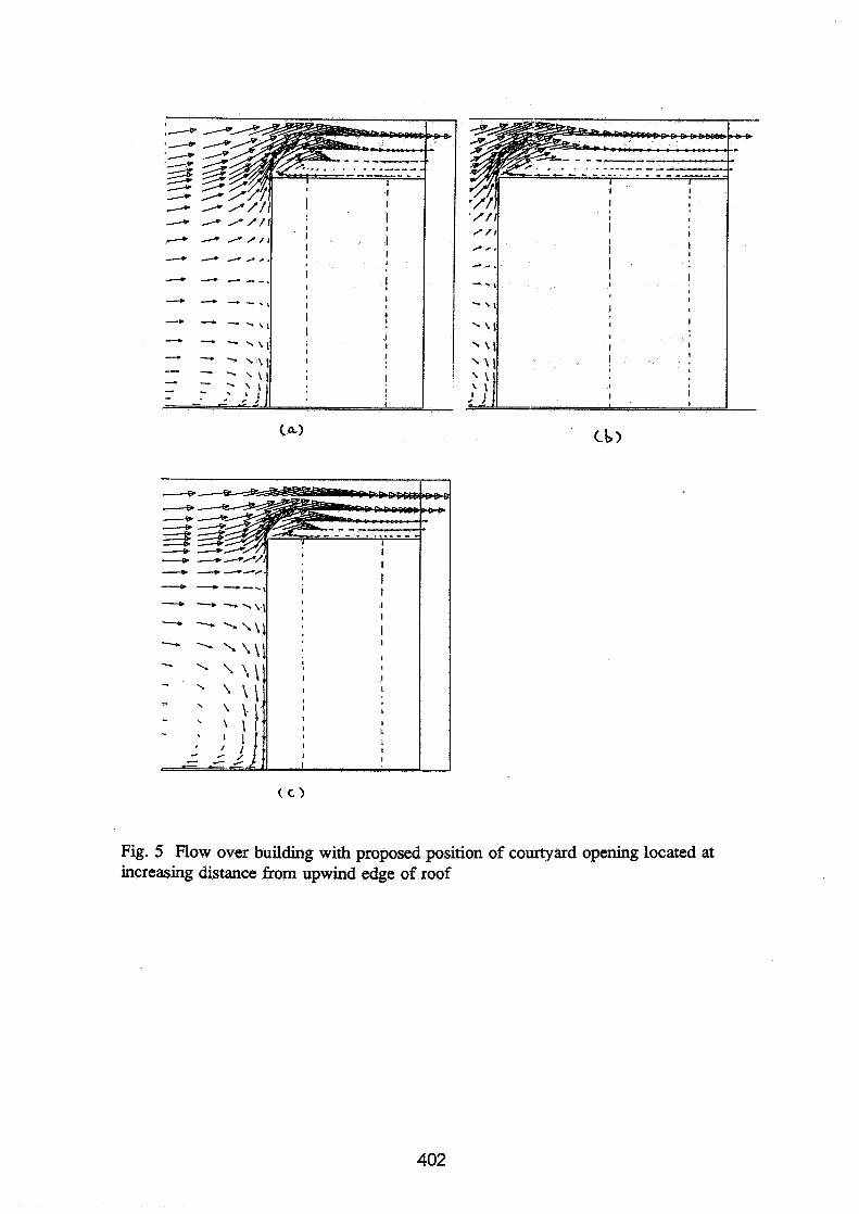
Fig. 5 Flow over building with proposed position of courtyard opening located at increasing distance from upwind edge of roof
4 A//-//
4 4 ----A,.
+ 4--.-., - - -.,, - ---'\\I - " ' . \ \ I - ' \ \ \ I - "U,, - ' ' \.\ ' ' I -:I.lil - - - / ' / -
I I i I I 8 I
I
: I : I
I
; I I
: I I
I ! I 1 I
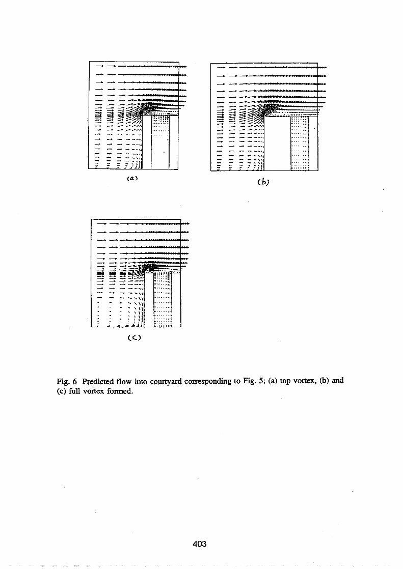
Fig. 6 Predicted flow into courtyard corresponding to Fig. 5; (a) top vortex, (b) and (c) full vortex formed.


Session 5: Posters - Measurement Techniques

Energy Impact of Ventilation and Air Infiltration 14th AlVC Conference, Copen hagen, Denmark
21 -23 September 1993
Development of a New Tracer-Gas Sampling System For Measuring Airflow in Ducts
K W Cheong, S B Riffat
School of Architecture, University of Nottingham, University Park Nottingham, NG7 2RD, UK
SYNOPSIS This paper is concerned with measurement of airflow in ducts using an active (pumped) sampling system. The system is capable of sampling tracer gases using either tubes packed with adsorbent or sample bags. A perfluorocarbon tracer (PFT) was injected into the ducts using thermostatically-controlled heating blocks. The samples were collected and analysed using a thermal desorber/gas analyser system. Laboratory and field testing of airflow in ducts was carried out. A large office building was studied for measurements of ventilation rate, ventilation efficiency and air quality. A questionnaire was also completed by office staff in order to assess air quality and thermal comfort.
1. INTRODUCTION Indoor air quality, thermal comfort and energy use in buildings are largely dependent on accurate balancing of air distribution systems. Airflows are usudly balanced using traditional instrumentation such as pitot tubes but these measurements can be inaccurate and time consuming as the velocity profile across the duct must be determined. Tracer-gas techniques offer alternative approach for measuring airflow in ducts and have several advantages [I].
Several investigations have been made of the application of the constant- injection and pulse-injection techniques for measuring of airflow in ducts [2- 41. These involved the injection of tracer gases such as SF, and N,O into the duct via either a mass-flow controller or a syringe followed by downstream sampling using a gas analyser. The passive tracer-gas technique using perfluorocarbons (PFTs) has also been examined [S] . In this case small tubes filled with PFT liquid, known as sources, are placed at the inlet of the duct and tubes packed with adsorbent, known as samplers, are placed downstream. The emission rate of the sources is dependent on the air temperature while the uptake rate of the samplers is significantly influenced by the air velocity and turbulence in the duct. The orientation of sample tube with respect to the flow also affects the uptake rate. As a result measurement errors using the passive PFT techniques are large.
This work examines the accuracy of an active (pumped) sampling technique. A perfluorocarbon tracer was injected at a constant rate into the duct using a thermostatically-controlled heating block and gas samples were collected using an automated sampling system. This system was used for airflow measurements in laboratory and field tests.
Field tests were carried out in a large building and this involved measurement of ventilation rates, ventilation efficiency and concentration of specific air pollutants. In addition, a questionnaire was completed by the office staff in order to assess air quality and thermal comfort.

2. DESCRIPTION OF THE SYSTEM The PFT system consists of the following:
2.1 Tracer Injection System Figure 1 shows the PFT tracer injection system. This simple system consists of a cylindrical aluminium block with a heating element inserted into the base. The block was bored to allow insertion of a small glass vessel containing the PFT liquid. The vessel is 3ml capacity and has a neck of 3mm diameter and 15mm length. Water is placed in the bore hole to ensure uniform heating throughout the glass vessel. A plastic cap is placed over the hole to prevent water from spilling over the aluminium block. A diffusion cap is placed at the outlet of the vessel to allow uniform dispersion of tracer gas into the duct.
A magnet is fixed to the heating block so that the injection unit can be attached to the duct wall during airflow measurements.
2.2 Tracer Sampling System The sampling system is shown in Figure 2. This consists of solenoid valves, tracer gas sampling tubes, a programmable logic controller, a manifold and a flowmeter. The system is capable of taking samples as frequently as once per second. Air at a constant rate may be drawn into each sampling tube using a a small pump. The sampling tubes are made of stainless steel and packed with adsorbent Chromosorb 102,60-80 mesh, supplied by Chrompack Ltd (see Figure 2).
The operation procedure of the system is as follows. At the beginning of each experiment the first solenoid valve opens and the pump is turned on. At the end of the desired sampling time, set by the programmable controller, the pump is turned off. The procedure is repeated until all samples have been collected.
If preferred, the sampling system could be connected to a group of sampling bags instead of the adsorbent sampling tubes (see Figure 3).
2.3 Tracer Gas Analysis Multi-Gas Analyser, type 1302, manufactured by Bruel & Kjaer, Denmark together with a Thermal Desorption System, type SBK 1355, manufactured by CBISS Ltd, UK was used for separation and analysis of the samples in the adsorbent (see Figure 3). The accuracy of the analyser was estimated to be within f 1%.
Analysis of these tubes consists of placing the tube in the thermal desorption system. The system desorbs the collected sample by heating the tube and flushing the desorbed material into a loop which is automatically connected to the multi-gas analyser. The analysis is completely automated and controlled by the thermal desorption system. The results are displayed on the multi-gas analyser.
The gas sample in the sampling bags are analysed by using the type 1302 multi-gas analyser.
3. THEORY Tracer gas is injected into the duct at a constant rate, q, (m3/s) and the resulting concentration (ppm) response, C, is measured. Assuming that the air and tracer gas are perfectly mixed within the duct, and concentration of tracer gas in the outside air is zero, the following equation can be used to determine airflow rate, F, (m3/s)
4. MEASUREMENT AND RESULTS Airflow measurements in duct systems were conducted in the laboratory and an air distribution system of a large office building located at Nottingham. The PFT system was used for different air flow rates and results were compared with measurements made by the pitot-static traverse method.
The ventilation efficiency of the mechanical ventilation system and air quality in this office building were studied. In addition, a questionnaire was completed by the office staff in order to provide a subjective assessment of the indoor air quality.
4.1 Laboratory Tests The experimental work was carried out using the duct system and instrument as shown in Figure 4. The duct system was constructed using a galvanised mild steel duct 6m long with a cross-section of 0.3 x 0.3m. The downstream end was connected to an axial fan by means of a diffuser. The flow rate through the duct was varied using a speed controller made by ABB Stromberg Drives, Finland. The fan was driven by an AC motor of 4 k W and with a maximum speed of 2880 rpm. The fan was manufactured by Elta Fans Ltd, UK.
Background contaminants in the adsorbent tubes can give rise to interference and inaccuracies in air flow measurements. To prevent this, all sampling tubes were cleaned before and after each use. The thermal desorption system is set to cleaning mode to remove contaminants contained in the adsorbent.
Airflow measurements commenced by filling the vessel with perfluoro-n- hexane (PP1) and then weighing it. Tracer gas was injected into the duct by placing the tracer injection system at a point upstream of the duct system. Samples were collected in clean tubes fitted into the sampling system via the sampling probes inserted into the duct downstream of the injection point. After 6 minutes, the injection and sampling process was stopped and the vessel was reweighed. The injection rate of tracer into the duct was determined by taking the difference in weight of the vessel and dividing by the duration of injection (i.e. 6 minutes). Analysis of the sampling tubes

were performed by setting the thermal desorption system to analytical mode. A calibration graph [units against concentration (in mg/m3) ] was required to determine the actual concentration of tracer-gas in tubes as the direct readout values from the multi-gas analyser required a factor adjustment. Once the injection rate and concentration of tracer-gas in the sampling tube are known, the airflow rate in the duct can be evaluated by using equation (1).
Additional air flow measurements were obtained by collecting samples in bags using sampling system and analysing them using the multi-gas analyser. The pitot-static traverse method was employed in the same experiment to provide a comparison between air flow measurements made using different techniques.
Tables 1 and 2 compare measurements of air flow rate made with a pitot tube and the PFT technique using sampling tubes and bags.
Table 1 Comparison of airflow measurements in a duct using a pitot tube and PFT technique, sampling tubes
Table 2 Comparison of airflow measurements in a duct using a pitot tube and PFT technique, sampling bags
Measurement of airflow rate obtained using the pitot-static traverse method and PFT technique using sampling tubes and bags were in close agreement. The difference between airflow rates estimating using the PFT technique (using tubes) and measurements made using a pitot-tube was in the range -4.2 to 7.1%. In the case of airflow rate measurements made using the PFT technique (using bags) and pitot-static traverse
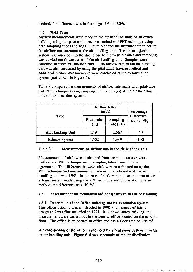
method, the difference was in the range -4.6 to -1.2%.
4.2 Field Tests Airflow measurements were made in the air handling units of an office building using the pitot-static traverse method and PFT technique using both sampling tubes and bags. Figure 5 shows the instrumentation set-up for airflow measurement at the air handling unit. The tracer injection system was inserted into the duct close to the fresh air inlet and sampling was carried out downstream of the air handling unit. Samples were collected in tubes via the manifold. The airflow rate in the air handling unit was also measured by using the pitot-static traverse method and additional airflow measurements were conducted at the exhaust duct system (not shown in Figure 5).
Table 3 compares the measurements of airflow rate made with pitot-tube and PFT technique (using sampling tubes and bags) at the air handling unit and exhaust duct system.
Table 3 ' Measurements of airflow rate in the air handling unit
Measurements of airflow rate obtained from the pitot-static traverse method and PFT technique using sampling tubes were in close agreement. The difference between airflow rates estimated using the PFT technique and measurements made using a pitot-tube at the air handling unit was 4.9%. In the case of airflow rate measurements at the exhaust system made using the PFT technique and pitot-static traverse method, the difference was - 10.2%.
4.3 Assessment of the Ventilation and Air Quality in an Office Building
4.3.1 Description of the Office Building and its Ventilation System This office building was constructed in 1990 to an energy efficient design and was first occupied in 1991. It is a two-storey building and measurement were carried out in the general office located on the ground floor. The office is an open-plan office and has a floor area of 126 m2.
Air conditioning of the office is provided by a heat pump system through an air-handling unit. Figure 6 shows schematic of the air distribution
system. The ventilation air from the air handling unit is delivered to the office through three air diffusers at the suspended ceiling. The air extracted from the office via two grilles is completely purged to the outside.
4.3.2 Description of Measurement
4.3.2.1 Measurement of Air Exchange Rate The air exchange rate in the office was measured using the tracer-gas decay technique. This technique involved an initial injection of SF6 tracer gas into the air space through the air handling unit. The tracer gas was allowed to mix for 10 minutes to establish a uniform concentration in the air space. The decay of SF6 tracer gas was monitored every 40 seconds over a period of 35 minutes, using the Binos 1000 Infra-red Gas Analyser, made by Rosemount GmbH, Hanau, Germany. The accuracy of the analyser was estimated to be within f2%. The tracer gas concentration data was analysed to determine the air-exchange rate for the office.
4.3.2.2 Age of Air and Ventilation Efficiency Evaluation of the ventilation efficiency of the mechanical ventilation system in a building is crucial as it provides information about the ability of the system to supply and extract air from the conditioned space. Information on the ventilation rate of the building is adequate if the air distribution in the building is uniform. Non-uniformities in an air distribution are believed to be responsible for some complaints about air quality.
Ventilation efficiency, E, was evaluated in the office. This evaluation consisted of measurements of local age of air in the office and average age of air at the system exhaust. The age of air was measured using the tracer-gas decay technique. This technique involved an initial injection of SF, tracer gas into the office through the air handling unit. The tracer gas was allowed to mix for 5 minutes to establish a uniform concentration in the air space. The decay of the tracer gas was monitored in the office and at the exhaust duct once every 40 seconds, using the Binos 1000 Infra-red analyser and Miran Portable Ambient Air Analyser, type 1B2, (made by Foxboro Company, USA), respectively, over a period of 40 minutes. The tracer-gas concentration data in the office and at the exhaust were analysed to determine the age of air, z, (min.). The ventilation efficiency of the mechanical ventilation system was determined by dividing the age of air at the exhaust,%,, by the age of air in the office, z,.
4.3.2.3 Monitoring Concentrations of CO,, CO and HCHO Monitoring of indoor air pollutants such as CO,, CO and HCHO was carried out at the office. Measurements were conducted at locations with the highest concentration of pollutants.

The concentration of CO,, CO and HCHO were measured using the Miran Portable Ambient Air Analyser. The accuracy of this analyser is estimated to be f 15%.
4.3.3 Results and Discussion
4.3.3.1 Evaluation of Air Exchange Rate Measurements were carried out on a calm day with a south-westerly wind at a speed of 0.5 m/s. Air infiltration could be neglected as the external wind pressure was low and it has a very tight building. The air exchange rate in the office was 3 ach. This is below the recommended value of 4 to 6 air changes given in the CIBSE Guide "Installation and Equipment Data" 161.
The air temperatures for both indoors and outdoors were 23.S°C and 22OC, respectively. The recommended air temperature in an office is in the range of 23.3 to 256°C for summer[7] . Thus we concluded that the indoor air temperature was withii the recommended value.
4.3.3.2 Evaluation of the Age of Air and Ventilation Efficiency The measurements showed that the age of air in the office was about 25 minutes (i.e. the length of time for fresh air to remain in the office is 25 minutes).
When there is a uniform distribution of air over the office air-space, the ventilation efficiency, E = 1. However, when there is a non-uniform distribution of air over the office air-space or in another words, some stagnant zones within office air-space, values of e are significantly less than 1. The ventilation efficiency of the system was found to be e = 0.75. The inefficiency of the system was partly due to the limited number and position of the air-supply diffusers and extract grilles in the office.
4.3.3.3 Evaluation of Concentrations of Indoor Air Pollutants The concentration of carbon dioxide in the office ranged from 610 to 690 ppm. These values are well below the ASHRAE standards[8] recommended value of 1000 ppm for continuous exposure.
Measurements showed that the concentration of carbon monoxide was 0.2 ppm. This is well below the acceptable indoor concentration of 9 P P ~ [ ~ I .
The average concentration of formaldehyde in the office was found to be 0.1 ppm. This coincides with the acceptable indoor concentration of 0.1 ppm[91.
4.3.4 Survey at the Office Building A subjective assessment of the effect of air quality on the health of the office staff was carried out. This was achieved by distributing a questionniare to the staff immediately after the objective measurement has been completed.
For this assessment, a total of 27 questionnaires were printed and distributed to the staff. The office staff comprised 19 males and 8 females. The average age of the staff was 33 years old.
4.3.4.1 Assessment of the Questionnaires The main types of complaint from the staff are shown in Figure 7. The majority of the complaints were about the stuffy atmosphere. About 40% of the staff found that the air in the office had an odour, was draughty, warm and dry. For the overall air quality rating, 55% of them were pleased with the air quality and the remaining 45% were dissatisfied.
The majority of the staff were absent for an average of 1 to 3 days per annum; 12.5% of them were absent for 4 to 6 days and 25% of the staff were not absent from work at all.
This subjective assessment showed that air quality at the office building is within tolerable limits and that the number of days lost due to illness is also within an acceptable range.
5. CONCLUSIONS A fast-response sampling system using a perfluorocarbon tracer (PFT) has been used for measurement of airflow in ducts. Measurements of airflow obtained using the PFT technique and pitot static traverse were in close agreement.
Results obtained from objective measurements and the subjective assessment revealed that the office building has some ventilation and air quality problems. The air exchange rate is below the recommended value and the air distribution system into the office is not well designed. This faults tended to produce an environment felt to be overwarm and stuffy by many office staff.
ACKNOWLEDGEMENTS We wish to acknowledge the assistance of Mr S. Nicholson, East Midlands Electricity. We also acknowledge the financial support of the UK Science and Engineering Research Council.
REFERENCES 1. Riffat, S.B. and Cheong, K.W., "Measurement of entrance length
and friction factor using tracer-gas technique", Proc. 12th AIVC Conf., Air Movement and Ventilation Control Within Building, Canada, Vol. 2, 1991, pp321-334.
2. Cheong, K.W. and Riffat, S.B., "Performance testing of HVAC systems using tracer-gas techniques", Ventilation '92 Symposium, USA, 1992.
3. Axley, J. and Persily, A.,"Integral mass balance and pulse injection tracer techniques", Proc. 9th AIVC Conf., Effective Technology- Research and Application, Belgium, 1988.
4. Riffat S.B., "A comparison of tracer-gas techniques for measuring airflow in a duct", Journal of the Institute of Energy, LXIII(454), 1990, pp18-21.
5. Sateri, J., "PFT measurements in ventilation ducts", Proc. 12th AIVC Conf., Air Movement and Ventilation Control Within Building, Canada, Vol. 1, pp375-386, 199 1.
6. CIBSE Guide, "Installation and Equipment Data", The Chartered Institution of Building Services Engineers, London, United Kingdom, 1986.
7. ASHRAE Handbook, "HVAC Applications", American Society of Heating, Refrigerating and Air Conditioning Engineers, Atlanta, USA, 1991.
8. ASHRAE standard ASHRAE 62-1989, "Ventilation for acceptable air qualtiy", American Society of Heating, Refrigeration and Air- conditioning Engineers Inc., 1989.
9. Raatschen, W., "Demand controlled ventilating system - State of the art review", International Energy Agency, Sweden, 1989.

Duct's Wall
- wKtng
Glass Vessel
Aluminium Block
I Heating Element
Figure 1 PFT tracer injection system
To Power Supply
Sampling tube with end caps
Figure 2 Tracer gas sampling system
- End Cap

Thermal Desorber System
Figure 3 Schematic of the thermal desorberlgas analysis system
Axial Fan
I
Air Exhaust 4 __lt
In
Tncm Sampling System
Traccr Injection System :
Control --&=- Box
INJECTION SAMPLING
Figure 4 Instrumentation for PFT technique
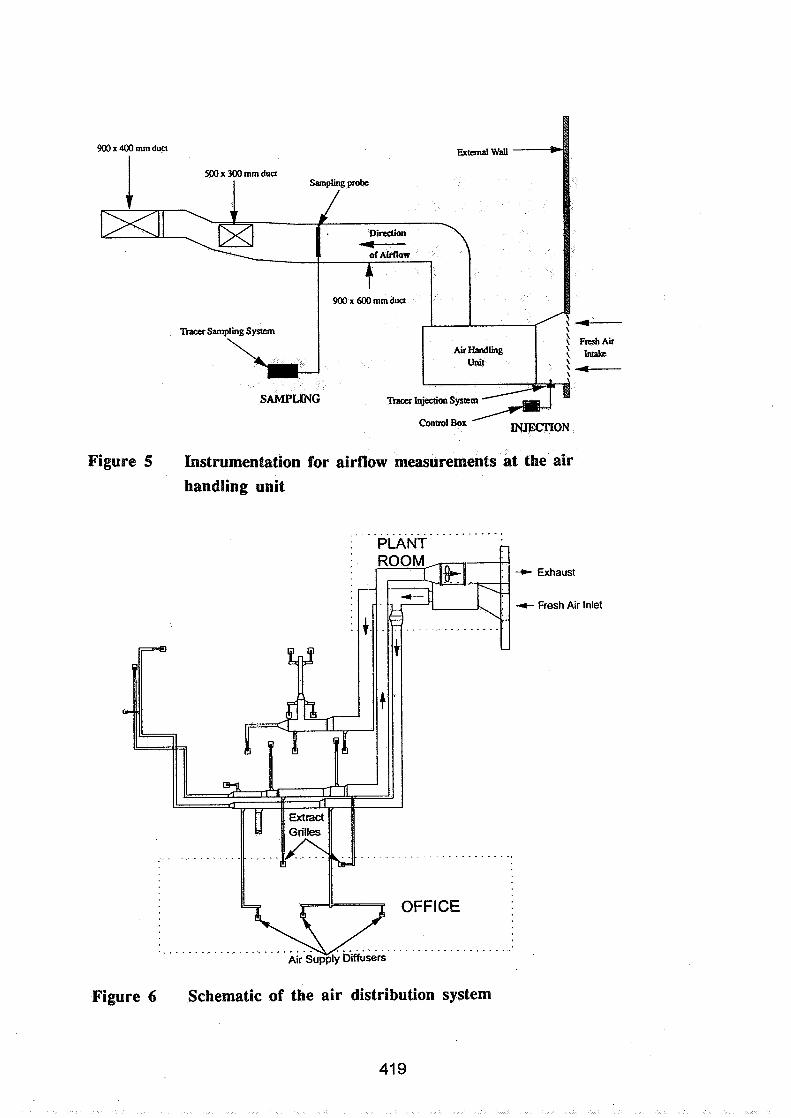
Ex& wall
500 x 300 mm dua Sampling probe
\ I I I \\ F& Air
SAMPLING T- Injection System
conno1 Box / TNJECTION
Figure 5 Instrumentation for airflow measurements at the air handling unit
Exhaust
Fresh Air Inlet
OFFICE
. . . . . . . . . ........... . . . . . . . . . . . . . - . . . . - . - - - -
Figure 6 Schematic of the air distribution system
41 9

No. of Comphiots, (96)
Figure 7 General complaints from staff
Energy Impact of Ventilation and Air Infiltration 14th AlVC Conference, Copenhagen, Denmark
21 -23 September 1993
Computer Modelling & Measurement of Airflow in an Environmental Chamber
J S Kohal, S B Riffat
Building Technology Group, School of Architecture, University of Nottingharn, University Park Nottingham, NG7 ZRD, UK

SYNOPSIS
The use of sulphur hexafluoride (SFs), nitrous oxide (N20) or carbon dioxide (C02) as tracer-gases have been examined for the measurement of airflow in a two-zone environmental chamber. A series of measurements were carried out to examine airflows through a doorway under natural convection, forced convection and combined natural and forced convection. Results were compared with those predicted using the =TIC computer program.
LIST OF SYMBOLS
C(t) C(0) H W T1 T2 AT t v F ACH
Concentration of tracer gas at t > 0 @pm) Concentration of tracer gas at t = 0 (ppm) Opening height (m) Opening width (m) Air temperature in zone 1 (W) Air temperature in zone 2 (W) Temperature difference (00 Time (s) Volume of zone (m3) Volumetric flow rate (m3/s) Air change rate (h-1)
1 . INTRODUCTION
Accurate prediction of air movement in buildings is an important factor influencing the design of HVAC systems, energy efficiency, thermal comfort and indoor air quality. Considerable effort has been invested in the development of airflow computer programs, eg., MULTIC (11, BREEZE (21, COMIS (3). However, further work to validate these models using experimental data is required before they can be used with confidence in ventilation studies.
Measurement of airflow in buildings can be accomplished using tracer-gas techniques (4) such as concentration-decay, constant-concentration and pulse-injection. The concentrationdecay technique is widely used for measurement of airflows as it requires relatively simple equipment. The decay technique involves the injection of a known amount of tracer-gas into a building followed by a period of mixing to establish a uniform tracer-gas concentration. The decay of gas concentration is then measured. Various tracer-gases have been used but their relative accuracies for estimating airflows are uncertain.
The first objective of this paper is to evaluate errors in airflow measurements using different tracer-gases such as SF6, N20 and C02. The second objective is to compare measured values of interzonal airflow with those predicted by the MULTIC computer program.
A series of measurements of airflow through a doorway in a two-zone environmental chamber have been carried out. Airflows under natural convection, forced convection and combined natural and forced convection were examined.

2 . EXPERIMENTAL
Experiments were carried out using an environmental chamber, Figure 1. The chamber consisted of two tightly sealed zones, each with dimensions of 2.5m x 3.0m x 2.4m. The chamber was constructed of plywood sheet with a cavity insulated using polystyrene.
Air was supplied to the chamber via a variable speed axial fan. The fan type, 315- D63SG/5/12/Bb was made by ELTA Fan Ltd. UK. The capacity of the fan was adjusted using a speed controller. A similar fan was used to extract the air from the chamber. The fans were connected to the chamber using ducts made of galvanised sheet of 0.3m diameter. Each zone was provided with three grilles (size = 2.0 m x 0.5 m) which were located on the side wall and ceiling of the chamber. The grilles with spiliters were used to supply and extract air from the chamber. The two zones were separated by a sliding doorway. The height (H) of the doorway could be adjusted but the width (W) was fixed at 0.7 m.
A multi-point sampling unit was used to collect tracer-gas samples from each zone for subsequent injection into a gas analyser, see Figure 2. The concentrations of SF6 and N20 tracer gas were measured using a BINOS 1 0 0 analyser made by Rosemount Ltd., Germany. The concentration of C02 was measured using MIRAN 1332 analyser made by Quantitech Ltd., UK.
The experimental procedure involved the initial injection of a tracer gas into the chamber. Following a mixing period of about 30 min, using fans, the decay of tracer gas was measured. Assuming that the concentration of tracer gas in the outdoor air is negligible and that there is no further generation of tracer gas in the zone after time zero, the following equation can be used to estimate the airflow rate.
3 . RESULTS AND DISCUSSION
3.1 Accuracy of Tracer-Gases for Measuring Airflows
A series of tests were conducted in the chamber using SF6, C02 and N20 tracer gases. Table 1 shows the experimental results.
The first tests were conducted using SF6 tracer-gas. Figure 3 shows typical variations of tracer-gas concentration with time for an air exchange rate of 42.6 h-1. The rate of change of tracer-gas concentration in the chamber was small at low airflow rates but increased at higher flow rates. Well-conditioned data was obtained during these measurements, as shown by the concentrationftime curve. This indicated that uniform tracer-gas concentration had been achieved in the chamber after a mixing period of 30 min. Figure 4 shows the variation of air change rate measured using a pitot tube and hot wire anemometer with air change rate measured using SF6 tracer-gas. The differences between air change rates measured using the SF6 tracer gas and measurements made using the pitot tube and hot wire anemometer are given by:
Table 1 shows comparison of air change rate measurements made using SF6, CO2 and N20 tracer gas with observations made using pitot tube and hot-wire methods.
The minimum and maximum values of Dyp and DTH were in the ranges - 34 to 25% and -32 to 14% respectively. The average values of DTp and D m were - 11 and 7% respectively.
The second tests were carried out using C02 as the tracer-gas. Figure 5 shows the concentration versus time curves for an air exchange rate of 28.5 h-1. The variation of air exchange rate measured using the pitot tube and hot-wire anemometer with air change rate measured using N20 is given in Figure 6. The minimum and maximum values of DTp and DTH were in the ranges - 14 to 18% and -4 to 10% respectively. The average values of Dyp and q.H were -1 and 4%, respectively. On this basis air change rate measured using SF6 and N20 were in closer agreement with pitot tube and hot-wire measurement than values obtained with C02.
The final set of measurements were carried out using N20. Figure 7 shows the concentration versus time curves for an air exchange rate of 41.2 h-1. The variation of air change rate measured using the pitot tube and hot-wire anemometer with air change rate measured using N20 is given in Figure 8. The minimum and maximum values of Drp and DTH were in the ranges - 14 to 18% and -4 to 10% respectively. The average values of DTp and Dm were -1 and 4%, respectively. On this basis air change rate measured using SF6 and N20 were in closer agreement with pitot tube and hot-wire measurement than values obtained with C02.
3.2 Airflow Measurements Between Two Zones
Measurements of airflow rate were carried out using the two-zone chamber. The concentration-decay technique using SF6 tracer gas was used in these tests. The experimental procedure involved the injection of tracer gas in zone 1 while the connecting doorway was closed. Following a mixing period of about 30 min, the sliding door between the two zones was opened to a certain height (eg, 10 cm) and the concentration of SF6 in each zone was measured simultaneously. SFdair samples were taken from various locations in each zone using sampling tubes connected to a manifold.
Experimental work involved investigation of interzonal airflow under the following conditions:
i) Natural convection ii) Forced convection iii) Combined natural and forced convection
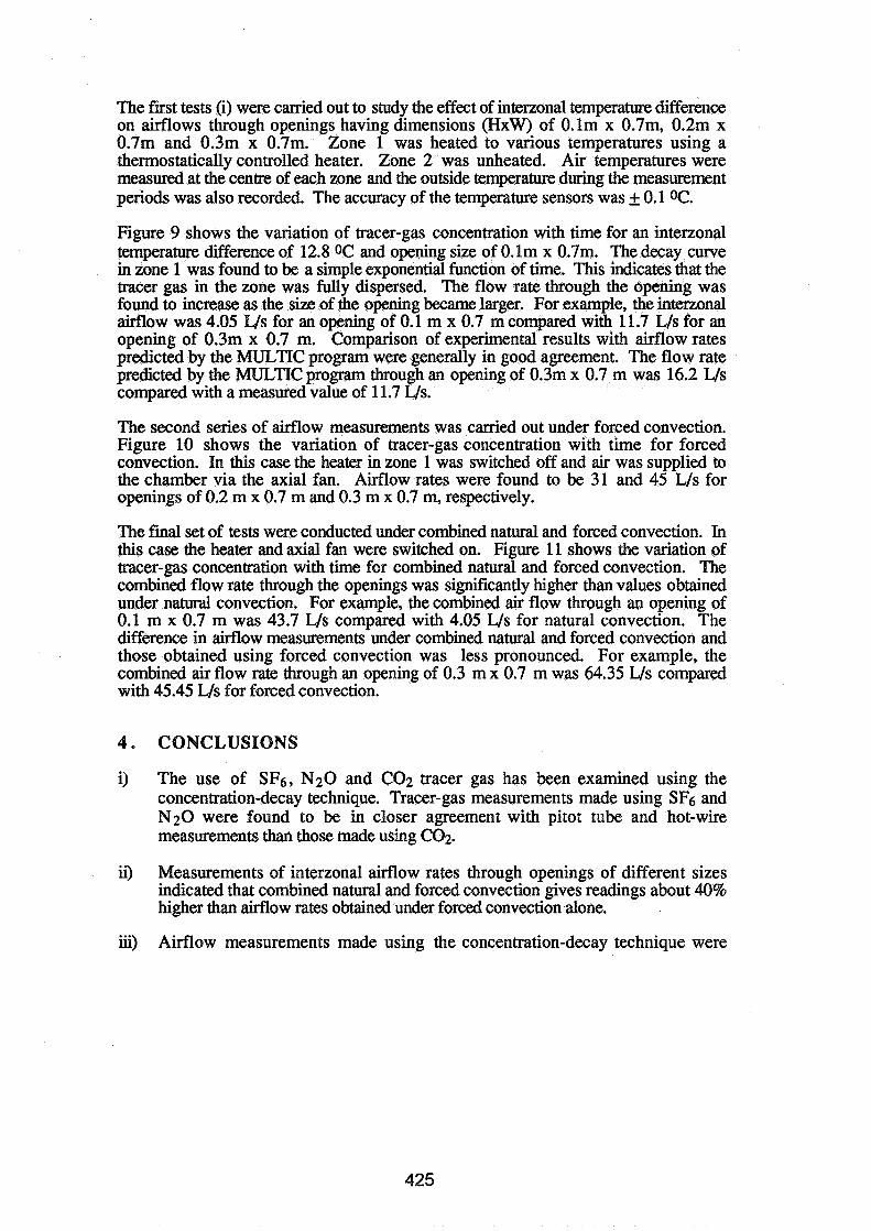
The first tests (i) were carried out to study the effect of intemnal temperature difference on airflows through openings having dimensions (HxW) of 0. lm x 0.7m, 0.2m x 0.7m and 0.3m x 0.7m. Zone 1 was heated to various temperatures using a thermostatically controlled heater. Zone 2 was unheated. Air temperatures were measured at the centre of each zone and the outside temperature during the measurement periods was also recorded. The accuracy of the temperature sensors was + 0.1 OC.
Figure 9 shows the variation of tracer-gas concentration with time for an interzonal temperature difference of 12.8 OC and opeI?ing size of O.lm x 0.7m. The decay curve in zone 1 was found to be a simple exponential function of time. This indicates that the tracer gas in the zone was fully dispersed. The flow rate through the opening was found to increase as the size of the opening became larger. For example, the interzonal airflow was 4.05 Us for an opening of 0.1 m x 0.7 m compared with 11.7 Lls for an opening of 0.3m x 0.7 m. Comparison of experimental results with airflow rates predicted by the MULTIC program were generally in good agreement. The flow rate predicted by the MULTIC program through an opening of 0.3m x 0.7 m was 16.2 Us compared with a measured value of 11.7 Us.
The second series of airflow measurements was carried out under forced convection. Figure 10 shows the variation of tracer-gas concentration with time for forced convection. In this case the heater in zone 1 was switched off and air was supplied to the chamber via the axial fan. Airflow rates were found to be 31 and 45 Lls for openings of 0.2 m x 0.7 m and 0.3 m x 0.7 m, respectively.
The final set of tests were conducted under combined natural and forced convection. In this case the heater and axial fan were switched on. Figure 11 shows the variation of tracer-gas concentration with time for combined natural and forced convection. The combined flow rate through the openings was significantly higher than values obtained under natural convection. For example, the combined air flow through an opening of 0.1 m x 0.7 m was 43.7 Lls compared with 4.05 L/s for natural convection. The difference in airflow measurements under combined natural and forced convection and those obtained using forced convection was less pronounced. For example, the combined air flow rate through an opening of 0.3 m x 0.7 m was 64.35 U s compared with 45.45 L/s for forced convection.
4 . CONCLUSIONS
i) The use of SF6, N 2 0 and C02 tracer gas has been examined using the concentration-decay technique. Tracer-gas measurements made using SF6 and N20 were found to be in closer agreement with pitot tube and hot-wire measurements than those made using C02.
ii) Measurements of interzonal airflow rates through openings of different sizes indicated that combined natural and forced convection gives readings about 40% higher than airflow rates obtained under forced convection alone.
iii) Airflow measurements made using the concentration-decay technique were

ACKNOWLEDGEMENT
We wish to express our thanks to Professor K.E. Siren, Helsinki University of Technology, for providing a copy of the MULTIC program.
REFERENCES
1. Siren, K., "A procedure for calculating concentration histories in dwellings" Building and Environment, 23(2), 103-1 14, 1988
2. BREEZE, "A multizone infiltration model", Air Infiltration Review, 9(1), 1-3, 1987
3. International Workshop COMIS, Conjunction of multizone infiitration specialist at Lawrence Berkeley Laboratory, Berkeley, CA, 198811989.
4. Lagus, P. and Persily, A.K., "A review of tracer-gas techniques for measuring airflow in buildings", ASHRAE Trans. 92(2), 1075- 1087,1985.
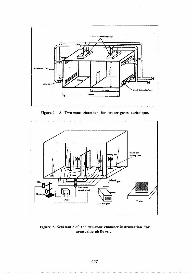
e -
2000 X 6Mhnm Diffu.an
2000 X MH)mm Diffuser
Figure 1 - A Two-zone chamber for tracer-gases technique.
Figure 2- Schematic of the two-zone chamber instrumation for measuring airflows .

0 50 100 150 200 250 300
nnle (minutes)
Figure 3 - The variation of SF, concentration with time, ACH = 42.6
Figure 4 - Comparison of air change rate measurements made using SF, tracer gas with observations made using pitot tube and hot-wire
methods.
Figure 5 - The variation of C O , concentration with time, ACH = 28.5
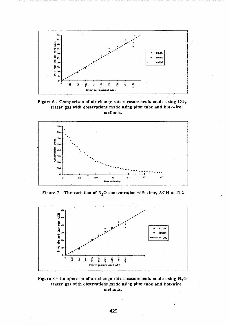
50 - 45 - -
ti 40--
0
T n m gas measured ACH
Figure 6 - Comparison of air change rate measurements made using CO, tracer gas with observations made using pitot tube and hot-wire
methods.
Figure 7 - The variation of N20 concentration with time, ACH = 41.2
Tracer gas measured ACII
Figure 8 - Comparison of air change rate measurements made using N20 tracer gas with observations made using pitot tube and hot-wire
methods.

Figure 9 - The variation of SF, concentration with time in zones 1 and 2; natural flow.
5001
0 100 203 300 4aJ SOD m 700 e53
Time (~conds)
450 - - 400 -- -
0 350--
~ 3 0 - -
4 250-- b
f "-' 3 I=- -
loo--
50
0 ,
Figure 10- The variation of SF, concentration with time in zones 1 and 2; forced flow.
. . I . . . . . . . . . . . . . . . * - - . . . . . . 0 100 203 300 400 500 600 m rn
Time (seconds)
Figure 11- The variation of SF6 concentration with time in zones 1 and 2; combined natural and forced flow.
600-
500 - Im-- 4 m-- ! t "-- U
100 - -
O P
- -
0 0 D ' J i i D
0 S f n o . O a o
0 " - . o o ~ o o
- * . . . I
0 100 203 30 403 So 600 700 800
Time (seconds) L
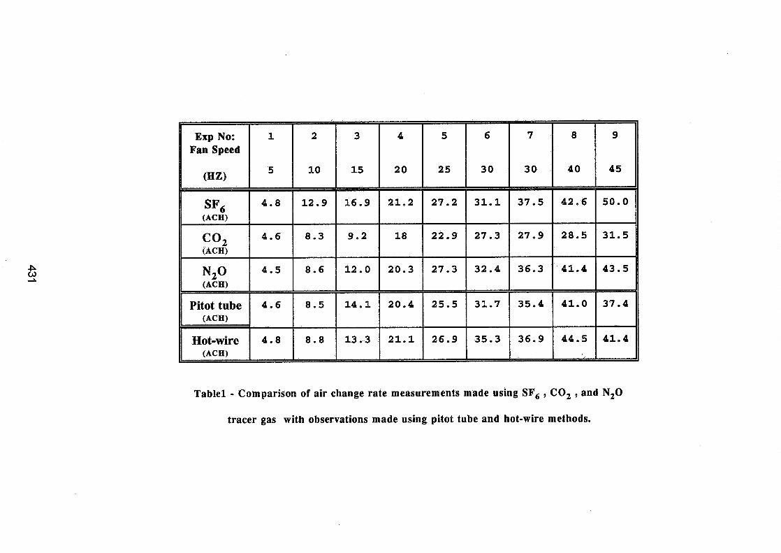
M
. c
m
3 - 9
* w
s
m
*
**
C,
s E
'El w
L
M
3
E
m 'I
2 3
w
z i
&m
w
E
M
o
-2 5
. S
ed a
ee
l 0
0 E,
g 'I
WJ
..II
B
f.. 2 M
: L
;; 8 2
'C
)


Energy Impact of Ventilation and Air Infiltration 14th AlVC Conference, Copenhagen, Denmark
21 -23 September 1993
Flow of Aerosol Particles Through Large Openings
N M Adam, S B Riffat
Building Technology Group, School of Architecture University of Nottingham, University Park Nottingham, NG7 2RD, UK
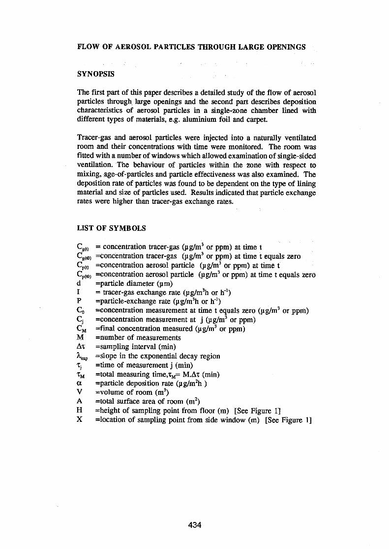
FLOW OF AEROSOL PARTICLES THROUGH LARGE OPENINGS
SYNOPSIS
The first part of this paper describes a detailed study of the flow of aerosol particles through large openings and the second part describes deposition characteristics of aerosol particles in a single-zone chamber lined with different types of materials, e.g. aluminium foil and carpet.
Tracer-gas and aerosol particles were injected into a naturally ventilated room and their concentrations with time were monitored. The room was fitted with a number of windows which allowed examination of single-sided ventilation. The behaviour of particles within the zone with respect to mixing, age-of-particles and particle effectiveness was also examined. The deposition rate of particles was found to be dependent on the type of lining material and size of particles used. Results indicated that particle exchange rates were higher than tracer-gas exchange rates.
LIST OF SYMBOLS
C,,, = concentration tracer-gas (pg/m3 or ppm) at time t Cg,, =concentration tracer-gas (pg/m3 or ppm) at time t equals zero Cp, =concentration aerosol particle (pg/m3 or ppm) at time t C,(,, =concentration aerosol particle (pg/m3 or ppm) at time t equals zero d =particle diameter (pm) I = tracer-gas exchange rate (pg/m3h or h-') P =particle-exchange rate (pg/m3h or h-') C, =concentration measurement at time t equals zero (pg/m3 or ppm) Cj =concentration measurement at j (pg/m3 or ppm) C, =final concentration measured (pg/m3 or ppm) M =number of measurements AT =sampling interval (min) h,, =slope in the exponential decay region zj =time of measurement j (min) T, =total measuring t i r n e , ~ ~ M.AT (min) a =particle deposition rate (pg/m2h ) V =volume of room (m3) A =total surface area of room (m2) H =height of sampling point from floor (m) [See Figure 11 X =location of sampling point from side window (m) [See Figure 11

=local age-of-tracer (min) =average age-of-tracer (rnin) =local age-of-particle (min) =average age-of-particle (min) =local tracer or particle-exchange indicator (%) =the system's average nominal time constant (min) =the local age-of-tracer (or particles) at a point (min) =wind speed (m/s) =wind direction ( degrees N) =indoor temperature - outdoor temperature ("C) =deposition velocity (cm/s)
1. INTRODUCTION
Particulate pollutants in buildings can have damaging effects on the health of the occupants and studies have shown that indoor aerosol particles strongly influence the incidence of sick building syndrome [I]. Indoor aerosols are not only asociated with outdoor sources (e.g. car exhaust emissions, coal and oil combustion, road dust) but also arise from a number of indoor sources (e.g. cigarette smoke, building materials, personal products). Aerosol particles can deposit in ventilation ducts and on surfaces of rooms or can be transported between zones; this can have serious effects in hospitals and buildings used by the pharmaceutical industry 121. Deposition of airborne particles in museums and galleries can lead to perceptible soiling within a short time and ultimately result in damage to works of art.
The concentration of indoor aerosol particles can be reduced by mechanical ventilation using extract fans or by natural ventiltion which allows air exchange between the indoor and the outdoor environment via windows and doorways. The distribution of fresh air and the total supply rate of fresh air are important aspects of natural ventilation 131. The airflow estimated using tracer-gas techniques [4-51, is not sufkient to describe the removal of particles as particle deposition rate, particle type, size, source and concentration must be taken into consideraton. This paper describes a detailed study of the flow of aerosol particles through large openings and the deposition characteristics of particles on different types of materials e.g. wood, aluminium foil and carpet.
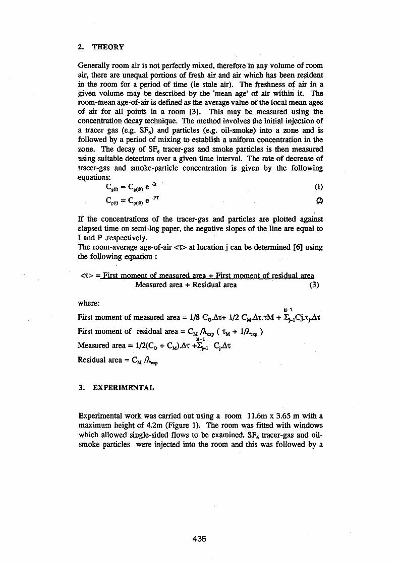
2. THEORY
Generally room air is not perfectly mixed, therefore in any volume of room air, there are unequal portions of fresh air and air which has been resident in the room for a period of time (ie stale air). The freshness of air in a given volume may be described by the 'mean age' of air within it. The room-mean age-of-air is defined as the average value of the local mean ages of air for all points in a room [3]. This may be measured using the concentration decay technique. The method involves the initial injection of a tracer gas (e.g. SF6) and particles (e.g. oil-smoke) into a zone and is followed by a period of mixing to establish a uniform concentration in the zone. The decay of SF6 tracer-gas and smoke particles is then measured using suitable detectors over a given time interval. The rate of decrease of tracer-gas and smoke-particle concentration is given by the following equations:
CgO = Cg(t0) e -It (1)
Cp(t) = c,,, e -m C9
If the concentrations of the tracer-gas and particles are plotted against elapsed time on semi-log paper, the negative slopes of the line are equal to I and P ,respectively. The room-average age-of-air <z> at location j can be determined [6] using the following equation :
<z> = First moment of measured area + First moment of residual area Measured area + Residual area (3)
where: M-1
First moment of measured area = 118 &.AT+ 112 C,.Az.zM + Xk,Cj.zj.A%
First moment of residual area = C, /h,, ( z, + l/hhrP ) M- 1
Measured area = 1/2(C0 + CM).A~ +Xk, Cj.A%
Residual area = C, /hex,,
3. EXPERMENTAL
Experimental work was carried out using a room 11.6m x 3.65 m with a maximum height of 4.2m (Figure 1). The room was fitted with windows which allowed single-sided flows to be examined. SF6 tracer-gas and oil- smoke particles were injected into the room and this was followed by a
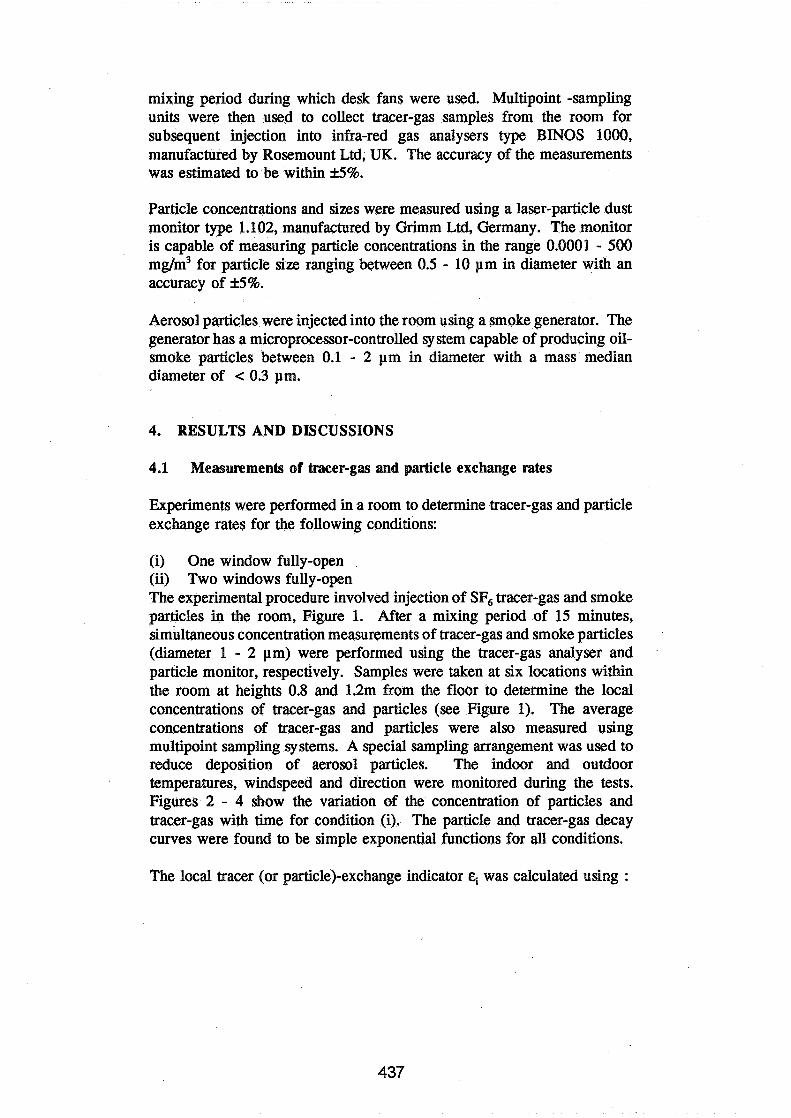
mixing period during which desk fans were used. Multipoint -sampling units were then used to collect tracer-gas samples from the room for subsequent injection into infra-red gas analysers type BINOS 1000, manufactured by Rosemount Ltd, UK. The accuracy of the measurements was estimated to be within f5%.
Particle concentrations and sizes were measured using a laser-particle dust monitor type 1.102, manufactured by Grirnm Ltd, Germany. The monitor is capable of measuring particle concentrations in the range 0.0001 - 500 mg/m3 for particle size ranging between 0.5 - 10 pm in diameter with an accuracy of f 5%.
Aerosol particles were injected into the room using a smoke generator. The generator has a microprocessor-controlled system capable of producing oil- smoke particles between 0.1 - 2 pm in diameter with a mass median diameter of < 0.3 pm.
4. RESULTS AND DISCUSSIONS
4.1 Measurements of tracer-gas and particle exchange rates
Experiments were performed in a room to determine tracer-gas and particle exchange rates for the following conditions:
(i) One window fully-open (ii) Two windows fully-open The experimental procedure involved injection of SF, tracer-gas and smoke particles in the room, Figure 1. After a mixing period of 15 minutes, simultaneous concentration measurements of tracer-gas and smoke particles (diameter 1 - 2 pm) were performed using the tracer-gas analyser and particle monitor, respectively. Samples were taken at six locations within the room at heights 0.8 and 1.2m from the floor to determine the local concentrations of tracer-gas and particles (see Figure 1). The average concentrations of tracer-gas and particles were also measured using multipoint sampling systems. A special sampling arrangement was used to reduce deposition of aerosol particles. The indoor and outdoor temperatures, windspeed and direction were monitored during the tests. Figures 2 - 4 show the variation of the concentration of particles and tracer-gas with time for condition (i). The particle and tracer-gas decay curves were found to be simple exponential functions for all conditions.
The local tracer (or particle)-exchange indicator % was calculated using :

Results indicated that local age-of-tracer is higher than the average age-of- tracer. Local tracer-gas indicators were found to be in the ranges 0.72 - 0.92 and 0.7 - 1.16 for conditions (i) and (ii), respectively.
The local age-of-particles was found to be generally lower than the average age-of-particles. For condition (i), local particle-exchange indicators were found to be in the ranges 0.47 - 2.78 and 0.89 - 2.92 for d > 1 pm and d > 2 pm, respectively.
The local average age-of-particles was found to be highest in the middle of the room. The local average age-of-particles was found to increase with increasing particle size. The age-of-tracer was greater than the age-of- particles.
Particle exchange rates were higher than tracer-gas exchange rates. The difference in tracer-gas and particle exchange rates is due to the deposition (or adsorption effect) of particles on the surfaces of the room. This was estimated using the following equation:
For condition (i), the deposition rates were in the ranges 0.92 - 6.57 (pg/m2h) and 0.83 - 3.85 @g/m2h) for d > 1 pm and d > 2 pm, respectively.
4.2 Measurements in a lined chamber
Experiments were performed in a chamber at different ventilation rates. The chamber was lined with the following materials:
(i) wood (unlined chamber) (ii) aluminium foil (iii) carpet
For each material SF, tracer-gas and oil-smoke particles were injected into the chamber. After a mixing period of 1 hour, simultaneous measurements of the concentrations of tracer-gas and oil-smoke particles were performed using the infra-red gas analyser and particle monitor, respectively. The tracer-gas and particle decay curves were found to be simple exponential functions for all conditions.

Table 3 shows experimental results for conditions (i) to (iii). Deposition rate, a, is obtained using Equation 4. Figures 5 - 7 show the variation of deposition rate with flow rate for wood, aluminium foil and carpet, respectively. The deposition rate on all materials was found to be dependent on the size of the particles. Particle exchange rates on wood and carpet was found to increase at air exchange rates above 0.9 h-' and 0.8 h-', respectively. For aluminium, the deposition rate was found to be highest at an air exchange rate of 0.5 h-' and then decreased. Similar results were obtained when R10 (silica oxide, SiO,, from Particle Technology Ltd., UK) aerosol particles were used instead of oil-smoke particles.
The deposition rate on wood and carpet was found to be several orders of magnitude higher than on aluminium foil. Low deposition rate on aluminium indicates that it would be possible to reduce particle deposition in buildings by using highly polished metal surfaces. The results also indicate that ventilation rate in buildings has a strong effect on particle deposition.
Table 3 also shows the average deposition velocity of the oil-smoke particles for various tests. The results indicated that the deposition velocity increased with increasing particle size. Deposition velocities in the chamber lined with wood and carpet were significantly higher than when aluminium foil was used.
5. CONCLUSIONS
(i) The results showed that particle exchange rates were higher than tracer-gas exchange rates. This was due to the deposition effect of particles on the surfaces of the room and chamber.
(ii) Deposition rate was found to be dependent on the size of particles and on the type of lining material used.
(iii) The results also indicated that ventilation rate in buildings has a strong effect on deposition of particles.
(iv) The room age-of-tracer was found to be greater than room age-of- particles.
REFERENCES
1. TURIEL, I. "Indoor air quality and human health" Stanford Univensity Press, Stanford, California, 1985

2. FARANCE, K. and WILKINSON, J. "Dusting down suspended particles"
Building Services, Vol 12, 1990, p 45-46
3. WALKER, R. R. and WHITE, M. K. "Single-sided natural ventilation - How deep an office?" Building Services Engineering Research and Technology, Vol 13(4), 1992, p 231-236
4. RIFFAT,. S B. "Comparison of tracer-gas techniques for measuring airflow in a duct" J. Institute of Energy, Vol LXIII, 545, 1990, p 18 -21
5. ADAM, N. M. and RIFFAT, S. B. "Deposition of aerosol particles in buildings" CLIMA 2000 Conference, London, UK, November 1-3, 1993 (accepted for publication)
6. Grieve, P.W. "Measuring ventilation using tracer-gases" Bruel and Kjaer, Technical Note , October, 1989, p 28
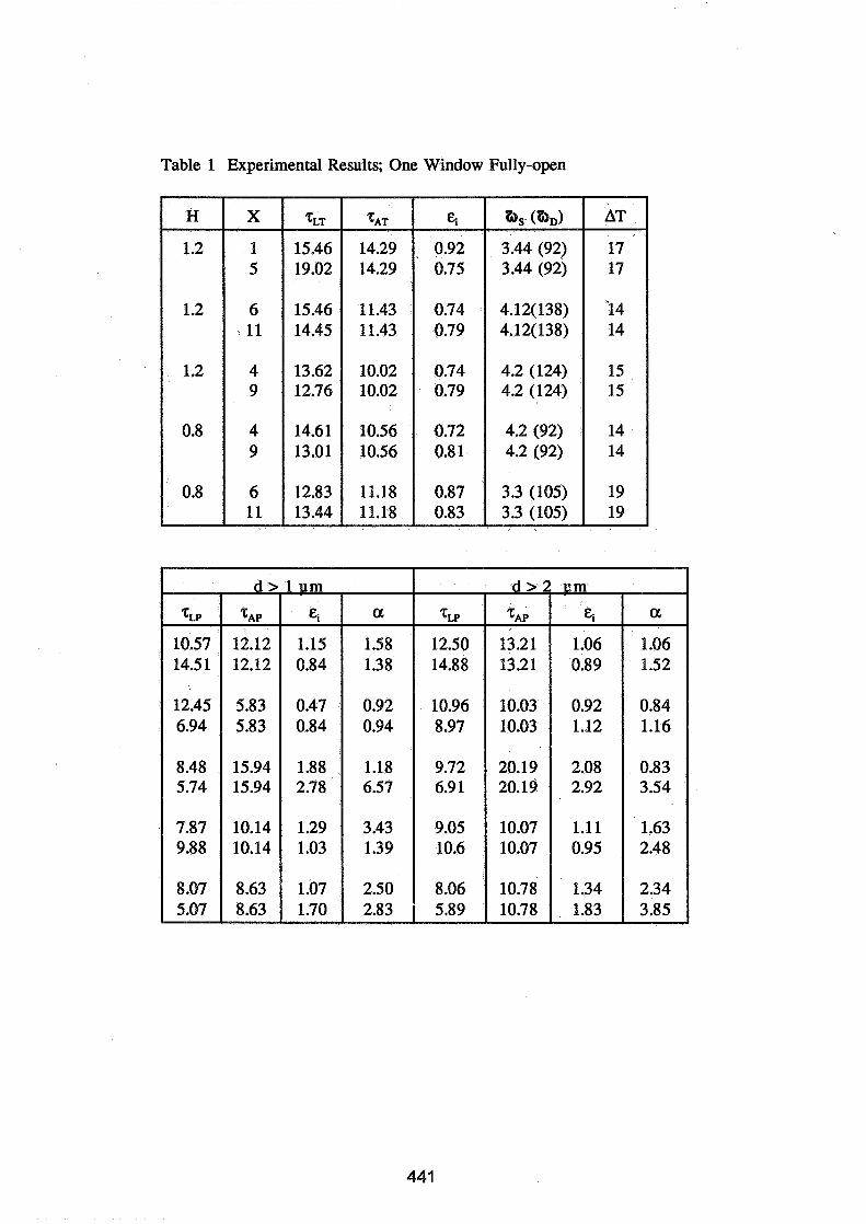
Table 1 Experimental Results; One Window Fully-open
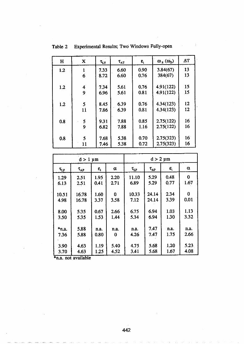
Table 2 Experimental Results; Two Windows Fully-open

Table 3 Results For Lined Chamber

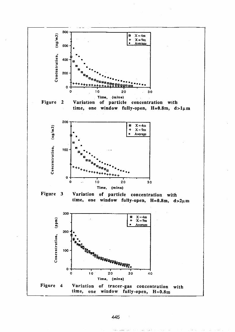
Figure
Figure
0 10 20 3 0
Time, (minsl
2 Variation of particle concentration with time, one window fully-open, H=O.Sm, d> lpm
0 - 10 20 3b Time, (mins)
3 Variation of particle concentration with time, one window fully-open, H=0.8m, d>2pm
0 0 10 2 0 3 0 40
Time, (mins)
Figure 4 Variation of tracer-gas concentration with time, one window fully-open, H=0.8m

I tracer-gas exchange rate, wood I 0.2
h
LI e4 E . M 9 Y
0.1 a 0 ." * .- V)
0 m. UJ n
0.0 0.0 0.2 0.4 0.6 0.8 1.0 1.2 1.4
Tracer exchange rate, (h-1) Figure 6 Variation of particle deposition rate with
tracer-gas exchange rate, aluminium
0.0 - 1 0.2 0.4 0.6 0.8 1 .O 1.2
Tracer exchange rate, (h-1) Figure 7 Variation of particle deposition rate with
tracer-gas exchange rate, carpet

Energy Impact of Ventilation and Air Infiltration 14th AlVC Conference, Copenhagen, Denmark
21 -23 September 1993
Mixing VS.Displacement Ventilaton in Terms of Air Diffusion Effectiveness
N O Breum, E Orhede
National Institute of Occupational Health, Lersoe Parkalle 105, DK-2100 Copenhagen, Denmark
SYNOPSIS
In occupational hygiene the common practice is to use dilution ventilation (MIXVENT) which ideally requires perfect mixing. Increasingly, however, displacement ventilation (DISPVENT) is being applied, ideally this involves fresh air displacing contaminated air without mixing. Keeping .&llXVENT as a reference the approach of intervention was used to estimate the potential of DISPVENT for improving environmental conditions in a garment sewing plant. Air exchange efficiency of MEVENT came to 49%. DISPVENT improved the efficiency to a level of 57%. In terms of local mean age of air DISPVENT improved conditions by a factor of 1.3. From the air diffusion effectiveness MIXVENT caused some short-circuiting of supply air to the exhaust grille. DISPVENT improved air diffusion effectiveness by a factor of 1.7, and no short-circuiting was observed. It is concluded that DISPVENT has potential for improving environmental conditions in industry.
1. INTRODUCTION
Ventilation systems based on the displacement design principle (DISPVENT) are rather common in Scandinavia. The aim of this design principle is to create supply-air conditions in the occupied zone, while the aim of traditional mixing systems (MIXVENT) is to create exhaust-air conditions throughout the room. Comprehensive data on the performance of displacement versus mixing ventilation are available from the laboratory. However, situations in real buildings may be different from those in the laboratory, and data from the laboratory may not be valid for real buildings. Therefore an intervention study of MIXVENT vs. DISPVENT has been made in a factory (a sewing plant). In this paper is given the data obtained on air renewal. Data on air quality and thermal conditions are reported elsewhere.") Models used for air renewal characterization are summarized first.
2. AIR FLOW PATTERNS
The age of a fluid element of air is defined to be the time that has passed since the element entered the space. Let the mean age at an arbitrary location, P, be denoted pp A transit time is needed by the fluid element to be locally felt. Let the mean transit time be denoted E,.
The fluid element is locally present for some time and then leave. Let mean presence time be denoted &. The three time concepts are related by@)
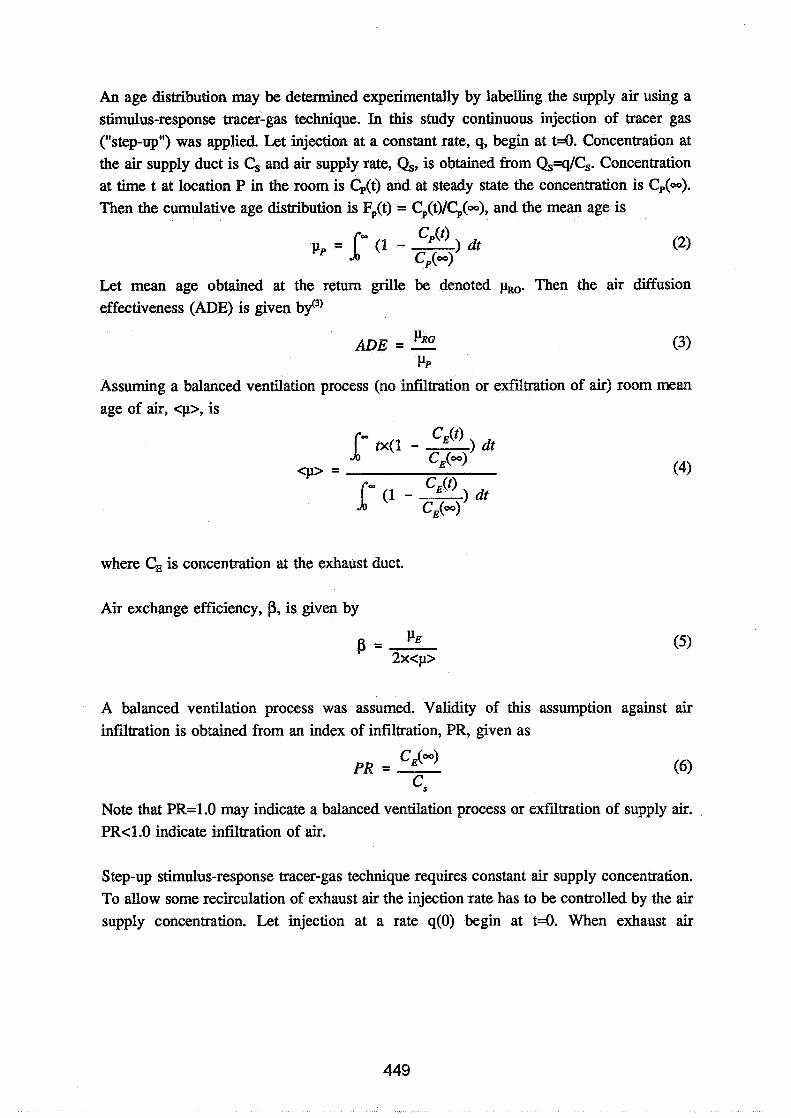
An age distribution may be determined experimentally by labelling the supply air using a stimulus-response tracer-gas technique. In this study continuous injection of tracer gas (''step-up") was applied. Let injection at a constant rate, q, begin at t=O. Concentration at the air supply duct is Cs and air supply rate, Q , is obtained from Q=q/Cs. Concentration at time t at location P in the room is Cp(t) and at steady state the concentration is Cp(-). Then the cumulative age distribution is Fp(t) = CP(t)/q(=), and the mean age is
Let mean age obtained at the return grille be denoted PRG. Then the air diffusion effectiveness (ADE) is given bf3)
PRG ADE = --. (3) PP
Assuming a balanced ventilation process (no infiltration or exfiltration of air) room mean age of air, <p>, is
where C, is concentration at the exhaust duct.
Air exchange efficiency, P, is given by
A balanced ventilation process was assumed. Validity of this assumption against air infiltration is obtained from an index of infiltration, PR, given as
Note that PR=1.0 may indicate a balanced ventilation process or exfiltration of supply air. PR4.0 indicate infiltration of air.
Step-up stimulus-response tracer-gas technique requires constant air supply concentration. To allow some recirculation of exhaust air the injection rate has to be controlled by the air supply concentration. Let injection at a rate q(0) begin at t=Q. When exhaust air

concentration has come to steady-state, the injection rate has arrived at a reduced constant level of q(-). From a tracer gas mass balance the proportion, RE, of supply air coming from exhaust air is.")
RE is an index of recirculation, and R E 4 is achieved for a full outdoor air system.
3. THE FACTORY
The study was performed in a sewing plant making uniforms for the army. The sewing operation was conducted in a production area with 70 sewing machines in close proximity to each other, each machine performing a separate operation on the component part of the clothing. Local exhaust systems were installed at all machines. Approximately 40 workers, mainly seated, were in the shop. Layout and a cross-section of the workshop (V=2,300 m3) are shown in Fig. 1. Based on workshop floor area the estimated convective heat load came to 14 W/m2.
At outset of the study MIXVENT (Fig. 1) was used. Fresh air was supplied at a constant rate by 14 diffusors at ceiling level. The heated and contaminated air was exhausted at the machines and from ceiling level by grilles in a duct running along the rear wall. Exhaust air was directed to a common duct. During second period of the study DISPVENT was used. Layout and a cross-section of the workshop are shown in Fig. 2, the only difference from Fig. 1 being a rearranged ducting of the ventilation system to serve air supply terminal devices standing on floor.
Section A-A
14.5 n 27.5 m
Fig 1. Layout and cross-section of the plant designed for MIXVENT (not to scale)

Section A-A
Fig. 2. Layout and cross-section of the plant designed for DiSPVENT (not to scale)
4. EXPERIMENTAL PROCEDURE
Performance of MIXVENT was tested for a 3-week period in early winter. Data were collected once a week - on monday, wednesday, and friday, respectively. Data were collected as breathing zone samples at workstation Nos. 1-8 (Fig. 1). Data were also obtained from supply and exhaust air, respectively. Keeping identical test procedures the performance of DISPVENT was tested late winter in a period of expected outdoor weather conditions being similar to early winter. The paired t-test were used for statistical analysis of data. Tests were performed at a 5% (or better) level of significance.
4.1 Production rate of the plant Throughout the study a constant production rate was assumed. Data on actual production rate were obtained for checking the validity of this assumption.
4.2 Flow fields of supplied air Tracer gas (SFd was injected into the aL supply duct. Some of the exhausted air was recirculated. To keep a constant supply air concentration the injected flow rate was manually adjusted to cancel out recirculated tracer gas. At t=Q the injected flow rate was q(0)=4.25 cm3/min.
Tracer gas concentrations at an estimated accuracy o f f 5% were collected sequentially with a 9-s sampling interval using a multipoint measuring unitJ4) F,(t) was estimated by fitting the function a(l-e-M+") to the data obtained. By integration, pp was estimated from Eq. 2. Mean transit time, E,, was estimated by solving the equation F,(t)=O. Finally, G, was
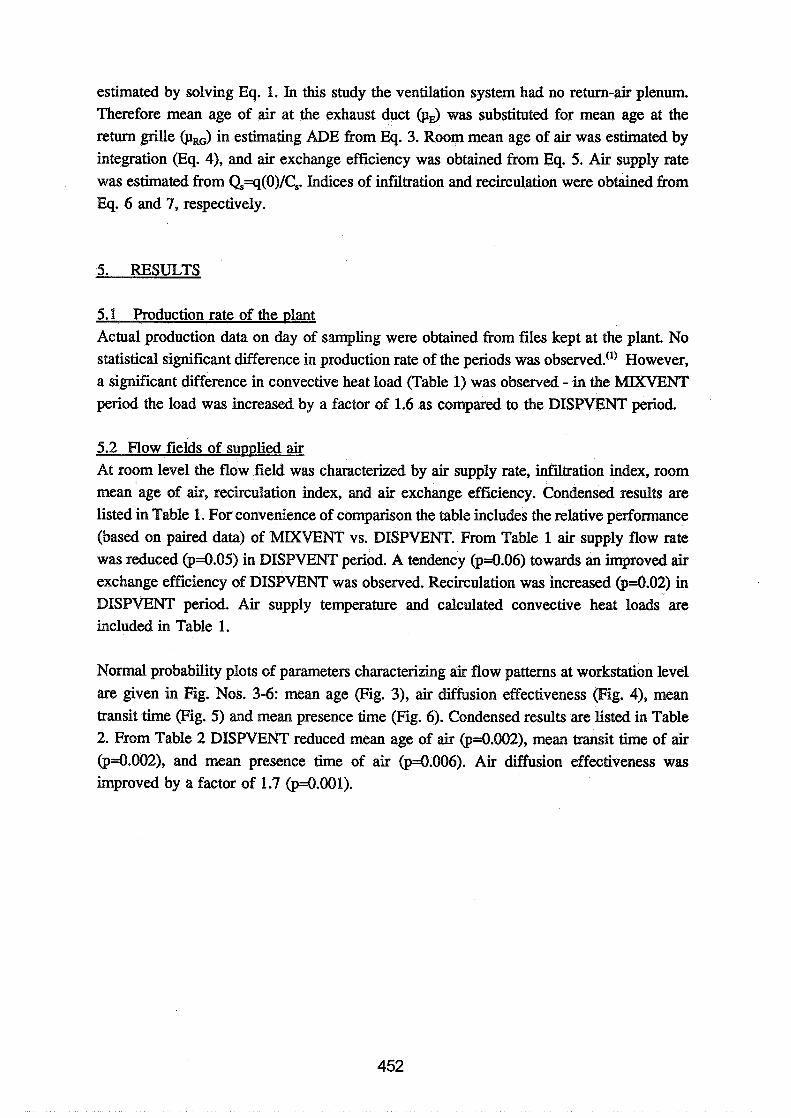
estimated by solving Eq. 1. In this study the ventilation system had no return-air plenum. Therefore mean age of air at the exhaust duct 013 was substituted for mean age at the return grille (pR& in estimating ADE from Eq. 3. Room mean age of air was estimated by integration (Eq. 4), and air exchange efficiency was obtained from Eq. 5. Air supply rate was estimated from Q=q(O)/C,. Indices of infiltration and recirculation were obtained from Eq. 6 and 7, respectively.
5. RESULTS
5.1 Production rate of the plant Actual production data on day of sampling were obtained from files kept at the plant. No statistical significant difference in production rate of the periods was observed.(') However, a signZcant difference in convective heat load (Table 1) was observed - in the MIXVENT period the load was increased by a factor of 1.6 as compared to the DISPVENT period.
5.2 Flow fields of supplied air At room level the flow field was characterized by air supply rate, Miltration index, room mean age of air, recirculation index, and air exchange efficiency. Condensed results are listed in Table 1. For convenience of comparison the table includes the relative performance (based on paired data) of MIXVENT vs. DISPVENT. From Table 1 air supply flow rate was reduced (p4.05) in DISPVENT period. A tendency (p4.06) towards an improved air exchange efficiency of DISPVENT was observed. Recirculation was increased (p4.02) in DISPVENT period. Air supply temperature and calculated convective heat loads are included in Table 1.
Normal probability plots of parameters characterizing air flow patterns at workstation level are given in Fig. Nos. 3-6: mean age (Fig. 3), air diffusion effectiveness (Fig. 4), mean transit time (Fig. 5) and mean presence time (Fig. 6). Condensed results are listed in Table 2. From Table 2 DISPVENT reduced mean age of air (p=0.002), mean transit time of air (p4.002), and mean presence time of air (p4.006). Air diffusion effectiveness was improved by a factor of 1.7 (p=0.001).
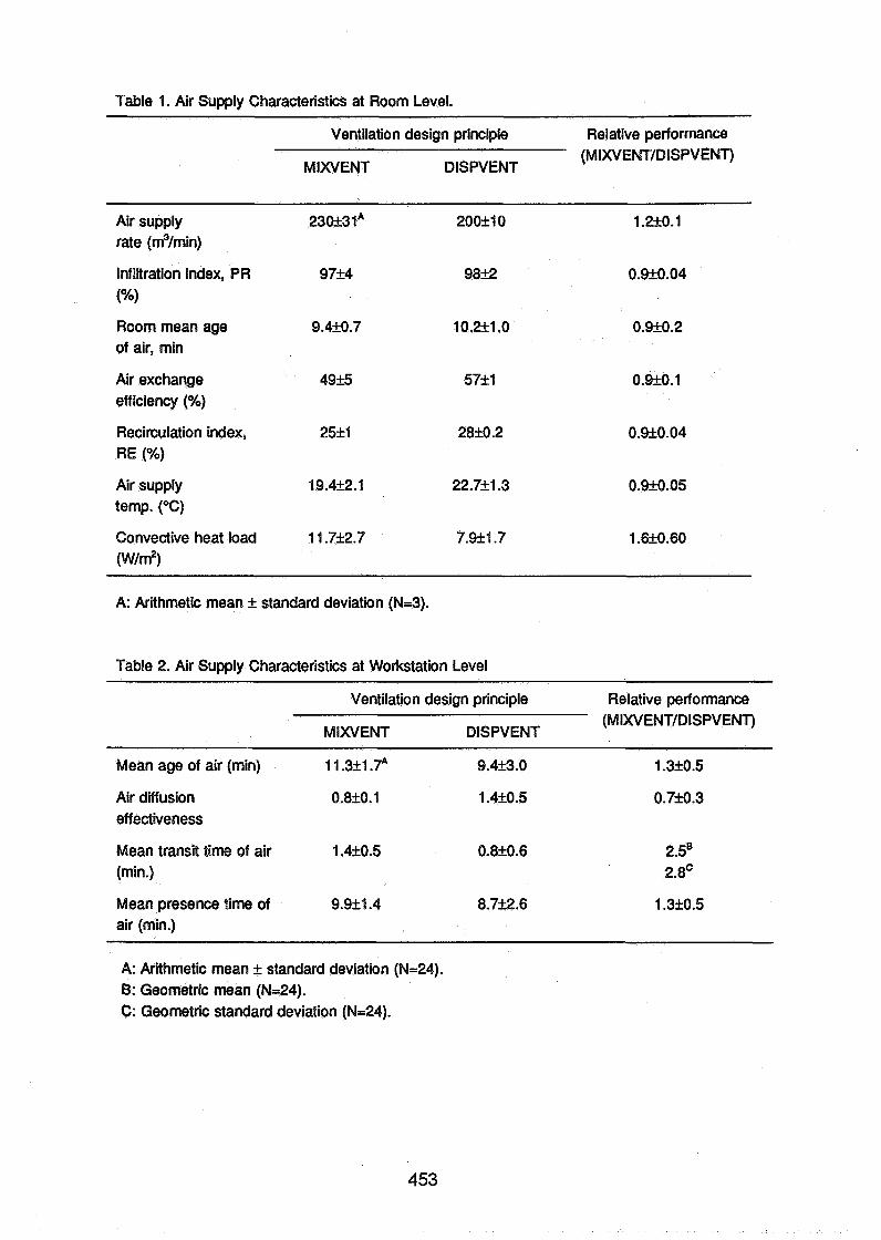
Table 1. Air Supply Characteristics at Room Level.
Ventilation design principle Relative performance (MIXVENT/DISPVENT)
MIXVENT DlSPVENT
Air supply 230rtr3 1 A 200rtr10 rate (m3/min)
Infiltration index, PR 97k4 9 8 B 0.9+_0.04
II"W Room mean age 9.4k0.7 1O.al.O 0.9k0.2 of air, min
Air exchange 4 9 s efficiency (YO)
Recirculation index, 25k1 RE (%)
Air supply temp. ("C)
Convective heat load 1 1.7k2.7
(W/m2)
A: Arithmetic mean f standard deviation (N=3).
Table 2. Air Supply Characteristics at Workstation Level
Ventilation design principle Relative performance
DISPVENT (M IXVENTIDISPVENT)
MIXVENT
Mean age of air (min) 1 1.3k1 .7A 9.4-13.0
Air diffusion effectiveness
Mean transit time of air 1.4-10.5 (min.)
Mean presence time of 9.9k1.4 air (min.)
A: Arithmetic mean k standard deviation (N=24). 6: Geometric mean (N-24). C: Geometric standard deviation (N=24).
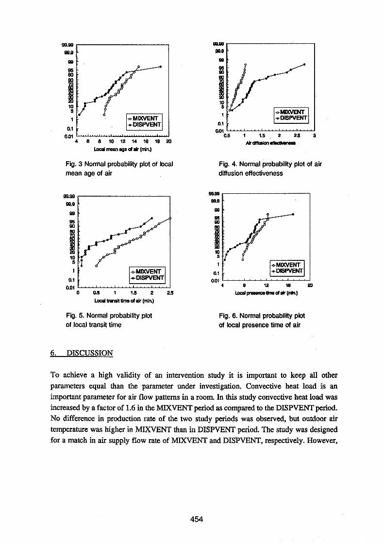
4 8 8 10 12 14 16 18 20
Local mean egs of alr (mln.)
Fig. 3 Normal probability plot of local mean age of air
0 0 3 1 1 . 5 2 2 5
Local t m d time d air (ntln.)
Fig. 5. Normal probability plot of local transit time
Fig. 4. Normal probability plot of air diffusion effectiveness
Fig. 6. Normal probability plot of local presence time of air
6. DISCUSSION
To achieve a high validity of an intervention study it is important to keep all other parameters equal than the parameter under investigation. Convective heat load is an important parameter for air flow patterns in a room. In this study convective heat load was increased by a factor of 1.6 in the MIXVENT period as compared to the DISPVENT period. No difference in production rate of the two study periods was observed, but outdoor air temperature was higher in MIXVENT than in DISPVENT period. The study was designed for a match in air supply flow rate of NT and DISPVENT, respectively. However,

air supply flow rate of DISPVENT was reduced by a factor of 1.2 as compared to MIXVENT (Table I). A balanced ventilation process is a basic assumption for the model of room mean age of air and air exchange efficiency, respectively. From the obtained
index (Table I) this was a valid assumption for the study.
At room level DISPVENT came out at an improved air exchange efficiency (57%) as compared to MIXVENT (49%). This finding was consistent with data from the lab~ratory.'~) Air supply flow rate of DISPVENT came out to be reduced as compared to MIXVENT. Nevertheless DISPVENT improved air renewal at local level (Table 2). Mean transit time of air was reduced by a factor of 2.5, mean presence time of air by a factor of 1.3, and local mean age of air by a factor of 1.3. Recent intervention studies came up with consistent findings reporting reductions in local mean age of air by a factor of 1.6-6.6@) and 2.0." If low-age supply air short-circuits to the return grille pRG should be less than pp; hence the ADE will be less than unity. The converse is true with a displacement flow att tern.'^) From Fig. 4 is observed that MIXVENT caused some short-circuiting (ADE4.0) and that DISPVENT caused a displacement flow pattern (ADE>1.0). DISPVENT improved conditions by a factor of 1.7 calculated from paired ADE data.
7. CONCLUSION
Using the approach of intervention at a factory the performance of MIXVENT was compared to DISPVENT in terms of air renewal. At room level DISPVENT improved air exchaqge efficiency from 49% (MIXVENT) to 57%. At workstation level DISPVENT improved air renewal. In terms of local mean age of air DISPVENT improved conditions by a factor of 1.3. From the air diffusion effectiveness MIXVENT caused some short- circuiting of supply air to the exhaust grille. DISPVENT improved air diffusion effectiveness by a factor of 1.7, and no short-circuiting was observed. It is concluded that DISPVENT has potential for improving environmental conditions in industry.
ACKNOWLEDGEMENT The study was supported by the Danish Working Environment Foundation (grant No. 1992- 11).

8. REFERENCES
1. BREUM, N.O. and ORHEDE, E. "Dilution vs. displacement ventilation - environmental conditions in a garment sewing plant" Am. Ind. Hygiene Assoc. J. 1993 (in press)
2. Breum, N.O. "Ventilation efficiency in an occupied office with displacement ventilation - a laboratory study" Env. Int. 18, 1992, pp353-361.
3. Fisk, W.J., Faulkner, D. and Prill, R. "Air exchange effectiveness of conventional and task ventilation for offices" ASHRAE Supplementary Proceedings of IAQ 91 Conference, 1991, pp30-34.
4. Breum, N.O. and Skotte, J. "Displacement air flow in a printing plant measured with a rapid response tracer gas system" Build. Serv. Res. Technol. 1991, pp39-43
5. Breum, N.O., Helbo, F. and Laustesen, 0. "Dilution versus Displacement Ventilation - an Intervention Study" Ann. Occ. Hyg. 33, 1989, pp321-329.
Energy lm pact of Ventilation and Air Infiltration 14th AlVC Conference, Copenhagen, Denmark
21 -23 September 1993
Influence of Air Infiltration on Heat Losses in Multi-Family Dwelling Houses
A Baranowski
Department of Heating, Ventilation and Dust Removal Technology, Environmental Engineering Faculty, Silesian Technical University, Gliwice, Poland
INFLUENCE OF AIR INFILTRATION ON HEAT LOSSES
IN MULTI - FAMILY DWELLING HOUSES
SYNOPSIS
The paper presents a proposal of numerical procedure for air flow simulation in
multi-zone buildings (up to 100 zones). This can work with 1 hour time-step
according to requirement of TRNSYS - a well-known modular system simulation
programme. Co-operation between TRNSYS and my own programme is analysed, taking a
typical Polish 5 - storey dwelling house as an object of simulation.
The proposed numerical procedure can also be run as an independent programme
calculating the ventilation air flow, air change rate and heat losses due to infiltration.
Simulation results for typical Polish heat season climate conditions are presented, analysing
results coming fiom TRNSYS and my own programme.
1. INTRODUCTION
Air change is one of the most important elements that form the flat microclimate.
The process of ventilating flats in multi-family dwelling-houses (particularly in low,
up-to-five-storeyed ones) is often still realized by natural (gravity) ventilation system. The air
change then takes place through the effect of air infiltration fiom the outside of a building.
The influence of infiltration on the process of ventilating flats is not usually estimated
properly. This has bad consequences both in inaccurate predicting energy consumption
required to cover the infiltration - resulted heat losses of a building and in disensuring the air
change to be suitable from the hygienic point of view.
2. AIR INFILTRATION IN RELATION TO THE HEAT LOAD OF A BUILDING
The calculating of a heat building requirement balance is significant both to minimize
energy input by optimum choice of heating and ventilation systems and to ensure the suitable
thermal comfort to the flat user. One of the more usehl simulation programmes that can be
applied in such calculations is the numerical module programme TRNSYS El], which
enables to make simulating calculations of required heat input a determined building
structure. In the case of natural ventilation system, the calculations are made with some error
since the TRNSYS package is not provided with the possibility to calculate air infiltration.
This quantity, however, may be declared for individual zones as an hourly air change rate.
This possibility is quite sufficient for the rooms or spaces with mechanical ventilation systems
in which air flows are organized in a determined degree and in a determined way. In the case
of natural ventilation, infiltration is formed spontaneously, owing to the variation of the
factors that force it. What is particularly important here is wind action, the velocity and
direction of wind being changed randomly.
In order to determine the real infiltration rate it is convenient to use the numerical
programme that enables to make simulating calculations of ventilating air flows in the
examined building. The calculations are carried out for steady, chosen parameters of ambient
climate, what makes the results should be treated as "accidental state" ones, i.e. concerning
a given, instantaneous disturbance [2] . Without doubt, the more accurate image of the
phenomenon can be obtained when the time variation of infiltration is available for given
zones of a building.
To achieve the run of variation of air flows in a multi-family dwelling-house the
numerical programme TRANSVEN was constructed, which makes it possible to simulate
the process of natural ventilation. The calculations are carried out in the quasi-dynamic
course with time step being declared and with the use of ambient climate generator. The
programme enables to make calculations in the object divided into 100 zones (e.g. the flats).
The calculations are based on the classical balance equations for individual zones but the
solution of systems of non-linear equations is reached differently that it is done in other
similar programms [3]. Here, a methode from the field of optimization theory was applied
that consists in searching the minimum value of specific target fbnction created. One of the
results of the calculations is the run of variation of air streams infiltrating each calculation
zone. It is transformed into an hourly air change rate and makes the TRNSYS input data set
describing the infiltration.
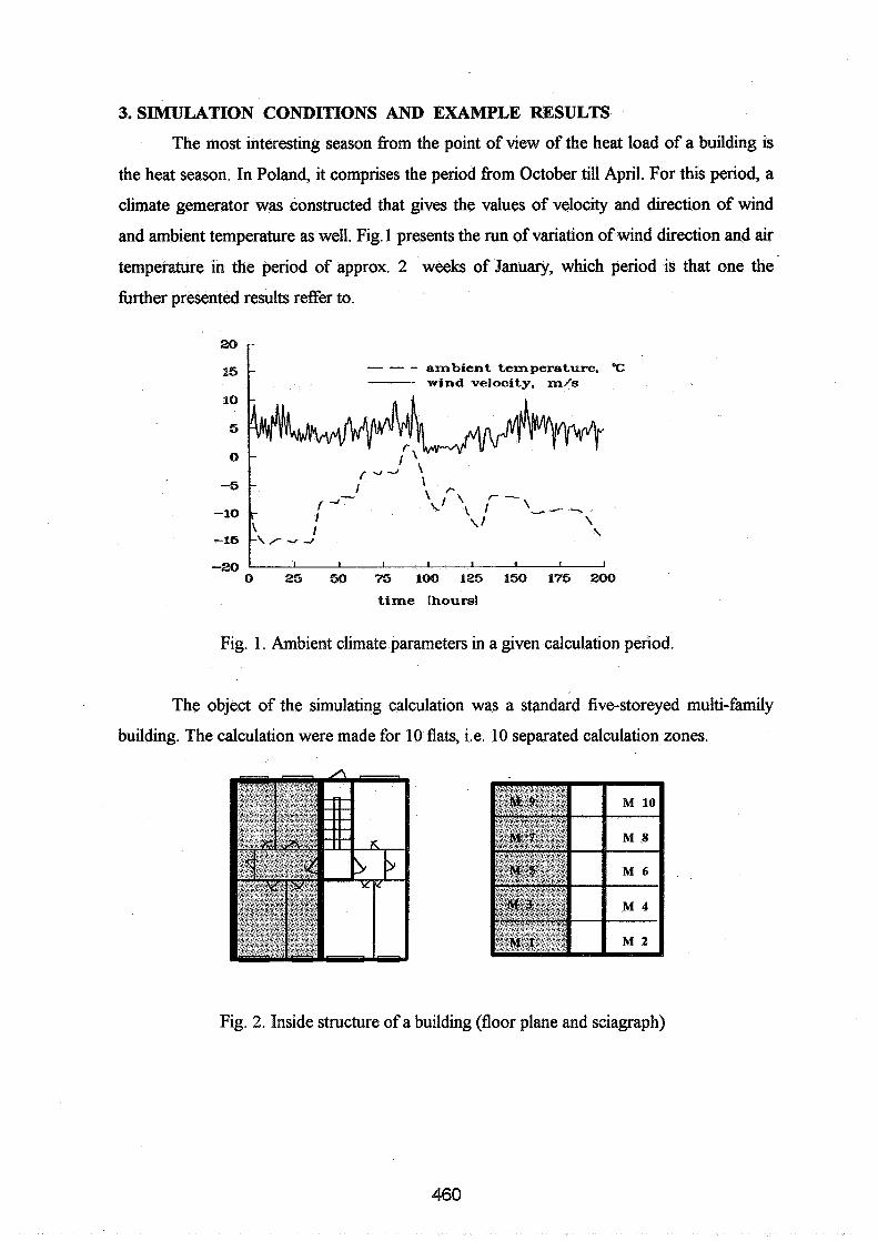
3. SIMULATION CONDITIONS AND EXAMPLE RESULTS
The most interesting season from the point of view of the heat load of a building is
the heat season. In Poland, it comprises the period from October till April. For this period, a
climate gemerator was constructed that gives the values of velocity and direction of wind
and ambient temperature as well. Fig. 1 presents the run of variation of wind direction and air
temperature in the period of approx. 2 weeks of January, which period is that one the
firther presented results reffer to.
20
l5 F - - - ambient te~nperature. OY=
wind velocity, m/s
-20 I I I 1 I I I 1 I
0 25 50 75 100 125 150 175 200
time lhoursl
Fig. 1. Ambient climate parameters in a given calculation period.
The object of the simulating calculation was a standard five-storeyed multi-family
building. The calculation were made for 10 flats, i.e. 10 separated calculation zones.
Fig. 2. Inside structure of a building (floor plane and sciagraph)
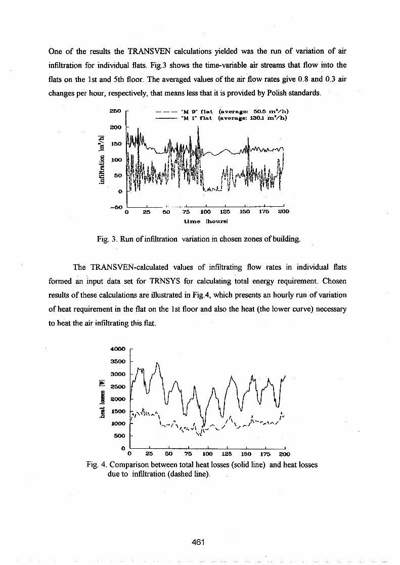
One of the results the TRANSVEN calculations yielded was the run of variation of air
infiltration for individual flats. Fig.3 shows the time-variable air streams that flow into the
flats on the 1st and 5th floor. The averaged values of the air flow rates give 0.8 and 0.3 air
changes per hour, respectively, that means less that it is provided by Polish standards.
--- 'M 9- flat (average: 50.5 ma/h) 'M I' flat (average: 130.1 m9/h)
- G
150 a - 8 loo 3 e! Y - G 50 G .r.
0
-50 I I , 1 I I
0 25 50 75 100 125 150 175 200
time lhoursl
Fig. 3. Run of infiltration variation in chosen zones of building.
The TRANSVEN-calculated values of infiltrating flow rates in individual flats
formed an input data set for TRNSYS for calculating total energy requirement. Chosen
results of these calculations are illustrated in Fig.4, which presents an hourly run of variation
of heat requirement in the flat on the 1st floor and also the heat (the lower curve) necessary
to heat the air infiltrating this flat.
Fig. 4. Comparison between total heat losses (solid line) and heat losses due to infiltration (dashed line).

It can be easily noted that infiltration takes the significant part (nearly a 50 per cent
one) in forming total heat load. Such an unfavourable result is connected with low ambient
temperature that occurs in this period - here -9 "C an average. In the result of analogous
calculations made for h&t season average ambient temperature equal to + 2.5 "C (for the
region of Silesia, Poland), the heat consumption for infiltration decreases to about 20-30 per
cent of total heat requirement of a building.
0 1 I I 1 I I I 1 I
0 25 50 75 LOO 125 150 175 200
time lhoursl
Fig. 5. Comparison of heat losses for infiltration in zone 'MI' : for constant air change rate (dashed line) and for varying infiltration (solid line).
The usefblness of calculation of air infiltration was confirmed in a simulating cycle
that was made with the use of TRNSYS for constant air change declared, identical for each
zone. The absolute minimum air change rate of 0.5 h-' was assumed.
Fig.5 shows the comparison between the infiltration-resulted heat losses due to the
infiltration calculated in a cycle of an hour and those due to the constant infiltration. The
average difference in energy input amouts 20 per cent.
4. CONCLUSIONS
The effect of infiltration in buildings with natural ventilation systems is unavoidable and also
desired. The tendency that occurs to tighten walls and window openings to a maximum
leads without doubt to decreasing heat losses of a building but on the other hand it produces
the unfavourable consequences, i.e. limits the necessary air change.
Natural ventilation is still the most conveninet way the air is changed, particulary in single-

or multi - family low detached houses. The results presented suggest that it is necessary to
seek a comparison between building coating tightness and transmitting the necessary amount
of ventilating air from the outside. It seems essential to apply new construction designes of
window woodwork and walls as well. They would allow, to a certain extent, to control the
process of infiltration, which is, by its nature, in large measure random.
The recognition of the extent of infiltration, which phenomenon varies with climate
conditions and which also greatly depends on location of a flat in the complex structure
of a building, can result in more accurate predicting energy input necessary to cover the
building heat reguirement, thus can be profitable in saving energy and money as well as in
improving the thermal comfort of flats [4].
What seem suitable for the abovementioned purposes are calculations of dynamic
variation of ventilating air as well as climate gemeretors, which simulate the specific
character of a given geographical region and which are constructed on the base of
statistically important data coming from many years' observations made by weather stations.
REFERENCES
1. "TRNSYS. A Transient System Simulation Program"
Solar Energy Laboratory, University of Wisconsin - Madison, 1990
2. NANTKA, M.B. and BARANOWSKI, A.
"The numerical modelling of natural ventilation processes at the wind effect as a
predominant one: state of the art and prospects"
Submittet for publications (in Polish.), 1990.
3. FEUSTEL, H.E. and DIEMS, J.
"A Survey of Air Flow Models for Multizone Structures"
Report of Lawrance Berkeley Laboratory. No LBL - 30288, 1991
4. JONES, P.J. and
"Computational Fluid Dynamics for Building Air Flow Prediction - Current Status and
Capabilities"
Building and Enviromentals, vo1.27, N" 3, 1992, pp32 1-338.

Energy Impact of Ventilation and Air Infiltration 14th AlVC Conference, Copenhagen, Denmark
21 -23 Septem ber 1993
Test and Simulation of Air Flows in Multizone Dwelling Houses: the Alternative Method of Air Flows Prediction
M B Nantka
Department of Heating, Ventilation and Dust Removal Technology, Environment Engineering Faculty, Silesian Technical University, 44-101 Gliwice, Poland
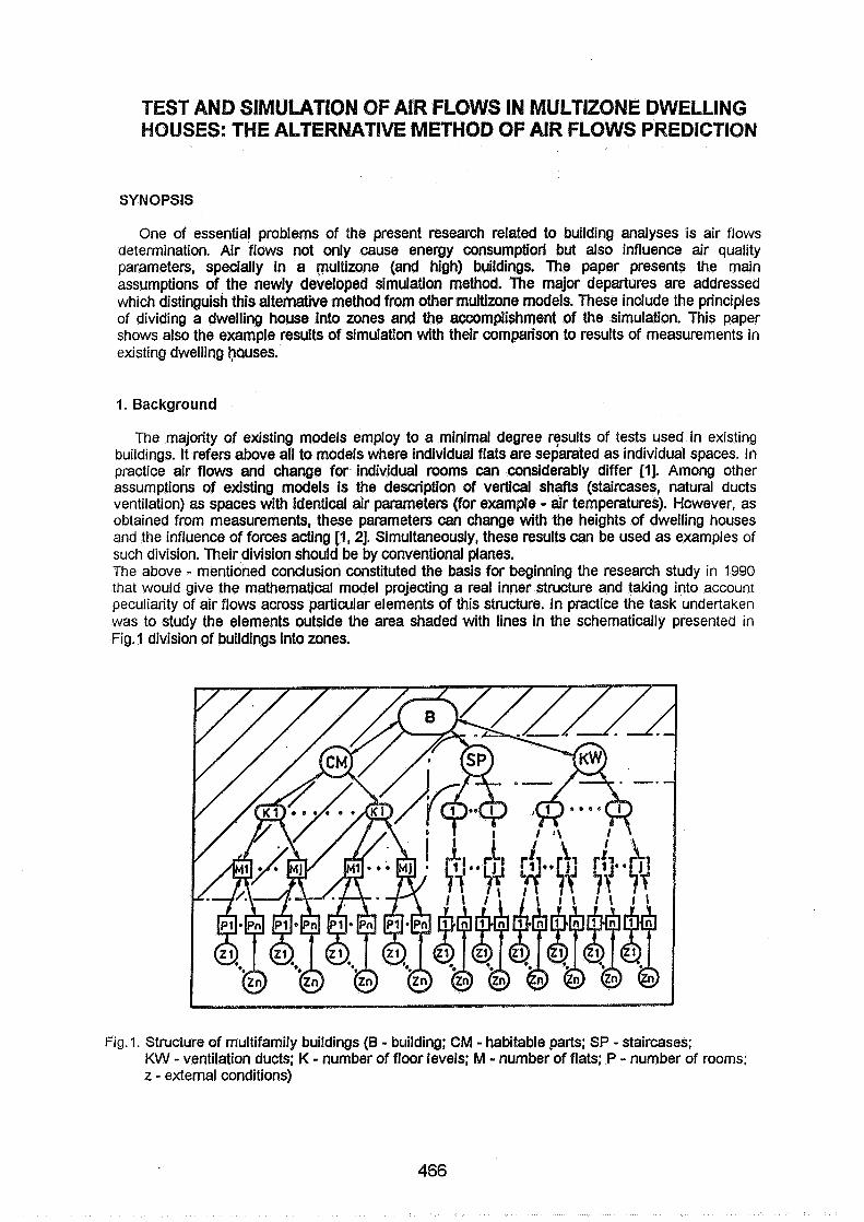
TEST AND SIMULATION OF AIR FLOWS IN MULTIZONE DWELLING HOUSES: THE ALTERNATIVE METHOD OF AIR FLOWS PREDICTION
SYNOPSIS
One of essential problems of the present research related to building analyses is air flows determination. Air flows not only cause energy consumptiod but also influence air quality parameters, specially in a multizone (and high) buildings. The paper presents the main assumptions of. the newly developed simulation method. The major departures are addressed which distinguish this alternative method from other multizone models. These include the principles of dividing a dwelling house into zones and the accomplishment of the simulation. This paper shows also the example results of simulation with their comparison to results of measurements in existing dwelling hauses.
1. Background
The majority of existing models employ to a minimal degree results of tests used in existing buildings. It refers above all to models where individual flats are separated as individual spaces. In practice air flows and change for individual rooms can considerably differ [I]. Among other assumptions of existing models is the description of vertical shafts (staircases, natural ducts ventilation) as spaces with identical air parameters (for example - air temperatures). However, as obtained from measurements, these parameters can change with the heights of dwelling houses and the influence of forces acting [I, 21. Simultaneously, these results can be used as examples of such division. Their division should be by conventional planes. The above - mentioned conclusion constituted the basis for beginning the research study in 1990 that would give the mathematical model projecting a real inner structure and taking into account peculiarity of air flows across particular elements of this structure. In practice the task undertaken was to study the elements outside the area shaded with lines in the schematically presented in Fig. 1 division of buildings into zones.
Fig. I . Structure of multifamily buildings (B - building; CM - habitable parts; SP - staircases; KW - ventilation ducts; K - number of floor levels; M - number of flats; P - number of rooms; z - external conditions)

2. New model conception and realisation of simulations
The basis of a new model conception were the above results of measurements in existing dwelling houses. According to them, the building is divided intg two types of zones. First type zones are spaces that result from existence of the internal partition walls. The second type constitute the zones that are the parts of communication shafts and natural ventilation ducts. Conventional zones are defined on the basis of various parameters betermining air flows in vertical shafts of a building. Finally, the building is replaced by a spatial aerial system joining separated zones lengthwise the distinguished air flow paths. As a result, the internal space of a building (which is a continuum), is replaced by a set of discrete elements, that are mutually combined. This set creates a system that stands for a building and its discrete elements are nodes (look Fig.2). A node is described by the air capacity, focused in the middle of the zone, and the co-ordinates locating the
Schematic floor plan of the. tested house with signification of the seperate zones
Fig.2. The substitute system for one of the tested buildings (example)
zone in the building. The description of the system is completed with'the input data fixing the state and the influence of the driving forces, and the air flow paths. Due to the lack of satisfying iteration methods for sets of non-linear equations (the large number of zones), the method of elementary balances was applied to solve the air flows in the system. This method accomplishes essential advantages. The main one is a possibility of physical interpreting of complex processes proceeding in complicated systems. This method has never been used before in the simulation of

the air flows in multizone building. Therefore, in order to use this method, the iterative conception must be elaborated. This conception is presented in Appendix For simulation of air flows in the substitute systems a new alternative computer ptogram SYMVENT was elaborated. This program was presented in the previous works of the author [2, 31. The program has many advantages; one of them is the possibility of constructing such a system that allows to simulate air flows detailed to any degree (i.e. agglomeration of inner spaces and driving forces, especially for declaration of wind pressure description).
3. The example results and comparisons
To illustrate the results of simulation, certain factors influencing the tested processes, such as the natural ventilation ducts, staircases, wind effect were sorted out. These results, presented below refer to a separated space (e.g. the real zones) located in 10-storey dwelling house. By modification of the layer in the substitute system in respect of the ventilation ducts, the staircase division and also for detailed wind pressure coefficients determination (for each window), the new network. system was obtained. Next, by making simulation in the conditions of measurements the total air change (e.g. WP(C)) from simulation and tests (by means of tracer gas method) were compared. Selected results of measurements fm) and their comparisons to simulation results (0) are presented on Fig.3. To estimate the correlation between calculated and measured air change rates, regression coefficients squares were calculated. This coefficient is about 0.89 for the system with modification (after modifications of the substitute system this coefficient was about 0.59). It is one basic proof of usefulness of the presented method.
WP(C), t/h -
TRACER GAS METHOD
Fig.3. The results of tests of air change - WP(C) - in the rooms situated in one of the tested buildings and correspondence of calculated (o) and measured (m) WP(C)
Among the other advantages of this method, the attention was paid to the correctness of the prevailing division of building area. The example results of these comparisons are illustrated in Fig.4. In the middle part of this figure the changing both of acting forces and air exchange for two
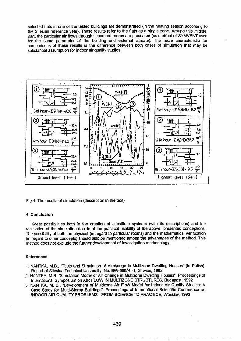
selected flats in one of the tested buildings are demonstrated (in the heating season according to the Silesian reference year). These results refer to the flats as a single zone. Around this middle, part, the particular air flows through separated rooms are presented (as a effect of SYMVENT used for the same parameter of the building and external climate). The more characteristic for comparisons of these results is the difference between both cases of simulation that may be substantial assumption for indoor air quality studies.
Ground level ( I-st 1
Il4 th hour -1@0~)=28.2 $
--
Highest level (5 th 1 '
Fig.4. The results of simulation (description in the text)
4. Conclusion
Great possibilities both in the creation of substitute systems (with its descriptions) and the realisation of the simulation decide of the practical usability of the above presented conceptions. The possibility of both the physical (in regard to particular rooms) and the mathematical verification (in regard to other concepts) should also be mentioned among the advantages of the method. This method does not exclude the further development of investigation methodology.
References
1. NANTKA, M.B., "Tests and Simulation of Airchange in Multizone Dwelling Houses" (in Polish), Report of Silesian Technical University, No. BW-969IRI-1, Gliwice, 1992
2. NANTKA, M.B. "Simulation Model of Air Change in Multizone Dwelling Houses", Proceedings of International Symposium on AIR FLOW IN MULTIZONE STRUCTURES, Budapest, 1992
3. NANTKA, M. B., "Development of Multizone Air Flow Model for Indoor Air Quality Studies: A Case Study for Multi-Storey Buildings", Proceedings of International Scientific Conference on INDOOR AIR QUALITY PROBLEMS - FROM SCIENCE TO PRACTICE, Warsaw, 1993
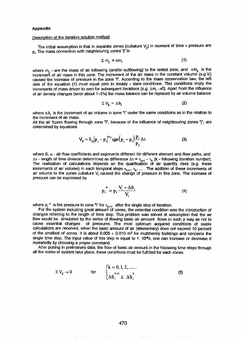
Appendix
Descridion of the iterative solution method
The initial assumption is that in separate zones (cubature Vji) in moment of time z pressure are pi. The mass connection with neighbouring zones "j" is
where mji - are the mass of air inflowing (andlor outflowing) to the tested zone, and Amji is the increment of air mass in this zone. The increment of the air mass in the constant volume (e.g.Vi) caused the increase of pressure in the zone "i". According to the mass conservation law, the left side of the equation (1) must equal zero in steady - state conditions. This conditions imply the increments of mass driven to zero for subsequent iterations (e.g. Ami 4). Apart from the influence of air density changes (error about ls2%) the mass balance can be replaced by air volume balance
where ASi is the increment of air volume in zone "in under the same conditions as in the relation to the increment of air mass. All the air fluxes flowing through zone "i", because of the influence of neighbouring zones "j", are determined by equations
where S, a - air flow coefficients and exponents different for different element and flow paths, and AT - length of time division determined as difference Az = T,, - T, (k - following iteration number). The realization of calculations depends on the qualification of air quantity rises (e.g. these increments of air volume) in each temporal steps T,,, zk, ... . The addition of these increments of air volume to the zones cubature Vi caused the change of pressure in this zone. The increase of pressure can be expressed by
where pi * is the pressure in zone "i" for zk+,, after the single step of iteration. For the system including great amount of zones, the essential condition was the introduction of
changes referring to the length of time step. This problem was solved at assumption that the air flow would be simulated by the series of flowing basic air amount flows in such a way as not to cause essential changes of pressures. The most optimum acquired conditions of stable calculations are received, when the basic amount of air (elementary) does not exceed 10 percent of the smallest of zones. It is about 0.005 s 0.010 m3 for multifamily buildings and concerns the single time step. The input value of this step is equal to 1- 10%, one can increase or decrease it repeatedly by choosing a proper command.
After putting in preliminary data, the flow of basic air amount in the following time steps through all the nodes of system take place; these conditions must be fulfilled for each zones.

The foregoing method with its original assumptions and supplements was used in the computer program SYMVENT. The source code of the program was written in Turbo Pascal V.5.5. The code consists of the main program and 6 modules comprising the procedures of starting calculations, reading and recording files with the description of the building structure.

Energy Impact of Ventilation and Air Infiltration 44th AlVC Conference, Copenhagen, Denmark
24 -23 September 4 993
Flow Paths in a Swedish Single Family House
Lund Institute of Technology, Department of Building ScienceIBuilding Services, P 0 Box 118, S-22100 Lund, Sweden

Synopsis
The traditional description of a flow system with a multicell model, Vi(t)=Qc(t)+p(t), may sometimes be to restrictive. The multicell theory require measurements, or reconstruo tion, of the tracer concentrations in a number of perfect and immediate mixed cells. Often, using of mixing fans and closing doors between cells are necessary to comply with the theory.
Another, very usefil and more general description of a flow system is through the weightingfinction. Unlike the multicell model this is not an internal model, but only an input- output model and it is thus less informative. Still, knowing the weighting knction is sufficient to determine the flows rates, the active volumes, the mean ages of exhaust air and of room air and the air exchange efficiencies.
Typically, these parameters are determined for each fIaw path fiom an input, often a supply air, to an output, often an exhaust air.
Contrary to common air exchange efficiency measurements, resulting in one ore a few figures, the determination of the weighting finction results in a complete model which is also suitable for simulations.
In this paper, the theory is only surveyed and no derivations are given. A single family house with exhaust ventilation is used to demonstrate the method.
List of Symbols
tracer gas concentration a diagonal matrix with the column or row vector x on the diagonal the 1 -column vector the 1-column vector with n, elements weighting finction matrix number of cells number of exhaust air flows number of supply air flows tracer gas injection flow time nominal time constant room mean age i:th moment of h(t) flow path matrix, n, by n, flow matrix, n by n volume matrix, n by n
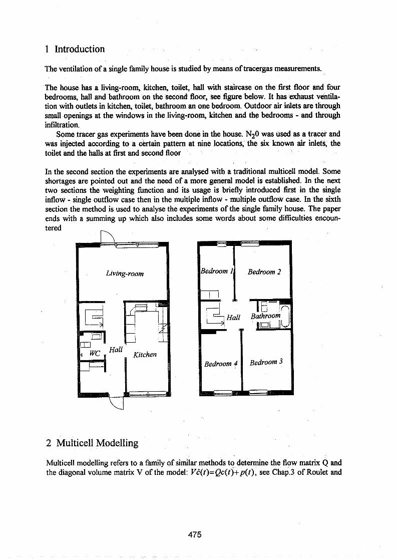
1 Introduction
The ventilation of a single family house is studied by means of tracergas measurements.
The house has a living-room, kitchen, toilet, hall with staircase on the first floor and four bedrooms, hall and bathroom on the second floor, see figure below. It has exhaust ventila- tion with outlets in kitchen, toilet, bathroom an one bedroom. Outdoor air inlets are through small openings at the windows in the living-room, kitchen and the bedrooms - and through infiltration.
Some tracer gas experiments have been done in the house. N20 was used as a tracer and was injected according to a certain pattern at nine locations, the six known air inlets, the toilet and the halls at first and second floor
In the second section the experiments are analysed with a traditional multicell model. Some shortages are pointed out and the need of a more general model is established. In the next two sections the weighting hnction and its usage is briefly introduced first in the single inflow - single outflow case then in the multiple inflow - multiple outflow case. In the sixth section the method is used to analyse the experiments of the single family house. The paper ends with a summing up which also includes some words about some difficulties encoun- tered
2 Multicell Modelling
Multicell modelling refers to a family of similar methods to determine the flow matrix Q and the diagonal volume matrix V of the model: Vi.(t)=Qc(t)+p(t), see ~hap.3 of Roulet and

Vandaele (1991). Here, an improved version of the method described in Hedin(1989) has been used. This is a single iterative method with a derivative or integral appioximBtion based on the so far found model and a constrained least square parameter estimation.
Two experiments will be presented, one with and one without mixing fans. The used equipment permits nine cells and a reference concentration measurements. The upstairs hall and bathroom was therefor treated as one cell and this door was open. All other doors were closed. Note that the two halls the staircase and the living-room are not separated by doors. This volume is neither well treated as one single cell nor as three separate cells as being tried here.
The two graphs below shows the modelled tracer concentrations, cmd(t), as a hnction of time. The small rings corresponds to the measurements The fit looks to be acceptable at least in the first case but the errors are in fact larger than in similar experiments in other houses. Without mixing fans the errors increase about four times.
The identified flow rates and volumes for the first case are shown in the tables below.
Air Flow Rates [Us]
j?om + bed- bed- bed- bed- hall kitchen living toilet bath../ in$ltra- total room1 room2 r00m3 room4 downstr. room hall tion
to &
bedroom I - 8.8 8.8 bedroom2 - 8.2 8.2 bedroom3 - 9.2 9.2 bedroom4 - 8.8 8.8
hall downstr 0.4 2.8 - 0.6 50.8 3.1 15.9 8.2 81.7 kitchen 4.7 - 4.2 8.8 living-room 0.3 0.7 1.5 0.7 42.1 - 8.0 10.5 64.8 toilet 14.8 .O 14.8 bathroom 1.0 5.7 7.2 5.3 7.1 13.0 - 4.5 43.8 ~ l t r a t i o n 7.2 1.8 0.5 13.1 8.2 11.7 20.0 62.5
Volumes [m3]
bed- bed- bed- bed- hall kitchen living- toilet bath../ total room1 room2 room3 room4 downstr room hall
19.7 23.5 32.6 26.6 27.5 40.8 56.9 6.6 31.6 265.6
Even if the fit looks good there are some problems worth to discuss. It is not easily seen from the graph above, but a closer look on the data shows that then injecting tracer to the downstairs hall the concentration became higher at the toilet then in (at least the measuring point) of the hall itself. This is due to an imperfect mixing in the hall (in relation to the large flow to the toilet and the location of the tracer injection). Such a situation cannot be explained by a multicell model, unless the number of cells is increased. Another, more easily seen, shortcoming is the bad modelling of the bedroom 2 concentration. Also this is probably
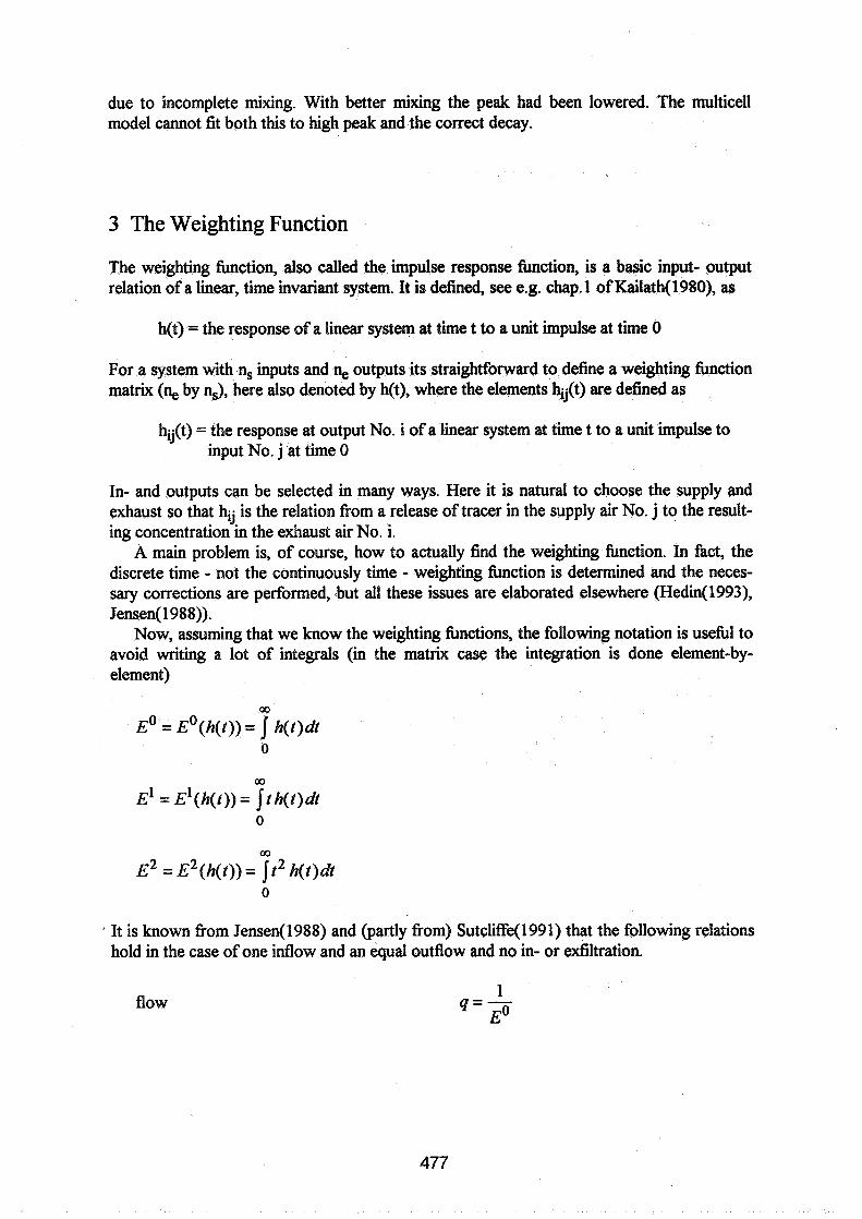
due to incomplete mixing. With better mixing the peak had been lowered. The multicell model cannot fit both this to high peak and the correct decay.
3 The Weighting Function
The weighting function, also called the impulse response hnction, is a basic input- output relation of a linear, time invariant system. It is defined, see e.g. chap. 1 of Kailath(l980), as
h(t) = the response of a linear system at time t to a unit impulse at time 0
For a system with nS inputs and n, outputs its straightforward to define a weighting function matrix (n, by %), here also denoted by h(t), where the elements h4(t) are defined as
hg(t) = the response at output No. i of a linear system at time t to a unit impulse to input No. j at time 0
In- and outputs can be selected in many ways. Here it is natural to choose the supply and exhaust so that hi,. is the relation from a release of tracer in the supply air No. j to the result- ing concentration in the exhaust air No. i.
A main problem is, of course, how to actually find the weighting hnction. In fact, the discrete time - not the continuously time - weighting hnction is determined and the neces- sary corrections are performed, but all these issues are elaborated elsewhere (Hedin(l993), Jensen(l988)).
Now, assuming that we know the weighting functions, the following notation is usehl to avoid writing a lot of integrals (in the matrix case the integration is done element-by- element)
It is known from Jensen(1988) and (partly from) Sutcliffe(l991) that the following relations hold in the case of one inflow and an equal outflow and no in- or exfiltration.
flow
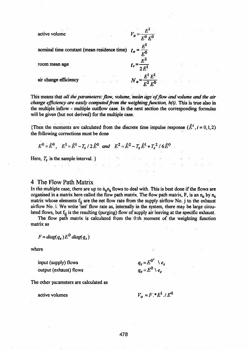
active volume
El nominal time constant (mean residence time) t , = -
E0
room mean age E2 tr=-
2 E'
air change efficiency E' EI Nu=-
E2 E0
This means that all the parameters:flau, volume, mean age of@ rmd volume and the air change efJiciency are easily computedfiom the weightingfinction, ho). This is true also in the multiple inflow - multiple outflow case. In the next section the corresponding formulas will be given (but not derived) for the multiple case.
{Then the moments are calculated fiom the discrete time impulse response ( k i , i = 0,1,2) the following corrections must be done
Here, T, is the sample interval. )
4 The Flow Path Matrix In the multiple case, there are up to %n, flows to deal with. This is best done if the flows are organised in a matrix here called the flow path matrix. The flow path matrix, F, is an n, by n, matrix whose elements f, are the net flow rate fiom the supply airflow No. j to the exhaust airflow No. i. We write 'net' flow rate as, internally in the system, there may be large circu- lated flows, but 4. is the resulting (purging) flow of supply air leaving at the specific exhaust.
The flow pat matrix is calculated fiom the 0:th moment of the weighting fiinction matrix as
1,
where
input (supply) flows %=E'' \ e, output (exhaust) flows 0 qe=E \ee
The other parameters are calculated as
active volumes V, =F.*E'.IEO
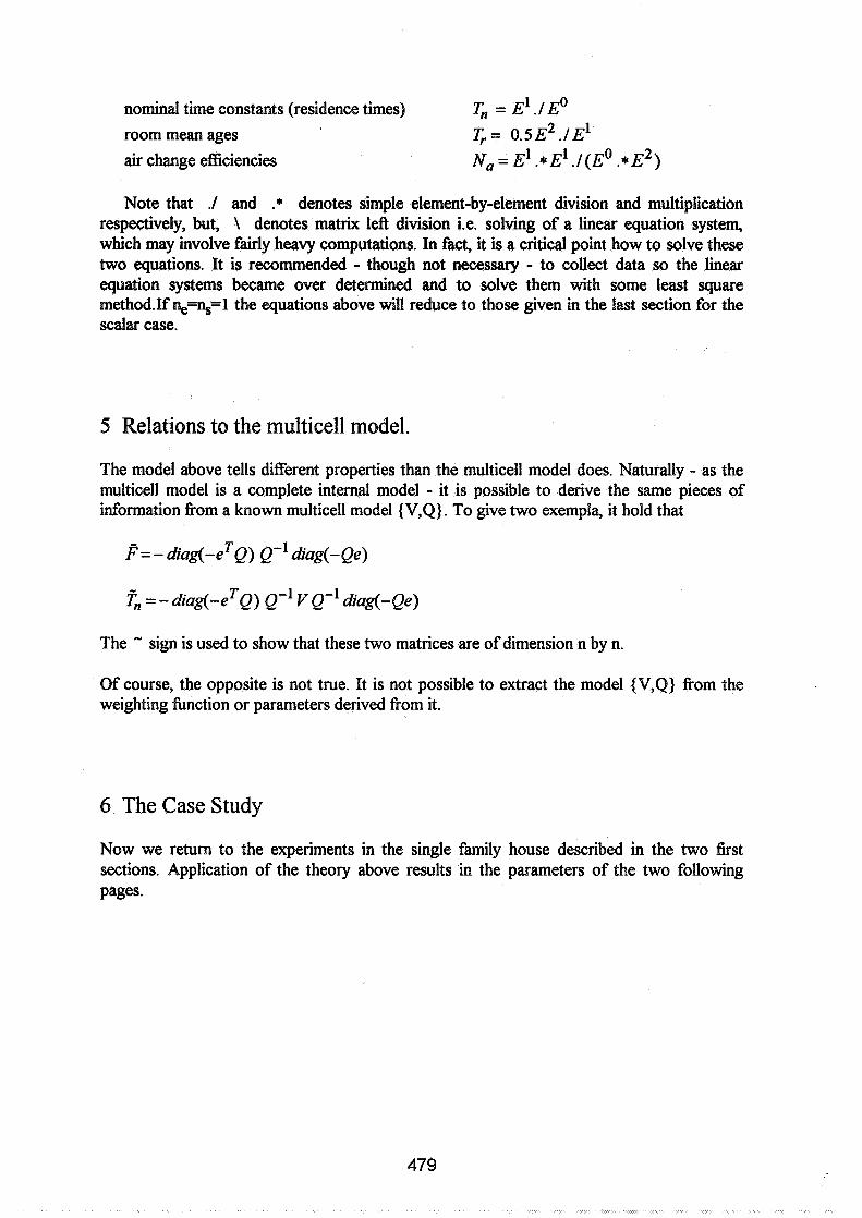
nominal time constants (residence times) T, = E' .IEO room mean ages T,= O.SE~.IE'
air change efficiencies N, = E' .*El ./(E0 .* E2)
Note that ./ and .* denotes simple element-by-element division and multiplication respectively, but, \ denotes matrix left division i.e. solving of a linear equation system, which may involve fairly heavy computations. In fact, it is a critical point how to solve these two equations. It is recommended - though not necessary - to collect data so the linear equation systems became over determined and to solve them with some least square method.If %->=l the equations above will reduce to those given in the last section for the scalar case.
5 Relations to the multicell model.
The model above tells different properties than the multicell model does. Naturally - as the multicell model is a complete internal model - it is possible to derive the same pieces of information from a known multicell model {V,Q). To give two exempla, it hold that
The " sign is used to show that these two matrices are of dimension n by n.
Of course, the opposite is not true. It is not possible to extract the model {V,Q) from the weighting fbnction or parameters derived from it.
6 The Case Study
Now we return to the experiments in the single family house described in the two first sections. Application of the theory above results in the parameters of the two following pages.

Air Flow Rates [Us]
supply9 bed- bed- bed- bed- living kitchen hall toilet bath./ i n m a - totalsupply room1 room2 room3 room4 room down hall tion + injltr.
exhaust & bedroom1 2.9 0.3 0.0 0.0 0.0 0.0 0.0 0.0 0.0 1.7 5.0 kitchen 0.1 0.2 0.2 0.2 0.2 2.3 0.1 0.0 0.1 5.1 8.3 toilet 1.0 2.1 2.1 2.3 3.6 0.1 4.0 0.0 1.0 2.3 18.5 bathroom 1.0 2.8 2.8 2.4 1.0 0.0 1.8 0.0 1.5 6.9 20.3
totalexhaust5.0 5.4 5.2 5.0 4.8 2.4 5.9 0.0 2.6 15.9 52.1
Active Volumes [m3]
supply 9 bed- rooml
exhaust & bedrooml 8 kitchen 1 toilet 11 bathroom 6
total exhaust 26
bed- bed- bed- living kitchen hall toilet bath./ total room2 room3 room4 room down hall supply
Nominal Time Constant [min]
supply 9 bed- bed- bed- bed- living kitchen hall toilet bath/ total room1 room2 room3 room4 room down hall supply
exhust 4 bedroom1 48 216 157 - - - - - 65 kitchen 153 218 238 151 125 69 151 - 206 203 toilet 193 228 157 119 39 196 74 - 75 111 bathroom 95 195 95 80 59 - 74 - 34 101
totalexhaust 87 210 127 101 46 75 75 0 54 103
Air Change Efficiencies [-I
supply 9 bed- bed- bed- bed- livrng kitchen hall toilet bath./ total room1 room2 room3 room4 room down hall supply
exhaust &
bedroom1 0.48 0.58 - - - - - - - 0.34 kitchen 0.78 0.63 0.68 0.68 0.58 0.53 0.66 - 0.62 0.47 roller 0.55 0.58 0.64 0.64 0.35 0.73 0.53 - 0.51 0.44 bathroom 0.51 0.48 0.55 0.62 0.54 - 0.62 - 0.30 0.40
totalexhaust 0.38 0.53 0.56 0.61 0.38 0.51 0.55 - 0.35 0.41
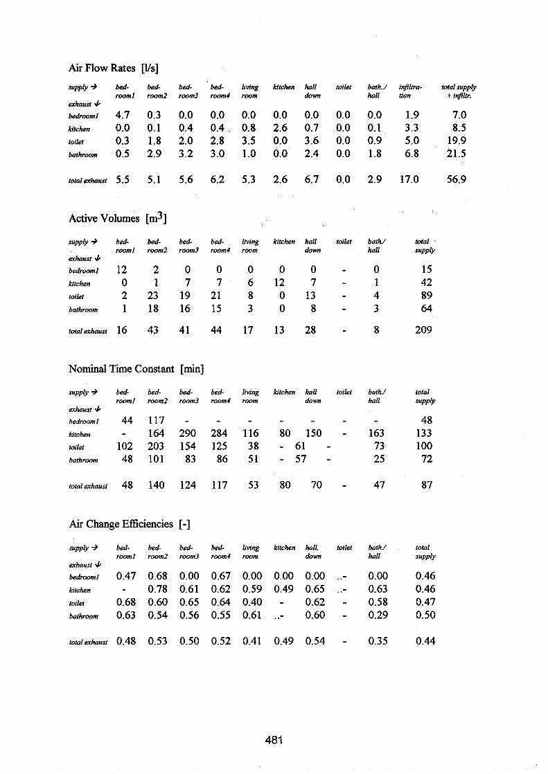
Air Flow Rates [Vs]
supply + bed- bed- bed- bed- living kitchen hall toilet bath.1 injltra- total supply room1 r m 2 room3 room4 room down hall tion + injltr.
exhaust 4 bedroom1 4.7 0.3 0.0 0.0 0.0 0.0 0.0 0.0 0.0 1.9 7.0 kitchen 0.0 0.1 0.4 0.4 0.8 2.6 0.7 0.0 0.1 3.3 8.5 toilet 0.3 1.8 2.0 2.8 3.5 0.0 3.6 0.0 0.9 5.0 19.9 bathroom 0.5 2.9 3.2 3.0 1.0 0.0 2.4 0.0 1.8 6.8 21.5
Active Volumes [m3]
supply+ bed- bed- bed- bed- liwng kitchen hall toilet bath1 total room1 room2 room3 room4 room down hall supply
exhaust 4 bedroom1 12 2 0 0 0 0 0 - 0 15 kitchen 0 1 7 7 6 12 7 - 1 42 toilet 2 23 19 21 8 0 13 - 4 89 bathroom 1 18 16 15 3 0 8 - 3 64
totalexhaust 16 43 41 44 17 13 28 - 8 209
Nominal Time Constant [min]
supply + bed- bed- bed- bed- liwng kitchen hall toilet bath./ total room1 room2 room3 room4 room down hall supply
exhaust
bedroom1 44 117 - - - - - - - 48 kitchen - 164 290 284 116 80 150 - 163 133 toilet 102 203 154 125 38 - 61 - 73 100 bathroom 48 101 83 86 51 - 57 - 25 72
total exhaust 48 140 124 117 53 80 70 - 47 87
Air Change Efficiencies [-I
supply9 bed- bed- bed- bed- lrvrng kitchen hall. toilet bath./ total rwml room2 room3 room4 room down hall supply
exhaust
bedroom1 0.47 0.68 0.00 0.67 0.00 0.00 0.00 . 0.00 0.46 kitchen - 0.78 0.61 0.62 0.59 0.49 0.65 . 0.63 0.46 toilet 0.68 0.60 0.65 0.64 0.40 - 0.62 - 0.58 0.47 bathroom 0.63 0.54 0.56 0.55 0.61 . 0.60 - 0.29 0.50
totalexhaust 0.48 0.53 0.50 0.52 0.41 0.49 0.54 - 0.35 0.44
7 Summing Up
Describing a single or multicell flow system, the first choice is the traditional multicell model Vt. = Qc + p . This model is easy to understand and easy to use . However, there are cases when this model fails. The description with a flow path matrix and the weighting fhction for each flow path may then be a good substitute. This model tells little about internal flows but it is sufficient to compute flow rates, active volumes, mean ages, and air efficiencies for each flow path.
Some problems and drawbacks associated with weighting fbnction modelling should be mentioned: 1) It is a time-invariant model. That means the flows must be constant (at least during the experiment). 2) If there are many inputs, then the method is very time consuming. A remedy to this may be to use a multiple gas equipment, which would shorten experimental time considerably. 3) It is not hard to construct (theoretical) examples, especially with circu- lated flows, when the weighting fbnction would be very hard to determine because a not negligible part of the response is coming after long time with low intensity thus giving a low signal-to-noise ratio. 4) Air infiltration and exfiltration, or to be more specific, air inflows that is not possible to homogeneously label with tracer and outflows where it is not possible to measure the mean tracer concentration will inherently cause problems and require addi- tional presumptions about the system.
References
Hedin, B. (1989): Identification Methods for Multiple Cell Systems. Proc 10th AIVC Conference, Espoo, Finland, 1989
Jensen, L. (1988a): Impulse Response Functions for Different Ventilation Principles. Report BKL 1988: 1 l(E), Lund Institute of Technology, Department of Building Science, Sweden
Jensen, L., (1988b): Determination of Impulse Response Functions for Flow Systems. Report BKL 1988: 10(E), Lund Institute of Technology, Department of Building Science, Sweden
Kailath T.(1980): Linear System. Prentice-Hall, Inc., Englewood Cliffs, N. J. Roulet, C-A, Vandaele L. (1991): Air Flow Patterns Within Buildings Measurement
Techniques. Technical Note AIVC 34. International Energy Agency, Air Infiltration and Ventilation Centre 199 1.
Sutcliffe, H. C. (1990): A Guide to Air Change Efficiency. Technical Note AIVC 28. International Energy Agency, Air Infiltration and Ventilation Centre 1990.

Energy Impact of Ventilation and Air Infiltration 14th AlVC Conference, Copenhagen, Denmark
21 -23 September 1993
Distributions of Expected Air Infiltration and Related Energy Use in Buildings Based on Statistical Methods with Independent or Correlated Parameters
A Nielsen
Narvik Institute of Technology, Building Science P 0 Box 385, N-8501 Narvik, Norway
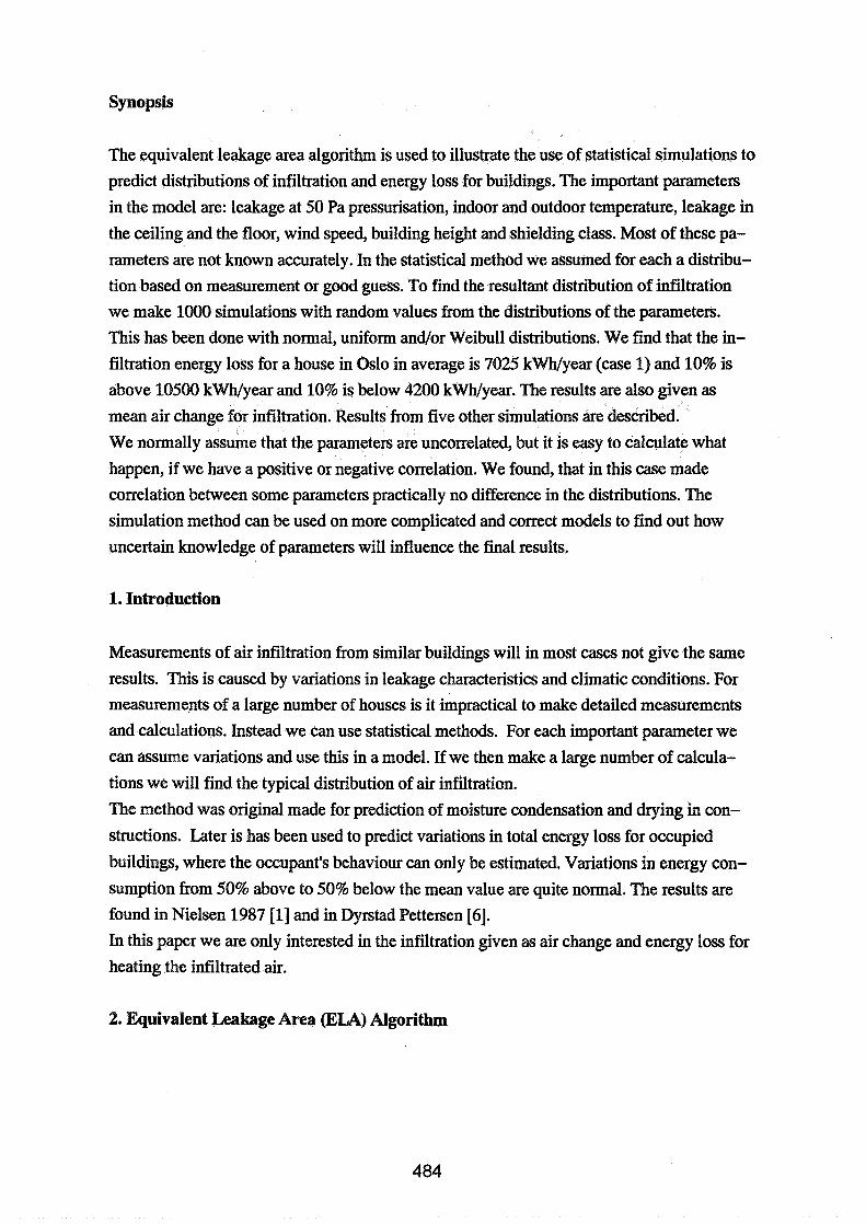
Synopsis
The equivalent leakage area algorithm is used to illustrate the use of statistical simulations to
predict distributions of infiltration and energy loss for buildings. The important parameters
in the model are: leakage at 50 Pa pressurisation, indoor and outdoor temperature, leakage in
the ceiling and the floor, wind speed, building height and shielding class. Most of these pa-
rameters are not known accurately. In the statistical method we assumed for each a distribu-
tion based on measurement or good guess. To find the resultant distribution of infiltration
we make 1000 simulations with random values from the distributions of the parameters.
This has been done with normal, uniform and/or Weibull distributions. We find that the in-
filtration energy loss for a house in Oslo in average is 7025 kWh/year (case 1) and 10% is
above 10500 kWh/year and 10% is below 4200 kWh/year. The results are also given as
mean air change for infiltration. Results from five other simulations are described.
We normally assume that the parameters are uncorrelated, but it is easy to calculate what
happen, if we have a positive or negative correlation. We found, that in this case made
correlation between some parameters practically no difference in the distributions. The
simulation method can be used on more complicated and correct models to find out how
uncertain knowledge of parameters will influence the final results.
I. Introduction
Measurements of air infiltration from similar buildings will in most cases not give the same
results. This is caused by variations in leakage characteristics and climatic conditions. For measurements of a large number of houses is it impractical to make detailed measurements
and calculations. Instead we can use statistical methods. For each important parameter we
can assume variations and use this in a model. If we then make a large number of calcula-
tions we will find the typical distribution of air infiltration.
The method was original made for prediction of moisture condensation and drying in con-
structions. Later is has been used to predict variations in total energy loss for occupied
buildings, where the occupant's behaviour can only be estimated. Variations in energy con-
sumption from 50% above to 50% below the mean value are quite normal. The results are
found in Nielsen 1987 [I] and in Dyrstad Pettersen [6].
In this paper we are only interested in the infiltration given as air change and energy loss for
heating the infiltrated air.
2. Equivalent Leakage Area (EM) Algorithm
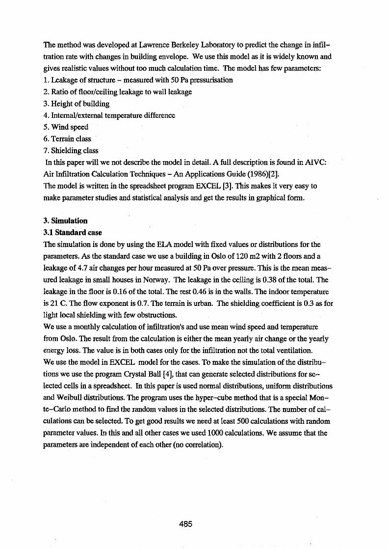
The method was developed at Lawrence Berkeley Laboratory to predict the change in infil-
tration rate with changes in building envelope. We use this model as it is widely known and
gives realistic values without too much calculation time. The model has few parameters:
1. Leakage of structure - measured with 50 Pa pressurisation
2. Ratio of floorlceiling leakage to wall leakage
3. Height of building
4. IntemaVextemal temperature difference
5. Wind speed
6. Terrain class
7. Shielding class
In this paper will we not describe the model in detail. A full description is found in AIVC:
Air Infiltration Calculation Techniques - An Applications Guide (1986)[2].
The model is written in the spreadsheet program EXCEL [3]. This makes it very easy to
make parameter studies and statistical analysis and get the results in graphical form.
3. Simulation 3.1 Standard case
The simulation is done by using the ELA model with fixed values or distributions for the
parameters. As the standard case we use a building in Oslo of 120 m2 with 2 floors and a
leakage of 4.7 air changes per hour measured at 50 Pa over pressure. This is the mean meas-
ured leakage in small houses in Norway. The leakage in the ceiling is 0.38 of the total. The
leakage in the floor is 0.16 of the total. The rest 0.46 is in the walls. The indoor temperature
is 21 C. The flow exponent is 0.7. The terrain is urban. The shielding coefficient is 0.3 as for
light local shielding with few obstructions.
We use a monthly calculation of infiltration's and use mean wind speed and temperature
fiom Oslo. The result fiom the calculation is either the mean yearly air change or the yearly
energy loss. The value is in both cases only for the infiltration not the total ventilation.
We use the model in EXCEL model for the cases. To make the simulation of the distribu-
tions we use the program Crystal Ball [4], that can generate selected distributions for se-
lected cells in a spreadsheet. In this paper is used normal distributions, uniform distributions
and Weibull distributions. The program uses the hyper-cube method that is a special Mon-
te-Carlo method to find the random values in the selected distributions. The number of cal-
culations can be selected. To get good results we need at least 500 calculations with random
parameter values. In this and all other cases we used 1000 calculations. We assume that the
parameters are independent of each other (no correlation).
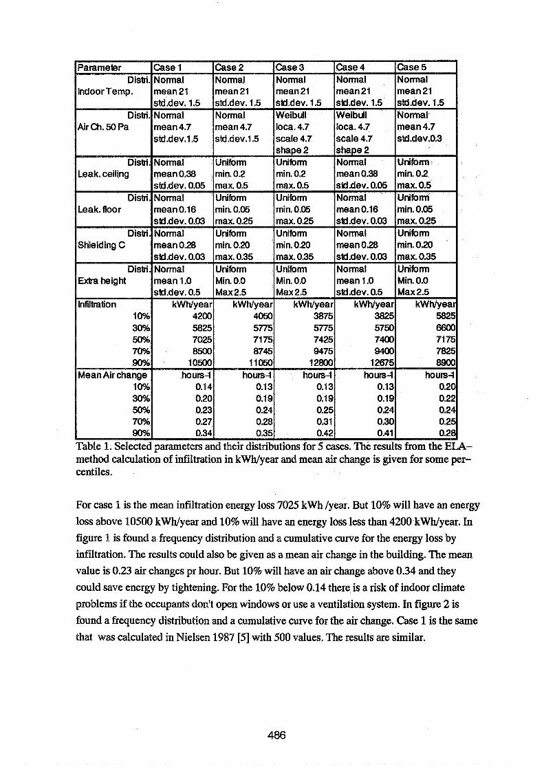
Table 1. Selected parameters and their distributions for 5 cases. The results from the ELA- method calculation of infiltration in kWh/year and mean air change is given for some per- centiles.
For case 1 is the mean infiltration energy loss 7025 kwh /year. But 10% will have an energy
loss above 10500 kWh/year and 10% will have an energy loss less than 4200 kWyear. In
figure 1 is found a frequency distribution and a cumulative curve for the energy loss by infiltration. The results could also be given as a mean air change in the building. The mean
value is 0.23 air changes pr hour. But 10% will have an air change above 0.34 and they
could save energy by tightening. For the 10% below 0.14 there is a risk of indoor climate
problems if the occupants don't open windows or use a ventilation system. In figure 2 is
found a frequency distribution and a cumulative curve for the air change. Case 1 is the same
that was calculated in Nielsen 1987 [5] with 500 values. The results are similar.
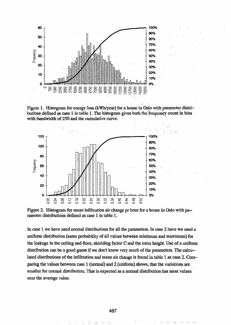
Figure 1. Histogram for energy loss (kwhlyear) for a house in Oslo with parameter distri- butions defined as case 1 in table 1. The histogram gives both the frequency count in bins with bandwidth of 250 and the cumulative curve.
Figure 2. Histogram for mean infiltration air change pr hour for a house in Oslo with pa- rameter distributions defined as case 1 in table l.
In case 1 we have used normal distributions for all the parameters. In case 2 have we used a
uniform distribution (same probability of all values between minimum and maximum) for
the leakage in the ceiling and floor, shielding factor C and the extra height. Use of a uniform
distribution can be a good guess if we don't know very much of the parameters. The calcu-
lated distributions of the infiltration and mean air change is found in table 1 as case 2. Com-
paring the values between case 1 (normal) and 2 (uniform) shows, that the variations are
smaller for normal distribution. That is expected as a normal distribution has most values
near the average value.
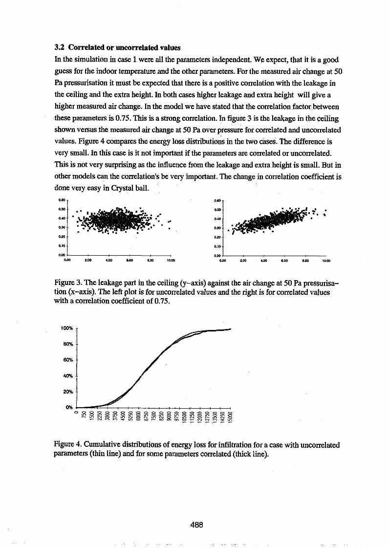
3.2 Correlated or uncorrelated values In the simulation in case 1 were all the parameters independent. We expect, that it is a good
guess for the indoor temperature and the other parameters. For the measured air change at 50
Pa pressurisation it must be expected that there is a positive correlation with the leakage in
the ceiling and the extra height. In both cases higher leakage and extra height will give a
higher measured air change. In the model we have stated that the correlation factor between
these parameters is 0.75. This is a strong correlation. In figure 3 is the leakage in the ceiling
shown versus the measured air change at 50 Pa over pressure for correlated and uncorrelated values. Figure 4 compares the energy loss distributions in the two cases. The difference is very small. In this case is it not important if the parameters are correlated or uncorrelated.
This is not very surprising as the influence fiom the leakage and extra height is small. But in other models can the correlation's be very important. The change in correlation coefficient is
done very easy in Crystal ball.
Figure 3. The leakage part in the ceiling (y-axis) against the air change at 50 Pa pressurisa- tion (x-axis). The left plot is for uncorrelated values and the right is for correlated values with a correlation coefficient of 0.75.
Figure 4. Cumulative distributions of energy loss for infiltration for a case with uncorrelated parameters (thin line) and for some parameters correlated (thick line).
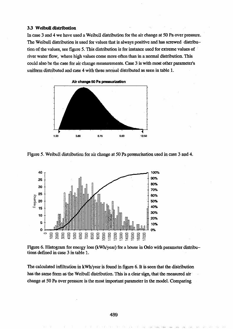
3 3 Weibull distribution In case 3 and 4 we have used a Weibull distribution for the air change at 50 Pa over pressure.
The Weibull distribution is used for values that is always positive and has screwed distribu-
tion of the values, see figure 5. This distribution is for instance used for extreme values of river water flow, where high values come more often than in a normal distribution. This
could also be the case for air change measurements. Case 3 is with most other parameter's
uniform distributed and case 4 with these normal distributed as seen in table 1.
Air change 50 Pa pressurization
Figure 5. Weibull distribution for air change at 50 Pa pressurisation used in case 3 and 4.
Figure 6. Histogram for energy loss (kWyear) for a house in Oslo with parameter distribu- tions defined in case 3 in table 1.
The calculated infiltration in kWh/year is found in figure 6. It is seen that the distribution
has the same form as the Weibull distribution. This is a clear sign, that the measured air
change at 50 Pa over pressure is the most important parameter in the model. Comparing

case 3 and 4 with 2 and 1 it is seen, that the 10% with the highest energy loss has increased
2000 kWNyear. Figure 6 is histogram for the energy loss with case 3. Note that there is a
column of 15 cases, where the energy consumption is above 17500 kWh. These are the ex- tremes - the highest value is 25600 kWh.
3.4 Measured air change at 50 Pa over pressure The statistical method can also be used to show the influence on measuring errofs on a re- sult. In case 5 we have measured the air change at 50 Pa for a house to 4.7 changes pr hour with a standard deviation of 0.3 changes pr hour. If the uncertainty for the rest of the pa-
rameters is as in case 2, we find an expected distribution of the energy loss for infiltration in
figure 7. From the figure we can find the mean value of 7175 kWh, but we must expect
variation from 5000 to 10OOO kWh/year.
Regression shows a good correlation among 50 Pa pressurisation air change and the mean
yearly value. A good prediction of the mean yearly air change can therefore be based on the
pressurisation test without exact knowledge of other parameters.
Figure 7. Histogram for energy loss (kWNyear) for a house in Oslo with parameter distribu- tions defined in case 5 in table 1.
4. Conclusions
The statistical method.with using random generated numbers has been used for calculations
of typical distributions in yearly infiltration air change and energy losses. To find the result-
ing distribution we must know the distribution for the parameters in the model either from
measurements or from good guesses. The resulting infiltration distribution depends mostly
on the air change at 50 Pa over pressure. A good knowledge of the 50 Pa leakage air change
can give good predictions. The knowledge of the distribution of energy losses for infiltration
can be important to see the possibility to save energy (high infiltration) or the risk of indoor
climate problems (low infiltration). In this case was it not very important if some of the pa-
rameters were correlated. This results is based on the equivalent leakage model and will of
cause not take into account complicated cases with different wind distributions and more
rooms in the building.
The simulation method is useful for other types of models either simplified or very compli-
cated. It is possible to find expected distribution for measuring a large number of cases and
it can be used for estimation of resulting errors in complicated measurements.
5. References
1. NIELSEN, A. F. Estimate of energy consumption in single family houses by using statistics. (In Norwegian) Norwegian Building Research Institute project report 20,1987
2. LIDDAMENT, W.L. Air Infiltration. Calculation Techniques - An Applications Guide Air Infiltration and Ventilation Centre, 1986
3. EXCEL, version 4.0, Microsoft, US. 1992
4. Crystal Ball, version 2.0, Decisioneering, Denver, US., 1991
5. NIELSEN, A. F. Use of statistics for predicting distributions of air infiltration, 8th AIVC conference: Ventilation technology research and applications, Proceedings paper 9, page 9.0-9.13,1987
6. DYRSTAD PETI'ERSEN, T. Analysis of statistical variations in energy consumption in dwellings Paper for 3rd. Nordic symposium in building Physics, Copenhagen September 1993

Energy Impact of Ventilation and Air Infiltration 14th AlVC Conference, Copenhagen, Denmark
21 -23 Septern ber 1993
A Four Zone Ventilation Test Facility
C E Brouns, J R Waters
Coventry University, School of the Built Environment, Priory Street, Coventry CV1 SFB, UK

ABSTRACT
This paper describes a laboratory model for the testing and validation of tracer gas measurement techniques. Previous attempts at experimental validation have often been limited to two zones, or a particular measurement strategy, or a particular range of flows.
The model consists of four zones, each of lm3 internal volume. The zones are connected so that all possible inter-zone flow paths exist. The flow down each path is driven by a pump and monitored by a flow meter. A control panel enables any combination of inter- zone flows to be set, within the capacity of the pumps. By the application of scaling, one can also represent real buildings in which the zones are not of equal volume.
The model may be used to validate tracer gas measurement techniques for the extraction of inter-zone flows and for the determination of Ventilation Effectiveness parameters. In principle, the model can be used with any tracer gas injection strategy and any tracer gas measuring method. Examples are given of the use of the model in exploring these parameters.
INTRODUCTION
The multi-zone theory is a well established method for modelling ventilation and airflows in all types of buildings. The model may be used to predict contaminant concentrations and to determine inter-zone flows from suitable measurements.
There are a large number of publications detailing the measurement of ventilation rates and inter-zonal airflows by tracer gas experiments. However, only a small number of these publications specifically describe validation measurements, where a comparison has been made between the flows obtained from tracer gas measurements, and those measured independently, by some type of flow meter.
Some early validation work was attempted by Afonso and Maldonado [I] who carried-out a series of four tests in a two zone model of a building, with a connecting door between the two zones. For each test, the opening of the door was varied, from fully closed to fully opened. A comparison between the measured and the calculated results led to the conclusion that the model can predict the effective volumes with a standard deviation of about 2 %, and that the airflow rates between the zones and the outside is feasible. Irwin and Edwards [2] attempted to validate a multiple tracer gas technique for the determination of airflows between three interconnected cells. The air movements between the three cells were indu~ed by means of ducted low speed fans, in combination with the air supply feeding the chambers. The air velocities in the supply ductwork were measured using a pitot tube and inclined-tube manometer, whilst the air velocities between cells were measured using a hot wire anemometer probe. Three series of measurements were carried-out, with different flow patterns for each series, making a total of twelve experiments. Errors between calculated and measured airflow rates were approximately f 20%, and that the effect of these errors on the air change rate for each chamber was approximately f 10%. A closer inspection of their results shows that the
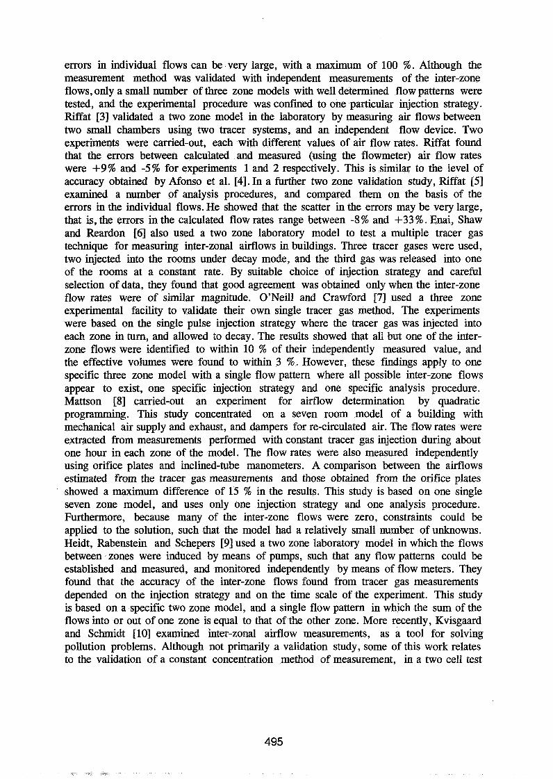
errors in individual flows can be very large, with a maximum of 100 %. Although the measurement method was validated with independent measurements of the inter-zone flows, only a small number of three zone models with well determined flow patterns were tested, and the experimental procedure was confined to one particular injection strategy. Riffat [3] validated a two zone model in the laboratory by measuring air flows between two small chambers using two tracer systems, and an independent flow device. Two experiments were carried-out, each with different values of air flow rates. Riffat found that the errors between calculated and measured (using the flowmeter) air flow rates were +9% and -5% for experiments 1 and 2 respectively. This is similar to the level of accuracy obtained by Afonso et al. 141. In a further two zone validation study, Riffat [5] examined a number of analysis procedures, and compared them on the basis of the errors in the individual flows. He showed that the scatter in the errors may be very large, that is, the errors in the calculated flow rates range between -8% and +33 %. Enai, Shaw and Reardon [6] also used a two zone laboratory model to test a multiple tracer gas technique for measuring inter-zonal airflows in buildings. Three tracer gases were used, two injected into the rooms under decay mode, and the third gas was released into one of the rooms at a constant rate. By suitable choice of injection strategy and careful selection of data, they found that good agreement was obtained only when the inter-zone flow rates were of similar magnitude. O'Neill and Crawford 171 used a three zone experimental facility to validate their own single tracer gas method. The experiments were based on the single pulse injection strategy where the tracer gas was injected into each zone in turn, and allowed to decay. The results showed that all but one of the inter- zone flows were identified to within 10 % of their independently measured value, and the effective volumes were found to within 3 %. However, these findings apply to one specific three zone model with a single flow pattern where all possible inter-zone flows appear to exist, one specific injection strategy and one specific analysis procedure. Mattson [8] carried-out an experiment for airflow determination by quadratic programming. This study concentrated on a seven room model of a building with mechanical air supply and exhaust, and dampers for re-circulated air. The flow rates were extracted from measurements performed with constant tracer gas injection during about one hour in each zone of the model. The flow rates were also measured independently using orifice plates and inclined-tube manometers. A comparison between the airflows estimated from the tracer gas measurements and those obtained from the orifice plates showed a maximum difference of 15 % in the results. This study is based on one single seven zone model, and uses only one injection strategy and one analysis procedure. Furthermore, because many of the inter-zone flows were zero, constraints could be applied to the solution, such that the model had a relatively small number of unknowns. Heidt, Rabenstein and Schepers [9] used a two zone laboratory model in which the flows between zones were induced by means of pumps, such that any flow patterns could be established and measured, and monitored independently by means of flow meters. They found that the accuracy of the inter-zone flows found from tracer gas measurements depended on the injection strategy and on the time scale of the experiment. This study is based on a specific two zone model, and a single flow pattern in which the sum of the flows into or out of one zone is equal to that of the other zone. More recently, Kvisgaard and Schmidt [lo] examined inter-zonal airflow measurements, as a tool for solving pollution problems. Although not primarily a validation study, some of this work relates to the validation of a constant concentration method of measurement, in a two cell test

house. The flow patterns selected in this case, were very nearly redundant, that is, the ratio of the sum of the flows into both zones over their respective volumes were nearly equal. Also, a symmetry effect could be observed in each zone, i.e. the flows from the outside to the inside of each zone and vice-versa were approximately the same.
Most of the experimental validation work to date, relates to specific cases, and is limited to the authors' particular requirements. That is, there appears to be no continuity, and little cross-referencing. None of the validation studies are complete, because they are restricted to the authors' own needs. Nearly all are limited to either two or three zone cases, and a restricted range of flow patterns.
There is, therefore, a need for a systematic experimental study of the extraction of inter- zone flows from tracer gas measurements, with the objective of validating any measurement and analysis method. For such validation to be complete, a range of different flow patterns must be tested in carefully controlled conditions. This is difficult to achieve in a full scale building, and points to the need for a multi-zone laboratory model in which the conditions can be accurately monitored.
DESIGN OF THE TI-ZONE LABORATORY MODEL
Requirements of the laboratory model
Several requirements have to be considered in the design of the multi-zone laboratory model. These are:- (i) The choice of the number of zones to be included in the model.
This is based on the need to offer as much flexibility as possible in the flow patterns, while providing a system which is reasonably easy to handle. A two zone model is not adequate, as it does not cater for re-circulation flows with complex eigenvalues, and limits the range of possible tracer gas experiments. A three zone model allows for a re-circulation with complex eigenvalues to take place. On the other hand, only two of the three zones can generate complex eigenvalues. Again, this restricts the range of flow patterns that can be tested. A four zone model also allows for a re-circulation with complex eigenvalues to arise. It is a property of the eigenvalues that they always occur in conjugate pairs. Therefore, in the case of a four zone model, either two or four zones can generate complex eigenvalues. Hence, all the necessary flow effects are included and can be tested. The need to incorporate more than four zones in the model is thus unnecessary, as it would not supply more information, and would also be more difficult to handle. A four zone model gives twenty possible inter-zonal flows and sixteen independent flows.
(ii) The scaling factor. Since the solution depends on the ratios of the flows to the volumes, it is simpler to design each zone in the model with an equal volume. Previous experience of model studies by Budek [I 11, suggests that enclosures of relatively small volumes are adequate. With that in mind, and considering the space available in our laboratory, each zone was designed with an internal volume of 1 m3.
Because all zones are fully mixed, boundary layer effects are insignificant, and therefore it is not necessary to match the Reynolds number. The only relevant scaling parameter is the time constant, T, It is known from simulation studies, for example Heidt et al. [12] and Sutcliffe 1131, that a minimum of two time constants of data are needed in the analysis procedure. The experiments must therefore span over at least two time constants. On the other hand, if the time constant relative to the sampling time interval of the tracer gas measuring equipment is short, then the number of data points available for the analysis procedure may be too small. Also, the time constant must be sufficiently long with respect to the operation of the tracer gas injection system. This led to selecting a time constant of the order of magnitude of 30 minutes for the system. With V= 1 m3, this gives a fresh air flow rate of 2 m3/hour into each zone. The flow patterns of greatest interest occur when the inter-zone flows are within a certain range on either side of the fresh air flow rate, typically from one tenth to ten times the fresh air flow rate. Below one tenth, the zones are effectively behaving independently. Above 10 times, the system is approaching a fully mixed state, when the single zone theory is sufficient. This gives a range of 0.2 to 20 m 3/hour, corresponding to flows between 3 to 300 l/min.
Generation of inter-zonal flows and their measurement.
Air flows between two zones can be generated either by means of miniature fans, or by means of air pumps. The choice is influenced by the method of flow measurement. The different options considered were: - i) Flow meters of the rotameter type which give a direct reading of the volumetric
flow rates in the pipes. ii) Orifice plates which measure the pressure differential, and which in turn must be
converted into volumetric air flows. iii) Hot wire anemometers, which give readings of the velocity of the air in the pipes.
Again, these readings have to be converted into volumetric flow rates. iv) Mass flow transducers which give a direct measure of the mass flow rates in the
pipes. However, this type of transducer is very expensive. As the model requires the independent measurement of twenty flows, the total cost of twenty mass flow transducers was found to be prohibitive. This option could therefore not be considered.
A comparison between the miniature fans and the air pumps for the different methods of measurement is as follows: - i) Miniature fans create small pressure differentials, and require large diameter
pipes which produce large dead volumes. ii) Air pumps create high pressure differentials, and therefore can be used with small
diameter pipes which in turn produce small dead volumes.
Both orifice plates and hot wire anemometers require that the pipe be of a sufficient length to ensure, in the measuring section, a distribution of velocities corresponding to a fully stable flow regime. The settling length required when using either an orifice plate or a hot wire anemometer, may be up to twenty times the diameter of the pipe in which the measurements are to be taken. Where miniature fans are used, pipes with an internal diameter of approximately 60 mrn would be required, therefore, the length of the pipes

must be at least 1.20 m for each flow path. As the model includes 20 independent flow paths, it was thought that the total amount of pipework required would be excessive with respect to the space available. Where air pumps are used, pipes with an internal diameter of about 6 mm can be used, therefore, the length of pipes must be at least 0.12 m. This option is more practical, but the diameter of the pipes would be too small for the reliable operation of either an orifice plate, or a hot wire anemometer. On the other hand, rotameters can be used with small diameter pipes and have the advantage that they are direct reading. This is a considerable advantage when flow patterns need to be set-up. From these considerations, it was decided to select a combination of small diaphragm air pumps and rotameters equipped with flow control valves.
The rotameters are calibrated for ambient temperature and pressure at their outlet. The accuracy claimed by the manufacturer ranges from + 1.25 % of the full scale deflection (FSD) for high flow rates, to + 2.5 % of the full scale deflection for low flow rates. The flows given by the flow meters are used for comparison with the flows obtained from tracer gas experiments, and so it was necessary to check the manufacturer's claim. To this end, a calibration rig was designed, using a simple water displacement method, as shown in figure 1.
Figure 1 - Schematic diagram of the flow meters calibration rig.
The outlet of the flow meter is placed so as to remain at atmospheric pressure. The air is allowed to flow through the tube into the calibration rig, thus displacing the water. The time, t, taken to collect a certain mass of water, M, is recorded, and is converted into a flow rate, F. Corrections are applied for the prevailing temperature, pressure and for any head of water remaining in the collecting vessel.
The calibration showed that the rotameters were all within the manufacturer's tolerances, provided the float was rotating freely.
The problem now consists in designing the system so that the pressure in each zone remains close to atmospheric and is not affected by the pressure changes in the inter- zonal flow paths. Firstly, each pump draws air from a zone, thus inducing a pressure rise in the flow path. Then, the air passes through the control valve which has the effect of
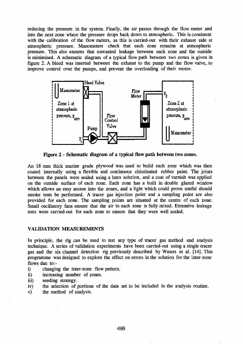
reducing the pressure in the system. Finally, the air passes through the flow meter and into the next zone where the pressure drops back down to atmospheric. This is consistent with the calibration of the flow meters, as this is carried-out with their exhaust side at atmospheric pressure. Manometers check that each zone remains at atmospheric pressure. This also ensures that unwanted leakage between each zone and the outside is minimised. A schematic diagram of a typical flow path between two zones is given in figure 2. A bleed was inserted between the exhaust to the pump and the flow valve, to improve control over the pumps, and prevent the overloading of their motor.
Figure 2 - Schematic diagram of a typical flow path between two zones.
An 18 mrn thick marine grade plywood was used to build each zone which was then coated internally using a flexible and continuous chlorinated rubber paint. The joints between the panels were sealed using a latex solution, and a coat of varnish was applied on the outside surface of each zone. Each zone has a built in double glazed window which allows an easy access into the zones, and a light which could prove useful should smoke tests be performed. A tracer gas injection point and a sampling point are also provided for each zone. The sampling points are situated at the centre of each zone. Small oscillatory fans ensure that the air in each zone is fully mixed. Extensive leakage tests were carried-out for each zone to ensure that they were well sealed.
VALIDATION MEAS
In principle, the rig can be used to test any type of tracer gas method and analysis technique. A series of validation experiments have been carried-out using a single tracer gas and the six channel detection rig previously described by Waters et al. [14]. This programme was designed to explore the effect on errors in the solution for the inter-zone flows due to: - i) changing the inter-zone flow pattern. ii) increasing number of zones. iii) seeding strategy. iv) the selection of portions of the data set to be included in the analysis routine. v) the method of analysis.
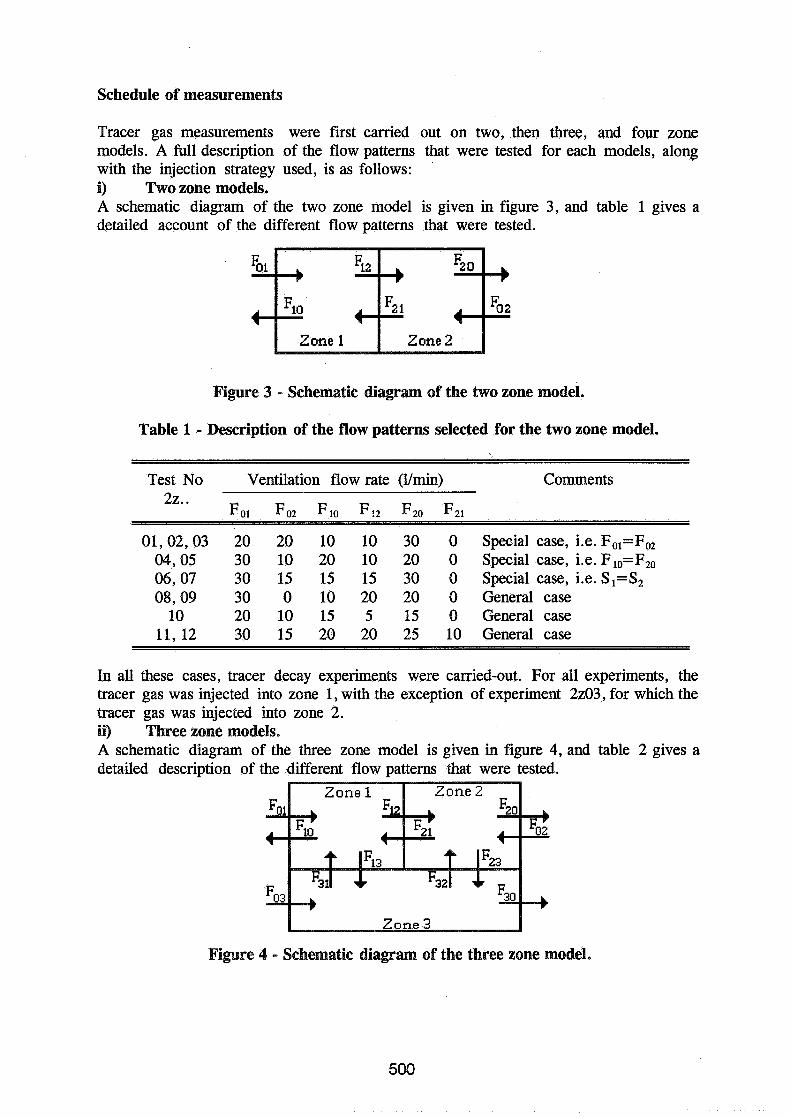
Schedule of measurements
Tracer gas measurements were first carried out on two, then three, and four zone models. A full description of the flow patterns that were tested for each models, along with the injection strategy used, is as follows:
'
i) Two zone models. A schematic diagram of the two zone model is given in figure 3, and table 1 gives a detailed account of the different flow patterns that were tested.
Figure 3 - Schematic diagram of the two zone model.
Table 1 - Description of the flow patterns selected for the two zone model.
Test No Ventilation flow rate (llmin) Comments LB..
Fo1 Fo2 Fl0 F12 F20 F21
01,02,03 20 20 10 10 30 0 Specialcase,i.e.Fol=F, 04,05 30 10 20 10 20 0 Special case, i.e. Fl0=F, 06,07 30 15 15 15 30 0 Specialcase,i.e.Sl=S2 08,09 30 0 10 20 20 0 General case
10 20 10 15 5 15 0 General case 11,12 30 15 20 20 25 10 General case
In all these cases, tracer decay experiments were carried-out. For all experiments, the tracer gas was injected into zone 1, with the exception of experiment 2203, for which the tracer gas was injected into zone 2. ii) Three zone models. A schematic diagram of the three zone model is given in figure 4, and table 2 gives a detailed description of the different flow patterns that were tested.
Figure 4 - Schematic diagram of the three zone model.

Table 2 - Description of the flow patterns selected for the three zone model.
Test Ventilation Flow Rates, F ;; (l/rnin)
Test F, (limb) - Comments
01 - 14 30 15 0 Special case, i.e. Fol=F,=Fo3 15 - 17 20 10 0 Special case, i.e. F ,,=F,= F3, 18 - 19 20 5 5 Special case, i.e. S ,=S2=S3
20 15 5 10 Special case, i.e. Sl=S2=S3 21 25 0 10 General case
The seeding strategies used, were as follows:-
- Tracer decay experiments were carried-out for tests 3 ~ 0 1 , 3 ~ 0 2 , 3 ~ 0 3 , 3 ~ 1 3 , 3 ~ 1 5 , 3z18,3z19,3z20 and 3221. In these cases, the tracer gas was injected into zone 1.
- Tracer decay experiments were carried-out for tests 3z04,3z05 and 3216. In these cases, the tracer gas was injected into zone 2.
- Tracer decay experiments were carried-out for tests 3206,3207 and 3217. In these cases, the tracer gas was injected into zone 3.
- Multiple step-up experiments were carried-out for tests 3z08,3z09,3z10 and 321 1. Although the duration of each tracer gas injection was of 30 minutes in all cases, the order in which the zones were injected varied. For experiments 3208 and 3209, the tracer gas was first injected into zone 1, then zone 2, and finally zone 3. For experiment 3210, the injection started in zone 3 followed by zone 1 and finally zone 2. For experiment 3zl1, the first injection took place in zone 2, followed by zone 3, and finally zone 1.
- A step-up experiment followed by a tracer decay was carried-out for test 3212. The tracer gas was injected into zone 1 for 60 minutes before being allowed to decay.
- A multiple pulse experiment was carried-out for test 3214. The tracer gas was injected at intervals of 40 minutes into zone 1 ,2 and 3 successively.
ii) Four zone models. A schematic diagram of the four zone model is given in figure 5, and table 3 gives a detailed description of the different flow patterns that were tested.
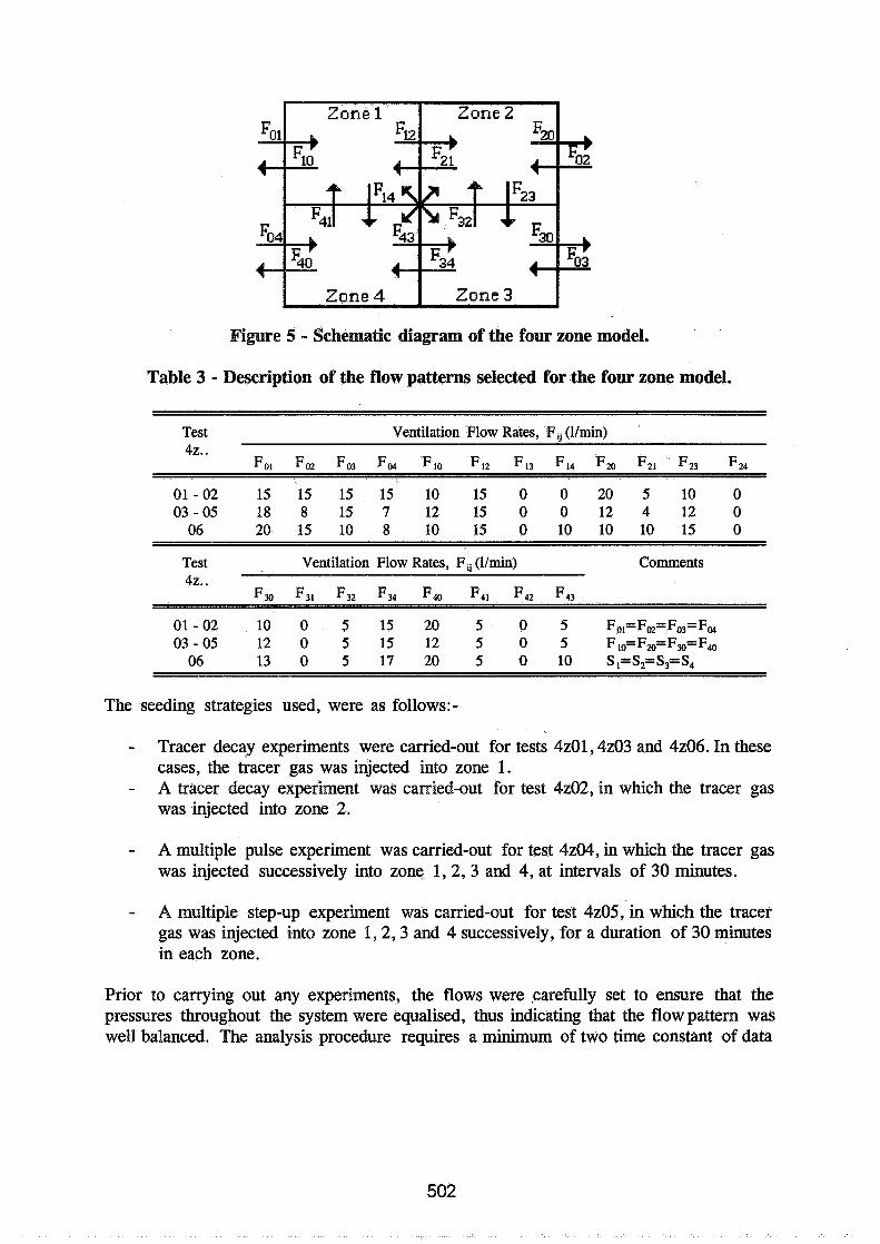
Figure 5 - Schematic diagram of the four zone model.
Table 3 - Description of the flow patterns selected for the four zone model.
Test Ventilation Flow Rates, F ij (llmin) 42..
F O l F, F, F04 F10 F12 F13 F14 F20 F21 F23 F24
01 - 02 15 15 15 15 10 15 0 0 20 5 10 0 03 - 05 18 8 15 7 12 15 0 0 12 4 12 0
Test Ventilation Flow Rates, F ij (llmin) Comments 1 -
The seeding strategies used, were as follows:-
- 1 racer aecay expermenrs were carnea-our ror rests 4zu1, 4zu5 ana 4zuo. m tnese - - cases, the tracer gas was injected into zone 1.
- A tracer decay experiment was carried-out for test 4202, in which the tracer gas was injected into zone 2.
- A multiple pulse experiment was carried-out for test 4204, in which the tracer gas was injected successively into zone 1 ,2 ,3 and 4, at intervals of 30 minutes.
- A multiple step-up experiment was carried-out for test 4205, in which the tracer gas was injected into zone 1 ,2 ,3 and 4 successively, for a duration of 30 minutes in each zone.
Prior to carrying out any experiments, the flows were carefully set to ensure that the pressures throughout the system were equalised, thus indicating that the flow pattern was well balanced. The analysis procedure requires a minimum of two time constant of data
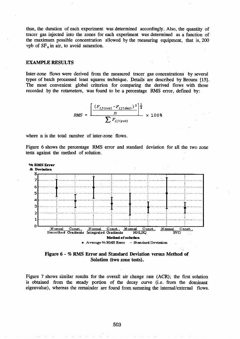
thus, the duration of each experiment was determined accordingly. Also, the quantity of tracer gas injected into the zones for each experiment was determined as a function of the maximum possible concentration allowed by the measuring equipment, that is, 200 vpb of SF, in air, to avoid saturation.
EXAMPLE RESULTS
Inter-zone flows were derived from the measured tracer gas concentrations by several types of batch processed least squares technique. Details are described by Brouns [15]. The most convenient global criterion for comparing the derived flows with those recorded by the rotameters, was found to be a percentage RMS error, defined by:
RMS = x 100% Fi j
where n is the total number of inter-zone flows.
Figure 6 shows the percentage RMS error and standard deviation for all the two zone tests against the method of solution.
,Normal Conct. , ,Normal Const. , ,Normal Const. , ,Normal Coast. , Smoothed C3radients Integrated Gradients NNLSQ SVD
Method of solution m Average % RNIS Ewor - Standard Deviation
Figure 6 - % RlMS Error and Standard Deviation versus Method of Solution (two zone tests).
Figure 7 shows similar results for the overall air change rate (ACR); the first solution is obtained from the steady portion of the decay curve (i.e. from the dominant eigenvalue), whereas the remainder are found from summing the internal/external flows.
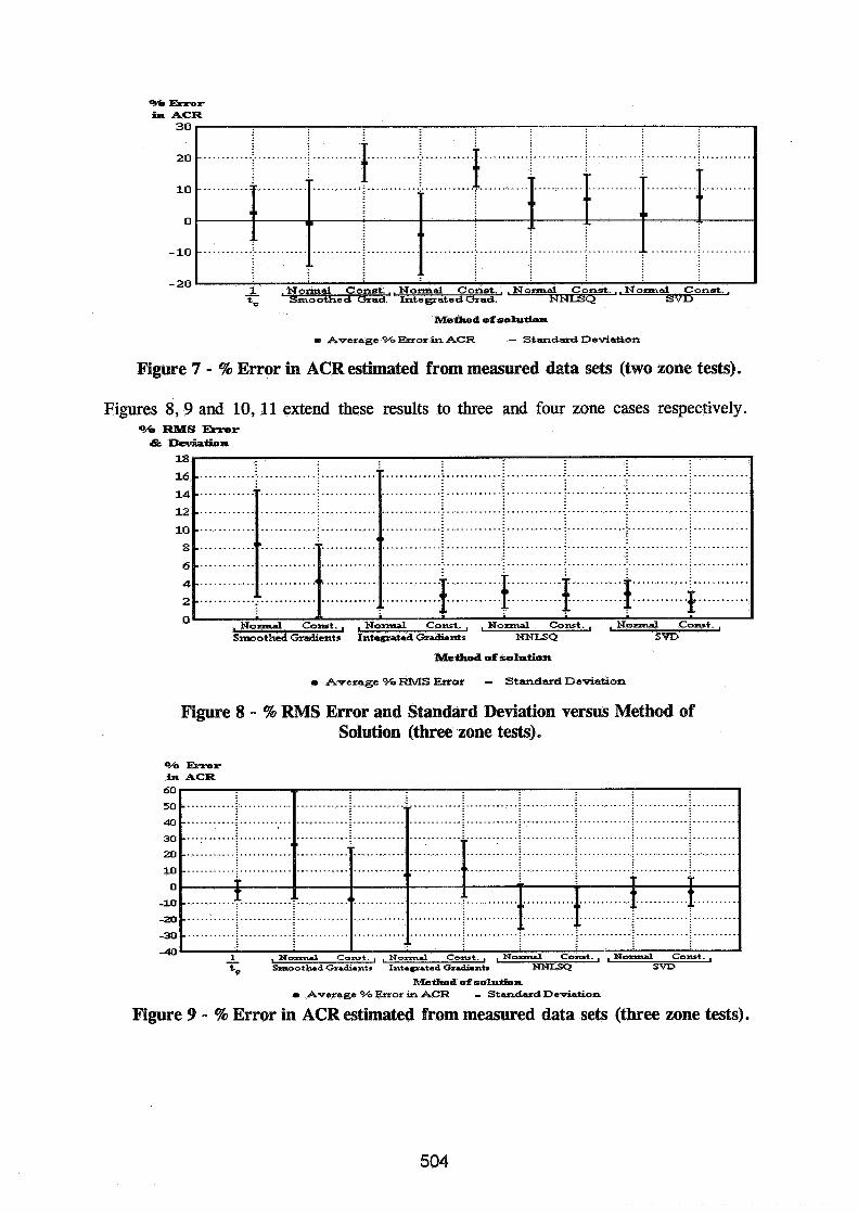
Error ACR
Method of solution
m Average ON- Error m ACR - Standard Deviation
figure 7 - % Error in ACR estimated from measured data sets (two zone tests).
Figures 8,9 and 10, 11 extend these results to three and four zone cases respectively. %6 RlMS Error & Dewlatian
, N o d Const., . N o d Const., , N o d Const., , N o n n d Const. , Smaothed Gradients Integrated Gradients NNLSQ SV13
Methad of solution
r Average O/o RNIS Error - Standard Deviation
Figure 8 - % RMS Error and Standard Deviation versus Method of Solution (three zone tests).
%a Error in ACR
Methad of solutbn r Average ONo Error in ACR - S t ~ d a r d Deviation
Figure 9 - % Error in ACR estimated from measured data sets (three zone tests).

%I RNTS Error d& DeviaiimIL
m Average O/o RMS Error - Standard Deviation
Figure 10 - % RMS Error and Standard Deviation versus Method of Solution (four zone tests).
%Error in ACR
t, S m o o t h e d Gradients I n t e g r a t e d Gradients NNLSQ SVD
hbthod of solutiaa
r A v e r a g e O/o Error in ACR - S t a n d a r d I3 e-i-iation
Figure 11 - % Error in ACR estimated from measured data sets (four zone tests).
Two main conclusions can be drawn from these results. These are:- i) m e inter-zone flows are reliably determined provided a non-negative least
squares (NNLSQ) or singular value decomposition (SVD) solution technique is used, with constraints where there are known flows. Other techniques are not as reliable.
ii) The overall air change rate is found most reliably from the steady state decay curve, that is when the dominant eigenvalue is controlling the rate of decay.
These conclusions become more clearly defined as the number of zones increases. The facility has been used for other validation studies, details of which are given by Brouns 1151.
REFERENCES
1. Afonso, C.F. and Maldonado, E.A.B. "A tracer gas procedure for the simultaneous evaluation of effective volumes and multizone air flows" Proceedings of the Third International Congress on Building Energy Management, ICBEM 1987, Volume 111, pp. 194-201, Lausanne, 1987.
2. Irwin, C. and Edwards, R.E. "'The validation of a multiple tracer gas technique for the determination of airflows between three interconnected cells " Air Infiltration Review, Volume 7, No. 4, pp. 4-5, August 1986.
3. Riffat, S.B. and Eid, M. "Measurement of air flows between the floors of houses using a portable SF, system" Energy and Buildings, Volume 12, pp. 67-75, 1988.
4. Afonso, C.F.A.;ZMaldonado, E.A.B.and Skaret, E. "A single tracer gas method to characterize multi-room air exchanges" Energy and Buildings, Volume 9, pp. 273-280, 1986.
5. Riffat, S.B. "Air flows between two zones: Accuracy of single tracer gas measurements for estimation" BSER & T, Volume 10, No. 2, pp. 85-88,1989.
6. Enai, M., Shaw, C.Y.and Reardon, J.T. "On the multiple tracer gas techniques for measuring interzonal airflows in buildings " AT-90-5-4- (3370), Preprint, ASHRAE Transactions, Volume 96, Part 1, 1990.
7. 09Neill, P.J. and Crawford,R.R. "Experimental validation of a single tracer gas technique for analysing airflows and effective volumes in multizone systems" Indoor Air '90, Proceedings of the 5th International Conference on Indoor Air Quality and Climate, Volume 4, Building and System Assessments and Solutions, pp. 425-430, J~lylAugust 1990.
8. Mattson, J.B. "An experiment for airflow determination by quadratic programming" Air Infiltration Review, Volume 1 1, No. 4, September 1990.
9. Heidt, F.D.; Rabenstein, R, and Schepers, 6. "Performance and comparison of tracer gas methods for measuring airflows in two zone buildings " ASHRAE Symposium on 'Field Studies of Ventilation Efficiency', USA, 1991.

10. Kvisgaard, B. and Schmidt, L. "Interzonal airflow measurement - A tool to solve pollution problems" Proceedings of the 12th AIVC Conference on Air Movement and Ventilation Control Within Buildings, Poster 28, Volume 2, pp. 335-350, Canada, September 1991.
11. Budek, H. "Experimental validation of a two zone air movement model with time lags" Dissertation, Coventry University (U.K.), 1988.
12. Heidt, F.D.,Rabenstein, R. and Schepers, G. "Comparison of tracer gas methods for measuring air flows in two zone buildings" Proceedings of the 12th AIVC Conference on Air Movement and Ventilation Control within Buildings, Poster 28, Volume 2, pp. 335-350, Canada, September 1991.
13. Sutcliffe, H.C. "Infiltration and air change studies in large single cell buildings" PhD Thesis, Coventry University (U.K.) , August 199 1.
14. Waters, J.R. ; Lawrance, G.V. and Jones, N. "A tracer gas decay system for monitoring air infiltration and air movement in large single cell buildings" Proceedings of the Symposium on Design and Protocol for Monitoring Air Quality, pp. 266-286, Cincinnati, Ohio, April 1987.
15. Brouns, C.E. "A study of the multi-zone air movement model" PhD Thesis, Coventry University, to be published.

Energy Impact of Ventilation and Air Infiltration 14th AlVC Conference, Copenhagen, Denmark
21 -23 September 1993
The Evaluation of Ventilation Effectiveness Measurements in a Four Zone Laboratory Test Facility
J R Waters, C E Brouns
Coventry University, School of the Built Environment Priory Street, Coventry CV1 SFB, UK

ABSTRACT
The Evaluation of Ventilation Effectiveness Measurements in a Four Zone Laboratory Test Facility
Improvements to ventilation systems for the purpose of saving energy may also affect the provision of good air quality. Measurement of ventilation effectiveness may be used to determine whether or not good fresh air distribution and satisfactory contaminant removal has been achieved in a specific case. However, for such measurements to be useful, it is necessary to establish recommended values of the parameters and to check the reliability of the measurement procedures. This paper is concerned with the second of these problems. It is well known that both air change efficiency and contaminant removal effectiveness can easily measured when there are clearly defined supply and exhaust ducts for the ventilating air, and there is no re-circulation. However, measurement become more difficult when these conditions are not satisfied. Also, in all cases, tracer gas measurements often require the estimation of end corrections to exponential decay curves, with a possibility of large errors. This paper reports on the first part of a systematic exploration of ventilation effectiveness measurement methods, carried out in the four zone test facility described by Brouns and Waters. Several different flow patterns and ventilation strategies are tested, and comparisons with some full scale measurements are made.
Energy Impact of Ventilation and Air Infiltration 14th AlVC Conference, Copenhagen, Denmark
21 -23 September 1993
Application of a New Method for Improved Multizone Model Predictions
A Schaelin; V Dorer," J van der Maas," A Moser*
* Energy Systems Laboratory (LES), Swiss Federal Institute of Technology of Zurich (ETHZ), ETH-Zentrum, CH8092 Zurich, Switzerland ** EMPA, Section 175, CH-8600 Dubendorf, Switzerland *" Lab. d9Energie Solaire et de Physique du Batiment (LESO-PB), Ecole Polytechnique Federale de Lausanne (EPFL), CH-1015 Lausanne, Switzerland
Abstract Multizone models are a common tool for calculating air and contaminant exchange within rooms of a building and between building and outside. Usually a whole room is then modelled by one calculation node with the assumption of homogeneously mixed conditions within this room. In real cases, however, temperature and contaminant concentrations vary in space. The exchange to the neighbouring nodes via the flow paths is then a function of the local values of these variables. Detailed knowledge can be obtained from the solution of the transport equations for the air flow pattern within the room at the expense of higher computation cost.
This work shows the application to several examples of a new method which includes results from detailed calculations for one room of importance in a multizone model of a whole building. The examples with air in/exfiltration, ventilation and contaminant propagation show the effects on the results of the prediction of the air flow and the contaminant spread by relaxing the homogeneity assumptions.
The proposed name of the method is "Detailed flow path value method" (DFPV method) as separate local variable values are considered for each flow path h m the room of importance to the neighbouring rooms instead of one average value. It is discussed in which situations the DFPV method can be expected to improve the multizone model predictions.
1. Introduction Multizone models are computer tools for calculating air and contaminant exchange between rooms of a building and between the building and outdoors. Usually a whole mom is modeled by one calculation node (a zone) under the assumption of homogeneous conditions within this mom.
In real cases, however, temperature and contaminant concentrations vary in space. The exchange to the neighbouring nodes is then a function of the local values of these variables near the flow paths within each zone. These local values are very strong functions of the position of heat and contaminant sources and of the resulting air flow pattern. The air flow pattern itself is determined rnainly by the heat sources and the mechanical and natural (e-g. open doors or windows) ventilation systems. Examples where local values have a strong influence on the multizone model predictions include:
Pollutant spread from a zone with a non-homogeneous concentration (i.e. a local source) into other rooms
Enclosures of large horizontal (e.g. open-plan offices) or vertical (e.g. atria, staircases) dimensions
Rooms with thermal stratification (e.g. displacement ventilation, open doors and windows) or generally complicated flows
Detailed knowledge about the air flow can be obtained from the field solution of the transport equations (Computational Fluid Dynamics, 0). In theory, the air flow pattern for the whole building could be solved, but in practice the computational effort is too high. A method which does the Cm> calculation for one room (or, generally, a small part of the building) only and allows it to feed the more adequate results somehow into the multizone formulation is a great help to improve the predictions of the whole building transport behaviour.
A link between multizone models and CFD can be also very useful the other way around, i.e. to calculate the CFD boundary conditions by the multizone program for a specific ventilation problem and for desired climatic conditions. This holds especially for cases with a combined mechanicaVnanual ventilation system, i.e. small mechanical exhaust systems with inlets and infiltration paths considerably influenced by stack and wind pressures.
This paper summarizes a method already presented in two previous papers [Schaelin et al. 1992,19931 to include results from detailed single-room calculations in mdtizone models for a more adequate description of the real cases. We propose the name "Detailed flow path value method'' as separate local variable values are considered for each flow path from the room of importance to the neighbouring rooms instead of one average value..
Parameter transfer between a multizone program and a detailed air flow simulation program is discussed The advantage of the method is then demonstrated in several example cases with air infiltration and exfiltration, mechanical ventilation, large openings and contaminant propagation.
Parameter studies of simple examples illustrate the importance of considering local values and are used to derive recommendations when the DFPV method is usefkl to improve multi- zone calculations. As more and more people use today "easy-teuse" CFD codes for ventila- tion design, there is only little additional work to improve the multizone model predictions.
2. The linking method between a multizone model and a CFD program
2.1. Brief description of multizone models (MZ model) and GFD (Computational Fluid Dynamics) programs
In a multizone model a building is represented by a network of nodes and links (flow paths) between nodes. Usually a whole room is modeled by one calculation node (a zone) with the assumption of homogeneous conditions within this room. Different connections (flow paths) between zones are described by functional relationships between mass flow and pressure difference. Figure la shows a simple example of a house with two rooms with wind from the left. Figure 1 b shows its network representation for the multizone modeler.
A system of algebraic equations derived from mass continuity is then set up. In the case of the presently used program COMIS Feustel et al. 1990,1992] the equations are solved for pressure. Mass flow is then derived from the pressure values; humidity and concentrations of contaminants are subsequently found from the calculated mass flow rates. Heat transfer is not considered by COMIS as also energy balance is not checked by COMIS, but temperature values are used as input boundary condition for the calculation of the mass flow between two nodes; even stratification profiles can be provided as input. The temperature values have to be known by experiments or calculated by a thermal building program.
In the example of Figure 1 b the node values 1 and 2 are calculated by the multizone pro- gram; the other nodes serve as boundary conditions. The results are in general time-depen- dent in accordance to the climatic data used in the input.
In a CFD program for the calculation of a single-room air flow pattern, the room is divided into a large number of cells (typically 10'000) and for each cell transport equations for mass, momentum, energy, turbulence quantities and concentrations of contaminants are solved. Figure lc shows schematically the detailed air flow pattern calculation for room 1. In the

--b- Wind
a) Room 1 Room 2
Figure I: a) Example house with living room and kitchen combination. b) Multizone network of the whole building. c) The same network with the kitchen (Room I ) calculated by CFD.
new method all the variable values at the air flow links to room 1 (zone 1) are treated specially in the multizone program part as discussed in the next sectioltrs.
The following variables are solved for and discussed for the here presented application:
* pressure
velocity components . temperature
concentrations of contaminants like humidity, CO2, smoke ... The turbulence variables depend on the turbulence model (the standard k-E model was used) and are not discussed in the present paper. In the present examples the commercial code PHOENICS was used mosten and Spalding 1987, Chen et al. 19901. The calculations have been performed in steady state, but could also be solved for time-varying boundary conditions. In most cases it is usually preferred to calculate stationary solutions for three or four different boundary conditions rather than the dynamical behaviour of the room air flow.
2.2. Method of detailed flow path values (DFPV method) Figure 2 demonstrates the principle of the new method for a single-room in comparison with a purely multizone solution, discussed for concentration values of a certain contaminant.
Figure 2a shows the way the purely multizone approach goes and which concentration values are taken. We assume for this example that the external wind from the left (see Figure la) forces the air to enter room 1 through the two infiltration paths (two windows) and to

leave room 1 through the exhaust to outside and through the exfiltration path to room 2. A certain room average value C1 is calcula- ted, determined by &wr, internal sources of C and the air change rate (see also examp- les in section 3). This value C1 is then also the same concentration value of the exhaust air and of the air which is passing to room 2.
Figure 2b shows the same situation for the new method where for room 1 detailed air flow and contaminant concentration patterns have been calculated. The air entering room 1 through the two infiltration paths is the same, but due to the concentration distribution, indicated by some contour lines in Figure 2b, the values at the exhaust, &d, and at the door to room 2, Cdoor, are different h m each other and also from the room average value. These values can be extremely different depending on the air flow pattern and the position of the contaminant sources as illustrated by the examples in section 3.
Coutdoor
Gutdoor 6 1 oom 2
a) oontamhant source
Cexh
Coutdoor
Goutdoor
b)
Figure 2: Schematic drawing of room I . a) Concentration values in multizone model. b) Concentration values in DFPV method.
Instead of one average variable value for node 1 (C1) different variable value (Cd and h r ) are fed to the multizone program for each flow path connecting other nodes (exhaust and room 2 in the example above).
A suggested name of the whole method is "method of detailed flow path values" @FPV). The following lines show which field values in the CFD program interact with the multizone program flow values across the CFD computation domain.
values in CFD program values in MZ program
pressure, velocity field * mass flow
local temperam field ++ heat flow
local concentration diseibution * contaminant propagation
The application recipe of the method works generally as follows for the case of one room with CFD calculation as part of a whole building:
* A full-case multizone calculation is performed first (i.e. for the whole building)
Flow path parameters are taken from this solution and transfered to the CFD program as input boundary conditions (see next section)
code is then run for the single-room
* Variable values at the flow paths to the neighbouring mms are transfered back to the multizone pro
In cases, where the new multizone values affect the solution values which have been transfed previously to the code as input boundary conditions, the whole procedure
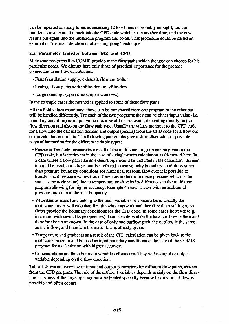
can be repeated as many times as necessary (2 to 3 times is probably enough), i.e. the multizone results are fed back into the CFD code which is run another time, and the new results put again into the multizone program and so on. This procedure could be called an external or "manual" iteration or also "ping-pongn-technique.
2.3. Parameter transfer between MZ and CFD
Multizone programs like COMIS provide many flow paths which the user can choose for his particular needs. We discuss here only those of practical importance for the present connection to air flow calculations:
Fans (ventilation supply, exhaust), flow controller
* Leakage flow paths with infiltration or exfiltration
Large openings (open doors, open windows)
In the example cases the method is applied to some of these flow paths.
All the field values mentioned above can be transferred from one program to the other but will be handed differently. For each of the two programs they can be either input value (i.e. boundary condition) or output value (i.e. a result) or irrelevant, depending mainly on the flow direction and also on the flow path type. Usually the values are input to the 0 code for a flow into the calculation domain and output (results) from the eED code for a flow out of the calculation domain. The following paragraphs give a short discussion of possible ways of interaction for the different variable types:
Pressure: The node pressure as a result of the multizone program can be given to the 0 code, but is irrelevant in the case of a single-room calculation as discussed here. In a case where a flow path like an exhaust pipe would be included in the calculation domain it could be used, but it is generally preferred to use velocity boundary conditions rather than pressure boundary conditions for numerical reasons. However it is possible to transfer local pressure values (i.e. differences to the room mean pressure which is the same as the node value) due to temperature or air velocity differences to the multizone program allowing for higher accuracy. Example 4 shows a case with an additional pressure term due to thermal buoyancy.
Velocities or laass flow belong to the main variables of concern here. Usually the multizone model will calculate first the whole network and therefore the resulting mass flows provide the boundary conditions for the CFD code. In some cases however (e.g. in a room with several large openings) it can also depend on the local air flow pattern and therefore be an unknown. In the case of only one outflow path, the outflow is the same as the inflow, and therefore the mass flow is already given.
as a result of the CFD calculation can be given back to the used as input boundary conditions in the case of the COMIS
higher accuracy.
a Concentrations are the other variables of concern. They will be input or output variable depending on the flow direction.
Table 1 shows an ovenriew of input and output p ters for different flow paths, as seen The role of the different variables depends mainly on the flow direc-
tion. The case of the large opening must be treated specially because bi-directional flow is possible and often occurs.

Table 1: Input and output parameters for CFD program for cijfferentflow paths (i = input parameter, o = output parameter).
For the contaminant transport the new concentrations (the above-mentioned output para- meters) can be fed directly into the contaminant modules of the multizone program without a second run. The Swiss version of COMIS (called COMERL) which was actually used for this application was adapted for this special type of input. With such local values, also tirne- dependent contaminant concentrations can be calculated under the assumption that the room air flow pattern remains unchanged.
Concentrations
i
o
i
o
ilo
Ventilation Inlet Ventilation outlet Leakage infiltration Leakage exf iltration
Large opening
3. Application examples of the DFPV method The method has been demonstrated with examples which show the importance of conside- ring non-homogeneous contaminant distributions, therefore enabling a more accurate prediction of the contaminant spread.
Velocity
i
if01 i
i(0) ilo
The first example, presented previously [Schaelin et al. 19921, shows how the air flow pattern in a room in a simple building with infiltration is calculated by a CFD program while most boundary conditions are given by the output of a multizone program. From the Cm) results for a 3-dimensional calculation, temperature and concentrations at those locations where outflow occurs can be fed back to the multizone program. The contaminant transport in the whole building can be calculated with the new input values. The results obtained by the new method differ by a factor of 2 from the purely multizonal approach (see Schaelin et al. 1992 for details).
Temperature
i
o i
o
ilo
The second example, presented previously [Schaelin et al. 19931, shows the contaminant distribution in a building with 2 rooms which are connected by a crack in between and with a window each to the outdoors. For a certain wind condition, a study with varied contaminance s o m e location in one room showed that the contaminance concentration in the second room varies by factar up to 5 for different source positions for a typical air flow pattern with three eddies in the first room (see Schaelin et al. 1993 for details).
The third (see section 3.1 below) example shows the contaminant distribution in a building with 3 rooms which are connected by cracks to outdoor and in between. A parameter study shows that the air flow pattern can change quite dramatically at moderate parameter changes. The forth example (see section 3.2 below) shows in a case where two rooms are connected by two flow paths finally the importance of taking buoyancy effects into account.
3.1. Example with 3 rooms and cracks (one connection between 2 zones)
In this example study the CFD calculation is only two ional in order to save computation time, and it has been done for the whole g including the surroundings. In a real application the calculation would be done only for room 1 with boundary conditions obtained from the DAZ calculations.

Figure 3a shows the basic geometry of a two-storey building. Each room measures 4.2 m x 3.0 m. In room 1, which is the room of importance, there are some obstacles, a heater of 100 W below the left crack, a unit contaminant source of S = 0.01 INS, one connection to room 2 and another one to room 3, at separate room heights. Cases with 3 different wind conditions have been investigated for three different contaminant source locations each. The cracks are 1 cm high and 0.2 m long to the outdoors and 3 cm high and 0.2 m long between the rooms.
Figure 3b shows a part of the flow field for a wind of 1 m/s and Figure 3c some contami- nant contour lines for source location 1 (Case 1.1). There is a separate smaller eddy in the lower right corner of room 1 yielding higher concentrations in that area of the room. The air
Source locations l ,2 ,3 Wind condition 1 m/s JCluraoMlrI
2 n 1.8 : 1.6 & 1.4 6 1.2
DFPV Room 3
.- 0 1
0.8 5 0.6 2 0.4 6 0.2
0
MZ Room 2 Wind condition 2.5 m/s
I MZ Room 2 Wind condition 5 m/s
DFPV Room 2 1
b Source location
Figure 3: a) Sketch of the geometry with 3 rooms. b) Air flavjield and c) contaminant contour lines for Case 1.1. d-f) Multizone and DFPV values in Room 2 and Room 3 for the 3 cases with wind velocities I , 2 5 and 5 m/s.

velocity through the infiltration crack in to room 1 is 1.145 m/s in the Case 1.1, hence a ventilation rate of r = 0.01 1 m3/s or 3.27 ach. The multizone concentration value in room 1 is is calculated in this case by C = S/r = 0.873 ppm in this case. The MZ concentrations in room 2 and room 3 are identical to this value because there is only one inflow path in each of these rooms.
Figures 3d-f show then graphically the Cm> concentration values in room 2 and room 3 for all the subcases (these values are equivalent to the DFPV values). For some location 3 the values in the other rooms do not differ and are the same as the EN: values. However as soon as the source is located near the smaller eddy, the concentration values differ dramatically h m the MZ value and are also very different b m room 2 to room 3.
It is also interesting to note that for some location 2 the concentration distribution changes strongly between the wind condition 1 m/s and 2.5 m/s, i.e. the air flow pattern changes signifcantly between these cases. The tendency shows that at higher wind velocities the air flow pattern yield homogeneous conditions in this geometry.
3.2. Example with 2 rooms and 2 connections in between This example is included as an illustration for buoyancy effects which are superimposed to the pure flow effects due to the wind pressure. The building geometry in this case is the same as in section 3.1, but with two rooms and one crack for each room to the outdoors and with two cracks between the two rooms at different heights. Room 2 is slightly warmer with a heat some of 100 W close to the right of the obstacle and a heat transfer of 20 W through the wall to room 1. Again the CFD calculation has been done for the whole building including the surroundings.
Figures 4a shows the air flow pattern inside the building for the case without wind and Figure 4b for a wind velocity of 0.3 m/s. In the case without wind a net flow occurs from room 2 to room 1 (to the left) due to buoyancy-caused pressure build-up of about 0.3 Pa inside room 2. Hence a net flow through the whole building to the left results.
At increased wind velocities from the left the net flow changes slowly to the right and very different flow pattern arise at such low wind velocities. Figures 4c-f show the velocities in the 4 cracks for wind velocities from 0.0 tn/s to 0.3 4 s . The consideration of inhomoge- neous distributions is more important at low wind velocities. The air flow distribution between the two rooms is then quite sensitive to a varied wind velocity. At higher wind velocities the buoyancy effects are dominated by wind pressure effects, and homogeneous distributions are more likely to occur.
4. In which situations is the DFPV method useful? Multizone programs are used for the air and contaminant distribution in a whole building, i.e. a net of many rooms, based on the assumption of homogeneously mixed conditions within each room (purely MZ regime). As soon as this assumption is no longer valid, which is quite often the case (as demonstrated by the examples), one has to consider the use of CFD calculations for at least a part of the building. The mixing conditions clearly depend on the type of air flow pattern.
If the conditions are very inhomogeneous in all the rooms, a Cm> calculation is needed for the whole building (possibly including the smundings of the building). This is the purely CFD application regime.
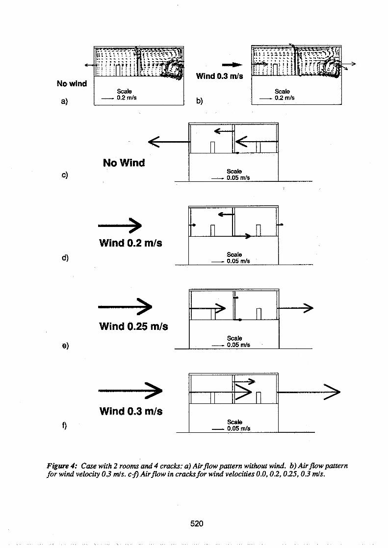
=-b-
Wind 0.3 mls
b)
No Wind
Wind 0.2 mls
Wind 0.25 rnls
Wind 0.3 rnls
Figure 4: Case with 2 rooms and 4 cracks: a) Airflow pattern without wind. b) Airflow pattern for wind velocity 0.3 d s . c-f) Airfrow in cracks for wind velocities 0.0,0.2,0.25,0.3 mls.
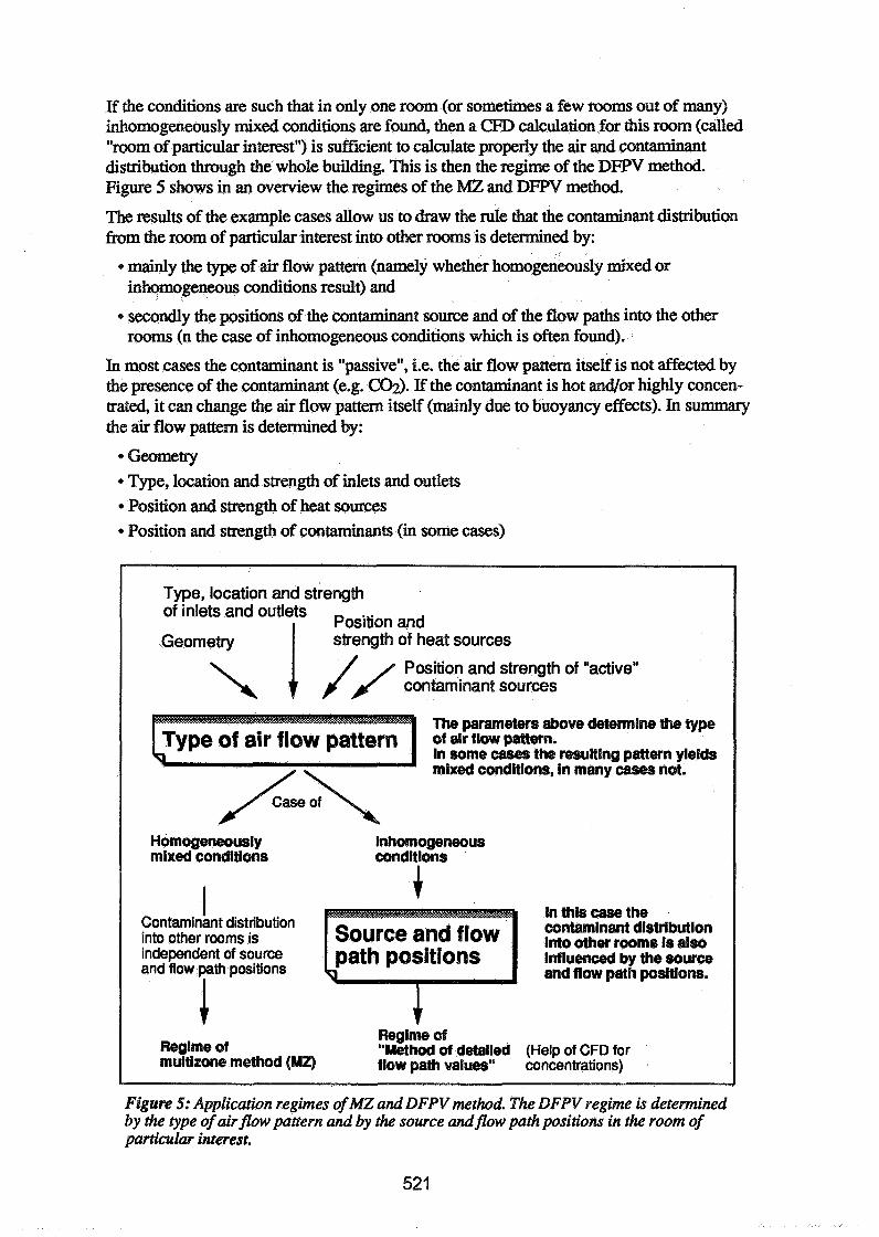
If the conditions are such that in only one room (or sometimes a few rooms out of many) inhomogeneously mixed conditions are found, then a CFD calculation for this room (called "room of particular interest") is sufficient to calculate properly the air and contaminant distribution through the whole building. This is then the regime of the DFPV method. Figure 5 shows in an overview the regimes of the MZ and DFPV method.
The results of the example cases allow us to draw the rule that the contaminant distribution fmm the room of particular interest into other rooms is determined by:
mainly the type of air flow pattern (namely whether homogeneously mixed or inhomogeneous conditions result) and
secondly the positions of the contaminant source and of the flow paths into the other rooms (n the case of inhomogeneous conditions which is often found).
In most cases the contaminant is "passive", i.e. the air flow pattern itself is not affected by the presence of the contaminant (e.g. CQ). If the contaminant is hot and/or highly concen- trated, it can change the air flow pattern itself (mainly due to buoyancy effects). In summary the air flow pattern is determined by:
Geometry 9 Type, location and strength of inlets and outlets
Position and strength of heat sources Position and strength of contaminants (in some cases)
Position and strength of "active" contaminant sources
The parameters above determine the type of air flow pattern. In some cases the resulting pattern ylelds mixed conditions, in many cases not.
In this case the
into other rooms is independent of source Influeneed by the source
and flow path positions.
Figure 5: Application regimes of MZ and DFPV method. The DFPV regime is determined by the type of airflow pattern and by the source andjbw path positions in the room of particular interest.

If the air flow pattern leads to homogeneously mixed conditions then the MZ model can give correct results, otherwise the DFPV method can be used to improve the MZ predictions. It is hardly possible to tell in advance whether mixed conditions will occur or not in a room. As an indication one could say that mixed conditions are very likely if there is only one large eddy in the whole room and if the wind pressure effects are dominant over buoyant effects. In the simple (but rare) case of piston-type flow the wnditions are extremely inhomoge- neous.
In many cases several eddies are intemctkg. That can lead to homogeneous concentration distributions depending on the source position only. The example in section 3.1 shows the strong effect of the source position on the contaminant distribution for an identical air flow pattern. In one case multizone calculation results are appropriate, in other cases not at all. Therefore the contaminant source position is the second impcntant parameter after the air flow pattern which determines the contaminant distribution.
The case of time-dependent problems
Multizone models are often used for time-dependent calculations over a certain period of time, in the case of contaminant distributions in a building typically for a whole day. A full CFD calculation for such a case is very time-consuming and requires also enormous amounts of data sturage. A combination with a multizone model can be very useful, as during the day the flow pattem changes only a few times substantially. For each of such a situation a steady-state CFD calculation can be done at very little additional work and computation time once the basic CFD case setup is done. The multizone model can then be applied with a few sets of CFD-MZ interface data and, possibly, a linear interpolation in between.
5. Conclusions A method for linking CFD detailed air flow pattern results with multizone models has been presented. The accmcy of results of multizone simulations is limited by the assumption of homogeneously mixed conditions in each node. This condition is not fulfilled in rnany cases of practical importance. Therefore the accuracy can be considerably enhanced by using the presented method.
The proposed name of the method is "method of detailed flow path values" (DFPV). Instead of the node variable value (the room average value) taken for each flow path to other nodes, a separate value from CFD calculation is provided for each flow path connecting this node with other nodes. In many cases no additional iterations (feeding back the new multiione results to the CFD code and repeating the procedure) are needed-, when needed in some cases, 2-3 iterations might be sufficient.
The method is demonstrated with simple examples which show the importance of considering non-homogeneous contaminant distributions. In the cases shown the calculated concentration values differ by up to a factor of 10 from the purely multizonal approach.
The DFPV method should be used when in only one or a few rooms of a building inhomogeneously mixed conditions are found. A CFD calculation for these few rooms is then sufficient to calculate properly the air and contaminant distribution through the whole building. An inhomogeneous contaminant distribution depends mainly on the air flow pattern and secondly on the contaminant source location.

* The method can also be applied to more complicated or even time-dependent cases. It can be used to determine detailed transfer values of all the variables solved in the multizone program like pressure, mass flows, temperature and contaminant concentrations. The method so far is suited for applications to cases where detailed air flow knowledge in a few room or only one room (in the important ones) is sufficient to give a better prediction of the overall air and contamination transport. In these cases, the method promises to improve the multizone model predictions with few additional CFD computations.
The method can also be used only for calculating appropriate boundary conditions for a CFD calculation of a room as part of a building.
Acknowledgements This work was financially supported by the Swiss Federal Office of Energy (BEW).
References Chen, Q.; A. Moser; and A. Huber. 1990. Prediction of buoyant, turbulent flow by a Low-
Reynolds-number k-& model. ASHRAE Trans., Vol. 96, pp. 3366-3375. Fanger P.O. 1989. The new equation for indoor air quality - The Human Equation: Health and
Comfort. Proc. Indoor Air Quality 89, San Diego, Ca., ASHRAE, pp. 1-9. Feustel, H.E.; and A. Rayner-Hooson. 1990. Fundamentals of the multizone air flow model -
COMIS. Technical Note AIVC 29. AIVC, Coventry, GB.. Feustel, H.E.; and A. Rayner-Hooson. 1992. CQMIS 1.0 - User Guide. AIVC, Coventry, GB. Rosten, H.I.; and D.B. Spalding. 1987. The PHQENICS reference manual, for Version 1.4,
Report No. TR/200. London: CHAM Ltd. Schaelin, A.; V. Dorm, J. van der Maas; and A. Moser. 1992. A new method for linking results
of detailed air flow pattern calculation with multizone models. Proc. 13th AIVC Conf., Nice, France, 15-18 Sept 1992, pg. 63-76.
Schaelin, A.; V. Dorer; J. van der Maas; and A. Moser. 1993. Improvement of multizone model predictions by detailed flow path values from CFD calculations. ASHRAE Trans., Vol. 99, DE-93-7-4.


Energy Impact of Ventilation and Air Infiltration 14th AlVC Conference, Copenhagen, Denmark
21 -23 Septern ber 1993
Balancing Ventilation Systems Using Thermography
I C Ward
Reader in Architectural Technology, Building Science Research Unit, School of Architectural Studies, The University of Shemeld, P 0 Box 595, The Arts Tower, Sheffield SIO 2UJ, UK
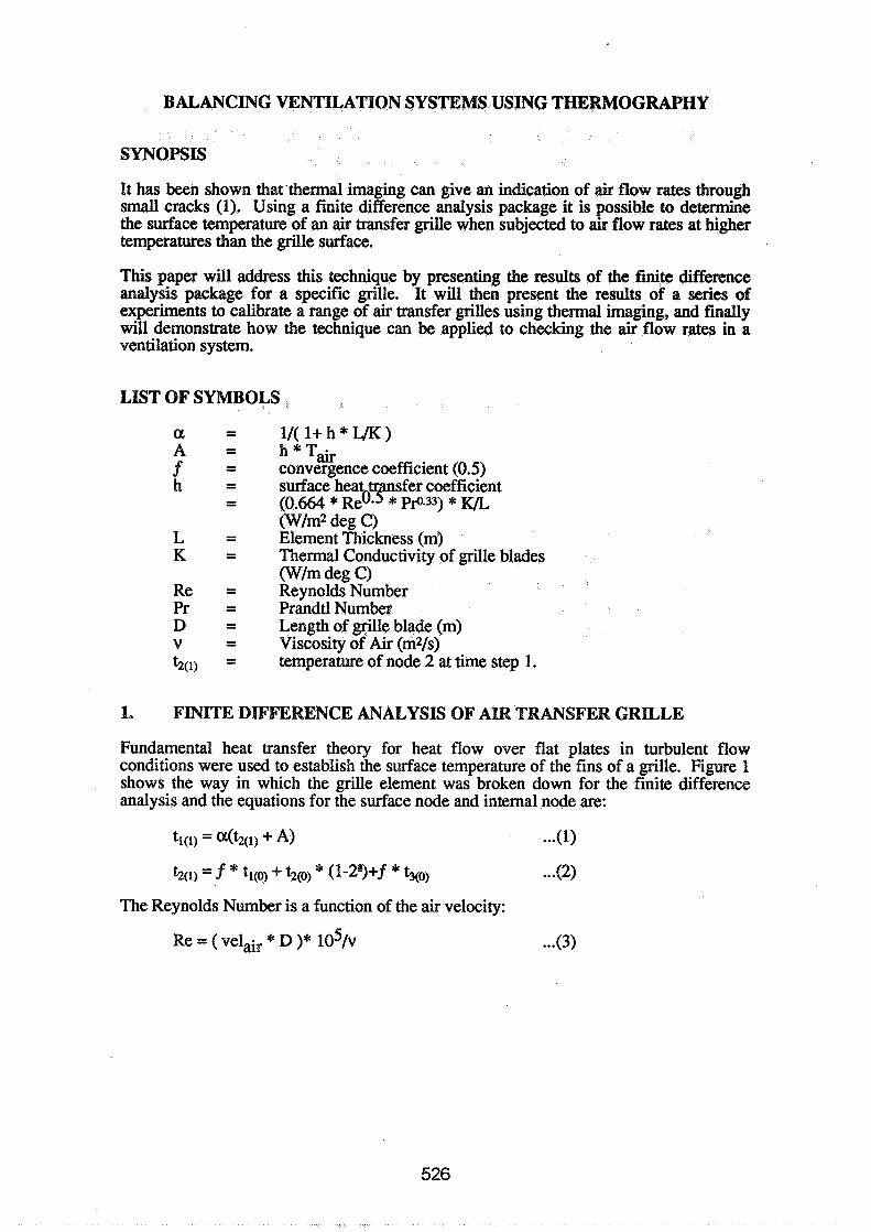
BALANCING VENTILATION SYSTEMS USING THERMOGRAPHY
SYNOPSIS
It has been shown that'thermal imaging can give an indication of air flow rates through small cracks (1). Using a finite difference analysis package it is possible to determine the surface temperature of an air transfer grille when subjected to air flow rates at higher temperatures than the grille surface.
This paper will address this technique by presenting the results of the finite difference analysis package for a specific grille. It will then present the results of a series of experiments to calibrate a range of air transfer grilles using thermal imaging, and finally will demonstrate how the technique can be applied to checking the air flow rates in a ventilation system.
LIST OF SYMBOLS
I/( l + h * U K ) h * Tair convergence coefficient (0.5) surface heat sfer coefficient (0.664 * Reo% W33) * K/L (W/m2 deg C) Element Thickness (m) Thermal Conductivity of grille blades (W/m deg C) Reynolds Number Prandtl Number Length of grille blade (m) Viscosity of Air (m2/s) temperature of node 2 at time step 1.
1. FINITE DIFFERENCE ANALYSIS OF AIR TRANSFER GRILLE
Fundamental heat transfer theory for heat flow over flat plates in turbulent flow conditions were used to establish the surface temperature of the fins of a grille. Figure 1 shows the way in which the grille element was broken down for the finite difference analysis and the equations for the surface node and internal node are:
b(1) = f * tl(0) + t2(0) * (1-2a)+f * t3(0) . . . (2)
The Reynolds Number is a function of the air velocity:

It can therefore be seen that the surface temperature is a function of the velocity of the air passing over it and therefore it should be possible to determine the velocity from a knowledge of the surface temperature history.
The above equations formed the basis of a finite difference programme which was written specifically to look at the surface temperature variations for different air flow rates.
Figure 2 shows the results of the analysis for a range of air flow rates which indicate that there is a significant difference in the surface temperature for different air flow rates.
2. INITIAL MEASUREMENTS USING REMOTE TEMPERATURE SENSING
Using a hand held Infra-Red thermometer with a print out facility, a domestic air grille's surface temperature was measured over a period of time when the heating system was switched on. The resulting plot (Figure 3) shows that the predicted air flow rate for this grille was approximately 2.5 4 s . Flow rates measured prior to and after the tests were in the region of 2.3 to 2.5 m/s which indicate that the IR technique may be able to predict air flow rates over grilles.
3. CALIBRATION OF AIR TRANSFER GRILLES
In order to establish if the technique described above was able to be applied to a ventilation system it was necessary to carry out a series of tests on a variety of air transfer grilles. A simple ventilation system incorporating air heater, dampers and variable pitch axial fans was constructed. A range of different grilles was made available by a large UK manufacturer and these were tested for a range of supply air temperatures and flow rates.
3.1 Surface Temperature: Variable Heat Input Rates
The first series of tests carried out were to establish if the variation in the surface temperature of a specific grille was a function of the air velocity and the heat input to the system.
Figure 4 shows the results of this series of tests and it is quite clear that as the heat input to the system was increased the surface temperature also increased. The air velocity also had an effect on the final conditions.
3.2 Surface Temperature: Different Grilles
The next series of tests were designed to establish if there were significent differences between the various grilles. Figure 5 shows the results of this series of tests and it is clear that each grille has it's own characteristic. However the differences are small and there could easily be an overlap in practice. At higher volume flow rates the differences disappear and all the grilles appear the same.
In order to establish if measuring the surface temperature of a grille could give an indication of the flow rate, if was suggested that the variation in the grille surface temperature with time could be treated as a first order equation. In practice this did not prove to be the case and a simple steady state surface temperature was found to be a better means of determining the flow rate.
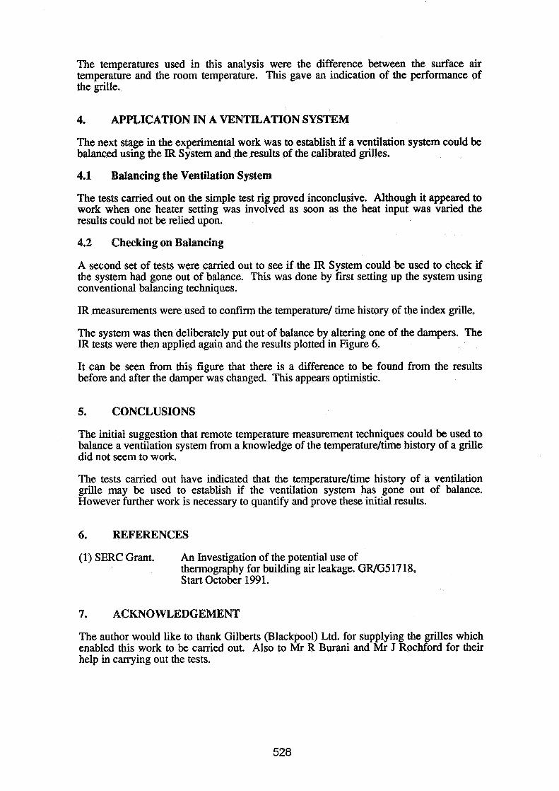
The temperatures used in this analysis were the difference between the surface air temperature and the room temperature. This gave an indication of the performance of the grille.
4. APPLICATION IN A VENTILATION SYSTEM
The next stage in the experimental work was to establish if a ventilation system could be balanced using the IR System and the results of the calibrated grilles.
4.1 Balancing the Ventilation System
The tests carried out on the simple test rig proved inconclusive. Although it appeared to work when one heater setting was involved as soon as the heat input was varied the results could not be relied upon.
4.2 Checking on Balancing
A second set of tests were carried out to see if the IR System could be used to check if the system had gone out of balance. This was done by first setting up the system using conventional balancing techniques.
IR measurements were used to confirm the temperature1 time history of the index grille.
The system was then deliberately put out of balance by altering one of the dampers. The IR tests were then applied again and the results plotted in Figure 6.
It can be seen from this figure that there is a difference to be found from the results before and after the damper was changed. This appears optimistic.
5. CONCLUSIONS
The initial suggestion that remote temperature measurement techniques could be used to balance a ventilation system from a knowledge of the temperatureltime history of a grille did not seem to work.
The tests carried out have indicated that the temperatureltime history of a ventilation grille may be used to establish if the ventilation system has gone out of balance. However further work is necessary to quantify and prove these initial results.
6. REFERENCES
(1) SERC Grant. An Investigation of the potential use of thermography for building air leakage. GRIGS 1718, Start October 199 1.
7. ACKNOWLEDGEMENT
The author would like to thank Gilberts (Blackpool) Ltd. for supplying the grilles which enabled this work to be carried out. Also to Mr R Burani and Mr J Rochford for their help in carrying out the tests.
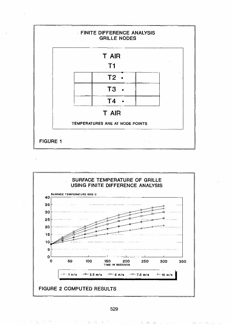
FINITE DIFFERENCE ANALYSIS GRILLE NODES
T AIR T I
T AIR TEMPERATURES ARE AT NODE POINTS
FIGURE 1
SURFACE TEMPERATURE OF GRILLE USING FINITE DIFFERENCE ANALYSIS
SURFACE TEMPERATURE DEG C 40
3 5
30
2 5
2 0
15
10
5
0 0 50 100 150 200 250 300 350
TIME I N SECONDS
FIGURE 2 COMPUTED RESULTS
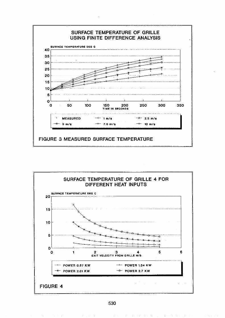
SURFACE TEMPERATURE OF GRILLE USING FINITE DIFFERENCE ANALYSIS
SURFACE TEMPERATURE DEG C
0 50 100 150 200 250 300 350 TIME IN SECONDS
MEASURED
FIGURE 3 MEASURED SURFACE TEMPERATURE
SURFACE TEMPERATURE OF GRILLE 4 FOR DIFFERENT HEAT INPUTS
SURFACE TEMPERATURE DEG C 20
15
10
5
0 0 1 2 3 4 5 6
EXIT VELOCITY FROM GRILLE MIS
FIGURE 4
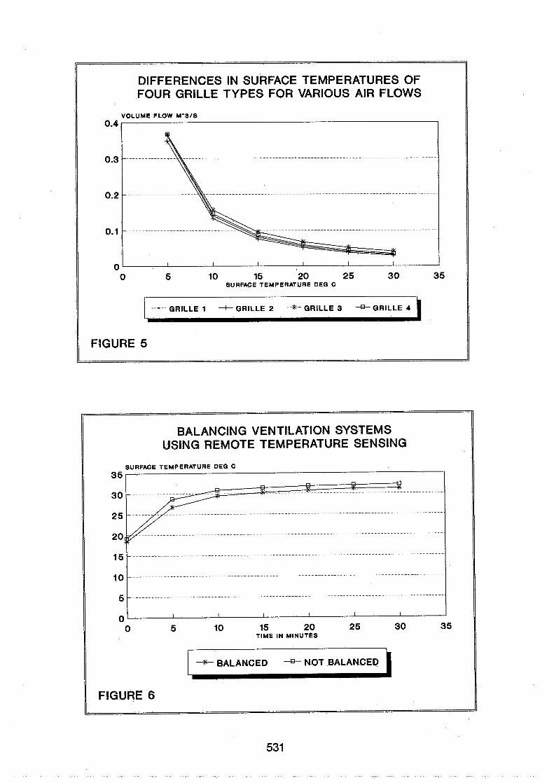


Energy Impact of Ventilation and Air Infiltration 14th AlVC Conference, Copenhagen, Denmark
21 -23 September 1993
Thermography: Its Applications for Building Air Leakage Measurements
J W Roberts, I C VVard
University of Sheffield, UK

Themography: Its applications for building air leakage measurements.
J. W. Roberts and I. C. Ward. University of Sheffield
Synopsis
Preliminary work [I] has indicated that thermography can be used to determine air leakage pathways from or to buildings. Accurate measurements have now been taken using temperam controllable enyironmental chambers. These results reinforce the potential use of thermography for this application,
In conjunction with the physical measurements a simulation has been carried out using computational fluid dynamics. The two sets of results are found to be in good agreement with each other thus validating the computer model, and give fimher proof of the adaptability of thermography for building air leakage measurements.
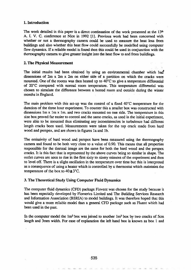
1. Introduction
The work detailed in this paper is a direct continuation of the work presented at the 13& A. I. V. C. conference at Nice in 1992 [I]. Previous work had been concmed with whether or not a thermography camera could be used to measure the heat loss h m buildings and also whether this heat flow could successfully be modelled using computer flow dynamics. If a reliable model is found then this could be used in conjunction with the thermography camera to give greater insight b to the heat flow to and from buildings.
2. The Physical Measurement
The initial results had been obtained by using an environmental chamber which hacq' dimensions of 2m x 2m x 2m on either side of a partition on which the cracks were mounted. One of the rooms was then heated up to 40'C to give a temperature differential of 20°C compared with normal room temperature. This temperature diffemtial was chosen to simulate the difference between a heated room and outside during the winter months in England.
The main problem with this set-up was the control of a fixed 40°C temperature for the duration of the three hour experiment. To counter this a smaller box was constructed with dimensions lm x l m x lm. and two cracks mounted on one side. The temperature in this size box proved far easier to control and the same cracks, as used in the initial experiment, were able to be mounted thus eliminating any inconsistencies in turbulence had different length cracks been used. Measurements were taken for the top crack made from hard wood and perspex, and are shown in figures l a and lb.
The ernissivity of hard wood and perspex have been measured using the thermography camera and found to be both very close to a value of 0.90. This means that all properties responsible for the t h e d image are the same for both the hard wood and the perspex cracks. It is this fact that is represented by the above curves being so similar in shape. The outlet curves are seen to rise in the first sixty to ninety minutes of the experiment and then to level off. There is a slight oscillation in the temperature over time but this is interpreted as a consequence of using a heater which is controlled by a thermostat which maintains the temperature of the box to 40f 3°C.
3. The Theoretical Study Using Computer Fluid Dynamics
The computer fluid dynamics (CFD) package Flovent was chosen for the study because it has been especially developed by Flomerics Limited and The Building Services Research and Information Association (BSRIA) to model buildings. It was therefore hoped that this would give a more reliable model than a general CFD package such as Fluent which had been used in the past.
In the computer model the lm3 box was joined to another lm3 box by two cracks of 5cm length and 3mm width. For ease of explanation the left hand box is known as box 1 and
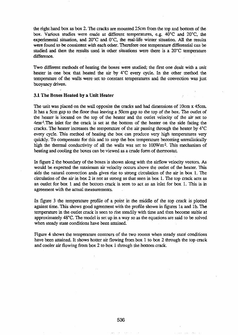
the right hand box as box 2. The cracks are mounted 25cm from the top and bottom of the box. Various studies were made at different temperatures, e.g. 40°C and 20°C, the experimental situation, and 20°C and O"C, the real-life winter situation. All the results were found to be consistent with each other. Therefore one temperature differential can be studied and then the results used in other situations were there is a 20°C temperature difference.
Two different methods of heating the boxes were studied; the first one dealt with a unit heater in one box that heated the air by 4'C every cycle, In the other method the temperature of the walls were-set to constant temperatures and the convection was just buoyancy driven.
3.1 The Boxes Heated by a Unit Heater
The unit was placed on the wall opposite the cracks and had dimensions of lOcm x 45cm. It has a 5cm gap to the floor thus leaving a 50cm gap to the top of the box. The outlet of the heater is located on the top of the heater and the outlet velocity of the air set to 411s-1.The inlet for the crack is set at the bottom of the heater on the side facing the cracks. The heater increases the temperature of the air passing through the heater by 4°C every cycle. This method of heating the box can produce very high temperatures very quickly. To compensate for this and to stop the box temperature becoming unrealistically high the thermal conductivity of all the walls was set to 100Wm-2. This mechanism of heating and cooling the boxes can be viewed as a crude form of thermostat.
In figure 2 the boundary of the boxes is shown along with the airflow velocity vectors. As would be expected the maximum air velocity occurs above the outlet of the heater. This aids the natural convection ands gives rise to strong circulation of the air in box 1. The circulation of the air in box 2 is not as strong as that seen in box 1. The top crack acts as an outlet for box 1 and the bottom crack is seen to act as an inlet for box 1. This is in agreement with the actual measurements.
In figure 3 the temperature profile of a point in the middle of the top crack is plotted against time. This shows good agreement with the profile shown in figures l a and lb. The temperature in the outlet crack is seen to rise steadily with time and then become stable at approximately 48°C. The model is set up in a way so as the equations are said to be solved when steady state conditions have been attained.
Figure 4 shows the temperature contours of the two rooms when steady state conditions have been attained. It shows hotter air flowing from box 1 to box 2 through the top crack and cooler air flowing from box 2 to box 1 through the bottom crack.
3.2 The Walls of the Boxes set to a Constant Temperature
In this set-up the boxes were heated up by setting the walls of the boxes to stay at a constant temperature. The walls in box 1 were set to be 40°C and the walls in box 2 were set to be 20°C. Figure 5, shows the airflow velocity vectors for this situation. As can be seen there is a far more even circulation or air between the two boxes than in the previous case. This is because there is no forced convection and only buoyancy effects are causing the convection. There is a good exchange of hotter air through the top crack and cooler air through the lower crack. This is given added proof by looking at figure 6, the temperature contours.
The temperature profile of a point in the middle of the top crack plotted against time is shown in figure 7. The temperature is seen to rise steadily with time and then become steady at approximately 31°C. It shows good agreement with the plots shown in figures l a and lb.
4. Conclusions
This paper has been concerned with the continuing work into extending the applications of themography. It has already proved itself to be a very adaptable tool for the measurement of the thermal profile of buildings. The results documented above are very consistent with each other and this gives us confidence both in the reliability of themography as a building science tool and in the computer models predicted by the computer fluid dynamic package Flovent.
Future work will concentrate on two main areas in the near future. The first will use the thermal camera to study the hot air flow out of window apertures and the cold air flow into buildings through window apertures. The second will develop the Flovent calculations to model more complicated and practical applications.
References
1. An investigation of the potential use of thermography for building air leakage measurements. J. W. Roberts, S. Sharples and I. C. Ward. Proceedings of the 13th AIVC conference, Nice, France, September 1992 p 598.

21. io jo ib 70 do lio 130 150 170 190 I - l - 8 - 4
T i e (minutes)
Figure la: Temperature of outlet crack made of hard wood plotted against time.
Time (minutes)
Figure 1 b: Temperature of outlet crack made of perspex plotted against time.

Vector
Figure 2: Flovent output showing aimow velocity vectors for the boxes heated by a unit heater. The heater is shown to the left of box 1.
Temperature
0.001 1.001
Iteration No. (E3)
Figure 3: Flovent output showing the temperature profile of a point in the middle of the top crack plotted against time for the boxes heated by a unit heater.

Fill Temperature
Figure 4: Flovent output showing the temperature contours for the boxes heated by a unit heater. The lighter areas correspond to hotter regions. The key is shown in 'C.
Vector
Figure 5: Flovent output showing airflow velocity vectors for the boxes set at a constant temperature.
Fill Temperature
Figure 6: Flovent output showing the temperature contours for the boxes set at a constant temperature. The lighter areas correspond to hotter regions.The key is shown in "C.
Iteration No.
32.0'
30.0-
28.0-
26.0-
24.0-
22.0,-
Figure 7: Hovent output showing the temperature profile of a point in the middle of the top crack plotted against time for the boxes set at a constant temperature.
Temperature
I I I I I
-
-
-
-
-
I I I
20.0' I I
101 201 301 401 501 601 1


Energy Impact of Ventilation and Air Infiltration 14th AlVC Conference, Copenhagen, Denmark
21 -23 September 1993
Visualization of Measured Three Dimensional Well Mixed Zones of Temperature in a Ventilated Space
M de Moor," D Berckmans*"
* Research Engineer, Department of Agric. Engng., Kardinaal Mercierlaan 92, B-3001 Leuven, Belgium ** Associate Professor, National Fund for Scientific Research, Belgium Dept of Agric Engng., Kardinaal Mercierlaan 92, B-3001 Leuven, Belgium
Energy impact of Ventilation and Air infiltration
14th AIVC Conference, Copenhagen, Denmark 2 1-23 September 1993
Visualization of measured three dimensional well mixed zones of temperature in a ventilated space
De Moor Maarten1, Berckmans DanieP
Abstract
A new model concept has been developed to model the three dimensional energy and mass transfer in an imperfectly mixed fluid. The model permits to predict the dynamic behaviour of the volumetric concentration of heat flow, mass flow and fluid flow. A laboratory test installation has been built to analyse the model capabilities to predict the dynamic behaviour of the air flow pattern within a ventilated space in order to control the energy and mass transfer in the ventilated space. This test installation permits to measure and to visualise well mixed zones of mass and energy concentration and gives the opportunity to visualise the air flow pattern in a quantitative way. Experiments have been done with this test installation in order to test the model concept.
The objective of this paper is to explain the possibilities of the test installation and the different measurement techniques that are used. Furthermore, experimental results will be given.
Maarten De Moor Belgium. 2~anie1 Berckmans
is research Engineer, Dept. of Agric. Engng. Kardinaal Mercierlaan 92, B-3001 h e n ,
is Associate Professor, National Fund for Scientific Research, Belgium, Dept. of Agric. Engng. Kardinaal Mercierlaan 92, B-3001 Leuven, Belgium.
1. Introduction
Mathematical models of physical phenomena are a basis for predicting the dynamical process behaviour and are essential in the design of optimal control strategies for these processes. In many processes the control of heat and mass transfer presents a major problem. A missing link is a reliable mathematical model for the dynamic behaviour for the dynamic fluid flow pattern in an imperfectly mixed fluid.
At present, mathematical models for fluid flow pattern are typically based on a discretisation of the physical laws that govern the behaviour of the fluid under study. The method is based on the classical approach of mass, momentum and energy balances (the so called white box modelling approach), which typically leads to partial differential equations such as convection -diffusion equations, Navier-Stokes, etc. The partial differential equations involved are conservation and continuity laws for momentum, enthalpy and mass flow. These are applied to one or more discrete volumes chosen to represent the system under study, i.e. the e&mtions are discretized on a grid both in time and space and on each point of the grid the state is calculated, typically by solving immense sets of linear equations at each time step. Such models are currently available for contaminant dispersal analysis, steady fluid flow analysis and thermal anaIysis. An important advantage of this modelling approach is the fact that reliable simulations are possible which are based on physical insight. There are still many technical and fundamental problems for classical computational fluid dynamics models. Some of the disadvantages are:
Existing modelling techniques are mainly developed for simulation in steady state. For control purposes however, the dynamic behaviour of the process subject to variations is to be modelled.
e Because of the number of grid points that is used, typically there is a model validation problem to ver@ whether the model is sufficiently accurate for the control purpose at hand.
e The approach does not allow to model the dynamic behaviour of the three dimensional fluid flow pattern. e The boundary conditions must be known before a model is useful
2. Objectives
Our overall hypothesis is that the fluid flow pattern generates a heat and mass transfer with resulting micro- climate conditions. The central objective of this paper is to demonstrate the capabilities of the test installation to visualise well mixed zones of temperature. Furthermore it is the objective to demonstrate the capabilities of the test installation to visualise and quantiij the air flow pattern. It is the aim to demonstrate by experimental results that there exist a relationship between the distribution of energy in a confined space and the resulting air flow pattern.
3. Measurement set-up
In order to develop and validate different model- and control strategies, a test installation was built to measure the three dimensional distribution of temperature and humidity and to estimate the dynamic behaviour of the volumetric concentration of heat flow and the mass flow and the fluid flow pattern as well. In this section a brief overview will be given about the capabilities of the test installation and the experimental conditions will be explained. The test installation has been described in more detail in literature (Berckmans et al., 1992).
3.1 The test chamber
The purpose for which the test chamber was built, is to generate stable air flow pattem and to measure the transient behaviour from one stable air flow pattern to another. It is indeed mentioned in literature (Barber and Ogilvie, 1982) that the fluid flow pattern plays an important role in the basic mechanism of energy and mass transfer within a fluid. The type of resulting fluid flow pattern will be determined by the characteristics of the used test room such as (Croom-Gale et al., 1975): geometry of the test room; geometry, dimensions and position of the air inlet; geometry, dimensions and position of the air outlet; temperature of the mounding walls; temperature difference between the incoming air and the air in the test room; inlet velocity of the
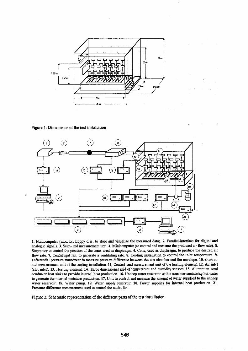
Figure 1 : Dimensions of the test installation
1. Minicomputer (monitor, floppy disc, to store and visualise the measured data). 2. Parallel-interface for digital and analogue signals. 3. Scan- and measurement unit. 4. Minicomputer (to control and measure the produced air flow rate). 5. Stepmotor to control the position of the cone, used as diaphragm. 6. Cone, used as diaphragm, to produce the desired air flow rate. 7. Centrifugal fan, to generate a ventilating rate. 8. Cooling installation to control the inlet temperature. 9. Differential pressure transducer to measure pressure difference between the test chamber and the envelope. 10. Control- and measurement unit of the cooling installation. 11. Control- and measurement unit of the heating element. 12. Air inlet (slot inlet). 13. Heating element. 14. Three dimensional grid of temperature and humidity sensors. 15. Aluminium semi conductor heat sinks to provide internal heat production. 16. Undeep water reservoir with a streamer containing hot water to generate the internal moisture production. 17. Unit to control and measure the amount of water supplied to the undeep water reservoir. 18. Water pump. 19. Water supply reservoir. 20. Power supplies for internal heat production. 21. Pressure difference measurement used to control the outlet fan.
Figure 2: Schematic representation of the different parts of the test installation
incoming air; turbulence of the air within the test room. Considering the conclusions in literature (Leonard, Mc, Quitty, 1985; Mullejans, 1966; Randall, Battams, 1979; Randall, 1979; Regenscheit, 1970) the foIlowing room geometry was taken: length = 3 m, width = 1.5 m; height = 2 m. To minimize the disturbing influence of the walls on the air flow pattern as caused by the surfiice temperature of the walls, a second building envelope (also in Plexiglas) was built around the primary test room. The different dimensions, geometry's and positions are shown on figure 1.
3.2 Measurement of the different input- and output variables
The input variables as measured in the test chamber are (figure 2): - the air flow rate - the temperature of the incoming air - the relative humidity of the incoming air - the amount of heat supplied to the test chamber - the internal heat production - the internal moisture production - pressure difference between the test chamber and the envelope
The considered output variables are: - the temperature and relative humidity of the internal room air - the quantified air flow pattern - the three-dimensional distribution of the temperature and humidity
For a more detailed desciiption of the measurement method, we refer to Berckmans et al. (1992).
4. Method: Model concept
According to what has been shown in literature (Berckmans, 1989; Timmons, 1980; Randall, 1979,1981), the total volume of a ventilated space is considered to be a non-perfectly mixed air space. Consequently it is assumed that there is a three dimensional air flow pattern in the building volume and (related) gradients in the local micro-environmental parameters (temperature, humidity). Although the building is considered to be a non-perfectly mixed air volume in this model concept, it is always possible to define a control volume or a well mixed zone as being the maximum three dimensional volume in which, by definition there is well mixed air. This means that within this control volume there are no gradients of temperature, humidity, gas concentration, air velocity etc. Consequently from the theoretical viewpoint this control volume is supposed to be infinitely small. It will be shown by experimental results that in reality this is not the case. When this concept is applied in reality the perfectly mixed volume indeed is a better mixed zone with acceptable gradients as dictated by the application. In the model concept there are two types of input variables: the global inputs and the local inputs (see figure 3). Initially the global inputs are ventilation rate V through the test installation and the heat supply Q from the heating system to the test installation (see figure 2). In addition to these, the local inputs to the control volume are the part Vc of the global ventilation rate that enters the control volume, the part Qc of the total internal heat production Q that enters the control volume and the part Wc of the total mass production that enters the control volume. Applying the law of mass conservation and the general law of total energy conservation on the control volume results in a temperature (T) and humidity (X) equation (Berckmans, 1992): '
In these equation the Greek symbols represent physical constants such as specific heat, specific mass etc. It is important to note that in equation (1)and (2) every parameter has a physical meaning as explained in Berckmans 1992. As shown in figure 3, the problem can be split up into two steps:
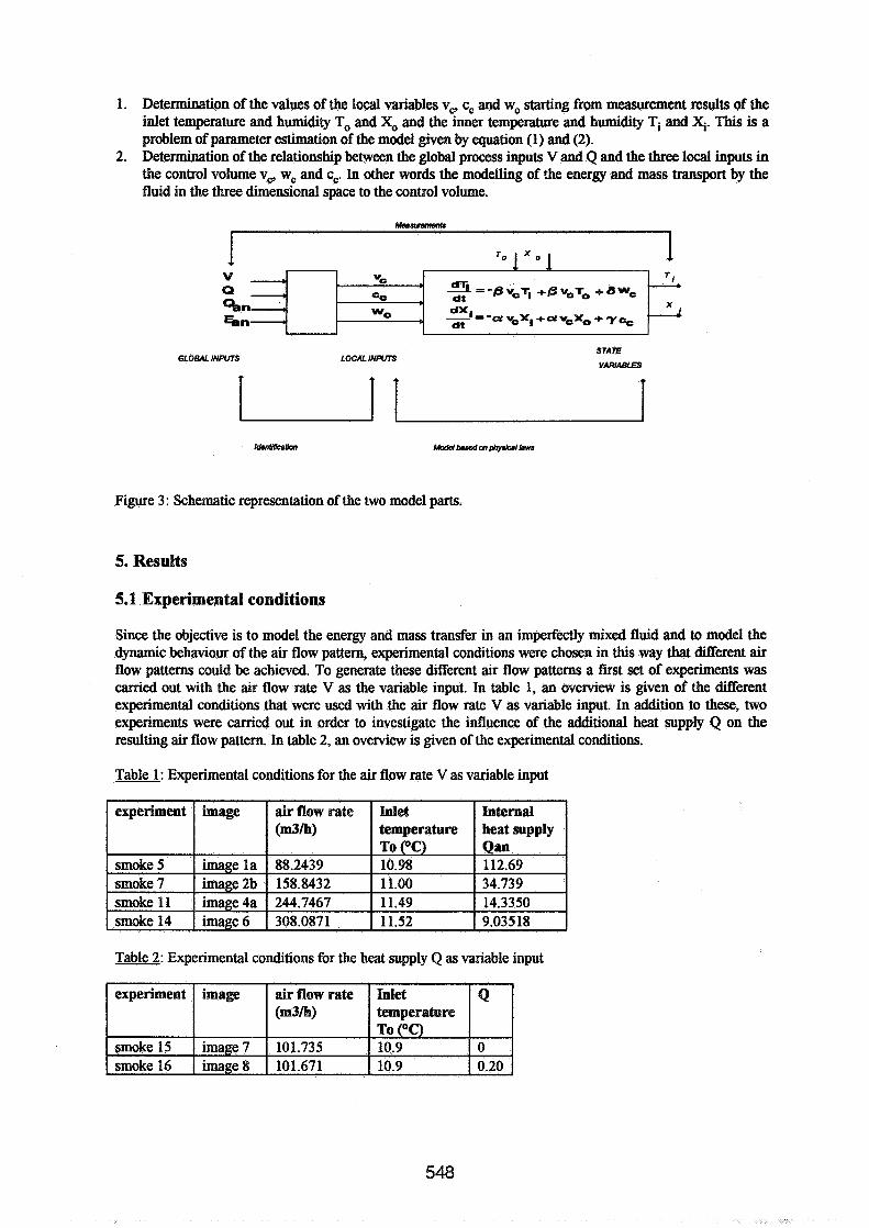
1. Determination of the values of the local variables vc, cc and wc starting from measurement results of the inlet temperature and humidity To and Xo and the inner temperature and humidity Ti and Y. This is a problem of parameter estimation of the model given by equation (1) and (2).
2. Determination of the relationship between the global process inputs V and Q and the three local inputs in the control volume v,, w, and c,. In other words the modelling of the energy and mass transport by the fluid in the three dimensional space to the control volume.
P + + V -
dl- *I Q ce * --L=-@v,l-, +f3vcT0+bWc - ~ e n x m
dt X
kn- wo
I =~=-Cr\hx,+Crvcxo+~~ dt - GLOBAL INPUTS LOCAL INPUTS
STATE
VARIABLES
Figure 3 : Schematic representation of the two model parts.
5. Results
5.1 Experimental conditions
Since the objective is to model the energy and mass transfer in an imperfectly mixed fluid and to model the dynamic behaviour of the air flow pattern, experimental conditions were chosen in this way that different air flow patterns could be achieved. To generate these different air flow patterns a first set of experiments was carried out with the air flow rate V as the variable input. In table 1, an overview is given of the different experimental conditions that were used with the air flow rate V as variable input. In addition to these, two experiments were carried out in order to investigate the influence of the additional heat supply Q on the resulting air flow pattern. In table 2, an overview is given of the experimental conditions.
Table 1 : Experimental conditions for the air flow rate V as variable input
Table 2: Experimental conditions for the heat supply Q as variable input
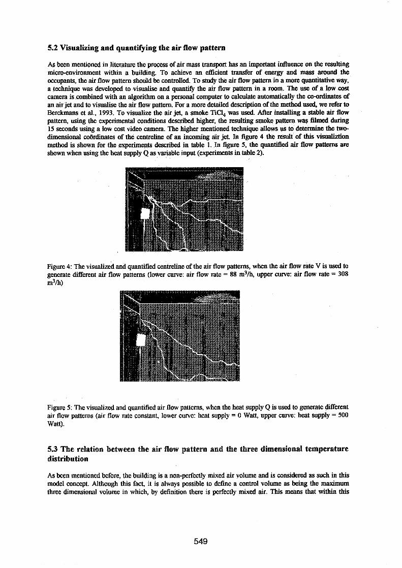
5.2 Visualizing and quantiQing the air flow pattern
As been mentioned in literature the process of air mass transport has an important influence on the resulting micro-environment within a building. To achieve an efficient transfer of energy and mass around the occupants, the air flow pattern should be controlled. To study the air flow pattern in a more quantitative way, a technique was developed to visualise and quantify the air flow pattern in a room. The use of a low cost camera is combined with an algorithm on a personal computer to calculate automatically the co-ordinates of an air jet and to visualise the air flow pattern. For a more detailed description of the method used, we refer to Berckmans et al., 1993. To visualize the air jet, a smoke TiC14 was used. After installing a stable air flow pattern, using the experimental conditions d e s c n i higher, the resulting smoke pattern was Nrned during 15 seconds using a low cost video camera. The higher mentioned technique allows us to determine the two- dimensional coOrdinates of the centreline of an incoming air jet. In figure 4 the result of this visualiztion method is shown for the experiments described in table 1. In figure 5, the quantified air flow pattern are shown when using the heat supply Q as variable input (experiments in table 2).
Figure 4: The visualized and quantified centreline of the air flow patterns, when the air flow rate V is used to generate different air flow patterns (lower m e : air flow rate = 88 m3/h, upper curve: air flow rate = 308 m3/h)
Figure 5: The visualized and quantified air flow patterns, when the heat supply Q is used to generate different air flow patterns (air flow rate constant, lower curve: heat supply = 0 Watt, upper m e : heat supply = 500 Watt).
5.3 The relation between the air flow pattern and the three dimensional temperature distribution
As been mentioned before, the building is a non-perfectly mixed air volume and is considered as such in this model concept. Although this fact, it is always possible to define a control volume as being the maximum three dimensional volume in which, by definition there is perfectly mixed air. This means that within this

control volume there are no gradients of temperature, humidity, gas concentration, air velocity etc. Consequently from the theoretical viewpoint this control volume is supposed to be infinitely small. It will be shown by experimental results that in reality this is not the case. When this concept is applied in reality the perfectly mixed volume indeed is a better mixed zone with acceptable gradients. In figure 6 a visualization is given of three dimensional well zones of temperature for three different air flow pattern shown in figure 4.
measwed air flow pattern measured control volumes
measured air flow pattern measured control volumes
Figure 6: The measured temperature distribution in the test installation as a function of the measured generated air flow pattern (figure 6a: experiment smoke7t, figure 6b: experiment smoke1 It and figure 6c: experiment smoke 14).
From this figure important conclusions can be dram regarding the temperature distribution in a ventilated space as a W o n of the air flow pattern. When the temperature gradient in the test installation is considered, it can be concluded that the temperature difference between maximum and minimum temperature in the test installation is larger with larger values of the air flow rate and dependent of the generated air flow pattern. Regarding the position of the control volumes, it can be concluded that for the given experimental inlet conditions (see 5.1) and for low air flow rates (falling air) the well mixed zones of low temperature (in relation to the given scale) are positioned in the lower part of the ventilated space (see figure 6). For air flow patterns generated using high values of the air flow rate on the contrary, the cold zones will be found in the upper part of ventilated space (see figure 6).
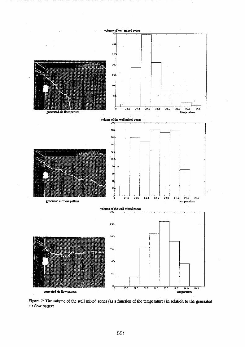
volume of well mixed zones
30
volume of the well mixed zones
'2
generated air flow pattern temperahrre
volume of the well mixed zones
3 0 0
generated air flow pattern temperature
Figure 7: The volume of the well mixed zones (as a function of the temperature) in relation to the generated air flow pattern

When the size of the well mixed zones is considered, it can be concluded from figure 7 that for an increasing air flow rate (and so different air flow patterns (figure 7a to 7c)) the largest control volume corresponds to a lower value of temperature. When unstable air flow pattem are installed (figure 7b) it can be concluded that the well mixed zones are equally spread in volume over the volume of the test installation as a whole.
6. Conclusions
In order to develop and validate different model- and control strategies, a test installation was built to measure the three dimensional distribution of temperature and humidity and to estimate the dynamic behaviour of the volumetric concentration of heat flow and the mass flow and the fluid flow pattern as well. In this paper a model concept with the notion of control volume was briefly explained. It was shown that the laboratory test room permits one: - to visualize the well mixed zones with constant temperature as &ned in the model concept, - to visualize the air flow pattern or more specifically: the centreline of an incoming air jet, - to quantify the three dimensional air flow pattem, - to do measurements on the steady state and transient behaviour of the inside temperature and humidity to validate the models capacity to predict the air flow pattem. From experimental results it could be concluded that the air flow pattem plays an important role in the distribution of energy within an imperfectly mixed air volume. Furthermore it was demonstrated that the air flow pattern is of great influence to the temperature gradient in the test installation and to the size and position of the well mixed zones as defined in the model concept.
References
BARBER, E.M., OGILVIE, J.R, 1982. "Incomplete mixing in ventilated spaces Part 1: Theoretical considerations". Can. Agric. Engng., Vol. 24., No 1, pp. 25-29.
BERCKMANS D., DE MOOR M, DE MOOR B., 1992. "Test installation to develop a new model concept to model and control the energy and mass transfer in a three dimensional imperfectly mixed space." Proceedings of Roomvent '92: Air distribution in rooms. Aalborg, Denmark, Sept 2-4,1992.
BERCKMANS, D., VAN DE WEYER K., DE MOOR, M., 1993. "Visualisation and quantification of the air flow pattern by using image analysis". Proceedings of the ATICconference to be held in Brussels, 17-19 February, 1993 (in press).
BERCKMANS D., DE MOOR M, DE MOOR B., 1992. "A new approach to modelling and control the energy and mass transfer in a three dimensional imperfectly mixed ventilated space." Proceedings of Roomvent '92: Air distribution in rooms. Aalborg, Denmark, Sept 2-4, 1992.
BERCKMANS, D., GOEDSEELS, V., 1989. Modelling and controlling ventilated agricultural structures, Proc. of the symposium "Building systems: Room air and.air contaminant distribution". Ed. Christianson, Illinois, USA, pp. 68-74.
CROOME-GALE, D.J. ROBERTS, B.M, 1975. "Air conditioning and ventilation in buildings", Perganon press, pp. 466,365-395. (1975)
LEONARD, J.J., MC QUIlTY, J.B. "Criteria for the control of cold ventilation air jets", ASAE paper no 85- 4014, 19 pp. (1985) .
MULLEJANS, H. "Uber die Ahnlichkeit der nicht-isothermen Stromung und den Warmeubergangen in Raumen mit Strahlluftung", Westdeutscher Verlag, Koln und Oplanden, pp.54. (1966)
RANDALL, J.M., BAlTAMS, V.A., "Stability criteria for airflow patterns in livestock buildings", J. agric. Engng. Res., 24, p. 361-374. (1979)
RANDALL, J.M. "The prediction of airflow patterns in livestock buildings", J. agric. Engng. Res., 20, p. 199- 215. (1979)
RANDALL, J.M., 1981. Ventilation system design in environmental aspects of housing for animal produdon Clark J. A., Butterworths, London, 35 1-369.
REGENSCHEIT, B. "Die Archimedes-Zahl", Gesundheits-Ingenietu Heft 6 ,9 1, 172- 176. (1970) TIMMONS, M.B., 1980. "Use of models to predict fluid flow motion in mechanically ventilated structures."
ASAE-Paper no 80-40 18,3 1 pp.
Session 6: Papers - Ventilation Modelling and Simulation

Energy lm pact of Ventilation and Air Infiltration 14th AlVC Conference, Copenhagen, Denmark
21 -23 September 1993
Neutral Pressure Levels in a Two-Storey Wood Frame House
J T Reardon, C-Y Shaw
Institute for Research in Construction, National Research Council of Canada, Montreal Road Campus, Ottawa, Ontario, KIA OR6, Canada

ABSTRACT
Neutral Pressure Levels in a Two-Storey Wood Frame House
Air infiltration continues to play a major role in the ventilation of houses, despite modern trends to increased airtightness of the building envelope. In colder climates, stack effect is the principal driving force for this natural air exchange. The neutral pressure level divides the envelope areas subjected to stack effect pressures driving infiltration from those subjected to pressures driving exfiltration. The neutral pressure level is therefore important to our understanding of stack driven air exchange and our ability to model it.
The neutral pressure level in a house is difficult to measure because calm conditions are needed to avoid distortions caused by the wind. In a recent research project a two-storey house was instrumented for automatic m inute-by-m inute measurements of weather conditions and envelope pressure at 22 locations around and its exterior walls. The dataset provides the measurements necessary for determination of the neutral pressure levels for four different leakage distributions created by opening and closing a flue and a basement vent. The data set covers a full range of weather conditions typical for a cold climate.
The neutral pressure levels for the four leakage distributions of the house were measured repeatedly, where wind conditions permitted. The statistical confidence levels for these NPL values are presented. Also, the full range of wind conditions encountered has produced guidelines for wind speeds which are acceptable for effective measurement of NPL values in situations where automatic instrumentation is not practical or possible. These results should be of interest to designers and researchers alike.
Energy Impact of Ventilation and Air Infiltration 14th AIVC Conference, Copenhagen, Denmark
21 -23 September 1993
Measurements of Air Change and Energy Loss with Large Open Outer Doors
* Narvik Institute of Technology, Building Science, P 0 Box 385, N-8501 Narvik, Noway ** NORUT Technology, P 0 Box 250, N-8501 Narvik, Noway
Synopsis The paper describes measurements made on large doors - 10 to 20 m2 in 2 buildings in
Narvik. The air change was measured with the tracer gas (SFg). The method of constant
concentration or decaying concentration of the tracer gas was used. The dosing, measuring and
calculation of the air change was made with a Briiel & Kjaer gas analyser type 1302 and
computer. Use of the decaying method was best with short opening times. The opening of the
door in 5 to 7 minutes gives an air exchange of 500 m3 to 1300 m3 or an air change from 0.2
to 1.0. The energy loss is from 2 to 8.5 kwh for each opening. Aiter opening of a door it takes
from 0.5 to 1 hour before we have stable temperature and air change again.
The results are compared with the theoretical formulas for gravity driven flow air change from
open doors. The number of openings and opening time of large doors is gives an energy loss
that is much larger than the transmission and infiltration loss.
1. Introduction
In calculations of energy consumption for building is the air change important. The air change
can be divided in two parts - ventilation and infiltration/exfiltration. The ventilation is con-
trolled by the ventilation equipment. The infiltration (air streaming from the outside to the
inside) can only be estimated, if it not measured, as it will depend on the air pressure difference
and the leakage area. None of these is known very accurate. The infiltration can only be
measured for a building. This measurement is normally done by measuring the air flow with a
certain over- or under pressure in the building. That is done with doors and windows closed.
In a real case will opening of windows and doors give an extra infiltration heat loss. Our
research [3] and [4] had the purpose of finding the heat loss and air change when a large door
is opened. This is compared with theoretical calculations fiom Kiel and Wilson 1986 [I].
2. Measuring objects
The measurements were made on two buildings in Narvik [4]. The first building is a laboratory
hall for NORUT Technology. The width was 15 m and the length was 27 m and an area of 405
m2. There was a large door on the short side with a height of 3.6 m and a width of 3.95 m. The
laboratory hall contained test rigs, that could influence on the air flow. This building was used
for the first series of measurements.
The second building is a wholesale distributor for grocers. The firm has a storage building of
6000 m2. All products are transported by lorries, so they have many large doors. To reduce the
heat loss from the storage is the doors placed in a front room of 440 m2. This room can be
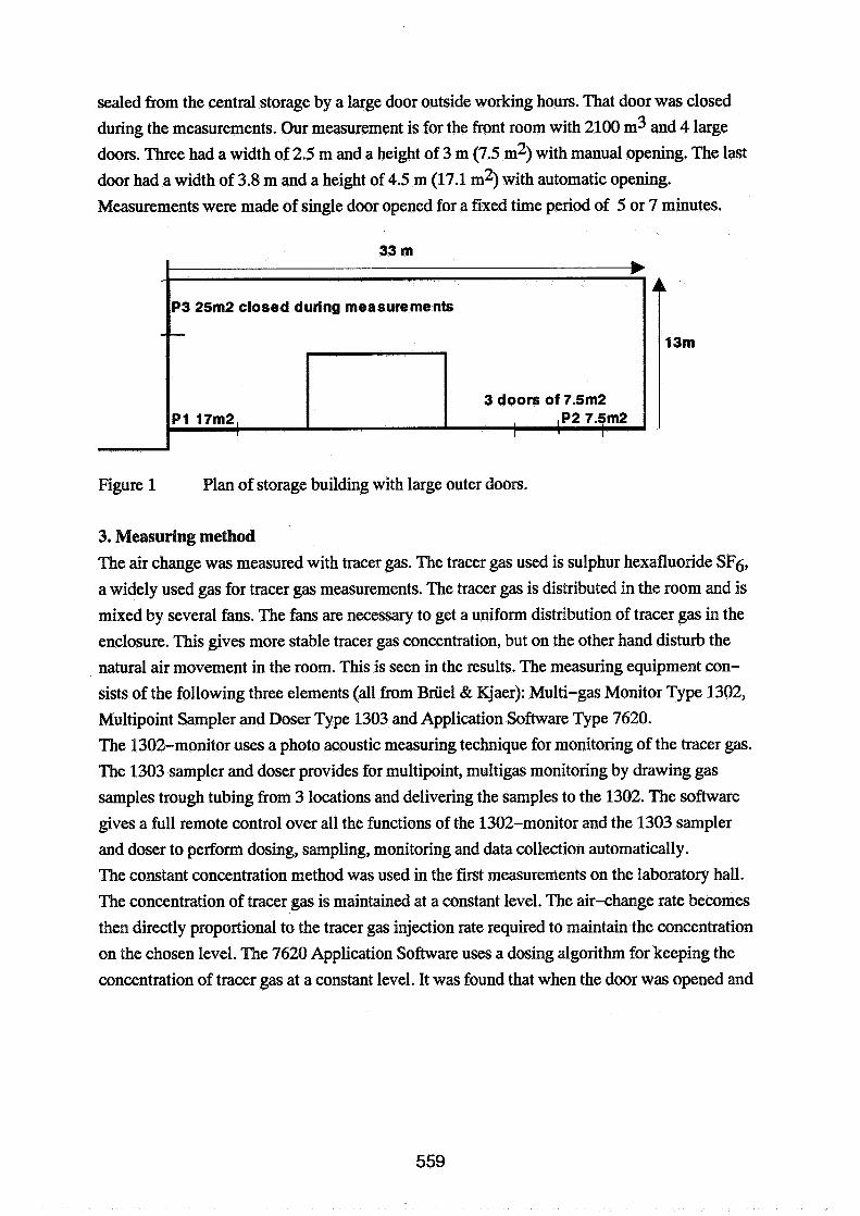
sealed from the central storage by a large door outside working hours. That door was closed
during the measurements. Our measurement is for the fiont room with 2100 m3 and 4 large
doors. Three had a width of 2.5 m and a height of 3 m (7.5 m2) with manual opening. The last
door had a width of 3.8 m and a height of 4.5 m (17.1 m2) with automatic opening.
Measurements were made of single door opened for a fixed time period of 5 or 7 minutes.
3 25m2 closed during measurements
3 doors of 7.5m2
Figure 1 Plan of storage building with large outer doors.
3. Measuring method
The air change was measured with tracer gas. The tracer gas used is sulphur hexafluoride SFg,
a widely used gas for tracer gas measurements. The tracer gas is distributed in the room and is
mixed by several fans. The fans are necessary to get a uniform distribution of tracer gas in the
enclosure. This gives more stable tracer gas concentration, but on the other hand disturb the
natural air movement in the room. This is seen in the results. The measuring equipment con-
sists of the following three elements (all from Briiel & Kjaer): Multi-gas Monitor Type 1302,
Multipoint Sampler and Doser Type 1303 and Application Software Type 7620.
The 1302-monitor uses a photo acoustic measuring technique for monitoring of the tracer gas.
The 1303 sampler and doser provides for multipoint, multigas monitoring by drawing gas
samples trough tubing from 3 locations and delivering the samples to the 1302. The software
gives a full remote control over all the functions of the 1302-monitor and the 1303 sampler
and doser to perform dosing, sampling, monitoring and data collection automatically.
The constant concentration method was used in the first measurements on the laboratory hall.
The concentration of tracer gas is maintained at a constant level. The air-change rate becomes
then directly proportional to the tracer gas injection rate required to maintain the concentration
on the chosen level. The 7620 Application Software uses a dosing algorithm for keeping the
concentration of tracer gas at a constant level. It was found that when the door was opened and
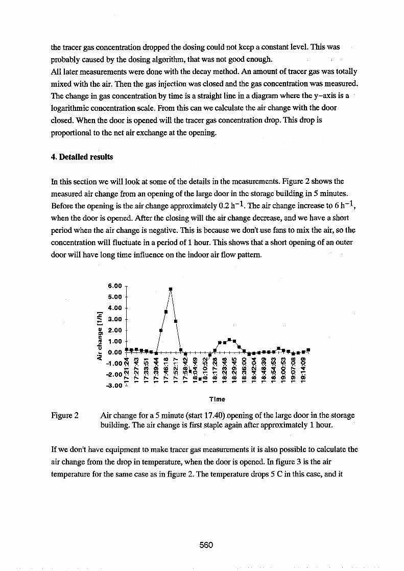
the tracer gas concentration dropped the dosing could not keep a constant level. This was
probably caused by the dosing algorithm, that was not good enough.
All later measurements were done with the decay method. An amount of tracer gas was totally
mixed with the air. Then the gas injection was closed and the gas concentration was measured.
The change in gas concentration by time is a straight line in a diagram where the y-axis is a
logarithmic concentration scale. From this can we calculate the air change with the door
closed. When the door is opened will the tracer gas concentration drop. This drop is
proportional to the net air exchange at the opening.
4. Detailed results
In this section we will look at some of the details in the measurements. Figure 2 shows the
measured air change fiom an opening of the large door in the storage building in 5 minutes.
Before the opening is the air change approximately 0.2 h-1. The air change increase to 6 hW1,
when the door is opened. After the closing will the air change decrease, and we have a short
period when the air change is negative. This is because we don't use fans to mix the air, so the
concentration will fluctuate in a period of 1 hour. This shows that a short opening of an outer
door will have long time influence on the indoor air flow pattern.
Time
Figure 2 Air change for a 5 minute (start 17.40) opening of the large door in the storage building. The air change is first staple again after approximately 1 hour.
If we don't have equipment to make tracer gas measurements it is also possible to calculate the
air change from the drop in temperature, when the door is opened. In figure 3 is the air
temperature for the same case as in figure 2. The temperature drops 5 C in this case, and it
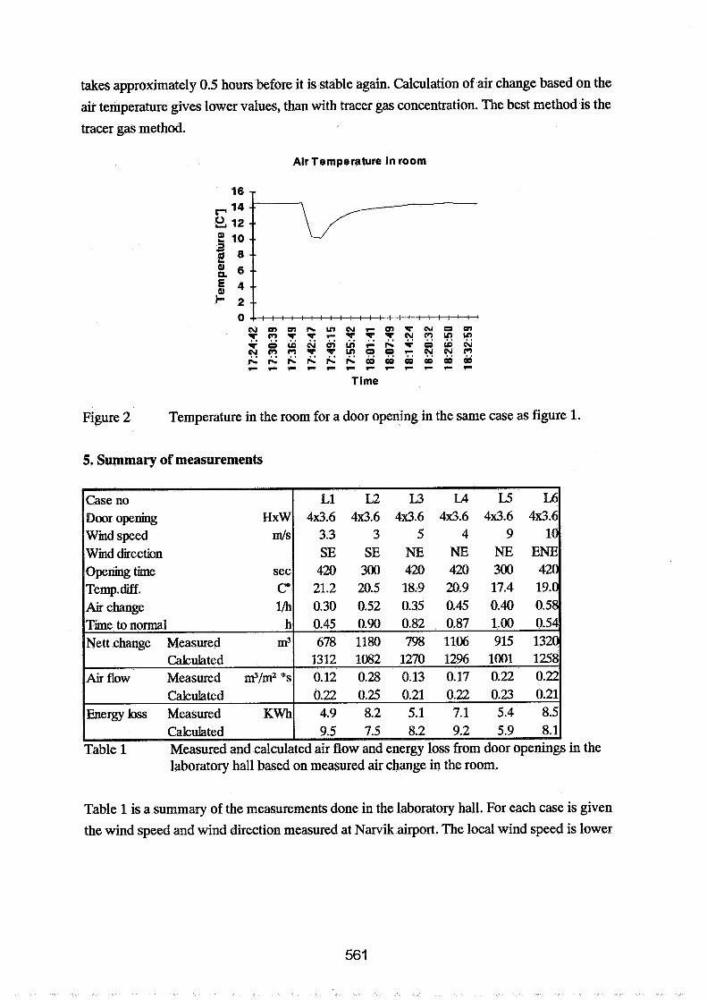
takes approximately 0.5 hours before it is stable again. Calculation of air change based on the
air temperature gives lower values, than with tracer gas concentration. The best method is the
tracer gas method.
Air Temperature in room
r r r r r r r r r r r r
Figure 2 Temperature in the room for a door opening in the same case as figure 1.
5. Summary of measurements
Case no Door opening Wmd speed Wind direction Opening time Temp. diff . Air change
Hxw d s
sec G lh
Time to normal h 0.45 0.90 0.82 0.87 1.00 0.54 Nett change Measured m' 678 1180 798 1106 915 1320
Calculated Air flow Measured d/m2 *s
Table 1 Measured and calculated air flow and energy loss from door openings in the
1312 1082 1270 12% 1001 1258 0.12 0.28 0.13 0.17 0.22 0.22
Cakulated Energy loss Measured K w h
laboratory hall based on measured air change in the room.
0.22 0.25 0.21 0.22 0.23 0.21 4.9 8.2 5.1 7.1 5.4 8.5
Table 1 is a summary of the measurements done in the laboratory hall. For each case is given
the wind speed and wind direction measured at Narvik airport. The local wind speed is lower

at the building site. The temperature difference between indoor and outdoor is given. The AC-
method (air change method) is used to calculate air flow (m3/m2s) through the door opening,
net air flow m3 and energy loss kwh based on the measured air change in the room, This
values are called measured. The values called calculated is based on the theory in chapter 6.
The time from the door opening until we have steady state air change is found to be from 0.5 to
1 hour. The opening of the door gives an air exchange of 700 m3 to 1300 m3 or an air change
from 0.45 to 1.0. The energy loss is from 5 to 8.5 kwh.
Table 2 Measured and calculated air flow and energy loss from door openings in the storage building based on measured air change in the room.
In table 2 and 3 is 7 cases of measurements on the storage building of air flow (m3/m2s)
through the door opening, net air flow m3 and energy loss kwh. For each case is given the
wind speed measured at the site near the door and wind direction measured at Narvik airport.
The opening of the door gives an air exchange of 200 m3 to 1500 m3 or an air change from 0.1
to 0.7. The energy loss is from 1 to 8 kwh. If the door is opened for longer time and more
times during the day will the loss be much higher. The first 5 cases (Sl-S5) are with a 7.5 m2
door and the last two (S6-S7) with a 17 m2 door.
The calculations also can be based on the tracer gas concentration as we find in table 3. We
call this method the decay methods, as decay of tracer gas was used. In this case we have the
gas concentration before and after in the table. We find that the measured vales from air
change with the 2 methods used in table 2 and 3 gives approximately the same values. This is
found in table 4.
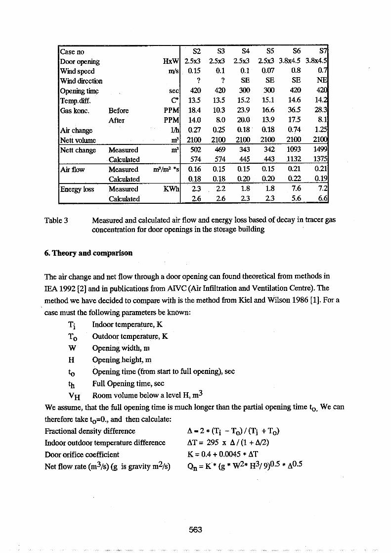
Table 3 Measured and calculated air flow and energy loss based of decay in tracer gas concentration for door openings in the storage building
6. Theory and comparison
The air change and net flow through a door opening can found theoretical from methods in
IEA 1992 [2] and in publications from AIVC (Air Infiltration and Ventilation Centre). The
method we have decided to compare with is the method from Kiel and Wilson 1986 El]. For a
case must the following parameters be known:
Ti Indoor temperature, K To Outdoor temperature, K W Opening width, m
H Opening height, m
to Opening time (from start to full opening), sec
th Full Opening time, sec
VH Room volume below a level H, m3
We assume, that the full opening time is much longer than the partial opening time to. We can
therefore take to=O., and then calculate:
Fractional density difference Aa2*(Ti -To)/(Ti +To) Indoor outdoor temperature difference AT= 295 x A/ ( l + A E )
Door orifice coefficient K = 0.4 + 0.0045 * AT
Net flow rate (m3/s) (g is gravity m2/s) Qn = K * (g * ~ 2 * H ~ I 9)O.S *

Time (s) t = th
The gravity driven exchange is found using:
If Q, * t 1 VH > 0.5 then V = V H * ( 1 - eWA*(t-B))
where A = 2 * Q n / VH
and B = ( 0.5 * VH / Qn) - 0.69 / A
I f Q n * t / V ~ < 0 . 5 then V=Qn * t
This method has been used for the theoretical calculations of air flow and air change in table 1 to 3.
'able 4. Comparison between the theory from Kiel and Wilson and measurement. Case numbers with L is fiom the laboratory hall (table 1). Case numbers with S is from the storage building with air change (table 2) or decay method (table 3).
Table 4 is a comparison between the theory and measurements. The measurement in the
laboratory hall gives large variations, that is not depending on the wind speed. It is possible the
test equipment in the room could reduce the air flow. We find the largest difference for case
S1 where the constant concentration was used. In all other cases is the difference below 25%.
Generally give the S-cases lower measured values than theory with low wind speed (0 -0.2
4 s ) and higher values with higher wind speed ( 0.5 - 1 4s) .
7. ENERGY LOSS FROM DOOR OPENINGS It is well known that open outer doors and windows will increase the air change and energy
loss. The flow through the doors will be a function of the temperature difference between
indoor and outdoor, the wind speed, the wind direction and the size of the room behind the
door and the air tightness of the room. The results of these measurements are that the air flow
normally is less than predicted by the theory gravity driven flow, and it is not possible to find a
clear influence of the wind speed. Opening af a door in 5 to 7 minutes gives an energy loss of 2
to 8 kwh. That does not look very important, but on a yearly basis is the energy loss from
openings 80-90% of the total loss , see Nielsen [5].
8. CONCLUSION Measurements of air change and heat loss can be done with tracer gas equipment. The best
method is the decay method. Comparison with the theoretical formula from Kiel and Wilson
[I] shows that the formula gives results comparable with measurements. The results have also
been compared with theoretical formulas from the Norwegian Building Research Institute, but
the difference was larger than the other formula. We would recommend more measurements
with tracer gas especially with higher wind speeds and other building types.
It is possible to get energy savings from using an air lock between the building and a lorry.
This is especially interesting in a cold climate, but it is difficult to predict the real energy
savings. This must be possible with tracer gas equipment.
9. REFERENCES 1. KIEL, D.E. and WILSON, D.J.:
Gravity driven flows through open doors, 7th AIC Conference - Occupant Interaction with ventilation system, Stratford - Upon - Avon, UK, 1986, p 15.1-15.15
2. IEA 1992: AIR FLOW THROUGH LARGE OPENINGS IN BUILDINGS Energy Conservation in Buildings and Community Systems Programme, Annex 20 Air Flow Patterns within Buildings, Sub task 2, Technical Report edited by J. van der Maas, Laboratoire dtEnergie Solaire et de Physique du Biitiment, Ecole Polytechnique Federal de Lausanne, CH-1015 Lausanne, Switzerland
3. OLSEN, E. AND NIELSEN, A,: Luftstremmer og varmetap gjennom porter (Air flow and heat loss through large doors), NORUT Teknologi, Publikationsnr FTAS A93005,1993, Narvik, Norway
4. OLSEN, E.: Feltunders~kelser av porter i Narvik (Field measurements on large doors in Narvik), NORUT Teknologi, Publikationsnr FTAS A93011,1993, Narvik, Norway
5. NIELSEN, A: Tetthet og U-vaerdier, Konsekvenser for energiforbruket, (Tightness and U-values, consequences for energy consumption), Building Detail Series 6472.642, Norwegian Building Reseach Institute, 1986

Energy Impact of Ventilation and Air Infiltration 14th AlVC Conference, Copenhagen, Denmark
21 -23 September 1993
Multizone Cooling Model for Calculating the Potential of Night Time Ventilation
J van der Maas, C-A Roulet
Laboratoire d9Energie Solaire et de Physique du Batiment, Ecole Polytechnique Fhderale de Lausanne, CH-1015 Lausanne, Switzerland
SYNOPSIS
One of the options to increase the energy efficiency of buildings in the cooling season, is to extract heat from the building envelope during the night by natural or forced ventilation. The exploitation of this technique by architects and designers requires the development of guide lines and a predesign tool showing how the potential cooling power depends on the influence of opening sizes and positions and on the interaction with the thermal mass. While a single zone model is sufficient to estimate rougly the heat extracted fiom the building, a multi zone extension allows one to predict the distribution of air and wall temperatures and therefore the distribution of cooling power over the air flow path (when the zones are ventilated in series). A zonal cooling model based on the principles of mass and energy conservation and coupling ventilation with both heat transfer and a thermal model for the walls. The parameters of the ventilation model are the size and position of the openings, the stack height, and climatic parameters like temperature swing and wind characteristics. The heat transfer is parametrized by the exposed surface area of thermal mass, while the heat storage for heavy weight constructions is only characterized by both that surface area and the thermal effusivity of the exposed wall material. The predictions are compared with measurements for a simple flow path configuration.
LIST OF SYMBOLS
ACH Ai a b,ff(m) Bi b
Air changes per hour (lh) area of opening i (m2) Thermal diffusivity, a=?dpc (m2/s) Effective wall thermal effusivity$of zone m (J/ (m2 K.s~-5) ) Biot number hWh (-) Thermal effusivity, b=d(hpc) [J/ (m2 ~.s0.5) ] Discharge coefficient Thermal heat capacity of air (J/kgK) wind pressure coefficient at opening i Fraction of S(m) for convective heat transfer Thermal heat capacity (JIkgK) Diffusion length, 6--J(at) (m) Wall thickness (m) Auxiliary heat gain in zone m (W) Fourier number, (-)
Heat flow rate (W) Ventilative heat gain in zone m (W)

Po Pext P r S(m) Sk(m) To T T,(m)
Text
Wall surface heat gain in zone m (W) Acceleration of gravity ( 4 ~ 2 ) Convective fraction of auxiliary heat gain in zone m (W) Height between centers of inlet and outlet opening (m) Global heat transfer coefficient (WIrn2~) Height above reference of bottom of zone m (m) Height above reference of air node in zone m (m) Convective heat transfer coefficient (WIm2K) Bottom opening between zones m and m+l (m) Top opening between zones m and m+l (m) Opening index : 1,2 Characteristic length (m) Thermal conductivity (WImK)
Mass flow rate (kg/s) Zone index : 1 ..N Pressure (Pa) Stack pressure (Pa) Wind pressure (Pa) Volume flow rate (m3ls) Height weighted mean inside air density (kg/m3) Air density in zone m (kg/m3) Air density at 273 K, 1.29 (kg/m3) External air density (kg/m3) Density (kg/m3) Gas constant for air, 287 (JIkgK) Total internal wall surface area of zone m (m2) Surface area of internal wall k in zone m (m2) Absolute temperature at O°C, 273 K average absolute air temperature (K) Characteristic air temperature in zone m (K) external air temperature (K)
inside air temperature (K) Characteristic wall temperature in zone m (K) inside outside air temperature difference (K) time (s) Air velocity, outflow, in opening i ( 4 s ) air velocity, inflow, in opening i ( 4 s ) wind reference velocity ( 4 s ) Volume (m3) Width of opening i (m)
1. INTRODUCTION
One of the options to increase the energy efficiency of buildings in the cooling season, is to extract heat from the building envelope during the night by natural or forced ventilation. The exploitation of this technique by architects and designers requires the development of guide lines and a predesign tool showing how the potential cooling power depends on the influence of opening sizes and positions and on the interaction with the thermal mass. Before discussing in more detail this option, it is instructive to briefly review situations where the ventilation strategy for cooling differs. Three types of ventilative cooling situations can be distinguished giving more or less importance to the link between ventilation and the thermal mass of the building.
(i) Cooling the human body by ventilation. First the situation where the outside air temperature is close to the building temperature so that the structure can not be cooled by ventilation alone (no link between ventilation and thermal mass).
However wind induced ventilation through open windows can cool the human body and increase comfort. The heat transfer coefficient between the skin and the air increases with higher air speed, and also when the air is not very humid, the evaporation is enhanced and the body is cooled. This type of ventilative cooling plays a basic role in increasing comfort in warm climates.
The cooling effect of ceiling fans in summer falls also in this category.
(ii) Cooling with high air temperatures. When the air temperature is higher than the building structure, one strategy is to reduce ventilation so that the occupant experiences the coolth of the inside building surfaces. Another strategy is to maximize the cooling of the ventilation air by the building mass and to provide in addition increased comfort through ventilative cooling of the human body. To keep the inside of the building cool the designer should reduce solar heat gains as much as possible by installing shading devices.
A particular situation arises when high inside air temperatures result from internal heat gains. This situation is characterized by air temperatures which are much higher than the wall temperatures. To reduce the capacity of cooling equipment the designer needs to know how the inside temperature depends on the ventilation rate and on the thennal mass.
(iii) Cooling the building structure. At ni'ght, the outside air is often lower in temperature than the building structure, so that the latter can be cooled by ventilation. But how to optimize the cooling? The sometimes heard statement, that "the building structure can be potentially cooled to the outside air temperature" is self-contradictory. This is because when the building is at the air temperature no heat transfer can occur. Indeed, during the cooling process the inside air temperature is always somewhere half-way between the outside air temperature and the wall surface temperature. To optimize ventilative cooling the designer should understand the link between ventilation, heat transfer and the distribution of thermal mass. While a large number of detailed building simulation models are available for the designer (see Ref. [I] and documents of IEA/ECB Annex 21), few experimental data on the cooling effect of ventilation are available in the literature.
In this paper we concentrate on the development of a simplified calculation method providing the needed output (energy, temperatures) using predesign input parameters (overall dimensions, average thermal properties of the building). The
model will be tested and improved by comparing with experimental data obtained on increasingly complex real configurations. In the following we present new results on a simple configuration, the effect of natural ventilation at night on the cooling of the central stairwell of a three storey building. The data are interpreted with a zonal cooling model based on the principles of mass and energy conservation.The air temperature of each zone follows from an energy balance between the ventilative cooling rate, the heat gain and the heat eansfer to the wall. A multi zone extension of the single zone model [Ref 21 gives additional information on the distribution of heat loss-rates and temperatures over the air flow path. (the zones are ventilated in series). Measurements for a single flow path configuration are analysed with an eight zone model. The thermal response of the stairwell is determined from an independent experiment as in [Ref 21. The limits of the model are discussed and briefly compared with detailed simulation models like COMIS and ESP.
VENTILATION MODELING
The cooling rate induced by ventilation is proportional to the mass flow rate. For single and multiple flow paths through the building, these flow rates can be determined by setting up a resistance and pressure network. But the ventilation model will be chosen as simple as possible to include only the parameters which play an important role for limiting high flow rates. Multi-zone air flow modeling is possible with multizone air flow simulation programmes like ESP and COMIS. These programmes have been mostly tested for small flow rates and validation of the COMIS programme is part of the work in the IEA/ECB Annex 23. An important source of uncertainty in the output of air flow simulation programmes is due to the input parameters. The total flow resistance over the flow path is often not easy to formulate (doors, shafts, corridors, window) and this paper will be limited to a single air flow path.
Single zone An example of a simplified air flow algorithm which contains the main features needed here is "AIDA" [3]. It calculates the inside pressure for which the flow balance equation in a single zone enclosure with small openings is satisfied. The flow through each opening is found from the difference between the inside pressure and the sum of the wind and stack pressures. The algorithm can easily be developed to include large openings (i.e. where two-way flow can occur) either by defining a large opening as a series of stacked horizontal slits, or by using the Cockroft algorithm which is implemented in ESP [4]. It is also possible to include temperature stratification by defining the inside temperature as a function of height. Because the fluctuating wind pressure effect is not included in the model it is discussed briefly. Fluctuating pressures. The ADA algorithm can be used to illustrate the variation of the inside pressure and therefore of the position of the neutral pressure level when openings or wind pressures are changed. When the wind velocity or direction are changing and the inside pressure increases, it takes some time before a sufficient amount of air has entered the building for the inside pressure to built up a new
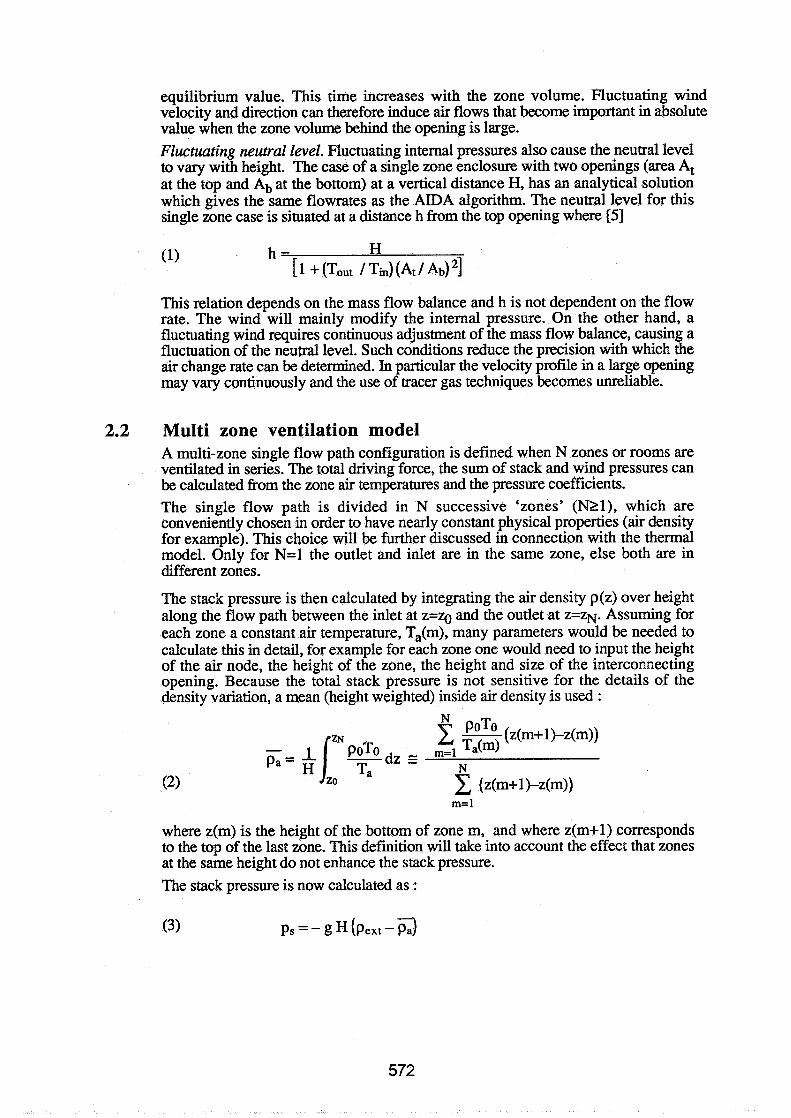
equilibrium value. This time increases with the zone volume. Fluctuating wind velocity and direction can therefore induce air flows that become important in absolute value when the zone volume behind the opening is large. Fluctuating neutral level. Fluctuating internal pressures also cause the neutral level to vary with height. The case of a single zone enclosure with two openings (area At at the top and Ab at the bottom) at a vertical distance H, has an analytical solution which gives the same flowrates as the AIDA algorithm. The neutral level for this single zone case is situated at a distance h from the top opening where [5]
This relation depends on the mass flow balance and h is not dependent on the flow rate. The wind will mainly modify the internal pressure. On the other hand, a fluctuating wind requires continuous adjustment of the mass flow balance, causing a fluctuation of the neutral level. Such conditions reduce the precision with which the air change rate can be determined. In particular the velocity profile in a large opening may vary continuously and the use of tracer gas techniques becomes unreliable.
2.2 Multi zone ventilation model A multi-zone single flow path configuration is defined when N zones or rooms are ventilated in series. The total driving force, the sum of stack and wind pressures can be calculated from the zone air temperatures and the pressure coefficients. The single flow path is divided in N successive 'zones' (NTl), which are conveniently chosen in order to have nearly constant physical properties (air density for example). This choice will be further discussed in connection with the thermal model. Only for N=l the outlet and inlet are in the same zone, else both are in different zones.
The stack pressure is then calculated by integrating the air density p(z) over height along the flow path between the inlet at z=zg and the outlet at z = z ~ . Assuming for each zone a constant air temperature, T,(m), many parameters would be needed to calculate this in detail, for example for each zone one would need to input the height of the air node, the height of the zone, the height and size of the interconnecting opening. Because the total stack pressure is not sensitive for the details of the density variation, a mean (height weighted) inside air density is used :
where z(m) is the height of the bottom of zone m, and where z(m+l) corresponds to the top of the last zone. This definition will take into account the effect that zones at the same height do not enhance the stack pressure. The stack pressure is now calculated as :
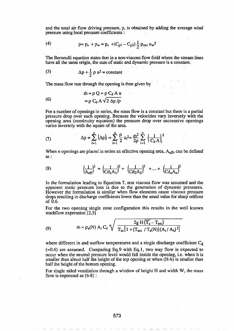
and the total air flow driving pressure, p, is obtained by adding the average wind pressure using local pressure coefficients :
The Bernoulli equation states that in a non-viscous flow field where the stream lines have all the same origin, the sum of static and dynamic pressure is a constant.
(5) Ap + - 1 p u2 = constant 2
The mass flow rate through the opening is then given by
For a number of openings in series, the mass flow is a constant but there is a partial pressure drop over each opening. Because the velocities vary inversely with the opening area (continuity equation) the pressure drop over successive openings varies inversely with the square of the area.
When n openings are placed in series an effective opening area, Aeff, can be defined as:
In the formulation leading to Equation 7, non viscous flow was assumed and the apparent static pressure loss is due to the generation of dynamic pressures. However the formulation is similar when flow elements cause viscous pressure drops resulting in discharge coefficients lower than the usual value for sharp orifices of 0.6. For the two opening single zone configuration this results in the well known stackflow expression [2,5]
where different in and outflow temperatures and a single discharge coefficient Cd ( ~ 0 . 6 ) are assumed. Comparing Eq.9 with Eq.1, two way flow is expected to occur when the neutral pressure level would fall inside the opening, i.e. when h is smaller than about half the height of the top opening or when (H-h) is smaller than half the height of the bottom opening. For single sided ventilation through a window of height H and width W, the mass flow is expressed as [6-81 :

For a single flow path it is not necessary to know the neutral pressure level explicitly. Due to the vertical flow resisitances the neutral level will depend on the flow rate. It is worth noting however that when multiple openings occur at the top and bottom of the configuration, grouping is sometimes possible using Eq.8, and then Eq. 1 applies again for the neutral level.
2.3 Cooling by ventilation When the zonal air temperatures, T,(m), are known the cooling rate for each zone is immediately available. The air temperature entering zone m is at the temperature of the previous zone Ta(m-1) and leaves the zone at Ta(m). The ventilation heat loss, aV(m), for zone m is therefore:
(10) aV (m) = rh Cp [Ta(m) - Ta(m-111
where 61, the air mass flow along the flowpath, is calculated from the ventilation model. The total ventilation heat loss from the flow path is
N (1 1) 0, = C Qv (m) = m Cp [Ta(N) - Ta(0lI
m=l
The zonal cooling rate cD,(m) should then be used in the heat balance for each zone.
3. THERMAL MODELING
The heat balance in the air node for each of the N-zones is obtained fiom the sum of the ventilation heat loss, OV(m), the heat transferred by convection between the wall and the air, Q,(m), and the convective heat gain in zone m, ag(m) :
(12) a, (m) + Ow (m) + a g (m) = 0
The heat flow at the wall-air interface in zone m depends on the convective heat transfer coefficient, h,, and the internal surface area of zone m, S(m) :
In general the convectively active heat exchanging surface area is smaller than the total internal wall surface area of zone m. This is illustrated in Figure 1. The fraction of S(m) for convective heat transfer is C,(m), so that Eq.13 is modified into
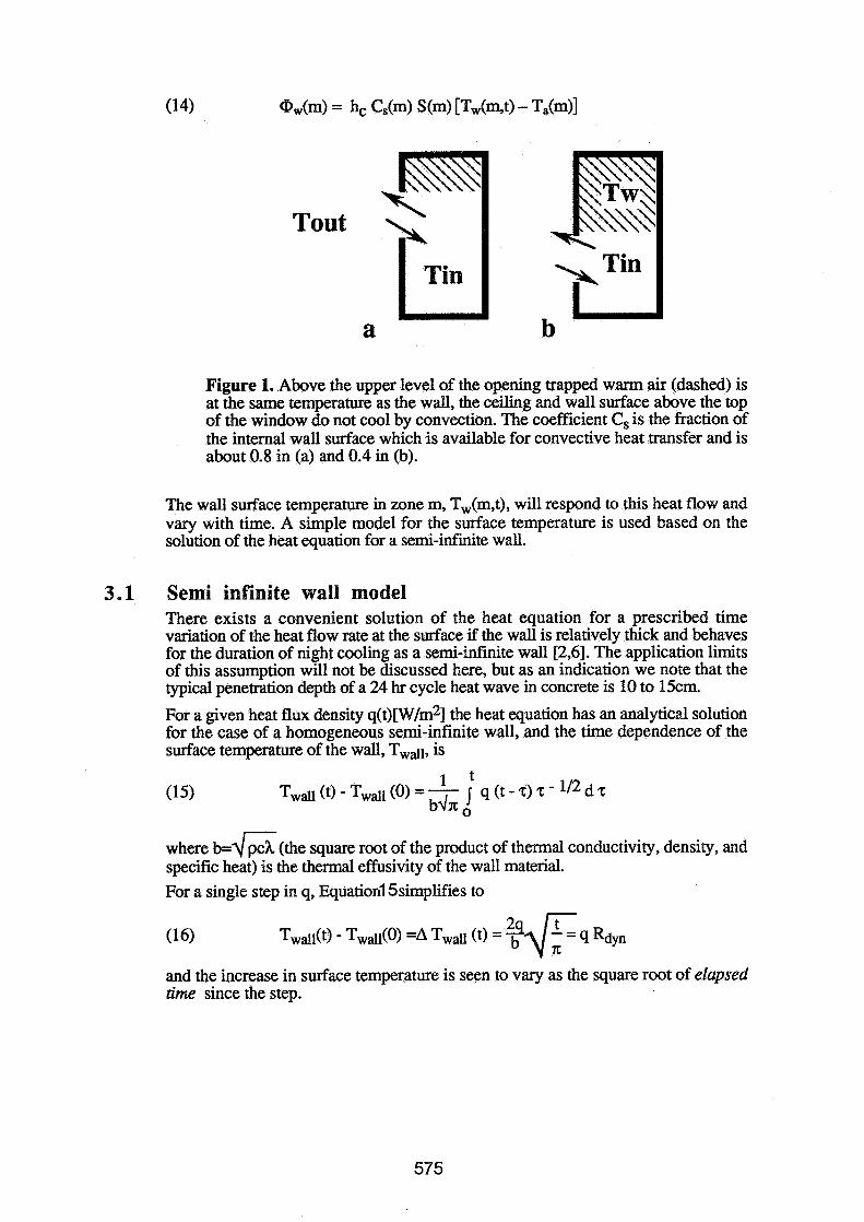
Tout
a
Figure 1. Above the upper level of the opening trapped warm air (dashed) is at the same temperature as the wall, the ceiling and wall surface above the top of the window do not cool by convection. The coefficient C, is the fraction of the internal wall surface which is available for convective heat transfer and is about 0.8 in (a) and 0.4 in (b).
The wall surface temperature in zone m, Tw(m,t), will respond to this heat flow and vary with time. A simple model for the surface temperature is used based on the solution of the heat equation for a semi-infinite wall.
3.1 Semi infinite wall model There exists a convenient solution of the heat equation for a prescribed time variation of the heat flow rate at the surface if the wall is relatively thick and behaves for the duration of night cooling as a semi-infinite wall [2,6]. The application limits of this assumption will not be discussed here, but as an indication we note that the typical penetration depth of a 24 hr cycle heat wave in concrete is 10 to 15cm.
For a given heat flux density q(t)w/m2] the heat equation has an analytical solution for the case of a homogeneous semi-infinite wall, and the time dependence of the surface temperature of the wall, Twdl, is
where b = G ( t h e square root of the product of thermal conductivity, density, and specific heat) is the thermal effusivity of the wall material. For a single step in q, Equation1 Ssimplifies to
and the increase in surface temperature is seen to vary as the square root of elapsed time since the step.

The superposition principle of the heat equation implies that when the function q(t) is given by a sum of step functions than the solution is given by a sum of solutions like Eq16 where time 't' is different for each step, being the elapsed time since the step happened. In Reference [2] the heat flux during night cooling was a function of time, but instead of dealing with the exact time history of heat flux, a history of constant q was assumed at each time step. This is a useful approximation when q is close to the time averaged value. When this is not acceptable as a solution, the time history can be approximated to any desired accuracy by a sum of step functions.
3.2 Thermal zonal response By applying a convective heat pulse to a closed zone m, the average heat flux at the wall will be q= @,(m) / S(m) and it is observed that the air temperature increases (in accordance with Eqs 13 and 16) like
where the typical time constant for air and little furniture is usually 10-30 minutes. After correction for background drift, AT,(t) /q and AT,(t) /q, can be plotted as a function of dt, providing a constant rate of change with slope 1.13lb. This experimental parameter b is called the effective thermal effusivity beff and characterizes the thermal response of the zone [2,6]. The experimental parameter beff is related to the thermal properties of the individual walls k of the zone m. If the surface areas are Sk(m), and the materials have nominal values for the thermal effusivities bk(m), there is the approximate relation :
where the sum over the n surfaces Sk(m) should equal S(m). Instead of having all the 2n input parameters for the individual wall surfaces, it is more practical to estimate bep
3.3 Multi zone cooling model The ventilative cooling model is obtained when the thermal zone model and the ventilation model are coupled through the air node temperatures. In Figure 2 the multizone cooling model is given schematically for three zones. Details of the used algorithm are given in Annex 1. With reference to Figure 2, the input parameters for each zone are :
- the exposed wall surface area S (m) and C,(m)
- the effective thermal effusivity bedm) - the initial wall temperature Tw(m)
- the internal heat gain a, (m)
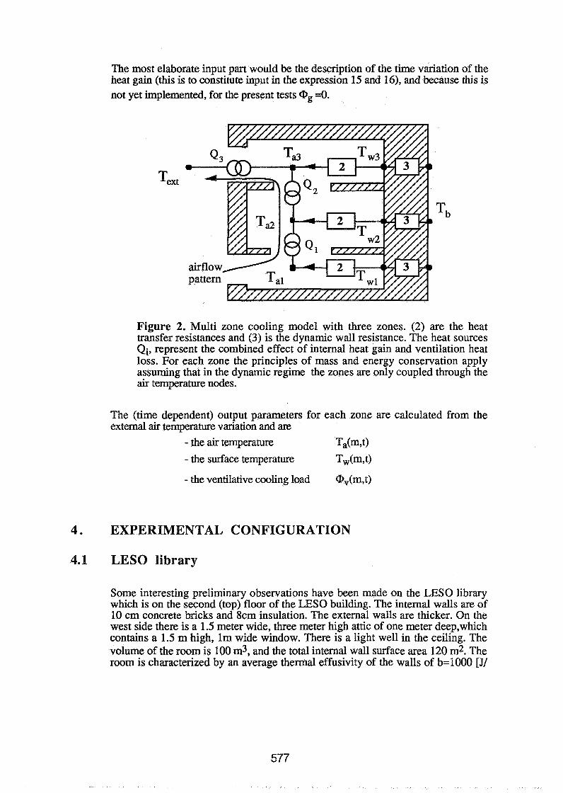
The most elaborate input part would be the description of the time variation of the heat gain (this is to constitute input in the expression 15 and 16), and because this is not yet implemented, for the present tests ==Q.
Figure 2. Multi zone cooling model with three zones. (2) are the heat transfer resistances and (3) is the dynamic wall resistance. The heat sources Qi, represent the combined effect of internal heat gain and ventilation heat loss. For each zone the principles of mass and energy conservation apply assuming that in the dynamic regime the zones are only coupled through the air temperature nodes.
The (time dependent) output parameters for each zone are calculated from the external air temperature variation and are
- the air temperature Ta(m,t) - the surface temperature T,(m,t)
- the ventilative cooling load @,(m,t)
4 . EXPERIMENTAL CONFIGURATION
4.1 LESO library
Some interesting preliminary observations have been made on the LESO library which is on the second (top) floor of the LESO building. The internal walls are of 10 cm concrete bricks and 8cm insulation. The external walls are thicker. On the west side there is a 1.5 meter wide, three meter high attic of one meter deep,which contains a 1.5 m high, lm wide window. There is a light well in the ceiling. The volume of the room is 100 m3, and the total internal wall surface area 120 m2. The room is characterized by an average thermal effusivity of the walls of b=l000 [JI
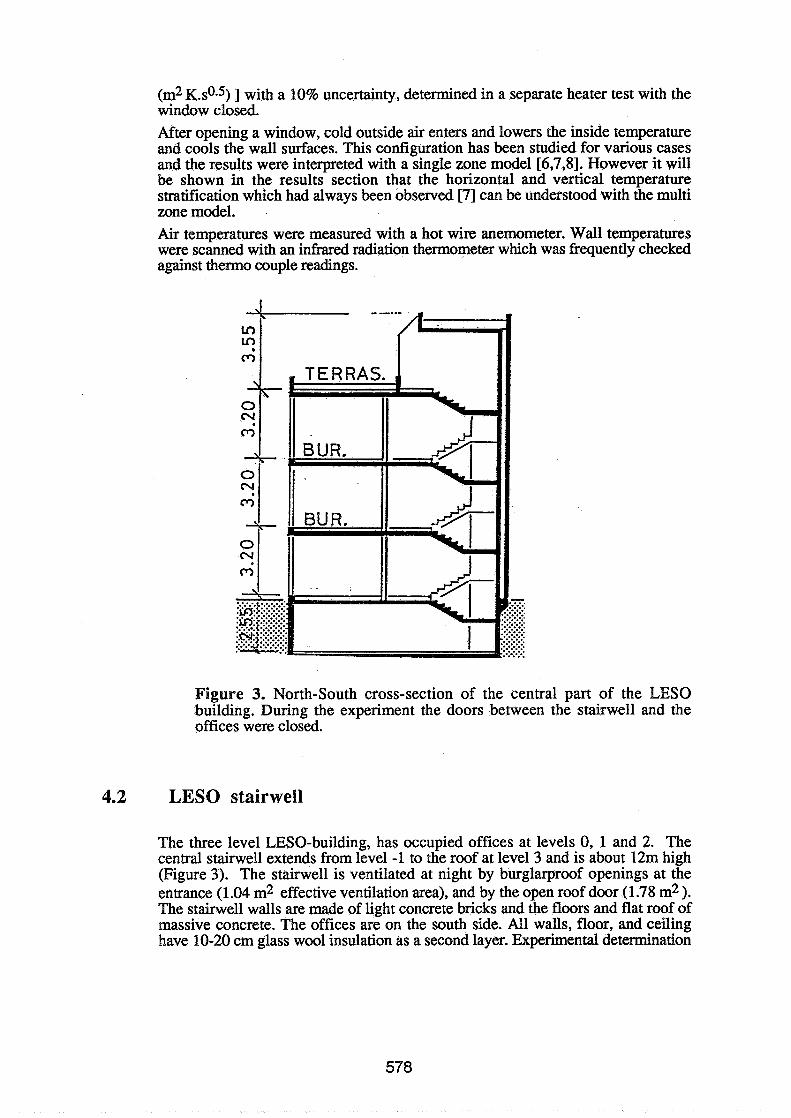
(m2 ~.s0.5) ] with a 10% uncertainty, determined in a separate heater test with the window closed. After opening a window, cold outside air enters and lowers the inside temperature and cools the wall surfaces. This configuration has been studied for various cases and the results were interpreted with a single zone model [6,7,8]. However it will be shown in the results section that the horizontal and vertical temperature stratification which had always been observed [7] can be understood with the multi zone model. .
Air temperatures were measured with a hot wire anemometer. Wall temperatures were scanned with an infrared radiation thermometer which was frequently checked against thermo couple readings.
Figure 3. North-South cross-section of the central part of the LESO building. During the experiment the doors between the stairwell and the offices were closed.
4.2 LESO stairwell
The three level LESO-building, has occupied offices at levels 0, 1 and 2. The central stairwell extends from level -1 to the roof at level 3 and is about 12m high (Figure 3). The stairwell is ventilated at night by burglarproof openings at the entrance (1.04 m2 effective ventilation area), and by the open roof door (1.78 m2 ). The stairwell walls are made of light concrete bricks and the floors and flat roof of massive concrete. The offices are on the south side. All walls, floor, and ceiling have 10-20 cm glass wool insulation as a second layer. Experimental determination

of the thermal effusivity [2] yielded a value of b=1100 Jl(m2KsO-5 ) with 10% uncertainty.
The total wall surface area of the stairwell (volume 4.5x8x15=540 m3) is calculated to be 700 m2 with a 10% uncertainty. The massive (20 to 30 cm thick) concrete stairwell itself is exposed on both sides and constitutes about 50% of the total heat- exchanging surface area. Air and wall temperatures were measured with calibrated Ptl00 temperature sensors and a datalogger system. The air temperature sensors were ventilated to avoid the influence of radiation by the warmer wall surfaces.
A heat flux probe was used with a stability and reproducibility better than 1 ~ l m 2 .
Figure 4. A layout of the library walls with a mapping of the drop in surface temperatures two hours after opening the window (TeXt=S0C). The floor is cooled strongly (north is to the right). The window is in the attic (grey) west.
Figure 5. Air flow pattern and definition of zones for the multizone model

5 . EXPERIMENTAL RESULTS
5.1 Results, LESO library In Figure 4, is shown a map of the drop of inside wall surface temperatures after a period of two hours with the window open. Before opening the window, the space was in quasi thermal equilibrium with initial temperatures all over the walls (2W0.5)OC. The floor surface was cooled by as much as 3OC in front of the window. Above the top of the window level (compare Figure I), the walls and ceiling temperature were not cooled by convection. In Figure 5, is shown the dominating air circulation (a gravity current flows from the window to the backwall) and the division into four zones. In Figure 6 the simulated surface and air temperatures are compared with measured data. Interestingly the horizontal and vertical temperature stratification is of the corect order of magnitude. For comparison, a single zone model would have taken the four zones together and predicting an air temperature of T,=15.9 and a surface temperature Tw=18.8 over the whole zone.
This example demonstrates that the multizone model produces a more realistic temperature distribution. The dominating air flow pattern should be known in advance however. Because of the influence of radiation between the walls (which is not included in the model) the model tends to overpredict temperature stratification for long cooling times. It should not be difficult however to add to the model, a first order correction for radiative coupling between the ceiling and the floor.
Figure 6. Cut through the library showing measured/simulated air (bold) and wall surface temperatures.
5.2 Results, LESO stairwell In Figure 7 are shown the measured air temperatures between 7 and 17 april at three levels in the stairwell, the ground level, the second level and in the sunspace at rooflevel. In the evening of 12 april the top and bottom ventilation openings of the
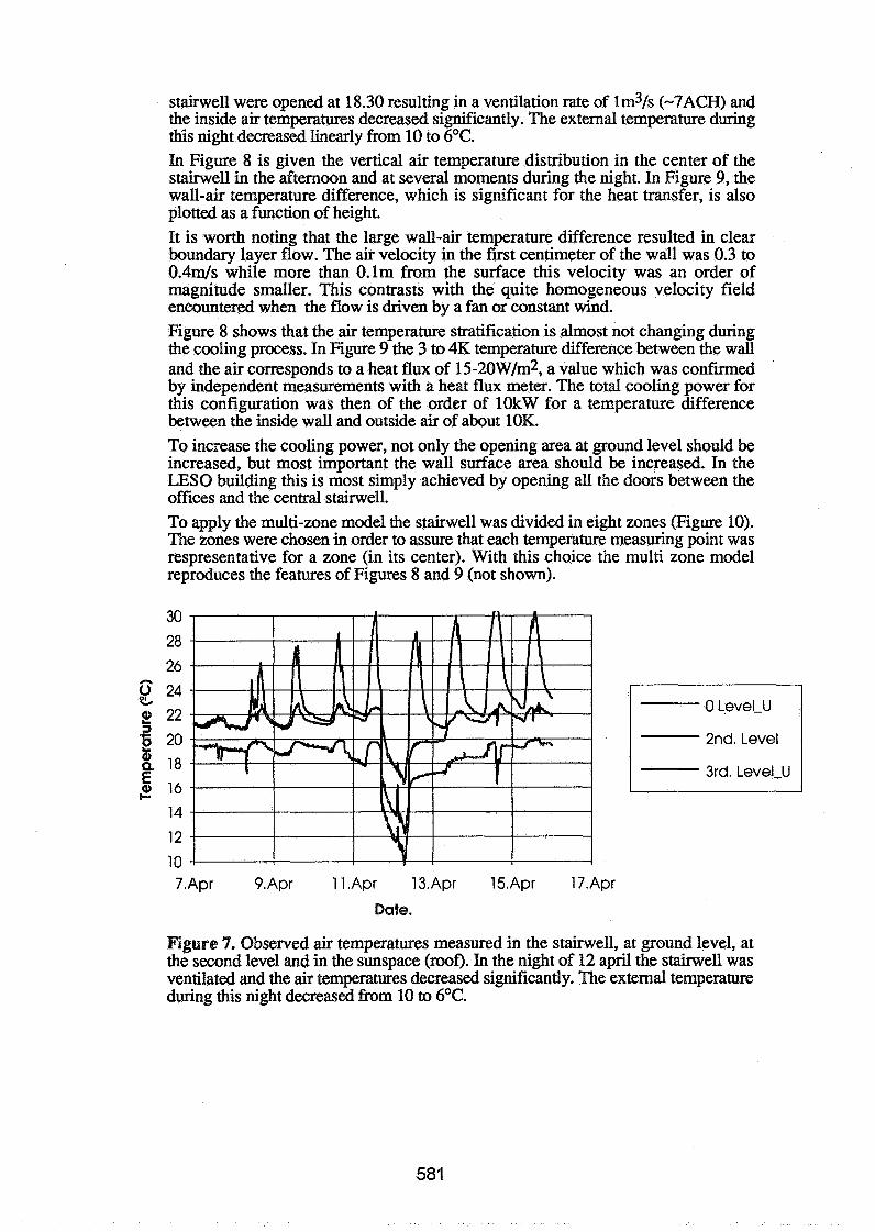
stairwell were opened at 18.30 resulting in a ventilation rate of lmvs (-TACH) and the inside air temperatures decreased significantly. The external temperature during this night decreased linearly from 10 to 6OC. In Figure 8 is given the vertical air temperature distribution in the center of the stairwell in the afternoon and at several moments during the night. In Figure 9, the wall-air temperature difference, which is significant for the heat transfer, is also plotted as a function of height. It is worth noting that the large wall-air temperature difference resulted in clear boundary layer flow. The air velocity in the first centimeter of the wall was 0.3 to 0.4m/s while more than O.lm from the surface this velocity was an order of magnitude smaller. This contrasts with the quite homogeneous velocity field encountered when the flow is driven by a fan or constant wind. Figure 8 shows that the air temperature stratification is almost not changing during the cooling process. In Figure 9 the 3 to 4K temperature difference between the wall and the air corresponds to a heat flux of 15-20Wlm2, a value which was confmed by independent measurements with a heat flux meter. The total cooling power for this configuration was then of the order of 10kW for a temperature difference between the inside wall and outside air of about 10K. To increase the cooling power, not only the opening area at ground level should be increased, but most important the wall surface area should be increased. In the LESO building this is most simply achieved by opening all the doors between the offices and the central stairwell. To apply the multi-zone model the stairwell was divided in eight zones (Figure 10). The zones were chosen in order to assure that each temperature measuring point was respresentative for a zone (in its center). With this choice the multi zone model reproduces the features of Figures 8 and 9 (not shown).
0 Level4
2nd. Level
3rd. Level-U
Date.
Figure 7. Observed air temperatures measured in the stairwell, at ground level, at the second level and in the sunspace (roof). In the night of 12 april the stairwell was ventilated and the air temperatures decreased significantly. The external temperature during this night decreased from 10 to 6OC.

hternal Air Tem~eratura
12
10
8
E 6 E C1) '5 4 x
2
0
-2 10 12 14 16 18 20 22 24 26 28 30
Temperature 6)
Figure 8. Observed air temperatures in the stairwell as a function of height above ground level.
Wall-Air Temperature Difference.
12
10
8
2 6 E .P 0 4 I
2 -x- 05:oO
0
-2 -4 -3 -2 -1 0 1 2 3 4 5 6
Difference 6)
Figure 9. Observed wall-air temperature difference as a function of height above ground level.

Figure 10. East-west stainvell section with indication of the eight zones used to compare with the experimentally measured temperatures.
6 DISCUSSION
The simplified model predicts correctly the order of magnitude of the temperature gradient fot the case of single sided ventilation as shown in Figure 6. Further, the decrease in air and wafl temperatures observed during night vendlarion of a stairwell and shown in Figore 7 is also reproduced by the model (the details of the comparison between measurements lurd the model can not be shown in this paper). A detailed comparison between the simplified model and more detailed bugding simulation models like ESP and COMIS will be performed. The f i t results show tbat for the particular problem under study (night ventilation over a single flow path) the simplified model explains the measured data sufficiently well requiring only few input parameters. More detailed thermal modeling (e.8. with ESP) will be necessary in particular for the simulation of a building over longer time periods, Also the mrrecr simulation of buildings that have low storage crcpacity and when the walls cannot be considered thick over a a one day period is reserved to detailed &is ,
While more detailed air flow modeling (e.g. COMIS) watlld be required when multiplc flow paths occur, the latter imply an Increased sensitivity of the output pmmerers for uncertainty in the input parameters. More w d must be done to Ism how to define the Limits of the zones. In articular when comparing with experiments, the calculated temperstures n ould be representative for the location of the temperature probes.
R

7 CONCLUSIONS
The effect of ventilative cooling was investigated and the data were analysed with a multi zonal cooling model based on the principles of mass and energy conservation. Applied to the cooling by single sided ventilation, it is found that the multi zone model has the advantage over the single zone model [2] that it gives additional information on the distribution of heat loss-rates and temperatures over the air flow path. The model is limited to the case where the airflow pattern is known in advance and where it can be assumed that the zones are ventilated in series. Measurements of the cooling of a stairwell by ventilation (single flow path configuration) are analysed with an eight zone model. The results show that the main features are reproduced. The model shows the influence of main design parameters like the opening position and size, and the exposed surface area of th& mass, and its distribution-
8 ACKNOWLEDGEMENTS
The authors acknowledge research support from the Swiss Federal Office of Energy (OFEN, Switzerland). The assistance of Pierre-Yves Bride1 and JosC-Antonio Rodriguez with the experiments and the data analysis was very much appreciated.
REFERENCES
[I] Kendrick J., 1993. "An overview of combined modelling of heat transport and air movement", Technical Note ArVC 40, Air Infiltration and Ventilation Centre, Coventry CV4 7EZ, GB.
[2] van der Maas J. and C-A Roulet, 1991. "Nighttime ventilation by stack effect". ASHRAE Transactions 1991 ,V.97,Pt. 1, 516-524.
131 Liddament M, 1989. "AEA - an air infiltration development algorithm", Air infiltration review, 11/1, p10-12; Palmiter L, 1990. "Mass flow for ADA", AIR 11/2.
[4] Clarke J A, 1985. Enerw simulation in building: design, Adam Hilger Ltd, Bristol, UK; Cockroft J P 1979. "Heat transfer and air flow in buildings", PhD Thesis, Univ. of
-.
Glasgow. [§I ASHRAE. (1985). 'ASHRAE handbook -1985 Fundamentals' Atlanta: American
Society of Heating, Refrigerating, and Air-Conditioning Engineers, Inc. [6] Van der Maas J.(editor), Allard F., Haghighat F., Liebecq G., Pelletret R.,
Bienfait D., Vandaele L. and Walker R, 1992. "Airflow through large openings in buildings", Technical Report of IEAIECB-Annex 20: Air flow patterns within buildings. (EPFLLESO-PB, CH-1015 Lausanne, Switzerland).
[7] Van der Maas J, Roulet C -A9 Hertig J -A, 1989. "Some aspects of gravity driven airflow through large openings in buildings" ASHRAE Transactions 1989, Vo1.95, Part 2, DD. 573-583
181 Jfin der Maas J., Roulet C.-A., 1990. "Ventilation and Energy loss rates after opening a window", Air infiltration review, Vol 11, No 4,1990, pp 12-15
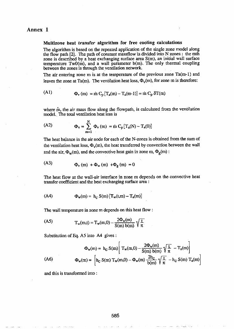
Annex 1
Multizone heat transfer algorithm for free cooling calculations The algorithm is based on the repeated application of the single zone model along the flow path [2]. The path of constant massflow is divided into N zones : the mth zone is described by a heat exchanging surface area S(m), an initial wall surface temperature TwO(m), and a wall parameter b(m). The only thermal coupling between the zones is through the ventilation network. The air entering zone m is at the temperature of the previous zone Ta(m-1) and leaves the zone at Ta(m). The ventilation heat loss, <D,(m), for zone m is therefore:
(All <a, (m) = m Cp [Ta(m) - ~ a ( m - 111 = m Cp 6T(m)
where m9 the air mass flow along the flowpath, is calculated from the ventilation model. The total ventilation heat loss is
N (A21 @, = C QV (m) = m Cp [Ta(N) - Ta(OlI
m=l
The heat balance in the air node for each of the N-zones is obtained from the sum of the ventilation heat loss, @,(m), the heat transferred by convection between the wall and the air, @,(m), and the convective heat gain in zone m, @&m) :
(A31 @, (m) + (m) +QTg (m) = 0
The heat flow at the wall-air interface in zone m depends on the convective heat transfer coefficient and the heat exchanging surface area :
The wall temperature in zone m depends on this heat flow :
Substitution of Eq. A5 into A4 gives :
and this is transformed into :
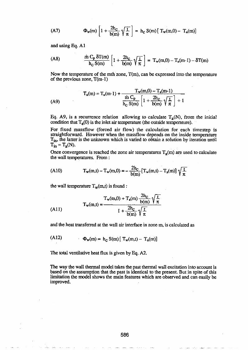
and using Eq. A 1
Now the temperature of the mth zone, T(m), can be expressed into the temperature of the previous zone, T(m- 1)
Eq. A9, is a recurrence relation allowing to calculate Ta(N), from the initial condition that Ta(0) is the inlet air temperature (the outside temperature). For fixed massflow (forced air flow) the calculation for each timestep is straightforward. However when the massflow depends on the inside temperature Tin, the latter is the unknown which is varied to obtain a solution by iteration until Ti, = Ta(N).
Once convergence is reached the zone air temperatures Ta(m) are used to calculate the wall temperatures. From :
the wall temperature T,(m,t) is found :
and the heat transferred at the wall air intexface in zone m, is calculated as
The total ventilative heat flux is given by Eq. A2.
The way the wall thermal model takes the past thermal wall excitation into account is based on the assumption that the past is identical to the present. But in spite of this limitation the model shows the main features which are observed and can easily be improved.
Energy Impact of Ventilation and Air Infiltration 14th AlVC Conference, Copenhagen, Denmark
21 -23 September 1993
Comparison of Multizone Air Flow Measurements and Simulations of the LESO Building Including Sensitivity Analysis
V Dorer,* J-M Furbringer"
* EMPA, Swiss Federal Laboratories for Materials Testing and Research, Section 175, Building Equipment, CH-8600 Dubendorf, Switzerland ** LESO-PB, Ecole Polytechnique Federale de Lausanne, CH-1015 Lausanne, Switzerland
Comparison of Multizone Air Flow Measurements and Simulations of the LESO Building including
Sensitivity Analysis
Viktor Dorer Jean-Marie Fiirbringer
Synopsis The LESO building is a three storey, medium-sized office building on the campus of the Swiss Institute of Technology in Lausanne. In this building component leakages have been carefully determined followed by extensive measurements of the boundary conditions as well as the air flows.
This paper first gives some basic concepts of the evaluation and the sensitivity analysis. Then, the measured data are compared with results from simulations performed with the COMIS multizone air flow program. The simulations include a sensitivity analysis which shows the influence of input errors on the calculated air flows. Leakage distribution, outdoor temperature, wind and wind pressure coefficient data are considered in this analysis.
The comparison shows good agreement for some cases. For other cases, the respective error bars of measured and calculated flows do not overlap and the agreement is poor.
The crucial part in such a comparison exercise is the modelling of the building. Especially for real buildings it is mostly very difficult to model the wind pressure accurately enough to be able to perform a conclusive comparison.
Future work aims at the development of flexible sensitivity analysis tools, which would be included in the simulation package and would be adaptable in a problem-oriented way to the actual case.
1 Introduction The goal of any computer code evaluation is to check that the program runs as specified, to assess its limits of application, to check its usability and, by a feedback effect, improve its performance.
The work presented in this paper deals with the evaluation of the multizone air flow model COMIS [I], in particular with the simulation code COMVEN. One step in this process is the comparison of measured and calculated data. Such a task requires sensitivity analysis and error propagation studies. The paper summarises the results for the application case "LESO building". The work presented has been performed within the Swiss project "ERL" 121 and now continues within the IEA-ECB Annex 23 "Multizone Air Flow Modelling", subtask 3, which also deals with the evaluation of COMIS [3].
The results of the Swiss project are comprehensively documented in [4]. Within Annex 23, comparisons between measured and calculated data are also made with data sets from other buildings, such as the ITALGAS-building [S] or the OPTIBAT test flat at INSA [6].
2 Comparison of simulations and experiments Comparing results from simulations and measurements must be understood as the comparison of two images of the reality, established on one side on the basis of algorithms and on the other side by using a specific measuring set up.
For many reasons, the calculated as well as the measured values contain errors. This has to be considered when comparing the two data sets. Agreement between results of measurements and simulations is concluded if there is a sufficient overlap of the respective error bars. More details on the

methodology for experimental comparison can be found in [7].
Confidence intervals for the simulation results have to be established using sensitivity and error propagation techniques on the basis of known or assumed errors in the input data. The techniques used for the present comparison are described below.
3 Sensitivity analysis The sensitivity analysis of a system is a statistical procedure necessary to determine the effect of specific input parameters on the output parameters. It highlights the parameters that affect the output results at the most. In other words, it shows which input parameters have to be determined with high accuracy and which parameters can be treated more generously.
For a specific case, sensitivity analysis is essential for the calculation of the propagation of errors in the input data and thus the confidence interval of the output data. A comprehensive description of sensitivity analysis techniques for the evaluation of air flow simulation can be found in [8].
In general, a sensitivity analysis would include in a first step all input pararneters describing the system, and a set of output parameters which covers all aspects of the problem. Nevertheless, for a multizone air flow problem, the number of input parameters is excessive for such a general approach. A reasonable set of relevant parameters has to be selected. At the initiation of this work it was thought that such a set could be defined once for a specific building. In the progress of the project it became clear that this selection is not only dependant on the building, but also on the specific case and also on which output parameters are of interest.
The next step in studying the effects of these relevant parameters is the determination of their ranges, hence defining the experimental domain. Here, the word "experimentat" refers to the numerical experience that constitutes a run of the code.
Full factorial design would consider all possible combinations considering the two values within the range for each relevant parameter, thus leading to 2R simulations (R: number of relevant parameters). The effects are estimated by fitting a polynomial function F(X) to a response Y which has been procured by running the set of experiments with the corresponding input vectors X. The polynomial F(X) can be more or less complicated depending on the level of interactions taken into account. The form used for this study is :
where N is the number of inputs used for each run of the experiment.
The coefficients ai are called the main effects of the parameter Xi and aij the conjugate effects of Xi and Xj. The relative effects ai/ao (aij/ao) are usually presented as the results, indicating in percentage the change of the selected output when varying Xi from its lowest to its highest level. The half effect ai 12 indicates the change from the centre to a limit of the range.
The values of the ai and aij coefficients are determined by running the code for a set of parameters selected in such a way that a well conditioned system of equations is obtained with a minimum number of runs. The methods for creating good experimental designs can be found in [9].
4 The LESO building The LESO building is a medium-sized administrative building constituted by nine south oriented cells with solar fagades, a few differently oriented rooms, and a staircase as shown in figure 1. Building related measurements, including aeraulic data, have been measured for many years. The data concerning the leakage characteristics and the air flows have been compiled in a set referred to as the "LESO data set" [lo].
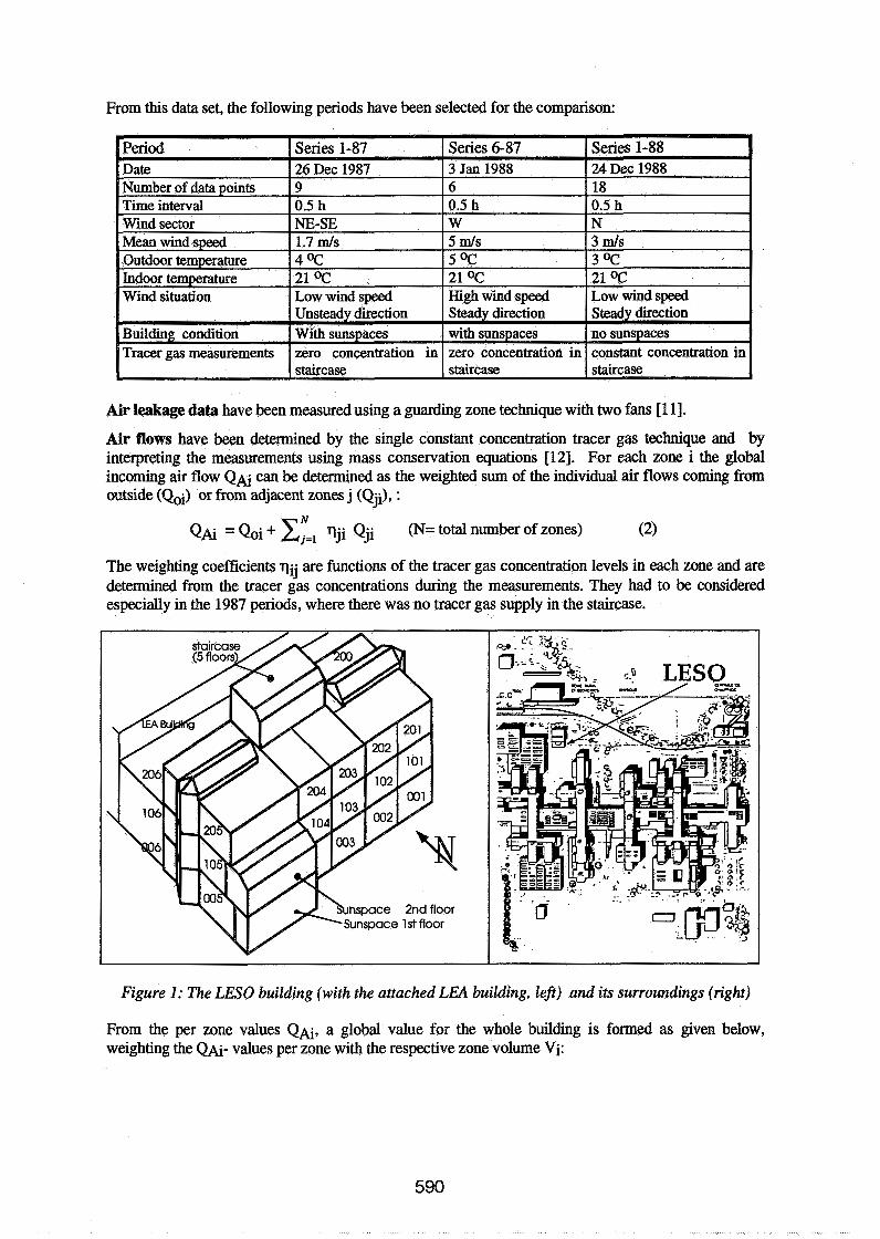
From this data set, the following periods have been selected for the comparison:
Air leakage data have been measured using a guarding zone technique with two fans [1 11.
Air flows have been detemined by the single constant concentration tracer gas technique and by interpreting the measurements using mass conservation equations [12]. For each zone i the global incoming air flow Q A ~ can be determined as the weighted sum of the individual air flows coming from outside (Qoi) or from adjacent zones j (Qji), :
N Q& = Q~~ + zjx1 qji Qji (N= total number of zones) (2)
The weighting coeffcients Vij are functions of the tracer gas concentration levels in each zone and are determined from the tracer gas concentrations during the measurements. They had to be considered especially in the 1987 periods, where there was no tracer gas supply in the staircase.
Figure 1: The LESO building (with the attached LEA building, left) and its surroundings (right)
From the per zone values Q&, a global value for the whole building is formed as given below, weighting the Q&- values per zone with the respective zone volume Vi:

i=l,N
In fact, this value does not differ significantly from the simple sum of all QA~- values.
Aeraulic model: For the sensitivity analysis as well as for the simulation of the measured periods, the building is represented by a network which consists of 11 zones and a total of 28 air flow links. These air flow links represent the measured leakages and are modelled by the well-known power law model for crack flow. Some measured coefficients have been split up arbitrarily between two or more conductance elements, especially in the staircase zone. The effect of the regrouped conductances is evaluated here. The consequences of the applied partition has been investigated in [13].
A typical section of such a network is given in figure 2 for the second floor of the building.
Figure 2: Typical section of theflow network ( Floor 2 for situation 1987).
5 Sensitivity analysis for the LESO building Experimental domain and observed output parameters
The experimental domain, that means the sets of relevant input parameters considered in this study are separated into two groups:
1. All the individual envelope leakage coefficients, the outdoor temperature and the wind speed, forming 12 sets of variables.
2. The wind pressure coefficients, forming 6 sets of variables per wind sector.
For the evaluation of a code, the performance with respect to all possible output options (e.g. energy losses, comfort, pollutant concentrations) should be considered. Thus, a well defined response set should have these completeness characteristics. In this study, for the purpose of comparison with measured values, only the incoming air flows QAi per zone have been chosen as the relevant output parameters. In addition, for the selection of the most relevant parameters, the mean age of air in the zone, calculated from the flow matrix has been considered.
MIS A
In order to speed up and automate the sensitivity analysis process, MISA, a multirun interface to COMVEN has been developed. This tool uses the basic input file, a file with the range for each input parameter included in the sensitivity analysis and a design file which contains the experimental matrix.
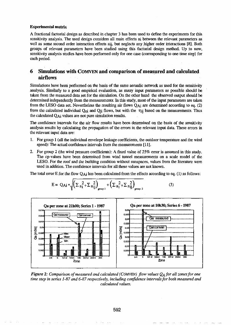
Experimental matrix
A fractional factorial design as described in chapter 3 has been used to def~ne the experiments for this sensitivity analysis. The used design considers all main effects ai between the relevant parameters as well as some second order interaction effects aij, but neglects any higher order interactions [8]. Both groups of relevant parameters have been studied using this factorial design method. Up to now, sensitivity analysis studies have been performed only for one case (corresponding to one time step) for each period.
6 Simulations with GOMVEN and comparison of measured and calculated airflows
Simulations have been performed on the basis of the same aeraulic network as used for the sensitivity analysis. Similarly to a good empirical evaluation, as many input parameters as possible should be taken from the measured data set for the simulation. On the other hand the observed output should be determined independently from the measurements. In this study, most of the input parameters are taken from the LESO data set. Nevertheless the resulting air flows a are determined according to eq. (2) from the calculated individual Qoi and Qji flows, but with the qij based on the measurements. Thus the calculated Q A ~ values are not pure simulation results.
The c ~ ~ d e n c e intervals for the air flow results have been determined on the basis of the sensitivity analysis results by calculating the propagation of the errors in the relevant input data. These errors in the relevant input data are:
1. For group 1 (all the individual envelope leakage coefficients, the outdoor temperature and the wind speed): The actual confidence intervals from the measurements [l 11.
2. For group 2 (the wind pressure coefficients): A fixed value of 25% error is assumed in this study. The cp-values have been determined from wind tunnel measurements on a scale model of the LESO. For the roof and the building condition without sunspaces, values from the literature were used in addition. The confidence intervals for all these values are not known.
The total error E for the flow Q A ~ has been calculated from the effects according to eq. (1) as follows:
Figure 2: Comparison of measured and calculated (COMVEN) flow values QA for all zones for one time step in series 1-87 and 6-87 respectively, including confidence intervals for both measured and
calculated values.
Qa per zone at 21h00, Series 1 - 1987
34 5 101-2 1034 105 201-2 m3-4 a5
Zone
Qa per zone at 10h30, Series 6 - 1987
Zone

Qa Building ; Series 1-1987
......* . . . ,*"o **'. 0- . I Winddir 1-QO <n ".,/ 0,.
\..-0' z c-
1 I 21h ' a h ' 2!3h Obh O1h
1.00
Time
Figure 3: Comparison of measured and calculated (C0MVEN)flow values QA for the whole building;
period 1-87
Figure 2 shows the measured and calculated air flows of each individual zone Q A ~ with their respective error bars for one time step in series 1-87 and in series 6-87 respectively.
In figure 3, measured and calculated room volume weighted total flows QA for the building are compared for the first winter period. Data for wind speed and direction are also plotted. The strong influence of the wind direction on the calculated flow can be clearly seen, but this is not reflected in the measured data. This fact can already lead to the conclusion that there might be some differencies between the influence of the wind on the tracer gas measurements and its influence on the calculated air flows.
Also for the period with stronger wind (6-87), rather large discrepancies exist between measurement and simulation. Again, the influence of the wind seems to be important. Better agreement is achieved for the 1-88 period.
Qa per zone at 22h30, Series 1 - 1988 Qa building; Series 1 - 1988
Zone 0 ~ ~ 2 3 ' 0 ' j S 2 ' 3 ' 4 ' 5 ' 6 ' 7 ' Time [h]
Figure 4: Comparison of measured and calculated flow values for period 1-88 QA~-values per zone (lefl and QA-value for the whole building (right).
7 Conclusions and future work Comparison of measured and calculated flows for the LESO building
For all three periods investigated, the calculated air flows are smaller than the measured ones. Most significant discrepancies between measurement and simulation are not in situations with low wind, but rather in that with strong wind. The reasons for the partially unsatisfactory compliance of measured and calculated data are not yet fully understood and subject of the ongoing work in Annex 23. Compared to eatlier work [4],[13], also the inclusion of the wind pressure coefficients into the set of relevant parameters (only with assumed errors though) did not lead to a significantly better agreement between the confidence intervals of measured and calculated air flows. Further investigations will include:
e The consideration of the influence of the building attached next to the LESO (the LEA building). o The evaluation of the concept of wind pressure coefficients in general for this heavily shielded
building, especially for the low wind speed cases. o The determination of the confidence intervals in the wind pressure coefficients used and the
measurement of wind pressures on the real building. e The consideration of possible errors in the qji - values used.
Sensitivity Analysis
When this sensitivity analysis work was initiated, it was assumed that one single set of relevant parameters could be established for a specific building. This work has shown, that the sensitivity and error propagation analysis has to be performed as case dependent. Consecutively, error propagation calculations cannot be based on one singular sensitivity analysis, but sensitivity and error propagation have to be seen as one integral analysis. For air flow studies over a larger time period, this task cannot be performed without a high degree of automation. As a consequence, present and future work concentrates on the development of flexible and powerful routines which will be integrated into the simulation code. This will form a valuable tool for the user of the program and allow him to perform on-line sensitivity and error propagation studies for the actual case under investigation. Besides factorial design, also Monte Carlo techniques will be used.
Program evaluation by comparing measurements and simulation results
It is absolutely necessary to know the accuracy of the measured data and that of the input data as well as the confidence intervals of the simulation results. The sensitivity and error propagation analysis procedures shown have proved to be a valuable tool for this kind of evaluation work.
As mentioned, both measurements and simulations are images of the reality. Thus, in order to be able to evaluate the program, one has to be sure that the data of the measured validation set and 'reality' are as close as possible. This is especially valid for the measured data used as input for the simulations.
As is shown in [6] and [14], measured and calculated air flow results are within 10% for a multizone structure also, if the real leakages and the pressure distribution on the fagades are accurately known.
A second, preliminary conclusion from the on-going evaluation work is that the measured building should not be too complex. In a complex building, there are many interactions between a large number of relevant parameters, making it very difficult to understand and explain the resulting air flow situation. Also, in a complex network, the pressure and thus the flow field can be in an unstable equilibrium condition and thus be very sensitive to small changes in the boundary conditions.
Application limits for multizone models
For most simulation tasks, the modelling and the defmition of the boundary conditions is the crucial part of the work. For multizone air flow simulations of real buildings, uncertainties in the leakage distribution and the modelling of the wind pressures may substantially limit the accuracy of the results.

Nevertheless it is expected that air flow simulation tools will be used more and more for the design of energy efficient ventilation systems and control strategies which provide a comfortable and healthy indoor air environment.
Acknowledgements The work of Frederik Huck for the simulations and the graphics and the contributions of Andreas Weber to the development of COMVEN and the MISA routines are gratefully acknowledged.
This work was supported by the Swiss Federal Department of Energy.
References 1. FEUSTEL, H.E. ET AL.: "Fundamentals of the Multizone Air Flow Model COMIS"
AIVC TN 29, Great Britain, May 1990.
2. Swiss Research Program "Energy Relevant Air Flows in Buildings", Yearly Progress Reports 1987-1992, F. Widder, PSI, CH- 5232 Villigen PSI-Ost, Switzerland.
3. ROULET, C.-A. AND FORBRINGER J.-M.: " IEA-ECB Annex 23, Subtask 3: The Evaluation of a Multizone Infiltration Computer Code", Proc. of International Symposium on Air Flow in Multizone Structures, Budapest, Hungary, 9 Sept. 1992.
4. DORER, V.; F~~RBRINGER, J.-M.; HUCK, F. AND ROULET, C.-A.: "Evaluation of COMERL with the LESO Dataset". Final Report ERL 34.1 , EMPA 175, CH-8600 Diibendorf, Switzerland, Dec. 1992.
5. F~~BRINGER, J.-M. AND BORCHIELLINI, R.: "Technique of Sensitivity Analysis applied to an Air Infiltration Multizone model.". ASHRAE summer meeting, Denver, July 1993.
6. FADIGA, A. : "Contribution A la caract4risation abraulique des b5timent.s. Etude des transferts drauliques dans les locaux multizones". Thesis at the INSA Lyon, France, 1993.
7. BOW, N.T. AND LOMAS, K.J.: "Empirical validation of Dynamic Thermal Programs of Buildings". Building Service Engineering Research and Technology, 6 (4), pp. 153- 162, 1985.
8. FURBRINGER, J.M.: "Evaluation Procedure Using Sensitivity Analysis of Model and Measurement". Proc. of International Symposium on Air Flow in Multizone Structures, Budapest, Hungary, 9 Sept. 1992.
9. Box, G.E.P.; HUNTER, W.G., AND HUNTER, J.S.: "Statistics for Experimenters: An Introduction to Design, Data Analysis and Model Building". Wiey Series in probability and mathematical statistics, John Wiley, New York, 1978.
10. FORBRINGER, J.-M.; COMPAGNON, R. AND ROULET, C.-A,: Projet NEFF 339.1 "Validation de programmes de calcul des Bchanges d'air A l'aide de mesures exfirirnentales". Final report, LESO-PB, EPFL, Lausanne, Switzerland, 1990.
11. FORBRINGER, J.-M. AND ROULET, C.-A.: "Study of the errors occurring in measurement of leakage distribution in buildings by multifan pressurisation". Building and Environment, vol26, no 2,1991.
12. COMPAGNON, R.;FORBRINGER, J.-M. AND JAKOB, M.: "Mesure d'khange &air entre les locaux et avec I'ext6rieur". Final report project NEFF 339.2, EPFL-LESO, Lausanne, Switzerland 1991.
13. FURBRINGER, J.-M.; DORER, V.; HUCK, F. AND WEBER, A.: "Air Flow Simulation of the LESO Building including a Comparison with Measurements and a Sensitivity Analysis", Proc. of INDOOR AIR 93', 1993.
14. MEGRI, A. C.: " ModBlisation des transferts abrauliques dans les b5timents multizones Quip6s d'un systeme de ventilation; prise en compte de la qualit4 de l'air"; Thesis INSA- CETHIL, Lyon, France, 1993.

Energy Impact of Ventilation and Air Infiltration 14th AlVC Conference, Copenhagen, Denmark
21 -23 September 1993
Proximity Effects: Air Infiltration and Ventilation Heat Loss of a Low-Rise Office Block Near a Tall Slab Building
* Building Research Establishment, Garston, Watford WD2 7JR, UK ** Department of Physics, Brunel University, Uxbridge KUB8 3PH, UK
Crown Copyright 1993 - Building Research Establishment
SUMMARY In the mid-1980s, two London architects postulated that deflection of higher speed air from tall slab buildings could increase air infiltration from a neighbouring low-rise block, increasing its associated ventilation heat loss. These issues have been of much concern during the past two decades among designers, developers and local authorities; especially those considering in-fill near tall buildings.
This preliminary study looks at the ventilation and space-heating loss of a three-storey low-rise office block located near a taller nine-storey slab building. A multi-zoned prediction program is used to determine the air infjdtration through the envelope of the low building and ventilation through its purpose-provided trickle ventilators. Measurements carried out in the Building Research Establishment's Environmental Wind Tunnel provide the necessary input data on surface wind pressure coefficients.
The wind tunnel measurements show that a tall building near to (and in line with) a low building markedly changes the distributions of wind pressures on the latter. Analysis carried out here confi is that this near-proximity does have an impact on ventilation. Compared with an isolated building:
(a) ventilation rates are reduced by as much as 35% for winds blowing normal to the front (broad) face,
(b) the average ventilation rates expected during the heating season are reduced by about 15% if the buildings are on an open site and by 10% if sheltered. However, adequate ventilation for occupants is met by using the controllable trickle ventilators, and
(c) overall space-heating requirements are marginally increased by 3% as a result of higher convective losses offsetting the reduced ventilation losses.
1. INTRODUCTION Tall slab buildings can create undesirable wind environments at ground level [I] by deflecting downwards the higher speeds encountered at the upper levels. In certain instances, a low-rise block located windward of a tall building not only stabilises the horizontal-axis vortex fonned in front of the tall building (Figure 1) but also enhances its strength.
In the mid-1980s, two London architects postulated [2] that deflection of higher speed air from tall slab buildings could increase air infjdtration from a neighbouring low-rise block thereby increasing its associated ventilation heat loss. These issues have been of considerable concern during the past two decades to designers, developers and local authorities, especially those considering in-fill near tall buildings.
The study reported here looks at ventilation and space-heating loss during the heating season of a three-storey low-rise office block located near a taller nine-storey slab building. To take into account infjdtration losses, this sthdy also looks at the effect different levels of envelope leakage have on this 'proximity effect'.
study uses the BRE multi-zoned prediction program BREEZE to de the air

infiltration through the building envelope and ventilation airflows through purpose- provided trickle ventilators. Measurements were carried out in the BRE Environmental Wind Tunnel to obtain the surface wind pressure coefficient data necessary for these predictions.
The expected ventilation performance (i.e. how often various ventilation rates are expected during occupied periods) of the building were obtained by combining the predicted ventilation characteristics with weather statistics at the building site. Space heating calculations were carried out using the expected average airchange rates in a standard CIBSE [3] design procedure.
2. PREDICTION SET-UP The BRE multi-celled ventilation prediction program BREEZE was used to carry out this study. This program has been previously validated with full-scale measurements [4]. In the program, the building is taken to have a number of interconnected zones, each at a specific pressure, with air moving from regions of high to low pressures. All internal doors were kept open in the simulations carried out in this study.
Pressure differentials are set up by both the action of wind on the external surface of the building and the temperature difference between inside and outside air. The amount of air flowing between the outside and various zones, or between the zones themselves, is governed by the magnitude of pressure differentials and by the type of flow path (such as open doors and windows). The analysis procedure applies methods of network flow computation and uses mass balance to obtain an interior static pressure within the building by requiring that the inflows and outflows for each zone balance.
BREEZE incorporates an algorithm which accounts for infiltration through the external envelope[5] and a unique implementing method for multi-celled buildings. Background leakage is modelled as leakage distributed over the whole of the permeable envelope.
2.1. Low-rise Building The low-rise building chosen for the study is the BRE low-energy office, which has been the subject of extensive heating, ventilation and energy-saving tests [6]. It is similar in form and size to many low-rise, medium-sized and naturally-ventilated office buildings in the UK. This three-storey building (Figure 2) is rectangular (60 m x 12 m) in plan with floor-to-ceiling heights of 2.6 m.
Offices are located on each floor along either side of a central conidor running along east-west. The main entrance to the building is on the north-facing facade. The estimated total volume of the building is 5430 m3 and the external surface area is 1930 m2.
Envelope leakage Previous work 171 indicated that it is possible to categorise the airtightness of UK buildings as either 'tight9, 'average' or 'leaky' if the air leakage Q through the envelope is respectively 5, 10 or 20 m3/h per m2 (of envelope area) when a pressure differential Ap of 25 Pa is maintained across it.
For use within the prediction program, the above values were translated to the form of the power-law equation
where n was set at 0.6 and the value of k was varied to simulate different envelope airtightness. This leakage was evenly distributed throughout the outside walls and roof.
Purpose-provided openings Previous work [8] showed that, during the heating season, trickle-ventilators with openable areas of 400 mm2 per m2 (of floor area) can provide adequate background ventilation to satisfy fresh air requirements for metabolic needs of occupants and to control body odour. Therefore, for this study, trickle-ventilators with appropriate openable areas were incorporated into the building envelope in each room.
The relationship between volume aimow rate, q and pressure difference Ap for these devices were taken to be 191:
where A is the area of the opening, C!, is a constant (= 0.61) usually known as the discharge coefficient and p is the density of air passing through the opening.
2.2. Wind Tunnel Tests Surface wind pressure coefficients for use in the prediction procedure were obtained by carrying out wind tests using 1:200 scale models of the three-storey, 9rn high building and a nine-storey, 27m high building with a similar plan form. With the two buildings in-line and their long faces parallel to each other, the following proximity configurations were tested:
(1) low building on its own, (2) low building with tall building at a separation of 27m (the height of the
tall building) (3) low building with tall building at a separation of 9m (the height of the
low building).
The pressure-tapped model of the low building, together with the nearby tall building model were mounted on a 1.75 m diameter turntable in the BRE Environmental Wind Tunnel. Measurements were carried out with a simulation of the approaching wind corresponding to that over suburban terrain at a scale of 1:200. Fuller details of the simulation are given in reference [lo].
All pressures were meamed using pressure transducers and scani-valve systems under on-line computer control. Details of the system and data-acquisition procedure can be found elsewhere [I I]. For each of 12 wind directions at 30' intervals, the pressure coefficients at all the taplpings on the low building were obtained by nomalising the measured pressures by the reference dynamic pressure. This reference was measured at roof-height of the low building and well upstream of the model.
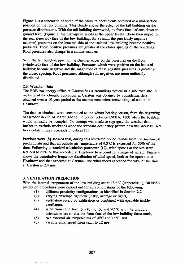
Figure 3 is a schematic of some of the pressure coefficients obtained at a mid-section position on the low building. This clearly shows the effect of the tall building on the pressure distributions. With the tall building downwind, its front face deflects down to ground level (Figure 1) the high-speed winds at the upper levels. These then impact on the rear (leeward) face of the low building. As a result, the previously negative (suction) pressures on the leeward side of the isolated low building become positive pressures. These positive pressures are greater at the closer spacing of the buildings. Roof pressures also change in a similar manner.
With the tall building upwind, the changes occur on the pressures on the front (windward) face of the low building. Pressures which were positive on the isolated building become negative and the magnitude of these negative pressures is greater at the closer spacing. Roof pressures, although still negative, are more uniformly distributed.
2.3. Weather Data The BRE low-energy office at Garston has surroundings typical of a suburban site. A measure of the climatic conditions at Garston was obtained by considering data obtained over a 10-year period at the nearest convenient meteorological station at Heathrow.
The data so obtained were constrained to the winter heating season, from the beginning of October to end of March and to the period between 0900 to 1800 when the building would normally be occupied. No attempt was made to segregate the weather data further to exclude weekends since the standard occupancy pattern of a full week is used to calculate energy demands in offices [3].
Previous work [$I showed that, during this restricted period, winds from the south-west predominate and that an outside air temperature of 9.3"C is exceeded for 50% of the time. Following a standard calculation procedure [12], wind speeds at the site were reduced to 62% of that recorded at Heathrow to account for change of terrain. Figure 4 shows the cumulative frequency distribution of wind speed, both at the open site at Heathrow and that expected at Garston. The wind speed exceeded for 50% of the time at Garston is 2.4 m/s.
3. VENTILATION PREDICTION With the internal temperature of the low building set at 18.5"C (Appendix l), BREEZE prediction procedures were carried out for all combinations of the following:
(1) different proximity configurations as identified in Section 2.2, (2) varying envelope tightness (leaky, average or tight), (3) ventilation solely by infiltration or combined with openable trickle-
ventilators, (4) wind from four directions (0, 30,60 and 90%) with the building
orientation set so that the front face of the low building faces north, (5) two external air temperatures of -6°C and 16"C, and (6) varying wind speed from calm to 12 4 s .
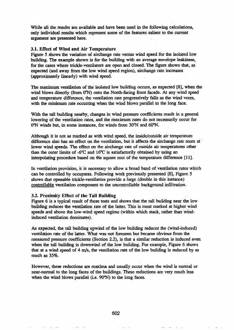
While a l l the results are available and have been used in the following calculations, only individual results which represent some of the features salient to the current argument are presented here.
3.1. Effect of Wind and Air Temperature Figure 5 shows the variation of airchange rate versus wind speed for the isolated low building. The example shown is for the building with an average envelope leakiness, for the cases where trickle-ventilators are open and closed. The figure shows that, as expected (and away fiom the low wind speed region), airchange rate increases (approximately linearly) with wind speed.
The maximum ventilation of the isolated low building occurs, as expected [8], when the wind blows directly (from OW) onto the North-facing front facade. At any wind speed and temperature difference, the ventilation rate progressively falls as the wind veers, with the minimum rate occurring when the wind blows parallel to the long face.
With the tall building nearby, changes in wind pressure coefficients result in a general lowering of the ventilation rates, and the maximum rates do not necessarily occur for 0% winds but, in some instances, for winds from 30% and 60%.
Although it is not as marked as with wind speed, the inside/outside air temperature difference also has an effect on the ventilation, but it affects the airchange rate more at lower wind speeds. The effect on the airchange rate of outside air temperatures other than the outer limits of -6°C and 16°C is satisfactorily obtained by using an interpolating procedure based on tlie square root of the temperature difference [ll].
In ventilation provision, it is necessary to allow a broad band of ventilation rates which can be controlled by occupants. Following work previously presented [8], Figure 5 shows that openable trickle-ventilators provide a large (double in this instance) controllable ventilation component to the uncontrollable background infjdtration.
3.2. Proximity Effect of the Tall Building Figure 6 is a typical result of these tests and shows that the tall building near the low building reduces the ventilation rate of the latter. This is most marked at higher wind speeds and above the low-wind speed regime (within which stack, rather than wind- induced ventilation dominates).
As expected, the tall building upwind of the low building reduces the (wind-induced) ventilation rate of the latter. What was not foreseen but became obvious from the measured pressure coefficients (Section 2.2), is that a similar reduction is induced even when the tall building is downwind of the low building. For example, Figure 6 shows that at a wind speed of 4 m/s, the ventilation rate of the low building is reduced by as much as 35%.
However, these reductions are maxima and usually occur when the wind is normal or to the long faces of the buildings. These reductions are very much less
when the wind blows parallel (i.e. 90%) to the long faces.
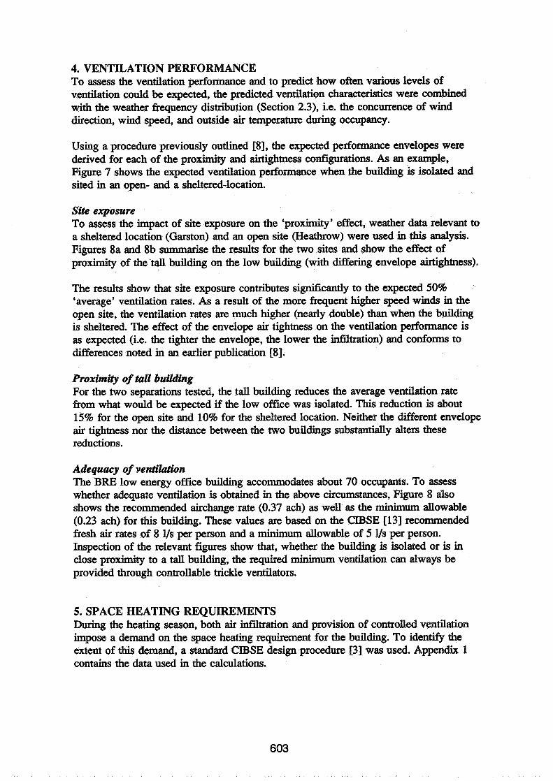
4. VENTILATION PERFORMANCE To assess the ventilation performance and to predict how often various levels of ventilation could be expected, the predicted ventilation characteristics were combined with the weather frequency distribution (Section 2.3), i.e. the concurrence of wind direction, wind speed, and outside air temperature during occupancy.
Using a procedure previously outlined 181, the expected performance envelopes were derived for each of the proximity and airtightness configurations. As an example, Figure 7 shows the expected ventilation performance when the building is isolated and sited in an open- and a sheltered-location.
Site exposure To assess the impact of site exposure on the 'proximity' effect, weather data relevant to a sheltered location (Garston) and an open site (Heathrow) were used in this analysis. Figures 8a and 8b summarise the results for the two sites and show the effect of proximity of the tall building on the low building (with differing envelope airtightness).
The results show that site exposure contributes significantly to the expected 50% 'average' ventilation rates. As a result of the more frequent higher speed winds in the open site, the ventilation rates are much higher (nearly double) than when the building is sheltered. The effect of the envelope air tightness on the ventilation performance is as expected (i.e. the tighter the envelope, the lower the infiltration) and conforms to differences noted in an earlier publication [8].
Proximity of tall building For the two separations tested, the tall building reduces the average ventilation rate from what would be expected if the low office was isolated. This reduction is about 15% for the open site and 10% for the sheltered location. Neither the different envelope air tightness nor the distance between the two buildings substantially alters these reductions.
Adequacy of ventilation The BRE low energy office building accommodates about 70 occupants. To assess whether adequate ventilation is obtained in the above circumstances, Figure 8 also shows the recommended airchange rate (0.37 ach) as well as the minimum allowable (0.23 ach) for this building. These values are based on the GIBSE [13] recommended fresh air rates of 8 l/s per person and a minimum allowable of 5 Vs per person. Inspection of the relevant figures show that, whether the building is isolated or is in close proximity to a tall building, the required minimum ventilation can always be provided through controllable trickle ventilators.
5. SPACE HEATING REQUIREMENTS During the heating season, both air Sitration and provision of controlled ventilation impose a demand on the space heating requirement for the building. To identify the extent of this demand, a standard CIBSE design procedure 131 was used. Appendix 1 contains the data used in the calculations.
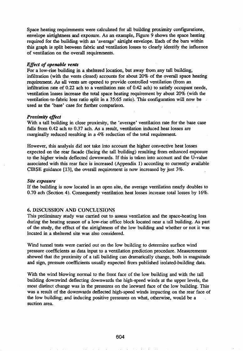
Space heating requirements were calculated for all building proximity configurations, envelope airtightness and exposure. As an example, Figure 9 shows the space heating required for the building with an 'average' airtight envelope. Each of the bars within this graph is split between fabric and ventilation losses to clearly identify the influence of ventilation on the overall requirements.
Eflect of opeituhle vents For a low-rise building in a sheltered location, but away from any tall building, infitration (with the vents closed) accounts for about 20% of the overall space heating requirement. As all vents are opened to provide controlled ventilation (from an infitration rate of 0.22 ach to a ventilation rate of 0.42 ach) to satisfy occupant needs, ventilation losses increase the total space heating requirement by about 20% (with the ventilation-to-fabric loss ratio split in a 3565 ratio). This configuration will now be used as the 'base' case for further comparison.
Proximity effect With a tall building in close proximity, the 'average' ventilation rate for the base case falls from 0.42 ach to 0.37 ach. As a result, ventilation induced heat losses are marginally reduced resulting in a 4% reduction of the total requirement.
However, this analysis did not take into account the higher convective heat losses expected on the rear facade (facing the tall building) resulting from enhanced exposure to the higher winds deflected downwards. If this is taken into account and the U-value associated with this rear face is increased (Appendix 1) according to currently available CIBSE guidance 1131, the overall requirement is now increased by just 3%.
Site exposure If the building is now located in an open site, the average ventilation nearly doubles to 0.70 ach (Section 4). Consequently ventilation heat losses increase total losses by 16%.
6. DISCUSSION AND CONCLUSIONS This preliminary study was carried out to assess ventilation and the space-heating loss during the heating season of a low-rise office block located near a tall building. As part of the study, the effect of the airtightness of the low building and whether or not it was located in a sheltered site was also considered.
Wind tunnel tests were carried out on the low building to determine surface wind pressure coefficients as data input to a ventilation prediction procedure. Measurements showed that the proximity of a tall building can dramatically change, both in magnitude and sign, pressure coefficients usually expected from published isolated-building data.
With the wind blowing normal to the front face of the low building and with the tall building downwind deflecting downwards the high-speed winds at the upper levels, the most distinct change was in the pressures on the leeward face of the low building. This was a result of the downwards deflected high-speed winds impacting on the rear face of the low building; and inducing positive pressures on what, otherwise, would be a suction area.

The consequence of this was that the predicted ventilation fell by as much as 35% compared with rates predicted for the building in isolation. These reductions occmed when the wind blew normal (or nearly normal) to the front (broad) face of the low building. ow ever, these changes did not occur with winds blowing parallel to the long faces of the two buildings.
The 'average' ventilation rates expected for 50% of the time during the heating season (and when the building is occupied) were evaluated using concurrent wind speed, wind direction and air temperature meteorological data. Results indicated that the 'proximity' effect reduces the 'average' rate by about 15% if the buildings are located in an open site and by 10% if sheltered. However, the required minimum ventilation rate for occupants can always be met by using controllable trickle ventilation.
The 'proximity' effect on the space heating requirement for the low building was assessed. Analysis showed that while the lower 'average9 ventilation rate reduced (by 4%) the heating requirement, this was offset by the higher fabric loss from the rear face of the buildings. The analysis predicted a slight overall increase of just 3%.
In conclusion, preliminary analysis shows that a tall building in near proximity to and in-line with a low-rise building has an impact on the ventilation of the latter. Compared with an isolated building:
(a) ventilation rates of the low building can be reduced by as much as 35% for winds blowing normal to the front (broad) face,
(b) average ventilation rates expected during the heating season can be reduced by 15% if it is an open site and by 10% if sheltered, and
(c) overall space-heating requirements are marginally increased by 3% as a result of higher convective losses offsetting the reduced ventilation losses.
ACKNOWLEDGEMENTS Thanks to Dr Eric Solomon of Engineering Computations for modifying and updating the BREEZE program to handle as effectively as possible the 5,000 or so separate computer runs necessary for this study.
REFERENCES 1. Penwarden A D and Wise A F E. Wind environment around buildings.
Building Research Establishment Report, WWO, 1975.
2. Gerry U K and Harvey G P. The abatement of wind nuisance in the vicinity of tower blocks. Greater London Council Reviews and Studies Series 18, 1983.
3. CIBS. Calculation of Energy Demands and Targets for the Design of New Buildings and Services. CIBS Building Energy Code 2(a), London: Chartered Institution of Building Services Engineers, 198 1.
Perera M D A E S, Walker R R, Hathaway M B, Oglesby 0 D and Warren P R. Natural ventilation in large and multicelled buildings: Theory, measurement and prediction. Commission of the European Communities Report EUR 10552 EN, 1986.
Perera M D A E S, Powell G, Walker R R and Jones P J. Ventilation performance of large buildings: Prediction using pressurisation measurements. Building Services Engineering Research and Technology, 1991, 12(3), 95-102.
Crisp V H, Fisk D J and Salvidge A C. The BRE Low-energy Ofice. Garston, BRE, 1984.
Perera M D A E S and Parkins L M. Airtightness of UK buildings: status and future possibilities. Environmental Policy and Practice, 1992, 11 (2).
Perera M D A E S. Controlled background ventilation for large commercial buildings. Proceedings of the 13th ANC Conference on Ventilation for Energy Eficiency and Optimum Indoor Air Quality, 1992.
Building Research Establishment. Principles of Natural Ventilation. BRE Digest 210. Garston, BRE, 1978.
Perera M D A E S. Shelter behind two-dimensional solid and porous fences. Journal of Wind Engineering and Industrial Aerodynamics, 1981, 8 89-104.
Perera M D A E S, Tull R G and Walker R R. Natural ventilation for a Crown court: developing statistical assessment techniques at the design stage. Proceedings of the 9th ANC Conference on E'ective Ventilation, 1988.
British Standards Institution. Code of practice for ventilation principles and designing for natural ventilation. British Standard BS 5925:1991, London, BSI, 1991.
The Chartered Institution of Building Services Engineers. CIBSE Guide, Volumes A and B, 1988.
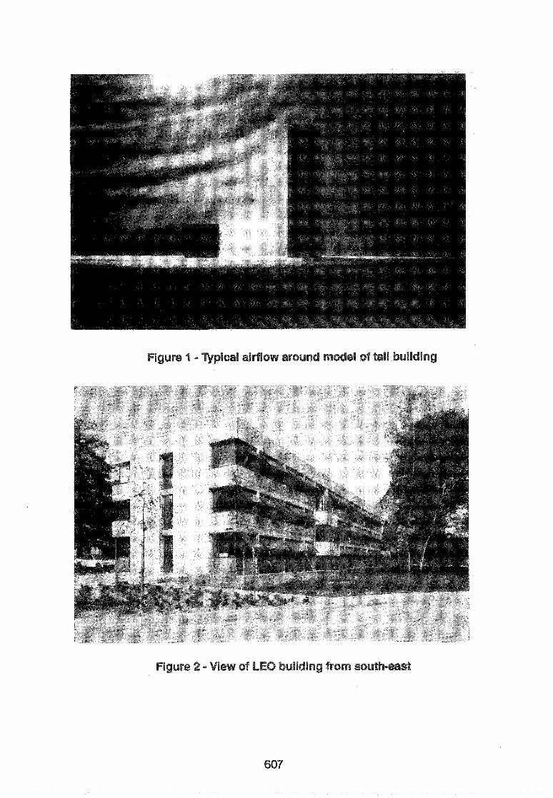
Flgslre 2 = View @9: LEO building from southas%

. Wind 0.23
Figure 3 - Wind pressure coefficients on centre-section of low rise with wind normal to long face.
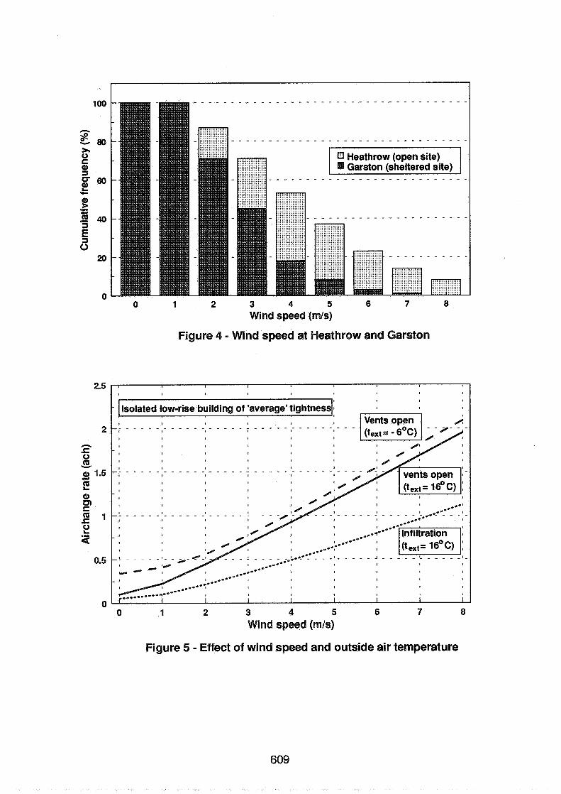
Heathrow (open 8ite) Garston (sheltered site) I I
1 2 3 4 5 6 7 8 Wind speed (mls)
Figure 4 - Wind speed at Heathrow and Garston
0 0 1 2 3 4 5 6 7 8
Wind speed (mls)
Figure 5 - Effect of wind speed and outside air temperature

I I I I I I I I I 0 1 2 3 4 5 6 7 8
Wind speed (mls)
Figure 6 - Proximity effect on ventilation rate
0 0 0.1 0.2 0.3 0.4 0.5 0.6 0.7 0.8 0.9 1 1.1 1.2 1.3 1.4 1.5
Average airchange rate (ach)
Figure 7 - Predicted ventilation performance

I3 With vents open [II1 Infiltration
. . . . . . . . . . . . . . . . . . . . . . . . . . . . . . . . . . . . . . . . . . . . . . .
H A - Isolated building B - Low-rise distance 9 m from high-rise
1 C-Low-risedistance27mfromhigh-rise
- 'Tight' building 'Average' building 'Leaky' building
ps izz iq . . . . . . . . . . . . . . . . . . . .
Figure 8.a - Airchange rates exceeded for 50% of the time
'Tight' building 'Average' building 'Leaky' buildlng
Figure 8.b - Airchange rates exceeded for 50% of the @me
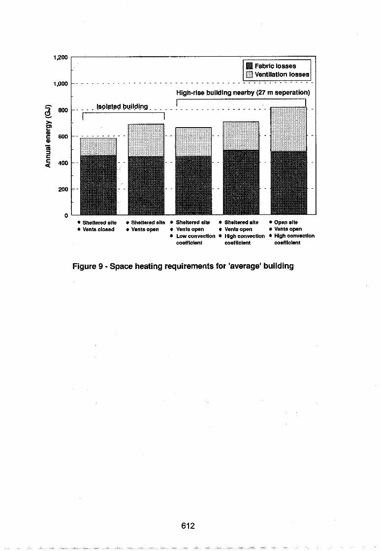
1,200
Ventilation losses I , O O O - - - - - - - - - - - - - - - - - - - - - - - - - - - - - - - - - - - - - - - - - - - - - - -
High-rise building nearby (27 m seperation) I I I
Sheltered site e Sheltered site e Sheltered site 0 Sheltered site Open site 4 Vents closed e Vents open Vents open e Vents open e Vents open
@ Low convection @ High convection High convection coefficient coefficient coefficient
Figure 9 - Space heating requirements for 'average-building
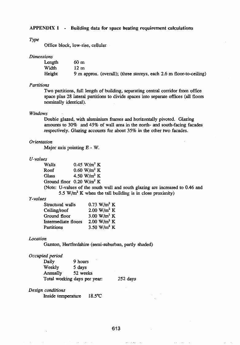
APPENDIX 1 - Building data for space heating requirement calculations
Type Office block, low-rise, cellular
Dimensions Length 60 m Width 12 m Height 9 m approx. (overall); (three storeys, each 2.6 m floor-to-ceiling)
Partitions Two partitions, full length of building, separating central corridor from office space plus 28 lateral partitions to divide spaces into separate offices (all floors nominally identical).
Windows Double glazed, with aluminium frames and horizontally pivoted. Glazing amounts to 30% and 45% of wall area in the north- and south-facing facades respectively. Glazing accounts for about 35% in the other two facades.
Orientation Major axis pointing E - W.
U-values Walls 0.45 Wlm2 K Roof 0.60 W/m2 K Glass 4.50 W/m2 K Ground floor 0.20 W/m2 K (Note: U-values of the south wall and south glazing are increased to 0.46 and
5.5 W/m2 K when the tall building is in close proximity) V-values
Structural walls 0.73 w/m2 K Ceiling/roof 2.00 w/m2 K Ground floor 3.00 w/m2 K Intermediate floors 2.00 W/m2 K Partitions 3.50 w/m2 K
Location Garston, Hertfordshire (semi-suburban, partly shaded)
Occupied period Daily 9 hours Weekly 5 days Annually 52 weeks Total working days per year: 252 days
Design conditions Inside temperature 18.5"C
