the impact of solar wind variability on pulsar timing - arxiv

Astronomy & Astrophysics manuscript no. aanda ©ESO 2020December 23, 2020

The impact of Solar wind variability on pulsar timingC. Tiburzi1?, G. M. Shaifullah1, 2, C. G. Bassa1, P. Zucca1, J. P. W. Verbiest3, 4, N. K. Porayko4, E. van der Wateren1, 5,R. A. Fallows1, R. A. Main4, G. H. Janssen1, 5, J. M. Anderson6, 7, A-.S. Bak Nielsen4, 3, J. Y. Donner4, 3, E. F. Keane8 J.Künsemöller3, S. Osłowski9, 10, J-.M. Grießmeier11, 12, M. Serylak13, 14, M. Brüggen15, B. Ciardi16, R.-J. Dettmar17, M.

Hoeft18, M. Kramer4, 19, G. Mann20, C. Vocks20

1 ASTRON − the Netherlands Institute for Radio Astronomy, Oude Hoogeveensedijk 4, 7991 PD Dwingeloo, The Netherlands2 Dipartimento di Fisica “G. Occhialini”, Università di Milano-Bicocca, Piazza della Scienza 3, I-20126, Milano, Italy3 Fakultät für Physik, Universität Bielefeld, Postfach 100131, 33501 Bielefeld, Germany4 Max-Planck-Institut für Radioastronomie, Auf dem Hügel 69, 53121 Bonn, Germany5 Department of Astrophysics/IMAPP, Radboud University, P.O. Box 9010, 6500 GL Nijmegen, The Netherlands6 Technische Universität Berlin, Institut für Geodäsie und Geoinformationstechnik, Fakultät VI, Sekr. H 12, Straße des 17. Juni 135,

10623 Berlin, Germany7 GFZ German Research Centre for Geosciences, Telegrafenberg, 14473 Potsdam, Germany8 SKA Organisation, Jodrell Bank, Macclesfield SK11 9FT, UK9 Gravitational Wave Data Centre, Swinburne University of Technology, P.O. Box 218, Hawthorn, VIC 3122, Australia

10 Centre for Astrophysics and Supercomputing, Swinburne University of Technology, P.O. Box 218, Hawthorn, VIC 3122, Australia11 LPC2E - Université d’Orléans / CNRS, 45071 Orléans cedex 2, France12 Station de Radioastronomie de Nançay, Observatoire de Paris, PSL Research University, CNRS, Univ. Orléans, OSUC,18330

Nançay, France13 South African Radio Astronomy Observatory, 2 Fir Street, Black River Park, Observatory 7925, South Africa14 Department of Physics and Astronomy, University of the Western Cape, Bellville, Cape Town 7535, South Africa15 Hamburger Sternwarte, University of Hamburg, Gojenbergsweg 112, 21029 Hamburg, Germany16 Max-Planck-Institut für Astrophysik, Karl-Schwarzschild-Straße 1, 85748 Garching b. München, Germany17 Ruhr University Bochum, Faculty of Physics and Astronomy, Astronomical Institute, 44780 Bochum, Germany18 Thüringer Landessternwarte, Sternwarte 5, 07778 Tautenburg, Germany19 Jodrell Bank Centre for Astrophysics, University of Manchester, M13 9PL, UK20 Leibniz-Institut für Astrophysik Potsdam (AIP), An der Sternwarte 16, 14482 Potsdam, Germany

Received MM DD, YYYY; accepted MM DD, YYYY

ABSTRACT

Context. High-precision pulsar timing requires accurate corrections for dispersive delays of radio waves, parametrized by the disper-sion measure (DM), particularly if these delays are variable in time. In a previous paper we studied the Solar-wind (SW) models usedin pulsar timing to mitigate the excess of DM annually induced by the SW, and found these to be insufficient for high-precision pulsartiming. Here we analyze additional pulsar datasets to further investigate which aspects of the SW models currently used in pulsartiming can be readily improved, and at what levels of timing precision SW mitigation is possible.Aims. Our goals are to verify: a) whether the data are better described by a spherical model of the SW with a time-variable amplituderather than a time-invariant one as suggested in literature, b) whether a temporal trend of such a model’s amplitudes can be detected.Methods. We use the pulsar-timing technique on low-frequency pulsar observations to estimate the DM and quantify how this valuechanges as the Earth moves around the Sun. Specifically, we monitor the DM in weekly to monthly observations of 14 pulsars takenwith parts of the LOw-Frequency ARray (LOFAR) across time spans of up to 6 years. We develop an informed algorithm to separatethe interstellar variations in DM from those caused by the SW and demonstrate the functionality of this algorithm with extensivesimulations. Assuming a spherically symmetric model for the SW density, we derive the amplitude of this model for each year ofobservations.Results. We show that a spherical model with time-variable amplitude models the observations better than a spherical model withconstant amplitude, but that both approaches leave significant SW induced delays uncorrected in a number of pulsars in the sample.The amplitude of the spherical model is found to be variable in time, as opposed to what has been previously suggested.

Key words. pulsars:general, solar wind, ISM: general, gravitational waves

1. Introduction

High-precision pulsar timing (Lorimer & Kramer 2004) is atechnique used to, for example, investigate irregularities in theSolar system planetary ephemerides (e.g. Caballero et al. 2018;Vallisneri et al. 2020), generate alternative time-scale references

? [email protected]

(e.g. Hobbs et al. 2020), test general relativity (e.g. Archibaldet al. 2018; Voisin et al. 2020) and alternative theories of grav-ity (e.g. Shao et al. 2013) or search for low-frequency gravi-tational waves with Pulsar Timing Arrays (PTAs, e.g. Tiburzi2018; Burke-Spolaor et al. 2019). In particular, a level of timingresiduals below 100 ns is usually indicated as the white-noise

Article number, page 1 of 14

arX

iv:2

012.

1172

6v1

[as

tro-

ph.H

E]

21

Dec

202

0

A&A proofs: manuscript no. aanda

threshold to achieve in PTA experiments (e.g., Janssen et al.2015; Siemens et al. 2013).

The sensitivity of these experiments can be significantly de-graded by various noise processes such as those caused by errorsin clock standards or inaccuracies in the planetary ephemerides.

One of the most common sources of noise in pulsar-timingdata (Lentati et al. 2016) is the variable amount of free electronsalong the line of sight (LoS). The radio waves coming from pul-sars are dispersed due to the ionized medium, leading to timedelays depending on the observing frequency, following the re-lation:

∆t =e2

2πmecDMf 2 = D

DMf 2 (1)

where ∆t is the time-delay (in s) induced at an observing fre-quency f (in MHz) with respect to infinite frequency, e is theelectron charge, me is the electron mass and c is the speedof light (e2/2πmec is the dispersion constant D = 1/(2.4 ×10−4) MHz2 pc−1 cm3 s, see Manchester & Taylor 1972) andDM is the dispersion measure (in pc cm−3):

DM =

∫LoS

ne(l) dl (2)

with ne being the electron density along the LoS.Variations in ne along the LoS induce DM fluctuations, caus-

ing changing ∆t contributions to the arrival times of pulsar radi-ation that need to be taken into account in pulsar timing exper-iments. The two main contributions to the DM along a certainLoS (for a comprehensive review, see Lam et al. 2016) are theionized interstellar medium (IISM) and the Solar wind (SW).In particular, the SW contribution to DM depends on the So-lar elongation of the pulsar (i.e., the projected angular separa-tion between the pulsar and the Sun), whose temporal variationstherefore induce DM time-fluctuations.

The SW has been recognized as a noise source that could in-duce false detections of gravitational waves in PTA experiments(Tiburzi et al. 2016).

The standard pulsar timing approach to mitigate the SW con-tribution (e.g., the International PTA data releases by Verbiestet al. 2016 and Perera et al. 2019a) typically consists in approx-imating the SW as a spherically symmetric distribution of elec-trons ne,sw (Edwards et al. 2006):

ne,sw = AAU

[1AU

r

]2(3)

where r is the distance between the pulsar and the Sun and AAU isthe free electron density of the Solar wind at 1 AU, reported to be7.9 and time-constant (Madison et al. 2019), and which we willhenceforth refer to as the amplitude of the SW density model.The DM contribution of this model is obtained by integratingEquation 3 along the LoS, and can be expressed as (Edwardset al. 2006; You et al. 2007b):

DMsw = 4.85 × 10−6AAUρ

sin ρpc cm−3 (4)

where ρ is the pulsar-Sun-observer angle. This model implicitlyassumes that the amplitude AAU is constant with time and inde-pendent of the ecliptic latitude of the pulsar. To account for thefact that this model may not be an optimal SW approximationat small Solar elongations, it is common to eliminate data pointstaken at close (< 5 degrees) angular distances from the Sun inpulsar timing experiments (Verbiest et al. 2016).

However, the SW is more complex than implied from thissimple model. Under Solar minimum conditions it is mostly bi-modal, with a fast stream seen above polar coronal holes, and aslow stream seen above a mostly-equatorial streamer belt (e.g.Coles 1996). A polar coronal hole can sometimes extend to-wards equatorial latitudes, allowing the fast and slow streamsto interact, leading to denser regions of compression at the lead-ing edge of the fast stream and rarefied regions following be-hind (e.g Schwenn 1990). Coronal Mass Ejections (CMEs) willfurther complicate this picture. The picture becomes even morecomplex as Solar activity increases towards a maximum, whenthe bi-modal structure effectively breaks down allowing coronalstreamers to extend to high latitudes. The reader is referred toSchwenn (2006) for a more detailed illustration of the SW sys-tem.

The shortcomings of the spherical model were neatly illus-trated in a recent publication by Tokumaru et al. (2020) whoobserved the Crab pulsar in 2018 using the Toyokawa Observa-tory. This paper also compared their results to SW conditions as-sessed from observations of interplanetary scintillation and coro-nal white light, and provided a useful discussion on how obser-vations of pulsars could also be used to assist research into theSW.

The aforementioned shortcomings led You et al. (2007a) topropose a revised SW model for the pulsar DM which consid-ered the SW as bimodal. The authors used different free-electronradial distributions for each of the two SW streams, and usedSolar magnetograms to decompose the LoS into parts affectedby one or the other component, the total contribution from theSolar-wind being the sum of these individual contributions. Thiswas demonstrated in the paper to better correct the DM for theSW contribution than the basic spherical model, but it shouldbe noted that the pulsar observations were taken during the ap-proach to solar minimum, when a bimodal solar wind structureis more evident.

Tiburzi et al. (2019) compared the performance of thesemodels on highly-sensitive, low-frequency observations ofPSR J0034−0534, while also allowing a time-variable amplitude(following the approach of You et al. 2012) in both of the mod-els. The authors demonstrated that neither model provided an ad-equate description of the SW impact on the dataset, but also thatthe spherical one performed better than the other. The observa-tions used in that paper were, however, taken at solar maximum,which may explain why the bimodal model did not perform bet-ter in that instance. More explanation of the possible reasons isgiven in Tiburzi et al. (2019).

In this article we expand on the analysis of Tiburzi et al.(2019), using a larger sample of pulsars to verify a) whether theSW DM contributions to these pulsar LoSs are better describedby a spherical model with a time-variable amplitude or a time-constant one as suggested in the literature (Edwards et al. 2006;Madison et al. 2019), and b) whether a consistent temporal trendcan be detected in the amplitudes of this model which might sug-gest that the bimodal approach be revisited in future work.

The article is structured as follows: in Section 2 we presentthe dataset and the selected pulsars, while in Section 3 we de-scribe the analysis. The results are presented in Section 4. InSection 5 we discuss future prospects, and in Section 6 we drawour conclusions.

2. Dataset

The utilized dataset comes from a number of pulsar monitoringcampaigns carried out with the high-band antennas of different


C. Tiburzi et al.: The impact of Solar wind variability on pulsar timing

subsets of the International LOFAR (LOw Frequency ARray)telescope (van Haarlem et al. 2013; Stappers et al. 2011): thesix German International LOFAR stations, the Swedish Inter-national LOFAR station, and the LOFAR Core. The observingbandwidth covers a frequency interval from ∼100 to ∼190 MHz,with a central frequency of about 150 MHz (variations of a fewMHz occur among the different observing sites). The recordeddata were coherently dedispersed, folded into 10-second-longsubintegrations modulo the pulse period, and divided into fre-quency channels of 195 kHz with the DSPSR software suite (vanStraten & Bailes 2011). The integration length ranges from 1 to3 hours with the international stations, and from 7 to 20 minuteswith the LOFAR core (for more details regarding the observa-tional setup, see Porayko et al. 2019; Donner et al. 2019 andTiburzi et al. 2019).

Together, the aforementioned observing campaigns monitormore than 100 pulsars. However, for the scope of this article,we selected pulsars with the following characteristics: a) eclip-tic latitude between −20 and +20 degrees, b) observing cadencehigher than once per month, c) more than one year of observ-ing time-span, d) without gaps between successive observationsexceeding 100 consecutive days. This results in a dataset of 43pulsars, whose sky locations are shown in Figure 1 and char-acteristics are reported in tables 1 and B.11, and for which wehave used all the data available until May 2019 (up to August2019 in some cases). This source list was further refined to 14sources that prove useful probes of the Solar wind, as discussedin Section 3.3.

3. Data analysis

In the following, we detail the analysis methods applied to thedata to obtain the DM values, disentangle the IISM-induced ef-fects, and identify the pulsars showing persistent SW signatures.We make use of the pulsar timing technique, which keeps trackof every pulsar rotation to model the evolution of the pulse pe-riod and phase over the timespan of our dataset. This allows us toaverage each observation in time and improve the signal-to-noiseratio (S/N).

3.1. Calculation of the DM values

For all observations, independent of the observing site, we re-moved radio-frequency interference, corrected for azimuth andelevation-dependent gain using the LOFAR beam model withinthe dreambeam package2, and applied band-limitations to retain acommon frequency range between ∼118 and ∼188 MHz3. Theseoperations were carried out using the psrchive software suite(Hotan et al. 2004; van Straten et al. 2012) and a modified ver-sion4 of the Coastguard software suite (Lazarus et al. 2016).

For each pulsar we then computed a DM value per observa-tion through the pulsar timing technique by proceeding as fol-lows. We first selected the dataset that covered the longest time-baseline. These observations were weighted by the square of1 Part of the reported values come from the ATNF pulsar cat-alog, https://www.atnf.csiro.au/research/pulsar/psrcat/(Manchester et al. 2005).2 https://github.com/2baOrNot2ba/dreamBeam3 Band-limiting is necessary to avoid biases in our results because theobserving sites record slightly different original bandwidths. The indi-cated frequency range is common to all of the observing sites (for moredetails, see Donner et al. 2019; Tiburzi et al. 2019).4 https://github.com/larskuenkel/iterative_cleaner, seealso Kuenkel (2017).

their S/N, added together and then fully averaged in time andpartially in frequency (usually down to 10 frequency channelsto increase the S/N5). Finally, the template was smoothed usinga wavelet smoothing scheme first introduced by Demorest et al.(2013). We then collected the observations obtained by all theobserving sites for that pulsar, we fully averaged them in timeand partially in frequency to the same resolution of the template.For each observation we then generated a set of ToAs associatedto the frequency channels with the psrchive software suite bycross-correlating the observation with the reference template.

A few exceptions to the aforementioned general template-generation scheme were adopted in case the pulsar was too faint,or bright but strongly affected by red noise (due to irregulari-ties in the pulsar rotation or extreme IISM-linked DM variations,that caused the template to appear broadened). In the first case,we averaged the longest dataset described earlier over frequencyand time to then produce an analytic template, obtained by ap-proximating the data-derived pulse profile with a sum of vonMises functions. In the second case, we used a small subset ofphase-aligned observations which were subsequently averagedand smoothed.

After generating a set of frequency-resolved ToAs per obser-vation, we used the tempo2 software suite for pulsar timing (Ed-wards et al. 2006) and the procedure outlined in Tiburzi et al.(2019) to calculate one DM value per observation6. We thencombined the DM time series from all the available observingsites, after subtracting the reference DM value.

3.2. Disentangling the IISM contribution

The obtained DM time series show variations due to both theSW and the IISM. To remove the influence of the IISM, for eachpulsar we proceeded as follows.

The DM time series was divided into 460-day long segmentscentered on the Solar conjunctions, i.e., adding an additional 1.5months of baseline to a 6-month time window on either side ofthe Solar conjunction. Hence, the segments overlap for about100 days. Segments that either contained gaps of more than 55days between successive observations, or those where the effec-tive time span is less than 368 days (80% of 460 days) werealso discarded, as they do not provide a long enough baseline toproperly define the IISM effects (this only affects initial and finalsegments).

The DM time series in each segment was modeled in aBayesian framework as the sum of a spherically-symmetric SWmodel (Equation 4) with AAU being a free parameter, and a poly-nomial to account for the IISM contribution. By simulating DMtime-series affected by Kolmogorov turbulence (Armstrong et al.1995), we found that a cubic polynomial was sufficient to modelthe DM variations due to the IISM on 460-day long segments(see the method’s validation in Appendix A). To account forany common systematic error in the estimation of the DM un-certainties, we inserted an additional parameter in the model,summed in quadrature with the DM uncertainties in the likeli-hood function. We used a Markov Chain Monte Carlo method(implemented using the emcee package; Foreman-Mackey et al.

5 For particularly faint pulsars we applied a larger frequency-averagingfactor.6 Note that, as for Tiburzi et al. (2019), the DM time derivatives in-cluded in the original timing model for that pulsar were only appliedto properly dedisperse the template and frequency-average the observa-tions, but they were not used in the subsequent determination of the DMvariations.


https://www.atnf.csiro.au/research/pulsar/psrcat/

https://github.com/2baOrNot2ba/dreamBeam

https://github.com/larskuenkel/iterative_cleaner


90

60

30

0

30

60

90b

90

60

30

0

30

60

90b

Observed sources

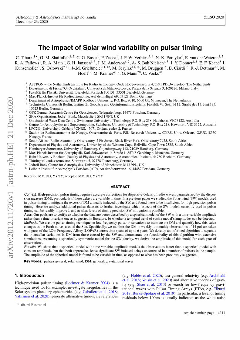
Fig. 1. Sky distribution in Galactic coordinates of selected (filled green circles) and rejected (unfilled red circles) pulsars from the lists in Table 1and Table B.1. Larger markers denote higher (median) precision of the measured DM. The dashed blue line marks the ecliptic and the dashed graylines show a region of ±20 degrees from the ecliptic. The background shows the merged all-sky Hα map from Finkbeiner (2003).

2013) to obtain the parameters of the cubic polynomial, the un-certainties correction parameter and the SW amplitude AAU, andaccount for the covariance of the SW amplitude with the parame-ters of the IISM model. We assigned flat priors to the polynomialcoefficients, and a flat and positive prior to the amplitude of theSW model and the uncertainties correction parameter.

As a final step, the modeled IISM contribution was sub-tracted from the DM time series. In the overlapping regionbetween two successive years, data points that lay within 6months of the preceding Solar approach were approximated bythe plasma model computed for the first year, while data pointswithin 6 months of the following Solar approach were approxi-mated by the one computed for the second year7. After estimat-ing the model, data points collected earlier than 6 months beforethe first Solar conjunction, and later than 6 months after the lastSolar conjunction were discarded.

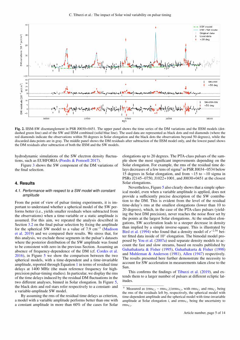
As an example of the final result, Figure 2 shows the IISMdisentanglement for PSR J0030+0451.

We note here that in Tiburzi et al. (2019) the authors demon-strated that the spherical model is a poor description of the SW,when tested against sufficiently sensitive data. Nevertheless, wehave adopted it in the procedure described above for two reasons.First, it was proven to be better among the two available mod-els compared in that work. Secondly, in Tiburzi et al. (2019) wefound that, while the spherical approximation could not modelthe short-term SW-induced DM variations, it provided a reason-able description of the long-term ones.

7 The overlap between adjacent years guarantees a continuous andsmooth IISM model across multiple years.

3.3. Final selection

The procedure outlined above allowed us to refine our pulsar se-lection by rejecting those sources where the SW signature is notreliably detected. Specifically, we retained a pulsar if and onlyif in more than half of the dataset: a) the model described in theprevious section was preferred over an IISM-only model as eval-uated by the Bayesian information criterion (BIC), b) the poste-rior distribution of the SW model’s amplitude was significantlydifferent from zero8.

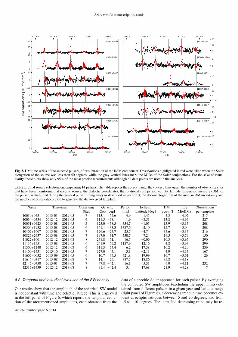
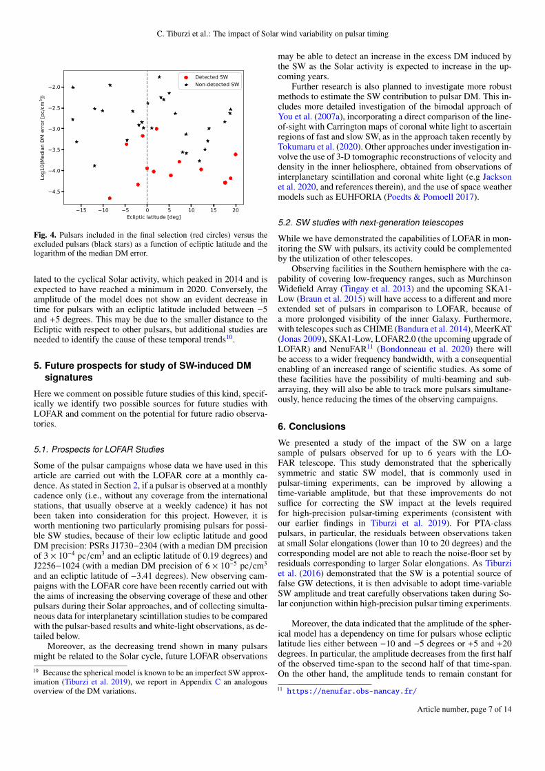
A total of 14 pulsars satisfied the mentioned requirements, asreported in Table 1 (for the discarded sources, see Table B.1 inthe Appendix). Among these there are the PTA-class millisecondpulsars J0030+0451, J0034−0534, J1022+1001, J2145−0750and J2317+1439 (Perera et al. 2019b), which, as expected, dis-play the best DM precision of the sample. We consider the 14 se-lected sources as well-suited for studying the electron density inthe SW at low frequencies in the Northern hemisphere. Figure 4shows that, for equal ecliptic latitude, the pulsars included in thefinal selection always present the best DM precision among thesources at the same Ecliptic latitudes. The few cases of sourceswith high DM precision where the SW is not detected, can be ex-plained typically by a combination of low S/N and a poor sam-pling cadence (e.g., PSR J1024−0719). For the few pulsars inwhich these causes are not applicable (e.g., PSR J0837+0610),we speculate that the reason lies in an asymmetry of the So-lar wind contribution with respect to the heliographic latitude.A more rigorous test of this hypothesis will be presented in afuture work through comparisons with data-derived magneto-

8 In PSR J1300+1240 only the first two years (out of a total five) meetthe requirements. However, we included it in the final selection aftervisually inspecting the DM time series and manually examining the re-sults.



Fig. 2. IISM-SW disentanglement in PSR J0030+0451. The upper panel shows the time series of the DM variations and the IISM models (dot-dashed green line) and of the SW and IISM combined (solid blue line). The used data are represented as black dots and red diamonds (where thered diamonds indicate the observations within 50 degrees in Solar elongation and the black dots the observations beyond 50 degrees), while thediscarded data points are in gray. The middle panel shows the DM residuals after subtraction of the IISM model only, and the lowest panel showsthe DM residuals after subtraction of both the IISM and the SW models.

hydrodynamic simulations of the SW electron density fluctua-tions, such as EUHFORIA (Poedts & Pomoell 2017).

Figure 3 shows the SW component of the DM variations ofthe final selection.

4. Results

4.1. Performance with respect to a SW model with constantamplitude

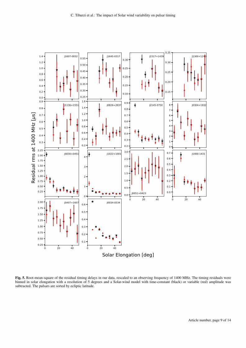
From the point of view of pulsar timing experiments, it is im-portant to understand whether a spherical model of the SW per-forms better (i.e., yields smaller residuals when subtracted fromthe observations) when a time-variable or a static amplitude isassumed. For this aim, we repeated the analysis described inSection 3.2 on the final pulsar selection by fixing the amplitudefor the spherical SW model to a value of 7.9 cm−3 (Madisonet al. 2019) and we compared their results. We stress that, forthis analysis, we exclude those segments in the pulsar’s datasetswhere the posterior distribution of the SW amplitude was foundto be consistent with zero in the previous Section. Assuming anabsence of frequency-dependence of the DM (cf. Cordes et al.2016), in Figure 5 we show the comparison between the twospherical models, with a time-dependent and a time-invariableamplitude, reported through Equation 1 in terms of residual timedelays at 1400 MHz (the main reference frequency for high-precision pulsar-timing studies). In particular, we display the rmsof the time delays induced by the residual DM fluctuations in thetwo different analyses, binned in Solar elongation. In Figure 5,the black dots and red stars refer respectively to a constant- anda variable-amplitude SW model.

By assuming the rms of the residual time delays as criterion,a model with a variable amplitude performs better than one witha constant amplitude in more than 60% of the cases for Solar

elongations up to 20 degrees. The PTA-class pulsars of the sam-ple show the most significant improvements depending on theSolar elongation. For example, the rms of the residual time de-lays decreases of a few tens of sigma9 in PSR J0034−0534 below15 degrees in Solar elongation, and from ∼15 to ∼10 sigma inPSRs J2145−0750, J1022+1001, and J0030+0451 at the closestSolar elongations.

Nevertheless, Figure 5 also clearly shows that a simple spher-ical model, even when a variable amplitude is applied, does notprovide a sufficiently precise description of the SW contribu-tion to the DM. This is evident from the level of the residualtime-delay’s rms at the smallest elongations (lower than 10 to20 degrees), which, in the case of the PTA-class pulsars (yield-ing the best DM precision), never reaches the noise floor set bythe points at the largest Solar elongations. At the smallest elon-gations, SW acceleration leads to a steeper decrease in densitythan implied by a simple inverse-square. This is illustrated byBird et al. (1994) who found that a density model of r−2.54 bet-ter fitted data inside of 10◦ elongation. The bimodal model pro-posed by You et al. (2007a) used separate density models to ac-count the fast and slow streams, based on results published byGuhathakurta & Fisher (1995), Guhathakurta & Fisher (1998)and Muhleman & Anderson (1981), Allen (1947) respectively.The results presented here further demonstrate the necessity toaccount for SW acceleration in measurements taken close to theSun.

This confirms the findings of Tiburzi et al. (2019), and ex-tends them to a larger number of pulsars at different ecliptic lat-itudes.

9 Measured as (rmsC,i − rmsV,i)/ermsV,i, with rmsV,i and rmsC,i beingthe rms of the residuals left by, respectively, the spherical model withtime-dependent amplitude and the spherical model with time-invariableamplitude at Solar elongation i, and ermsV,i being the uncertainty tormsV,i.



2013.6 2014.9 2016.3 2017.7 2019.0

0

25

50 J0030+0451

0

5

10J0034-0534

0

50 J0051+0423

−100

0

100 J0304+1932

−25

0

25 J0407+1607

0

20 J0826+2637

56500 57000 57500 58000 58500MJD

0

50J1022+1001

2013.6 2014.9 2016.3 2017.7 2019.0

0

10

20J1136+1551

0

5J1300+1240

0

10J1400-1431

−10

0

10J1607-0032

−10

0

10J1645-0317

0

20J2145-0750

56500 57000 57500 58000 58500MJD

0

10J2317+1439

DM variatio

ns [1

0−4 pc/cm

3 ]

Fig. 3. DM time series of the selected pulsars, after subtraction of the IISM component. Observations highlighted in red were taken when the Solarelongation of the source was less than 50 degrees, while the gray vertical lines mark the MJDs of the Solar conjunctions. For the sake of visualclarity, these plots show only 95% of the most precise measurements although all data points are used in the analysis.

Table 1. Final source selection, encompassing 14 pulsars. The table reports the source name, the covered time-span, the number of observing sitesthat have been monitoring that specific source, the Galactic coordinates, the rotational spin period, ecliptic latitude, dispersion measure (DM) ofthe pulsar, as measured during the general pulsar timing analysis described in Section 3, the decimal logarithm of the median DM uncertainty andthe number of observations used to generate the data-derived template.

Name Time-span Observing Galactic Period Ecliptic DM Log ObservationsSites Coo. [deg] [ms] Latitude [deg] [pc/cm3] M(eDM) per template

J0030+0451 2013-01 2019-05 7 113.1 −57.6 4.9 1.45 4.3 −4.02 215J0034−0534 2012-12 2019-05 6 111.5 −68.1 1.9 −8.53 13.8 −4.66 227J0051+0423 2013-08 2019-05 5 123.0 −58.5 354.7 −1.05 13.9 −3.17 208J0304+1932 2013-08 2019-05 6 161.1 −33.3 1387.6 2.10 15.7 −3.0 208J0407+1607 2013-08 2019-05 7 176.6 −25.7 25.7 −4.74 35.6 −3.37 216J0826+2637 2013-08 2019-05 7 197.0 31.7 530.7 7.24 19.5 −3.79 150J1022+1001 2012-12 2019-08 8 231.8 51.1 16.5 −0.06 10.3 −3.95 290J1136+1551 2013-08 2019-05 6 241.9 69.2 1187.9 12.16 4.8 −3.97 299J1300+1240 2012-12 2019-08 6 311.3 75.4 6.2 17.58 10.2 −4.29 239J1400−1431 2015-10 2019-05 7 327.0 45.1 3.1 −2.11 4.9 −4.33 167J1607−0032 2013-09 2019-05 6 10.7 35.5 421.8 19.99 10.7 −3.61 26J1645−0317 2013-08 2019-08 7 14.1 26.1 387.7 18.86 35.8 −4.18 4J2145−0750 2013-01 2019-08 7 47.8 −42.1 16.1 5.31 9.0 −4.11 232J2317+1439 2012-12 2019-08 8 91.4 −42.4 3.4 17.68 21.9 −4.28 7

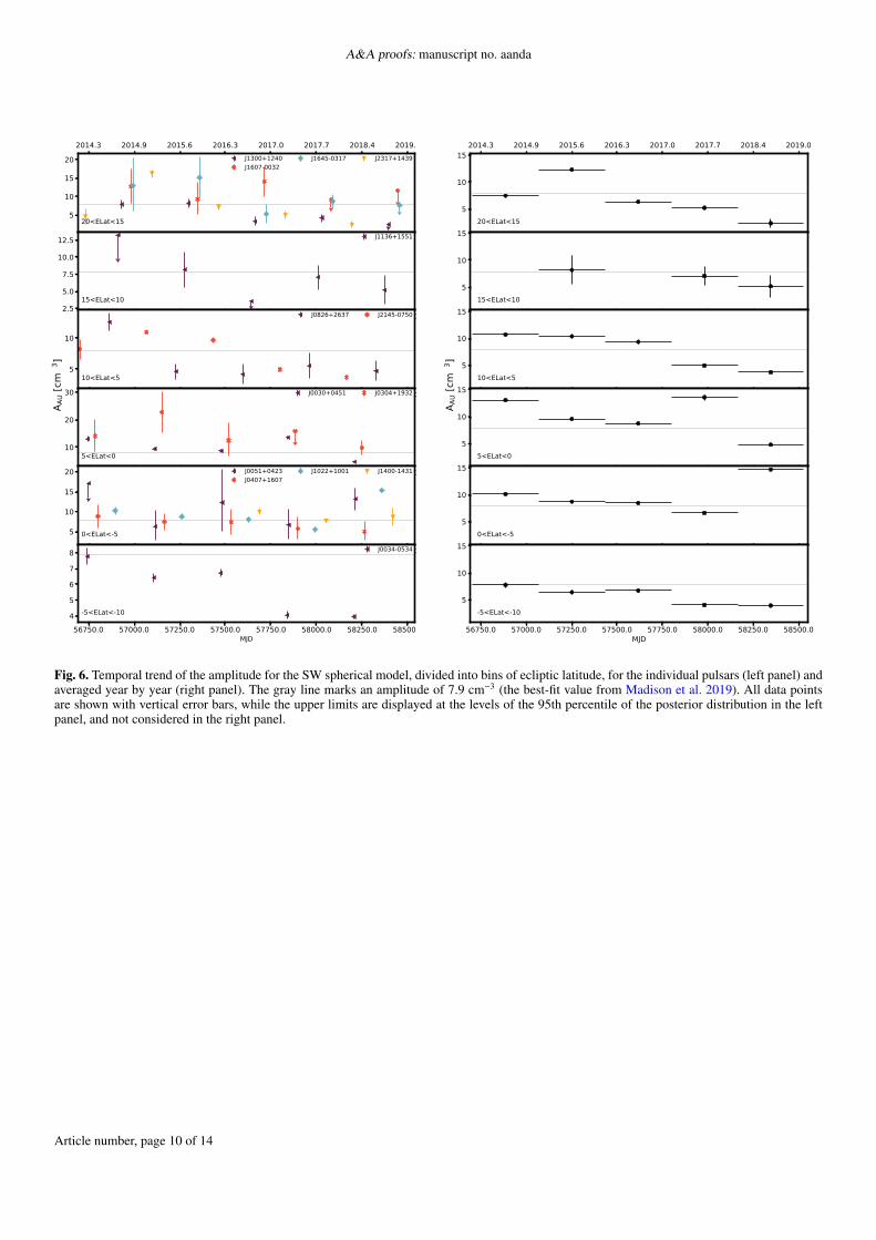
4.2. Temporal and latitudinal evolution of the SW density

Our results show that the amplitude of the spherical SW modelis not constant with time and ecliptic latitude. This is displayedin the left panel of Figure 6, which reports the temporal evolu-tion of the aforementioned amplitudes, each obtained from the

data of a specific Solar approach for each pulsar. By averagingthe computed SW amplitudes (excluding the upper limits) ob-tained from different pulsars in a given year and latitude range(right panel of Figure 6), a decreasing trend in time becomes ev-ident at ecliptic latitudes between 5 and 20 degrees, and from−5 to −10 degrees. The identified decreasing trend may be re-



−15 −10 −5 0 5 10 15 20Ecliptic latitude [deg]

−4.5

−4.0

−3.5

−3.0

−2.5

−2.0

Log1

0(M

edia

n DM

e o

[pc

/cm

3 ])

Detected SWNon-detected SW

Fig. 4. Pulsars included in the final selection (red circles) versus theexcluded pulsars (black stars) as a function of ecliptic latitude and thelogarithm of the median DM error.

lated to the cyclical Solar activity, which peaked in 2014 and isexpected to have reached a minimum in 2020. Conversely, theamplitude of the model does not show an evident decrease intime for pulsars with an ecliptic latitude included between −5and +5 degrees. This may be due to the smaller distance to theEcliptic with respect to other pulsars, but additional studies areneeded to identify the cause of these temporal trends10.

5. Future prospects for study of SW-induced DMsignatures

Here we comment on possible future studies of this kind, specif-ically we identify two possible sources for future studies withLOFAR and comment on the potential for future radio observa-tories.

5.1. Prospects for LOFAR Studies

Some of the pulsar campaigns whose data we have used in thisarticle are carried out with the LOFAR core at a monthly ca-dence. As stated in Section 2, if a pulsar is observed at a monthlycadence only (i.e., without any coverage from the internationalstations, that usually observe at a weekly cadence) it has notbeen taken into consideration for this project. However, it isworth mentioning two particularly promising pulsars for possi-ble SW studies, because of their low ecliptic latitude and goodDM precision: PSRs J1730−2304 (with a median DM precisionof 3 × 10−4 pc/cm3 and an ecliptic latitude of 0.19 degrees) andJ2256−1024 (with a median DM precision of 6 × 10−5 pc/cm3

and an ecliptic latitude of −3.41 degrees). New observing cam-paigns with the LOFAR core have been recently carried out withthe aims of increasing the observing coverage of these and otherpulsars during their Solar approaches, and of collecting simulta-neous data for interplanetary scintillation studies to be comparedwith the pulsar-based results and white-light observations, as de-tailed below.

Moreover, as the decreasing trend shown in many pulsarsmight be related to the Solar cycle, future LOFAR observations10 Because the spherical model is known to be an imperfect SW approx-imation (Tiburzi et al. 2019), we report in Appendix C an analogousoverview of the DM variations.

may be able to detect an increase in the excess DM induced bythe SW as the Solar activity is expected to increase in the up-coming years.

Further research is also planned to investigate more robustmethods to estimate the SW contribution to pulsar DM. This in-cludes more detailed investigation of the bimodal approach ofYou et al. (2007a), incorporating a direct comparison of the line-of-sight with Carrington maps of coronal white light to ascertainregions of fast and slow SW, as in the approach taken recently byTokumaru et al. (2020). Other approaches under investigation in-volve the use of 3-D tomographic reconstructions of velocity anddensity in the inner heliosphere, obtained from observations ofinterplanetary scintillation and coronal white light (e.g Jacksonet al. 2020, and references therein), and the use of space weathermodels such as EUHFORIA (Poedts & Pomoell 2017).

5.2. SW studies with next-generation telescopes

While we have demonstrated the capabilities of LOFAR in mon-itoring the SW with pulsars, its activity could be complementedby the utilization of other telescopes.

Observing facilities in the Southern hemisphere with the ca-pability of covering low-frequency ranges, such as MurchinsonWidefield Array (Tingay et al. 2013) and the upcoming SKA1-Low (Braun et al. 2015) will have access to a different and moreextended set of pulsars in comparison to LOFAR, because ofa more prolonged visibility of the inner Galaxy. Furthermore,with telescopes such as CHIME (Bandura et al. 2014), MeerKAT(Jonas 2009), SKA1-Low, LOFAR2.0 (the upcoming upgrade ofLOFAR) and NenuFAR11 (Bondonneau et al. 2020) there willbe access to a wider frequency bandwidth, with a consequentialenabling of an increased range of scientific studies. As some ofthese facilities have the possibility of multi-beaming and sub-arraying, they will also be able to track more pulsars simultane-ously, hence reducing the times of the observing campaigns.

6. Conclusions

We presented a study of the impact of the SW on a largesample of pulsars observed for up to 6 years with the LO-FAR telescope. This study demonstrated that the sphericallysymmetric and static SW model, that is commonly used inpulsar-timing experiments, can be improved by allowing atime-variable amplitude, but that these improvements do notsuffice for correcting the SW impact at the levels requiredfor high-precision pulsar-timing experiments (consistent withour earlier findings in Tiburzi et al. 2019). For PTA-classpulsars, in particular, the residuals between observations takenat small Solar elongations (lower than 10 to 20 degrees) and thecorresponding model are not able to reach the noise-floor set byresiduals corresponding to larger Solar elongations. As Tiburziet al. (2016) demonstrated that the SW is a potential source offalse GW detections, it is then advisable to adopt time-variableSW amplitude and treat carefully observations taken during So-lar conjunction within high-precision pulsar timing experiments.

Moreover, the data indicated that the amplitude of the spher-ical model has a dependency on time for pulsars whose eclipticlatitude lies either between −10 and −5 degrees or +5 and +20degrees. In particular, the amplitude decreases from the first halfof the observed time-span to the second half of that time-span.On the other hand, the amplitude tends to remain constant for

11 https://nenufar.obs-nancay.fr/


https://nenufar.obs-nancay.fr/


pulsars with an ecliptic latitude included between −5 and +5degrees. Additional studies will be necessary to recognize thecause of these trends, and whether they are in connection to theSolar cycle activity.

While the investigation of new SW models for high-precisionpulsar timing was not in the scope of the current work, a series ofmeasures can be adopted to mitigate the SW-induced noise (as-suming the absence of frequency-dependent DM or scattering):

– Carrying out observations with wideband observing re-ceivers may allow, in combination with the usage offrequency-resolved templates, a precise determination oftime-dependent DM (due to the IISM, the SW or both) thatcan be then used to correct the noise induced by variable dis-persion;

– Carrying out simultaneous observations at low and high fre-quency to allow a precise DM determination by using thelow-frequency data. This can be then used to correct thehigh-frequency ToAs;

– If obtaining simultaneous observations is not possible, it maybe of aid carrying out high-cadence, low-frequency observa-tions (ideally once every two or three days) for two weeksaround the Solar conjunction. The DM values obtained fromthese observations can be interpolated and used as correctionscheme for high-frequency observations. The high-cadenceof the observations is important in this case because, asshown by Niu et al. (2017), the fast SW variability may in-validate the DM corrections if the high- and low-frequencyobservations are separated by more than one day;

– For pulsars with a flat spectral index, it may be meaningfulto carry out observations at very high frequencies (at S bandor more), where the DM-induced noise is marginal, and ap-ply the spherical SW model by choosing an amplitude ac-cordingly to, e.g., the results of this article depending on thepulsar’s ecliptic latitude. However, this approach implies thata certain amount of timing noise will be left in the data, es-pecially the ones taken close to the Solar conjunction. More-over, Lam et al. (2018) demonstrated that observing frequen-cies lower than 1 GHz are more optimal to achieve high pre-cision in pulsar timing experiments.

Data Availability

The data underlying this article that were collected with the In-ternational LOFAR Stations and with the LOFAR core under stillprivate observing programs, will be shared on reasonable requestto the corresponding author. The data underlying this article col-lected with the LOFAR core and under public observing pro-grams are available at: https://lta.lofar.eu/.The initial timing models, the ToA files and the DM time se-ries for the pulsars used in this article are publicly availableon Zenodo from the 1st of January 2021 (DOI: 10.5281/zen-odo.4247554).Acknowledgements. This work is part of the research program Soltrack withproject number 016.Veni.192.086, which is partly financed by the Dutch Re-search Council (NWO). The authors thank the anonymous referee for their sup-port and useful comments. CT This paper is partially based on data obtainedwith: i) the German stations of the International LOFAR Telescope (ILT), con-structed by ASTRON (van Haarlem et al. 2013) and operated by the GermanLOng Wavelength (GLOW) consortium (https://www.glowconsortium.de/) during station-owners time and proposals LC0_014, LC1_048, LC2_011,LC3_029, LC4_025, LT5_001, LC9_039, LT10_014; ii) the LOFAR core, dur-ing proposals LC0_011, DDT0003, LC1_027, LC1_042, LC2_010, LT3_001,LC4_004, LT5_003, LC9_041, LT10_004, LPR12_010; iii) the Swedish stationof the ILT during observing proposals carried out from May 2015 to January2018. We made use of data from the Effelsberg (DE601) LOFAR station funded

by the Max-Planck-Gesellschaft; the Unterweilenbach (DE602) LOFAR stationfunded by the Max-Planck-Institut für Astrophysik, Garching; the Tautenburg(DE603) LOFAR station funded by the State of Thuringia, supported by theEuropean Union (EFRE) and the Federal Ministry of Education and Research(BMBF) Verbundforschung project D-LOFAR I (grant 05A08ST1); the Pots-dam (DE604) LOFAR station funded by the Leibniz-Institut für Astrophysik,Potsdam; the Jülich (DE605) LOFAR station supported by the BMBF Verbund-forschung project D-LOFAR I (grant 05A08LJ1); and the Norderstedt (DE609)LOFAR station funded by the BMBF Verbundforschung project D-LOFAR II(grant 05A11LJ1). The observations of the German LOFAR stations were car-ried out in the stand-alone GLOW mode, which is technically operated and sup-ported by the Max-Planck-Institut für Radioastronomie, the ForschungszentrumJülich and Bielefeld University. We acknowledge support and operation of theGLOW network, computing and storage facilities by the FZ-Jülich, the MPIfRand Bielefeld University and financial support from BMBF D-LOFAR III (grant05A14PBA) and D-LOFAR IV (grants 05A17PBA and 05A17PC1), and by thestates of Nordrhein-Westfalia and Hamburg. MB acknowledges support from theDeutsche Forschungsgemeinschaft under Germany’s Excellence Strategy - EXC2121 "Quantum Universe" - 390833306. CT acknowledges support from On-sala Space Observatory for the provisioning of its facilities/observational sup-port. The Onsala Space Observatory national research infrastructure is fundedthrough Swedish Research Council grant No 2017-00648. GS was supported bythe Netherlands Organization for Scientific Research NWO(TOP2.614.001.602).JPWV acknowledges support by the Deutsche Forschungsgemeinschaft (DFG)through the Heisenberg program (Project No. 433075039).


https://lta.lofar.eu/

https://www.glowconsortium.de/

https://www.glowconsortium.de/


0.0

0.2

0.4

0.6

0.8

1.0

1.2

1.4 J1607-0032

0.25

0.30

0.35

0.40

0.45

0.50

0.55J1645-0317

0.10

0.15

0.20

0.25

0.30J2317+1439

0.15

0.20

0.25

0.30

0.35J1300+1240

0.3

0.4

0.5

0.6

0.7

0.8

0.9J1136+1551

0.2

0.4

0.6

0.8

1.0

1.2

1.4

1.6J0826+2637

0.2

0.3

0.4

0.5

0.6

0.7

0.8

0.9J2145-0750

0

1

2

3

4

5

6

7

8 J0304+1932

0.25

0.50

0.75

1.00

1.25

1.50

1.75

2.00

2.25J0030+0451

0

1

2

3

4J1022+1001

0 20 400.0

0.5

1.0

1.5

2.0

2.5

3.0

J0051+0423

0 20 40

0.0

0.1

0.2

0.3

0.4

0.5

0.6

0.7 J1400-1431

0 20 400.25

0.50

0.75

1.00

1.25

1.50

1.75

2.00 J0407+1607

0 20 40

0.1

0.2

0.3

0.4

0.5

0.6 J0034-0534

Solar Elongation [deg]

Resid

ual rms a

t 140

0 MHz

[μs]

Fig. 5. Root-mean-square of the residual timing delays in our data, rescaled to an observing frequency of 1400 MHz. The timing residuals werebinned in solar elongation with a resolution of 5 degrees and a Solar-wind model with time-constant (black) or variable (red) amplitude wassubtracted. The pulsars are sorted by ecliptic latitude.



2014.3 2014.9 2015.6 2016.3 2017.0 2017.7 2018.4 2019.0

5

10

15

20

20<ELat<15

J1300+1240J1607-0032

J1645-0317 J2317+1439

56750 57000 57250 57500 57750 58000 58250 585002.5

5.0

7.5

10.0

12.5

15<ELat<10

J1136+1551

56750 57000 57250 57500 57750 58000 58250 58500

5

10

10<ELat<5

J0826+2637 J2145-0750

56750 57000 57250 57500 57750 58000 58250 58500

10

20

30

5<ELat<0

J0030+0451 J0304+1932

56750 57000 57250 57500 57750 58000 58250 58500

5

10

15

20

0<ELat<-5

J0051+0423J0407+1607

J1022+1001 J1400-1431

56750.0 57000.0 57250.0 57500.0 57750.0 58000.0 58250.0 58500.0MJD

4

5

6

7

8

-5<ELat<-10

J0034-0534

A AU [cm

−3]

2014.3 2014.9 2015.6 2016.3 2017.0 2017.7 2018.4 2019.0

5

10

15

20<ELat<15

56750 57000 57250 57500 57750 58000 58250 58500

5

10

15

15<ELat<10

56750 57000 57250 57500 57750 58000 58250 58500

5

10

15

10<ELat<5

56750 57000 57250 57500 57750 58000 58250 58500

5

10

15

5<ELat<0

56750 57000 57250 57500 57750 58000 58250 58500

5

10

15

0<ELat<-5

56750.0 57000.0 57250.0 57500.0 57750.0 58000.0 58250.0 58500.0MJD

5

10

15

-5<ELat<-10

A AU [cm

−3]

Fig. 6. Temporal trend of the amplitude for the SW spherical model, divided into bins of ecliptic latitude, for the individual pulsars (left panel) andaveraged year by year (right panel). The gray line marks an amplitude of 7.9 cm−3 (the best-fit value from Madison et al. 2019). All data pointsare shown with vertical error bars, while the upper limits are displayed at the levels of the 95th percentile of the posterior distribution in the leftpanel, and not considered in the right panel.



Appendix A: Effectiveness of the IISM-SWdisentangling scheme

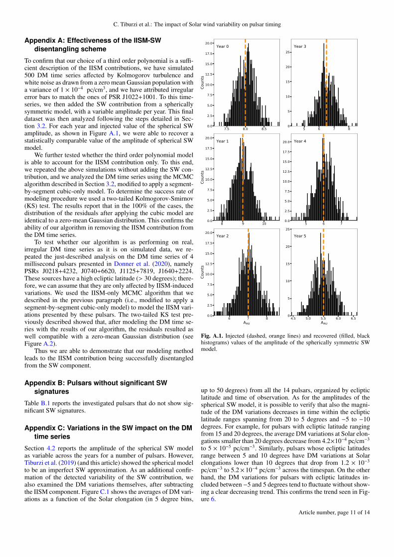
To confirm that our choice of a third order polynomial is a suffi-cient description of the IISM contributions, we have simulated500 DM time series affected by Kolmogorov turbulence andwhite noise as drawn from a zero mean Gaussian population witha variance of 1 × 10−4 pc/cm3, and we have attributed irregularerror bars to match the ones of PSR J1022+1001. To this time-series, we then added the SW contribution from a sphericallysymmetric model, with a variable amplitude per year. This finaldataset was then analyzed following the steps detailed in Sec-tion 3.2. For each year and injected value of the spherical SWamplitude, as shown in Figure A.1, we were able to recover astatistically comparable value of the amplitude of spherical SWmodel.

We further tested whether the third order polynomial modelis able to account for the IISM contribution only. To this end,we repeated the above simulations without adding the SW con-tribution, and we analyzed the DM time series using the MCMCalgorithm described in Section 3.2, modified to apply a segment-by-segment cubic-only model. To determine the success rate ofmodeling procedure we used a two-tailed Kolmogorov-Smirnov(KS) test. The results report that in the 100% of the cases, thedistribution of the residuals after applying the cubic model areidentical to a zero-mean Gaussian distribution. This confirms theability of our algorithm in removing the IISM contribution fromthe DM time series.

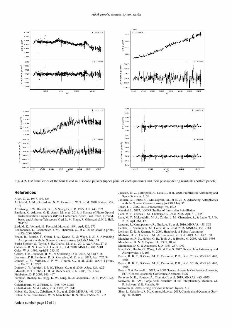
To test whether our algorithm is as performing on real,irregular DM time series as it is on simulated data, we re-peated the just-described analysis on the DM time series of 4millisecond pulsars presented in Donner et al. (2020), namelyPSRs J0218+4232, J0740+6620, J1125+7819, J1640+2224.These sources have a high ecliptic latitude (> 30 degrees); there-fore, we can assume that they are only affected by IISM-inducedvariations. We used the IISM-only MCMC algorithm that wedescribed in the previous paragraph (i.e., modified to apply asegment-by-segment cubic-only model) to model the IISM vari-ations presented by these pulsars. The two-tailed KS test pre-viously described showed that, after modeling the DM time se-ries with the results of our algorithm, the residuals resulted aswell compatible with a zero-mean Gaussian distribution (seeFigure A.2).

Thus we are able to demonstrate that our modeling methodleads to the IISM contribution being successfully disentangledfrom the SW component.

Appendix B: Pulsars without significant SWsignatures

Table B.1 reports the investigated pulsars that do not show sig-nificant SW signatures.

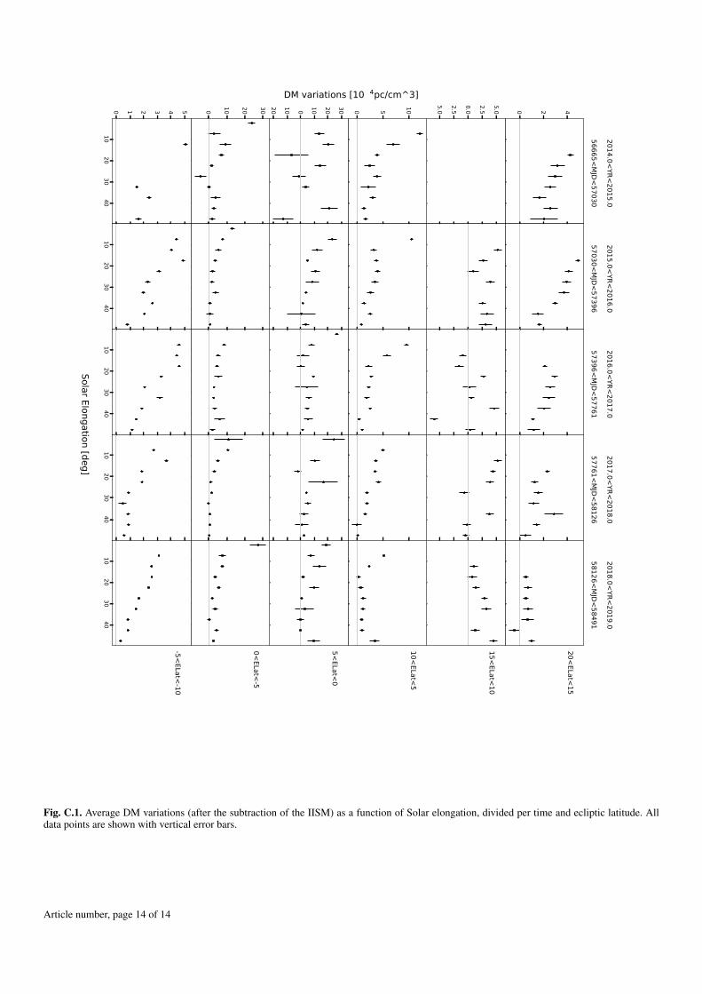
Appendix C: Variations in the SW impact on the DMtime series

Section 4.2 reports the amplitude of the spherical SW modelas variable across the years for a number of pulsars. However,Tiburzi et al. (2019) (and this article) showed the spherical modelto be an imperfect SW approximation. As an additional confir-mation of the detected variability of the SW contribution, wealso examined the DM variations themselves, after subtractingthe IISM component. Figure C.1 shows the averages of DM vari-ations as a function of the Solar elongation (in 5 degree bins,

7.5 8.0 8.50.0

2.5

5.0

7.5

10.0

12.5

15.0

17.5

20.0

Coun

ts

Year 0

5 6 7 80

5

10

15

20

25Year 3

8 9 100.0

2.5

5.0

7.5

10.0

12.5

15.0

17.5

20.0

Coun

ts

Year 1

5 6 70.0

2.5

5.0

7.5

10.0

12.5

15.0

17.5

20.0 Year 4

6 7 8AAU

0.0

2.5

5.0

7.5

10.0

12.5

15.0

17.5

20.0

Coun

ts

Year 2

4.5 5.0 5.5 6.0 6.5AAU

0

5

10

15

20

25

Year 5

Fig. A.1. Injected (dashed, orange lines) and recovered (filled, blackhistograms) values of the amplitude of the spherically symmetric SWmodel.

up to 50 degrees) from all the 14 pulsars, organized by eclipticlatitude and time of observation. As for the amplitudes of thespherical SW model, it is possible to verify that also the magni-tude of the DM variations decreases in time within the eclipticlatitude ranges spanning from 20 to 5 degrees and −5 to −10degrees. For example, for pulsars with ecliptic latitude rangingfrom 15 and 20 degrees, the average DM variations at Solar elon-gations smaller than 20 degrees decrease from 4.2×10−4 pc/cm−3

to 5 × 10−5 pc/cm−3. Similarly, pulsars whose ecliptic latitudesrange between 5 and 10 degrees have DM variations at Solarelongations lower than 10 degrees that drop from 1.2 × 10−3

pc/cm−3 to 5.2× 10−4 pc/cm−3 across the timespan. On the otherhand, the DM variations for pulsars with ecliptic latitudes in-cluded between −5 and 5 degrees tend to fluctuate without show-ing a clear decreasing trend. This confirms the trend seen in Fig-ure 6.



Fig. A.2. DM time series of the four tested millisecond pulsars (upper panel of each quadrant) and their post-modeling residuals (bottom panels).

ReferencesAllen, C. W. 1947, 107, 426Archibald, A. M., Gusinskaia, N. V., Hessels, J. W. T., et al. 2018, Nature, 559,

73Armstrong, J. W., Rickett, B. J., & Spangler, S. R. 1995, ApJ, 443, 209Bandura, K., Addison, G. E., Amiri, M., et al. 2014, in Society of Photo-Optical

Instrumentation Engineers (SPIE) Conference Series, Vol. 9145, Ground-based and Airborne Telescopes V, ed. L. M. Stepp, R. Gilmozzi, & H. J. Hall,914522

Bird, M. K., Volland, H., Paetzold, M., et al. 1994, ApJ, 426, 373Bondonneau, L., Grießmeier, J. M., Theureau, G., et al. 2020, arXiv e-prints,

arXiv:2009.02076Braun, R., Bourke, T., Green, J. A., Keane, E., & Wagg, J. 2015, Advancing

Astrophysics with the Square Kilometre Array (AASKA14), 174Burke-Spolaor, S., Taylor, S. R., Charisi, M., et al. 2019, A&A Rev., 27, 5Caballero, R. N., Guo, Y. J., Lee, K. J., et al. 2018, MNRAS, 481, 5501Coles, W. A. 1996, Ap&SS, 243, 87Cordes, J. M., Shannon, R. M., & Stinebring, D. R. 2016, ApJ, 817, 16Demorest, P. B., Ferdman, R. D., Gonzalez, M. E., et al. 2013, ApJ, 762, 94Donner, J. Y., Verbiest, J. P. W., Tiburzi, C., et al. 2020, arXiv e-prints,

arXiv:2011.13742Donner, J. Y., Verbiest, J. P. W., Tiburzi, C., et al. 2019, A&A, 624, A22Edwards, R. T., Hobbs, G. B., & Manchester, R. N. 2006, 372, 1549Finkbeiner, D. P. 2003, 146, 407Foreman-Mackey, D., Hogg, D. W., Lang, D., & Goodman, J. 2013, PASP, 125,

306Guhathakurta, M. & Fisher, R. 1998, 499, L215Guhathakurta, M. & Fisher, R. R. 1995, 22, 1841Hobbs, G., Guo, L., Caballero, R. N., et al. 2020, MNRAS, 491, 5951Hotan, A. W., van Straten, W., & Manchester, R. N. 2004, PASA, 21, 302

Jackson, B. V., Buffington, A., Cota, L., et al. 2020, Frontiers in Astronomy andSpace Sciences, 7, 76

Janssen, G., Hobbs, G., McLaughlin, M., et al. 2015, Advancing Astrophysicswith the Square Kilometre Array (AASKA14), 37

Jonas, J. L. 2009, IEEE Proceedings, 97, 1522Kuenkel, L. 2017, LOFAR Studies of Interstellar ScintillationLam, M. T., Cordes, J. M., Chatterjee, S., et al. 2016, ApJ, 819, 155Lam, M. T., McLaughlin, M. A., Cordes, J. M., Chatterjee, S., & Lazio, T. J. W.

2018, ApJ, 861, 12Lazarus, P., Karuppusamy, R., Graikou, E., et al. 2016, MNRAS, 458, 868Lentati, L., Shannon, R. M., Coles, W. A., et al. 2016, MNRAS, 458, 2161Lorimer, D. R. & Kramer, M. 2004, Handbook of Pulsar AstronomyMadison, D. R., Cordes, J. M., Arzoumanian, Z., et al. 2019, ApJ, 872, 150Manchester, R. N., Hobbs, G. B., Teoh, A., & Hobbs, M. 2005, AJ, 129, 1993Manchester, R. N. & Taylor, J. H. 1972, 10, 67Muhleman, D. O. & Anderson, J. D. 1981, 247, 1093Niu, Z.-X., Hobbs, G., Wang, J.-B., & Dai, S. 2017, Research in Astronomy and

Astrophysics, 17, 103Perera, B. B. P., DeCesar, M. E., Demorest, P. B., et al. 2019a, MNRAS, 490,

4666Perera, B. B. P., DeCesar, M. E., Demorest, P. B., et al. 2019b, MNRAS, 490,

4666Poedts, S. & Pomoell, J. 2017, in EGU General Assembly Conference Abstracts,

EGU General Assembly Conference Abstracts, 7396Porayko, N. K., Noutsos, A., Tiburzi, C., et al. 2019, MNRAS, 483, 4100Schwenn, R. 1990, Large-Scale Structure of the Interplanetary Medium, ed.

R. Schwenn & E. Marsch, 99Schwenn, R. 2006, Living Reviews in Solar Physics, 3, 2Shao, L., Caballero, R. N., Kramer, M., et al. 2013, Classical and Quantum Grav-

ity, 30, 165019



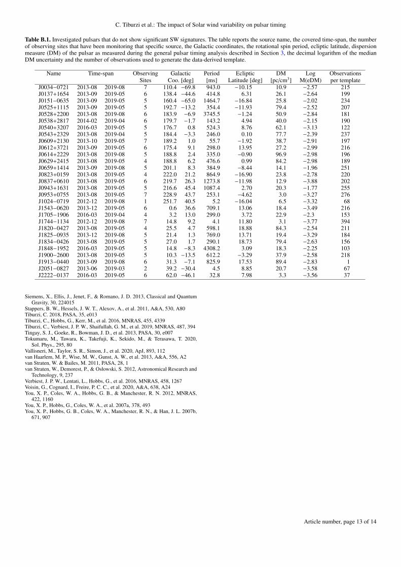
Table B.1. Investigated pulsars that do not show significant SW signatures. The table reports the source name, the covered time-span, the numberof observing sites that have been monitoring that specific source, the Galactic coordinates, the rotational spin period, ecliptic latitude, dispersionmeasure (DM) of the pulsar as measured during the general pulsar timing analysis described in Section 3, the decimal logarithm of the medianDM uncertainty and the number of observations used to generate the data-derived template.

Name Time-span Observing Galactic Period Ecliptic DM Log ObservationsSites Coo. [deg] [ms] Latitude [deg] [pc/cm3] M(eDM) per template

J0034−0721 2013-08 2019-08 7 110.4 −69.8 943.0 −10.15 10.9 −2.57 215J0137+1654 2013-09 2019-05 6 138.4 −44.6 414.8 6.31 26.1 −2.64 199J0151−0635 2013-09 2019-05 5 160.4 −65.0 1464.7 −16.84 25.8 −2.02 234J0525+1115 2013-09 2019-05 5 192.7 −13.2 354.4 −11.93 79.4 −2.52 207J0528+2200 2013-08 2019-08 6 183.9 −6.9 3745.5 −1.24 50.9 −2.84 181J0538+2817 2014-02 2019-04 6 179.7 −1.7 143.2 4.94 40.0 −2.15 190J0540+3207 2016-03 2019-05 5 176.7 0.8 524.3 8.76 62.1 −3.13 122J0543+2329 2013-08 2019-04 5 184.4 −3.3 246.0 0.10 77.7 −2.39 237J0609+2130 2013-10 2019-05 7 189.2 1.0 55.7 −1.92 38.7 −2.91 197J0612+3721 2013-09 2019-05 6 175.4 9.1 298.0 13.95 27.2 −2.99 216J0614+2229 2013-08 2019-08 5 188.8 2.4 335.0 −0.90 96.9 −2.98 196J0629+2415 2013-08 2019-05 4 188.8 6.2 476.6 0.99 84.2 −2.98 189J0659+1414 2013-09 2019-08 5 201.1 8.3 384.9 −8.44 14.1 −1.96 251J0823+0159 2013-08 2019-05 4 222.0 21.2 864.9 −16.90 23.8 −2.78 220J0837+0610 2013-08 2019-05 6 219.7 26.3 1273.8 −11.98 12.9 −3.88 202J0943+1631 2013-08 2019-05 5 216.6 45.4 1087.4 2.70 20.3 −1.77 255J0953+0755 2013-08 2019-05 7 228.9 43.7 253.1 −4.62 3.0 −3.27 276J1024−0719 2012-12 2019-08 1 251.7 40.5 5.2 −16.04 6.5 −3.32 68J1543−0620 2013-12 2019-05 6 0.6 36.6 709.1 13.06 18.4 −3.49 216J1705−1906 2016-03 2019-04 4 3.2 13.0 299.0 3.72 22.9 −2.3 153J1744−1134 2012-12 2019-08 7 14.8 9.2 4.1 11.80 3.1 −3.77 394J1820−0427 2013-08 2019-05 4 25.5 4.7 598.1 18.88 84.3 −2.54 211J1825−0935 2013-12 2019-08 5 21.4 1.3 769.0 13.71 19.4 −3.29 184J1834−0426 2013-08 2019-05 5 27.0 1.7 290.1 18.73 79.4 −2.63 156J1848−1952 2016-03 2019-05 5 14.8 −8.3 4308.2 3.09 18.3 −2.25 103J1900−2600 2013-08 2019-05 5 10.3 −13.5 612.2 −3.29 37.9 −2.58 218J1913−0440 2013-09 2019-08 6 31.3 −7.1 825.9 17.53 89.4 −2.83 1J2051−0827 2013-06 2019-03 2 39.2 −30.4 4.5 8.85 20.7 −3.58 67J2222−0137 2016-03 2019-05 6 62.0 −46.1 32.8 7.98 3.3 −3.56 37

Siemens, X., Ellis, J., Jenet, F., & Romano, J. D. 2013, Classical and QuantumGravity, 30, 224015

Stappers, B. W., Hessels, J. W. T., Alexov, A., et al. 2011, A&A, 530, A80Tiburzi, C. 2018, PASA, 35, e013Tiburzi, C., Hobbs, G., Kerr, M., et al. 2016, MNRAS, 455, 4339Tiburzi, C., Verbiest, J. P. W., Shaifullah, G. M., et al. 2019, MNRAS, 487, 394Tingay, S. J., Goeke, R., Bowman, J. D., et al. 2013, PASA, 30, e007Tokumaru, M., Tawara, K., Takefuji, K., Sekido, M., & Terasawa, T. 2020,

Sol. Phys., 295, 80Vallisneri, M., Taylor, S. R., Simon, J., et al. 2020, ApJ, 893, 112van Haarlem, M. P., Wise, M. W., Gunst, A. W., et al. 2013, A&A, 556, A2van Straten, W. & Bailes, M. 2011, PASA, 28, 1van Straten, W., Demorest, P., & Osłowski, S. 2012, Astronomical Research and

Technology, 9, 237Verbiest, J. P. W., Lentati, L., Hobbs, G., et al. 2016, MNRAS, 458, 1267Voisin, G., Cognard, I., Freire, P. C. C., et al. 2020, A&A, 638, A24You, X. P., Coles, W. A., Hobbs, G. B., & Manchester, R. N. 2012, MNRAS,

422, 1160You, X. P., Hobbs, G., Coles, W. A., et al. 2007a, 378, 493You, X. P., Hobbs, G. B., Coles, W. A., Manchester, R. N., & Han, J. L. 2007b,

671, 907



0 2 4

56665<MJD<57030

2014.0<YR<2015.0

57030<MJD<57396

2015.0<YR<2016.0

57396<MJD<57761

2016.0<YR<2017.0

57761<MJD<58126

2017.0<YR<2018.0

20<ELat<15

58126<MJD<58491

2018.0<YR<2019.0

−5.0

−2.5

0.0

2.5

5.015<ELat<10

0 5 1010<ELat<5

−20

−10 0 10 20 305<ELat<0

0 10 20 300<ELat<-5

1020

3040

0 1 2 3 4 5

1020

3040

1020

3040

1020

3040

1020

3040

-5<ELat<-10

Solar E ongation [deg]

DM variations [10−4pc/cm^3]

Fig. C.1. Average DM variations (after the subtraction of the IISM) as a function of Solar elongation, divided per time and ecliptic latitude. Alldata points are shown with vertical error bars.


the impact of solar wind variability on pulsar timing - arxiv

Documents