the swinburne intermediate latitude pulsar survey
TRANSCRIPT
arX
iv:a
stro
-ph/
0105
126v
1 8
May
200
1Mon. Not. R. Astron. Soc. 000, 000–000 (0000) Printed 17 January 2014 (MN LATEX style file v1.4)
The Swinburne Intermediate Latitude Pulsar Survey
R.T. Edwards, M. Bailes, W. van Straten and M.C. BrittonCentre for Astrophysics and Supercomputing, Swinburne University of Technology, P.O. Box 218 Hawthorn, VIC 3122, Australia
17 January 2014
ABSTRACT
We have conducted a survey of intermediate Galactic latitudes using the 13-beam21-cm multibeam receiver of the Parkes 64-m radio telescope. The survey covered theregion enclosed by 5◦ < |b| < 15◦ and −100◦ < l < 50◦ with 4,702 processed pointingsof 265 s each, for a total of 14.5 days of integration time. Thirteen 2 × 96-channelfilterbanks provided 288 MHz of bandwidth at a centre frequency of 1374 MHz, one-bit sampled every 125 µs and incurring ∼DM/13.4 cm−3 pc samples of dispersionsmearing. The system was sensitive to slow and most millisecond pulsars in the regionwith flux densities greater than approximately 0.3–1.1 mJy. Offline analysis on the 64-node Swinburne workstation cluster resulted in the detection of 170 pulsars of which69 were new discoveries. Eight of the new pulsars, by virtue of their small spin periodsand period derivatives, may be recycled and have been reported elsewhere. The slowpulsars discovered are typical of those already known in the volume searched, beingof intermediate to old age. Several pulsars experience pulse nulling and two displayvery regular drifting sub-pulses. We discuss the new discoveries and provide timingparameters for the 48 slow pulsars for which we have a phase-connnected solution.
Key words: methods: observational – pulsars: general – surveys
1 INTRODUCTION
By the late 1990s radio pulsar surveys had resulted in thediscovery of ∼700 pulsars, spawning numerous studies withwide ranging implications for astrophysics and physics ingeneral. Despite having been first discovered over a quar-ter of a century earlier, pulsars with unique and interest-ing properties (e.g. Wolszczan & Frail 1992; Johnston et al.1992b; Johnston et al. 1993; Bell et al. 1995; Stappers et al.1996) continued to be uncovered by surveys which alsoserved the purpose of providing a larger sample for statis-tical analyses of classes of pulsars and pulsar binaries (e.g.Lyne et al. 1998).
Nearly all early surveys were conducted at low frequen-cies (ν ≃ 400 MHz) due to the steep spectrum (α ≃ −1.6,where S ∝ να; Lorimer et al. 1995) characteristic of mi-crowave radiation from pulsars and the faster sky cover-age afforded by the larger telescope beam at these frequen-cies. However, two effects that hamper the detection of cer-tain pulsars at low frequencies can be avoided by using ahigher frequency. Firstly, for small Galactic latitudes thebackground of Galactic synchrotron emission comprises themain contribution to the system temperature at these fre-quencies. The spectrum of this radiation is steep (α ≃ −2.6;Lawson et al. 1987) and at high frequencies generally repre-sents an insignificant contribution compared to the thermalreceiver noise. Since they share the low Galactic z-height oftheir progenitor population, young pulsars in particular are
selected against in low frequency surveys due to the elevatedsky background temperature. Secondly, radiation propagat-ing through the interstellar medium is subject to ‘scatter-ing’ due to multi-path propagation, effectively convolvingthe light curve with an exponential of a time constant thatscales as ν−4 (Ables, Komesaroff & Hamilton 1970). Sincethe minimum detectable mean flux density in pulsar obser-vations is proportional to [δ/(1 − δ)]1/2 where δ is the ef-fective pulse duty cycle, scatter-broadening of the receivedpulses hampers the detection of pulsars at low frequencies,especially those with short spin period such as the interest-ing and important class of ‘millisecond’ pulsars, and (again)young pulsars. Moreover, by conducting a survey at high fre-quencies one is sensitive to pulsars with flatter spectra thatwere missed in earlier surveys.
With the rise in availability of affordable computingpower in the 1980s it became feasible to process surveyswith fast sampling rates and large numbers of pointings, asrequired for large scale high frequency surveys for millisec-ond pulsars. Clifton et al. (1992) and Johnston et al. (1992a)conducted highly successful 20-cm pulsar surveys near theGalactic plane, discovering 86 pulsars between them, includ-ing a high fraction of young pulsars. However, the surveysdid not have sufficient sensitivity at high time resolution todiscover any millisecond pulsars. In addition, for the reasonsmentioned above the surveys concentrated on the Galacticplane and hence the samples of detected pulsars were of
c© 0000 RAS
2 R.T. Edwards, M. Bailes, W. van Straten and M.C. Britton
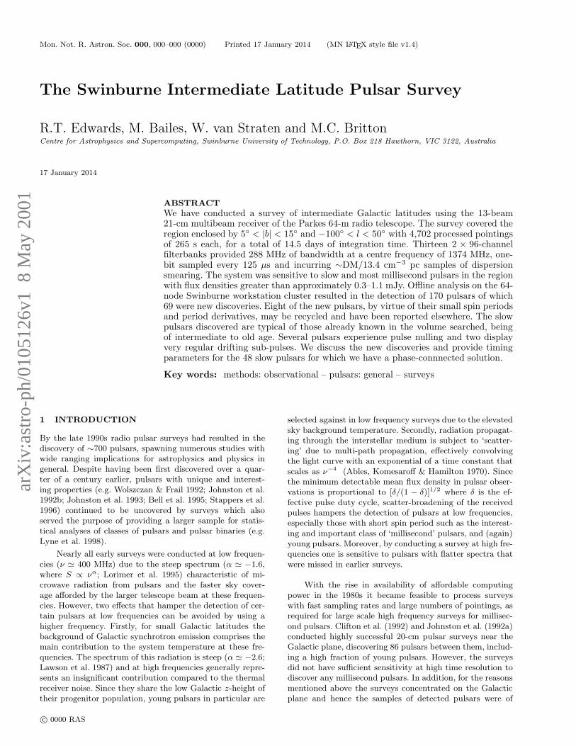
Figure 1. The multibeam tessellation unit shown with circlesdepicting the half-power points of beams. A unit is observed withfour offset pointings, one of which is hatched in the above forclarity. The shape made by the 52 beams can be seamlessly self-tessellated.
reduced value in modelling the Galactic pulsar populationcompared to larger surveys.
In 1997 the Australia Telescope National Facility com-missioned a new 21-cm 13-feed multibeam receiver, primar-ily for HI surveys (Henning et al. 2000; Barnes et al. 2001).The large instantaneous sky coverage and excellent sensitiv-ity also makes the system a powerful pulsar survey instru-ment and this led to the commencement of a long-runningdeep survey of the southern Galactic plane (|b| < 5◦) whichis expected to almost double the known population (Lyneet al. 2000; Camilo et al. 2000). We conducted Monte Carlosimulations similar to those discussed by Toscano et al.(1998) and found that a shallower ‘flanking’ survey shoulddiscover a sizeable population of pulsars with unprecedentedtime efficiency in an area of sky not previously sampled athigh frequencies. Based on this result we conducted sucha survey between 1998 August and 1999 August. The sur-vey proved highly successful, discovering 69 pulsars includ-ing two pulsar binaries containing heavy CO white dwarfs,one of which will coalesce in less than a Hubble time withdramatic and unknown consequences (Edwards & Bailes2001b), and a further four binary and two (perhaps three)isolated recycled pulsars with important implications fortheories of binary evolution (Edwards & Bailes 2001a). Inthis paper we report in detail on the observing system, anal-ysis procedures, sensitivity and completeness. We discussdetections of previously known pulsars and present the newsample of slow pulsars, including timing results for thosewith solutions.
2 OBSERVATIONS AND ANALYSIS
2.1 Hardware Configuration and Survey
Observations
The 64-m Parkes radio telescope was used with the 13-beam21-cm receiver (Staveley-Smith et al. 1996) which provides300 MHz of bandwidth and a system temperature of ∼21 K.Signals from the two orthogonal polarisations of each beamwere mixed with a local oscillator before being fed to anarray of 26 96-channel filterbanks. Each filterbank channelwas 3 MHz wide and the band was centred at a frequencyof 1374 MHz. The detected signals from corresponding po-larisation pairs in each channel were summed and high passfiltered (with a time constant of ∼0.9 s; Manchester et al.2000) before being integrated and one-bit sampled every 125µs. The data stream was written to magnetic tape (DLT7000) for offline processing, as well as being made availableto online interference monitoring software in near-real-timevia the computer network. With the exception of the sam-pling interval, the system was identical to that used for theGalactic plane survey (Manchester et al. 2001).
The receiver feeds are arranged in such a way as to al-low coverage of the sky in a hexagonal grid, with beamsoverlapping at their approximate half-power points (7′ fromthe beam centre). A group of four pointings results in theuniform coverage of a roughly circular shape ∼ 1 degreein radius which in turn can be efficiently tessellated (seeFigure 1). The region enclosed by 5◦ < |b| < 15◦ and−100◦ < l < 50◦ was covered in 4,764 265-s proposed point-ings, amounting to only 14.6 days of integration time. Mostof these pointings were observed in several week-long ob-serving runs between August 1998 and August 1999.
2.2 Search Analysis Procedure
The processing of the 64-tape ∼ 1.6 terabyte data set wasperformed on the Swinburne Supercluster, a network of 64Compaq Alpha workstations. Before searching for pulsars,each beam was analysed for the presence of powerful signalsthat appeared in only a few filterbank channels, a commontype of interference signal. When such signals were present,samples in the culprit channels were zeroed, a process thatdoes not incur too much loss of sensitivity since this variesas the square root of the effective bandwidth. In addition,broad-band periodic signals that appear in large numbersof beams in any given 30-minute period were detected andlogged to a file for later reference.
To correct for the effects of non-linearity in the dis-persion relation, data from the 96 filterbank channels werepadded with 32 dummy channels in such a way as to al-low linear de-dispersion of the resulting 128 channels, asused by the Galactic plane survey collaboration. This en-abled the use of the fast ‘tree’ algorithm of Taylor (1974)to partially de-disperse the data into eight trial dispersionmeasures in each of sixteen sub-bands. Whilst the linearityof dispersion with respect to channel number would enablefull de-dispersion (that is, 128 trial DMs with no sub-banddivisions), in order to limit storage requirements and to al-low the recording of frequency-resolved pulse profiles to aidin suspect scrutiny, application of the algorithm was stoppedafter the production of eight DMs.
The tree algorithm produces trial DMs up to the ‘diag-onal’ DM of 17.0 cm−3 pc, where the dispersion delay across
c© 0000 RAS, MNRAS 000, 000–000
The Swinburne Intermediate Latitude Pulsar Survey 3
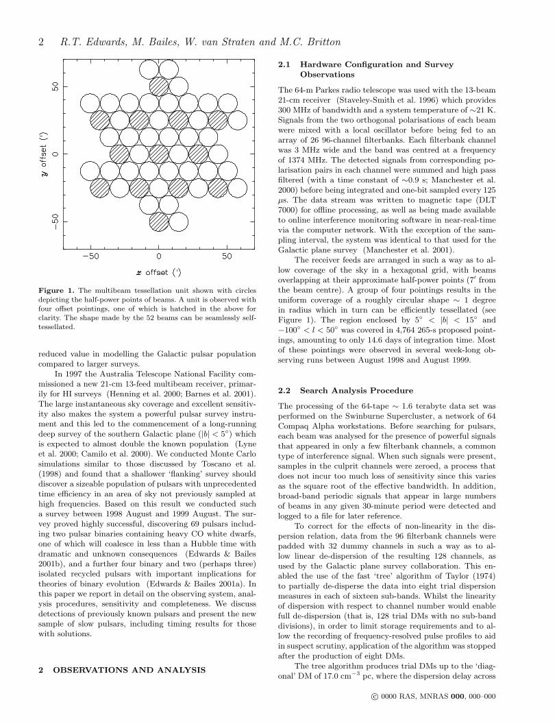
Figure 2. Sky coverage for the survey. Ellipses represent groups of four inter-meshed pointings. Shades of grey represent the density ofcoverage, from unobserved (white) to observed twice (black).
one sub-band in units of samples is equal to the number ofchannels used to form it. It should be noted that in previ-ous surveys where the linear dispersion approximation wasacceptable for the tree stage, this parameter was approxi-mately equal to the DM at which the smearing induced ineach channel was one sample interval. The latter parame-ter is commonly quoted in conjunction with the samplinginterval to give an indication of the time resolution avail-able to pulsars of various DMs in a pulsar survey. For thepresent survey this value varies from 9.4 to 17.5 cm−3 pcdepending on the centre frequency of the channel, and forevaluation purposes one should use the geometric mean of13.4 cm−3 pc. The tree algorithm was extended to also pro-duce time series for 1–2 times the diagonal DM, and beyondthis value the sample interval was doubled by summing ofsamples before re-application of the algorithm, and the pro-cess repeated to produce time series with 2–4, 4–8, 8–16 and16–32 times the diagonal DM.
The periodicity search itself was based on that of theParkes Southern Pulsar Survey (Manchester et al. 1996),generalized and modified to handle the large number of spu-rious interference signals present in the multibeam data.Time series were constructed at 375 trial values of disper-sion measure from 0 to 562.5 cm−3 pc by summing partiallyde-dispersed sub-bands in the nearest DM with the appro-priate time offsets. The trial DMs were spaced in such a waythat the effective smearing induced due to the difference be-tween the DM of a pulsar and the nearest trial DM was nomore than twice that induced by the finite width of individ-
ual filterbank channels. The time series were filtered with aboxcar of width 2048 ms to remove the effects of receivernoise and gain variations during the course of the observa-tion, before being Fourier transformed and detected to formthe fluctuation power spectrum.
For signals with frequencies lying on the boundary be-tween two spectral bins the result is two components of equalmagnitude and opposite sign in the adjacent bins. To main-tain sensitivity to such signals we also computed the differ-ence of each bin and its neighbours and used half the squaredmagnitude of the results as alternative estimates of spectralpower. For each bin the highest of the three power valuescomputed was chosen for use in the final power spectrum.In the case of the zero-DM time series, this spectrum waschecked for the occurrence of any signal with a frequencyclose to one earlier logged as a broad band interference sig-nal contemporaneous with this observation. Should such asignal be present, its exact extent in the spectrum was as-sessed and the corresponding bins zeroed in this and allother power spectra searched in this beam. The spectrumabove a frequency of 1/12 Hz was then searched for signifi-cant spikes compared to a local mean (to compensate for theoverall redness of the spectrum). Harmonics were summedand the process repeated for up to 16 harmonics to main-tain sensitivity to signals with short duty cycles. Significantsignals at any level of harmonic summing were recorded andafter all trial dispersion measures had been searched the setof signals was correlated into a number of candidates, eachcovering signals of similar pulse period occurring at multiple
c© 0000 RAS, MNRAS 000, 000–000
4 R.T. Edwards, M. Bailes, W. van Straten and M.C. Britton
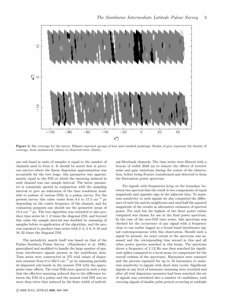
Figure 3. Estimated minimum detectable mean flux density(Smin) as a function of pulse period for intrinsic pulse widthsof 10◦ (solid lines) and 90◦ (dashed lines) at dispersion measuresof 0, 10, 30, 100 and 300 cm−3 pc (in order of increasing Smin for agiven pulse period). Points represent undetected pulsars which liewithin 10′ of an observed beam, where flux density measurementshave been published. Flux densities published without uncertain-ties are plotted without error bars and in such cases the relativeuncertainty is probably around 50 per cent.
trial DMs. The top 99 candidates in each beam were sub-ject to a fine search (by means of maximisation of signal tonoise ratio, S/N) in period and dispersion measure aroundthe best values found in the spectral search. Pertinent infor-mation including the resulting best profile, grey scale mapsof pulse profiles as a function of time and radio frequencyand of signal to noise as a function of period and dispersionmeasure were saved to disk.
2.3 Suspect Scrutiny, Confirmation and Timing
Observations
The final stage of analysis was human viewing. The largenumber of beams and the prevalence of interference signalspresented considerable complications to the viewing processdue to the volume of candidates produced. In previous sur-veys (e.g. Manchester et al. 1996) candidates of similar pe-riod occurring in multiple beams contemporaneously weregenerally taken as interference signals and ignored. In thecase of results from this survey, the plethora of interferencesignals across the spectrum resulted in the misinterpreta-tion of many pulsars as interference. It was found that thislimited the applicability of this approach to the handful ofperiods that appeared more than ∼ 250 times on any tape.All remaining candidates with signal to noise ratios greaterthan eight (of which there were several hundred thousand)were then scrutinized by a human viewer and promising sig-nals scheduled for confirmation by re-observation.
Human viewing of all suspects with S/N > 8 was ex-
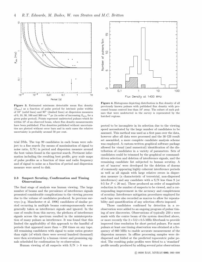
Figure 4. Histograms depicting distribution in flux density of allpreviously known pulsars with published flux density with pro-cessed beams centred less than 10′ away. The subset of such pul-sars that were undetected in the survey is represented by thehatched regions.
pected to be incomplete in its selection due to the viewingspeed necessitated by the large number of candidates to beassessed. This method was used as a first pass over the data,however after all data were processed and the 30 GB resultset assembled, a more complete candidate analysis schemewas employed. A custom-written graphical software packageallowed for visual (and numerical) identification of the dis-tribution of candidates in a variety of parameters. Sets ofcandidates could be trimmed by the graphical or command-driven selection and deletion of interference signals, and theremaining candidate list subjected to human scrutiny. Aset of ‘macros’ were developed for the deletion of dozensof commonly appearing highly coherent interference periodsas well as all signals with large relative errors in disper-sion measure (a characteristic of terrestrial, non-dispersedinterference) and any candidate with a S/N less than 9 (or9.5 for P < 20 ms). These produced an order of magnitudereduction in the number of suspects to be viewed, and a cor-responding improvement in the accuracy and completenessof scrutiny. Interference mitigation procedures employed foreach tape were also recorded as macros to allow for repeata-bility and quantification of any selection effects imposed.
Those candidates confirmed by detection in a re-observation were added to an ongoing program of pulsar tim-ing of new discoveries. Observations of typically 250 s weremade with the centre beam of the system described above,or more recently the 2×512×0.5-MHz filterbank to provideimproved time resolution for short period pulsars. For mostpulsars at least one timing observation was obtained at a fre-quency of 660 MHz to enable accurate measurement of thedispersion measure. In offline processing samples were de-dispersed and folded at the predicted topocentric pulse pe-riod. The resulting pulse profiles were fitted to a ‘standard’profile usually produced by adding several prior observations
c© 0000 RAS, MNRAS 000, 000–000
The Swinburne Intermediate Latitude Pulsar Survey 5
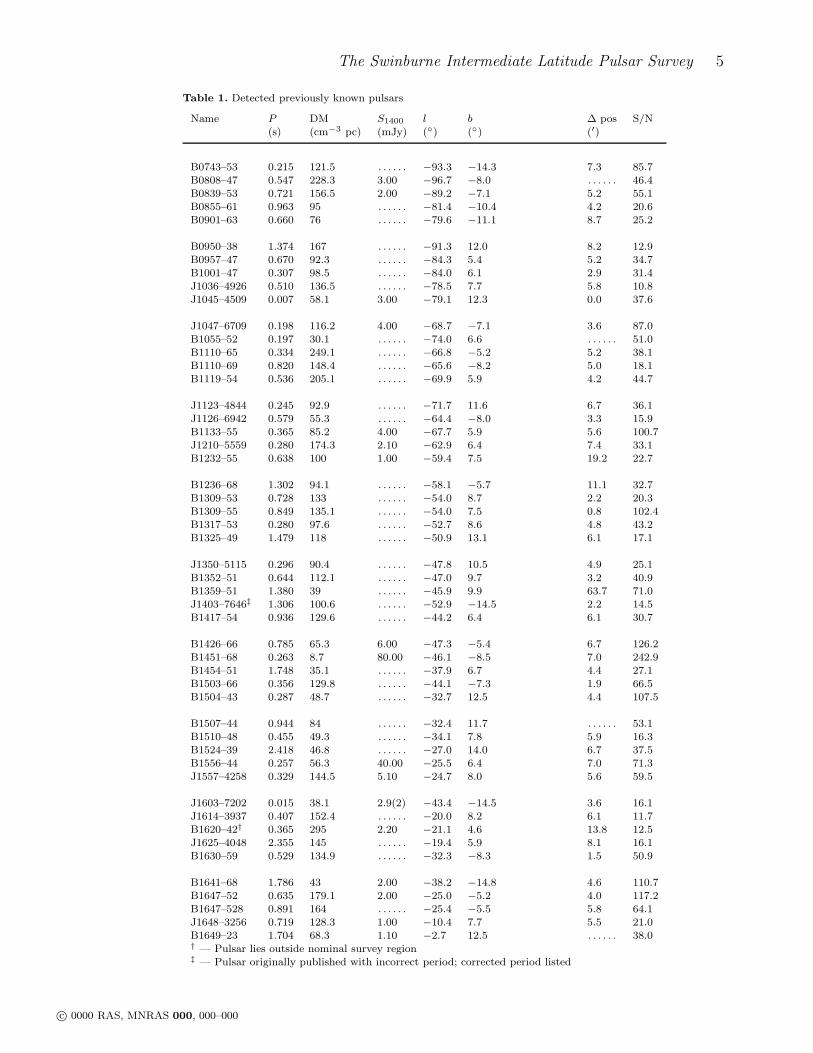
Table 1. Detected previously known pulsars
Name P DM S1400 l b ∆ pos S/N(s) (cm−3 pc) (mJy) (◦) (◦) (′)
B0743–53 0.215 121.5 . . . . . . −93.3 −14.3 7.3 85.7B0808–47 0.547 228.3 3.00 −96.7 −8.0 . . . . . . 46.4B0839–53 0.721 156.5 2.00 −89.2 −7.1 5.2 55.1B0855–61 0.963 95 . . . . . . −81.4 −10.4 4.2 20.6B0901–63 0.660 76 . . . . . . −79.6 −11.1 8.7 25.2
B0950–38 1.374 167 . . . . . . −91.3 12.0 8.2 12.9B0957–47 0.670 92.3 . . . . . . −84.3 5.4 5.2 34.7B1001–47 0.307 98.5 . . . . . . −84.0 6.1 2.9 31.4J1036–4926 0.510 136.5 . . . . . . −78.5 7.7 5.8 10.8J1045–4509 0.007 58.1 3.00 −79.1 12.3 0.0 37.6
J1047–6709 0.198 116.2 4.00 −68.7 −7.1 3.6 87.0B1055–52 0.197 30.1 . . . . . . −74.0 6.6 . . . . . . 51.0B1110–65 0.334 249.1 . . . . . . −66.8 −5.2 5.2 38.1B1110–69 0.820 148.4 . . . . . . −65.6 −8.2 5.0 18.1B1119–54 0.536 205.1 . . . . . . −69.9 5.9 4.2 44.7
J1123–4844 0.245 92.9 . . . . . . −71.7 11.6 6.7 36.1J1126–6942 0.579 55.3 . . . . . . −64.4 −8.0 3.3 15.9B1133–55 0.365 85.2 4.00 −67.7 5.9 5.6 100.7J1210–5559 0.280 174.3 2.10 −62.9 6.4 7.4 33.1B1232–55 0.638 100 1.00 −59.4 7.5 19.2 22.7
B1236–68 1.302 94.1 . . . . . . −58.1 −5.7 11.1 32.7B1309–53 0.728 133 . . . . . . −54.0 8.7 2.2 20.3B1309–55 0.849 135.1 . . . . . . −54.0 7.5 0.8 102.4B1317–53 0.280 97.6 . . . . . . −52.7 8.6 4.8 43.2B1325–49 1.479 118 . . . . . . −50.9 13.1 6.1 17.1
J1350–5115 0.296 90.4 . . . . . . −47.8 10.5 4.9 25.1B1352–51 0.644 112.1 . . . . . . −47.0 9.7 3.2 40.9B1359–51 1.380 39 . . . . . . −45.9 9.9 63.7 71.0J1403–7646‡ 1.306 100.6 . . . . . . −52.9 −14.5 2.2 14.5B1417–54 0.936 129.6 . . . . . . −44.2 6.4 6.1 30.7
B1426–66 0.785 65.3 6.00 −47.3 −5.4 6.7 126.2B1451–68 0.263 8.7 80.00 −46.1 −8.5 7.0 242.9B1454–51 1.748 35.1 . . . . . . −37.9 6.7 4.4 27.1B1503–66 0.356 129.8 . . . . . . −44.1 −7.3 1.9 66.5B1504–43 0.287 48.7 . . . . . . −32.7 12.5 4.4 107.5
B1507–44 0.944 84 . . . . . . −32.4 11.7 . . . . . . 53.1B1510–48 0.455 49.3 . . . . . . −34.1 7.8 5.9 16.3B1524–39 2.418 46.8 . . . . . . −27.0 14.0 6.7 37.5B1556–44 0.257 56.3 40.00 −25.5 6.4 7.0 71.3J1557–4258 0.329 144.5 5.10 −24.7 8.0 5.6 59.5
J1603–7202 0.015 38.1 2.9(2) −43.4 −14.5 3.6 16.1J1614–3937 0.407 152.4 . . . . . . −20.0 8.2 6.1 11.7B1620–42† 0.365 295 2.20 −21.1 4.6 13.8 12.5J1625–4048 2.355 145 . . . . . . −19.4 5.9 8.1 16.1B1630–59 0.529 134.9 . . . . . . −32.3 −8.3 1.5 50.9
B1641–68 1.786 43 2.00 −38.2 −14.8 4.6 110.7B1647–52 0.635 179.1 2.00 −25.0 −5.2 4.0 117.2B1647–528 0.891 164 . . . . . . −25.4 −5.5 5.8 64.1J1648–3256 0.719 128.3 1.00 −10.4 7.7 5.5 21.0B1649–23 1.704 68.3 1.10 −2.7 12.5 . . . . . . 38.0† — Pulsar lies outside nominal survey region‡ — Pulsar originally published with incorrect period; corrected period listed
c© 0000 RAS, MNRAS 000, 000–000
6 R.T. Edwards, M. Bailes, W. van Straten and M.C. Britton
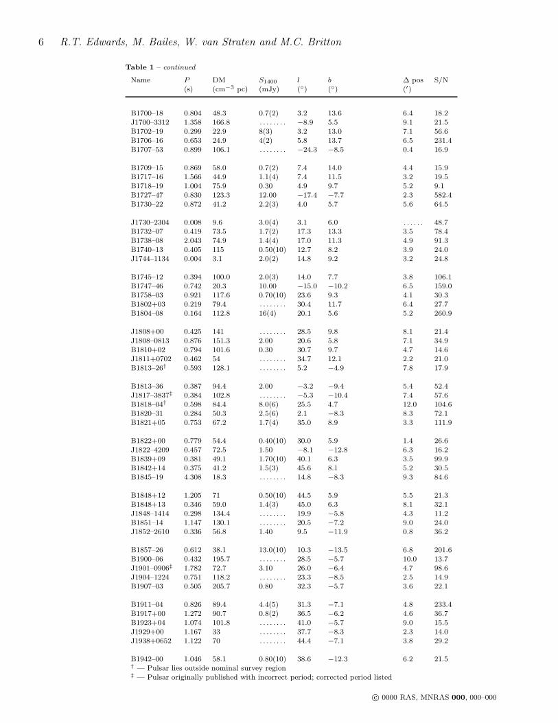
Table 1 – continued
Name P DM S1400 l b ∆ pos S/N(s) (cm−3 pc) (mJy) (◦) (◦) (′)
B1700–18 0.804 48.3 0.7(2) 3.2 13.6 6.4 18.2J1700–3312 1.358 166.8 . . . . . . . . −8.9 5.5 9.1 21.5B1702–19 0.299 22.9 8(3) 3.2 13.0 7.1 56.6B1706–16 0.653 24.9 4(2) 5.8 13.7 6.5 231.4B1707–53 0.899 106.1 . . . . . . . . −24.3 −8.5 0.4 16.9
B1709–15 0.869 58.0 0.7(2) 7.4 14.0 4.4 15.9B1717–16 1.566 44.9 1.1(4) 7.4 11.5 3.2 19.5B1718–19 1.004 75.9 0.30 4.9 9.7 5.2 9.1B1727–47 0.830 123.3 12.00 −17.4 −7.7 2.3 582.4B1730–22 0.872 41.2 2.2(3) 4.0 5.7 5.6 64.5
J1730–2304 0.008 9.6 3.0(4) 3.1 6.0 . . . . . . 48.7B1732–07 0.419 73.5 1.7(2) 17.3 13.3 3.5 78.4B1738–08 2.043 74.9 1.4(4) 17.0 11.3 4.9 91.3B1740–13 0.405 115 0.50(10) 12.7 8.2 3.9 24.0J1744–1134 0.004 3.1 2.0(2) 14.8 9.2 3.2 24.8
B1745–12 0.394 100.0 2.0(3) 14.0 7.7 3.8 106.1B1747–46 0.742 20.3 10.00 −15.0 −10.2 6.5 159.0B1758–03 0.921 117.6 0.70(10) 23.6 9.3 4.1 30.3B1802+03 0.219 79.4 . . . . . . . . 30.4 11.7 6.4 27.7B1804–08 0.164 112.8 16(4) 20.1 5.6 5.2 260.9
J1808+00 0.425 141 . . . . . . . . 28.5 9.8 8.1 21.4
J1808–0813 0.876 151.3 2.00 20.6 5.8 7.1 34.9B1810+02 0.794 101.6 0.30 30.7 9.7 4.7 14.6J1811+0702 0.462 54 . . . . . . . . 34.7 12.1 2.2 21.0B1813–26† 0.593 128.1 . . . . . . . . 5.2 −4.9 7.8 17.9
B1813–36 0.387 94.4 2.00 −3.2 −9.4 5.4 52.4J1817–3837‡ 0.384 102.8 . . . . . . . . −5.3 −10.4 7.4 57.6B1818–04† 0.598 84.4 8.0(6) 25.5 4.7 12.0 104.6B1820–31 0.284 50.3 2.5(6) 2.1 −8.3 8.3 72.1B1821+05 0.753 67.2 1.7(4) 35.0 8.9 3.3 111.9
B1822+00 0.779 54.4 0.40(10) 30.0 5.9 1.4 26.6J1822–4209 0.457 72.5 1.50 −8.1 −12.8 6.3 16.2B1839+09 0.381 49.1 1.70(10) 40.1 6.3 3.5 99.9B1842+14 0.375 41.2 1.5(3) 45.6 8.1 5.2 30.5B1845–19 4.308 18.3 . . . . . . . . 14.8 −8.3 9.3 84.6
B1848+12 1.205 71 0.50(10) 44.5 5.9 5.5 21.3B1848+13 0.346 59.0 1.4(3) 45.0 6.3 8.1 32.1J1848–1414 0.298 134.4 . . . . . . . . 19.9 −5.8 4.3 11.2B1851–14 1.147 130.1 . . . . . . . . 20.5 −7.2 9.0 24.0J1852–2610 0.336 56.8 1.40 9.5 −11.9 0.8 36.2
B1857–26 0.612 38.1 13.0(10) 10.3 −13.5 6.8 201.6B1900–06 0.432 195.7 . . . . . . . . 28.5 −5.7 10.0 13.7J1901–0906‡ 1.782 72.7 3.10 26.0 −6.4 4.7 98.6J1904–1224 0.751 118.2 . . . . . . . . 23.3 −8.5 2.5 14.9B1907–03 0.505 205.7 0.80 32.3 −5.7 3.6 22.1
B1911–04 0.826 89.4 4.4(5) 31.3 −7.1 4.8 233.4B1917+00 1.272 90.7 0.8(2) 36.5 −6.2 4.6 36.7B1923+04 1.074 101.8 . . . . . . . . 41.0 −5.7 9.0 15.5J1929+00 1.167 33 . . . . . . . . 37.7 −8.3 2.3 14.0J1938+0652 1.122 70 . . . . . . . . 44.4 −7.1 3.8 29.2
B1942–00 1.046 58.1 0.80(10) 38.6 −12.3 6.2 21.5† — Pulsar lies outside nominal survey region‡ — Pulsar originally published with incorrect period; corrected period listed
c© 0000 RAS, MNRAS 000, 000–000
The Swinburne Intermediate Latitude Pulsar Survey 7
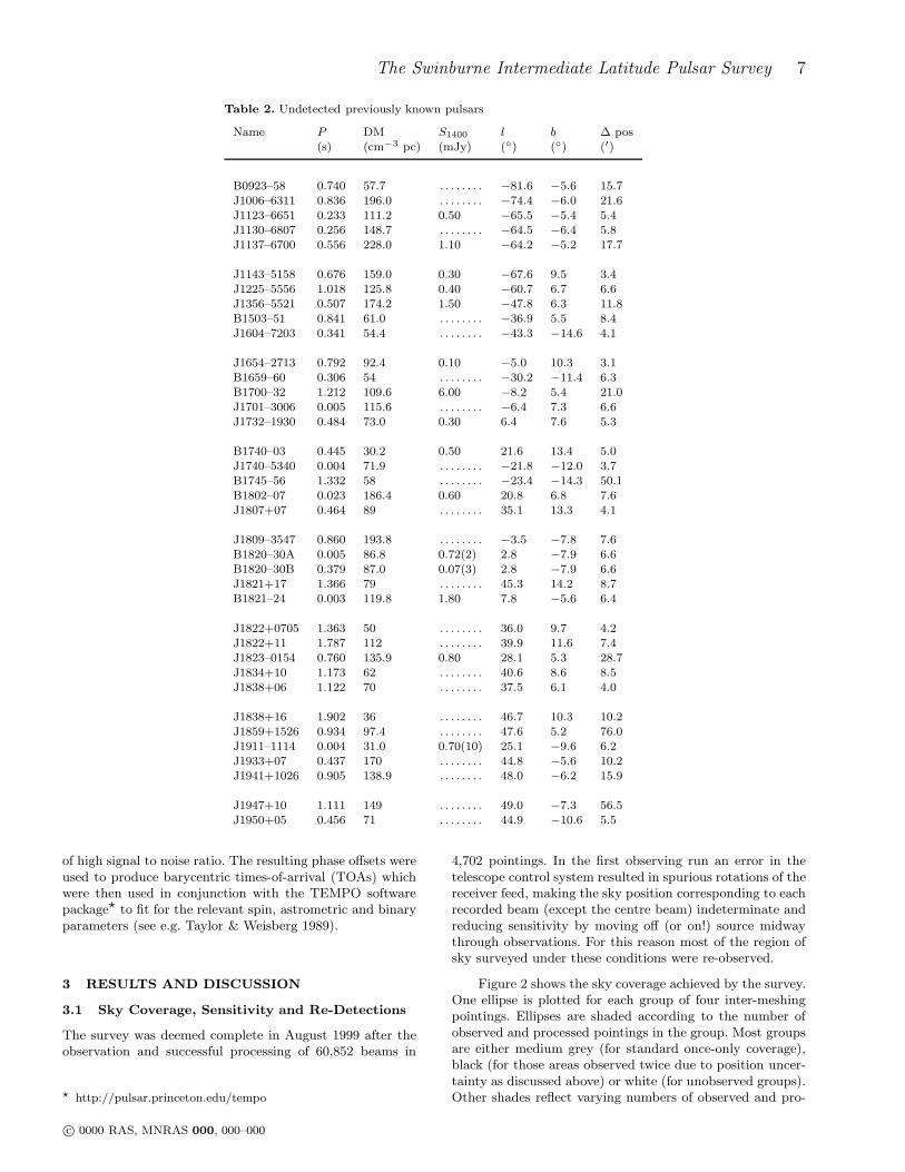
Table 2. Undetected previously known pulsars
Name P DM S1400 l b ∆ pos(s) (cm−3 pc) (mJy) (◦) (◦) (′)
B0923–58 0.740 57.7 . . . . . . . . −81.6 −5.6 15.7J1006–6311 0.836 196.0 . . . . . . . . −74.4 −6.0 21.6J1123–6651 0.233 111.2 0.50 −65.5 −5.4 5.4J1130–6807 0.256 148.7 . . . . . . . . −64.5 −6.4 5.8J1137–6700 0.556 228.0 1.10 −64.2 −5.2 17.7
J1143–5158 0.676 159.0 0.30 −67.6 9.5 3.4J1225–5556 1.018 125.8 0.40 −60.7 6.7 6.6J1356–5521 0.507 174.2 1.50 −47.8 6.3 11.8B1503–51 0.841 61.0 . . . . . . . . −36.9 5.5 8.4J1604–7203 0.341 54.4 . . . . . . . . −43.3 −14.6 4.1
J1654–2713 0.792 92.4 0.10 −5.0 10.3 3.1B1659–60 0.306 54 . . . . . . . . −30.2 −11.4 6.3B1700–32 1.212 109.6 6.00 −8.2 5.4 21.0J1701–3006 0.005 115.6 . . . . . . . . −6.4 7.3 6.6J1732–1930 0.484 73.0 0.30 6.4 7.6 5.3
B1740–03 0.445 30.2 0.50 21.6 13.4 5.0J1740–5340 0.004 71.9 . . . . . . . . −21.8 −12.0 3.7B1745–56 1.332 58 . . . . . . . . −23.4 −14.3 50.1B1802–07 0.023 186.4 0.60 20.8 6.8 7.6J1807+07 0.464 89 . . . . . . . . 35.1 13.3 4.1
J1809–3547 0.860 193.8 . . . . . . . . −3.5 −7.8 7.6B1820–30A 0.005 86.8 0.72(2) 2.8 −7.9 6.6B1820–30B 0.379 87.0 0.07(3) 2.8 −7.9 6.6J1821+17 1.366 79 . . . . . . . . 45.3 14.2 8.7B1821–24 0.003 119.8 1.80 7.8 −5.6 6.4
J1822+0705 1.363 50 . . . . . . . . 36.0 9.7 4.2J1822+11 1.787 112 . . . . . . . . 39.9 11.6 7.4J1823–0154 0.760 135.9 0.80 28.1 5.3 28.7J1834+10 1.173 62 . . . . . . . . 40.6 8.6 8.5J1838+06 1.122 70 . . . . . . . . 37.5 6.1 4.0
J1838+16 1.902 36 . . . . . . . . 46.7 10.3 10.2J1859+1526 0.934 97.4 . . . . . . . . 47.6 5.2 76.0J1911–1114 0.004 31.0 0.70(10) 25.1 −9.6 6.2J1933+07 0.437 170 . . . . . . . . 44.8 −5.6 10.2J1941+1026 0.905 138.9 . . . . . . . . 48.0 −6.2 15.9
J1947+10 1.111 149 . . . . . . . . 49.0 −7.3 56.5J1950+05 0.456 71 . . . . . . . . 44.9 −10.6 5.5
of high signal to noise ratio. The resulting phase offsets wereused to produce barycentric times-of-arrival (TOAs) whichwere then used in conjunction with the TEMPO softwarepackage⋆ to fit for the relevant spin, astrometric and binaryparameters (see e.g. Taylor & Weisberg 1989).
3 RESULTS AND DISCUSSION
3.1 Sky Coverage, Sensitivity and Re-Detections
The survey was deemed complete in August 1999 after theobservation and successful processing of 60,852 beams in
⋆ http://pulsar.princeton.edu/tempo
4,702 pointings. In the first observing run an error in thetelescope control system resulted in spurious rotations of thereceiver feed, making the sky position corresponding to eachrecorded beam (except the centre beam) indeterminate andreducing sensitivity by moving off (or on!) source midwaythrough observations. For this reason most of the region ofsky surveyed under these conditions were re-observed.
Figure 2 shows the sky coverage achieved by the survey.One ellipse is plotted for each group of four inter-meshingpointings. Ellipses are shaded according to the number ofobserved and processed pointings in the group. Most groupsare either medium grey (for standard once-only coverage),black (for those areas observed twice due to position uncer-tainty as discussed above) or white (for unobserved groups).Other shades reflect varying numbers of observed and pro-
c© 0000 RAS, MNRAS 000, 000–000
8 R.T. Edwards, M. Bailes, W. van Straten and M.C. Britton
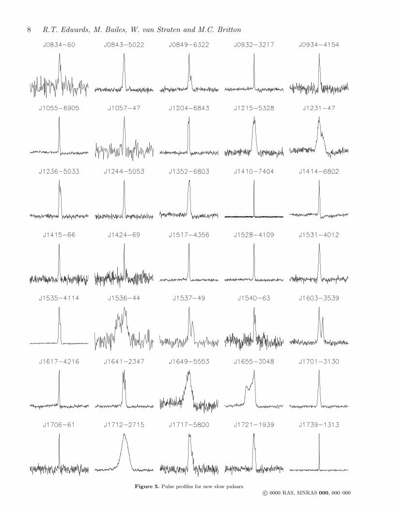
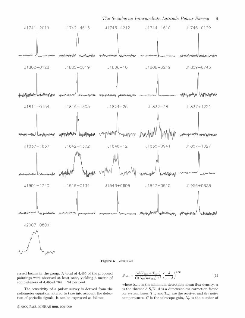
Figure 5. Pulse profiles for new slow pulsarsc© 0000 RAS, MNRAS 000, 000–000
The Swinburne Intermediate Latitude Pulsar Survey 9
Figure 5 – continued
cessed beams in the group. A total of 4,465 of the proposedpointings were observed at least once, yielding a metric ofcompleteness of 4,465/4,764 = 94 per cent.
The sensitivity of a pulsar survey is derived from theradiometer equation, altered to take into account the detec-tion of periodic signals. It can be expressed as follows,
Smin =αβ(Trec + Tsky)
G(Np∆νtobs)1/2
(
δ
1 − δ
)1/2
(1)
where Smin is the minimum detectable mean flux density, αis the threshold S/N, β is a dimensionless correction factorfor system losses, Trec and Tsky are the receiver and sky noisetemperatures, G is the telescope gain, Np is the number of
c© 0000 RAS, MNRAS 000, 000–000
10 R.T. Edwards, M. Bailes, W. van Straten and M.C. Britton
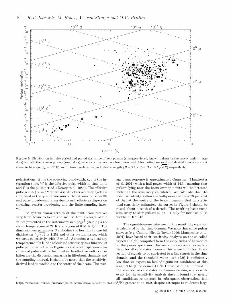
Figure 6. Distribution in pulse period and period derivative of new pulsars (stars),previously known pulsars in the survey region (largedots) and all other known pulsars (small dots), where such values have been measured. Also plotted are solid and dashed lines of constant
characteristic age (τc ≡ P/2P ) and inferred surface magnetic field strength (B = 3.2 × 10¹⁹ G s−1/2
√
P P ) respectively.
polarisations, ∆ν is the observing bandwidth, tobs is the in-tegration time, W is the effective pulse width in time unitsand P is the pulse period (Dewey et al. 1985). The effectivepulse width (W = δP where δ is the observed duty cycle) iscomputed as the quadrature sum of the intrinsic pulse widthand pulse broadening terms due to such effects as dispersionsmearing, scatter-broadening and the finite sampling inter-val.
The system characteristics of the multibeam receivervary from beam to beam and we use here averages of the
values presented at the instrument web page†, yielding a re-ceiver temperature of 21 K and a gain of 0.64 K Jy−1. Thedimensionless parameter β embodies the loss due to one-bitdigitisation (
√
π/2 ≃ 1.25) and other system losses, whichwe treat collectively with β = 1.5. Assuming a typical skytemperature of 2 K, the calculated sensitivity as a function ofpulse period is plotted in Figure 3 for several dispersion mea-sures and pulse widths. Included in the effective width calcu-lation are the dispersion smearing in filterbank channels andthe sampling interval. It should be noted that the sensitivityderived is that available at the centre of the beam. The aver-
†
http://www.atnf.csiro.au/research/multibeam/lstavele/description.html
age beam response is approximately Gaussian (Manchesteret al. 2001) with a half-power width of 14.3′, meaning thatpulsars lying near the beam overlap points will be detectedwith half the sensitivity calculated. We calculate that themean sensitivity within the half-power radius is 73 per centof that at the centre of the beam, meaning that for statis-tical sensitivity estimates, the curves in Figure 3 should beraised about a tenth of a decade. The resulting basic meansensitivity to slow pulsars is 0.3–1.1 mJy for intrinsic pulsewidths of 10◦–90◦.
The signal-to-noise ratio used in the sensitivity equationis calculated in the time domain. We note that some pulsarsurveys (e.g. Camilo, Nice & Taylor 1996; Manchester et al.2001) have based their sensitivity analysis on the so-called‘spectral’ S/N, computed from the amplitudes of harmonicsin the power spectrum. Our search code computes such avalue for all candidates, however this is used only for the se-lection of signals to be subjected to a fine search in the timedomain, and the threshold value used (5.0) is sufficientlylow that we expect no loss of significant candidates at thisstage. The (time domain) S/N threshold of 8.0 imposed inthe selection of candidates for human viewing is also irrel-evant for the sensitivity analysis since it found that nearlyall candidates re-detected in subsequent observations hadS/Ns greater than 10.0, despite attempts to re-detect large
c© 0000 RAS, MNRAS 000, 000–000
The Swinburne Intermediate Latitude Pulsar Survey 11
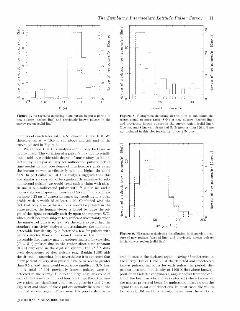
Figure 7. Histograms depicting distribution in pulse period ofnew pulsars (dashed line) and previously known pulsars in thesurvey region (solid line).
numbers of candidates with S/N between 8.0 and 10.0. Wetherefore use α = 10.0 in the above analysis and in thecurves plotted in Figure 3.
We caution that this analysis should only be taken asapproximate. The variation of a pulsar’s flux due to scintil-lation adds a considerable degree of uncertainty to its de-tectability, and particularly for millisecond pulsars lack oftime resolution and prevalence of interference signals causethe human viewer to effectively adopt a higher thresholdS/N. In particular, whilst this analysis suggests that thisand similar surveys could be significantly sensitive to sub-millisecond pulsars, we would treat such a claim with skep-ticism. A sub-millisecond pulsar with P = 0.8 ms and amoderately low dispersion measure of 25 cm−3 pc would ex-perience 0.25 ms of dispersion smearing, resulting in a pulseprofile with a width of at least 110◦. Combined with thefact that only 4 or perhaps 8 bins would be present in thepulse profile, the human viewer is forced to judge the ori-gin of the signal essentially entirely upon the reported S/N,which itself becomes subject to significant uncertainty whenthe number of bins is so few. We therefore expect that thestandard sensitivity analysis underestimates the minimumdetectable flux density by a factor of a few for pulsars withperiods shorter than a millisecond. Likewise, the minimumdetectable flux density may be underestimated for very slow(P > 5 s) pulsars due to the rather short time constant(0.9 s) employed in the digitiser system. The P−1/2 dutycycle dependence of slow pulsars (e.g. Rankin 1990) aidsthe situation somewhat, but nevertheless it is expected thata few percent of very slow pulsars have pulse widths greaterthan 0.5 s, and these would experience significant S/N loss.
A total of 101 previously known pulsars were re-detected in the survey. Due to the large angular extent ofeach of the tessellated units of four pointings, the actual sur-vey regions are significantly non-rectangular in l and b (seeFigure 2) and three of these pulsars actually lie outside thenominal survey region. There were 135 previously discov-
Figure 8. Histograms depicting distribution in maximum de-tected signal to noise ratio (S/N) of new pulsars (dashed line)and previously known pulsars in the survey region (solid line).One new and 8 known pulsars had S/Ns greater than 120 and arenot included in this plot for clarity in low S/N bins.
Figure 9. Histograms depicting distribution in dispersion mea-sure of new pulsars (dashed line) and previously known pulsarsin the survey region (solid line).
ered pulsars in the declared region, leaving 37 undetected inthe survey. Tables 1 and 2 list the detected and undetectedknown pulsars, including for each pulsar the period, dis-persion measure, flux density at 1400 MHz (where known),position in Galactic coordinates, angular offset from the cen-tre of the beam in which it was detected (where known, orthe nearest processed beam for undetected pulsars), and thesignal to noise ratio of detections. In most cases the valuesfor period, DM and flux density derive from the works of
c© 0000 RAS, MNRAS 000, 000–000
12 R.T. Edwards, M. Bailes, W. van Straten and M.C. Britton
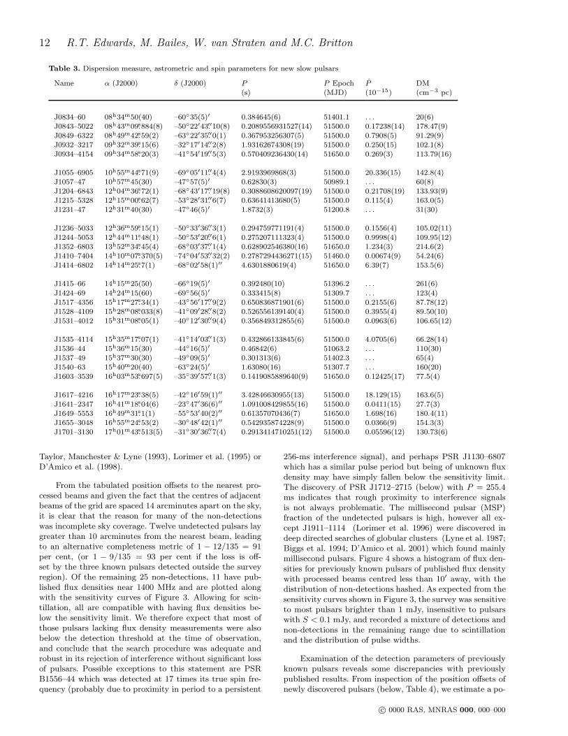
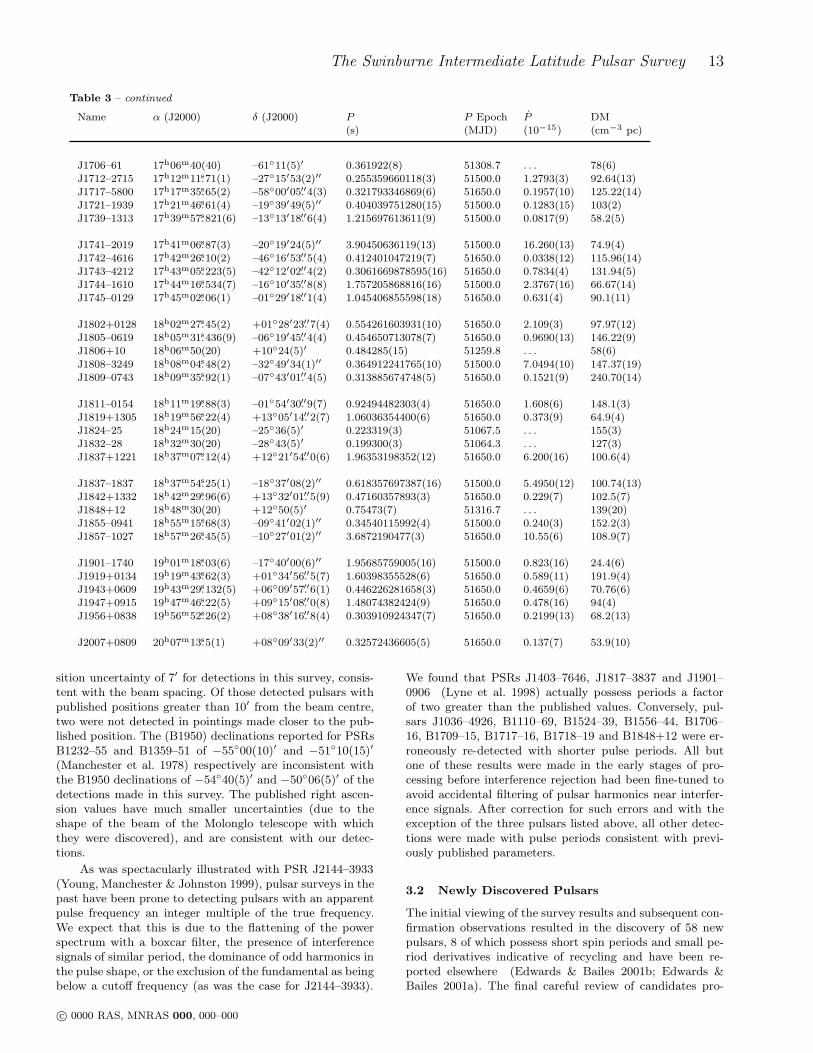
Table 3. Dispersion measure, astrometric and spin parameters for new slow pulsars
Name α (J2000) δ (J2000) P P Epoch P DM(s) (MJD) (10−15) (cm−3 pc)
J0834–60 08h34m50(40) –60◦35(5)′ 0.384645(6) 51401.1 . . . 20(6)J0843–5022 08h43m09.s884(8) –50◦22′43.′′10(8) 0.2089556931527(14) 51500.0 0.17238(14) 178.47(9)J0849–6322 08h49m42.s59(2) –63◦22′35.′′0(1) 0.367953256307(5) 51500.0 0.7908(5) 91.29(9)J0932–3217 09h32m39.s15(6) –32◦17′14.′′2(8) 1.93162674308(19) 51500.0 0.250(15) 102.1(8)J0934–4154 09h34m58.s20(3) –41◦54′19.′′5(3) 0.570409236430(14) 51650.0 0.269(3) 113.79(16)
J1055–6905 10h55m44.s71(9) –69◦05′11.′′4(4) 2.9193969868(3) 51500.0 20.336(15) 142.8(4)J1057–47 10h57m45(30) –47◦57(5)′ 0.62830(3) 50989.1 . . . 60(8)J1204–6843 12h04m36.s72(1) –68◦43′17.′′19(8) 0.3088608620097(19) 51500.0 0.21708(19) 133.93(9)J1215–5328 12h15m00.s62(7) –53◦28′31.′′6(7) 0.63641413680(5) 51500.0 0.115(4) 163.0(5)J1231–47 12h31m40(30) –47◦46(5)′ 1.8732(3) 51200.8 . . . 31(30)
J1236–5033 12h36m59.s15(1) –50◦33′36.′′3(1) 0.294759771191(4) 51500.0 0.1556(4) 105.02(11)J1244–5053 12h44m11.s48(1) –50◦53′20.′′6(1) 0.275207111323(4) 51500.0 0.9998(4) 109.95(12)J1352–6803 13h52m34.s45(4) –68◦03′37.′′1(4) 0.628902546380(16) 51650.0 1.234(3) 214.6(2)J1410–7404 14h10m07.s370(5) –74◦04′53.′′32(2) 0.2787294436271(15) 51460.0 0.00674(9) 54.24(6)J1414–6802 14h14m25.s7(1) –68◦02′58(1)′′ 4.6301880619(4) 51650.0 6.39(7) 153.5(6)
J1415–66 14h15m25(50) –66◦19(5)′ 0.392480(10) 51396.2 . . . 261(6)
J1424–69 14h24m15(60) –69◦56(5)′ 0.333415(8) 51309.7 . . . 123(4)J1517–4356 15h17m27.s34(1) –43◦56′17.′′9(2) 0.650836871901(6) 51500.0 0.2155(6) 87.78(12)J1528–4109 15h28m08.s033(8) –41◦09′28.′′8(2) 0.526556139140(4) 51500.0 0.3955(4) 89.50(10)J1531–4012 15h31m08.s05(1) –40◦12′30.′′9(4) 0.356849312855(6) 51500.0 0.0963(6) 106.65(12)
J1535–4114 15h35m17.s07(1) –41◦14′03.′′1(3) 0.432866133845(6) 51500.0 4.0705(6) 66.28(14)J1536–44 15h36m15(30) –44◦16(5)′ 0.46842(6) 51063.2 . . . 110(30)J1537–49 15h37m30(30) –49◦09(5)′ 0.301313(6) 51402.3 . . . 65(4)J1540–63 15h40m20(40) –63◦24(5)′ 1.63080(16) 51307.7 . . . 160(20)J1603–3539 16h03m53.s697(5) –35◦39′57.′′1(3) 0.1419085889640(9) 51650.0 0.12425(17) 77.5(4)
J1617–4216 16h17m23.s38(5) –42◦16′59(1)′′ 3.42846630955(13) 51500.0 18.129(15) 163.6(5)J1641–2347 16h41m18.s04(6) –23◦47′36(6)′′ 1.091008429855(16) 51500.0 0.0411(15) 27.7(3)J1649–5553 16h49m31.s1(1) –55◦53′40(2)′′ 0.61357070436(7) 51650.0 1.698(16) 180.4(11)J1655–3048 16h55m24.s53(2) –30◦48′42(1)′′ 0.542935874228(9) 51500.0 0.0366(9) 154.3(3)J1701–3130 17h01m43.s513(5) –31◦30′36.′′7(4) 0.2913414710251(12) 51500.0 0.05596(12) 130.73(6)
Taylor, Manchester & Lyne (1993), Lorimer et al. (1995) orD’Amico et al. (1998).
From the tabulated position offsets to the nearest pro-cessed beams and given the fact that the centres of adjacentbeams of the grid are spaced 14 arcminutes apart on the sky,it is clear that the reason for many of the non-detectionswas incomplete sky coverage. Twelve undetected pulsars laygreater than 10 arcminutes from the nearest beam, leadingto an alternative completeness metric of 1 − 12/135 = 91per cent, (or 1 − 9/135 = 93 per cent if the loss is off-set by the three known pulsars detected outside the surveyregion). Of the remaining 25 non-detections, 11 have pub-lished flux densities near 1400 MHz and are plotted alongwith the sensitivity curves of Figure 3. Allowing for scin-tillation, all are compatible with having flux densities be-low the sensitivity limit. We therefore expect that most ofthose pulsars lacking flux density measurements were alsobelow the detection threshold at the time of observation,and conclude that the search procedure was adequate androbust in its rejection of interference without significant lossof pulsars. Possible exceptions to this statement are PSRB1556–44 which was detected at 17 times its true spin fre-quency (probably due to proximity in period to a persistent
256-ms interference signal), and perhaps PSR J1130–6807which has a similar pulse period but being of unknown fluxdensity may have simply fallen below the sensitivity limit.The discovery of PSR J1712–2715 (below) with P = 255.4ms indicates that rough proximity to interference signalsis not always problematic. The millisecond pulsar (MSP)fraction of the undetected pulsars is high, however all ex-cept J1911–1114 (Lorimer et al. 1996) were discovered indeep directed searches of globular clusters (Lyne et al. 1987;Biggs et al. 1994; D’Amico et al. 2001) which found mainlymillisecond pulsars. Figure 4 shows a histogram of flux den-sities for previously known pulsars of published flux densitywith processed beams centred less than 10′ away, with thedistribution of non-detections hashed. As expected from thesensitivity curves shown in Figure 3, the survey was sensitiveto most pulsars brighter than 1 mJy, insensitive to pulsarswith S < 0.1 mJy, and recorded a mixture of detections andnon-detections in the remaining range due to scintillationand the distribution of pulse widths.
Examination of the detection parameters of previouslyknown pulsars reveals some discrepancies with previouslypublished results. From inspection of the position offsets ofnewly discovered pulsars (below, Table 4), we estimate a po-
c© 0000 RAS, MNRAS 000, 000–000
The Swinburne Intermediate Latitude Pulsar Survey 13
Table 3 – continued
Name α (J2000) δ (J2000) P P Epoch P DM(s) (MJD) (10−15) (cm−3 pc)
J1706–61 17h06m40(40) –61◦11(5)′ 0.361922(8) 51308.7 . . . 78(6)J1712–2715 17h12m11.s71(1) –27◦15′53(2)′′ 0.255359660118(3) 51500.0 1.2793(3) 92.64(13)J1717–5800 17h17m35.s65(2) –58◦00′05.′′4(3) 0.321793346869(6) 51650.0 0.1957(10) 125.22(14)J1721–1939 17h21m46.s61(4) –19◦39′49(5)′′ 0.404039751280(15) 51500.0 0.1283(15) 103(2)J1739–1313 17h39m57.s821(6) –13◦13′18.′′6(4) 1.215697613611(9) 51500.0 0.0817(9) 58.2(5)
J1741–2019 17h41m06.s87(3) –20◦19′24(5)′′ 3.90450636119(13) 51500.0 16.260(13) 74.9(4)J1742–4616 17h42m26.s10(2) –46◦16′53.′′5(4) 0.412401047219(7) 51650.0 0.0338(12) 115.96(14)J1743–4212 17h43m05.s223(5) –42◦12′02.′′4(2) 0.3061669878595(16) 51650.0 0.7834(4) 131.94(5)J1744–1610 17h44m16.s534(7) –16◦10′35.′′8(8) 1.757205868816(16) 51500.0 2.3767(16) 66.67(14)J1745–0129 17h45m02.s06(1) –01◦29′18.′′1(4) 1.045406855598(18) 51650.0 0.631(4) 90.1(11)
J1802+0128 18h02m27.s45(2) +01◦28′23.′′7(4) 0.554261603931(10) 51650.0 2.109(3) 97.97(12)J1805–0619 18h05m31.s436(9) –06◦19′45.′′4(4) 0.454650713078(7) 51650.0 0.9690(13) 146.22(9)J1806+10 18h06m50(20) +10◦24(5)′ 0.484285(15) 51259.8 . . . 58(6)
J1808–3249 18h08m04.s48(2) –32◦49′34(1)′′ 0.364912241765(10) 51500.0 7.0494(10) 147.37(19)J1809–0743 18h09m35.s92(1) –07◦43′01.′′4(5) 0.313885674748(5) 51650.0 0.1521(9) 240.70(14)
J1811–0154 18h11m19.s88(3) –01◦54′30.′′9(7) 0.92494482303(4) 51650.0 1.608(6) 148.1(3)J1819+1305 18h19m56.s22(4) +13◦05′14.′′2(7) 1.06036354400(6) 51650.0 0.373(9) 64.9(4)J1824–25 18h24m15(20) –25◦36(5)′ 0.223319(3) 51067.5 . . . 155(3)J1832–28 18h32m30(20) –28◦43(5)′ 0.199300(3) 51064.3 . . . 127(3)J1837+1221 18h37m07.s12(4) +12◦21′54.′′0(6) 1.96353198352(12) 51650.0 6.200(16) 100.6(4)
J1837–1837 18h37m54.s25(1) –18◦37′08(2)′′ 0.618357697387(16) 51500.0 5.4950(12) 100.74(13)J1842+1332 18h42m29.s96(6) +13◦32′01.′′5(9) 0.47160357893(3) 51650.0 0.229(7) 102.5(7)J1848+12 18h48m30(20) +12◦50(5)′ 0.75473(7) 51316.7 . . . 139(20)J1855–0941 18h55m15.s68(3) –09◦41′02(1)′′ 0.34540115992(4) 51500.0 0.240(3) 152.2(3)J1857–1027 18h57m26.s45(5) –10◦27′01(2)′′ 3.6872190477(3) 51650.0 10.55(6) 108.9(7)
J1901–1740 19h01m18.s03(6) –17◦40′00(6)′′ 1.95685759005(16) 51500.0 0.823(16) 24.4(6)J1919+0134 19h19m43.s62(3) +01◦34′56.′′5(7) 1.60398355528(6) 51650.0 0.589(11) 191.9(4)J1943+0609 19h43m29.s132(5) +06◦09′57.′′6(1) 0.446226281658(3) 51650.0 0.4659(6) 70.76(6)J1947+0915 19h47m46.s22(5) +09◦15′08.′′0(8) 1.48074382424(9) 51650.0 0.478(16) 94(4)J1956+0838 19h56m52.s26(2) +08◦38′16.′′8(4) 0.303910924347(7) 51650.0 0.2199(13) 68.2(13)
J2007+0809 20h07m13.s5(1) +08◦09′33(2)′′ 0.32572436605(5) 51650.0 0.137(7) 53.9(10)
sition uncertainty of 7′ for detections in this survey, consis-tent with the beam spacing. Of those detected pulsars withpublished positions greater than 10′ from the beam centre,two were not detected in pointings made closer to the pub-lished position. The (B1950) declinations reported for PSRsB1232–55 and B1359–51 of −55◦00(10)′ and −51◦10(15)′
(Manchester et al. 1978) respectively are inconsistent withthe B1950 declinations of −54◦40(5)′ and −50◦06(5)′ of thedetections made in this survey. The published right ascen-sion values have much smaller uncertainties (due to theshape of the beam of the Molonglo telescope with whichthey were discovered), and are consistent with our detec-tions.
As was spectacularly illustrated with PSR J2144–3933(Young, Manchester & Johnston 1999), pulsar surveys in thepast have been prone to detecting pulsars with an apparentpulse frequency an integer multiple of the true frequency.We expect that this is due to the flattening of the powerspectrum with a boxcar filter, the presence of interferencesignals of similar period, the dominance of odd harmonics inthe pulse shape, or the exclusion of the fundamental as beingbelow a cutoff frequency (as was the case for J2144–3933).
We found that PSRs J1403–7646, J1817–3837 and J1901–0906 (Lyne et al. 1998) actually possess periods a factorof two greater than the published values. Conversely, pul-sars J1036–4926, B1110–69, B1524–39, B1556–44, B1706–16, B1709–15, B1717–16, B1718–19 and B1848+12 were er-roneously re-detected with shorter pulse periods. All butone of these results were made in the early stages of pro-cessing before interference rejection had been fine-tuned toavoid accidental filtering of pulsar harmonics near interfer-ence signals. After correction for such errors and with theexception of the three pulsars listed above, all other detec-tions were made with pulse periods consistent with previ-ously published parameters.
3.2 Newly Discovered Pulsars
The initial viewing of the survey results and subsequent con-firmation observations resulted in the discovery of 58 newpulsars, 8 of which possess short spin periods and small pe-riod derivatives indicative of recycling and have been re-ported elsewhere (Edwards & Bailes 2001b; Edwards &Bailes 2001a). The final careful review of candidates pro-
c© 0000 RAS, MNRAS 000, 000–000
14 R.T. Edwards, M. Bailes, W. van Straten and M.C. Britton
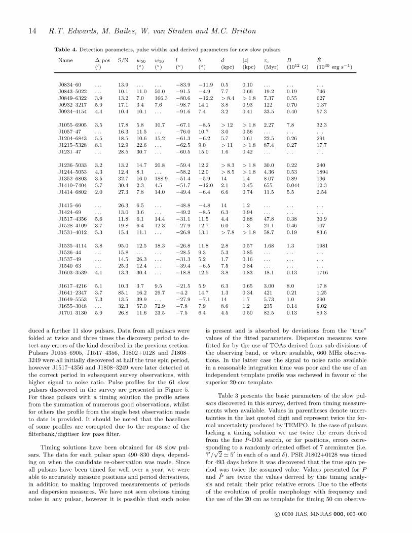
Table 4. Detection parameters, pulse widths and derived parameters for new slow pulsars
Name ∆ pos S/N w50 w10 l b d |z| τc B E(′) (◦) (◦) (◦) (◦) (kpc) (kpc) (Myr) (1012 G) (1030 erg s−1)
J0834–60 . . . 13.9 . . . . . . −83.9 −11.9 0.5 0.10 . . . . . . . . .J0843–5022 . . . 10.1 11.0 50.0 −91.5 −4.9 7.7 0.66 19.2 0.19 746J0849–6322 3.9 13.2 7.0 166.3 −80.6 −12.2 > 8.4 > 1.8 7.37 0.55 627J0932–3217 5.9 17.1 3.4 7.6 −98.7 14.1 3.8 0.93 122 0.70 1.37J0934–4154 4.4 10.4 10.1 . . . −91.6 7.4 3.2 0.41 33.5 0.40 57.3
J1055–6905 3.5 17.8 5.8 10.7 −67.1 −8.5 > 12 > 1.8 2.27 7.8 32.3J1057–47 . . . 16.3 11.5 . . . −76.0 10.7 3.0 0.56 . . . . . . . . .J1204–6843 5.5 18.5 10.6 15.2 −61.3 −6.2 5.7 0.61 22.5 0.26 291J1215–5328 8.1 12.9 22.6 . . . −62.5 9.0 > 11 > 1.8 87.4 0.27 17.7J1231–47 . . . 28.5 30.7 . . . −60.5 15.0 1.6 0.42 . . . . . . . . .
J1236–5033 3.2 13.2 14.7 20.8 −59.4 12.2 > 8.3 > 1.8 30.0 0.22 240J1244–5053 4.3 12.4 8.1 . . . −58.2 12.0 > 8.5 > 1.8 4.36 0.53 1894J1352–6803 3.5 32.7 16.0 188.9 −51.4 −5.9 14 1.4 8.07 0.89 196J1410–7404 5.7 30.4 2.3 4.5 −51.7 −12.0 2.1 0.45 655 0.044 12.3J1414–6802 2.0 27.3 7.8 14.0 −49.4 −6.4 6.6 0.74 11.5 5.5 2.54
J1415–66 . . . 26.3 6.5 . . . −48.8 −4.8 14 1.2 . . . . . . . . .
J1424–69 . . . 13.0 3.6 . . . −49.2 −8.5 6.3 0.94 . . . . . . . . .J1517–4356 5.6 11.8 6.1 14.4 −31.1 11.5 4.4 0.88 47.8 0.38 30.9J1528–4109 3.7 19.8 6.4 12.3 −27.9 12.7 6.0 1.3 21.1 0.46 107J1531–4012 5.3 15.4 11.1 . . . −26.9 13.1 > 7.8 > 1.8 58.7 0.19 83.6
J1535–4114 3.8 95.0 12.5 18.3 −26.8 11.8 2.8 0.57 1.68 1.3 1981J1536–44 . . . 15.8 . . . . . . −28.5 9.3 5.3 0.85 . . . . . . . . .J1537–49 . . . 14.5 26.3 . . . −31.3 5.2 1.7 0.16 . . . . . . . . .J1540–63 . . . 25.3 12.4 . . . −39.4 −6.5 7.5 0.84 . . . . . . . . .J1603–3539 4.1 13.3 30.4 . . . −18.8 12.5 3.8 0.83 18.1 0.13 1716
J1617–4216 5.1 10.3 3.7 9.5 −21.5 5.9 6.3 0.65 3.00 8.0 17.8J1641–2347 3.7 85.1 16.2 29.7 −4.2 14.7 1.3 0.34 421 0.21 1.25J1649–5553 7.3 13.5 39.9 . . . −27.9 −7.1 14 1.7 5.73 1.0 290J1655–3048 . . . 32.3 57.0 72.9 −7.8 7.9 8.6 1.2 235 0.14 9.02J1701–3130 5.9 26.8 11.6 23.5 −7.5 6.4 4.5 0.50 82.5 0.13 89.3
duced a further 11 slow pulsars. Data from all pulsars werefolded at twice and three times the discovery period to de-tect any errors of the kind described in the previous section.Pulsars J1055–6905, J1517–4356, J1802+0128 and J1808–3249 were all initially discovered at half the true spin period,however J1517–4356 and J1808–3249 were later detected atthe correct period in subsequent survey observations, withhigher signal to noise ratio. Pulse profiles for the 61 slowpulsars discovered in the survey are presented in Figure 5.For those pulsars with a timing solution the profile arisesfrom the summation of numerous good observations, whilstfor others the profile from the single best observation madeto date is provided. It should be noted that the baselinesof some profiles are corrupted due to the response of thefilterbank/digitiser low pass filter.
Timing solutions have been obtained for 48 slow pul-sars. The data for each pulsar span 490–830 days, depend-ing on when the candidate re-observation was made. Sinceall pulsars have been timed for well over a year, we wereable to accurately measure positions and period derivatives,in addition to making improved measurements of periodsand dispersion measures. We have not seen obvious timingnoise in any pulsar, however it is possible that such noise
is present and is absorbed by deviations from the “true”values of the fitted parameters. Dispersion measures werefitted for by the use of TOAs derived from sub-divisions ofthe observing band, or where available, 660 MHz observa-tions. In the latter case the signal to noise ratio availablein a reasonable integration time was poor and the use of anindependent template profile was eschewed in favour of thesuperior 20-cm template.
Table 3 presents the basic parameters of the slow pul-sars discovered in this survey, derived from timing measure-ments when available. Values in parentheses denote uncer-tainties in the last quoted digit and represent twice the for-mal uncertainty produced by TEMPO. In the case of pulsarslacking a timing solution we use twice the errors derivedfrom the fine P -DM search, or for positions, errors corre-sponding to a randomly oriented offset of 7 arcminutes (i.e.7′/
√2 ≃ 5′ in each of α and δ). PSR J1802+0128 was timed
for 493 days before it was discovered that the true spin pe-riod was twice the assumed value. Values presented for Pand P are twice the values derived by this timing analy-sis and retain their prior relative errors. Due to the effectsof the evolution of profile morphology with frequency andthe use of the 20 cm as template for timing 50 cm observa-
c© 0000 RAS, MNRAS 000, 000–000
The Swinburne Intermediate Latitude Pulsar Survey 15
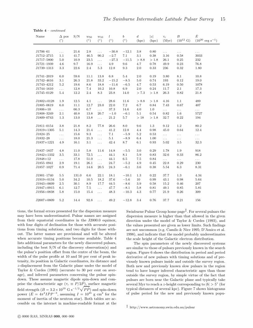
Table 4 – continued
Name ∆ pos S/N w50 w10 l b d |z| τc B E(′) (◦) (◦) (◦) (◦) (kpc) (kpc) (Myr) (1012 G) (1030 erg s−1)
J1706–61 . . . 21.6 2.8 . . . −30.8 −12.1 3.8 0.80 . . . . . . . . .J1712–2715 1.1 41.7 46.5 90.2 −2.7 7.1 3.1 0.38 3.16 0.58 3033J1717–5800 5.0 10.9 23.5 . . . −27.3 −11.5 > 8.8 > 1.8 26.1 0.25 232J1721–1939 4.6 9.7 16.9 . . . 4.9 9.6 4.7 0.78 49.9 0.23 76.8J1739–1313 3.3 22.6 2.4 5.3 12.8 9.3 2.0 0.33 236 0.32 1.80
J1741–2019 6.0 59.6 11.1 13.8 6.8 5.4 2.0 0.19 3.80 8.1 10.8J1742–4616 3.1 26.3 21.8 33.2 −15.2 −8.5 5.0 0.74 193 0.12 19.0J1743–4212 5.2 19.6 8.6 18.8 −11.6 −6.5 4.7 0.53 6.19 0.50 1078J1744–1610 . . . 12.8 7.4 10.2 10.8 6.9 2.0 0.24 11.7 2.1 17.3J1745–0129 5.4 12.2 2.4 8.3 23.8 14.0 > 7.3 > 1.8 26.3 0.82 21.8
J1802+0128 1.9 12.5 4.1 . . . 28.6 11.6 > 8.8 > 1.8 4.16 1.1 489J1805–0619 6.0 11.1 12.7 23.0 22.0 7.2 6.7 0.84 7.43 0.67 407J1806+10 . . . 66.3 6.7 . . . 37.3 14.6 4.0 1.0 . . . . . . . . .
J1808–3249 2.1 40.8 13.8 20.7 −1.0 −6.1 5.1 0.54 0.82 1.6 5727J1809–0743 1.3 13.0 13.8 . . . 21.2 5.7 > 18 > 1.8 32.7 0.22 194
J1811–0154 3.8 21.8 8.2 77.8 26.6 8.0 9.6 1.3 9.12 1.2 80.2J1819+1305 5.1 14.3 21.4 . . . 41.2 12.8 4.4 0.98 45.0 0.64 12.4J1824–25 . . . 15.6 9.3 . . . 7.1 −5.9 5.2 0.53 . . . . . . . . .J1832–28 . . . 18.0 21.3 . . . 5.1 −8.9 6.4 1.00 . . . . . . . . .J1837+1221 4.9 16.1 3.1 . . . 42.4 8.7 6.1 0.93 5.02 3.5 32.3
J1837–1837 4.8 11.0 5.8 11.6 14.8 −5.5 3.0 0.29 1.78 1.9 918J1842+1332 3.5 33.1 72.5 . . . 44.1 8.1 5.9 0.83 32.6 0.33 86.2J1848+12 . . . 17.8 51.0 . . . 44.1 6.5 7.5 0.84 . . . . . . . . .J1855–0941 2.9 19.1 26.1 . . . 24.7 −5.2 4.9 0.45 22.8 0.29 230J1857–1027 0.9 71.4 14.6 20.5 24.3 −6.1 3.6 0.38 5.54 6.3 8.31
J1901–1740 5.5 131.0 6.6 22.1 18.1 −10.1 1.3 0.22 37.7 1.3 4.34J1919+0134 5.0 34.2 10.5 18.2 37.6 −5.6 10 0.99 43.1 0.98 5.64J1943+0609 2.5 30.1 8.9 17.7 44.5 −8.6 3.9 0.58 15.2 0.46 207J1947+0915 6.1 12.7 7.5 . . . 47.7 −8.1 5.8 0.81 49.1 0.85 5.81J1956+0838 5.8 15.0 15.4 . . . 48.3 −10.3 4.3 0.77 21.9 0.26 309
J2007+0809 5.2 14.4 92.8 . . . 49.2 −12.8 3.4 0.76 37.7 0.21 156
tions, the formal errors presented for the dispersion measuremay have been underestimated. Pulsar names are assignedfrom their equatorial coordinates in the J2000.0 equinox,with four digits of declination for those with accurate posi-tions from timing solutions, and two digits for those with-out. The latter names are provisional and will be alteredwhen accurate timing positions become available. Table 4lists additional parameters for the newly discovered pulsars,including the best S/N of the discovery observation(s) andthe pulsar’s position offset from the centre of the beam, thewidth of the pulse profile at 10 and 50 per cent of peak in-tensity, its position in Galactic coordinates, its distance andz-displacement from the Galactic plane under the model ofTaylor & Cordes (1993) (accurate to 30 per cent on aver-age), and inferred parameters concerning the pulsar spin-down. These assume magnetic dipole spin-down and com-prise the characteristic age (τc ≡ P/2P ), surface magnetic
field strength (B = 3.2×10¹⁹ G s−1/2√
PP ) and spin-downpower (E = 4π2IPP−3, assuming I = 1045 g cm2 for themoment of inertia of the neutron star). Both tables are ac-cessible on the internet in machine-readable format at the
Swinburne Pulsar Group home page‡. For several pulsars thedispersion measure is higher than that allowed in the givendirection under the model of Taylor & Cordes (1993), andthe values presented are given as lower limits. Such findingsare not uncommon (e.g. Camilo & Nice 1995; D’Amico et al.1998), and indicate that the model probably underestimatesthe scale height of the Galactic electron distribution.
The spin parameters of the newly discovered systemsare similar to those of pulsars previously known in the searchregion. Figure 6 shows the distribution in period and periodderivative of new pulsars with timing solutions and of pre-viously known pulsars inside and outside the survey region.Both new and previously known slow pulsars in the regiontend to have longer inferred characteristic ages than thoseoutside the survey region, by simple virtue of the fact thatpulsars are born near the Galactic plane and typically takeseveral Myr to reach a z-height corresponding to |b| > 5◦ (fortypical distances of several kpc). Figure 7 shows histogramsof pulse period for the new and previously known popu-
‡ http://www.astronomy.swin.edu.au/pulsar
c© 0000 RAS, MNRAS 000, 000–000
16 R.T. Edwards, M. Bailes, W. van Straten and M.C. Britton
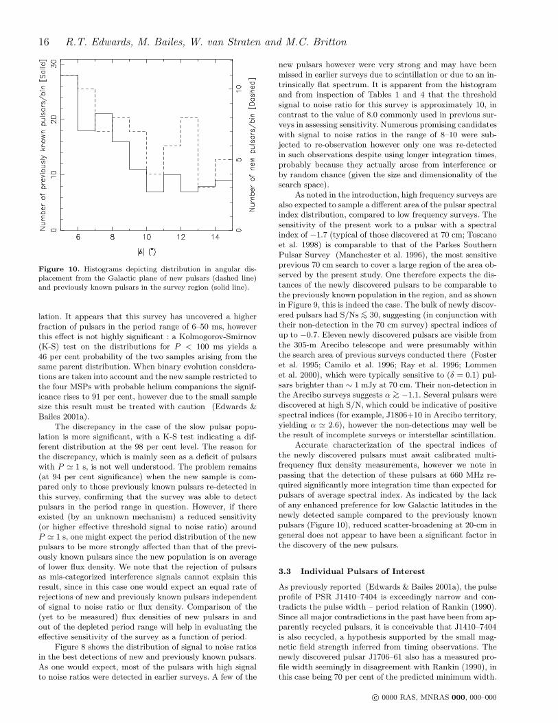
Figure 10. Histograms depicting distribution in angular dis-placement from the Galactic plane of new pulsars (dashed line)and previously known pulsars in the survey region (solid line).
lation. It appears that this survey has uncovered a higherfraction of pulsars in the period range of 6–50 ms, howeverthis effect is not highly significant : a Kolmogorov-Smirnov(K-S) test on the distributions for P < 100 ms yields a46 per cent probability of the two samples arising from thesame parent distribution. When binary evolution considera-tions are taken into account and the new sample restricted tothe four MSPs with probable helium companions the signif-icance rises to 91 per cent, however due to the small samplesize this result must be treated with caution (Edwards &Bailes 2001a).
The discrepancy in the case of the slow pulsar popu-lation is more significant, with a K-S test indicating a dif-ferent distribution at the 98 per cent level. The reason forthe discrepancy, which is mainly seen as a deficit of pulsarswith P ≃ 1 s, is not well understood. The problem remains(at 94 per cent significance) when the new sample is com-pared only to those previously known pulsars re-detected inthis survey, confirming that the survey was able to detectpulsars in the period range in question. However, if thereexisted (by an unknown mechanism) a reduced sensitivity(or higher effective threshold signal to noise ratio) aroundP ≃ 1 s, one might expect the period distribution of the newpulsars to be more strongly affected than that of the previ-ously known pulsars since the new population is on averageof lower flux density. We note that the rejection of pulsarsas mis-categorized interference signals cannot explain thisresult, since in this case one would expect an equal rate ofrejections of new and previously known pulsars independentof signal to noise ratio or flux density. Comparison of the(yet to be measured) flux densities of new pulsars in andout of the depleted period range will help in evaluating theeffective sensitivity of the survey as a function of period.
Figure 8 shows the distribution of signal to noise ratiosin the best detections of new and previously known pulsars.As one would expect, most of the pulsars with high signalto noise ratios were detected in earlier surveys. A few of the
new pulsars however were very strong and may have beenmissed in earlier surveys due to scintillation or due to an in-trinsically flat spectrum. It is apparent from the histogramand from inspection of Tables 1 and 4 that the thresholdsignal to noise ratio for this survey is approximately 10, incontrast to the value of 8.0 commonly used in previous sur-veys in assessing sensitivity. Numerous promising candidateswith signal to noise ratios in the range of 8–10 were sub-jected to re-observation however only one was re-detectedin such observations despite using longer integration times,probably because they actually arose from interference orby random chance (given the size and dimensionality of thesearch space).
As noted in the introduction, high frequency surveys arealso expected to sample a different area of the pulsar spectralindex distribution, compared to low frequency surveys. Thesensitivity of the present work to a pulsar with a spectralindex of −1.7 (typical of those discovered at 70 cm; Toscanoet al. 1998) is comparable to that of the Parkes SouthernPulsar Survey (Manchester et al. 1996), the most sensitiveprevious 70 cm search to cover a large region of the area ob-served by the present study. One therefore expects the dis-tances of the newly discovered pulsars to be comparable tothe previously known population in the region, and as shownin Figure 9, this is indeed the case. The bulk of newly discov-ered pulsars had S/Ns <∼ 30, suggesting (in conjunction withtheir non-detection in the 70 cm survey) spectral indices ofup to −0.7. Eleven newly discovered pulsars are visible fromthe 305-m Arecibo telescope and were presumably withinthe search area of previous surveys conducted there (Fosteret al. 1995; Camilo et al. 1996; Ray et al. 1996; Lommenet al. 2000), which were typically sensitive to (δ = 0.1) pul-sars brighter than ∼ 1 mJy at 70 cm. Their non-detection inthe Arecibo surveys suggests α >∼ −1.1. Several pulsars werediscovered at high S/N, which could be indicative of positivespectral indices (for example, J1806+10 in Arecibo territory,yielding α ≃ 2.6), however the non-detections may well bethe result of incomplete surveys or interstellar scintillation.
Accurate characterization of the spectral indices ofthe newly discovered pulsars must await calibrated multi-frequency flux density measurements, however we note inpassing that the detection of these pulsars at 660 MHz re-quired significantly more integration time than expected forpulsars of average spectral index. As indicated by the lackof any enhanced preference for low Galactic latitudes in thenewly detected sample compared to the previously knownpulsars (Figure 10), reduced scatter-broadening at 20-cm ingeneral does not appear to have been a significant factor inthe discovery of the new pulsars.
3.3 Individual Pulsars of Interest
As previously reported (Edwards & Bailes 2001a), the pulseprofile of PSR J1410–7404 is exceedingly narrow and con-tradicts the pulse width – period relation of Rankin (1990).Since all major contradictions in the past have been from ap-parently recycled pulsars, it is conceivable that J1410–7404is also recycled, a hypothesis supported by the small mag-netic field strength inferred from timing observations. Thenewly discovered pulsar J1706–61 also has a measured pro-file width seemingly in disagreement with Rankin (1990), inthis case being 70 per cent of the predicted minimum width.
c© 0000 RAS, MNRAS 000, 000–000
The Swinburne Intermediate Latitude Pulsar Survey 17
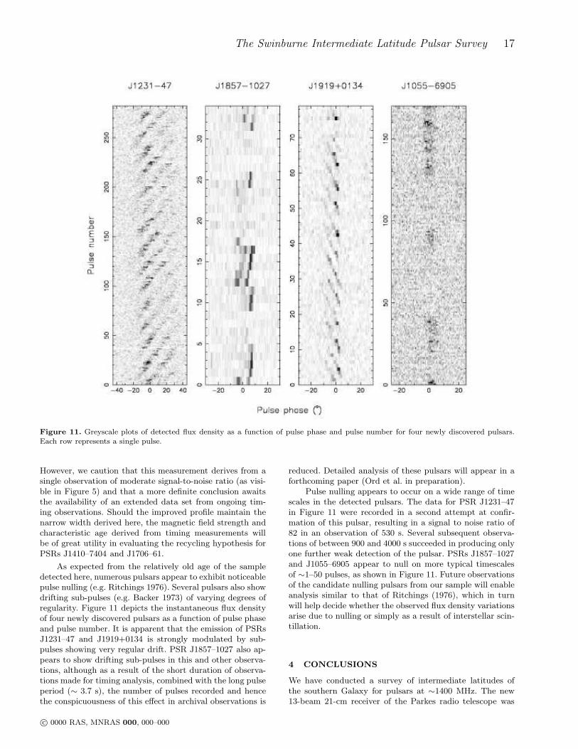
Figure 11. Greyscale plots of detected flux density as a function of pulse phase and pulse number for four newly discovered pulsars.Each row represents a single pulse.
However, we caution that this measurement derives from asingle observation of moderate signal-to-noise ratio (as visi-ble in Figure 5) and that a more definite conclusion awaitsthe availability of an extended data set from ongoing tim-ing observations. Should the improved profile maintain thenarrow width derived here, the magnetic field strength andcharacteristic age derived from timing measurements willbe of great utility in evaluating the recycling hypothesis forPSRs J1410–7404 and J1706–61.
As expected from the relatively old age of the sampledetected here, numerous pulsars appear to exhibit noticeablepulse nulling (e.g. Ritchings 1976). Several pulsars also showdrifting sub-pulses (e.g. Backer 1973) of varying degrees ofregularity. Figure 11 depicts the instantaneous flux densityof four newly discovered pulsars as a function of pulse phaseand pulse number. It is apparent that the emission of PSRsJ1231–47 and J1919+0134 is strongly modulated by sub-pulses showing very regular drift. PSR J1857–1027 also ap-pears to show drifting sub-pulses in this and other observa-tions, although as a result of the short duration of observa-tions made for timing analysis, combined with the long pulseperiod (∼ 3.7 s), the number of pulses recorded and hencethe conspicuousness of this effect in archival observations is
reduced. Detailed analysis of these pulsars will appear in aforthcoming paper (Ord et al. in preparation).
Pulse nulling appears to occur on a wide range of timescales in the detected pulsars. The data for PSR J1231–47in Figure 11 were recorded in a second attempt at confir-mation of this pulsar, resulting in a signal to noise ratio of82 in an observation of 530 s. Several subsequent observa-tions of between 900 and 4000 s succeeded in producing onlyone further weak detection of the pulsar. PSRs J1857–1027and J1055–6905 appear to null on more typical timescalesof ∼1–50 pulses, as shown in Figure 11. Future observationsof the candidate nulling pulsars from our sample will enableanalysis similar to that of Ritchings (1976), which in turnwill help decide whether the observed flux density variationsarise due to nulling or simply as a result of interstellar scin-tillation.
4 CONCLUSIONS
We have conducted a survey of intermediate latitudes ofthe southern Galaxy for pulsars at ∼1400 MHz. The new13-beam 21-cm receiver of the Parkes radio telescope was
c© 0000 RAS, MNRAS 000, 000–000
18 R.T. Edwards, M. Bailes, W. van Straten and M.C. Britton
used to rapidly cover to moderate depth a large region ofsky flanking the area of the deeper ongoing Galactic planesurvey (Lyne et al. 2000; Camilo et al. 2000). The inter-ference environment was formidable, however developmentof a comprehensive scheme for the rejection of pulsar can-didates arising from interference enabled the realisation ofthe full expected survey sensitivity of approximately 0.5 mJyfor slow and most millisecond pulsars. The survey was highlysuccessful, detecting 170 pulsars of which 69 were previouslyunknown, in a relatively short observing campaign. The newdiscoveries are not significantly more distant than the previ-ously known population in this region of sky, indicating thatthe success of the survey is attributable to its sampling ofa different portion of the broad distribution of pulsar spec-tral indices. The detected sample, in combination with thoseof the Galactic plane and high-latitude surveys (when com-plete), will prove invaluable for population modelling due tothe use of a common observing system to cover a large areaof sky at high radio frequency.
Among the most interesting new objects are two recy-cled pulsars with massive white dwarf companions (Ed-wards & Bailes 2001b), four with probable low-mass Hedwarf companions, two isolated millisecond pulsars, and one‘slow’ pulsar with a very narrow pulse profile and small pe-riod derivative, suggestive of recycling in a scenario similarto those of the known double neutron star systems (Ed-wards & Bailes 2001a). As expected from the large Galacticz-height of much of the survey volume, the detected popula-tion of slow pulsars was relatively old and as such exhibited ahigh fraction of pulsars showing nulling and sub-pulse mod-ulation. Two pulsars show very regular drifting sub-pulsesand are analysed in detail elsewhere (Ord et al. in prepara-tion).
ACKNOWLEDGMENTS
We thank the members of the Galactic plane Parkes multi-beam pulsar survey collaboration for the use of equipmentbuilt for that survey, and for the exchange of observing timeto improve the regularity of timing observations. The freeexchange of software and information between the Galac-tic plane collaboration and the authors was a pleasant anduseful arrangement. We are grateful for the high level of sup-port provided by the staff of the CSIRO/ATNF Parkes radiotelescope in the event of system failures. We thank the ref-eree for detailed comments and suggestions which improvedthe manuscript. RTE acknowledges the support of an Aus-tralian Postgraduate Award. MB is an ARC Senior ResearchFellow, and this research was supported by the ARC LargeGrants Scheme.
REFERENCES
Ables J. G., Komesaroff M. M., Hamilton P. A., 1970, As-trophys. Lett., 6, 147
Backer D. C., 1973, ApJ, 182, 245
Barnes D. G. et al., 2001, MNRAS, in press
Bell J. F., Bessell M. S., Stappers B. W., Bailes M.,Kaspi V. M., 1995, ApJ, 447, L117
Biggs J. D., Bailes M., Lyne A. G., Goss W. M.,Fruchter A. S., 1994, MNRAS, 267, 125
Camilo F., Nice D. J., 1995, ApJ, 445, 756
Camilo F., Nice D. J., Shrauner J. A., Taylor J. H., 1996,ApJ, 469, 819
Camilo F. et al., 2000, in Kramer M., Wex N., Wielebin-ski R., eds, Pulsar Astronomy - 2000 and Beyond,IAU Colloquium 177. Astronomical Society of thePacific, San Francisco, p. 3, astro-ph/9911185
Camilo F., Nice D. J., Taylor J. H., 1996, ApJ, 461, 812
Clifton T. R., Lyne A. G., Jones A. W., McKenna J., Ash-worth M., 1992, MNRAS, 254, 177
D’Amico N., Stappers B. W., Bailes M., Martin C. E.,Bell J. F., Lyne A. G., Manchester R. N., 1998, MN-RAS, 297, 28
D’Amico N., Lyne A. G., Manchester R. N., Possenti A.,Camilo F., 2001, ApJ, 548, L171
Dewey R. J., Taylor J. H., Weisberg J. M., Stokes G. H.,1985, ApJ, 294, L25
Edwards R. T., Bailes M., 2001a, ApJ, in press, astro-ph/0102026
Edwards R. T., Bailes M., 2001b, ApJ, 547, L37
Foster R. S., Cadwell B. J., Wolszczan A., Anderson S. B.,1995, ApJ, 454, 826
Henning P. A. et al., 2000, AJ, 119, 2686
Johnston S., Lyne A. G., Manchester R. N., Kniffen D. A.,D’Amico N., Lim J., Ashworth M., 1992a, MNRAS,255, 401
Johnston S., Manchester R. N., Lyne A. G., Bailes M.,Kaspi V. M., Qiao G., D’Amico N., 1992b, ApJ, 387,L37
Johnston S. et al., 1993, Nature, 361, 613
Kramer M., Wex N., Wielebinski R., eds, Pulsar Astronomy- 2000 and Beyond, IAU Colloquium 177, Astronom-ical Society of the Pacific, San Francisco, 2000
Lawson K. D., Mayer C. J., Osborne J. L., Parkinson M. L.,1987, MNRAS, 225, 307
Lommen A. N., Zepka A., Backer D. C., McLaughlin M.,Cordes J. M., Arzoumanian Z., Xilouris K., 2000,ApJ, 545, 1007
Lorimer D. R., Yates J. A., Lyne A. G., Gould D. M., 1995,MNRAS, 273, 411
Lorimer D. R., Lyne A. G., Bailes M., Manchester R. N.,
c© 0000 RAS, MNRAS 000, 000–000
The Swinburne Intermediate Latitude Pulsar Survey 19
D’Amico N., Stappers B. W., Johnston S., Camilo F.,1996, MNRAS, 283, 1383
Lyne A. G., Brinklow A., Middleditch J., Kulkarni S. R.,Backer D. C., Clifton T. R., 1987, Nature, 328, 399
Lyne A. G. et al., 1998, MNRAS, 295, 743
Lyne A. G. et al., 2000, MNRAS, 312, 698
Manchester R. N., Lyne A. G., Taylor J. H., Durdin J. M.,Large M. I., Little A. G., 1978, MNRAS, 185, 409
Manchester R. N. et al., 1996, MNRAS, 279, 1235
Manchester R. N. et al., 2000, in Kramer M., Wex N.,Wielebinski R., eds, Pulsar Astronomy - 2000 andBeyond, IAU Colloquium 177. Astronomical Societyof the Pacific, San Francisco, p. 49
Manchester R. N. et al., 2001, MNRAS, Submitted.
Rankin J. M., 1990, ApJ, 352, 247
Ray P. S., Thorsett S. E., Jenet F. A., van Kerkwijk M. H.,Kulkarni S. R., Prince T. A., Sandhu J. S., Nice D. J.,1996, ApJ, 470, 1103
Ritchings R. T., 1976, MNRAS, 176, 249
Stappers B. W. et al., 1996, ApJ, 465, L119
Staveley-Smith L. et al., 1996, Proc. Astr. Soc. Aust., 13,243
Taylor J. H., Cordes J. M., 1993, ApJ, 411, 674
Taylor J. H., Weisberg J. M., 1989, ApJ, 345, 434
Taylor J. H., Manchester R. N., Lyne A. G., 1993, ApJS, 88,529
Taylor J. H., 1974, A&AS, 15, 367
Toscano M., Bailes M., Manchester R., Sandhu J., 1998,ApJ, 506, 863
Wolszczan A., Frail D. A., 1992, Nature, 355, 145
Young M. D., Manchester R. N., Johnston S., 1999, Nature,400, 848
c© 0000 RAS, MNRAS 000, 000–000