the impact of cash flow volatility on discretionary investment
TRANSCRIPT
University of Pennsylvania University of Pennsylvania
ScholarlyCommons ScholarlyCommons
Accounting Papers Wharton Faculty Research
12-1999
The Impact of Cash Flow Volatility on Discretionary Investment The Impact of Cash Flow Volatility on Discretionary Investment
and the Costs of Debt and Equity Financing and the Costs of Debt and Equity Financing
Bernadette A. Minton
Catherine M. Schrand University of Pennsylvania
Follow this and additional works at: https://repository.upenn.edu/accounting_papers
Part of the Accounting Commons, and the Finance Commons
Recommended Citation Recommended Citation Minton, B. A., & Schrand, C. M. (1999). The Impact of Cash Flow Volatility on Discretionary Investment and the Costs of Debt and Equity Financing. Journal of Financial Economics, 54 (3), 423-460. http://dx.doi.org/10.1016/S0304-405X(99)00042-2
This paper is posted at ScholarlyCommons. https://repository.upenn.edu/accounting_papers/23 For more information, please contact [email protected].
The Impact of Cash Flow Volatility on Discretionary Investment and the Costs of The Impact of Cash Flow Volatility on Discretionary Investment and the Costs of Debt and Equity Financing Debt and Equity Financing
Abstract Abstract We show that higher cash flow volatility is associated with lower average levels of investment in capital expenditures, R&D, and advertising. This association suggests that firms do not use external capital markets to fully cover cash flow shortfalls but rather permanently forgo investment. Cash flow volatility also is associated with higher costs of accessing external capital. Moreover, these higher costs, as measured by some proxies, imply a greater sensitivity of investment to cash flow volatility. Thus, cash flow volatility not only increases the likelihood that a firm will need to access capital markets, it also increases the costs of doing so.
Keywords Keywords cash flow volatility, investment, cost of equity financing, cost of debt financing
Disciplines Disciplines Accounting | Finance
This journal article is available at ScholarlyCommons: https://repository.upenn.edu/accounting_papers/23
The Impact of Cash Flow Volatility on Discretionary Investment and the Costs of Debt and Equity
Financing
Bernadette A. Minton* and Catherine Schrand**
Preliminary: Comments welcome Please do not quote without permission
August, 1998
*Ohio State University. **university of Pennsylvania. Previous versions of this paper were titled "Costs of Accounting Income versus Cash Flow Volatility. " We wish to thank Gordon Bodnar, John Core, Peter Easton, Chris Geczy, Bob Holthausen, Sara Moeller, Tim Opler, Tony Sanders, Rene Stulz, Ralph Walkling, Franco Wong, an anonymous referee, and workshop participants at the Wharton Corporate Finance seminar, the Ohio State University Finance Seminar, Harvard Financial Decisions and Control Conference, the University of Rochester Ph.D. seminar for helpful comments. Minton thanks the Dice Center for Financial Economics for financial support. Please address comments to either Bernadette A. Minton at Fisher College of Business, The Ohio State University, 1775 College Road, Columbus, OH, 43210-1399, (614) 688-3125, [email protected]; or Catherine Schrand at The Wharton School, University of Pennsylvania, 2427 Steinberg Hall-Dietrich Hall, Philadelphia, PA, 19104, (215) 898-6798, [email protected].
The Impact of Cash Flow Volatility on Discretionary Investment and the Costs of Debt and Equity
Financing
Abstract
We document that cash flow volatility is associated with lower levels of investment in capital expenditures, R&D, and advertising. Thus, firms do not turn to external capital markets to fully cover cash-flow short falls. Consistent with this conclusion, we document that the sensitivity of investment to cash flow volatility is greater for firms with higher costs of capital market access. In addition, cash flow and earnings volatility are associated with these higher costs. Thus, volatility not only increases the likelihood that a firm will need to access capital markets, it also increases the costs of doing so.
JEL Classification: G31
Keywords: Cash flow volatility; earnings volatility; investment; cost of equity financing; cost of debt financing
The Impact of Cash Flow Volatility on Discretionary Investment and the Costs of Debt and Equity
Financing
L Introduction
"As risk managers, we spend much of our time examining the factors that cause cash flows to fluctuate.
This is important work, since low cash flows may throw budgets into disarray, distract managers from productive
work, defer capital expenditure or delay debt repayments. By avoiding these deadweight losses, risk managers can
rightly claim they add to shareholder value." (See Shimko, 1997 .) This paper provides the first direct descriptive
evidence that such deadweight losses associated with cash flow volatility exist
We document that discretionary investment levels are negatively related to cash flow volatility based on
an analysis of non-financial firms over the years 1988 to 1995. Firms with higher levels of cash flow volatility
have lower capital expenditures, research and development costs, and advertising expenses. One explanation for
this relation is that different levels of investment produce different volatilities due to the nature of the investments.
However, we also show that the volatilities of capital expenditures, R&D costs, and advertising expenses are
positively associated with cash flow volatility. We would expect no association between the volatility of
investment and cash flow volatility if the documented relation is a simple story about differential payoffs across
different types of investments. As further evidence that volatility induces the observed lower investment, we show
that firms experiencing cash shortfalls (relative to their own historical experience) have significantly discretionary
investment than firms that are not experiencing shortfalls.
These results suggest that firms do not use external debt and equity markets to smooth cash flow
volatility. If they did, we would not observe a link between volatility of operating cash flows (before financing)
and discretionary investment Consistent with this interpretation of the results, we show that the sensitivity of
investment to volatility is mitigated for large firms and firms with better S&P bond ratings, greater analyst
following, lower total equity price risk, and lower summary measures of firms' costs of accessing equity capital
(derived from principal component analysis). These firms, which we claim have lower costs of accessing external
capital markets, are able to smooth cash flows through time. In addition, firms that hold higher cash reserves have
a lower sensitivity of investment to volatility.
-1-
These results lead to a question of why firms with volatile cash flows do not use external capital markets
during periods of low cash realizations to fund investment. As one explanation, we show that the costs of
accessing capital markets also are related to the volatility of a firm' s cash flows. Thus, we do not conclude that
lower investment by firms with volatile cash flows is suboptimal. Rather, the lower investment for these firms is
related to lower assessed net present values due to higher costs of funding.
We examine the relation between volatility and our proxies for the costs of accessing external capital
markets. In this analysis, we recognize that our proxies are related to assessments of expected future cash flow
volatility. However, empirical evidence indicates that earnings levels are a better predictor of future cash flow
levels than are historical cash flow levels (e.g. , Sloan, 1996). Extending this notion to volatilities, we test whether
our proxies for the costs of accessing external capital markets are incrementally associated with cash flow volatility
or earnings volatility.
The results indicate that cash flow volatility is relevant to some costs while earnings volatility is relevant
to others. Specifically, cash flow volatility and not earnings volatility is significantly related to worse Standard &
Poor's bond ratings and lower analyst following. Earnings volatility and not cash flow volatility is related to
higher stock market betas, and lower dividend payout ratios. Cash flow and earnings volatility are both
statistically related to total equity price risk. These results have implications for risk-management decisions
related to the choice between hedging earnings versus cash flows.
The paper proceeds as follows. Section 2 discusses predictions about the impact of cash flow volatility
on discretionary investment. Section 3 describes our metrics for cash flow volatility and the methodology for
measuring the association between volatility and investment, and Section 4 reports the results of these tests. In
Section 5, we examine whether the sensitivity of investment to cash flow volatility is mitigated for firms with
lower costs of accessing capital markets. Section 6 presents the empirical analyses of the relations between cash
flow and earnings volatility and the costs of accessing capital markets. Section 7 provides concluding remarks.
2. Outline of predictions and relation to prior literature
In this section, we discuss the impact of cash flow volatility on discretionary investment. We predict that
a firm 's cash flow volatility over a period will be negatively associated with its average discretionary investment
-2-
during the same period. This prediction relies on two conditions. The first condition is that a firm with higher
cash flow volatility is more likely to incur states in which its internal cash levels are insufficient to make
investments. The second condition is that covering cash shortfalls is costly so that a firm does not use external
capital markets to smooth the effects of volatility.
Our tests for a negative relation between volatility and investment are presented in Sections 4 and 5. In
Section 4, we describe the results of annual cross-sectional regressions of capital expenditures, research and
development costs, and advertising expenses as proxies for discretionary investment on cash flow volatility. We
also more directly examine whether firms that experience a cash shortfall have lower discretionary investment than
firms in an excess cash position. In Section 5, we test whether the negative relation between discretionary
investment and volatility is mitigated for firms that have lower costs of accessing external capital markets.
We are not the first to claim that cash flow volatility is costly because it affects investment The risk
management literature has made this claim in the context of explaining hedging activities that reduce cash flow
volatility. The risk management theories suggest that the costs of accessing external capital markets to fund
investment when internal cash flows are insufficient are greatest for firms with volatile cash flows (Shapiro and
Titman (1986) , Lessard (1990) , Stulz (1990) and Froot, Scharfstein, and Stein (1993)) . Consistent with these
predictions, empirical research on risk management practices documents that firms that have the greatest expected
benefits from reducing volatility are more active in risk management activities (G&zy, Minton, and Schrand,
1997, Mian, 1996, Nance, Smith, and Smithson, 1993, and Tufano, 1996). The direct evidence in this paper of an
association between volatility and discretionary investment complements the findings of these indirect tests.
Our empirical evidence is also related to prior work on the association between liquidity and investment
(Fazzari, Hubbard, and Peterson, FHP, 1988 and 1998 ; Hoshi, Kashyap, and Scharfstein, 1991; Kaplan and
Zingales, KZ, 1997; and Lamont, 1997). All of these studies document a positive association between liquidity
(as measured by cash flow, cash stock, or the sum of cash flow and cash stock) and investment (as measured by
capital expenditures scaled by beginning of period capital) . FHP also document that investment-cash flow
sensitivities are greater for firms with low dividend payout ratios. They interpret these results as evidence that the
sensitivities are proxies for a firm's degree of financing constraint However, there is some debate about the
-3-
interpretation of the FHP results with the debate focusing on the definition of financing constraints (i.e., KZ, 1997
and FHP, 1988 and 1998) .
Our analysis represents a departure from this literature which argues that investment-cash flow
sensitivities are proxies for firms' financing constraints. This interpretation requires an assumption that the
constraints are sufficient to actually deter investment If investment is not deterred for financially constrained
firms, but is simply more costly, one would observe no difference between the investment-cash flow sensitivities of
constrained and unconstrained firms. In contrast to this literature, we claim that a firm' s costs of capital market
access are related to volatility, and we examine the associations between the various proxies for the costs of
financing and volatility.
This analysis of the relation between volatility and the costs of capital market access examines not only
cash flow volatility, but also earnings volatility. Anecdotal evidence suggests that firms believe earnings volatility
matters. For example, MacDonald (1997) states: "It is no secret on Wall Street that investors place a greater
value on companies with steadily rising earnings than they do on companies whose profits move up and down
erratically." Likewise, Nocera (1997) suggests that, "The surest way to keep analysts on your side is come up
with consistently good earnings . .. " In addition, a recent survey reports that 49% of firms indicate that managing
fluctuations in cash flows is a primary objective of hedging while 42% manage accounting earnings
(Wharton/CIBC Wood Gundy, 1996). Presumably , these contrasting hedging decisions are both attempts to
maximize firm value.
One rational explanation for the focus of investors (equityholders and debtholders) on earnings volatility
even though they consume cash flows is that investors use historical earnings volatility to predict future cash flow
volatility. At the time that investors price a firm' s debt and equity, future cash flow volatility is uncertain. If
volatility is correlated with factors that are priced, and if earnings volatility is a good predictor of cash flow
volatility, then earnings volatility will be associated with a firm's cost of financing. In Section 6, we test whether
it is earnings volatility or cash flow volatility that is more significantly related to a series of proxies for a firm's
cost of accessing external debt and equity markets. To the extent that earnings volatility and cash flow volatility
are associated with different costs, then which a firm chooses to manage is an important risk management decision.
-4-
Our view that historical volatility is related to equity and debt prices because investors use it to predict
future volatility provides another insight related to risk management. This claim suggests that equity and debt
prices should depend on the investors' assessments of the expected persistence of the historical volatility into
future periods. Prior literature has suggested that equity returns to announcements of unexpected earnings levels
are greater if these earnings are more likely to persist into the future (permanent earnings) relative to earnings that
represent one-time gains or losses (transitory earnings) (Kormendi and Lipe. 1987; Easton and Zmijewski, 1989;
Freeman and Tse, 1992). We extend this notion of persistence in earnings and cash flow levels to the volatility of
earnings and cash flows and suggest that the expected persistence of the volatility affects its price. Consequently,
how a firm achieves its observed level of historical volatility, and thus its persistence, will affect the price of
volatility.
An important research question related to risk management is whether one means of risk management to
reduce volatility is equivalent to other means. For example, are the effects of using financial derivatives to reduce
short-term volatility similar to the effects of other strategies that might be viewed as longer-term commitments to
risk management (such as moving a plant overseas to reduce foreign exchange price risk)? This paper provides a
starting point for analyzing the effectiveness of different types of hedging strategies to reduce deadweight losses
associated with volatility by documenting (1) the relation between volatility and particular proxies for the costs of
accessing debt and equity markets, and (2) whether each proxy is associated with earnings volatility or cash flow
volatility. These fundamental observations are necessary to construct tests of whether the source of a firm's
volatility is a factor in its costs of accessing capital markets.
3. Methodology
3.1 Measures of volatility
In this section, we define operating cash flow (OPCF) and our methodology for measuring the volatility in
operating cash flow. We measure OPCF before R&D and advertising expenses. This metric represents the cash
flow available for discretionary investment.
We define quarterly operating cash flow as Sales (Compustat data item 2) less Cost of Goods Sold (30)
less Selling, General and Administrative Expenses (1) less the change in working capital for the period. Quarterly
-5-

selling, general and administrative expenses exclude one-quarter of annual research and development costs (46)
and advertising expenses (45) when those data items are available. Working capital is the sum of the non-missing
amounts for accounts receivable, inventory, and other current assets (current assets other than cash and short-term
investments) less the sum of the non-missing amounts for accounts payable, income taxes payable, and other
current liabilities (current liabilities).
We measure volatility in operating cash flow for all non-financial firms on Compustat as the coefficient of
variation (CV) for a firm's quarterly OPCF over the six-year period preceding each of the eight sample years from
1988 through 1995. T hus, for the sample year 1995, the coefficient of variation is calculated over the 24 quarters
from the first quarter of 1989 to the fourth fiscal quarter of 1994. A firm is included in the sample for a given year
if it has at least 15 non-missing observations during the 24 quarters. The coefficient of variation is the standard
deviation of operating cash flow scaled by the absolute value of the mean over the same period. The resulting
metric is a unitless measure of variation that has been used in prior studies (Albrecht and Richardson, 1990, and
Michelson Jordan-Wagner, and Wootton, 1995) .
We adjust the CV of each firm-year observation relative to the median for all sample firms in the same
two-digit SIC code for the same sample year. We use industry-adjusted coefficients of variation to control for
natural variation across industries in volatility due to the nature of the firms ' operations. In addition, industry
adjusted variables control for quarterly seasonality in cash flows that may differ across industries. Because of the
industry adjusting, we eliminate firms in industries with less than ten firms with available data. We also delete
seventy firm-year observations representing twenty-six firms with operating cash flow data that are classified as
being in reorganization or liquidation based on their Standard & Poor's (S&P) stock ratings.
Our final annual samples consist of between 867 firms (1988) and 1,135 firms (1995) with available
operating cash flow data. Table 1 summarizes the number of firms by industry for the 1995 sample. The
distributions of firms in other sample years are similar. The sample represents 35 separate two-digit SIC codes.
The distribution of the sample firms across industries is consistent with the distribution of firms on Compustat
except that our sample excludes firms in the financial services industry.
[INSERT TABLE 1.]
-6-
3.2 Volatility and discretionary investment
We examine the impact of volatility on investment using the following model:
INVESTMENT = a 11 + a 1 CVCF + a 2CONTROL + s (1)
INVESTMENT is one of three proxies for discretionary investment: capital expenditures, R&D costs,
and advertising expenses. Capital expenditures (CAPEX) are gross capital expenditures (Compustat data item 90)
scaled by the firm's total assets. R&D costs are measured as the ratio of annual R&D (Compustat data item 46) to
total assets. Advertising expenses are measured as the ratio of annual advertising (Compustat data item 45) to
total assets. CVCF is the continuous series of industry-adjusted coefficients of variation in operating cash flows.
We compute average capital expenditures, R&D costs, and advertising expenses for the same rolling six-
year periods over which we measure volatility. Because the average investment variables are measured
contemporaneously with volatility, the results of the regression analyses indicate whether firms with higher
volatility during a given period make lower average investments during that same period. We industry-adjust the
three proxies for discretionary investment relative to the median for all sample firms in the same two-digit SIC
code for the same sample year. Industry-adjusting the proxy variables for investment controls for variation across
industries in capital intensity and growth during the sample period.
In addition to cash flow volatility as an explanatory variable, we include two control variables (labeled
collectively, CONTROL). The control variables, identified in KZ and FHP, among others, measure growth. FHP
identify sales growth as a significant determinant of capital expenditures. We measure sales growth as average
annual sales growth for the same rolling six-year periods over which we measure volatility. We use the average
market-to-book ratio, measured for the same rolling six-year periods over which we measure volatility, as a proxy
for growth opportunities.1 FHP and KZ also include other factors in the regression equations that estimate the
determinants of investment. However, it is the growth variables that are consistently significant across various
studies. Like the dependent variable and the coefficient of variation, these variables are industry-adjusted.
1 Both FHP and KZ use variants of Tobin' s Q as a proxy for growth opportunities. KZ measure Tobin's Q as the ratio of the market value of assets to the book value of assets. FHP measure Tobin 's Q using replacement costs.
-7-
A potential methodological issue is that the level of a firm's cash flows, rather than their volatility, is the
important determinant of discretionary investment, and that there is a relation between volatilities and levels. We
use the coefficient of variation to measure volatility which eliminates the possibility for a mechanical relation
between volatility and cash flow levels. However, the potential for an economic relation between the CV and the
level remains. Table 2 presents descriptive statistics of the industry-adjusted coefficients of variation and levels
(scaled by total revenues) of operating cash flow for all sample firms for 1995. Results for other years are similar.
In Panel A. we rank firms into deciles (annually) based on industry-adjusted coefficients of variation in
cash flows. Means are reported for decile 1 (the lowest volatility measure) , decile 2, decile 3, the middle four
deciles as a group (deciles 4 through 7), decile 8, decile 9, and decile 10 (the highest volatility measure). We
remove the top ten percent of decile 10 (top one percent of the sample firms).2 The increases in the coefficients of
variation are non-linear across the deciles. 3 The industry-adjusted levels of operating cash flow, scaled by
revenues, display a negative association with cash flow volatility.
[INSERT TABLE 2.]
In Panel B. we rank firms into deciles (annually) based on industry-adjusted cash flow levels. A firm is
classified as LOW, MEDIUM, or HIGH if it is in the lowest three, middle four or highest three decile rankings,
respectively, of the sample firms with respect to its industry-adj usted operating cash flows. As in Panel A, there is
an inverse relation between industry-adjusted cash flow volatility and cash flow levels. Panel B also documents
that the standard deviations of the coefficients of variation vary across the levels.
Because of the negative relation between cash volatility and cash flow levels documented in Table 2, we
include in equation (1) variables to control for the industry-adjusted level of a firm's cash flows (scaled by
revenues) .
INVESTMENT = b 11 + b 1 LOCF + b 2 HICF + b :1CVCF +
b4CVCF * LOCF + b :;CVCF * HICF + b
6CONTROL + s
2lnstead of deleting outliers in our analyses. we downweight influential observations and winsorize the data. Specifically. we set all coefficients of variation which are greater than 100 equal to 100. We chose 100 because. in general. this represents the 99
11'
percentile. After we winsorize the data. the series are more normal with means much closer in value to the medians. 3The mean results are driven by some outliers. The medians follow a similar. although less dramatic. pattern.
-8-
(2)
LOCF (HICF) is an indicator variable equal to one if the firm is in the lowest (highest) three deciles based on its
industry-adjusted cash flow.4
We estimate equations (1) and (2) annually using ordinary least squares regressions over the eight years
from 1988 to 1995 and present the means of the annual estimations. When capital expenditures are the dependent
variable, we have only seven years of data from 1989 forward due to missing data in 1988. To test the hypothesis
that the mean coefficient estimate is statistically different from zero, we calculate and report a z-statistic
( z = i I(CJ (t) l JCN -1) ) ) where[] and lcr (t) I are the average and standard deviation of the annual t -statistics,
respectively, and N is the number of annual observations.5 Influential observations in the annual regressions are
downweighted by the method of Welsch (1980).
4. Results
4.1 Regression analysis
Table 3, Panel A, reports the mean of the annual coefficient estimates from regression equations (1) and
(2) using industry-adjusted average capital expenditures, R&D costs, and advertising expenses as proxies for
discretionary investment. We do not present the coefficient estimates on the control variables. Consistent with the
results of FHP and KZ, average annual industry-adjusted sales growth has a positive and significant association
with investment and average annual industry-adjusted book-to-market ratios have a negative and significant
association.
[INSERT TABLE 3.]
Overall, discretionary investment levels are sensitive to cash flow volatility. In the regressions that
include only an intercept and the coefficient of variation (equation (1 )) , higher industry-adjusted operating cash
4The specification of equation (2) as a pooled regression with sepamte parameter estimates across groups is most efficient only if the standard deviations of the independent variables are similar across the groups (Greene. p. 236). Table 2. however. indicates that this is not the case in our sample. ln the case of dissimilar variances. the appropriate technique is to estimate equation (1) separately for each group. The results of the analysis using sepamtely specified equations are qualitatively similar to those obtained from the pooled regression. 5 An alternative test statistic is z * = 1 I ..fN 2_ ;~ 1 t ; I -J k ; I ( k ; - 2) where t; is the t -statistic for year i and k; is the degrees of
freedom (see Healy. Kang and Palepu. 1987). z* assumes the annual parameter estimates are independent and is likely overstated; z corrects for the potential lack of independence.
-9-
flow volatility is associated with significantly lower industry-adjusted capital expenditures, research and
development costs, and advertising expenses after controlling for industry-adjusted sales growth and growth
opportunities (book-to-market ratios). The results of regressions that include controls for the levels of cash flows
(equation (2)) similarly show that capital expenditures and advertising expenses are negatively and significantly
related to operating cash flow volatility.
Volatility is not an equally significant determinant of investment across all levels of cash flows. The
negative relations between investment and volatility hold only for firms with moderate or high levels of cash flows.
As Panel A reports, for low-cash flow firms the negative relations between volatility and capital expenditures(-
0.0002) and advertising costs (-0.0012) are eliminated (coefficient estimate on CVOPCF*LO = 0.0002) or
mitigated (coefficient estimate on CVOPCF*LO = 0.0007). Similarly, R&D costs are negatively associated with
cash flow volatility only for firms with high levels of cash flows.
The low cash flow firms, however, have lower average industry-adjusted capital expenditures than firms
with moderate levels of cash flows. The intercept (0.0022) and the coefficient estimate on the interaction term
between the intercept and the indicator variable for the low group (-0.0043) indicate that average capital
expenditures as a percentage of total assets are 0.0021 below the industry median for firms with low industry
adjusted cash flows. In contrast, firms with high cash flows have average capital expenditures that are 0.0046
above the industry median. These results suggest that cash flow level has a first-order effect on a firm's
investment decisions when cash flows are below some threshold. Above the threshold, volatility affects the
investment decision, but below the threshold volatility is unimportant.
In interpreting the results of the regressions in Panel A, Table 3, causality is an obvious concern. Our
interpretation of these results is that cash flow volatility, on average, leads to lower investment. However, an
alternative explanation is that different levels of investment (the dependent variable) produce different volatilities
due to the nature of the investments. In order to differentiate these explanations for a relation between investment
and volatility, we estimate the association between cash flow volatility and the industry-adjusted volatilities of the
three proxy variables for investment. We measure these volatilities over the same time period as that over which
we measure the volatility of operating cash flow. If cash flow volatility leads to lower investment, then we expect
a positive association between cash flow volatility and the volatility of investment. However, if different levels of
-10-
investment (the dependent variable) produce different volatilities, we expect no association between the volatility
of investment and cash flow volatility.
The results of the regressions in which we use the volatilities of our three proxies for discretionary
investment as the dependent variables (Panel B of Table 3) indicate that there is a positive association between
operating cash flow volatility and the volatility of investment. These results are consistent with our interpretation
that higher cash flow volatility leads to lower levels of capital expenditures, R&D costs, and advertising expenses.
The results do not suggest that a firm's investment decisions drive the volatility of its operating cash flows.
Another concern is that the level of a firm's operating cash flow or the volatility of its cash flows could be
correlated with firm characteristics such as financial distress or financial constraint, and distressed firms invest
less. Thus, the coefficient estimates on the measures of volatility are reflecting the effects of financial distress on
investment In Table 4, we test whether firm characteristics which are proxies for financial distress vary with a
firm's cash flow level and its cash flow volatility.
[INSERT TABLE 4.]
The univariate tests in Table 4 indicate that the cash flow level rankings and the CVs are correlated with
firm-specific facto rs that measure distress. Firms with low levels of operating cash flows, which might indicate
distress, have statistically and significantly higher industry-adjusted book-to-market ratios, earnings-price ratios,
and debt-equity ratios and lower industry-adjusted dividend payout ratios and S&P bond ratings than firms with
high levels of cash flows. In addition, these firms hold higher cash reserves. Likewise, firms with higher
coefficients of variation in operating cash flows have lower dividend payout ratios, higher debt -equity ratios,
higher sales growth, worse S&P bond ratings, and hold higher cash reserves.
Given the significant relations in Table 4, we examine whether financially distressed firms are driving the
results. We identify and eliminate financially distressed firms in our sample and re-estimate the relation between
volatility and investment (equations (1 ) and (2)) . Since there is no consensus on a measure of financial distress,
we identify distressed firms using eight different metrics taken from existing studies. W e identify a firm as
distressed for a sample year if it has:
-11-

1) Speculative grade debt (S&P bond ratings greater than or equal to 13 on Compustat).
2) A negative earnings-price ratio.
3) Negative average annual asset growth calculated over the rolling six-year periods preceding each of the
sample years.
4) Average total assets (calculated over the rolling six-year periods) that are in the lowest quartile of total
assets for all firms in the sample. The annual thresholds range from $79 million to $107 million.
5) A debt-equity ratio (defined as the book value of long-term debt scaled by the book values of long-term
debt plus common equity plus preferred stock) in the sample year that is in the highest quartile of debt
equity ratios for all firms in the sample. The annual thresholds range from 0.51 to 0.52.
6) An average dividend payout ratio (calculated over the rolling six-year periods) less than 10%.
7) Average cash holdings (calculated over the rolling six-year periods) that are in the lowest quartile of cash
holdings for all firms in the sample. Cash holdings are defined as short-term cash and cash equivalents
scaled by the firm size (SIZE) which is measured as the market value of equity plus the book value of
debt. The annual thresholds range from 0.02 to 0.04.
8) An average interest coverage ratio (defined as average operating income divided by average interest
expense) that is in the lowest quartile of interest coverage ratios for all firms in the sample. The annual
thresholds range from 1.1 to 1.2.
Barth, Beaver, and Landsman (BBL. 1997) identify speculative grade S&P bond ratings, negative
earnings-price ratios, low total assets, negative asset growth, and a high ratio of debt-to-total assets as either
precursors to bankruptcy or determinants of S&P bond ratings. BBL also identify negative book-to-market ratios
as precursors to bankruptcy, but we already eliminate firms with negative book-to-market ratios from the sample.
Fazzari, Hubbard, and Peterson (1988) establish the 10% cutoff on the dividend payout ratio to identify a firm as
financially constrained. The use of the interest coverage ratio as a proxy for financial constraint is consistent with
Kaplan and Zingales (1997) .
The results for each of the eight reduced samples (not presented) are qualitatively similar to those reported
in Table 3. Specifically, we find that higher industry-adjusted operating cash flow volatility is associated with
-12-
significantly lower industry-adjusted capital expenditures, research and development costs, and advertising
expenses (after controlling for industry-adjusted sales growth and growth opportunities) . Thus, financially
distressed firms are not driving the results.
4.2 Cash shortfall and investment
The results in the previous section show that firms with more volatile cash flows have lower discretionary
investment, on average. The motivation for examining the relation between volatility and investment is that firms
with greater volatility are more likely to experience periods of cash-flow shortfalls. As more direct evidence that
shortfalls in cash flows are associated with lower investment, we examine the capital expenditures, R&D and
advertising of firms that are experiencing shortfalls.
We define a firm to be in a shortfall position when it is in the lower quartile of the sample firms with
respect to its industry-adjusted operating cash flows. As a benchmark against which to evaluate the investments of
this group, we examine the investments of firms in the upper quartile which we assume are in an excess cash flow
position. As a robustness check of our definition of "cash," we separately identify firms in shortfall positions as
those in the lower quartile based on operating cash flows that are not industry-adjusted.
[INSERT TABLE 5.]
The results in Table 5 are consistent with the previous results and indicate that firms that experience cash
shortfalls have lower industry-adjusted levels of discretionary investment (capital expenditures, R&D costs, and
advertising expenses) than those with excess cash flow. The differences are significant at less than the 1% level in
tests including observations from the full sample period. In annual tests, these differences are significant in all
sample years for capital expenditures and R&D. When we do not industry adjust, only capital expenditures and
advertising expenses are significantly different.
5. Cross-sectional variation in the relation between investment and volatility
-13-
Our prediction of a negative relation between volatility and investment assumes that firms face costs of
accessing external capital markets to smooth volatility. In this section, we examine whether the costs of accessing
capital markets exacerbate the sensitivity of investment to cash flow volatility.
5.1 Methodology
The regression equation that we estimate is an augmented version of equation (2) that includes an
interaction variable that is the product of the industry-adjusted coefficient of variation of operating cash flow
(CVCF) and a proxy for the cost of accessing capital markets (CAPCOST).
INVESTMENT = c 11 + c 1LOCF + c 2HICF + c:1CVCF + c 4 CVCF * LOCF
+ c,CVCF * HICF + c"CVCF * CAPCOST + c 7CONTROL + 8 (3)
The interaction variable measures whether cross-sectional variation in the costs of accessing capital
markets mitigates (or exacerbates) the impact of volatility on investment levels. Because it is difficult to
accurately measure the costs of external financing relative to internal financing, we use several proxies for a firm's
costs of accessing debt and equity markets. Table 6 describes the detailed calculation of each variable.
[INSERT TABLE 6.]
We use yield-to-maturity (YTM) and S&P bond rating (SPBOND) as proxies for a firm's costs of
accessing debt markets. The worse (higher) a firm's S&P bond rating, the higher its debt financing costs as
reflected in its yield-to-maturity (Calomiris, Himmelberg, and Wachtel, 1995; Ogden, 1987).
We use four separate proxies for a firm's cost of equity: systematic risk (BETA) , total equity price risk
(crRET), analyst following (ANALYST), and dividend payout ratios (DIY). In a Sharpe-Lintner world, cross
sectional variation in firms' costs of equity is the direct result of cross-sectional variation in firms ' betas. Thus, if
the Sharpe-Lintner CAPM is an accurate representation of the world, the higher a firm's stock beta, the higher is
its cost of raising equity capitaL If, however, the Sharpe-Lintner CAPM is not an accurate representation of the
world, then other systematic factors which affect the risk-adjusted discount rate will be subsumed in the residual of
-14-
the market model regression that is used to estimate equity betas. Additionally, changing any of the assumptions
underlying the Sharpe-Lintner CAPM model can lead to a role for unsystematic risk in the cost of equity. In this
case, the higher the total risk of a firm's stock (systematic risk plus unsystematic risk) , the higher is its cost of
raising equity capitaL
Analyst following, as a proxy for the cost of accessing equity capital, is intended to measure the degree of
information asymmetry between the firm and external capital markets. Botosan (1997) summarizes two
explanations for a positive association between information asymmetry and a firm's cost of equity. First, greater
information reduces transactions costs which creates greater demand for a firm's securities. The greater demand
increases liquidity and "liquidity-enhancing policies can increase the value of the firm by reducing its cost of
capital." (See Amihud and Mendelson, 1988, p.7 .) Second, greater information reduces estimation risk about the
value of a firm's equity. Lower estimation risk will reduce the cost of equity if estimation risk is non-diversifiable.
We predict that greater analyst following represents a lower cost of accessing equity based on an assumption that
analyst following is negatively associated with information asymmetry (Lang and Lundholm, 1996; Brennan and
Hughes, 1991).
Finally, we use dividend payout ratios (DIY) as a proxy for a firm's cost of accessing equity because
demand for a firm's stock is a function of its dividend policy. Despite the dividend irrelevance proposition in
perfect capital markets (Miller and Modigliani, 1961), empirical evidence indicates that capital markets value
dividends because of liquidity constraints when equityholders are unable to borrow and lend freely, or because
dividends provide a credible signal of management's private information (Asquith and Mullins, 1983; Aharony
and Swary, 1980; Lang and Litzenberger, 1989; and Hepworth, 1953) . These theories predict that dividends
create liquidity, and liquidity is associated with a lower cost of accessing capital markets.
We also use three summary measures of a firm's cost of capital market access. First, we examine the
effect of firm size (LOGSIZE, the natural logarithm of SIZE) on the sensitiv ity of a firm's investment to cash flow
volatility. We predict that large firms have lower costs of accessing capital markets than those of small firms.
Relative to small firms, large firms have less information asymmetry (Atiase, 1985; Brennan and Hughes, 1991 ;
Collins, Kothari and Rayburn, 1987) and lower costs of issuing securities (Ritter, 1987) . We also compute a
-1 5-
firm's weighted-average cost of capital (WACC). Finally, we use principal components analysis to compute a
summary measure of a firm's cost of equity market access.
In the principal components analysis we include the four proxy variables for equity costs (BETA, crRET,
DIV, ANALYST) as well as LOGSIZE, average daily trading volume, and average daily bid-ask spread. Based
on this analysis, we identify two factors that have eigenvalues greater than one. Together these factors retain
approximately 65% of the variation in the input variables. The variables with significant loadings for the first
factor are the natural logarithm of firm size, the standard deviation of returns, bid-ask spreads, and analyst
following (all industry-adjusted) . The variables with significant loadings for the second factor are industry-
adjusted beta and industry-adjusted trading volume. We use the factor scores (after oblique rotation) and the
standardized industry-adjusted input variables to create two factors that we include in equation (3) as proxies for
the cost of accessing equity markets: EQTYCOSTl and EQTYCOST2.6
In addition to our proxies for the costs of accessing capital markets, we examine the impact of a firm's
holdings of internal cash reserves (CASH) on the sensitivity of its investment to cash flow volatility. Firms with
high cash reserves are less likely to need to access external capital markets in periods of shortfalls in current-period
cash flows. Clearly, we do not claim that firms with high cash reserves have lower costs of accessing capital.
Rather, cash reserves act as a substitute for external capital markets to smooth cash flow volatility.
[INSERT TABLE 7 .]
Table 7 reports the results of these regressions. We report the full set of mean coefficient estimates when
S&P bond ratings are the dependent variable. For the other regressions, the mean coefficient estimates for all
variables except the interaction variable are qualitatively similar. Hence, we report only the mean coefficient
estimate on the interaction variable to focus on these results. As in Table 3, we do not report the coefficient
estimates on the control variables. To test the hypothesis that the mean coefficient estimate is significantly
6As an alternative to using the factor scores to weight each observation. we also create factors by equally weighting only the input variables with factor scores greater than 0.55 in the initial analysis (after rotation) in all years. This procedure reduces measurement error associated wit h inputs that have little impact on the factors. The two versions of the first factor have a correlation greater than 0.99 in all years. The two versions of the second factor have a correlation of approximately 0.95 in all years. The results of the analysis with either pair of factors are qualitatively similar.
-1 6-
different from zero, we report a z-statistic that corrects for the possibility that the coefficient estimates are not
independent Influential observations in the annual regressions are downweighted by the method of Welsch
(1980).
The results in Table 7 indicate that the negative association between operating cash flow volatility and
capital expenditures is mitigated for firms with lower costs of accessing external capital markets. We observe
positive and significant coefficient estimates on the interaction variables between operating cash flow volatility
analyst following (ANALYST) and firm size (SIZE), and negative and significant coefficient estimates on the
interaction with S&P bond ratings (SPBOND), total equity price risk (crRET), and the two factors that summarize
a finn' s cost of accessing equity markets. If analyst following and firm size are proxies for lower costs of
accessing capital markets and S&P bond ratings and total equity price risk are proxies for higher costs, then these
results suggest that less costly access to external capital markets mitigates the sensitivity of discretionary
investment to internal cash flow volatility. In addition, firms that hold higher cash reserves, which reduce the need
to access external capital markets in periods of cash-flow shortfalls, have a lower sensitivity of investment to cash
flow volatility.
6. Volatility and the cost of accessing capital markets
In this section, we examine whether volatility affects a firm's cost of accessing capital markets. Our
results in the previous section indicate only that these costs exacerbate the sensitivity of a finn' s investment to its
cash flow volatility. Those tests ignore the underlying source of cross-sectional differences in firms' costs of
accessing capital markets. In this section, we investigate whether volatility is a potential source of these
differences.
6.1 Explanations for the relation between volatility and proxies for costs
There are two important issues related to the discussion of the association between volatility and the
expected costs of accessing debt and equity financing. The first issue is whether it is cash flow volatility or
accounting earnings volatility that affects the costs of financing. Because equityholders and debtholders consume
cash flow, it is reasonable to assume that future cash flow volatility is relevant in valuation. However, it is not
-17-
clear whether historical cash flow volatility or historical earnings volatility is a better predictor of future cash
flow volatility_7
The second issue is which cash flows or accounting earnings are relevant to the debt and equityholders of
a firm. Operating cash flows do not represent the flows on which equityholders and debtholders have a claim.
Equity holders have a claim on residual cash flows after debtholders are paid. Debtholders have a claim on cash
flows after the results of all firm decisions including investment decisions. We address each of these two issues as
we discuss the association between volatility and financing costs.
6.1.a. Costs of accessing debt
We predict that a firm's cost of debt financing as measured by its S&P bond rating and y ield-to-maturity
is positively related to future cash flow volatility. With interim payments, volatility increases a firm's probability
of default, other things equaL For a firm to avoid technical default, cash flows in every period must be sufficient to
cover the firm's debt service requirements. Higher cash flow volatility increases the probability that the firm' s
cash flow realization in any given payment period will not cover its debt service requirements.8 The cash flows
that are relevant in debt valuation are cash flows after investment.
Although we are not aware of any direct empirical evidence on the association between cash flow
volatility and the cost of debt, there is an abundance of indirect empirical evidence on the association between
earnings volatility and the cost of debt. Event studies show negative returns at announcements of accounting rule
changes that are predicted to increase earnings volatility and indicate that the magnitude of the reaction is
positively related to a firm's debt constraints. (See, for example, Collins, Rozeff, and Dhaliwal, 1981, and Lys,
1984.) Other studies show that firms adjust their real activities to avoid volatility, and that the extent of these
7Whether historical earnings volatility or cash flow volatility is the better predictor of future cash flow volatility is an empirical question. Related empirical evidence suggests that historical accounting earnings. rather than historical cash flows. are a better predictor of future cash flows (Bowen. Burgstahler and Daley. 1986. Sloan. 1996; Finger. 1994; Dechow . 1994). Following Sloan (1996) . we perform an analysis of the predictive ability of historical earnings and cash flow volatility for future cash flow volatility. We create t en portfolios of ftrms based on the volatility of historical cash flows and the volatility of historical earnings. For each portfolio. we measure the mean subsequent cash flow volatility for the firms in t he portfolio. The results (not presented) indicate that cash flow volatility is the better predictor of future cash flow volatility over short horizons. However. cash flow volatility and earnings volatility converge to equally good predictors of subsequent cash flow volatility over time horizons of six years. Our results for volatility are not as strong as the results for levels in Sloan (1996) . One possible explanation for the difference is that changes in volatility are difficult to identifY. This difficulty arises because our annual measures of volatility are calculated over a six-year period. and therefore. each annual observation has five years of overlapping data. 8Trueman and Titman (1988) make a similar prediction. They demonstrate that the incentives to smooth income and the costs of volatility are related to industry classification because the probability and costs of bankruptcy vary across industries.
-18-
adj ustments varies cross-sectionally with firms' debt constraints. (See, for example, Bartov, 1993, and Imhoff and
Thomas, 1988) . These papers suggest that managers have incentives to smooth income because smoother earnings
reduce debtholders' estimates of the volatility of the firm's fu ture cash flows and, consequently, the firm's cost of
borrowing.
6.1.b. Costs of accessing equity
We predict positive associations between volatility and systematic risk (BET A) and total equity price risk
(crRET) which represent two of our proxies for the costs of accessing equity. If cash flow (or earnings) volatility
is correlated with a risk that is priced, then we will observe a positive association between volatility and these
market risk measures. Note that we are testing a joint hypothesis that cash flow volatility is correlated with a
price-relevant risk and that the market impounds this information in security prices (Beaver, Kettler, and Scholes,
1970). We examine whether systematic and total equity price risk (crRET) are associated with net cash flows and
net income, after both investment and interest charges, because equityholders are the residual claimants to a firm's
cash flows and earnings.
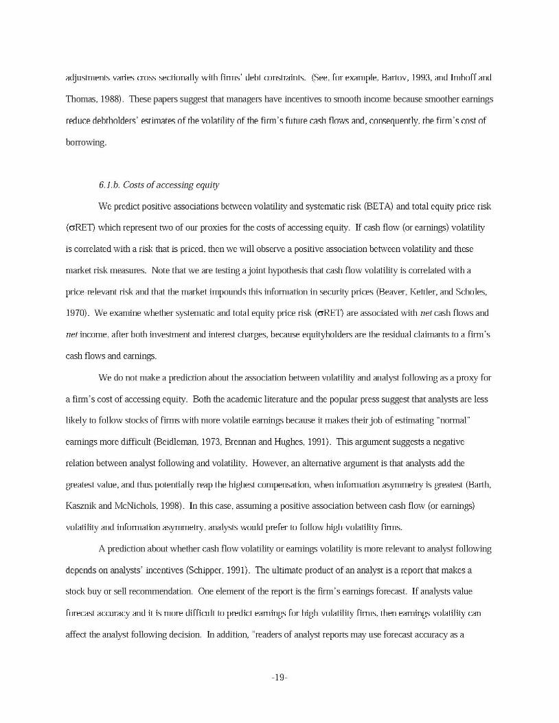
We do not make a prediction about the association between volatility and analyst following as a proxy for
a firm' s cost of accessing equity. Both the academic literature and the popular press suggest that analysts are less
likely to follow stocks of firms with more volatile earnings because it makes their job of estimating "normal"
earnings more difficult (Beidleman, 1973, Brennan and Hughes, 1991). This argument suggests a negative
relation between analyst following and volatility. However, an alternative argument is that analysts add the
greatest value, and thus potentially reap the highest compensation, when information asymmetry is greatest (Barth,
Kasznik and McNichols, 1998). In this case, assuming a positive association between cash flow (or earnings)
volatility and information asymmetry, analysts would prefer to follow high-volatility firms.
A prediction about whether cash flow volatility or earnings volatility is more relevant to analyst following
depends on analysts' incentives (Schipper, 1991). The ultimate product of an analyst is a report that makes a
stock buy or sell recommendation. One element of the report is the firm' s earnings forecast If analysts value
forecast accuracy and it is more difficult to predict earnings for high-volatility firms, then earnings volatility can
affect the analyst following decision. In addition, "readers of analyst reports may use forecast accuracy as a
-1 9-
quantitative measure of the quality of the overall report; this effect will create a preference for accuracy ... "
(Schipper, 1991). However, the analyst's stock recommendation decision also depends on other factors that can
be related to cash flows and not earnings. Thus, cash flow volatility will be an important determinant of analyst
following if it affects the analysts' overall ability to make stock buy/sell recommendations.
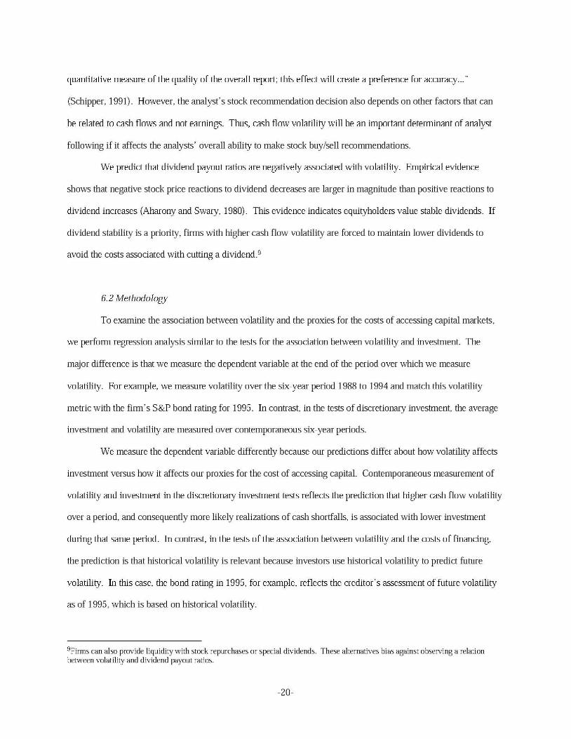
We predict that dividend payout ratios are negatively associated with volatility. Empirical evidence
shows that negative stock price reactions to dividend decreases are larger in magnitude than positive reactions to
dividend increases (Aharony and Swary, 1980). This evidence indicates equityholders value stable dividends. If
dividend stability is a priority, firms with higher cash flow volatility are forced to maintain lower dividends to
avoid the costs associated with cutting a dividend.9
6.2 Methodology
To examine the association between volatility and the proxies for the costs of accessing capital markets,
we perform regression analysis similar to the tests for the association between volatility and investment. The
major difference is that we measure the dependent variable at the end of the period over which we measure
volatility. For example, we measure volatility over the six-year period 1988 to 1994 and match this volatility
metric with the firm's S&P bond rating for 1995. In contrast, in the tests of discretionary investment, the average
investment and volatility are measured over contemporaneous six-year periods.
We measure the dependent variable differently because our predictions differ about how volatility affects
investment versus how it affects our proxies for the cost of accessing capital. Contemporaneous measurement of
volatility and investment in the discretionary investment tests reflects the prediction that higher cash flow volatility
over a period, and consequently more likely realizations of cash shortfalls, is associated with lower investment
during that same period. In contrast, in the tests of the association between volatility and the costs of financing,
the prediction is that historical volatility is relevant because investors use historical volatility to predict future
volatility. In this case, the bond rating in 1995, for example, reflects the creditor's assessment of future volatility
as of 1995, which is based on historical volatility.
9Firms can also provide liquidity with stock repurchases or special dividends. These alternatives bias against observing a relation between volatility and dividend payout ratios.
-20-

In order to examine the incremental impact of cash flow volatility and earnings volatility on our proxies
for the costs of accessing capital markets, we estimate augmented versions of equations (1 ) and (2) . The
augmented version of equation (1) includes continuous measures of both earnings and cash flow volatility. The
augmented version of equation (2) includes both cash flow and earnings volatility as well as variables to control
for the industry-adjusted levels of a firm's cash flows and earnings.
In each regression equation we also include control variables that have been identified in prior literature
as determinants of the dependent variable. The control variables are different for each proxy for the costs of
accessing capital markets. Because these control variables are not the focus of our analysis, we do not describe
them in detail and we do not present the coefficient estimates on these variables with the regression results. Table
8 summarizes the control variables, the predicted signs, and the source that justifies the use of the variable as a
control.
[INSERT TABLE 8.]
The cash flow and earnings metrics in this analysis should represent the cash flow or earnings on which
the stakeholder that creates the cost has a claim. In addition to OPCF, we measure the volatility of cash flow after
investment but before financing costs (CVCFAI), net cash flow (NETCF), operating income (CVOPINC), and net
income (NETINC), calculated as follows:
Calculation of variables: Operating cash flow (OPCF)
Depreciation and amortization + Change in working capital (as defined in Section 3.1)
Operating income (OPINC)
Net capital expenditures: to Gross capital expenditures Capitalized interest After-tax proceeds from sales of PPE
Compustat Data Item
#5
#90 #147/4
#83 * (1 - TR)
1Drhe proceeds from the sale of property. plant. and equipment (PPE). R&D and advertising are assumed to be zero if these data are missing on Compustat. C ross capital expenditures are missing for interim quarters during the year for some ftrms. lf the fourth quarter accumulated capital expenditures are missing. then the capital expenditures are assumed to be zero for the year.
-21-
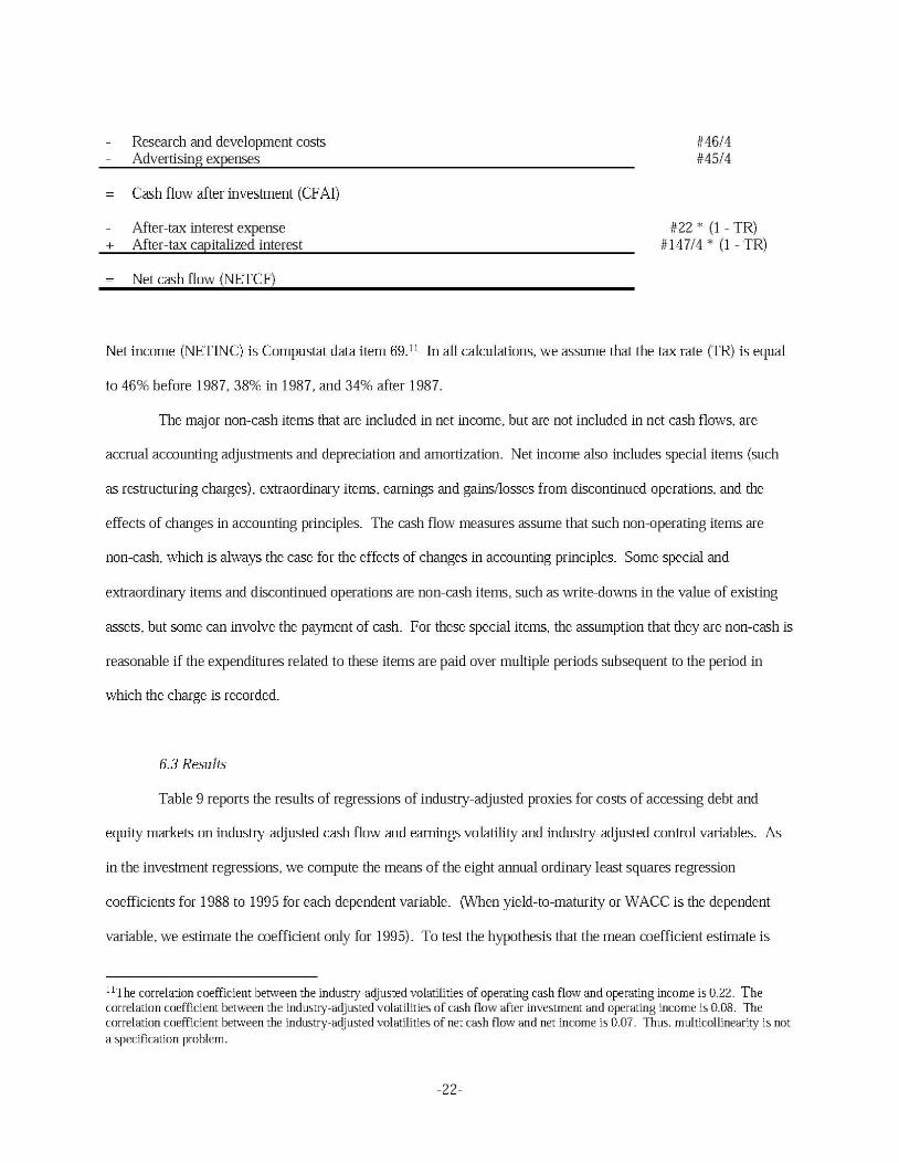
Research and development costs Advertising expenses
Cash flow after investment (CF AI)
After -tax interest expense + After-tax capitalized interest
Net cash flow (NETCF)
#46/4 #45/4
#22 * (1 - TR) #14 7/4 * (1 - TR)
Net income (NETINC) is Compustat data item 69.11 In all calculations, we assume that the tax rate (TR) is equal
to 46% before 1987, 38% in 1987, and 34% after 1987.
The major non-cash items that are included in net income, but are not included in net cash flows, are
accrual accounting adjustments and depreciation and amortization. Net income also includes special items (such
as restructuring charges), extraordinary items, earnings and gains/losses from discontinued operations, and the
effects of changes in accounting principles. The cash flow measures assume that such non-operating items are
non-cash, which is always the case for the effects of changes in accounting principles. Some special and
extraordinary items and discontinued operations are non-cash items, such as write-downs in the value of existing
assets, but some can involve the payment of cash. For these special items, the assumption that they are non-cash is
reasonable if the expenditures related to these items are paid over multiple periods subsequent to the period in
which the charge is recorded.
6.3 Results
Table 9 reports the results of regressions of industry-adjusted proxies for costs of accessing debt and
equity markets on industry-adjusted cash flow and earnings volatility and industry-adjusted control variables. As
in the investment regressions, we compute the means of the eight annual ordinary least squares regression
coefficients for 1988 to 1995 for each dependent variable. (When yield-to-maturity or WACC is the dependent
variable, we estimate the coefficient only for 1995) . To test the hypothesis that the mean coefficient estimate is
11The correlation coefficient between the industry-adjusted volatilities of operating cash flow and operating income is 0.22. The correlation coefficient between the industry-adjusted volatilities of cash flow after investment and operating income is 0.08. The correlation coefficient between the industry-adjusted volatilities of net cash flow and net income is 0.07. Thus. multicollinearity is not a specification problem.
-22-
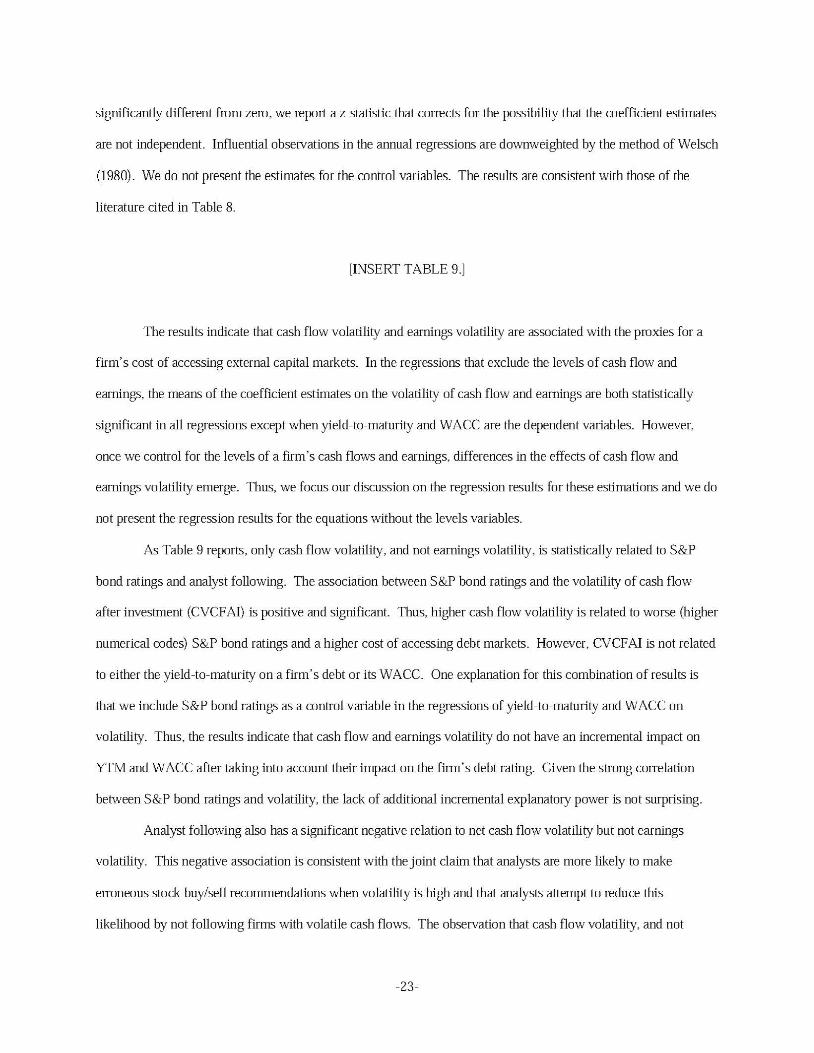
significantly different from zero, we report a z-statistic that corrects for the possibility that the coefficient estimates
are not independent Influential observations in the annual regressions are downweighted by the method of Welsch
(1980). We do not present the estimates for the control variables. The results are consistent with those of the
literature cited in Table 8.
[INSERT TABLE 9.]
The results indicate that cash flow volatility and earnings volatility are associated with the proxies for a
firm's cost of accessing external capital markets. In the regressions that exclude the levels of cash flow and
earnings, the means of the coefficient estimates on the volatility of cash flow and earnings are both statistically
significant in all regressions except when yield-to-maturity and WACC are the dependent variables. However,
once we control for the levels of a firm's cash flows and earnings, differences in the effects of cash flow and
earnings volatility emerge. Thus, we focus our discussion on the regression results for these estimations and we do
not present the regression results for the equations without the levels variables.
As Table 9 reports, only cash flow volatility, and not earnings volatility, is statistically related to S&P
bond ratings and analyst following. The association between S&P bond ratings and the volatility of cash flow
after investment (CVCF AI) is positive and significant. Thus, higher cash flow volatility is related to worse (higher
numerical codes) S&P bond ratings and a higher cost of accessing debt markets. However, CVCFAI is not related
to either the yield-to-maturity on a firm's debt or its WACC. One explanation for this combination of results is
that we include S&P bond ratings as a control variable in the regressions of yield-to-maturity and W ACC on
volatility. Thus, the results indicate that cash flow and earnings volatility do not have an incremental impact on
YTM and W ACC after taking into account their impact on the firm's debt rating. Given the strong correlation
between S&P bond ratings and volatility, the lack of additional incremental explanatory power is not surprising.
Analyst following also has a significant negative relation to net cash flow volatility but not earnings
volatility. This negative association is consistent with the joint claim that analysts are more likely to make
erroneous stock buy/sell recommendations when volatility is high and that analysts attempt to reduce this
likelihood by not following firms with volatile cash flows. The observation that cash flow volatility, and not
-23-
earnings volatility, is related to analyst following suggests that analysts do not focus on expected earnings forecast
precision when deciding to follow a firm.
We also document in Table 9 that earnings volatility, and not cash flow volatility, is significantly
associated with higher stock market betas and lower dividend payout ratios, both of which represent a higher cost
of accessing equity capitaL 12 The regression results for beta suggest that earnings volatility is correlated with a
risk that is priced, and that the market assesses at least part of this operating risk as systematic. Moreover, the
significance of earnings volatility rather than cash flow volatility indicates that the market assesses that earnings
volatility is the better measure of the priced risk. The observation that dividend payout ratios are negatively
associated with earnings volatility rather than cash flow volatility is consistent with the observation that dividend
restrictions in bond covenants are frequently based on accounting earnings realizations (Smith and Warner, 1979).
Finally, Table 9 reports that cash flow and earnings volatility are both statistically related to total equity
price risk (as measured by the standard deviation of returns). Taken together with the observation that only net
earnings volatility affects beta, this result suggests that net cash flow volatility affects the costs of equity through
its association with systematic factors that are not captured by beta or unsystematic risk.
Finally, conditional on the level of a firm' s net cash flows or income, volatility appears to have a second-
order effect on analyst following, equity betas, total equity price risk, and dividend payout ratios. In particular, the
analyst following of firms with high levels of cash flows is significantly and positively associated with net cash
flow volatility. (The coefficient estimate on CVCF is -0.0237 and the coefficient estimate on CVCF*HICF is
0.27 4 7.) This result is consistent with the proposition that analysts can earn rents by following firms where there
is a greater demand for information, but only for firms with high levels of net cash flow.
In the case of betas, standard deviations of returns (crRET), and dividend payout ratios, it is the firms
with low net income levels (or cash flow levels for crRET), that are distinguished from firms with either moderate
or high levels. Specifically, for low-level firms, the association between volatility and each of these proxies is not
statistically different from zero. However, the intercepts indicate that these firms have higher equity betas, higher
equity price risk, and lower dividend payout ratios, on average. Thus, similar to the results about the relation
12We also estimate these regressions using only cash flow volatility and the levels of a firm' s cash flows. These regressions indicate that cash flow volatility is not statistically related to stock market betas and is statistically negatively related to dividend payout mtios.
-24-
between volatility and discretionary investment, volatility only affects a firm's costs of accessing equity capital
above some threshold leveL Below this threshold, volatility is unimportant
In sum, the results in Table 9 support the proposition that volatility increases a firm's costs of accessing
external capital to cover cash shortfalls. If financially constrained firms maintain investment but at this higher cost
of funding it, we will observe differences in the net returns on investment. We will not, however, observe that
more financially constrained firms have lower investment cash flow sensitivities unless the costs are sufficiently
high to deter investment Thus, this evidence offers a potential explanation for the mixed results about whether
investment-cash flow sensitivities are good proxies for financing constraints (FHP, 1988 and 1998 and KZ, 1997) .
7. Summary and conclusions
In this paper, we provide direct evidence that cash flow volatility is associated with lower levels of
investment in discretionary items including capital expenditures, research and development costs, and advertising
expenses. The sensitivity of investment to cash flow volatility is reduced, but not eliminated, for firms that hold
higher buffer stocks of cash and for firms with lower costs of accessing external capital markets.
Moreover, volatility increases the costs of accessing external capital markets that can be used to smooth
internal cash flow volatility. In the examination of the impact of volatility on proxies for the costs of capital
market access, we consider not only cash flow volatility but also earnings volatility. S&P bond ratings and analyst
following are related to cash flow volatility but not earnings volatility. In contrast, beta and dividend payout ratios
are related to earnings volatility but not cash flow volatility. Total equity price risk is related to both. The relative
importance of earnings volatility to beta, total equity price risk, and dividend payout ratios suggests that
equityholders view historical earnings volatility as a good predictor of future cash flow volatility.
These results have several important implications for risk mangers. First, the results indicate that hedging
cash flow volatility and earnings volatility will accomplish different objectives. Hedging cash flow volatility will
reduce the likelihood that a firm needs to access external capital to cover shortfalls. However, hedging earnings
volatility can reduce the costs of accessing external markets if the firm does require additional capital. Second, our
evidence suggests that the expected persistence of the effectiveness of a risk management strategy into future
periods is important The proxies for the costs of accessing capital markets, in theory, are related to assessments
-25-

of expected future cash flow volatility, but our evidence indicates that these proxies are correlated with historical
volatility. One interpretation of this result is that historical volatility is used to predict future volatility. If this is
the case, then risk management decisions that reduce historical volatility, but which are not expected to have a
persistent effect on volatility, will not reduce a firm's costs of accessing external markets. Although this study
does not directly address whether the source of a firm's volatility, and thus its persistence, is related to the costs of
volatility, our results offer a starting point for contemplation.
Finally, while we document that there are costs associated with a firm's chosen level of volatility, we do
not claim that a firm should reduce volatility to zero in order to eliminate these costs. Rather, these costs are one
element that a firm should consider in its decisions regarding risk management The firm must then decide how to
trade-off the potential for the costs of volatility in terms of reduced capital expenditures against the costs of
managing volatility.
-26-
References
Aharony, Joseph and Itzhak Swary, 1980, Quarterly dividend and earnings announcements and stockholders' returns: An empirical analysis, Journal of Finance 35,1 - 11.
Albrecht, David, N. and Frederick M. Richardson, 1990, Income smoothing by economy sector, Journal of Business, Finance and Accounting 17, 713- 730.
Alford, Andrew W. and James R Boatsman, 1995, Predicting long-term stock return volatility: Implications for accounting and valuation of equity derivatives, Accounting Review 70, 599-618.
Amihud, Yakov and Haim Mendelson, Liquidity and asset prices: Financial management implications, 1988, Vol 7, Financial Management, 5-1 5.
Asquith, Paul and David W. Mullins, Jr.. 1983, The impact of initiating dividend payments on shareholders' wealth, Journal of Business 56, 77-95.
Atiase, Rowland K., 1985, Predisclosure information, firm capitalization, and security price behavior around earnings announcements, Journal of Accounting Research 23, 21-36.
Balog, Stephen], 1991, What an analyst wants from you, Financial Executive 7, 4 7-52.
Banz, Rolf W., 1981, The relationship between return and market value of common stocks, Journal of Financial Economics 9, 3-18.
Barth, Mary E., William H. Beaver, and Wayne R Landsman, 1997, Relative Valuation Roles of Equity Book Value and Net Income as a Function of Financial Health, Working paper, Stanford University.
Barth, Mary E., Ron Kasznik, and Maureen F. McNichols, 1998, Analyst coverage and intangible assets, Working paper, Stanford University.
Bartov, E., 1993, The timing of asset sales and earnings manipulation, Accounting Review 68, 840-85 5.
Beaver, William, P. Kettler, and Myron Scholes, 1970, The association between market determined and accounting determined risk measures, Accounting Review, 654-682.
Beidleman, Carl R , 1973, Income smoothing: The role of management, Accounting Review 38, 653-66 7.
Belsey, D. A., E. Kuh, andRE. Welsch, 1980, Regression diagnostics : Identifying influential data and potential sources of multicollinearity (John Wiley, New York).
Bhushan, Ravi, 1989, Collection of information about publicly traded firms theory and evidence, Journal of Accounting and Economics 11, 183-206.
Botosan, Christine, 1997, Disclosure level and the cost of equity capital, Accounting Review 72, 323-349.
Bowen, R M., D. Burgstahler, and L Daley, 1986, Evidence on the relationships between earnings and various measures of cash flow, Accounting Review 61 , 713-725.
Brennan, Michael and Patricia]. Hughes, 1991, Stock prices and the Supply of Information, Journal of Finance 46, 1665-1691.
Calomiris, Charles W., Charles P. Himmelberg, and Paul Wachtel, 1995, Commercial paper, corporate finance, and the business cycle: A microeconomic perspective, Carnegie-Rochester Series on Public Policy 42, 203-250.
-27-
Cheung, Kee H., Thomas H. Mclnish, Robert A. Wood, and Donald]. Wyhowski, 1995, Production of information asymmetry, and the bid-ask spread: Empirical evidence from analysts ' forecasts, Journal of Banking and Finance 19, 1025-1046.
Chung, Yin-W ong and Lilian K Ng, 1992, Stock price dynamics and firm size: An empirical investigation, Journal of Finance 4 7, 1985-1997.
Collins, Daniel W ., S.P. Kothari, and Judy D. Rayburn, 1987, Firm size and the information content of prices with respect to earnings, Journal of Accounting and Economics 9, 111-138.
Collins, Daniel W ., MichaelS. Rozeff, and DanS. Dhaliwal, 1981, The economic determinants of the market reaction to proposed mandatory accounting changes in the oil and gas industry, Journal of Accounting and Economics 3, 3 7-71.
Dechow, Patricia, 1994, Accounting earnings and cash flows as measures of firm performance: The role of accounting accruals, Journal of Accounting and Economics, 3-42.
Easton, Peter D. and Mark E. Zmijewski, 1989, Cross-sectional variation in the stock market response to accounting earnings announcements, Journal of Accounting Research 11, 11 7-141.
Ederington, Louis H., Jess B. Yawitz, and Brian E. Roberts, 1987, The information content of bond ratings, Journal of Financial Research 10, 211-226.
Fazzari, Steven M., R Glenn Hubbard, and Bruce C. Petersen, 1988, Financing constraints and corporate investment, Brookings Papers on Economic Activity, 141 -1 95.
Fazzari, Steven M., R Glenn Hubbard, and Bruce C. Petersen, 1998, Investment- Cash flow sensitivities are useful: A comment on Kaplan and Zingales, Working paper, Columbia University.
Finger, Catherine, 1994, The ability of earnings to predict future earnings and cash flow , Journal of Accounting Research 32, 210-223.
Freeman, Robert and Senyo Tse, 1992, A nonlinear model of security price responses to unexpected earnings, Journal of Accounting Research 30, 185-209.
Froot, Kenneth, David Scharfstein, and Jeremy Stein, 1993, Risk management: Coordinating investment and financing policies, The Journal of Finance 48, 1629-1658.
GB-czy, Christopher, Bernadette A. Minton, and Catherine Schrand, 1997, W hy firms use currency derivatives, Journal of Finance 52, 1323-1354.
Greene, W illiam H., 1993, Econometric Analysis, Second edition, (MacMillan Publishing Co., New York) .
Hamada, Robert S ., 1972, The effect of the firm's capital structure on the systematic risk of common stocks, Journal of Finance, 435-452.
Healy, Paul M., Sok-Hyon Kang, and Krishna G. Palepu, 1987, The effect of accounting procedure changes on CEOs' cash salary and bonus compensation, Journal of Accounting and Economics 9, 7-34.
Hepworth, SamueL R, 1953, Smoothing periodic income, Accounting Review 28, 32-39.
Hoshi, Takeo, Anil Kashyap, and David Scharfstein, 1991, Corporate structure, liquidity, and investment: Evidence from Japanese industrial groupings, Quarterly Journal of Economics 56, 33-60.
Imhoff, G., and]. Thomas, 1988, Economic consequences of accounting standards: The lease disclosure rule change, Journal of Accounting and Economics, 277-31 0.
-28-
Kaplan, Robert S. and Gabriel Urwitz, 1979, Statistical model of bond ratings: A methodological inquiry, Journal of Business 52, 231-261.
Kaplan, Steven N. and Luigi Zingales, 1997, Do investment-cash flow sensitivities provide useful measures of financing constraints?, Quarterly J ournal of Economic , 169-215.
Kormendi, Roger and Robert Lipe, 1987, Earnings innovations, earnings persistence, and stock returns, Journal of Business 60, 323-346.
Lamont, Owen, 1997, Cash flow and investment: Evidence from internal capital markets, Journal of Finance 52, 83-111.
Lang, Larry H.P. and Robert H. Litzenberger, 1989, Dividend Announcements: Cash Flow Signalling vs. Free Cash Flow Hypothesis, Journal of Financial Economics 24, 181-191.
Lang and Lundholm, 1996, Corporate disclosure policy and analyst behavior, Accounting Review 71, 467-492.
Lessard, Donald, 1990, Global competition and corporate finance in the 1990s, Journal of Applied Corporate Finance 3, 59-72.
Lys, T., 1984, Mandated accounting changes and debt covenants: The case of oil and gas accounting, Journal of Accounting and Economics, 39-65.
MacDonald, Elizabeth, 1997, FASB rule on the wild sidewalk, Wall Street Journal, Sept 30, Cl.
Mian, Shehzad L, 1996, Evidence on corporate hedging policy, Journal of Financial and Quantitative Analysis 31, 419-439.
Michelson, S. E., ]. Jordan-Wagner, and C. W. Wootton, 1995, A market based analysis of income smoothing, Journal of Business Finance and Accounting 22, 1179-1193.
Miller, M.H. and F. Modigliani, 1961, Dividend policy, growth and the valuation of shares, Journal of Finance 34, 411-433.
Nance, Deana R , Clifford W. Smith, ]r., and Charles W. Smithson, 1993, On the determinants of corporate hedging, Journal of Finance 48, 267-284.
Nocera, Joseph, 1997 Who really moves the market? Securities analysts are Wall Street's new stars, Fortune, Oct. 27, 90.
O'Brien, Patricia C. and Ravi Bhushan, 1990, Analyst following and institutional ownership, Journal of Accounting Research 28, 55-76.
Ogden, Joseph P., 1987, Determinants of the ratings and yields on corporate bonds: Tests of the contingent claims model, Journal of Financial Research 10, 329-339.
Ritter, Jay R., 1987, The cost of going public, Journal of Financial Economics 19, 269-281.
Schipper, Katherine, 1991, Commentary on analysts' forecasts, Accounting Horizons 5, 105-121.
Shapiro, Alan, and Sheridan Titman, 1986, An integrated approach to corporate risk management, in Joel Stern and Donald Chew, eds.: The Revolution in Corporate Finance (Basil Blackwell, LTD, England and Basil Blackwell, Inc. Cambridge, MA).
Shimko, David, 1997, Yearnings Per Share, Risk 10, No.9.
-29-
Sloan, Richard, 1996, Using earnings and free cash flow to evaluate corporate performance, Journal of Applied Corporate Finance, 70-78_
Smith, Clifford W., ]r_ and Jerold B. Warner, 1979, On financial contracting: An analysis of bond covenants, Journal of Financial Economics 7, 117-1 61.
Smith, Clifford W., Jr. and Ross L Watts, 1992, The investment opportunity set and corporate financing, dividend, and compensation policies, Journal of Financial Economics 32, 263-292.
Stulz, Rene, 1990, Managerial discretion and optimal financing policies, Journal of Financial Economics 26, 3-28_
Tufano, Peter, 1996, W ho manages risk? An empirical examination of risk management practices in the gold mining industry, Journal of Finance 51, 1097-1137_
Trueman, Brett and Titman, Sheridan, 1988, An explanation for accounting income smoothing, Journal of Accounting Research 26 (Supplement) , 127-139_
Welsch, R E., 1980, Regression sensitivity analysis and bounded-influence estimation, in: ]_ Kmenta and ]_B. Ramsay, eds., Evaluation of Econometric Models (Academic Press, New York) , 153-167_
Wharton School/CIBC Wood Gundy , 1996, 1995 Survey of derivatives usage by U.S. non-financial firms (University of Pennsylvania) _
-30-

Table 1 Summary of firms and industries in the sample.
Sample firms include all firms in two-digit SIC industries in which there are at least ten firms with data available on at least one of the cash flow or accounting earnings metrics that are used in this paper. The number of sample firms reported is the number with data available for operating cash flow (OPCF) for 1995. The firms are on the Compustat quarterly data tapes from 1989 to 1994.
Industry Two-digit Number of Name SIC Code sample firms
Metal Mining 10 19 Oil and Gas Extraction 13 57 Building Construction-General Contractors, Operative Builders 15 11 Non-building Construction 16 -
Food and Kindred Products 20 46 Textile Mill Products 22 23 Apparel and Other Finished Products 23 20 Lumber and Wood Products, except Furniture 24 13 Furniture and Fixtures 25 15 Paper and Allied Products 26 27 Printing, Publishing and Allied 27 35 Chemicals and Allied Products 28 92 Petroleum Refining and Related Industries 29 30 Rubber and Miscellaneous Plastic Products 30 30 Stone, Clay, Glass, and Concrete Products 32 15 Primary Metal Industries 33 46 Fabricated Metal, except Machinery, Transportation Equipment 34 42 Machinery, except Electrical 35 112 Electrical, Electrical Machinery, Equipment, Supplies 36 99 Transportation Equipment 37 40 Measuring Instruments; Photographic Goods; Watches 38 57 Miscellaneous Manufacturing Industries 39 19 Water Transportation 44 1 Transportation by Air 45 -
Communication 48 15 Electric, Gas, Sanitary Services 49 16 Durable Goods-Wholesale 50 37 Non-Durable Goods-Wholesale 51 29 General Merchandise Stores 53 20 Food Stores 54 15 Auto Dealers, Gas Stations 55 -
Apparel and Accessory Stores 56 13 Furniture, Home Furnishings Stores 57 -
Eating and Drinking Places 58 22 Miscellaneous Retail 59 26 Business Services 73 51 Motion Pictures 78 -Amusement, except Motion Pictures 79 12 Health Services 80 16 Environmental Services 87 14
1, 135
-31-
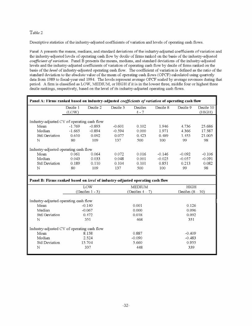
T able 2
Descriptive statistics of the industry-adjusted coefficients of v ariation and levels of operating cash flows.
Panel A presents the means, medians, and standard deviations of the industry-adjusted coefficients of variation and the industry-adjusted levels of operating cash flow by decile of firms ranked on the basis of the industry-adjusted coefficient of variation. Panel B presents the means, medians, and standard deviations of the industry-adjusted levels and the industry-adjusted coefficients of variation of operating cash flow by decile of firms ranked on the basis of the level of industry-adjusted operating cash flow. The coefficient of variation is defined as the ratio of the standard deviation to the absolute value of the mean of operating cash flows (OPCF) calculated using quarterly data from 1989 to fiscal-year end 1994. The levels represent average OPCF scaled by average revenues during that period. A firm is classified as LOW, MEDIUM, or HIGH if it is in the lowest three, middle four or highest three decile rankings, respectively, based on the level of its industry-adjusted operating cash flows.
Panel A: Firms ranked based on industry-adjusted coefficients of variation of operating cash flow
Decile 1 Decile 2 Decile 3 Deciles Decile 8 Decile 9 Decile 10 (LOW) 4 - 7 (HIGH)
Industry-adjusted CV of operating cash flow Mean - 1.769 -0.893 -0.601 0. 102 1.946 4.736 25.686 Median - 1.665 -0.894 -0.594 0.000 1.971 4.366 17.587 Std Deviation 0 .610 0.092 0.077 0.423 0.489 1.453 21.005 N 80 109 137 500 100 99 98
Industry-adjusted operating cash flow Mean 0.061 0.064 0.072 0.016 -0.146 -0 .092 -0.106 Median 0 .043 0.033 0.048 0.001 -0.025 -0 .057 -0.091 Std Deviation 0 .189 0.110 0.104 0. 101 0.851 0 .213 0.082 N 80 109 137 500 100 99 98
Panel B: Firms ranked based on level of industry-adjusted operating cash flow
LOW MEDIUM HIGH (Deciles 1 - 3) (Deciles 4 - 7) Deciles (8 - 10)
Industry-adjusted operating cash flow Mean -0 .140 0 .001 0 .126 Median -0.067 0.000 0 .096 Std Deviation 0 .472 0 .018 0 .092 N 351 468 351
Industry-adjusted CV of operating cash flow Mean 8 .1 58 0 .887 -0 .409 Median 2.524 -0 .090 -0 .483 Std Deviation 15.704 5.660 0 .955 N 337 448 339
-32-
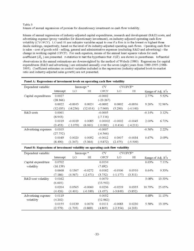
Table 3 Means of arnmal regressions of proxies for discretionary investment on cash flow volatility.
Means of annual regressions ofindushy -adjusted capital expenditures, research and development (R&D) costs, and advertising expense (proxy variables for discretionary investment), on industry-adjusted operating cash flow volatility (CVOPCF). LO and HI are indicator variables equal to one if a firm is in the lowest or highest three decile rankings, respectively, based on the level of its industty-adjusted operating cash flows. Operating cash flow is sales - cost of goods sold - selling, general and administrative expenses (excluding R&D and advertising) - the change in working capital (OPCF). For each equation, means of the annual least squares values for each coefficient ( a ,, ) are presented. z-statistics to test the hypothesis that E (a ) are shown in parentheses. Influential
observations in the annual estimations are downweighted by the method of Welsch (1980). Regressions for capital expenditures (R&D and advertising) are estimated annually over the seven (eight) years from 1989-1995 (1988-1995). Coefficient estimates on control variables included in the regressions (industty-adjusted book-to-market ratio and industty-adjusted sales growth) are not presented.
Panel A: Regressions of investment levels on operating cash flow volatility
Dependent variable: Intercept * cv CVOPCF*
Intercept LO HI OPCF LO HI Range of Adj . R 2s
Capital expenditures 0.0027 -0.0002 2.77% 5.52%
(28.366) (-23.267)
0.0022 -0.0043 0.0024 -0.0002 0.0002 -0.0016 9.26% 12.96%
(12.035) (-8.236) (12.014) (-7.969) (5.290) (-4.1 40)
R&D costs 0.0061 -0.0005 -0.14% 3.12%
(8.943) (-7.116)
0.0019 -0.0019 0.0085 0.00002 -0.0002 -0.0045 2.00% 6.71%
(3.453) ( -1.079) (6.061) (-0.081) (-0.414) (-4.2 11)
Advertising expenses 0.0105 -0.0007 -0.56% 2.22%
(27.752) (-6.566)
0.0049 0.0020 0.0092 -0.0012 0.0007 -0.0034 0.67% 3.09%
(8.490) (1.347) (5.364) (-5.872) (2.475) ( -5.509)
Panel B: Regressions of investment volatility on operating cash flow volatility
Dependent variable: Intercept * cv CVOPCF*
Intercept LO HI OPCF LO HI Range of Adj . R 2s
Capital expenditure 0.0702 0.0134 0.63% 7.11%
volatility ( 16. 159) (7.692)
0.0668 0.1307 -0.0272 0.0182 -0.0106 0.0510 0.64% 9.33%
(7.186) (4.567) (-2.471) (3.752) (-1.1 77) (3.31 1)
R&D cost volatility 0.0162 0.0070 5.08% 13.53%
(6.601) (13.592)
0.0204 0.0565 -0.0060 0.0236 -0.0219 0.0335 10.79% 25.05%
(4.426) (4.401) (-0.189) (4.457) ( -3.849) (3.852)
Advertising expense 0.011 9 0.0052 4.68% 11.15%
volatility ( 4.202) (12.982)
0.0155 0.0139 0.0076 0.0111 -0.0083 0.0230 5.58% 13.19%
(2.579) (1. 705) (0.869) (4.805) ( -2.354) (4.203)
-33-
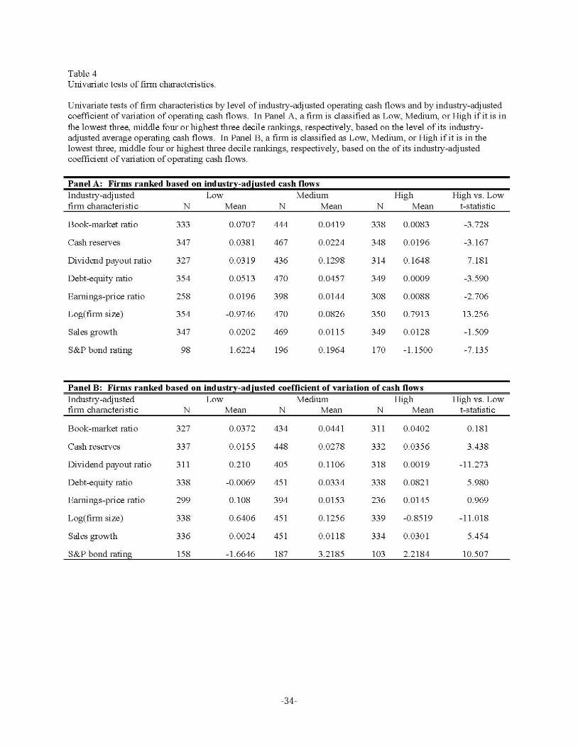
Table 4 Univariate tests of finn characteristics.
Univariate tests of firm characteristics by level of industry-adjusted operating cash flows and by industry-adjusted coefficient of variation of operating cash flows. In Panel A, a finn is classified as Low, Medium, or High if it is in the lowest three, middle four or highest three decile rankings, respectively, based on the level of its industryadjusted average operating cash flows. In Panel B, a finn is classified as Low, Medium, or High if it is in the lowest three, middle four or highest three decile rankings, respectively, based on the of its industry-adjusted coefficient of variation of operating cash flows.
Panel A: Firms ranked based on industr;t-adjusted cash flows Industry-adjusted Low Medium High High vs. Low finn characteristic N Mean N Mean N Mean t-statistic
Book-market ratio 333 0 .0707 444 0 .0419 338 0.0083 -3.728
Cash reserves 347 0 .0381 467 0.0224 348 0.0 196 -3.167
Dividend payout ratio 327 0 .031 9 436 0 .1298 3 14 0.1648 7. 181
Debt-equity ratio 354 0 .051 3 470 0 .0457 349 0.0009 -3.590
Earnings-price ratio 258 0 .0196 398 0 .01 44 308 0.0088 -2.706
Log(fmn size) 354 -0 .9746 470 0 .0826 350 0.7913 13.256
Sales growth 347 0 .0202 469 0.0115 349 0.0 128 -1.509
S&P bond rating 98 1.6224 196 0 .1964 170 -1.1500 -7.135
Panel B: Firms ranked based on industry-adjusted coefficient of variation of cash flows Industry-adjusted Low Medium High High vs. Low finn characteristic N Mean N Mean N Mean t-statistic
Book-market ratio 327 0 .0372 434 0.0441 3 11 0.0402 0.181
Cash reserves 337 0 .0155 448 0 .0278 332 0.0356 3.438
Dividend payout ratio 3 11 0 .210 405 0 .1106 318 0.00 19 -11.273
Debt-equity ratio 338 -0 .0069 451 0.0334 338 0.0821 5.980
Earnings-price ratio 299 0 .108 394 0.0153 236 0.0 145 0.969
Log(fmn size) 338 0 .6406 451 0 .1256 339 -0.8519 -1 1.018
Sales growth 336 0 .0024 451 0 .0118 334 0.0301 5.454
S&P bond rating 158 -1.6646 187 3.2185 103 2.2 184 10.507
-34-
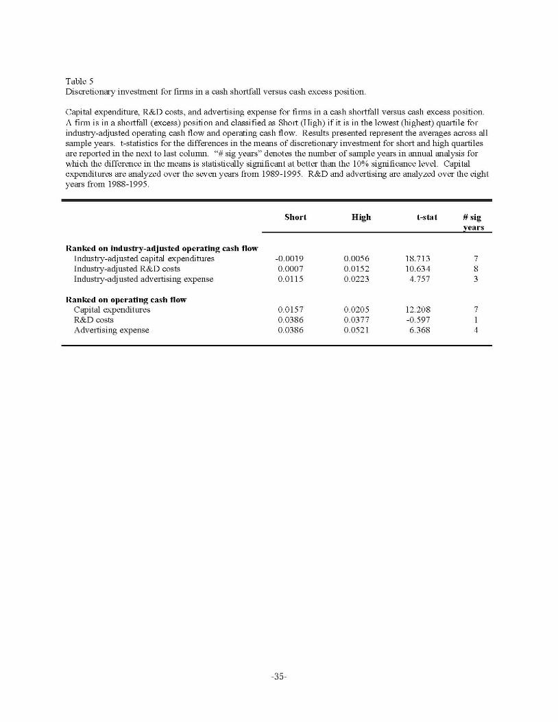
Table 5 Discretionary investment for firms in a cash shortfall versus cash excess position.
Capital expenditure, R&D costs, and advertising expense for firms in a cash shortfall versus cash excess position. A firm is in a shortfall (excess) position and classified as Short (High) if it is in the lowest (highest) quartile for industry-adjusted operating cash flow and operating cash flow . Results presented represent the averages across all sample years. t-statistics for the differences in the means of discretionary investment for short and high quartiles are reported in the next to last column. "# sig years" denotes the number of sample years in annual analysis for which the difference in the means is statistically significant at better than the 10% significance level. Capital expenditures are analyzed over the seven years from 1989-1995. R&D and advertising are analyzed over the eight years from 1988-1995.
Ranked on industry-adjusted operating cash flow Industry-adjusted capital expenditures Industry-adjusted R&D costs Industry-adjusted advertising expense
Ranked on operating cash flow Capital expenditures R&D costs Advertising expense
Short
-0.0019 0.0007 0.0115
0.0157 0.0386 0.0386
-35-
High
0.0056 0.0152 0.0223
0.0205 0.0377 0.052 1
t-stat
18.713 10.634 4.757
12.208 -0.597 6.368
# sig ears
7 8 3
7 1 4
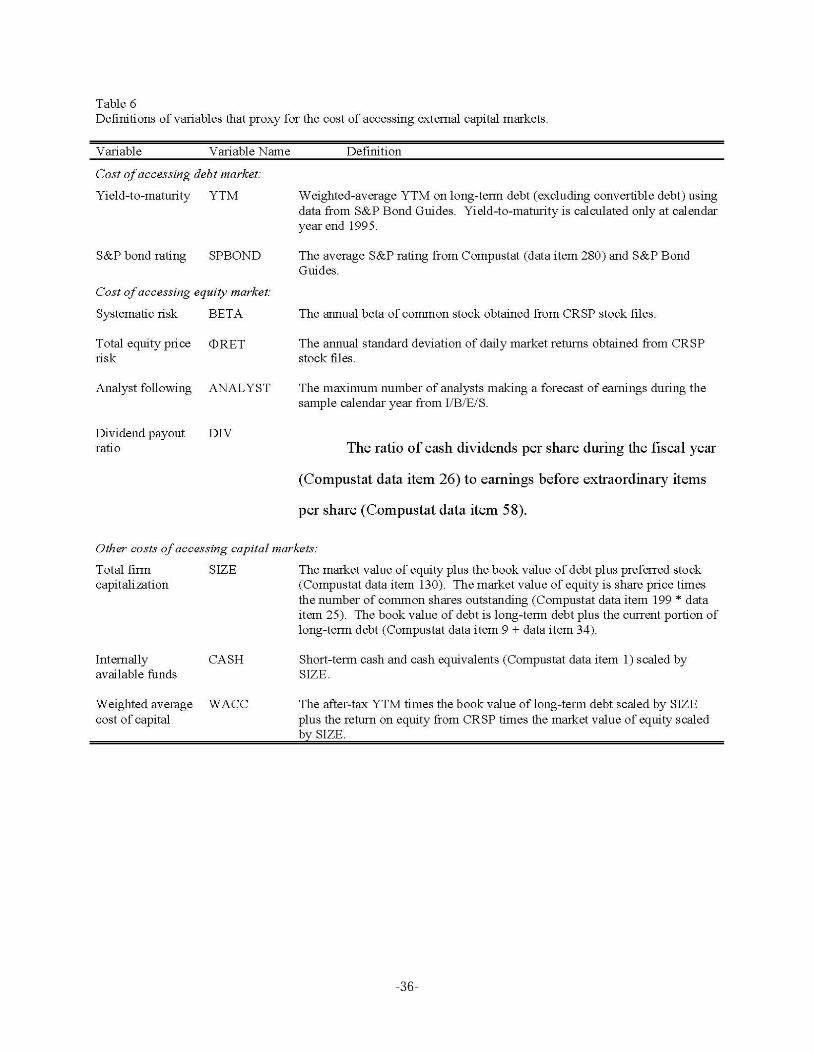
Table 6 Definitions of variables that proxy for the cost of accessing external capital markets.
Variable Variable Name
Cost of accessing debt market:
Yield-to-maturity YTM
S&P bond rating SPBOND
Cost of accessing equity market:
Systematic risk BET A
Total equity price <DRET risk
Analyst following ANALYST
Dividend payout DIV ratio
Definition
Weighted-average YTM on long-term debt (excluding convertible debt) using data from S&P Bond Guides. Yield-to-maturity is calculated only at calendar year end 1995.
The average S&P rating from Compustat (data item 280) and S&P Bond Guides.
The annual beta of common stock obtained from CRSP stock flles.
The annual standard deviation of daily market returns obtained from CRSP stock files.
The maximum number of analysts making a forecast of earnings during the sample calendar year from 1/B/E/S.
The ratio of cash dividends per share during the fiscal year
(Compustat data item 26) to earnings before extraordinary items
per share (Compustat data item 58).
Other costs of accessing capital markets:
Total flrm SIZE capitalization
Internally CASH available funds
Weighted average WACC cost of capital
The market value of equity plus the book value of debt plus preferred stock (Compustat data item 130). The market value of equity is share price times the number of common shares outstanding (Compustat data item 199 * data item 25). The book value of debt is long-term debt plus the current portion of long-term debt (Compustat data item 9 + data item 34).
Short-term cash and cash equivalents (Compustat data item 1) scaled by SIZE.
The after-tax YTM times the book value oflong-term debt scaled by SIZE plus the return on equity from CRSP times the market value of equity scaled b SIZE.
-36-
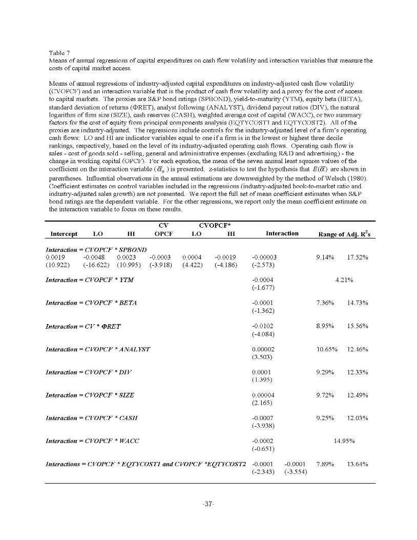
Table 7 Means of annual regressions of capital expenditures on cash flow volatility and interaction variables that measure the costs of capital market access.
Means of annual regressions of industry-adjusted capital expenditures on industry-adjusted cash flow volatility (CVOPCF) and an interaction variable that is the product of cash flow volatility and a proxy for the cost of access to capital markets. The proxies are S&P bond mtings (SPBOND), yield-to-maturity (YTM), equity beta (BETA), standard deviation of returns (<DRET), analyst following (ANALYST), dividend payout ratios (DIV), the natural log arithm of firm size (SIZE), cash reserves (CASH), weighted average cost of capital (VV ACC), or two summary factors for the cost of equity from principal components analysis (EQTYCOSTl and EQTYCOST2). All of the proxies are industry-adjusted. The regressions include controls for the industry-adjusted level of a firm's operating cash flows: LO and HI are indicator variables equal to one if a finn is in the lowest or highest three decile rankings, respectively, based on the level of its industry-adjusted operating cash flows. Operating cash flow is sales- cost of goods sold - selling, general and administrative expenses (excluding R&D and advertising) - the change in working capital (OPCF). For each equation, the mean of the seven annual least squares values of the coefficient on the interaction variable ( a,1 ) is presented. z-statistics to test the hypothesis that E(a) are shown in
parentheses. Influential observations in the annual estimations are downweighted by the method of Welsch (1980). Coefficient estimates on control variables included in the regressions (industry-adjusted book-to-market ratio and industry-adjusted sales growth) are not presented. We report the full set of mean coefficient estimates when S&P bond ratings are the dependent variable. For the other regressions, we report only the mean coefficient estimate on the interaction variable to focus on these results.
Intercept LO HI
Interaction = CVOPCF * SPBOND
cv OPCF
0.0019 -0.0048 0.0023 -0.0003 ( 10.922) (-16.622) (10.995) (-3.918)
Interaction = CVOPCF * YTM
Interaction= CVOPCF * BETA
Interaction = CV * 41RET
Interaction= CVOPCF *ANALYST
Interaction = CVOPCF * DIV
Interaction = CVOPCF * SIZE
Interaction = CVOPCF * CASH
Interaction= CVOPCF * WACC
CVOPCF* LO HI
0.0004 (4.422)
-0.0019 (-4.1 86)
InteractiollS = CVOPCF * EQTYCOSTJ and CVOPCF *EQTYCOST2
-37-
Interaction Range of Adj. R 2s
-0.00003 9. 14% 17.52% (-2.573)
-0.0004 4.21% ( -1.677)
-0.0001 7.36% 14.73% (-1.362)
-0.0102 8.95% 15.56% (-4.084)
0.00002 10.65% 12.46% (3.503)
0.0001 9.29% 12.33% ( 1.395)
0.00004 9.72% 12.49% (2.165)
-0.0007 9.25% 12.03% (-3.938)
-0.0002 14.95% (-0.651)
-0.0001 -0.0001 7.89% 13.64% (-2.343) ( -3.554)
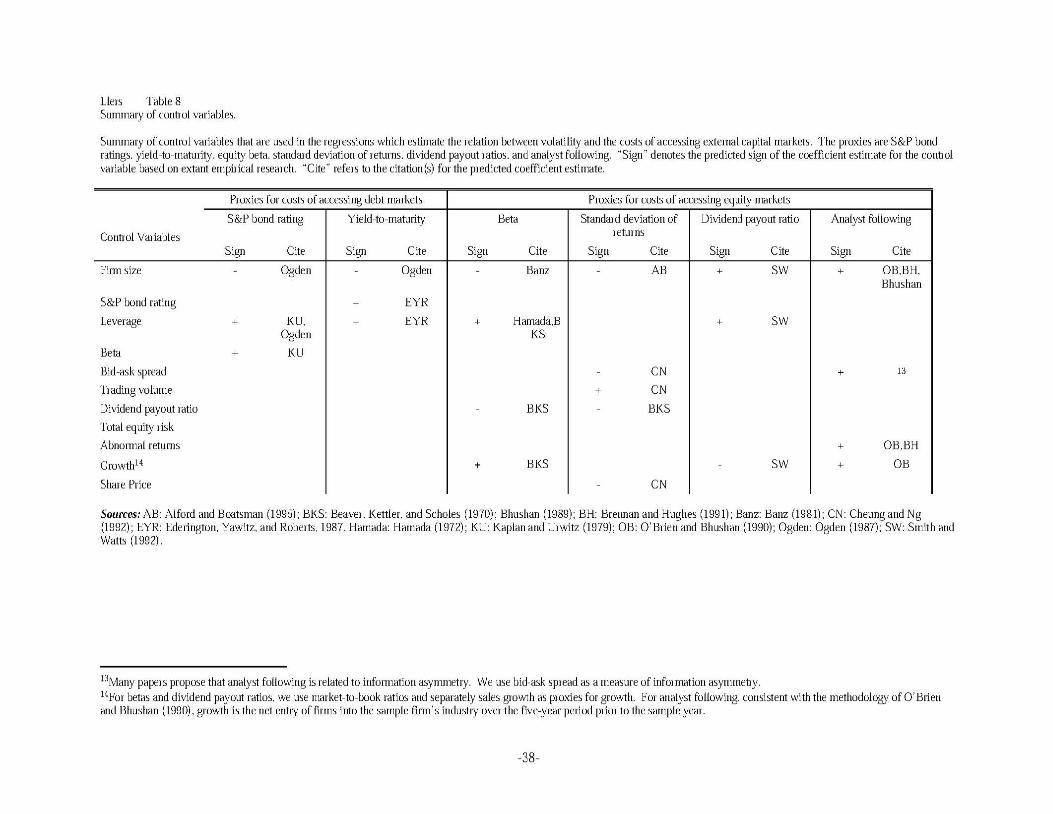
Llers Table 8 Summary of control variables.
Summary of control variables that me used in the regressions which estimate the relation between volatility and the co~ts of accessing extemal capital markets. The proxies me S&P bond ratings. yield-to-maturity. equity beta. standard deviation of returns. dividend payout ratios. and analyst following. "Sign" denotes the predicted sign of the coefficient estimate for the control variable based on extant empirical research. "Cite" refers to the citatiun(s) for the predicted coefficient estimate.
Proxies for costs of accessing debt markets Proxies for costs of accessing equity markets
S&P bond rating Yield-to-maturity Beta Standard deviation of Dividend payout ratio Analyst following
Control Variables returns
Sign Cite Sign Cite Sign Cite Sign Cite Sign Cite Sign Cite
Finn size - Ogden - Ogden - 13anz - AB + sw + OB.BH. Bhushan
S&P bond rating + EYR
Leverage + KU. + EYR + Harnada.B + sw Ogden KS
Beta + KU
Bid-ask spread - CN + J:l
Trading volume + CN
Dividend payout ratio - BKS - BKS
Total equity risk
Abnormal retums + OB.BH
Growth14 + BKS - sw + OB
Share Price - CN
Sourres: AB: Alford and Boatsman (1995); BKS: Beaver. Kettler. and Scholes (1970); Bhushan (1989); BH: Brennan and Hughes (1991); 13anz: Banz (1981); CN: Cheung and Ng (1992); EYR: Ederington. Yawitz. and Roberts. 1987. Hamada: Hamada (1972); KU: Kaplan and Urwitz (1979); OB: 0 ' Brien and Bhushan (1990); Ogden: Ogden (1987); SW: Smith and Watts (1992).
BMany papers propose that analy~t following is related to information asymmetry. We use bid-ask spread as a measure of information asymmetry. 14For betas and dividend payout ratios. we use market-to-book ratios and separately sales grmMh as proxies for growth. Fur analyst following. consbtent with the methodology of O'Brien and Bhushan (1990) . growth is the net entry of firms into the sample finn· s indu~try over the five-year period prior to the sample year.
-38-
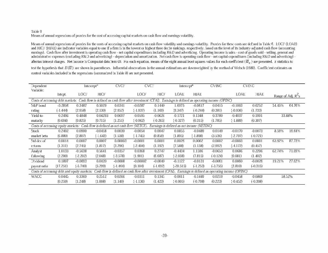
Table 9 Means of annual regressions of proxies fur the cu~t of accessing capital markets on cash flow and earnings volatility.
Means of annual regressions of proxies fur the costs of accessing capital markets on cash flow volatility and earnings volatility. Proxies fur these costs me defined in Table 6. LOCF (LOAE) and HICF (HlAE) are indicator variables equal to one if a finn is in the luwe~t or highest three decile rankings. respectively. based on the level of its industry-adjusted cash flow (accounting earnings). Cash flow after investment is operating cash flow - net capital expenditures including R&D and adve1tising. Operating income is sales - cost of goods sold - selling. general and administrative expenses (excluding R&D and advertising) - depreciation and ammtizatiun. Net cash flow is operating cash flow - net capital txpenditures (including R&D and advertising) -aftertax interest charges. Net income is Cumpustat data item 69. Fur each equation. means of the eight annual least squares values fur each coefficient ( a ,t ) are presented. z-statistics to
test the hypothesis that E (a) are shown in parentheses. Influential observations in the annual estimations are duwnweighted by the method of Welsch (1980). Coefficient estimates on
control variables included in the regressions (surnrnarized in Table 8) are nut presented.
Dependent Variable:
Intercept* CVCF CVCF Intercept* CVINC CVINC
Intcpt. LOG' HICF LOCF HICF LOAE HlAE LOAE
Costs of accessing debt markets: Cash flow is defined as cash flow after investment (CFAI). Earnings is defined as operating income (OPINC)
S&P bond -0.2856 0.3482 0.5029 0.0341 -0.0287 0.1440 1.6975 -0.0617 0.0415 -0.1003 rating (-1.444) (2.958) (2.130) (2.952) (-1.937) (1.169) (9.347) (-0.244) (0.381) (-0.936)
Yield-to- 0.2496 0.4848 0.04293 0.0697 -0.0595 -0.0626 -0.1721 0.1348 0.3780 -0.4037 maturity (0.604) (0.825) (0.715) (1.25 1) (-0.962) (-0.265) (-0.327) (0.315) (1.785) (-1.889)
Costs of accessing equity markets: Cash flow is defined as net cash flow (NETCF). Earnings is defined as net income (NETINC)
Stuck 0.2402 0.0900 -0.04 18 0.0030 -0.0054 0.0047 0.0855 -0.0489 0.0149 market beta (6.880) (2.807) (-1.643) (1.538) (-1.745) (0.859) (1.895) (-1.898) (3 .536)
0.0014 0.0007 0.0007 o oooo:~ -o.oom o ooo1 o.0026 0.0002 0.0002 (1.311) (2.745) (1.817) r:~.296l r-2404l r1192l (7.588) (1.138) (2.992) (3.296) (-2.404) (1.192)
1.0133 -0.5638 0.564 1 y~t 1.0133 -0.5638 0 564 1 -0.0357 0.0368 0 27 47 -0.4434 11596 -0.0653 (.2.200) (-2.202) (2.048) g (2.200) (-2.202) (2.048) (-3.578) (1.901) (6.687) (-2.038) (7.815) (-0.1 24)
-0.0170 (-2.797)
-0.0003 (-4.172)
0.0686 (0.081)
Dividend 0.1807 -0.0693 0.0420 -0.0008 -0.00002 -0.0040 -0.1122 -0.0131 -0.0061 0.0060 payout ratio (17.251) (-5.740) (5.299) (-1.464) (0.104) (-1.692) (-20.515) (-1.253) (-3.755) (3.810)
Costs of accessing debt and equity markets: Cash flow is defined as cash flow after investment (CFAI). Earnings is defined as operating income (OPINC)
WACC 0.0445 0.3360 0.2512 0.0266 -0.0311 0.1345 -0.0011 -0.1449 0.0219 -0.0458 (0.259) (1.248) (1.008) (1.140) (- 1.1 36) (1.423) (-0.005) (-0. 798) (0.223) (-0.452)
-39-
HlAE
0.6252 (1.733)
0.1901 (0.307)
-0.0073 (-0.721)
0.0001 (0.457)
0.2206 (1.402)
-0.0026 (-0.315)
-0.0869 (-0.308)
Range of Adi. R2s
54.45% 64.76%
33.88%
8.59% 19.64%
63.92% 87.73%
62.74% 71.09%
19 .21% 27.02%
58.52%