temperature profiles and hardness estimation of laser welded
TRANSCRIPT

Temperature profiles and hardness estimation of laser welded heat affected zone in low carbon steel Axel Lundberg One year Master's Degree Computational Materials Science June 2014

MT624A Temperature profiles and hardness of laser weld HAZ Axel Lundberg
ii
Avdelningen för Materialvetenskap och Tillämpad Matematik
Malmö Högskola
205 06 MALMÖ
Division of Material Science and Applied Mathematics
Faculty of Technology and science
Malmö University
S-205 06 MALMÖ
Sweden
Temperature profiles and hardness
estimation of laser welded heat affected
zone in low carbon steel
Axel Lundberg
Examiner: Christina Bjerkén
Supervisor: John C. Ion
One year Master's Degree
Computational Materials Science June 2014

MT624A Temperature profiles and hardness of laser weld HAZ Axel Lundberg
i
Abstract Thermal modelling of hardness in the heat-affected zone (HAZ) in a laser welded steel plate
is a cumbersome process both in calculation and simulation. The analysis is however
important as the microstructural phase transformations induced by welding may cause
unwanted hardness levels in the HAZ compared with that of the parent material. In this
thesis analytical equations have been implemented and checked for validity against
simulations made by other authors and against experimental values.
With such a large field as thermal modelling, the thesis had to be narrowed down to
make the analysis more subject focused. Limitations made were for mathematical modelling
only looking at a two-dimensional heat flow in welded plates; in this thesis only the
analytical solution to the heat flow is considered. The work was also directed towards steel;
such a material as used largely all over the globe. As laser welding is a fast and cost-
effective process, an analysis of hardness is of great importance.
Work was divided into three overlapping parts; the first was to derive and understand the
work done in the field of thermal modelling of welds, thus understanding the mathematics
behind the basic problem. This modelling provides a number of curves and parameters from
a thermal cycle, thus enabling one to do the hardness analysis correctly.
Secondly, this mathematical modelling was applied to a number of cases, simulating
different circumstances. This was done using self-programmed Graphical User Interfaces
(GUI) for convenience. This enables engineers to easily plug in the materials and processing
properties and thus simulate the required parameters and curves for further analysis.
Lastly, a GUI for simulating the hardness of any point in the HAZ was programmed and
used, thus implementing and validating the equations. A theoretical introduction of the
phases induced in the HAZ is also included, in order of understanding the problems of
unwanted hardness in the HAZ of laser-welded steel.
Main conclusions of this thesis:
Mathematical modelling of heat transfer in welds by Rosenthal (1946) is still
applicable for modern laser welding apparatus.
The empirical model presented by Ion et al. (1984) is not applicable with
experimental results of hardness in the HAZ of the steels investigated here.
Equations by Ion (2005) are accurate for simulating the hardness.
The analytical solutions investigated are superior to numerical solutions with regard
to quick, simple simulations of thermal cycles and hardness. Numerical solutions
allows for more advanced modelling, which can be lengthy.
Preheating the steel prior to welding is favourable in reducing hardness levels,
especially with steel of higher carbon equivalent.
Keywords: Laser welding, HAZ, heat-affected zone, hardness, heat equation, thermal
modelling, thermal cycle, Rosenthal

MT624A Temperature profiles and hardness of laser weld HAZ Axel Lundberg
ii

MT624A Temperature profiles and hardness of laser weld HAZ Axel Lundberg
iii
Sammanfattning Termisk modellring av hårdhet genom beräkning och simulering av den värmepåverkade
zonen i en lasersvetsad stålplatta är en omfattande process. Dock är analysen viktig då
mikrostrukturella fastransformationer förorsakade av svetsningen kan ge oönskade
hårdhetsnivåer av den värmepåverkade zonen jämfört med hårdeheten i basmaterialet. I
denna avhandling har analytiska ekvationer implementerats och testats för validitet mot
simuleringar gjorda av andra författare och mot experimentella värden.
Eftersom termisk modellering av svetsar är ett omfattande område var avhandlingen
tvungen att smalnas av för att göra analysen mer fokuserad. Begränsningar gjordes för den
matematiska modelleringen genom att endast titta på två-dimensionellt värmeflöde i
svetsade plattor där endast den analytiska lösningen är av intresse. Arbetet har också
inriktats mot stål då detta material är vida använt över hela världen. Då lasersvetsning är en
snabb och kostnadseffektiv process så är hårdhetsanalysen av största vikt.
Avhandlingen är uppdelad i tre övergripande delar; den första är att ta fram och förstå
arbetet som gjorts inom termisk modellering av svetsar, alltså förstå matematiken bakom
problemet. Modelleringen är till för att producera diagram parametrar från en termisk cykel,
för att kunna fortgå med korrekt hårdhets analys.
För det andra så sätts den matematiska modelleringen på prov i ett antal situationer som
var och en simulerar olika förutsättningar. Detta gjordes i ett grafiskt användargränssnitt av
ren bekvämlighet. Detta gör att ingenjörer lätt kan implementera olika egenskaper för
materialet och få fram diagram och kurvor.
Sist, ett liknande grafisk användargränssnitt för att simulera hårdheten i valfri punkt i
den värmepåverkade zonen programmerades och därigenom implementerades ekvationerna
som denna avhandling handlar om i grund och botten. En teoretisk bakgrund till
fasomvandlingen är också inkluderad som förklaring till grundproblemet med oönskad
hårdhet i den värmepåverkade zonen i lasersvetsat stål.
Huvudslutsatser i avhandlingen:
Matematisk modellering av värmeöverföring i svetsar genomförd av Rosenthal är
fortfarande applicerbar på modern lasersvetsningsapparatur.
Den empiriska modellen från Ion et al. (1984) är ej applicerbar med godkänt resultat
för hårdhetsuppskattning.
Ekvationerna från Ion (2005) är statistiskt godkända för att simulera hårdhet.
Den analytiska lösningen är överlägsen den numeriska när det gäller snabb och enkel
implementering för att simulera termiska cykler och hårdhet, medan den numeriska
lösningen kan ta i beaktning mera avancerade egenskaper.
Förvärming av stålet innan svetsning kan vara mycket fördelaktigt för hårdheten i
den värme-påverkade zonen, speciellt vid högre kolekvivalent.
Nyckelord: laser-svetsning, värme påverkad zon, hårdhet, värmeledningsekvationen, termisk
modellering, termisk cykel, Rosenthal

MT624A Temperature profiles and hardness of laser weld HAZ Axel Lundberg
iv

MT624A Temperature profiles and hardness of laser weld HAZ Axel Lundberg
v
.
Preface This master´s thesis was written as the last step toward a one-year master´s degree in
Computational Materials Science at Malmö University. Work was initiated in February 2014
under the supervision of John C. Ion of Malmö University and was finished in June the same
year. The total extent of this dissertation is 15 credits.
The motivation for this thesis and the introduction to the field was made by the supervisor.
Thanks to my supervisor for his interest in advising me and thus making this possible. He
created the foundation on which to build further. Many hours have been spent behind the
MacBook, on which this has been written, with programming, reading and writing. I hope
that it one day will be worth the effort. A really special thanks to my family and especially
my better half, Guðný, who put up with me during this time of life…
Kristianstad
June 2014
Axel Lundberg

MT624A Temperature profiles and hardness of laser weld HAZ Axel Lundberg
vi

MT624A Temperature profiles and hardness of laser weld HAZ Axel Lundberg
vii
Nomenclature Symbol Definition Unit
Absorptivity ---
Transformation temperature K
Carbon equivalent wt%
Hb Vickers hardness number of bainite HV
Hfp Vickers hardness number of ferrite-pearlite mixture HV
Hm Vickers hardness number of martensite HV
Hmax Vickers hardness number of HAZ HV
K0 Bessel function ---
Nhet Heterogeneous nucleation rate ---
T Temperature K
T0 Initial temperature K
Tm Melting temperature K
Tp Peak temperature K
TMs Temperature at which martensite starts to form K
TM50 Temperature at which martensite formation is 50% complete K
TMf Temperature at which martensite formation is complete K
V’ Cooling rate at 923 K K h-1
Vb Volume fraction of bainite ---
Vfp Volume fraction of ferrite-pearlite mixture ---
Vm Volume fraction of martensite ---
a Thermal diffusivity m2 s
-1
c Specific heat capacity J kg-1
K-1
d Thickness m
e Base of natural logarithms, 2.718 ---
f Matrix volume fraction available ---
k Boltzmann’s constant, 1.381 J K-1
q Beam power J s-1
(W)
r Lateral distance from centre of a through-thickness heat source M
t Time s
x,y,z,ξ Spatial coordinates ---
w Width M
Laplace operator ---
Differential operator ---
λ Thermal conductivity J s-1
m-1
K-1
ρ Density kg m-3
ΔGm Activation energy for atomic migration per atom J mol-1
ΔG* Activation energy barrier for nucleation of the critical nucleus radius J mol-1
Δt8-5 Time to cool from 800 to 500°C s
Cooling time for 50 % martensite formation s
Cooling time for 50 % bainite formation s
Cooling time for 0 % ferrite-pearlite mixture s
Cooling time for 0 % bainite formation s

MT624A Temperature profiles and hardness of laser weld HAZ Axel Lundberg
viii
MT624A Temperature profiles and hardness of laser weld HAZ Axel Lundberg
ix
Contens
1 Introduction ...................................................................................................................... 1
1.1 Background ............................................................................................................................. 1
1.2 Purpose .................................................................................................................................... 2
1.3 Objectives ................................................................................................................................ 2
1.4 Limitations............................................................................................................................... 2
1.5 Method..................................................................................................................................... 3
2 Laser welding and related welding processes ................................................................ 5
2.1 Regions of the weld-zone ........................................................................................................ 5
2.2 Why study the HAZ-microstructure? ...................................................................................... 6
3 Mathematical modelling .................................................................................................. 7
3.1 The equations of heat flow in the HAZ ................................................................................... 7
3.2 Temperature-time profile in the HAZ ................................................................................... 10
3.2.1 Time constants derived from temperature-time profile.................................................. 12
3.3 Peak temperature-distance relationship ................................................................................. 13
3.4 Input energy – HAZ width relationship ................................................................................. 14
3.5 Verification Rosenthal thermal modelling ............................................................................ 16
3.5.1 Rosenthal modelling for different materials ...................................................................... 18
4 Evolution of microstructure in the HAZ ..................................................................... 19
4.1 Eutectoid transformation – pearlite, bainite or martensite formation .................................... 19
4.1.1 Pearlite formation ........................................................................................................... 20
4.1.2 Bainite formation ........................................................................................................... 21
4.1.3 Martensite formation ...................................................................................................... 22
4.2 Transformation rates to TTT-diagrams – theoretical approach ............................................. 23
5 Hardness in HAZ ........................................................................................................... 29
5.1 Analytical equations of phase volume fraction in low carbon steels ..................................... 29
5.2 Hardness calculations by rule of mixtures ............................................................................. 31

MT624A Temperature profiles and hardness of laser weld HAZ Axel Lundberg
x
6 Results and discussion – thermal modelling ................................................................ 33
6.1 Thermal modelling simulations ............................................................................................. 33
6.1.1 MATLAB® implemented GUI for thermal simulation ................................................. 33
6.1.2 Graphical simulations of thermal modelling .................................................................. 34
6.2 Discussion of thermal modelling ........................................................................................... 45
7 Results and discussion – empirical hardness estimation ............................................ 49
7.1 Empirical hardness estimation using calculated volume fractions ........................................ 49
7.1.1 MATLAB® implemented GUI for hardness simulation ............................................... 49
7.1.2 Graphical results of hardness simulations ...................................................................... 50
7.2 Discussion of empirical hardness simulation ........................................................................ 63
8 Results and discussion – graphical hardness estimation ............................................ 65
9 Conclusion ...................................................................................................................... 67
9.1 Conclusions ........................................................................................................................... 67
9.2 Future work – Possible improvements .................................................................................. 69
10 References ..................................................................................................................... 71
Appendix A: MATLAB® GUI-code for temperature profiles ......................................... 73
Appendix B: MATLAB® GUI-code for hardness estimation .......................................... 79
Appendix C: Table for hardness simulation comparison ................................................. 83

MT624A Temperature profiles and hardness of laser weld HAZ Axel Lundberg
1
1 Introduction
1.1 Background
Two or more pieces of metal can be joined together, using some type of welding apparatus.
This welding apparatus might contain a high powered laser beam, thus being a laser welding
apparatus. When this weld is made, the weld fuses the two pieces together by heating the
base-material to melt. When this happens, both a weld bead (the area of fused and molten
base material) and the heat affected zone (HAZ) are formed. The HAZ is formed when the
heat radiates from the bead via conduction in the base-material, thus the heat will transform
the material in this zone and in the welding situation induce phase transformations. When
phase transformations occur, the mechanical properties of the HAZ will differ slightly from
those of the base material, if the welded piece is of steel or other weldable metals.
This problem has long been studied, in which the foundation is one of many differential
equations derived for certain problems. This heat transfer problem, as welding is, looks into
the solutions for the heat equation as the basis for further mathematical modelling. When this
differential equation is solved for the selected problem, specifically for the analytical
solutions, as this work describes, one can produce temperature profiles for specified energy
input and desired mechanical properties of base material.
By then looking at what is produced by this analytical solution and its temperature
profiles, the phases of the HAZ may be studied. By producing a time-temperature-
transformation (TTT) diagram, the phase volume fractions in the HAZ are derived and
compared with selected calculations. These volume fractions then help determine the
hardness.
Phase transformations are important to study because when they occur, the base material
will possess different properties to the HAZ. In industry there is a certain measure of
hardness that is considered to be maximum allowed, a value that if exceeded might lead to
cracks or failure of any construction. It is therefore of great importance to study the weld
HAZ in order to fabricate constructions that will withstand the forces put on them at all
times. Cyclic loads are one of the greatest threats to a brittle weld, as these tests its strength
over a timespan and a large number of load cycles until fatigue of the weld cause it to break.
This project is aimed at determining whether or not one can use models derived in 1984
and 1996 (Ion 2005, p.532-535) and if they are applicable on modern low carbon steels. If
not, further studies are required.

MT624A Temperature profiles and hardness of laser weld HAZ Axel Lundberg
2
1.2 Purpose
Investigating the phases within the weld HAZ is very important in assessing the mechanical
properties of a selected weld. By knowing these properties, constructions can be made more
durable. Verifying if one may or may not use the equations described by Ion et al. (1984) or
the equations in Ion (2005, p.534) is the main purpose. The aim is to be able to establish if
new equations are needed in order to initiate further work in this field. Other objectives are
to find if the thermal modelling by Rosenthal (1946) may be used as validation for hardness
simulations and laser welding applications.
1.3 Objectives
The main objective of this thesis is to evaluate the hardness of a weld HAZ, using
experimental data and analytical modelling. The first step is to analyse the mathematics
behind the heat-problem using thermal modelling, further on into the solutions to produce
temperature profiles. Then different diagrams will be produced for certain steel compositions
that will be used when investigating hardness. Values will then be compared to experimental
values obtained for modern steels, thus confirming or falsifying the old equations and
methods.
1.4 Limitations
The mathematical modelling will only be valid for 2-dimensional heat flow for the analytical
solution of laser welded low carbon steel plates. This means that the laser beam will
penetrate the entire plate of base-material. This is done in order to narrow the amount of
analytical equations stated in the modelling part, but also because 3-dimensional heat flow,
as found in partial penetration welds, is a much more computer demanding operation.
Limitation to the carbon equivalent of the parent material will be made so that all the low-
carbon steels analysed are eutectoid or hypo-eutectoid, thus the carbon equivalent will be at
maximum CEq = 0.78 wt %. The analysis is only about the HAZ, so what happens in the weld
bead or otherwise in the base-material is neglected.

MT624A Temperature profiles and hardness of laser weld HAZ Axel Lundberg
3
1.5 Method
A literature study aims to establish the state of the art of the modelling methods. These
topics will be mathematical modelling of heat transfer problems, the solutions to this
differential equation, TTT-diagrams, phase transformations in steels and model based
hardenability. Other subjects that will be addressed are how this mathematical modelling
generates the temperature profiles needed for further analysis, but also some experimental
literature values. Thus no physical experiment will be performed, but the values obtained
from an experiment performed in literature will be used as validation further on in the thesis.
The first analysis, described in Ch. 3 below, is how the mathematics are formed from the
initial differential equation to the final, specified, analytical solutions to the limitations of the
problem. This deduces the thermal/mathematical modelling part of this thesis.
The second analysis, described in Ch. 4, will consist of how the phases are formed in the
HAZ and how to construct the necessary diagrams in order for interpretation of the results
from temperature profiles. These profiles are brought forth in the first analysis and then used
for understanding in the phase transformation process of the base material in the HAZ.
The last analysis, described in Ch. 5 is how the hardness is calculated. This chapter will
also contain the part where the theories behind interpreting the hardness diagrams and in
what region of the diagram one want to recognize.
This will be rounded off by a results part where results are divided into the same
disposition as the theoretical analysis. This ends with a discussion and interpretation of the
results, were the main objective be considered and further work proposed.
To handle the data in a correct and smooth way and produce plots, MATLAB® will be
used. Inside MATLAB®
, small graphical user interfaces (GUI:s) will be constructed. This
will assist the author and others to follow, to interpret data and plot the necessary curves and
calculate data easily. The algorithm of these GUI:s will be presented inside the thesis,
although the computer code for them may be found in App. A and App. B.

MT624A Temperature profiles and hardness of laser weld HAZ Axel Lundberg
4

MT624A Temperature profiles and hardness of laser weld HAZ Axel Lundberg
5
2 Laser welding and related welding processes
The basic physics behind the laser and how it can be used in the materials processing area
will not be dealt with in this thesis. Although if interested is awaken, many books like Ion
(2005) have been written on the subject of laser apparatus and involved processes.
During the process, when the high-powered laser beam is impinged upon the surface of
the adjacent base material, the beam has to be of sufficient power and focused, all in order to
initiate vaporization. When this is achieved the material will start to melt and then fuse (Ion
2005, p.396-397). When the beam of the welding apparatus is travelling transversely to the
work piece, a narrow channel will be formed, called the keyhole. This keyhole is what
eventually forms the weld bead. This keyhole effect is what makes the laser welding process
so efficient according to Fabbro et al. (2000), thus modelling of this process is of highest
interest. The efficiency can be traced to that there is a narrow bead in the centre, adjacent to
a relatively small HAZ and also that there is a high aspect ratio of the welded zone
(depth/width) (Ion 2005, p. 435).
This laser process is also of great improvement over traditional arc welding due to that it
has a lower energy input per unit length that produces this relatively narrow HAZ. This
means that thermal distortion of the work piece is not that significant. This is of course more
applicable the thinner the plate, which has a higher degree of warping during greater amount
of energy input (Sokolov et al. 2011).
2.1 Regions of the weld-zone
What is important is to distinguish between the two zones of the weld, seen clearly in
Fig. 2.1, where the present work is concentrated upon the HAZ. This is due to that the bead
material will somewhat resemble the base-material. The grains grow in a columnar
morphological way, something that is also observed of rapidly cooling base-materials.
Therefore the physical properties and microstructure of the weld bead can be stated as less of
interest in the hardness investigation due to the resembling to the base material (Yilbas et al.
2010 and Ion 1984, p.48-49)

MT624A Temperature profiles and hardness of laser weld HAZ Axel Lundberg
6
Figure 2.1: Welding zones: WM-weld metal and BM-Base material, for 3-dimensional heat flow
(Adapted from Poorhaydari et al. 2005).
2.2 Why study the HAZ-microstructure?
In the HAZ, the rapid thermal cycles will not result in the same microstructural grain
growth as in the bead, but instead phase transformations of the low carbon steel that occur in
the HAZ of the weld are induced by the high cooling rates of the weld passing. These phase
transformations in the HAZ of the welded steel may induce a hardness that is higher than
preferred, thus making the weld more brittle and less ductile compared to the parent
material. Very fast cooling rates may also induce martensite formation in the HAZ, which
also induces unwanted embrittlement (Yilbas et al. 2010) and (Ion et al. 1984). One good
way of reducing the unwanted hardness levels in the HAZ of the weld is to raise the preheat
temperature. The problem will then be a much more complicated work process, whilst only
gaining approximately 20 % difference in the HAZ microstructure compared to an unheated
work piece (Sokolov et al. 2011). This thesis starts with the mathematical modelling and
continues looking at the formation of various microstructural changes in hypo-eutectoid and
eutectic low carbon steels to begin with. In the hypo-eutectoid region most of the induced
transformations are results of changing from austenite ( ) into mainly martensite, pearlite-
ferrite mixture and bainite. These phases and constituents are in turn built up different but
they all contain the chemical compound cementite (Fe3C) in various amounts, see Ch. 4.
MT624A Temperature profiles and hardness of laser weld HAZ Axel Lundberg
7
3 Mathematical modelling
As stated before, the welding process induces melting and vaporization by a high-powered
laser beam in a base-material. How is heat flow caused by a moving line heat source
modelled? This heat flow development can be described mathematically using appropriate
heat transfer equations. Note that experimental procedures are necessary in order to verify
the equations (Poorhaydari et al. 2005). One example is that bringing forth a model
predicting the fusion depth of the weld within 0.01 mm would be unreasonable as the
limitation in fabrication welding would be approximately 0.15 mm even during the best of
conditions (Ion 1984, p.32).
3.1 The equations of heat flow in the HAZ
Heat flow in welding, whether it is arc or laser welding, is a very complex mathematically
descriptive situation. This process can be divided into three different situations: Transient-,
quasi- and steady state (Bass 1983, p.183).
Quasi-steady state heat flow is presenting a situation in which the observed temperature
field from a chosen moving heat source is constant. In order to find the analytical solutions
to this complex welding heat flow problem, solution to the partial differential equation of
energy conservation seen as Eq. (3.1) is needed (Darmadi et al. 2011).
(3.1)
Where is the thermal diffusivity in either spatial coordinate. If the material that is of
interest is an isotropic homogenous material, the thermal diffusivity a will be constant in all
space-coordinates (x,y,z). If then the Gaussian-distributed temperature field varies in both
space and time, the differential equation becomes Eq. (3.2) (Nunes 1983):
(3.2)
If the heat is supplied to the weld with a constant speed v, moving along the x-axis like in
Fig. 3.1, Eq. (3.2) may be rewritten with the point heat source as the origin of the problem.
By defining a variable , where is the specific length from the origin to the
specified point along the x-axis and then differentiating Eq. (3.2) with respect to the new
variable, Eq. (3.3) is developed (Goldak et al.1986).
(3.3)

MT624A Temperature profiles and hardness of laser weld HAZ Axel Lundberg
8
Figure 3.1: Co-ordinate system and geometry of plate welding (Ion et al. 1984).
Now in order to show that Eq. (3.3) can be reduced to Eq. (3.4), one needs to show that the
solid is of infinite length, compared with the extent of the point heat source and the heat
sources extent (Ion et al. 1984). Then the temperature distribution around this particular
source will be constant. This state is then referred to as a quasi-stationary state, which
mathematically can be related to that (Pavel 2008).
(3.4)
Fig. 3.2 shows the quasi-stationary state, where the temperature will be at its peak just below
the heat source moving along x-axis at the velocity v. The temperature then decreases over
time and distance, which is shown by the isotherms.
Figure 3.2: 3-dimensional keyhole temperature distribution around a moving heat source
(Ion 1984, p.35).

MT624A Temperature profiles and hardness of laser weld HAZ Axel Lundberg
9
The next step in the process to find an analytical solution of the heat flow differential
equation are some basic assumptions made by Rosenthal (1946), who is often referred to
first in work about heat flow in welds in general (Kamala et al. 1993). The assumptions are
according to Ion (1984, p.33):
i. Heat is provided by a point heat source.
ii. Both latent heat of phase transformations and the fusion of the weld bead are
neglected, i.e. no energy is generated by material transformation.
iii. Thermal properties of the welded material are not dependent on temperature; this is
of course not true, but assumption made in original solution.
iv. Heat flow occurs only by conduction in the work piece; no heat losses through
surface.
v. Speed v will be constant; reasonable for automated welding processes.
Rosenthal (1946) presented the analytical solution to Eq. (3.4), by the use of complex
mathematical modelling and his assumptions. The work can be summarized in two main
equations (Eq. 3.5 and 3.6 resp.), the first describing 3-dimensional heat-flow, this from a
surface heat source, where heat is conducted radially through the material. The other
describes the 2-dimensional situation, where heat is only conducted laterally in the material.
Fig. 3.3 schematically show both these conditions. The heat flow will of course, despite
assumptions made by Rosenthal (1946), dissipate through the surfaces of the work piece,
although not shown in Fig. 3.3.
Figure 3.3: Heat-flow (orange) in thin-plate respectively thick-plate, i.e. 2D respectively 3D.

MT624A Temperature profiles and hardness of laser weld HAZ Axel Lundberg
10
( )
(
) {(
) } (3.5)
( )
(
) (
) (3.6)
For this step one need to notice that firstly the preheat/initial temperature T0 is added as the
initial temperature of the plates being welded and q is the power of the weld apparatus
(Darmadi et al. 2011). Secondly, K0 represents the Bessel-function of second kind and zero
order and while (Bass 1983, p.182). According to
Poorhaydari et al. (2005) simplifications of Eq. (3.5) and (3.6) were made by Easterling and
Ashby in order to produce thermal cycles for the HAZ, see Eq. (3.7) and (3.8).
( )
(
( )
) (3.7)
( )
( ) (
( )
) (3.8)
Further on in the project the focus will be on the 2-dimensional solution. There the
z-coordinate is ignored, and the thickness d of the plate is used directly as the solution
heavily depends on this parameter (Bass 1983, p.182).
3.2 Temperature-time profile in the HAZ
For the first task, the goal is to produce a temperature versus time plot. The problem faced
here is that the assumption made earlier in order to solve Eq. (3.4) was for a quasi-stationary
state, thus meaning the assumptions cannot be applied when seeking the temperature
distribution in a fixed point (Darmadi et al. 2011).
As this project is only looking at 2-dimensional cases, the heat only disperses laterally.
If one considers the point in the plane, x = 0, this gives: and ( ) .
Now r is defined as the lateral displacement in the plane, i.e. the distance from the point of
interest to the weld centre line. Then and ( ) , thus reaching Eq. (3.9).
( )
(
) (3.9)

MT624A Temperature profiles and hardness of laser weld HAZ Axel Lundberg
11
In order to reach the goal, thus producing a plot, which is principally shown in Fig. 3.4, the
exponential part of Eq. (3.8) must be considered mathematically. This was done by Ion
(1984, p.37) in order to obtain Eq. 3.9. Another addition is that if one considers a thin plate
solution, i.e. a 2-dimensional heat-flow, some of the input form the laser will escape through
the plate. Ion et al. (1996) defines the factor ( ), which is the absorptivity of the
welded plate of the beam in laser welding.
( )
(
) (3.10)
The factor Aq/(vd) (called absorbed energy per area unit) is broken out, as these parameters
are what may be controlled by the welding machine chosen, as well as producing the plots
with width versus Aq/(vd) (Darmadi et al. 2011).
Figure 3.4: Schematic plot of temperature versus time (Ion et al. 1984).
If the cooling curve is divided as in Fig. (3.4), it is easy to understand how Eq. (3.10)
actually works. The exponential part will control the rapid heating and when the time tends
towards infinity; this part tends to 1. The inverse part of Eq. (3.10) controls the cooling
phase of the curve (Ion 1984, p.38).
Equation (3.10) is highly sensitive to the radius r of the weld, because the radius is
sensitive to unpredictable variations. This knowledge is crucial if Eq. (3.10) should be used
practically (Poorhaydari et al. 2005). Profiles produced by Eq. (3.10) may be validated by
being plotted against a profile that has been arisen experimentally, work that has been done
by both Ion et al. (1984) and by Poorhaydari et al. (2005). Though their experimental
procedures differ somewhat, thin steel plates in which holes were drilled into the HAZ where
used in both experiments. Small thermocouples where placed in the holes, where the
temperature was then measured in order to plot the experimental curve that can be compared
with curves produced by the analytical solution, Eq. (3.10).

MT624A Temperature profiles and hardness of laser weld HAZ Axel Lundberg
12
3.2.1 Time constants derived from temperature-time profile
From the profile as in Fig. 3.4, where temperature is calculated from each separate time step,
two important time constants need to be described. These two quantities can be seen in Fig.
3.5. Firstly the constant is described as the time to reach peak temperature. The constant
is evaluated by differentiating Eq. 3.10 with respect to time and setting the resulting
differential to zero, thus obtaining Eq. (3.11) (Poorhaydari et al. 2005). Below, e is base of
the natural logarithm.
(
)
(3.11)
Secondly the cooling time; is stated. This refers to the severity of the quench through
phase transformations, i.e. the time taken to cool from 800 to 500 . The cooling time is
stated as the inverse part of Eq. (3.11), multiplied by a weight factor for the temperatures
that one seeks (Ion et al. 1984). It is important to note that, according to Ion et al. (1984), if
the peak temperature is below 900 , Eq. (3.12) may not be used.
(
)
(3.12)
where:
(
( )
( ) ) (3.13)
Figure 3.5: Typical temperature-time profile with time constants showed (Ion et al. 1984).
Eq. (3.11) and (3.12) are found to be reasonably suited for the estimation of the constants
cooling temperature and peak temperature, but according to Ion (1984, p.42) some
calibrations must be made to the welding equipment in order to get accurate answers. They
are though good for estimating the variations of and about a known value with a

MT624A Temperature profiles and hardness of laser weld HAZ Axel Lundberg
13
change in welding conditions. Another thing to note is that the cooling time is totally
independent of the distance from the point heat source, at least when one looks at the HAZ.
This has been proven both numerically and experimentally, which supports the analytical
solution (Poorhaydari et al. 2005).
In Ch. 5 the deduction of why the cooling time, , is so important, is stated. This is
the real connection between the thermal modelling and the actual hardness simulations. The
fact that the volume fractions of phases are heavily dependent on the cooling rate is
mentioned in the early work done by Ion et al. (1984). This situation, that if the energy put
into the weld increases the cooling time, was experimentally confirmed by Poorhaydari et al.
(2005). In their work, they published Fig. 3.6. The shifting to the right in the figure shows
that the cooling time drastically increases as input energy increases. The slight difference
between the peaks of the thermal cycles (Input energy 1-3) in Fig. 3.6 is due to that the
thermocouples that measure temperature were placed at slight different places in order to
reach the same peak temperature, Tp (Poorhaydari et al. 2005).
Figure 3.6: Measured temperature profiles showing drastic increase in cooling time of weld HAZ
(Adapted from Poorhaydari et al. 2005).
3.3 Peak temperature-distance relationship
The meaning of the parameter Tp can be found in Fig. 3.5. This is the variation of peak
temperature with respect to distance from heat source. Eq. (3.14) is obtained using that the
condition at the peak is , thus differentiating Eq. (3.10) with respect to time.
(
)
(
) (3.14)
Both Poorhaydari et al. (2005) and Ion et al. (1984) pointed out that using Eq. (3.14) directly
versus radius from heat source would only show the variation of the peak temperature over
the HAZ. This is because this radius r will include some part of the molten weld pool, thus
not following the Rosenthal (1946) assumptions of a single-phase material.

MT624A Temperature profiles and hardness of laser weld HAZ Axel Lundberg
14
3.4 Input energy – HAZ width relationship
The last goal of the thermal modelling in this project will be to look into the relation between
the input energy and width of the HAZ. This is interesting when studying the HAZ
geometry. This geometry will be examined later, thus finding the hardness and the
composition of the HAZ. The hardness will be plotted against the input energy, in order to
evaluate the hardness of the weld in a proper manner, by looking at the phase
transformations inside the HAZ (Ion et al. 1984).
The width of the HAZ can be calculated in two major ways, firstly Ion (2005, p.436)
states that: if the input energy to the HAZ is q’, then , where is the radius
of the molten weld pool. By substitution of this into Eq. (3.12) the same author states that:
(
)
[
( )
( )] (3.15)
Where Tm is the melting temperature and AC1 is the transformation temperature at the end of
the HAZ. When using Eq. (3.15), it must be noticed that some part of the actual weld bead
will be taken into the calculation. It is one of the assumptions that the thermal properties of
the material do not change during welding. This makes for a slight overestimation of the
HAZ-width, so the calculated value will be slightly greater than the experimental value (Ion
1984, p.39).
Tekriwal et al. (1988) also support this theory, which show that the HAZ will increase
somewhat by the transient heat from the weld, which makes the quasi-steady state somewhat
questionable. The second theory is stated by Poorhaydari et al. (2005), who state that the
width of the HAZ is found when calculating the radius-Tm and the radius-AC1 from Eq. (3.12),
then combining them:
(
)
[( )
( )( )] (3.16)
Which is the same as Eq. (3.15), which is used to be consistent with the rest of the project.
As comparison for results, Eq. (3.16) is important but not dealt with further. Eq. (3.17) and
(3.18) resp. may be used to calculate transition-temperatures as a function of composition
(Kamala et al. 1993):
(3.17)
(3.18)

MT624A Temperature profiles and hardness of laser weld HAZ Axel Lundberg
15
Fig. 3.7 is taken from the study made by Poorhaydari et al. (2005). It shows both the 2 and
3-dimensional HAZ-widths, compared with actual experimental values evaluated by the
same. Important to note is that they plot the width against the heat input, not the energy
input, but the schematics of the plot remain the same with both. Fig. 3.7 provides a good
visual impression that the analytical solution gives computed values within the range of the
experimental values. This simulation has been performed numerically by Piekarska et al.
(2012) who deduced roughly the same conclusion. Their research on how the laser properties
affect the weld was conclusive about the thermal modelling in the sense that simulated
numerical values had the best fit, between the two analytical solutions.
Figure 3.7: HAZ-widths from three different solutions (Adapted from Poorhaydari et al. 2005)

MT624A Temperature profiles and hardness of laser weld HAZ Axel Lundberg
16
3.5 Verification Rosenthal thermal modelling
Before going through what is produced by the GUI developed using the mathematical theory
about thermal modelling, remarks will be made about the validity of the modelling, therefore
discussing the validity of the graphs produced. Fig. 3.8 shows two curves derived by
experiments made with real welding apparatus versus the curves derived with thermal
modelling according to the functions and solutions, Eq. (3.10) and (3.12) compiled by
Rosenthal (1946).
Figure 3.8: Experimental versus thermal modelling values of temperature profiles (Ion et al. 1984).
The preface towards Fig. 3.8 was underlying experiments using a weld simulator; the whole
line represent the experimental curve, thus the thermal modelling is shown as the broken
line. Minor holes were drilled into the underside of a plate, in order to penetrate the HAZ,
thus gaining sufficient data to plot the profiles. Thermocouples were spot-welded inside the
holes, thus measuring the cooling time of the welding cycle (Ion 1984, p.20).
The validity of Rosenthal’s thermal modelling of a heat point source is sufficient enough, the
differences between the two curves are minor and more importantly, the reasons are known.
In section 3.1 the general solution to the Rosenthal equation was presented, and with it the
assumptions to get the solution (Ion 1984, p.33). As suggested by Ion (1984), these
assumptions play a crucial role in the error estimation, especially when stating that the
thermal properties of a material are constant.

MT624A Temperature profiles and hardness of laser weld HAZ Axel Lundberg
17
This phenomena has been questioned by several authors, e.g. Goldak et al. (1986), who
incorporates not only one, but two of the original assumptions into their numerical model.
According to them, the original analysis made by Rosenthal (1946) cannot be extended to
incorporate the thermal properties due to their non-linear nature. To clarify what Goldak et
al. (1986) means by error estimation, Fig. 3.9 was derived to prove that there is a difference.
They state that the effect is so profound on the analytical solution that the numerical slution
is significantly better, especially for the 3-dimensional heat-flow case. The work-cost of
actually incorporating these non-linear thermal properties into the numerical analysis is
trivial according to Pavel (2008), stating that the numerical solution is the most satisfying
with appropriate data supplied.
Figure 3.9: Effect of thermal properties on a computed weld curve in steel,
(a) being variable properties, (b) being constant (Adapted from Goldak et al.1986).
Further discussed is the incorporation of latent heat developed by the weld bead. The most
difficult things to analyse are partly solid-state transformations, e.g. the austenite-pearlite
reaction, partly the transformation surface, in which the liquid-solid boundary is formed. The
latter is very difficult to incorporate exactly in the analytical solution, due to there being a
discontinuity in the thermal gradient of the boundary, when forming the moving boundary,
traveling along the weld-axis with the weld apparatus (Goldak et al. 1986). This phenomena
is also pointed out by Ion (1984) that states the following about the analytical solution; “It
cannot, however, describe the latent heat evolved from phase transformations and weld bead
solidification, although these phenomena do not affect the kinetics of grain growth, particle
coarsening etc. significantly.” (Ion et al. 1984, p. 92)

MT624A Temperature profiles and hardness of laser weld HAZ Axel Lundberg
18
3.5.1 Rosenthal modelling for different materials
It was important to implement in the GUI easy access to a materials-library, in order to see if
the Rosenthal (1946) equations would work on other material in theory. The validity of
usage of these equations on different materials other than steel is not thoroughly developed,
but work carried out by Kou (1981) supports that the equations may be used, although Kou
(1981) prefers the usage of numerical modelling. In Fig. 3.10a the thermal cycle for a weld-
pass in 6061-aluminium is shown, thus providing the author with somewhat of verification.
The simulation cannot be reproduced, as Kou (1981) does not provide all the setup
parameters for reproduction of analytical simulation.
The difference provided for welding aluminium shows that there is not much of a
difference between numerical and analytical modelling, despite the age of the article by Kou
(1981), which supports that computer computations may have improved in later years. Fig.
3.10a also supports the singularity problem of analytical modelling, taken up in the results,
were temperature approaches infinity at small radii. Further, the weld pool calculations
made, seen in Fig. 3.10b, is not accurate, but provides sufficient correlation for interpretation
of results. Lastly, the latent heat of fusion-problem is also stated as an error-estimation, since
this is not implemented in the analytical solution to the heat-transfer solution provided by
Rosenthal (1946) (Kou 1981).
Figure 3.10a and b: Comparison of analytical versus numerical modelling for aluminium (Adapted from Kou 1981).
Kou (1981) also identifies the same observation in aluminium that Poorhaydari et al. (2005)
has pointed out in Fig. 3.6, that cooling time is highly dependent on the input/absorbed
energy, but also makes the note that aluminium specifically depends heavily on preheating.
Both the cooling time and buckling-effect in parent-material are drastically reduced when
preheating, but as a result the weld pool will extend, therefore making for more HAZ-region
and doubling solidification times of phase transformation.

MT624A Temperature profiles and hardness of laser weld HAZ Axel Lundberg
19
4 Evolution of microstructure in the HAZ
Steels of different compositions will be the focus in this thesis, thus only hypo-eutectoid and
eutectoid steels are considered. By this limitation, phases of transformations are limited to
and simulation of hardness is easier. Also that alloying components may form undesired
precipitates of mixed compositions that are hard to control in the analytical solution (Ion et
al. 1984).
Figure 4.1: Sequence of steps for a technical solution in general and thesis specific.
Fig. 4.1 shows the evolution, which is often applicable for many technical problems
including this thesis. This procedure is emphasised, as the mathematical/thermal modelling
and solution to such a problem has been shown in the previous chapter that brings on the
physical interpretation and then discussion of results that could result in technical solutions.
4.1 Eutectoid transformation – pearlite, bainite or martensite formation
In order to further explain what will happen in the microstructure of the HAZ, one needs to
consider Fig. 4.2. The eutectoid composition will form at 0.78 wt% C.
Figure 4.2: Simplified phase diagram of low carbon steels, adapted from lecture1.
1 Ion, J. (2013). Lecture 6 – Phase transformations in steels. Phase transformations, MT622A. Malmö University.

MT624A Temperature profiles and hardness of laser weld HAZ Axel Lundberg
20
What happens when the welding equipment passes a certain point in the base-material, the
HAZ microstructure will change depending on both the temperature and the cooling time,
. The hardness of any point chosen inside the HAZ can be calculated by using the rule
of mixture (Ion et al. 1984). This is done when knowing the correct volume fractions of
bainite, austenite, pearlite and martensite.
But before this happens the necessary calculations for composition of the microstructure
must be made for the chosen steel to arrive at volume fractions and knowing the hardness of
each constituent (Goldak et al. 2005, p.148). When the cooling occurs and the temperature
falls below the AC1 temperature, which is calculated by Eq. (3.18), the austenite ( ) will
become supersaturated with both the phases ferrite ( ) and cementite ( ) (see Eq. 4.1).
As a result of further cooling these two phases will make up either the microconstituent;
pearlite ( ) or the non-equilibrium phase; bainite ( ), a reaction highly
dependent on one important factor; cooling time (Porter et al. 2008, p.312).
(4.1)
4.1.1 Pearlite formation
The microconstituent pearlite is formed through diffusion of carbon in the austenite, growing
into the surroundings as a sheet-lamellae type microstructure. This is due to that the lamellae
are consisting of either cementite or ferrite that nucleates on the grain boundaries in the
austenite. According to Hawbolt et al. (1983) the mechanism of phase growth initiation is
totally random, either the ferrite or the cementite starts to grow along grain boundaries first.
The rate of transformation is deduced by the TTT-diagram, which will be constructed in
a later chapter in this report. The actual volume fraction is deduced by the rate of
undercooling, i.e. the cooling rate. Rate of formation is at its peak around 550 , around the
nose of the C-curve in the TTT-diagram that is shown in Fig. 4.3 (Porter et al. 2008, p.332).
Note that this curve is only schematic and the result will be different when different
compositions of steels and alloys are considered, which is discussed in section 4.2.
Figure 4.3: Schematic plot of a TTT-diagram for the formation from austenite (Adapted from Porter et al.2008, p.333).

MT624A Temperature profiles and hardness of laser weld HAZ Axel Lundberg
21
4.1.2 Bainite formation
The second thing that may happen, if the cooling time is relatively short, is that bainite will
nucleate. The composition of bainite is the same as pearlite, although microstructurally they
are significantly different. It may seem like the two products are the same and form the same
C-shaped curve in the TTT-diagram (See Fig. 4.3a), but this product is more complicated to
derive and categorize, something that has been dealt with several times before (Hawbolt et
al. 1983).
At a relatively high temperature during cooling, around 350 - 550 , bainite will form a
needle-type structure, which is called upper bainite. According to Porter et al. (2008, p.334)
amongst others, deduction that microstructurally bainite is heavily dependent on the forming
temperature. While both constituents grow in roughly the same temperature span in the TTT-
diagram, the distinct difference lies within their crystallography and formation of the latter.
Upper bainite will form the characteristic needle-shape, as ferrite nucleates into the
surrounding austenite along the grain boundary. Whilst the undercooling, which is large at
this stage, is controlling the nucleation, these lath-needles thickens to such a degree that they
become supersaturated with carbon, which in turn builds up the cementite in the
microstructure of the HAZ (Porter et al. 2008, p.334-335).
Lower bainite will form at lower temperatures and higher undercooling below the A1
temperature, but a main temperature for the formation is hard to depict. This mainly depends
on the carbon content of the steel at which it forms in, thus being a highly complicated
transition development not stated in this report (Hawbolt et al. 1983)
In the end the difference of the two will not matter, as the fact that bainite is formed as
two different types of microstructure is disregarded in the hardness derivation later on. What
can be stated though is that bainite formation is a non-resolved issue, a dispute, initiated by
Ko et al. (1952), which is still on going. Basically bainite may be formed by a diffusion-
controlled process, or as a product of shear-transformation by surface relief (Porter et al.
2008, p.337-339).

MT624A Temperature profiles and hardness of laser weld HAZ Axel Lundberg
22
4.1.3 Martensite formation
When passing the eutectoid point in the iron-carbon phase diagram, thus producing a low-
carbon-steel, one last non-equilibrium phase may be recognized, called martensite ( ). If the
cooling time for the passing of the weld is sufficiently rapid, the time for the eutectodial
diffusion-controlled decomposition process is not enough, resulting in a diffusionless
transformation of the austenite (Sourmail et al. 2005).
The transformation process is not fully understood, thus being a very complex
experiment to observe, due to the high speeds of formation that according to Porter et al.
(2008, p.397) may approach the speed of sound at roughly 800 - 1100 m/s. This
transformation procedure is deduced by, in carbon steels, that the austenite carbon ( )
will stay the same in the transition to martensite-carbon ( ).
Figure 4.4: Typical martensite structure, dark areas
represent high carbon content (Ion 2005).
When this supersaturated solid martensite is formed like in Fig. 4.4, the result in a weld is
high brittlement. Wang et al. (1993) state that the martensite together with the overheated
coarse-bainite will be the weakest point in hardness terms in the weld-HAZ. The simplest
explanation to this phenomenon that influence strength and toughness of martensitic steels,
for any austenitic grain size, the martensite will have a finer grain structure, and hence the
steel will be stronger but not necessarily ductile enough (Wang et al. 1993)
.

MT624A Temperature profiles and hardness of laser weld HAZ Axel Lundberg
23
4.2 Transformation rates to TTT-diagrams – theoretical approach
The main objective of deriving the hardness of the HAZ may be done by using the analytical
approach of rule of mixture (Eq. 5.14), which incorporates the volume fractions of each
phase. These volume fractions may be deduced by a graphical approach of a TTT-diagram,
which in turn can be produced in theoretical approach introduced in this thesis.
The idea is by making general approximations to go from fraction transformation that is
made temperature dependent, to the TTT-diagram, a process presented in Fig. 4.5 This will
be presented as a thought, as it is recognised that the work involved to complete this theory
is too cumbersome to be completed in the time frame of this thesis.
Figure 4.5: Schematic transformation to TTT-diagram conversation (Adapted from Porter et al. 2008, p.285).
The theory starts by knowing from previous work by Lee et al. (1993) amongst others, that
the curve on a TTT-diagram is c-shaped when the transformation rate is controlled by
heterogeneous nucleation. Eq. (4.2) deduces the number of possible nucleation-sites (Porter
et al. 2008, p.257).
(
) (
) (4.2)
An approximation must be made, due to that Eq. (4.2) assumes spherical formation of nuclei
in the solid solution. This is not true for martensite, which may form as any shape, but it is a
necessary assumption to go further in theory (Sourmail et al. 2005). This estimation of
formation of grain size effect on the general theory could although be neglected, if one has
enough experimental data to support such an assumption.

MT624A Temperature profiles and hardness of laser weld HAZ Axel Lundberg
24
The next step in the construction of necessary diagrams is to consider the equation, that
controls the volume fraction transformed at varying time and constant temperature, the
Avrami equation, see Eq. (4.3). This equation stated, as was developed to describe the
growth and nucleation rates involved in transformation of precipitates, but in this case used
to describe the phase transformations of the weld HAZ during specific cooling times
(Hawbolt et al. 1983).
( ), (4.3)
where is the volume fraction transformed and
( ) . (4.4)
The construction of Eq. (4.3) is so that the equation itself is not explicitly temperature-
dependent, which is the basic idea of this theoretical approach. Contained in Eq. (4.3) is c,
the parameter of which in turn is controlled by partly the nucleation rate described by Eq.
(4.2) and partly by the parameter that controls the nucleus development in three-dimensions,
i.e. describing how spheres are formed in the solid solution. The parameter n is temperature-
independent, instead controlled by the nature of the transformation, being between one and
four. The higher the number, the higher the degree of freedom to transform into, n = 4 being
close to a three-dimensional nucleation procedure in theory. Both k and n can be calculated
using a diagram as shown in Fig. 4.6 (Porter et al. 2008, p.287-288).
Figure 4.6: Eutectoid steel transformation versus logarithmic time plot for 675 2
2 Ion, J. (2013). Lecture 6 – Phase transformations in steels. Phase transformations, MT622A. Malmö University.

MT624A Temperature profiles and hardness of laser weld HAZ Axel Lundberg
25
Next step includes a theoretical approach to the nucleation process, where one needs to
assume that both the energy barrier and activation barrier can be put into one
constant for all analysed temperatures, called . This assumption is the most cumbersome
part of all work, thus the nucleation formation of critical nucleus radii r* is temperature
dependent. Fig. 4.7 shows the problem of the Gibbs free energy barrier (Porter et al. 2008,
p.264).
Figure 4.7: The two energy barriers that has to be crossed
for critical radius to be formed (Adapted from Porter et al. 2008, p.191)
By now knowing from Fig. 4.6 that at t = 102 s, 50 % of the austenite has transformed into
pearlite for the eutectoid composition and that NHET is the nucleation rate at a certain
specified time t could be translated into amount of volume % transformed we obtain Eq.
(4.5). The last fact is that in order for this to construct volume fraction transformed versus
time diagrams, it has to have the same predictability as Eq. (4.3):
(
) (4.5)
by assuming that .
By using Fig. 4.6 at 948 K (675 ), one can assume the following:
(
)
The n-value can be calculated from the Avrami-expression for steel or other materials. This
would be done when controlling the curve produced by the expression above, by obtaining: 1
< n < 4 (Porter et al. 2008, p.287).
MT624A Temperature profiles and hardness of laser weld HAZ Axel Lundberg
26
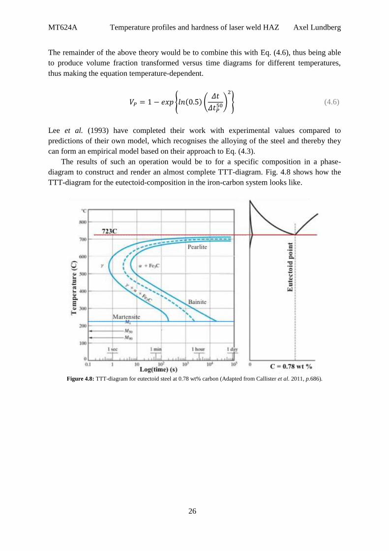
The remainder of the above theory would be to combine this with Eq. (4.6), thus being able
to produce volume fraction transformed versus time diagrams for different temperatures,
thus making the equation temperature-dependent.
{ ( ) (
)
} (4.6)
Lee et al. (1993) have completed their work with experimental values compared to
predictions of their own model, which recognises the alloying of the steel and thereby they
can form an empirical model based on their approach to Eq. (4.3).
The results of such an operation would be to for a specific composition in a phase-
diagram to construct and render an almost complete TTT-diagram. Fig. 4.8 shows how the
TTT-diagram for the eutectoid-composition in the iron-carbon system looks like.
Figure 4.8: TTT-diagram for eutectoid steel at 0.78 wt% carbon (Adapted from Callister et al. 2011, p.686).

MT624A Temperature profiles and hardness of laser weld HAZ Axel Lundberg
27
Following the schematic Fig. 4.5 which is a template for construction of TTT-diagrams, the
three blue curves in Fig. 4.9 represent different amounts of volume fraction transformed,
were the left most one is 1 % transformed, the broken line is 50 % transformed and the right
most one is 99 % transformed. The three temperatures in the bottom represent the
martensitic formation temperatures, which are stated as Eq. (4.7 – 4.9) (Ion 2005, p.534)
where the element symbols refer to concentration in wt %.
( ) (4.7)
( ) (4.8)
( ) (4.9)

MT624A Temperature profiles and hardness of laser weld HAZ Axel Lundberg
28

MT624A Temperature profiles and hardness of laser weld HAZ Axel Lundberg
29
5 Hardness in HAZ
After deducing the resulting phase transformational products, one needs to consider the
transformation of these numbers into usable applicable hardness notifications for chosen
welding and material-parameters. Contours of the constant hardness is represented and
calculated using the cooling time derived by Eq. (3.12) that is then used in the equations for
hardness calculations. Further calculations will make use of empirical equations based on the
derived chemical composition of the HAZ. Noticeable is that hardness above 350 HV is not
desirable (Ion et al. 1984). This is due to the fact that hardness is closely coupled to the
mechanical properties of the weld itself, thus reflecting the ability to withstand especially
dynamic loading cycles putting stresses upon the weld-area. The desired result is shown
schematically in Fig. 5.1, with the same basic structure (Ion 2005, p.535).
Figure 5.1: Typical microstructure - time diagram, schematic (Ion 2005).
Observation can be made in Fig 5.1 that the logarithmic cooling time scale is inversely
related to the applied energy from the welding apparatus, where the absorbed energy per area
unit is a linear scale along the x-axis contra the logarithmic scale of the cooling time
(Poorhaydari et al. 2005).
5.1 Analytical equations of phase volume fraction in low carbon steels
In order to arrive at a suitable diagram, the chosen carbon equivalent, see Eq. (5.1), which
must be derived for further calculations. All of the equations below are quoted from the
same source; Ion (2005), if none other is stated.

MT624A Temperature profiles and hardness of laser weld HAZ Axel Lundberg
30
(5.1)
Where element symbols refer to the composition in wt %. This carbon equivalent is
important for Eq. (5.2) to (5.5), in order to be able to calculate the necessary critical cooling
times for diagram construction:
( ) (5.1)
( ) (5.3)
( ) (5.4)
{ (
) } (5.5)
Where is he cooling time for 50 % martensite formation in seconds, likewise
is
cooling time for 0 % ferrite formation, is cooling time for 0 % bainite formation and
the cooling time for 50 % bainite formation. Next the volume fractions are stated as Eq.
(5.6) to (5.8).
{ ( ) (
)
} (5.6)
{ ( ) (
)
} (5.7)
( ) (5.8)
Where is the volume fraction of martensite, volume fraction of bainite and is the
volume fraction for ferrite-pearlite mixture. Important to note is that these equations, when
used for evaluating the hardness in the HAZ, are only applicable for a carbon content in the
range of: 0.1 < CEq < 0.5 (wt%) (Ion et al. 1996). In accordance to the work by Lee et al.
(1993) they state that some empirical equations are applicable even up to CEq < 0.8 (wt%).
MT624A Temperature profiles and hardness of laser weld HAZ Axel Lundberg
31
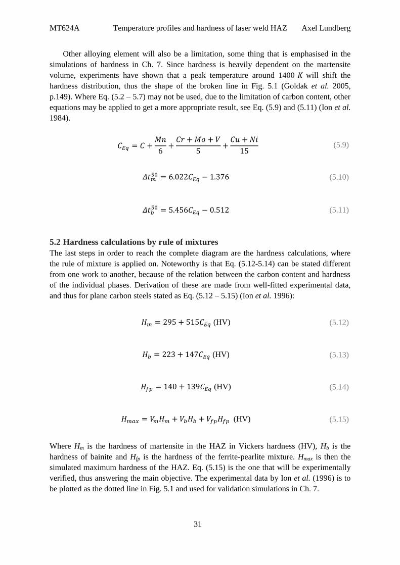
Other alloying element will also be a limitation, some thing that is emphasised in the
simulations of hardness in Ch. 7. Since hardness is heavily dependent on the martensite
volume, experiments have shown that a peak temperature around 1400 will shift the
hardness distribution, thus the shape of the broken line in Fig. 5.1 (Goldak et al. 2005,
p.149). Where Eq. (5.2 – 5.7) may not be used, due to the limitation of carbon content, other
equations may be applied to get a more appropriate result, see Eq. (5.9) and (5.11) (Ion et al.
1984).
(5.9)
(5.10)
(5.11)
5.2 Hardness calculations by rule of mixtures
The last steps in order to reach the complete diagram are the hardness calculations, where
the rule of mixture is applied on. Noteworthy is that Eq. (5.12-5.14) can be stated different
from one work to another, because of the relation between the carbon content and hardness
of the individual phases. Derivation of these are made from well-fitted experimental data,
and thus for plane carbon steels stated as Eq. (5.12 – 5.15) (Ion et al. 1996):
(HV) (5.12)
(HV) (5.13)
(HV) (5.14)
(HV) (5.15)
Where Hm is the hardness of martensite in the HAZ in Vickers hardness (HV), Hb is the
hardness of bainite and Hfp is the hardness of the ferrite-pearlite mixture. Hmax is then the
simulated maximum hardness of the HAZ. Eq. (5.15) is the one that will be experimentally
verified, thus answering the main objective. The experimental data by Ion et al. (1996) is to
be plotted as the dotted line in Fig. 5.1 and used for validation simulations in Ch. 7.

MT624A Temperature profiles and hardness of laser weld HAZ Axel Lundberg
32
Eq. (5.12 – 5.14) are relevant to plain carbon steels from which they are calculated.
Eq. (5.9 – 5.11) must be used for these alloyed steels, to calculate the hardness of each phase
is also different, not just the carbon-equivalent CEq (See Eq. 5.16 – 5.18) but other alloying
elements are included. The cooling rate V’ may be calculated according to Goldak et al.
(2005, p.149) by Eq. (5.19), where Eq. (3.12) is included:
(5.16)
( ) (5.17)
( ) (5.18)
(
) (
) (5.19)

MT624A Temperature profiles and hardness of laser weld HAZ Axel Lundberg
33
6 Results and discussion – thermal modelling
This chapter will be describing the thermal modelling produced by the mathematical
procedure explained in Ch. 3. A MATLAB® Graphical User Interface (GUI) developed by
the author produces the plotted functions, which represent the results in this chapter.
Ch. 7 describes data obtained using the empirical equations stated in Ch. 5, where results
will be produced in volume fraction diagrams and estimated hardness of chosen simulation,
also represented in diagrams.
Lastly, Ch. 8 will carry out the hardness estimation using a simpler graphical estimation
using TTT-diagrams, where results will be compared to those of Ch. 7.
6.1 Thermal modelling simulations
6.1.1 MATLAB® implemented GUI for thermal simulation
In order to easily derive the graphs, a GUI was developed for representation, although in this
project the plots will take into the figures one-by-one. This section will just briefly show the
GUI and how it looks like when used accurately. The code for this GUI may be found in
App. A and the front facia of the program can be seen in Fig. 6.1.
Figure 6.1: Basic MATLAB® GUI starting screen, with plotted functions.

MT624A Temperature profiles and hardness of laser weld HAZ Axel Lundberg
34
All the equations used in the background of this GUI are stated in the mathematical
modelling from Ch. 3. The equations are gathered from Ion (2005) and Ion et al. (1984) with
one exception for the critical thickness equation. This is taken from the work done by
Poorhaydari et al. (2005), which is according to them used as a boundary to determine when
the criteria for through-welding, 3-dimensional heat flow are attained.
6.1.2 Graphical simulations of thermal modelling
The first run with the thermal modelling was performed based on data described by
Kannatey-Asibu (2009) who in his book, see p. 239-245, makes temperature modelling,
along with the modified Bessel-function first seen in Eq. (3.6), in order to calculate the
temperature in a specific point in the HAZ. To validate the GUI-implementation; the
analytical simulation by Kannatey-Asibu (2009, p.239-245) will be replicated and presented
in Fig. 6.2. The following conditions were used in Eq. (3.10) (Simulation 6.1):
Power input, q = 6 kW
Plate thickness, d = 2.5 mm
Welding speed, v = 50 mm/s
Initial temperature, T0 = 298 K
Absorptivity, A = 0.7 (70%)
Density, = 7870 kg/m3
Specific heat capacity, = 452 J/kg K
Thermal conductivity, k = 73 W/m K
Radius, r =3.2 mm
Table 6.1: Comparison of calculation of replicated analytical model.
Calculation method Temperature (K) Mean relative error
Kannatey-Asibu 2009 (p.239-245) 985.4 1.34 %
Ion 2005 (p.532-535) 972.2
Figure 6.2: Temperature profile obtained by simulation 6.1with peak temperature at 972.2 K.

MT624A Temperature profiles and hardness of laser weld HAZ Axel Lundberg
35
Following that the tolerance is somewhere about 0.15 mm (Ion et al. 1984) and the plate is
2.5 mm, thus the tolerance would be 6 %, the experiment replication of 1.34 % mean relative
error calculated in Table 6.1 is acceptably lower than the tolerance of manufacturing
thickness limitations. Next simulation will consist of the properties that are stated as pre-set
for the start-up facia of the GUI. The material data is taken from Ion (2005) whilst welding
parameters are chosen in conjunction with the supervisor. Following conditions were used in
Eq. (3.1) and (3.14) (Simulation 6.2):
Power input, q = 4 kW
Plate thickness, d = 5 mm
Welding speed, v= 20 mm/s
Initial temperature, T0 = 298
Absorptivity, A = 0.7 (70%)
Density, = 7790 kg/m3
Specific heat capacity, = 560 J/kg K
Thermal conductivity, k = 32.5 W/m K
Distance, r =2.3 mm
Figure 6.3: Temperature versus time profile for pre-set values in GUI from simulation 6.2.
Figure 6.4: Radius versus peak temperature for pre-set values in GUI from simulation 6.2.

MT624A Temperature profiles and hardness of laser weld HAZ Axel Lundberg
36
Figure 6.5: Input energy versus HAZ-width plot for pre-set values in GUI from simulation 6.2.
Table 6.2: Calculated properties by GUI pre-set values.
Absorbed energy (J/mm2) ( ) HAZ-width (mm) Tp (K) dC
56.00 4.871 2.150 1648 10.39
Fig. 6.3 - 6.5 and Table 6.2 is interpreting what the GUI produces with the help of the
equations used. Caution should be taken when considering the HAZ-width. This value will
be a slight overestimation due to the original assumptions; this will be discussed later on.
When using the GUI with these equations, it is very important that the radius to the point
of interest is specified correctly. Eq. (3.10) is especially sensitive, as the radius will be
squared in the exponential part, the part that controls the heating of the HAZ. This is
explained in Fig. 3.4. In Fig. 6.6 different radii have been implemented for the same energy
input to show the previous statement and it visualises the sensitivity of the radius to the heat-
source. The problem using these equations is when the radius will be very small, thus the
answer will be incorrect as shown by Eq. (6.1) (Simulation 6.3):
( ) (
) (6.1)
Table 6.3: Results for simulation 6.3
Radii (mm) TP (K) Absorbed input (J/mm2) ( )
1.20
1.60
2.00
2.40
2.80
3.20
3.60
2265
1770
1484
1286
1145
1039
957
42.78 2.842

MT624A Temperature profiles and hardness of laser weld HAZ Axel Lundberg
37
Figure 6.6: Plot showing sensitivity to radii shifting versus time.
This phenomenon can be shown by plotting peak temperature versus radius from heat-source
to end HAZ that has been done for the different radii (See Table 6.3) in Fig. 6.7, which
shows that TP rises to infinity approaching the heat-source. This fundamental problem in
Eq. (3.10) has been analysed by Darmadi et al. (2011), whom compared the analytical values
with the numerical to get the best fit.
Figure 6.7: TP versus radius plot for actual energy input.

MT624A Temperature profiles and hardness of laser weld HAZ Axel Lundberg
38
Next simulation will replicate the experimental procedure of Poorhaydari et al. (2005) by
shifting the absorbed energy to obtain results to confirm that the analytical equations work as
the experiment. The parameters that are not changed are the same as in simulation 6.2 and
results are presented in Fig. 6.8. Following parameters were changed in Eq. (3.10) and (3.14)
(Simulation 6.4):
Plate thickness, d = 4 mm
Figure 6.8: Simulation of shifting input energy for cooling time derivation.
Table 6.4: Results of shifting input energy simulation
Laser power (W) Absorbed energy (J/mm2) ( )
1500
3000
4500
6000
13.13
26.25
39.38
52.50
0.27
1.07
2.41
4.28
Results derived experimentally by Poorhaydari et al. (2005) concluded that the cooling time
is very much dependent on the energy absorbed in the welding process. Noteworthy is the
cooling times them selves. With a welding apparatus of 1500 W power-output and the
parameters chosen for the simulation, an extremely quick cooling time is derived. This time
would give a significant martensite volume-fraction formation in the HAZ, and when
weighting with the rule of mixture (Eq. 5.14), the hardness would be high compared to the
parent-material.

MT624A Temperature profiles and hardness of laser weld HAZ Axel Lundberg
39
Figure 6.9: Calculated values from simulation 6.4 with interpolated fitted curve-showing relationship.
Observation in Fig. 6.9 can be made that a point has been plotted at an absorbed energy
lower than that of the first point in Table 6.4, which is only as an interpolation-point, but can
not be discussed theoretically as this point cross the critical thickness which in turn is
heavily controlled by the factor input energy per unit length (q/v). This observation has been
pointed out for aluminium as well, where this factor has a profound effect on the thermal
cycle theoretically, numerically and experimentally (Kou 1981).
Fig. 6.9 is important as the analytical solution shows that increasing the power more will
eventually tend to stabilise the amount of absorbed energy, thus when absorbed energy
approaches 200 J/mm2 the extra power input will only theoretically increase the cooling
time. Following Eq. (6.2) this implies that there is a fundamental calculation problem that
the analytical solution is thought to be depending on the fact of a constant absorption-factor
(A). This observation may imply that A is not constant, but follows a theoretically non-
linear/linear behaviour, that is dependent on either or both material properties and laser
properties.
(
)
(6.2)
The last diagram produced in simulation 6.4 is Fig. 6.10 produced by Eq. (3.14), where TP
has been plotted against r. This is done in order to deduce if the analytical equations will
follow the fundamental thermodynamic principle that the heat would dissipate faster at a
smaller amount of absorbed energy. According to the simulation done by Darmadi et al.
(2011) they confirm this by numerical principles, but it works the same with analytical
calculations. The biggest difference would be that their numerical implementation uses
thermal properties of non-linear nature, which is difficult to implement in the analytical
solution, see section 3.5.

MT624A Temperature profiles and hardness of laser weld HAZ Axel Lundberg
40
Figure 6.10: Results for TP versus r, from simulation 6.4.
Two more simulations will be made before discussion of the general thoughts on the
analytical solution to the thermal modelling problem. This is done to get total understanding
of what happens when changing of parameters in order to understand the hardness-problems
of the HAZ when cooling times are to fast.
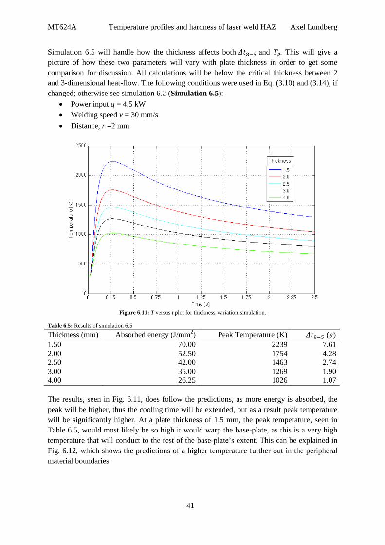
MT624A Temperature profiles and hardness of laser weld HAZ Axel Lundberg
41
Simulation 6.5 will handle how the thickness affects both and Tp. This will give a
picture of how these two parameters will vary with plate thickness in order to get some
comparison for discussion. All calculations will be below the critical thickness between 2
and 3-dimensional heat-flow. The following conditions were used in Eq. (3.10) and (3.14), if
changed; otherwise see simulation 6.2 (Simulation 6.5):
Power input q = 4.5 kW
Welding speed v = 30 mm/s
Distance, r =2 mm
Figure 6.11: T versus t plot for thickness-variation-simulation.
Table 6.5: Results of simulation 6.5
Thickness (mm) Absorbed energy (J/mm2) Peak Temperature (K) ( )
1.50
2.00
2.50
3.00
4.00
70.00
52.50
42.00
35.00
26.25
2239
1754
1463
1269
1026
7.61
4.28
2.74
1.90
1.07
The results, seen in Fig. 6.11, does follow the predictions, as more energy is absorbed, the
peak will be higher, thus the cooling time will be extended, but as a result peak temperature
will be significantly higher. At a plate thickness of 1.5 mm, the peak temperature, seen in
Table 6.5, would most likely be so high it would warp the base-plate, as this is a very high
temperature that will conduct to the rest of the base-plate’s extent. This can be explained in
Fig. 6.12, which shows the predictions of a higher temperature further out in the peripheral
material boundaries.

MT624A Temperature profiles and hardness of laser weld HAZ Axel Lundberg
42
Figure 6.12: Results for TP versus r, from simulation 6.5.
Identification needs to bee done with the fact that simulation 6.5 is done with a constant
energy input (q/v) of 150 J/mm. The difference in this and the absorbed energy is important
to recognise, as the absorbed energy (Aq/vd) will differ with varying thickness. The amount
of absorbed energy will be higher at smaller thickness due to the base-plate’s ability to be
easily penetrated by the output power of the welding apparatus. But the cost of this is the
risk of distortion in the base-plate and the enlarged HAZ, which follows that if the absorbed
energy is greater, the width will be greater, see Eq. (3.15).
Figure 6.13: Results plot for simulation 6.5.

MT624A Temperature profiles and hardness of laser weld HAZ Axel Lundberg
43
For better understanding of simulation 6.5, Fig. 6.13 shows the diagram plotted for thickness
versus both peak temperature and cooling time. This is done to see how the two parameters
follow the thickness variation mathematically.
The interpolated curves of the simulation results are plotted as seen in Fig. 6.13, which
shows that for each input-energy, there will be an intersection at which the cooling time will
dissipate faster than the peak temperature. The problem will be to plot closer to d = 0,
were both the thickness would be to small, but also that both curves would most probably
tend towards infinity.
Last simulation will show the implemented function of material choice in the GUI that
will give a picture of how the temperature profile will depend heavily on material/thermal
properties. Fig. 6.14 shows the temperature profile with the following conditions in Eq.
(3.10) are used (Simulation 6.6):
Power input q = 5 kW
Welding speed, v = 15 mm/s
Distance, r =2 mm
Plate thickness, d = 8 mm
Figure 6.14: T versus t plot for different materials.
Table 6.6: Results of simulation 6.6
Material Density
(kg/m3)
Thermal
conductivity
(W/mK)
Heat
capacity
(J/kgmK)
Thermal
diffusivity
(mm2/s)
Peak
temperature
(K)
( )
Low-carbon
steel
Titanium
Gold
AISI304-steel
Nickel
7790
4500
19300
7870
8900
32.5
23.0
296
25.5
72.0
560
523
132
450
560
7.45
9.77
116
7.20
14.4
1106
1797
1638
1294
1006
1.32
3.46
0.25
2.07
0.52

MT624A Temperature profiles and hardness of laser weld HAZ Axel Lundberg
44
Fig. 6.14 show that when changing the material for the same amount of input energy,
differences according to thermal properties will occur. By analysing Table 6.6 we can
deduce some key-factors in the changing thermal cycles. Observation of how cooling time is
dependent on thermal conductivity is well shown by the difference in low-carbon steel and
nickel, which both have the same specific heat capacity. Nickel has about double the value
of thermal conductivity compared to low-carbon steel, but the cooling time is 60 % faster.
This is also applicable for gold, which has a very high conductivity, thus the cooling time
will be very rapid, as the material properties state that heat dissipates faster. Observation can
be made that gold should have, in relation to the very high conductivity, an extremely rapid
cooling time. But as in Eq. (3.10) the cooling is governed by the inverse part, the high
density and heat capacity will extend this time. Heating the gold plate will be very quick,
due to the very high thermal diffusivity, thus the heat can travel very fast in the material, and
as this is controlling the inverse factor in the heating exponential part of Eq. (3.10).
Further observation can be made about Eq. (3.14), where the peak temperature for both
gold and titanium can be compared. This equation is governed by density and heat capacity
( ) in the inverse; therefore the peak temperature will correlate somewhat. The difference
in the materials and their curves will be the calculation of cooling time, where gold’s high
thermal conductivity will control the inverse part of Eq. (3.12), thus decreasing the cooling
time compared to that of titanium.

MT624A Temperature profiles and hardness of laser weld HAZ Axel Lundberg
45
6.2 Discussion of thermal modelling
The general analysis using the Rosenthal (1946) derived equations may be used for easier
application in the industry, but it is not without its drawbacks. In the above simulations using
the equations implemented in the MATLAB® GUI, discussion will follow.
In section 3.5 the problems using the original equations are highlighted. The basic
problem has been dealt with by Darmadi et al. (2011). They state that the analytical
modelling is much weaker than the numerical analysis in the sense that assumptions made by
Rosenthal (1946) in the analytical solution to the heat transfer equation are the biggest
errors. In the numerical solution these errors are not included as this numerical model may
incorporate things as the non-linear thermal properties or that the conductive heat inside the
parent material may dissipate into the plate surroundings.
Firstly the thermal properties are dependent on temperature, a property that is very hard
to implement in the analytical solution because of its non-linear nature. The analytical
solution would then have to be solved for every step of change in thermal properties as they
change for each in temperature. That would be unreasonable, compared to the solution by
numerical analysis. Further it was necessary to state that the heat from the heat source would
only dissipate through conduction in the parent-material, i.e. no heat dissipates through
surface. This fact is the one were least work has been done by others recently. This is mostly
likely due to that the fact that transformation take place inside the microstructure of the HAZ
or in the surroundings of the welded area, not outside in the base-plate-surroundings.
The largest problem is that the latent heat developed in the weld-bead is not
implemented in Rosenthal solutions. Both plots of Fig. 6.4 and 6.5 are therefore
overestimating their results a small amount. Plotting peak temperature versus radius will
only be an estimation of the calculation for the two parameters. The plots show the principle
dissipation of temperature through the parent-plate, but result should be handled with care
and analysed further if were to be used in actual material analysis. The schematics of such a
plot are although confirmed by Fig. 6.6 were the thermal cycles are plotted and the peak
temperatures will form the base for Fig. 6.7, showing that the schematic plot of peak
temperature against radius is correlating although the model is not considering the latent heat
development. The curve in Fig. 6.6 showing thermal cycle for a radius of r = 1.2 mm should
be treated as only schematic, as a peak temperature of approximately 2250 K is unreasonable
and would distort the base-plate.
This renders the next topic of the Rosenthal (1946) analytical modelling that Equation
3.10 houses a singularity problem at small radii, explained in Eq. (6.1). This can not be
overrun, as the radii is evaluated in square by the exponential part controlling the heating of
the base-plate, which makes the analytical solution useless at small radii with constant
absorbed energy. Thought should be taken when simulating with small radii and nearing the
melting temperature of the parent-material, because after that point the errors will be too big
to validate the simulation analytically. This problem is only erasable in a numerical model,
which may handle singularities by evaluating several points around the analysis point
chosen, although it is not easy to implement.

MT624A Temperature profiles and hardness of laser weld HAZ Axel Lundberg
46
This work has been handled by both Darmadi et al. (2011) and Kou (1981), where both use a
weighting method of combining the numerical and analytical results for a complete analysis,
which is observed in Fig. 6.15. This shows how schematically one can handle the singularity
problem of the analytical solution, by combining with other approaches, thus providing a full
picture of the model.
Figure 6.15: Temperature profile very close to the weld line, longitudinal to weld (Adapted from Darmadi 2011)
Following observation made during simulation 6.4, when increasing the amount of input
power of the welding apparatus, the increase in absorbed energy will make the cooling time
eventually tend toward infinity. Meaning that at some point, a miniscule increase in power
input will significantly increase the cooling time. This is believed to depend on the constant
absorptivity set to A = 0.7 by Ion (2005). Caution should be taken, because very absorbed
energy-value is not applicable in practice, as there is a limit to how much power could be put
into the base-material plate. In theory if the thickness d is decreased for a specified constant
power input q, the absorbed energy would increase, but then as the parent-material plate-
thickness decreases, so does the ability to cope with high power inputs. This means that Fig.
6.9 will be a theoretical approach to the problem, but although makes for a discussion on
weather it is applicable to state that absorptivity A is a constant, linear or a non-linear
relation to the power input (q/v). This work would be very extensive and is not covered in
this thesis. Another thought would be to form easy and practically applicable curves for
deducing the amount of input energy for specific thicknesses and material (thermal)
properties, thus implementing the absorptivity A from an experimental approach.
Simulation 6.5 induced a change in thickness for a constant input energy. From Fig. 6.11
one can see that as the thickness d increases, the peak temperature will decrease in
accordance, as well as decreasing the cooling time significantly. The higher absorbed energy
at thinner plates is due to the construction of Eq. (3.10), where thickness d is controlling the
denominator of the absorbed energy. In theory this will of course increase at thinner plates,
in practical manners it has the meaning that the heat generated by the weld will be higher

MT624A Temperature profiles and hardness of laser weld HAZ Axel Lundberg
47
further out relative to the thickness, something that is graphically illustrated by Fig. 6.12.
This Figure is only used as a graphical tool to show that in a thicker plate, the heat will have
more difficulty to travel through the material, thus the curve in Fig. 6.12 shows a flatter
curve for a thinner plate relative to a thick plate. Fig. 6.13 implements the results from the
simulation as two curves plotted in the same space to see the correlation between the two
calculated variables; Tp and . They both follow a non-linear trace, although the
interpolated curves are not true, as they should tend towards infinity when thickness d goes
towards 0 mm. This error is traced to both the calculations made with Rosenthal equations,
that includes the error from original assumptions, but also that the simulations is only done
for smallest thickness d = 1.5 mm as smaller values would give a non-realistic value, only
applicable in theory.
Last simulation, 6, deduces that the thermal modelling is applicable for other material
than steel, where validation made by Kou (1981) stands as reference. The equations used
follow what the predictions of the thermal properties suggest, but caution should be taken
when using them in practice, not only as theoretical results.
Other errors that must be noticed is that calculations with a peak temperature below
900 should not be used according to Ion (2005) due to their non-valid nature when
calculated. If the width of the HAZ is calculated using Eq. (3.15), the temperature at end of
HAZ TR must not be to close a value to the melting temperature Tm, see Eq. (3.17) and
(3.18), as this will give an even more faulty calculation of the width, as this already includes
a part of the molten weld-pool according to original assumptions of thermal modelling, see
section 3.1.

MT624A Temperature profiles and hardness of laser weld HAZ Axel Lundberg
48
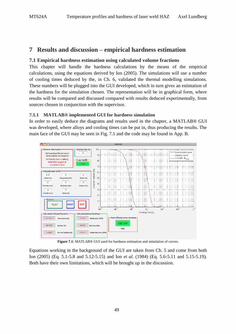
MT624A Temperature profiles and hardness of laser weld HAZ Axel Lundberg
49
7 Results and discussion – empirical hardness estimation
7.1 Empirical hardness estimation using calculated volume fractions
This chapter will handle the hardness calculations by the means of the empirical
calculations, using the equations derived by Ion (2005). The simulations will use a number
of cooling times deduced by the, in Ch. 6, validated the thermal modelling simulations.
These numbers will be plugged into the GUI developed, which in turn gives an estimation of
the hardness for the simulation chosen. The representation will be in graphical form, where
results will be compared and discussed compared with results deduced experimentally, from
sources chosen in conjunction with the supervisor.
7.1.1 MATLAB® implemented GUI for hardness simulation
In order to easily deduce the diagrams and results used in the chapter, a MATLAB® GUI
was developed, where alloys and cooling times can be put in, thus producing the results. The
main face of the GUI may be seen in Fig. 7.1 and the code may be found in App. B.
Figure 7.1: MATLAB® GUI used for hardness estimation and simulation of curves.
Equations working in the background of the GUI are taken from Ch. 5 and come from both
Ion (2005) (Eq. 5.1-5.8 and 5.12-5.15) and Ion et al. (1984) (Eq. 5.6-5.11 and 5.15-5.19).
Both have their own limitations, which will be brought up in the discussion.

MT624A Temperature profiles and hardness of laser weld HAZ Axel Lundberg
50
7.1.2 Graphical results of hardness simulations
First simulation in this results chapter of hardness will consist of a simulations where the
carbon equivalent CEq is altered to see how the curves react. By using Eq. (5.1 -5.5), Ion et
al. (1996) has noted that the limitation of this model is a carbon content of about C = 0.18
wt%, this will be observed in the discussion. Fig. 7.2 shows how altering only the carbon
content affects the curves, whilst in Fig. 7.3 and 7.4, manganese, resp. silicon-content will be
altered as these are the two alloys used by Eq. (5.5). Following conditions were used
(Simulation 7.1):
Power input q = 3.5 kW
Plate thickness, d = 6 mm
Welding speed, v = 15 mm/s
Initial temperature, T0 = 298
Absorptivity, A = 0.7 (70%)
Average density, = 7790 kg/m3
Average specific heat capacity, = 560 J/kg K
Thermal conductivity, k = 32.5 W/m K
Melting temperature, Tm = 1804
Figure 7.2: Altering the carbon contents to get different carbon equivalent.
Table 7.1: Results of both thermal and hardness modelling for simulation 7.1.
Carbon content
(wt%)
Carbon equivalent
(wt%)
Absorbed
energy (J/mm2)
Cooling time (s) Hardness
(HV)
0.10 0.10
27.2 1.15
213
0.14 0.14 255
0.18 0.18 330

MT624A Temperature profiles and hardness of laser weld HAZ Axel Lundberg
51
Fig. 7.3 shows how altering the manganese content will affect both carbon equivalent and
hardness. The limits for using this model are again adapted from Ion et al. (1996) where the
maximum empirical manganese content is 1.4 wt%. The variables derived from thermal
modelling will be the same here as used in Table 7.1.
Figure 7.3: Altering the manganese content, thus carbon equivalent to derive hardness.
Table 7.2: Results of altering manganese content.
Carbon content
(wt%)
Manganese content
(wt%)
Carbon equivalent
(wt%) Hardness (HV)
0.12
0.40 0.153 276
0.80 0.187 342
1.20 0.220 389
Table 7.2 and 7.3 show that the hardness will increase rather much when introducing alloys
into the low carbon steel. The last curve, where the carbon equivalent approaches a high
value is hard to deduce, as there actually is an empirical limitation to the model.
In order to get comparison for the hardness versus carbon equivalent, the silicon also
needs to be altered. Lastly, these will be combined in Fig. 7.5 where both the manganese and
the silicon will be altered, then the results of all these altering’s will be visualised in Fig. 7.6
showing how the hardness develops when alloys are introduced in different ways, seen in
Table 7.4. Note that these results are only schematic, as these alloying combinations are not
actual steel types used in the industry.

MT624A Temperature profiles and hardness of laser weld HAZ Axel Lundberg
52
Figure 7.4: Altering the silicon content, thus the carbon equivalent to derive hardness.
Table 7.3: Results of altering silicon content.
Carbon content
(wt%)
Silicon content
(wt%)
Carbon equivalent
(wt%) Hardness (HV)
0.12
0.18 0.128 242
0.36 0.135 249
0.54 0.143 258
Now by altering carbon, manganese and silicon, Fig. 7.5 shows what happens with the
hardness at this stage. This is done in order to get validation that the model actually follows
the equation for carbon equivalent stated by Ion (2005).

MT624A Temperature profiles and hardness of laser weld HAZ Axel Lundberg
53
Figure 7.5: Altering either alloy or carbon to get results of hardness.
Table 7.4: Results of altering all the alloying components in steel using equations from Ion (2005)
Carbon content
(wt%)
Manganese
content (wt%)
Silicon content
(wt%)
Carbon equivalent
(wt%)
Hardness
(HV)
0.10 0.40 0.18 0.141 266
0.14 0.40 0.18 0.181 342
0.10 0.80 0.18 0.174 330
0.10 0.40 0.36 0.148 280
The results from Table 7.4 can be seen in Fig. 7.6, where the overall impression is that if one
increases the carbon content or the alloying composition, the carbon equivalent will increase
following Eq. (5.1) thus increasing the hardness of the weld HAZ. This is due to that when
the alloys raise the carbon equivalent, the curve of volume fractions will shift to the right,
thus the composition of the HAZ will get an increased martensite volume fraction.
According to Eq. (5.1), the increase of carbon content has the most significant effect on the
hardness. This happens when increasing the carbon equivalent makes for both shifting
curves and by that the martensite hardness will increase. As the martensite is the hardest
phase measured in HV, it also affects the overall hardness the most. Note should be taken,
that the distance between curves are not equal, as the x-axis is logarithmic.
A problem has been noted that Eq. (5.1 – 5.5) and (5.12 – 5.14), taken from Ion (2005)
has a limit of around CEq = 0.24 wt% as the empirical model developed only has values
below this limit. A comparison is done with Eq. (5.9 – 5.11) and (5.16 - 5.18) taken from Ion
et al. (1984), that might work for hypo-eutectic steels of higher carbon equivalent. Test for
hyper-eutectic will not be included in this thesis, therefore max CEq = 0.78, the eutectic
composition.

MT624A Temperature profiles and hardness of laser weld HAZ Axel Lundberg
54
Figure 7.6: Results of simulation 7.1 showing typical trending of hardness.
Fig. 7.6 shows that the trend of all the lines is that increasing carbon equivalent will result in
increased hardness, which follows the proportions of Eq. (5.1). Observation is made that
changing the carbon content will shift the curves the most between each step of content
increase, but by altering the manganese content will result in the biggest shift in hardness,
although the increase in manganese also results in the biggest increase of carbon content
compared to silicon.

MT624A Temperature profiles and hardness of laser weld HAZ Axel Lundberg
55
Simulations 7.2 will use the model by Ion et al. (1984) for comparison. Note that manganese
and carbon will alter the carbon equivalent, as silicon is not included in Eq. (5.9), but it is
included in Eq. (5.16 – 5.18). Simulation 7.2 can be seen in Fig. 7.7 and results in Table 7.5
(Simulation 7.2):
Figure 7.7: Simulation 7.2 using model by Ion et al. (1984).
Table 7.5: Results of altering all the alloying components in steel using model by Ion et al. (1984).
Carbon content
(wt%)
Manganese
content (wt%)
Silicon content
(wt%)
Carbon equivalent
(wt%)
Hardness
(HV)
0.10 0.40 0.18 0.167 277
0.14 0.40 0.18 0.207 303
0.10 0.80 0.18 0.233 317
0.10 0.40 0.36 0.167 313
The problem when using the model derived by Ion et al. (1984) on modern low carbon steels
becomes apparent by the results above. As these steels often is consisting of carbon,
manganese and silicon, with additional alloys of minute content of around wt% < 0.05, the
three mentioned, will be those who affects the hardness most significantly as the model by
Ion (2005, p. 534) is only dependent on manganese and silicon in the calculation.(Sokolov et
al. 2011).
As silicon is not added into Eq. (5.9), it does not affect the carbon equivalent, but in turn
it affects Eq. (5.16 – 5.18), thus it in turn affects the hardness seen in Table 7.5. There one
sees that row one and row four has the same carbon equivalent but row four has a 13 %
higher hardness in the HAZ. This may be misguiding when using, but Simulation 7.3 shows
that the model by Ion et al. (1984) can be used for high carbon content, such as eutectic
steel. Same conditions as in simulation 7.1 are used, where parameters used may be seen in
Table 7.1.

MT624A Temperature profiles and hardness of laser weld HAZ Axel Lundberg
56
Fig. 7.8 shows the curves produced for steels with higher carbon content and the results are
seen in Table 7.6, simulation 7.3:
Figure 7.8: Results of simulation 7.3 using higher carbon equivalent and model by Ion et al. (1984).
Table 7.6: Results of simulation 7.3 altering the alloying components in steel using model by Ion et al. (1984).
Carbon content
(wt%)
Manganese
content (wt%)
Silicon content
(wt%)
Carbon equivalent
(wt%)
Hardness
(HV)
0.78 0 0 0.78
0.78
0.78
0.78
887
0.70 0.48 0 816
0.78 0 0.36 897
0.70 0.48 0.36 826
Simulation 7.3 reveals a serious problem with the
empirical model. Such a high hardness, of above
800 HV, would only work as a theoretical value,
not applicable in practice. This suggests that
neither of the empirical models tested may not be
applied to carbon steel with a very high carbon
equivalent. Fig. 7.9 shows how the hardness will
deviate, but at values above the limit of 350 HV
(Sokolov et al. 2011) one may deduce that a
reasonable maximum carbon equivalent of
around CEq = 0.28 is to be set.
Figure 7.9: Results of simulation 7.3.

MT624A Temperature profiles and hardness of laser weld HAZ Axel Lundberg
57
Before simulating what happens when altering the cooling time to derive the hardness on
different time steps, an experiment by Sokolov et al. (2011) will be replicated and compared.
They derived the hardness for thick pieces of s355 constructional steel by experiment. Using
very powerful laser-apparatus they achieved penetration welding, i.e. 2-dimensional heat
flow, even in 20 – 25 mm thick pieces. The composition of s355 steel is taken from their
work, while the thermal properties are adapted from Piekarska et al. (2012). Following
conditions were used, with results in Fig. 7.10 and Table 7.7 (Simulation 7.4):
Power input, q = 20 - 25 kW
Welding speed, v = 40 mm/s
Plate thickness, d = 20 mm
Initial temperature, T0 = 298
Absorptivity, A = 0.7 (70%)
Average density, = 7900 kg/m3
Average specific heat capacity, = 477 J/kg K
Thermal conductivity, k = 42.7 W/m K
Figure 7.10: Results of simulation 7.4 using parameters from Sokolov et al. (2011).
Table 7.7: Results of simulation 7.4 with difference between experimental and empirical method.
Laser-
power
(kW)
Absorbed
energy
(J/mm2)
Cooling
time (s)
Carbon
equivalent
(wt%)
Hardness
simulation
(HV)
Hardness
Sokolov et
al. (2011)
(HV)
Relative
mean error
(%)
20 17.50 0.45 0.225
429.1 432.7 0.83
25 21.88 0.66 421.3 425.5 0.91

MT624A Temperature profiles and hardness of laser weld HAZ Axel Lundberg
58
Simulation 7.4 shows that the empirical approach using equations by Ion (2005) works well,
considering a less than one percent difference. It may be a coincidence for these results only.
It should be noted that the thermal simulation made to deduce the cooling time warned for a
precise cross over the limit between 2 and 3-dimensional heat flow, but this was neglected to
show the results. In the experiment by Sokolov et al. (2011) they deduced by sections of the
weld that by using the laser-power stated, a 2-dimensional heat flow is induced. It must be
implied that the composition of the s355 steel may vary and was by meaning kept below
CEq = 0.235, thus being in the range where equations by Ion (2005) may be used, therefore
verifying that they may be used for modern low carbon steels.
The fifth simulation in this chapter will be using different cooling times, i.e. altering the
welding speed, in order to arrive at the graphical representation of the broken line in Fig. 5.1.
Fictional simulations will be used to schematically show the broken line, these will be
marked. The parameters and compositions used for the thermal modelling and the hardness
estimations are taken from Ion et al. (1996) for comparison (Simulation 7.5):
Power input q = 3.8 kW
Plate thickness, d = 6 mm
Melting temperature, TM = 1801
Average density, = 7860 kg/m3
Average specific heat capacity, = 680 J/kg K
Thermal conductivity, k = 30 W/m K
1st Steel type: Fe37B, CEq = 0.171 wt%
2nd
Steel type: HSE, CEq = 0.238 wt%
Figure 7.11: Results for comparison with Fig. 5.1 using data from Ion et al. (1996).

MT624A Temperature profiles and hardness of laser weld HAZ Axel Lundberg
59
Table 7.8: Results of shifting welding simulation 7.5.
Welding speed
(mm/s)
Absorbed energy
(J/mm2)
Cooling time (s) Hardness
Fe37B (HV)
Hardness
HSE (HV)
f* ---- 0.001 383.2 417.4
70.00 6.33 0.055 382.9 417.2
25.00 17.73 0.431 369.8 415.8
20.00 22.17 0.675 352.0 413.5
17.50 25.33 0.881 335.7 411.0
16.00 27.71 1.054 320.6 408.4
14.50 30.57 1.283 302.0 404.1
13.00 34.10 1.597 280.3 397.2
11.50 38.55 2.041 260.4 385.8
10.00 44.33 2.690 249.7 366.6
7.50 59.11 4.798 245.7 305.0
3.50 122.70 22.030 208.9 267.6
f* ---- 100 183.1 249.3
f* ---- 1000 175.8 240.5 *Fictive simulation, theoretical value, only for schematic plotting and calculations purpose.
The results of hardness simulation can be seen in Table 7.8, where the results are plotted
against one another in Fig. 7.11. What can be deduces by this simulation is that the
schematic plot seen in Fig. 5.1 is correct, where the broken line is here represented by the
points plotted. The difference between the two steels can clearly be seen in the table, where
the shifting of the curves for both bainite and martensite to the right for HSE, due to the
higher carbon equivalent, makes for a higher hardness value further in the plot. HSE steel
simulation shows that the cooling curve for martensite is shifted much to the right compared
to the Fe37B, thus the hardness will be higher, due to higher martensite volume fraction in
the HAZ, which is validated by the results. Also that the hardness should be higher, due to
higher carbon equivalent in HSE compares Fe37B, which has been shown by earlier
simulations, see Fig. 7.6.

MT624A Temperature profiles and hardness of laser weld HAZ Axel Lundberg
60
Before the final simulation when comparing experimental and simulated results, simulation
7.6 will bring forth a statement from section 2.2, to test how much the preheat temperature
affects weld-hardness. Conditions used in this simulation are the same as in simulation 7.5
(except for welding speed v), but by altering the preheat temperature one would be able to
decrease the hardness, which will of course affect Eq. (3.13) heavily, thus also affecting the
cooling time of Eq. (3.12). Simulation 7.6:
Table 7.9: Results of simulation 7.6, altering preheat temperature T0.
Preheat temperature
( ) Cooling time (s)
Hardness Fe37B
(HV)
Hardness HSE
(HV)
273 (0) 0.59 359 409
298 (25) 0.68 352 406
323 (50) 0.77 345 405
373 (100) 1.02 323 400
423 (150) 1.41 292 391
473 (200) 2.03 261 371
523 (250) 3.09 248 332
573 (300) 5.12 245 278
623 (350) 9.69 238 256
673 (400) 22.86 206 250
723 (450) 95.55* 183 242
*Simulation should be seen as a purely theoretical value.
Figure 7.12: Results of simulation 7.6 made graphical for easy interpretation.
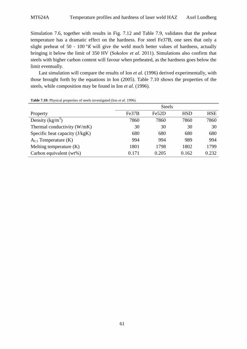
MT624A Temperature profiles and hardness of laser weld HAZ Axel Lundberg
61
Simulation 7.6, together with results in Fig. 7.12 and Table 7.9, validates that the preheat
temperature has a dramatic effect on the hardness. For steel Fe37B, one sees that only a
slight preheat of 50 - 100 will give the weld much better values of hardness, actually
bringing it below the limit of 350 HV (Sokolov et al. 2011). Simulations also confirm that
steels with higher carbon content will favour when preheated, as the hardness goes below the
limit eventually.
Last simulation will compare the results of Ion et al. (1996) derived experimentally, with
those brought forth by the equations in Ion (2005). Table 7.10 shows the properties of the
steels, while composition may be found in Ion et al. (1996).
Table 7.10: Physical properties of steels investigated (Ion et al. 1996).
Steels
Property Fe37B Fe52D HSD HSE
Density (kg/m3) 7860 7860 7860 7860
Thermal conductivity (W/mK) 30 30 30 30
Specific heat capacity (J/kgK) 680 680 680 680
AC1 Temperature (K) 994 994 989 994
Melting temperature (K) 1801 1798 1802 1799
Carbon equivalent (wt%) 0.171 0.205 0.162 0.232

MT624A Temperature profiles and hardness of laser weld HAZ Axel Lundberg
62
The parameters used will be given in Table 7.10, taken directly from Ion et al. (1996).
Values of hardness in Table 7.11 are set up so the value deduced experimentally is inside
brackets, whereas the simulated value, deduced by this thesis is outside the brackets.
(Simulation 7.7):
Table 7.11: simulated results versus experimental values in parenthesis of hardness.
HAZ Hardness (HV)
Plate thickness
(mm)
Power
(kW)
Speed
(mm/s)
Applied energy
(J/mm2)
Fe37B Fe52D HSD HSE
4.0
2.5
10.00 63 245
(234)
254
(248)
291
(363)
292
(339)
23.33 27 326
(340)
368
(348)
404
(413)
409
(407)
3.8
35.00 27 345
(328)
376
(368)
402
(378)
408
(413)
40.00 23 318
(283)
386
(413)
408
(395)
412
(413)
6.0
3.8
6.67 94 233
(210)
221
(210)
256
(283)
259
(293)
10.00 63 245
(222)
254
(245)
278
(339)
299
(334)
13.33 47 232
(214)
282
(269)
341
(373)
354
(378)
5.0
18.33 47 225
(212)
290
(286)
349
(363)
362
(358)
23.33 36 262
(242)
340
(325)
385
(368)
393
(413)
8.0 5.0
8.33 75 235
(218)
253
(242)
279
(321)
274
(293)
10.00 63 245
(215)
254
(237)
301
(325)
292
(312)
Mean relative
error 10 % 5 % 9 % 7 %
Discussion of results may be found in the next part below.

MT624A Temperature profiles and hardness of laser weld HAZ Axel Lundberg
63
7.2 Discussion of empirical hardness simulation
Simulation 7.1 was done in order to see if the implemented model reacted according to what
is expected, that is an increase in hardness when increasing the carbon equivalent in the
observed steels. Fig. 7.2- 7.4 shows the expected results, Fig. 7.2 shows a large space
between curves, thus a great variation in hardness values is observed, reflected also in
Fig. 7.4, where small increments gives less of increase in hardness. Caution should be taken,
thus the model used, Ion (2005), is an empirical model, which has its limits. The model will
not work above a carbon equivalent of about CEq = 0.24, where especially Eq. (5.5) will
show clear singularity problems due to its empirically derived nature as it is interpolated
from experimental data. If one instead want to use the equations by Ion et al. (1984), the
problem facing is that most modern low-carbon steels will incorporate silicon as a major
alloying component, thus this element not being taken into Eq. (5.9). This problem is
reflected well by Fig. 7.7 in simulation 7.2, where the results are considered inconclusive.
The model also uses an estimated cooling rate V’ in Eqs 5.16 – 5.18, which is hard to
deduce, thus rendering the usage of this model unpractical for modern use. The advantage is
that it may be used at higher levels of carbon equivalent than Ion (2005), but it has its limits
here as well. Simulation 7.3 shows how unrealistic a simulation using a very high carbon
equivalent and the model by Ion et al. (1984) is, when reaching hardness levels above 800
HV, values only theoretically achievable. Ion et al. (1996), Sokolov et al. (2011) amongst
others point out acceptable levels of hardness as 350 HV.
Simulations 5 thus show how the carbon equivalent will affect the hardness drastically.
HSE-steel with a high carbon equivalent has a much higher hardness at same cooling times
as Fe37B, where acceptable hardness levels is achieved approximately four times as fast, at
0.675 s for Fe37B against 2.690 s for HSE. This verifies the necessity of appropriate
hardness versus cooling time-diagrams; although caution should be shown to what empirical
model was used to deduce the hardness levels.
All of the above simulations have been implemented using cooling times derived by the
analytical solution to the thermal/mathematical modelling, thus it brings its own errors
along. Validity of thermal modelling has been deduced as appropriate, but thermal modelling
deducing cooling times using numerical analysis will be superior if more accurate values is
needed. In turn this would result in an accurate thermal cycle, but the empirical model for
deriving the hardness is still very approximate, with an error margin of about 10 %
according to Ion et al. (1996). These error margins are deduced by the fact that the carbon
equivalent is only deduced by three components of the alloy, thus rejecting the remaining
ones.
Using the latter stated error-margin, simulation 7.7 shows acceptable mean relative error
of 10 % or less for the four steels simulated. One should although be cautious, where the
experimental values, as well as simulated results may vary in accordance. Simulation may
vary due to steps of thermal modelling into hardness empirical model, giving errors along
the way. Notable is that the relative mean error for each material varies, where Fe37B has
eight out of 11 simulations above 10 % relative error, whilst Fe52D has none. This may be
down to the composition, where Fe52D has higher carbon content, thus a relatively higher
carbon equivalent. Therefore the errors deduced in both HSE and HDE-steels may be traced

MT624A Temperature profiles and hardness of laser weld HAZ Axel Lundberg
64
to their alloying composition and carbon content, as they both show that four out of 11
simulations have 10 % relative error or more.
The later statement may also be the reason that simulation 7.4 shows a small relative
error of less than 1 %. Note should be taken that the hardness value taken from Sokolov et
al. (2011) is an average hardness in the HAZ, not a point-hardness. Nevertheless such a
small relative error reflects the validity of the model deduced and presented by Ion (2005).
Plotting the two data-arrays show no trends of hardness errors deduced by applied energy,
where distribution of errors a significantly equal.
Simulation 7.6 is reflecting what was brought up was has been stated in section 2.2,
where Table 7.9 and Fig. 7.12 significantly validates that preheating the steel prior to
welding will affect the hardness drastically. Although preheating is a practically
cumbersome process, one might argue that it may give hardness levels below the limit of
350 HV (Sokolov et al. 2011) even a slight preheat. For steels with higher carbon equivalent
a higher preheat is needed, but this might also favour, as these steel already are hard to bring
below the limit thanks to their composition.
The simulations, seen in Table 7.11, have been repeated in App. C, for the equations by
Ion et al. (1984). If one follows the same mean relative error procedure as for the equations
by Ion (2005), it may be deduced that they are not applicable for the steels tested as all of the
simulations ended up showing mean relative error of 20 % or more. Many of the simulations
that failed the most may be traced to Eq. (5.16 – 5.18), where one has to specify all the
alloying components to be calculated in the carbon equivalent. This makes for a somewhat
faulty simulations, where the answers may not be as accurate as one had hoped. Eq. (5.19)
for the cooling rate is a big factor in the error; as it decreases the hardness in Eq. (5.16 -5.18)
already at relatively fast cooling times. Therefore many of the simulations in App. C are way
of, often lower than the experimental.

MT624A Temperature profiles and hardness of laser weld HAZ Axel Lundberg
65
8 Results and discussion – graphical hardness estimation
This part will conclude if the theory in Ch.4 may be used for estimation of hardness in the
HAZ and serves only as a theoretical approach to if the analysis made graphically is
sustainable against a much more elaborate empirical analysis, such as the on presented in
Ch. 7. The analysis will utilize an already created TTT-diagram for a hypo-eutectoid steel
with a carbon equivalent of CEq = 0.45 wt%. Due to this factor, only the equations by Ion et
al. (1984) may be applied to the problem.
The analysis is based on the cooling times printed in Figure 8.1, where the times have
been adapted form simulation 7.7, Ch. 7. This approach is very crude, thus predicted results
using the empirical hardness approach uses an adapted composition of modern low carbon
steels (Sokolov et al. 2011).
Figure 8.1: TTT-diagram of hypo-eutectoid steel of CEQ = 0.45 wt% with simulated cooling times
(Adapted from Callister et al. 2011, p.699).
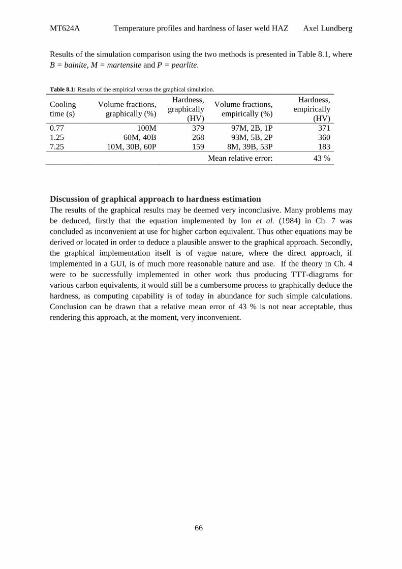
MT624A Temperature profiles and hardness of laser weld HAZ Axel Lundberg
66
Results of the simulation comparison using the two methods is presented in Table 8.1, where
B = bainite, M = martensite and P = pearlite.
Table 8.1: Results of the empirical versus the graphical simulation.
Cooling
time (s)
Volume fractions,
graphically (%)
Hardness,
graphically
(HV)
Volume fractions,
empirically (%)
Hardness,
empirically
(HV)
0.77 100M 379 97M, 2B, 1P 371
1.25 60M, 40B 268 93M, 5B, 2P 360
7.25 10M, 30B, 60P 159 8M, 39B, 53P 183
Mean relative error: 43 %
Discussion of graphical approach to hardness estimation
The results of the graphical results may be deemed very inconclusive. Many problems may
be deduced, firstly that the equation implemented by Ion et al. (1984) in Ch. 7 was
concluded as inconvenient at use for higher carbon equivalent. Thus other equations may be
derived or located in order to deduce a plausible answer to the graphical approach. Secondly,
the graphical implementation itself is of vague nature, where the direct approach, if
implemented in a GUI, is of much more reasonable nature and use. If the theory in Ch. 4
were to be successfully implemented in other work thus producing TTT-diagrams for
various carbon equivalents, it would still be a cumbersome process to graphically deduce the
hardness, as computing capability is of today in abundance for such simple calculations.
Conclusion can be drawn that a relative mean error of 43 % is not near acceptable, thus
rendering this approach, at the moment, very inconvenient.

MT624A Temperature profiles and hardness of laser weld HAZ Axel Lundberg
67
9 Conclusion
This final part of the report gives some concluding remarks, mainly referring to the question
given in section 1.3. Also, potential improvement areas of the analysis are brought forth.
9.1 Conclusions
The first question to be answered were if the Rosenthal model was valid and if it solutions
may be implemented into a quick and easy to use program, in order to derive quick
calculations. This basic theory about thermal cycles and thermal modelling has been dealt
with in Ch.3, where the verification has been dealt with in Ch. 3.5. Although this is an
analysis of the analytical solution to the heat transfer problem, it provides a very quick way
to derive the thermal cycles needed for further analysis, together with purposely-calculated
parameters. The analytical solution was deemed valid for the usage in this thesis, although it
is not without flaws. Many of the problems may be traced to the original solution proposed
to the differential equation of heat transfer of quasi-stationary state. Using these analytical
solutions plugged into the GUI is although very easy, but this tool require, to a larger extent,
critical evaluation of the results calculated. But the entire thermal cycle may be brought forth
with ease; it gives one great choice in the analysis of both thermal analyses and hardness
evaluation in the HAZ. However, it again requires wise choices of the user to get results
applicable in practical situations. The equations of thermal modelling have been employed
by other authors on different materials, where the validity has been stated as statistically
satisfying, but not without flaws. There are advantages of doing the thermal cycle-analysis
by numerical means,
Next, a program was brought forth for the simulation of the hardness of the HAZ, and
how the phases were distributed in terms of volume fractions. This is a rather straightforward
suite, where one only has to plug in few variables in order to get results. Again though
caution by the user has to be made, reasonable thinking about the derived results must be
made. The program may work for a higher carbon equivalent, but the results may be deemed
inconclusive at further analysis, which may be connected to the empirical model used in the
background. Although the main interest of the program was fulfilled, easy interpretation and
usage. Using computers of current standard, solving problems in any of the GUI:s takes no
longer than a few seconds, but basic understanding of the equations used must be meet, as
well as understanding the phase transformation shortly brought forth in Ch. 4. Also in Ch. 4,
a theory about making a fast way to produce diagrams that could be used for graphical
interpretation of hardness simulation. This was unfortunately put aside as the workload was
deemed to cumbersome for the timeframe of this thesis.
Secondly, the question about if one may use the empirical model brought forth by Ion
(2005). The work was done on a basis of simulating and comparing to other experimental
work, but also comparing to results of other empirical models, such as equations by Ion et al.
(1984).

MT624A Temperature profiles and hardness of laser weld HAZ Axel Lundberg
68
One may say that comparing the values to experiments of certain age is not relevant, but the
conclusion is that the accuracy of the simulation is valid for both low carbon steels of some
age and that of which is used today. When comparing the model to work done in 2011 the
validity is significantly accurate, thus confirming the experimental results within a
statistically valid region. The limitations will although be a great drawback, as the carbon
equivalent of more modern steel-types are approaching the maximum of the empirical
model, thus there is argument for developing a new set of equations. The model by Ion
(2005) is also sparse in considering the alloying components, but it although works very well
in predicting the hardness inside the HAZ. Even though the model is predicting accurate, any
engineer working with the topic, should still be cautious and evaluate the simulation due to
singularity related issues in thermal modelling, which may be reflected in the hardness
simulation.
Whether or not, the objective has been to deal with the task in an easy manner, thus
significantly reducing the time to incorporate the analytical solution, by fitting them into
GUI:s, which is a fast and graphically simple way of dealing with the simulations needed for
further interpretations. But experience in the field and some discretising of the results are
needed in order to make them valid for the tasks at were it would be brought forth about.
Even the simplest computations require the engineer to highlight reasoning and the errors of
the analyses should be weighed in for significance of the simulation if to be used for other
than purely theoretical purpose. Of course the theoretical values are of importance, but when
using results for a practical manner, caution is advised and more advanced models for
calculation may be better at hand.
Important conclusions in thesis:
The thermal analysis using mathematical modelling by the solutions proposed firstly
by Rosenthal (1946) is applicable for theoretical and practical applications, if the
engineers using them are familiar with the potential problems of the analytical
solution.
The solutions may also be applied to other material than carbon-steels, with some
restrictions to material that has thermal properties varying significantly with
temperature, as solution to the heat-equation are based on assumptions of these.
The equations by Ion (2005) of heat transfer are applicable with the stated absorption
for laser welding and HAZ-property simulation.
When simulating the hardness of the HAZ of a weld, the equations by Ion et al.
(1984) may not be applied for valid results when using compositions of more modern
carbon steels due to its approximation of the carbon equivalent, see Eq. (5.9).
The Equations by Ion (2005) are valid for modern low-carbon steels, although
reasoning and understanding of the hardness simulation-results of the HAZ produced
must be made and scrutinised by engineer with basic understanding of the area.
Testing against experimental values show significant correlation of the values
derived simulated.
Preheating may favour the hardness levels in low-carbon steels, although being a
cumbersome process practically achievable.

MT624A Temperature profiles and hardness of laser weld HAZ Axel Lundberg
69
9.2 Future work – Possible improvements
Developing two GUI:s and understanding all the things involved in the process of hardness
in the HAZ was time consuming. There is simply not enough time to dive into the topics that
one finds really noticeable in the discussions, as many of the thoughts that arrive are too
cumbersome for the time space at hand. Below is a list with different areas where future
work could be focused:
The thermal modelling by Rosenthal needs updating in several fields to incorporate
some of the assumptions made, see section 3.1, in order to compete better with the
numerical solutions made by many authors. The most urgent is the latent heat
developed in the weld bead that may cause further phase transformation in the HAZ.
If found that enveloping both the thermal properties of the material and that there are
surface losses through conduction to the surroundings into the analytical model it
would be considered much more accurate. At this point though, implementing the
non-linear thermal properties of any material would be a very cumbersome process
for the analytical solution.
More work should be done in finding a empirical model that spans greater carbon
equivalents, or defining different models for different spans of composition. This
would of course demand a project of great proportions to cover many different types
of steel.
Research done in the field of TTT-diagrams and finding the hardness by graphical
interpretation could be of interest, mostly for practical usage in the industry. But it
might be too cumbersome, and therefore more forfeitable to develop a program
relying entirely on the empirical models developed.
More attention should be attained towards what preheating the steel prior to welding
actually does. Is the results really so significant or is it just a product of the equation
used for deriving the cooling time? One might argue that it would make significant
difference in the industry if this is the case when dealing with unwanted hardness.

MT624A Temperature profiles and hardness of laser weld HAZ Axel Lundberg
70

MT624A Temperature profiles and hardness of laser weld HAZ Axel Lundberg
71
10 References Bass, M. (1983). Laser materials processing. Elsevier Butterworth-Heinemann, Oxford.
Callister, W. D., Retwisch, D. G. (2011). Materials science and engineering, 8th ed., John
Wiley & sons Pte Ltd. Hoboken, NJ.
Darmadi, D.B., Norrish, J. & Tieu, A.K. (2011). Analytical and finite element solutions for
temperature profiles in welds using varied heat source model. World academy of science,
engineering and technology, 81(N/A): 154-162.
Fabbro, R. & Chouf, K. (2000). Keyhole modelling during laser welding. Journal of applied
physics, 87(9): 4075-4083
Goldak, J., Bibby, M., Moore, J., House, R. & Patel, B. (1986). Computer modelling of heat
flow in welds. Metallurgical transactions B. 17(3): 587-600.
Goldak, J.A. & Akhlaghi, M. (2005). Computational welding mechanics. Springer, New
York.
Hansen, J. L. (2003). Numerical modelling of welding induced stresses. Diss., Technical
university of Denmark, Lyngby, Univ.
Hawbolt, E. B., Chau, B. & Brimacombe, J., K. (1983). Kinetics of austenite-pearlite
transformations in eutectoid carbon steel. Metallurgical transactions A, 14(9): 1803-1815.
Ion, J. C. (1984). Modelling of microstructural changes in steels due to fusion welding,
Diss., University of Luleå, Univ., Sweden.
Ion, J.C., Easterling, K.E., & Ashby, M.F. (1984). A second report on diagrams of
microstructure and hardness for heat-affected zones in welds. Acta metal, 32(11): 1949-
1962.
Ion, J. C., Salminen, A. S. & Sun, Z. (1996). Process diagrams for laser beam welding of
carbon manganese steel. Welding journal, 75(7): 225-232.
Ion, J.C. (2005). Laser processing of engineering materials. Elsevier Butterworth-
Heinemann, Oxford.
Kannatey-Asibu, E. Jr. (2009). Principles of laser materials processing. John Wiley & sons
Pte Ltd. Hoboken, NJ.
Kamala, V. & Goldak, J.A. (1993). Errors due to two-dimensional approximation in heat
transfer analysis of welds. Welding journal, 72(9): 440-446.
Ko, T., & Cottrell, S.A. (1952). The formation of bainite. J. Iron and steel inst., 172: 307-
N/A.
Kou, S. (1981). Simulation of heat flow during the welding of thin plates. Metallurgical
transactions A, 12A (N/A): 2025-2030.
Lee, J. L., Bhadeshia, H. K. D. H. (1993). A methodology for the predicting of time-
temperature-transformation diagrams. Materials science and engineering, A171(N/A): 223-
230.
Mathworks. (2014). MATLAB® – creating graphical user interfaces. The Mathworks,
Natick, MA.
Nunes, A.C. JR. (1983). An extended Rosenthal weld model. Welding journal, 62(6): 165-
170.
Pavel, L. (2008). A general solution of 3-D quasi-steady-state problem of a moving heat
source in a semi-infinite solid. Mechanics research communications, 35(N/A): 151-157.
MT624A Temperature profiles and hardness of laser weld HAZ Axel Lundberg
72
Piekarska, W., Kubiak, M. & Saternus, Z. (2012). Numerical modelling of thermal and
structural strain in laser welding process. Archives of metallurgy and materials, 57(4): 1220
– 1227.
Poorhaydari, B., Patchett, M. & Ivey, D.G. (2005). Estimation of cooling rate in the
welding of plates with intermediate thickness. Welding journal, 84(10): 149-155.
Porter, D.A., Easterling, K.E. & Sherif, M.Y. (2008). Phase transformations in metals and
alloys. 3rd
ed. Taylor&Francis, Boca Raton, US.
Rosenthal, D. (1946). The theory of moving sources of heat and its application to metal
treatments. Transactions of the American society of Mechanical Engineers, 68(11): 849-866.
Sokolov, M., Salminen, A., Kuznetsov, M. & Tsibulskiy, I. (2011). Laser welding and weld
hardness analysis of thick section S355 structural steel. Materials and design, 32(N/A):
5127-5131.
Sourmail, T. & Garcia-Mateo, C. (2005). A model for predicting the MS temperatures of
steels. Computational material science, 34(2): 213-218.
Tekriwal, P. & Mazumder, J. (1988). Finite element analysis of three-dimensional transient
heat transfer in GMA welding. Welding journal, 67(N/A): 150-156.
Wang, Z., Xu, B. & Ye, C. (1993). Study of the martensite structure at the weld interface
and the fracture toughness of dissimilar metal joints. Welding journal, 72(8): 397-402.
Yilbas, B.S., Arif, A.F.M. & Abdul Aleem, B.J. (2010). Laser welding of low carbon steel
and thermal stress analysis. Optics and laser technology, 42(5): 760-768.

MT624A Temperature profiles and hardness of laser weld HAZ Axel Lundberg
73
Appendix A: MATLAB® GUI-code for temperature profiles function varargout = NewWeld(varargin) gui_Singleton = 1; gui_State = struct('gui_Name', mfilename, ... 'gui_Singleton', gui_Singleton, ... 'gui_OpeningFcn', @NewWeld_OpeningFcn, ... 'gui_OutputFcn', @NewWeld_OutputFcn, ... 'gui_LayoutFcn', [] , ... 'gui_Callback', []); if nargin && ischar(varargin{1}) gui_State.gui_Callback = str2func(varargin{1}); end if nargout [varargout{1:nargout}] = gui_mainfcn(gui_State, varargin{:}); else gui_mainfcn(gui_State, varargin{:}); end function NewWeld_OpeningFcn(hObject, eventdata, handles, varargin) handles.output = hObject; guidata(hObject, handles); function varargout = NewWeld_OutputFcn(hObject, eventdata, handles) varargout{1} = handles.output; %-----------------Listbox of material choice----------------- function listbox1_Callback(hObject, eventdata, handles) Type_of_material=get(handles.listbox1,'Value'); if Type_of_material==1; set(handles.Tm,'String',1810); set(handles.roe,'String',7790); set(handles.lamda,'String',32.5); set(handles.c,'String',560); set(handles.Tr,'String',996); elseif Type_of_material==2; set(handles.Tm,'String',1773); set(handles.roe,'String',7870); set(handles.lamda,'String',25.5); set(handles.c,'String',450); set(handles.Tr,'String',694); elseif Type_of_material==3; set(handles.Tm,'String',1950); set(handles.roe,'String',4500); set(handles.lamda,'String',23); set(handles.c,'String',523); set(handles.Tr,'String','No value'); elseif Type_of_material==4; set(handles.Tm,'String',1726); set(handles.roe,'String',8900); set(handles.lamda,'String',72); set(handles.c,'String',560); set(handles.Tr,'String','No value'); elseif Type_of_material==5; set(handles.Tm,'String',932); set(handles.roe,'String',2704); set(handles.lamda,'String',238); set(handles.c,'String',1000); set(handles.Tr,'String','No value'); elseif Type_of_material==6; set(handles.Tm,'String',1356); set(handles.roe,'String',8930); set(handles.lamda,'String',375); set(handles.c,'String',471); set(handles.Tr,'String','No value'); elseif Type_of_material==7; set(handles.Tm,'String',693); set(handles.roe,'String',7140); set(handles.lamda,'String',111); set(handles.c,'String',420); set(handles.Tr,'String','No value'); elseif Type_of_material==8; set(handles.Tm,'String',1340); set(handles.roe,'String',19300); set(handles.lamda,'String',296); set(handles.c,'String',132); set(handles.Tr,'String','No value'); end

MT624A Temperature profiles and hardness of laser weld HAZ Axel Lundberg
74
function listbox1_CreateFcn(hObject, eventdata, handles) if ispc && isequal(get(hObject,'BackgroundColor'),
get(0,'defaultUicontrolBackgroundColor')) set(hObject,'BackgroundColor','white'); end function d_Callback(hObject, eventdata, handles) function d_CreateFcn(hObject, eventdata, handles) if ispc && isequal(get(hObject,'BackgroundColor'),
get(0,'defaultUicontrolBackgroundColor')) set(hObject,'BackgroundColor','white'); end function Tm_Callback(hObject, eventdata, handles) function Tm_CreateFcn(hObject, eventdata, handles) if ispc && isequal(get(hObject,'BackgroundColor'),
get(0,'defaultUicontrolBackgroundColor')) set(hObject,'BackgroundColor','white'); end function roe_Callback(hObject, eventdata, handles) function roe_CreateFcn(hObject, eventdata, handles) if ispc && isequal(get(hObject,'BackgroundColor'),
get(0,'defaultUicontrolBackgroundColor')) set(hObject,'BackgroundColor','white'); end function lamda_Callback(hObject, eventdata, handles) function lamda_CreateFcn(hObject, eventdata, handles) if ispc && isequal(get(hObject,'BackgroundColor'),
get(0,'defaultUicontrolBackgroundColor')) set(hObject,'BackgroundColor','white'); end function c_Callback(hObject, eventdata, handles) function c_CreateFcn(hObject, eventdata, handles) if ispc && isequal(get(hObject,'BackgroundColor'),
get(0,'defaultUicontrolBackgroundColor')) set(hObject,'BackgroundColor','white'); end function text12_DeleteFcn(hObject, eventdata, handles) function v_Callback(hObject, eventdata, handles) function v_CreateFcn(hObject, eventdata, handles) if ispc && isequal(get(hObject,'BackgroundColor'),
get(0,'defaultUicontrolBackgroundColor')) set(hObject,'BackgroundColor','white'); end function A_Callback(hObject, eventdata, handles) function A_CreateFcn(hObject, eventdata, handles) if ispc && isequal(get(hObject,'BackgroundColor'),
get(0,'defaultUicontrolBackgroundColor')) set(hObject,'BackgroundColor','white'); end function q_Callback(hObject, eventdata, handles) function q_CreateFcn(hObject, eventdata, handles) if ispc && isequal(get(hObject,'BackgroundColor'),
get(0,'defaultUicontrolBackgroundColor')) set(hObject,'BackgroundColor','white'); end function r_Callback(hObject, eventdata, handles) function r_CreateFcn(hObject, eventdata, handles) if ispc && isequal(get(hObject,'BackgroundColor'),

MT624A Temperature profiles and hardness of laser weld HAZ Axel Lundberg
75
get(0,'defaultUicontrolBackgroundColor')) set(hObject,'BackgroundColor','white'); end function T0_Callback(hObject, eventdata, handles) function T0_CreateFcn(hObject, eventdata, handles) if ispc && isequal(get(hObject,'BackgroundColor'),
get(0,'defaultUicontrolBackgroundColor')) set(hObject,'BackgroundColor','white'); end function Tr_Callback(hObject, eventdata, handles) function Tr_CreateFcn(hObject, eventdata, handles) if ispc && isequal(get(hObject,'BackgroundColor'),
get(0,'defaultUicontrolBackgroundColor')) set(hObject,'BackgroundColor','white'); end % --- Executes on button press in plot. function plot_Callback(hObject, eventdata, handles) % hObject handle to plot (see GCBO) % eventdata reserved - to be defined in a future version of MATLAB® % handles structure with handles and user data (see GUIDATA) %-------------------Taking in from input------------------------ d=str2num(get(handles.d,'String')); A=str2num(get(handles.A,'String')); v=str2num(get(handles.v,'String')); q=str2num(get(handles.q,'String')); r=str2num(get(handles.r,'String')); T0=str2num(get(handles.T0,'String')); Tm=str2num(get(handles.Tm,'String'));
Tr=str2num(get(handles.Tr,'String')); roe=str2num(get(handles.roe,'String'));
lamda=str2num(get(handles.lamda,'String')); c=str2num(get(handles.c,'String')); t0=str2num(get(handles.t0,'String')); t_end=str2num(get(handles.t_end,'String')); %-------------------Basic calculations------------------------ d=d./1000; v=v./1000; r=r./1000; in_en=((A.*q)./(v.*d)); roe_c=roe.*c; a=lamda./roe_c; t=t0:0.0005:t_end; in_en_plot=linspace(0,100,500); %---------------------Setting stop!--------------------------- if A>1 errordlg('Absorptivity cannot be more than 100%!') return end if t0>t_end errordlg('Check time settings...') return end if v>0.030 errordlg('!Welding speed very high, >30mm/s!') end if in_en>120.*1e6 errordlg('!Absorbed energy seems to high! >120 J/mm^2') return end if r<0 || r>2.*d; errordlg('Weld radius is either <0 or >2d!') return end set(handles.output_in_en,'String',in_en./1e6); set(handles.a_out,'String',a.*1e6); %-------------------Calculation AXES-1------------------------ T=T0+in_en*(1./sqrt(4.*pi.*roe_c.*lamda.*t)).*exp(-((r.^2)./(4.*a.*t))); [Tp,num]=max(T); axes(handles.axes1) plot(t,T,'r',t(num),Tp,'ko'), grid on xlabel('Time (s)'), ylabel('Temperature (K)') title('Plot 1: Temp. vs. Time') legend('Temperature profile','Current Tp') axis([t0 t_end min(T) Tp+50]) if Tp<900

MT624A Temperature profiles and hardness of laser weld HAZ Axel Lundberg
76
errordlg('OBS: Peak-temp below 900K may give faulty calculations!') end %---------------------Delta-t---------------------- theta2=(1./((773-T0).^2))-(1./((1073-T0).^2)); delta_t=(in_en.^2).*(1./(4.*pi.*lamda.*roe_c)).*theta2; set(handles.D_t,'String',delta_t); set(handles.peak_temp,'String',Tp); %-------------------Calculation AXES-2------------------------ axes(handles.axes2) %----------------Peak-T vs. distance--------------- r_plot=0.0005:0.00005:(0.09+r); Tp1=T0+(in_en.*sqrt(2./(pi.*exp(1))).*(1./(2.*roe_c.*r_plot))); Tp_ny=T0+in_en.*sqrt(2./(pi.*exp(1))).*(1./(2.*roe_c.*r)); plot(r_plot,Tp1,'b',r,Tp_ny,'r.'), axis([0 0.03 0 3000]), grid on xlabel('Weld radius (m)'), ylabel('Peak temperature (K)') title('Weld radius vs. Temp'), legend('Curve','Current radius') %-------------------Calculation AXES-3------------------------ axes(handles.axes3); Type_of_material=get(handles.listbox1,'Value'); %------------------CALCULATIONS-------------------- if Type_of_material==1 || Type_of_material==2 in_en=in_en/1e6; theta1=(1/roe_c).*(1./(Tr-T0)-1./(Tp-T0)); w=(in_en_plot.*sqrt(1./(2.*pi.*exp(1))).*theta1)*1e9; wny=(in_en.*sqrt(1/(2.*pi.*exp(1))).*theta1)*1e9; set(handles.w_calc,'String',wny); plot(in_en_plot,w,'g',in_en,wny,'k.'), grid on xlabel('Absorbed energy Aq/vd (J/mm^2)'), ylabel('HAZ-width (mm)') title('Absorbed energy vs. HAZ-width'), legend('Curve','Current HAZ-
width') else axes(handles.axes3) imshow('Warnigforgraph.png') end %------------------CRITICAL THICKNESS-------------------- d1=((1./(773-T0))+(1./(1073-T0))); d2=((A.*q)./(2.*roe_c.*v)); d_c=sqrt(d1.*d2); set(handles.d_crit,'String',d_c.*1000) if d>d_c errordlg('Warning, critical thickness between 2D to 3D heat-flow
exceeded!!!') return end function output_in_en_Callback(hObject, eventdata, handles) function output_in_en_CreateFcn(hObject, eventdata, handles) if ispc && isequal(get(hObject,'BackgroundColor'),
get(0,'defaultUicontrolBackgroundColor')) set(hObject,'BackgroundColor','white'); end function Resetbutton_Callback(hObject, eventdata, handles) %-------------------Resetting plots-------------------- axes(handles.axes1) cla reset; axes(handles.axes2) cla reset; axes(handles.axes3) cla reset; %-------------------Resetting values-------------------- set(handles.Tm,'String',1810); set(handles.roe,'String',7790); set(handles.lamda,'String',32.5); set(handles.c,'String',560); set(handles.Tr,'String',996); set(handles.listbox1,'Value',1) %-------------------Resetting outputs------------------- set(handles.D_t,'String',0); set(handles.peak_temp,'String',0); set(handles.output_in_en,'String',0); set(handles.w_calc,'String',0); set(handles.a_out,'String',0); set(handles.d_crit,'String',0) %-------------------Resetting other------------------- set(handles.T0,'String',298); set(handles.d,'String',5);

MT624A Temperature profiles and hardness of laser weld HAZ Axel Lundberg
77
set(handles.A,'String',0.7); set(handles.q,'String',4000); set(handles.v,'String',10); set(handles.r,'String',2.3); set(handles.t0,'String',0); set(handles.t_end,'String',10); function t0_Callback(hObject, eventdata, handles) function t0_CreateFcn(hObject, eventdata, handles) if ispc && isequal(get(hObject,'BackgroundColor'),
get(0,'defaultUicontrolBackgroundColor')) set(hObject,'BackgroundColor','white'); end function t_end_Callback(hObject, eventdata, handles) function t_end_CreateFcn(hObject, eventdata, handles) if ispc && isequal(get(hObject,'BackgroundColor'),
get(0,'defaultUicontrolBackgroundColor')) set(hObject,'BackgroundColor','white'); end function a_out_Callback(hObject, eventdata, handles) function a_out_CreateFcn(hObject, eventdata, handles) if ispc && isequal(get(hObject,'BackgroundColor'),
get(0,'defaultUicontrolBackgroundColor')) set(hObject,'BackgroundColor','white'); end function D_t_Callback(hObject, eventdata, handles) function D_t_CreateFcn(hObject, eventdata, handles) if ispc && isequal(get(hObject,'BackgroundColor'),
get(0,'defaultUicontrolBackgroundColor')) set(hObject,'BackgroundColor','white'); end function peak_temp_Callback(hObject, eventdata, handles) function peak_temp_CreateFcn(hObject, eventdata, handles) if ispc && isequal(get(hObject,'BackgroundColor'),
get(0,'defaultUicontrolBackgroundColor')) set(hObject,'BackgroundColor','white'); end function w_calc_Callback(hObject, eventdata, handles) function w_calc_CreateFcn(hObject, eventdata, handles) if ispc && isequal(get(hObject,'BackgroundColor'),
get(0,'defaultUicontrolBackgroundColor')) set(hObject,'BackgroundColor','white'); end function Exitbutton_Callback(hObject, eventdata, handles) close all function pushbutton7_Callback(hObject, eventdata, handles) Infoweldaxel function d_crit_Callback(hObject, eventdata, handles) function d_crit_CreateFcn(hObject, eventdata, handles) if ispc && isequal(get(hObject,'BackgroundColor'),
get(0,'defaultUicontrolBackgroundColor')) set(hObject,'BackgroundColor','white'); end

MT624A Temperature profiles and hardness of laser weld HAZ Axel Lundberg
78

MT624A Temperature profiles and hardness of laser weld HAZ Axel Lundberg
79
Appendix B: MATLAB® GUI-code for hardness estimation function varargout = newceq(varargin) gui_Singleton = 1; gui_State = struct('gui_Name', mfilename, ... 'gui_Singleton', gui_Singleton, ... 'gui_OpeningFcn', @newceq_OpeningFcn, ... 'gui_OutputFcn', @newceq_OutputFcn, ... 'gui_LayoutFcn', [] , ... 'gui_Callback', []); if nargin && ischar(varargin{1}) gui_State.gui_Callback = str2func(varargin{1}); end if nargout [varargout{1:nargout}] = gui_mainfcn(gui_State, varargin{:}); else gui_mainfcn(gui_State, varargin{:}); end function newceq_OpeningFcn(hObject, eventdata, handles, varargin) handles.output = hObject; guidata(hObject, handles); function varargout = newceq_OutputFcn(hObject, eventdata, handles) varargout{1} = handles.output; function C_Callback(hObject, eventdata, handles) function C_CreateFcn(hObject, eventdata, handles) if ispc && isequal(get(hObject,'BackgroundColor'),
get(0,'defaultUicontrolBackgroundColor')) set(hObject,'BackgroundColor','white'); end function Mn_Callback(hObject, eventdata, handles) function Mn_CreateFcn(hObject, eventdata, handles) if ispc && isequal(get(hObject,'BackgroundColor'),
get(0,'defaultUicontrolBackgroundColor')) set(hObject,'BackgroundColor','white'); end function Si_Callback(hObject, eventdata, handles) function Si_CreateFcn(hObject, eventdata, handles) if ispc && isequal(get(hObject,'BackgroundColor'),
get(0,'defaultUicontrolBackgroundColor')) set(hObject,'BackgroundColor','white'); end function Cr_Callback(hObject, eventdata, handles) function Cr_CreateFcn(hObject, eventdata, handles) if ispc && isequal(get(hObject,'BackgroundColor'),
get(0,'defaultUicontrolBackgroundColor')) set(hObject,'BackgroundColor','white'); end function Mo_Callback(hObject, eventdata, handles) function Mo_CreateFcn(hObject, eventdata, handles) if ispc && isequal(get(hObject,'BackgroundColor'),
get(0,'defaultUicontrolBackgroundColor')) set(hObject,'BackgroundColor','white'); end function Cu_Callback(hObject, eventdata, handles) function Cu_CreateFcn(hObject, eventdata, handles) if ispc && isequal(get(hObject,'BackgroundColor'),
get(0,'defaultUicontrolBackgroundColor'))

MT624A Temperature profiles and hardness of laser weld HAZ Axel Lundberg
80
set(hObject,'BackgroundColor','white'); end function V_Callback(hObject, eventdata, handles) function V_CreateFcn(hObject, eventdata, handles) if ispc && isequal(get(hObject,'BackgroundColor'),
get(0,'defaultUicontrolBackgroundColor')) set(hObject,'BackgroundColor','white'); end function Ni_Callback(hObject, eventdata, handles) function Ni_CreateFcn(hObject, eventdata, handles) if ispc && isequal(get(hObject,'BackgroundColor'),
get(0,'defaultUicontrolBackgroundColor')) set(hObject,'BackgroundColor','white'); end function edit9_Callback(hObject, eventdata, handles) function edit9_CreateFcn(hObject, eventdata, handles) if ispc && isequal(get(hObject,'BackgroundColor'),
get(0,'defaultUicontrolBackgroundColor')) set(hObject,'BackgroundColor','white'); end function delta_t_Callback(hObject, eventdata, handles) function delta_t_CreateFcn(hObject, eventdata, handles) if ispc && isequal(get(hObject,'BackgroundColor'),
get(0,'defaultUicontrolBackgroundColor')) set(hObject,'BackgroundColor','white'); end function Vm1_Callback(hObject, eventdata, handles) function Vm1_CreateFcn(hObject, eventdata, handles) if ispc && isequal(get(hObject,'BackgroundColor'),
get(0,'defaultUicontrolBackgroundColor')) set(hObject,'BackgroundColor','white'); end function Vb_Callback(hObject, eventdata, handles) function Vb_CreateFcn(hObject, eventdata, handles) if ispc && isequal(get(hObject,'BackgroundColor'),
get(0,'defaultUicontrolBackgroundColor')) set(hObject,'BackgroundColor','white'); end function Vfp_Callback(hObject, eventdata, handles) function Vfp_CreateFcn(hObject, eventdata, handles) if ispc && isequal(get(hObject,'BackgroundColor'),
get(0,'defaultUicontrolBackgroundColor')) set(hObject,'BackgroundColor','white'); end function Hm_Callback(hObject, eventdata, handles) function Hm_CreateFcn(hObject, eventdata, handles) if ispc && isequal(get(hObject,'BackgroundColor'),
get(0,'defaultUicontrolBackgroundColor')) set(hObject,'BackgroundColor','white'); end function Hb_Callback(hObject, eventdata, handles) function Hb_CreateFcn(hObject, eventdata, handles) if ispc && isequal(get(hObject,'BackgroundColor'),
get(0,'defaultUicontrolBackgroundColor')) set(hObject,'BackgroundColor','white'); end function Hfp_Callback(hObject, eventdata, handles)

MT624A Temperature profiles and hardness of laser weld HAZ Axel Lundberg
81
function Hfp_CreateFcn(hObject, eventdata, handles) if ispc && isequal(get(hObject,'BackgroundColor'),
get(0,'defaultUicontrolBackgroundColor')) set(hObject,'BackgroundColor','white'); end function Hmax_Callback(hObject, eventdata, handles) function Hmax_CreateFcn(hObject, eventdata, handles) if ispc && isequal(get(hObject,'BackgroundColor'),
get(0,'defaultUicontrolBackgroundColor')) set(hObject,'BackgroundColor','white'); end % --- Executes on button press in pushbutton1. function pushbutton1_Callback(hObject, eventdata, handles) C=str2num(get(handles.C,'String')); Mn=str2num(get(handles.Mn,'String')); Si=str2num(get(handles.Si,'String'));
Cr=str2num(get(handles.Cr,'String')); Cu=str2num(get(handles.Cu,'String'));
Mo=str2num(get(handles.Mo,'String')); V=str2num(get(handles.V,'String')); Ni=str2num(get(handles.Ni,'String')); Delta_t=str2num(get(handles.delta_t,'String')); %----------------IF-sats for Ceq----------------- if C>0.2315 Ceq=C+(Mn/6)+((Mo+Cr+V)/5)+((Cu+Ni)/15); %Ion 1984 V_prim=(300./Delta_t)*(1./3600); delta_t50m=exp((6.022*Ceq)-1.376); delta_t50b=exp((5.456*Ceq)-0.512); Hm=127+949*C+27*Si+11*Mn+8*Ni+16*Cr+21*V_prim; Hb=-323+185*C+330*Si+153*Mn+65*Ni+144*Cr+191*Mo... +(89+53*C-55*Si-22*Mn-10*Ni-20*Cr-33*Mo).*V_prim Hfp=42+223*C+53*Si+30*Mn+12.6*Ni+7*Cr+19*Mo+... (10-19*Si+4*Ni+8*Cr+130*V).*V_prim Vm=exp(log(0.5)*((Delta_t/delta_t50m).^2)); Vb=exp(log(0.5)*((Delta_t/delta_t50b).^2))-Vm; Vfp=1-(Vm+Vb); Hmax=Vm*Hm+Vb*Hb+Vfp*Hfp; else Ceq=C+(Mn/12)+(Si/24); %Ion 2005 delta_t50m=exp((17.724*Ceq)-2.926); delta_t0f=exp((19.954*Ceq)-3.944); %Max ceq=0.175!!!! delta_t0b=exp((16.929*Ceq)+1.453); delta_t50b=exp(log((delta_t0b*delta_t0f)/2)); Hm=295+515*Ceq; Hb=223+147*Ceq; Hfp=140+139*Ceq; Vm=exp(log(0.5)*((Delta_t/delta_t50m).^2)); Vb=exp(log(0.5)*((Delta_t/delta_t50b).^2))-Vm; Vfp=1-(Vm+Vb); Hmax=Vm*Hm+Vb*Hb+Vfp*Hfp; end set(handles.Vm,'String',Vm*100); set(handles.Vb,'String',Vb*100); set(handles.Vfp,'String',Vfp*100); set(handles.Hm,'String',Hm); set(handles.Hb,'String',Hb); set(handles.Hfp,'String',Hfp); set(handles.Hmax,'String',Hmax); set(handles.Ceq,'String',Ceq); delta_t_plot=0.01:0.01:10000; Vm_plot=exp(log(0.5).*((delta_t_plot./delta_t50m).^2)); Vb_plot=exp(log(0.5).*((delta_t_plot./delta_t50b).^2)); %---------------PLOTTING----------------- axes(handles.axes1) cla reset; semilogx(delta_t_plot,Vm_plot*100,'k',delta_t_plot,Vb_plot*100,'r') grid on,hold on line([Delta_t,Delta_t],[0.00001,100],'LineStyle','--','LineWidth',1) legend('Martensite curve','Bainite curve','Chosen \Deltat_{8-5}') xlabel('Cooling time (s)','FontSize',14),ylabel('Volume fraction
(%)','FontSize',14) set(gca,'FontSize',14); axis([0.01 10000 0 100]) set(gca, 'XTicklabel', {0.01 0.1 1 10 100 1000 10000}) plot(delta_t50m,50,'r*',delta_t50b,50,'b*'),hold on

MT624A Temperature profiles and hardness of laser weld HAZ Axel Lundberg
82
if Ceq<0.1749 plot(delta_t0f,100,'b*',delta_t0b,0,'b*'), hold on end function Vm_Callback(hObject, eventdata, handles) function Vm_CreateFcn(hObject, eventdata, handles) if ispc && isequal(get(hObject,'BackgroundColor'),
get(0,'defaultUicontrolBackgroundColor')) set(hObject,'BackgroundColor','white'); end % --- Executes on button press in pushbutton2. function pushbutton2_Callback(hObject, eventdata, handles) close all % --- Executes on button press in pushbutton3. function pushbutton3_Callback(hObject, eventdata, handles) close(gcbf) newceq function Ceq_Callback(hObject, eventdata, handles) function Ceq_CreateFcn(hObject, eventdata, handles) if ispc && isequal(get(hObject,'BackgroundColor'),
get(0,'defaultUicontrolBackgroundColor')) set(hObject,'BackgroundColor','white'); end function Delta_t_Callback(hObject, eventdata, handles) function Delta_t_CreateFcn(hObject, eventdata, handles) if ispc && isequal(get(hObject,'BackgroundColor'),
get(0,'defaultUicontrolBackgroundColor')) set(hObject,'BackgroundColor','white'); end function edit34_Callback(hObject, eventdata, handles) function edit34_CreateFcn(hObject, eventdata, handles) if ispc && isequal(get(hObject,'BackgroundColor'),
get(0,'defaultUicontrolBackgroundColor')) set(hObject,'BackgroundColor','white'); end function edit33_Callback(hObject, eventdata, handles) function edit33_CreateFcn(hObject, eventdata, handles) if ispc && isequal(get(hObject,'BackgroundColor'),
get(0,'defaultUicontrolBackgroundColor')) set(hObject,'BackgroundColor','white'); end

MT624A Temperature profiles and hardness of laser weld HAZ Axel Lundberg
83
Appendix C: Table for hardness simulation comparison
Table C.1: Hardness simulation using model by Ion et al. (1984).
HAZ Hardness (HV)
Plate thickness
(mm)
Power
(kW)
Speed
(mm/s)
Applied energy
(J/mm2)
Fe37B Fe52D HSD HSE
4.0
2.5
10.00 63 107
(234)
128
(248)
350
(363) 324 (339)
23.33 27 303
(340)
320
(348)
273
(413) 297 (407)
3.8
35.00 27 316
(328)
322
(368)
275
(378) 298 (413)
40.00 23 293
(283)
305
(413)
262
(395) 287 (413)
6.0
3.8
6.67 94 98
(210)
105
(210)
134
(283) 130 (293)
10.00 63 105
(222)
125
(245)
341
(339) 315 (334)
13.33 47 215
(214)
264
(269)
401
(373) 400 (378)
5.0
18.33 47 239
(212)
286
(286)
393
(363) 395 (358)
23.33 36 337
(242)
347
(325)
326
(368) 343 (413)
8.0 5.0
8.33 75 98
(218)
106
(242)
220
(321) 200 (293)
10.00 63 107
(215)
128
(237)
350
(325) 324 (312)
Relative mean
error 31 % 28 % 21 % 20 %
Table C.1 replicates what was done in simulation 7.7, purely for the purpose of comparison
in the results and conclusions-.part. It can be concluded that the errors are significantly too
large for this to be an experiment that can be validated and therefore useful in the simulation
of HAZ hardness.