synthesis and digital music 7.1. introduction - lpthe
TRANSCRIPT
CHAPTER 7
Synthesis and digital music
7.1. Introduction
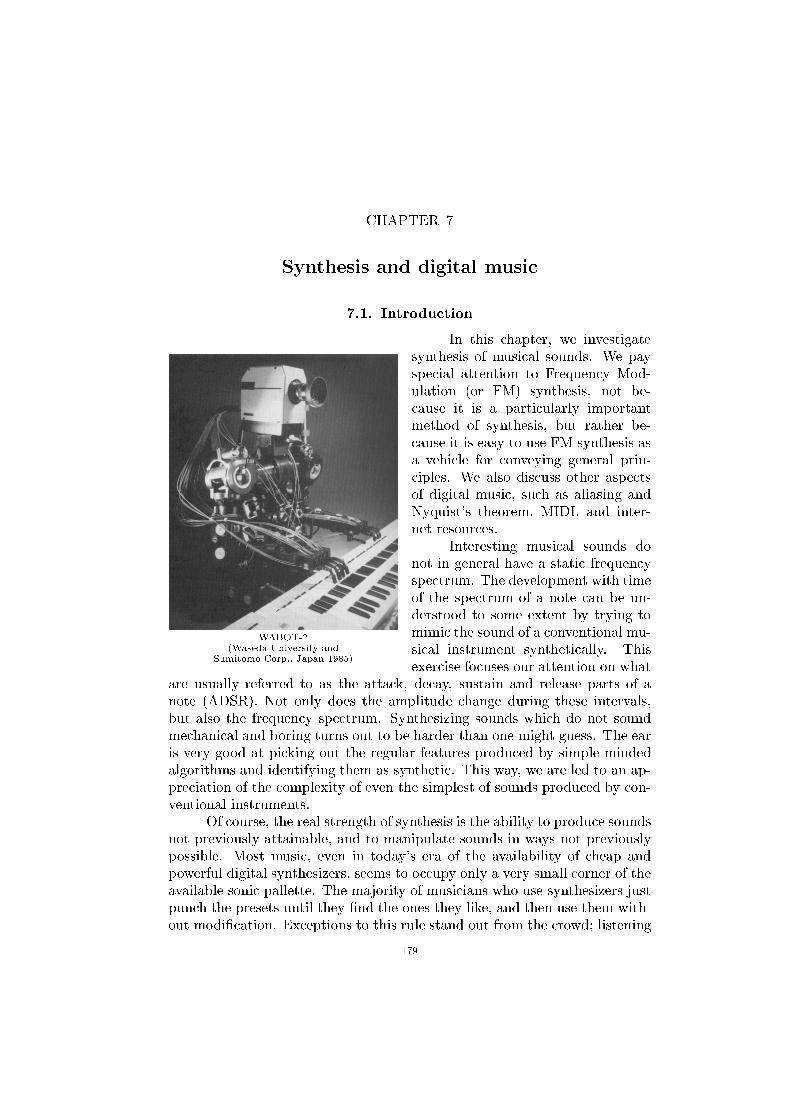
WABOT-2(Waseda University and
Sumitomo Corp., Japan 1985)
In this chapter, we investigatesynthesis of musical sounds. We payspecial attention to Frequency Mod-ulation (or FM) synthesis, not be-cause it is a particularly importantmethod of synthesis, but rather be-cause it is easy to use FM synthesis asa vehicle for conveying general prin-ciples. We also discuss other aspectsof digital music, such as aliasing andNyquist's theorem, MIDI, and inter-net resources.
Interesting musical sounds donot in general have a static frequencyspectrum. The development with timeof the spectrum of a note can be un-derstood to some extent by trying tomimic the sound of a conventional mu-sical instrument synthetically. Thisexercise focuses our attention on what
are usually referred to as the attack, decay, sustain and release parts of anote (ADSR). Not only does the amplitude change during these intervals,but also the frequency spectrum. Synthesizing sounds which do not soundmechanical and boring turns out to be harder than one might guess. The earis very good at picking out the regular features produced by simple mindedalgorithms and identifying them as synthetic. This way, we are led to an ap-preciation of the complexity of even the simplest of sounds produced by con-ventional instruments.
Of course, the real strength of synthesis is the ability to produce soundsnot previously attainable, and to manipulate sounds in ways not previouslypossible. Most music, even in today's era of the availability of cheap andpowerful digital synthesizers, seems to occupy only a very small corner of theavailable sonic pallette. The majority of musicians who use synthesizers justpunch the presets until they �nd the ones they like, and then use them with-out modi�cation. Exceptions to this rule stand out from the crowd; listening
179
180 7. SYNTHESIS AND DIGITAL MUSIC
to a recording by the Japanese synthesist Tomita, for example, one is struckimmediately by the skill expressed in the shaping of the sound.
Further listening: (See Appendix R)
Isao Tomita, Pictures at an Exhibition (Mussorgsky).
7.2. Digital signals
The commonest method of dig-ital representation of sound is aboutas simple minded as you can get. Todigitize an analog signal, the signal issampled a large number of times a sec-ond, and a binary number representsthe height of the signal at each sam-ple time. Both of these processes aresometimes referred to as quantization
(don't worry, there's no quantum me-chanics involved here), but it is impor-tant to realize that the processes areseparate, and need to be understoodseparately.
For example, the Compact Discis based on a sample rate of 44.1 KHz,or 44,100 sample points per second.1
At each sample point, a sixteen digitbinary number represents the height of the waveform at that point.
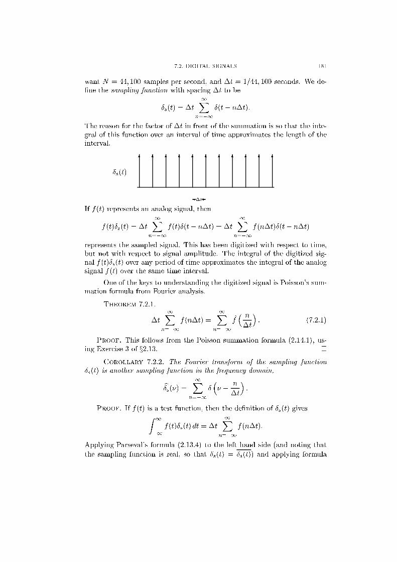
One way to represent the process of sampling a signal is as multiplica-tion by a stream of Dirac delta functions (see x2.15). Let N denote the sam-ple rate, measured in samples per second, and let �t = 1=N denote the in-terval between sample times. So for example for compact disc recording we
1It is annoying that the default sample rate for DAT (Digital Audio Tape) is 48 KHz,thereby making it diÆcult to make a digital copy on CD directly from DAT. This seemsto be the result of industry paranoia at the idea that anyone might make a digital copy ofmusic from a CD (DAT was originally designed as a consumer format, but never took o�except among the music business professionals). The excuse that the higher sample ratefor DAT gives a higher cuto� frequency and therefore better audio �delity is easily seenthrough in light of the fact that the improvement is about three quarters of a tone, whichis essentially insigni�cant.
Fortunately, the ratio 48; 000=44; 100 can be written as a product of small fractions,4=3�8=7�5=7, which suggests an easy method of digital convertion. To multiply the sam-ple rate by 4=3, for example, we use linear interpolation to quadruple the sample rate andthen omit two out of every three sample points. This gives much better �delity than con-verting to an analog signal and then back to digital.
7.2. DIGITAL SIGNALS 181
want N = 44; 100 samples per second, and �t = 1=44; 100 seconds. We de-�ne the sampling function with spacing �t to be
Æs(t) = �t
1Xn=�1
Æ(t� n�t):
The reason for the factor of �t in front of the summation is so that the inte-gral of this function over an interval of time approximates the length of theinterval.
Æs(t)
6 6 6 6 6 6 6 6 6 6 6
�-�t
If f(t) represents an analog signal, then
f(t)Æs(t) = �t
1Xn=�1
f(t)Æ(t� n�t) = �t
1Xn=�1
f(n�t)Æ(t� n�t)
represents the sampled signal. This has been digitized with respect to time,but not with respect to signal amplitude. The integral of the digitized sig-nal f(t)Æs(t) over any period of time approximates the integral of the analogsignal f(t) over the same time interval.
One of the keys to understanding the digitized signal is Poisson's sum-mation formula from Fourier analysis.
Theorem 7.2.1.
�t
1Xn=�1
f(n�t) =
1Xn=�1
f̂� n
�t
�: (7.2.1)
Proof. This follows from the Poisson summation formula (2.14.1), us-ing Exercise 3 of x2.13. �
Corollary 7.2.2. The Fourier transform of the sampling function
Æs(t) is another sampling function in the frequency domain,
bÆs(�) = 1Xn=�1
�� � n
�t
�:
Proof. If f(t) is a test function, then the de�nition of Æs(t) givesZ1
�1
f(t)Æs(t) dt = �t1X
n=�1
f(n�t):
Applying Parseval's formula (2.13.4) to the left hand side (and noting that
the sampling function is real, so that Æs(t) = Æs(t)) and applying formula
182 7. SYNTHESIS AND DIGITAL MUSIC
(7.2.1) to the right hand side, we obtainZ1
�1
f̂(�)bÆs(�) d� = 1Xn=�1
f̂� n
�t
�:
The required formula for bÆs(�) follows. �
Corollary 7.2.3. The Fourier transform of a digital signal f(t)Æs(t) is
dfÆs(�) = 1Xn=�1
f̂�� � n
�t
�which is periodic in the frequency domain, with period equal to the sampling
frequency 1=�t.
Proof. By Theorem 2.16.1(ii), we havedfÆs(�) = (f̂ � Æ̂s)(�);and by Corollary 7.2.2, this is equal toZ
1
�1
f̂(u)1X
n=�1
�� � n
�t� u�du =
1Xn=�1
f̂�� � n
�t
�: �
7.3. Nyquist's theorem
Nyquist's theorem2 states that the maximum frequency that can berepresented when digitizing an analog signal is exactly half the sampling rate.Frequencies above this limit will give rise to unwanted frequencies below theNyquist frequency of half the sampling rate.
To explain the reason for this, consider a pure sinusoidal wave with fre-quency �, for example
f(t) = A cos(2��t):
Given a sample rate of N = 1=�t samples per second, the height of the func-tion at the Mth sample is given by
f(M=N) = A cos(2��M=N):
If � is greater than N=2, say � = N=2 + �, then
f(M=N) = A cos(2�(N=2 + �)M=N)
= A cos(�M + 2��M=N)
= (�1)MA cos(2��M=N):
Changing the sign of � makes no di�erence to the outcome of this calcula-tion, so this gives exactly the same answer as the waveform with � = N=2��instead of � = N=2 + �. To put it another way, the sample points in
2Harold Nyquist, Certain topics in telegraph transmission theory, Transactions of theAmerican Institute of Electrical Engineers, April 1928. Nyquist retired from Bell Labs in1954 with about 150 patents to his name. He was renowned for his ability to take a complexproblem and produce a simple minded solution that was far superior to other approaches.
7.3. NYQUIST'S THEOREM 183
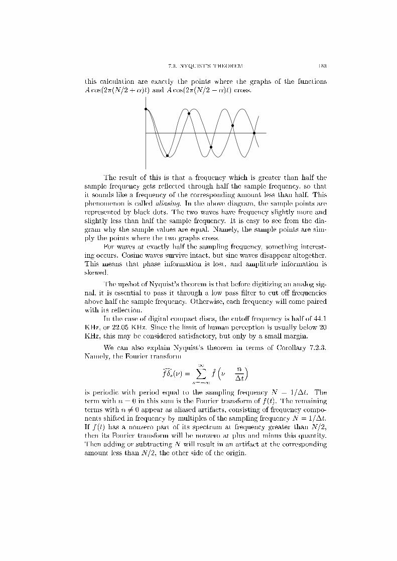
this calculation are exactly the points where the graphs of the functionsA cos(2�(N=2 + �)t) and A cos(2�(N=2 � �)t) cross.
The result of this is that a frequency which is greater than half thesample frequency gets re ected through half the sample frequency, so thatit sounds like a frequency of the corresponding amount less than half. Thisphenomenon is called aliasing. In the above diagram, the sample points arerepresented by black dots. The two waves have frequency slightly more andslightly less than half the sample frequency. It is easy to see from the dia-gram why the sample values are equal. Namely, the sample points are sim-ply the points where the two graphs cross.
For waves at exactly half the sampling frequency, something interest-ing occurs. Cosine waves survive intact, but sine waves disappear altogether.This means that phase information is lost, and amplitude information isskewed.
The upshot of Nyquist's theorem is that before digitizing an analog sig-nal, it is essential to pass it through a low pass �lter to cut o� frequenciesabove half the sample frequency. Otherwise, each frequency will come pairedwith its re ection.
In the case of digital compact discs, the cuto� frequency is half of 44.1KHz, or 22.05 KHz. Since the limit of human perception is usually below 20KHz, this may be considered satisfactory, but only by a small margin.
We can also explain Nyquist's theorem in terms of Corollary 7.2.3.Namely, the Fourier transform
dfÆs(�) = 1Xn=�1
f̂�� � n
�t
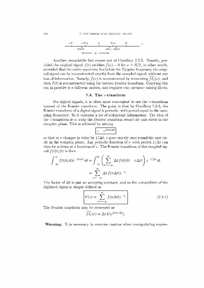
�is periodic with period equal to the sampling frequency N = 1=�t. Theterm with n = 0 in this sum is the Fourier transform of f(t). The remainingterms with n 6= 0 appear as aliased artifacts, consisting of frequency compo-nents shifted in frequency by multiples of the sampling frequency N = 1=�t.If f(t) has a nonzero part of its spectrum at frequency greater than N=2,then its Fourier transform will be nonzero at plus and minus this quantity.Then adding or subtracting N will result in an artifact at the correspondingamount less than N=2, the other side of the origin.
184 7. SYNTHESIS AND DIGITAL MUSIC
�N �N=2 0 N=2 N
signalsignal alias
� -N
�
Another remarkable fact comes out of Corollary 7.2.3. Namely, pro-vided the original signal f(t) satis�es f̂(�) = 0 for � � N=2, in other words,provided that the entire spectrum lies below the Nyquist frequency, the origi-nal signal can be reconstructed exactly from the sampled signal, without any
loss of information. Namely, f̂(�) is reconstructed by truncatingdfÆs(�), andthen f(t) is reconstructed using the inverse Fourier transform. Carrying thisout in practise is a di�erent matter, and requires very accurate analog �lters.
7.4. The z-transform
For digital signals, it is often more convenient to use the z-transforminstead of the Fourier transform. The point is that by Corollary 7.2.3, theFourier transform of a digital signal is periodic, with period equal to the sam-pling frequency. So it contains a lot of redundant information. The idea ofthe z-transform is to wrap the Fourier transform round the unit circle in thecomplex plane. This is achieved by setting
z = e2�i��t
so that as � changes in value by 1=�t, z goes exactly once round the unit cir-cle in the complex plane. Any periodic function of � with period 1=�t canthen be written as a function of z. The Fourier transform of the sampled sig-nal f(t)Æs(t) is thenZ
1
�1
f(t)Æs(t)e�2�i�t dt =
Z1
�1
1X
n=�1
�t f(t)Æ(t� n�t)
!z�t=�t dt
=1X
n=�1
�t f(n�t)z�n:
The factor of �t is just an annoying constant, and so the z-transform of thedigitized signal is simply de�ned as
F (z) =1X
n=�1
f(n�t)z�n: (7.4.1)
The Fourier transform may be recovered asdfÆs(�) = �t F (e2�i��t):
Warning. It is necessary to exercise caution when manipulating expres-
7.5. DIGITAL FILTERS 185
sions like equation (7.4.1), because of Euler's joke. Here's the joke. Considera signal which is constant over all time,
F (z) = � � � + z2 + z + 1 + z�1 + z�2 + : : :
=
1Xn=�1
zn:
Divide this in�nite sum up into two parts, and sum them separately.
F (z) = (� � � + z2 + z + 1) + (z�1 + z�2 + : : : )
=1
1� z+
z�1
1� z�1
=1
1� z+
1
z � 1= 0:
This is clearly nonsense. The problem is that the �rst parenthesized sumonly converges for jzj > 1, while the second sum only converges for jzj < 1.So there is no value of z for which both sums make sense simultaneously.
The resolution of this problem is only to allow signals with some �nitestarting point. So we assume that f(n�t) = 0 for all large enough negativevalues of n. Then the sum converges inside the unit circle in the complexplane.
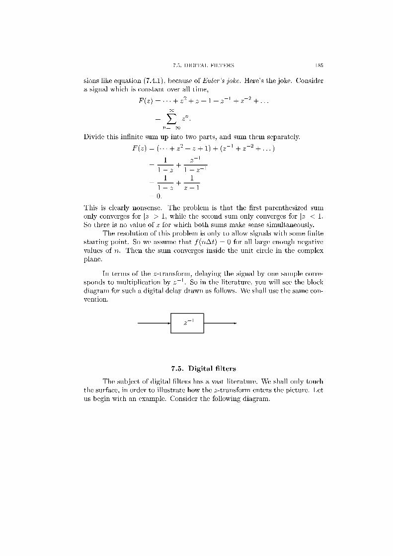
In terms of the z-transform, delaying the signal by one sample corre-sponds to multiplication by z�1. So in the literature, you will see the blockdiagram for such a digital delay drawn as follows. We shall use the same con-vention.
z�1- -
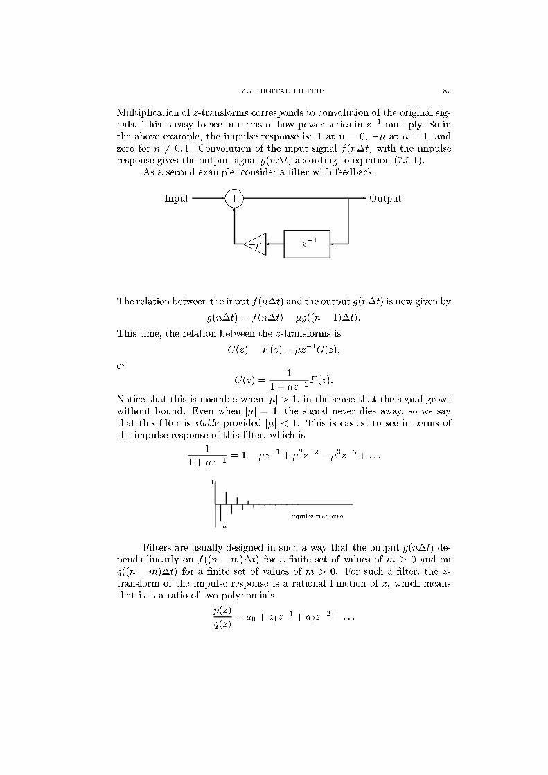
7.5. Digital �lters
The subject of digital �lters has a vast literature. We shall only touchthe surface, in order to illustrate how the z-transform enters the picture. Letus begin with an example. Consider the following diagram.
186 7. SYNTHESIS AND DIGITAL MUSIC
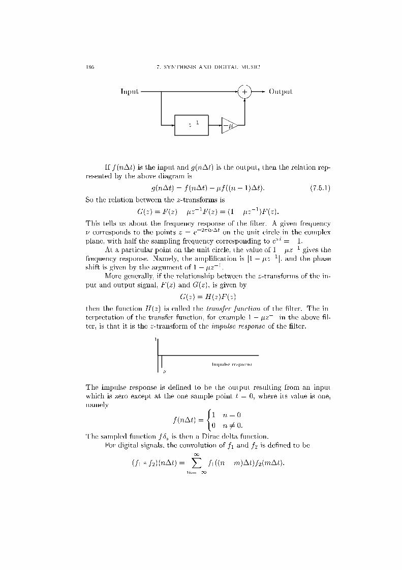
z�1- -���
HHH��
6����+- -Input Output
If f(n�t) is the input and g(n�t) is the output, then the relation rep-resented by the above diagram is
g(n�t) = f(n�t)� �f((n� 1)�t): (7.5.1)
So the relation between the z-transforms is
G(z) = F (z) � �z�1F (z) = (1� �z�1)F (z):
This tells us about the frequency response of the �lter. A given frequency� corresponds to the points z = e�2�i��t on the unit circle in the complexplane, with half the sampling frequency corresponding to e�i = �1.
At a particular point on the unit circle, the value of 1��z�1 gives thefrequency response. Namely, the ampli�cation is j1 � �z�1j, and the phaseshift is given by the argument of 1� �z�1.
More generally, if the relationship between the z-transforms of the in-put and output signal, F (z) and G(z), is given by
G(z) = H(z)F (z)
then the function H(z) is called the transfer function of the �lter. The in-terpretation of the transfer function, for example 1 � �z�1 in the above �l-ter, is that it is the z-transform of the impulse response of the �lter.
1
��
Impulse response
The impulse response is de�ned to be the output resulting from an inputwhich is zero except at the one sample point t = 0, where its value is one,namely
f(n�t) =
(1 n = 0
0 n 6= 0:
The sampled function fÆs is then a Dirac delta function.For digital signals, the convolution of f1 and f2 is de�ned to be
(f1 � f2)(n�t) =1X
m=�1
f1((n�m)�t)f2(m�t):
7.5. DIGITAL FILTERS 187
Multiplication of z-transforms corresponds to convolution of the original sig-nals. This is easy to see in terms of how power series in z�1 multiply. So inthe above example, the impulse response is: 1 at n = 0, �� at n = 1, andzero for n 6= 0; 1. Convolution of the input signal f(n�t) with the impulseresponse gives the output signal g(n�t) according to equation (7.5.1).
As a second example, consider a �lter with feedback.
z�1 ��HH
H�����
6����+- -Input Output
The relation between the input f(n�t) and the output g(n�t) is now given by
g(n�t) = f(n�t)� �g((n� 1)�t):
This time, the relation between the z-transforms is
G(z) = F (z)� �z�1G(z);
or
G(z) =1
1 + �z�1F (z):
Notice that this is unstable when j�j > 1, in the sense that the signal growswithout bound. Even when j�j = 1, the signal never dies away, so we saythat this �lter is stable provided j�j < 1. This is easiest to see in terms ofthe impulse response of this �lter, which is
1
1 + �z�1= 1� �z�1 + �2z�2 � �3z�3 + : : :
1
��
Impulse response
Filters are usually designed in such a way that the output g(n�t) de-pends linearly on f((n �m)�t) for a �nite set of values of m � 0 and ong((n �m)�t) for a �nite set of values of m > 0. For such a �lter, the z-transform of the impulse response is a rational function of z, which meansthat it is a ratio of two polynomials
p(z)
q(z)= a0 + a1z
�1 + a2z�2 + : : :
188 7. SYNTHESIS AND DIGITAL MUSIC
The coeÆcients a0; a1; a2; : : : are the values of the impulse response at t = 0,t = �t, t = 2�t, . . .
The coeÆcients an tend to zero as n tends to in�nity, if and only if thepoles � of p(z)=q(z) satisfy j�j < 1. This can be seen in terms of the com-plex partial fraction expansion of the function p(z)=q(z).
The location of the poles inside the unit circle has a great deal of ef-fect on the frequency response of the �lter. If there is a pole near the bound-ary, it will cause a local maximum in the frequency response, which is calleda resonance. The frequency is given in terms of the argument of the positionof the pole by
� = (sample rate)� (argument)=2�:
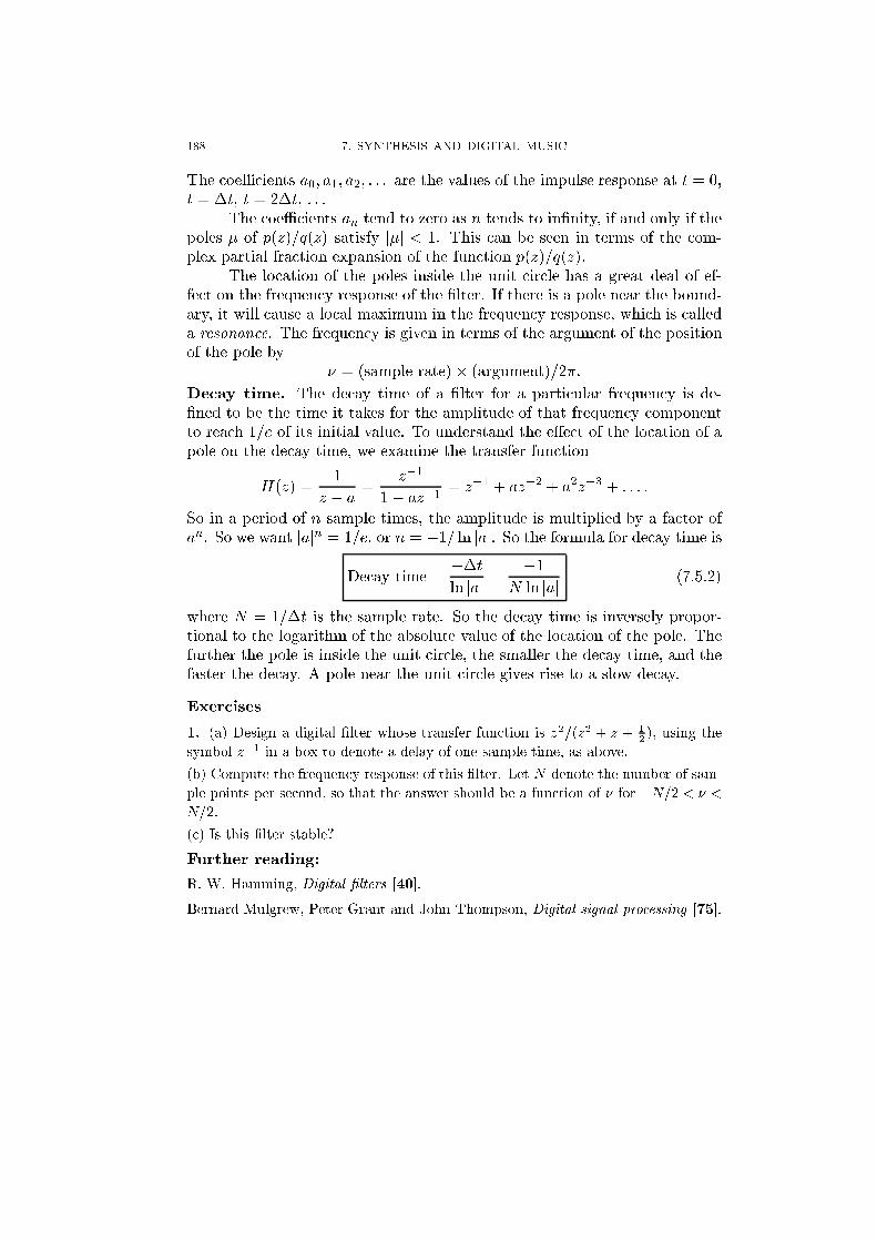
Decay time. The decay time of a �lter for a particular frequency is de-�ned to be the time it takes for the amplitude of that frequency componentto reach 1=e of its initial value. To understand the e�ect of the location of apole on the decay time, we examine the transfer function
H(z) =1
z � a=
z�1
1� az�1= z�1 + az�2 + a2z�3 + : : : :
So in a period of n sample times, the amplitude is multiplied by a factor ofan. So we want jajn = 1=e, or n = �1= ln jaj. So the formula for decay time is
Decay time =��tln jaj =
�1N ln jaj (7.5.2)
where N = 1=�t is the sample rate. So the decay time is inversely propor-tional to the logarithm of the absolute value of the location of the pole. Thefurther the pole is inside the unit circle, the smaller the decay time, and thefaster the decay. A pole near the unit circle gives rise to a slow decay.
Exercises
1. (a) Design a digital �lter whose transfer function is z2=(z2 + z + 12 ), using the
symbol z�1 in a box to denote a delay of one sample time, as above.
(b) Compute the frequency response of this �lter. Let N denote the number of sam-
ple points per second, so that the answer should be a function of � for �N=2 < � <
N=2.
(c) Is this �lter stable?
Further reading:
R. W. Hamming, Digital �lters [40].
Bernard Mulgrew, Peter Grant and John Thompson, Digital signal processing [75].
7.7. ENVELOPES AND LFOS 189
7.6. The discrete Fourier transform
The discrete Fourier transform is
F (k) =1
N
N�1Xn=0
f(n)e�2�ink=N
f(n) =
N�1Xk=0
F (k)e2�ikn=N :
The fast Fourier transform is a way to compute the discrete Fourier trans-form using 2N log2N operations rather than N2. The number of samplepoints N has to be a power of two for it to be this eÆcient, but the algo-rithm works for any highly composite value of N .
Further reading:
G. D. Bergland, A guided tour of the fast Fourier transform, IEEE Spectrum 6(1969), 41{52.
James W. Cooley and John W. Tukey, An algorithm for the machine calculation of
complex Fourier series, Math. of Computation 19 (1965), 297{301. This is usually
regarded as the original article announcing the fast Fourier transform as a practical
algorithm.
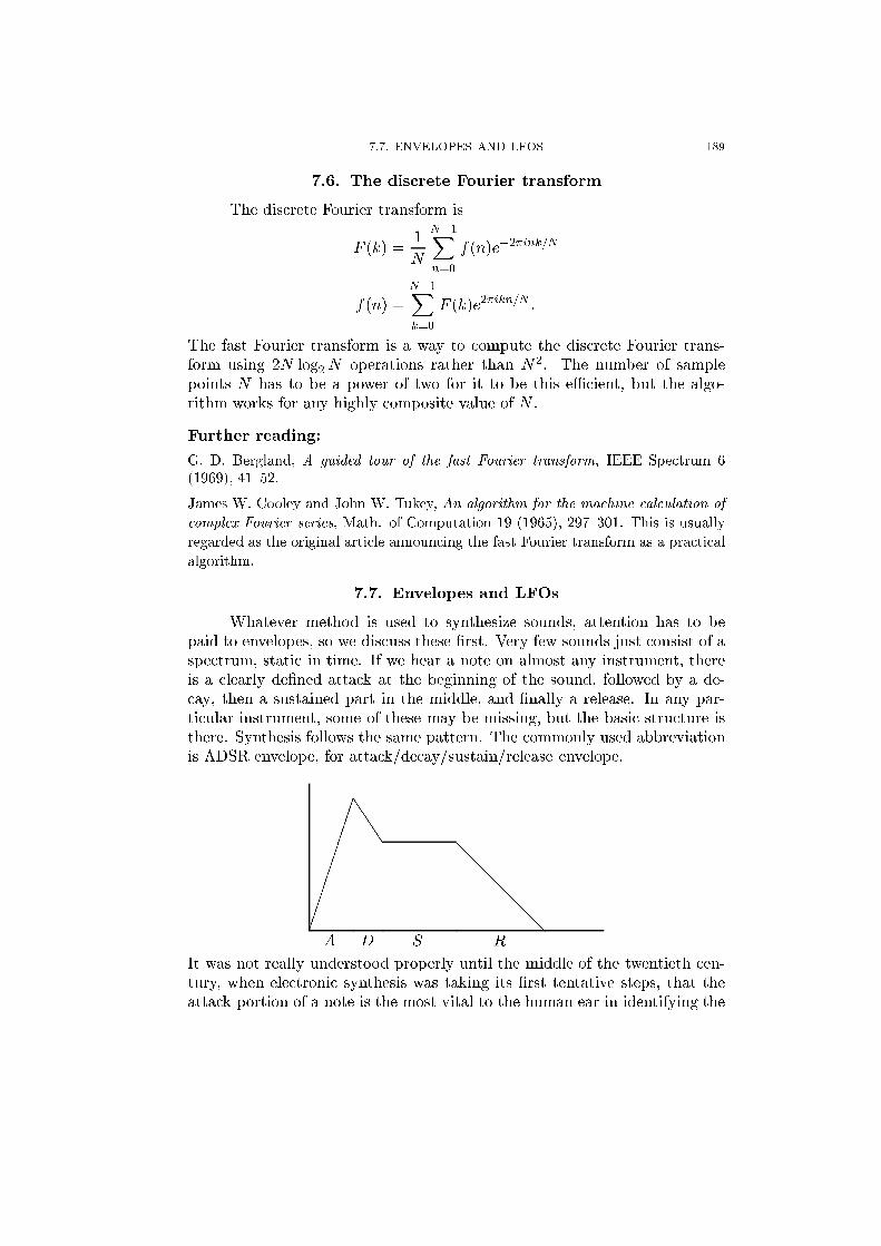
7.7. Envelopes and LFOs
Whatever method is used to synthesize sounds, attention has to bepaid to envelopes, so we discuss these �rst. Very few sounds just consist of aspectrum, static in time. If we hear a note on almost any instrument, thereis a clearly de�ned attack at the beginning of the sound, followed by a de-cay, then a sustained part in the middle, and �nally a release. In any par-ticular instrument, some of these may be missing, but the basic structure isthere. Synthesis follows the same pattern. The commonly used abbreviationis ADSR envelope, for attack/decay/sustain/release envelope.
����������JJJJ
@@@@@@
A D S R
It was not really understood properly until the middle of the twentieth cen-tury, when electronic synthesis was taking its �rst tentative steps, that theattack portion of a note is the most vital to the human ear in identifying the
190 7. SYNTHESIS AND DIGITAL MUSIC
instrument. The transients at the beginning are much more di�erent fromone instrument to another than the steady part of the note.
On a typical synthesizer, there are a number of envelope generators.Each one determines how the amplitude of the output of some component ofthe system varies with time. It is important to understand that amplitude ofthe �nal signal is not the only attribute which is assigned an envelope. Forexample, when a bell sounds, initially the frequency spectrum is very rich,but many of the partials die away very quickly leaving a purer sound. Mim-icking this sort of behavior using FM synthesis turns out to be relatively easy,by assigning an envelope to a modulating signal, which controls timbre. Weshall discuss this further when we discuss FM synthesis, but for the momentwe note that aspects of timbre are often controlled with an envelope genera-tor. When the synthesizer is controlled by a keyboard, as is often the case,it is usual to arrange that depressing a key initiates the attack, and releas-ing the key initiates the release portion of the envelope.
An envelope generator produces an envelope whose shape is determinedby a number of programmable parameters. These parameters are usuallygiven in terms of levels and rates. Here is an example of how an envelopemight work in a typical keyboard synthesizer or other MIDI controlled en-vironment. Level 0 is the level of the envelope at the \key on" event. Rate1 then determines how fast the level changes, until it reaches level 1. Thenit switches to rate 2 until level 2 is reached, and then rate 3 until level 3 isreached. Level 3 is then in e�ect until the \key o�" event, when rate 4 takese�ect until level 4 is reached. Finally, level 4 is the same as level 0, so thatwe are ready for the next \key on" event. In this example, there are twoseparate components to the decay phase of the envelope. Some synthesizersmake do with only one, and some have even more.
Similar in concept to the envelope is the low frequency oscillator orLFO. This produces an output which is usually in the range 0.1{20 Hz, andwhose waveform is usually something like triangle, sawtooth (up or down),sine, square or random. The LFO is used to produce repeating changes insome controllable parameter. Examples include pitch control for vibrato, andamplitude or timbre control for tremolo. The LFO can also be used to con-trol less obvious parameters such as the cuto� and resonance of a �lter, orthe pulse width of a square wave (pulse width modulation, or PWM), seeExercise 6 in x2.4.
The parameters associated with an LFO are rate (or frequency), depth(or amplitude), waveform, and attack time. Attack time is used when the ef-fect is to be introduced gradually at the beginning of the note.
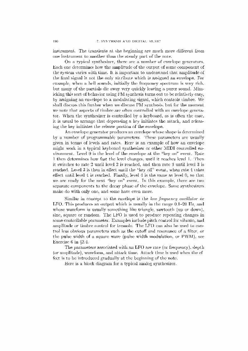
Here is a block diagram for a typical analog synthesizer.
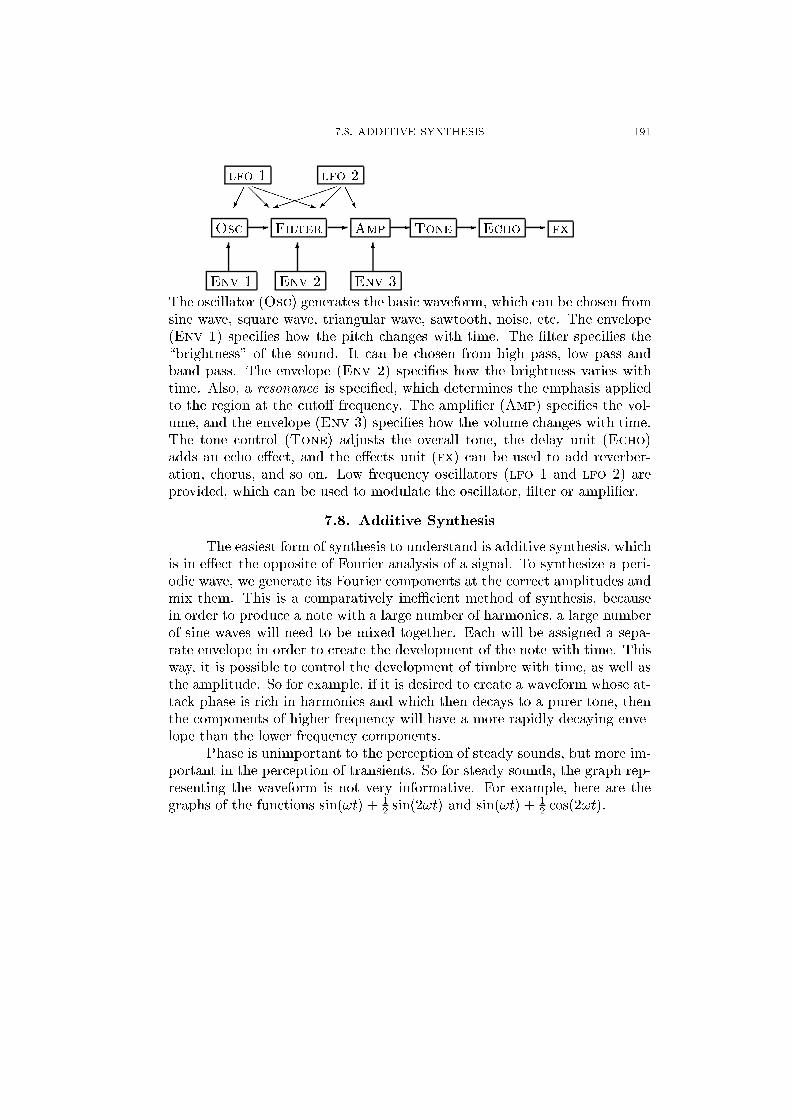
7.8. ADDITIVE SYNTHESIS 191
Osc - Filter - Amp - Tone - Echo - fx
Env 1
6
Env 2
6
Env 3
6
lfo 1 lfo 2
���@@RPPPPPq
�����)��
AAU
The oscillator (Osc) generates the basic waveform, which can be chosen fromsine wave, square wave, triangular wave, sawtooth, noise, etc. The envelope(Env 1) speci�es how the pitch changes with time. The �lter speci�es the\brightness" of the sound. It can be chosen from high pass, low pass andband pass. The envelope (Env 2) speci�es how the brightness varies withtime. Also, a resonance is speci�ed, which determines the emphasis appliedto the region at the cuto� frequency. The ampli�er (Amp) speci�es the vol-ume, and the envelope (Env 3) speci�es how the volume changes with time.The tone control (Tone) adjusts the overall tone, the delay unit (Echo)adds an echo e�ect, and the e�ects unit (fx) can be used to add reverber-ation, chorus, and so on. Low frequency oscillators (lfo 1 and lfo 2) areprovided, which can be used to modulate the oscillator, �lter or ampli�er.
7.8. Additive Synthesis
The easiest form of synthesis to understand is additive synthesis, whichis in e�ect the opposite of Fourier analysis of a signal. To synthesize a peri-odic wave, we generate its Fourier components at the correct amplitudes andmix them. This is a comparatively ineÆcient method of synthesis, becausein order to produce a note with a large number of harmonics, a large numberof sine waves will need to be mixed together. Each will be assigned a sepa-rate envelope in order to create the development of the note with time. Thisway, it is possible to control the development of timbre with time, as well asthe amplitude. So for example, if it is desired to create a waveform whose at-tack phase is rich in harmonics and which then decays to a purer tone, thenthe components of higher frequency will have a more rapidly decaying enve-lope than the lower frequency components.
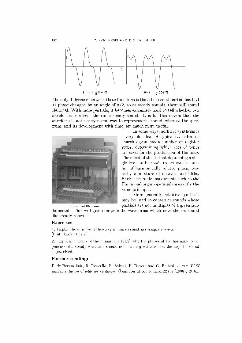
Phase is unimportant to the perception of steady sounds, but more im-portant in the perception of transients. So for steady sounds, the graph rep-resenting the waveform is not very informative. For example, here are thegraphs of the functions sin(!t) + 1
2 sin(2!t) and sin(!t) + 12 cos(2!t).
192 7. SYNTHESIS AND DIGITAL MUSIC
t
sin t+ 12 sin 2t
t
sin t+ 12 cos 2t
The only di�erence between these functions is that the second partial has hadits phase changed by an angle of �=2, so as steady sounds, these will soundidentical. With more partials, it becomes extremely hard to tell whether twowaveforms represent the same steady sound. It is for this reason that thewaveform is not a very useful way to represent the sound, whereas the spec-trum, and its development with time, are much more useful.
Hammond B3 organ
In some ways, additive synthesis isa very old idea. A typical cathedral orchurch organ has a number of registerstops, determining which sets of pipesare used for the production of the note.The e�ect of this is that depressing a sin-gle key can be made to activate a num-ber of harmonically related pipes, typ-ically a mixture of octaves and �fths.Early electronic instruments such as theHammond organ operated on exactly thesame principle.
More generally, additive synthesismay be used to construct sounds whosepartials are not multiples of a given fun-
damental. This will give non-periodic waveforms which nevertheless soundlike steady tones.
Exercises
1. Explain how to use additive synthesis to construct a square wave.[Hint: Look at x2.2]
2. Explain in terms of the human ear (x1.2) why the phases of the harmonic com-
ponents of a steady waveform should not have a great e�ect on the way the sound
is perceived.
Further reading:
F. de Bernardinis, R. Roncella, R. Saletti, P. Terreni and G. Bertini, A new VLSI
implementation of additive synthesis, Computer Music Journal 22 (3) (1998), 49{61.
7.9. PHYSICAL MODELING 193
7.9. Physical modeling
The idea of physical modeling is to take a physical system such as amusical instrument, and to mimic it digitally. We give one simple example toillustrate the point. We examined the wave equation for the vibrating stringin x3.1, and found d'Alembert's general solution
y = f(x+ ct) + g(x� ct):
Given that time is quantized with sample points at spacing �t, it makes senseto quantize the position along the string at intervals of �x = c�t. Then attime n�t and position m�x, the value of y is
y = f(m�x+ nc�t) + g(m�x� nc�t)
= f((m+ n)c�t) + g((m � n)c�t):
To simplify the notation, we write
y�(n) = f(nc�t); y+(n) = g(nc�t)
so that y� and y+ represent the parts of the wave traveling left, respectivelyright along the string. Then at time n�t and position m�x we have
y = y�(m+ n) + y+(m� n):
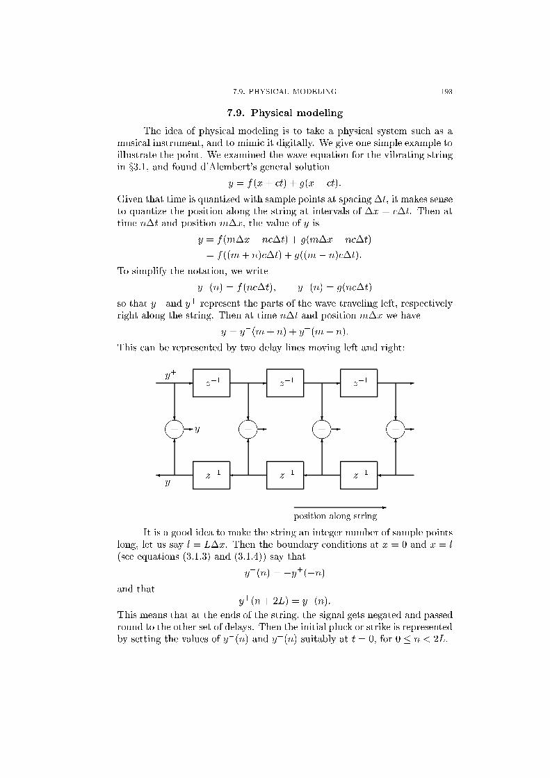
This can be represented by two delay lines moving left and right:
- - - -
� � � �
6 6 6 6
? ? ? ?
����
����
����
����
+ + + +- - - -
z�1 z�1 z�1
z�1 z�1 z�1
-position along string
y+
y
y�
It is a good idea to make the string an integer number of sample pointslong, let us say l = L�x. Then the boundary conditions at x = 0 and x = l(see equations (3.1.3) and (3.1.4)) say that
y�(n) = �y+(�n)and that
y+(n+ 2L) = y+(n):
This means that at the ends of the string, the signal gets negated and passedround to the other set of delays. Then the initial pluck or strike is representedby setting the values of y�(n) and y+(n) suitably at t = 0, for 0 � n < 2L.
194 7. SYNTHESIS AND DIGITAL MUSIC
Thinking in terms of digital �lters, the z-transform of the y+ signal
Y +(z) = y+(0) + y+(1)z�1 + y+(2)z�2 + : : :
satis�es
Y +(z) = z�2LY +(z) + (y+(0) + y+(1)z�1 + � � �+ y+(2L� 1))
or
Y +(z) =y+(0)z2L + y+(1)z2L�1 + � � � + y+(2L� 1)z
z2L � 1:
The poles are equally spaced on the unit circle, so the resonant frequenciesare multiples of N=2L, where N is the sample frequency. Since the poles areactually on the unit circle, the resonant frequencies never decay.
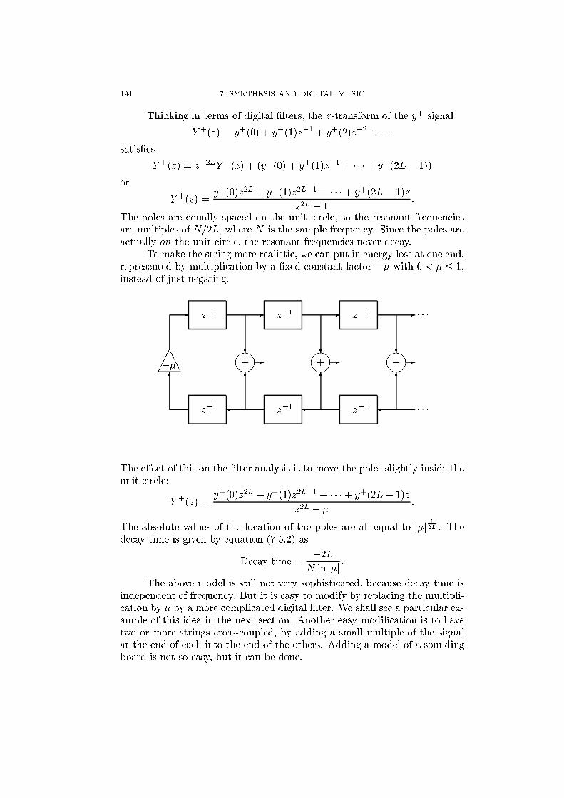
To make the string more realistic, we can put in energy loss at one end,represented by multiplication by a �xed constant factor �� with 0 < � � 1,instead of just negating.
- - - . . .
� � � . . .
6 6 6 6
? ? ?
����
����
����
+ + +�����AAA
-
- - -
z�1 z�1 z�1
z�1 z�1 z�1
The e�ect of this on the �lter analysis is to move the poles slightly inside theunit circle:
Y +(z) =y+(0)z2L + y+(1)z2L�1 + � � � + y+(2L� 1)z
z2L � �:
The absolute values of the location of the poles are all equal to j�j 12L . Thedecay time is given by equation (7.5.2) as
Decay time =�2L
N ln j�j :
The above model is still not very sophisticated, because decay time isindependent of frequency. But it is easy to modify by replacing the multipli-cation by � by a more complicated digital �lter. We shall see a particular ex-ample of this idea in the next section. Another easy modi�cation is to havetwo or more strings cross-coupled, by adding a small multiple of the signalat the end of each into the end of the others. Adding a model of a soundingboard is not so easy, but it can be done.
7.10. THE KARPLUS{STRONG ALGORITHM 195
Further reading:
M. Laurson, C. Erkut, V. V�alim�aki and M. Kuuskankare, Methods for modeling re-
alistic playing in acoustic guitar synthesis, Computer Music Journal 25 (3) (2001),38{49.
Julius O. Smith III, Physical modeling using digital waveguides, Computer MusicJournal 16 (4) (1992), 74{87.
Julius O. Smith III, Acoustic modeling, appears as article 7 in Roads et al [94], pages
221{263.
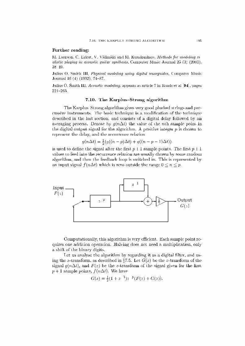
7.10. The Karplus{Strong algorithm
The Karplus{Strong algorithm gives very good plucked strings and per-cussive instruments. The basic technique is a modi�cation of the techniquedescribed in the last section, and consists of a digital delay followed by anaveraging process. Denote by g(n�t) the value of the nth sample point inthe digital output signal for the algorithm. A positive integer p is chosen torepresent the delay, and the recurrence relation
g(n�t) = 12 (g((n� p)�t) + g((n� p� 1)�t))
is used to de�ne the signal after the �rst p+1 sample points. The �rst p+1values to feed into the recurrence relation are usually chosen by some randomalgorithm, and then the feedback loop is switched in. This is represented byan input signal f(n�t) which is zero outside the range 0 � n � p.
6
?
Input
F (z)
����- z�p -
- z�1
?
����+ -
���
HHH12
- Output
G(z)
Computationally, this algorithm is very eÆcient. Each sample point re-quires one addition operation. Halving does not need a multiplication, onlya shift of the binary digits.
Let us analyse the algorithm by regarding it as a digital �lter, and us-ing the z-transform, as described in x7.5. Let G(z) be the z-transform of thesignal g(n�t), and F (z) be the z-transform of the signal given for the �rstp+ 1 sample points, f(n�t). We have
G(z) = 12 (1 + z�1)z�p(F (z) +G(z)):
196 7. SYNTHESIS AND DIGITAL MUSIC
This gives
G(z) =z + 1
2zp+1 � z � 1F (z);
and so the z-transform of the impulse response is (z + 1)=(2zp+1 � z � 1).The poles are the solutions of the equation
2zp+1 � z � 1 = 0:
These are roughly equally spaced around the unit circle, at amplitude justless than one. The solution with smallest argument corresponds to the fun-damental of the vibration, with argument roughly 2�=(p + 1
2). A more pre-cise analysis is given in x7.11.
The e�ect of this is a plucked string sound with pitch determined bythe formula
pitch = (sample rate)=(p+ 12):
Since p is constrained to be an integer, this restricts the possible frequenciesof the resulting sound in terms of the sample rate. Changing the value of pwithout introducing a new inital values results in a slur, or tie between notes.
A simple modi�cation of the algorithm gives drumlike sounds. Namely,a number b is chosen with 0 � b � 1, and
g(n�t) =
(+12(g((n� p)�t) + g((n� p� 1)�t) with probability b
�12(g((n� p)�t) + g((n� p� 1)�t)) with probability 1� b:
The parameter b is called the blend factor. Taking b = 1 gives the originalplucked string sound. The value b = 1
2 gives a drumlike sound. With b = 0,the period is doubled and only odd harmonics result. This gives some inter-esting sounds, and at high pitches this gives what Karplus and Strong de-scribe as a plucked bottle sound.
Another variation described by Karplus and Strong is what they calldecay stretching. In this version, the recurrence relation
g(n�t) =
(g((n� p)�t) with probability 1� �12(g((n � p)�t) + g((n� p� 1)�t)) with probability �:
The stretch factor for this version is 1=�, and the pitch is given by
pitch = (sample rate)=(p+ �2 ):
Setting � = 0 gives a non-decaying periodic signal, while setting � = 1 givesthe original algorithm described above.
There are obviously a lot of variations on these algorithms, and manyof them give interesting sounds.
7.11. Filter analysis for the Karplus{Strong algorithm
We saw in the last section that in order to understand the Karplus{Strong algorithm in its simplest form, we need to locate the zeros of the poly-nomial 2zp+1 � z � 1, where p is a positive integer. In order to do this, we
7.11. FILTER ANALYSIS FOR THE KARPLUS{STRONG ALGORITHM 197
begin by rewriting the equation as
2zp+1
2 = z1
2 + z�1
2 :
Since we expect z to have absolute value close to one, the imaginary part ofz1
2 + z�1
2 will be very small. If we ignore this imaginary part, then the nthzero of the polynomial around the unit circle will have argument equal to2n�=(p+ 1
2 ). So we write
z = (1� ")e2n�i=(p+1
2)
and calculate ", ignoring terms in "2 and higher powers. Already from theform of this approximation, we see that the resonant frequency correspond-ing to the nth pole is equal to nN=(p+ 1
2 ), where N is the sample frequency.This means that the di�erent resonant frequencies are at multiples of a fun-damental frequency of N=(p + 1
2 ).We have
2zp+1
2 = 2(1� ")p+1
2 � 2� 2(p+ 12)";
and
z12 + z�
12 = (1� ")
12 en�i=(p+
12) + (1� ")�
12 e�n�i=(p+
12)
� (1� 12")(1 +
12 i(
2n�p+ 1
2
)� 18(
2n�p+ 1
2
)2)
+ (1 + 12")(1 � 1
2 i(2n�p+ 1
2
)� 18(
2n�p+ 1
2
)2)
� 2� � n�p+ 1
2
�2+ 1
2 i"(2n�p+ 1
2
):
So equating the real parts, we �nd that the approximate value of " is
" � n2�2
2(p+ 12 )3:
Using the approximation ln(1� ") � �", equation (7.5.2) gives
Decay time � 2(p+ 12)3
Nn2�2
where N is the sample rate. This means that the lower harmonics are decay-ing more slowly than the higher harmonics, in accordance with the behaviorof a plucked string.
Further reading:
D. A. Ja�e and J. O. Smith III, Extensions of the Karplus{Strong plucked string
algorithm, Computer Music Journal 7 (2) (1983), 56{69. Reprinted in Roads [92],481{494.
M. Karjalainen, V. V�alim�aki and T. Tolonen, Plucked-string models: From the
Karplus{Strong algorithm to digital waveguides and beyond, Computer Music Jour-nal 22 (3) (1998), 17{32.
K. Karplus and A. Strong, Digital synthesis of plucked string and drum timbres,Computer Music Journal 7 (2) (1983), 43{55. Reprinted in Roads [92], 467{479.
F. R. Moore, Elements of computer music [72], page 279.
198 7. SYNTHESIS AND DIGITAL MUSIC
C. Roads, The computer music tutorial [93], page 293.
C. Sullivan, Extending the Karplus{Strong plucked-string algorithm to synthesize
electric guitar timbres with distortion and feedback, Computer Music Journal 14 (3),
26{37.
7.12. Amplitude and frequency modulation
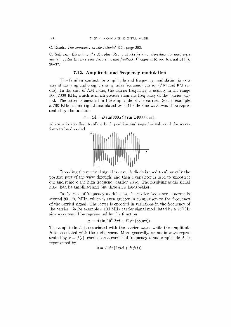
The familiar context for amplitude and frequency modulation is as away of carrying audio signals on a radio frequency carrier (AM and FM ra-dio). In the case of AM radio, the carrier frequency is usually in the range500{2000 KHz, which is much greater than the frequency of the carried sig-nal. The latter is encoded in the amplitude of the carrier. So for examplea 700 KHz carrier signal modulated by a 440 Hz sine wave would be repre-sented by the function
x = (A+B sin(880�t)) sin(1400000�t);
where A is an o�set to allow both positive and negative values of the wave-form to be decoded.
t
x
Decoding the received signal is easy. A diode is used to allow only thepositive part of the wave through, and then a capacitor is used to smooth itout and remove the high frequency carrier wave. The resulting audio signalmay then be ampli�ed and put through a loudspeaker.
In the case of frequency modulation, the carrier frequency is normallyaround 90{120 MHz, which is even greater in comparison to the frequencyof the carried signal. The latter is encoded in variations in the frequency ofthe carrier. So for example a 100 MHz carrier signal modulated by a 440 Hzsine wave would be represented by the function
x = A sin(108:2�t+B sin(880�t)):
The amplitude A is associated with the carrier wave, while the amplitudeB is associated with the audio wave. More generally, an audio wave repre-sented by x = f(t), carried on a carrier of frequency � and amplitude A, isrepresented by
x = A sin(2��t+Bf(t)):
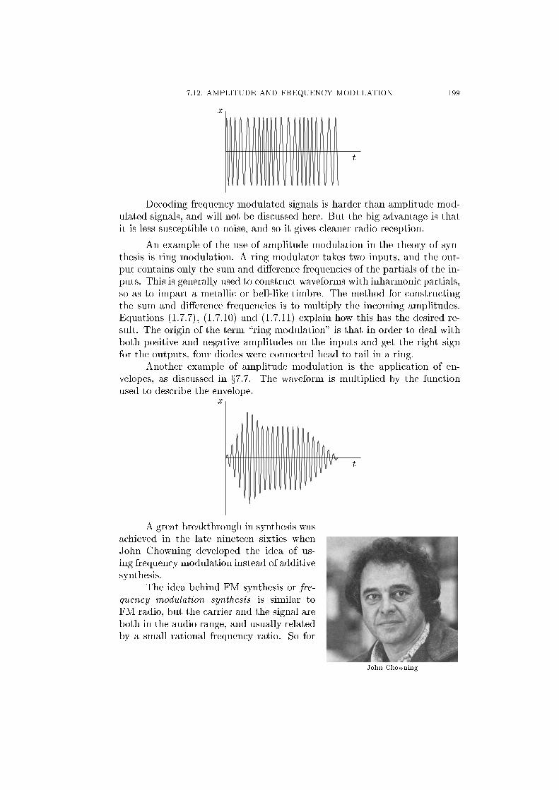
7.12. AMPLITUDE AND FREQUENCY MODULATION 199
t
x
Decoding frequency modulated signals is harder than amplitude mod-ulated signals, and will not be discussed here. But the big advantage is thatit is less susceptible to noise, and so it gives cleaner radio reception.
An example of the use of amplitude modulation in the theory of syn-thesis is ring modulation. A ring modulator takes two inputs, and the out-put contains only the sum and di�erence frequencies of the partials of the in-puts. This is generally used to construct waveforms with inharmonic partials,so as to impart a metallic or bell-like timbre. The method for constructingthe sum and di�erence frequencies is to multiply the incoming amplitudes.Equations (1.7.7), (1.7.10) and (1.7.11) explain how this has the desired re-sult. The origin of the term \ring modulation" is that in order to deal withboth positive and negative amplitudes on the inputs and get the right signfor the outputs, four diodes were connected head to tail in a ring.
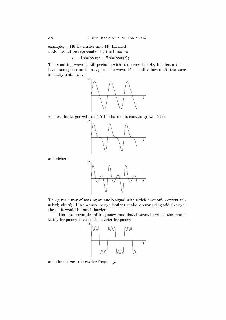
Another example of amplitude modulation is the application of en-velopes, as discussed in x7.7. The waveform is multiplied by the functionused to describe the envelope.
t
x
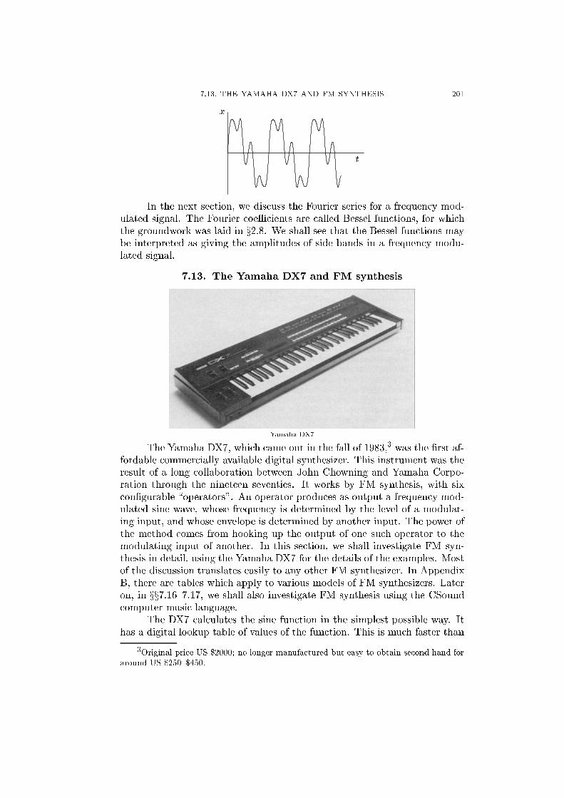
John Chowning
A great breakthrough in synthesis wasachieved in the late nineteen sixties whenJohn Chowning developed the idea of us-ing frequency modulation instead of additivesynthesis.
The idea behind FM synthesis or fre-
quency modulation synthesis is similar toFM radio, but the carrier and the signal areboth in the audio range, and usually relatedby a small rational frequency ratio. So for
200 7. SYNTHESIS AND DIGITAL MUSIC
example, a 440 Hz carrier and 440 Hz mod-ulator would be represented by the function
x = A sin(880�t +B sin(880�t)):
The resulting wave is still periodic with frequency 440 Hz, but has a richerharmonic spectrum than a pure sine wave. For small values of B, the waveis nearly a sine wave
t
x
whereas for larger values of B the harmonic content grows richer
t
x
and richer.
t
x
This gives a way of making an audio signal with a rich harmonic content rel-atively simply. If we wanted to synthesize the above wave using additive syn-thesis, it would be much harder.
Here are examples of frequency modulated waves in which the modu-lating frequency is twice the carrier frequency
t
x
and three times the carrier frequency.
7.13. THE YAMAHA DX7 AND FM SYNTHESIS 201
t
x
In the next section, we discuss the Fourier series for a frequency mod-ulated signal. The Fourier coeÆcients are called Bessel functions, for whichthe groundwork was laid in x2.8. We shall see that the Bessel functions maybe interpreted as giving the amplitudes of side bands in a frequency modu-lated signal.
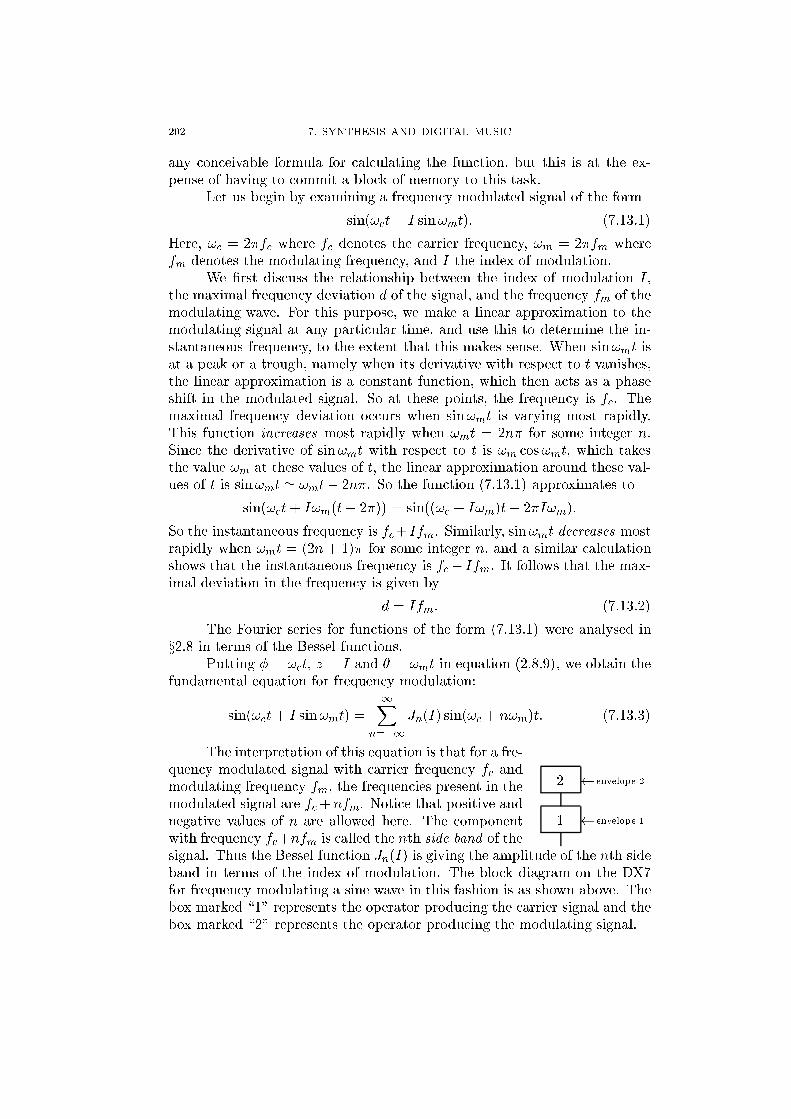
7.13. The Yamaha DX7 and FM synthesis
Yamaha DX7
The Yamaha DX7, which came out in the fall of 1983,3 was the �rst af-fordable commercially available digital synthesizer. This instrument was theresult of a long collaboration between John Chowning and Yamaha Corpo-ration through the nineteen seventies. It works by FM synthesis, with sixcon�gurable \operators". An operator produces as output a frequency mod-ulated sine wave, whose frequency is determined by the level of a modulat-ing input, and whose envelope is determined by another input. The power ofthe method comes from hooking up the output of one such operator to themodulating input of another. In this section, we shall investigate FM syn-thesis in detail, using the Yamaha DX7 for the details of the examples. Mostof the discussion translates easily to any other FM synthesizer. In AppendixB, there are tables which apply to various models of FM synthesizers. Lateron, in xx7.16{7.17, we shall also investigate FM synthesis using the CSoundcomputer music language.
The DX7 calculates the sine function in the simplest possible way. Ithas a digital lookup table of values of the function. This is much faster than
3Original price US $2000; no longer manufactured but easy to obtain second hand foraround US $250{$450.
202 7. SYNTHESIS AND DIGITAL MUSIC
any conceivable formula for calculating the function, but this is at the ex-pense of having to commit a block of memory to this task.
Let us begin by examining a frequency modulated signal of the form
sin(!ct+ I sin!mt): (7.13.1)
Here, !c = 2�fc where fc denotes the carrier frequency, !m = 2�fm wherefm denotes the modulating frequency, and I the index of modulation.
We �rst discuss the relationship between the index of modulation I,the maximal frequency deviation d of the signal, and the frequency fm of themodulating wave. For this purpose, we make a linear approximation to themodulating signal at any particular time, and use this to determine the in-stantaneous frequency, to the extent that this makes sense. When sin!mt isat a peak or a trough, namely when its derivative with respect to t vanishes,the linear approximation is a constant function, which then acts as a phaseshift in the modulated signal. So at these points, the frequency is fc. Themaximal frequency deviation occurs when sin!mt is varying most rapidly.This function increases most rapidly when !mt = 2n� for some integer n.Since the derivative of sin!mt with respect to t is !m cos!mt, which takesthe value !m at these values of t, the linear approximation around these val-ues of t is sin!mt ' !mt� 2n�. So the function (7.13.1) approximates to
sin(!ct+ I!m(t� 2�)) = sin((!c + I!m)t� 2�I!m):
So the instantaneous frequency is fc+Ifm. Similarly, sin!mt decreases mostrapidly when !mt = (2n + 1)� for some integer n, and a similar calculationshows that the instantaneous frequency is fc� Ifm. It follows that the max-imal deviation in the frequency is given by
d = Ifm: (7.13.2)
The Fourier series for functions of the form (7.13.1) were analysed inx2.8 in terms of the Bessel functions.
Putting � = !ct, z = I and � = !mt in equation (2.8.9), we obtain thefundamental equation for frequency modulation:
sin(!ct+ I sin!mt) =
1Xn=�1
Jn(I) sin(!c + n!m)t: (7.13.3)
1 envelope 1
2 envelope 2
The interpretation of this equation is that for a fre-quency modulated signal with carrier frequency fc andmodulating frequency fm, the frequencies present in themodulated signal are fc+nfm. Notice that positive andnegative values of n are allowed here. The componentwith frequency fc+nfm is called the nth side band of thesignal. Thus the Bessel function Jn(I) is giving the amplitude of the nth sideband in terms of the index of modulation. The block diagram on the DX7for frequency modulating a sine wave in this fashion is as shown above. Thebox marked \1" represents the operator producing the carrier signal and thebox marked \2" represents the operator producing the modulating signal.
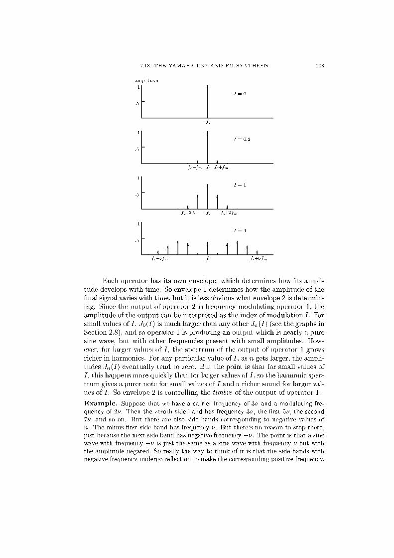
7.13. THE YAMAHA DX7 AND FM SYNTHESIS 203
:5
1
amplitude
I = 06
fc
:5
1
I = 0:26
fc6fc�fm 6fc+fm
:5
1
I = 16
fc
6 6
6fc�2fm6fc+2fm
:5
1
I = 4
6
fc
6 66 66 6
6fc�5fm
6fc+5fm
Each operator has its own envelope, which determines how its ampli-tude develops with time. So envelope 1 determines how the amplitude of the�nal signal varies with time, but it is less obvious what envelope 2 is determin-ing. Since the output of operator 2 is frequency modulating operator 1, theamplitude of the output can be interpreted as the index of modulation I. Forsmall values of I, J0(I) is much larger than any other Jn(I) (see the graphs inSection 2.8), and so operator 1 is producing an output which is nearly a puresine wave, but with other frequencies present with small amplitudes. How-ever, for larger values of I, the spectrum of the output of operator 1 growsricher in harmonics. For any particular value of I, as n gets larger, the ampli-tudes Jn(I) eventually tend to zero. But the point is that for small values ofI, this happens more quickly than for larger values of I, so the harmonic spec-trum gives a purer note for small values of I and a richer sound for larger val-ues of I. So envelope 2 is controlling the timbre of the output of operator 1.
Example. Suppose that we have a carrier frequency of 3� and a modulating fre-quency of 2�. Then the zeroth side band has frequency 3�, the �rst 5�, the second7�, and so on. But there are also side bands corresponding to negative values ofn. The minus �rst side band has frequency �. But there's no reason to stop there,just because the next side band has negative frequency ��. The point is that a sinewave with frequency �� is just the same as a sine wave with frequency � but withthe amplitude negated. So really the way to think of it is that the side bands withnegative frequency undergo re ection to make the corresponding positive frequency.
204 7. SYNTHESIS AND DIGITAL MUSIC
Notice also in this example that 3+2n is always an odd number, so only oddmultiples of � appear in the resulting frequency spectrum. In general, the frequencyspectrum will depend in an interesting way on the ratio of fm to fc. If the ratio isa ratio of small integers, the resulting frequency spectrum will consist of multiplesof a fundamental frequency. Otherwise, the spectrum is said to be inharmonic.
Let us calculate the spectrum in this example for various values of I . Firstwe use a small value such as I = 0:2. Consulting Appendix B, we see that J0(I) �0:9900, J1(I) � 0:0995, J2(I) � 0:0050 and Jn(I) is negligibly small for n � 3.Using equation (2.8.4) (J
�n(I) = (�1)nJn(I)), we see that J�1(I) � �0:0995,
J�2(I) � 0:0050 and J
�n(I) is negligibly small for n � 3. So the frequency modu-lated signal is approximately
0:0050 sin(2�(��)t)� 0:0995 sin(2��t) + 0:9900 sin(2�(3�)t)
+ 0:0995 sin(2�(5�)t) + 0:0050 sin(2�(7�)t):
Since sin(�x) = � sin(x), this is
�0:1045 sin(2��t) + 0:9900 sin(6��t) + 0:0995 sin(10��t) + 0:0050 sin(14��t):
This will be perceived as a note with fundamental frequency �, but with very strongthird harmonic.
Now let us carry out the same calculation with a larger value of I , sayI = 3. Again consulting Appendix B, we see that J0(I) � �0:2601, J1(I) � 0:3391,J2(I) � 0:4861, J3(I) � 0:3091, J4(I) � 0:1320, J5(I) � 0:0430, J6(I) � 0:0114,J7(I) � 0:0025, J8(I) � 0:0005, and only around n � 8 is Jn(I) negligibly small. Sothe harmonic spectrum of the resulting frequency modulated signal is much richer,and the �rst few terms are given by
� 0:0430 sin(2�(�7�)t) + 0:1320 sin(2�(�5�)t)� 0:3091 sin(2�(�3�)t)
+ 0:4861 sin(2�(��)t)� 0:3991 sin(2��t)� 0:2601 sin(2�(3�)t)
+ 0:3391 sin(2�(5�)t) + 0:4861 sin(2�(7�)t)
which makes
�0:8852 sin(2��t) + 0:0490 sin(6��t) + 0:2071 sin(10��t) + 0:5291 sin(14��t);
but it is clear that even higher harmonics than this are present with fairly large mag-nitude, up to about the seventeenth harmonic (3 + 2 � 7 = 17), and then it startstailing o�. So the resulting note is very rich in harmonics. Notice also how we haveconspired to choose I so that the amplitude of the third harmonic is now very small.
Suppose, for example, that operator 2 is assigned an envelope which starts at
zero, peaks near the beginning, and then tails o� to zero. Then the resulting fre-
quency modulated signal will start o� as a pure sine wave, fairly quickly attain a
rich harmonic spectrum, and then tail o� again into a fairly pure sine wave. It is
easy to see that the possibilities opened up with even two operators is fairly wide.
In terms of block diagrams, additive synthesis for a waveform with �vesinusoidal components is represented as follows.
1 2 3 4 5
7.13. THE YAMAHA DX7 AND FM SYNTHESIS 205
So in the above example, to synthesize the corresponding sound additivelywould require a large number of oscillators. The exact number would dependon where the cuto� for audibility occurs.
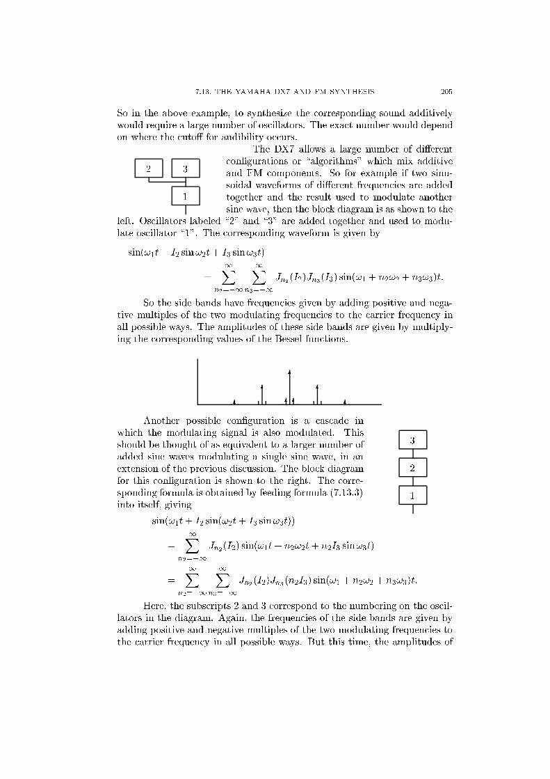
1
32
The DX7 allows a large number of di�erentcon�gurations or \algorithms" which mix additiveand FM components. So for example if two sinu-soidal waveforms of di�erent frequencies are addedtogether and the result used to modulate anothersine wave, then the block diagram is as shown to the
left. Oscillators labeled \2" and \3" are added together and used to modu-late oscillator \1". The corresponding waveform is given by
sin(!1t+ I2 sin!2t+ I3 sin!3t)
=1X
n2=�1
1Xn3=�1
Jn2(I2)Jn3(I3) sin(!1 + n2!2 + n3!3)t:
So the side bands have frequencies given by adding positive and nega-tive multiples of the two modulating frequencies to the carrier frequency inall possible ways. The amplitudes of these side bands are given by multiply-ing the corresponding values of the Bessel functions.
6
666 6
6 6
1
2
3
Another possible con�guration is a cascade inwhich the modulating signal is also modulated. Thisshould be thought of as equivalent to a larger number ofadded sine waves modulating a single sine wave, in anextension of the previous discussion. The block diagramfor this con�guration is shown to the right. The corre-sponding formula is obtained by feeding formula (7.13.3)into itself, giving
sin(!1t+ I2 sin(!2t+ I3 sin!3t))
=1X
n2=�1
Jn2(I2) sin(!1t+ n2!2t+ n2I3 sin!3t)
=
1Xn2=�1
1Xn3=�1
Jn2(I2)Jn3(n2I3) sin(!1 + n2!2 + n3!3)t:
Here, the subscripts 2 and 3 correspond to the numbering on the oscil-lators in the diagram. Again, the frequencies of the side bands are given byadding positive and negative multiples of the two modulating frequencies tothe carrier frequency in all possible ways. But this time, the amplitudes of
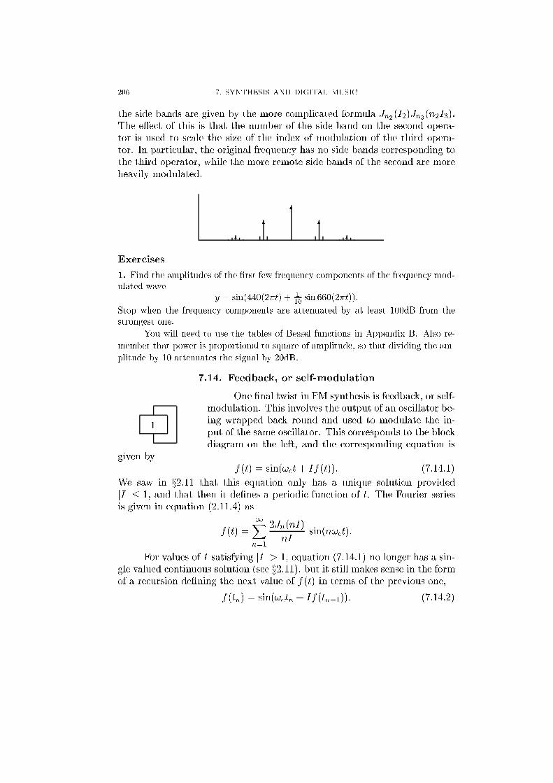
206 7. SYNTHESIS AND DIGITAL MUSIC
the side bands are given by the more complicated formula Jn2(I2)Jn3(n2I3).The e�ect of this is that the number of the side band on the second opera-tor is used to scale the size of the index of modulation of the third opera-tor. In particular, the original frequency has no side bands corresponding tothe third operator, while the more remote side bands of the second are moreheavily modulated.
6
6 6
6 6
Exercises
1. Find the amplitudes of the �rst few frequency components of the frequency mod-ulated wave
y = sin(440(2�t) + 110 sin 660(2�t)):
Stop when the frequency components are attenuated by at least 100dB from thestrongest one.
You will need to use the tables of Bessel functions in Appendix B. Also re-
member that power is proportional to square of amplitude, so that dividing the am-
plitude by 10 attenuates the signal by 20dB.
7.14. Feedback, or self-modulation
1
One �nal twist in FM synthesis is feedback, or self-modulation. This involves the output of an oscillator be-ing wrapped back round and used to modulate the in-put of the same oscillator. This corresponds to the blockdiagram on the left, and the corresponding equation is
given byf(t) = sin(!ct+ If(t)): (7.14.1)
We saw in x2.11 that this equation only has a unique solution providedjIj � 1, and that then it de�nes a periodic function of t. The Fourier seriesis given in equation (2.11.4) as
f(t) =1Xn=1
2Jn(nI)
nIsin(n!ct):
For values of I satisfying jIj > 1, equation (7.14.1) no longer has a sin-gle valued continuous solution (see x2.11), but it still makes sense in the formof a recursion de�ning the next value of f(t) in terms of the previous one,
f(tn) = sin(!ctn + If(tn�1)): (7.14.2)
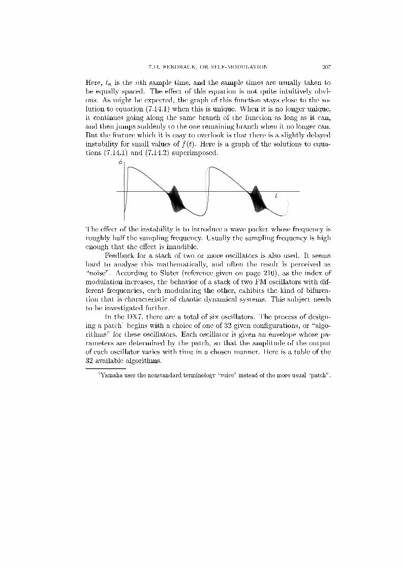
7.14. FEEDBACK, OR SELF-MODULATION 207
Here, tn is the nth sample time, and the sample times are usually taken tobe equally spaced. The e�ect of this equation is not quite intuitively obvi-ous. As might be expected, the graph of this function stays close to the so-lution to equation (7.14.1) when this is unique. When it is no longer unique,it continues going along the same branch of the function as long as it can,and then jumps suddenly to the one remaining branch when it no longer can.But the feature which it is easy to overlook is that there is a slightly delayedinstability for small values of f(t). Here is a graph of the solutions to equa-tions (7.14.1) and (7.14.2) superimposed.
t
�
The e�ect of the instability is to introduce a wave packet whose frequency isroughly half the sampling frequency. Usually the sampling frequency is highenough that the e�ect is inaudible.
Feedback for a stack of two or more oscillators is also used. It seemshard to analyse this mathematically, and often the result is perceived as\noise". According to Slater (reference given on page 210), as the index ofmodulation increases, the behavior of a stack of two FM oscillators with dif-ferent frequencies, each modulating the other, exhibits the kind of bifurca-tion that is characteristic of chaotic dynamical systems. This subject needsto be investigated further.
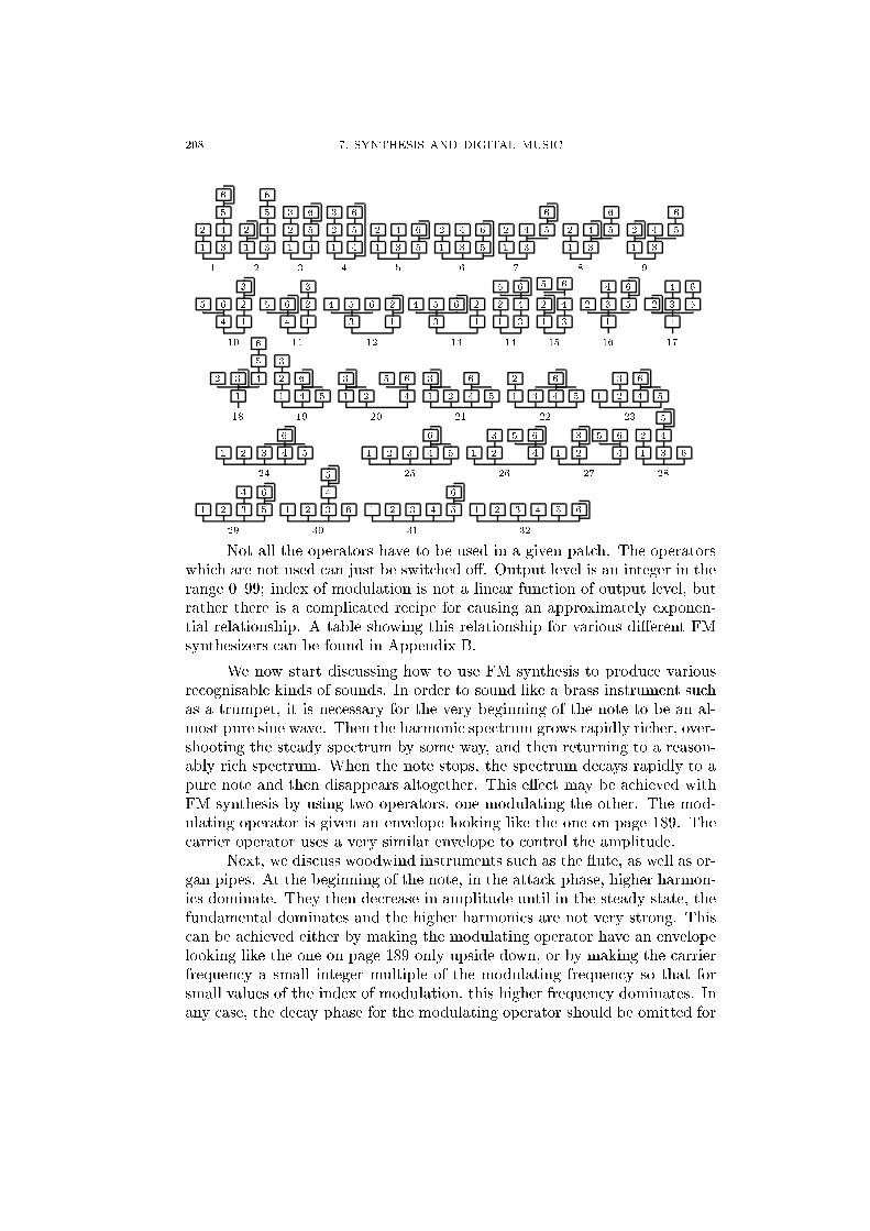
In the DX7, there are a total of six oscillators. The process of design-ing a patch4 begins with a choice of one of 32 given con�gurations, or \algo-rithms" for these oscillators. Each oscillator is given an envelope whose pa-rameters are determined by the patch, so that the amplitude of the outputof each oscillator varies with time in a chosen manner. Here is a table of the32 available algorithms.
4Yamaha uses the nonstandard terminology \voice" instead of the more usual \patch".
208 7. SYNTHESIS AND DIGITAL MUSIC
1
2
3
4
5
6
1
1
2
3
4
5
6
2
1
2
3
4
5
6
3
1
2
3
4
5
6
4
1
2
3
4
5
6
5
1
2
3
4
5
6
6
1
2
3
4 5
6
7
1
2
3
4 5
6
8
1
2
3
4 5
6
9
1
2
3
4
5 6
10
1
2
3
4
5 6
11
1
2
3
4 5 6
12
1
2
3
4 5 6
13
1
2
5
3
4
6
14
1
2
5
3
4
6
15
1
2 3
4
5
6
16
1
2 3
4
5
6
17
1
2 3 4
5
6
18
1
2
3
4 5
6
19
1 2
3
4
5 6
20
1 2
3
4 5
6
21
1 3
2
4 5
6
22
1 2
3
4 5
6
23
1 2 3 4 5
6
24
1 2 3 4 5
6
25
1 2
3
4
5 6
26
1 2
3
4
5 6
27
1
2
3
4
5
6
28
1 2 3
4
5
6
29
1 2 3
4
5
6
30
1 2 3 4 5
6
31
1 2 3 4 5 6
32
Not all the operators have to be used in a given patch. The operatorswhich are not used can just be switched o�. Output level is an integer in therange 0{99; index of modulation is not a linear function of output level, butrather there is a complicated recipe for causing an approximately exponen-tial relationship. A table showing this relationship for various di�erent FMsynthesizers can be found in Appendix B.
We now start discussing how to use FM synthesis to produce variousrecognisable kinds of sounds. In order to sound like a brass instrument suchas a trumpet, it is necessary for the very beginning of the note to be an al-most pure sine wave. Then the harmonic spectrum grows rapidly richer, over-shooting the steady spectrum by some way, and then returning to a reason-ably rich spectrum. When the note stops, the spectrum decays rapidly to apure note and then disappears altogether. This e�ect may be achieved withFM synthesis by using two operators, one modulating the other. The mod-ulating operator is given an envelope looking like the one on page 189. Thecarrier operator uses a very similar envelope to control the amplitude.
Next, we discuss woodwind instruments such as the ute, as well as or-gan pipes. At the beginning of the note, in the attack phase, higher harmon-ics dominate. They then decrease in amplitude until in the steady state, thefundamental dominates and the higher harmonics are not very strong. Thiscan be achieved either by making the modulating operator have an envelopelooking like the one on page 189 only upside down, or by making the carrierfrequency a small integer multiple of the modulating frequency so that forsmall values of the index of modulation, this higher frequency dominates. Inany case, the decay phase for the modulating operator should be omitted for
7.14. FEEDBACK, OR SELF-MODULATION 209
a more realistic sound. For some woodwind instruments such as the clarinet,it is necessary to make sure that predominantly odd harmonics are present.This can be achieved, as in the example on page 203, by setting fc = 3f andfm = 2f , or some variation on this idea.
Percussive sounds have a very sharp attack and a roughly exponentialdecay. So an envelope looking like the graph of x = e�t is appropriate for theamplitude. Usually a percussive instrument will have an inharmonic spec-trum, so that it is appropriate to make sure that fc and fm are not in a ra-tio which can be expressed as a ratio of small integers. We saw in Exercise 1of x6.2 that the golden ratio is in some sense the number furthest from be-ing able to be approximated well by ratios of small integers, so this is a goodchoice for producing spectra which will be perceived as inharmonic. Alter-natively, the analysis carried out in x3.5 can be used to try to emulate thefrequency spectrum of an actual drum.
Section x7.15 and the ones following it consist of an introduction to thepublic domain computer music language CSound. One of our goals will beto describe explicit implementations of two operator FM synthesis realizingthe above descriptions.
Further reading on FM synthesis:
J. Bate, The e�ect of modulator phase on timbres in FM synthesis, Computer Mu-sic Journal 14 (3) (1990), 38{45.
John Chowning, The synthesis of complex audio spectra by means of frequency mod-
ulation, J. Audio Engineering Society 21 (7) (1973), 526{534. Reprinted as chapter1 of Roads and Strawn [95], pages 6{29.
John Chowning, Frequency modulation synthesis of the singing voice, appeared inMathews and Pierce [66], chapter 6, pages 57{63.
Chowning and Bristow [13].
A. Horner, Double-modulator FM matching of instrument tones, Computer MusicJournal 20 (2) (1996), 57{71.
A. Horner, A comparison of wavetable and FM parameter spaces, Computer MusicJournal 21 (4) (1997), 55{85.
A. Horner, J. Beauchamp and L. Haken, FM matching synthesis with genetic algo-
rithms, Computer Music Journal 17 (4) (1993), 17{29.
M. LeBrun, A derivation of the spectrum of FM with a complex modulating wave,Computer Music Journal 1 (4) (1977), 51{52. Reprinted as chapter 5 of Roads andStrawn [95], pages 65{67.
F. R. Moore, Elements of computer music [72], pages 316{332.
D. Morrill, Trumpet algorithms for computer composition, Computer Music Journal1 (1) (1977), 46{52. Reprinted as chapter 2 of Roads and Strawn [95], pages 30{44.
C. Roads, The computer music tutorial [93], pages 224{250.
210 7. SYNTHESIS AND DIGITAL MUSIC
S. Saunders, Improved FM audio synthesis methods for real-time digital music gen-
eration, Computer Music Journal 1 (1) (1977), 53{55. Reprinted as chapter 3 ofRoads and Strawn [95], pages 45{53.
W. G. Schottstaedt, The simulation of natural instrument tones using frequency
modulation with a complex modulating wave, Computer Music Journal 1 (4) (1977),46{50. Reprinted as chapter 4 of Roads and Strawn [95], pages 54{64.
D. Slater, Chaotic sound synthesis, Computer Music Journal 22 (2) (1998), 12{19.
B. Truax, Organizational techniques for c : m ratios in frequency modulation, Com-
puter Music Journal 1 (4) (1977), 39{45. Reprinted as chapter 6 of Roads and
Strawn [95], pages 68{82.
7.15. CSound
CSound is a public domain synthesis program written by Barry Vercoeat the Media Lab in MIT in the C programming language. It has been com-piled for various platform, and both source code and executables are freelyavailable.
The program takes as input two �les, called the orchestra �le and thescore �le. The orchestra �le contains the instrument de�nitions, or how tosynthesize the desired sounds. It makes use of almost every known methodof synthesis, including FM synthesis, the Karplus{Strong algorithm, phasevocoder, pitch envelopes, granular synthesis and so on, to de�ne the instru-ments. The score �le uses a language similar in conception to MIDI but dif-ferent in execution, in order to describe the information for playing the in-struments, such as amplitude, frequency, note durations and start times. Theutility MIDI2CS mentioned in x7.24 provides a exible way of turning MIDI�les into CSound score �les. The �nal output of the CSound program is a�le in some chosen sound format, for example a WAV �le or an AIFF �le,which can be played through a computer sound card, downloaded into a syn-thesizer with sampling features, or written onto a CD.
We limit ourselves to a brief description of some of the main featuresof CSound, with the objective of getting as far as describing how to realiseFM synthesis. The examples are adapted from the CSound manual.
Getting it. The source code and executables for a number of platforms canbe obtained from
ftp://ftp.maths.bath.ac.uk/pub/dream/
(mirrored at ftp://ftp.musique.umontreal.ca/pub/mirrors/dream/)
as can the manual and some example �les. For a minimalist installationon an MS-DOS (or Windows) based machine, get the �le csound new412.zipfrom the subdirectory newest/ at the above site (or a later version if available;the above version was released on March 6, 2001). Unzip it5 into a directory
5To unzip a �le under Windows, get hold of Winzip from winzip.com. This is share-ware, but can be used inde�nitely without registration. If you prefer to use a free utility,get hold of Info-ZIP's free MS-DOS based program unzip.exe (138 kB) from
7.15. CSOUND 211
of your choice, and make sure the directory is in your path by editing theautoexec.bat �le if necessary. If you are really short of space, delete every-thing except the �les csound.txt, csound.exe and dos4gw.exe (total around 1megabyte), and you will still be able to run all the examples described here.Make a new subdirectory for your orchestra and score �les, and run CSoundfrom that subdirectory. Instructions for running CSound can be found onpage 213.
If you are running in an MS-DOS window under Windows 95/98/MEor NT/2000, the above still works, but the �le csound con412.zip contains asmaller and more eÆcient version of just the csound.exe �le and the csound.txt�le; you won't need dos4gw.exe. The disadvantage is that the displays arein ascii instead of full screen graphics. There is also a Windows front endin csound win412.zip. This is capable of realtime sound output and realtimeMIDI handling, which the MS-DOS version is not, but apart from that, it isquite primitive. For example, the program needs to restart every time it isrun, and cannot just replay the output.
The most up to date version of the manual is version 4.10, which canbe found at
http://lakewoodsound.com/csound/download.htm
This version does not seem to have made it onto the Bath ftp site mentionedabove.
The orchestra �le. This �le has two main parts, namely the header section,which de�nes the sample rate, control rate, and number of output channels,and the instrument section which gives the instrument de�nitions. Each in-strument is given its own number, which behaves like a patch number on asynthesizer.
The header section has the following format (everything after a semi-colon is a comment):
sr = 44100 ; sample rate in samples per secondkr = 4410 ; control rate in control signals per secondksmps = 10 ; ksmps = sr/kr must be an integer, samples per control periodnchnls = 1 ; number of channels (7.15.1)
An instrument de�nition consists of a collection of statements whichgenerate or modify a digital signal. For example the statements
instr 1asig oscil 10000, 440, 1
out asigendin (7.15.2)
generate a 440 Hz wave with amplitude 10000, and send it to an output. Thetwo lines of code representing the waveform generator are encased in a pair
http://www.cdrom.com/pub/infozip/UnZip.html|there is also a copy on my machine:ftp://byrd.math.uga.edu/pub/win/compression/unzip.exe
212 7. SYNTHESIS AND DIGITAL MUSIC
of statements which de�ne this to be an instrument. For WAV �le output,the possible range of amplitudes before clipping takes e�ect is from �32768to +32767, for a total of 215 possible values. The �nal argument 1 is a wave-form number. This determines which waveform is taken from an f statementin the score �le (see below). In our �rst example below, it will be a sine wave.The label asig is allowed to be any string beginning with a (for \audio sig-nal"). So for example a1 would have worked just as well. The oscil statementis one of CSound's many signal generators, and its e�ect is to output peri-odic signals made by repeating the values passed to it, appropriately scaledin amplitude and frequency. There is also another version called oscili, withthe same syntax, which performs linear interpolation rather than truncationto �nd values at points between the sample points. This is slower by approx-imately a factor of two, but in some situations it can lead to better soundingoutput. In general, it seems to be better to use oscil for sound waves and os-cili for envelopes (see page 215).
As it stands, the instrument (7.15.2) isn't very useful, because it canonly play one pitch. To pass a pitch, or other attributes, as parameters fromthe score �le to the orchestra �le, an instrument uses variables named p1, p2,p3, and so on. The �rst three have �xed meanings, and then p4, p5, . . . canbe given other meanings. If we replace 440 by p5,
asig oscil 10000, p5, 1
then the parameter p5 will determine pitch.
The score �le. Each line begins with a letter called an opcode, which de-termines how the line is to be interpreted. The rest of the line consists of nu-merical parameter �elds p1, p2, p3, and so on. The possible opcodes are:
f (function table generator),
i (instrument statement; i.e., play a note),
t (tempo),
a (advance score time; i.e., skip parts),
b (o�set score time),
v (local textual time variation),
s (section statement),
r (repeat sections),
m and n (repeat named sections),
e (end of score),
c (comment; semicolon is preferred).
If a line of the score �le does not begin with an opcode, it is treated as a con-tinuation line.
Each parameter �eld consists of a oating point number with optionalsign and optional decimal point. Expressions are not permitted.
7.15. CSOUND 213
An f statement calls a subroutine to generate a set of numerical val-ues describing a function. The set of values is intended for passing to theorchestra �le for use by an instrument de�nition. The available subroutinesare called GEN01, GEN02, . . . . Each takes some number of numerical argu-ments. The parameter �elds of an f statement are as follows.
p1 Waveform number
p2 When to begin the table, in beats
p3 Size of table; a power of 2, or one more, maximum 224
p4 Number of GEN subroutine
p5, p6, . . . Parameters for GEN subroutine
Beats are measured in seconds, unless there is an explicit t (tempo) state-ment; in our examples, t statements are omitted for simplicity.
So for example, the statement
f1 0 8192 10 1
uses GEN10 to produce a sine wave, starting \now", of size 8192, and assignsit to waveform 1. The subroutine GEN10 produces waveforms made up ofweighted sums of sine waves, whose frequencies are integer multiples of thefundamental. So for example
f2 0 8192 10 1 0 0.5 0 0.333
produces the sum of the �rst �ve terms in the Fourier series for a squarewave, and assigns it to waveform 2.
An i statement activates an instrument. This is the kind of statementused to \play a note". Its parameter �elds are as follows.
p1 Instrument number
p2 Starting time in beats
p3 Duration in beats
p4, p5, . . . Parameters used by the instrument
An e statement denotes the end of a score. It consists of an e on a lineon its own. Every score �le must end in this way.
For example, if instrument 1 is given by (7.15.2) then the score �le
f1 0 8192 10 1 ; use GEN10 to create a sine wavei1 0 4 ; play instr 1 from time 0 for 4 secse (7.15.3)
will play a 440Hz tone for 4 seconds.
Running CSound. The program CSound was designed as a command lineprogram, and although various front ends have been designed for it, the com-mand line remains the most convenient method. Having installed CSoundaccording to the instructions that accompany the program, the proceedureis to create an orchestra �le called <�lename>.orc and a score �le called
214 7. SYNTHESIS AND DIGITAL MUSIC
<�lename>.sco using your favorite (ascii) text processor.6 The basic syntaxfor running CSound is
csound < ags> <�lename>.orc <�lename>.sco
For example, if your �les are called ditty.orc and ditty.sco, and you want aWAV �le output, then use the -W ag (this is case sensitive).
csound -W ditty.orc ditty.sco
This will produce as output a �le called test.wav. If you want some othername, it must be speci�ed with the -o ag.
csound -W -o ditty.wav ditty.orc ditty.sco (7.15.4)
If you want to suppress the graphical displays of the waveforms, which csoundgives by default, this is achieved with the -d ag.
We are now ready to run our �rst example. Make two text �les, onecalled ditty.orc containing the statements (7.15.1) followed by (7.15.2), andone called ditty.sco containing the statements (7.15.3). If the program is prop-erly installed, then typing the command (7.15.4) at the command line shouldproduce a �le ditty.wav. Playing this �le through a sound card or other au-dio device should then sound a pure sine wave at 440Hz for 4 seconds.
Warning. Both the orchestra and the score �le are case sensitive. If youare having problems running CSound on the above orchestra and score �les,check that you have typed everything in lower case.
There is also an annoying feature, which is that if the last line of textin the input �le does not have a carriage return, then a wave �le will be gen-erated, but it will be unreadable. So it is best to leave a blank line at theend of each �le.
Our \ditty" wasn't really very interesting, so let's modify it a bit. Inorder to be able to vary the amplitude and pitch, let us modify the instru-ment (7.15.2) to read
instr 1asig oscil p4, p5, 1 ; p4 = amplitude, p5 = frequency
out asigendin (7.15.5)
Now we can play the �rst ten notes of the harmonic series (see page 99) us-ing the following score �le.
6Word processors such as Word Perfect or Word by default save �les with special for-matting characters embedded in them. CSound will choke on these characters. In MS-DOS, the command
edit <�lename>
will invoke a simple ascii text processor whose output will not choke CSound in this way.If you are running in an MS-DOS box inside Windows, the command
notepad <�lename>
will start up the ascii text processor called notepad in a separate window, which is moreconvenient for switching between the editor and running CSound.
7.15. CSOUND 215
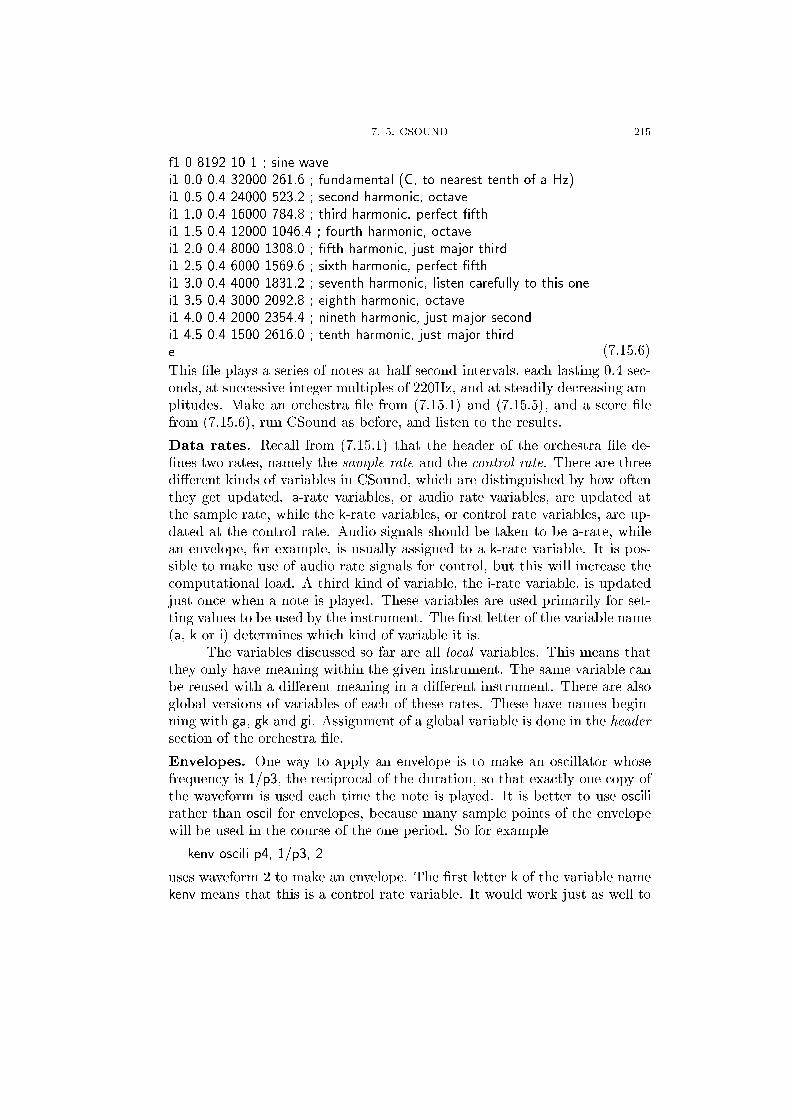
f1 0 8192 10 1 ; sine wavei1 0.0 0.4 32000 261.6 ; fundamental (C, to nearest tenth of a Hz)i1 0.5 0.4 24000 523.2 ; second harmonic, octavei1 1.0 0.4 16000 784.8 ; third harmonic, perfect �fthi1 1.5 0.4 12000 1046.4 ; fourth harmonic, octavei1 2.0 0.4 8000 1308.0 ; �fth harmonic, just major thirdi1 2.5 0.4 6000 1569.6 ; sixth harmonic, perfect �fthi1 3.0 0.4 4000 1831.2 ; seventh harmonic, listen carefully to this onei1 3.5 0.4 3000 2092.8 ; eighth harmonic, octavei1 4.0 0.4 2000 2354.4 ; nineth harmonic, just major secondi1 4.5 0.4 1500 2616.0 ; tenth harmonic, just major thirde (7.15.6)
This �le plays a series of notes at half second intervals, each lasting 0.4 sec-onds, at successive integer multiples of 220Hz, and at steadily decreasing am-plitudes. Make an orchestra �le from (7.15.1) and (7.15.5), and a score �lefrom (7.15.6), run CSound as before, and listen to the results.
Data rates. Recall from (7.15.1) that the header of the orchestra �le de-�nes two rates, namely the sample rate and the control rate. There are threedi�erent kinds of variables in CSound, which are distinguished by how oftenthey get updated. a-rate variables, or audio rate variables, are updated atthe sample rate, while the k-rate variables, or control rate variables, are up-dated at the control rate. Audio signals should be taken to be a-rate, whilean envelope, for example, is usually assigned to a k-rate variable. It is pos-sible to make use of audio rate signals for control, but this will increase thecomputational load. A third kind of variable, the i-rate variable, is updatedjust once when a note is played. These variables are used primarily for set-ting values to be used by the instrument. The �rst letter of the variable name(a, k or i) determines which kind of variable it is.
The variables discussed so far are all local variables. This means thatthey only have meaning within the given instrument. The same variable canbe reused with a di�erent meaning in a di�erent instrument. There are alsoglobal versions of variables of each of these rates. These have names begin-ning with ga, gk and gi. Assignment of a global variable is done in the headersection of the orchestra �le.
Envelopes. One way to apply an envelope is to make an oscillator whosefrequency is 1/p3, the reciprocal of the duration, so that exactly one copy ofthe waveform is used each time the note is played. It is better to use oscilirather than oscil for envelopes, because many sample points of the envelopewill be used in the course of the one period. So for example
kenv oscili p4, 1/p3, 2
uses waveform 2 to make an envelope. The �rst letter k of the variable namekenv means that this is a control rate variable. It would work just as well to
216 7. SYNTHESIS AND DIGITAL MUSIC
make it an audio rate variable by using a name like aenv, but it would de-mand greater computation time, and result in no audible improvement.
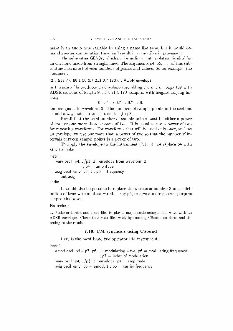
The subroutine GEN07, which performs linear interpolation, is ideal foran envelope made from straight lines. The arguments p4, p5, . . . of this sub-routine alternate between numbers of points and values. So for example, thestatement
f2 0 513 7 0 80 1 50 0.7 213 0.7 170 0 ; ADSR envelope
in the score �le produces an envelope resembling the one on page 189 withADSR sections of length 80, 50, 213, 170 samples, with heights varying lin-early
0! 1! 0:7! 0:7! 0;
and assigns it to waveform 2. The numbers of sample points in the sectionsshould always add up to the total length p3.
Recall that the total number of sample points must be either a powerof two, or one more than a power of two. It is usual to use a power of twofor repeating waveforms. For waveforms that will be used only once, such asan envelope, we use one more than a power of two so that the number of in-tervals between sample points is a power of two.
To apply the envelope to the instrument (7.15.5), we replace p4 withkenv to make
instr 1kenv oscili p4, 1/p3, 2 ; envelope from waveform 2
; p4 = amplitudeasig oscil kenv, p5, 1 ; p5 = frequency
out asigendin
It would also be possible to replace the waveform number 2 in the def-inition of kenv with another variable, say p6, to give a more general purposeshaped sine wave.
Exercises
1. Make orchestra and score �les to play a major scale using a sine wave with an
ADSR envelope. Check that your �les work by running CSound on them and lis-
tening to the result.
7.16. FM synthesis using CSound
Here is the most basic two operator FM instrument:
instr 1amod oscil p6 � p7, p6, 1 ; modulating wave, p6 = modulating frequency
; p7 = index of modulationkenv oscili p4, 1/p3, 2 ; envelope, p4 = amplitudeasig oscil kenv, p5 + amod, 1 ; p5 = carrier frequency
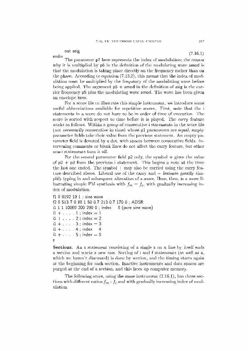
7.16. FM SYNTHESIS USING CSOUND 217
out asigendin
(7.16.1)
The parameter p7 here represents the index of modulation; the reasonwhy it is multiplied by p6 in the de�nition of the modulating wave amod isthat the modulation is taking place directly on the frequency rather than onthe phase. According to equation (7.13.2), this means that the index of mod-ulation must be multiplied by the frequency of the modulating wave beforebeing applied. The argument p5 + amod in the de�nition of asig is the car-rier frequency p5 plus the modulating wave amod. The wave has been givenan envelope kenv.
For a score �le to illustrate this simple instrument, we introduce someuseful abbreviations available for repetitive scores. First, note that the istatements in a score do not have to be in order of time of execution. Thescore is sorted with respect to time before it is played. The carry featureworks as follows. Within a group of consecutive i statements in the score �le(not necessarily consecutive in time) whose p1 parameters are equal, emptyparameter �elds take their value from the previous statement. An empty pa-rameter �eld is denoted by a dot, with spaces between consecutive �elds. In-tervening comments or blank lines do not a�ect the carry feature, but othernon-i statements turn it o�.
For the second parameter �eld p2 only, the symbol + gives the valueof p2 + p3 from the previous i statement. This begins a note at the timethe last one ended. The symbol + may also be carried using the carry fea-ture described above. Liberal use of the carry and + features greatly sim-plify typing in and subsequent alteration of a score. Here, then, is a score il-lustrating simple FM synthesis with fm = fc, with gradually increasing in-dex of modulation.
f1 0 8192 10 1 ; sine wavef2 0 513 7 0 80 1 50 0.7 213 0.7 170 0 ; ADSRi1 1 1 10000 200 200 0 ; index = 0 (pure sine wave)i1 + . . . . 1 ; index = 1i1 + . . . . 2 ; index = 2i1 + . . . . 3 ; index = 3i1 + . . . . 4 ; index = 4i1 + . . . . 5 ; index = 5e
Sections. An s statement consisting of a single s on a line by itself endsa section and starts a new one. Sorting of i and f statements (as well as a,which we haven't discussed) is done by section, and the timing starts againat the beginning for each section. Inactive instruments and data spaces arepurged at the end of a section, and this frees up computer memory.
The following score, using the same instrument (7.16.1), has three sec-tions with di�erent ratios fm : fc and with gradually increasing index of mod-ulation.
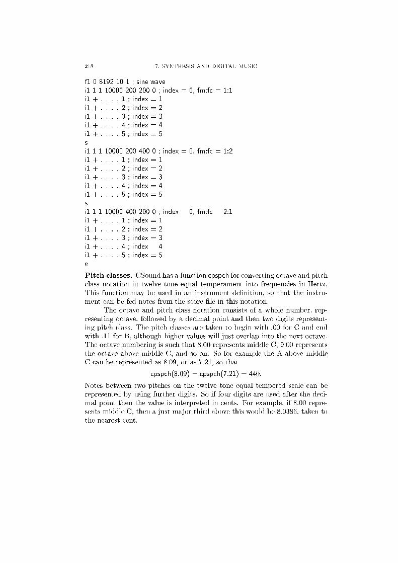
218 7. SYNTHESIS AND DIGITAL MUSIC
f1 0 8192 10 1 ; sine wavei1 1 1 10000 200 200 0 ; index = 0, fm:fc = 1:1i1 + . . . . 1 ; index = 1i1 + . . . . 2 ; index = 2i1 + . . . . 3 ; index = 3i1 + . . . . 4 ; index = 4i1 + . . . . 5 ; index = 5si1 1 1 10000 200 400 0 ; index = 0, fm:fc = 1:2i1 + . . . . 1 ; index = 1i1 + . . . . 2 ; index = 2i1 + . . . . 3 ; index = 3i1 + . . . . 4 ; index = 4i1 + . . . . 5 ; index = 5si1 1 1 10000 400 200 0 ; index = 0, fm:fc = 2:1i1 + . . . . 1 ; index = 1i1 + . . . . 2 ; index = 2i1 + . . . . 3 ; index = 3i1 + . . . . 4 ; index = 4i1 + . . . . 5 ; index = 5e
Pitch classes. CSound has a function cpspch for converting octave and pitchclass notation in twelve tone equal temperament into frequencies in Hertz.This function may be used in an instrument de�nition, so that the instru-ment can be fed notes from the score �le in this notation.
The octave and pitch class notation consists of a whole number, rep-resenting octave, followed by a decimal point and then two digits represent-ing pitch class. The pitch classes are taken to begin with .00 for C and endwith .11 for B, although higher values will just overlap into the next octave.The octave numbering is such that 8.00 represents middle C, 9.00 representsthe octave above middle C, and so on. So for example the A above middleC can be represented as 8.09, or as 7.21, so that
cpspch(8.09) = cpspch(7.21) = 440:
Notes between two pitches on the twelve tone equal tempered scale can berepresented by using further digits. So if four digits are used after the deci-mal point then the value is interpreted in cents. For example, if 8.00 repre-sents middle C, then a just major third above this would be 8.0386, taken tothe nearest cent.
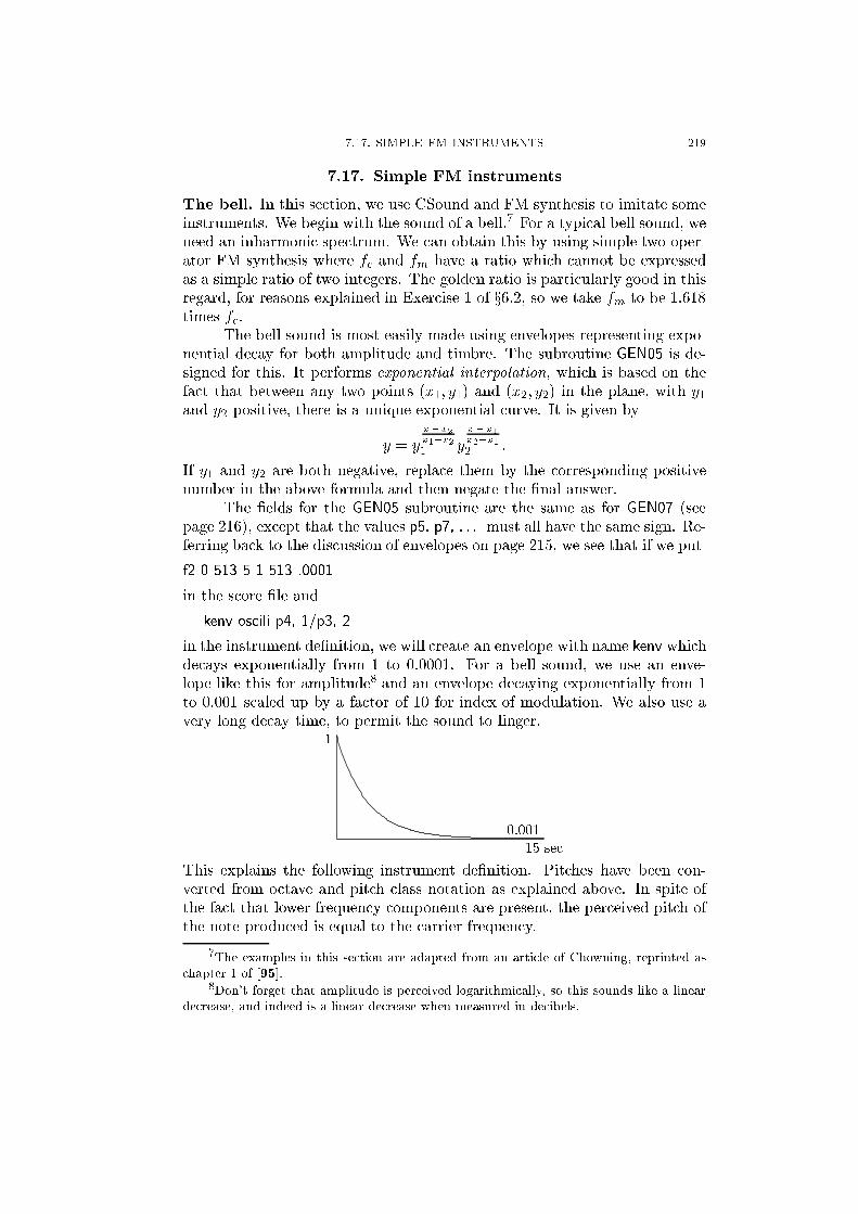
7.17. SIMPLE FM INSTRUMENTS 219
7.17. Simple FM instruments
The bell. In this section, we use CSound and FM synthesis to imitate someinstruments. We begin with the sound of a bell.7 For a typical bell sound, weneed an inharmonic spectrum. We can obtain this by using simple two oper-ator FM synthesis where fc and fm have a ratio which cannot be expressedas a simple ratio of two integers. The golden ratio is particularly good in thisregard, for reasons explained in Exercise 1 of x6.2, so we take fm to be 1.618times fc.
The bell sound is most easily made using envelopes representing expo-nential decay for both amplitude and timbre. The subroutine GEN05 is de-signed for this. It performs exponential interpolation, which is based on thefact that between any two points (x1; y1) and (x2; y2) in the plane, with y1and y2 positive, there is a unique exponential curve. It is given by
y = yx�x2
x1�x2
1 yx� x1
x2�x1
2 :
If y1 and y2 are both negative, replace them by the corresponding positivenumber in the above formula and then negate the �nal answer.
The �elds for the GEN05 subroutine are the same as for GEN07 (seepage 216), except that the values p5, p7, . . . must all have the same sign. Re-ferring back to the discussion of envelopes on page 215, we see that if we put
f2 0 513 5 1 513 .0001
in the score �le and
kenv oscili p4, 1/p3, 2
in the instrument de�nition, we will create an envelope with name kenv whichdecays exponentially from 1 to 0.0001. For a bell sound, we use an enve-lope like this for amplitude8 and an envelope decaying exponentially from 1to 0.001 scaled up by a factor of 10 for index of modulation. We also use avery long decay time, to permit the sound to linger.
1
0.00115 sec
This explains the following instrument de�nition. Pitches have been con-verted from octave and pitch class notation as explained above. In spite ofthe fact that lower frequency components are present, the perceived pitch ofthe note produced is equal to the carrier frequency.
7The examples in this section are adapted from an article of Chowning, reprinted aschapter 1 of [95].
8Don't forget that amplitude is perceived logarithmically, so this sounds like a lineardecrease, and indeed is a linear decrease when measured in decibels.
220 7. SYNTHESIS AND DIGITAL MUSIC
instr 1 ; FM bellifc = cpspch(p5) ; carrier frequencyifm = cpspch(p5) * 1.618 ; modulating frequency
kenv oscili p4, 1/p3, 2 ; envelope, p3 = duration, exp decay f2; p4 = amplitude
ktmb oscili ifm * 10, 1/p3, 3 ; timbre envelope, max = 10, exp decay f3amod oscil ktmb, ifm, 1 ; modulatorasig oscil kenv, ifc + amod, 1 ; carrier
out asigendin
Here is the score �le to play notes E, C, D, G for a chime, using this instru-ment.
f1 0 8192 10 1f2 0 513 5 1 513 .0001f3 0 513 5 1 513 .001i1 1 15 8000 8.04 ; 15 seconds at amplitude 8000 at middle Ci1 2.5 . . 8.00i1 4 . . 8.02i1 5.5 . . 7.07e
A general purpose instrument. It is not hard to modify the instrumentdescribed above to make a general purpose two operator FM synthesis in-strument.
instr 1 ; Two operator FM instrumentifc = cpspch(p5) * p6 ; p6 = carrier frequency multiplierifm = cpspch(p5) * p7 ; p7 = modulator frequency multiplier
kenv oscili p4, 1/p3, p8 ; p3 = duration; p4 = amplitude, p8 = carrier envelopektmb oscili ifm * p10, 1/p3, p9 ; p9 = modulator envelope; p10 = maximum index of modulationamod oscil ktmb, ifm, 1 ; modulatorasig oscil kenv, ifc + amod, 1 ; carrier
out asigendin
The rest of the examples in this section are described in terms of this setup.
The wood drum. To make a reasonably convincing wood drum, the am-plitude envelope is made up of two exponential curves using GEN05,
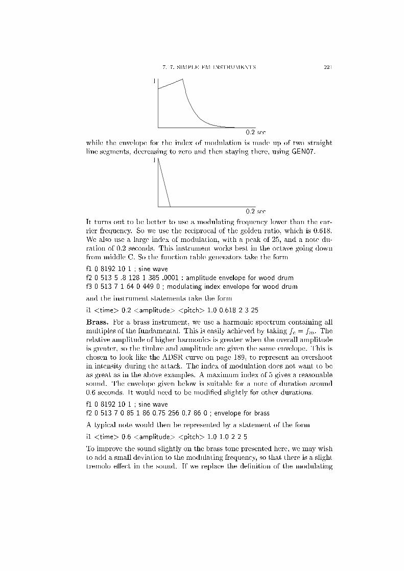
7.17. SIMPLE FM INSTRUMENTS 221
1
0.2 sec
while the envelope for the index of modulation is made up of two straightline segments, decreasing to zero and then staying there, using GEN07.
1
0.2 sec
It turns out to be better to use a modulating frequency lower than the car-rier frequency. So we use the reciprocal of the golden ratio, which is 0.618.We also use a large index of modulation, with a peak of 25, and a note du-ration of 0.2 seconds. This instrument works best in the octave going downfrom middle C. So the function table generators take the form
f1 0 8192 10 1 ; sine wavef2 0 513 5 .8 128 1 385 .0001 ; amplitude envelope for wood drumf3 0 513 7 1 64 0 449 0 ; modulating index envelope for wood drum
and the instrument statements take the form
i1 <time> 0.2 <amplitude> <pitch> 1.0 0.618 2 3 25
Brass. For a brass instrument, we use a harmonic spectrum containing allmultiples of the fundamental. This is easily achieved by taking fc = fm. Therelative amplitude of higher harmonics is greater when the overall amplitudeis greater, so the timbre and amplitude are given the same envelope. This ischosen to look like the ADSR curve on page 189, to represent an overshootin intensity during the attack. The index of modulation does not want to beas great as in the above examples. A maximum index of 5 gives a reasonablesound. The envelope given below is suitable for a note of duration around0.6 seconds. It would need to be modi�ed slightly for other durations.
f1 0 8192 10 1 ; sine wavef2 0 513 7 0 85 1 86 0.75 256 0.7 86 0 ; envelope for brass
A typical note would then be represented by a statement of the form
i1 <time> 0.6 <amplitude> <pitch> 1.0 1.0 2 2 5
To improve the sound slightly on the brass tone presented here, we may wishto add a small deviation to the modulating frequency, so that there is a slighttremolo e�ect in the sound. If we replace the de�nition of the modulating
222 7. SYNTHESIS AND DIGITAL MUSIC
frequency by the statement
ifm = cpspch(p5) * p7 + 0.5
then this will have the required e�ect.
Woodwind. For woodwind instruments, higher harmonics are present dur-ing the attack, and then the low frequencies enter. So we want the carrierfrequency to be a multiple of the modulating frequency, and use an envelope
of the form�� C
Cfor the carrier and
�� for the modulator. So
the function table generators take the form
f1 0 8192 10 1 ; sine wavef2 0 513 7 0 50 1 443 1 20 0 ; amplitude envelope for woodwindf3 0 513 7 0 50 1 463 1 ; modulating index envelope for woodwind
For a clarinet, where odd harmonics dominate, we take fc = 3fm and a max-imum index of 2. A basson sound is produced by giving the odd harmonicsa more irregular distribution. This can be achieved by taking fc = 5fm anda maximum index of 1.5.
7.18. Further techniques in CSound
The CSound language is vast. In this section, we cover just a few ofthe features which we have not touched on in the previous sections. For moreinformation, see the CSound manual.
Tempo. The default tempo is 60 beats per minute, or one beat per second.To change this, a tempo statement is put in the score �le. An example of thesimplest form of tempo statement is
t 0 80
which sets the tempo to 80 beats per minute. The �rst argument (p1) of thetempo statement must always be zero. A tempo statement with more argu-ments causes accelerandos and ritardandos. The arguments are alternatelytimes in beats (p1 = 0, p3, p5 . . . ) and tempi in beats per minute (p2, p4,p6, . . . ). The tempi between the speci�ed times are calculate by making thedurations of beats vary linearly. So for example the tempo statement
t 0 100 20 120 40 120
causes the initial tempo to be 100 beats per minute. By the twentieth beat,the tempo is 120 beats per minute. But the number of beats per minute isnot linear between these values. Rather, the durations decrease linearly from0.6 seconds to 0.5 seconds over the �rst twenty beats. The tempo is thenconstant from beat 20 until beat 40. By default, the tempo remains constantafter the last beat where it is speci�ed, so in this example the last two pa-rameters are super uous.
7.18. FURTHER TECHNIQUES IN CSOUND 223
The tempo statement is only valid within the score section (cf.page 217) in which it is placed, and only one tempo statement may be usedin each section. Its location within the section is irrelevant.
Stereo and Panning. For stereo output, we want to set nchnls = 2 in theheader of the orchestra �le (7.15.1). In the instrument de�nition, instead ofusing out, we use outs with two arguments. So for example to do a simplepan from left to right, we might want the following lines in the instrumentde�nition.
kpanleft lineseg 0, p3, 1kpanright = 1 - kpanleft
outs asig * kpanleft, asig * kpanright
The problem with this method of panning is that the total sound energy isproportional to the square of amplitude, summed over the two channels. Soin the middle of the pan, the total energy is only 1=
p2 times the total enery
on the left or right. So it sounds like there's a hole in the middle. The easiestway to correct this is to take the square root of the straight line produced bythe signal generator lineseg. So for example we could have the following lines.
kpan lineseg 0, p3, 1kpanleft = sqrt(kpan)kpanright = sqrt(1-kpan)
Since sin2 � + cos2 � = 1, another way to keep uniform total sound energy isas follows.
kpan lineseg 0, p3, 1ipibytwo = 1.5708kpanleft = sin(kpan * ipibytwo)kpanright = sqrt((1 - kpan) * ipibytwo)
A good trick for obtaining what sounds like a wider sweep for the pan, es-pecially when using headphones to listen to the output, is to make the anglego from ��=4 to 3�=4 instead of 0 to �=2. This can be achieved by replac-ing the de�nition of kpan above with the following line.
kpan lineseg -0.5, p3, 1.5
A more realistic pan takes account of the fact that at the far reaches ofthe sweep, the sound should not be entirely concentrated in one channel. Aslightly delayed version can be fed into the other channel, with delay vary-ing up to about 0.7 seconds at the extreme end of the sweep.
Display and spectral display. There is a facility for displaying either awaveform or its spectrum, in an instrument �le. So for example the instru-ment
instr 1asig oscil 10000 440 1
out asig
224 7. SYNTHESIS AND DIGITAL MUSIC
display asig p3endin
is the same as (7.15.2), except that the extra line causes the graph of asig (oflength p3) to be displayed. If the ag -d (see page 214) is set, this line makesno di�erence at all. Replacing the display line with
disp�t asig p3, 1024
causes a fast Fourier transform of asig to be displayed, using an input win-dow size of 1024 points. The number of points must be a power of two be-tween 16 and 4096.
Arithmetic. In the orchestra �le, variables represent signed oating pointreal numbers. The standard arithmetic operations +, �, * (times) and / (di-vide) can be used, as well as parentheses to any depth. Powers are denoteda ^ b, but b is not allowed to be audio rate. The expression a % b returns areduced modulo b. Among the available functions are
int (integer part)frac (fractional part)abs (absolute value)exp (exponential function, raises e to the given power)log and log10 (natural and base ten logarithm; argument must be positive)sqrt (square root)sin, cos and tan (sine, cosine and tangent, argument in radians)sininv, cosinv, taninv (arcsine, arccos and arctan, answer in radians)sinh, cosh and tanh (hyperbolic sine, cosine and tangent)rnd (random number between zero and the argument)birnd (random number bewteen plus and minus the argument)
Conditional values can also be used. For example,
(ka > kb ? 3 : 4)
has value 3 if ka is greater than kb, and 4 otherwise. Comparisons may bemade using
> (greater than)< (less than)>= (greater than or equal to)<= (less than or equal to)== (equal to)!= (not equal to).
Expressions, as well as variables, may be compared in this way, but audiorate variables and expressions are not permitted.
Automatic score generation. There are a number of methods of avoidingthe tedious process of writing a score �le for CSound. One method is to usethe score translator program scot. This takes a text �le <�lename>.sc writ-ten in a compressed score notation and writes out a score �le <�lename>.sco.
7.19. OTHER METHODS OF SYNTHESIS 225
Another is to use Cscore, which is a program for making and manipulatingscore �les. The user writes a control program in the C language, which makesuse of a set of function de�nitions contained in a header �le cscore.h. Finally,there is MIDI2CS, a program which takes a MIDI �le as input, and outputsa score �le. There is also a considerable amount of support for MIDI withinthe CSound language.
DirectCSound is a realtime version of CSound for the PC, and can beobtained from Gabriel Maldonado's home page at
http://web.tiscalinet.it/G-Maldonado/home2.htm
I have not tried it out, so I cannot comment on how well it works, but itlooks promising.
Further reading on CSound:
Richard Boulanger, The CSound book [9].
Electronic Musician, Feb 1998 issue.
Keyboard, Jan 1997 issue.
7.19. Other methods of synthesis
Sampling is not really a form of synthesis at all, but is often used indigital synthesizers. It is usual to sample sounds at only a small collection ofpitches, and then to pitch shift by stretching or compressing the waveform,in order to �ll in the gaps. Pitch shifting a digital signal introduces high fre-quency noise, related to the fact that the sample rate is not being shifted atthe same time. This is removed using a low pass �lter.
Wavetable synthesis is a method related to sampling, in which digitallyrecorded wave �les are used as raw material to produce sounds which are asort of hybrid between synthesis and sampling. It is usual to use one wave�le for the attack portion of the sound, and another for the sustain portion.In the case of the sustain portion, a whole number of periods of the sound areused to form a loop which is repeated. An envelope is then applied to shapethe sound, and then �nally the result is pitch shifted and put through a lowpass �lter. An exception to this general proceedure is \one shot" sounds suchas short percussive sounds. These are usually just recorded as a single wave-�le without looping.
Granular synthesis is a method where the sound comes in small pack-ets called grains, whose duration is usually of the order of ten milliseconds.Thousands of these grains are used in each second, to create a sound texture.Usually, some algorithm is used for describing large quantities of grains at atime, so that each grain does not have to be described separately.
Further reading on granular synthesis:
S. Cavaliere and A. Piccialli, Granular synthesis of musical signals, appears as arti-cle 5 in Roads et al [94], pages 155{186.
226 7. SYNTHESIS AND DIGITAL MUSIC
John Duesenberry, Square one: a world in a grain of sound, Electronic Musician,November 1999.
Curtis Roads, Granular synthesis of sound, Computer Music Journal 2 (2) (1978),61{62. A revised and updated version of this article appears as chapter 10 of Roadsand Strawn [95], pages 145{159.
Curtis Roads, Granular synthesis, Keyboard, June 1997.
7.20. The phase vocoder
The phase vocoder is a method of sound analysis and manipulation. Itis based on the technique of applying a discrete Fourier transform to smallwindows of the original sound. The transform may then be manipulated, and�nally the sound may reconstructed from the manipulated transform. Forexample, it is not hard to stretch a sound without altering the pitch usingthis technique.
Further reading:
Mark Dolson, The phase vocoder: a tutorial, Computer Music Journal 10 (4) (1986),14{27.
M.-H. Serra, Introducing the phase vocoder, appears as article 2 in Roads et al [94],
pages 31{90.
7.21. Chebychev polynomials
Composition of functions in general is a good way of obtaining syn-thetic tones. For example, if we take a basic cosine wave cos �t and composeit with the function f(x) = 2x2 � 1 then we obtain
2 cos2 �t� 1 = cos 2�t:
So composing with this function has the e�ect of doubling frequency. Thecorresponding functions for arbitrary integer multiples of frequency are calledthe Chebychev9 polynomials of the �rst kind, which we now investigate.
Let Tn(x) be the polynomial de�ned inductively by T0(x) = 1, T1(x) =x, and for n > 1,
Tn(x) = 2xTn�1(x)� Tn�2(x):
Thus for example we have
T2(x) = 2x2 � 1;
T3(x) = 4x3 � 3x;
T4(x) = 8x4 � 8x2 + 1
T5(x) = 16x5 � 20x3 + 5x
T6(x) = 32x6 � 48x4 + 18x2 � 1
T7(x) = 64x7 � 112x5 + 56x3 � 7x:
9Other spellings for this name include Tchebyche� and Chebichev.
7.22. DIGITAL FORMATS FOR MUSIC 227
Lemma 7.21.1. For n � 0 we have Tn(cos �t) = cosn�t.
Proof. The proof is by induction on n. We begin by observing that
cos �t cos(n� 1)�t� sin �t sin(n� 1)�t = cosn�t
cos �t cos(n� 1)�t+ sin �t sin(n� 1)�t = cos(n� 2)�t
(see x1.7), so that adding and rearranging, we have
cosn�t = 2 cos �t cos(n� 1)�t� cos(n� 2)�t:
Now for n = 0 and n = 1, the statement of the lemma is obvious fromthe de�nition. For n � 2, assuming the statement to be true for smaller val-ues of n, we have
Tn(cos �t) = 2 cos �t Tn�1(cos �t)� Tn�2(cos �t)
= 2 cos �t cos(n� 1)�t� cos(n� 2)�t
= cosn�t:
So by induction, the lemma is true for all n � 0. �
Using a weighted sum of Chebychev polynomials and composing, wecan obtain a waveform with the corresponding weights for the harmonics.Changing the weighting with time will change the timbre of the resultingtone. So for example, if we apply the operation
T1 +13T3 +
15T5 +
17T7 +
19T9 +
111T11
to a cosine wave, we obtain an approximation to a square wave (see equation(2.2.8)). This operation will turn any mixture of cosine waves into the samemixture of square waves.
Exercises
1. Show that y = Tn(x) satis�es Chebychev's di�erential equation
(1� x2)d2y
dx2� x
dy
dx+ n2y = 0:
2. Show that
Tn(x) = xn �
�n
2
�xn�2(1� x2) +
�n
4
�xn�4(1� x2)2 � : : :
3. Draw a graph of y = Tn(x) for �1 � x � 1 and 0 � n � 5.
7.22. Digital formats for music
Error correcting codes, cross interleaved Reed{Solomon codes
228 7. SYNTHESIS AND DIGITAL MUSIC
7.23. MIDI
Most synthesizers these days talk to each other and to computers viaMIDI cables. MIDI stands for \Musical Instrument Digital Interface". It isan internationally agreed data transmission protocol, introduced in 1982, forthe transmission of musical information between di�erent digital devices. It isimportant to realise that in general there is no waveform information presentin MIDI, unless the message is a \sample dump". Instead, most MIDI mes-sages give a short list of abstract parameters for an event.
There are three basic types of MIDI message: note messages, controllermessages, and system exclusive messages. Note messages carry informationabout the starting time and stopping time of notes, which patch (or voice)should be used, the volume level, and so on. Controller messages change pa-rameters like chorus, reverb, panning, master volume, etc. System exclusivemessages are for transmitting information speci�c to a given instrument ordevice. They start with an identi�er for the device, and the body can con-tain any kind of information in a format proprietary to that device. Thecommonest kind of system exclusive messages are for transmitting the datafor setting up a patch on a synthesizer.
The MIDI standard also includes some hardware speci�cations. It spec-i�es a baud rate of 31:25 KBaud. For modern machines this is very slow, butthe for the moment we are stuck with this standard. One of the results ofthis is that systems often su�er from MIDI \bottlenecks," which can causeaudibly bad timing. The problem is especially bad with MIDI data involvingcontinually changing values of a control variable such as volume or pitch.
Further reading:
S. de Furia and J. Scacciaferro, MIDI programmer's handbook [32].
F. R. Moore, The dysfunctions of MIDI, Computer Music Journal 12 (1) (1988), 19{28.
J. Rothstein, MIDI, A comprehensive introduction [100].
Eleanor Selfridge-Field (Editor), Donald Byrd (Contributor), David Bainbridge
(Contributor), Beyond MIDI: The Handbook of Musical Codes, M. I. T. Press (1997).
7.24. Software and internet resources
The information in this section is, of course, very volatile. So it is likelythat by the time you are reading this, a lot of the information will alreadybe out of date.
Scales and Temperaments: The best internet resource on the subject ofscales, temperaments and tunings is
http://www.xs4all.nl/�huygensf/doc/bib.html
This is part of the Huygens-Fokker Foundation website, maintained byManuel Op de Coul, and consists of a giant bibliography together with links
7.24. SOFTWARE AND INTERNET RESOURCES 229
to other internet resources on the subject. The front page of the website is at
http://www.xs4all.nl/�huygensf/english/
Also on the same website, a discography of microtonal music can be found at
http://www.xs4all.nl/�huygensf/doc/discs.html
A large collection of scales and temperaments can be found at
http://www.xs4all.nl/�huygensf/doc/scales.zip
and the Scala scales and temperaments software can be found at
http://www.xs4all.nl/�huygensf/scala/
To subscribe to the alternate tunings email discussion group, send an emptyemail message to [email protected].
Just Intonation Network: http://www.dnai.com/�jinetwk/
Bohlen{Pierce scale: http://members.aol.com/bpsite/index.html
Music Theory: Sites o�ering free music theory tuition online include
Easy Music Theory (Gary Ewer): http://www.musictheory.halifax.ns.ca/
Java Music Theory: http://academics.hamilton.edu/music/spellman/JavaMusic/
Online Music Instruction Page (Ken Fansler):http://orathost.cfa.ilstu.edu/�kwfansle/onlinemusicpage.htm
Practical Music Theory: http://www.teoria.com/java/eng/java.htm
Sound editors: There are some good shareware sound editors. Among thebest are:
Cool Edit: http://www.syntrillium.com/cooledit/index.html
Goldwave: http://www.goldwave.com/
Acid Wav: http://www.polyhedric.com/software/acid/
There are two freeware audio frequency analysers for the PC called
Spectrogram: http://www.monumental.com/rshorne/gram.html
Frequency analyzer: http://www.hitsquad.com/smm/programs/Frequency/
CSound: This free software is described in x7.15. Versions for various plat-forms (PC, Mac, Unix, Atari, NeXT) are available from
ftp://ftp.maths.bath.ac.uk/pub/dream/
To subscribe to the email discussion group for CSound, send an empty mes-sage to [email protected]. Further information about CSoundcan be found at the following www pages:
http://www.mitpress.com/e-books/csound/frontpage.html
(the CSound front page, MIT Press)
230 7. SYNTHESIS AND DIGITAL MUSIC
http://www.bright.net/�dlphilp/dp csound.html
(Dave Phillips' PC CSound page)
http://www.bright.net/�dlphilp/linux csound.html
(Dave Phillips' Linux CSound page)
http://music.dartmouth.edu/�dupras/wCsound/csoundpage.html
(Martin Dupras' CSound page)
A utility for PC and Unix called MIDI2CS, written by Rudiger Borrmann,converts MIDI �les to Csound scores. It is available from
http://www.snafu.de/�rubo/songlab/midi2cs/csound.html
A utility for emulating the Yamaha DX7 with CSound can be found at Je�Harrington's site
http://www.parnasse.com/dx72csnd.shtml
Other synthesis software: This is a rapidly expanding �eld, and newproducts turn up almost every week. The ones I know of are as follows.
Audio Architect (PC): http://www.audiarchitect.com/
Bitheadz Retro AS-1 (Mac): http://www.bitheadz.com (free demo)
CLM (Common Lisp Music, freeware):http://www-ccrma.stanford.edu/CCRMA/Software/clm/clm.html
CMix (Next, Linux, Sparc, SGI, PowerMac; freeware):http://www.music.princeton.edu/winham/cmix.html
Cybersound Studio (Mac, Win 95/98/ME): http://www.cybersound.com
Cycling '74 (Mac + Opcode Max): http://www.cycling74.com (free demo)
Grain Wave (Mac shareware): http://www.nmol.com/users/mikeb/
Ik Multimedia's Groovemaker and Ax�e (Mac, Win 95/98/ME):http://www.ikmultimedia.com (free demo)
Lemur (Mac): http://datura.cerl.uiuc.edu/Lemur/AboutLemur.html
Native Instruments Reaktor/Generator/Transformator (Win 95/98/ME):http://www.native-instruments.com/ (free demo)
Nemesis GigaSampler (Win 95/98/ME): http://www.nemesismusic.com
Nyquist (freeware):http://www.cs.cmu.edu/afs/cs.cmu.edu/project/music/web/music.software.html
Seer Systems Reality: http://www.seersystems.com
Steinberg Rebirth RB-338 (Mac, Win 95/98/ME/NT):http://www.us.steinberg.net (free demo)
Synthesis Toolkit (C++ code):http://www-ccrma.stanford.edu/CCRMA/Software/STK/
7.24. SOFTWARE AND INTERNET RESOURCES 231
Virtual Sampler (Win 95/98/ME/NT):This can be found at Sonic Spot, http://www.sonicspot.com/, or at MAZ,http://www.maz-sound.com/. It is shareware, and the unregistered versiondoes everything but save sounds. It includes a complete Yamaha DX7 emu-lation.
The most impressive site for information on the processes and control of syn-thesis is Electronic Music Interactive, at
http://nmc.uoregon.edu/emi/emi.html
Synthesizers and patches: The best general websites for synthesizers andpatches are
Synthesizer and Midi Links Page:http://www.interlog.com/�spinner/lbquirke/synthesis/links/
Synth Site: http://www.sonicstate.com/bbsonic/synth/index.cfm
At the anonymous ftp site ftp.ucsd.edu, in the subdirectory /midi/patches,there are patches for Casio CZ-1, CZ-2, Ensoniq ESQ1, SQ1, Kawai K1, K4,K5, XD-5, Korg M1, T3, WS (Wavestation), Roland D10, D5, D50, D70,SC55, U20, and Yamaha DX7, FB01, TX81Z, SY22, SY55, SY77, SY85.
For the Yamaha DX7, there is a web page which I maintain at
http://www.math.uga.edu/�djb/dx7.html
which contains, among other things, a patch archive and instructions for join-ing the email discussion group.
Typesetting software:
CMN (Common Music Notation, freeware for NeXT and SGI machines):http://ccrma-www.stanford.edu/CCRMA/Software/cmn/cmn.html
Finale is a commercial music notation package for the Mac and PC Win-dows (current version Finale 98), and is available from Coda Music Software.Their web site
http://www.codamusic.com/
has more information. A free demonstration version of the program is avail-able on this web site. Without academic discount, Finale is very expensive,but with academic discount it costs about $200{$250. To subscribe to theemail discussion group for Finale, send an email message to [email protected]
with the phrase \subscribe Finale" or \subscribe Finale-Digest" in the body ofthe message. To be removed from the list, send \signo� Finale" or \signo�
Finale-Digest" to the same address.
Finale forum (not sanctioned by Coda Music): http://www.cmp.net/�nale/
Finale Resource Page: http://www.peabody.jhu.edu/�skot/�nale/�n home.html
Ftp site for Finale users: ftp://ftp.shsu.edu/pub/�nale/
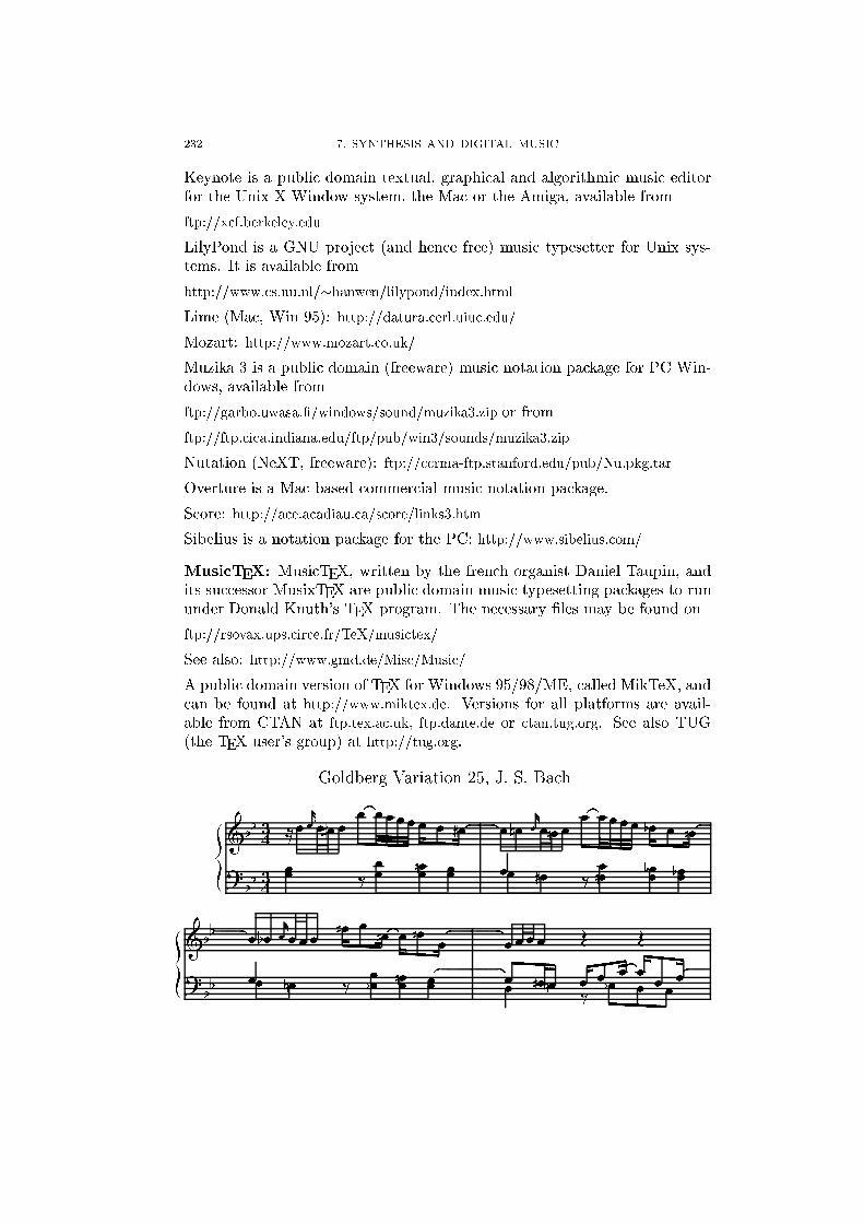
232 7. SYNTHESIS AND DIGITAL MUSIC
Keynote is a public domain textual, graphical and algorithmic music editorfor the Unix X Window system, the Mac or the Amiga, available from
ftp://xcf.berkeley.edu
LilyPond is a GNU project (and hence free) music typesetter for Unix sys-tems. It is available from
http://www.cs.uu.nl/�hanwen/lilypond/index.html
Lime (Mac, Win 95): http://datura.cerl.uiuc.edu/
Mozart: http://www.mozart.co.uk/
Muzika 3 is a public domain (freeware) music notation package for PC Win-dows, available from
ftp://garbo.uwasa.�/windows/sound/muzika3.zip or from
ftp://ftp.cica.indiana.edu/ftp/pub/win3/sounds/muzika3.zip
Nutation (NeXT, freeware): ftp://ccrma-ftp.stanford.edu/pub/Nu.pkg.tar
Overture is a Mac based commercial music notation package.
Score: http://ace.acadiau.ca/score/links3.htm
Sibelius is a notation package for the PC: http://www.sibelius.com/
MusicTEX: MusicTEX, written by the french organist Daniel Taupin, andits successor MusixTEX are public domain music typesetting packages to rununder Donald Knuth's TEX program. The necessary �les may be found on
ftp://rsovax.ups.circe.fr/TeX/musictex/
See also: http://www.gmd.de/Misc/Music/
A public domain version of TEX for Windows 95/98/ME, called MikTeX, andcan be found at http://www.miktex.de. Versions for all platforms are avail-able from CTAN at ftp.tex.ac.uk, ftp.dante.de or ctan.tug.org. See also TUG(the TEX user's group) at http://tug.org.
Goldberg Variation 25, J. S. Bach
�IG
2222
34
34
!!@!
)! !4! !
?
!
!!
z{! ! !CCCCDD
!|!!AA! !
!!AACCz!z
!!{! 6! )!
z!!|! !
?
!
|!!
z{! ! !CCCCDD
!x!!AAx! !
!x!AACC|!z
�IG
2222
!!{!2! )!
|!! ! !
?
AAz! !
x!!AACCz!|!!z{AA! |!
!!AACC!zz
!{!{! ! !
z!AAACCC
|!!
? ! !>
x! ��! !z{ GG! !>
DD!GG
II!z
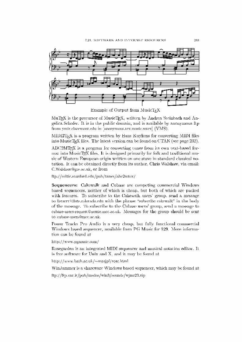
7.24. SOFTWARE AND INTERNET RESOURCES 233
�IG
2222
!{!AAAz!@! )!CC!
!z! !?
!(!!
z{!|! !IIIIJJ
!|!!!|!
|!x!
!!|}! !
����x!!|
|!x!}! ! )!
!!! ! !
?
!
!|!
z{! ! !IIIIJJx!z!|!|! !
!!!!
|}!|!x!
!|
�IG
2222
z!!}!z! )!
!!!|! !
?
|! !������x!
!!z! !z!
!!x! ! !
!z!x!|!|!z |
!{!}!x! ! !z!
!? ! !>
! ��
! !z{!���!���!>
��
!z{!���!���!z
Example of Output from MusicTEX
MuTEX is the precursor of MusicTEX, written by Andrea Steinbach and An-gelica Schofer. It is in the public domain, and is available by anonymous ftpfrom ymir.claremont.edu in [anonymous.tex.music.mtex] (VMS).
MIDI2TEX is a program written by Hans Kuykens for converting MIDI �lesinto MusicTEX �les. The latest version can be found on CTAN (see page 232).
ABC2MTEX is a program for converting tunes from its own text-based for-mat into MusicTEX �les. It is designed primarily for folk and traditional mu-sic of Western European origin written on one stave in standard classical no-tation. It can be obtained directly from its author, Chris Walshaw, via email:[email protected], or from
ftp://celtic.stanford.edu/pub/tunes/abc2mtex/
Sequencers: Cakewalk and Cubase are competing commercial Windowsbased sequencers, neither of which is cheap, but both of which are packedwith features. To subscribe to the Cakewalk users' group, send a messageto [email protected] with the phrase \subscribe cakewalk" in the bodyof the message. To subscribe to the Cubase users' group, send a message [email protected]. Messages for the group should be sentto [email protected].
Power Tracks Pro Audio is a very cheap, but fully functional commercialWindows based sequencer, available from PG Music for $29. More informa-tion can be found at
http://www.pgmusic.com/
Rosegarden is an integrated MIDI sequencer and musical notation editor. Itis free software for Unix and X, and it may be found at
http://www.bath.ac.uk/�masjpf/rose.html
WinJammer is a shareware Windows based sequencer, which may be found at
ftp://ftp.cnr.it/pub/msdos/win3/sounds/wjmr23.zip
234 7. SYNTHESIS AND DIGITAL MUSIC
WinJammer Pro (I'm not sure what the di�erence is) is in the same direc-tory, as wjpro.zip.
Random music: There are a number of freeware/shareware probabilisticmusic programs designed to run under Windows.
Aleatoric composer (shareware):ftp://oak.oakland.edu/msdos/music/alcomp11.zip
Art Song 2.3 (shareware): http://members.aol.com/strohbeen/fmlsw.html
FMusic 1.9 (freeware): http://members.aol.com/dsinger594/caman/fmusic19.zip
FractMus 2.3 (freeware): ftp://ftp.cdrom.com/pub/win95/music/frctmu25.zip
Fractal Tune Smithy (freeware/shareware):http://matrix.crosswinds.net/�fractalmelody/index.htm
Improvise 1.2 (shareware):ftp://ftp.cnr.it/pub/msdos/win3/sounds/impvz120.zip
Make-Prime-Music (freeware):http://members.tripod.de/Latrodectus98/index.html
Mandelbrot Music (freeware): http://www.�n.ne.jp/�yokubota/mandele.shtml
MusiNum 2.08 (freeware):http://www.forwiss.uni-erlangen.de/�kinderma/musinum/musinum.html
QuasiFractalComposer 2.01 (freeware):http://members.tripod.com/�paulwhalley/
Tangent (free/shareware): http://www.randomtunes.com/
The Well Tempered Fractal 3.0 (freeware):http://www-ks.rus.uni-stuttgart.de/people/schulz/fmusic/wtf/wtf30.zip
MIDI: The MIDI speci�cation can be obtained via email by sending a mes-sage with the phrase GET MIDISPEC PACKAGE in the message body, [email protected]. There are archives of MIDI �les available at
ftp://ftp.cs.ruu.nl/MIDI/DOC/archives/
ftp://ftp.waldorf-gmbh.de/pub/midi/
There are two programs called mf2t and t2mf which convert standard MIDI�les into human readable ASCII text and back again. The MIDI home pageon the WWW is
http://www.eeb.ele.tue.nl/midi/index.html
A good starting point for information about MIDI is the Northwestern Uni-versity site
http://nuinfo.nwu.edu/musicschool/links/projects/midi/expmidiindex.html
Academic Computer Music: The following departments in Americanuniversities have programs in computer music. CalArts (David Rosenboom,
7.24. SOFTWARE AND INTERNET RESOURCES 235
Morton Subotnick), Carnegie Mellon (Roger Dannenberg), MIT (Tod Ma-chover, Barry Vercoe), Princeton (Paul Lansky), Stanford (John Chowning,Chris Cha�e, Perry Cook, etc.), SUNY Bu�alo (David Felder, Cort Lippe),UC Berkeley (David Wessel), UCSD (Miller Puckett, F. Richard Moore,George Lewis, Peter Otto).
IRCAM is an institution in Paris for computer music, which has an anony-mous ftp site at ftp.ircam.fr. In particular, the music/programming environ-ment MAX can be found there.
Music Theory Online (the Online Journal of the Society for Music Theory)can be found at
http://boethius.music.ucsb.edu/mto/mtohome.html
FAQs: There are several FAQs (\Frequently Asked Questions" and their an-swers) available on the internet. Two that I know of are available from the sitexcf.berkeley.edu, either by anonymous ftp or by email. They are the electronicand computer music FAQ, in /pub/misc/netjam/doc/ECMFAQ and the compo-sition FAQ, in /pub/misc/netjam/doc/FAQ/composition/compositionFAQ.entire.Or send an email message to [email protected] with the subjectline \request for ECM FAQ", respectively \request for composition FAQ".
Other resources: The following are some interesting WWW pages:
Everyone seems to want to know more about the infamous \Mozart e�ect".Volume VII, Issue 1 (Winter 2000) of MuSICA Research Notes is devoted tothis much overpublicized and misunderstood topic, and can be found at
http://www.musica.uci.edu/mm/V7I1W00.html
http://www.oulu.�/music.html is a directory of music sites.
http://www.music.indiana.edu/misc/music-resources.html is a catalog of musicresources.
http://sunsite.unc.edu/pub/ianc/index.html is the Internet Underground MusicArchive.
To subscribe to the electronic music email discussion group, send a messageto [email protected] with the line \SUB EMUSIC-L" in the body. Messagesfor the group should be sent to [email protected]. For the digests only, re-place EMUSIC-L with EMUSIC-D.
Online papers: See Appendix O for a selection of relevant papers whichcan be downloaded from academic journals.
