Chapter 4

Stochastic Generalized AssignmentProblem∗

Introduction

Pairing problems constitute a vast family of problems in CO. Different versions of these problemshave been studied since the mid 1950s due both to their many applications and to the challenge ofunderstanding their combinatorial nature. The range of problems in this group is very wide. Some canbe easily solved in polynomial time, whereas others are extremely difficult. The simplest one is theAssignment Problem, that can be easily solved by the Hungarian Algorithm (Kuhn 1955). MatchingProblems appear when the underlying graph is no longer bipartite and are much more involved,although they can still be solved in polynomial time (Edmonds 1965). On the other extreme, theGeneralized Assignment Problem is a very difficult CO problem that is NP-hard.

In general terms, the Assignment Problem consists of finding the best assignment of items toagents according to a predefined objective function. Among its many applications, we mention theassignment of tasks to workers, of jobs to machines, of fleets of aircraft to trips, or the assignmentof school buses to routes. However, in most practical applications, each agent requires a quantity ofsome limited resource to process a given job. Therefore, the assignments have to be made taking intoaccount the resource availability of each agent. The problem derived from the classical AssignmentProblem by taking into account these capacity constraints is known as the Generalized AssignmentProblem (GAP). Among its many applications, we find assignment of variable length commercials intotime slots, assignment of jobs to computers in a computer network (Balachandran 1972), distributionof activities to the different institutions when making a project plan (Zimokha and Rubinshtein 1988),etc. Besides these applications, it also appears as a subproblem in a variety of combinatorial problemslike Vehicle Routing (Fisher and Jaikumar 1981) or Plant Location (Ross and Soland 1977; Dıaz2001). A survey of exact and heuristic algorithms to solve the GAP can be found in Cattrysse andVan Wassenhove (1992). More recently, (Savelsbergh 1997) proposed a Branch and Price algorithm,and different metaheuristic approaches have been proposed by other authors (Chu and Beasley 1997;Dıaz and Fernandez 2001; Yagiura, Tamaguchi, and Ibaraki 1998; Yagiura, Ibaraki, and Glover 1999).

As mentioned before, the GAP is a very challenging problem, not only because it is NP-hard, butalso because the decision problem to know if a given instance is feasible is NP-complete (Martelloand Toth 1990). In fact, the GAP is in practice even more difficult, since most of its applications have

∗The contents of this chapter areincluded in Albareda-Sambola and Fernandez (2000) and Albareda-Sambola, vander Vlerk, and Fernandez (2002).

45

Stochastic GAP

a stochastic nature. Stochasticity can be due to two different sources. On the one hand, it appearswhen the actual amount of resource needed to process the jobs by the different agents is not known inadvance. This happens, for instance, when assigning software development tasks to programmers; thetime needed for each task is not known a priori. Similarly, the actual running times of jobs are notknown when they are assigned to processors. This is due to the fact that the actual running times ofjobs depend on the overall load of the system. In all these cases, the amount of resource consumedwhen assigning tasks to agents should be modeled with continuous random variables.

The second source of stochasticity is uncertainty about the presence or absence of individualjobs. In such cases, there is a set of potential jobs, but only a subset of them will have to beactually processed. This subset is not known when the assignment has to be decided. This is the caseof emergency services, or the assignment of repairmen to machines. In this situation, the resourcerequirement of each job can be modeled as a random variable with Bernoulli distribution. This kind ofstochasticity has also been considered in other problems, such as stochastic routing problems (Bermanand Simchi-Levi 1988; Laporte, Louveaux, and Mercure 1994)

The stochasticity in the GAP studied in this thesis is of the latter type. The problem will bemodeled as a stochastic programming problem with recourse.

We are aware of only two papers addressing any type of stochastic assignment problems. Mine,Fukushima, Ishikawa, and Sawa (1983) present a heuristic for an assignment problem with stochasticside constraints. The second paper (Albareda-Sambola and Fernandez 2000), partially contained inthis chapter, proposes some heuristics based on approximation models for the SGAP with Bernoullidemands.

To the best of our knowledge, no results on exact algorithms for any type of stochastic GAP areknown.

In this chapter, we consider the following SGAP: After the assignment is decided, each job requiresto be processed with some known probability. In this context, we can think that jobs are customersrequiring some service with a demand distributed as a Bernoulli random variable. The problem ismodeled as a recourse problem. Assignments of customers to agents are decided a priori. Oncethe actual demands are known, if the capacity of an agent is violated, some of its assigned jobs arereassigned to underloaded agents at a prespecified cost. For a given instance of the problem, theoverall demand of the customers requiring service can be bigger than the total capacity. In this case,part of the customers are lost, and a penalty cost is paid.

The objective is to minimize the expected total costs. The costs consist of two terms: the as-signment costs, and the expected penalties for reassigned and/or lost customers. This problem hasrelatively complete recourse, i.e., the second-stage problem is feasible for any a priori assignment andany realization of the demand. Additionally, due to the assumption that demands are binary, we canbuild a model for the second-stage problem where only the right-hand side contains non-deterministicelements.

We propose three versions of an exact algorithm for this SGAP. All versions have in common thatthe (nonconvex, discontinuous) recourse function is replaced by a convex approximation, which is exactat all binary first-stage solutions. Next, a cutting procedure is used to iteratively generate a partialdescription of this convex approximation of the recourse function, following the ideas presented in VanSlyke and Wets (1969) and in Laporte and Louveaux (1992). Integrality of the first-stage variables isaddressed using branch and bound techniques.

The first version of the algorithm has the structure of a branch and cut algorithm. At each node,cuts are iteratively added until no more violated valid constraints are found. Then, if the current

46

Models

solution is not integer, branching is performed.

However, in the considered SGAP, the separation problem to find the new cut to be added ishighly time consuming because it requires the evaluation of the convex approximation of the recoursefunction. To reduce the number of evaluations of this function, a second version has been designedwhere, at each iteration, an integer problem is solved using branch and bound. Once an integerassignment is found, the associated cut is computed and added. The algorithm terminates when theinteger solution found does not violate the associated constraint. This approach makes a great effortto find integer solutions even at the earliest stages when the information about the recourse functionis rather poor.

A third strategy has been designed as a tradeoff between the other two. The idea is to avoid theexcessive number of evaluations of the recourse function as well as to reduce the time invested to reachintegrality. At each node of the enumeration tree, an associated cut is computed. If the solution ofthe node is integer, the cut is added and the current problem is reoptimized. Otherwise, branching isperformed and the new cut is added to the descendant nodes.

All three versions of the exact algorithm compute the same upper and lower bounds initially. Theupper bound is obtained with the heuristics presented in Section 4.2. The lower bound is found bysolving a family of stochastic linear subproblems with the L-shaped algorithm.

The remainder of this chapter is organized as follows: In Section 4.1 the two-stage problem ismodeled and its properties are studied. In particular, we introduce a convex approximation of thenon-convex recourse function. The proposed heuristics are presented in 4.2 and the exact algorithmsare described in Section 4.3. After that, Section 4.4 gives a description of the lower bound. In Section4.5 some strategies to improve the performance of the algorithms are discussed. Finally, computationalexperiences and conclusions are presented in Sections 4.6 and 4.7 respectively.

4.1 Problem description and modeling

The GAP consists of finding the cheapest assignment of a set of jobs to a set of agents such thateach job is assigned exactly to one agent and capacity constraints on some resource are satisfied.

Let I and J be the index sets of agents and jobs, respectively, with |I| = ns and |J | = nt. Wedefine, for i ∈ I and j ∈ J ,

cij is the cost of assigning job j to agent i;

dij is the amount of resource needed by agent i to perform task j;

bi is the resource capacity of agent i (i ∈ I), and B =∑

i∈I bi

and

xij takes the value 1 if job j is assigned to agent i, and 0 otherwise.

47

Stochastic GAP

Using this notation, the GAP is modeled as:

minimize∑

i∈I

∑

j∈J

cijxij

subj. to∑

i∈I

xij = 1 j ∈ J

∑

j∈J

dijxij 6 bi i ∈ I

xij ∈ {0, 1} i ∈ I, j ∈ J.

Most often, however, the assignment of jobs to agents must be decided before the actual values ofthe demands for resource capacity dij , i ∈ I, j ∈ J , are known, so that the above model is no longervalid. In what follows, ξ denotes the random vector of demands, and we assume that, once the valuesof the vector ξ become available, it is possible to reassign some of the jobs, incurring costs Kj , j ∈ J .

Assuming that the values of ξij , i ∈ I, j ∈ J are agent independent (that is, for each j ∈ J ,ξij = ξj ∀i ∈ I) and that they are Bernoulli random variables, the problem can be formulated usingthe following recourse model:

(FSP) minimize Q(x)

subj. to∑

i∈I

xij = 1 j ∈ J

xij ∈ {0, 1} i ∈ I, j ∈ J,

where∗ Q(x) := Eξv(x, ξ) is the recourse function, and

(SSP) v(x, ξ) = minimize∑

i∈I

∑

j∈J

cijyij +∑

j∈J

Kjzj

subj. to yij + zj > qjxij i ∈ I, j ∈ J∑

i∈I

yij > ξj j ∈ J

∑

j∈J

yij 6 bi i ∈ I

yij ∈ {0, 1} i ∈ I, j ∈ J

zj ∈ {0, 1} j ∈ J.

At the first stage, each job is provisionally assigned to an agent. The second-stage problemdetermines the final assignment pattern once the demands are known. Variables yij ((i, j) ∈ I × J)are defined like xij , and zj (j ∈ J) denote those jobs with nonzero demand that have been reassigned.The first group of constraints (from now on, flag constraints) set zj to 1 if job j has nonzero demandand it is not assigned to the same agent it was assigned to a priori. The other constraints ensure thatall jobs with nonzero demand are actually assigned to an agent and that capacities of the agents arenot violated, respectively.

∗E stands for mathematical expectation.

48

Models

FSP is a two-stage recourse model with binary variables in both stages. Thus, in addition todifficulties caused by integrality of the first-stage variables, the recourse function Q is non-convexin general. Indeed, since the parameters ξ are discretely distributed, it is lower semicontinuous butdiscontinuous in general (Schultz 1993). Moreover, evaluation of Q for a given x calls for solving manysecond-stage problems, which, in this case, are binary programming problems. Since these second-stage problems are not easily solvable, this is computationally very demanding. In the next subsectionwe show how to overcome these problems by redefining the second-stage problem.

Convex approximation of the recourse function

First we introduce an alternative formulation of the second-stage problem for GAP. Subsequently,we show that this new formulation has a nice mathematical property, which allows to drop the integerrestrictions on the second-stage variables.

Proposition 4.1.1. Given a feasible solution x of FSP and ξ a 0-1 vector, SSP is equivalent to

(SSP2) minimize∑

i∈I

∑

j∈J

cijyij +∑

i∈I

∑

j∈J

Kjzij

subj. to yij + zij > ξjxij i ∈ I, j ∈ J∑

i∈I

yij > ξj j ∈ J

∑

j∈J

yij 6 bi i ∈ I

yij ∈ {0, 1} i ∈ I,j ∈ J

zij ∈ {0, 1} i ∈ I,j ∈ J

Proof. Let (y∗, z∗) be an optimal solution to SSP2. From the fact that for a feasible point x eachjob is assigned a priori to exactly one agent it follows that, in the optimal solution, for a fixed j ∈ Jat most one of the variables z∗ij (i ∈ I) takes value 1 and the others are 0. So, zj = maxi∈I z∗ij , (y∗, z)is a feasible point for SSP, with the same objective function value as (y∗, z∗).

Similarly, given an optimal solution (y∗, z∗) of SSP, a feasible solution (y∗, z) of SSP2 with thesame objective value can be built as follows:

- If z∗j = 0, take zij = 0, ∀i ∈ I.

- If z∗j = 1, because of the structure of x, only one of the flag constraints is tight, say (i1, j). Then,set zi1j = 1 and zij = 0, ∀i 6= i1.

Thus, both models lead to the same optimal value.

Proposition 4.1.2. The matrix defining the feasible region of SSP2 is totally unimodular (TU).

Proof.

The structure of the matrix is:

49

Stochastic GAP

A =

(Ins·nt Ins·nt

M O

)

where M is the matrix of a transportation problem, which is known to be TU. By Proposition III.2.1in Nemhauser and Wolsey (1988), the matrices

M1 =(

Ins·nt

M

)and M2 =

M1 Ins·nt+ns+nt

are also TU. Finally, since A is a submatrix of M2, it is TU as well.

Since the matrix defining the feasibility region of SSP2 is totally unimodular, its linear relaxationwill have integer optimal solutions whenever the right-hand side is integral; moreover, in that case,the optimal values of SSP2 and its relaxation are equal.

Assuming that the capacities bi, i ∈ I, are integral, the right-hand side of SSP3 is integral forevery feasible (i.e., binary) first-stage solution to the GAP. Thus, using Propositions 4.1.1 and 4.1.2,we redefine the function v(x, ξ) as the optimal value of the LP problem

(SSP3) minimize∑

i∈I

∑

j∈J

cijyij +∑

j∈J

Kjzj

yij + zj > ξjxij i ∈ I, j ∈ J∑

i∈I

yij > ξj j ∈ J

∑

j∈J

yij 6 bi i ∈ I

yij ∈ [0, 1] i ∈ I, j ∈ J

zj > 0 j ∈ J

As stated in Proposition 4.1.1, this function coincides with the previously defined v(x, ξ) in allfeasible vectors x, for any demand vector ξ. This is not true for fractional vectors x, but this causesno problems since such x are not feasible anyway. The advantages of defining v as the value functionof a second-stage problem with continuous variables are two-fold: (i) the evaluation of v can be done(much) faster; (ii) the mathematical properties of v are much nicer. In particular, the new function vis a convex function of x. As we will discuss below, these properties carry over to the recourse functionQ, which is defined as the expectation of v.

Remark 4.1.1. Observing that SSP3 is simply the LP relaxation of the original second-stage SSP,the question rises whether the constraint matrix of this problem is TU itself. As we show below, thisis not the case.

Consider the submatrix of SSP formed by columns corresponding to variables y00, y10 and z0, andthe two rows of the first group concerning variables y00 and y10, and the row in the second group

50

Heuristic Solutions

concerning job 0. This submatrix equals

1 0 10 1 11 1 0

with determinant −2, so that it is not TU. This submatrix occurs in any instance with at least onejob and two agents; matrices of all non-trivial instances are therefore not TU.

Consequently, there is no guarantee that SSP3 yields the correct optimal value for all integer right-hand sides. However, Propositions 4.1.1 and 4.1.2 imply that SSP3 does give the correct value for allrelevant right-hand sides, i.e., those corresponding to feasible first-stage solutions.

Properties of the recourse function

Before introducing our algorithm, we present some well-known properties of the recourse functionQ. Discussion on these and other properties in a general context can be found in the textbooks (Birgeand Louveaux 1997; Kall and Wallace 1994; Prekopa 1995).

Remark 4.1.2. Assuming thatnt 6 B (4.1)

it follows that FSP is a two-stage program with relatively complete recourse. Assuming in additionthat Kj > 0, j ∈ J , it follows that, for every realization of the demand vector ξ, the second-stagevalue function v is finite for all x ∈ Rns·nt .

If (4.1) is not satisfied, relatively complete recourse is obtained by introducing a dummy agent0 ∈ I with enough capacity in the second stage, which handles excess demand at a unit penalty cost P .That is, this dummy agent has assignment costs c0j = P −Kj , j ∈ J , since any a posteriori assignmentto it will also induce the corresponding reassignment penalty Kj ; it makes no sense, however, to payboth penalties at the same time.

Proposition 4.1.3. The function Q is finite and convex. Moreover, since the random parameters arediscretely distributed, Q is a polyhedral function.

Proposition 4.1.4. Let S be the index set of scenarios (realizations). For s ∈ S, let ps be theprobability of scenario s and ξs the corresponding demand vector, so that

Q(x) =∑

s∈S

psv(x, ξs), x ∈ Rns·nt . (4.2)

Let λ(x, ξs) be a vector of dual prices for the first set of constraints in SSP3 for the pair (x, ξs). Thenu(x),

u(x) =∑

s∈S

psλ(x, ξs)diag(ξs1, . . . , ξ

snt

), (4.3)

is a subgradient of Q at x. Here, ξsj is a vector of |J | components, all equal to the demand of customer

j in scenario s.

4.2 Heuristic Solutions for the Stochastic Generalized AssignmentProblem

In this section we present three heuristics for the SGAP under consideration. All heuristics consistin solving an auxiliary deterministic model that approximates FSP.

51

Stochastic GAP

Heuristic A: Chance Constrained Model

The first of the proposed approximation models is a chance constrained model. Since the sum ofBernoulli i.i.d. variables is a Binomial, and we know its distribution, it is easy to find the deterministicequivalent for problems where sums of ξ variables appear in probabilistic constraints.

Penalties for reassignments are likely to have higher values than the assignment costs, so, it isdesirable to have solutions where a small number of reassignments is likely to be needed. We proposea model where capacity violations are only allowed to occur with a prespecified probability α. If aplant i has k customers assigned, the probability that reassignments are needed is given by:

P[More than bi among k customers have demand] =k∑

s=bi+1

(k

s

)ps(1− p)k−s.

Thus, by taking

K(bi, p, α) = max

k ∈ Z |

k∑

s=bi+1

(k

s

)ps(1− p)k−s 6 α

,

we can find good assignments as the solutions of

minimize∑

i∈I

∑

j∈J

cijxij (4.4)

subj. to∑

i∈I

xij > 1 j ∈ J (4.5)

∑

j∈J

xij 6 K(bi, p, α) i ∈ I, j ∈ J (4.6)

xij ∈ {0, 1} i ∈ I, j ∈ J. (4.7)

Note that, since K(bi, p, α) takes integer values, and demands are binary, integrality constraintscan be dropped in the resolution of the problem.

The choice of the parameter α will determine the quality of this model as an approximation of FSP.High values of α can lead to bad assignments, in the sense of capacity constraints violations, whereasthe problem can become infeasible for small values. Since feasibility is easily checkable for model(4.4)-(4.7), the strategy we propose is to initially set α to a small value, and increase it successivelyuntil the model becomes feasible.

Heuristic B: Transportation Model

In general terms, the model proposed as the basis of Heuristic A uses auxiliary capacities for theplants that guarantee the feasibility of the assignment problem, but that are tight enough as to avoidunbalanced workloads for the agents. What we use as an alternative to Heuristic A is to solve a similarmodel, but using simpler auxiliary capacities. The values we propose for the new capacities are

bi =⌈bi

nt

B

⌉

52

Heuristic Solutions

That is, we propose to take capacities proportional to the real ones, but large enough as to globallysatisfy the demands of all the customers.

The model to solve now is (4.4)-(4.7) where constraints (4.6) have been replaced by∑

j∈J

xij 6 bi, i ∈ I.

Note that, again, total unimodularity of the constraints matrix and integrality of the right hand sideallow us to solve the problem without taking into account the integrality constraints (4.7) explicitly.

Heuristic C: Generalized Assignment Problem

Both approaches presented above for the stochastic GAP try to avoid reassignments as much aspossible while taking into account the a priori assignment costs. However,once all necessary reas-signments have been done, the actual assignment costs can differ significantly from the original ones.What we propose next is to give priorities to the customers in such a way that those customers withwider ranges of assignment costs have more stable assignments.

Let δj be the ratio between the range of assignment costs corresponding to customer j, and thetotal range of costs,

δj0 =max{cij0 |i ∈ I} −min{cij0 |i ∈ I}

max{cij |i ∈ I, j ∈ J} −min{cij |i ∈ I, j ∈ J} ,

and R the expected ratio between the aggregated demand and the total capacity.

R =p nt

B.

In problems with small values of R there is a low probability that capacity violations occur. So,reassignments are not likely to be needed too often. On the contrary, when R takes large values,one can expect that reassignments will be often carried out, and it is in those cases that stability ofcustomers j with large values of δj can be profitable.

Priorities are given to the customers by assigning them different demands, depending on theirassociated range ratio δj . We use the parameter R to scale the influence of δ in function of thestructure of the problem. The demands we use are

dj = 1 + R δj ,

where a minimum value 1 is set to prevent degenerate problems with customers whose demand is tooclose to 0.

Again, the capacities of the plants must be replaced by suitable values, for the resulting problem tobe feasible. This time, however, feasibility is not as easy to state as it was in the former cases, wherecustomers demands where always set to 1. As in the former model, we chose capacities proportionalto the original ones but this time, the scaling factor is a bit more involved. We take, for each plant,the ratio

ri = ntbi

B,

as an indicator of the number of customers it should assume. Then, we define the auxiliary capacities

bi = ρ d ri,

53

Stochastic GAP

where d is the average demand of the customers, and ρ is a scaling factor used to ensure feasibility.

Using these definitions for the demands and the capacities, we can find promising a priori assign-ments by solving the problem

minimize∑

i∈I

∑

j∈J

cijxij (4.8)

subj. to∑

i∈I

xij = 1 j ∈ J (4.9)

∑

j∈J

djxij 6 bi i ∈ I, j ∈ J (4.10)

xij ∈ {0, 1} i ∈ I, j ∈ J. (4.11)

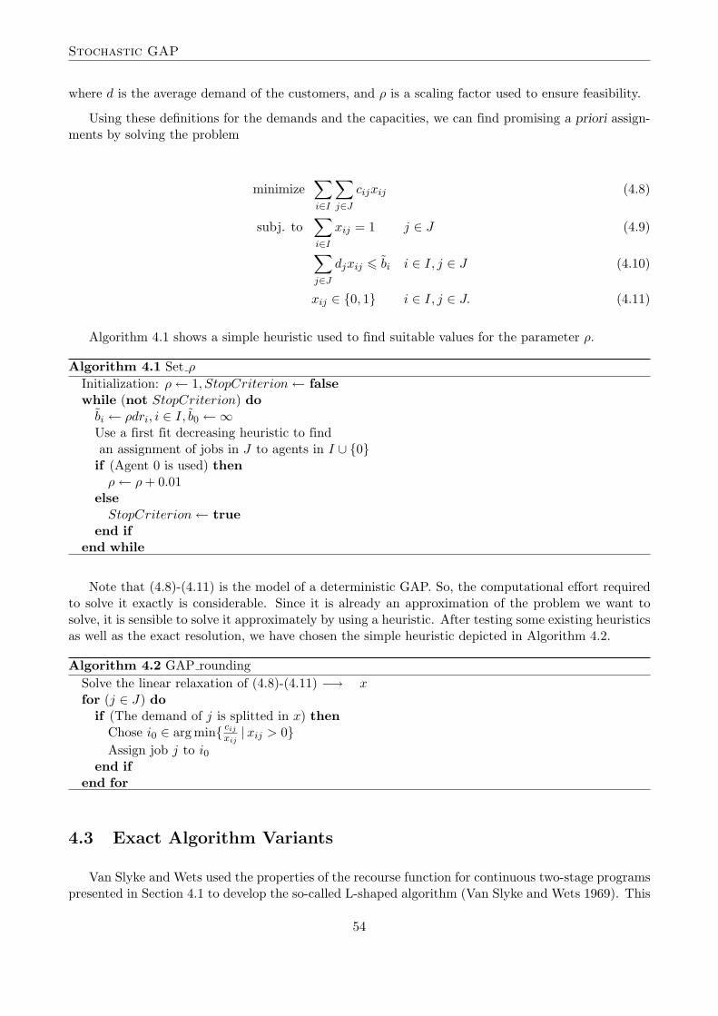
Algorithm 4.1 shows a simple heuristic used to find suitable values for the parameter ρ.

Algorithm 4.1 Set ρ

Initialization: ρ ← 1, StopCriterion ← falsewhile (not StopCriterion) do

bi ← ρdri, i ∈ I, b0 ←∞Use a first fit decreasing heuristic to findan assignment of jobs in J to agents in I ∪ {0}if (Agent 0 is used) then

ρ ← ρ + 0.01else

StopCriterion ← trueend if

end while

Note that (4.8)-(4.11) is the model of a deterministic GAP. So, the computational effort requiredto solve it exactly is considerable. Since it is already an approximation of the problem we want tosolve, it is sensible to solve it approximately by using a heuristic. After testing some existing heuristicsas well as the exact resolution, we have chosen the simple heuristic depicted in Algorithm 4.2.

Algorithm 4.2 GAP roundingSolve the linear relaxation of (4.8)-(4.11) −→ xfor (j ∈ J) do

if (The demand of j is splitted in x) thenChose i0 ∈ arg min{ cij

xij|xij > 0}

Assign job j to i0end if

end for

4.3 Exact Algorithm Variants

Van Slyke and Wets used the properties of the recourse function for continuous two-stage programspresented in Section 4.1 to develop the so-called L-shaped algorithm (Van Slyke and Wets 1969). This

54

Exact Solution

algorithm exploits the structure of the recourse function within a cutting plane scheme similar toBenders’ partitioning algorithm.

The basic idea of that algorithm is to substitute the objective functionQ(x) of FSP by a continuousvariable θ and to include a constraint of the form

θ > Q(x)

in the definition of the feasible region (4.8)-(4.11). This constraint is initially relaxed and successivelyapproximated by a set of linear cuts:

θ > α + βx,

which are called optimality cuts.

In this work we will use two kinds of optimality cuts. From Propositions 4.1.3 and 4.1.4 we derivecuts of the form:

θ > Q(x) + 〈x− x, u(x)〉, (4.12)

where 〈·, ·〉 denotes the usual inner product. We will call (4.12) ∂-optimality cuts to distinguish themfrom the L-L-optimality cuts defined below.

Integrality in two-stage programming was first addressed in (Wollmer 1980) where programs withbinary first-stage variables are considered. In that paper, an implicit enumeration scheme is presentedwhich includes the generation of optimality cuts at every feasible solution generated. More recently,Laporte and Louveaux (see Laporte and Louveaux 1992) presented a branch and cut algorithm, alsofor two-stage recourse problems with binary first-stage variables. They introduced a class of optimalitycuts that are valid at all binary first-stage solutions, for general second-stage variables. The structureof these cuts, given a binary vector x, is

θ > (Q(x)− L)

(∑

xi=1

xi −∑

xi=0

xi

)− (Q(x)− L)(

∑

i

xi − 1) + L (4.13)

where L is a global lower bound of Q (See Carøe and Tind 1998 for a generalization of these results).

We will refer to (4.13) as L-L-optimality cuts. In addition, for our GAP problem ∂-optimalitycuts can be used due to the equivalent reformulation of the second-stage problem using continuoussecond-stage variables, as derived in Section 4.1.

We will combine both kinds of optimality cuts. Note that both types of cuts are sharp at the(binary) solution at which they are generated, i.e. they are tangent to the recourse function at thatpoint.

The three versions of the algorithm presented in this work deal with integrality of the first-stagevariables by means of a branch and bound scheme, and approach the recourse function by successivelyadding optimality cuts. The difference between them is the order in which these operations are done.

BFCS (Branch first, cut second) seeks for violated cuts and adds them once an integer solution isfound.

BCS (Branch and cut simultaneously) adds violated cuts at each node of the tree, if they exist,and branches if there is any non-integer variable.

CFBS (Cut first, branch second) iteratively adds cuts to the problem at a node until no moreviolated cuts are found and then it branches.

55

Stochastic GAP

Using the reformulation presented in Section 4.1, the recourse function Q of our problem is convex.Consequently, ∂-optimality cuts generated at fractional vectors x are valid for all feasible (binary)solutions. Hence, they can be generated at any node of a branch-and-cut scheme. On the other hand,by definition L–L-optimality cuts can only be generated at binary vectors.

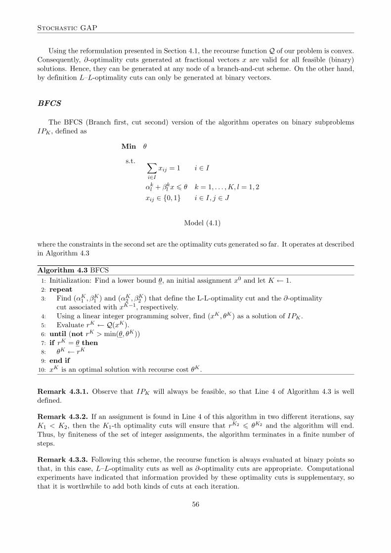
BFCS

The BFCS (Branch first, cut second) version of the algorithm operates on binary subproblemsIPK , defined as

Min θ

s.t. ∑

i∈I

xij = 1 i ∈ I

αkl + βk

l x 6 θ k = 1, . . . , K, l = 1, 2xij ∈ {0, 1} i ∈ I, j ∈ J

Model (4.1)

where the constraints in the second set are the optimality cuts generated so far. It operates at describedin Algorithm 4.3

Algorithm 4.3 BFCS1: Initialization: Find a lower bound θ, an initial assignment x0 and let K ← 1.2: repeat3: Find (αK

1 , βK1 ) and (αK

2 , βK2 ) that define the L-L-optimality cut and the ∂-optimality

cut associated with xK−1, respectively.4: Using a linear integer programming solver, find (xK , θK) as a solution of IPK .5: Evaluate rK ← Q(xK).6: until (not rK > min(θ, θK))7: if rK = θ then8: θK ← rK

9: end if10: xK is an optimal solution with recourse cost θK .

Remark 4.3.1. Observe that IPK will always be feasible, so that Line 4 of Algorithm 4.3 is welldefined.

Remark 4.3.2. If an assignment is found in Line 4 of this algorithm in two different iterations, sayK1 < K2, then the K1-th optimality cuts will ensure that rK2 6 θK2 and the algorithm will end.Thus, by finiteness of the set of integer assignments, the algorithm terminates in a finite number ofsteps.

Remark 4.3.3. Following this scheme, the recourse function is always evaluated at binary points sothat, in this case, L–L-optimality cuts as well as ∂-optimality cuts are appropriate. Computationalexperiments have indicated that information provided by these optimality cuts is supplementary, sothat it is worthwhile to add both kinds of cuts at each iteration.

56

Exact Solution

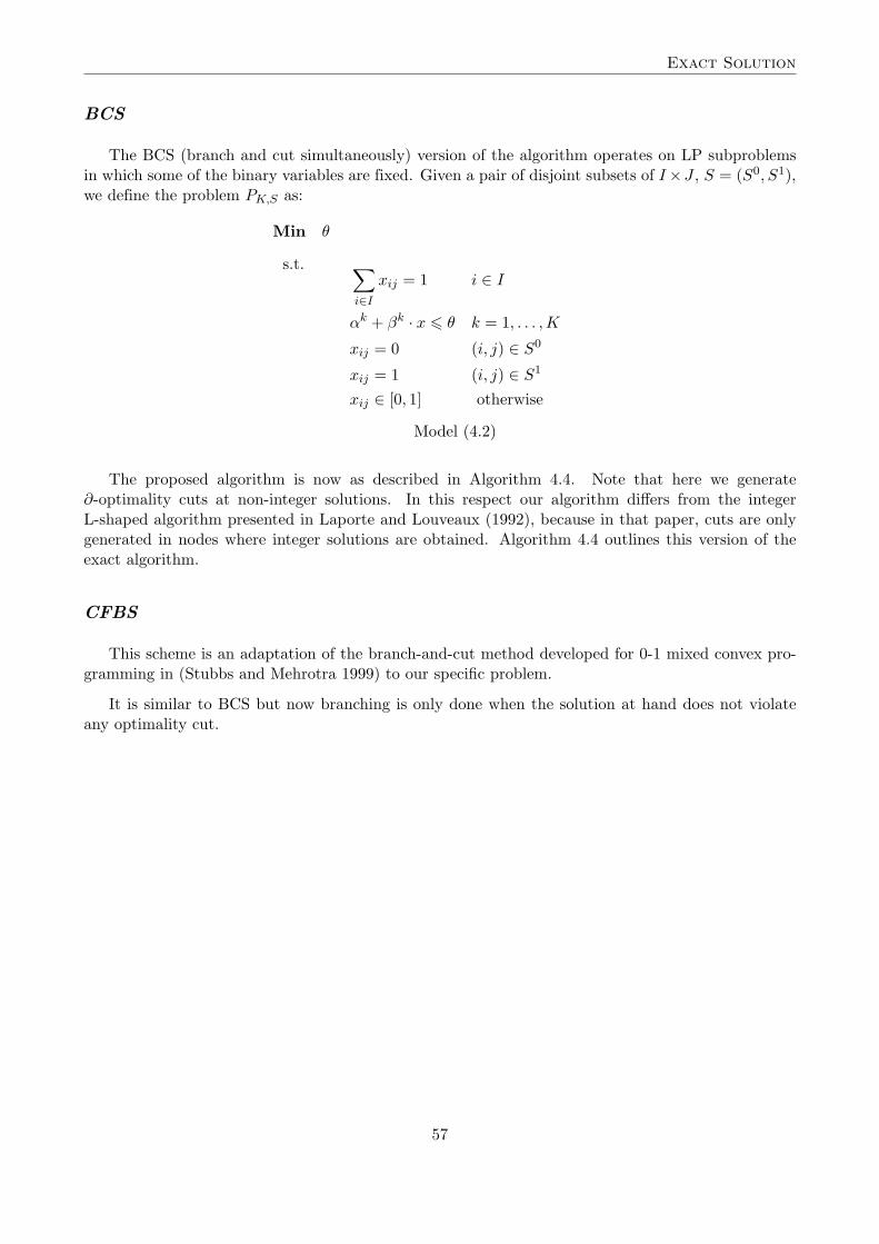
BCS

The BCS (branch and cut simultaneously) version of the algorithm operates on LP subproblemsin which some of the binary variables are fixed. Given a pair of disjoint subsets of I×J , S = (S0, S1),we define the problem PK,S as:

Min θ

s.t. ∑

i∈I

xij = 1 i ∈ I

αk + βk · x 6 θ k = 1, . . . , K

xij = 0 (i, j) ∈ S0

xij = 1 (i, j) ∈ S1

xij ∈ [0, 1] otherwise

Model (4.2)

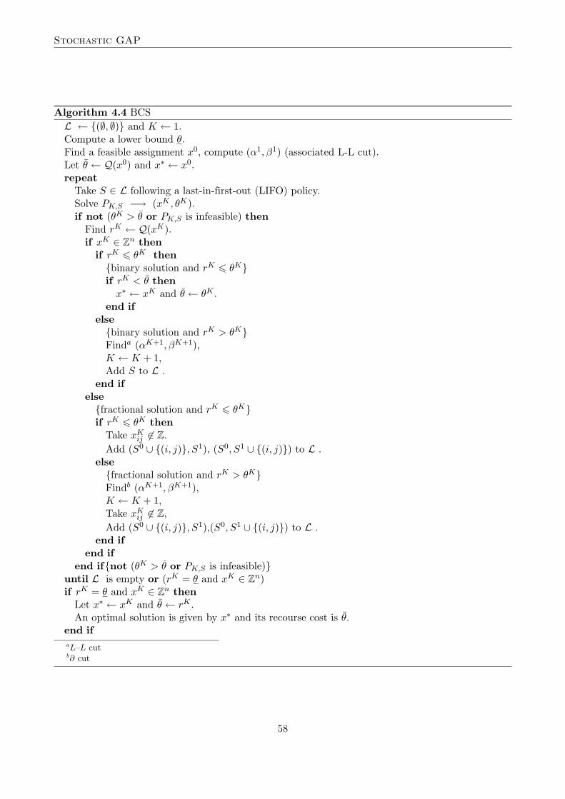
The proposed algorithm is now as described in Algorithm 4.4. Note that here we generate∂-optimality cuts at non-integer solutions. In this respect our algorithm differs from the integerL-shaped algorithm presented in Laporte and Louveaux (1992), because in that paper, cuts are onlygenerated in nodes where integer solutions are obtained. Algorithm 4.4 outlines this version of theexact algorithm.

CFBS

This scheme is an adaptation of the branch-and-cut method developed for 0-1 mixed convex pro-gramming in (Stubbs and Mehrotra 1999) to our specific problem.

It is similar to BCS but now branching is only done when the solution at hand does not violateany optimality cut.

57

Stochastic GAP

Algorithm 4.4 BCSL ← {(∅, ∅)} and K ← 1.Compute a lower bound θ.Find a feasible assignment x0, compute (α1, β1) (associated L-L cut).Let θ ← Q(x0) and x∗ ← x0.repeat

Take S ∈ L following a last-in-first-out (LIFO) policy.Solve PK,S −→ (xK , θK).if not (θK > θ or PK,S is infeasible) then

Find rK ← Q(xK).if xK ∈ Zn then

if rK 6 θK then{binary solution and rK 6 θK}if rK < θ then

x∗ ← xK and θ ← θK .end if

else{binary solution and rK > θK}Finda (αK+1, βK+1),K ← K + 1,Add S to L .

end ifelse{fractional solution and rK 6 θK}if rK 6 θK then

Take xKij 6∈ Z.

Add (S0 ∪ {(i, j)}, S1), (S0, S1 ∪ {(i, j)}) to L .else{fractional solution and rK > θK}Findb (αK+1, βK+1),K ← K + 1,Take xK

ij 6∈ Z,Add (S0 ∪ {(i, j)}, S1),(S0, S1 ∪ {(i, j)}) to L .

end ifend if

end if{not (θK > θ or PK,S is infeasible)}until L is empty or (rK = θ and xK ∈ Zn)if rK = θ and xK ∈ Zn then

Let x∗ ← xK and θ ← rK .An optimal solution is given by x∗ and its recourse cost is θ.

end ifaL–L cutb∂ cut

58

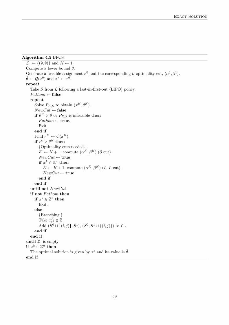
Exact Solution

Algorithm 4.5 BFCSL ← {(∅, ∅)} and K ← 1.Compute a lower bound θ.Generate a feasible assignment x0 and the corresponding ∂-optimality cut, (α1, β1).θ ← Q(x0) and x∗ ← x0.repeat

Take S from L following a last-in-first-out (LIFO) policy.Fathom ← falserepeat

Solve PK,S to obtain (xK , θK).NewCut ← falseif θK > θ or PK,S is infeasible then

Fathom ← true.Exit.

end ifFind rK ← Q(xK).if rk > θK then{Optimality cuts needed.}K ← K + 1, compute (αK , βK) (∂ cut).NewCut ← trueif xk ∈ Zn then

K ← K + 1, compute (αK , βK) (L–L cut).NewCut ← true

end ifend if

until not NewCutif not Fathom then

if xk ∈ Zn thenExit.

else{Branching.}Take xK

ij 6∈ Z.Add (S0 ∪ {(i, j)}, S1), (S0, S1 ∪ {(i, j)}) to L .

end ifend if

until L is emptyif xk ∈ Zn then

The optimal solution is given by x∗ and its value is θ.end if

59

Stochastic GAP

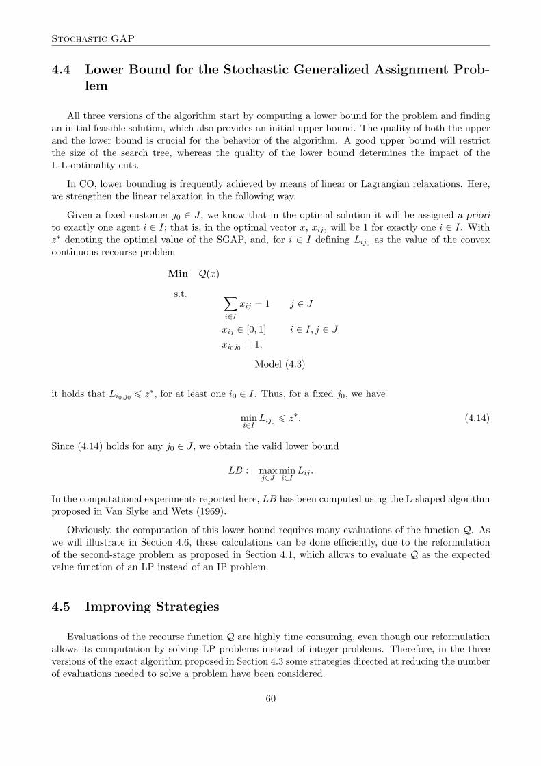
4.4 Lower Bound for the Stochastic Generalized Assignment Prob-lem

All three versions of the algorithm start by computing a lower bound for the problem and findingan initial feasible solution, which also provides an initial upper bound. The quality of both the upperand the lower bound is crucial for the behavior of the algorithm. A good upper bound will restrictthe size of the search tree, whereas the quality of the lower bound determines the impact of theL-L-optimality cuts.

In CO, lower bounding is frequently achieved by means of linear or Lagrangian relaxations. Here,we strengthen the linear relaxation in the following way.

Given a fixed customer j0 ∈ J , we know that in the optimal solution it will be assigned a priorito exactly one agent i ∈ I; that is, in the optimal vector x, xij0 will be 1 for exactly one i ∈ I. Withz∗ denoting the optimal value of the SGAP, and, for i ∈ I defining Lij0 as the value of the convexcontinuous recourse problem

Min Q(x)

s.t. ∑

i∈I

xij = 1 j ∈ J

xij ∈ [0, 1] i ∈ I, j ∈ J

xi0j0 = 1,

Model (4.3)

it holds that Li0,j0 6 z∗, for at least one i0 ∈ I. Thus, for a fixed j0, we have

mini∈I

Lij0 6 z∗. (4.14)

Since (4.14) holds for any j0 ∈ J , we obtain the valid lower bound

LB := maxj∈J

mini∈I

Lij .

In the computational experiments reported here, LB has been computed using the L-shaped algorithmproposed in Van Slyke and Wets (1969).

Obviously, the computation of this lower bound requires many evaluations of the function Q. Aswe will illustrate in Section 4.6, these calculations can be done efficiently, due to the reformulationof the second-stage problem as proposed in Section 4.1, which allows to evaluate Q as the expectedvalue function of an LP instead of an IP problem.

4.5 Improving Strategies

Evaluations of the recourse function Q are highly time consuming, even though our reformulationallows its computation by solving LP problems instead of integer problems. Therefore, in the threeversions of the exact algorithm proposed in Section 4.3 some strategies directed at reducing the numberof evaluations needed to solve a problem have been considered.

60

Computational Results

Initial Cuts

The first-stage problem contains no information about the capacities of the agents and the prob-ability of demand. Consequently, until a few cuts are generated, the solutions of problems IPK andPK,S are almost meaningless.

The first attempt to improve the behavior of all three versions of the algorithm, has been toconsider a few feasible assignments and to generate the corresponding cuts, before any optimizationis performed.

To choose such assignments, several options have been considered: obtained at random, by solvinglinear approximations of the problem, and so on. The choice that gave better results was to consider,for each agent, the assignment of all jobs to it. This leads to an initial set of ns optimality cuts. Inthis phase, ∂–optimality cuts have been used.

Integrality Cuts

The branch and cut scheme has been reinforced with cover cuts derived from the optimality cutsand a global upper bound for Q.

These cover cuts are lifted using the methodology presented in (Wolsey 1998). The order of variablelifting is decisive for the results. In this work lexicographical order has been chosen.

4.6 Computational Results

Computations have been made on a SUN sparc station 10/30 with 4 hyperSPARC processors at100 MHz., SPECint95 2.35. To solve the problems IPK and PK,S CPLEX 6.0 was used.

Problem Statistics

All three versions of the algorithm have been tested on a set of 46 randomly generated instances.

The number of agents ranges from 2 to 4, and the number of customers, from 4 to 15. Demandprobabilities have been selected from the set

{0.1, 0.2, 0.4, 0.6, 0.8, 0.9},

and capacities have been chosen in such a way that the ratio of total capacity to total demand rangesfrom 0.5 to 2.

Evaluation of Q

Efficient evaluation of the function Q is crucial for both the computation of the lower bound LBas well as for all variants of the proposed algorithm.

Due to the reformulation of the second-stage problem as proposed in Section 4.1, which allows toevaluate Q as the expected value function of an LP instead of an IP problem, these calculations canbe done much faster.

61

Stochastic GAP

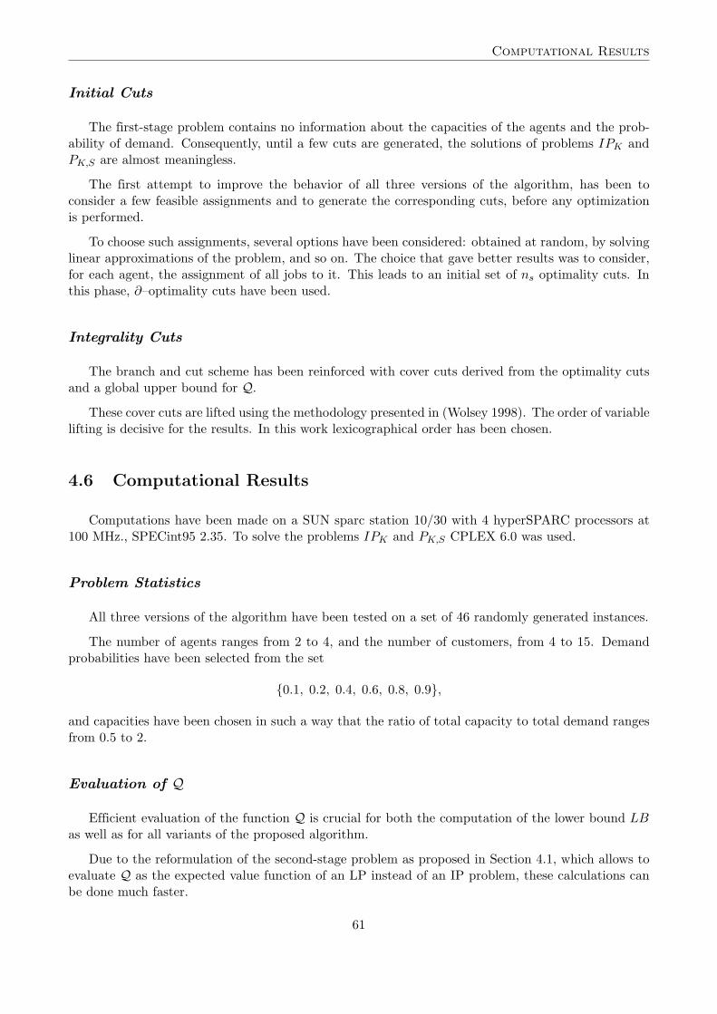
In support of this claim, Table 4.1 shows average CPU times (for each group of instances withgiven dimensions) for evaluating Q using both formulations. For each instance, Q was evaluated inthe corresponding optimal binary solution, and also in a randomly generated fractional solution (thatis feasible with respect to the first set of constraints in FSP).

Table 4.1: Average CPU times for evaluating Q at binaryand fractional solutions.

dimbinary x fractional x

Q ∼ IP Q ∼ LP Q ∼ IP Q ∼ LP2× 4 0.09 0.02 0.46 0.034× 8 2.37 0.31 14.08 0.523× 7 1.08 0.07 10.21 0.243× 8 2.46 0.16 20.96 0.373× 9 5.41 0.30 122.61 0.75

3× 10 11.79 0.63 160.04 1.223× 15 468.39 24.79 16000† 75.084× 7 1.50 0.09 11.57 0.294× 8 3.21 0.19 24.64 0.77

Table 4.1 shows that by using the reformulation of Q as proposed in Section 4.1, the evaluationtimes are reduced by a factor up to almost 19 for binary arguments. This effect is even stronger whenthe argument is fractional, because then it is harder to find integer solutions of SSP. In the latter casethe speedup factor exceeds 200 for the 3× 15 instance.

As we will see below, solving an instance from our set of test problems typically takes severalhundreds of evaluations of Q.

Computational Results

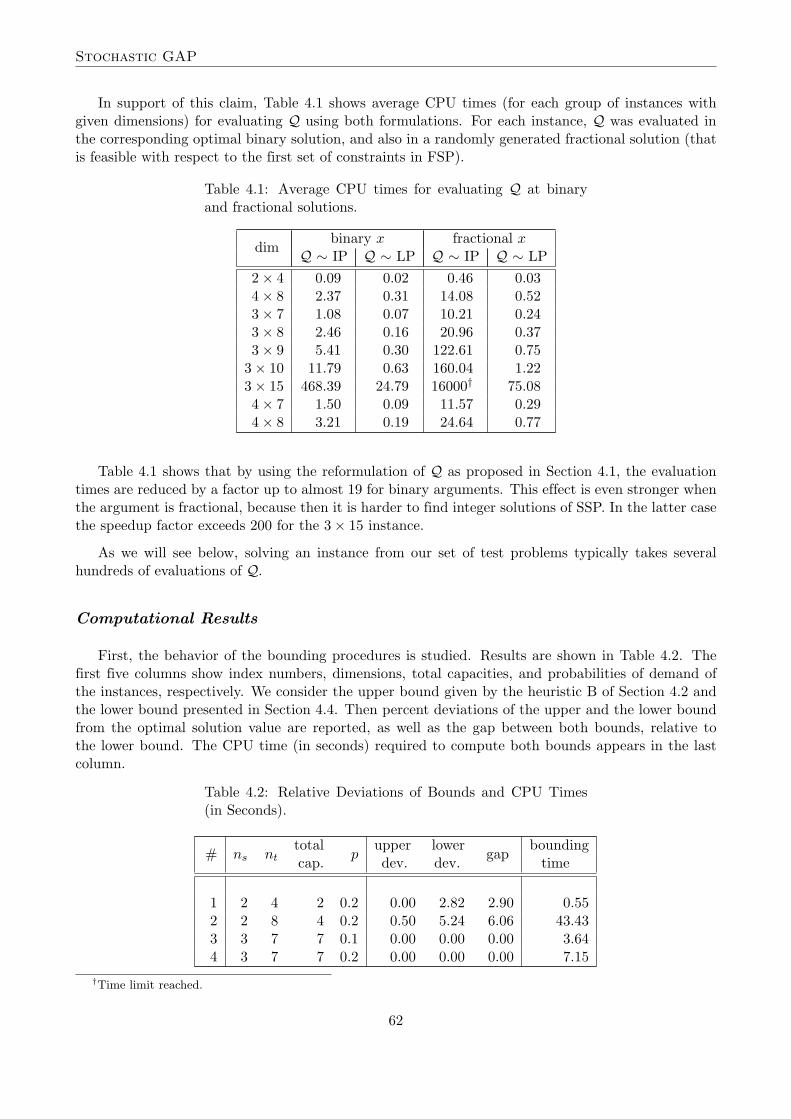
First, the behavior of the bounding procedures is studied. Results are shown in Table 4.2. Thefirst five columns show index numbers, dimensions, total capacities, and probabilities of demand ofthe instances, respectively. We consider the upper bound given by the heuristic B of Section 4.2 andthe lower bound presented in Section 4.4. Then percent deviations of the upper and the lower boundfrom the optimal solution value are reported, as well as the gap between both bounds, relative tothe lower bound. The CPU time (in seconds) required to compute both bounds appears in the lastcolumn.

Table 4.2: Relative Deviations of Bounds and CPU Times(in Seconds).

# ns nttotal

pupper lower bounding

cap. dev. dev.gap

time

1 2 4 2 0.2 0.00 2.82 2.90 0.552 2 8 4 0.2 0.50 5.24 6.06 43.433 3 7 7 0.1 0.00 0.00 0.00 3.644 3 7 7 0.2 0.00 0.00 0.00 7.15

†Time limit reached.

62

Computational Results

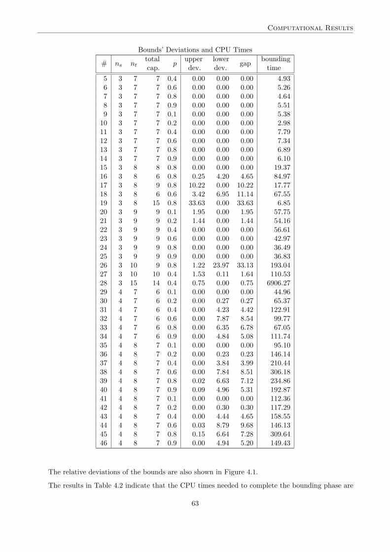
Bounds’ Deviations and CPU Times

# ns nttotal

pupper lower bounding

cap. dev. dev.gap

time5 3 7 7 0.4 0.00 0.00 0.00 4.936 3 7 7 0.6 0.00 0.00 0.00 5.267 3 7 7 0.8 0.00 0.00 0.00 4.648 3 7 7 0.9 0.00 0.00 0.00 5.519 3 7 7 0.1 0.00 0.00 0.00 5.38

10 3 7 7 0.2 0.00 0.00 0.00 2.9811 3 7 7 0.4 0.00 0.00 0.00 7.7912 3 7 7 0.6 0.00 0.00 0.00 7.3413 3 7 7 0.8 0.00 0.00 0.00 6.8914 3 7 7 0.9 0.00 0.00 0.00 6.1015 3 8 8 0.8 0.00 0.00 0.00 19.3716 3 8 6 0.8 0.25 4.20 4.65 84.9717 3 8 9 0.8 10.22 0.00 10.22 17.7718 3 8 6 0.6 3.42 6.95 11.14 67.5519 3 8 15 0.8 33.63 0.00 33.63 6.8520 3 9 9 0.1 1.95 0.00 1.95 57.7521 3 9 9 0.2 1.44 0.00 1.44 54.1622 3 9 9 0.4 0.00 0.00 0.00 56.6123 3 9 9 0.6 0.00 0.00 0.00 42.9724 3 9 9 0.8 0.00 0.00 0.00 36.4925 3 9 9 0.9 0.00 0.00 0.00 36.8326 3 10 9 0.8 1.22 23.97 33.13 193.0427 3 10 10 0.4 1.53 0.11 1.64 110.5328 3 15 14 0.4 0.75 0.00 0.75 6906.2729 4 7 6 0.1 0.00 0.00 0.00 44.9630 4 7 6 0.2 0.00 0.27 0.27 65.3731 4 7 6 0.4 0.00 4.23 4.42 122.9132 4 7 6 0.6 0.00 7.87 8.54 99.7733 4 7 6 0.8 0.00 6.35 6.78 67.0534 4 7 6 0.9 0.00 4.84 5.08 111.7435 4 8 7 0.1 0.00 0.00 0.00 95.1036 4 8 7 0.2 0.00 0.23 0.23 146.1437 4 8 7 0.4 0.00 3.84 3.99 210.4438 4 8 7 0.6 0.00 7.84 8.51 306.1839 4 8 7 0.8 0.02 6.63 7.12 234.8640 4 8 7 0.9 0.09 4.96 5.31 192.8741 4 8 7 0.1 0.00 0.00 0.00 112.3642 4 8 7 0.2 0.00 0.30 0.30 117.2943 4 8 7 0.4 0.00 4.44 4.65 158.5544 4 8 7 0.6 0.03 8.79 9.68 146.1345 4 8 7 0.8 0.15 6.64 7.28 309.6446 4 8 7 0.9 0.00 4.94 5.20 149.43

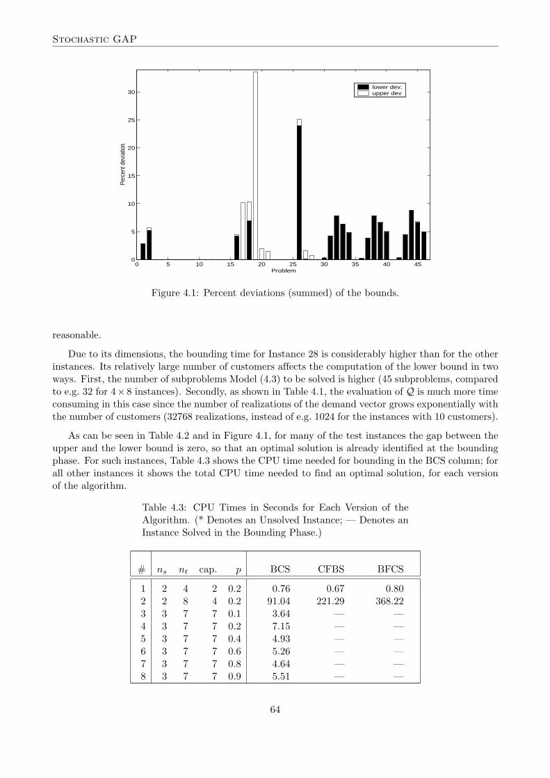
The relative deviations of the bounds are also shown in Figure 4.1.

The results in Table 4.2 indicate that the CPU times needed to complete the bounding phase are

63

Stochastic GAP

0 5 10 15 20 25 30 35 40 450

5

10

15

20

25

30

Problem

Perc

ent d

evia

tion

lower dev.upper dev

Figure 4.1: Percent deviations (summed) of the bounds.

reasonable.

Due to its dimensions, the bounding time for Instance 28 is considerably higher than for the otherinstances. Its relatively large number of customers affects the computation of the lower bound in twoways. First, the number of subproblems Model (4.3) to be solved is higher (45 subproblems, comparedto e.g. 32 for 4× 8 instances). Secondly, as shown in Table 4.1, the evaluation of Q is much more timeconsuming in this case since the number of realizations of the demand vector grows exponentially withthe number of customers (32768 realizations, instead of e.g. 1024 for the instances with 10 customers).

As can be seen in Table 4.2 and in Figure 4.1, for many of the test instances the gap between theupper and the lower bound is zero, so that an optimal solution is already identified at the boundingphase. For such instances, Table 4.3 shows the CPU time needed for bounding in the BCS column; forall other instances it shows the total CPU time needed to find an optimal solution, for each versionof the algorithm.

Table 4.3: CPU Times in Seconds for Each Version of theAlgorithm. (* Denotes an Unsolved Instance; — Denotes anInstance Solved in the Bounding Phase.)

# ns nt cap. p BCS CFBS BFCS

1 2 4 2 0.2 0.76 0.67 0.802 2 8 4 0.2 91.04 221.29 368.223 3 7 7 0.1 3.64 — —4 3 7 7 0.2 7.15 — —5 3 7 7 0.4 4.93 — —6 3 7 7 0.6 5.26 — —7 3 7 7 0.8 4.64 — —8 3 7 7 0.9 5.51 — —

64

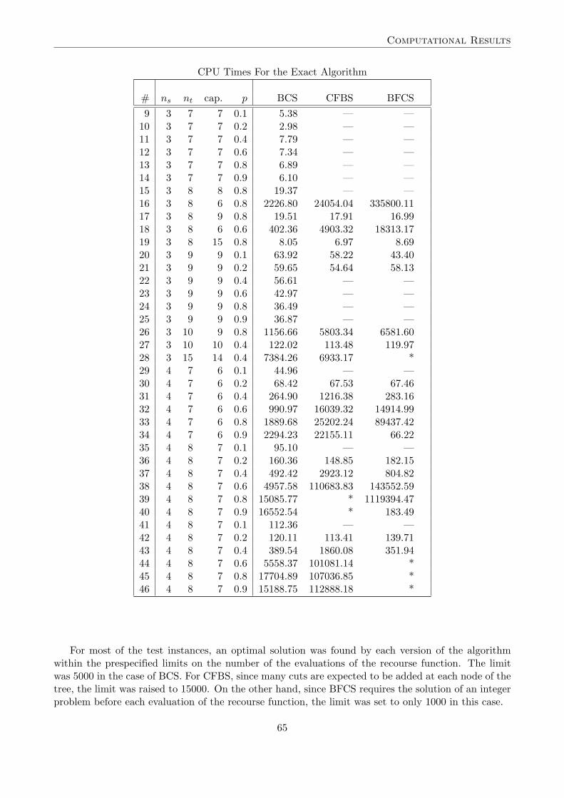
Computational Results

CPU Times For the Exact Algorithm

# ns nt cap. p BCS CFBS BFCS9 3 7 7 0.1 5.38 — —

10 3 7 7 0.2 2.98 — —11 3 7 7 0.4 7.79 — —12 3 7 7 0.6 7.34 — —13 3 7 7 0.8 6.89 — —14 3 7 7 0.9 6.10 — —15 3 8 8 0.8 19.37 — —16 3 8 6 0.8 2226.80 24054.04 335800.1117 3 8 9 0.8 19.51 17.91 16.9918 3 8 6 0.6 402.36 4903.32 18313.1719 3 8 15 0.8 8.05 6.97 8.6920 3 9 9 0.1 63.92 58.22 43.4021 3 9 9 0.2 59.65 54.64 58.1322 3 9 9 0.4 56.61 — —23 3 9 9 0.6 42.97 — —24 3 9 9 0.8 36.49 — —25 3 9 9 0.9 36.87 — —26 3 10 9 0.8 1156.66 5803.34 6581.6027 3 10 10 0.4 122.02 113.48 119.9728 3 15 14 0.4 7384.26 6933.17 *29 4 7 6 0.1 44.96 — —30 4 7 6 0.2 68.42 67.53 67.4631 4 7 6 0.4 264.90 1216.38 283.1632 4 7 6 0.6 990.97 16039.32 14914.9933 4 7 6 0.8 1889.68 25202.24 89437.4234 4 7 6 0.9 2294.23 22155.11 66.2235 4 8 7 0.1 95.10 — —36 4 8 7 0.2 160.36 148.85 182.1537 4 8 7 0.4 492.42 2923.12 804.8238 4 8 7 0.6 4957.58 110683.83 143552.5939 4 8 7 0.8 15085.77 * 1119394.4740 4 8 7 0.9 16552.54 * 183.4941 4 8 7 0.1 112.36 — —42 4 8 7 0.2 120.11 113.41 139.7143 4 8 7 0.4 389.54 1860.08 351.9444 4 8 7 0.6 5558.37 101081.14 *45 4 8 7 0.8 17704.89 107036.85 *46 4 8 7 0.9 15188.75 112888.18 *

For most of the test instances, an optimal solution was found by each version of the algorithmwithin the prespecified limits on the number of the evaluations of the recourse function. The limitwas 5000 in the case of BCS. For CFBS, since many cuts are expected to be added at each node of thetree, the limit was raised to 15000. On the other hand, since BFCS requires the solution of an integerproblem before each evaluation of the recourse function, the limit was set to only 1000 in this case.

65

Stochastic GAP

0 5 10 15 20 25 30 35 40 45

0

5

10

15

20

Problem

log 2 C

PU ti

me

BCS CFBSBFCS

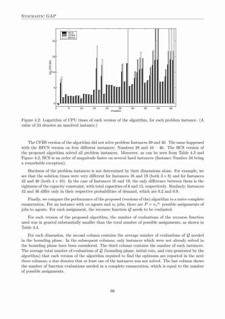
Figure 4.2: Logarithm of CPU times of each version of the algorithm, for each problem instance. (Avalue of 24 denotes an unsolved instance.)

The CFBS version of the algorithm did not solve problem Instances 39 and 40. The same happenedwith the BFCS version on four different instances: Numbers 28 and 44 – 46. The BCS version ofthe proposed algorithm solved all problem instances. Moreover, as can be seen from Table 4.3 andFigure 4.2, BCS is an order of magnitude faster on several hard instances (Instance Number 34 beinga remarkable exception).

Hardness of the problem instances is not determined by their dimensions alone. For example, wesee that the solution times were very different for Instances 16 and 19 (both 3× 8) and for Instances42 and 46 (both 4× 10). In the case of Instances 16 and 19, the only difference between them is thetightness of the capacity constraint, with total capacities of 6 and 15, respectively. Similarly, Instances42 and 46 differ only in their respective probabilities of demand, which are 0.2 and 0.9.

Finally, we compare the performance of the proposed (versions of the) algorithm to a naive completeenumeration. For an instance with ns agents and nt jobs, there are P = ns

nt possible assignments ofjobs to agents. For each assignment, the recourse function Q needs to be evaluated.

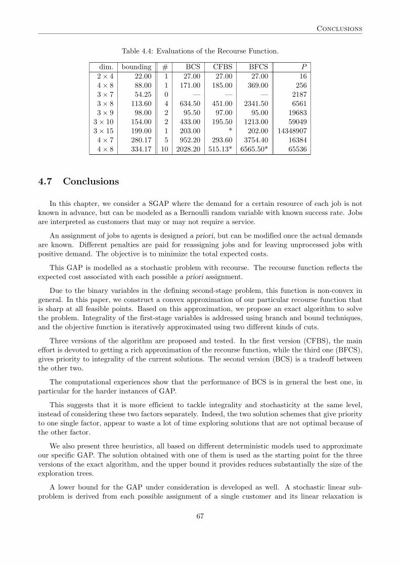
For each version of the proposed algorithm, the number of evaluations of the recourse functionused was in general substantially smaller than the total number of possible assignments, as shown inTable 4.4.

For each dimension, the second column contains the average number of evaluations of Q neededin the bounding phase. In the subsequent columns, only instances which were not already solved inthe bounding phase have been considered. The third column contains the number of such instances.The average total number of evaluations of Q (bounding phase, initial cuts, and cuts generated by thealgorithm) that each version of the algorithm required to find the optimum are reported in the nextthree columns; a star denotes that at least one of the instances was not solved. The last column showsthe number of function evaluations needed in a complete enumeration, which is equal to the numberof possible assignments.

66

Conclusions

Table 4.4: Evaluations of the Recourse Function.

dim. bounding # BCS CFBS BFCS P

2× 4 22.00 1 27.00 27.00 27.00 164× 8 88.00 1 171.00 185.00 369.00 2563× 7 54.25 0 — — — 21873× 8 113.60 4 634.50 451.00 2341.50 65613× 9 98.00 2 95.50 97.00 95.00 19683

3× 10 154.00 2 433.00 195.50 1213.00 590493× 15 199.00 1 203.00 * 202.00 143489074× 7 280.17 5 952.20 293.60 3754.40 163844× 8 334.17 10 2028.20 515.13* 6565.50* 65536

4.7 Conclusions

In this chapter, we consider a SGAP where the demand for a certain resource of each job is notknown in advance, but can be modeled as a Bernoulli random variable with known success rate. Jobsare interpreted as customers that may or may not require a service.

An assignment of jobs to agents is designed a priori, but can be modified once the actual demandsare known. Different penalties are paid for reassigning jobs and for leaving unprocessed jobs withpositive demand. The objective is to minimize the total expected costs.

This GAP is modelled as a stochastic problem with recourse. The recourse function reflects theexpected cost associated with each possible a priori assignment.

Due to the binary variables in the defining second-stage problem, this function is non-convex ingeneral. In this paper, we construct a convex approximation of our particular recourse function thatis sharp at all feasible points. Based on this approximation, we propose an exact algorithm to solvethe problem. Integrality of the first-stage variables is addressed using branch and bound techniques,and the objective function is iteratively approximated using two different kinds of cuts.

Three versions of the algorithm are proposed and tested. In the first version (CFBS), the maineffort is devoted to getting a rich approximation of the recourse function, while the third one (BFCS),gives priority to integrality of the current solutions. The second version (BCS) is a tradeoff betweenthe other two.

The computational experiences show that the performance of BCS is in general the best one, inparticular for the harder instances of GAP.

This suggests that it is more efficient to tackle integrality and stochasticity at the same level,instead of considering these two factors separately. Indeed, the two solution schemes that give priorityto one single factor, appear to waste a lot of time exploring solutions that are not optimal because ofthe other factor.

We also present three heuristics, all based on different deterministic models used to approximateour specific GAP. The solution obtained with one of them is used as the starting point for the threeversions of the exact algorithm, and the upper bound it provides reduces substantially the size of theexploration trees.

A lower bound for the GAP under consideration is developed as well. A stochastic linear sub-problem is derived from each possible assignment of a single customer and its linear relaxation is

67

Stochastic GAP

solved using the L-shaped algorithm. The actual lower bound is obtained from the solutions to thesesubproblems. This lower bound has proved to be very tight in the computational experiments.

CPU times required to obtain both bounds are relatively small for all but one instance. In 43%of the cases, the bounding phase was sufficient to identify an optimal solution. On the other hand,there are also a few instances with a large gap between the bounds.

For those instances where the bounding phase did not already provide an optimal solution, theexact algorithm gave satisfactory results. Times required to solve such instances were reasonable,taking into account the high difficulty of the problem. The success of the algorithm is mostly due tothe approximation of the recourse function that we use. It is much faster to evaluate than the originalrecourse function and moreover it is convex, which allows to obtain good approximations using acutting plane procedure.

68